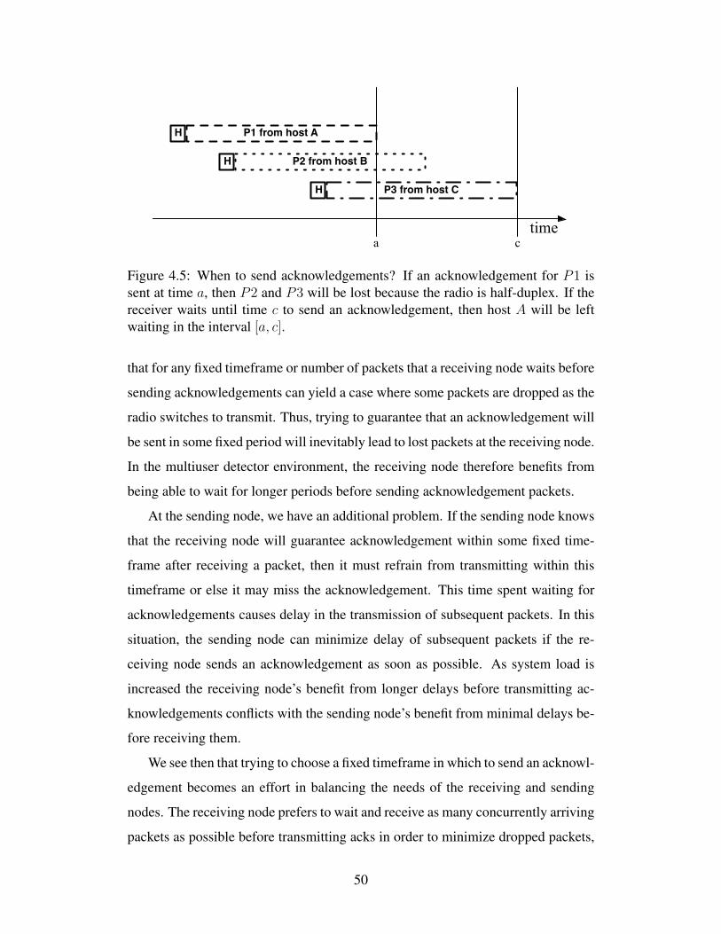
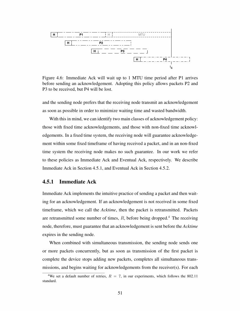
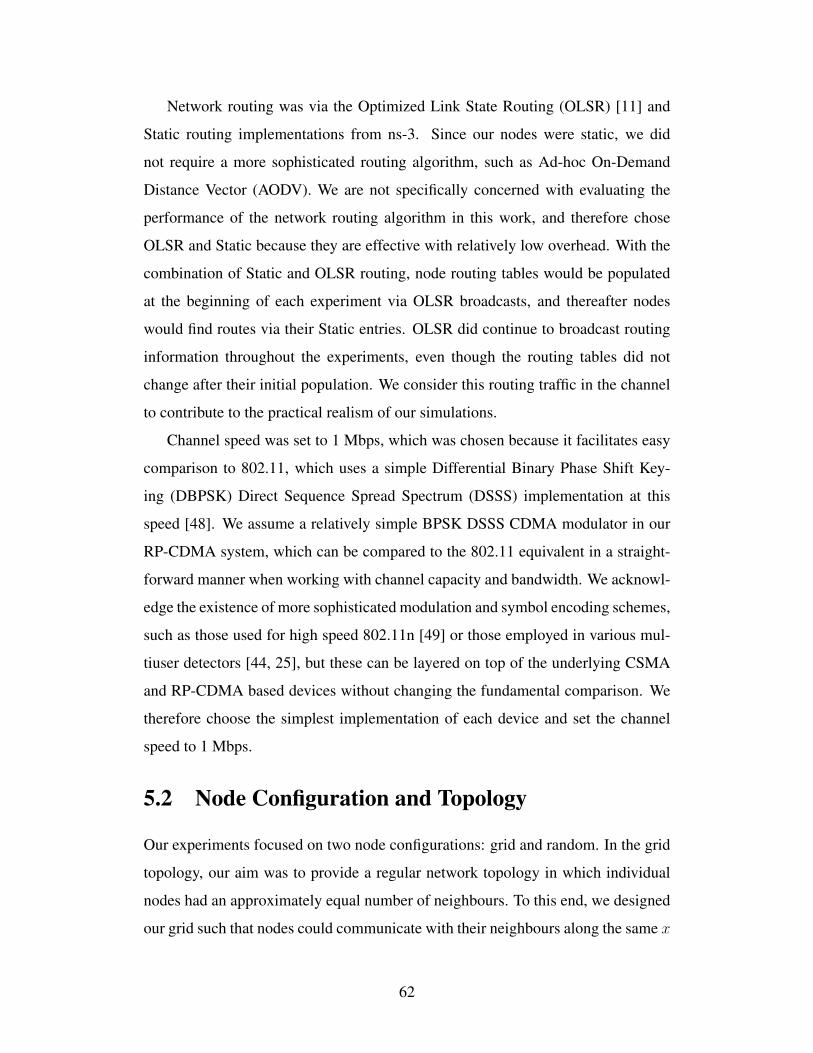
University of Alberta A MAC P ROTOCOL FOR MULTIHOP RP-CDMA AD HOC WIRELESS NETWORKS by Todd Mortimer A thesis submitted to the Faculty of Graduate Studies and Research in partial fulfillment of the requirements for the degree of Master of Science Department of Computing Science c Todd Mortimer Fall 2012 Edmonton, Alberta Permission is hereby granted to the University of Alberta Libraries to reproduce single copies of this thesis and to lend or sell such copies for private, scholarly or scientific research purposes only. Where the thesis is converted to, or otherwise made available in digital form, the University of Alberta will advise potential users of the thesis of these terms. The author reserves all other publication and other rights in association with the copyright in the thesis, and except as herein before provided, neither the thesis nor any substantial portion thereof may be printed or otherwise reproduced in any material form whatever without the author’s prior written permission.
Transcript
University of Alberta
A MAC PROTOCOL FOR MULTIHOP RP-CDMA AD HOCWIRELESS NETWORKS
by
Todd Mortimer
A thesis submitted to the Faculty of Graduate Studies and Researchin partial fulfillment of the requirements for the degree of
Permission is hereby granted to the University of Alberta Libraries to reproduce singlecopies of this thesis and to lend or sell such copies for private, scholarly or scientific
research purposes only. Where the thesis is converted to, or otherwise made available indigital form, the University of Alberta will advise potential users of the thesis of these
terms.
The author reserves all other publication and other rights in association with the copyrightin the thesis, and except as herein before provided, neither the thesis nor any substantialportion thereof may be printed or otherwise reproduced in any material form whatever
without the author’s prior written permission.
Abstract
RP-CDMA is a wireless multiple access technique that utilizes multiple spreading
codes and a multiuser detector to enhance link reliability and performance. We
propose a simple MAC protocol on top of the RP-CDMA Phy and apply it to the
multihop ad hoc network model. In addition to a MAC, we propose two signifi-
cant extensions to RP-CDMA aimed at improving throughput and reliability. We
test our network device using the ns-3 network simulator and compare its perfor-
mance to that of the well known 802.11 CSMA model. Our simulations confirm that
RP-CDMA can substantially improve link reliability and network performance, but
that a link level acknowledgement mechanism is required to ensure packet delivery
across the network. We investigate a simple acknowledgement policy and conclude
that it enables simultaneous high throughput and packet delivery while maintaining
low latency.
Acknowledgements
Foremost I would like to thank Dr. Janelle Harms for her guidance and patience,
particularly when I was indulging my impulses. Thanks for letting me disappear
into the MAC layer - I know we started out up higher. I would also like to thank
Dr. Christian Schlegel for his feedback and suggestions as I recast RP-CDMA
for my purposes. My conversations with Dr. Ivan Fair and Majid Ghanbarinejad
were invaluable for understanding what’s actually going on in a radio, and I am
grateful for their time and assistance. Of course, I must also thank my wife, Erin,
whose endless support in everything outside academics has made the academics
themselves so much more manageable.
Finally, I would like to thank the Department of National Defence and the Cana-
dian Forces, whose sponsorship has made all of this possible. I hope the investment
The proliferation of wireless data networks in the last decade has provided ever
faster and more robust service. Since 1999, the popular 802.11 standard has pro-
gressed in data rate from an initial 1 Mbps to up to 600 Mbps in the current revi-
sion [49]. At the same time, fundamental limitations of the wireless channel have
necessitated increasingly complex signalling protocols and increasing bandwidth
allocations in order to support these ever faster services [39]. The primary lim-
itation which all wireless systems must contend with is the shared nature of the
wireless channel. Because any devices working in the same wireless channel must
necessarily share it with other devices in the network, mechanisms and protocols
for dividing up the available bandwidth among all of the network peers must be
developed. The result is that each device necessarily has only partial access to the
full channel capacity, and any errors in the coordination of channel sharing result in
transmission collisions, lost data, and diminished link reliability.
This problem is particularly evident in ad hoc networks. An ad hoc network is
one in which the network nodes join a common channel in the absence of any fixed
infrastructure or network controlling authority [45]. These nodes build a logical
network using the wireless channel and exchange routing information in order to
cooperatively pass traffic across the network. This is in contrast to the more familiar
base station model in which nodes join a network created and managed by a central
network node. The central node is responsible for admitting each network peer and
coordinating their transmissions so as to not collide.
We are specifically interested in the multihop ad hoc model here because of the
1
additional challenges it presents compared to the base station model. In the presence
of a base station, network nodes need only coordinate their transmissions with the
base station, which can strictly control the behaviour of all of the nodes and ensure
that each node gets their share of the channel. Each node passes all of their traffic
through the base station and the base station tells the nodes when to transmit and
when to listen, so there is no need coordinate with any other node in the network.
In an ad hoc network, individual network nodes must coordinate among themselves
in order to pass messages between any of their peers. In the event that two nodes
cannot communicate directly, a multihop ad hoc network will pass messages from
node to node between the message originator and destination. Since the radio is a
half duplex device, nodes must decide when to exclusively transmit and when to
listen. Dividing up which nodes will transmit, to which other nodes, when they
do so, and how their transmissions are sent turns out to be a complex operation
in an environment which lacks any sort of central authoritative coordinating entity.
The consequence of getting this coordination function wrong is data loss, which
either results in delays as packets are retransmitted or outright loss as data simply
disappears from the network. The ad hoc environment is therefore somewhat more
challenging to work in, and presents unique problems that do not have obvious
solutions.
There are many ways in which several peers might coordinate access to a com-
mon wireless channel. Perhaps the most obvious approach is to try to avoid trans-
mitting at the same time as other nodes, which is the principle behind the popular
802.11 wireless standard [48]. Alternately, the available medium can be divided up
into multiple subchannels, and nodes can coordinate access to these subchannels in
a non-interfering way. Three of the most common ways to divide up the wireless
medium are to set up a time schedule (TDMA), divide different peers into different
non-interfering frequency groups (FDMA), or to use spread spectrum techniques
such as code division to separate users into different code channels (CDMA) [23].
Each of these methods has their own drawbacks, which we will discuss in Chap-
ter 2, but fundamentally they all suffer from the same limitation imposed by the
shared nature of the wireless channel: Because nodes need to avoid collisions they
2
must organize multiple access to the channel, but this coordination must be done
using the shared channel itself. The coordination traffic, therefore, is itself subject
to collisions which causes the loss of both data traffic and coordination traffic. The
loss of coordination traffic may cause further data loss as the access coordination
function breaks down.
The root of this problem is the nature of the wireless channel itself and its unre-
liability due to collisions. Were the channel reliable such that multiple nodes could
transmit simultaneously without having to coordinate channel access then we could
dispense with the coordination function altogether. Without the need to coordi-
nate channel access then the decision of whether an ad hoc network node transmits
at any given time is simplified to deciding whether the intended receiver node is
listening. Determining whether a neighbouring node is listening is the inverse of
deciding whether they are transmitting, which can be simply estimated by listening
to the channel itself.1 With a reliable link it should therefore be possible for us to
construct an ad hoc network in which nodes can decide whether or not to transmit
without consulting any other nodes or external sources of information.
In this dissertation, we propose an ad hoc Medium Access Control (MAC) pro-
tocol built on top of such a reliable link, and evaluate its performance compared to
traditional 802.11 Carrier Sense Multiple Access (CSMA). This reliable link was
proposed by Schlegel et al.[42], and uses code division to separate individual pack-
ets into private channels, with the result that multiple packets can arrive simultane-
ously at a receiver with only a relatively small probability of colliding. We propose
two extensions to the link itself, and on top of it we propose a simple MAC protocol
which does not require any coordination between nodes. Our aim is to show that
with a reliable link it is possible to build ad hoc networks which exhibit improved
reliability, and hence performance, compared to networks built on top of traditional
wireless links.
In the remainder of this chapter we motivate our work by first discussing the
wireless link reliability problem in general and then identifying the characteristics
1We assume that nodes are continuously awake and do not have a sleep / wake cycle or someother mechanism which causes them to have periods in which nodes are neither transmitting norlistening.
3
of a theoretical wireless link that would address this problem. With the problem
articulated, we identify a potential solution and then describe our approach to mea-
suring and testing its effectiveness.
1.1 Wireless Network Reliability
We are interested here in a reliable wireless ad hoc network. Network reliability
ultimately depends on link level reliability, with the successful routing of packets
through the network being dependent on the successful passing of packets across
each link along the way. As discussed above, the fundamental problem with wire-
less link reliability is the shared nature of the wireless channel.
If we take a moment to look back at wired Ethernet networks, we recall that
these networks once also had shared channels with the use of hubs, and also ex-
perienced collisions and loss. In Ethernet, the collision problem was solved by
switching from hubs to switches, which provided each node in the network with a
private channel to the switch. With the widespread deployment of switched packet
networks over interference-resistant cabling, reliable wired links have enabled ever
faster wired networks and eroded the requirement for complex protocols at the
MAC and link layers [50].
It is therefore natural to ask how we could achieve the same thing in a wireless
network. It is possible to separate transmissions into separate channels using ei-
ther time, frequency or code division, but the problem then becomes one of channel
coordination. Which node gets what channel, when and for how long? In an ad
hoc network a node may have a requirement to communicate with any or several of
its neighbours, and must therefore coordinate with each of them in order to decide
which time slot, frequency or spreading code to use for a given transmission. As
more load is placed on the network and more nodes contend for the same chan-
nel resources, this distributed coordination of orderly access to the channel breaks
down, resulting in declining link reliability and system performance.
Thus, in an ad hoc network, coordinating access to the shared wireless medium
among disparate nodes poses a significant challenge, particularly as this coordina-
4
tion must be done using the wireless medium itself. This difficulty in coordinating
the orderly access to the shared wireless medium has resulted in complex MAC
and link layer standards for wireless networks [48], with limited success [56, 40].
Additionally, even if we could perform this coordination perfectly each node could
still access only a fraction of the total channel capacity, since nodes must take turns
transmitting and receiving.
Finally, the wireless channel must contend with external noise and interference.
There may be many wireless devices in a given area, each of which contributes
energy, and hence noise, to the wireless medium. Transmissions may reflect or
scatter off of physical objects in the environment on their way to their destination,
which can cause signal fading, multipath interference, or echoes, all of which must
be suppressed or otherwise handled by the wireless receiver [32]. In contrast, wired
networks are less susceptible to external interference, which can often be addressed
simply with shielded cabling, and the properties of the wire can be controlled so as
to mitigate against unrecoverable signal fading or distortion.
We see then that wireless network reliability is a different sort of problem from
its wired counterpart. Nonetheless, we can look to the wired link to identify those
properties which have enabled its rapid advancement in reliability and performance,
and try to construct a wireless link that exhibits some or all of those properties.
1.2 Problem Description
Ideally, we would like wireless networks to be more like wired networks, with sim-
ple and reliable links and protocols. In a modern wired network, the wire provides
each node with a private channel to their next hop, and is constructed so as to be re-
sistant to external interference. Under these conditions, there is no requirement for
nodes to coordinate access to the network, and so each node can transmit randomly
and simultaneously up to the capacity of the link. Translating this to a wireless
context, we desire a wireless link that holds the three qualities:
1. Each node has a private channel to each of their peers.
2. Signals are resistant to interference.
5
3. Each node can access the channel without coordinating with its peers.
We will see that each of these properties is already available in the ad hoc wire-
less link, but not always together with the others. For example, we can easily
achieve private channels between peers by assigning each node a unique frequency
for communicating with each of its neighbours, but in order to use those frequencies
effectively the transmitting node must coordinate with an intended receiver about
when to switch to the private channel [46]. Similarly, we can adopt spread spectrum
techniques, such as code division, to overcome reasonable levels of external and in-
ternal interference, but must then coordinate between nodes for which spreading
codes or subcarriers to use, lest the signals be missed and lost [22]. Finally, we can
eschew coordination and have nodes simply broadcast when they have data traffic,
as in ALOHA [3], but this means that all nodes must work in a single channel.
Our problem is therefore to identify a means of accessing the wireless channel
that exhibits all three of these desirable properties simultaneously.
1.3 Aim
We shall see that a multiple access method, Random Packet Code Division Multiple
Access (RP-CDMA ) [42], has been proposed in the literature that comes very close
to meeting all of our desirable properties. We propose to apply this method to the
multihop ad hoc context and evaluate its reliability and performance, compared to
the popular Carrier Sense Multiple Access (CSMA) 802.11 standard.
RP-CDMA is a type of CDMA protocol that uses multiple spreading codes to
separate individual packets into private channels, where a channel is defined by
its spreading code. It therefore provides private channels for each communication,
and has the same interference-resistant properties of other CDMA protocols. By
virtue of its packet format, RP-CDMA also offers completely uncoordinated and
asynchronous channel access. It is these three qualities that make RP-CDMA a
promising candidate for a reliable wireless link. Previous work has investigated
the reliability and performance characteristics of RP-CDMA over single network
hops [43, 16], and here we investigate its application in the general multihop ad hoc
6
context. Our aim is therefore to establish RP-CDMA as a suitable multiple access
method for reliable, high performance, ad hoc networks.
1.4 Approach
In order to test our thesis that RP-CDMA can form the basis of a reliable wireless
ad hoc link we undertook a performance study using simulation. To this end we
implemented a simulated RP-CDMA transceiver, constructed a MAC protocol on
top of it, and then tested the reliability and performance of multihop ad hoc net-
works using this network device. We evaluated our results both absolutely and in
comparison to an 802.11 network device under the same conditions.
In the process of our performance study we developed algorithms which define
the functioning of our proposed MAC protocol and identified parameters which
may be adjusted to optimize system performance under particular conditions. By
permuting each of these parameters throughout their range, we examined their ef-
fects on link reliability and system performance. In this dissertation we describe
the algorithms which make up our proposed MAC protocol and report the results of
our performance study.
1.5 Contributions
This work has two main contributions. The first contribution is our MAC protocol
itself, including the algorithms it employs and two extensions to the RP-CDMA
protocol which we propose to further improve reliability and performance. The
second contribution is our performance study, in which we test and evaluate the
RP-CDMA based network device and compare it to the familiar 802.11 CSMA
device.
The remainder of this dissertation proceeds first with a discussion of relevant
related work in Chapter 2 starting with other approaches to addressing our prob-
lem and their shortcomings, followed by a discussion of related RP-CDMA work.
Chapter 3 describes the RP-CDMA Physical Layer (Phy) specifically, and we dis-
cuss how we simulate this Phy in ns-3. We describe our MAC protocol in Chapter
7
4, and detail our algorithms for deciding when to send packets and managing ac-
knowledgements.
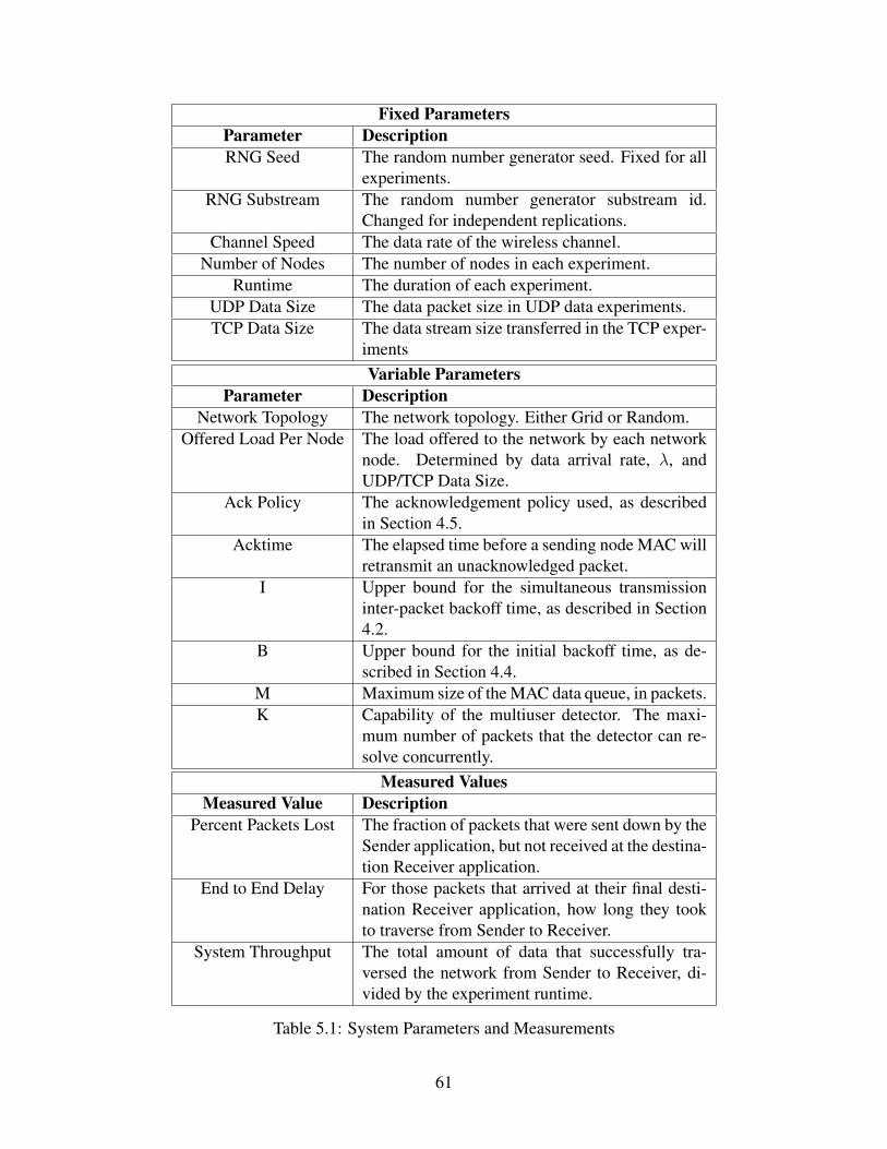
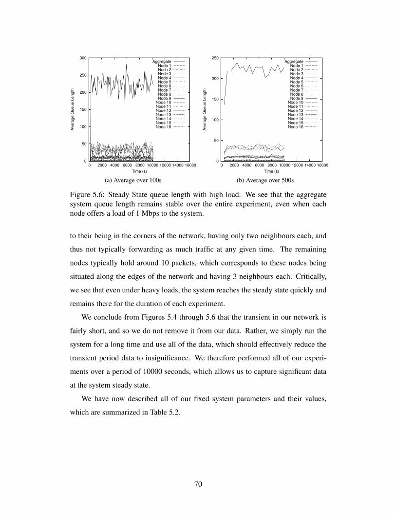
Chapter 5 opens the discussion of our performance study. In this chapter we
describe our experimental setup, node configuration and method of generating data
traffic across the network, as well as describe our measurements and performance
parameters. Our results are presented in Chapter 6. Finally, we conclude and dis-
cuss some avenues for future work in Chapter 7.
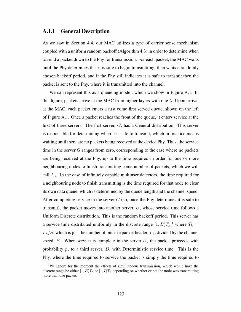
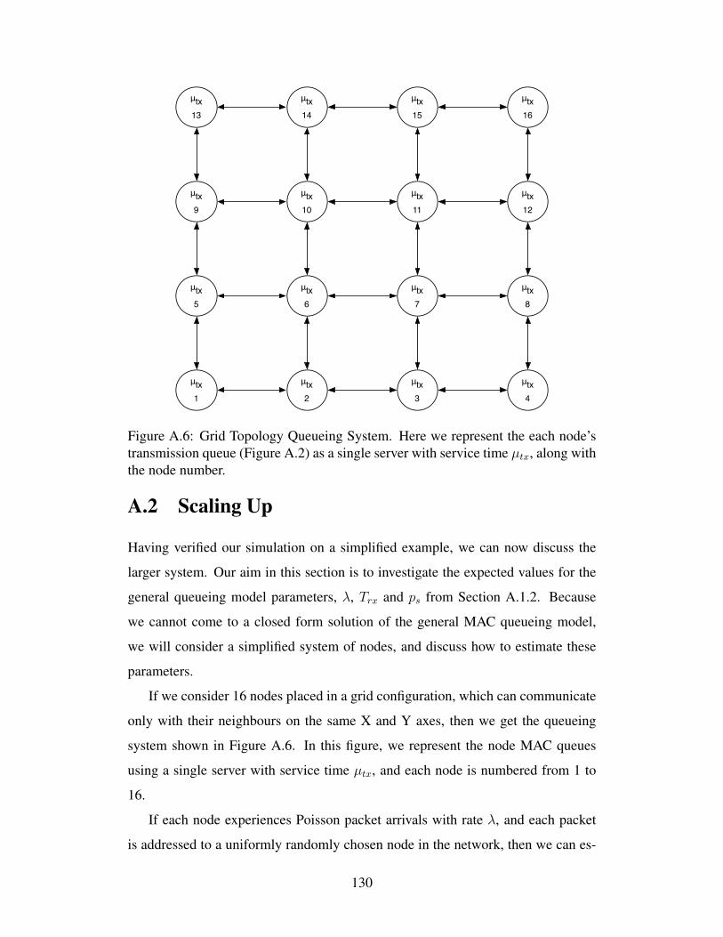
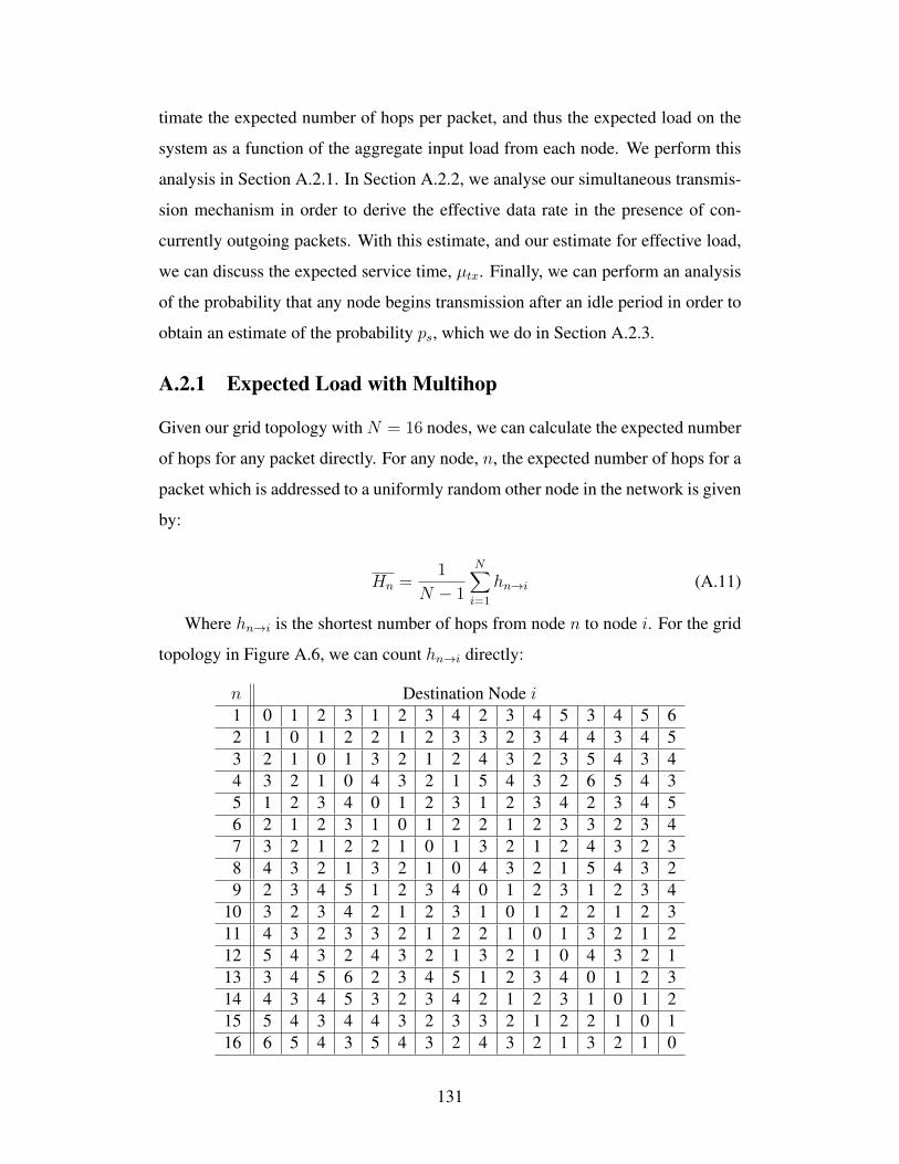
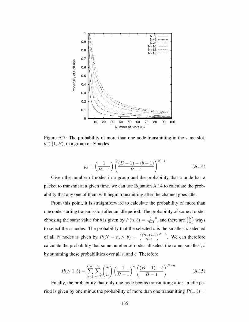
Appendix A discusses a theoretical model of our system, which we use to verify
our model on a simplified example.
8
Chapter 2
Related Work
In this chapter, we present a brief literature review of methods for improving wire-
less link reliability with a focus on their application in ad hoc networks. We begin
in Section 2.1 with a discussion of some classical ways of dealing with the problem
posed by interference and collisions, including carrier sense and collision avoid-
ance (CSMA/CA), time division (TDMA), frequency division (FDMA), and code
division (CDMA). After briefly evaluating these types of systems and their appli-
cation in ad hoc networks, we discuss RP-CDMA as a promising choice for ad hoc
networks in Section 2.2.
2.1 Other Approaches to Improving Network Relia-bility
We discussed in Chapter 1 the problem posed by the unreliable wireless medium,
and concluded that the primary difficulty was that transmissions interfere with each
other and cause packets to become unresolvable, which necessitates coordinating
access to the channel. There have been many attempts to resolve this problem, with
varying degrees of success [29].
An obvious way to avoid collisions is to try to avoid transmitting at the same
time as other network nodes. This is the principle behind the popular carrier sense
multiple access with collision avoidance (CSMA/CA) mechanism, which is prob-
ably most widely known as the basis for the MAC in the popular 802.11 series
of IEEE standards [48] in which it is called the Distributed Coordination Function
9
(DCF). In this scheme, nodes sense the wireless medium and apply a clear channel
assessment algorithm to determine whether it is occupied or not. If the channel is
determined to be not busy for a short period of time then the node proceeds with
its transmission. If the channel is determined to be busy then transmission is de-
ferred until the channel is not busy, after which nodes apply a binary exponential
backoff waiting period before attempting transmission again. In this way, several
nodes all waiting to transmit into the channel will probabilistically have one node
begin transmitting first, which will prevent the others from transmitting at the same
time and thus prevent collisions. In addition to this basic CSMA/CA mechanism,
802.11 specifies an optional channel reservation mechanism in which nodes wish-
ing to transmit will attempt to reserve the channel via special control packets that
reserve the channel (RTS) and acknowledge that it is reserved (CTS). Nodes which
overhear the RTS/CTS exchange will hold their own transmissions until the nodes
which reserved the channel have completed their transmission.
The RTS/CTS mechanism is intended to alleviate the hidden node problem,
which occurs when two nodes which cannot communicate with each other have
a shared neighbour. In this instance both of the nodes may sense the channel to
be free while the other is transmitting, which causes collisions and packet loss at
their shared neighbour. The intent with the 802.11 RTS/CTS mechanism is for both
sender and receiver to broadcast their channel reservation, which should prevent
hidden nodes from transmitting. Unfortunately, because the communications range
of the 802.11 radio is less than the interference range, there exists a space around
each node in which it is impossible to detect the channel reservation RTS/CTS ex-
change, but nonetheless possible to cause interference at the receiver. K. Xu et
al.[55] studied this problem and determined that an effective solution would be
for nodes to artificially limit which other nodes they communicate with, which
they view as a suboptimal solution to the problem. The converse of the hidden
node problem is the exposed node problem, which is caused when a given node ob-
serves a channel reservation RTS and holds its transmission, but is actually too far
away from the intended receiver to cause interference. The exposed node, therefore,
wastes potential bandwidth.
10
Because the 802.11 CSMA/CA mechanism is vulnerable to the hidden and ex-
posed node problems, and the RTS/CTS channel reservation mechanism is of lim-
ited effectiveness, S. Xu et al.[56] concluded that 802.11 is not suitable for multihop
ad hoc networks. Additionally, the RTS/CTS serves as an example of the limited
utility of attempting to coordinate access to the contended channel using the channel
itself. If the primary problem with the shared wireless channel is packet collisions
and interference, adding another layer of coordination packets into the channel may
be counterproductive. This is the conclusion reached by Ray et al.[40], who con-
cluded that in the ad hoc context, the addition of RTS/CTS packets eventually leads
to congestion and decreased performance under increasing load.
There have been several attempts to modify the 802.11 DCF to avoid or alleviate
its problems, such as adding scheduling on top of the RTS/CTS exchange [33] or
coordinating non-interfering transmissions together [5], or predicting interfering
transmissions using node topology [34, 19], but none of them fully overcome the
limitations of the CSMA/CA and RTS/CTS approach to avoiding collisions.
Rather than attempt to avoid collisions in a single shared channel, an alternate
approach is to separate transmissions into non-interfering channels. There are three
common ways in which we can perform channel separation: using time, frequency
or code division. A channel is therefore one of a time slot, a frequency band, or a
spreading code. Each of these mechanisms has their own challenges.
In general terms, channel separation techniques in ad hoc networks typically
proceed similarly, following the same basic steps:
1. Nodes are synchronized into a series of rounds. At the beginning of each
round, nodes all join the control channel.
2. Nodes who wish to communicate with one another indicate their desire to do
so using some channel reservation exchange.
3. Successful channel reservations either select or are allocated a channel.
4. Transmitting or receiving nodes switch to their allocated channels and ex-
change data.
11
The immediate problem with channel separation schemes that operate in this
manner is the synchronization of all the nodes in order to coordinate the channel
separation. Because ad hoc networks do not have any central authority or base sta-
tion which can dictate synchronization information, nodes must somehow decide
collectively when rounds begin and end. Fundamentally, this is the same prob-
lem that synchronization is attempting to solve: In order to not interfere with one
another, nodes must coordinate their transmissions, but in order to coordinate their
transmissions they must coordinate synchronization. Synchronization must be done
over the wireless channel itself, which makes synchronization vulnerable to inter-
ference and packet collisions. This is precisely the problem that motivates us here
to find a coordination-free ad hoc MAC.
Nonetheless, there exist channel separation mechanisms which attempt to per-
form each of time, frequency and code division. Zhu et al.[58] and Tang et al.[53]
both attempt TDMA in ad hoc networks, with varying success, while So et al.[46]
describe a FDMA system that envisions an 802.11 style RTS/CTS mechanism uti-
lizing multiple frequency channels. All of these systems require very tight timing
synchronization in order to operate effectively, and all are vulnerable to errors in-
troduced by coordination failures. FDMA systems such as the one presented in
[46], which have nodes switching their radios to different channels, are addition-
ally susceptible to a novel form of the hidden node problem in which some node
misses channel coordination traffic at the beginning of a round and selects the same
channel as another node for transmission.
Recently, Veyseh et al.[54] proposed a novel FDMA system that utilizes or-
thogonal frequency division multiple access (OFDMA) to separate transmissions
into OFDM subcarriers. OFDM is an increasingly popular choice for high capacity
broadband networks [57], and has been selected by the 3rd Generation Partnership
Project (3GPP) mobile phone standards group for the recently launched Long Term
Evolution (LTE) standard [1]. The appealing property of OFDM based systems
is that, while signals are separated into many subcarriers on separate frequencies
(called tones), all communications take place in a single frequency band. The or-
thogonal, frequency divided subcarriers are separated at the receiver using a fast
12
fourier transform (FFT), which means that if several users are communicating si-
multaneously on different groups of subcarriers then a single receiver can success-
fully decode all of them simultaneously. The ad hoc protocol proposed in [54]
proposes to do exactly this, and assigns users individual sets of tones which they
use to communicate. The proposed protocol avoids the global synchronization of
nodes by employing local synchronization between a single sending node and sev-
eral receivers. The coordination problem is not completely alleviated, however, and
a node which wishes to transmit must still initiate a transmission via request through
a control channel and negotiate which subcarriers will be used for which transmis-
sions. This coordination is subject to failure just as in any other protocol, and the
time required to perform coordination negatively affects system performance.
Rather than coordinating access to time slots, frequency bands or subcarriers,
CDMA systems coordinate access to spreading codes. The use of spreading codes
in CDMA systems allows for the joint detection of overlapping transmissions, and
makes CDMA systems resistant to interference and collisions. In these systems,
each outgoing bit is multiplied (spread)1 in the transmitter by a high frequency
pseudo-noise signal, which turns the bit signal into high frequency ’noise’ in the
channel. At the receiver, the same code is applied to the noise, which results in the
signal being recovered (despread). If multiple signals overlap at the receiver, the
application of each signals’ spreading code to the aggregate noise can return each
original signal in turn, which makes CDMA very attractive as the basis for an ad
hoc network radio. If we can allow for the overlapping of signals at the receiver and
still recover them, then we have effectively solved the collision problem and found
our reliable wireless link.
In order for a receiving node to be able to recover a CDMA signal from one of
its neighbours it must first know what spreading code was used at the transmitter.
This either requires nodes to have codes assigned to them ahead of time and which
are globally known, or it requires nodes to coordinate their communications using
a control channel. In the ad hoc context it is often impractical to assign codes to all
1Multiplied in this context typically means the bit signal is combined with the string of pseudo-random 0 and 1 bits using exclusive or (xor).
13
nodes and then distribute the book of codes to all of the other users, so codes are
typically selected through an on-line coordination process as they are needed. Typ-
ical schemes of this type have been proposed by Jin et al., which either have nodes
elect a single node to act as a temporary or pseudo base station [21], or which rely
on a channel reservation process much like RTS/CTS [22]. Thus, CDMA systems
in the ad hoc context typically suffer from the coordination problem as much as
their TDMA and FDMA counterparts.
However, the dominant problem in CDMA systems is not the coordination prob-
lem, but rather the near-far problem, which severely limits the ability of network
nodes to resolve overlapping signals [38]. Without this ability to resolve overlap-
ping transmissions there is little incentive to use CDMA at all, as the resistance to
interference and collisions properties are lost. The near-far problem occurs when
two incoming signals arrive with highly variable signal strengths, which is com-
mon when one transmitter is very near to the receiver and the other transmitter is
relatively far away. When this happens, the far signal is not recoverable even after
despreading because the near signal drowns it out. Thus, CDMA based ad hoc sys-
tems must coordinate their transmission powers as well as their codes in order to
achieve high performance over irregular ad hoc topologies.
Attempts to address the near-far problem typically involve adding power con-
trol information into the channel reservation process, such as in the proposal by Su
et al.[52], which proves to be more effective than similar schemes which do not
include power control. But by this point we are quite far from our intended aim,
which was to find a coordination-free ad hoc MAC protocol. If we wish to use
conventional CDMA detectors in our ad hoc network we must coordinate the distri-
bution of spreading codes and the transmission powers of each node in the network,
all in a distributed fashion. Even with all of this, coordination failures can still lead
to reliability problems, as all of this coordination is done over the wireless channel
itself.
In summary, single channel ad hoc systems tend to suffer from packet collisions,
and attempts to avoid collisions using CSMA/CA are prone to error. Attempts to
resolve these errors with coordination functions such as the 802.11 RTS/CTS mech-
14
anism are not entirely effective, and may actually be counterproductive. Thus, it is
natural to investigate channel separation schemes for ad hoc networks as a means
to separate different users’ transmissions from one another. Channel separation
systems typically involve either tight time synchronization or some other form of
distributed coordination to control access to a limited number of time slots or fre-
quency bands, which reduces the error potential from all traffic in the single channel
to only the coordination traffic in the coordination channel, but which nonetheless
is still prone to error in the same way. CDMA systems are promising due to their
inherent resistance to interference, which promises to remove the requirement for
node synchronization, but they also introduce new problems of code and power
coordination between nodes.
It is with this in mind that we turn our attention to Random Packet CDMA
(RP-CDMA), which uses a novel packet format to overcome the requirement to co-
ordinate spreading codes, and a powerful multiuser detector to overcome the near-
far problem. With these problems resolved, RP-CDMA appears to be a promising
candidate for a reliable ad hoc wireless link.
2.2 Random Packet CDMA
RP-CDMA was first proposed by Kota and Schlegel et al. [28, 42], as a means
of uncoordinated, random channel access. In this initial effort, data packets were
transmitted in two parts by sending the packet header over a common header chan-
nel and the packet payload in a randomly selected data payload channel. The header
portion of each packet contained only enough information to identify and decode
the remainder of the packet in the payload channel, and the header channel was
thus comparatively lightly loaded under the assumption of large payloads. Each
node would listen to the header channel in order to identify transmissions in the
payload channels, and thus no coordination between nodes was required in order to
exchange spreading codes. Packet payloads were decoded in a multiuser detector,
which is a CDMA receiver capable up decoding up to K overlapping transmis-
sions simultaneously. The header channel was modelled as a lightly loaded Spread
15
ALOHA channel, and the system was found to be limited by the capability of the
multiuser detector, K. With the use of iterative decoding in the multiuser detec-
tor, the authors concluded that the system could approach the Shannon limit of the
multiple access channel and was therefore limited by the capability of the multiuser
detector, as opposed to collision-limited in the common header channel. This is an
important result, since the common header channel is the only contended resource
in the RP-CDMA system. By showing that random access to this common resource
was sufficient to approach the information-theoretic bound on capacity, the system
was freed from the requirement to coordinate between nodes for wireless medium
access. This work was confirmed with traffic scenarios involving alternating light
and heavy users, along with a capacity analysis in Kempter et al.[24].
Kempter [25] subsequently examined the application of various multiuser de-
tectors in the RP-CDMA system in an effort to determine what kind of multiuser
detector would be required to match the initial results presented in [42], which as-
sumed an ideal detector capable of decoding any packet identified from the header
channel. This work confirmed that the header channel is not collision-limited, but
rather limited by the capability of the receiver in both the header detector and pay-
load multiuser detector. Various types of multiuser detectors were considered in
both [25] and [26], which concluded that a Partitioned Spreading CDMA receiver
performed best both in terms of reasonable spreading code lengths and resistance
to the near-far effect, but critically illustrated that high system performance could
be maintained even under high load [26].
Nagaraj et al. applied a CSMA channel access scheme to the common RP-
CDMA header channel in [35], and determined that overall system throughput
could be improved over the spread ALOHA random access case under particu-
lar traffic scenarios. Subsequently, Nagaraj et al.[36] reexamined the performance
characteristics of a random channel access scheme with a multiuser detector, and
concluded that as multiuser detector capability goes to infinity, system throughput
asymptotically approaches the optimal value. This result is both derived analyti-
cally and confirmed with simulations on a fully connected network with a simplified
packet reception model.
16
Although random access may be optimal in the limit of multiuser detector capa-
bility, it is not optimal with limited detector capability. For the case of the limited
multiuser detector, Ghanbarinejad et al. proposed an adaptive probabilistic MAC
protocol for multiuser detector capable systems in which nodes used channel traffic
estimates to feed a probabilistic model of whether a node transmitted or not in a
given time slot [16, 17]. This work is similar in spirit to that presented by Kempter
et al.[24], which also adopted a feedback based adaptive MAC, and also concluded
that an adaptive probabilistic model is suitable for maintaining traffic loads below
the multiuser detector limit, K, compared to ALOHA style random transmission.
We found that much of the literature is focused on the relative performance of
various types of multiuser detectors, such as Kempter et al.[25, 26], or interested in
developing MAC protocols which maximize transmitter parallelism, such as Ghan-
barinejad et al.[16]. As a result, network configurations or simulations are typically
simplified to include a single receiver and several transmitters, as in [16], or sim-
ply to consider the probability of header collisions in the common header channel
as a measure of successful transmission, as in [42]. These approaches address the
transmission side of the packet transfer process, but ignore the state of the receiv-
ing node and specifically ignore whether the intended receiving node is actually
prepared to receive when a transmission begins. The CSMA work of Nagaraj et
al.[35] includes a notion of node behaviour during neighbour transmissions in their
performance evaluation, but this work appears to also consider only the probability
of a packet header collision and the probability of exceeding the detector capabil-
ity as the basis for system throughput. While these performance measures may be
appropriate in the case of a base station style of network in which multiple nodes
all communicate only with a powerful base station, it is not clear that it applies to
the multihop ad hoc network case. Specifically, in an ad hoc network it is not only
required that there be no header collision for a transmission to be successful, but it
is also required that the intended receiver not be transmitting at the same time, as a
half duplex radio cannot simultaneously transmit and receive. This aspect appears
to often be overlooked in the literature we surveyed. A node may find the header
channel unoccupied when it wishes to transmit, but if it is currently receiving one
17
or more packet payloads - which may or may not be intended for it - then it cannot
switch to transmit unless it is willing to drop the current incoming packet(s). Simi-
larly, a node may find the header channel unoccupied when having a packet to send
to some neighbouring node, but if the neighbour is transmitting a packet payload
then it makes no sense to begin transmission to it until it finishes transmitting itself.
Thus, the state of the receiving node is an important factor when deciding whether
or not a particular transmission was successful.
With this in mind, we are focused on the application of RP-CDMA in a multihop
ad hoc network. Our survey of the literature provides evidence that the application
of a multiuser detector in ad hoc networks may have significant reliability and per-
formance advantages. Specifically, we believe that a sufficiently powerful multiuser
detector can let us approach the capacity of the multiple access channel, but we feel
that realistic ad hoc network conditions have not been adequately considered to this
point. As such, we seek to confirm that RP-CDMA can be applied successfully in
a general multihop ad hoc environment via network simulation.
18
Chapter 3
Random Packet CDMA
RP-CDMA is a novel wireless CDMA protocol in which each packet is encoded in
two parts [42]. The packet header is encoded with a common spreading code that is
known to all nodes, and the payload is encoded with a randomly generated spread-
ing code. An identifier for the payload spreading code is placed in the header, so, as
a receiving node decodes the packet header, they obtain the code used to decode the
payload. Thus, each packet is self contained and any network node is able to decode
any packet in the network without any requirement to know beforehand which pay-
load code was used. When combined with a multiuser detector, RP-CDMA enables
a single node to receive several packets concurrently.
In this chapter, we first discuss RP-CDMA in general and follow with the de-
tails of our simulated implementation. Our general discussion of RP-CDMA in-
cludes its fundamental characteristics, including packet composition and transmis-
sion, spreading code selection, effective bandwidth and channel capacity. We then
discuss multiple packet reception and how the multiuser detector enables the recep-
tion of concurrent packets. These general properties are put into the context of our
reliable link properties from Chapter 1, and we will see how RP-CDMA addresses
each of them. With this theoretical discussion completed, we describe in detail how
our simulated RP-CDMA network device works, and describe the algorithms used
in our simulated device in order to transmit and receive packets.
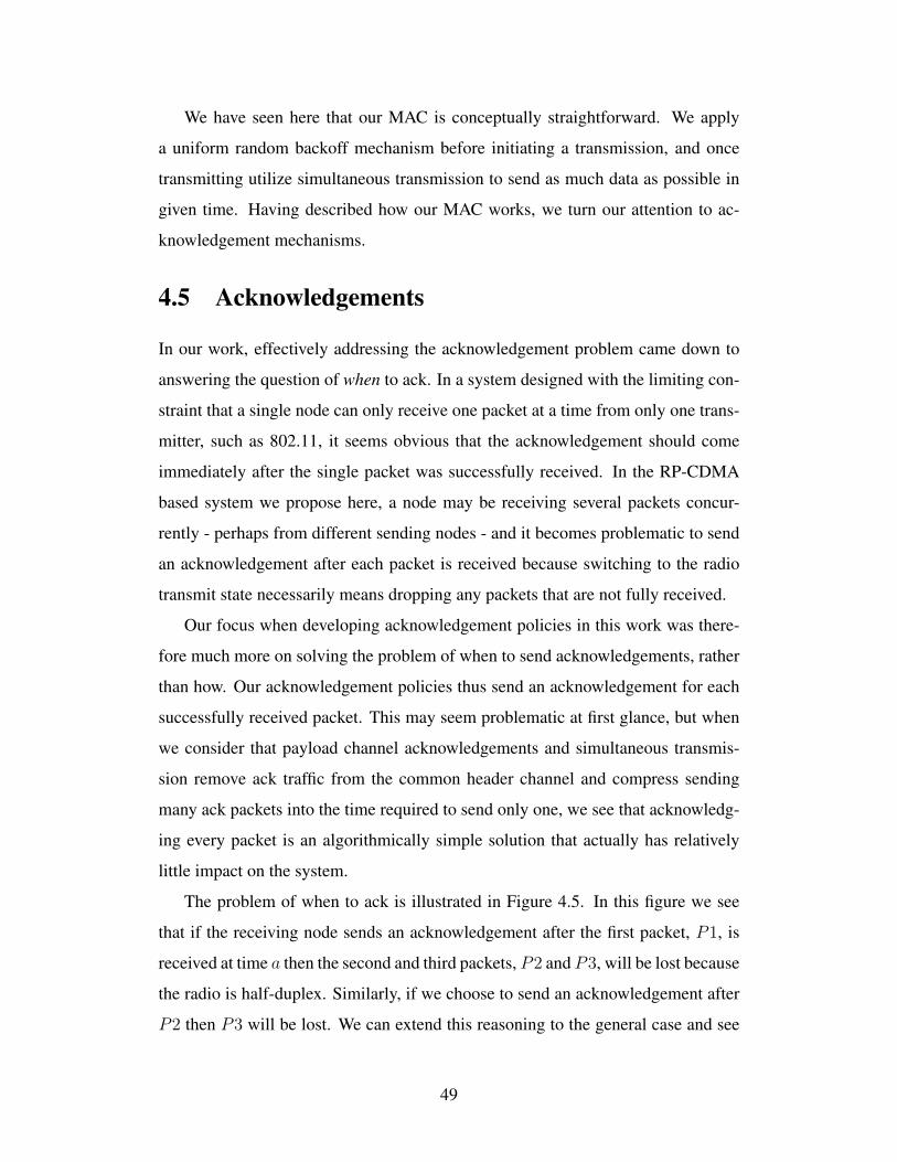
19
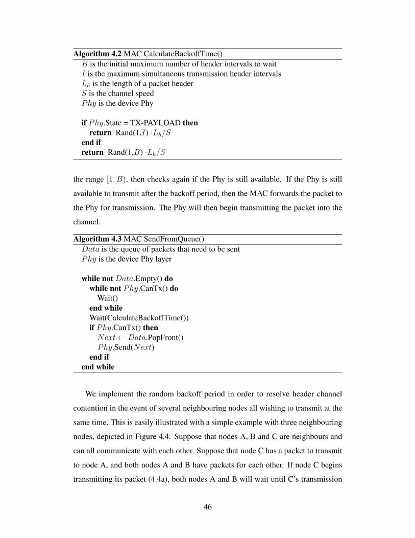
sync code id data
Packet HeaderLh
Packet PayloadLd
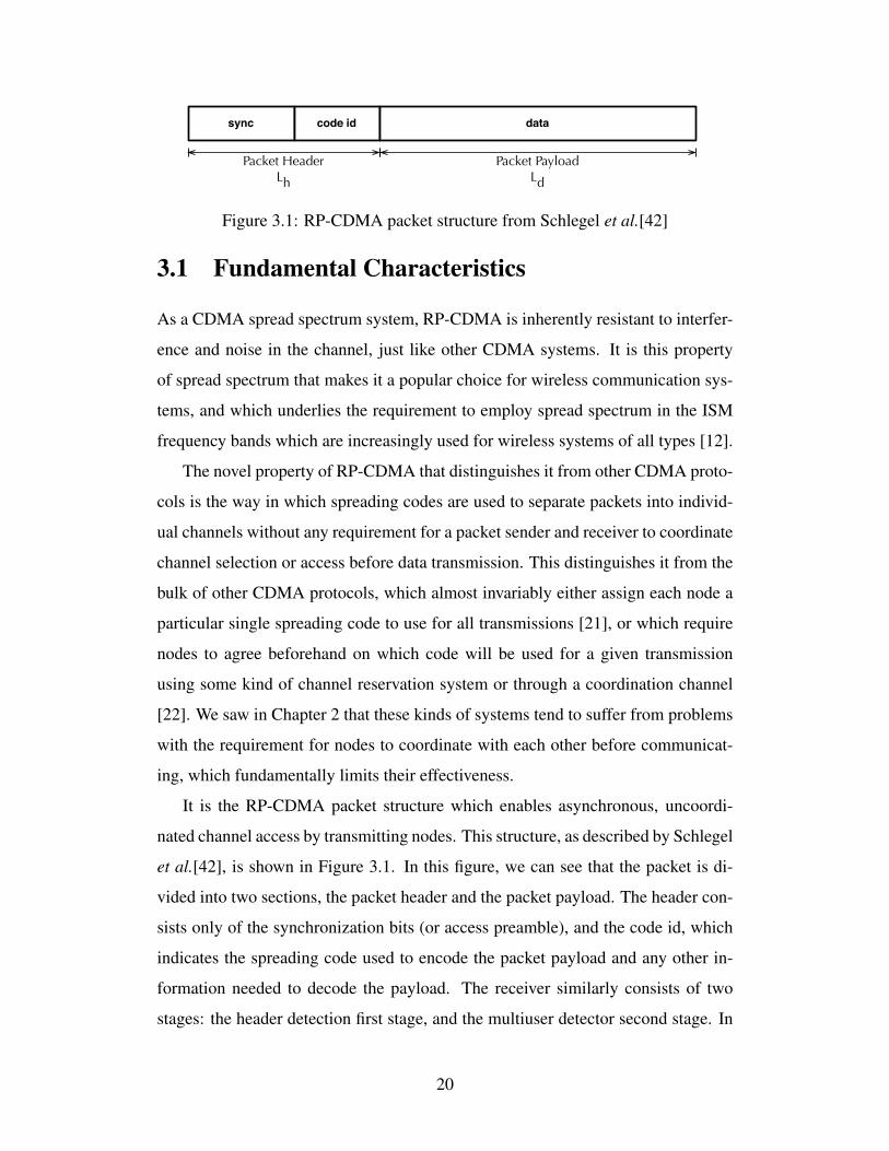
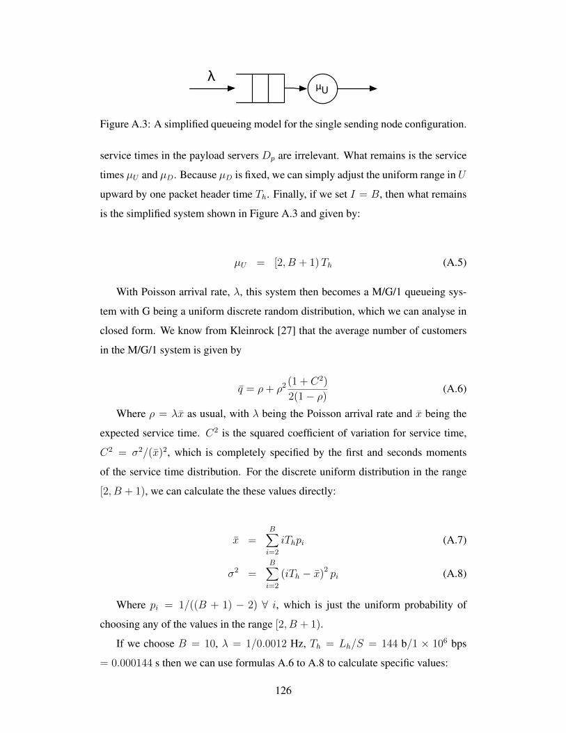
Figure 3.1: RP-CDMA packet structure from Schlegel et al.[42]
3.1 Fundamental Characteristics
As a CDMA spread spectrum system, RP-CDMA is inherently resistant to interfer-
ence and noise in the channel, just like other CDMA systems. It is this property
of spread spectrum that makes it a popular choice for wireless communication sys-
tems, and which underlies the requirement to employ spread spectrum in the ISM
frequency bands which are increasingly used for wireless systems of all types [12].
The novel property of RP-CDMA that distinguishes it from other CDMA proto-
cols is the way in which spreading codes are used to separate packets into individ-
ual channels without any requirement for a packet sender and receiver to coordinate
channel selection or access before data transmission. This distinguishes it from the
bulk of other CDMA protocols, which almost invariably either assign each node a
particular single spreading code to use for all transmissions [21], or which require
nodes to agree beforehand on which code will be used for a given transmission
using some kind of channel reservation system or through a coordination channel
[22]. We saw in Chapter 2 that these kinds of systems tend to suffer from problems
with the requirement for nodes to coordinate with each other before communicat-
ing, which fundamentally limits their effectiveness.
It is the RP-CDMA packet structure which enables asynchronous, uncoordi-
nated channel access by transmitting nodes. This structure, as described by Schlegel
et al.[42], is shown in Figure 3.1. In this figure, we can see that the packet is di-
vided into two sections, the packet header and the packet payload. The header con-
sists only of the synchronization bits (or access preamble), and the code id, which
indicates the spreading code used to encode the packet payload and any other in-
formation needed to decode the payload. The receiver similarly consists of two
stages: the header detection first stage, and the multiuser detector second stage. In
20
the first stage, the receiver synchronizes to the header synchronization bits and ac-
quires the timing of the incoming packet. Once timing is recovered, the first stage
of the receiver decodes the code id portion of the packet, which contains all of the
information required to decode the packet payload, and hands this off to the second
stage along with the timing information. The second stage then decodes the packet
payload, recovering the data.
Because all nodes use the same spreading code to encode packet headers, any
node in the network can decode any packet header, and therefore can decode any
packet in the network. Fundamentally, this enables network nodes to operate asyn-
chronously, as there is no requirement to coordinate transmissions with other nodes
in order to exchange spreading codes or timing information.
3.1.1 Spreading Code Selection
The way in which the packet header is transmitted, in terms of spreading code used
or data encoding scheme, does not have to be the same as that of the payload in the
RP-CDMA system. It is in fact reasonable to select a stronger spreading code or
higher transmission power for the packet header than for the payloads because the
header channel is the only practically contended channel in the RP-CDMA system
[25].1 Thus, it is possible that multiple headers using the same spreading code
could overlap at a single receiver, and because the header detection stage is critical
in acquiring the packet timing, we may therefore employ a longer spreading code
for the packet header in order to achieve more gain, transmit headers with more
power, or we may choose a spreading code that has a low degree of autocorrelation.
For the payload spreading codes, we may employ any class of spreading codes
that we like, so long as there are sufficient codes such that it is unlikely that any
two neighbouring nodes will select the same code at the same time. Schlegel et
al.[42] suggest maximal length sequences (m-sequences) as possible candidates
due to their desirable autocorrelation and pseudorandom properties, but settle on
1Technically, the payload channels are also contended, but we shall see that by allowing for avery large number of payload channels the probability that two neighbouring nodes simultaneouslyselect the same one is insignificant, which is why we say the header channel is the only practicallycontended resource.
21
random codes for the purposes of their analysis. This is a reasonable choice in the
asynchronous ad hoc environment, since asynchronously arriving packets will be
randomly offset from one another anyway, which will change the correlation values
between any specifically chosen set of codes.
3.1.2 Bandwidth and Channel Capacity
The bandwidth of a CDMA system is given by the length of the spreading code
employed and the bandwidth of the unspread signal, using Ws = GWd, where Ws
is the bandwidth of the spread signal, G is the spreading gain (which is the same
as the length of the spreading code), and Wd is the bandwidth of the original data
signal, which depends on the rate of carrier modulation, which for binary signalling
is simply Wd = 2R, where R is the data rate [51]. RP-CDMA is no different from
other CDMA systems in this regard, and the bandwidth occupied by RP-CDMA
depends on the length of spreading codes used in both the packet header and pay-
load. Because RP-CDMA is intended to be used for overlapping signals, the codes
chosen should be long enough to provide a low error rate in the low signal to noise
environment. Throughout our work, we assume a data rate of R = 1 Mbps, and
thus we will always assume the bandwidth of the RP-CDMA signal is given by
Ws = GWd = 2KR = 2K, where we assume that the number of users supported
by the multiuser detector, K, is equal to the length of the spreading codes used,
G, so we assume K = G. It is worth pointing out that Ws = 2K is a somewhat
pessimistic assumption, as more sophisticated signalling can achieve modulation
rates less than the data rate, and the number of users supportable in some multiuser
detectors is greater than the spreading code length. In particular, it should be pos-
sible to achieve K = 2G with sufficiently powerful decoders [42], but we assume
K = G throughout this dissertation.
The upper bound on the capacity of the channel is given by the Shannon limit
[51]:
C = Ws log2(1 + SNIR) (3.1)
Where C is the channel capacity in bits per second, Ws is the bandwidth of the
22
channel in Hertz, and SNIR is the signal to interference plus noise ratio, SNIR =
Ps
N0+∑N
i=1Pi
. SNIR is simply the ratio of the signal power to the cumulative other
noise in the channel, which is just the thermal noise, N0, plus the sum of the signal
strength of all the other transmissions in the channel, denoted by the sum of the
individual signal strengths, Pi.
In RP-CDMA , the upper limit of the channel capacity thus depends on the band-
width used - which itself depends on the spreading code length - and the relative
signal strengths of all the signals in the channel. For our purposes, we are mostly
interested in the performance of our MAC protocol on top of the RP-CDMA link.
It has been established in the literature that with a sufficiently capable multiuser de-
tector it is possible to approach the Shannon limit for channel capacity [42, 25, 43],
and so we work within this result. Specifically, we assume a fixed data rate for our
transmissions of 1 Mbps, and leave the details of the data encoding, transmission
power levels, and multiuser detector decoding processes alone. This is not unusual,
as the literature routinely assumes, for the purposes of analysis, that a multiuser de-
tector of capability K can successfully decode up to K overlapping signals without
error, leaving aside the same transceiver operation details, as in [16, 36].
3.2 Multiple Packet Reception
A basic iterative multiuser detector consists of a simple interference suppression
stage in front of a parallel bank of single channel decoders [44, 43]. The interfer-
ence suppression stage takes the aggregate received signal in and passes it to the
single channel decoders. As the decoders successfully decode their data, they pass
it back to the interference suppression stage, which then modifies the received sig-
nal passed back to the decoders. This feedback loop between the decoders and the
interference suppression stage allows for the iterative decoding of all of the indi-
vidual signals comprising the aggregate received signal. A multiuser detector with
capability K can decode up to K overlapping signals simultaneously, with the de-
coders made up of a fixed bank of decoding circuits, or possibly software processes
started up on demand by the receiver as packets arrive [42, 28].
23
There have been several types of multiuser detector proposed and studied in the
literature, such as the simple linear matched filter, the decorrelator, and the min-
imum mean squared error (MMSE) decoder [44]. There are also decoders which
perform iterative signal cancellation, such as that proposed by Holtzman [18], and
which integrate signal cancellation with other techniques, such as in Partitioned
Spreading [41, 25]. Iterative cancellation decoders perform just as well as other
decoders when the signals arrive with equal power, but have an advantage when
multiple signals arrive with different power levels [42, 8, 25]. In this case, the it-
erative cancellation of signals allows the receiver to successfully decode all of the
incoming packets from strongest signal to weakest, in what is sometimes called
’onion-peeling’ [44, 25]. This property provides the receiver with inherent near-far
resistance [41], which we have already seen is a problem in CDMA systems, and
particularly in ad hoc CDMA systems.
Because of their performance with unequal signal powers, we will assume through-
out this dissertation that the multiuser detector employed in the RP-CDMA device
is of the iterative signal cancellation kind. The use of an iterative cancellation mul-
tiuser detector in RP-CDMA enables the final desirable property of the system by
eliminating the requirement for nodes to coordinate their transmission power levels,
which is the last problematic coordination point for CDMA systems. The employ-
ment of an iterative cancellation receiver allows RP-CDMA network nodes to trans-
mit with whatever power level seems appropriate for their purpose, and specifically
without input from their neighbours.
In addition to eliminating the need for nodes to coordinate with one another be-
fore transmitting, the capability of the multiuser detector to better resolve signals
when they are distributed in signal strength indicates that we can utilize transmis-
sion power as a second axis - in addition to time - in which to separate transmissions
within a given frequency band. Signals arriving in the same frequency band at the
same time can be successfully recovered using iterative cancellation from the most
powerful signal to the weakest signal. This property turns the near-far problem from
a weakness of CDMA systems to a strength. We will return to this in Chapter 4.
24
3.3 Desirable Properties
In summary, because RP-CDMA employs code division, individual signals are re-
sistant to external interference in the same way as traditional CDMA systems. By
placing payload spreading codes in packet headers, each packet is transmitted in
a private channel and is decodable by any node in the network, with no require-
ment for coordination between nodes before transmitting data. Finally, the ability
to simultaneously decode multiple packets spread over a range of signal strengths
eliminates the need for nodes to coordinate their transmission powers. Thus, there
is no requirement for nodes to coordinate their transmission at all in the RP-CDMA
system, and, in these ways, RP-CDMA can achieve much of what we want from a
wireless link:
1. Random payload codes provide packet level private channels, except for packet
headers.
2. Code division provides resistance to interference, both external and from
other packets.
3. Multiple packet reception and packet formatting eliminate the need for chan-
nel access coordination.
Having now discussed what RP-CDMA is, how it works, and why it seems
promising as a basis for our reliable link, we can now move on to a discussion of
how we simulate it in ns-3.
3.4 Simulation of RP-CDMA
We simulate RP-CDMA in ns-3 through a custom network device. Since our aim
is to design a MAC protocol that uses a RP-CDMA based Phy to build an efficient
wireless network device, we must simulate the RP-CDMA Phy. We simulate this
down to the level of packets being sent through a wireless channel to other nodes
in the network. At this level we simply pass packets between nodes as a series of
bytes, and so do not simulate the actual encoding of bits or transmission waveforms.
25
In general, a packet passed from the MAC layer to our RP-CDMA based Phy
will have a randomly selected payload spreading code assigned to it, the RP-CDMA
Phy header prepended, and be sent into a common wireless channel from which
it is received by all other nodes in the channel. The receiving Phy must decide
whether the received signal can be decoded based on the state of the receiver and
the instantaneous channel noise conditions, and then perform packet decoding in
the multiuser detector. In order for packet decoding to happen successfully, the Phy
must therefore simulate the working of a multiuser detector, as well as track the
noise level in the channel in order to measure interference.
In this section, we describe our simulated RP-CDMA Phy from the point of
view of a packet being sent down from the MAC layer from a transmitting node.
We follow the packet as it passes through the channel and into a receiving Phy. In
so doing, we describe our RP-CDMA Phy header, how we track channel noise, de-
code packet headers and payloads, and finally simulate the working of the multiuser
detector and pass packets up to the receiving MAC layer.
3.4.1 Simulator Preliminaries
Because we will discuss our algorithms, experimental design, and results in the
context of the simulator, it is useful at this point to briefly describe the simulator we
use, how it functions, and to what level of detail we simulate the network.
All of our simulations are performed with with the ns-3 network simulator.2
Though similarly named, ns-3 is not derived from the more familiar ns-2 project3,
but is an entirely new codebase and the respective development teams are not affili-
ated. That said, ns-3 aims to provide a highly realistic discrete event driven network
simulation stack upon which to perform network research down to the packet level
[30]. To this end, ns-3 provides a complete network stack, which allows researchers
to create realistic simulations from the application layer down to the physical layer
and into physical channels. At the application layer, programs have a normal net-
work sockets interface which takes packets and bytestreams. At the physical layer,
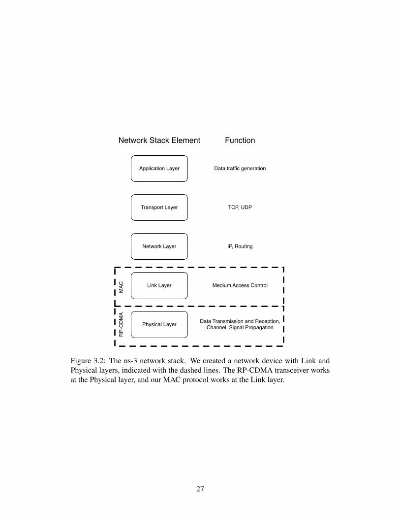
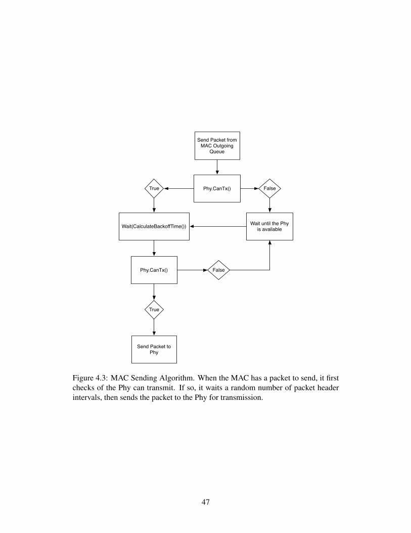
Data Transmission and Reception,Channel, Signal Propagation
MAC
RP-
CD
MA
Figure 3.2: The ns-3 network stack. We created a network device with Link andPhysical layers, indicated with the dashed lines. The RP-CDMA transceiver worksat the Physical layer, and our MAC protocol works at the Link layer.
27
channels provide facilities to model signal fading, interference and propagation de-
lay. The networking stack itself is modelled on the real world Linux kernel network
stack, to the degree that the actual network stack from a host Linux system can be
substituted for the simulator stack should a researcher wish to do so. Since the sim-
ulator is entirely software, it is possible for a researcher to simply modify various
parts of the realistic network stack and run simulations to evaluate performance.
This is, in fact, the network simulator’s raison d’etre.
The ns-3 network simulator is an event driven simulator. This means that the
passage of time is simulated simply by executing a series of scheduled events. Any
component in the simulation can schedule an event to occur at some point in the
future and defines what action to take when the event is triggered. Once triggered,
the simulator performs the scheduled action. In this way, we can incorporate the
passage of time into our simulations. For example, when a packet is transmitted
by some node into the channel, we calculate the arrival time of that packet at each
other node in the channel by considering the transmission propagation speed and the
distance between the nodes. Once the arrival time is calculated, we can schedule the
simulator to process the arrival of the packet at that time. In this way, the simulator
can drive the simulation simply by processing events in the order of their scheduled
execution times.
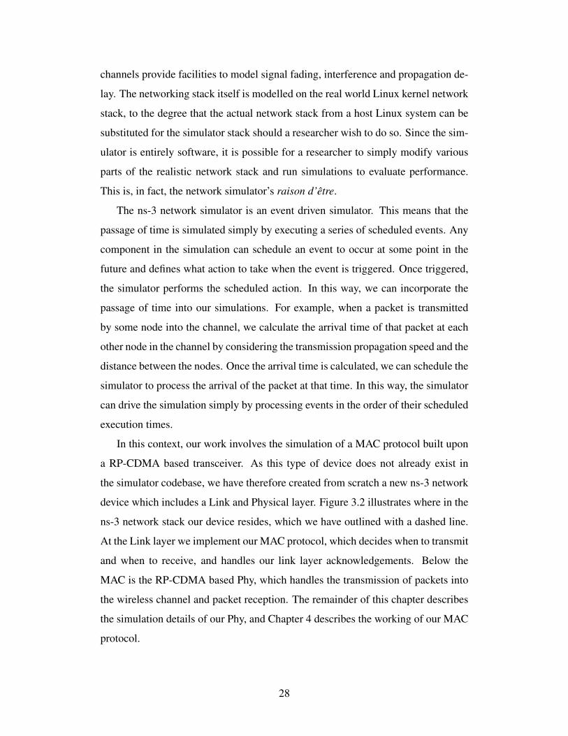
In this context, our work involves the simulation of a MAC protocol built upon
a RP-CDMA based transceiver. As this type of device does not already exist in
the simulator codebase, we have therefore created from scratch a new ns-3 network
device which includes a Link and Physical layer. Figure 3.2 illustrates where in the
ns-3 network stack our device resides, which we have outlined with a dashed line.
At the Link layer we implement our MAC protocol, which decides when to transmit
and when to receive, and handles our link layer acknowledgements. Below the
MAC is the RP-CDMA based Phy, which handles the transmission of packets into
the wireless channel and packet reception. The remainder of this chapter describes
the simulation details of our Phy, and Chapter 4 describes the working of our MAC
protocol.
28
3.4.2 Header Description
In the literature, the RP-CDMA header is usually described as containing only the
synchronization bits (or access preamble) and the payload code id [42, 28, 25].4
In theory, these two fields are all that is minimally required in order to identify the
packet payload and decode it, as they are sufficient for the radio receiver to first lock
on to the incoming transmission using the synchronization bits, and then identify
the payload spreading code to hand off to the multiuser detector for decoding. In
practice, the receiver needs to know other bits of information about the packet in
order to complete the decoding process, such as the length of the packet, any error
correction information, and any particulars about the encoding process such as the
amount of redundant information or information rate. This payload information
could be included in the packet payload itself, but we would then be putting the
payload decoder in the position of needing to decode some of the payload in order
to get all of the information required to decode the payload.
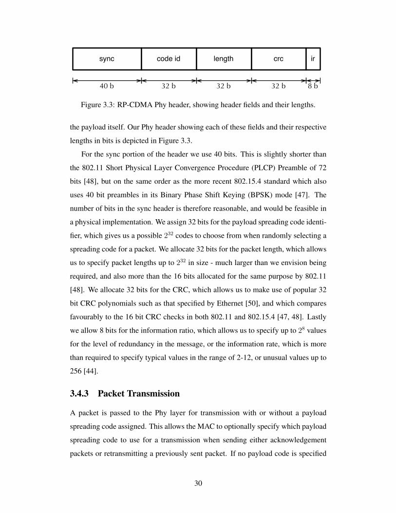
In our implementation, we include the synchronization bits, payload spread-
ing code id, packet length, packet cyclic redundancy check (CRC) and the packet
encoding information rate in the RP-CDMA Phy header. The extra fields beyond
the synchronization bits and the payload spreading code are included with the Phy
header instead of with the packet payload because they enable the multiuser detec-
tor to perform decoding of the payload without any additional information. Our
aim in doing this is to simplify the decoding of packet payloads in the multiuser
detector. To this end, we include the packet length so the multiuser detector will
know how long a packet is going to be, and thus when a specific transmission is
expected to end. The CRC is included so that the multiuser detector can easily per-
form basic error detection over the entire packet, and the information rate informs
the multiuser detector how much of the payload is redundant information to be used
for error detection and correction. Together, these fields enable the multiuser detec-
tor to decode the packet payload without having to consult any information inside
4We assume that the authors mean ’code id’ to be any information required to decode the packetpayload and not only the actual payload spreading code, but we could not find a detailed headerspecification in the literature.
29
sync code id length crc ir
40 b 32 b 32 b 32 b 8 b
Figure 3.3: RP-CDMA Phy header, showing header fields and their lengths.
the payload itself. Our Phy header showing each of these fields and their respective
lengths in bits is depicted in Figure 3.3.
For the sync portion of the header we use 40 bits. This is slightly shorter than
the 802.11 Short Physical Layer Convergence Procedure (PLCP) Preamble of 72
bits [48], but on the same order as the more recent 802.15.4 standard which also
uses 40 bit preambles in its Binary Phase Shift Keying (BPSK) mode [47]. The
number of bits in the sync header is therefore reasonable, and would be feasible in
a physical implementation. We assign 32 bits for the payload spreading code identi-
fier, which gives us a possible 232 codes to choose from when randomly selecting a
spreading code for a packet. We allocate 32 bits for the packet length, which allows
us to specify packet lengths up to 232 in size - much larger than we envision being
required, and also more than the 16 bits allocated for the same purpose by 802.11
[48]. We allocate 32 bits for the CRC, which allows us to make use of popular 32
bit CRC polynomials such as that specified by Ethernet [50], and which compares
favourably to the 16 bit CRC checks in both 802.11 and 802.15.4 [47, 48]. Lastly
we allow 8 bits for the information ratio, which allows us to specify up to 28 values
for the level of redundancy in the message, or the information rate, which is more
than required to specify typical values in the range of 2-12, or unusual values up to
256 [44].
3.4.3 Packet Transmission
A packet is passed to the Phy layer for transmission with or without a payload
spreading code assigned. This allows the MAC to optionally specify which payload
spreading code to use for a transmission when sending either acknowledgement
packets or retransmitting a previously sent packet. If no payload code is specified
30
by the MAC, then the Phy will randomly select a spreading code. With the payload
spreading code decided, the Phy will construct the Phy header for the packet, as
described above in Section 3.4.2, and begin the process for transmitting a packet
into the channel. Once the packet has been transmitted, the Phy will return the
payload spreading code to the MAC.
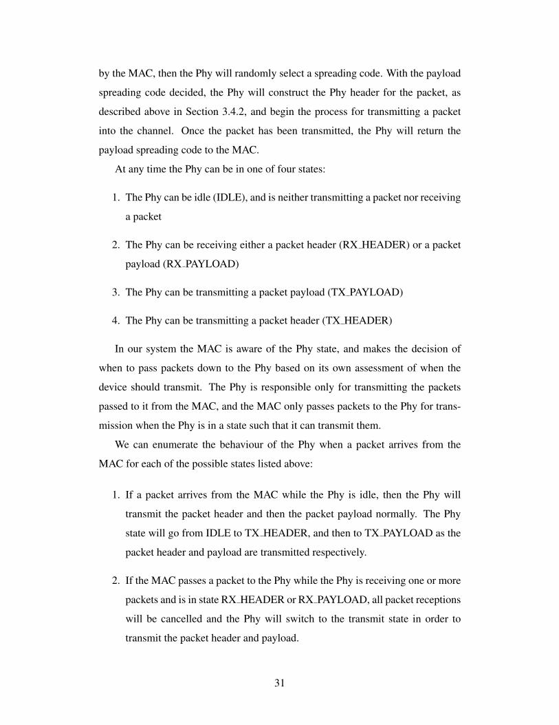
At any time the Phy can be in one of four states:
1. The Phy can be idle (IDLE), and is neither transmitting a packet nor receiving
a packet
2. The Phy can be receiving either a packet header (RX HEADER) or a packet
payload (RX PAYLOAD)
3. The Phy can be transmitting a packet payload (TX PAYLOAD)
4. The Phy can be transmitting a packet header (TX HEADER)
In our system the MAC is aware of the Phy state, and makes the decision of
when to pass packets down to the Phy based on its own assessment of when the
device should transmit. The Phy is responsible only for transmitting the packets
passed to it from the MAC, and the MAC only passes packets to the Phy for trans-
mission when the Phy is in a state such that it can transmit them.
We can enumerate the behaviour of the Phy when a packet arrives from the
MAC for each of the possible states listed above:
1. If a packet arrives from the MAC while the Phy is idle, then the Phy will
transmit the packet header and then the packet payload normally. The Phy
state will go from IDLE to TX HEADER, and then to TX PAYLOAD as the
packet header and payload are transmitted respectively.
2. If the MAC passes a packet to the Phy while the Phy is receiving one or more
packets and is in state RX HEADER or RX PAYLOAD, all packet receptions
will be cancelled and the Phy will switch to the transmit state in order to
transmit the packet header and payload.
31
3. If a packet arrives from the MAC while the Phy is transmitting a packet pay-
load, then the Phy will transmit the packet header and payload concurrently
with the already outgoing packet payload, with the Phy state switching to
TX HEADER and then back to TX PAYLOAD as the header and payload
go out. This is the basis of Simultaneous Transmission, which we discuss
in Section 4.2. If a packet arrives which brings the number of simultaneous
transmissions up to the limit of the multiuser detector,K, then the Phy signals
the MAC that no more packets can be transmitted.
4. The MAC will not pass a packet to the Phy when it is already transmitting
another packet header and is in the state TX HEADER.
We see then that once a packet is received from the MAC, the Phy will begin
transmitting it into the channel.
3.4.4 Channel Characteristics
Once transmitted from the Phy into the channel, the channel schedules packet ar-
rival at all other nodes in the channel. The distance, d, between the transmitting
node and each other node is calculated, and the transmission power, Ptx, is atten-
uated using the ns-3 Log Distance Propagation Loss Model, which decreases the
power at the receiver, Prx, using the formula:
Prx = Ptx − Lref − 10 · 3 · log10(d/dref ) (3.2)
Where Lref is the loss at the reference distance, dref , all distances are in metres
(m), and power is in decibels referenced to one milliwatt (dBm). For distances less
than the reference distance, d < dref , the signal strength is not attenuated, and so
Prx = Ptx. In ns-3, the default reference distance is 1.0 m, with Lref = 46.6777
dB, which is the Friis loss at 1 m and 5.15 GHz [30].
Once the power is attenuated with the propagation model, the packet is sched-
uled to arrive from the transmitter at each other node in the network using a straight-
forward constant speed delay, where the propagation delay is given by:
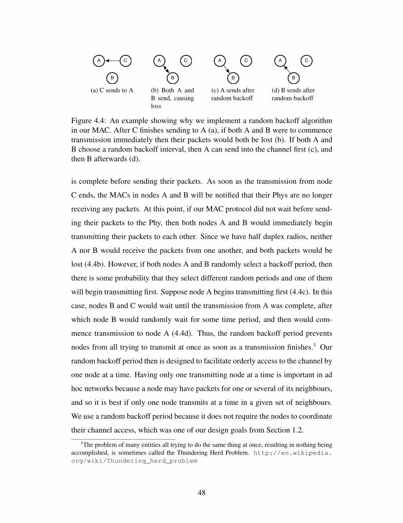
32
H P
H P
H P
H P
Time
Power
t1 t2 t3 t4
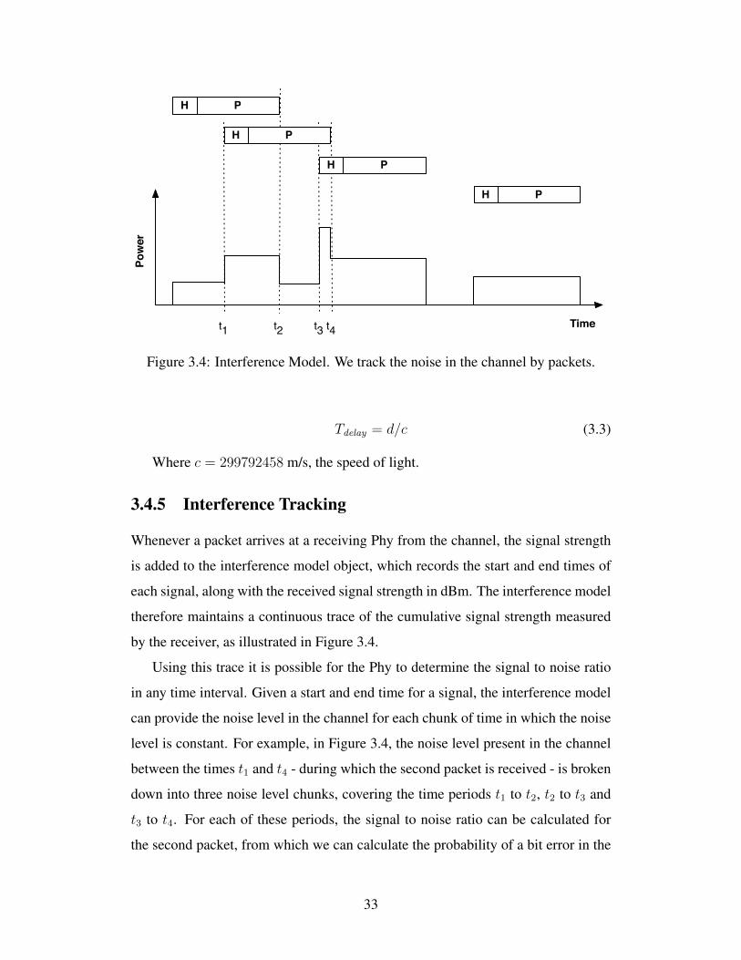
Figure 3.4: Interference Model. We track the noise in the channel by packets.
Tdelay = d/c (3.3)
Where c = 299792458 m/s, the speed of light.
3.4.5 Interference Tracking
Whenever a packet arrives at a receiving Phy from the channel, the signal strength
is added to the interference model object, which records the start and end times of
each signal, along with the received signal strength in dBm. The interference model
therefore maintains a continuous trace of the cumulative signal strength measured
by the receiver, as illustrated in Figure 3.4.
Using this trace it is possible for the Phy to determine the signal to noise ratio
in any time interval. Given a start and end time for a signal, the interference model
can provide the noise level in the channel for each chunk of time in which the noise
level is constant. For example, in Figure 3.4, the noise level present in the channel
between the times t1 and t4 - during which the second packet is received - is broken
down into three noise level chunks, covering the time periods t1 to t2, t2 to t3 and
t3 to t4. For each of these periods, the signal to noise ratio can be calculated for
the second packet, from which we can calculate the probability of a bit error in the
33
decoding of the given signal, and therefore calculate the probability of an error in
decoding the packet.
3.4.6 Packet Reception
Upon arriving at a receiver the packet signal strength and duration are recorded in
the device interference model, as described in Section 3.4.5. Once the interference
from the transmission is recorded, the Phy decides if it can actually decode the
packet. This happens in two phases: header reception and payload reception.
Because the packet header is sent using the common header spreading code, the
Phy is capable of decoding only one header at a time. The Phy must successfully
decode the packet header, extract its contents as described in Section 3.4.2, and then
pass off the payload reception job to the multiuser detector, which then decodes the
packet payload.
When a packet arrives from the channel at the receiving Phy, the Phy first de-
cides if it will be able to synchronize to and decode the header portion of the packet.
In general, the Phy will be able to decode the header if the signal power at the re-
ceiver is greater than some minimum detection threshold, and the device is in a
state such that it will be capable of detecting and devoting resources to header and
payload decoding. Therefore, when a packet header arrives at the receiving Phy, the
Phy will accept the packet and schedule the decoding of the packet header unless
any of the following criteria is met:
1. The signal strength is below the device detection threshold.
2. The device is transmitting.
3. The device is receiving another packet header (this is a header collision).
4. The device is already receiving K packets.
If the packet does not meet any of these criteria, then the Phy will accept the
packet and schedule a header decoding event for the time when the header will have
completely arrived at the receiver. Once the header has arrived, the Phy will calcu-
late the probability of successful header detection based on the signal to noise ratio
34
in the interval between when the header began and ended, and compare this proba-
bility to a uniform random number between 0 and 1 to determine header reception
success. If successful the Phy will decode the header and then pass the packet in-
formation, including the payload spreading code and packet length, to the multiuser
detector for payload decoding.
3.4.7 Multiple Packet Reception
The multiuser detector can decode up to K packets simultaneously. In our imple-
mentation, the multiuser detector simply schedules a packet decoding event when
the packet is due to have finished arriving, and then computes the probability of
successful packet reception based on the signal to noise ratio measured by the inter-
ference model in the time between when the packet payload started and ended at the
receiver. This probability of successful reception depends on the characteristics of
the receiver and the type of error correction coding used, which we are free to sub-
stitute into our model based on the type of multiuser detector we wish to test in our
simulator. In particular, for the ideal receiver which always successfully decodes K
packets regardless of interference, we have the probability of successful reception
equal to 1. So in the ideal case, as long as the packet is not dropped by the Phy
for one of the reasons above, then it will be successfully received by the multiuser
detector. In this work, we performed all of our experiments with ideal receivers.
Once decoded by the multiuser detector, the received packet is passed up to the
MAC layer for handling and processing.
3.5 Summary
In this chapter, we began by discussing the properties of RP-CDMA as proposed
by Schlegel et al.[42]. This discussion included the fundamental properties of RP-
CDMA , including packet format, selection of spreading codes, required bandwidth,
and the properties of the multiuser detector. We related these properties to our
desired link properties from Chapter 1, and concluded that RP-CDMA could offer
us private channels for each packet, interference resistance, and coordination free
35
transmissions, and was thus a suitable candidate for a reliable wireless ad hoc link.
With the theoretical evaluation complete, we began the discussion of how we
simulated RP-CDMA in the ns-3 network simulator. We began with the basic de-
tails of how the simulator works and then described our RP-CDMA packet header
format, which is designed to allow a packet payload to be decoded by the multiuser
detector without having to refer to any information in the packet payload itself. We
then traced a packet through the RP-CDMA Phy, as it was passed down from the
MAC, through the Phy, and into the channel. Once in the channel, we described
how a packet arrives and is processed by the receiving node Phy, including inter-
ference tracking, header collision detection, and multiple packet reception in the
multiuser detector, before being passed up to the receiving node MAC.
Having completed this discussion of RP-CDMA and how we simulate it, we
can now move on to the discussion our MAC, which drives the RP-CDMA Phy and
is one of the main contributions of this work.
36
Chapter 4
MAC Description
In this chapter we will describe the details of our MAC protocol, which we designed
to operate on top of the RP-CDMA Phy. This MAC protocol and the accompa-
nying performance study is the main contribution of our work, and our aim is to
demonstrate that the RP-CDMA based network device can achieve relatively high
reliability and performance on an ad hoc network with a simple MAC protocol such
as the one described in this chapter.
Before describing the details of our MAC protocol, we first motivate its de-
sign in Section 4.1. We will see that the addition of the multiuser detector changes
the nature of the link reliability and performance problem, which motivates us to
propose two extensions to the standard RP-CDMA protocol: Simultaneous Trans-
mission and Payload Channel Acknowledgements. These extensions are designed
to make maximum use of the multiuser detector, improve system performance, and
reduce congestion in the common header channel. After describing these exten-
sions in Sections 4.2 and 4.3, we then describe our MAC protocol in Section 4.4,
and discuss acknowledgement policies in Section 4.5.
4.1 Motivation
Our investigation into the application of RP-CDMA in the multihop ad hoc con-
text was initially motivated by the observation that modern wireless ad hoc systems
suffered from the problems of packet collisions and interference, which fundamen-
tally limited their reliability and performance. Initially, we experimented with RP-
37
CDMA by modifying the ns-3 802.11 stack to simulate a multiuser detector at the
physical layer, leaving the 802.11 MAC intact. These early experiments found that
packet losses due to collisions were indeed significantly reduced, as we had hoped,
but that system performance compared to the 802.11 CSMA model, while better,
was not dramatically improved. Based on these early experiments, we decided to
abandon the 802.11 model entirely and implemented RP-CDMA in its own sim-
ulated device from scratch. Our early experiments with this device found, again,
that even with our own MAC on top of the multiuser detector, our performance was
improved over the previous result, but not dramatically so.
When we investigated what was limiting the performance of our ad hoc network
even after the elimination of losses due to interference, the reduction of packet colli-
sions to negligible levels, and the removal of any need for nodes to coordinate their
transmissions, we found that there were two main causes of performance degrada-
tion: First, the dominant cause of packet loss was due to the receiving node being
in the transmit state when a packet arrived, and so the half duplex nature of the
radio became a significant problem, since nodes cannot both transmit and receive
simultaneously.1 Second, because an ad hoc network node may transmit to any
one of its neighbours either for packet forwarding or to actually deliver a message,
nodes must listen to their neighbours for incoming packets. This requirement fun-
damentally limited the performance of the system, as nodes had to wait for their
neighbours to finish transmitting a packet before commencing their own transmis-
sions.
Coupled with our observation that nodes were spending significant time waiting
for neighbour transmissions to finish, we observed that the multiuser detectors were
not being significantly loaded at any time, despite each node having large queues
of packets waiting to be transmitted. Rather, we found that with only one or two
nodes in a group transmitting at any given time (and the rest all waiting for the
transmissions to finish), the multiuser detectors in each node did not typically have
to handle more than one or two incoming packets at a time. This is a problem some-
1Notwithstanding the recent work by Choi et al.[10], who have constructed a prototype fullduplex radio using a clever form of signal cancellation.
38
what unique to an ad hoc system where nodes must all listen to their neighbours,
and absent from a base station type system where all nodes transmit to the base
station. In a base station style system, such as that examined by Ghanbarinejad
et al.[16], maximizing the number of concurrently transmitting nodes is a viable
strategy to make the most use of multiuser detectors. In contrast, maximizing the
number of concurrently transmitting nodes in an ad hoc system only increases the
probability that the intended recipient of any transmission is transmitting itself, and
that the packet will be lost due to the half duplex nature of the radio.
Our early experiments with RP-CDMA in ad hoc networks were therefore of
limited success. Link reliability was significantly improved, but as we increased
the system load we still lost packets due to the half duplex nature of the radio,
and system throughput was limited by the need for nodes to take turns transmitting
to each other. Our problem therefore became how to limit the time nodes spent
transmitting while simultaneously increasing the number of packets transmitted.
Our solution to this problem lies in the multiuser detector. Our observation that
nodes’ multiuser detectors were relatively under-utilized while the transmit queues
filled up illustrated that our system was no longer constrained by the receiver capa-
bility, as it was when the system was limited by packet collisions and coordination,
but rather the system was now transmit capability limited. This observation has
motivated the design of our MAC protocol, in which we have coupled the powerful
multiuser detector with an aggressive transmission mechanism designed to mini-
mize the amount of time each node spends transmitting while making full use of
the multiuser detector capability.
We therefore propose to extend the RP-CDMA Phy with two additional features:
Simultaneous Transmission and Payload Channel Acknowledgements. We discuss
these features in the following sections, after which we will be in a position from
which we can describe our MAC protocol and acknowledgement mechanisms.
39
4.2 Simultaneous Transmission
Simultaneous transmission is motivated by the observation that there is no require-
ment for packets arriving concurrently at a receiver to have been transmitted by
different senders. Furthermore, when we consider that a multiuser detector can re-
ceive multiple packets simultaneously it makes sense to pair this capability with an
equally capable transmitter. We therefore propose to exploit the capability of the
multiuser detector by having a transmitting node compute and transmit the aggre-
gate waveform of multiple packets, each with unique payload spreading codes and
power levels. In this way, a transmitter can use a single frequency band to separate
data in both time and transmission power. The only restriction is that packet headers
be staggered so as to not overlap and collide, and that a node not transmit a number
of simultaneous packets beyond the capability of the multiuser detector, K, since
there is no advantage in transmitting more packets simultaneously than the receiver
is able to successfully decode. Aside from these restrictions, we are free to transmit
multiple packets concurrently to one or many network peers.
Simultaneous transmission is effectively the inverse of multiple packet recep-
tion, but instead of the receiver decoding multiple packets simultaneously using
their unique spreading codes and iterative cancellation, the transmitter encodes mul-
tiple packets simultaneously using unique spreading codes and signal aggregation.
By assigning each packet a power level and then computing the aggregate waveform
of all packets, the transmitter is able to concurrently spread multiple packets over
the range of transmitter power capability. On the receive side, the multiuser detector
uses iterative cancellation to successively decode each packet from most powerful
to least powerful. In this way, a single transmitter can send up to K packets si-
multaneously - where K is the capability of the multiuser detector - as long as the
packet headers are staggered so as to not overlap. Because each packet is encoded
using a unique spreading code, there is no restriction on the intended recipients of
these aggregated packets, as the multiuser detectors at each other network node will
be capable of decoding all of the simultaneous packets in the same manner as if the
packets had arrived from different transmitters simultaneously.
40
H P3 to host A
H P1 to host A
H P2 to host B
time
pow
er
1..I Lh
1..I Lh
a b
Figure 4.1: Simultaneous transmission of multiple packets to one or more receivingnodes, with spreading code indicated by line type. Note that only packet headersshare a spreading code, and are therefore staggered so as to not overlap by somenumber of packet header intervals, denoted by Lh. In a given frequency band, wedistribute data in both time and power, which allows us to transmit multiple packetsin the same time it takes to transmit just one packet, denoted here between points aand b.
Simultaneous transmission is illustrated in Figure 4.1, which shows three pack-
ets being transmitted simultaneously. Each packet payload is encoded with a unique
spreading code, indicated by the line type, and is labelled with the intended receiver
of the packet. Figure 4.1 also illustrates how simultaneous transmission enables us
to reduce the time a node spends transmitting while increasing the amount of data
transmitted, because it enables a single transmitter to fit more data into unit time.
Note that the transmitter is able to commence transmission of packets P2 and P3
before the transmission of P1 is complete, which means that both P2 and P3 will
finish transmission earlier than they would if they were transmitted one at a time.
Being able to fit more data into unit time allows each node to reduce the amount of
time spent in the transmit state, which we expect will reduce the number of packets
lost due to the half duplex nature of the radio. At the same time, by fitting more
data into unit time, more time is available to other nodes in the system for their
turns transmitting.
The risk with simultaneous transmission is that in the event of two or more
nodes beginning transmission at the same time many packets may be lost to header
collisions rather than just one or two. This risk can be illustrated if we imagine
the classic hidden node problem, where two sending nodes share a receiving node
41
but cannot communicate with each other. Without simultaneous transmission, if the
two sending nodes each transmit one packet such that their headers collide at the
receiving node then both packets will be lost. With simultaneous transmission, the
same situation could result in up to K packets lost from each sending node, or 2K
packets in total.
In order to mitigate this risk, we stagger simultaneous packet headers by a ran-
dom number of packet header intervals, which we denote by Lh.2 After transmitting
a packet header the transmitter waits for a number of header intervals in the range
[1, I), and then begins transmitting the next packet. Now if two sending nodes be-
gin transmitting at exactly the same time to a common receiving node, their first
packets will collide at the receiving node, but because we randomly stagger each
subsequent simultaneous packet it is possible that their headers will interleave and
be successfully received. Thus, in the case where two nodes begin transmission at
the same time, traffic from either of them destined for third parties may still be re-
coverable. This is why we randomly stagger our packet headers rather than transmit
all of the packet headers in a block.
Simultaneous transmission is our primary solution to the transmitter bottleneck
we observed in our early RP-CDMA experiments. By sending several packets con-
currently, a single sending node is able to exploit the full capability of the multiuser
detector at the receiver while reducing the time required to send a given amount of
data.
4.3 Payload Channel Acknowledgements
Payload channel acknowledgement refers to the practice of encoding both the packet
header and payload of an acknowledgement packet (Ack) using the payload spread-
ing code of the packet being acknowledged. This is in contrast to the standard RP-
CDMA procedure of encoding the packet header using a common code, and the
payload with a random code. Because the transmitter knows which payload codes
it used to send packets to its neighbours, it can listen for acknowledgements us-
2A packet header interval is just the time it takes to transmit one packet header, which we saw inFigure 3.3 has Lh = 144 b = 18 B.
42
H P
H P
H P
timepower
Figure 4.2: Payload Channel Acknowledgements. By sending both the header andpayload of an Ack packet using the payload spreading code of the packet beingacknowledged, load is reduced on the common header channel. In this figure, thetype of line used to depict the packet headers and payloads represents their differ-ent spreading codes. Because the packet headers for Ack packets are sent using apayload code instead of the common header code, multiple Ack packets can be sentconcurrently.
ing those same codes, and both the header and payload of the acknowledgement
packet can be encoded using this payload code. In this way, acknowledgments are
sent entirely in the packet payload channel, and do not impact the common header
channel. Furthermore, when combined with simultaneous transmission, up to K
acknowledgement packets can be transmitted simultaneously with no requirement
to stagger the packet headers. As a result, a transmitter can send up to K acknowl-
edgements in the same time it takes to send one, which significantly reduces the
load that acknowledgement packets place on the transmitter and network.
This is depicted in Figure 4.2, where we show two Ack packets and one data
packet being sent simultaneously. Again, the spreading code used to transmit a
particular packet header or payload is indicated by line type. Because Ack packet
headers are each sent with the same code as their payload, there is no requirement
to stagger Ack packet headers.
Payload channel acknowledgements further reduce the time spent by a node in
the transmit state, which allows each node more time to transmit new data. This
further enables our MAC to minimize the amount of time spent transmitting, and
by reducing the number of headers sent in the common header channel, decreases
the probability of packet header collisions.
43
4.4 MAC Protocol
We can now begin our discussion of our MAC protocol. Because we are interested
in simple MAC protocols that do not require coordination between nodes, we con-
sider a simple random backoff based MAC. This MAC is similar in spirit to the
802.11 backoff mechanism, but whereas 802.11 uses a binary exponential back-
off algorithm to determine how long to wait after failing to gain the channel, we
use a simple uniformly random backoff interval with no feedback or adjustment in
the event of successful or failed transmission. Our backoff mechanism is therefore
simpler than that in 802.11 [48].
Our MAC maintains a drop tail queue of packets which have arrived from the
network layer but have not yet been transmitted. This queue can hold up to M
packets, and any packets which arrive while the queue is full are dropped. Once
a packet enters the queue, the MAC begins the process of trying to send it. When
having a packet to send, the MAC first checks the Phy to determine if it is ’safe’
to transmit and, if so, sends the packet to the Phy for transmission after waiting
a random number of packet header intervals in the range [1, B). If the Phy starts
receiving a packet while the MAC is waiting, then the transmission is postponed
until the transceiver becomes available again, at which time the MAC repeats the
random backoff procedure.
Algorithm 4.1 shows the Phy level evaluation of whether it is ’safe’ to transmit.
This algorithm simply returns true if the Phy is idle or if it is currently transmitting
fewer than K packet payloads, and otherwise returns false. It is worth noting here
that we are using the Phy state to find our solution to the problem of determining
whether or not the channel is occupied at any given time. A more common solution
to this problem is to perform a clear channel assessment (CCA) by estimating the
noise floor in the channel and comparing that estimate with the current channel con-
ditions [48]. In our solution, we consider the channel to be unoccupied if the Phy is
not actively receiving any packets. This means that we are not performing a CCA
in the same manner as 802.11, but are rather substituting the CCA function for the
activity status of the Phy. This is conceptually simpler than trying to guess what the
44
noise floor is in the clear 802.11 channel, and also practically simpler since the Phy
knows directly whether or not it is currently processing any incoming packets. The
potential risk of assessing whether or not it is safe to transmit at a given time in this
manner is that it may ignore evidence that there is traffic in the channel that has not
been picked up by the receiver. This eventually depends on the properties of the
radio receiver, such as the average number of header synchronization bits required
before the receiver acquires the timing of a particular signal or the packet encod-
ing scheme chosen, but we proceed on the assumption that if the radio is actually
capable of reliably detecting and synchronizing on an incoming transmission, then
our mechanism of simply querying the Phy for its status would be sufficient in a
real implementation, particularly since the RP-CDMA system is highly tolerant of
overlapping transmissions.
Algorithm 4.1 Phy CanTx()MPR is the multiuser detector, with capability KTxList is the list of packets currently being transmittedState is the state of the transmitter.
if State = IDLE thenreturn true
end ifif State = TX-PAYLOAD and TxList.size ≤ MPR.K then
return trueend ifreturn false
Algorithm 4.2 shows the algorithm for selecting a random backoff period be-
fore beginning a transmission. In order to support simultaneous transmission, this
function checks the Phy for its state and returns a random time in the range [1, B)
header intervals initially, or in the range [1, I) for simultaneous transmission.
Algorithm 4.3 puts these two together into the algorithm that executes whenever
the device has data to send, and is visually illustrated in Figure 4.3. In this diagram,
when the MAC has a packet waiting to be sent from its queue, it enters the diagram
at the top. It first checks if the Phy is ready to transmit. If not, then the MAC
will wait until the Phy notifies it that it is available to transmit. Once the Phy
is available, then the MAC waits a random number of packet header intervals in
45
Algorithm 4.2 MAC CalculateBackoffTime()B is the initial maximum number of header intervals to waitI is the maximum simultaneous transmission header intervalsLh is the length of a packet headerS is the channel speedPhy is the device Phy
if Phy.State = TX-PAYLOAD thenreturn Rand(1,I) ·Lh/S
end ifreturn Rand(1,B) ·Lh/S
the range [1, B), then checks again if the Phy is still available. If the Phy is still
available to transmit after the backoff period, then the MAC forwards the packet to
the Phy for transmission. The Phy will then begin transmitting the packet into the
channel.
Algorithm 4.3 MAC SendFromQueue()Data is the queue of packets that need to be sentPhy is the device Phy layer
We implement the random backoff period in order to resolve header channel
contention in the event of several neighbouring nodes all wishing to transmit at the
same time. This is easily illustrated with a simple example with three neighbouring
nodes, depicted in Figure 4.4. Suppose that nodes A, B and C are neighbours and
can all communicate with each other. Suppose that node C has a packet to transmit
to node A, and both nodes A and B have packets for each other. If node C begins
transmitting its packet (4.4a), both nodes A and B will wait until C’s transmission
46
Phy.CanTx()
Wait(CalculateBackoffTime())
Send Packet to Phy
FalseTrue
Wait until the Phy is available
Send Packet from MAC Outgoing
Queue
Phy.CanTx() False
True
Figure 4.3: MAC Sending Algorithm. When the MAC has a packet to send, it firstchecks of the Phy can transmit. If so, it waits a random number of packet headerintervals, then sends the packet to the Phy for transmission.
47
A C
B
(a) C sends to A
A C
B
(b) Both A andB send, causingloss
A C
B
(c) A sends afterrandom backoff
A C
B
(d) B sends afterrandom backoff
Figure 4.4: An example showing why we implement a random backoff algorithmin our MAC. After C finishes sending to A (a), if both A and B were to commencetransmission immediately then their packets would both be lost (b). If both A andB choose a random backoff interval, then A can send into the channel first (c), andthen B afterwards (d).
is complete before sending their packets. As soon as the transmission from node
C ends, the MACs in nodes A and B will be notified that their Phys are no longer
receiving any packets. At this point, if our MAC protocol did not wait before send-
ing their packets to the Phy, then both nodes A and B would immediately begin
transmitting their packets to each other. Since we have half duplex radios, neither
A nor B would receive the packets from one another, and both packets would be
lost (4.4b). However, if both nodes A and B randomly select a backoff period, then
there is some probability that they select different random periods and one of them
will begin transmitting first. Suppose node A begins transmitting first (4.4c). In this
case, nodes B and C would wait until the transmission from A was complete, after
which node B would randomly wait for some time period, and then would com-
mence transmission to node A (4.4d). Thus, the random backoff period prevents
nodes from all trying to transmit at once as soon as a transmission finishes.3 Our
random backoff period then is designed to facilitate orderly access to the channel by
one node at a time. Having only one transmitting node at a time is important in ad
hoc networks because a node may have packets for one or several of its neighbours,
and so it is best if only one node transmits at a time in a given set of neighbours.
We use a random backoff period because it does not require the nodes to coordinate
their channel access, which was one of our design goals from Section 1.2.
3The problem of many entities all trying to do the same thing at once, resulting in nothing beingaccomplished, is sometimes called the Thundering Herd Problem. http://en.wikipedia.org/wiki/Thundering_herd_problem
48
We have seen here that our MAC is conceptually straightforward. We apply
a uniform random backoff mechanism before initiating a transmission, and once
transmitting utilize simultaneous transmission to send as much data as possible in
given time. Having described how our MAC works, we turn our attention to ac-
knowledgement mechanisms.
4.5 Acknowledgements
In our work, effectively addressing the acknowledgement problem came down to
answering the question of when to ack. In a system designed with the limiting con-
straint that a single node can only receive one packet at a time from only one trans-
mitter, such as 802.11, it seems obvious that the acknowledgement should come
immediately after the single packet was successfully received. In the RP-CDMA
based system we propose here, a node may be receiving several packets concur-
rently - perhaps from different sending nodes - and it becomes problematic to send
an acknowledgement after each packet is received because switching to the radio
transmit state necessarily means dropping any packets that are not fully received.
Our focus when developing acknowledgement policies in this work was there-
fore much more on solving the problem of when to send acknowledgements, rather
than how. Our acknowledgement policies thus send an acknowledgement for each
successfully received packet. This may seem problematic at first glance, but when
we consider that payload channel acknowledgements and simultaneous transmis-
sion remove ack traffic from the common header channel and compress sending
many ack packets into the time required to send only one, we see that acknowledg-
ing every packet is an algorithmically simple solution that actually has relatively
little impact on the system.
The problem of when to ack is illustrated in Figure 4.5. In this figure we see
that if the receiving node sends an acknowledgement after the first packet, P1, is
received at time a then the second and third packets, P2 and P3, will be lost because
the radio is half-duplex. Similarly, if we choose to send an acknowledgement after
P2 then P3 will be lost. We can extend this reasoning to the general case and see
49
H P3 from host C
H P1 from host A
H P2 from host B
timea c
Figure 4.5: When to send acknowledgements? If an acknowledgement for P1 issent at time a, then P2 and P3 will be lost because the radio is half-duplex. If thereceiver waits until time c to send an acknowledgement, then host A will be leftwaiting in the interval [a, c].
that for any fixed timeframe or number of packets that a receiving node waits before
sending acknowledgements can yield a case where some packets are dropped as the
radio switches to transmit. Thus, trying to guarantee that an acknowledgement will
be sent in some fixed period will inevitably lead to lost packets at the receiving node.
In the multiuser detector environment, the receiving node therefore benefits from
being able to wait for longer periods before sending acknowledgement packets.
At the sending node, we have an additional problem. If the sending node knows
that the receiving node will guarantee acknowledgement within some fixed time-
frame after receiving a packet, then it must refrain from transmitting within this
timeframe or else it may miss the acknowledgement. This time spent waiting for
acknowledgements causes delay in the transmission of subsequent packets. In this
situation, the sending node can minimize delay of subsequent packets if the re-
ceiving node sends an acknowledgement as soon as possible. As system load is
increased the receiving node’s benefit from longer delays before transmitting ac-
knowledgements conflicts with the sending node’s benefit from minimal delays be-
fore receiving them.
We see then that trying to choose a fixed timeframe in which to send an acknowl-
edgement becomes an effort in balancing the needs of the receiving and sending
nodes. The receiving node prefers to wait and receive as many concurrently arriving
packets as possible before transmitting acks in order to minimize dropped packets,
50
H P3
H P1
H P2
H MTU
t4
H P4
Figure 4.6: Immediate Ack will wait up to 1 MTU time period after P1 arrivesbefore sending an acknowledgement. Adopting this policy allows packets P2 andP3 to be received, but P4 will be lost.
and the sending node prefers that the receiving node transmit an acknowledgement
as soon as possible in order to minimize waiting time and wasted bandwidth.
With this in mind, we can identify two main classes of acknowledgement policy:
those with fixed time acknowledgements, and those with non-fixed time acknowl-
edgements. In a fixed time system, the receiving node will guarantee acknowledge-
ment within some fixed timeframe of having received a packet, and in an non-fixed
time system the receiving node makes no such guarantee. In our work we refer
to these policies as Immediate Ack and Eventual Ack, respectively. We describe
Immediate Ack in Section 4.5.1, and Eventual Ack in Section 4.5.2.
4.5.1 Immediate Ack
Immediate Ack implements the intuitive practice of sending a packet and then wait-
ing for an acknowledgement. If an acknowledgement is not received in some fixed
timeframe, which we call the Acktime, then the packet is retransmitted. Packets
are retransmitted some number of times, R, before being dropped.4 The receiving
node, therefore, must guarantee that an acknowledgement is sent before the Acktime
expires in the sending node.
When combined with simultaneous transmission, the sending node sends one
or more packets concurrently, but as soon as transmission of the first packet is
complete the device stops adding new packets, completes all simultaneous trans-
missions, and begins waiting for acknowledgements from the receiver(s). For each
4We set a default number of retries, R = 7, in our experiments, which follows the 802.11standard.
51
sent packet, if an Ack is not received in the Acktime then the sending node retrans-
mits the packet immediately, up to R times. After receiving a packet the receiving
node tries to send an Ack immediately, but will delay for a time period long enough
to complete reception of a single maximum sized packet, which is just the device
MTU divided by the channel speed. This is illustrated in Figure 4.6, where the
imaginary packet labelled MTU indicates the amount of time the receiving node
will allow before switching to transmit and sending acknowledgements for P1, P2,
and P3. This waiting time permits the receiving node to finish reception of any
packets from the same sending node that were sent simultaneously with the first
packet before sending acknowledgements. If packets are still being received after
waiting for the MTU period (from a third node), the receiving node will break off
packet reception in order to send Acks. From the receiving node point of view
this acknowledgement policy implements a guaranteed fixed time after receiving
a packet in which an acknowledgement will be sent, while still allowing several
packets to be received concurrently. From the sending node point of view, the Im-
mediate Ack policy may be thought of as a type of ’Stop and Wait’, since the sender
stops sending and waits for acknowledgements after sending out some number of
simultaneous packets along with the first packet.
The choice for Acktime therefore should be longer than the minimum time in
which a receiving node could possibly complete the first packet reception, wait one
MTU period, and then transmit an Ack. In practice we also add a small random
time period to the standard Acktime when deciding how long to wait before re-
transmitting an unacknowledged packet. This small random time is meant to avoid
replaying packet header collisions. What we mean here is if it happens that two
nodes begin transmitting such that their packet headers collide at a receiver, then
those packets will be lost. If both nodes then retransmit their packets after wait-
ing for the Acktime, then the packets will collide again at the same receiver. In this
situation, the two sending nodes will deterministically collide with their retransmis-
sions each time they retransmit. In order to avoid this situation, each sending node
adds a small random time value to the Acktime, which serves to slightly randomize
node retransmission time. When retransmitting several packets, a single node must
52
be careful to not schedule retransmissions such that the packet headers overlap, and
so each node ensures that its scheduled retransmission times are strictly increasing.
We are now in a position where we can write our algorithms for sending node
retransmission and receiving node acknowledgement transmission. We show these
algorithms in Algorithms 4.4 through 4.7. We begin with the algorithm used in the
sending node when a packet is sent from the MAC down to the Phy for transmis-
sion, the Immediate Ack OnSend(), Algorithm 4.4. This algorithm sets the packet
retransmission counter to zero and calls the ScheduleRetransmission() Algorithm
4.5 to schedule the retransmission time for the packet, p. When the scheduled event
fires, the packet is immediately retransmitted via the Retransmit() Algorithm 4.6. If
an acknowledgement for a packet arrives before the scheduled retransmission, then
the retransmission event is cancelled.
Algorithm 4.4 Immediate Ack OnSend(p)p is the packet just transmitted
p.retransmissions← 0ScheduleRetransmission(p)
Algorithm 4.5 Immediate Ack ScheduleRetransmission(p)p is the packet to schedule retransmission formin retry time is the earliest a retransmission can be scheduledAcktime is the minimum waiting time before retransmittingB is the maximum initial backoff periodLh is the packet header lengthS is the channel speed
X ← Rand(1,B) ·Lh/SW ← Now() +Acktime +Xif W < min retry time thenW ← min retry time +X
end ifmin retry time ← W + Lh/SSchedule(W , Retransmit(p))
Upon receiving a packet, a receiving node will attempt to send an Ack within the
fixed time it would take to receive a MTU sized packet. This is shown in Algorithm
4.7, which details the algorithm used when a data packet is received.
53
Algorithm 4.6 Immediate Ack Retransmit(p)p is the packet to retransmitR is the maximum number of retransmission attempts
p.retransmissions← p.retransmissions + 1Phy.Send(p)if p.retransmissions < R then
ScheduleRetransmission(p)end if
Algorithm 4.7 Immediate Ack DataReceived()p is the data packet receivedDev is the network devicePhy is the network device PhyS is the channel speed
MaxWait← Now() + Dev.MTU / Swhile not Phy.CanTx() and Now() <MaxWait do
Wait()end whilePhy.Send(p.Ack)
These algorithms constitute our fixed time acknowledgement policy. We now
describe our non-fixed time acknowledgement policy.
4.5.2 Eventual Ack
Whereas the Immediate Ack policy is designed to guarantee to the sender that an ac-
knowledgement will be sent for a received packet within some fixed timeframe, the
Eventual Ack policy is designed to minimize the disruption that acknowledgements
have on the receiving network device. In terms of when to send acknowledgements,
as illustrated in Figure 4.5, the receiving node chooses to send acknowledgements
whenever all packet receptions are complete, and so will never break into a packet
reception to send an acknowledgement. At the sending node, it does not make
any sense to wait indefinitely for an acknowledgement, and so the sending node
continues sending data normally, trusting that past packets will be acknowledged
whenever their recipients have an opportunity to get around to it.
In implementation, this acknowledgement policy is simpler than the Immediate
54
Ack policy. At the receiving node, waiting until all packet receptions are complete
is equivalent to waiting for the channel to become free, and so Ack packets can be
inserted into the regular outbound data queue, but given priority over ordinary data.
At the sending node, data packets are simply pushed out as soon as possible. The
primary difficulty for the sending node is deciding when a packet has been lost.
Because a packet acknowledgement may arrive at effectively any time, the absence
of an acknowledgement packet does not necessarily mean that the packet was lost,
only that its acknowledgement was not yet sent.
To enable a node to accurately identify lost packets, we can rely on the ordering
of sent and acknowledged packets. Each node maintains four ordered lists: Data,
Retries, Acks, and Sent. In the sending node, when a packet is passed to the device
MAC from the network layer for transmission, it is put into the Data list, and after
being sent to the Phy layer and transmitted the packet goes into the Sent list. At
the receiving node, when a data packet is received an Ack is put into the Acks list.
Whenever the device assesses that it is safe to transmit, as determined by the MAC
SendFromQueue() Algorithm 4.3, then the device will transmit packets from the
Acks, Retries and Data lists in that order. In this way, Ack packets are prioritized
first, Retry packets second, and new packets last.
Because Ack packets are put into the Acks list in the same order in which their
data packets were received and the sender maintains the Sent list in the same order
in which packets were sent, the sequence of Ack packets from a receiving node
should therefore be in the same order as the corresponding packets in the sending
node Sent list. This enables the accurate identification of lost packets by the sending
node: After getting an Ack from a receiving node, the sending node can mark as
lost any packet that was sent to the same receiving node and is between the front
of the Sent list and the acknowledged packet. Lost packets are put into the Retries
list, and upon retransmission are moved to the end of the Sent list to preserve the
ordering.
The Eventual Ack policy slightly modifies the SendFromQueue() function in
the MAC to support sending packets from each of the Acks, Retries and Data
queues in priority. Algorithm 4.8 shows the modification, where we simply send
55
data from each of the queues in order. In this version, SendFromQueue() will trans-
mit Ack packets until all waiting Acks are sent or the multiuser detector limit of K
is reached. Afterwards, if it is still clear to transmit after sending Acks, then the
device will transmit one Retry or one new Data packet. Note that the device con-
tinually checks the Phy CanTx() method to determine that it is still safe to transmit,
since each packet sent may change the state of the device. In particular, after send-
ing a Retry packet, the next call to the Phy CanTx() method will return false because
the device will be transmitting the retried packet header.
Algorithm 4.8 Eventual Ack SendFromQueue()Data, Retries, Acks, Sent are ordered lists.Phy is the device Phy layer
while not Data.Empty() and not Retries.Empty() and not Acks.Empty() dowhile not Phy.CanTx() do
Wait()end whileWait(CalculateBackoffTime())while Phy.CanTx() and not Acks.Empty() doPhy.Send(Acks.PopFront())
end whileif Phy.CanTx() and not Retries.Empty() thenNext← Retries.PopFront()Phy.Send(Next)Sent.MoveToBack(Next)
end ifif Phy.CanTx() and not Data.Empty() thenNext← Data.PopFront()Phy.Send(Next)Sent.PushBack(Next)
end ifend while
Algorithm 4.9 shows how the device identifies previously sent packets as having
been lost. This procedure simply iterates through the Sent list looking for a match
to the Acknowledged packet. Any packets that were sent to the same receiving node
before the Acknowledged packet are marked for retransmission, since the ordering
of the Sent and Acks lists ensures that an Ack would have already been sent had the
packet been received successfully.
56
Algorithm 4.9 Eventual Ack ReceiveAck(Ack)Ack is the Ack just received
for i = Sent.First to i = Sent.Last doif Sent[i].Destination = Ack.Sender then
if Sent[i].Sequence = Ack.Sequence thenSent.Erase(i)return
elseRetries.PushBack(Sent[i])
end ifend if
end for
The only remaining case to handle is the instance where all of the packets sent
to a particular receiving node are lost. If this happens, then the sending node will
never receive any Acks for any of those packets, and will therefore never identify
those packets as lost using Algorithm 4.9. To guard against this, we can employ
a very long timer in the sending node which, when it expires, marks a packet for
retransmission. Thus, in Eventual Ack, we employ very long values for Acktime,
and when a packet remains in the Sent list for longer than Acktime it is put into the
Retries list.
4.6 Summary
In this chapter we have described our RP-CDMA network device MAC layer. We
began by motivating our design decisions, and specifically noted that the addition
of the multiuser detector in the receiver changes the system performance limitation
from that of packet reception capability to packet transmission capability. This ob-
servation motivated our two extensions to the RP-CDMA protocol, simultaneous
transmission and payload channel acknowledgements, which aim to pair the pow-
erful multiuser detector with an equally powerful transmitter in the ad hoc network
environment. We then described the algorithms which determine how our MAC de-
cides when to transmit, and finally discussed the acknowledgement problem in the
presence of multiuser detectors. Particularly, we found that the possibility of receiv-
57
ing several overlapping packets simultaneously complicates the decision of when to
send acknowledgement packets. Finally, we outlined two acknowledgement poli-
cies which we implemented in our system, one which guarantees acknowledge-
ments in a fixed timeframe after packet reception, and one which does not.
58
Chapter 5
Experimental Setup
The goal of our performance study is to evaluate the reliability and performance of
our RP-CDMA network device in the multihop ad hoc context, so our experiments
were designed to allow us to perform this evaluation. The ns-3 simulator and our
RP-CDMA MAC protocol have several configurable parameters which we describe
here, and at the end of each experiment we measured the performance of the system.
In this chapter we will describe each of our configurable parameters, whether they
were fixed or varied between experiments, and what output we measured to evaluate
performance.
Each of our experiments consisted of some number of nodes placed in a two
dimensional field with sufficient spacing between them such that the network is
connected but not fully connected. This ensured that there was some degree of
multihop required for packets to traverse from one end of the network to the other.
During experiments each node generated data traffic with exponentially distributed
packet inter-arrival times and uniformly distributed destination node.
In each experiment we measured the number of packets which entered the net-
work and packets which arrived at their final destination. For each packet arriving
at its final destination, we recorded the time it took to traverse the network from its
originating node. At the end of each experiment, we used the aggregate statistics of
all the packets which successfully arrived at their final destination to determine how
many packets were lost, average system throughput and average end to end delay.
For ease of reference, we show all of the fixed values, variables, and measured
values in Table 5.1. In this table, the fixed parameters are set globally for all exper-
59
iments, and the variable parameters are the system parameters we will investigate
in our performance study. The measured values are our performance metrics.
The remainder of this chapter describes the setup and configuration of our ex-
periments in detail. Our aim is to enable the reader to create similar or identical
experiments in ns-3, and so we will discuss some of the implementation details in
the simulator. We begin with a discussion of the simulator configuration in Section
5.1, followed by the node configuration and network topology in Section 5.2. We
then discuss how the nodes behaved during each experiment, and particularly how
they generated traffic in Section 5.3. We discuss system calibration and experiment
duration in Section 5.4 and then how we measure system performance in Section
5.5. Section 5.6 describes a 2k factor analysis investigating the relative impacts that
our variable system parameters have on performance.
5.1 Simulator Configuration
We describe here the configuration of the ns-3 simulator, with the aim of providing
sufficient detail to enable the independent replication of our results.
Random numbers were generated using the built in ns-3 random number gen-
erator (RNG), which itself is based on the MRG32k3a generator by LEcuyer et
al.[31]. This is the same RNG as that used in ns-2, and features a large number
of independent streams, each of which has a large number of substreams. Specific
streams and substreams can be selected via seeds and run numbers. Each random
number variable in ns-3 uses its own RNG. Since substreams of the same stream
do not overlap, we used a single seed and advanced the run number to produce
independent trials. In all of our experiments, we used a seed value of 12345 and
incremented the run number from 1 to the number of trials we wished to perform.
We performed most of our experiments with 10 trials, and therefore usually used
run numbers 1 through 10. Experiments with significantly more trials did not appre-
ciably affect our results, and so we considered 10 to be sufficient for our purposes.
Our experiments are therefore reproducible by setting the seed and run number to
the same as the trial we wish to reproduce.
60
Fixed ParametersParameter DescriptionRNG Seed The random number generator seed. Fixed for all
experiments.RNG Substream The random number generator substream id.
Changed for independent replications.Channel Speed The data rate of the wireless channel.
Number of Nodes The number of nodes in each experiment.Runtime The duration of each experiment.
UDP Data Size The data packet size in UDP data experiments.TCP Data Size The data stream size transferred in the TCP exper-
imentsVariable Parameters
Parameter DescriptionNetwork Topology The network topology. Either Grid or Random.
Offered Load Per Node The load offered to the network by each networknode. Determined by data arrival rate, λ, andUDP/TCP Data Size.
Ack Policy The acknowledgement policy used, as describedin Section 4.5.
Acktime The elapsed time before a sending node MAC willretransmit an unacknowledged packet.
I Upper bound for the simultaneous transmissioninter-packet backoff time, as described in Section4.2.
B Upper bound for the initial backoff time, as de-scribed in Section 4.4.
M Maximum size of the MAC data queue, in packets.K Capability of the multiuser detector. The maxi-
mum number of packets that the detector can re-solve concurrently.
Measured ValuesMeasured Value Description
Percent Packets Lost The fraction of packets that were sent down by theSender application, but not received at the destina-tion Receiver application.
End to End Delay For those packets that arrived at their final desti-nation Receiver application, how long they tookto traverse from Sender to Receiver.
System Throughput The total amount of data that successfully tra-versed the network from Sender to Receiver, di-vided by the experiment runtime.
Table 5.1: System Parameters and Measurements
61
Network routing was via the Optimized Link State Routing (OLSR) [11] and
Static routing implementations from ns-3. Since our nodes were static, we did
not require a more sophisticated routing algorithm, such as Ad-hoc On-Demand
Distance Vector (AODV). We are not specifically concerned with evaluating the
performance of the network routing algorithm in this work, and therefore chose
OLSR and Static because they are effective with relatively low overhead. With the
combination of Static and OLSR routing, node routing tables would be populated
at the beginning of each experiment via OLSR broadcasts, and thereafter nodes
would find routes via their Static entries. OLSR did continue to broadcast routing
information throughout the experiments, even though the routing tables did not
change after their initial population. We consider this routing traffic in the channel
to contribute to the practical realism of our simulations.
Channel speed was set to 1 Mbps, which was chosen because it facilitates easy
comparison to 802.11, which uses a simple Differential Binary Phase Shift Key-
ing (DBPSK) Direct Sequence Spread Spectrum (DSSS) implementation at this
speed [48]. We assume a relatively simple BPSK DSSS CDMA modulator in our
RP-CDMA system, which can be compared to the 802.11 equivalent in a straight-
forward manner when working with channel capacity and bandwidth. We acknowl-
edge the existence of more sophisticated modulation and symbol encoding schemes,
such as those used for high speed 802.11n [49] or those employed in various mul-
tiuser detectors [44, 25], but these can be layered on top of the underlying CSMA
and RP-CDMA based devices without changing the fundamental comparison. We
therefore choose the simplest implementation of each device and set the channel
speed to 1 Mbps.
5.2 Node Configuration and Topology
Our experiments focused on two node configurations: grid and random. In the grid
topology, our aim was to provide a regular network topology in which individual
nodes had an approximately equal number of neighbours. To this end, we designed
our grid such that nodes could communicate with their neighbours along the same x
62
1
16
12
8
43
7
11
15
2
6
10
1413
9
5
125 m
125 m
R
Figure 5.1: Grid Topology Configuration. In this topology, nodes can communicatewith their neighbours on the same x and y axis, but cannot communicate diagonally.This is illustrated with the node communication radius R, centred on node 11.
and y axis, but could not communicate diagonally. This is illustrated in Figure 5.1.
In this figure, the node communication radius is illustrated with the circle of radius
R centred on node 11. We used a 4× 4 grid of nodes in all of our grid experiments,
as this offered a network with a maximum of 6 hops on which experiments would
complete on available hardware in a reasonable period of time.
The distance between nodes of 125 m was chosen empirically. We performed
experiments over a range of node spacings and measured the packet loss as we
increased the distance between nodes. From these results we selected a distance
that would allow nodes to communicate along the x and y axes, but not diagonally.
We show our packet loss results in Figure 5.2. In this figure, we can see that as the
inter-node spacing increases to 160 m that system packet loss increases to 100%,
indicating that we have surpassed the effective range of the nodes. We can see
that if we space the nodes at 125 m, then the diagonal distance between nodes is√
1252 + 1252 ≈ 177 m, which is beyond the maximum transmission distance.
We derive the same result analytically using the device default transmit power,
63
0
20
40
60
80
100
0 20 40 60 80 100 120 140 160 180 200
% P
acke
t L
oss
Distance between nodes (m)
Loss RP-CDMA
Figure 5.2: Grid topology effective range. As we increase the distance betweennodes, we see that packet loss increases to 100% when the inter-node distance istoo large. From this we can estimate the effective range of the nodes.
64
15
14
13
12
11
10
9
8
7
6
5
4
3
2
1
0
(a)
15
14
13
12
11
10
9
8
7
65
4
3
2
1
0
(b)
15
14
13
12
11
10
9
8
7
6
5
4
3
2
1
0
(c)
15
1413
12
11
10
9
8
7
6
5
4 3
2
1
0
(d)
15
14
13
12
11
10
9
8
7
6
5
4
3
2
10
(e)
15
14
13
12
11
10
9
8
7
6
5
4
3
2
1
0
(f)
15
14
13
12
11
109
8
7
6
5
4
32
1
0
(g)
15
14
13
12
11
109
8
7
6
5
4
3
2
1
0
(h)
15
14
13
12
11
10
9 8
7
6
5
4
3
2
1
0
(i)
15
14
1312
11
10
9
8
7
6
5
4
3
2
10
(j)
Figure 5.3: The 16-node random topologies tested.
our loss propagation model, and the device detection threshold. We use a default
transmit power of 16.0206 dBm and a detection threshold of -96 dBm, and we can
solve for the maximum distance using Equation 3.2:
d = dref · 10Ptx−Prx−Lref
30
= 1.0 · 1016.0206+96−46.6777
30
= 150.6942
Which agrees with our observation that packet loss increases to 100% after 150
m. Note that we have chosen our default transmit power and detection threshold
to match those of the ns-3 802.11 model, which facilitates comparison between the
two.
In addition to our grid topology, we also experimented with random topologies.
In these experiments we generated 10 different random connected topologies with
the same average node density as our grid topology, so 16 nodes inside a 375× 375
m box. Node placement was uniformly random in both x and y. These topologies
are shown in Figure 5.3.
Nodes were static throughout each experiment, since we are interested here in
65
evaluating the effects of the reliable link on packet loss and system performance,
which does not require node mobility.
5.3 Node Behaviour
Each simulation started with a 200 second warm up period in which nodes identified
routes through the network to each other node. In these 200 seconds, the OLSR
routing protocol exchanged routing information with each neighbour several times,
until the routing table was fully populated. OLSR continued to update the routing
tables throughout the experiment, but because the nodes were not mobile the routing
tables did not change after the initial warm up period. Once the routing tables were
populated, the ns-3 Static routing algorithm was able to return routes to each other
node in the network.
After the warm up period, each node began generating data traffic. Data traffic
was one of either UDP or TCP traffic, described below, though we performed the
majority of our experiments using UDP. Each node was equipped with a Sender and
a Receiver application, which resided at the topmost Application layer in the ns-3
network stack, illustrated in Figure 3.2. The Sender application was responsible
for generating data and sending it into the network, and the Receiver application
would listen to the network for data addressed to itself. Each node’s Sender would
schedule its next send event using a local exponential random variable with a mean
value specified as part of the experiment. When these events were triggered, the
node would uniformly randomly select another node in the network and send a
fixed sized chunk of data to its respective Receiver. Our experiments were with a
fixed data size and varying mean time between send events. In this way, we were
able to gradually increase the offered load per node to the network and measure the
effect.
As each packet was generated and sent into the network it was tagged with a
monotonically increasing 32 bit sequence number unique to the originating Sender.1
At the Receiver, the tuple formed by the originating node and the sequence number
1Each 16 node experiment typically generated a number of packets on the order of millions, sowe are not concerned about the sequence numbers wrapping.
66
formed a unique packet identifier which we used to eliminate duplicates. Each
Receiver maintained a buffer of the last 60 seconds worth of received packets, which
was checked for duplicates before a newly arrived packet was counted. In this way,
we eliminated duplicate packets at the Receiver.
At the end of each experiment we had a 20 second cool down period during
which nodes would continue to pass traffic across the network but would not gener-
ate any more new traffic. In this way, we ensured that the last few packets generated
had enough time to arrive at their final destination. Any packets still in the network
at simulation end time after the cool down period were counted and considered lost.
5.3.1 UDP Data
For the UDP data, packet size was fixed at 1500 B. Thus, at each send event a node
would send a single 1500 B packet into the network to another randomly selected
node. After sending a single packet, a node would schedule its next send event,
which would be sent to another randomly selected node.
1500 B packets were used because this is the MTU for Ethernet basic frames
[50], and therefore seems like a reasonable size packet to work with. After IP, MAC
and Phy headers, each 1500 B packet occupied 1569 B in the physical channel.
5.3.2 TCP Data
For TCP data flows, we used larger data sizes and correspondingly larger mean time
between send events. When using TCP, each node would randomly select another
node in the network and send it 100 kB of data. After initiating a data transfer nodes
would then schedule the next sending event, which would initiate data transfer to
another node in the network. Thus, it was possible that a node may have had more
than one TCP transfer in progress simultaneously. Our selection of 100 kB for our
data transfer size was based on the size of the average basic web page, which is on
the order of a few hundred kilobytes [13]. By default, the ns-3 TCP implementation
uses the New Reno implementation [15].
In this work, we tested TCP data transfers only in the grid configuration.
67
0
500000
1e+06
1.5e+06
2e+06
2.5e+06
3e+06
3.5e+06
0 2000 4000 6000 8000 10000 12000
Th
rou
gh
pu
t (b
ps)
Time (s)
RP-CDMA Throughput
Figure 5.4: Steady state system throughput, sampled every 5 seconds and averagedover 100 second intervals. We see here that the system enters steady state almostimmediately.
5.4 Calibration and Runtime
Before embarking on a series of experiments, it is prudent to evaluate our system
performance at steady state and verify both that it reaches steady state and how long
it takes to do so. The simplest way to do this is to periodically sample the system
performance and visually identify the steady state region.
We show such a sample in Figure 5.4, which shows the sampled system through-
put for a data run with 16 nodes in the grid topology and an offered load per node
of approximately 0.18 Mbps, for a total offered load to the system of approximately
2.8 Mbps. In this chart, data traffic begins at 200 seconds and terminates at 10200
seconds. We see that during this period the system throughput is approximately 2.8
Mbps, with some oscillation around this value.
For the same experiment, we can also measure the data queue lengths of all the
nodes in the system, which we show in Figure 5.5. We can see in this figure that
the individual node queues are typically holding around one packet or less, and the
system as a whole averages a little less than 6 packets waiting at any time. We can
Figure 5.5: Steady State queue length. We show the average queue length of eachnode along with the system aggregate queue length for both (a) 100 second averagesand (b) 500 second averages, sampled every 5 seconds.
increase the number of samples in each data point to eliminate some of the noise
from Figure 5.5a, which results in Figure 5.5b. In this figure, we can see that only
four nodes are typically holding a packet at any given time: Nodes 6, 7, 10 and 11.
If we recall the grid topology from Figure 5.1, we see that these four nodes are in
the middle of the grid, and therefore have more neighbours and are more likely to
forward traffic across the network.
Finally, we seek to confirm that our system is stable under heavy loads, and so
perform the same experiment as above but we increase the offered load per node
from 0.18 Mbps to 1.0 Mbps, which is the highest offered load per node tested in
any of our experiments in this work, and is also equal to the channel speed. Figure
5.6 shows our results, where we can see that the total number of packets waiting
in the system oscillates between 200 and 250 for the duration of our experiment.
We also see the separation of nodes into three distinct groups, which correspond
to the number of neighbours each has. One set of nodes, Nodes 6, 7, 10 and 11,
typically hold between 30 and 40 packets, which we again attribute to their being
in the middle of the grid topology and each having four neighbours. Nodes 1, 4,
13 and 16 average around 1 or 2 packets when sampled, which we can attribute
Figure 5.6: Steady State queue length with high load. We see that the aggregatesystem queue length remains stable over the entire experiment, even when eachnode offers a load of 1 Mbps to the system.
to their being in the corners of the network, having only two neighbours each, and
thus not typically forwarding as much traffic at any given time. The remaining
nodes typically hold around 10 packets, which corresponds to these nodes being
situated along the edges of the network and having 3 neighbours each. Critically,
we see that even under heavy loads, the system reaches the steady state quickly and
remains there for the duration of each experiment.
We conclude from Figures 5.4 through 5.6 that the transient in our network is
fairly short, and so we do not remove it from our data. Rather, we simply run the
system for a long time and use all of the data, which should effectively reduce the
transient period data to insignificance. We therefore performed all of our experi-
ments over a period of 10000 seconds, which allows us to capture significant data
at the system steady state.
We have now described all of our fixed system parameters and their values,
which are summarized in Table 5.2.
70
Fixed ParametersParameter ValueRNG Seed 12345
RNG Substream 1-10Channel Speed 1 Mbps
Number of Nodes 16Runtime 10000 s
UDP Data Size 1500 BTCP Data Size 100 kB
Table 5.2: Fixed System Parameters
5.5 Measurements
Since our goal is to evaluate the reliability and performance of the RP-CDMA based
ad hoc network, we measured the system packet loss, end to end delay, and through-
put for each experiment. These three metrics together allow us to estimate the
system reliability through packet loss and delay, and performance through system
throughput. In the remainder of this section, we discuss our measured metrics in
detail.
5.5.1 Packet Loss
Packet loss was measured by counting the number of unique packets that arrived
at their destination Receiver application compared to the number of packets sent
into the network by the Sender applications. Thus, packet generation and reception
was counted at the application layer, which is the topmost layer in the ns-3 network
stack shown in Figure 3.2. At this level, the Sender and Receiver applications are
shielded from what is happening below them in the stack, and only interact with the
transport layer below them. In particular, the Receiver only ever sees a packet when
that packet is addressed to it specifically. Thus, intermediate nodes which merely
forward packets on their way to their final destination do not see or count packets
as they are forwarded along a route with multiple hops.
One of the consequences of our measurement methodology is that the actual
traffic present on the network is somewhat higher than what we measure. Since we
71
only measure end to end packet loss at the application layer, we ignore all of the
other network traffic required in order to support the network itself. Specifically,
none of routing packets, retransmissions nor acknowledgement packets are seen
at the application layer, since these are generated in the network and link layers.
These additional sources of network traffic are present in all of our experiments,
and do have an effect on our results, but are just not counted directly. Recall that
OLSR continues to broadcast routing information throughout each experiment, and
if we utilize an acknowledgement mechanism then acknowledgement packets and
retransmissions also add to the load on the network. All of these things are present
in the simulated wireless channel and therefore impact the system performance,
but are not seen by the application layer and so are not counted when we measure
packet loss.
We do this because we are interested in the reliability of the network from the
point of view of the primary customer, which is the user. To count routing traffic and
particularly retransmissions towards system packet loss is not meaningful because it
does not capture the level of service afforded to the user by the network. Similarly,
performing experiments in the absence of this traffic detracts from the realism of
the simulation.
5.5.2 System Throughput
We calculated system throughput as a function of packet loss. Specifically, the prod-
uct of the number of packets which were not lost and the size of those data packets
gives us the number of bytes passed through the network, which we divide by the
simulation run time to get the throughput. Again, we make these measurements
from the application layer, and so only the size of the actual data portion of each
packet was counted. So, if a Sender application passes a 1500 B packet down to the
UDP transport layer, when that packet is eventually received at the target Receiver
application, the contribution to system throughput is 1500 B.
Again, this shields our measurements from the implementation details of the
network. A 1500 B packet generates 1569 B in the RP-CDMA channel, which pro-
portionally increases the load on the network. Since we are interested in the system
72
performance from the point of view of the user, we only measure how much user
data successfully traverses the network. As the system itself is actually transport-
ing somewhat more than just the 1500 B sent from the application layer once we
account for IP, MAC, Link, and Phy headers, some readers may wish to call our
measurement the Goodput, but we use the term Throughput in our work.
5.5.3 Average Delay
End to end delay is simply the difference between the time when a packet is deliv-
ered at its final destination and when it was generated and sent into the network. We
use a ns-3 packet tag to indicate the time when a packet was generated at the Sender
application. This tag is checked by the destination Receiver, which records the time
taken for the given packet to traverse the network. Packet Tags are a convenience
abstraction in the ns-3 simulator, and do not contribute to the size of a data packet
as it passes through the network stack.
5.6 2k Factorial Analysis
Having discussed our fixed parameters and our measured values, we now turn our
attention to the variable parameters listed in Table 5.1. The first three of these pa-
rameters - network topology, offered load per node and acknowledgement policy -
represent the major factors in our performance study. In our results, we will first in-
vestigate system performance on the grid topology, then on random topologies, and
on each topology we will investigate the effect of our acknowledgement policies.
Each of our results will be presented as a set of curves showing the effect on our
three measured values as a function of offered load per node. This leaves several
of our RP-CDMA device parameters to investigate: the time before retransmission
(Acktime), simultaneous packet spacing maximum (I), initial backoff maximum
(B), MAC data queue length (M ), and multiuser detector capability (K). To get
an appreciation for how these device variables impact system performance, we can
design a 2k factorial series of experiments [20] with a fixed offered load per node,
network topology, and acknowledgement policy.
73
We performed a 25 set of experiments on our grid topology, with offered load
per node of 0.5 Mbps and the Eventual Ack policy. We varied the RP-CDMA device
parameters Acktime, I , B, M , and K in the following ranges:
Variable Low (-1) High (+1) Input LabelAcktime 0.5 s 3.0 s xA
I 2 10 xBB 2 80 xCM 50 ∞ xDK 11 ∞ xE
With 5 variables, we must perform 25 = 32 experiments for each of the possible
combinations of the high and low values for our parameters. Table 5.3 shows each
of our experimental inputs, along with the results of our 3 measured values.
We can calculate the Sum of Squares Total (SST), or total variation, for each of
our measured values using the usual formula SST =∑25
i=1(yi−y), where yi iterates
over each of the results for a measured value, and y is the average of those results.
We can then calculate how much of the variation is attributable to the variables
xA...B, and all of their combinations, xAB, xAC , . . . , xABCDE . These results are
shown in Table 5.4. In this table, we see that the capability of the multiuser detector
(xE) is the dominant factor which affects all three of our performance metrics. In
particular, packet loss and system throughput are almost entirely attributable to the
capability of the multiuser detector, which accounts for approximately 98% of the
variation in our results. End to end delay performance is also mostly attributable to
the capability of the multiuser detector, xE ≈ 29%, though the size of the MAC data
queue also has a significant impact, xD ≈ 15%, as well as the interaction between
the two, xDE ≈ 15%. The effects of the simultaneous packet spacing, xB, and
the initial backoff window, xC , both also accounted for a non-negligible amount of
the variation in the end to end delay, accounting for xB ≈ 2.9% and xC ≈ 6.3%
state and runtime. We have also described our system measurements, which we
will use to evaluate system performance in our experiments, and performed a basic
analysis of how our variable system parameters impact system performance on our
grid topology. We now move on to our results.
77
Chapter 6
Results
In this chapter, we present our results. Along with the algorithms which constitute
our MAC and acknowledgement policies, this performance study is the main con-
tribution of of our work. Here, we will explore the reliability and performance of
our RP-CDMA network device on both grid and random topologies, and investigate
the effectiveness of our acknowledgement policies. After an initial assessment and
comparison to 802.11 CSMA, we will investigate the effect of changing our variable
device parameters with the aim of maximizing system reliability and performance.
Each of the results in this chapter shows the effect of varying one of the variable
parameters from Table 5.1 while keeping the others fixed. For each value of our
varied parameter we generated a data series measuring the system performance as
the offered load per node was increased. All of our data series were then plotted
on the charts, which allows us to see the effect of changing the variable parameter.
Each data series was composed from 10 independent trials with identical inputs but
incremented RNG substream. Error was calculated as the 95% confidence intervals
over our 10 independent trials.
This chapter proceeds through our results starting with our grid topology in
Section 6.1. On this topology, we initially compare 802.11 performance with our
RP-CDMA device without acknowledgements. We then investigate the effect of
varying the capability of the multiuser detector, K, the effect of the Immediate and
Eventual acknowledgement mechanisms, and also briefly investigate TCP perfor-
mance. With this initial investigation on grid topologies completed, we present our
results on random topologies in Section 6.2. On random topologies we investigated
78
the effect of each of our variable system parameters, with the aim of maximizing the
RP-CDMA system performance. After analysing the effects of each of our system
parameters, we will again compare the RP-CDMA result to that of 802.11.
6.1 Grid Topology
Recall that our grid topology consisted of 16 nodes separated such that they could
communicate with their neighbours on the x and y axes, but not diagonally, as per
Figure 5.1. We present results here for 802.11, RP-CDMA without acknowledge-
ments, with the Immediate Ack Policy, and finally with the Eventual Ack policy.
Our aim in this series of experiments is to analyse the relative performance of our
system and acknowledgement policies in a fixed, regular topology. We then apply
the lessons learned on the grid system to random topologies in Section 6.2.
6.1.1 802.11 CSMA and RP-CDMA No Ack
We begin with a simple evaluation of the 802.11 system and compare it to RP-
CDMA without acknowledgements. Before presenting our results, we briefly dis-
cuss how we fairly compare 802.11 to RP-CDMA .
Our experiments with 802.11 were performed simply by replacing the RP-
CDMA network device with the stock ns-3 802.11 network device in the simulator
and running the same series of experiments that we performed with RP-CDMA . In
order to compare the two fairly, we limited the RP-CDMA experiments to the same
bandwidth as that occupied by 802.11.
In the 1 Mb DSSS mode, 802.11 utilizes differential binary phase shift keying
(DBPSK) to transmit data in the 2.4 GHz ISM band. Each symbol is DSSS modu-
lated with an 11-chip Barker sequence, which spreads the 1 Mbps data signal over
22 MHz using the formula B = 2R‖~c‖, where R is the data rate, and ‖~c‖ is the
magnitude of the spreading code used [51, 48]. The bandwidth occupied by 802.11
is therefore 22 MHz [48].
We can construct a corresponding case with RP-CDMA by utilizing the same
data rate and spreading code length. With a spreading code length of 11, we as-
79
sume we can have a multiuser detector with capability at least K = 11 [42]. With
equal bandwidth, we can fairly compare the performance of the 802.11 CSMA pro-
tocol with that of our RP-CDMA protocol. In addition to constraining RP-CDMA
to a multiuser detector with K = 11 when comparing to 802.11, we also ideal-
ized the 802.11 Phy to ignore interference effects. Because our experiments with
RP-CDMA were conducted under the assumption that the multiuser detector can
successfully resolve up to K overlapping signals, and therefore ignored interfer-
ence effects in the channel, we made the same assumption when experimenting
with 802.11.
With interference effects ignored, we can isolate the relative effectiveness of
the 802.11 CSMA collision avoidance approach and contrast it with the RP-CDMA
approach of mitigating collisions by putting packets into individual channels. We
disabled the optional 802.11 RTS/CTS mechanism throughout, since it does not
obviously improve system performance, may actually impair it [55, 40], and our
initial experiments indicated it was of limited usefulness.
Figure 6.1 shows our results for No Ack on the grid topology, where we have
compared to the 802.11 result under the same configuration. Recall that in No Ack,
nodes began transmitting packets after a short random backoff period when they
were not busy receiving any packets and continued to send packets simultaneously
until there were no more to send. Receiving nodes did not send acknowledgement
packets, and so if a packet was lost in the network then the system did not try to
recover. In these results, we limited our multiuser detector to capability K = 11, in
order to fairly compare 802.11 with RP-CDMA .
We see that even when limited to K = 11, RP-CDMA offered superior perfor-
mance across the entire tested range. We can see in Figure 6.1a that RP-CDMA lost
fewer packets than 802.11 under the same loads, which corresponds to the higher
measured system throughput shown in Figure 6.1c. We see in Figure 6.1b that
RP-CDMA offered much improved end to end delay compared to 802.11 and was
on the order of 200 ms at the highest load tested. The end to end delay result for
802.11 has a strange artifact around 0.1 Mbps where delay briefly decreases, then
resumes increasing as as offered load per node reaches approximately 0.1 Mbps.
80
This is a byproduct of the grid network topology, and indicates that as the load on
the system increases its multihop capability is affected. Specifically, as the 802.11
system drops more packets, the only packets that successfully reach their intended
Receiver - and which are subsequently measured - are those which do not require
a large number of hops. Thus, the measured average delay briefly decreases, and
then steadily rises again as load continues to increase.
We can examine the relative causes for packet loss in the RP-CDMA case to
try to determine why packets were lost in the network. For the RP-CDMA No
Ack experiments, we have three possible causes for packets being lost at the re-
ceiver: Header Collisions, Transmitting, and Receiving errors. A Header Collision
happens if more than one packet header overlaps at the receiver. In this case, the re-
ceiver will only synchronize to the first packet to arrive and all others will be lost.1
A Transmitting error occurs when a packet arrives while the intended receiver is
transmitting, and is thus incapable of receiving due to its half-duplex radio. All
packets that arrive while a node is transmitting are dropped. A Receiving error can
occur for a number of reasons in our model, but in the case of RP-CDMA No Ack,
Receiving errors occur when a particular receiver’s multiuser detector capability is
exceeded. So for a multiuser detector with capability K = 11, any packets that
arrive concurrently beyond the 11th packet are lost.
Figure 6.2 shows the relative reasons for packet loss as a function of offered
load per node for the RP-CDMA No Ack experiment with overall losses shown in
Figure 6.1a. Figure 6.2 shows us that as we increase the offered load per node, the
fraction of lost packets that are lost due to exceeded multiuser detector capability
grows, while the fraction of packets lost due to header collisions drops. It makes
sense that as the offered load per node increases that more packets would be lost
due to exceeded multiuser detector capability, and thus proportionally less due to
1This is exactly the same behaviour as the ns-3 802.11 implementation, which continues to at-tempt to decode the first packet to arrive and decides afterwards whether the interference from thecollided packet is sufficient to cause the first packet to be lost. Some models would drop all packetsinvolved in a collision [17], but in the ns-3 802.11 model and in reality the receiver would continueto attempt to decode the first packet. The possibility that some data may be recoverable from CDMAsystems even in the event of collisions is the same property which allows Spread ALOHA using asingle spreading code to recover from some collisions [4].
81
0
20
40
60
80
100
0 0.1 0.2 0.3 0.4 0.5 0.6 0.7 0.8 0.9 1
% P
acket Loss
Offered Load per Node (Mb/s)
802.11 (no RTS/CTS)RP-CDMA No Ack
(a) Average Packet Loss
0
1000
2000
3000
4000
5000
6000
7000
0 0.1 0.2 0.3 0.4 0.5 0.6 0.7 0.8 0.9 1
Avera
ge D
ela
y (
ms)
Offered Load per Node (Mb/s)
802.11 (no RTS/CTS)RP-CDMA No Ack
(b) Average Delay
0
0.5
1
1.5
2
2.5
3
3.5
4
4.5
0 0.1 0.2 0.3 0.4 0.5 0.6 0.7 0.8 0.9 1
Avera
ge T
hro
ughput (M
b/s
)
Offered Load per Node (Mb/s)
802.11 (no RTS/CTS)RP-CDMA No Ack
(c) Average System Throughput
Topology GridAck Policy No Ack
Acktime N/AI 10B 10M ∞K 11
(d) Parameters
Figure 6.1: RP-CDMA with no acknowledgements (No Ack), and limited to mul-tiuser detector capability K = 11 on the grid topology. Without any acknowledge-ment mechanism, RP-CDMA offers superior metrics across the entire tested rangecompared to 802.11.
82
0
10
20
30
40
50
60
70
80
90
100
0 0.1 0.2 0.3 0.4 0.5 0.6 0.7 0.8 0.9 1
% P
acket Loss
Offered Load per Node (Mb/s)
Header CollisionsTransmitting
Receiving (K Exceeded)
Figure 6.2: RP-CDMA No Ack Loss Reasons with K = 11. We see that as theoffered load per node increases, the proportion of packets that are lost due to thecapability of the multiuser detector being exceeded grows as a fraction of all lostpackets.
packet header collisions. It is thus worthwhile to examine how system performance
could be affected by a more capable multiuser detector.
Figure 6.3 shows our results when we remove the K = 11 restriction on our
RP-CDMA multiuser detector, keeping all other things constant. Compared to the
K = 11 case, increasing the capability of the multiuser detector results in lower
packet loss and higher throughput at the cost of marginally higher end to end delay.
These results are expected, as increasing the number of delivered packets in the
network is expected to increase the time required to deliver each of them. Our result
for packet loss is particularly encouraging, as the number of packets lost drops from
more than 50% to less than 20% at the upper end of our offered load.
We have now seen that with equal bandwidth, our RP-CDMA based system
outperforms the 802.11 CSMA system, and that given an infinite multiuser detec-
tor, RP-CDMA can perform much better. Since we do not have infinite capability
multiuser detectors in reality, it makes sense to examine what multiuser detector
capability would be required to approach the K =∞ ideal case.
83
0
10
20
30
40
50
60
0 0.1 0.2 0.3 0.4 0.5
% P
acket Loss
Offered Load per Node (Mb/s)
RP-CDMA No Ack K=11RP-CDMA No Ack K=inf
(a) Average Packet Loss
30
40
50
60
70
80
90
100
0 0.1 0.2 0.3 0.4 0.5
Avera
ge D
ela
y (
ms)
Offered Load per Node (Mb/s)
RP-CDMA No Ack K=11RP-CDMA No Ack K=inf
(b) Average Delay
0
1
2
3
4
5
6
7
0 0.1 0.2 0.3 0.4 0.5
Avera
ge T
hro
ughput (M
b/s
)
Offered Load per Node (Mb/s)
RP-CDMA No Ack K=11RP-CDMA No Ack K=inf
(c) Average System Throughput
Topology GridAck Policy No Ack
Acktime N/AI 10B 10M ∞K Varied
(d) Parameters
Figure 6.3: RP-CDMA No Ack with K = ∞. We see that increasing the capabil-ity of the multiuser detector, K, from 11 to ∞ yields superior performance in allmetrics.
84
0
10
20
30
40
50
60
0 0.1 0.2 0.3 0.4 0.5
% P
acket Loss
Offered Load per Node (Mb/s)
No Ack K=11No Ack K=30No Ack K=50No Ack K=70
No Ack K=100No Ack K=inf
(a) Average Packet Loss
30
40
50
60
70
80
90
100
110
0 0.1 0.2 0.3 0.4 0.5
Avera
ge D
ela
y (
ms)
Offered Load per Node (Mb/s)
No Ack K=11No Ack K=30No Ack K=50No Ack K=70
No Ack K=100No Ack K=inf
(b) Average Delay
0
1
2
3
4
5
6
7
0 0.1 0.2 0.3 0.4 0.5
Avera
ge T
hro
ughput (M
b/s
)
Offered Load per Node (Mb/s)
No Ack K=11No Ack K=30No Ack K=50No Ack K=70
No Ack K=100No Ack K=inf
(c) Average System Throughput
Topology GridAck Policy No Ack
Acktime N/AI 10B 10M ∞K Varied
(d) Parameters
Figure 6.4: RP-CDMA No Ack for varying multiuser detector capability, K. Wesee here that for values of K greater than approximately K = 50 that our results arealmost identical to the infinitely capable multiuser detector.
85
Figure 6.4 shows our results for a range of values for K. We see that per-
formance approaches the ideal result as K increases, with K = 50 being almost
indistinguishable from the ideal, K = ∞, result. For values of K higher than 50,
the results overlap with the K = ∞ result. Our review of the literature leads us
to believe that detector capabilities in the range of K = 50 are not unreasonable
[36, 17].
While it is encouraging that our RP-CDMA based device can significantly out-
perform the 802.11 CSMA based device, we still lose significant numbers of pack-
ets under relatively high loads, even with infinitely capable detectors. This observa-
tion motivates our investigation of acknowledgement mechanisms, which we begin
in the following section.
6.1.2 Immediate Ack
Recall that the Immediate Ack policy is a fixed time interval acknowledgement
policy, and so a receiving node will guarantee that an acknowledgement will be
sent for a received packet within some fixed time interval. Because the sending
node knows when to expect an acknowledgement, it will stop transmitting and wait
to receive acknowledgements after sending some number of simultaneous packets.
Immediate Ack is compared to No Ack in Figure 6.5, which shows Immediate
Ack with various values for Acktime plotted against No Ack for the ideal, K = ∞
case. We see that under light load the Immediate Ack policy can achieve lower end
to end packet loss with roughly equal throughput compared to No Ack, but at the
cost of higher latency as nodes must stop and wait for acknowledgements before
continuing. As the offered load per node increases, the Immediate Ack policy be-
gins to fail and packet losses climb rapidly. Under higher loads, the Immediate Ack
policy regularly breaks off packet receptions in order to send acknowledgements
and retransmissions. This has a cascading effect, where cancelled receptions incur
more retransmissions, which cause more cancelled receptions, and so on. Under
these load conditions it becomes better to simply not send acknowledgements at
all, and we see that the Immediate Ack policy eventually begins to perform worse
in every metric than No Ack. Note the scale of the horizontal axis in Figure 6.5,
86
which is shorter than the scale we have been using previously.
We attempted several modifications to the Immediate Ack protocol, including
varying values for Acktime in the receiving node and varying values for the ac-
knowledgement transmission time in the receiving node. None of our experiments
yielded better results than those presented in Figure 6.5. The fundamental prob-
lem with the Immediate Ack policy is that nodes must continually switch between
sending and receiving in order to meet the fixed times for sending and receiving
acknowledgement packets, which results in compounding packet losses as the load
on the network increases. On the receiving side packets are lost as the receiving
node switches to transmit acknowledgements and cuts off packet reception, and on
the sending size, bandwidth is wasted and delay incurred as sending nodes wait for
acknowledgements.
Given this result, we ask how do we maintain the desirable characteristics of the
No Ack policy - the low latency and high system throughput - while keeping packet
loss low or negligible, such as with the Immediate Ack policy under low load. Our
proposed solution to this problem is the Eventual Ack policy.
6.1.3 Eventual Ack
Recall that the rationale behind the Eventual Ack policy was that even under rela-
tively high load a significant portion of packets successfully traverse the network,
and we need only an effective way to identify those few lost packets. With Eventual
Ack, the sending node thus continues to send data packets and does not wait for ac-
knowledgements, just as in the No Ack policy. When the channel becomes free a
receiving node sends any accumulated Acks first, then any packets which need to be
retransmitted, and finally any new packets. When a receiving node eventually trans-
mits acknowledgement packets, the corresponding sending nodes can then identify
which, if any, of their previously transmitted packets were lost and schedule them
for retransmission. From the point of view of the MAC layer, the Eventual Ack pol-
icy superficially resembles the No Ack policy in that acknowledgements are treated
much the same as ordinary data traffic, and the sending node does not wait for ac-
knowledgements before continuing with other transmissions. Eventual Ack differs
87
-5
0
5
10
15
20
25
0 0.02 0.04 0.06 0.08 0.1 0.12 0.14 0.16 0.18
% P
acket Loss
Offered Load per Node (Mb/s)
Acktime=40msAcktime=70msAcktime=90ms
No Ack
(a) Average Packet Loss
0
200
400
600
800
1000
1200
1400
0 0.02 0.04 0.06 0.08 0.1 0.12 0.14 0.16 0.18
Avera
ge D
ela
y (
ms)
Offered Load per Node (Mb/s)
Acktime=40msAcktime=70msAcktime=90ms
No Ack
(b) Average Delay
0
0.5
1
1.5
2
2.5
3
0 0.02 0.04 0.06 0.08 0.1 0.12 0.14 0.16 0.18
Avera
ge T
hro
ughput (M
b/s
)
Offered Load per Node (Mb/s)
Acktime=40msAcktime=70msAcktime=90ms
No Ack
(c) Average System Throughput
Topology GridAck Policy Immediate Ack
Acktime VariedI 10B 10M ∞K ∞
(d) Parameters
Figure 6.5: Immediate Ack performance with ideal multiuser detector and gridtopology. We see that sending acknowledgements after receiving a packet can im-prove link reliability under light load, but these gains are lost as load increases.
88
from No Ack in that it does use acknowledgements to confirm packet reception, and
differs from Immediate Ack in relying primarily on the ordering of acknowledge-
ments to infer lost packets, leaving the timeout mechanism as only a guard against
all packets to a given neighbour being lost.
Our aim in this section is to determine the bounds of our approach. By testing
our system on the fixed, regular grid topology, we can determine the upper bounds
of our system performance by testing with idealized parameters. To this end, our
experimental baseline in this section will use the same parameters as our best re-
sults for No Ack with the infinitely capable multiuser detector, namely K = ∞,
initial backoff maximum B = 10, simultaneous transmission backoff I = 10 and
data queue size M = ∞. Figure 6.6 shows our results comparing RP-CDMA No
Ack to Eventual Ack under these conditions. These results show the effectiveness
of the Eventual Ack policy, which offers superior packet delivery rates and system
throughput compared to No Ack across the tested range. Our system throughput
result shows that even under high load the system effectively carries all of the traf-
fic offered to it, at the cost of a slightly higher delay. At the highest load tested,
packet loss for the Eventual Ack policy was on the order of 0.3%, which indicates
that our acknowledgement mechanism successfully identified and retransmitted lost
packets. This result is very encouraging, as it shows that given sufficient resources,
the RP-CDMA based net device with a simple acknowledgement policy is capa-
ble of achieving negligible packet loss with reasonable delay on a multihop ad hoc
wireless network, for our given number of nodes and network topology.
We tested a range of values for Acktime in the range 0.25 ≥ Acktime ≥ 1.5 s
and found that for values greater than 0.5 s, the results were effectively identical.
We therefore take the parameters in Figure 6.6d as our baseline, and our results
with these parameters on the grid topology to be the upper bound on the possible
performance of our system. From here, we will attempt to approach this upper
bound with different network transport and topologies. In the remainder of our
results, we will first briefly investigate TCP performance on the grid, and we will
then return to UDP data on random topologies.
89
0
2
4
6
8
10
12
14
16
18
20
0 0.05 0.1 0.15 0.2 0.25 0.3 0.35 0.4 0.45 0.5
% P
acket Loss
Offered Load per Node (Mb/s)
No AckEventual Ack
(a) Average Packet Loss
20
40
60
80
100
120
140
160
0 0.05 0.1 0.15 0.2 0.25 0.3 0.35 0.4 0.45 0.5
Avera
ge D
ela
y (
ms)
Offered Load per Node (Mb/s)
No AckEventual Ack
(b) Average Delay
0
1
2
3
4
5
6
7
8
0 0.05 0.1 0.15 0.2 0.25 0.3 0.35 0.4 0.45 0.5
Avera
ge T
hro
ughput (M
b/s
)
Offered Load per Node (Mb/s)
No AckEventual Ack
(c) Average System Throughput
Topology GridAck Policy Varied
Acktime 0.5 sI 10B 10M ∞K ∞
(d) Parameters
Figure 6.6: Eventual Ack policy compared to No Ack on the grid topology withK = ∞ and Acktime= 0.5 s. Eventual Ack offers lower packet loss within ourtested range while maintaining low end to end delay and high throughput.
90
6.1.4 TCP Data
In this section, we briefly investigate TCP performance on the grid. We saw above
that with UDP data, the system was able to effectively carry all of the load offered to
it by the nodes. TCP performance on wireless links has previously been identified
as a significant problem [9, 14, 37], and there have been several proposals in the
literature to modify TCP in various ways to overcome these problems [6]. Among
the reasons often cited for poor TCP performance over wireless links is that packet
loss is often attributable to collisions or other link layer loss, which TCP incorrectly
reacts to as congestion [14]. With a reliable RP-CDMA link, we expect that TCP
performance will be improved.
We recall that with TCP data, each node would randomly select another node
in the network and send it 100 kB via TCP. Because TCP breaks up this data and
transfers it in smaller chunks, we show here only our system throughput result and
omit the end to end delay of each TCP encapsulated packet, which is not indicative
of overall performance, and the packet loss, which is not meaningful because TCP
guarantees packet delivery.
We show our results with TCP data transfers in Figure 6.7, which shows (a)
TCP performance with RP-CDMA compared to 802.11 and (b) TCP performance
with RP-CDMA with both K = 11 and K = ∞. In these results, we see that
RP-CDMA does indeed improve system throughput compared to 802.11, but does
not approach the performance obtained with UDP transfers. Furthermore, we see
in 6.7b that this result is not sensitive to the capability of the multiuser detector, and
that increasing the detector capability from K = 11 to K = ∞ does not improve
TCP performance.
It is natural to ask what is happening to cause these results. Whereas system
throughput with UDP packets improved steadily as we increased the load offered to
the system, TCP briefly improves, but beyond approximately 120 kbps of offered
load per node rapidly declines and begins to level off at approximately 200 kbps
of system throughput. We examined the congestion windows of each of the TCP
sockets in the system, and found that the window size steadily increased initially,
but would sometimes collapse down to the slow start value and remain there. As
91
0
0.2
0.4
0.6
0.8
1
1.2
1.4
1.6
1.8
2
0 0.1 0.2 0.3 0.4 0.5
Ave
rag
e T
hro
ug
hp
ut
(Mb
/s)
Offered Load per Node (Mb/s)
802.11 (no RTS/CTS)No Ack K=11
(a) RP-CDMA compared to 802.11
0
0.2
0.4
0.6
0.8
1
1.2
1.4
1.6
1.8
2
0 0.1 0.2 0.3 0.4 0.5
Ave
rag
e T
hro
ug
hp
ut
(Mb
/s)
Offered Load per Node (Mb/s)
No Ack K=infNo Ack K=11
(b) RP-CDMA K = 11 compared to K =∞
Figure 6.7: TCP Data Transfer Results. TCP achieves better performance with RP-CDMA than with 802.11, but does not approach the performance achieved withUDP.
TCP sockets reduced their throughput, the number of sockets with data to trans-
fer would increase as the nodes continued to initiate transmissions to other nodes.
With more sockets attempting transfers, system throughput was further degraded
as contention for available resources increased. We know from our results with
RP-CDMA No Ack that some packets are lost in the system (Figure 6.6), and we
therefore suggest that it is possible that the reasons for our TCP performance re-
sults are partially attributable to the same causes as identified with 802.11 - namely
that losses at the link layer cause TCP to react inappropriately and assume network
congestion.
Our experiments with TCP in ns-3 were also delayed by bugs in the ns-3 TCP
implementation. Until very recently, a bug existed in the ns-3 TCP stack which
caused sockets to occasionally stall completely, which made it impossible to per-
form meaningful experiments. While we do not believe that our results here are
attributable to problems with the ns-3 TCP implementation, it is nonetheless a pos-
sibility.
Regardless, our results with TCP are somewhat disappointing. We had hoped
that a reliable link would significantly alleviate or eliminate the well known prob-
lems with TCP over wireless links, but found that while RP-CDMA does perform
92
better than 802.11, it does not fundamentally change the nature of the problem,
which is that under heavier loads TCP performance rapidly diminishes. We believe
this topic deserves further investigation, which we recommend in Section 7.2, but
for now return to UDP data transfers and investigate our system performance over
random topologies.
6.2 Random Topologies
Now that we have seen how our system performs on a regular grid topology, we
investigate random topologies. We will use UDP data transfers in the remainder of
our results, and our aim is to approach the result obtained on the grid topologies,
which, with UDP data, was effectively negligible packet loss and low latency. We
shall see in this section that achieving high reliability and performance on random
topologies is more difficult than on the grid topology, and so we will investigate
the performance effects of varying our system parameters in the following sections.
Once we have identified a set of our system parameters that achieve high reliability
and performance with ideal receivers, we will take away our ideal receiver assump-
tions and will limit both the size of the data queue, M , and the multiuser detector
capability, K. With this completed, we will return to our comparison with 802.11.
6.2.1 No Ack
We begin again with No Ack. Figure 6.8 shows a comparison between No Ack on
the grid topology and No Ack on random topologies with ideal receivers. In this
figure, we can see that the performance on our random topologies was similar to
that of the grid topology, with the exception of end to end delay, which increased
rapidly compared to the grid case.
It is straightforward to understand why the average end to end delay is higher on
the random topologies. Compared to the grid topology, the random topologies have
areas of relatively high and low node density. In the areas of high node density, it
is less probable that a given node will begin transmitting first after determining that
93
0
2
4
6
8
10
12
14
16
18
20
0 0.05 0.1 0.15 0.2 0.25 0.3 0.35 0.4 0.45 0.5
% P
acket Loss
Offered Load per Node (Mb/s)
No Ack on GridNo Ack on Random
(a) Average Packet Loss
0
50
100
150
200
250
300
350
400
450
0 0.05 0.1 0.15 0.2 0.25 0.3 0.35 0.4 0.45 0.5
Avera
ge D
ela
y (
ms)
Offered Load per Node (Mb/s)
No Ack on GridNo Ack on Random
(b) Average Delay
0
1
2
3
4
5
6
7
0 0.05 0.1 0.15 0.2 0.25 0.3 0.35 0.4 0.45 0.5
Avera
ge T
hro
ughput (M
b/s
)
Offered Load per Node (Mb/s)
No Ack on GridNo Ack on Random
(c) Average System Throughput
Topology VariedAck Policy No Ack
Acktime N/AI 10B 10M ∞K ∞
(d) Parameters
Figure 6.8: No Ack performance on grid and random topologies. We see that onthe random topologies, packet loss is slightly less, but delay is higher.
94
it is safe to transmit.2 Thus, packets waiting to be transmitted from a given sending
node will wait relatively longer in the outbound data queue. As a result, the average
time taken to reach a given destination is longer. Note that even with this increased
delay, system throughput is comparable to the grid topology case, and packet loss
is slightly lower under higher loads.
Despite this positive result, our RP-CDMA device still exhibits unacceptably
high packet loss without an acknowledgement mechanism, and so we turn our at-
tention to the Eventual Ack policy.
6.2.2 Eventual Ack
On random topologies, Eventual Ack performance was seriously degraded com-
pared to the grid topology case, as can be seen in Figure 6.9. In this figure, we
can see that Eventual Ack on random topologies initially performed similarly to the
grid result, but as offered load per node exceeded approximately 0.15 Mbps, system
performance degraded rapidly. At this highest offered load per node, packet loss on
the random topologies was greater than 80% and end to end delay was on the order
of 30 seconds.
When we compared Eventual Ack to No Ack on the random topologies the re-
sults were similar and are shown in Figure 6.10. In this figure, we see that Eventual
Ack initially performed better than No Ack, but as the offered load per node in-
creased, the performance began to degrade. Again, this indicates the system sensi-
tivity to node density. In particular, when several nodes were all within transmission
range of one another each node waited longer before gaining access to the channel.
As each node offered more load to the network, it became more difficult for any
node to transmit their queued acknowledgements before the Acktime retransmission
timers fired in the respective sending nodes. In this case, a sending node retransmit-
ted prematurely, which caused further load on the network, resulting in more delays
and premature retransmissions. The result was that system performance degraded
rapidly beyond a particular offered load per node.
We have many parameters which we can vary in our MAC, and in the following
2The probability of a node transmitting first is shown in Appendix Equation A.14
95
-10
0
10
20
30
40
50
60
70
80
90
0 0.05 0.1 0.15 0.2 0.25 0.3 0.35 0.4 0.45 0.5
% P
acket Loss
Offered Load per Node (Mb/s)
Eventual Ack on RandomEventual Ack on Grid
(a) Average Packet Loss
-10000
0
10000
20000
30000
40000
50000
60000
0 0.05 0.1 0.15 0.2 0.25 0.3 0.35 0.4 0.45 0.5
Avera
ge D
ela
y (
ms)
Offered Load per Node (Mb/s)
Eventual Ack on RandomEventual Ack on Grid
(b) Average Delay
0
1
2
3
4
5
6
7
8
0 0.05 0.1 0.15 0.2 0.25 0.3 0.35 0.4 0.45 0.5
Avera
ge T
hro
ughput (M
b/s
)
Offered Load per Node (Mb/s)
Eventual Ack on RandomEventual Ack on Grid
(c) Average System Throughput
Topology VariedAck Policy Eventual Ack
Acktime 0.5 sI 10B 10M ∞K ∞
(d) Parameters
Figure 6.9: Eventual Ack performance on grid and random topologies. We see herethat compared to the grid topology, Eventual Ack on random topologies performspoorly.
96
-10
0
10
20
30
40
50
60
70
80
90
0 0.05 0.1 0.15 0.2 0.25 0.3 0.35 0.4 0.45 0.5
% P
acket Loss
Offered Load per Node (Mb/s)
No AckEventual Ack, Acktime=0.5s
(a) Average Packet Loss
-10000
0
10000
20000
30000
40000
50000
60000
0 0.05 0.1 0.15 0.2 0.25 0.3 0.35 0.4 0.45 0.5
Avera
ge D
ela
y (
ms)
Offered Load per Node (Mb/s)
No AckEventual Ack, Acktime=0.5s
(b) Average Delay
0
1
2
3
4
5
6
7
0 0.05 0.1 0.15 0.2 0.25 0.3 0.35 0.4 0.45 0.5
Avera
ge T
hro
ughput (M
b/s
)
Offered Load per Node (Mb/s)
No AckEventual Ack, Acktime=0.5s
(c) Average System Throughput
Topology RandomAck Policy Varied
Acktime 0.5 sI 10B 10M ∞K ∞
(d) Parameters
Figure 6.10: Eventual Ack policy compared to No Ack on random topologies. Wesee that Eventual Ack does not perform as well as No Ack under higher loads, aspackets are retransmitted prematurely.
97
sections we vary each of them to determine their effects on system performance,
in an attempt to improve performance on our random topologies. We will begin
in Section 6.2.3 by investigating the eventual ack retransmission timeout value,
Acktime. We will then adjust the inter packet spacing for simultaneous transmission,
I , discussed in Section 4.2. After that, we will investigate in Sections 6.2.5 and
6.2.6 the MAC initial backoff period, B, and data queue size M , from Section 4.4.
Finally, we will put all of this together in Section 6.2.7, where we will vary the
capability of the multiuser detector, K, to determine what kind of capability we
might need to achieve good results.
6.2.3 Effect of Varying Acktime
We tested various values for the worst case timer mechanism in the range 0.5s ≤
Acktime ≤ 3.0s. These results are shown in Figure 6.11, and show that as the Ack-
time increased, system performance improved and eventually surpassed that of No
Ack. This shows that as we remove the premature or unnecessary retransmissions
from the channel, Eventual Ack was able to correctly identify only those packets
that were actually lost, and retransmit only those.
What is most interesting about these results is that as we increased the Ack-
time, all of our performance metrics were steadily improved. As Acktime increased,
packet losses decreased, delay was reduced, and system throughput increased. Fur-
thermore, the confidence intervals in our results became more narrow, indicating
that not only was the system performing better, but was also more stable. With these
observations in mind, we suggest that it may improve system performance even fur-
ther if we disabled the retry timer altogether, and effectively set Acktime = ∞. If
we recall, the Acktime retry timer mechanism was only intended as a guard against
the edge case scenario in which all packets to a given neighbour node were lost.
Rather than performing this function, it seems that the timer retry mechanism is
actually more likely to cause unnecessary retransmissions, which in turn causes
packet loss rather than alleviates it. The consequence of disabling this retry timer is
that we will no longer be able to recover from the case when all packets to a given
neighbour are lost, which means that it will have to be dealt with by upper layers
98
-10
0
10
20
30
40
50
60
70
80
90
0 0.05 0.1 0.15 0.2 0.25 0.3 0.35 0.4 0.45 0.5
% P
acket Loss
Offered Load per Node (Mb/s)
No AckEventual Ack, Acktime=0.5sEventual Ack, Acktime=1.0sEventual Ack, Acktime=1.5sEventual Ack, Acktime=3.0s
(a) Average Packet Loss
-10000
0
10000
20000
30000
40000
50000
60000
0 0.05 0.1 0.15 0.2 0.25 0.3 0.35 0.4 0.45 0.5
Avera
ge D
ela
y (
ms)
Offered Load per Node (Mb/s)
No AckEventual Ack, Acktime=0.5sEventual Ack, Acktime=1.0sEventual Ack, Acktime=1.5sEventual Ack, Acktime=3.0s
(b) Average Delay
0
1
2
3
4
5
6
7
8
9
0 0.05 0.1 0.15 0.2 0.25 0.3 0.35 0.4 0.45 0.5
Avera
ge T
hro
ughput (M
b/s
)
Offered Load per Node (Mb/s)
No AckEventual Ack, Acktime=0.5sEventual Ack, Acktime=1.0sEventual Ack, Acktime=1.5sEventual Ack, Acktime=3.0s
(c) Average System Throughput
Topology RandomAck Policy Eventual Ack
Acktime VariedI 10B 10M ∞K ∞
(d) Parameters
Figure 6.11: Evantual Ack with varying Acktime. We see here that as we increasethe Acktime, the performance of the Eventual Ack policy begins to surpass that ofthe No Ack policy.
99
in the network stack. Given that the intended outcome of not protecting against
this case in the MAC layer is that overall packet loss is reduced, we consider this
consequence to be acceptable.
We see in Figure 6.12 the result of setting Acktime = ∞. In this figure, we
see that for most of the tested range, the longer Acktime value did not significantly
alter the results, but as the offered load per node approached 0.5 Mbps, we see that
disabling the timer retry mechanism yielded superior packet loss and end to end
delay results. Additionally, the confidence intervals for our results were smaller,
indicating improved system stability.
From these results, we conclude that having the timer retry mechanism is un-
necessary and even counterproductive. It is clearly not required in order to achieve
high performance in our system, and the Eventual Ack policy appears to be able
to accurately identify lost packets through the ordering of sent and acknowledged
packets alone.
6.2.4 Effect of Varying Simultaneous Packet Spacing, I
We now turn our attention to the simultaneous packet spacing, I . Recall from Sec-
tion 4.2 that I is the maximum number of header intervals between simultaneous
packets transmitted from a single sender. Higher values of I will mean that simul-
taneous packets will be more spread out in time, and smaller values for I mean
simultaneous packets will be more compressed. We have thus far presented all of
our results with I = 10, which matches our value for the initial backoff period
B = 10. This number was chosen arbitrarily, and we now investigate whether
I = 10 is the optimal value, or if some other value yields improved performance.
Our primary concern here is that if we reduce the value of I too much, then we
may lose more packets to header collisions in the event that more than one node
begins transmitting at about the same time within range of a common neighbour.
Said differently, while we are less concerned about the hidden node problem in RP-
CDMA , it is still possible for packet headers to collide, and in the hidden node
situation packing simultaneous packet headers together more tightly may result in
more header collisions. Alternately, if we choose a value of I that is too large,
Figure 6.12: Eventual Ack with Acktime = ∞. We see here that disabling thetimer retry mechanism in Eventual Ack yields superior metrics for packet loss, endto end delay and system throughput under high loads.
101
then simultaneous packets may be spaced somewhat farther apart, in which case the
average number of simultaneous packets will fall and we will make less efficient
use of the available time in which a given node may transmit.
We tested various values for I in the range 2 ≤ I ≤ 10, and show our results
in Figure 6.13. We see in this figure that for progressively smaller values of I that
performance improved. In particular, end to end delay was smaller for smaller I ,
while the effects on packet loss or throughput were less obvious. In order to see
if there was any noticeable effect on packet loss for varying I , we expanded our
offered load per node range out from 0.5 Mbps to 1 Mbps, which is equal to the
channel speed.
We see in Figure 6.14 our results after expanding the range of our experiments.
It is evident from these results that we can achieve better performance for smaller
values of I , and so we choose I = 2 as our preferred value. Note that for I = 2, our
algorithm for randomly selecting a number of backoff slots is constrained to always
select 1, since we choose an integer slot in the range [1, I), and so always choose 1
for I = 2. It is worth mentioning that we considered choosing I = 0, and thus not
staggering simultaneous packet headers at all, but chose not to in order to provide
some spacing between packet headers in which to allow the theoretical transceiver
time to hand off one packet to the multiuser detector and prepare to sync to the next
one, similar to the role of the SIFS time in 802.11 [48].
Of final note with these results, we can see in Figure 6.14c that the system
maintained almost linear throughput to offered load per node with the inter-packet
spacing set to I = 2. This is notable because for an offered load per node of 1
Mbps, which is the top of our tested range, each node in the network was able to
access a capacity almost equal to the channel speed, which is also 1 Mbps. This
demonstrates the potential of simultaneous transmission, as it allows transmitting
nodes to fit large amounts of data into whatever slice of the shared channel they are
able to access.
102
0
0.5
1
1.5
2
2.5
3
0 0.05 0.1 0.15 0.2 0.25 0.3 0.35 0.4 0.45 0.5
% P
acket Loss
Offered Load per Node (Mb/s)
I=2I=5I=7
I=10
(a) Average Packet Loss
0
100
200
300
400
500
600
700
800
0 0.05 0.1 0.15 0.2 0.25 0.3 0.35 0.4 0.45 0.5
Avera
ge D
ela
y (
ms)
Offered Load per Node (Mb/s)
I=2I=5I=7
I=10
(b) Average Delay
0
1
2
3
4
5
6
7
8
0 0.05 0.1 0.15 0.2 0.25 0.3 0.35 0.4 0.45 0.5
Avera
ge T
hro
ughput (M
b/s
)
Offered Load per Node (Mb/s)
I=2I=5I=7
I=10
(c) Average System Throughput
Topology RandomAck Policy Eventual Ack
Acktime ∞I VariedB 10M ∞K ∞
(d) Parameters
Figure 6.13: Eventual Ack with varying simultaneous packet spacing, I . We seehere that shorter values for I provide improving system performance. For I = 2,simultaneous packets are uniformly spaced with one packet header between them.
103
-5
0
5
10
15
20
25
0 0.1 0.2 0.3 0.4 0.5 0.6 0.7 0.8 0.9 1
% P
acket Loss
Offered Load per Node (Mb/s)
I=2I=7
(a) Average Packet Loss
0
500
1000
1500
2000
2500
3000
0 0.1 0.2 0.3 0.4 0.5 0.6 0.7 0.8 0.9 1
Avera
ge D
ela
y (
ms)
Offered Load per Node (Mb/s)
I=2I=7
(b) Average Delay
0
2
4
6
8
10
12
14
16
0 0.1 0.2 0.3 0.4 0.5 0.6 0.7 0.8 0.9 1
Avera
ge T
hro
ughput (M
b/s
)
Offered Load per Node (Mb/s)
I=2I=7
(c) Average System Throughput
Topology RandomAck Policy Eventual Ack
Acktime ∞I VariedB 10M ∞K ∞
(d) Parameters
Figure 6.14: Eventual Ack with I = 2 and I = 7. We see here that for very highoffered loads, that we achieve better performance with I = 2, rather than largervalues.
104
-5
0
5
10
15
20
25
30
35
0 0.1 0.2 0.3 0.4 0.5 0.6 0.7 0.8 0.9 1
% P
acket Loss
Offered Load per Node (Mb/s)
B=2B=5
B=10B=12B=15B=20B=30B=40B=60B=80
(a) Average Packet Loss
0
200
400
600
800
1000
1200
1400
1600
1800
0 0.1 0.2 0.3 0.4 0.5 0.6 0.7 0.8 0.9 1
Avera
ge D
ela
y (
ms)
Offered Load per Node (Mb/s)
B=2B=5
B=10B=12B=15B=20B=30B=40B=60B=80
(b) Average Delay
0
2
4
6
8
10
12
14
16
0 0.1 0.2 0.3 0.4 0.5 0.6 0.7 0.8 0.9 1
Avera
ge T
hro
ughput (M
b/s
)
Offered Load per Node (Mb/s)
B=2B=5
B=10B=12B=15B=20B=30B=40B=60B=80
(c) Average System Throughput
Topology RandomAck Policy Eventual Ack
Acktime ∞I 2B VariedM ∞K ∞
(d) Parameters
Figure 6.15: Eventual Ack with varying initial backoff, B.
6.2.5 Effect of Varying Initial Backoff Period, B
Having selected a preferred inter-packet spacing, I , we turn our attention to the
initial backoff period, B. With a shorter initial backoff interval range we expect
that the probability of more than one node starting to transmit at the same time will
be higher.3 We expect that this higher probability of multiple nodes transmitting at
the same time will result in more lost packets due to both packet header collisions
and packets arriving while the receiving node is in the transmit state.
3This expectation is derived in the Appendix Section A.2.3.
105
0
0.5
1
1.5
2
0 0.1 0.2 0.3 0.4 0.5 0.6 0.7 0.8 0.9 1
Re
tra
nsm
issio
ns /
Se
nt
Pa
cke
t
Offered Load per Node (Mb/s)
B=2B=5
B=10B=12B=15B=20B=30B=40B=60B=80
Figure 6.16: Number of retransmissions per sent packet for various values ofB. Wesee here that for values ofB > 10, the number of retransmissions is only marginallyimproved.
Our results for various values ofB are shown in Figure 6.15. From these results,
we can see that a value for B = 2 was clearly worse in every metric than our other
tested values. For all other values we tested, our results for packet loss and delay
were within error of each other, indicating that our system is less sensitive to the
range of possible initial backoff periods. This is understandable if we consider
that the job of the acknowledgement policy is to retransmit packets after they are
detected to be lost. Thus, even if smaller values of B yielded increased numbers of
lost packets, as long as the acknowledgement and retransmission mechanism was
effective then those packets would eventually reach their intended receiver node and
be counted.
It is instructive, therefore, to examine the number of retransmissions for each of
our possible values for B. These results are shown in Figure 6.16, which shows the
number of retransmissions per sent packet as a function of the offered load per node.
We measured the number of retransmissions at the MAC level, and the number of
sent packets at the application level, and so this metric tells us the average number
of times each packet sent into the network was retransmitted. We see from these
106
results that for values ofB > 10, the improvement in the number of retransmissions
was marginal, while the overall system performance was approximately the same.
If we substantially increased the initial backoff period B into the range of 60 or 80
header intervals we did note a decrease in the average number of packets lost under
high loads and the average number of retransmissions per packet, but the effect on
system throughput and end to end delay was less clear.4
We conclude from this discussion that our system can achieve reasonable per-
formance with initial backoff periods in the range B ≥ 10. For more dense node
configurations than tested here we expect that larger initial backoff periods would
benefit system performance, but that for our purposes setting B = 10 is sufficient
to achieve high performance.
6.2.6 Effect of Limited Device Data Queue Size, M
Up to this point, we have considered systems with infinite data queues but recognize
that this is an unrealistic assumption. We therefore wish to identify how limiting
the size of the MAC data queue affects performance. We expect that as the MAC
queue decreases in size that more packets will be dropped both as they arrive from
the sending node application layer and from neighbouring nodes.
Our results are shown in Figure 6.17, which shows that as we increased the
device queue length system performance increased towards the infinite queue length
result, which was as expected. As we increased the length of the data queue the
number of lost packets decreased and system throughput correspondingly increased,
at the cost of higher end to end delay. This result makes sense when we consider that
a shorter data queue means that fewer packets would be accepted into the system for
transmission, but each accepted packet would have less time to wait as the overall
number of packets accepted into the system (and hence the load) was smaller.
At this point in our performance study we have identified several parameters we
can vary in order to increase the performance of our system, and now begin turning
our attention towards what would achievable in a realistic device. To this end, we4In the Appendix, Figure A.7 shows that this result is attributable to the probability of more than
one node starting transmission at the same time becoming insensitive to the initial backoff periodfor values in the range B > 30.
107
-10
0
10
20
30
40
50
60
0 0.1 0.2 0.3 0.4 0.5 0.6 0.7 0.8 0.9 1
% P
acket Loss
Offered Load per Node (Mb/s)
M=50M=100M=200
M=inf
(a) Average Packet Loss
0
200
400
600
800
1000
1200
0 0.1 0.2 0.3 0.4 0.5 0.6 0.7 0.8 0.9 1
Avera
ge D
ela
y (
ms)
Offered Load per Node (Mb/s)
M=50M=100M=200
M=inf
(b) Average Delay
0
2
4
6
8
10
12
14
16
0 0.1 0.2 0.3 0.4 0.5 0.6 0.7 0.8 0.9 1
Avera
ge T
hro
ughput (M
b/s
)
Offered Load per Node (Mb/s)
M=50M=100M=200
M=inf
(c) Average System Throughput
Topology RandomAck Policy Eventual Ack
Acktime ∞I 2B 10M VariedK ∞
(d) Parameters
Figure 6.17: Eventual Ack with limited MAC data queue size, M .
108
wish to select a value for the maximum queue length, M , that we can adopt going
forward in our experiments and which is not objectionable from a memory resource
point of view. If we consider the default Queue object in ns-3, we see that it has a
default maximum length of 100 [2], which for our 1500 B sized packets, works out
to 150 kB of queue memory, plus some extra for packet headers, etc.. This seems
reasonable, and so we adopt M = 100 for our subsequent experiments.
6.2.7 Effect of Limited Multiuser Detectors
Finally, we turn our attention to limiting values for the multiuser detector, K. We
began investigating the limitations imposed by realistic systems in the previous sec-
tion, and found that limiting the amount of buffering available in the sending nodes
has the expected effect on system performance, and that larger queues result in bet-
ter packet delivery rates at the cost of higher latency. In this section, we investigate
limitations on the multiuser detector capability, K, and try to determine what kind
of detector we would need in order to approach the ideal case where K =∞.
Figure 6.18 shows how the multiuser detector capability, K, impacted the sys-
tem performance. In this figure, we show our ideal results against results with
limited multiuser detector capability. Typical values for K found in the literature
are in the range 5 ≤ K ≤ 20 [43], though values of 100 ≤ K ≤ 500 are sometimes
discussed [17, 36]. Our results show that as we increased the detector capability
system performance steadily approached the ideal, K = ∞, result. Specifically,
for each value of K tested, system performance matched the ideal result for some
range of offered loads per node, and this range increased in size as we increased the
detector capability. These results are as expected, though when we compare them
to the results shown in Figure 6.4, where we varied K on the grid topology, we can
see the net effects of the random topology and particularly the limited data queue
size.
6.2.8 Comparision to 802.11 CSMA
Finally, we can compare our RP-CDMA device performance with that of 802.11 on
our random topologies. Again, we limit ourselves to K = 11 in order to make a fair
109
-10
0
10
20
30
40
50
60
70
80
0 0.1 0.2 0.3 0.4 0.5 0.6 0.7 0.8 0.9 1
% P
acket Loss
Offered Load per Node (Mb/s)
K=11K=16K=30K=50
K=100K=inf
(a) Average Packet Loss
0
200
400
600
800
1000
1200
1400
1600
1800
0 0.1 0.2 0.3 0.4 0.5 0.6 0.7 0.8 0.9 1
Avera
ge D
ela
y (
ms)
Offered Load per Node (Mb/s)
K=11K=16K=30K=50
K=100K=inf
(b) Average Delay
0
2
4
6
8
10
12
0 0.1 0.2 0.3 0.4 0.5 0.6 0.7 0.8 0.9 1
Avera
ge T
hro
ughput (M
b/s
)
Offered Load per Node (Mb/s)
K=11K=16K=30K=50
K=100K=inf
(c) Average System Throughput
Topology RandomAck Policy Eventual Ack
Acktime ∞I 2B 10M 100K Varied
(d) Parameters
Figure 6.18: Eventual Ack with limited multiuser detector and data queue sizeM = 100.
110
bandwidth comparison, and also limit our device to a data queue size of M = 100,
with parameters B = 10, I = 2. These results are shown in Figure 6.19. We see in
these results that the RP-CDMA device again performed better than 802.11 across
the tested range.
6.3 Summary
In this chapter we started with an initial assessment of RP-CDMA on a simple grid
topology, and found that RP-CDMA system performance exceeded that of 802.11
even without any acknowledgement policy. We experimented with two acknowl-
edgement policies, one which guaranteed packet acknowledgement within a fixed
time frame and one that that did not. We found that the fixed time acknowledge-
ment policy did not perform well, primarily because of the need to cut off multiple
packet receptions in order to meet acknowledgement time guarantees. In contrast,
the Eventual Ack policy, which did not guarantee when acknowledgements would
be sent, performed very well on our grid topology and effectively reduced packet
losses to negligible values even under high loads while maintaining low end to end
delay.
On random topologies, we investigated the effect of varying the Acktime for
our Eventual Ack acknowledgement mechanism and found that timed retransmis-
sions were unnecessary, and could actually be counterproductive. We adjusted the
amount of spacing between simultaneously transmitted packets, I , and found that it
was better to try to fit more packets into less time than to worry about packet header
collisions between different transmitting nodes. When we varied the initial backoff
period before transmission was initiated, B, we found that overall system perfor-
mance was not highly sensitive to values for B > 10 on our 16 node topologies.
After investigating these system parameters, we found that the RP-CDMA system
could maintain an almost linear throughput response to offered load per node up to
the channel speed of the network.
After exploring the limits of system performance with ideal receivers, we ap-
plied limitations to both the data queue size in the MAC, M , and the capability
111
0
20
40
60
80
100
0 0.1 0.2 0.3 0.4 0.5 0.6 0.7 0.8 0.9 1
% P
acket Loss
Offered Load per Node (Mb/s)
802.11 (no RTS/CTS)RP-CDMA Eventual Ack K=11
(a) Average Packet Loss
0
1000
2000
3000
4000
5000
6000
0 0.1 0.2 0.3 0.4 0.5 0.6 0.7 0.8 0.9 1
Avera
ge D
ela
y (
ms)
Offered Load per Node (Mb/s)
802.11 (no RTS/CTS)RP-CDMA Eventual Ack K=11
(b) Average Delay
0
0.5
1
1.5
2
2.5
3
3.5
4
4.5
5
0 0.1 0.2 0.3 0.4 0.5 0.6 0.7 0.8 0.9 1
Avera
ge T
hro
ughput (M
b/s
)
Offered Load per Node (Mb/s)
802.11 (no RTS/CTS)RP-CDMA Eventual Ack K=11
(c) Average System Throughput
Topology RandomAck Policy Eventual Ack
Acktime ∞I 2B 10M 100K 11
(d) Parameters
Figure 6.19: Eventual Ack compared to 802.11 on random topologies. We see herethat the RP-CDMA device performs better than the 802.11 device across the testedrange.
112
of the multiuser detector, K. We found that limiting the resources available to the
system reduced its performance under high loads, but that as we allocated more re-
sources to the system in terms of queue space or multiuser detector capability that
system performance approached the ideal result. Finally, we showed that even with
limited capability our RP-CDMA device offered superior performance to 802.11
under identical conditions.
From our results, we conclude that RP-CDMA is a promising wireless mul-
tiple access protocol for multihop ad hoc networks. By sending packet payloads
in private channels and employing a multiuser detector to enable the spreading of
simultaneous packets over varying transmission power levels, RP-CDMA can pro-
vide wireless nodes with reliable links to their neighbours. We have investigated
the effects of several device parameters on system performance on both grid and
random topologies, and found that it is possible to set parameter values which si-
multaneously enabled both low packet loss and low latency. We have seen that with
reasonable resource limits on the device data queue and multiuser detector capabil-
ity the RP-CDMA device can continue to provide relatively high system throughput
while maintaining low latency, and in particular can deliver superior performance
to 802.11 in the same bandwidth.
113
Chapter 7
Conclusions and Future Work
7.1 Conclusions
In this dissertation we have investigated the application of RP-CDMA to wireless
multihop ad hoc networks with the aim of improving wireless link reliability and
network performance. We have proposed extending the standard RP-CDMA proto-
col with simultaneous transmission and payload channel acknowledgements, with
the goal of improving network throughput and reliability while maintaining a rela-
tively light load on the common packet header channel. We have described a simple
MAC that can be built on top of the RP-CDMA multiple access method that main-
tains low latency and high throughput even under high load, and presented a simple
acknowledgement policy that reliably delivers packets while maintaining these de-
sirable qualities.
We have performed simulations of our RP-CDMA network device using ns-3 on
a 16 node network in both grid and random topologies. Our results showed that the
RP-CDMA net device is capable of maintaining high packet delivery and through-
put in addition to low latency even under heavy load - up to the point where each
node in the network offered a load equal to the channel speed. We have compared
our results to the popular 802.11 CSMA/CA multiple access method, and found
our RP-CDMA device offers superior performance and reliability across our tested
range.
In our introduction we suggested that the steadily increasing performance and
reliability of wired networks is rooted in the nature of the wired link, and asked
114
how a wireless link might have the same qualities. We identified RP-CDMA as
a promising wireless link option because of the novel way in which it transmits
packets in randomly assigned private channels without any coordination required
between sender and receiver. By eliminating the need to coordinate between nodes
for medium access, we were able to propose a simple MAC protocol and acknowl-
edgement policy that enabled high system throughput and low delay while reliably
delivering packets over multiple network hops. Our simulation results suggest that
a reliable wireless link can enable reliable, high performance multihop ad hoc net-
works.
7.2 Future Work
In this dissertation we have universally presented results employing an ideal re-
ceiver which neglected interference. While CDMA is resistant to interference, it
would be informative to consider its effects in our simulations. As future work we
would like to verify our device performance with interference effects included. At
the same time as we consider interference, it would also be useful to apply error cor-
rection and information coding mechanisms in order to more closely approximate
a realistic multiuser detector.
If we step up from the network device level, we believe that it would be worth-
while to investigate end to end reliability mechanisms between the sending and
receiving nodes at the network transport level. We briefly investigated TCP per-
formance in Section 6.1.4, and found that while RP-CDMA improved performance
compared to 802.11, it did not approach the performance obtained with UDP. We
believe that TCP is worthy of further investigation, particularly an investigation into
the effect of our Eventual Ack policy on performance, and investigating modifica-
tions to TCP which may improve performance such as TCP Vegas [7]. While mod-
ifications to TCP have already been shown to to marginally improve performance
over wireless links [14], we do not believe we should limit ourselves to TCP-only
solutions and believe it would be worthwhile to investigate alternate end to end
reliability mechanisms that specifically leverage the properties of the RP-CDMA
115
link.
In addition to the ad hoc network context, it would be informative to investi-
gate the performance of RP-CDMA in an infrastructure network setting with a base
station. In situations where network traffic is primarily in one direction, a highly
capable base station - perhaps with a radio for both the downlink and uplink - may
offer high performance. In particular, it would be worthwhile to investigate the
performance of our RP-CDMA device when applied to the conference problem in
which many clients attempt to access a base station simultaneously. Some work has
already been done that is applicable to this context, such as in [16, 17], and it would
be worthwhile to undertake a performance study with simulated network devices.
In this work, we examined only simple acknowledgement policies which ac-
knowledged every packet. We justified this by noting that payload channel acknowl-
edgements and simultaneous transmission made the impact of acknowledgements
on the system acceptable for our purposes. With this said, more sophisticated ac-
knowledgement policies, such as collective or cumulative acknowledgements, are
worth investigating, particularly in the context of low capability multiuser detectors.
Finally, in the course of designing our MAC protocol and doing our perfor-
mance study, we received many suggestions for possible modifications or improve-
ments which might improve performance. These suggestions included modifica-
tions to the Phy header designed to reduce the size or number of headers in the
common channel, modifications to the MAC transmission algorithm which could
selectively ignore some incoming transmissions if they were deemed not impor-
tant, and modifications to the sending of acknowledgement packets which would
see them squeezed out during packet reception without having to drop packets. We
resisted the urge to experiment with these modifications at the time in the name of
maintaining simplicity, but we acknowledge that it would be worthwhile to investi-
[3] N Abramson. THE ALOHA SYSTEM. In Proceedings of the Fall JointComputer Conference, November 17-19, 1970.
[4] N Abramson. Multiple access in wireless digital networks. Proceedings of theIEEE, 82(9):1360–1370, 1994.
[5] A Acharya, A Misra, and S Bansal. MACA-P: a MAC for concurrent trans-missions in multi-hop wireless networks. Pervasive Computing and Commu-nications, 2003. (PerCom 2003). Proceedings of the First IEEE InternationalConference on, pages 505–508, 2003.
[6] A Al Hanbali, E Altman, and P Nain. A survey of TCP over ad hoc networks.IEEE Communications Surveys & Tutorials, 7(3):22–36, 2005.
[7] L.S Brakmo and L.L Peterson. TCP Vegas: end to end congestion avoidanceon a global Internet. Selected Areas in Communications, IEEE Journal on,13(8):1465–1480, 1995.
[8] MV Burnashev, CB Schlegel, WA Krzymien, and Z Shi. Analysis of the Dy-namics of Iterative Interference Cancellation in Iterative Decoding. Problemsof Information Transmission, 40(4):297–317, 2004.
[9] Shan Chen, B Bensaou, and Ka Lok Hung. Performance of Different TCPVariants in IEEE 802.11 WLAN and the TCP-WOW Algorithm. In GlobalTelecommunications Conference, 2009. GLOBECOM 2009. IEEE, pages 1–6,2009.
[10] Jung Choi, Mayank Jain, Kannan Srinivasan, Phil Levis, and Sachin Katti.Achieving single channel, full duplex wireless communication. MobiCom2010, pages 1–12, 2010.
[11] T Clausen and P Jacquet. RFC 3626 - Optimized Link State Routing Protocol(OLSR). IETF RFC3626, 2003.
[12] Federal Communications Commission. Electronic Code of Federal Regula-tions: Title 47: Telecommunication.
[13] J Domcnech, A Pont, and J Sahuquillo. A user-focused evaluation of webprefetching algorithms. Computer Communications, 30:2213–2224, 2007.
117
[14] S.M ElRakabawy, C Lindemann, and M.K Vernon. Improving TCP perfor-mance for multihop wireless networks. In Dependable Systems and Networks,2005. DSN 2005. Proceedings. International Conference on, pages 684–693,2005.
[15] S Floyd and T Henderson. RFC 2582. IETF RFC2582, April 1999.
[16] M Ghanbarinejad, C Schlegel, and P Gburzynski. Adaptive ProbabilisticMedium Access in MPR-Capable Ad-Hoc Wireless Networks. In GlobalTelecommunications Conference, 2009. GLOBECOM 2009. IEEE, pages 1–5, 2009.
[17] M Ghanbarinejad and Christian Schlegel. Controlled random access with mul-tipacket reception and traffic uncertainty. GLOBECOM Workshops (GC Wk-shps), 2010 IEEE, pages 1238–1242, 2010.
[18] Holtzman. DS/CDMA successive interference cancellation. Spread SpectrumTechniques and Applications, 1994. IEEE ISSSTA ’94., IEEE Third Interna-tional Symposium on, pages 69–78 vol.1, 1994.
[19] Seung Min Hur, Shiwen Mao, Y Hou, Kwanghee Nam, and J Reed. ALocation-Assisted MAC Protocol for Multi-Hop Wireless Networks. Wire-less Communications and Networking Conference, 2007.WCNC 2007. IEEE,pages 322–327, 2007.
[20] Raj Jain. The Art of Computer Systems Performance Analysis. John Wiley &Sons, New York, 1991.
[21] Kyu-Tae Jin and Dong-Ho Cho. A MAC algorithm for energy-limited ad-hocnetworks. Vehicular Technology Conference, 2000. IEEE VTS-Fall VTC 2000.52nd, 1:219–222 vol.1, 2000.
[22] Kyu-Tae Jin and Dong-Ho Cho. Multi-code MAC for multi-hop wireless adhoc networks. Vehicular Technology Conference, 2002. Proceedings. VTC2002-Fall. 2002 IEEE 56th, 2:1100–1104 vol.2, 2002.
[23] R Jurdak and C Lopes. A survey, classification and comparative analysis ofmedium access control protocols for ad hoc networks. Communications Sur-veys & Tutorials, 6(1):2–16, 2004.
[24] R Kempter and C Schlegel. Capacity and QoS analysis for a novel packetbased wireless access system. Vehicular Technology Conference, 2003. VTC2003-Fall. 2003 IEEE 58th, 3:1432–1436 Vol. 3, 2003.
[25] Roland Kempter. MODELING AND EVALUATION OF THROUGHPUT,STABILITY AND COVERAGE OF RP-CDMA IN WIRELESS NETWORKS.PhD thesis, University of Utah, November 2006.
[26] Roland Kempter, Peiman Amini, and Behrouz Farhang-Boroujeny. Enhancingthe Performance of Random Access Networks with Random Packet CDMAand Joint Detection. EURASIP Journal on Advances in Signal Processing,2009:1–17, 2009.
[27] Leonard Kleinrock. Queueing Systems. Volume 1: Theory. John Wiley &Sons, New York, 1975.
118
[28] P Kota and C Schlegel. A wireless packet multiple access method exploit-ing joint detection. In Communications, 2003. ICC ’03. IEEE InternationalConference on, pages 2985–2989, 2003.
[29] S Kumar and V Raghavan. Medium Access Control protocols for ad hocwireless networks: A survey. Ad Hoc Networks, 2006.
[30] Mathieu Lacage and Thomas Henderson. Yet another network simulator. Pro-ceeding from the 2006 workshop on ns-2: the IP network simulator, page 12,2006.
[31] Pierre L’Ecuyer, Richard Simard, E. Jack Chen, and W. David Kelton. AnObject-Oriented Random-Number Package with Many Long Streams andSubstreams. Operations Research, 50(6):pp. 1073–1075, 2002.
[32] Jhong S. Lee and Leonard E. Miller. The effect of path diversity (RAKE)on link reliability in CDMA cellular systems-a realistic assessment of sys-tem capacity. Personal, Indoor and Mobile Radio Communications, 1996.PIMRC’96., Seventh IEEE International Symposium on, 3:1130–1134 vol.3,1996.
[33] Joo Ghee Lim, Chun Tung Chou, and Nyandoro. A Cut-through MACfor Multiple Interface, Multiple Channel Wireless Mesh Networks. Wire-less Communications and Networking Conference, 2007.WCNC 2007. IEEE,pages 2373–2378, 2007.
[34] K Mittal and E Belding. RTSS/CTSS: mitigation of exposed terminals in static802.11-based mesh networks. Wireless Mesh Networks, 2006. WiMesh 2006.2nd IEEE Workshop on, pages 3–12, 2006.
[35] S Nagaraj and C Schlegel. A channel accessing scheme with joint detectionreceivers in ad hoc networks. In Wireless Communications and NetworkingConference, 2004. WCNC. 2004 IEEE, pages 381–386, 2004.
[36] S Nagaraj, D Truhachev, and C Schlegel. Analysis of a Random ChannelAccess Scheme with Multi-Packet Reception. In Global TelecommunicationsConference, 2008. IEEE GLOBECOM 2008. IEEE, pages 1–5, 2008.
[37] Kitae Nahm, Ahmed Helmy, and C C Jay Kuo. TCP over multihop 802.11networks: issues and performance enhancement. In MobiHoc ’05: Proceed-ings of the 6th ACM international symposium on Mobile ad hoc networkingand computing. ACM Request Permissions, May 2005.
[38] Dejan M Novakovic and Miroslav L Dukic. Evolution of the power controltechniques for DS-CDMA toward 3G wireless communication systems. Com-munications Surveys & Tutorials, IEEE, 3(4):2–15, 2000.
[39] T Paul and T Ogunfunmi. Evolution, insights and challenges of the PHYlayer for the emerging ieee 802.11n amendment. Communications Surveys &Tutorials, IEEE, 11(4):131–150, 2009.
[40] S Ray, J B Carruthers, and D Starobinski. RTS/CTS-Induced Congestion inAd Hoc Wireless LANs. In Wireless Communications and Networking, 2003.WCNC-03, pages 1516–1521. IEEE, 2003.
[41] C Schlegel. CDMA with Partitioned Spreading. Communications Letters,IEEE, 11(12):913–915, 2007.
119
[42] C Schlegel, R Kempter, and P Kota. A novel random wireless packet multipleaccess method using CDMA. Wireless Communications, IEEE Transactionson, 5(6):1362–1370, 2006.
[43] Christian Schlegel and Eric Bouton. Multi-code wireless packet random ac-cess. MILITARY COMMUNICATIONS CONFERENCE, 2010 - MILCOM2010, pages 731–736, 2010.
[44] Christian Schlegel and Alex Grant. Coordinated Multiuser Communications.Springer, 2006.
[45] S Sesay, Z Yang, and J He. A survey on mobile ad hoc wireless network.Information Technology Journal, 3(2):168–175, 2004.
[46] Jungmin So and Nitin Vaidya. Multi-channel mac for ad hoc networks: han-dling multi-channel hidden terminals using a single transceiver. ACM inter-national symposium on Mobile Ad Hoc Networking and Computing, pages222–233, 2004.
[47] LAN MAN Standards Committee of the IEEE Computer Society. IEEEStandard for Information technology- Telecommunications and informationexchange between systems- Local and metropolitan area networks- Specificrequirements–Part 15.4: Wireless MAC and PHY Specifications for Low-RateWPANs. IEEE, September 2006.
[48] LAN MAN Standards Committee of the IEEE Computer Society. IEEE Stan-dard for Information technology—Telecommunications and information ex-change between systems—Local and metropolitan area networks— Specificrequirements Part 11: Wireless LAN Medium Access Control (MAC) andPhysical Layer (PHY) Specifications. IEEE Standard, 2007.
[49] LAN MAN Standards Committee of the IEEE Computer Society. IEEE Stan-dard for Information Technology—Telecommunications and information ex-change between systems—LANs and MANs—Specific requirements—Part11: WLAN MAC and PHY Specifications—Amendment 5: Enhancementsfor Higher Throughput. IEEE, pages 1–536, October 2009.
[50] LAN MAN Standards Committee of the IEEE Computer Society. IEEE Std802.3-2008, Section One. IEEE, pages 1–671, January 2009.
[51] William Stallings. Data and Computer Communications. Prentice Hall, UpperSaddle River, NJ, 07458, ninth edition, 2011.
[52] Hang Su and Xi Zhang. A Spreading Code MAC Protocol for Multi-HopWireless Ad Hoc Networks. Communications, 2007. ICC ’07. IEEE Interna-tional Conference on, pages 3590–3595, 2007.
[53] Z Tang and J Garcia-Luna-Aceves. A protocol for topology-dependent trans-mission scheduling in wireless networks. Wireless Communications and Net-working . . . , pages 1333–1337 vol.3, 1999.
[54] M Veyseh, J.J Garcia-Luna-Aceves, and H.R Sadjadpour. Cross-Layer Chan-nel Allocation Protocol for OFDMA Ad Hoc Networks. In Global Telecom-munications Conference (GLOBECOM 2010), 2010 IEEE, pages 1–6, 2010.
120
[55] Kaixin Xu, M Gerla, and Sang Bae. How effective is the IEEE 802.11RTS/CTS handshake in ad hoc networks. IEEE Global TelecommunicationsConference, 1:72–76 vol.1, 2002.
[56] Shugong Xu and Tarek Saadawi. Does the IEEE 802.11 MAC protocol workwell in multihop wireless ad hoc networks? Communications Magazine, June2001.
[57] Hujun Yin and Siavash Alamouti. OFDMA: A Broadband Wireless AccessTechnology. Sarnoff Symposium, 2006 IEEE, pages 1–4, 2006.
[58] Chenxi Zhu and MS Corson. A five-phase reservation protocol (FPRP) formobile ad hoc networks. Wireless Networks, 7(4):371–384, 2001.
121
Appendix A
Theoretical Model
In this appendix we perform analysis on our system to better understand how it be-
haves. We begin with a discussion of what our MAC looks like from the queueing
model perspective in Section A.1, starting with a general description in Sections
A.1.1 and A.1.2, followed by a simplified model that we can validate in the sim-
ulator in Section A.1.3. Following our simplified analysis, we estimate the effect
on system performance of a scaled up system consisting of 16 nodes in a grid con-
figuration in Section A.2. We begin with a discussion of the effective load on the
network given multihop in Section A.2.1, followed by a discussion of the expected
transmission time for some number of packets given simultaneous transmission in
Section A.2.2. Finally, we finish in Section A.2.3 with a discussion of the probabil-
ity of any node beginning to transmit after the channel becomes unoccupied, and in
particular the probability that more than one node begins transmitting at the same
time.
A.1 Queueing Analysis
In general, an accurate queueing model for our MAC is more complex than we
can analyse in closed form. We can, however, describe the system in general and
then use simplifying assumptions to reduce our general model to a simplified one
which submits to closed form analysis. In this section, we will first describe how
our system looks from the queueing model point of view, and then proceed with a
simplified model which we can verify in the simulator.
122
A.1.1 General Description
As we saw in Section 4.4, our MAC utilizes a type of carrier sense mechanism
coupled with a uniform random backoff (Algorithm 4.3) in order to determine when
to send a packet down to the Phy for transmission. For each packet, the MAC waits
until the Phy determines that it is safe to begin transmitting, then waits a randomly
chosen backoff period, and if the Phy still indicates it is safe to transmit then the
packet is sent to the Phy, where it is transmitted into the channel.
We can represent this as a queueing model, which we show in Figure A.1. In
this figure, packets arrive at the MAC from higher layers with rate λ. Upon arrival
at the MAC, each packet enters a first come first served queue, shown on the left
of Figure A.1. Once a packet reaches the front of the queue, it enters service at the
first of three servers. The first server, G, has a General distribution. This server
is responsible for determining when it is safe to transmit, which in practice means
waiting until there are no packets being received at the device Phy. Thus, the service
time in the server G ranges from zero, corresponding to the case where no packets
are being received at the Phy, up to the time required in order for one or more
neighbouring nodes to finish transmitting some number of packets, which we will
call Trx . In the case of infinitely capable multiuser detectors, the time required for
a neighbouring node to finish transmitting is the time required for that node to clear
its own data queue, which is determined by the queue length and the channel speed.
After completing service in the server G (so, once the Phy determines it is safe to
transmit), the packet moves into another server, U , whose service time follows a
Uniform Discrete distribution. This is the random backoff period. This server has
a service time distributed uniformly in the discrete range [1, B)Th,1 where Th =
Lh/S, which is just the number of bits in a packet header, Lh, divided by the channel
speed, S. When service is complete in the server U , the packet proceeds with
probability ps to a third server, D, with Deterministic service time. This is the
Phy, where the time required to service the packet is simply the time required to
1We ignore for the moment the effects of simultaneous transmission, which would have thediscrete range be either [1, B)Th or [1, I)Th depending on whether or not the node was transmittingmore than one packet.
123
U DGλ ps
MAC Phy
Figure A.1: A general queue model of our MAC. Packets enter the system at theleft, and exit the system into the channel on the right.
transmit the packet into the channel. So for the server D, the service time is just
Thp = Lhp/S. The probability ps is the probability that the Phy will indicate that it
is safe to transmit at the end of service at server U , so ps is the probability that the
Phy does not begin receiving a packet from a neighbouring node in that time period.
Thus, the probability ps is a function of the number of neighbours for a given node,
the fraction of those neighbours who have a packet to transmit, and the probability
that any one of those neighbours with a packet begins transmitting before service at
U is complete. In the event that the packet completes service at server U but does
not proceed to server D, the packet will return to the first server in the chain, G.
Once a packet has finished service at server D then the next packet from the data
queue enters service at server G.
A.1.2 Simultaneous Transmission
If we add simultaneous transmission into our model, then we need to change the
service time functions for each of our servers to accommodate the case when a node
transmits more than one packet simultaneously. When transmitting simultaneously,
the service time at G is zero, at U is uniformly in the range [1, I)Th, and at D
becomes just the time required to transmit the packet header, Th. Additionally, we
must add K deterministic servers to the end of our model in order to represent the
transmission time of packet payloads up to the capability of the multiuser detector.
We thus arrive at the following system:
124
μU μDμGλ ps
μDp
μDp
1 ... K
MAC Phy
Figure A.2: A general queue model of our MAC, incorporating simultaneous trans-mission. Packets enter the system at the left, and exit the system into the channelon the right. Note the K deterministic queues at the end of the system, which areresponsible for transmitting up to K packet payloads.
µG =
0 : When IDLE0 : When TX PAYLOAD
Trx : Otherwise(A.1)
µU =
{[1, I)Th : When TX PAYLOAD
[1, B)Th : Otherwise (A.2)
µD = Th (A.3)
µDp = Tp (A.4)
This system is shown in Figure A.2. The system can thus service up to K
packets concurrently in the payload servers indicated by Dp[1...K], and as a packet
moves from the header transmission server, D, to one of the payload servers, the
next packet from the queue enters service at server G.
A.1.3 Simplified Model
The system represented in Figure A.2 is difficult to represent in closed form, par-
ticularly because the service time for any one packet depends partially on the prob-
ability that some other node is transmitting (µG) and on ps, which represents that
probability that the packet proceeds from server U to server D instead of returning
the server G. We can, however, create a simplified model in which these compli-
cations are removed. If we create a system with a single sending node and single
receiving node, we can create a system in which the service time µG = 0 for all
packets in the sending node, ps = 1, and, due to simultaneous transmission, the
125
μUλ
Figure A.3: A simplified queueing model for the single sending node configuration.
service times in the payload servers Dp are irrelevant. What remains is the service
times µU and µD. Because µD is fixed, we can simply adjust the uniform range in U
upward by one packet header time Th. Finally, if we set I = B, then what remains
is the simplified system shown in Figure A.3 and given by:
µU = [2, B + 1)Th (A.5)
With Poisson arrival rate, λ, this system then becomes a M/G/1 queueing sys-
tem with G being a uniform discrete random distribution, which we can analyse in
closed form. We know from Kleinrock [27] that the average number of customers
in the M/G/1 system is given by
q = ρ+ ρ2 (1 + C2)
2(1− ρ)(A.6)
Where ρ = λx as usual, with λ being the Poisson arrival rate and x being the
expected service time. C2 is the squared coefficient of variation for service time,
C2 = σ2/(x)2, which is completely specified by the first and seconds moments
of the service time distribution. For the discrete uniform distribution in the range
[2, B + 1), we can calculate the these values directly:
x =B∑i=2
iThpi (A.7)
σ2 =B∑i=2
(iTh − x)2 pi (A.8)
Where pi = 1/((B + 1) − 2) ∀ i, which is just the uniform probability of
choosing any of the values in the range [2, B + 1).
If we choose B = 10, λ = 1/0.0012 Hz, Th = Lh/S = 144 b/1 × 106 bps
= 0.000144 s then we can use formulas A.6 to A.8 to calculate specific values:
126
x = 0.000864s
σ2 = 1.3824× 10⁻⁷
ρ = 0.72
C2 = 0.1851
q = 1.81714
Where q is the expected number of packets in the system, including packets in
the queue and in service. The expected number of packets in only the queue is given
by [27]:
qq = q − ρ = 1.0971 (A.9)
We can simulate this simplified system and compare the simulated results with
our predictions above. In our simulated implementation, we measure the number
of packets waiting in the MAC queue, which does not include any packets being
transmitted by the Phy. Specifically, a packet leaves the MAC queue and is passed
to the Phy when it passes from the serverU to the serverD, which we have indicated
in Figures A.1 and A.2 with a dashed line. Thus, when we measure the number of
packets in the MAC queue during an experiment, we expect that some of the time
the packet currently ’in service’ is in the MAC queue, and some of the time it is in
the Phy. Thus, we expect that some of the time the number of packets measured in
the MAC queue will represent all of the packets in the system (q) and some of the
time it will represent only the number of packets in the queue (qq). Since a packet
spends Th time in the Phy (server D), then we expect that the probability of finding
a packet in service at the Phy to be Th/x, and so we can combine equations A.6 and
A.9 to get the expected number of packets measured in the MAC queue during an
experiment:
q =Thxqq +
(1− Th
x
)q (A.10)
Which, for the same parameters we list above, gives us an expected MAC queue
length in our simulation of q = 1.6971.
127
0
0.5
1
1.5
2
2.5
0 2000 4000 6000 8000 10000 12000
Num
Packets
in M
AC
Queue (
q)
Time (s)
Sending NodeExpected
Figure A.4: The measured MAC queue length for the single sending node example.
We performed 10 independent trials of this single sender experiment. In each
trial we measured the MAC queue length of the sending node every 5 seconds over
10000 seconds, and then took the average of the 10 trials. The result is shown
in Figure A.4, where we have plotted the average of each 20 measurements (so
the average queue length over 100 seconds) for the sending node along with the
expected value. In this figure we see that the average queue length of the sending
node fluctuates around the expected value, and when we calculate the average and
95% confidence interval for our measured values, we find q = 1.7023 ± 0.02727,
which is within error of our expected value of q = 1.6971.
We performed the same experiment with a different packet arrival rate, λ =
1/0.024, which yields expectations:
x = 0.000864s
σ2 = 1.3824× 10⁻⁷
128
0
0.01
0.02
0.03
0.04
0.05
0.06
0 2000 4000 6000 8000 10000 12000
Num
Packets
in M
AC
Queue (
q)
Time (s)
Sending NodeExpected
Figure A.5: The measured MAC queue length for the single sending node examplewith light load.
ρ = 0.036
C2 = 0.1851
q = 0.03679
q = 0.03079
Our results from this experiment are shown in Figure A.5. We can see again in
this result that the measured queue length fluctuates around the expected value, and
when we take the average of our measurements and the 95% confidence intervals,
we get q = 0.03065± 0.002406, which is again within error of our expected value
of q = 0.03079.
From these results, we conclude that our simplified queueing model accurately
represents our simulation in this example.
129
μtx13
μtx14
μtx15
μtx16
μtx9
μtx10
μtx11
μtx12
μtx5
μtx6
μtx7
μtx8
μtx1
μtx2
μtx3
μtx4
Figure A.6: Grid Topology Queueing System. Here we represent the each node’stransmission queue (Figure A.2) as a single server with service time µtx, along withthe node number.
A.2 Scaling Up
Having verified our simulation on a simplified example, we can now discuss the
larger system. Our aim in this section is to investigate the expected values for the
general queueing model parameters, λ, Trx and ps from Section A.1.2. Because
we cannot come to a closed form solution of the general MAC queueing model,
we will consider a simplified system of nodes, and discuss how to estimate these
parameters.
If we consider 16 nodes placed in a grid configuration, which can communicate
only with their neighbours on the same X and Y axes, then we get the queueing
system shown in Figure A.6. In this figure, we represent the node MAC queues
using a single server with service time µtx, and each node is numbered from 1 to
16.
If each node experiences Poisson packet arrivals with rate λ, and each packet
is addressed to a uniformly randomly chosen node in the network, then we can es-
130
timate the expected number of hops per packet, and thus the expected load on the
system as a function of the aggregate input load from each node. We perform this
analysis in Section A.2.1. In Section A.2.2, we analyse our simultaneous transmis-
sion mechanism in order to derive the effective data rate in the presence of con-
currently outgoing packets. With this estimate, and our estimate for effective load,
we can discuss the expected service time, µtx. Finally, we can perform an analysis
of the probability that any node begins transmission after an idle period in order to
obtain an estimate of the probability ps, which we do in Section A.2.3.
A.2.1 Expected Load with Multihop
Given our grid topology with N = 16 nodes, we can calculate the expected number
of hops for any packet directly. For any node, n, the expected number of hops for a
packet which is addressed to a uniformly random other node in the network is given
by:
Hn =1
N − 1
N∑i=1
hn→i (A.11)
Where hn→i is the shortest number of hops from node n to node i. For the grid
topology in Figure A.6, we can count hn→i directly: