Permission is hereby granted to the University of Alberta Libraries to reproduce single copies of this thesis and to lend or sell such copies for private, scholarly or scientific research purposes only. Where the thesis is
converted to, or otherwise made available in digital form, the University of Alberta will advise potential users of the thesis of these terms.
The author reserves all other publication and other rights in association with the copyright in the thesis and,
except as herein before provided, neither the thesis nor any substantial portion thereof may be printed or otherwise reproduced in any material form whatsoever without the author's prior written permission.
“We are so fortunate in this pursuit
Of renewed growth
Of ‘first blooms’ and ‘leaf outs’
That allows a sense of marvel at nature’s capacity for regeneration
Gladly we observe, with eyes open and senses keen,
Into the secret spaces
And well-known places
In search of spring’s return, and signs of awakening
Eager for the changes –
They are as much in ourselves
As in the tender shoots of coltsfoot or showy willow catkins
That brave the late snows, persevere, then thrive!”
– Spring Musings, by E. Slatter, Jasper (2010)
“I do think we gain immeasurably by participation in a survey of this kind.
There is so much beauty in nature - that passes us by if we never learn to
observe it.” – A. McKinstry, Oyen (1987)
“With the changes in climate, I think it's important to help scientists
document what's happening in the local plant communities. It's a small
contribution plus it's easy and enjoyable. It helps to keep me attuned to the
bio-community and I feel connected to a virtual world of other plant
observers.” – V. Demuth, fire tower watcher (2009)
Dedication
This thesis is dedicated to the over 650 Albertans who participated in Alberta
PlantWatch starting in 1987. They freely contributed their time to observe and
report plant development dates, and this invaluable information now provides
clear evidence of the biotic effects of climate warming. These observers also
contributed insightful comments on seasonal changes in weather as well as plants,
birds, butterflies, bees, etc. They sent interesting questions, photos or plant
specimens, comments on the program - and poems (see front page).
Observers were dedicated and persistent. The data received over the 20 years from
1987 to 2006 amounted to 47,000 records. Over half of those records were from
observers who reported for a decade or more!
There are definite benefits from PlantWatching. Observers soon learn the normal
sequence of plant ‘appearances’ in spring - that crocus blooms within a few days
of aspen, and lilac follows chokecherry, which follows saskatoon, etc. This
knowledge of nature’s calendar was once widespread. When Samuel de
Champlain visited the Cape Cod area in 1605, first nations people advised him to
“plant corn on the day the white oak leaf is the size of the red squirrel’s footprint”.
Plant phenology can provide best timing for many activities, from planting the
garden to planning a holiday for hiking or fishing.
Abstract
In documenting biological response to climate change, the Intergovernmental
Panel on Climate Change used phenology studies from many parts of the world,
but data from high latitudes of North America are scarce. This thesis reports
climate trends and corresponding changes in sequential bloom times for seven
plant species in the central parklands of Alberta, Canada (52–57° north latitude).
The data span seven decades (1936–2006), drawing on historic Agriculture
Canada data, observations by the Federation of Alberta Naturalists, and the
Alberta PlantWatch program in both urban and rural areas of central Alberta.
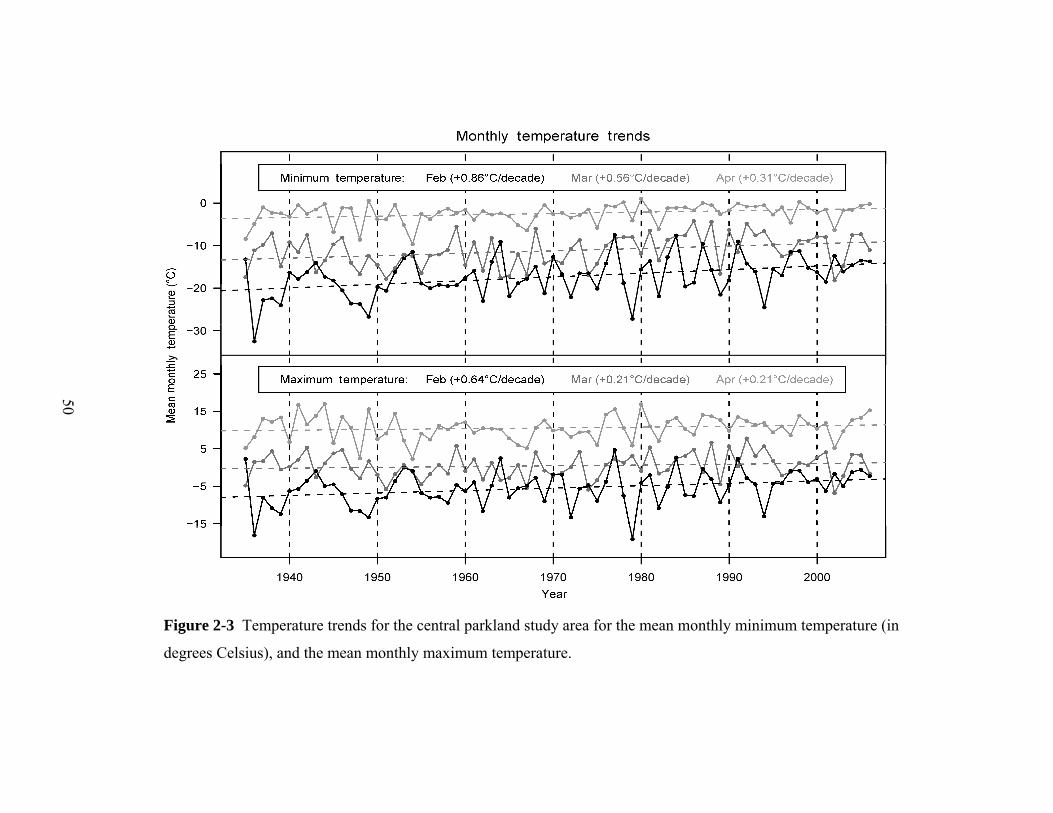
An analysis of historical weather station data revealed a substantial warming
signal over the study period (1936–2006), which ranged from +5.3°C for mean
monthly temperature in February to +1.5°C in May. The earliest blooming species
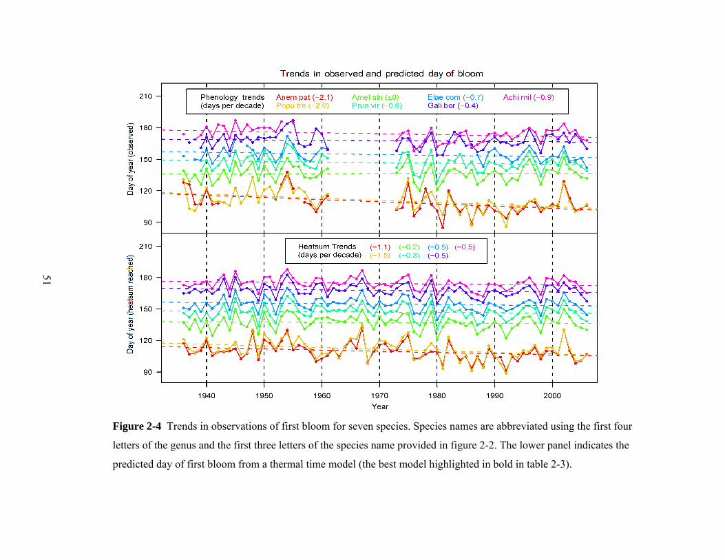
(Populus tremuloides and Anemone patens) advanced their bloom dates by two
weeks over seven decades, while the later species advanced their bloom dates
between zero and six days. Early-blooming species advanced faster than predicted
by thermal time models, which may be due to decreased diurnal temperature
fluctuations. This unexpectedly sensitive response resulted in an increased
exposure to late spring frosts.
A criticism by climate change skeptics is that the observed warming signal is an
artifact of the increasing heat island effect of growing cities. The current dataset
offered the opportunity to test this claim due to the spatially and temporally
extensive phenology database. The data indeed show an increasing heat island
effect over the period 1931–2006 in both weather station data and plant
phenology response. Across all seven plant species, the advance in phenology
observed in Edmonton was 2.1 days (±0.9 SE) greater than in the surrounding
rural areas over the last 70 years. This accounted for one third of the general
warming signal, while the remaining advance of 3.7 days observed in rural
settings was attributed to climate change.
Finally, as guidance for those initiating new observer networks, an analysis of
factors that determined the quality of the PlantWatch phenological data was
carried out. The thesis concludes with recommendations for effective volunteer
training, observer motivation, and program protocols.
Acknowledgements
First and foremost, a huge thanks to my supervisor Andreas Hamann, a
professional ‘data wrangler’ whose skills with statistics contributed greatly to this
thesis. His patience and generosity with time were greatly appreciated. He also
supported my work with a student stipend from his NSERC discovery and Alberta
Ingenuity grants. After 20+ years of largely volunteer work on PlantWatch, this
income was a big bonus. I look forward to future collaboration and publications
with Andreas. Thanks as well to my thesis committee members: Arturo Sanchez’s
keen interest in phenology and insightful comments led to stimulating discussions.
Ellen MacDonald also welcomed me to her ‘clan Mac’ student meetings and
home parties during the year Andreas was on sabbatical.
My husband Geoff Holroyd helped with editing articles and kindly provided many
hot suppers for a late-returning grad student! My generous father Jacques
Beaubien had a love of science and the outdoors that informed and inspired me,
and together we explored much of Canada including the arctic. My mother
Miriam Beaubien passed on her photographic memory and a delight in wild plants
and wild spaces.
Dr. Walter Moser, my MSc supervisor who in 1987 launched me on this
phenological trajectory, continues to encourage my efforts. In recent years my
writing group (composed of Anayansi Cohen, Esther Kamunya, and Xianli Wang)
provided a wealth of help with writing, analysis, and presentations, plus
encouragement and camaraderie. Dave Roberts also helped considerably with data
analysis. Editing help included Myrka Hall Beyer, Linda Seale, and for observer
communications: Linda Kershaw. Plant photographs used in presentations,
webpages and publications were provided by Linda Kershaw and other botanists,
PlantWatch observers, plus fellow provincial and territorial PlantWatch
coordinators. Since 1996, I have enjoyed communications, workshops, and
friendship with these coordinators. We all benefitted from help provided by
Environment Canada’s NatureWatch coordinator -- in recent years the highly
effective Marlene Doyle. Alberta PlantWatch’s webpage has been supported in
recent years by Nature Alberta, in particular their technology wizard Vid Bijelic;
his talents are appreciated.
Fellow students in our grad lab, the Spatial information systems (SIS) lab on the
8th floor of the General Services building, provided great conversation and
company over the last six years. This evolving group has included Patrick Asante,
has recently been assembled at the National Centre for Ecological Analysis and
Synthesis in California (Wolkovich 2012).
9
Biotic drivers of phenology must also be considered, affecting a genetic response.
Bloom timing is influenced by pressures from pollinators or seed dispersers, as
well as predators that consume flowers or seeds (Elzinga et al. 2007). The ability
of a plant to flower at the ‘right’ time is crucial to maximize reproduction via
exposure to pollinators (spring winds or insects) and to exploit best the available
growing season to produce seeds.
1.4. Species differences in thermal time response
An example of a particularly well-studied woody species is Syringa vulgaris
(common purple lilac). This ornamental, widely-cultivated shrub is used
internationally by phenology networks, including Canada PlantWatch
(Environment Canada 2010). A study of lilac bloom dates from 251 locations in
the USA found the coefficient of variation of thermal time to flowering was
smallest using a base temp of -0.6º C (Caprio 1974). Examples for well-studied
boreal species include pines, included in the Alberta Plantwatch program since
2000. Di-Giovanni et al. (1996) researched timing of operations to reduce pollen
contamination in pine seed orchards. They found for maximum pollen release of
Pinus banksiana (jack pine) from 3 northern Ontario locations, the best
combination was a base temperature of 4ºC and start date of April 17, with a
resulting heat sum of 288.6 degree days.
Base (or threshold) temperatures for heat sum accumulation for budbreak and
bloom differ among plant life forms and geographic regions. In the Earth’s
temperate zone, threshold values often range from 0-5°C for woody plants.
Herbaceous plants generally have higher base temperatures of 6-10 ºC, but these
10
are lower (0-6 ºC) for spring ephemerals and alpine plants. Leafing in some
species of Populus can occur at temperatures as low as 0 ºC (Larcher 2003).
While the heat sum requirements for a stage such as first pollen shed are relatively
constant for a plant species among years, location is important. Single species
studies show that populations at higher latitudes or altitudes tend to respond more
quickly to spring increases in temperature (Li et al. 2010). This is likely an
adaptation to a shorter growing season.
Species react independently to climate warming (Sparks and Carey 1995, Abu-
Asab et al. 2001) but generally species that bloom in early spring are more
sensitive to and thus better reflect changes in temperature (Menzel et al. 2006).
Populus tremuloides (a tree) and Anemone patens (herbaceous forb) are two
species that start the PlantWatch bloom sequence. These two “start of spring”
Alberta plants generally bloom within 2 days of each other and flowering occurs
soon after snowmelt. But in years of deep spring snow, tree buds can respond to
rising temperatures more quickly. In these years Populus may have a smaller heat
sum and earlier bloom than Anemone. Therefore the interaction of plant life form
and snow depth may influence spring phenology in Alberta.
For a given location, the sequence of phenological events is very uniform, and
thus the timing of one event can predict the subsequent timing of an event for that
or another plant species. In Edmonton, the two shrubs Amelanchier alnifolia
(saskatoon) and Prunus pensylvanica (pin cherry) generally start bloom within
one day of each other (unpublished data). Delbart et al. (2005) found a tight
correlation between woody species events using remotely sensed data from
Siberia: the mean difference between leafing times for Betula (birch) and Populus
11
tremula (a close relation of the North American P. tremuloides and also called
‘aspen’) was 3 days (SD = 4.7). At the start of the growing season both flowering
and leafing events are highly correlated, and therefore sub-canopy flowering
events can be used to predict the timing of forest green-up.
This review has focused on perennial plants, which were selected for phenological
study in Alberta as they persist for years in a location and develop in response to
increasing temperature. In contrast to perennials, annual plants’ bloom times
depend somewhat on when the seed germinated and plant growth began. For
many herbaceous annual plants including some grass species, photoperiod is the
cue for flowering. But as photoperiod is unchanging from year to year for any
specific location and date, any trend in spring blooming time for an annual plant
would indicate that other factors are important.
1.5. Documentation of climate change
Due to its direct dependence on temperature and because it is readily observable,
spring phenology in temperate zones has served as important source of evidence
for climate change. The majority of global phenology data are from Europe.
Menzel (2000) analysed data from cloned woody plants (13 trees and 3 shrubs)
from International Phenological Gardens across Europe (1959-1996). Over this
period, spring events including leaf unfolding and flowering advanced by 2
days/decade. In Estonia, Ahas (1999) found that plant bloom times for 1952-1996
(45 years) advanced from 1.4 to 2.9 days/ decade. Fitter (2002) examined first
bloom dates (1954 to 2000: 47 years) for 385 British plant species (grasses, forbs,
woody plants) and noted an advance of 4.5 days in the recent decade (1991-2000)
12
as compared to the previous 37 years; this translates to a shift of 0.9 days earlier/
decade. A major review that includes the above papers summarized 254 mean
national time series from 21 European countries (1971 – 2000) and concluded that
the mean advance of spring and summer was 2.5 days per decade (Menzel et al.
2006). The phenology patterns closely matched the warming noted across 19
countries. But there was no indication of plants adapting to climate warming; in a
comparison of phenology records across the 20th century in Germany, plant
species’ response to temperature did not change over time (Menzel et al. 2005).
A review of global phenological studies over the last century revealed a 10-20
day lengthening of the growing season over the last few decades, with the largest
trend to earlier spring onset (Linderholm 2006). In the mid-1970’s there was a
shift to increasing temperatures, reflected in a shift to earlier phenological
development on a wide scale (Walther et al. 2002). An excellent review by Bertin
(2008) summarizes published studies and notes generalizations including the
following: a) early spring stages show greater advances over time than later
stages, b) abundant spatial variation in phenological shifts has been reported, and
c) species differ in their phenological response.
In North America, Abu-Asab (2001) noted mean first flowering advances of 0.8
days/ decade for 89 of 100 angiosperm species in Washington, DC, over the years
1970 to 1999 (30 years). These were correlated with increases in minimum
temperature. Bradley et al. (1999) compared bird and plant data for Aldo
Leopold’s cabin over six decades 1936-1998, with a 30-year gap after the first
decade. Of 21 plant species starting bloom before June 1, six species showed
regressions with statistically significant trends to earlier bloom. Averaging all 55
13
phenophases showed a shift to earlier development by 1.2 days/ decade. For the
western USA, trends over 38 years (1957-1994) were 2 days/ decade earlier for
first bloom of Syringa vulgaris (common purple lilac), and 3.8 days/ decade for
Lonicera sp. (honeysuckle) (Cayan et al. 2001). They also noted increasing spring
temperatures of 1-3 ºC and earlier streamflow pulse dates beginning in the 1970s.
In Canada, Houle (2007) used herbarium specimens and found a 0.2 to 0.6 days/
decade shift to earlier bloom over 100 yrs (1900 to 2000) in three areas of Quebec
and Ontario, for 18 spring flowering herbaceous plants. This study also found a 2-
3 day advance/ ºC increase, and evidence of a heat island effect for Montreal. In
Edmonton, Alberta, a ‘spring flowering index’ which combined responses of three
woody species showed an 8 day shift to earlier development over the period 1936-
1996: 61 years, ie 1.3 days/ decade. The earliest appearing species, Populus
tremuloides, showed a doubling of this trend: 2.6 days/ decade over the 20th
century (Beaubien and Freeland 2000). There is a relative scarcity of published
data on trends in phenology in North America.
Comparing trends from various studies is challenging as they vary with respect to
species, phenophases, time span, and geographic area. However, the literature
paints a common picture of changes in spring timing. In Europe, spring phases are
earlier by 1.2 to 3.1 days/ decade and in North America by 0.8 to 3.8 days/decade
(Menzel 2003). Generally, ground-based studies show a shift to earlier spring of
2.3 to 5.2 days / decade over the 3 decades up to 2006 in response to warming,
confirmed by remote sensing studies (IPCC 2007).
14
1.6. Heat island effects
The urban heat island effect poses one potential technical problem in interpreting
the causes of observed trends in spring plant development timing. Many of the
published phenology data are from urban centres, where conditions are warmer
than in the surrounding rural areas. This heat island effect is caused by the
absorptive and radiative properties of roads and structures, as well as emissions
from heating, industry and vehicles (Defila and Clot 2003). To study the changing
influence of city size, population statistics are often used (Barry and Chorley
2010).
In central Europe, spring phenophases for early spring phases in 10 city locations
(1980 to 1995) were four days earlier than in rural locations, and trends were
larger trends in more recent years (Rötzer et al. 2000). In eastern Canada, analysis
of herbarium specimens of Tussilago farfara (coltsfoot) showed major shifts to
earlier bloom of 15-31 days since the early 20th century, in the cities of Montreal
and Quebec (Lavoie and Lachance 2006). No trend was found for rural areas.
This would indicate that in cold climates this urban effect is considerable and
needs to be addressed in our analyses. As well, urban systems provide surrogates
for studies of climate change, to help predict the impacts of future increasing
temperature and CO₂ levels.
15
1.7. Protocols for phenology observation programs
There are several different methods to conduct phenological studies. The simplest
type of survey is an annual "snapshot" study, where many observers survey plant
development stages over a large area at a specified date (e.g. the “May Species
Count” by Nature Alberta). Another survey type makes use of large networks of
volunteers that record specific growth stages or phenophases on selected species
whenever they occur (e.g. Canada PlantWatch, or the German Weather Service
phenology observation program). Some studies are restricted to expert observers
and researchers that make use of repeat observations on tagged plants, which
usually results in better data quality. Other sources for phenology data that can
contribute to studies of long-term trends in phenology include historic explorer’s
journals, herbarium records, daily pollen count data (from medical researchers),
and for recent decades: satellite observations.
Phenological data are relatively simple to record, and extensive datasets from
amateur and professional observers have been assembled in many parts of the
world. Phenology studies have seen a resurgence of interest and many new
volunteer networks have been initiated in recent decades. These include the
federal expansion of Canada PlantWatch (Environment Canada 2010), Britain’s
program to track phenology of plants and animals (Woodland Trust UK 2012),
and the Netherlands ‘nature’s calendar” (Milieusysteemanalyse 2012). The USA
National Phenological Network had its official launch March 2009 (USA-NPN
2012). Aspects of phenology globally including history, networks, research by
taxa or biome, modeling, and applications including remote sensing are described
in two “bibles of phenology” (Lieth 1974, Schwartz 2003). PlantWatch in Canada
16
is potentially a very useful tool to help Canadians understand, mitigate, and adapt
to the expected changes in climate as well as the potential impacts on biodiversity
and society. Since 2000, the author has been science advisor for the national
program Canada PlantWatch (Environment Canada 2010). The history of
phenology in Canada is described in Beaubien (1991) and (Schwartz and
Beaubien 2003).
Sources of variation in phenology data include the plants (genotype), the observer
(skill and experience), the site (geographic location and microclimate), and the
weather (Beaubien 1991, Beaubien and Johnson 1994, Schaber 2002). The
influence of temperature is strongest for early-blooming spring species (Beaubien
and Freeland 2000, Menzel et al. 2006), and thus these may be the best species to
track for climate change studies.
1.8. Thesis structure
In this thesis, I quantify plant spring phenology of up to 25 plant species in
response to climate and climate change in Alberta. Available data include 20
years of field data collected by myself and provincial volunteers 1987–2006, plus
additional databases for the periods 1936–1961 and 1973–1986 from other
researchers. My goal is to determine (1) how different species have responded to
climate change over the last seven decades, and (2) how heat island effects may
exaggerate the climate change response in the city versus rural areas. Because
new phenology survey networks continue to appear in the United States and
Europe, I will further develop recommendations on observation protocols, species
17
selection and quality control based on a quantitative analysis of the Alberta
PlantWatch volunteer network.
My aim for Research Chapter #1: Long-term trends in spring phenology is to
document changes in timing of first bloom for seven plant species using
phenology data from three sources for Alberta’s central parkland from 1936 to
2006. In this chapter I will also attempt to build a predictive model of abiotic
drivers of spring phenology and test whether additional factors that are not usually
part of thermal time models contribute to spring phenology for these plant
species. For herbaceous species, snow depth may influence the timing of spring
flowering. Frost events may damage reproductive tissues and thus prevent or
delay flowering. Lastly, I ask whether changes in plant-climate synchronization
could create potential problems for future plant survival. For example, aspen is
said to bloom in general a month before the last killing frost. In springtime is the
timing of last frost shifting at the same rate as the plant response? To detect which
species may be most vulnerable to observed and projected climate change, I
investigate trends in timing of last spring frosts.
The Research Chapter #2: Heat island effects looks at potential bias in
phenology trends that may emerge due to observation location. Urban
environments are often warmer than rural areas due to anthropogenic changes,
causing shifts to earlier plant development in spring. This urban heat island effect
is additive to the general pattern of climate warming, and may confound an
understanding of its effects if urban population growth takes place at the same
time as general climate warming. Therefore, studies of plant response both inside
and outside urban centres are needed to disentangle these two potential causes of
18
shifts in plant timing. In this chapter I will analyze the heat island effect in
Edmonton, Alberta, based on rural and urban weather station records for the
period 1916 to 2004, as well as urban phenology records for the period 1936-1961
and rural and urban phenology records 1987-2006. I will attempt to visualize the
urban heat island effect via spatial interpolation for 1987-2006 data, with
comprehensive spatial coverage, and I will further try to quantify what proportion
of the overall warming effect relative to the 1936-1961 period is attributable to an
increasing heat island effect (due to population growth and urbanization), rather
than to climate warming.
The goal of my Research Chapter #3: Plant phenology for citizen scientists, is to
develop better methodologies and more robust observer protocols for the Canada
PlantWatch program and similar efforts elsewhere. I will review options for both
selection of species and growth stages for observation, as well as for recruitment
and training of observers. I will make recommendations on the best plant species
and phases to track climate change, and recommend how to design studies to
minimize observer error and maximize data quality. I will look for correlation
between ease of observation of plant species and phenophases, and reporting
accuracy. Better quality data might be expected for plant species that are abundant
and widespread, lack similar-looking species, have conspicuous flowers, and have
a short blooming period in spring. Secondly, I will analyze whether the
supplementary microhabitat data gathered by the Alberta PlantWatch program
(e.g. location slope and aspect, distance to buildings, etc.) improved the accuracy
of observations. Finally, I will investigate whether experienced long-term
observers provide better data (i.e. data that correlate better with climatic factors)
than short-term observers. I synthesize the results to help those who wish to
19
initiate new observer networks regarding observer recruitment and training,
effectiveness of program protocols, and selection of species and bloom stages.
1.9. References
Abu-Asab, M. S., P. M. Peterson, S. G. Shetler, and S. S. Orli. 2001. Earlier plant flowering in spring as a response to global warming in the Washington, DC, area. Biodiversity and Conservation 10:597-612.
Ahas, R. 1999. Long-term phyto-, ornitho- and ichthyophenological time-series
analyses in Estonia. International Journal of Biometeorology 42:119-123. Barry, R. G. and R. J. Chorley. 2010. Atmosphere, weather, and climate. 9th
edition. Routledge, London; New York. Beaubien, E. G. 1991. Phenology of vascular plant flowering in Edmonton and
across Alberta, MSc thesis. University of Alberta, Edmonton. Beaubien, E. G. 2012. Alberta Plantwatch. http://plantwatch.naturealberta.ca Beaubien, E. G. and H. J. Freeland. 2000. Spring phenology trends in Alberta,
Canada: links to ocean temperature. International Journal of Biometeorology 44:53-59.
Beaubien, E. G. and M. Hall-Beyer. 2003. Plant phenology in western Canada:
trends and links to the view from space. Environmental Monitoring and Assessment 88:419-429.
Beaubien, E. G. and D. L. Johnson. 1994. Flowering plant phenology and weather
in Alberta, Canada. International Journal of Biometeorology 38:23-27. Bertin, R. I. 2008. Plant phenology and distribution in relation to recent climate
change. Journal of the Torrey Botanical Society 135:126-146. Bird, C. D. 1983. 1982 Alberta flowering dates. Alberta naturalist 13:1-4. Boyer, W. D. 1973. Air temperature, heat sums, and pollen shedding phenology
of longleaf pine. Ecology 54:420-426. Bradley, N. L., A. C. Leopold, J. Ross, and W. Huffaker. 1999. Phenological
changes reflect climate change in Wisconsin. Proceedings of the National Academy of Sciences of the United States of America 96:9701-9704.
20
Campbell, R. K. and A. I. Sugano. 1975. Phenology of bud burst in Douglas-fir related to provenance, photoperiod, chilling, and flushing temperature. Botanical Gazette 136:290-298.
Cannell, M. G. R. 1989. Chilling and thermal time and the date of flowering of
trees. Pages 99-113 in 47th University of Nottingham Easter School in Agricultural Science. Butterworths, London, April 18-22, 1988, Sutton Bonington, England.
Cannell, M. G. R. and R. I. Smith. 1983. Thermal time, chill days and prediction
of budburst in Picea sitchensis. Journal of Applied Ecology 20:951-963. Caprio, J. M. 1974. The solar thermal unit concept in problems related to plant
development and potential evapotranspiration. Pages 353-364 in H. Lieth, editor. Phenology and seasonality modeling. Springer, New York.
Cayan, D. R., S. A. Kammerdiener, M. D. Dettinger, J. M. Caprio, and D. H.
Peterson. 2001. Changes in the onset of spring in the western United States. Bulletin of the American Meteorological Society 82:399-415.
Chuine, I. and E. G. Beaubien. 2001. Phenology is a major determinant of tree
species range. Ecology Letters 4:500-510. Cleland, E. E., N. R. Chiariello, S. R. Loarie, H. A. Mooney, and C. B. Field.
2006. Diverse responses of phenology to global changes in a grassland ecosystem. Proceedings of the National Academy of Sciences of the United States of America 103:13740-13744.
Defila, C. and B. Clot. 2003. Long-term urban-rural comparisons. Pages 541-554
in M. D. Schwartz, editor. Phenology: an integrative environmental science. Kluwer Academic Publishers, Dordrecht, the Netherlands.
Delbart, N., L. Kergoat, T. Le Toan, J. Lhermitte, and G. Picard. 2005.
Determination of phenological dates in boreal regions using normalized difference water index. Remote Sensing of Environment 97:26-38.
Di-Giovanni, F., P. G. Kevan, and G.-E. Caron. 1996. Estimating the timing of
maximum pollen release from jack pine (Pinus banksiana Lamb.) in northern Ontario. The Forestry Chronicle 72:166-169.
Diekmann, M. 1996. Relationship between flowering phenology of perennial
herbs and meteorological data in deciduous forests of Sweden. Canadian Journal of Botany-Revue Canadienne De Botanique 74:528-537.
21
Elzinga, J. A., A. Atlan, A. Biere, L. Gigord, A. E. Weis, and G. Bernasconi. 2007. Time after time: flowering phenology and biotic interactions. Trends in Ecology & Evolution 22:432-439.
the physical science basis. Cambridge University Press, Cambridge, UK; New York, NY, USA.
Karl, T., J. Lawrimore, and A. Leetma. 2005. Observational and modeling
evidence of climate change. Pages 11-17. Environmental management, Air and waste management association magazine for environmental managers.
Kross, A., R. Fernandes, J. Seaquist, and E. Beaubien. 2011. The effect of the
temporal resolution of NDVI data on season onset dates and trends across
22
Canadian broadleaf forests. Remote Sensing of Environment 115:1564-1575.
Landsberg, J., D. R. Butler, and M. R. Thorpe. 1974. Apple bud and blossom
temperatures. Journal of Horticultural Science & Biotechnology 49:227-239.
Larcher, W. 2003. Physiological plant ecology: ecophysiology and stress
physiology of functional groups. 4th edition. Springer. Lavoie, C. and D. Lachance. 2006. A new herbarium-based method for
reconstructing the phenology of plant species across large areas. American Journal of Botany 93:512-516.
Lechowicz, M. J. 1984. Why do temperate deciduous trees leaf out at different
times? Adaptation and ecology of forest communities. American Naturalist 6:821-842.
Li, H. T., X. L. Wang, and A. Hamann. 2010. Genetic adaptation of aspen
(Populus tremuloides) populations to spring risk environments: a novel remote sensing approach. Canadian Journal of Forest Research-Revue Canadienne De Recherche Forestiére 40:2082-2090.
Lieth, H., editor. 1974. Phenology and seasonality modeling. Springer-Verlag,
New York. Linderholm, H. W. 2006. Growing season changes in the last century.
Agricultural and Forest Meteorology 137:1-14. Lindsey, A. A. and J. E. Newman. 1956. Use of official weather data in spring
time - temperature analysis of an Indiana phenological record. Ecology 37:812-823.
Mbogga, M. S., A. Hamann, and T. L. Wang. 2009. Historical and projected
climate data for natural resource management in western Canada. Agricultural and Forest Meteorology 149:881-890.
Menzel, A. 2000. Trends in phenological phases in Europe between 1951 and
1996. International Journal of Biometeorology 44:76-81. Menzel, A. 2003. Plant phenological fingerprints. Pages 319-329 in M. D.
Schwartz, editor. Phenology, an integrative environmental science. Kluwer Academic Publishers, Dordrecht, the Netherlands.
Menzel, A., N. Estrella, and A. Testka. 2005. Temperature response rates from
long-term phenological records. Climate Research 30:21-28.
23
Menzel, A., T. H. Sparks, N. Estrella, E. Koch, A. Aasa, R. Ahas, K. Alm-Kubler,
P. Bissolli, O. Braslavska, A. Briede, F. M. Chmielewski, Z. Crepinsek, Y. Curnel, A. Dahl, C. Defila, A. Donnelly, Y. Filella, K. Jatcza, F. Mage, A. Mestre, O. Nordli, J. Peñuelas, P. Pirinen, V. Remisova, H. Scheifinger, M. Striz, A. Susnik, A. J. H. Van Vliet, F. E. Wielgolaski, S. Zach, and A. Zust. 2006. European phenological response to climate change matches the warming pattern. Global Change Biology 12:1969-1976.
Milieusysteemanalyse, L. 2012. der Natuurkalendar,
http://www.natuurkalender.nl/. Wageningen, the Netherlands. August 2012.
Myking, T. and O. M. Heide. 1995. Dormancy release and chilling requirement of
buds of latitudinal ecotypes of Betula pendula and Betula pubescens. Tree Physiology 15:697-704.
Orton, D. 1989. Coincide: The Orton system of pest management. 1st edition.
American Nurseryman Publishing Company, Chicago. Peñuelas, J., T. Rutishauser, and I. Filella. 2009. Phenology feedbacks on climate
change. Science 324:887-888. Rathcke, B. and E. P. Lacey. 1985. Phenological patterns of terrestrial plants.
Annual Review of Ecology and Systematics 16:179-214. Rigby, J. R. and A. Porporato. 2008. Spring frost risk in a changing climate.
Geophysical Research Letters 35:1-5. Rötzer, T., R. Grote, and H. Pretzsch. 2004. The timing of bud burst and its effect
on tree growth. International Journal of Biometeorology 48:109-118. Rötzer, T., M. Witenzeller, H. Häckel, and J. Nekovar. 2000. Phenology in central
Europe - differences and trends of spring phenophases in urban and rural areas. International Journal of Biometeorology 44:60-67.
Schaber, J. 2002. Phenology in Germany in the 20th century: methods, analyses
and models PhD. Scheifinger, H., A. Menzel, E. Koch, and C. Peter. 2003. Trends of spring time
frost events and phenological dates in Central Europe. Theoretical and Applied Climatology 74:41-51.
Schwartz, M. D., editor. 2003. Phenology, an integrative environmental science.
Kluwer Academic Publishers, Dordrecht, the Netherlands.
24
Schwartz, M. D., R. Ahas, and A. Aasa. 2006. Onset of spring starting earlier across the Northern Hemisphere. Global Change Biology 12:343-351.
Schwartz, M. D. and E. G. Beaubien. 2003. Chapter 2.4. North America. Pages
57–73 in M. D. Schwartz, editor. Phenology: an integrative environmental science. Kluwer, Dordrecht.
Sparks, T. H. and P. D. Carey. 1995. The responses of species to climate over 2
centuries - an analysis of the Marsham phenological record, 1736-1947. Journal of Ecology 83:321-329.
USA-NPN. 2012. USA National Phenology Network, http://www.usanpn.org/.
August 2012. Walther, G. R., E. Post, P. Convey, A. Menzel, C. Parmesan, T. J. C. Beebee, J.
M. Fromentin, O. Hoegh-Guldberg, and F. Bairlein. 2002. Ecological responses to recent climate change. Nature 416:389-395.
White, L. M. 1979. Relationship between meteorological measurements and
flowering of index species to flowering of 53 plant species. Agricultural Meteorology 20:189-204.
Wolkovich, E. 2012. Phenology Literature Review,
http://knb.ecoinformatics.org/knb/metacat/wolkovich.24.3/knb. Knowledge Network for Biocomplexity. National Centre for Ecological Analysis and Synthesis, San Diego, California. August 2012.
Woodland Trust UK. 2012. Nature's Calendar,
http://www.naturescalendar.org.uk. Citizens report timing of spring and fall events in nature. Woodland Trust and Centre for Hydrology and Ecology. August 2012.
25
Chapter 2 - Spring Flowering Response to Climate
Change between 1936 and 2006 in Alberta, Canada 1
Summary
In documenting biological response to climate change, the IPCC has used
phenology studies from many parts of the world, but few are available from high
latitudes of North America. Here, we evaluate climate trends and corresponding
changes in sequential bloom times for seven plant species in the central parklands
of Alberta, Canada (latitude 52–57° north). We found a substantial warming
signal over the study period of 71 years (1936–2006), which ranged from an
increase of 5.3°C in the mean monthly temperatures for February to an increase of
1.5°C in those for May. The earliest-blooming species’ (Populus tremuloides and
Anemone patens) bloom dates advanced by two weeks during the seven decades,
whereas the later-blooming species’ bloom dates advanced between zero and six
days. The early-blooming species’ bloom dates advanced faster than was
predicted by thermal time models, which we attribute to decreased diurnal
temperature fluctuations. This unexpectedly sensitive response results in an
increased exposure to late spring frosts.
1 A version of this chapter has been published as: Beaubien E., Hamann, A. 2011.
Spring flowering response to climate change between 1936 and 2006 in Alberta,
Canada. BioScience 61: 514–524.
26
2.1 Introduction
The scientific field of phenology, defined as the study of the seasonal timing of
life cycle events, has seen a recent revival with climate change being a prominent
issue. Sparks and colleagues (2009) noted that the use of the term ‘phenology’ in
the scientific literature has become seven times more common between 1990 and
2008. In documenting biological response to global climate change the
Intergovernmental Panel on Climate Change (IPCC 2007) has relied on
phenology studies as compelling evidence that species and ecosystems respond to
global climate change (Rosenzweig et al. 2007). Particularly for perennial plants
in temperate zones, temperature exposure over time is the main driver for spring
development, including the timing of bloom and leafout (Rathcke and Lacey
1985, Bertin 2008). This makes spring phenology one of the most sensitive,
immediate, and easily-observed responses to changing climate in temperate
regions (e.g. Schwartz et al. 2006).
The use of phenology observations to document climate variability and climate
change has a long history. In 1956, Arakawa published an article entitled
“Climatic change as revealed by the flowering dates of the cherry blossoms at
Kyoto”. He analyzed a long-term record of dates when the emperor held the
annual cherry blossom festival that reached back to the ninth century (Arakawa
1955, 1956). Remarkable phenology records covering more than two centuries
also exist for European countries, starting with observations by Linnaeus in the
18th century (Parmesan 2006). In a meta-analysis for Europe, Menzel and
colleagues (2006) compiled an astonishing 125,000 time series recorded for more
than 500 plant species in 21 countries.
27
Although a number of famous historical figures have been involved in early,
systematic phenology observations, including Thomas Jefferson as well as Henry
David Thoreau and Aldo Leopold (Stoller 1956, Miller-Rushing and Primack
2008), long-term records of phenology observation are comparatively scarce in
North America when compared with Europe (Schwartz and Beaubien 2003). A
notable analysis was carried out by Aldo Leopold’s daughter N. L. Bradley and
son A. C. Leopold. They compared Aldo Leopold’s 1935–1945 Wisconsin farm
records (Leopold and Jones 1947) with data on 36 plant species collected in the
same area from 1976 to 1998 (Bradley et al. 1999). Another major long-term
observation effort is the phenology network established by Caprio (1957),
recording phenology of lilac (Syringa vulgaris) and honeysuckle cultivars
(Lonicera spp.) with the help of local garden clubs in 12 western US states until
1994 (Cayan et al. 2001). A similar lilac-honeysuckle network, which still exists
today, was established in 1959 in the northeastern US states and eastern Canadian
provinces (Schwartz and Reiter 2000). However, there is a notable lack of
phenology data for western Canada and Alaska where the spring warming signal
over the last 50 years has been most pronounced globally (Rosenzweig et al.
2007).
Besides documenting global change, trends in plant phenology can reveal
important ecological consequences associated with climate change (Parmesan
2006, Cleland et al. 2007). Plant populations are finely tuned to local frost risk
environments at the beginning and end of the growing season, and phenological
traits are usually highly heritable and often subject to strong selection pressures
(Campbell and Sugano 1975, Vitasse et al. 2009, Li et al. 2010). The timing of
28
spring plant development balances the need to avoid damage due to late spring
frosts while maximizing the use of the available growing season in competition
with other species (Lechowicz 1984, Leinonen and Hanninen 2002). Therefore,
plants at northern latitudes and at high elevation break bud relatively early, i.e. the
need to utilize the growing season takes relative precedence over avoiding late
spring frost damage. This has been documented in many common garden studies
for wide-ranging plant species (reviewed by Li et al. 2010).
The timing of spring development in virtually all temperate perennial plants is
primarily controlled by temperature (Rathcke and Lacey 1985, Hunter and
Lechowicz 1992). Plants require a certain amount of exposure to warm
temperatures before leafout or flowering occurs. Exposure to warm temperature
over time can be measured in degree days, which is the sum of average daily
temperatures above a base value. A common base temperature is 5°C, which is
widely used to calculate growing degree days in agriculture. For a given species,
this amount of warm temperature over time, referred to as required heat sum, is
largely constant and can be used to predict bloom times from daily temperature
records in what is called a thermal time model (Bertin 2008). The required heat
sum for spring development is a genetically controlled adaptive trait (Leinonen
and Hanninen 2002). Heat sum accumulation allows plants to respond to an
unpredictable onset of the growing season, which can easily vary by a month in
northern latitudes.
If spring development were exclusively driven by exposure to warm temperature,
climate change would not affect the match of plant development with the
available growing season. However, additional factors are known to modulate the
29
timing of spring development. Photoperiod may delay bud break if warm
temperatures arrive unusually early (Menzel et al. 2005). Some plants also require
a certain amount of exposure to cool temperatures following bud set in fall before
they start development in response to warm spring temperatures. This is referred
to as a chilling requirement, which is measured by summing exposure to
moderately cool temperatures, typically between 0 and 10°C. This is thought to
guard plants from prematurely breaking bud during mid-winter thaws. In both
cases climate warming would be expected to delay spring response. Plants may be
constrained by photoperiod effects that prevent early development, or in warmer
regions they may not receive sufficient exposure to cold temperature to release
them from dormancy (Bertin 2008).
Another factor that impacts spring phenological response at high latitudes and
high elevation is the prevalence of snow (Inouye and Wielgolaski 2003,
Wielgolaski and Inouye 2003). A deep spring snowpack further shortens the
growing season and once the snow has melted plant response is often immediate,
suggesting very low heat sum requirements, and making the release from snow a
primary driver of spring phenology. This also has important implications for the
effects of climate change. A smaller snowpack due to either higher temperatures
or less precipitation would lead to earlier release from snow, an earlier start of
plant development, and potentially higher frost exposure (Inouye 2008).
In the present article, we report results from spring flowering observations
conducted over approximately seven decades (1936–2006) in Alberta, western
Canada. We analyzed first bloom dates for seven plant species that come into
flower in a temporal sequence between early April and June. The first objective of
30
this study was to attempt to provide evidence of plant response to global climate
change for a higher latitude location of western North America, a region where
long-term data coverage is scarce. Secondly, we asked whether phenology trends
correspond to observed temperature trends according to spring thermal time
models, or alternatively, whether other factors influence spring development,
which would potentially lead to altered sequences of bloom time. Finally, we
investigated whether shifts in bloom time have led to changes in exposure of
species to late spring frosts.
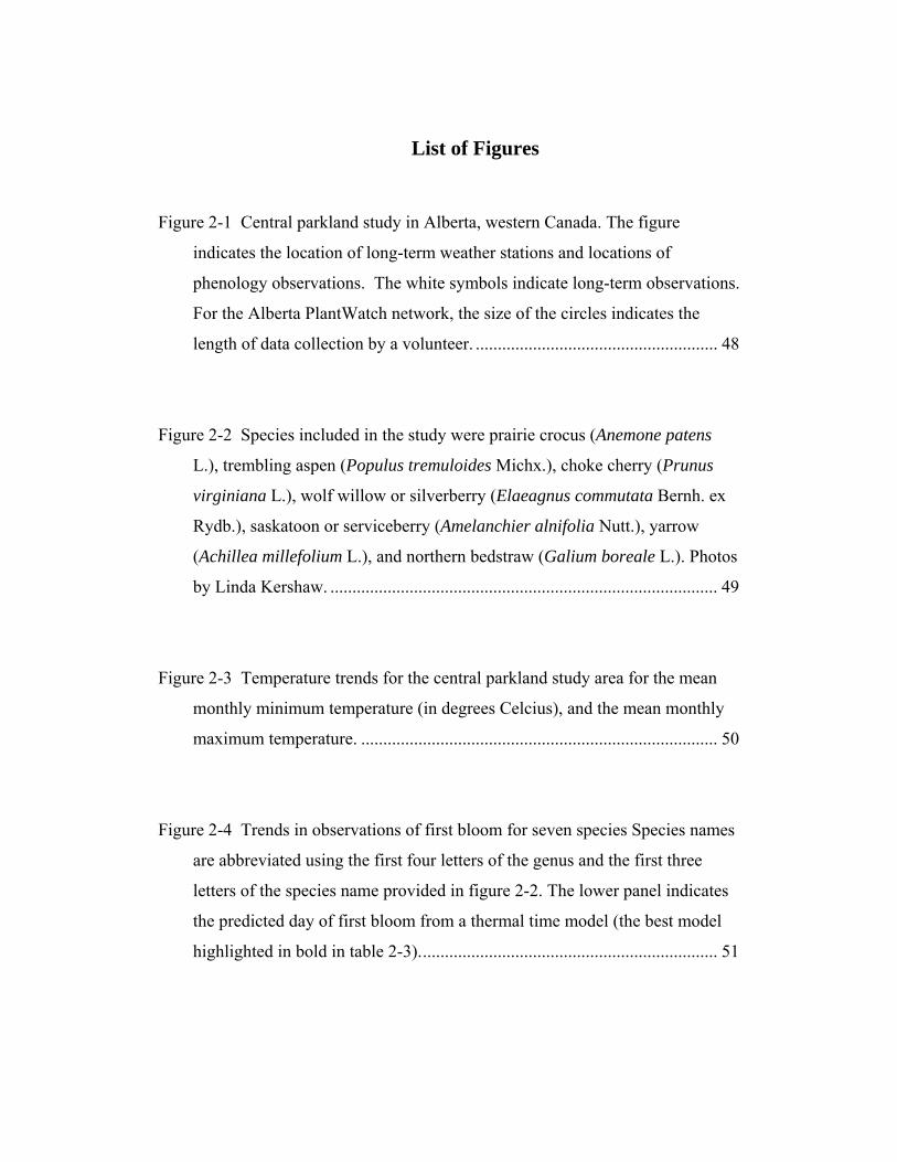
2.2 Phenology observations in central Alberta
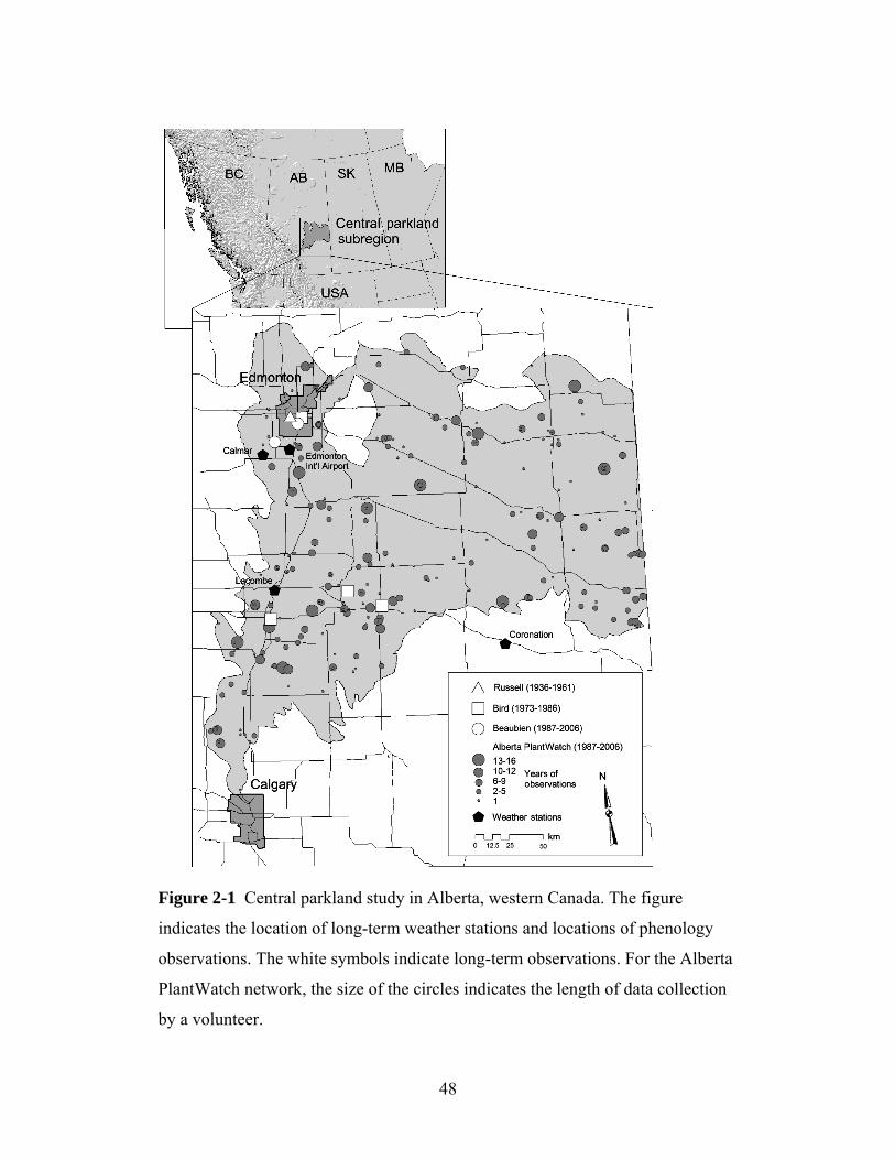
We evaluated observations from a phenology network across the central parkland
of Alberta (figure 2-1). This ecological subregion covers approximately 50,000
km² and is situated between the boreal forest to the north and the warmer and
drier grasslands to the south. The native vegetation consists of open forests
dominated by two poplars (Populus tremuloides Michx. and Populus balsalmifera
L.), white spruce (Picea glauca [Moench] Voss) and birch (Betula spp.) as well as
prairie vegetation found under drier microsite conditions. However, much of the
native vegetation has been converted to agricultural use because the area has some
of the best soils in Canada. Intensive phenology observations began in 1936 with
a program by Agriculture Canada, in which the timing of wheat development as
well as bloom times for 50 native plant species were recorded over 26 years. The
purpose of this program was to identify indicator events to guide the timing of
agricultural activities (Russell 1962). This program ended in 1961, which resulted
in a data gap of 11 years before botanist Dr. Charles Bird initiated a new research
program, which tracked bloom times for 12 native species between 1973 and
31
1986. The data were collected by a network of citizen scientists (Bird 1983)
supplemented by Bird’s own observations (figure 2-1). This network was
extended by EB in 1987, and in its current form, the volunteer observers record
data for one or more of 25 species (plantwatch.naturealberta.ca). Since 1987, this
network has collected data from approximately 650 observers, with up to 240
observers reporting each year. The plant species for this phenology network were
selected primarily based on the plants’ wide distribution and short bloom period
in spring, the ease of their identification by citizens, and the lack of similar-
looking species. For additional background on these data series, see Beaubien and
Johnson (1994) and Beaubien and Freeland (2000).
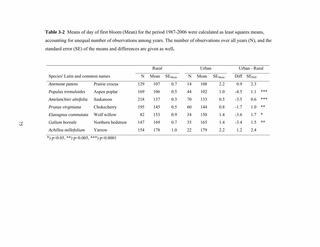
This study evaluates the dates of first bloom for several plant species. First bloom
was defined as a plant stage where the first flower buds had opened in an
observed tree or shrub, or in a patch of smaller plants. We requested that the
observers report on plants that were situated in flat areas away from heat sources
such as walls of houses. Observers were asked to select plants that approximately
represented the average bloom time for that species in their area (i.e., that were
not the first or last of that species to bloom). Therefore, our first bloom data do
not represent the earliest-blooming individuals of a population (as in Miller-
Rushing et al. 2008). Rather, it is a developmental stage sampled to represent a
local population. Generally, the first bloom stage is simplest to observe and yields
more temporally-precise data than later bloom stages, which can be harder to
estimate. Because many of the data (1987–2006) were compiled from multiple
individual plant observations, we used the annual mean bloom date from all
available points in the central parkland. The annual first bloom dates were
compiled by species and year from all three datasets and used for statistical
32
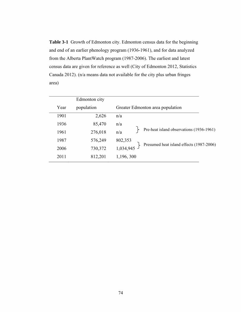
analysis and graphical presentation. Except for the first dataset, collected 1936–
1961 (Russell 1962), we excluded phenology data from the greater Edmonton
area. Edmonton’s human population has grown at an exponential rate to over one
million from 85,000 at the beginning of this research (Statistics Canada 2010). It
is therefore possible that urban heat island effects on temperature may confound
data on climate change trends (e.g. Rötzer et al. 2000) .
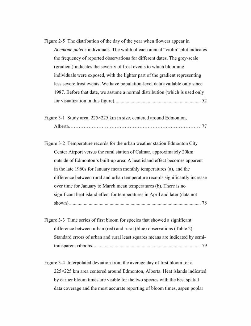
The three observation programs, those of Russell (1962), Bird (1983), and
Beaubien (Beaubien and Johnson 1994, Beaubien and Freeland 2000) included
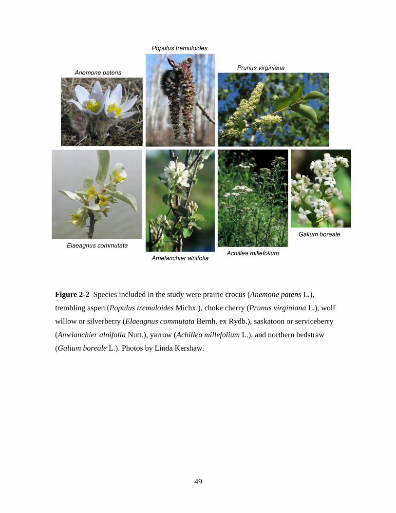
the same four woody and three herbaceous (non-woody) plant species (figure 2-
2). The first species to bloom is the prairie crocus (Anemone patens L.), which is
found in grasslands throughout the northern hemisphere and blooms soon after
snow-melt. Usually blooming within two days of the prairie crocus is the
trembling aspen (Populus tremuloides Michx.), one of the most common and
widely-distributed tree species in North America. It is the first tree in Alberta to
shed pollen and produce leaves in spring. About 25 days later, the saskatoon or
serviceberry (Amelanchier alnifolia Nutt.), blooms. The saskatoon is a widespread
tall woody shrub with edible berries that were the most important plant food for
the prairie Blackfoot First Nations. The remaining four species follow in
approximately eight-day intervals, starting with the choke cherry (Prunus
virginiana L.), a tall woody shrub that is also widespread throughout North
America. The wolf willow or silverberry (Elaeagnus commutata Bernh. ex Rydb.)
is a nitrogen-fixing, medium-sized shrub with a short, well-defined bloom period
and an overpowering smell that aids correct identification. The northern bedstraw
(Galium boreale L.) is another widely-distributedandeasily‐identified
willow or silverberry (Elaeagnus commutata Bernh. ex Rydb.), saskatoon or serviceberry
(Amelanchier alnifolia Nutt.), yarrow (Achillea millefolium L.), and northern bedstraw
(Galium boreale L.). Photos by Linda Kershaw.
50 50
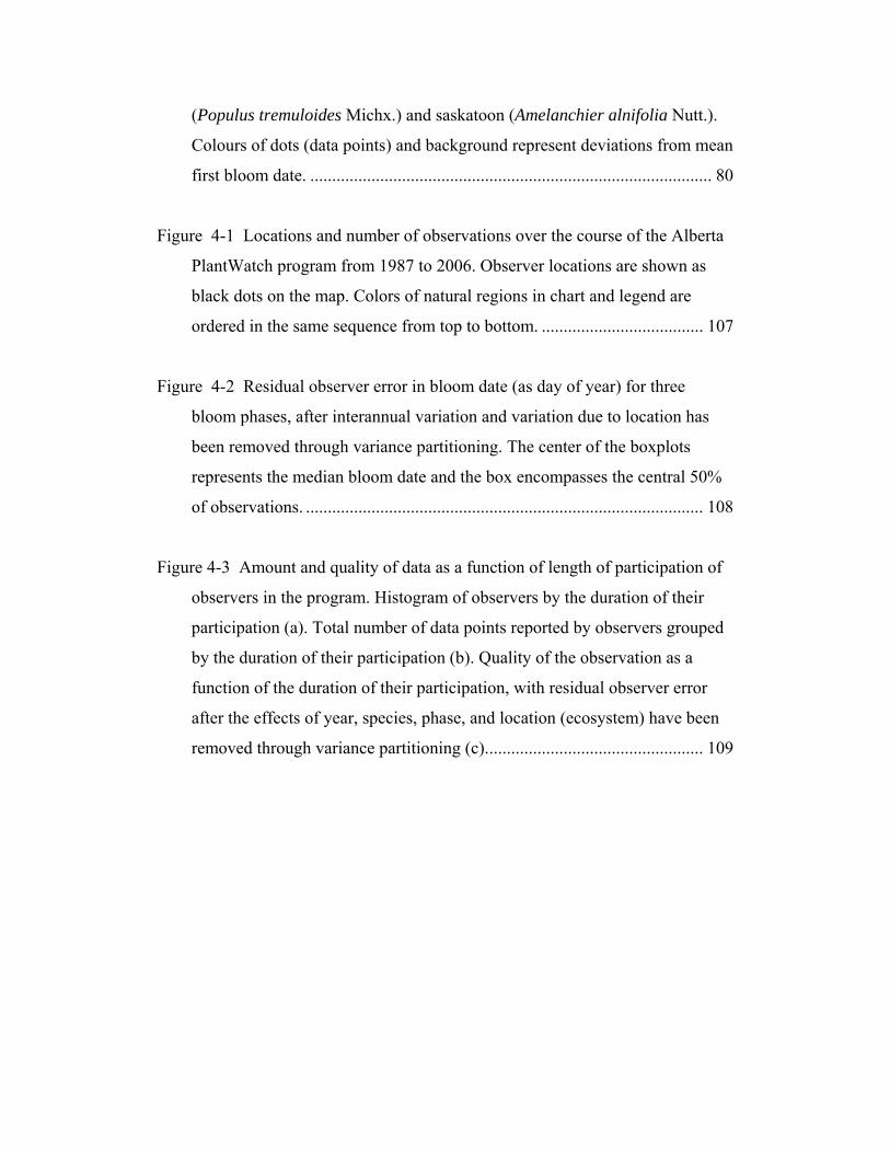
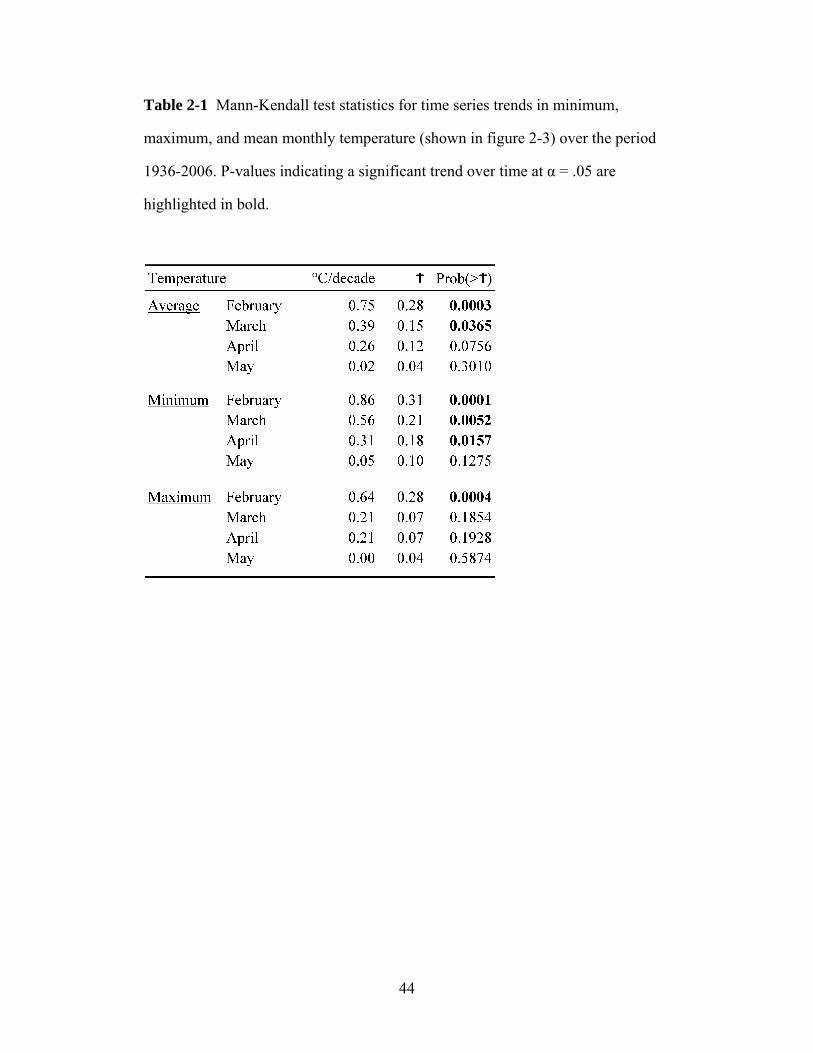
Figure 2-3 Temperature trends for the central parkland study area for the mean monthly minimum temperature (in
degrees Celsius), and the mean monthly maximum temperature.
51 51
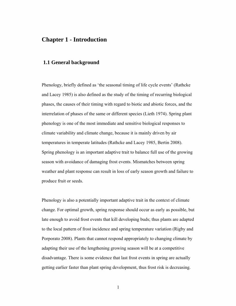
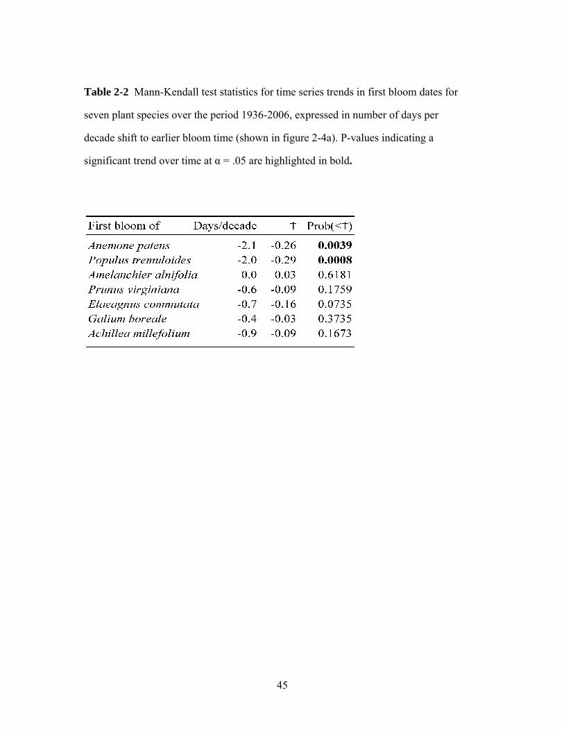
Figure 2-4 Trends in observations of first bloom for seven species. Species names are abbreviated using the first four
letters of the genus and the first three letters of the species name provided in figure 2-2. The lower panel indicates the
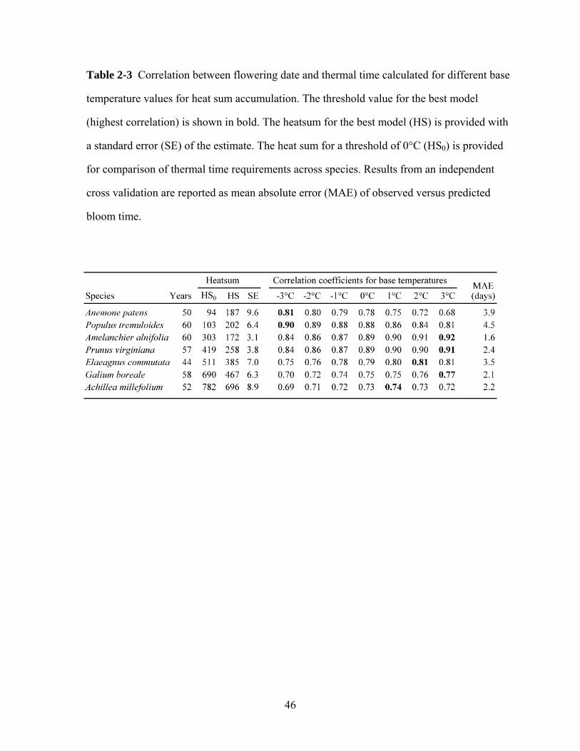
predicted day of first bloom from a thermal time model (the best model highlighted in bold in table 2-3).
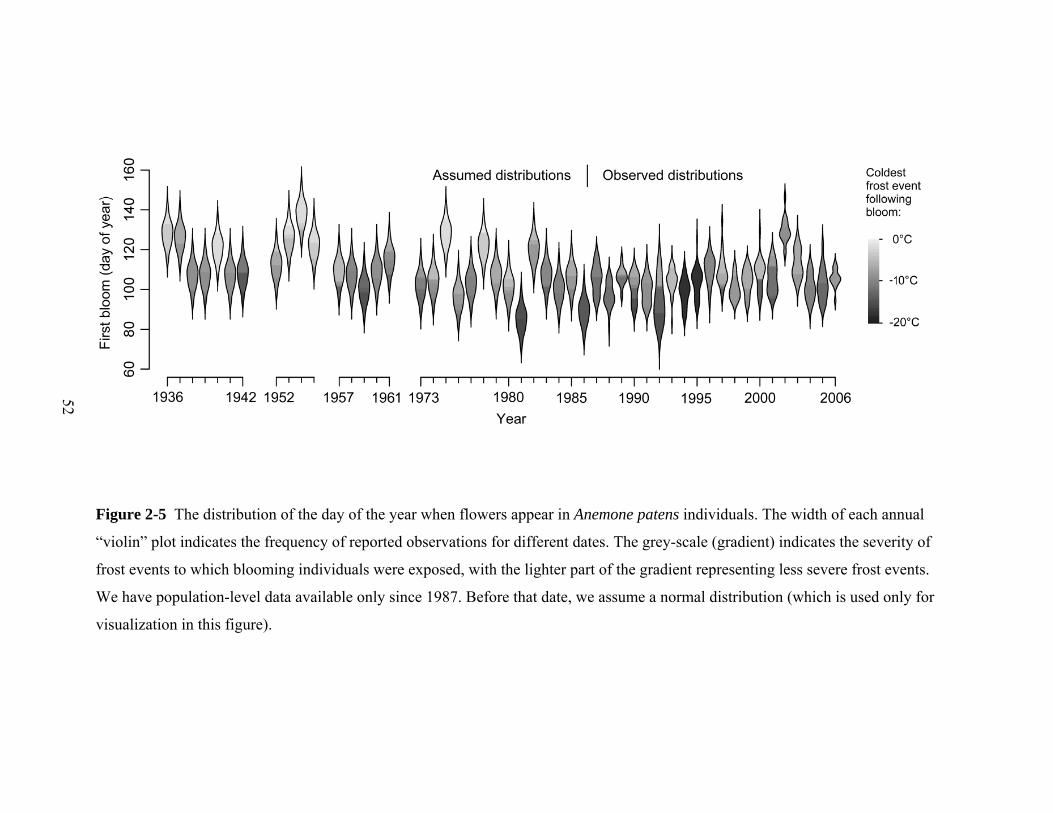
52 52
Figure 2-5 The distribution of the day of the year when flowers appear in Anemone patens individuals. The width of each annual
“violin” plot indicates the frequency of reported observations for different dates. The grey-scale (gradient) indicates the severity of
frost events to which blooming individuals were exposed, with the lighter part of the gradient representing less severe frost events.
We have population-level data available only since 1987. Before that date, we assume a normal distribution (which is used only for
visualization in this figure).
53
2.8 References
AHCCD. 2009. Adjusted Historical Canadian Climate Data. http://www.cccma.bc.ec.gc.ca/hccd. Environment Canada. February 2009.
Amano, T., R. J. Smithers, T. H. Sparks, and S. W.J. 2010. A 250-year index of
first flowering dates and its response to temperature changes. Proceedings of the Royal Society B-Biological Sciences 277:2451-2457.
Arakawa, H. 1955. Twelve centuries of blooming dates of the cherry blossoms in
the city of Kyoto and its own vicinity. Pure and Applied Geophysics 30:147-150.
Arakawa, H. 1956. Climatic change as revealed by the blooming dates of the
cherry blossoms at Kyoto. Journal of Meteorology 13:599-600. Badeck, F. W., A. Bondeau, K. Bottcher, D. Doktor, W. Lucht, J. Schaber, and S.
Sitch. 2004. Responses of spring phenology to climate change. New Phytologist 162:295-309.
Beaubien, E. G. and H. J. Freeland. 2000. Spring phenology trends in Alberta,
Canada: links to ocean temperature. International Journal of Biometeorology 44:53-59.
Beaubien, E. G. and D. L. Johnson. 1994. Flowering plant phenology and weather
in Alberta, Canada. International Journal of Biometeorology 38:23-27. Bertin, R. I. 2008. Plant phenology and distribution in relation to recent climate
change. Journal of the Torrey Botanical Society 135:126-146. Bird, C. D. 1983. 1982 Alberta flowering dates. Alberta Naturalist 13:1-4. Bonhomme, R. 2000. Bases and limits to using 'degree day' units. European
Journal of Agronomy 13:1-10. Bradley, N. L., A. C. Leopold, J. Ross, and W. Huffaker. 1999. Phenological
changes reflect climate change in Wisconsin. Proceedings of the National Academy of Sciences of the United States of America 96:9701-9704.
Campbell, R. K. and A. I. Sugano. 1975. Phenology of bud burst in Douglas-fir
related to provenance, photoperiod, chilling, and flushing temperature. Botanical Gazette 136:290-298.
54
Caprio, J. M. 1957. Phenology of lilac bloom in Montana. Science 126:1344-1345.
Cayan, D. R., S. A. Kammerdiener, M. D. Dettinger, J. M. Caprio, and D. H.
Peterson. 2001. Changes in the onset of spring in the western United States. Bulletin of the American Meteorological Society 82:399-415.
Chuine, I., K. Kramer, and H. Hänninen. 2003. Chapter 4.1. Plant development
models. Pages 217-235 in M. Schwartz, editor. Phenology: An Integrative Environmental Science. Kluwer Academic Publishers, Dordrecht.
Cleland, E. E., I. Chuine, A. Menzel, H. A. Mooney, and M. D. Schwartz. 2007.
Shifting plant phenology in response to global change. Trends in Ecology & Evolution 22:357-365.
Easterling, D. R., B. Horton, P. D. Jones, T. C. Peterson, T. R. Karl, D. E. Parker,
M. J. Salinger, V. Razuvayev, N. Plummer, P. Jamason, and C. K. Folland. 1997. Maximum and minimum temperature trends for the globe. Science 277:364-367.
Hannerz, M. 1999. Evaluation of temperature models for predicting bud burst in
Norway spruce. Canadian Journal of Forest Research-Revue Canadienne De Recherche Forestiere 29:9-19.
Hipel, K. and A. McLeod. 1994. Time Series Modelling of Water Resources and
Environmental Systems. Elsevier, Amsterdam. Hunter, A. F. and M. J. Lechowicz. 1992. Predicting the timing of budburst in
temperate trees. Journal of Applied Ecology 29:597-604. Inouye, D. 2008. Effects of climate change on phenology, frost damage, and floral
abundance of montane wildflowers. Ecology 89:353-362. Inouye, D. and F. Wielgolaski. 2003. Chapter 3.5. High altitude climates. Pages
195-214 in M. Schwartz, editor. Phenology: An Integrative Environmental Science. Kluwer Academic Publishers, Dordrecht.
the physical science basis. Cambridge University Press, Cambridge, UK; New York, NY, USA.
Karl, T. R., P. Jones, R. Knight, G. Kukla, N. Plummer, V. Razuvayev, K. Gallo,
J. Lindseay, R. Charlson, and T. Peterson. 1993. A new perspective on recent global warming - asymmetric trends of daily maximum and minimum temperature. Bulletin of the American Meteorological Society 74:1007-1023.
55
Lechowicz, M. J. 1984. Why do temperate deciduous trees leaf out at different
times? Adaptation and ecology of forest communities. American Naturalist 6:821-842.
Leinonen, I. and H. Hanninen. 2002. Adaptation of the timing of bud burst of
Norway spruce to temperate and boreal climates. Silva Fennica 36:695-701.
Leinonen, I. and K. Kramer. 2002. Applications of phenological models to predict
the future carbon sequestration potential of boreal forests. Climatic Change 55:99-113.
Leopold, A. C. and S. E. Jones. 1947. A phenological record for Sauk and Dane
counties, Wisconsin,1935-1945. Ecological Monographs 17:81-122. Li, H. T., X. L. Wang, and A. Hamann. 2010. Genetic adaptation of aspen
(Populus tremuloides) populations to spring risk environments: a novel remote sensing approach. Canadian Journal of Forest Research 40:2082-2090.
Linkosalo, T., R. Hakkinen, and H. Hanninen. 2006. Models of the spring
phenology of boreal and temperate trees: is there something missing? Tree Physiology 26:1165-1172.
Mbogga, M. S., A. Hamann, and T. L. Wang. 2009. Historical and projected
climate data for natural resource management in western Canada. Agricultural and Forest Meteorology 149:881-890.
Menzel, A., N. Estrella, and A. Testka. 2005. Temperature response rates from
long-term phenological records. Climate Research 30:21-28. Menzel, A., T. H. Sparks, N. Estrella, E. Koch, A. Aasa, R. Ahas, K. Alm-Kubler,
P. Bissolli, O. Braslavska, A. Briede, F. M. Chmielewski, Z. Crepinsek, Y. Curnel, A. Dahl, C. Defila, A. Donnelly, Y. Filella, K. Jatcza, F. Mage, A. Mestre, O. Nordli, J. Peñuelas, P. Pirinen, V. Remisova, H. Scheifinger, M. Striz, A. Susnik, A. J. H. Van Vliet, F. E. Wielgolaski, S. Zach, and A. Zust. 2006. European phenological response to climate change matches the warming pattern. Global Change Biology 12:1969-1976.
Miller-Rushing, A. J., D. W. Inouye, and R. B. Primack. 2008. How well do first
flowering dates measure plant responses to climate change? The effects of population size and sampling frequency. Journal of Ecology 96:1289-1296.
56
Miller-Rushing, A. J. and R. B. Primack. 2008. Global warming and flowering times in Thoreau's Concord: A community perspective. Ecology 89:332-341.
Moss, E. H. and J. G. Packer. 1983. Flora of Alberta: a manual of flowering
plants, conifers, ferns, and fern allies found growing without cultivation in the Province of Alberta, Canada. University of Toronto Press, Toronto.
Parmesan, C. 2006. Ecological and evolutionary responses to recent climate
change. Annual Review of Ecology Evolution and Systematics 37:637-669.
Rathcke, B. and E. P. Lacey. 1985. Phenological patterns of terrestrial plants.
Annual Review of Ecology and Systematics 16:179-214. Réaumur, R. 1735. Observation du thermometer, faites à Paris pendant l’année
1735, comparés avec celles qui ont été faites sous la ligne, à l’Isle de France, à Alger et en quelques-unes de nos isles de l’Amérique. Paris: Mémoires de l’Académie des Sciences, 1735.
Root, T. L., J. T. Price, K. R. Hall, S. H. Schneider, C. Rosenzweig, and J. A.
Pounds. 2003. Fingerprints of global warming on wild animals and plants. Nature 421:57-60.
Rosenzweig, C., G. Casassa, D. J. Karoly, A. Imeson, C. Liu, A. Menzel, S.
Rawlins, T. L. Root, B. Seguin, and P. Tryjanowski. 2007. Assessment of Observed Changes and Responses in Natural and Managed Systems. Pages 79-131 in M. Parry, O. Canziani, J. Palutikof, P. van der Linden, and C. Hanson, editors. Climate change 2007: Impacts, Adaptation and Vulnerability. Contribution of Working Group II to the Fourth Assessment Report of the Intergovernmental Panel on Climate Change. Cambridge University Press, Cambridge, UK.
Rötzer, T., M. Witenzeller, H. Häckel, and J. Nekovar. 2000. Phenology in central
Europe - differences and trends of spring phenophases in urban and rural areas. International Journal of Biometeorology 44:60-67.
Russell, R. C. 1962. Phenological records of the prairie flora. Canadian Plant
Disease Survey 42:162-166. Schaber, J. and F. W. Badeck. 2003. Physiology-based phenology models for
forest tree species in Germany. International Journal of Biometeorology 47:193-201.
57
Scheifinger, H., A. Menzel, E. Koch, and C. Peter. 2003. Trends of spring time frost events and phenological dates in Central Europe. Theoretical and Applied Climatology 74:41-51.
Schleip, C., T. H. Sparks, N. Estrella, and A. Menzel. 2009. Spatial variation in
onset dates and trends in phenology across Europe. Climate Research 39:249-260.
Schwartz, M. D., R. Ahas, and A. Aasa. 2006. Onset of spring starting earlier
across the Northern Hemisphere. Global Change Biology 12:343-351. Schwartz, M. D. and E. G. Beaubien. 2003. Chapter 2.4. North America. Pages
57–73 in M. D. Schwartz, editor. Phenology: an integrative environmental science. Kluwer Academic Publishers, Dordrecht.
Schwartz, M. D. and B. E. Reiter. 2000. Changes in North American spring.
International Journal of Climatology 20:929-932. Sparks, T. H., A. Menzel, and N. C. Stenseth. 2009. European cooperation in
plant phenology: Introduction. Climate Research 39:175-177. Statistics Canada. 2010. Statistics Canada historical census records for Edmonton
http://www.statcan.gc.ca. January 2010. Stoller, L. 1956. A note on Thoreau's place in the history of phenology. Isis
47:172-181. Vitasse, Y., S. Delzon, C. Bresson, R. Michalet, and A. Kremer. 2009. Altitudinal
differentiation in growth and phenology among populations of temperate-zone tree species growing in a common garden. Canadian Journal of Forest Research 39:1259-1269.
White, L. M. 1995. Predicting flowering of 130 plants at 8 locations with
temperature and daylength. Journal of Range Management 48:108-114. Wielgolaski, F. and D. Inouye. 2003. Chapter 3.4. High latitude climates. Pages
175-194 in M. Schwartz, editor. Phenology: An Integrative Environmental Science. Kluwer Academic Publishers, Dordrecht.
Wielgolaski, F. E. 1999. Starting dates and basic temperatures in phenological
observations of plants. International Journal of Biometeorology 42:158-168.
58
Chapter 3 - Urban Heat Island Effects Partially Explain
Earlier Blooming of Plants in Edmonton, Canada
Summary
An important criticism by climate change skeptics is that much of the observed
warming signal is an artifact of the increasing heat island effect of growing cities
where weather stations are frequently located. As heat island effects of urban
centers intensify over time due to population and economic growth they are
confounded with general climate warming trends. Here, we quantify heat island
effects over a period of 70 years based on weather station and phenology data
from urban and rural areas around Edmonton, a city at 53°N latitude. Due to the
high spatial density of the observer network, we were able to, for the first time,
create a continuous heat island map through interpolation from phenology data.
Further, we documented an increasing heat island effect over the period 1931–
2006 in both weather station data and plant phenology response. Across all seven
plant species, the advance in phenology observed in Edmonton was 2.1 days (±0.9
SE) greater than in the surrounding rural areas, with the heat island effect
accounting for one third of the total warming signal.
59
3.1 Introduction
There has been a long-standing discussion among climatologists whether urban
heat island effects explain a significant proportion of the observed global warming
signal (e.g. Parker 2004). Many factors influence the urban heat island. First, the
impact on local climate is influenced by the size of the city. As the intensity of the
urban heat island is proportional to the log of the urban population (Oke 1987),
population statistics are most often used to estimate changes in heat island
(Landsberg 1981, Barry and Chorley 2010). Next, the change of land cover from
vegetation to hardened surfaces (concrete, asphalt, brick, etc.) causes at least two
reductions in summer cooling from evapotranspiration: loss of soil with its water
storing capacity and loss of vegetation with evaporative cooling potential (Oke
1987). In addition, the hardened material has a high thermal mass and is slow to
cool at night, releasing heat into the atmosphere. In north temperate North
America, major urban-rural temperature differences are generally seen in the
winter season, due to emissions from burning fossil fuels for heating and transport
(Landsberg 1981, Hinkel and Nelson 2007). The presence of wind also has short-
term effects on the heat island; greatest urban-rural temperature differences are
found on calm nights, but this effect diminishes on windy nights (Landsberg
1981).
The timing of spring blooming and leafout of perennial plants in temperate
climates is driven mainly by the rate of increasing temperature after mid winter
(Rathcke and Lacey 1985). After a warmer than usual winter and spring, plants
bloom earlier than average. Studies of shifts in plant phenology in the northern
60
hemisphere generally show trends towards earlier bloom and leafout times
(Menzel et al. 2006, Bertin 2008), and in Europe higher population density was
associated with earlier plant response timing (Estrella et al. 2009). The geographic
extent of the urban influence on plant response can be considerable. In one remote
sensing study, urban land cover was second in importance after elevation as a
driver of landscape phenology, affecting the start of the growing season up to 32
km from the centres of large cities (Elmore et al. 2012). Another study based on
satellite data showed that earlier urban budburst, compared to surrounding rural
areas, was found in 75% of temperate cities examined, but only in 33% of tropical
cities (Gazal et al. 2008).
Phenology observations done on the ground in North America, Europe and China
have shown that flowering in spring-blooming plants starts earlier in cities than in
rural surroundings (Neil and Wu 2006). But compared to North American cities,
European cities have smaller urban-rural temperature differences, perhaps due to a
greater density of the rural population, greater extent of forest clearing and
generally lower heights of buildings in Europe (Oke 1987, Barry and Chorley
2010). A comparison of 10 urban-rural areas in Europe found that city spring
bloom times for one herbaceous and three woody plant species were four days
earlier than rural bloom times, over the period 1951-1995 (Rötzer et al. 2000). But
a study of three German cities (1980 to 2009) did not find significant differences
in phenology due to urbanization (Jochner et al. 2012). In North America, data are
limited on the effects of urban heat island on plant phenology. Studies have
largely focused on herbarium specimens solely from urban areas (Primack et al.
2004, Houle 2007, Neil et al. 2010), were limited to a single non-native plant
61
species (Ziska et al. 2003, Lavoie and Lachance 2006), or relied on satellite
imagery for evidence of change (Zhang et al. 2004, Gazal et al. 2008).
In Europe and Asia, remote sensing data showed that mean annual city
temperatures were about 0.8°C warmer than nearby rural areas, whereas in the
USA city temperatures were 1-3 °C warmer (Zhang et al. 2004). The effects of the
urban heat island on plant phenology are also smaller in Europe and Asia than in
North America (Zhang et al. 2004). In the Alaskan community of Barrow (71° N
latitude), the urban area was 2.2 °C warmer than the rural area, based on spatial
averages for the period 1 December 2001 to 31 March 2002 (Hinkel et al. 2003).
Expanding temperate urban centres have similar temperature patterns to those
caused by general climate warming, where minimum temperatures are increasing
faster than maximum temperatures, thus reducing the daily temperature range
(Easterling et al. 1997). Mimet et al. (2009) took measurements along a gradient
from outside the city to city centre (Rennes in France) and found an increase in
minimum temperature accompanied by a trend to earlier plant phases. This
reduction in diurnal temperature variability increases the rate of temperature
accumulation in heat sum calculations and could be the reason for an observed
increase in the sensitivity of phenological response over 70 years in central
Alberta (Beaubien and Hamann 2011a).
The spatial pattern of temperatures in cities influences plant response. Another
study along an urban-rural gradient showed that the allergenic ragweed (Ambrosia
artemisiifolia) had earlier flowering and increased pollen production closer to the
city centre of Baltimore, Maryland (Ziska et al. 2003). Secondly, the pace of
increasing spring temperatures can also affect urban-rural phenology differences.
62
Periods of high temperature in spring can cause synchronous blooming in urban
and rural areas, whereas cool periods may lead to larger urban-rural differences in
bloom times (Jochner et al. 2011). Lastly, urban heat island effects on phenology
may vary according to the plant species or phenophase (growth stage) observed.
The study by Roetzer et al. (2000) indicated that the ‘start of season’ plants (those
that flower earliest in spring) react more strongly to temperature, showing a
bigger heat island effect, i.e. more difference between urban and rural bloom
times.
In 10 central European cities, spring phenophases for four early-blooming plants
showed larger city trends to earlier onset for more recent years (1980 to 1995)
(Rötzer et al. 2000). The analysis of trends for the period from 1951 to 1995
showed tendencies towards earlier flowering in all regions, but only 22% were
significant at the 5% level. However the trend to earlier bloom was bigger in rural
areas, perhaps due to differences in rates of urbanisation. In this study the rural
stations were not far from city centres. Few studies have been done on the effect
of urban heat islands on phenology in North America. In eastern Canada, Lavoie
and Lachance (2006) used 216 herbarium specimens of the non-native Tussilago
farfara (coltsfoot) from southern Quebec and found that in the urban centres of
Montreal and Quebec, there were major shifts of 15-31 days to earlier bloom
since the early 20th century. No trend was found for rural areas. In light of this
large urban-rural difference it is odd that this European species was shown to be
relatively unresponsive to temperature in a study in Finland: flowering dates had a
correlation of only 0.30 with the best heat sum, while correlations of other species
were 0.66–0.90 (Heikinheimo and Lappalainen 1997). Research in central Europe
has been hampered by lack of adequate urban phenology data (Jochner et al.
63
2011), or in much of Europe, lack of truly rural data due to a generally urbanized
landscape. Jeong et al. (2011) report on trends in spring temperatures and
flowering times for four shrubs in nine cities of South Korea, 1954-2004. Urban
warming resulted in an advance of many days to many weeks in bloom dates, and
the size of this shift to earlier blooming was related to the degree of urbanization.
But information on changes in rural areas, for comparison, is not presented.
In the rural area surrounding Edmonton, Alberta (the study area for this paper),
there is substantive evidence of climate warming. Minimum February
temperatures in this Central Parkland ecozone increased by 6 °C over the 70 years
1936-2006 (Beaubien and Hamann 2011a). While it is not the subject of this
study, we concur with Parker (2004) and Wickham et al. (2011) that overall
climate warming is not a consequence of urban development. There is a need to
understand the difference between temperatures and the biotic response both
inside and outside cities, and few studies have quantified heat island effects with
rigorous rural-urban comparisons. In this article we contribute what could be an
extreme case of urban heat island effect on plant response in spring, due to a
quickly expanding city, a cool boreal climate, and considerable trends to early
blooming. Our dataset is unique in having data on many plant species from both
urban and rural sites in western Canada. We ask: what is the contribution of the
urban heat island to the climate warming signal?
64
3.2 Methods
3.2.1 Study area and phenology observations
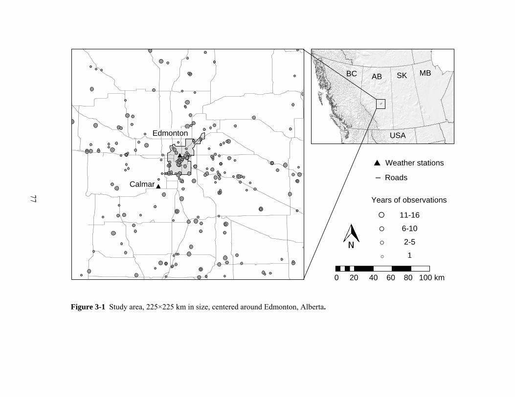
Our study area included the city of Edmonton, Alberta, Canada (53.54° N latitude,
113.49° W longitude, altitude 660 m) and surroundings, an area of continental
climate with warm summers and dry cold winters (Figure 3-1). Using plant
phenology records from Alberta PlantWatch, we selected species with abundant
rural and urban data. For additional information on this program and database see
Environment Canada 2009, Beaubien and Hamann 2011a, Beaubien and Hamann
2011b, and Beaubien 2012. Alberta PlantWatch data for 1987-2006 consisted of
over 47000 observations of bloom and leafing dates of plants, gathered by 650
observers.
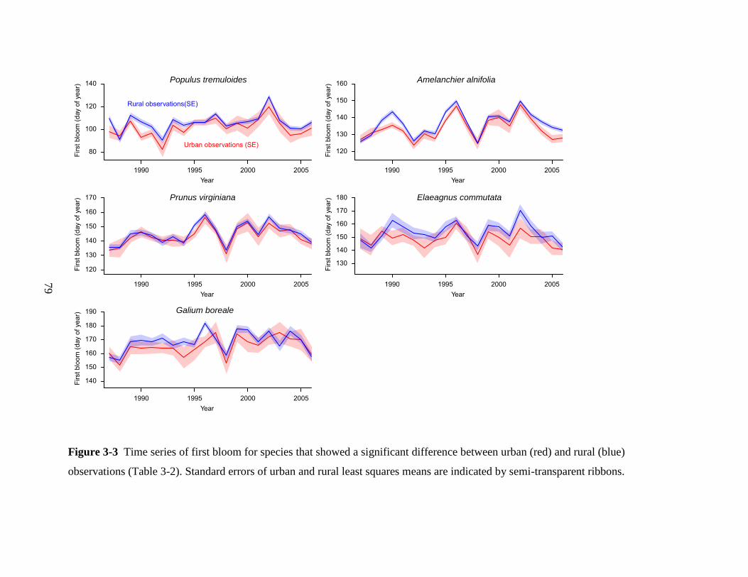
We selected the phenophase ‘first bloom’ for analysis, as it had more abundant
data. For the period 1987 to 2001, first bloom was defined as “10% of flower buds
open”. After 2001 the definition became “first flowers open in three different
places on a woody shrub or tree”, or “first flowers open in a patch of herbaceous
plants”. For the tree Populus tremuloides the updated definition was “the date
when the catkins on the observed male tree first start shedding pollen in 3
different places”. We added 1060 records from data gathered by E. Beaubien for
plants in the city and at the rural Devonian Botanic Garden, 10 km west of the
southwest corner of the city boundary. In this dataset, ‘first bloom’ was defined as
“1-25% of flower buds now open”. To reflect conditions in the years when
Edmonton was a smaller city, we used historic first bloom data (one date per
65
species per year) for 1936 to 1961, from a study done by Agriculture Canada
(Russell 1962). These Edmonton observations were largely done on the
University of Alberta campus close to the centre of the city. The following species
were included in this study: Prairie crocus (Anemone patens L.), aspen poplar
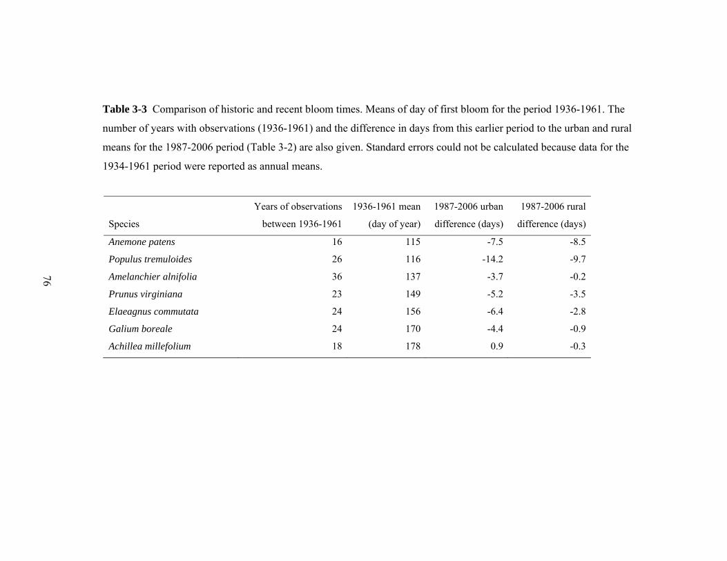
Table 3-3 Comparison of historic and recent bloom times. Means of day of first bloom for the period 1936-1961. The
number of years with observations (1936-1961) and the difference in days from this earlier period to the urban and rural
means for the 1987-2006 period (Table 3-2) are also given. Standard errors could not be calculated because data for the
1934-1961 period were reported as annual means.
Species
Years of observations
between 1936-1961
1936-1961 mean
(day of year)
1987-2006 urban
difference (days)
1987-2006 rural
difference (days)
Anemone patens 16 115 -7.5 -8.5
Populus tremuloides 26 116 -14.2 -9.7
Amelanchier alnifolia 36 137 -3.7 -0.2
Prunus virginiana 23 149 -5.2 -3.5
Elaeagnus commutata 24 156 -6.4 -2.8
Galium boreale 24 170 -4.4 -0.9
Achillea millefolium 18 178 0.9 -0.3
77
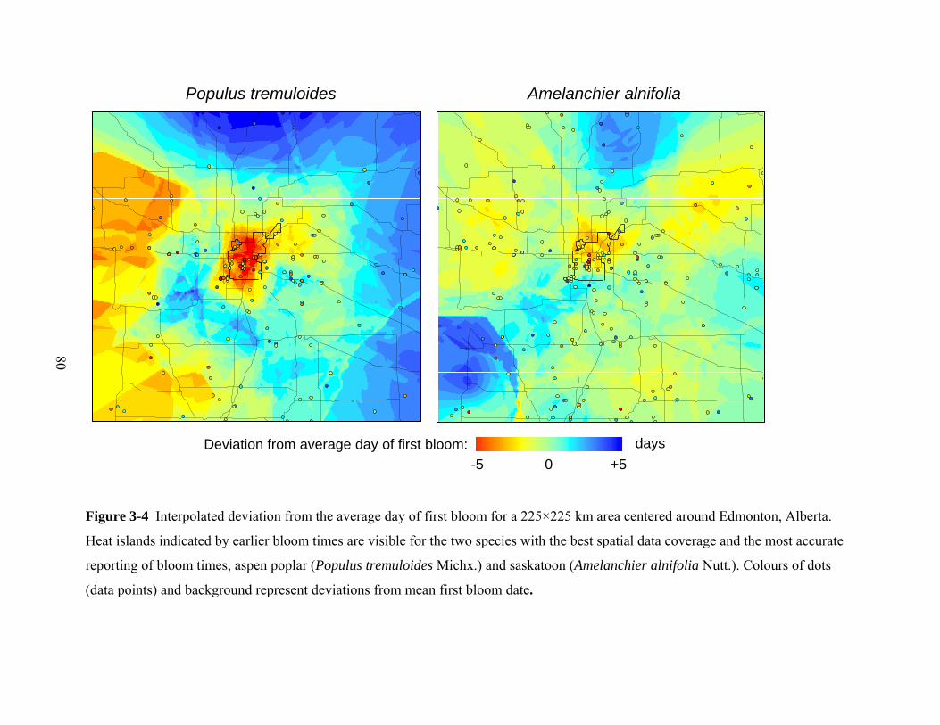
Figure 3-1 Study area, 225×225 km in size, centered around Edmonton, Alberta.
0 20 40 60 80 100 km
Years of observations
A
A
A
A
11-16
6-10
2-5
1
Weather stations
– Roads
Edmonton
Calmar
USA
BC AB SK MB
78
a)
b)
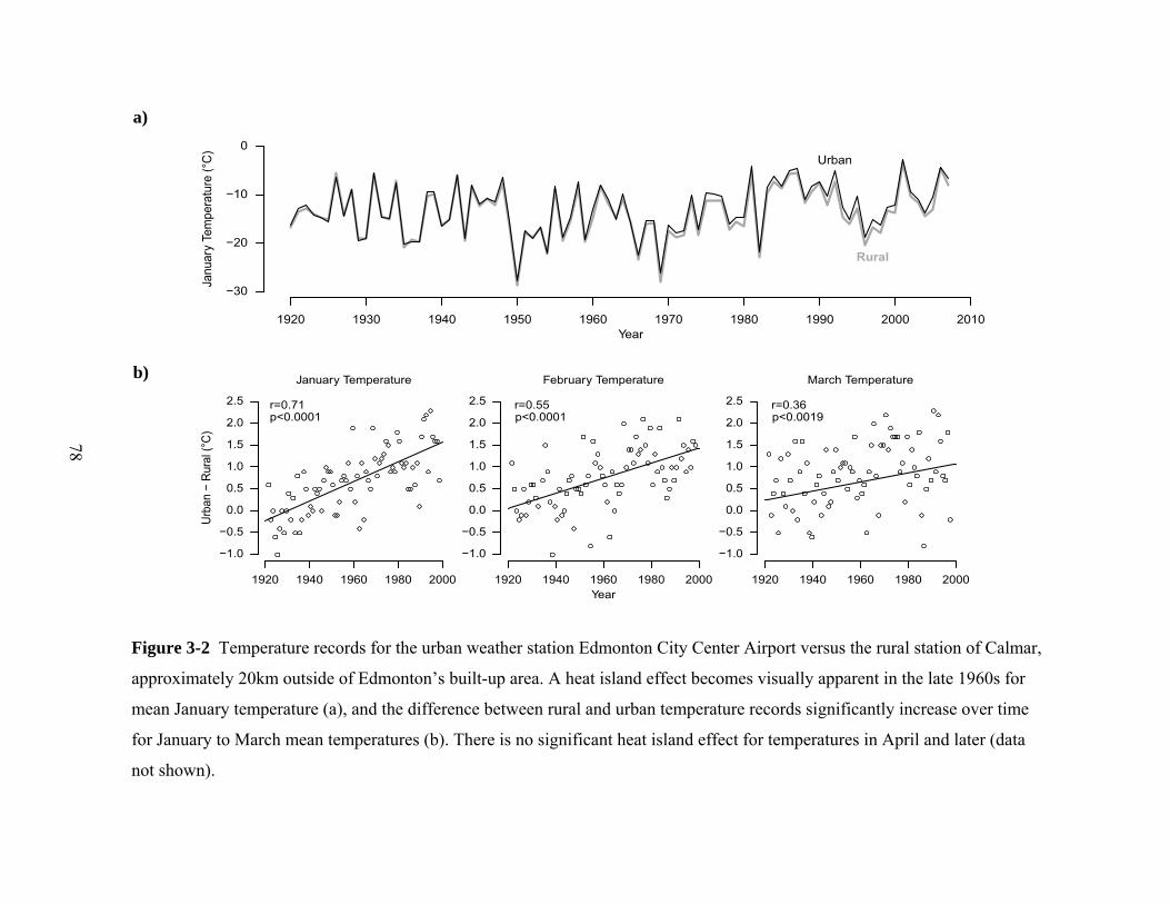
Figure 3-2 Temperature records for the urban weather station Edmonton City Center Airport versus the rural station of Calmar,
approximately 20km outside of Edmonton’s built-up area. A heat island effect becomes visually apparent in the late 1960s for
mean January temperature (a), and the difference between rural and urban temperature records significantly increase over time
for January to March mean temperatures (b). There is no significant heat island effect for temperatures in April and later (data
not shown).
79
Figure 3-3 Time series of first bloom for species that showed a significant difference between urban (red) and rural (blue)
observations (Table 3-2). Standard errors of urban and rural least squares means are indicated by semi-transparent ribbons.
Populus tremuloides Amelanchier alnifolia
Elaeagnus commutata Prunus virginiana
Galium boreale
80
Figure 3-4 Interpolated deviation from the average day of first bloom for a 225×225 km area centered around Edmonton, Alberta.
Heat islands indicated by earlier bloom times are visible for the two species with the best spatial data coverage and the most accurate
reporting of bloom times, aspen poplar (Populus tremuloides Michx.) and saskatoon (Amelanchier alnifolia Nutt.). Colours of dots
(data points) and background represent deviations from mean first bloom date.
Populus tremuloides Amelanchier alnifolia
Deviation from average day of first bloom: -5 0 +5
days
81
3.5. References
AHCCD. 2009. Adjusted Historical Canadian Climate Data.
http://www.cccma.bc.ec.gc.ca/hccd. Environment Canada. February 2009. ASRD. 2005. Standards for Tree Improvement in Alberta. Alberta Sustainable
Resource Development. Lands and Forest Division. Barry, R. G. and R. J. Chorley. 2010. Atmosphere, weather, and climate. 9th
edition. Routledge, London; New York. Beaubien, E. G. and H. J. Freeland. 2000. Spring phenology trends in Alberta,
Canada: links to ocean temperature. International Journal of Biometeorology 44:53-59.
Beaubien, E. G. and A. Hamann. 2011a. Spring Flowering Response to Climate
Change between 1936 and 2006 in Alberta, Canada. BioScience 61:514-524.
Beaubien, E. G. and A. Hamann. 2011b. Plant phenology networks of citizen
scientists: recommendations from two decades of experience in Canada. International Journal of Biometeorology 55:833-841.
Beaubien, E. G. 2012. Alberta Plantwatch http://plantwatch.naturealberta.ca.
Nature Alberta, Edmonton, Alberta. September 2012. Bertin, R. I. 2008. Plant phenology and distribution in relation to recent climate
change. Journal of the Torrey Botanical Society 135:126-146. City of Edmonton. 2012. Census History.
www.edmonton.ca/city_government/municipal_census/census-history.aspx. March 2012
Dixon, A. F. G. 2003. Climate change and phenological asynchrony. Ecological
Entomology 28:380-381. Easterling, D. R., B. Horton, P. D. Jones, T. C. Peterson, T. R. Karl, D. E. Parker,
M. J. Salinger, V. Razuvayev, N. Plummer, P. Jamason, and C. K. Folland. 1997. Maximum and minimum temperature trends for the globe. Science 277:364-367.
Elmore, A. J., S. M. Guinn, B. J. Minsley, and A. D. Richardson. 2012.
Landscape controls on the timing of spring, autumn, and growing season length in mid-Atlantic forests. Global Change Biology 18:656-674.
ESRI. 2011. Kriging for ArcGIS Desktop 10.0. Online support files.
Environmental Systems Research Institute (ESRI). http://help.arcgis.com/en/arcgisdesktop/10.0/help/index.html#//009z0000006n000000.htm, Redlands, CA. July 2012.
Estrella, N., T. H. Sparks, and A. Menzel. 2009. Effects of temperature, phase
type and timing, location, and human density on plant phenological responses in Europe. Climate Research 39:235-248.
Gazal, R., M. A. White, R. Gillies, E. Rodemaker, E. Sparrow, and L. Gordon.
2008. GLOBE students, teachers, and scientists demonstrate variable differences between urban and rural leaf phenology. Global Change Biology 14:1568-1580.
Heikinheimo, M. and H. Lappalainen. 1997. Dependence of the flower bud burst
of some plant taxa in Finland on effective temperature sum: implications for climate warming. Annales Botanici Fennici 34:229-243.
Hinkel, K. M. and F. E. Nelson. 2007. Anthropogenic heat island at Barrow,
Alaska, during winter: 2001-2005. Journal of Geophysical Research-Atmospheres 112.1-12.
Hinkel, K. M., F. E. Nelson, A. F. Klene, and J. H. Bell. 2003. The urban heat
island in winter at Barrow, Alaska. International Journal of Climatology 23:1889-1905.
Houle, G. 2007. Spring-flowering herbaceous plant species of the deciduous
forests of eastern Canada and 20th century climate warming. Canadian Journal of Forest Research-Revue Canadienne De Recherche Forestiere 37:505-512.
Jeong, J. H., C. H. Ho, H. W. Linderholm, S. J. Jeong, D. Chen, and Y. S. Choi.
2011. Impact of urban warming on earlier spring flowering in Korea. International Journal of Climatology 31:1488-1497.
Jochner, S. C., I. Beck, H. Behrendt, C. Traidl-Hoffmann, and A. Menzel. 2011.
Effects of extreme spring temperatures on urban phenology and pollen production: a case study in Munich and Ingolstadt. Climate Research 49:101-112.
Jochner, S. C., T. H. Sparks, N. Estrella, and A. Menzel. 2012. The influence of
altitude and urbanisation on trends and mean dates in phenology (1980–2009). International Journal of Biometeorology 56:387–394.
83
Kudo, G., Y. Nishikawa, T. Kasagi, and S. Kosuge. 2004. Does seed production
of spring ephemerals decrease when spring comes early? Ecological Research 19:255-259.
Landsberg, H. E. 1981. The urban climate. Academic Press, New York. Lavoie, C. and D. Lachance. 2006. A new herbarium-based method for
reconstructing the phenology of plant species across large areas. American Journal of Botany 93:512-516.
Luo, Z. K., O. J. Sun, Q. S. Ge, W. T. Xu, and J. Y. Zheng. 2007. Phenological
responses of plants to climate change in an urban environment. Ecological Research 22:507-514.
Menzel, A., T. H. Sparks, N. Estrella, E. Koch, A. Aasa, R. Ahas, K. Alm-Kubler,
P. Bissolli, O. Braslavska, A. Briede, F. M. Chmielewski, Z. Crepinsek, Y. Curnel, A. Dahl, C. Defila, A. Donnelly, Y. Filella, K. Jatcza, F. Mage, A. Mestre, O. Nordli, J. Peñuelas, P. Pirinen, V. Remisova, H. Scheifinger, M. Striz, A. Susnik, A. J. H. Van Vliet, F. E. Wielgolaski, S. Zach, and A. Zust. 2006. European phenological response to climate change matches the warming pattern. Global Change Biology 12:1969-1976.
Mimet, A., V. Pellissier, H. Quenol, R. Aguejdad, V. Dubreuil, and F. Roze.
2009. Urbanisation induces early flowering: evidence from Platanus acerifolia and Prunus cerasus. International Journal of Biometeorology 53:287-298.
Moss, E. H. and J. G. Packer. 1983. Flora of Alberta : a manual of flowering
plants, conifers, ferns, and fern allies found growing without cultivation in the Province of Alberta, Canada. University of Toronto Press, Toronto.
Neil, K. and J. Wu. 2006. Effects of urbanization on plant flowering phenology: A
review. Urban Ecosystems 9:243-257. Neil, K. L., L. Landrum, and J. G. Wu. 2010. Effects of urbanization on flowering
phenology in the metropolitan Phoenix region of USA: Findings from herbarium records. Journal of Arid Environments 74:440-444.
Oke, T. R. 1987. Boundary layer climates. 2nd edition. Methuen, London; New
York. Parker, D. E. 2004. Large-scale warming is not urban. Nature 432:290.
84
Primack, D., C. Imbres, R. B. Primack, A. J. Miller-Rushing, and P. Del Tredici. 2004. Herbarium specimens demonstrate earlier flowering times in response to warming in Boston. American Journal of Botany 91:1260-1264.
R Development Core Team. 2008. R: A language and environment for statistical
computing. R foundation for statistical computing. Vienna, Austria. Rathcke, B. and E. P. Lacey. 1985. Phenological patterns of terrestrial plants.
Annual Review of Ecology and Systematics 16:179-214. Rötzer, T., M. Witenzeller, H. Häckel, and J. Nekovar. 2000. Phenology in central
Europe - differences and trends of spring phenophases in urban and rural areas. International Journal of Biometeorology 44:60-67.
Russell, R. C. 1962. Phenological records of the prairie flora. Canadian Plant
Disease Survey 42:162-166. SAS Institute. 2008. Sas stat 9.2 User’s guide. Cary NC. Statistics Canada. 2012. Population and dwelling counts, for Canada, provinces
and territories, and census subdivisions (municipalities), 2011 and 2006 censuses. www.statcan.gc.ca. March 2012.
White, M. A., K. M. de Beurs, K. Didan, D. W. Inouye, A. D. Richardson, O. P.
Jensen, J. O'Keefe, G. Zhang, R. R. Nemani, W. J. D. van Leeuwen, J. F. Brown, A. de Wit, M. Schaepman, X. M. Lin, M. Dettinger, A. S. Bailey, J. Kimball, M. D. Schwartz, D. D. Baldocchi, J. T. Lee, and W. K. Lauenroth. 2009. Intercomparison, interpretation, and assessment of spring phenology in North America estimated from remote sensing for 1982-2006. Global Change Biology 15:2335-2359.
Wickham, C., J. Curry, D. Groom, R. Jacobsen, R. Muller, S. Perlmutter, R.
Rohde, A. Rosenfeld, and J. Wurtele. 2011. Influence of Urban Heating on the Global Temperature Land Average Using Rural Sites Identified from MODIS Classifications. http://berkeleyearth.org/pdf/berkeley-earth-uhi.pdf. The Berkeley Earth Project. November 2011.
Wolkovich, E. M., B. I. Cook, J. M. Allen, T. M. Crimmins, J. L. Betancourt, S.
E. Travers, S. Pau, J. Regetz, T. J. Davies, N. J. B. Kraft, T. R. Ault, K. Bolmgren, S. J. Mazer, G. J. McCabe, B. J. McGill, C. Parmesan, N. Salamin, M. D. Schwartz, and E. E. Cleland. 2012. Warming experiments underpredict plant phenological responses to climate change. Nature 485:494-497.
85
Zhang, X. Y., M. A. Friedl, C. B. Schaaf, A. H. Strahler, and A. Schneider. 2004. The footprint of urban climates on vegetation phenology. Geophysical Research Letters 31:1-4.
Ziska, L. H., D. E. Gebhard, D. A. Frenz, S. Faulkner, B. D. Singer, and J. G.
Straka. 2003. Cities as harbingers of climate change: Common ragweed, urbanization, and public health. Journal of Allergy and Clinical Immunology 111:290-295.
86
Chapter 4 - Plant Phenology Networks of Citizen
Scientists: Recommendations from Two Decades of
Experience in Canada2
Summary
Plant phenology networks of citizen scientists have a long history and have
recently contributed to our understanding of climate change effects on
ecosystems. This paper describes the development of the Alberta and Canada
PlantWatch programs, which coordinate networks of citizen scientists who track
spring development timing for common plants. Tracking spring phenology is
highly suited to volunteers and with effective volunteer management, observers
will stay loyal to a phenology program for many years. Over two decades
beginning in 1987, Alberta PlantWatch volunteers reported 47,000 records, the
majority contributed by observers who participated more than nine years. We
present a quantitative analysis of factors that determine the quality of these
phenological data and explore sources of variation. Our goal is to help those who
wish to initiate new observer networks with an analysis of the effectiveness of
program protocols including selected plant species and bloom stages.
2 A version of this paper has been published as: Beaubien E., Hamann, A. 2011. Plant phenology networks of citizen scientists: recommendations from two decades of experience in Canada. International Journal of Biometeorology. 55 (6) 833-841.
87
4.1 Introduction
Many parts of the world are experiencing rapid climate change, and biological
data are needed to understand how ecosystems are responding. We have
previously shown trends to earlier spring bloom times over the last century in
response to increased winter and spring temperatures (Beaubien and Freeland
2000, Beaubien and Hamann 2011). This article tells the story of harnessing the
energy of citizen scientists to track the effects of climate change across Canada.
Specifically, we describe the development of the Alberta and Canada PlantWatch
programs, and we provide a quantitative analysis of factors that determine data
quality. This analysis is based on the Alberta PlantWatch program, the longest-
running plant phenology network in Canada for recent decades, drawing on
47,000 records reported between 1987 and 2006. Data quality is an important
consideration for volunteer citizen science programs (Bonney et al. 2009; Delaney
et al. 2008) and our analysis of program protocols is presented to help those
planning new networks. Because the article is written for scientists who wish to
recruit citizens for a plant phenology network, we offer some additional
information on program development in the form of an extended introduction
below.
4.1.1 History of Canadian phenology networks
The first large-scale Canadian phenology observer network started in Alberta in
1973. This decade-long survey of bloom dates of wild plants was initiated through
the Federation of Alberta Naturalists (Bird, 1982) and was revived as the Alberta
88
Wildflower Survey in 1987 (Beaubien and Johnson 1994). This program has
continued since that time, renamed Alberta PlantWatch in 2002. This project
began as part of an MSc thesis (Beaubien 1991) supervised by ecologist Dr.
Walter Moser, with the goal of exploring the potential for phenology in Alberta.
By 1995, E. Beaubien had added to the Alberta program a Web-based program
called Prairie PlantWatch. In 1997 it was renamed Canada PlantWatch with more
indicator plant species added to gather data from Canada’s west coast, eastern
provinces, and Arctic (Schwartz and Beaubien 2003, Beaubien and Hall-Beyer
2003). In 2000, the federal Environmental Monitoring and Assessment Network
led by Tom Brydges of Environment Canada, added PlantWatch to their other
NatureWatch citizen science activities (www.naturewatch.ca). Coordinators were
found for all thirteen provinces and territories.
Since 2002, the Canada PlantWatch program has been the umbrella organization
for several regional programs in Canada’s provinces and territories. The position
of national coordinator has been a full-time position paid for by Environment
Canada, in charge of four citizen science programs including PlantWatch. The
coordinator had a budget to develop promotional materials and maintain the
website (www.plantwatch.ca). In recent years a small portion of the budget was
provided to regional coordinators to cover the annual costs of promotion and
mailing to observers. Promotional materials and program protocols were
developed in conjunction with regional coordinators, who met annually during the
initial development of the program to coordinate their efforts and exchange ideas.
Regional coordinators are not paid specifically for their contributions to the
PlantWatch program, but they typically hold positions at universities, botanic
89
gardens, or non-profit nature organizations where PlantWatch-related work fits
under the institutions’ general mandate.
The main goal for this Canadian program is to understand better both temporal
and geographic patterns of how vegetation is responding to climate warming.
Some of the results from this program are now appearing in the scientific
literature (Beaubien and Hamann 2011, Kross et al. 2011, Vasseur et al. 2001).
4.1.2 Program promotion and volunteer recruitment
In 1988, an illustrated booklet describing the Alberta Wildflower Survey and 15
selected native plants was distributed to potential observers. Over the period
1987-1990, promotion included articles in all major Alberta newspapers and 14
society or government newsletters, as well as 13 talks, 2 radio interviews and 4
posters at conferences (appendix 5 in Beaubien 1991). A diverse group of
volunteer observers was engaged, including people who recorded weather
variables for Environment Canada, and fire tower staff from northern forests
(Koch 2010). Other promotional efforts included the publication of a pocket-size
booklet ‘PlantWatch: Canada in Bloom’ in 2002, with an updated edition released
in 2010, which supports identification and provides reporting instructions for 39
species.
Another important means of communication are Websites and on-line tools.
Alberta observers who wish to learn about PlantWatch, or report their data
electronically, can choose from two sites: our Alberta Website
(plantwatch.fanweb.ca) or the Environment Canada Website
90
(www.plantwatch.ca). Observers can determine location information of their
observations with on-line tools, report bloom or leafing data including photos, and
edit their past data. New Alberta observers receive a mailed package with booklet,
extra ‘how to’ information, and a paper data sheet. The majority of Alberta
observers report data on paper or emailed data sheets rather than online. Reported
phenology observations are also downloadable for research on the Environment
Canada Website.
4.1.3 Volunteer motivation and retention
We have made an effort to retain PlantWatch observers for many years to build
their knowledge of plant identification and spring development stages, thus
increasing the likelihood of accurate reporting. For example, a new observer may
need several weeks in late winter and spring to learn to distinguish male from
female trees in a complex species such as the aspen poplar tree Populus
tremuloides. To be able to reward effectively and retain volunteers, coordinators
need to know why observers join PlantWatch. A study of motives for long-term
participation by 150 volunteers in an ‘Adopt-a-Stream’ program revealed the
following as most important: enjoying learning, helping the environment, feeling
needed, having time for reflection, and benefitting from a well-organized program
with good leadership (Ryan et al. 2001). No specific studies of PlantWatch
volunteers’ motivations have yet been published.
In Alberta, PlantWatch participants receive regular communication by mail and
email with thanks or reminders to send data. Newsletters summarize interesting
comments from observers about the relative earliness of the season, abundance of
91
flowers or berries, effects of spring snow or frost, and insect activities. In some
years, results of data analysis were provided. Personal notes were added if needed,
to request details on locations or dates submitted and to answer observers’
questions. Believing that it is better to keep a known observer for as long as
possible rather than to find and train new people, EB sent observers reminder
newsletters for up to four years after they stopped submitting data. Departing
volunteers were sent a thank you letter and a certificate.
It is important to make the PlantWatch volunteer experience as enjoyable and
flexible as possible to maintain interest in the program. Observers can collect data
near their homes at times that suit them, and report on just one plant if their time
is limited. Participants gain awareness of the natural world around them; this
field-based knowledge builds science skills and benefits society as it creates the
commitment needed for true stewardship and conservation of wild habitats.
PlantWatch encourages youth to make observations outdoors on a regular basis in
spring. There is now a ‘nature deficit disorder’ among children, whose increasing
use of electronic devices coincides with reduced contact with nature (Louv 2008).
To encourage teachers, a PlantWatch Teacher Guide was posted on the Alberta
Website in 2001and then updated in 2009 in English and French
(www.plantwatch.ca). A wallchart helps maintain program visibility in schools
and parks during the busy spring season (plantwatch.fanweb.ca).
Relying on volunteers with a long-term commitment to the program allows for the
gathering of quality data from a wide area at a manageable cost. The advantages
of using volunteers over paid technicians are that they are committed, often more
careful, mature, and will participate for many years (Droege 2007).
92
4.1.4 Goals for this paper
The following analysis focuses on the findings of Alberta PlantWatch for the
years 1987 to 2006. We use these data to provide a quantitative analysis of factors
that determine data quality to aid the development of program protocols and
species selection. We ask: How do the observed plant species differ in both timing
and variability of bloom date, and how suitable is each for volunteer observation?
How do the observed bloom phases differ in variability? How long did observers
stay involved with Alberta PlantWatch, and how did this affect the quantity and
quality of data reported?
4.2 Materials and methods
4.2.1 Species selection
The main criteria for including a plant species for observation by volunteers are
wide distribution, abundance in suitable habitat, and ease of recognition. Plant
species must be perennial (not annual), so that the timing of bloom does not
depend on the seeding or germination time. The species should preferably be
monoecious (having both male and female flower parts on the same plant). In
dioecious species such as poplar trees, male plants should be observed rather than
female plants for which exact bloom times are often hard to observe. Species
complexes with many species or subspecies of similar appearance that may have
different flowering times should be avoided. Because the primary objective is to
93
track climate variability and climate change, plants that bloom at the start of
spring are preferred. Their bloom timing is usually more closely linked to
temperature accumulation than plants that bloom later in the season (Fitter and
Fitter 2002).
Flowers of selected species should bloom for a short period to minimize observer
error in observing bloom stages. Flowers should ideally stay open once bloom
begins so that first bloom can be clearly identified. For example, lilacs meet this
criterion but dandelions close on cloudy days. The degree of herbivory is
important; selected plants should have flower buds that are not attractive to
caterpillars, rabbits, deer, etc. It can be both useful and problematic to select
native plants that have horticultural cultivars that look similar and are hard to
distinguish from a wild specimen, because the genetics and phenology of cultivars
may vary from those of wild populations. Cultivars of the plant could be
distributed to observers as cloned plants that are identical genetically, thus
removing this source of variation in bloom date. However, if cultivars exist for a
plant species, it is necessary to ask observers to report whether a garden plant or a
wild plant was observed. For an extensive discussion of how to select organisms
for phenology studies see Leopold and Jones (1947).
There are obviously few species that fit all these criteria well. The larger the
geographic area of the observer network, the more difficult it is to find species
that are, for example, abundant everywhere and without similar-looking related
taxa. Some subjective judgment needs to be applied. Alberta PlantWatch species
fulfill most of the selection criteria (Table 4-1).
94
4.2.2 Observer protocols
Observers were instructed to report the calendar date for bloom phases. First
bloom was defined as “the first flowers open in three different places on a woody
shrub or tree”, or “first flowers open in a patch of herbaceous plants”. Mid bloom
was defined as “50% of flower buds open” and full bloom was defined as “90% of
flower buds open”. Observation of full bloom ended in 2002, when protocols
were adjusted to match better those used in Europe. The purpose of reporting at
least two bloom stages was to increase the accuracy of the data, as observers
would need to revisit the plants over a period of time.
Secondly, observers were asked to report the location of their plants. Most rural
observers used an Alberta coordinate system of township, range, section, and
quarter section, a system that represents geographic locations to the nearest 400m.
Since the Web-based program began in 1995, observers have been asked to
georeference their data with exact geographic coordinates using Web-based maps
or a global positioning system (GPS). On the PlantWatch Websites, observers
now zoom in to their observed plant’s location on a map and that
latitude/longitude is automatically added to their data report.
Thirdly, observers were also encouraged to tag individual shrubs or trees, or
patches of small plants, and to re-visit those plants every year. The recommended
frequency of spring visits was at least every two days to ensure that first bloom
was accurately observed. Ideally, observed plants should be located on a flat area
and away from heat sources such as buildings. To deal with habitat variation, we
asked observers to add environmental details to indicate whether the plant was in
95
a sunny or shady location, on a flat area or on a slope, and in what proximity to
buildings.
4.2.3 Analysis
For statistical analyses we calculated least squares means (lsmeans) for day of
year for phenology observations by species, bloom phase, year, and ecosystem
using the general linear model procedure PROC GLM of the SAS statistical
software package (SAS Institute 2008). Ecosystems were based on the Alberta
Natural Region and Subregion system (Natural Regions Committee 2006) and we
used this system to account generally for phenological differences between
regions of Alberta. We further calculated variance components to attribute the
total variance in the phenological dataset to various possible causes. Variance
components were estimated with the restricted maximum likelihood method
implemented with PROC VARCOMP (SAS Institute 2008). For this analysis we
worked with a reduced dataset including only the 15 species that were part of the
program since the beginning in 1987. Because environmental data on plant
shading and exposure were transcribed only for the years 1996-2002, 2005 and
2006, these nine years were used. The main effects and treatment levels that we
included for the variance partitioning were years (nine years of data), species (15
species), phase (first bloom, mid bloom and full bloom), location (20 natural
subregions), shading (sunny, half shade, full shade), and exposure (nine treatment
levels). The nine treatment levels were a combination of slope and aspect. We
distinguished two slope levels that were reported as flat, versus gentle or steep
slope. Aspect was summarized for analysis as south facing (S, SE, SW), north
facing (N, NE, NW), west or east facing. Summary statistics and variance
96
components were visualized with histograms, box plots, and area charts using the
R programming environment (R Development Core Team 2008).
4.3 Results and discussion
4.3.1 Location and number of observations
The reported observations of the Alberta PlantWatch program between 1987 and
2006 are shown in Figure 4-1, broken down by natural subregion. Most of the
observations were reported from the Central Parklands region of Alberta and the
Dry Mixedwood region 2, immediately north of the Central Parklands. The area
of next most abundant observations is the city of Calgary. This reflects the human
population distribution of Alberta and much of the agriculturally-productive zones
of the province. It may also reflect the area of most promotional effort at the
beginning of the program. The chart of numbers of observers over the years (not
shown) has a very similar shape to Figure 4-1.
At the start in 1987 and 1988, the Alberta PlantWatch program built on the
success and popularity of the Federation of Alberta Naturalists program that had
run in the previous decade. About 200 naturalists including previous observers
were contacted and 3000 copies of a 22-page illustrated booklet describing the
Alberta Wildflower Survey were distributed to potential observers at the
beginning of the program. The early promotion resulted in a rapid recruitment and
a peak of more than 2,500 observations in the second year (Figure 4-1).
Interestingly, there was a steady decline after the initial promotional effort, and
97
again after a second peak. This pattern reflects the time commitment of the
program coordinator (E. Beaubien), who was engaged with graduate research
until 1991. After completion of her thesis she was again able to devote a major
portion of her time to engaging and communicating with observers. This
increased observations to a peak of 3,500 observations in 1993. These intensive
promotional efforts decreased after the program was firmly established and
energy was diverted to establishing a national Web-based PlantWatch.
The number of observations in Alberta did not increase either after Canada
PlantWatch was established, or after on-line reporting became available in 1995.
The numbers actually decreased steadily from the 1993 peak (Figure 4-1). It is
therefore quite apparent that the success of a volunteer network relies
considerably on the efforts of local coordinators to communicate with potential
and existing observers. Though considerable promotional energy was devoted to
engaging school classes over the two decades in Alberta, little data resulted.
Teachers were initially enthusiastic, with students tagging plants and many
observing dates in spring, but the step of actually reporting data was often missed.
This could be remedied in future by regular spring reminder emails or incentive
programs.
Even though the efforts of regional leaders are key to the success of a volunteer
network, it is useful to have a national umbrella organization. For Canada,
PlantWatch was organized regionally by province and territory, but it could
potentially involve finer divisions, where local champions of the program can
better maintain personal contact with the volunteers. In our experience, the
regional coordinators were very effective in giving promotional talks and
98
handling questions from the public. On the other hand, national coordination
provided essential cohesiveness to the program and helped to minimize costs of
promotional materials and Website development and maintenance. The national
coordinator found new regional coordinators, gathered their program suggestions,
hosted conference calls, and supervised updates of Website and promotional
materials. Meetings at coordinator workshops helped regional coordinators share
ideas for projects such as teacher guides, posters, and brochures and initiate
applications for funding. This work resulted in numerous grants for at least the
northern coordinators to promote involvement of citizens in tracking data needed
to reveal the effect of climate change.
4.3.2 Variability of observations by species and phase
To quantify the variability in phenology records that was due to the observer error
(or other non-documented effects) as opposed to being caused by climate, we used
a variance partitioning approach. Figure 4-2 shows the residual variation of
phenology observations, after effects of year, location (but not species and bloom
phase) have been accounted for as least squares means in the general linear model.
Figure 4-2 includes plant species observed since the beginning of the program and
which have the largest amount of data. In addition, we report number of
observations, the median bloom date, and the inter-quartile range (25% of
observations above and below the median) of bloom date for all species (Table 4-
2). We followed the scientific nomenclature of Moss (1983). We found that the
least variable species (smallest values of inter-quartile range) were Amelanchier
alnifolia (saskatoon or serviceberry), Elaeagnus commutata (wolf willow), Lilium
philadelphicum (western wood lily) and Prunus virginiana (chokecherry). These
99
are species that bloom quickly, and are thus better phenology ‘indicator’ plants
(Leopold and Jones, 1947). Other useful species were Anemone patens (prairie
crocus) and Populus tremuloides (aspen poplar), because they bloom early, are
widespread and the bloom dates show reasonably low variation (Figure 4-2, Table
4-2).
Interestingly, the variability in bloom phases was only moderately increased for
the full bloom phase with average inter-quartile ranges of 7.6 days, 7.4 days, and
8.9 days for first, mid, and full bloom across all species, respectively. A paired t -
test revealed that there was no statistical difference between first and mid-bloom,
but the full-bloom inter-quartile range differed significantly from the earlier
phases with p-values < 0.001. We conclude, somewhat to our own surprise since
first bloom is generally easier to recognize, that first and mid bloom observations
are equally accurate in this provincial data compilation. In future they could
possibly be combined using a species specific adjustment. If the total number of
observations is low, and standard errors of the estimates could be improved by
increasing N, a more accurate first-bloom estimate for Achillea millefolium (as an
example) may be obtained by including mid-bloom values minus the difference
calculated from median values in table 4-2 (183–174=9 days). If the data are
normally distributed all calculations could be done using means.
4.3.3 Variance partitioning
Next, we ask if the residual variation shown as boxplots in Figure 4-2 can be
attributed to causes other than species, phase, year, and location. Results from
100
partitioning of variance components are shown in Table 4-3. Additional factors
included were environmental details for observed plants including exposure to sun
or shade, position on flat land or slope with a directional aspect, and proximity to
buildings. However, none of these additional factors contributed very much to the
overall variation in the entire dataset. This does not necessarily mean that some of
these factors were not important for at least some species in some locations. The
effects of micro-climate due to slope and aspect clearly would have an effect on
bloom times in steep ravines (Jackson 1966) or in mountainous regions. However,
none of these effects could be generalized to be important for studies at a
provincial scale.
After all reported species, phase, year, location, and environmental factors have
been accounted for, we still have an 8.4% residual variance (Table 4-3). Potential
explanations for this residual variation include unknown microsite effects, natural
genetic variation in plant populations, or erroneous reporting of flowering dates.
While this is difficult to quantify, we made an attempt to reveal residual variance
that is caused by observer error. The expectation would be that long-term program
participants, who often rely on familiar tagged plants, should report less variable
data than one-time observers who may not correctly identify a plant or bloom
stage. We therefore grouped our data into log-2 classes of the number of years an
observer has been a participant in the Alberta PlantWatch program (Fig 3a).
While we have many observers who reported only for one or two years, more than
half of our data originate from observers who have stayed with the program for a
decade or more (Fig 3b). It is interesting to note that their observations are just
slightly less variable than data submitted by short-term observers (Fig 3c).
101
We think that it is essential for observers to be properly trained in recognition of
species and phases, and that many years of experience observing plants
contributes to better data. Also, long-term observers usually report on multiple
species over many years (Fig 3b, class 9-16 years), contributing disproportionally
to the amount of data. However, the residual variance for different observer
groups in Figure 4-3c suggests that even data from one-time reporters are largely
unbiased (i.e. not over- or underestimating the mean bloom dates), and almost as
temporally precise as data provided by long-term observers. This would suggest
that observer networks could focus on obtaining large numbers of observations
regardless of how long individual observers stay with the program, without
compromising data quality.
Our findings support other research that suggests that networks of citizen
scientists can gather high-quality data for scientific research. An evaluation of 395
European monitoring projects of flora and fauna concluded that volunteer-based
projects provide relatively reliable data and unbiased results (Schmeller et al.
2008). Bonney et al. (2009) report that ‘citizen science projects have been
remarkably successful in advancing scientific knowledge’. A study by Delaney et
al. (2008) suggests that even data collected by primary school students can
provide quality biological data. We should note that other researchers report a
more pronounced ‘learning effect’ where new participants in volunteer-based
monitoring programs are the source for most of the variation in observer ability,
with improvements in data collection over time (Dickinson et al. 2010).
102
4.4 Conclusions and recommendations
With respect to selecting suitable species for plant-watch programs, we can
recommend a number of species that fit one or more of the desirable attributes of
blooming early, over a relatively short period, with low variability, and that are
and Populus tremuloides (aspen poplar). Some of these species have North
American or even circumboreal distributions. For setting up observer networks in
other regions, related species such as Populus tremula in Europe might be taken
into consideration.
With respect to observation protocols, our data suggest that it is useful to
distinguish between first, mid, and full bloom phases, which represent sequential
stages in individuals (trees and shrubs) or patches of smaller plants. All three
stages provide data that can be used with appropriate adjustments to estimate any
particular bloom stage, particularly if data are scarce for particular years, species,
or regions. Data describing the micro-environment of observed plants, such as
shading, proximity to buildings, or slope and aspect did not have a significant
effect on bloom dates in our study. We think that further research restricted to
particular species and locations might yield different insights, but our conclusion
is that at least provincial or national scale analyses are not compromised if
volunteers do not report such data.
We think that it is essential for observers to be properly trained in recognition of
species and phases, and that many years of experience observing plants
103
contributes to better data. We also found that long-term observers contributed
disproportionally to the total amount of data reported. Nevertheless, our analysis
suggests that even data from one-time reporters are unbiased and precise and that
efforts to include, for example, school children, are a worthwhile endeavor. This
result is supported by other publications on citizen science networks, although a
‘learning effect’ where new participants in volunteer-based monitoring programs
are the source for most of the variation has been found by others.
To encourage and keep volunteers in this citizen science program, we need
coordination that identifies and meets the needs and interests of observers, and
provides appropriate training, frequent feedback, and rewards. As this support of
volunteers requires considerable financial and other resources, government
support is essential and has been the backbone of many long-term phenology
networks in the United States and Europe. As Bonney et al. (2009) notes: “An
effective citizen science program requires staff dedicated to direct and manage
project development; participant support; and data collection, analysis, and
curation. Such a program can be costly; the Cornell Laboratory of Ornithology’s
current citizen science budget exceeds $1 million each year … Considering the
quantity of high-quality data that citizen science projects are able to collect once
the infrastructure for a project is created, the citizen science model is cost-
effective over the long term.”
104
Table 4-1 Species included in the Alberta PlantWatch program and characteristics that affect
species’ suitability for phenology citizen science networks. “Abund.” is species abundance in its
habitat.
Species Type Distribution Abund. Similar taxa Herbivory
Achillea millefolium L. herb throughout AB high one introduced no
Amelanchier alnifolia Nutt. shrub throughout AB high none occas.
Anemone patens L. herb throughout AB high none yes
Artostaphylos uva ursi (L.) Spreng. shrub throughout AB high one frequent no
Cornus canadensis L. herb forested AB high none no
Dryas integrifolia M. Vahl, D. octopetala L. shrub alpine high two included no
Elaeagnus commutata Bernh. ex Rydb. shrub forested AB medium none no
Epilobium angustifolium L. herb throughout AB high none yes
Fragaria virginiana Duchesne, F.vesca L. herb throughout AB high two included no
Gaillardia aristata Pursh herb southern AB medium none no
Galium boreale L. herb throughout AB high none no
Larix laricina (Du Roi) K. Koch tree forested AB high one introduced no
Lathyrus ochroleucus Hook. herb throughout AB high none yes
Ledum groenlandicum Oeder shrub forested AB high none no
Lilium philadelphicum L. herb throughout AB low none yes
Linnaea borealis L. shrub throughout AB medium none no
Pinus contorta Loudon tree western AB medium one frequent no
Populus tremuloides (Michx.) tree throughout AB high one frequent no
Prunus virginiana L. shrub throughout AB high one frequent no
Saxifraga oppositifolia L. shrub alpine medium none no
Smilacina stellata (L). Desf. herb throughout AB high none no
Syringa vulgaris L. shrub introduced medium many cultivars no
Taraxacum officinale Weber herb introduced high none no
Thermopsis rhombifolia (Nutt.) Richards. herb southern AB medium none no
Viola adunca J.E. Smith herb throughout AB high one rare no
105
Table 4-2 Observation and phenology statistics for species included in the Alberta PlantWatch program. For both median bloom date and interquartile range (which is a measure of variation in bloom dates) variation due to year and location has been removed through variance partitioning.
Table 4-3 Variance in bloom date explained by different species, locations,
bloom phases, and environmental factors. Variance components were estimated
with the restricted maximum likelihood method.
Effect (treatment levels) Variance
componentSpecies (15 species) 72.7 % Phase (first, mid, full) 9.6 % Year (1996-2002, 2005, 2006) 5.5 % Location (20 subregions) 3.7 % Shading (sunny, half shade, full shade) 0.1 % Exposure (N, E, S, W and slope) 0.1 % Near building (yes, no) 0.0 % Residual variance 8.4 %
107
Figure 4-1 Locations and number of observations over the course of the Alberta PlantWatch program from 1987 to 2006.
Observer locations are shown as black dots on the map. Colors of natural regions in chart and legend are ordered in the same
sequence from top to bottom.
108
Figure 4-2 Residual error in bloom date (as day of year) for three bloom phases,
after interannual variation and variation due to location have been removed
through variance partitioning. The center of the boxplots represents the median
bloom date and the box encompasses the central 50% of observations.
109
Figure 4-3 Amount and quality of data as a function of length of participation of
observers in the program. Histogram of observers by the duration of their
participation (a). Total number of data points reported by observers grouped by
the duration of their participation (b). Quality of the observation as a function of
the duration of their participation, with residual observer error after the effects of
year, species, phase, and location (ecosystem) have been removed through
variance partitioning (c).
a
b
c
110
References
Beaubien, E. G. 1991. Phenology of vascular plant flowering in Edmonton and
across Alberta, MSc thesis. University of Alberta, Edmonton. Beaubien, E. G. and H. J. Freeland. 2000. Spring phenology trends in Alberta,
Canada: links to ocean temperature. International Journal of Biometeorology 44:53-59.
Beaubien, E. G. and M. Hall-Beyer. 2003. Plant phenology in western Canada:
trends and links to the view from space. Environmental Monitoring and Assessment 88:419-429.
Beaubien, E. G. and A. Hamann. 2011. Spring Flowering Response to Climate
Change between 1936 and 2006 in Alberta, Canada. BioScience 61:514-524.
Beaubien, E. G. and D. L. Johnson. 1994. Flowering plant phenology and weather
in Alberta, Canada. International Journal of Biometeorology 38:23-27. Bird, C. D. 1983. 1982 Alberta flowering dates. Alberta naturalist 13:1-4. Bonney, R., C. Cooper, J. Dickinson, S. Kelling, T. Phillips, and J. Shirk. 2009.
Citizen science: a developing tool for expanding science knowledge and scientific literacy. BioScience 59:977-984.
Delaney, D., C. Sperling, C. Adams, and B. Leung. 2008. Marine invasive
species: Validation of citizen science and implications for national monitoring networks. Biological Invasions 10:117-128.
Dickinson, J., B. Zuckerberg, and D. Bonter. 2010. Citizen science as an
ecological research tool: challenges and benefits. Annual Review of Ecology and Systematics 41:49-172.
Droege, S. 2007. Just because you paid them doesn't mean their data are any
better. Pages 13-26 in C. McEver, R. Bonney, J. Dickinson, S. Kelling, K. Rosenberg, and J. Shirk, editors. Citizen Science Toolkit Conference Proceedings, Cornell Lab of Ornithology.
Fitter, A. H. and R. S. R. Fitter. 2002. Rapid changes in flowering time in British
plants. Science 296:1689-1691. Jackson, M. T. 1966. Effects of microclimate on spring flowering phenology.
Ecology 47:407-415.
111
Koch, E. 2010. Global framework for data collection-Data bases, data availability, future networks, online databases. Pages 23-24 in I. L. Hudson and M. Keatley, editors. Phenological Research, Methods for Environmental and Climate Change Analysis. Springer Science and Business Media.
Kross, A., R. Fernandes, J. Seaquist, and E. Beaubien. 2011. The effect of the
temporal resolution of NDVI data on season onset dates and trends across Canadian broadleaf forests. Remote Sensing of Environment 115:1564-1575.
Leopold, A. C. and S. E. Jones. 1947. A phenological record for Sauk and Dane
counties, Wisconsin,1935-1945. Ecological Monographs 17:81-122. Louv, R. 2008. Last child in the woods: saving our children from nature-deficit
disorder. Algonquin Books of Chapel Hill, Chapel Hill, NC. Natural Regions Committee. 2006. Natural regions and Subregions of Alberta.
Compiled by D. Downing and W. Pettapiece. Alberta Environment. Government of Alberta, Edmonton, AB.
R Development Core Team. 2008. R: A language and environment for statistical
computing. http://www.Rproject.org. R foundation for statistical computing, Vienna, Austria.
Ryan, R., R. Kaplan, and R. Grese. 2001. Predicting volunteer commitment in
environmental stewardship programmes. Journal of Environmental Planning and Management 44:629-648. .
SAS Institute. 2008. SAS STAT 9.2 User’s guide. Cary NC. Schmeller, D., P. Henry, R. Julliard, B. Gruber, J. Clobert, et al. 2009.
Advantages of volunteer-based biodiversity monitoring in Europe. Conservation Biology 23:307–316.
Schwartz, M. D. and E. G. Beaubien. 2003. Chapter 2.4. North America. Pages
57–73 in M. D. Schwartz, editor. Phenology: an integrative environmental science. Kluwer Academic Publishers, Dordrecht.
Vasseur, L., R. Guscott, and P. Mudie. 2001. Monitoring of spring flower
phenology in Nova Scotia: comparison over the last century. Northeast Naturalist 8:393-402.
112
Thesis Synthesis and Conclusions
In this thesis I posed questions about the effects of abiotic drivers on plant
phenology and the influence of the urban heat island, and about the effectiveness
of the PlantWatch program protocols. In this section I summarize the thesis results
and provide answers to the initial research questions.
1) Has the timing of first bloom changed for plant species in Alberta’s central
parkland between 1936 and 2006? Do changes in phenology relate to global
climate change or changes in other abiotic factors?
We found a substantial directional increase of winter and early spring
temperatures, with average minimum temperatures in February showing the most
pronounced signal (6°C over seven decades). The early-blooming species
(Populus tremuloides and Anemone patens) showed the biggest advance in bloom
dates of 14 days over seven decades, representing an advance of 2 days/decade.
The later-blooming species’ bloom dates advanced between zero and six days.
A predictive heat sum model for first bloom dates explained most of the variation
in plant phenology data by observed temperature trends and inter-annual
temperature variation. Further analysis showed that other factors including
precipitation (rain and snow) and fall chilling (exposure to cool temperatures that
leads to winter hardiness) did not contribute significantly to the development
timing for these plant species. But plant bloom times have changed faster than
thermal time calculations would predict, i.e. the plant response became more
113
sensitive to temperature over the 71 years. The data indicated that minimum
temperature may be a better predictor for first bloom than maximum or average
temperatures. Because much of the global warming signal is due to pronounced
increases in winter and early spring minimum temperatures, this sensitive
response could be maladaptive as explained in the next section.
2) Could changes in plant-climate synchronization create potential problems for
future plant survival?
The risk of frost damage to plants in early spring is increasing in central Alberta,
as the timing of last frost is shifting at a slower rate than the plant response over
seven decades. The timing of bloom of the herbaceous Anemone patens and
woody Populus tremuloides occurred increasingly in periods of frosts below
-10°C. Of the plant species analysed, these two appear to be the most vulnerable
to climate change trends with respect to plant-climate synchronization.
This documentation of shifts in spring vegetation response to warming adds to
other evidence of forest changes in the Central Parkland. A large proportion of
drought-sensitive tree species have died in response to dry years beginning in
1998: Populus balsalmifera (balsalm poplar), Betula papyrifera (birch) and Picea
glauca (white spruce) but also the hardier Populus tremuloides (Michaelian et al.
2011). This increasing drought in the grassland-forest ecotone may lead to
habitats more suitable for grasses than trees (Henderson and Thorpe 2010).
The ecological implications of shifts in flowering time are numerous (Walther et
al. 2002). Phenological mismatches can cause negative consequences for fitness
114
and survival in spring trophic interactions (Kudo et al. 2004, Hegland et al. 2008).
Partnerships of plants with pollinators can be impacted if the spring sequence of
flower bloom appearances spreads out to the point where gaps in nectar
availability occur (Post et al. 2008). Plant pollinators such as bees depend on a
continual supply of nectar and pollen from flowers over their active spring and
summer season. If start-of-spring plant species such as P. tremuloides and A.
patens are now blooming much earlier while species that bloom in mid-spring
such as Amelanchier alnifolia (saskatoon) and Prunus virginiana (chokecherry)
are blooming only slightly earlier, there may now be increasingly ‘lean’ periods
for insect pollinators. With lengthening growing seasons there may also be nectar
gaps at the end of summer, with ideal weather for insects but with the majority of
native plant blooming finished.
3) How much has the urban heat island of Edmonton in central Alberta
contributed to earlier blooming in the city as compared to the surrounding
rural area? What is the contribution of this urban heat island to the general
climate warming signal?
A potential confounding factor in analyzing effects of climate change on bloom
times is an increasing heat island effect due to population growth in urban areas
where many of the phenology observations are obtained. Some phenological
studies have incorporated urban data without analysis of urban-rural differences
(Beaubien and Freeland 2000, Luo et al. 2007), or reported on a European rural
landscape which is so similar to urban areas that little heat island effect on
phenology can be seen (Jochner et al. 2012). This data offered a unique
115
opportunity to disentangle the effects of global climate trends, and urban climate
trends caused by increasing population growth.
We could identify a heat island effect in both weather station data and phenology
data. Starting in the late 1960’s, temperatures in the month of January showed the
greatest increase in urban-rural differences (city warmer than rural). In response to
the higher city temperatures, five plant species showed significant earlier
blooming than their rural counterparts by 1.7 to 4.5 days, with Populus
tremuloides showing the biggest differences. Comparing bloom dates from the
recent decades of 1987-2006 to the historic 1936-1961 period, we determined the
proportion of the overall warming effect that is attributable to an increasing heat
island effect (due to city growth) rather than to climate warming. Based on the
mean differences in bloom time of seven plant species, 36% of the observed
warming signal in Edmonton was due to the heat island effect. Spatial
interpolation of the 1987-2006 plant phenology data revealed an urban heat island
effect for P. tremuloides and A. alnifolia.
4) With the goal of guiding the development of better and more robust
observer protocols for the Canada PlantWatch program and similar efforts
elsewhere, I answered a number of questions related to data quality from
volunteer phenology observer networks:
Which are the best plant species to track the effects of climate change, and which
bloom phases should be reported to obtain the most accurate bloom times? Better
quality data might be expected for plant species which are abundant and
widespread, lack similar-looking species, have conspicuous flowers, and have a
116
short blooming period in spring. A number of species have several of these
desirable attributes and also show low intra-annual variability in bloom dates.
These species were Anemone patens, Populus tremuloides, Amelanchier alnifolia,
Prunus virginiana, and Elaeagnus commutata. The phases first and mid bloom
were found to have no significant difference in variability.
Does the supplementary microhabitat data gathered by the Alberta PlantWatch
program (e.g. location slope and aspect, distance to buildings, etc.) improve the
accuracy of observations? An analysis of micro-environmental data including
slope and aspect revealed no significant effect on bloom dates at a provincial
scale. A more detailed analysis at a larger (ecoregion) scale may reveal different
results.
Finally, do experienced long-term observers provide better data (i.e. data that
correlate better with climatic factors) than short term observers? The analysis
showed that the data from experienced observers showed slightly less variation,
but that even data from one-time reporters was precise and valuable.
Thanks to the participation of about 650 individual observers over 20 years, the
Alberta PlantWatch program gathered 47000 records for 25 plant species. The
benefit of harnessing the skills and energy of volunteers is that as “eyes of
science”, they can provide information on the environment over a wide area.
Observers showed considerable fidelity to PlantWatch; more than half of the data
were from observers who stayed with the program for a decade or more. Such
committed volunteers can actually be preferable to paid technicians, as they are
often more careful, mature, and will participate for many years (Droege 2007).
117
These long-term, observer-gathered phenological data may provide some of the
best tools to understand the effects of climate changes. The results of experiments
with artificial warming do not agree with the results using long term phenology
data; in fact they greatly underestimate how much plants change their leafing and
flowering phenology with warming (Wolkovich et al. 2012). While there is huge
interest from the remote sensing community in correlating satellite measures of
green-up with ground-based phenological observations, the results are still very
inconsistent (Schwartz and Hanes 2009, White et al. 2009). Thus the expansion of
citizen science programs like PlantWatch is essential. Henderson and Thorpe
(2010, p. 98) note that for climate change: “One important practical adaptation
measure will be effective environmental and ecological monitoring…. Programs
like PlantWatch, which tracks the effects that climate variability and trends have
on wild vegetation, will be invaluable. Resulting data can provide an index of the
expected and realized impacts of shifts in climate”.
References
Beaubien, E. G. and H. J. Freeland. 2000. Spring phenology trends in Alberta,
Canada: links to ocean temperature. International Journal of Biometeorology 44:53-59.
Droege, S. 2007. Just because you paid them doesn't mean their data are any
better. Pages 13-26 in C. McEver, R. Bonney, J. Dickinson, S. Kelling, K. Rosenberg, and J. Shirk, editors. Citizen Science Toolkit Conference Proceedings, Cornell Lab of Ornithology.
Hegland, S. J., A. Nielsen, A. Lazaro, A.-L. Bjerknes, and O. Totland. 2008. How
does climate warming affect plant-pollinator interactions? Ecology Letters 11:1-12.
Henderson, N. and J. Thorpe. 2010. Ecosystems and Biodiversity. Pages 80-116
in D. Sauchyn, H. Diaz, and S. Kulshreshtha, editors. The new normal. The Canadian prairies in a changing climate. Canadian Plains Research Centre Regina, Saskatchewan.
118
Jochner, S. C., T. H. Sparks, N. Estrella, and A. Menzel. 2012. The influence of altitude and urbanisation on trends and mean dates in phenology (1980–2009). International Journal of Biometeorology 56:387–394.
Kudo, G., Y. Nishikawa, T. Kasagi, and S. Kosuge. 2004. Does seed production
of spring ephemerals decrease when spring comes early? Ecological Research 19:255-259.
Luo, Z. K., O. J. Sun, Q. S. Ge, W. T. Xu, and J. Y. Zheng. 2007. Phenological
responses of plants to climate change in an urban environment. Ecological Research 22:507-514.
Michaelian, M., E. H. Hogg, R. J. Hall, and E. Arsenault. 2011. Massive mortality
of aspen following severe drought along the southern edge of the Canadian boreal forest. Global Change Biology 17:2084-2094.
Post, E. S., C. Pedersen, C. C. Wilmers, and M. C. Forchhammer. 2008.
Phenological sequences reveal aggregate life history response to climatic warming. Ecology 89:363-370.
Schwartz, M. D. and J. M. Hanes. 2009. Continental-scale phenology: warming
and chilling. International Journal of Climatology 30:1595-1598. Walther, G. R., E. Post, P. Convey, A. Menzel, C. Parmesan, T. J. C. Beebee, J.
M. Fromentin, O. Hoegh-Guldberg, and F. Bairlein. 2002. Ecological responses to recent climate change. Nature 416:389-395.
White, M. A., K. M. de Beurs, K. Didan, D. W. Inouye, A. D. Richardson, O. P.
Jensen, J. O'Keefe, G. Zhang, R. R. Nemani, W. J. D. van Leeuwen, J. F. Brown, A. de Wit, M. Schaepman, X. M. Lin, M. Dettinger, A. S. Bailey, J. Kimball, M. D. Schwartz, D. D. Baldocchi, J. T. Lee, and W. K. Lauenroth. 2009. Intercomparison, interpretation, and assessment of spring phenology in North America estimated from remote sensing for 1982-2006. Global Change Biology 15:2335-2359.
Wolkovich, E. M., B. I. Cook, J. M. Allen, T. M. Crimmins, J. L. Betancourt, S.
E. Travers, S. Pau, J. Regetz, T. J. Davies, N. J. B. Kraft, T. R. Ault, K. Bolmgren, S. J. Mazer, G. J. McCabe, B. J. McGill, C. Parmesan, N. Salamin, M. D. Schwartz, and E. E. Cleland. 2012. Warming experiments underpredict plant phenological responses to climate change. Nature 485:494-497.