University of Alberta
Probing Molecular Interactions of Comb-type Polymers in
Air/Water/Solids Interfaces
By
Ling Zhang
A thesis submitted to the Faculty of Graduate Studies and Research
in partial fulfillment of the requirements for the degree of
Master of Science
in
Chemical Engineering
Department of Chemical and Materials Engineering
©Ling Zhang
Fall 2012
Edmonton, Alberta
Permission is hereby granted to the University of Alberta Libraries to reproduce single copies of this
thesis and to lend or sell such copies for private, scholarly or scientific research purposes only. Where the
thesis is converted to, or otherwise made available in digital form, the University of Alberta will advise
potential users of the thesis of these terms.
The author reserves all other publication and other rights in association with the copyright in the thesis and,
except as herein before provided, neither the thesis nor any substantial portion thereof may be printed or
otherwise reproduced in any material form whatsoever without the author's prior written permission.
ABSTRACT
Over the past decade, comb-type copolymers have attracted much attention
in polymer chemistry and physics, nanotechnology, bioengineering and industrial
applications. Using a surface forces apparatus (SFA), the molecular and surface
interactions of two different kinds of comb-type polymers, polystyrene-graft-
polyethylene oxide (PS-g-PEO) and polycarboxylate ether (PCE), were
investigated under different solution conditions. Long-range repulsive forces were
measured between PS-g-PEO films which were due to the steric hindrance
between swollen PEO brushes and could be well described by the Alexander–de
Gennes (AdG) scaling theory. Molecular forces and rheology study of PCE-
kaolinite suspension showed that PCE molecules could induce bridging forces
between kaolinite surfaces at low polymer concentration while lead to steric
repulsion at high concentration, affected by solution conditions (e.g., pH). The
results provide important insights into fundamental understanding of molecular
interaction mechanisms of comb-type polymers at air/water/solids interfaces and
the development of novel functional polymers/coatings for engineering and
biomedical applications.
ACKNOWLEDGEMENT
I would like to express my sincere gratitude to Professor Hongbo Zeng and
Professor Qingxia (Chad) Liu, for their valuable suggestions, help as well as
encouragement during my MSc Study. Without their help and strong support, I
could not complete the M.Sc. program so quickly and smoothly.
It was Dr. Zeng, my supervisor, who guided me into the research field of
surface science and intermolecular forces of polymers which is now I am so
interested in. Every time I discussed the research work with Dr. Zeng, the most
important thing I learned is the way how he thinks about questions as well as his
enthusiasm towards the research work. Besides that, he also gave me
opportunities to be involved in other research fields which helped me gain more
and were also beneficial for my further study.
Dr. Liu is a very experienced and knowledgeable professor from whom I
leant the attitude to the scientific research. We need critical thinking, an open
mind, creativity and team work. He can always take time out from him busy
schedule to meet every student in the group and also give us inspirations in the
research work.
I am also very grateful to the postdoctoral fellow in the group, Qingye Lu,
for her great patience and help with operating the surface forces apparatus (SFA).
Many thanks to other members in my group including Ali Faghihnejad, Yaguan Ji
and also thanks Jie Ru, Shengqun Wang in Dr. Xu’s group, for their kind help and
training me on some instruments.
I want to also thank my best friend here Jing Deng for her accompany no
matter what happened and I also really appreciate my friend Xinwei Cui, who
gave me guidance both in the research and life, and could also always stand by
my side and support me.
I would like to thank my father, mother and my twin brother. Without their
support and encouragement, I would never be able to live a good life here and to
make my M.Sc. studies so smooth.
TABLE OF CONTENTS
CHAPTER 1 INTRODUCTION ..................................................................... 1
1.1 Comb-type polymers ............................................................................... 1
1.1.1 Conformations of comb-type polymers ............................................... 1
1.1.2 Review of previous work on comb-type polymers ............................... 3
1.2 Intermolecular and surface forces ........................................................... 4
1.2.1 van de Waals force .............................................................................. 4
1.2.2 Electrostatic double layer force .......................................................... 5
1.2.3 Steric repulsion and bridging force .................................................... 7
References ........................................................................................................... 9
CHAPTER 2 EXPERIMENTAL TECHNIQUES ...................................... 11
2.1 The surface forces apparatus (SFA) ...................................................... 11
2.2 Multiple beam interferometry (MBI) .................................................... 15
2.3 Mica sheets preparation ........................................................................ 17
2.4 Normal force measurement ................................................................... 19
2.5 Adhesion measurement using SFA (contact mechanics — JKR theory)
21
2.6 Other techniques ................................................................................... 22
2.7 X-ray Photoelectron Spectroscopy (XPS) ............................................ 25
References ......................................................................................................... 27
CHAPTER 3 PROBING MOLECULAR AND SURFACE
INTERACTIONS OF COMB-TYPE POLYMER POLYSTYRENE-GRAFT-
POLYETHYLENE OXIDE (PS-G-PEO) ......................................................... 29
3.1 Introduction ........................................................................................... 29
3.2 Materials and Experimental Methods ................................................... 31
3.2.1 Materials and samples preparation .................................................. 31
3.2.2 Surface force measurement in aqueous solution using SFA ............. 33
3.2.3 Adhesion measurement (contact mechanics) in air using SFA ......... 35
3.2.4 Contact angle measurement .............................................................. 36
3.2.5 AFM imaging .................................................................................... 36
3.2.6 X-ray photoelectron spectroscopy (XPS) .......................................... 37
3.3 Results and Discussion ......................................................................... 38
3.3.1 Characterization of PS-g-PEO polymer film .................................... 38
3.3.2 Interaction forces between PS-g-PEO films in NaCl solution .......... 42
3.4 Surface energy of PS-g-PEO film ......................................................... 50
3.4.1 Contact mechanics test ..................................................................... 50
3.4.2 Surface energy by three-probe-liquid contact angle measurement .. 54
3.5 Conclusion ............................................................................................ 57
Acknowledgement ............................................................................................ 58
Supplementary Information .............................................................................. 59
X-ray photoelectron spectroscopy (XPS) ...................................................... 59
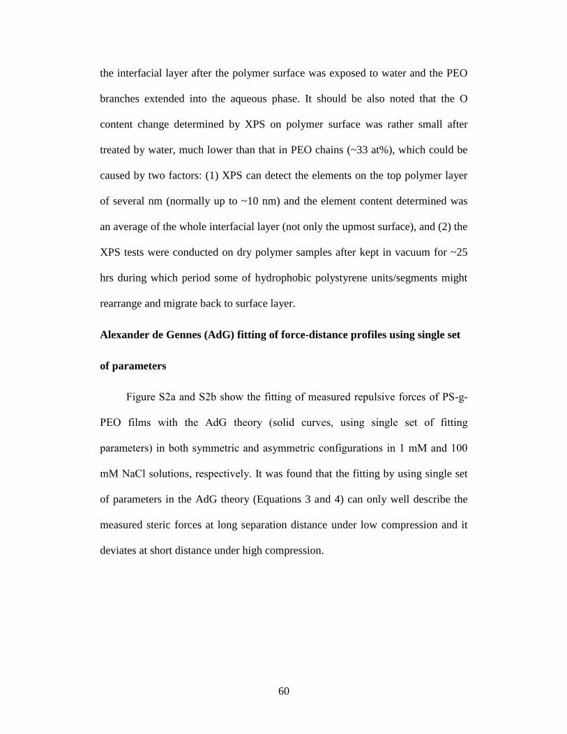
Alexander de Gennes (AdG) fitting of force-distance profiles using single set
....................................................................................................................... 60
of parameters ..................................................................................................... 60
References ......................................................................................................... 62
CHAPTER 4 EFFECT OF POLYCARBOXYLATE ETHER COMB-
TYPE POLYMER ON VISCOSITY AND INTERFACIAL PROPERTIES
OF KAOLINITE CLAY SUSPENSION .......................................................... 67
4.1 Introduction ........................................................................................... 67
4.2 Materials ............................................................................................... 69
4.3 Experimental Methods .......................................................................... 70
4.3.1 Sample preparation ........................................................................... 70
4.3.2 Viscosity measurement ...................................................................... 71
4.3.3 Zeta potential measurement .............................................................. 71
4.3.4 Settling tests ...................................................................................... 72
4.3.5 Measurement of interaction force using Surface Forces Apparatus 72
4.4 Results and discussion .......................................................................... 73
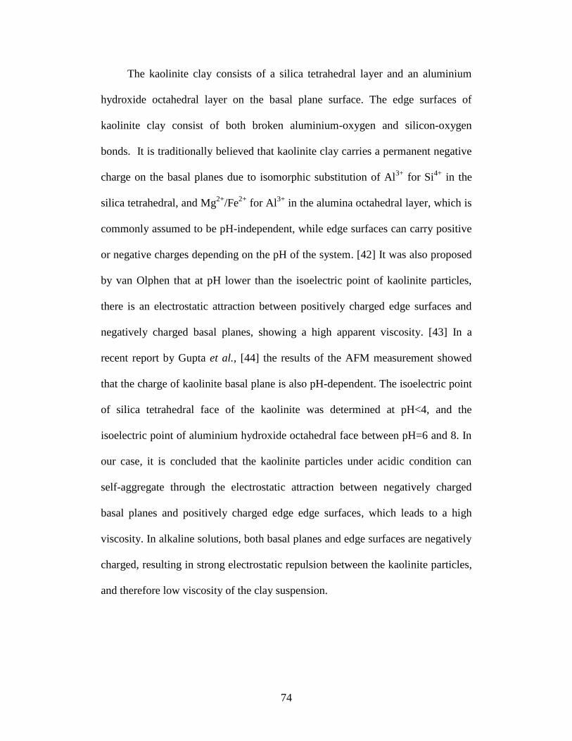
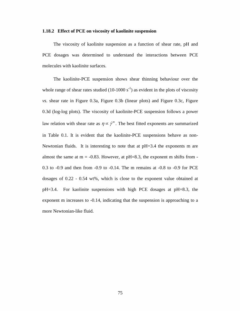
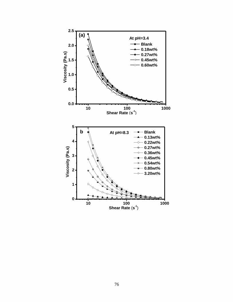
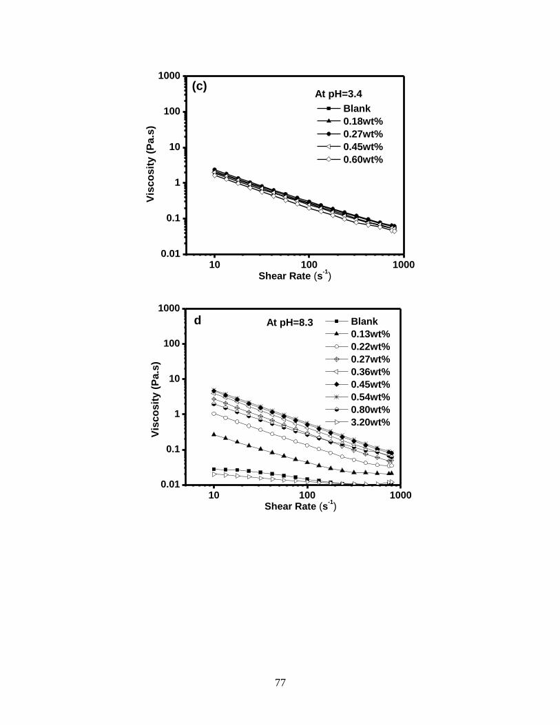
4.4.1 Impact of pH on viscosity of kaolinite suspensions .......................... 73
4.4.2 Effect of PCE on viscosity of kaolinite suspension ........................... 75
4.4.3 Settling tests ...................................................................................... 84
4.4.4 Interactions between kaolinite clay particles and PCE polymer ...... 87
4.5 Conclusion ............................................................................................ 97
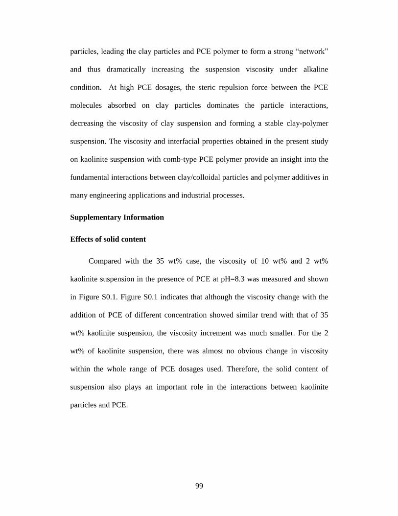
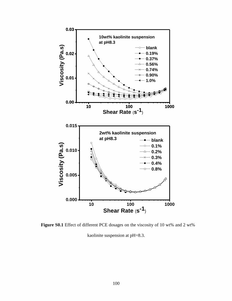
Supplementary Information .............................................................................. 99
Effects of solid content .................................................................................. 99
References ....................................................................................................... 101
CHAPTER 5 SUMMARY ........................................................................... 105
References ....................................................................................................... 108
LIST OF TABLES
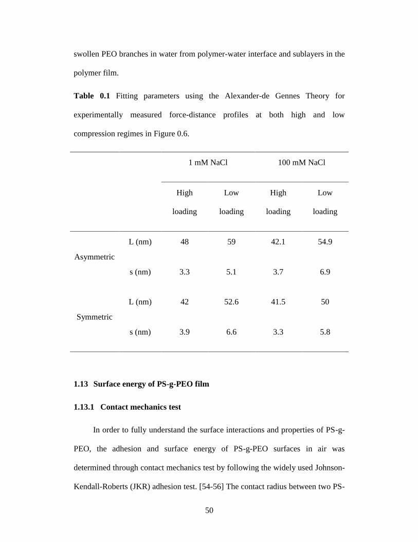
Table 3.1 Fitting parameters using the Alexander-de Gennes Theory for
experimentally measured force-distance profiles at both high and low
compression regimes in Figure 3.6. ....................................................... 50
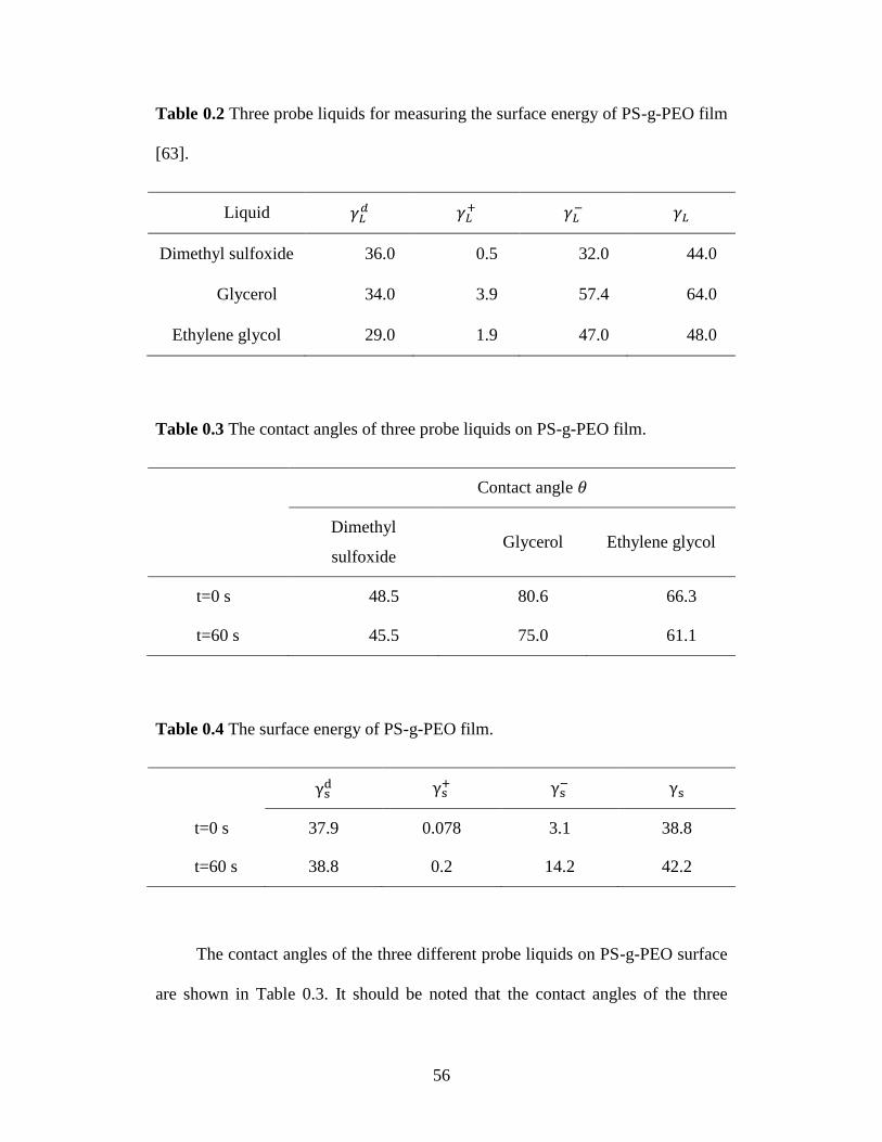
Table 3.2 Three probe liquids for measuring the surface energy of PS-g-PEO film.
............................................................................................................... 56
Table 3.3 The contact angles of three probe liquids on PS-g-PEO film. .............. 56
Table 3.4 The surface energy of PS-g-PEO film. ................................................. 56
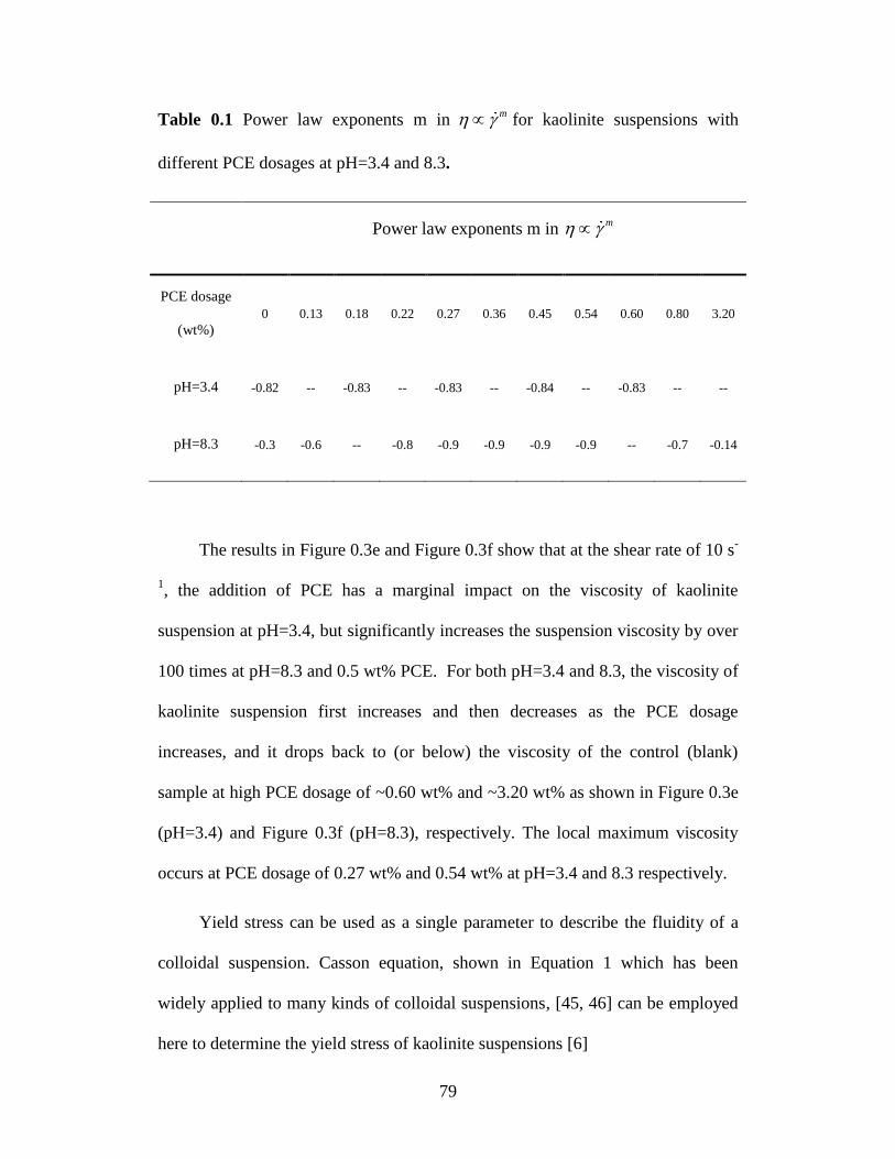
Table 4.1 Power law exponents m in m for kaolinite suspensions with
different PCE dosages at pH=3.4 and 8.3. ............................................. 79
LISTS OF FIGURES
Figure 1.1 Comb-type polymers with flexible (a) homopolymer graft chains, (b)
copolymer graft chains, (c) hetero-graft chains, and (d) branched graft
chains. ...................................................................................................... 2
Figure 1.2 Schematic of double layer structure on a negatively charged surface in
a liquid. .................................................................................................... 7
Figure 2.1 Schematic drawing of SFA 2000 ......................................................... 12
Figure 2.2 Schematic drawing of a typical SFA experimental setup .................... 14
Figure 2.3 FECO fringes in a typical force measurement (two mica surfaces in
adhesive contact) .................................................................................... 15
Figure 2.4 Schematic of FECO fringes to measure the radius of local curvature of
two surfaces. .......................................................................................... 17
Figure 2.5 The schematic drawing of mica sheets preparation procedure: (a)
trimming, (b) splitting, (c) peeling, (d) cutting and (e) silvering. .......... 19
Figure 2.6 Schematic of the principle of normal force measurement ................... 20
Figure 2.7 Schematic drawing of AFM working principle ................................... 24
Figure 2.8 Illustration of contact angle of a liquid on a solid surface................... 25
Figure 2.9 A brief schematic of photoelectron emission process ......................... 26
Figure 3.1 Chemical structure of comb-type polymer PS-g-PEO used in this study.
............................................................................................................... 33
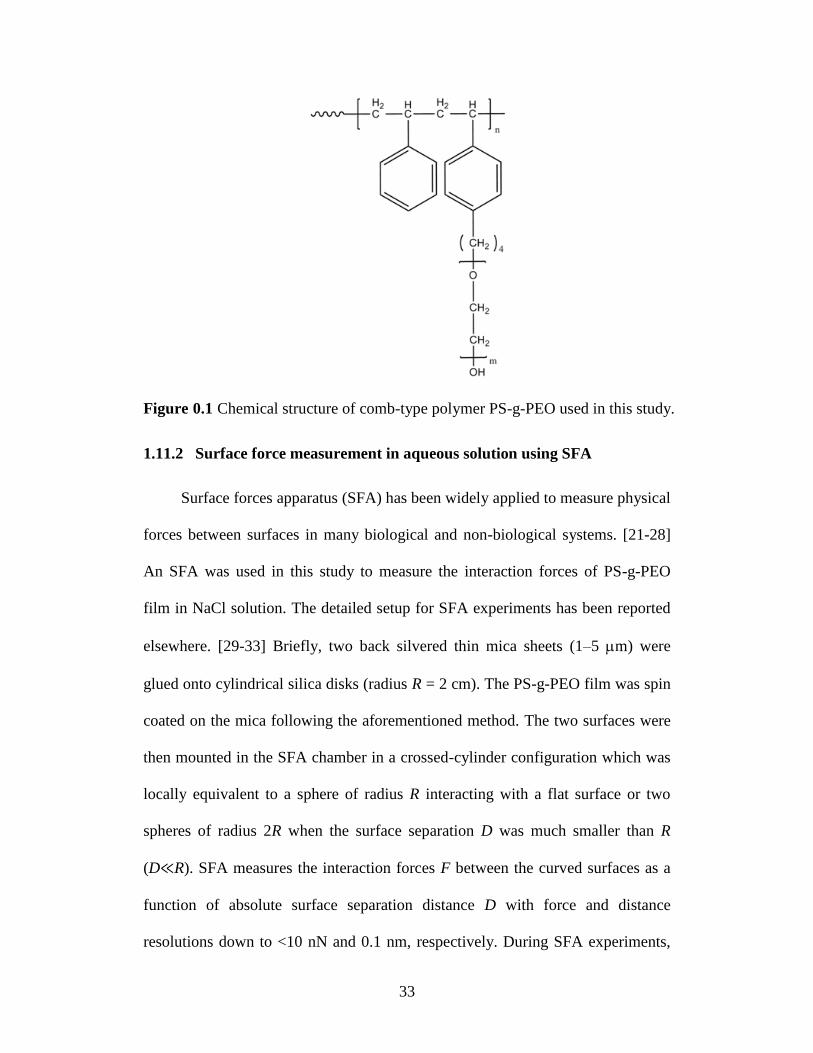
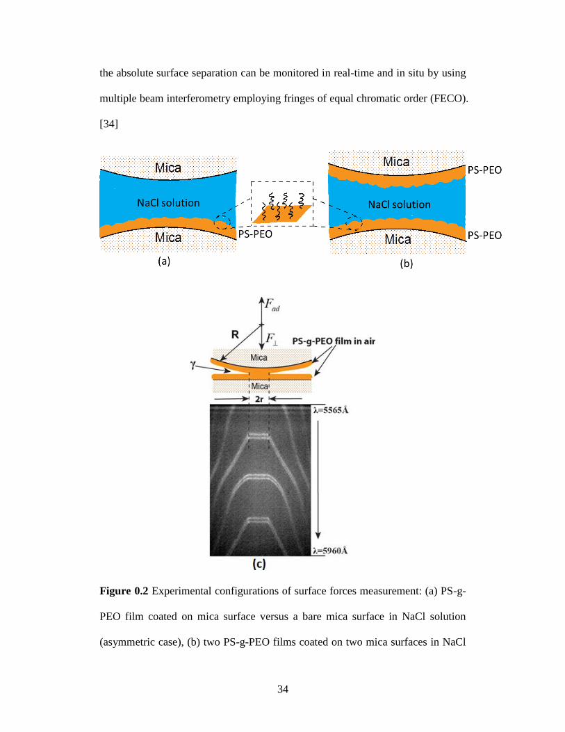
Figure 3.2 Experimental configurations of surface forces measurement: (a) PS-g-
PEO film coated on mica surface versus a bare mica surface in NaCl
solution (asymmetric case), (b) two PS-g-PEO films coated on two mica
surfaces in NaCl solution (symmetric case), (c) schematic of two
polymer surfaces in adhesive contact in air and typical FECO fringes. 34
Figure 3.3 The AFM images of PS-g-PEO film (a) before treatment, (b) after
water treatment. ..................................................................................... 40
Figure 3.4 Contact angle of water on spin-coated PS-g-PEO film. ...................... 42
Figure 3.5 Force-distance profiles between a PS-g-PEO polymer film and a bare
mica surface (asymmetric configuration) and between two PS-g-PEO
polymer films (symmetric configuration) in aqueous solution of (a) 1
mM NaCl (b) 100 mM NaCl. ................................................................. 43
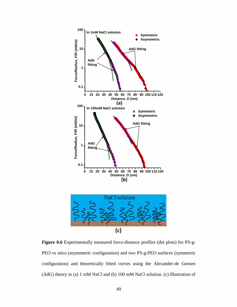
Figure 3.6 Experimentally measured force-distance profiles (dot plots) for PS-g-
PEO vs mica (asymmetric configuration) and two PS-g-PEO surfaces
(symmetric configuration) and theoretically fitted curves using the
Alexander-de Gennes (AdG) theory in (a) 1 mM NaCl and (b) 100 mM
NaCl solution. (c) Illustration of swollen PEO branches in water from
polymer-water interface and sublayers in the polymer film. ................. 49
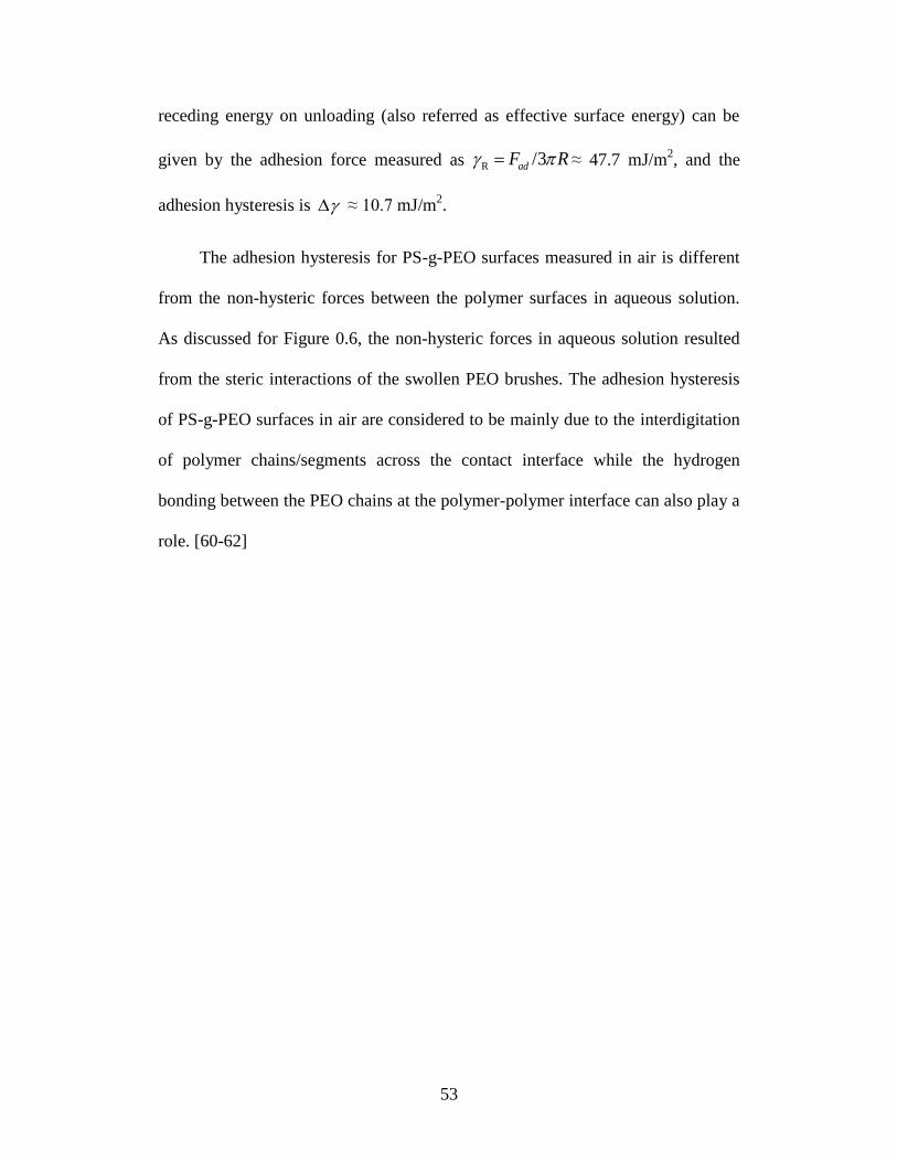
Figure 3.7 Contact diameter 2r vs. applied load F obtained through the JKR
loading-unloading test for two PS-g-PEO films. Red solid line is the
fitted curve for the loading path using the JKR model. ......................... 54
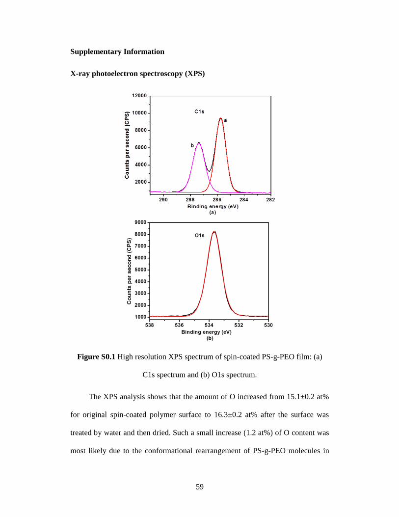
Figure S3.1 High resolution XPS spectrum of spin-coated PS-g-PEO film: (a) C1s
spectrum and (b) O1s spectrum. ............................................................ 59
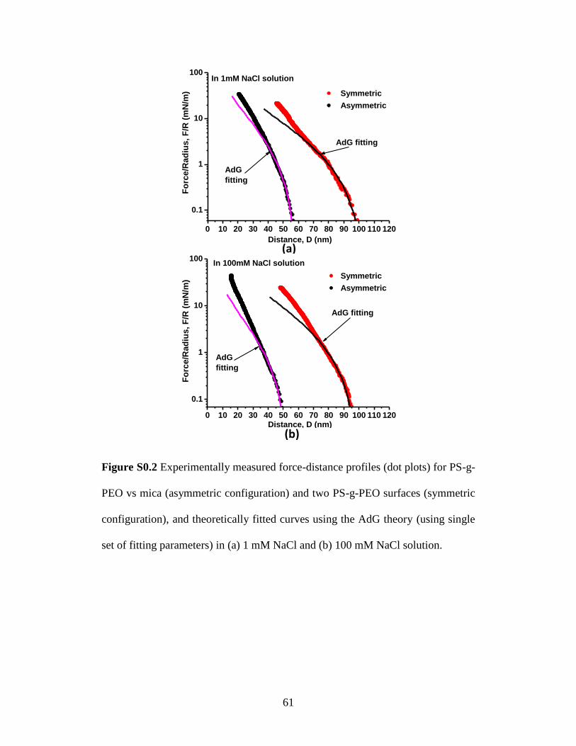
Figure S3.2 Experimentally measured force-distance profiles (dot plots) for PS-g-
PEO vs mica (asymmetric configuration) and two PS-g-PEO surfaces (symmetric
configuration), and theoretically fitted curves using the AdG theory (using single
set of fitting parameters) in (a) 1 mM NaCl and (b) 100 mM NaCl solution.
61
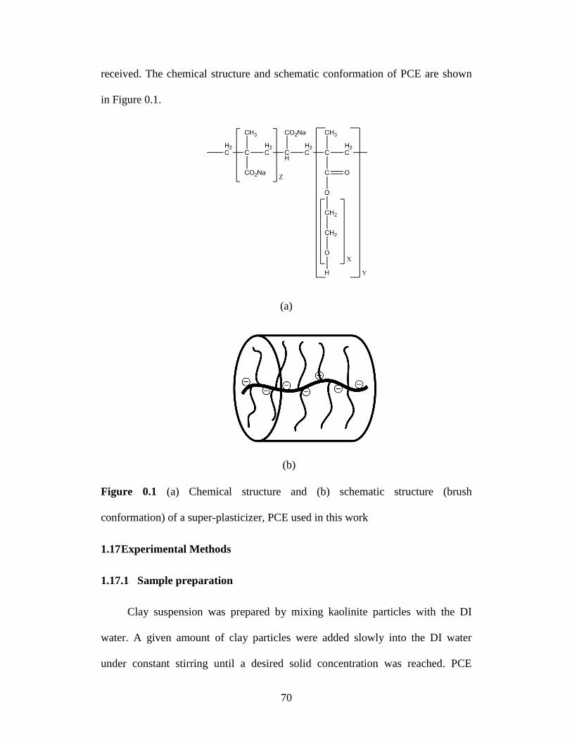
Figure 4.1 (a) Chemical structure and (b) schematic structure (brush
conformation) of a super-plasticizer, PCE used in this work ................ 70
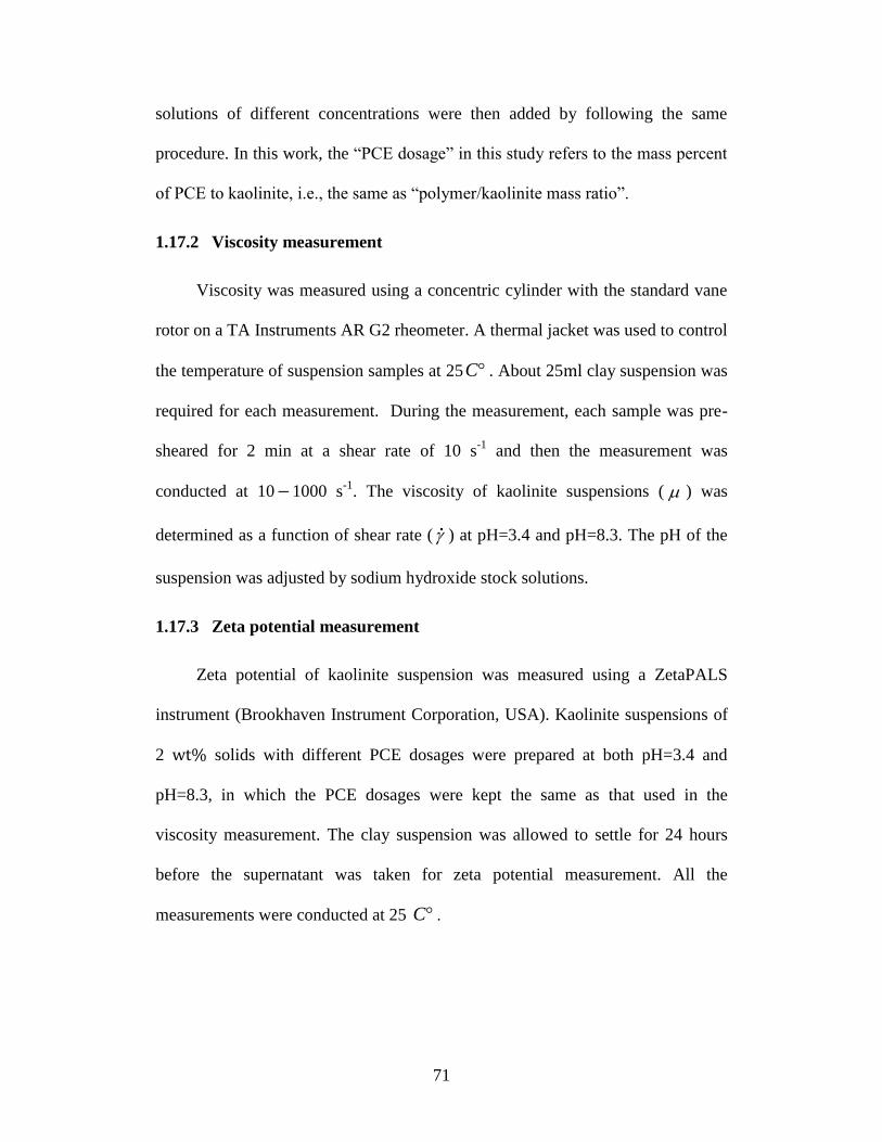
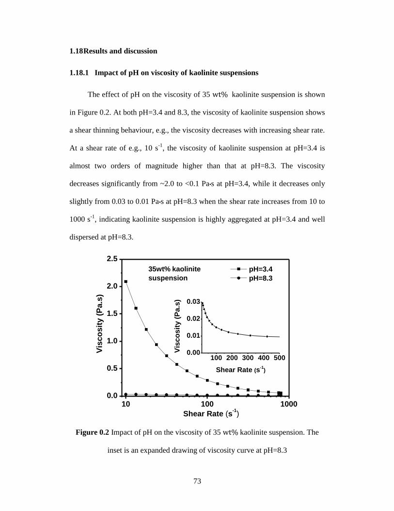
Figure 4.2 Impact of pH on the viscosity of 35 wt% kaolinite suspension. The
inset is an expanded drawing of viscosity curve at pH=8.3 ................... 73
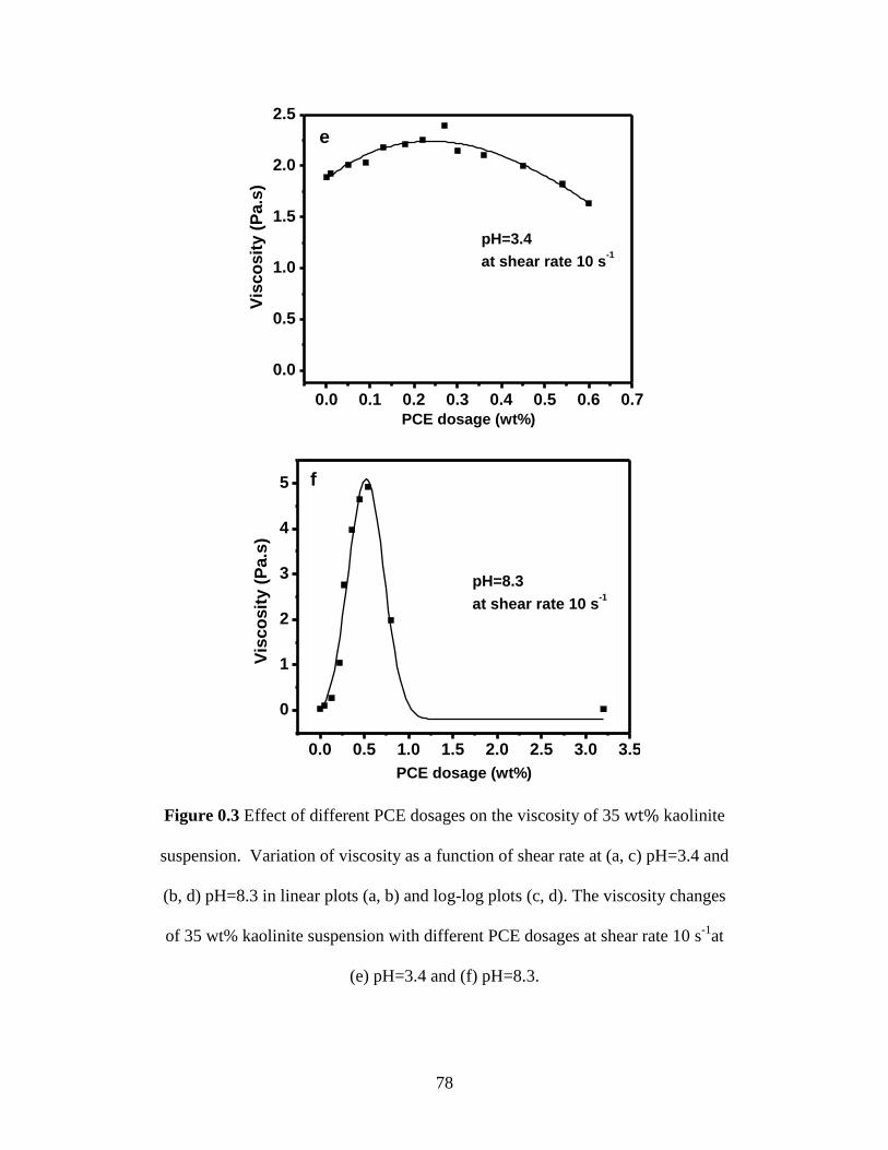
Figure 4.3 Effect of different PCE dosages on the viscosity of 35 wt% kaolinite
suspension. Variation of viscosity as a function of shear rate at (a, c)
pH=3.4 and (b, d) pH=8.3 in linear plots (a, b) and log-log plots (c, d).
The viscosity changes of 35 wt% kaolinite suspension with different
PCE dosages at shear rate 10 s-1
at (e) pH=3.4 and (f) pH=8.3. ............. 78
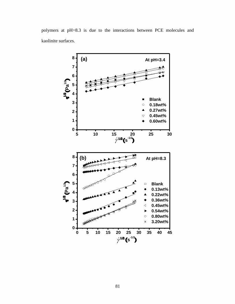
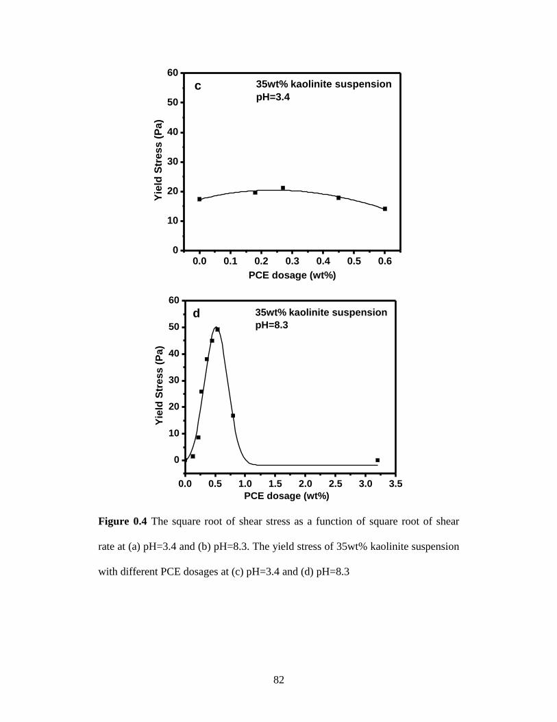
Figure 4.4 The square root of shear stress as a function of square root of shear rate
at (a) pH=3.4 and (b) pH=8.3. The yield stress of 35wt% kaolinite
suspension with different PCE dosages at (c) pH=3.4 and (d) pH=8.3 . 82
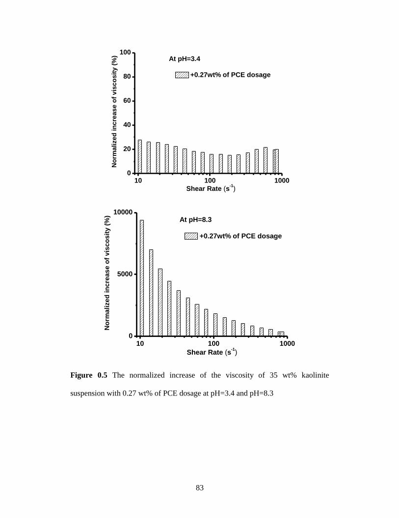
Figure 4.5 The normalized increase of the viscosity of 35 wt% kaolinite
suspension with 0.27 wt% of PCE dosage at pH=3.4 and pH=8.3 ........ 83
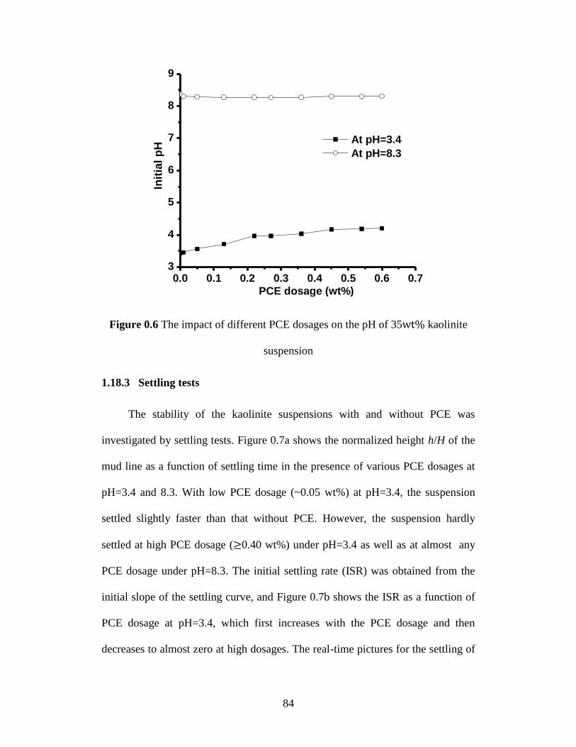
Figure 4.6 The impact of different PCE dosages on the pH of 35wt% kaolinite
suspension .............................................................................................. 84
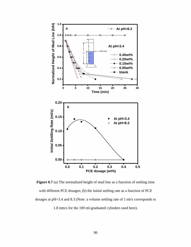
Figure 4.7 (a) The normalized height of mud line as a function of settling time
with different PCE dosages; (b) the initial settling rate as a function of
PCE dosages at pH=3.4 and 8.3 (Note: a volume settling rate of 1 ml/s
corresponds to 1.8 mm/s for the 100 ml-graduated cylinders used here).
............................................................................................................... 86
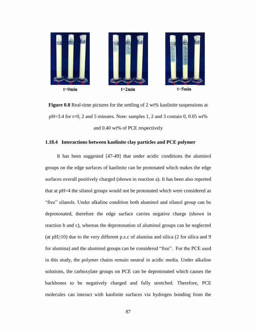
Figure 4.8 Real-time pictures for the settling of 2 wt% kaolinite suspensions at
pH=3.4 for t=0, 2 and 5 minutes. Note: samples 1, 2 and 3 contain 0,
0.05 wt% and 0.40 wt% of PCE respectively ........................................ 87
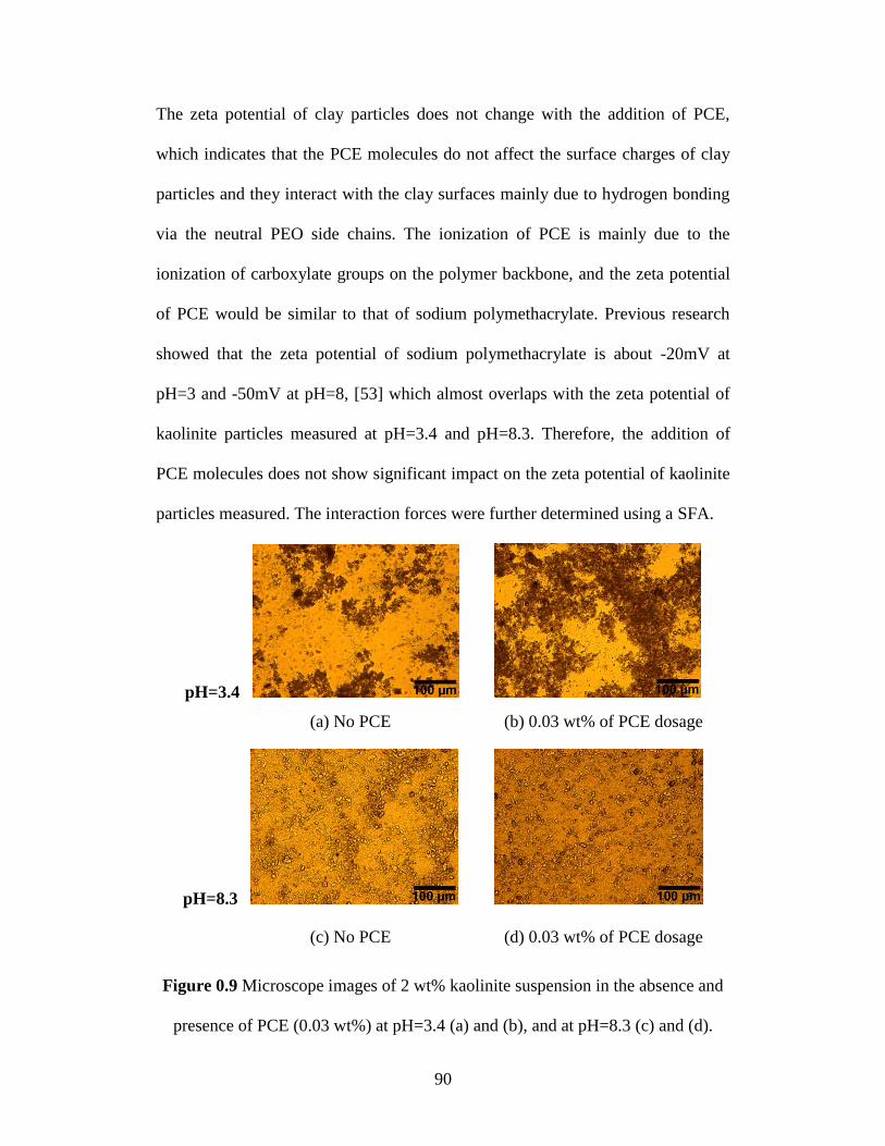
Figure 4.9 Microscope images of 2 wt% kaolinite suspension in the absence and
presence of PCE (0.03 wt%) at pH=3.4 (a) and (b), and at pH=8.3 (c)
and (d). ................................................................................................... 90
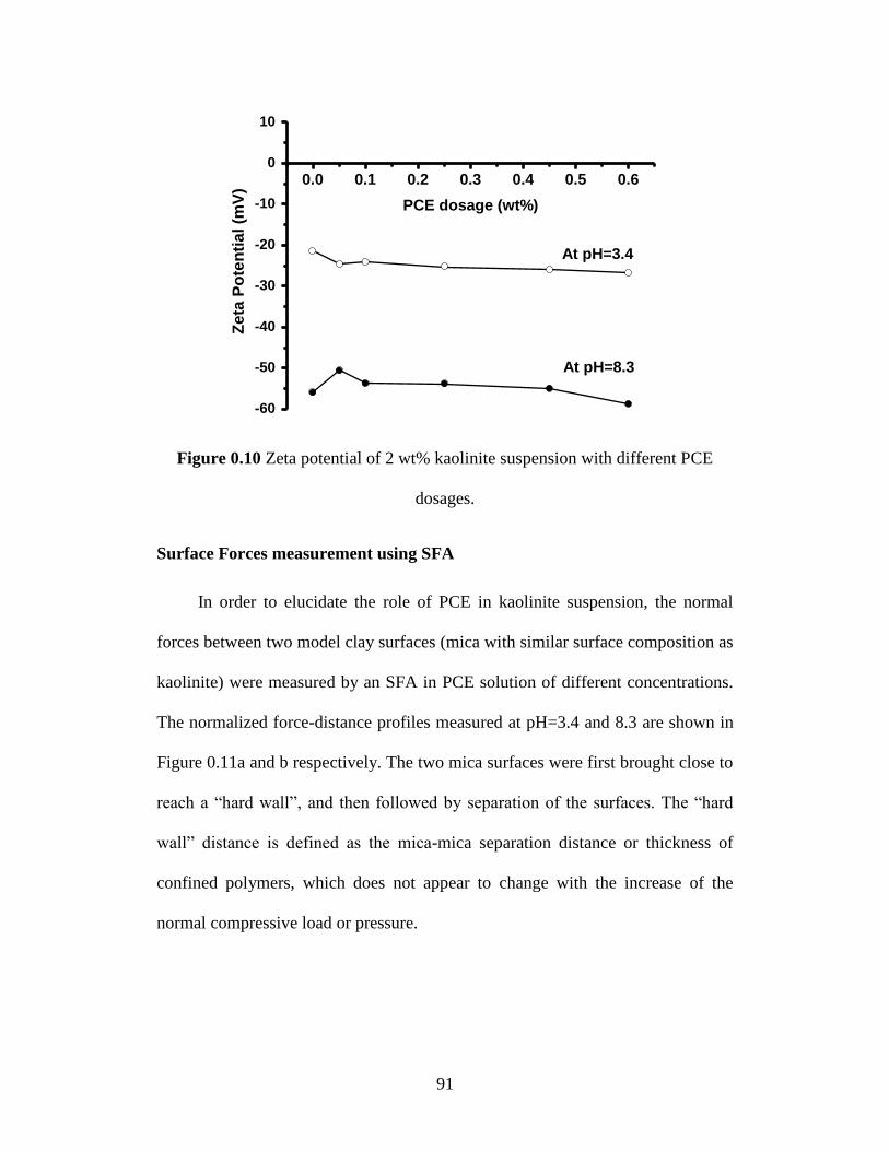
Figure 4.10 Zeta potential of 2 wt% kaolinite suspension with different PCE
dosages. .................................................................................................. 91
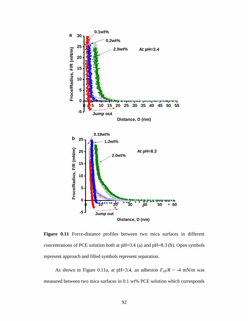
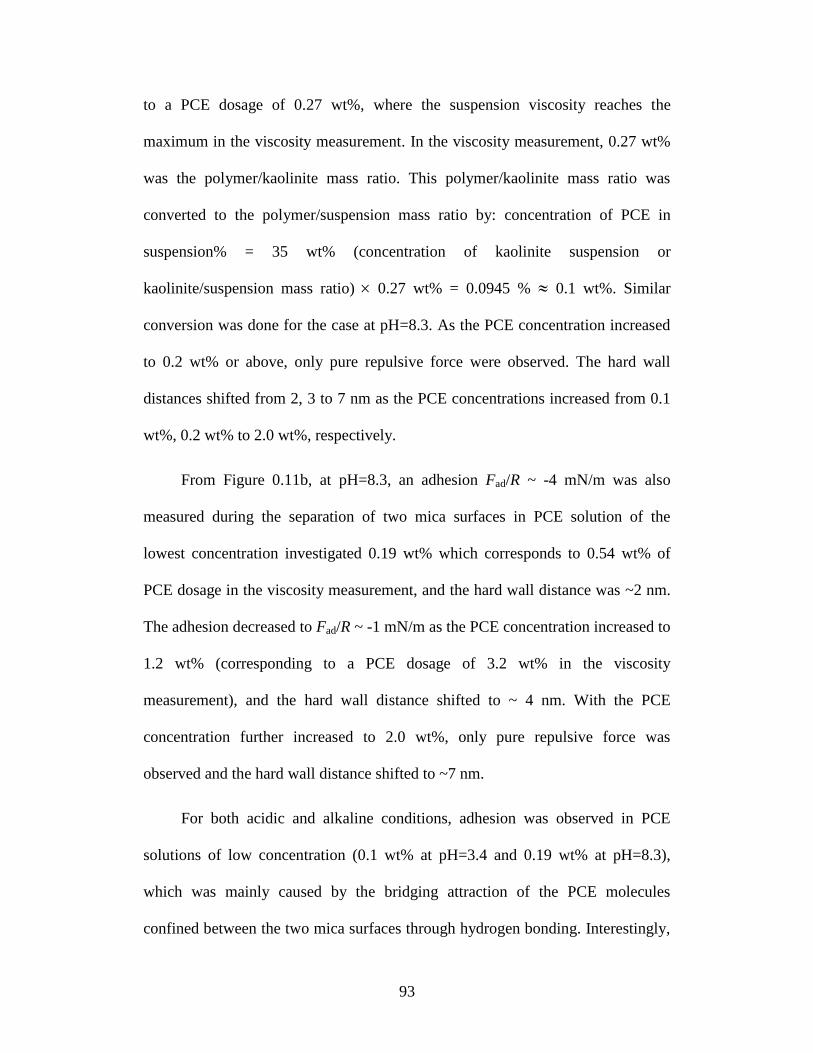
Figure 4.11 Force-distance profiles between two mica surfaces in different
concentrations of PCE solution both at pH=3.4 (a) and pH=8.3 (b). Open
symbols represent approach and filled symbols represent separation. .. 92
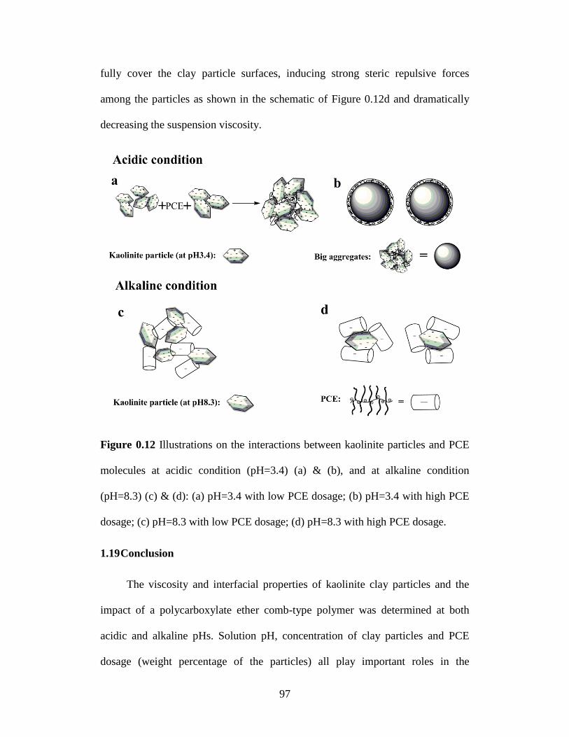
Figure 4.12 Illustrations on the interactions between kaolinite particles and PCE
molecules at acidic condition (pH=3.4) (a) & (b), and at alkaline
condition (pH=8.3) (c) & (d): (a) pH=3.4 with low PCE dosage; (b)
pH=3.4 with high PCE dosage; (c) pH=8.3 with low PCE dosage; (d)
pH=8.3 with high PCE dosage. .............................................................. 97
Figure S4.1 Effect of different PCE dosages on the viscosity of 10 wt% and 2 wt%
kaolinite suspension at pH=8.3. ........................................................... 100
SYMBOLS AND NOMENCLATURE
A Hamaker constant, J
D separation distance between surfaces, m
jumpD distance one surface jump apart from the other surface, m
appliedD the distance to move the surfaces at the base of the double-
cantilever force springs, m
actualD the actual distance that the surfaces move relative to each other, m
R1, R2 radius of spherical particles, m
0
n , 0
1n wavelength move of the nth and (n-1)th fringe, m
D electrical potential, V
0 surface potential of a particle, V
inverse Debye length, m-1
gR radius of gyration, m
l length of the repeating unit in the polymer, m
N number of repeating units in the polymer
surface coverage of polymer on the surface, m-2
s mean distance between the attachment points of adsorbed polymer
chains, m
sK spring constant, N/m
adhesionF , Fad adhesion force, N
γ surface energy, mJ/m2
γA surface energy in the loading (advancing) process, mJ/m2
γR surface energy in the unloading (receding) process, mJ/m2
∆γ the hysteresis of surface energy, mJ/m2
γeff effective surface energy, mJ/m2
SG surface energy at solid and gas interface, mJ/m2
SL surface energy at solid and liquid interface, mJ/m2
LG surface energy at liquid and gas interface, mJ/m2
d the dispersive component (Lifshitz-Van der Waals interactions),
mJ/m2
,
the polar components (Lewis acid-base), mJ/m2
r radius of contact area, m
F applied load normally to the surface, N
R radius of the cylindrical silica disc, m
K elastic moduli, N/m2
apparent viscosity, Pa.s
shear rate, s-1
τ shear stress, Pa
c Casson yield stress, Pa
c Casson viscosity, Pa.s
ω angular velocity, rad/s
the torque, Nm
hν X-ray photon energy, eV
bE binding energy, eV
Ek kinetic energy of photoelectron, eV
( )P D repulsive pressure between two surfaces, Pa
T temperature, C
L brush layer thickness, m
k Boltzmann constant, 1.381 × 10⁻²³
J K-1
E1, E2 Young’s moduli, N/m2
ν1, ν2 Poisson’s ratios
W, adW adhesion energy, mJ/m
2
1
CHAPTER 1 INTRODUCTION
1.1 Comb-type polymers
Functionalities of polymer coatings play important roles in numerous
engineering and biomedical applications, ranging from adhesion, lubrication,
wettability control, drug delivery, stabilization/destabilization of colloids to
antifouling treatments. During the past decade, comb-type polymers have
attracted much attention in polymer chemistry and physics, nanotechnology and
bioengineering, which are special copolymers with many branches grafted to a
polymer backbone. Since only limited work is available on the molecular forces
of comb-type polymers, this thesis work will provide some insights into the
fundamental understanding of their molecular interaction mechanisms and
designing and developing novel polymers and polymer coatings with engineering
and biomedical applications.
1.1.1 Conformations of comb-type polymers
There are many kinds of comb-type polymers with different chemical
structures in backbones and graft chains. Both backbone and graft chains can be
flexible or stiff and the graft chains can be also homopolymers or copolymers [1,
2]. Figure 0.1 shows some typical structures of comb-type polymers with flexible
graft chains. For comb-type polymers with the same chemical composition in
backbone and graft chains, the polymer conformation can be controlled by
varying the density and length of side chains as well as the solvent environment.
Comb-type polymers with much denser side chains normally induce stronger
2
intramolecular steric interactions resulting in stretched backbones. Varying
solution pH can make certain comb-type polymers either negatively or positively
charged, leading to fully stretched conformation due to the intramolecular
electrostatic repulsive forces. The solvent conditions (i.e. good solvent, bad
solvent and theta (θ) solvent) also show strong impact on the polymer
conformations [3]. In a good solvent, the favourable interactions between solvent
molecules and polymer chains cause the polymers to expand. In a bad solvent, the
interactions between polymer molecules are more favoured so that it leads the
polymer molecules to coil. The theta (θ) solvent is also called ideal solvent in
which the polymer acts as an ideal chain which can be modelled by using the free
jointed chain model.
Figure 0.1 Comb-type polymers with flexible (a) homopolymer graft chains, (b)
copolymer graft chains, (c) hetero-graft chains, and (d) branched graft chains.
3
1.1.2 Review of previous work on comb-type polymers
Comb-type polymers, with their special and interesting architecture, have
attracted much attention in the fields of polymer chemistry and physics,
nanotechnology, bioengineering and industrial applications. During the past two
decades, much work has been focused on the synthesis and characterization of
well-defined comb-type polymers using different synthesis methods and
experimental techniques including gel permeation chromatography (GPC), light
scattering (LS), viscosity measurement, atomic force microscopy (AFM), surface
sensitive sum-frequency generation (SFG), etc. [1, 2, 4-8] Since the comb-type
polymer may form brush conformation at the solid/water/air interfaces, some
experimental work was reported on the adsorption behaviour and conformation of
comb-type polymers, [6-8] and some other work focused on the theoretical
modelling [9, 10]. Comb-type polycarboxylate ether (PCE) has been reported to
be effective additives in stabilizing different colloidal systems by using viscosity
measurement, isotherm adsorption, zeta potential measurement, etc. [7, 11-15]
Normally, the backbone of the comb-type polymer can act as the adsorbing chain
and graft side chains can extend from the surfaces performing as polymer brushes.
Comb-type polymers, such as poly(L-lysine)-g-poly(ethylene glycol),
poly(ethylenimine)-graft-poly(ethylene glycol) and polyacrylonitrile-graft-
poly(ethylene oxide), have also been investigated in terms of the properties for
applications of lubricants or anti-fouling coatings in bioengineering [16, 17].
4
1.2 Intermolecular and surface forces
The main objective of this study is to probe the molecular forces of comb-
type polymers at water/solid/air interfaces to provide some fundamental insights
into the design and development of functional and novel polymers with important
industrial applications ranging from adhesives, lubricants, dispersants to anti-
fouling materials. In this section, I describe the surface and intermolecular forces
involved in this study including van de Waals forces, electrostatic force, polymer
bridging force and steric repulsive force.
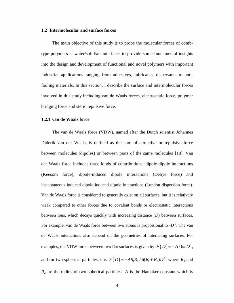
1.2.1 van de Waals force
The van de Waals force (VDW), named after the Dutch scientist Johannes
Diderik van der Waals, is defined as the sum of attractive or repulsive force
between molecules (dipoles) or between parts of the same molecules [18]. Van
der Waals force includes three kinds of contributions: dipole-dipole interactions
(Keesom force), dipole-induced dipole interactions (Debye force) and
instantaneous induced dipole-induced dipole interactions (London dispersion force).
Van de Waals force is considered to generally exist on all surfaces, but it is relatively
weak compared to other forces due to covalent bonds or electrostatic interactions
between ions, which decays quickly with increasing distance (D) between surfaces.
For example, van de Waals force between two atoms is proportional to -D-7. The van
de Waals interactions also depend on the geometries of interacting surfaces. For
examples, the VDW force between two flat surfaces is given by 3/ 6F D A D ,
and for two spherical particles, it is 2
1 2 1 2/ 6( )F D AR R R R D , where R1 and
R2 are the radius of two spherical particles. A is the Hamaker constant which is
5
dependent on the chemical nature of interacting molecules or surfaces and defined
as 2
1 2A C , where C is the coefficient in the atom-atom pair potential, ρ1and
ρ2 are the number of atoms per volume in the two bodies.
1.2.2 Electrostatic double layer force
The electrical double layer is a structure forming on a surface of an object
(solid, air bubble, liquid drop) when it is placed in an aqueous surrounding. The
double layer refers to the two layers near the surface. A typical schematic of
double layer structure on a negatively charged surface in an aqueous solution is
shown in Figure 0.2. [19] The first layer is called stern layer (i.e. Helmholtz layer)
where the counter ions adsorb on the surface that is immobile. The second layer
next to the first layer is called the diffuse layer or Gouy-Chapman layer. The
diffuse layer consists of mobile ions that normally obey Poisson-Boltzmann
statistics and associated with the surface via Coulomb force. The potential at the
point or plane between the Stern layer and diffuse layer is called the zeta potential.
In the diffuse layer (the right side from the stern layer), the electrical
potential decays exponentially following the equation (between two flat surface),
0 exp( )D D . 1 is called Debye length and also considered as the
double layer thickness. Therefore, when the two surfaces approach each other, the
diffuse layers become overlapped and the repulsive force is induced, called
electrostatic double layer force. The electrostatic double layer force is essential for
the stabilization of many colloidal dispersions and polymer systems such as
polyelectrolytes.
6
When an electric filed is applied across an electrolyte solution, the viscous
forces acting on the charged particles in the suspension tend to oppose the
particles' movement towards the electrode with opposite charges. When these two
opposing forces reach equilibrium, the movement of the particles in suspension
will exhibit a constant velocity, which is commonly referred as its electrophoretic
mobility. Based on this model, the zeta potential of the particles can be described
by the Smoluchowski equation as shown in Eq. 1.1. ,
2 ( )
3E
f ka
(1.1)
where μE is electrophoretic mobility, ε is dielectric constant, ζ is zeta potential and
η is viscosity of suspension. f(ka) is so-called Henry’s function and a is the
particle radius. Two values are generally used as approximations for the f(Ka)
determination, either 1.5 or 1.0. f(ka)=1.5 is referred to as the Smoluchowski
approximation, which is normally applied to particles larger than about 0.2
microns. f(ka)=1.0 is commonly used for small particles in low dielectric constant
media (e.g., non-aqueous measurements), referred to as the Huckel approximation.
7
Figure 0.2 Schematic of double layer structure on a negatively charged surface in
a liquid.
1.2.3 Steric repulsion and bridging force
In my study, the steric and bridging forces occurred between two surfaces
bearing polymers or between two surfaces in the medium of polymer solution.
When two surfaces covered with polymers opposing to each other, the net
interactions include the polymer-polymer and polymer-surface interactions.
Normally, the polymer-polymer interaction results in repulsive force referred as
steric repulsive force and polymer-surface interaction can either lead to repulsive
force or attractive force (bridging force). The conformation of a polymer depends
on the condition of its surroundings, such as solvent quality, temperature, etc. [3]
8
If a polymer is in an ideal state which means the movement of the polymer cannot
be affected by the monomer-monomer interactions, the dimension of the polymer
molecule can be defined by the radius of gyration ( gR ),
6g
l NR (1.2)
where l is the length of the repeating unit and N is the number of repeating units in
the polymer. There are two regimes of the polymer conformations which are
dependent on the surface coverage of the polymer on the surfaces. The surface
coverage is the number of polymer chains adsorbing on the surface per unit area
and the relation with the mean distance s between the two anchoring points of
adsorbed polymer chains is shown in Eq. 1.3.
2
1
s (1.3)
When the surface coverage is lower (s> gR ) and covered with a number of
separated polymer blobs with height and size given by Rg which do not overlap,
the polymer chains are in a regime called mushroom regime. Under high surface
coverage (s≪ gR ), the polymers are in a so-called brush regime, whose surface
interactions can be normally described by the Alexander de Gennes theory. [18,
20-22] In these two regimes, the steric repulsive interaction energy can be
described by different equations or models [22]. However, the attractive
component (or so-called bridging force) has no simple expression because the
bridging force depends on the type of interactions (i.e., specific or non-specific)
between the polymer and the opposite surface.
9
References
[1] S.S. Sheiko, B.S. Sumerlin, K. Matyjaszewski, Prog Polym Sci, 33 (2008)
759.
[2] M.F. Zhang, A.H.E. Muller, J Polym Sci Pol Chem, 43 (2005) 3461.
[3] M.M. Coleman, Fundamentals of Polymer Science: An Introductory Text,
Second Edition, CRC Press, 1998.
[4] K. Ito, Y. Tomi, S. Kawaguchi, Macromolecules, 25 (1992) 1534.
[5] M. Wintermantel, M. Schmidt, Y. Tsukahara, K. Kajiwara, S. Kohjiya,
Macromol Rapid Comm, 15 (1994) 279.
[6] M. Lesti, S. Ng, J. Plank, J Am Ceram Soc, 93 (2010) 3493.
[7] Q.P. Ran, P. Somasundaran, C.W. Miao, J.P. Liu, S.S. Wu, J. Shen, J Disper
Sci Technol, 31 (2010) 790.
[8] K.S. Gautam, A. Dhinojwala, Macromolecules, 34 (2001) 1137.
[9] A. Sartori, A. Johner, J.L. Viovy, J.F. Joanny, Macromolecules, 38 (2005)
3432.
[10] I.I. Potemkin, Macromolecules, 39 (2006) 7178.
[11] C.P. Whitby, P.J. Scales, F. Grieser, T.W. Healy, G. Kirby, J.A. Lewis, C.F.
Zukoski, J Colloid Interf Sci, 262 (2003) 274.
[12] A. Zingg, F. Winnefeld, L. Holzer, J. Pakusch, S. Becker, R. Figi, L.
Gauckler, Cement Concrete Comp, 31 (2009) 153.
10
[13] H. Hommer, J Eur Ceram Soc, 29 (2009) 1847.
[14] J. Plank, C. Schroefl, M. Gruber, M. Lesti, R. Sieber, J Adv Concr Technol,
7 (2009) 5.
[15] Q.P. Ran, P. Somasundaran, C.W. Miao, J.P. Liu, S.S. Wu, J. Shen, J Colloid
Interf Sci, 336 (2009) 624.
[16] S. Lee, M. Muller, M. Ratoi-Salagean, J. Voros, S. Pasche, S.M. De Paul,
H.A. Spikes, M. Textor, N.D. Spencer, Tribol Lett, 15 (2003) 231.
[17] M.A. Brady, F.T. Limpoco, S.S. Perry, Langmuir, 25 (2009) 744.
[18] J. Israelachvili, Intermolecular and Surface Forces, third ed., Academic
Press, 2011.
[19] D. Myers, Surfaces, Interfaces, and Colloids: Principles and Applications,
2nd edtion ed., John Wiley & Sons, Inc, New York, 1999.
[20] M. Akbulut, A.R.G. Alig, Y. Min, N. Belman, M. Reynolds, Y. Golan, J.
Israelachvili, Langmuir, 23 (2007) 3961.
[21] P.G. Degennes, Adv Colloid Interfac, 27 (1987) 189.
[22] F. Li, F. Pincet, Langmuir, 23 (2007) 12541.
11
CHAPTER 2 EXPERIMENTAL TECHNIQUES
1.3 The surface forces apparatus (SFA)
Surface forces apparatus (SFA) has been used for several decades to directly
measure the intermolecular forces between surfaces. Since the first apparatus was
described by Tabor, Winterton and Israelachvili in 1969 [1, 2], SFA has been
being significantly developed and improved. [3-6]
After the development of early versions of SFA which can only measure the
forces between surfaces in air or vacuum, the SFA Mk I was described by
Israelachvili and Adam which allows the force measurement both in controlled
vapors and liquids [3]. The travelling distance of mica surface controlled by the
motor-driven micrometer and piezoelectric crystals was improved from
micrometer to the angstrom level. In 1987, Israelachvili described the SFA Mk II
as an improved version of the Mk I which allowed the upper surface to be moved
in the lateral direction. Therefore, frictional forces can be also measured by using
an SFA. The force sensitivity reached to <10 nN, which is the same with that of
normal force measurement [7, 8].
In order to make SFA be used in much more complex systems, the Mk III,
developed by Israelachvili and McGuiggan (1985-1989), was much more compact
than the previous versions and also better for systems where the surfaces needed
to be completely immersed in liquids. Moreover, a new attachment so-called
bimorph slider was developed for the friction force measurement [5, 9].
12
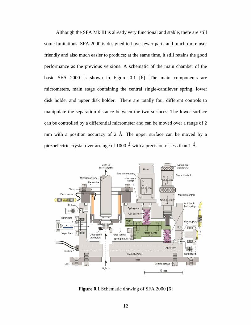
Although the SFA Mk III is already very functional and stable, there are still
some limitations. SFA 2000 is designed to have fewer parts and much more user
friendly and also much easier to produce; at the same time, it still retains the good
performance as the previous versions. A schematic of the main chamber of the
basic SFA 2000 is shown in Figure 0.1 [6]. The main components are
micrometers, main stage containing the central single-cantilever spring, lower
disk holder and upper disk holder. There are totally four different controls to
manipulate the separation distance between the two surfaces. The lower surface
can be controlled by a differential micrometer and can be moved over a range of 2
mm with a position accuracy of 2 Ǻ. The upper surface can be moved by a
piezoelectric crystal over arrange of 1000 Ǻ with a precision of less than 1 Ǻ.
Figure 0.1 Schematic drawing of SFA 2000 [6]
13
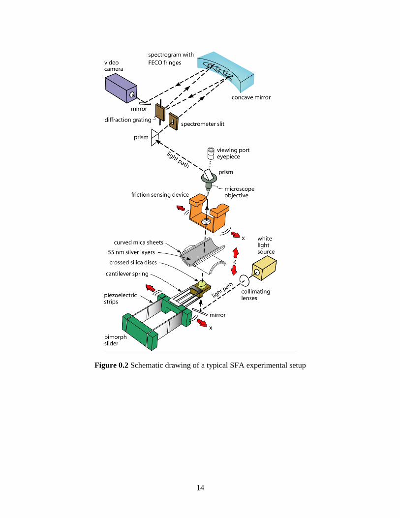
Figure 0.2 shows a brief setup of a typical SFA experiment. Two back
silvered molecular smooth mica surfaces are glued onto two cylindrical silica
discs (of radius R). The two surfaces are placed in a crossed cylinder
configuration which is locally equivalent to a sphere (of radius R) near a flat
surface or to two spheres (of radius 2R) close together when the separation
distance D≪R. The absolute surface separation distance can be monitored by
using an optical technique called multiple beam interference (MBI), which is
described in details in the next section. During experiments, white light passes
normally through the two surfaces and the merging interference light beam is
focused on the grating spectrometer which generates a series of Fringes of Equal
Chromatic Order (FECO) [10, 11]. Typical FECO fringe pattern is shown in
Figure 0.3.
14
Figure 0.2 Schematic drawing of a typical SFA experimental setup
15
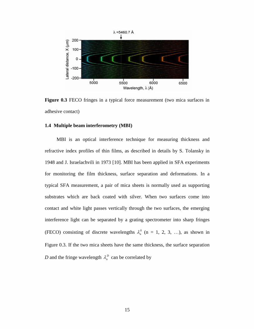
Figure 0.3 FECO fringes in a typical force measurement (two mica surfaces in
adhesive contact)
1.4 Multiple beam interferometry (MBI)
MBI is an optical interference technique for measuring thickness and
refractive index profiles of thin films, as described in details by S. Tolansky in
1948 and J. Israelachvili in 1973 [10]. MBI has been applied in SFA experiments
for monitoring the film thickness, surface separation and deformations. In a
typical SFA measurement, a pair of mica sheets is normally used as supporting
substrates which are back coated with silver. When two surfaces come into
contact and white light passes vertically through the two surfaces, the emerging
interference light can be separated by a grating spectrometer into sharp fringes
(FECO) consisting of discrete wavelengths 0
n (n = 1, 2, 3, …), as shown in
Figure 0.3. If the two mica sheets have the same thickness, the surface separation
D and the fringe wavelength D
n can be correlated by
16
00 0
1
2 0 0 0 2
1
2 sin 1 / / 1 /tan(2 / )
(1 )cos 1 / / 1 / ( 1)
n
D
n n n
D
n
D
n
nn n
D
, (2.1)
where ‘+’ refers to odd order fringes (n odd), and ‘-’ refers to even order fringes
(n even). /mica , where mica is the refractive index of mica at D
n , and
is the refractive index of the medium between the two mica surfaces at D
n . For
separation less than 30 nm, the Eq. (2.1) can be simplified to the following two
approximate equations
0( )
2
D
n n n
mica
DnF
for n odd (positive sign in Eq.(2.1)) (2.1a)
0
2
( )
2
D
n n n micaDnF
for n even (negative sign in Eq.(2.1)) (2.1b)
where 0 0 0
1 1/ ( )nn nnF . By using the above equations, the distance D can be
determined by measuring the shifts in wavelengths of an odd and adjacent even
fringe. The accuracy is about 1 Ǻ for measurement of D in the range of 0-200 nm.
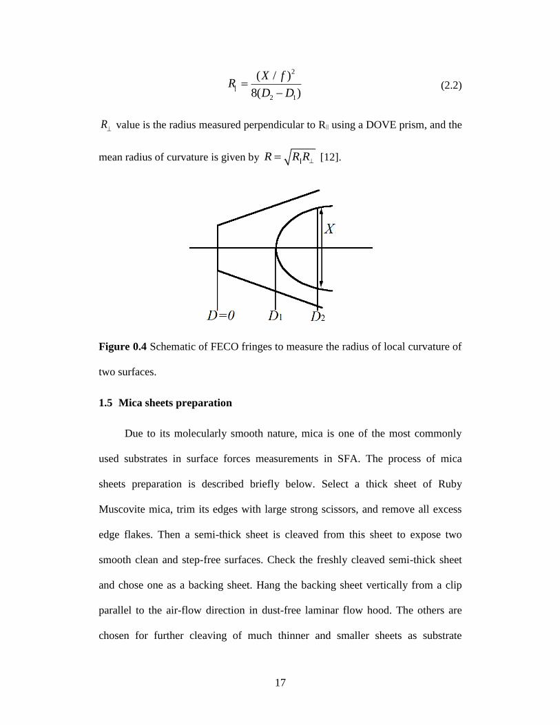
The local radius of curvature of the surfaces is normally used to normalize
the measured surface forces, which can be determined directly from the shape of
the FECO fringes by measuring two distances D1 and D2 as well as the lateral
distance X on any fringe as shown in Figure 0.4. If the spectrometer-microscope
magnification factor is f, the radius Rǀǀ is given by Eq. 2.2.
17
2
2 1
( / )
8( )
XR
f
D D
(2.2)
R value is the radius measured perpendicular to Rǀǀ using a DOVE prism, and the
mean radius of curvature is given by R R R [12].
Figure 0.4 Schematic of FECO fringes to measure the radius of local curvature of
two surfaces.
1.5 Mica sheets preparation
Due to its molecularly smooth nature, mica is one of the most commonly
used substrates in surface forces measurements in SFA. The process of mica
sheets preparation is described briefly below. Select a thick sheet of Ruby
Muscovite mica, trim its edges with large strong scissors, and remove all excess
edge flakes. Then a semi-thick sheet is cleaved from this sheet to expose two
smooth clean and step-free surfaces. Check the freshly cleaved semi-thick sheet
and chose one as a backing sheet. Hang the backing sheet vertically from a clip
parallel to the air-flow direction in dust-free laminar flow hood. The others are
chosen for further cleaving of much thinner and smaller sheets as substrate
18
surfaces for force experiment. The thin sheet should be peeled away very slowly,
without tearing or sticking occurring. Then the Pt wire cutting method is used to
cut the uniform part of the sheet from the whole thin sheet followed by placing the
thin and uniform sheet onto the backing sheet.
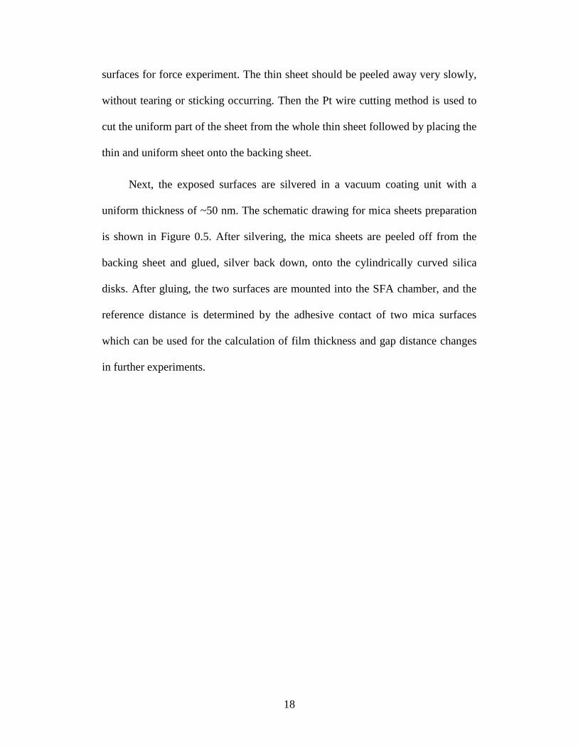
Next, the exposed surfaces are silvered in a vacuum coating unit with a
uniform thickness of ~50 nm. The schematic drawing for mica sheets preparation
is shown in Figure 0.5. After silvering, the mica sheets are peeled off from the
backing sheet and glued, silver back down, onto the cylindrically curved silica
disks. After gluing, the two surfaces are mounted into the SFA chamber, and the
reference distance is determined by the adhesive contact of two mica surfaces
which can be used for the calculation of film thickness and gap distance changes
in further experiments.
19
Figure 0.5 The schematic drawing of mica sheets preparation procedure: (a)
trimming, (b) splitting, (c) peeling, (d) cutting and (e) silvering.
1.6 Normal force measurement
Normal forces between the surfaces are measured based on the Hooke’s
law, and the changed forcesF K x , where
sK is the spring constant
supporting the lower surface and applied actualx D D . The applied separation
distance appliedD is measured by the differential micrometer, motor-driven fine
micrometer and piezoelectric crystal tube. The actual separation distance between
two surfaces actualD is determined by the MBI technique. The resolution of the
20
force measured using SFA is normally <10 nN and the accuracy of distance
measurement is <1 Ǻ [11].
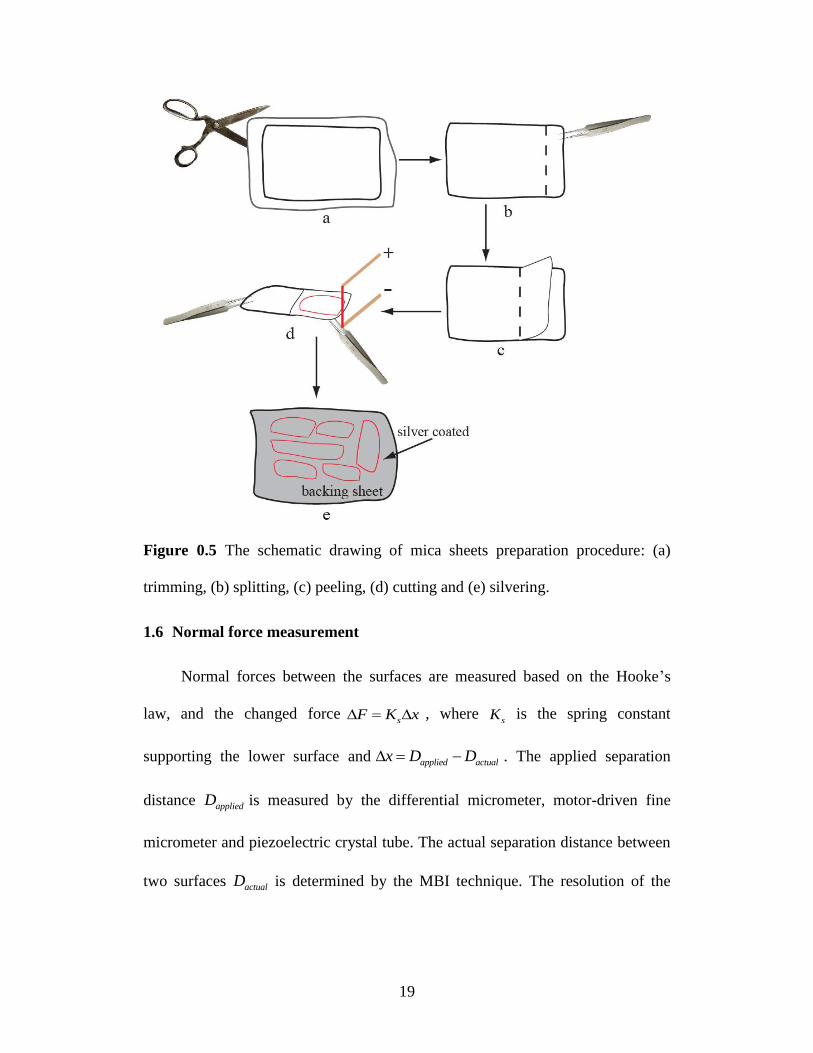
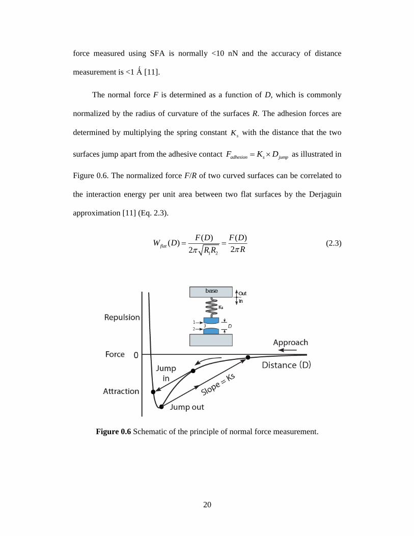
The normal force F is determined as a function of D, which is commonly
normalized by the radius of curvature of the surfaces R. The adhesion forces are
determined by multiplying the spring constant sK with the distance that the two
surfaces jump apart from the adhesive contact adhesion jums pF K D as illustrated in
Figure 0.6. The normalized force F/R of two curved surfaces can be correlated to
the interaction energy per unit area between two flat surfaces by the Derjaguin
approximation [11] (Eq. 2.3).
1 2
( ) ( )( )
22flat
F D F DW D
RR R (2.3)
Figure 0.6 Schematic of the principle of normal force measurement.
21
1.7 Adhesion measurement using SFA (contact mechanics — JKR theory)
Surface energy γ is one of the most important parameters for characterizing
surface properties. The surface deformation during contact and the adhesion
between two purely elastic and smooth curved surfaces of the same materials can
be described by the Johnson-Kendall-Roberts (JKR) theory given by Eq. 2.4 [13],
23 6 12 6
Rr R R R
KF F
(2.4)
where r is the contact radius, F is the applied load, and R is radius of local
curvature.
The experimental procedure for determining the surface adhesion and
surface energy is conducted as follows. Right after the two surfaces jump into
contact, finite load is applied gradually to the lower surface against the upper
surface till a maximum load is reached. Different waiting times can be chosen
under the maximum load to investigate the time effect, and then tensile load is
applied continuously till the two surfaces jump apart. During the loading-
unloading process, the contact diameter (2r) is monitored as a function of the
applied load ( F) in real time through the FECO fringes. [14, 15], which forms
the so-called “JKR plot”. The maximum tensile load where the two surfaces jump
out is also recorded and referred as the adhesion force Fad [16, 17].
The surface energy determined from the adhesion force (Eq. 2.5) usually
coincides with the value obtained from the fitted loading curve for non-hysteretic
systems (the adhesion energies difference of loading (advancing) and unloading
(receding) paths, ∆γ= γR-γA is small).
22
/ 3adF R (2.5)
If a system is hysteretic (∆γ > 0), the unloading path cannot be fitted by the
JKR model and an effective surface energy γeff is defined as γR (non-JKR) = γeff =
Fad /3πR. It should be noted that normally the thermodynamic γ value can be still
obtained from the fitting parameter of the loading curve using the JKR equation.
1.8 Other techniques
There are some other techniques used in this thesis research to investigate
the surface/interfacial properties of solid surfaces or polymer thin films, including
rheology measurement, atomic force microscopy (AFM), contact angle
measurement, X-ray photoelectron spectroscopy (XPS), etc.
The viscosity measurement of a suspension is often used as a simple method
to investigate the interactions between solids and a liquid medium. A rotational
rheometer employing the cylinder geometry can be used to determine the
viscosity of suspension. The working principle of rotational rheometer is briefly
described as follows. A specific torque is applied to the suspension, and then the
angular velocity can be obtained. Or an angular velocity is applied resulting in the
determination of the torque. The applied torque can be varied in different
experiments. Normally, a graph of apparent viscosity ( ) versus shear rate ( ) is
plotted. The shear rate ( ) and the shear stress (τ) can be determined by the
angular velocity (ω) and the torque ( ), respectively, and the viscosity can be
obtained from the ratio between shear stress (τ) and shear rate ( ). [18]
23
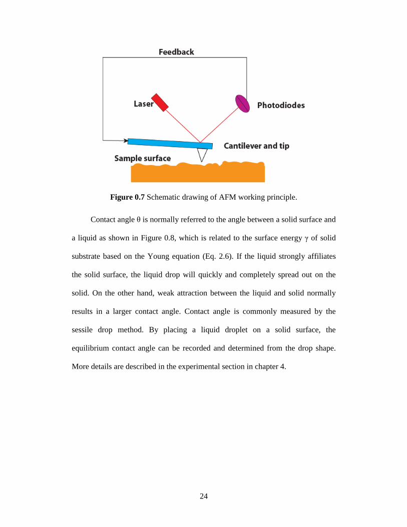
Atomic force microscopy (AFM) was invented by Binning et al. in 1986.
AFM has been widely used for over two decades for both force measurements and
the imaging of various materials. The AFM consists of a cantilever with a sharp
tip at its end that is used to scan the specimen surface. The cantilever is typically
silicon or silicon nitride. When the tip is brought into proximity of a sample
surface, forces between the tip and the sample lead to a deflection of the
cantilever according to Hooke's law. The schematic of working principle of an
AFM is shown in Figure 0.7. There are three modes of AFM: contact mode, non-
contact mode, and tapping mode. Here the tapping mode is briefly described for
obtaining the topography of surfaces. In this mode, the cantilever is externally
oscillated at or close to its fundamental resonance frequency. An electronic
feedback loop ensures that the oscillation amplitude remains constant, such that a
constant tip-sample interaction is maintained during scanning. Forces that act
between the sample and the tip will not only cause a change in the oscillation
amplitude, but also change in the resonant frequency and phase of the cantilever.
These changes in oscillation with respect to the external reference oscillation
provide information about the sample's characteristics [19].
24
Figure 0.7 Schematic drawing of AFM working principle.
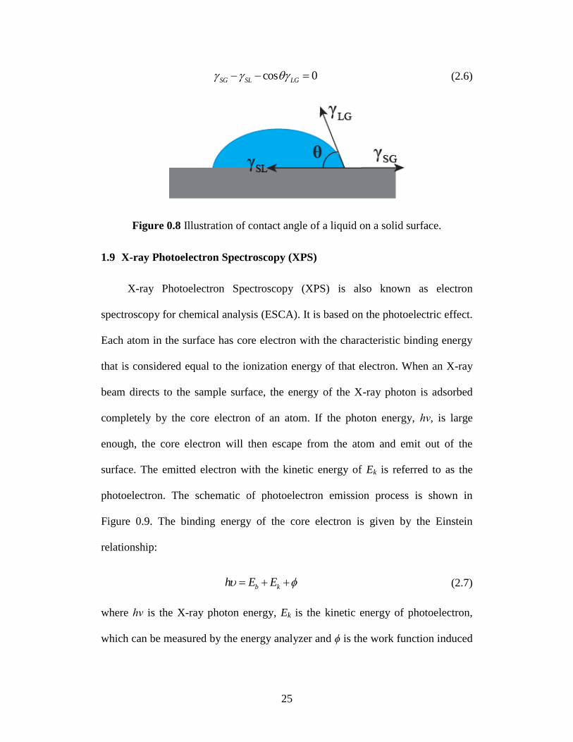
Contact angle θ is normally referred to the angle between a solid surface and
a liquid as shown in Figure 0.8, which is related to the surface energy γ of solid
substrate based on the Young equation (Eq. 2.6). If the liquid strongly affiliates
the solid surface, the liquid drop will quickly and completely spread out on the
solid. On the other hand, weak attraction between the liquid and solid normally
results in a larger contact angle. Contact angle is commonly measured by the
sessile drop method. By placing a liquid droplet on a solid surface, the
equilibrium contact angle can be recorded and determined from the drop shape.
More details are described in the experimental section in chapter 4.
25
cos 0SG SL LG (2.6)
Figure 0.8 Illustration of contact angle of a liquid on a solid surface.
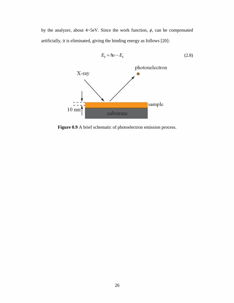
1.9 X-ray Photoelectron Spectroscopy (XPS)
X-ray Photoelectron Spectroscopy (XPS) is also known as electron
spectroscopy for chemical analysis (ESCA). It is based on the photoelectric effect.
Each atom in the surface has core electron with the characteristic binding energy
that is considered equal to the ionization energy of that electron. When an X-ray
beam directs to the sample surface, the energy of the X-ray photon is adsorbed
completely by the core electron of an atom. If the photon energy, hν, is large
enough, the core electron will then escape from the atom and emit out of the
surface. The emitted electron with the kinetic energy of Ek is referred to as the
photoelectron. The schematic of photoelectron emission process is shown in
Figure 0.9. The binding energy of the core electron is given by the Einstein
relationship:
b kh E E (2.7)
where hν is the X-ray photon energy, Ek is the kinetic energy of photoelectron,
which can be measured by the energy analyzer and ϕ is the work function induced
26
by the analyzer, about 4~5eV. Since the work function, ϕ, can be compensated
artificially, it is eliminated, giving the binding energy as follows [20]:
b kE h E (2.8)
Figure 0.9 A brief schematic of photoelectron emission process.
27
References
[1] D. Tabor, Winterto.Rh, Proc R Soc Lon Ser-A, 312 (1969) 435.
[2] D. Tabor, Chem Ind-London, (1971) 969.
[3] J.N. Israelachvili, G.E. Adams, Nature, 262 (1976) 773.
[4] J.N. Israelachvili, Faraday Discuss, 65 (1978) 20.
[5] J.N. Israelachvili, P.M. Mcguiggan, J Mater Res, 5 (1990) 2223.
[6] J. Israelachvili, Y. Min, M. Akbulut, A. Alig, G. Carver, W. Greene, K.
Kristiansen, E. Meyer, N. Pesika, K. Rosenberg, H. Zeng, Rep Prog Phys, 73
(2010).
[7] J.N. Israelachvili, Abstr Pap Am Chem S, 198 (1989) 172.
[8] J. Israelachvili, P Natl Acad Sci USA, 84 (1987) 4722.
[9] P.M. Mcguiggan, J.N. Israelachvili, J Mater Res, 5 (1990) 2232.
[10] Israelac.Jn, J Colloid Interf Sci, 44 (1973) 259.
[11] J. Israelachvili, Intermolecular and Surface Forces, third ed., Academic
Press, 2011.
[12] Israelac.Jn, D. Tabor, Proc R Soc Lon Ser-A, 331 (1972) 19.
[13] K.L. Johnson, K. Kendall, A.D. Roberts, Proc R Soc Lon Ser-A, 324 (1971)
301.
[14] N. Maeda, N.H. Chen, M. Tirrell, J.N. Israelachvili, Science, 297 (2002) 379.
28
[15] N.H. Chen, N. Maeda, M. Tirrell, J. Israelachvili, Macromolecules, 38 (2005)
3491.
[16] H.B. Zeng, N. Maeda, N.H. Chen, M. Tirrell, J. Israelachvili,
Macromolecules, 39 (2006) 2350.
[17] H.B. Zeng, M. Tirrell, J. Israelachvili, J Adhesion, 82 (2006) 933.
[18] M.M. Malik, M. Jeyakumar, M.S. Hamed, M.J. Walker, S. Shankar, J Non-
Newton Fluid, 165 (2010) 733.
[19] H. Kaczmarek, R. Czajka, M. Nowicki, D. Oldak, Polimery-W, 47 (2002)
775.
[20] J.C. Vickerman, I. Gilmore, Surface Analysis: The Principal Techniques, 2nd
ed., John Wiley and Sons, 2009.
29
CHAPTER 3 PROBING MOLECULAR AND SURFACE
INTERACTIONS OF COMB-TYPE POLYMER
POLYSTYRENE-GRAFT-POLYETHYLENE OXIDE (PS-G-
PEO)1
1.10 Introduction
Functionalities of polymer coatings play important roles in numerous
engineering and biomedical applications, ranging from adhesion, lubrication,
wettability control, drug delivery, stabilization/destabilization of colloids to
antifouling treatments. Block copolymers are composed of blocks of different
polymerized monomers. Amphiphilic diblock or tri-block copolymers, with both
hydrophobic and hydrophilic units, have attracted much interest due to their
interesting interfacial properties, i.e., interfacial aggregation behaviour, self-
assembly in bulk solutions or on substrates, dewetting and surface interactions.
An amphiphilic block polymer is able to adsorb or anchor one block onto a solid
substrate while extend the other bock into a favourable solution medium acting as
a swollen brush layer with many important engineering applications. [1-14] For
example, poly(ethylene oxide)/poly(propylene oxide)/poly(ethylene oxide) or
PEO-PPO-PEO shows good potential in the development of polymeric additives
for antifriction and/or antiwear, which has been studied in terms of its adsorption
behaviour on different substrates, phase behaviours, morphology, and surface
1 A version of this chapter has been submitted for publication. L. Zhang, H. Zeng,
Q. Liu 2012. Journal of Physical and Chemistry, C (under review).
30
interactions. [2, 4, 6, 8-10] Diblock copolymer polystyrene/polyethylene oxide
(PS-b-PEO), with various PEO contents and molecular weights, was extensively
studied regarding to its properties at water-air interfaces using Langmuir Blodgett
balance technique. [3-5, 7, 13] The micelle formation, self-assembly morphology
and surface forces of PS-b-PEO in organic solvents have also been investigated.
[11, 12]
During the past decade, comb-type copolymers have attracted much
attention in polymer chemistry and physics, nanotechnology and bioengineering,
which are special copolymers with many branches grafted to a polymer backbone.
Comb-type amphiphilic copolymers have been considered as an alternative
approach to amphiphilic block copolymers for hydrophobic drug solubilization
and drug delivery. The comb-type copolymers can be fabricated with diverse
architectures with multifunctionalities such as stimuli-responsive properties and
site-specific targeting capabilities. Spencer and coworkers reported that Poly(L-
lysine)-g-Poly(ethylene glycol) or PLL-g-PEG of different PLL/PEO ratios can
adsorb on metal oxide surfaces, and the friction force and attachment mechanism
of proteins on PLL-g-PEG layer were measured by using atomic force microscope
(AFM) and pin-on-disk tribometry. [15-17] Brady et al. investigated the solvent-
dependent friction force of poly(ethylenimine)-graft-poly(ethylene glycol)
brushes using AFM. [18] Asatekin et al. studied the antifouling properties of
membranes containing polyacrylonitrile-graft-poly(ethylene oxide). [19] Njikang
et al. reported self-assembly behaviors of arborescent polystyrene-graft-
poly(ethylene oxide). [20] In these early studies, polyethylene oxide (PEO) was
31
widely used which has been found to be promising in the development of
functional brush copolymers/coatings with important bioengineering applications,
e.g., antifouling. Although the applications of comb-shaped amphiphilic
copolymers are rapidly increasing, understanding of their fundamental molecular
interactions still remains limited.
In this work, the molecular interactions and surface properties of an
amphiphilic comb-type copolymer with a polystyrene backbone and a
polyethylene oxide side chains (PS-grafted-PEO or PS-g-PEO) were investigated
using a surface forces apparatus (SFA) and an AFM, which provides new insights
into the fundamental understanding of molecular and surface interaction
mechanisms of comb-shaped copolymers and development of novel polymers and
coatings with antifriction or antifouling properties.
1.11 Materials and Experimental Methods
1.11.1 Materials and samples preparation
Polystyrene-g-poly(ethylene oxide) (PS-g-PEO) comb-type copolymer
(number average molecular weight Mn = 24500 g/mol, Mn of the polymer
backbone is ~6000 g/mol, Mn of each PEO branch is ~4500 g/mol, average
number of monomers on each PEO branch chain is ~102.3, polydispersity
Mw/Mn =1.6) was purchased from Polymer Source Ltd. and used as received.
The chemical structure of PS-g-PEO is shown in Figure 0.1. High-performance
liquid chromatography (HPLC)-grade toluene purchased from Fisher Scientific
was used as received. Ruby mica sheets were purchased from S & J Trading Inc.
(Glen Oaks, NY). High-purity anhydrous sodium chloride (Sigma-Aldrich, 99.999
32
+ %) was used as received. Milli-Q water with a resistance of 18.2 MΩcm was
used for preparing the aqueous solutions needed.
PS-g-PEO film was prepared by spin coating method. Briefly, PS-g-PEO
was first dissolved in toluene to prepare a 0.5 wt% solution. Freshly cleaved mica
sheets were used as supporting substrates for preparation of polymer thin films by
spin coating (~1000 rpm for about 40s). The thin film samples were dried under
reduced pressure (~50 mmHg) overnight (>12 h) to remove the solvent, and then
used for contact angle, topographic imaging and surface forces measurements.
The thickness of polymer films used in this study was controlled about 15-30 nm
which did not show significant impact for the results obtained. The polymer film
thickness was measured in situ using an optical interferometry employing fringes
of equal chromatic order (FECO) in the SFA. The polymer film thickness was
also confirmed by spin coating a film on silicon wafer cleaned with ethanol and
UV/Ozone cleaner and then determined using a Sopra GESP-5
spectroscopic ellipsometer (France).
33
Figure 0.1 Chemical structure of comb-type polymer PS-g-PEO used in this study.
1.11.2 Surface force measurement in aqueous solution using SFA
Surface forces apparatus (SFA) has been widely applied to measure physical
forces between surfaces in many biological and non-biological systems. [21-28]
An SFA was used in this study to measure the interaction forces of PS-g-PEO
film in NaCl solution. The detailed setup for SFA experiments has been reported
elsewhere. [29-33] Briefly, two back silvered thin mica sheets (1–5 m) were
glued onto cylindrical silica disks (radius R = 2 cm). The PS-g-PEO film was spin
coated on the mica following the aforementioned method. The two surfaces were
then mounted in the SFA chamber in a crossed-cylinder configuration which was
locally equivalent to a sphere of radius R interacting with a flat surface or two
spheres of radius 2R when the surface separation D was much smaller than R
(D≪R). SFA measures the interaction forces F between the curved surfaces as a
function of absolute surface separation distance D with force and distance
resolutions down to <10 nN and 0.1 nm, respectively. During SFA experiments,
34
the absolute surface separation can be monitored in real-time and in situ by using
multiple beam interferometry employing fringes of equal chromatic order (FECO).
[34]
Figure 0.2 Experimental configurations of surface forces measurement: (a) PS-g-
PEO film coated on mica surface versus a bare mica surface in NaCl solution
(asymmetric case), (b) two PS-g-PEO films coated on two mica surfaces in NaCl
35
solution (symmetric case), (c) schematic of two polymer surfaces in adhesive
contact in air and typical FECO fringes.
In this study, the interaction forces of PS-g-PEO were measured in 1 mM
and 100 mM NaCl solution by SFA in two different configurations as shown in
Figure 0.2: (a) a PS-g-PEO polymer film versus a bare mica surface (asymmetric),
and (b) two opposing PS-g-PEO films (symmetric). The thickness of dry polymer
film was measured by using the mica-mica adhesive contact as a reference.
During force measurement, the reference distance (D = 0) was determined at the
adhesive contact between a bare mica surface and a polymer surface (asymmetric
case) or between the two polymer surfaces (symmetric case) in air. The surface
force measurements were repeated for at least three independent pairs of samples
with three different interaction positions for each pair of samples under a fixed
experimental condition.
1.11.3 Adhesion measurement (contact mechanics) in air using SFA
The adhesion of PS-g-PEO films in air and the surface energy of comb-type
polymer were determined by contact mechanics test using an SFA. The contact
mechanics tests on the polymer surfaces were done for dry (and smooth) polymer
films (in order to obtain the surface energy, it should be noted that the recent
report by Benz et al. showed roughness plays a critical role in the contact
mechanics of polymer surfaces [35]). The experimental setup of contact
mechanics measurement in SFA has been described in details previously. [36, 37]
Briefly, two PS-g-PEO films coated on mica were brought into adhesive contact
in air in the SFA, and then finite compressive load was applied. The contact area
36
(or contact diameter 2r) was monitored through FECO fringes (see Figure 0.2c)
with increasing load F in real time till a maximum load ( maxF, ~35.3 mN in this
study) was reached. Then unloading process was initiated by gradually reducing
the compressive load till the two surfaces were separated (jumped apart) under a
critical tensile load which was referred as the adhesion force Fad. The contact
mechanics (contact diameter versus applied load) and adhesion were then
analyzed using the Johnson-Kendall-Roberts (JKR) theory, and adhesion energy
of the polymer surface was obtained. [38, 39]
1.11.4 Contact angle measurement
The contact angle of water on PS-g-PEO surface was measured by a sessile
drop method using a Krüss drop shape analysis system (DSA 10-MK2, Germany).
A Milli-Q water sessile drop was placed on the sample surface, and the interaction
process between water drop and polymer surface was recorded by a video camera.
The video was then converted to images and the contact angle was determined by
fitting the shape of the sessile drop on the polymer surface. The contact angles of
three different probe liquids (water, ethylene glycol and glycerol) were also
measured. The Good-Van Oss model [40, 41] was applied to determine the
surface energy of the PS-g-PEO film.
1.11.5 AFM imaging
Surface morphology and roughness of PS-g-PEO films with and without
water treatment were characterized using an AFM in tapping mode (Agilent
technologies 5500, Agilent, Santa Barbara, CA, USA). The impact of water on
37
surface morphology of PS-g-PEO was investigated by immersing the polymer
film in Milli-Q water for 30 min. The polymer film (after the exposure to water)
was dried under reduced pressure (~50 mmHg) for ~30 min before AFM imaging.
At least three samples (1 cm ×1 cm) were imaged at different (>5) positions of
the same surface under each condition, and the typical images were presented.
1.11.6 X-ray photoelectron spectroscopy (XPS)
XPS was employed to determine the top surface chemical composition of
PS-g-PEO films. 1 cm × 1 cm polymer film samples were prepared for the XPS
measurements which were performed at Alberta Center for Surface and
Engineering Science (ACSES) using Kratos Axis Ultra Spectrometer employing a
monochromated Al-K α X-ray source (hυ = 1486.71 eV). The spectrometer was
calibrated with the binding energy (84.0 eV) of Au 4f7/2 with reference to Fermi
level. The pressure of analysis chamber during experiments was controlled below
5×10⁻¹⁰
Torr. A hemispherical electron-energy analyser working at the pass
energy of 20 eV was used to collect core-level spectra while survey spectrum
within a range of binding energies from 0 to 1100 eV was collected at analyser
pass energy of 160 eV. Charge effects were corrected by using C 1s peak at 284.8
eV. A Shirley background was applied to subtract the inelastic background of
core-level peaks. Non-linear optimization was used to determine the peak model
parameters such as peak positions, widths and peak intensities by using the
Marquardt Algorithm (Casa XPS).
38
1.12 Results and Discussion
1.12.1 Characterization of PS-g-PEO polymer film
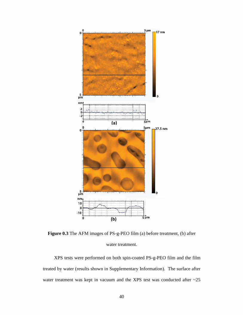
AFM images of spin-coated PS-g-PEO film and the polymer film after
treated with water are shown in Figure 0.3 (a) and (b). The spin-coated PS-g-PEO
film has a root-mean-square (rms) roughness of ~1.2 nm. After the polymer films
were exposed to water for 30 min and fully dried, the surface became rougher and
the rms roughness increased to ~7.0 nm. Interesting polymer surface patterns were
also observed after water treatment (in Figure 0.3b). Similar surface patterns and
polymer aggregation were previously reported for amphiphilic block polymers at
air/water interface and in bulk solutions, which are mainly due to the
intermolecular and intramolecular interactions of amphiphilic polymer segments
and solvents and significantly depend on the polymer molecular structure,
molecular weight and solution conditions. [42-45] A complete investigation on
the evolution of surface pattern and molecular conformation of comb-type PS-g-
PEO polymer in water and at water/air interface and the impact of molecular
weight and structure will be reported in a separate study. Contact angle
measurements were used to evaluate the hydrophilicity of the PS-g-PEO surfaces.
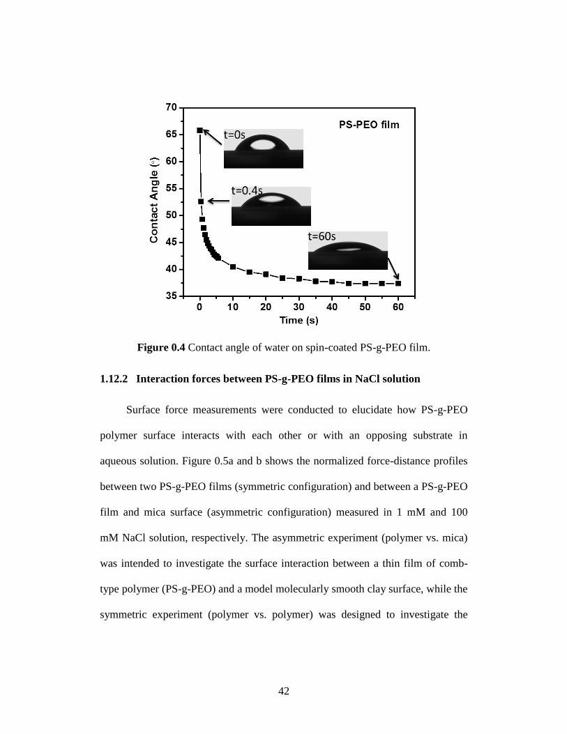
The contact angle of water on the PS-g-PEO film and its evolution with time are
shown in Figure 0.4. The spin-coated PS-g-PEO film showed an initial water
contact ~66°, which decreased sharply by over 10° in less than one second and
then gradually reached ~37° in about 60 s. The contact angle did not change with
further increasing time. The decrease of the water contact angle indicates the PS-
g-PEO surface turned more hydrophilic after it was exposed to water because of
39
the strong interactions between hydrophilic PEO side chains and water molecules
governed by hydrogen bonding and van der Waals forces. It is mostly likely that
after contacting with water, the PEO chains became fully hydrated and tended to
extend out from the solid surface into the water phase, and such conformation
rearrangement also contributed to surface roughness change as shown in the AFM
images (Figure 0.3).
40
Figure 0.3 The AFM images of PS-g-PEO film (a) before treatment, (b) after
water treatment.
XPS tests were performed on both spin-coated PS-g-PEO film and the film
treated by water (results shown in Supplementary Information). The surface after
water treatment was kept in vacuum and the XPS test was conducted after ~25
(a)
(b)
41
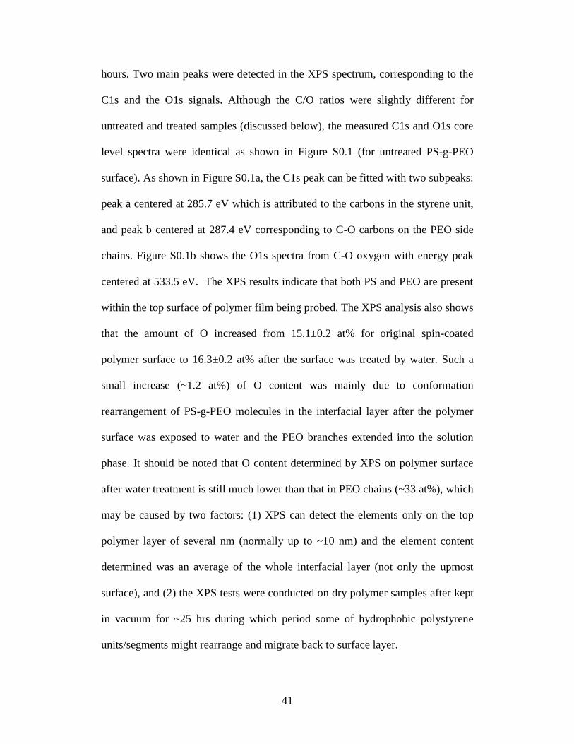
hours. Two main peaks were detected in the XPS spectrum, corresponding to the
C1s and the O1s signals. Although the C/O ratios were slightly different for
untreated and treated samples (discussed below), the measured C1s and O1s core
level spectra were identical as shown in Figure S0.1 (for untreated PS-g-PEO
surface). As shown in Figure S0.1a, the C1s peak can be fitted with two subpeaks:
peak a centered at 285.7 eV which is attributed to the carbons in the styrene unit,
and peak b centered at 287.4 eV corresponding to C-O carbons on the PEO side
chains. Figure S0.1b shows the O1s spectra from C-O oxygen with energy peak
centered at 533.5 eV. The XPS results indicate that both PS and PEO are present
within the top surface of polymer film being probed. The XPS analysis also shows
that the amount of O increased from 15.1±0.2 at% for original spin-coated
polymer surface to 16.3±0.2 at% after the surface was treated by water. Such a
small increase (~1.2 at%) of O content was mainly due to conformation
rearrangement of PS-g-PEO molecules in the interfacial layer after the polymer
surface was exposed to water and the PEO branches extended into the solution
phase. It should be noted that O content determined by XPS on polymer surface
after water treatment is still much lower than that in PEO chains (~33 at%), which
may be caused by two factors: (1) XPS can detect the elements only on the top
polymer layer of several nm (normally up to ~10 nm) and the element content
determined was an average of the whole interfacial layer (not only the upmost
surface), and (2) the XPS tests were conducted on dry polymer samples after kept
in vacuum for ~25 hrs during which period some of hydrophobic polystyrene
units/segments might rearrange and migrate back to surface layer.
42
Figure 0.4 Contact angle of water on spin-coated PS-g-PEO film.
1.12.2 Interaction forces between PS-g-PEO films in NaCl solution
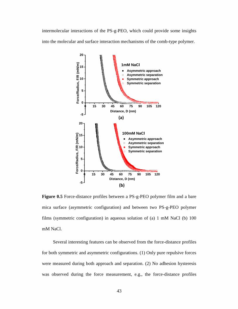
Surface force measurements were conducted to elucidate how PS-g-PEO
polymer surface interacts with each other or with an opposing substrate in
aqueous solution. Figure 0.5a and b shows the normalized force-distance profiles
between two PS-g-PEO films (symmetric configuration) and between a PS-g-PEO
film and mica surface (asymmetric configuration) measured in 1 mM and 100
mM NaCl solution, respectively. The asymmetric experiment (polymer vs. mica)
was intended to investigate the surface interaction between a thin film of comb-
type polymer (PS-g-PEO) and a model molecularly smooth clay surface, while the
symmetric experiment (polymer vs. polymer) was designed to investigate the
43
intermolecular interactions of the PS-g-PEO, which could provide some insights
into the molecular and surface interaction mechanisms of the comb-type polymer.
Figure 0.5 Force-distance profiles between a PS-g-PEO polymer film and a bare
mica surface (asymmetric configuration) and between two PS-g-PEO polymer
films (symmetric configuration) in aqueous solution of (a) 1 mM NaCl (b) 100
mM NaCl.
Several interesting features can be observed from the force-distance profiles
for both symmetric and asymmetric configurations. (1) Only pure repulsive forces
were measured during both approach and separation. (2) No adhesion hysteresis
was observed during the force measurement, e.g., the force-distance profiles
0 15 30 45 60 75 90 105 120
-5
0
5
10
15
20
1mM NaCl
Asymmetric approach
Asymmetric separation
Symmetric approach
Symmetric separation
Fo
rce
/Ra
diu
s,
F/R
(m
N/m
)
Distance, D (nm)
(a)
(b)
0 15 30 45 60 75 90 105 120
-5
0
5
10
15
20
Asymmetric approach
Asymmetric separation
Symmetric approach
Symmetric separation
100mM NaCl
Fo
rce
/Ra
diu
s,
F/R
(m
N/m
)
Distance, D (nm)
44
obtained during approach and separation almost overlap, which is mainly
attributed to the large excluded volume of the hydrated PEO chains and the steric
repulsive forces between the swollen PEO chains, thus hindering the
interdigitation. [46-48] Such non-hysteretic behaviour of PEO chains has been
previously reported for several PEO associated polymer/biopolymer systems, and
PEO chains/coatings are also well known for their anti-fouling properties to some
other polymers/biopolymers. [46, 49] However, it should be noted that shearing,
long contact time and increased temperature could induce the hysteretic behaviour
of PEO chains in certain systems. [46, 47, 49, 50] (3) The force-distance profiles
measured in 1 mM and 100 mM NaCl are very similar, which indicates ionic
strength of solution has no significant impact on the interaction forces of polymer
surfaces. The small difference on the force-distance profiles during approach and
separation at high ionic strength for the symmetric case was not considered to be
significant. The force-distance profiles almost overlap at high load, and the small
difference at low load might be due to the conformational difference and change
of the swollen PEO chains under compression associated with approach and
separation. More importantly, no adhesion nor significant adhesion hysteresis
were observed, which indicates that the steric interaction between the swollen
PEO chains dominated the surface interaction, and interdigitation or
interpenetration of the PEO changes on the two opposing surfaces was very
limited. (4) The thickness of confined polymer layer between the two mica
surfaces increased after the polymer surfaces were exposed to NaCl aqueous
solution. In other words, the polymer films appeared “thicker” in the aqueous
45
solution than in the dry state. The distance D=0 in Figure 0.5 was referred as the
adhesive contact between bare mica and dry polymer surface or between two dry
polymer surfaces in air. D shifted to ~20 nm and ~45 nm for asymmetric and
symmetric configurations, respectively, which is higher than the height change
from AFM imaging. The AFM imaging of polymer surface was taken in air where
the film (after water treatment) under dry condition, while the surface forces were
measured in aqueous solution. Thus, the thickness change of the swelling polymer
film in aqueous solution would be expected to be larger than that in fully dried
state. The shift of the thickness of confined polymer was most likely due to the
swelling of hydrophilic PEO side chains and molecular conformation
rearrangement of the comb-type polymers leading to surface morphology change,
which is consistent with the observations from contact angle measurement and
AFM imaging. As shown in the contact angle measurements, it is suggested that
hydrophilic PEO side chains may extend out from the polymer film into water and
act as swollen brushes which makes the surface more hydrophilic. The fully
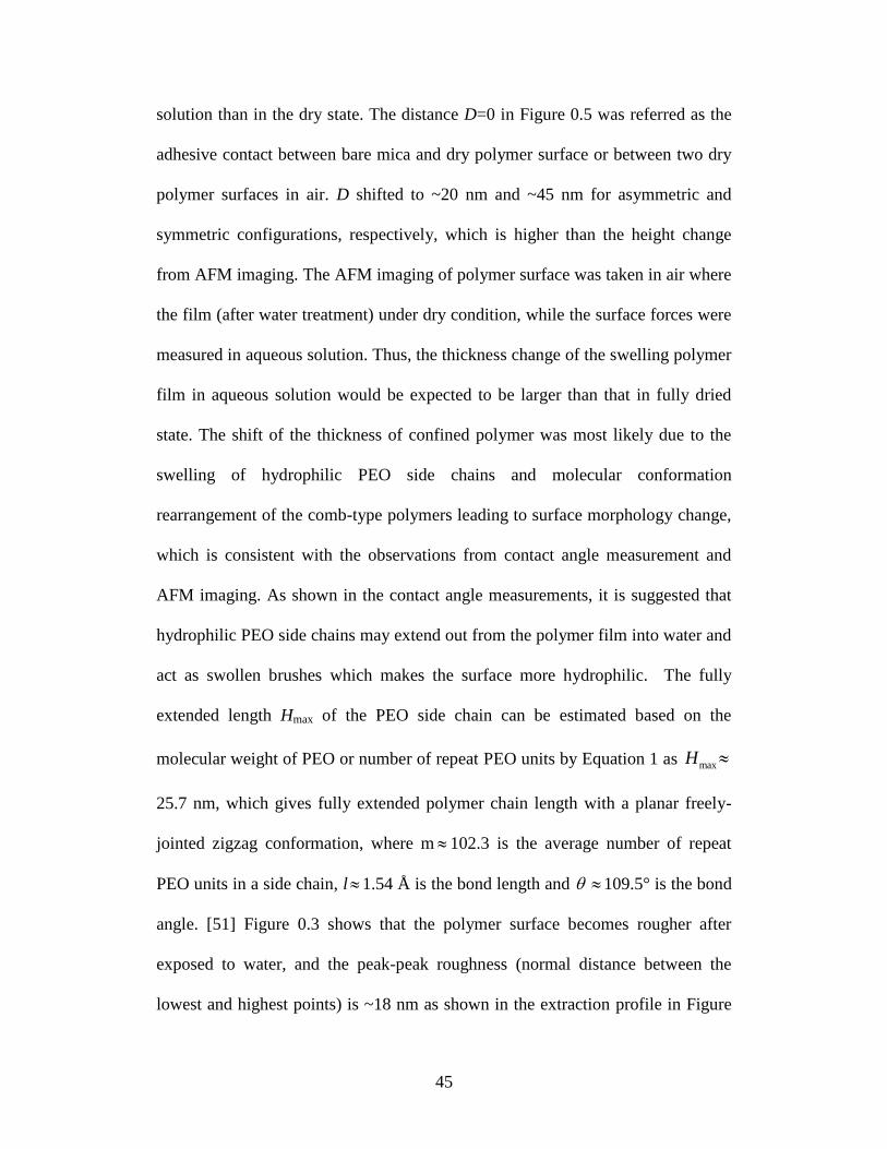
extended length Hmax of the PEO side chain can be estimated based on the
molecular weight of PEO or number of repeat PEO units by Equation 1 as maxH
25.7 nm, which gives fully extended polymer chain length with a planar freely-
jointed zigzag conformation, where m 102.3 is the average number of repeat
PEO units in a side chain, l1.54 Å is the bond length and 109.5° is the bond
angle. [51] Figure 0.3 shows that the polymer surface becomes rougher after
exposed to water, and the peak-peak roughness (normal distance between the
lowest and highest points) is ~18 nm as shown in the extraction profile in Figure
46
0.3b. Thus, the sum of the peak-peak surface roughness and fully extended PEO
chain length gives ~44 nm (~18 nm plus ~26 nm) for a single polymer film
(asymmetric case), and ~90 nm for two polymer films (symmetric case). It should
be also noted that the AFM imaging in Figure 0.3b was done in air after the film
was dried, and the polymer film would be swollen in water leading to a longer
range of interaction. The above estimated values were close to the range of
repulsive forces measured in Figure 0.5 (e.g., ~50 nm and ~100 nm for
asymmetric and symmetric configurations, respectively).
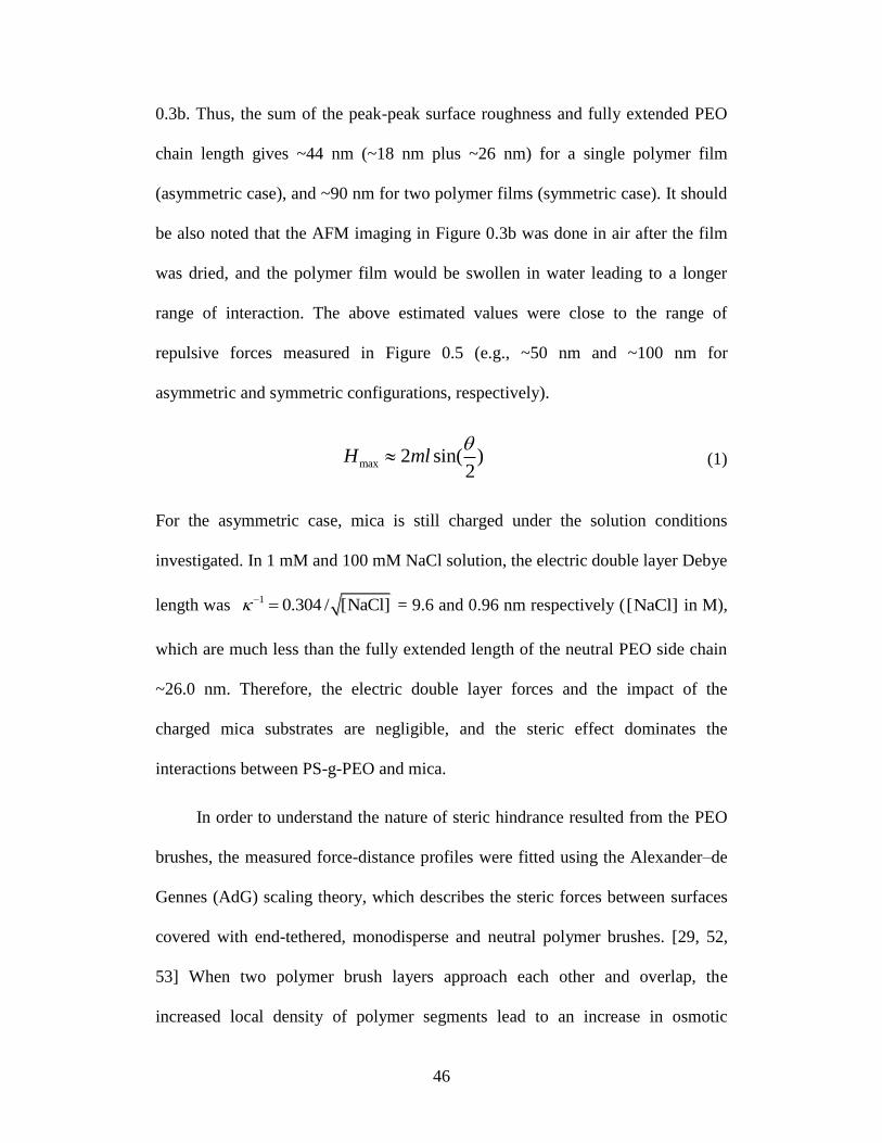
max 2 sin( )2
H ml
(1)
For the asymmetric case, mica is still charged under the solution conditions
investigated. In 1 mM and 100 mM NaCl solution, the electric double layer Debye
length was 1 0.304 / [NaCl] = 9.6 and 0.96 nm respectively ([NaCl] in M),
which are much less than the fully extended length of the neutral PEO side chain
~26.0 nm. Therefore, the electric double layer forces and the impact of the
charged mica substrates are negligible, and the steric effect dominates the
interactions between PS-g-PEO and mica.
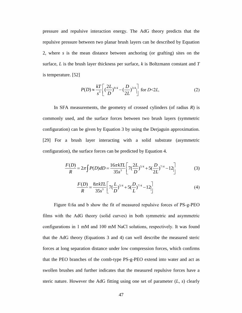
In order to understand the nature of steric hindrance resulted from the PEO
brushes, the measured force-distance profiles were fitted using the Alexander–de
Gennes (AdG) scaling theory, which describes the steric forces between surfaces
covered with end-tethered, monodisperse and neutral polymer brushes. [29, 52,
53] When two polymer brush layers approach each other and overlap, the
increased local density of polymer segments lead to an increase in osmotic
47
pressure and repulsive interaction energy. The AdG theory predicts that the
repulsive pressure between two planar brush layers can be described by Equation
2, where s is the mean distance between anchoring (or grafting) sites on the
surface, L is the brush layer thickness per surface, k is Boltzmann constant and T
is temperature. [52]
9/4 3/4
3
2( ) ( ) ( )
2
kT L DP D
s D L
for D<2L, (2)
In SFA measurements, the geometry of crossed cylinders (of radius R) is
commonly used, and the surface forces between two brush layers (symmetric
configuration) can be given by Equation 3 by using the Derjaguin approximation.
[29] For a brush layer interacting with a solid substrate (asymmetric
configuration), the surface forces can be predicted by Equation 4.
5/4 7/4
3
( ) 16 22 ( ) 7( ) 5( ) 12
35 2
F D kTL L DP D dD
R s D L
(3)
5/4 7/4
3
( ) 87( ) 5( ) 12
35
F D kTL L D
R s D L
(4)
Figure 0.6a and b show the fit of measured repulsive forces of PS-g-PEO
films with the AdG theory (solid curves) in both symmetric and asymmetric
configurations in 1 mM and 100 mM NaCl solutions, respectively. It was found
that the AdG theory (Equations 3 and 4) can well describe the measured steric
forces at long separation distance under low compression forces, which confirms
that the PEO branches of the comb-type PS-g-PEO extend into water and act as
swollen brushes and further indicates that the measured repulsive forces have a
steric nature. However the AdG fitting using one set of parameter (L, s) clearly
48
deviates from the experimental data at high load regime, as shown in the Figure
S0.2 in Supplementary Information. Such deviation could be resulted from two
aspects: (i) the PEO side chains from both polymer-water interface and sublayers
can extend into water and the swollen PEO chains were not monodisperse
brushes, as illustrated in Figure 0.6c (it is noted that Figure 0.6c was simply
proposed to illustrate the possibility of swelling of PEO side chains in water from
upmost polymer-water interface and sublayers in the polymer film, and the actual
conformations could be more complex.); (ii) the conformation of PEO chains and
local segment density increased with applied load while the surface morphology
might also change with increasing load. Thus two independent sets of fitting
parameters were used to better fit the force-distance curves at both low and high
compression regimes (in Figure 0.6). The values of fitted parameters s and L are
summarized in Table 1. It should be noted that the parameter s in the Alexander–
de Gennes (AdG) theory stands for the mean distance between grafting sites of
polymer brushes (while not the grafting density). Therefore the s value would
decrease under higher compression. As shown in Table 0.1, the s value at short
distance in the high load regime is close to half of that at long distance in the low
load regime (for example, s=6.6 nm and 3.9 nm in the low and high load regimes,
respectively, for asymmetric configuration in 1 mM NaCl shown in Figure 0.6a),
indicating a much denser brush layer under higher load conditions.
49
Figure 0.6 Experimentally measured force-distance profiles (dot plots) for PS-g-
PEO vs mica (asymmetric configuration) and two PS-g-PEO surfaces (symmetric
configuration) and theoretically fitted curves using the Alexander-de Gennes
(AdG) theory in (a) 1 mM NaCl and (b) 100 mM NaCl solution. (c) Illustration of
(a)
0 10 20 30 40 50 60 70 80 90 100 110 120
0.1
1
10
100
Distance, D (nm)
Fo
rce/R
ad
ius,
F/R
(m
N/m
)
In 1mM NaCl solution
Symmetric
Asymmetric
AdG fitting
AdG
fitting
0 10 20 30 40 50 60 70 80 90 100 110 120
0.1
1
10
100
AdG
fitting
In 100mM NaCl solution
Fo
rce/R
ad
ius,
F/R
(m
N/m
)
Distance, D (nm)
Symmetric
Asymmetric
AdG fitting
(b)
50
swollen PEO branches in water from polymer-water interface and sublayers in the
polymer film.
Table 0.1 Fitting parameters using the Alexander-de Gennes Theory for
experimentally measured force-distance profiles at both high and low
compression regimes in Figure 0.6.
1 mM NaCl 100 mM NaCl
High
loading
Low
loading
High
loading
Low
loading
Asymmetric
L (nm) 48 59 42.1 54.9
s (nm) 3.3 5.1 3.7 6.9
Symmetric
L (nm) 42 52.6 41.5 50
s (nm) 3.9 6.6 3.3 5.8
1.13 Surface energy of PS-g-PEO film
1.13.1 Contact mechanics test
In order to fully understand the surface interactions and properties of PS-g-
PEO, the adhesion and surface energy of PS-g-PEO surfaces in air was
determined through contact mechanics test by following the widely used Johnson-
Kendall-Roberts (JKR) adhesion test. [54-56] The contact radius between two PS-
51
g-PEO surfaces monitored through the FECO fringes in real time were plotted as
a function of the applied load for both loading and unloading processes, as shown
in Figure 0.7. It is interesting to note that the loading and unloading plots do not
overlap and follow the same path and adhesion hysteresis is observed. The contact
radius during the unloading process is larger than that during loading under the
same compressive load, and a finite tensile load is needed to separate the two
surfaces, commonly referred as the adhesion force, adF ≈-9 mN. The JKR model
is also applied to better understand the contact and adhesion behavior of PS-g-
PEO surfaces observed. [54, 57] According to the JKR model, when two purely
elastic curved surfaces are pressed against each other by an external load F, the
relation between contact radius r and load F can be described by Equation 5,
where W is the adhesion energy (for two surfaces of the same material W=2, and
is the surface energyK is the equivalent modulus which is related to the
Young’s moduli E1 and E2, and Poisson’s ratios ν1 and ν2 by Equation 6, and R
is the radius of local curvature given by Equation 7. [54]
23
2
3 6 3
3 / 2 3 / 2
Rr F RW RF RW
K
RF RW RW
K
W
(5)
2 2
1 2
1 2
1 11 3
4K E E
(6)
1 2
1 1 1
R R R (7)
3 / 2aad dF RW (8)
52
In JKR tests, the adhesion hysteresis can be defined as = ( R – A )0,
where A is the advancing surface energy on loading, and R is the receding
energy on unloading. is a measure of the energy dissipated during a complete
loading-unloading cycle. [54, 58, 59] For non-hysteretic systems, the loading and
unloading paths are the same where =0 and A R , and the JKR
Equation shows that the surfaces will detach or jump apart at a critical tensile load
which gives the adhesion or ‘pull-off’ force adF as shown in Equation 8. For two
surfaces of the same materials, the surface energy of the materials can be
determined by A R 2 /3/ad adW F R = = = . However, in hysteretic systems
such as polymers of low molecular weight, the loading (advancing) and unloading
(receding) paths are not the same, as the case for PS-g-PEO in this study. As
shown in Figure 0.7, the loading path can be fitted reasonably well with the JKR
model (Equation 5) because A is usually insensitive to different surface
treatments of polymer surfaces and the surface energy obtained from the JKR
fitting is often close to the thermodynamic value , [36] while the unloading path
cannot be fitted due to the adhesion hysteresis. The fitted value from the loading
path was considered to be close to the thermodynamic surface energy of the PS-g-
PEO film, [36] which was compared with the value obtained from the contact
angle measurement. While the receding energy on unloading was also shown and
compared with the advancing energy, which was to show the adhesion hysteresis.
The JKR fitting for the loading path leads to A = 37.0 mJ/m2 which can be
considered as the thermodynamic surface energy of the PS-g-PEO film. The
53
receding energy on unloading (also referred as effective surface energy) can be
given by the adhesion force measured as R /3adF R ≈ 47.7 mJ/m2, and the
adhesion hysteresis is ≈ 10.7 mJ/m2.
The adhesion hysteresis for PS-g-PEO surfaces measured in air is different
from the non-hysteric forces between the polymer surfaces in aqueous solution.
As discussed for Figure 0.6, the non-hysteric forces in aqueous solution resulted
from the steric interactions of the swollen PEO brushes. The adhesion hysteresis
of PS-g-PEO surfaces in air are considered to be mainly due to the interdigitation
of polymer chains/segments across the contact interface while the hydrogen
bonding between the PEO chains at the polymer-polymer interface can also play a
role. [60-62]
54
Figure 0.7 Contact diameter 2r vs. applied load F obtained through the JKR
loading-unloading test for two PS-g-PEO films. Red solid line is the fitted curve
for the loading path using the JKR model.
1.13.2 Surface energy by three-probe-liquid contact angle measurement
The surface energy of PS-g-PEO surface was also determined by sessile
drop method based on the contact angle measurements of three probe liquids. In
the Good & Van Oss model, [40, 41] the surface energy can be written as
Equation 9, where is the surface energy, d is the dispersive component
(Lifshitz-Van der Waals interactions), and and
are the polar components
(Lewis acid-base).
2d (9)
-20 -10 0 10 20 30 400
20
40
60
80
100
120
Co
nta
ct
dia
mete
r, 2
r (u
m)
Normal load, (mN)
loading
unloading
JKR fitting
Jump out
F
adF
55
The relation between liquid contact angle , surface tension of liquid, and
surface energy components of solid surface and liquid can be given by Equation
10, where L and S represent the liquid and solid phases, respectively.
(1 cos ) 2 d d
L S L S L L S (10)
In order to determine the surface energy components of the solid, d
S , S
and S , at least three different probe liquids of known energy components should
be used in contact angle measurements and then three equations can be obtained.
Thus, the energy components of the solid surface can be determined by Equation
11, where L1, L2 and L3 denote the three different probe liquids, respectively.
21
1 1 1 1
2 2 1
1
2
33
2
33 1
cos 1
2 cos 1
cos 1
ddL L Ls
d
L L
L
s L
s L
L
d
L L L
(11)
The three probe liquids used in this study were Dimethyl sulfoxide (DMSO),
Glycerol and Ethylene glycol, and their surface tension components are given in
Table 0.2.
56
Table 0.2 Three probe liquids for measuring the surface energy of PS-g-PEO film
[63].
Liquid
Dimethyl sulfoxide 36.0 0.5 32.0 44.0
Glycerol 34.0 3.9 57.4 64.0
Ethylene glycol 29.0 1.9 47.0 48.0
Table 0.3 The contact angles of three probe liquids on PS-g-PEO film.
Contact angle
Dimethyl
sulfoxide Glycerol Ethylene glycol
t=0 s 48.5 80.6 66.3
t=60 s 45.5 75.0 61.1
Table 0.4 The surface energy of PS-g-PEO film.
t=0 s 37.9 0.078 3.1 38.8
t=60 s 38.8 0.2 14.2 42.2
The contact angles of the three different probe liquids on PS-g-PEO surface
are shown in Table 0.3. It should be noted that the contact angles of the three
57
probe liquids on PS-g-PEO all became slightly smaller with time as shown in
Table 0.3, but they all reached a static angle within a minute, which indicates that
the polymer surface, especially the PEO branches, could have certain
conformation rearrangement induced by their molecular interactions with the
contacting liquids. The surface energy components of PS-g-PEO film was then
calculated by using Equations 11, and the surface energy was determined to be
38.8 mJ/m2, which is excellent agreement with the value obtained from the JKR
contact mechanics test by SFA. Thus, the surface energy of PS-g-PEO film was
determined to be 38.0 1.0 mJ/m2. The calculated surface energy of PS-g-PEO
film increased slightly to 42.2 mJ/m2 by using the contact angles at t=60 s. It is
noted that the surface energies reported for PS and PEO are about 34-40 mJ/m2
and 41.5-44.0 mJ/m2, respectively. [9, 64, 65] Thus, it is evident from the increase
of the surface energy that conformation rearrangement of PEO chains occurred at
polymer-liquid interfaces as discussed above.
1.14 Conclusion
The surface properties and molecular interactions of comb-type polymer
PS-g-PEO were investigated in both NaCl solution and air by using SFA, AFM
and contact angle measurements. It is evident from the water contact angle
measurement that the PEO branch chains can rearrange their conformations and
extend into the aqueous solution due to the strong van de Waals force and
hydrogen bonding between hydrophilic PEO segments and water molecules. The
change of polymer surface morphology was confirmed by AFM imaging and SFA
force measurement. Only pure repulsive forces were detected in both symmetric
58
(polymer vs. polymer) and asymmetric (polymer vs. mica) configurations in NaCl
solutions. The ionic strength of NaCl solution showed negligible effect on the
interaction forces of PS-g-PEO films due to the neutral nature of PEO branches.
The long-range repulsive forces can be well fitted by the Alexander-de Gennes
scaling theory, indicating that the repulsive forces between mica-polymer and
polymer-polymer have a steric origin, which mainly arise from the interactions of
the neutral swollen PEO brushes in aqueous solutions. The surface energy of PS-
g-PEO film was determined to be 38.0 1.0 mJ/m2 by both adhesion mechanics
test and three-probe liquid contact angle measurement. The PS-g-PEO comb-type
copolymer shows good potential in antifouling related applications. As PEO has
been found to be promising and widely used in the development of antifouling
surfaces, our results on comb-type PS-g-PEO may also provide some insights into
fundamental understanding of surface properties and molecular interaction
mechanisms of comb-type copolymers and development of functional
polymers/coatings with strong antifouling capabilities for important engineering
and biomedical applications.
Acknowledgement
This research was supported by a Collaborative Research and Development
(CRD) Grant Award from the Natural Sciences and Engineering Research
Council of Canada (NSERC) and Teck Metals Ltd. The authors also acknowledge
the support of an NSERC Discovery Grant Award and an NSERC RTI Grant
Award (for a Surface Forces Apparatus, SFA).
59
Supplementary Information
X-ray photoelectron spectroscopy (XPS)
Figure S0.1 High resolution XPS spectrum of spin-coated PS-g-PEO film: (a)
C1s spectrum and (b) O1s spectrum.
The XPS analysis shows that the amount of O increased from 15.1±0.2 at%
for original spin-coated polymer surface to 16.3±0.2 at% after the surface was
treated by water and then dried. Such a small increase (1.2 at%) of O content was
most likely due to the conformational rearrangement of PS-g-PEO molecules in
60
the interfacial layer after the polymer surface was exposed to water and the PEO
branches extended into the aqueous phase. It should be also noted that the O
content change determined by XPS on polymer surface was rather small after
treated by water, much lower than that in PEO chains (~33 at%), which could be
caused by two factors: (1) XPS can detect the elements on the top polymer layer
of several nm (normally up to ~10 nm) and the element content determined was
an average of the whole interfacial layer (not only the upmost surface), and (2) the
XPS tests were conducted on dry polymer samples after kept in vacuum for ~25
hrs during which period some of hydrophobic polystyrene units/segments might
rearrange and migrate back to surface layer.
Alexander de Gennes (AdG) fitting of force-distance profiles using single set
of parameters
Figure S2a and S2b show the fitting of measured repulsive forces of PS-g-
PEO films with the AdG theory (solid curves, using single set of fitting
parameters) in both symmetric and asymmetric configurations in 1 mM and 100
mM NaCl solutions, respectively. It was found that the fitting by using single set
of parameters in the AdG theory (Equations 3 and 4) can only well describe the
measured steric forces at long separation distance under low compression and it
deviates at short distance under high compression.
61
Figure S0.2 Experimentally measured force-distance profiles (dot plots) for PS-g-
PEO vs mica (asymmetric configuration) and two PS-g-PEO surfaces (symmetric
configuration), and theoretically fitted curves using the AdG theory (using single
set of fitting parameters) in (a) 1 mM NaCl and (b) 100 mM NaCl solution.
(a)
0 10 20 30 40 50 60 70 80 90 100 110 120
0.1
1
10
100
Fo
rce/R
ad
ius,
F/R
(m
N/m
)
Distance, D (nm)
In 1mM NaCl solution
Symmetric
Asymmetric
AdG
fitting
AdG fitting
(b)
0 10 20 30 40 50 60 70 80 90 100 110 120
0.1
1
10
100
Distance, D (nm)
Fo
rce/R
ad
ius,
F/R
(m
N/m
)
In 100mM NaCl solution
Symmetric
Asymmetric
AdG fitting
AdG
fitting
62
References
[1] M.A. Bevan, S.N. Petris, D.Y.C. Chan, Langmuir, 18 (2002) 7845.
[2] M.A. Bevan, D.C. Prieve, Langmuir, 16 (2000) 9274.
[3] R.B. Cheyne, M.G. Moffitt, Langmuir, 22 (2006) 8387.
[4] J.K. Cox, K. Yu, B. Constantine, A. Eisenberg, R.B. Lennox, Langmuir, 15
(1999) 7714.
[5] A.M.G. daSilva, E.J.M. Filipe, J.M.R. dOliveira, J.M.G. Martinho, Langmuir,
12 (1996) 6547.
[6] D. Guzonas, D. Boils, M.L. Hair, Macromolecules, 24 (1991) 3383.
[7] J. Juarez, S. Goy-Lopez, A. Cambon, M.A. Valdez, P. Taboada, V. Mosquera,
J Phys Chem C, 114 (2010) 15703.
[8] Y. Li, H.Y. Liu, J.L. Song, O.J. Rojas, J.P. Hinestroza, Acs Appl Mater Inter,
3 (2011) 2349.
[9] C. Neto, M. James, A.M. Telford, Macromolecules, 42 (2009) 4801.
[10] B. Reining, H. Keul, H. Hocker, Polymer, 43 (2002) 7145.
[11] N.V. Salim, Q.P. Guo, J Phys Chem B, 115 (2011) 9528.
[12] D. Scalarone, J. Tata, F. Caldera, M. Lazzari, O. Chiantore, Mater Chem
Phys, 128 (2011) 166.
[13] J. Zhang, H.Q. Cao, X.H. Wan, Q.F. Zhou, Langmuir, 22 (2006) 6587.
[14] B.H. Pettersen, L. Bergflodt, J. Sjoblom, Colloid Surface A, 127 (1997) 175.
63
[15] G.L. Kenausis, J. Voros, D.L. Elbert, N.P. Huang, R. Hofer, L. Ruiz-Taylor,
M. Textor, J.A. Hubbell, N.D. Spencer, J Phys Chem B, 104 (2000) 3298.
[16] S. Lee, M. Muller, M. Ratoi-Salagean, J. Voros, S. Pasche, S.M. De Paul,
H.A. Spikes, M. Textor, N.D. Spencer, Tribol Lett, 15 (2003) 231.
[17] S.S. Perry, X.P. Yan, F.T. Limpoco, S. Lee, M. Muller, N.D. Spencer, Acs
Appl Mater Inter, 1 (2009) 1224.
[18] M.A. Brady, F.T. Limpoco, S.S. Perry, Langmuir, 25 (2009) 7443.
[19] A. Asatekin, S. Kang, M. Elimelech, A.M. Mayes, J Membrane Sci, 298
(2007) 136.
[20] G.N. Njikang, L. Cao, M. Gauthier, Macromol Chem Phys, 209 (2008) 907.
[21] J.N. Israelachvili, G.E. Adams, J Chem Soc Farad T 1, 74 (1978) 975.
[22] J.N. Israelachvili, P.M. Mcguiggan, J Mater Res, 5 (1990) 2223.
[23] D. Leckband, J. Israelachvili, Q Rev Biophys, 34 (2001) 105.
[24] T.L. Kuhl, D.E. Leckband, D.D. Lasic, J.N. Israelachvili, Biophys J, 66
(1994) 1479.
[25] H. Zeng, Y. Tian, T.H. Anderson, M. Tirrell, J.N. Israelachvili, Langmuir, 24
(2008) 1173.
[26] Y.J. Min, M. Akbulut, J.R. Sangoro, F. Kremer, R.K. Prud'homme, J.
Israelachvili, J Phys Chem C, 113 (2009) 16445.
[27] Y.J. Min, M. Akbulut, N. Belman, Y. Golan, J. Zasadzinski, J. Israelachvili,
Nano Lett, 8 (2008) 246.
64
[28] D.D. Lowrey, K. Tasaka, J.H. Kindt, X. Banquy, N. Belman, Y. Min, N.S.
Pesika, G. Mordukhovich, J.N. Israelachvili, Tribol Lett, 42 (2011) 117.
[29] J. Israelachvili, Intermolecular and Surface Forces, third ed., Academic
Press, 2011.
[30] J. Israelachvili, Y. Min, M. Akbulut, A. Alig, G. Carver, W. Greene, K.
Kristiansen, E. Meyer, N. Pesika, K. Rosenberg, H. Zeng, Rep Prog Phys, 73
(2010) 1.
[31] Q.Y. Lu, J. Wang, A. Faghihnejad, H.B. Zeng, Y. Liu, Soft Matter, 7 (2011)
9366.
[32] A. Natarajan, J.G. Xie, S.Q. Wang, Q.X. Liu, J. Masliyah, H.B. Zeng, Z.H.
Xu, J Phys Chem C, 115 (2011) 16043.
[33] F.C. Teng, H.B. Zeng, Q.X. Liu, J Phys Chem C, 115 (2011) 17485.
[34] Israelac.Jn, J Colloid Interf Sci, 44 (1973) 259.
[35] M. Benz, K.J. Rosenberg, E.J. Kramer, J.N. Israelachvili, J Phys Chem B,
110 (2006) 11884.
[36] N.H. Chen, N. Maeda, M. Tirrell, J. Israelachvili, Macromolecules, 38 (2005)
3491.
[37] N. Maeda, N.H. Chen, M. Tirrell, J.N. Israelachvili, Science, 297 (2002) 379.
[38] H.B. Zeng, N. Maeda, N.H. Chen, M. Tirrell, J. Israelachvili,
Macromolecules, 39 (2006) 2350.
[39] H.B. Zeng, M. Tirrell, J. Israelachvili, J Adhesion, 82 (2006) 933.
65
[40] C.J. Vanoss, Colloid Surface A, 78 (1993) 1.
[41] C.J. Vanoss, R.J. Good, M.K. Chaudhury, J Colloid Interf Sci, 111 (1986)
378.
[42] R. Gunawidjaja, S. Peleshanko, K.L. Genson, C. Tsitsilianis, V.V. Tsukruk,
Langmuir, 22 (2006) 6168.
[43] I. Lynch, L. Piculell, J Phys Chem B, 108 (2004) 7515.
[44] I.I. Perepichka, A. Badia, C.G. Bazuin, Acs Nano, 4 (2010) 6825.
[45] E.W. Price, S. Harirchian-Saei, M.G. Moffitt, Langmuir, 27 (2011) 1364.
[46] S.L. McGurk, R.J. Green, G.H.W. Sanders, M.C. Davies, C.J. Roberts, S.J.B.
Tendler, P.M. Williams, Langmuir, 15 (1999) 5136.
[47] T. Pettersson, A. Naderi, R. Makuska, P.M. Claesson, Langmuir, 24 (2008)
3336.
[48] U. Raviv, J. Frey, R. Sak, P. Laurat, R. Tadmor, J. Klein, Langmuir, 18
(2002) 7482.
[49] S.R. Sheth, D. Leckband, P Natl Acad Sci USA, 94 (1997) 8399.
[50] J. Israelachvili, P Natl Acad Sci USA, 94 (1997) 8378.
[51] M.M. Coleman, Fundamentals of Polymer Science: An Introductory Text,
Second Edition, CRC Press, 1998.
[52] P.G. Degennes, Adv Colloid Interfac, 27 (1987) 189.
[53] M. Akbulut, A.R.G. Alig, Y. Min, N. Belman, M. Reynolds, Y. Golan, J.
Israelachvili, Langmuir, 23 (2007) 3961.
66
[54] K.L. Johnson, K. Kendall, A.D. Roberts, Proc R Soc Lon Ser-A, 324 (1971)
301.
[55] B.X. Zhao, N. Pesika, K. Rosenberg, Y. Tian, H.B. Zeng, P. McGuiggan, K.
Autumn, J. Israelachvili, Langmuir, 24 (2008) 1517.
[56] H.B. Zeng, N. Pesika, Y. Tian, B.X. Zhao, Y.F. Chen, M. Tirrell, K.L.
Turner, J.N. Israelachvili, Langmuir, 25 (2009) 7486.
[57] B. Benli, J. Nalaskowski, S. Assemi, M.S. Celik, J.D. Miller, J Adhes Sci
Technol, 25 (2011) 1159.
[58] F.P. Bowden, Tabor, D., The friction and lubrication of solids, Clarendon
Press, Oxford, 1986.
[59] K.L. Johnson, Contact mechanics, Cambridge University Press, Cambridge
Cambridgeshire, New York, 1985.
[60] M. Deruelle, M. Tirrell, Y. Marciano, H. Hervet, L. Leger, Faraday Discuss,
98 (1994) 55.
[61] M. Aubouy, L. Leger, Y. Marciano, E. Raphael, H.R. Brown, Aip Conf Proc,
(1996) 3.
[62] M. Deruelle, L. Leger, M. Tirrell, Macromolecules, 28 (1995) 7419.
[63] M. Rankl, S. Laib, S. Seeger, Colloid Surface B, 30 (2003) 177.
[64] T. Ghoshal, M.T. Shaw, C.T. Bolger, J.D. Holmes, M.A. Morris, J Mater
Chem, 22 (2012) 12083.
[65] M. Tirrell, Langmuir, 12 (1996) 4548.
67
CHAPTER 4 EFFECT OF POLYCARBOXYLATE ETHER
COMB-TYPE POLYMER ON VISCOSITY AND
INTERFACIAL PROPERTIES OF KAOLINITE CLAY
SUSPENSION2
1.15 Introduction
The viscosity and interfacial properties of clay mineral suspensions are
important for many engineering and industrial applications including processing
of ceramics, manufacture of cements, formulation of inks and paints, production
of pulp and paper, transportation of coal [1] and flotation of minerals. [2, 3] For
instance, industrial waste residues known as tailings contain a large amount of
clay particles. The treatment of such waste residues has been a major challenge
for decades in coal, mineral processing and oil sands industry. Extensive research
has been conducted to understand the interfacial properties and interactions
between flocculants and clay particles in the context of investigating the
flocculation of clay suspensions for tailings treatment. [4-8] On one hand, fine
clay particles disperse well and will retard the settling performance of mineral
tailings. On the other hand, clay can also self-aggregate in pigment for paper
coating and in cementitious system. In paper coatings, the pigment content can be
as high as 60-70% and efficient dispersants are normally needed to stabilize the
pigment suspension. [9] In cement, clay particles have a significant impact on its
2 A version of this chapter has been published. L. Zhang, Q. Lu, Z. Xu, Q. Liu, H.
Zeng 2012. Journal of Colloid and Interface Science. 378: 222–231.
68
rheological properties, reducing the fluidity of cement and leading to higher water
consumption in order to maintain appropriate workability of cement. Therefore, a
polymeric modifier is often used to reduce the water content of cement and to
retain its workability when large quantities of industrial wastes such as slag and
fly ash were present in the concrete mixture. [10-12]
Polymer additives have been widely used in various colloidal suspensions to
either stabilize or flocculate the colloidal particles, depending on the purpose of
applications. Comb type polymers have been shown to be effective additives in
stabilizing different colloidal systems. [4, 13-22] In cement industry, for example,
the comb type polymer, polycarboxylate ethers (PCEs), has been commonly used
to control the stability and rheology of process streams and known as super-
plasticizers or water-reducing admixtures. The addition of this comb type polymer
PCE to fresh concrete can impact the interfacial properties between particles and
liquid medium, controlling the bulk physical properties (i.e., viscosity) of
suspensions and reducing water to cement ratio of the hardened paste. [22-25] The
dispersing effect of PCE is suggested to be mainly due to the adsorption of these
polymers on particle surfaces, which induces electrostatic and/or steric repulsive
forces among the particles. [26] The comb type polymer PCE consists of a
negatively charged backbone and neutral polyethylene-oxide (PEO) side chains,
as illustrated in Figure 0.1. Both the length and number of side chains can be
varied to manipulate the adsorption behaviour of PCEs and their ability to control
the stability of dispersions. Although great efforts have been devoted to
investigating the interaction mechanisms between various polymer surfaces,
69
brushes and thin films using different techniques including atomic force
microscope (AFM) and surface forces apparatus (SFA), [27-35] few study is
available on the interactions in clay suspensions containing comb-type polymers.
In this work, kaolinite clay particles were chosen as a model system, due to
its wide range of applications in many industrial processes and products, to
investigate the effects of PCE on the viscosity and interfacial properties of the
kaolinite suspensions. Combined with settling tests, various fundamental
measurements including viscosity, zeta potential and surface forces provide
complementary information regarding the interactions between PCE and kaolinite
particles, and their consequences on stability of kaolinite suspensions. The results
obtained in this study provide an insight into the basic interaction mechanisms
between clay particles and polymer additives in many colloidal suspensions,
which is of both practical and fundamental importance.
1.16 Materials
The kaolinite clay used in this project was purchased from Kentucky
Tennessee Clay Co. The particle size distribution was determined with a
MasterSizer 2000 to be D90=19.38 μm, D50=4.69 μm and D10=0.16 μm. D90=19.38
μm means that the mean diameter of 90 wt% particles is below 19.38 μm.
D50=4.69 μm and D10=0.16 μm suggest that the mean diameter of over 50 wt%
and 10wt% of particles is below 4.69 μm and 0.16 μm, respectively. Aqueous
solutions were prepared in 18.2 MΩ cm deionized water (Millipore, Mississauga,
ON, Canada). PCE Melflux 2651F provided by BASF (Germany) was used as
70
received. The chemical structure and schematic conformation of PCE are shown
in Figure 0.1.
(a)
(b)
Figure 0.1 (a) Chemical structure and (b) schematic structure (brush
conformation) of a super-plasticizer, PCE used in this work
1.17 Experimental Methods
1.17.1 Sample preparation
Clay suspension was prepared by mixing kaolinite particles with the DI
water. A given amount of clay particles were added slowly into the DI water
under constant stirring until a desired solid concentration was reached. PCE
71
solutions of different concentrations were then added by following the same
procedure. In this work, the “PCE dosage” in this study refers to the mass percent
of PCE to kaolinite, i.e., the same as “polymer/kaolinite mass ratio”.
1.17.2 Viscosity measurement
Viscosity was measured using a concentric cylinder with the standard vane
rotor on a TA Instruments AR G2 rheometer. A thermal jacket was used to control
the temperature of suspension samples at 25C . About 25ml clay suspension was
required for each measurement. During the measurement, each sample was pre-
sheared for 2 min at a shear rate of 10 s-1
and then the measurement was
conducted at 10 1000 s-1
. The viscosity of kaolinite suspensions ( ) was
determined as a function of shear rate ( ) at pH=3.4 and pH=8.3. The pH of the
suspension was adjusted by sodium hydroxide stock solutions.
1.17.3 Zeta potential measurement
Zeta potential of kaolinite suspension was measured using a ZetaPALS
instrument (Brookhaven Instrument Corporation, USA). Kaolinite suspensions of
2 wt% solids with different PCE dosages were prepared at both pH=3.4 and
pH=8.3, in which the PCE dosages were kept the same as that used in the
viscosity measurement. The clay suspension was allowed to settle for 24 hours
before the supernatant was taken for zeta potential measurement. All the
measurements were conducted at 25 C .
72
1.17.4 Settling tests
Kaolinite suspension of 2 wt% solids was prepared and mixed for 24 hours
to ensure that the kaolinite suspension was well dispersed. The prepared
suspensions were then transferred to 100 ml-graduated cylinders for settling tests.
Time required for the mud line (the solid-liquid interface) to descend by every 10
ml was recorded. The settling curve was constructed by plotting the normalized
mud-line height (h/H) as a function of time, where H and h were the initial height
of suspension and the height of the mud line at specified time, respectively. The
initial settling rate (ISR) was obtained from the initial slope of the settling curve.
1.17.5 Measurement of interaction force using Surface Forces Apparatus
Interaction forces as a function of separation distance (D) between two mica
surfaces (model clay surfaces) in PCE solutions were determined using a surface
forces apparatus (SFA). The detailed setup for SFA experiments has been
reported elsewhere. [36-40] Briefly, two thin mica sheets (1–5 m) were glued
onto cylindrical silica disks of radius R = 2 cm. The two silica disks were
mounted in the SFA chamber in a crossed-cylinder configuration which was
locally equivalent to a sphere of radius R interacting with a flat surface or two
spheres of radius 2R when the surface separation D was much smaller than R. In
SFA experiments, the absolute surface separation (D) was determined in real-time
using fringes of equal chromatic order (FECO) in a multiple beam interferometry.
[41, 42] In this study, the reference distance (D = 0) was determined at the
adhesive contact between the two bare mica surfaces in air.
73
1.18 Results and discussion
1.18.1 Impact of pH on viscosity of kaolinite suspensions
The effect of pH on the viscosity of 35 wt% kaolinite suspension is shown
in Figure 0.2. At both pH=3.4 and 8.3, the viscosity of kaolinite suspension shows
a shear thinning behaviour, e.g., the viscosity decreases with increasing shear rate.
At a shear rate of e.g., 10 s-1
, the viscosity of kaolinite suspension at pH=3.4 is
almost two orders of magnitude higher than that at pH=8.3. The viscosity
decreases significantly from ~2.0 to <0.1 Pa•s at pH=3.4, while it decreases only
slightly from 0.03 to 0.01 Pa•s at pH=8.3 when the shear rate increases from 10 to
1000 s-1
, indicating kaolinite suspension is highly aggregated at pH=3.4 and well
dispersed at pH=8.3.
Figure 0.2 Impact of pH on the viscosity of 35 wt% kaolinite suspension. The
inset is an expanded drawing of viscosity curve at pH=8.3
10 100 10000.0
0.5
1.0
1.5
2.0
2.5
100 200 300 400 5000.00
0.01
0.02
0.03
Vis
co
sit
y (
Pa
.s)
Shear Rate (s-1)
pH=3.4
pH=8.3
35wt% kaolinite
suspension
Vis
co
sit
y (
Pa.s
)
Shear Rate (s-1
)
74
The kaolinite clay consists of a silica tetrahedral layer and an aluminium
hydroxide octahedral layer on the basal plane surface. The edge surfaces of
kaolinite clay consist of both broken aluminium-oxygen and silicon-oxygen
bonds. It is traditionally believed that kaolinite clay carries a permanent negative
charge on the basal planes due to isomorphic substitution of Al3+
for Si4+
in the
silica tetrahedral, and Mg2+
/Fe2+
for Al3+
in the alumina octahedral layer, which is
commonly assumed to be pH-independent, while edge surfaces can carry positive
or negative charges depending on the pH of the system. [42] It was also proposed
by van Olphen that at pH lower than the isoelectric point of kaolinite particles,
there is an electrostatic attraction between positively charged edge surfaces and
negatively charged basal planes, showing a high apparent viscosity. [43] In a
recent report by Gupta et al., [44] the results of the AFM measurement showed
that the charge of kaolinite basal plane is also pH-dependent. The isoelectric point
of silica tetrahedral face of the kaolinite was determined at pH<4, and the
isoelectric point of aluminium hydroxide octahedral face between pH=6 and 8. In
our case, it is concluded that the kaolinite particles under acidic condition can
self-aggregate through the electrostatic attraction between negatively charged
basal planes and positively charged edge edge surfaces, which leads to a high
viscosity. In alkaline solutions, both basal planes and edge surfaces are negatively
charged, resulting in strong electrostatic repulsion between the kaolinite particles,
and therefore low viscosity of the clay suspension.
75
1.18.2 Effect of PCE on viscosity of kaolinite suspension
The viscosity of kaolinite suspension as a function of shear rate, pH and
PCE dosages was determined to understand the interactions between PCE
molecules with kaolinite surfaces.
The kaolinite-PCE suspension shows shear thinning behaviour over the
whole range of shear rates studied (10-1000 s-1
) as evident in the plots of viscosity
vs. shear rate in Figure 0.3a, Figure 0.3b (linear plots) and Figure 0.3c, Figure
0.3d (log-log plots). The viscosity of kaolinite-PCE suspension follows a power
law relation with shear rate as m . The best fitted exponents are summarized
in Table 0.1. It is evident that the kaolinite-PCE suspensions behave as non-
Newtonian fluids. It is interesting to note that at pH=3.4 the exponents m are
almost the same at m = -0.83. However, at pH=8.3, the exponent m shifts from -
0.3 to -0.9 and then from -0.9 to -0.14. The m remains at -0.8 to -0.9 for PCE
dosages of 0.22 - 0.54 wt%, which is close to the exponent value obtained at
pH=3.4. For kaolinite suspensions with high PCE dosages at pH=8.3, the
exponent m increases to -0.14, indicating that the suspension is approaching to a
more Newtonian-like fluid.
76
10 100 10000.0
0.5
1.0
1.5
2.0
2.5
Blank
0.18wt%
0.27wt%
0.45wt%
0.60wt%V
isco
sit
y (
Pa.s
)
Shear Rate (s-1)
At pH=3.4(a)
10 100 10000
1
2
3
4
5
Blank
0.13wt%
0.22wt%
0.27wt%
0.36wt%
0.45wt%
0.54wt%
0.80wt%
3.20wt%
Vis
co
sit
y (
Pa
.s)
Shear Rate (s-1)
At pH=8.3b
77
10 100 10000.01
0.1
1
10
100
1000
Blank
0.18wt%
0.27wt%
0.45wt%
0.60wt%V
isc
os
ity
(P
a.s
)
Shear Rate (s-1)
At pH=3.4(c)
10 100 10000.01
0.1
1
10
100
1000
Blank
0.13wt%
0.22wt%
0.27wt%
0.36wt%
0.45wt%
0.54wt%
0.80wt%
3.20wt%
Vis
co
sit
y (
Pa
.s)
Shear Rate (s-1)
At pH=8.3d
78
Figure 0.3 Effect of different PCE dosages on the viscosity of 35 wt% kaolinite
suspension. Variation of viscosity as a function of shear rate at (a, c) pH=3.4 and
(b, d) pH=8.3 in linear plots (a, b) and log-log plots (c, d). The viscosity changes
of 35 wt% kaolinite suspension with different PCE dosages at shear rate 10 s-1
at
(e) pH=3.4 and (f) pH=8.3.
0.0 0.1 0.2 0.3 0.4 0.5 0.6 0.7
0.0
0.5
1.0
1.5
2.0
2.5
pH=3.4
at shear rate 10 s-1
Vis
co
sit
y (
Pa.s
)
PCE dosage (wt%)
e
0.0 0.5 1.0 1.5 2.0 2.5 3.0 3.5
0
1
2
3
4
5
pH=8.3
at shear rate 10 s-1
Vis
co
sit
y (
Pa.s
)
PCE dosage (wt%)
f
79
Table 0.1 Power law exponents m in m for kaolinite suspensions with
different PCE dosages at pH=3.4 and 8.3.
Power law exponents m in m
PCE dosage
(wt%) 0 0.13 0.18 0.22 0.27 0.36 0.45 0.54 0.60 0.80 3.20
pH=3.4 -0.82 -- -0.83 -- -0.83 -- -0.84 -- -0.83 -- --
pH=8.3 -0.3 -0.6 -- -0.8 -0.9 -0.9 -0.9 -0.9 -- -0.7 -0.14
The results in Figure 0.3e and Figure 0.3f show that at the shear rate of 10 s-
1, the addition of PCE has a marginal impact on the viscosity of kaolinite
suspension at pH=3.4, but significantly increases the suspension viscosity by over
100 times at pH=8.3 and 0.5 wt% PCE. For both pH=3.4 and 8.3, the viscosity of
kaolinite suspension first increases and then decreases as the PCE dosage
increases, and it drops back to (or below) the viscosity of the control (blank)
sample at high PCE dosage of ~0.60 wt% and ~3.20 wt% as shown in Figure 0.3e
(pH=3.4) and Figure 0.3f (pH=8.3), respectively. The local maximum viscosity
occurs at PCE dosage of 0.27 wt% and 0.54 wt% at pH=3.4 and 8.3 respectively.
Yield stress can be used as a single parameter to describe the fluidity of a
colloidal suspension. Casson equation, shown in Equation 1 which has been
widely applied to many kinds of colloidal suspensions, [45, 46] can be employed
here to determine the yield stress of kaolinite suspensions [6]
80
c c , (1)
where is the shear rate, is the shear stress of the suspension, c and c are
the Casson yield stress and Casson viscosity, respectively. We can determine c
by extrapolating the fitted curve to 0 .
Figure 0.4a and Figure 0.4b show a linear relationship between the square
roots of shear stress and shear rate , indicating that the Casson equation
is valid here and can be applied to determine the yield stress of kaolinite
suspensions as shown in Figure 0.4c and Figure 0.4d. The maximum yield stress
was obtained at the same PCE dosage as that we obtain the maximum viscosity,
indicating that kaolinite suspension has the lowest fluidity at PCE dosage of ~
0.27 wt% and ~ 0.54 wt% for pH=3.4 and 8.3, respectively. The normalized
increment of viscosity ( ) /PCE Control Control of 35 wt% kaolinite suspension with
a PCE dosage of 0.27 wt% under different shear rates is shown in Figure 0.5,
which clearly indicates that the increase of suspension viscosity due to the
presence of PCE is hundreds of times higher at pH=8.3 than that at pH=3.4.
The viscosity of pure PCE in water with the same dosages as that in the
above kaolinite-PCE suspension was measured at pH=3.4 and 8.3, which was
0.001-0.002 Pa•s under shear rates between 10-1000 s-1
, which is almost the same
as the viscosity of water. It was also found that the addition of PCE had negligible
impact on the pH of kaolinite suspension, as shown in Figure 0.6. The above
results indicate that the dramatic increase in viscosity with the addition of PCE
81
polymers at pH=8.3 is due to the interactions between PCE molecules and
kaolinite surfaces.
5 10 15 20 25 300
1
2
3
4
5
6
7
8
P
a1/2
(a) At pH=3.4
Blank
0.18wt%
0.27wt%
0.45wt%
0.60wt%
s-1/2
0 5 10 15 20 25 30 35 40 450
1
2
3
4
5
6
7
8
At pH=8.3(b)
Blank
0.13wt%
0.22wt%
0.36wt%
0.45wt%
0.54wt%
0.80wt%
3.20wt%
Pa
1/2
s-1/2
82
Figure 0.4 The square root of shear stress as a function of square root of shear
rate at (a) pH=3.4 and (b) pH=8.3. The yield stress of 35wt% kaolinite suspension
with different PCE dosages at (c) pH=3.4 and (d) pH=8.3
0.0 0.1 0.2 0.3 0.4 0.5 0.60
10
20
30
40
50
60
c 35wt% kaolinite suspension
pH=3.4
Yie
ld S
tress (
Pa)
PCE dosage (wt%)
0.0 0.5 1.0 1.5 2.0 2.5 3.0 3.5
0
10
20
30
40
50
60
PCE dosage (wt%)
d
Yie
ld S
tress (
Pa)
35wt% kaolinite suspension
pH=8.3
83
Figure 0.5 The normalized increase of the viscosity of 35 wt% kaolinite
suspension with 0.27 wt% of PCE dosage at pH=3.4 and pH=8.3
10 100 10000
20
40
60
80
100
No
rma
lize
d in
cre
as
e o
f v
isc
os
ity
(%
)
Shear Rate (s-1)
At pH=3.4
+0.27wt% of PCE dosage
10 100 10000
5000
10000
No
rma
lize
d in
cre
as
e o
f v
isc
os
ity
(%
)
Shear Rate (s-1)
At pH=8.3
+0.27wt% of PCE dosage
84
Figure 0.6 The impact of different PCE dosages on the pH of 35wt% kaolinite
suspension
1.18.3 Settling tests
The stability of the kaolinite suspensions with and without PCE was
investigated by settling tests. Figure 0.7a shows the normalized height h/H of the
mud line as a function of settling time in the presence of various PCE dosages at
pH=3.4 and 8.3. With low PCE dosage (~0.05 wt%) at pH=3.4, the suspension
settled slightly faster than that without PCE. However, the suspension hardly
settled at high PCE dosage (≥0.40 wt%) under pH=3.4 as well as at almost any
PCE dosage under pH=8.3. The initial settling rate (ISR) was obtained from the
initial slope of the settling curve, and Figure 0.7b shows the ISR as a function of
PCE dosage at pH=3.4, which first increases with the PCE dosage and then
decreases to almost zero at high dosages. The real-time pictures for the settling of
0.0 0.1 0.2 0.3 0.4 0.5 0.6 0.73
4
5
6
7
8
9
Init
ial
pH
PCE dosage (wt%)
At pH=3.4
At pH=8.3
85
2 wt% kaolinite suspensions in the presence of 0, 0.05 wt% and 0.40 wt% PCE
dosages at pH=3.4 for t=0, 2 and 5 minutes are also shown in Figure 0.8. The
above results indicate that under alkaline conditions PCE polymer is always a
good dispersant for kaolinite suspension, while under acidic condition it acts as a
good dispersant only at high dosages.
86
Figure 0.7 (a) The normalized height of mud line as a function of settling time
with different PCE dosages; (b) the initial settling rate as a function of PCE
dosages at pH=3.4 and 8.3 (Note: a volume settling rate of 1 ml/s corresponds to
1.8 mm/s for the 100 ml-graduated cylinders used here).
0.2
0.4
0.6
0.8
1.0
1.2
0 5 10 15 20 25 30
At pH=8.3
At pH=3.4
0.40wt%
0.20wt%
0.10wt%
0.05wt%
blank
Time (min)
No
rma
lize
d H
eig
ht
of
Mu
d L
ine
(h
/H)
a
0.0 0.1 0.2 0.3 0.4 0.5
0.00
0.05
0.10
0.15
0.20
At pH=3.4
At pH=8.3
Init
ial
Se
ttll
ing
Ra
te (
ml/
s)
PCE dosage (wt%)
b
87
Figure 0.8 Real-time pictures for the settling of 2 wt% kaolinite suspensions at
pH=3.4 for t=0, 2 and 5 minutes. Note: samples 1, 2 and 3 contain 0, 0.05 wt%
and 0.40 wt% of PCE respectively
1.18.4 Interactions between kaolinite clay particles and PCE polymer
It has been suggested [47-49] that under acidic conditions the aluminol
groups on the edge surfaces of kaolinite can be protonated which makes the edge
surfaces overall positively charged (shown in reaction a). It has been also reported
that at pH=4 the silanol groups would not be protonated which were considered as
“free” silanols. Under alkaline condition both aluminol and silanol group can be
deprotonated, therefore the edge surface carries negative charge (shown in
reaction b and c), whereas the deprotonation of aluminol groups can be neglected
(at pH≥10) due to the very different p.z.c of alumina and silica (2 for silica and 9
for alumina) and the aluminol groups can be considered “free”. For the PCE used
in this study, the polymer chains remain neutral in acidic media. Under alkaline
solutions, the carboxylate groups on PCE can be deprotonated which causes the
backbones to be negatively charged and fully stretched. Therefore, PCE
molecules can interact with kaolinite surfaces via hydrogen bonding from the
88
PEO side chains and/or electrostatic interaction from the backbones depending on
solution conditions.
Acidic condition
(a)
Alkaline condition
(b)
(c)
Effects of pH on the interaction mechanism
At pH=3.4, the edge surfaces of kaolinite particles are positively charged
(aluminol groups are protonated) which can interact with the negatively charged
basal planes, thus the particles can self-aggregate and form clay aggregates as
shown in the microscopic images in Figure 0.9a, which leads to a higher viscosity
than that in alkaline solutions. At pH=3.4, the addition of PCE shows weak
impact on the viscosity of kaolinite suspension. It is proposed that the PCE
molecules are able to interact with the kaolinite surface via hydrogen bonding
between the PEO side chains and “free” silanol groups, which bring the relatively
89
clay aggregates in Figure 0.9a together and form larger kaolinite agglomerates as
shown in the microscopic image of Figure 0.9b.
At pH=8.3, the kaolinite particles are well dispersed due to electrostatic
repulsion between negatively charged basal planes and edge surfaces as shown in
Figure 0.9c, and no significant aggregates were observed after the addition of
PCE as shown in Figure 0.9d.
Hommer [50] investigated the interactions between PCE and silica, and
reported that PCE molecules can be stretched in the aqueous solution due to the
repulsion force between both negatively charged silica particles and polymer
backbone. Under alkaline condition, the side chains can interact with the silica
particles and the PCE molecules adopt a brush-like conformation. In the present
study, at pH=8.3, the viscosities of kaolinite suspension showed hundreds of times
difference at low and high dosages of PCE, which indicates that at pH=8.3 the
interactions between PCE and kaolinite surface would be similar to the silica case
reported by Hommer. [50] The interaction between PCE and clay surfaces was
further investigated by zeta potential measurement and surface force measurement.
Zeta potential of kaolinite particles in the presence of different PCE dosages
at both pH=3.4 and 8.3 is shown in Figure 0.10. It should be noted that the zeta
potential measurement was made mainly on the fine particles, i.e., supernatant of
clay suspension after settling, as mentioned in Experimental Methods. The point
of zero charge (pzc) of kaolinite particles was reported to be about pH=2~3. [51,
52] Therefore, the zeta potential of kaolinite particles measured in this study were
both negative at pH=3.4 (-20 mV) and pH=8.3 (-55 mV) in the absence of PCE.
90
The zeta potential of clay particles does not change with the addition of PCE,
which indicates that the PCE molecules do not affect the surface charges of clay
particles and they interact with the clay surfaces mainly due to hydrogen bonding
via the neutral PEO side chains. The ionization of PCE is mainly due to the
ionization of carboxylate groups on the polymer backbone, and the zeta potential
of PCE would be similar to that of sodium polymethacrylate. Previous research
showed that the zeta potential of sodium polymethacrylate is about -20mV at
pH=3 and -50mV at pH=8, [53] which almost overlaps with the zeta potential of
kaolinite particles measured at pH=3.4 and pH=8.3. Therefore, the addition of
PCE molecules does not show significant impact on the zeta potential of kaolinite
particles measured. The interaction forces were further determined using a SFA.
pH=3.4
(a) No PCE (b) 0.03 wt% of PCE dosage
pH=8.3
(c) No PCE (d) 0.03 wt% of PCE dosage
Figure 0.9 Microscope images of 2 wt% kaolinite suspension in the absence and
presence of PCE (0.03 wt%) at pH=3.4 (a) and (b), and at pH=8.3 (c) and (d).
91
Figure 0.10 Zeta potential of 2 wt% kaolinite suspension with different PCE
dosages.
Surface Forces measurement using SFA
In order to elucidate the role of PCE in kaolinite suspension, the normal
forces between two model clay surfaces (mica with similar surface composition as
kaolinite) were measured by an SFA in PCE solution of different concentrations.
The normalized force-distance profiles measured at pH=3.4 and 8.3 are shown in
Figure 0.11a and b respectively. The two mica surfaces were first brought close to
reach a “hard wall”, and then followed by separation of the surfaces. The “hard
wall” distance is defined as the mica-mica separation distance or thickness of
confined polymers, which does not appear to change with the increase of the
normal compressive load or pressure.
0.0 0.1 0.2 0.3 0.4 0.5 0.6
-60
-50
-40
-30
-20
-10
0
10
Ze
ta P
ote
nti
al
(mV
)
PCE dosage (wt%)
At pH=3.4
At pH=8.3
92
Figure 0.11 Force-distance profiles between two mica surfaces in different
concentrations of PCE solution both at pH=3.4 (a) and pH=8.3 (b). Open symbols
represent approach and filled symbols represent separation.
As shown in Figure 0.11a, at pH=3.4, an adhesion Fad/R ~ -4 mN/m was
measured between two mica surfaces in 0.1 wt% PCE solution which corresponds
0 5 10 15 20 25 30 35 40 45 50 55
-5
0
5
10
15
20
25
30
2.0wt%
0.2wt%
Fro
ce
/Ra
diu
s,
F/R
(m
N/m
)
Distance, D (nm)
0.1wt%
Jump out
At pH=3.4
a
0 10 20 30 40 50 60
-5
0
5
10
15
20
25
At pH=8.3
Fro
ce
/Ra
diu
s,
F/R
(m
N/m
)
Distance, D (nm)
2.0wt%
1.2wt%
0.19wt%
Jump out
b
93
to a PCE dosage of 0.27 wt%, where the suspension viscosity reaches the
maximum in the viscosity measurement. In the viscosity measurement, 0.27 wt%
was the polymer/kaolinite mass ratio. This polymer/kaolinite mass ratio was
converted to the polymer/suspension mass ratio by: concentration of PCE in
suspension% = 35 wt% (concentration of kaolinite suspension or
kaolinite/suspension mass ratio) 0.27 wt% = 0.0945 % 0.1 wt%. Similar
conversion was done for the case at pH=8.3. As the PCE concentration increased
to 0.2 wt% or above, only pure repulsive force were observed. The hard wall
distances shifted from 2, 3 to 7 nm as the PCE concentrations increased from 0.1
wt%, 0.2 wt% to 2.0 wt%, respectively.
From Figure 0.11b, at pH=8.3, an adhesion Fad/R ~ -4 mN/m was also
measured during the separation of two mica surfaces in PCE solution of the
lowest concentration investigated 0.19 wt% which corresponds to 0.54 wt% of
PCE dosage in the viscosity measurement, and the hard wall distance was ~2 nm.
The adhesion decreased to Fad/R ~ -1 mN/m as the PCE concentration increased to
1.2 wt% (corresponding to a PCE dosage of 3.2 wt% in the viscosity
measurement), and the hard wall distance shifted to ~ 4 nm. With the PCE
concentration further increased to 2.0 wt%, only pure repulsive force was
observed and the hard wall distance shifted to ~7 nm.
For both acidic and alkaline conditions, adhesion was observed in PCE
solutions of low concentration (0.1 wt% at pH=3.4 and 0.19 wt% at pH=8.3),
which was mainly caused by the bridging attraction of the PCE molecules
confined between the two mica surfaces through hydrogen bonding. Interestingly,
94
the maximum viscosity of PCE solution was observed at the same PCE
concentration (dosages of ~ 0.27 wt% and ~ 0.54 wt% for pH=3.4 and 8.3
respectively) as shown in Figure 0.3e and f, which indicates that the bridging
adhesion between clay surfaces by PCE enhanced the viscosity of clay
suspension, but much more significantly for the alkaline solution at pH=8.3.
At pH=3.4, as the PCE concentration increased to 0.2 wt% or above, no
bridging adhesion was measured, in consistent with the viscosity measurement
shown in Figure 0.3e that the viscosity of kaolinite suspension with the same PCE
dosage at pH=3.4 dropped back to or even slightly below the initial suspension
viscosity without PCE. The increased hard distance at high PCE concentration
indicates that the excess PCE molecules in the suspension induced strong steric
repulsion between clay particles or small aggregates. The surface force
measurements in Figure 0.11a, together with the viscosity results shown in Figure
0.3a, Figure 0.3c and Figure 0.3e for kaolinite suspensions under acidic condition,
indicate that the high viscosity of kaolinite suspension at pH=3.4 is mainly due to
the presence of clay aggregates and determined by the strong electrostatic
interaction between negatively charged clay basal planes and positively charged
edge surfaces, while the presence of PCE molecules and their interaction with
clay particles have relatively weak impact on the suspension viscosity.
Under alkaline condition (pH=8.3), PCE molecules are fully stretched in
aqueous solution and show the comb-shape configuration. The extended PEO side
chains are able to form hydrogen bonding with clay surfaces and other PEO
chains of other PCE molecules, which is evident by the bridging adhesion
95
measured between mica surfaces at low PCE concentrations (≤1.2 wt%) shown in
Figure 0.11b. As mica has similar surface composition as kaolinite, PCE can
bridge the kaolinite particles in the suspension at pH=8.3 when the solid particles
are concentrated enough and the PCE concentration is not too high. The strong
bridging attraction makes the kaolinite particles and PCE suspension form a
strong “network” together with the associated water, leading to the high viscosity
measured for concentrated kaolinite suspension (35 wt%) in the presence of PCE
of low dosages shown in Figure 0.3f. The concentrated kaolinite suspension
ensures that the particle separation is close enough so the PCE molecules are able
to induce the attractive bridging force. Such a dramatic increase of viscosity was
not observed for kaolinite suspension of lower clay concentrations (10 wt% and 2
wt%) as shown in Figure S0.1 in the Supplementary Information. At pH=8.3, as
the concentration of PCE solution increases, the surface coverage of PCE polymer
on both mica surfaces increases, and the intermolecular hydrogen bonding among
the PCE molecules also increases. The comb-shaped PCE molecules adsorbed on
mica act as polymer brushes, leading to strong steric repulsion when the two mica
surfaces approach each other, which is evident by the relatively longer range of
repulsion during the approaching force-distance profiles shown in Figure 0.11b
than that measured at pH 3.4 in Figure 0.11a. As a result, at high PCE
concentration, the steric repulsion arisen from the absorbed PCE and the PCE
molecules in the solution prevents the formation of inter-locked kaolinite-PCE
“network”, and the highly hydrated comb-shaped PCE act further as a lubricant
96
between the clay particles, which leads to a dramatic decrease of the suspension
viscosity.
Schematic model of interactions between PCE and kaolinite particles
Based on the above results via the various techniques including viscosity
measurement, microscopic imaging, settling tests, zeta potential and surface
forces measurement, a schematic model for the interactions between PCE
molecules and kaolinite particles is proposed in Figure 0.12. Figure 0.12a shows
that at pH=3.4 kaolinite clay particles can self-aggregate through the electrostatic
attraction between negatively charged clay basal planes and positively charged
edge surfaces, and a low dosage of PCE can bring small aggregates together via
the hydrogen bonding between PEO side chains and clay surfaces. At higher
dosages, PCE molecules can fully cover the self-aggregated clay particles (Figure
0.12b) and induce strong steric repulsion between these aggregates.
At pH=8.3 and low PCE dosage, PCE polymer can bridge the kaolinite
particles together as long as the distance between clay particles and polymer is
close enough, as shown in the schematic of Figure 0.12c. Under alkaline condition,
the PCE polymer is fully stretched and comb-shaped due to the repulsive force
between negatively charged carboxylate groups on the backbone and steric
interactions between highly hydrated PEO side chains. Therefore, for
concentrated kaolinite suspension under alkaline condition, PCE molecules are
able to bind particles together and form a strong network via hydrogen bonding
between PCE molecules and particle surfaces, which significantly enhances the
suspension viscosity by over 100 times. At high PCE dosages, the PCE molecules
97
fully cover the clay particle surfaces, inducing strong steric repulsive forces
among the particles as shown in the schematic of Figure 0.12d and dramatically
decreasing the suspension viscosity.
Figure 0.12 Illustrations on the interactions between kaolinite particles and PCE
molecules at acidic condition (pH=3.4) (a) & (b), and at alkaline condition
(pH=8.3) (c) & (d): (a) pH=3.4 with low PCE dosage; (b) pH=3.4 with high PCE
dosage; (c) pH=8.3 with low PCE dosage; (d) pH=8.3 with high PCE dosage.
1.19 Conclusion
The viscosity and interfacial properties of kaolinite clay particles and the
impact of a polycarboxylate ether comb-type polymer was determined at both
acidic and alkaline pHs. Solution pH, concentration of clay particles and PCE
dosage (weight percentage of the particles) all play important roles in the
98
viscosity and interfacial properties of the clay suspension. For 35 wt% kaolinite
suspension without PCE polymer, the viscosity of clay suspension in acidic
condition (pH=3.4) is over 100 times higher than that in alkaline condition
(pH=8.3). At pH=3.4, the addition of PCE comb-type polymer did not
significantly affect the viscosity of kaolinite suspension, but at pH=8.3 it
dramatically enhanced the suspension viscosity by over 100 times at low PCE
dosage (≤0.6 wt%) and then decreased the suspension viscosity back to original
value when further increasing the PCE dosage (≥3 wt%). PCE comb-type polymer
was shown to be a good dispersant for kaolinite suspension under alkaline
condition for almost all PCE dosages, and no obvious settling or particle
aggregation was observed. However under acidic condition, the PCE acts as a
good dispersant only at relatively high dosage (e.g., ≥0.4 wt%). For suspensions
with low solid clay content (10 wt% and 2 wt%), the PCE comb-type polymer
showed much weaker impact on the viscosity of clay suspension (see the effects
of solid content in the Supplementary Information).
The impact of pH and presence of PCE polymer on the viscosity of clay
suspension and its interfacial properties was further elucidated by determining the
intermolecular and surface interactions among the clay particles and PCE
molecules. Under acidic condition, the high viscosity of kaolinite suspension was
mainly attributed to the electrostatic attraction between negatively charged basal
planes and positively edge surfaces. For highly concentrated clay suspension, as
the particles were close to certain critical distance the PCE molecules could
induce attractive bridging interaction via hydrogen bonding between clay
99
particles, leading the clay particles and PCE polymer to form a strong “network”
and thus dramatically increasing the suspension viscosity under alkaline
condition. At high PCE dosages, the steric repulsion force between the PCE
molecules absorbed on clay particles dominates the particle interactions,
decreasing the viscosity of clay suspension and forming a stable clay-polymer
suspension. The viscosity and interfacial properties obtained in the present study
on kaolinite suspension with comb-type PCE polymer provide an insight into the
fundamental interactions between clay/colloidal particles and polymer additives in
many engineering applications and industrial processes.
Supplementary Information
Effects of solid content
Compared with the 35 wt% case, the viscosity of 10 wt% and 2 wt%
kaolinite suspension in the presence of PCE at pH=8.3 was measured and shown
in Figure S0.1. Figure S0.1 indicates that although the viscosity change with the
addition of PCE of different concentration showed similar trend with that of 35
wt% kaolinite suspension, the viscosity increment was much smaller. For the 2
wt% of kaolinite suspension, there was almost no obvious change in viscosity
within the whole range of PCE dosages used. Therefore, the solid content of
suspension also plays an important role in the interactions between kaolinite
particles and PCE.
100
Figure S0.1 Effect of different PCE dosages on the viscosity of 10 wt% and 2 wt%
kaolinite suspension at pH=8.3.
10 100 10000.00
0.01
0.02
0.03
10 100 10000.00
0.01
0.02
0.03
blank
10wt% kaolinite suspension
at pH8.3
Vis
co
sit
y (
Pa.s
)
Shear Rate (s-1)
0.19%
0.37%
0.56%
0.74%
0.90%
1.0%
10 100 10000.000
0.005
0.010
0.015
Vis
co
sit
y (
Pa
.s)
Shear Rate (s-1)
blank
0.1%
0.2%
0.3%
0.4%
0.8%
2wt% kaolinite suspension
at pH8.3
101
References
[1] M.E. Holuszko, J.S. Laskowski, Coal Prep, 24 (2004) 179.
[2] D. Tao, X.H. Zhou, D. Kennedy, P. Dopico, J. Hines, Sep Sci Technol, 45
(2010) 604.
[3] D. Tao, G.L. Chen, X.H. Zhou, C. Zhao, M.M. Fan, M. Aron, J. Wright, Can
Metall Quart, 46 (2007) 243.
[4] O.B. Adeyinka, S. Samiei, Z.H. Xu, J.H. Masliyah, Can J Chem Eng, 87
(2009) 422.
[5] S.H. Chang, R.K. Gupta, M.E. Ryan, J Rheol, 36 (1992) 273.
[6] P. Mpofu, J. Addai-Mensah, J. Ralston, Int J Miner Process, 71 (2003) 247.
[7] M.L. Taylor, G.E. Morris, P.G. Self, R.S. Smart, J Colloid Interf Sci, 250
(2002) 28.
[8] J. Long, H. Li, Z. Xu, J.H. Masliyah, Aiche J, 52 (2006) 371.
[9] M. Sjoberg, L. Bergstrom, A. Larsson, E. Sjostrom, Colloid Surface A, 159
(1999) 197.
[10] V.S. Ramachandran, Cement Concrete Comp, 20 (1998) 149.
[11] K. Yoshioka, E. Sakai, M. Daimon, A. Kitahara, J Am Ceram Soc, 80 (1997)
2667.
[12] K.L. Konan, C. Peyratout, M. Cerbelaud, A. Smith, J.P. Bonnet, A. Jacquet,
Appl Clay Sci, 42 (2008) 252.
[13] W.Y. Yang, J.W. Qian, Z.Q. Shen, J Colloid Interf Sci, 273 (2004) 400.
102
[14] J. Long, Z. Xu, J.H. Masliyah, Energ Fuel, 19 (2005) 1440.
[15] P. Mpofu, J. Addai-Mensah, J. Ralston, J Colloid Interf Sci, 271 (2004) 145.
[16] A. McFarlane, K. Bremmell, J. Addai-Mensah, J Colloid Interf Sci, 293
(2006) 116.
[17] H. Xiao, Z. Liu, N. Wiseman, J Colloid Interf Sci, 216 (1999) 409.
[18] C.P. Whitby, P.J. Scales, F. Grieser, T.W. Healy, G. Kirby, J.A. Lewis, C.F.
Zukoski, J Colloid Interf Sci, 262 (2003) 274.
[19] C. Li, X. Yu, P. Somasundaran, Colloid Surface, 66 (1992) 39.
[20] M. Kinoshita, Y. Yuki, K. Saitou, T. Takahashi, Kobunshi Ronbunshu, 52
(1995) 357.
[21] R.J. Flatt, I. Schober, E. Raphael, C. Plassard, E. Lesniewska, Langmuir, 25
(2009) 845.
[22] L. Ferrari, J. Kaufmann, F. Winnefeld, J. Plank, J Colloid Interf Sci, 347
(2010) 15.
[23] A. Zingg, F. Winnefeld, L. Holzer, J. Pakusch, S. Becker, R. Figi, L.
Gauckler, Cement Concrete Comp, 31 (2009) 153.
[24] A. Kauppi, K.A. Andersson, L. Bergstrom, Cement Concrete Res, 35 (2005)
133.
[25] F. Winnefeld, S. Becker, J. Pakusch, T. Gotz, Cement Concrete Comp, 29
(2007) 251.
103
[26] A. Zingg, F. Winnefeld, L. Holzer, J. Pakusch, S. Becker, L. Gauckler, J
Colloid Interf Sci, 323 (2008) 301.
[27] J. Long, Z.H. Xu, J.H. Masliyah, Langmuir, 22 (2006) 1652.
[28] A.R. Al-Hashmi, P.F. Luckham, Colloid Surface A, 358 (2010) 142.
[29] W. Sun, J. Long, Z.H. Xu, J.H. Masliyah, Langmuir, 24 (2008) 14015.
[30] H. Haschke, M.J. Miles, V. Koutsos, Macromolecules, 37 (2004) 3799.
[31] U. Raviv, S. Giasson, N. Kampf, J.F. Gohy, R. Jerome, J. Klein, Langmuir,
24 (2008) 8678.
[32] N. Kampf, J.F. Gohy, R. Jerome, J. Klein, J Polym Sci Pol Phys, 43 (2005)
193.
[33] P.F. Luckham, J. Klein, J Chem Soc Faraday T, 86 (1990) 1363.
[34] M.A. Bevan, D.C. Prieve, Langmuir, 16 (2000) 9274.
[35] S. Biggs, Langmuir, 11 (1995) 156.
[36] J. Israelachvili, Intermolecular and Surface Forces, third ed., Academic
Press, 2011.
[37] J. Israelachvili, Y. Min, M. Akbulut, A. Alig, G. Carver, W. Greene, K.
Kristiansen, E. Meyer, N. Pesika, K. Rosenberg, H. Zeng, Rep Prog Phys, 73
(2010) 1.
[38] A. Natarajan, J.G. Xie, S.Q. Wang, Q.X. Liu, J. Masliyah, H.B. Zeng, Z.H.
Xu, J Phys Chem C, 115 (2011) 16043.
[39] F.C. Teng, H.B. Zeng, Q.X. Liu, J Phys Chem C, 115 (2011) 17485.
104
[40] Q.Y. Lu, J. Wang, A. Faghihnejad, H.B. Zeng, Y. Liu, Soft Matter, 7 (2011)
9366.
[41] Israelac.Jn, J Colloid Interf Sci, 44 (1973) 259.
[42] B. Rand, I.E. Melton, J Colloid Interf Sci, 60 (1977) 308.
[43] H. van Olphen, Introduction to Clay Colloid, Interscience (Wiley), New
York, 1963.
[44] V. Gupta, J.D. Miller, J Colloid Interf Sci, 344 (2010) 362.
[45] W.J. Tseng, C.H. Wu, Acta Mater, 50 (2002) 3757.
[46] A.R. Studart, E. Amstad, M. Antoni, L.J. Gauckler, J Am Ceram Soc, 89
(2006) 2418.
[47] E. Pefferkorn, L. Nabzar, A. Carroy, J Colloid Interf Sci, 106 (1985) 94.
[48] E. Pefferkorn, L. Nabzar, R. Varoqui, Colloid Polym Sci, 265 (1987) 889.
[49] F.F. Peng, P.K. Di, J Colloid Interf Sci, 164 (1994) 229.
[50] H. Hommer, J Eur Ceram Soc, 29 (2009) 1847.
[51] L.M. Vane, G.M. Zang, J Hazard Mater, 55 (1997) 1.
[52] Y. Yukselen, A. Kaya, Water Air Soil Poll, 145 (2003) 155.
[53] F. Nsib, N. Ayed, Y. Chevalier, Colloid Surface A, 286 (2006) 17.
105
CHAPTER 5 SUMMARY
The molecular interactions of two comb-type polymers PS-g-PEO and PCE
have been investigated at air/water/solid interfaces, both of which have the same
grafted side chains (polyethylene oxide). From the above studies, it was found
that the two comb-type polymers show completely different interfacial properties
and molecular interactions in aqueous solutions.
For comb-type polymer PS-g-PEO, only pure repulsive forces were detected
in both symmetric (polymer vs. polymer) and asymmetric configurations
(polymer vs. mica) in NaCl solutions and all the forces detected were independent
on the ionic strength of NaCl solution due to the neutral nature of PEO branches.
The long-range repulsive forces were attributed to the steric hindrance arising
from the interactions of neutral swollen PEO brushes in aqueous solutions which
was supported by the well fitted forces curves using Alexander-de Gennes scaling
theory. The contact angle measurement provided evidence that he PEO branch
chains can rearrange their conformations and extend into the aqueous solution due
to the strong van de Waals force and hydrogen bonding between hydrophilic PEO
segments and water molecules.
The polycarboxylate ether (PCE) comb-type polymer shows great impact on
the concentrated kaolinite suspension and the interaction forces of PCE solutions
between two mica surfaces (modelled clay surfaces) were completely different
with the first case. Solution pH, concentration of clay particles and PCE dosage
(weight percentage of the particles) all play important roles in the viscosity and
106
interfacial properties of the clay suspension. At pH=3.4, the addition of PCE
comb polymer did not significantly affect the viscosity of kaolinite suspension,
but at pH=8.3 it dramatically enhanced the suspension viscosity by over 100 times
at low PCE dosage (≤0.6 wt%) and then decreased the suspension viscosity back
to original value when further increasing the PCE dosage (≥3 wt%). For
suspensions with low solid clay content (10 wt% and 2 wt%), the PCE comb
polymer showed much weaker impact on the viscosity of clay suspension.
Combined with the results of surface force measurement, it is elucidated that at
lower PCE dosages, the high viscosity of kaolinite suspension was mainly
attributed to the electrostatic attraction between negatively charged basal planes
and positively edge surfaces under acidic condition. However, under alkaline
condition, as the particles were close to certain critical distance in highly
concentrated clay suspension, the PCE molecules could induce attractive bridging
interaction via hydrogen bonding between clay particles, leading the clay particles
and PCE polymer to form a strong “network” and thus dramatically increasing the
suspension viscosity. At high PCE dosages, the steric repulsion force between the
PCE molecules absorbed on clay particles dominates the particle interactions,
decreasing the viscosity of clay suspension and forming a stable clay-polymer
suspension.
Previous reports have shown that polyethylene oxide (PEO) homopolymer,
and its grafted polymers and copolymers (di-block and tri-block) have a wide
range of applications. [1-5] This thesis work suggests that comb-type PS-g-PEO
and PCE and their derivatives may also have important engineering applications
107
(e.g., in mineral processing), which will be further investigated in future work.
The above research further implies that the properties of comb-type polymers may
be manipulated in terms of functional groups on the backbone and side chains,
length and density of side chains, and the chemical composition of side chains
(homopolymer or copolymer) for different applications. The results in this thesis
provide important insights into fundamental understanding of molecular
interaction mechanisms of comb-type polymers at air/water/solid interfaces and
the development of novel functional polymers/coatings for engineering and
biomedical applications.
108
References
[1] M.V. Smalley, H.L.M. Hatharasinghe, I. Osborne, J. Swenson, S.M. King,
Langmuir, 17 (2001) 3800.
[2] P. Mpofu, J. Addai-Mensah, J. Ralston, Int J Miner Process, 71 (2003) 247.
[3] C.P. Whitby, P.J. Scales, F. Grieser, T.W. Healy, G. Kirby, J.A. Lewis, C.F.
Zukoski, J Colloid Interf Sci, 262 (2003) 274.
[4] P. Mpofu, J. Addai-Mensah, J. Ralston, J Colloid Interf Sci, 271 (2004) 145.
[5] Q.P. Ran, P. Somasundaran, C.W. Miao, J.P. Liu, S.S. Wu, J. Shen, J Colloid
Interf Sci, 336 (2009) 624.