University of Alberta

Optimization of Industrial Shop Scheduling Using Simulation and Fuzzy Logic

by

Sima Rokni

A thesis submitted to the Faculty of Graduate Studies and Research in partial fulfillment of the requirements for the degree of

Master of Science in

Construction Engineering and Management

Department of Civil and Environmental Engineering

©Sima Rokni Spring 2010

Edmonton, Alberta

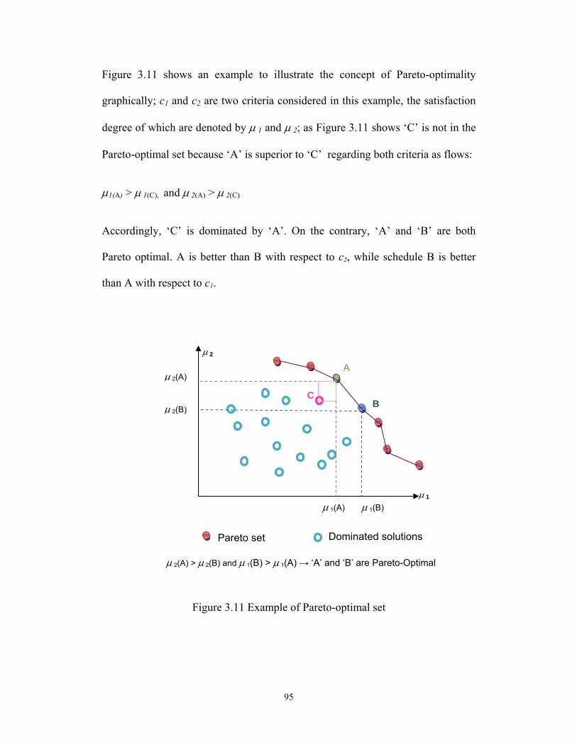
Permission is hereby granted to the University of Alberta Libraries to reproduce single copies of this thesis and to lend or sell such copies for private, scholarly or scientific research purposes only. Where the thesis is

converted to, or otherwise made available in digital form, the University of Alberta will advise potential users of the thesis of these terms.

The author reserves all other publication and other rights in association with the copyright in the thesis and,

except as herein before provided, neither the thesis nor any substantial portion thereof may be printed or otherwise reproduced in any material form whatsoever without the author's prior written permission.

Examining Committee Dr. Aminah Robinson Fayek, Civil and Environmental Engineering Dr. Yasser Mohamed, Civil and Environmental Engineering Dr. John Doucette, Mechanical Engineering

Abstract

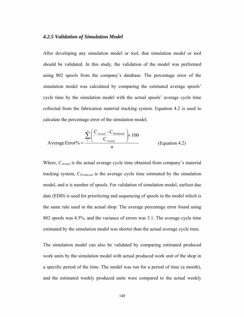
The percentage of shop fabrication, including pipe spool fabrication, has been

increasing on industrial construction projects during the past years. Industrial

fabrication has a great impact on construction projects due to the fact that the

productivity is higher in a controlled environment than in the field, and therefore

time and cost of construction projects are reduced by making use of industrial

fabrication. Effective planning and scheduling of the industrial fabrication

processes is important for the success of construction projects.

This thesis focuses on developing a new framework for optimizing shop

scheduling, particularly pipe spool fabrication shop scheduling. The proposed

framework makes it possible to capture uncertainty of the pipe spool fabrication

shop while accounting for linguistic vagueness of the decision makers’

preferences using simulation modeling and fuzzy set theory. The implementation

of the proposed framework is discussed using a real case study of a pipe spool

fabrication shop.

In this thesis, first, a simulation based scheduling framework is presented based

on the integration of relational database management system, product modeling,

process modeling, and heuristic approaches. Next, a framework for optimization

of the industrial shop scheduling with respect to multiple criteria is proposed.

Fuzzy set theory is used to linguistically assess different levels of satisfaction for

the selected criteria. Additionally, an executable scheduling toolkit is introduced

as a decision support system for pipe spool fabrication shop.

Acknowledgment

I would like to express my gratitude to my supervisor, Dr. Robinson Fayek, to

whom I am deeply indebted for her support and guidance during my research. I

would also like to thank my thesis examination committee members, Dr. Yasser

Mohamed and Dr. John Doucette.

I would like to genuinely thank Ledcor Industrial for providing me with data and

facilitating my work by sharing their knowledge in a friendly manner.

Especially, I need to thank my husband Yasser who supported me by all means. I

am also grateful to my parents, my sisters, and my brother for their love and

encouragements.

Last but not least, I would like to thank my friends and fellow graduate students

for their supports and friendship.

To my husband

Yasser

And to my parents

For their love, and supports

Table of Contents CHAPTER 1 - Background and Problem Statement .............................................. 1 

1.1 Overview ....................................................................................................... 1 

1.2 Research Objective and Expected Contributions .......................................... 4 

1.3 Research Methodology .................................................................................. 5 

1.4 Thesis Organization ....................................................................................... 7 

1.5 References ..................................................................................................... 9 

CHAPTER 2 - A Simulation-Based Framework for Industrial Shop Scheduling 10 

2.1 Introduction ................................................................................................. 10 

2.2 Background .................................................................................................. 11 

2.2.1 Discrete Event Simulation in Construction ........................................... 11 

2.2.2 Industrial Shop Scheduling ................................................................... 12 

2.3 Spool Fabrication Processes ........................................................................ 14 

2.4 Scheduling Problem ..................................................................................... 21 

2.5 A Simulation-based Framework for Industrial Fabrication Scheduling ...... 23 

2.5.1 Proposed Framework............................................................................. 26 

2.5.2 Product Hierarchy Modeling ................................................................. 29 

2.5.3 Scheduling Engine................................................................................. 40 

2.5.4 Simulation Environment ....................................................................... 45 

2.6 Potential Improvements for Further Development ...................................... 51 

2.6.1 Additional Data Collection Needed to Enhance the Model .................. 51 

2.6.2 Developing a Fuzzy Expert System to Estimate the Productivity ........ 52 

2.6.3 Incorporate Uncertainty in Form of Fuzzy Numbers ............................ 57 

2.7 Conclusions ................................................................................................. 57 

2.8 References ................................................................................................... 59 

CHAPTER 3 - An Optimization Framework for Multi-Criteria Industrial Shop

Scheduling............................................................................................................. 64 

3.1 Introduction ................................................................................................. 64 

3.2 Background .................................................................................................. 64 

3.2.1 Scheduling Optimization Methods ........................................................ 64 

3.2.2 Multi-Criteria Scheduling ..................................................................... 68 

3.2.3 Fuzzy Set Theory and Techniques in Construction .............................. 70 

3.2.4 Fuzzy Logic in Construction Scheduling .............................................. 73 

3.3 Proposed Framework for Identifying Optimum Combinatorial Dispatching

Rule .................................................................................................................... 75 

3.4 Phase 1: Identifying Primary Criteria for Scheduling ................................. 78 

3.4.1 Primary Criteria Selection ..................................................................... 81 

3.4.2 Fuzzy Multiple Performance Measure .................................................. 85 

3.5 Phase 2: Combinatorial Dispatching Rules ................................................. 89 

3.6 Phase 3: Identifying Candidate Rules .......................................................... 94 

3.7 Phase 4: Selecting a Compromise Solution ................................................. 99 

3.7.1 Fuzzy C-Means Clustering .................................................................. 101 

3.7.2 Statistical Analysis .............................................................................. 106 

3.7.3 Selecting the Appropriate Rule ........................................................... 112 

3.8 Conclusions ............................................................................................... 114 

3.9 References ................................................................................................. 116 

CHAPTER 4 - Case Study: Scheduling of Pipe Spool Fabrication Shop Using

Simulation and Fuzzy Logic ............................................................................... 122 

4.1 Introduction ............................................................................................... 122 

4.2 Simulation Modeling of Pipe Spool Fabrication ....................................... 123 

4.2.1 Assumptions ........................................................................................ 125 

4.2.2 Database .............................................................................................. 127 

4.2.3 Simulation Environment ..................................................................... 130 

4.2.4 User Interface ...................................................................................... 134 

4.2.5 Validation of Simulation Model .......................................................... 140 

4.2.6 Experimenting with Different Scheduling Rules ................................ 142 

4.3 Implementation of Multi-Criteria Scheduling Framework on the Case Study

......................................................................................................................... 143 

4.3.1 Validation of the Results ..................................................................... 156 

4.4 Conclusion ................................................................................................. 158 

4.5 References ................................................................................................. 159 

CHAPTER 5 - Conclusions ................................................................................ 160 

5.1 Research Summary .................................................................................... 160 

5.2 Research Contributions.............................................................................. 163 

5.3 Recommendations for Future Research ..................................................... 166 

Appendix A Definitions and Illustrations of Welds ........................................... 169 

List of Tables Table 2.1 Sample process plan for pipe spool fabrication shop ........................... 38 

Table 2.2 Scheduling Heuristic Rules ................................................................... 42 

Table 2.3 SPS Modeling Elements for Pipe Spool Fabrication Shop ................... 47 

Table 2.4 Factors Influencing Fitting Productivity ............................................... 55 

Table 2.5 Factors Influencing Cutting Productivity ............................................. 56 

Table 2.6 Factors Influencing Welding Productivity ............................................ 56 

Table 3.1 The Correlation Matrix of Scheduling Criteria for the Pipe Spool

Fabrication ............................................................................................................ 84 

Table 3.2 Groups of Correlated Criteria ............................................................... 85 

Table 3.3 Range of Different Criteria for Pipe Spool Fabrication ........................ 86 

Table 3.4 Cluster Centers of Trade-off Areas ..................................................... 105 

Table 3.5 Performance of an Example Rule for Fifteen Different Scenarios ..... 107 

Table 3.6 Expected Membership Value of an Example Rule to Five Different

Clusters ............................................................................................................... 110 

Table 3.7 Expected Membership Values and Variances of Two Sample

Dispatching Rules with Respect to Five Clusters ............................................... 111 

Table 3.8 Linguistic performance of the ample dispatching rules ...................... 113 

Table 4.1 List of Entities’ Attributes in Central Database .................................. 129 

Table 4.2 Icons Used for Elements of Simulation Model ................................... 130 

Table 4.3 Sample Results of Scheduling Heuristic for Two Weeks ................... 143 

Table 4.4 Linguistic Description of Each Trade-off Area and the Prototypes of

Each Cluster ........................................................................................................ 151 

Table 4.5 Linguistic Performance of the Selected Dispatching Rules ................ 153 

Table 4.6 Performance of the Selected Dispatching Rules for the Case Study .. 155 

Table 4.7 Validation Results ............................................................................... 157 

List of Figures

Figure 2.1 Components of pipe spool (adopted from Sadeghi and Fayek (2008)) 16 

Figure 2.2 Assembly parts of a spool.................................................................... 17 

Figure 2.3 Example of roll welding constraint: (a) Roll welding is feasible; (b)

Roll welding is not feasible (adopted from Sadeghi and Fayek (2008)) .............. 18 

Figure 2.4 Flowchart of pipe spool fabrication process ........................................ 20 

Figure 2.5 Overview of scheduling problem ........................................................ 21 

Figure 2.6 Architecture of proposed framework for industrial fabrication

scheduling ............................................................................................................. 28 

Figure 2.7 Typical work breakdown structure for spool fabrication .................... 30 

Figure 2.8 Components and assemblies of a spool ............................................... 32 

Figure 2.9 Heuristic search algorithm used for determining types of welds ........ 33 

Figure 2.10 Examples of different types of position welds .................................. 36 

Figure 2.11 Product hierarchy (PH) for spool ...................................................... 37 

Figure 2.12 Process model for spool in relation to spool’s product model .......... 40 

Figure 2.13 The processes and elements of pipe spool fabrication template ........ 50 

Figure 2.14 The structure of fuzzy expert system ................................................. 54 

Figure 3.1 The concept of low and high utilization in traditional sets (adopted

from Pedrycz and Gomide (2007)) ....................................................................... 71 

Figure 3.2 The concept of low and high utilization in fuzzy sets (adopted from

Pedrycz and Gomide (2007)) ................................................................................ 71 

Figure 3.3 Membership function for being highly utilized ................................... 72 

Figure 3.4 The proposed framework for multi-criteria industrial shop scheduling

............................................................................................................................... 77 

Figure 3.5 Simulation results of applying three simple dispatching rules on a

spool fabrication shop (maximum tardiness vs. average flow time) .................... 82 

Figure 3.6 Simulation results of applying eight simple dispatching rules on a

spool fabrication shop (make-span vs. average flow time) ................................... 83 

Figure 3.7 Membership function of acceptable values for minimization of criteria

q............................................................................................................................. 88 

Figure 3.8 Membership function of acceptable values for maximization of criteria

q............................................................................................................................. 88 

Figure 3.9 Performance of ATC rule with different k values ............................... 91 

Figure 3.10 Performance of ATC rule and proposed dispatching rules for spool

fabrication shop (Pareto frontier) .......................................................................... 93 

Figure 3.11 Example of Pareto-optimal set .......................................................... 95 

Figure 3.12 Generating candidate dispatching rules ............................................. 97 

Figure 3.13 Pareto optimal set for a sample scenario ........................................... 98 

Figure 3.14 Trade-off areas on a Pareto frontier ................................................. 100 

Figure 3.15 Linguistic trade-off areas for two criteria: average flow time and

maximum tardiness ............................................................................................. 104 

Figure 3.16 Membership functions of linguistic terms obtained from FCM ...... 105 

Figure 3.17 Data points represinting each dispatching rule ................................ 107 

Figure 4.1 A schematic layout drawing of a bay in a pipe spool fabrication shop

............................................................................................................................. 122 

Figure 4.2 Structure of simulation model for case study .................................... 124 

Figure 4.3 Dummy legs....................................................................................... 127 

Figure 4.4 Input and output tables in central database ........................................ 128 

Figure 4.5 Relationships between company’s databases and simulation model via

VB.net and Access .............................................................................................. 135 

Figure 4.6 User interface for simulation model .................................................. 136 

Figure 4.7 User interface for simulation model, selecting the scheduling rule .. 137 

Figure 4.8 User interface for simulation model: revising the layout and shop

configurations (inputs to simulation model) ....................................................... 138 

Figure 4.9 User interface for simulation model: cycle time for each spool ........ 139 

Figure 4.10 The process of identifying the Pareto optimal set for case study .... 145 

Figure 4.11 Performance values of different dispatching rules for the first scenario

............................................................................................................................. 146 

Figure 4.12 Performance values of different dispatching rules for all scenarios 148 

Figure 4.13 The expected membership value of each dispatching rule to every

cluster .................................................................................................................. 150 

Figure A1 Socket weld and butt weld ................................................................. 169 

Figure A2 Re-pads and dummy leg .................................................................... 169 

1

CHAPTER 1 - Background and Problem Statement

1.1 Overview

Satisfying customers’ ever growing expectations has become a significant

challenge for survival in today’s extremely competitive marketplace. The

response of researchers and practitioners in academia and industry to this

challenge contributes to the development of new concepts, strategies, and even

research disciplines (Ebrahimy 2006).

One of the research areas developed in response to such a challenge is operations

research (OR). Over the years, firms and corporations have been trying to

improve their performance, productivity, and profitability by using and adopting

the studies developed on topics such as factory layout, inventory control, process

control, scheduling, and resource utilization. Amongst all topics in the operations

research area, one of the most popular research topics is sequencing and

scheduling, which plays an important role in the success of organizations: for

instance, effective scheduling enables corporations to increase throughput, reduce

cycle time, reduce work in progress inventory and thus reduce cost. Therefore,

scheduling has attracted significant research for the last five decades.

Scheduling as a form of decision making deals with the allocation of resources to

activities over given time periods, and its target is optimizing one or more

objective functions. It plays an important role in production systems,

manufacturing, and also transportation (Pinedo 2008). The resources and

activities may take different forms. For example, resources can be machines in a

2

workshop, runways at an airport, crews at a construction site, and so on. The

activities can be operations in a production process, take-offs and landings at an

airport, stages in a construction process, and so on. There are also various forms

of objectives. One objective may be the minimization of the completion time of

the last activity (i.e. Make Span), and another may be the minimization of average

flow time or the minimization of number of activities completed after their

particular due dates. A comprehensive introduction to scheduling can be found in

French (1982), Brucker (2007), Pinedo (2008), and Baker and Trietsch (2009).

The construction industry has employed and adopted some concepts and tools of

scheduling. There are many studies that have used project scheduling techniques

such as critical path method (CPM) and Program Evaluation and Review

Technique (PERT) in construction for controlling and managing construction

projects, risk analysis, resource leveling, and resource forecasting. However, the

quantity of research conducted in developing a feasible schedule for shop

environments in the area of industrial construction is very limited. Although many

research projects have been carried out to analyze the productivity of several shop

floors in industrial construction, there have been few studies on developing

feasible and optimized schedules for the shop floors. Notably, CPM and PERT are

tools for presenting schedules, but not for developing optimum or good schedules.

Most scheduling problems are known to be NP-hard, meaning that the problems

do not have a polynomial time algorithm. The time required for solving the

problem grows exponentially with an increasing number of machines or jobs.

3

Accordingly, a great deal of work has been dedicated to development and analysis

of approximate algorithms.

Although most scheduling problems are solved based on a single criterion (i.e.

objective), there are some studies on multi-criteria scheduling problems due to the

fact that in practice these problems often have multiple criteria. In multi-criteria

scheduling, several objectives are considered in the problem. Optimizing all

objectives in such problems is impossible, given that in most cases the objectives

conflict with each other. Therefore, such scheduling problems do not have a

single optimum solution. There exist a set of different solutions, which produce

trade-offs (i.e. conflicting scenarios) among different criteria, which means that a

solution that is extreme with respect to one criterion requires a compromise in

other criteria (Kalyanmoy 2001). Consequently, in multi-criteria scheduling, the

problem is modeled by taking into account the preferences and experience of

decision makers. Depending on the preferences of the decision maker, some

objectives are considered more important than others, or a degree of satisfaction is

measured for each objective based on the expectation of the decision maker. This

approach makes it possible to construct a set of satisfactory solutions according to

the preferences of the decision maker. It is important for the decision maker to

have a set of possible solutions to be able to select the most suitable solution

based on the state of the existing decision at a given time. Particularly, the

preferences of the decision makers are usually described in natural language.

Therefore, the application of the fuzzy set theory is an appropriately good fit in

order to account for imprecise linguistic aspirations of the decision maker.

4

The research presented in this thesis is intended to develop a new framework for

optimizing industrial shop scheduling, specifically, pipe spool fabrication shop

scheduling, with respect to multiple criteria. The methodology provides the

opportunity to capture the uncertainty of the industrial shop, while accounting for

the linguistic vagueness of the decision makers’ preferences by using simulation

modeling and fuzzy set theory. Furthermore, a scheduling toolkit is developed as

a decision support system for a pipe spool fabrication shop. This toolkit provides

decision makers with the opportunity to select an appropriate scheduling solution

based on their objectives.

1.2 Research Objective and Expected Contributions

The main objective of this study is to develop an application using concepts and

methods of job shop scheduling problems for a pipe spool fabrication shop in

order to reach a reasonable, and near optimum schedule subject to decision

makers’ implicit objectives. To realize these objectives, three steps are identified:

1. Understanding theory, algorithms, and systems of scheduling

2. Developing a simulation model based on Product Model (PM) to model

scheduling problems in spool fabrication shop

3. Developing a model to solve scheduling problems for spool fabrication

shop by heuristics, and using fuzzy set theory to solve multi-objective

scheduling problems

The research contributions of this study include:

5

1. Using and adopting concepts and theories such as production scheduling in

industrial construction management.

2. Modeling a new scheduling problem in construction management as well

as production research.

3. Developing a novel simulation model, based on product modeling

connected to the database of the industrial shop. This simulation model

can be used as a baseline for future studies on the spool fabrication shop.

4. Developing a new method of solving multi-criteria (objective) scheduling

using fuzzy set theory.

The research also contributes to the industry by developing a toolkit, which can be

used as a decision support system by coordinators and superintendants of spool

fabrication shops for the sequencing and scheduling of jobs in the fabrication

shop. Using the proposed toolkit, they can improve productivity, throughput, and

the shop’s works in progress, as well as ensure that jobs are completed on time.

The toolkit has been developed using VB.NET and Simphony.Net as an

underlying simulation environment.

1.3 Research Methodology

This research was conducted using the following methodology: first, spool

fabrication shop processes and stages each spool should go through during the

fabrication of spools were identified. The fabrication processes were mapped out

by questioning and interviewing the fabrication shop staff. Moreover, the

6

procedures were studied by observing and visiting the shop floor. The constraints

and limitations of resources were also verified in order to properly model the

fabrication shop. Additionally, the configuration and constraints of the shop,

including space constraints, safety constraints, and constructability constraints,

were identified.

A product model was then developed for spools using both a spool fabrication

shop database, as well as drawings of spools from the drafting department’s

database, in order to identify jobs and model the spool fabrication. In reality, the

way the components or assemblies connect to each other (for example, whether

two pipes make parallel or perpendicular connections) may change the time and

even the type of the process that should be performed on that assembly or spool.

Therefore, the product model was designed to incorporate the 3-D relational

geometric attributes of the product, i.e. spools, the type and shape of the product

components, the relationship between the product components, shop process

information, and constraints of the shop. The product model was developed in

MS-Access, which was the central database to connect to the simulation model.

Subsequently, a Special Purpose Simulation (SPS) template for pipe spool

fabrication was developed in Simphony.Net© (Hajjar and Abourisk 2002), which

is an object oriented environment for building SPS templates using VB.net

programming language. The SPS template is connected to the central database to

use the developed product model. Using the developed SPS template, a simulation

model was developed for a real case study.

7

In the next step, common criteria on which the schedules should be evaluated, i.e.

objective functions, were identified. Then, suitable dispatching rules and

heuristics were identified, and new combinatorial dispatching rules were

established by combining and weighting multiple parameters. The performance of

each rule with respect to different criteria was measured for different scenarios

using the simulation model. Then, the performance values estimated by the

simulation model were exported to Excel sheets. Fuzzy membership functions

were used to evaluate the satisfaction degree of each. Conflicting criteria and the

linguistic trade-offs between them were identified using the concept of fuzzy set

theory. The data set obtained from the simulation results was analyzed using the

concept of Pareto-optimality and Fuzzy C-Means clustering (FCM). In addition,

Fuzzy C-Means clustering (FCM) was used to categorize the performance values

obtained from the simulation model for different scenarios. The probability and

possibility analyses were performed on the results to identify the most efficient

and robust rules for each linguistic trade-off between conflicting criteria.

1.4 Thesis Organization

Chapter 2 of this thesis presents an enhanced simulation-based framework for

industrial fabrication scheduling. In this chapter the concepts and ideas of

scheduling of shop environments, heuristic rules, and simulation modeling is

provided. The existing simulation modeling frameworks (Song et al. 2006;

Sadeghi and Fayek 2008) are extended and used to develop a toolkit for

automated scheduling of the industrial fabrication shop.

8

Chapter 3 of the thesis focuses on developing a framework for solving multi-

criteria scheduling with respect to the linguistic preferences of the decision maker

using Fuzzy C-Means clustering and fuzzy set theory. In this chapter the concepts

and ideas of fuzzy set theory and its application to the multi-objective scheduling

problem are briefly introduced. Moreover, the previous studies on these concepts

are summarized.

Chapter 4 of this thesis discusses the implementation of the simulation-based

framework for industrial fabrication scheduling, and the multi-criteria scheduling

framework on a real case study to experiment with the effectiveness of the

scheduling model. The results are validated to identify the accuracy of the

proposed methodology for multi-criteria scheduling.

Chapter 5 of this thesis describes the conclusions, contributions, and

recommendations for future research.

9

1.5 References

Baker, Kenneth R., and Trietsch. D. (2009), Principles of sequencing and scheduling, Hoboken, N.J.: John Wiley.

Brucker (2007), Scheduling Algorithms, Springer, Berlin.

Ebrahimy Khorramabady, Y. (2006). “Simphony Supply Chain Simulator: a toolkit for modeling supply chain coordination and information sharing.” M.Sc. thesis, University of Alberta, Edmonton, Alberta.

French, S. (1982), Sequencing and scheduling: An introduction to the mathematics of the job shop, Wiley, New York.

Hajjar, D., and AbouRizk, S. M. (2002). “Unified modeling methodology for construction simulation.” Journal of Construction Engineering and Management, 128(2), 174–185.

Kalyanmoy, D. (2001). Multi-Objective Optimization Using Evolutionary Algorithms. John Wiley & Sons, New Jersey.

Pinedo, M. (2008). Scheduling: Theory, Algorithms, and Systems, Springer, NewYork.

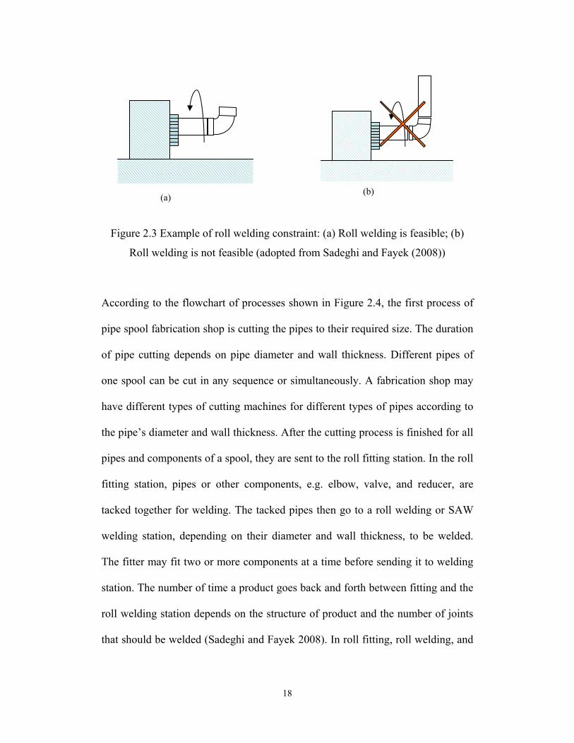
Sadeghi, N., and Fayek, A. R. (2008). “A framework for simulating industrial construction processes.” Proceedings - Winter Simulation Conference, art. 4736347, pp. 2396-2401.

Song, L., Wang, P., and AbouRizk, S. M. (2006). “A Virtual Shop Modeling system for Industrial Fabrication Shops.” Simulation Modelling Practice and Theory, 14(5), 649-662.

10

CHAPTER 2 - A Simulation-Based Framework for

Industrial Shop Scheduling

2.1 Introduction

In this chapter, an enhanced framework for developing simulation-based

scheduling for industrial construction is proposed. The proposed framework

enhances the existing simulation models, and can be used as a toolkit for

automated scheduling. The proposed framework is developed based on the

integration of database management systems, product modeling, simulation

modeling, and heuristic approaches to streamline the scheduling process of

industrial fabrication shops. The proposed framework is illustrated and discussed

using pipe spool fabrication processes.

The background of simulation modeling and industrial shop scheduling is

presented in section 2.2. The previous models are also reviewed in this section to

justify the need for extending the functionality of existing simulation models. The

processes of spool fabrication are explained in Section 2.3. Section 2.4 provides

the formulation of the industrial shop scheduling problem. Section 2.5 presents

the proposed simulation-based scheduling framework. The potential improvement

for the future development of the framework is reviewed in section 2.6. Section

2.7 summarizes the contributions of this chapter.

11

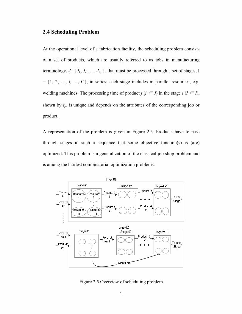
2.2 Background

2.2.1 Discrete Event Simulation in Construction

Discrete event simulation is a common technique for modeling manufacturing and

construction systems. Overviews on simulation and its application in industries,

such as electronics manufacturing, shipbuilding, and bridge fabrication are

available in several publications (Banks 1998; Law and Kelton 2000; Jahangirian

et al. 2009).

Discrete event simulation has been widely used in construction industry since

Halpin (1977) developed the first construction simulation system, CYClic

Operation NEtwork (CYCLONE). It is defined as a chronological sequence of

events and transitions between those events. MicroCYCLONE was developed by

Lluch and Halpin (1982) to increase the functionality of CYCLONE. Many

discrete event simulation frameworks have been developed to address

construction operation simulation problems after that, such as RESQUE (Chang

1986), CIPROS (Odeh 1992), HSM (Sawhney 1994), STROBOSCOPE (Martinez

1996) and Simphony© (Hajjar and AbouRizk 1999).

Simphony© is based on Special Purpose Simulation (SPS) (Kim 2007), which

provides a user-friendly interface and allows the developer to build the model

intuitively. It also provides graphical and hierarchical modeling. Simphony© is

capable of modeling complex and large construction projects by using modular

and hierarchical structures (Davila Borrego 2004).

12

2.2.2 Industrial Shop Scheduling

There are two main types of scheduling problems in the construction industry.

The first type is project scheduling, which is activity-oriented and concerns

project resource usage, total project cost, and total project duration. In project

scheduling, the sequences of activities are determined to optimize one or a set of

objective functions while meeting the precedence constraints. The target in this

type of scheduling problem usually involves addressing a trade-off between

project resources, project cost, and project duration. Examples of this type of

scheduling are construction scheduling of infrastructure, tunnels, and building

construction projects. Several studies have been done on such scheduling

problems based on critical path method (CPM), including studies carried out by

Schmidt and Horning (1990), which aims to modify resource allocation in CPM;

Fan et al. (2003), in which an object oriented scheduling method is introduced;

Karim and Adeli (1997), to schedule highway constructions; Chan et al. (1996),

which models resource allocation in project scheduling; Karim and Adeli (1999),

which models construction scheduling and change management; Leu and Yang

(1999), which models construction project scheduling using genetic algorithm;

and Adeli and Karim (2001) and Zhang (2006), which optimize projects’ resource

utilization using search algorithms.

The second type of scheduling problem is production scheduling, which includes

scheduling of jobs through multiple work centers to complete the jobs. An

example of production scheduling is the scheduling of industrial fabrication, such

as steel and spool fabrication shops. The jobs in spool fabrication scheduling are

13

the spools that are being fabricated by going through cutting, fitting, and welding

stations or work centers. The usual target in the second type of scheduling

problems is to find the best sequence of production or fabrication jobs, which

optimizes an objective function or a set of objective functions such as the total

flow time, incidents of lateness, or average resource usage. Industrial fabrication

scheduling as a major branch of production scheduling problems is job-based.

The term “industrial construction” is used for construction of facilities for basic

industries such as petrochemical plants, nuclear power plants, and oil/gas

production facilities (Barrie and Paulson 1992). Some parts of industrial

construction projects can be pre-fabricated in the controlled environment of

fabrication shops. Industrial shop fabrication has had a great impact on reducing

on-site fabrication and installation and therefore reducing the cost of construction

projects due to reduced uncertainty in a controlled shop environment.

Consequently, the percentage of shop fabrication in construction, including steel

fabrications and pipe spool fabrication, has been increasing during the last decade.

This means that the success of a project depends on effective short-term job-based

planning and scheduling, which requires higher levels of modeling accuracy. As

existing project management systems such as Microsoft Project and Primavera

Project Planner are activity-oriented, they cannot be applied effectively to

industrial fabrication scheduling problems (Karumanasseri and AbouRizk 2002).

Production engineers usually schedule an industrial fabrication project by creating

a practical master production schedule for the project. On the shop floor,

experienced superintendents try to complete the jobs by the delivery date

14

estimated in the master production schedule (Song et al. 2006). In this approach,

scheduling is based on personal experience, information from component

drawings, and knowledge of shop status. Today’s complex shop environments,

complex products, and many potential influencing factors make it difficult for the

human mind to process the information required for an accurate analysis of such a

production system. Therefore, developing a scheduling technique to analyze and

capture all these complexities would contribute to the better planning and

scheduling of fabrication shops.

Traditionally, simulation models are used to mimic the real-world systems and

processes in order to analyze and improve the productivity of the systems. In the

last decade, simulation has been used as an effective technique for generating and

developing production schedules in manufacturing systems (Mazzioti and Home

1997; Marito and Lee 1997; Siva Kumar 1999; Gupta and Sivakumar 2002).

2.3 Spool Fabrication Processes

Spool fabrication is an industrial shop that produces pipe spools to be used in pipe

spool modules, which are then utilized in developing modular construction units

in refineries and oil processing plants (Mohamed et al. 2007). Spool fabrication

processes in a typical fabrication shop involve cutting, fitting, tacking, and

welding (Wang 2006). Each spool is a portion of a piping system composed of a

number of pipes and fittings, such as elbows and tees, valves, reducers, and

supports, assembled together according to fabrication drawings. Figure 2.1 shows

15

an example of a spool which is composed of five pipes, three elbows, one valve,

and one reducer.

In the pipe spool fabrication shop, three methods of welding are usually

employed: (1) roll welding, in which the welder uses a pipe turner to weld faster;

(2) SAW welding, which is the fastest method of welding using the Submerged

Arc Welding (SAW) machine; and (3) position welding, which takes much longer

than the other methods as the welder cannot use any machine to turn the pipes.

SAW is done by the SAW machine, and its duration is less than roll or position

welding. In roll welding, the welder does not move the rod; instead, the pipe is

turned by a roll welding machine (pipe turner or chuck positioner), while in

position welding, the welder must move the welding rod around the pipe to weld

the pipe. Position welding is used when the pipe has long branches and cannot be

rolled by a pipe turner. In order to properly simulate the fabrication shop, these

three types of welding should be modeled separately for each spool.

16

Figure 2.1 Components of pipe spool (adopted from Sadeghi and Fayek (2008))

In the spool fabrication shop, the fitter usually breaks down the spool into smaller

assemblies (Figure 2.2) that are easier for fabrication (Sadeghi and Fayek 2008).

Each assembly contains several piping components (such as pipes, elbows, tees,

valves, etc.) as the most basic elements in the fabrication process. During the

fabrication of spool some processes, such as cutting, are performed on piping

components. Piping components then are assembled together to produce

Elbow 3

Pipe 5

Weld E

Weld F

Weld I

Pipe 4

Weld G

Weld H

Reducer

Pipe 3

Pipe 2

Pipe

1 Elbow

2

Elbow 1

Weld D

Weld C

Weld B

Weld A

Valve 1

17

assemblies. This procedure is continued until the final product or spool is

produced. As previously mentioned, welding operations can be performed by

three different methods, including position welding method, roll welding method,

and SAW method. For roll welding and SAW operation there are physical

constraints. For example, roll welding cannot be performed on assemblies with

long branches as shown in Figure 2.3. On the other hand, SAW and roll welding

are more efficient due to the fact that in these two welding methods not only is the

welding process faster, but also the quality of weld is better than position welding.

To comply with such constraints, each spool is decomposed into assemblies to use

roll welding and SAW as much as possible. Therefore, a spool is broken down to

assemblies in such a way that the position welding is minimized with respect to

technological constraints.

Figure 2.2 Assembly parts of a spool

Assembly 1

Assembly 2

The joint that should be position welded.

18

Figure 2.3 Example of roll welding constraint: (a) Roll welding is feasible; (b)

Roll welding is not feasible (adopted from Sadeghi and Fayek (2008))

According to the flowchart of processes shown in Figure 2.4, the first process of

pipe spool fabrication shop is cutting the pipes to their required size. The duration

of pipe cutting depends on pipe diameter and wall thickness. Different pipes of

one spool can be cut in any sequence or simultaneously. A fabrication shop may

have different types of cutting machines for different types of pipes according to

the pipe’s diameter and wall thickness. After the cutting process is finished for all

pipes and components of a spool, they are sent to the roll fitting station. In the roll

fitting station, pipes or other components, e.g. elbow, valve, and reducer, are

tacked together for welding. The tacked pipes then go to a roll welding or SAW

welding station, depending on their diameter and wall thickness, to be welded.

The fitter may fit two or more components at a time before sending it to welding

station. The number of time a product goes back and forth between fitting and the

roll welding station depends on the structure of product and the number of joints

that should be welded (Sadeghi and Fayek 2008). In roll fitting, roll welding, and

(a) (b)

19

SAW processes, the assemblies of spool are completed to be sent to a position

fitting station.

In the next step, assemblies of spool are fit and tacked together by the fitter. Then,

the spool is produced into the final product by performing the position welding

process. The final fitting and position welding usually are performed in the same

station (Sadeghi and Fayek 2008), which means that there is no material handling

between these two processes. After the final fitting and welding, the quality check

process is carried out to ensure the quality of welds. The quality check can be

performed at any stage of processes, but it is usually implemented after position

welding. During the spool fabrication process, components, assemblies, and

spools are handled and moved by bridge cranes.

20

 

Figure 2.4 Flowchart of pipe spool fabrication process

Typical Material Flow 

Occasional Material Flow

Cutting

Fitting and Tacking

Position Weld

Quality Check

Need SAW Weld?

SAW Welding

Need Roll Weld?

Roll Welding

Need More Fitting?

Fitting and Tacking for Position welding 

Yes No

Yes No

Yes

No

21

2.4 Scheduling Problem

At the operational level of a fabrication facility, the scheduling problem consists

of a set of products, which are usually referred to as jobs in manufacturing

terminology, J= {J1, J2, … , Jn. }, that must be processed through a set of stages, I

= {1, 2, …, i, …, C}, in series; each stage includes m parallel resources, e.g.

welding machines. The processing time of product j (j ∈ J) in the stage i (I ∈ I),

shown by tji, is unique and depends on the attributes of the corresponding job or

product.

A representation of the problem is given in Figure 2.5. Products have to pass

through stages in such a sequence that some objective function(s) is (are)

optimized. This problem is a generalization of the classical job shop problem and

is among the hardest combinatorial optimization problems.

Figure 2.5 Overview of scheduling problem

22

The production-scheduling techniques in the literature can be divided into three

major categories: exact algorithms, meta-heuristic techniques, and constructive

heuristics. Exact algorithms or mathematical algorithms, e.g. branch and bound,

guarantee to find an optimal solution but are case-based and include many

simplifying assumptions. Meta-heuristic techniques, such as genetic algorithms

(GA), sacrifice the guarantee of finding optimal solutions in order to get near-

optimum solutions in reasonable and practical computational times. According to

Osman and Laporte (1996), a meta-heuristic is an intelligent searching and

learning method for exploring the feasible space. Constructive heuristics such as

dispatching rules (or priority rules) are the fastest scheduling algorithms and need

less computational time (Zobolas et al. 2008). Scheduling optimization problems

are known to be NP-hard (non-deterministic polynomial-time hard), meaning that

there is no polynomial time algorithm to solve such problems (Baker and Trietsch

2009). The time required for solving these scheduling problems grows

exponentially with an increasing number of machines or jobs. Therefore,

mathematical algorithms are not appropriate for the scheduling of industrial

fabrication facilities. While meta-heuristics can produce a good sequence of jobs

to get a near-optimum solution, they make the controlling problem of shop floor

more complicated and they should also re-run as the jobs’ composition in the shop

changes. These problems make it difficult to use meta-heuristics in practice and

provide a satisfactory solution.

Constructive heuristic techniques generate solutions from scratch by gradually

adding parts of the solution to the initially empty partial solution. Constructive

23

heuristics are the fastest approximate algorithms. Their advantage in

computational time requirements is counterbalanced by generally inferior quality

solutions when compared to meta-heuristic techniques. However, they are often

preferred to meta-heuristic techniques due to fact that they are easier and faster to

implement, and provide a satisfactory solution.

2.5 A Simulation-based Framework for Industrial Fabrication

Scheduling

Although simulation-based scheduling techniques has been widely applied in

manufacturing systems (Gupta and Sivakumar 2002), their application in

industrial fabrication is limited (Mohamed et al. 2007; Taghaddos et al. 2009).

Some researchers have developed frameworks for industrial fabrication virtual

planning (Song et al. 2006; Sadeghi and Fayek 2008). These frameworks are

useful for long term planning purposes, yet there are still some challenges in using

them for scheduling purposes. The industrial fabrication planning and scheduling

frameworks are generally comprised of two main components. The first

component is a product model, which helps define the jobs to be fabricated or that

pass through the production line. The second component is a production or

process model, which calculates the time of each process for each job or each

major part of a job. Processes usually include cutting, fitting and welding, as

discussed in Section 3.2. The challenges hindering the use of the proposed

frameworks also relate to these components.

24

Firstly, the product models proposed for industrial fabrication, although

theoretically correct, do not recognize the importance of geometrical properties of

the spools at different levels of the product model and the fact that different

processes in industrial fabrication should be performed at different levels of the

work breakdown structure (product model). In industrial construction, products

are decomposed into smaller pieces, known as assemblies, at the operational level

in order to meet the constraints and limitations of the shop as explained earlier.

Thus, each product usually travels in the system not as one entity but as raw

materials or different components (Sadeghi and Fayek 2008). For that reason,

Sadeghi and Fayek (2008) have extended the product model suggested by Song et

al. (2006) to model the flow of raw materials and components of a product as

individual entities in a simulation model. However, the product model developed

by Sadeghi and Fayek (2008) does not consider the geometrical properties at each

level of the product model. In reality, the way the components or assemblies

connect to each other, e.g. whether two pipes make perpendicular or parallel

connections, may change the time and even the type of process that should be

performed on that assembly or spool. By ignoring the geometrical properties of

the components of an assembly, any assembly with a certain quantity of

components, e.g. any assembly with a certain linear meters of pipe and certain

number of welds, is modeled exactly the same. Any configuration of the product

model that ignores the geometrical properties at different levels of the product

model hinders the development of an accurate scheduling framework.

25

Secondly, the process models used to calculate the time of each process for a job

or parts of a job are not accurate enough for short-term planning. The proposed

process models are based on simple statistical modeling or neural networks. In the

proposed process models, the processing time of each activity is represented by a

probabilistic distribution, which is calculated using productivity values estimated

by experts and the amount of work units for each spool. The variance of such a

probabilistic distribution is usually high due to the variety of products. For

example, using this information suggests that welds with identical diameter inches

have the same duration regardless of different thicknesses or types, which is not

accurate. If the durations of different processes for the jobs cannot be calculated

accurately enough, the scheduling results will not be accurate.

In addition to the above challenges, these frameworks only discuss the need to use

a scheduling algorithm or schema, without referring to the type of scheduling

method to be used or proposing any practical solution for incorporating the

scheduling engine into the framework. The choice of the scheduling algorithm is

very important. For instance, while meta-heuristics such as adaptive memory

programming, ants systems, evolutionary methods, genetic algorithms, and greedy

search procedures can produce a good sequence of the jobs to get a near optimum

solution, the fact that they should be run on a daily basis as the composition of the

jobs in the shop changes makes them quite unattractive for practical purposes.

In this section an enhanced framework for the industrial fabrication scheduling

problem is introduced. This framework has been developed to address the

limitations identified in the previous frameworks, as discussed. This research

26

enhances and extends the framework suggested by Song et al. (2006) in order to

consider optimality of the schedule with respect to the user’s criteria, 3-D

geometric attributes of the product, and the site’s constraints and factors affecting

the product and process model.

2.5.1 Proposed Framework

To overcome the aforementioned challenges, the following aspects are considered

in the proposed framework:

• 3-D geometric attributes of the product;

• type and shape of the product components;

• relationship between the product components;

• shop process information;

• constraints of the shop, i.e. space constraints, safety constraints, and

constructability constraints, which are not included in the current modeling

frameworks.

The framework for industrial fabrication scheduling proposed in this chapter has

three major components:

1. The product hierarchy modeling component, which consists of the product

model and the process model;

2. The simulation environment, which models the production and is linked to

the product and process models;

3. The scheduling engine.

27

The overall architecture of the proposed framework is illustrated in Figure 2.6.

The product hierarchy modeling (PHM) provides a mechanism to define the

industrial fabrication products by capturing the complexity and uniqueness of the

products by defining entity hierarchy (EH). The PHM is implemented in a central

database system, which is a relational database management system (RDBMS).

The central database interfaces with shop drawings and gets the product’s

information from CAD drawings and the material information database. It uses

the product’s information and shop constraints to build the product hierarchy

(PH). The process model defines the processes that should be performed on each

product. The EH is then constructed by integration of product and process data.

The EH is used to produce entities for the simulation model.

The scheduling engine includes a library of heuristic rules, i.e. dispatching rules,

that can be used in the simulation model for sequencing the products. The

heuristic rule is to prioritize the jobs waiting in the queue of a machine: the job

with the highest priority is selected to be processed in the corresponding machine.

Each time a new job enters the queue of a machine, the jobs in the queue are

prioritized based on the selected dispatching rule. The heuristic rules can be tested

in the simulation model. The performance of each rule is measured by various

statistics that are collected during simulation runs, including tardiness statistics of

completed jobs, mean flow time, machine utilisation, and queuing statistics, e.g.

average waiting time. The production schedule generated by each scheduling rule

is maintained in the central database. Based on the performance measure of each

heuristic rule, the decision maker can select the appropriate production schedule.

28

The simulation environment enables the user to reproduce the industrial

fabrication facility as a computer model. The simulation environment models

different components of an industrial shop including production lines (or bays),

working stations, shop configurations (such as shop layout, number of working

station, and storage capacity), movement paths, handling, equipment, and labour.

A pipe spool fabrication template is developed to model the components of the

pipe spool fabrication shop.

Figure 2.6 Architecture of proposed framework for industrial fabrication

scheduling

Other performance values (Resource Utilization, Production Rate,

Tardiness)

Schedule Reports

Output of the system

Scheduling Engine

Heuristic Rules

Library

Scheduling Rule

Facility Information:

• Shop configuration

• Resources • Constraints • Operating

hours (Shift hours, working days, and etc.)

Simulation Environment

Discrete Event

Simulation

Product Hierarchy Modeling

Shop’s Constraints

Entity Hierarchy

Product Hierarchy

Process Model

Central Database

Shop’s Databases

Orders CAD

Drawings

Material Information

29

2.5.2 Product Hierarchy Modeling

The product hierarchy modeling system is used for defining the product and

identifying its most basic components, i.e. product atomic components (Xu et al.

2003), as well as recognizing the product’s processes and operations. The system

is developed using CAD drawings and RDBMS.

2.5.2.1 Product Hierarchy

Every level of the product model (PM) represents a level of the product’s work

breakdown structure (WBS) and corresponding processes. A typical WBS for a

project in pipe spool fabrication shop is shown in Figure 2.7. In the pipe spool

fabrication shop, each spool corresponds to a project. Each spool is detailed on a

fabrication drawing, which is prepared by the drafting department based on the

project’s ISO drawings and requirements from the client. Several spools are

usually grouped into batches by the project coordinator before they are issued to

the work stations. As mentioned earlier, in the operational level of industrial

fabrication shops, the product is usually broken down into smaller assemblies that

are easier for fabrication. All welding processes of an assembly are done by roll

welding and SAW welding. Each assembly contains several components (such as

pipes, elbows, tees, valves, etc.) as the most basic elements in the fabrication

process.

Collecting product data for industrial fabrication is challenging and time

consuming because of large amount of unique products. Generally, CAD systems

30

of pipe spool fabrication allow exporting all components’ data of a product into

an external standard file structure. Examples of components’ data include

physical and material feature of pipes, valves, and fittings, as well as 3-D

coordinates of each component obtained from the spool’s drawing. Form and

quantity of welds are other examples of information that can be exported to an

external file. Therefore, the automation of generating product components is an

easy task. However, the main challenge is developing the product hierarchy using

this information. The product hierarchy is developed using logical groupings from

product components based on the shop’s limitations and standards.

Figure 2.7 Typical work breakdown structure for spool fabrication

Product of Fabrication Facility

31

In order to develop the product hierarchy model of spools, assemblies and the

quantity of each type of weld (position, roll, and SAW) should be known. In the

previous practices of fabrication shop simulation (Sadeghi and Fayek 2008),

probabilistic distributions are generally used for these quantities. Probabilistic

distributions are generally known as the best representation of uncertainty in the

simulation models. Probabilistic distributions are used when required information

for estimating a deterministic number does not exist, or when there is random

uncertainty. The variance of the probabilistic distributions can be reduced by

considering factors that affect the variables (AbouRizk and Sawhney 1993).

In this case, having the 3-D geometry of spools from the CAD drawings, it is

possible to identify the assemblies of the spool and determine their attributes to

develop the product hierarchy model. This problem can be solved as a

combinatorial optimization problem in which the sequence of welding should be

optimized considering minimization of position welding as an objective function.

Considering the spool shown in Figure 2.8 as a simple example, the optimum

sequence of welding for the spool is E-D-B-A-C, which minimizes the amount of

position welding and results in two assemblies and one position weld (weld C);

therefore, Assembly 1 includes pipe3, pipe2, and elbow1 connected together by

weld A and weld B, while assembly 2 includes all other components such as

pipe1, elbow2 and valve1. At the same time, choosing E-D-C-A-B as the

sequence of welding operations results in three assemblies and two position welds

(Welds B and C). Other sequences of the welds result in either an equal or more

number of position welds.

32

Figure 2.8 Components and assemblies of a spool

Although this problem can be solved by any meta-heuristic or exact algorithm

optimization techniques, these techniques are not feasible approaches due to the

large number of spools, some of which have up to 25 welds. As a result, a hybrid

heuristic algorithm is developed to complete the product hierarchy model

automatically, using exported data from CAD drawings and material information

databases. The algorithm is shown in Figure 2.9.

Pipe 3

Pipe 2

Pipe

1 Elbow 1

Assembly 1

Assembly 2

Elbow 2

Weld A

Weld B

Weld C

Weld D

Weld EValve 1

33

Figure 2.9 Heuristic search algorithm used for determining types of welds

34

In the proposed algorithm (Figure 2.9), based on an initial candidate sequence of

welds, the components of the spool are sequentially connected together to form a

new piece with new dimensions and coordinates for each weld. At each stage of

connecting the pieces, if both roll welding and SAW welding are not feasible

based on physical and technological constraints, the weld is determined as a

position weld and the spool is broken down to assemblies at the corresponding

weld. The process is repeated for several sequences and the best sequence that

results in minimum position welds is selected. Therefore, the assemblies resulting

from the best sequence are identified as the assemblies of the spool in the PH. The

main challenge in the search algorithm is the large number of solutions in the

search space; for example, for a spool with four welds the number of possible

sequences is ‘4!’ or ‘24’. Therefore, the proposed algorithm employs heuristic

rules to identify types of certain welds, based on the form of welds and joints in

order to reduce the search space.

As shown in Figure 2.9, two types of position welding are considered in the

algorithm. In the spool fabrication shop there are different forms of welds, which

can be obtained from the spool’s drawing. An example of these forms of welds is

the butt weld, which involves welding a joint by fastening its ends together

without overlapping, and socket weld, in which a pipe is inserted into a recessed

area of a valve, fitting, or another pipe. Different forms of welds are depicted in

Appendix I.

As illustrated in Figure 2.10, some forms of welds can only be done using

position welding. The term “position2” refers to these forms of welds. “Position1”

35

is the term used to refer to forms of welds that can be done by any method of

welding, i.e. roll, SAW, and position, but are recognized as position welding by

the proposed algorithm due to the long branches of the spool pieces, i.e.

assemblies, and physical restrictions of the shop. The position2 welds are

identified at the first step, “step1,” of the algorithm, as shown in Figure 2.9. In

the second step, small branches that do not influence the results are identified as

roll or SAW welds, based on the diameter and wall thickness of the components.

In the third step, the new coordinates for the pieces that were built in step1 and

step2 are identified. Step1, step2, and step3 of the proposed algorithm reduce the

search space. The rest of the algorithm is an iterative search process to sequence

the unidentified welds and find the best solution. Constraints used in this

algorithm, including the radius of rotation constraint for roll and SAW welds, as

well as the diameter and wall thickness constraints for SAW welds, are

determined by the shop manager and can be changed through the interface

developed for the case study developed for a pipe spool fabrication.

The proposed hybrid heuristic algorithm was tested for ninety-eight spools

collected from various projects at a pipe spool fabrication shop in Alberta. The

accuracy of the results was calculated by Equation 2.1.

(Equation 2.1)

Where, Nc is the number of spools in the assemblies and type of welds that are

predicted correctly by the model, and N is the total number of spools. The

accuracy of the results was 87%, based on the tested spools. In other words, the

NN

accuracy c=%

36

results for 87% of the spools were the same as what foremen identified in the

drawings, and happened in the shop floor. The results for other spools were

slightly different from foremen and estimators’ inputs, mostly by one weld.

Figure 2.10 Examples of different types of position welds

As a result of performing the proposed hybrid heuristic algorithm, the product

hierarchy (PH) is constructed as shown in Figure 2.11. The developed PH

involves three levels: the final product, which in case of pipe spool fabrication

shop is the spool, is in the first level; the assemblies of the product are in the

second level; and the components of each assembly, which are in fact the

product’s raw materials, are in the third level. The PH carries physical features of

the product, assemblies, and components, as shown in Figure 2.11. Examples of

physical features include the type of material, weight, and length, as well as the 3-

Shoe

Elbow 

Pipe2

Pipe1

Form: Shoe/Anchor This joint should be position welded because of the form of weld. Type: (Position weld type 2)

Form: Butt weld This joint should be position welded because of the size of the branch and technological constraints. Type: (Position weld type 1)

Form: Butt weld Type: Roll weld

37

D coordinates. Each level of PH is connected to the upper and lower level by an

ID number in the central database.

Figure 2.11 Product hierarchy (PH) for spool

2.5.2.2 Process Model

Depending on a product’s unique attributes, different processes may be performed

on the product. Common processes performed on almost all products are cutting,

fitting, welding, and testing. Different processes are performed on different levels

of a product’s PH. For example, the cutting process is performed on the

component level, which is the lowest level of PH. Then the components are

attached together to produce assemblies, which are at a higher level of PH.

Product (Spool)

Assembly 1

Assembly 2

Component 1

Component 1

Component 2

Product Attributes

Weight

Surface Area

Project ID

Batch ID

Product IDProduct Attributes

Project ID

Batch ID

Product ID

3-D Dimension

Weight

3-D Dimension

Product Attributes

Assembly ID

Relational Geometry

Relational Geometry

38

Finally, assemblies are put together to produce the final product. Therefore, the

elements of every level of PH are assigned within a process model. The process

model specifies the operations and their respective sequence. The process model

also contains the appropriate stations and resources for each operation.

Consequently, the ability to more accurately differentiate between different

assemblies or spools is very critical to the accuracy of the process model and

therefore to the successful implementation of the scheduling framework. Table

3.1 shows a sample process plan for spool fabrication shop. It is assumed that the

assemblies of a spool can be handled in parallel. Also each assembly may go

through the fitting and welding stations several times which is modeled using

probabilistic distribution based on the number of parts (i.e. components) of the

assembly.

Table 2.1 Sample process plan for pipe spool fabrication shop

Operation Level Of PH

Station Resource Sequence

Cutting Level 3 Cutting Station Cutter 1 SAW Fitting Level 2 WorkStation - SAW Fitter 2

SAW Welding Level 2 WorkStation - SAW Welder 3 Roll Fitting Level 2 WorkStation – Roll Fitting Fitter 4

Roll Welding Level 2 WorkStation – Roll Welding Welder 5 Position Fitting Level 1 WorkStation – Position Fitter 6

Position Welding Level 1 WorkStation – Position Welder 7 Quality Check Level 1 Checking Station QC Crew 8

Having the product model information the processing time of each operation is

estimated using the Equation 2.2:

39

j

ijij nw

wut

)(Pr ×= (Equation 2.2)

Where, ijt the processing time of job i for the process j, jPr is man-hours required

per unit of the work for process j (Equation 2.3), wui is the amount of work unit of

job i, and nwj is the number of workers that are working on the product in process

j.

unitsWorkofAmounthoursman −

=Pr (Equation 2.3)

The productivity value for each process depends on the on the product’s physical

attribute and weld’s specification such as form of weld, type of material, and wall

thickness and is provided in tables in central database.

In the context of simulation model, products or components routed through

processes are represented by entity flow (Song et al. 2006). Figure 2.12 is an

extension of the product hierarchy model shown in Figure 2.11. In Figure 2.12,

the process model is illustrated in relation to the overall product model of the

spool. As illustrated in this figure, processes and their attributes can be defined at

different levels of product hierarchy model to construct entity hierarchy (EH),

which is used to produce entities for the simulation model. The EH defines

different assemblies and components of each spool as an exclusive entity.

Therefore, different components and assemblies of spool can flow as unique

entities in the simulation model. Moreover, the process information for each

40

entity is identified as shown in Figure 2.12. The developed EH is maintained in

this central database, which is connected to the simulation model.

Figure 2.12 Process model for spool in relation to spool’s product model

2.5.3 Scheduling Engine

The scheduling engine contains a library of heuristic rules, i.e. dispatching rules,

including shortest remaining processing time (SRPT), shortest imminent

Product

Assembly 1

Assembly 2

Component 1

Component 1

Component 2

Product Attributes

Process Information

Weight

Surface Area

Project ID

Batch ID

Product ID

Process 1

Process 2

Station Required

Processing Time

Product Attributes

Process Information

Project ID

Batch ID

Product ID

Process 1

Process 2

Station Required

Processing Time

3-D Dimension

Weight

3-D Dimension

Product Attributes

Process Information

Assembly ID

Relational Geometry

Relational Geometry

41

processing time (SI), longest remaining processing time (LRPT), longest

imminent processing time (LI), first come first served (FCFS), minimum

remaining processing time per imminent processing time (RPT/I), fewest

remaining operation (FRO), minimum remaining processing time per remaining

operation (RPT/O), earliest due date (EDD), minimum slack (SLACK), minimum

slack per operation, and least critical ratio (CR). The user can select the

appropriate heuristic rule, and the model produces a schedule based on the

selected heuristic. Heuristic rules are formulated in Table 2.2.

The following is the definition of symbols used in the Table 2.2:

• is the priority index, where the product with the smaller value of priority

index has the higher priority;

• tji is the processing time of product j in the stage i;

• is the present date;

• di is the due date of product i;

• Si is the set of remaining stations or processes through which the product i

should pass to be completed;

• Iij is an indicator variable, which is 1 if the product i should be processed

in stage j and is 0 if otherwise;

• ri is the release time of product i in the system. Usually the product is

released when all corresponding materials and drawings are ready.

z

p

42

Table 2.2 Scheduling Heuristic Rules

NO. Rule Rule Description Formulation

1 SRPT Shortest Remaining Processing Time

2 SI Shortest Imminent Processing Time

3 LRPT Operation with longest remaining job

processing times

4 LI Longest Imminent Processing Time

5 FCFS The first operation in the queue of jobs

waiting for the same machine

6 RPT/I Shortest Remaining Processing Time per

Imminent Processing Time

7 FRO Fewest Remaining Operations

8 EDD Earliest Due Date

9 Slack Minimum Slack time

10 Slack/OPN Least Slack per Number of Remaining

Operation

11 Slack/totalP Minimum slack per total processing time

12 CR least Critical Ratio ( Time to due date per total

remaining production time)

∑∈

=Sj

ijtz

ijtz =

∑∈

−=Sj

ijtz

ijtz −=

ijrz =

ijSj

ij ttz ∑∈

=

∑∈

=Sj

ijIz

idz =

∑∈

−−=Sj

iji tpdz

∑∑∈∈

−−=Sj

ijSj

iji Itpdz

∑∑∈∈

−−=Sj

ijSj

iji ttpdz

∑∈

−=Sj

iji tpdz

43

2.5.3.1 Shortest Remaining Processing Time (SRPT)

Remaining processing time is defined as the time required for processing all

remaining operations for product. According to this rule, products with the least

remaining processing time will be scheduled. This rule is used for reducing

average flow time.

2.5.3.2 Shortest Imminent Processing Time (SI)

Imminent processing time is defined as the time required for processing the

upcoming operation for a product. According to this rule, products with the least

imminent processing time will be scheduled first.

2.5.3.3 Longest Remaining Processing Time (LRPT)

According to this rule, products with the highest remaining processing time will

be scheduled before orders with a higher value. This rule is used to reduce the

mean lateness of products.

2.5.3.4 Longest Imminent Processing Time (LI)

Based on this rule, products with the highest remaining processing time will be

scheduled before orders with a higher value. This rule is used to reduce the mean

lateness of products.

44

2.5.3.5 First Come First Served (FCFS)

According to this rule, the product with the earliest release date will be scheduled

first.

2.5.3.6 Fewest Remaining Operation (FRO)

Remaining operation is the total number of operations that should still be

performed on a product in the system. This rule selects a product with lowest

number of remaining operations to increase the system production rate.

2.5.3.7 Minimum Remaining Processing Time per Remaining Operation

(RPT/O)

Based on this rule, at every station the product with the least value of remaining

processing time per remaining operation is scheduled first.

2.5.3.8 Earliest Due Date (EDD)

For each product a due date is assigned in the database, which determines when

this product is required to be at site. According to this rule, products with earlier

due dates will be given higher priority.

2.5.3.9 Minimum Slack (SLACK)

The difference between the base date and the due date minus the cycle time for

the product is defined as slack, which is the amount of time available before work

45

must start to ensure the project is finished on time. According to this rule,

products with the least slack will be scheduled first.

2.5.3.10 Minimum Slack per Operation

Based on the minimum slack per operation rule, product with the least slack per

number of remaining operations is scheduled first.

2.5.3.11 Least Critical Ratio (CR)

Critical ratio is defined as the ratio of remaining time to due date of a product and

the processing time of the product. The model calculates the critical ratio for each

product by calculating the actual time left between ‘‘current date’’ and the due

date of the product. The product with the lowest critical ratio is scheduled first.

The performance of the system under each heuristic is recorded. After comparing

the heuristics, the one with the best performance is selected by the user. The

selected rule then is used to build the schedule by use of the simulation

environment. The interface is illustrated in Chapter4.

2.5.4 Simulation Environment

The simulation environment enables the user to model the fabrication shop

including shop components, resources, and working stations. The simulation

model identifies the performance of the system by determining the production rate

of the system, resource utilization, flow time, and tardiness of products.

Furthermore, the simulation model integrated with a scheduling engine produces a

46

production schedule for the system. A customized discrete event simulation tool is

developed for modeling any industrial fabrication facility. The simulation is

connected to a central database to import products defined by the product

hierarchy in the central database.

2.5.4.1 Special Purpose Simulation Model for Industrial Fabrication

This section introduces the Special Purpose Simulation (SPS) template that was

developed by the author to model the processes of industrial fabrications.

Although the SPS template is originally designed for pipe spool fabrication shops,

it can be used for any other industrial fabrication facility, such as steel fabrication

shop. The SPS template was developed in Simphony.net© (Hajjar and Abourizk

2002), which is an object-oriented environment for building SPS templates using

VB.net programming language. The SPS templates allow users to model a project

within the domain for which SPS templates are designed, using visual modeling

elements. The SPS template developed for pipe spool fabrication includes 12

modeling elements: industrial shop, product, dispatch controller, cutting station,

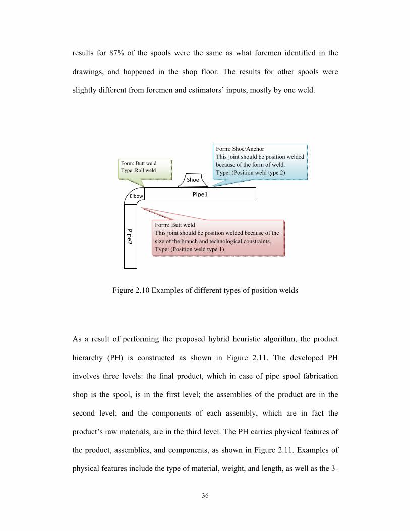
bay, product hierarchy adjusting, worker, material handling, crane, waiting,

working station, and output reports. Table 2.3 presents a brief description of these

elements.

47

Table 2.3 SPS Modeling Elements for Pipe Spool Fabrication Shop

Element Description

Worker This element represents the labourers such as fitters and welders as resources.

Waiting This element models the buffer areas where the product can wait for resources, station, and handling.

Crane The crane element models the material handling resources, such as bridge cranes, and tower crane.

Working Station

This element models a station which is performing a specific fabricating process such as cutting, fitting, or welding. In this element the priority of the products are determined based on the selected heuristic rule 

Material Handling

The material handling element, along with the crane element, models the process of handling material between stations.

Industrial Shop This element contains all elements of the fabrication shop. It also contains all scheduling heuristic rules.

Product

The product element connects the simulation model to the central database. It imports products defined by the product hierarchy model in the central database to the simulation environment. It then releases products according to their release time specified in the database (based on their expected material release date). 

Cutting Station This element represents a cutting station.

Bay All stations and resources are the sub-elements of this element. Bay is a production line of industrial fabrication. There might be several bays (or production lines) in the industrial fabrication.

Dispatch Controller

Allocates spools to each bay based on the average waiting time for processing in that bay or queue length. It also considers facility constraints for some bays such as weight, diameter, and material group.

Product Hierarchy Adjusting

Before every station is a product hierarchy adjusting element. It adjusts the product to the appropriate level of its hierarchy.

Output Reports

This element exports data collected for the fabrication plant, products, stations, resources, and the material handling system to the central database for reporting and analysis by users. The reports include production rate, resource utilization, waiting times, and start time and finish time of every operation for each product.

48

The most important element is the product element, which connects the

simulation model to the central database to import products into the simulation

model. This element then sends the products into a dispatch controller element. In

this element, the job is dispatched to the appropriate production line (bay)

according to the average waiting time, queue length, and buffer capacity, i.e.

storage capacity, of the bay. The physical and technological constraints of

equipment pieces in the bay are also modeled in the dispatch controller. In

summary, this element models the decision making process performed by

foremen and superintendents of the industrial fabrication shop, and sends out the

product to the appropriate bay. The bay element sends out the product to the

appropriate station according to the process plan of the product. Before every

operation there is a product hierarchy adjusting element to adjust the product to

the appropriate level of product hierarchy. If the operation corresponds to a higher

hierarchy of the product’s hierarchy model, the element assembles the

components to a higher level. If the operation corresponds to a lower level of

product hierarchy model, the product hierarchy adjusting element decomposes the

product to the lower level of product hierarchy.

In the station element, there is a process controller which controls the product’s

process plan and directs the product to the appropriate operation. Furthermore, the

station is capable of calculating the priority index of the jobs that are waiting to be

processed based on the selected scheduling heuristic rules. The library of

scheduling heuristic rules is available in the industrial shop element. The user can

select the appropriate heuristic rule from the available alternative in the industrial

49

shop element. For each bay there is a common buffer that is modeled by waiting

element. The storage capacity is controlled by a dispatch element, and the product

waits in the dispatch element until there is enough space in the related buffer.

Every product waits in the buffer until the resources and stations are available.

The SPS template also includes an output reports element, named “Output

Reports”, for exporting the results of the simulation experiment to the central

database. This element exports data collected for the fabrication facility, products,

stations, resources, and the material handling system to the central database for

reporting and analysis by users. The reports include production rate, resource

utilization, waiting times, as well as the start date and finish date of every

operation for each product for reporting and analysis by users. The schedule

report is generated based on the integration of the start and finish time of every

operation for each spool, the working calendar, e.g. shift hours and working days;

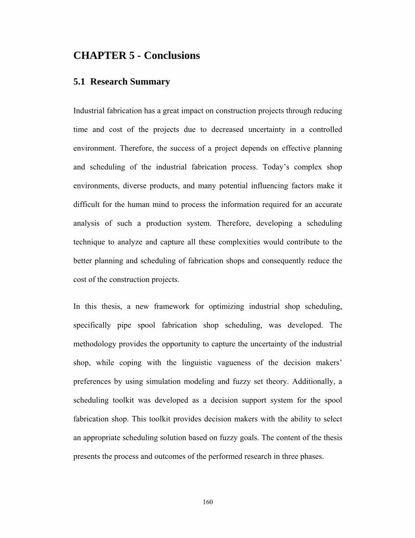
and the starting date of the simulation. Figure 2.13 depicts the described elements

and process. The implementation of the model is described in Chapter 4 of this

thesis.

50

Figure 2.13 The processes and elements of pipe spool fabrication template

Industrial Shop: • Database Address 

• Scheduling Heuristic Rules 

Dispatch Controller

Bay 1

Entities

1 2 3

Central Database (In MS ACCESS)

Maintains product (i.e. Spool) hierarchy model based on which the entities of simulation model

are generated

Product

Assembly 1

Assembly 2

Component 1 Component 1 Component 2

Product Attributes

Process Information

Product Attributes

Product Attributes

Process Information

Process Information

Simulation

Product Bay 1

Bay 1

Elements of pipe spool fabrication template

Decision making Action

Scheduling Rules

Database

Product Hierarchy Adjusting

Cutting Station

Product Hierarchy Adjusting

Working Station1

(Process 1)

Working Station2

(Process 2)

Product Hierarchy Adjusting

Material Handling

Material Handling

Material Handling

Storage…

Entity transfers in

Resources: • Number of Working Areas • Workers

Entity is sent to the queue

Are the resources available?

Select entity based on the heuristic rule

Capture the available resource

Process the entity

Release resource

Yes

51

2.6 Potential Improvements for Further Development

The following are some potential improvements to the simulation model that may

increase its accuracy and capabilities:

2.6.1 Additional Data Collection Needed to Enhance the Model

Simulation is an analysis tool used to analyze the system by producing data. The

data produced by the simulation is directly affected by the input data. If the data

that populates the model is incorrect or incomplete, the simulation model is not

usable. Because simulation is not yet an accepted part of the business practices of

most companies, these practices are not structured with simulation in mind. The

data collected within the company may be appropriate for tasks undertaken by

managers or assembly workers, but not always useful in simulation. The

simulation analyst then struggles to make use of the data collected for other

purposes (Portnaya 2004).

For example, in the current project, the durations of activities should be calculated

from their productivity (man-hours/ diameter inches) using Equation 2.4:

j

iij

nDI

tij

)(Pr ×= (Equation 2.4)

Where, tij the processing time of job i for the process j, Prij is man-hours required

per unit of the work (Productivity), DI is the amount of work unit of job i, which

is measured in terms of diameter inches of the product, and nj is the number of

workers working in the work station j.

52

However, the productivity value for each product (i.e. spool) is not the same. In

addition, the available productivity values are not separated for different activities

such as roll welding SAW welding, and position welding. Therefore, some

assumptions must be considered based on expert opinion to separate the values for

different activities. The main problem in calculating productivity is that the

available productivity value is given by diameter inches, while different factors

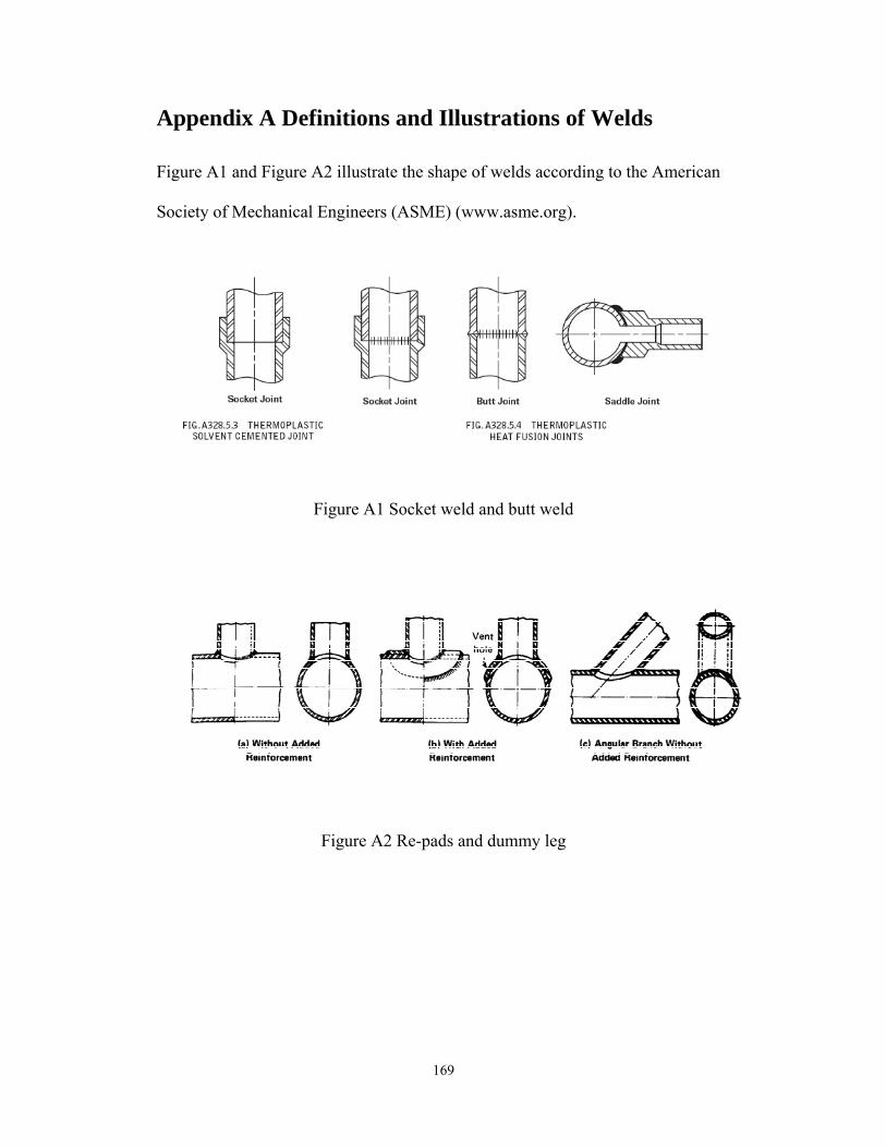
such as wall thickness, material, and different weld type (butt weld, socket weld,

dummy leg, etc.) are not considered in calculating diameter inches. In addition,

the shape and geometry of a spool influences the productivity value for each

spool. Therefore, in order to have an accurate simulation model, it is important to

estimate the productivity of each process for every spool. A fuzzy expert system

is one of the best methods for calculating productivity, since it is capable of

considering both qualitative (i.e. subjective) and quantitative (i.e. objective)

factors in estimating productivity.

2.6.2 Developing a Fuzzy Expert System to Estimate the Productivity

Productivity is usually measured by cost per unit of work or man-hour per unit of

work. Because the spool fabrication shop is labour-intensive, productivity is

measured by man-hour per unit of the work. There are several productivity

models in the literature. Lu (2000) developed a model based on ANN (Artificial

Neural Networks) to estimate the productivity of spool fabrication shops. Song

(2004) developed a productivity model for steel fabrication shops based on ANN

and incorporated it with simulation modelling. In another study (Oduba 2002), a

fuzzy expert system was developed to estimate the productivity of industrial

53

construction. Shaheen (2005) developed a fuzzy expert system to estimate the

productivity of excavation for use in simulation models.

In order to obtain more accurate results for duration of each activity for each

spool, the productivity should be measured based on the characteristics and

complexity of products and resources. A fuzzy expert system is an appropriate

method for calculating productivity, since it is capable of considering both

qualitative (i.e. subjective) and quantitative (i.e. objective) factors in estimating

productivity. A general overview of the structure of fuzzy expert system is shown

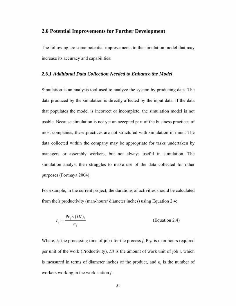
in Figure 2.14. As shown in Figure 2.14 the fuzzy expert system consists of input

interface, fuzzy inference, and output interface. The input interface accepts the

inputs and converts them into propositions that fuzzy inference can use to activate

fuzzy rules (Pedrycz and Gomide 2007). The rule base consists of a set of “if-

then” rules that describes the relationship between inputs and output. The

database stores the membership function of fuzzy sets and the value of the

parameters of rule based model. Fuzzy inference performs the inference

operations on the fuzzy rules. The output interface transforms the results of fuzzy

inference into an appropriate format, such as a fuzzy set or crisp value (Pedrycz

and Gomide 2007). As illustrated in Figure 2.14 the inputs of the fuzzy expert

system are the characteristics of resource, such as skill of workers, and the

characteristics of the products, which can be obtained from the product model.

The output of the fuzzy expert system is the productivity value, which can be used

in Equation 2.4 to calculate the duration of each activity for every product.

54

Figure 2.14 The structure of fuzzy expert system

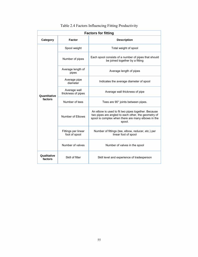
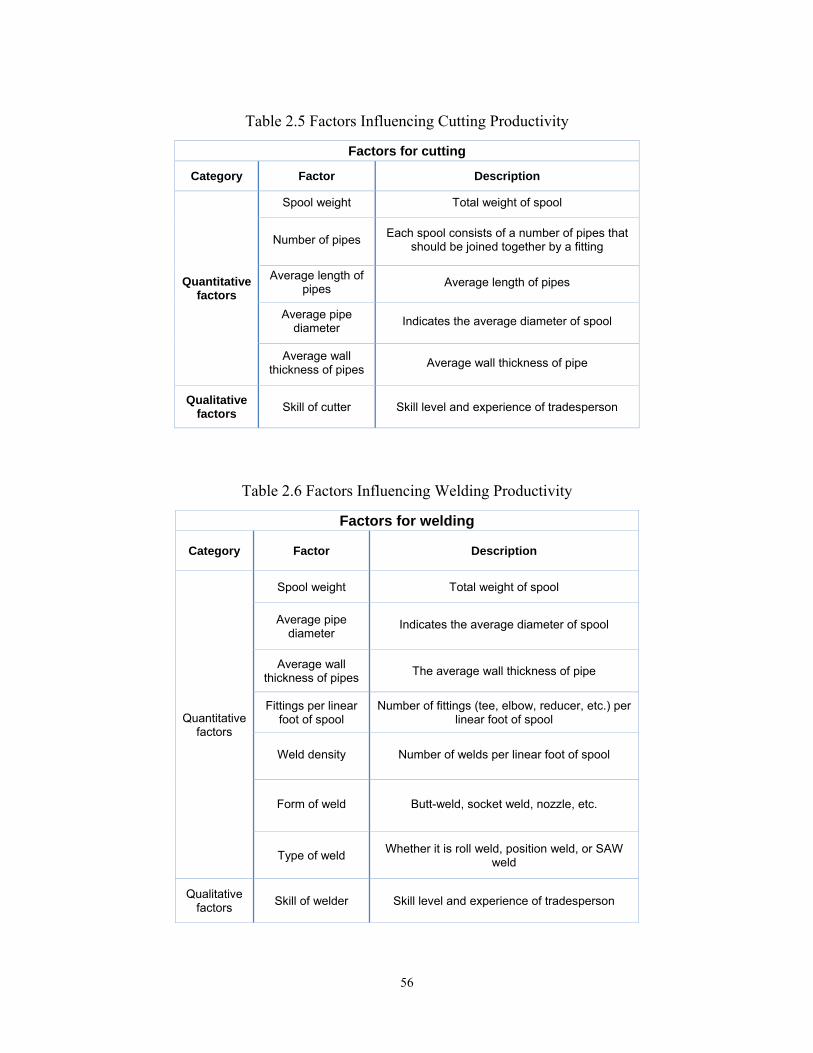
Some important factors that should be considered in developing the fuzzy expert

system for welding, cutting, and fitting activities are illustrated in Table 2.4, Table

2.5, and Table 2.6. These factors are identified by shop foremen and estimators,

and can be used as the inputs of the fuzzy expert system shown in Figure 2.14.

The quantitative factors in the above mentioned tables are the characteristics of

the jobs, and the qualitative factors are the characteristics of the resources.

Fuzzy

Inference

Data base

Rule base

Input Interface

Input 1

Input 2

Input n

.

.

.

Output InterfaceProduct

Model

Fuzzy Expert System

Productivity

Input Output

Resource Characteristics

Output

55

Table 2.4 Factors Influencing Fitting Productivity

Factors for fitting

Category Factor Description

Quantitative factors

Spool weight Total weight of spool

Number of pipes Each spool consists of a number of pipes that should be joined together by a fitting

Average length of pipes Average length of pipes

Average pipe diameter Indicates the average diameter of spool

Average wall thickness of pipes Average wall thickness of pipe

Number of tees Tees are 90° joints between pipes.

Number of Elbows

An elbow is used to fit two pipes together. Because two pipes are angled to each other, the geometry of spool is complex when there are many elbows in the

spool.

Fittings per linear foot of spool

Number of fittings (tee, elbow, reducer, etc.) per linear foot of spool

Number of valves Number of valves in the spool

Qualitative factors Skill of fitter Skill level and experience of tradesperson

56

Table 2.5 Factors Influencing Cutting Productivity 

Factors for cutting

Category Factor Description

Quantitative factors

Spool weight Total weight of spool

Number of pipes Each spool consists of a number of pipes that should be joined together by a fitting

Average length of pipes Average length of pipes

Average pipe diameter Indicates the average diameter of spool

Average wall thickness of pipes Average wall thickness of pipe

Qualitative factors Skill of cutter Skill level and experience of tradesperson

Table 2.6 Factors Influencing Welding Productivity

Factors for welding

Category Factor Description

Quantitative factors

Spool weight Total weight of spool

Average pipe diameter

Indicates the average diameter of spool

Average wall thickness of pipes The average wall thickness of pipe

Fittings per linear foot of spool

Number of fittings (tee, elbow, reducer, etc.) per linear foot of spool

Weld density Number of welds per linear foot of spool

Form of weld Butt-weld, socket weld, nozzle, etc.

Type of weld Whether it is roll weld, position weld, or SAW weld

Qualitative factors Skill of welder Skill level and experience of tradesperson

57

2.6.3 Incorporate Uncertainty in Form of Fuzzy Numbers

The output of the fuzzy expert system is usually converted to a crisp value or

fuzzy set (Pedrycz and Gommide). Therefore, if the estimation model is

developed to identify the productivity for each activity, as explained in Section

2.6.2, the output of the model will be in the form of deterministic values or fuzzy

numbers. Shaheen (2005) has integrated the fuzzy expert system and the

simulation model by converting the output of the fuzzy expert system to a crisp

value. However, the crisp (i.e. deterministic) value obtained from the output of the

expert system cannot represents the uncertainty exists in the inputs. The

uncertainty regarding the duration can be modeled using fuzzy sets.

Consequently, fuzzy discrete event simulation can be applied to use the fuzzy

output of the fuzzy expert system.

2.7 Conclusions

In this chapter, a framework is developed for modeling industrial fabrications at

the process level. The proposed framework was developed based on pipe spool

fabrication shop. This framework addresses the shortcomings of previous systems

by considering: (i) 3-D geometric attributes of the product, (ii) the type and shape

of the product components, (iii) relationships between the product components,

(iv) shop process information, and (v) constraints of the shop. Moreover, the

framework includes a scheduling engine to help the decision maker produce

feasible schedules by using an appropriate scheduling heuristic.

58

The entities of the simulation model are generated using the actual products of the

pipe spool fabrication shop, the information of which is available in database of

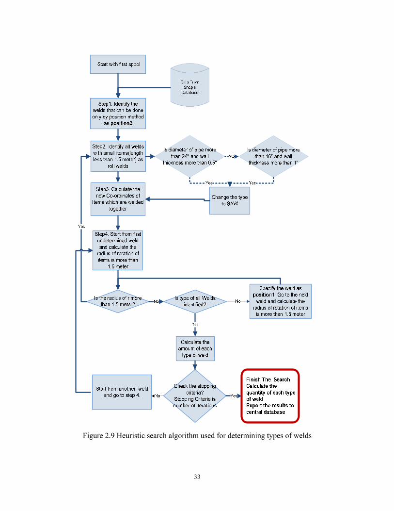
the company. A heuristic search algorithm was developed to create product model

based on the CAD drawings and database of the company. The heuristic search

algorithm considers geometric attributes of the product, the type and shape of the

product, the type and shape of the product components, shop process information,

and constraints of the shop.

59

2.8 References

AbouRizk, S. M., and Hajjar, D. (1998). “A framework for applying simulation in construction.” Canadian Journal of Civil Engineering, 25(3), 604-617.

AbouRizk, S.M. and Sawhney, A. (1993). "Subjective and Interactive Duration Estimation." Canadian Journal of Civil Engineering, CSCE, 20, 457-470.

Adeli, H., and Karim, A. (2001). Construction Scheduling, Cost Optimization, and Management—A New Model Based on Neurocomputing and Object Technologies. Spon Press, London.

Agbulos A., Mohamed Y., Al-Hussein M., AbouRizk S., and Roesch J. (2005). “Application of Lean Concepts and Simulation Analysis to Improve Efficiency of Drainage Operations.” Journal of Construction Engineering and Management, ASCE, 132(3), 291-299.

Banks J. (1998). Handbook of Simulation. John Wiley & Sons, New York, NY .

Barrie, D. S., and Paulson, B. C. (1992). Professional Construction Management, Including C.M., Design-Construct, and General Contracting. McGraw-Hill, New York, NY.

Chan, W. T., Chua, D. K. H. and Kannan, G. (1996). “Construction resource scheduling with genetic algorithms.” Journal of Construction Engineering and Management, ASCE, 122(2), 125–32.

Cheng, T., and Yan, R. (2009). “Integrating Messy Genetic Algorithms and Simulation to Optimize Resource Utilization.” Computer-Aided Civil & Infrastructure Engineering, 24(6), 401-415.

Davila Borrego, L. F. (2004). "Simulation-based scheduling of module assembly yards with logical and physical constraints." Ph.D. thesis, University of Alberta, Edmonton, Alberta.

60

Dossick, C. S., Mukherjee, A., Rojas, E. M., and Tebo, C. (2009). “Developing Construction Management Events in Situational Simulations.” Computer-Aided Civil and Infrastructure Engineering, 24(4), 1-13.

Fan, S.-L., Tserng, H. P., and Wang, M.-T. (2003). “Development of an object-oriented scheduling model for construction projects.” Automation in Construction, 12 (3), 283-302.

Farrar, J. M., AbouRiz, S., and Mao, X. (2004). “Generic Implementation of Lean Concepts in Simulation Models.” Lean Construction Journal, Volume 1, No. 1, 1-23.

Gupta, A. K., and Sivakumar, A. I. (2002). “Simulation Based Multiobjective Schedule Optimization In Semiconductor Manufacturing.” Proceedings of the 34th conference on Winter simulation, 1862-1870. Hajjar, D., and AbouRizk, S. M. (1999). "Simphony: An Environment For Building Special Purpose Construction Simulation Tools." WSC '99: Proceedings of the 31st conference on Winter simulation, ACM, New York, NY, USA, 998-1006.

Hajjar, D., and AbouRizk, S. M. (2002). “Unified Modeling Methodology For Construction Simulation.” Journal of Construction Engineering and Management, 128(2), 174–185.

Halpin, D. W. (1977). “CYCLONE: Method for Modeling of Job Site Processes.” Journal of the Construction Division, ASCE, 103(3), 489-499.

Hopp, W. J., and Spearman, M. L. (2001). Factory physics. 2nd. ed., Irwin McGraw-Hill, New York.

Jaafari, A. and Doloi, H. K. (2002). “A Simulation Model For Life Cycle Project Management.” Computer-Aided Civil and Infrastructure Engineering, Vol. 17, 162-74.

Jahangirian, M., Eldabi, T., Naseer, A., Stergioulas, L. K., and Young, T. (2009). “Simulation In Manufacturing And Business: A Review.” European Journal of Operational Research, In Press, Corrected Proof.

61

Karim, A., and Adeli, H. (1999). “CONSCOM: An OO Construction Scheduling And Change Management System.” Journal of Construction Engineering and Management, ASCE 125 (5), pp. 368–376.

Karim, A., and Adeli, H. (1997). “Scheduling/Cost Optimization and Neural Dynamics Model for Construction.” Journal of Construction Engineering and Management. 123(4), 450-458.

Kim, J. (2007). "An investigation of activity duration input modeling by duration variance ratio for simulation-based construction scheduling." Ph.D. thesis, Rutgers, The State University of New Jersey, New Brunswick, New Jersey.

Kim, K., and Paulson Jr., B. C. (2003). “Multi-Agent Distributed Coordination Of Project Schedule Changes.” Computer-Aided Civil and Infrastructure Engineering, 18 (6), pp. 412-425.

Law, A. M., and Kelton, W. D. (2000). Simulation Modeling and Analysis. McGraw-Hill, New York, NY.

Leu, S. S. and Yang, C. H. (1999). “A Genetic-Algorithm-Based Resource-Constrained Construction Scheduling System.” Construction Management and Economics, 17, 767–76.

Lluch, J. and Halpin, D. W. (1982). “Construction Operations And Microcomputers” Journal of Construction Division, ASCE, 108(CO1), 129-145.

Martinez, J. C. (1996). "Stroboscope: State And Resource Based Simulation Of Construction Processes." Ph.D. thesis, University of Michigan, Ann Arbor, Michigan.

Mohamed, Y., Borrego, D., Francisco, L., Al-Hussein, M., Abourizk, S., and Hermann, U. (2007). “Simulation-Based Scheduling Of Module Assembly Yards: Case Study.” Engineering, Construction and Architectural Management, 14(3), 293-311.

Odeh, A. M. (1992). "CIPROS: Knowledge-Based Construction Integrated Project And Process Planning Simulation System." Ph.D. thesis, University of Michigan, Ann Arbor, Michigan.

62

Pritsker, A., O'Reilly, J., and LaVal, D. (1997). Simulation with visual SLAM and AweSim. Wiley, New York.

Sadeghi, N., and Fayek, A. R. (2008). “A Framework For Simulating Industrial Construction Processes.” Proceedings - Winter Simulation Conference, art. 4736347, pp. 2396-2401

Sawhney, A. (1994). "Simulation-based planning for construction." Ph.D. thesis, University of Alberta, Edmonton, Alberta.

Sawhney, A., and AbouRizk, S. (1995). “HSM - Simulation-based Project Planning Method for Construction Projects.” Journal of Construction Engineering and Management, ASCE, Volume 121, No. 3, 297-303.

Schmidt, R. J., and Horning, D. (1990). “Scheduling Parallel Computations with Successive CPM Domains.” Computer-Aided Civil and Infrastructure Engineering, 5 (4), 251-268.

Shaheen, A. (2005). “A framework for integrating fuzzy set theory and discrete event simulation in construction engineering.” Ph.D. thesis, University of Alberta, Edmonton, Alberta.

Song, L., Wang, P., and AbouRizk, S. M. (2006). “A Virtual Shop Modeling system for Industrial Fabrication Shops.” Simulation Modelling Practice and Theory, 14(5), 649-662.

Taghaddos, H, AbouRizk, S., Mohamed, Y., and Hermann, R. (2009). “Integrated Simulation-Based Scheduling for Module Assembly Yard.” ASCE Conf. Proc. 339, 129.

Wang, P. (2006). “Production-based Large Scale Construction Simulation Modeling.” Ph.D. thesis, University of Alberta, Edmonton, Alberta.

Xu, J., AbouRizk, S. M., and Fraser, C. (2003). “Integrated Three-Dimensional Computer-Aided Design And Discrete-Event Simulation Models.” Canadian Journal of Civil Engineering, 30 (2), 449–459.

63

Zhang, H., Tam, C. M., and Li, H. (2006). “Multimode Project Scheduling Based On Particle Swarm Optimization.” Computer-Aided Civil and Infrastructure Engineering, 21 (2), 93-103.

Zhou, F., AbouRizk, S. M., and Al-Battaineh, H. T. (2009). “Optimisation Of Construction Site Layout Using A Hybrid Simulation-Based System.” Simulation Modelling Practice and Theory, 17(2): 348-363

64

CHAPTER 3 - An Optimization Framework for Multi-

Criteria Industrial Shop Scheduling

3.1 Introduction

Optimizing production scheduling has received great attention in the recent

academic literature due to its critical role in industry. It has become one of the

most important steps for improving productivity and customer satisfaction in

modern manufacturing. This chapter proposes a framework for optimization of

industrial shop scheduling with respect to multiple criteria. Fuzzy set theory is

used to linguistically assess different levels of satisfaction for the selected criteria.

Moreover, a survey of the literature related to multi-criteria scheduling is

presented in this chapter to justify the need for a new approach to multi-criteria

scheduling. This chapter also introduces fuzzy set theory and its application in

construction.

3.2 Background

3.2.1 Scheduling Optimization Methods

Production scheduling approaches to solve scheduling problems are classified into

three categories: (1) mathematical approaches, e.i. exact algorithms, such as

branch and bound, (2) meta-heuristic approaches, and (3) heuristic approaches.

The mathematical methods are only applicable to problems of smaller size

because of the NP-hard nature of the scheduling problem. An NP-hard problem is

a problem for which it is impossible to mathematically find a general solution.

65

This usually happens because of the phenomenon known as the exponential

expansion of the feasible area, which is the region containing all possible

solutions to an optimization problem. The machine scheduling problem and all its

different branches, such as shop scheduling problems, have been shown to be NP-

hard problems (Brucker 2007; Pinedo 2008; and Baker and Trietsch 2009). A

simple example of machine scheduling problems can easily illustrate the

exponential expansion of the feasible region. Given ‘n’ jobs that can be assigned

to two different machines to be processed, the possible number of different

combinations of jobs that can be assigned to each machine is 2n. Furthermore,

considering the number of possible sequences for those combinations, the size of

the feasible region, that is the number of possible solutions, will be of the order of

n!*2n. This means, for a real size problem with a multiple number of stations and

resources, the number of possible solutions grows exponentially with the number

of jobs that should be scheduled, and therefore mathematical approaches cannot

be used to solve such problems (Baker and Trietsch 2009).

Meta-heuristic approaches have been developed to overcome the mathematical

complexities of scheduling problems and to solve a wider range of scheduling

problems. In meta-heuristic methods, a modified search algorithm is employed by

utilizing an iterative generation process for developing and exploring the feasible

space in order to find a near-optimum solution (Osman and Laporte 1996). The

advantage of meta-heuristic methods is the fact that they commonly produce a

good solution that is an acceptable sequence of the jobs. However, these methods

are time-consuming for production engineers, and they should be repeated any

66

time that a change is introduced to the system. Therefore for real-size problems

heuristic methods are usually preferred. The low computational time, their

simplicity, and the fact that they can be used along with simulation models have

made heuristic methods the preferred method among practitioners and researchers

in academia and industry.

Dispatching rules, i.e. priority rules, are a class of heuristic methods, which are

commonly used in the industry because of their simplicity and practicality. The

fact that they are online scheduling methods makes them suitable for the dynamic

environment of the shop in the sense that they can react to changes in the system

setup, such as new shop arrivals and unpredicted interruptions, without

consuming too much time to reschedule. Dispatching rules are used for

prioritizing jobs and selecting the next job, which is waiting in the queue, to be

processed (Bitran and Dada 1983). Dispatching rules can be used together with

simulation models to generate a near optimum schedule. The main challenge of

using dispatching rules is that no specific rule is known to be the best consistently

for all problems, even though they are proven to produce the optimal solution for

certain small size problems. Therefore, many studies have been conducted to

identify the performance of dispatching rules for different situations (Blackstone

et al. 1982; Sabuncuoglu and Homertzheim 1992; Jones et al. 1995; Babiceanu et

al. 2005). The studies have shown that some rules perform consistently better than

others in optimizing certain objective functions (Blackstone et al. 1982). For

example, shortest processing time (SPT) optimizes the average flow time of jobs

in the shop for most situations. Nevertheless, it is still difficult to conclude the

67

general usefulness of a rule for a system without testing it. Dispatching problems

has not received enough attention in the literature (Kuo et al. 2008). Examples of

research conducted on dispatching problems in the literature are the work of

Barrett and Barman (1986), which studied the minimization of tardiness in two-

stage flow shops considering five possible dispatching rules, and the work of

Sarper and Heny (1996), which proposed a simulation approach to solve

scheduling problems for a two–stage flow shop considering six possible

dispatching rules.

The industrial shop scheduling problem studied in this research, which is

explained in Chapter 2, is a hybrid flow shop scheduling (HFS), in which a set of

n jobs are to be processed in a series of m stages with several parallel machine

optimizing a given objective function. The HFS problem is, in most cases, NP-

hard. For example, HFS restricted to two processing stages, even when one stage

includes two machines and the other one a single machine, is NP-hard (Gupta

1988). Also, the flow shop scheduling, which is the special case of HFS including

a single machine per stage, and the parallel machine scheduling, which includes a

single stage with several machines, are also NP-hard (Garey and Johnson 1979;

Ruiz and Vazquez-Rodriguez 2009). Nevertheless, the problem might be solved

polynomially for some instances with special properties and precedence

relationships (Djellab and K. Djellab 2002; and Ruiz and Vazquez-Rodriguez

2009). According to the survey carried out by Ruiz and Vazquez-Rodriguez

(2009), the largest HFS instances solved by mathematical approaches is a two-

stage regular HFS (unconstrained number of machines in stages 1 and 2) with

68

make-span criterion. This problem is solved effectively using branch and bound

(B&B), which is the preferred technique for solving HFS (Ruiz and Vazquez-

Rodriguez 2009). However, the proposed algorithm could not solve many

medium instances (20–50 jobs) (Ruiz and Vazquez-Rodriguez 2009). Moreover,

a two-stage problem with multiple identical parallel machines at each stage has

been studided by Choi and Lee (2009). They have proposed a B&B method for

the minimization of tardy jobs. Ruiz and Vazquez-Rodriguez (2009) concluded

that the exact algorithms are still incapable of solving medium and large instances

and are too complex for real world problems, despite their relative success.

Therefore, it is necessary to study non-exact but efficient heuristics. More detailed

reviews of B&B algorithms can be found in Kis and Pesch (2005).

3.2.2 Multi-Criteria Scheduling

Although most studies conducted by researchers have focused on single objective

scheduling problems, real life scheduling problems usually consist of multiple

conflicting objectives. Therefore, there has been an increasing interest in multi-

criteria scheduling during the last decade (Lei 2009). According to a survey

performed by Lei (2009), most multi-criteria scheduling problems are small size

problems, which are solved by meta-heuristic algorithms such as genetic

algorithms (GA) and ant colony optimization (ACO). Examples of multi-criteria

scheduling by meta-heuristic algorithms are frameworks introduced by Ishibuchi

and Murata (1998), Leung and Wang (2000), Kacem et al. (2002), and Petrovic et

al. (2007). In these frameworks, multiple criteria are combined into one fitness

function to conduct the iteration processes. The aforementioned algorithms are

69

not practically used for real size problems in the industry because of the

computational time of algorithms, complexity of the shop environment, and

uniqueness of jobs.

A real industrial shop involves dynamic changes of the job set, material shortage,

and uncertain environment. On the other hand, industrial shops require fast

response time and high flexibility to the changes of the production condition and

interruptions in the shop condition such as material shortage, changes in the

drawings, and arrival of rush orders. The main drawback of the meta-heuristic

optimization approaches is that the procedure of optimizing a schedule for every

job set is time consuming and impractical for real life problems (Fanti et al.

1998). It is argued that such approaches, although they improve the performance

of the shop floor, make the control problem of the shop floor more complicated

(Yang et al. 2007). In addition, the implementation of the proposed approaches in

industrial engineering literature needs a sophisticated shop floor control system

that can perform the algorithms and control the system (Yang et al. 2007), which

is not applicable in industrial construction projects. Therefore, developing a

scheduling solution that identifies a robust combinatorial dispatching rule is very

important for a dynamic shop environment. A robust combinatorial dispatching

rule that produces good performance in situations could decrease the complexity

of operational decision making and control, and provide a valuable practical tool

for real applications.

For this purpose, a new framework is proposed in this chapter to find a robust

combinatorial dispatching rule for industrial shops, specifically pipe spool

70

fabrication shops. The framework is developed using the Pareto-optimality

concept combined with fuzzy set theory for multi-criteria optimization. A

simulation model is developed using the framework described in Chapter 2 to

evaluate the performance of each combinatorial rule. The performance values

measured by the simulation model are then transformed to membership degrees in

term of the degree of closeness to the ideal solution (or the degree of satisfaction),

in which ‘1’ means the ideal solution and ‘0’ means the worst solution based on

the corresponding criteria.

3.2.3 Fuzzy Set Theory and Techniques in Construction

The concept of fuzzy set theory was introduced by Lotfi Zadeh (1965) as an

extension of the classical set theory. Fuzzy sets are sets with partial membership

function. In classical set theory, an element either belongs or does not belong to a

set (Zimmermann 1985). It is not allowed to be included in a set and its

complementary set at the same time. Fuzzy set theory allows the gradual

membership of elements to a set. This is described by the term “membership

degree,” which has a value in real interval of [0, 1]. The membership degree

indicates the degree that the elements are compatible with the properties of the

fuzzy set (Klir and Yuan 1995). Therefore, a fuzzy set provides shades of gray

rather than black and white, which is in better agreement to the human way of

thinking (Chan et al. 2009). A good example is the situation of using imprecise

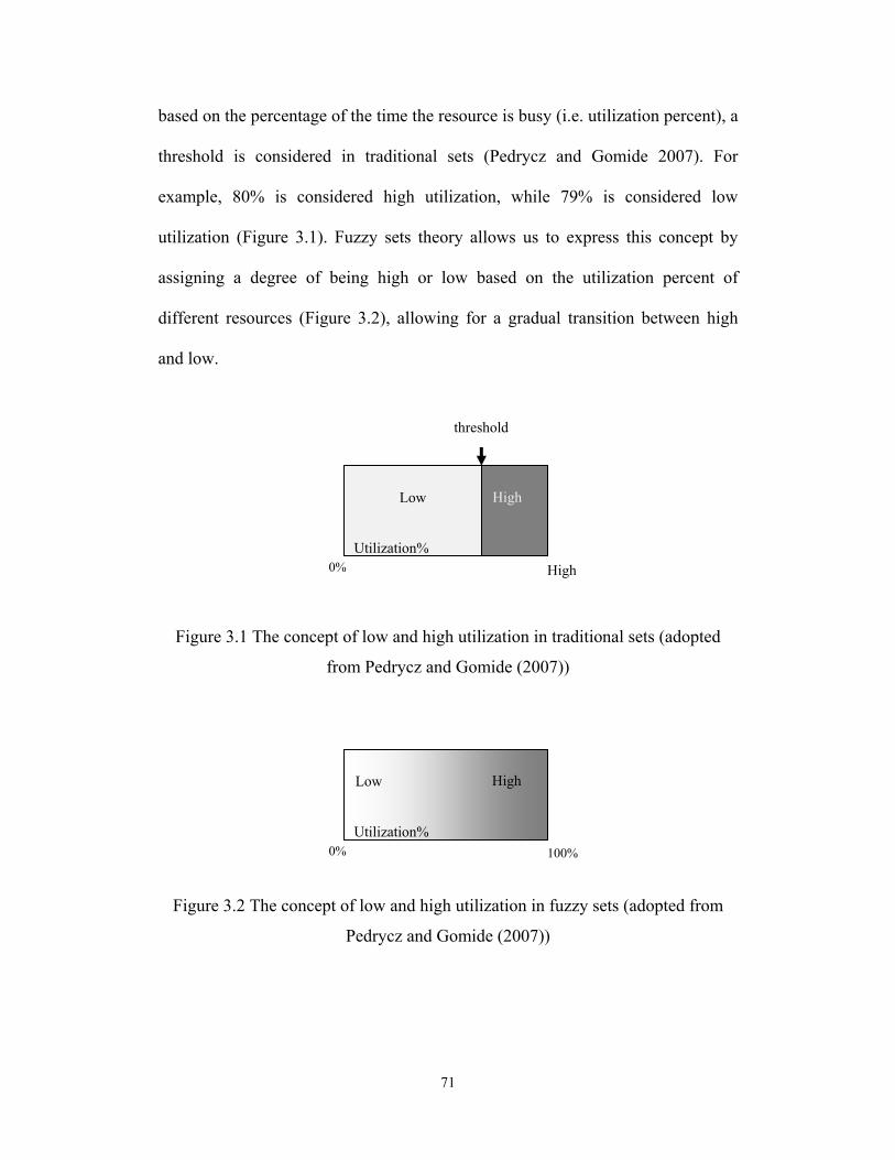
and vague propositions like "the utilization of the resource is high." In Figures 3.1

and 3.2 below, a non-fuzzy set (crisp set) and a fuzzy set are illustrated for

resource utilization. To identify whether the resource utilization is high or low

71

based on the percentage of the time the resource is busy (i.e. utilization percent), a

threshold is considered in traditional sets (Pedrycz and Gomide 2007). For

example, 80% is considered high utilization, while 79% is considered low

utilization (Figure 3.1). Fuzzy sets theory allows us to express this concept by

assigning a degree of being high or low based on the utilization percent of

different resources (Figure 3.2), allowing for a gradual transition between high

and low.

Figure 3.1 The concept of low and high utilization in traditional sets (adopted

from Pedrycz and Gomide (2007))

Figure 3.2 The concept of low and high utilization in fuzzy sets (adopted from

Pedrycz and Gomide (2007))

Low

High

100% 0% Utilization%

High

Low

High

0% Utilization%

threshold

72

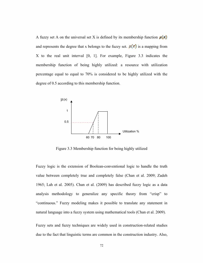
A fuzzy set A on the universal set X is defined by its membership function

and represents the degree that x belongs to the fuzzy set. is a mapping from

X to the real unit interval [0, 1]. For example, Figure 3.3 indicates the

membership function of being highly utilized: a resource with utilization

percentage equal to equal to 70% is considered to be highly utilized with the

degree of 0.5 according to this membership function.

Figure 3.3 Membership function for being highly utilized

Fuzzy logic is the extension of Boolean-conventional logic to handle the truth

value between completely true and completely false (Chan et al. 2009; Zadeh

1965; Lah et al. 2005). Chan et al. (2009) has described fuzzy logic as a data

analysis methodology to generalize any specific theory from “crisp” to

“continuous.” Fuzzy modeling makes it possible to translate any statement in

natural language into a fuzzy system using mathematical tools (Chan et al. 2009).

Fuzzy sets and fuzzy techniques are widely used in construction-related studies

due to the fact that linguistic terms are common in the construction industry. Also,

1

0.5

60 70

μ(x)

80

Utilization %

100

73

subjective nature of some variables (e.g. skill of workers), lack of data, and

uncertainty due to vagueness rather than randomness can be addressed by

applying fuzzy techniques. Some of the studies which implemented fuzzy

techniques are: predicting industrial construction labour productivity (Fayek and

Oduba 2005), integration of fuzzy set theory with continuous simulation to

modeling uncertain production environments (Dohnal 1983; Fishwick 1991; Negi

and Lee 1992; Southall and Wyatt 1988). Lam et al. (2001) developed a decision-

making model using a combination of the fuzzy optimization and the fuzzy

reasoning technique which can be applied to construction project management

problems by suggesting an optimal path of cash flow that results in minimum

resource usage. The proposed model combines quantitative and qualitative

variables, and is used for analyzing the best time to invest in a new project (Lam

et al. 2001). Furthermore, fuzzy goal programming has been used to analyze

uncertainty in optimization models (Deporter and Ellis 1990; Gungor 2001; Suer

et al. 2008).

3.2.4 Fuzzy Logic in Construction Scheduling

Fuzzy logic and fuzzy mathematical models have been used successfully in

project scheduling. For example, fuzzy set concepts were used in project

scheduling (Ayyub and Haldar 1984) to consider uncertainties in different project

settings, which provides possible completion times for each activity in a network.

Furthermore, Lorterapong and Moselhi (1996) developed a new network

scheduling method based on fuzzy sets theory for estimating of the durations of

construction activities. Using this method, the imprecise activity durations can be

74

modeled (Lorterapong and Moselhi 1996). Bonnal et al. (2004) proposed a

framework based on fuzzy sets to address the resource-constrained fuzzy project-

scheduling problem. Orodñez-Oliveros and Fayek (2005) formulated a new tool

to create an updated schedule and to evaluate the consequences of delays on the

project.

Fuzzy mathematical models have been used in multi-criteria project scheduling.

For instance, fuzzy goal programming and critical path methods (CPM) were used

to minimize total cost, total completion time, and total crashing cost in project

scheduling (Wang and Liang 2004). Moreover, fuzzy genetics algorithm was used

to optimize the multi-skilled labour allocation in the construction projects (Tong

and Tam 2003). Castro et al. (2009) used fuzzy mathematical models integrated

with critical path method (CPM) to optimize a construction project’s schedule

with respect to project completion time and crashing costs.

The application of fuzzy set theory and fuzzy techniques in the area of industrial

construction is limited. However, there are some fuzzy-based methods developed

for manufacturing and industrial systems that can be used in the area of industrial

construction. For example, Petroni and Rizzi (2002) developed a fuzzy logic-

based methodology to rank shop floor dispatching rules. The drawbacks of this

approach are, firstly, that the methodology relies solely on expert judgment to

identify the performance of a dispatching rule, and secondly, that only a few

simple dispatching rules are considered in this method.

75

3.3 Proposed Framework for Identifying Optimum Combinatorial

Dispatching Rule

The overall architecture of the proposed framework is illustrated in Figure 3.4. As

illustrated in Figure 3.4, the proposed framework consists of 4 phases through

which a robust composite dispatching rule is identified. In the first phase, the

primary criteria on which the performance of the shop should be optimized is

identified. Then a membership function for each criterion is developed to measure

the distance between the performance of each combinatorial dispatching rule

identified by the simulation model and the ideal value of corresponding criterion.

The second phase of the proposed framework focuses on designing new

combinatorial rules. In this phase, appropriate dispatching rules are identified, and

new combinatorial dispatching rules are developed in addition to common

combinatorial rules in the literature. In the third phase, first a random set of jobs is

selected and the performance of each predefined dispatching rule is measured

using the simulation model. Then the candidate dispatching rules are chosen using

the concept of Pareto-optimality. Each rule in the Pareto frontier is selected as a

candidate rule. This process is repeated several times using different sets of

random jobs to obtain all possible candidate rules for further analysis. In phase

four, all candidate rules are clustered based on their performance value for each

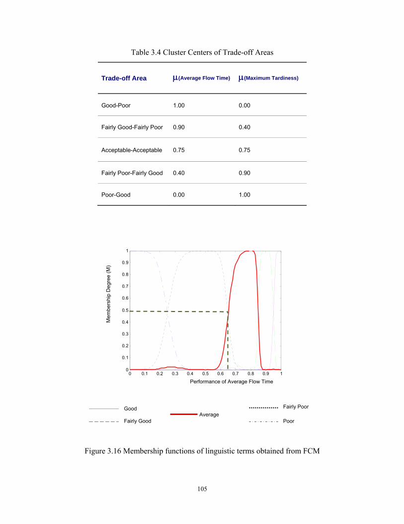
primary criterion. The data are clustered using fuzzy C-means clustering (FCM).

The clustering process identifies different classes of trade-off, or zones of

compromise, between primary criteria in terms of linguistic variables such as

poor, fairly poor, acceptable, fairly good, and good. As a result, the decision

76

maker can choose one of the zones based on his or her preferences. Finally, the

statistics of each rule are collected in the fifth phase in order to select a robust

solution based on the preferences of the decision maker. The remainder of this

chapter is dedicated to further discussion of each phase of the proposed approach.

77

Figure 3.4 The proposed framework for multi-criteria industrial shop scheduling

Phase 1 Primary criteria selection

Phase 2 Designing new composite rules

Simulation Model

Phase 3 Selecting candidate combinatorial dispatching rules

Simulation

Pareto-Optimality

Candidate combinatorial dispatching rules

Selected trade-off zone

by user

Phase 4 Selecting appropriate Dispatching Rule for each trade-off area

Fuzzy C-means clustering

Determining appropriate rule for each cluster, which represents a trade-off between multiple criteria

Robust combinatorial dispatching rule

78

3.4 Phase 1: Identifying Primary Criteria for Scheduling

The performance of an applied dispatching rule is evaluated by the degree to

which it optimizes a given scheduling criterion such as production throughput,

make-span, utilization, tardiness, and lateness (Chan et al. 2002). The lateness of

the job (i.e. product) j in a given schedule σ, Lj (σ),is defined as the difference

between the completion time of job j, Cj (σ), and due date of job j, dj, as shown in

Equation 3.1.

Lj (σ) = Cj (σ) − dj (Equation 3.1)

The value of lateness is ‘0’ when the job is on time, negative when the job is

early, or positive when the job is late. The tardiness of job j in schedule σ, Tj (σ),

is defined as the maximum of lateness and ‘0’, which is obtained from Equation

3.2.

Tj (σ) = max { Cj (σ) − dj, 0} = max {Lj (σ), 0} (Equation 3.2)

The difference between lateness and tardiness lies in the fact that the value of

tardiness is never negative (Pinedo 2008). The opposite of tardiness for job Jj is

earliness, Ej (σ), which is defined as:

Ej (σ) = max {dj − Cj (σ), 0}. (Equation 3.3)

According to surveys (Smith et al. 1986; Gupta et al. 1990; and Chan et al. 2002),

the most important scheduling criteria in the manufacturing systems, which are

also used in industrial construction projects, are:

79

• Minimizing (weighted) average lateness (w

L )

∑

∑

=

== n

jj

j

n

jj

w

w

LwL

1

1)(

)(σ

σ (Equation 3.4)

• Minimizing (weighted) average tardiness (w

T )

∑

∑

=

== n

jj

j

n

jj

w

w

TwT

1

1)(

)(σ

σ (Equation 3.5)

• Maximizing average flow time ( F )

∑=

=n

jjCnF

1)(1)( σσ (Equation 3.6)

• Minimizing maximum lateness (Lmax) :

)(max)(max σσ jjLL = (Equation 3.7)

• Minimizing maximum tardiness (Tmax)

)(max)(max σσ jjTT = (Equation 3.8)

• Minimizing maximum completion time, or make-span (Cmax)

)(max)(max σσ jjCC = (Equation 3.9)

80

• Total (weighted) flow time (w

F )

)()(1

σσ j

n

jj

wCwF ∑

=

= (Equation 3.10)

• Maximizing machine utilization (U%)

Where, n is the number of jobs, i.e. products, j ∈ {1, 2, …, n}, and σ is a possible

sequence of jobs, i.e. possible schedule. Given the schedule σ, the starting time of

job j in σ is denoted as Sj (σ), Cj (σ) is used to denote its completion time, and dj is

its due date. Respectively, wj is the weight of job j in terms of the importance of

the job j. Besides, Lj (σ) is the lateness of job j obtained from Equation 3.1, and

Tj (σ) is the tardiness of job j in σ calculated by Equation 3.2. The indicator

function Uj (σ) is used to identify whether job j is tardy (then Uj = 1) or on time

(then Uj = 0) in σ. Correspondingly, )(σw

L is the weighted average lateness,

)(σw

T is the weighted average tardiness, )(σF is average flow time, )(max σL is

maximum lateness, )(max σT is maximum tardiness, )(max σC is make-span, and

)(σw

F is total weighted flow time. Resource utilization (U%) is usually measured

as the percentage of time that a resource is busy.

In addition to the aforementioned criteria, total earliness, which is defined in

Equation 3.3, might be of interest due to inventory costs or limited inventory

capacity. The emphasis on considering average earliness as an objective function

started with the growing interest in just-in-time (JIT) production, which supports

the idea that earliness should be discouraged (Baker and Trietsch 2009). In JIT

81

production, a job that is completed earlier than its due date should be held in

inventory and delivered on its due date. Therefore, finishing a job earlier than its

due date results in inventory carrying costs. For example, spools that have been

completed in a pipe spool fabrication shop should be usually delivered to the

module yard. The due date of the spools is the start time of processes of the

module yard. Consequently, spools that are ready earlier than their due date

should be held in inventory until they can be used in module yard.

3.4.1 Primary Criteria Selection

The ultimate objective of every decision maker is to improve the performance of

the shop floor in all aspects such as resource utilization, production throughput,

and tardiness or lateness of the jobs. However, this objective is not practicable on

the operational level of decision making in scheduling. Figure 3.5 and Figure 3.6

show examples of conflict between some criteria. In Figure 3.5, the performance

of two conflicting criteria, including average flow time and maximum tardiness,

using different dispatching rules are shown. Dispatching rules used in this

illustration are shortest processing time (SPT), earliest due date (EDD), and

minimum slack time (SLACK), all of which are explained in Chapter 2. As can be

seen in Figure 3.5, minimizing the average flow time, which increases the

production throughput, leads to a high maximum tardiness. Figure 3.6 illustrates

the performance of average flow time and make-span using different dispatching

rules. Dispatching rules in this example includes shortest remaining processing

time (SRPT), shortest imminent processing time (SI), longest processing time

(LPT), longest remaining processing time (LRPT), shortest remaining processing

82

time per imminent processing time (RPT/I), fewest remaining operations (FRO),

earliest due date (EDD), and minimum slack (SLACK). All aforementioned

dispatching rules are explained in Chapter 2. Figure 3.6 shows that minimizing

the average flow time results in a higher make-span. Therefore, it is difficult to

simultaneously satisfy these conflicting criteria.

Figure 3.5 Simulation results of applying three simple dispatching rules on a

spool fabrication shop (maximum tardiness vs. average flow time)

0.0

20.0

40.0

60.0

80.0

SRPTEDD

Slack

Average Folw time

Maximum Tardiness

hours

83

Figure 3.6 Simulation results of applying eight simple dispatching rules on a

spool fabrication shop (make-span vs. average flow time)

Multiple runs of the simulation model of a pipe spool fabrication showed that the

average flow time is correlated with the weekly production, which means that

both of them can be optimized simultaneously. Correspondingly, make-span, total

tardiness, and maximum tardiness are optimized concurrently. Table 3.1 shows

the correlation matrix of criteria, which is calculated using the simulation results

for different dispatching rules. In Table 3.1, the correlation coefficient indicates

the strength and direction of a linear relationship between two criteria. In general

statistical practice, correlation, or co-relation, refers to the departure of two

variables from independence, although it does not imply causation. If two criteria

are strongly correlated with each other, it is unnecessary to use both criteria in

scheduling optimization since addressing one of them results in acceptable results

for both criteria. The negative correlation between two criteria states that they are

0.010.020.030.040.050.060.070.080.090.0100.0

SRPT SI LPT LRPT RPT/I FRO EDD Slack

Ave. Folw time Make Span

hours

84

conflicting with each other. Based on the results shown in Table 3.1, the criteria

are categorized into three groups, as shown in Table 3.2. Two criteria are in the

same group if the correlation between them is more than 0.7. The criteria in each

group are optimized simultaneously and therefore, one criterion from each

category can represent all criteria for that category in the scheduling optimization

problem.

Table 3.1 The Correlation Matrix of Scheduling Criteria for the Pipe Spool Fabrication

Ave

. Flo

w ti

me

Mak

e-S

pan

Max

. Tar

dine

ss

No.

of T

ardy

Job

s

Tota

l Tar

dine

ss

Tota

l Ear

lines

s

Mea

n Ta

rdin

ess

Ave

. Res

ourc

e U

sage

Ave. Flow time - -0.4 0.0 0.8 0.5 -0.9 0.2 0.7

Make-Span - - 0.6 -0.4 -0.2 0.5 0.2 -0.6

Max. Tardiness - - - 0.1 0.7 0.1 0.8 -0.3

No. of Tardy Jobs - - - - 0.5 -0.9 0.3 0.6

Total Tardiness - - - - - -0.7 0.7 0.4

Total Earliness - - - - - - 0.0 -0.8

Mean Tardiness - - - - - - - -0.3

Ave. Resource Usage - - - - - - - -

In the first step of the first phase of the proposed scheduling framework, a sub-

category of the criteria presented in the earlier section should be selected by the

user. The user, who can be an industry practitioner or an academic researcher, can

choose a subset of criteria to be used as the objective functions for the

85

optimization problem. For example, minimization of maximum tardiness and

minimization of average flow time are two main objectives that are important for

the coordinator of a pipe spool fabrication shop. The total earliness is used when

there are limitations in the inventory (such as limitation of the space or cost) and,

therefore, JIT scheduling is of interest.

Table 3.2 Groups of Correlated Criteria

Group 1 Group 2 Group 3

Average Flow time

Number of Tardy Jobs

Average Resource Utilization

Make-Span

Maximum Tardiness

Total Tardiness

Mean Tardiness

Total Earliness

3.4.2 Fuzzy Multiple Performance Measure

The fact that the value of each criterion belongs to a different range of variables

makes it very difficult to evaluate and compare the solutions. For example, the

value of resource utilization is normally measured in terms of the percentage of

the time the resource is being used; therefore, it is shown by a number between

‘0’ and ‘100,’ while the value of make-span, average flow time, and maximum

tardiness are measured in days and belong to different ranges. Table 3.3 shows an

example of the range of values for pipe spool fabrication; the numbers in Table

3.3 are scaled for confidentiality purposes. In addition, some parameters, such as

utilization, should be maximized, while some objectives, such as average flow

86

time and make-span, should be minimized. Therefore, the concept of fuzzy sets

(Bellman and Zadeh 1970) can be used to associate a membership degree with

each value indicating the degree of satisfaction of the solution for the

corresponding criterion.

Table 3.3 Range of Different Criteria for Pipe Spool Fabrication

  

Ave

rage

Flo

w ti

me

(Day

s)

Mak

e-S

pan

(Day

s)

Max

imum

Tar

dine

ss

(Day

s)

Num

ber o

f Tar

dy

Jobs

Tota

l Tar

dine

ss

(Day

s)

Tota

l Ear

lines

s (D

ays)

Aver

age

Res

ourc

e U

tiliz

atio

n (%

)

Minimum Value 6 40 10 2 27 3156 70

Maximum Value 25 45 35 12 300 4094 95

Bellman and Zadeh (1970) used fuzzy sets to represent criteria and constraints to

combine different performance measures in multi-attribute decision making. Let

D = {D1, D2, …, Dn} be a set of alternative dispatching rules and f = {f1, f2, …, fc}

be a set of criteria (or objective functions), where c is the number of criteria, and

fq is the value of qth criterion. Considering Aq as the subset of the feasible values

for the qth criteria, each dispatching rule in D, Di, is associated with a vector

μ(Di)=( μ1(Di), μ2(Di), …, μq(Di),…, μc(Di)), where μq(Di) is interpreted as the

degree to which the criterion q is satisfied by Di in the subset Aq. Membership

values (μq(Di)) are between 0 and 1, where a value of 0 indicates no membership,

87

which is equivalent to no satisfaction, and a value of 1 indicates full membership,

which is equivalent to full satisfaction.

The membership function of feasible values for each criterion is shown in Figure

3.7 and Figure 3.8. In this example trapezoidal membership functions are used

(Zimmermann 1987). In Figure 3.7 and Figure 3.8, *qf is the ideal value of the

criterion q, and Hqf is the unacceptable value of criterion q. The membership

function for fuzzy sets shown in Figure 3.7 and Figure 3.8 are formulated as

shown in Equation 3.11 and Equation 3.12, respectively.

⎪⎪⎪

⎩

⎪⎪⎪

⎨

⎧

≤

≤≤−

−

≤

=

H

H

H

H

qq

qqqqq

qq

qq

iq

ff

fffff

ff

ff

D

0

1

)( **

*

μ (Equation 3.11)

⎪⎪⎪

⎩

⎪⎪⎪

⎨

⎧

≤

≤≤−

−

≤

=

*

**

1

0

)(

qq

qqqHqq

qq

qq

iq

ff

fffffff

ff

DH

H

H

μ (Equation 3.12)

88

Figure 3.7 Membership function of acceptable values for minimization of criteria

q

Figure 3.8 Membership function of acceptable values for maximization of criteria

q

0

0.2

0.4

0.6

0.8

1

fq*

Criteria q that should be Minimized

Value(f(q))

μ(q)

0

0.2

0.4

0.6

0.8

1

fqH fq*

Criteria q that should be Maximized

Value(f(q))

μ(q)

*qf

Hqf

Hqf

*qf

89

3.5 Phase 2: Combinatorial Dispatching Rules

The concept of combinatorial dispatching rules is to combine more than one

parameter to produce better results. The parameter is usually referred to as the

attribute of the job or station. Examples of parameters referring to attributes of the

jobs are total processing time, due date, and slack. The average waiting time or

queue length are examples of parameters referring to the attribute of a station.

Simple dispatching are functions of a single parameter, which address one

criterion. For example, as shown in Figure 3.5 and Figure 3.6, shortest imminent

processing time (SI) optimizes average flow time, while earliest due date (EDD)

and minimum slack (SLACK) rule optimize the maximum tardiness and make-

span simultaneously. Studies on the combinatorial dispatching rule in construction

project scheduling are limited. So far, two examples of combinatorial dispatching

rule have been introduced in the literature (Bhaskaran and Pinedo 1992; Pinedo

2008): the cost over time (COVERT) rule and the apparent tardiness cost (ATC).

The formulation of COVERT and ATC are given in Equation 3.13 and Equation

3.14 (Vepsalainen and Morton 1987). Both ATC and COVERT rules are a

combination of slack and processing time parameters. In Equation 3.13 and

Equation 3.14, processing time and slack of job j is denoted by tj and uj;

respectively t represents average processing time. In these equations the scaling

factor, k, is used to weight the slack parameter. Slack of job j is calculated by

Equation 3.15, in which di and p represent the due date of job j and the present

time.

90

tkutk

tZ j

jj ×

−××=

)(1 (Equation 3.13)

))(

exp(1tk

ut

Z j

jj ×

−= (Equation 3.14)

ptdu jjj −−= (Equation 3.15)

Scheduling performance of every combinatorial dispatching rule depends on their

scaling factor values (Pfund et al. 2008; Chen et al. 2007). For example, the

performance of ATC rule using different values of k is illustrated in Figure 3.9 for

a spool fabrication shop. As shown in Figure 3.9, the satisfaction degree of each

criterion varies for different k values in ATC rule. Small values of k make the

slack parameter more influential and therefore it results in a high satisfaction

degree for sum of the tardiness and low satisfaction degree for average flow time,

while large values of k increase the weight of processing time and therefore make

the SPT rule more important. Consequently, a large value of k results in a high

degree of satisfaction for average flow time.

91

Figure 3.9 Performance of ATC rule with different k values

In addition to the two combinatorial rules in the literature, three new

combinatorial rules are designed and introduced in this research by defining a

combination of a set of parameters with relative weights as shown in Equation

3.16, Equation 3.17, and Equation 3.18. The relative weights, indicated by w1 and

w2 in each equation, identify the contribution of different parameters in the rule;

moreover, Zj, indicates the priority of job j. The higher values of Zj indicate the

higher priority of the job j. Finally, processing time, due date, slack, and critical

ratio of job j are denoted by tj, dj, uj, and CRj. The critical ratio of job j, CRj, is an

index calculated by dividing the time remaining until due date by the work time

remaining as shown in Equation 3.19. Each parameter should be normalized over

interval [0, 1] to be applied in the same magnitude in the equation. Therefore, the

exponential function is used to smoothly normalize each parameter based on the

equation of the ATC rule (Vepsalainen and Morton 1987). Negative exponential

0.0

0.2

0.4

0.6

0.8

1.0

1 2 3 4 5 6 7 8 9 10

Sum of T (Tardiness)

Ave. Flow time

0.3   0.4 0.5  0.8 1.3 1.5 1.6 6.8 11.6 11.9              0.3   0.4 0.5  0.8 1.3 1.5 1.6 6.8 11.6 11.9              K

μ(q)

k 

92

function is a non-linear method for normalization that is used to smoothly

normalize the data set (Lin et al 2005). Respectively, k1 and k2 are constant values

for normalization.

))(

exp())(

exp(2

21

1 kt

wkd

wZ jjj

−×+

−×= (Equation 3.16)

))(

exp())(

exp(1

21

1 kt

wku

wZ jjj

−×+

−×= (Equation 3.17)

))(

exp())(

exp(2

21

1 kt

wkCR

wZ jjj

−×+

−×= (Equation 3.18)

∑∈

−=

Sjij

ij

t

pdCR (Equation 3.19)

As discussed earlier, due date in the scheduling criteria can be classified in three

groups, and the criteria in each group can be optimized simultaneously. Equation

3.16, Equation 3.17, and Equation 3.16 are the weighted sum of two parameters,

where the first parameter in each equation is usually used to satisfy the criteria in

group1, including average flow time, number of tardy jobs, and average resource

utilization. The second parameter in each equation is for satisfying criteria in

group2, including make-span, maximum tardiness, total tardiness, and mean

tardiness. Total earliness, which is in group3, is not of the interest in this study,

because most industrial shops in Alberta do not have storage limitations.

Using ATC, COVERT, and the three new proposed combinatorial dispatching

rules with different weights, four hundred rules are designed for scheduling.

93

Several simulation runs on the pipe spool fabrication showed that the ATC rule

outperforms the COVERT rule, and the performance of the ATC rule is better

than COVERT regarding to all criteria. Therefore, the COVERT rule was ignored

and the number of rules was decreased to three hundred rules. Using the proposed

dispatching rules and ATC rule together results in covering more compromise

solutions on the Pareto- optimal frontier rather than using only ATC rule, as

illustrated in Figure 3.10. Figure 3.10 shows that the proposed rules are more

effective than ATC as they can span a wider area and stretch the Pareto frontier.

The COVERT rule does not appear on the Pareto frontier, since its performance

was dominated by the ATC rule.

Figure 3.10 Performance of ATC rule and proposed dispatching rules for spool

fabrication shop (Pareto frontier)

0.2

0.4

0.6

0.8

1.0

0.2 0.4 0.6 0.8 1.0

ATC Rule Proposed Rules All Together

μ (Ave. Flow Time)

μ (Max. Tardiness)

94

3.6 Phase 3: Identifying Candidate Rules

The principal of Pareto-optimality is used in multiple objective optimization

problems. Consider a set of several criteria by c = {c1, c2, …, cn}; correspondingly,

the satisfaction degree of the criteria is shown by μ = { μ 1, μ 2, …, μ n}, where μ 2

is the satisfaction degree of criterion c2 indicating the performance value of

criterion c2. With respect to several, i.e. more than one, criteria, if it is not

possible to increase the performance value of one criterion without decreasing the

performance value of other criteria by applying each dispatching rule, a set of

solutions that are feasible and not better than one another can be obtained.

Although these solutions are better than each other with respect to identical

criterion, no solution is superior to others with respect to all criteria. These

solutions are Pareto-optimal and are called a Pareto-optimal set and establish the

Pareto frontier. If a solution is Pareto optimal (Ehrgott 2005), it is called a non-

dominated point. On the other hand, a solution is called dominated if some other

solutions would make at least one criterion better off without compromising any

other criterion. In order to identify the Pareto frontier, the non-dominated solution

in set D, where D indicates the set of all solutions, should be identified. d̂ is

Pareto optimal if the following conditions are satisfied:

There is no d  D such that μq(d) ≥μq( d̂ ) for q = 1, . . . , n and μi(d) >μi( d̂ )

for some i {1, . . . , q}

95

Figure 3.11 shows an example to illustrate the concept of Pareto-optimality

graphically; c1 and c2 are two criteria considered in this example, the satisfaction

degree of which are denoted by μ 1 and μ 2; as Figure 3.11 shows ‘C’ is not in the

Pareto-optimal set because ‘A’ is superior to ‘C’ regarding both criteria as flows:

μ1(A) > μ 1(C), and μ 2(A) > μ 2(C)

Accordingly, ‘C’ is dominated by ‘A’. On the contrary, ‘A’ and ‘B’ are both

Pareto optimal. A is better than B with respect to c2, while schedule B is better

than A with respect to c1.

Figure 3.11 Example of Pareto-optimal set

μ 1

A

CB

μ 2

μ 1(B)

μ 2(A) > μ 2(B) and μ 1(B) > μ 1(A) → ‘A’ and ‘B’ are Pareto-Optimal

Pareto set Dominated solutions

μ 2(A)

μ 2(B)

μ 1(A)

96

Simulation models can be used to test different scenarios for a system. In this

framework, simulation modeling is applied for identifying candidate rules.

Candidate rules are rules that are in the Pareto frontier for each simulation

experiment. The objective of this phase is to reduce the number of alternative

dispatching rules by disregarding the rules that do not appear in the Pareto frontier

set in any simulation experiment. In this step, a database consisting of a set of

candidate dispatching rules and their performance values is constructed.

Figure 3.12 illustrates a summary of the proposed approach. As indicated in

Figure 3.12, the approach includes two loops. The external loop models multiple

scenarios by selecting different sets of spool in multiple time horizons of the shop.

In each scenario, all alternative rules are tested, and their performance for each

criterion is measured using proposed fuzzy sets (Equation 3.11 and Equation

3.12) through the internal loop. As a result, the rules in the Pareto optimal set are

added to candidate rules.

97

Figure 3.12 Generating candidate dispatching rules

Is the Rule in Pareto Frontier?

Yes

Generate Scenario

Experiment with Simulation Model

Store the results, scenario, dispatching rule, and

performance

Add the Dispatching rule to Candidate rules

Repeat m times

Yes

No

Finish all dispatching rules?

Select Dispatching rule Select next dispatching rule

Database of Candidate Dispatching Rules: • Satisfaction degree of each dispatching rule for

each criterion for every scenario.

NO

External Loop

Internal Loop

Transform the performance values to fuzzy satisfaction degree using Equation 3.11

and Equation 3.12

Output

98

Figure 3.13 illustrates the results of a sample scenario, which includes two

objective functions. As a result of this phase, a knowledge base, including a set of

candidate dispatching rules and the statistics of the performance of each rule

under different scenarios, is developed. The framework of developing the

simulation model is described in Chapter 2. This framework is applied using

VB.NET programming and the simulation model, the development of which is

explained in Chapter 2. The results of each simulation run are exported

automatically to an Excel file. The Pareto-optimal set is automatically identified

in the Excel sheets through a VBA macro. The program can determine the Pareto

set with respect to the criteria selected by the user. The implementation of the

algorithm will be explained through a case study in Chapter 4.

Figure 3.13 Pareto optimal set for a sample scenario

0.000

0.200

0.400

0.600

0.800

1.000

1.200

0.000 0.200 0.400 0.600 0.800 1.000 1.200

Average

 Flow Tim

e

Maximum Tardiness

Dominated Priority rules Pareto Frontier

99

3.7 Phase 4: Selecting a Compromise Solution

In this phase of the framework, the structure of the data set that has been obtained

in previous phases is identified in terms of the trade-off areas between the primary

criteria. Each area represents a linguistic relationship between the solutions in that

area and the corresponding criteria, i.e, the performance of each solution on the

related criterion. Figure 3.14 graphically demonstrates the concept of trade-off

area on a Pareto frontier for two criteria, c1 and c2, the performance of which are

shown by μ1 and μ2. Five trade-off areas are considered as an example in Figure

3.14, including poor-good, fairly poor-fairly good, acceptable-acceptable, fairly

good- fairly poor, and good-poor. This approach helps to consider changes in the

performance of each dispatching rule in different scenarios when selecting the

appropriate dispatching rule. Each trade-off area is represented by a linguistic

term. The membership function of each linguistic term can be developed using

expert judgment or numerical methods such as Fuzzy C-Means clustering (FCM)

(Pedrycz and Gomide 2007). In this framework, FCM is used to group the Pareto

frontier into the five aforementioned areas, and to determine the membership

function of each linguistic term. The membership grade of each data point in each

area is also determined using FCM.

Fuzzy clustering is commonly used to deliver comprehensive information about

the structure in numeric data (Bezdek 1981; Pedrycz 2005; Pedrycz and Gomide

2007). Fuzzy clusters form a granular representation of data (Zadeh 1996, Zadeh

2005, Pedrycz 2009), which helps categorize the data into groups that better

100

represent the distribution of the data. In fuzzy clustering, each data point is

assigned a membership grade with respect to each cluster so that the sum of those

membership grades for each data point equals one. The membership grade of an

individual data point with respect to a cluster is an indicator of the position of that

data point relative to the center of the cluster within the structure of the data.

Figure 3.14 Trade-off areas on a Pareto frontier

There are two main reasons to use fuzzy clustering for the set of data that is the

outcome of the previous phases of the proposed. The first is to convert the

structure of the data into a linguistic representation with which the end-user in the

industry can easily interface. The second reason is that each dispatching rule is

μ2

Acceptable Fairly Good

Good Fairly Poor

Poor

Acceptable

5

μ1

1

4

2

3

Fairly G

ood G

oodFairly Poor

Poor

101

represented by more than one data point, where each data point represents the

performance of the dispatching rule in a different scenario (i.e. set of spool). In

such a situation, the extent of belonging to the Pareto frontier cannot be

represented by a crisp number or by a statistical moment, which only indicates the

probability of being on the Pareto frontier without considering the proximity of

the data points to the Pareto frontier. Using fuzzy C-means clustering together

with probability of fuzzy event can help to address the aforementioned problem.

3.7.1 Fuzzy C-Means Clustering

Fuzzy C-Means clustering (FCM) is one of the most common methods for

determining the structure of data. It is also used to determine membership

functions based on numeric data. According to Pedrycz and Gomide (2007), with

a collection of an N-dimensional data set, which in our case is a collection of

alternative dispatching rules, {Xk}, k= 1, 2, 3, …, N, Fuzzy C-Means clustering is

used to identify the structure of the data set by determining a collection of C

clusters with respect to minimization of the objective function formulated in

Equation 3.20, representing the sum of the squared distances of each data point

from cluster centers being regarded as prototypes.

2

1 1ik

C

i

N

k

mik VXuQ −= ∑∑

= =

(Equation 3.20)

In Equation 3.20, V= {V1, V2, … Vc} are the n-dimensional prototypes of c

clusters (or cluster center); || . || represents the distance between Xk and Vi, and m

is the fuzzification coefficient, which is usually a number greater than ‘1’. The

102

fuzzification coefficient determines the fuzziness of the resulting clusters. As m

approaches ‘1’, the partition becomes hard, while by increasing m, m →∞, the

partition becomes fuzzy. Respectively, U=[uik] represents a partition matrix of

allocating the data to corresponding clusters, which satisfies the following

properties:

],1,0[∈iku (Equation 3.21a)

,11

=∑=

c

iiku (Equation 3.21b)

,01

nuN

kik << ∑

=

(Equation 3.21c)

Where uik represents the membership degree of Xk to prototype Vi.

The FCM algorithm introduced by Pedrycz and Gomide (2007) is used to cluster

the data points into a number of groups and determine the membership degree of

each data point to each cluster. The algorithm includes the following steps:

1. Choose a value for c, m, and ε, a small positive constant.

2. Generate a random fuzzy C-partition U0 and set the iteration number t= 0.

3. Given the membership values, U0, the prototypes are calculated by

Equation 3.22.

∑

∑

=

== N

k

mtik

N

kk

mtik

ti

u

XuV

1

)(

1

)(

)(

)(

)( (Equation 3.22)

4. Given the new prototypes )(tiV the updated membership values )1( +t

iku are

calculated by Equation 3.23.

103

)1(2

12)(

2)(

)1( 1−

=

+

∑⎟⎟⎟

⎠

⎞

⎜⎜⎜

⎝

⎛

−

−=

mc

j tjk

tik

tik

VX

VXu (Equation 3.23)

5. Repeat Step 3 and step 4 until the predefined number of iterations is

reached or the following condition is satisfied:

ε≤−+ )()1( tt UU (Equation 3.24)

The aforementioned FCM algorithm is applied on the data points obtained in

Phase 3 of the framework using a MATLAB program. As a result of performing

FCM, a number of trade-off areas are identified. Moreover, every data point has a

degree of membership to each area. Figure 3.15 shows five trade-off areas, which

are obtained by implementing FCM on the dataset. The cluster centers (or

prototypes) are identified in Figure 3.15. Each area in Figure 3.15 is defined

linguistically, as shown in Table 3.4. The values of cluster centers determined

from FCM are also shown in Table 3.4. For example, the linguistic term

‘acceptable-acceptable’ indicates that the performance of dispatching rules that lie

in this area is acceptable regarding both criteria, which are average flow time and

maximum tardiness. Correspondingly, the linguistic term ‘fairly good-fairly poor’

states that the performance of dispatching rules that are in this area is fairly good

regarding to average flow time, and fairly poor regarding to maximum tardiness.

Figure 3.16 shows the membership functions of linguistic terms obtained from

FCM (Equation 3.23) (Pedrycz and Gomide 2007). The linguistic terms include

good, fairly good, average, fairly poor, and poor, which are derived based on

expert’s oponin. As shown in Figure 3.16, the horizontal axis refers to

104

performance value of a criterion, which is measured in terms of satisfaction

degree of the criterion, and the vertical axis indicates the degree to which each

value belongs to each linguistic term. For example, the performance value of a

sample rule shown in Figure 3.15 is 0.6 with respect to maximum tardiness and

0.75 with respect to average flow time. Therfore, with respect to maximum

tardiness, the rule is acceptable to degree of 0.5 and Fairly poor to degree of 0.5

(Figure 3.16), and with respect to Average flow time the rule is acceptable with

degree of 1.0. The sample dispatching rule is in the ‘acceptable-acceptable’ trade-

off area.

Figure 3.15 Linguistic trade-off areas for two criteria: average flow time and

maximum tardiness

0 0.1 0.2 0.3 0.4 0.5 0.6 0.7 0.8 0.9 10

0.1

0.2

0.3

0.4

0.5

0.6

0.7

0.8

0.9

1

Acceptable-Acceptable Fairly Poor- Fairly Good

Fairly Good-Fairly Poor Poor-Good

Good-Poor

Average Flow Time

Maximum Tardiness

Sample rule: Ave. Flow Time: 0.75 Max. Tardiness: 0.65

105

Table 3.4 Cluster Centers of Trade-off Areas

Trade-off Area μ(Average Flow Time) μ(Maximum Tardiness)

Good-Poor 1.00 0.00

Fairly Good-Fairly Poor 0.90 0.40

Acceptable-Acceptable 0.75 0.75

Fairly Poor-Fairly Good 0.40 0.90

Poor-Good 0.00 1.00

Figure 3.16 Membership functions of linguistic terms obtained from FCM

0 0.1 0.2 0.3 0.4 0.5 0.6 0.7 0.8 0.9 10

0.1

0.2

0.3

0.4

0.5

0.6

0.7

0.8

0.9

1

Fairly Good

Good Average

Poor

Fairly Poor

Mem

bers

hip

Deg

ree

(M)

Performance of Average Flow Time

106

3.7.2 Statistical Analysis

Each dispatching rule is represented by several data points in the data structure, as

shown in Figure 3.17. These data points represent the performance of the

corresponding dispatching rule for different scenarios. Each data point is

associated with a vector indicating its membership value to every cluster.

Consequently, each dispatching rule has several membership degrees to each

cluster because it is represented by several data points. Table 3.5 shows the

satisfaction degree of two criteria (average flow time and maximum tardiness) for

a dispatching rule and fifteen different scenarios, where one represents full

satisfaction of the criteria and zero means no satisfaction. Each scenario

constitutes a data point. This table also shows the membership degrees of each

data point to clusters u1, u2, u3, u4 and u5.

The membership value of a data point to each cluster is calculated by Equation

3.25.

)1(2

12

2

1−

=∑

⎟⎟⎟

⎠

⎞

⎜⎜⎜

⎝

⎛

−

−=

mc

j jk

ik

ik

VX

VXu (Equation 3.25)

In Equation 3.25, X = {X1, X2, …, XN} is the set of given data points, where Xk is a

vector indicating the kth data point. V = {V1, V2, …, VN} is the set of prototypes (or

cluster centers), where Vj is a vector indicating the jth prototype. uik is the

membership value of Xk to Vi.

107

Figure 3.17 Data points represinting each dispatching rule

Table 3.5 Performance of an Example Rule for Fifteen Different Scenarios

Scenario Avg. Flow time Max. Tardiness u1 u2 u3 u4 u5

1 0.3 0.8 0.01 0.04 0.09 0.66 0.2 2 0.3 0.7 0.07 0.18 0.19 0.37 0.19 3 0.5 0.9 0.00 0.00 0.00 1.00 0.00 4 0.3 0.7 0.02 0.08 0.13 0.57 0.21 5 0.4 0.8 0.01 0.02 0.06 0.86 0.05 6 0.4 1.0 0.00 0.02 0.05 0.87 0.06 7 0.6 0.9 0.00 0.02 0.11 0.86 0.01 8 0.6 1.0 0.01 0.02 0.14 0.81 0.02 9 0.5 0.8 0.00 0.02 0.06 0.91 0.01

10 0.6 1.0 0.01 0.02 0.14 0.81 0.02 11 0.5 0.9 0.00 0.00 0.00 1.00 0.00 12 0.7 0.9 0.01 0.04 0.67 0.28 0.01 13 0.3 0.8 0.01 0.04 0.09 0.66 0.2 14 0.8 1.0 0.01 0.07 0.68 0.22 0.02 15 0.6 1.0 0.01 0.02 0.14 0.81 0.02

•All other dispatching rules * Rule number 340

0 0.1 0.2 0.3 0.4 0.5 0.6 0.7 0.8 0.9 10

0.1

0.2

0.3

0.4

0.5

0.6

0.7

0.8

0.9

1Average Flow Time

Maximum Tardiness

108

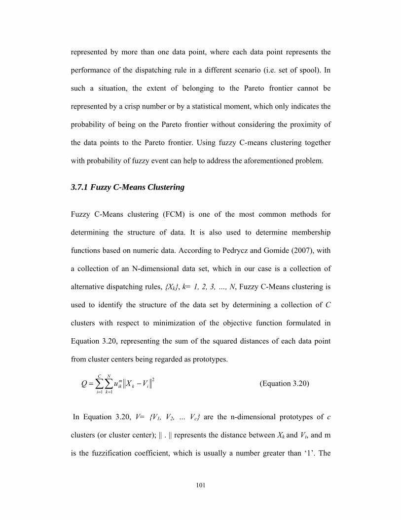
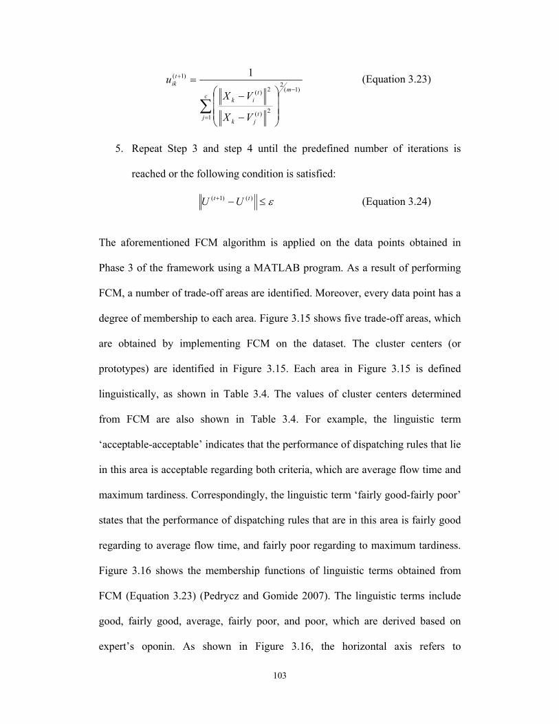
Using the membership degree of each dispatching rule to a cluster for different

scenarios, the concept of the probability of a fuzzy event (Zadeh 1968; Zadeh

1975) is used to calculate the expected membership value (Pedrycz and Gomide

2007) of each dispatching rule, r, to the kth cluster.

According to Zadeh (1968), an event is a precisely specified collection of points

in a sample space in probability theory, while there are situations in which an

event is a fuzzy collection of points, e.g. “it is a warm day.” By using the concept

of fuzzy sets and probability theory, the probability of a fuzzy event can be

measured. Assuming that P(x) is the probability measure of x, and A(x) is the

membership function of a fuzzy event, ‘A’, the probability of A can be measured

by Equation 3.26 (Zadeh 1968). E(A) is the probability of event ‘A’, which is also

defined as the expected value of the membership function A(x) (Zadeh 1968;

Pedrycz and Gomide 2007).

∫=x

dxxPxAAE )()()( (Equation 3.26)

In a similar manner, data points representing a dispatching rule constitute a fuzzy

collection of points or a fuzzy event. Therefore, the expected membership degree

of a dispatching rule to a cluster can be calculated as the expected value of the

membership degrees of all those data points using Equation 3.27, where n equals

the number of data points or scenarios. Equation 3.27 is the discrete form of

Equation 3.26, where the probability of each data point is equal to one over the

total number of data points (n).

109

∑=j

jrkrk u

nuE 1)( (Equation 3.27)

Where, E(urk) is the expected value of the membership degree of the rth

dispatching rule to the kth cluster; j denotes the jth scenario and n is the total

number of scenarios.

The expected membership value of a dispatching rule with respect to each cluster

identifies the degree to which that rule belongs to that cluster. Given the fact that

each cluster represents an area on the Pareto-optimal frontier where the

satisfaction of each objective function or criterion is associated with a linguistic

term (Table 3.4), the expected membership values calculated using Equation 3.27

assess the degree to which the associated rule can satisfy a criterion to the extent

of that linguistic value.

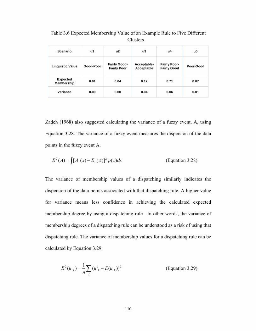
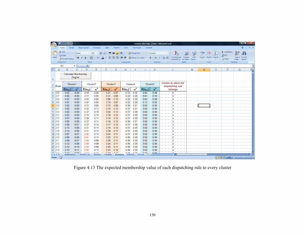
Table 3.6 shows the expected membership values of a sample dispatching rule

with respect to five clusters presented in Figure 3.15 and Table 3.4. The expected

values in Table 3.6 clearly show that the sample dispatching rule has a higher

degree of membership to cluster u4. This means that the sample dispatching rule

has a fairly good performance in minimizing the maximum tardiness but it has a

fairly poor performance in minimizing the average flow time.

110

Table 3.6 Expected Membership Value of an Example Rule to Five Different Clusters

Scenario u1 u2 u3 u4 u5

Linguistic Value Good-Poor Fairly Good-Fairly Poor

Acceptable-Acceptable

Fairly Poor-Fairly Good Poor-Good

Expected Membership 0.01 0.04 0.17 0.71 0.07

Variance 0.00 0.00 0.04 0.06 0.01

Zadeh (1968) also suggested calculating the variance of a fuzzy event, A, using

Equation 3.28. The variance of a fuzzy event measures the dispersion of the data

points in the fuzzy event A.

dxxpAExAAE )()]()([)( 22 −= ∫ (Equation 3.28)

The variance of membership values of a dispatching similarly indicates the

dispersion of the data points associated with that dispatching rule. A higher value

for variance means less confidence in achieving the calculated expected

membership degree by using a dispatching rule. In other words, the variance of

membership degrees of a dispatching rule can be understood as a risk of using that

dispatching rule. The variance of membership values for a dispatching rule can be

calculated by Equation 3.29.

22 ))((1)( rkj

jrkrk uEu

nuE −= ∑ (Equation 3.29)

111

Table 3.6 also shows the variances of membership values of a sample dispatching

rule’s data points with respect to five clusters. The variance of the membership

values with respect to cluster u4 is only 0.06, This low variance translates into a

higher confidence and lower risk in achieving similar results by using the sample

dispatching rule.

Dispatching rules can be compared using both their expected membership degree

and variance of membership degrees. Rule A dominates rule B with respect to one

cluster if rule A has a higher expected membership degree to that cluster and a

lower variance of membership degrees to that cluster. When neither of the two

dispatching rules dominates the other one, the user needs to choose the trade-off

between expected membership value and variance. Table 3.7 shows two sample

dispatching rules where sample rule 1 clearly dominates sample rule 2 with

respect to cluster u4, however neither of the rules dominates the other one with

respect to cluster u5.

Table 3.7 Expected Membership Values and Variances of Two Sample Dispatching Rules with Respect to Five Clusters

  Scenario u1 u2 u3 u4 u5

  Linguistic Value

Good-Poor

Fairly Good-Fairly Poor

Acceptable-Acceptable

Fairly Poor-Fairly Good

Poor- Good

Sample rule #1

Expected Membership 0.01 0.04 0.17 0.71 0.07

Variance 0 0 0.04 0.06 0.01

Sample rule #2

Expected Membership 0.01 0.02 0.05 0.12 0.8

Variance 0 0 0.05 0.08 0.2

112

3.7.3 Selecting the Appropriate Rule

The decision making process based on the results of the statistical analysis and

Fuzzy C-means clustering is comprise of two main steps.

First the decision maker should identify the desired compromise among the

multiple objective functions initially introduced to the framework as all the

objective functions cannot be fully satisfied by use of a single dispatching rule.

This means that the decision maker has to choose a linguistic value or a trade-off

zone on the Pareto optimal frontier. For example in the case presented in Table

3.7, the decision maker can select a trade-off zone or compromise solution,

including “good-poor”, “fairly good-fairly poor”, “acceptable-acceptable”, “fairly

poor-fairly good”, and “poor-good”. Each linguistic value represents a fuzzy

cluster of data points. This fuzzy cluster is associated with a series of dispatching

rules that have a high expected membership function with respect to that cluster.

In the second step of the decision making process, the decision maker should

choose a dispatching rule from this group of dispatching rules by comparing their

expected membership values and variances. Although ultimately one dispatching

rule may have the highest expected membership value to the identified cluster, the

decision maker may opt to use another dispatching rule with a lower expected

membership and a lower variance to reduce the uncertainty (variance). The

second step of the decision making process, like the first step, requires a choice by

the decision maker on the trade-off between the expected membership value and

the variance of membership values of the dispatching rules.

113

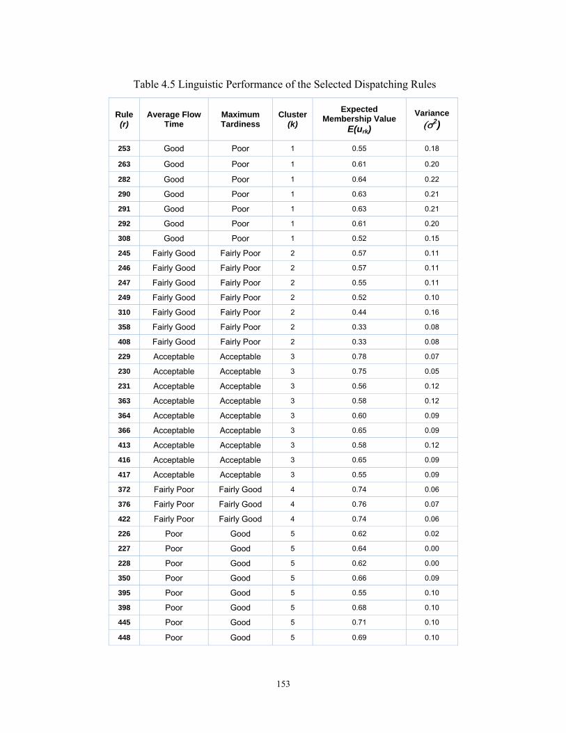
For example, Table 3.8 shows the linguistic performances of sample selected

rules. In this table, the expected membership indicates the possibility to which the

performance of the selected rule fits the linguistic term, and the variance indicates

the confidence that the performance of the selected rules matches the linguistic

terms. The expert can select the appropriate rule based on the linguistic

performance of the rule and the expected membership and variance values. For

instance, if the decision maker looks for good average flow time and poor

maximum tardiness, he/she can select rule #1, rule #2, or rule #3. In case the

confidence in the performance of the rule is important for the decision maker

he/she can select rule#1, which has a lower variance.

Table 3.8 Linguistic performance of the ample dispatching rules

Rule (r)

Average Flow Time Max Tardiness Expected

Membership Variance

rule #1 Good Poor 0.55 0.18 rule #2 Good Poor 0.61 0.20 rule #3 Good Poor 0.64 0.22 rule #4 Fairly Good Fairly Poor 0.57 0.11 rule #5 Fairly Good Fairly Poor 0.57 0.11 rule #6 Fairly Good Fairly Poor 0.55 0.11 rule #7 Acceptable Acceptable 0.75 0.05 rule #8 Acceptable Acceptable 0.56 0.12 rule #9 Acceptable Acceptable 0.58 0.12

rule #10 Fairly Poor Fairly Good 0.69 0.08 rule #11 Fairly Poor Fairly Good 0.56 0.09 rule #12 Fairly Poor Fairly Good 0.74 0.06 rule #13 Poor Good 0.62 0.02 rule #14 Poor Good 0.64 0.00 rule #15 Poor Good 0.62 0.00

114

3.8 Conclusions

In this chapter, a new framework for solving multi-criteria shop scheduling is

developed. Using the proposed framework, the uncertainty incorporated with the

shop environment can be captured by applying every dispatching rule to a set of

different scenarios and utilizing statistical analysis to measure expected

membership values and variances. In this chapter, new combinatorial dispatching

rules are proposed in addition to existing combinatorial dispatching rules in order

to address more than one criterion in schedule optimization. The significance of

the proposed framework is in its ability to optimize a multi-criteria industrial shop

scheduling problem while taking some other aspects into account:

1. The framework makes it possible to combine various dispatching rules

with different weights to address multiple criteria in scheduling.

2. The framework provides the opportunity to evaluate different performance

indices, which are in conflict with each other, using the concepts of fuzzy

sets.

3. The framework uses fuzzy set theory to represent different trade-off areas

between conflicting performance indices in the Pareto frontier (or Pareto

optimal set).

4. The framework makes it possible to take into account the uncertainty of

the performance of each dispatching rule through running each

dispatching rule for different scenarios using the simulation model.

115

Furthermore, using Fuzzy C-Means clustering for analysis of the performance of

dispatching rules makes it possible to convert the structure of the data, which is

obtained from the simulation model, into a linguistic representation. Using that

linguistic representation, the end-user in the industry can easily interpret the

numerical results and choose the proper dispatching rule. Fuzzy C-Means

clustering also accounts for the fact that each dispatching rule can satisfy a given

criterion to a different degree, depending on the set of jobs being scheduled.

Moreover, fuzzy clustering makes it possible to consider the quality of belonging

of each dispatching rule to a Pareto frontier in the amalgamation of all the results

of all scenarios, which cannot be represented by a crisp number or by a statistical

moment. The statistical methods can only specify the probability of being on the

Pareto frontier without considering the proximity of the data points to the Pareto

frontier.

Finally, linguistic variables and statistical data are connected together by the

concept of probability of a fuzzy event (Zadeh 1968; and Zadeh 1975), which is

interpreted as the expected membership value by Pedrycz and Gomide (2007).

Also using the variance of membership values (Pedrycz and Gomide 2007) of a

dispatching rule, the confidence in the expected membership value of each

dispatching rule with respect to each cluster can be determined.

116

3.9 References

Arikan, F., and Gungor, Z. (2001). “An application of fuzzy goal programming to a multiobjective project network problem.” Fuzzy Sets Syst., 119(1), 49–58.

Ayyub, B. M., and Haldar, A. (1984). “Project scheduling using fuzzy set concepts.” ASCE, Journal of Construction Engineering and Management, 110(4), 189–203.

Babiceanu, R. F., Frank Chen, F., and Sturges, R. H, (2005). “Real-time holonic scheduling of material handling operations in a dynamic manufacturing environment.” Robotics and Computer-Integrated Manufacturing, 21(4-5), 328–337.

Baker, K. R., and Trietsch, D. (2009). Principles of sequencing and scheduling. John Wiley & Sons, New Jersey.

Barrett, R. T., and Barman, S. (1986). “Slam II Simulation Study of a Simplified Flow Shop.” Simulation, 47(5), 181–189.

Bellman, R. E., and Zadeh, L. A. (1970). “Decision Making In Fuzzy environment.” Management Science, 17(4), 141–164.

Bezdek, J.C. (1981). Pattern Recognition with Fuzzy Objective Function Algorithms. Plenum Press, New York.

Bhaskaran, K., and Pinedo, M. (1992). “Dispatching,” Chapter 83. In Handbook of industrial engineering, Salvendy, G. (ed.). John Wiley & Sons, New Jersey.

Bitran, G. R., Dada, M., and Sison, L. O. (1983). “A simulation model for job shop scheduling.” Working papers from Massachusetts Institute of Technology (MIT). Sloan. No 1402-83. <http://dspace.mit.edu/handle/1721.1/2035>

Blackstone, J. H., Phillips, D. T., and Hogg, G. L. (1982). “A state of art survey of dispatching rules for manufacturing job shop operation.” International Journal of Production Research, 20(1), 27–45.

117

Bonnal, P., Gourc, D., and Lacoste, G. (2004). “Where do we stand with fuzzy project scheduling?” Journal of Construction Engineering and Management, 130(1), 114–123.

Brucker (2007), Scheduling Algorithms, Springer, Berlin.

Castro-Lacouture, D., Süer, G., Gonzalez-Joaqui, J., and Yates, J. (2009). “Construction Project Scheduling with Time, Cost, and Material Restrictions Using Fuzzy Mathematical Models and Critical Path Method.” Journal of Construction Engineering & Management, 135(10), 1096–1104.

Chan, A. P. C., Chan, D. W. M., and Yeung, J. F. Y. (2009). “Overview of the Application of ``Fuzzy Techniques'' in Construction Management Research.” Journal of Construction Engineering and Management, 135(11), 1241–1252.

Chan, F. T. S., Chan, H. K., and Kazerooni, A. (2002). “A Fuzzy Multi-Criteria Decision-Making Technique for Evaluation of Scheduling Rules.” International Journal of Advanced Manufacturing Technology, 20, 103–113.

Chen, Y., Fowler, J. W., Pfund, M. E., and Montgomery, D. C. (2007). “Methodologies for parameterization of composite dispatching rules”. ASU working paper ASUIE ORPS-2007-019. Industrial Engineering, Arizona State University. <http://ie.fulton.asu.edu/research/workingpaper/ wps.php>

Choi, H.-S., Lee, D.-H. (2009). “Scheduling algorithms to minimize the number of tardy jobs in two-stage hybrid flow shops.” Computers and Industrial Engineering, 56 (1), pp. 113-120.

Deporter, E. L., and Ellis, K. P. (1990). “Optimization of project networks with goal programming and fuzzy linear programming.” Comput. Ind. Eng., 19(1–4), 500–504.

Djellab, H., and Djellab, K. (2002). “Preemptive hybrid flowshop scheduling problem of interval orders.” European Journal of Operational Research, 137 (1), pp. 37–49.

Dohnal, M. (1983). “Fuzzy simulation of industrial problems.” Computers in Industry, 4(4), 347–352.

118

Ehrgott, M. (2005). Multicriteria Optimization. Springer, Berlin, second edition.

Fanti, M. P., Maione, B., Naso, D., and Turchiano, B. (1998). “Genetic multi-criteria approach to flexible line scheduling.” International Journal of Approximate Reasoning, 19(1-2), 5–21.

Fayek, A. R., and Oduba, A. (2005). “Predicting industrial construction labour productivity using fuzzy expert systems.” Journal of Construction Engineering and Management, 131(8), 938–941.

Fishwick, P. A. (1991). “Fuzzy simulation: Specifying and identifying qualitative models.” International Journal of General Systems, 19, 295–316.

Garey, M.R. and Johnson, D.S. (1979). Computers and intractability: a guide to the theory of NP-completeness, A Series of Books in Freeman, W.H. (1979). the Mathematical Sciences, San Francisco.

Gupta, Jatinder N.D. (1988). “Two-Stage, Hybrid Flowshop Scheduling Problem.” Journal of the Operational Research Society, 39 (4), pp. 359-364.

Hajjar, D., and AbouRizk, S. M. (2002). “Unified modeling methodology for construction simulation.” Journal of Construction Engineering and Management, 128(2), 174–185. http://www.sciencedirect.com/science/article/B6VCT-4XFFJN7 1/2/d6a44e8a526f549d622bfa4d500b22e5

Ishibuchi, H., and Murata, T. (1998) “A multi-objective genetic local search algorithm and its application to flowshop scheduling.” IEEE/SMC Trans., Part C 28(1998), 392–403.

Jones, A., Rabelo, L., and Yih, Y. (1995). “A hybrid approach for real-time sequencing and scheduling.” International Journal of Computer Integrated Manufacturing, 8(2), 145–154.

Kacem, I., Hammadi, S., and Borne, P. (2002). “Pareto-optimality approach for flexible job-shop scheduling problems: hybridization of evolutionary algorithms and fuzzy logic.” Math. Comput. Simulat. 60, 245–276.

119

Kis T., Pesch E. (2005). “A review of exact solution methods for the non-preemptive multiprocessor flowshop problem.” European Journal of Operational Research, 164 (3 SPEC. ISS.), pp. 592-608.

Klir, G. J., and Yuan, Bo. (1995). Fuzzy sets and fuzzy logic: theory and applications. Prentice Hall: Upper Saddle River, NJ.

Kuo, Y., Yang, T., Cho, C., and Tseng, Y. (2008). “Using simulation and multi-criteria methods to provide robust solutions to dispatching problems in a flow shop with multiple processors.” Mathematics and Computer in Simulation, 78(1), 40–56.

Lah, M. T., Zupancic, B., and Krainer, A. (2005). “Fuzzy control for the illumination and temperature comfort in a test chamber.” Build. Environ., 40(12), 1626–1637."

Lam, K. C., So, A. T. P., Hu, T., Ng, T., Yuen, R. K. K., Lo, S. M., Cheung, S. O., and Yang, H. W. (2001). “An integration of the fuzzy reasoning technique and the fuzzy optimization method in construction project management decision-making.” Constr. Manage. Econom., 19(1), 63–76.

Lei, D. (2009). “Multi-objective production scheduling.” International Journal of Advanced Manufacturing Technology, 43(9-10), 925–938.

Leung, Y. W., and Wang, Y. (2000). “Multi-objective programming using uniform design and genetic algorithm.” IEEE/SMC Trans., Part C 30 (2000), 293–303.

Lorterapong, P., and Moselhi, O. (1996). “Project-network analysis using fuzzy sets theory.” J. Constr. Eng. Manage., (122)4, 308–318.

Negi, D. S., and Lee, E. S. (1992). “Analysis and simulation of fuzzy queues.” Fuzzy Sets and Systems, 46, 321–330.

Osman, I. H., and Laporte, G. (1996). “Metaheuristics: A bibliography.” Annals of Operations Research, (63), 513–623.

Pedrycz, W. (2005). Knowledge-Based Clustering. John Wiley, Hoboken, NJ.

120

Pedrycz, W. (2009). “Statistically grounded logic operators in fuzzy sets.” European Journal of Operational Research, 193(2), 520–529.

Pedrycz, W., and Gomide, F. (2007). Fuzzy systems engineering: toward human-centric computing. IEEE Press, John Wiley & Sons, New Jersey.

Petrovic, D., Duenas, A., and Petrovic, S. (2007). “Decision support tool for multi-objective job shop scheduling problems with linguistically quantified decision functions.” Decision Support Systems, 43(4), 1527–1538.

Pfund, M., Fowler, J. W., Gadkari, A., and Chen, Y. (2008). “Scheduling jobs on parallel machines with setup times and ready times.” Computers and Industrial Engineering, 54(4), 764–782.

Pinedo, M. (2008). Scheduling: Theory, Algorithms, and Systems, Springer, NewYork.

Ruiz, R., Vazquez-Rodriguez, J. A. (2009). “The hybrid flow shop scheduling problem.” European Journal of Operational Research, In Press, Corrected Proof, Available online 13 October 2009,

Sabuncuoglu, I. and Hommertzheim, D.L., (1992), “Experimental investigation of FMS machine and AGV scheduling rules against the mean flow-time criterion.” Int. J. Prod. Res., (30), 1617–1635.

Sadeghi, N. (2009). “Combined Fuzzy and Probabilistic Simulation for Construction Management.” M.Sc. thesis, University of Alberta, Edmonton, Alberta.

Sarper, H., Henry, M. C. (1996). “Combinatorial evaluation of six dispatching rules in a dynamic two-machine flow shop.” Omega, 24(1), 73–81.

Southall, J. T., and Wyatt, M. D. (1988). “Investigation using simulation models into manufacturing/distribution chain relationships.” BPICS Control, 4(5), 29–34.

Suer, A. G., Arikan, F., and Babayigit, C. (2008). “Bi-objective cell loading problem with nonzero setup times with fuzzy aspiration levels in labor intensive manufacturing cells.” Int. J. Prod. Res., 46(2), 371–404.

121

Tong, T. K. L., and Tam, C. M. (2003). “Fuzzy optimization of labor allocation by genetic algorithms.” Eng., Constr., Archit. Manage., 10(2), 146–155.

Vepsalainen, A. P. J., and Morton, T. E. (1987). “Priority Rules for Job Shops with Weighted Tardiness Costs.” Management Science, 33(8), 1035–1047.

Wang, R. C., and Liang, T. F. (2004). “Project management decisions with multiple fuzzy goals.” Constr. Manage. Econom., 22(10), 1047–1056.

Yang, T., Kuo, Y., and Cho, C. (2007). “A genetic algorithms simulation approach for the multi-criteria combinatorial dispatching decision problem.” European Journal of Operation Research, 176(3), 1859–1873.

Zadeh, L. A. (1965). Fuzzy sets. Information and Control, 8, 338–53.

Zadeh, L. A. (1968). “Probability measures of fuzzy events.” Journal of Mathematical Analysis and Applications, 23(2), 421–427.

Zadeh, L. A. (1975). “The concept of linguistic variable and its application to approximate reasoning-I.” Information sciences, 8(3), 199–249.

Zadeh, L. A. (1996). “Fuzzy logic = Computing with words.” IEEE Transactions on Fuzzy Systems, 4, 103–111.

Zadeh, L. A. (2002). “Toward a perception-based theory of probabilistic reasoning with imprecise probabilities.” Journal of Statistical Planning and Inference, 105(1), 233–264.

Zadeh, L. A. (2005). “Toward a generalized theory of uncertainty (GTU)—An outline.” Information Sciences, 172(1-2), 1–40.

Zimmermann, H.J. (1978). “Fuzzy programming and linear programming with several objective functions.” Fuzzy Sets and Systems, 1(1), 45–56.

Zimmermann, H.J. (1991). Fuzzy set theory and its applications. Dordrecht: Kluwer, second edition.

122

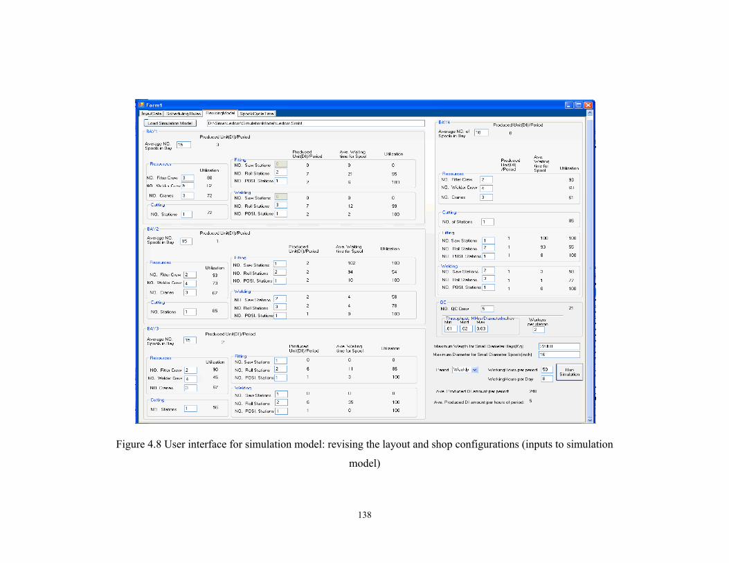
CHAPTER 4 - Case Study: Scheduling of Pipe Spool

Fabrication Shop Using Simulation and Fuzzy Logic

4.1 Introduction

In this chapter, the proposed framework for simulation-based scheduling of

industrial fabrication is implemented on a real case study of a pipe spool

fabrication shop in Edmonton, Alberta. First, a simulation model is developed for

the case study using the simulation modeling framework proposed in Chapter 2.

Then the appropriate dispatching rule is identified using the multi-criteria

scheduling framework proposed in Chapter 3. The simulation model presented

here is developed for processes from the cutting station to the QC (Quality Check)

station. Hydro-test, stress relief, painting, and shipping to the module yard are not

considered in this model. Moreover, it is assumed that all materials and drawings

are available when a spool is issued to the shop floor. The actual case study

involves four bays, all of which are included in the simulation model. As shown

in Figure 4.1, a bay is a production line including different stations through which

spools are processed.

Figure 4.1 A schematic layout drawing of a bay in a pipe spool fabrication shop

123

Section 4.2 elaborates on the characteristics of the case study, as well as

assumptions considered in developing this case study. Furthermore, the proposed

simulation model is validated in Section 4.2. In Section 4.3, the proposed

framework for multi-criteria scheduling is implemented on the case study. The

results are then validated using test data.

4.2 Simulation Modeling of Pipe Spool Fabrication

The pipe spool fabrication processes are comprehensively described in Chapter 2.

The case study includes 802 spools, which are sent to the shop floor over one

month. As shown in Figure 4.2, after generating spools in the simulation model,

spools are assigned to each bay based on their material group, weight, and size.

Then, the spools are sent to the cutting station. In the next step of the simulation

model, the model breaks down the spool into its assemblies based on the entity

hierarchy (EH) of the spool, which is held in the central database. After roll

welding and SAW welding of all the spool’s assemblies are completed, the

assemblies are then sent for position fitting and position welding. Quality check

(QC) is the last process performed on the spool. Material handling is modeled

between stations to calculate the utilization of cranes. As Figure 4.2 illustrates, the

SAW welding process and the roll welding process are modeled separately.

124

Figure 4.2 Structure of simulation model for case study

125

4.2.1 Assumptions

In order to simulate the fabrication shop, some assumptions have been made

according to the experts’ (shop foremen’s Supervisor, Quality Assurance

Coordinator, and Estimator) information. These assumptions help to speed up the

development of the simulation model based on available data.

In this simulation model, only the following steps of spool fabrication are

modeled: cutting, SAW welding, roll fitting, roll welding, position fitting,

position welding, and QC. It is assumed that in the current configuration of the

fabrication shop, bottlenecks are not due to tasks like hydro-testing and painting,

so these activities do not directly affect the productivity of the fabrication shop.

Moreover, the simulation model is designed with the assumption that all materials

are available for the spools while the model is run. In other words, it is assumed

that the fabrication of a spool starts when all materials are available.

The processing time of each operation is estimated using the Equation 4.1:

j

ij

nwwu )(Pr

t ij

×= (Equation 4.1)

Where, tij the processing time of job i for the process j, Prj is man-hours required

per unit of the work for process j (Equation 2.3), wui is the amount of work unit of

job i, which is measured in diameter inches, and nwj is the number of workers that

are working on the product in process j.

126

Since the historical data do not specify different types of welds, e.g. position,

SAW, and roll, the following assumptions are made about the durations of

different types of welding methods according to the Operations Manager of the

Ledcor fabrication shop:

• wall thickness<= 1.000" WT (Wall Thickness)

o roll weld = base weld unit (diameter inches)

o SAW = 0.8 × base weld unit

o position = 1.75 × base weld unit

• wall thickness > 1.000" WT

o SAW = base weld unit (diameter inches)

o position = 1.5 × base weld unit

Pipes with wall thickness greater than 1.000" should be welded by the SAW

machine.

Some assumptions were considered for calculating the duration of welding of

different welds. These are explained in Appendix A, based on information

available for butt welds (defined in Appendix A):

• Dummy legs are similar to butt welds if they are 90° to the header (Figure

4.3). The duration of welding 45° dummy legs (Figure 4.3) is close to butt

welds.

• The duration of re-pad welds is considered to be 2.0 × duration of butt

weld.

127

o Re-pad welds are considered to be somewhere between 1.5 and 2.0

x duration of butt weld.

• The duration of welding for socket welds is 0.80 × duration for butt welds.

Finally, the available man-hour data do not include separate information for

fitting and handling. Therefore, it is assumed that fitting and handling are done

together. To calculate crane utilization, it is assumed that the crane supports the

handling and fitting somewhere between 20 and 30 percent of the fitting time.

6.  

7.  

8.  

Figure 4.3 Dummy legs

4.2.2 Database

The central database holds the entity hierarchy (EH) information and is connected

to the simulation model. The central database also holds the output results of the

simulation model, which include the start and finish time of each process for

every spool. Figure 4.4 shows the input table and the output table in the central

database. The input table contains the entity hierarchy information. A special

element is utilized in the simulation model to generate the entities using the input

table in the central database. The central database is generated using the

a) 90° Dummy leg b) Angular Dummy leg

128

company’s database and drawings of the pipe spool fabrication spool fabrication.

It is connected to the simulation model through the user interface developed in

VB.Net. The data in the central database, which are carried by entities in the

simulation model as each entity’s attributes, are listed in Table 4.1. In Table 4.1, a

spool is the final product of the pipe spool fabrication shop. Respectively, an

assembly is defined as the most basic element of a spool that does not need

position welding, and components such as pipes, elbows, valves, etc. are the most

basic elements of a spool. Chapter 2 contains a comprehensive explanation about

pipe spool fabrication processes and the entity hierarchy model.

Figure 4.4 Input and output tables in central database

129

Table 4.1 List of Entities’ Attributes in Central Database

Spool Assemblies Components

Product Information

Spool ID

Control Number

Project ID

Batch ID

Issue date

RAS (required at site date or due date)

Material Type

Total work units

Length

Weight

Number of assemblies

Number of pipes

Number of Elbows

Number of Tees

Number of Valves

Total number of fittings

Spool ID

Control Number

Project ID

Batch ID

Assembly ID

Total work units

Length

Weight

SAW welding work unit

Roll welding work unit

Number of assemblies

Number of pipes

Number of Elbows

Number of Tees

Number of Valves

Total number of fittings

Spool ID

Control Number

Project ID

Batch ID

Assembly ID

Component ID

Length

Weight

Diameter

Wall thickness

Start Co-ordinate

End Co-ordinate

Process Information

Processing time of the position fitting

Processing time of position welding

Processing time of quality check

Processing time of the roll fitting

Processing time of the roll welding

Processing time of the SAW fitting

Processing time of SAW welding

Processing time of Cutting

130

4.2.3 Simulation Environment

A SPS template was developed to simulate the pipe spool fabrication shop in

Simphony.Net©. The SPS template can be also used for other industrial

fabrication facilities such as steel fabrication shops. The development of the SPS

template is discussed in Chapter 2. In this section, the elements of this template

used for modeling the case study are explained in detail. Also, the inputs and

outputs of each element are introduced in this section. The input parameters can

be changed through the developed user interface. The outputs of the elements can

be viewed through the user interface after running the model. Table 4.2

summarizes the elements and the corresponding icons used in the model.

Table 4.2 Icons Used for Elements of Simulation Model

Element Icon Element Icon

Fab-Shop

Working Station

Start

Generate

Dispatch controller

Assembly

Bay Crane

Cutting Station

Material handling

Worker

Bay

Waiting file

131

4.2.3.1 Fab-Shop

The Fab-Shop element contains all elements of a fabrication shop. The inputs of

this element include database path, as well as the dispatching rule, which is used

for scheduling the spools. The output includes work units produced per week.

4.2.3.2 Start

This element links the simulation model to the central database and produces

spools based on entity hierarchy model in the central database. The start element

fires the spools as entities according to their issue date in the central database. The

issue date is the date that all materials and drawings of the spools are available

and is pulled out of the fabrication status database of the shop.

4.2.3.3 Bay

All stations are child (sub) elements of this element. The input is the average

number of spools can be in the bay. The outputs include production (produced

work units) per week. The average number of spools is used to model the lay

down area that is distributed through the fabrication shop.

The case study includes four bays. Two bays (Bay 2 and Bay 4) are for heavy

wall and large diameter spools, and two bays (Bay 1 and Bay 3) are for standard

wall and small diameter spools. According to fabrication shop foremen, stainless

steel spools should be processed separately from carbon steel spools to prevent

cross-contamination; therefore, stainless steel spools are processed in Bay 3

regardless of their weight and size (diameter).

132

4.2.3.4 Dispatch Controller

The dispatch controller element allocates spools to each bay based on their

weight, diameter, and material group. The dispatch controller also checks the

waiting time of spools in a bay and sends the spools to the appropriate bay with

the lowest average waiting time in order to uniformly allocate the workload to the

bays.

4.2.3.5 Cutting Station

This element represents a cutting station. The input is the number of stations. The

outputs include work units produced per week, average waiting time for spools,

and the utilization of a station.

4.2.3.6 Worker

This element represents the fitters and welders as a resource. The input of this

element is the number of workers. The output includes utilization percentage of

workers. Two types of workers are considered in the model: fitter and welder.

4.2.3.7 Waiting File

The waiting file element is for spools waiting for resources. The output of this

element is the average waiting time for spools.

4.2.3.8 Working Station

This element represents a working station in which a specified process, such as

roll fitting or roll welding, is performed on a spool. The input of this element is

133

number of stations. The output of this element includes work units produced per

week, average waiting time for spools, and utilization percentage of the station.

4.2.3.9 Generate

The generate element adjusts the entity to the required level of entity hierarchy by

generating the assemblies for each spool based on the entity hierarchy model in

the central database.

4.2.3.10 Assembly

The assembly element adjusts the level of the entity to the required level of the

entity hierarchy model by gathering all the assemblies of spools together. The

assembly element is developed by enhancing the methodology proposed by Wang

(2006) and Sadeghi and Fayek (2008) using the information in the central

database.

4.2.3.11 Crane

This element represents the bridge crane as a resource for material handling. Each

bay includes a number of bridge cranes for handling material and spools between

stations.

4.2.3.12 Material handling

This element represents the material handling between stations in fabrication

shop. This element does not need any input.

134

4.2.4 User Interface

Using VB.net, the user interface is provided to control input to the simulation

model and to develop an entity hierarchy model using the database and drawings

of pipe spool fabrication shops as described in Chapter 3. Figure 4.5 illustrates the

relationship between a pipe spool fabrication shop’s database and the simulation

model through Access and VB.net. The user interface of the model (Figure 4.6)

consists of four sections. As shown in Figure 4.7, the first section is for revising

the spools in the database and calculating man-hours and each type of weld for

each spool to develop the entity hierarchy. Figure 4.7 also shows the second

section, which allows the user to select the dispatching rule and to determine the

working hours and shift hours of the fabrication. Figure 4.8 shows the third

section, which can be viewed by clicking on “Revising Model” at the top of the

interface. This section is for revising the layout and the configuration of the pipe

spool fabrication shop in the simulation model. Examples of such revisions

include changing the number of stations and resources. After running the

simulation, the results for each station and bay appear in this section. The results

of the simulation model for spool cycle time (in days) and delivery dates are

saved in the database connected to the model. These results can be viewed

through the interface in the third section by clicking on “spools cycle time” at the

top of the user interface, as illustrated in Figure 4.9.

135

Figure 4.5 Relationships between company’s databases and simulation model via

VB.net and Access

Access Database

(Maintains inputs of simulation model) Spools going through simulation model

Man-hours for every activity for each spool Physical attribute of spool

VB.Net Interface and Program

Calculating number of each type of weld for every spool Calculating man-hours of each activity for every spool Pull physical attribute of each spool from ACORN and save it in Access

Simulation Model

Simulates the processes of the pipe spool fabrication shop

Company’s Databases:

Drawings, Spool Information, Material Information, Batch Level

Information

Project

AProject

B …

136

Figure 4.6 User interface for simulation model

137

Figure 4.7 User interface for simulation model, selecting the scheduling rule

138

Figure 4.8 User interface for simulation model: revising the layout and shop configurations (inputs to simulation

model)

139

Figure 4.9 User interface for simulation model: cycle time for each spool

140

4.2.5 Validation of Simulation Model

After developing any simulation model or tool, that simulation model or tool

should be validated. In this study, the validation of the model was performed

using 802 spools from the company’s database. The percentage error of the

simulation model was calculated by comparing the estimated average spools’

cycle time by the simulation model with the actual spools’ average cycle time

collected from the fabrication material tracking system. Equation 4.2 is used to

calculate the percentage error of the simulation model.

n

n

Actual

Actual∑ ×⎟⎟⎠

⎞⎜⎜⎝

⎛

= 1

Predicted 100C

C-C

Error% Average (Equation 4.2)

Where, CActual is the actual average cycle time obtained from company’s material

tracking system, CPredicted is the average cycle time estimated by the simulation

model, and n is number of spools. For validation of simulation model, earliest due

date (EDD) is used for prioritizing and sequencing of spools in the model which is

the same rule used in the actual shop. The average percentage error found using

802 spools was 4.5%, and the variance of errors was 3.1. The average cycle time

estimated by the simulation model was shorter than the actual average cycle time.

The simulation model can also be validated by comparing estimated produced

work units by the simulation model with actual produced work unit of the shop in

a specific period of the time. The model was run for a period of time (a month),

and the estimated weekly produced units were compared to the actual weekly

141

produced units that were obtained from the company’s weekly production reports.

The percentage error was calculated using Equation 4.3.

Equation 4.3

Where, Actual is the actual weekly produced units in the shop; Predicted is the

weekly produced units estimated by the simulation model, i is equal to the

individual week number, and n equals the total number of weeks. The percentage

error obtained from Equation 4.3 was 4.1%, which is acceptable.

The possible explanation for this discrepancy is that the rework was not

simulated. In addition, it was assumed that all materials and drawings of the

spools issuing to the shop are available, whereas sometimes, there are material

shortages and changes in the drawings in reality. Furthermore, the simulation

model cannot model many dynamic changes of the shop floor, such as rush orders

or shop managers’ decisions. As explained in chapter 2, the simulation model can

be improved busing following developments:

• The percentage of rework is not modeled in the current study due to lack

of information for rework. One of the further developments of the model

could include modeling rework in simulation studies using probabilistic

distributions in the simulation model.

100Actual

Predicted-Actual

Error% 1 i

ii

×=∑

=

n

n

i

142

• The productivity values used for calculating the duration of activities are

obtained from estimation department which is not accurate. Additional

data collections, such as time study, must be

• Because the spool fabrication shop is labour-intensive, productivity is

highly affected by the skill of the labourers in the shop. Since the skill of

labourers is a subjective factor, a fuzzy expert system is one of the best

models for calculating productivity, because it is capable of considering

both qualitative and quantitative factors in estimating productivity. The

important factors that affect the productivity of pipe spool fabrication

processes are introduced in Chapter 2. These factors can be used to

developed fuzzy rules based on experts’ judgment to develop a fuzzy

expert system for determining the productivity of pipe spool fabrication

processes.

4.2.6 Experimenting with Different Scheduling Rules

The performance of different heuristic rules for a two week schedule is shown in

Table 4.3, as an example. The values used in Table 4.3 are not the actual numbers

from the experiment, due to the confidentiality issue. The heuristic rules used in

Table 4.3 are explained in Chapter 2. As shown in Table 4.3, EDD reduces the

maximum tardiness, average tardiness, and number of tardy jobs, while SI reduces

the average flow time and increases the weekly production of the shop. Usually,

the criteria related to tardiness, such as maximum tardiness and average tardiness,

are more important to the shop managers because of the importance of customer

143

satisfaction. However, when the shop is heavily loaded with several projects,

reducing the flow time would be of interest.

Table 4.3 Sample Results of Scheduling Heuristic for Two Weeks

Heuristic Rule

Ave

rage

Flo

w ti

me

(Hr)

Mak

e- S

pan

(Hr)

Max

Tar

dine

ss

(Hr)

Num

ber o

f Tar

dy

Jobs

Tota

l Tar

dine

ss

(Hr)

Tota

l Ear

lines

s (H

r)

Ave

rage

Res

ourc

e U

tiliz

atio

n (%

)

Ave

rage

wee

kly

Prod

uced

wor

k un

its

(Dia

met

er In

ches

)

SRPT 13 89 47 4 186 8177 94 5416

SI 13 86 44 4 177 8187 94 5416

LPT 50 82 70 18 596 6316 91 4456

LRPT 50 82 62 18 599 6312 92 4456

LI 54 85 58 19 709 6223 94 4456

FCFO 22 77 61 9 297 7740 92 5216

RPT/I 18 89 61 6 231 7945 87 3816

TotalO/IP 53 85 58 19 710 6272 91 3816

FRO 22 88 58 10 216 7648 87 3880

EDD 33 77 21 5 54 6804 90 3816

Slack 44 82 23 4 304 6404 93 3816

Slack / OPN 45 82 29 14 304 6361 92 3840

Slack / TotalP 51 82 53 20 538 6218 93 3816

4.3 Implementation of Multi-Criteria Scheduling Framework on

the Case Study

In this section, the multi-criteria scheduling framework described in Chapter 3 is

implemented on the case study. According to the Operations Manager of the spool

fabrication shop, the maximum tardiness and average flow time are usually the

most important criteria in the fabrication shop. Since the cost of storage does not

144

have a remarkable effect on the total cost of the projects, the earliness is not

considered in the scheduling of this case study. As discussed in Chapter 3, the

average flow time, average resource utilization, and number of tardy jobs are

correlated with each other and can be improved simultaneously. Also, The make-

span, maximum tardiness, total tardiness, and mean tardiness of the pipe spool

fabrication shop can be improved simultaneously. Therefore, by addressing

average flow time and maximum tardiness, other criteria improve at the same

time, although they are not as important as the two selected criteria.

Combinatorial dispatching rules are used in this case study, which are described

in Chapter 3. Using the dispatching rules introduced in Chapter 3, three hundred

rules are constructed to be used in this framework. Thirty scenarios are generated

by selecting random sets of spool from the fabrication shop database for different

time horizons, e.g. the first week of August or second week of August, to

experiment with the rules and implement the framework.

As discussed in Chapter 3, for each scenario a set of candidate dispatching rules is

obtained. The candidate dispatching rules are the rules that are in the Pareto-

optimal set when running each scenario. A program is developed in VB.Net to

automatically run a simulation model for every scenario and export the

performance value of criteria into an Excel sheet. The flow chart of the program is

shown in Figure 4.10.

145

Figure 4.10 The process of identifying the Pareto optimal set for case study

The results of the first scenario are shown in Figure 4.11. In Figure 4.11, the each

criterion is marked by ‘Yes’ or ‘No’; if it is marked as ‘Yes,’ the criterion is

considered in calculating the Pareto-optimal set. By clicking on the calculate

button, the Pareto optimal set is calculated based on the selected criteria. If a

dispatching rule is Pareto-optimal, the corresponding cell is changed to ‘1’. Also

the performance values are fizzified in terms of satisfaction degree using Equation

3.11 and Equation 3.12, which are introduced in Chapter 3.

Generate scenario

Experiment with simulation model

Calculate the Pareto-optimal set

Repeat for all

dispatching rules

Select dispatching Rule

Export the results to the Excel sheet

Rep

eat f

or a

ll th

irty

scen

ario

s

146

Figure 4.11 Performance values of different dispatching rules for the first scenario

Calculate button: by clicking on this button the Pareto-optimal set is calculated based on selected criteria

Selecting Criteria: if ‘Yes’ the criterion is considered in calculating Pareto- optimal set.

Max/Min: determining which criteria should be maximized and which criteria should be minimized in order to fuzzify the values in terms of satisfaction degree

147

Figure 4.12 shows the performance values of different dispatching rules for all

scenarios, which are automatically collected from multiple spreadsheets by

clicking on ‘Collect’. The data set then is used in MATLAB for Fuzzy C-Means

clustering (FCM). Next, the membership degree of every data point to each trade-

off area (cluster) is exported to the Excel sheet, which is shown in Figure 4.13.

The expected membership degree of each cluster then is calculated according to

Equation 3.27, which is described in Chapter 3.

148

Figure 4.12 Performance values of different dispatching rules for all scenarios

149

Figure 4.13 shows the spreadsheet that contains the expected membership value

of each dispatching rule to every cluster. The expected membership value is used

to determine the cluster to which a dispatching rule belongs. Furthermore, the

expected membership value determines the proximity of a dispatching rule to the

center of a cluster, which represents an area on the Pareto-optimal frontier, where

the satisfaction of every objective function or criterion is associated with a

linguistic value, which is shown in Table 4.4. Therefore, the higher value of

expected membership indicates that the performance of the corresponding

dispatching rule is closer to the linguistic description of the cluster. On the other

hand, the variance of the membership degree refers to the robustness of the

dispatching rule, which indicates the consistency of the performance of the

dispatching rule in different scenarios. Therefore, the ideal situation for each

trade-off area is selecting the dispatching rule with the highest expected

membership value and the lowest variance. High expected membership value

indicates that the possibility that the rule fits the linguistic description is high, and

therefore it shows that the corresponding rule satisfies the linguistic preference of

the decision makers.

150

Figure 4.13 The expected membership value of each dispatching rule to every cluster

151

In Table 4.4, μ(Average Flow Time) and μ(Maximum Tardiness) indicate the

satisfaction degree associated with the linguistic variables, which describes the

performance of the corresponding rules . For example, the performance of rules in

cluster 1 is good with respect to average flow time and poor with respect to

maximum tardiness. The satisfaction degree of ‘1’ indicates full satisfaction, or a

linguistic term of “good” performance. The satisfaction degree of ‘0’ represents

no satisfaction, or a linguistic term of “poor” performance.

Table 4.4 Linguistic Description of Each Trade-off Area and the Prototypes of Each Cluster

Cluster 1 2 3 4 5

Linguistic Trade-off

area

Average Flow Time Good Fairly Good Acceptable Fairly Poor Poor

Maximum Tardiness Poor Fairly Poor Acceptable Fairly Good Good

μ(Average Flow Time) 1.00 0.85 0.75 0.40 0.00

μ(Maximum Tardiness) 0.00 0.40 0.75 0.85 1.00

Table 4.5 shows the selected rules for each cluster. E(urk) in Table 4.5 refers to the

expected membership value of dispatching rule ‘r’ to the kth cluster. Table 4.5

includes the linguistic value of the performance of the selected rules. Based on the

results of Table 4.5, the user can select the appropriate rules in the user interface

of the simulation model, which was shown in Figure 4.7, to generate the schedule

of the fabrication shop. The appropriate rule is selected by the decision maker

152

using the linguistic description given in Table 4.5. The decision maker may

consider the variance and expected membership value to determine how well the

rule fits the linguistic description, and how robust the performance of rule is in

different scenarios.

As explained in Chapter 3, in the first step of decision making, the decision maker

selects a trade-off area (cluster) using Table 4.4. Then the decision maker chooses

an appropriate rule from the corresponding group of dispatching rules by

comparing their expected membership values and variances. The expected

membership degree is used to rank the dispatching rules based on how well they

fit the corresponding linguistic description, while the variance is used to rank the

dispatching rules regarding the robustness and the confidence level of their

performance.

For example, if the decision maker selects “fairly poor-fairly good” (cluster 4) as

the trade off area from Table 4.4, the decision maker can select rules 372, 376,

422, from Table 4.6. The decision maker can select either the rule with highest

expected membership value, rule 376, or the rule with the lowest variance, rule

422 or rule 372, based on his/her preferences. The higher expected membership

value is equivalent to a better match between the performance of the rule and the

corresponding linguistic descriptions, while the lower variance is equivalent to

greater confidence that the performance of the rule will match the linguistic

descriptions.

153

Table 4.5 Linguistic Performance of the Selected Dispatching Rules

Rule (r)

Average Flow Time

Maximum Tardiness

Cluster (k)

Expected Membership Value

E(urk)

Variance (σ2)

253 Good Poor 1 0.55 0.18

263 Good Poor 1 0.61 0.20

282 Good Poor 1 0.64 0.22

290 Good Poor 1 0.63 0.21

291 Good Poor 1 0.63 0.21

292 Good Poor 1 0.61 0.20

308 Good Poor 1 0.52 0.15

245 Fairly Good Fairly Poor 2 0.57 0.11

246 Fairly Good Fairly Poor 2 0.57 0.11

247 Fairly Good Fairly Poor 2 0.55 0.11

249 Fairly Good Fairly Poor 2 0.52 0.10

310 Fairly Good Fairly Poor 2 0.44 0.16

358 Fairly Good Fairly Poor 2 0.33 0.08

408 Fairly Good Fairly Poor 2 0.33 0.08

229 Acceptable Acceptable 3 0.78 0.07

230 Acceptable Acceptable 3 0.75 0.05

231 Acceptable Acceptable 3 0.56 0.12

363 Acceptable Acceptable 3 0.58 0.12

364 Acceptable Acceptable 3 0.60 0.09

366 Acceptable Acceptable 3 0.65 0.09

413 Acceptable Acceptable 3 0.58 0.12

416 Acceptable Acceptable 3 0.65 0.09

417 Acceptable Acceptable 3 0.55 0.09

372 Fairly Poor Fairly Good 4 0.74 0.06

376 Fairly Poor Fairly Good 4 0.76 0.07

422 Fairly Poor Fairly Good 4 0.74 0.06

226 Poor Good 5 0.62 0.02

227 Poor Good 5 0.64 0.00

228 Poor Good 5 0.62 0.00

350 Poor Good 5 0.66 0.09

395 Poor Good 5 0.55 0.10

398 Poor Good 5 0.68 0.10

445 Poor Good 5 0.71 0.10

448 Poor Good 5 0.69 0.10

154

Table 4.7 shows the performance of selected rules with respect to different criteria

for pipe spool fabrication shop. The values shown in the table are factored due to

the confidentiality issues. As shown in the table the productivity of the shop

(diameter inches per week) can be most improved by minimizing average flow

time using rules in cluster 1. Also, the maximum tardiness of spools can be most

improved using the rules in cluster 5. For example, using rule 253 in cluster 1, the

average productivity of the shop can be improved by 23% , as shown in Equation

4.4, comparing to the results of current heuristic rule used in the shop, earliest due

date (EDD).

%231002403

2403-2959% tImprovemen =×= (Equation 4.4)

Consequently, the productivity of shop can be improved by 556 diameter inches

per week (Equation 4.5). Assuming that completing one diameter inches takes 0.5

man-hours, the total saving in man-hours would be 278 hours in a week (Equation

4.6).

5562403-2959)( tImprovemen ==DI/week (Equation 4.5)

2785.0556)( Saving Total =×=− hours/weekman (Equation 4.6)

In Equation 4.5, DI refers to diameter inches, which is spool fabrication shop’s

work unit.

155

Table 4.6 Performance of the Selected Dispatching Rules for the Case Study

Rule Cluster E(μ(Avg. Flow Time)) E(μ(max. Tardiness))Avg.

Flow time (days)

Max. Tardiness

(days)

Avg. Productivity

(diameter inches/week)

EDD - - 69 25 2403 SPT - - 39 32 2527 253 1 0.89 0.34 8 12 2959 263 1 0.91 0.3 8 13 2973 282 1 0.92 0.46 7 10 2980 290 1 0.92 0.45 7 10 2980 291 1 0.92 0.45 7 10 2980 292 1 0.92 0.35 7 12 2980 308 1 0.92 0.58 7 8 2980 245 2 0.9 0.63 8 7 2966 246 2 0.9 0.63 8 7 2966 247 2 0.87 0.6 8 8 2944 249 2 0.82 0.57 9 8 2908 310 2 0.89 0.5 8 9 2959 358 2 0.8 0.6 9 8 2893 408 2 0.89 0.6 8 8 2959 229 3 0.72 0.76 10 5 2835 230 3 0.66 0.73 11 5 2792 231 3 0.87 0.7 8 6 2944 363 3 0.72 0.7 10 6 2835 364 3 0.78 0.81 9 4 2879 366 3 0.74 0.85 10 4 2850 413 3 0.72 0.7 10 6 2835 416 3 0.74 0.8 10 4 2850 417 3 0.72 0.77 10 5 2835 340 4 0.54 0.9 12 3 2705 370 4 0.64 0.9 11 3 2777 372 4 0.58 0.9 12 3 2734 376 4 0.5 0.88 13 3 2676 422 4 0.58 0.9 12 3 2734 423 4 0.56 0.89 12 3 2719 426 4 0.5 0.88 13 3 2676 226 5 0.51 0.89 13 3 2683 227 5 0.64 0.91 11 2 2777 228 5 0.69 0.9 10 3 2814 350 5 0.5 0.88 13 3 2676 395 5 0.06 0.95 19 2 2357 398 5 0.02 0.97 19 1 2328 445 5 0.06 0.96 19 2 2357 448 5 0.02 0.97 19 1 2328

156

4.3.1 Validation of the Results

The results of implementing the multi-criteria scheduling framework shown in

Table 4.5 and Table 4.6 are obtained through generating different scenarios, i.e.

random sets of spools, and applying dispatching rules on these scenarios.

Therefore, the results may be sensitive to the attributes of the generated scenarios.

To verify the extent of such sensitivity a validation is required. For validation of

the presented results, ten scenarios were generated by selecting random spools as

testing scenarios. The selected dispatching rules shown in Table 4.6 were

performed on the testing scenarios using the simulation model. The membership

value of each dispatching rule to the corresponding trade-off area was calculated

and compared to the expected membership value in Table 4.8. The average

percentage of error for each dispatching rule (er %) is calculated using Equation

4.7.

n

uuEe

nj

rkrk

r

∑ −= 1

)(% (Equation 4.7)

Where, )( rkuE is the expected membership value of rth dispatching rule to the

kth cluster based on Table 4.6, is the actual membership value calculated for

jth scenario, and n is number of scenarios. The results are shown in Table 4.8. As

shown in Table 4.8, the average error is 2.7%, which means that in average the

membership value of each dispatching rule to each cluster is different from the

expected membership values by 2.7% percent. The maximum error is 7.3%, and

jrku

157

the percentage of mis-clustered dispatching rules for the validation data is 5%,

which means that the linguistic terms assigned to 5% of dispatching rules are

different for the validation scenarios.

Table 4.7 Validation Results

Rule (r)

Original results

Validation Results er%

Original results

Validation Results

E(urk) Ave.(urk) Cluster Cluster 253 0.55 0.51 5.8 1 1 263 0.61 0.62 1.6 1 1 282 0.64 0.67 4.5 1 1 290 0.63 0.59 6.8 1 1 291 0.63 0.60 5.0 1 1 292 0.61 0.60 1.7 1 1 308 0.52 0.50 4.0 1 1 245 0.57 0.60 5.0 2 2 246 0.57 0.55 3.6 2 2 247 0.55 0.53 3.8 2 2 249 0.52 0.54 3.7 2 2 310 0.44 0.47 7.3 2 1 358 0.33 0.36 5.7 2 2 408 0.33 0.32 3.1 2 2 229 0.78 0.76 2.6 3 3 230 0.75 0.74 1.4 3 3 231 0.56 0.57 1.8 3 3 363 0.58 0.60 3.3 3 3 364 0.60 0.58 3.4 3 3 366 0.65 0.66 1.5 3 3 413 0.58 0.59 1.7 3 3 416 0.65 0.65 0.0 3 3 417 0.55 0.55 0.0 3 3 340 0.69 0.67 3.0 4 4 370 0.56 0.55 1.8 4 4 372 0.74 0.79 6.3 4 4 376 0.76 0.77 1.3 4 4 422 0.74 0.76 2.6 4 4 423 0.75 0.74 1.4 4 4 426 0.76 0.76 0.0 4 4 226 0.62 0.63 1.6 5 5 227 0.64 0.65 1.5 5 5 228 0.62 0.62 0.0 5 5 350 0.66 0.67 1.5 5 4 395 0.55 0.56 1.8 5 5 398 0.68 0.68 0.0 5 5 445 0.71 0.70 1.4 5 5 448 0.69 0.70 1.4 5 5

Error Average Error (%) 2.7 Percentage of

Mis-Clustered Data (%)

5% Maximum Error (%) 7.3

158

4.4 Conclusion

This chapter presents the implementation of the scheduling frameworks on a pipe

spool fabrication shop in Edmonton, Alberta as a case study. Firstly, the

simulation-based scheduling framework developed in Chapter 2 was implemented

in the case study. An executable toolkit was created for simulation-based

scheduling of the pipe spool fabrication shop using VB.Net programming. The

model was validated using the data collected from company’s database and

productivity reports. The error of the model was calculated by comparing the

actual weekly production of the case study to the weekly production estimated by

the simulation model. The error of the model was 4.1%, which is acceptable.

Moreover, the average error of estimating cycle time of the spools, calculated

using 802 spools, was 4.5%.

Furthermore, the multi-criteria scheduling framework developed in Chapter 3 was

implemented on the same case study. Through this framework, appropriate

dispatching rules for optimizing two objective functions, i.e. minimizing average

flow time and maximum tardiness, were identified. By means of Fuzzy C-Means

clustering, the dispatching rules were linked to the objective functions through

fuzzy rules. The results were validated by comparing the performance of the

selected dispatching rules on the test data with the expected performance, which

was estimated by the model. The average error obtained from validation was

2.7%, which is acceptable for the pipe spool fabrication shop.

159

4.5 References

American Society of Mechanical Engineers (ASME) (2002). Process Piping; ASME Code for Pressure Piping, B31ASME B31.3-2002.

Sadeghi, N., and Fayek, A. R. (2008). “A Framework For Simulating Industrial Construction Processes.” Proceedings - Winter Simulation Conference, art. 4736347, pp. 2396-2401

Wang, P. (2006). “Production-based Large Scale Construction Simulation Modeling.” Ph.D. thesis, University of Alberta, Edmonton, Alberta.

160

CHAPTER 5 - Conclusions

5.1 Research Summary

Industrial fabrication has a great impact on construction projects through reducing

time and cost of the projects due to decreased uncertainty in a controlled

environment. Therefore, the success of a project depends on effective planning

and scheduling of the industrial fabrication process. Today’s complex shop

environments, diverse products, and many potential influencing factors make it

difficult for the human mind to process the information required for an accurate

analysis of such a production system. Therefore, developing a scheduling

technique to analyze and capture all these complexities would contribute to the

better planning and scheduling of fabrication shops and consequently reduce the

cost of the construction projects.

In this thesis, a new framework for optimizing industrial shop scheduling,

specifically pipe spool fabrication shop scheduling, was developed. The

methodology provides the opportunity to capture the uncertainty of the industrial

shop, while coping with the linguistic vagueness of the decision makers’

preferences by using simulation modeling and fuzzy set theory. Additionally, a

scheduling toolkit was developed as a decision support system for the spool

fabrication shop. This toolkit provides decision makers with the ability to select

an appropriate scheduling solution based on fuzzy goals. The content of the thesis

presents the process and outcomes of the performed research in three phases.

161

The first phase of the research, presented in Chapter 2 of this thesis, focuses on

the development of an enhanced framework for simulation-based scheduling of

industrial construction. The proposed framework is developed based on the

integration of a relational database management system, product modeling,

simulation modeling, and heuristic approaches to streamline the scheduling

process of industrial fabrication shops, particularly pipe spool fabrication shops.

In this phase, first, the concepts of production scheduling and the simulation

modeling were reviewed. Next, the spool fabrication shop processes, stages that

each spool should go through during the fabrication, the constraints and

limitations of resources, and the configurations and constraints of the shop were

identified. A product model was then developed for spools to identify jobs and

model the spool fabrication processes. The product model was designed to

incorporate the 3-D relational geometric attributes of the spools, the type and

shape of the spool components, the relationship between the spool components,

shop process information, and constraints of the shop. Subsequently, a set of

heuristic rules were introduced for use in scheduling in the simulation model.

Finally, a Special Purpose Simulation (SPS) template for pipe spool fabrication

was developed in Simphony.Net©, which is an object-oriented environment for

building SPS templates using VB.net programming language. The SPS template is

connected to the central database to use the developed product model for

generating the entities of the simulation model. The SPS template is also capable

of incorporating different heuristic rules for the scheduling of the fabrication

shop.

162

The second phase of the research, presented in Chapter 3 of this thesis, focuses on

optimizing the scheduling of industrial fabrication. Given that real life industrial

scheduling problems usually consist of multiple criteria, in this phase, a

framework for optimization of the industrial shop scheduling with respect to

multiple criteria was developed. Fuzzy set theory was used to linguistically assess

different levels of satisfaction for the selected criteria. New combinatorial

dispatching rules were established by combining and weighting multiple

parameters, such as processing time, due date, and slack of the spools. The

performance of each rule with respect to different criteria was estimated for

different scenarios using the simulation model. Fuzzy membership functions were

used to evaluate the satisfaction degree of each conflicting criterion, the value of

which was estimated by the simulation model. The data set obtained from the

simulation results for different scenarios was analyzed using the concept of

Pareto-optimality and Fuzzy C-Means clustering (FCM). The linguistic trade-offs

between the criteria were identified using the concepts of fuzzy set theory. In

addition, FCM was used to categorize the performance values obtained from the

simulation model for different scenarios. The probability and possibility analyses

were performed on the results to identify the most efficient and robust rules for

each linguistic trade-off between conflicting criteria.

The last phase of the research, presented in Chapter 4 of this thesis, focuses on

developing a simulation-based scheduling model for a real case study. The multi-

criteria scheduling framework proposed in phase 2 was implemented on the case

study. A scheduling toolkit, which enables the decision maker to select an

163

appropriate scheduling solution based on fuzzy goals, was developed as a decision

support system for a spool fabrication shop. The toolkit has been developed using

VB.NET and Simphony.Net as an underlying simulation environment. The

validation of the simulation model and the proposed optimization methodology

were performed in this phase using actual data. Comparison of the results showed

an acceptable accuracy of the outputs of the simulation model and the multi-

criteria scheduling framework.

5.2 Research Contributions

This thesis introduces a framework for micro-modeling of pipe spool fabrication

processes at the operational level. The methodology incorporates the relational

geometry of the spools at different levels of the product model. The processing

time of each activity can be calculated accurately because of the detailed product

model developed in this framework. This methodology facilitates the assignment

of different levels of product modelling to different processes. It is capable of

capturing the uniqueness of the products of the pipe spool fabrication process. As

a result, the effect of the characteristics of each component of a product on the

duration of different activities is considered for use in discrete event simulation.

The simulation model that is developed for pipe spool fabrication is connected to

the database of the company to read the exact information of the pipes from the

database and create more accurate Product Models (PM) for the entities in the

simulation model. A heuristic search algorithm was developed for creating the

product model of pipe spool fabrication shops using CAD drawings and the

164

database of the company. The heuristic search algorithm considers 3-D geometric

attributes of the product, the type and shape of the product components,

relationships between the product components, shop process information, and

constraints of the shop. Moreover, the framework includes a scheduling engine to

help the decision maker produce feasible schedules by using an appropriate

scheduling heuristic.

The proposed multi-criteria scheduling framework captures the uncertainty

inherent in the shop environment, by applying every dispatching rule to a set of

different scenarios and utilizing statistical analysis to measure expected

membership values and variances. The significance of the proposed framework is

in its ability to optimize a multi-criteria industrial shop scheduling problem while

taking the following aspects into account:

1. New combinatorial dispatching rules are proposed in addition to existing

combinatorial dispatching rules in order to address more than one criterion

in scheduling optimization.

2. The framework provides the opportunity to evaluate different performance

indices, which are in conflict with each other, using the concepts of fuzzy

sets.

3. The framework uses fuzzy set theory to represent different trade-off areas

between conflicting performance indices in the Pareto frontier (or Pareto-

optimal set).

165

4. The framework makes it possible to take into account the uncertainty of

the performance of each dispatching rule through running each

dispatching rule for different scenarios using the simulation model.

5. Using Fuzzy C-Means clustering for analysis of the performance of

dispatching rules, the structure of the data, which is obtained from the

simulation model, is converted into a linguistic representation. Using that

linguistic representation, the end-user in the industry can easily interpret

the numerical results and choose the proper dispatching rule. Fuzzy C-

Means clustering also accounts for the fact that each dispatching rule can

satisfy a given criterion to a different degree depending on the set of jobs

being scheduled.

6. Fuzzy C-Means clustering makes it possible to consider the quality of

belonging of each dispatching rule to a Pareto frontier in the

amalgamation of all the results of all scenarios, which cannot be

represented by a crisp number or by a statistical moment. Statistical

methods can only specify the probability of being on the Pareto frontier

without considering the proximity of the data points to the Pareto frontier.

7. The decision maker can express his/her preferences linguistically.

8. Linguistic variables and statistical data are connected together by the

concept of probability of a fuzzy event, which is interpreted as the

expected membership value. Also, using the variance of membership

values of a dispatching rule, the confidence in the expected membership

166

value of each dispatching rule with respect to each cluster can be

determined.

The industrial contributions of this research include developing a simulation-

based scheduling toolkit, which can be used as a decision support system by

coordinators and superintendants of pipe spool fabrication shops for automated

scheduling. This application improves the performance of the shop in terms of

increasing productivity, throughput, and the shop’s works in progress, and also

reduces the tardiness of the spools, by applying the appropriate dispatching rule

and optimizing the schedule of the pipe spool fabrication shop. Moreover, the

toolkit can be used to explore if- then scenarios to determine possible

improvements in the shop, such as improving number of resources or working

stations. Finally, the developed scheduling tool can be used as a tool for better

planning and control of the shop floor. The multi-criteria scheduling framework

enables the decision makers to develop different objective functions to suit the

requirements of company, while considering different levels of satisfaction for

each objective function.

5.3 Recommendations for Future Research

The limitation of simulation model developed in this thesis is that it is more static

than the shop floor and cannot consider the changes and mangers’ decision

making during the fabrication. Moreover, the product model can be improved by

performing a more accurate data collection, including time study for different

167

types of welds. Furthermore, the proposed for multi-criteria scheduling does not

produce a quite optimum answer, but gives the best answer from a set of rules.

The following are numerous areas that have the potential for future research:

1. The percentage of rework is not modeled in the current study due to lack

of information for rework. One of the further developments of the model

could include modeling rework in simulation studies using probabilistic

distributions in the simulation model.

2. Because the spool fabrication shop is labour-intensive, productivity is

highly affected by the skill of the labourers in the shop. Since the skill of

labourers is a subjective factor, a fuzzy expert system is one of the best

models for calculating productivity, because it is capable of considering

both qualitative and quantitative factors in estimating productivity. The

important factors that affect the productivity of pipe spool fabrication

processes are introduced in Chapter 2. These factors can be used to

developed fuzzy rules based on experts’ judgment to develop a fuzzy

expert system for determining the productivity of pipe spool fabrication

processes.

3. To use the output of fuzzy expert systems in the simulation model and to

appropriately model the subjective uncertainty of the shop, such as skill of

the labourers, the output of the fuzzy expert systems should be

transformed to fuzzy set and be used in simulation models for modeling

the duration of the activities.

168

4. A combined fuzzy and probabilistic discrete event simulation framework

can be developed to consider the fuzzy durations of the activities, which

are obtained from experts’ judgment or fuzzy expert systems.

5. The simulation-based scheduling framework can be extended to facilitate

the integration of the scheduling toolkit with other shop information

systems and planning tools for simulation output analysis. This integration

will help to the development of a fully digitized fabrication environment

for advanced project planning and control.

6. The suggested framework for multi-criteria scheduling can be extended to

optimize the resource allocation and the site layout of the fabrication shop,

such as the number of resources, and the number of stations by integrating

fuzzy set theory and meta-heuristic searches such as genetic algorithms

(GA).

169

Appendix A Definitions and Illustrations of Welds

Figure A1 and Figure A2 illustrate the shape of welds according to the American

Society of Mechanical Engineers (ASME) (www.asme.org).

Figure A1 Socket weld and butt weld

Figure A2 Re-pads and dummy leg

170

Butt Weld: Butt welding is welding a joint by fastening its ends together without

overlapping.

Socket Weld: A socket weld is a pipe attachment detail in which a pipe is

inserted into a recessed area of a valve or fitting, and then fillet welded between

its outside diameter and the fitting end. Generally, it is used for piping whose

nominal diameter is 2 inches (50 mm) or smaller.

Re-Pad weld: Re-pad is reinforcement to the dummy leg or nozzle weld.

Dummy Leg (Figure A6): The dummy leg is a piece of open pipe welded to the

outside of an elbow or pipe.

Nozzle: A short length of pipe which is welded to a vessel at one end and is

chambered at the other end for butt welding.