329
University of Balochistan Quetta Ph.D. THESIS RATE OF DUST FALL AND PARTICULATES ANALYSIS IN QUETTA: MUHAMMAD SAMI October 29 th , 2009 Department of Chemistry
University of Balochistan Quetta
Ph.D. THESIS R A T E O F D U S T F A L L A N D P A R T I C U L A T E S A N A L Y S I S I N Q U E T T A :
MUHAMMAD SAMI
October 29th, 2009
Department of Chemistry
Dedication
The more I know, the more I come to know that I don’t know…
Dedicated to all those, who have been toiling to eradicate chaos, fear & uncertainty by sustaining the delicate divinely set natural intra & inter balance among diverse lingual, cultural, political, economical & ecological systems of this universe in order to bring peace, tolerance & harmony in both sensual and eternal worlds by following the path of all chosen ones/Messengers/Prophets of Allah, particularly the very last one MUHAMMAD(PBUH)…
University of BalochistanQuetta
Ph.D. THESISRATE OF DUST FALL AND
PARTICULATES ANALYSIS IN QUETTA:MUHAMMAD SAMI
October 29th, 2009
Department of Chemistry
University of Balochistan
Quetta
I HEREBY RECOMMEND THAT THE THESIS/DISSERTATION PREPARED UNDER MY SUPERVISION
BY Muhammad Sami
“Rate of Dust Fall and Particulates Analysis in Quetta.” SUBMITTED IN PARTIAL FULFILLMENT OF THE REQUIREMENTS FOR THE DEGREE OF DOCTOR
OF PHILOSOPHY IN CHEMISTRY
Dissertation Supervisor: Prof. Dr. Sher Akbar
Department of Chemistry


i
PREFACE This thesis is submitted to the Faculty of Basic Sciences at the
University of Balochistan, Quetta, Pakistan in order to meet the requirements
for obtaining the Ph.D. degree. The research work was carried out at the
Department of Chemistry, Geological Survey of Pakistan Quetta, Central Hi
Tech. Lab. of University of Balochistan, Quetta, and PCSIR (Pakistan Council
of Scientific and Industrial Research, Quetta). Above all I would like to
express my gratitude to my very honorable supervisor Prof. Dr. Sher Akbar for
his tremendous supervision during my whole studies and for his enthusiasm
and daily guidance.
I would like to say thanks to the very respectable (Ex-Dean Quality
Assurance Prof. Dr. Abul Nabi), Prof. Dr. Yaqoob, Dr. Muzaffar Khan and Dr.
Amir Waseem (Chemistry Department, University of Balochistan, Quetta) for
always boosting my confidence. I owe a debt of gratitude to Prof. Dr. Yasmin
Zahra Jafri (Chairperson, Department of Statistics) and Prof. Dr. S. Mohsin
Raza (Meritorious Professor, Department of Physics) for their priceless
guidance in developing the statistical ARIMA modeling in order to make
predictions.
I am also indebted for the cooperation purely on volunteer basis of my
buddies/Assistant Professors Abdur Rab Kakar, Waja Basheer Baloch and
Saddaqat of education department (Colleges), for voluntarily helping me in
collecting dust samples and boosting my morale through encouragement and
healthy criticism. Here I must say thanks to all those private/public site/station
owners, who permitted us to keep dust fall collectors on the roofs of their
property. I am also gratified to the Education Department (Colleges Section)
ii
of Balochistan Provincial Government for granting me study leave to embark
upon this Ph.D. research programme.
Last but not least, I would like to thank my whole family for being there
for me or not being there but with their invocations from the beginning to the
final stage of this thesis, and a very special thanks to my (late) father, whose
sweet memories are the assets of mine and would always haunt me till my last
breath.
Finally so thanks to Almighty Allah for paving way for me to
accomplish this task.
Quetta 29th, October 2009
MUHAMMAD SAMI
iii
S U M M A R Y This thesis presents an ample research work conducted at the end of a
severe drought spell from 1997 to 2002 (6 years) in Balochistan, Quetta. This
by and large caused irreparable damage to the whole region, and the arid
region of Balochistan including its fast developing capital 'Quetta' in
particular. Till the inception of my research work, no major study had been
conducted whatsoever apropos of Quetta by focusing specifically on the
chosen topic of mine "rate of dust fall and particulates analysis in Quetta".
Though there are sophisticated equipments available in order to monitor the
burden of particulates in ambient air, yet what matters is the rate of settlement
of those particulates per square area per unit time, including their sizes, shape,
chemical nature, and quantitative presence of toxic metals in them in relation
to the meteorological conditions. In addition to all that the geographical
location and geological nature of the region play a pivotal role in this aspect as
well.
Keeping in view all the above mentioned conditions and the bowl
shape of Quetta valley at an altitude of 5550 feet above sea level, an area of
2653 Km2 (narrow between the mountains of 'MURDAR' and 'CHILTAN')
between east and west and a bit wider between the hills of ‘TAKTOO and
ZARGHOON' in north and north west, a conventional but laborious method
was adopted to monitor the rate of dust fall for the crucial year of 2004 on
daily basis.
For the next four years (2005-09) the dust fall samples were collected
on monthly basis, because the severe drought situation was almost disappeared
and pragmatically it was impossible for me alone to collect the samples on
iv
daily basis as well. However, on weekly basis or randomly I had to keep a
strict check on my dust collectors.
Simultaneously with the help of all collected samples and
meteorological data the rate of dust fall per square area per unit time, the
amount of heavy/toxic metals Pb, Zn, Mn, Ni, Cr, Co present in the collected
dust fall samples was detected with the help of atomic absorption
spectrophotometer (AAS) and the quantity of Na and K was calculated with
flame photometer. The particle size determination on wt. % basis for nine
fractions (PM<1.0, PM1.0-2.5, PM2.5-5, PM5-10, PM10-15, PM15-25, PM25-50, PM50-100
and PM>100) was carried out by using ASTM (American Standard Test
Method). Moreover, the typical chemical composition of the dust fall was
determined for loss on ignition, silica and oxides of aluminum, iron, calcium,
magnesium, sodium and potassium to match the samples with the chemical
composition of the soil of Quetta, 'DASHT-E-LUT' (Iran) and 'Dalbindin'
desert in Pakistan.
Initially ARMA modeling was tried, but due to the random non
stationary data, it was not found to be suitable for our results. Therefore,
ARIMA (Auto regressive integrated moving average) and SARIMA (Seasonal
Auto regressive integrated moving average) modeling were selected, which
were found properly applicable for our data/results. Three sites out of ten
sampling sites were selected in this regard, keeping in view the optimum
(Maximum and Minimum) and moderate levels of dust fall at those locations.
In a nut shell Quetta was found to be one of the very few top most dust fall hit,
toxic and heavy elements particularly Pb (lead) contaminated atmosphere
cities of the globe.
v
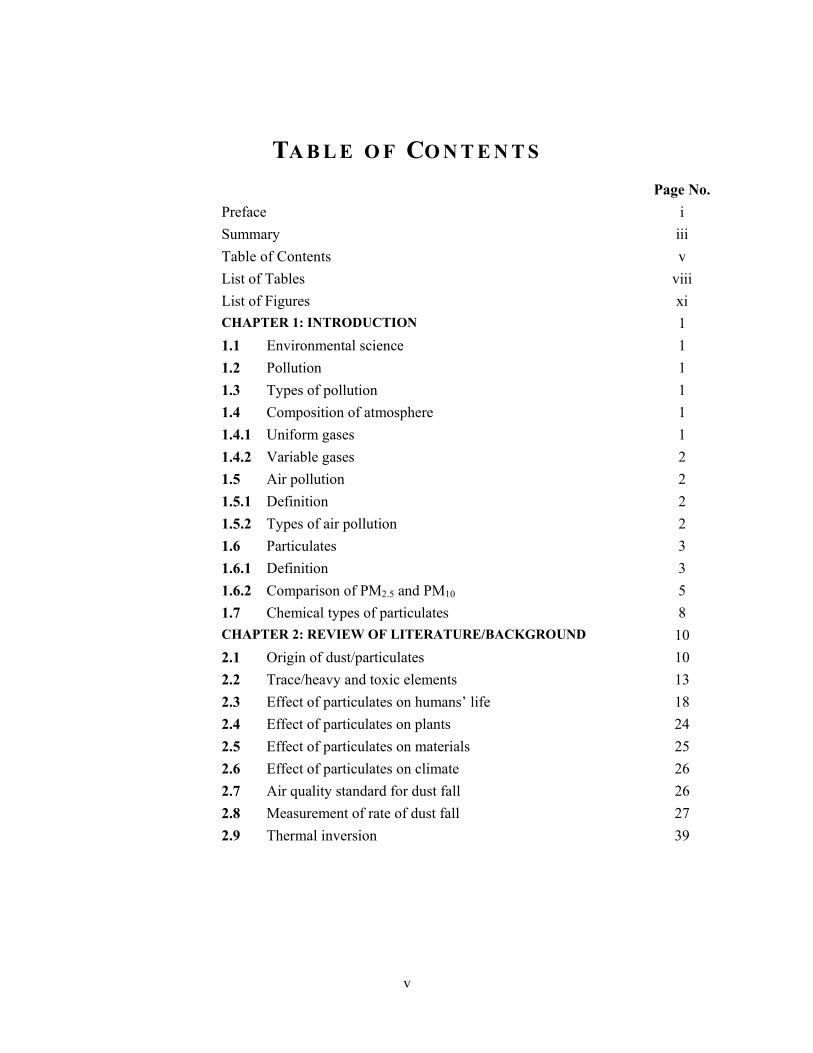
TA B L E O F CO N T E N T S
Page No. Preface i Summary iii Table of Contents v List of Tables viii List of Figures xi CHAPTER 1: INTRODUCTION 1 1.1 Environmental science 1 1.2 Pollution 1 1.3 Types of pollution 1 1.4 Composition of atmosphere 1 1.4.1 Uniform gases 1 1.4.2 Variable gases 2 1.5 Air pollution 2 1.5.1 Definition 2 1.5.2 Types of air pollution 2 1.6 Particulates 3 1.6.1 Definition 3 1.6.2 Comparison of PM2.5 and PM10 5 1.7 Chemical types of particulates 8 CHAPTER 2: REVIEW OF LITERATURE/BACKGROUND 10 2.1 Origin of dust/particulates 10 2.2 Trace/heavy and toxic elements 13 2.3 Effect of particulates on humans’ life 18 2.4 Effect of particulates on plants 24 2.5 Effect of particulates on materials 25 2.6 Effect of particulates on climate 26 2.7 Air quality standard for dust fall 26 2.8 Measurement of rate of dust fall 27 2.9 Thermal inversion 39
vi
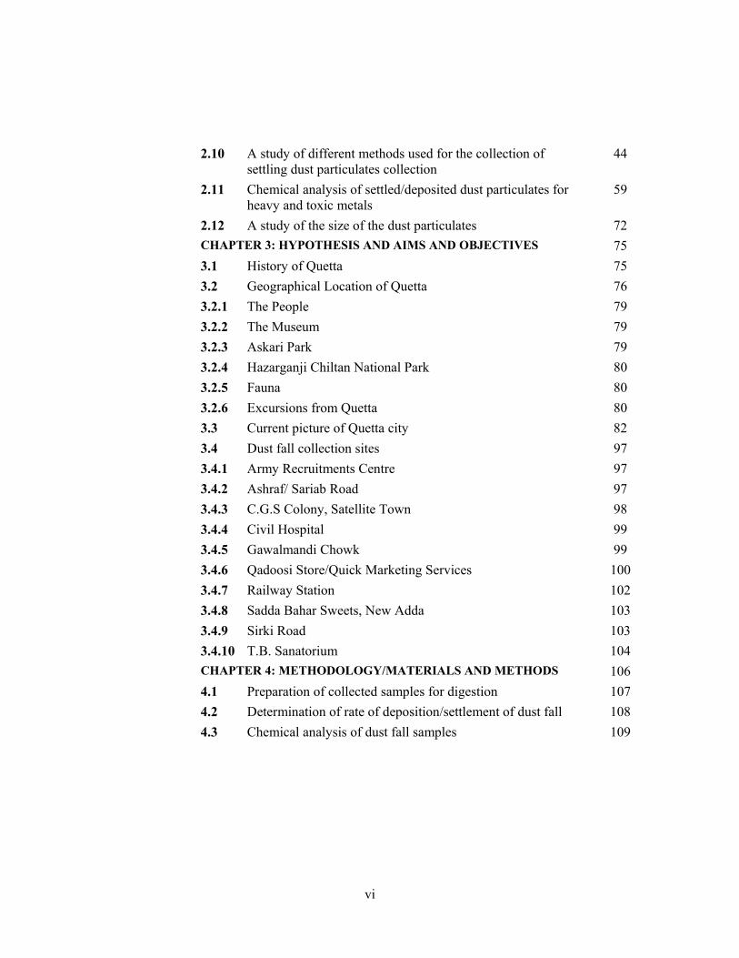
2.10 A study of different methods used for the collection of
settling dust particulates collection 44
2.11 Chemical analysis of settled/deposited dust particulates for heavy and toxic metals
59
2.12 A study of the size of the dust particulates 72 CHAPTER 3: HYPOTHESIS AND AIMS AND OBJECTIVES 75 3.1 History of Quetta 75 3.2 Geographical Location of Quetta 76 3.2.1 The People 79 3.2.2 The Museum 79 3.2.3 Askari Park 79 3.2.4 Hazarganji Chiltan National Park 80 3.2.5 Fauna 80 3.2.6 Excursions from Quetta 80 3.3 Current picture of Quetta city 82 3.4 Dust fall collection sites 97 3.4.1 Army Recruitments Centre 97 3.4.2 Ashraf/ Sariab Road 97 3.4.3 C.G.S Colony, Satellite Town 98 3.4.4 Civil Hospital 99 3.4.5 Gawalmandi Chowk 99 3.4.6 Qadoosi Store/Quick Marketing Services 100 3.4.7 Railway Station 102 3.4.8 Sadda Bahar Sweets, New Adda 103 3.4.9 Sirki Road 103 3.4.10 T.B. Sanatorium 104 CHAPTER 4: METHODOLOGY/MATERIALS AND METHODS 106 4.1 Preparation of collected samples for digestion 107 4.2 Determination of rate of deposition/settlement of dust fall 108 4.3 Chemical analysis of dust fall samples 109
vii
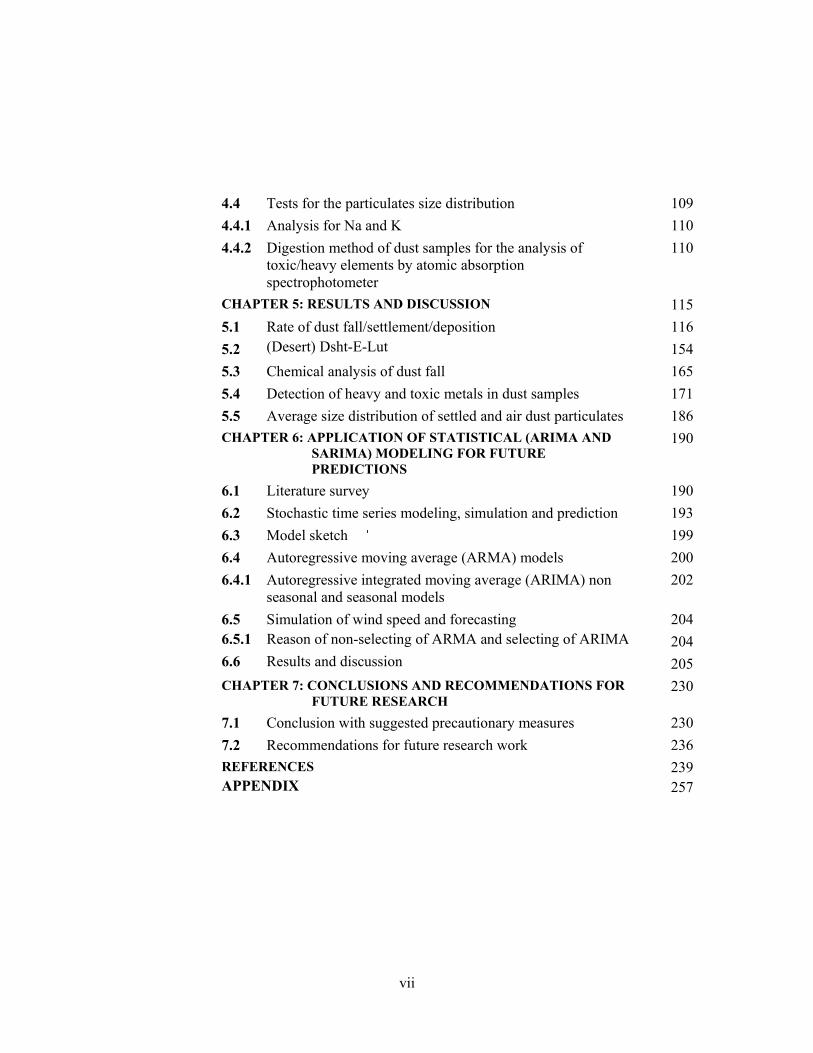
4.4 Tests for the particulates size distribution 109 4.4.1 Analysis for Na and K 110 4.4.2 Digestion method of dust samples for the analysis of
toxic/heavy elements by atomic absorption spectrophotometer
110
CHAPTER 5: RESULTS AND DISCUSSION 115 5.1 Rate of dust fall/settlement/deposition 116 5.2 (Desert) Dsht-E-Lut 154 5.3 Chemical analysis of dust fall 165 5.4 Detection of heavy and toxic metals in dust samples 171 5.5 Average size distribution of settled and air dust particulates 186 CHAPTER 6: APPLICATION OF STATISTICAL (ARIMA AND
SARIMA) MODELING FOR FUTURE PREDICTIONS
190
6.1 Literature survey 190 6.2 Stochastic time series modeling, simulation and prediction 193 6.3 Model sketch 199 6.4 Autoregressive moving average (ARMA) models 200 6.4.1 Autoregressive integrated moving average (ARIMA) non
seasonal and seasonal models 202
6.5 Simulation of wind speed and forecasting 204 6.5.1 Reason of non-selecting of ARMA and selecting of ARIMA 204 6.6 Results and discussion 205 CHAPTER 7: CONCLUSIONS AND RECOMMENDATIONS FOR
FUTURE RESEARCH 230
7.1 Conclusion with suggested precautionary measures 230 7.2 Recommendations for future research work 236 REFERENCES
APPENDIX 239 257
viii
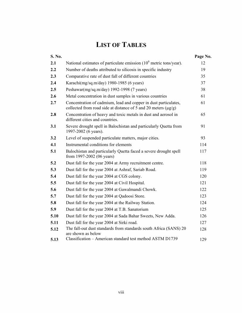
LIST OF TABLES
S. No. Page No. 2.1 National estimates of particulate emission (106 metric tons/year). 12 2.2 Number of deaths attributed to silicosis in specific industry 19 2.3 Comparative rate of dust fall of different countries 35 2.4 Karachi(mg/sq.m/day) 1980-1985 (6 years) 37 2.5 Peshawar(mg/sq.m/day) 1992-1998 (7 years) 38 2.6 Metal concentration in dust samples in various countries 61 2.7 Concentration of cadmium, lead and copper in dust particulates,
collected from road side at distance of 5 and 20 meters (µg/g) 61
2.8 Concentration of heavy and toxic metals in dust and aerosol in different cities and countries.
65
3.1 Severe drought spell in Balochistan and particularly Quetta from 1997-2002 (6 years).
91
3.2 Level of suspended particulate matters, major cities. 93 4.1 Instrumental conditions for elements 114 5.1 Balochistan and particularly Quetta faced a severe drought spell
from 1997-2002 (06 years) 117
5.2 Dust fall for the year 2004 at Army recruitment centre. 118 5.3 Dust fall for the year 2004 at Ashraf, Sariab Road. 119 5.4 Dust fall for the year 2004 at CGS colony. 120 5.5 Dust fall for the year 2004 at Civil Hospital. 121 5.6 Dust fall for the year 2004 at Gawalmandi Chowk. 122 5.7 Dust fall for the year 2004 at Qadoosi Store. 123 5.8 Dust fall for the year 2004 at the Railway Station. 124 5.9 Dust fall for the year 2004 at T.B. Sanatorium 125 5.10 Dust fall for the year 2004 at Sada Bahar Sweets, New Adda. 126 5.11 Dust fall for the year 2004 at Sirki road. 127 5.12 The fall-out dust standards from standards south Africa (SANS) 20
are shown as below 128
5.13 Classification – American standard test method ASTM D1739 129
ix
5.14 Average monthly rate of dust fall for the year 2004 (mg/m2/day) 130
5.15 Average monthly rate of dust fall for the year 2005 (mg/m2/day) 134
5.16 Average monthly Rate of dust fall for the year 2006 (mg/m2/day) 136
5.17 Average monthly Rate of dust fall for the year 2007 (mg/m2/day) 139
5.18 Average monthly Rate of dust fall for the year 2008 (mg/m2/day) 142
5.19 Average monthly Rate of dust fall from the year 2004-2008
(mg/m2/day) 144
5.20
5.21a
5.22
Monthly average rate of dust fall at Karachi (1980-1985)
Monthly average rate of dust fall at Peshawar (1992-1998)
Monthly average rate of dust fall at Quetta (2004-2008)
157 157
158
5.21b Rate of dust fall of different countries (mg/m2/day) 161 5.34 Typical natural trace element concentrations of surface soils 168 5.35a 5.35b
Typical chemical compositions of dust fall at Quetta for the year
2004-2008.
Average typical chemical compositions of dust fall at Quetta for the
year 2004-2008 during the thermal inversion spells.
169
169
5.36 Average typical chemical composition of dust fall at Karachi for the
year 1980-1985. 170
5.37 Average typical chemical composition of dust fall at Peshawar for
the year 1992-1998. 170
5.38 CALA directory laboratory. 174 5.39 Concentration of heavy and toxic metals in the dust fall at Quetta
during 2004 (µg/g (ppm) 175
5.40 Concentration of heavy and toxic metals in the dust fall at Quetta
during 2005 (µg/g (ppm) 176
5.41 Concentration of heavy and toxic metals in the dust fall at Quetta
during 2006 (µg/g (ppm) 176
5.42 Concentration of heavy and toxic metals in the dust fall at Quetta
during 2007 (µg/g (ppm) 177
x
5.43 Concentration of heavy and toxic metals in the dust fall at Quetta
during 2008 (µg/g (ppm) 177
5.44 Average concentration of heavy and toxic metals in the dust fall at
Quetta detected during 2004-08 µg/g (ppm) 178
5.45 Average concentration of heavy and toxic metals of Quetta from
2004-08 179
5.46 Concentration of heavy and toxic metals in dust and aerosol in
different cities and countries. 184
5.47a 5.47b
Average size distribution of dust fall 2004-08 at Quetta. fraction
% age by weight
Average size distribution of dust fall during thermal inversion period
(days) 2004-08 at Quetta, fraction % age by weight.
188
189
6.1 ARIMA & SARIMA Tables of 3 selected sites 206 5.22a 5.22b
Mean daily temperature (2004)
Mean monthly temperature 257 258
5.23 Daily precipitation (2004) 258 5.24 Daily precipitation (2005) 259 5.25 Daily precipitation (2006) 259 5.26 Daily precipitation (2007) 260 5.27 Daily precipitation (2008) 260 5.28 Wind speed (2004) 261 5.29 Wind speed (2005) 262 5.30 Wind speed (2006) 263 5.31 Wind speed (2007) 264 5.32 Wind speed (2008) 265 5.33 Daily visibility of Quetta 2004-08 272
xi
LIST OF FIGURES AND GRAPHS
S. No. Page No. 1.1 A typical benzene-extractable fraction an organic particulate
respirable in 1µ range 9
2.1 Soot particle from the combustion of fossil fuel 21 2.2 Satellite pictures 28 2.3 Asian dust rises to ~2km (1km above terrain) 28 2.4 Plume rises from the surface (at about 300 m) 29 2.5a 2.5b
Satellite picture of dust plume Heavy dust plume
30 31
2.6 Wind speed 40 2.7 Inversion layers 41 2.8 Depiction of thermal inversion layers. 41 2.9 London UK, 1952 42 2.10 Graph showing massive deaths due to the Thermal Inversion of
London in 1952
42
2.11 (a-e)
Donora PA—1948 43
2.12 Sample collector 45 2.13 Photograph of a typical dust trap 49 2.14 (a-c)
Dust watch standard single bucket collector 51
2.15 Dust watch standard four buckets collector 52 2.16 Position of bird strike preventer and supporting
struts 54
2.17 Cross section through the collecting bowl of the Frisbee type of dust deposit gauge (from Hall, Upton and Marsland, 1993)
54
3.1 Normal annual precipitation rate of Quetta city 82 3.2 Normal annual wind pattern of Quetta city 82 3.3 Normal annual temperature of Quetta city 83 3.4 Bruce Street, Quetta, before the earthquake 84 3.5 Another view of the devastation in Bruce Road 84
3.6 Depletion of ground water in Quetta city 86
xii
3.7 Improper disposal of solid waste/hospital waste at Quetta city 87
3.8 (a-d)
Haphazard ‘Quetta city’ growth, pathetic public transport etc 88
3.9 (a-b)
Los Angeles CA, inversion layers 89
3.10 Smog US global 90
3.11 (a-e)
Photos of Quetta while dust wrapped the city 93
3.12 Map of Balochistan and Quetta 95
3.13 Ten Selected Samples Collection sites of Quetta City 96
4.1 4.2 (a-f)
Flame photometer
Photographs while getting AAS & other instruments training at
Central Hi-Tech. Lab; U.O.B & working at PCSIR Labs. Quetta
110 113
5.1 Graph showing monthly rate of dust fall at Quetta (mg/m2/day)
(2004) 128
5.2 Graph showing average monthly rate of dust fall at Quetta
(mg/m2/day) (2004) 131
5.3 Graph showing average monthly rate of dust fall at Quetta
(mg/m2/day) (2005) 134
5.4 Graph showing average monthly rate of dust fall at Quetta
(mg/m2/day) (2005) 135
5.5 Graph showing average monthly rate of dust fall at Quetta
(mg/m2/day) (2006) 137
5.6 Graph showing average monthly rate of dust fall at Quetta
(mg/m2/day) (2006) 138
5.7 Graph showing average monthly rate of dust fall at Quetta
(mg/m2/day) (2007) 139
5.8 Graph showing average monthly rate of dust fall at Quetta
(mg/m2/day) (2007) 140
xiii
5.9 Graph showing average monthly rate of dust fall at Quetta
(mg/m2/day) (2008) 142
5.10 Graph showing average monthly rate of dust fall at Quetta
(mg/m2/day) (2008) 143
5.11 Graph showing average monthly rate of dust fall at Quetta
(mg/m2/day) from 2004 to 2008 145
5.12 Graph showing average monthly rate of dust fall at Quetta
(mg/m2/day) from 2004 to 2008 151
5.13 Graph showing rate of dust fall at Karachi (mg/m2/day) 158
5.14 Graph showing rate of dust fall at Karachi (mg/m2/day) 159
5.15 Graph showing rate of dust fall at Peshawar (mg/m2/day) 159
5.16 Graph showing rate of dust fall at Peshawar (mg/m2/day) 160
5.17 Graph showing rate of dust fall at Quetta (mg/m2/day) 160
5.18 Graph showing rate of dust fall in different countries. 161
5.19 Graph showing rate of dust fall at Quetta (mg/m2/day) 162
5.20 Graph showing comparative rate of dust fall at Karachi (1980-1985),
Peshawar (1992-1998) and Quetta (2004-2008)(mg/m2/day) 162
1
CHAPTER 1
INTRODUCTION
1.1 ENVIRONMENTAL SCIENCES:
It is an inter subject range of study that defines problems instigated by
anthropological use of natural world and pursues solutions for those problems.
1.2 POLLUTION:
The disturbance in the balance of naturally harmonized systems or
cycles by increasing or decreasing any one of the constituents
anthropologically is called Pollution.
1.3 TYPES OF POLLUTION:
Air Pollution
Water Pollution
Soil Pollution
Noise Pollution
Light Pollution
Aesthetic Pollution, etc.
1.4 COMPOSITION OF ATMOSPHERE:
1.4.1 Uniform gases:
Nitrogen (N2) ~ 78%, (O2) ~ 21%, Argon (Ar), trace gases (Neon,
Helium, Methane (CH4), etc.) ~ 1%.

2
1.4.2 Variable gases:
Water vapor (H2Ov), O3, CO2.
1.5 AIR POLLUTION:
1.5.1 Definition:
There is a divine set inter and intra equilibrium between the
different hydrological, oxygen, nitrogen, phosphate and sulphur cycles
of eco-system. So is in the case of our atmosphere (The disturbance in
the said set divine dynamic equilibrium of the atmosphere by injecting
certain pollutants Naturally or Anthroprogenically is called Air
Pollution.
1.5.2 TYPES OF AIR POLUTION:
Air pollutants are divided into two categories.
(1) Primary Pollutants
(2) Secondary Pollutants
(1) Primary Pollutants:
Primary pollutants include carbon mono-oxide (CO), hydrocarbons,
particulates, sulphur dioxide (SO2) and nitrogen compounds [1].
• Particulates, part
• Carbon monoxide, CO
• Sulphur oxides, SOx
• Nitrogen oxides, NOx
3
• Hydrocarbons, HC
(2) Secondary Pollutants:
Whereas ozone (O3), peroxyacetyl nitrates (PAN), lead and toxic
chemicals are considered as the secondary pollutants. So far numerous
compounds have been known in polluted cities air, but their collaboration, for
instance, soot chemistry, is very multifaceted. Photochemical pollution is
nowadays more communal than was initially assumed. It happens so
extensively that is significant to converse as well. Nitrogen existing in the air
and as a contamination in fossils fuels changes to nitric oxide in emitted gases.
Similarly, other trace contaminations can provide increase to a diversity of
contaminant gases in release. The occurrence of chlorine and sulfur in fuels
outcomes in the discharge of gaseous chlorine and sulfur compounds [1].
In USA, about 140 to 150 million tons of pollutants are given to the air
every year. Industries account for 20 to 30 million tons, space heating 10 to 15
million tons, refuse disposal 5 to 10 million tons and motor vehicles 90 million
tons or more [1].
• Ozone, O3 O ║ • Peroxyacetylnitrates (PAN) (CH3-C-OONO2)
• Lead and toxic chemicals.
1.6 PARTICULATES:
1.6.1 Definition:
Any material, except uncombined water, that exists in the solid or
liquid state in the atmosphere or gas stream at standard condition or “Small
4
solid particles including lead from gasoline additives and liquid droplets (or
aerosols) such as dust, ash, soot, lint, pollen, smoke, spores, algal cells and
other suspended materials; originally applied only to solid particles but now
extended to droplets of liquid are collectively termed as particulates” [2].
It should be kept in mind that the total particulate matter burden of
ambient air is less important than the chemical nature, size and rate of
deposition/settlement/fall of the particulates. The particulates possess large
areas in general and hence present good sites for sorption of various inorganic
and organic matters [2].
The most important physical property is size. Particulates range in size
from a diameter of 0.0002 µ (about the size of small molecule) to a diameter
of 500 µ (1µ= 10-6 meter) having lifetimes varying from a few seconds to
several months. This lifetime, however depends on the settling rate, which
again depends upon the size and density of the particles and turbulence of air
[2]. Particulates matter in the air is generally divided into further two
categories depending upon their size and diameter.
(i) Particles whose effective diameter is less than 5 microns are
classified as suspended materials because their falling rate under
gravity is so low that due to air movement they remain suspended
in air for a long time.
(ii) Particulates with diameter greater than 5 microns are identified
as settleable materials. It is the material, which is found settled on trees,
buildings and is noticed even by naked eyes until the rain washes it away. The
material thus collected is commonly called dust fall.
5
Particle (also called particulate matter or PM) pollution is the term
used aiming at a blend of solid and liquid drops exist in the atmosphere. Few
particulates for instance smoke; dirt, soot or dust could be visualized without
any equipment as they are having pretty big sizes. While some are this much
small that could only be spotted with the devices like electron microscope.
Particulates comprise of inhalable ‘coarse’ (rough) particulates containing the
diameter within 2.5-10 µm, ‘fine’ particulates having sizes ≤ 2.5 µm and the
particulates having the sizes ≤ 0.1µ (0.0000001 m) are termed as ultra-fine
particles.
1.6.2 COMPARISON OF PM2.5 AND PM10:
• PM2.5 and PM10 refers to size of particles in microns (µ)
• Recall size of a micron:
– 1 µ = 1 millionth of a meter = 0.000001 m
– 70 µ = thickness of human hair = 0.00007 m
– 10 µ = Respirable PM = 0.00001 m
– 2.5 µ = Fine PM = 0.0000025 m
– 0.1 µ = Ultra-fine PM = 0.0000001 m
The number of particles in the atmosphere varies from several hundred
per cm3 in clean air to more than 100,000 per cm3 in highly polluted air, in
urban areas like Karachi, Peshawar and Quetta the particulates mass level may
range from 60 µg to 20000 µg per m3.
Sporadic plumes of particulates could wrap the city in winters, which
cause a severe nuisance among the residents (as experienced by Quettaites
6
during our research period 2004-08) vis-à-vis their daily life and health. The
presence of any heavy industry in city causes the production of aerosols,
which are an amalgamation of primary and secondary particulates in the
atmosphere. Primary particulates (e.g. ultra fines having the size below 1µ in
diameter) along with trace metals e.g. Fe, Na, Zn, K etc. might emerge directly
from diverse sources mainly from soil originated dust [3], whereas secondary
particulates appearance in the atmosphere from gaseous release of sulfur
dioxide, oxides of nitrogen, ammonia, and heavy organic gases. Resultant
aerosol development may take place under dull air circumstances, following
old mixed gaseous emanations from diverse basis, and when contaminants
produced on earlier days build up or are recycled by winds and are stocked up
suddenly in surface-based inversions. Severe and chronic bronchio-pulmonar
diseases are the reasons of dust and particulates bound discharge in the
environment. They are usually linked with PAH (poly-aromatic
hydrocarbons), PCP (penta-chlor-phenol) and furans / dioxins, as they gamely
stuck on non-volatile aerosols. These particulates have a tendency to
concentrate in the bronchio-pulmonar region where they are simply immersed
by the tissue. Besides that, since these particles mostly hold heavy metals, PM
characterize a considerable origin of the toxic load accumulated by humans,
which frankly cause cardio-vascular diseases. Unluckily, current PM-detectors
record merely particulates matter. Nevertheless, research works have found
that particulates number is far more pertinent than their cluster. Therefore,
usual finding apparatus spotlights on cluster merely, therefore sense only a
part of the particulates record. Diesel vapors are particularly troublesome since
they hold nitro-aromates; a set of chemicals which are used to speed up the
7
incineration course of diesel fuel. Nitro-aromatic sort of compounds are
notorious for their tendency of causing mutagenic effect within the GIT
(gastro-intestinal tract). At the start they become the reason of diarrhea.
A massive segment of the globe’s population settled in the huge cities
developed approximately 5% to 50% for the last two centuries.
Anthropologists assess that till the year 2030 about two third of the global
population would dwell in large cities and towns. The high rise of urbanization
has produced many environmental nuisances for instance scarcity of water
supply and sewerage system, over congestion, inadequate transport, slums,
haphazard and unplanned development, particularly for the metropolitan areas
like, Karachi, Lahore, Quetta etc. The main environmental problems of
Karachi are water pollution, marine pollution, disposal of solid waste and air
pollution. Among this environmental degradation, key worry is air pollution
that is upsetting the settled regions. Traffic and industries emit pollutants into
the environment as chief supplier. A few decades ago traffic did not play an
important role in air pollution. Today it is the major supply of pollutant in the
urbanized and industrialized countries. With an improved standard of living
and increased demand on the transport sector, automobile re1ated pollution is
fast growing into a problem of serious dimension in our cities. This is caused
not only by rapid rise in number of automobiles but also due to narrow roads,
slow moving traffic, unfavorable driving cycles, poor enforcement of the laws
relating to vehicles road worthiness and poor emission control measures etc.
[4].
8
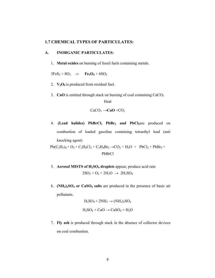
1.7 CHEMICAL TYPES OF PARTICULATES:
A. INORGANIC PARTICULATES:
1. Metal oxides on burning of fossil fuels containing metals.
3FeS2 + 8O2 → Fe3O4 + 6SO2
2. V2O5 is produced from residual fuel.
3. CaO is emitted through stack on burning of coal containing CaCO3
Heat
CaCO3 →CaO +CO2
4. (Lead halides) PbBrCl, PbBr2 and PbCl2are produced on
combustion of leaded gasoline containing tetraethyl lead (anti
knocking agent)
Pb(C2H5)4 + O2 + C2H4Cl2 + C2H4Br2 →CO2 + H2O + PbCl2 + PbBr2 +
PbBrCl
5. Aerosol MISTS of H2SO4 droplets appear, produce acid rain
2SO2 + O2 + 2H2O → 2H2SO4
6. (NH2)2SO4 or CaSO4 salts are produced in the presence of basic air
pollutants.
H2SO4 + 2NH3 → (NH2)2SO4
H2SO4 + CaO → CaSO4 + H2O
7. Fly ash is produced through stack in the absence of collector devices
on coal combustion.
9
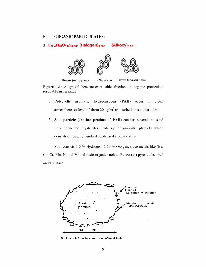
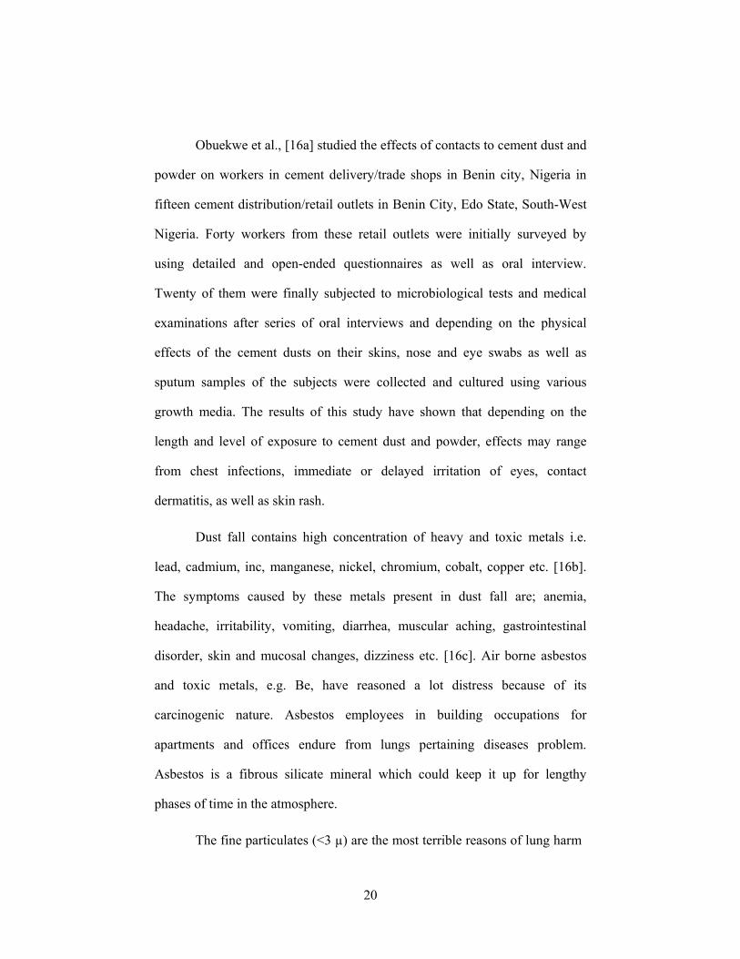
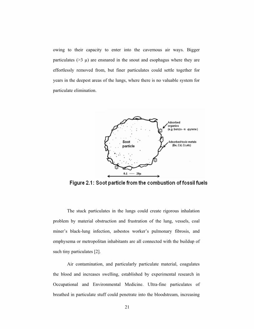
B. ORGANIC PARTICULATES:
1. C32.4H48O3.8S0.083 (Halogen)0.065 (Alkoxy)0.12
Figure 1.1: A typical benzene-extractable fraction an organic particulate respirable in 1µ range
2. Polycyclic aromatic hydrocarbons (PAH) occur in urban
atmospheres at level of about 20 µg/m3 and sorbed on soot particles.
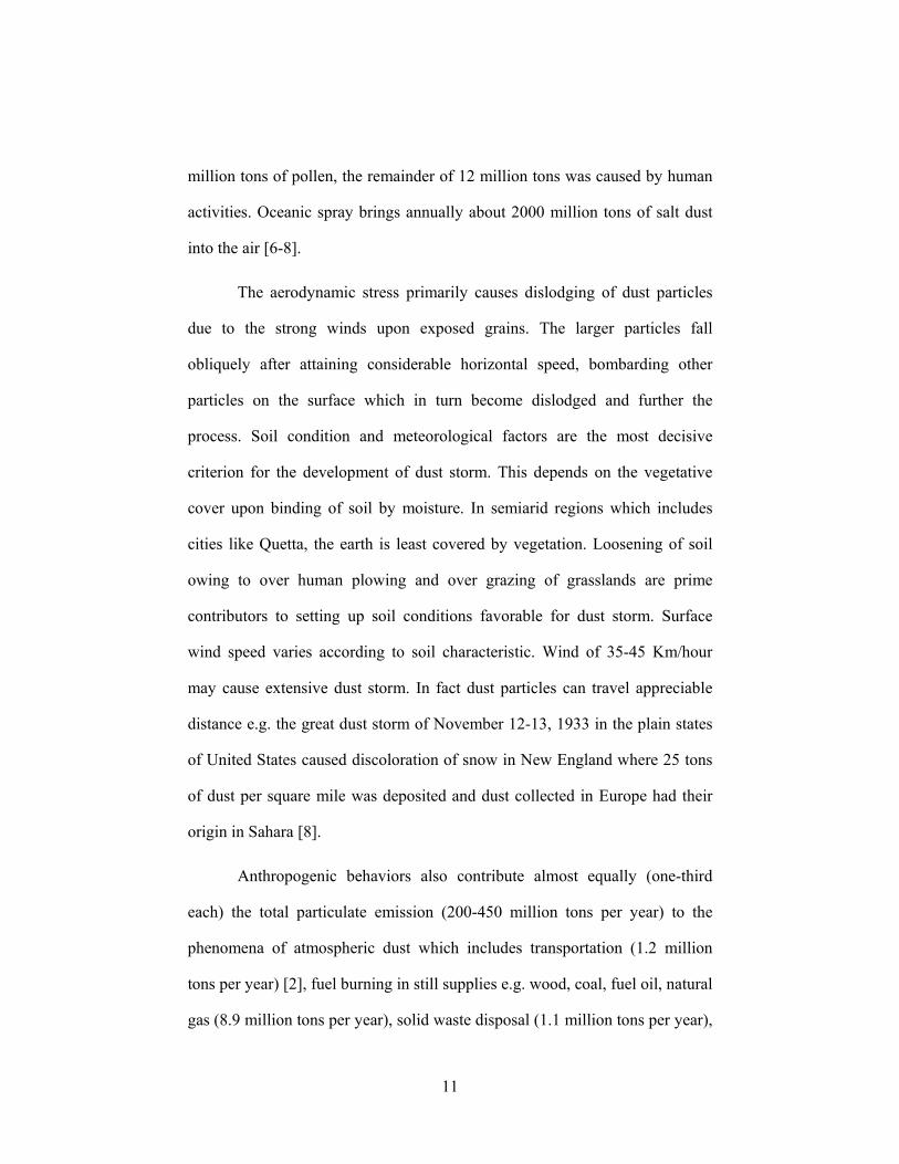
3. Soot particle (another product of PAH) consists several thousand
inter connected crystallites made up of graphitic platelets which
consists of roughly hundred condensed aromatic rings.
Soot consists 1-3 % Hydrogen, 5-10 % Oxygen, trace metals like (Be,
Cd, Cr, Mn, Ni and V) and toxic organic such as Benzo (α-) pyrene absorbed
on its surface.

10
CHAPTER 2
LITERATURE REVIEW/BACKGROUND
2.1 ORIGIN OF DUST/PARTICULATES:
Our atmosphere contains between one and three billion tons of dust
and other particles at any given time. Wind assists in keeping this dust
airborne, but gravity wins most of the time, forcing the dust particles
earthward, proving the old adage: “what goes up, must come down due to
gravitational force 'g'.” Dust comes from many different sources. Some, like
the by-product of the combustion of fossil fuels, are man-made. Others come
from natural sources – like sea-spray blowing off the ocean, or dust blowing in
from the desert. Dust comprises inorganic matter, such as sand particles, as
well as a large amount of organic matter, including pollen, spores, moulds, and
viruses. These minute particles, ranging in size from around 100 micro meters
(µm) to a few nano metres (nm), invade our airspace every day, a part of life
that we aren’t even aware of, except when we dust the furniture [5].
Through a natural and as well anthropogenically dust enters into
atmosphere. There are numerous natural processes injecting particulate matter
into the atmosphere (800-2000 million tons each year) [2]. The natural
operations which inject huge amount of particulate matter into the air are
volcano eruptions, oceanic spray, dust storm, gusting of dust and dirt or soil by
the storm. It has been reported that up to 15% of the total settleable dust and
an estimated 25% of suspended particulate matter is of natural origin. It has
been estimated that over the United States about 43 million tons dust settled
per year. Of this, 31 million tons was from natural resources including one
11
million tons of pollen, the remainder of 12 million tons was caused by human
activities. Oceanic spray brings annually about 2000 million tons of salt dust
into the air [6-8].
The aerodynamic stress primarily causes dislodging of dust particles
due to the strong winds upon exposed grains. The larger particles fall
obliquely after attaining considerable horizontal speed, bombarding other
particles on the surface which in turn become dislodged and further the
process. Soil condition and meteorological factors are the most decisive
criterion for the development of dust storm. This depends on the vegetative
cover upon binding of soil by moisture. In semiarid regions which includes
cities like Quetta, the earth is least covered by vegetation. Loosening of soil
owing to over human plowing and over grazing of grasslands are prime
contributors to setting up soil conditions favorable for dust storm. Surface
wind speed varies according to soil characteristic. Wind of 35-45 Km/hour
may cause extensive dust storm. In fact dust particles can travel appreciable
distance e.g. the great dust storm of November 12-13, 1933 in the plain states
of United States caused discoloration of snow in New England where 25 tons
of dust per square mile was deposited and dust collected in Europe had their
origin in Sahara [8].
Anthropogenic behaviors also contribute almost equally (one-third
each) the total particulate emission (200-450 million tons per year) to the
phenomena of atmospheric dust which includes transportation (1.2 million
tons per year) [2], fuel burning in still supplies e.g. wood, coal, fuel oil, natural
gas (8.9 million tons per year), solid waste disposal (1.1 million tons per year),
12
miscellaneous processes i.e. forest fire, structural fire, coal refuse burning,
agricultural burning (9.6 million tons per year) and industrial processes (7.5
million tons per year) [9a]. In developed countries like USA the annual
particulate emission is about 20×106 tones, including 5×10⁶ tons of fine
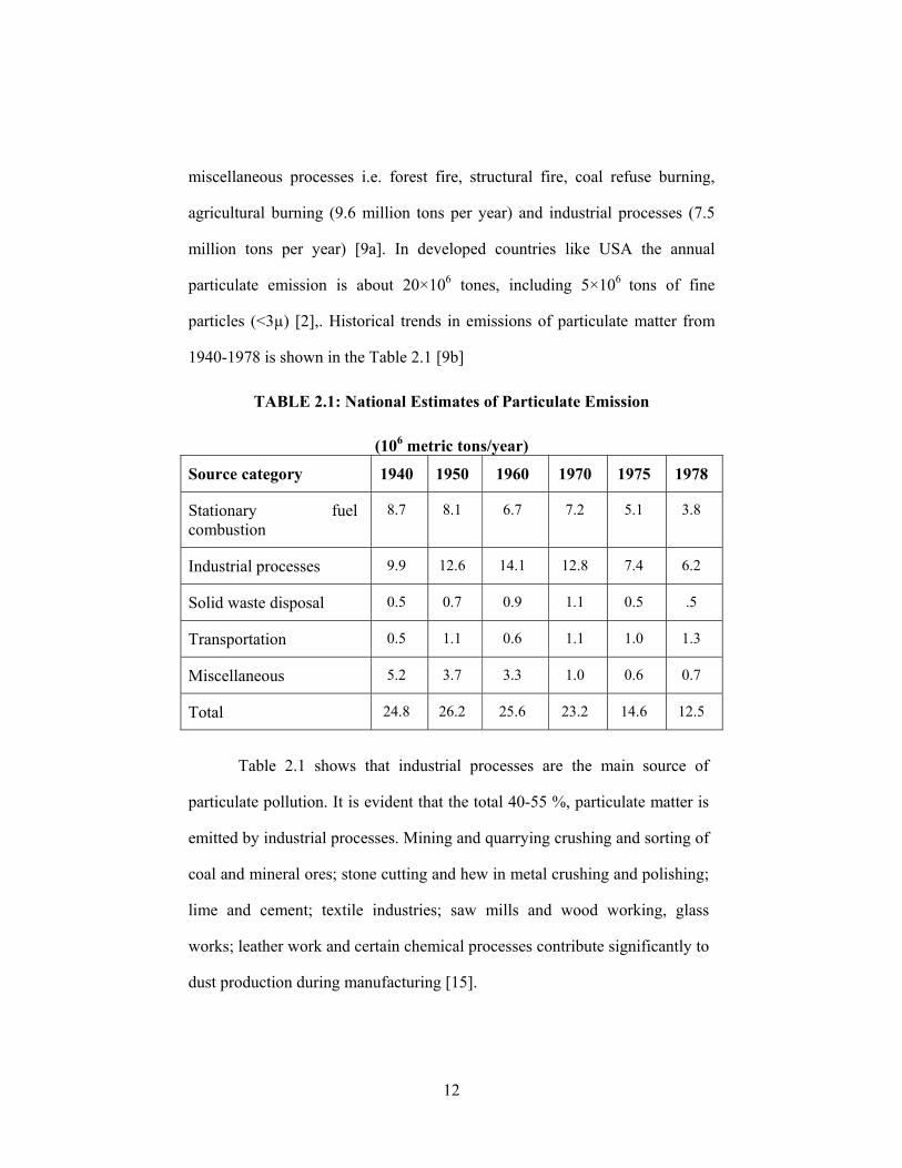
particles (<3µ) [2],. Historical trends in emissions of particulate matter from
1940-1978 is shown in the Table 2.1 [9b]
TABLE 2.1: National Estimates of Particulate Emission
(106 metric tons/year)
Source category 1940 1950 1960 1970 1975 1978
Stationary fuel combustion
8.7 8.1 6.7 7.2 5.1 3.8
Industrial processes 9.9 12.6 14.1 12.8 7.4 6.2
Solid waste disposal 0.5 0.7 0.9 1.1 0.5 .5
Transportation 0.5 1.1 0.6 1.1 1.0 1.3
Miscellaneous 5.2 3.7 3.3 1.0 0.6 0.7
Total 24.8 26.2 25.6 23.2 14.6 12.5
Table 2.1 shows that industrial processes are the main source of
particulate pollution. It is evident that the total 40-55 %, particulate matter is
emitted by industrial processes. Mining and quarrying crushing and sorting of
coal and mineral ores; stone cutting and hew in metal crushing and polishing;
lime and cement; textile industries; saw mills and wood working, glass
works; leather work and certain chemical processes contribute significantly to
dust production during manufacturing [15].
13
2.2 TRACE/HEAVY AND TOXIC ELEMENTS:
The scattering of trace metals in air particulates has been detected to be
reliant on meteorological states. It has been stated that metal substances
display an activist relationship with temperature and an opposite association
with rainfall. Wind rate and track have also been affecting the trace metal
division in fine and coarse particulates parts. Furthermore, in the dearth of
further atmospheric pollutants trace metal quantities are taken as a valuable
guide of air quality of the local environment. Many statistical models have
been recommended for enhanced classification of atmospheric particulates.
The multivariate statistical techniques, principal component analysis (PCA)
and cluster analysis (CA) are deemed a sturdy mean to recognize the causes
and to comprehend the sharing of trace metals in the ambiance [10].
Another study on division of heavy metals in the deposits of Lagos
Lagoon was conducted by Nwajei and Gagophien. The concentrations of
cadmium, lead, nickel, chromium, copper, zinc, iron, manganese, cobalt and
mercury in the sediments of the Lagos Lagoon were determined by atomic
absorption spectrophotometry in the year 1998. The respective limits of the
quantities of the metals were Cd: 0.13-8.60, Pb: 4.10-295.70; Ni: 11.60-
149.40, Cr: 23.30-167.20, Cu: 4.80-102.70, Zn: 27.30-323.70, Fe: 10579.80-
85548.00, Mn: 276.00-748.00, Co: 6.40-41.50 and Hg: 0.04-0.53 mg/kg-1 dry
weight. It highlighted the impact of domestic and industrial discharge of waste
on the levels of cadmium, lead, nickel, chromium, copper, zinc, iron,
manganese, cobalt and mercury metals in the sediments of Lagos Lagoon and
compared the distribution of metals in top and bottom sediments [11].
14
Air pollution intensity in Pakistan’s most populated cities are amongst
the uppermost in the globe and mountaineering, originating grave health
problems. The height of ambient particulates smolder particulates and dust,
that become responsible of respiratory illness, are usually double the global
mean and above than five times as elevated as in industrial countries and Latin
America [12a] as was investigated while a study of atmospheric pollution due
to vehicular exhaust at the hectic roads in Peshawar by Khan et al., [12c].
For contact evaluation, it is essential to calculate particulate release
intensities, and as well to establish particulate trend after releases, because
they are moved away from the release source. Trace elements in the ambiance
are linked with dust particulates, which are included mostly of dust, and fly
ash particulates and some trace elements might be in the gaseous state. Even
though dust particulates are generally more than 5 µm in thickness, there is
always the possibility that some dust will consist of windblown clay
particulates which are by description smaller than 2 µm in width. There are
several field studies in which soils were analyzed for various trace elements.
For example, Bradford et al analyzed soil and plant samples taken from
several location around a 1500 MW power station in Nevada and found
decrease in concentration for Ca, Mg, Sr, Ba and B in saturation extracts of
surface soils and similar effects for Ca, Sr and B in plant samples [13a].
Pinto stated that vehicle donations occurred from exhaust releases
enhanced in Pb; from corrosion as Fe; tire wear particulates developed in Zn;
brake coatings augmented in Cr, Ba and Mn; and cement particles resulting
from roadways by scrape. The major constituents releases from diesel and
15
gasoline fueled automobiles are organic carbon (O.C) and elemental carbon
(EC). It is reported that most of the PM emitted by motor vehicles is in the PM
size range [13b].
Ahmed et al., [13c] observed heavy metals concentration in free fall
dust along a main road. They analyzed free fall dust for determining the
contents of heavy metal elements such as Pb, Cd, Zn, Ni and Cu. A decrease
in heavy metal concentrations by moving away from the road was
significantly apparent at Muredkey, Ferozwala and Shahdra, whereas at Kala
Shah Kaku heavy metals concentrations were not significant by moving away
from the road. Relatively higher concentrations of Pb, Zn, Cu, and Cd were
observed at Shahdra near the road, which may be attributed to traffic density at
the respective site.
They also elaborated about heavy metals concentration in Roadside
dust. At Murdkey, concentrations of Pb, Zn and Ni decreased with moving
away from GT-road. Whereas Cd and V showed almost same concentrations
at all distances. At Kala Shah Kaku, Pb, Cd, Ni and Zn concentrations
followed the decreasing trend by moving away from the highway, however the
amount of V was same at all distances. Concentrations of whole metals in the
highway shoulders dust of Ferozwala decreased with moving away from GT-
road. At Shahdra, concentrations of Zn, Ni and Pb followed the same
decreasing trend while Cd and V concentrations did not follow the above
trend. Maximum concentration of Pb in roadside dust was found at Shahdra
(14 mg/Kg) near to the road. This may be due to greater traffic density at the
respective sites. Relatively greater concentration of Cd in roadside dust was
16
found at Ferozwala (0.96 mg/Kg) and Kala Shah Kaku (0.95 mg/Kg). This
might be owing to the occurrence of zinc – cadmium smelting industries in the
Kala Shah Kaku industrial estates. Concentration of Zn in roadside dust was
found to be greater at Muredkey (33.6 mg/Kg). Relatively greater
concentration of Ni in roadside dust was observed at Kala Shah Kaku (40.7
mg/Kg) close to the road. This may be because of the existence of industrial
estate there. Most of these industries used oil and coal for combustion purpose,
which are the primary sources of emission of Ni [13c].
A recent study was conducted in Islamabad regarding classification of
chosen metals in ambient air hovering particulate stuff regarding
meteorological circumstances [14].
There has been an increasing apprehension on the atmospheric
pollution trouble arising from industrialization, transportation: urbanization
and additional anthropogenic actions. The problem has got additional severe
notice because of the existence of heavy toxic trace metals in ambient air
floating particulate material in the air. Numerous studies have paid attention
on elemental composition of environmental aerosol particulates'. The character
of climate circumstances on the way to "explain the sharing of aerosols in the
environment”, have been reported by several workers. These researches have
provided evidence for a correlation between metal concentrations in aerosols
and weather limitations such as humidity, temperature, wind speed and
rainfall. Divergence in metal stuffing, with diurnal limits, was as well
documented for diverse regions of the globe. These data exhibited a positive
relationship among metal substance and temperature, whilst an opposite
17
correlation was recorded with some changeable as moisture and precipitation.
The said researches held the truth that weather aspects have an imperative
function to the allocation and elemental amount of floating particulate stuff in
the environment [14].
Similar to the majority other under-developed countries, the
progressions of industrial growth and urbanization in Pakistan have not moved
at the speed essential for ecological protection, consequential in many troubles
occurring from unfettered environmental pollution. For many years, in the
capital city, Islamabad, the transportation change has mounted up enormously,
and additionally, an industrialized zone set up at the core of the city to fulfill
the necessities of industrial merchandise for a large inhabitants section. As a
result, the neighboring city inhabitants are nowadays confronting distinctive
unsympathetic fitness consequences of air contaminants that are produced
from industrial releases and enlarged automobiles thickness [14].
An earlier research held in the city proved that the local environment
was overloaded with ambient air hovering particulate stuff loaded with heavy
toxic trace metals, with intensities in extreme surplus to those in the
surroundings environment. Consequently, the city environment might now be
assumed analogous with any disgustingly contaminated city of the globe. The
research pointed out considerable humans enrichment of trace metal
absorption in road region dumped earth crust, water and air linked to the city
region [14].
18
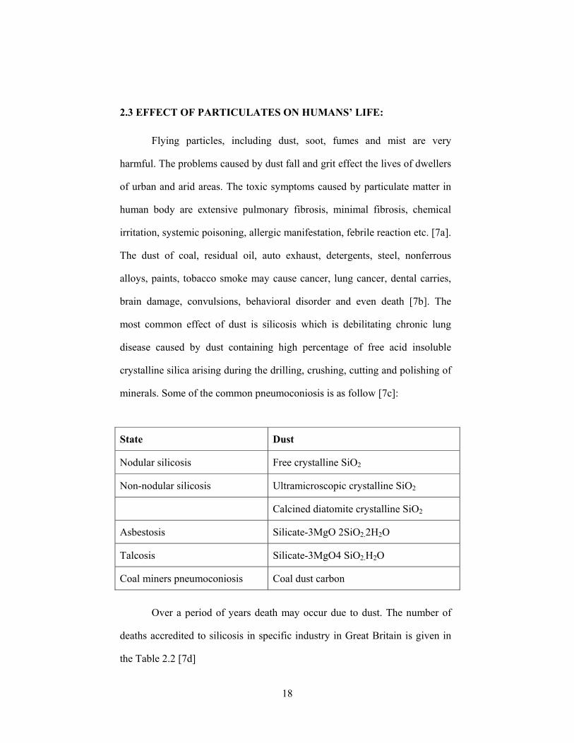
2.3 EFFECT OF PARTICULATES ON HUMANS’ LIFE:
Flying particles, including dust, soot, fumes and mist are very
harmful. The problems caused by dust fall and grit effect the lives of dwellers
of urban and arid areas. The toxic symptoms caused by particulate matter in
human body are extensive pulmonary fibrosis, minimal fibrosis, chemical
irritation, systemic poisoning, allergic manifestation, febrile reaction etc. [7a].
The dust of coal, residual oil, auto exhaust, detergents, steel, nonferrous
alloys, paints, tobacco smoke may cause cancer, lung cancer, dental carries,
brain damage, convulsions, behavioral disorder and even death [7b]. The
most common effect of dust is silicosis which is debilitating chronic lung
disease caused by dust containing high percentage of free acid insoluble
crystalline silica arising during the drilling, crushing, cutting and polishing of
minerals. Some of the common pneumoconiosis is as follow [7c]:
State Dust
Nodular silicosis Free crystalline SiO2
Non-nodular silicosis Ultramicroscopic crystalline SiO2
Calcined diatomite crystalline SiO2
Asbestosis Silicate-3MgO 2SiO2.2H2O
Talcosis Silicate-3MgO4 SiO2.H2O
Coal miners pneumoconiosis Coal dust carbon
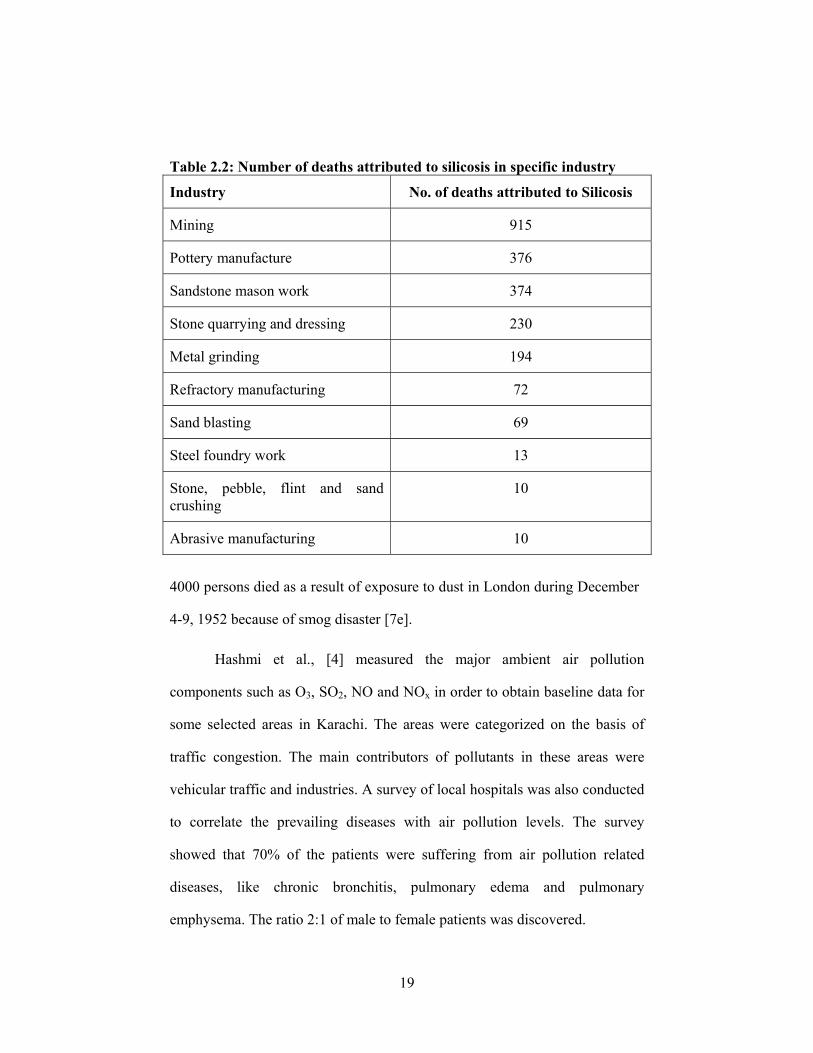
Over a period of years death may occur due to dust. The number of
deaths accredited to silicosis in specific industry in Great Britain is given in
the Table 2.2 [7d]
19
Table 2.2: Number of deaths attributed to silicosis in specific industry
Industry No. of deaths attributed to Silicosis
Mining 915
Pottery manufacture 376
Sandstone mason work 374
Stone quarrying and dressing 230
Metal grinding 194
Refractory manufacturing 72
Sand blasting 69
Steel foundry work 13
Stone, pebble, flint and sand crushing
10
Abrasive manufacturing 10
4000 persons died as a result of exposure to dust in London during December
4-9, 1952 because of smog disaster [7e].
Hashmi et al., [4] measured the major ambient air pollution
components such as O3, SO2, NO and NOx in order to obtain baseline data for
some selected areas in Karachi. The areas were categorized on the basis of
traffic congestion. The main contributors of pollutants in these areas were
vehicular traffic and industries. A survey of local hospitals was also conducted
to correlate the prevailing diseases with air pollution levels. The survey
showed that 70% of the patients were suffering from air pollution related
diseases, like chronic bronchitis, pulmonary edema and pulmonary
emphysema. The ratio 2:1 of male to female patients was discovered.
20
Obuekwe et al., [16a] studied the effects of contacts to cement dust and
powder on workers in cement delivery/trade shops in Benin city, Nigeria in
fifteen cement distribution/retail outlets in Benin City, Edo State, South-West
Nigeria. Forty workers from these retail outlets were initially surveyed by
using detailed and open-ended questionnaires as well as oral interview.
Twenty of them were finally subjected to microbiological tests and medical
examinations after series of oral interviews and depending on the physical
effects of the cement dusts on their skins, nose and eye swabs as well as
sputum samples of the subjects were collected and cultured using various
growth media. The results of this study have shown that depending on the
length and level of exposure to cement dust and powder, effects may range
from chest infections, immediate or delayed irritation of eyes, contact
dermatitis, as well as skin rash.
Dust fall contains high concentration of heavy and toxic metals i.e.
lead, cadmium, inc, manganese, nickel, chromium, cobalt, copper etc. [16b].
The symptoms caused by these metals present in dust fall are; anemia,
headache, irritability, vomiting, diarrhea, muscular aching, gastrointestinal
disorder, skin and mucosal changes, dizziness etc. [16c]. Air borne asbestos
and toxic metals, e.g. Be, have reasoned a lot distress because of its
carcinogenic nature. Asbestos employees in building occupations for
apartments and offices endure from lungs pertaining diseases problem.
Asbestos is a fibrous silicate mineral which could keep it up for lengthy
phases of time in the atmosphere.
The fine particulates (<3 µ) are the most terrible reasons of lung harm
21
owing to their capacity to enter into the cavernous air ways. Bigger
particulates (>3 µ) are ensnared in the snout and esophagus where they are
effortlessly removed from, but finer particulates could settle together for
years in the deepest areas of the lungs, where there is no valuable system for
particulate elimination.
The stuck particulates in the lungs could create rigorous inhalation
problem by material obstruction and frustration of the lung, vessels, coal
miner’s black-lung infection, asbestos worker’s pulmonary fibrosis, and
emphysema or metropolitan inhabitants are all connected with the buildup of
such tiny particulates [2].
Air contamination, and particularly particulate material, coagulates
the blood and increases swelling, established by experimental research in
Occupational and Environmental Medicine. Ultra-fine particulates of
breathed in particulate stuff could penetrate into the bloodstream, increasing
22
the risk that their "coagulating" effects on macrophages may have an effect
on the plaques discovered on blood vessels walls. Macrophages are a main
constituent of arterial plaques. This could help to elucidate why air
contamination is connected with an amplified danger of heart attacks, stroke,
and deteriorating respiratory troubles [17].
Kaplan and his colleagues [18] found that there could be a connection
among elevated intensity of air contamination and the danger of appendicitis.
Fresh investigation findings revealed at the 73rd Annual Scientific Meeting of
the American College of Gastroenterology in Orlando, suggests a novel
connection. Dr. Kaplan et al discovered more than 5,000 adults who were
admitted at hospitals for appendicitis in Calgary between 1999 and 2006
having used data from Environment Canada's National Air Pollution
Surveillance (NAPS) monitors that gather hourly intensities of particulate
substance of diverse sizes as well other air contaminants.
Baccarelli [19] supported by grants from the Environmental Protection
Agency Particulate Matter Center; National Institute of Environmental Health
Sciences; MIUR Internationalization Program; and from the CARIPLO
Foundation and Lombardy region reviewed contact to particulate substances
smaller than 10 micrometers in thickness between 870 patients who had been
identified with deep vein thrombosis in Lombardy, Italy, between 1995 and
2005. Long-standing contact to air contamination shows to be linked with a
greater than before risk of deep vein thrombosis, blood coagulates in the thigh
or Deep Leg Veins, as said by a fresh editorial. Contact to particulates air
contamination, very little particulates of solid and liquid chemicals which
23
appear from flaming fossil fuels and supplementary supplies; have been
coupled to the amplified menace of increasing or dying from heart ailment and
stroke. It is worth mentioning here that I myself have got the varicose vein
problem for a long time therefore this research finding tempted me more to
pay more heeds on my research work.
Blood coagulation danger might boost estimations of Death numbers
by contamination [20]. Air contamination "has become so much worldwide
above the last century as to be normally professed as a usual natural thing, 'the
lazy, hazy days of summer," writes Brook of the University of Michigan, Ann
Arbor, in a supplementary editorial." At the same time since we have found
out to exist inside this smog with no regret, air contamination is neither normal
nor tender," he carries on. "Although the utter cardiovascular danger caused to
one person at any particular time position is little, owing to the world over and
continuous type of contact, particulate material positions as the 13th topmost
reason of worldwide deaths (approximately 800,000 deaths annually)" [21].
Baccarelli et al., [19] showed proof of a fresh sort of fitness threats
linked with pollution, he writes. "If future studies maintain their conclusions
and tackle some of the limits, it might be established that the real sum of the
health trouble created by air pollution, previously identified to be terrific,
might be yet superior than ever predicted,".
Schwartz [22], that study was published in the March 15, 2006 issue of
the American Thoracic Society journal, The American Journal of Respiratory
and Critical Care Medicine) — SAN DIEGO, public having diabetes, heart
failure, chronic obstructive pulmonary disease and inflammatory diseases such
24
as rheumatoid arthritis are at greater risk of death when they are contacted to
particulate air contamination, or soot, for one or more years, as said by a
research shared at the American Thoracic Society International Conference on
May 22nd.
Lisabeth [23] in a fresh study probed the link amid short-range contact
to ambient fine particulates material and the threat of stroke and established
that yet small contaminant intensities can boost that danger.
Lanone and colleagues [24] report states that Paris tubes create flying
dust particulates that can harm the lungs of travelers, scientists in France are
covering in a research of the Paris tube system.
Lisabeth [23] and Lisabeth et al., [25] in a research discovered the
connection among temporary contact to ambient fine particulate stuff and the
danger of stroke and established that still small contaminant intensities could
boost that menace.
Air Pollution condenses the blood [26], study shows.
From mainly particulate material, coagulates the blood and increases
swelling [27].
2.4 EFFECT OF PARTICULATES ON PLANTS:
Comparatively minute research has been carried out on the effects of
particulates on vegetation. Dust deposited on the leaves, when combined with
a mist or light rain, forms a thick crust on upper leaf surface. The entrusted
dust interfere with the gaseous exchange and affect photosynthesis in the
plant by shielding out needed sunlight and upsetting the process of CO2
25
exchange with the atmosphere. Low rate of photosynthesis reduces the total
sugar and reducing sugar contents in the leaves and also decreases
carbohydrates [18]. The degradation of chlorophyll contents of the lichen
physcia adscendens has been observed [19].
2.5 EFFECT OF PARTICULATES ON MATERIALS:
Airborne particles including soot, dust, fumes and mist are potentially
harmful for a variety of materials. The extent and type of damage depend upon
the chemical composition and physical state of the pollutant. Extensive
chemical damage occurs when the particulates themselves are corrosive or
when they carry toxic substances along with them particularly in urban and
industrial atmospheres [2]. Particulates with sulphur containing compounds
accelerate corrosion. Painted surfaces are very susceptible to particulate
damage before the paint is dry. Some particulate fumes and mist react directly
with dry painted surfaces and cause considerable damage. Paint damage is
common on automobile frequently parked near industrial plants [20]. Soiling
due to air born particles from manmade sources results in increased cleaning
costs for buildings and other materials and frequent cleaning reduces the
useful life of fabrics. Dust fall carrying acid and soluble salts also contribute to
the chemical decay of marble, sculptures, lime stone, dolomite stone work and
concrete structure if it [21].
On 3rd December, 1984 in Bhophal (India) the Union Carbide factory,
which manufactured Carbaryl (Carbamate pesticide) by using methyl
isocynate (MIC), a disaster happened. Due to the sudden leakage of MIC more
than 10,000 people died, 1,000 people became blind while more than 1 lakh
26
people continue to suffer from various disorders. Further the soil within a 16
Km radius was coated with thick dust as a result of MIC leakage, and its
fertility lost for the next ten years [2].
2.6 EFFECT OF PARTICULATES ON CLIMATE:
Particulates in the ambiance decrease visibility by spreading and
assimilation of astral rays. They manipulate the environment in the course of
the development of smoke, precipitation and snowfall, by performing as
nucleus on which water condensation may happen. Atmospheric particulates
intensities could be linked with the level of rainfall over cities and their
peripheries [2].
2.7 AIR QUALITY STANDARD FOR DUST FALL:
Nevertheless research standards have been laid down for the
permissible concentrations of various pollutants in air but no such standard is
available for the rate of dust fall that could be considered safe for human in
particular and other living beings in general. Perhaps it is because of the fact
that dust fall alone is not an indicator of hazard to human or animal health. As
a rough estimate dust fall should not exceed 5 tons/Km2 per month [14].
Settled dust intensities are showed in units of mass settled larger than time
mg/m2/day. Although no Statutory (legislative) range or rate for deposited
dust in the UK or Europe is given, a frequently used principle assessment is
200mg/m2/day.

27
CLASSIFICATION – AMERICAN STANDARD TEST METHOD ASTM D1739
Dust = Milligrams/day/square meter
Classification - ASTM S.A. German Din Air
Department of Environmental Affairs and Tourism
Equivalent Quality Monthly Limit
Slight <250 650 – Non-industrial
Moderate 251 – 500 limit
Heavy 501 – 1200 1300 – Industrial limit
Very heavy >1200
Units are normally monitored weekly and particulate collected
fortnightly or monthly if uninterrupted monitoring is carried out or shorter
periods if limited to a small area evaluation wants to be measured. To help in
building the masses (weight) indicate somewhat we note the mass of some
daily objects:
A. – Paracetamol tablet=608.83 mg
B. – After handling the Paracetamol tablet=608.63 mg
C. – Pinch of salt=140.31 mg
D. – A single drop of homeopathic medicine=75.32 mg (as the drop
evaporated, the mass dropped by about 1.5 mg per second).
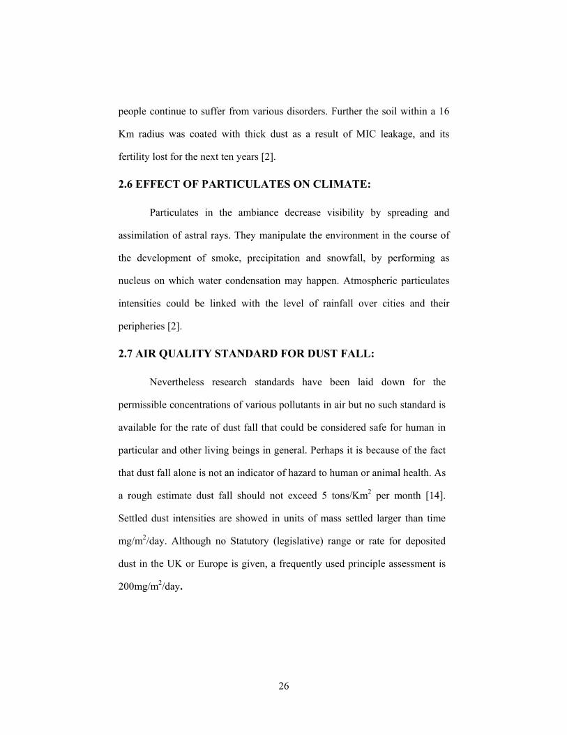
2.8 MEASUREMENT OF RATE OF DUST FALL:
There are numerous sophisticated devices, with which the total burden
of particulates in ambient atmosphere could easily be determined. For
instance a satellite Terra equipped with five gadgets (two Moderate-
Resolution Imaging Spectroradiometer (MODIS) and Multi-angle Imaging
28
Spectroradiometer (MISR) particularly for observing the
particulates/aerosols) was launched by NASA in December 1999 in order to
monitor clouds and aerosols with (MODIS) and to distinguish among
different sorts of plumes, particulates, and planes allowing scientists to
establish worldwide aerosol quantities with exceptional accurateness by
means of (MISR).
Figure 2.2: Satellite pictures
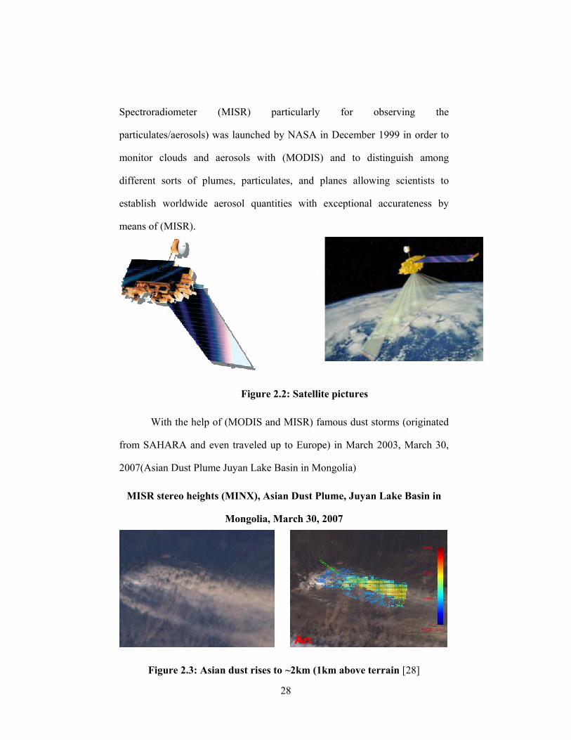
With the help of (MODIS and MISR) famous dust storms (originated
from SAHARA and even traveled up to Europe) in March 2003, March 30,
2007(Asian Dust Plume Juyan Lake Basin in Mongolia)
MISR stereo heights (MINX), Asian Dust Plume, Juyan Lake Basin in
Mongolia, March 30, 2007
Figure 2.3: Asian dust rises to ~2km (1km above terrain [28]
29
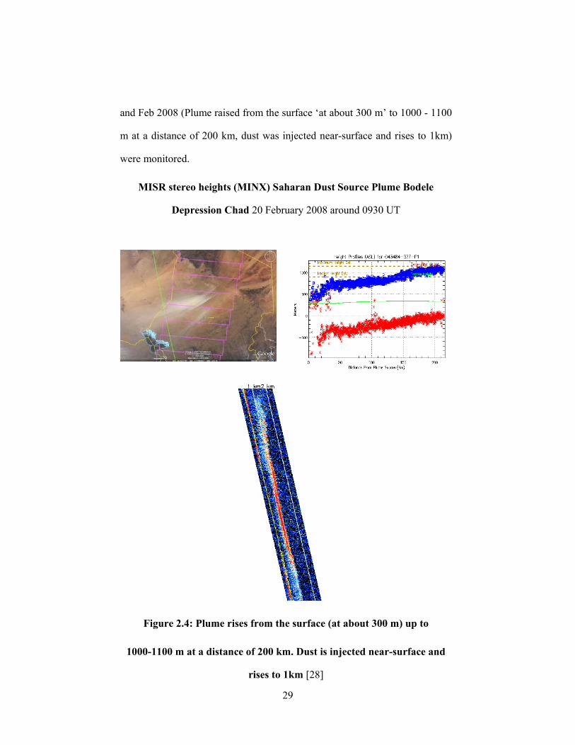
and Feb 2008 (Plume raised from the surface ‘at about 300 m’ to 1000 - 1100
m at a distance of 200 km, dust was injected near-surface and rises to 1km)
were monitored.
MISR stereo heights (MINX) Saharan Dust Source Plume Bodele
Depression Chad 20 February 2008 around 0930 UT
Figure 2.4: Plume rises from the surface (at about 300 m) up to
1000-1100 m at a distance of 200 km. Dust is injected near-surface and
rises to 1km [28]
30
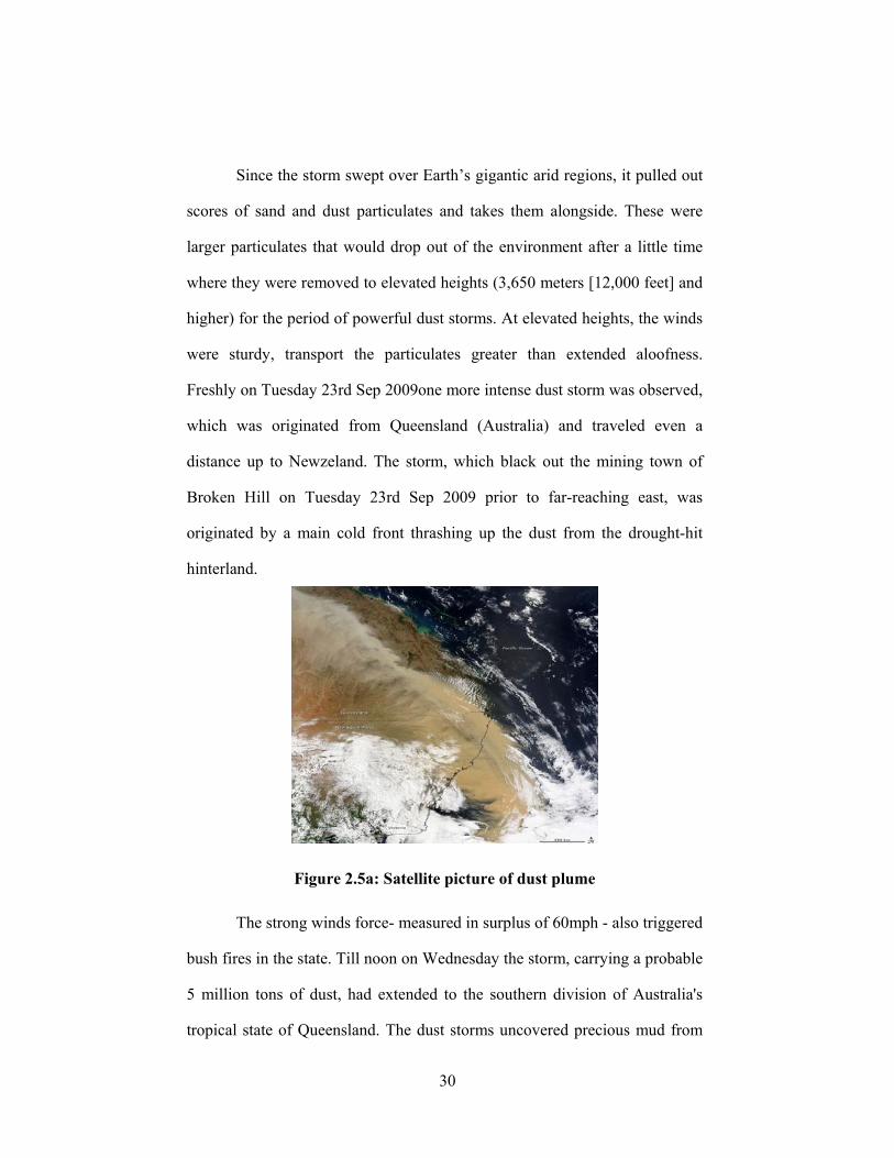
Since the storm swept over Earth’s gigantic arid regions, it pulled out
scores of sand and dust particulates and takes them alongside. These were
larger particulates that would drop out of the environment after a little time
where they were removed to elevated heights (3,650 meters [12,000 feet] and
higher) for the period of powerful dust storms. At elevated heights, the winds
were sturdy, transport the particulates greater than extended aloofness.
Freshly on Tuesday 23rd Sep 2009one more intense dust storm was observed,
which was originated from Queensland (Australia) and traveled even a
distance up to Newzeland. The storm, which black out the mining town of
Broken Hill on Tuesday 23rd Sep 2009 prior to far-reaching east, was
originated by a main cold front thrashing up the dust from the drought-hit
hinterland.
Figure 2.5a: Satellite picture of dust plume
The strong winds force- measured in surplus of 60mph - also triggered
bush fires in the state. Till noon on Wednesday the storm, carrying a probable
5 million tons of dust, had extended to the southern division of Australia's
tropical state of Queensland. The dust storms uncovered precious mud from

31
farmlands. At one stage up to 75,000 tons of dust per hour was gusted across
Sydney and dumped in the Pacific Ocean. 'We've got a mixture of dynamics
which have been erecting for ten months already - floods, droughts and strong
winds,' said Craig Strong from Dust Watch at Griffith University in
Queensland. 'Add to these factors the existing drought circumstances that
diminish the plants cover and the earth surface is at its most susceptible to
storm erosion.'
Figure 2.5b: Heavy dust Plume
Health officials, in the meantime, have insisted citizens having asthma
or inhalation troubles to wait indoors. The authorized air quality index for
New South Wales recorded pollutant levels as high as 4,164 in Sydney. A
level above 200 is measured dangerous.
But having kept in mind that the total particulate matter burden of
ambient air is less important than the chemical nature, size and rate of
deposition/settlement/fall of the particulates” the particulates possess large
32
areas in general and hence present good sites for sorption of various inorganic
and organic matters [2]. Scientists/researchers have to use different simple
conventional tiring painstaking methods in order to calculate the amount of
dust fall/settled per square area per time.
The concentration of atmospheric dust is measured by calculating the
amount of dust settled per square area, size of particles and their chemical
composition. Samplers used to identify fine particle fractions typically are
designed to have inlet and sub stage cut points that are as sharp as possible.
Miller et al., [29] proposed a sampler cut point of 15 microns related to
respiratory system deposition but did not recommend desirable cut point
sharpness. Some of the commonly used particulate matter samplers
employing direct mass measurement techniques include the Total high
volume sampler, the dichotomous sampler, cyclone sampler, high volume
sampler with size selective inlet, cascade impactors etc.
Total suspended particulate high volume sampler is the US
Environmental protection agency [30] reference method for total suspended
particulate. The heap of particulates collected on the filter is measured from
the difference between weights before and after exposure. Quartz fiber and
glass fiber are used as filter medium [31]. The principle of particle separation
in dichotomous sampler collects two particle size fractions, 0 to 2.5 micron
and 2.5 to about 15 microns. Teflon membrane filters with porosities as large
as 2 microns can be used in the sampler and have been shown to have
essentially 100% collection efficiency [31]. Lippman and Chan [32]
summarized the available cyclone samplers for ambient particle sampling
33
below 10 microns and noted that the separation effectiveness of cyclones can
be designed to match respiratory deposition curves. Wedding et al., [33]
demonstrated that the cyclone separation principle can be applied to larger
particle, 15 micron sampler inlet. Glass fiber filter was used as a filter
medium in the cyclone sampler used in the Community Health
Environmental Surveillance Studies (CHESS) [34]. Lippman [35] discussed
the effect of sample flow rate on the performance of cyclone sampler. Knight
and Lichti [36] compared the performance of the 10 mm cyclone sampler to
that of horizontal elutriators and noted that the results were comparable if
appropriate flow rates were used. To meet the monitoring requirements for
inhalable particles (LP) as proposed by Miller et al., [29] Environmental
Protection Agency (EPA) commissioned the design of a size selective inlet
for existing total suspended particulate high volume samplers to provide a
single 0 to 15 micron particle size fraction and it has been tested by
McFarland and Ortiz [37]. Cascade impactor samplers have 2 to 10 stages
and are commercially available. Lee and Goranson [38] modified a
commercially available impactor sampler to obtain larger mass collection on
each stage. These have also been designed to mount on a high-volume
sampler. Cascade impactors are not normally operated in routine monitoring
networks because of the manual labor required for sampling and analysis.
Although sampling systems are not extremely complex, careful operation is
required to obtain reliable data; especially if coated collection surfaces are
[39] examined the inlet of the cascade sampler and determined that particles
larger than 10 microns were unlikely to reach the collection stages because of
substantial wall losses. Larger particles in atmosphere have appreciable
34
settling velocities. They are collected by deposition in a dust fall container
and this standard method is considered as the best procedure [40, 41].
Significant work on the measurement of rate of dust fall has been
undertaken in developed as well as in developing countries. In mid-1950’s,
monthly dust fall (tons per square mile per month) for a number of cities in
North American and Great Britain has been determined and given below:
Detroit, 72.0 tons; New York City, 67.5 tons; Chicago, 61.2 tons;
Cincinnati, 34.0 tons; Los Angeles, 33.3 tons; Pittsburgh, 45.7 tons;
Rochester, 26.4 tons [42]. Birmingham, 27.8 tons; Glasgow (east), 26.6 tons;
Leeds (park square), 35.9 tons; Manchester, 42.9 tons. Radermacher et al.,
[43] conducted a thorough research on the dust fall and heavy metal
deposition in the state of North Rhine-Westphalia, Germany. The average
annual dust fall at the city for years (1980, 1981, 1984, 1985, 1986 and 1988)
was (0.18, 0.19, 0.16, 0.15, 0.14, and 0.13) grams per square meter per day
respectively [44-46]. They stated that significant changes have happened in
the past five years and during 1986 (0.14 g/m2.day), the total dust fall was the
lowest of the last 23 years. The study of Okubo et al., [47] revealed that the
mean value of dust fall at Kodatsuno-Spot Kanazawa City, Japan was 5.77
tons per square kilometer per month during 1974-1986. In Japan, there are
more than twelve hundred dust fall collecting stations, whose results are
reported regularly every year by Air Observation Board, Japan [48]. The rate
of dust fall in some other countries in different years has also been summed
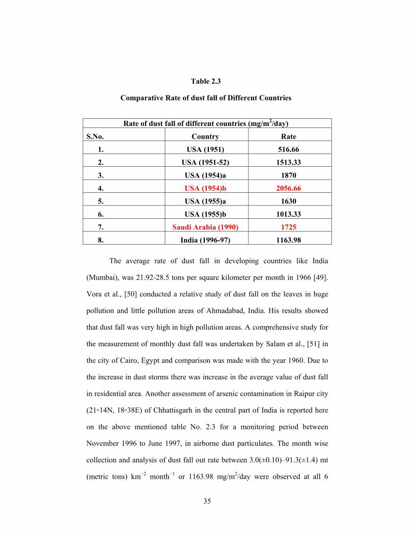
up in the following Table No. 2.3
35
Table 2.3
Comparative Rate of dust fall of Different Countries
Rate of dust fall of different countries (mg/m2/day)
S.No. Country Rate
1. USA (1951) 516.66
2. USA (1951-52) 1513.33
3. USA (1954)a 1870
4. USA (1954)b 2056.66
5. USA (1955)a 1630
6. USA (1955)b 1013.33
7. Saudi Arabia (1990) 1725
8. India (1996-97) 1163.98
The average rate of dust fall in developing countries like India
(Mumbai), was 21.92-28.5 tons per square kilometer per month in 1966 [49].
Vora et al., [50] conducted a relative study of dust fall on the leaves in huge
pollution and little pollution areas of Ahmadabad, India. His results showed
that dust fall was very high in high pollution areas. A comprehensive study for
the measurement of monthly dust fall was undertaken by Salam et al., [51] in
the city of Cairo, Egypt and comparison was made with the year 1960. Due to
the increase in dust storms there was increase in the average value of dust fall
in residential area. Another assessment of arsenic contamination in Raipur city
(21◦14N, 18◦38E) of Chhattisgarh in the central part of India is reported here
on the above mentioned table No. 2.3 for a monitoring period between
November 1996 to June 1997, in airborne dust particulates. The month wise
collection and analysis of dust fall out rate between 3.0(±0.10)–91.3(±1.4) mt
(metric tons) km−2 month−1 or 1163.98 mg/m2/day were observed at all 6
36
sampling sites. Anthropogenic and environmental factors play important roles
in the contribution of arsenic in airborne particulate matters [52]. Similarly an
assessment was carried to measure the dust fall rates at eight localities in
Riyadh city during the period 21 March-June 21, 1990. High rates of dust fall
were recorded in all districts with an average of 24.48 tons/km2/month and a
range of 9.87-51.76 ton/km2/month at an average of 1725 mg/m2/day. The
collected dust samples were analyzed for the following contents: Sulphate,
nitrate, chloride, calcium, sodium, potassium, lead and tar. The results are
discussed and compared with other findings [53]. In USA the rate of dust fall
has consistently been recorded / monitored for a long time and in 1954 the
average rate of dust fall recorded in 2056.66 mg/m2/day, which was beyond
the extremely high set limits.
Very little heed has been paid to the atmospheric pollutants in general
and to the dust fall in particular. Minor data is available for some big cities of
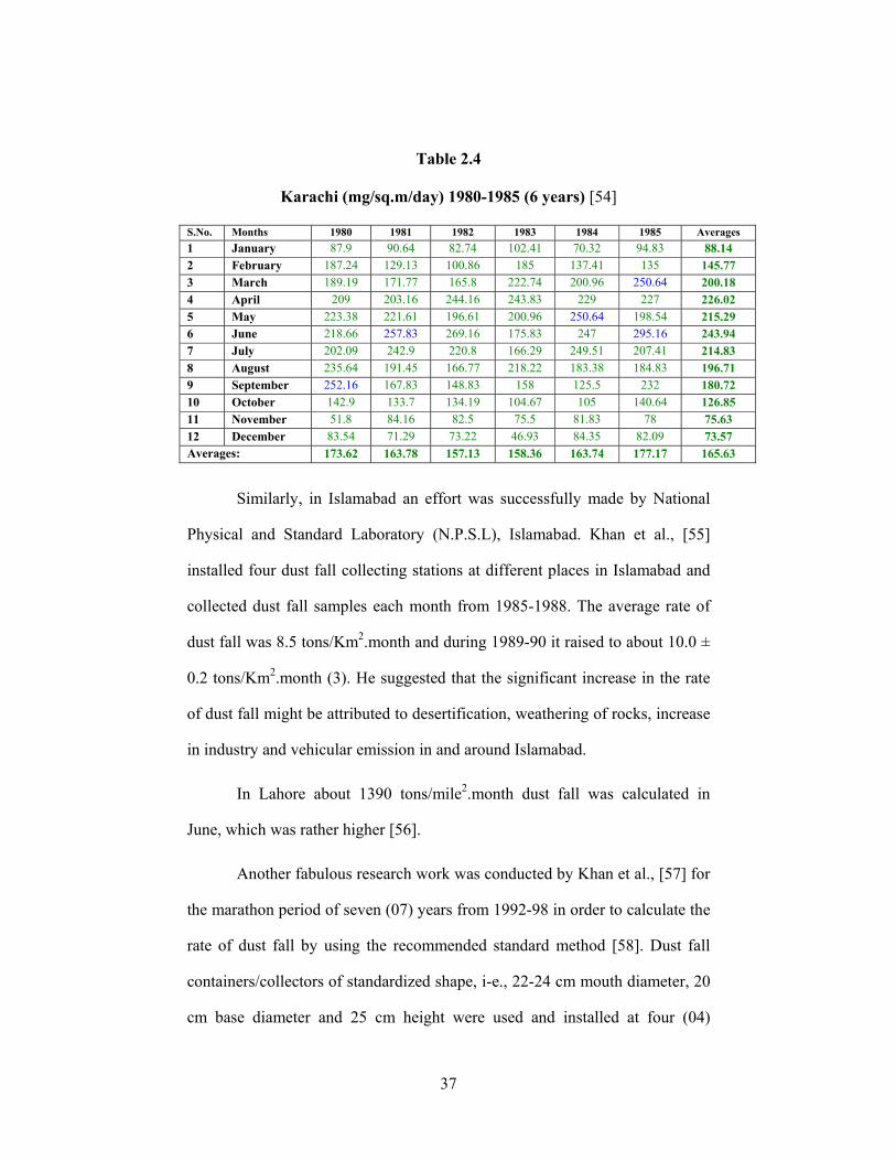
Pakistan. Beg et al., [54] carried out six (06) years work from 1980-1985 for
the rate, composition and quantity of dust fall in Karachi at two (02) locations.
The dust fall was measured by exposing dust fall containers of standardized
shape and size at the said two sites for a period of one calendar month
corrected to 30 ±2 days. The monthly average dust fall obtained between 13.0
to 15.7 tons per square kilometer per month (157.13 to 177.17 mg/m2/day). It
was concluded by Beg et al., [54] that dust fall caused by the construction
activities, automobile exhaust and industrial emission of cement factories.
37
Table 2.4
Karachi (mg/sq.m/day) 1980-1985 (6 years) [54]
S.No. Months 1980 1981 1982 1983 1984 1985 Averages 1 January 87.9 90.64 82.74 102.41 70.32 94.83 88.14 2 February 187.24 129.13 100.86 185 137.41 135 145.77 3 March 189.19 171.77 165.8 222.74 200.96 250.64 200.18 4 April 209 203.16 244.16 243.83 229 227 226.02 5 May 223.38 221.61 196.61 200.96 250.64 198.54 215.29 6 June 218.66 257.83 269.16 175.83 247 295.16 243.94 7 July 202.09 242.9 220.8 166.29 249.51 207.41 214.83 8 August 235.64 191.45 166.77 218.22 183.38 184.83 196.71 9 September 252.16 167.83 148.83 158 125.5 232 180.72 10 October 142.9 133.7 134.19 104.67 105 140.64 126.85 11 November 51.8 84.16 82.5 75.5 81.83 78 75.63 12 December 83.54 71.29 73.22 46.93 84.35 82.09 73.57 Averages: 173.62 163.78 157.13 158.36 163.74 177.17 165.63
Similarly, in Islamabad an effort was successfully made by National
Physical and Standard Laboratory (N.P.S.L), Islamabad. Khan et al., [55]
installed four dust fall collecting stations at different places in Islamabad and
collected dust fall samples each month from 1985-1988. The average rate of
dust fall was 8.5 tons/Km2.month and during 1989-90 it raised to about 10.0 ±
0.2 tons/Km2.month (3). He suggested that the significant increase in the rate
of dust fall might be attributed to desertification, weathering of rocks, increase
in industry and vehicular emission in and around Islamabad.
In Lahore about 1390 tons/mile2.month dust fall was calculated in
June, which was rather higher [56].
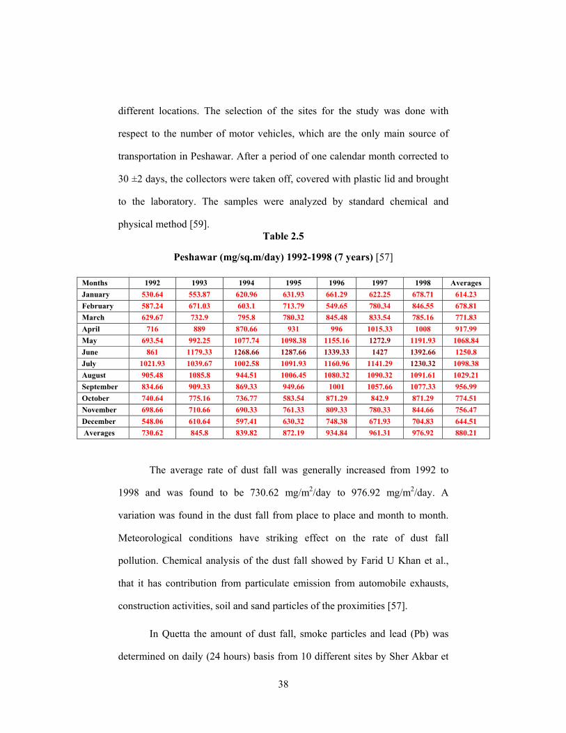
Another fabulous research work was conducted by Khan et al., [57] for
the marathon period of seven (07) years from 1992-98 in order to calculate the
rate of dust fall by using the recommended standard method [58]. Dust fall
containers/collectors of standardized shape, i-e., 22-24 cm mouth diameter, 20
cm base diameter and 25 cm height were used and installed at four (04)
38
different locations. The selection of the sites for the study was done with
respect to the number of motor vehicles, which are the only main source of
transportation in Peshawar. After a period of one calendar month corrected to
30 ±2 days, the collectors were taken off, covered with plastic lid and brought
to the laboratory. The samples were analyzed by standard chemical and
physical method [59]. Table 2.5
Peshawar (mg/sq.m/day) 1992-1998 (7 years) [57]
The average rate of dust fall was generally increased from 1992 to
1998 and was found to be 730.62 mg/m2/day to 976.92 mg/m2/day. A
variation was found in the dust fall from place to place and month to month.
Meteorological conditions have striking effect on the rate of dust fall
pollution. Chemical analysis of the dust fall showed by Farid U Khan et al.,
that it has contribution from particulate emission from automobile exhausts,
construction activities, soil and sand particles of the proximities [57].
In Quetta the amount of dust fall, smoke particles and lead (Pb) was
determined on daily (24 hours) basis from 10 different sites by Sher Akbar et
Months 1992 1993 1994 1995 1996 1997 1998 Averages January 530.64 553.87 620.96 631.93 661.29 622.25 678.71 614.23 February 587.24 671.03 603.1 713.79 549.65 780.34 846.55 678.81 March 629.67 732.9 795.8 780.32 845.48 833.54 785.16 771.83 April 716 889 870.66 931 996 1015.33 1008 917.99 May 693.54 992.25 1077.74 1098.38 1155.16 1272.9 1191.93 1068.84 June 861 1179.33 1268.66 1287.66 1339.33 1427 1392.66 1250.8 July 1021.93 1039.67 1002.58 1091.93 1160.96 1141.29 1230.32 1098.38 August 905.48 1085.8 944.51 1006.45 1080.32 1090.32 1091.61 1029.21 September 834.66 909.33 869.33 949.66 1001 1057.66 1077.33 956.99 October 740.64 775.16 736.77 583.54 871.29 842.9 871.29 774.51 November 698.66 710.66 690.33 761.33 809.33 780.33 844.66 756.47 December 548.06 610.64 597.41 630.32 748.38 671.93 704.83 644.51 Averages 730.62 845.8 839.82 872.19 934.84 961.31 976.92 880.21
39
al., on daily basis the dust fall was found between 0.3844-0.5291 grams and
on monthly basis between 11.5321-15.8721 grams [194]. Another study was
conducted by Sami et al on the same pattern in order to ascertain the
concentration of Pb and smoke particles emitted from vehicles and the rate of
dust fall on daily (24 hours) basis, which was found between 1.5-4.3 grams
from five different sites by using deposit gauge method, while between 1.1-2.4
grams on 10 different sites by using Petri dish method [195].
2.9 THERMAL INVERSION:
As has been quoted earlier that “It should be kept in mind that the total
particulate matter burden of air is less important than the chemical nature, size
and rate of deposition/settlement/fall of the particulates”. The particulates
possess large areas in general and hence present good sites for sorption of
various inorganic and organic matters [2].
The rate of deposition/settlement/fall of the particulates depends upon
following two factors.
(1). Particulates Size
(2). Weather
Rate of settlement/deposition of Particulates is inversely proportional
to their size. Larger the size of the particulates would be, shorter the time they
would take to settle and vice versa.
Air pollution and weather are linked in two ways.
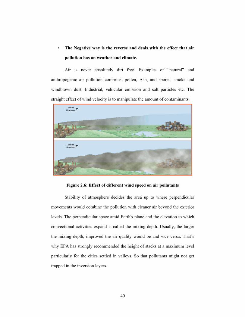
• Positive way concerns the influence that weather conditions have
on the dilution and dispersal of air pollutants.
40
• The Negative way is the reverse and deals with the effect that air
pollution has on weather and climate.
Air is never absolutely dirt free. Examples of “natural” and
anthropogenic air pollution comprise: pollen, Ash, and spores, smoke and
windblown dust, Industrial, vehicular emission and salt particles etc. The
straight effect of wind velocity is to manipulate the amount of contaminants.
Figure 2.6: Effect of different wind speed on air pollutants
Stability of atmosphere decides the area up to where perpendicular
movements would combine the pollution with cleaner air beyond the exterior
levels. The perpendicular space amid Earth's plane and the elevation to which
convectional activities expand is called the mixing depth. Usually, the larger
the mixing depth, improved the air quality would be and vice versa. That’s
why EPA has strongly recommended the height of stacks at a maximum level
particularly for the cities settled in valleys. So that pollutants might not get
trapped in the inversion layers.
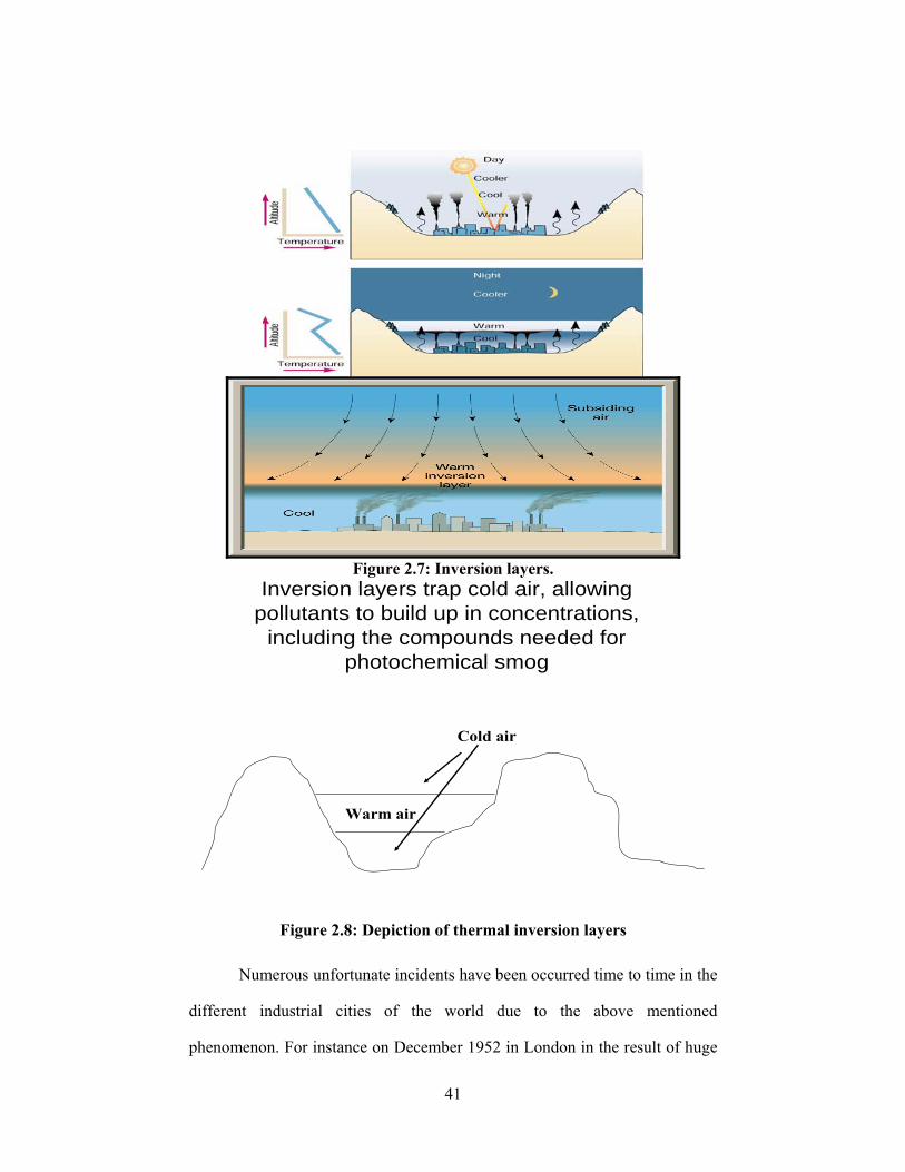
41
Figure 2.7: Inversion layers.
Inversion layers trap cold air, allowing pollutants to build up in concentrations,
including the compounds needed for photochemical smog
Cold air
Warm air
Figure 2.8: Depiction of thermal inversion layers
Numerous unfortunate incidents have been occurred time to time in the
different industrial cities of the world due to the above mentioned
phenomenon. For instance on December 1952 in London in the result of huge
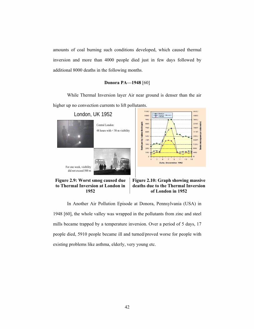
42
amounts of coal burning such conditions developed, which caused thermal
inversion and more than 4000 people died just in few days followed by
additional 8000 deaths in the following months.
Donora PA—1948 [60]
While Thermal Inversion layer Air near ground is denser than the air
higher up no convection currents to lift pollutants.
London, UK 1952
Central London:
48 hours with < 50 m visibility
For one week, visibility did not exceed 500 m
Figure 2.9: Worst smog caused due to Thermal Inversion at London in
1952
Figure 2.10: Graph showing massive deaths due to the Thermal Inversion
of London in 1952
In Another Air Pollution Episode at Donora, Pennsylvania (USA) in
1948 [60], the whole valley was wrapped in the pollutants from zinc and steel
mills became trapped by a temperature inversion. Over a period of 5 days, 17
people died, 5910 people became ill and turned/proved worse for people with
existing problems like asthma, elderly, very young etc.
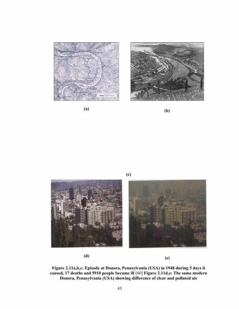
43
(a)
(b)
(c)
(d)
(e)
Figure 2.11a,b,c: Episode at Donora, Pennsylvania (USA) in 1948 during 5 days it caused, 17 deaths and 5910 people became ill [60] Figure 2.11d,e: The same modern
Donora, Pennsylvania (USA) showing difference of clear and polluted air
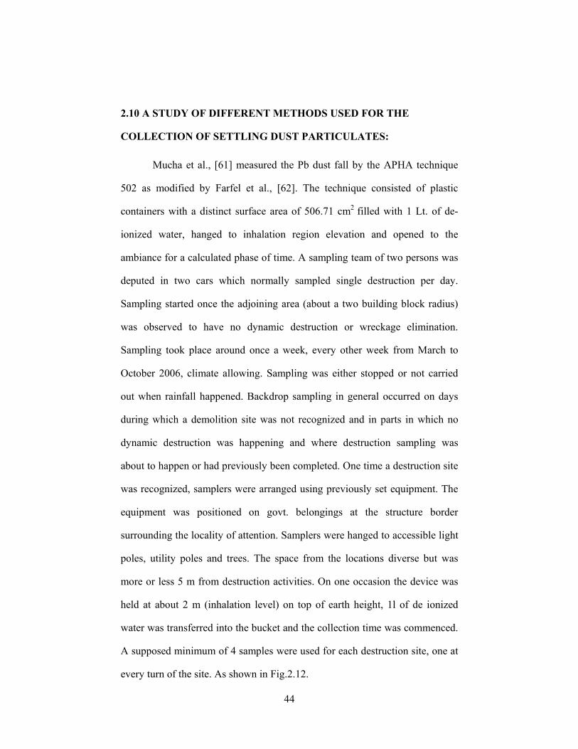
44
2.10 A STUDY OF DIFFERENT METHODS USED FOR THE
COLLECTION OF SETTLING DUST PARTICULATES:
Mucha et al., [61] measured the Pb dust fall by the APHA technique
502 as modified by Farfel et al., [62]. The technique consisted of plastic
containers with a distinct surface area of 506.71 cm2 filled with 1 Lt. of de-
ionized water, hanged to inhalation region elevation and opened to the
ambiance for a calculated phase of time. A sampling team of two persons was
deputed in two cars which normally sampled single destruction per day.
Sampling started once the adjoining area (about a two building block radius)
was observed to have no dynamic destruction or wreckage elimination.
Sampling took place around once a week, every other week from March to
October 2006, climate allowing. Sampling was either stopped or not carried
out when rainfall happened. Backdrop sampling in general occurred on days
during which a demolition site was not recognized and in parts in which no
dynamic destruction was happening and where destruction sampling was
about to happen or had previously been completed. One time a destruction site
was recognized, samplers were arranged using previously set equipment. The
equipment was positioned on govt. belongings at the structure border
surrounding the locality of attention. Samplers were hanged to accessible light
poles, utility poles and trees. The space from the locations diverse but was
more or less 5 m from destruction activities. On one occasion the device was
held at about 2 m (inhalation level) on top of earth height, 1l of de ionized
water was transferred into the bucket and the collection time was commenced.
A supposed minimum of 4 samples were used for each destruction site, one at
every turn of the site. As shown in Fig.2.12.
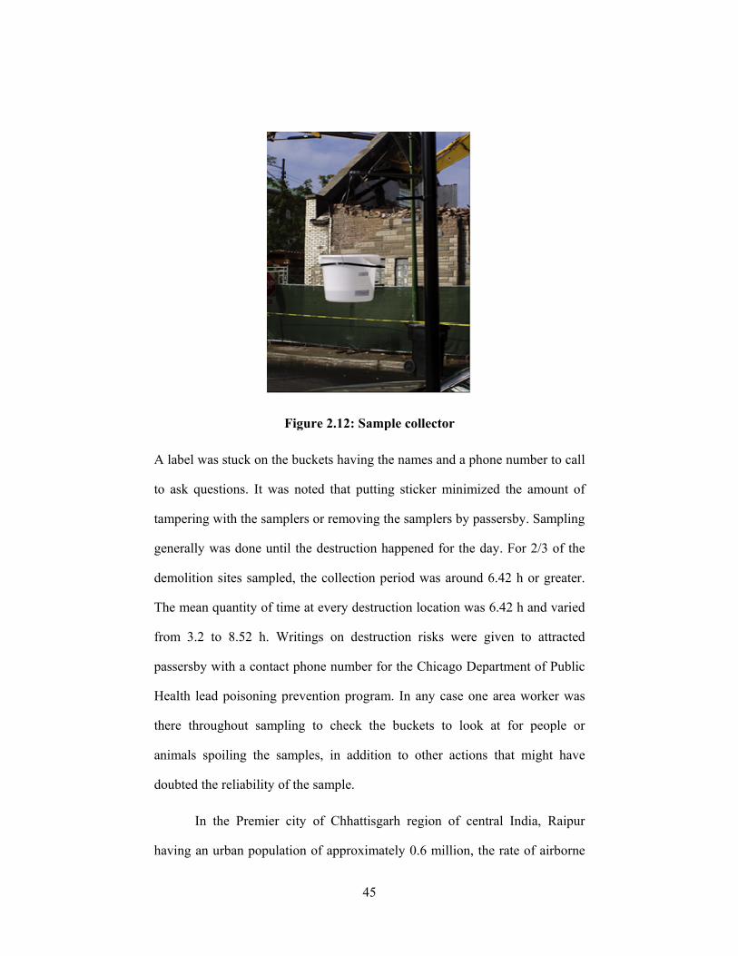
45
Figure 2.12: Sample collector
A label was stuck on the buckets having the names and a phone number to call
to ask questions. It was noted that putting sticker minimized the amount of
tampering with the samplers or removing the samplers by passersby. Sampling
generally was done until the destruction happened for the day. For 2/3 of the
demolition sites sampled, the collection period was around 6.42 h or greater.
The mean quantity of time at every destruction location was 6.42 h and varied
from 3.2 to 8.52 h. Writings on destruction risks were given to attracted
passersby with a contact phone number for the Chicago Department of Public
Health lead poisoning prevention program. In any case one area worker was
there throughout sampling to check the buckets to look at for people or
animals spoiling the samples, in addition to other actions that might have
doubted the reliability of the sample.
In the Premier city of Chhattisgarh region of central India, Raipur
having an urban population of approximately 0.6 million, the rate of airborne
46
dust particulates fall was found out by Deb et al., [52] having followed the
procedure recommended in the literature [63] for a monitoring period between
November 1996 to June 1997. The dust collection glass jars used, were
cylindrical in figure having a diameter of 15 cm, and a height of 45 cm. In all,
six sampling sites were selected in the study area. In each sampling site, four
separate samplers in different directions at a radial space of 50 m were placed
for the most precise sampling. All values obtained at a particular sampling site
were, thus, the average of 4 samplings. Distilled water was kept in every
collector to prevent sample loss by gusting air. The collectors were kept in
guard-frames at heights of 5–15 m above the earth altitude, depending on the
obstructions in the individual site [64]. The jars were examined each week and
changed by fresh collection jars after duration of 30 days. The prevailing
weather periods in this part of India are July–October, spring (southwest
monsoon); March–June, summer; November–February, winter. The pre and
post monsoon month measurements were made of the dust fall rate
concentration, and flux of arsenic for a whole hydrological period for every
sampling location. The dust fall rate was calculated for every location with the
following equation [65].
R = 1.273 (W/D2) × (30/N) ×104 where
R = dust fall rate, in mt km−2 month−1;
W = the total weight of dust fall-out in the collecting of samples;
N = number of sampling days.
The dried particulate fall-out sample (0.1–0.5 g) was taken in a 50-mL
beaker and leached with cold and concentrated HCl-HNO3 (3:1) acid (2–4 ml).
47
The residue after filtration was digested for 1 hr with hot (50◦C) and diluted
(1:10) HNO3 acid (3 ml) and the digested residue was filtered and the filtrate
was combined with the leachate and diluted to a known volume (25 ml) in a
volumetric flask [66].
Crabtree [67], of Texas, USA researched to measure the quantity of
dust that was being settled over the area and to find out whether there is a
relationship among dust settlement and various meteorological limits for
example wind rate, wind track, temperature and rainfall. Dust settlement was
found out by investigating the mass of dust that was deposited per unit of area.
With the intention to ascertain the rate at which the dust was being settled the
weight of the dust settled was divided by the time above which the dust was
collected. An analogous investigation plan was carried out by Singer et al.,
[68] in order to assess the rate of dust fall happened over Dead Sea for a
period of three years. Dust Samples were collected with the interval of each
two months having the settlement rate 6.7-15.2 g/m2/annum1 and 11.4-
24.7g/m2/annum1 in winter and summer respectively. Besides that average
particulates size was detected 10µm varying between 8-20µm. A very few
particles were having the size more than 100µm. An increase in the annual
dust settlement was recorded during the three years period as well as
particulates spreading was recorded from medium to long range movement of
the dust.
Samara and Tsitouridou [69] conducted a same sort of experiment by
collecting dust samples with the interval of every one month. Particulate size
and rates of settlement of particular ionic substances were determined as well.
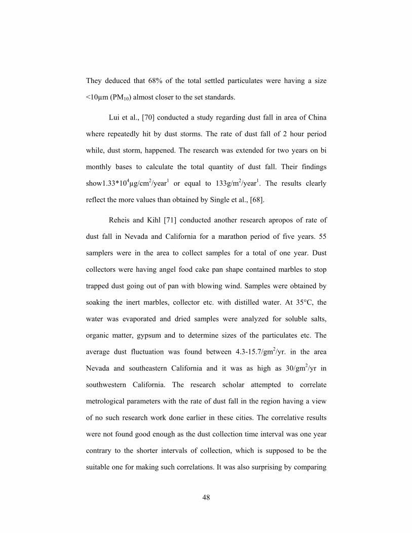
48
They deduced that 68% of the total settled particulates were having a size
<10µm (PM10) almost closer to the set standards.
Lui et al., [70] conducted a study regarding dust fall in area of China
where repeatedly hit by dust storms. The rate of dust fall of 2 hour period
while, dust storm, happened. The research was extended for two years on bi
monthly bases to calculate the total quantity of dust fall. Their findings
show1.33*104µg/cm2/year1 or equal to 133g/m2/year1. The results clearly
reflect the more values than obtained by Single et al., [68].
Reheis and Kihl [71] conducted another research apropos of rate of
dust fall in Nevada and California for a marathon period of five years. 55
samplers were in the area to collect samples for a total of one year. Dust
collectors were having angel food cake pan shape contained marbles to stop
trapped dust going out of pan with blowing wind. Samples were obtained by
soaking the inert marbles, collector etc. with distilled water. At 35°C, the
water was evaporated and dried samples were analyzed for soluble salts,
organic matter, gypsum and to determine sizes of the particulates etc. The
average dust fluctuation was found between 4.3-15.7/gm2/yr. in the area
Nevada and southeastern California and it was as high as 30/gm2/yr in
southwestern California. The research scholar attempted to correlate
metrological parameters with the rate of dust fall in the region having a view
of no such research work done earlier in these cities. The correlative results
were not found good enough as the dust collection time interval was one year
contrary to the shorter intervals of collection, which is supposed to be the
suitable one for making such correlations. It was also surprising by comparing
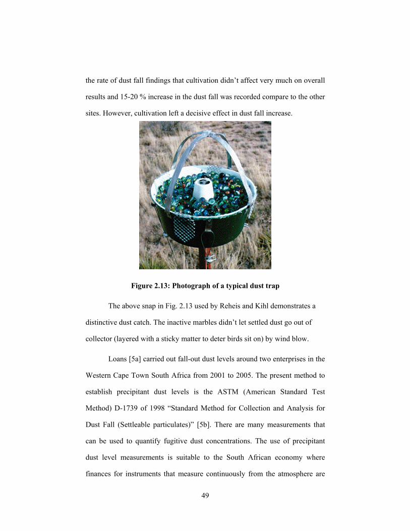
49
the rate of dust fall findings that cultivation didn’t affect very much on overall
results and 15-20 % increase in the dust fall was recorded compare to the other
sites. However, cultivation left a decisive effect in dust fall increase.
Figure 2.13: Photograph of a typical dust trap
The above snap in Fig. 2.13 used by Reheis and Kihl demonstrates a
distinctive dust catch. The inactive marbles didn’t let settled dust go out of
collector (layered with a sticky matter to deter birds sit on) by wind blow.
Loans [5a] carried out fall-out dust levels around two enterprises in the
Western Cape Town South Africa from 2001 to 2005. The present method to
establish precipitant dust levels is the ASTM (American Standard Test
Method) D-1739 of 1998 “Standard Method for Collection and Analysis for
Dust Fall (Settleable particulates)” [5b]. There are many measurements that
can be used to quantify fugitive dust concentrations. The use of precipitant
dust level measurements is suitable to the South African economy where
finances for instruments that measure continuously from the atmosphere are
50
not usually available. While single open buckets partly-filled with a capture
medium will accumulate all precipitating dust, this does not establish
precipitant dust emanating from a given direction unless the bucket is closed
to any dust from other directions [5c]. Such open buckets are also subject to
inaccuracies due to wind turbulence within the buckets, lower air densities
over the bucket and other factors [5c]. The single bucket precipitant dust
collection method [5b] “is a crude and nonspecific test method, but it is useful
in the study of long term trends” [5b]. There are many different types of
equipment that are used to monitor precipitant dust levels. Gerry Kuhn
Environmental and Hygiene Engineering have used a method [5b, d] based on
the American Standard Test Method [5b]. The equipment used to measure the
dust is called the “Dust Watch” unit [5d]. The unit is wind operated and
different buckets open under different wind conditions. The unit has four
buckets that are used for directional identification of localized dust sources as
well as to identify ambient precipitant dust concentrations [5d]. The Dust
Watch unit has four buckets that face north, south, east, and west respectively.
The export bucket is defined as the bucket that is in line with the industry or
factory being monitored. The precipitant dust from the dust source is
predominantly collected in the export bucket. The export bucket is also the
bucket that is used for legislative compliance purposes, as this is the bucket
that collects the dust being exported from the source towards the sensitive
area. The Dust Watch units prevent the ground level dust from contaminating
the precipitant dust sample by the specially-designed lid that covers the
buckets. The lid prevents wind-blown dust from being collected when the
wind speed is greater than about 3 m/s. The only way that ground level dust
51
can be deposited into the bucket is if the wind is gusting at regular intervals,
thus lifting dust into the air and into the buckets. Ground level wind-blown
dust that is larger than 100 micron is not normally lifted to a height higher
than two meters and a particle size analysis will be able to confirm if there is
contamination from ground level dust. The water in the buckets collects the
dust [5e].
(a)
(b)
(c)
Figure 2.14a,b,c: Dust watch standard single bucket collectors
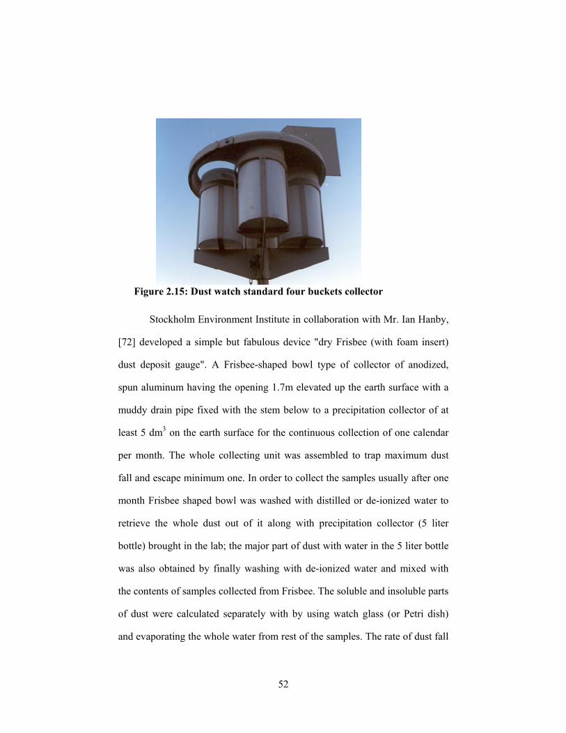
52
Figure 2.15: Dust watch standard four buckets collector
Stockholm Environment Institute in collaboration with Mr. Ian Hanby,
[72] developed a simple but fabulous device "dry Frisbee (with foam insert)
dust deposit gauge". A Frisbee-shaped bowl type of collector of anodized,
spun aluminum having the opening 1.7m elevated up the earth surface with a
muddy drain pipe fixed with the stem below to a precipitation collector of at
least 5 dm3 on the earth surface for the continuous collection of one calendar
per month. The whole collecting unit was assembled to trap maximum dust
fall and escape minimum one. In order to collect the samples usually after one
month Frisbee shaped bowl was washed with distilled or de-ionized water to
retrieve the whole dust out of it along with precipitation collector (5 liter
bottle) brought in the lab; the major part of dust with water in the 5 liter bottle
was also obtained by finally washing with de-ionized water and mixed with
the contents of samples collected from Frisbee. The soluble and insoluble parts
of dust were calculated separately with by using watch glass (or Petri dish)
and evaporating the whole water from rest of the samples. The rate of dust fall
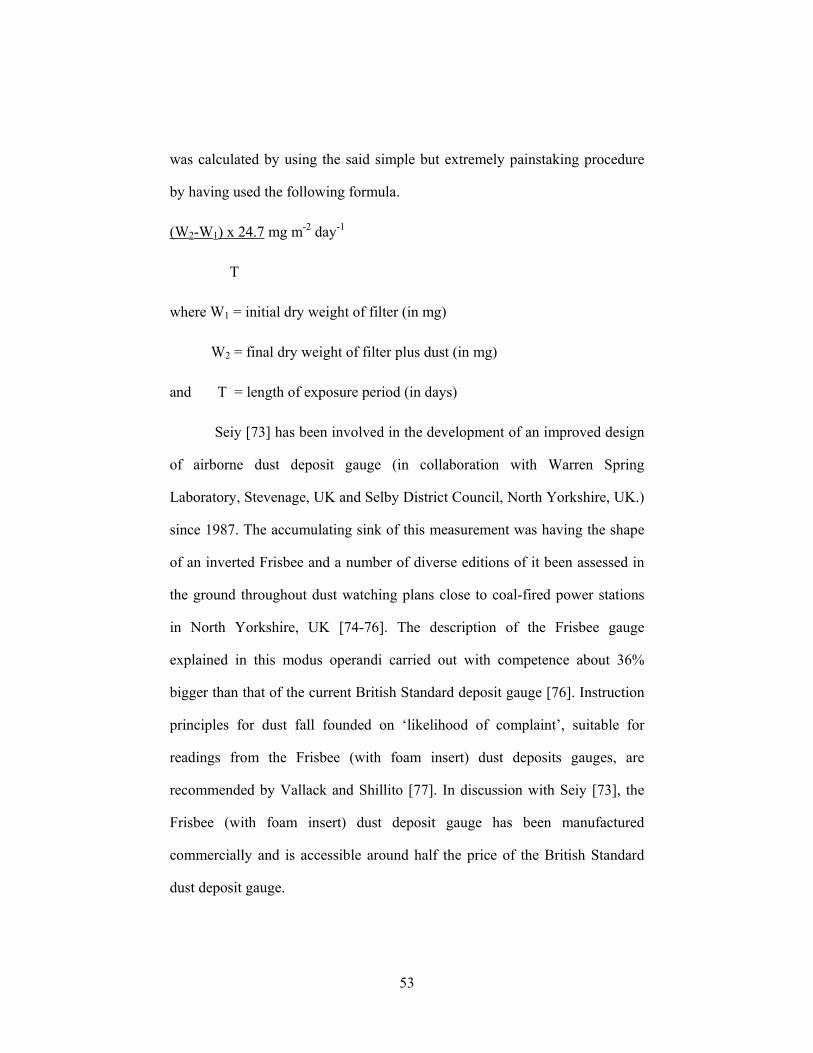
53
was calculated by using the said simple but extremely painstaking procedure
by having used the following formula.
(W2-W1) x 24.7 mg m-2 day-1
T
where W1 = initial dry weight of filter (in mg)
W2 = final dry weight of filter plus dust (in mg)
and T = length of exposure period (in days)
Seiy [73] has been involved in the development of an improved design
of airborne dust deposit gauge (in collaboration with Warren Spring
Laboratory, Stevenage, UK and Selby District Council, North Yorkshire, UK.)
since 1987. The accumulating sink of this measurement was having the shape
of an inverted Frisbee and a number of diverse editions of it been assessed in
the ground throughout dust watching plans close to coal-fired power stations
in North Yorkshire, UK [74-76]. The description of the Frisbee gauge
explained in this modus operandi carried out with competence about 36%
bigger than that of the current British Standard deposit gauge [76]. Instruction
principles for dust fall founded on ‘likelihood of complaint’, suitable for
readings from the Frisbee (with foam insert) dust deposits gauges, are
recommended by Vallack and Shillito [77]. In discussion with Seiy [73], the
Frisbee (with foam insert) dust deposit gauge has been manufactured
commercially and is accessible around half the price of the British Standard
dust deposit gauge.
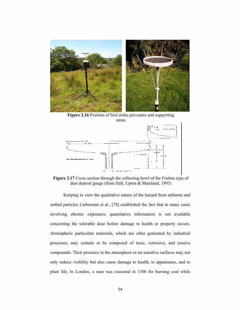
54
Figure 2.16 Position of bird strike preventor and supporting
struts
Figure 2.17 Cross section through the collecting bowl of the Frisbee type of
dust deposit gauge (from Hall, Upton & Marsland, 1993)
Keeping in view the qualitative nature of the hazard from airborne and
settled particles Lieberman et al., [78] established the fact that in many cases
involving chronic exposures, quantitative information is not available
concerning the tolerable dose before damage to health or property occurs.
Atmospheric particulate materials, which are often generated by industrial
processes, may contain or be composed of toxic, corrosive, and erosive
compounds. Their presence in the atmosphere or on sensitive surfaces may not
only reduce visibility but also cause damage to health, to appearance, and to
plant life, In London, a man was executed in 1306 for burning coal while
55
Parliament was in session. Present monitoring systems are designed either to
meet legal limit at ions or to obtain sufficient information, about the nature of
the particulate air pollution to permit remedial action. Thus, the present
systems are used to observe the particulate debris that is deposited on
horizontal or vertical surfaces, to observe the particles suspended in the
ambient atmosphere, or to monitor the vents and stacks associated with a
process that may cause emission of particulate debris. It should be emphasized
that scientifically justified limitations on tolerable levels of particulate air
pollution are not quantitatively known. The complicating factors such as
environmental conditions, contributing pollutants, synergistic effects,
collection site status, and health deterioration or damage cannot be specifically
stated for any single air pollutant or for a simple combination of air pollutants.
Limitations have been set by industrial hygienists concerned with such aspects
as control of radioactive hazards. Maximum-acceptable concentration (MAC)
limits have been set for 8-hour exposures of healthy working male individuals
in reasonably controlled environments. These limits, however, are not useful
for generalized air pollution control. Air pollution results in exposure of the
entire cross section of population from strong, young men to newborn infants
under environmental conditions that are widely variable and uncontrolled. The
best MAC limits are only one part of the input for finding the tolerable air
pollutant levels. Combinations of materials may act in a synergistic manner
not completely defined. Even more important, long exposure times at low
levels have not been adequately studied. Esthetic considerations involved in
seeing a clear view as compared to a smoky view are also of real, but
immeasurable, importance in setting air-pollutant-concentration limitations.
56
When a qualitative analysis of particulate contamination is required, a quantity
of particles is usually collected and analyzed by procedures similar to those
used in any analytical laboratory. Physical measurements range from direct
observation of the particles in the atmosphere and of their effects as they
deposit or interact with various substrates to indirect observation of
interactions between the particles and the means of measurement. The
techniques ranging from routine to conceptual are in varied stakes of
development. Present instrumental techniques are capable of very high
sensitivity for analysis of particulate contamination. An excellent sensitivity is
required because of the lack of quantitative information for tolerable
contamination levels. In general, the analysis of particulate contamination is
based on physical measurements. In categorizing the instruments used for
monitoring particulate air pollutants, the methods in terms of instrument types,
of monitored pollutants, of effects of monitored pollutants, or of instrumental
applications may be considered. The authors have chosen instrumental
applications as the most useful way to categorize the instruments used the
examination of settled particles, of airborne particles, and of the emitting
sources considered. The settled dust particles from the atmosphere may have
irritating and corrosive effects and are usually very obviously present. They
are usually measured and reported in terms of mass of material of several
types per unit area. Sizes of airborne particles permit inhalation and retention
in the respiratory system; thus, health hazards occur. Air borne particles also
cause reduced visibility in the atmosphere. These particles are measured in
terms of mass per unit gas volume, number of particles per unit gas volume,
or, indirectly, as a visibility through the atmosphere. Emissions are of interest
57
because they are normally the source of both settled and airborne particles and
are a direct indication of the processes that cause air pollution. They are
usually measured in terms of mass per unit volume of emission, visibility
through the emission, or as mass of materials emitted per specific process or
process subdivision. Instruments used [78] in one monitoring application can
often be used in another. However, correlations from one application to
another are usually difficult and often impossible. For example, settled dust
must come from the atmosphere. In a fixed volume covering a given area, a
direct correlation should be found. However, the differences in settling rates
for particles of different Stokes’ diameters and the presence of random eddy
currents through the atmosphere make such a direct correlation impossible.
Some of the instrumental techniques, methods, and devices used to
analyze particulate air pollution will be discussed. Particle-collection
techniques are applicable to both particle analysis and particle control
(collection of particles removes ‘them from the environment). In situ
measurement techniques are applicable to analysis only.
Instruments for settled-particle analysis are perhaps the simplest
devices. Interpretation of results may be complex because of the diverse nature
of the deposition of particulate material in the settled particle collectors, the
so-called “dust jars.” The dust jar is usually a glass, metal, or plastic container,
6 inches in diameter and 8 inches in height. It is placed in a stand at a level
where restrained dust from the normal traffic is not lifted to its interior. A
layer of liquid is placed in the bottom of the jar. During winter or inclement
weather, antifreeze may be added. A fungicide or algaecide should be included
58
to prevent growth of cultures that could change the reported results. Bird
guards are usually used to prevent birds from perching on the edge of the jar
and adding deposits to the fluid in the jar. Jars are usually left out for a period
of 1 month is taken after the settled material is thoroughly dispersed. The
liquid is evaporated, and the settled material is analyzed in terms of weight per
unit area in the jar; the result then is extrapolated to unit weight per square
meter or, in some cases, per square mile. It is also possible to extract, with
suitable solvents, the organic-soluble and water soluble components to
determine combustible materials, and to report each component separately
[50]. Another device used for determination of settled particulate material is
the tacky or adhesive sheet. The adhesive-coated sheet is uncovered to the
environment for a set phase of time, ranging from 1 hour to 1 wk. The sheet is
then examined visually for specific particulate contamination. In some cases,
magnification with f~ low-powered microscope may be necessary [51]. A
variation on the above technique allows the use of nutrient plates for analysis
of bacteriological debris, especially in the interiors of hospital rooms. The
nutrient plates are exposed for a suitable time period, and viable colonies are
visually counted to indicate the level of bacteriological contamination in the
atmosphere. In general, measurement of settled particulate material is helpful
in determining trends in air pollution. Trends in airborne particles often follow
trends in settled particles and, therefore, long-term changes in air pollution can
usually be followed by observing the levels of settled debris. However,
quantitative correlations between ambient air-pollution levels in terms of mass
per unit volume in the atmosphere and the total number or mass of settled
particles are difficult, if not impossible, to obtain.
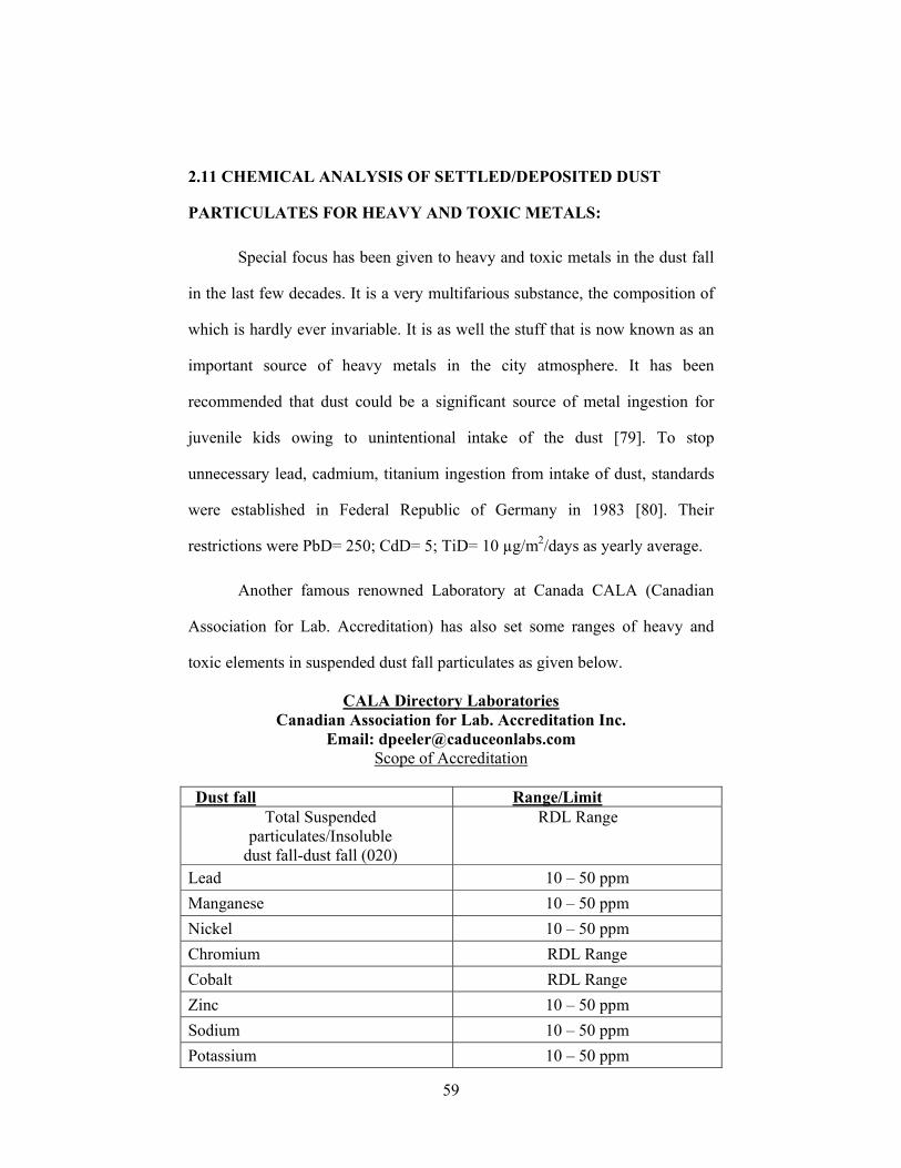
59
2.11 CHEMICAL ANALYSIS OF SETTLED/DEPOSITED DUST
PARTICULATES FOR HEAVY AND TOXIC METALS:
Special focus has been given to heavy and toxic metals in the dust fall
in the last few decades. It is a very multifarious substance, the composition of
which is hardly ever invariable. It is as well the stuff that is now known as an
important source of heavy metals in the city atmosphere. It has been
recommended that dust could be a significant source of metal ingestion for
juvenile kids owing to unintentional intake of the dust [79]. To stop
unnecessary lead, cadmium, titanium ingestion from intake of dust, standards
were established in Federal Republic of Germany in 1983 [80]. Their
restrictions were PbD= 250; CdD= 5; TiD= 10 µg/m2/days as yearly average.
Another famous renowned Laboratory at Canada CALA (Canadian
Association for Lab. Accreditation) has also set some ranges of heavy and
toxic elements in suspended dust fall particulates as given below.
CALA Directory Laboratories Canadian Association for Lab. Accreditation Inc.
Email: [email protected] Scope of Accreditation
Dust fall Range/Limit
Total Suspended particulates/Insoluble
dust fall-dust fall (020)
RDL Range
Lead 10 – 50 ppm Manganese 10 – 50 ppm Nickel 10 – 50 ppm Chromium RDL Range Cobalt RDL Range Zinc 10 – 50 ppm Sodium 10 – 50 ppm Potassium 10 – 50 ppm
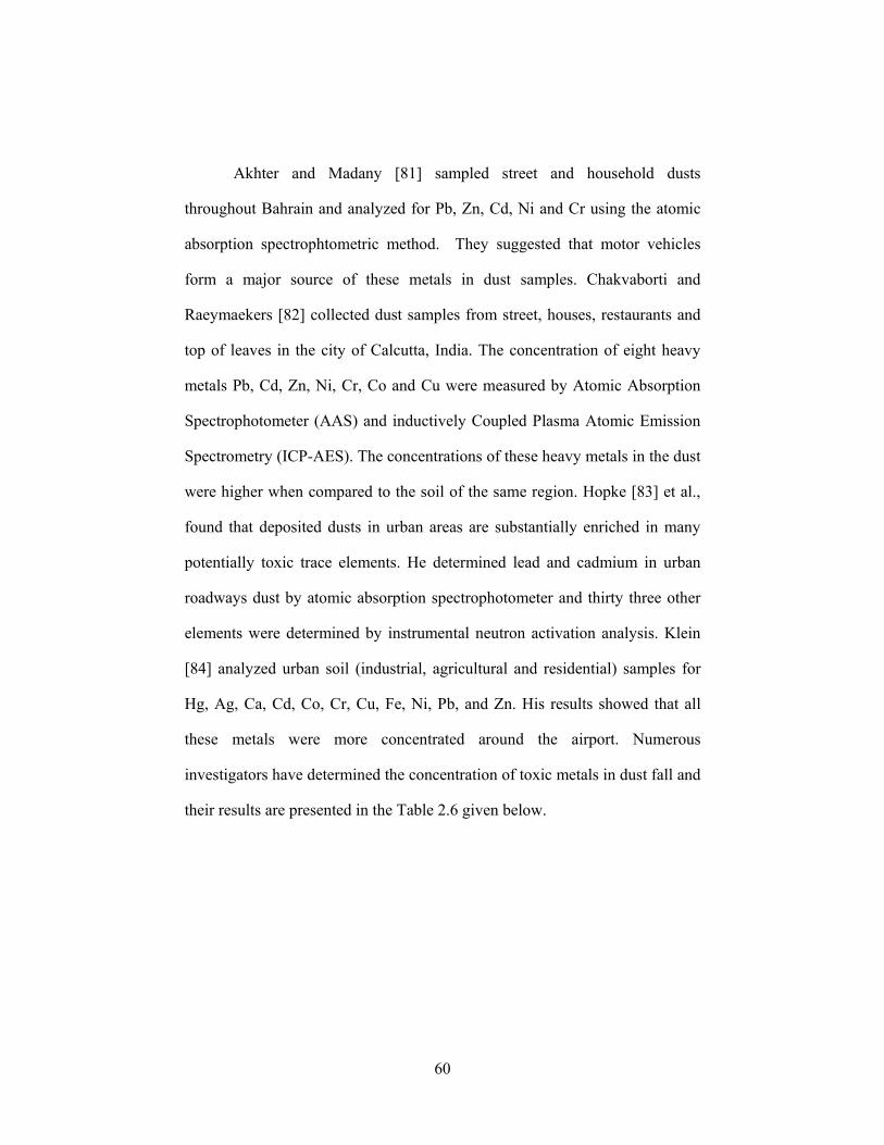
60
Akhter and Madany [81] sampled street and household dusts
throughout Bahrain and analyzed for Pb, Zn, Cd, Ni and Cr using the atomic
absorption spectrophtometric method. They suggested that motor vehicles
form a major source of these metals in dust samples. Chakvaborti and
Raeymaekers [82] collected dust samples from street, houses, restaurants and
top of leaves in the city of Calcutta, India. The concentration of eight heavy
metals Pb, Cd, Zn, Ni, Cr, Co and Cu were measured by Atomic Absorption
Spectrophotometer (AAS) and inductively Coupled Plasma Atomic Emission
Spectrometry (ICP-AES). The concentrations of these heavy metals in the dust
were higher when compared to the soil of the same region. Hopke [83] et al.,
found that deposited dusts in urban areas are substantially enriched in many
potentially toxic trace elements. He determined lead and cadmium in urban
roadways dust by atomic absorption spectrophotometer and thirty three other
elements were determined by instrumental neutron activation analysis. Klein
[84] analyzed urban soil (industrial, agricultural and residential) samples for
Hg, Ag, Ca, Cd, Co, Cr, Cu, Fe, Ni, Pb, and Zn. His results showed that all
these metals were more concentrated around the airport. Numerous
investigators have determined the concentration of toxic metals in dust fall and
their results are presented in the Table 2.6 given below.
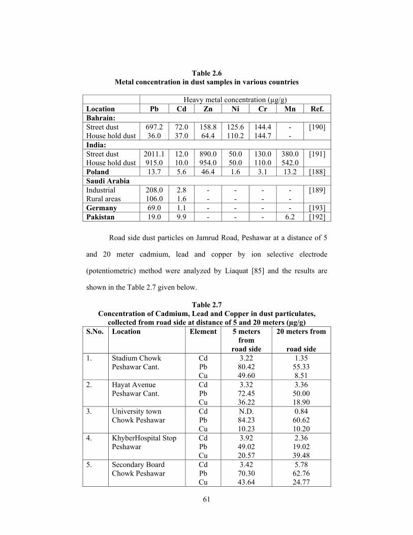
61
Table 2.6 Metal concentration in dust samples in various countries
Heavy metal concentration (µg/g) Location Pb Cd Zn Ni Cr Mn Ref. Bahrain: Street dust 697.2 72.0 158.8 125.6 144.4 - [190] House hold dust 36.0 37.0 64.4 110.2 144.7 - India: Street dust 2011.1 12.0 890.0 50.0 130.0 380.0 [191] House hold dust 915.0 10.0 954.0 50.0 110.0 542.0 Poland 13.7 5.6 46.4 1.6 3.1 13.2 [188] Saudi Arabia Industrial 208.0 2.8 - - - - [189] Rural areas 106.0 1.6 - - - - Germany 69.0 1.1 - - - - [193] Pakistan 19.0 9.9 - - - 6.2 [192]
Road side dust particles on Jamrud Road, Peshawar at a distance of 5
and 20 meter cadmium, lead and copper by ion selective electrode
(potentiometric) method were analyzed by Liaquat [85] and the results are
shown in the Table 2.7 given below.
Table 2.7 Concentration of Cadmium, Lead and Copper in dust particulates,
collected from road side at distance of 5 and 20 meters (µg/g) S.No. Location Element 5 meters
from 20 meters from
road side road side 1. Stadium Chowk Cd 3.22 1.35 Peshawar Cant. Pb 80.42 55.33 Cu 49.60 8.51 2. Hayat Avenue Cd 3.32 3.36 Peshawar Cant. Pb 72.45 50.00 Cu 36.22 18.90 3. University town Cd N.D. 0.84 Chowk Peshawar Pb 84.23 60.62 Cu 10.23 10.20 4. KhyberHospital Stop Cd 3.92 2.36 Peshawar Pb 49.02 19.02 Cu 20.57 39.48 5. Secondary Board Cd 3.42 5.78 Chowk Peshawar Pb 70.30 62.76 Cu 43.64 24.77
62
Samples of road side dust were collected in the months of April, May,
and June 1990 by Yousufzai [86] from forty one locations along the
intersection of major roads where traffic density was found to be high. Heavy
metals such as Pb, Zn, Mn, Cu, and Cd were estimated. The range of average
concentration of Pb was around 810 to 4527, Zn 112 to 2215, Cu 46 to 315,
Mn 72 to 481 and Cd 0.2 to 4.5 ppm. The daily average traffic was also
recorded. A definite correlation was found between mean Pb level and daily
average traffic. It was concluded that the major source of Pb in road side dust
of Karachi city was mostly contributed by leaded gasoline from vehicular
traffic. Raising children in high leaded environment will definitely have long
term effect on mental and physical behavior in future.
The analysis of Pb, Zn, Ni, Mn, Cr, and Co in dust fall samples were
collected from various deposition sites in urban Saeed et al., [87] during the
period January 1993 to December 1994. Dust fall samples were collected in
accordance with the standard method [88]. A plastic bucket of about 22-24 cm
mouth diameter, 20 cm diameter and 25 cm height was secured in a bucket
shape cage mounted on a metallic pole. After a period of one calendar month,
the bucket was taken off, covered with plastic lid and brought to the
laboratory. Samples were sieved (30 mesh) to exclude materials like leaves,
insects, twigs, stones if any and a portion was dried at 105°C for 24 hours and
weighed. The samples were digested and analyzed on atomic absorption
spectrophotometer (Pye Unicam Model CB 2PX England) in Zeeman flame
mode. Results show that dust fall samples contained significant levels of
metals studied. The average concentrations (µg/g) of Pb, Zn, Mn, Ni, Cr and
Co were found to be 425, 763, 358, 637, 83, and 54 respectively. It was
63
suggested that vehicles form a major source of these metals in dust fall
samples.
Yoursufzai et al., [89] conducted a research work for the measurement
of major ambient air pollution components O3, SO2, CO, NO, NOx,PM10,
methane, non-methane along with the metrological parameters at sub-urban
area of Karachi in a mobile laboratory. The average concentration of O3 was
found to be between 4.62 and 20.36 ppb, SO2 0.73 and 4.69 ppb, CO 0.14 and
0.77 ppm, NO 0.92 and 2.73 ppb, NOx 3.1 and 7.5 ppb, PM10 142 and 251 µg
m-3, methane 1.09 and 2.7 ppm, non-methane hydrocarbon 0.41 and 0.96 ppm.
Krolak [90] carried out a research work for the detection of the
concentration of heavy metals Cu, Zn, Mn, Cr, Ni, Pb and Cd in falling dust in
Eastern Mazowieckie Province (Poland) in 1995-1998. Neither dust fall
crossed the allowed limits nor Pb and Cd. It was also found that the elements
(Pb and Zn) having low melting points were present larger in settled dust
particulates, specifically in the scorching heat vis-à-vis summer. Ni was found
the most stable among all the other metals. Thermal and electric power
industries were discovered the major sources of these metals.
Nwajei et al., [11] worked on the distribution of heavy metals in the
sediments of Lagos Lagoon (Nigeria) in order to find out the concentrations of
Cd, Pb, Ni, Cr, Cu, Zn, Fe, Mn, Co and Hg with the help of AAS in the year
1998. The respective ranges of metals were Cd: 0.13-8.60, Pb: 4.10-295.70,
Ni: 11.60-149.40, Cr: 23.30-167.20, Cu: 4.80-102.70, Zn: 27.30-323.70, Fe:
10579.80-85548.00, Mn: 276.00-748.00, Co: 6.40-41.50 and Hg: 0.04-0.53
mg kg-1 dry weight. The data showed considerable variation in the values from
64
one sampling station to the other. Sampling station 3 (Iddo) showed the
highest values of metals.
An investigation was carried out by Khan et al., [57] in Peshawar for
the detection of Pb, Zn, Mn, Ni, Co and Cr in insoluble dust fall (1993-98) by
using atomic absorption spectrophotometric technique. Elemental
concentrations of the studied elements did not vary significantly at different
sample location. A comparison of the elemental contents with the local soil
was also made. Soil, road dust, vehicle exhaust, metallic corrosion, tire wear,
zinc compounds in rubber material, galvanized material, weathering and
corrosion of building material were some of the possible sources of heavy
metals pollution in Peshawar. The concentration of Pb, Zn, Mn, Ni, Cr and Co
in the dust given below in the table 2.6 was compared with the concentration
of these metals in soil of Peshawar. Imdadullah et al., [91] reported the
concentration (mg kg-1) of Pb, Zn, Mn, Ni, Cr and Co in the soil of Peshawar
to be 1.19, 17.39, 20.61, 5.71, 2.06 and 2.40 respectively. That suggested that
heavy metals ultimately settle down on the earth as soil acts as a recipient of
all types of wet and dry depositions from the atmosphere. Substantial amount
of heavy metals is added to the soil through air.
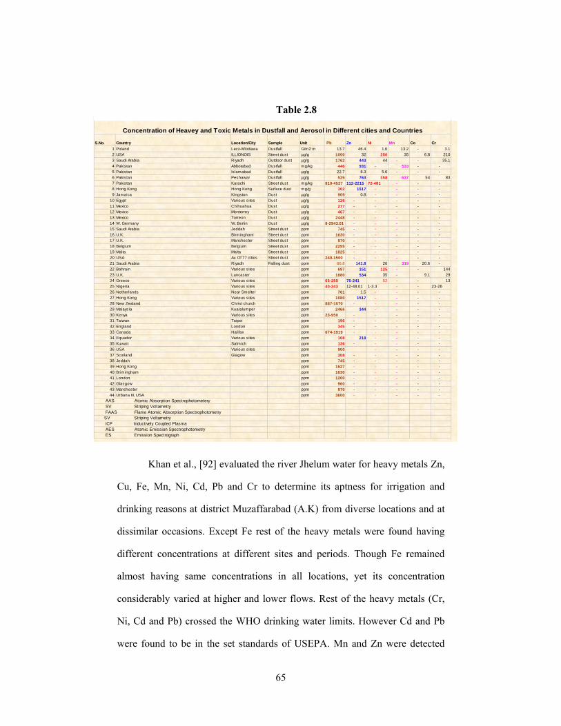
65
Table 2.8
S.No. Country Location/City Sample Unit Pb Zn Ni Mn Co Cr1 Poland Lecz-Wlodawa Dustfall G/m2 m 13.7 46.4 1.6 13.2 - 3.12 USA ILLIONOIS Street dust µg/g 1000 32 250 35 6.8 2103 Saudi Arabia Riyadh Outdoor dust µg/g 1762 443 44 - - 35.14 Pakistan Abbotabad Dustfall mg/kg 446 931 - 533 - -5 Pakistan Islamabad Dustfall µg/g 22.7 8.3 5.6 - - -6 Pakistan Peshawar Dustfall µg/g 525 763 358 637 54 837 Pakistan Karachi Street dust mg/kg 810-4527 112-2215 72-481 - - -8 Hong Kong Hong Kong Surface dust mg/g 302 1517 - - - -9 Jamaica Kingston Dust µg/g 909 0.8 - - - -
10 Egypt Various sites Dust µg/g 126 - - - - -11 Mexico Chihuahua Dust µg/g 277 - - - - -12 Mexico Monterrey Dust µg/g 467 - - - - -13 Mexico Torreon Dust µg/g 2448 - - - - -14 W. Germany W. Berlin Dust µg/g 8-2943.01 - - - - -15 Saudi Arabia Jeddah Street dust ppm 745 - - - - -16 U.K. Birmingham Street dust ppm 1630 - - - - -17 U.K. Manchester Street dust ppm 970 - - - - -18 Belgium Belgium Street dust ppm 2255 - - - - -19 Malta Malta Street dust ppm 1825 - - - - -20 USA Av. Of 77 cities Street dust ppm 240-1500 - - - - -21 Saudi Arabia Riyadh Falling dust ppm 66.8 141.8 26 319 20.6 -22 Bahrain Various sites ppm 697 151 125 - - 14423 U.K. Lancaster ppm 1880 534 35 - 9.1 2924 Greece Various sites ppm 65-259 75-241 52 - - 1325 Nigeria Various sites ppm 40-243 12-48.01 1-3.3 - - 23-2626 Netherlands Near Smelter ppm 761 1.5 - - - -27 Hong Kong Various sites ppm 1080 1517 - - - -28 New Zealand Christ church ppm 887-1070 - - - - -29 Malaysia Kualalumper ppm 2466 344 - - - -30 Kenya Various sites ppm 23-950 - - - - -31 Taiwan Taipei ppm 196 - - - - -32 England London ppm 345 - - - - -33 Canada Halifax ppm 674-1919 - - - - -34 Equador Various sites ppm 108 218 - - - -35 Kuwait Salmich ppm 136 - - - - -36 USA Various sites ppm 900 - - - -37 Scotland Glagow ppm 308 - - - - -38 Jeddah ppm 745 - - - - -39 Hong Kong ppm 1627 - - - - -40 Brimingham ppm 1630 - - - - -41 London ppm 1200 - - - - -42 Glasgow ppm 960 - - - - -43 Manchester ppm 970 - - - - -44 Urbana III, USA ppm 3600 - - - - -
AAS Atomic Absorption Spectrophotometery SV Striping Voltametry FAAS Flame Atomic Absorption Spectrophotometry SV Striping Voltametry ICP Inductively Coupled Plasma AES Atomic Emission Spectrophotometry ES Emission Spectrograph
Concentration of Heavey and Toxic Metals in Dustfall and Aerosol in Different cities and Countries
Khan et al., [92] evaluated the river Jhelum water for heavy metals Zn,
Cu, Fe, Mn, Ni, Cd, Pb and Cr to determine its aptness for irrigation and
drinking reasons at district Muzaffarabad (A.K) from diverse locations and at
dissimilar occasions. Except Fe rest of the heavy metals were found having
different concentrations at different sites and periods. Though Fe remained
almost having same concentrations in all locations, yet its concentration
considerably varied at higher and lower flows. Rest of the heavy metals (Cr,
Ni, Cd and Pb) crossed the WHO drinking water limits. However Cd and Pb
were found to be in the set standards of USEPA. Mn and Zn were detected
66
within the WHO and USEPA set limits for irrigating and drinking needs.
Nevertheless Fe was found to be dangerous for human’s usage contrary to its
allowable range for irrigation. But Cu was detected even more than the
standards set for irrigation at elevated stream.
Khan et al., [93] conducted another excellent study to detect the toxic
and trace metals Cd, Pb, Zn, Cu, Mn, Ni, Cr and Co in dust, dust fall/soil at
Peshawar. It was found that the said elements emitted into the urban air from
different sources like coal and petroleum burning, municipal incinerators,
automobile exhaust, refuse burning, pesticide use in agricultural, diverse
industrial manufacturing process etc. and being an ultimate sink for all types
of pollutants. To assess health hazard and other problems posed by metal
component, information was needed on their concentrations, particle size and
chemical forms. Therefore a review was done in the Table No.2.6 for these
toxic and traces metals concentrations in dust/dust fall particulates and soil.
Ahmad et al., [13] studied the dispersion gradient of free fall dust and
heavy metal elements concentration in dust along a main road at Lahore
(Pakistan). Gradient of mass flux of free fall-fall dust was measured at
distances 50, 100 and 200 m away from grand trunk road at four different
locations in addition to detect the metal concentrations in free fall dust and soil
samples too. Average monthly free-fall dust values were found to be decreased
as the distance increased. Monthly free fall dust ranged between 24-96
tons/km2/month at 50 m, 15-90 tons/km2/month at 100 m and 9-27
tons/km2/month at 200 m distance, which implied that maximum reduction in
the range of 62-71 % had occurred at 200 m distance. Free- fall dust values
67
were found to be alarmingly higher than permissible limit (5tons/km2/month).
Samples of soil up to 3 inches depth from different locations on analysis
showed the accumulation of these metals decreased with depth. Higher values
of mass flux of free fall particles and metal elements loadings Dispersion
gradient of metal elements, measured at three distances (50, 100 and 200 m),
showed decrease as distance increased road indicated that vehicle exhaust
emissions could be the major cause of particles and heavy metals.
Shah et al., [14] characterized Na, K, Fe, Pb, Zn, Mn, Cd, Ni and Co in
airborne particulate matter in relation to meteorological conditions in
Islamabad, Pakistan on glass fiber filters using high volume air-sampler. The
quantification of the metals was done by the flame atomic absorption method
using HNO3 as a sample digestion medium. Among all the analyzed metals
maximum average concentration was found of Na (1.632 µg/m3), followed by
K (0.932 µg/m3), Pb, Fe and Zn showed mean concentrations of 0.267 µg/m3,
0.574 µg/m3 and 0.645 µg/m3, respectively. The metal-to-metal and metals-to-
meteorological parametric correlations were investigated. Strong positive
correlations were observed between K-Fe (r=0.704), K-Zn (r=0.679) and Fe-
Mn (r=0.561), while Cd and Co showed some significant negative correlation
with other metals. Significantly, positive correlation was observed for the Cr
and Ni concentrations with temperature, while the relative humidity was
mostly negatively correlated with selected trace metals except Na. The
sunshine parameters also indicated a negative correlation with metal
concentration, as was the case with wind speed. The pan evaporation showed
significant negative correlation with Na, K, Fe and Zn, while positive with Cr
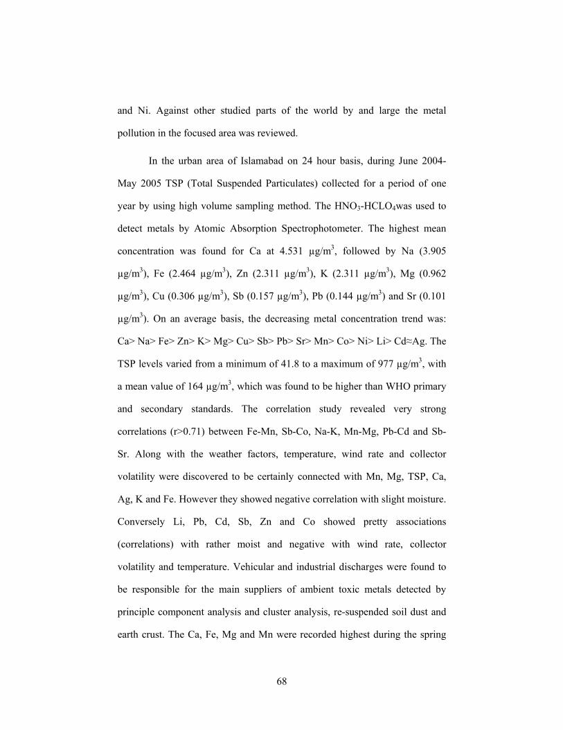
68
and Ni. Against other studied parts of the world by and large the metal
pollution in the focused area was reviewed.
In the urban area of Islamabad on 24 hour basis, during June 2004-
May 2005 TSP (Total Suspended Particulates) collected for a period of one
year by using high volume sampling method. The HNO3-HCLO4was used to
detect metals by Atomic Absorption Spectrophotometer. The highest mean
concentration was found for Ca at 4.531 µg/m3, followed by Na (3.905
µg/m3), Fe (2.464 µg/m3), Zn (2.311 µg/m3), K (2.311 µg/m3), Mg (0.962
µg/m3), Cu (0.306 µg/m3), Sb (0.157 µg/m3), Pb (0.144 µg/m3) and Sr (0.101
µg/m3). On an average basis, the decreasing metal concentration trend was:
Ca> Na> Fe> Zn> K> Mg> Cu> Sb> Pb> Sr> Mn> Co> Ni> Li> Cd≈Ag. The
TSP levels varied from a minimum of 41.8 to a maximum of 977 µg/m3, with
a mean value of 164 µg/m3, which was found to be higher than WHO primary
and secondary standards. The correlation study revealed very strong
correlations (r>0.71) between Fe-Mn, Sb-Co, Na-K, Mn-Mg, Pb-Cd and Sb-
Sr. Along with the weather factors, temperature, wind rate and collector
volatility were discovered to be certainly connected with Mn, Mg, TSP, Ca,
Ag, K and Fe. However they showed negative correlation with slight moisture.
Conversely Li, Pb, Cd, Sb, Zn and Co showed pretty associations
(correlations) with rather moist and negative with wind rate, collector
volatility and temperature. Vehicular and industrial discharges were found to
be responsible for the main suppliers of ambient toxic metals detected by
principle component analysis and cluster analysis, re-suspended soil dust and
earth crust. The Ca, Fe, Mg and Mn were recorded highest during the spring
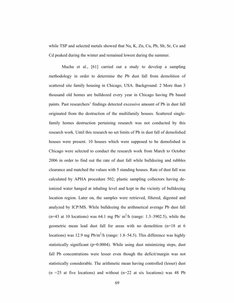
69
while TSP and selected metals showed that Na, K, Zn, Cu, Pb, Sb, Sr, Co and
Cd peaked during the winter and remained lowest during the summer.
Mucha et al., [61] carried out a study to develop a sampling
methodology in order to determine the Pb dust fall from demolition of
scattered site family housing in Chicago, USA. Background: 2 More than 3
thousand old homes are bulldozed every year in Chicago having Pb based
paints. Past researchers’ findings detected excessive amount of Pb in dust fall
originated from the destruction of the multifamily houses. Scattered single-
family homes destruction pertaining research was not conducted by this
research work. Until this research no set limits of Pb in dust fall of demolished
houses were present. 10 houses which were supposed to be demolished in
Chicago were selected to conduct the research work from March to October
2006 in order to find out the rate of dust fall while bulldozing and rubbles
clearance and matched the values with 5 standing houses. Rate of dust fall was
calculated by APHA procedure 502; plastic sampling collectors having de-
ionized water hanged at inhaling level and kept in the vicinity of bulldozing
location region. Later on, the samples were retrieved, filtered, digested and
analyzed by ICP/MS. While bulldozing the arithmetical average Pb dust fall
(n=43 at 10 locations) was 64.1 mg Pb/ m2/h (range: 1.3–3902.5), while the
geometric mean lead dust fall for areas with no demolition (n=18 at 6
locations) was 12.9 mg Pb/m2/h (range: 1.8–54.5). This difference was highly
statistically significant (p=0.0004). While using dust minimizing steps, dust
fall Pb concentrations were lesser even though the deficit/margin was not
statistically considerable. The arithmetic mean having controlled (lesser) dust
(n =25 at five locations) and without (n=22 at six locations) was 48 Pb
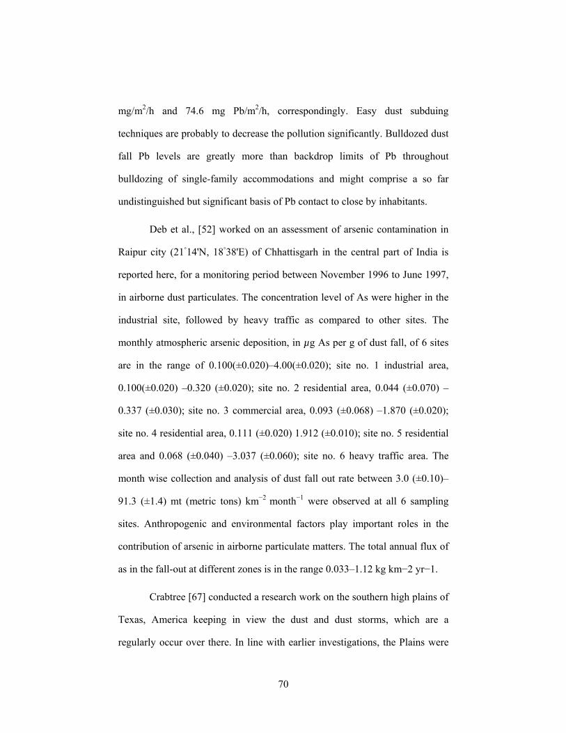
70
mg/m2/h and 74.6 mg Pb/m2/h, correspondingly. Easy dust subduing
techniques are probably to decrease the pollution significantly. Bulldozed dust
fall Pb levels are greatly more than backdrop limits of Pb throughout
bulldozing of single-family accommodations and might comprise a so far
undistinguished but significant basis of Pb contact to close by inhabitants.
Deb et al., [52] worked on an assessment of arsenic contamination in
Raipur city (21◦14'N, 18◦38'E) of Chhattisgarh in the central part of India is
reported here, for a monitoring period between November 1996 to June 1997,
in airborne dust particulates. The concentration level of As were higher in the
industrial site, followed by heavy traffic as compared to other sites. The
monthly atmospheric arsenic deposition, in µg As per g of dust fall, of 6 sites
are in the range of 0.100(±0.020)–4.00(±0.020); site no. 1 industrial area,
0.100(±0.020) –0.320 (±0.020); site no. 2 residential area, 0.044 (±0.070) –
0.337 (±0.030); site no. 3 commercial area, 0.093 (±0.068) –1.870 (±0.020);
site no. 4 residential area, 0.111 (±0.020) 1.912 (±0.010); site no. 5 residential
area and 0.068 (±0.040) –3.037 (±0.060); site no. 6 heavy traffic area. The
month wise collection and analysis of dust fall out rate between 3.0 (±0.10)–
91.3 (±1.4) mt (metric tons) km−2 month−1 were observed at all 6 sampling
sites. Anthropogenic and environmental factors play important roles in the
contribution of arsenic in airborne particulate matters. The total annual flux of
as in the fall-out at different zones is in the range 0.033–1.12 kg km−2 yr−1.
Crabtree [67] conducted a research work on the southern high plains of
Texas, America keeping in view the dust and dust storms, which are a
regularly occur over there. In line with earlier investigations, the Plains were
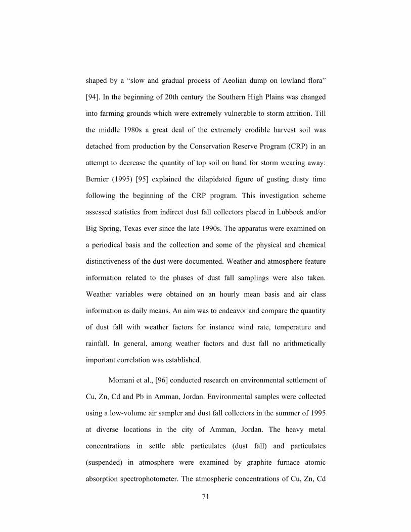
71
shaped by a “slow and gradual process of Aeolian dump on lowland flora”
[94]. In the beginning of 20th century the Southern High Plains was changed
into farming grounds which were extremely vulnerable to storm attrition. Till
the middle 1980s a great deal of the extremely erodible harvest soil was
detached from production by the Conservation Reserve Program (CRP) in an
attempt to decrease the quantity of top soil on hand for storm wearing away:
Bernier (1995) [95] explained the dilapidated figure of gusting dusty time
following the beginning of the CRP program. This investigation scheme
assessed statistics from indirect dust fall collectors placed in Lubbock and/or
Big Spring, Texas ever since the late 1990s. The apparatus were examined on
a periodical basis and the collection and some of the physical and chemical
distinctiveness of the dust were documented. Weather and atmosphere feature
information related to the phases of dust fall samplings were also taken.
Weather variables were obtained on an hourly mean basis and air class
information as daily means. An aim was to endeavor and compare the quantity
of dust fall with weather factors for instance wind rate, temperature and
rainfall. In general, among weather factors and dust fall no arithmetically
important correlation was established.
Momani et al., [96] conducted research on environmental settlement of
Cu, Zn, Cd and Pb in Amman, Jordan. Environmental samples were collected
using a low-volume air sampler and dust fall collectors in the summer of 1995
at diverse locations in the city of Amman, Jordan. The heavy metal
concentrations in settle able particulates (dust fall) and particulates
(suspended) in atmosphere were examined by graphite furnace atomic
absorption spectrophotometer. The atmospheric concentrations of Cu, Zn, Cd
72
and Pb were 170, 344, 3.8 and 291 ng/m3, respectively. The intensity of these
elements in the dust fall settlement was 505, 94, 74 and 3.1 µg/g, respectively.
The fluctuations and dehydrated settling rates of these heavy metals were
detected and judged against the results of other international researchers. The
enhancement coefficients of the heavy metals in the dust fall were 12.1, 6.1,
11.7, and 1.1 for Zn, Cu, Pb, and Cd, respectively and were detected to be
considerable.
The chemical composition of the Black Sea aerosol was calculated by
Kubilay et al., [97] in July 1992 CoMSBLACK 92 cruise on board R/V
BilinL. It was found that the chemical composition of the Black Sea aerosols
could vary extremely swiftly in line with alteration in the wind rule. The
power of the Saharan desert particulates could change the elemental quantities
of trace metals. The dispatch has been summed up on enhancement feature
figures to allow relationship with earlier and upcoming researches. Such heaps
could play a significant function in the current condition of the ocean. As the
environmental participation of oxidized nitrogen (NO3+NO2-N) could attain
13% of the total inorganic nitrogen contribution of the Danube, Lead (Pb)
contribution arrived at 39% of this riverine involvement.
2.12 A STUDY OF THE SIZE OF THE DUST PARTICULATES:
Khan [98] found the particulates size distribution % by weight for ten
(10) different sizes (211, 150, 125, 105, 76, 65, 53, 44, 42 and < 42µm) for the
period of three years 1992-1994 at three different sites. Spatial changes in
whole poised particulate matter (TSP) were examined by Shah et al., [99] for
the sharing of metals and particulates volume portions in the town and rural
73
ambiance of Islamabad, Pakistan. The metals Fe, Mn, Pb, Cd, Cr, Zn, Co, Ni,
Na and K, and the particulates divisions of four (04) diverse mass classes (<
2.5, 2.5-10, 10-100 and > 100 µm) were integrated in the research. TSP
samples were collected on glass filament filters by means of high volume
samplers and amount of metals was ascertained by using Atomic Absorption
Spectrometry using HNO3 based wet digestion. At the city site, Na was
leading at 2.384 µg/m3 followed by K, Fe and Zn with 0.778, 0.667 and 0.567
µg/m3 as average amounts, correspondingly. The metal levels for the rural
locations varied from 0.002 µg/m3 for Cd to 1.077 µg/m3 for Na. Nevertheless,
evaluated with the city site, average Pb amounts proved an approximately dual
improvement, i.e. 0.163 Vs. 0.327 µg/m3. Metals and particulates dimension
foundation recognition was completed by means of Principal Component
Analysis and Cluster Analysis. Five bases were pointed out for the city
location: soil, industrial, metallurgical industries, excavation activities and
automobile emissions. For the countryside site, four causes were witnessed in
terms of excavation activities automotive emissions, metallurgical industries
and agricultural. For the countryside location, four bases were traced in terms
of excavation activities, agricultural, metallurgical units and automotive
emissions. Jointly, each city and rural sites, PM10-100 emerged as a major
contributor to TSP, subsequently PM2.5-10, PM<2.5 and PM>100 correspondingly.
The metals proved generally optimistic association with fine particulates
portions (PM10-100, PM>100). The level of Ni, Mn, Co, Na, K and Fe was
determined to be poorer than those of the different polluted Asian cities of the
world.
74
Shah and Shaheen [10] for nine different segments (PM<1.0, PM1.0-2.5,
PM2.5-5.0, PM5.0-10, PM10-15, PM15-25, PM25-50, PM50-100 and PM>100) studied the
ambient air particulates material by gathering it on glass fiber filters in city
ambiance of Islamabad, Pakistan, using high volume sampler. The particulates
samples were investigated for 10 selected metals (Na, Zn, Fe, K, Pb, Mn, Cr,
Cd, Co and Ni) by FAAS technique. Utmost average involvement was
observed for Fe (1.761 µg/m3), afterward Na (1.661 µg/m3), Zn (1.021 µg/m3),
K (0.488 µg/m3), and Pb (0.128 µg/m3). The particulates dimension
determination on vol. % basis for seven fractions (PM<1.0, PM1.0-2.5, PM2.5-5,
PM5-10, PM15-25, PM50-100 and PM>100 µm) was done by means of Mastersizer.
Shah et al., [100], PM5.0-10 were detected to be most plentiful in the
local ambiance subsequently PM2.5-5 and PM15-25 whilst coarse/giant
particulates (PM50-100 and PM>100) proved lesser part. The trace metals were
detected to be mostly linked with lesser intensities whereas comparative
moisture proved negative relationship. The origin detection was done by main
constituent examination and bunch study. Five metal bases were known:
vehicular emissions, industrial, metallurgical operations, soil derived dust and
garbage burning. In general, 181 particulates samples were collected,
throughout September 2003-March 2004, a phase obvious by a common 'dry
spell' (no precipitation) with approximately 50% or with a reduction of
comparative moisture and dull ambiance circumstances existing throughout.
75
CHAPTER 3
HYPOTHESIS/AIMS AND OBJECTIVES
3.1 HISTORY OF QUETTA:
In the beginning a loose tribal confederation, Balochistan was later on
divided into four principalities that were sometimes under Persian, sometimes
Afghan suzerainty. In the 19th century British troops tried to subdue the
inhabitants until a treaty in 1876 gave them autonomy in exchange for British
army outposts along the Afghan border and strategic roads, on the exchange
for British army outposts along the Afghan border and strategic roads. On the
division of India in 1947 the Khan of Kalat declared Balochistan independent;
the insurrection was crushed by the new Pakistani army after eight months.
Three rebellions followed the last being from 1973 to 1977, when 3,300
Pakistani soldiers lost their lives and some 6,000 Balochs embraced
martyrdom as well. Quetta more commonly called the fruit basket of Pakistan
is the capital of Balochistan and used to be one of the most beautiful cities due
to its small population and well planned infrastructure. Plums, peaches,
pomegranates, apricots, apples, some unique varieties of melon like "Garma"
and cherries, pistachios and almonds are all grown in abundance. Some
pistachios also grow in Qila Saif ullah. Saffron grows very well on mountains
around 5000 ft (1524 meters) high. It is being cultivated on a commercial scale
here. The yellow and red varieties of tulip grow wild around Quetta.
Quetta is an important trade centre; other industries include fruit
canning and chromite mining. In 1876 the British acquired Quetta by treaty
with the Khan of Kalat. The city was capital of the British province of
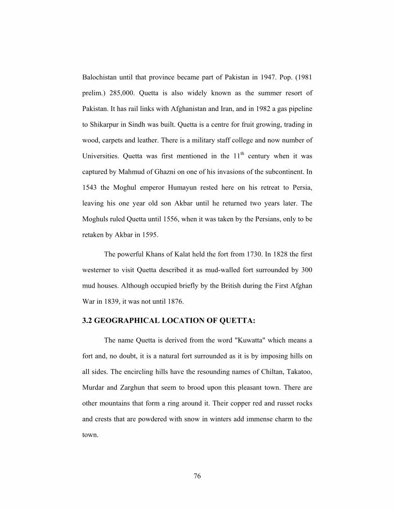
76
Balochistan until that province became part of Pakistan in 1947. Pop. (1981
prelim.) 285,000. Quetta is also widely known as the summer resort of
Pakistan. It has rail links with Afghanistan and Iran, and in 1982 a gas pipeline
to Shikarpur in Sindh was built. Quetta is a centre for fruit growing, trading in
wood, carpets and leather. There is a military staff college and now number of
Universities. Quetta was first mentioned in the 11th century when it was
captured by Mahmud of Ghazni on one of his invasions of the subcontinent. In
1543 the Moghul emperor Humayun rested here on his retreat to Persia,
leaving his one year old son Akbar until he returned two years later. The
Moghuls ruled Quetta until 1556, when it was taken by the Persians, only to be
retaken by Akbar in 1595.
The powerful Khans of Kalat held the fort from 1730. In 1828 the first
westerner to visit Quetta described it as mud-walled fort surrounded by 300
mud houses. Although occupied briefly by the British during the First Afghan
War in 1839, it was not until 1876.
3.2 GEOGRAPHICAL LOCATION OF QUETTA:
The name Quetta is derived from the word "Kuwatta" which means a
fort and, no doubt, it is a natural fort surrounded as it is by imposing hills on
all sides. The encircling hills have the resounding names of Chiltan, Takatoo,
Murdar and Zarghun that seem to brood upon this pleasant town. There are
other mountains that form a ring around it. Their copper red and russet rocks
and crests that are powdered with snow in winters add immense charm to the
town.
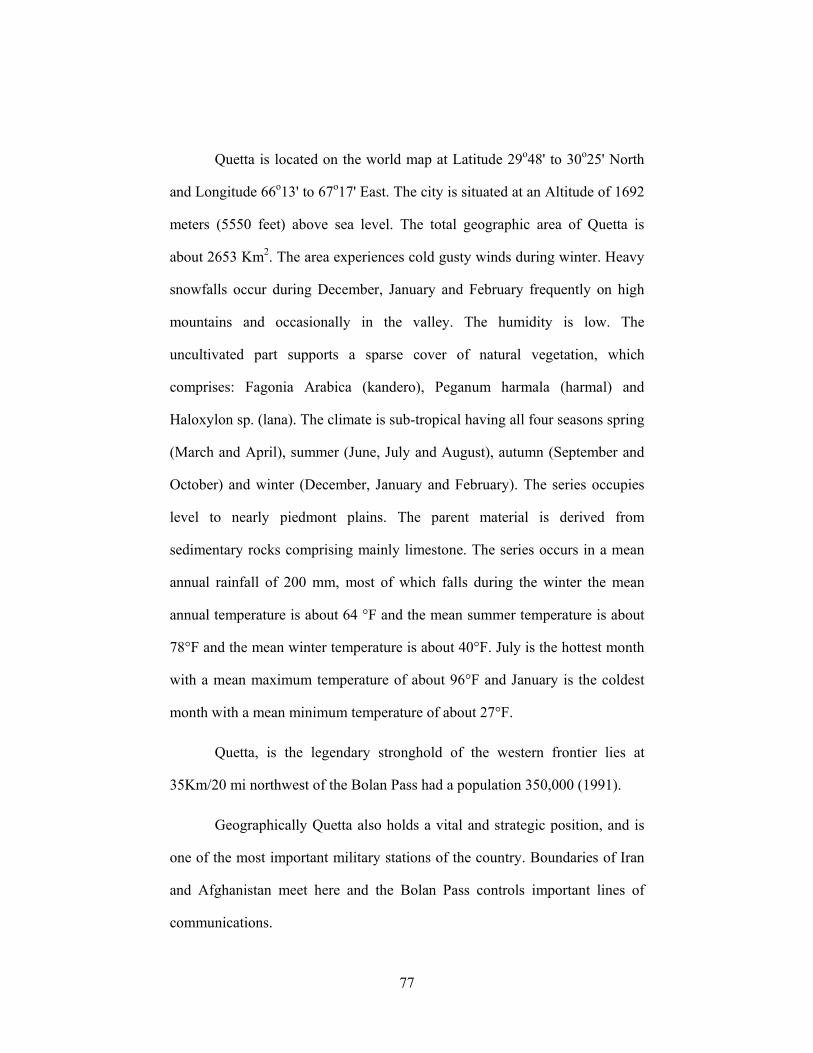
77
Quetta is located on the world map at Latitude 29o48' to 30o25' North
and Longitude 66o13' to 67o17' East. The city is situated at an Altitude of 1692
meters (5550 feet) above sea level. The total geographic area of Quetta is
about 2653 Km2. The area experiences cold gusty winds during winter. Heavy
snowfalls occur during December, January and February frequently on high
mountains and occasionally in the valley. The humidity is low. The
uncultivated part supports a sparse cover of natural vegetation, which
comprises: Fagonia Arabica (kandero), Peganum harmala (harmal) and
Haloxylon sp. (lana). The climate is sub-tropical having all four seasons spring
(March and April), summer (June, July and August), autumn (September and
October) and winter (December, January and February). The series occupies
level to nearly piedmont plains. The parent material is derived from
sedimentary rocks comprising mainly limestone. The series occurs in a mean
annual rainfall of 200 mm, most of which falls during the winter the mean
annual temperature is about 64 °F and the mean summer temperature is about
78°F and the mean winter temperature is about 40°F. July is the hottest month
with a mean maximum temperature of about 96°F and January is the coldest
month with a mean minimum temperature of about 27°F.
Quetta, is the legendary stronghold of the western frontier lies at
35Km/20 mi northwest of the Bolan Pass had a population 350,000 (1991).
Geographically Quetta also holds a vital and strategic position, and is
one of the most important military stations of the country. Boundaries of Iran
and Afghanistan meet here and the Bolan Pass controls important lines of
communications.
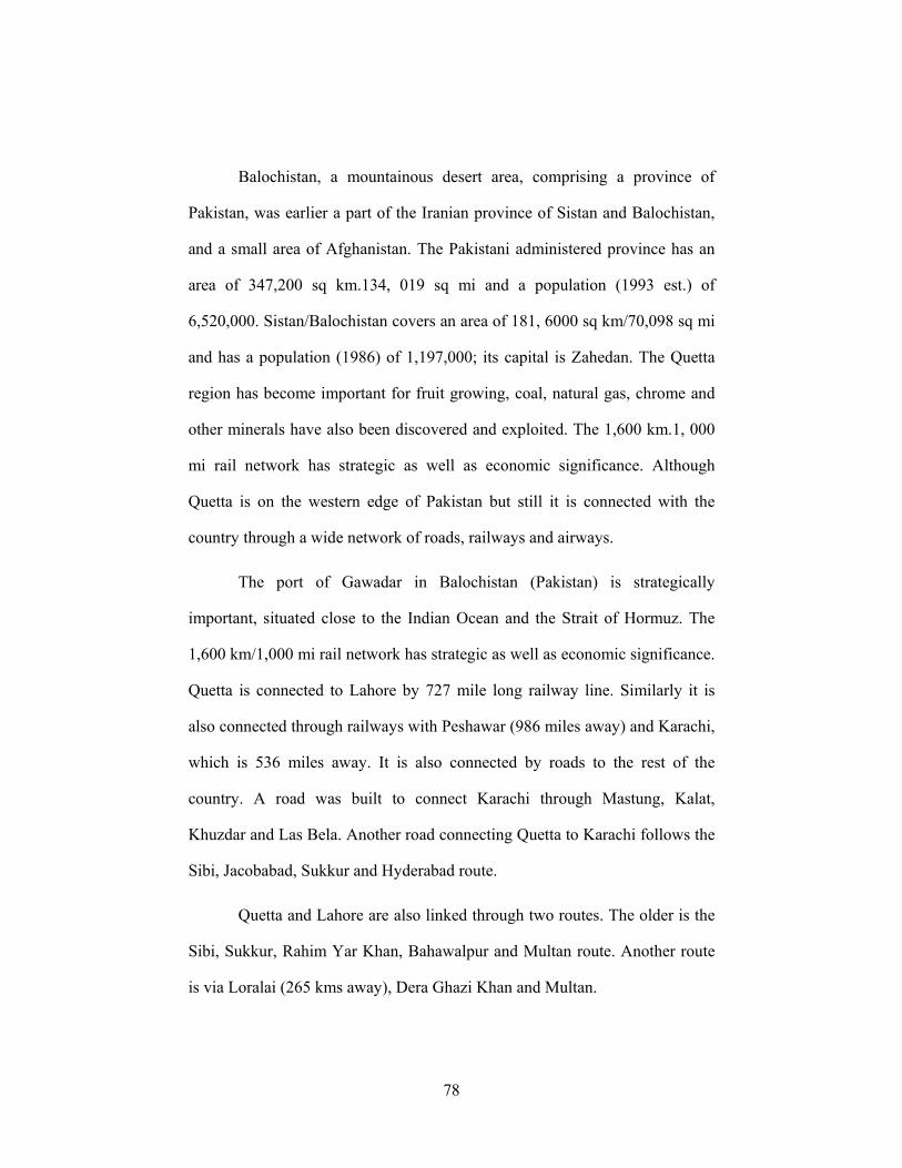
78
Balochistan, a mountainous desert area, comprising a province of
Pakistan, was earlier a part of the Iranian province of Sistan and Balochistan,
and a small area of Afghanistan. The Pakistani administered province has an
area of 347,200 sq km.134, 019 sq mi and a population (1993 est.) of
6,520,000. Sistan/Balochistan covers an area of 181, 6000 sq km/70,098 sq mi
and has a population (1986) of 1,197,000; its capital is Zahedan. The Quetta
region has become important for fruit growing, coal, natural gas, chrome and
other minerals have also been discovered and exploited. The 1,600 km.1, 000
mi rail network has strategic as well as economic significance. Although
Quetta is on the western edge of Pakistan but still it is connected with the
country through a wide network of roads, railways and airways.
The port of Gawadar in Balochistan (Pakistan) is strategically
important, situated close to the Indian Ocean and the Strait of Hormuz. The
1,600 km/1,000 mi rail network has strategic as well as economic significance.
Quetta is connected to Lahore by 727 mile long railway line. Similarly it is
also connected through railways with Peshawar (986 miles away) and Karachi,
which is 536 miles away. It is also connected by roads to the rest of the
country. A road was built to connect Karachi through Mastung, Kalat,
Khuzdar and Las Bela. Another road connecting Quetta to Karachi follows the
Sibi, Jacobabad, Sukkur and Hyderabad route.
Quetta and Lahore are also linked through two routes. The older is the
Sibi, Sukkur, Rahim Yar Khan, Bahawalpur and Multan route. Another route
is via Loralai (265 kms away), Dera Ghazi Khan and Multan.
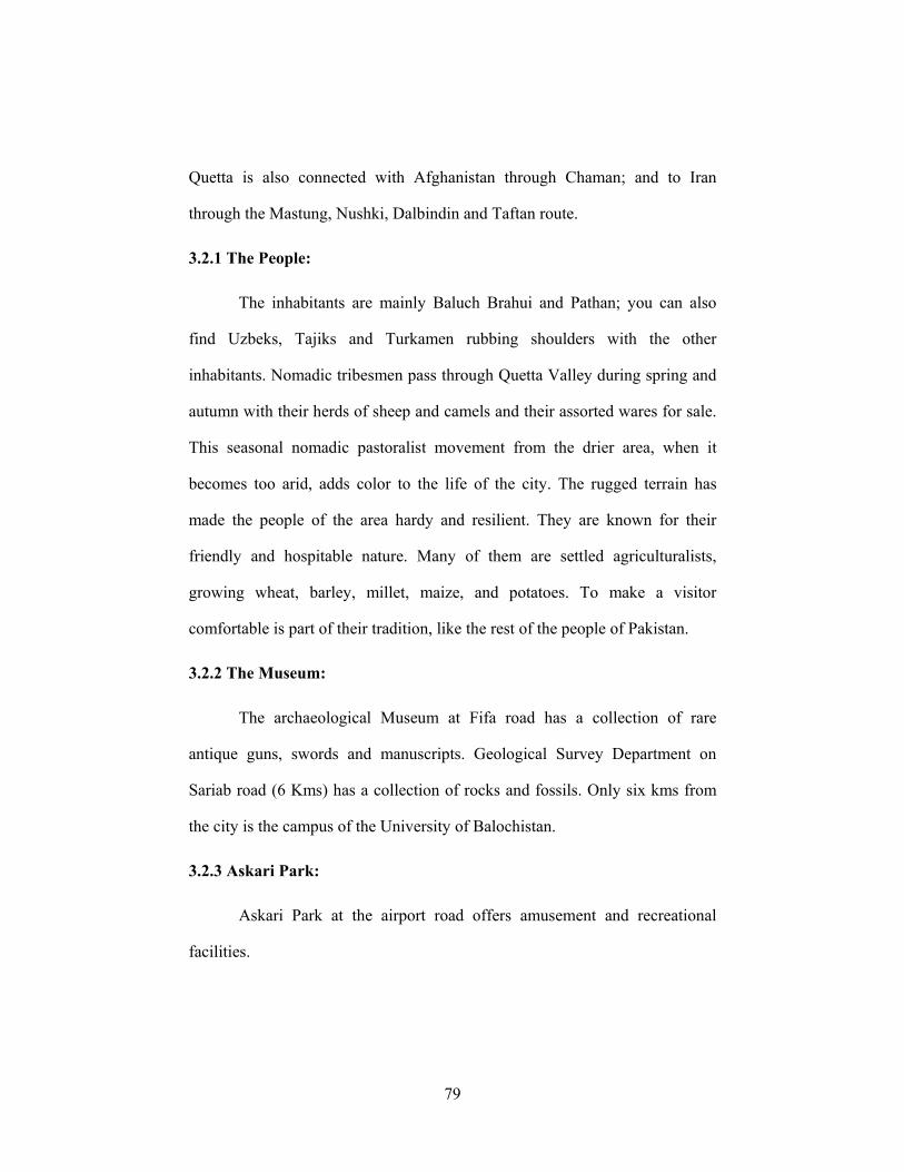
79
Quetta is also connected with Afghanistan through Chaman; and to Iran
through the Mastung, Nushki, Dalbindin and Taftan route.
3.2.1 The People:
The inhabitants are mainly Baluch Brahui and Pathan; you can also
find Uzbeks, Tajiks and Turkamen rubbing shoulders with the other
inhabitants. Nomadic tribesmen pass through Quetta Valley during spring and
autumn with their herds of sheep and camels and their assorted wares for sale.
This seasonal nomadic pastoralist movement from the drier area, when it
becomes too arid, adds color to the life of the city. The rugged terrain has
made the people of the area hardy and resilient. They are known for their
friendly and hospitable nature. Many of them are settled agriculturalists,
growing wheat, barley, millet, maize, and potatoes. To make a visitor
comfortable is part of their tradition, like the rest of the people of Pakistan.
3.2.2 The Museum:
The archaeological Museum at Fifa road has a collection of rare
antique guns, swords and manuscripts. Geological Survey Department on
Sariab road (6 Kms) has a collection of rocks and fossils. Only six kms from
the city is the campus of the University of Balochistan.
3.2.3 Askari Park:
Askari Park at the airport road offers amusement and recreational
facilities.
80
3.2.4 Hazarganji Chiltan National Park:
In the Hazarganji Chiltan National Park, 20 kms. south-west of Quetta,
‘Markhors’ have been given protection. The park is spread over 32500 acres,
altitude ranging from 2021 to 3264 meters. Hazarganji literally means "Of a
thousand treasures". In the folds of these mountains, legend has it, there are
over a thousand treasures buried, reminders of the passage of great armies
down the corridors of history. The Bactrains, Scything, Mongols and then the
great migrating hordes of Bloch, all passed this way.
3.2.5 Fauna:
Markhor of which there are five distinct kinds, is the national animal of
Pakistan. The kind that is photographed the most often is the Chiltan Markhor
which, because of its long horns looks very conspicuous. Ever since the
markhor has been given protection its number has multiplied. Other animals in
the park are straight horned markhors, "Gad" wild sheep) and leopards which
occasionally migrate to the park from other areas, wolves, striped hyena,
hares, wild cats and porcupines. Many birds like partridge, warblers, shikras,
blue rock pigeon, rock nuthatch, red gilled choughs, golden eagle, sparrow,
hawks, falcons and bearded vultures are either found here or visit the park in
different seasons. Reptiles like monitor and other wild lizards, eckos, Afghan
tortoise, python, cobra, horned viper and Levantine may also be seen in the
park.
3.2.6 Excursions from Quetta:
Karkhasa is a recreation Park situated at distance of 10 kms to the west
of Quetta. It is a 16 kms long narrow valley having a variety of flora like
81
Ephedrine, Artimisia and Sophora. The Urak valley is 21 kms from Quetta
City. The road is lined on either side with wild roses and fruit orchards.
Peaches, plums, apricot and apples of many varieties are grown in this valley.
The waterfall at the end of the Urak valley, which is full of apple and apricot
orchards, makes an interesting picnic spot.
A little short of the place where the Urak valley begins and 10 kms
from Quetta is the Hanna Lake, where benches and pavilions on terraces have
been provided. Golden fish in the lake, comes swimming right up to the edge
of the lake. A little distance away, the waters of the lake take on a greenish
blue tint. Right where the water ends, pine trees have been planted on the grass
filled slopes. The greenish-blue waters of the lake provide a rich contrast to
the sandy brown of the hills in the background. One can promenade on the
terraces. Wagon service operates form city bus station at Circular road.
Some 50 kms from Quetta is the valley of Pishin with its numerous
fruit orchards, which are irrigated by "Karaz", a kind of artificial spring made
by boring holes into rocks to bring to the surface the subterranean water.
Sixteen kms from Pishin is the man-made lake Bund Khushdil Khan. Its cool
gentle waters attract many visitors for duck shooting in early winter.
At a distance of 70 kms from Quetta on Sibi road is situated a popular
picnic spot known as Pir Ghaib. Here a waterfall cascades down rocky
mountain side making its way through many streams and ponds among the
shady palm trees. You need a 4-wheel-drive vehicle to reach the spot from the
main road.

82
3.3 CURRENT PICTURE OF THE QUETTA CITY:
In normal weather conditions of Quetta precipitation occurs around 58
mm mostly in winter season due to the wind patterns originate clouds from the
Turkey and Greece seas, black sea near Jordan and Persian Gulf while in
summer the average precipitations happen up to 13 mm as the track originates
from Gulf of Bangal and causes heavy downpour in the most parts of India
and Pakistan, doesn’t pass through the 90% area of Balochistan and results
mostly dry spells or very less rain.
Normal annual precipitation rate ofQuetta city
Weather
Clouds and Precipitation
0102030405060
Janua ryMarch
May July
September
Novembe r
Month
Pre
cipi
tatio
n (m
m)
Series1
Normal annual wind pattern ofQuetta city
Wind Speed Quetta
0
10
20
30
40
50
60
January
March MayJu
ly
September
November
Months
Kts
Mean Wind SpeedMax Wind Speed
Weather (Contd…)
Figure 3.1: Figure 3.2:
Normally the maximum Temperature of Quetta reaches up to almost
35°C in summer and during it drops below to −6 °C.
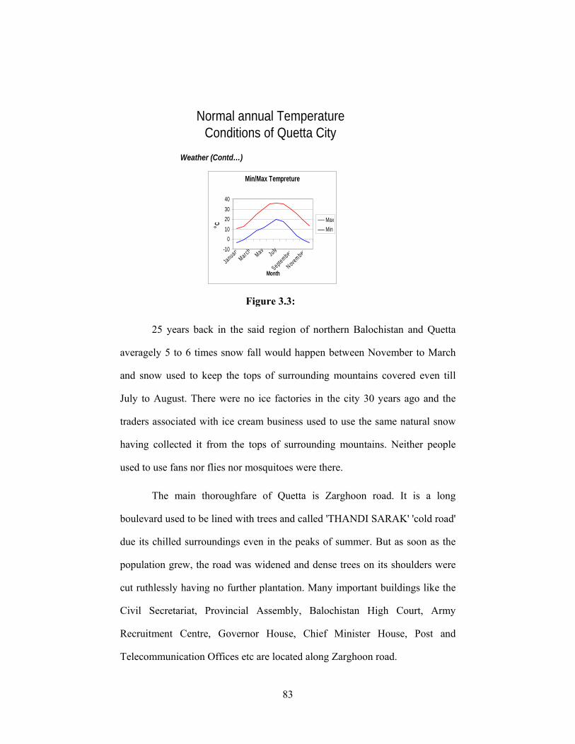
83
Normal annual Temperature Conditions of Quetta City
Min/Max Tempreture
-100
10203040
JanuaryMarch May
July
September
November
Month
o C MaxMin
Weather (Contd…)
Figure 3.3:
25 years back in the said region of northern Balochistan and Quetta
averagely 5 to 6 times snow fall would happen between November to March
and snow used to keep the tops of surrounding mountains covered even till
July to August. There were no ice factories in the city 30 years ago and the
traders associated with ice cream business used to use the same natural snow
having collected it from the tops of surrounding mountains. Neither people
used to use fans nor flies nor mosquitoes were there.
The main thoroughfare of Quetta is Zarghoon road. It is a long
boulevard used to be lined with trees and called 'THANDI SARAK' 'cold road'
due its chilled surroundings even in the peaks of summer. But as soon as the
population grew, the road was widened and dense trees on its shoulders were
cut ruthlessly having no further plantation. Many important buildings like the
Civil Secretariat, Provincial Assembly, Balochistan High Court, Army
Recruitment Centre, Governor House, Chief Minister House, Post and
Telecommunication Offices etc are located along Zarghoon road.
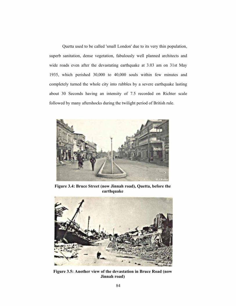
84
Quetta used to be called 'small London' due to its very thin population,
superb sanitation, dense vegetation, fabulously well planned architects and
wide roads even after the devastating earthquake at 3.03 am on 31st May
1935, which perished 30,000 to 40,000 souls within few minutes and
completely turned the whole city into rubbles by a severe earthquake lasting
about 30 Seconds having an intensity of 7.5 recorded on Richter scale
followed by many aftershocks during the twilight period of British rule.
Figure 3.4: Bruce Street (now Jinnah road), Quetta, before the
earthquake
Figure 3.5: Another view of the devastation in Bruce Road (now
Jinnah road)
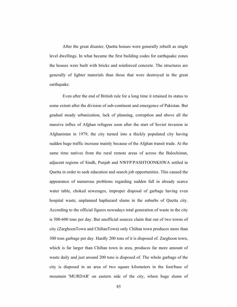
85
After the great disaster, Quetta houses were generally rebuilt as single
level dwellings. In what became the first building codes for earthquake zones
the houses were built with bricks and reinforced concrete. The structures are
generally of lighter materials than those that were destroyed in the great
earthquake.
Even after the end of British rule for a long time it retained its status to
some extent after the division of sub-continent and emergence of Pakistan. But
gradual steady urbanization, lack of planning, corruption and above all the
massive influx of Afghan refugees soon after the start of Soviet invasion in
Afghanistan in 1979, the city turned into a thickly populated city having
sudden huge traffic increase mainly because of the Afghan transit trade. At the
same time natives from the rural remote areas of across the Balochistan,
adjacent regions of Sindh, Punjab and NWFP/PASHTOONKHWA settled in
Quetta in order to seek education and search job opportunities. This caused the
appearance of numerous problems regarding sudden fall in already scarce
water table, choked sewerages, improper disposal of garbage having even
hospital waste, unplanned haphazard slums in the suburbs of Quetta city.
According to the official figures nowadays total generation of waste in the city
is 500-600 tons per day. But unofficial sources claim that out of two towns of
city (ZarghoonTown and ChiltanTown) only Chiltan town produces more than
300 tons garbage per day. Hardly 200 tons of it is disposed of. Zarghoon town,
which is far larger than Chiltan town in area, produces far more amount of
waste daily and just around 200 tons is disposed of. The whole garbage of the
city is disposed in an area of two square kilometers in the foot/base of
mountain 'MURDAR' on eastern side of the city, where huge slums of
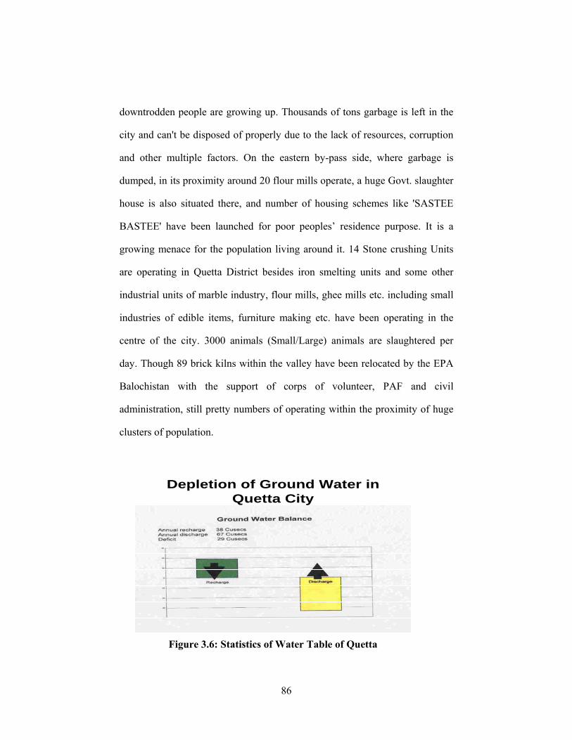
86
downtrodden people are growing up. Thousands of tons garbage is left in the
city and can't be disposed of properly due to the lack of resources, corruption
and other multiple factors. On the eastern by-pass side, where garbage is
dumped, in its proximity around 20 flour mills operate, a huge Govt. slaughter
house is also situated there, and number of housing schemes like 'SASTEE
BASTEE' have been launched for poor peoples’ residence purpose. It is a
growing menace for the population living around it. 14 Stone crushing Units
are operating in Quetta District besides iron smelting units and some other
industrial units of marble industry, flour mills, ghee mills etc. including small
industries of edible items, furniture making etc. have been operating in the
centre of the city. 3000 animals (Small/Large) animals are slaughtered per
day. Though 89 brick kilns within the valley have been relocated by the EPA
Balochistan with the support of corps of volunteer, PAF and civil
administration, still pretty numbers of operating within the proximity of huge
clusters of population.
Depletion of Ground Water in Quetta City
Figure 3.6: Statistics of Water Table of Quetta
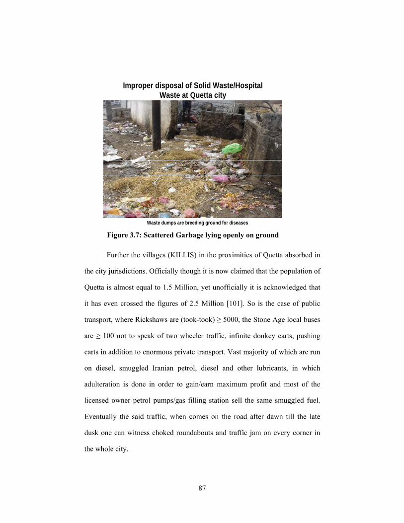
87
Improper disposal of Solid Waste/Hospital Waste at Quetta city
Waste dumps are breeding ground for diseases
Figure 3.7: Scattered Garbage lying openly on ground
Further the villages (KILLIS) in the proximities of Quetta absorbed in
the city jurisdictions. Officially though it is now claimed that the population of
Quetta is almost equal to 1.5 Million, yet unofficially it is acknowledged that
it has even crossed the figures of 2.5 Million [101]. So is the case of public
transport, where Rickshaws are (took-took) ≥ 5000, the Stone Age local buses
are ≥ 100 not to speak of two wheeler traffic, infinite donkey carts, pushing
carts in addition to enormous private transport. Vast majority of which are run
on diesel, smuggled Iranian petrol, diesel and other lubricants, in which
adulteration is done in order to gain/earn maximum profit and most of the
licensed owner petrol pumps/gas filling station sell the same smuggled fuel.
Eventually the said traffic, when comes on the road after dawn till the late
dusk one can witness choked roundabouts and traffic jam on every corner in
the whole city.
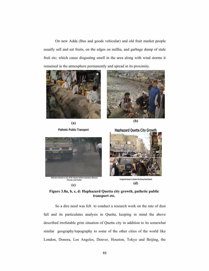
88
On new Adda (Bus and goods vehicular) and old fruit market people
usually sell and eat fruits, on the edges on nullha, and garbage dump of stale
fruit etc; which cause disgusting smell in the area along with wind storms it
remained in the atmosphere permanently and spread in its proximity.
(a)
(b)
Pathetic Public Transport
Vehicular emission is one of the reasons behind respiratory illnesses (Circular road Quetta)
(c)
Haphazard Quetta City Growth
Congested bazaar in Quetta City (Suraj Ganj Bazaar) (d)
Figure 3.8a, b, c, d: Haphazard Quetta city growth, pathetic public transport etc.
So a dire need was felt to conduct a research work on the rate of dust
fall and its particulates analysis in Quetta, keeping in mind the above
described irrefutable grim situation of Quetta city in addition to its somewhat
similar geography/topography to some of the other cities of the world like
London, Donora, Los Angeles, Denver, Houston, Tokyo and Beijing, the
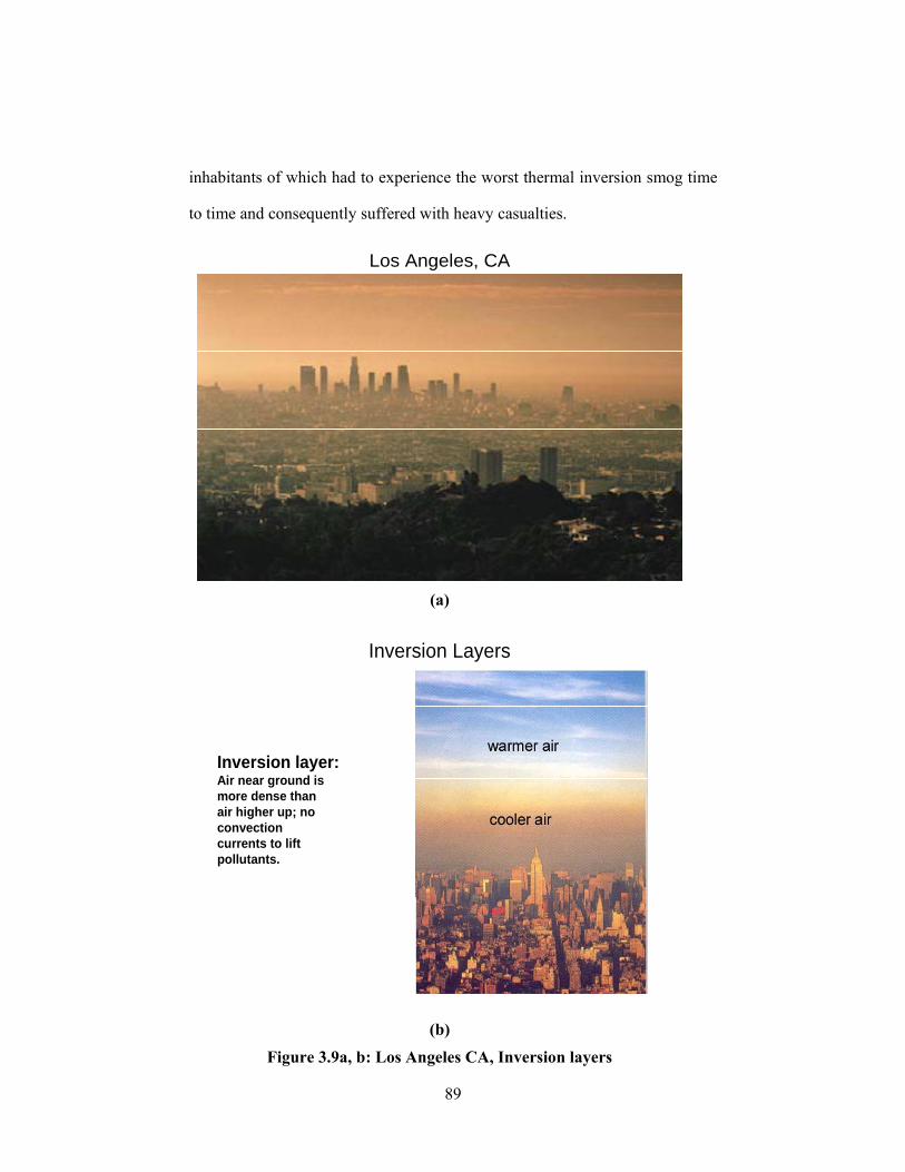
89
inhabitants of which had to experience the worst thermal inversion smog time
to time and consequently suffered with heavy casualties.
Los Angeles, CA
(a)
Inversion Layers
Inversion layer:Air near ground is more dense thanair higher up; no convectioncurrents to lift pollutants.
(b)
Figure 3.9a, b: Los Angeles CA, Inversion layers

90
Smog – US, global
Denver Houston
BeijingTokyo
Figure 3.10: Smog US and Global
Above all a severe 6 years spell of drought from 1997-2002 hit
Balochistan including Quetta [101], during that either precipitation didn’t
happen whatsoever or very rare light showers were reported in a few scattered
parts of Balochistan. Its adverse impacts were vividly noticed in Northern
Balochistan including Quetta, where scorching heat intensity mounted and the
temperature increased between 38-40°C from May and June to August and
September (Table 3.1).
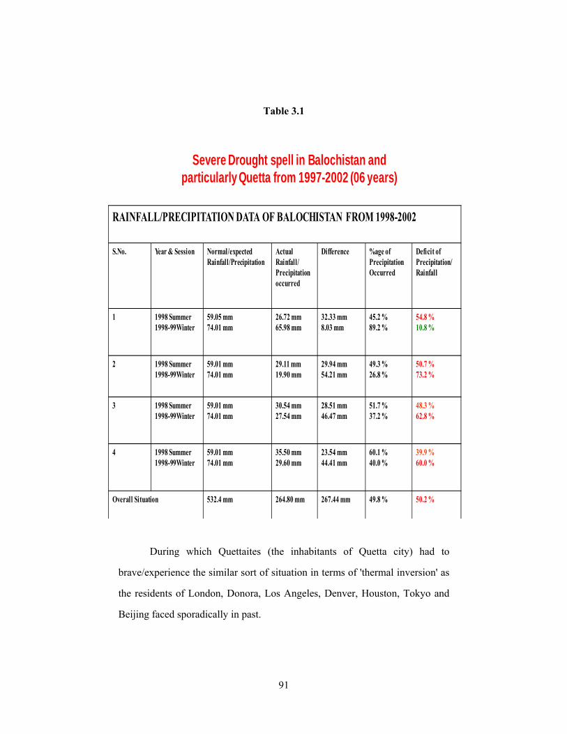
91
Table 3.1
Severe Drought spell in Balochistan and particularly Quetta from 1997-2002 (06 years)
RAINFALL/PRECIPITATION DATA OF BALOCHISTAN FROM 1998-2002
S.No. Year & Session Normal/expected Rainfall/Precipitation
Actual Rainfall/ Precipitation occurred
Difference %age of Precipitation Occurred
Deficit of Precipitation/ Rainfall
1 1998 Summer1998-99Winter
59.05 mm74.01 mm
26.72 mm65.98 mm
32.33 mm8.03 mm
45.2 %89.2 %
54.8 %10.8 %
2 1998 Summer1998-99Winter
59.01 mm74.01 mm
29.11 mm19.90 mm
29.94 mm54.21 mm
49.3 %26.8 %
50.7 %73.2 %
3 1998 Summer1998-99Winter
59.01 mm74.01 mm
30.54 mm27.54 mm
28.51 mm46.47 mm
51.7 %37.2 %
48.3 %62.8 %
4 1998 Summer1998-99Winter
59.01 mm74.01 mm
35.50 mm29.60 mm
23.54 mm44.41 mm
60.1 %40.0 %
39.9 %60.0 %
Overall Situation 532.4 mm 264.80 mm 267.44 mm 49.8 % 50.2 %
During which Quettaites (the inhabitants of Quetta city) had to
brave/experience the similar sort of situation in terms of 'thermal inversion' as
the residents of London, Donora, Los Angeles, Denver, Houston, Tokyo and
Beijing faced sporadically in past.
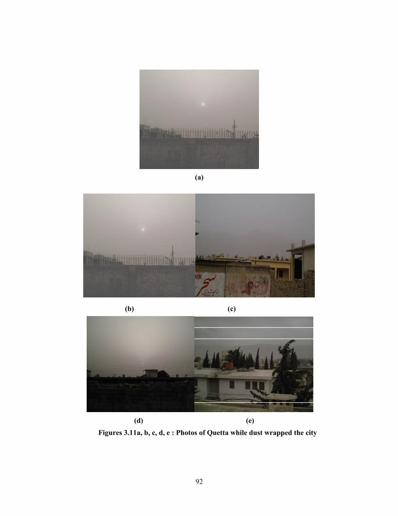
92
(a)
(b) (c)
(d) (e)
Figures 3.11a, b, c, d, e : Photos of Quetta while dust wrapped the city
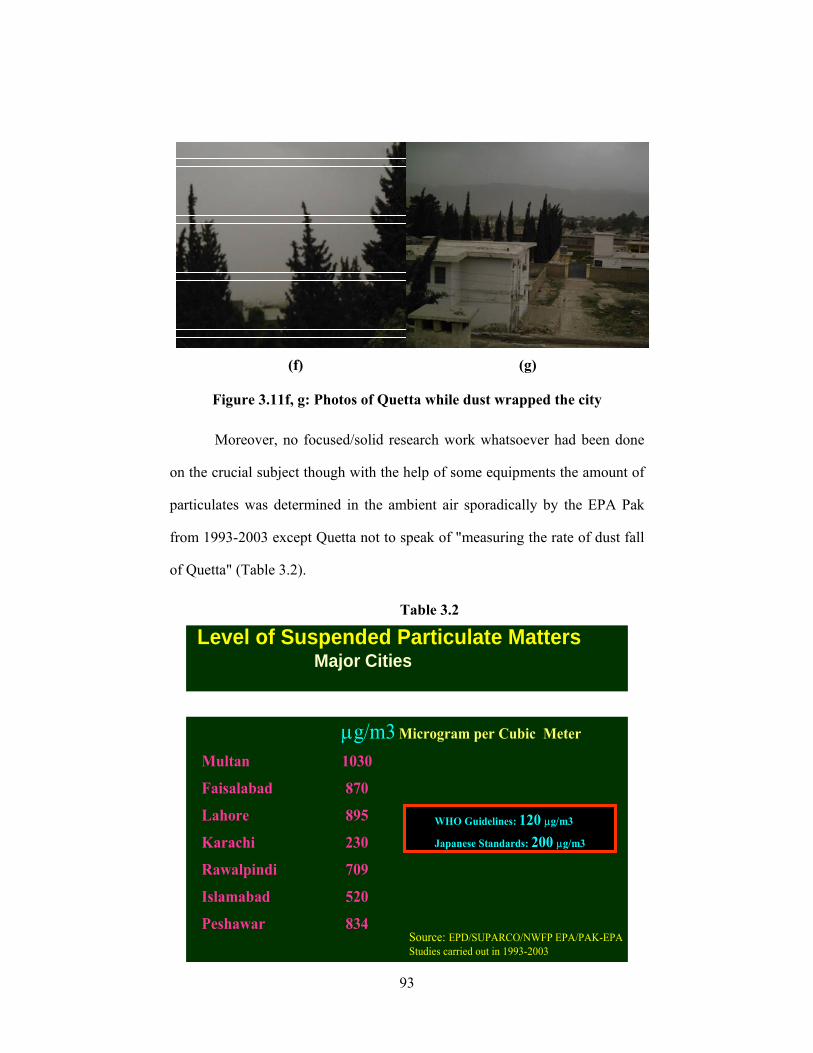
93
(f) (g)
Figure 3.11f, g: Photos of Quetta while dust wrapped the city
Moreover, no focused/solid research work whatsoever had been done
on the crucial subject though with the help of some equipments the amount of
particulates was determined in the ambient air sporadically by the EPA Pak
from 1993-2003 except Quetta not to speak of "measuring the rate of dust fall
of Quetta" (Table 3.2).
Table 3.2
Level of Suspended Particulate MattersMajor Cities
µg/m3 Microgram per Cubic Meter
Multan 1030
Faisalabad 870
Lahore 895
Karachi 230
Rawalpindi 709
Islamabad 520
Peshawar 834Source: EPD/SUPARCO/NWFP EPA/PAK-EPAStudies carried out in 1993-2003
WHO Guidelines: 120 µg/m3
Japanese Standards: 200 µg/m3
94
However numbers of researches have been conducted in the different
famous cities across the globe and in the different cities of Pakistan (like
Karachi, Islamabad and Peshawar) as well on the rate of fall/settlement of dust
particulates [102].
The above mentioned extremely important factors tempted my
honorable supervisor and me to carry out profound research work in this
regard. So that we could owe the debt of our beloved Quetta city upon us by
suggesting some solid measures in order to rehabilitate its beauty, cleanliness
and calmness.
Therefore following objectives/goals were set to conduct our research
work.
1. To find the rate of dust fall in Quetta.
2. To ascertain the origin of dust plumes hit Quetta particularly
during very rare thermal inversion episodes in the end of
drought spell.
3. To detect the quantity of toxic/heavy elements Pb, Zn, Mn, Ni,
Cr, Co, Na and K present in dust fall samples.
4. To discover the percentage of particles having different sizes in
the dust fall.
5. To make a prediction of dust fall and amount of toxic/heavy
elements for the coming period by using statistical ARIMA and
SARIMA modeling.
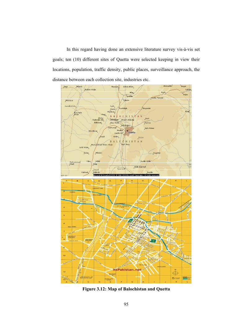
95
In this regard having done an extensive literature survey vis-à-vis set
goals; ten (10) different sites of Quetta were selected keeping in view their
locations, population, traffic density, public places, surveillance approach, the
distance between each collection site, industries etc.
Figure 3.12: Map of Balochistan and Quetta
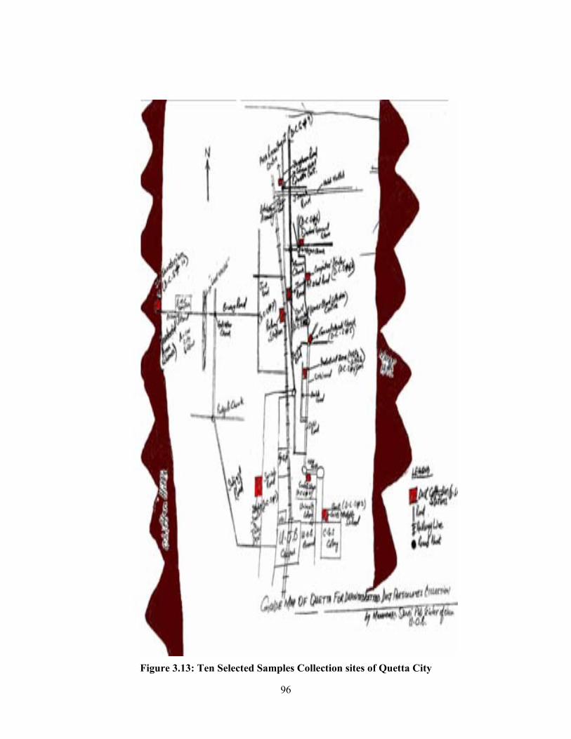
96
Figure 3.13: Ten Selected Samples Collection sites of Quetta City
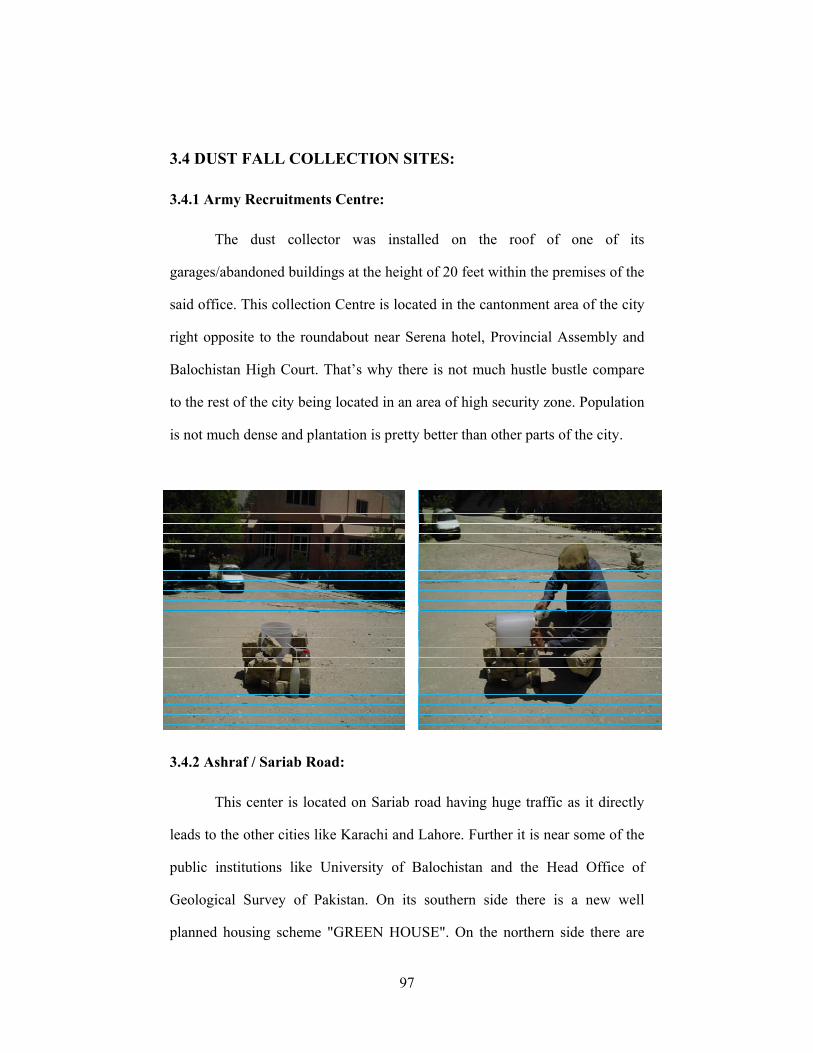
97
3.4 DUST FALL COLLECTION SITES:
3.4.1 Army Recruitments Centre:
The dust collector was installed on the roof of one of its
garages/abandoned buildings at the height of 20 feet within the premises of the
said office. This collection Centre is located in the cantonment area of the city
right opposite to the roundabout near Serena hotel, Provincial Assembly and
Balochistan High Court. That’s why there is not much hustle bustle compare
to the rest of the city being located in an area of high security zone. Population
is not much dense and plantation is pretty better than other parts of the city.
3.4.2 Ashraf / Sariab Road:
This center is located on Sariab road having huge traffic as it directly
leads to the other cities like Karachi and Lahore. Further it is near some of the
public institutions like University of Balochistan and the Head Office of
Geological Survey of Pakistan. On its southern side there is a new well
planned housing scheme "GREEN HOUSE". On the northern side there are
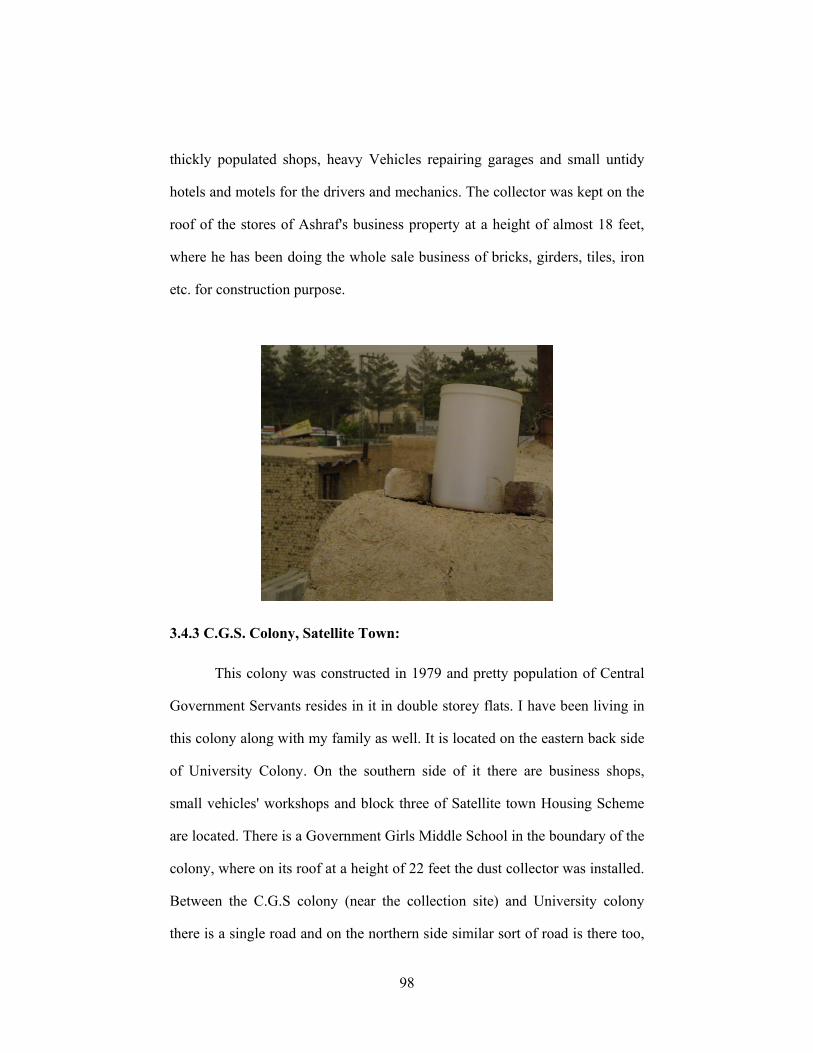
98
thickly populated shops, heavy Vehicles repairing garages and small untidy
hotels and motels for the drivers and mechanics. The collector was kept on the
roof of the stores of Ashraf's business property at a height of almost 18 feet,
where he has been doing the whole sale business of bricks, girders, tiles, iron
etc. for construction purpose.
3.4.3 C.G.S. Colony, Satellite Town:
This colony was constructed in 1979 and pretty population of Central
Government Servants resides in it in double storey flats. I have been living in
this colony along with my family as well. It is located on the eastern back side
of University Colony. On the southern side of it there are business shops,
small vehicles' workshops and block three of Satellite town Housing Scheme
are located. There is a Government Girls Middle School in the boundary of the
colony, where on its roof at a height of 22 feet the dust collector was installed.
Between the C.G.S colony (near the collection site) and University colony
there is a single road and on the northern side similar sort of road is there too,
99
both roads remain pretty busy for the whole day but at night remain almost
deserted.
3.4.4 Civil Hospital:
The dust fall collector was placed on the roof 'MOLANA UMER
FOUNDATION' at a height of 17feet adjacent to the civil hospital located in
the heart of city right on one the main busiest roads 'JINNAH ROAD'. Day
and night the road remain busy. Particularly in day time mostly the traffic jam
is witnessed due to the congested road and the massive burden of patients on
the single oldest public hospital located inside the city. On the opposite of road
there is cluster of Pharmaceutical/chemist/Medical stores, some hotels, other
business shops and even pushing cart hawkers etc., who encroach the road and
even footpaths on its both sides in order to earn their bread and butter.
3.4.5 Gawalmandi Chowk:
It is the roundabout of four roads and for the whole day traffic remains
either jam or moves at the snail pace due to the all five roads, which joins at
100
this location. 'Sirki' road joins it with 'NEW ADDA' known as new bus stand
on southern side, 'KAWARI' road leads towards northern side to the main city,
'MACKONGY' road leads to the old city, 'KACHRA' (Garbage) road on
eastern side leads to a chaotic slum of mostly muddy type of houses known as
'PASHTOON-ABAD' and another road towards east-north side guides to the
densely crowded old city. On the bottle neck of this junction of 5 roads the
dust collector was installed on the roof of an old 'Union Council' office (which
has not been demolished in order to widen the road) at the height of 13 feet.
This is the junction, where two roads ('SIRKI' road & 'KACHRA' road) out of
only four routes link the old Quetta city with the newly settled Quetta city.
3.4.6 Qadoosi Store/Quick Marketing Services:
These are in fact two sites, which were alternatively used as one of the
ten sites used to collect the dust fall samples. Both are located from one
another almost 200-300 meters away from each other. 'QADOOSI STORE', a
famous mutli-departmental grocery store is located right in the heart of Quetta
city in the east-north corner of 'MAYZAN CHOWK'. Old store has been
101
demolished and a new store has just been constructed there at the same place.
From here the junction of 'MAYZAN CHOWK', a road ‘SHARA-E-
LIAQUAT’ links to 'LIAQAT BAZAR' on southern direction, other leads to
the western side through the famous 'KANDHARI BAZAR' up to 'MANNAN
CHOWK' and further links with the 'ZARGHOON ROAD', another
‘MISSION’ road on northern side links cantonment, fourth ‘TOGI’ road
through north-eastern side of this dust collection site links to an ethnic
(Persian speaking) population settled on the eastern side of the city in a
massive cluster of houses called 'MAREE-A-ABAD, fifth road on eastern side
leads to the 'LANDA BAZAR' old used items market and further to the old
city. For almost two and half years, the dust collector was fixed on its roof at a
height of almost 20 feet. This site remains busy day and night being situated in
the middle of hub of business on all sides of it. Similarly, its alternate dust fall
samples collection station 'QUICK MARKETING SERVICES', is located on
Art School road and is one of the pioneers of computers marketing related
business in the city. On art school road there are old city residences, which are
gradually being sold to the business men due to its location in the middle of
city and adjacent to the most famous 'LIAQUAT BAZAR'. The road remains
busy for the whole day and night. The dust collector was kept on its roof as
well at a height of 19 feet for the rest of the two and half years initially due to
the law and order situation, when some firing was done on a religious
procession near 'QADOOSI STORE' and later on due to the re-construction of
the 'QADOOSI STORE'.
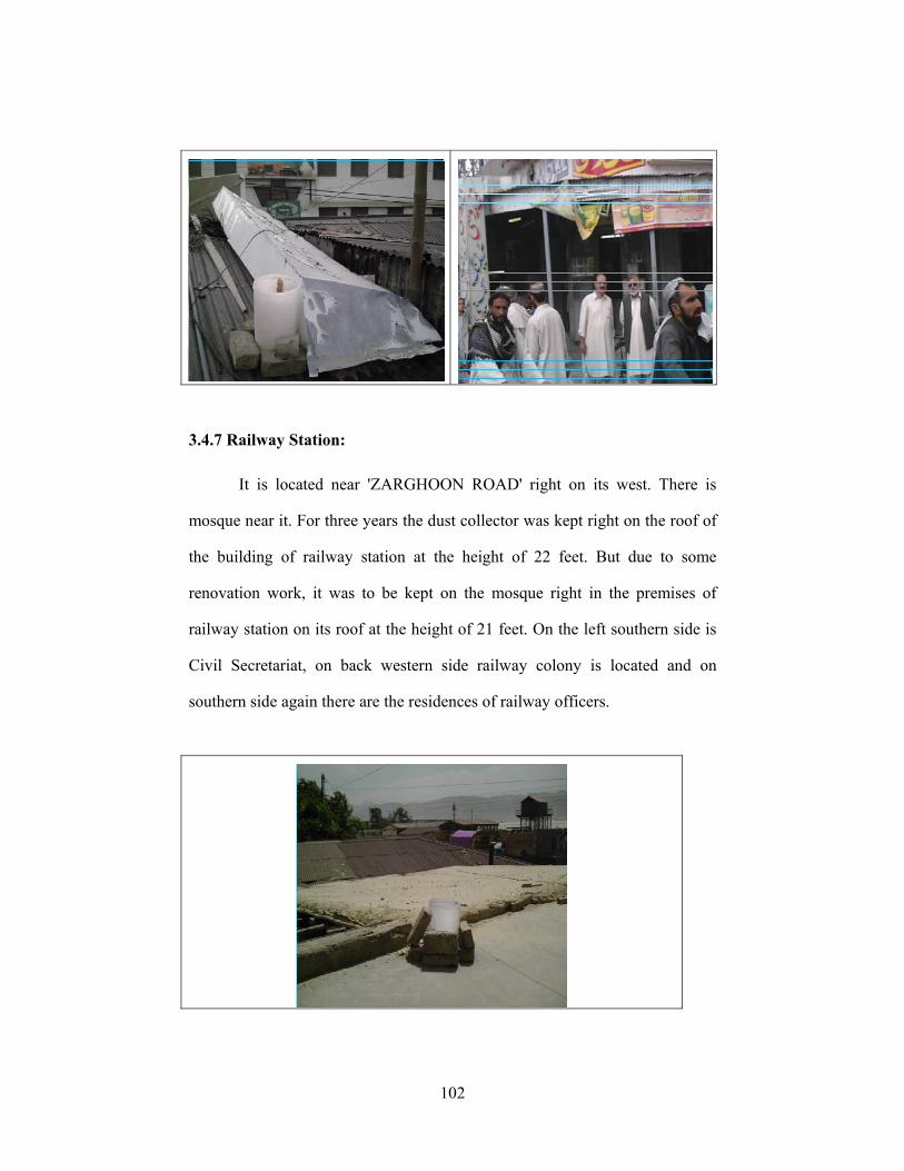
102
3.4.7 Railway Station:
It is located near 'ZARGHOON ROAD' right on its west. There is
mosque near it. For three years the dust collector was kept right on the roof of
the building of railway station at the height of 22 feet. But due to some
renovation work, it was to be kept on the mosque right in the premises of
railway station on its roof at the height of 21 feet. On the left southern side is
Civil Secretariat, on back western side railway colony is located and on
southern side again there are the residences of railway officers.

103
3.4.8 SADDA BAHAR Sweets New Adda:
This site (Sweets Shop) is located near satellite town, where there were
bus and truck stands. A round about is close to it on south- eastern side. On its
back southern side a huge graveyard is located and on eastern side road leads
to satellite town, on western side the road link it with Sariab road, and the road
on southern side is 'Sirki road", which links it with 'GWALMANDI CHOWK'
and ultimately the old city. This area also remains busy particularly in day
time. The dust collector was placed on its roof at the height of 25 feet.
3.4.9 Sirki Road:
This road links old city and new city (satellite town etc.). It used to be
the only industrial area of the city. Though most of the new industry is now set
up on the western and southern side out of the city, yet old industries like
'CHILTAN GHEE MILL', 'DITTU & SONS, furniture industry, flour mills
etc. are still working in the area situated on Sirki road. The dust collector was
placed on the roof, initially on the roof of NATIONAL BANK for almost
three years at a height of 18 feet & later on the roof of 'DITTU & SONS' at the
height of 20 feet just to check the variance in the results on the same place.
This dust collection site is located in the described industrial area on the
western side of the Sirki road, businesses shops across the road having thick
population of 'KACCHI-ABADI' entirely muddy with some muddy-brick
houses in a slummy disorder are situated on its eastern side.
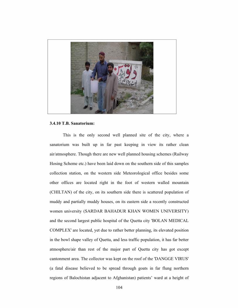
104
3.4.10 T.B. Sanatorium:
This is the only second well planned site of the city, where a
sanatorium was built up in far past keeping in view its rather clean
air/atmosphere. Though there are new well planned housing schemes (Railway
Hosing Scheme etc.) have been laid down on the southern side of this samples
collection station, on the western side Meteorological office besides some
other offices are located right in the foot of western walled mountain
(CHILTAN) of the city, on its southern side there is scattered population of
muddy and partially muddy houses, on its eastern side a recently constructed
women university (SARDAR BAHADUR KHAN WOMEN UNIVERSITY)
and the second largest public hospital of the Quetta city 'BOLAN MEDICAL
COMPLEX' are located, yet due to rather better planning, its elevated position
in the bowl shape valley of Quetta, and less traffic population, it has far better
atmosphere/air than rest of the major part of Quetta city has got except
cantonment area. The collector was kept on the roof of the 'DANGGE VIRUS'
(a fatal disease believed to be spread through goats in far flung northern
regions of Balochistan adjacent to Afghanistan) patients’ ward at a height of
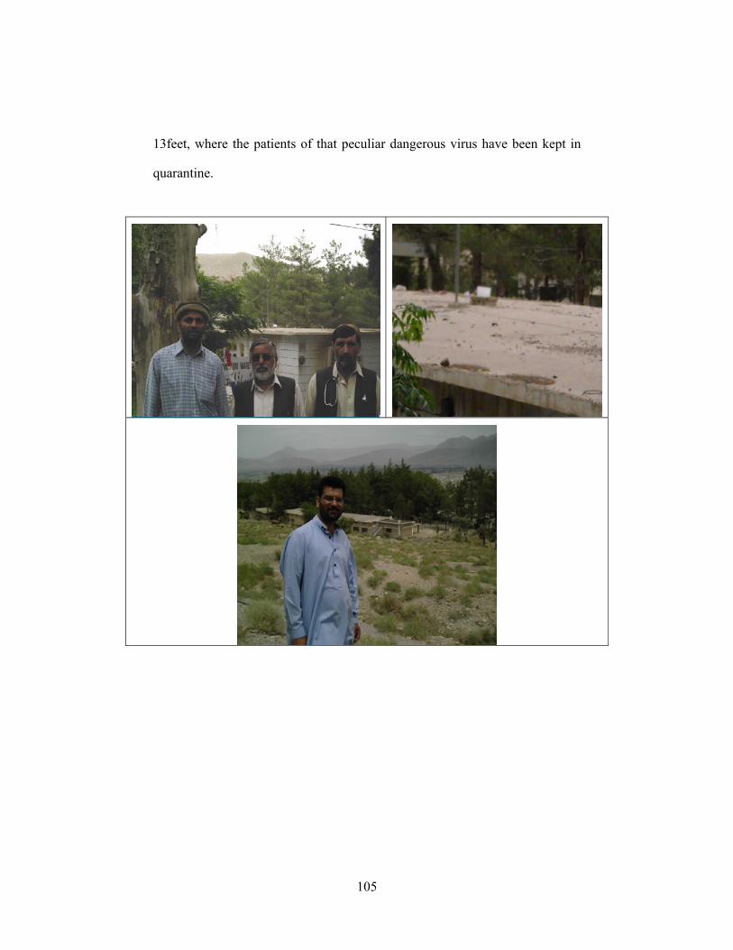
105
13feet, where the patients of that peculiar dangerous virus have been kept in
quarantine.
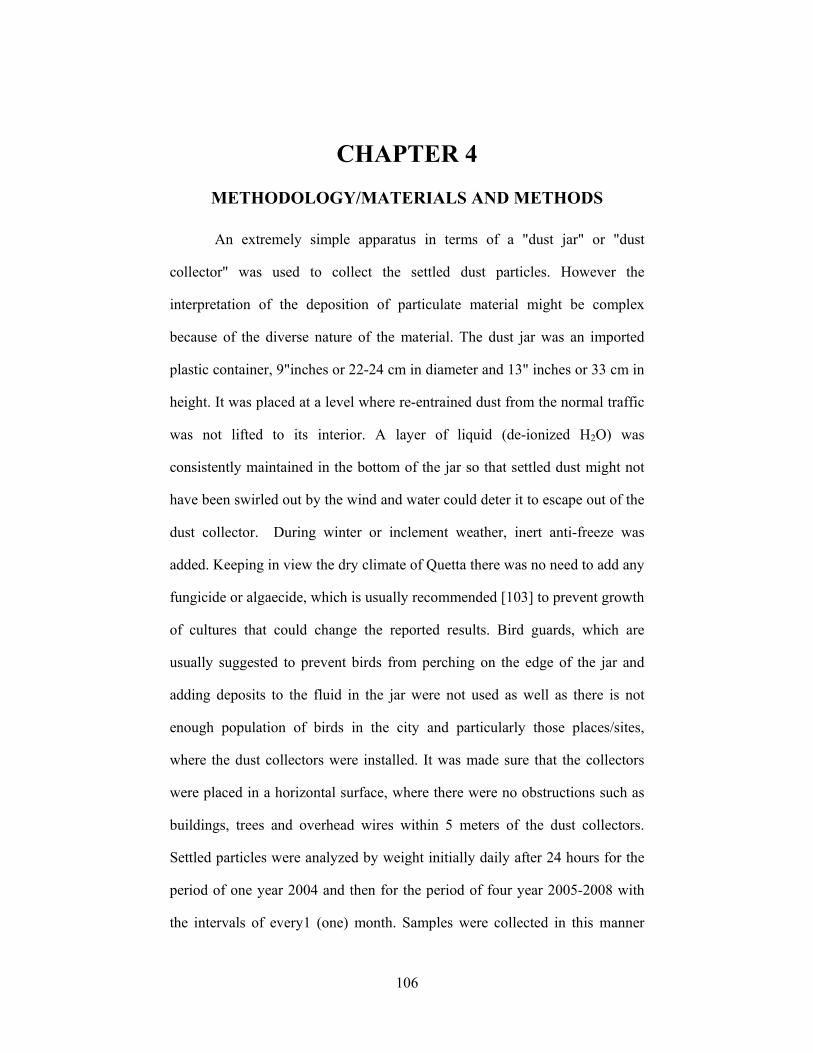
106
CHAPTER 4
METHODOLOGY/MATERIALS AND METHODS
An extremely simple apparatus in terms of a "dust jar" or "dust
collector" was used to collect the settled dust particles. However the
interpretation of the deposition of particulate material might be complex
because of the diverse nature of the material. The dust jar was an imported
plastic container, 9"inches or 22-24 cm in diameter and 13" inches or 33 cm in
height. It was placed at a level where re-entrained dust from the normal traffic
was not lifted to its interior. A layer of liquid (de-ionized H2O) was
consistently maintained in the bottom of the jar so that settled dust might not
have been swirled out by the wind and water could deter it to escape out of the
dust collector. During winter or inclement weather, inert anti-freeze was
added. Keeping in view the dry climate of Quetta there was no need to add any
fungicide or algaecide, which is usually recommended [103] to prevent growth
of cultures that could change the reported results. Bird guards, which are
usually suggested to prevent birds from perching on the edge of the jar and
adding deposits to the fluid in the jar were not used as well as there is not
enough population of birds in the city and particularly those places/sites,
where the dust collectors were installed. It was made sure that the collectors
were placed in a horizontal surface, where there were no obstructions such as
buildings, trees and overhead wires within 5 meters of the dust collectors.
Settled particles were analyzed by weight initially daily after 24 hours for the
period of one year 2004 and then for the period of four year 2005-2008 with
the intervals of every1 (one) month. Samples were collected in this manner
107
that an aliquot of the liquid was taken after the settled material was thoroughly
dispersed. The liquid would evaporate, and the settled material was analyzed
in terms of weight per unit area in the jar; the result then was extrapolated to
unit weight per square area in terms of in some cases, in grams per square
meter per month, or in tons per square km per month or in most recommended
cases in mgs per square meter per day or month.
It is also possible to extract the settled dust samples, with suitable
solvents, the organic-soluble and water soluble components to determine
combustible materials, and to report each component separately [104]. Before
installing the dust collectors, these were cleaned with detergents, washed
thoroughly with tap water and then rinsed with distilled and finally with de-
ionized water. The mouth was covered with sterilized lid, and was taken to the
sites in order to install on the selected place. For the first year 2004 after every
24 hours (one day), the samples were collected from all the ten different sites
by using de-ionized water in the plastic bottles pre-washed properly with de-
ionized water. While collecting the samples from 2005-2008 (04) years with
the gap of every one month of calendar year corrected to 30± days, dust
collectors were regularly monitored and de-ionized water level was not let dry
by keeping up its level around 500-600 milliliters.
4.1 PREPARATION OF COLLECTED SAMPLES FOR
DIGESTION:
Insoluble matter for instance stones were either removed manually from
the dust samples depending upon their size, while collecting samples from the
spots/sites. After that collected samples in plastic bottles having de-ionized
108
H2O were manually shacked well in order to dissolve the soluble remaining
part of dust fall before filtering it by normal sieve (25-30 lattices) so as to
separate the remaining dead insects, small stones or any insoluble material
other than dust. Then filtrate was again filtered through Whattman No. 41 or
42 papers directly into a one liter volumetric flask in such a way that it was
inclined in an inverted position over the filtering funnel and the jet of de-
ionized bottle was used to wash down all the dust left in the beaker. Finally the
level of volumetric flask was filled up to its mark of one liter.
The filter paper having insoluble residual dust was dried in an oven at
100-105°C up to a constant weight to remove the water. It was cooled for 25
minutes in a dedicator. A blank Whatmann No. 41 or 42 filter paper was first
moistened with de-ionized H2O and dried up to 100-105°C, cooled and
weighed in the similar fashion finally to subtract it from that containing dust.
In this way merely the insoluble part of the dust was obtained. For soluble dust
fall, two aliquots of 50 ml each were taken from the filtrate in pre-weighed
china dishes, evaporated to dryness on steam bath, dried at 100-105°C in an
oven, cooled and weighed. The results of these duplicate evaporations were
averaged and calculated for one liter. The sum of the insoluble and soluble
dust gave the total weight of the dust.
4.2 DETERMINATION OF RATE OF
DEPOSITION/SETTLEMENT OF DUST FALL:
The average rate of dust fall was calculated by the following formula:
W= w (dissolved + un-dissolved) × 30 mg m2day1 Ac× Nd Where

109
W = Total wt. of dust fall (dissolved + un-dissolved) in a month (30 days)
'w' = Weight of total dust fall actually collected over Nd (No. of days)
Ac = Area of the mouth of dust collector (m2)
Nd = Actual number of days.
4.3 CHEMICAL ANALYSIS OF DUST FALL SAMPLES:
It was carried out for the loss on ignition, for the quantitative analysis
of Silica as (SiO2), Aluminum as (Al2O3), Iron as (Fe2O3), Calcium as (CaO),
Magnesium as (MgO), Sodium as (Na2O) and Potassium as (K2O) by standard
physical and chemical methods [105].
4.4 TESTS FOR THE PARTICULATES SIZE DISTRIBUTION:
Mesh size distribution was used to determine the fractionation on wt.
% basis for nine size categories: PM<1.0, PM1.0-2.5, PM2.5-5.0, PM5.0-10, PM10-15,
PM15-25, PM25-50, PM50-100 and PM>100, as it is yet supposed to be one of the
suitable methods using ASTM (American Standard Test Method) [106].
Though another method to determine the particle size determination using
Mastersizer 2000 (Malvern, Ver. 3.01, UK) by Shah et al., [100],Shah et al.,
[99] and Shah and Shaheen [14] on vol. % basis for seven, four to nine
fractions (PM<1.0, PM1.0-2.5, PM2.5-5, PM5-10, PM15-25, PM50-100and PM>100µm),
(Pm<2.5, PM2.5-10, PM10-100 and PM>100 µm) and (PM<1.0, PM1.0-2.5, PM2.5-5.0,
PM5.0-10, PM10-15, PM15-25, PM25-50, PM50-100and PM>100 µm) was supposed to
be one of the best methods as well, ironically in spite of having had a keen
desire to use it, it couldn’t be used due to its non-availability in any
institutions of even the capital of our province (Balochistan), Quetta not to
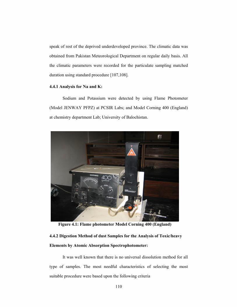
110
speak of rest of the deprived underdeveloped province. The climatic data was
obtained from Pakistan Meteorological Department on regular daily basis. All
the climatic parameters were recorded for the particulate sampling matched
duration using standard procedure [107,108].
4.4.1 Analysis for Na and K:
Sodium and Potassium were detected by using Flame Photometer
(Model JENWAY PFPZ) at PCSIR Labs; and Model Corning 400 (England)
at chemistry department Lab; University of Balochistan.
Figure 4.1: Flame photometer Model Corning 400 (England)
4.4.2 Digestion Method of dust Samples for the Analysis of Toxic/heavy
Elements by Atomic Absorption Spectrophotometer:
It was well known that there is no universal dissolution method for all
type of samples. The most needful characteristics of selecting the most
suitable procedure were based upon the following criteria
111
(1) the tendency to dissolve the sample completely having no
insoluble resides
(2) pragmatically prompt and safe & sound
(3) no possible dangers of sample loss by volatility, adsorption on
the walls of the apparatus and
(4) removal of sample contamination from the reagents used while
dissolution process
The majority of dissolution methods involve dry ashing or wet
digestion using one or a combination of concentrated mineral acids [197]. So,
numerous acid combinations for instance HNO3+HCl, HNO3+HCLO4 and
HF+HCLO4 were attempted for the digestion. Eventually the combination of
4:1 (v/v) HNO3+HCLO4[109] was found most suitable for the substances like
dust fall samples, soil samples and clay minerals etc contrary to the
combination HF+HCLO4 used by Khan et al., [110] used.
Approximately 0.5 grams of the dust fall sample was taken in a
platinum crucible by adding few drops of de-ionized H2O merely to moisten it.
Then 5 cm3 of 6M HCLO4 and 6 cm3 of HNO3 were put into the crucible. The
crucible was kept on a sand bath in order to destroy the organic matter till the
mixture was evaporated leaving behind HCLO4. Then the crucible was kept on
a heating plate until HCLO4 was totally evaporated. The inner sides of the
crucible were washed with a stream of de-ionized H2O and dried again. The
method was repeated twice again. After that 10 drops of 6M HClO4 and 20 ml
of de-ionized H2O were added to the residue. Finally 6 cm3 of 30% H2O2 was
added to oxidize any resistant organic matter if presented. The whole mixture
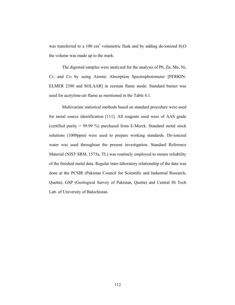
112
was transferred to a 100 cm3 volumetric flask and by adding de-ionized H2O
the volume was made up to the mark.
The digested samples were analyzed for the analysis of Pb, Zn, Mn, Ni,
Cr, and Co by using Atomic Absorption Spectrophotometer [PERKIN-
ELMER 2380 and SOLAAR] in zeeman flame mode. Standard burner was
used for acetylene-air flame as mentioned in the Table 4.1.
Multivariate statistical methods based on standard procedure were used
for metal source identification [111]. All reagents used were of AAS grade
(certified purity > 99.99 %) purchased from E-Merck. Standard metal stock
solutions (1000ppm) were used to prepare working standards. De-ionized
water was used throughout the present investigation. Standard Reference
Material (NIST SRM, 1573a, TL) was routinely employed to ensure reliability
of the finished metal data. Regular inter-laboratory relationship of the data was
done at the PCSIR (Pakistan Council for Scientific and Industrial Research,
Quetta), GSP (Geological Survey of Pakistan, Quetta) and Central Hi Tech
Lab. of University of Balochistan.
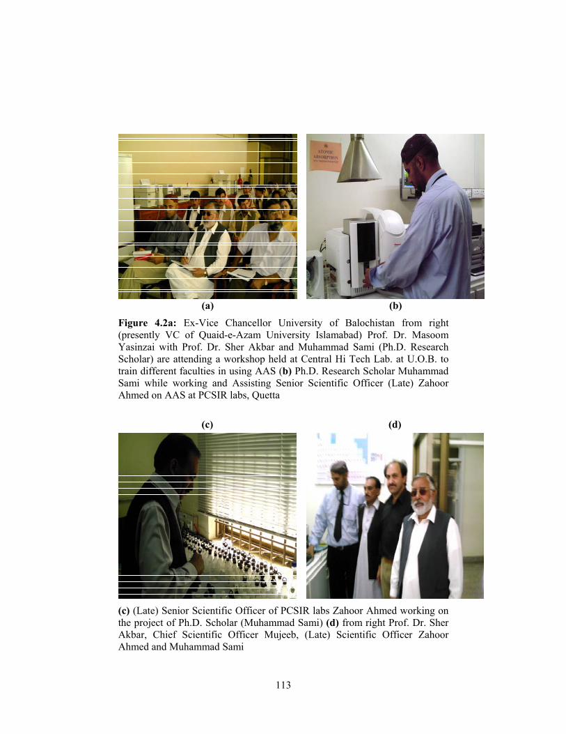
113
(a) (b)
Figure 4.2a: Ex-Vice Chancellor University of Balochistan from right (presently VC of Quaid-e-Azam University Islamabad) Prof. Dr. Masoom Yasinzai with Prof. Dr. Sher Akbar and Muhammad Sami (Ph.D. Research Scholar) are attending a workshop held at Central Hi Tech Lab. at U.O.B. to train different faculties in using AAS (b) Ph.D. Research Scholar Muhammad Sami while working and Assisting Senior Scientific Officer (Late) Zahoor Ahmed on AAS at PCSIR labs, Quetta
(c) (d)
(c) (Late) Senior Scientific Officer of PCSIR labs Zahoor Ahmed working on the project of Ph.D. Scholar (Muhammad Sami) (d) from right Prof. Dr. Sher Akbar, Chief Scientific Officer Mujeeb, (Late) Scientific Officer Zahoor Ahmed and Muhammad Sami
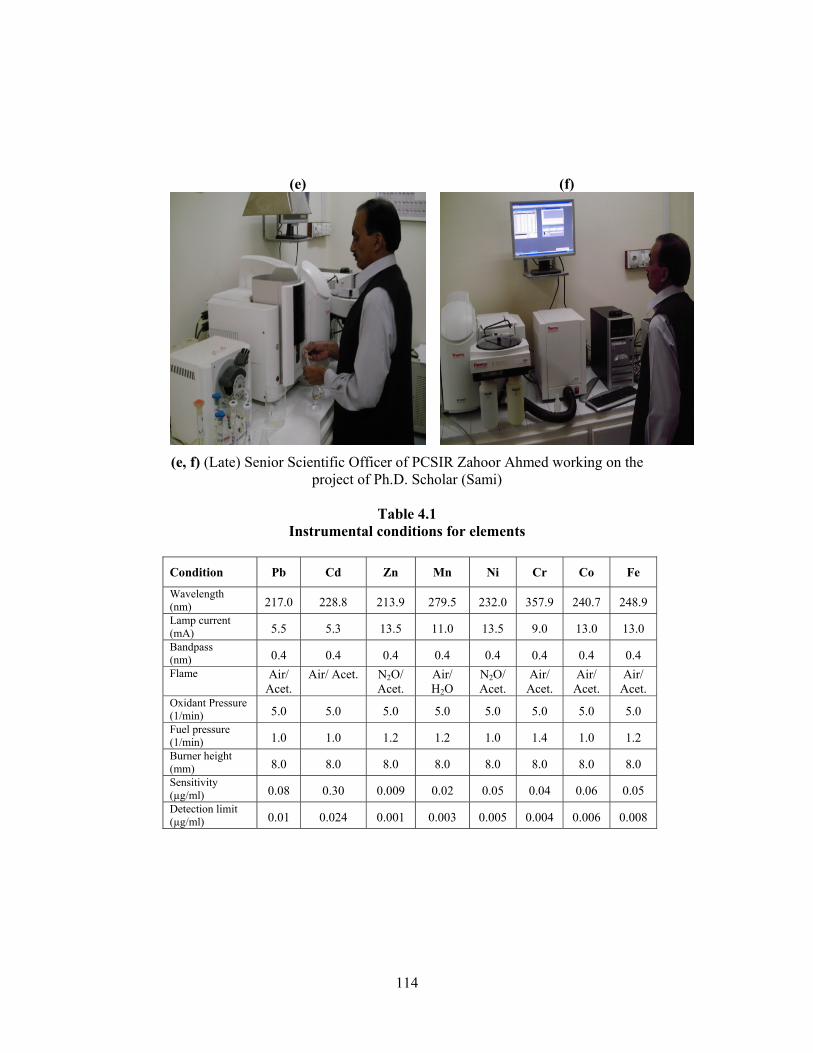
114
(e) (f)
(e, f) (Late) Senior Scientific Officer of PCSIR Zahoor Ahmed working on the project of Ph.D. Scholar (Sami)
Table 4.1
Instrumental conditions for elements Condition Pb Cd Zn Mn Ni Cr Co Fe
Wavelength (nm) 217.0 228.8 213.9 279.5 232.0 357.9 240.7 248.9 Lamp current (mA) 5.5 5.3 13.5 11.0 13.5 9.0 13.0 13.0 Bandpass (nm) 0.4 0.4 0.4 0.4 0.4 0.4 0.4 0.4 Flame Air/
Acet. Air/ Acet. N2O/
Acet. Air/ H2O
N2O/ Acet.
Air/ Acet.
Air/ Acet.
Air/ Acet.
Oxidant Pressure (1/min) 5.0 5.0 5.0 5.0 5.0 5.0 5.0 5.0 Fuel pressure (1/min) 1.0 1.0 1.2 1.2 1.0 1.4 1.0 1.2 Burner height (mm) 8.0 8.0 8.0 8.0 8.0 8.0 8.0 8.0 Sensitivity (µg/ml) 0.08 0.30 0.009 0.02 0.05 0.04 0.06 0.05 Detection limit (µg/ml) 0.01 0.024 0.001 0.003 0.005 0.004 0.006 0.008
115
CHAPTER 5
RE S U L T S A N D D I S C U S S I O N
Results pertaining to prime goal of determining the "rate of dust fall in
Quetta 2004-2008" have been given in a sequence manner in the tables on
daily basis for the year 2004 and on monthly basis for the years 2005, 2006,
2007 & 2008 for the all ten selected sites of Quetta. Tables 5.2 to 5.11 show
the rate of dust fall for all the months of year 2004 on daily basis for all ten
selected sites (Army Recruitment Center, Ashraf Sariab Road, C.G.S colony,
Civil Hospital, Gawalmandi Chowk, Qadoosi Store / Quick Marketing
Services, Railway Station, Sada Bahar Sweets, Sirki Road& T.B. Sanatorium).
Tables 5.14 to 5.18 represent the average rate of dust fall for the year 2004,
2005, 2006, 2007 & 2008 on monthly basis for all the ten selected sites.
Meteorological data showing mean daily temperature of 2004, mean monthly
temperature for the years 2005, 2006, 2007 & 2008, daily precipitation of
2004, 2005, 2006, 2007 & 2008, daily wind speed and daily wind direction
from the 2004-2008 are given in their corresponding tables. Daily visibility
data in terms of UTC (Universal Coordinated Time) & PST (Pakistani
Standard Time) twice per day (at 0000 UTC & 1200 UTC) or (at 8:00 a.m.
&5:00 p.m.) is given in Table 5.37. Typical average annual chemical
composition of dust fall is mentioned in Tables 5.35. Average annual particle
size distribution of dust fall is shown in Table 5.47. Finally the average annual
concentrations of heavy/toxic metals are given in Tables 5.44 & 5.45.
116
5.1 RATE OF DUST FALL/SETTLEMENT/DEPOSITION:
It is vividly evident from the data given in Table 5.1 from the year
1997-2002 that whole Balochistan and particularly Quetta faced a severe
drought spell [101]. A drought is a period of abnormally dry weather which
persists long enough to produce a serious hydrologic imbalance. It is a slow
onset, “creeping phenomenon”. It emerges, when in an area there is a 50% less
precipitation occurs than the normal rainfall happens in that region. Drought
gradually emerged in the beginning of 90s and its intensity reached on its
acme/culmination from 1997-2002. Though it was abating in the year 2004,
when we commenced collecting dust samples on daily basis from the 10
different locations all along Quetta, yet it caused massive dust fall compare to
the normal conditions.
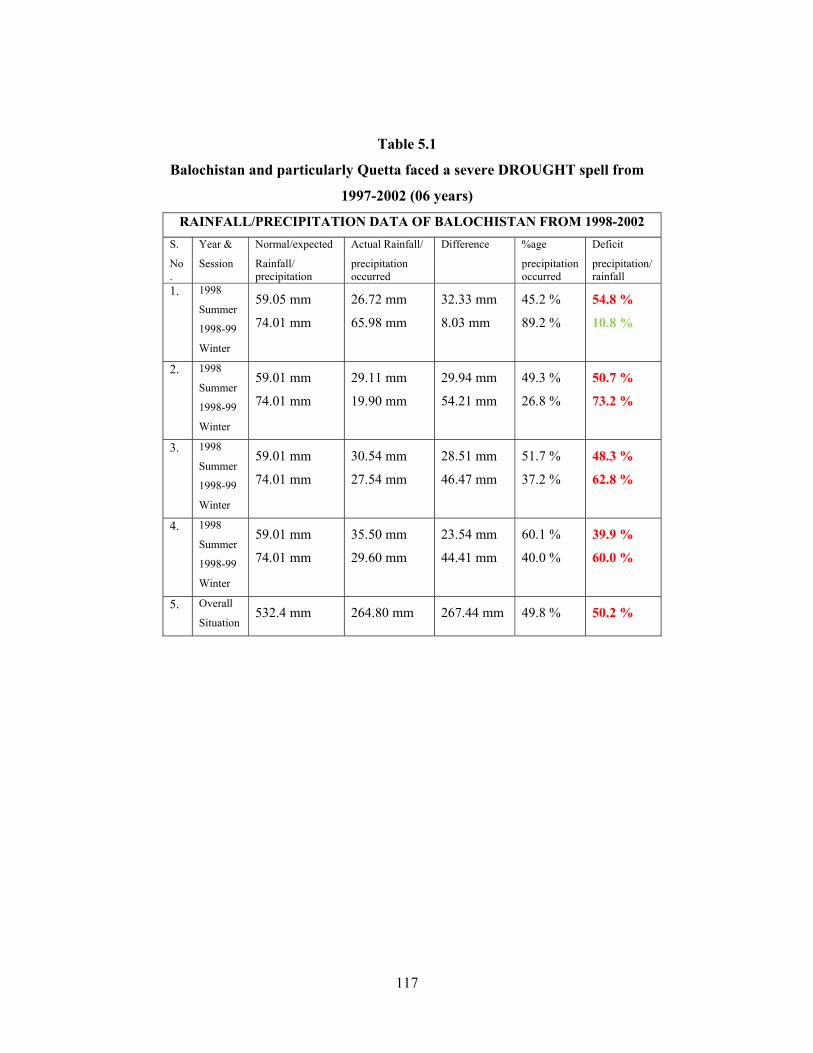
117
Table 5.1
Balochistan and particularly Quetta faced a severe DROUGHT spell from
1997-2002 (06 years)
RAINFALL/PRECIPITATION DATA OF BALOCHISTAN FROM 1998-2002 S. Year & Normal/expected Actual Rainfall/ Difference %age Deficit
No.
Session Rainfall/ precipitation
precipitation occurred
precipitation occurred
precipitation/ rainfall
1. 1998
Summer
1998-99
Winter
59.05 mm 74.01 mm
26.72 mm 65.98 mm
32.33 mm 8.03 mm
45.2 % 89.2 %
54.8 % 10.8 %
2. 1998
Summer
1998-99
Winter
59.01 mm 74.01 mm
29.11 mm 19.90 mm
29.94 mm 54.21 mm
49.3 % 26.8 %
50.7 % 73.2 %
3. 1998
Summer
1998-99
Winter
59.01 mm 74.01 mm
30.54 mm 27.54 mm
28.51 mm 46.47 mm
51.7 % 37.2 %
48.3 % 62.8 %
4. 1998
Summer
1998-99
Winter
59.01 mm 74.01 mm
35.50 mm 29.60 mm
23.54 mm 44.41 mm
60.1 % 40.0 %
39.9 % 60.0 %
5. Overall
Situation 532.4 mm 264.80 mm 267.44 mm 49.8 % 50.2 %
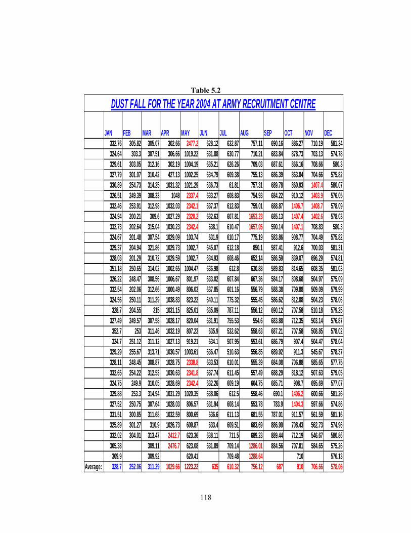
118
Table 5.2
JAN FEB MAR APR MAY JUN JUL AUG SEP OCT NOV DEC332.76 305.82 305.07 302.66 2477.2 628.12 632.87 757.11 690.16 886.27 710.19 581.34324.64 303.3 307.51 306.66 1019.22 631.88 630.77 710.21 683.84 878.73 703.13 574.78329.61 303.05 312.16 302.19 1004.19 635.21 626.26 709.03 687.61 866.16 708.66 580.3327.79 301.07 310.42 427.13 1002.25 634.79 609.38 755.13 686.39 863.84 704.66 575.82330.89 254.73 314.25 1031.32 1021.29 636.73 61.81 757.31 689.78 860.93 1407.4 580.07326.51 249.39 308.33 1048 2337.4 633.27 608.83 754.93 684.22 910.12 1403.9 576.05332.46 253.91 312.98 1032.03 2342.1 637.37 612.83 759.01 688.87 1406.7 1408.7 578.09324.94 200.21 309.6 1027.29 2320.2 632.63 607.81 1653.23 685.13 1407.4 1402.6 578.03332.73 202.64 315.04 1030.23 2342.4 638.1 610.47 1657.05 590.14 1407.1 708.83 580.3324.67 201.48 307.54 1029.09 103.74 631.9 610.17 775.19 583.86 908.77 704.49 575.82329.37 204.94 321.86 1029.73 1002.7 645.07 612.18 850.1 587.41 912.6 700.03 581.31328.03 201.29 310.72 1029.59 1002.7 634.93 608.46 652.14 586.59 839.07 696.29 574.81351.18 250.65 314.02 1002.65 1004.47 636.98 612.8 630.88 589.83 814.65 608.35 581.03326.22 248.47 308.56 1006.67 801.97 633.02 607.84 667.36 584.17 808.68 504.97 575.09332.54 202.06 312.66 1000.49 806.03 637.85 601.16 556.79 588.38 709.88 509.09 579.99324.56 250.11 311.29 1038.83 823.22 640.11 775.32 555.45 586.62 812.88 504.23 578.06328.7 204.55 315 1031.15 825.01 635.09 787.11 556.12 690.12 707.58 510.18 579.25
327.49 249.57 307.58 1028.17 820.04 631.91 755.53 554.6 683.88 712.35 503.14 576.87352.7 253 311.46 1032.19 807.23 635.9 532.62 558.63 687.21 707.58 508.85 578.02324.7 251.12 311.12 1027.13 919.21 634.1 507.95 553.61 686.79 907.4 504.47 578.04
329.29 255.67 313.71 1030.57 1003.61 636.47 510.63 556.85 689.92 911.3 545.67 578.37328.11 248.45 308.87 1028.75 2338.8 633.53 610.01 555.39 684.08 706.88 585.65 577.75332.65 254.22 312.53 1030.63 2341.8 637.74 611.45 557.49 688.29 818.12 507.63 579.05324.75 249.9 310.05 1028.69 2342.4 632.26 609.19 604.75 685.71 908.7 695.69 577.07329.88 253.3 314.94 1031.29 1020.35 638.06 612.5 558.46 690.1 1406.2 600.66 581.26327.52 250.75 307.64 1028.03 806.57 631.94 608.14 553.78 783.9 1404.3 597.66 574.86331.51 300.85 311.68 1032.59 800.69 636.6 611.13 681.55 787.01 911.57 561.59 581.16325.89 301.27 310.9 1026.73 609.87 633.4 609.51 683.69 886.99 708.43 562.73 574.96332.02 304.01 313.47 2412.7 623.36 638.11 711.5 689.23 889.44 712.19 546.67 580.86305.38 309.11 2476.7 623.08 631.89 709.14 1286.01 884.56 707.81 584.65 575.26309.9 309.92 620.41 709.48 1288.64 710 576.13
Average: 328.7 252.06 311.29 1029.66 1223.22 635 610.32 756.12 687 910 706.66 578.06
DUST FALL FOR THE YEAR 2004 AT ARMY RECRUITMENT CENTRE
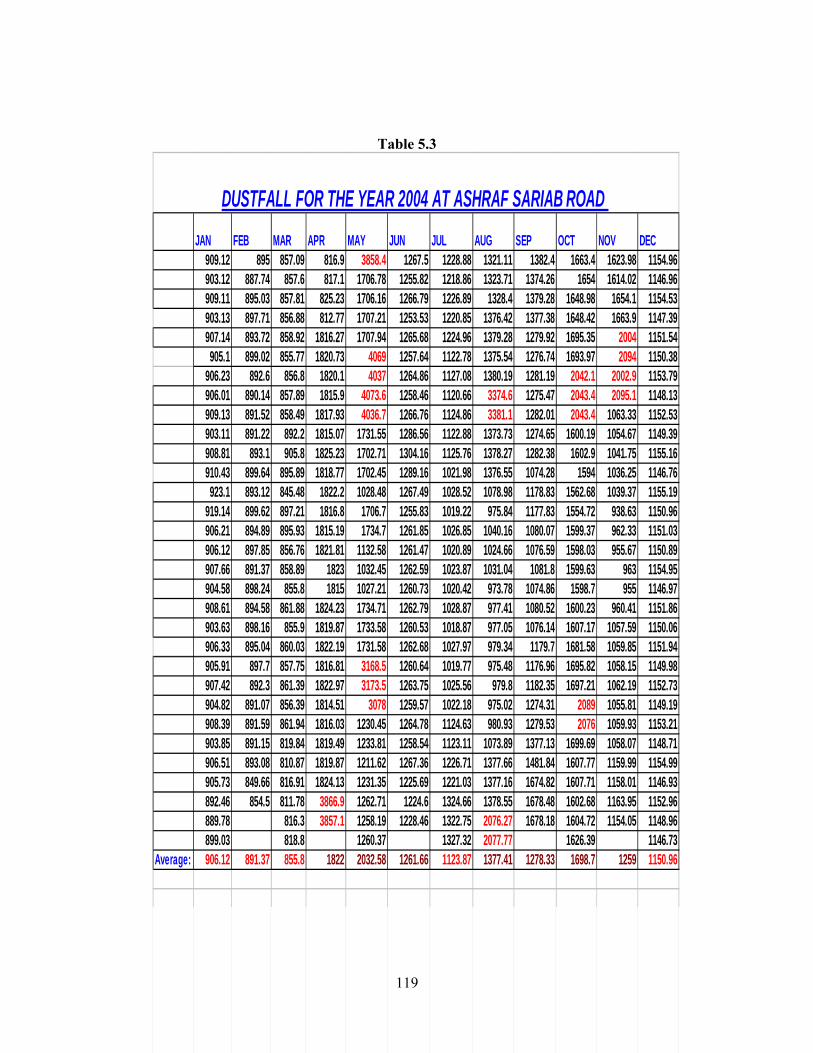
119
Table 5.3
JAN FEB MAR APR MAY JUN JUL AUG SEP OCT NOV DEC909.12 895 857.09 816.9 3858.4 1267.5 1228.88 1321.11 1382.4 1663.4 1623.98 1154.96903.12 887.74 857.6 817.1 1706.78 1255.82 1218.86 1323.71 1374.26 1654 1614.02 1146.96909.11 895.03 857.81 825.23 1706.16 1266.79 1226.89 1328.4 1379.28 1648.98 1654.1 1154.53903.13 897.71 856.88 812.77 1707.21 1253.53 1220.85 1376.42 1377.38 1648.42 1663.9 1147.39907.14 893.72 858.92 1816.27 1707.94 1265.68 1224.96 1379.28 1279.92 1695.35 2004 1151.54905.1 899.02 855.77 1820.73 4069 1257.64 1122.78 1375.54 1276.74 1693.97 2094 1150.38
906.23 892.6 856.8 1820.1 4037 1264.86 1127.08 1380.19 1281.19 2042.1 2002.9 1153.79906.01 890.14 857.89 1815.9 4073.6 1258.46 1120.66 3374.6 1275.47 2043.4 2095.1 1148.13909.13 891.52 858.49 1817.93 4036.7 1266.76 1124.86 3381.1 1282.01 2043.4 1063.33 1152.53903.11 891.22 892.2 1815.07 1731.55 1286.56 1122.88 1373.73 1274.65 1600.19 1054.67 1149.39908.81 893.1 905.8 1825.23 1702.71 1304.16 1125.76 1378.27 1282.38 1602.9 1041.75 1155.16910.43 899.64 895.89 1818.77 1702.45 1289.16 1021.98 1376.55 1074.28 1594 1036.25 1146.76923.1 893.12 845.48 1822.2 1028.48 1267.49 1028.52 1078.98 1178.83 1562.68 1039.37 1155.19
919.14 899.62 897.21 1816.8 1706.7 1255.83 1019.22 975.84 1177.83 1554.72 938.63 1150.96906.21 894.89 895.93 1815.19 1734.7 1261.85 1026.85 1040.16 1080.07 1599.37 962.33 1151.03906.12 897.85 856.76 1821.81 1132.58 1261.47 1020.89 1024.66 1076.59 1598.03 955.67 1150.89907.66 891.37 858.89 1823 1032.45 1262.59 1023.87 1031.04 1081.8 1599.63 963 1154.95904.58 898.24 855.8 1815 1027.21 1260.73 1020.42 973.78 1074.86 1598.7 955 1146.97908.61 894.58 861.88 1824.23 1734.71 1262.79 1028.87 977.41 1080.52 1600.23 960.41 1151.86903.63 898.16 855.9 1819.87 1733.58 1260.53 1018.87 977.05 1076.14 1607.17 1057.59 1150.06906.33 895.04 860.03 1822.19 1731.58 1262.68 1027.97 979.34 1179.7 1681.58 1059.85 1151.94905.91 897.7 857.75 1816.81 3168.5 1260.64 1019.77 975.48 1176.96 1695.82 1058.15 1149.98907.42 892.3 861.39 1822.97 3173.5 1263.75 1025.56 979.8 1182.35 1697.21 1062.19 1152.73904.82 891.07 856.39 1814.51 3078 1259.57 1022.18 975.02 1274.31 2089 1055.81 1149.19908.39 891.59 861.94 1816.03 1230.45 1264.78 1124.63 980.93 1279.53 2076 1059.93 1153.21903.85 891.15 819.84 1819.49 1233.81 1258.54 1123.11 1073.89 1377.13 1699.69 1058.07 1148.71906.51 893.08 810.87 1819.87 1211.62 1267.36 1226.71 1377.66 1481.84 1607.77 1159.99 1154.99905.73 849.66 816.91 1824.13 1231.35 1225.69 1221.03 1377.16 1674.82 1607.71 1158.01 1146.93892.46 854.5 811.78 3866.9 1262.71 1224.6 1324.66 1378.55 1678.48 1602.68 1163.95 1152.96889.78 816.3 3857.1 1258.19 1228.46 1322.75 2076.27 1678.18 1604.72 1154.05 1148.96899.03 818.8 1260.37 1327.32 2077.77 1626.39 1146.73
Average: 906.12 891.37 855.8 1822 2032.58 1261.66 1123.87 1377.41 1278.33 1698.7 1259 1150.96
DUSTFALL FOR THE YEAR 2004 AT ASHRAF SARIAB ROAD
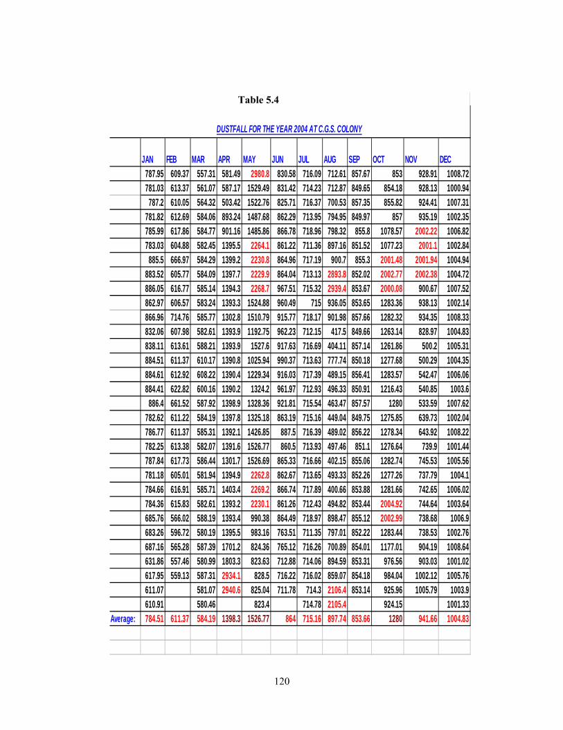
120
Table 5.4
JAN FEB MAR APR MAY JUN JUL AUG SEP OCT NOV DEC787.95 609.37 557.31 581.49 2980.8 830.58 716.09 712.61 857.67 853 928.91 1008.72781.03 613.37 561.07 587.17 1529.49 831.42 714.23 712.87 849.65 854.18 928.13 1000.94
787.2 610.05 564.32 503.42 1522.76 825.71 716.37 700.53 857.35 855.82 924.41 1007.31781.82 612.69 584.06 893.24 1487.68 862.29 713.95 794.95 849.97 857 935.19 1002.35785.99 617.86 584.77 901.16 1485.86 866.78 718.96 798.32 855.8 1078.57 2002.22 1006.82783.03 604.88 582.45 1395.5 2264.1 861.22 711.36 897.16 851.52 1077.23 2001.1 1002.84
885.5 666.97 584.29 1399.2 2230.8 864.96 717.19 900.7 855.3 2001.48 2001.94 1004.94883.52 605.77 584.09 1397.7 2229.9 864.04 713.13 2893.8 852.02 2002.77 2002.38 1004.72886.05 616.77 585.14 1394.3 2268.7 967.51 715.32 2939.4 853.67 2000.08 900.67 1007.52862.97 606.57 583.24 1393.3 1524.88 960.49 715 936.05 853.65 1283.36 938.13 1002.14866.96 714.76 585.77 1302.8 1510.79 915.77 718.17 901.98 857.66 1282.32 934.35 1008.33832.06 607.98 582.61 1393.9 1192.75 962.23 712.15 417.5 849.66 1263.14 828.97 1004.83838.11 613.61 588.21 1393.9 1527.6 917.63 716.69 404.11 857.14 1261.86 500.2 1005.31884.51 611.37 610.17 1390.8 1025.94 990.37 713.63 777.74 850.18 1277.68 500.29 1004.35884.61 612.92 608.22 1390.4 1229.34 916.03 717.39 489.15 856.41 1283.57 542.47 1006.06884.41 622.82 600.16 1390.2 1324.2 961.97 712.93 496.33 850.91 1216.43 540.85 1003.6
886.4 661.52 587.92 1398.9 1328.36 921.81 715.54 463.47 857.57 1280 533.59 1007.62782.62 611.22 584.19 1397.8 1325.18 863.19 715.16 449.04 849.75 1275.85 639.73 1002.04786.77 611.37 585.31 1392.1 1426.85 887.5 716.39 489.02 856.22 1278.34 643.92 1008.22782.25 613.38 582.07 1391.6 1526.77 860.5 713.93 497.46 851.1 1276.64 739.9 1001.44787.84 617.73 586.44 1301.7 1526.69 865.33 716.66 402.15 855.06 1282.74 745.53 1005.56781.18 605.01 581.94 1394.9 2262.8 862.67 713.65 493.33 852.26 1277.26 737.79 1004.1784.66 616.91 585.71 1403.4 2269.2 866.74 717.89 400.66 853.88 1281.66 742.65 1006.02784.36 615.83 582.61 1393.2 2230.1 861.26 712.43 494.82 853.44 2004.92 744.64 1003.64685.76 566.02 588.19 1393.4 990.38 864.49 718.97 898.47 855.12 2002.99 738.68 1006.9683.26 596.72 580.19 1395.5 983.16 763.51 711.35 797.01 852.22 1283.44 738.53 1002.76687.16 565.28 587.39 1701.2 824.36 765.12 716.26 700.89 854.01 1177.01 904.19 1008.64631.86 557.46 580.99 1803.3 823.63 712.88 714.06 894.59 853.31 976.56 903.03 1001.02617.95 559.13 587.31 2934.1 828.5 716.22 716.02 859.07 854.18 984.04 1002.12 1005.76611.07 581.07 2940.6 825.04 711.78 714.3 2106.4 853.14 925.96 1005.79 1003.9610.91 580.46 823.4 714.78 2105.4 924.15 1001.33
Average: 784.51 611.37 584.19 1398.3 1526.77 864 715.16 897.74 853.66 1280 941.66 1004.83
DUSTFALL FOR THE YEAR 2004 AT C.G.S. COLONY
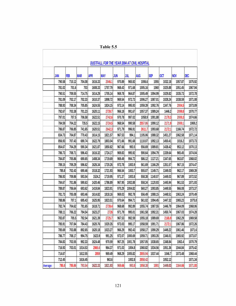
121
Table 5.5
JAN FEB MAR APR MAY JUN JUL AUG SEP OCT NOV DEC790.58 710.12 704.08 1616.33 2046.1 970.89 965.92 1006.6 1055 1032.18 1057.87 1075.92781.02 701.6 703 1608.33 1707.79 968.43 971.68 1005.16 1060 1025.88 1051.45 1067.94790.51 709.55 714.75 1614.29 1705.14 969.78 964.87 1005.49 1094.99 1029.82 1035.73 1072.78781.09 702.17 702.33 1610.37 1898.72 969.54 972.73 1006.27 1087.01 1028.24 1038.59 1071.08788.93 708.34 705.85 1624.55 1824.15 973.14 995.93 1059.39 1092.76 1347.76 2004.5 1073.09792.67 703.38 701.23 1620.11 2739.7 966.18 991.67 1057.37 1089.24 1446.2 2099.8 1070.77797.01 707.5 706.58 1622.51 2742.6 970.78 997.02 1058.9 1091.88 2170.3 2000.3 1074.66784.59 704.22 735.5 1622.15 2724.5 968.54 990.58 2557.86 1090.12 2171.9 2000.1 1069.2786.87 706.85 741.65 1620.51 2642.3 971.79 996.91 2611.7 1093.68 2172.1 1166.74 1072.72834.73 704.87 770.43 1614.15 1821.57 967.53 994.1 1105.06 1088.32 1451.27 1062.58 1071.14856.93 707.43 690.74 1622.79 1803.04 971.66 991.68 1110.07 1092.13 1450.41 1016.2 1073.73854.67 704.29 590.34 1621.87 1850.82 967.66 993.5 556.69 1089.81 1438.42 953.12 1070.13786.73 708.71 596.43 1616.32 1724.17 969.83 995.92 590.64 1094.79 1339.64 965.45 1074.04784.87 705.86 690.65 1408.34 1719.69 969.49 994.72 586.12 1127.21 1347.65 963.87 1068.02789.15 709.29 596.62 1626.34 1720.26 972.78 1003.9 561.69 1166.29 1351.57 967.15 1074.47
785.8 702.43 690.46 1518.32 1721.93 966.54 1003.7 555.07 1149.71 1349.03 962.17 1069.39786.93 709.86 593.54 1524.2 1719.95 971.37 1003.8 558.38 1140.07 1449.03 967.89 1072.52784.67 701.86 590.63 1420.46 1786.89 967.95 1002.88 558.34 1120.93 1445.94 961.53 1071.93789.87 706.64 693.62 1419.84 1823.91 970.29 1004.82 560.27 1093.85 1449.55 966.08 1073.37781.73 705.08 693.46 1614.82 1818.16 969.03 992.78 556.49 1088.15 1448.51 1063.24 1070.49788.86 707.1 695.43 1625.95 1823.51 970.64 994.71 561.02 1094.45 1447.32 1065.23 1075.8782.74 704.62 791.65 1618.71 2739.4 968.68 992.89 1055.74 1087.55 1446.79 1064.09 1068.06788.11 706.22 794.54 1623.27 2726 971.79 995.01 1061.58 1092.31 1450.74 1067.03 1074.28783.87 705.5 792.54 1621.39 2725.7 967.53 992.59 1055.18 1089.69 2165.9 1062.29 1069.58785.91 707.84 784.43 1620.76 1020.35 973.03 995.17 1058.59 1091.71 2172.1 1067.86 1072.26785.69 703.88 892.65 1620.18 1023.27 966.29 992.43 1058.17 1090.29 1449.22 1061.46 1071.6786.77 708.17 994.75 1623.9 991.25 972.07 1000.69 1059.71 1093.35 1346.01 1065.92 1073.07784.83 703.55 992.33 1624.48 970.59 967.25 1001.78 1057.05 1038.65 1348.84 1063.4 1070.79716.93 703.01 1014.53 2065.6 964.37 971.03 1004.8 1060.82 1034.56 1051.36 1044.84 1075.42714.67 1612.55 2059 969.49 968.29 1005.82 2055.94 1037.44 1046.7 1073.48 1068.44712.45 1616.45 963.6 1002.8 2058.42 1052.12 1071.34
Average: 785.8 705.86 793.54 1622.33 1821.93 969.66 993.8 1058.38 1091 1449.03 1164.66 1071.93
DUSTFALL FOR THE YEAR 2004 AT CIVIL HOSPITAL
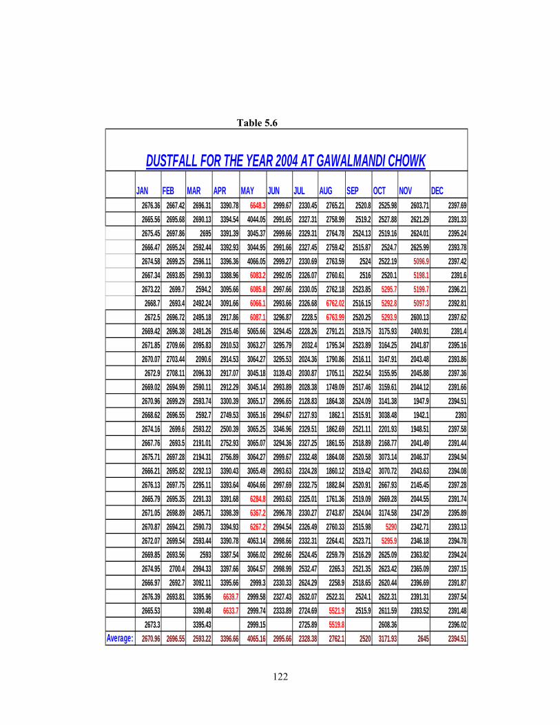
122
Table 5.6
JAN FEB MAR APR MAY JUN JUL AUG SEP OCT NOV DEC2676.36 2667.42 2696.31 3390.78 6648.3 2999.67 2330.45 2765.21 2520.8 2525.98 2603.71 2397.692665.56 2695.68 2690.13 3394.54 4044.05 2991.65 2327.31 2758.99 2519.2 2527.88 2621.29 2391.332675.45 2697.86 2695 3391.39 3045.37 2999.66 2329.31 2764.78 2524.13 2519.16 2624.01 2395.242666.47 2695.24 2592.44 3392.93 3044.95 2991.66 2327.45 2759.42 2515.87 2524.7 2625.99 2393.782674.58 2699.25 2596.11 3396.36 4066.05 2999.27 2330.69 2763.59 2524 2522.19 5096.9 2397.422667.34 2693.85 2590.33 3388.96 6083.2 2992.05 2326.07 2760.61 2516 2520.1 5198.1 2391.62673.22 2699.7 2594.2 3095.66 6085.8 2997.66 2330.05 2762.18 2523.85 5295.7 5199.7 2396.212668.7 2693.4 2492.24 3091.66 6066.1 2993.66 2326.68 6762.02 2516.15 5292.8 5097.3 2392.812672.5 2696.72 2495.18 2917.86 6087.1 3296.87 2228.5 6763.99 2520.25 5293.9 2600.13 2397.62
2669.42 2696.38 2491.26 2915.46 5065.66 3294.45 2228.26 2791.21 2519.75 3175.93 2400.91 2391.42671.85 2709.66 2095.83 2910.53 3063.27 3295.79 2032.4 1795.34 2523.89 3164.25 2041.87 2395.162670.07 2703.44 2090.6 2914.53 3064.27 3295.53 2024.36 1790.86 2516.11 3147.91 2043.48 2393.862672.9 2708.11 2096.33 2917.07 3045.18 3139.43 2030.87 1705.11 2522.54 3155.95 2045.88 2397.36
2669.02 2694.99 2590.11 2912.29 3045.14 2993.89 2028.38 1749.09 2517.46 3159.61 2044.12 2391.662670.96 2699.29 2593.74 3300.39 3065.17 2996.65 2128.83 1864.38 2524.09 3141.38 1947.9 2394.512668.62 2696.55 2592.7 2749.53 3065.16 2994.67 2127.93 1862.1 2515.91 3038.48 1942.1 23932674.16 2699.6 2593.22 2500.39 3065.25 3346.96 2329.51 1862.69 2521.11 2201.93 1948.51 2397.582667.76 2693.5 2191.01 2752.93 3065.07 3294.36 2327.25 1861.55 2518.89 2168.77 2041.49 2391.442675.71 2697.28 2194.31 2756.89 3064.27 2999.67 2332.48 1864.08 2520.58 3073.14 2046.37 2394.942666.21 2695.82 2292.13 3390.43 3065.49 2993.63 2324.28 1860.12 2519.42 3070.72 2043.63 2394.082676.13 2697.75 2295.11 3393.64 4064.66 2997.69 2332.75 1882.84 2520.91 2667.93 2145.45 2397.282665.79 2695.35 2291.33 3391.68 6284.8 2993.63 2325.01 1761.36 2519.09 2669.28 2044.55 2391.742671.05 2698.89 2495.71 3398.39 6367.2 2996.78 2330.27 2743.87 2524.04 3174.58 2347.29 2395.892670.87 2694.21 2590.73 3394.93 6267.2 2994.54 2326.49 2760.33 2515.98 5290 2342.71 2393.132672.07 2699.54 2593.44 3390.78 4063.14 2998.66 2332.31 2264.41 2523.71 5295.9 2346.18 2394.782669.85 2693.56 2593 3387.54 3066.02 2992.66 2524.45 2259.79 2516.29 2625.09 2363.82 2394.242674.95 2700.4 2994.33 3397.66 3064.57 2998.99 2532.47 2265.3 2521.35 2623.42 2365.09 2397.152666.97 2692.7 3092.11 3395.66 2999.3 2330.33 2624.29 2258.9 2518.65 2620.44 2396.69 2391.872676.39 2693.81 3395.96 6639.7 2999.58 2327.43 2632.07 2522.31 2524.1 2622.31 2391.31 2397.542665.53 3390.48 6633.7 2999.74 2333.89 2724.69 5521.9 2515.9 2611.59 2393.52 2391.482673.3 3395.43 2999.15 2725.89 5519.8 2608.36 2396.02
Average: 2670.96 2696.55 2593.22 3396.66 4065.16 2995.66 2328.38 2762.1 2520 3171.93 2645 2394.51
DUSTFALL FOR THE YEAR 2004 AT GAWALMANDI CHOWK

123
Table 5.7
JAN FEB MAR APR MAY JUN JUL AUG SEP OCT NOV DEC1370.91 1067.53 1208.06 2114.76 2829.6 1650.51 1447.62 1668.56 1634.63 1637.43 1770.46 1543.421358.75 1060.73 1200.32 2108.56 2503.33 1643.49 1441.4 1661.76 1633.37 1621.59 1779.2 1535.921370.46 1064.84 1205.27 2132.55 2489.45 1647.96 1447.26 1668.12 1638.13 1633.7 1784.77 1540.621359.2 1063.42 1203.11 2130.77 2483.45 1646.04 1461.76 1662.2 1629.87 1645.32 1799.89 1538.72
1369.14 1037.06 1206.69 2113.39 2407.77 1649.69 1466.5 1666.64 1638.01 1621.78 3184.3 1541.041360.52 1031.2 1201.69 2009.93 3325.1 1644.31 1462.52 1663.6 1629.99 1622.89 3180.4 1538.831366.46 1036.95 1206.58 2034.03 3327.8 1648.81 1464.6 1665.29 1637.37 2837.24 3187.8 1542.51363.2 1031.31 1201.8 2029.29 3308.6 1645.19 1464.42 3665.07 1630.63 2836.13 3186.9 1536.84
1367.79 1005.53 604.56 2032.45 3328.5 1650.49 1465.77 3666.72 1636.41 2855.3 1678.66 1540.381461.87 1002.73 903.82 2030.87 2404.45 1663.51 1463.25 1663.6 1631.59 1916.74 1689.75 1538.961570.15 1007.42 907.27 2034.73 2489.38 1658.75 1286.73 1167.42 1634.57 1917 1694.91 1540.381559.51 830.84 901.11 2028.59 2483.52 1646.25 1282.29 1162.9 1633.43 1612.02 1698.36 1538.961668.32 835.3 905.59 2032.09 2408.68 1649.57 1287.65 1168.49 1635.11 1615.9 1666.59 1542.261661.34 864.13 602.79 2031.23 2403.44 1844.43 1261.37 1161.83 1632.89 1613.12 1666.3 1537.081666.93 867.32 606.29 2033.85 2396.56 1850.44 1265.28 1196.01 1636.58 1715.18 1668 1539.671664.83 830.94 602.09 2029.47 2496.34 1843.56 1263.74 1194.31 1631.42 1713.84 1640.33 1538.261668.89 936.87 604.19 2033.18 2406.45 1847.63 1366.42 1196.6 1638.1 1615.92 1630.43 1540.211360.77 931.39 902.2 2030.14 2404.22 1846.37 1363.32 1183.42 1629.9 1606.06 1594.23 1539.131366.34 1034.55 907.36 2033.91 2505.39 1749.36 1364.51 1187.84 1637 1802.96 1599.55 1543.371363.32 1033.71 901.02 2129.41 2508.36 1744.64 1462.51 1162.48 1631 1812.28 1595.11 1535.971368.22 1035.61 906.17 2134.7 2506.56 1648.15 1467.54 1165.16 1634.56 1813.1 159.03 1542.031361.44 1032.65 1202.21 2128.62 3324.5 1645.85 1461.48 1161.75 1633.44 1914.51 1596 1537.311370.38 1134.52 1204.53 2128.65 3359.5 1650.39 1565.07 1165.53 1634.96 1914.68 1597.44 1539.861259.28 1133.74 1503.85 2129.5 3309.5 1543.61 1563.95 1164.79 1633.04 2833.72 1597.22 1539.481170.86 1237.18 1506.85 2132.56 2355.34 1543.23 1566.25 1666.4 1636.83 2836.59 1500.36 1540.91158.8 1231.08 1501.53 2130.76 1656.34 1446.77 1662.77 1663.92 1631.17 1912.43 1594.3 1538.44
1067.55 1206.57 2107.63 2133.45 1657.56 1449.11 1666.72 1647.27 1638.12 1764.96 1550.06 1543.191062.11 1201.69 2100.75 2134.67 1654.26 1444.89 1662.3 1643.05 1629.88 1764.06 1544.6 1536.151069.63 1202.96 2106.07 2873.89 1657.56 1450 1667.71 1638.16 1635 1785.73 1538.63 1541.841060.07 2102.31 2869.43 1653.36 1444 1661.31 3132.16 1633 1783.29 1544.33 1537.351062.73 2105.18 1655.14 1666.51 3138.57 1774.34 1541.08
Average: 1364.83 1034.13 1204.19 2131.66 2506.45 1647 1464.51 1665.16 1634 1914.51 1797.33 1539.67
DUSTFALL FOR THE YEAR 2004 AT QADOOSI STORE
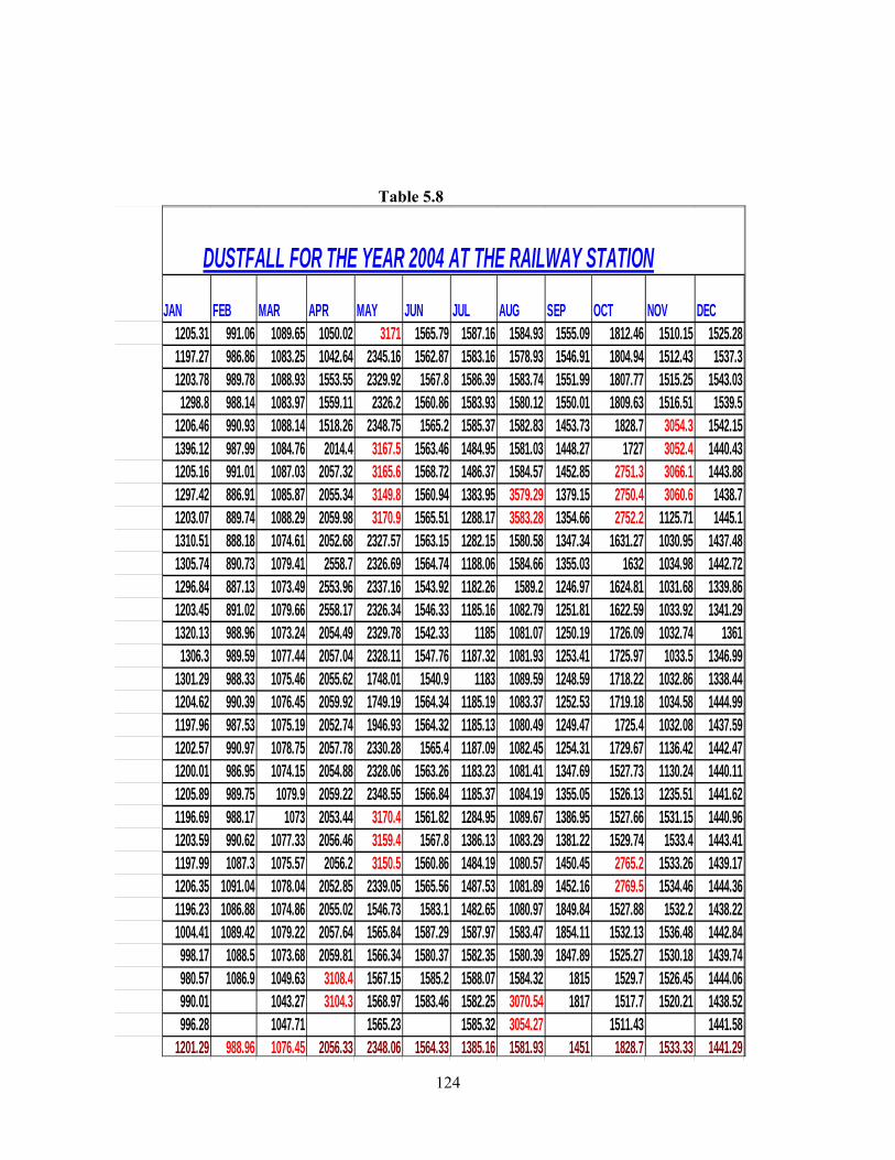
124
Table 5.8
JAN FEB MAR APR MAY JUN JUL AUG SEP OCT NOV DEC1205.31 991.06 1089.65 1050.02 3171 1565.79 1587.16 1584.93 1555.09 1812.46 1510.15 1525.281197.27 986.86 1083.25 1042.64 2345.16 1562.87 1583.16 1578.93 1546.91 1804.94 1512.43 1537.31203.78 989.78 1088.93 1553.55 2329.92 1567.8 1586.39 1583.74 1551.99 1807.77 1515.25 1543.031298.8 988.14 1083.97 1559.11 2326.2 1560.86 1583.93 1580.12 1550.01 1809.63 1516.51 1539.5
1206.46 990.93 1088.14 1518.26 2348.75 1565.2 1585.37 1582.83 1453.73 1828.7 3054.3 1542.151396.12 987.99 1084.76 2014.4 3167.5 1563.46 1484.95 1581.03 1448.27 1727 3052.4 1440.431205.16 991.01 1087.03 2057.32 3165.6 1568.72 1486.37 1584.57 1452.85 2751.3 3066.1 1443.881297.42 886.91 1085.87 2055.34 3149.8 1560.94 1383.95 3579.29 1379.15 2750.4 3060.6 1438.71203.07 889.74 1088.29 2059.98 3170.9 1565.51 1288.17 3583.28 1354.66 2752.2 1125.71 1445.11310.51 888.18 1074.61 2052.68 2327.57 1563.15 1282.15 1580.58 1347.34 1631.27 1030.95 1437.481305.74 890.73 1079.41 2558.7 2326.69 1564.74 1188.06 1584.66 1355.03 1632 1034.98 1442.721296.84 887.13 1073.49 2553.96 2337.16 1543.92 1182.26 1589.2 1246.97 1624.81 1031.68 1339.861203.45 891.02 1079.66 2558.17 2326.34 1546.33 1185.16 1082.79 1251.81 1622.59 1033.92 1341.291320.13 988.96 1073.24 2054.49 2329.78 1542.33 1185 1081.07 1250.19 1726.09 1032.74 13611306.3 989.59 1077.44 2057.04 2328.11 1547.76 1187.32 1081.93 1253.41 1725.97 1033.5 1346.99
1301.29 988.33 1075.46 2055.62 1748.01 1540.9 1183 1089.59 1248.59 1718.22 1032.86 1338.441204.62 990.39 1076.45 2059.92 1749.19 1564.34 1185.19 1083.37 1252.53 1719.18 1034.58 1444.991197.96 987.53 1075.19 2052.74 1946.93 1564.32 1185.13 1080.49 1249.47 1725.4 1032.08 1437.591202.57 990.97 1078.75 2057.78 2330.28 1565.4 1187.09 1082.45 1254.31 1729.67 1136.42 1442.471200.01 986.95 1074.15 2054.88 2328.06 1563.26 1183.23 1081.41 1347.69 1527.73 1130.24 1440.111205.89 989.75 1079.9 2059.22 2348.55 1566.84 1185.37 1084.19 1355.05 1526.13 1235.51 1441.621196.69 988.17 1073 2053.44 3170.4 1561.82 1284.95 1089.67 1386.95 1527.66 1531.15 1440.961203.59 990.62 1077.33 2056.46 3159.4 1567.8 1386.13 1083.29 1381.22 1529.74 1533.4 1443.411197.99 1087.3 1075.57 2056.2 3150.5 1560.86 1484.19 1080.57 1450.45 2765.2 1533.26 1439.171206.35 1091.04 1078.04 2052.85 2339.05 1565.56 1487.53 1081.89 1452.16 2769.5 1534.46 1444.361196.23 1086.88 1074.86 2055.02 1546.73 1583.1 1482.65 1080.97 1849.84 1527.88 1532.2 1438.221004.41 1089.42 1079.22 2057.64 1565.84 1587.29 1587.97 1583.47 1854.11 1532.13 1536.48 1442.84998.17 1088.5 1073.68 2059.81 1566.34 1580.37 1582.35 1580.39 1847.89 1525.27 1530.18 1439.74980.57 1086.9 1049.63 3108.4 1567.15 1585.2 1588.07 1584.32 1815 1529.7 1526.45 1444.06990.01 1043.27 3104.3 1568.97 1583.46 1582.25 3070.54 1817 1517.7 1520.21 1438.52996.28 1047.71 1565.23 1585.32 3054.27 1511.43 1441.58
1201.29 988.96 1076.45 2056.33 2348.06 1564.33 1385.16 1581.93 1451 1828.7 1533.33 1441.29
DUSTFALL FOR THE YEAR 2004 AT THE RAILWAY STATION
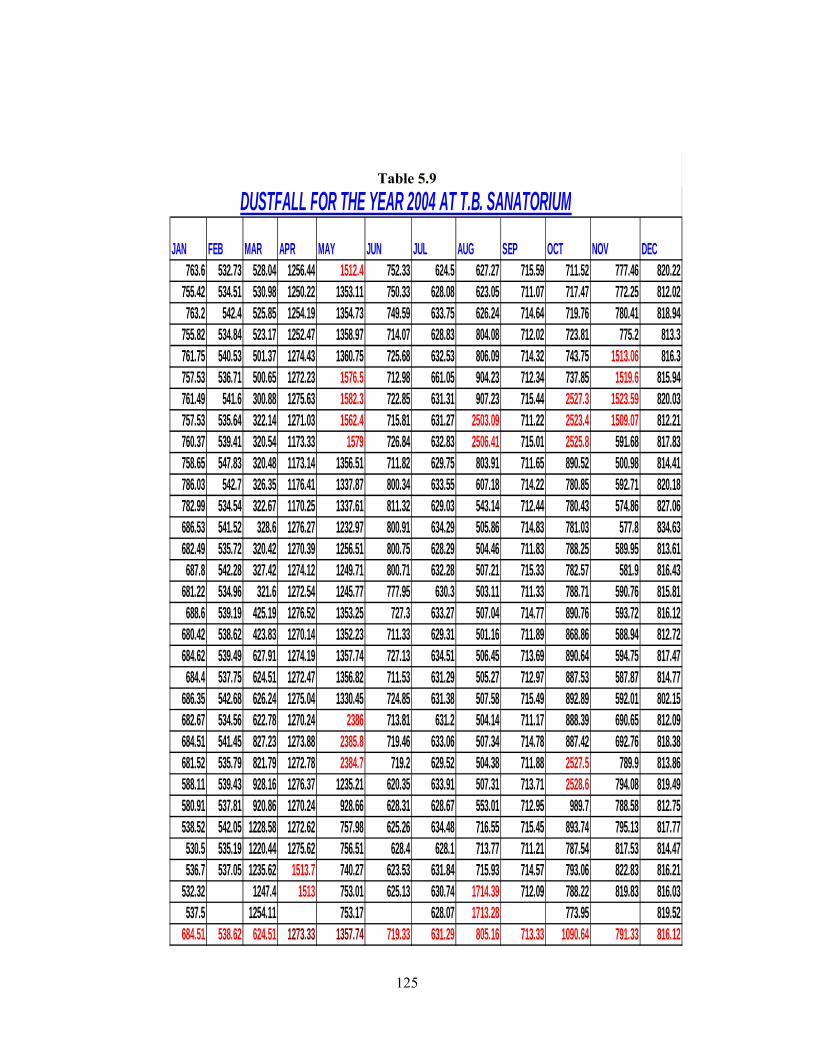
125
Table 5.9
JAN FEB MAR APR MAY JUN JUL AUG SEP OCT NOV DEC763.6 532.73 528.04 1256.44 1512.4 752.33 624.5 627.27 715.59 711.52 777.46 820.22
755.42 534.51 530.98 1250.22 1353.11 750.33 628.08 623.05 711.07 717.47 772.25 812.02763.2 542.4 525.85 1254.19 1354.73 749.59 633.75 626.24 714.64 719.76 780.41 818.94
755.82 534.84 523.17 1252.47 1358.97 714.07 628.83 804.08 712.02 723.81 775.2 813.3761.75 540.53 501.37 1274.43 1360.75 725.68 632.53 806.09 714.32 743.75 1513.06 816.3757.53 536.71 500.65 1272.23 1576.5 712.98 661.05 904.23 712.34 737.85 1519.6 815.94761.49 541.6 300.88 1275.63 1582.3 722.85 631.31 907.23 715.44 2527.3 1523.59 820.03757.53 535.64 322.14 1271.03 1562.4 715.81 631.27 2503.09 711.22 2523.4 1509.07 812.21760.37 539.41 320.54 1173.33 1579 726.84 632.83 2506.41 715.01 2525.8 591.68 817.83758.65 547.83 320.48 1173.14 1356.51 711.82 629.75 803.91 711.65 890.52 500.98 814.41786.03 542.7 326.35 1176.41 1337.87 800.34 633.55 607.18 714.22 780.85 592.71 820.18782.99 534.54 322.67 1170.25 1337.61 811.32 629.03 543.14 712.44 780.43 574.86 827.06686.53 541.52 328.6 1276.27 1232.97 800.91 634.29 505.86 714.83 781.03 577.8 834.63682.49 535.72 320.42 1270.39 1256.51 800.75 628.29 504.46 711.83 788.25 589.95 813.61687.8 542.28 327.42 1274.12 1249.71 800.71 632.28 507.21 715.33 782.57 581.9 816.43
681.22 534.96 321.6 1272.54 1245.77 777.95 630.3 503.11 711.33 788.71 590.76 815.81688.6 539.19 425.19 1276.52 1353.25 727.3 633.27 507.04 714.77 890.76 593.72 816.12
680.42 538.62 423.83 1270.14 1352.23 711.33 629.31 501.16 711.89 868.86 588.94 812.72684.62 539.49 627.91 1274.19 1357.74 727.13 634.51 506.45 713.69 890.64 594.75 817.47684.4 537.75 624.51 1272.47 1356.82 711.53 631.29 505.27 712.97 887.53 587.87 814.77
686.35 542.68 626.24 1275.04 1330.45 724.85 631.38 507.58 715.49 892.89 592.01 802.15682.67 534.56 622.78 1270.24 2386 713.81 631.2 504.14 711.17 888.39 690.65 812.09684.51 541.45 827.23 1273.88 2385.8 719.46 633.06 507.34 714.78 887.42 692.76 818.38681.52 535.79 821.79 1272.78 2384.7 719.2 629.52 504.38 711.88 2527.5 789.9 813.86588.11 539.43 928.16 1276.37 1235.21 620.35 633.91 507.31 713.71 2528.6 794.08 819.49580.91 537.81 920.86 1270.24 928.66 628.31 628.67 553.01 712.95 989.7 788.58 812.75538.52 542.05 1228.58 1272.62 757.98 625.26 634.48 716.55 715.45 893.74 795.13 817.77530.5 535.19 1220.44 1275.62 756.51 628.4 628.1 713.77 711.21 787.54 817.53 814.47536.7 537.05 1235.62 1513.7 740.27 623.53 631.84 715.93 714.57 793.06 822.83 816.21
532.32 1247.4 1513 753.01 625.13 630.74 1714.39 712.09 788.22 819.83 816.03537.5 1254.11 753.17 628.07 1713.28 773.95 819.52
684.51 538.62 624.51 1273.33 1357.74 719.33 631.29 805.16 713.33 1090.64 791.33 816.12
DUSTFALL FOR THE YEAR 2004 AT T.B. SANATORIUM
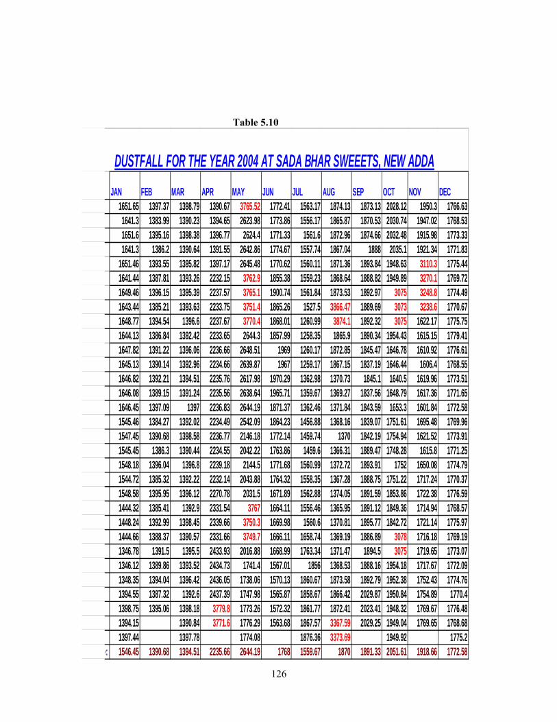
126
Table 5.10
JAN FEB MAR APR MAY JUN JUL AUG SEP OCT NOV DEC1651.65 1397.37 1398.79 1390.67 3765.52 1772.41 1563.17 1874.13 1873.13 2028.12 1950.3 1766.631641.3 1383.99 1390.23 1394.65 2623.98 1773.86 1556.17 1865.87 1870.53 2030.74 1947.02 1768.531651.6 1395.16 1398.38 1396.77 2624.4 1771.33 1561.6 1872.96 1874.66 2032.48 1915.98 1773.331641.3 1386.2 1390.64 1391.55 2642.86 1774.67 1557.74 1867.04 1888 2035.1 1921.34 1771.83
1651.46 1393.55 1395.82 1397.17 2645.48 1770.62 1560.11 1871.36 1893.84 1948.63 3110.3 1775.441641.44 1387.81 1393.26 2232.15 3762.9 1855.38 1559.23 1868.64 1888.82 1949.89 3270.1 1769.721649.46 1396.15 1395.39 2237.57 3765.1 1900.74 1561.84 1873.53 1892.97 3075 3248.8 1774.491643.44 1385.21 1393.63 2233.75 3751.4 1865.26 1527.5 3866.47 1889.69 3073 3238.6 1770.671648.77 1394.54 1396.6 2237.67 3770.4 1868.01 1260.99 3874.1 1892.32 3075 1622.17 1775.751644.13 1386.84 1392.42 2233.65 2644.3 1857.99 1258.35 1865.9 1890.34 1954.43 1615.15 1779.411647.82 1391.22 1396.06 2236.66 2648.51 1969 1260.17 1872.85 1845.47 1646.78 1610.92 1776.611645.13 1390.14 1392.96 2234.66 2639.87 1967 1259.17 1867.15 1837.19 1646.44 1606.4 1768.551646.82 1392.21 1394.51 2235.76 2617.98 1970.29 1362.98 1370.73 1845.1 1640.5 1619.96 1773.511646.08 1389.15 1391.24 2235.56 2638.64 1965.71 1359.67 1369.27 1837.56 1648.79 1617.36 1771.651646.45 1397.09 1397 2236.83 2644.19 1871.37 1362.46 1371.84 1843.59 1653.3 1601.84 1772.581545.46 1384.27 1392.02 2234.49 2542.09 1864.23 1456.88 1368.16 1839.07 1751.61 1695.48 1769.961547.45 1390.68 1398.58 2236.77 2146.18 1772.14 1459.74 1370 1842.19 1754.94 1621.52 1773.911545.45 1386.3 1390.44 2234.55 2042.22 1763.86 1459.6 1366.31 1889.47 1748.28 1615.8 1771.251548.18 1396.04 1396.8 2239.18 2144.5 1771.68 1560.99 1372.72 1893.91 1752 1650.08 1774.791544.72 1385.32 1392.22 2232.14 2043.88 1764.32 1558.35 1367.28 1888.75 1751.22 1717.24 1770.371548.58 1395.95 1396.12 2270.78 2031.5 1671.89 1562.88 1374.05 1891.59 1853.86 1722.38 1776.591444.32 1385.41 1392.9 2331.54 3767 1664.11 1556.46 1365.95 1891.12 1849.36 1714.94 1768.571448.24 1392.99 1398.45 2339.66 3750.3 1669.98 1560.6 1370.81 1895.77 1842.72 1721.14 1775.971444.66 1388.37 1390.57 2331.66 3749.7 1666.11 1658.74 1369.19 1886.89 3078 1716.18 1769.191346.78 1391.5 1395.5 2433.93 2016.88 1668.99 1763.34 1371.47 1894.5 3075 1719.65 1773.071346.12 1389.86 1393.52 2434.73 1741.4 1567.01 1856 1368.53 1888.16 1954.18 1717.67 1772.091348.35 1394.04 1396.42 2436.05 1738.06 1570.13 1860.67 1873.58 1892.79 1952.38 1752.43 1774.761394.55 1387.32 1392.6 2437.39 1747.98 1565.87 1858.67 1866.42 2029.87 1950.84 1754.89 1770.41398.75 1395.06 1398.18 3779.8 1773.26 1572.32 1861.77 1872.41 2023.41 1948.32 1769.67 1776.481394.15 1390.84 3771.6 1776.29 1563.68 1867.57 3367.59 2029.25 1949.04 1769.65 1768.681397.44 1397.78 1774.08 1876.36 3373.69 1949.92 1775.2
e: 1546.45 1390.68 1394.51 2235.66 2644.19 1768 1559.67 1870 1891.33 2051.61 1918.66 1772.58
DUSTFALL FOR THE YEAR 2004 AT SADA BHAR SWEEETS, NEW ADDA
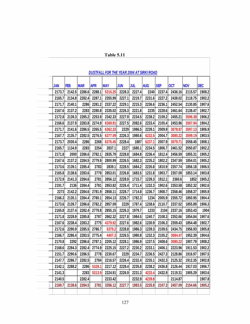
127
Table 5.11
JAN FEB MAR APR MAY JUN JUL AUG SEP OCT NOV DEC2173.7 2142.5 2286.6 2288.1 5316.25 2228.3 2227.4 2240 2237.4 2436.16 2115.57 1908.22165.7 2134.8 2282.4 2287.1 2355.99 2227.1 2219.7 2231.6 2227.2 2438.02 2118.75 1902.22171.7 2140.1 2286 2281.2 2337.22 2229.1 2215.3 2236.6 2236.1 2452.54 2130.85 1907.62167.6 2137.2 2283 2280.8 2335.02 2226.3 2221.8 2235 2228.6 2461.64 2138.47 1902.72172.8 2139.3 2285.2 2253.9 2342.33 2227.9 2234.5 2238.2 2109.2 2455.21 3596.38 1906.22166.6 2137.9 2283.8 2274.9 6369.91 2227.5 2082.6 2233.4 2105.4 2453.96 3597.94 1904.22171.7 2141.6 2286.5 2265.5 6362.33 2229 1986.5 2239.1 2009.9 3078.97 3597.13 1906.92167.7 2135.7 2282.5 2276.5 6377.09 2226.3 1980.6 6232.5 2004.7 3080.22 3599.19 1903.52173.7 2030.4 2286 2268 6376.45 2228.4 1887 6237.1 2007.9 3079.71 2058.45 1908.12165.7 1134.9 2283 2254 2837.1 2227 1680.1 2234.5 1806.7 2461.52 2050.87 1902.22171.8 2000 2286.6 2782.1 2835.79 2228.8 1684.8 2236.4 1812.4 2456.59 1855.31 1905.22167.6 2137.2 2284.5 2779.9 2800.99 2226.5 1682.3 2235.2 1802.2 2347.59 1854.01 1905.22173.6 2139.1 2285.4 2783 2839.1 2228.5 1684.2 2235.8 1810.9 2357.74 1856.18 1906.52165.8 2138.6 2283.6 2779 2853.01 2226.8 1683.5 1231.8 1903.7 2357.09 1853.14 1903.82172.9 2141.3 2284.6 2781 2856.12 2228.9 1715.7 1239.3 1912.1 2360.6 1852 1905.22191.7 2136 2284.4 2781 2853.82 2226.4 1711.4 1232.3 1902.6 2353.58 1852.32 1902.6
2273 2142.2 2284.6 2781.9 2858.11 2228.7 1714.8 1236.7 1908.7 2358.46 1858.37 1905.92166.3 2135.1 2284.4 2780.1 2854.13 2226.7 1782.3 1234 2005.9 2355.72 1850.95 1904.42173.6 2139.7 2286.6 2782.2 2857.09 2229 1787.4 1238.6 2110.7 2337.02 1855.89 1906.32165.8 2137.4 2282.4 2779.8 2855.15 2226.3 1979.7 1233 2104 2337.16 1853.43 19042171.8 2228.9 2285.8 2787 2862.32 2227.8 1984.5 1240.7 2108.3 2352.66 1854.84 1907.62167.6 2238.4 2283.2 2775 4379.92 2227.6 1982.6 1230.9 2106.3 2359.43 1854.48 1902.72172.6 2290.9 2285.5 2786.7 5379.2 2228.8 1986.3 1239.3 2109.5 2434.75 1956.93 1905.82166.7 2286.4 2283.5 2775.4 4407.3 2226.5 1980.8 1232.3 2105.2 3084.47 1952.39 1904.62170.8 2292 2286.6 2787.1 2205.12 2228.1 1986.9 1237.5 2408.6 3080.22 1907.79 1908.22168.6 2284.3 2282.4 2774.9 2225.15 2227.2 2230.2 2233.1 2406.1 2223.96 1911.53 1902.22151.7 2290.6 2286.5 2778 2230.67 2229 2234.7 2236.5 2427.3 2128.86 1916.97 1907.52147.7 2286.7 2282.5 2784 2216.57 2226.4 2232.4 2235.1 2432.3 2125.32 1912.35 1902.82142.1 2288.2 2286 5328.1 2217.12 2228.4 2235.8 2238.2 2436.8 2126.44 1917.03 1906.72141.3 2283 5313.9 2224.91 2226.9 2231.3 4233.4 2432.9 2119.31 1905.29 1903.62140.5 2282.4 2233.42 2232.9 4239.8 2114.87 1907.8
: 2169.7 2138.6 2284.5 2781 3356.12 2227.7 1983.5 2235.8 2107.3 2457.09 2154.66 1905.2
DUSTFALL FOR THE YEAR 2004 AT SIRKI ROAD
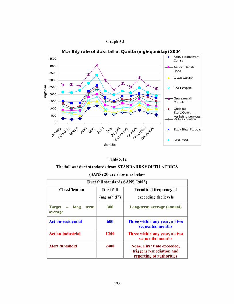
128
Graph 5.1
Monthly rate of dust fall at Quetta (mg/sq.m/day) 2004
0
500
1000
1500
2000
2500
3000
3500
4000
4500
Janu
ary
Febr
uary
March
April
May
June Ju
ly
Augus
t
Septem
ber
Octobe
r
Novem
ber
Decem
ber
Months
mg/
sq.m
Army Recruitment Centre
Ashraf SariabRoad
C.G.S Colony
Civil Hospital
Gaw almandiChow k
QadoosiStore/QuickMarketing servicesRailw ay Station
Sada Bhar Sw eets
Sirki Road
Table 5.12
The fall-out dust standards from STANDARDS SOUTH AFRICA
(SANS) 20 are shown as below
Dust fall standards SANS (2005)
Classification Dust fall
(mg m-2 d-1)
Permitted frequency of
exceeding the levels
Target – long term average
300 Long-term average (annual)
Action-residential 600 Three within any year, no two sequential months
Action-industrial 1200 Three within any year, no two sequential months
Alert threshold 2400 None. First time exceeded, triggers remediation and reporting to authorities
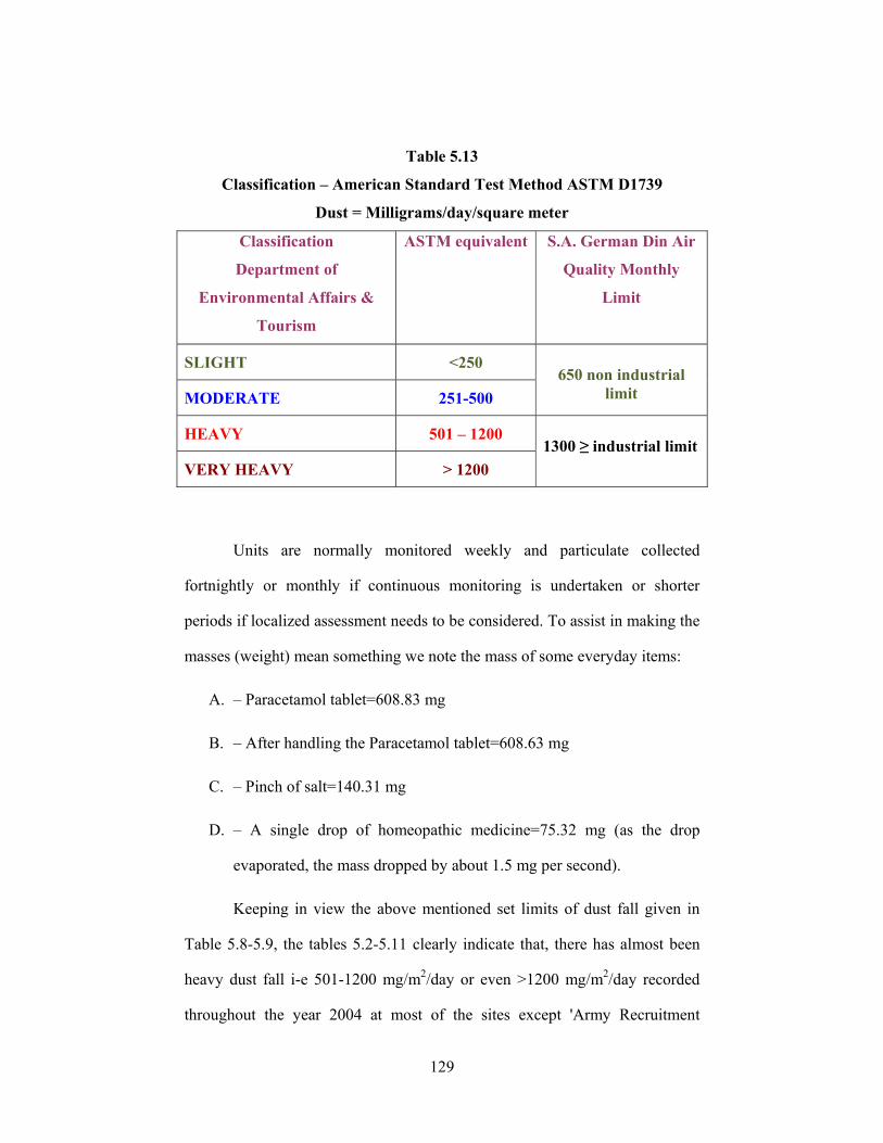
129
Table 5.13
Classification – American Standard Test Method ASTM D1739
Dust = Milligrams/day/square meter
Classification
Department of
Environmental Affairs &
Tourism
ASTM equivalent S.A. German Din Air
Quality Monthly
Limit
SLIGHT <250 650 non industrial
limit MODERATE 251-500
HEAVY 501 – 1200 1300 ≥ industrial limit
VERY HEAVY > 1200
Units are normally monitored weekly and particulate collected
fortnightly or monthly if continuous monitoring is undertaken or shorter
periods if localized assessment needs to be considered. To assist in making the
masses (weight) mean something we note the mass of some everyday items:
A. – Paracetamol tablet=608.83 mg
B. – After handling the Paracetamol tablet=608.63 mg
C. – Pinch of salt=140.31 mg
D. – A single drop of homeopathic medicine=75.32 mg (as the drop
evaporated, the mass dropped by about 1.5 mg per second).
Keeping in view the above mentioned set limits of dust fall given in
Table 5.8-5.9, the tables 5.2-5.11 clearly indicate that, there has almost been
heavy dust fall i-e 501-1200 mg/m2/day or even >1200 mg/m2/day recorded
throughout the year 2004 at most of the sites except 'Army Recruitment
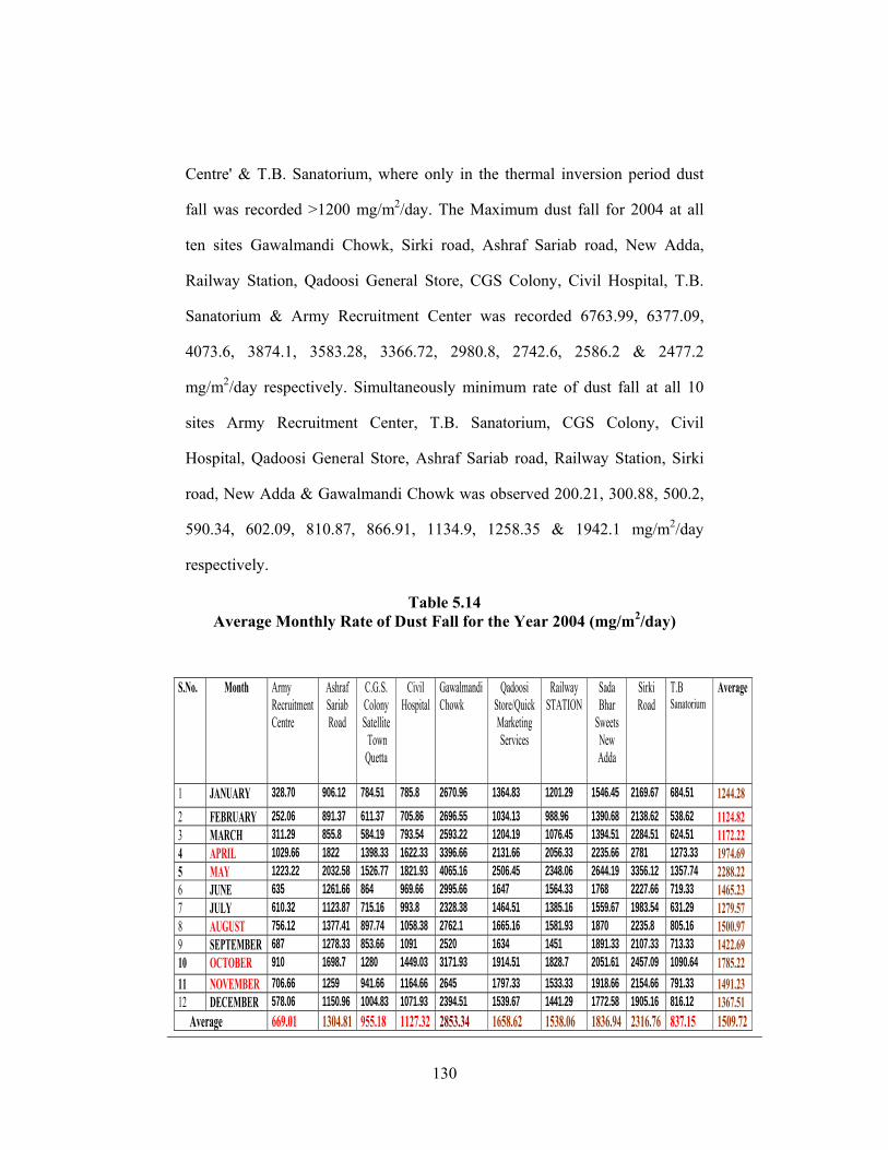
130
Centre' & T.B. Sanatorium, where only in the thermal inversion period dust
fall was recorded >1200 mg/m2/day. The Maximum dust fall for 2004 at all
ten sites Gawalmandi Chowk, Sirki road, Ashraf Sariab road, New Adda,
Railway Station, Qadoosi General Store, CGS Colony, Civil Hospital, T.B.
Sanatorium & Army Recruitment Center was recorded 6763.99, 6377.09,
4073.6, 3874.1, 3583.28, 3366.72, 2980.8, 2742.6, 2586.2 & 2477.2
mg/m2/day respectively. Simultaneously minimum rate of dust fall at all 10
sites Army Recruitment Center, T.B. Sanatorium, CGS Colony, Civil
Hospital, Qadoosi General Store, Ashraf Sariab road, Railway Station, Sirki
road, New Adda & Gawalmandi Chowk was observed 200.21, 300.88, 500.2,
590.34, 602.09, 810.87, 866.91, 1134.9, 1258.35 & 1942.1 mg/m2/day
respectively.
Table 5.14 Average Monthly Rate of Dust Fall for the Year 2004 (mg/m2/day)
S.No. Month Army Recruitment Centre
Ashraf Sariab Road
C.G.S. Colony Satellite Town Quetta
Civil Hospital
Gawalmandi Chowk
Qadoosi Store/Quick Marketing Services
Railway STATION
Sada Bhar
Sweets New Adda
Sirki Road
T.B Sanatorium
Average
1 JANUARY 328.70 906.12 784.51 785.8 2670.96 1364.83 1201.29 1546.45 2169.67 684.51 1244.28 2 FEBRUARY 252.06 891.37 611.37 705.86 2696.55 1034.13 988.96 1390.68 2138.62 538.62 1124.82 3 MARCH 311.29 855.8 584.19 793.54 2593.22 1204.19 1076.45 1394.51 2284.51 624.51 1172.22 4 APRIL 1029.66 1822 1398.33 1622.33 3396.66 2131.66 2056.33 2235.66 2781 1273.33 1974.69 5 MAY 1223.22 2032.58 1526.77 1821.93 4065.16 2506.45 2348.06 2644.19 3356.12 1357.74 2288.22 6 JUNE 635 1261.66 864 969.66 2995.66 1647 1564.33 1768 2227.66 719.33 1465.23 7 JULY 610.32 1123.87 715.16 993.8 2328.38 1464.51 1385.16 1559.67 1983.54 631.29 1279.57 8 AUGUST 756.12 1377.41 897.74 1058.38 2762.1 1665.16 1581.93 1870 2235.8 805.16 1500.97 9 SEPTEMBER 687 1278.33 853.66 1091 2520 1634 1451 1891.33 2107.33 713.33 1422.69 10 OCTOBER 910 1698.7 1280 1449.03 3171.93 1914.51 1828.7 2051.61 2457.09 1090.64 1785.22 11 NOVEMBER 706.66 1259 941.66 1164.66 2645 1797.33 1533.33 1918.66 2154.66 791.33 1491.23 12 DECEMBER 578.06 1150.96 1004.83 1071.93 2394.51 1539.67 1441.29 1772.58 1905.16 816.12 1367.51 Average 669.01 1304.81 955.18 1127.32 2853.34 1658.62 1538.06 1836.94 2316.76 837.15 1509.72
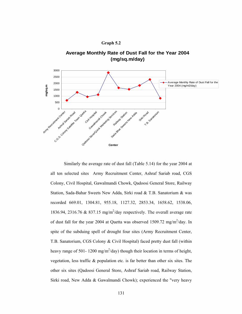
131
Graph 5.2
Average Monthly Rate of Dust Fall for the Year 2004 (mg/sq.m/day)
0
500
1000
1500
2000
2500
3000
Army R
ecrui
tmen
t Cen
ter
Ashraf
Sariab R
oad
C.G.S. C
olony
Sate
llite To
wn Que
tta
Civil H
ospita
l
Gawalm
andi C
howk
Qadoo
si Store/
Quick M
arketi
ng Servi
ces
Railway
Station
Sada B
har S
weets
New A
dda
Sirki R
oad
T.B. San
atoriu
m
Center
mg/
sq.m
Average Monthly Rate of Dust Fall for theYear 2004 (mg/m2/day)
Similarly the average rate of dust fall (Table 5.14) for the year 2004 at
all ten selected sites Army Recruitment Center, Ashraf Sariab road, CGS
Colony, Civil Hospital, Gawalmandi Chowk, Qadoosi General Store, Railway
Station, Sada-Bahar Sweets New Adda, Sirki road & T.B. Sanatorium & was
recorded 669.01, 1304.81, 955.18, 1127.32, 2853.34, 1658.62, 1538.06,
1836.94, 2316.76 & 837.15 mg/m2/day respectively. The overall average rate
of dust fall for the year 2004 at Quetta was observed 1509.72 mg/m2/day. In
spite of the subduing spell of drought four sites (Army Recruitment Center,
T.B. Sanatorium, CGS Colony & Civil Hospital) faced pretty dust fall (within
heavy range of 501- 1200 mg/m2/day) though their location in terms of height,
vegetation, less traffic & population etc. is far better than other six sites. The
other six sites (Qadoosi General Store, Ashraf Sariab road, Railway Station,
Sirki road, New Adda & Gawalmandi Chowk); experienced the "very heavy

132
dust fall" (> 1200 mg/m2/day) or even more than set Industrial limit (> 1300
mg/m2/day). Two sites out of these six sites even touched or crossed the "alert
threshold limit" (2400 mg/m2/day). We the residents of Quetta bewilderedly
experienced the phenomenon of thermal inversion in our life span for the very
first time. During the periods/days of thermal inversion in 2004 (on 29-30
April, 01May, 06-09 May, 22-24 May, 07-09 October, 25-30 October & 05-08
November) heavy dust cloud wrapped the whole Quetta valley. The dust fall
data collected in those particular days even at the minimum dust receiving
stations in normal conditions (Army Recruitment Center & T.B. Sanatorium)
was significantly heavy or even beyond the alert threshold limits not to speak
of rest of the sites. The distinctiveness of my research work was that
painstaking collection of samples on daily basis for the year 2004 (though
some days collection for some days in the said year 2004 couldn’t be done due
to law and order and other reasons, the values were assessed with the
contemporary value of other sides on the same missing days with the mean
average of the value of the same site), when in the days of thermal inversion
on daily basis dust fall was recorded. Those days (the readings of which have
been highlighted in red color) were 29th, 30th April, 1st, 6th-9th May, 22nd May
to 24th May, 8th-9th August, 30th, 31st August, 7th-9th October, 24th, 25th October
& 5th-8th November 2004. The dust fall recorded in those was exceptionally
high. Having been trapped under the warm lid the fine and ultra-fine
particulates of dust remained suspended in the atmosphere for a long time and
wrapped the city in those continuous days. Luckily from the point of view of
environmentalists though Quetta doesn’t have heavy industry, in spite of the
absence of photochemical smog, the dust particulates triggered the intensity of
133
diseases of the patients already had been suffering with asthma, tuberculosis,
angina, depression, anxiety, blood pressure etc. Further it harmed and
aggravated the already suffering growth of vegetation. Flights were cancelled
and markets, public places & streets turned deserted caused the business
activities bearish as well. The absence of heavy industry resulted in the
absence of photochemical smog and proved to be a blessing in disguise for
Quettaites as, inhabitants of the city didn’t face the worst situations as the
population of London, Donora, Los Angeles etc. had to face, which caused
massive causalities within few days. Because of the bowl shape of the Quetta
valley, the said dust during the thermal inversion periods took normally 4-5 or
sometimes even 7 days to completely settle down/sink in a deadly calm wind
or got diluted/cleared by drifting away with the wind as soon as the lid of
warm inversion layer gradually removed by the changing wind pattern,
atmospheric pressure and temperature. From Table A-J it can also simply be
deduced that dust fall varies from place to place and from time to time having
great importance as it could give some idea about the local factors, which
could contribute to the atmospheric dust fall and would be summed up in the
end of discussion.
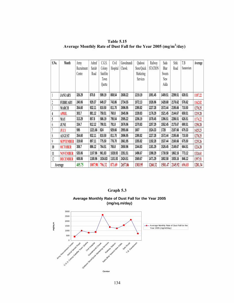
134
Table 5.15 Average Monthly Rate of Dust Fall for the Year 2005 (mg/m2/day)
S.No. Month Army Recruitment Centre
Ashraf Sariab Road
C.G.S. Colony Satellite Town Quetta
Civil Hospital
Gawalmandi Chowk
Qadoosi Store/Quick Marketing Services
Railway STATION
Sada Bhar
Sweets New Adda
Sirki Road
T.B Sanatorium
Average
1 JANUARY 326.29 870.8 599.19 808.54 2608.22 1219.19 1091.45 1409.51 2299.51 639.51 1187.22 2 FEBRUARY 240.06 929.37 649.37 743.86 2734.55 1072.13 1026.96 1428.68 2176.62 576.62 1162.82 3 MARCH 354.60 932.11 810.50 811.70 2696.95 1390.82 1227.28 1572.44 2195.66 710.50 1270.25 4 APRIL 303.7 881.12 759.51 760.8 2645.96 1339.83 1176.29 1521.45 2144.67 659.51 1219.28 5 MAY 313.29 857.8 586.19 795.54 2595.22 1206.19 1078.45 1396.51 2286.51 626.51 1174.22 6 JUNE 334.7 912.12 790.51 791.8 2676.96 1370.83 1207.29 1552.45 2175.67 690.51 1250.28 7 JULY 595 1221.66 824 929.66 2955.66 1607 1524.33 1728 2187.66 679.33 1425.23 8 AUGUST 354.60 932.11 810.50 811.70 2696.95 1390.82 1227.28 1572.44 2195.66 710.50 1270.25 9 SEPTEMBER 319.60 897.11 775.50 776.70 2661.95 1355.82 1192.28 1537.44 2160.66 675.50 1235.26 10 OCTOBER 308.7 886.12 764.51 765.8 2650.96 1344.83 1181.29 1526.45 2149.67 664.51 1224.28 11 NOVEMBER 535.06 1107.96 961.83 1028.93 2351.51 1496.67 1398.29 1730.58 1862.16 773.12 1324.61 12 DECEMBER 608.06 1180.96 1034.83 1101.93 2424.51 1569.67 1471.29 1802.58 1935.16 846.12 1397.51 Average 405.75 1007.98 796.32 873.69 2657.86 1383.95 1260.32 1581.47 2145.92 696.03 1281.34
Graph 5.3
Average Monthly Rate of Dust Fall for the Year 2005 (mg/sq.m/day)
0
500
1000
1500
2000
2500
3000
Army R
ecrui
tmen
t Cen
ter
Ashraf
Sariab R
oad
C.G.S. C
olony
Sate
llite To
wn Que
tta
Civil H
ospita
l
Gawalm
andi C
howk
Qadoo
si Store/
Quick M
arketi
ng Servi
ces
Railway
Station
Sada B
har S
weets
New A
dda
Sirki R
oad
T.B. San
atoriu
m
Center
mg/
sq.m
Average Monthly Rate of Dust Fall for theYear 2005 (mg/m2/day)

135
Graph 5.4
Average Monthly Rate of Dust fall for the year 2005 (mg/sq.m/day)
0
500
1000
1500
2000
2500
3000
3500
Jan Feb Mar Apr May Jun Jul Aug Sep Oct Nov Dec
Months
mg/
sq.m
Army Recruitment Center
Ashraf Sariab Road
C.G.S. Colony Satellite Tow nQuettaCivil Hospital
Gaw almandi Chow k
Qadoosi Store/Quick MarketingServicesRailw ay Station
Sada Bhar Sw eets New Adda
Sirki Road
T.B. Sanatorium
After a marathon dry spell at last in December 2004 Quetta received
40.2mm rainfall and in the beginning of 2005 town was hit by heavy down
pour in January, February & March having 33.7, 129.2 & 63.3mm of rainfall.
Keeping in view the drastic change in weather, the samples were started to be
collected with the interval of every one calendar month from all the same 10
sites. Further it was humanly impossible as well to continue the collection on
daily basis. The average rate of dust fall observed on all ten selected sites
Army Recruitment Center, Ashraf Sariab road, CGS Colony, Civil Hospital,
Gawalmandi Chowk, Qadoosi General Store, Railway Station, Sada-Bahar
Sweets New Adda, Sirki road & T.B. Sanatorium & was recorded 405.75,
1007.98, 796.32, 873.69, 2657.88, 1383.95, 1260.32, 1581.47, 2145.47 &
696.03 mg/m2/day respectively. The overall average rate of dust fall for the
year 2005 was recorded 1281.34 mg/m2/day, which is significantly less
(228.38 mg/m2/day) than the overall average of the year 2004. It is evident
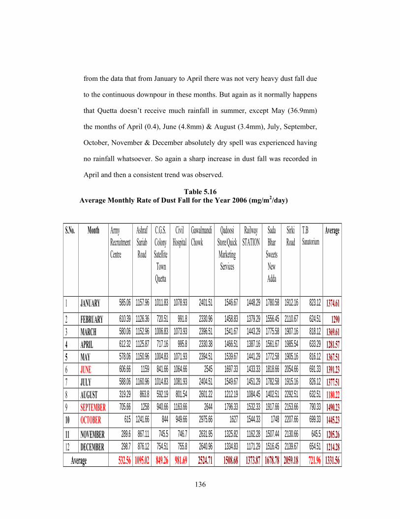
136
from the data that from January to April there was not very heavy dust fall due
to the continuous downpour in these months. But again as it normally happens
that Quetta doesn’t receive much rainfall in summer, except May (36.9mm)
the months of April (0.4), June (4.8mm) & August (3.4mm), July, September,
October, November & December absolutely dry spell was experienced having
no rainfall whatsoever. So again a sharp increase in dust fall was recorded in
April and then a consistent trend was observed.
Table 5.16 Average Monthly Rate of Dust Fall for the Year 2006 (mg/m2/day)
S.No. Month Army Recruitment Centre
Ashraf Sariab Road
C.G.S. Colony Satellite Town Quetta
Civil Hospital
Gawalmandi Chowk
Qadoosi Store/Quick Marketing Services
Railway STATION
Sada Bhar
Sweets New Adda
Sirki Road
T.B Sanatorium
Average
1 JANUARY 585.06 1157.96 1011.83 1078.93 2401.51 1546.67 1448.29 1780.58 1912.16 823.12 1374.612 FEBRUARY 610.39 1126.36 720.51 991.8 2330.96 1458.83 1379.29 1556.45 2110.67 624.51 12903 MARCH 580.06 1152.96 1006.83 1073.93 2396.51 1541.67 1443.29 1775.58 1907.16 818.12 1369.614 APRIL 612.32 1125.87 717.16 995.8 2330.38 1466.51 1387.16 1561.67 1985.54 633.29 1281.575 MAY 578.06 1150.96 1004.83 1071.93 2394.51 1539.67 1441.29 1772.58 1905.16 816.12 1367.516 JUNE 606.66 1159 841.66 1064.66 2545 1697.33 1433.33 1818.66 2054.66 691.33 1391.237 JULY 588.06 1160.96 1014.83 1081.93 2404.51 1549.67 1451.29 1782.58 1915.16 826.12 1377.518 AUGUST 319.29 863.8 592.19 801.54 2601.22 1212.19 1084.45 1402.51 2292.51 632.51 1180.229 SEPTEMBER 705.66 1258 940.66 1163.66 2644 1796.33 1532.33 1917.66 2153.66 790.33 1490.2310 OCTOBER 615 1241.66 844 949.66 2975.66 1627 1544.33 1748 2207.66 699.33 1445.2311 NOVEMBER 289.6 867.11 745.5 746.7 2631.95 1325.82 1162.28 1507.44 2130.66 645.5 1205.2612 DECEMBER 298.7 876.12 754.51 755.8 2640.96 1334.83 1171.29 1516.45 2139.67 654.51 1214.28 Average 532.56 1095.02 849.26 981.69 2524.71 1508.68 1373.87 1678.78 2059.18 721.96 1331.56
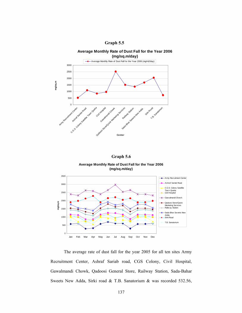
137
Graph 5.5
Average Monthly Rate of Dust Fall for the Year 2006 (mg/sq.m/day)
0
500
1000
1500
2000
2500
3000
Army R
ecrui
tmen
t Cen
ter
Ashraf
Sariab R
oad
C.G.S. C
olony
Sate
llite To
wn Que
tta
Civil H
ospita
l
Gawalm
andi C
howk
Qadoo
si Store/
Quick M
arketi
ng Servi
ces
Railway
Station
Sada B
har S
weets
New A
dda
Sirki R
oad
T.B. San
atoriu
m
Center
mg/
sq.m
Average Monthly Rate of Dust Fall for the Year 2006 (mg/m2/day)
Graph 5.6
Average Monthly Rate of Dust Fall for the Year 2006 (mg/sq.m/day)
0
500
1000
1500
2000
2500
3000
3500
Jan Feb Mar Apr May Jun Jul Aug Sep Oct Nov Dec
mg/
sq.m
Army Recruitment Center
Ashraf Sariab Road
C.G.S. Colony SatelliteTow n QuettaCivil Hospital
Gaw almandi Chow k
Qadoosi Store/QuickMarketing ServicesRailw ay Station
Sada Bhar Sw eets NewAddaSirki Road
T.B. Sanatorium
The average rate of dust fall for the year 2005 for all ten sites Army
Recruitment Center, Ashraf Sariab road, CGS Colony, Civil Hospital,
Gawalmandi Chowk, Qadoosi General Store, Railway Station, Sada-Bahar
Sweets New Adda, Sirki road & T.B. Sanatorium & was recorded 532.56,
138
1095.02, 849.26, 2524.71, 1508.68, 1373.87, 1678.78, 2059.18 & 721.96
mg/m2/day respectively. Similarly the overall average of the year 2005 was
1331.56 mg/m2/day, which is slightly more (50.22 mg/m2/day) than the
previous year 2005. It was again because of the change in weather as the
precipitation occurred during March, August, November & December 2006
was 26.1, 54.9, 46.9 & 43.8mm respectively, while rest of the 08 months
received meager drizzling. The maximum dust fall during the year 2006 was
recorded in the mid of year due to the earlier described one peculiar
metrological conditions of low atmospheric pressure in the mid of summer
from May up to September, high winds & geographical location of Quetta.
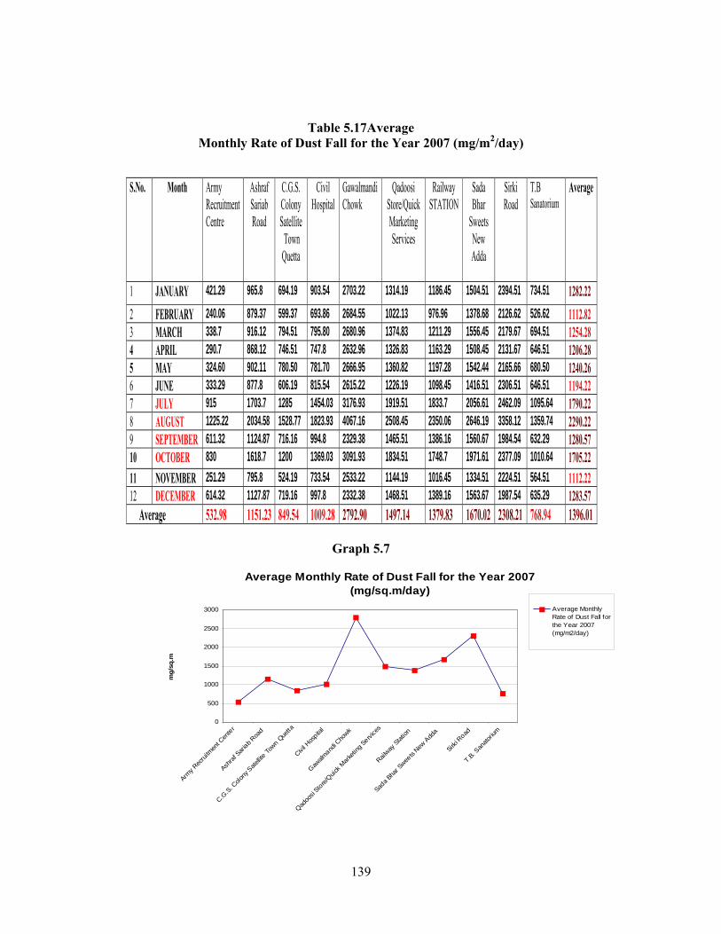
139
Table 5.17Average Monthly Rate of Dust Fall for the Year 2007 (mg/m2/day)
S.No. Month Army Recruitment Centre
Ashraf Sariab Road
C.G.S. Colony Satellite Town Quetta
Civil Hospital
Gawalmandi Chowk
Qadoosi Store/Quick Marketing Services
Railway STATION
Sada Bhar
Sweets New Adda
Sirki Road
T.B Sanatorium
Average
1 JANUARY 421.29 965.8 694.19 903.54 2703.22 1314.19 1186.45 1504.51 2394.51 734.51 1282.22 2 FEBRUARY 240.06 879.37 599.37 693.86 2684.55 1022.13 976.96 1378.68 2126.62 526.62 1112.82 3 MARCH 338.7 916.12 794.51 795.80 2680.96 1374.83 1211.29 1556.45 2179.67 694.51 1254.28 4 APRIL 290.7 868.12 746.51 747.8 2632.96 1326.83 1163.29 1508.45 2131.67 646.51 1206.28 5 MAY 324.60 902.11 780.50 781.70 2666.95 1360.82 1197.28 1542.44 2165.66 680.50 1240.26 6 JUNE 333.29 877.8 606.19 815.54 2615.22 1226.19 1098.45 1416.51 2306.51 646.51 1194.22 7 JULY 915 1703.7 1285 1454.03 3176.93 1919.51 1833.7 2056.61 2462.09 1095.64 1790.22 8 AUGUST 1225.22 2034.58 1528.77 1823.93 4067.16 2508.45 2350.06 2646.19 3358.12 1359.74 2290.22 9 SEPTEMBER 611.32 1124.87 716.16 994.8 2329.38 1465.51 1386.16 1560.67 1984.54 632.29 1280.57 10 OCTOBER 830 1618.7 1200 1369.03 3091.93 1834.51 1748.7 1971.61 2377.09 1010.64 1705.22 11 NOVEMBER 251.29 795.8 524.19 733.54 2533.22 1144.19 1016.45 1334.51 2224.51 564.51 1112.22 12 DECEMBER 614.32 1127.87 719.16 997.8 2332.38 1468.51 1389.16 1563.67 1987.54 635.29 1283.57 Average 532.98 1151.23 849.54 1009.28 2792.90 1497.14 1379.83 1670.02 2308.21 768.94 1396.01
Graph 5.7
Average Monthly Rate of Dust Fall for the Year 2007
(mg/sq.m/day)
0
500
1000
1500
2000
2500
3000
Army R
ecrui
tmen
t Cen
ter
Ashra
f Sari
ab Roa
d
C.G.S. C
olony
Sate
llite To
wn Que
tta
Civil H
ospita
l
Gawalm
andi C
howk
Qadoo
si Store/
Quick M
arketi
ng Servi
ces
Railway
Station
Sada B
har S
weets
New A
dda
Sirki R
oad
T.B. San
atoriu
m
mg/
sq.m
Average MonthlyRate of Dust Fall forthe Year 2007(mg/m2/day)
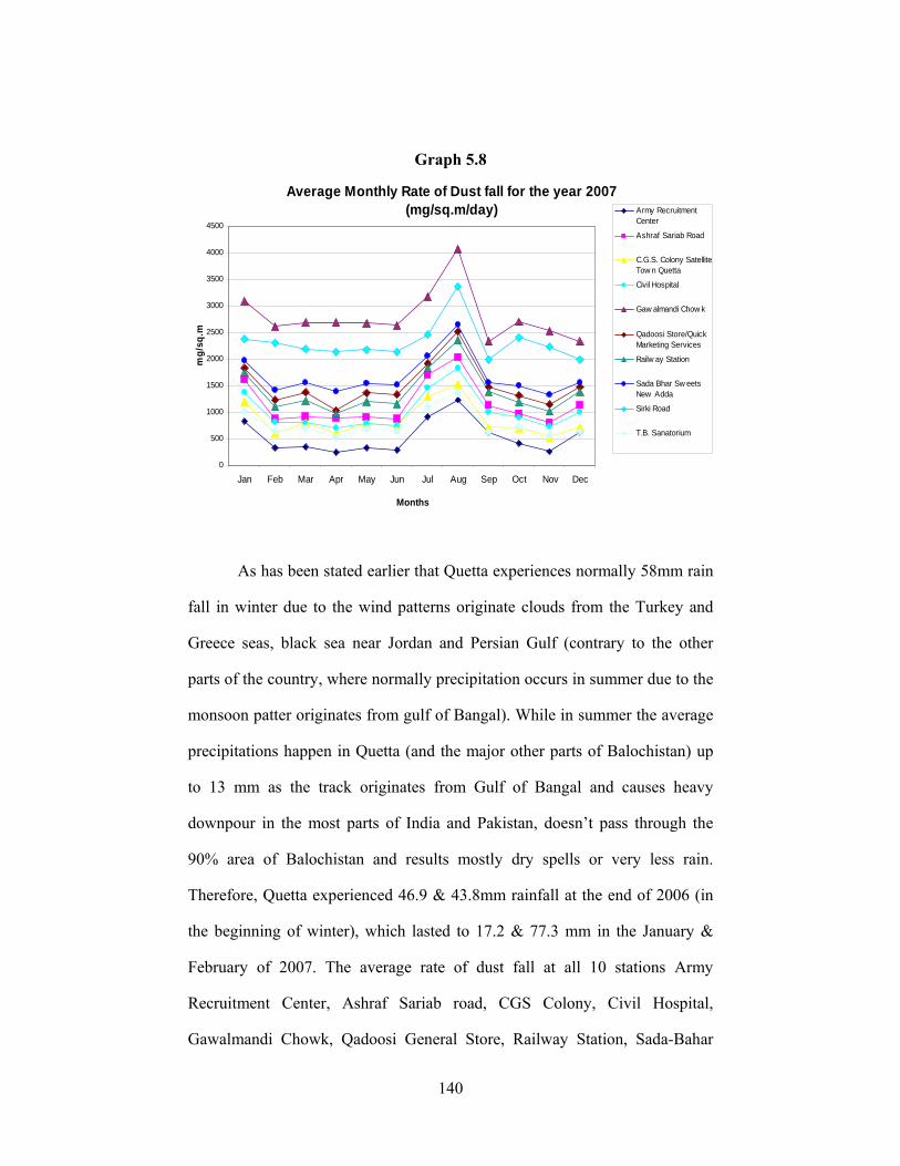
140
Graph 5.8
Average Monthly Rate of Dust fall for the year 2007 (mg/sq.m/day)
0
500
1000
1500
2000
2500
3000
3500
4000
4500
Jan Feb Mar Apr May Jun Jul Aug Sep Oct Nov Dec
Months
mg/
sq.m
Army RecruitmentCenter
Ashraf Sariab Road
C.G.S. Colony SatelliteTow n Quetta
Civil Hospital
Gaw almandi Chow k
Qadoosi Store/QuickMarketing Services
Railw ay Station
Sada Bhar Sw eetsNew Adda
Sirki Road
T.B. Sanatorium
As has been stated earlier that Quetta experiences normally 58mm rain
fall in winter due to the wind patterns originate clouds from the Turkey and
Greece seas, black sea near Jordan and Persian Gulf (contrary to the other
parts of the country, where normally precipitation occurs in summer due to the
monsoon patter originates from gulf of Bangal). While in summer the average
precipitations happen in Quetta (and the major other parts of Balochistan) up
to 13 mm as the track originates from Gulf of Bangal and causes heavy
downpour in the most parts of India and Pakistan, doesn’t pass through the
90% area of Balochistan and results mostly dry spells or very less rain.
Therefore, Quetta experienced 46.9 & 43.8mm rainfall at the end of 2006 (in
the beginning of winter), which lasted to 17.2 & 77.3 mm in the January &
February of 2007. The average rate of dust fall at all 10 stations Army
Recruitment Center, Ashraf Sariab road, CGS Colony, Civil Hospital,
Gawalmandi Chowk, Qadoosi General Store, Railway Station, Sada-Bahar
141
Sweets New Adda, Sirki road & T.B. Sanatorium for the year 2007was
recorded 532.98, 1151.23, 849.54, 1009.28, 2792.90, 1497.14, 1379.83,
1670.02, 2308.21 & 768.94 mg/m2/day respectively. So a descending trend
was observed till February and a consistent horizontal movement (Graph 5.8)
was witnessed from February to June due to the 20.1, 8.1 & 34.4 mm rainfall.
But from May and particularly soon after June a sharp increase in dust fall was
observed again due to very low atmospheric pressure and very little or no
precipitation in the successive months. Then again there was a sudden
decrease happened up to the mid of November and then finally little increase
took place in the dust fall till December due to the rather high atmospheric
pressure and calm weather and bearish activity in the markets of Quetta
though there was extremely low (5.0mm) rainfall recorded in December. The
reason of the lesser population of inhabitants and traffic is because of the
severe cold weather of the city as most of the population shifts to the hotter
places of the province and other parts of the country at the beginning of winter
as soon as the educational institutions are closed for winter vacations. The
overall rate of dust fall for the year 2007 detected 1396.01 mg/m2/day, was
again (64.45 mg/m2/day) more than the previous year 2006.
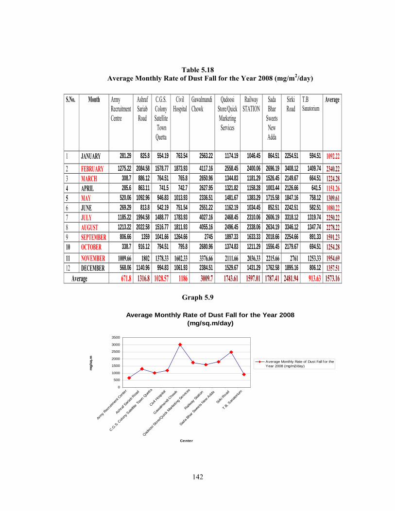
142
Table 5.18 Average Monthly Rate of Dust Fall for the Year 2008 (mg/m2/day)
S.No. Month Army Recruitment Centre
Ashraf Sariab Road
C.G.S. Colony Satellite Town Quetta
Civil Hospital
Gawalmandi Chowk
Qadoosi Store/Quick Marketing Services
Railway STATION
Sada Bhar
Sweets New Adda
Sirki Road
T.B Sanatorium
Average
1 JANUARY 281.29 825.8 554.19 763.54 2563.22 1174.19 1046.45 864.51 2254.51 594.51 1092.222 FEBRUARY 1275.22 2084.58 1578.77 1873.93 4117.16 2558.45 2400.06 2696.19 3408.12 1409.74 2340.223 MARCH 308.7 886.12 764.51 765.8 2650.96 1344.83 1181.29 1526.45 2149.67 664.51 1224.284 APRIL 285.6 863.11 741.5 742.7 2627.95 1321.82 1158.28 1003.44 2126.66 641.5 1151.265 MAY 520.06 1092.96 946.83 1013.93 2336.51 1481.67 1383.29 1715.58 1847.16 758.12 1309.616 JUNE 269.29 813.8 542.19 751.54 2551.22 1162.19 1034.45 852.51 2242.51 582.51 1080.227 JULY 1185.22 1994.58 1488.77 1783.93 4027.16 2468.45 2310.06 2606.19 3318.12 1319.74 2250.228 AUGUST 1213.22 2022.58 1516.77 1811.93 4055.16 2496.45 2338.06 2634.19 3346.12 1347.74 2278.229 SEPTEMBER 806.66 1359 1041.66 1264.66 2745 1897.33 1633.33 2018.66 2254.66 891.33 1591.2310 OCTOBER 338.7 916.12 794.51 795.8 2680.96 1374.83 1211.29 1556.45 2179.67 694.51 1254.2811 NOVEMBER 1009.66 1802 1378.33 1602.33 3376.66 2111.66 2036.33 2215.66 2761 1253.33 1954.6912 DECEMBER 568.06 1140.96 994.83 1061.93 2384.51 1529.67 1431.29 1762.58 1895.16 806.12 1357.51 Average 671.8 1316.8 1028.57 1186 3009.7 1743.61 1597.01 1787.41 2481.94 913.63 1573.16
Graph 5.9
Average Monthly Rate of Dust Fall for the Year 2008 (mg/sq.m/day)
0
500
1000
1500
2000
2500
3000
3500
Army R
ecrui
tmen
t Cen
ter
Ashra
f Sar
iab Roa
d
C.G.S
. Colo
ny S
atellit
e Town Q
uetta
Civil H
ospita
l
Gawalm
andi C
howk
Qadoo
si Sto
re/Quic
k Mar
ketin
g Servi
ces
Railway
Stat
ion
Sada B
har S
weets
New A
dda
Sirki R
oad
T.B. S
anato
rium
Center
mg/
sq.m
Average Monthly Rate of Dust Fall for theYear 2008 (mg/m2/day)
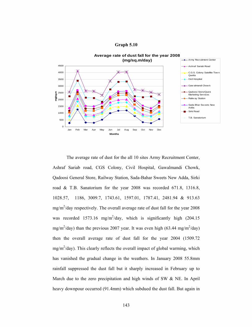
143
Graph 5.10
Average rate of dust fall for the year 2008 (mg/sq.m/day)
0
500
1000
1500
2000
2500
3000
3500
4000
4500
Jan Feb Mar Apr May Jun Jul Aug Sep Oct Nov Dec
Months
mg/
sq.m
Army Recruitment Center
Ashraf Sariab Road
C.G.S. Colony Satellite Tow nQuetta
Civil Hospital
Gaw almandi Chow k
Qadoosi Store/QuickMarketing Services
Railw ay Station
Sada Bhar Sw eets NewAdda
Sirki Road
T.B. Sanatorium
The average rate of dust for the all 10 sites Army Recruitment Center,
Ashraf Sariab road, CGS Colony, Civil Hospital, Gawalmandi Chowk,
Qadoosi General Store, Railway Station, Sada-Bahar Sweets New Adda, Sirki
road & T.B. Sanatorium for the year 2008 was recorded 671.8, 1316.8,
1028.57, 1186, 3009.7, 1743.61, 1597.01, 1787.41, 2481.94 & 913.63
mg/m2/day respectively. The overall average rate of dust fall for the year 2008
was recorded 1573.16 mg/m2/day, which is significantly high (204.15
mg/m2/day) than the previous 2007 year. It was even high (63.44 mg/m2/day)
then the overall average rate of dust fall for the year 2004 (1509.72
mg/m2/day). This clearly reflects the overall impact of global warming, which
has vanished the gradual change in the weathers. In January 2008 55.8mm
rainfall suppressed the dust fall but it sharply increased in February up to
March due to the zero precipitation and high winds of SW & NE. In April
heavy downpour occurred (91.4mm) which subdued the dust fall. But again in
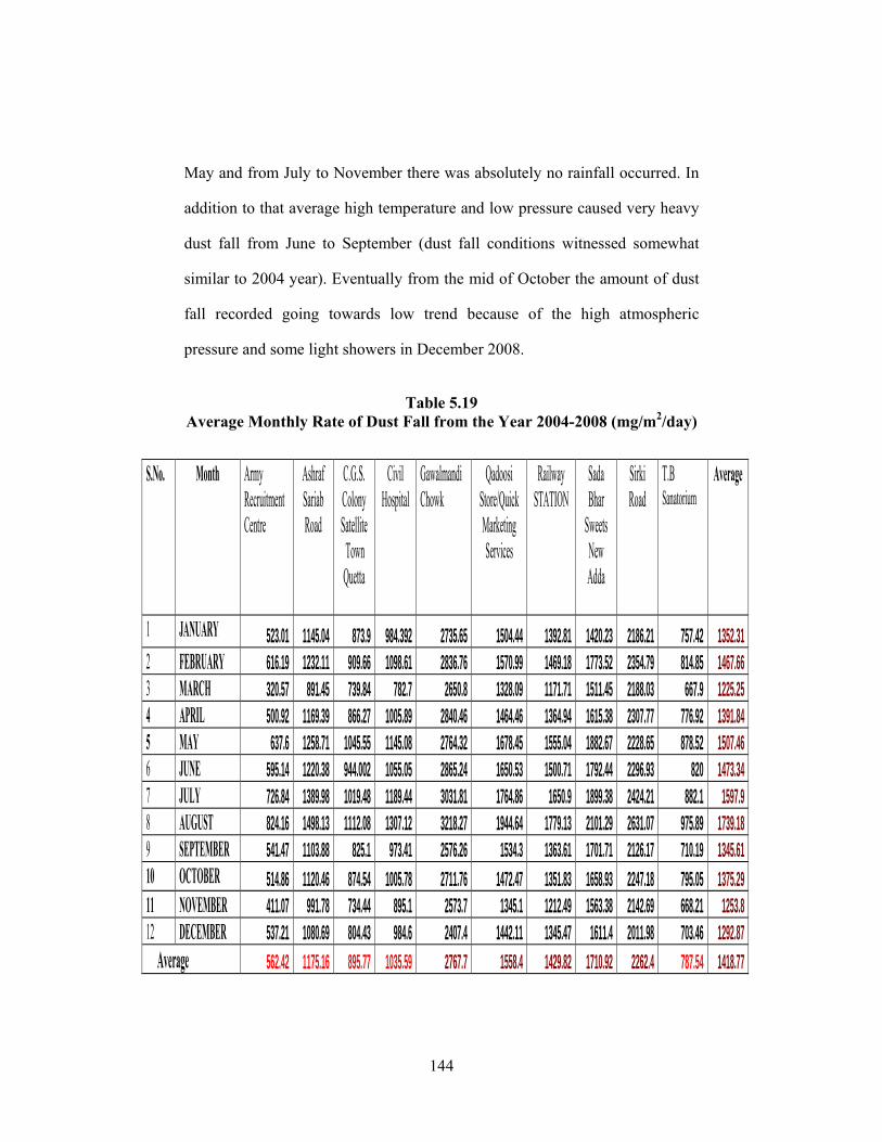
144
May and from July to November there was absolutely no rainfall occurred. In
addition to that average high temperature and low pressure caused very heavy
dust fall from June to September (dust fall conditions witnessed somewhat
similar to 2004 year). Eventually from the mid of October the amount of dust
fall recorded going towards low trend because of the high atmospheric
pressure and some light showers in December 2008.
Table 5.19 Average Monthly Rate of Dust Fall from the Year 2004-2008 (mg/m2/day)
S.No. Month Army Recruitment Centre
Ashraf Sariab Road
C.G.S. Colony Satellite Town Quetta
Civil Hospital
Gawalmandi Chowk
Qadoosi Store/Quick Marketing Services
Railway STATION
Sada Bhar
Sweets New Adda
Sirki Road
T.B Sanatorium
Average
1 JANUARY 523.01 1145.04 873.9 984.392 2735.65 1504.44 1392.81 1420.23 2186.21 757.42 1352.312 FEBRUARY 616.19 1232.11 909.66 1098.61 2836.76 1570.99 1469.18 1773.52 2354.79 814.85 1467.663 MARCH 320.57 891.45 739.84 782.7 2650.8 1328.09 1171.71 1511.45 2188.03 667.9 1225.254 APRIL 500.92 1169.39 866.27 1005.89 2840.46 1464.46 1364.94 1615.38 2307.77 776.92 1391.845 MAY 637.6 1258.71 1045.55 1145.08 2764.32 1678.45 1555.04 1882.67 2228.65 878.52 1507.466 JUNE 595.14 1220.38 944.002 1055.05 2865.24 1650.53 1500.71 1792.44 2296.93 820 1473.347 JULY 726.84 1389.98 1019.48 1189.44 3031.81 1764.86 1650.9 1899.38 2424.21 882.1 1597.98 AUGUST 824.16 1498.13 1112.08 1307.12 3218.27 1944.64 1779.13 2101.29 2631.07 975.89 1739.189 SEPTEMBER 541.47 1103.88 825.1 973.41 2576.26 1534.3 1363.61 1701.71 2126.17 710.19 1345.6110 OCTOBER 514.86 1120.46 874.54 1005.78 2711.76 1472.47 1351.83 1658.93 2247.18 795.05 1375.2911 NOVEMBER 411.07 991.78 734.44 895.1 2573.7 1345.1 1212.49 1563.38 2142.69 668.21 1253.812 DECEMBER 537.21 1080.69 804.43 984.6 2407.4 1442.11 1345.47 1611.4 2011.98 703.46 1292.87 Average 562.42 1175.16 895.77 1035.59 2767.7 1558.4 1429.82 1710.92 2262.4 787.54 1418.77
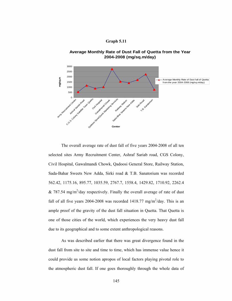
145
Graph 5.11
Average Monthly Rate of Dust Fall of Quetta from the Year 2004-2008 (mg/sq.m/day)
0
500
1000
1500
2000
2500
3000
Army R
ecru
itmen
t Cen
ter
Ashra
f Sar
iab Roa
d
C.G.S
. Colo
ny S
atellit
e Town Q
uetta
Civil H
ospita
l
Gawalm
andi C
howk
Qadoo
si Sto
re/Quic
k Mar
ketin
g Servi
ces
Railway
Stat
ion
Sada B
har S
weets
New A
dda
Sirki R
oad
T.B. S
anato
rium
Center
mg/
sq.m Average Monthly Rate of Dust fall of Quetta
from the year 2004-2008 (mg/sq.m/day)
The overall average rate of dust fall of five years 2004-2008 of all ten
selected sites Army Recruitment Center, Ashraf Sariab road, CGS Colony,
Civil Hospital, Gawalmandi Chowk, Qadoosi General Store, Railway Station,
Sada-Bahar Sweets New Adda, Sirki road & T.B. Sanatorium was recorded
562.42, 1175.16, 895.77, 1035.59, 2767.7, 1558.4, 1429.82, 1710.92, 2262.4
& 787.54 mg/m2/day respectively. Finally the overall average of rate of dust
fall of all five years 2004-2008 was recorded 1418.77 mg/m2/day. This is an
ample proof of the gravity of the dust fall situation in Quetta. That Quetta is
one of those cities of the world, which experiences the very heavy dust fall
due to its geographical and to some extent anthropological reasons.
As was described earlier that there was great divergence found in the
dust fall from site to site and time to time, which has immense value hence it
could provide us some notion apropos of local factors playing pivotal role to
the atmospheric dust fall. If one goes thoroughly through the whole data of

146
dust fall collected for five years and compare them with each other, it could
easily be figured out that out of ten selected site, the two sites (Army
Recruitment Center and T.B. Sanatorium) got the least amount while other
two sites (Gawalmandi Chowk and Sirki road) received the very high level of
dust fall. Three other sites (Sada Bahar Sweets new Adda, Qadoosi Store &
Railway Station were nothing short of heavy dust fall receiving stations. As
heavy amount of dust fall observed on these three sites as well. While Ashraf
Sariab road, CGS Colony & Civil Hospital could be termed as comparatively
medium dust fall receiving centers. Otherwise, yet if among these two so-
called medium dust fall receiving sites (Ashraf Sariab road & Civil Hospital)
are compared with the international standards, they are ranked among very
heavy dust fall receiving centers (having > 1200 mg/m2/day average rate of
dust fall in 05 years).
Army Recruitment Center is located in Cantonment area and due to
regular maintenance and cleanliness, less traffic and humans population and
being located in the proximity of high-profile Government offices like
Balochistan High Court, Serena Hotel and above all properly well-developed
area of cantonment having pretty vegetation contrary to the rest of the city, it
received the minimum amount of dust fall. Further it is situated almost in the
center of the whole city/valley. So the dust plumes striking Quetta become less
dense or dilute (till they hit this station) due to the presence of dense
population, buildings, trees etc. all around from the edges to the core of the
city (this site) in a circumference of around 2653 Km2. Consequently the least
amount in terms of average rate of dust fall from 2004-08 (562.42 mg/m2/day)
was detected on this site. Later on the results of size of dust particulates prove
147
that merely the major amount of fine and ultra-fine particulates, which remain
present in atmosphere for a long time at a high altitude, were detected rather
more at this site.
T.B. Sanatorium was built in English period at a site, where the
tuberculosis and asthmatic patients prone to the air pollutants might have an
environment free of particulates and other air pollutants. Its location on the
extreme west of the city near the foot of the 'Chiltan' Mountain at the highest
point of the bowled shape valley makes it having a clean environmental site
than rest of the city. The ridge of the 'Chiltan' deters the dust blowing from the
western or south western side of the city, to strike on the site. Even though the
mounting population and increasing traffic has badly effected the air
environment of the whole city by and large, nevertheless the unique natural
location of this site doesn't let fall prey to the air pollutants particularly dust
particulates. That is why the least amount of overall rate of average dust fall
for the 5 years 2004-08 was recorded (787.54 mg/m2/day) at this site as well
besides Army Recruitment Center.
The location of C.G.S Colony at well planned satellite town on the
southern part of the city in recent decades developed area though having huge
but properly settled population was also not extremely dust polluted (received
average dust fall for the said 5 years areas 895.77 mg/m2/day) compare to
most of the other areas of Quetta.
Another important site Civil Hospital is located in the heart of city and
is surrounded by all around the congested cluster of residential, Govt. offices,
trading centers etc. The roads on its all four sides remain busy twenty four
148
hours. On chemical analysis it was found that the amount of average dust fall
particulates for the 5 years 2004-08 (1035.59 mg/m2/day) contained the smoke
particles as well in pretty amount due to the massive traffic particularly moves
at the snail pace on its eastern, southern & northern sides. The 'Jinnah' road on
eastern side mostly remains blocked for traffic because of its narrowness and
indiscriminately allowed public transport in terms of large bunker type old
'local' stone age buses, which not only emit huge amount of un-burnt/semi-
burnt and other carcinogenic particulates of diesel fuel in already suffocated
atmosphere but also cause traffic jam triggering the emission of more Pb
contained vehicular exhaust.
'Ashraf ' iron merchant located at one of the main entrances in the city
on southern part, is surrounded by muddy constructed shops, workshops and a
small newly developed residential scheme 'green house' on its western,
northern & southern sides simultaneously. On eastern side across the Sariab
road, the Government buildings like Geological Survey of Pakistan,
University of Balochistan etc. are having green belts. Therefore it was only hit
from three sides by the dust particulates having an average 5 years dust fall
1175.16 mg/m2/day, while the front eastern part didn’t affect it much.
Quetta 'Railway Station' is also one of those few public places/sites set
up with the establishment of city. Being the sole railway station of the city on
its eastern front mostly there is a jam packed rush could be witnessed. The
northern, western and southern sides of it are mostly populated with the
thickly extremely small cabin type quarters of railway employees, encroached
streets & roads by the food vendors, grocery shops, the continuous shunting
149
activities of railway locomotives and the busy narrow roads having thick
traffic are enough to increase the air pollutants in addition to the average dust
particulates settled & collected there for the said 5 years 1429.82 mg/m2/day.
'Qadoosi store' is also one of few sites located right in the middle of the
city (center of the bowl receiving dust particulates adhered with lead halides
PbBrCl, PbBr2& PbCl2 are produced on combustion of leaded gasoline
containing tetraethyl lead, an anti-knocking agent), where all around of it wild
business activities have been carried out since the foundation of the city.
Massive vehicular emission was additional reason along with dust particulates
(average rate of dust fall recorded for the said 5 years1558.4 mg/m2/day) due
to it pathetic atmospheric pollution. There if someone stands for a while, could
easily feel suffocation, eye burn, nuisance and sore throat.
'Sada Bahar' sweets shop is located adjacent to "new Adda (bus &
goods vehicle stop on its northern & eastern sides)" in the southern part of the
city near Satellite town. On its western side there is a lane of thickly populated
business shops, slummy restaurants, on northern side again the same sort of
business shops and fruit and vegetables markets remained hectic in day time.
The junction (roundabout) and dilapidated roads always running with choked
sewage right in front of the site and randomly populated huge graveyard right
on its southern side along with an old muddy village having poor sanitations
etc. are enough to trigger the particulates amount in addition to the dust
plumes, which strike this area due to its naked position in the absence of any
high rise buildings in its vicinities, which might have prevent it from the dust
plumes mostly hit it from southern and western sides. The average rate of dust

150
fall recorded for the set 5 years on this site was 1710.92 mg/m2/day
comparatively higher than the earlier described 7 sites.
'Sirki road' was the second most dust particulates receiving site having
the average rate of dust fall 2262.4 mg/m2/day for the said 5 years. As it is
located in the middle of old and new city linking both with the route called
'Sirki road', having diverse industries adjacent to all its four sides. On the
eastern side across the road there are huge populations of old classical muddy
houses built in haphazard manner with extremely narrow passages/streets. It
received the very huge dust fall hitting it particularly from the open northern,
eastern, western and to some extent northern parts of it. It also included the
industrial emitted waste as well in terms of Metal oxides, V2O5, CaO, Aerosol
MISTS of H2SO4 droplets, (NH2)2SO4 or CaSO4 salts, Polycyclic aromatic
hydrocarbons (PAH) sorbed on soot particles & Fly ash emitting from the
stacks of few remaining brick kilns were located on the eastern part of the
muddy houses. However EPA (Environmental Protection Agency of
Balochistan) strongly recommended, which enforced the local and provincial
governments to relocate the brick kilns out of the city.
The 10th site found to be the most vulnerable for all sort of air pollution
and specifically against dust particulates pollution, was the 'GAWALMANDI
CHOWK'. Five narrow roads having huge traffic moving to all corners of city
join on this bottle neck spot, where day and night traffic remains jam small
infinite shops on both shoulder of each road along with encroachments by the
every shopkeeper and extremely contracted each single roads for both side
traffic are enough to jam the traffic on this site. Though later on the local govt.
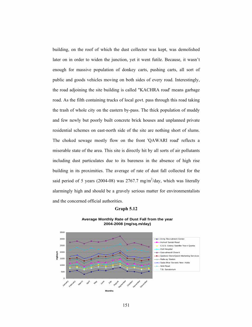
151
building, on the roof of which the dust collector was kept, was demolished
later on in order to widen the junction, yet it went futile. Because, it wasn’t
enough for massive population of donkey carts, pushing carts, all sort of
public and goods vehicles moving on both sides of every road. Interestingly,
the road adjoining the site building is called "KACHRA road' means garbage
road. As the filth containing trucks of local govt. pass through this road taking
the trash of whole city on the eastern by-pass. The thick population of muddy
and few newly but poorly built concrete brick houses and unplanned private
residential schemes on east-north side of the site are nothing short of slums.
The choked sewage mostly flow on the front 'QAWARI road' reflects a
miserable state of the area. This site is directly hit by all sorts of air pollutants
including dust particulates due to its bareness in the absence of high rise
building in its proximities. The average of rate of dust fall collected for the
said period of 5 years (2004-08) was 2767.7 mg/m2/day, which was literally
alarmingly high and should be a gravely serious matter for environmentalists
and the concerned official authorities.
Graph 5.12
Average Monthly Rate of Dust Fall from the year 2004-2008 (mg/sq.m/day)
0
500
1000
1500
2000
2500
3000
3500
Janu
ary
Febru
ary
March
April
MayJu
ne July
Augu
st
Septem
ber
Octobe
r
Novem
ber
Decem
ber
Months
mg/
sq.m
Army Recruitment Center
Ashraf Sariab Road
C.G.S. Colony Satellite Tow n Quetta
Civil Hospital
Gaw almandi Chow k
Qadoosi Store/Quick Marketing Services
Railw ay Station
Sada Bhar Sw eets New Adda
Sirki Road
T.B. Sanatorium
152
The monthly trend of the rate of dust fall of 10 selected sites for all 5
years 2004-08 shows that on the whole in January to April all sites showed a
linear trend having around minimum dust fall at the respective centers and a
bit fluctuation in February upward, in march downward and in April again
upward up to the same level of January. But in April it started to increase in a
consistent mounting trend till August due to the change in weather of summer
having high temperatures, low atmospheric pressure and high dusty winds
particularly in the marathon dry spells. After August it again showed a
downward trend because of the dropping in the mercury level with a minor
increased variation in October and decrease in November up to the minimum
level of dust fall. Finally it again showed a mild increase in December again
due to the metrological conditions. The overall seasonal trend shows that in
winter (except some days in drought period), the rate of dust fall remains at
minimum level due to the high atmospheric pressure and precipitations, while
in summer it increases up to the maximum level in the mid of summer due to
the high temperature, low atmospheric pressure, high winds and minor rare
rainfall.
As meteorological conditions is also one of the major factors among
other geographical and geological factors. Therefore meteorological data was
also obtained from the Pakistan Meteorological Department containing daily
temperatures, daily wind speed & direction, daily precipitation, daily visibility
etc. in order to make a solid deduction. The whole data given in their
respective tables strongly supports and validates this research work. The data
shows that there was absolutely no precipitation occurred in the months of
January, March, April, June, July, August & October in the first year of
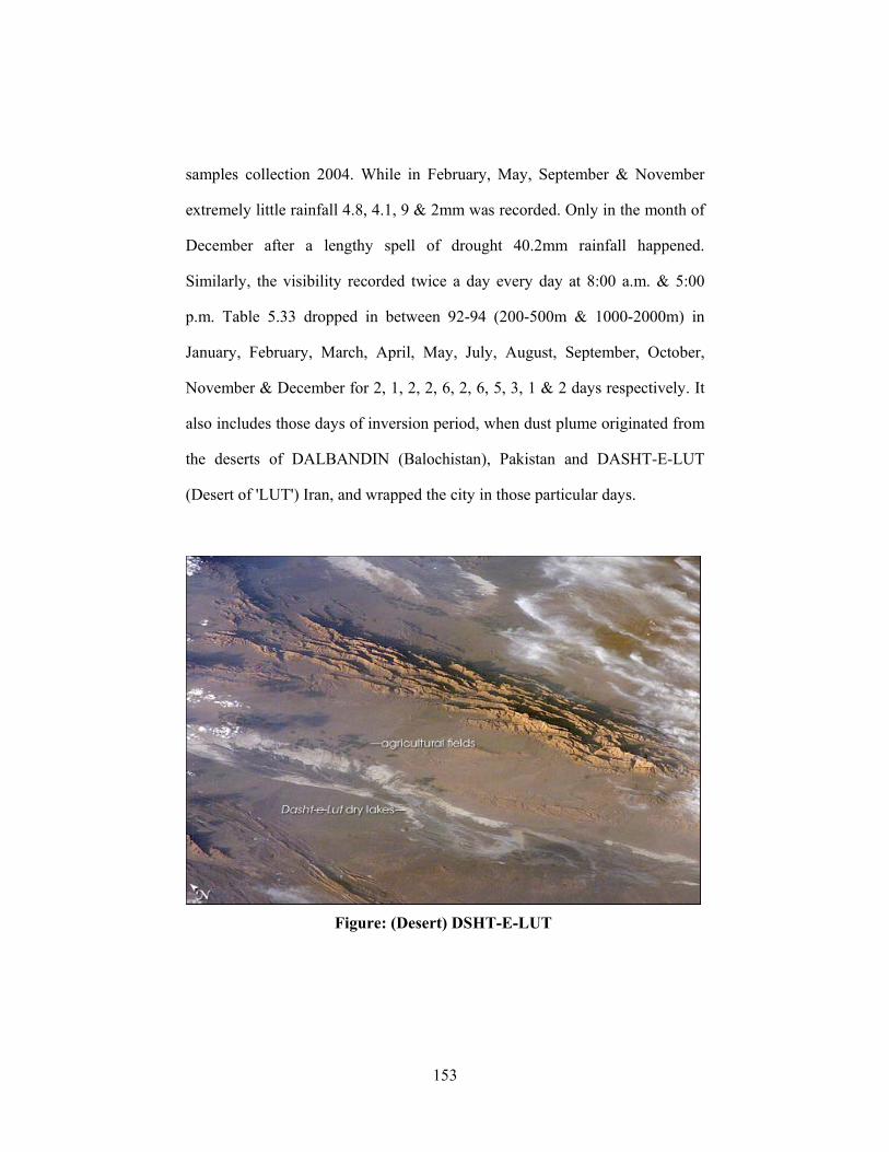
153
samples collection 2004. While in February, May, September & November
extremely little rainfall 4.8, 4.1, 9 & 2mm was recorded. Only in the month of
December after a lengthy spell of drought 40.2mm rainfall happened.
Similarly, the visibility recorded twice a day every day at 8:00 a.m. & 5:00
p.m. Table 5.33 dropped in between 92-94 (200-500m & 1000-2000m) in
January, February, March, April, May, July, August, September, October,
November & December for 2, 1, 2, 2, 6, 2, 6, 5, 3, 1 & 2 days respectively. It
also includes those days of inversion period, when dust plume originated from
the deserts of DALBANDIN (Balochistan), Pakistan and DASHT-E-LUT
(Desert of 'LUT') Iran, and wrapped the city in those particular days.
Figure: (Desert) DSHT-E-LUT
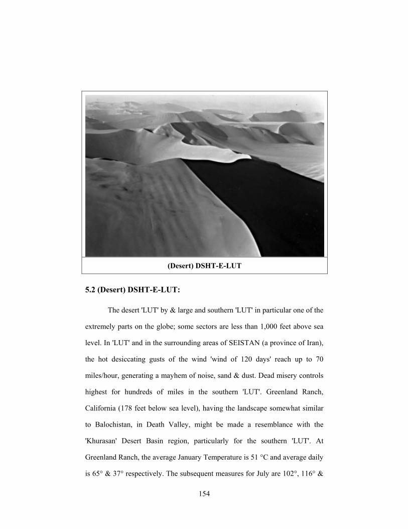
154
5.2 (Desert) DSHT-E-LUT:
The desert 'LUT' by & large and southern 'LUT' in particular one of the
extremely parts on the globe; some sectors are less than 1,000 feet above sea
level. In 'LUT' and in the surrounding areas of SEISTAN (a province of Iran),
the hot desiccating gusts of the wind 'wind of 120 days' reach up to 70
miles/hour, generating a mayhem of noise, sand & dust. Dead misery controls
highest for hundreds of miles in the southern 'LUT'. Greenland Ranch,
California (178 feet below sea level), having the landscape somewhat similar
to Balochistan, in Death Valley, might be made a resemblance with the
'Khurasan' Desert Basin region, particularly for the southern 'LUT'. At
Greenland Ranch, the average January Temperature is 51 °C and average daily
is 65° & 37° respectively. The subsequent measures for July are 102°, 116° &
(Desert) DSHT-E-LUT
155
88°. The extraordinary highest from 85° in January to 127° or even up to 134°
in July has been noted. Intensities in southern 'LUT' might cross these values
keeping in view its geography. Imagine the average rainfall at Greenland
Ranch is 1.5", ranging from 4.5" in 1912 to none for a decade till 1929, what
would be the state of 'LUT', which is having far severe conditions than at
Greenland Ranch. The 'LUT' Desert consists of several large basins separated
by shabby mountains and ridges, covering an area of about 200 by 100 miles.
The west desert contains wind-swept corridors separating high ridges. The east
is a sea of sand. Winds pile the sand into dunes up to 500 feet high, as tall as
Washington's monument. The 'LUT' is so menacing that not even bacteria can
exist. Research factions numerously brought sterilized milk into the 'LUT' and
then stored it uncovered in temperatures that could beat 160 degrees
Fahrenheit even in the shadow. The milk remained sterile.
A profound cognizance apropos of the gravity of very heavy rate of
dust fall could be figured out by comparing my findings with some of the
cities in our federation (Pakistan) and international ones.
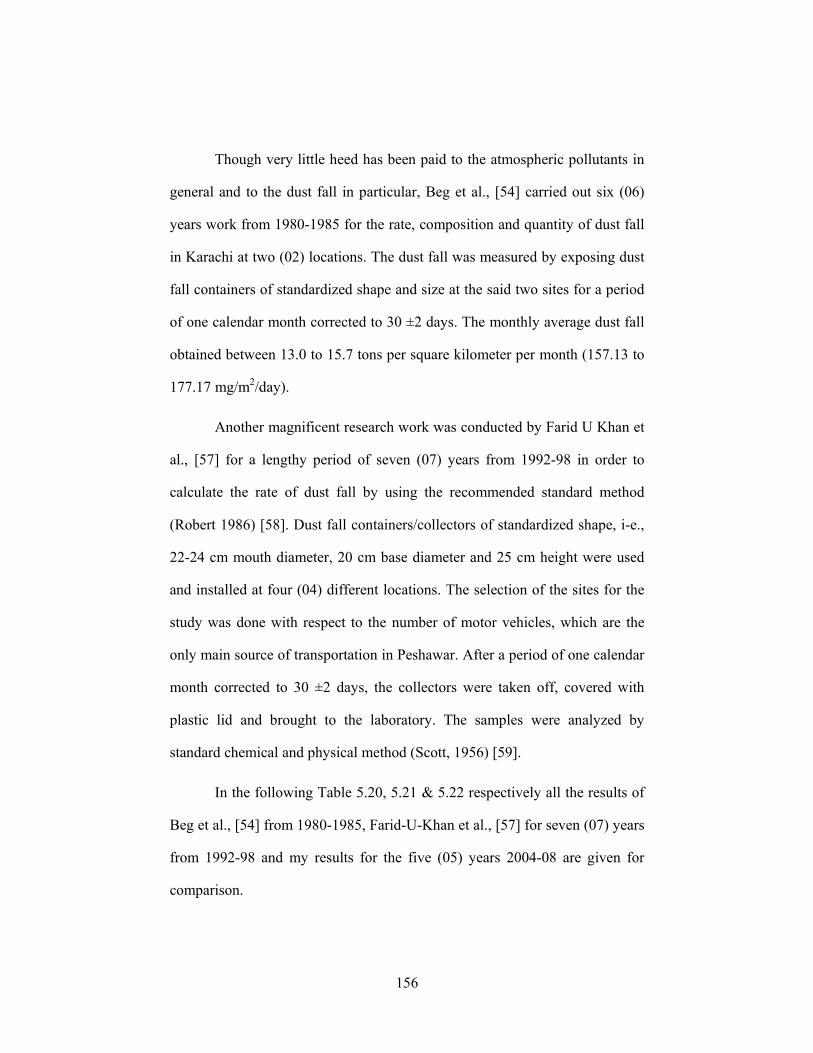
156
Though very little heed has been paid to the atmospheric pollutants in
general and to the dust fall in particular, Beg et al., [54] carried out six (06)
years work from 1980-1985 for the rate, composition and quantity of dust fall
in Karachi at two (02) locations. The dust fall was measured by exposing dust
fall containers of standardized shape and size at the said two sites for a period
of one calendar month corrected to 30 ±2 days. The monthly average dust fall
obtained between 13.0 to 15.7 tons per square kilometer per month (157.13 to
177.17 mg/m2/day).
Another magnificent research work was conducted by Farid U Khan et
al., [57] for a lengthy period of seven (07) years from 1992-98 in order to
calculate the rate of dust fall by using the recommended standard method
(Robert 1986) [58]. Dust fall containers/collectors of standardized shape, i-e.,
22-24 cm mouth diameter, 20 cm base diameter and 25 cm height were used
and installed at four (04) different locations. The selection of the sites for the
study was done with respect to the number of motor vehicles, which are the
only main source of transportation in Peshawar. After a period of one calendar
month corrected to 30 ±2 days, the collectors were taken off, covered with
plastic lid and brought to the laboratory. The samples were analyzed by
standard chemical and physical method (Scott, 1956) [59].
In the following Table 5.20, 5.21 & 5.22 respectively all the results of
Beg et al., [54] from 1980-1985, Farid-U-Khan et al., [57] for seven (07) years
from 1992-98 and my results for the five (05) years 2004-08 are given for
comparison.
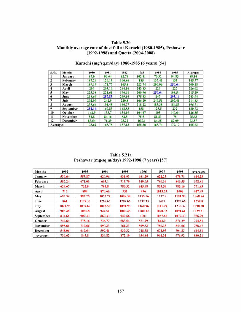
157
Table 5.20 Monthly average rate of dust fall at Karachi (1980-1985), Peshawar
(1992-1998) and Quetta (2004-2008)
Karachi (mg/sq.m/day) 1980-1985 (6 years) [54]
S.No. Months 1980 1981 1982 1983 1984 1985 Averages 1 January 87.9 90.64 82.74 102.41 70.32 94.83 88.14 2 February 187.24 129.13 100.86 185 137.41 135 145.77 3 March 189.19 171.77 165.8 222.74 200.96 250.64 200.18 4 April 209 203.16 244.16 243.83 229 227 226.02 5 May 223.38 221.61 196.61 200.96 250.64 198.54 215.29 6 June 218.66 257.83 269.16 175.83 247 295.16 243.94 7 July 202.09 242.9 220.8 166.29 249.51 207.41 214.83 8 August 235.64 191.45 166.77 218.22 183.38 184.83 196.71 9 September 252.16 167.83 148.83 158 125.5 232 180.72 10 October 142.9 133.7 134.19 104.67 105 140.64 126.85 11 November 51.8 84.16 82.5 75.5 81.83 78 75.63 12 December 83.54 71.29 73.22 46.93 84.35 82.09 73.57 Averages: 173.62 163.78 157.13 158.36 163.74 177.17 165.63
Table 5.21a Peshawar (mg/sq.m/day) 1992-1998 (7 years) [57]
Months 1992 1993 1994 1995 1996 1997 1998 Averages January 530.64 553.87 620.96 631.93 661.29 622.25 678.71 614.23 February 587.24 671.03 603.1 713.79 549.65 780.34 846.55 678.81 March 629.67 732.9 795.8 780.32 845.48 833.54 785.16 771.83 April 716 889 870.66 931 996 1015.33 1008 917.99 May 693.54 992.25 1077.74 1098.38 1155.16 1272.9 1191.93 1068.84 June 861 1179.33 1268.66 1287.66 1339.33 1427 1392.66 1250.8 July 1021.93 1039.67 1002.58 1091.93 1160.96 1141.29 1230.32 1098.38 August 905.48 1085.8 944.51 1006.45 1080.32 1090.32 1091.61 1029.21 September 834.66 909.33 869.33 949.66 1001 1057.66 1077.33 956.99 October 740.64 775.16 736.77 583.54 871.29 842.9 871.29 774.51 November 698.66 710.66 690.33 761.33 809.33 780.33 844.66 756.47 December 548.06 610.64 597.41 630.32 748.38 671.93 704.83 644.51 Average: 730.62 845.8 839.82 872.19 934.84 961.31 976.92 880.21
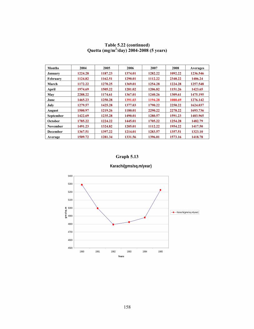
158
Table 5.22 (continued) Quetta (mg/m2/day) 2004-2008 (5 years)
Graph 5.13
Karachi(gms/sq.m/year)
4500
4600
4700
4800
4900
5000
5100
5200
5300
5400
1980 1981 1982 1983 1984 1985
Years
gms/
sq.m
Karachi(gms/sq.m/year)
Months 2004 2005 2006 2007 2008 Averages January 1224.28 1187.23 1374.01 1282.22 1092.22 1236.546 February 1124.82 1162.51 1290.01 1112.22 2340.22 1406.24 March 1172.22 1270.25 1369.01 1254.28 1224.28 1257.548 April 1974.69 1505.22 1281.02 1206.82 1151.26 1423.65 May 2288.22 1174.61 1367.01 1240.26 1309.61 1475.195 June 1465.23 1250.28 1391.03 1194.28 1080.69 1276.142 July 1279.57 1425.28 1377.03 1790.22 2250.22 1624.037 August 1500.97 1219.26 1180.01 2290.22 2278.22 1693.736 September 1422.69 1235.28 1490.01 1280.57 1591.23 1403.965 October 1785.22 1224.22 1445.01 1705.22 1254.28 1482.79 November 1491.23 1324.82 1205.01 1112.22 1954.22 1417.50 December 1367.51 1397.22 1214.01 1283.57 1357.51 1323.10 Average 1509.72 1281.34 1331.56 1396.01 1573.16 1418.78
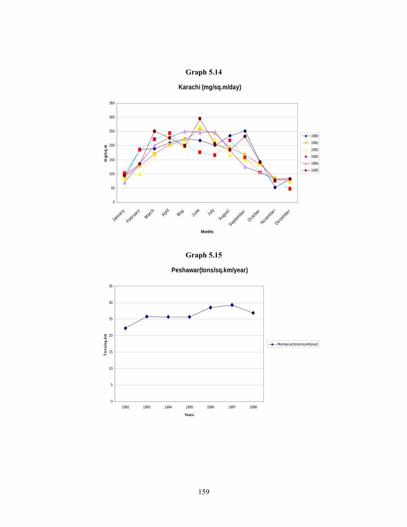
159
Graph 5.14
Karachi (mg/sq.m/day)
0
50
100
150
200
250
300
350
Janu
ary
Februa
ryMarc
hApri
lMay Ju
ne July
Augus
t
Septem
ber
Octobe
r
Novembe
r
Decembe
r
Months
mg/
sq.m
1980
1981
1982
1983
1984
1985
Graph 5.15
Peshawar(tons/sq.km/year)
0
5
10
15
20
25
30
35
1992 1993 1994 1995 1996 1997 1998
Years
Tons
/sq.
km
Peshaw ar(tons/sq.km/year)
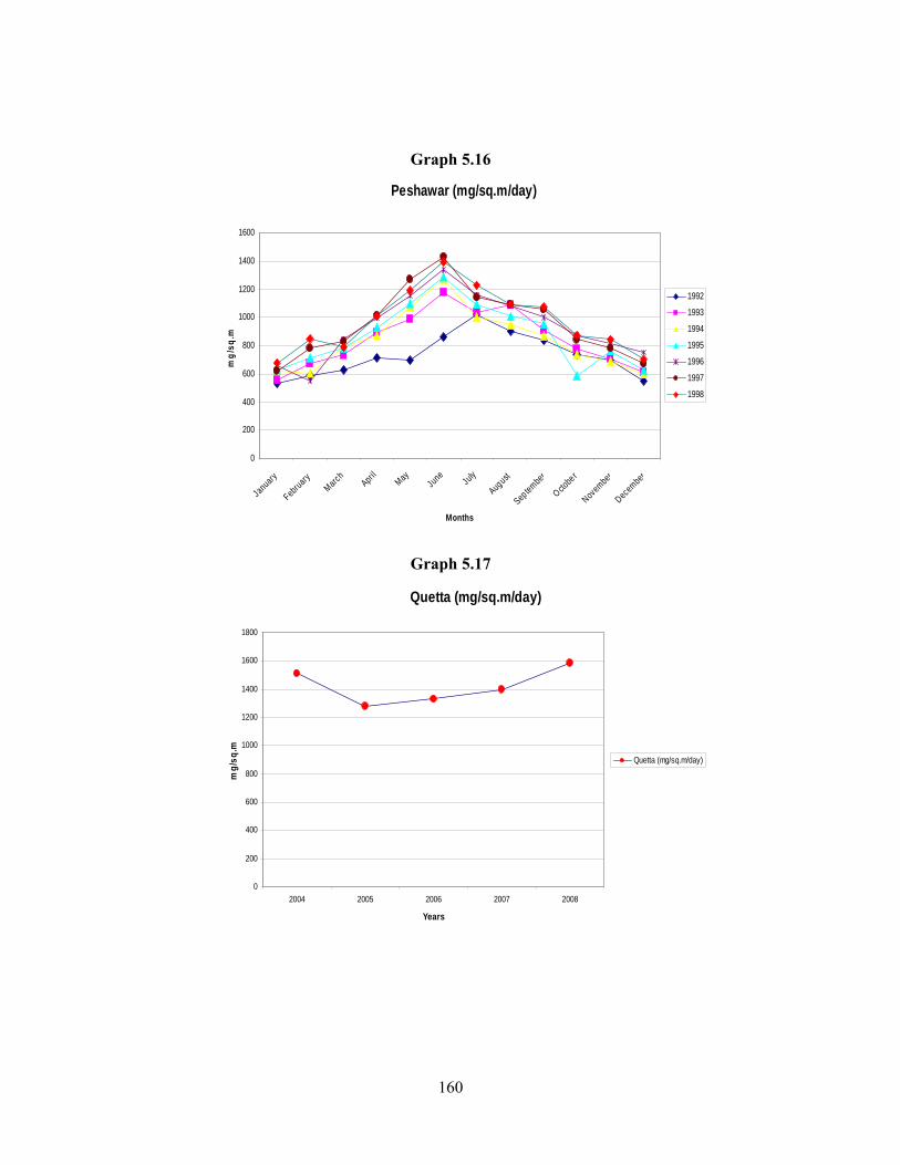
160
Graph 5.16
Peshawar (mg/sq.m/day)
0
200
400
600
800
1000
1200
1400
1600
January
FebruaryMarch
April MayJune
July
August
Sep tember
Octobe r
November
December
Months
mg/
sq.m
1992
1993
1994
1995
1996
1997
1998
Graph 5.17
Quetta (mg/sq.m/day)
0
200
400
600
800
1000
1200
1400
1600
1800
2004 2005 2006 2007 2008
Years
mg/
sq.m
Quetta (mg/sq.m/day)
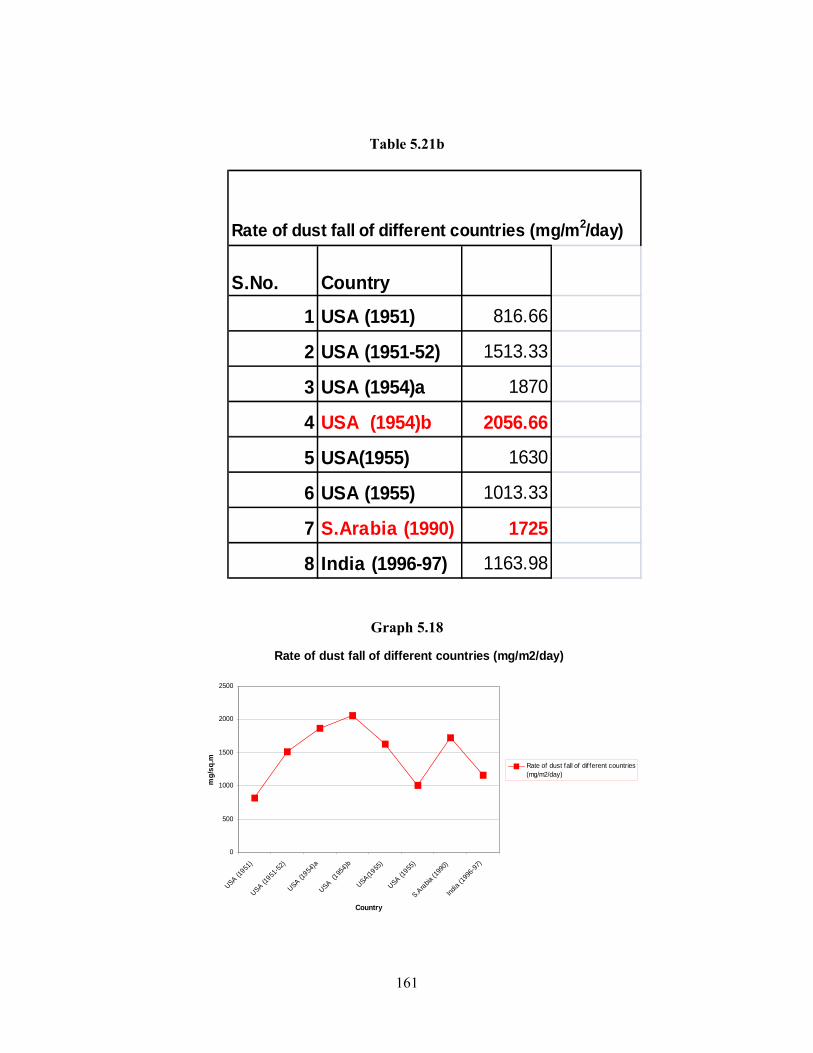
161
Table 5.21b
Graph 5.18
Rate of dust fall of different countries (mg/m2/day)
0
500
1000
1500
2000
2500
USA (1951
)
USA (1951
-52)
USA (1954
)a
USA (195
4)b
USA(1955
)
USA (1955
)
S.Arabia
(199
0)
India
(1996
-97)
Country
mg/
sq.m
Rate of dust fall of dif ferent countries(mg/m2/day)
Rate of dust fall of different countries (mg/m2/day)
S.No. Country
1 USA (1951) 816.66
2 USA (1951-52) 1513.33
3 USA (1954)a 1870
4 USA (1954)b 2056.66
5 USA(1955) 1630
6 USA (1955) 1013.33
7 S.Arabia (1990) 1725
8 India (1996-97) 1163.98
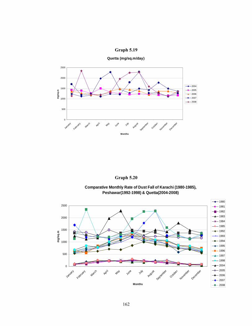
162
Graph 5.19
Quetta (mg/sq.m/day)
0
500
1000
1500
2000
2500
Janu
ary
Februa
ryMarc
hApri
lMay
June Ju
ly
Augus
t
Septem
ber
Octobe
r
Novem
ber
Decem
ber
Months
mg/
sq.m
2004
2005
2006
2007
2008
Graph 5.20
Comparative Monthly Rate of Dust Fall of Karachi (1980-1985), Peshawar(1992-1998) & Quetta(2004-2008)
0
500
1000
1500
2000
2500
Janu
ary
Februa
ryMarc
hApri
lMay
June Ju
ly
Augus
t
Septem
ber
Octobe
r
Novem
ber
Decem
ber
Months
mg/
sq.m
1980
1981
1982
1983
1984
1985
1992
1993
1994
1995
1996
1997
1998
2004
2005
2006
2007
2008
163
The above mentioned tables 5.20 and 5.21 and Graph 5.13-5.20 and
particularly the Graph 5.20 are self-explanatory enough to describe the
situation of dust fall at Quetta in comparison with the international and two
major cities Karachi & Peshawar in Pakistan. International data clearly shows
that even on four (04) different past occasions (1951-52, 1954a, 1954b, 1955
& 1990) 4 cities of US & one city of Saudi Arabia were having more average
annual rate of dust fall (1513.33, 1870, 2056.66, 1725 mg/m2/day) than the
average annual rate of dust fall at Quetta (1418.76 mg/m2/day) not to speak of
nowadays, when the air pollution has reached beyond the alarming rate. That
has caused global warming, severity of weather, uncertainty in weather
changes, drought spells in most parts of the world, excessive floods in other
parts of the world, melting of polar ice caps etc.
Similarly the average annual rate of dust fall in Karachi & Peshawar
has been compared with average annual rate of dust fall at Quetta found by me
in Table 5.18& Graph No.5.20. It is vivid that the Quetta has got far more
average rate of dust fall than the both cities Karachi & Peshawar. Though both
cities are far larger than Quetta in size/area and population, yet they
experienced far lesser amount of dust fall than Quetta. Particularly Karachi,
where the dust fall is within the international set range <250 for slighter limits
and has been marked with green values. The primary reason for that is the
presence of excessive humidity in the atmosphere of the Karachi city as it is a
coastal city. Further plantation in Karachi is also far more than Quetta.
On the other hand Peshawar has got more average annual rate of dust
fall than Karachi because of its comparatively lesser humidity and topography.
164
But it had even far lesser average annual rate of dust fall than Quetta had.
Besides other multiple reasons described earlier, the primary reason of Quetta
having more average rate of dust fall than other cities of Pakistan is the semi-
arid zone sort of geography and climate of Quetta city. The sole unanimous
phenomena between all three cities (Karachi, Peshawar & Quetta) of Pakistan
is that all had faced heavy annual rate of dust fall in the mid of summer (Graph
5.20) due to high temperatures and resultant low atmospheric pressures.
In the beginning of year 2005, January, February, March & April
Quetta received heavy downpours 33.7, 129.2, 63.3 & 36.9mm besides in
April, June & August very light scattered showers 0.4, 4.8 & 3.4mm
respectively. However, again July, September, October, November &
December complete dry spells were observed having 0 (zero) rainfall. Due to
heavy rainfall only January, March & April experienced the poor visibility in
between 92-94 (200-500m & 1000-2000m) for 2, 2 & 2 days respectively.
During the year 2006, January, February, March, May, July, August,
November & December experienced the 9.5, 6.5, 26.1, 10.7, 5.6, 2.5, 54.9,
46.9 & 43.8mm rainfall. Nevertheless June, September & October again didn’t
have any rainfall whatsoever. The low visibility in between 92-94 (200-500m
& 1000-2000m) was recorded for the January, March, July, August,
September, October & November having 1, 1, 4, 1, 11, 2 & 2 days
respectively.
In 2007, January, February, March, April, June, July, November &
December received 17.2, 77.3, 20.0, 8.1, 34.4, 8.0, 3.5 & 5.0mm rainfall,
while May, August, September & October, received absolutely no (zero)
165
rainfall having dry spells. The visibility in between 92-94 (200-500m & 1000-
2000m) was recorded for the January, February, July, August, September,
October & November containing 2, 1, 7, 3, 4, 5, 2 and extremely low visibility
on 11th December for one day even up to 91 (50-200m 'objects visible at 50m
but not at 200m') was recorded.
In 2008, January, April, June & December received the 55.8, 91.4, 9.1,
& 7.4mm precipitation. While a long dry spell was also experienced along
with very heavy (even a bit more dust fall than the year 2004) in February,
March, May, July, August, September, October & November having zero (0)
rainfall. The visibility recorded in between 92-94 (200-500m & 1000-2000m)
for the months of January, February, March, May, June, July, August,
September, October & December for 3, 4, 2, 2, 7, 6, 12, 9, 5 & 1 days
respectively. Once again for one each day of 21st February & 19th December
2008 had the visibility 91(50-200m 'objects visible at 50m but not at 200m').
However other than those above mentioned days having low visibility, there
were numerous occasions during the thermal inversion periods in 2004 and
2008, when visibility sometimes even reduced up to zero.
5.3 CHEMICAL ANALYSIS OF DUST FALL:
In order to find the origin of dust particulates, chemical analyses of the
samples were carried out sporadically. The loss on ignition, silica and oxides
aluminum, iron, calcium, magnesium, sodium and potassium was found out. It
could be observed from the results given in Table 5.35a; that the chemical
composition collected at different sites is by and large same but varies with
thermal inversion periods. It is important to describe the average annual
166
chemical composition of the dust fall collected in normal usual conditions
mostly consists of (loss on ignition: 20.62%, SiO2: 44.29%, Al2O3: 13.20%,
Fe2O3: 4.56%, CaO: 14.86%, MgO: 1.81%, Na2O: 1.16% and K2O: 0.79%)
Table 5.35a. This obviously points out that under normal conditions (other
than extremely rare period of thermal inversion) dust fall is from the local
earth crust strongly calcareous, moderately fine textured soils developed in
mixed Pleistocene piedmont alluvium derived from CHILTAN, MURDAR,
MASLAKH & TAKATO ranges having a structural (cambic) B horizon of the
series occurs in an arid subtropical continental highland climate and occupies
level to nearly piedmont plains of CHILTAN, MURDAR, MASLAKH &
TAKATO ranges of loam horizon a (substratum) rock layer consists of a
buried profile [112]. It has a brown/dark brown, friable, massive, strongly
calcareous silty clay loam topsoil underlain by dark yellowish brown, friable,
weak coarse sub-angular blocky, strongly calcareous silty clay, which
originates from the local areas like unpaved dusty shoulders of roads,
undeveloped dusty soil land within and in the suburbs of city, neglected
sanitation, and muddy houses mainly of those villages, which have been
merged in the city with its expansion and last but not least due to deadly dry
atmospheric conditions prevail mostly for the whole year. The results were
matched with the already soil pertaining research of the city and were found
exactly accurate [113].
In addition to that the dust fall samples particularly collected in the
thermal inversion spells, were having a fair ribbon sort of texture had almost
no gritty particles reflected its silty clay loam nature. When chemically
analyzed in order to confirm the origin of dust plume, chemical composition
167
of the samples verified the satellite images of different meteorological
agencies of the world, claiming that the dust plumes origin was the deserts of
DALBINDIN (Pakistan) &'DASHT-E-LUT' (Iran). Those specific dust
samples were having (loss on ignition: 24.64, SiO2: 39.19, Al2O3: 9.15, Fe2O3:
3.36, CaO: 20.92, MgO: 10.91, Na2O: 13.66and K2O: 20.99) Table 5.35b. The
results on matching with already done research [114] of the said areas' [115]
soil were found exactly to be the similar chemical composition having similar
percentages of all constituents present in them. It confirmed the source of the
dust particulates plumes hit Quetta city for the very first time in the life span
of even elders. The Brown to light olive brown color of dust showed that it
was a mixture of silt loam & silty clay coarse loam to very fine sandy loam
occasionally loam (soil) of extreme aridic region dust contained soot, smoke,
un-burnt heavily adulterate Iranian smuggled fuel, vehicular emission,
aerosols, dried residual sewage etc. Other important minerals detected in
pretty concentration, were the oxides and hydroxides of Na, K, Mg, Ca.
However, Fe & Mn, were found in lesser concentration, which determine the
color of many soils and have a high sorption capacity for trace elements; again
the concentration of carbonates were comparatively high than silicates had
lesser concentration, which has a major influence on the pH of soils; and in
some cases, phosphates, sulphides, sulphates and chlorides [116]. In
comparison with Peshawar & Karachi the chemical composition of all samples
of dust fall particulates under normal windy conditions deduced that the color
from yellowish brown to dark yellowish brown when moist in uncultivated
areas; or it may range from brown/dark brown to very dark grayish brown
when moist in cultivated areas; and light olive brown dry; in texture very fine
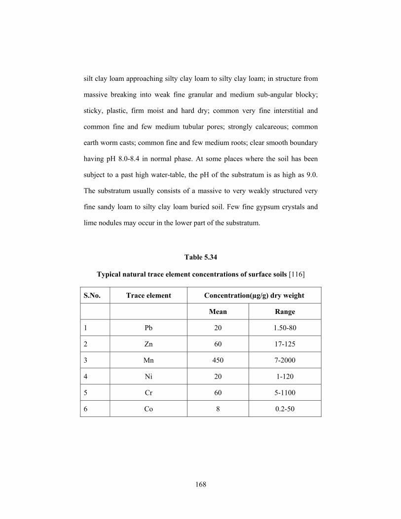
168
silt clay loam approaching silty clay loam to silty clay loam; in structure from
massive breaking into weak fine granular and medium sub-angular blocky;
sticky, plastic, firm moist and hard dry; common very fine interstitial and
common fine and few medium tubular pores; strongly calcareous; common
earth worm casts; common fine and few medium roots; clear smooth boundary
having pH 8.0-8.4 in normal phase. At some places where the soil has been
subject to a past high water-table, the pH of the substratum is as high as 9.0.
The substratum usually consists of a massive to very weakly structured very
fine sandy loam to silty clay loam buried soil. Few fine gypsum crystals and
lime nodules may occur in the lower part of the substratum.
Table 5.34
Typical natural trace element concentrations of surface soils [116]
S.No. Trace element Concentration(µg/g) dry weight
Mean Range
1 Pb 20 1.50-80
2 Zn 60 17-125
3 Mn 450 7-2000
4 Ni 20 1-120
5 Cr 60 5-1100
6 Co 8 0.2-50
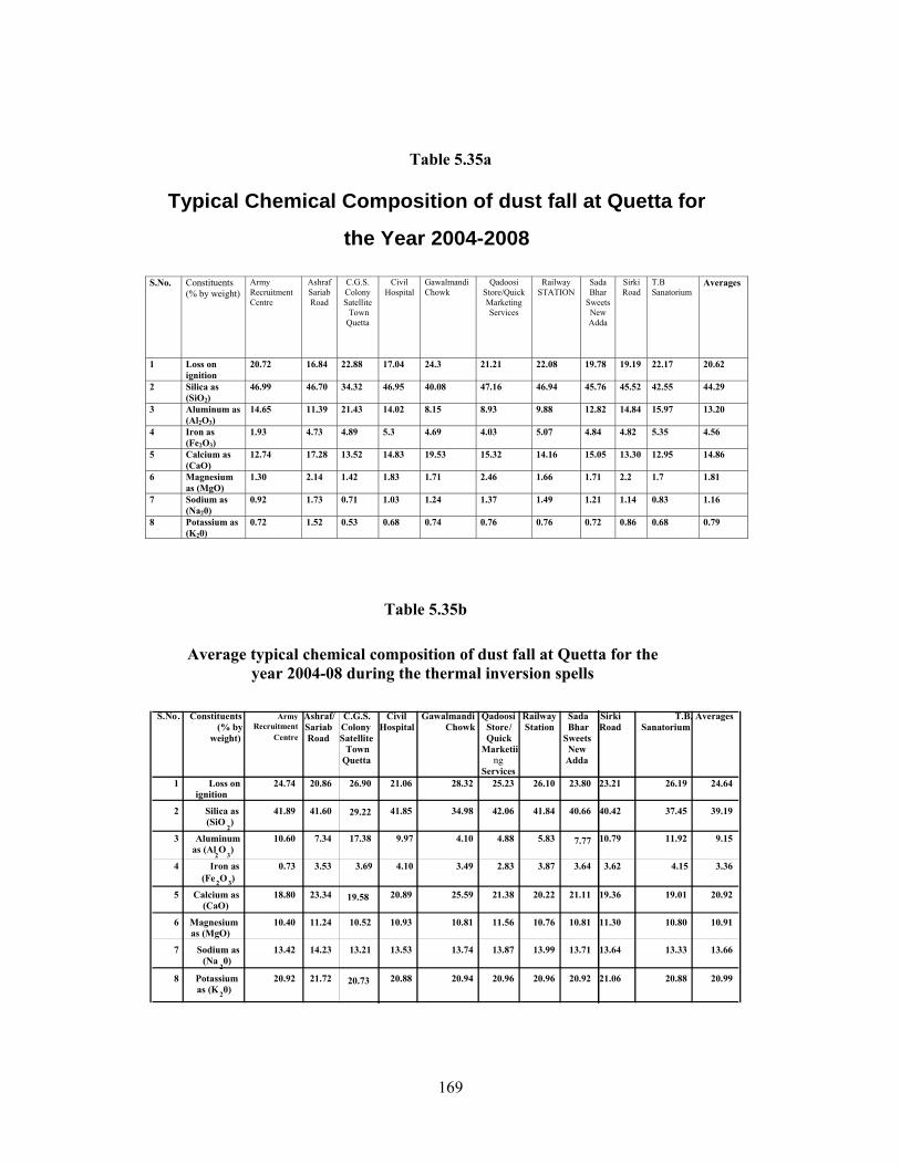
169
Table 5.35a
Typical Chemical Composition of dust fall at Quetta for
the Year 2004-2008
S.No. Constituents (% by weight)
Army Recruitment Centre
Ashraf Sariab Road
C.G.S. Colony Satellite Town Quetta
Civil Hospital
Gawalmandi Chowk
Qadoosi Store/Quick Marketing Services
Railway STATION
Sada Bhar
Sweets New Adda
Sirki Road
T.B Sanatorium
Averages
1 Loss on ignition
20.72 16.84 22.88 17.04 24.3 21.21 22.08 19.78 19.19 22.17 20.62
2 Silica as (SiO2)
46.99 46.70 34.32 46.95 40.08 47.16 46.94 45.76 45.52 42.55 44.29
3 Aluminum as (Al2O3)
14.65 11.39 21.43 14.02 8.15 8.93 9.88 12.82 14.84 15.97 13.20
4 Iron as (Fe2O3)
1.93 4.73 4.89 5.3 4.69 4.03 5.07 4.84 4.82 5.35 4.56
5 Calcium as (CaO)
12.74 17.28 13.52 14.83 19.53 15.32 14.16 15.05 13.30 12.95 14.86
6 Magnesium as (MgO)
1.30 2.14 1.42 1.83 1.71 2.46 1.66 1.71 2.2 1.7 1.81
7 Sodium as (Na20)
0.92 1.73 0.71 1.03 1.24 1.37 1.49 1.21 1.14 0.83 1.16
8 Potassium as (K20)
0.72 1.52 0.53 0.68 0.74 0.76 0.76 0.72 0.86 0.68 0.79
Table 5.35b
Average typical chemical composition of dust fall at Quetta for the year 2004-08 during the thermal inversion spells
S.No. Constituents
(% by weight)
Army Recruitment
Centre
Ashraf/ SariabRoad
C.G.S. ColonySatellite
Town Quetta
Civil Hospital
GawalmandiChowk
QadoosiStore/ Quick
Marketiing
Services
Railway Station
SadaBhar
Sweets New Adda
SirkiRoad
T.B.Sanatorium
Averages
1 Loss on ignition
24.74 20.86 26.90 21.06 28.32 25.23 26.10 23.80 23.21 26.19 24.64
2 Silica as (SiO
2 )41.89 41.60 29.22 41.85 34.98 42.06 41.84 40.66 40.42 37.45 39.19
3 Aluminum as (Al
2 O3 ) 10.60 7.34 17.38 9.97 4.10 4.88 5.83 7.77 10.79 11.92 9.15
4 Iron as (Fe2 O3 )
0.73 3.53 3.69 4.10 3.49 2.83 3.87 3.64 3.62 4.15 3.36
5 Calcium as (CaO)
18.80 23.34 19.58 20.89 25.59 21.38 20.22 21.11 19.36 19.01 20.92
6 Magnesium as (MgO)
10.40 11.24 10.52 10.93 10.81 11.56 10.76 10.81 11.30 10.80 10.91
7 Sodium as (Na
2 0)13.42 14.23 13.21 13.53 13.74 13.87 13.99 13.71 13.64 13.33 13.66
8 Potassium as (K 2 0)
20.92 21.72 20.73 20.88 20.94 20.96 20.96 20.92 21.06 20.88 20.99
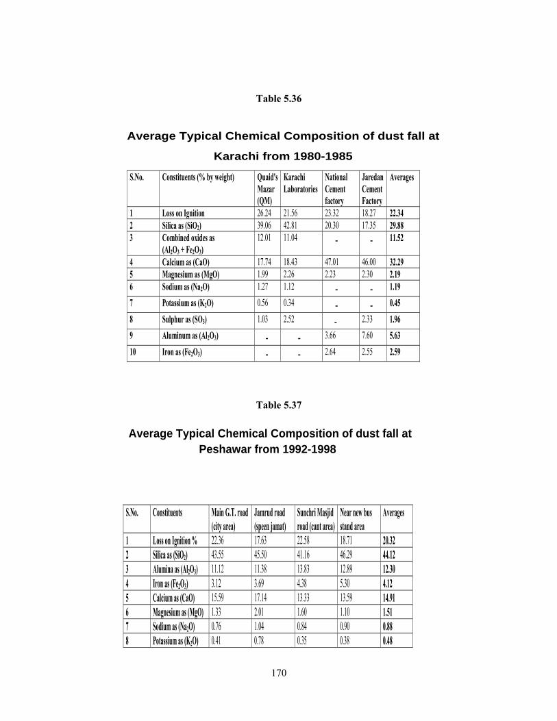
170
Table 5.36
Average Typical Chemical Composition of dust fall at
Karachi from 1980-1985
S.No. Constituents (% by weight) Quaid's Mazar (QM)
Karachi Laboratories
National Cement factory
Jaredan Cement Factory
Averages
1 Loss on Ignition 26.24 21.56 23.32 18.27 22.34 2 Silica as (SiO2) 39.06 42.81 20.30 17.35 29.88 3 Combined oxides as
(Al2O3 + Fe2O3) 12.01 11.04 - - 11.52
4 Calcium as (CaO) 17.74 18.43 47.01 46.00 32.29 5 Magnesium as (MgO) 1.99 2.26 2.23 2.30 2.19 6 Sodium as (Na2O) 1.27 1.12 - - 1.19 7 Potassium as (K2O) 0.56 0.34 - - 0.45 8 Sulphur as (SO3) 1.03 2.52 - 2.33 1.96 9 Aluminum as (Al2O3) - - 3.66 7.60 5.63 10 Iron as (Fe2O3) - - 2.64 2.55 2.59
Table 5.37
Average Typical Chemical Composition of dust fall at Peshawar from 1992-1998
S.No. Constituents Main G.T. road (city area)
Jamrud road (speen jamat)
Sunchri Masjid road (cant area)
Near new bus stand area
Averages
1 Loss on Ignition % 22.36 17.63 22.58 18.71 20.32 2 Silica as (SiO2) 43.55 45.50 41.16 46.29 44.12 3 Alumina as (Al2O3) 11.12 11.38 13.83 12.89 12.30 4 Iron as (Fe2O3) 3.12 3.69 4.38 5.30 4.12 5 Calcium as (CaO) 15.59 17.14 13.33 13.59 14.91 6 Magnesium as (MgO) 1.33 2.01 1.60 1.10 1.51 7 Sodium as (Na2O) 0.76 1.04 0.84 0.90 0.88 8 Potassium as (K2O) 0.41 0.78 0.35 0.38 0.48
171
5.4 DETECTION OF HEAVY & TOXIC METALS IN DUST
SAMPLES:
The trace elements composition of soil may significantly influence the
elemental composition of the vegetation, eventually which effects the animal
and human tissues or fluids through the food chain. In order to assess the blow
of trace element pollution, it is mandatory to have the knowledge of natural
elemental levels and chemical compositions of the earth's environment. The
earth's crust contains extremely few trace elements. Majority of them are
present as soluble simple salts (Na, K, Rb), cationic constituents in
aluminosilicates (Li, Be, Cs), insoluble carbonate or sulphates (Mg, Ca, Sr,
Ba), oxides, (B, Al, Si, Sc, Ti, V, Cr, Mn, Lanthanides), or sulphides (Fe, Co,
Ni, Cu, Zn, Ga, Ge, As, Se, Mo, Cd, Sn, Sb, Hg, Tl, Pb, Bi). Soils are assumed
as sinks for trace elements, and that is why an important role plays in the
environmental cycling of elements. The mineral constituents of soils are
normally directly related to the parent rock and type of weathering processes.
The principal components of soil are inorganic materials: sand, silt and clay.
Clay minerals may contain low levels of trace elements as structural
components but their surface properties (area and electrical charge) play a
pivotal role in regulating the buffer and sink properties of soils. Results
pertaining to the concentration of heavy & toxic metals (µg/g) in dust fall
samples collected during the 5 years period 2004-08 are given in Table 5.39-
5.43. The concentrations of Pb, Zn, Mn, Ni, Cr & Co were determined with
the help of AAS (Atomic Absorption Spectrophotometer) and the
concentrations of Na & K were found with the help of Flame Photometer. The
concentrations of all Pb, Zn, Mn, Ni, Cr, Co Na & K for the year 2004 were
172
found to lie in the range 981-4430, 49-830, 30-712, 73-412, 15-127, 07-73,
25-73 & 39-88 respectively are given in Table 5.39. Table 5.40shows the
concentration of the said elements for the year 2005 found to lie in the range
973-4425, 47-828, 24-703, 68-411, 96-126, 02-70, 08-40 & 06-43
respectively. The levels of the all said metals for the year 2006 was found to
lie in the range 971-4411, 37-827, 21-711, 68-407, 15-113, 09-69, 05-38 &
07-41 respectively are showed in Table 5.41. Similarly the amounts of all
described metals for the year 2007 was found to lie in the range 988-4438, 51-
838, 28-725, 77-410, 27-127, 11-74, 01-32 & 01-34 respectively are displayed
in Table 5.42 respectively. Finally the Table 5.43 shows the concentrations of
all metals for the year 2008 found to lie in the range 986-4437, 55-835, 44-
718, 77-421, 23-139, 11-80, 36-77 & 32-83 respectively.
There are 90 naturally occurring elements on the earth crust. These
metals are put in the atmosphere from the soil driven [3], automobiles &
industrial origins [117,118]. The amount and chemical composition vastly
vary between and within environmental, geological, biological or marine
systems. The elemental composition of earth crust is mainly O, Si, Al, Fe, Ca,
Na, K, and Mg, while the human body is H, O, C, N, Ca, P, K and Cl. From a
biological point of view, trace elements are most easily be divided in three
categories: essential, non-essential and toxic. The trace elements essential for
all living organisms like plants, animals and humans are those, which play
vital biochemical roles in terms of metabolic cycle in plants by having direct
impact on the organisms so that they could not develop and the reduction of
which consistently results in a deficiency syndrome and reduction reverses the
abnormalities. The trace elements fulfilling these needs are As, Co, Cr, Cu, F,
173
Fe, I, Mn, Mo, Ni, Se, Si, Sn, V and Zn. Besides that there are many non-
essential elements e.g. Li, B, Ge, Rb and Sr are found in the body tissues and
fluid but for which inevitability no evidence has been established. However,
some elements for instance Cd, Hg, and Pb are distinctively categorized as
toxic elements because of their detrimental effects even at low levels.
Nevertheless, all trace elements are supposed to be the toxic elements when
their levels cross the unanimously set limits of safe exposure [116].
It has generally been found out throughout the densely populated cities
of the developed, developing & underdeveloped world, that the environment
of those cities in terms of plants, soil, water & air carry alarming amount of
toxic and heavy metals such as Pb, Zn, Mn, Ni, Cr, Co, Na & K besides
numerous other pollutants [119]. Multiple factors for instance automobiles,
industrial emission and weathered materials are the reason of the rise in the
concentrations of trace elements in massively settled areas. The elements Pb,
Zn, Mn, Ni, Cr, Co, Cu & Cd have been spotted out entering & increasing
from the weather source [120,121]. In addition to adding Pb in the
environment particularly in air automobiles also increase Cd, Cu, Zn, Fe, Cr
and Ni [122,123]. The elevating concentration of Zn, Ni, and Cr might be due
to the erosion of vehicles tyres. It has been described that vehicles tires and
wear and tears are one the major sources of the said elements [124]. Another
factor has been found out to be the kind of road surface as the concentration of
elements Pb, Zn and Cu are supposed to increase from the pavements, to the
choked sewerage and flowing sewage on the middle of roads most of the time
in underdeveloped and corrupt countries like ours (Pakistan) [125]. More
factors need to be measured / determined in order to understand the trend of
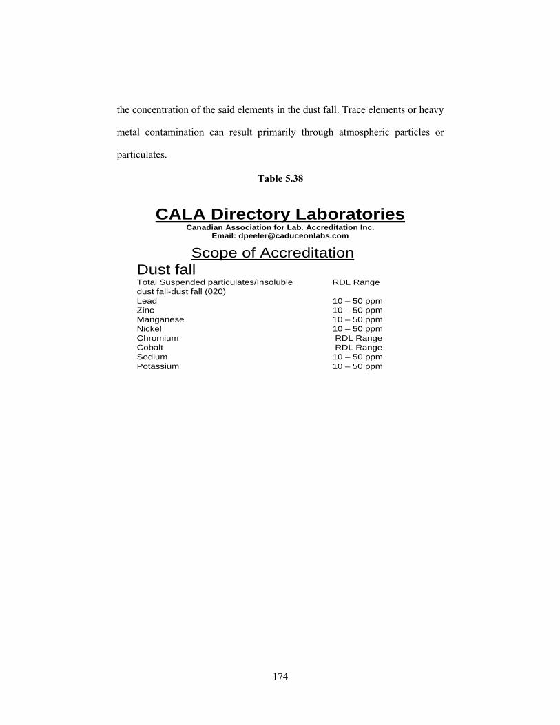
174
the concentration of the said elements in the dust fall. Trace elements or heavy
metal contamination can result primarily through atmospheric particles or
particulates.
Table 5.38
CALA Directory LaboratoriesCanadian Association for Lab. Accreditation Inc.
Email: [email protected]
Scope of AccreditationDust fallTotal Suspended particulates/Insoluble RDL Rangedust fall-dust fall (020) Lead 10 – 50 ppmZinc 10 – 50 ppmManganese 10 – 50 ppmNickel 10 – 50 ppmChromium RDL RangeCobalt RDL RangeSodium 10 – 50 ppmPotassium 10 – 50 ppm

175
Table 5.39
Concentration of heavy and toxic metals in the dust fall at Quetta detected during 2004 µg/g (ppm)
61.65035.671.1301.7525.6604.92668.3Average:
39250715733049981T.B. Sanatorium10
8368691123967087903018Sirki Road9
644229623336557012389Sada Bhar Sweets, New Adda8
766537793476707602401Railway Station7
8873731274127128304430Qadoosi Store/Quick Marketing Service6
705852993816987874423Gawalmandi Chowk5
585341833626857843417Civil Hospital4
52471132861706121824C.G.S. Colony Satellite Town, Quetta3
463720583196246201870Ashraf Sariab Road2
403217443083041161930Army Recruitment Center1
KNaCoCrNiMnZnPbLocationS.No.
Graph 5.21
Trend showing the amount of heavy and toxic elements in the dust fall at Quetta in 2004
0200400600800
10001200140016001800200022002400260028003000320034003600380040004200440046004800
Army R
ecrui
tmen
t Cen
ter
Ashraf
Sariab R
oad
C.G.S. C
olony
Sate
llite To
wn, Que
tta
Civil H
ospita
l
Gawalm
andi C
howk
Qadoo
si Store/
Quick M
arketi
ng Servi
ce
Railway
Station
Sada B
har S
weets,
New
Add
a
Sirki R
oad
T.B. San
atoriu
m
Centers
µg/g
(ppm
)
Pb
Zn
Mn
Ni
Cr
Co
Na
K
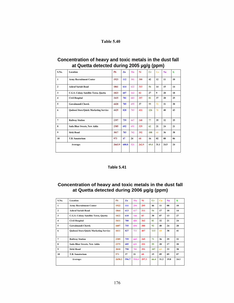
176
Table 5.40
Concentration of heavy and toxic metals in the dust fall at Quetta detected during 2005 µg/g (ppm)
2424.531.169.4262.9521600.82663.9Average:
06080216682447973T.B. Sanatorium10
3836601083927027833017Sirki Road9
212421623296516922385Sada Bhar Sweets, New Adda8
353235773406677592397Railway Station7
4340701264117038284425Qadoosi Store/Quick Marketing Service6
30315199376957854420Gawalmandi Chowk5
252837813576837813415Civil Hospital4
1820927821626071823C.G.S. Colony Satellite Town, Quetta3
141514563136226141861Ashraf Sariab Road2
101112423003011121923Army Recruitment Center1
KNaCoCrNiMnZnPbLocationS.No.
Table 5.41
Concentration of heavy and toxic metals in the dust fall at Quetta detected during 2006 µg/g (ppm)
24.119.831.266.4297.3518.4596.72658.2Average:
07050915682137971T.B. Sanatorium10
3833631073917017903010Sirki Road9
201720553316316852375Sada Bhar Sweets, New Adda8
322936713456657592389Railway Station7
4138691134077118274411Qadoosi Store/Quick Marketing Service6
282448923806947554407Gawalmandi Chowk5
242132813626847803411Civil Hospital4
27130730831666101822C.G.S. Colony Satellite Town, Quetta3
141017543116176131864Ashraf Sariab Road2
100811462952941111922Army Recruitment Center1
KNaCoCrNiMnZnPbLocationS.No.
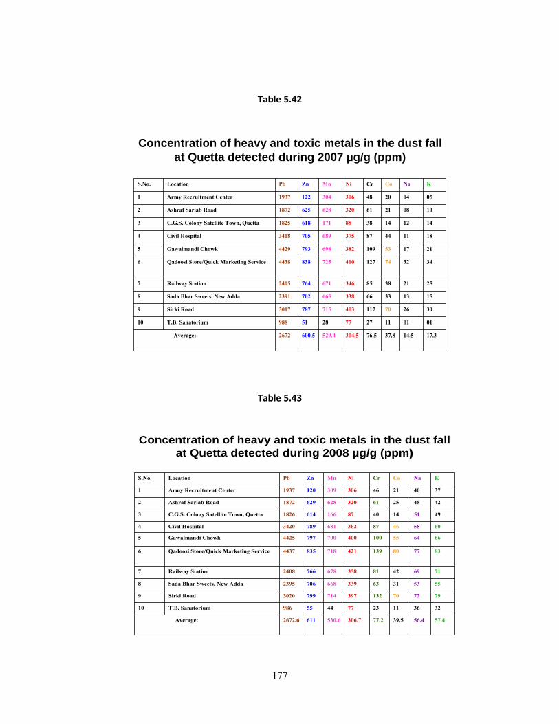
177
Table 5.42
Concentration of heavy and toxic metals in the dust fall at Quetta detected during 2007 µg/g (ppm)
17.314.537.876.5304.5529.4600.52672Average:
01011127772851988T.B. Sanatorium10
3026701174037157873017Sirki Road9
151333663386657022391Sada Bhar Sweets, New Adda8
252138853466717642405Railway Station7
3432741274107258384438Qadoosi Store/Quick Marketing Service6
2117531093826987934429Gawalmandi Chowk5
181144873756897053418Civil Hospital4
14121438881716181825C.G.S. Colony Satellite Town, Quetta3
100821613206286251872Ashraf Sariab Road2
050420483063041221937Army Recruitment Center1
KNaCoCrNiMnZnPbLocationS.No.
Table 5.43
Concentration of heavy and toxic metals in the dust fall at Quetta detected during 2008 µg/g (ppm)
57.456.439.577.2306.7530.66112672.6Average:
32361123774455986T.B. Sanatorium10
7972701323977147993020Sirki Road9
555331633396687062395Sada Bhar Sweets, New Adda8
716942813586787662408Railway Station7
8377801394217188354437Qadoosi Store/Quick Marketing Service6
6664551004007007974425Gawalmandi Chowk5
605846873626817893420Civil Hospital4
49511440871666141826C.G.S. Colony Satellite Town, Quetta3
424525613206286291872Ashraf Sariab Road2
374021463063091201937Army Recruitment Center1
KNaCoCrNiMnZnPbLocationS.No.
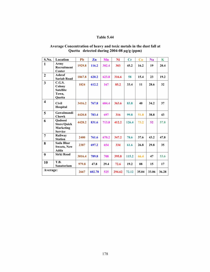
178
Table 5.44
Average Concentration of heavy and toxic metals in the dust fall at Quetta detected during 2004-08 µg/g (ppm)
S.No. Location Pb Zn Mn Ni Cr Co Na K 1 Army
Recruitment Center
1929.8 116.2 302.4 303 45.2 16.2 19 20.4
2 Ashraf Sariab Road 1867.8 620.2 623.8 316.6 58 15.4 23 19.2
3 C.G.S. Colony Satellite Town, Quetta
1824 612.2 167 85.2 33.4 11 28.6 32
4 Civil Hospital
3416.2 767.8 684.4 363.6 83.8 40 34.2 37
5 Gawalmandi Chowk 4420.8 783.4 697 316 99.8 51.8 38.8 43
6 Qadoosi Store/Quick Marketing Service
4428.2 831.6 713.8 412.2 126.4 73.2 52 57.8
7 Railway Station 2400 761.6 670.2 347.2 78.6 37.6 43.2 47.8
8 Sada Bhar Sweets, New Adda
2387 697.2 654 334 61.6 26.8 29.8 35
9 Sirki Road 3016.4 789.8 708 395.8 115.2 66.4 47 53.6
10 T.B. Sanatorium 979.8 47.8 29.4 72.6 19.2 08 15 17
Average: 2667 602.78 525 294.62 72.12 35.04 33.06 36.28
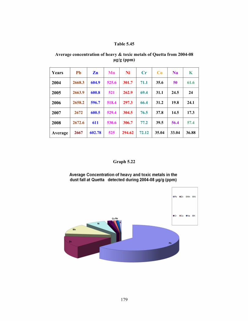
179
Table 5.45
Average concentration of heavy & toxic metals of Quetta from 2004-08 µg/g (ppm)
Years Pb Zn Mn Ni Cr Co Na K
2004 2668.3 604.9 525.6 301.7 71.1 35.6 50 61.6
2005 2663.9 600.8 521 262.9 69.4 31.1 24.5 24
2006 2658.2 596.7 518.4 297.3 66.4 31.2 19.8 24.1
2007 2672 600.5 529.4 304.5 76.5 37.8 14.5 17.3
2008 2672.6 611 530.6 306.7 77.2 39.5 56.4 57.4
Average 2667 602.78 525 294.62 72.12 35.04 33.04 36.88
Graph 5.22
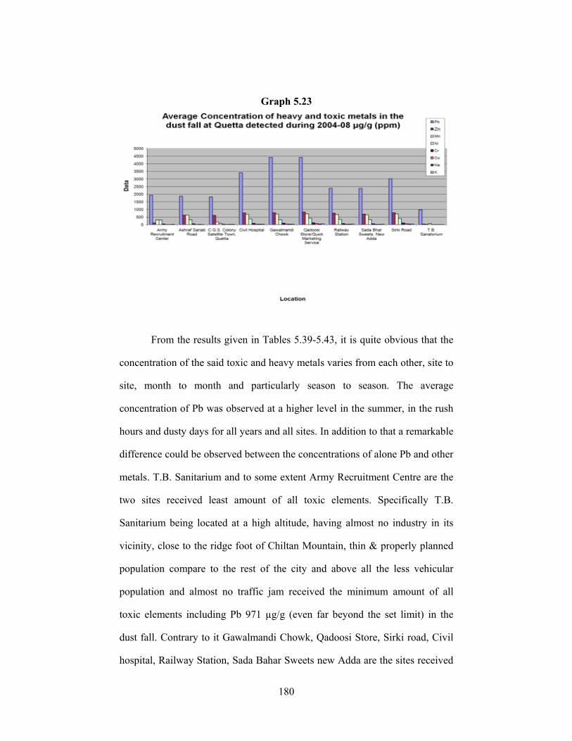
180
Graph 5.23
From the results given in Tables 5.39-5.43, it is quite obvious that the
concentration of the said toxic and heavy metals varies from each other, site to
site, month to month and particularly season to season. The average
concentration of Pb was observed at a higher level in the summer, in the rush
hours and dusty days for all years and all sites. In addition to that a remarkable
difference could be observed between the concentrations of alone Pb and other
metals. T.B. Sanitarium and to some extent Army Recruitment Centre are the
two sites received least amount of all toxic elements. Specifically T.B.
Sanitarium being located at a high altitude, having almost no industry in its
vicinity, close to the ridge foot of Chiltan Mountain, thin & properly planned
population compare to the rest of the city and above all the less vehicular
population and almost no traffic jam received the minimum amount of all
toxic elements including Pb 971 µg/g (even far beyond the set limit) in the
dust fall. Contrary to it Gawalmandi Chowk, Qadoosi Store, Sirki road, Civil
hospital, Railway Station, Sada Bahar Sweets new Adda are the sites received
181
the maximum amount of all toxic elements particularly Pb e.g. 4438 µg/g at
Qadoosi Store. The major source is obviously the automobile emission due to
heavily contaminated fuel and lengthy traffic jams on these sites. Pb is added
to fuel as an anti-knocking agent to prevent the accumulation of large
quantities of PbO within the combustion engine and thus prevent engine
knocking, tetraethyl lead, mixed with alkylethylmethyl lead, diethymethyl lead
and ethyltrimethyl lead additives. The addition of Pb scavengers, ethylene
dibromide or dichloride, results in the emission of volatile lead halides PbBr2,
PbBrCl, Pb(OH)Br, (PbO)2PbBr2 into the environment through the exhaust
gas. The European Community maximum allowable Lead concentration in
ambient air is 2µgm−3, whereas the concentration of >8 µgm−3 (motorways)
and ~2-3 µgm−3 (urban roads) are common. Around 70-75% is emitted from
the exhaust as inorganic salt of lead and about 1% is evolved unchanged as
tetra alkyl lead [126]. Evaporation loss of fuel from fuel tanks and carburetors
becomes the reason as well tetra alkyl compounds to the atmospheric dust.
The organic lead compounds are volatile and remain in air however the
inorganic salts are liberated as particles. The concentration of Pb in different
gasoline was detected to be (g/dm3) PSO= 0.64, CALTEX=0.55 and
PBS=0.54 [127]. Lead contained paints have also left extensive effect on Pb
concentration in the dust [128]. Other sources of Pb plumbing, glazed pottery
solder used in tin cans, old pewter etc. it is found in rocks as galena (PbS) at
concentration of 0.1-10mg/kg. During weathering Pb2+ can form carbonates
and has the tendency to be integrated in clay minerals, in Fe and Mn oxides
and in organic matter. Lead contamination of soils is a primary problem for
humans and animals as well. Normal surface soil levels are typically less than
182
40mg/kg, but with because of metal mining it sometimes increased up to
450mg/kg and sewage slugged farmland as in the suburbs of Quetta might
increase up to (80-300mg/kg). Plants instead of mainly taking up Pb from soil
receive it with the deposition of lead particulates onto the foliar surface of
plants, from where it turns a dietary source for animals and humans. Normal
limits of Pb on food stuff are <2mg/kg (dry weight); while improved levels
alongside motorways (20-950mg/kg), batter works (34-600mg/kg), and metal
processing industrial sites (45-2714mg/kg). The UK standard for Pb in food is
1mg/kg, with the exception of baby food, which is 0.2mg/kg. The WHO
(World Health Organization) has recommended that a tolerable intake of Pb
per day for an adult is 430µg [116].
Zn is widely used in the production of non-corrosive ally, brass in
galvanizing steel and iron and it is also used in some lubricating oil as an
important component and in many Zn-containing additives for instance as
antioxidant Zn [129]. It showed the same trend as Pb showed on all sites. The
sites like Qadoosi General Store 838 µg/g, Gawalmandi Chowk, Sada Bahar
Sweets, Ashraf Sariab Road, Railway Station, CGS Colony etc. having larger
population and more vehicular jam, so these sites gave more Zn keeping in
view its extensive usage in lubricants. While again the sites like T.B.
Sanitarium 37 µg/g, Army Recruitment Center showed lower values of Zn due
to thin traffic.
The most probable source of Cr could be abrasion of chrome-plating
and alloys in motor vehicles. Additional sources are leather tanning, textile
dying, electroplating, laundry chemicals and wear of wear of metal plating,
183
which contribute Cr to atmosphere dust fall. It was found to be present in the
samples from 15-132 ppm.
Ni is mostly used either as the metal or its alloy i.e. Ni coating on Cu
or Fe and Ni plating articles. Ni was detected in the dust fall between the
optimum ranges of 68-411ppm on the similar trend of minimum at T.B.
Sanitarium and maximum at Qadoosi Store. Residual oil, coal, tobacco,
chemical catalyst and nonferrous alloys are some of the sources of
atmospheric nickel pollution. The variation in the concentration was due to
smoke. It has been reported that the smoke of single cigarette release about
2.2-2.3 µg/g of Ni to the atmosphere [130].
The concentration of Mn was detected in the dust fall at T.B.
Sanatorium and Qadoosi Store on optimum levels of 21-725 µg/g. Its high
concentration might be due to its use is metal alloys, dry cell batteries, feed
additives, fertilizers, pigments, dryers, wood preservatives, coating welding
rods, paints and chemical detergents. Being an important constituent of
explosive, Mn is liberated in the air through fire display and several types of
crackers used at different occasions.
Even though an exact source of Co in the environment is difficult to
find out, yet most probably the use of Co in high speed diesel, steel, cemented
carbide, high temperature alloy in industry and as a catalyst in different
industrial processes contribute significantly to atmosphere Cobalt pollution.
The concentration of Co was detected minimum at T.B. Sanitarium (2 µg/g)
and maximum at Qadoosi Store (80 µg/g).
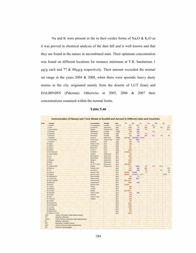
184
Na and K were present in the in their oxides forms of Na2O & K2O as
it was proved in chemical analysis of the dust fall and is well known and that
they are found in the nature in uncombined state. Their optimum concentration
was found on different locations for instance minimum at T.B. Sanitarium 1
µg/g each and 77 & 88µg/g respectively. Their amount exceeded the normal
set range in the years 2004 & 2008, when there were sporadic heavy dusty
storms in the city originated mainly from the deserts of LUT (Iran) and
DALBINDIN (Pakistan). Otherwise in 2005, 2006 & 2007 their
concentrations remained within the normal limits.
Table 5.46
S.No. Country Location/City Sample Unit Pb Zn Ni Mn Co Cr1 Poland Lecz-Wlodawa Dustfall G/m2 m 13.7 46.4 1.6 13.2 - 3.12 USA ILLIONOIS Street dust µg/g 1000 32 250 35 6.8 2103 Saudi Arabia Riyadh Outdoor dust µg/g 1762 443 44 - - 35.14 Pakistan Abbotabad Dustfall mg/kg 446 931 - 533 - -5 Pakistan Islamabad Dustfall µg/g 22.7 8.3 5.6 - - -6 Pakistan Peshawar Dustfall µg/g 525 763 358 637 54 837 Pakistan Karachi Street dust mg/kg 810-4527 112-2215 72-481 - - -8 Hong Kong Hong Kong Surface dust mg/g 302 1517 - - - -9 Jamaica Kingston Dust µg/g 909 0.8 - - - -
10 Egypt Various sites Dust µg/g 126 - - - - -11 Mexico Chihuahua Dust µg/g 277 - - - - -12 Mexico Monterrey Dust µg/g 467 - - - - -13 Mexico Torreon Dust µg/g 2448 - - - - -14 W. Germany W. Berlin Dust µg/g 8-2943.01 - - - - -15 Saudi Arabia Jeddah Street dust ppm 745 - - - - -16 U.K. Birmingham Street dust ppm 1630 - - - - -17 U.K. Manchester Street dust ppm 970 - - - - -18 Belgium Belgium Street dust ppm 2255 - - - - -19 Malta Malta Street dust ppm 1825 - - - - -20 USA Av. Of 77 cities Street dust ppm 240-1500 - - - - -21 Saudi Arabia Riyadh Falling dust ppm 66.8 141.8 26 319 20.6 -22 Bahrain Various sites ppm 697 151 125 - - 14423 U.K. Lancaster ppm 1880 534 35 - 9.1 2924 Greece Various sites ppm 65-259 75-241 52 - - 1325 Nigeria Various sites ppm 40-243 12-48.01 1-3.3 - - 23-2626 Netherlands Near Smelter ppm 761 1.5 - - - -27 Hong Kong Various sites ppm 1080 1517 - - - -28 New Zealand Christ church ppm 887-1070 - - - - -29 Malaysia Kualalumper ppm 2466 344 - - - -30 Kenya Various sites ppm 23-950 - - - - -31 Taiwan Taipei ppm 196 - - - - -32 England London ppm 345 - - - - -33 Canada Halifax ppm 674-1919 - - - - -34 Equador Various sites ppm 108 218 - - - -35 Kuwait Salmich ppm 136 - - - - -36 USA Various sites ppm 900 - - - -37 Scotland Glagow ppm 308 - - - - -38 Jeddah ppm 745 - - - - -39 Hong Kong ppm 1627 - - - - -40 Brimingham ppm 1630 - - - - -41 London ppm 1200 - - - - -42 Glasgow ppm 960 - - - - -43 Manchester ppm 970 - - - - -44 Urbana III, USA ppm 3600 - - - - -
AAS Atomic Absorption Spectrophotometery SV Striping Voltametry FAAS Flame Atomic Absorption Spectrophotometry SV Striping Voltametry ICP Inductively Coupled Plasma AES Atomic Emission Spectrophotometry ES Emission Spectrograph
Concentration of Heavey and Toxic Metals in Dustfall and Aerosol in Different cities and Countries
185
While comparing the concentrations of all toxic and heavy metals in
dust fall given in Table 5.39-5.45 with the international data in Table 5.46, it
could be observed that the average annual concentration of Pb at Quetta was
detected (2667 µg/g) is less than the average annual concentration only a few
more cities across the globe like Karachi (29889 µg/g [131] and USA, Urbana
III (3600 µg/g) [132]. However, some the cities (former) W.Germany,
W.Berlin (8-2943 µg/g) [133], Malaysia, Kaulampur (2466 µg/g) [134],
Mexico, Torreon (2448 µg/g) [135] and Belgium (2255 µg/g) [136] were
having the lesser average annual concentration of Pb than at Quetta was
detected by me. The average concentration of Zn detected by me for the said 5
years was (602.78 µg/g), which is far more than the normal set limit. It is
anyhow less than Peshawar (763 µg/g) [87,137], and more than some of the
cities like UK, Lancaster (534 µg/g) [138,139], (547 µg/g) Saudi Arabia,
Riyadh and (112-2215 µg/g) Pakistan, Karachi [140] etc. Similarly the
concentrations of Mn, Ni, Cr, Co, Na & K given in Tables W, X & Y were
though having the concentrations of said toxic and heavy elements mostly
within the set limits by the Canadian Association for Lab. Accreditation Inc.
given in Table 5.38 in 2005, 2006 &2007, yet the said elements show higher
concentrations in the year 2004 & 2008 due to the unusual extreme dusty
thermal inversion conditions. On the whole almost the same trend somewhat
similar to Pb & Zn have been showed by Mn, Ni, Cr, Co, Na & K compare to
some cities of the world, where their concentration was less, and with some it
was more. It infers that dust particulates are extremely multifarious substance,
the composition of which is seldom constant. All the urban densely populated
cities are enriched of heavy metals. Masses residing in urban parts are more
186
vulnerable to the people living in rural and far flung areas. By and large
Quetta is almost on the top of the few extremely toxic (elements particularly
Pb) polluted cities in the world and the major reason of it is its bowl shape
geography, small area (space), huge humans and vehicular population during
the previous decades [141,142] and the massive toxic emission of traffic
mostly running on.
5.5 AVERAGE SIZE DISTRIBUTION OF SETTLED & AIR DUST
PARTICULATES:
In most cases the maximum pollution levels are within a few
kilometers of the emission source, but small particulate and aerosol pollutants
can contaminate all areas of a city or even a region. Several studies have
shown a slow accumulation of Pb in both the Arctic and Antarctic regions
since the introduction of lead alkyl additives to petrol in the early [116].
Keeping in view this established fact settled/fallen particles size contrary to
the airborne suspended detection, settled/deposited dust particulates [100,
99,10],fractionation on wt. % basis was got for nine size categories: PM<1.0,
PM1.0-2.5, PM2.5-5.0, PM5.0-10, PM10-15, PM15-25, PM25-50, PM50-100 and PM>100 by
using standard methods for sieve analysis [106] in contrast with the
particulates size determination on vol. % basis by using Mastersizer 2000
(Malvern, Ver. 3.01, UK [10]due to its non-availability in any institutions of
even Quetta city not to speak of Balochistan province. The data on particulates
size categorization showed in Table 5.47a, depicts the average annual wt. %
segments detected in Quetta for the said period of 2004-08 from the 10
selected sites. The data clearly shows that on the average, the PM10-15 portion
187
is the largest, at 16.37 wt. %, followed by PM5.0-10& PM15-25 at 15.48 & 13.00
wt. % respectively. The particulates parts PM2.5-5.0, PM25-50 & PM50-100
showed significant concentrations at 12.09, 11.11 & 10.64 wt. % as well, the
giant particulates PM>100 were having the concentration of 9.78 wt. % and the
fine and ultra fine particulates PM1.0-2.5 & PM<1.0 were found to be present at
8.68 & 5.16 wt. % respectively. In Quetta the southern winds are dominant
mostly in the day times of summer and in winter the northern winds usually hit
the city. The southern regional and local winds of summer are mostly
responsible for the heavy dust fall in the city carrying sub-urban, rural and
rarely during the lengthy dry spells, in the thermal inversion period (as was
witnessed drop regional dust into the urban settled parts of the bowled shape
city. The wind direction and extremely low humidity (having almost dry
atmosphere) therefore play an important role in mixing the air masses of these
different atmospheric fragments.
During the thermal inversion spells (days) the average % age of each
particulate present in the dust fall is given in Table 5.47 b; which clearly
shows that the amount of particulates having sizes PM15-25, PM10-15, PM5.0-10,
PM2.5-5.0, PM1.0-2.5& PM<1.0 were ≥12 % by weight. However, the PM25-50,
PM50-100, & PM>100 were found between the % age weight concentrations of
5.86-7.67. The reason is obvious that the particles having lesser sizes traveled
a greater distance between the lengthy severe arid and deserted belt of Iran and
Pakistan.
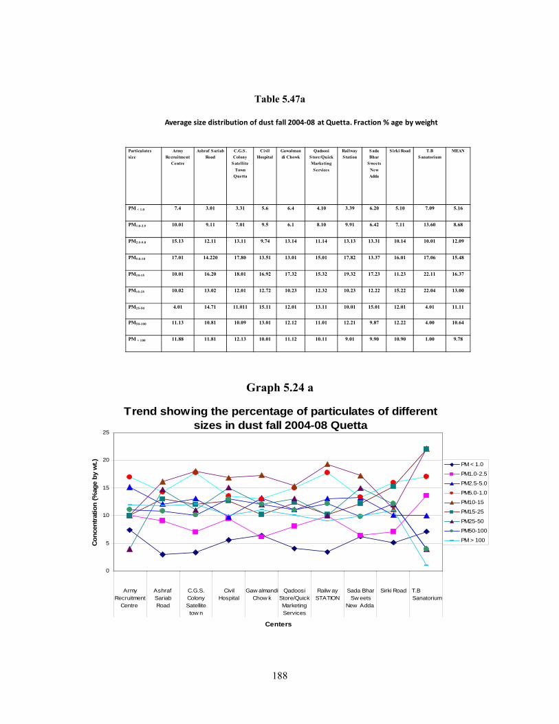
188
Table 5.47a
Average size distribution of dust fall 2004‐08 at Quetta. Fraction % age by weight
Particulates size
Army Recruitment
Centre
Ashraf SariabRoad
C.G.S . Colony
Satellite Town
Quetta
Civil Hospital
Gawalmandi Chowk
QadoosiStore/Quick Marketing
Services
Railway Station
SadaBhar
Sweets New Adda
Sirki Road T.B Sanatorium
MEAN
PM < 1.0 7.4 3.01 3.31 5.6 6.4 4.10 3.39 6.20 5.10 7.09 5.16
PM1.0-2.5 10.01 9.11 7.01 9.5 6.1 8.10 9.91 6.42 7.11 13.60 8.68
PM2.5-5.0 15.13 12.11 13.11 9.74 13.14 11.14 13.13 13.31 10.14 10.01 12.09
PM5.0-10 17.01 14.220 17.80 13.51 13.01 15.01 17.82 13.37 16.01 17.06 15.48
PM10-15 10.01 16.20 18.01 16.92 17.32 15.32 19.32 17.23 11.23 22.11 16.37
PM15-25 10.02 13.02 12.01 12.72 10.23 12.32 10.23 12.22 15.22 22.04 13.00
PM25-50 4.01 14.71 11.011 15.11 12.01 13.11 10.01 15.01 12.01 4.01 11.11
PM50-100 11.13 10.81 10.09 13.01 12.12 11.01 12.21 9.87 12.22 4.00 10.64
PM > 100 11.88 11.81 12.13 10.01 11.12 10.11 9.01 9.90 10.90 1.00 9.78
Graph 5.24 a
Trend showing the percentage of particulates of different sizes in dust fall 2004-08 Quetta
0
5
10
15
20
25
ArmyRecruitment
Centre
AshrafSariabRoad
C.G.S.ColonySatellitetow n
CivilHospital
Gaw almandiChow k
QadoosiStore/QuickMarketingServices
Railw aySTATION
Sada BharSw eets
New Adda
Sirki Road T.B Sanatorium
Centers
Con
cent
ratio
n (%
age
by w
t.) PM < 1.0
PM1.0-2.5
PM2.5-5.0
PM5.0-1.0
PM10-15
PM15-25
PM25-50
PM50-100
PM > 100
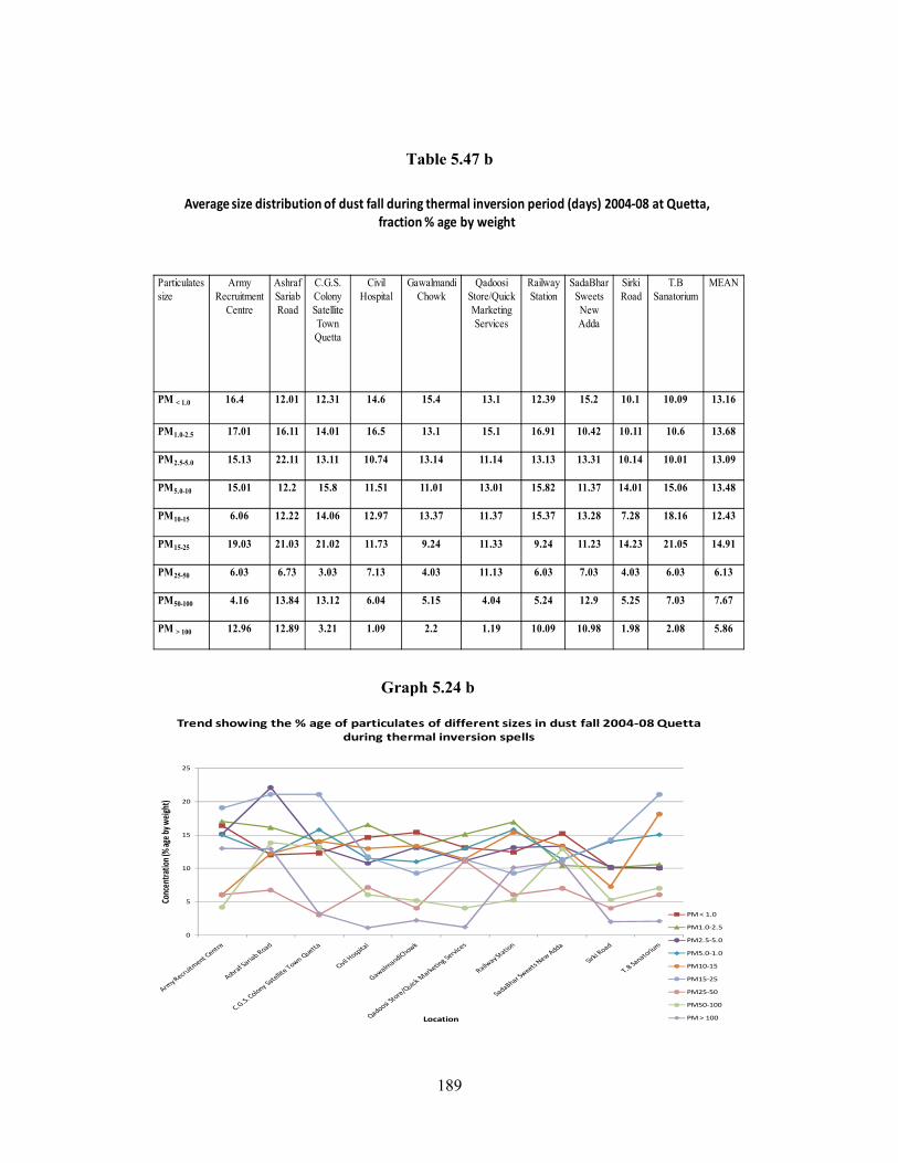
189
Table 5.47 b
Average size distribution of dust fall during thermal inversion period (days) 2004‐08 at Quetta, fraction % age by weight
Particulates size
Army Recruitment
Centre
AshrafSariabRoad
C.G.S. Colony Satellite Town Quetta
Civil Hospital
GawalmandiChowk
QadoosiStore/Quick Marketing Services
Railway Station
SadaBharSweets New Adda
SirkiRoad
T.B Sanatorium
MEAN
PM < 1.0 16.4 12.01 12.31 14.6 15.4 13.1 12.39 15.2 10.1 10.09 13.16
PM1.0-2.5 17.01 16.11 14.01 16.5 13.1 15.1 16.91 10.42 10.11 10.6 13.68
PM2.5-5.0 15.13 22.11 13.11 10.74 13.14 11.14 13.13 13.31 10.14 10.01 13.09
PM5.0-10 15.01 12.2 15.8 11.51 11.01 13.01 15.82 11.37 14.01 15.06 13.48
PM10-15 6.06 12.22 14.06 12.97 13.37 11.37 15.37 13.28 7.28 18.16 12.43
PM15-25 19.03 21.03 21.02 11.73 9.24 11.33 9.24 11.23 14.23 21.05 14.91
PM25-50 6.03 6.73 3.03 7.13 4.03 11.13 6.03 7.03 4.03 6.03 6.13
PM50-100 4.16 13.84 13.12 6.04 5.15 4.04 5.24 12.9 5.25 7.03 7.67
PM > 100 12.96 12.89 3.21 1.09 2.2 1.19 10.09 10.98 1.98 2.08 5.86
Graph 5.24 b
Trend showing the % age of particulates of different sizes in dust fall 2004‐08 Quetta during thermal inversion spells
0
5
10
15
20
25
Concen
tratio
n (% age b
y weight)
Location
PM < 1.0
PM1.0‐2.5
PM2.5‐5.0
PM5.0‐1.0
PM10‐15
PM15‐25
PM25‐50
PM50‐100
PM > 100
190
CHAPTER 6
APPLICATION OF STATISTICAL (ARIMA & SARIMA)
MODELING FOR FUTURE PREDICTIONS OF DUST FALL
RATE
6.1 LITERATURE SURVEY:
Stochastic time series model such as ARMA (p,q), non- seasonal
ARIMA and seasonal ARIMA (SARIMA) models were developed to simulate
and forecast hourly averaged wind speed and average annual and monthly rate
of dust fall sequences on five (05) year data ,.i.e., 2004-08 of Quetta, Pakistan.
Stochastic Time Series Models take into consideration numerous fundamental
features of wind rate including autocorrelation, non-Gaussian distribution and
non-stationarity. The positive correlation between consecutive wind speed
observations is taken into account by fitting ARMA process to wind speed
data. The data are normalized to make their distributions approximately
Gaussian and standardized to remove scattering of transformed data
(stationary, i.e., without chaos).Diurnal variations has been taken into account
to observe forecasts and its reliance on lead times. Though the ARMA (p,q)
model is suitable for prediction interval and probability forecasts, nevertheless
this model is only suitable for both long ranges (1-6 hours) and short range (1-
2 hours) indicates that forecast values are the deciding components for an
appropriate wind energy conversion system, WECS. ARMA processes cannot
be applied for non-stationary (chaotic) and random data. Non-seasonal
ARIMA models and the prediction equations for each month and indeed for
each season of five (05) meteorological years 2004-08, rate of dust fall data is
191
predicted. The seasonal ARIMA (SARIMA) and its prediction equations for
each month of five (05) years data were also studied. With non- stationarity or
chaos in data, stochastic simulator in the ARIMA processes even though its
prediction equations do not effectively work, yet ARIMA is good enough to
forecast relatively short range reliable values. Various statistical techniques
are used on five (05) years, .i.e., 2004-08 data of dust fall, average humidity,
rainfall, maximum and minimum temperatures, respectively. The relationships
to regression analysis time series (RATS) are developed for determining the
overall trend of these climate parameters on the basis of which forecast models
can be corrected and modified. Badescu [143] made use of ARIMA models to
forecast daily average surface pressures. His study is of much relevance to us
for reasons that the surface pressure would certainly effect the dust fall rate
and indeed the concentration of pollutants at various locations. We shall,
however, give due considerations of this study in later stages while looking
into a more generalized ARIMA model. However, our SARIMA model will
take into account such considerations indirectly, Badescu et al., [144]
performed the statistical of ambient air pollution in Delhi. A state space model
was developed by using Kalmin filter formulation for the prediction of various
pollutants and repairable suspended particulate matter. The approach was
found quiet pertinent. They used the ARX model (Auto-Regressive) with
exogenous input, which to our analysis are not adequate. We discarded
ARMA modeling for reasons that the dust fall rate and the concentration of
various pollutants follow random nature or non-stationarity. The ARMA
modeling could be used only if the data is standardized. This unfortunately
had not been done by Chelani et al Instead we developed ARIMA & SARIMA
192
models for dust fall rate and indeed their predictions are provided with
prediction equations. A tremendous scattering of predicted data was noted in
the ARX modeling of [145] urban air pollution was studied by them with time
series analysis by using ANN (Artificial Neural Network) and ARIMA
models. ANN was found relatively better than ARIMA on the basis of root
mean square estimation and other several statistical tests. It was established by
us that the ARIMA and SARIMA models could be considered relatively better
than ANN models due to diurnal (seasonal) variations. It was taken into
account in our studies the diurnal variations by considering the diurnal
variations by considering interrelationship between ARIMA and SARIMA.
Bruce et al., [146] followed dual cost function approaches as an alternative to
time series but this analysis is premature for our study unless we find forecast
estimates in conformity with our future experimental data. Los Angeles
performed time series analysis of particulate matter in air by using ACF (Auto
Correlative Function) [147], ARIMA and regression analysis. To our surprise
ARMA model didn’t work for our data as a consequence of which the ACF
wouldn’t be considered. The regression analysis is, of course important too,
but we avoided it because there are diverse statistical tests needed to support
the analysis. Kolehanainen et al., [148] coined a new technique by developing
hybrid neural network modeling for air quality forecasting. They followed
self-organized map algorithm (SOM), Sammon’s mapping and fuzzy distance
metrics. They categorized the clusters of data by overlapping multilayer
perceptron (MLP) models. Needless to mention their work was logically
pertinent and could be used for our data, too. We shall look into such kind of
models in near future but we are handicap due to non-availability of diverse
193
algorithms. Moshrik et al., [149] developed crop evapotranspiration time
series simulation model by using ARIMA. This reflects the strength and
validity of ARIMA model in most of the reported literature.
6.2 STOCHASTIC TIME SERIES MODELING, SIMULATION
AND PREDICTION:
A technique of predicting dust fall yield a few hours before, from a
dust fall collector with which suspended/settled dust fall under ‘g’
(gravitational force), is required to ensure efficient measures, which might be
taken in order to avoid its maximum calamity. Time series modeling of dust
fall has been the subject of many discussions because of the interest in its rate
of deposition, which proves mostly to be catastrophic. When the records of
dust fall are incomplete or of too short a duration or the handling and storage
of large values of the data are not desirable, then a time series model is needed
.Since dust fall is a reason of wind velocity, atmospheric pressure, geography
and topography of the area etc, generally the simulation are derived from
simulations of wind speed. Dust fall simulations can be done with Monto
Carlo techniques that depend upon exclusively on the anticipated factors of the
trivial distribution of wind speeds.
Craggs et al., [150], Aguiar and Pereira [151] and Mora-Lopez and
Sidrarch-de-Cardona [152] made some important contributions from modeling
and simulation point of view, having used stochastic simulation by ARIMA
(autoregressive integrated moving average) modeling of solar irradiation, a
time dependent autoregressive Gaussian model (TAG) for generating synthetic
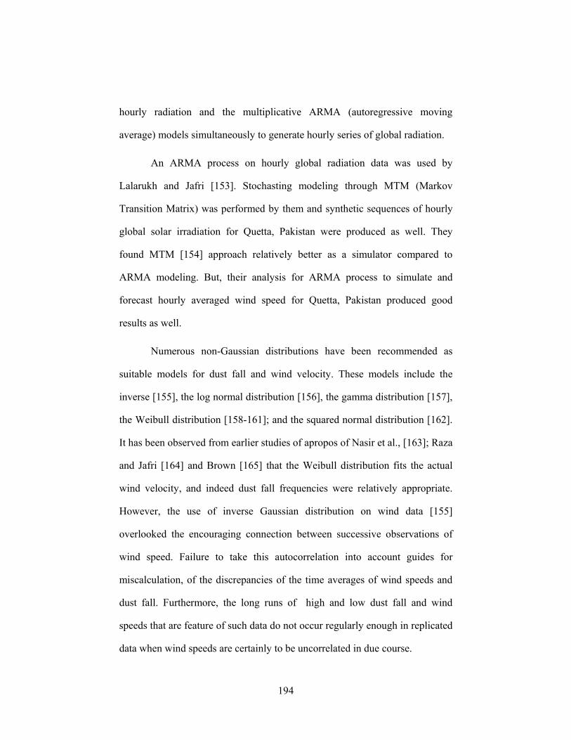
194
hourly radiation and the multiplicative ARMA (autoregressive moving
average) models simultaneously to generate hourly series of global radiation.
An ARMA process on hourly global radiation data was used by
Lalarukh and Jafri [153]. Stochasting modeling through MTM (Markov
Transition Matrix) was performed by them and synthetic sequences of hourly
global solar irradiation for Quetta, Pakistan were produced as well. They
found MTM [154] approach relatively better as a simulator compared to
ARMA modeling. But, their analysis for ARMA process to simulate and
forecast hourly averaged wind speed for Quetta, Pakistan produced good
results as well.
Numerous non-Gaussian distributions have been recommended as
suitable models for dust fall and wind velocity. These models include the
inverse [155], the log normal distribution [156], the gamma distribution [157],
the Weibull distribution [158-161]; and the squared normal distribution [162].
It has been observed from earlier studies of apropos of Nasir et al., [163]; Raza
and Jafri [164] and Brown [165] that the Weibull distribution fits the actual
wind velocity, and indeed dust fall frequencies were relatively appropriate.
However, the use of inverse Gaussian distribution on wind data [155]
overlooked the encouraging connection between successive observations of
wind speed. Failure to take this autocorrelation into account guides for
miscalculation, of the discrepancies of the time averages of wind speeds and
dust fall. Furthermore, the long runs of high and low dust fall and wind
speeds that are feature of such data do not occur regularly enough in replicated
data when wind speeds are certainly to be uncorrelated in due course.
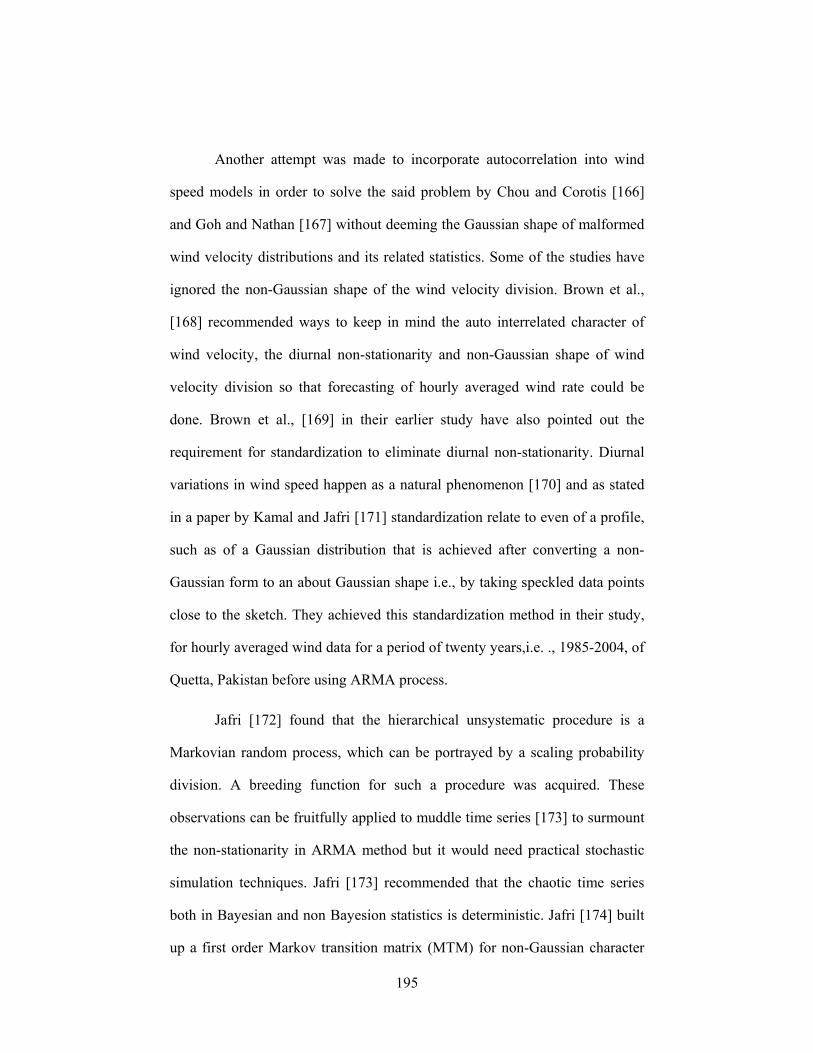
195
Another attempt was made to incorporate autocorrelation into wind
speed models in order to solve the said problem by Chou and Corotis [166]
and Goh and Nathan [167] without deeming the Gaussian shape of malformed
wind velocity distributions and its related statistics. Some of the studies have
ignored the non-Gaussian shape of the wind velocity division. Brown et al.,
[168] recommended ways to keep in mind the auto interrelated character of
wind velocity, the diurnal non-stationarity and non-Gaussian shape of wind
velocity division so that forecasting of hourly averaged wind rate could be
done. Brown et al., [169] in their earlier study have also pointed out the
requirement for standardization to eliminate diurnal non-stationarity. Diurnal
variations in wind speed happen as a natural phenomenon [170] and as stated
in a paper by Kamal and Jafri [171] standardization relate to even of a profile,
such as of a Gaussian distribution that is achieved after converting a non-
Gaussian form to an about Gaussian shape i.e., by taking speckled data points
close to the sketch. They achieved this standardization method in their study,
for hourly averaged wind data for a period of twenty years,i.e. ., 1985-2004, of
Quetta, Pakistan before using ARMA process.
Jafri [172] found that the hierarchical unsystematic procedure is a
Markovian random process, which can be portrayed by a scaling probability
division. A breeding function for such a procedure was acquired. These
observations can be fruitfully applied to muddle time series [173] to surmount
the non-stationarity in ARMA method but it would need practical stochastic
simulation techniques. Jafri [173] recommended that the chaotic time series
both in Bayesian and non Bayesion statistics is deterministic. Jafri [174] built
up a first order Markov transition matrix (MTM) for non-Gaussian character
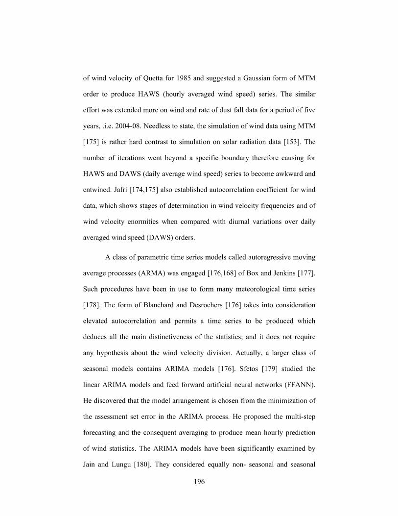
196
of wind velocity of Quetta for 1985 and suggested a Gaussian form of MTM
order to produce HAWS (hourly averaged wind speed) series. The similar
effort was extended more on wind and rate of dust fall data for a period of five
years, .i.e. 2004-08. Needless to state, the simulation of wind data using MTM
[175] is rather hard contrast to simulation on solar radiation data [153]. The
number of iterations went beyond a specific boundary therefore causing for
HAWS and DAWS (daily average wind speed) series to become awkward and
entwined. Jafri [174,175] also established autocorrelation coefficient for wind
data, which shows stages of determination in wind velocity frequencies and of
wind velocity enormities when compared with diurnal variations over daily
averaged wind speed (DAWS) orders.
A class of parametric time series models called autoregressive moving
average processes (ARMA) was engaged [176,168] of Box and Jenkins [177].
Such procedures have been in use to form many meteorological time series
[178]. The form of Blanchard and Desrochers [176] takes into consideration
elevated autocorrelation and permits a time series to be produced which
deduces all the main distinctiveness of the statistics; and it does not require
any hypothesis about the wind velocity division. Actually, a larger class of
seasonal models contains ARIMA models [176]. Sfetos [179] studied the
linear ARIMA models and feed forward artificial neural networks (FFANN).
He discovered that the model arrangement is chosen from the minimization of
the assessment set error in the ARIMA process. He proposed the multi-step
forecasting and the consequent averaging to produce mean hourly prediction
of wind statistics. The ARIMA models have been significantly examined by
Jain and Lungu [180]. They considered equally non- seasonal and seasonal
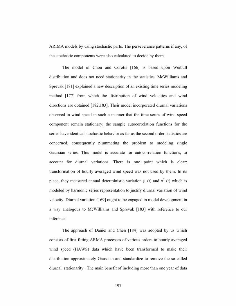
197
ARIMA models by using stochastic parts. The perseverance patterns if any, of
the stochastic components were also calculated to decide by them.
The model of Chou and Corotis [166] is based upon Weibull
distribution and does not need stationarity in the statistics. McWilliams and
Sprevak [181] explained a new description of an existing time series modeling
method [177] from which the distribution of wind velocities and wind
directions are obtained [182,183]. Their model incorporated diurnal variations
observed in wind speed in such a manner that the time series of wind speed
component remain stationary; the sample autocorrelation functions for the
series have identical stochastic behavior as far as the second order statistics are
concerned, consequently plummeting the problem to modeling single
Gaussian series. This model is accurate for autocorrelation functions, to
account for diurnal variations. There is one point which is clear:
transformation of hourly averaged wind speed was not used by them. In its
place, they measured annual deterministic variation µ (t) and σ2 (t) which is
modeled by harmonic series representation to justify diurnal variation of wind
velocity. Diurnal variation [169] ought to be engaged in model development in
a way analogous to McWilliams and Sprevak [183] with reference to our
inference.
The approach of Daniel and Chen [184] was adopted by us which
consists of first fitting ARMA processes of various orders to hourly averaged
wind speed (HAWS) data which have been transformed to make their
distribution approximately Gaussian and standardize to remove the so called
diurnal stationarity . The main benefit of including more than one year of data
198
in the model development is the increased trustworthiness of the estimates of
the model parameter. The methods of changing and standardization were not
likened but favored this approach for the grounds that the model had the
tendency of using wind data of more than one year.
MINITAB (version 11) for ARMA, non-seasonal ARIMA and
seasonal ARIMA modeling and simulation was used by us. ARIMA models
are used to model a special class of non- stationary series. Seasonal ARIMA
(SARIMA) models are used to incorporate cyclic components in models. In
other words, ARIMA models are, in theory the most general class of models
(Parsimonious) for forecasting a time series which can be stationarized by
transformations such as differencing and logging. SARIMA has the same
structure as ARIMA. Both non seasonal and seasonal models on monthly and
annually averaged rate of dust fall data for 2004-08 were used. For non-
seasonal ARIMA modeling and simulation, the six options i.e., random walk
ARIMA (0,1,0), differenced first order autoregressive model ARIMA (1,1,0),
constant ARIMA (0,1,1), linear exponential smoothing (LES) without constant
ARIMA (0,2,1) or (0,2,2) and mixed ARIMA (1,1,1) are tried for each month
and on four seasons. Non seasonal ARIMA (0, 1, 1) which deals with
exponential growth and constant incorporates simple exponential smoothing
(SES) model. MA (1) coefficients correspond to 1-α in the SES formula. The
term α is called training parameter. For LES without constant, MA (1)
coefficient corresponds to 2α. For seasonal ARIMA (SARIMA) modeling and
simulation, the seven options, i.e., SARIMA(0,1,1)x(0,1,1)12,
SARIMA(0,0,0)x(0,1,0)12 with constant, SARIMA(0,1,0)x(0,1,0)12
SARIMA(1,0,1)x(0,1,1)12 with constant, SARIMA following SES with
199
α=0.4772 and Brown’s SARIMA(LES) with α = 0.2106 are tried for each
month only. The most often used model of ARIMA is SARIMA (0, 1, 1) x (0,
1, 1)12 which strictly follows seasonal exponential smoothing. SARIMA (0, 1,
0) x (0, 1, 0)12 is also known as seasonal random trend (SRT) model. The
alternate to SRT model is seasonal random walk model, .i.e., SARIMA (1, 0,
0) x (0, 1, 0)12. There is, of course, a difference between seasonal and simple
exponential models. The values of θ = 1- α is used in exponential smoothing
formulas. The greatest choice is chosen by bearing in mind the mainly
minimum chi- squared value at 5% confidence gap.
6.3 MODELING SKETCH:
• Having used various time series modeling, simulation and prediction,
we could disentangle the unfocused parts of researches plus the areas
which were overstressed. It is already established that statistical
techniques like ARMA, ARIMA, non-seasonal ARIMA and seasonal
ARIMA have capabilities to simplify statistical techniques and achieve
modeling of time series wind and dust fall data.
• The ARMA was initially applied to forecast the average monthly and
annual rate of dust fall.
• Finally ARIMA and SARIMA modeling was found extremely
appropriate for our dust fall data in addition to the meteorological
conditions prevailed while our samples collection period of 2004-08.
200
6.4 AUTOREGRESSIVE MOVING AVERAGE (ARMA)
MODELS:
ARMA models integrate prediction not only past values of the data but
past values of the prediction residuals as well. It was assumed that the
generating mechanism is probabilistic and that the observed series with
equally spaced time interval {x1, x2, xt,} is a realization of a stochastic process
{x1, x2,…,xt,}. Typically, the process was supposed to be stationary and
described by a class of linear models. We were anxious with an idea of
population which evaluates the properties of the probability model used to
generate the observed series. The first order autoregressive (AR) model is
given by
Xt =Φ (Xt-1- µ ) + Z(t) --------------------------(1)
Eq.1 is a simple example of stochastic process. The uncertainty derives
from the variable Zt which is purely a random disturbance term with a mean of
zero and a variance of σt2.. Zt is purely random in the sense that the correlation
between any two of its values at different points in the time is zero. Remaining
features of the model are determined by the parameters µ and Φ, if Φ <I. The
observations fluctuate around µ, which is then called the mean of the process.
Further lagged values Xt-2, Xt-3, and so on as well as the lagged of the
disturbances term could be added enabling a more complicated pattern
dependence to be modeled. A general ARMA (p,q) model can be written as
Xt - µ = Φ1 ( Xt-1 - µ ) +Φ2( Xt-2 - µ ) +…+Φp ( Xt-p - µ )+ Zt + θ1 ( Zt-1) + θ2
(Zt-2)+…+ θq (Zt-q) ---------------- (2)
201
where { Φp } and { θq } are the coefficients of the autoregressive (AR) and the
moving average (MA) parts, respectively, and {Z } is white noise with mean
zero and variance σ2 . We assume Zt is normally distributed, that is, Zt~ N (0,
σ2). Using the backward shift operator B defined by BjXt = X t-j ,the ARMA
(p,q) model can be written as
Φ(B) Xt = θ (B) Zt-q -------------- (3)
where
Φ (B) = 1- Φ1 B – Φ2 B2 - ,…,- Φp Bp ------------ (4)
and
θ (B) = 1- θ1B - θ2 B2 - ,…,- θq Bq --------------(5)
We generally assume that the polynomials Φ(xt) and θ(xt) have no common
zeros. When Xt is a vector, we have a multivariate or vector ARMA model.
Since we are using non stationary data, .i.e., hourly averaged wind data,
therefore, the standardization is imperative for ARMA modeling Kamal and
Jafri (1997). We translate eq (2) into Φ1 B,…,- Φp Bp)U*n,y = (1- θ1 B-,…-
θqBq) an,y --------------(6)
where U*n,y = [ Un,y – µ(t)] / σ(t) ,.i.e., the standardized hourly averaged wind
speed data (after removing diurnal non stationarity from the wind speed data
Un,y), Un,y is hourly averaged wind speed for the yth year, y = 1,2,Y is the
number of years of observation and n = 1,2, N is the number of observations
of a given month of the year. B is the backward shift operator such that BU*n,y
= U*n-1,y ; Φ1,Φ2,,…, Φp are the autoregressive parameter ; θ1, θ2, ,…, θq are the
moving average parameters; and an,y is the white noise process equivalent to

202
Zt-q Bq (uncorrelated random variable with mean zero and variance σ2). It is
obvious that the moving average parameters will be equal to zero if the model
is a pure autoregressive process. Since ARMA processes were not used in our
studies as it would require three main steps, .i.e., identification, estimation and
diagnostic checking. ARMA modeling did not work on our dust fall data. It
yielded very poor ACF (autocorrelation function) and PACF (partial
autocorrelation function), respectively.
6.4.1 Autoregressive Integrated Moving Average (ARIMA) Non Seasonal
and Seasonal Models:
ARIMA models are used to model a special class of non-stationary
series. Seasonal ARIMA (SARIMA) model are used to incorporate cyclic
components in models. We can split the time series into deterministic and
stochastic components. The proportion of variance for each component can be
modeled through Monto Carlo simulations. The stochastic component can be
analyzed for persistence in time series using Box and Jenkins [177].
The general non seasonal ARIMA model is autoregressive to order p
and moving average to order q , and operator on the dth differences of Zt,
where {Zt} are time series values for
t = 1,2,…, N and N is number of observations. Defining
Bs Zt= Zt-s , ∇ s = (1-Bs), d
s∇ = (1-Bs)d ------------------(7)
where d = 0,1,…, B is the backward shift operator, s is the period of the
season (s = 12 in our present case for each month) and∇ is the difference
operator. The general non seasonal ARIMA model can be written as:
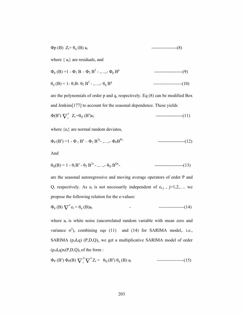
203
Φp (B) Zt= θq (B) at -----------------(8)
where { at} are residuals, and
Φp (B) =1 - Φ1 B – Φ2 B2 - ,…,- Φp Bp -------------------(9)
θq (B) = 1- θ1B- θ2 B2 - ,…,- θq Bq -------------------(10)
are the polynomials of order p and q, respectively. Eq (8) can be modified Box
and Jenkins[177] to account for the seasonal dependence. These yields
Φ(Bs) d
s∇ Zt =θQ (Bs)et ------------------(11)
where {et} are normal random deviates,
ΦP (Bs) =1 - Φ 1 Bs – Φ2 B2s- ,…,- ΦPBPs ------------------(12)
And
θQ(B) = 1 - θ1Bs - θ2 B2s - ,…,- θQ BQs- -------------------(13)
are the seasonal autoregressive and moving average operators of order P and
Q, respectively. As et is not necessarily independent of et-j , j=1,2,…. we
propose the following relation for the e-values:
Φp (B) d∇ et = θq (B)at - -----------------(14)
where at is white noise (uncorrelated random variable with mean zero and
variance σ2), combining eqs (11) and (14) for SARIMA model,. i.e.,
SARIMA (p,d,q) (P,D,Q)s, we get a multiplicative SARIMA model of order
(p,d,q)x(P,D,Q)s of the form :
ΦP (Bs) ΦP(B) D
s∇ d∇ Zt = θQ (Bs) θq (B) at ------------------(15)

204
Time series prediction with harmonic analysis can also be accomplished [180].
Theories on regression analysis time series have long been established [185-
187].
6.5 SIMULATION OF WIND SPEED AND FORECASTING:
Brown et al., [168] obtained the model by the steps which would not
be enlisted here. Autocorrelation functions for the observed and simulated data
were found in agreements. All these models can be used to forecast dust fall
few hours in advance. The process of forecasting of dust fall is quite similar to
the process of simulation. In fact a simulated value of dust fall can be regarded
as a one hour ahead forecast to which a random error has been added.
We found sporadic changes in autocorrelation function (ACF) and
indeed in partial autocorrelation function (PACF), as a consequence of which,
the ARMA model did not work. We find that ARMA processes when dealt
with transformed standardized data (hourly dust fall rate) give way to
relatively better precision in forecasts. But the aperiodic variation in ACF &
PACF resulted in larger values of error terms. ARIMA & SARIMA models
are useful only for diurnal dust fall rate, i.e., cyclic stochastic components in
the dust fall.
6.5.1 Reason of Non-Selecting of ARMA & Selecting of ARIMA:
The average daily data of dust fall for the five years (2004-2008) was
taken. ARMA model didn’t work for reasons that our data followed non-
stationary in dust fall, which is random. ARMA model cannot be applied for
non-stationarity and random data. This is why ARMA model in our case failed
badly. We wanted to establish with ARMA modeling the ACF (Auto
205
Correlation Function) and PACF (Partial Auto Correlation Function) but none
of these worked. Therefore, we shifted towards ARIMA modeling, which is
applicable to non-stationary and random data. ARMA modeling can be used if
we translate the non-staionarity into stationarity by some standardized
procedures, i.e., by considering mean and standard deviations. This is a
cumbersome process and evolves a lot of statistical calculations.
6.6 RESULTS AND DISCUSSION:
We considered locations such as GAWALMANDI & T.B. Sanatorium
on the basis of optimum dust fall rate, i.e., the most maximum in
GAWALMANDI & the second most minimum in the T.B. Sanatorium. To
reflect the statistical variations in between the optimum values we considered
a third location C.G.S. Colony, which will provide statistical variations with
respect to mean values of the optimum dust fall rate. Table 6.1 for ARIMA &
SARIMA are shown on the basis of categorization for seasons such as the
spring of Quetta comprises of February, March and April, and so is the case
for other seasons, for GAWALMANDI, T.B. Sanatorium & C.G.S. Colony,
respectively. Each table for different locations for each month of the season
both for ARIMA & SARIMA provides prediction equations obtained for each
month of the season both from ARIMA & SARIMA models, which are
beneficial to predict the dust fall rate for larger as well as shorter lead times.
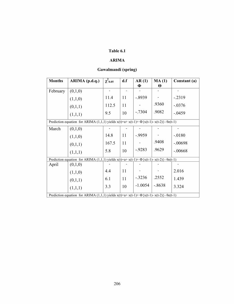
206
Table 6.1
ARIMA
Gawalmandi (spring) Months ARIMA (p.d.q.) χ2
0.05 d.f AR (1) Φ
MA (1) Θ
Constant (a)
February (0,1,0)
(1,1,0)
(0,1,1)
(1,1,1)
-
11.4
112.5
9.5
-
11
11
10
-
-.8939 -
-.7304
-
-
.9360
.9082
-
-.2319
-.0376
-.0459
Prediction equation for ARIMA (1,1,1) yields x(t)=a+ x(t-1)+ Ф{x(t-1)- x(t-2)}- θe(t-1) March (0,1,0)
(1,1,0)
(0,1,1)
(1,1,1)
-
14.8
167.5
5.8
-
11
11
10
-
-.9959 -
-.9283
-
-
.9408
.9629
-
-.0180
-.00698
-.00668
Prediction equation for ARIMA (1,1,1) yields x(t)=a+ x(t-1)+ Ф{x(t-1)- x(t-2)}- θe(t-1) April (0,1,0)
(1,1,0)
(0,1,1)
(1,1,1)
-
4.4
6.1
3.3
-
11
11
10
-
-
-.3236
-1.0054
-
-
.2552
-.8638
-
2.016
1.439
3.324
Prediction equation for ARIMA (1,1,1) yields x(t)=a+ x(t-1)+ Ф{x(t-1)- x(t-2)}- θe(t-1)
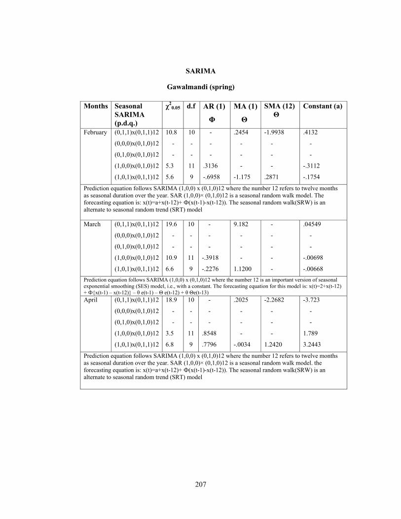
207
SARIMA
Gawalmandi (spring)
Months Seasonal SARIMA (p.d.q.)
χ20.05 d.f AR (1)
Φ
MA (1)
Θ
SMA (12) Θ
Constant (a)
February (0,1,1)x(0,1,1)12
(0,0,0)x(0,1,0)12
(0,1,0)x(0,1,0)12
(1,0,0)x(0,1,0)12
(1,0,1)x(0,1,1)12
10.8
-
-
5.3
5.6
10
-
-
11
9
-
-
-
.3136
-.6958
.2454
-
-
-
-1.175
-1.9938
-
-
-
.2871
.4132
-
-
-.3112
-.1754
Prediction equation follows SARIMA (1,0,0) x (0,1,0)12 where the number 12 refers to twelve months as seasonal duration over the year. SAR (1,0,0)× (0,1,0)12 is a seasonal random walk model. The forecasting equation is: x(t)=a+x(t-12)+ Ф(x(t-1)-x(t-12)). The seasonal random walk(SRW) is an alternate to seasonal random trend (SRT) model March (0,1,1)x(0,1,1)12
(0,0,0)x(0,1,0)12
(0,1,0)x(0,1,0)12
(1,0,0)x(0,1,0)12
(1,0,1)x(0,1,1)12
19.6
-
-
10.9
6.6
10
-
-
11
9
-
-
-
-.3918
-.2276
9.182
-
-
-
1.1200
-
-
-
-
-
.04549
-
-
-.00698
-.00668
Prediction equation follows SARIMA (1,0,0) x (0,1,0)12 where the number 12 is an important version of seasonal exponential smoothing (SES) model, i.e., with a constant. The forecasting equation for this model is: x(t)=2+x(t-12) + Ф{x(t-1) – x(t-12)} – θ e(t-1) – Θ e(t-12) + θ Θe(t-13) April (0,1,1)x(0,1,1)12
(0,0,0)x(0,1,0)12
(0,1,0)x(0,1,0)12
(1,0,0)x(0,1,0)12
(1,0,1)x(0,1,1)12
18.9
-
-
3.5
6.8
10
-
-
11
9
-
-
-
.8548
.7796
.2025
-
-
-
-.0034
-2.2682
-
-
-
1.2420
-3.723
-
-
1.789
3.2443
Prediction equation follows SARIMA (1,0,0) x (0,1,0)12 where the number 12 refers to twelve months as seasonal duration over the year. SAR (1,0,0)× (0,1,0)12 is a seasonal random walk model. the forecasting equation is: x(t)=a+x(t-12)+ Ф(x(t-1)-x(t-12)). The seasonal random walk(SRW) is an alternate to seasonal random trend (SRT) model
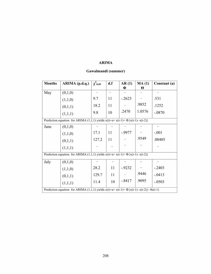
208
ARIMA
Gawalmandi (summer)
Months ARIMA (p.d.q.) χ20.05 d.f AR (1)
Φ MA (1) Θ
Constant (a)
May (0,1,0)
(1,1,0)
(0,1,1)
(1,1,1)
-
9.7
18.2
9.8
-
11
11
10
-
-.2623 -
.2470
-
-
.9852
1.0576
-
.531
.1252
-.0870
Prediction equation for ARIMA (1,1,1) yields x(t)=a+ x(t-1)+ Ф{x(t-1)- x(t-2)}
June (0,1,0)
(1,1,0)
(0,1,1)
(1,1,1)
-
17.1
127.2 -
-
11
11 -
-
-.9977 -
-
-
-
.9549 -
-
-.001
.00405 -
Prediction equation for ARIMA (1,1,1) yields x(t)=a+ x(t-1)+ Ф{x(t-1)- x(t-2)}
July (0,1,0)
(1,1,0)
(0,1,1)
(1,1,1)
-
28.2
129.7
11.4
-
11
11
10
-
-.9232 -
-.8417
-
-
.9446
.9095
-
-.2403
-.0413
-.0503
Prediction equation for ARIMA (1,1,1) yields x(t)=a+ x(t-1)+ Ф{x(t-1)- x(t-2)}- θe(t-1)
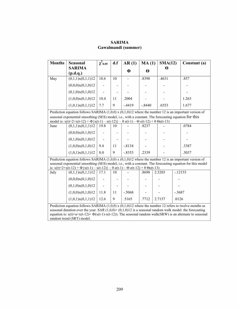
209
SARIMA Gawalmandi (summer)
Months Seasonal SARIMA (p.d.q.)
χ20.05 d.f AR (1)
Φ
MA (1)
Θ
SMA(12) Θ
Constant (a)
May (0,1,1)x(0,1,1)12
(0,0,0)x(0,1,0)12
(0,1,0)x(0,1,0)12
(1,0,0)x(0,1,0)12
(1,0,1)x(0,1,1)12
18.6
-
-
10.4
7.7
10
-
-
11
9
-
-
-
.2004
-.4419
.8398
-
-
-
-.8440
.4631
-
-
-
.6553
.857
-
-
1.263
1.677
Prediction equation follows SARIMA (1,0,0) x (0,1,0)12 where the number 12 is an important version of seasonal exponential smoothing (SES) model, i.e., with a constant. The forecasting equation for this model is: x(t)=2+x(t-12) + Ф{x(t-1) – x(t-12)} – θ e(t-1) – Θ e(t-12) + θ Θe(t-13) June (0,1,1)x(0,1,1)12
(0,0,0)x(0,1,0)12
(0,1,0)x(0,1,0)12
(1,0,0)x(0,1,0)12
(1,0,1)x(0,1,1)12
19.8
-
-
9.4
8.0
10
-
-
11
9
-
-
-
-.8134
-.8353
.8237
-
-
-
.2339
-
-
-
-
-
.0784
-
-
.3387
.3037
Prediction equation follows SARIMA (1,0,0) x (0,1,0)12 where the number 12 is an important version of seasonal exponential smoothing (SES) model, i.e., with a constant. The forecasting equation for this model is: x(t)=2+x(t-12) + Ф{x(t-1) – x(t-12)} – θ e(t-1) – Θ e(t-12) + θ Θe(t-13) July (0,1,1)x(0,1,1)12
(0,0,0)x(0,1,0)12
(0,1,0)x(0,1,0)12
(1,0,0)x(0,1,0)12
(1,0,1)x(0,1,1)12
17.1
-
-
11.8
12.6
10
-
-
11
9
-
-
-
-.5068
.5165
.8698
-
-
-
.7712
2.5203
-
-
-
2.7157
-.12155
-
-
-.3687
.0126
Prediction equation follows SARIMA (1,0,0) x (0,1,0)12 where the number 12 refers to twelve months as seasonal duration over the year. SAR (1,0,0)× (0,1,0)12 is a seasonal random walk model. the forecasting equation is: x(t)=a+x(t-12)+ Ф(x(t-1)-x(t-12)). The seasonal random walk(SRW) is an alternate to seasonal random trend (SRT) model.

210
ARIMA
Gawalmandi (autumn)
Months ARIMA (p.d.q.) χ20.05 d.f AR (1)
Φ MA (1) Θ
Constant (a)
August (0,1,0)
(1,1,0)
(0,1,1)
(1,1,1)
-
0.4
1.4
0.1
-
11
11
10
-
-1.000
-1.009 -
-
-
.8981
-.0325
-
-3.237
-.5870
-3.223
Prediction equation for ARIMA (1,1,1) yields x(t)=a+ x(t-1)+ Ф{x(t-1)- x(t-2)}- θe(t-1) September (0,1,0)
(1,1,0)
(0,1,1)
(1,1,1)
-
22.7
146.1
16.6
-
11
11
10
-
-.9579 -
-.9430
-
-
.9373
1.0574
-
-.0075
-.0141
.0072
Prediction equation for ARIMA (1,1,1) yields x(t)=a+ x(t-1)+ Ф{x(t-1)- x(t-2)}- θe(t-1) October (0,1,0)
(1,1,0)
(0,1,1)
(1,1,1)
-
10.1
10.0
6.8
-
11
11
10
-
-.4231 -
-.9981
-
-
.4519
-.8879
-
.762
.437
1.049
Prediction equation for ARIMA (1,1,1) yields x(t)=a+ x(t-1)+ Ф{x(t-1)- x(t-2)}- θe(t-1)
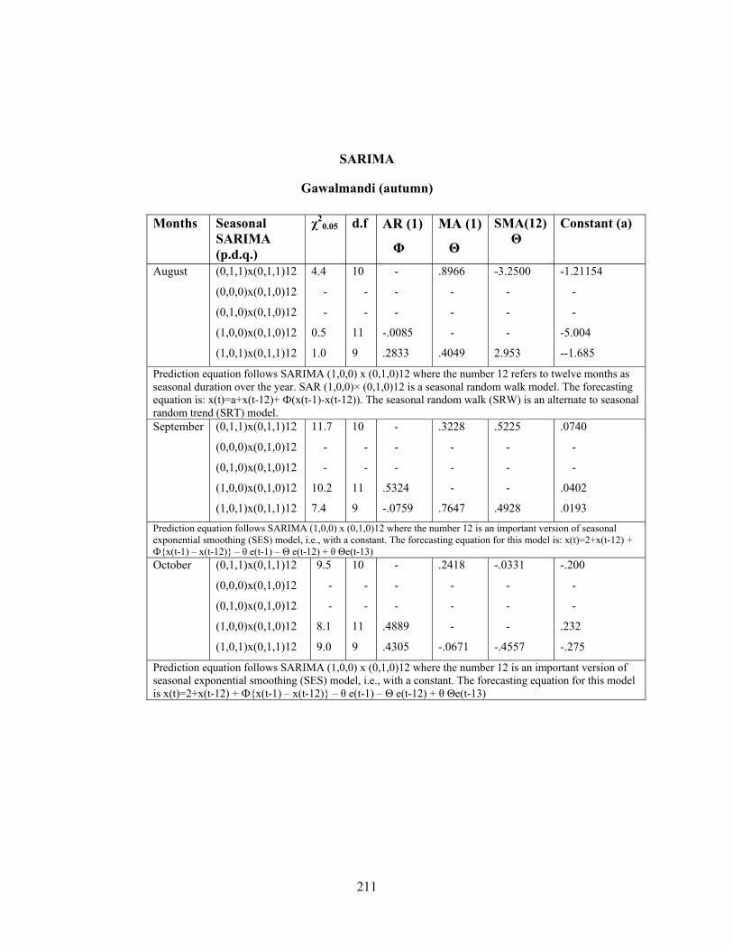
211
SARIMA
Gawalmandi (autumn)
Months Seasonal SARIMA (p.d.q.)
χ20.05 d.f AR (1)
Φ
MA (1)
Θ
SMA(12) Θ
Constant (a)
August (0,1,1)x(0,1,1)12
(0,0,0)x(0,1,0)12
(0,1,0)x(0,1,0)12
(1,0,0)x(0,1,0)12
(1,0,1)x(0,1,1)12
4.4
-
-
0.5
1.0
10
-
-
11
9
-
-
-
-.0085
.2833
.8966
-
-
-
.4049
-3.2500
-
-
-
2.953
-1.21154
-
-
-5.004
--1.685
Prediction equation follows SARIMA (1,0,0) x (0,1,0)12 where the number 12 refers to twelve months as seasonal duration over the year. SAR (1,0,0)× (0,1,0)12 is a seasonal random walk model. The forecasting equation is: x(t)=a+x(t-12)+ Ф(x(t-1)-x(t-12)). The seasonal random walk (SRW) is an alternate to seasonal random trend (SRT) model. September (0,1,1)x(0,1,1)12
(0,0,0)x(0,1,0)12
(0,1,0)x(0,1,0)12
(1,0,0)x(0,1,0)12
(1,0,1)x(0,1,1)12
11.7
-
-
10.2
7.4
10
-
-
11
9
-
-
-
.5324
-.0759
.3228
-
-
-
.7647
.5225
-
-
-
.4928
.0740
-
-
.0402
.0193
Prediction equation follows SARIMA (1,0,0) x (0,1,0)12 where the number 12 is an important version of seasonal exponential smoothing (SES) model, i.e., with a constant. The forecasting equation for this model is: x(t)=2+x(t-12) + Ф{x(t-1) – x(t-12)} – θ e(t-1) – Θ e(t-12) + θ Θe(t-13) October (0,1,1)x(0,1,1)12
(0,0,0)x(0,1,0)12
(0,1,0)x(0,1,0)12
(1,0,0)x(0,1,0)12
(1,0,1)x(0,1,1)12
9.5
-
-
8.1
9.0
10
-
-
11
9
-
-
-
.4889
.4305
.2418
-
-
-
-.0671
-.0331
-
-
-
-.4557
-.200
-
-
.232
-.275
Prediction equation follows SARIMA (1,0,0) x (0,1,0)12 where the number 12 is an important version of seasonal exponential smoothing (SES) model, i.e., with a constant. The forecasting equation for this model is x(t)=2+x(t-12) + Ф{x(t-1) – x(t-12)} – θ e(t-1) – Θ e(t-12) + θ Θe(t-13)
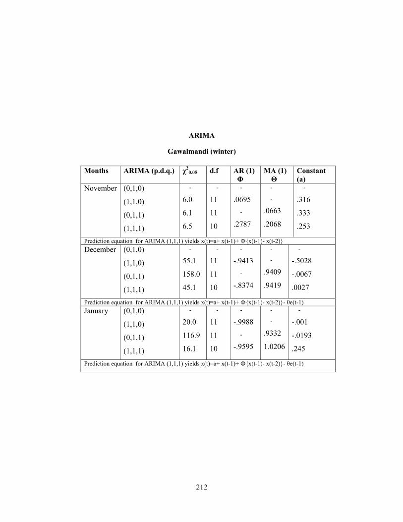
212
ARIMA
Gawalmandi (winter)
Months ARIMA (p.d.q.) χ20.05 d.f AR (1)
Φ MA (1) Θ
Constant (a)
November (0,1,0)
(1,1,0)
(0,1,1)
(1,1,1)
-
6.0
6.1
6.5
-
11
11
10
-
.0695 -
.2787
-
-
.0663
.2068
-
.316
.333
.253
Prediction equation for ARIMA (1,1,1) yields x(t)=a+ x(t-1)+ Ф{x(t-1)- x(t-2)} December (0,1,0)
(1,1,0)
(0,1,1)
(1,1,1)
-
55.1
158.0
45.1
-
11
11
10
-
-.9413 -
-.8374
-
-
.9409
.9419
-
-.5028
-.0067
.0027
Prediction equation for ARIMA (1,1,1) yields x(t)=a+ x(t-1)+ Ф{x(t-1)- x(t-2)}- θe(t-1) January (0,1,0)
(1,1,0)
(0,1,1)
(1,1,1)
-
20.0
116.9
16.1
-
11
11
10
-
-.9988 -
-.9595
-
-
.9332
1.0206
-
-.001
-.0193
.245
Prediction equation for ARIMA (1,1,1) yields x(t)=a+ x(t-1)+ Ф{x(t-1)- x(t-2)}- θe(t-1)
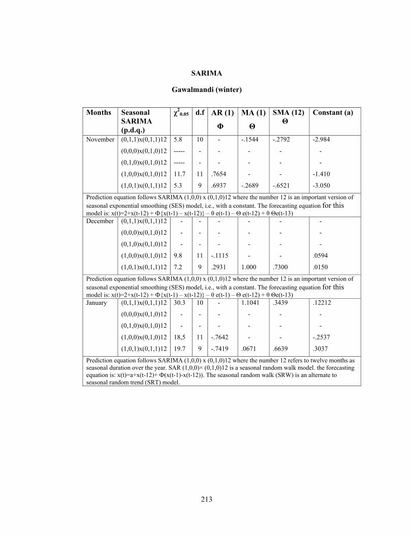
213
SARIMA
Gawalmandi (winter)
Months Seasonal SARIMA (p.d.q.)
χ20.05 d.f AR (1)
Φ
MA (1)
Θ
SMA (12) Θ
Constant (a)
November (0,1,1)x(0,1,1)12
(0,0,0)x(0,1,0)12
(0,1,0)x(0,1,0)12
(1,0,0)x(0,1,0)12
(1,0,1)x(0,1,1)12
5.8
-----
-----
11.7
5.3
10
-
-
11
9
-
-
-
.7654
.6937
-.1544
-
-
-
-.2689
-.2792
-
-
-
-.6521
-2.984
-
-
-1.410
-3.050
Prediction equation follows SARIMA (1,0,0) x (0,1,0)12 where the number 12 is an important version of seasonal exponential smoothing (SES) model, i.e., with a constant. The forecasting equation for this model is: x(t)=2+x(t-12) + Ф{x(t-1) – x(t-12)} – θ e(t-1) – Θ e(t-12) + θ Θe(t-13) December (0,1,1)x(0,1,1)12
(0,0,0)x(0,1,0)12
(0,1,0)x(0,1,0)12
(1,0,0)x(0,1,0)12
(1,0,1)x(0,1,1)12
-
-
-
9.8
7.2
-
-
-
11
9
-
-
-
-.1115
.2931
-
-
-
-
1.000
-
-
-
-
.7300
-
-
-
.0594
.0150
Prediction equation follows SARIMA (1,0,0) x (0,1,0)12 where the number 12 is an important version of seasonal exponential smoothing (SES) model, i.e., with a constant. The forecasting equation for this model is: x(t)=2+x(t-12) + Ф{x(t-1) – x(t-12)} – θ e(t-1) – Θ e(t-12) + θ Θe(t-13) January (0,1,1)x(0,1,1)12
(0,0,0)x(0,1,0)12
(0,1,0)x(0,1,0)12
(1,0,0)x(0,1,0)12
(1,0,1)x(0,1,1)12
30.3
-
-
18,5
19.7
10
-
-
11
9
-
-
-
-.7642
-.7419
1.1041
-
-
-
.0671
.3439
-
-
-
.6639
.12212
-
-
-.2537
.3037
Prediction equation follows SARIMA (1,0,0) x (0,1,0)12 where the number 12 refers to twelve months as seasonal duration over the year. SAR (1,0,0)× (0,1,0)12 is a seasonal random walk model. the forecasting equation is: x(t)=a+x(t-12)+ Ф(x(t-1)-x(t-12)). The seasonal random walk (SRW) is an alternate to seasonal random trend (SRT) model.
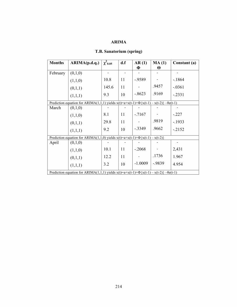
214
ARIMA
T.B. Sanatorium (spring)
Months ARIMA(p.d.q.) χ20.05 d.f AR (1)
Φ MA (1) Θ
Constant (a)
February (0,1,0)
(1,1,0)
(0,1,1)
(1,1,1)
-
10.8
145.6
9.3
-
11
11
10
-
-.9589 -
-.8623
-
-
.9457
.9169
-
-.1864
-.0361
-.2331
Prediction equation for ARIMA(1,1,1) yields x(t)=a+x(t-1)+Ф{x(t-1) – x(t-2)} –θe(t-1) March (0,1,0)
(1,1,0)
(0,1,1)
(1,1,1)
-
8.1
29.8
9.2
-
11
11
10
-
-.7167 -
-.3349
-
-
.9819
.9662
-
-.227
-.1933
-.2152
Prediction equation for ARIMA(1,1,0) yields x(t)=a+x(t-1)+Ф{x(t-1) – x(t-2)}April (0,1,0)
(1,1,0)
(0,1,1)
(1,1,1)
-
10.1
12.2
3.2
-
11
11
10
-
-.2068 -
-1.0009
-
-
.1736
-.9839
-
2,431
1.967
4.954
Prediction equation for ARIMA(1,1,1) yields x(t)=a+x(t-1)+Ф{x(t-1) – x(t-2)} –θe(t-1)
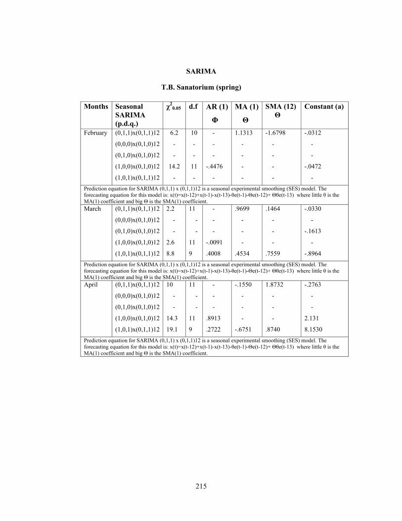
215
SARIMA
T.B. Sanatorium (spring)
Months Seasonal SARIMA (p.d.q.)
χ20.05 d.f AR (1)
Φ
MA (1)
Θ
SMA (12) Θ
Constant (a)
February (0,1,1)x(0,1,1)12
(0,0,0)x(0,1,0)12
(0,1,0)x(0,1,0)12
(1,0,0)x(0,1,0)12
(1,0,1)x(0,1,1)12
6.2
-
-
14.2
-
10
-
-
11
-
-
-
-
-.4476
-
1.1313
-
-
-
-
-1.6798
-
-
-
-
-.0312
-
-
-.0472
-
Prediction equation for SARIMA (0,1,1) x (0,1,1)12 is a seasonal experimental smoothing (SES) model. The forecasting equation for this model is: x(t)=x(t-12)+x(t-1)-x(t-13)-θe(t-1)-Θe(t-12)+ Θθe(t-13) where little θ is the MA(1) coefficient and big Θ is the SMA(1) coefficient. March (0,1,1)x(0,1,1)12
(0,0,0)x(0,1,0)12
(0,1,0)x(0,1,0)12
(1,0,0)x(0,1,0)12
(1,0,1)x(0,1,1)12
2.2
-
-
2.6
8.8
11
-
-
11
9
-
-
-
-.0091
.4008
.9699
-
-
-
.4534
.1464
-
-
-
.7559
-.0330
-
-.1613
-
-.8964
Prediction equation for SARIMA (0,1,1) x (0,1,1)12 is a seasonal experimental smoothing (SES) model. The forecasting equation for this model is: x(t)=x(t-12)+x(t-1)-x(t-13)-θe(t-1)-Θe(t-12)+ Θθe(t-13) where little θ is the MA(1) coefficient and big Θ is the SMA(1) coefficient. April (0,1,1)x(0,1,1)12
(0,0,0)x(0,1,0)12
(0,1,0)x(0,1,0)12
(1,0,0)x(0,1,0)12
(1,0,1)x(0,1,1)12
10
-
-
14.3
19.1
11
-
-
11
9
-
-
-
.8913
.2722
-.1550
-
-
-
-.6751
1.8732
-
-
-
.8740
-.2763
-
-
2.131
8.1530
Prediction equation for SARIMA (0,1,1) x (0,1,1)12 is a seasonal experimental smoothing (SES) model. The forecasting equation for this model is: x(t)=x(t-12)+x(t-1)-x(t-13)-θe(t-1)-Θe(t-12)+ Θθe(t-13) where little θ is the MA(1) coefficient and big Θ is the SMA(1) coefficient.
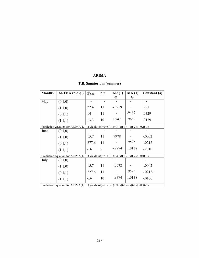
216
ARIMA
T.B. Sanatorium (summer)
Months ARIMA (p.d.q.) χ20.05 d.f AR (1)
Φ MA (1) Θ
Constant (a)
May (0,1,0)
(1,1,0)
(0,1,1)
(1,1,1)
-
22.4
14
13.3
-
11
11
10
-
-.3259 -
.0547
-
-
.9467
.9682
-
.991
.0329
.0179
Prediction equation for ARIMA(1,1,1) yields x(t)=a+x(t-1)+Ф{x(t-1) – x(t-2)} –θe(t-1) June (0,1,0)
(1,1,0)
(0,1,1)
(1,1,1)
-
15.7
277.6
6.6
-
11
11
9
-
.9978 -
-.9774
-
-
.9525
1.0138
-
-.0002
-.0212
-.2010
Prediction equation for ARIMA(1,1,1) yields x(t)=a+x(t-1)+Ф{x(t-1) – x(t-2)} –θe(t-1) July (0,1,0)
(1,1,0)
(0,1,1)
(1,1,1)
-
15.7
227.6
6.6
-
11
11
10
-
-.9978 -
-.9774
-
-
.9525
1.0138
-
-.0002
-.0212-
-.0106
Prediction equation for ARIMA(1,1,1) yields x(t)=a+x(t-1)+Ф{x(t-1) – x(t-2)} –θe(t-1)
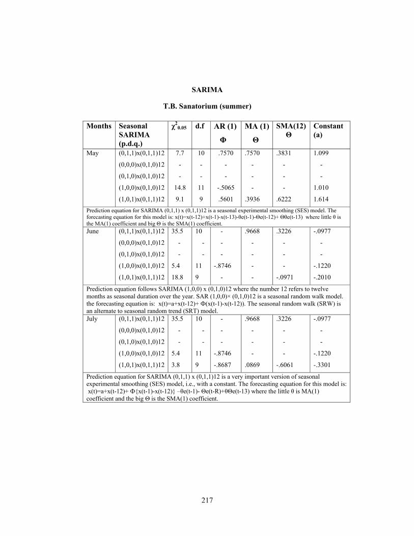
217
SARIMA
T.B. Sanatorium (summer)
Months Seasonal SARIMA (p.d.q.)
χ20.05 d.f AR (1)
Φ
MA (1)
Θ
SMA(12) Θ
Constant (a)
May (0,1,1)x(0,1,1)12
(0,0,0)x(0,1,0)12
(0,1,0)x(0,1,0)12
(1,0,0)x(0,1,0)12
(1,0,1)x(0,1,1)12
7.7
-
-
14.8
9.1
10
-
-
11
9
.7570
-
-
-.5065
.5601
.7570
-
-
-
.3936
.3831
-
-
-
.6222
1.099
-
-
1.010
1.614
Prediction equation for SARIMA (0,1,1) x (0,1,1)12 is a seasonal experimental smoothing (SES) model. The forecasting equation for this model is: x(t)=x(t-12)+x(t-1)-x(t-13)-θe(t-1)-Θe(t-12)+ Θθe(t-13) where little θ is the MA(1) coefficient and big Θ is the SMA(1) coefficient. June (0,1,1)x(0,1,1)12
(0,0,0)x(0,1,0)12
(0,1,0)x(0,1,0)12
(1,0,0)x(0,1,0)12
(1,0,1)x(0,1,1)12
35.5
-
-
5.4
18.8
10
-
-
11
9
-
-
-
-.8746
-
.9668
-
-
-
-
.3226
-
-
-
-.0971
-.0977
-
-
-.1220
-.2010
Prediction equation follows SARIMA (1,0,0) x (0,1,0)12 where the number 12 refers to twelve months as seasonal duration over the year. SAR (1,0,0)× (0,1,0)12 is a seasonal random walk model. the forecasting equation is: x(t)=a+x(t-12)+ Ф(x(t-1)-x(t-12)). The seasonal random walk (SRW) is an alternate to seasonal random trend (SRT) model. July (0,1,1)x(0,1,1)12
(0,0,0)x(0,1,0)12
(0,1,0)x(0,1,0)12
(1,0,0)x(0,1,0)12
(1,0,1)x(0,1,1)12
35.5
-
-
5.4
3.8
10
-
-
11
9
-
-
-
-.8746
-.8687
.9668
-
-
-
.0869
.3226
-
-
-
-.6061
-.0977
-
-
-.1220
-.3301
Prediction equation for SARIMA (0,1,1) x (0,1,1)12 is a very important version of seasonal experimental smoothing (SES) model, i.e., with a constant. The forecasting equation for this model is: x(t)=a+x(t-12)+ Ф{x(t-1)-x(t-12)} –θe(t-1)- Θe(t-R)+θΘe(t-13) where the little θ is MA(1) coefficient and the big Θ is the SMA(1) coefficient.
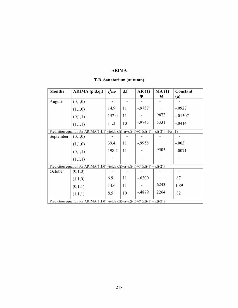
218
ARIMA
T.B. Sanatorium (autumn)
Months ARIMA (p.d.q.) χ20.05 d.f AR (1)
Φ MA (1) Θ
Constant (a)
August (0,1,0)
(1,1,0)
(0,1,1)
(1,1,1)
-
14.9
152.0
11.3
-
11
11
10
-
-.9737 -
-.9745
-
-
.9672
.5331
-
-.0927
-.01507
-.0414
Prediction equation for ARIMA(1,1,1) yields x(t)=a+x(t-1)+Ф{x(t-1) – x(t-2)} –θe(t-1) September (0,1,0)
(1,1,0)
(0,1,1)
(1,1,1)
-
39.4
198.2 -
-
11
11 -
-
-.9958 -
-
-
-
.9505 -
-
-.003
-.0071 -
Prediction equation for ARIMA(1,1,0) yields x(t)=a+x(t-1)+Ф{x(t-1) – x(t-2)}October (0,1,0)
(1,1,0)
(0,1,1)
(1,1,1)
-
6.9
14.6
8.5
-
11
11
10
-
-.6200 -
-.4879
-
-
.6243
.2264
-
.87
1.89
.82
Prediction equation for ARIMA(1,1,0) yields x(t)=a+x(t-1)+Ф{x(t-1) – x(t-2)}
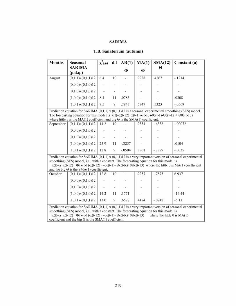
219
SARIMA
T.B. Sanatorium (autumn)
Months Seasonal SARIMA (p.d.q.)
χ20.05 d.f AR(1)
Φ
MA(1)
Θ
SMA(12) Θ
Constant (a)
August (0,1,1)x(0,1,1)12
(0,0,0)x(0,1,0)12
(0,1,0)x(0,1,0)12
(1,0,0)x(0,1,0)12
(1,0,1)x(0,1,1)12
6.4
-
-
8.4
7.5
10
-
-
11
9
-
-
-
.0783
.7843
.9228
-
-
-
.5747
.4267
-
-
-
.5323
-.1214
-
-
.0308
-.0569
Prediction equation for SARIMA (0,1,1) x (0,1,1)12 is a seasonal experimental smoothing (SES) model. The forecasting equation for this model is x(t)=x(t-12)+x(t-1)-x(t-13)-θe(t-1)-Θe(t-12)+ Θθe(t-13) where little θ is the MA(1) coefficient and big Θ is the SMA(1) coefficient.September (0,1,1)x(0,1,1)12
(0,0,0)x(0,1,0)12
(0,1,0)x(0,1,0)12
(1,0,0)x(0,1,0)12
(1,0,1)x(0,1,1)12
14.2
-
-
25.9
12.8
10
-
-
11
9
-
-
-
-.3257
-.0504
.9354
-
-
-
.8861
-.6338
-
-
-
-.7879
-.00072
-
-
.0104
-.0035
Prediction equation for SARIMA (0,1,1) x (0,1,1)12 is a very important version of seasonal experimental smoothing (SES) model, i.e., with a constant. The forecasting equation for this model is x(t)=a+x(t-12)+ Ф{x(t-1)-x(t-12)} –θe(t-1)- Θe(t-R)+θΘe(t-13) where the little θ is MA(1) coefficient and the big Θ is the SMA(1) coefficient. October (0,1,1)x(0,1,1)12
(0,0,0)x(0,1,0)12
(0,1,0)x(0,1,0)12
(1,0,0)x(0,1,0)12
(1,0,1)x(0,1,1)12
12.8
-
-
14.2
13.0
10
-
-
11
9
-
-
-
.1771
.6527
.9257
-
-
-
.4474
-.7875
-
-
-
-.0742
6.937
-
-
-14.44
-6.11
Prediction equation for SARIMA (0,1,1) x (0,1,1)12 is a very important version of seasonal experimental smoothing (SES) model, i.e., with a constant. The forecasting equation for this model is x(t)=a+x(t-12)+ Ф{x(t-1)-x(t-12)} –θe(t-1)- Θe(t-R)+θΘe(t-13) where the little θ is MA(1) coefficient and the big Θ is the SMA(1) coefficient.
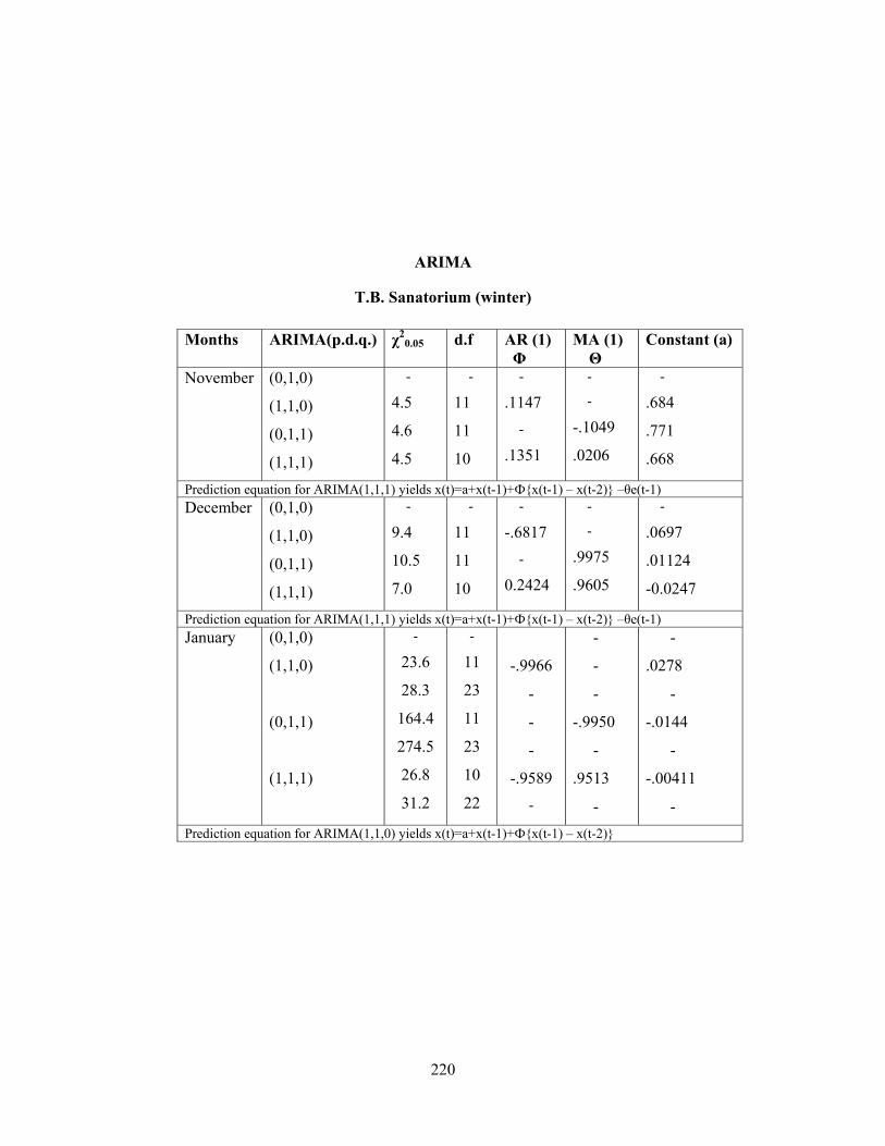
220
ARIMA
T.B. Sanatorium (winter)
Months ARIMA(p.d.q.) χ20.05 d.f AR (1)
Φ MA (1) Θ
Constant (a)
November (0,1,0)
(1,1,0)
(0,1,1)
(1,1,1)
-
4.5
4.6
4.5
-
11
11
10
-
.1147 -
.1351
-
-
-.1049
.0206
-
.684
.771
.668
Prediction equation for ARIMA(1,1,1) yields x(t)=a+x(t-1)+Ф{x(t-1) – x(t-2)} –θe(t-1) December (0,1,0)
(1,1,0)
(0,1,1)
(1,1,1)
-
9.4
10.5
7.0
-
11
11
10
-
-.6817 -
0.2424
-
-
.9975
.9605
-
.0697
.01124
-0.0247
Prediction equation for ARIMA(1,1,1) yields x(t)=a+x(t-1)+Ф{x(t-1) – x(t-2)} –θe(t-1) January (0,1,0)
(1,1,0)
(0,1,1)
(1,1,1)
-
23.6
28.3
164.4
274.5
26.8
31.2
-
11
23
11
23
10
22
-.9966
-
-
-
-.9589 -
-
-
-
-.9950
-
.9513
-
-
.0278
-
-.0144
-
-.00411
- Prediction equation for ARIMA(1,1,0) yields x(t)=a+x(t-1)+Ф{x(t-1) – x(t-2)}
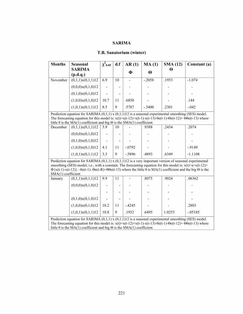
221
SARIMA
T.B. Sanatorium (winter)
Months Seasonal SARIMA (p.d.q.)
χ20.05 d.f AR (1)
Φ
MA (1)
Θ
SMA (12) Θ
Constant (a)
November (0,1,1)x(0,1,1)12
(0,0,0)x(0,1,0)12
(0,1,0)x(0,1,0)12
(1,0,0)x(0,1,0)12
(1,0,1)x(0,1,1)12
6.9
-
-
10.7
8.5
10
-
-
11
9
-
-
-
.6850
.5787
-.2058
-
-
-
-.3400
.1953
-
-
-
.2301
-1.074
-
-
.144
-.042
Prediction equation for SARIMA (0,1,1) x (0,1,1)12 is a seasonal experimental smoothing (SES) model. The forecasting equation for this model is: x(t)=x(t-12)+x(t-1)-x(t-13)-θe(t-1)-Θe(t-12)+ Θθe(t-13) where little θ is the MA(1) coefficient and big Θ is the SMA(1) coefficient.December (0,1,1)x(0,1,1)12
(0,0,0)x(0,1,0)12
(0,1,0)x(0,1,0)12
(1,0,0)x(0,1,0)12
(1,0,1)x(0,1,1)12
3.9
-
-
4.1
3.3
10
-
-
11
9
-
-
-
-.0792
-.5896
.9388
-
-
-
.4893
.2434
-
-
-
.6349
.2074
-
-
-.9149
-1.1108
Prediction equation for SARIMA (0,1,1) x (0,1,1)12 is a very important version of seasonal experimental smoothing (SES) model, i.e., with a constant. The forecasting equation for this model is: x(t)=a+x(t-12)+ Ф{x(t-1)-x(t-12)} –θe(t-1)- Θe(t-R)+θΘe(t-13) where the little θ is MA(1) coefficient and the big Θ is the SMA(1) coefficient. January (0,1,1)x(0,1,1)12
(0,0,0)x(0,1,0)12
(0,1,0)x(0,1,0)12
(1,0,0)x(0,1,0)12
(1,0,1)x(0,1,1)12
9.9
-
-
-
18.2
10.8
11
-
-
-
11
9
-
-
-
-
-.4245
.1932
.8075
-
-
-
-
.6495
.9024
-
-
-
-
1.0253
.06362
-
-
-
.2803
-.05185
Prediction equation for SARIMA (0,1,1) x (0,1,1)12 is a seasonal experimental smoothing (SES) model. The forecasting equation for this model is: x(t)=x(t-12)+x(t-1)-x(t-13)-θe(t-1)-Θe(t-12)+ Θθe(t-13) where little θ is the MA(1) coefficient and big Θ is the SMA(1) coefficient.

222
ARIMA
CGS Colony (spring) Months ARIMA (p.d.q.) χ2
0.05 d.f AR (1) Φ
MA (1) Θ
Constant (a)
February (0,1,0)
(1,1,0)
(0,1,1)
(1,1,1)
-
3.9
111.9
2.1
-
11
11
10
-
-.5163
-
-.0952
-
-
.9490
.9451
-
-.298
.4492
.5138
The prediction equation for non-seasonal ARIMA (1,1,1) yields x(t)=a+x(t-1)+Ф(x(t-1)-x(t-2))-
θe(t-1) where a is constant, e is the error at period (t-1), Ф=AR(1) and θ=MA(1)
March (0,1,0)
(1,1,0)
(0,1,1)
(1,1,1)
-
8.7
121.1
2.8
-
11
11
10
-
-.9355
-
-.8315
-
-
.9491
.8979
-
-.2360
-.0375
-.02664
The prediction equation for non-seasonal ARIMA (1,1,1) yields x(t)=a+x(t-1)+Ф(x(t-1)-x(t-2))-θe(t-1) where a is constant, e is the error at period (t-1), Ф=AR(1) and θ=MA(1) April (0,1,0)
(1,1,0)
(0,1,1)
(1,1,1)
-
6.0
9.0
3.9
-
11
11
10
-
-.3438
-
-.10005
-
-
.2812
-1.0180
-
2.078
1.436
5.143
The prediction equation for non-seasonal ARIMA (1,1,1) yields x(t)=a+x(t-1)+Ф(x(t-1)-x(t-2))-θe(t-1) where a is constant, e is the error at period (t-1), Ф=AR(1) and θ=MA(1)
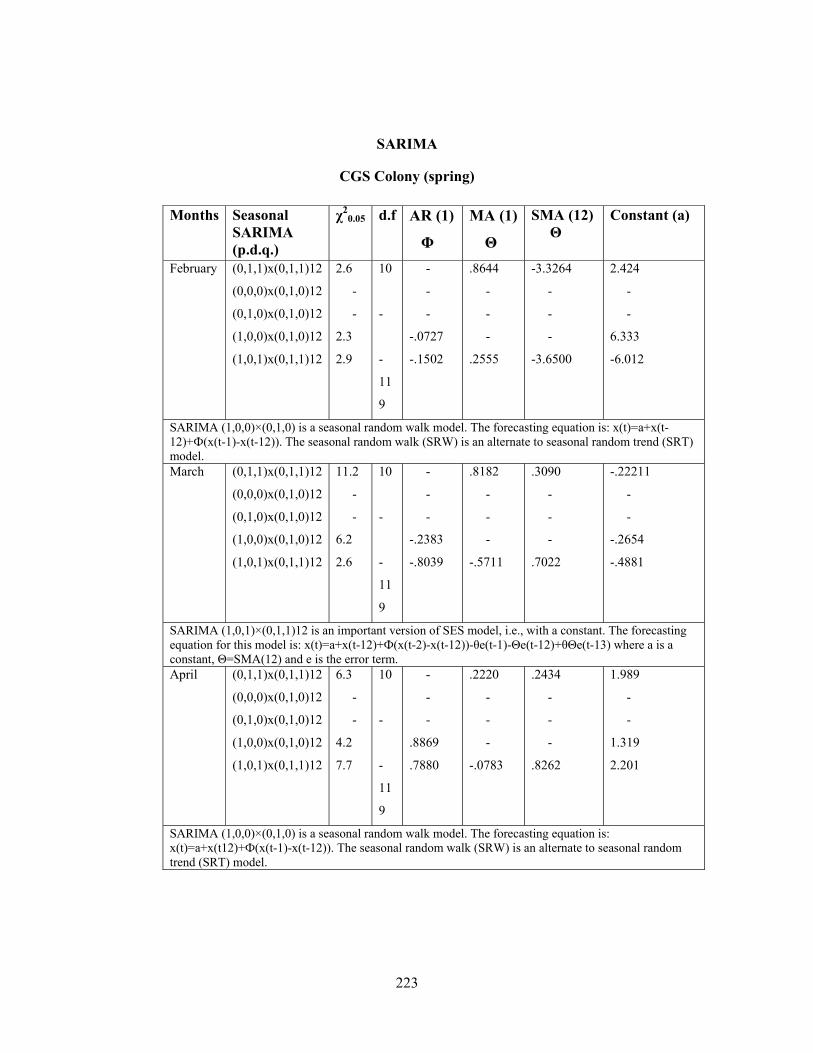
223
SARIMA
CGS Colony (spring)
Months Seasonal SARIMA (p.d.q.)
χ20.05 d.f AR (1)
Φ
MA (1)
Θ
SMA (12) Θ
Constant (a)
February (0,1,1)x(0,1,1)12
(0,0,0)x(0,1,0)12
(0,1,0)x(0,1,0)12
(1,0,0)x(0,1,0)12
(1,0,1)x(0,1,1)12
2.6
-
-
2.3
2.9
10
-
-
11
9
-
-
-
-.0727
-.1502
.8644
-
-
-
.2555
-3.3264
-
-
-
-3.6500
2.424
-
-
6.333
-6.012
SARIMA (1,0,0)×(0,1,0) is a seasonal random walk model. The forecasting equation is: x(t)=a+x(t-12)+Ф(x(t-1)-x(t-12)). The seasonal random walk (SRW) is an alternate to seasonal random trend (SRT) model. March (0,1,1)x(0,1,1)12
(0,0,0)x(0,1,0)12
(0,1,0)x(0,1,0)12
(1,0,0)x(0,1,0)12
(1,0,1)x(0,1,1)12
11.2
-
-
6.2
2.6
10
-
-
11
9
-
-
-
-.2383
-.8039
.8182
-
-
-
-.5711
.3090
-
-
-
.7022
-.22211
-
-
-.2654
-.4881
SARIMA (1,0,1)×(0,1,1)12 is an important version of SES model, i.e., with a constant. The forecasting equation for this model is: x(t)=a+x(t-12)+Ф(x(t-2)-x(t-12))-θe(t-1)-Θe(t-12)+θΘe(t-13) where a is a constant, Θ=SMA(12) and e is the error term. April (0,1,1)x(0,1,1)12
(0,0,0)x(0,1,0)12
(0,1,0)x(0,1,0)12
(1,0,0)x(0,1,0)12
(1,0,1)x(0,1,1)12
6.3
-
-
4.2
7.7
10
-
-
11
9
-
-
-
.8869
.7880
.2220
-
-
-
-.0783
.2434
-
-
-
.8262
1.989
-
-
1.319
2.201
SARIMA (1,0,0)×(0,1,0) is a seasonal random walk model. The forecasting equation is: x(t)=a+x(t12)+Ф(x(t-1)-x(t-12)). The seasonal random walk (SRW) is an alternate to seasonal random trend (SRT) model.
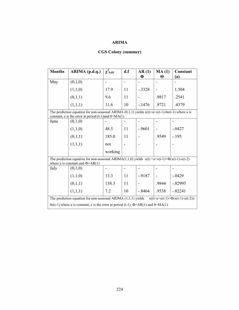
224
ARIMA
CGS Colony (summer)
Months ARIMA (p.d.q.) χ20.05 d.f AR (1)
Φ MA (1) Θ
Constant (a)
May (0,1,0)
(1,1,0)
(0,1,1)
(1,1,1)
-
17.9
9.6
11.6
-
11
11
10
-
-.3328
-
-.1476
-
-
.9817
.9721
-
1.504
.2541
.4379 The prediction equation for non-seasonal ARIMA (0,1,1) yields x(t)=a+x(t-1)-θe(t-1) where a is constant, e is the error at period (t-1)and θ=MA(1) June (0,1,0)
(1,1,0)
(0,1,1)
(1,1,1)
-
48.5
185.0
not
working
-
11
11
-
-
-.9601
-
-
-
-
.9549
-
-
-.0427
-.195
-
The prediction equation for non-seasonal ARIMA(1,1,0) yields x(t) =a+x(t-1)+Ф(x(t-1)-x(t-2) where a is constant and Ф=AR(1)July (0,1,0)
(1,1,0)
(0,1,1)
(1,1,1)
-
13.3
138.3
7.2
-
11
11
10
-
-.9187
-
-.8464
-
-
.9844
.9538
-
-.0429
-.02995
-.02241 The prediction equation for non-seasonal ARIMA (1,1,1) yields x(t)=a+x(t-1)+Ф(x(t-1)-x(t-2))-
θe(t-1) where a is constant, e is the error at period (t-1), Ф=AR(1) and θ=MA(1)
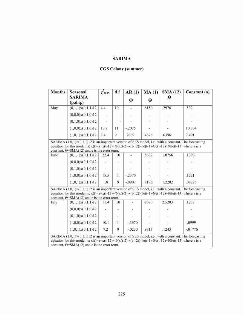
225
SARIMA
CGS Colony (summer)
Months Seasonal SARIMA (p.d.q.)
χ20.05 d.f AR (1)
Φ
MA (1)
Θ
SMA (12) Θ
Constant (a)
May (0,1,1)x(0,1,1)12
(0,0,0)x(0,1,0)12
(0,1,0)x(0,1,0)12
(1,0,0)x(0,1,0)12
(1,0,1)x(0,1,1)12
4.4
-
-
13.9
7.4
10
-
-
11
9
-
-
-
-.2075
.2069
.8150
-
-
-
.4678
.2976
-
-
-
.6396
.532
-
-
10.804
7.491
SARIMA (1,0,1)×(0,1,1)12 is an important version of SES model, i.e., with a constant. The forecasting equation for this model is: x(t)=a+x(t-12)+Ф(x(t-2)-x(t-12))-θe(t-1)-Θe(t-12)+θΘe(t-13) where a is a constant, Θ=SMA(12) and e is the error term.June (0,1,1)x(0,1,1)12
(0,0,0)x(0,1,0)12
(0,1,0)x(0,1,0)12
(1,0,0)x(0,1,0)12
(1,0,1)x(0,1,1)12
22.4
-
-
15.5
1.8
10
-
-
11
9
-
-
-
-.2370
-.0907
.8637
-
-
-
.8196
1.0756
-
-
-
1.2202
.1396
-
-
.1221
.08225
SARIMA (1,0,1)×(0,1,1)12 is an important version of SES model, i.e., with a constant. The forecasting equation for this model is: x(t)=a+x(t-12)+Ф(x(t-2)-x(t-12))-θe(t-1)-Θe(t-12)+θΘe(t-13) where a is a constant, Θ=SMA(12) and e is the error term.July (0,1,1)x(0,1,1)12
(0,0,0)x(0,1,0)12
(0,1,0)x(0,1,0)12
(1,0,0)x(0,1,0)12
(1,0,1)x(0,1,1)12
11.4
-
-
10.1
7.2
10
-
-
11
9
-
-
-
-.3670
-.0230
.8080
-
-
-
.9913
2.5203
-
-
-
.1243
.1239
-
-
-.0999
-.01776
SARIMA (1,0,1)×(0,1,1)12 is an important version of SES model, i.e., with a constant. The forecasting equation for this model is: x(t)=a+x(t-12)+Ф(x(t-2)-x(t-12))-θe(t-1)-Θe(t-12)+θΘe(t-13) where a is a constant, Θ=SMA(12) and e is the error term.
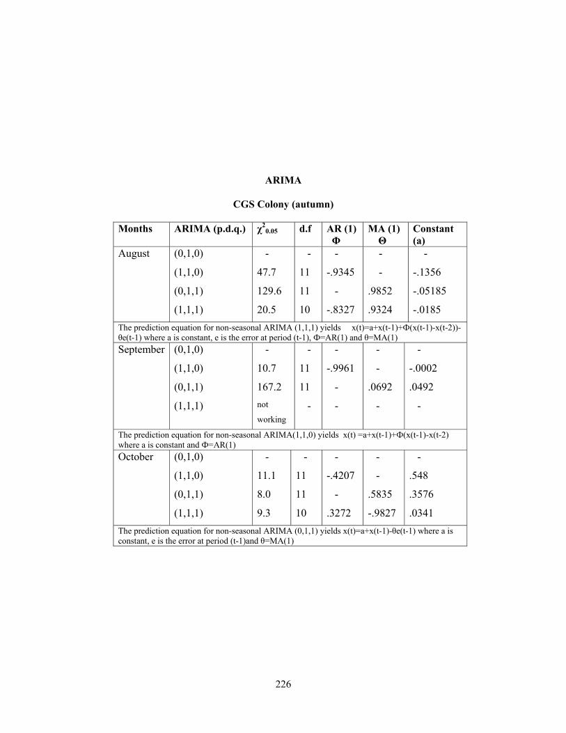
226
ARIMA
CGS Colony (autumn)
Months ARIMA (p.d.q.) χ2
0.05 d.f AR (1) Φ
MA (1) Θ
Constant (a)
August (0,1,0)
(1,1,0)
(0,1,1)
(1,1,1)
-
47.7
129.6
20.5
-
11
11
10
-
-.9345
-
-.8327
-
-
.9852
.9324
-
-.1356
-.05185
-.0185 The prediction equation for non-seasonal ARIMA (1,1,1) yields x(t)=a+x(t-1)+Ф(x(t-1)-x(t-2))-θe(t-1) where a is constant, e is the error at period (t-1), Ф=AR(1) and θ=MA(1) September (0,1,0)
(1,1,0)
(0,1,1)
(1,1,1)
-
10.7
167.2 not
working
-
11
11
-
-
-.9961
-
-
-
-
.0692
-
-
-.0002
.0492
-
The prediction equation for non-seasonal ARIMA(1,1,0) yields x(t) =a+x(t-1)+Ф(x(t-1)-x(t-2) where a is constant and Ф=AR(1)October (0,1,0)
(1,1,0)
(0,1,1)
(1,1,1)
-
11.1
8.0
9.3
-
11
11
10
-
-.4207
-
.3272
-
-
.5835
-.9827
-
.548
.3576
.0341 The prediction equation for non-seasonal ARIMA (0,1,1) yields x(t)=a+x(t-1)-θe(t-1) where a is constant, e is the error at period (t-1)and θ=MA(1)
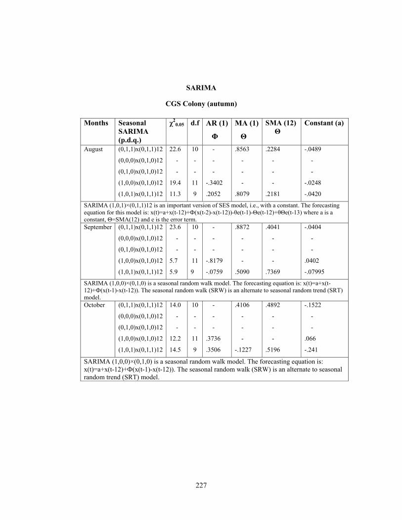
227
SARIMA
CGS Colony (autumn)
Months Seasonal SARIMA (p.d.q.)
χ20.05 d.f AR (1)
Φ
MA (1)
Θ
SMA (12) Θ
Constant (a)
August (0,1,1)x(0,1,1)12
(0,0,0)x(0,1,0)12
(0,1,0)x(0,1,0)12
(1,0,0)x(0,1,0)12
(1,0,1)x(0,1,1)12
22.6
-
-
19.4
11.3
10
-
-
11
9
-
-
-
-.3402
.2052
.8563
-
-
-
.8079
.2284
-
-
-
.2181
-.0489
-
-
-.0248
-.0420
SARIMA (1,0,1)×(0,1,1)12 is an important version of SES model, i.e., with a constant. The forecasting equation for this model is: x(t)=a+x(t-12)+Ф(x(t-2)-x(t-12))-θe(t-1)-Θe(t-12)+θΘe(t-13) where a is a constant, Θ=SMA(12) and e is the error term.September (0,1,1)x(0,1,1)12
(0,0,0)x(0,1,0)12
(0,1,0)x(0,1,0)12
(1,0,0)x(0,1,0)12
(1,0,1)x(0,1,1)12
23.6
-
-
5.7
5.9
10
-
-
11
9
-
-
-
-.8179
-.0759
.8872
-
-
-
.5090
.4041
-
-
-
.7369
-.0404
-
-
.0402
-.07995
SARIMA (1,0,0)×(0,1,0) is a seasonal random walk model. The forecasting equation is: x(t)=a+x(t-12)+Ф(x(t-1)-x(t-12)). The seasonal random walk (SRW) is an alternate to seasonal random trend (SRT) model. October (0,1,1)x(0,1,1)12
(0,0,0)x(0,1,0)12
(0,1,0)x(0,1,0)12
(1,0,0)x(0,1,0)12
(1,0,1)x(0,1,1)12
14.0
-
-
12.2
14.5
10
-
-
11
9
-
-
-
.3736
.3506
.4106
-
-
-
-.1227
.4892
-
-
-
.5196
-.1522
-
-
.066
-.241
SARIMA (1,0,0)×(0,1,0) is a seasonal random walk model. The forecasting equation is: x(t)=a+x(t-12)+Ф(x(t-1)-x(t-12)). The seasonal random walk (SRW) is an alternate to seasonal random trend (SRT) model.
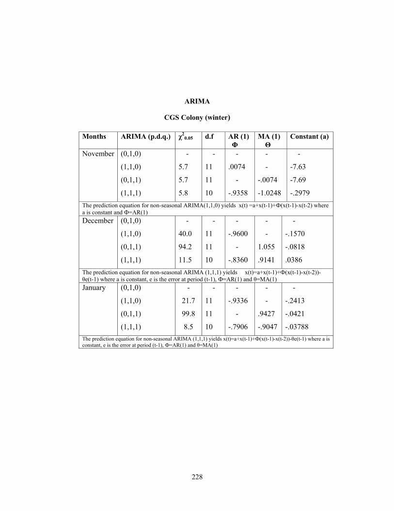
228
ARIMA
CGS Colony (winter) Months ARIMA (p.d.q.) χ2
0.05 d.f AR (1) Φ
MA (1) Θ
Constant (a)
November (0,1,0)
(1,1,0)
(0,1,1)
(1,1,1)
-
5.7
5.7
5.8
-
11
11
10
-
.0074
-
-.9358
-
-
-.0074
-1.0248
-
-7.63
-7.69
-.2979 The prediction equation for non-seasonal ARIMA(1,1,0) yields x(t) =a+x(t-1)+Ф(x(t-1)-x(t-2) where a is constant and Ф=AR(1) December (0,1,0)
(1,1,0)
(0,1,1)
(1,1,1)
-
40.0
94.2
11.5
-
11
11
10
-
-.9600
-
-.8360
-
-
1.055
.9141
-
-.1570
-.0818
.0386 The prediction equation for non-seasonal ARIMA (1,1,1) yields x(t)=a+x(t-1)+Ф(x(t-1)-x(t-2))-θe(t-1) where a is constant, e is the error at period (t-1), Ф=AR(1) and θ=MA(1) January (0,1,0)
(1,1,0)
(0,1,1)
(1,1,1)
-
21.7
99.8
8.5
-
11
11
10
-
-.9336
-
-.7906
-
-
.9427
-.9047
-
-.2413
-.0421
-.03788 The prediction equation for non-seasonal ARIMA (1,1,1) yields x(t)=a+x(t-1)+Ф(x(t-1)-x(t-2))-θe(t-1) where a is constant, e is the error at period (t-1), Ф=AR(1) and θ=MA(1)
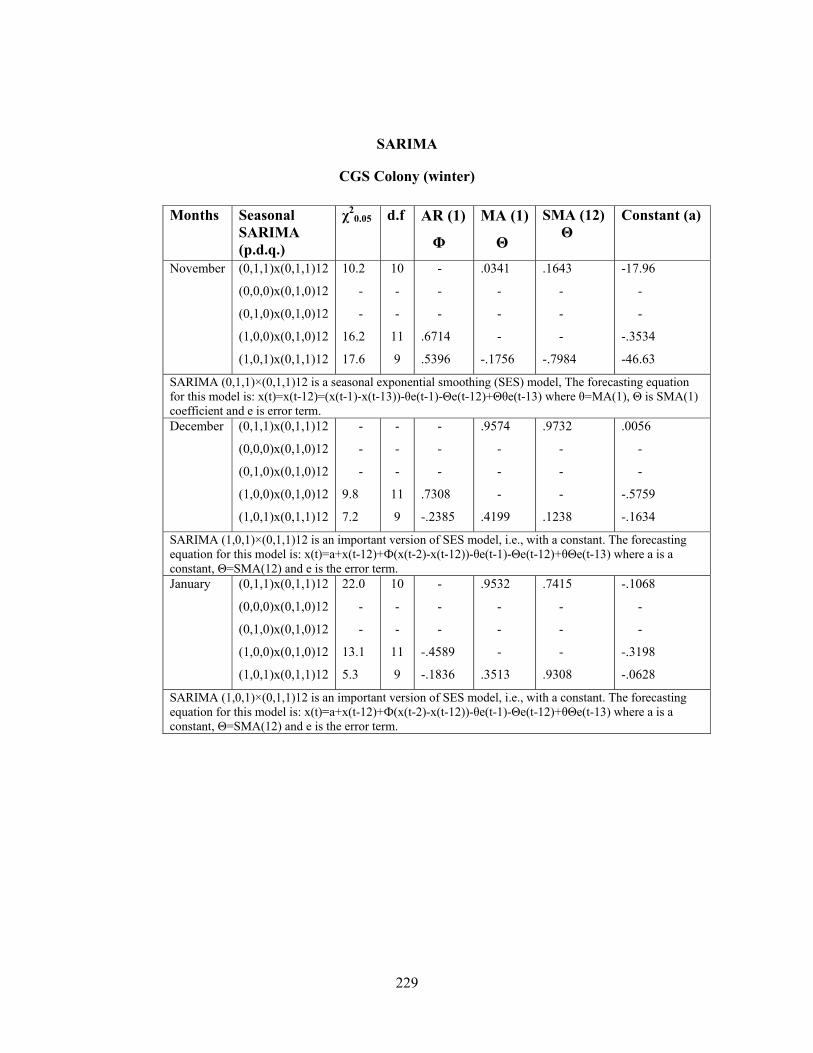
229
SARIMA
CGS Colony (winter)
Months Seasonal SARIMA (p.d.q.)
χ20.05 d.f AR (1)
Φ
MA (1)
Θ
SMA (12) Θ
Constant (a)
November (0,1,1)x(0,1,1)12
(0,0,0)x(0,1,0)12
(0,1,0)x(0,1,0)12
(1,0,0)x(0,1,0)12
(1,0,1)x(0,1,1)12
10.2
-
-
16.2
17.6
10
-
-
11
9
-
-
-
.6714
.5396
.0341
-
-
-
-.1756
.1643
-
-
-
-.7984
-17.96
-
-
-.3534
-46.63
SARIMA (0,1,1)×(0,1,1)12 is a seasonal exponential smoothing (SES) model, The forecasting equation for this model is: x(t)=x(t-12)=(x(t-1)-x(t-13))-θe(t-1)-Θe(t-12)+Θθe(t-13) where θ=MA(1), Θ is SMA(1) coefficient and e is error term. December (0,1,1)x(0,1,1)12
(0,0,0)x(0,1,0)12
(0,1,0)x(0,1,0)12
(1,0,0)x(0,1,0)12
(1,0,1)x(0,1,1)12
-
-
-
9.8
7.2
-
-
-
11
9
-
-
-
.7308
-.2385
.9574
-
-
-
.4199
.9732
-
-
-
.1238
.0056
-
-
-.5759
-.1634
SARIMA (1,0,1)×(0,1,1)12 is an important version of SES model, i.e., with a constant. The forecasting equation for this model is: x(t)=a+x(t-12)+Ф(x(t-2)-x(t-12))-θe(t-1)-Θe(t-12)+θΘe(t-13) where a is a constant, Θ=SMA(12) and e is the error term.January (0,1,1)x(0,1,1)12
(0,0,0)x(0,1,0)12
(0,1,0)x(0,1,0)12
(1,0,0)x(0,1,0)12
(1,0,1)x(0,1,1)12
22.0
-
-
13.1
5.3
10
-
-
11
9
-
-
-
-.4589
-.1836
.9532
-
-
-
.3513
.7415
-
-
-
.9308
-.1068
-
-
-.3198
-.0628
SARIMA (1,0,1)×(0,1,1)12 is an important version of SES model, i.e., with a constant. The forecasting equation for this model is: x(t)=a+x(t-12)+Ф(x(t-2)-x(t-12))-θe(t-1)-Θe(t-12)+θΘe(t-13) where a is a constant, Θ=SMA(12) and e is the error term.
230
CHAPTER 7
CONCLUSIONS AND RECOMMENDATIONS FOR
FUTURE RESEARCH
7.1 Conclusions with suggested precautionary measures:
• Quetta is the one of the top most dust fall hit/effected cities across the
world due to its geographical location, severe arid zonal topographic
nature, south western gust and dusty wind pattern sporadically bringing
heavy dust plumes from the regional deserts of Dalbandin (Pakistan) &
DASHT-E-LUT (Iran), extremely less plantation, collapsed
infrastructure, poor sanitation, marathon drought spells, decreasing
water table, dry sub-tropical climate having extremely low humidity, ,
deteriorating poor planning, corruption etc.
• Unfortunately, Quetta is again on the top most cities of globe having
very high level of Pb (lead) in its suffocating atmosphere. The major
contributor of pollutants are automobiles running on Pb contaminated
fuel/gas, a large part of which is smuggled from Iran and adulterated
before its distribution in order to gain more and more profit.
• Due to scarcity of industries, luckily the concentrations of other heavy
and toxic elements in air were not on an alarming level. That is why the
phenomenon of photochemical smog has not been experienced so far.
Though the occurrence of thermal inversion spells, Quetta has been
completed wrapped/blanketed in dust cloud time and again continuously
for three to four days which, of course, triggered the particulates
associated diseases (for instance, asthma, bronchitis, blood pressure,
231
nuisance causing depression & anxiety etc), yet it couldn’t have caused
those much deaths as were reported in the cases of Donora and London
(UK).
• We inferred from the statistical modeling ARIMA equations of our
maximum dust fall receiving site ‘Gawalmandi’ for spring [February
(1,1,1) yields x(t)=a+ x(t-1)+ Ф{x(t-1)- x(t-2)}- θe(t-1), March (1,1,1)
yields x(t)=a+ x(t-1)+ Ф{x(t-1)- x(t-2)}- θe(t-1) & April (1,1,1) yields
x(t)=a+ x(t-1)+ Ф{x(t-1)- x(t-2)}- θe(t-1)], summer [May (1,1,1) yields
x(t)=a+ x(t-1)+ Ф{x(t-1)- x(t-2)}, June (1,1,1) yields x(t)=a+ x(t-1)+
Ф{x(t-1)- x(t-2)} & July (1,1,1) yields x(t)=a+ x(t-1)+ Ф{x(t-1)- x(t-2)}-
θe(t-1)], & autumn [August (1,1,1) yields x(t)=a+ x(t-1)+ Ф{x(t-1)- x(t-
2)}- θe(t-1), September (1,1,1) yields x(t)=a+ x(t-1)+ Ф{x(t-1)- x(t-2)}-
θe(t-1) & October (1,1,1) yields x(t)=a+ x(t-1)+ Ф{x(t-1)- x(t-2)}- θe(t-
1))] & winter are [November (1,1,1) yields x(t)=a+ x(t-1)+ Ф{x(t-1)-
x(t-2)}, December (1,1,1) yields x(t)=a+ x(t-1)+ Ф{x(t-1)- x(t-2)}- θe(t-
1) & January (1,1,1) yields x(t)=a+ x(t-1)+ Ф{x(t-1)- x(t-2)}- θe(t-1)]
and SARIMA equations of the same ‘Gawalmandi’ site for spring
[February x(t)=a+x(t-12)+ Ф(x(t-1)-x(t-12)), March x(t)=2+x(t-12) +
Ф{x(t-1) – x(t-12)} – θ e(t-1) – Θ e(t-12) + θ Θe(t-13) & April
x(t)=a+x(t-12)+ Ф(x(t-1)-x(t-12))], summer [May x(t)=2+x(t-12) +
Ф{x(t-1) – x(t-12)} – θ e(t-1) – Θ e(t-12) + θ Θe(t-13), June x(t)=2+x(t-
12) + Ф{x(t-1) – x(t-12)} – θ e(t-1) – Θ e(t-12) + θ Θe(t-13) & July
x(t)=a+x(t-12)+ Ф(x(t-1)-x(t-12))], autumn [August x(t)=a+x(t-12)+
Ф(x(t-1)-x(t-12)), September x(t)=2+x(t-12) + Ф{x(t-1) – x(t-12)} – θ
e(t-1) – Θ e(t-12) + θ Θe(t-13) & October x(t)=2+x(t-12) + Ф{x(t-1) –
232
x(t-12)} – θ e(t-1) – Θ e(t-12) + θ Θe(t-13)] & winter are [November
x(t)=2+x(t-12) + Ф{x(t-1) – x(t-12)} – θ e(t-1) – Θ e(t-12) + θ Θe(t-13),
December x(t)=2+x(t-12) + Ф{x(t-1) – x(t-12)} – θ e(t-1) – Θ e(t-12) +
θ Θe(t-13) & January x(t)=a+x(t-12)+ Ф(x(t-1)-x(t-12))], respectively.
• Similarly the statistical modeling ARIMA equations of our second
minimum dust fall receiving site ‘T.B. Sanatorium’ for spring
[February (1,1,1) yields x(t)=a+x(t-1)+Ф{x(t-1) – x(t-2)} –θe(t-1),
March (1,1,0) yields x(t)=a+x(t-1)+Ф{x(t-1) – x(t-2)} & April (1,1,1)
yields x(t)=a+x(t-1)+Ф{x(t-1) – x(t-2)} –θe(t-1)], summer [May (1,1,1)
yields x(t)=a+x(t-1)+Ф{x(t-1) – x(t-2)} –θe(t-1), June (1,1,1) yields
x(t)=a+x(t-1)+Ф{x(t-1) – x(t-2)} –θe(t-1) & July (1,1,1) yields
x(t)=a+x(t-1)+Ф{x(t-1) – x(t-2)} –θe(t-1)], & autumn [August (1,1,1)
yields x(t)=a+x(t-1)+Ф{x(t-1) – x(t-2)} –θe(t-1), September (1,1,0)
yields x(t)=a+x(t-1)+Ф{x(t-1) – x(t-2)} & October (1,1,0) yields
x(t)=a+x(t-1)+Ф{x(t-1) – x(t-2)}] & winter are [November (1,1,1)
yields x(t)=a+x(t-1)+Ф{x(t-1) – x(t-2)} –θe(t-1), December (1,1,1)
yields x(t)=a+x(t-1)+Ф{x(t-1) – x(t-2)} –θe(t-1) & January x(t)=a+x(t-
1)+Ф{x(t-1) – x(t-2)}] and SARIMA equations of the same ‘T.B.
Sanatorium’ site for spring [February x(t)=x(t-12)+x(t-1)-x(t-13)-θe(t-
1)-Θe(t-12)+ Θθe(t-13), March x(t)=x(t-12)+x(t-1)-x(t-13)-θe(t-1)-Θe(t-
12)+ Θθe(t-13) & April x(t)=x(t-12)+x(t-1)-x(t-13)-θe(t-1)-Θe(t-12)+
Θθe(t-13)], summer [May x(t)=x(t-12)+x(t-1)-x(t-13)-θe(t-1)-Θe(t-12)+
Θθe(t-13), June x(t)=a+x(t-12)+ Ф(x(t-1)-x(t-12)) & July x(t)=a+x(t-
12)+ Ф{x(t-1)-x(t-12)} –θe(t-1)- Θe(t-R)+θΘe(t-13)], autumn [August
x(t)=x(t-12)+x(t-1)-x(t-13)-θe(t-1)-Θe(t-12)+ Θθe(t-13), September
233
x(t)=a+x(t-12)+ Ф{x(t-1)-x(t-12)} –θe(t-1)- Θe(t-R)+θΘe(t-13) &
October x(t)=a+x(t-12)+ Ф{x(t-1)-x(t-12)} –θe(t-1)- Θe(t-R)+θΘe(t-13)]
& winter are [November x(t)=x(t-12)+x(t-1)-x(t-13)-θe(t-1)-Θe(t-12)+
Θθe(t-13), December x(t)=a+x(t-12)+ Ф{x(t-1)-x(t-12)} –θe(t-1)- Θe(t-
R)+θΘe(t-13) & January x(t)=x(t-12)+x(t-1)-x(t-13)-θe(t-1)-Θe(t-12)+
Θθe(t-13)], correspondingly.
• Finally the statistical modeling ARIMA equations of our moderate (in a
comparative with other sites of the Quetta city though it received very
huge amount of average rate of dust fall vis-a-vis most of cities of the
world) dust fall receiving site ‘C.G.S. Colony’ for spring [February
x(t)=a+x(t-1)+Ф(x(t-1)-x(t-2))-θe(t-1), March x(t)=a+x(t-1)+Ф(x(t-1)-
x(t-2))-θe(t-1)& April x(t)=a+x(t-1)+Ф(x(t-1)-x(t-2))-θe(t-1)], summer
[May x(t)=a+x(t-1)-θe(t-1), June x(t) =a+x(t-1)+Ф(x(t-1)-x(t-2) & July
x(t)=a+x(t-1)+Ф(x(t-1)-x(t-2))-θe(t-1)], & autumn [August x(t)=a+x(t-
1)+Ф(x(t-1)-x(t-2))-θe(t-1), September x(t) =a+x(t-1)+Ф(x(t-1)-x(t-2) &
October x(t)=a+x(t-1)-θe(t-1)] & winter are [November x(t) =a+x(t-
1)+Ф(x(t-1)-x(t-2), December x(t)=a+x(t-1)+Ф(x(t-1)-x(t-2))-θe(t-1) &
January x(t)=a+x(t-1)+Ф(x(t-1)-x(t-2))-θe(t-1)] and SARIMA equations
of the same ‘C.G.S. Colony’ site for spring [February x(t)=a+x(t-
12)+Ф(x(t-1)-x(t-12)), March x(t)=a+x(t-12)+Ф(x(t-2)-x(t-12))-θe(t-1)-
Θe(t-12)+θΘe(t-13) & April x(t)=a+x(t-12)+Ф(x(t-1)-x(t-12))], summer
[May x(t)=a+x(t-12)+Ф(x(t-2)-x(t-12))-θe(t-1)-Θe(t-12)+θΘe(t-13),
June x(t)=a+x(t-12)+Ф(x(t-2)-x(t-12))-θe(t-1)-Θe(t-12)+θΘe(t-13) &
July x(t)=a+x(t-12)+Ф(x(t-2)-x(t-12))-θe(t-1)-Θe(t-12)+θΘe(t-13)],
autumn [August x(t)=a+x(t-12)+Ф(x(t-2)-x(t-12))-θe(t-1)-Θe(t-
234
12)+θΘe(t-13), September x(t)=a+x(t-12)+Ф(x(t-1)-x(t-12)) & October
x(t)=a+x(t-12)+Ф(x(t-1)-x(t-12))] & winter are [November x(t)=x(t-
12)=(x(t-1)-x(t-13))-θe(t-1)-Θe(t-12)+Θθe(t-13), December x(t)=a+x(t-
12)+Ф(x(t-2)-x(t-12))-θe(t-1)-Θe(t-12)+θΘe(t-13) & January x(t)=a+x(t-
12)+Ф(x(t-2)-x(t-12))-θe(t-1)-Θe(t-12)+θΘe(t-13)], in that order.
• Statistical ARIMA modeling reflects that our ARIMA & SARIMA and
the prediction equations, which we developed, are beneficial to look into
design and engineering consideration to make environment of Quetta
clean from dust fall rate. With these predictions equations, we could
suggest remedial solutions to minimize the dust fall and indeed to make
our environment clean by evolving natural eco system.
• The prediction equations for dust fall rate for each month categorized
with respect to seasons, both for ARIMA and SARIMA are given in
their corresponding tables.
• Shoulders of the city roads should be brick lined in order to avoid the
dust derives into the atmosphere by the vehicles & local blustery winds.
• The construction materials should strictly be deterred to dump on the
road.
• Solid extremely contaminated sewage should be avoided to pile up on
the shoulders of the drains.
• Co-friendly tree plantation should be done on scientific grounds, for
instance, in terms of loose plantation rather thick plantation, etc.
235
• Smuggled Iranian petrol should be regulated in such a manner that the
people associated with this trade should not suffer, as in the absence of
any other jobs opportunities, it is the sole bread and butter wining source
of theirs. This would stop adulteration in the smuggled Iranian fuel as
well, which causes huge Pb pollution.
• All the brick kilns and iron smelting units should be shifted at a distant
place from the settled areas.
• Old Stone Aged buses should be banned. Instead green public transport
should be launched by government, itself. It would certainly break the
ice and tempt/induce private (public) transport owners to include new
vehicles in their crew by replacing with old ones and their monopoly,
services; fares could also be reduced in a competitive environment.
• More and more public parks, family parks, grassy playing grounds be
built and old ones like NAWAB AKBAR BUGTI (SHAHEED) stadium
be properly maintained and renovated. In particular the only but unique
‘HAZARGANJI’ national park having rare species like MARKHOR
(which are on the verge of extinction) could be rescued by planting more
and more trees in it, which would extremely be beneficial for abating the
intensity of dust plumes passing through this track with the north
western winds and strike at Quetta.
• More and more overhead/flyovers and under passes should be built to
minimize the numerous traffic jams, which could be witnessed daily on
so many bottle neck sort of crossings in every part of the Quetta city.
236
• A proper awareness campaign should also be commenced to educate
masses regarding this creeping menace.
• Above all a sense of ownership should be cultivated in the hearts and
minds of the sons of the soil by emancipating them politically,
economically and, last but not least, linguistically & culturally. So that
they may get on board and ultimately could counter the corruption
eventually to make the environment of their city peaceful, clean and
tranquilizing.
7.2 RECOMMENDATIONS FOR FUTURE RESEARCH WORK:
• Keeping in view the geographical nature, meteorological conditions of
the area (Quetta and Balochistan) and present findings, a consistent
monitoring mechanism should be planned in order to find out the rate of
dust fall out door as well as indoor, their sizes (which matter a lot on
humans health due to their adsorbing tendency of toxic elements,
carcinogenic organic compounds etc. on them because of having larger
surface area and complex structures) by using the modern equipments
(e.g. Mastersizer 2000, Malvern, Ver. 3.01, U.K.) more precisely and
accurately.
• As it is an established scientific fact that dust usually contains pretty
concentration of radioactive elements (e.g. Rn) in it, therefore an
extensive research work should be conducted to find their nature and
concentration in it.
• Zeolites, which are widely used in the modern period [196] as
scavengers in different industries in order to gain maximum product by
237
avoiding the loss of a major chunk of the costly raw material (for
instance in the fractional distillation of petroleum), could also effectively
be used on the similar pattern to get clean environment particularly air
by finding the effective techniques of their usages for the said vital
purpose.
• The prediction equations of ARIMA & SARIMA, if correlated
analytically, would also provide a rationale such as diurnal variations for
shorter lead times. For this a different statistical analysis is needed may
be a logistic regression analysis or logit. We can also accomplish
multivariate analysis of parameters of both ARIMA & SARIMA.
Therefore, there is a dire need to evolve hybrid models such as mixing
of ARIMA & SARIMA with any expert system (Intelligent System) to
inculcate minor diurnal variations, the noise effect & the corresponding
sporadic variations.
• Therefore diurnal variations (cyclic stochastic components) should be
incorporated in model development such as in ARIMA & SARIMA.
• Modeling & simulation of asymptotic departure (optimum variations)
from randomness are needed to be developed. This would help resolving
the optimum dust fall rate for each location in Quetta.
• The division of trace elements cannot be detached as well from that of
particulates size, specifically PM2.5-5.0 and PM<1.0, scattered in the
atmosphere. Therefore a correlative & multivariate statistics having all
data could be applied to find out the correlation between toxic elements
connected with peculiar sizes and shapes of dust particulates and to

238
explore the local atmosphere in more detail, which is undergoing
remarkable anthropogenic translocations.
239
REFERENCES:
1. Mehboobani, A.K., Automobile Pollution Vehicle Emission and
Pollution Control, Ashish Publishing House, New Delhi, 41 (1991).
2. Kumar, De. A., Environmental Chemistry, 3rd Ed., New Age
International (P) Limited, Publishers New Delhi, (1986).
3. Smith, D.J.T., Harrison, R.M., Luhana, L., Casimiro, A.P., Castro, L.M.,
Tariq, M.N., Hayat, S., Quraishi, T., Concentrations of Particulate
Airborne Polycyclic Aromatic Hydrocarbons and Metals Collected in
Lahore, Pakistan. Atmos. Environ, 30, 4031 (1996).
4. Hashmi, D.R. and Qaim Khani, M.I., Environmental Impact Assessment
of Air Pollution in Different Areas of Karachi., Pak. J. Sci. Ind. Res, 46
(6), 399 (2003).
5. (a) Loan, C. Fall-out Dust Levels Around Two Enterprises in the
Western Cape of South Africa from 2001 to 2005. A Research Report
Submitted to the Faculty of Science, University of the Witwatersrand,
Johannesburg, in Partial Fulfillment of the Requirements for the Degree
of Master of Public Health. Cape Town, 1 (2007).
(b) Standard test method for collection and measurement of dustfall
(Settleable particulate matter)., Designation., D. 1739-98., West
Conshohocken, P.A., (Reprinted from the Annual Book of ASTM
standards).
(c) DustWatch – Fallout dust monitoring – Sampling and assessment
procedure manual, 2005., Available from Gerry Kuhn Environmental
and Hygiene Engineering, U.R.L., http://www.gkehe.8m.com., Accessed
May 03, (2005).
(d) Rodrigues M. New dust monitoring technology developed,
Engineering News, weekly feature, 11 (2002).
(e) Brooks, K., Schwar, M.J.R., Dust deposition and the soiling of
glossy surfaces, Environ. Pollut., 129-41, 43, (1987).
240
6. Khan, Z.A., Khan, F.U., Khan, G.M., and Ahmad, M., Sci. Tech., in the
Islamic World, 9 (2), 103 (1991).
7. (a) Encyclopedia of Chemical Technology Intersciences, 5, 299 (1954).
(b) Stoke, H.S., and Seager, S.L., Environmental Chemistry, Air and
Water Pollution, Scott., Foresman and Company, U.S.A., (1972).
(c) Khan, G.M., Khan, Z.A., and Zaidi, S.S.H., Sci. Tech. & Dev., 8 (1),
27 (1989).
(d) Thrope’s Dictionary of Applied Chemistry, 4th Ed., 4, 94 (1955).
(e) Encyclopedia Britannica, 7, 764 (1961).
8. Parkinson, G.R., Am. Met. Soc., (1956).
9. (a) U.S., Deptt. of Health, Education and Welfare, Nationwide
Inventory of Air Pollutant Emission, (1968).
(b) U.S., E.P.A., National Air Pollutant Emission Estimates, 1940-1976.
E.P.A.,-600/6-82-003., Res. Tri. Park. N.C., (1978).
10. Shah, M.H., and Shaheen, N., Statistical Analysis of Atmospheric Trace
Metals and Particulate Fractions in Islamabad, Pakistan. J. Haz. Mat.,
147, 759 (2007).
11. Nwajei, G.E., and Gagophien, P.O., Distribution of Heavy Metals in the
Sediments of Lagos Lagoon. Pak. J. Sci. Ind. Res., 43 (6), 338 (2000).
12. (a) Economic Survey of Pakistan, 175 (2004).
(b) Khan, M., Khan, A.R., Aslam, M.T., Anwer, T., and Shah, J., Study
of Atmospheric Pollution Due to Vehicular Exhaust at the Busy
Cross Roads in Peshawar City (Pakistan) and its Minimizing
Measures. J. Chem. Soc Pak., 30 (1), 16 (2008).
13. (a) Bradford, G.R., Page, A.L., Straughan, I.R., and Phung, H.T., A
Study of the deposition of fly ash on desert soils and vegetation
adjacent to a coal-fired generating station in D.C. Adriano and I.L.
241
Brisbin (eds), Environmental Chemistry and Cycling Processes,
Tech. Inform. Center U.S. Dept. Energy, CONF-760429, 383 (1978).
(b) Pinto, J.P., National Center for Environmental Assessment (MD-52),
U.S. Environmental Protection Agency, Research Triangle Park,
N.C., 27711 (2001).
(c) Ahmad, M., Usman, M., Ahmad, N., and Shafiq, T., Dispersion
Gradient of Free Fall Dust and Heavy Metal Elements Concentration
in Dust Along a Main Road., Jour. Chem. Soc. Pak., 28 (6), 567
(2006).
14. Shah, M.H., Shaheen, N., and Jaffar, M., Characterization of Selected
Metals in Airborne Suspended Particulate Matter in Relation to
Meteorological Conditions., Jour. Chem. Soc. Pak., 29 (6), 598 (2007).
15. U.S., E.P.A., National Air Pollutant Emission Estimates, 1970-1978,
E.P.A.,-450/4-80-002., Res. Tri Park N.C., (1980).
16. (a) Obuekwe, I.F., and Okoh, L.I., Effects of Exposures of Cement Dust
and Powder on Workers in Cement Distribution/Retail Outlets in
Benin City, Nigeria. Pak. J. Sci. Ind. Res., 48 (1), 23 (2005).
(b) Schwar, M.J.R., and Alexander, d.j., Sci. Total Environ., 68, 45
(1988).
(c) Khan, F.U., Iqbal, Z and Zaidi, S.S.H., Sci. Tech. & Dev., 9 (2), 30
(1990).
17. Blood Clots. Science Daily, Feb., 24, (2005).
18. Kaplan and Colleagues, Appendicitis, University of Calgary, Science
Daily, Oct., 7, (2008).
19. Baccarelli, A., Harvard School of Public Health, Boston Science Daily,
May, 12, (2008).
20. Arch. Intern. Med., 168 (9), 909 (2008).
242
21. Brook, R.D., University of Michigan, Ann., Arbor, in an Accompanying
Editorial.
22. Schwartz, J., Environmental Epidemiology at the Harvard School of
Public Health in Boston, Science Daily, May 22, (2006).
23. Lisabeth, L., Stroke Program., Science Daily, June 2, (2008).
24. Lanone, S., and Colleagues Chemical Research in Toxicology, Science
Daily Oct., 4, (2007).
25. Lisabeth, Escobar, J., Dvonch, J., Sanchez, B., Majersik, J., Brown, D.,
Smith, M., and Morgenstern, L., Ambient Air Pollution and Risk of
Ischemic Stroke and T.I.A., Annals of Neurology, Published online May
28, (2008).
26. Air Pollution Thickens The Blood, Study Shows, Science Daily, Br.
Med. J., February, 24, (2005).
27. Especially Particulate Matter Thickens the Blood and Boosts
Inflammation, Science Daily Retrieved, (2002).
28. Credit, M., and Garay, J.P.L., M.I.S.R., Stereo Heights (M.I.N.X.)
Saharan Dust Source Plume Bodele Depression Chad, 20, February,
around 09:30 U.T., (2008).
29. Miller, F.J., Gardner, D.E., Grahanr, J.A., Lee, R.E., Wilson, W.E., and
Bachmann, J. D. J., Air Pollut., Control Assoc., 29, 610 (1979).
30. U.S., E.P.A., National Primary and Secondary Ambient Air Quality
Standards, 40 C.F.R., 50, 12 (1979).
31. Liu, B.H.Y., Pui, D.Y.H., Rubow, K.L. and Kuhlmey, G.A., Progress
Report – Grant Report, R., 804600, Univ. of Minnesota, Minneapolis,
M.N. (1978).
32. Lippman, M., and Chan, T.L. Luft., 39, 7 (1979).
33. Weeding, J.B., McFarl, A.R., and Cernak, J.E. Environ. Sci. Technol.,
11, 387 (1977).
243
34. Barnard, W.F., Manual Methods, E.P.A.,-600/1-76-011, U.S., E.P.A.,
Res. Tri. Park, N.C., (1976).
35. Lippman, M., J. Am. Ind. Hyg. Assoc., 31, 138 (1970).
36. Knight, G., and Liehtn, K., J. Am. Ind. Hyg. Assoc., 31, 437 (1970).
37. McFarland, A.R., and Ortiz, C.A., Progress Report, Texas A., and M.
Univ. Res., Found College Station, T.X., (1979).
38. Lee, R.E., and Goranson, S., Environ. Sci. Technol., 6, 1019 (1972).
39. American Society for Testing Materials (A.S.T.M.), Standard Method
for Collection of Dust Fall (Settleable Particulates) D., 1739.
40. Robert, A.H., TR-2 Air Pollution Measurements Committee, J. Air
Pollut., Control Assoc., 16 (7), 372 (1966).
41. Paul, L.M. and Francis, R.H., Air Pollution Handbook McGraw Hill
Book Company, 2 (1956).
42. The Investigation of Atmospheric Pollution, 26th Report, Dept. Sci. Ind.
Res., (Brit.), (1949).
43. Radermachar, L., Prinz, B., and Rudolph, H., Schriflenr Landesanst
Immissionsschutz Essen, 67, 7 (1989).
44. Prinz, B., Scholl, G., and Rudolph, H., Schriftenr Landesanst,
Immissionschutz Essen, 56 (1982).
45. Radermachar, L., Prinz, B., and Rudolph, H., Schriflenr Landesanst
Immissionsschutz Essen, 64, 7 (1986).
46. Radermachar, L., Prinz, B., and Rudolph, H., Schriflenr Landesanst
Immissionsschutz Essen, 65, 7 (1987).
47. Okubo, N., and Miyazaki, M., Hokuriku Koshu Ersel Gakkarshi, 14 (1),
54 (1987).
48. Reports on Measurement Data in Air Pollution Monitoring Stations,
Published by Air Observation Board, Japan, (1985).
244
49. Zutshi, P.K., Sequeira, R., Mahadevan, T.N., and Banerjee, T., Proceed.
Semin. Pollut. Hum. Environ., 365 (1970).
50. Vora, A.B., Bhatnager, A.R., and Patel, J.S., J. Environ. Bio., 7 (3), 155
(1986).
51. Salam, M.S. A., and Sowelim, M. A., Atom. Environ., 1 (3), 211 (1967).
52. Deb, M.K., Thakur, M., Mishra, R.K., and Bodhankar, N., Assessment
of Atmospheric Arsenic Level in Airborne Dust Particulates of an Urban
City of Central India, Water, Air, and Soil Pollution, 140, 57 (2002).
53. Taib, N.T., and Jarrar, B.M., Dust fall in Riyadh City During March 21
to June 21, (1990), Department of Zoology, College of Science, King
Saud University, (1994).
54. Beg, M.A.A., Mahmood, S.N., and Yousufzai, A.H.K., Environmental
Problems of Karachi, Part III, Estimation of Dust Fall, Pak. J. Sci. Res.,
34 (2), 52 (1991).
55. Khan, Z.A., Kalim, Y., and Aidi, S.S.H., Sci. Technol. Dev., 9 (1), 35
(1990).
56. Environ., Profile of Pakistan, Environ., and Urban Affairs Div., Govt.,
of Pakistan, (1986).
57. Khan, F.U., Shakila, B., Ghauri, E.G., and Ahmad, M., Air pollution in
Peshawar (Rate of Dustfall), Pak. J. Sci. Ind. Res., 45 (1), 1 (2002).
58. Lewis, R.G., and Bond, A.E., Measurement of Atmospheric
Concentrations of Common Household Pesticides, U.S., Environmental
Protection Agency Research Triangle Park, N.C., 27711, U.S.A., (1986).
59. Scott and Burgy, An area in the San Gabriel Mountains which had Been
Burned by a Wildfire in the fall of C1, An Analysis of Variance of the
Data Indicated Highly Significant iahs., (1956).
60. Donora Internet (wikkipidea) Pennsylvinia (U.S.A.), P.A., (1948).
245
61. Mucha, A.P., Stites, N., Evens, A., MacRoy, P.M., Persky, V.W., and
Jacobs, D.E., Lead dustfall from Demolition of Scattered Site Family
Housing, Developing Sampling Methodology, Environmental Research,
109, 143 (2009).
62. Farfel, M.R., Orlova, A.O., et al., A Study of Urban Housing
Demolitions as Sources of Lead in Ambient Dust, Demolition Practices
and Exterior Dust Fall, Environ., Health Prospect, 111 (9), 1228 (2003).
63. Harrison, R. M., and Perry, R., Handbook of Air Pollution Analysis, 2nd
ed., Chapman & Hall, London, 634 (1986).
64. N.A.P.R.C., Report, The Measurement of Air Pollutants, National Air
Pollution Research Council,Coronasha, U.S.A., 360 (1981).
65. Kikuo, O., Trace Analysis of Atmospheric Samples, Halsted Press Book
Kdanasha, Ltd., Tokyo, 312 (1977).
66. G.B.C., Manual, (1989)Deb., M.K., Thakur, M., Mishra, R.K., and
Bodhankar, N., Assessment of Atmospheric Arsenic Level in Airborne
Dust Particulates of an Urban City of Central India, Water Air, and Soil
Pollution, 140, 57 (2002).
67. Crabtree, G.W., Dustfall on the Southern High Plains of Texas, A Thesis
in Atmospheric Science, (2005).
68. Singer, A., Ganor, E., Dultz, S., and Fischer, W., Dust Deposition Over
the Dead Sea, Journal of Arid Environments, 53, 41 (2003).
69. Samara and Tsitouridou,Fine and Coarse Ionic Aerosol Components in
Relation to Wet and Dry Deposition, Water, Air, and Soil Pollution,
102, 71 (2000).
70. Atmospheric Environment, A.E., International – Asia a China Center of
Desert Research, Beijing Normal University, 19 Xinjiekouwai Street,
Beijing, 100875, China, 38, 1699 (2004).
71. Reheis, M. C., and Kihl, R., Dust Deposition in Southern Nevada and
California, 1984-1989, Relations to Climate, Source Area, and Source
246
Lithology, Journal of Geophysical Research, A.S.T.M., 100, D 5, 8893
(1995).
72. Hanby, I., A.S.T.M., 4 Elston Hall, Elston, Newark N.G.23, 5 N.P., U.K
(email: [email protected]).
73. Seiy., Stockholm Environment Institute-York (SEI-Y) Biology
Department, University of York, York, Y.O., 10, 5 Y.W., U. K.
74. Vallack, H.W., and Chadwick M.J., A Field Comparison of Dust
Deposit Gauge Performance at Two Sites in Yorkshire (1987-1989),
Atmospheric Environment, 26A, 1445 (1992).
75. Vallack, H.W., and Chadwick M.J., Monitoring Airborne Dust in a High
Density Coal-Field Power Station Region in North Yorkshire,
Atmospheric Environment, 80, 177 (1993).
76. Vallack, H.W., A Field Evaluation of Frisbee-type dust deposit gauges,
Atmospheric Environment, 29, 1465 (1995).
77. Vallack, H.W., and Shilito, D.E., Suggested Guidelines for Deposited
Ambient Dust, Atmospheric Environment, 32, 2737 (1998).
78. Lieberman, A., and Schipma, P., Air Pollution Monitoring
Instrumentation, “A Survey” Prepared for N.A.S.A., under Contract
N.A. S., w-1716 by the IIT Research Institute Centre, Chicago, III
(1969).
79. Fergusson, J.E., and Kim, N.D. Sci., Total Environment, 100, 125
(1991).
80. Ewers, U., Brockhaus, A., Frier, I., Jerman, E., and Dolgner, R., Heavy
Metal Environment, 5th Int. Conf., 1420 (1985).
81. Akhter and Madany Enviromental Health Regional Bibliography, 5,
(1993).
82. Chakraborti, D. and Reymaekers, B., Int. J. Environ. Anal. Chem., 32,
121 (1988).
247
83. Hopke, P.K., Lamb, R.E., and Natusch, D.F.S., Multielemental
Characterization of Urban Roadway dust, Environ. Sci. Technol., 14 (2),
164 (1980).
84. Klein, D.H., Environ. Sci., and Technol., 6 (6), 560 (1972).
85. Liaquat, A.K., M.Phil., Thesis, N.C.E., in Phy. Chem., Univ. of
Peshawar, (1987-88).
86. Yousufzai, A.H.K., Lead and the Heavy Metals in the Street Dust of
Metropolitan City of Karachi, Pak. J. Sci. Ind. Res., 34 (5), 167 (1991).
87. Saeed, A., Ullah, F., and Shah, M.T., Heavy Metal Analysis in Dustfall
of Peshawar Region-Pakistan, Science Technology & Development, 17
(2), 44 (1998).
88. Herrick, R. A., "T.R.,-2-Air Pollution Measurements Committee,
"Recommended Standard Method for Continuing Dust fall survey",
(A.M.P., 1, Revision), J., Air Pollut., Control Assoc., 16, 7 (1966).
89. Measurement of Major Ambient Air Pollution Components at Sub-
Urban Area of Karachi, Pak. J. Sci. Ind. Res., 42 (4), 161 (1999).
90. Krolak, Heavy Metals in Falling Dust in Eastern Mazowieckie Province,
Polish, J. Environ., Studies, 9 (6), 517 (2000).
91. Imdadullah, M., Khan, N., Jamal, M., Khattak, R.A., Heavy Metals (Cu,
Fe, Mn, Zn, Cd, Co, Ni, Mo, Cr and Pb) Status in Some Selected Soils
of Peshawar and Nowsehra Districts, J. Chem. Soc. Pak., 23 (1), 23
(2001).
92. Khan, M.J., Evaluation of River Jehlum Water for Heavy Metals (Zn,
Cu, Fe, Mn, Ni, Cd, Pb and Cr) and it’s Suitability for Irrigation and
Drinking Purposes at District Muzaffarabad (A.K.), Jour. Chem. Soc.
Pak., 26, No. 4, (2004).
93. Khan, F.U., Shakila, B., and Ashfaq, M., Investigation of Pb, Zn, Mn,
Ni, Co and Cr in Insoluble Dust fall, Pak. J. Sci. Ind. Res., 46 (2), 104
(2003).
248
94. Gustovson, T.C., and Holliday, V. T., Eolian Sedimentation and Soil
Development on Semi-Arid to Sub humid Grassland, Tertiary Ogallala
and Quaternary Blackwater Draw Formations, Texas and New Mexico
High Plains, Journal of Sedimentary Research, 69, 622 (1999).
95. Bernier, S.A., Climatology of Dust and Triggering Mechanisms across
West Texas, M.Sc., thesis, Texas Tech., University, Lubbock, 238
(1995).
96. Mumani, K.A., Giries, A.G., and Jaradat, Q.M., Atmospheric deposition
of Pb, Zn, Cu and Cd in Amman, Jordan, Turk, J. Chem., 24, 231
(2000).
97. Kubilay, N., Yemenicioglu, S., and Saydam, A.C., Airborne Material
Collections and their Chemical Composition over the Black Sea, Marine
Pollution Bulletin, 30 (7), 475 (1995).
98. Khan, F.U., A Dissertation Submitted to the University of Peshawar in
Partial Fulfillment of the Requirements for the Degree of Master of
Philosophy in Physical Chemistry, (1996).
99. Shah, M.H., Journal of Environmental Management, 78, 128 (2006).
100. Shah, M.H., Shaheen, N., Jafar, M., Saqib, M., Distribution of Lead in
Relation to Size of Airborne Particulate Matter in Islamabad, Pakistan, J.
Environ. Manag., 70, 95 (2004).
101. Daily Jang, Quetta, Monday 12th March, (2007).
102. E.P.D., / S.U.P.A.R.C.O., / N. W. F. P., (Pshtoonkhwa), E. P. P., / Pak.,
- E.P.A., “Level of Suspended Particulate Matters, (Major Cities)”,
(1993-2003).
103. Lieberman, A.,N. A. S. A., Air Pollution Monitoring Instrumentation,
“A Survey” Prepared for N.A.S.A., under Contract N.A. S., w-1716 by
the IIT Research Institute Centre, Chicago, III (1969).
104. Paxton, R., Measuring Rate of Dust Fall, Rock Products, J. Vd., 54 (2),
114 (1951).
249
105. Furman, N.K., "Standard Methods of Chemical Analysis", Van, I.D.,
Nostrand, Co. Inc., New York, (1962).
106. A.S.T.M., D 4220408, "Standard Methods for Sieve Analysis", (1987).
107. J.I.C.A., Pak., E.P.A., Environmental Investigations in Pakistan, Air and
Water Quality in Lahore, Rawalpindi and Islamabad, Japan International
Cooperation Agency-Pakistan Environmental Protection Agency, Joint
Report, (2000).
108. Quiterio, S.L., Sousa, C.R.S., Arbilla, G., Escaleira, V., Metals in
Airborne Particulate Matter in the Industrial District of Santa Cruz, Rio
de Janeiro, in an Annual Period, Atmos. Environ., 38, 321 (2004).
109. National Institute of Occupational Safety and Health, N.I.O.S.H.,
Method 7300, N.I.O.S.H., Manual of Analytical Methods, Cincinnati,
(1984).
110. Edward, J., Atomic Absorption Spectroscopy, "Techniques and
Instrumentation in Analytical Chemistry", Cantle, Elsevier, 5, 313
(1982).
111. Rangosta, M., Caggiano, R., Emilio, M., Macchiato: Multivariate
Analysis for Investigating Profile Sources of Atmosphere Heavy Metals
Emissions, J. Appl. Stat. Sci., 10, 210 (2001).
112. Bakar, A., and Jackson R.O., Soil Survey of Pakistan and Geological
Map of Pakistan, Geological Survey of Pakistan, Quetta, (1964).
113. Soil Survey Staff (U.S.D.A.), Soil Taxonomy-Agriculture Handbook,
No., 436 U.S., Department of Agriculture, Washington, D.C., (1975).
114. Ali, S.I., and Ahmad, S.M., Geological Survey of Iran and Geological
Survey of Pakistan, Development of Groundwater Resources for
Processing of Copper Gold Ores of Saindak Deposits Chagai District,
Balochistan, Proceedings National Seminar on "Water Resources
Development and its Management in Arid Areas, 1, 205 (1990).
250
115. Pakistan Council of Research in Water Resources, Water Resources
Research Centre, Quetta.
116. Fifield, F.W., and Haines, P.J., Environmental Analytical Chemistry 2nd
Edition (2000).
117. Pirrone, N., Keeler, G.J., and Warner, P.O., Trends of Ambient
Concentration and Deposition Fluxes of Particulate Trace Metals in
Detroit from 1982 to 1992, Sci., Total Environ., 162, 43 (1995).
118. Horvath, H., Kasahara, M., Pesava, P., the Size Distribution and
Composition of Atmospheric Aerosol at a Rural and Nearby Urban
Location, J., Aerosol Sci., 27, 417 (1996).
119. Page, A.L., and Gange, T., J. Environ. Sci. Technol., 4, 140 (1970).
120. Schwar, M.J.R., and Alexander, D., J. Sci., Total Environ., 68, 45
(1998).
121. Manday, I.M., Ali, S.A., and Akhtar, M.S., Environ. Sci. Technol., 16,
123 (1990).
122. Fergusson, J.E. and Kim, N.D. Sci., Total Environ., 100, 125 (1991).
123. Ali, F.A., and Nasrullah, M., Inc. Conf., Athers, T.D. Lekkas, (eds.),
C.E.P., Consultants, Edinburgh, 2, 559 (1985).
124. Horrison, R.M., Laxen, D.P.H., and Wilson, S., J. Environ. Sci., and
Technol., 15 (1981).
125. Davis, D.J.A., Watt, J.M., and Thornton, I. Sci., Total Environ., 67, 177
(1987).
126. Taqvi, S.I.H., “M.P.hil., Thesis "Department of Chemistry, University of
Karachi, Karachi, (1993).
127. Jan, M.R., Rashid, H., and Pervaiz, M., Physical Chemistry (Peshawar),
8 (1), 18 (1990).
128. Dains, R.H., Mott, H., and Chiko, D.M., Environ. Sci. Technol., 4, 318
(1970).
251
129. Horrison, R.M., Environ. Sci. Technol., 11, 89 (1979).
130. Brief, R.S., and Balanchard, W.J., "Metal Carbonyl in the Petroleum
Industry," Arch Environ., Health, 23, 373 (1971).
131. Yousafzai, A.H.K., Pak. J. Sci. Ind. Res., 1991, 34 (5).
132. Salomon, R.L., Hartford, J.W., Environ. Sci. Technol., 10, 773 (1976).
133. Kazeemi, A. Form. Stadts-Hygiene, 40, 153 (1989).
134. Ramlan, M.N., and Badri, M.A., Environ. Technol., Letters, 10, 435
(1989).
135. Benin, A.L., Sargent, J.D., Dalton, M., and Roda, S., Environ., Health
Perspectives, 107 (4), 279 (1999).
136. Bruaux, P., and Svartengren, M. National Institute of Health, Hygiene
and Epidemiology, Ministry of Health, Brussels (1985).
137. Wong, J.W.C., and Mark, N.K., Environ. Technol., 18 (1), 109 (1997).
138. Chakraborti, D., and Raeymaekers, B., Intern. J. Environ., and Anal.
Chem., 32, 121 (1998).
139. Alrajhi, M.A., Seaward, M.R.D., and Alaamer, A.S., Environ. Internl.,
22 (3), 315 (1996).
140. Yousafzai, A.H.K., Durdana, H.R. and Salam, A., J. Chem. Soc. Pak.,
20 (3), (2000).
141. Fang, G.C., Chang, C.N., Wu, Y.S., Wang, V., Fu, P.P.C., Yang, D.G.,
Chen, S.C., Chia-Chium, C., The Study of Fine and Coarse Particles and
Metallic Elements for the Daytime and Nighttime in Suburban Area of
Central Taiwan, Taichung Chemosphere, 41, 639 (2000).
142. Horyath, H., and Kasahara, M., and Pesava, P., The Size Distribution
and Composition of Atmosphere Aerosol at a Rural and Nearby Urban
Location, J. Aerosol Sci., 27, 417 (1996).
143. Badescu, V., Meteorol. Atomos. Phys., 78, 195 (2001).
252
144. Chelani, A.B., Gajghate, D.G., Tamhane, S.M., and Hasan, M.Z., Water,
Air, and Soil Pollution, 132, 315 (2001).
145. Chelani, A.B., Dunea, D., Oprea, M. and Lungu, E., (Romania) (596)
Modeling, Identification, and Control, (2008).
146. Bruce, L., and Ahrendsen, J., Agr. Apphed. Econ., (1993).
147. Kong, J.Y.H., ‘Time Series Analysis of Particulate Matter 2.5 in the San
JoaquinValley’, University of California, A Thesis Submitted in Partial
Satisfaction of the Requirements for the Degree Master of Science in
Statistics, (2008).
148. Kolehanainen, M., Environ. Monitor. Assess., 65, 277 (2000).
149. Hamdi, M.M.R., Jordan, J. Earth and Environ. Sci., 1 (1), 33 (2008).
150. Craggs, C., Conway, E., and Pearsall, N.M., Renewable Energy,
“Stochastic Simulation using ARIMA Modeling of Solar Irradiance”,
18, 445 (1999).
151. Aguiar, R., and Collares-Pereira, M., Solar Energy. “Time Dependent
Autoregressive Gaussian Model for Generating Synthetic Hourly
Radiation”, 49, No 3, 167 (1992).
152. Mora-Lopez, L.L., and Sidrach-de-Cardona, M., Solar Energy,
“Multiplicative ARMA Models to Generate Hourly Series of Solar
Global Irradiance Model”, 63, No.5, 283 (1998).
153. Kamal, Lalarukh and Jafri, Y.Z., “Stochastic Modeling and Generation
of Synthetic Sequences of Hourly Global Solar Irradiation at Quetta,
Pakistan”, Renewable Energy, 18, 565 (1999).
154. Kamal, Lalarukh and Jafri, Y.Z., “Time Series Models to Simulate and
Forecast Hourly Averaged Wind in Quetta, Pakistan”, Solar Energy, 61,
No.1, 23 (1997).
155. Bardsley, W.E., “Note on the use of the Inverse Gaussian Distribution
for Wind Energy Application”, J. Appl. Meteor., 19, 1126 (1980).
253
156. Luna, R.E., and Church H. W., “Estimation of Long Term
Concentrations using a Universal Wind Speed Distribution”, J. Appl.
Meteor., 13, 910 (1974).
157. Sherlock, R.H, “Analyzing Winds for Frequency and Duration on
Atmospheric Pollution”, Meteor Monogr., No. 4, American Meteor.
Soc., 42 (1951).
158. Hennessey, J.P. Jr., “Some Aspects of Wind Power Statistic”, J. Appl.
Meteor., 16, 119 (1977).
159. Justus, C.G., Hargraves W.R., and Yacin, A., “Nationwide Assessment
of Potential Output from Wind Power Generators”, J. Appl. Meteor., 15,
673 (1976).
160. Stewart, D.A., and Essenwanger, O.M., “Frequency Distribution of
Wind Speed near the Surface”, J. Appl. Meteor., 17, 1633 (1978).
161. Takle, E.S., and Brown, J.M., “Notes on the use of Weibull statistics to
characterize wind Speed Data”, J. Appl. Meteor., 17, 556 (1978).
162. Carlin, J., and Haslett, J., “The Probability Distribution of Wind Power
from a Dispersed Array of Wind Power from a Dispersed Array of Wind
Turbine Generators”, J. Appl. Meteor., 21, 303 (1982).
163. Nasir, S.M., Raza, S.M., and Jafri, Y.Z., Renewable Energy, “Wind
Energy Resource Potential at Quetta, Pakistan”, 1 (2), 263 (1991).
164. Raza, S.M., and Jafri, Y.Z., “Wind Energy Estimation at Quetta”, In
Proc VIII Int. Symp., Alternate Energy Sources, Veziroglu, T. N.(ed.),
University of Miami, 14 (1987).
165. Brown, B.G., Katz, R.W., and Murphy, A.A., “An Evaluation of
Statistical Distribution of Wind Power,” Seventh Conference on
Probability and Statistics in Atmospheric Sciences”, Monterey,
American, Meteor. Soc., 142 (1981).
254
166. Chou, K.C., and Corotis, R.B., “Simulation of Hourly Wind Speed and
Wind Power”, Solar Energy, 26 (3), 199 (1981).
167. Goh, T.N., and Nathan, G.K., “A Statistical Methodology for Study with
Characteristics from a Close Array of Stations”, Wind Engineering, 3,
197 (1979).
168. Brown, B.G., Kate, R. W., and Murphy, A. A, “Time Series Models to
Simulate and Forecast Wind Speed and Wind Power”, J. Appl. Meteor.,
23, 1184 (1984).
169. Brown, B.G., Katz, R.W., Murphy, A.A., and Peterson, B.A., “Time
Series Model for Simulating Hourly Wind Power”, Rep.No. B.P.A., 82-
10, D.O.E., /B.P.,-154, Dept. Atoms. Sci., 51, (1982).
170. Jafri, Y.Z., Farooqui, N., Durrani, A.U., and Raza, S.M., “Estimation of
Wind Energy”, Solar and Wind Technology, 6 (5), 605 (1989).
171. Kamal, Lalarukh and Jafri, Y.Z., “Simulation of Weibull Distribution of
HAWS”, Sci. Intl., 8 (2), 113 (1996).
172. Jafri, Y.Z., “Hierarchical Random Process”, Sci. Int’l., (Lahore), 8 (1),
13 (1996).
173. Jafri, Y.Z., “is Chaotic Time Series Deterministic”? Sci. Int’l. (Lahore),
8 (1), 1 (1996).
174. Jafri, Y.Z., “Markov Transition Matrix for non-Gaussian Nature of
Wind Speed”, Sci. Int’l., (Lahore), 7, (2), 241 (1995).
175. Jafri, Y.Z., M.Phil., Thesis, “Applications of Stochastic and Time Series
model”, University of Balochistan, Sariab Road, Quetta-87300,
Pakistan, (2001).
176. Blanchard, M., and Desrochers, G., “Generation of Auto Correlated
Wind Speeds for Wind Energy Conversion System Studies”, Solar
Energy, 33, 571 (1984).
255
177. Box, G.E.P., and Jenkins, G.M., “Time Series Analysis, Forecasting and
Control”, Holden-Day, San Francisco, (1976).
178. Katz, R.W. and Skaggs, R.H, “On the Use of Autoregressive Moving
Average Processes to Model Meteorological Time Series”, Mon. Wea.
Rev., 109, 479 (1981).
179. Sfetsos, “A Novel Approach for the Forecasting of Mean Hourly Wind
Speed Time Series”, Renewable Energy, 27, 163 (2002).
180. Jain, P.K., and Lungu, E.M., “Stochastic Models for Sunshine Duration
and Solar Irradiation”, Renewable Energy, 27, 197 (2002).
181. McWilliams, B., and Sprevak, D., “The Simulation of Hourly Wind
Speed and Duration”, Mathematics and Computers in Simulation, 24, 54
(1982).
182. McWilliams, B., Newmann, M.M., and Sprevak, D., Wind Engineering,
3 (4), 269 (1979).
183. McWilliams, B., and Sprevak, D., “Time Series Models for Horizontal
Wind”, Wind Engineering, 6 (4), 219 (1982).
184. Daniel, A.R., and Chen, A.A., “Stochastic Simulation and Forecasting of
Hourly Averaged Wind Speed Sequences in Jamaica”, Solar Energy, 46
(1), 1 (1991).
185. Gujarati, Damodar, N., “Basic Econometrics”, 2nd Edition, McGraw-
Hill, International Edition, Singapore, (1988).
186. Chapra, S.C., and Canale, R.P., Numerical Methods for Engineers, 2nd
Ed., McGraw-Hill, Singapore, (1990).
187. Rawlings, John O., “Applied Regression Analysis, A Research Tool”,
Wads wroth and Brooks Inc., Belmont, California, U.S.A., (1988).
188. Salman, M. S. A., and Sowelim, M.A., Atom. Environ., 1 (3), 211
(1967).
256
189. Khan, Z.A., Kalim, Y., and Zaidi, S.S., Sci. Technol., and Dev., 9 (1),
35 (1990).
190. Akhtar, M.S., and Madany, M.I., Water, Air and Soil Pollution, 66, 111
(1993).
191. Chakraborti, D., and Reymaekers, B., Int., J., Environ., Anal., Chem.,
32, 121 (1988).
192. Khan, F., and Khan, S.A., Bangladesh J. Sci. Ind. Research., (1996).
193. Furman, N. K., “Standard methods of Chemical Analysis”, I. D. Van.,
Nostrand Co. Inc., New York (1962).
194. Akbar, S., Kakar, M. K,. Sami, M., Sarwar, G., and Khan, M., “Dust
fall, Smoke Particles and Photochemical Smog in Quetta City”, Res. J.,
U.O.B., 2 (2), 12 (2004).
195. Sami, M., Waseem, A., and Akbar, S., “Quantitative Estimation of Dust
fall and Smoke Particles in Quetta Valley”, J., Zhejiang Univ., Science
B, 7 (7), 542 (2006).
196. Sher, A., Shahnaz, R., Hussain, T., and Sami, M., “Cd2+ Ion-Exchanged
Type-A Zeolites and their Thermal Analysis”, J. Chem. Soc. Pak., 31, 4
(2009).
197. Haines, P.J., and Fifield, F.W., “Environmental Analytical Chemistry”,
2nd edition, (2000).
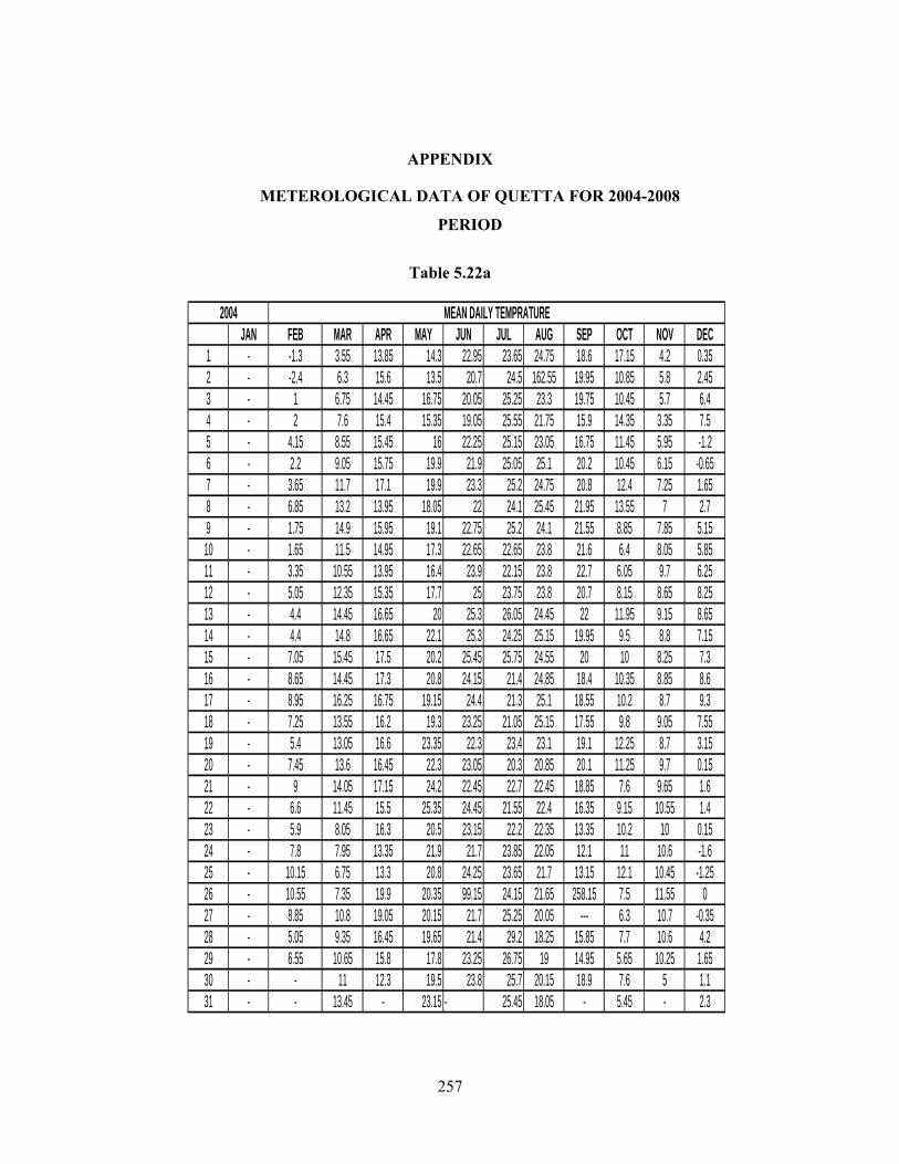
257
APPENDIX
METEROLOGICAL DATA OF QUETTA FOR 2004-2008
PERIOD
Table 5.22a
JAN FEB MAR APR MAY JUN JUL AUG SEP OCT NOV DEC1 - -1.3 3.55 13.85 14.3 22.95 23.65 24.75 18.6 17.15 4.2 0.352 - -2.4 6.3 15.6 13.5 20.7 24.5 162.55 19.95 10.85 5.8 2.453 - 1 6.75 14.45 16.75 20.05 25.25 23.3 19.75 10.45 5.7 6.44 - 2 7.6 15.4 15.35 19.05 25.55 21.75 15.9 14.35 3.35 7.55 - 4.15 8.55 15.45 16 22.25 25.15 23.05 16.75 11.45 5.95 -1.26 - 2.2 9.05 15.75 19.9 21.9 25.05 25.1 20.2 10.45 6.15 -0.657 - 3.65 11.7 17.1 19.9 23.3 25.2 24.75 20.8 12.4 7.25 1.658 - 6.85 13.2 13.95 18.05 22 24.1 25.45 21.95 13.55 7 2.79 - 1.75 14.9 15.95 19.1 22.75 25.2 24.1 21.55 8.85 7.85 5.1510 - 1.65 11.5 14.95 17.3 22.65 22.65 23.8 21.6 6.4 8.05 5.8511 - 3.35 10.55 13.95 16.4 23.9 22.15 23.8 22.7 6.05 9.7 6.2512 - 5.05 12.35 15.35 17.7 25 23.75 23.8 20.7 8.15 8.65 8.2513 - 4.4 14.45 16.65 20 25.3 26.05 24.45 22 11.95 9.15 8.6514 - 4.4 14.8 16.65 22.1 25.3 24.25 25.15 19.95 9.5 8.8 7.1515 - 7.05 15.45 17.5 20.2 25.45 25.75 24.55 20 10 8.25 7.316 - 8.65 14.45 17.3 20.8 24.15 21.4 24.85 18.4 10.35 8.85 8.617 - 8.95 16.25 16.75 19.15 24.4 21.3 25.1 18.55 10.2 8.7 9.318 - 7.25 13.55 16.2 19.3 23.25 21.05 25.15 17.55 9.8 9.05 7.5519 - 5.4 13.05 16.6 23.35 22.3 23.4 23.1 19.1 12.25 8.7 3.1520 - 7.45 13.6 16.45 22.3 23.05 20.3 20.85 20.1 11.25 9.7 0.1521 - 9 14.05 17.15 24.2 22.45 22.7 22.45 18.85 7.6 9.65 1.622 - 6.6 11.45 15.5 25.35 24.45 21.55 22.4 16.35 9.15 10.55 1.423 - 5.9 8.05 16.3 20.5 23.15 22.2 22.35 13.35 10.2 10 0.1524 - 7.8 7.95 13.35 21.9 21.7 23.85 22.05 12.1 11 10.6 -1.625 - 10.15 6.75 13.3 20.8 24.25 23.65 21.7 13.15 12.1 10.45 -1.2526 - 10.55 7.35 19.9 20.35 99.15 24.15 21.65 258.15 7.5 11.55 027 - 8.85 10.8 19.05 20.15 21.7 25.25 20.05 --- 6.3 10.7 -0.3528 - 5.05 9.35 16.45 19.65 21.4 29.2 18.25 15.85 7.7 10.6 4.229 - 6.55 10.65 15.8 17.8 23.25 26.75 19 14.95 5.65 10.25 1.6530 - - 11 12.3 19.5 23.8 25.7 20.15 18.9 7.6 5 1.131 - - 13.45 - 23.15 - 25.45 18.05 - 5.45 - 2.3
MEAN DAILY TEMPRATURE2004
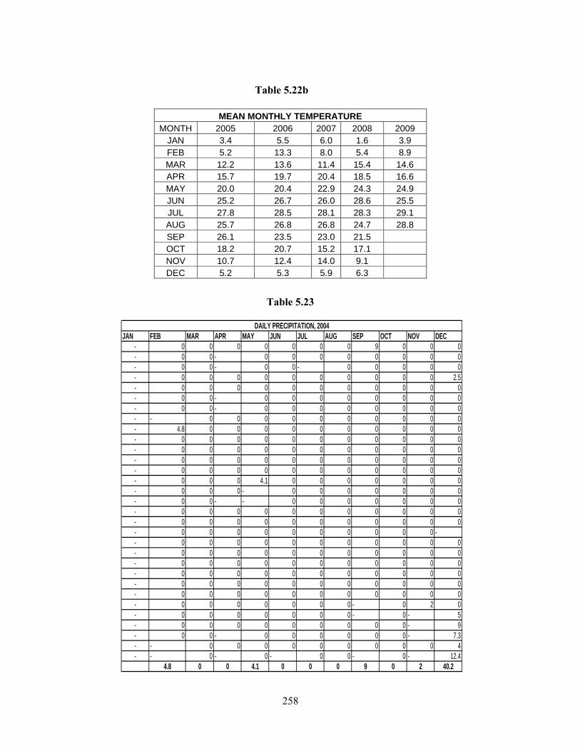
258
Table 5.23
JAN FEB MAR APR MAY JUN JUL AUG SEP OCT NOV DEC- 0 0 0 0 0 0 0 9 0 0 0- 0 0 - 0 0 0 0 0 0 0 0- 0 0 - 0 0 - 0 0 0 0 0- 0 0 0 0 0 0 0 0 0 0 2.5- 0 0 0 0 0 0 0 0 0 0 0- 0 0 - 0 0 0 0 0 0 0 0- 0 0 - 0 0 0 0 0 0 0 0- - 0 0 0 0 0 0 0 0 0 0- 4.8 0 0 0 0 0 0 0 0 0 0- 0 0 0 0 0 0 0 0 0 0 0- 0 0 0 0 0 0 0 0 0 0 0- 0 0 0 0 0 0 0 0 0 0 0- 0 0 0 0 0 0 0 0 0 0 0- 0 0 0 4.1 0 0 0 0 0 0 0- 0 0 0 - 0 0 0 0 0 0 0- 0 0 - - 0 0 0 0 0 0 0- 0 0 0 0 0 0 0 0 0 0 0- 0 0 0 0 0 0 0 0 0 0 0- 0 0 0 0 0 0 0 0 0 0 -- 0 0 0 0 0 0 0 0 0 0 0- 0 0 0 0 0 0 0 0 0 0 0- 0 0 0 0 0 0 0 0 0 0 0- 0 0 0 0 0 0 0 0 0 0 0- 0 0 0 0 0 0 0 0 0 0 0- 0 0 0 0 0 0 0 0 0 0 0- 0 0 0 0 0 0 0 - 0 2 0- 0 0 0 0 0 0 0 - 0 - 5- 0 0 0 0 0 0 0 0 0 - 9- 0 0 - 0 0 0 0 0 0 - 7.3- - 0 0 0 0 0 0 0 0 0 4- - 0 - 0 - 0 0 - 0 - 12.4
4.8 0 0 4.1 0 0 0 9 0 2 40.2
DAILY PRECIPITATION, 2004
Table 5.22b
MEAN MONTHLY TEMPERATURE MONTH 2005 2006 2007 2008 2009
JAN 3.4 5.5 6.0 1.6 3.9 FEB 5.2 13.3 8.0 5.4 8.9 MAR 12.2 13.6 11.4 15.4 14.6 APR 15.7 19.7 20.4 18.5 16.6 MAY 20.0 20.4 22.9 24.3 24.9 JUN 25.2 26.7 26.0 28.6 25.5 JUL 27.8 28.5 28.1 28.3 29.1 AUG 25.7 26.8 26.8 24.7 28.8 SEP 26.1 23.5 23.0 21.5 OCT 18.2 20.7 15.2 17.1 NOV 10.7 12.4 14.0 9.1 DEC 5.2 5.3 5.9 6.3
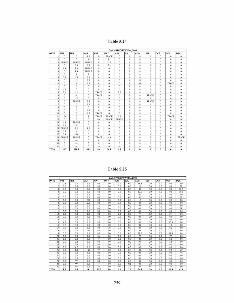
259
Table 5.24
DATE JAN FEB MAR APR MAY JUN JUL AUG SEP OCT NOV DEC1 0 0 9.6 0 TRACE 0 0 0 0 0 0 02 0 0 13.2 0 3.1 0 0 0 0 0 0 03 TRACE TRACE TRACE 0 12.1 0 0 0 0 0 0 04 0 0.3 0.5 0 7.3 0 0 0 0 0 0 05 6.4 7.8 TRACE 0 0 0 0 0 0 0 0 06 0 9.9 TRACE 0 0 0 0 0 0 0 0 07 0 8 8 0 0 0 0 0 0 0 0 08 0.8 4.3 7.2 0 0 0 0 0 0 0 0 09 0 13 0.2 0 0 0 0 2.8 0 0 0 0
10 0 8 0.5 0 0 0 0 0.6 0 0 TRACE 011 0 0 0 0 0 0 0 0 0 0 0 012 1.2 0 0 0 0 0 0 0 0 0 0 013 3.1 4.1 0 TRACE 0 3.6 0 0 0 0 0 014 0 13.1 0 TRACE 0 0 0 0 TRACE 0 0 015 0 11.5 0 0 0 0 0 0 0 0 0 016 0 TRACE 2.8 0 0 0 0 0 TRACE 0 0 017 0 0 1.4 0 0 0 0 0 0 0 0 018 0 0 0 0 0 0 0 0 0 0 0 019 0 0 0.6 0 0 0 0 0 0 0 0 020 0 0 1.7 TRACE 0 0 0 0 0 0 0 021 17.4 0 8 TRACE TRACE 1.2 0 0 0 0 TRACE 022 0 0 0 0.4 TRACE TRACE 0 0 0 0 0 023 1.4 TRACE 0 0 0 0 0 0 0 0 0 024 2.2 10.2 0 0 0 0 0 0 0 0 0 025 TRACE 8.2 9.6 0 0 0 0 0 0 0 0 026 0.3 4 0 0 0 0 0 0 0 0 0 027 0.9 26.8 0 0 0 0 0 0 0 0 0 028 TRACE TRACE 0 TRACE 14.4 0 0 0 0 0 0 TRACE29 0 --- 0 0 0 0 0 0 0 0 0 030 0 --- 0 0 0 0 0 0 0 0 0 031 0 --- 0 --- 0 --- 0 0 --- 0 --- 0
TOTAL 33.7 129.2 63.3 0.4 36.9 4.8 0 3.4 0 0 0 0
DAILY PRECIPITATION, 2005
Table 5.25
DATE JAN FEB MAR APR MAY JUN JUL AUG SEP OCT NOV DEC1 0.4 0.0 0.0 0.0 0.0 0.0 0.0 18.3 0.0 0.0 0.0 0.02 0.0 0.0 0.0 0.0 0.0 0.0 0.0 2.0 0.0 0.0 0.0 TR3 0.0 0.0 0.0 0.0 0.0 0.0 0.0 0.0 0.0 0.0 0.0 10.54 0.0 0.0 0.0 0.0 0.0 0.0 0.0 12.3 0.0 0.0 0.0 18.55 0.0 0.0 1.7 0.0 0.0 0.0 0.0 0.0 0.0 0.0 0.0 2.06 0.0 0.0 0.0 0.0 0.0 0.0 0.0 6.2 0.0 0.0 0.0 TR7 0.0 0.0 TR 0.0 0.0 0.0 0.0 1.3 0.0 0.0 0.0 0.08 0.0 0.0 2.8 0.0 0.0 0.0 0.0 0.0 0.0 0.0 0.0 0.09 0.0 0.0 0.0 1.2 0.0 0.0 0.0 0.0 0.0 0.0 0.0 0.0
10 0.0 0.0 0.0 0.0 0.0 0.0 0.0 0.0 0.0 0.0 0.0 TR11 0.0 0.0 0.0 0.0 0.0 0.0 0.0 0.0 0.0 0.0 0.0 0.012 0.0 0.0 1.2 0.0 0.0 0.0 0.0 TR 0.0 0.0 2.4 0.013 0.0 0.0 0.2 0.0 0.0 0.0 0.0 0.0 0.0 0.0 0.0 0.014 0.0 0.0 0.0 1.1 0.0 0.0 0.0 0.0 0.0 0.0 0.0 0.015 4.3 0.0 0.0 0.0 0.0 0.0 0.0 0.0 0.0 0.0 10.6 0.016 3.2 0.0 0.0 0.0 0.0 0.0 0.0 0.2 0.0 0.0 1.8 0.017 0.0 0.0 0.0 0.0 5.6 0.0 0.0 0.0 0.0 0.0 8.2 0.018 1.0 0.0 TR 0.0 0.0 0.0 0.0 3.6 0.0 0.0 7.3 0.019 0.0 0.0 2.6 0.0 0.0 0.0 0.0 10.8 0.0 0.0 11.6 0.020 0.0 0.0 1.0 8.4 0.0 0.0 0.0 TR 0.0 0.0 TR 0.021 0.0 0.0 0.0 TR 0.0 0.0 0.0 0.0 0.0 0.0 2.2 0.022 0.0 0.2 0.0 0.0 0.0 0.0 0.0 0.0 0.0 0.0 2.8 0.023 0.0 0.6 0.0 0.0 0.0 0.0 0.0 0.2 0.0 0.0 0.0 0.024 0.0 4.7 0.0 0.0 0.0 0.0 0.0 0.0 0.0 0.0 0.0 0.025 0.0 1.0 16.5 TR 0.0 0.0 0.0 0.0 0.0 0.0 0.0 5.226 0.0 0.0 0.1 0.0 0.0 0.0 0.0 0.0 0.0 0.0 0.0 7.627 0.0 0.0 0.0 0.0 0.0 0.0 0.0 0.0 0.0 0.0 0.0 0.028 0.0 0.0 0.0 0.0 0.0 0.0 0.0 0.0 0.0 0.0 0.0 0.029 0.0 *** 0.0 0.0 0.0 0.0 0.0 0.0 0.0 0.0 0.0 0.030 0.6 *** 0.0 TR 0.0 0.0 0.1 0.0 0.0 0.0 0.0 0.031 0.0 *** 0.0 *** 0.0 *** 2.4 0.0 *** 0.0 *** 0.0
TOTAL 9.5 6.5 26.1 10.7 5.6 0.0 2.5 54.9 0.0 0.0 46.9 43.8
DAILY PRECIPITATION, 2006
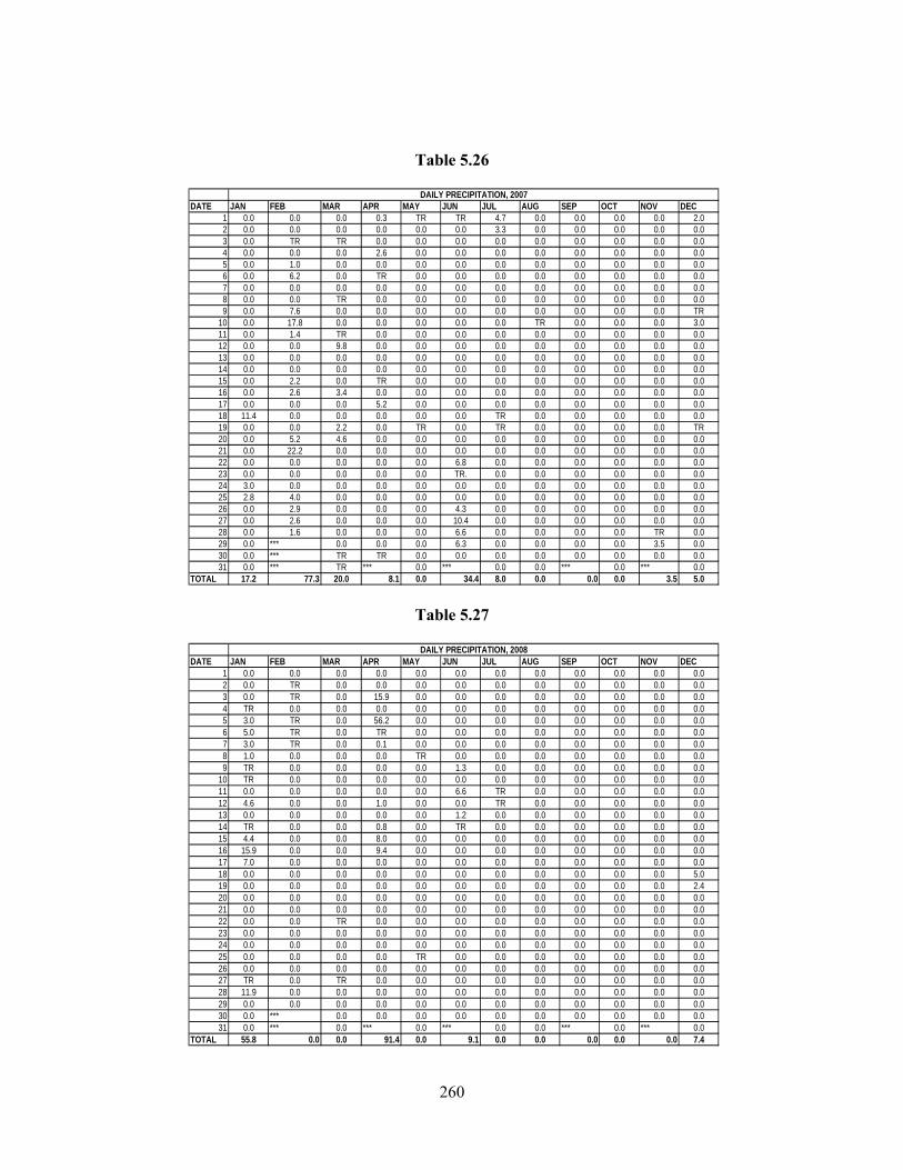
260
Table 5.26
DATE JAN FEB MAR APR MAY JUN JUL AUG SEP OCT NOV DEC1 0.0 0.0 0.0 0.3 TR TR 4.7 0.0 0.0 0.0 0.0 2.02 0.0 0.0 0.0 0.0 0.0 0.0 3.3 0.0 0.0 0.0 0.0 0.03 0.0 TR TR 0.0 0.0 0.0 0.0 0.0 0.0 0.0 0.0 0.04 0.0 0.0 0.0 2.6 0.0 0.0 0.0 0.0 0.0 0.0 0.0 0.05 0.0 1.0 0.0 0.0 0.0 0.0 0.0 0.0 0.0 0.0 0.0 0.06 0.0 6.2 0.0 TR 0.0 0.0 0.0 0.0 0.0 0.0 0.0 0.07 0.0 0.0 0.0 0.0 0.0 0.0 0.0 0.0 0.0 0.0 0.0 0.08 0.0 0.0 TR 0.0 0.0 0.0 0.0 0.0 0.0 0.0 0.0 0.09 0.0 7.6 0.0 0.0 0.0 0.0 0.0 0.0 0.0 0.0 0.0 TR
10 0.0 17.8 0.0 0.0 0.0 0.0 0.0 TR 0.0 0.0 0.0 3.011 0.0 1.4 TR 0.0 0.0 0.0 0.0 0.0 0.0 0.0 0.0 0.012 0.0 0.0 9.8 0.0 0.0 0.0 0.0 0.0 0.0 0.0 0.0 0.013 0.0 0.0 0.0 0.0 0.0 0.0 0.0 0.0 0.0 0.0 0.0 0.014 0.0 0.0 0.0 0.0 0.0 0.0 0.0 0.0 0.0 0.0 0.0 0.015 0.0 2.2 0.0 TR 0.0 0.0 0.0 0.0 0.0 0.0 0.0 0.016 0.0 2.6 3.4 0.0 0.0 0.0 0.0 0.0 0.0 0.0 0.0 0.017 0.0 0.0 0.0 5.2 0.0 0.0 0.0 0.0 0.0 0.0 0.0 0.018 11.4 0.0 0.0 0.0 0.0 0.0 TR 0.0 0.0 0.0 0.0 0.019 0.0 0.0 2.2 0.0 TR 0.0 TR 0.0 0.0 0.0 0.0 TR20 0.0 5.2 4.6 0.0 0.0 0.0 0.0 0.0 0.0 0.0 0.0 0.021 0.0 22.2 0.0 0.0 0.0 0.0 0.0 0.0 0.0 0.0 0.0 0.022 0.0 0.0 0.0 0.0 0.0 6.8 0.0 0.0 0.0 0.0 0.0 0.023 0.0 0.0 0.0 0.0 0.0 TR. 0.0 0.0 0.0 0.0 0.0 0.024 3.0 0.0 0.0 0.0 0.0 0.0 0.0 0.0 0.0 0.0 0.0 0.025 2.8 4.0 0.0 0.0 0.0 0.0 0.0 0.0 0.0 0.0 0.0 0.026 0.0 2.9 0.0 0.0 0.0 4.3 0.0 0.0 0.0 0.0 0.0 0.027 0.0 2.6 0.0 0.0 0.0 10.4 0.0 0.0 0.0 0.0 0.0 0.028 0.0 1.6 0.0 0.0 0.0 6.6 0.0 0.0 0.0 0.0 TR 0.029 0.0 *** 0.0 0.0 0.0 6.3 0.0 0.0 0.0 0.0 3.5 0.030 0.0 *** TR TR 0.0 0.0 0.0 0.0 0.0 0.0 0.0 0.031 0.0 *** TR *** 0.0 *** 0.0 0.0 *** 0.0 *** 0.0
TOTAL 17.2 77.3 20.0 8.1 0.0 34.4 8.0 0.0 0.0 0.0 3.5 5.0
DAILY PRECIPITATION, 2007
Table 5.27
DATE JAN FEB MAR APR MAY JUN JUL AUG SEP OCT NOV DEC1 0.0 0.0 0.0 0.0 0.0 0.0 0.0 0.0 0.0 0.0 0.0 0.02 0.0 TR 0.0 0.0 0.0 0.0 0.0 0.0 0.0 0.0 0.0 0.03 0.0 TR 0.0 15.9 0.0 0.0 0.0 0.0 0.0 0.0 0.0 0.04 TR 0.0 0.0 0.0 0.0 0.0 0.0 0.0 0.0 0.0 0.0 0.05 3.0 TR 0.0 56.2 0.0 0.0 0.0 0.0 0.0 0.0 0.0 0.06 5.0 TR 0.0 TR 0.0 0.0 0.0 0.0 0.0 0.0 0.0 0.07 3.0 TR 0.0 0.1 0.0 0.0 0.0 0.0 0.0 0.0 0.0 0.08 1.0 0.0 0.0 0.0 TR 0.0 0.0 0.0 0.0 0.0 0.0 0.09 TR 0.0 0.0 0.0 0.0 1.3 0.0 0.0 0.0 0.0 0.0 0.0
10 TR 0.0 0.0 0.0 0.0 0.0 0.0 0.0 0.0 0.0 0.0 0.011 0.0 0.0 0.0 0.0 0.0 6.6 TR 0.0 0.0 0.0 0.0 0.012 4.6 0.0 0.0 1.0 0.0 0.0 TR 0.0 0.0 0.0 0.0 0.013 0.0 0.0 0.0 0.0 0.0 1.2 0.0 0.0 0.0 0.0 0.0 0.014 TR 0.0 0.0 0.8 0.0 TR 0.0 0.0 0.0 0.0 0.0 0.015 4.4 0.0 0.0 8.0 0.0 0.0 0.0 0.0 0.0 0.0 0.0 0.016 15.9 0.0 0.0 9.4 0.0 0.0 0.0 0.0 0.0 0.0 0.0 0.017 7.0 0.0 0.0 0.0 0.0 0.0 0.0 0.0 0.0 0.0 0.0 0.018 0.0 0.0 0.0 0.0 0.0 0.0 0.0 0.0 0.0 0.0 0.0 5.019 0.0 0.0 0.0 0.0 0.0 0.0 0.0 0.0 0.0 0.0 0.0 2.420 0.0 0.0 0.0 0.0 0.0 0.0 0.0 0.0 0.0 0.0 0.0 0.021 0.0 0.0 0.0 0.0 0.0 0.0 0.0 0.0 0.0 0.0 0.0 0.022 0.0 0.0 TR 0.0 0.0 0.0 0.0 0.0 0.0 0.0 0.0 0.023 0.0 0.0 0.0 0.0 0.0 0.0 0.0 0.0 0.0 0.0 0.0 0.024 0.0 0.0 0.0 0.0 0.0 0.0 0.0 0.0 0.0 0.0 0.0 0.025 0.0 0.0 0.0 0.0 TR 0.0 0.0 0.0 0.0 0.0 0.0 0.026 0.0 0.0 0.0 0.0 0.0 0.0 0.0 0.0 0.0 0.0 0.0 0.027 TR 0.0 TR 0.0 0.0 0.0 0.0 0.0 0.0 0.0 0.0 0.028 11.9 0.0 0.0 0.0 0.0 0.0 0.0 0.0 0.0 0.0 0.0 0.029 0.0 0.0 0.0 0.0 0.0 0.0 0.0 0.0 0.0 0.0 0.0 0.030 0.0 *** 0.0 0.0 0.0 0.0 0.0 0.0 0.0 0.0 0.0 0.031 0.0 *** 0.0 *** 0.0 *** 0.0 0.0 *** 0.0 *** 0.0
TOTAL 55.8 0.0 0.0 91.4 0.0 9.1 0.0 0.0 0.0 0.0 0.0 7.4
DAILY PRECIPITATION, 2008
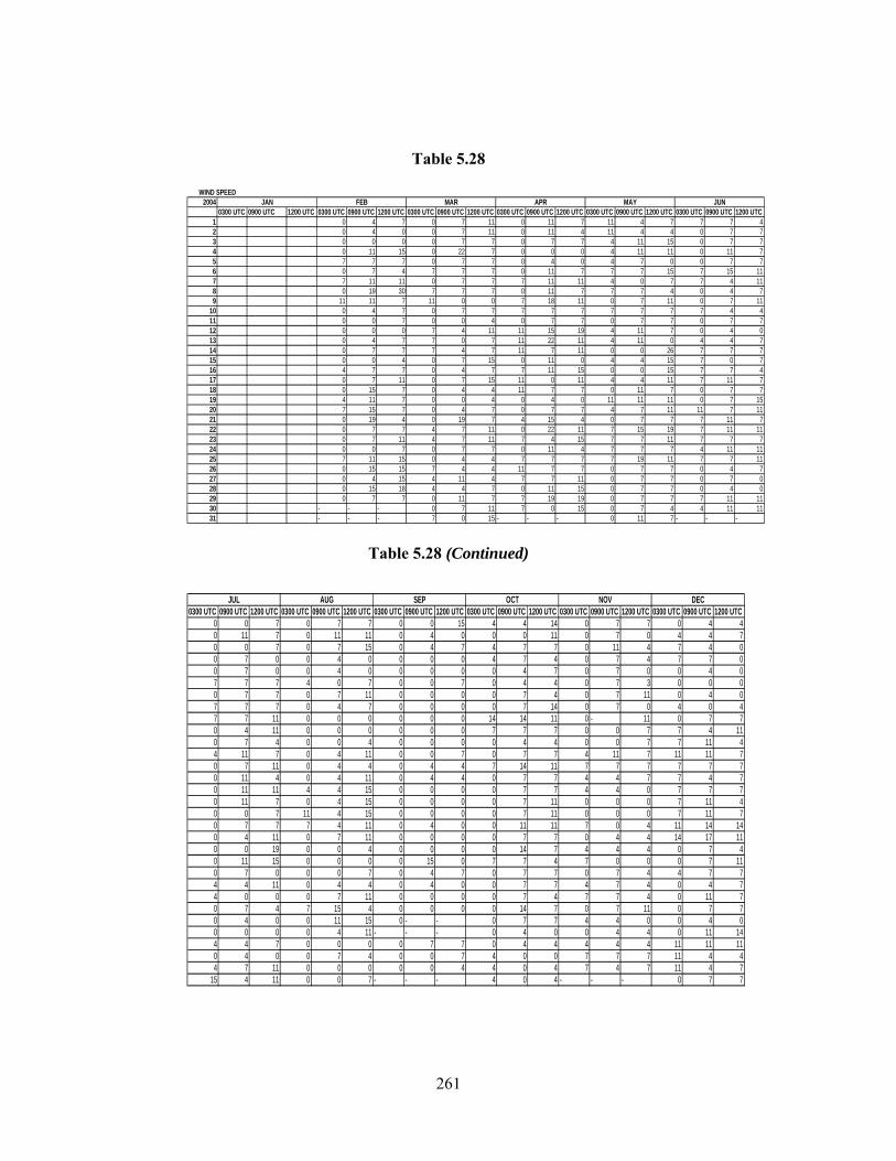
261
Table 5.28
20040300 UTC 0900 UTC 1200 UTC 0300 UTC 0900 UTC 1200 UTC 0300 UTC 0900 UTC 1200 UTC 0300 UTC 0900 UTC 1200 UTC 0300 UTC 0900 UTC 1200 UTC 0300 UTC 0900 UTC 1200 UTC
1 0 4 7 0 7 11 0 11 7 11 4 7 7 7 42 0 4 0 0 7 11 0 11 4 11 4 4 0 7 73 0 0 0 0 7 7 0 7 7 4 11 15 0 7 74 0 11 15 0 22 7 0 0 0 4 11 11 0 11 75 7 7 7 0 7 7 0 4 0 4 7 0 0 7 76 0 7 4 7 7 7 0 11 7 7 7 15 7 15 117 7 11 11 0 7 7 7 11 11 4 0 7 7 4 118 0 19 30 7 7 7 0 11 7 7 7 4 0 4 79 11 11 7 11 0 0 7 18 11 0 7 11 0 7 11
10 0 4 7 0 7 7 7 7 7 7 7 7 7 4 411 0 0 7 0 0 4 0 7 7 0 7 7 0 7 712 0 0 0 7 4 11 11 15 19 4 11 7 0 4 013 0 4 7 7 0 7 11 22 11 4 11 0 4 4 714 0 7 7 7 4 7 11 7 11 0 0 26 7 7 715 0 0 4 0 7 15 0 11 0 4 4 15 7 0 716 4 7 7 0 4 7 7 11 15 0 0 15 7 7 417 0 7 11 0 7 15 11 0 11 4 4 11 7 11 718 0 15 7 0 4 4 11 7 7 0 11 7 0 7 719 4 11 7 0 0 4 0 4 0 11 11 11 0 7 1520 7 15 7 0 4 7 0 7 7 4 7 11 11 7 1121 0 19 4 0 19 7 4 15 4 0 7 7 7 11 722 0 7 7 4 7 11 0 22 11 7 15 19 7 11 1123 0 7 11 4 7 11 7 4 15 7 7 11 7 7 724 0 0 7 0 7 7 0 11 4 7 7 7 4 11 1125 7 11 15 0 4 4 7 7 7 7 19 11 7 7 1126 0 15 15 7 4 4 11 7 7 0 7 7 0 4 727 0 4 15 4 11 4 7 7 11 0 7 7 0 7 028 0 15 18 4 4 7 0 11 15 0 7 7 0 4 029 0 7 7 0 11 7 7 19 19 0 7 7 7 11 1130 - - - 0 7 11 7 0 15 0 7 4 4 11 1131 - - - 7 0 15 - - - 0 11 7 - - -
WIND SPEEDAPRMARJAN FEB JUNMAY
Table 5.28 (Continued)
0300 UTC 0900 UTC 1200 UTC 0300 UTC 0900 UTC 1200 UTC 0300 UTC 0900 UTC 1200 UTC 0300 UTC 0900 UTC 1200 UTC 0300 UTC 0900 UTC 1200 UTC 0300 UTC 0900 UTC 1200 UTC0 0 7 0 7 7 0 0 15 4 4 14 0 7 7 0 4 40 11 7 0 11 11 0 4 0 0 0 11 0 7 0 4 4 70 0 7 0 7 15 0 4 7 4 7 7 0 11 4 7 4 00 7 0 0 4 0 0 0 0 4 7 4 0 7 4 7 7 00 7 0 0 4 0 0 0 0 0 4 7 0 7 0 0 4 07 7 7 4 0 7 0 0 7 0 4 4 0 7 3 0 0 00 7 7 0 7 11 0 0 0 0 7 4 0 7 11 0 4 07 7 7 0 4 7 0 0 0 0 7 14 0 7 0 4 0 47 7 11 0 0 0 0 0 0 14 14 11 0 - 11 0 7 70 4 11 0 0 0 0 0 0 7 7 7 0 0 7 7 4 110 7 4 0 0 4 0 0 0 0 4 4 0 0 7 7 11 44 11 7 0 4 11 0 0 7 0 7 7 4 11 7 11 11 70 7 11 0 4 4 0 4 4 7 14 11 7 7 7 7 7 70 11 4 0 4 11 0 4 4 0 7 7 4 4 7 7 4 70 11 11 4 4 15 0 0 0 0 7 7 4 4 0 7 7 70 11 7 0 4 15 0 0 0 0 7 11 0 0 0 7 11 40 0 7 11 4 15 0 0 0 0 7 11 0 0 0 7 11 70 7 7 7 4 11 0 4 0 0 11 11 7 0 4 11 14 140 4 11 0 7 11 0 0 0 0 7 7 0 4 4 14 17 110 0 19 0 0 4 0 0 0 0 14 7 4 4 4 0 7 40 11 15 0 0 0 0 15 0 7 7 4 7 0 0 0 7 110 7 0 0 0 7 0 4 7 0 7 7 0 7 4 4 7 74 4 11 0 4 4 0 4 0 0 7 7 4 7 4 0 4 74 0 0 0 7 11 0 0 0 0 7 4 7 7 4 0 11 70 7 4 7 15 4 0 0 0 0 14 7 0 7 11 0 7 70 4 0 0 11 15 0 - - 0 7 7 4 4 0 0 4 00 0 0 0 4 11 - - - 0 4 0 0 4 4 0 11 144 4 7 0 0 0 0 7 7 0 4 4 4 4 4 11 11 110 4 0 0 7 4 0 0 7 4 0 0 7 7 7 11 4 44 7 11 0 0 0 0 0 4 4 0 4 7 4 7 11 4 7
15 4 11 0 0 7 - - - 4 0 4 - - - 0 7 7
DECNOVOCTSEPAUGJUL

262
Table 5.29
20050300 UTC 0900 UTC 1200 UTC 0300 UTC 0900 UTC 1200 UTC 0300 UTC 0900 UTC 1200 UTC 0300 UTC 0900 UTC 1200 UTC 0300 UTC 0900 UTC 1200 UTC 0300 UTC 0900 UTC 1200 UTC
1 7 4 7 0 4 0 0 14 7 0 0 0 14 7 7 0 0 02 0 4 0 0 11 14 0 7 11 0 0 0 7 0 11 0 0 03 0 7 4 14 14 18 4 7 7 4 4 4 11 0 4 0 0 04 7 11 4 0 11 7 0 11 0 0 0 4 0 7 0 0 0 05 0 0 4 4 11 14 0 4 0 7 7 11 0 0 0 0 0 06 0 0 0 4 0 4 7 14 18 7 7 28 0 0 4 0 4 47 7 0 7 0 0 4 0 4 7 28 28 28 11 7 4 7 0 08 0 4 4 4 14 7 7 14 18 14 11 14 0 --- 18 0 0 09 4 4 4 0 11 14 0 7 4 14 11 11 7 14 4 0 0 0
10 4 7 7 7 14 14 0 14 14 4 11 14 0 7 0 0 0 011 7 14 11 7 11 11 0 4 11 4 0 0 0 4 7 0 7 412 0 11 4 4 4 11 0 7 7 7 4 0 7 7 7 7 14 1413 4 0 0 0 0 0 0 0 0 0 7 14 7 11 --- 0 7 414 4 4 7 0 0 0 0 4 0 18 7 11 0 0 --- 0 7 1115 0 0 0 4 14 15 4 0 14 11 0 7 --- --- --- 7 7 716 0 0 4 7 4 4 0 0 7 0 4 0 --- --- --- 0 0 717 0 4 4 7 4 11 4 0 18 4 4 0 --- --- --- 0 4 718 0 4 4 0 7 11 0 7 14 0 0 0 --- --- --- 0 7 1119 0 0 0 4 4 4 11 18 7 7 7 4 --- --- --- 11 4 2520 7 0 7 0 0 0 14 18 21 0 7 14 --- --- --- 0 28 1421 0 19 18 0 4 0 4 4 11 0 0 15 --- --- --- 7 1 1122 11 21 11 7 11 11 11 11 14 0 0 0 --- --- --- 0 7 1123 0 7 14 4 11 7 0 14 11 11 14 4 --- --- --- 0 4 1124 11 0 4 0 0 0 0 4 21 0 0 7 --- --- --- 0 4 1125 11 14 14 0 0 0 11 14 7 0 11 11 --- --- --- 0 11 2126 11 14 11 0 11 11 7 11 7 0 19 22 --- --- --- 0 7 727 0 7 7 0 0 0 7 4 11 0 7 15 --- --- --- 7 4 728 0 4 7 0 11 7 4 0 7 4 7 4 --- --- --- 11 4 429 0 7 7 --- --- --- 0 11 11 0 7 7 --- --- --- 4 4 1430 0 0 7 --- --- --- 4 7 4 0 0 4 --- --- --- 1 7 731 0 7 7 --- 0 --- 0 7 11 --- --- --- --- --- --- --- --- ---
MAY JUNJAN FEB MAR APRWIND SPEED
Table 5.29 (Continued)
0300 UTC 0900 UTC 1200 UTC 0300 UTC 0900 UTC 1200 UTC 0300 UTC 0900 UTC 1200 UTC 0300 UTC 0900 UTC 1200 UTC 0300 UTC 0900 UTC 1200 UTC 0300 UTC 0900 UTC 1200 UTC0 4 14 4 4 0 7 7 7 4 4 4 0 0 11 0 4 07 4 4 4 4 4 0 4 7 4 7 11 7 4 7 0 4 0
11 0 14 0 0 4 0 4 0 4 4 0 0 4 4 0 4 711 4 11 4 7 7 7 4 4 0 7 7 4 4 4 0 0 414 4 4 4 4 14 4 0 4 4 4 0 0 4 0 4 4 418 7 21 7 7 18 4 4 11 4 11 11 0 7 7 0 4 011 8 0 4 11 11 7 4 0 4 4 0 7 7 7 11 7 4
7 17 14 14 11 14 11 7 11 0 4 7 4 7 4 0 4 40 0 0 7 7 11 4 7 7 7 4 7 7 7 14 11 4 00 7 11 0 11 0 7 7 4 0 11 7 7 7 4 0 0 74 7 7 4 4 14 7 11 7 7 4 4 0 7 7 0 7 74 4 4 14 7 18 4 14 0 4 0 7 0 7 4 4 4 07 0 4 7 7 7 4 0 4 0 0 11 0 4 0 0 7 00 7 7 7 0 14 11 7 11 4 0 7 7 0 4 0 7 44 7 18 0 7 14 11 7 11 0 7 7 0 7 7 0 4 07 4 0 7 4 11 7 4 7 0 4 7 7 11 0 0 7 74 7 7 4 7 7 0 4 11 4 4 0 0 7 11 4 7 74 7 0 0 11 11 4 0 4 4 4 7 0 0 4 4 4 74 4 4 0 25 7 4 0 0 4 4 11 4 7 11 4 7 70 4 7 4 4 14 4 4 7 4 4 7 7 7 11 0 4 00 7 7 7 4 0 0 7 7 7 0 4 4 7 4 0 4 44 7 0 7 4 11 4 11 7 0 7 0 0 4 4 0 4 07 4 11 0 11 7 4 7 14 0 4 4 4 7 4 0 4 47 7 11 7 4 11 0 0 7 0 7 0 0 4 4 0 0 44 4 7 4 14 7 4 7 4 0 0 0 0 4 4 0 0 04 4 4 7 0 11 0 11 7 0 4 4 0 14 7 7 4 04 7 4 4 4 11 4 7 0 4 0 0 0 7 11 0 7 00 4 4 4 0 4 0 0 0 0 0 4 0 0 0 0 4 04 0 7 4 14 14 0 4 0 0 7 7 0 11 7 0 7 77 4 0 4 7 7 0 4 7 4 7 11 7 7 4 0 14 44 7 7 11 4 7 --- --- --- 0 7 0 --- --- --- 0 7 7
JUL AUG SEP OCT NOV DEC
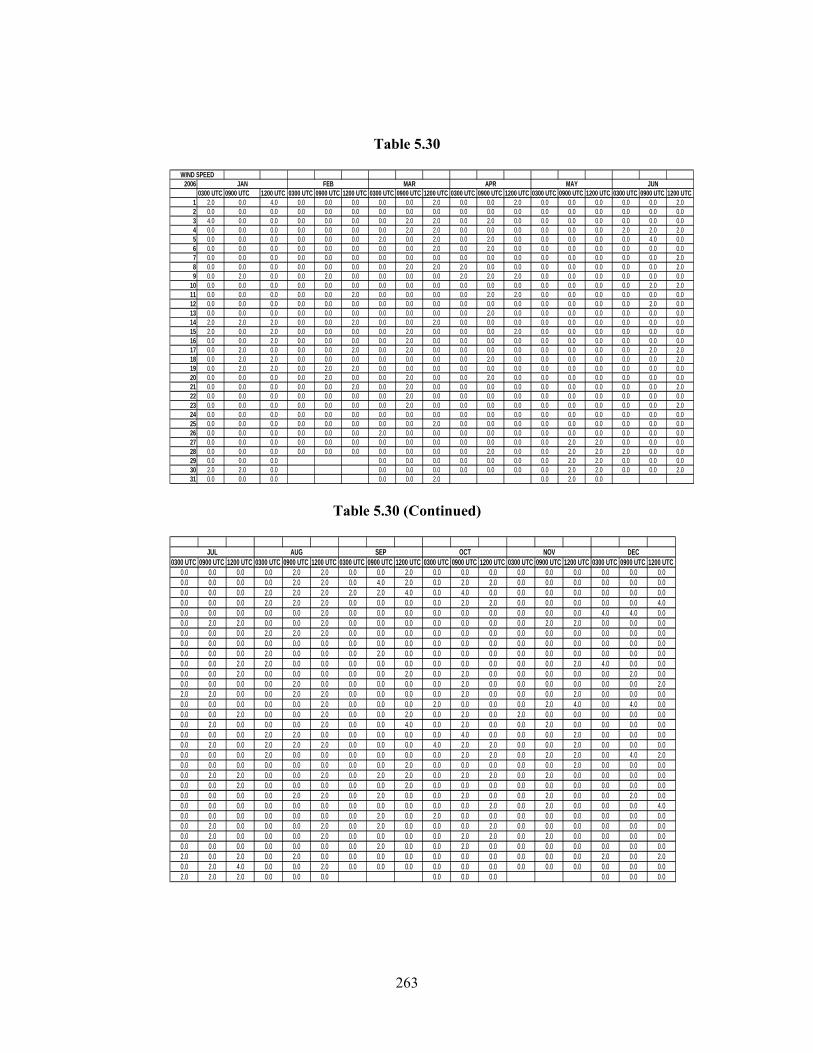
263
Table 5.30
20060300 UTC 0900 UTC 1200 UTC 0300 UTC 0900 UTC 1200 UTC 0300 UTC 0900 UTC 1200 UTC 0300 UTC 0900 UTC 1200 UTC 0300 UTC 0900 UTC 1200 UTC 0300 UTC 0900 UTC 1200 UTC
1 2.0 0.0 4.0 0.0 0.0 0.0 0.0 0.0 2.0 0.0 0.0 2.0 0.0 0.0 0.0 0.0 0.0 2.02 0.0 0.0 0.0 0.0 0.0 0.0 0.0 0.0 0.0 0.0 0.0 0.0 0.0 0.0 0.0 0.0 0.0 0.03 4.0 0.0 0.0 0.0 0.0 0.0 0.0 2.0 2.0 0.0 2.0 0.0 0.0 0.0 0.0 0.0 0.0 0.04 0.0 0.0 0.0 0.0 0.0 0.0 0.0 2.0 2.0 0.0 0.0 0.0 0.0 0.0 0.0 2.0 2.0 2.05 0.0 0.0 0.0 0.0 0.0 0.0 2.0 0.0 2.0 0.0 2.0 0.0 0.0 0.0 0.0 0.0 4.0 0.06 0.0 0.0 0.0 0.0 0.0 0.0 0.0 0.0 2.0 0.0 2.0 0.0 0.0 0.0 0.0 0.0 0.0 0.07 0.0 0.0 0.0 0.0 0.0 0.0 0.0 0.0 0.0 0.0 0.0 0.0 0.0 0.0 0.0 0.0 0.0 2.08 0.0 0.0 0.0 0.0 0.0 0.0 0.0 2.0 2.0 2.0 0.0 0.0 0.0 0.0 0.0 0.0 0.0 2.09 0.0 2.0 0.0 0.0 2.0 0.0 0.0 0.0 0.0 2.0 2.0 2.0 0.0 0.0 0.0 0.0 0.0 0.0
10 0.0 0.0 0.0 0.0 0.0 0.0 0.0 0.0 0.0 0.0 0.0 0.0 0.0 0.0 0.0 0.0 2.0 2.011 0.0 0.0 0.0 0.0 0.0 2.0 0.0 0.0 0.0 0.0 2.0 2.0 0.0 0.0 0.0 0.0 0.0 0.012 0.0 0.0 0.0 0.0 0.0 0.0 0.0 0.0 0.0 0.0 0.0 0.0 0.0 0.0 0.0 0.0 2.0 0.013 0.0 0.0 0.0 0.0 0.0 0.0 0.0 0.0 0.0 0.0 2.0 0.0 0.0 0.0 0.0 0.0 0.0 0.014 2.0 2.0 2.0 0.0 0.0 2.0 0.0 0.0 2.0 0.0 0.0 0.0 0.0 0.0 0.0 0.0 0.0 0.015 2.0 0.0 2.0 0.0 0.0 0.0 0.0 2.0 0.0 0.0 0.0 2.0 0.0 0.0 0.0 0.0 0.0 0.016 0.0 0.0 2.0 0.0 0.0 0.0 0.0 2.0 0.0 0.0 0.0 0.0 0.0 0.0 0.0 0.0 0.0 0.017 0.0 2.0 0.0 0.0 0.0 2.0 0.0 2.0 0.0 0.0 0.0 0.0 0.0 0.0 0.0 0.0 2.0 2.018 0.0 2.0 2.0 0.0 0.0 0.0 0.0 0.0 0.0 0.0 2.0 0.0 0.0 0.0 0.0 0.0 0.0 2.019 0.0 2.0 2.0 0.0 2.0 2.0 0.0 0.0 0.0 0.0 0.0 0.0 0.0 0.0 0.0 0.0 0.0 0.020 0.0 0.0 0.0 0.0 2.0 0.0 0.0 2.0 0.0 0.0 2.0 0.0 0.0 0.0 0.0 0.0 0.0 0.021 0.0 0.0 0.0 0.0 0.0 2.0 0.0 2.0 0.0 0.0 0.0 0.0 0.0 0.0 0.0 0.0 0.0 2.022 0.0 0.0 0.0 0.0 0.0 0.0 0.0 2.0 0.0 0.0 0.0 0.0 0.0 0.0 0.0 0.0 0.0 0.023 0.0 0.0 0.0 0.0 0.0 0.0 0.0 2.0 0.0 0.0 0.0 0.0 0.0 0.0 0.0 0.0 0.0 2.024 0.0 0.0 0.0 0.0 0.0 0.0 0.0 0.0 0.0 0.0 0.0 0.0 0.0 0.0 0.0 0.0 0.0 0.025 0.0 0.0 0.0 0.0 0.0 0.0 0.0 0.0 2.0 0.0 0.0 0.0 0.0 0.0 0.0 0.0 0.0 0.026 0.0 0.0 0.0 0.0 0.0 0.0 2.0 0.0 0.0 0.0 0.0 0.0 0.0 0.0 0.0 0.0 0.0 0.027 0.0 0.0 0.0 0.0 0.0 0.0 0.0 0.0 0.0 0.0 0.0 0.0 0.0 2.0 2.0 0.0 0.0 0.028 0.0 0.0 0.0 0.0 0.0 0.0 0.0 0.0 0.0 0.0 2.0 0.0 0.0 2.0 2.0 2.0 0.0 0.029 0.0 0.0 0.0 0.0 0.0 0.0 0.0 0.0 0.0 0.0 2.0 2.0 0.0 0.0 0.030 2.0 2.0 0.0 0.0 0.0 0.0 0.0 0.0 0.0 0.0 2.0 2.0 0.0 0.0 2.031 0.0 0.0 0.0 0.0 0.0 2.0 0.0 2.0 0.0
JAN FEB MAR APR MAY JUNWIND SPEED
Table 5.30 (Continued)
0300 UTC 0900 UTC 1200 UTC 0300 UTC 0900 UTC 1200 UTC 0300 UTC 0900 UTC 1200 UTC 0300 UTC 0900 UTC 1200 UTC 0300 UTC 0900 UTC 1200 UTC 0300 UTC 0900 UTC 1200 UTC0.0 0.0 0.0 0.0 2.0 2.0 0.0 0.0 2.0 0.0 0.0 0.0 0.0 0.0 0.0 0.0 0.0 0.00.0 0.0 0.0 0.0 2.0 2.0 0.0 4.0 2.0 0.0 2.0 2.0 0.0 0.0 0.0 0.0 0.0 0.00.0 0.0 0.0 2.0 2.0 2.0 2.0 2.0 4.0 0.0 4.0 0.0 0.0 0.0 0.0 0.0 0.0 0.00.0 0.0 0.0 2.0 2.0 2.0 0.0 0.0 0.0 0.0 2.0 2.0 0.0 0.0 0.0 0.0 0.0 4.00.0 0.0 0.0 0.0 0.0 2.0 0.0 0.0 0.0 0.0 0.0 0.0 0.0 0.0 0.0 4.0 4.0 0.00.0 2.0 2.0 0.0 0.0 2.0 0.0 0.0 0.0 0.0 0.0 0.0 0.0 2.0 2.0 0.0 0.0 0.00.0 0.0 0.0 2.0 2.0 2.0 0.0 0.0 0.0 0.0 0.0 0.0 0.0 0.0 0.0 0.0 0.0 0.00.0 0.0 0.0 0.0 0.0 0.0 0.0 0.0 0.0 0.0 0.0 0.0 0.0 0.0 0.0 0.0 0.0 0.00.0 0.0 0.0 2.0 0.0 0.0 0.0 2.0 0.0 0.0 0.0 0.0 0.0 0.0 0.0 0.0 0.0 0.00.0 0.0 2.0 2.0 0.0 0.0 0.0 0.0 0.0 0.0 0.0 0.0 0.0 0.0 2.0 4.0 0.0 0.00.0 0.0 2.0 0.0 0.0 0.0 0.0 0.0 2.0 0.0 2.0 0.0 0.0 0.0 0.0 0.0 2.0 0.00.0 0.0 0.0 0.0 2.0 0.0 0.0 0.0 0.0 0.0 2.0 0.0 0.0 0.0 0.0 0.0 0.0 2.02.0 2.0 0.0 0.0 2.0 2.0 0.0 0.0 0.0 0.0 2.0 0.0 0.0 0.0 2.0 0.0 0.0 0.00.0 0.0 0.0 0.0 0.0 2.0 0.0 0.0 0.0 2.0 0.0 0.0 0.0 2.0 4.0 0.0 4.0 0.00.0 0.0 2.0 0.0 0.0 2.0 0.0 0.0 2.0 0.0 2.0 0.0 2.0 0.0 0.0 0.0 0.0 0.00.0 2.0 0.0 0.0 0.0 2.0 0.0 0.0 4.0 0.0 2.0 0.0 0.0 2.0 0.0 0.0 0.0 0.00.0 0.0 0.0 2.0 2.0 0.0 0.0 0.0 0.0 0.0 4.0 0.0 0.0 0.0 2.0 0.0 0.0 0.00.0 2.0 0.0 2.0 2.0 2.0 0.0 0.0 0.0 4.0 2.0 2.0 0.0 0.0 2.0 0.0 0.0 0.00.0 0.0 0.0 2.0 0.0 0.0 0.0 0.0 0.0 0.0 2.0 2.0 0.0 2.0 2.0 0.0 4.0 2.00.0 0.0 0.0 0.0 0.0 0.0 0.0 0.0 2.0 0.0 0.0 0.0 0.0 0.0 2.0 0.0 0.0 0.00.0 2.0 2.0 0.0 0.0 2.0 0.0 2.0 2.0 0.0 2.0 2.0 0.0 2.0 0.0 0.0 0.0 0.00.0 0.0 2.0 0.0 0.0 0.0 0.0 0.0 2.0 0.0 0.0 0.0 0.0 0.0 0.0 0.0 0.0 0.00.0 0.0 0.0 0.0 2.0 2.0 0.0 2.0 0.0 0.0 2.0 0.0 0.0 2.0 0.0 0.0 2.0 0.00.0 0.0 0.0 0.0 0.0 0.0 0.0 0.0 0.0 0.0 0.0 2.0 0.0 2.0 0.0 0.0 0.0 4.00.0 0.0 0.0 0.0 0.0 0.0 0.0 2.0 0.0 2.0 0.0 0.0 0.0 0.0 0.0 0.0 0.0 0.00.0 2.0 0.0 0.0 0.0 2.0 0.0 2.0 0.0 0.0 0.0 2.0 0.0 0.0 0.0 0.0 0.0 0.00.0 2.0 0.0 0.0 0.0 2.0 0.0 0.0 0.0 0.0 2.0 2.0 0.0 2.0 0.0 0.0 0.0 0.00.0 0.0 0.0 0.0 0.0 0.0 0.0 2.0 0.0 0.0 2.0 0.0 0.0 0.0 0.0 0.0 0.0 0.02.0 0.0 2.0 0.0 2.0 0.0 0.0 0.0 0.0 0.0 0.0 0.0 0.0 0.0 0.0 2.0 0.0 2.00.0 2.0 4.0 0.0 0.0 2.0 0.0 0.0 0.0 0.0 0.0 0.0 0.0 0.0 0.0 0.0 0.0 0.02.0 2.0 2.0 0.0 0.0 0.0 0.0 0.0 0.0 0.0 0.0 0.0
JUL AUG SEP OCT NOV DEC
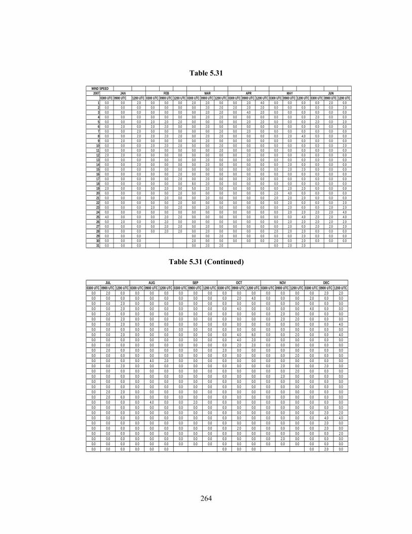
264
Table 5.31
20070300 UTC 0900 UTC 1200 UTC 0300 UTC 0900 UTC 1200 UTC 0300 UTC 0900 UTC 1200 UTC 0300 UTC 0900 UTC 1200 UTC 0300 UTC 0900 UTC 1200 UTC 0300 UTC 0900 UTC 1200 UTC
1 0.0 0.0 2.0 0.0 0.0 0.0 2.0 2.0 0.0 0.0 2.0 4.0 0.0 0.0 0.0 0.0 2.0 0.02 0.0 0.0 0.0 0.0 0.0 0.0 0.0 2.0 2.0 2.0 2.0 2.0 0.0 0.0 0.0 0.0 0.0 2.03 0.0 0.0 0.0 0.0 0.0 0.0 0.0 2.0 2.0 0.0 4.0 2.0 0.0 0.0 0.0 0.0 0.0 0.04 0.0 0.0 0.0 0.0 0.0 0.0 0.0 2.0 2.0 0.0 0.0 0.0 0.0 0.0 0.0 2.0 0.0 0.05 0.0 0.0 0.0 2.0 2.0 2.0 0.0 0.0 0.0 0.0 2.0 2.0 0.0 0.0 0.0 2.0 0.0 2.06 0.0 2.0 0.0 2.0 2.0 0.0 0.0 2.0 0.0 0.0 0.0 0.0 0.0 0.0 0.0 0.0 0.0 0.07 0.0 0.0 2.0 0.0 0.0 0.0 0.0 0.0 2.0 0.0 2.0 0.0 0.0 0.0 0.0 0.0 0.0 0.08 0.0 0.0 2.0 2.0 2.0 2.0 0.0 2.0 2.0 0.0 0.0 0.0 0.0 2.0 4.0 0.0 0.0 0.09 0.0 2.0 0.0 0.0 0.0 0.0 0.0 2.0 0.0 0.0 0.0 0.0 0.0 0.0 0.0 0.0 0.0 0.0
10 0.0 0.0 0.0 2.0 2.0 2.0 0.0 0.0 2.0 0.0 0.0 0.0 0.0 0.0 0.0 0.0 0.0 2.011 0.0 0.0 0.0 0.0 0.0 0.0 0.0 0.0 2.0 0.0 0.0 0.0 0.0 0.0 0.0 0.0 0.0 0.012 2.0 2.0 0.0 0.0 0.0 0.0 0.0 0.0 0.0 0.0 2.0 0.0 0.0 0.0 0.0 0.0 0.0 0.013 0.0 0.0 0.0 0.0 0.0 0.0 0.0 2.0 0.0 0.0 0.0 0.0 0.0 0.0 0.0 0.0 0.0 0.014 0.0 0.0 2.0 0.0 0.0 0.0 0.0 2.0 0.0 0.0 0.0 0.0 0.0 2.0 0.0 0.0 0.0 0.015 0.0 0.0 0.0 0.0 0.0 0.0 0.0 0.0 0.0 0.0 0.0 0.0 0.0 2.0 2.0 0.0 0.0 0.016 0.0 0.0 0.0 0.0 0.0 2.0 0.0 0.0 0.0 0.0 0.0 0.0 0.0 0.0 0.0 0.0 0.0 0.017 0.0 0.0 0.0 0.0 0.0 2.0 0.0 2.0 0.0 0.0 2.0 0.0 0.0 0.0 0.0 0.0 0.0 0.018 0.0 0.0 0.0 0.0 0.0 0.0 8.0 2.0 0.0 0.0 0.0 0.0 0.0 0.0 0.0 0.0 0.0 0.019 2.0 0.0 0.0 0.0 2.0 0.0 5.0 2.0 0.0 0.0 0.0 0.0 0.0 2.0 2.0 0.0 0.0 0.020 0.0 0.0 0.0 0.0 0.0 2.0 0.0 0.0 0.0 0.0 0.0 0.0 2.0 4.0 0.0 0.0 0.0 0.021 0.0 0.0 0.0 0.0 2.0 0.0 0.0 2.0 0.0 0.0 0.0 0.0 2.0 2.0 2.0 0.0 0.0 0.022 0.0 0.0 0.0 0.0 0.0 2.0 0.0 0.0 0.0 0.0 0.0 0.0 0.0 2.0 0.0 0.0 0.0 2.023 0.0 0.0 0.0 2.0 0.0 2.0 0.0 2.0 0.0 0.0 0.0 0.0 0.0 2.0 0.0 0.0 2.0 2.024 0.0 0.0 0.0 0.0 0.0 0.0 0.0 0.0 0.0 0.0 0.0 0.0 0.0 2.0 2.0 2.0 2.0 4.025 4.0 0.0 0.0 0.0 2.0 2.0 0.0 0.0 0.0 0.0 0.0 0.0 0.0 0.0 4.0 2.0 2.0 4.026 0.0 2.0 0.0 0.0 2.0 0.0 0.0 0.0 0.0 0.0 0.0 0.0 0.0 2.0 2.0 2.0 2.0 2.027 0.0 0.0 0.0 0.0 2.0 2.0 0.0 2.0 0.0 0.0 0.0 0.0 0.0 2.0 0.0 2.0 2.0 2.028 0.0 0.0 0.0 0.0 2.0 2.0 0.0 2.0 0.0 0.0 0.0 0.0 2.0 2.0 2.0 0.0 0.0 0.029 0.0 0.0 0.0 0.0 0.0 2.0 0.0 0.0 0.0 0.0 0.0 2.0 0.0 0.0 0.030 0.0 0.0 0.0 2.0 0.0 0.0 0.0 0.0 0.0 2.0 0.0 2.0 0.0 0.0 0.031 0.0 0.0 0.0 0.0 2.0 2.0 0.0 2.0 2.0
MAY JUNFEB MAR APRWIND SPEED
JAN
Table 5.31 (Continued)
0300 UTC 0900 UTC 1200 UTC 0300 UTC 0900 UTC 1200 UTC 0300 UTC 0900 UTC 1200 UTC 0300 UTC 0900 UTC 1200 UTC 0300 UTC 0900 UTC 1200 UTC 0300 UTC 0900 UTC 1200 UTC0.0 2.0 0.0 0.0 0.0 0.0 0.0 0.0 0.0 0.0 0.0 0.0 0.0 0.0 0.0 0.0 2.0 2.00.0 0.0 0.0 0.0 0.0 0.0 0.0 0.0 0.0 0.0 2.0 4.0 0.0 0.0 0.0 2.0 0.0 0.00.0 0.0 2.0 0.0 0.0 0.0 0.0 0.0 0.0 0.0 0.0 0.0 0.0 0.0 0.0 0.0 0.0 0.00.0 0.0 2.0 0.0 0.0 0.0 0.0 0.0 0.0 0.0 4.0 0.0 0.0 0.0 0.0 4.0 0.0 0.00.0 2.0 0.0 0.0 0.0 0.0 0.0 0.0 0.0 0.0 0.0 0.0 0.0 2.0 0.0 0.0 0.0 0.00.0 0.0 2.0 0.0 0.0 0.0 0.0 0.0 0.0 0.0 0.0 0.0 0.0 2.0 2.0 0.0 0.0 0.00.0 0.0 2.0 0.0 0.0 0.0 0.0 0.0 0.0 0.0 0.0 0.0 0.0 0.0 0.0 0.0 0.0 4.00.0 0.0 0.0 0.0 0.0 0.0 0.0 0.0 0.0 0.0 0.0 0.0 0.0 0.0 0.0 0.0 0.0 0.00.0 0.0 2.0 0.0 0.0 0.0 0.0 0.0 0.0 0.0 4.0 6.0 0.0 0.0 2.0 0.0 0.0 4.00.0 0.0 0.0 0.0 0.0 0.0 0.0 0.0 0.0 0.0 4.0 2.0 0.0 0.0 0.0 0.0 0.0 0.00.0 0.0 0.0 0.0 0.0 0.0 0.0 0.0 0.0 0.0 2.0 2.0 0.0 0.0 0.0 0.0 0.0 0.00.0 2.0 0.0 0.0 0.0 0.0 0.0 0.0 0.0 2.0 0.0 0.0 0.0 0.0 0.0 0.0 0.0 0.00.0 0.0 0.0 0.0 0.0 0.0 0.0 0.0 0.0 0.0 0.0 0.0 0.0 0.0 2.0 0.0 0.0 0.00.0 0.0 0.0 0.0 4.0 2.0 0.0 0.0 0.0 0.0 0.0 0.0 0.0 0.0 0.0 0.0 0.0 0.00.0 0.0 2.0 0.0 0.0 0.0 0.0 0.0 0.0 0.0 0.0 0.0 0.0 2.0 0.0 0.0 2.0 0.00.0 0.0 0.0 0.0 0.0 0.0 0.0 0.0 0.0 0.0 0.0 0.0 0.0 0.0 2.0 0.0 0.0 0.00.0 0.0 0.0 0.0 0.0 0.0 0.0 0.0 0.0 0.0 0.0 0.0 0.0 2.0 0.0 0.0 0.0 0.00.0 0.0 0.0 0.0 0.0 0.0 0.0 0.0 0.0 0.0 0.0 0.0 0.0 0.0 0.0 0.0 0.0 0.00.0 0.0 0.0 0.0 0.0 0.0 0.0 0.0 0.0 0.0 0.0 0.0 0.0 0.0 0.0 0.0 0.0 0.00.0 2.0 2.0 0.0 0.0 0.0 0.0 0.0 0.0 0.0 0.0 0.0 0.0 0.0 0.0 0.0 0.0 0.00.0 2.0 6.0 0.0 0.0 0.0 0.0 0.0 0.0 0.0 0.0 0.0 0.0 0.0 0.0 0.0 0.0 0.00.0 0.0 0.0 0.0 4.0 0.0 0.0 2.0 0.0 0.0 0.0 0.0 0.0 0.0 0.0 0.0 0.0 0.00.0 0.0 0.0 0.0 0.0 0.0 0.0 0.0 0.0 0.0 0.0 0.0 0.0 0.0 0.0 0.0 0.0 0.00.0 0.0 0.0 0.0 0.0 0.0 0.0 0.0 0.0 0.0 0.0 0.0 0.0 0.0 0.0 0.0 2.0 2.00.0 0.0 0.0 0.0 0.0 0.0 0.0 0.0 0.0 0.0 0.0 0.0 0.0 0.0 0.0 0.0 4.0 4.00.0 0.0 0.0 0.0 0.0 0.0 0.0 0.0 0.0 0.0 0.0 0.0 0.0 0.0 0.0 0.0 2.0 0.00.0 0.0 0.0 0.0 0.0 0.0 0.0 0.0 0.0 0.0 2.0 0.0 0.0 0.0 0.0 0.0 2.0 0.00.0 0.0 0.0 0.0 0.0 0.0 0.0 0.0 0.0 0.0 0.0 0.0 0.0 0.0 0.0 0.0 0.0 2.00.0 0.0 0.0 0.0 0.0 0.0 0.0 0.0 0.0 0.0 0.0 0.0 0.0 2.0 0.0 0.0 0.0 0.00.0 0.0 0.0 0.0 0.0 0.0 0.0 0.0 0.0 0.0 0.0 0.0 0.0 0.0 0.0 0.0 0.0 0.00.0 0.0 0.0 0.0 0.0 0.0 0.0 0.0 0.0 0.0 2.0 0.0
OCT NOV DECJUL AUG SEP
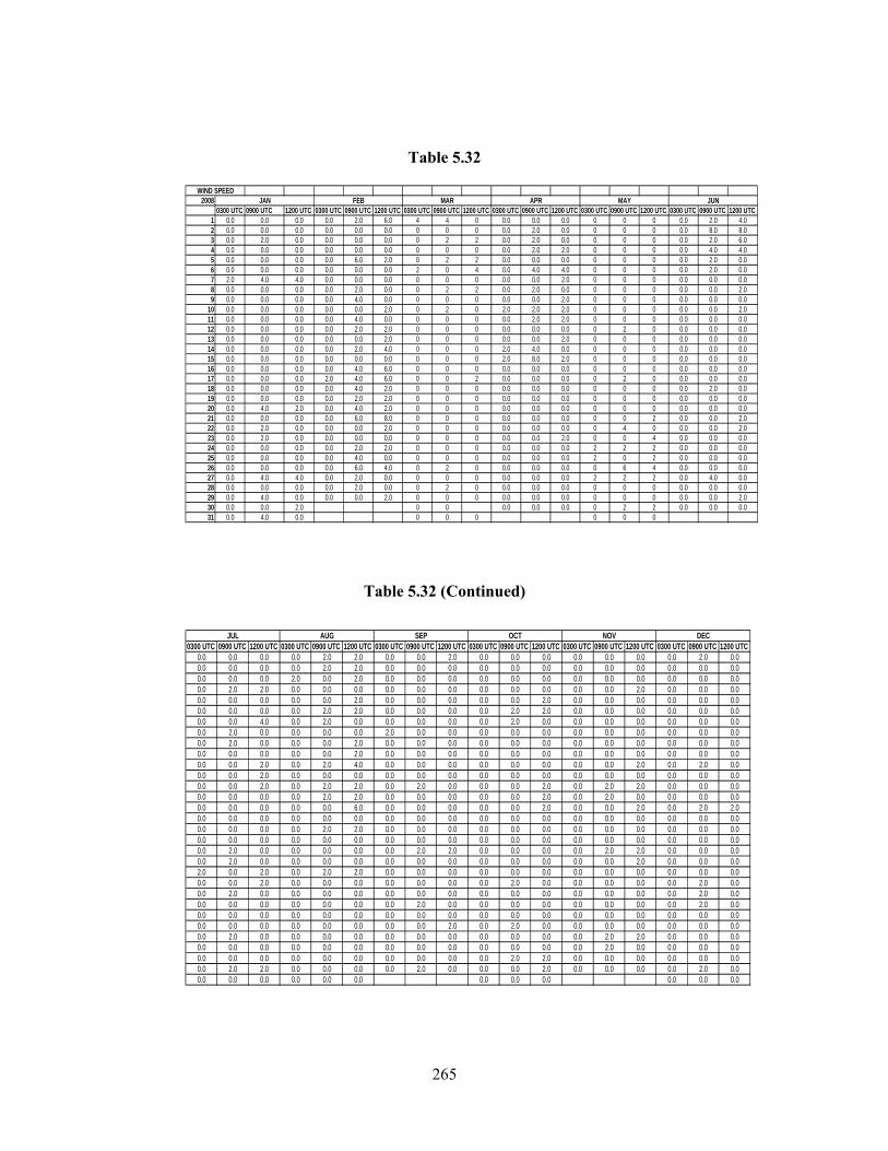
265
Table 5.32
20080300 UTC 0900 UTC 1200 UTC 0300 UTC 0900 UTC 1200 UTC 0300 UTC 0900 UTC 1200 UTC 0300 UTC 0900 UTC 1200 UTC 0300 UTC 0900 UTC 1200 UTC 0300 UTC 0900 UTC 1200 UTC
1 0.0 0.0 0.0 0.0 2.0 6.0 4 4 0 0.0 0.0 0.0 0 0 0 0.0 2.0 4.02 0.0 0.0 0.0 0.0 0.0 0.0 0 0 0 0.0 2.0 0.0 0 0 0 0.0 8.0 8.03 0.0 2.0 0.0 0.0 0.0 0.0 0 2 2 0.0 2.0 0.0 0 0 0 0.0 2.0 6.04 0.0 0.0 0.0 0.0 0.0 0.0 0 0 0 0.0 2.0 2.0 0 0 0 0.0 4.0 4.05 0.0 0.0 0.0 0.0 6.0 2.0 0 2 2 0.0 0.0 0.0 0 0 0 0.0 2.0 0.06 0.0 0.0 0.0 0.0 0.0 0.0 2 0 4 0.0 4.0 4.0 0 0 0 0.0 2.0 0.07 2.0 4.0 4.0 0.0 0.0 0.0 0 0 0 0.0 0.0 2.0 0 0 0 0.0 0.0 0.08 0.0 0.0 0.0 0.0 2.0 0.0 0 2 2 0.0 2.0 0.0 0 0 0 0.0 0.0 2.09 0.0 0.0 0.0 0.0 4.0 0.0 0 0 0 0.0 0.0 2.0 0 0 0 0.0 0.0 0.0
10 0.0 0.0 0.0 0.0 0.0 2.0 0 2 0 2.0 2.0 2.0 0 0 0 0.0 0.0 2.011 0.0 0.0 0.0 0.0 4.0 0.0 0 0 0 0.0 2.0 2.0 0 0 0 0.0 0.0 0.012 0.0 0.0 0.0 0.0 2.0 2.0 0 0 0 0.0 0.0 0.0 0 2 0 0.0 0.0 0.013 0.0 0.0 0.0 0.0 0.0 2.0 0 0 0 0.0 0.0 2.0 0 0 0 0.0 0.0 0.014 0.0 0.0 0.0 0.0 2.0 4.0 0 0 0 2.0 4.0 0.0 0 0 0 0.0 0.0 0.015 0.0 0.0 0.0 0.0 0.0 0.0 0 0 0 2.0 8.0 2.0 0 0 0 0.0 0.0 0.016 0.0 0.0 0.0 0.0 4.0 6.0 0 0 0 0.0 0.0 0.0 0 0 0 0.0 0.0 0.017 0.0 0.0 0.0 2.0 4.0 6.0 0 0 2 0.0 0.0 0.0 0 2 0 0.0 0.0 0.018 0.0 0.0 0.0 0.0 4.0 2.0 0 0 0 0.0 0.0 0.0 0 0 0 0.0 2.0 0.019 0.0 0.0 0.0 0.0 2.0 2.0 0 0 0 0.0 0.0 0.0 0 0 0 0.0 0.0 0.020 0.0 4.0 2.0 0.0 4.0 2.0 0 0 0 0.0 0.0 0.0 0 0 0 0.0 0.0 0.021 0.0 0.0 0.0 0.0 6.0 8.0 0 0 0 0.0 0.0 0.0 0 0 2 0.0 0.0 2.022 0.0 2.0 0.0 0.0 0.0 2.0 0 0 0 0.0 0.0 0.0 0 4 0 0.0 0.0 2.023 0.0 2.0 0.0 0.0 0.0 0.0 0 0 0 0.0 0.0 2.0 0 0 4 0.0 0.0 0.024 0.0 0.0 0.0 0.0 2.0 2.0 0 0 0 0.0 0.0 0.0 2 2 2 0.0 0.0 0.025 0.0 0.0 0.0 0.0 4.0 0.0 0 0 0 0.0 0.0 0.0 2 0 2 0.0 0.0 0.026 0.0 0.0 0.0 0.0 6.0 4.0 0 2 0 0.0 0.0 0.0 0 6 4 0.0 0.0 0.027 0.0 4.0 4.0 0.0 2.0 0.0 0 0 0 0.0 0.0 0.0 2 2 2 0.0 4.0 0.028 0.0 0.0 0.0 0.0 2.0 0.0 0 2 0 0.0 0.0 0.0 0 0 0 0.0 0.0 0.029 0.0 4.0 0.0 0.0 0.0 2.0 0 0 0 0.0 0.0 0.0 0 0 0 0.0 0.0 2.030 0.0 0.0 2.0 0 0 0.0 0.0 0.0 0 2 2 0.0 0.0 0.031 0.0 4.0 0.0 0 0 0 0 0 0
FEB MAR APR MAY JUNWIND SPEED
JAN
Table 5.32 (Continued)
0300 UTC 0900 UTC 1200 UTC 0300 UTC 0900 UTC 1200 UTC 0300 UTC 0900 UTC 1200 UTC 0300 UTC 0900 UTC 1200 UTC 0300 UTC 0900 UTC 1200 UTC 0300 UTC 0900 UTC 1200 UTC0.0 0.0 0.0 0.0 2.0 2.0 0.0 0.0 2.0 0.0 0.0 0.0 0.0 0.0 0.0 0.0 2.0 0.00.0 0.0 0.0 0.0 2.0 2.0 0.0 0.0 0.0 0.0 0.0 0.0 0.0 0.0 0.0 0.0 0.0 0.00.0 0.0 0.0 2.0 0.0 2.0 0.0 0.0 0.0 0.0 0.0 0.0 0.0 0.0 0.0 0.0 0.0 0.00.0 2.0 2.0 0.0 0.0 0.0 0.0 0.0 0.0 0.0 0.0 0.0 0.0 0.0 2.0 0.0 0.0 0.00.0 0.0 0.0 0.0 0.0 2.0 0.0 0.0 0.0 0.0 0.0 2.0 0.0 0.0 0.0 0.0 0.0 0.00.0 0.0 0.0 0.0 2.0 2.0 0.0 0.0 0.0 0.0 2.0 2.0 0.0 0.0 0.0 0.0 0.0 0.00.0 0.0 4.0 0.0 2.0 0.0 0.0 0.0 0.0 0.0 2.0 0.0 0.0 0.0 0.0 0.0 0.0 0.00.0 2.0 0.0 0.0 0.0 0.0 2.0 0.0 0.0 0.0 0.0 0.0 0.0 0.0 0.0 0.0 0.0 0.00.0 2.0 0.0 0.0 0.0 2.0 0.0 0.0 0.0 0.0 0.0 0.0 0.0 0.0 0.0 0.0 0.0 0.00.0 0.0 0.0 0.0 0.0 2.0 0.0 0.0 0.0 0.0 0.0 0.0 0.0 0.0 0.0 0.0 0.0 0.00.0 0.0 2.0 0.0 2.0 4.0 0.0 0.0 0.0 0.0 0.0 0.0 0.0 0.0 2.0 0.0 2.0 0.00.0 0.0 2.0 0.0 0.0 0.0 0.0 0.0 0.0 0.0 0.0 0.0 0.0 0.0 0.0 0.0 0.0 0.00.0 0.0 2.0 0.0 2.0 2.0 0.0 2.0 0.0 0.0 0.0 2.0 0.0 2.0 2.0 0.0 0.0 0.00.0 0.0 0.0 0.0 2.0 2.0 0.0 0.0 0.0 0.0 0.0 2.0 0.0 2.0 0.0 0.0 0.0 0.00.0 0.0 0.0 0.0 0.0 6.0 0.0 0.0 0.0 0.0 0.0 2.0 0.0 0.0 2.0 0.0 2.0 2.00.0 0.0 0.0 0.0 0.0 0.0 0.0 0.0 0.0 0.0 0.0 0.0 0.0 0.0 0.0 0.0 0.0 0.00.0 0.0 0.0 0.0 2.0 2.0 0.0 0.0 0.0 0.0 0.0 0.0 0.0 0.0 0.0 0.0 0.0 0.00.0 0.0 0.0 0.0 0.0 0.0 0.0 0.0 0.0 0.0 0.0 0.0 0.0 0.0 0.0 0.0 0.0 0.00.0 2.0 0.0 0.0 0.0 0.0 0.0 2.0 2.0 0.0 0.0 0.0 0.0 2.0 2.0 0.0 0.0 0.00.0 2.0 0.0 0.0 0.0 0.0 0.0 0.0 0.0 0.0 0.0 0.0 0.0 0.0 2.0 0.0 0.0 0.02.0 0.0 2.0 0.0 2.0 2.0 0.0 0.0 0.0 0.0 0.0 0.0 0.0 0.0 0.0 0.0 0.0 0.00.0 0.0 2.0 0.0 0.0 0.0 0.0 0.0 0.0 0.0 2.0 0.0 0.0 0.0 0.0 0.0 2.0 0.00.0 2.0 0.0 0.0 0.0 0.0 0.0 0.0 0.0 0.0 0.0 0.0 0.0 0.0 0.0 0.0 2.0 0.00.0 0.0 0.0 0.0 0.0 0.0 0.0 2.0 0.0 0.0 0.0 0.0 0.0 0.0 0.0 0.0 2.0 0.00.0 0.0 0.0 0.0 0.0 0.0 0.0 0.0 0.0 0.0 0.0 0.0 0.0 0.0 0.0 0.0 0.0 0.00.0 0.0 0.0 0.0 0.0 0.0 0.0 0.0 2.0 0.0 2.0 0.0 0.0 0.0 0.0 0.0 0.0 0.00.0 2.0 0.0 0.0 0.0 0.0 0.0 0.0 0.0 0.0 0.0 0.0 0.0 2.0 2.0 0.0 0.0 0.00.0 0.0 0.0 0.0 0.0 0.0 0.0 0.0 0.0 0.0 0.0 0.0 0.0 2.0 0.0 0.0 0.0 0.00.0 0.0 0.0 0.0 0.0 0.0 0.0 0.0 0.0 0.0 2.0 2.0 0.0 0.0 0.0 0.0 0.0 0.00.0 2.0 2.0 0.0 0.0 0.0 0.0 2.0 0.0 0.0 0.0 2.0 0.0 0.0 0.0 0.0 2.0 0.00.0 0.0 0.0 0.0 0.0 0.0 0.0 0.0 0.0 0.0 0.0 0.0
JUL AUG SEP OCT NOV DEC
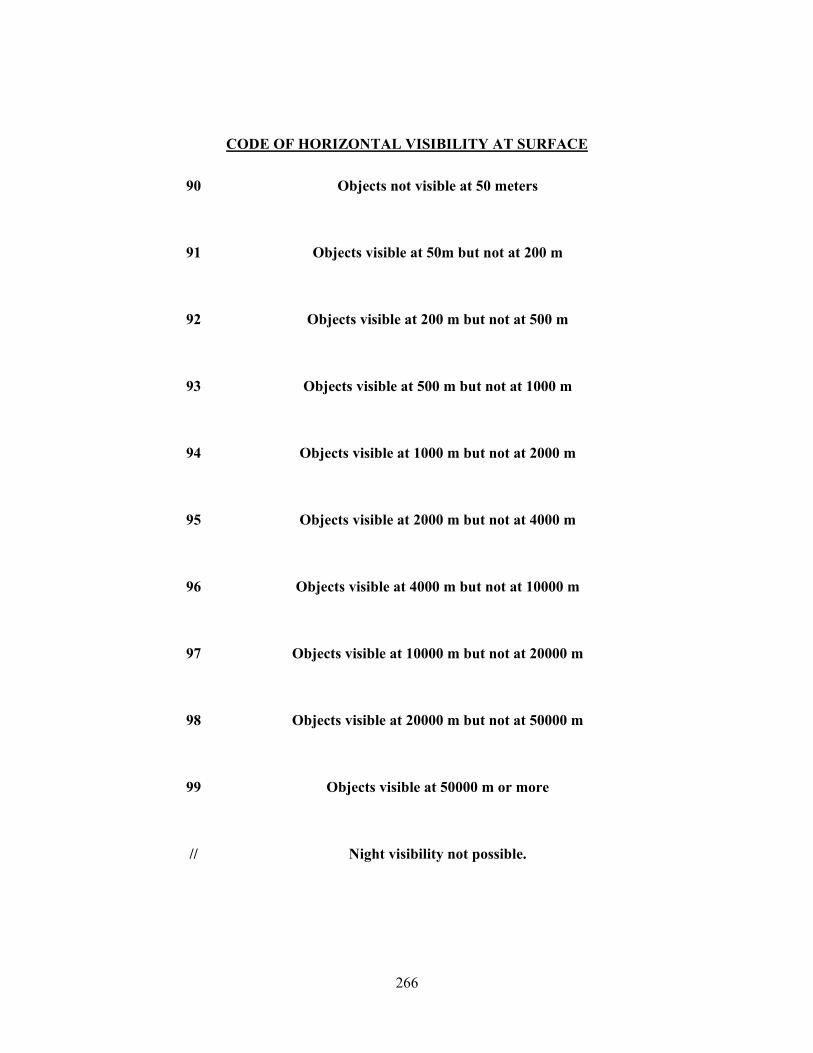
266
CODE OF HORIZONTAL VISIBILITY AT SURFACE
90 Objects not visible at 50 meters
91 Objects visible at 50m but not at 200 m
92 Objects visible at 200 m but not at 500 m
93 Objects visible at 500 m but not at 1000 m
94 Objects visible at 1000 m but not at 2000 m
95 Objects visible at 2000 m but not at 4000 m
96 Objects visible at 4000 m but not at 10000 m
97 Objects visible at 10000 m but not at 20000 m
98 Objects visible at 20000 m but not at 50000 m
99 Objects visible at 50000 m or more
// Night visibility not possible.
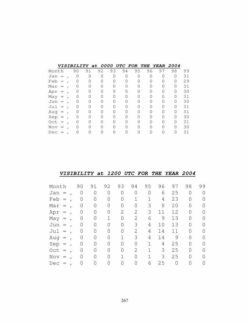
267
VISIBILITY at 0000 UTC FOR THE YEAR 2004 Month 90 91 92 93 94 95 96 97 98 99 Jan = , 0 0 0 0 0 0 0 0 0 31 Feb = , 0 0 0 0 0 0 0 0 0 29 Mar = , 0 0 0 0 0 0 0 0 0 31 Apr = , 0 0 0 0 0 0 0 0 0 30 May = , 0 0 0 0 0 0 0 0 0 31 Jun = , 0 0 0 0 0 0 0 0 0 30 Jul = , 0 0 0 0 0 0 0 0 0 31 Aug = , 0 0 0 0 0 0 0 0 0 31 Sep = , 0 0 0 0 0 0 0 0 0 30 Oct = , 0 0 0 0 0 0 0 0 0 31 Nov = , 0 0 0 0 0 0 0 0 0 30 Dec = , 0 0 0 0 0 0 0 0 0 31
VISIBILITY at 1200 UTC FOR THE YEAR 2004
Month 90 91 92 93 94 95 96 97 98 99 Jan = , 0 0 0 0 0 0 6 25 0 0 Feb = , 0 0 0 0 1 1 4 23 0 0 Mar = , 0 0 0 0 0 3 8 20 0 0 Apr = , 0 0 0 2 2 3 11 12 0 0 May = , 0 0 1 0 2 6 9 13 0 0 Jun = , 0 0 0 0 3 4 10 13 0 0 Jul = , 0 0 0 0 2 4 14 11 0 0 Aug = , 0 0 0 1 3 4 14 9 0 0 Sep = , 0 0 0 0 0 1 4 25 0 0 Oct = , 0 0 0 0 2 1 3 25 0 0 Nov = , 0 0 0 1 0 1 3 25 0 0 Dec = , 0 0 0 0 0 6 25 0 0 0
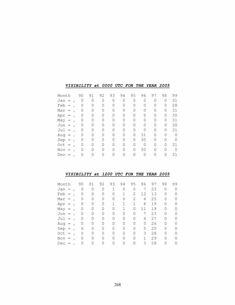
268
VISIBILITY at 0000 UTC FOR THE YEAR 2005
Month 90 91 92 93 94 95 96 97 98 99 Jan = , 0 0 0 0 0 0 0 0 0 31 Feb = , 0 0 0 0 0 0 0 0 0 28 Mar = , 0 0 0 0 0 0 0 0 0 31 Apr = , 0 0 0 0 0 0 0 0 0 30 May = , 0 0 0 0 0 0 0 0 0 31 Jun = , 0 0 0 0 0 0 0 0 0 30 Jul = , 0 0 0 0 0 0 0 0 0 31 Aug = , 0 0 0 0 0 0 31 0 0 0 Sep = , 0 0 0 0 0 0 30 0 0 0 Oct = , 0 0 0 0 0 0 0 0 0 31 Nov = , 0 0 0 0 0 0 30 0 0 0 Dec = , 0 0 0 0 0 0 0 0 0 31
VISIBILITY at 1200 UTC FOR THE YEAR 2005
Month 90 91 92 93 94 95 96 97 98 99 Jan = , 0 0 0 1 0 0 7 23 0 0 Feb = , 0 0 0 0 1 2 12 13 0 0 Mar = , 0 0 0 0 0 2 4 25 0 0 Apr = , 0 0 0 1 1 1 8 19 0 0 May = , 0 0 0 0 1 0 11 19 0 0 Jun = , 0 0 0 0 0 0 7 23 0 0 Jul = , 0 0 0 0 0 0 4 27 0 0 Aug = , 0 0 0 0 0 0 5 26 0 0 Sep = , 0 0 0 0 0 0 5 25 0 0 Oct = , 0 0 0 0 0 0 3 28 0 0 Nov = , 0 0 0 0 0 0 1 29 0 0 Dec = , 0 0 0 0 0 0 3 28 0 0

269
VISIBILITY at 0000 UTC FOR THE YEAR 2006
Month 90 91 92 93 94 95 96 97 98 99 Jan = , 0 0 0 0 0 0 0 0 0 31 Feb = , 0 0 0 0 0 0 0 0 0 28 Mar = , 0 0 0 0 0 0 0 0 0 31 Apr = , 0 0 0 0 0 0 0 0 0 30 May = , 0 0 0 0 0 0 0 0 0 31 Jun = , 0 0 0 0 0 0 0 0 0 30 Jul = , 0 0 0 0 0 0 0 0 0 31 Aug = , 0 0 0 0 0 0 0 0 0 31 Sep = , 0 0 0 0 0 0 0 0 0 30 Oct = , 0 0 0 0 0 0 0 0 0 31 Nov = , 0 0 0 0 0 0 0 0 0 30 Dec = , 0 0 0 0 0 0 0 0 0 31
VISIBILITY at 1200 UTC FOR THE YEAR 2006
Month 90 91 92 93 94 95 96 97 98 99 Jan = , 0 0 0 0 0 1 5 25 0 0 Feb = , 0 0 0 0 0 0 1 27 0 0 Mar = , 0 0 0 0 0 0 9 22 0 0 Apr = , 0 0 0 0 0 0 9 21 0 0 May = , 0 0 0 0 0 5 8 18 0 0 Jun = , 0 0 0 1 0 0 4 25 0 0 Jul = , 0 0 0 0 1 3 15 12 0 0 Aug = , 0 0 0 0 0 2 16 13 0 0 Sep = , 0 0 0 0 0 1 6 23 0 0 Oct = , 0 0 0 0 0 2 1 28 0 0 Nov = , 0 0 0 0 0 9 21 0 0 0 Dec = , 0 0 0 0 0 1 5 25 0 0
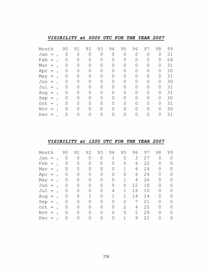
270
VISIBILITY at 0000 UTC FOR THE YEAR 2007
Month 90 91 92 93 94 95 96 97 98 99 Jan = , 0 0 0 0 0 0 0 0 0 31 Feb = , 0 0 0 0 0 0 0 0 0 28 Mar = , 0 0 0 0 0 0 0 0 0 31 Apr = , 0 0 0 0 0 0 0 0 0 30 May = , 0 0 0 0 0 0 0 0 0 31 Jun = , 0 0 0 0 0 0 0 0 0 30 Jul = , 0 0 0 0 0 0 0 0 0 31 Aug = , 0 0 0 0 0 0 0 0 0 31 Sep = , 0 0 0 0 0 0 0 0 0 30 Oct = , 0 0 0 0 0 0 0 0 0 31 Nov = , 0 0 0 0 0 0 0 0 0 30 Dec = , 0 0 0 0 0 0 0 0 0 31
VISIBILITY at 1200 UTC FOR THE YEAR 2007
Month 90 91 92 93 94 95 96 97 98 99 Jan = , 0 0 0 0 1 0 3 27 0 0 Feb = , 0 0 0 0 0 0 6 22 0 0 Mar = , 0 0 0 0 0 1 6 24 0 0 Apr = , 0 0 0 0 0 0 6 24 0 0 May = , 0 0 0 0 0 1 4 26 0 0 Jun = , 0 0 0 0 0 0 12 18 0 0 Jul = , 0 0 0 0 4 1 16 10 0 0 Aug = , 0 0 1 0 1 1 14 14 0 0 Sep = , 0 0 0 0 0 2 7 21 0 0 Oct = , 0 0 0 0 0 2 4 25 0 0 Nov = , 0 0 0 0 0 0 2 28 0 0 Dec = , 0 0 0 0 0 1 9 21 0 0
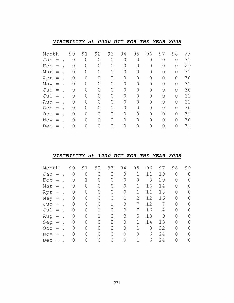
271
VISIBILITY at 0000 UTC FOR THE YEAR 2008
Month 90 91 92 93 94 95 96 97 98 // Jan = , 0 0 0 0 0 0 0 0 0 31 Feb = , 0 0 0 0 0 0 0 0 0 29 Mar = , 0 0 0 0 0 0 0 0 0 31 Apr = , 0 0 0 0 0 0 0 0 0 30 May = , 0 0 0 0 0 0 0 0 0 31 Jun = , 0 0 0 0 0 0 0 0 0 30 Jul = , 0 0 0 0 0 0 0 0 0 31 Aug = , 0 0 0 0 0 0 0 0 0 31 Sep = , 0 0 0 0 0 0 0 0 0 30 Oct = , 0 0 0 0 0 0 0 0 0 31 Nov = , 0 0 0 0 0 0 0 0 0 30 Dec = , 0 0 0 0 0 0 0 0 0 31
VISIBILITY at 1200 UTC FOR THE YEAR 2008
Month 90 91 92 93 94 95 96 97 98 99 Jan = , 0 0 0 0 0 1 11 19 0 0 Feb = , 0 1 0 0 0 0 8 20 0 0 Mar = , 0 0 0 0 0 1 16 14 0 0 Apr = , 0 0 0 0 0 1 11 18 0 0 May = , 0 0 0 0 1 2 12 16 0 0 Jun = , 0 0 0 1 3 7 12 7 0 0 Jul = , 0 0 1 0 3 7 16 4 0 0 Aug = , 0 0 1 0 3 5 13 9 0 0 Sep = , 0 0 0 2 0 1 14 13 0 0 Oct = , 0 0 0 0 0 1 8 22 0 0 Nov = , 0 0 0 0 0 0 6 24 0 0 Dec = , 0 0 0 0 0 1 6 24 0 0
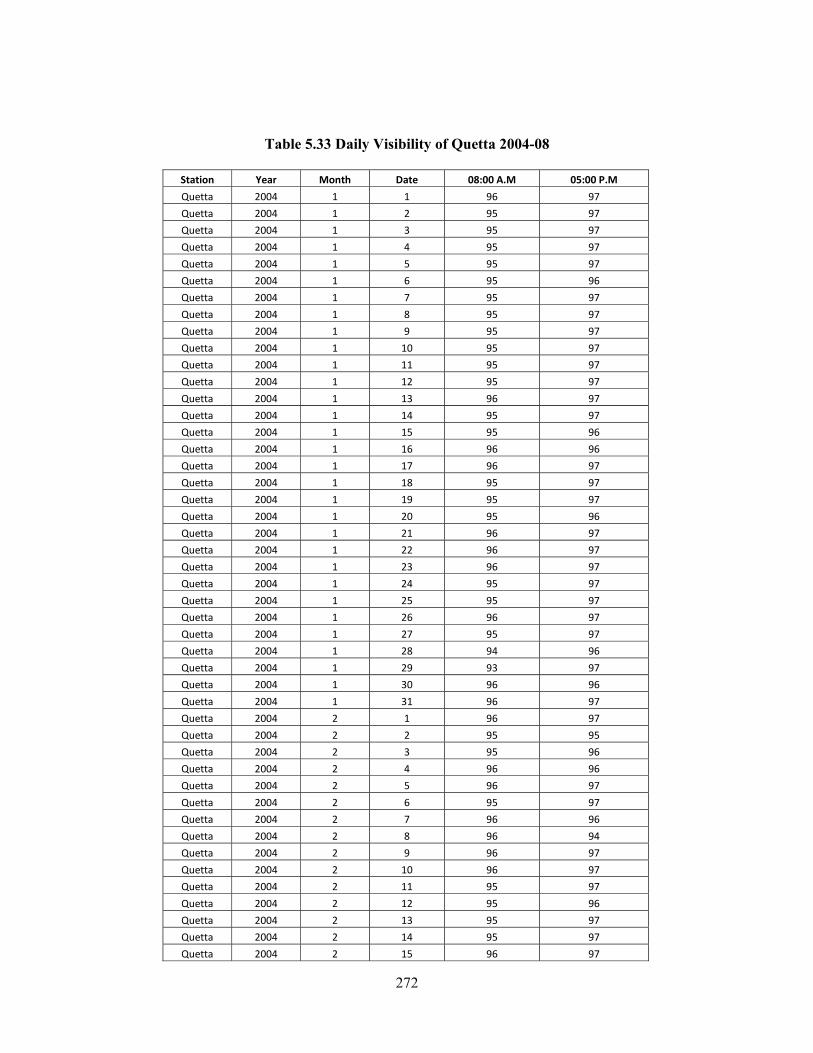
272
Table 5.33 Daily Visibility of Quetta 2004-08
Station Year Month Date 08:00 A.M 05:00 P.M
Quetta 2004 1 1 96 97
Quetta 2004 1 2 95 97
Quetta 2004 1 3 95 97
Quetta 2004 1 4 95 97
Quetta 2004 1 5 95 97
Quetta 2004 1 6 95 96
Quetta 2004 1 7 95 97
Quetta 2004 1 8 95 97
Quetta 2004 1 9 95 97
Quetta 2004 1 10 95 97
Quetta 2004 1 11 95 97
Quetta 2004 1 12 95 97
Quetta 2004 1 13 96 97
Quetta 2004 1 14 95 97
Quetta 2004 1 15 95 96
Quetta 2004 1 16 96 96
Quetta 2004 1 17 96 97
Quetta 2004 1 18 95 97
Quetta 2004 1 19 95 97
Quetta 2004 1 20 95 96
Quetta 2004 1 21 96 97
Quetta 2004 1 22 96 97
Quetta 2004 1 23 96 97
Quetta 2004 1 24 95 97
Quetta 2004 1 25 95 97
Quetta 2004 1 26 96 97
Quetta 2004 1 27 95 97
Quetta 2004 1 28 94 96
Quetta 2004 1 29 93 97
Quetta 2004 1 30 96 96
Quetta 2004 1 31 96 97
Quetta 2004 2 1 96 97
Quetta 2004 2 2 95 95
Quetta 2004 2 3 95 96
Quetta 2004 2 4 96 96
Quetta 2004 2 5 96 97
Quetta 2004 2 6 95 97
Quetta 2004 2 7 96 96
Quetta 2004 2 8 96 94
Quetta 2004 2 9 96 97
Quetta 2004 2 10 96 97
Quetta 2004 2 11 95 97
Quetta 2004 2 12 95 96
Quetta 2004 2 13 95 97
Quetta 2004 2 14 95 97
Quetta 2004 2 15 96 97

273
Quetta 2004 2 16 95 97
Quetta 2004 2 17 95 96
Quetta 2004 2 18 95 97
Quetta 2004 2 19 95 97
Quetta 2004 2 20 95 95
Quetta 2004 2 21 95 97
Quetta 2004 2 22 95 97
Quetta 2004 2 23 95 97
Quetta 2004 2 24 95 97
Quetta 2004 2 25 95 97
Quetta 2004 2 26 95 96
Quetta 2004 2 27 95 97
Quetta 2004 2 28 95 97
Quetta 2004 2 29 95 97
Quetta 2004 3 1 95 96
Quetta 2004 3 2 96 97
Quetta 2004 3 3 95 97
Quetta 2004 3 4 95 96
Quetta 2004 3 5 95 96
Quetta 2004 3 6 95 96
Quetta 2004 3 7 95 96
Quetta 2004 3 8 95 96
Quetta 2004 3 9 95 96
Quetta 2004 3 10 94 97
Quetta 2004 3 11 94 96
Quetta 2004 3 12 95 96
Quetta 2004 3 13 95 96
Quetta 2004 3 14 95 96
Quetta 2004 3 15 95 95
Quetta 2004 3 16 95 97
Quetta 2004 3 17 95 95
Quetta 2004 3 18 95 96
Quetta 2004 3 19 95 97
Quetta 2004 3 20 95 96
Quetta 2004 3 21 95 95
Quetta 2004 3 22 96 97
Quetta 2004 3 23 96 97
Quetta 2004 3 24 96 97
Quetta 2004 3 25 96 97
Quetta 2004 3 26 95 97
Quetta 2004 3 27 95 96
Quetta 2004 3 28 96 97
Quetta 2004 3 29 96 96
Quetta 2004 3 30 95 97
Quetta 2004 3 31 96 97
Quetta 2004 4 1 969 96
Quetta 2004 4 2 96 96
Quetta 2004 4 3 95 96
Quetta 2004 4 4 95 96

274
Quetta 2004 4 5 95 97
Quetta 2004 4 6 96 97
Quetta 2004 4 7 96 97
Quetta 2004 4 8 95 96
Quetta 2004 4 9 96 94
Quetta 2004 4 10 95 97
Quetta 2004 4 11 95 97
Quetta 2004 4 12 96 96
Quetta 2004 4 13 96 96
Quetta 2004 4 14 96 97
Quetta 2004 4 15 96 97
Quetta 2004 4 16 96 94
Quetta 2004 4 17 95 96
Quetta 2004 4 18 95 96
Quetta 2004 4 19 95 95
Quetta 2004 4 20 95 95
Quetta 2004 4 21 95 96
Quetta 2004 4 22 96 95
Quetta 2004 4 23 96 97
Quetta 2004 4 24 96 97
Quetta 2004 4 25 95 97
Quetta 2004 4 26 95 96
Quetta 2004 4 27 96 95
Quetta 2004 4 28 96 97
Quetta 2004 4 29 95 93
Quetta 2004 4 30 93 93
Quetta 2004 5 1 95 97
Quetta 2004 5 2 95 96
Quetta 2004 5 3 95 94
Quetta 2004 5 4 95 97
Quetta 2004 5 5 95 97
Quetta 2004 5 6 96 95
Quetta 2004 5 7 94 95
Quetta 2004 5 8 94 96
Quetta 2004 5 9 96 97
Quetta 2004 5 10 95 97
Quetta 2004 5 11 95 97
Quetta 2004 5 12 96 97
Quetta 2004 5 13 96 97
Quetta 2004 5 14 96 96
Quetta 2004 5 15 96 96
Quetta 2004 5 16 94 95
Quetta 2004 5 17 95 96
Quetta 2004 5 18 96 96
Quetta 2004 5 19 96 95
Quetta 2004 5 20 96 94
Quetta 2004 5 21 96 96
Quetta 2004 5 22 95 92
Quetta 2004 5 23 94 95

275
Quetta 2004 5 24 95 97
Quetta 2004 5 25 95 96
Quetta 2004 5 26 96 97
Quetta 2004 5 27 95 95
Quetta 2004 5 28 95 97
Quetta 2004 5 29 95 97
Quetta 2004 5 30 95 97
Quetta 2004 5 31 95 96
Quetta 2004 6 1 96 96
Quetta 2004 6 2 95 96
Quetta 2004 6 3 96 97
Quetta 2004 6 4 95 96
Quetta 2004 6 5 95 96
Quetta 2004 6 6 96 95
Quetta 2004 6 7 94 94
Quetta 2004 6 8 94 96
Quetta 2004 6 9 95 95
Quetta 2004 6 10 95 97
Quetta 2004 6 11 96 97
Quetta 2004 6 12 96 96
Quetta 2004 6 13 96 97
Quetta 2004 6 14 96 94
Quetta 2004 6 15 96 94
Quetta 2004 6 16 94 97
Quetta 2004 6 17 95 95
Quetta 2004 6 18 95 95
Quetta 2004 6 19 95 95
Quetta 2004 6 20 96 96
Quetta 2004 6 21 96 96
Quetta 2004 6 22 95 96
Quetta 2004 6 23 95 96
Quetta 2004 6 24 95 97
Quetta 2004 6 25 95 97
Quetta 2004 6 26 95 96
Quetta 2004 6 27 95 96
Quetta 2004 6 28 95 96
Quetta 2004 6 29 95 97
Quetta 2004 6 30 95 97
Quetta 2004 7 1 95 97
Quetta 2004 7 2 95 97
Quetta 2004 7 3 95 96
Quetta 2004 7 4 95 97
Quetta 2004 7 5 95 96
Quetta 2004 7 6 95 96
Quetta 2004 7 7 93 96
Quetta 2004 7 8 95 94
Quetta 2004 7 9 94 95
Quetta 2004 7 10 94 95
Quetta 2004 7 11 95 97
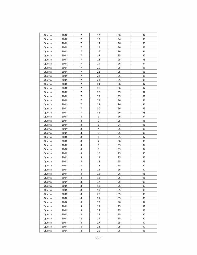
276
Quetta 2004 7 12 96 97
Quetta 2004 7 13 94 96
Quetta 2004 7 14 96 96
Quetta 2004 7 15 96 96
Quetta 2004 7 16 96 96
Quetta 2004 7 17 95 97
Quetta 2004 7 18 95 96
Quetta 2004 7 19 96 94
Quetta 2004 7 20 95 95
Quetta 2004 7 21 95 96
Quetta 2004 7 22 95 96
Quetta 2004 7 23 95 96
Quetta 2004 7 24 96 97
Quetta 2004 7 25 96 97
Quetta 2004 7 26 95 97
Quetta 2004 7 27 95 97
Quetta 2004 7 28 96 96
Quetta 2004 7 29 96 96
Quetta 2004 7 30 96 95
Quetta 2004 7 31 96 95
Quetta 2004 8 1 96 94
Quetta 2004 8 2 95 95
Quetta 2004 8 3 94 96
Quetta 2004 8 4 95 96
Quetta 2004 8 5 95 96
Quetta 2004 8 6 95 97
Quetta 2004 8 7 96 96
Quetta 2004 8 8 93 94
Quetta 2004 8 9 93 94
Quetta 2004 8 10 95 95
Quetta 2004 8 11 95 96
Quetta 2004 8 12 95 96
Quetta 2004 8 13 95 97
Quetta 2004 8 14 96 97
Quetta 2004 8 15 96 96
Quetta 2004 8 16 95 96
Quetta 2004 8 17 95 95
Quetta 2004 8 18 95 93
Quetta 2004 8 19 95 95
Quetta 2004 8 20 95 96
Quetta 2004 8 21 95 96
Quetta 2004 8 22 96 97
Quetta 2004 8 23 95 97
Quetta 2004 8 24 95 96
Quetta 2004 8 25 95 97
Quetta 2004 8 26 95 97
Quetta 2004 8 27 95 97
Quetta 2004 8 28 95 97
Quetta 2004 8 29 95 96
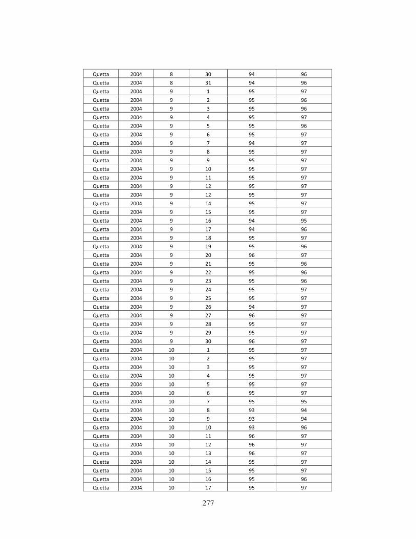
277
Quetta 2004 8 30 94 96
Quetta 2004 8 31 94 96
Quetta 2004 9 1 95 97
Quetta 2004 9 2 95 96
Quetta 2004 9 3 95 96
Quetta 2004 9 4 95 97
Quetta 2004 9 5 95 96
Quetta 2004 9 6 95 97
Quetta 2004 9 7 94 97
Quetta 2004 9 8 95 97
Quetta 2004 9 9 95 97
Quetta 2004 9 10 95 97
Quetta 2004 9 11 95 97
Quetta 2004 9 12 95 97
Quetta 2004 9 12 95 97
Quetta 2004 9 14 95 97
Quetta 2004 9 15 95 97
Quetta 2004 9 16 94 95
Quetta 2004 9 17 94 96
Quetta 2004 9 18 95 97
Quetta 2004 9 19 95 96
Quetta 2004 9 20 96 97
Quetta 2004 9 21 95 96
Quetta 2004 9 22 95 96
Quetta 2004 9 23 95 96
Quetta 2004 9 24 95 97
Quetta 2004 9 25 95 97
Quetta 2004 9 26 94 97
Quetta 2004 9 27 96 97
Quetta 2004 9 28 95 97
Quetta 2004 9 29 95 97
Quetta 2004 9 30 96 97
Quetta 2004 10 1 95 97
Quetta 2004 10 2 95 97
Quetta 2004 10 3 95 97
Quetta 2004 10 4 95 97
Quetta 2004 10 5 95 97
Quetta 2004 10 6 95 97
Quetta 2004 10 7 95 95
Quetta 2004 10 8 93 94
Quetta 2004 10 9 93 94
Quetta 2004 10 10 93 96
Quetta 2004 10 11 96 97
Quetta 2004 10 12 96 97
Quetta 2004 10 13 96 97
Quetta 2004 10 14 95 97
Quetta 2004 10 15 95 97
Quetta 2004 10 16 95 96
Quetta 2004 10 17 95 97

278
Quetta 2004 10 18 97 97
Quetta 2004 10 19 96 97
Quetta 2004 10 20 96 97
Quetta 2004 10 21 96 97
Quetta 2004 10 22 95 97
Quetta 2004 10 23 95 97
Quetta 2004 10 24 95 97
Quetta 2004 10 25 95 96
Quetta 2004 10 26 95 97
Quetta 2004 10 27 95 97
Quetta 2004 10 28 96 97
Quetta 2004 10 29 95 97
Quetta 2004 10 30 95 97
Quetta 2004 10 31 93 97
Quetta 2004 11 1 95 97
Quetta 2004 11 2 95 97
Quetta 2004 11 3 95 97
Quetta 2004 11 4 95 97
Quetta 2004 11 5 95 97
Quetta 2004 11 6 94 97
Quetta 2004 11 7 95 97
Quetta 2004 11 8 95 97
Quetta 2004 11 9 95 97
Quetta 2004 11 10 95 97
Quetta 2004 11 11 95 97
Quetta 2004 11 12 95 97
Quetta 2004 11 13 95 97
Quetta 2004 11 14 95 97
Quetta 2004 11 15 95 97
Quetta 2004 11 16 95 97
Quetta 2004 11 17 95 97
Quetta 2004 11 18 95 97
Quetta 2004 11 19 95 97
Quetta 2004 11 20 95 97
Quetta 2004 11 21 95 97
Quetta 2004 11 22 95 97
Quetta 2004 11 23 95 97
Quetta 2004 11 24 95 97
Quetta 2004 11 25 95 95
Quetta 2004 11 26 96 96
Quetta 2004 11 27 95 96
Quetta 2004 11 28 95 96
Quetta 2004 11 29 95 93
Quetta 2004 11 30 95 97
Quetta 2004 12 1 96 97
Quetta 2004 12 2 96 97
Quetta 2004 12 3 95 96
Quetta 2004 12 4 95 97
Quetta 2004 12 5 95 97
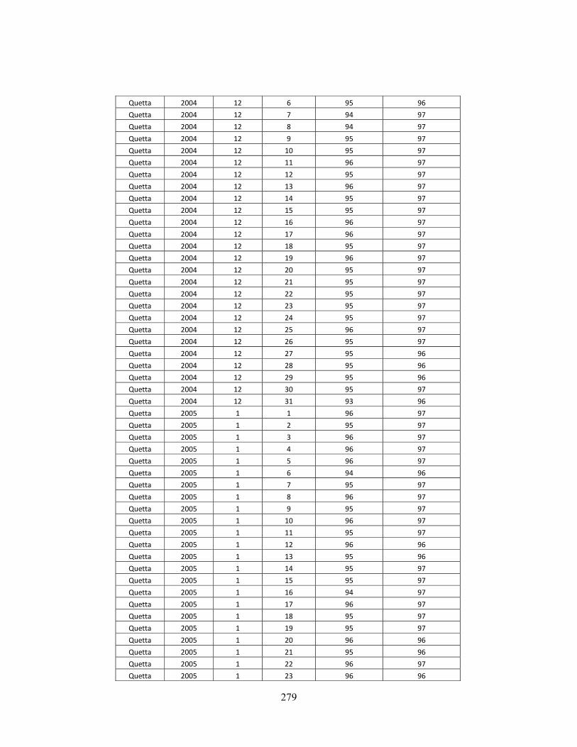
279
Quetta 2004 12 6 95 96
Quetta 2004 12 7 94 97
Quetta 2004 12 8 94 97
Quetta 2004 12 9 95 97
Quetta 2004 12 10 95 97
Quetta 2004 12 11 96 97
Quetta 2004 12 12 95 97
Quetta 2004 12 13 96 97
Quetta 2004 12 14 95 97
Quetta 2004 12 15 95 97
Quetta 2004 12 16 96 97
Quetta 2004 12 17 96 97
Quetta 2004 12 18 95 97
Quetta 2004 12 19 96 97
Quetta 2004 12 20 95 97
Quetta 2004 12 21 95 97
Quetta 2004 12 22 95 97
Quetta 2004 12 23 95 97
Quetta 2004 12 24 95 97
Quetta 2004 12 25 96 97
Quetta 2004 12 26 95 97
Quetta 2004 12 27 95 96
Quetta 2004 12 28 95 96
Quetta 2004 12 29 95 96
Quetta 2004 12 30 95 97
Quetta 2004 12 31 93 96
Quetta 2005 1 1 96 97
Quetta 2005 1 2 95 97
Quetta 2005 1 3 96 97
Quetta 2005 1 4 96 97
Quetta 2005 1 5 96 97
Quetta 2005 1 6 94 96
Quetta 2005 1 7 95 97
Quetta 2005 1 8 96 97
Quetta 2005 1 9 95 97
Quetta 2005 1 10 96 97
Quetta 2005 1 11 95 97
Quetta 2005 1 12 96 96
Quetta 2005 1 13 95 96
Quetta 2005 1 14 95 97
Quetta 2005 1 15 95 97
Quetta 2005 1 16 94 97
Quetta 2005 1 17 96 97
Quetta 2005 1 18 95 97
Quetta 2005 1 19 95 97
Quetta 2005 1 20 96 96
Quetta 2005 1 21 95 96
Quetta 2005 1 22 96 97
Quetta 2005 1 23 96 96

280
Quetta 2005 1 24 96 97
Quetta 2005 1 25 95 96
Quetta 2005 1 26 95 93
Quetta 2005 1 27 96 97
Quetta 2005 1 28 95 97
Quetta 2005 1 29 95 97
Quetta 2005 1 30 95 97
Quetta 2005 1 31 95 97
Quetta 2005 2 1 94 97
Quetta 2005 2 2 95 97
Quetta 2005 2 3 95 97
Quetta 2005 2 4 96 96
Quetta 2005 2 5 95 96
Quetta 2005 2 6 95 96
Quetta 2005 2 7 95 96
Quetta 2005 2 8 96 97
Quetta 2005 2 9 96 97
Quetta 2005 2 10 96 97
Quetta 2005 2 11 96 97
Quetta 2005 2 12 96 96
Quetta 2005 2 13 95 96
Quetta 2005 2 14 96 96
Quetta 2005 2 15 96 96
Quetta 2005 2 16 95 97
Quetta 2005 2 17 95 96
Quetta 2005 2 18 95 94
Quetta 2005 2 19 95 97
Quetta 2005 2 20 95 97
Quetta 2005 2 21 95 97
Quetta 2005 2 22 95 97
Quetta 2005 2 23 96 96
Quetta 2005 2 24 96 96
Quetta 2005 2 25 95 95
Quetta 2005 2 26 94 95
Quetta 2005 2 27 96 96
Quetta 2005 2 28 95 97
Quetta 2005 3 1 95 97
Quetta 2005 3 2 95 96
Quetta 2005 3 3 96 97
Quetta 2005 3 4 95 97
Quetta 2005 3 5 94 97
Quetta 2005 3 6 96 97
Quetta 2005 3 7 96 97
Quetta 2005 3 8 96 96
Quetta 2005 3 9 96 97
Quetta 2005 3 10 95 97
Quetta 2005 3 11 96 97
Quetta 2005 3 12 95 97
Quetta 2005 3 13 94 97

281
Quetta 2005 3 14 95 97
Quetta 2005 3 15 95 97
Quetta 2005 3 16 96 97
Quetta 2005 3 17 95 97
Quetta 2005 3 18 96 97
Quetta 2005 3 19 95 96
Quetta 2005 3 20 96 97
Quetta 2005 3 21 96 97
Quetta 2005 3 22 96 97
Quetta 2005 3 23 96 96
Quetta 2005 3 24 95 97
Quetta 2005 3 25 96 95
Quetta 2005 3 26 95 95
Quetta 2005 3 27 96 97
Quetta 2005 3 28 95 97
Quetta 2005 3 29 95 97
Quetta 2005 3 30 96 97
Quetta 2005 3 31 95 97
Quetta 2005 4 1 96 97
Quetta 2005 4 2 94 97
Quetta 2005 4 3 96 97
Quetta 2005 4 4 96 97
Quetta 2005 4 5 96 96
Quetta 2005 4 6 95 93
Quetta 2005 4 7 94 94
Quetta 2005 4 8 95 96
Quetta 2005 4 9 95 96
Quetta 2005 4 10 95 97
Quetta 2005 4 11 95 97
Quetta 2005 4 12 95 97
Quetta 2005 4 13 96 96
Quetta 2005 4 14 96 97
Quetta 2005 4 15 96 97
Quetta 2005 4 16 96 97
Quetta 2005 4 17 95 97
Quetta 2005 4 18 96 97
Quetta 2005 4 19 96 97
Quetta 2005 4 20 96 96
Quetta 2005 4 21 96 96
Quetta 2005 4 22 95 97
Quetta 2005 4 23 96 97
Quetta 2005 4 24 95 96
Quetta 2005 4 25 95 96
Quetta 2005 4 26 96 97
Quetta 2005 4 27 95 97
Quetta 2005 4 28 96 96
Quetta 2005 4 29 96 97
Quetta 2005 4 30 96 ‐99
Quetta 2005 5 1 96 97
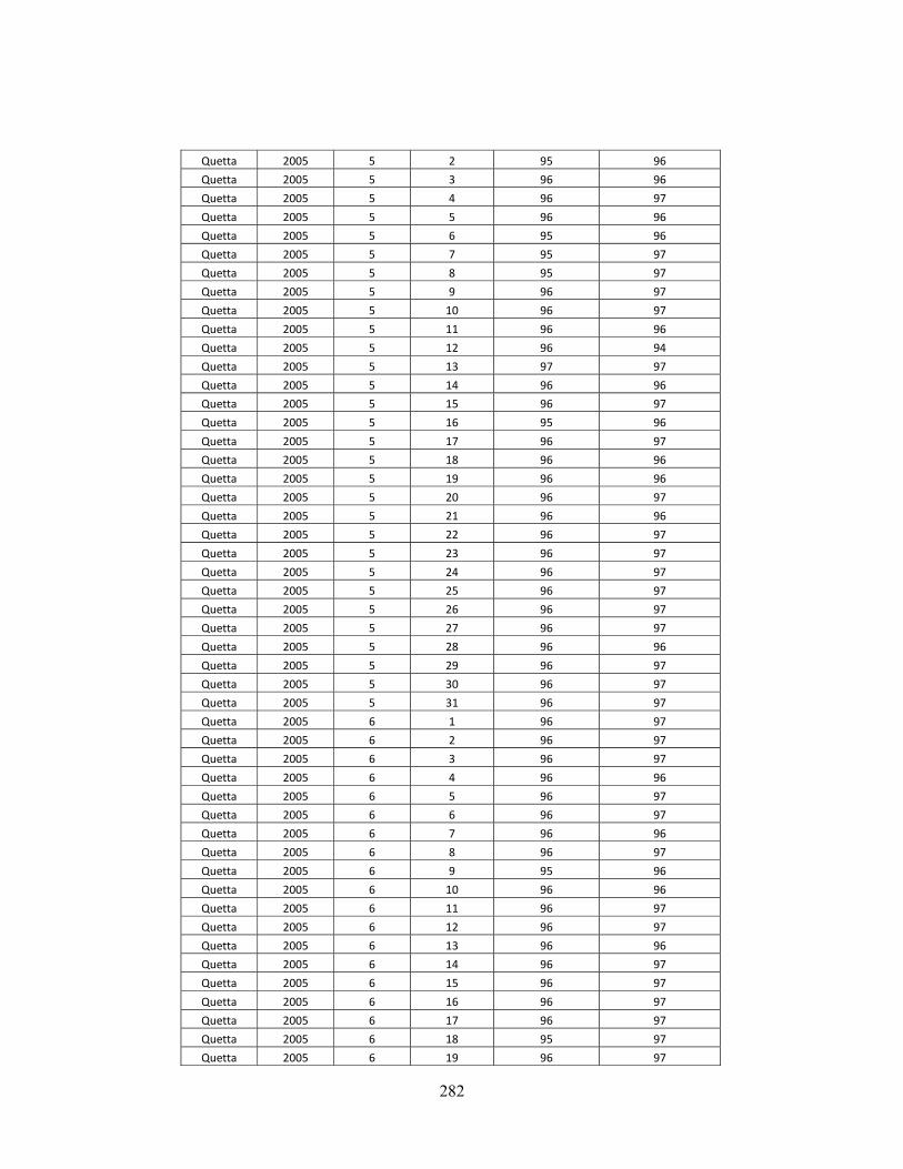
282
Quetta 2005 5 2 95 96
Quetta 2005 5 3 96 96
Quetta 2005 5 4 96 97
Quetta 2005 5 5 96 96
Quetta 2005 5 6 95 96
Quetta 2005 5 7 95 97
Quetta 2005 5 8 95 97
Quetta 2005 5 9 96 97
Quetta 2005 5 10 96 97
Quetta 2005 5 11 96 96
Quetta 2005 5 12 96 94
Quetta 2005 5 13 97 97
Quetta 2005 5 14 96 96
Quetta 2005 5 15 96 97
Quetta 2005 5 16 95 96
Quetta 2005 5 17 96 97
Quetta 2005 5 18 96 96
Quetta 2005 5 19 96 96
Quetta 2005 5 20 96 97
Quetta 2005 5 21 96 96
Quetta 2005 5 22 96 97
Quetta 2005 5 23 96 97
Quetta 2005 5 24 96 97
Quetta 2005 5 25 96 97
Quetta 2005 5 26 96 97
Quetta 2005 5 27 96 97
Quetta 2005 5 28 96 96
Quetta 2005 5 29 96 97
Quetta 2005 5 30 96 97
Quetta 2005 5 31 96 97
Quetta 2005 6 1 96 97
Quetta 2005 6 2 96 97
Quetta 2005 6 3 96 97
Quetta 2005 6 4 96 96
Quetta 2005 6 5 96 97
Quetta 2005 6 6 96 97
Quetta 2005 6 7 96 96
Quetta 2005 6 8 96 97
Quetta 2005 6 9 95 96
Quetta 2005 6 10 96 96
Quetta 2005 6 11 96 97
Quetta 2005 6 12 96 97
Quetta 2005 6 13 96 96
Quetta 2005 6 14 96 97
Quetta 2005 6 15 96 97
Quetta 2005 6 16 96 97
Quetta 2005 6 17 96 97
Quetta 2005 6 18 95 97
Quetta 2005 6 19 96 97

283
Quetta 2005 6 20 96 97
Quetta 2005 6 21 96 97
Quetta 2005 6 22 95 97
Quetta 2005 6 23 96 97
Quetta 2005 6 24 96 97
Quetta 2005 6 25 96 96
Quetta 2005 6 26 95 96
Quetta 2005 6 27 95 97
Quetta 2005 6 28 96 97
Quetta 2005 6 29 96 97
Quetta 2005 6 30 96 96
Quetta 2005 7 1 96 97
Quetta 2005 7 2 96 97
Quetta 2005 7 3 96 97
Quetta 2005 7 4 96 97
Quetta 2005 7 5 96 97
Quetta 2005 7 6 96 96
Quetta 2005 7 7 96 96
Quetta 2005 7 8 96 97
Quetta 2005 7 9 96 97
Quetta 2005 7 10 96 97
Quetta 2005 7 11 96 96
Quetta 2005 7 12 96 97
Quetta 2005 7 13 96 97
Quetta 2005 7 14 96 97
Quetta 2005 7 15 96 97
Quetta 2005 7 16 96 97
Quetta 2005 7 17 96 97
Quetta 2005 7 18 96 97
Quetta 2005 7 19 96 97
Quetta 2005 7 20 96 97
Quetta 2005 7 21 96 97
Quetta 2005 7 22 96 97
Quetta 2005 7 23 95 97
Quetta 2005 7 24 96 97
Quetta 2005 7 25 95 97
Quetta 2005 7 26 96 97
Quetta 2005 7 27 96 97
Quetta 2005 7 28 96 97
Quetta 2005 7 29 96 97
Quetta 2005 7 30 95 97
Quetta 2005 7 31 96 97
Quetta 2005 8 1 96 97
Quetta 2005 8 2 96 97
Quetta 2005 8 3 96 97
Quetta 2005 8 4 96 97
Quetta 2005 8 5 96 97
Quetta 2005 8 6 96 97
Quetta 2005 8 7 95 97

284
Quetta 2005 8 8 96 96
Quetta 2005 8 9 96 96
Quetta 2005 8 10 96 97
Quetta 2005 8 11 96 97
Quetta 2005 8 12 95 97
Quetta 2005 8 13 95 96
Quetta 2005 8 14 95 97
Quetta 2005 8 15 96 97
Quetta 2005 8 16 95 97
Quetta 2005 8 17 95 97
Quetta 2005 8 18 95 97
Quetta 2005 8 19 95 97
Quetta 2005 8 20 95 97
Quetta 2005 8 21 95 97
Quetta 2005 8 22 95 97
Quetta 2005 8 23 96 97
Quetta 2005 8 24 96 97
Quetta 2005 8 25 96 97
Quetta 2005 8 26 95 97
Quetta 2005 8 27 96 97
Quetta 2005 8 28 96 96
Quetta 2005 8 29 95 96
Quetta 2005 8 30 95 97
Quetta 2005 8 31 96 97
Quetta 2005 9 1 96 97
Quetta 2005 9 2 96 97
Quetta 2005 9 3 95 97
Quetta 2005 9 4 95 97
Quetta 2005 9 5 95 97
Quetta 2005 9 6 95 97
Quetta 2005 9 7 95 97
Quetta 2005 9 8 96 97
Quetta 2005 9 9 95 97
Quetta 2005 9 10 96 96
Quetta 2005 9 11 95 96
Quetta 2005 9 12 96 96
Quetta 2005 9 13 95 97
Quetta 2005 9 14 96 96
Quetta 2005 9 15 96 97
Quetta 2005 9 16 96 96
Quetta 2005 9 17 95 97
Quetta 2005 9 18 95 97
Quetta 2005 9 19 96 97
Quetta 2005 9 20 96 97
Quetta 2005 9 21 95 97
Quetta 2005 9 22 95 97
Quetta 2005 9 23 95 97
Quetta 2005 9 24 95 97
Quetta 2005 9 25 95 97

285
Quetta 2005 9 26 95 97
Quetta 2005 9 27 95 97
Quetta 2005 9 28 95 97
Quetta 2005 9 29 95 97
Quetta 2005 9 30 95 97
Quetta 2005 10 1 96 97
Quetta 2005 10 2 95 97
Quetta 2005 10 3 95 97
Quetta 2005 10 4 95 97
Quetta 2005 10 5 95 97
Quetta 2005 10 6 95 97
Quetta 2005 10 7 95 97
Quetta 2005 10 8 95 97
Quetta 2005 10 9 95 97
Quetta 2005 10 10 95 97
Quetta 2005 10 11 95 97
Quetta 2005 10 12 95 96
Quetta 2005 10 13 95 96
Quetta 2005 10 14 95 97
Quetta 2005 10 15 95 97
Quetta 2005 10 16 95 97
Quetta 2005 10 17 95 97
Quetta 2005 10 18 95 97
Quetta 2005 10 19 95 97
Quetta 2005 10 20 95 97
Quetta 2005 10 21 96 97
Quetta 2005 10 22 95 97
Quetta 2005 10 23 96 97
Quetta 2005 10 24 95 97
Quetta 2005 10 25 95 97
Quetta 2005 10 26 96 97
Quetta 2005 10 27 95 97
Quetta 2005 10 28 96 97
Quetta 2005 10 29 95 96
Quetta 2005 10 30 96 97
Quetta 2005 10 31 95 97
Quetta 2005 11 1 96 97
Quetta 2005 11 2 95 97
Quetta 2005 11 3 96 97
Quetta 2005 11 4 95 97
Quetta 2005 11 5 96 97
Quetta 2005 11 6 95 97
Quetta 2005 11 7 95 97
Quetta 2005 11 8 96 97
Quetta 2005 11 9 96 97
Quetta 2005 11 10 96 96
Quetta 2005 11 11 96 97
Quetta 2005 11 12 96 97
Quetta 2005 11 13 96 97

286
Quetta 2005 11 14 96 97
Quetta 2005 11 15 96 97
Quetta 2005 11 16 96 97
Quetta 2005 11 17 96 97
Quetta 2005 11 18 96 97
Quetta 2005 11 19 96 97
Quetta 2005 11 20 96 97
Quetta 2005 11 21 96 97
Quetta 2005 11 22 95 97
Quetta 2005 11 23 96 97
Quetta 2005 11 24 96 97
Quetta 2005 11 25 96 97
Quetta 2005 11 26 96 97
Quetta 2005 11 27 96 97
Quetta 2005 11 28 96 97
Quetta 2005 11 29 96 97
Quetta 2005 11 30 96 97
Quetta 2005 12 1 95 97
Quetta 2005 12 2 95 97
Quetta 2005 12 3 96 97
Quetta 2005 12 4 96 97
Quetta 2005 12 5 95 97
Quetta 2005 12 6 95 97
Quetta 2005 12 7 96 97
Quetta 2005 12 8 96 96
Quetta 2005 12 9 96 97
Quetta 2005 12 10 95 97
Quetta 2005 12 11 95 97
Quetta 2005 12 12 95 97
Quetta 2005 12 13 95 97
Quetta 2005 12 14 96 97
Quetta 2005 12 15 96 97
Quetta 2005 12 16 95 97
Quetta 2005 12 17 95 97
Quetta 2005 12 18 96 97
Quetta 2005 12 19 95 96
Quetta 2005 12 20 95 97
Quetta 2005 12 21 95 97
Quetta 2005 12 22 95 97
Quetta 2005 12 23 95 97
Quetta 2005 12 24 95 97
Quetta 2005 12 25 95 97
Quetta 2005 12 26 95 96
Quetta 2005 12 27 96 97
Quetta 2005 12 28 96 97
Quetta 2005 12 29 96 97
Quetta 2005 12 30 96 97
Quetta 2005 12 31 96 96
Quetta 2006 1 1 96 95

287
Quetta 2006 1 2 96 97
Quetta 2006 1 3 96 97
Quetta 2006 1 4 96 97
Quetta 2006 1 5 96 97
Quetta 2006 1 6 96 96
Quetta 2006 1 7 96 97
Quetta 2006 1 8 96 97
Quetta 2006 1 9 96 97
Quetta 2006 1 10 96 97
Quetta 2006 1 11 96 97
Quetta 2006 1 12 96 97
Quetta 2006 1 13 96 97
Quetta 2006 1 14 96 96
Quetta 2006 1 15 96 96
Quetta 2006 1 16 96 97
Quetta 2006 1 17 96 97
Quetta 2006 1 18 96 97
Quetta 2006 1 19 96 97
Quetta 2006 1 20 92 97
Quetta 2006 1 21 96 97
Quetta 2006 1 22 96 97
Quetta 2006 1 23 96 97
Quetta 2006 1 24 96 97
Quetta 2006 1 25 96 97
Quetta 2006 1 26 96 97
Quetta 2006 1 27 96 97
Quetta 2006 1 28 96 96
Quetta 2006 1 29 96 96
Quetta 2006 1 30 96 96
Quetta 2006 1 31 96 97
Quetta 2006 2 1 96 97
Quetta 2006 2 2 96 97
Quetta 2006 2 3 96 97
Quetta 2006 2 4 96 97
Quetta 2006 2 5 96 97
Quetta 2006 2 6 96 97
Quetta 2006 2 7 96 97
Quetta 2006 2 8 96 97
Quetta 2006 2 9 96 97
Quetta 2006 2 10 96 97
Quetta 2006 2 11 96 97
Quetta 2006 2 12 96 97
Quetta 2006 2 13 96 96
Quetta 2006 2 14 96 97
Quetta 2006 2 15 96 97
Quetta 2006 2 16 96 97
Quetta 2006 2 17 95 97
Quetta 2006 2 18 96 97
Quetta 2006 2 19 96 97

288
Quetta 2006 2 20 96 97
Quetta 2006 2 21 96 97
Quetta 2006 2 22 96 97
Quetta 2006 2 23 96 97
Quetta 2006 2 24 96 97
Quetta 2006 2 25 96 97
Quetta 2006 2 26 96 97
Quetta 2006 2 27 96 97
Quetta 2006 2 28 96 97
Quetta 2006 3 1 96 97
Quetta 2006 3 2 96 96
Quetta 2006 3 3 96 96
Quetta 2006 3 4 96 97
Quetta 2006 3 5 96 96
Quetta 2006 3 6 96 97
Quetta 2006 3 7 96 96
Quetta 2006 3 8 96 97
Quetta 2006 3 9 96 97
Quetta 2006 3 10 96 97
Quetta 2006 3 11 96 97
Quetta 2006 3 12 96 96
Quetta 2006 3 13 95 97
Quetta 2006 3 14 96 97
Quetta 2006 3 15 96 97
Quetta 2006 3 16 96 97
Quetta 2006 3 17 96 97
Quetta 2006 3 18 96 96
Quetta 2006 3 19 96 96
Quetta 2006 3 20 96 97
Quetta 2006 3 21 96 97
Quetta 2006 3 22 96 97
Quetta 2006 3 23 96 96
Quetta 2006 3 24 96 97
Quetta 2006 3 25 94 96
Quetta 2006 3 26 96 97
Quetta 2006 3 27 96 97
Quetta 2006 3 28 96 97
Quetta 2006 3 29 96 97
Quetta 2006 3 30 96 97
Quetta 2006 3 31 96 96
Quetta 2006 4 1 96 97
Quetta 2006 4 2 96 97
Quetta 2006 4 3 96 97
Quetta 2006 4 4 96 97
Quetta 2006 4 5 96 97
Quetta 2006 4 6 96 97
Quetta 2006 4 7 96 97
Quetta 2006 4 8 96 96
Quetta 2006 4 9 96 96

289
Quetta 2006 4 10 96 96
Quetta 2006 4 11 96 97
Quetta 2006 4 12 96 97
Quetta 2006 4 13 96 96
Quetta 2006 4 14 96 97
Quetta 2006 4 15 96 97
Quetta 2006 4 16 96 97
Quetta 2006 4 17 96 97
Quetta 2006 4 18 96 97
Quetta 2006 4 19 96 97
Quetta 2006 4 20 96 96
Quetta 2006 4 21 96 97
Quetta 2006 4 22 96 96
Quetta 2006 4 23 96 97
Quetta 2006 4 24 96 97
Quetta 2006 4 25 96 97
Quetta 2006 4 26 96 97
Quetta 2006 4 27 96 97
Quetta 2006 4 28 96 96
Quetta 2006 4 29 96 96
Quetta 2006 4 30 96 96
Quetta 2006 5 1 96 96
Quetta 2006 5 2 96 96
Quetta 2006 5 3 96 97
Quetta 2006 5 4 96 97
Quetta 2006 5 5 96 97
Quetta 2006 5 6 96 97
Quetta 2006 5 7 96 97
Quetta 2006 5 8 96 97
Quetta 2006 5 9 96 97
Quetta 2006 5 10 95 97
Quetta 2006 5 11 96 97
Quetta 2006 5 12 96 97
Quetta 2006 5 13 95 96
Quetta 2006 5 14 95 95
Quetta 2006 5 15 96 96
Quetta 2006 5 16 96 95
Quetta 2006 5 17 96 96
Quetta 2006 5 18 95 95
Quetta 2006 5 19 95 95
Quetta 2006 5 20 96 96
Quetta 2006 5 21 96 96
Quetta 2006 5 22 96 97
Quetta 2006 5 23 96 97
Quetta 2006 5 24 96 97
Quetta 2006 5 25 95 97
Quetta 2006 5 26 96 97
Quetta 2006 5 27 96 97
Quetta 2006 5 28 96 95

290
Quetta 2006 5 29 96 96
Quetta 2006 5 30 96 97
Quetta 2006 5 31 96 97
Quetta 2006 6 1 95 97
Quetta 2006 6 2 95 97
Quetta 2006 6 3 95 96
Quetta 2006 6 4 95 96
Quetta 2006 6 5 95 97
Quetta 2006 6 6 95 97
Quetta 2006 6 7 95 97
Quetta 2006 6 8 95 97
Quetta 2006 6 9 95 97
Quetta 2006 6 10 96 97
Quetta 2006 6 11 96 97
Quetta 2006 6 12 96 97
Quetta 2006 6 13 96 97
Quetta 2006 6 14 96 97
Quetta 2006 6 15 96 97
Quetta 2006 6 16 95 97
Quetta 2006 6 17 95 97
Quetta 2006 6 18 95 97
Quetta 2006 6 19 95 97
Quetta 2006 6 20 95 97
Quetta 2006 6 21 96 96
Quetta 2006 6 22 95 97
Quetta 2006 6 23 96 97
Quetta 2006 6 24 95 97
Quetta 2006 6 25 96 97
Quetta 2006 6 26 96 93
Quetta 2006 6 27 96 97
Quetta 2006 6 28 96 96
Quetta 2006 6 29 95 97
Quetta 2006 6 30 96 97
Quetta 2006 7 1 96 97
Quetta 2006 7 2 96 96
Quetta 2006 7 3 96 97
Quetta 2006 7 4 96 97
Quetta 2006 7 5 95 96
Quetta 2006 7 6 96 96
Quetta 2006 7 7 95 96
Quetta 2006 7 8 95 96
Quetta 2006 7 9 94 96
Quetta 2006 7 10 95 96
Quetta 2006 7 11 95 95
Quetta 2006 7 12 94 95
Quetta 2006 7 13 94 94
Quetta 2006 7 14 94 95
Quetta 2006 7 15 95 97
Quetta 2006 7 16 95 97

291
Quetta 2006 7 17 96 97
Quetta 2006 7 18 96 97
Quetta 2006 7 19 96 97
Quetta 2006 7 20 96 97
Quetta 2006 7 21 96 97
Quetta 2006 7 22 96 96
Quetta 2006 7 23 96 97
Quetta 2006 7 24 96 96
Quetta 2006 7 25 96 96
Quetta 2006 7 26 95 96
Quetta 2006 7 27 95 96
Quetta 2006 7 28 95 95
Quetta 2006 7 29 96 96
Quetta 2006 7 30 96 96
Quetta 2006 7 31 96 97
Quetta 2006 8 1 96 96
Quetta 2006 8 2 96 97
Quetta 2006 8 3 96 96
Quetta 2006 8 4 96 96
Quetta 2006 8 5 97 97
Quetta 2006 8 6 96 96
Quetta 2006 8 7 96 97
Quetta 2006 8 8 96 95
Quetta 2006 8 9 96 96
Quetta 2006 8 10 96 97
Quetta 2006 8 11 96 97
Quetta 2006 8 12 94 97
Quetta 2006 8 13 96 97
Quetta 2006 8 14 96 97
Quetta 2006 8 15 96 96
Quetta 2006 8 16 96 96
Quetta 2006 8 17 96 96
Quetta 2006 8 18 96 96
Quetta 2006 8 19 95 96
Quetta 2006 8 20 96 97
Quetta 2006 8 21 95 96
Quetta 2006 8 22 96 97
Quetta 2006 8 23 96 96
Quetta 2006 8 24 96 97
Quetta 2006 8 25 95 97
Quetta 2006 8 26 96 97
Quetta 2006 8 27 95 96
Quetta 2006 8 28 95 96
Quetta 2006 8 29 95 96
Quetta 2006 8 30 96 96
Quetta 2006 8 31 96 95
Quetta 2006 9 1 96 95
Quetta 2006 9 2 96 96
Quetta 2006 9 3 96 96
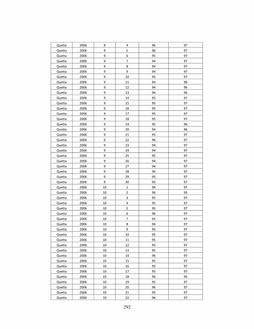
292
Quetta 2006 9 4 96 97
Quetta 2006 9 5 96 97
Quetta 2006 9 6 95 97
Quetta 2006 9 7 94 97
Quetta 2006 9 8 94 97
Quetta 2006 9 9 94 97
Quetta 2006 9 10 95 97
Quetta 2006 9 11 94 96
Quetta 2006 9 12 94 96
Quetta 2006 9 13 94 96
Quetta 2006 9 14 95 97
Quetta 2006 9 15 95 97
Quetta 2006 9 16 95 97
Quetta 2006 9 17 95 97
Quetta 2006 9 18 95 97
Quetta 2006 9 19 95 96
Quetta 2006 9 20 94 96
Quetta 2006 9 21 95 97
Quetta 2006 9 22 96 97
Quetta 2006 9 23 94 97
Quetta 2006 9 24 94 97
Quetta 2006 9 25 95 97
Quetta 2006 9 26 94 97
Quetta 2006 9 27 94 97
Quetta 2006 9 28 94 97
Quetta 2006 9 29 95 97
Quetta 2006 9 30 95 97
Quetta 2006 10 1 94 97
Quetta 2006 10 2 96 95
Quetta 2006 10 3 95 97
Quetta 2006 10 4 95 97
Quetta 2006 10 5 95 97
Quetta 2006 10 6 96 97
Quetta 2006 10 7 95 97
Quetta 2006 10 8 94 97
Quetta 2006 10 9 95 97
Quetta 2006 10 10 95 97
Quetta 2006 10 11 95 97
Quetta 2006 10 12 95 97
Quetta 2006 10 13 95 97
Quetta 2006 10 14 96 97
Quetta 2006 10 15 95 97
Quetta 2006 10 16 95 97
Quetta 2006 10 17 95 97
Quetta 2006 10 18 96 95
Quetta 2006 10 19 95 97
Quetta 2006 10 20 96 97
Quetta 2006 10 21 95 97
Quetta 2006 10 22 96 97

293
Quetta 2006 10 23 95 97
Quetta 2006 10 24 95 97
Quetta 2006 10 25 95 97
Quetta 2006 10 26 96 97
Quetta 2006 10 27 96 97
Quetta 2006 10 28 96 97
Quetta 2006 10 29 96 97
Quetta 2006 10 30 95 97
Quetta 2006 10 31 96 97
Quetta 2006 11 1 96 97
Quetta 2006 11 2 95 97
Quetta 2006 11 3 95 97
Quetta 2006 11 4 94 97
Quetta 2006 11 5 95 97
Quetta 2006 11 6 95 97
Quetta 2006 11 7 95 97
Quetta 2006 11 8 95 97
Quetta 2006 11 9 95 96
Quetta 2006 11 10 95 96
Quetta 2006 11 11 95 96
Quetta 2006 11 12 96 97
Quetta 2006 11 13 95 97
Quetta 2006 11 14 96 96
Quetta 2006 11 15 96 96
Quetta 2006 11 16 95 96
Quetta 2006 11 17 96 96
Quetta 2006 11 18 94 96
Quetta 2006 11 19 96 97
Quetta 2006 11 20 95 97
Quetta 2006 11 21 95 97
Quetta 2006 11 22 96 97
Quetta 2006 11 23 96 97
Quetta 2006 11 24 96 97
Quetta 2006 11 25 95 97
Quetta 2006 11 26 96 97
Quetta 2006 11 27 96 96
Quetta 2006 11 28 95 97
Quetta 2006 11 29 95 97
Quetta 2006 11 30 95 97
Quetta 2006 12 1 95 97
Quetta 2006 12 2 96 95
Quetta 2006 12 3 96 97
Quetta 2006 12 4 96 97
Quetta 2006 12 5 96 97
Quetta 2006 12 6 95 97
Quetta 2006 12 7 95 97
Quetta 2006 12 8 95 96
Quetta 2006 12 9 96 97
Quetta 2006 12 10 96 97
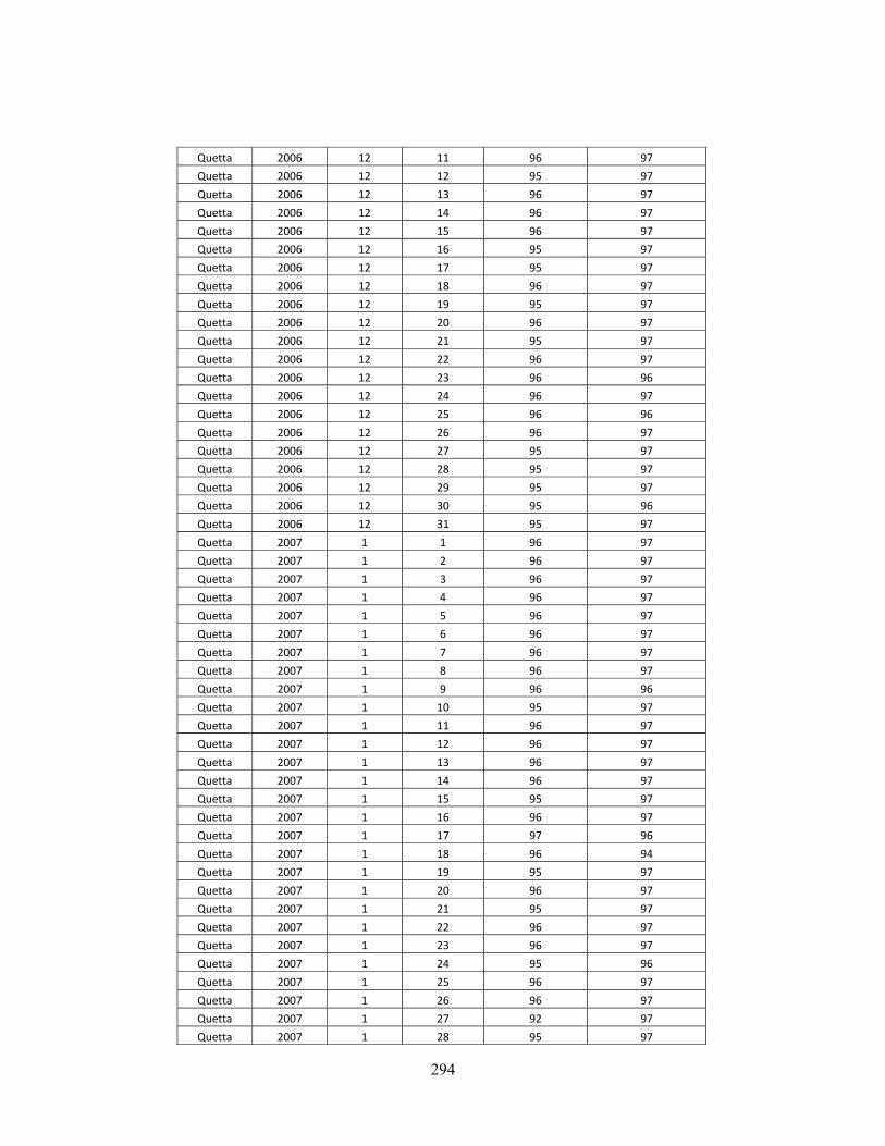
294
Quetta 2006 12 11 96 97
Quetta 2006 12 12 95 97
Quetta 2006 12 13 96 97
Quetta 2006 12 14 96 97
Quetta 2006 12 15 96 97
Quetta 2006 12 16 95 97
Quetta 2006 12 17 95 97
Quetta 2006 12 18 96 97
Quetta 2006 12 19 95 97
Quetta 2006 12 20 96 97
Quetta 2006 12 21 95 97
Quetta 2006 12 22 96 97
Quetta 2006 12 23 96 96
Quetta 2006 12 24 96 97
Quetta 2006 12 25 96 96
Quetta 2006 12 26 96 97
Quetta 2006 12 27 95 97
Quetta 2006 12 28 95 97
Quetta 2006 12 29 95 97
Quetta 2006 12 30 95 96
Quetta 2006 12 31 95 97
Quetta 2007 1 1 96 97
Quetta 2007 1 2 96 97
Quetta 2007 1 3 96 97
Quetta 2007 1 4 96 97
Quetta 2007 1 5 96 97
Quetta 2007 1 6 96 97
Quetta 2007 1 7 96 97
Quetta 2007 1 8 96 97
Quetta 2007 1 9 96 96
Quetta 2007 1 10 95 97
Quetta 2007 1 11 96 97
Quetta 2007 1 12 96 97
Quetta 2007 1 13 96 97
Quetta 2007 1 14 96 97
Quetta 2007 1 15 95 97
Quetta 2007 1 16 96 97
Quetta 2007 1 17 97 96
Quetta 2007 1 18 96 94
Quetta 2007 1 19 95 97
Quetta 2007 1 20 96 97
Quetta 2007 1 21 95 97
Quetta 2007 1 22 96 97
Quetta 2007 1 23 96 97
Quetta 2007 1 24 95 96
Quetta 2007 1 25 96 97
Quetta 2007 1 26 96 97
Quetta 2007 1 27 92 97
Quetta 2007 1 28 95 97
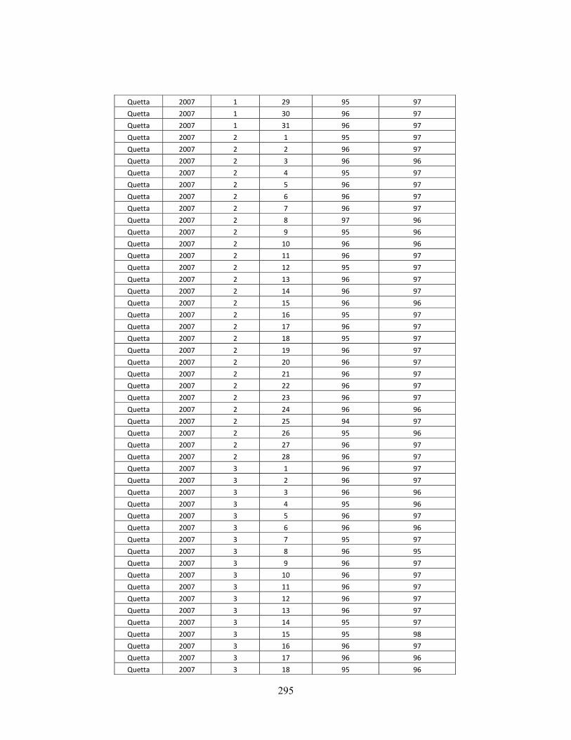
295
Quetta 2007 1 29 95 97
Quetta 2007 1 30 96 97
Quetta 2007 1 31 96 97
Quetta 2007 2 1 95 97
Quetta 2007 2 2 96 97
Quetta 2007 2 3 96 96
Quetta 2007 2 4 95 97
Quetta 2007 2 5 96 97
Quetta 2007 2 6 96 97
Quetta 2007 2 7 96 97
Quetta 2007 2 8 97 96
Quetta 2007 2 9 95 96
Quetta 2007 2 10 96 96
Quetta 2007 2 11 96 97
Quetta 2007 2 12 95 97
Quetta 2007 2 13 96 97
Quetta 2007 2 14 96 97
Quetta 2007 2 15 96 96
Quetta 2007 2 16 95 97
Quetta 2007 2 17 96 97
Quetta 2007 2 18 95 97
Quetta 2007 2 19 96 97
Quetta 2007 2 20 96 97
Quetta 2007 2 21 96 97
Quetta 2007 2 22 96 97
Quetta 2007 2 23 96 97
Quetta 2007 2 24 96 96
Quetta 2007 2 25 94 97
Quetta 2007 2 26 95 96
Quetta 2007 2 27 96 97
Quetta 2007 2 28 96 97
Quetta 2007 3 1 96 97
Quetta 2007 3 2 96 97
Quetta 2007 3 3 96 96
Quetta 2007 3 4 95 96
Quetta 2007 3 5 96 97
Quetta 2007 3 6 96 96
Quetta 2007 3 7 95 97
Quetta 2007 3 8 96 95
Quetta 2007 3 9 96 97
Quetta 2007 3 10 96 97
Quetta 2007 3 11 96 97
Quetta 2007 3 12 96 97
Quetta 2007 3 13 96 97
Quetta 2007 3 14 95 97
Quetta 2007 3 15 95 98
Quetta 2007 3 16 96 97
Quetta 2007 3 17 96 96
Quetta 2007 3 18 95 96

296
Quetta 2007 3 19 96 96
Quetta 2007 3 20 96 97
Quetta 2007 3 21 96 97
Quetta 2007 3 22 96 97
Quetta 2007 3 23 95 97
Quetta 2007 3 24 96 97
Quetta 2007 3 25 96 97
Quetta 2007 3 26 96 97
Quetta 2007 3 27 96 97
Quetta 2007 3 28 96 97
Quetta 2007 3 29 96 97
Quetta 2007 3 30 96 97
Quetta 2007 3 31 96 97
Quetta 2007 4 1 97 97
Quetta 2007 4 2 ‐96 97
Quetta 2007 4 3 96 96
Quetta 2007 4 4 96 97
Quetta 2007 4 5 96 97
Quetta 2007 4 6 96 97
Quetta 2007 4 7 96 97
Quetta 2007 4 8 96 97
Quetta 2007 4 9 95 97
Quetta 2007 4 10 96 97
Quetta 2007 4 11 95 97
Quetta 2007 4 12 96 97
Quetta 2007 4 13 96 97
Quetta 2007 4 14 96 96
Quetta 2007 4 15 96 96
Quetta 2007 4 16 96 97
Quetta 2007 4 17 96 97
Quetta 2007 4 18 96 97
Quetta 2007 4 19 96 96
Quetta 2007 4 20 96 97
Quetta 2007 4 21 96 97
Quetta 2007 4 22 96 97
Quetta 2007 4 23 96 97
Quetta 2007 4 24 96 97
Quetta 2007 4 25 96 97
Quetta 2007 4 26 96 97
Quetta 2007 4 27 96 97
Quetta 2007 4 28 96 97
Quetta 2007 4 29 96 97
Quetta 2007 4 30 96 96
Quetta 2007 5 1 96 97
Quetta 2007 5 2 96 97
Quetta 2007 5 3 96 97
Quetta 2007 5 4 96 96
Quetta 2007 5 5 96 97
Quetta 2007 5 6 96 97
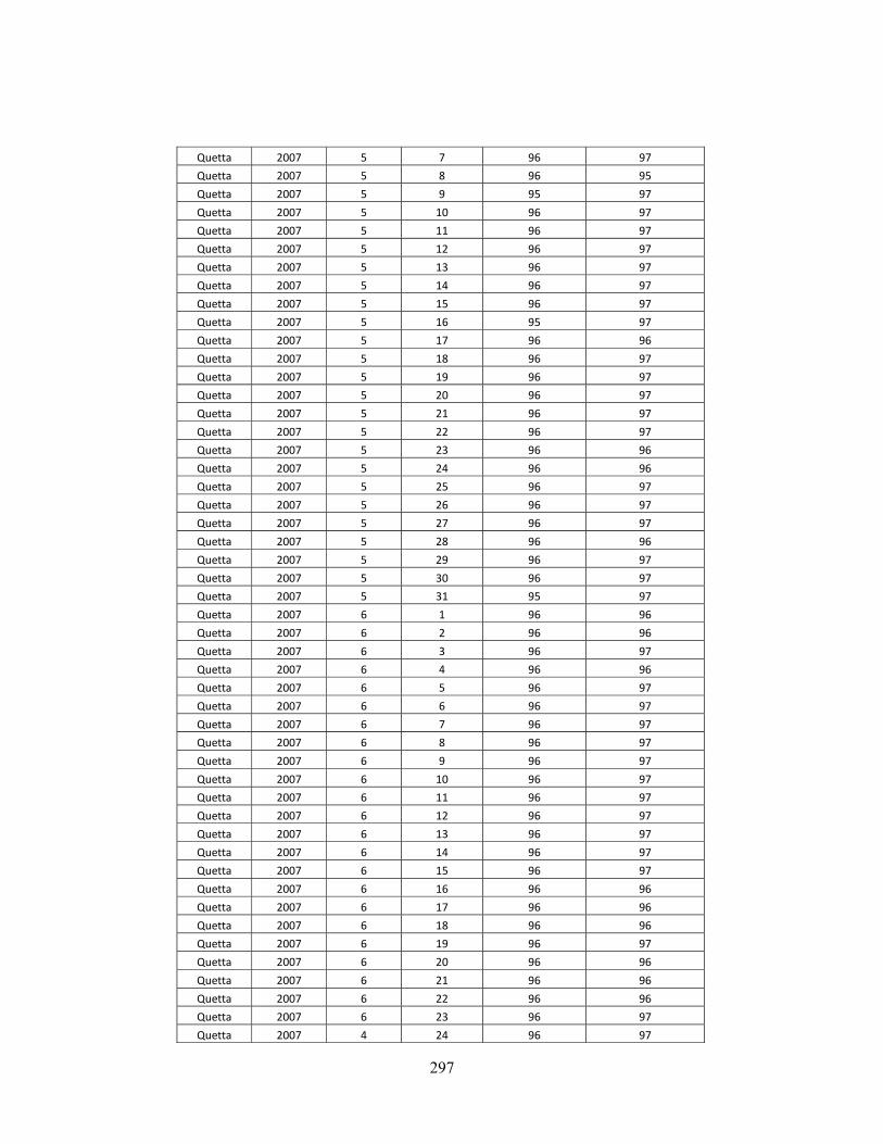
297
Quetta 2007 5 7 96 97
Quetta 2007 5 8 96 95
Quetta 2007 5 9 95 97
Quetta 2007 5 10 96 97
Quetta 2007 5 11 96 97
Quetta 2007 5 12 96 97
Quetta 2007 5 13 96 97
Quetta 2007 5 14 96 97
Quetta 2007 5 15 96 97
Quetta 2007 5 16 95 97
Quetta 2007 5 17 96 96
Quetta 2007 5 18 96 97
Quetta 2007 5 19 96 97
Quetta 2007 5 20 96 97
Quetta 2007 5 21 96 97
Quetta 2007 5 22 96 97
Quetta 2007 5 23 96 96
Quetta 2007 5 24 96 96
Quetta 2007 5 25 96 97
Quetta 2007 5 26 96 97
Quetta 2007 5 27 96 97
Quetta 2007 5 28 96 96
Quetta 2007 5 29 96 97
Quetta 2007 5 30 96 97
Quetta 2007 5 31 95 97
Quetta 2007 6 1 96 96
Quetta 2007 6 2 96 96
Quetta 2007 6 3 96 97
Quetta 2007 6 4 96 96
Quetta 2007 6 5 96 97
Quetta 2007 6 6 96 97
Quetta 2007 6 7 96 97
Quetta 2007 6 8 96 97
Quetta 2007 6 9 96 97
Quetta 2007 6 10 96 97
Quetta 2007 6 11 96 97
Quetta 2007 6 12 96 97
Quetta 2007 6 13 96 97
Quetta 2007 6 14 96 97
Quetta 2007 6 15 96 97
Quetta 2007 6 16 96 96
Quetta 2007 6 17 96 96
Quetta 2007 6 18 96 96
Quetta 2007 6 19 96 97
Quetta 2007 6 20 96 96
Quetta 2007 6 21 96 96
Quetta 2007 6 22 96 96
Quetta 2007 6 23 96 97
Quetta 2007 4 24 96 97

298
Quetta 2007 4 25 96 97
Quetta 2007 4 26 96 97
Quetta 2007 4 27 96 97
Quetta 2007 4 28 96 97
Quetta 2007 4 29 96 97
Quetta 2007 4 30 96 96
Quetta 2007 5 1 96 97
Quetta 2007 5 2 96 97
Quetta 2007 5 3 96 97
Quetta 2007 5 4 96 96
Quetta 2007 5 5 96 97
Quetta 2007 5 6 96 97
Quetta 2007 5 7 96 97
Quetta 2007 5 8 96 95
Quetta 2007 5 9 95 97
Quetta 2007 5 10 96 97
Quetta 2007 5 11 96 97
Quetta 2007 5 12 96 97
Quetta 2007 5 13 96 97
Quetta 2007 5 14 96 97
Quetta 2007 5 15 96 97
Quetta 2007 5 16 95 97
Quetta 2007 5 17 96 96
Quetta 2007 5 18 96 97
Quetta 2007 5 19 96 97
Quetta 2007 5 20 96 97
Quetta 2007 5 21 96 97
Quetta 2007 5 22 96 97
Quetta 2007 5 23 96 96
Quetta 2007 5 24 96 96
Quetta 2007 5 25 96 97
Quetta 2007 5 26 96 97
Quetta 2007 5 27 96 97
Quetta 2007 5 28 96 96
Quetta 2007 5 29 96 97
Quetta 2007 5 30 96 97
Quetta 2007 5 31 95 97
Quetta 2007 6 1 96 96
Quetta 2007 6 2 96 96
Quetta 2007 6 3 96 97
Quetta 2007 6 4 96 96
Quetta 2007 6 5 96 97
Quetta 2007 6 6 96 97
Quetta 2007 6 7 96 97
Quetta 2007 6 8 96 97
Quetta 2007 6 9 96 97
Quetta 2007 6 10 96 97
Quetta 2007 6 11 96 97
Quetta 2007 6 12 96 97

299
Quetta 2007 6 13 96 97
Quetta 2007 6 14 96 97
Quetta 2007 6 15 96 97
Quetta 2007 6 16 96 96
Quetta 2007 6 17 96 96
Quetta 2007 6 18 96 96
Quetta 2007 6 19 96 97
Quetta 2007 6 20 96 96
Quetta 2007 6 21 96 96
Quetta 2007 6 22 96 96
Quetta 2007 6 23 96 97
Quetta 2007 6 24 96 97
Quetta 2007 6 25 96 96
Quetta 2007 6 26 96 97
Quetta 2007 6 27 97 97
Quetta 2007 6 28 96 96
Quetta 2007 6 29 96 96
Quetta 2007 6 30 96 97
Quetta 2007 7 1 96 97
Quetta 2007 7 2 96 96
Quetta 2007 7 3 94 95
Quetta 2007 7 4 93 96
Quetta 2007 7 5 95 97
Quetta 2007 7 6 96 97
Quetta 2007 7 7 96 97
Quetta 2007 7 8 96 97
Quetta 2007 7 9 96 96
Quetta 2007 7 10 95 97
Quetta 2007 7 11 96 97
Quetta 2007 7 12 95 96
Quetta 2007 7 13 95 96
Quetta 2007 7 14 95 96
Quetta 2007 7 15 94 94
Quetta 2007 7 16 95 96
Quetta 2007 7 17 96 96
Quetta 2007 7 18 95 96
Quetta 2007 7 19 95 97
Quetta 2007 7 20 96 94
Quetta 2007 7 21 93 94
Quetta 2007 7 22 94 94
Quetta 2007 7 23 95 96
Quetta 2007 7 24 95 96
Quetta 2007 7 25 95 96
Quetta 2007 7 26 95 97
Quetta 2007 7 27 95 96
Quetta 2007 7 28 95 96
Quetta 2007 7 29 95 96
Quetta 2007 7 30 96 96
Quetta 2007 7 31 96 97
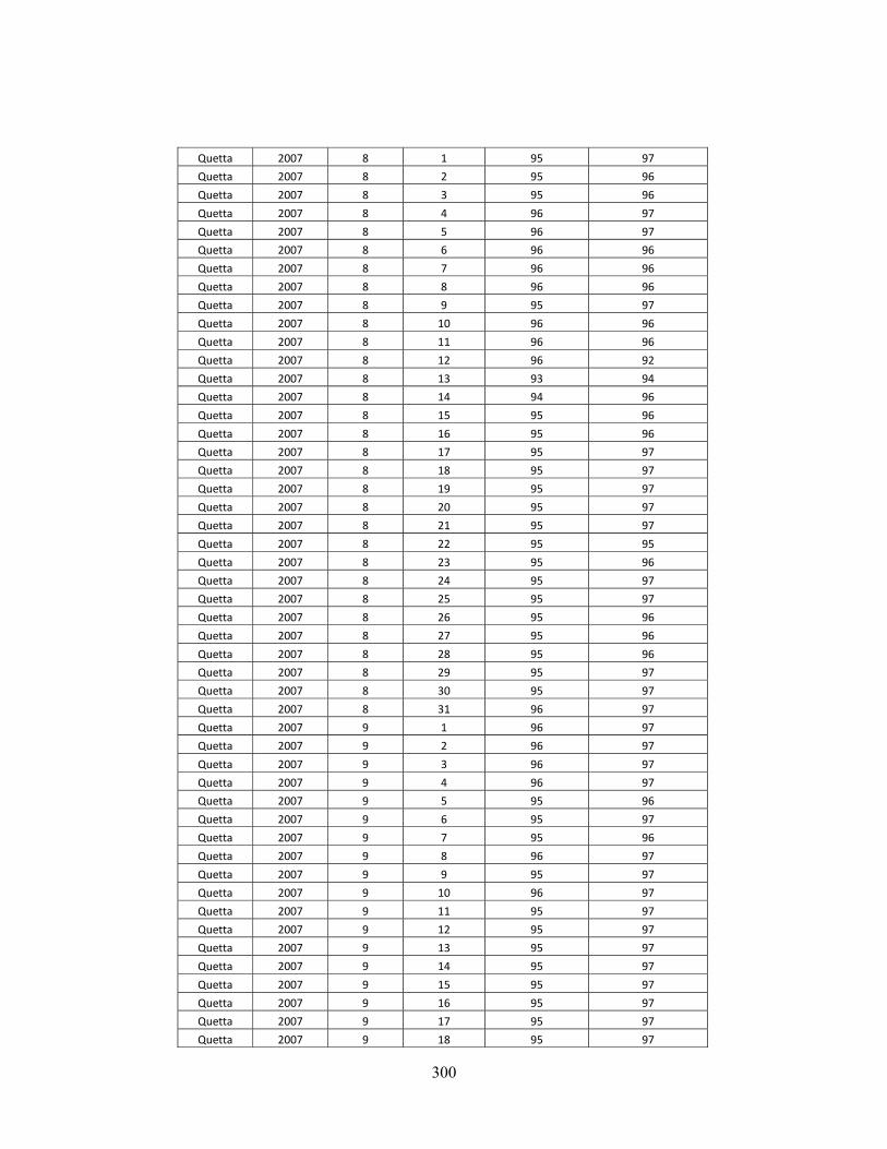
300
Quetta 2007 8 1 95 97
Quetta 2007 8 2 95 96
Quetta 2007 8 3 95 96
Quetta 2007 8 4 96 97
Quetta 2007 8 5 96 97
Quetta 2007 8 6 96 96
Quetta 2007 8 7 96 96
Quetta 2007 8 8 96 96
Quetta 2007 8 9 95 97
Quetta 2007 8 10 96 96
Quetta 2007 8 11 96 96
Quetta 2007 8 12 96 92
Quetta 2007 8 13 93 94
Quetta 2007 8 14 94 96
Quetta 2007 8 15 95 96
Quetta 2007 8 16 95 96
Quetta 2007 8 17 95 97
Quetta 2007 8 18 95 97
Quetta 2007 8 19 95 97
Quetta 2007 8 20 95 97
Quetta 2007 8 21 95 97
Quetta 2007 8 22 95 95
Quetta 2007 8 23 95 96
Quetta 2007 8 24 95 97
Quetta 2007 8 25 95 97
Quetta 2007 8 26 95 96
Quetta 2007 8 27 95 96
Quetta 2007 8 28 95 96
Quetta 2007 8 29 95 97
Quetta 2007 8 30 95 97
Quetta 2007 8 31 96 97
Quetta 2007 9 1 96 97
Quetta 2007 9 2 96 97
Quetta 2007 9 3 96 97
Quetta 2007 9 4 96 97
Quetta 2007 9 5 95 96
Quetta 2007 9 6 95 97
Quetta 2007 9 7 95 96
Quetta 2007 9 8 96 97
Quetta 2007 9 9 95 97
Quetta 2007 9 10 96 97
Quetta 2007 9 11 95 97
Quetta 2007 9 12 95 97
Quetta 2007 9 13 95 97
Quetta 2007 9 14 95 97
Quetta 2007 9 15 95 97
Quetta 2007 9 16 95 97
Quetta 2007 9 17 95 97
Quetta 2007 9 18 95 97
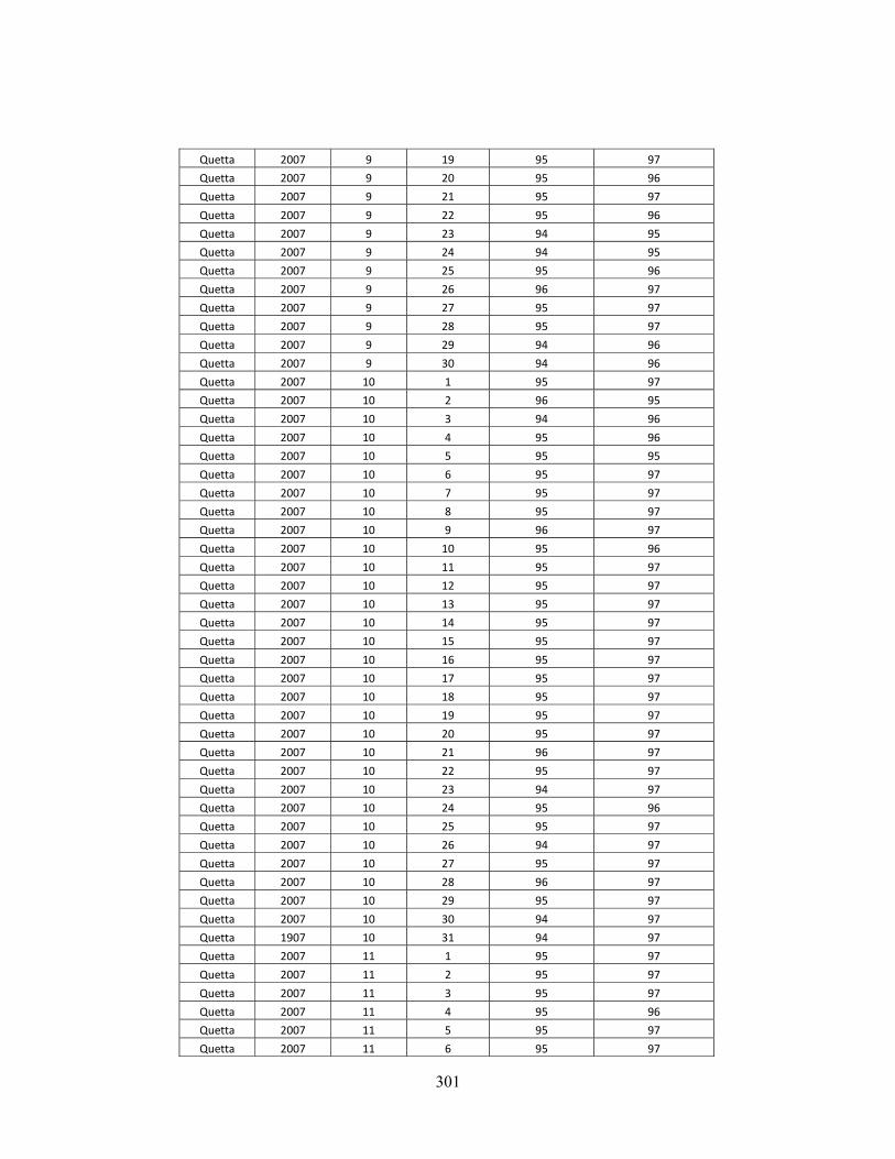
301
Quetta 2007 9 19 95 97
Quetta 2007 9 20 95 96
Quetta 2007 9 21 95 97
Quetta 2007 9 22 95 96
Quetta 2007 9 23 94 95
Quetta 2007 9 24 94 95
Quetta 2007 9 25 95 96
Quetta 2007 9 26 96 97
Quetta 2007 9 27 95 97
Quetta 2007 9 28 95 97
Quetta 2007 9 29 94 96
Quetta 2007 9 30 94 96
Quetta 2007 10 1 95 97
Quetta 2007 10 2 96 95
Quetta 2007 10 3 94 96
Quetta 2007 10 4 95 96
Quetta 2007 10 5 95 95
Quetta 2007 10 6 95 97
Quetta 2007 10 7 95 97
Quetta 2007 10 8 95 97
Quetta 2007 10 9 96 97
Quetta 2007 10 10 95 96
Quetta 2007 10 11 95 97
Quetta 2007 10 12 95 97
Quetta 2007 10 13 95 97
Quetta 2007 10 14 95 97
Quetta 2007 10 15 95 97
Quetta 2007 10 16 95 97
Quetta 2007 10 17 95 97
Quetta 2007 10 18 95 97
Quetta 2007 10 19 95 97
Quetta 2007 10 20 95 97
Quetta 2007 10 21 96 97
Quetta 2007 10 22 95 97
Quetta 2007 10 23 94 97
Quetta 2007 10 24 95 96
Quetta 2007 10 25 95 97
Quetta 2007 10 26 94 97
Quetta 2007 10 27 95 97
Quetta 2007 10 28 96 97
Quetta 2007 10 29 95 97
Quetta 2007 10 30 94 97
Quetta 1907 10 31 94 97
Quetta 2007 11 1 95 97
Quetta 2007 11 2 95 97
Quetta 2007 11 3 95 97
Quetta 2007 11 4 95 96
Quetta 2007 11 5 95 97
Quetta 2007 11 6 95 97

302
Quetta 2007 11 7 95 97
Quetta 2007 11 8 95 97
Quetta 2007 11 9 95 97
Quetta 2007 11 10 95 97
Quetta 2007 11 11 95 97
Quetta 2007 11 12 95 97
Quetta 2007 11 13 95 97
Quetta 2007 11 14 95 97
Quetta 2007 11 15 95 97
Quetta 2007 11 16 95 97
Quetta 2007 11 17 95 97
Quetta 2007 11 18 94 97
Quetta 2007 11 19 94 97
Quetta 2007 11 20 95 97
Quetta 2007 11 21 95 97
Quetta 2007 11 22 95 97
Quetta 2007 11 23 95 97
Quetta 2007 11 24 97 97
Quetta 2007 11 25 95 97
Quetta 2007 11 26 95 97
Quetta 2007 11 27 95 97
Quetta 2007 11 28 95 96
Quetta 2007 11 29 96 97
Quetta 2007 11 30 95 97
Quetta 2007 12 1 96 96
Quetta 2007 12 2 95 96
Quetta 2007 12 3 95 96
Quetta 2007 12 4 95 97
Quetta 2007 12 5 95 97
Quetta 2007 12 6 95 97
Quetta 2007 12 7 95 97
Quetta 2007 12 8 95 97
Quetta 2007 12 9 96 96
Quetta 2007 12 10 96 95
Quetta 2007 12 11 91 97
Quetta 2007 12 12 95 97
Quetta 2007 12 13 95 97
Quetta 2007 12 14 95 96
Quetta 2007 12 15 95 97
Quetta 2007 12 16 95 97
Quetta 2007 12 17 95 97
Quetta 2007 12 18 96 96
Quetta 2007 12 19 96 96
Quetta 2007 12 20 96 97
Quetta 2007 12 21 96 96
Quetta 2007 12 22 96 97
Quetta 2007 12 23 96 96
Quetta 2007 12 24 96 97
Quetta 2007 12 25 96 97

303
Quetta 2007 12 26 96 97
Quetta 2007 12 27 96 97
Quetta 2007 12 28 96 97
Quetta 2007 12 29 96 97
Quetta 2007 12 30 96 97
Quetta 2007 12 31 96 97
Quetta 2008 1 1 95 97
Quetta 2008 1 2 95 97
Quetta 2008 1 3 96 97
Quetta 2008 1 4 96 96
Quetta 2008 1 5 95 96
Quetta 2008 1 6 95 96
Quetta 2008 1 7 96 96
Quetta 2008 1 8 96 97
Quetta 2008 1 9 96 97
Quetta 2008 1 10 96 96
Quetta 2008 1 11 96 97
Quetta 2008 1 12 96 96
Quetta 2008 1 13 92 97
Quetta 2008 1 14 96 95
Quetta 2008 1 15 95 96
Quetta 2008 1 16 96 96
Quetta 2008 1 17 96 96
Quetta 2008 1 18 96 97
Quetta 2008 1 19 96 97
Quetta 2008 1 20 96 97
Quetta 2008 1 21 96 97
Quetta 2008 1 22 96 97
Quetta 2008 1 23 96 97
Quetta 2008 1 24 96 97
Quetta 2008 1 25 96 97
Quetta 2008 1 26 96 97
Quetta 2008 1 27 96 96
Quetta 2008 1 28 94 96
Quetta 2008 1 29 92 97
Quetta 2008 1 30 96 97
Quetta 2008 1 31 96 97
Quetta 2008 2 1 96 96
Quetta 2008 2 2 92 96
Quetta 2008 2 3 96 96
Quetta 2008 2 4 96 97
Quetta 2008 2 5 94 96
Quetta 2008 2 6 96 96
Quetta 2008 2 7 96 97
Quetta 2008 2 8 96 97
Quetta 2008 2 9 96 97
Quetta 2008 2 10 96 97
Quetta 2008 2 11 96 97
Quetta 2008 2 12 96 97
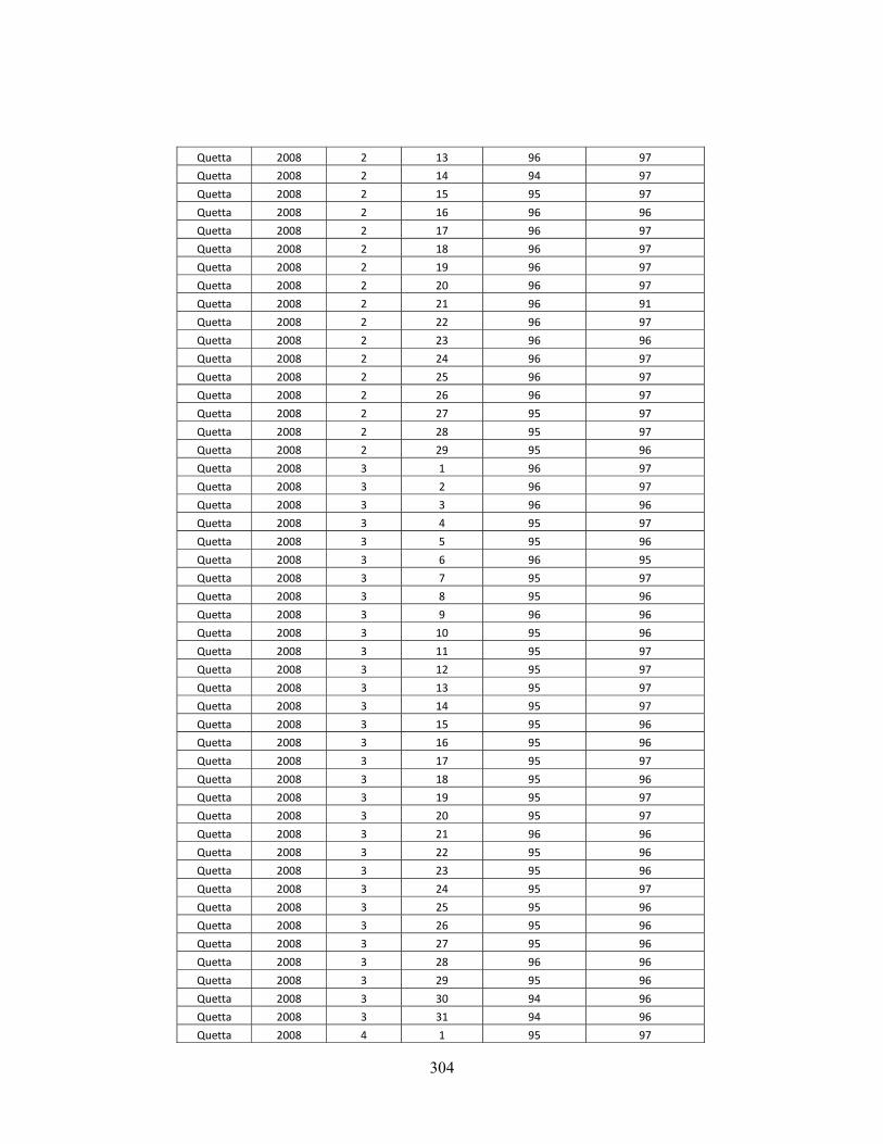
304
Quetta 2008 2 13 96 97
Quetta 2008 2 14 94 97
Quetta 2008 2 15 95 97
Quetta 2008 2 16 96 96
Quetta 2008 2 17 96 97
Quetta 2008 2 18 96 97
Quetta 2008 2 19 96 97
Quetta 2008 2 20 96 97
Quetta 2008 2 21 96 91
Quetta 2008 2 22 96 97
Quetta 2008 2 23 96 96
Quetta 2008 2 24 96 97
Quetta 2008 2 25 96 97
Quetta 2008 2 26 96 97
Quetta 2008 2 27 95 97
Quetta 2008 2 28 95 97
Quetta 2008 2 29 95 96
Quetta 2008 3 1 96 97
Quetta 2008 3 2 96 97
Quetta 2008 3 3 96 96
Quetta 2008 3 4 95 97
Quetta 2008 3 5 95 96
Quetta 2008 3 6 96 95
Quetta 2008 3 7 95 97
Quetta 2008 3 8 95 96
Quetta 2008 3 9 96 96
Quetta 2008 3 10 95 96
Quetta 2008 3 11 95 97
Quetta 2008 3 12 95 97
Quetta 2008 3 13 95 97
Quetta 2008 3 14 95 97
Quetta 2008 3 15 95 96
Quetta 2008 3 16 95 96
Quetta 2008 3 17 95 97
Quetta 2008 3 18 95 96
Quetta 2008 3 19 95 97
Quetta 2008 3 20 95 97
Quetta 2008 3 21 96 96
Quetta 2008 3 22 95 96
Quetta 2008 3 23 95 96
Quetta 2008 3 24 95 97
Quetta 2008 3 25 95 96
Quetta 2008 3 26 95 96
Quetta 2008 3 27 95 96
Quetta 2008 3 28 96 96
Quetta 2008 3 29 95 96
Quetta 2008 3 30 94 96
Quetta 2008 3 31 94 96
Quetta 2008 4 1 95 97

305
Quetta 2008 4 2 95 95
Quetta 2008 4 3 96 96
Quetta 2008 4 4 95 97
Quetta 2008 4 5 95 97
Quetta 2008 4 6 96 96
Quetta 2008 4 7 95 97
Quetta 2008 4 8 95 96
Quetta 2008 4 9 96 96
Quetta 2008 4 10 96 96
Quetta 2008 4 11 95 96
Quetta 2008 4 12 96 97
Quetta 2008 4 13 95 97
Quetta 2008 4 14 96 96
Quetta 2008 4 15 96 96
Quetta 2008 4 16 96 97
Quetta 2008 4 17 95 97
Quetta 2008 4 18 95 97
Quetta 2008 4 19 96 96
Quetta 2008 4 20 95 96
Quetta 2008 4 21 96 97
Quetta 2008 4 22 96 96
Quetta 2008 4 23 95 97
Quetta 2008 4 24 95 97
Quetta 2008 4 25 95 97
Quetta 2008 4 26 95 97
Quetta 2008 4 27 95 97
Quetta 2008 4 28 95 97
Quetta 2008 4 29 95 97
Quetta 2008 4 30 95 97
Quetta 2008 5 1 96 97
Quetta 2008 5 2 95 97
Quetta 2008 5 3 95 96
Quetta 2008 5 4 95 96
Quetta 2008 5 5 96 97
Quetta 2008 5 6 95 97
Quetta 2008 5 7 96 96
Quetta 2008 5 8 95 95
Quetta 2008 5 9 96 96
Quetta 2008 5 10 95 97
Quetta 2008 5 11 95 97
Quetta 2008 5 12 95 96
Quetta 2008 5 13 95 96
Quetta 2008 5 14 95 97
Quetta 2008 5 15 95 97
Quetta 2008 5 16 95 97
Quetta 2008 5 17 96 94
Quetta 2008 5 18 96 97
Quetta 2008 5 19 96 97
Quetta 2008 5 20 95 97
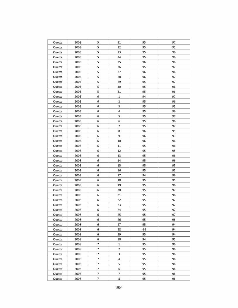
306
Quetta 2008 5 21 95 97
Quetta 2008 5 22 95 95
Quetta 2008 5 23 95 96
Quetta 2008 5 24 95 96
Quetta 2008 5 25 96 96
Quetta 2008 5 26 95 97
Quetta 2008 5 27 96 96
Quetta 2008 5 28 96 97
Quetta 2008 5 29 95 97
Quetta 2008 5 30 95 96
Quetta 2008 5 31 95 96
Quetta 2008 6 1 94 97
Quetta 2008 6 2 95 96
Quetta 2008 6 3 95 95
Quetta 2008 6 4 95 96
Quetta 2008 6 5 95 97
Quetta 2008 6 6 95 96
Quetta 2008 6 7 95 97
Quetta 2008 6 8 96 95
Quetta 2008 6 9 96 93
Quetta 2008 6 10 96 96
Quetta 2008 6 11 95 96
Quetta 2008 6 12 95 95
Quetta 2008 6 13 95 96
Quetta 2008 6 14 95 96
Quetta 2008 6 15 95 95
Quetta 2008 6 16 95 95
Quetta 2008 6 17 94 96
Quetta 2008 6 18 95 95
Quetta 2008 6 19 95 96
Quetta 2008 6 20 95 97
Quetta 2008 6 21 95 96
Quetta 2008 6 22 95 97
Quetta 2008 6 23 95 97
Quetta 2008 6 24 95 97
Quetta 2008 6 25 95 97
Quetta 2008 6 26 95 96
Quetta 2008 6 27 95 94
Quetta 2008 6 28 ‐99 94
Quetta 2008 6 29 95 94
Quetta 2008 6 30 94 95
Quetta 2008 7 1 95 96
Quetta 2008 7 2 95 96
Quetta 2008 7 3 95 96
Quetta 2008 7 4 95 96
Quetta 2008 7 5 95 96
Quetta 2008 7 6 95 96
Quetta 2008 7 7 95 96
Quetta 2008 7 8 95 96

307
Quetta 2008 7 9 95 95
Quetta 2008 7 10 95 96
Quetta 2008 7 11 95 96
Quetta 2008 7 12 95 94
Quetta 2008 7 13 95 95
Quetta 2008 7 14 95 95
Quetta 2008 7 15 95 96
Quetta 2008 7 16 95 97
Quetta 2008 7 17 95 96
Quetta 2008 7 18 95 96
Quetta 2008 7 19 95 97
Quetta 2008 7 20 95 95
Quetta 2008 7 21 94 94
Quetta 2008 7 22 95 95
Quetta 2008 7 23 95 96
Quetta 2008 7 24 95 97
Quetta 2008 7 25 95 96
Quetta 2008 7 26 94 95
Quetta 2008 7 27 95 92
Quetta 2008 7 28 95 94
Quetta 2008 7 29 95 95
Quetta 2008 7 30 95 96
Quetta 2008 7 31 95 96
Quetta 2008 8 1 95 95
Quetta 2008 8 2 96 96
Quetta 2008 8 3 96 96
Quetta 2008 8 4 96 96
Quetta 2008 8 5 95 95
Quetta 2008 8 6 95 96
Quetta 2008 8 7 95 97
Quetta 2008 8 8 95 96
Quetta 2008 8 9 94 95
Quetta 2008 8 10 95 94
Quetta 2008 8 11 92 92
Quetta 2008 8 12 92 94
Quetta 2008 8 13 94 94
Quetta 2008 8 14 94 95
Quetta 2008 8 15 94 96
Quetta 2008 8 16 94 96
Quetta 2008 8 17 95 97
Quetta 2008 8 18 95 96
Quetta 2008 8 19 95 96
Quetta 2008 8 20 94 97
Quetta 2008 8 21 95 97
Quetta 2008 8 22 95 96
Quetta 2008 8 23 95 96
Quetta 2008 8 24 94 96
Quetta 2008 8 25 94 97
Quetta 2008 8 26 95 97
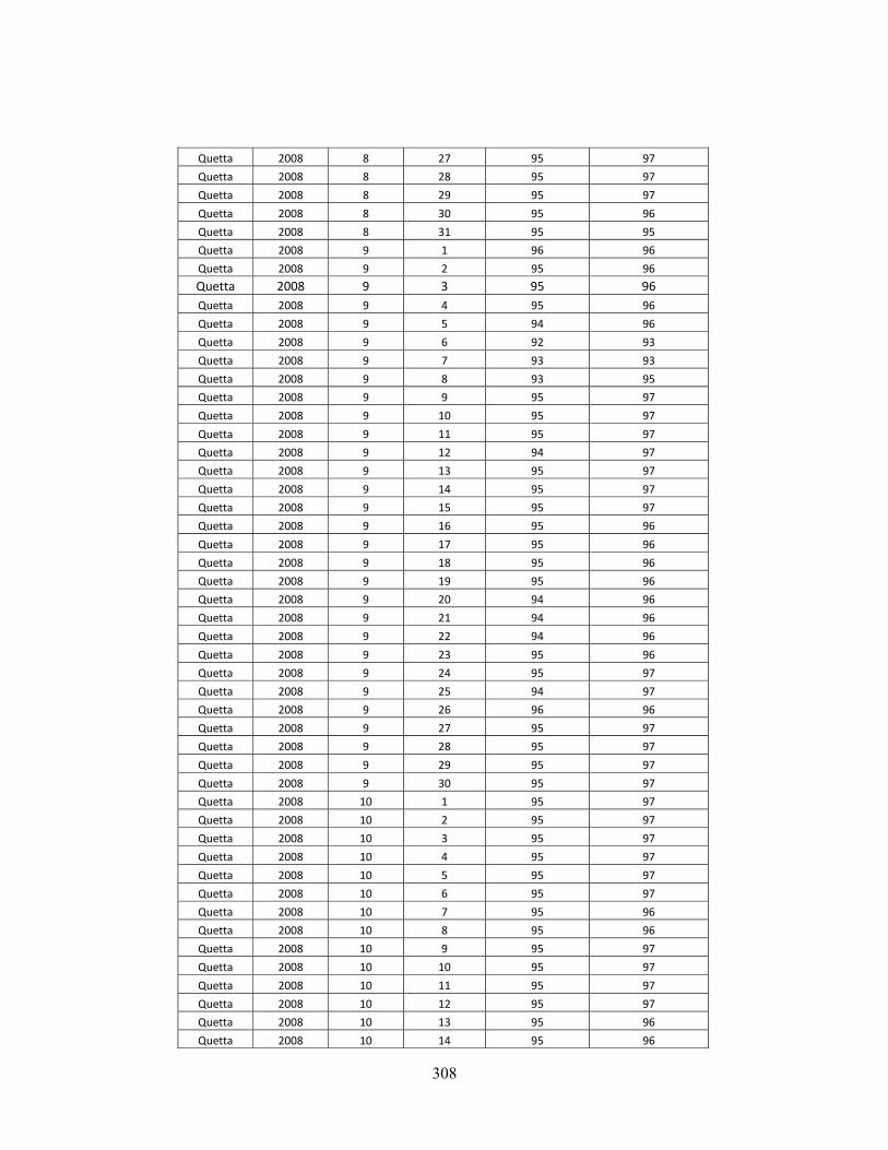
308
Quetta 2008 8 27 95 97
Quetta 2008 8 28 95 97
Quetta 2008 8 29 95 97
Quetta 2008 8 30 95 96
Quetta 2008 8 31 95 95
Quetta 2008 9 1 96 96
Quetta 2008 9 2 95 96
Quetta 2008 9 3 95 96 Quetta 2008 9 4 95 96
Quetta 2008 9 5 94 96
Quetta 2008 9 6 92 93
Quetta 2008 9 7 93 93
Quetta 2008 9 8 93 95
Quetta 2008 9 9 95 97
Quetta 2008 9 10 95 97
Quetta 2008 9 11 95 97
Quetta 2008 9 12 94 97
Quetta 2008 9 13 95 97
Quetta 2008 9 14 95 97
Quetta 2008 9 15 95 97
Quetta 2008 9 16 95 96
Quetta 2008 9 17 95 96
Quetta 2008 9 18 95 96
Quetta 2008 9 19 95 96
Quetta 2008 9 20 94 96
Quetta 2008 9 21 94 96
Quetta 2008 9 22 94 96
Quetta 2008 9 23 95 96
Quetta 2008 9 24 95 97
Quetta 2008 9 25 94 97
Quetta 2008 9 26 96 96
Quetta 2008 9 27 95 97
Quetta 2008 9 28 95 97
Quetta 2008 9 29 95 97
Quetta 2008 9 30 95 97
Quetta 2008 10 1 95 97
Quetta 2008 10 2 95 97
Quetta 2008 10 3 95 97
Quetta 2008 10 4 95 97
Quetta 2008 10 5 95 97
Quetta 2008 10 6 95 97
Quetta 2008 10 7 95 96
Quetta 2008 10 8 95 96
Quetta 2008 10 9 95 97
Quetta 2008 10 10 95 97
Quetta 2008 10 11 95 97
Quetta 2008 10 12 95 97
Quetta 2008 10 13 95 96
Quetta 2008 10 14 95 96

309
Quetta 2008 10 15 95 95
Quetta 2008 10 16 95 96
Quetta 2008 10 17 94 96
Quetta 2008 10 18 95 97
Quetta 2008 10 19 94 97
Quetta 2008 10 20 94 97
Quetta 2008 10 21 94 97
Quetta 2008 10 22 95 97
Quetta 2008 10 23 95 97
Quetta 2008 10 24 95 97
Quetta 2008 10 25 95 97
Quetta 2008 10 26 95 96
Quetta 2008 10 27 95 96
Quetta 2008 10 28 94 97
Quetta 2008 10 29 95 97
Quetta 2008 10 30 95 97
Quetta 2008 10 31 95 97
Quetta 2008 11 1 95 97
Quetta 2008 11 2 95 96
Quetta 2008 11 3 95 97
Quetta 2008 11 4 95 97
Quetta 2008 11 5 95 97
Quetta 2008 11 6 95 97
Quetta 2008 11 7 95 97
Quetta 2008 11 8 95 97
Quetta 2008 11 9 94 97
Quetta 2008 11 10 95 97
Quetta 2008 11 11 95 96
Quetta 2008 11 12 95 96
Quetta 2008 11 13 95 97
Quetta 2008 11 14 95 97
Quetta 2008 11 15 95 97
Quetta 2008 11 16 95 97
Quetta 2008 11 17 95 97
Quetta 2008 11 18 95 97
Quetta 2008 11 19 96 97
Quetta 2008 11 20 96 97
Quetta 2008 11 21 95 97
Quetta 2008 11 22 95 97
Quetta 2008 11 23 95 97
Quetta 2008 11 24 95 97
Quetta 2008 11 25 95 97
Quetta 2008 11 26 96 96
Quetta 2008 11 27 95 97
Quetta 2008 11 28 95 97
Quetta 2008 11 29 95 97
Quetta 2008 11 30 95 96
Quetta 2008 12 1 95 97
Quetta 2008 12 2 95 97
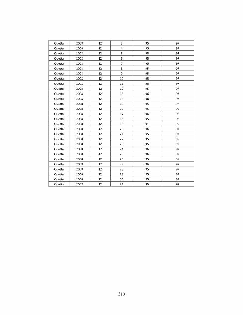
310
Quetta 2008 12 3 95 97
Quetta 2008 12 4 95 97
Quetta 2008 12 5 95 97
Quetta 2008 12 6 95 97
Quetta 2008 12 7 95 97
Quetta 2008 12 8 95 97
Quetta 2008 12 9 95 97
Quetta 2008 12 10 95 97
Quetta 2008 12 11 95 97
Quetta 2008 12 12 95 97
Quetta 2008 12 13 96 97
Quetta 2008 12 14 96 96
Quetta 2008 12 15 95 97
Quetta 2008 12 16 95 96
Quetta 2008 12 17 96 96
Quetta 2008 12 18 95 96
Quetta 2008 12 19 91 95
Quetta 2008 12 20 96 97
Quetta 2008 12 21 95 97
Quetta 2008 12 22 95 97
Quetta 2008 12 23 95 97
Quetta 2008 12 24 96 97
Quetta 2008 12 25 96 97
Quetta 2008 12 26 95 97
Quetta 2008 12 27 96 97
Quetta 2008 12 28 95 97
Quetta 2008 12 29 95 97
Quetta 2008 12 30 95 97
Quetta 2008 12 31 95 97


