UNIVERSITY OF CALGARY
Density Prediction for Mixtures of Heavy Oil and Solvents
by
FATEMEH SARYAZDI
A THESIS
SUBMITTED TO THE FACULTY OF GRADUATE STUDIES
IN PARTIAL FULFILMENT OF THE REQUIREMENTS FOR THE
DEGREE OF MASTER OF SCIENCE
DEPARTMENT OF CHEMICAL AND PETROLEUM ENGINEERING
CALGARY, ALBERTA
August, 2012
© FATEMEH SARYAZDI 2012
ii
UNIVERSITY OF CALGARY
FACULTY OF GRADUATE STUDIES
The undersigned certify that they have read, and recommend to the Faculty of
Graduate Studies for acceptance, a thesis entitled “Density Prediction for Mixtures
of Heavy Oil and Solvents” submitted by FATEMEH SARYAZDI in partial
fulfillment of the requirements of the degree of MASTER OF SCIENCE IN
ENGINEERING.
Supervisor, Dr. HARVEY W. YARRANTON
Dr. WILLIAM Y. SVRCEK
Dr. ZHANGXING CHEN
Dr. LAURENCE R. LINES
Date
iii
Abstract
The design of solvent-based and solvent-assisted heavy oil and bitumen recovery
processes requires the accurate prediction of the physical properties of heavy oil
mixed with solvents. In particular, density is a critical parameter for gravity
drainage and gravity separation based processes. It has proven challenging to
accurately predict the density of these mixtures, particularly when the solvent is a
dissolved gas. The objective of this thesis is to develop a straightforward method to
predict the density of heavy oils or bitumens diluted with liquid solvents and
dissolved gases.
Most mixtures of heavy oil and solvents are well below their critical point, and
therefore liquid phase density prediction methods are appropriate. Excess volume
based mixing rules were investigated with a binary interaction parameter used to
relate the excess volume to the composition of the mixture. The mixing rules were
tested on literature data for binary mixtures of hydrocarbons. The binary interaction
parameters were found to correlate to the normalized difference in the molar
volumes of the binary pairs.
To apply these mixing rules to a liquid containing a dissolved gas, the effective
liquid density of the dissolved gas is required. However, while effective liquid
densities have been used to estimate petroleum densities, values have only been
developed for a very limited range of conditions. Nor have these values been
rigorously tested. In this thesis, the effective liquid densities of light n-alkanes were
determined by linearly extrapolating the molar volumes of higher n-alkane (C7 and
up) versus their molecular weight. The extrapolated molar volumes were converted
to the mass density and correlated to temperature and pressure.
iv
The correlation was validated on density data on n-alkane binary mixtures from the
literature and from this thesis. Densities were measured with an Anton Paar density
meter from room temperature to 175˚C and from 10 to 40 MPa for ethane, propane,
and n-butane as the dissolved gas and n-decane, toluene, and cyclooctane as the
heavier liquid component. The effective liquid densities applied with regular
solution mixing rules (zero excess volume) predicted the densities of these mixtures
with an average absolute relative deviation (AARD) less than 1%.
Finally, the mixing rules and effective densities were tested on diluted bitumens.
Densities were measured from room temperature to 175˚C and from 0.1 to 10 MPa
for bitumen/propane (this project), and bitumen/ethane, bitumen/ n-butane, and
bitumen/n-heptane (as part of another project, Motahhari, 2012). The regular
solution mixing rules (zero excess volume) predicted the mixture densities with an
AARD less than 1%. The AARD was reduced to less than 0.15% with fitted excess
volume mixing rules. The binary interaction parameters were correlated to the
normalized molar volume difference with a quadratic expression. The AARD with
the correlated parameters was less than 0.4%.
Overall, the excess volume mixing rules with the correlated interaction parameters
predict the density of diluted bitumens to almost within experimental error as long
as the mixture is subcritical and the component densities are known at the
conditions of interest. The proposed method is suitable for hand calculations and
could be implemented in a simulator with an appropriate database of component
densities.
v
Acknowledgement
First of all, I am deeply indebted to my supervisor, Dr. Harvey W. Yarranton for his
support, encouragement and constant guidance during my Master’s degree program.
It was an honor for me to be a member of his research group.
I also would like to express my deepest gratitude to our PVT lab manager Florian
Schoeggl for his teaching and technical support he provided during experimental
work.
I am also thankful to Elaine Baydak and Hamed reza Motahhari for their assistance
and great help during my master’s thesis.
I am thankful to the Department of Chemical and Petroleum Engineering,
Asphaltene and Emulsion Research Group, Faculty of Graduate Studies at the
University of Calgary for their assistant, NSERC, Shell Energy Ltd., Schlumberger-
DBR, Petrobras for their financial support throughout my Masters Program.
Finally, from the deepest of my heart, I would like to thank my husband for his
constant support and encouragement. I am really grateful for his caring and
understanding.
vi
Dedication
I dedicated this Dissertation to:
My Parents and My Husband
vii
Table of Contents
University of Calgary ............................................................................................. II
Abstract ................................................................................................................ III
Acknowledgement ................................................................................................. V
Dedication ............................................................................................................ VI
Table of Contents ................................................................................................ VII
List of Tables ........................................................................................................ IX
List of Figures and Illustrations ............................................................................. XI
List of Symbols, Abbreviation and Nomenclature .............................................. XIV
CHAPTER ONE: INTRODUCTION ...................................................................... 1
1.1 OBJECTIVES ..................................................................................................... 3
1.2 ORGANIZATION OF THESIS ............................................................................... 4
CHAPTER TWO: LITERATURE REVIEW .......................................................... 5
2.1 DENSITY OF HYDROCARBON LIQUID MIXTURES ................................................ 5
2.1.1 General Behavior of Liquid Mixtures ............................................................. 5
2.1.1.1 Partial Molar Volume .............................................................................. 6
2.1.1.2 Excess Molar Volumes ............................................................................ 8
2.1.2 Behaviour of Liquid-Liquid Hydrocarbon Mixtures ....................................... 8
2.1.3 Behaviour of Liquid Hydrocarbons with Dissolved Gas ............................... 12
2.2 MODELING THE DENSITY OF LIQUID HYDROCARBON MIXTURES ..................... 14
2.2.1 Mixing Rule ................................................................................................. 14
2.2.2 Density Correlations..................................................................................... 15
2.2.3 Corresponding States ................................................................................... 23
2.2.4 Equation of State (EOS) ............................................................................... 28
2.3 MODELING THE DENSITY OF LIQUID WITH DISSOLVED GAS ............................. 35
2.4 HEAVY OIL CHEMISTRY ................................................................................. 37
2.4.1 Definition and Classification ........................................................................ 37
2.4.2 Heavy Oil Composition ................................................................................ 39
2.5 DENSITY OF BITUMEN AND MIXTURES WITH SOLVENT .................................... 44
2.5.1 Density of Heavy Oil and Bitumen ............................................................... 44
2.5.1.1 Measurement of Heavy Oil and Bitumen Density .................................. 44
2.5.1.2 Effect of the Temperature on Heavy Oil and Bitumen Density ............... 44
2.5.1.3 Effect of Pressure on Heavy Oil and Bitumen Density ........................... 46
viii
2.5.2 Density of Heavy Oil and Solvent Mixtures ................................................. 46
2.5.3 Density Modeling for Mixtures of Heavy Oil and Solvents ........................... 49
2.6 SUMMARY ..................................................................................................... 53
CHAPTER THREE: EXPERIMENTAL METHODS ........................................... 54
3.1 MATERIALS ................................................................................................... 54
3.2 APPARATUS DESCRIPTION .............................................................................. 55
3.2.1 Anton Paar Density Meter ............................................................................ 55
3.2.2 Quizix Pump ................................................................................................ 57
3.2.3 Back Pressure Regulator (BPR) .................................................................... 57
3.2.4 Air Bath Temperature Control ...................................................................... 57
3.3 APPARATUS CALIBRATION ............................................................................. 58
3.4 SAMPLE PREPARATION ................................................................................... 60
3.5 EXPERIMENTAL PROCEDURE .......................................................................... 63
3.6 APPARATUS CLEAN-UP................................................................................... 64
CHAPTER FOUR: RESULT AND DISCUSSION ............................................... 65
4.1 DENSITY OF MIXTURES OF LIQUID HYDROCARBONS ....................................... 65
4.2 DENSITY OF MIXTURES WITH GAS DISSOLVED IN A HYDROCARBON LIQUID .... 73
4.2.1 New Effective Density Correlation for Light n-Alkanes ............................... 76
4.2.2 Validation of New Effective Density Correlation ......................................... 78
4.3 BITUMEN DENSITY CORRELATION .................................................................. 92
4.4 DILUTED BITUMEN DENSITY .......................................................................... 94
CHAPTER FIVE: CONCLUSION AND RECOMMENDATION ...................... 102
5.1 SUMMARY ................................................................................................... 102
5.2 CONCLUSIONS .............................................................................................. 102
5.3 RECOMMENDATIONS .................................................................................... 103
REFERENCES ................................................................................................... 105
APPENDIX A – PURE HYDROCARBON MIXTURES DENSITY DATA ...... 115
APPENDIX B – DEAD BITUMENS DENSITY DATA .................................... 129
APPENDIX C – ADDITIONAL DENSITY DATA ............................................ 132
APPENDIX D - ERROR ANALYSIS ................................................................ 133
ix
List of Tables
Table 2-1. Tait Correlation for n-alkanes (Dymond and Malhotra, 1987).............. 19
Table 2-2. Comparison of Requirements and range of applicability of methods
studied by Rea et. al. (1973) ................................................................................ 26
Table 2-3. Absolute average deviation of saturated liquid density predictions,
temperature between 323.10 and 437.10 K. .......................................................... 33
Table 2-4. UNITAR Classification of oil by physical properties at 15.6°C (Gray,
1994) ................................................................................................................... 37
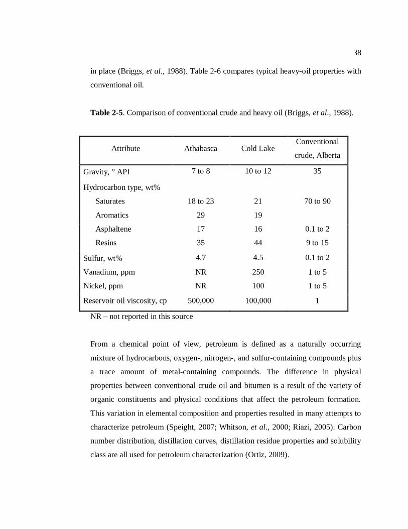
Table 2-5. Comparison of conventional crude and heavy oil (Briggs, et al., 1988).38
Table 4-1. Pure hydrocarbon mixtures for which density was measured by Chevalier
et al.(1990). ......................................................................................................... 67
Table 4-2. βij values for different types of pure hydrocarbon mixtures .................. 68
Table 4-3. The fitting parameters of the new effective density correlation. ........... 78
Table 4-4. Summary of the pure hydrocarbon mixtures and their composition, and
temperature and pressure range for which density data collected. ......................... 80
Table 4-5. AAD, AARD, MAD, and MARD of pure hydrocarbon mixtures. ........ 89
Table 4-6. Comparison between the effective liquid density of dissolved gas
components with their API liquid density value at standard condition. ................. 91
Table 4-7. Fitted parameters for Bitumens A and B. ............................................. 94
Table 4-8. The composition, temperatures, and pressures of the diluted bitumens for
which density data were collected. ....................................................................... 94
Table 4-9. The composition, temperatures, and pressures of the diluted bitumens for
which density data were collected. ....................................................................... 98
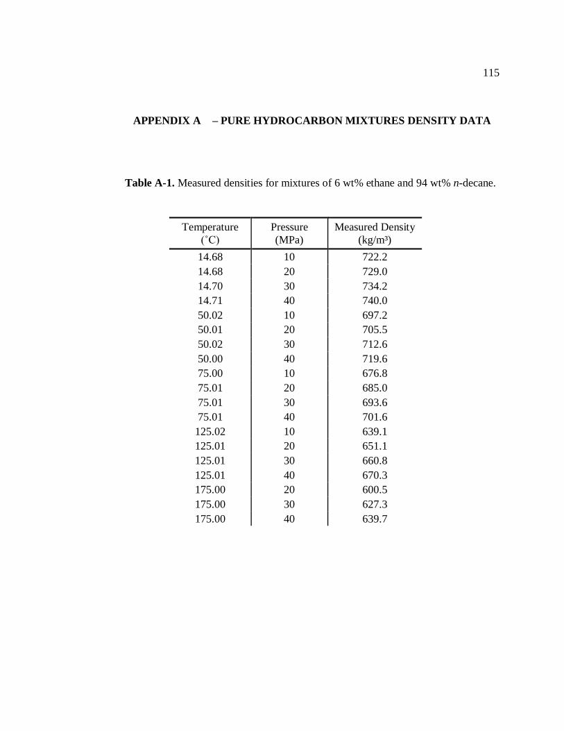
Table A-1. Measured densities for mixtures of 6 wt% ethane and 94 wt% n-
decane……………………………………………………………………………..115
Table A-2. Measured densities for mixtures of 12.5 wt% ethane and 87.5 wt% n-
decane……………………………………………………………………………..116
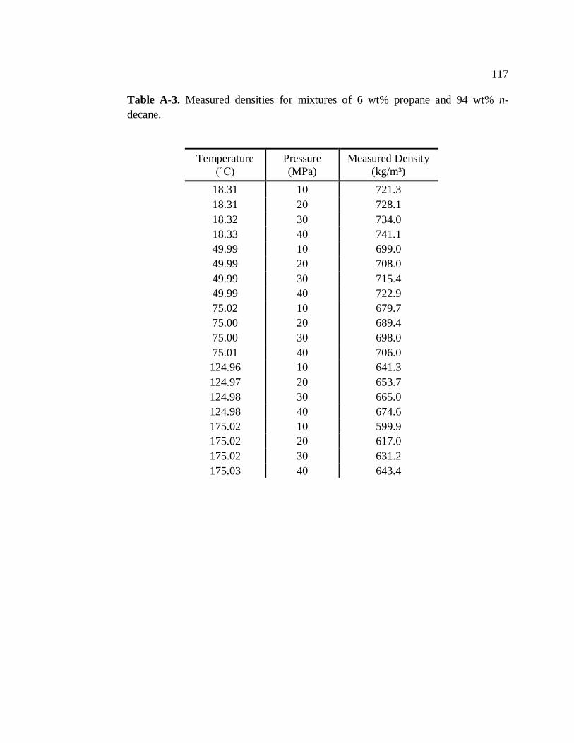
Table A-3. Measured densities for mixtures of 6 wt% propane and 94 wt% n-
decane......................................................................................................................117
Table A-4. Measured densities for mixtures of 12.5 wt% propane and 87.5 wt% n-
decane…………………………………………………………………………….118
Table A-5. Measured densities for mixtures of 25 wt% propane and 75 wt% n-
decane…………………………………………………………..…………………119
Table A-6. Measured densities for mixtures of 6 wt% propane and 94 wt%
Toluene................................................................................................................... .120
Table A-7. Measured densities for mixtures of 12.5 wt% propane and 87.5 wt%
Toluene……………………………………………………………………………121
Table A-8. Measured densities for mixtures of 25 wt% propane and 75 wt%
x
Toluene…………………………………………………………………………....122
Table A-9. Measured densities for mixtures of 6 wt% propane and 94 wt%
Cyclooctane…………………………………………………………………….....123
Table A-10. Measured densities for mixtures of 12.5 wt% propane and 87.5 wt%
Cyclooctane…………………………………………………………………….…124
Table A-11. Measured densities for mixtures of 25 wt% propane and 75 wt%
Cyclooctane…………………………………………………………………….…125
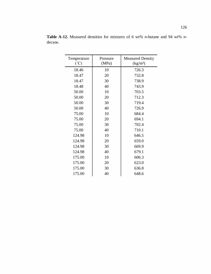
Table A-12. Measured densities for mixtures of 6 wt% n-butane and 94 wt% n-
decane……………………………………………………………………………..126
Table A-13. Measured densities for mixtures of 12.5 wt% n-butane and 87.5 wt% n-
decane…………………………………………………………………………..…127
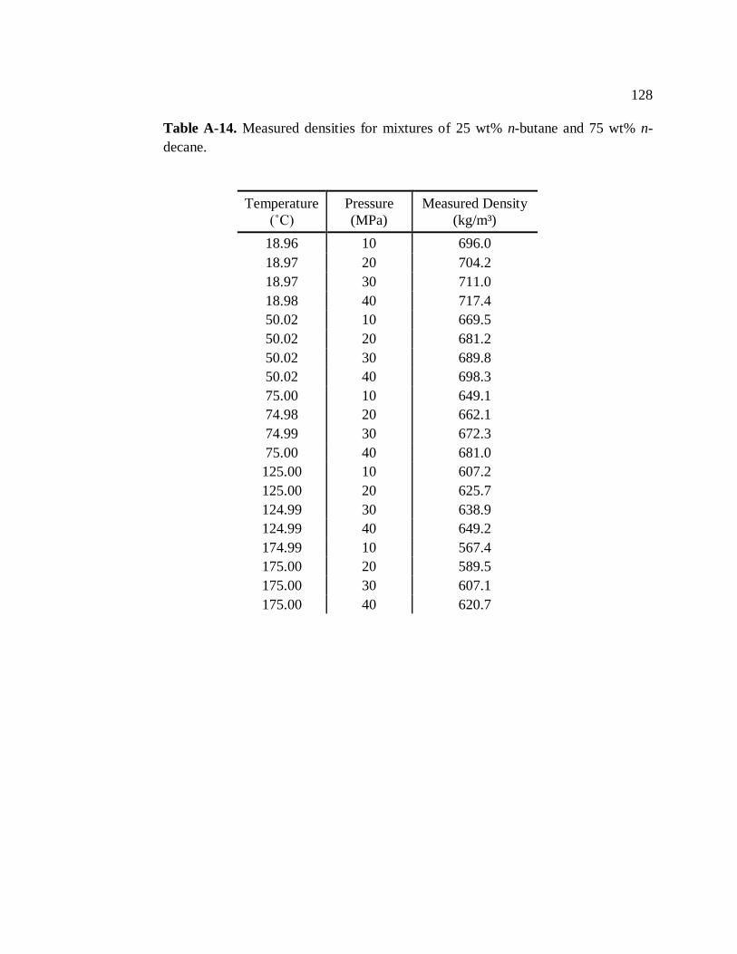
Table A-14. Measured densities for mixtures of 25 wt% n-butane and 75 wt% n-
decane…………………………………………………………………………. …128
Table B-1. Measured densities for dead bitumen A………………………….…...129
Table B-2. Measured densities for dead bitumen B……………………………....131
Table C-1. Measured densities of n-decane diluted Heavy Oil at 23 ˚C. (Kumar,
2012).......................................................................................................................132
Table C-2. Measured densities of toluene diluted Bitumen A Maltene. (Sanchez,
2012)……………………………………………………………………………...132
Table D-1. Composition accuracy of pure hydrocarbon mixtures……………….134
Table D-2. Error Analysis of Pure Hydrocarbon Mixtures……………………………...136
Table D-3. Error Analysis of Pure Diluted Bitumen……………………………………..138
xi
List of Figures and Illustrations
Figure 2–1. The slope of the plot of volume vs. Molar fraction is partial molar
volume. Line I and II show the slop of the plot in two specific compositions. For
line I the slop is positive and for line II the slop is negative. ................................... 7
Figure 2–2. Excess molar volumes for n-hexane (x) and n-alkanes (1-x) at 298.15
K. (data adapted from Goates et al., (1981)) ........................................................... 8
Figure 2–3. Excess molar volumes for cyclohexane (x) with n-alkanes (1-x) at
298.15 K. (data adapted from Goates et al., (1979)) ............................................... 9
Figure 2–4. Maximum values of excess molar volume, vE, of binary mixtures versus
the carbon number (n) of the n-alkane component at 298.15 K. (data adapted from
Alonso et al., (1983)) ........................................................................................... 10
Figure 2–5. Excess molar volume of equimolar mixtures of 1,1-dimethylpropyl
ether + n-alkane vs. n-alkane carbon number. (data adapted from Witek et al., 1997)
............................................................................................................................ 11
Figure 2–6. Variation of the density with composition at 333.15 K versus different
pressures. (data adapted from Canet et al., (2002)) ............................................... 13
Figure 2–7. The process of dissolving a gas component in a liquid mixture .......... 35
Figure 2–8. Effect of molecular structure on boiling point (Boduszynski, 1987) ... 40
Figure 2–9. Schematic of SARA fractionation procedure. .................................... 41
Figure 2–10. Effect of solvent carbon number on insolubles (Speight, 2007)........ 42
Figure 2–11. A hypothetical Asphaltene structure, A, B and C represent larger
aromatic clusters (Strausz, et al., 1992). Note the structure is larger than typical for
an asphaltene monomer and represents an amalgamated aggregate. ...................... 43
Figure 2–12. The effect of temperature on the density of some Western Canadian
crudes .................................................................................................................. 45
Figure 2–13. Effect of pressure on density of CH4-saturated bitumen, adopted from
Mehrotra and Svrcek, (1985)................................................................................ 47
Figure 2–14. Effect of temperature on the density of mixtures of athabasca bitumen
with propane (Badamchi-zadeh et al., 2009) ........................................................ 48
Figure 3–1. Schematic of the density measurement apparatus.............................. 55
Figure 3–2. Comparison between literature data and experimental data for n-butane
density at 75˚C. .................................................................................................... 59
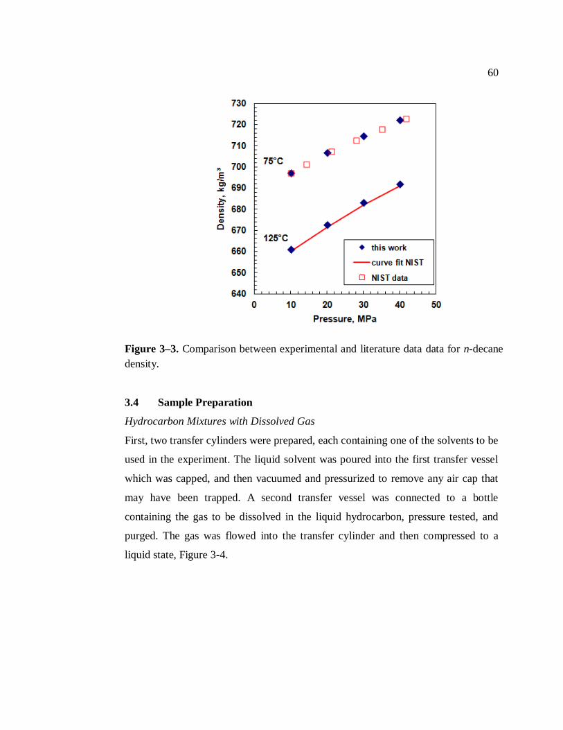
Figure 3–3. Comparison between literature data and experimental data for n-decane
density at 75˚C. .................................................................................................... 60
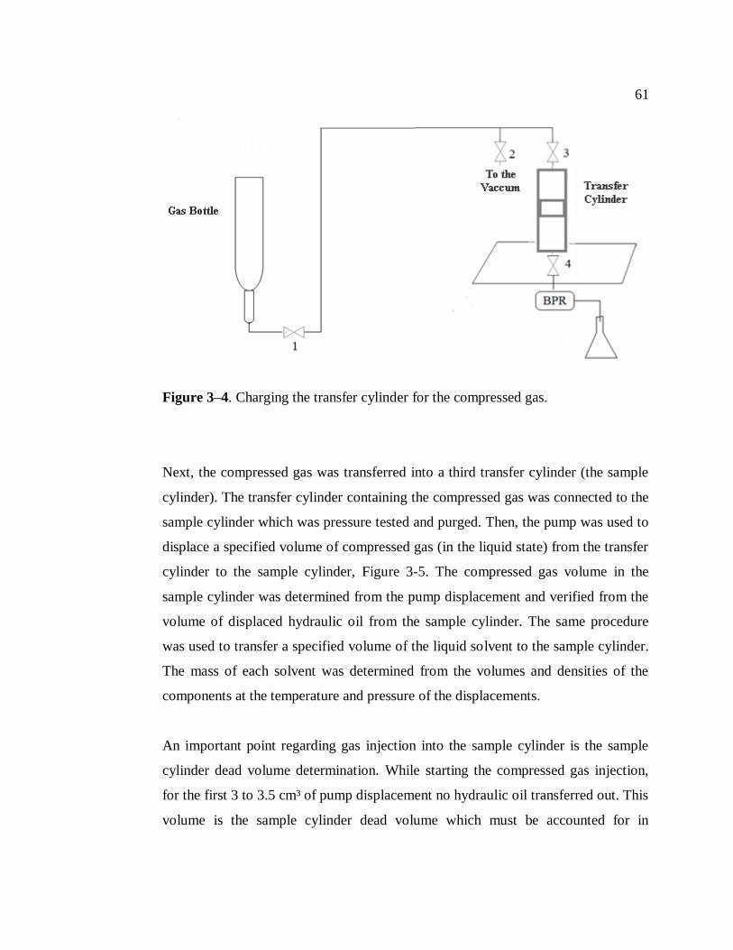
Figure 3–4. Charging the transfer cylinder for the compressed gas. ...................... 61
Figure 3–5. Charging from transfer cylinder to the sample cylinder. .................... 62
Figure 4–1. Measured and fitted density of mixtures of n-hexane + n-heptane. ..... 69
Figure 4–2. Measured and fitted density of mixtures of n-hexane + n-hexadecane.70
xii
Figure 4–3. Measured and fitted density of mixtures of cyclohexane + n-
hexadecane. ......................................................................................................... 70
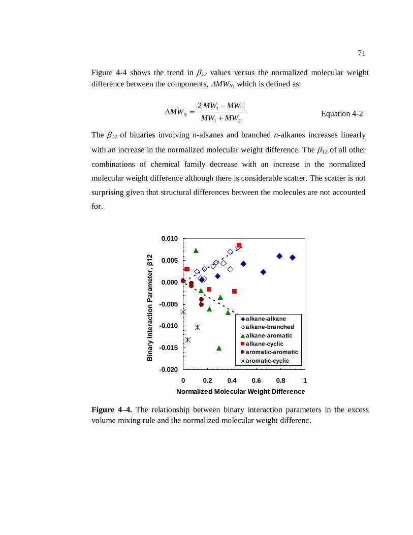
Figure 4–4. The relationship between binary interaction parameters in the excess
volume mixing rule and the normalized molecular weight difference. .................. 71
Figure 4–5. The relationship between binary interaction parameters in the excess
volume mixing rule and the normalized specific volume difference. .................... 72
Figure 4–6. n-Alkane molar volumes versus molecular weight at 80°C and 10 MPa.
............................................................................................................................ 73
Figure 4–7. Effective liquid density of lower n-alkanes at 80°C and different
pressures. ............................................................................................................. 74
Figure 4–8. Comparison of extrapolated n-alkane molar volumes from Tharanivasan
et al. (2011) with experimentally derived molar volume of methane at 80°C and 10
MPa. .................................................................................................................... 75
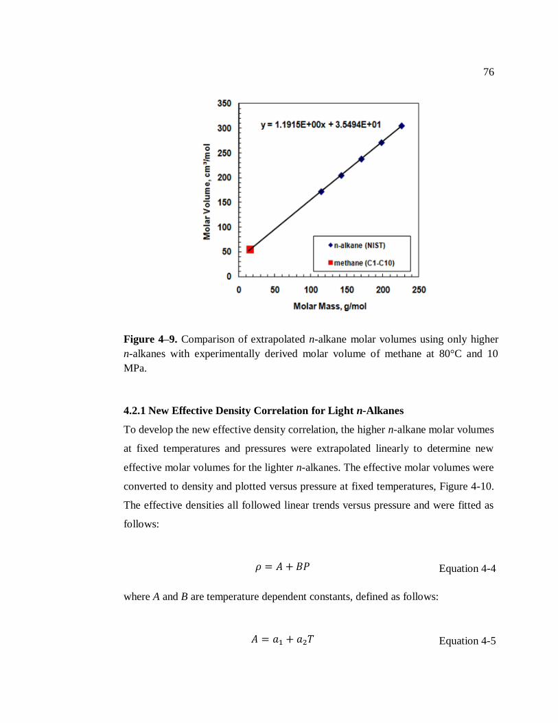
Figure 4–9. Comparison of extrapolated n-alkane molar volumes using only higher
n-alkanes with experimentally derived molar volume of methane at 80°C and 10
MPa. .................................................................................................................... 76
Figure 4–10. New effective density of lower n-alkane series at 80°C and different
pressures. ............................................................................................................. 77
Figure 4–11. Measured and predicted densities for mixtures of 6 wt% propane and
94 wt% n-decane. ................................................................................................ 81
Figure 4–12. Measured and predicted densities for mixtures of 12.5 wt% propane
and 87.5 wt% n-decane. ....................................................................................... 81
Figure 4–13. Measured and predicted densities for mixtures of 25 wt% propane and
75 wt% n-decane. ................................................................................................ 82
Figure 4–14. Reduced temperature and pressure at which the effective density
correlation gives more than 3% error in mixture densities (to right of each point). 83
Figure 4–15. Predicted versus measured density for mixtures of n-butane and n-
decane.................................................................................................................. 84
Figure 4–16. Predicted versus measured density for mixtures of propane and n-
decane.................................................................................................................. 85
Figure 4–17. Predicted versus measured density for mixtures of ethane and n-
decane.................................................................................................................. 85
Figure 4–18. Predicted versus measured density for mixtures of ethane and n-
tetradecane (Kariznovi et al., 2012)...................................................................... 86
Figure 4–19. Predicted versus measured density for mixtures of ethane and n-
octadecane (Nourizadeh et al., 2012) ................................................................... 86
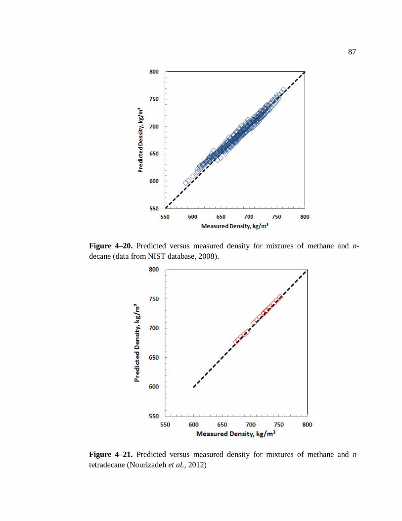
Figure 4–20. Predicted versus measured density for mixtures of methane and n-
decane (data from NIST database, 2008). ............................................................. 87
xiii
Figure 4–21. Predicted versus measured density for mixtures of methane and n-
tetradecane (Nourizadeh et al., 2012) ................................................................... 87
Figure 4–22. Predicted versus measured density for mixtures of methane and n-
octadecane (Kariznovi et al., 2012) ...................................................................... 88
Figure 4–23. Predicted versus measured density for mixtures of propane and
toluene. ................................................................................................................ 90
Figure 4–24. Predicted versus measured density for mixtures of propane and
cyclooctane. ......................................................................................................... 90
Figure 4–25. Predicted versus measured density for mixtures of methane (C1) and
toluene: a) regular solution mixing rule; b) excess volume mixing rule with ij = -
0.006.................................................................................................................... 91
Figure 4–26. Measured and correlated density of Bitumen A. .............................. 93
Figure 4–27. Measured and correlated density of Bitumen B. ............................... 93
Figure 4–28. Calculated versus measured density for n-heptane (C7) diluted
Bitumen A: a) regular solution mixing rule; b) excess volume mixing rule with ij =
+0.022. ................................................................................................................ 96
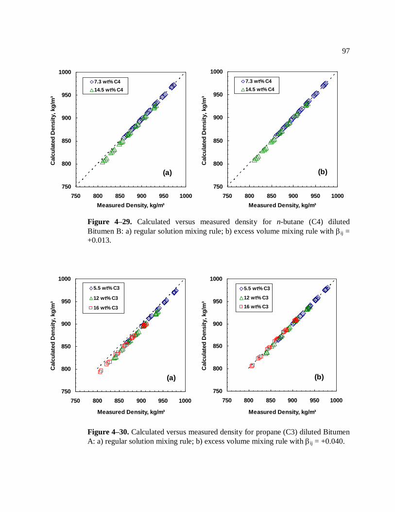
Figure 4–29. Calculated versus measured density for n-butane (C4) diluted Bitumen
B: a) regular solution mixing rule; b) excess volume mixing rule with ij = +0.013.
............................................................................................................................ 97
Figure 4–30. Calculated versus measured density for propane (C3) diluted Bitumen
A: a) regular solution mixing rule; b) excess volume mixing rule with ij = +0.040.
............................................................................................................................ 97
Figure 4–31. Calculated versus measured density for ethane (C2) diluted Bitumen
A: a) regular solution mixing rule; b) excess volume mixing rule with ij = -0.001.
............................................................................................................................ 98
Figure 4–32. Comparison of binary interaction parameters for diluted bitumens and
pure hydrocarbon mixtures................................................................................. 101
Figure 4–33. Density of bitumen diluted with n-alkanes at: a) 50°C and 2.5 MPa; b)
100°C and 10 MPa. Equation 4-13 was used to determine the ij for the excess
volume mixing rule. ........................................................................................... 101
xiv
List of Symbols, Abbreviation and Nomenclature
Abbreviation
APR Advanced Peng-Robinson
ARC Alberta Research Counsil
BPR Back Pressure Regulator
CN Carbon Number
EoS Equation of State
HC Hydrocarbon
MW Molecular Weight
PR Peng-Robinson
SRK Soave-Redlich-Kwong
SG Specific Gravity
SF Shrinkage factor
Wt% Weight Percent
List of Symbols
a Attractive constant in Equation of State
b Repulsive constant in Equation of State
c Volume translation
cn Characteristic carbon number
ZRA Racket compressibility factor
Mixture pseudo-volume
m Mass fraction
x Mole fraction
P Pressure
T Temperature
v Molar volume
R Universal gas constant
Z Compressibilty
n Number of moles
Greek Symbols
ρ Density
ω Acentric factor
xv
β Compressibility
βij Binary interaction parameter between two component i and j
φ Volume fraction
Subscripts
ave Average
C Critical
I Component i
J Component j
mix Mixture
N Normalized
R Reduced
S Saturated
0 Reference
Superscripts
E Excess
1
CHAPTER ONE: INTRODUCTION
As the supply of conventional oil resources shrinks, unconventional hydrocarbon
feedstocks, such as bitumen and heavy oils, have been recognized as alternate
energy sources (Sarkar, 1984). However, primary recovery techniques have had
limited success for heavy oils and bitumens due to the high viscosity of the oil. In
Canada, steam based methods are often applied to reduce the oil viscosity and
improve recovery (Kokal and Sayegh, 1990). Unfortunately, these methods require
significant amounts of natural gas, which is costly, and water, which is in limited
supply. For example, almost 34 m3 of natural gas and 0.2 m
3 of groundwater are
required to produce one barrel of bitumen (Canada’s Oil Sand Report, 2007).
Solvent or solvent-assisted recovery methods are alternatives that may reduce the
energy and water requirements for these processes.
Solvent based recovery processes such as VAPEX (Vapor Extraction) and ES-
SAGD (Enhanced Solvent – Steam Assisted Gravity Drainage) involve gravity
drainage and therefore depend strongly on the density of the solvent diluted heavy
oil (or bitumen). Many surface processes involve the dilution of bitumen with
solvent. For example, heavy oil is diluted for oil-water separation where the density
contrast between the oil and water is critical for effective separation. Heavy oils are
also diluted to reduce their viscosity for pipeline transportion and to modify
properties during refining. Hence, the density of heavy oil and solvent liquid
mixtures is a critical property for the design and operation of both reservoir and
surface processes (Audonnet and Padua, 2004).
While some data are available for the density of bitumens and dissolved gases, there
are significant gaps. Ward and Clark (1950) were the first, to present experimental
density data for Athabasca bitumen. Jacob et al. (1980) measured the viscosity for
dead Athabasca bitumen and bitumen saturated with CO2, CH4, and N2 over a wide
2
range of pressures and temperatures. Mehrotra and Svrcek (1985) published data
sets for the viscosity, density and gas solubility for N2, CO, CH4, CO2, and C2H6 in
a number of dead and live bitumens. Yarranton et al. (2008) and Badamchi-Zadeh et
al. (2009) measured the density of mixtures of propane and Athabasca bitumen and
also propane/CO2 and Athabasca bitumen. However, to date, there has not been a
systematic investigation of the density of mixtures of heavy oil and dissolved gases
that include the n-alkane series up to butane.
Nor has there been a systematic study on the prediction of density for these
mixtures. Marra et al. (1988) reviewed a variety of approaches for predicting the
density of hydrocarbon mixtures including regular solution mixing rules, partial
molar or excess volumes, corresponding states principle, and the equations of state.
In case of diluted bitumen mixtures, Mehrotra and Svrcek modeled the density of
Alberta bitumen saturated with CO2 and C2H6 by applying and Peng-Robinson
equation of state. Kokal and Sayegh (1990) and Loria et al., (2009) also applied
modified Peng-Robinson equation of state to predict the gas-saturated bitumen
density. In general, although a cubic equation-of-state is a useful tool for predicting
phase behavior such as saturation pressures, it does not provide accurate density
predictions for mixtures over a wide range of conditions.
This thesis focuses on regular solution and excess volume mixing rules which are
applied to the component densities. With a regular solution, the volumes of the
components are additive. With a non-regular solution, the volumes are not additive
and the deviation can be expressed as an excess volume. A significant challenge
with this approach is how to handle mixtures with dissolved gases. In this case, the
pure gas component has a gas density while its density when part of a liquid mixture
is more like that of a liquid. One approach to this problem is to use “effective”
liquid densities for the dissolved gas. The effective liquid density is the hypothetical
density of a gas component when it is part of the liquid mixture.
3
Tharanivasan et al. (2011) developed a correlation for calculating effective density
of light n-alkane series. They applied pure liquid hydrocarbon molar volume data
from NIST (National Institute of Standard and Technology) database to estimate the
effective liquid molar volumes (and densities) of the gaseous n-alkanes. However,
Tharanivasan’s correlation is inaccurate at pressures lower than 10 MPa and must
be modified to apply to the lower pressures of interest to heavy oil reservoir and
surface applications.
1.1 Objectives
The purpose of this research is to measure and model the density mixtures of
bitumen with different solvents and particularly dissolved gases. One objective is to
evaluate regular solution and excess volume mixing rules for the density of diluted
bitumens. A second objective is to develop a correlation to predict the effective
liquid density of dissolved light n-alkane gases. Density data for pure hydrocarbon
mixtures and for diluted bitumens are collected to test the mixing rules and the
proposed correlation. For pure hydrocarbon systems, the tests are performed on
densities measured for binary mixtures with components of different size and from
different chemical families. For the diluted bitumen, the tests are performed on
densities measured with liquid and dissolved gas diluents. The specific objectives
are to:
1. Measure the density of mixtures of pure hydrocarbons including: n-decane with
ethane, propane, and n-butane; toluene with propane; and cyclooctane with
propane.
2. Develop a correlation for the effective liquid densities of light n-alkanes based
on extrapolated n-alkane molar volumes.
3. Test the proposed correlation on the data for the pure hydrocarbon systems.
4. Measure the density of mixtures of bitumen with ethane, propane, n-butane,
and n-heptane.
4
5. Model the density of diluted bitumen using the effective density correlation and
test both regular solution and excess volume mixing rules.
6. Determine excess volumes for non-regular mixtures and generalize if required
1.2 Organization of Thesis
This thesis is organized into five chapters as outlined below.
Chapter 2 presents a review of the data and modeling for mixtures of pure
hydrocarbons. The models include the regular solution mixing rule, partial and
excess molar volumes, corresponding states, and equations of state. Heavy oil
chemistry and the density of diluted heavy oil are also reviewed.
Chapter 3 presents the chemicals and materials used in the experiments; a
description of the apparatus and calibration techniques, sample preparation
procedures both for pure hydrocarbon mixtures and diluted bitumen mixtures, and
the density measurement procedure.
Chapter 4 examines density data for liquid/liquid pure hydrocarbon mixtures from
the literature and tests both regular solution and excess volume mixing rules on
these data. Then, the effective density correlation developed by Tharanivasan is
evaluated and a modified correlation is presented. The density is tested on the data
collected in this thesis for liquid hydrocarbon mixtures with dissolved gases.
Finally, the mixing rules and effective density correlation are applied to the data
collected for the diluted bitumen.
Chapter 5 summarizes the major finding of this thesis and provides
recommendations for future work.
5
2 CHAPTER TWO: LITERATURE REVIEW
In this chapter, the density of hydrocarbon mixtures is examined and the different
approaches taken for modeling these mixtures are presented. Finally, heavy oil
chemistry is briefly reviewed and the modeling of diluted heavy oil density is
discussed.
2.1 Density of Hydrocarbon Liquid Mixtures
2.1.1 General Behavior of Liquid Mixtures
The simplest liquid mixtures are ideal solutions. An ideal solution is a mixture in
which the intermolecular forces between like neighbours and between unlike
neighbours are the same. Formally, an ideal solution is a solution for which each
component obeys Raoult’s law:
where pi is the vapour pressure of the component i as part of the solution, xi is the
composition and pi* is the vapour pressure of the pure substance i at the same
temperature.
Another requirement for an ideal solution is that there is no volume change and or
enthalpy change upon mixing. In this case, the volume and mass are both additive
parameters and the density can be calculated as follows
j
j
jj
j
mix w
m
1
Vj
Equation 2-2
where mj is component mass, Vj is component volume, and is the component
volume fraction.
Equation 2-1
6
A liquid mixture where the volumes are additive is termed a regular solution.
Regular solutions are not necessarily ideal although ideal solutions are regular. If
the composition of a regular hydrocarbon mixture is known, the density of the
components can be determined based on density data or correlations and the
mixture density estimated with Equation 2-2. This method is only valid for regular
solutions and is difficult to apply to petroleum where the fluid composition is ill-
defined.
In contrast to regular solutions, where volumes are strictly additive and mixing is
always complete, the volume of a non-regular solution is not the simple sum of the
volumes of the component pure liquids and solubility is not guaranteed over the
whole composition range. Two analytical methods to determine the specific volume
(or density) of a liquid mixture are partial molar volumes and excess molar
volumes.
2.1.1.1 Partial Molar Volume
The partial molar volume is the contribution that a component of a mixture makes
to the overall volume of the solution and is defined as follows:
where is the partial molar volume of the component j, V is the volume of the
mixture, and n is the moles of component j. The partial molar volume can be
thought of as the slope of the plot of the total volume versus a changing amount of
the component j when the temperature, pressure, and moles of the other components
are all held constant, Figure 2-1.
Once the partial molar volumes of the components of a mixture are known, the
specific volume of the mixture, vmix, is given by:
Equation 2-4
Equation 2-3
7
where xj is the molar fraction of each component. The density of the mixture is
given by:
Equation 2-5
where mix is the mass density of the mixture and is molecular weight.
Figure 2–1. Mixture volume versus molar composition for a hypothetical binary
mixture. The slope is the partial molar volume which can be positive (Line I) or
negative (Line II).
The use of partial volumes to predict mixture properties is not common, since
partial molar volume data are not easy to obtain. Many correlations derived based
on this approach are for a mixture containing a specific gas, while in practice we
may have a mixture of gases dissolved in the liquid. In addition, these correlations
are mostly in graphical form and are not suitable for computer calculations. Since
these methods are empirical in nature, there can be large errors when extrapolating
beyond the range of variables used to develop the correlation (Kokal and Sayegh,
1990).
8
2.1.1.2 Excess Molar Volumes
The excess molar volume is the difference between the actual molar volume and the
ideal molar volume of a mixture (Shana'a et al., 1968):
Equation 2-6
where vE is the excess molar volume and vi° is the molar volume of the pure
component i at the same temperature and pressure as the mixture. The use of excess
volume methods for hydrocarbon mixtures is discussed later.
2.1.2 Behaviour of Liquid-Liquid Hydrocarbon Mixtures
Hydrocarbons form nearly regular mixtures but there are small excess volumes of
mixing as shown in Figure 2-2 and Figure 2-3. The excess volumes of hydrocarbon
mixtures are typically less than 0.5 cm³/mol (approximately 0.3% of the molar
volume of the mixture). Hence, the error from assuming ideal mixing is usually
small and can be neglected in many practical applications.
Figure 2–2. Excess molar volumes for n-hexane (x) and n-alkanes (1-x) at 298.15 K
(adapted from Goates et al., 1981)
9
Figure 2–3. Excess molar volumes for cyclohexane (x) with n-alkanes (1-x) at
298.15 K. (adapted from Goates et al., 1979)
There are two main contributors to the excess volume of hydrocarbon mixtures:
differences in the size (or chain length) of the components and differences in their
chemical family. There is a systematic increase in the magnitude of vE as the size
difference of similar hydrocarbons increases. For n-alkane mixtures, the excess
volumes become more negative as the size difference between the components
increase, Figure 2-2. It appears that similar molecules of different size pack more
efficiently leading to a decrease in volume (increase in density).
For mixtures of cyclohexanes and n-alkanes, the excess volumes become more
positive as the size difference increases, Figure 2-3. Gόmez-Ibáñez and Liu (1961)
showed that for binary mixtures of cyclohexane with n-hexane with n-dodecane, the
excess volume was independent of the temperature. They also observed that the
excess volume increased as the length of the paraffin increased. They showed that
the excess volume was linearly related to 1/ (CN+2) with a negative slope.
10
Alonso et al. (1983) measured the excess molar volume for five different aromatic +
n-alkane mixtures including p-xylene + n-alkane, o-xylene + n-alkane, m-xylene +
n-alkane, benzene + n-alkane, and toluene + n-alkane at 298.15 K. They plotted the
maximum value of excess volume against the carbon number of the n-alkane
component, Figure 2-4. Although some excess volumes were negative at low carbon
numbers, in all cases the excess volumes became more positive as the size
difference between the molecules increased. The methylated aromatics had lower
excess mixing volumes with the n-alkanes than the unsubstituted aromatics. It
appears that when unlike components are mixed together, the average distance
between the molecules usually increases because the repulsive force between them
is higher. The increase in distance (or volume) increases as the size difference of the
molecules increases.
Figure 2–4. Maximum values of excess molar volume, v
E, of binary mixtures versus
the carbon number (n) of the n-alkane component at 298.15 K. (data adapted from
Alonso et al., (1983).
11
Non-zero excess volumes are expected when a hydrocarbon is mixed with a non-
hydrocarbon. For example, Witek, et al., (1997) measured the excess molar volume
for the binary mixtures of with 1,1-dimethylpropyl ether with benzene,
cyclohexane, hexane, octane, decane, dodecane, tetradecane and hexadecane. The
excess volumes increased with increasing n-alkane carbon number up to n-octane
and then decreased at higher carbon numbers, Figure 2-5. It appears that both
increases repulsion and packing play in a role in the excess volumes of these
mixtures.
Figure 2–5. Excess molar volume of equimolar mixtures of 1,1-dimethylpropyl ether
+ n-alkane vs. n-alkane carbon number. (data adapted from Witek et al., 1997)
Other data for binary hydrocarbon mixtures include: the excess molar volume for
the binary mixtures of hexane, decane, hexadecane and squalane with benzene at
298.15 K (Lal et al., 2000); densities of different pure hydrocarbon binary mixtures
such as cyclohexane with n-hexane, n-heptane, n-octane, n-nonane,n-decane and
12
benzene and mixtures of n-hexane with n-heptane, n-octane, n-nonane,n-decane at
different temperatures (Goates et al. 1977, 1979, 1981); densities of binary mixtures
of n-alkanes (Hutching and Van Hook, 1985; Schrodt and Akel, 1989; Chevalier et.
al., 1990; Cooper and Asfour, 1991; Oliveira and Wakeham, 1992; Wu and Asfour,
1994; Aucejo et. al., 1995). The observations from these datasets are consistent with
those reported above.
2.1.3 Behaviour of Liquid Hydrocarbons with Dissolved Gas
Lee et al. (1966) presented density data for mixture of methane and n-decane.
Knapstad et al. (1990) also measured the liquid density for this mixture at four
different methane compositions in the temperature range 20-150˚C and at pressures
up to 40 MPa. Canet et al. (2002) compared the Knapstad et al. (1990) and Lee et
al. (1966) data and observed a significant difference between their results, possibly
because they were obtained at different conditions. To fill this gap in the data, they
measured monophasic liquid densities for binary mixtures of methane with decane
at high pressures (up to 140 MPa) and in the temperature range 293.15 to 373.15 K.
They showed that for each composition the density increases with pressure, Figure
2-6, and decreases with temperature. The behaviour was the same as would be
expected for a mixture of two liquid components. Audonnet and Pádua (2004) also
measured the density of methane from 303 to 393 K and pressure up to 75 MPa.
They correlated their results with the Tait equation, which will be explained in
Section 2.2.2.
13
Figure 2–6. Variation of the density with composition at 333.15 K versus different
pressures. (data adapted from Canet et al., (2002))
Shana'a and Canfield (1968) presented saturated liquid density for light
hydrocarbons such as methane, ethane, propane and their binary and ternary
mixtures. The density were reported at -165˚C over a wide range of compositions.
They also studied the applicability of principle of congruence (Brønsted et al.,
1946) according to which the thermodynamic properties of a mixture of n-alkanes
are determined by an average chain length :
Equation 2-7
where ni is the number of carbon atoms in a molecule of ith species, and xi is the
mole fraction of that species in the mixture. Their results for the methane-decane
mixture did not show a good match with this principle suggesting that molecular
packing could be a significant factor.
Aschcroft and Isa (1997) studied the effect of dissolved gases on the density of
heavier hydrocarbons. They measured the density for mixtures of dissolved methane
14
and some other gas components such as air, nitrogen, oxygen, hydrogen and carbon
dioxide with higher n-alkanes from heptane to hexadecane and also cyclohexane,
methylcyclohexane and toluene. To study the effect of dissolved gas on the density
of higher n-alkanes, they plotted the density difference between gas-saturated
density and degassed density versus n-alkane chain length. Except for mixtures with
carbon dioxide and methane, the density differences were rather small and
decreased linearly with increasing n-alkane carbon number. For methane and carbon
dioxide, the effect was much larger and carbon dioxide, in contrast to the other
gases, caused an increase in density.
2.2 Modeling the Density of Liquid Hydrocarbon Mixtures
There are four main approaches to calculate the density of a liquid mixture: mixing
rules, density correlations, corresponding states, and equations-of-state (EOS). Each
method is presented below.
2.2.1 Mixing Rule
Mixing rules based on component densities were presented in Section 2.1.1.
Typically, hydrocarbon liquid mixtures are assumed to be regular solutions or
excess volume methods are used. Goates, et al., (1977, 1979, 1981) calculated the
excess molar volume for mixtures including n-alkane/n-alkane, cycloalkane/n-
alkane, cycloalkane/aromatic binaries at temperatures 283.15, 298.15, and 313.15.
They expressed the excess molar volume as a function of composition as follows:
Equation 2-8
where x denotes the mole fraction, and Aj values were optimized to fit the
experimental data. For n-alkane/n-alkane mixtures the summation upper limit in
Equation 2-8 is 2. They presented the Aj values in tabular form. For cycloalkane/n-
alkane mixtures, they obtained an excellent fit to Equation 2-8 for each mixture at
15
all three temperatures by expressing the first two coefficients in this equation as
quadratic function of temperature T as follows:
A2 and A3 were temperature independent. The coefficients a0, b0, c0, a1, b1, c1, A2, A3
were summarized in tabular form. In case of cycloalkane/aromatic mixtures they
measured the excess volume for the mixture of cyclohexane/benzene at 298.15 K,
and correlated the data with Equation 2-8, the absolute average deviation was less
than 0.0007 cm3/mol
-1.
Witek et al., (1997) derived the excess molar volumes data for their mixtures from
density experimental values using the following relation:
where subscripts 1 and 2 denote the two components. Then they fitted Equation 2-8
to the data derived from Equation 2-10, and presented the best fit coefficients in
tabular form. Lal et al. (2000) did the same for binary mixtures of hexane, decane,
hexadecane and squalane with benzene at 298.15 K. They showed that for all
mixtures the standard deviation in is less than 0.005cm3.mol
-1.
2.2.2 Density Correlations
An alternative to mixing rules applied to component densities is to treat the mixture
as a single component fluid and apply a density correlation. In this case, the
parameters of the correlation must be correlated to the component properties.
Equation 2-9a
Equation 2-9b
Equation 2-10
16
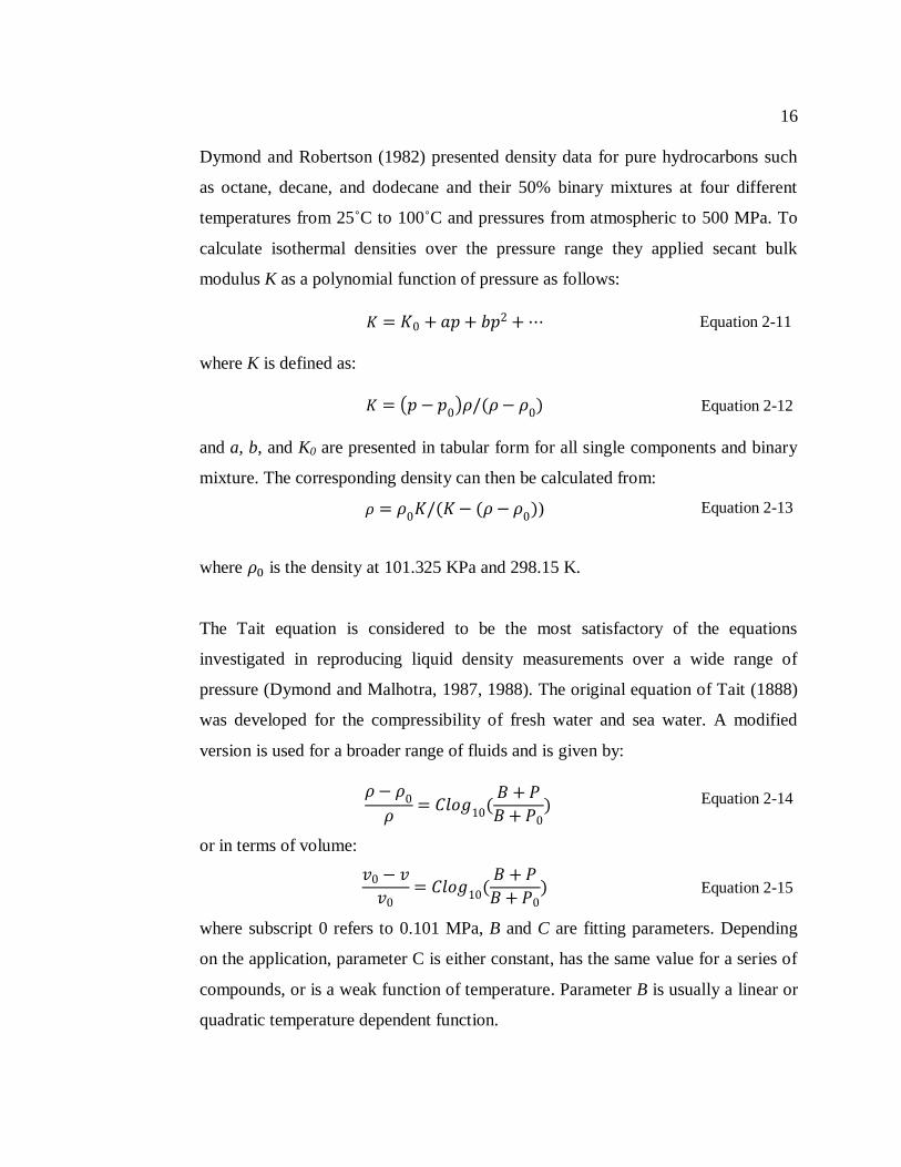
Dymond and Robertson (1982) presented density data for pure hydrocarbons such
as octane, decane, and dodecane and their 50% binary mixtures at four different
temperatures from 25˚C to 100˚C and pressures from atmospheric to 500 MPa. To
calculate isothermal densities over the pressure range they applied secant bulk
modulus K as a polynomial function of pressure as follows:
Equation 2-11
where K is defined as:
Equation 2-12
and a, b, and K0 are presented in tabular form for all single components and binary
mixture. The corresponding density can then be calculated from:
) Equation 2-13
where is the density at 101.325 KPa and 298.15 K.
The Tait equation is considered to be the most satisfactory of the equations
investigated in reproducing liquid density measurements over a wide range of
pressure (Dymond and Malhotra, 1987, 1988). The original equation of Tait (1888)
was developed for the compressibility of fresh water and sea water. A modified
version is used for a broader range of fluids and is given by:
Equation 2-14
or in terms of volume:
Equation 2-15
where subscript 0 refers to 0.101 MPa, B and C are fitting parameters. Depending
on the application, parameter C is either constant, has the same value for a series of
compounds, or is a weak function of temperature. Parameter B is usually a linear or
quadratic temperature dependent function.
17
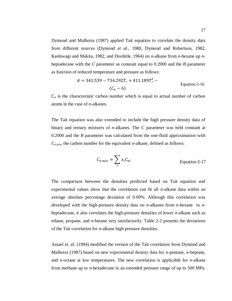
Dymond and Malhotra (1987) applied Tait equation to correlate the density data
from different sources (Dymond et al., 1980, Dymond and Robertson, 1982,
Kashiwagi and Makita, 1982, and Doolittle, 1964) on n-alkane from n-hexane up n-
heptadecane with the C parameter as constant equal to 0.2000 and the B parameter
as function of reduced temperature and pressure as follows:
Equation 2-16
Cn is the characteristic carbon number which is equal to actual number of carbon
atoms in the case of n-alkanes.
The Tait equation was also extended to include the high pressure density data of
binary and ternary mixtures of n-alkanes. The C parameter was held constant at
0.2000 and the B parameter was calculated from the one-fluid approximation with
Cn,mix, the carbon number for the equivalent n-alkane, defined as follows:
The comparison between the densities predicted based on Tait equation and
experimental values show that the correlation can fit all n-alkane data within an
average absolute percentage deviation of 0.09%. Although this correlation was
developed with the high-pressure density data on n-alkanes from n-hexane to n-
heptadecane, it also correlates the high-pressure densities of lower n-alkane such as
ethane, propane, and n-butane very satisfactorily. Table 2-2 presents the deviations
of the Tait correlation for n-alkane high pressure densities.
Assael et. al. (1994) modified the version of the Tait correlation from Dymond and
Malhotra (1987) based on new experimnetal denisty data for n-pentane, n-heptane,
and n-octane at low temperatures. The new correlation is applicable for n-alkane
from methane up to n-hexadecane in an extended pressure range of up to 500 MPa.
Equation 2-17
18
The overal average deviation of the calculated values from those of experimental
measurements is ±0.10%. They modified the parameter B as follows:
for C2H6 to C16H34,
Equation 2-18
where
for C2H6 to C7H16, D=0
for C7H16 to C16H34, D = 0.8 (Cn -7)
and for CH4,
Equation 2-19
There are two main advantages for the improved correlation compared with the old
one (Dymond and Malhotra, 1987): 1) methane was included in the correlation; 2)
the temperature and pressure range was extended. For n-alkane mixtures, they
predicted the mixture density from the pure components densities, assuming there is
no volume change upon mixing. The mixture density was therefore calculated by,
Equation 2-20
19
Table 2-1. Tait Correlation for n-alkanes (Dymond and Malhotra, 1987)
Cibulka and Hnĕdkovskỳ (1996) presented the Tait equation parameters in a tabular
form in temperature and pressure range within the liquid state. They also compared
the results from their fits with those from Assael et al. (1994) and showed that the
deviations are either within or close to the experimental error and are mostly
negative at lower temperature and pressure and positive at higher pressure.
20
Aalto, et al. (1996) applied the Hankinson-Thomson correlation (Hankinson and
Thomson, 1979) to calculate saturate liquid densities and the Chang-Zhao equation
(Chang and Zhao, 1990) to calculate the density in the compressed liquid region.
The Hankinson-Thomson correlation is given by:
where vs is the molar volume of the saturated liquid, v* is a characteristic molar
volume, which is required for each pure compound, VR()
is a spherical model
function, and VR(0)
represents the deviation from spherical molecule behavior.
The Chang-Zhao equation is given by:
where is reduced pressure and is reduced pressure of saturated vapor. C and
D are constants and A and B are modified as following equations:
where a and b values are fitting parameters presented in tabular form, and Tr is
reduced temperature.
Equation 2-21
Equation 2-22
Equation 2-23
Equation 2-24
Equation 2-25
Equation 2-26
21
Aalto, et al. (1996) applied their correlation to a database containing 4426 density
points for 29 pure alkanes and alkenes to fit their model. They compared their
results with those from the two correlations they applied in their work and it was
found that their model was the most accurate of the three models. In the second part
of their work, they tried to apply their correlation to mixtures. They considered the
mixture as a hypothetical pure fluid having the parameter values calculated by
mixing rules. They tried 75 combinations of the mixing rules applying 4223 density
data point for 49 binary and ternary hydrocarbon systems. The new model was
compared to the original HBT correlation (Thomson, et. al., 1982), and based on the
comparison it was found that the new model was more accurate than HBT and
could be applied at higher temperatures near the critical point.
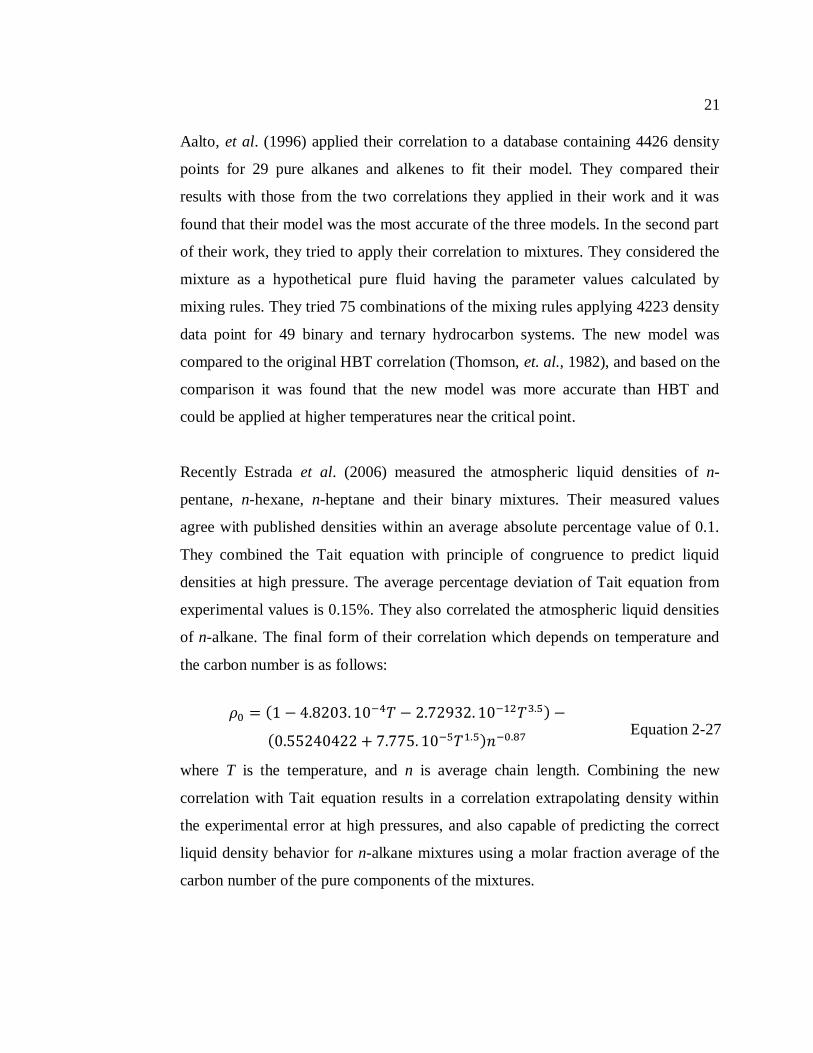
Recently Estrada et al. (2006) measured the atmospheric liquid densities of n-
pentane, n-hexane, n-heptane and their binary mixtures. Their measured values
agree with published densities within an average absolute percentage value of 0.1.
They combined the Tait equation with principle of congruence to predict liquid
densities at high pressure. The average percentage deviation of Tait equation from
experimental values is 0.15%. They also correlated the atmospheric liquid densities
of n-alkane. The final form of their correlation which depends on temperature and
the carbon number is as follows:
where T is the temperature, and n is average chain length. Combining the new
correlation with Tait equation results in a correlation extrapolating density within
the experimental error at high pressures, and also capable of predicting the correct
liquid density behavior for n-alkane mixtures using a molar fraction average of the
carbon number of the pure components of the mixtures.
Equation 2-27
22
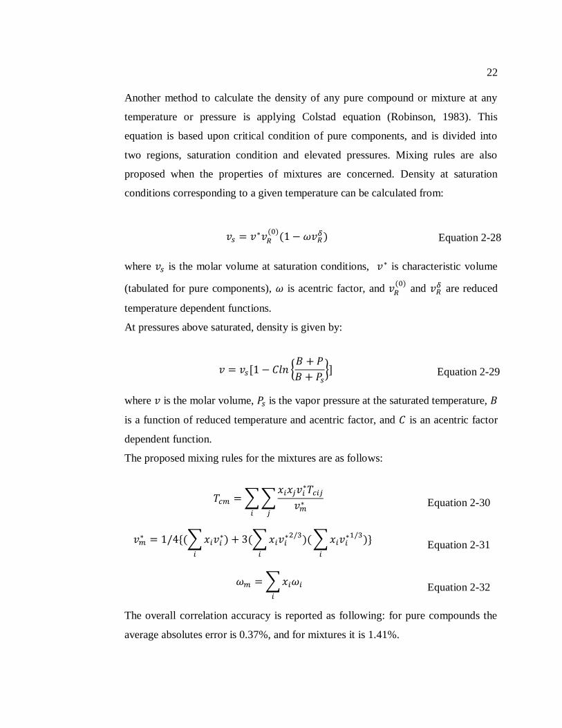
Another method to calculate the density of any pure compound or mixture at any
temperature or pressure is applying Colstad equation (Robinson, 1983). This
equation is based upon critical condition of pure components, and is divided into
two regions, saturation condition and elevated pressures. Mixing rules are also
proposed when the properties of mixtures are concerned. Density at saturation
conditions corresponding to a given temperature can be calculated from:
where is the molar volume at saturation conditions, is characteristic volume
(tabulated for pure components), is acentric factor, and
and are reduced
temperature dependent functions.
At pressures above saturated, density is given by:
where is the molar volume, is the vapor pressure at the saturated temperature,
is a function of reduced temperature and acentric factor, and is an acentric factor
dependent function.
The proposed mixing rules for the mixtures are as follows:
The overall correlation accuracy is reported as following: for pure compounds the
average absolutes error is 0.37%, and for mixtures it is 1.41%.
Equation 2-28
Equation 2-29
Equation 2-30
Equation 2-31
Equation 2-32
23
2.2.3 Corresponding States
The principle of corresponding states holds that fluid properties, such as density, are
the same for most fluids when plotted in reduced coordinates. A reduced property
for a fluid is a given property divided by its value at the critical point of the fluid.
For example, the reduced density at a given reduced temperature and pressure is
expected to be the same for most fluids, particularly dispersion force dominated
fluids such as hydrocarbons.
The graphical Lu Chart method (Lu, 1959) is one of the recommended correlations
in predicting the compressed liquid densities. This correlation is based on the
following approach, suggested by Watson (1943):
where and are the desired density and the density at reference condition,
respectively., and K1 and KR are corresponding correlating parameters. The K
factors are given in graphical form as function of reduced pressure and reduced
temperature. This correlation is valid for a reduced temperature range of 0.5 to 1.0,
and reduced pressure range from saturation to 30.0.
Rea et al., 1973 presented the correlating parameters for Lu Chart, K factors, as a
set of generalized polynomial in terms Tr and Pr. The final form of the equation is as
follows:
where Ai is given by
The values of Bj,i coefficients are presented in tabular form.
Equation 2-33
Equation 2-34
Equation 2-35
24
One of the alternative analytical methods for graphical Lu Chart method is the
generalized equation developed by Yen and Wood (1966) for pure hydrocarbons.
The equation is explicitly relating reduced density to reduced temperature and
reduced pressure. For pure hydrocarbons, usually one corresponding state equation
is applied for saturated liquids and another one for compressed liquids. Francis
(1959) fitted the following equation to the experimental data of saturated pure
liquids with a good accuracy:
where A, B, C, and E are specific coefficients, and T is temperature.
However, Eq. 2-36 is not applicable for temperatures near the critical region. Martin
(1959) improved the correlation near the critical region with the following four
parameter expression:
where is the reduced saturated liquid density (/c where c is the critical
density) and A, B, C, and D are fluid specific constants. Yen and Wood (1966)
found the fourth term in Equation 2-37 to have little effect on its accuracy.
Literature data for sixty-two pure compounds was fitted satisfactorily with the
following three parameter equation:
The coefficients A, B, and D are presented either in tabular form or as generalized
function of the critical compressibility, Zc = Pcvc/RTc, where Pc, Tc, and vc are the
critical pressure temperature and volume respectively, and R is the universal gas
constant.
Equation 2-36
Equation 2-37
Equation 2-38
25
The undersaturated (compressed) liquid density increases with an increase in
pressure and can be correlated as follows:
where the sum of the and is the isothermal pressure effect. The term
is the increase in reduced density for a pure liquid from the vapour pressure
to a given pressure for compound with Zc equal to 0.27. The term is zero for
Zc=0.27 and is a non-zero correction for the isothermal pressure effect on density
for compounds with other Zc values. has been calculated as a function of
reduced temperature and pressure ΔPr and Tr and then fitted to the following
equation:
where , , , and are all defined as function of reduced temperature.
For compounds of the other selected Zc values 0.29, 0.25, 0.23, it is necessary to
calculate values. The values have been calculated as function of ΔPr and Tr
and then fitted to the following equation:
where I, J, K are all defined as function of reduced temperature.
Another alternative analytical method for Lu Chart method is a generalized
correlation presented by Chueh and Prausnitz (1969), as follow:
Equation 2-39
Equation 2-40
Equation 2-41
Equation 2-42
26
where is the compressibility at saturation given as a function of Tr and ω. The
accuracy of the correlation for liquid densities at elevated pressure depends strongly
on the value of the saturated liquid density applied (Rea et al., 1973). The Racket
equation (1970) is an easy and accurate method to predict the saturated liquid
densities over the entire temperature range up to critical temperature (Spencer and
Danner, 1972). This equation is given by:
where ZRA is a specific constant for each compound. If no ZRA is available, Zc can be
used with some loss in accuracy.
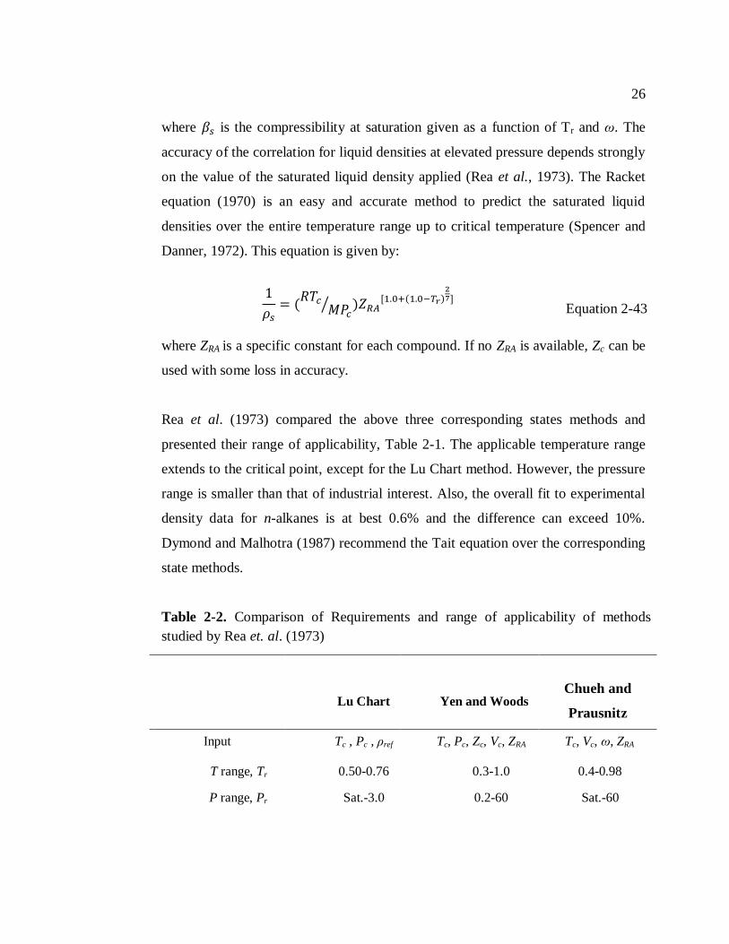
Rea et al. (1973) compared the above three corresponding states methods and
presented their range of applicability, Table 2-1. The applicable temperature range
extends to the critical point, except for the Lu Chart method. However, the pressure
range is smaller than that of industrial interest. Also, the overall fit to experimental
density data for n-alkanes is at best 0.6% and the difference can exceed 10%.
Dymond and Malhotra (1987) recommend the Tait equation over the corresponding
state methods.
Table 2-2. Comparison of Requirements and range of applicability of methods
studied by Rea et. al. (1973)
Equation 2-43
Lu Chart
Yen and Woods
Chueh and
Prausnitz
Input Tc , Pc , ρref Tc, Pc, Zc, Vc, ZRA Tc, Vc, ω, ZRA
T range, Tr 0.50-0.76 0.3-1.0 0.4-0.98
P range, Pr Sat.-3.0 0.2-60 Sat.-60
27
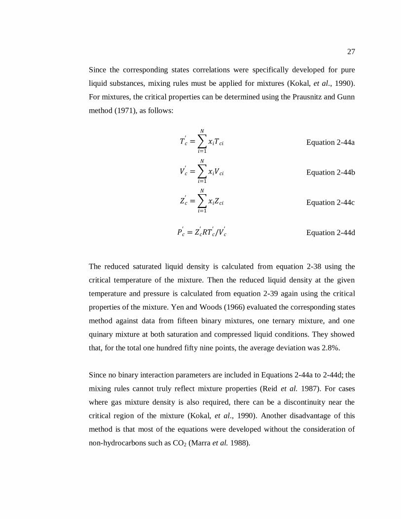
Since the corresponding states correlations were specifically developed for pure
liquid substances, mixing rules must be applied for mixtures (Kokal, et al., 1990).
For mixtures, the critical properties can be determined using the Prausnitz and Gunn
method (1971), as follows:
The reduced saturated liquid density is calculated from equation 2-38 using the
critical temperature of the mixture. Then the reduced liquid density at the given
temperature and pressure is calculated from equation 2-39 again using the critical
properties of the mixture. Yen and Woods (1966) evaluated the corresponding states
method against data from fifteen binary mixtures, one ternary mixture, and one
quinary mixture at both saturation and compressed liquid conditions. They showed
that, for the total one hundred fifty nine points, the average deviation was 2.8%.
Since no binary interaction parameters are included in Equations 2-44a to 2-44d; the
mixing rules cannot truly reflect mixture properties (Reid et al. 1987). For cases
where gas mixture density is also required, there can be a discontinuity near the
critical region of the mixture (Kokal, et al., 1990). Another disadvantage of this
method is that most of the equations were developed without the consideration of
non-hydrocarbons such as CO2 (Marra et al. 1988).
Equation 2-44a
Equation 2-44b
Equation 2-44c
Equation 2-44d
28
2.2.4 Equation of State (EOS)
The simplest equation of state is the ideal gas law:
where P is pressure, R, is the universal gas constant and T is temperature. However,
as its name implies, the ideal gas law can only describe the behaviour of an ideal
gas. The real gas law is given by:
where Z is the compressibility factor. The real gas law can describe the behaviour of
a non-ideal gas but not a liquid. To describe both gas and liquid behaviour,
equations of state generally consist of two terms representing the repulsion and
attraction forces. Van der Waals (1873) proposed the first general equation of state
as follows:
Equation 2-47
where a is the attraction parameter and b is the repulsion parameter (or excluded
volume).
The van der Waals equation shows two crucial improvements comparing with the
ideal gas law. First, the prediction of liquid behaviour is more accurate because at
high pressure the volume reaches a limiting value, the excluded volume:
Equation 2-48
Second, the prediction of non-ideal gas behaviour is improved. The term RT/(v-b)
approximates ideal behaviour and the term a/v² accounts for non-ideal behaviour.
Peng Robinson Equation of State
After the introduction of the van der Waals equation of state (EOS), many other
cubic EOS correlations were developed from the Redlich-Kwong EOS (1949) to the
P = RT/v Equation 2-45
P = ZRT/v Equation 2-46
29
Peng-Robinson EOS (1976). Most petroleum engineering applications rely on the
Peng-Robinson EOS or a modified Peng-Robinson EOS. The Peng and Robinson
(1976) equation of state (PR EOS) is a two-constant equation that resulted in
improved vapour-liquid equilibrium description and also improved liquid density
predictions. The PR EOS is given by:
Equation 2-49
where,
Equation 2-50a
Equation 2-50b
Equation 2-50c
Equation 2-50d
where Tc is critical temperature, Pc is critical pressure, Tr is reduced temperature and
w is acentric factor. The PR EOS can also be expressed or in terms the Z factor (Z =
Pv/RT) as follows:
where,
Equation 2-52a
Equation 2-52b
Equation 2-52c
Although the PR EOS is in widespread application for the description of pure
component vapour pressures and the vapour liquid equilibrium of mixtures, the
predictions of volumetric properties like density, are relatively poor.
Equation 2-51
30
Volume Translation
The density predictions from an equation of state can be improved using a shift
along the volume axis, which leaves the predicted phase equilibrium unchanged.
The volume translation concept was first proposed by Martin (1979). In an
independent study, Peneloux et al. (1982) introduced molar translation, c, to
improve the accuracy of the Soave-Redlich-Kwong (1972) equation of state. The
parameter c can be defined as follows:
where is the saturated liquid volume as predicted by equation of state and
is the experimental saturated liquid volume at a reduced temperature
Tr=0.7. For pure hydrocarbon up to n-decane the following correlation was
presented by Peneloux et al. (1982):
where Tc and Pc are the critical properties of the pure components and ZRA is the
Rackett compressibility factor.
Jhaveri and Youngren (1988) proposed volume shifts for light hydrocarbon for the
Peng-Robinson equation of state. They defined a dimensionless shift parameter s,
as follows:
where b is the co-volume in the EOS. For light hydrocarbons up to n-hexane, s is
represented as a power function of the molecular weight (Mw) by the same authors,
Equation 2-53
Equation 2-54
Equation 2-55
Equation 2-56
31
d and e were also presented for n-alkanes.
Soreide (1989) presented two different temperature dependent correlations. The first
is applicable to light components such as CO2, N2, CH4, C2H6, and to some extent
C3H8 at temperatures higher than critical temperature and is given by:
The second is applicable to components such as C3H8, i-C4H10, n-C4H10, i-C5H10, n-
C5H10, n- C6H10, benzene and is given by:
Magoulas and Tassios (1990) presented another temperature-dependent expression
for c as a function of critical parameters (Tc, Pc, Zc) and acentric factor,
where,
Equation 2-57
Equation 2-58
Equation 2-59
Equation 2-60
Equation 2-61
Equation 2-62
32
where is the critical compressibility factor calculated without volume translation.
Its value is 0.3074 for the Peng-Robinson EOS. Zc is also given by the expression
proposed by Czerwienski et al. (1988) valid up to n-eicosane,
Ungerer and Batut (1997) also suggested a new expression for the volume
translation as a function of temperature and molecular weight:
where
and A and B are expressed in cm³/mol.K and cm³/mol, respectively.
After calculating volume translation term for mixture components, the
pseudovolume for the mixture, , is defined as follows:
Substitution of for in the EOS improves the predictions of volumetric
properties.
Equation 2-63
Equation 2-64
A=0.023-0.00056.MW Equation 2-65a
B=-34.5+0.4666.MW Equation 2-65b
Equation 2-66
33
de Sant’Ana et al. (1998) compared all the above correlations on the determination
of the molar volume of pure hydrocarbon liquid densities (up to C15). Table 2-3 and
Table 2-4 describe the density prediction of different methods by showing the
absolute average error. Table 2-3 shows the absolute average error for high pressure
density prediction, while Table 2-4 shows the absolute average error for saturated
liquid densities.
Table 2-3. Absolute average deviation of saturated liquid density predictions,
temperature between 323.10 and 437.10 K.
component Jhaveri and
Youngren
Soreide Magoulas
and Tassios
Ungerer
and Batut
AAD(%) AAD(%) AAD(%) AAD(%)
n-Hexane 4.17 1.92 1.69 5.77
n-Heptane 1.21 1.49 0.74 1.8
n-Nonane 2.39 4.48 1.13 0.72
n-Undecane 3.27 inapplicable 1.44 0.35
n-Dodecane 3.37 inapplicable 1.44 0.53
n-Tridecane 3.68 inapplicable 1.78 0.81
Cyclopentane Inapplicable inapplicable 1.31 5.76
Cyclohexane Inapplicable 3.54 2.98 1.64
Ethylbenzene 0.44 inapplicable 1.87 1.05
Butylbenzene 0.76 inapplicable 1.96 0.55
Hexylbenzene 1.83 inapplicable 1.49 0.2
Methylcyclopentane Inapplicable inapplicable 1.97 1.55
Methylcyclohexane 1.03 inapplicable 2.17 2.77
Propylcyclopentane Inapplicable inapplicable 2.23 3.14
Propylcyclohexane 3.17 inapplicable 2.40 4.45
Butylcyclohexane 3.87 inapplicable 2.48 4.62
1-Methylnaphtalene Inapplicable inapplicable 3.92 1.36
2-methylnaphtalene Inapplicable inapplicable 3.27 1.81 Saturated liquid densities
tested 2.43 2.86 2.02 2.16
34
The Jhaveri and Youngren (1988) method as well as Ungerer and Batut (1997)
correlation provide very good predictions in the entire pressure-temperature domain
investigated. However, a number of disadvantages must be considered when
applying a specific volume translation method. The Jhaveri and Youngren (1988) as
well as the Soreide (1989) correlations are only applicable for a limited number of
hydrocarbons, which makes them inappropriate for reservoir fluid applications.
Another issue with Jhaveri and Youngren (1988) correlation is that the volume
translation is independent of temperature which restricts temperature extrapolation
at high pressure. On the other hand, the method of Ungere and Batut (1997) can be
easily applied since only the molecular weight of the components is needed.
Therefore, only this method is recommended for reservoir fluid applications.
EOS are commonly applied to predict the phase behaviour of hydrocarbon mixtures,
two factors restrict their practical application as a predictive tool. First, even the
simplest cubic EOS has two or three adjustable parameters and requires the solution
of a cubic equation. Second, the EOS must be tuned with real data from the system
under consideration. Hence, one must know the answer or at least partial answer a
priori to use an EOS. Typically, the saturation properties of the system, including
density, are used as benchmarks and the EOS and volume translation parameters are
adjusted to match these data. Once matched the the benchmarks, it is assumed that
the EOS will provide accurate predictions at any other set of conditions. This is not
necessarily true. Thus, from the practical point of view, one must know the answer
before an EOS can be used (Marra et al. 1988).
Even with volume translation, the prediction of fluid properties from an equation of
state are subject to error due to the inherent limitation on the accuracy of the
equation of state and to the limitation in the characterization of the fluid. This
characterization might be the most significant source of error when dealing with
crude oil (Loria et al., 2009).
35
2.3 Modeling the Density of Liquid with Dissolved Gas
The density of mixtures with dissolved gases can be modeled directly, although not
necessarily accurately, with the equations of state or corresponding states methods.
However, when mixture densities are modeled using mixing rules, a liquid mixture
with a dissolved gas is a special case. The density of the gas dissolved in the liquid
is not the same as the density of the pure gas, Figure 2-7. What then is the correct
density to use in a regular solution mixing rule such as Equation 2-2. One solution
is to determine the density of the gas in a hypothetical liquid state; that is, its
effective density when part of a liquid mixture.
Figure 2–7. The process of dissolving a gas component in a liquid mixture
Standing and Katz (1942) presented an empirical correlation based on this method
to determine the density of liquid hydrocarbon mixtures containing dissolved
methane and ethane. Using compressibilities and thermal expansion coefficients,
they extrapolated measured mixture densities to a reference condition of 101.325
kPa and 15.7°C. Then, they calculated the densities of methane and ethane from the
mixture densities and a regular solution mixing rule. It was assumed that propane
and any higher carbon number components behaved as regular solutions.
The method was originally designed to determine live oil densities. Since the
solution gas composition is usually unknown, Standing and Katz (1942) developed
an applicable correlation for calculating the density when only the oil API gravity,
the gas gravity, and the solution GOR are known. The method is graphical and not
suitable for computer modeling.
36
Tharanivasan et.al. (2011) developed empirical correlations to predict the effective
density of the dissolved gas component in petroleum. His correlations were divided
into two separate groups, one correlation for n-pentane and higher n-alkane and the
other one for light n-alkane from methane up to n-butane and i-butane. The density
data for the higher n-alkanes were fit at a given temperature using a pressure-
dependent compressibility as follows:
Equation 2-67
where o is the density in kg/m³ at 101 kPa, 1 is the compressibility at high
pressure, and where 1 + is the compressibility at low pressure, is
the decay rate from the low to high pressure compressibility, and P is the pressure
in kPa. The correlation parameters were then related to temperature as follows:
where , , and n are fit parameters and T is temperature in K.
For methane, ethane, propane, n-butane, and i-butane the molar volume of the
higher n-alkanes were plotted versus their molar mass and fit with a quadratic
equation. The plot was extrapolated for lighter n-alkane to estimate the molar
volume (and therefore density). The extrapolated densities were fit in the same
procedure as for higher carbon number components with Equation 2-67 but the
temperature dependent parameters were modified as follows:
Equation 2-70a
Equation 2-70b
Equation 2-70c
Equation 2-68
Equation 2-69
37
The fit parameters for the light hydrocarbons were given in a tabular form.
2.4 Heavy Oil Chemistry
2.4.1 Definition and Classification
The word petroleum, which is derived from the Latin petra and oleum, literally
means rock oil. The petroleum industry generally identifies petroleum (also called
crude oil) by its geographic location (e.g. West Texas Intermediate, Brent, or
Oman), API gravity (an oil industry measure of density) and sulfur content are
commonly measured of the value of a crude oil. Crude oils are classified into
different grades based on the physical properties, Table 2-5.
Table 2-4. UNITAR Classification of oil by physical properties at 15.6°C (Gray,
1994)
Conventional petroleum is the part of petroleum which exists in the reservoir in the
liquid state and is mobile enough to flow naturally from the reservoir into the well
bore. Heavy oils have a much higher viscosity (and lower API gravity) than
conventional petroleum, and usually cannot be produced with primary recovery
techniques (Speight, 2007). Heavy oils also have higher asphaltene, sulfur, and
metal contents compared to conventional oils and are more difficult to refine.
Bitumens are even more viscous than heavy oils and are found in oil sand deposits
(Speight, 2007). The largest heavy oil and bitumen resources are located in Canada,
Venezuela, and the Soviet Union and include more than 90% of the world heavy oil
Viscosity (mPa.s) Density (Kg/m3) API Gravity(°API)
Conventional Oil < 102
< 934 >20
Heavy Oil 102 - 10
5 934 – 1000 20 – 10
Bitumen > 102
> 1000 < ~ 10
38
in place (Briggs, et al., 1988). Table 2-6 compares typical heavy-oil properties with
conventional oil.
Table 2-5. Comparison of conventional crude and heavy oil (Briggs, et al., 1988).
Attribute Athabasca Cold Lake Conventional
crude, Alberta
Gravity, ° API 7 to 8 10 to 12 35
Hydrocarbon type, wt%
Saturates 18 to 23 21 70 to 90
Aromatics 29 19
Asphaltene 17 16 0.1 to 2
Resins 35 44 9 to 15
Sulfur, wt% 4.7 4.5 0.1 to 2
Vanadium, ppm NR 250 1 to 5
Nickel, ppm NR 100 1 to 5
Reservoir oil viscosity, cp 500,000 100,000 1
NR – not reported in this source
From a chemical point of view, petroleum is defined as a naturally occurring
mixture of hydrocarbons, oxygen-, nitrogen-, and sulfur-containing compounds plus
a trace amount of metal-containing compounds. The difference in physical
properties between conventional crude oil and bitumen is a result of the variety of
organic constituents and physical conditions that affect the petroleum formation.
This variation in elemental composition and properties resulted in many attempts to
characterize petroleum (Speight, 2007; Whitson, et al., 2000; Riazi, 2005). Carbon
number distribution, distillation curves, distillation residue properties and solubility
class are all used for petroleum characterization (Ortiz, 2009).
39
2.4.2 Heavy Oil Composition
Boduszynski et al. (1987, 1988) developed analytical procedures for the detailed
molecular characterization of heavy crude oils and petroleum residues. They related
heteroatom (S, N, O, V. Ni, Fe) concentration, hydrogen deficiency (H/C atomic
ratio), molecular weight distribution and also molecular chemical composition of
heavy petroleums to their atmospheric equivalent boiling point. Figure 2–8
summarized some of their key observations. For a given homologous series of
compounds, the boiling point increases with molecular weight. At any given
molecular weight, the paraffins have the lowest boiling point. Compounds with
aromatic rings or a functional group capable of hydrogen bonding have higher
boiling point at a given molecular weight because the intermolecular attractive
forces are larger. Figure 2-8 highlights the complexity of crude oils and the
challenges in modeling their properties. In particular, density models or mixing
rules must contend with a complex mixture of hydrocarbons and heteroatomic
species.
40
Figure 2–8. Effect of molecular structure on boiling point (Boduszynski, 1987)
Approximately 20 to 40 wt% of a heavy oil can be distilled and characterized into
boiling fractions. Since the residue fraction is so large, heavy oil and bitumen is
often divided into solubility and polarity classes instead. The most common method
to obtain such classes is SARA fractionation, Figure 2-9, which provides four
fractions: saturates (S), aromatics (A), resins (R), and asphaltene (A). Saturates
consist of non-polar hydrocarbons such as n-paraffins, iso-paraffins, and
naphthenes. Aromatics are the components which adsorb on silica gel and are made
41
up of species with benzene rings. They may have more than one benzene ring, and
also contain attached saturated groups. Resins adsorb in clay and are soluble in the
common organic solvents such as pentane and heptanes. They are also aromatic
molecules but are larger, more polar, and more heteroatomic than the aromatics.
Asphaltene are the materials which are insoluble in n-paraffins such as n-pentane
and n-heptane but soluble in aromatic solvents such as toluene. Asphaltenes have
some unique features and are discussed in more detail below.
Figure 2–9. Schematic of SARA fractionation procedure.
Asphaltenes are dark brown to black friable solids that are precipitated from
petroleum and bitumen by addition of a non-polar hydrocarbon (Speight, 2007). The
classical definition is that asphaltenes are soluble in benzene and insoluble in low
molecular weight n-alkane petroleum-derived solvent. The definition is imprecise
because different solvents precipitate a different amount of asphaltenes, Figure 2-
10, with slightly different properties. Therefore, asphaltenes must be defined by the
procedure used to extract them from the bitumen.
42
Figure 2–10. Effect of solvent carbon number on insolubles (Speight, 2007).
Nonetheless, asphaltenes obtained from different sources are similar. They are the
most aromatic, polar, heteroatomic, and dense species in crude oils. Although
determining the real structure of asphaltenes has proved to be difficult, they mostly
consist of condensed aromatic nuclei that carry alkyl and alicyclic constituents with
hetero-elements (such as nitrogen, oxygen, and sulfur), Figure 2-11. The proportion
of asphaltenes in petroleum changes with origin, depth, API gravity of the crude oil,
and the sulfur content of the crude oil (Kokal, et al., 1995).
0
10
20
30
40
50
60
2 4 6 8 10
wt%
pre
cip
itat
ed
n-alkane carbon number
43
Figure 2–11. A hypothetical Asphaltene structure, A, B and C represent larger
aromatic clusters (Strausz, et al., 1992). Note the structure is larger than typical for
an asphaltene monomer and represents an amalgamated aggregate.
Asphaltenes (or at least some of the asphaltenes) are known to self-associate,
forming aggregates of 6-10 molecules (Speight, 2007; Yarranton et al., 2000).
Asphaltene self-association has been observed by different techniques including
interfacial tension measurements, molar mass measurement which demonstrated
that the asphaltene molar mass distribution is not constant. Asphaltene association
depends on temperature and composition (Agrawala and Yarranton, 2001). This
self-association mechanism is still debated and has been modeled as colloidal
44
aggregation or analogously to linear polymerization (Agrawala and Yarranton,
2001). It is not known what role, if any, aggregation plays in the density of mixtures
including asphaltenes.
2.5 Density of Bitumen and Mixtures with Solvent
2.5.1 Density of Heavy Oil and Bitumen
2.5.1.1 Measurement of Heavy Oil and Bitumen Density
Several techniques are used to determine bitumen (or heavy oil) density such as
pycnometers, displacement, digital density meters, and hydrometers which are
described in ASTM D70, ASTM D71, ASTM 4052, and ASTM D1298,
respectively (Speight, 2001). Since bitumen is highly viscous, sometimes dilution
with a solvent is required to obtain a measurement. The densities of series of a
bitumen/solvent mixture are determined using the desired method and the bitumen
density is calculated from a mixing rule. An important point regarding this density
determination is to assure that solution non-idealities are accounted for in
calculation procedure; if this is not the case, some bias will be introduced into the
determination (Helper and Hsi, 1989) Other problems which can interfere with the
accurate bitumen density determination are:
Residual solids or residual solvent may remain with the bitumen, if an extraction
step is applied to isolate bitumen
Light ends may be lost from bitumen during the isolation step
2.5.1.2 Effect of the Temperature on Heavy Oil and Bitumen Density
Figure 2-12 shows that the density for different Western Canadian crude oils
decreases linearly with temperature. As reported by AOSTRA (1989) Bulkowsky
and Prill studied the density variation of four Athabasca bitumen sample over the
temperature range of 0 to 150˚C and correlated their data as follows:
45
where and 0 are the density kg/m³ at the given temperature (T in ˚C) and 0°C,
respectively.
Gewers (1965) presented the densities of samples of Cold lake and Athabasca
bitumens over the temperature range of 0 to 150˚C. His data can be represented by
the following equations:
8.1 ˚API Athabasca bitumen
10.4 ˚API Cold Lake bitumen
Figure 2–12. The effect of temperature on the density of some Western Canadian
crudes (data from present work).
Equation 2-71
46
2.5.1.3 Effect of Pressure on Heavy Oil and Bitumen Density
The density of crude oil liquid phases increases exponentially with pressure
although a linear approximation is often adequate. Density calculation for oil at
pressures higher than saturation pressure is accomplished by applying the
isothermal compressibility (McCain, 1990) as follows:
where is the density at the saturation pressure, and is the isothermal
compressibility. and can be related to temperature as follows:
where a1, a2, c1, and c2 are constants. Equations 2-71 to 2-74 can be used to fit and
interpolate bitumen liquid density over any given temperature and pressure range.
2.5.2 Density of Heavy Oil and Solvent Mixtures
Mehrotra and Svrcek studied the density and viscosity of several bitumens saturated
with dissolved gas including: Athabasca bitumen saturated with CO2, CH4, and N2
(1982), Marguerite Lake bitumen saturated with CO2, Athabasca bitumen saturated
with CO, and C2H6 (1985), Peace River and Wabasca bitumen saturated with N2,
CO, CH4, CO2 and C2H6 (1985), and Cold Lake bitumen saturated with N2, CH4,
CO2, and C2H6 (1988). They observed that the density decreased with increasing
temperature and pressure, Figure 2-13.
Since their experiments were performed at saturation conditions and not fixed
composition, their data include several effects. Recall that the solubility of the
dissolved gas decreases with increasing temperature but increases with increasing
Equation 2-72
Equation 2-73
Equation 2-74
47
pressure. Therefore, the mixture density in their experiments is expected to increase
as the temperature increases but decrease as the pressure increases. However, the
density of the bitumen itself is expected to change in the opposite direction; that is
to decreases as temperature increases and increase as pressure increases. The overall
changes in density are a combination of these effects.
Figure 2–13. Effect of pressure on density of CH4-saturated bitumen, adopted from
Mehrotra and Svrcek, (1985)
Ashcroft et al., (1992) measured the density of seven different crude oils diluted
with toluene, cyclohexane, n-heptane, and seven other paraffinic solvents at
48
temperatures of 15ºC and 25ºC and atmospheric pressure. They presented the results
in terms of plot of percentage relative excess volume or specific excess volume
versus solvent mass fraction. Their results showed that the volumetric behavior of
these mixtures were similar to the excess volume of binary mixtures of pure
hydrocarbons, Figure 2-2 and 2-3. The maxima appear, at or close to, mass fraction
equal to 0.5. For toluene and cyclohexane diluted bitumen, the excess volume was
positive (expansion upon mixing), while for paraffinic diluted crude oil, the excess
volume was negative. The shrinkage was greatest for the lowest-boiling point
solvent.
Badamchi-zadeh et al., (2009) studied the density of Athabasca bitumen saturated
with propane, Figure 2-14. They observed that the density decreased linearly with
temperature at each composition. They assumed no volume change upon mixing
and predicted the densities within the accuracy of the measurement except at the
highest propane content (25.5 wt%). Given the scatter in the data, it is not clear if
the propane/bitumen mixtures form regular solutions or exhibit small excess
volumes of mixing.
Figure 2–14. Effect of temperature on the density of mixtures of athabasca bitumen
with propane (Badamchi-zadeh et al., 2009)
49
2.5.3 Density Modeling for Mixtures of Heavy Oil and Solvents
Robinson (1983) modeled the density of diluted crude oils based on the Costald
equation which permits inclusion of light end components in the mixture at high
temperature and pressure. He compared his results for diluted crude oil at 15ºC and
1.013 atm with those ones from API Standard 2450. The overall average deviation
was 0.25%.
Erno et al., (1994) measured the volume and density of heavy oil blended with
condensates at 15ºC and 50ºC. They converted the volume to the shrinkage factor
by applying the measured volumes of oil, condensate, and blend. They found
observed shrinkage when a condensate was added to heavy oil. For blends up to
30% condensate, they fitted the shrinkage as follows:
where xc is the condensate volume fraction, and a, b, and c are equal to 0.0249,
-3.31∙10-4
,and 0.823∙10-6
respectively.
Marra et al. (1988) demonstrated that mixing rules can also be used to model the
density of a mixture of crude oil and solvents. They applied the regular solution
concept to develop a simple model for calculating the density of CO2/crude oil
mixtures with engineering accuracy. The mixture density is expressed as follows:
where is the pseudo-liquid density of the system containing CO2, is the
mixture mass, is the pseudo-liquid volume of the system, is the
hydrocarbon mass, is the CO2 mass, is the pseudo-liquid density of the
hydrocarbon and is the pseudo-liquid density of the CO2. If mixture density
Equation 2-75
Equation 2-76
50
data are available, the apparent density of CO2 can be calculated by rearranging
Equation 2-76 as follows:
The apparent liquid density of CO2 can be plotted versus the pseudo-liquid system
density. This plot can be further broken down based on the weight percent of CO2 in
the mixture. This shows that the apparent liquid density of CO2 is a function of CO2
concentration as well as pseudo-liquid system density. Since both apparent liquid
density of CO2 and pseudo-liquid system density both were unknown, the
correlation requires a trial-and-error solution. To eliminate this trial-and-error
solution, a third-order polynomial equation was developed as follows:
where
and
With the correlation in this form, the density can be calculated directly at the
appropriate reservoir pressure and temperature.
Most density modeling for bitumen/solvent systems has been done with cubic
equations of state. Mehrotra et al. (1985) modeled the density of Alberta bitumen
saturated with CO2 and C2H6 using Peng-Robinson equation of state. They
discussed different critical properties correlations including those proposed by
Equation 2-77
Equation 2-78
Equation 2-79
Equation 2-80
51
Cavet (1962), Bergman (1976), Kesler et al. (1976), Huang (1977), and Whitson
(1980). They applied all the above correlations to estimate the critical properties of
bitumen pseudo-components, and summarized the results separately for Athabasca
and Peace River bitumens. The results show that for lighter pseudo-components, the
predicted critical properties from each correlation are similar but for the heaviest
pseudo-component the differences are significant. The predicted Tc, Pc and w were
used in the Peng-Robinson EOS to predict density values. For the density data for
gas-saturated bitumen the predicted densities were highly dependent on which
properties correlation was applied. The predicted density values for CO2-saturated
bitumen were higher than the experimental data for Athabasca bitumen and lower
for Peace River bitumen. The best prediction for Athabasca bitumen was with Lee-
Kesler correlation, 3.6% deviation, and for Peace River was with Bergmann-Cavet
correlation, 2.1%. The predicted densities of gas-saturated bitumen decreased
linearly with temperature for all cases. Increasing the pressure also resulted in a
slight reduction in density, contrary to the expected behavior.
Kokal and Sayegh (1990) modeled the density data for four different Alberta
bitumens (Athabasca, Peace Rive, Wabasca, and Cold Lake) from Svrcek and
Mehrotra (1982, 1984, 1985). They determined the volume translation parameter for
pure components separately below the critical temperature (Equation 2-70) and
above the critical temperature (Equation 2-82):
where c is the volume translation parameter, is the liquid molar volume calculated
from EoS, R is the universal gas constant, and are the component critical
temperature and pressure, and is the Racket compressibility factor.
Equation 2-81
Equation 2-82
52
For mixtures, the c parameter is obtained from the following equation:
where is the components volume translation parameter, and is the component
mole fraction in the mixture. For all systems, the average absolute error percent of
the density predictions was less than 1%.
Loria et al., (2009) develop a new tuning method for the volume translation
parameters applied in the Peng-Robinson equation of state to predict gas-saturated
bitumen densities from Strauzs and Lown (2003). The first step was to calculate the
critical properties, acentric factor, specific gravity and molecular weight of each
pseudo-component based on Lee-Kesler property correlations. Then, the liquid
volume, , of each pseudo-component was calculated as follows.
Once the liquid volume of each pseudo-component is calculated, the volume
translation for each component, ci, was determined as follows:
where vi,PR is the calculated molar volume of the pseudo-component from the EOS
without volume translation. The mixture molar volume is then given by:
and the mixture density was calculated from the corrected molar volume and the
average molecular weight. Note, Loria et al. (2009) set the binary interaction
Equation 2-83
Equation 2-84
Equation 2-85
Equation 2-86
53
parameters for all components to zero. The average absolute error in the calculated
densities was 0.83%.
2.6 Summary
There is currently no generalized method to accurately predict the density of diluted
heavy oils. The most comprehensive method is the equation of state. However,
cubic equations of state (the most commonly used form of EOS) require volume
translation to obtain accurate densities. Generalized volume translations are only
accurate over a limited range of temperatures and pressures and are not usually very
accurate for mixtures. Reasonably density predictions can be obtained if the volume
translation is tuned to a particular dataset but the tuned translations are not likely to
be accurate beyond the conditions used to tune them.
An alternative is to determine the density of hydrocarbon mixtures from correlations
and mixing rules. However, these correlations are usually restricted to the liquid
region and do not easily accommodate dissolved gases. This option is still
appropriate for diluted heavy oils because, in practice, they are almost always far
below their critical point and therefore well into the liquid phase region.
54
3 CHAPTER THREE: EXPERIMENTAL METHODS
This chapter describes the experimental methods used for measuring the density of
mixtures of pure hydrocarbon liquids and bitumen diluted with a hydrocarbon liquid
and with a dissolved hydrocarbon gas. The pure hydrocarbon mixtures include:
propane and n-decane, propane and toluene, propane and cyclooctane, butane and n-
decane and ethane and n-decane. The hydrocarbons used for the diluted bitumen
mixtures are propane and n-heptane. The materials and apparatus are described and
the experimental procedure is discussed.
3.1 Materials
Ethane 99% purity, propane 99.5% purity and n-butane 99.5% purity were
purchased from PraxAir Canada Inc. Decane 99.7% purity, cyclo-octane purity ≥
99%, and omnisolv high purity toluene 99.99% purity, were purchased from Fischer
Scientific, Sigma-Aldrich, and VWR respectively. Technical grade acetone and
toluene were applied for cleaning the apparatus and were supplied by VWR.
Reverse osmosis water supplied by the University of Calgary water plant and
Nitrogen 99.9% purity from PraxAir was used for apparatus calibration.
Two samples of bitumen from the same source (WC-B-B2 and WC-B-B3) were
received from Shell Energy Canada. This bitumen was recovered from a steam
assisted gravity process and was distilled by ARC (Alberta Research Counsel) to
remove water and solids. For convenience WC-B-B2 and WC-B-B3 bitumen are
denoted as Bitumen A and Bitumen B, respectively, throughout the thesis.
55
3.2 Apparatus Description
Figure 3-1 shows the schematic of the apparatus which consists of two transfer
vessels connected on either side of an Anton Paar mPDS 2000V3 density meter. An
air bath enclosed the apparatus and maintained a fixed temperature. The pressure
was maintained and controlled by a Quizix Pump model Q5200. The main
components of the apparatus are described below.
Figure 3–1. Schematic of the density measurement apparatus.
3.2.1 Anton Paar Density Meter
The in-line Anton Paar DMA HPM density meter cell has a built-in temperature
sensor which was used to measure the equilibrium temperature. The cell is
connected by an interface module to an Anton Paar mPDS 2000V3 evaluation unit
displaying the meter oscillation period and the temperature. The oscillation period
was measured with precision of ±0.001 micro seconds and the temperature
56
measured with a precision of 0.01 C. Both are required to obtain an accurate density
from the density meter.
The Anton Paar density meter is based on the measurement of the period of
harmonic oscillation of a quartz U-tube. The sample fluid is injected into the U-tube
and its density alters the oscillation period. The U-tube can be described as un-
damped oscillation of a mass suspended from a spring (Lagourette et al., 1992). The
period of oscillation for an oscillator with one degree of freedom is given by:
M
E2 Equation 3-1
where is the oscillation period, E is the elasticity constant of the spring, and M is
the summation of U-tube mass and the sample fluid mass given by:
00 .VMM Equation 3-2
where Mo is the U-tube mass, and Vo and are the volume and density of the fluid
in the U-tube. Substituting Equation 3-3 into Equation 3-4 and rearranging gives:
0
02
0
24 V
M
V
E
Equation 3-3
The above equation is simplified as follows:
BA DD 2.
Equation 3-4
where DA and DB are pressure and temperature dependent constants They are
determined at any given temperature and pressure from a calibration to two fluids of
known densities. Once the constants are known, the density of the sample fluid can
be determined. The calibration procedure is outlined in Section 3.3.
57
3.2.2 Quizix Pump
The Quizix SP-5200 pump system has three functions: 1) accurate volumetric
injection for sample preparation, 2) sample mixing, 3) pressure control during the
experiment. Sample preparation is described later. The process which creates the
sample mixture ensures that the total composition is correct but does not ensure that
the mixture is uniform throughout the total volume. The sample is mixed by flowing
it through the density meter between the two sample cylinders with the pump in a
volumetric flow mode. The mixture is considered uniform when a constant
period/density is observed when the entire sample is displaced through it. The
direction of flow through the meter is determined with the use of control vales
which will allow the hydraulic fluid from the pump either into the sample cylinder
or discharge to the back pressure regulator.
The final function of the pump is to provide an accurate stable pressure at which to
take the readings once the fluid has equilibriated at temperature. To achieve
constant pressure, the pump is set in a constant pressure mode and allowed to settle
to a zero flow rate at the given temperature equilibrium.
3.2.3 Back Pressure Regulator (BPR)
The BPR has two main functions: 1) is to act as a safety relief valve to protect
against over pressurization of the system during temperature increases, 2) to
maintain a constant pressure for mixing ensuring that the fluid mixed in the
apparatus is always above the mixture bubble pressure. The BPR back pressure is
set by adjusting the pressure in the BPR air control cylinder.
3.2.4 Air Bath Temperature Control
The test fluid temperature is maintained using the air bath model POM-136B-1. It
has self-tuning temperature controller that regulates the input power to the heating
element of the air bath to maintain the temperature within ±0.1°C. The air bath is
equipped with a circulating fan to reduce temperature gradients inside the air bath.
58
For accuracy in experimental data the air bath temperature is adjusted to provide the
equilibrium temperature based on the temperature readings from the Anton Paar
meter’s high accuracy temperature sensor. The precision of the sensor is ±0.01 C.
Hence, the accuracy of the temperature is limited by consistency of the air bath
control rather than the temperature sensor.
3.3 Apparatus Calibration
Apparatus calibration has three key factors which must be confirmed or adjusted
for: temperature, pressure, and density. The first two factors are straightforward.
First, the Anton Paar comes from the factory with a temperature certification.
Second, the pressure is read from the pump pressure which was confirmed versus a
lab calibration gauge.
The density is determined from the two unknown density meter constants (Equation
3-4) which must be calibrated. The density meter was calibrated to nitrogen and
degassed reverse osmosis water for temperatures of 25, 50, 75, 125, and 175 °C and
pressures of 10, 12.5, 15, 17.5, 20, 25, 30, 35, and 40 MPa. The densities of the
calibration fluids were taken from the Anton Paar DMA HPM manual. The
calibration constants were determined at each temperature and pressure and linearly
interpolated versus the period squared for intermediate conditions. Note, the
accuracy of the temperature control at 25°C was not sufficient for calibration
purposes. Therefore, a linear extrapolation (with a correction factor based on
measured n-decane densities at 18°C) was used to estimate the density meter
constants for any measurements at temperatures below 50ºC. The n-decane densities
were compared with data from NIST (standard reference database, version 2008) for
the correction.
The pure components density data were compared with literature values to verify
the calibration. Figure 3-2 and 3-3 show the comparison between the literature
density data and experimental values of propane and n-decane at various
59
temperatures, respectively. The AARD for propane is 0.17% and for n-decane is
0.12%. The AARD are within the error of the measurements. Note that the error in
the measurements in this work is smaller than the symbols in Figures 3-2 and 3-3.
Figure 3–2. Comparison between experimental and literature data for propane
density.
60
Figure 3–3. Comparison between experimental and literature data data for n-decane
density.
3.4 Sample Preparation
Hydrocarbon Mixtures with Dissolved Gas
First, two transfer cylinders were prepared, each containing one of the solvents to be
used in the experiment. The liquid solvent was poured into the first transfer vessel
which was capped, and then vacuumed and pressurized to remove any air cap that
may have been trapped. A second transfer vessel was connected to a bottle
containing the gas to be dissolved in the liquid hydrocarbon, pressure tested, and
purged. The gas was flowed into the transfer cylinder and then compressed to a
liquid state, Figure 3-4.
61
Figure 3–4. Charging the transfer cylinder for the compressed gas.
Next, the compressed gas was transferred into a third transfer cylinder (the sample
cylinder). The transfer cylinder containing the compressed gas was connected to the
sample cylinder which was pressure tested and purged. Then, the pump was used to
displace a specified volume of compressed gas (in the liquid state) from the transfer
cylinder to the sample cylinder, Figure 3-5. The compressed gas volume in the
sample cylinder was determined from the pump displacement and verified from the
volume of displaced hydraulic oil from the sample cylinder. The same procedure
was used to transfer a specified volume of the liquid solvent to the sample cylinder.
The mass of each solvent was determined from the volumes and densities of the
components at the temperature and pressure of the displacements.
An important point regarding gas injection into the sample cylinder is the sample
cylinder dead volume determination. While starting the compressed gas injection,
for the first 3 to 3.5 cm³ of pump displacement no hydraulic oil transferred out. This
volume is the sample cylinder dead volume which must be accounted for in
62
composition calculations. . The reported compositions are estimated to be accurate
to within 0.30 wt% (see Appendix D for details).
Figure 3–5. Charging from transfer cylinder to the sample cylinder.
Diluted Bitumens
Diluted bitumen samples were prepared using a contactor which consisted of a 600
cm³ horizontal 5 cm diameter cylinder equipped with a piston at each end and a
perforated plate placed in the middle of the cylinder. Heating tape was used to
control the temperature. Before each experiment, the contactor was cleaned and
weighed. Compressed gas was displaced to the contactor as described previously.
The contactor was reweighed to verify the mass of compressed gas in the sample
vessel. The same procedure was used to inject the required volume of bitumen. The
contactor was again weighed to determine the mass of bitumen. Then, the sample
63
was brought to 50ºC and compressed to above its bubble point. The sample was
displaced back and forth through the mixing plate in the contactor for
approximately 8 hours per day. The pressure and volume were monitoring over
night and the mixture was considered to be equilibrated when there was no longer
any volume or pressure change, typically after one week of mixing. After the
sample had equilibrated it was transferred to the transfer vessel used for the
experiment. The reported compositions are estimated to be accurate to within 0.3
wt% (see Appendix D for details).
3.5 Experimental Procedure
The sample cylinder, containing the test fluid, was connected to the apparatus as
shown in Figure 3-1. A second empty transfer cylinder was connected to the other
end of the apparatus and the whole apparatus was pressure tested with compressed
air to 40 MPa. The apparatus was depressurized and vacuumed. Then, the test fluid
was displaced into the apparatus from the sample cylinder. Once the system was
filled to a pressure greater than bubble pressure, the fluid was displaced back and
forth through the apparatus from one vessel to the other one to obtain a uniform
mixture. It usually took 4 passes through the equipment to create a uniform mixture
where the density was uniform throughout the displacement.
To begin a density measurement, the air bath was set to the target temperature.
When the temperature reading by Anton Paar temperature sensor was constant for
one hour at the intended temperature, the pump was used to set the target pressure.
Once the pressure was constant for 10 minutes, the oscillation period in the Anton
Paar evaluation unit was recorded. Note: there was no flow through the density
meter cell and therefore the fluid pressure inside the density meter was equal to the
pump pressure. Then the conditions were set for the next measurement.
In this thesis, densities were measured at five temperatures from room temperature
up to 175˚C for each mixture and pure component for each mixture at 10, 20, 30,
64
and 40 MPa with a repeat measurement done at 50ºC. The pure component density
was compared with literature data available to verify the accuracy of the
measurements, as noted previously. The pure component densities were repeatable
to within ±0.33 kg/m³, Appendix D based on a 90% confidence interval. Densities
for diluted bitumens (six temperatures from room temperature up to 175˚C and five
pressures from atmospheric to 10 MPa) were measured by Hamed Motahhari as part
of another project using the same procedures. These data are also used in this thesis.
The diluted bitumen densities were repeatable to within ±0.18 kg/m³, Appendix D.
3.6 Apparatus Clean-up
After taking the measurements for a sample fluid, the apparatus was cleaned before
the next experiment. For the hydrocarbon mixtures, the apparatus was depressurized
and the transfer vessels removed. The lines and density meter were flushed at room
temperature with toluene, followed by acetone, and then dried. The transfer vessels
were also washed with toluene and acetone, and then dried. For the diluted
bitumens, the sample was displaced to one transfer vessel which was depressurized
and emptied. The transfer vessel was filled with toluene, reconnected to the
apparatus. The toluene was then displaced back and forth five times through the
apparatus at room temperature over a time span of not less than half a day. The
toluene wash was repeated approximately 5 times until the toluene was clear. A
final wash was performed at 100ºC for approximately one day including the time
for heating and cooling.
65
4 CHAPTER FOUR: RESULT AND DISCUSSION
In this chapter, effective liquid densities are determined for n-alkanes and the
regular solution and excess volume mixing rules are applied to diluted bitumens.
First, the mixing rules are tested on density data for mixtures of pure liquid
hydrocarbons. Then, the validity of the effective density correlation presented by
Tharanivasan et al. (2011) is discussed and a modified correlation is presented. The
new correlation is tested on density data for liquid hydrocarbon mixtures containing
dissolved gas. Finally, the new correlation and the proposed mixing rules are tested
on the density data collected for diluted bitumens.
4.1 Density of Mixtures of Liquid Hydrocarbons
Mixtures of liquid hydrocarbons were examined to test the excess volume based
mixing rule that is the basis of the modeling in this thesis. Chevalier et al. (1990)
presented a comprehensive dataset for the density of mixtures of liquid
hydrocarbons including binary mixtures of n-alkane/n-alkane, n-alkane/branched, n-
alkane/cyclic, n-alkane/aromatic, aromatic/cyclic, and aromatic/aromatic. Table 4-1
summarizes the systems for which density was measured. All the measurements
were taken at 298.15 K and 101 kPa.
The densities of each binary system were fitted with an excess volume mixing rule
of the following form:
Equation 4-1
where 1, 2, w1, and w2 are the component densities and mass fractions,
respectively, and 12 is the binary interaction coefficient between the two
components. The last term in the equation is the excess volume. When 12 is zero,
66
the excess volume is zero and the binary pair forms a regular solution. The values of
12 used to fit the Chevalier et al. dataset are provided in Table 4-2.
67
Table 4-1. Pure hydrocarbon mixtures for which density was measured by Chevalier
et al.(1990).
68
Table 4-2. βij values for different types of pure hydrocarbon mixtures
Mixture βij Mixture βij
n-alkane + n-alkane n-alkane + aromatic
hexane + heptanes 0.0006 decane + benzene -0.0150
hexane + octane 0.0014 hexane + o-xylene 0.0073
hexane + decane 0.0042 decane + o-xylene -0.0019
hexane + dodecane 0.0024 tetradecane + o-xylene -0.0034
hexane + tetradecane 0.0060 decane + toluene -0.0061
hexane + hexadecane 0.0057 tetradecane + toluene -0.0070
n-alkane + branched n-alkane + cyclic
hexane + isooctane 0.0009 hexadecane + cyclohexane -0.0085
decane + isooctane 0.0025 hexane + methylcyclohexane 0.0030
tetradecane + isooctane 0.0046 decane + methylcyclohexane -0.0017
decane + 3methylpentane 0.0037 hexadecane+ methylcyclohexane -0.0021
hexadecane + 3methylpentane 0.0080
tetradecane + 2methylhexane 0.0044 aromatic + branched
decane + 2,2dimethylpentane 0.0031 benzene + o-xylene -0.0052
hexadecane + 2,2dimethylpentane 0.0069 benzene + p-xylene -0.0041
decane + 2,2dimethylhexane 0.0008 toluene + o-xylene -0.0009
hexadecane + 2,2dimethylhexane 0.0030 toluene + p-xylene -0.0002
o-xylene + p-xylene 0.0003
cyclic + aromatic
cyclohexane + benzene -0.0131
cyclohexane + o-xylene -0.0103
methylcyclohexane + toluene -0.0067
69
Not surprisingly, components of similar size in the same chemical family form
nearly regular solutions. For example, the mixture of n-hexane and n-heptane can be
fitted with a regular solution mixing rule (12 = zero) with an absolute average
deviation of only 0.01%, Figure 4-1. As the size difference between the molecules
increases, the excess volume also increases. For example, a 12 of +0.0057 is
required to fit the densities of mixtures of n-hexane and n-hexadecane, Figure 4-2.
Mixtures of molecules of different chemical families also tend to have non-zero
excess volumes. Figure 4-3 shows that, although the density of cyclohexane and n-
hexadecane are similar, their mixtures do not form regular solutions and a 12 of -
0.0085 is required to fit the data.
Figure 4–1. Measured and fitted density of mixtures of n-hexane + n-heptane (data
adapted from Chevalier, et al., (1990)).
70
Figure 4–2. Measured and fitted density of mixtures of n-hexane + n-hexadecane
(data adapted from Chevalier, et al., (1990)).
.
Figure 4–3. Measured and fitted density of mixtures of cyclohexane + n-hexadecane
(data adapted from Chevalier, et al., (1990)).
71
Figure 4-4 shows the trend in 12 values versus the normalized molecular weight
difference between the components, MWN, which is defined as:
The 12 of binaries involving n-alkanes and branched n-alkanes increases linearly
with an increase in the normalized molecular weight difference. The 12 of all other
combinations of chemical family decrease with an increase in the normalized
molecular weight difference although there is considerable scatter. The scatter is not
surprising given that structural differences between the molecules are not accounted
for.
Figure 4–4. The relationship between binary interaction parameters in the excess
volume mixing rule and the normalized molecular weight differenc.
-0.020
-0.015
-0.010
-0.005
0.000
0.005
0.010
0 0.2 0.4 0.6 0.8 1
Normalized Molecular Weight Difference
BinaryInteractionParameter,β12
alkane-alkane
alkane-branched
alkane-aromatic
alkane-cyclic
aromatic-aromatic
aromatic-cyclic
21
212
MWMW
MWMWMWN
Equation 4-2
72
Figure 4-5 shows that a better correlation is observed when 12 values are plotted
versus the normalized specific volume difference of the two components which is
defined as:
where v is the specific volume (the inverse of mass density). In this case, the 12 of
mixtures of components from the same chemical family all increase linearly on the
same trend line with increasing normalized specific volume difference.
Interestingly, the 12 of mixtures of components from different chemical families all
appear to group on another positive trend line. There is some scatter, particularly at
lower values of normalized specific volume difference and therefore it is not clear
how well the trends will extrapolate to diluted bitumen systems.
Figure 4–5. The relationship between binary interaction parameters in the excess
volume mixing rule and the normalized specific volume difference.
-0.02
-0.015
-0.01
-0.005
0
0.005
0.01
0.015
0 0.1 0.2 0.3 0.4
Normalized Specific Volume Difference
BinaryInteractionParameter,β
12
alkane-alkane
alkane-branched
aromatic-aromatic
alkane-aromatic
alkane-cyclic
aromatic-cyclic
21
212
vv
vvvN
Equation 4-3
73
4.2 Density of Mixtures with Gas Dissolved in a Hydrocarbon Liquid
It is proposed to calculate the density for mixtures containing a dissolved gas
component using the same mixing rule as applied to liquid mixtures but with an
effective liquid density for the gas. Tharanivasan et al. (2011) determined effective
densities for n-alkanes at pressures above 10 MPa. They extrapolated the molar
volumes of liquid n-alkanes plotted versus molecular weight to determine
hypothetical or “effective” liquid molar volumes of lower n-alkanes that were gases
in their pure state. The molar volume data were fitted with a quadratic equation at
fixed temperatures and pressures, Figure 4-6.
Figure 4–6. n-Alkane molar volumes versus molecular weight at 80°C and 10 MPa.
The effective molar volumes were converted to effective liquid densities ( =
MW/v) and then plotted versus pressure at each fixed temperature, Figure 4-7. The
hypothetical data for each component were fitted with an exponential function of
temperature and pressure. Tharanavasan et al. (2011) used the effective densities to
predict the density of a live conventional oil within experimental error. However,
74
there are two issues with Tharanivasan et al. correlation. First, the correlation
underestimates densities at pressures lower than 10 MPa, Figure 4-7. Second, the
correlation has not been rigorously tested on mixtures of hydrocarbons with
dissolved gases.
Figure 4–7. Effective liquid density of lower n-alkanes at 80°C and different
pressuress from Tharanivasan et al., 2011.
The Tharanivasan et al. correlation was tested on the density of mixtures of
methane and n-decane (NIST standard reference database, version 2008). As will be
discussed later, these mixtures are nearly regular solutions. The effective liquid
density for methane was calculated from the regular solution mixing rule and
compared with the value predicted from Tharanivasan et al. (2011). Figure 4-8
shows that the back-calculated methane density falls below the extrapolated curve.
0
100
200
300
400
500
600
700
0 20000 40000 60000 80000 100000
Pressure, kPa
Eff
ecti
ve D
en
sit
y, kg
/m³
n-butane
propane
ethane
methane
fitted
75
Examining Figure 4-8, it appears that the molar volumes of the lightest liquid n-
alkanes are skewed to higher values because these n-alkanes are approaching their
critical points. When the molar volumes of only the higher n-alkanes are
considered, Figure 4-9, the molar volume trend is linear and extrapolates almost
exactly to the experimentally derived effective density of methane. Therefore, the
correlation was redeveloped using on the molar volumes of the higher liquid n-
alkanes whose molar volumes were linearly related to their molecular weight.
Figure 4–8. Comparison of extrapolated n-alkane molar volumes from Tharanivasan
et al. (2011) with experimentally derived molar volume of methane at 80°C and 10
MPa.
76
Figure 4–9. Comparison of extrapolated n-alkane molar volumes using only higher
n-alkanes with experimentally derived molar volume of methane at 80°C and 10
MPa.
4.2.1 New Effective Density Correlation for Light n-Alkanes
To develop the new effective density correlation, the higher n-alkane molar volumes
at fixed temperatures and pressures were extrapolated linearly to determine new
effective molar volumes for the lighter n-alkanes. The effective molar volumes were
converted to density and plotted versus pressure at fixed temperatures, Figure 4-10.
The effective densities all followed linear trends versus pressure and were fitted as
follows:
where A and B are temperature dependent constants, defined as follows:
Equation 4-4
Equation 4-5
77
where a1, a2, b1, and b2 are fitting parameters. The values for the parameters are
provided in Table 4-3. The linear effective density equations are recommended for
n-heptane and lower carbon number hydrocarbons. For n-alkanes higher than n-
heptane, the Tharanivasan et al. (2011) correlation based on measured densities,
Equation 2-67, is recommended. Note, the new correlation now matches the
effective densities at all pressures including below 10 MPa. Also, all of the
proposed correlations are only valid in the liquid region and will be inaccurate near
the critical point.
Figure 4–10. New effective density of lower n-alkane series at 80°C and different
pressures.
Equation 4-6
78
Table 4-3. The fitting parameters of the new effective density correlation.
Component a1 a2 b1 b2
kg/m³ kg/m3K kPa
-1 kPa
-1.K
-1
Methane 532.157 -0.69737 0.0004261 1.1426E-06
Ethane 704.9 -0.82749 0.0002144 2.0115E-06
propane 793.847 -0.85489 5.309E-05 2.4404E-06
n-butane 846.443 -0.85024 -5.45E-05 2.6479E-06
n-pentane 878.006 -0.82817 -9.23E-05 2.6481E-06
n-hexane 901.512 -0.80985 -0.000142 2.6846E-06
n-heptane 918.603 -0.791551 -0.000177 2.6919E-06
4.2.2 Validation of New Effective Density Correlation
The new correlation was validated against density data collected for three types of
hydrocarbon mixtures: n-alkane/n-alkane, n-alkane/aromatic, and n-alkane/cyclic.
Table 4-4 summarizes the mixtures, composition, and conditions for which density
data were obtained. The data for methane/n-decane and methane/toluene were
obtained from the NIST database (NIST standard reference database, version 2008)
and the data for methane/n-tetradecane, methane/n-octadecane, ethane/n-
tetradecane, and ethane/n-octadecane are obtained from Nourizadeh et al., (2012)
and Kariznovi et al., (2012) work, respectively. The rest of the data were measured
in this work and are tabulated in Appendix A.
The mixtures of propane and n-decane are presented as an example to illustrate the
performance of the new correlation. The densities of these mixtures are shown at
different temperatures and pressures at compositions of 6, 12.5, and 25 wt% in
Figures 4-11 to 4-13, respectively. The mixture densities were predicted using the
regular solution mixing rule and the effective densities from the new correlation
(dashed lines on all figures). The predicted densities are generally within 1% of the
79
measured values except at conditions where the mixture is approaching its critical
point; that is, at high temperature, low pressure, and high dissolved gas content. The
good agreement with the data indicates that mixtures of propane and n-decane do
form regular or nearly regular solutions and that the effective densities are accurate
at least for mixtures of n-alkanes. However, it is necessary to develop a criterion
related to the proximity to the critical point to identify where the correlation breaks
down.
80
Table 4-4. Summary of the pure hydrocarbon mixtures and their composition, and
temperature and pressure range for which density data collected.
Mixture Composition
(wt%)
Temperature
Range (˚C)
Pressure
Range (MPa) Source
methane/n-decane
4.6, 10.1, 20.8
4.9, 9.7, 14.5,
26, 71.8
38 – 171
20 – 100
Up to 70
Up to 140
Lee et al.,
(1966)
Canet et al.,
(2002)
methane/n-tetradecane 0.7 – 4.4 22 – 175 Saturation
Pressure
Nourizadeh et
al., (2012)
methane/n-octadecane 0.5 – 3.4 50 – 175 Saturation
Pressure
Kariznovi et al.,
(2012)
ethane/n-tetradecane 1.7 – 52 50 – 150 Saturation
Pressure
Kariznovi et al.,
(2012)
ethane/n-octadecane 1.2 – 39 50 – 150 Saturation
Pressure
Nourizadeh et
al., (2012)
ethane/n-decane 6, 12.5 20 – 175 10 – 40 this work
propane/n-decane 6, 12.5, 25 20 – 175 10 – 40 this work
n-butane/n-decane 6, 12.5, 25 20 – 175 10 – 40 this work
methane/toluene 5.5, 9.3, 14.8,
23.7, 76.8 20 – 100 Up to 140
Baylaucq et al.,
(2003)
propane/ toluene 6, 12.5, 25 20 – 175 10 – 40 this work
propane/cyclooctane 6, 12.5, 25 20 – 175 10 – 40 this work
81
Figure 4–11. Measured and predicted densities for mixtures of 6 wt% propane and
94 wt% n-decane.
Figure 4–12. Measured and predicted densities for mixtures of 12.5 wt% propane
and 87.5 wt% n-decane.
82
Figure 4–13. Measured and predicted densities for mixtures of 25 wt% propane and
75 wt% n-decane.
To develop a criterion to define the range of validity of the correlation, the limiting
pressure and temperature were identified at which the error in the calculated mixture
density exceeded 1%. The critical point of the mixture was determined using the
Advanced Peng Robinson Equation of State in VMGSimTM
software (Virtual
Material Group Ltd.) with the default interaction parameters. The limiting
temperature and pressure were converted to reduced coordinates and then the
reduced limiting temperatures and pressures for all the binary mixtures measured in
this work were plotted, Figure 4-14. Each symbol represents the boundary between
accuracy less than 1% (to the right) or better than 1% (to the left). Most of the
boundary points cluster along a line and therefore the following criterion was
defined for the valid range of the correlation:
Equation 4-7
83
Only the data for 12.5 wt% ethane in n-decane violated the criterion. Possible
explanations are: a composition error in the data, the criterion does not apply to
more extreme differences in component properties, the critical point of the mixture
is calculated incorrectly, or excess volumes must be accounted for. Note that the
critical temperatures of diluted bitumens are expected to be high except at very high
dilutions and therefore the effective density correlation is expected to be valid for
all conditions of interest to this work.
Figure 4–14. Reduced temperature and pressure at which the effective density
correlation gives more than 1% error in mixture densities (to right of each point).
The criterion, Equation 4-7, was used to screen the data listed in Table 4-4. The
accuracy of the correlation was then assessed against all of the screened data.
Dispersion plots of the predicted density versus measured density for mixtures of
butane/n-decane, propane/n-decane, ethane/n-decane, ethane/n-tetradecane,
ethane/n-octadecane, methane/n-decane, methane/n-tetradecane, and methane/n-
84
octadecane are shown in Figures 4-15 to 4-22, respectively. The average absolute
deviation (AAD), average absolute relative deviation (AARD), maximum absolute
deviation (MAD), and maximum absolute relative deviation (MARD) for each case
are summarized in Table 4-5. The predicted densities are generally in very good
agreement with data with the highest deviations occurring when the fluid
approaches the critical region and reaches the boundary where the correlation is no
longer valid. There is no clear evidence of a systematic deviation at higher solvent
contents that would be expected if there were excess volumes of mixing. There is
some scatter in the ethane/n-decane and methane/n-decane mixture data which
could obscure the excess mixing volumes. Nonetheless, based on the data available,
it is concluded that these mixtures of n-alkanes form regular or nearly regular
solutions.
Figure 4–15. Predicted versus measured density for mixtures of n-butane and n-
decane.
85
Figure 4–16. Predicted versus measured density for mixtures of propane and n-
decane.
Figure 4–17. Predicted versus measured density for mixtures of ethane and n-
decane.
86
Figure 4–18. Predicted versus measured density for mixtures of ethane and n-
tetradecane (Kariznovi et al., 2012).
Figure 4–19. Predicted versus measured density for mixtures of ethane and n-
octadecane (Nourizadeh et al., 2012)
87
Figure 4–20. Predicted versus measured density for mixtures of methane and n-
decane (data from NIST database, 2008).
Figure 4–21. Predicted versus measured density for mixtures of methane and n-
tetradecane (Nourizadeh et al., 2012)
88
Figure 4–22. Predicted versus measured density for mixtures of methane and n-
octadecane (Kariznovi et al., 2012)
89
Table 4-5. AAD, AARD, MAD, and MARD of pure hydrocarbon mixtures.
Mixture AAD
(kg/m3)
AARD
(%)
MAD
(kg/m3)
MARD
(%)
n-butane / n-decane 1.8 0.26 6.5 0.97
propane / n-decane 2.0 0.30 6.5 0.97
ethane / n-decane 5.4 0.75 8.3 0.96
ethane / n-tetradecane 3.5 0.53 7.5 1.15
ethane/ n-octadecane 3.8 0.57 6.3 0.95
methane / n-decane 6.2 0.93 19.5 3.06
methane / n-tetradecane 2.8 0.40 4.1 0.57
methane / n-octadecane 3.5 0.50 6.8 0.95
propane / toluene 2.5 0.33 6.9 0.99
propane / cyclooctane 2.4 0.32 7.1 0.95
methane / toluene 3.5 0.47 14.9 2.90
Dispersion plots for the densities of mixtures of propane/toluene,
propane/cyclooctane, and methane/toluene are also shown in Figures 4-23 to 4-25,
respectively. The AD, ARD, MAD, and MARD for the predicted densities of these
mixtures are provided in Table 4-5. The results are similar to those obtained for
mixtures of n-alkanes. Hence, the effective densities appear to be valid for any
hydrocarbon mixtures. Again, there is little evidence of excess mixing volumes
except perhaps for the mixtures of methane and toluene, Figure 4-25. Table 4-6
compares the effective density values for methane, ethane, propane, and n-butane
with API density values (API, 1992).
90
Figure 4–23. Predicted versus measured density for mixtures of propane and toluene.
Figure 4–24. Predicted versus measured density for mixtures of propane and
cyclooctane.
91
Figure 4–25. Predicted versus measured density for mixtures of methane (C1) and
toluene: a) regular solution mixing rule; b) excess volume mixing rule with ij = -
0.006.
Table 4-6. Comparison between the effective liquid density of dissolved gas
components with their API liquid density value at standard condition.
Compound Liquid density @ 60 F
and 1 atm (kg/m³)
Effective density @ 60 F
and 1 atm (kg/m³)
ARD
(%)
methane 299.7 330.5 10
ethane 355.9 465.7 31
propane 506.5 546.7 7.9
n-butane 583.4 600.6 3.0
92
4.3 Bitumen Density Correlation
Before considering the density of diluted bitumens, it is necessary to determine the
density of the bitumens themselves. The measured densities are shown for Bitumens
A and B in Figure 4-26 and 4-27, respectively, and are tabulated in Appendix B. In
order to calculate mixture densities at conditions in between the measured bitumen
values, the bitumen density data were correlated as follows:
where P is the pressure in MPa, is the density at atmospheric pressure, and co is
the oil compressibility. The atmospheric density and oil compressibility were
related to temperature as follows:
where T is the temperature, and AB, BB, CB, and DB are fitting parameters. The fitted
parameters for Bitumens A and B are provided in Table 4-7. The correlations fit the
density data with an AAD of 0.32 for Bitumen A and 0.26 for Bitumen B and an
AARD of 0.03% for both bitumen A and B (solid lines in Figures 4-26 and 4-27).
The density of Bitumen B was approximately 2 kg/m³ greater than that of Bitumen
A at any given temperature and pressure. The small difference in density may arise
from small differences in the amount of light ends in each sample after their
treatment to remove water and solids.
Equation 4-8
Equation 4-9
Equation 4-10
93
Figure 4–26. Measured and correlated density of Bitumen A.
Figure 4–27. Measured and correlated density of Bitumen B.
94
Table 4-7. Fitted parameters for Bitumens A and B.
Bitumen AB
(kg/m³)
BB
(kg/m³K)
CB
(1/MPA x 104)
DB
(1/K)
Bitumen A 1204.5 -0.6496 1.295 0.0045
Bitumen B 1205.4 -0.6470 1.488 0.0041
4.4 Diluted Bitumen Density
Table 4-8 summarizes the bitumen mixtures and conditions for which the density
was measured. The data for propane diluted bitumen were collected in this work.
The data for the other diluted bitumens were collected by Motahhari in the same lab
(As part of another project with AER group, 2012). Note, Bituman A was used for
the measurements with n-heptane and propane while Bitumen B was used for the
measurements with ethane and n-butane.
Table 4-8. The composition, temperatures, and pressures of the diluted bitumens for
which density data were collected.
Mixture Composition
(wt%)
Temperature
Range (˚C)
Pressure
Range (MPa) Source
Bitumen A / n-heptane 15, 30 20 - 175 0.1 – 10 Motahhari
(2011)
Bitumen B / n-butane 7.3, 14.5 20 - 175 0.1- 10 Motahhari
(2012)
Bitumen A / propane 5.5, 12, 16 20 - 150 1 – 10 This work
Bitumen B / ethane 5.2 20 - 150 2.5 - 12.5 Motahhari
(2012)
95
Figures 4-28 to 4-31 are dispersion plots of the calculated versus measured density
for bitumen diluted with n-heptane, n-butane, propane, and ethane, respectively.
The density was calculated with the regular solution mixing rule (a) and the excess
volume mixing rule (b). For heptane, butane, and propane the measured density was
higher than the density calculated from the regular solution mixing rule. In other
words, the mixtures shrank upon mixing (negative excess volume. There is a
significant size difference between the solvent molecules and the majority of the
molecules in the bitumen. The shrinkage is likely a consequence of different sized
molecules packing more efficiently than similar sized molecules. The shrinkages
observed for the dissolved gases were similar to that observed for the liquid mixture
of heptane and bitumen. Even with the regular solution mixing rule, the average
absolute deviations did not exceed 9 kg/m³, Table 4-9, only slightly outside the
accuracy of the measured mixture densities (±3 kg/m³ based on ±0.5 wt% accuracy
in the composition measurement). Hence, the effective liquid density correlations
appear to be valid for diluted bitumens as well as mixtures of pure hydrocarbons.
The mixtures of ethane and bitumen appear to be regular solutions. However, the
data may be anomalous given that mixtures of more dissimilar components are
expected to be less ideal. It is possible that there is a composition error that skews
the data or that the effective liquid density determined for liquid ethane is slightly
too high. There is insufficient information to reach a definite conclusion at this time.
There also may be a systematic difference between Bitumen A and Bitumen B.
Bitumen A appears to form less regular solutions with the n-alkanes than Bitumen
B. Given that both bitumen samples were obtained from the same source, it seems
unlikely that the physical behaviour of the two samples would differ. Rather, the
differences may arise from non-representative sampling. For example, if the
bitumen samples were not perfectly homogeneous, the subsamples used to measure
the bitumen density may not be identical to the subsamples used to measure the
diluted bitumen densities.
96
The density data were also fitted with the excess volume mixing rule and a single
binary interaction parameter for each diluted bitumen system. The binary interaction
parameters used to fit the data are provided in Table 4-9 along with the deviations
for the regular solution mixing rule and excess volume mixing rule. The excess
volume mixing rule fit the data almost within the precision of the individual density
measurements (±0.4 kg/m³ based on ±0.5°C temperature fluctuation).
Figure 4–28. Calculated versus measured density for n-heptane (C7) diluted
Bitumen A: a) regular solution mixing rule; b) excess volume mixing rule with ij =
+0.022.
750
800
850
900
950
1000
750 800 850 900 950 1000
Measured Density, kg/m³
Calc
ula
ted
Den
sit
y, kg
/m³
15 wt% C7
30 wt% C7
(a)
750
800
850
900
950
1000
750 800 850 900 950 1000
Measured Density, kg/m³
Calc
ula
ted
Den
sit
y, kg
/m³
15 wt% C7
30 wt% C7
(b)
97
Figure 4–29. Calculated versus measured density for n-butane (C4) diluted
Bitumen B: a) regular solution mixing rule; b) excess volume mixing rule with ij =
+0.013.
Figure 4–30. Calculated versus measured density for propane (C3) diluted Bitumen
A: a) regular solution mixing rule; b) excess volume mixing rule with ij = +0.040.
750
800
850
900
950
1000
750 800 850 900 950 1000
Measured Density, kg/m³
Calc
ula
ted
Den
sit
y, kg
/m³
7.3 wt% C4
14.5 wt% C4
(a)
750
800
850
900
950
1000
750 800 850 900 950 1000
Measured Density, kg/m³C
alc
ula
ted
Den
sit
y, kg
/m³
7.3 wt% C4
14.5 wt% C4
(b)
750
800
850
900
950
1000
750 800 850 900 950 1000
Measured Density, kg/m³
Calc
ula
ted
Den
sit
y, kg
/m³
5.5 wt% C3
12 wt% C3
16 wt% C3
(a)
750
800
850
900
950
1000
750 800 850 900 950 1000
Measured Density, kg/m³
Calc
ula
ted
Den
sit
y, kg
/m³
5.5 wt% C3
12 wt% C3
16 wt% C3
(b)
98
Figure 4–31. Calculated versus measured density for ethane (C2) diluted Bitumen
A: a) regular solution mixing rule; b) excess volume mixing rule with ij = -0.001.
Table 4-9. AAD, AARD, MAD, and MARD of diluted bitumen mixtures.
Mixture
Regular Solution
Mixing Rule
Excess Volume
Mixing Rule
AAD
(kg/m³)
ARD
(%) ij
AAD
(kg/m³)
ARD
(%)
Bitumen A + n-heptane 7.3 0.83 +0.022 1.1 0.13
Bitumen B + n-butane 2.8 0.33 +0.013 1.1 0.12
Bitumen A + propane 8.9 1.0 +0.040 0.6 0.07
Bitumen B + ethane 0.4 0.04 -0.001 0.4 0.04
Additional data were also available for n-decane diluted heavy oil (Kumar, 2012)
and toluene diluted Bitumen A maltenes (Sanchez, 2012). The fitted ij for the
750
800
850
900
950
1000
750 800 850 900 950 1000
Measured Density, kg/m³
Calc
ula
ted
Den
sit
y, kg
/m³
(a)
750
800
850
900
950
1000
750 800 850 900 950 1000
Measured Density, kg/m³C
alc
ula
ted
Den
sit
y, kg
/m³
(b)
99
respective mixtures were -0.002 and 0.008. The data are provided in Appendix C.
The ij values for these mixtures are in good agreement with the values found for
mixtures of pure hydrocarbons, Figure 4-32.
The best fit values of ij for the diluted bitumens do not appear to follow a clear
trend. For example, the βij values required to match each data point for each
bitumen/solvent system were calculated and compared with the ij values
determined for pure hydrocarbon mixtures, Figure 4-32. Although for each solvent,
the ij values appear to increase as the normalized specific volume difference
increases, the average ij values from solvent to solvent are scattered. For instance,
the ij data for n-heptane and propane appear to fall on a linear extrapolation of the
ij of the pure hydrocarbon mixtures (dashed line) whereas the data for n-butane and
ethane deviate significantly from this trend.
To make density predictions for mixtures without density data, it is necessary to
predict ij. One approach is to fit the ij to the normalized specific volume
difference. The following quadratic extrapolation (solid line) provides a more
optimized but still imperfect fit for all of the mixtures:
The quadratic extrapolation is plausible given that mixtures of an n-alkane with a
non-hydrocarbon do show a maximum in the excess mixing volumes when plotted
against carbon number of the n-alkane (see Figure 2-5). However, the correlation is
inexact possibly because the calculated densities of the mixtures can be skewed by
small errors in the effective liquid densities and bitumen densities.
The quadratic fit of the βij was used to calculate the density of the diluted bitumen
mixtures. Figure 4-33 shows the measured and calculated densities of the diluted
bitumens at 50°C (a) and 100°C (b). The AAD and AARD are less than 3.6 kg/m³
Equation 4-11
100
and 0.4%, respectively, at all temperatures, pressures, and compositions considered.
In other words, using effective liquid densities and the excess volume mixing rule
with the ij from Equation 4-11 provides a density prediction for diluted bitumens
that is within 3.6 kg/m³ of the measured values. An alternative is to use an average
constant ij of approximately 0.02. With a ij of 0.02, the AAD and AARD are less
than 4.5 kg/m³ and 0.5%, respectively, at all temperatures, pressures, and
compositions considered.
101
Figure 4–32. Comparison of binary interaction parameters for diluted bitumens and
pure hydrocarbon mixtures.
Figure 4–33. Density of bitumen diluted with n-alkanes at: a) 50°C and 2.5 MPa; b)
100°C and 10 MPa. Equation 4-11 was used to determine the ij for the excess
volume mixing rule.
102
5 CHAPTER FIVE: CONCLUSION AND RECOMMENDATION
5.1 Summary
Density was measured for n-alkane binary mixtures at pressures from 10 to 40 MPa
and temperatures from room temperature up to 175˚C. The mixtures included: n-
decane plus ethane, propane, and n-butane; toluene and propane; cylooctane and
propane. Density data were also collected for bitumen diluted with: ethane
(Motahhari, 2012), propane, n-butane (Motahhri, 2012), and n-heptane at pressures
from atmospheric up to 10 MPa.
A new density correlation was developed based on the effective density concept
introduced by Tharanivasan et al., (2011). To determine the effective densities of
light n-alkanes, the molar volume data of higher n-alkanes (C7 and up) were linearly
extrapolated versus molecular weight. The calculated effective liquid molar
volumes of the lower n-alkane were converted to mass density and then correlated
to temperature and pressure. A criterion related to the critical temperature and
pressure of the mixture was developed to define the range of validity for the
correlation. The effective density correlation was then applied to predict the density
of diluted bitumens.
5.2 Conclusions
The main conclusions from this thesis are presented below:
1. The density of hydrocarbon mixtures can be modeled, generally within
experimental error, using a symmetric excess volume based mixing rule. The
mixing rule includes a binary interaction parameter which can be determined
by fitting experimental data. The binary interaction parameters for
hydrocarbon pairs appear to correlate to the normalized molar volume
difference between the two components.
103
2. A correlation was developed for the effective liquid density of dissolved
gases. The effective density values were linearly pressure dependent and the
model applied parameters which were linearly temperature dependent. The
correlation when applied with a regular solution mixing rule, predicted the
density of mixtures of pure hydrocarbons within measurement error. The
correlation is applicable in the liquid region and is suitable for bitumen and
solvent mixtures.
3. Shrinkage was observed when bitumen was diluted with an n-alkane; in other
words, there is a negative excess volume for these mixtures. The shrinkage
was typically less than 1%. Such shrinkage is typical when mixing
hydrocarbons of different size and indicates a more efficient packing at the
molecular level.
4. Binary interation parameters were required to fit the density of diluted
bitumens. The βij values for diluted bitumens did not follow a consistent trend.
Nonetheless, they were correlated to the normalized difference in molar
volume with a quadratic function. The mixture densities were predicted to
within 3.6 kg/m³ using this correlation.
5.3 Recommendations
To improve the effective density model and to enhance its capability the following
recommendations are made in terms of experimental data and modeling methods:
1. For pure hydrocarbon mixtures, data were collected for different types of
mixtures involving light n-alkanes including n-alkane/n-alkane, n-
alkane/aromatic, and n-alkane/cyclic pairs. It is recommended to evaluate n-
alkane/branched alkane mixtures to extend the applicability of the model.
104
2. In this thesis, the only gases studied as solvents were hydrocarbons.
However, other gases such as CO2 and N2an be also applied in solvent-
assisted heavy oil recovery techniques. These gases could be considered in
future studies to extend the applicability of the effective density model.
3. Mixtures of ethane and bitumen appear to form regular solutions. However
mixtures of more dissimilar components are expected to be less ideal. It is
possible that there is a composition error or that the effective liquid density
determined for liquid ethane is slightly too high. It is recommended to
collect more data on the mixture of ethane diluted bitumen to validate the
results presented in this thesis.
105
References
Aalto, M., Keskinen, K. I., Aittamaa, J., and Liukkonen, S. (1996). An Improved
Correlation for Compressed Liquid Densities of Hydrocarbon. Part 1. Pure
Compounds. Fluid Phase Equilibria , 114, 1-19.
Agrawala, M., Yarranton, H.W. (2001). An Asphaltene Association Model
Analogous to Linear Polymerization, Industrial and Engineering Chemistry, 4664-
4672.
Alonso, M. C., Poveda Vilches, J. L., Sanchez-Pajares, R. G., and Delgado, J. N.
(1983). Excess Volumes of (Tolunene + n-alkanes). Chemical Thermodynamics ,
913-917.
American Petroleum Institute Technical Data Book, Petroleum Refining, Refining
Department, 5th
Edition, New York, May 1992.
Ashcroft, S., Isa, M. (1997). Effect of the Dissolved Gases on the Densities of
Hydrocarbons, Chemical and Engineering Data, 1244-1248.
Ashcroft, S., Bookers, D., and Turner, J. (1992). Volumetric Behaviour of Mixtures
of Crude Oils and Light Hydrocarbons. Journal of Institute of Energy , 131-136.
Assael, M. J., Dymond, J. H., and D., E. (1994). An Improved Representation for n-
Alkane Liquid Densities. International Journal of Thermophysics , 155-164.
Aucejo, A., Burguet, M. C., Munoz, R., and Marques, J. L. (1995). Densities,
Viscosities, and Refractive Indices of Some n-Alkane Binary Liquid Systems at
298.15 K. Chemical and Engineering Data , 141-147.
Audonnet, F., and Padua, A. A. (2004). Viscosity and Density of Mixtures of
methane and n-decane from 298 to 393 K and up to 75 MPa. Fluid Phase Equilibria,
235-244.
Badamchi-Zadeh, A., Yarranton, H. W., W.Y, a. S., and B.B, M. (2009). Phase
Behaviour and Physical Property Measurements for VAPEX Solvents: Part I.
Propane and Athabasca Bitumen . Canadian Petroleum Technology , 54-61.
Badamchi-Zadeh, A., Yarranton, H., Maini, B., and Satyro, M. (2009). Phase
Behaviour and Physical Property Measurements for VAPEX Solvents: Part II.
Propane, Carbon Dioxide and Athabasca Bitumen . Canadian Petroleum
Technology , 57-65.
106
Bergman, D. (1976). Prediction of the Phase Behavior of the Natural Gas. PhD
Thesis, Univeristy of Michigan .
Boduszynski, M. (1987). Composition of Heavy Petroleums. 1. Molecular
Weight,Hydrogen Deficiency, and Heteroatom Concentration as a Function of
Atmospheric Equivalent Boiling Point up to 1400 OF (760 "C). Energy and Fuels ,
2-11.
Boduszynski, M. (1988). Composition of Heavy Petroleums. 2. Molecular
Characterization. Energy and Fules , 597-613.
Briggs, P., Baron, R., and Fulleylove, R. (1988). Development of Heavy Oil
Reservoirs. Petroleum Technology , 206-214.
brØnsted, J. N., and Koefoed, J. (1946). Det. Kgl. Danske Videnske Selsk. Mat.
Fys. Medd. , 22, 1-32.
Canada's Oil Sands—Opportunities and Challenges to 2015: An Update..
http://www.neb.gc.ca/clfnsi/rnrgynfmtn/nrgyrprt/lsnd/pprtntsndchllngs20152006/qa
pprtntsndchllngs20152006-eng.html, National Energy Board of Canada, 2007-06-
30, 2007
Canet, X., Baylaucq, A., Boned, C. (2002). High-Pressure (up to 140 MPa)
Dynamic Viscosity of the Methane + Decane System. International Journal of
Thermophysics, 1469-1486.
Cavet, R. H. (1962). Physical Data for Distillation Calculation Vapor-Liquid
Equilibria. 27th mid-year meeting of API, Division of Refining . San Francisco.
Chang, C., and Zhao, X. (1990). A new generalized equation for predicting volumes
of compressed liquids. Fluid Phase Equilibria , 231-238.
Chevalier, J. L., Petrlno, P. J., and Gaston-Bonhomme, Y. H. (1990). Viscosity and
Density of Some Aliphatic, Cyclic, and Aromatic Hydrocarbons Binary Liquid
Mixtures. Chemical Engineering Data , 206-212.
Chueh, P. L., and Prausnitz, J. M. (1969). A Generalized Correlation for the
Compressibilities of Normal Liquids. AIChE , 471-472.
Cibulka, I., and Hneˇdkovsky, L. (1996). Liquid Densities at Elevated Pressures of
n-Alkanes from C5 to C16:A Critical Evaluation of Experimental Data. Chemical
and Engineering Data , 657-668.
107
Cooper, E. F., and Asfour, A. A. (1991). Densities and Kinematic Viscosities of
Some C6-Cl6 n-Alkane Binary Liquid Systems at 293.15 K. Chemical Engineering
Data , 285-288.
Czerwienski, G. J., Tomasula, P., and Tassios, D. (1988). Vapor - liquid equilibria
with the vdW - 711 equation of state. Fluid Phase Equilibria , 63-83.
de Sant'Anaa, H., Ungerer, P., and de Hemptinne, J. (1999). Evaluation of an
improved volume translation for the prediction of hydrocarbon volumetric
properties. Fluid Phase Equilibria , 193-204.
Doolittle, A. (1964). Specific Volumes of n-Alkanes. Chemical and Engineering
Data , 275-279.
Dymond, J. H., and Malhotra, R. (1987). Densities of n-Alkanes and Their Mixtures
at Elevated Pressures. International Journal of Thermophysics , 541-555.
Dymond, J. H., and Robertson, J. (1982). (p,r,T) of some pure n-alkanes and binary
mixtures of n-alkanes in the range 298 to 373 K and 0.1 to 500 MPa. Chemical
Thermodynamics , 14, 51-59.
Dymond, J. H., Young, K. J., and D., I. J. (1980). Transport properties of
nonelectrolyte liquid mixtures—II. Viscosity coefficients for the n-hexane + n-
hexadecane system at temperatures from 25 to 100‡C at pressures up to the freezing
pressure or 500 MPa. International Journal of Thermophysics , 345-373.
Dymond, J., and Malhotra, R. (1988). The Tait Equation: 100 Years On.
International Journal of Thermophysics , 941-951.
Erno, B., Chriest, J., and Given, R. (1994). Equation Predicts Shrinkage of Heavy
Oil/Condensate Blens. OilandGas Journal , 62-67.
Estrada, M. R., Iglesias-Silva, G. A., and Hall, K. R. (2006). Experimental
Measurements and Prediction of Liquid Densities fo n-alkane Mixtures. Chemical
Thermodynamics , 38, 337-347.
Francis, A. (1959). Pressure-Temperature-Density Relations of Pure Liquids.
Chemical and Engineering Science , 37-46.
Goates, J. R., B, O. J., and B, G. R. (1981). Excess Volumes of n-hexane + n-
heptane, + n-octane, + n-nonane, and + n-decane at 283.15, 298.15, and 313.15 K.
Chemical Thermodynamics , 907-913.
108
Goates, J. R., Ott, J. B., and B., M. J. (1977). Determination of excess volumes in
cyclohexane+ benzene and+ n-hexane with a vibrating-tube densimeter. Chemical
Thermodynamics , 9, 249-257.
Goates, J. R., Ott, J. B., and Grigg, R. B. (1979). Excess Volumes of Cyclo-hexane
+ n-hexane, + n-heptane, + n-octane, + n-nonane, + n-decane. Chemical
Thermodynamics, 497-506.
Gomez-Ibanez, J. D., and Liu, T.-C. (1961). The Excess Volume of Cyclohexane
and Some Normal Alkane. Physical Chemistry, 2148-2151.
Gray, M. (1994). Upgrading Petroleum Residues and Heavy Oils. New York:
Marcel Dekker.
Gunn, R., and Yamada, T. (1971). A Corresponding State Correlation of Saturated
Liquid Volumes. AIChE, 1341-1345.
Hepler, L. G., and Hsi, C. (1989). AOSTRA Technical Handbook on Oil Sands,
Bitumen and Heavy Oils. Edmonton, AB, Canada: Alberta Oil Sands Technology
and Research Authority.
Harnett, D. L., (1982). Statistical Methods, 3rd
Edition, Addision-Wesley
Publication Company.
Hankinson, R., and Thompson, G. (1979). A New Correlation for Saturated
Densities of Liquids and Their Mixtures. AICheE, 659-663.
Huang, P. (1977). Characterization and Thermodynamic Correlations for Undefined
Hydrocarbon Mixtures. PhD Thesis, The Pennsylvania State University .
Hutchings, R. S., and Van Hook, W. A. (1985). Excess Molar Volumes and
deviations from congruence of some binary solutions of an n-alkane in another n-
alkane. Chemical Thermodynamics, 523-529.
Jacobs, F., Donelly, J. K., Stanislav, J., and SVrcek, W. (1980). Viscosity of Gas-
saturated Bitumen . Canadian Petroleum Technology , 46-50.
Jhaveri, B. S., and Youngren, G. K. (1988). Three-Parameter Modification of the
Peng-Robinson Equation of State To Improve Volumetric Predictions . Society of
Petroleum Engineers , 1033-1040.
109
Kariznovi, M., Nourizadeh, H., Abedi, J. (2011). Measurement and Modeling of
Liquid Saturated Properties (Solubility, Density, and Viscosity) of (Ethane + n-
Tetradecane) Binary Systems. Chemical and Engineering Data, 3669-3672.
Kariznovi, M., Nourizadeh, H., Abedi, J. (2012). Measurement and Equation of
State Prediction of Vapor-Liquid Equilibrium and Physical Properties for the
System Methane + n-Octadecane. Fluid Phase Equilibria, 102-106.
Kashiwagi, H., and Makita, T. (1982). Viscosity of twelve hydrocarbon liquids in
the temperature range 298–348 K at pressures up to 110 MPa. International Journal
of Thermophysics , 289-305.
Kesler, M., and Lee, B. (1976). Improve Prediction of Enthalpy of Fractions.
Hydrocarbon Processing , 55, 153-158.
Knapstad, B., Skjolsvik, P. A., and Oye, H. A. (1990). Viscosity of the n-Decane -
Methane System in the liquid phase. Physical Chemistry , 94, 1156-1165.
Kokal, S. L., and Sayegh, S. G. (1995). Asphaltene: The Cholesterol of Petroleum.
Kokal, S. L., and Sayegh, S. G. (1990). Gas-saturated bitumen density predictions
using the volume-translated Peng-Robinson equation of state. Chemical and
Petroleum Technology , 77-82.
Lagourette, B., Boned, C., Saint-Guirons, H., Xans, P., and Zhou, H. (1992).
Densimeter calibration method versus temperature and pressure. Measurement
Science and Technology , 699-703.
Lal, K., Tripathi, N., and Dubey, G. (2000). Densities, Viscosities, and Refractive
Indices of Binary Liquid Mixtures of Hexane, Decane, Hexadecane, and Squalan
with Benzene at 298.15 K. Chemical Engineering Data , 961-964.
Lee, A. L., Gonzalez, M. H., and Eakin, B. E. (1966). Viscosity of Methane/n-
Decane Mixtures. Chemical and Engineerin Data , 11, 281-287.
Lee, I., and Kesler, M. (1975). A Generalized Thermodynamic Correlation Based
on Three-Parameter Corresponding States. AIChE , 21, 510-527.
Loria, H., Pereira-Almao, P., and Satyro, M. (2009). Prediction of Density and
Viscosity of Bitumen Using the Peng-Robinson Equation of State . Industrial and
Engineering Chemistry Research , 10129-10135.
110
Magoulas, K., and Tassios, D. (1990). Thermophysical properties of n-Alkanes
from C1 to C20 and their prediction for higher ones. Fluid Phase Equilibria , 119-
140.
Marra, R., Poettmann, F., and Thompson, R. (1988). Density of Crude Oil Saturated
with CO2. Society of Petroleum Engineering , 815-821.
Martin, J. (1979). Cubic Equations of State-Which? Industrial and Engineering
Chemistry Fundamentals , 81-97.
Martin, J. (1959). Thermodynamic and Transport Properties of Gases, Liquids, and
Solids. New York: American Society of Mechanical Engineers and Mc-Graw Hill.
McCain, W. (1990). The Properties of Petroleum Fluids. Tulsa, Oklahama:
PennWell Publishing Company.
Mehrotra, A. K., and Svrcek, W. Y. (1982). Viscosity, Density and Gas Solubility
Data for Oil Sand Bitumens. Part I: Athabasca Bitumen Saturated with CO and
C2H6. AOSTRA JOURNAL RESEARCH , 263-268.
Mehrotra, A. K., and Svrcek, W. Y. (1985). Viscosity, Density and Gas Solubility
Data for Oil Sand Bitumens. Part II: Peace Rive Bitumen Saturated with N2, CO,
CH4, CO2 and C2H6. AOSTRA JOURNAL OF RESEARCH , 269-279.
Mehrotra, A. K., and Svrcek, W. Y. (1985). Viscosity, Density and Gas Solubility
Data for Oil Sand Bitumens. Part III: Wabasca Bitumen Saturated with N2, CO,
CH4, CO2 and C2H6. AOSTRA JOURNAL OF RESEARCH , 83-93.
Mehrotra, A., and Svrcek, W. (1985). Bitumen Density and Gas Solubility
Predictions Using the Peng-Robinson Equation of State. AOSTRA Journal of
Research , 215-226.
Mehrotra, A., and Svrcek, W. (1988). Properties of Cold Lake Bitumen Saturated
with Pure Gases and Gas Mixtures. Canadian Journal of Chemical Engineering ,
656-665.
NIST Standard Reference Database; NIST/TRC Source Database; WinSource,
Version 2008.
Nourizadeh, H., Kariznovi, M., Abedi, J. (2012). Experimental Measurement and
Equation of State Modeling of Liquid Saturated Properties (Solubility, Density, and
Viscosity) of (Ethane + n-Octadecane) Binary Systems. Chemical and Engineering
Data, 137-141.
111
Nourizadeh, H., Kariznovi, M., Abedi, J. (2012). Vapor-liquid Equilibrium
Measurement and Thermodynamic Modeling of Binary Systems (Methane + n-
Tetradecane). Fluid Phase Equilibria, 96-101.
Oliveira, C., and Wakeham, W. (1992). The Viscosity of Five Liquid Hydrocarbons
at Pressures Up to 250 MPa. International Journal of Thermophysics , 773-790.
Ortiz Gonzalez, D. (2009, April). Effect of Surfactants on Asphaltene Interfacial
Films and Stability of Water-in-Oil Emulsions. PhD Thesis . Calgary, Alberta,
Canada.
Péneloux, A., Rauzy, E., and Fréze, E. (1982). A consistent correction for Redlich-
Kwong-Soave volumes. Fluid Phase Equilibria , 7-23.
Peng, D., and Robinson, D. (1976). A new two-constant equation of state. Industrial
and Engineering Chemistry Fundamental , 59-64.
Racket, H. G. (1970). Equation of State for Saturated Liquids. Chemical and
Engineering Data, 514-517.
Rea, H., Spencer, C., and Danner, R. (1973). Effect of pressure and temperature on
the liquid densities of pure hydrocarbons. Chemical and Engineering Data , 227-
230.
Redlich, O., and Kwong, J. (1949). An equation of state. Fugacities of gaseous
solutions. Chemical Reviews , 233-244.
Reid, R., Prauznitz, J., and Poling, B. (1987). The Properties of Gases and liquids
(4th Edition ed.). New York: McGraw-Hill.
Riazi, M. (2005). Characterization and properties of petroleum fractions. Astm Intl.
Robinson, E. (1983). Calculate Density of Spiked Crudes. Hydrocarbon Processing ,
115-120.
Sarkar, M. (1984). Property Prediction-Gas Saturated Bitumen. Masters Thesis.
Calgary, Alberta, Canada.
Schrodt, J., and Akel, R. (1989). Binary Liquid Viscosities and Their Estimation
from Classical Solution Thermodaynamics. Chemical Engineering Data , 8-13.
Shana'a, M., and Canfield, F. (1968). Liquid Denisty and Excess Volume of Light
Hydrocarbon Mixtures at -165 C. Transactions of the Faraday Society , 2281-2286.
112
Soave, G. (1972). Equilibrium constants from a modified Redlich—Kwong
equation of state. Chemical Engineering Science , 1197-1203.
Sǿreide, I., Improved Phase Behavior Predictions of Petroleum Reservoir Fluids
From a
Cubic Equation of State, “Dr. Ing. Dissertation, Norwegian Inst. Of Technology,
1989
Speight, J. (2001). Handbook of Petroleum Analysis. Laramie, Wyoming: John
Wiley and Sons.
Speight, J. (2007). The Chemistry and Technology of Petroleum. New York: Marcel
Dekker Inc.
Spencer, C., and Danner, R. (1972). Improved Equation for Prediction of Saturated
Liquid Density. Chemical and Engineering Data, 236-241.
Standing, M. B., and Katz, D. L. (1942). Density of Crude Oil Saturated with
Natural Gas. 146.
Strausz, O., and Lown, E. M. (2003). The Chemistry of Alberta Oil Sands Bitumens
and Heavy Oils. Calgary, AB, Canada: Alberta Energy Research Institute.
Strausz, O., Mojelsky, T., and Lown, E. (1992). The molecular structure of
asphaltene: an unfolding story. Fuel , 1355-1363.
Svrcek, W. Y., and Mehrotra, A. (1982). Gas Solubility, Viscosity and density
measurements for Athabasca Bitumen . Canadian Petroleum Technology , 31-38.
Tait, P. (1888). Physics and Chemistry of the Voyage of HMS Challenger.
Tharanivasan, A., Yarranton, H., and Taylor, S. (2011). Application of a Regular
Solution-Based Model to Asphaltene Precipitaion from Live Oils. Energy and Fuel ,
25, 528-538.
Thomson, G., Brobst, K., and Hankinson, R. (1982). An Improved Correlation for
Denisties of Compressed Liquids and Liquid Mixtures. AIChE , 671-676.
Ungerer, P., and Batut, C. (1997). Prediction of the Volumetric Properties of
Hydrocarbons with an Improved Volume Translation Method. Oil and Gas Science
and Technology , 609-623.
Van der Waals, J. D. (1873) Over de Continuiteit van den Gas-en Vloeistoftoestand.
Thesis, Leiden.
113
VMG Sim Software, (2010). Virtual Material Group Ltd., Version 6.0. Calgary.
AB, Canada
Ward, S. H., and Clarke, K. (1950). Determination of Viscosity and Specific
Gravities of the Oils in Samples of Athabasca Bituminous Sand. Edmonton,
Alberta: Alberta Research Council.
Watson, K. (1943). Thermodynamics of the Liquid State. Industrial and
Engineering Chemistry , 398-406.
Whitson, C. (1980). Charazterizing Hydrocarbon Plus Fractions . EUROPEC
Conference. London.
Witek, M., Goldon, A., Hofman, T., and Domanska, U. (1997). Denisties and
Excess Volumes of Methyl 1,1-Dimethylpropyl Ether + Benzene or Cyclohexane or
an Alkane (C6-C16) at 298.15 K. Chemical Engineering Data, 60-63.
Wu, J., and Asfour, A. (1994). Densities and excess molar volumes of eight n-
alkane binary systems at 293.15 and 298.15 K. Fluid Phase Equilibria , 305-315.
Yarranton, H. W, Badamchi-Zadeh, A, Satyro, M. A., Maini, B.B (2008). Phase
Behaviour and Physical Properties of Athabasca Bitumen, Propane and CO2.
Canadian International Petroleum Conference (pp. 1-7). Calgary: Petroleum
Society.
Yarranton, H., Alboudwarej, H., and Jakher, R. (2000). Investigation of Asphaltene
Association with Vapor Pressure Osmometry and Interfacial Tension
Measurements. Industrial and Engineering Chemistry , 2916-2924.
Yen, L., and Woods, S. (1966). A Generalized Equation for Computer Calculation
of Liquid Densities. AIChE, 95-99.
115
APPENDIX A – PURE HYDROCARBON MIXTURES DENSITY DATA
Table A-1. Measured densities for mixtures of 6 wt% ethane and 94 wt% n-decane.
Temperature
(˚C)
Pressure
(MPa)
Measured Density
(kg/m³)
14.68 10 722.2
14.68 20 729.0
14.70 30 734.2
14.71 40 740.0
50.02 10 697.2
50.01 20 705.5
50.02 30 712.6
50.00 40 719.6
75.00 10 676.8
75.01 20 685.0
75.01 30 693.6
75.01 40 701.6
125.02 10 639.1
125.01 20 651.1
125.01 30 660.8
125.01 40 670.3
175.00 20 600.5
175.00 30 627.3
175.00 40 639.7
116
Table A-2. Measured densities for mixtures of 12.5 wt% ethane and 87.5 wt% n-
decane.
Temperature
(˚C)
Pressure
(MPa)
Measured Density
(kg/m³)
21.72 10 679.9
21.71 20 688.4
21.71 30 695.8
21.70 40 701.9
50.00 10 653.0
50.00 20 665.9
50.00 30 673.6
50.00 40 680.9
74.99 10 633.4
74.99 20 646.4
74.99 30 655.5
74.99 40 663.0
124.99 10 582.9
124.99 20 601.8
124.99 30 616.0
124.99 40 627.2
174.99 20 554.0
174.99 30 575.0
174.99 40 590.4
117
Table A-3. Measured densities for mixtures of 6 wt% propane and 94 wt% n-
decane.
Temperature
(˚C)
Pressure
(MPa)
Measured Density
(kg/m³)
18.31 10 721.3
18.31 20 728.1
18.32 30 734.0
18.33 40 741.1
49.99 10 699.0
49.99 20 708.0
49.99 30 715.4
49.99 40 722.9
75.02 10 679.7
75.00 20 689.4
75.00 30 698.0
75.01 40 706.0
124.96 10 641.3
124.97 20 653.7
124.98 30 665.0
124.98 40 674.6
175.02 10 599.9
175.02 20 617.0
175.02 30 631.2
175.03 40 643.4
118
Table A-4. Measured densities for mixtures of 12.5 wt% propane and 87.5 wt% n-
decane.
Temperature
(˚C)
Pressure
(MPa)
Measured Density
(kg/m³)
19.24 10 706.2
19.24 20 713.1
19.22 30 721.1
19.20 40 727.4
49.98 10 685.2
49.98 20 695.1
49.98 30 702.7
49.98 40 710.6
74.98 10 664.5
74.98 20 675.2
74.98 30 684.1
74.97 40 692.2
124.97 10 624.0
124.98 20 637.9
124.99 30 649.9
124.99 40 660.0
175.00 10 579.8
175.01 20 599.5
175.01 30 615.2
175.01 40 628.1
119
Table A-5. Measured densities for mixtures of 25 wt% propane and 75 wt% n-
decane.
Temperature
(˚C)
Pressure
(MPa)
Measured Density
(kg/m³)
19.26 10 673.2
19.27 20 681.6
19.28 30 689.3
19.29 40 698.6
50.00 10 652.7
50.00 20 663.8
50.00 30 672.7
50.01 40 681.2
75.02 10 628.8
75.01 20 641.1
75.00 30 651.7
75.00 40 661.4
124.98 10 582.1
125.00 20 599.8
125.01 30 614.5
125.01 40 626.5
174.99 10 530.4
175.01 20 557.1
175.01 30 576.8
175.00 40 592.2
120
Table A-6. Measured densities for mixtures of 6 wt% propane and 94 wt% toluene.
Temperature
(˚C)
Pressure
(MPa)
Measured Density
(kg/m³)
20.09 10 844.8
20.11 20 852.4
20.14 30 859.3
20.16 40 865.6
49.99 10 818.6
49.98 20 827.5
49.99 30 835.2
49.99 40 843.2
75.02 10 794.3
75.02 20 804.6
75.03 30 813.6
75.03 40 822.2
125.00 10 746.5
125.01 20 760.5
125.01 30 772.4
125.01 40 782.7
175.02 10 694.0
175.00 20 713.9
175.01 30 729.8
175.01 40 743.2
121
Table A-7. Measured densities for mixtures of 12.5 wt% propane and 87.5 wt%
toluene.
Temperature
(˚C)
Pressure
(MPa)
Measured Density
(kg/m³)
20.3 10 809.3
20.31 20 817.4
20.31 30 824.9
20.31 40 831.4
50.00 10 782.2
50.00 20 791.7
50.00 30 800.0
50.01 40 808.4
75.01 10 757.2
75.01 20 767.8
75.00 30 777.9
75.00 40 786.9
125.01 10 704.9
125.02 20 721.1
125.02 30 734.6
125.02 40 746.2
175.01 10 648.6
175.01 20 672.5
175.02 30 690.9
175.02 40 705.8
122
Table A-8. Measured densities for mixtures of 25 wt% propane and 75 wt%
toluene.
Temperature
(˚C)
Pressure
(MPa)
Measured Density
(kg/m³)
20.12 10 760.6
20.14 20 769.7
20.16 30 777.8
20.18 40 784.3
49.95 10 731.7
49.95 20 743.5
49.96 30 753.0
49.96 40 762.3
75.01 10 706.2
75.02 20 719.6
75.02 30 730.9
75.02 40 740.9
125.01 10 651.3
124.97 20 671.9
124.99 30 687.3
124.99 40 700.1
175.01 10 589.7
175.00 20 619.8
175.00 30 641.1
175.00 40 658.2
123
Table A-9. Measured densities for mixtures of 6 wt% propane and 94 wt%
cyclooctane.
Temperature
(˚C)
Pressure
(MPa)
Measured Density
(kg/m³)
20.18 10 823.2
20.18 20 828.8
20.18 30 834.0
20.18 40 839.6
50.02 10 792.8
50.02 20 802.3
50.02 30 810.7
50.02 40 818.6
75.02 10 770.7
75.02 20 779.7
75.02 30 788.6
75.02 40 797.2
125.02 10 733.3
125.02 20 743.0
125.01 30 752.1
125.01 40 762.7
175.00 10 692.7
175.00 20 707.3
175.00 30 719.7
175.00 40 755.2
124
Table A-10. Measured densities for mixtures of 12.5 wt% propane and 87.5 wt%
cyclooctane.
Temperature
(˚C)
Pressure
(MPa)
Measured
Density (kg/m³)
20.41 10 791.4
20.41 20 797.9
20.42 30 804.0
20.42 40 809.8
49.99 10 766.0
49.99 20 774.8
49.99 30 781.9
49.99 40 788.9
74.99 10 746.4
74.99 20 756.0
74.99 30 764.1
74.99 40 771.7
124.97 10 703.4
124.97 20 716.1
124.97 30 726.9
124.97 40 736.3
175.03 10 657.2
175.02 20 674.8
175.02 30 688.9
175.01 40 701.1
125
Table A-11. Measured densities for mixtures of 25 wt% propane and 75 wt%
cyclooctane.
Temperature
(˚C)
Pressure
(MPa)
Measured Density
(kg/m³)
20.85 10 744.1
20.85 20 753.3
20.85 30 759.5
20.85 40 765.8
50.03 10 718.5
50.03 20 728.8
50.02 30 736.9
50.02 40 745.1
74.99 10 695.6
74.99 20 707.2
74.99 30 716.8
74.99 40 725.8
125.00 10 649.1
125.00 20 664.9
125.00 30 678.1
124.99 40 689.1
175.02 10 595.5
175.02 20 619.8
175.03 30 638.1
175.03 40 652.7
126
Table A-12. Measured densities for mixtures of 6 wt% n-butane and 94 wt% n-
decane.
Temperature
(˚C)
Pressure
(MPa)
Measured Density
(kg/m³)
18.46 10 726.3
18.47 20 732.8
18.47 30 738.9
18.48 40 743.9
50.00 10 703.5
50.00 20 712.3
50.00 30 719.4
50.00 40 726.9
75.00 10 684.4
75.00 20 694.1
75.00 30 702.4
75.00 40 710.1
124.98 10 646.5
124.98 20 659.0
124.98 30 669.9
124.98 40 679.1
175.00 10 606.3
175.00 20 623.0
175.00 30 636.8
175.00 40 648.6
127
Table A-13. Measured densities for mixtures of 12.5 wt% n-butane and 87.5 wt%
n-decane.
Temperature
(˚C)
Pressure
(MPa)
Measured Density
(kg/m³)
18.36 10 715.6
18.36 20 721.4
18.36 30 728.4
18.37 40 733.0
50.01 10 692.8
50.01 20 701.1
50.01 30 708.6
50.01 40 716.3
74.98 10 672.9
74.98 20 682.6
74.98 30 691.3
74.98 40 699.3
125.00 10 633.9
125.00 20 646.5
125.00 30 658.1
125.00 40 667.6
175.01 10 591.3
175.01 20 609.3
175.00 30 624.1
175.00 40 636.9
128
Table A-14. Measured densities for mixtures of 25 wt% n-butane and 75 wt% n-
decane.
Temperature
(˚C)
Pressure
(MPa)
Measured Density
(kg/m³)
18.96 10 696.0
18.97 20 704.2
18.97 30 711.0
18.98 40 717.4
50.02 10 669.5
50.02 20 681.2
50.02 30 689.8
50.02 40 698.3
75.00 10 649.1
74.98 20 662.1
74.99 30 672.3
75.00 40 681.0
125.00 10 607.2
125.00 20 625.7
124.99 30 638.9
124.99 40 649.2
174.99 10 567.4
175.00 20 589.5
175.00 30 607.1
175.00 40 620.7
129
APPENDIX B – DEAD BITUMENS DENSITY DATA
Table B-1. Measured densities for dead bitumen A.
Temperature
(˚C)
Pressure
(MPa)
Measured Density
(kg/m³)
19.4 0.1 1014.924
19.4 2.5 1015.911
19.4 5 1017.028
19.4 7.5 1018.455
19.4 10 1019.955
35 0.1 1004.325
35 2.5 1005.159
35 5 1006.375
35 7.5 1007.893
35 10 1009.370
50 0.1 994.200
50 2.5 995.326
50 5 996.709
50 7.5 998.237
50 10 999.514
75 0.1 978.323
75 2.5 979.719
75 5 981.288
75 7.5 982.680
75 10 984.261
100 0.1 962.882
100 2.5 964.522
100 5 966.242
100 7.5 967.852
100 10 969.528
125 0.1 945.677
125 2.5 947.602
125 5 949.528
125 7.5 951.067
125 10 953.123
130
Table B-1: Continued
Temperature
(˚C)
Pressure
(MPa)
Measured Density
(kg/m³)
150 0.1 929.152
150 2.5 931.338
150 5 933.351
150 7.5 935.386
150 10 937.319
175 2.5 915.516
175 5 917.846
175 7.5 920.247
175 10 922.220
131
Table B-2. Measured densities for dead bitumen B.
Temperature
(˚C)
Pressure
(MPa)
Measured Density
(kg/m³)
19.7 0.1 1016.3
19.7 2.5 1017.6
19.7 5 1018.9
19.7 7.5 1020.1
19.7 10 1021.6
50 0.1 995.9
50 2.5 997.3
50 5 998.6
50 7.5 999.9
50 10 1001.3
75 0.1 979.9
75 2.5 981.5
75 5 983.0
75 7.5 984.3
75 10 985.9
100 0.1 964.0
100 2.5 965.8
100 5 967.5
100 7.5 969.1
100 10 970.6
125 0.1 947.6
125 2.5 949.6
125 5 951.4
125 7.5 953.0
125 10 954.9
150 0.1 931.3
150 2.5 933.7
150 5 935.8
150 7.5 937.6
150 10 939.5
175 2.5 917.6
175 5 919.9
175 7.5 922.0
175 10 923.9
132
APPENDIX C – ADDITIONAL DENSITY DATA
Table C-1. Measured densities of n-decane diluted Heavy Oil at 23 ˚C. (Kumar,
2012)
n-decane Mass Fraction
(wt%)
Measured Density
(kg/m³)
0 983.0
15 934.8
25 904.3
30 889.1
35 876.5
100 726.0
Table C-2. Measured densities of toluene diluted Bitumen A Maltene. (Sanchez,
2012)
Maltene Mass Fraction
(wt%)
Measured Density
(kg/m³)
0.969 985.2
0.843 966.3
0.624 940.2
0.461 917.9
0.418 912.1
0.321 901.4
0.226 892.6
0.129 880.5
0.023 869.4
0.006 867.6
0.002 867.2
0.001 867.0
133
6 APPENDIX D - ERROR ANALYSIS
D.1. Accuracy Estimation for Mixture Compositions
The composition of the hydrocarbon mixtures were calculated from the volume
displacements of each phase as follows:
Equation D-1
where V is volume, is density, and 1 and 2 indicate the first and second fluid displaced.
The accuracy of the densities is affected by the accuracy of the measured pressure and
temperature as well as the accuracy of the original density data. The accuracy of the
original density data is in the order of 0.5 kg/m³ (NIST Standard Database, version 2008).
The temperature was constant to within ±0.01 ˚C and therefore had negligible effect on
the density. The accuracy of the pressure gauge used for the displacements was ±100 kPa
which could lead to a density error of 1 kg/m³. Overall, the potential error in the densities
is 1.5 kg/m³.
The first volume displacement is the difference between the estimated dead volume and
the fluid displacement. The largest source of error by far is the dead volume with a
potential error of ±0.5 cm³. The second volume is simply the volume of displaced fluid.
The error in the pump displacement is ±0.01 cm³.
The compositions were calculated assuming the maximum and minimum errors in each
volume and density. The maximum errors are reported in Table D1. Note, the diluted
bitumen compositions were based on gravimetric measurements and the maximum errors
were approximately 0.2 wt% (Motahhari (2012), As part of another project in AER lab).
134
Table D-1. Composition accuracy of pure hydrocarbon mixtures
Mixture Composition (wt%) Variation (±)
C2/C10 6.00 0.20
C2/C10 12.50 0.21
C3/C10 6.00 0.29
C3/C10 12.50 0.26
C3/C10 25.00 0.26
C4/C10 6.00 0.29
C4/C10 12.50 0.29
C4/C10 25.00 0.28
C3/Tol 6.00 0.26
C3/Tol 12.50 0.26
C3/Tol 25.00 0.25
C3/Cyclooctane 6.00 0.26
C3/Cyclooctane 12.50 0.26
C3/Cyclooctane 25.00 0.25
D.2. Repeatability of Density Data
Totals of 44 and 48 repeat measurements were performed for the hydrocarbon mixtures
and diluted bitumens, respectively. The data are presented in Table D-1 and D-2, respectively.
The standard deviations of the hydrocarbon mixture and the diluted bitumen data were 0.33 and
0.18 kg/m³, respectively. The 90% confidence interval of the pure hydrocarbon systems and
diluted bitumen were ±0.54 and ±0.29, respectively. Details are provided below.
First, the mean and standard deviation for each pair of measurements were calculated.
The mean is defined as:
where is the mean, n is the number of repeat measurements, and xi is a measured value.
The sample standard deviation, s, defined as:
Equation D-2
135
It was assumed that the sources of error for each hydrocarbon mixture were the same and
the average sample deviation was calculated from the variances of each measurement pair
using Equation D-3. The same procedure was followed for the diluted bitumens.
To calculate the confidence interval for a single measurement, x, it was assumed that the errors
followed a normal distribution. The characteristic parameter of the normal distribution, Z, is
defined as:
The confidence interval is then given by:
where is the probability a measurement falls outside the confidence interval.
A confidence interval of 90% was utilized in all the error analyzes corresponding to α/2 = 0.05
and giving Z = 1.645 on the cumulative normal distribution table (Harnett, 1982). For a single
measurement and a 90% confidence interval, Equation D-5 becomes:
Equation D-3
Equation D-4
Equation D-5
Equation D-6
136
Table D-2. Error Analysis of Pure Hydrocarbon Mixtures.
Mixture T
(˚C)
P
(MPa)
Solvent
Content
(wt%)
ρ
(1st Pass)
kg/m³
ρ
(2nd Pass)
kg/m³
ρ (avg)
kg/m³ Variance
C2/C10 125 10 6.0 639.1 639.4 639.3 0.01
C2/C10 125 20 6.0 651.1 651.1 651.1 0.00
C2/C10 125 30 6.0 660.8 660.7 660.7 0.00
C2/C10 125 40 6.0 670.3 670.3 670.3 0.00
C2/C10 125 10 12.5 582.9 581.3 582.1 0.67
C2/C10 125 20 12.5 601.8 600.2 601.0 0.66
C2/C10 125 30 12.5 616.0 615.5 615.8 0.05
C2/C10 125 40 12.5 627.2 626.3 626.7 0.19
C3/C10 75 10 6.0 679.7 679.4 679.6 0.02
C3/C10 75 20 6.0 689.4 689.4 689.4 0.00
C3/C10 75 30 6.0 698.0 698.0 698.0 0.00
C3/C10 75 40 6.0 706.0 705.9 706.0 0.00
C3/C10 75 10 12.5 664.5 663.4 664.0 0.30
C3/C10 75 20 12.5 675.2 675.3 675.2 0.00
C3/C10 75 30 12.5 684.1 684.3 684.2 0.02
C3/C10 75 40 12.5 692.2 692.2 692.2 0.00
C3/C10 75 10 25.0 628.8 630.3 629.5 0.54
C3/C10 75 20 25.0 641.1 641.3 641.2 0.01
C3/C10 75 30 25.0 651.7 652.8 652.3 0.27
C3/C10 75 40 25.0 661.4 663.0 662.2 0.65
C3/C10 50 10 6.0 818.6 818.3 818.5 0.02
137
Table D-2. Continued.
Mixture T
(˚C)
P
(MPa)
Solvent
Content
(wt%)
ρ
(1st Pass)
kg/m³
ρ
(2nd Pass)
kg/m³
ρ (avg)
kg/m³ Variance
C3/C10 50 20 6.0 827.5 827.8 827.7 0.02
C3/C10 50 30 6.0 835.2 835.6 835.4 0.03
C3/C10 50 40 6.0 843.2 843.6 843.4 0.03
C3/C10 75 10 12.5 757.2 757.4 757.3 0.01
C3/C10 75 20 12.5 767.8 768.1 768.0 0.02
C3/C10 75 30 12.5 777.9 777.9 777.9 0.00
C3/C10 75 40 12.5 786.9 786.8 786.9 0.00
C3/C10 125 10 25.0 651.3 653.1 652.2 0.85
C3/C10 125 20 25.0 671.9 672.2 672.1 0.02
C3/C10 125 30 25.0 687.3 687.7 687.5 0.06
C3/C10 125 40 25.0 700.1 700.1 700.1 0.00
C4/C10 125 10 6.0 646.5 646.2 646.4 0.02
C4/C10 125 20 6.0 659.0 659.3 659.1 0.02
C4/C10 125 30 6.0 669.9 670.2 670.0 0.03
C4/C10 125 40 6.0 679.1 678.8 678.9 0.02
C4/C10 125 10 12.5 633.9 633.8 633.8 0.00
C4/C10 125 20 12.5 646.5 646.3 646.4 0.00
C4/C10 125 30 12.5 658.1 658.1 658.1 0.00
C4/C10 125 40 12.5 667.6 667.5 667.6 0.00
C4/C10 175 10 25.0 567.4 567.3 567.4 0.01
C4/C10 175 20 25.0 589.5 589.3 589.4 0.00
C4/C10 175 30 25.0 607.1 607.0 607.0 0.01
C4/C10 175 40 25.0 620.7 620.5 620.6 0.01
138
Table D-3. Error Analysis of Diluted Bitumen Mixtures.
Mixture T (˚C) P
(MPa)
Solvent
Content
(wt%)
ρ
(1st Pass)
kg/m³
ρ
(2nd Pass)
kg/m³
ρ (avg)
kg/m³ Variance
Bit/C7 50 0.1 15.00 930.4 930.8 930.6 0.04
Bit/C7 50 2.5 15.00 931.8 932.2 932.0 0.04
Bit/C7 50 5 15.00 933.5 933.9 933.7 0.03
Bit/C7 50 7.5 15.00 935.2 935.6 935.4 0.05
Bit/C7 50 10 15.00 936.9 937.2 937.1 0.02
Bit/C7 75 0.1 15.00 913.8 913.3 913.5 0.06
Bit/C7 75 2.5 15.00 915.5 915.0 915.2 0.06
Bit/C7 75 5 15.00 917.4 917.0 917.2 0.06
Bit/C7 75 7.5 15.00 919.1 918.6 918.9 0.07
Bit/C7 75 10 15.00 920.9 920.3 920.6 0.09
Bit/C7 100 0.1 15.00 896.5 895.9 896.2 0.08
Bit/C7 100 2.5 15.00 898.4 898.0 898.2 0.05
Bit/C7 100 5 15.00 900.4 899.8 900.1 0.07
Bit/C7 100 7.5 15.00 902.4 901.8 902.1 0.09
Bit/C7 100 10 15.00 904.3 904.0 904.2 0.04
Bit/C7 125 0.1 15.00 878.3 878.2 878.3 0.00
Bit/C7 125 2.5 15.00 880.6 880.6 880.6 0.00
Bit/C7 125 5 15.00 882.9 882.8 882.9 0.00
Bit/C7 125 7.5 15.00 885.0 884.9 885.0 0.00
Bit/C7 125 10 15.00 887.3 887.3 887.3 0.00
Bit/C7 150 2.5 15.00 863.5 863.6 863.6 0.00
Bit/C7 150 5 15.00 866.1 866.3 866.2 0.01
Bit/C7 150 7.5 15.00 868.6 868.7 868.6 0.00
Bit/C7 150 10 15.00 871.0 871.1 871.0 0.01
Bit/C7 50 2.5 30.00 872.8 872.9 872.9 0.00
Bit/C7 50 5 30.00 874.7 874.9 874.8 0.01
Bit/C7 50 7.5 30.00 876.6 876.7 876.6 0.00
Bit/C7 50 10 30.00 878.6 878.6 878.6 0.00
Bit/C7 75 2.5 30.00 854.8 855.1 854.9 0.02
139
Table D-3. Continued.
Mixture T (˚C) P
(MPa)
Solvent
Content
(wt%)
ρ
(1st Pass)
kg/m³
ρ
(2nd Pass)
kg/m³
ρ (avg)
kg/m³ Variance
Bit/C7 75 5 30.00 857.0 857.3 857.1 0.03
Bit/C7 75 7.5 30.00 858.9 859.1 859.0 0.02
Bit/C7 75 10 30.00 861.0 861.1 861.1 0.01
Bit/C7 100 2.5 30.00 837.3 837.2 837.2 0.00
Bit/C7 100 5 30.00 839.5 839.5 839.5 0.00
Bit/C7 100 7.5 30.00 841.8 841.7 841.7 0.01
Bit/C7 100 10 30.00 844.3 844.2 844.2 0.01
Bit/C7 125 2.5 30.00 818.9 818.5 818.7 0.03
Bit/C7 125 5 30.00 821.5 821.3 821.4 0.01
Bit/C7 125 7.5 30.00 824.2 823.8 824.0 0.03
Bit/C7 125 10 30.00 826.8 826.5 826.7 0.02
Bit/C4 50 2.5 7.25 947.5 947.0 947.2 0.08
Bit/C4 50 5 7.25 949.1 948.5 948.8 0.08
Bit/C4 50 7.5 7.25 950.8 950.2 950.5 0.08
Bit/C4 50 10 7.25 952.4 951.8 952.1 0.09
Bit/C4 75 2.5 7.25 929.9 929.6 929.7 0.01
Bit/C4 75 5 7.25 931.6 931.5 931.6 0.01
Bit/C4 75 7.5 7.25 933.4 933.1 933.2 0.02
Bit/C4 75 10 7.25 935.0 934.7 934.9 0.02
7