UNIVERSITY OF CALGARY Exploiting Multithreaded...

UNIVERSITY OF CALGARY

Exploiting Multithreaded Architectures to Improve Data Management Operations

by

Layali Rashid

A THESIS

SUBMITTED TO THE FACULTY OF GRADUATE STUDIES

IN PARTIAL FULFILMENT OF THE REQUIREMENTS FOR THE

DEGREE OF MASTER OF SCIENCE

DEPARTMENT OF ELECTRICAL AND COMPUTER ENGINEERING

CALGARY, ALBERTA

September, 2007

© Layali Rashid 2007

ii

UNIVERSITY OF CALGARY

FACULTY OF GRADUATE STUDIES

The undersigned certify that they have read, and recommend to the Faculty of Graduate

Studies for acceptance, a thesis entitled Exploiting Multithreaded Architectures to

Improve Data Management Operations submitted by Layali Rashid in partial fulfilment of

the requirements of the degree of Master of Science.

Supervisor, Dr. Wessam Hassanien

Department of Electrical and Computer Engineering

Dr. Diwakar Krishnamurthy


Dr. Behrouz Homayoun Far


Dr. Reda Elhajj

Department of Computer Science

______________________________

Date

iii

Abstract

On-Chip parallelism is emerging as a new generation of multithreading in

computer architectures. On-Chip parallelism is a form of integrating multiple instruction

streams or cores onto a single processor, while sharing vital hardware resources including

caches and/or execution units. Data management operations suffer from high cache miss

rates due to the large datasets and to random access patterns. Sequential database

operations with high level of data dependencies limit the parallelization efforts. Thus,

database operations fall far short from fully exploiting the underlying hardware resources.

This thesis presents a novel technique for constructive data sharing and

parallelism for hash join on the state-of-the-art architectures. We propose architecture-

aware optimizations to boost the performance of advanced sort and index algorithms. We

analyze the memory-hierarchy performance for major database operations through

extensive experiments to identify benefits and bottlenecks for the modern architectures.

iv

Acknowledgements

Many thanks to my supervisor Wessam Hassanein for her valuable advice,

guidance and financial support. She kindly granted me her precious time to review my

work and to give me critical comments about it.

I gratefully thank my mother Majd Abaza and my brothers Mohamed, Motaz and

Kareem Rashid for their love, inseparable support and prayers. This thesis would not have

been possible without their help.

v

To Majd

vi

Table of Contents

Approval Page ..................................................................................................................... ii

Abstract ..............................................................................................................................iii

Acknowledgements ............................................................................................................ iv

Dedication ........................................................................................................................... v

Table of Contents ............................................................................................................... vi

List of Tables....................................................................................................................viii

List of Figures .................................................................................................................... ix

CHAPTER 1 INTRODUCTION ........................................................................................ 1

1.1 Thesis Contributions ................................................................................................. 2

1.2 Hash Join................................................................................................................... 3

1.3 Sort ............................................................................................................................ 3

1.4 Index.......................................................................................................................... 4

1.5 Simultaneous Multithreaded Architectures............................................................... 4

1.6 Chip Multiprocessors Architectures.......................................................................... 5

CHAPTER 2 THE HASH JOIN ALGORITHMS .............................................................. 8

2.1 Introduction ............................................................................................................... 8

2.2 Hash Join................................................................................................................. 12

2.3 Related Work........................................................................................................... 15

2.4 Dual-Threaded Architecture Aware Hash Join ....................................................... 19

2.4.1 The Build Index Partition Phase ..................................................................... 20

2.4.2 The Build and the Probe Index Partition Phase .............................................. 21

2.4.3 The Probe Phase.............................................................................................. 23

2.5 Experimental Methodology..................................................................................... 25

2.6 Results for the Dual-Threaded Hash Join ............................................................... 28

2.6.1 Partitioning vs. Non-Partitioning vs. Index Partitioning ................................ 28

2.6.2 Dual-threaded Hash Join................................................................................. 31

2.7 Results for the Dual-threaded Architecture-Aware Hash Join................................ 33

2.8 Analyzing the AA_HJ+GP+SMT Algorithm.......................................................... 36

2.8.1 Analyzing the Phases of the Hash Join Algorithms........................................ 38

2.9 Extending AA_HJ for more than two Threads........................................................ 40

2.10 Results for the Multi-Threaded Architecture-Aware Hash Join ........................... 42

2.11 Memory-Analysis for the Multi-Threaded Architecture-Aware Hash Join .......... 46

2.12 Conclusions ........................................................................................................... 49

CHAPTER 3 THE SORT ALGORITHMS ...................................................................... 51

3.1 Introduction ............................................................................................................. 51

3.2 Sort Algorithms ....................................................................................................... 52

3.3 Radix Sort................................................................................................................ 53

3.4 Radix Sort Related Work ........................................................................................ 56

3.4.1 Memory-Optimized Radix Sorts for Uniprocessors ....................................... 56

3.4.2 Parallel Radix Sorts......................................................................................... 57

vii

3.5 Our Parallel Radix Sort ........................................................................................... 59


3.7 Radix Sort Results................................................................................................... 62

3.8 Quick Sort ............................................................................................................... 69

3.9 Quicksort Related Work.......................................................................................... 70

3.9.1 Memory-Optimized Quicksort for Uniprocessors .......................................... 70

3.9.2 Parallel Quick Sorts ........................................................................................ 70

3.10 Our Parallel Quicksort........................................................................................... 72

3.11 Quicksort Results .................................................................................................. 73

3.12 Conclusions ........................................................................................................... 77

CHAPTER 4 THE INDEXES ALGORITHMS................................................................ 80

4.1 Introduction ............................................................................................................. 80

4.2 Index Tree ............................................................................................................... 82

4.3 Related Work on Improving CSB+-Tree ................................................................ 84

4.4 Multithreaded CSB+-Tree....................................................................................... 85


4.6 Results ..................................................................................................................... 87

4.7 Conclusions ............................................................................................................. 92

CHAPTER 5 CONCLUSIONS AND FUTURE WORK ................................................. 93

5.1 Conclusions ............................................................................................................. 93

5.2 Future Work ............................................................................................................ 95

BIBLIOGHRAPHY .......................................................................................................... 96

viii

List of Tables

Table 2-1: Machines Specifications .................................................................................. 26

Table 2-2: Number of Tuples for Machine 1 .................................................................... 27

Table 2-3: Number of Tuples for Machine 2 .................................................................... 28

Table 3-1: Memory Characterization for LSD Radix Sort with Different Datasets ......... 63

Table 3-2: Memory Characterization for Memory-Tuned Quick Sort with Different

Datasets ..................................................................................................................... 73

Table 3-3: The Sort Results for Machine 1 ....................................................................... 79

Table 3-4: The Sort Results for Machine 2 ....................................................................... 79

ix

List of Figures

Figure 1-1: The SMT Architecture...................................................................................... 5

Figure 1-2: Comparison between the SMT and the Dual Core Architectures .................... 6

Figure 1-3: Combining the SMT and the CMP Architectures ............................................ 7

Figure 2-1: The L1 Data Cache Load Miss Rate for Hash Join.......................................... 9

Figure 2-2: The L2 Cache Load Miss Rate for Hash Join .................................................. 9

Figure 2-3: The Trace Cache Miss Rate for Hash Join ..................................................... 10

Figure 2-4: Typical Relational Table in RDBMS ............................................................. 12

Figure 2-5: Database Join.................................................................................................. 13

Figure 2-6: Hash Natural-join Process .............................................................................. 13

Figure 2-7: Hash Table Structure ...................................................................................... 14

Figure 2-8: Hash Join Base Algorithm.............................................................................. 15

Figure 2-9: AA_HJ Build Phase Executed by one Thread................................................ 21

Figure 2-10: AA_HJ Probe Index Partitioning Phase Executed by one Thread ............... 22

Figure 2-11: AA_HJ S-Relation Partitioning and Probing Phases.................................... 24

Figure 2-12: AA_HJ Multithreaded Probing Algorithm................................................... 25

Figure 2-13: Timing for three Hash Join Partitioning Techniques ................................... 30

Figure 2-14: Memory Usage for three Hash Join Partitioning Techniques ...................... 31

Figure 2-15: Timing for Dual-threaded Hash Join............................................................ 32

Figure 2-16: Memory Usage for Dual-threaded Hash Join............................................... 33

Figure 2-17: Timing Comparison of all Hash Join Algorithms ........................................ 34

Figure 2-18: Memory Usage Comparison of all Hash Join Algorithms ........................... 35

Figure 2-19: Speedups due to the AA_HJ+SMT and the AA_HJ+GP+SMT

Algorithms................................................................................................................. 35

Figure 2-20: Varying Number of Clusters for the AA_HJ+GP+SMT.............................. 37

x

Figure 2-21: Varying the Selectivity for Tuple Size = 100Bytes...................................... 37

Figure 2-22: Time Breakdown Comparison for the Hash Join Algorithms for tuple

sizes 20Bytes and 100Bytes ...................................................................................... 39

Figure 2-23: Timing for the Multi-threaded Architecture-Aware Hash Join.................... 43

Figure 2-24: Speedups for the Multi-Threaded Architecture-Aware Hash Join............... 44

Figure 2-25: Memory Usage for the Multi-Threaded Architecture-Aware Hash Join...... 44

Figure 2-26: Time Breakdown Comparison for Hash Join Algorithms............................ 45

Figure 2-27: The L1 Data Cache Load Miss Rate for NPT and AA_HJ .......................... 46

Figure 2-28: Number of Loads for NPT and AA_HJ........................................................ 47

Figure 2-29: The L2 Cache Load Miss Rate for NPT and AA_HJ................................... 48

Figure 2-30: The Trace Cache Miss Rate for NPT and AA_HJ ....................................... 48

Figure 2-31: The DTLB Load Miss Rate for NPT and AA_HJ........................................ 49

Figure 3-1: The LSD Radix Sort ....................................................................................... 54

Figure 3-2: The Counting LSD Radix Sort Algorithm ..................................................... 55

Figure 3-3: Parallel Radix Sort Algorithm........................................................................ 61

Figure 3-4: Radix Sort Timing for the Random Datasets on Machine 2 .......................... 64

Figure 3-5: Radix Sort Timing for the Gaussian Datasets on Machine 2 ......................... 65

Figure 3-6: Radix Sort Timing for Zero Datasets on Machine 2 ...................................... 65

Figure 3-7: Radix Sort Timing for the Random Datasets on Machine 1 .......................... 66

Figure 3-8: Radix Sort Timing for the Gaussian Datasets on Machine 1 ......................... 67

Figure 3-9: Radix Sort Timing for the Zero Datasets on Machine 1 ................................ 67

Figure 3-10: The DTLB Stores Miss Rate for the Radix Sort on Machine 2 (Random

Datasets) .................................................................................................................... 68

Figure 3-11: The L1 Data Cache Load Miss Rate for the Radix Sort on Machine 2

(Random Datasets) .................................................................................................... 69

Figure 3-12: Quicksort Timing for the Random Datasets on Machine 2.......................... 74

xi

Figure 3-13: Quicksort Timing for the Random Dataset on Machine 1 ........................... 75

Figure 3-14: Quicksort Timing for the Gaussian Datasets on Machine 2......................... 75

Figure 3-15: Quicksort Timing for the Gaussian Dataset on Machine 1 .......................... 76

Figure 3-16: Quicksort Timing for the Zero Datasets on Machine 2................................ 76

Figure 3-17: Quicksort Timing for the Zero Dataset on Machine 1 ................................. 77

Figure 4-1: Search Operation on an Index Tree ................................................................ 82

Figure 4-2: Differences between the B+-Tree and the CSB+-Tree .................................. 83

Figure 4-3: Dual-Threaded CSB+-Tree for the SMT Architectures ................................. 86

Figure 4-4: Timing for the Single and Dual-Threaded CSB+-Tree .................................. 88

Figure 4-5: The L1 Data Cache Load Miss Rate for the Single and Dual-Threaded

CSB+-Tree................................................................................................................. 88

Figure 4-6: The Trace Cache Miss Rate for the Single and Dual-Threaded CSB+-Tree . 89

Figure 4-7: The L2 Load Miss Rate for the Single and Dual-Threaded CSB+-Tree........ 90

Figure 4-8: The DTLB Load Miss Rate for the Single and Dual-Threaded CSB+-Tree.. 91

Figure 4-9: The ITLB Load Miss Rate for the Single and Dual-Threaded CSB+-Tree ... 91

1

Chapter 1

Introduction

Recent advances in parallel processor architectures have established a new era in

computer organization. State-of-the-art parallel architectures are classified into three

categories: (1) Simultaneous Multithreaded architectures (SMT); multiple threads

(instruction streams) execute concurrently on the same processor sharing all but few

hardware resources. Examples of commercial SMT machines include the IBM® Power 5,

the Intel® Xeon

®, and the Intel

® Pentium

® 4 HT. (2) Chip Multiprocessors (CMP); One

chip contains multiple processor cores usually sharing the second level cache and the bus.

Examples of commercial CMP processors include the AMD® Athlon 64 X2, the Intel

®

Core Duo and the SUN® UltraSPARC IV. (3) A combination of (1), (2) and Symmetric

Multiprocessors (SMP, where multiple processors are sharing single main memory). An

example of SMP architecture is the Intel® Quad Xeon

®. These new forms of multithreading

have opened opportunities for the improvement of software operations to better utilize the

underlying hardware resources.

As Database Management Systems (DBMSs) are integrated in almost all public and

private organizations, it is essential to have efficient implementations of database

operations. Therefore, improving the performance by intelligently exploiting the critical

hardware resources without creating contention. DBMS falls far short from obtaining their

2

optimal performance mainly due to two reasons (1) memory-related bottlenecks: database

operations manage large quantities of data that rarely fit in the machine hardware-caches. In

addition, accesses to the machine main memory or IO devices have high penalties.

Therefore, reducing cache miss rates is vital to enhance the performance of database

operations. (2) Lack of parallelism: this is largely controlled by the characteristics of

database operations, and the level of data-dependencies they exhibit. For example, if phase

two in a database operation requires data that is generated by phase one, then the execution

of these two phases has to be serialized such that phase two does not begin until phase one

is completed.

1.1 Thesis Contributions

This thesis presents the following contributions: (1) we characterize the

performance of the most important database operations, in particular we target hash join,

sort and index algorithms. Throughout our analysis we identify the benefits and bottlenecks

gained from the new parallel architectures. (2) We propose architecture-aware

multithreaded database algorithms. Our work uses main memory database systems

(MMDB), where all the data resides in memory. MMDB in the simplest implementation is

stored in a volatile RAM which loses all its data upon power failure. Modern MMDB are

usually equipped with technologies such as non-volatile RAM to restore the data in its

consistent form in case of power failure or booting. We use state-of-the-art architectures

including the SMT architecture in an Intel® Pentium

® 4 HT processor, and a combination of

SMT, CMP and SMP technologies in the Intel® Quad Xeon

® Dual Core processors.

3

Many challenges arise when designing algorithms for modern architectures. For

example, sharing some of the vital resources in SMT and CMP architectures can result in

either performance improvements (e.g., one thread prefetching data for another) or

performance degradation (e.g., two threads conflicting in the shared caches or execution

units). Moreover, compiler techniques are not efficient enough to get optimal performance

for the new architectures [9].

1.2 Hash Join

Hash join suffers from high data dependencies between its phases, and randomly

accessing large data structures that does not usually fit in caches [1]. In Chapter 1 we study

the hash join and propose a multi-threaded Architecture-Aware Hash Join algorithm

(AA_HJ). AA_HJ takes advantage of the underlying shared caches in modern architectures

and partitions the working load efficiently between threads. Moreover, AA_HJ maintains

good cache data locality. Our timing results show a performance improvement up to 2.9x

for the Intel® Pentium

® 4 HT and up to 4.6x in the Intel

® Quad Xeon

® Dual Core machine,

compared to single threaded hash join.

1.3 Sort

The Sort operation has a wide range of variations, from which very few gain good

performance for different datasets [25] (e.g. Random vs. non-Random datasets) and

hardware characteristics (e.g. large vs. small cache sizes). However, one of the most

important issues in building multithreaded sorts is the fact that these algorithms are

sequential. In Chapter 3 we analyze two of the main sort algorithms, radix sort and quick

4

sort. We show that both algorithms have relatively good memory performance in both of

our machines. Our results illustrate that due to the high processing load (CPU-intensive) for

the radix sort; its performance gain on the Intel® Pentium

® 4 HT is limited by the shared

execution units (resource stalls). While we gain up to 3x improvement in performance on

the Quad Intel® Xeon

® Dual Core processors. Quick sort shows good performance on both

machines. Speedups of 0.3x and 4.16x are recorded on Intel® Pentium

® 4 HT and Quad

Intel® Xeon

® Dual Core processors, respectively. However, the absolute execution times for

radix sort are smaller than that for quick sort for all datasets.

1.4 Index

Recent studies [11] have shown that more than 50% of the execution time in index

database operations is spent waiting for data to be fetched from main memory. CSB+-trees

were introduced to speedup index structure operations, mainly the search and update. In

Chapter 4 we propose a multithreading technique to utilize the two threads available in an

Intel® Pentium

® 4 HT platform and create a constructive cache-level sharing. Our technique

gains speedups ranging from 19% to 68% for dual-threaded CSB+-tree compared to the

single-threaded version from CSB+-tree on the Intel® Pentium

® 4 HT.

1.5 Simultaneous Multithreaded Architectures

Simultaneous Multithreaded architectures (SMT) ( [48], [67], [68]) allow two

threads to run simultaneously on a single processor. In SMT architectures the majority of

the resources are shared between the two threads (e.g. caches, functional units, buses etc.),

therefore improving the utilization of these resources. Figure 1-1 shows an abstract view of

5

a superscalar processor, multiprocessor and SMT processor. Superscalar processors

exploit instruction-level parallelism by integrating multiple functional units in one

processor. As a result, one flow of instructions is executed at any given time (Thread 1).

Multiprocessors replicate all resources available in a superscalar processor to be able to

execute multiple instruction streams (Threads 1 and 2) simultaneously. SMT supports

executing multiple threads on a superscalar processor. In order for the underlying hardware

to distinguish between multiple threads, one architectural state is reserved for each thread.

An architectural state includes the contents for general purpose registers, control registers,

etc. Sharing the memory hierarchy by the two threads in an SMT processor can result in

either constructive (where one thread prefetches for the other) or destructive (where one

thread evicts the data of the other) behavior.

Figure 1-1: The SMT Architecture

1.6 Chip Multiprocessors Architectures

Chip Multiprocessor (CMP) [26] is a form of multithreaded architectures, where

more than one processor are integrated on a single chip. Each processor in a CMP has its

own functional units and L1 cache, however, the L2 cache and the bus interface are shared

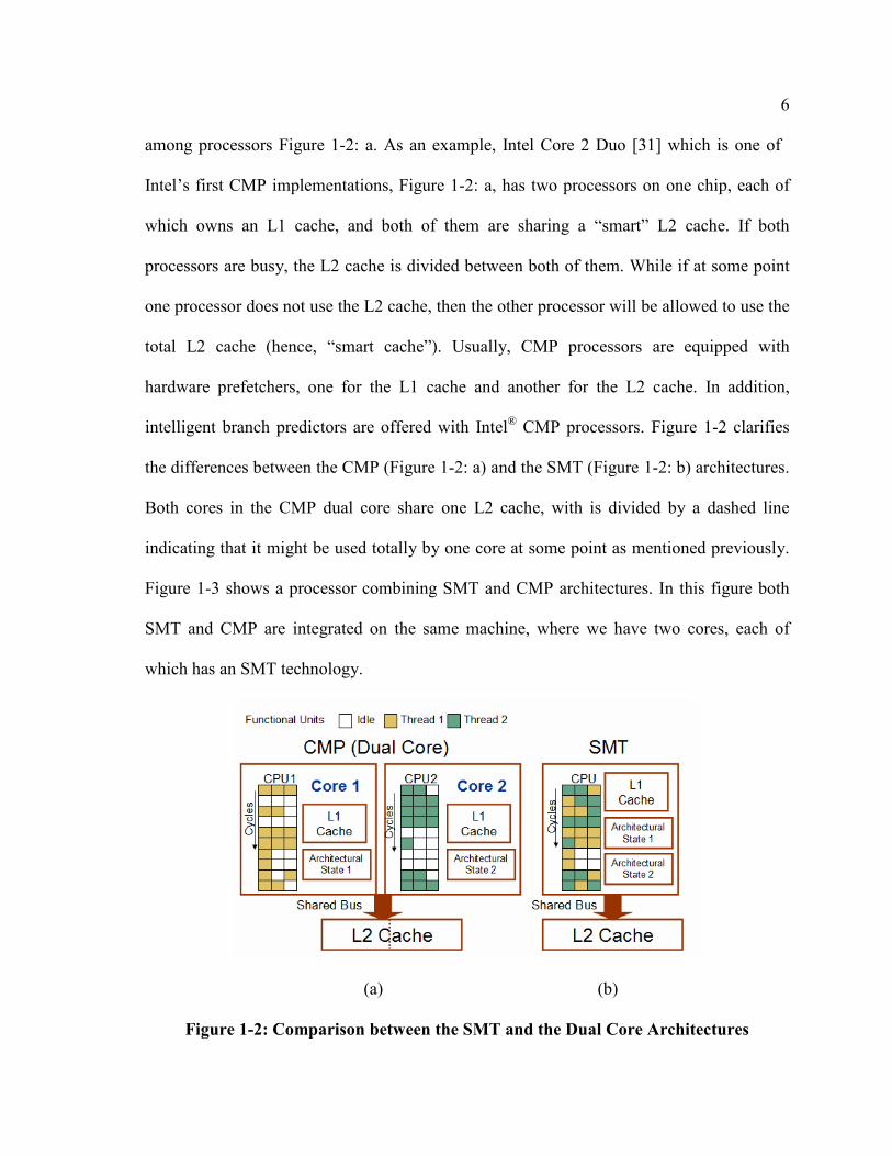
6

among processors Figure 1-2: a. As an example, Intel Core 2 Duo [31] which is one of

Intel’s first CMP implementations, Figure 1-2: a, has two processors on one chip, each of

which owns an L1 cache, and both of them are sharing a “smart” L2 cache. If both

processors are busy, the L2 cache is divided between both of them. While if at some point

one processor does not use the L2 cache, then the other processor will be allowed to use the

total L2 cache (hence, “smart cache”). Usually, CMP processors are equipped with

hardware prefetchers, one for the L1 cache and another for the L2 cache. In addition,

intelligent branch predictors are offered with Intel® CMP processors. Figure 1-2 clarifies

the differences between the CMP (Figure 1-2: a) and the SMT (Figure 1-2: b) architectures.

Both cores in the CMP dual core share one L2 cache, with is divided by a dashed line

indicating that it might be used totally by one core at some point as mentioned previously.

Figure 1-3 shows a processor combining SMT and CMP architectures. In this figure both

SMT and CMP are integrated on the same machine, where we have two cores, each of

which has an SMT technology.

(a) (b)

Figure 1-2: Comparison between the SMT and the Dual Core Architectures

7

Another form of parallelism that can be combined with SMT and CMP is Symmetric

Multi-Processor, (SMP) Figure 1-1. In our experiments, we use a combination of CMP,

SMT and SMP technologies in one server to show the usefulness of our algorithms. Our

server has Quad Intel® Xeon

® processors; each processor is dual core, each core is

equipped with SMT technology.

Figure 1-3: Combining the SMT and the CMP Architectures

8

Chapter 2

The Hash Join Algorithms

2.1 Introduction

To boost the performance of the hardware-platforms several approaches have been

considered, one of the most promising optimizations is to maximize the utilization of the

architecture through resource sharing. Two different variations are available for the

resource sharing techniques: (1) sharing the memory-hierarchy or part of it (e.g. SMT,

CMP and SMP). (2) Sharing everything on the processor chip and dedicating small

additional hardware to manage threads (e.g. SMT).

As information management becomes an integral part of our everyday life, database

management systems (DBMSs) gain further importance as a critical commercial

application. The performance of DBMSs has been less than optimal due to their poor

memory performance ( [1], [14], [28], [29], [30]). Main memory database systems (MMDB)

[3], where all the data resides in memory, suffer from large cache misses and low CPU

utilization. Ailamaki et. al. [1] show that MMDB are memory-bound, and most memory

stalls are due to the first level instruction cache and the second level unified cache misses.

Hash join (an optimized join operation that uses hash tables data structures) is one of the

most important operations commonly used in current commercial DBMSs [63]. We

9

characterize the main memory-hash join [3] algorithm in a modern server designed with

both SMT and CMP technologies (Quad Intel® Xeon

® Dual-Core server) with 4GByte main

memory. Our hash join processes two relations of 250MByte and 500MByte size (so they

can fit in our 4GByte main memory). We use the Intel® VTune Performance Analyzer for

Linux 9.0 [34] to collect several vital hardware events. Figure 2-1 shows that the level one

(L1) data cache load miss rate ranges from 4.7% to 5.3% while varying the tuple (record)

size. Taking into account that L1 miss latency does not exceed 10 cycles, we find that the

L1 data cache does not affect the overall performance of the hash join.

4.4%

4.5%

4.6%

4.7%

4.8%

4.9%

5.0%

5.1%

5.2%

5.3%

5.4%

20 60 100 140Tuple Size (Byte)

L1 Load M

iss R

ate

Figure 2-1: The L1 Data Cache Load Miss Rate for Hash Join

0%

10%

20%

30%

40%

50%

60%

70%


L2 Load M

iss R

ate

Figure 2-2: The L2 Cache Load Miss Rate for Hash Join

10

Next, we characterize the unified level two (L2) cache in Figure 2-2. The L2

cache load miss rate varies from 29% for tuple size = 140Bytes to 64% for tuple size =

20Bytes.

As the L2 cache load miss latency is usually larger than 100 cycles, our results agree with

[1], that the L2 cache load miss rate is a critical factor in main-memory hash join

performance. Figure 2-3 shows the L1 Instruction Trace Cache (TC) miss rate for the hash

join. We find that the maximum TC miss rate we get is very small and does not exceed

0.14%.

0.00%

0.02%

0.04%

0.06%

0.08%

0.10%

0.12%

0.14%

0.16%

20 60 100 140Tuple (Size)

Trace Cache M

iss Rate

Figure 2-3: The Trace Cache Miss Rate for Hash Join

In summary, the L2 cache miss rate has a major impact on the hash join performance.

Therefore, reducing the L2 cache miss rate is one of our targets while improving the hash

join performance.

In this chapter we achieve the following main contributions:

1. We analyze and study the different phases of traditional hash join algorithms using

one of the most practical join algorithms (the Grace Algorithm [38]).

2. We apply improvements to the different hash join phases to enhance their single

thread performance.

11

3. We study the performance of straight forward multithreaded algorithms of the

hash join.

4. We propose a multithreaded hash join algorithm that takes advantage of the

underlying multithreaded architecture by sharing data between threads in the same

processor. Thus, reducing cache conflicts and using one thread to prefetch data for

the other. We refer to our algorithm as an Architecture-Aware Hash Join (AA_HJ).

5. We show that our proposed algorithm can be easily integrated with the recent (yet

orthogonal) improvements to the single threaded hash join operation to achieve high

performance. In particular, we take advantage of the software group prefetching

technique proposed by [10].

To the best of our knowledge, no other work has proposed a multithreaded hash join

algorithm that takes advantage of the underlying SMT and CMP hardware. In this Chapter

we study the performance of our proposed hash join algorithm on the Intel® Pentium

® 4 HT

(dual-threaded) processor and the Intel® Quad Xeon

® Dual Core server (up to 16 threads).

On the first machine we achieve speedups ranging from 2.1 to 2.9 times compared to the

Grace hash join. While on the second machine our speedups range from 2 to 4.6 times

depending on the tuple size.

The rest of this chapter is organized as follows: Section 2.2 describes the concepts

of databases and hash join . Section 2.3 presents related work on improving hash join

database operations for modern systems. Section 2.4 describes the details of our proposed

dual-threaded version from AA_HJ. Section 2.5 describes the experimental methodology.

In Section 2.6 we present the timing and memory usage results on the Intel® Pentium

® 4

HT processor for the dual-threaded hash join. Section 2.7 shows timing and memory study

12

of our proposed dual-threaded AA_HJ on the same machine.

Section 2.8 shows detailed analysis of dual-threaded AA_HJ that includes time breakdown

of its different phases. Section 2.9 introduces our multithreaded AA_HJ designed to serve

system with multiple threads (rather than two as in Section 2.4), and we show its results on

the Intel® Quad Xeon

® Dual Core server in Section 2.10. Section 2.11 characterizes the

hardware performance for AA_HJ and digs deep into its memory behaviour using the Intel®

VTune Performance Analyzer. Finally, conclusions are provided in Section 2.12.

2.2 Hash Join

This section introduces database management systems (DBMSs) and hash join

operations [3]. The relational database management system (RDBMS) model is the

traditional DBMS originally presented by Edgar F. Codd [13]. RDBMS is a tabular

representation of a database, where records (tuples) represent the rows and attributes

represent the columns. Figure 2-4 shows an example of a relational table.

Figure 2-4: Typical Relational Table in RDBMS

Queries initiated to the RDBMS include retrieving tuples that satisfy some

conditions, updating, and deleting tuples. Some queries request data that exists in two

relations (tables), this occurs when for example an employee works for two departments,

where each departments’ employees are stored in a separate table. Figure 2-5 shows another

example of joining two tables. The datasets are organized such that some employees have

13

their names and salaries stored in one table, while the departments and provinces are

stored in another table. To retrieve all the data for any employee whose ID is in both tables,

we perform a natural-join.

Figure 2-5: Database Join

Natural join is one variation of a join in which we ask to retrieve all tuples from

both relations whose join-key (ID in Figure 2-5) matches. This is one of the most popular

types of joins. In its simplest form, joining two relations can be processed by two nested

loops, where the outer loop reads a tuple from the large relation, and the inner loop scans

the smaller relation looking for tuples with keys equal to that for the outer tuple. A more

efficient (and the most popular) implementation for the join query is the hash join which is

shown in Figure 2-6. In a hash join, a hash table is constructed from the smaller relation

(usually called R or build relation). Next, tuples are probed from the larger relation (usually

called S or probe relation) one by one using the hash table.

Figure 2-6: Hash /atural-join Process

14

A hash table structure is shown in Figure 2-7. It is an array of buckets, where

each bucket has a pointer to a linked list of cells. Each cell has a pointer to a tuple in the

build relation, and a hash value generated from the joining key of this tuple. After building

the hash table, the probe relations’ tuples are read one by one. For each S tuple read, the

joining key hash value is computed, and then the bucket number is calculated from the hash

value. The proper bucket (cells array) is accessed, and each cell’s hash value is compared

against the S tuple’s hash value for a match. If a match occurs, the pointer in that cell is

dereferenced so as to load the build relation R tuple, whose key will be compared against

the probe S tuple’s key for a match. If we have a match then both the build and probe tuples

are projected into the output buffer.

Figure 2-7: Hash Table Structure

A hash join requires random accesses to the hash table during the probing phase, and

random accesses to the R-relation to retrieve the matched tuples. To reduce the memory

access latency resulting from these random accesses, previous efforts have concentrated on

storing the data tables as close to the CPU as possible. For disk-resident databases

(DRDBs) ( [3], [21]) both the R and S-relations are partitioned into clusters (partitions) that

fit in the main memory. This algorithm is widely known as the “Grace Hash Join”. While

for MMDB, a similar partition-based approach called “cache partitioning” (a.k.a. Direct

15

Cache, DC) is used. In DC partitioning ( [10], [22], [39], [47], [62]) the R and S-relations

are partitioned into clusters such that each R cluster and its corresponding hash table fit in

the highest level cache (largest cache) in the machine. This is done prior to any hash join

processing. The partition-based hash join algorithm is shown in

Figure 2-8.

partition R into R0, R1,…, Rn-1 partition S into S0, S1,…, Sn-1 for i = 0 until i = n-1

use Ri to build hash-tablei for i = 0 until i = n-1

probe Si using hash-tablei

Figure 2-8: Hash Join Base Algorithm

In the naïve parallel hash join [46] both relations are partitioned among the available

processors p in a multi-processor system, for example. This is done by dividing the S and

R-relation into p clusters (blocks), such that each cluster has approximately the same

number of tuples. Then each processor uses its R-relation-cluster to build one global hash

table. Multiple writes to the same memory location are synchronized by latches. In the final

step of the parallel hash join, each processor probes its cluster using the global hash table.

2.3 Related Work

In this section we present related work in improving the performance of hash join

operations on uniprocessors, SMP, SMT and CMP architectures. Many researchers have

studied and improved the cache behaviour of hash join operations ( [5], [10], [12], [22],

[23], [44], [47], [61], [62], [70], [71]) in both single-threaded ( [5], [10], [47], [62]) and

multi-threaded ( [12] [22], [23], [44], [61], [70]) environments.

16

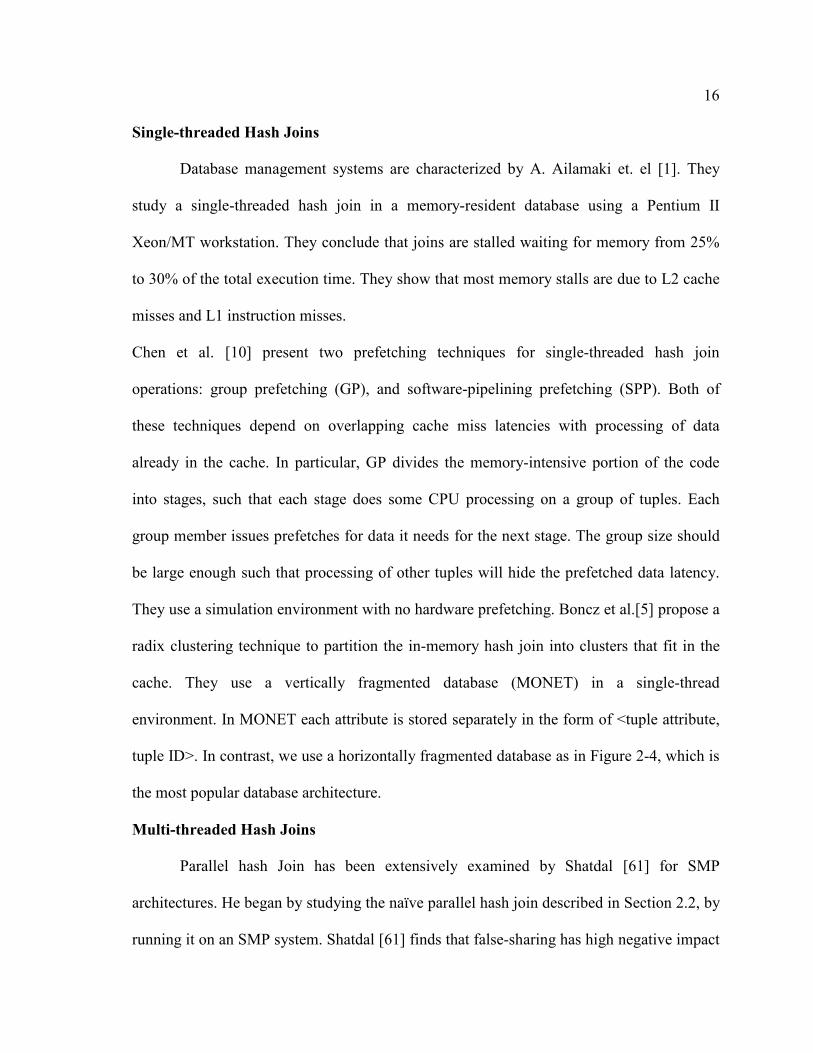
Single-threaded Hash Joins

Database management systems are characterized by A. Ailamaki et. el [1]. They

study a single-threaded hash join in a memory-resident database using a Pentium II

Xeon/MT workstation. They conclude that joins are stalled waiting for memory from 25%

to 30% of the total execution time. They show that most memory stalls are due to L2 cache

misses and L1 instruction misses.

Chen et al. [10] present two prefetching techniques for single-threaded hash join

operations: group prefetching (GP), and software-pipelining prefetching (SPP). Both of

these techniques depend on overlapping cache miss latencies with processing of data

already in the cache. In particular, GP divides the memory-intensive portion of the code

into stages, such that each stage does some CPU processing on a group of tuples. Each

group member issues prefetches for data it needs for the next stage. The group size should

be large enough such that processing of other tuples will hide the prefetched data latency.

They use a simulation environment with no hardware prefetching. Boncz et al. [5] propose a

radix clustering technique to partition the in-memory hash join into clusters that fit in the

cache. They use a vertically fragmented database (MONET) in a single-thread

environment. In MONET each attribute is stored separately in the form of <tuple attribute,

tuple ID>. In contrast, we use a horizontally fragmented database as in Figure 2-4, which is

the most popular database architecture.

Multi-threaded Hash Joins

Parallel hash Join has been extensively examined by Shatdal [61] for SMP

architectures. He began by studying the naïve parallel hash join described in Section 2.2, by

running it on an SMP system. Shatdal [61] finds that false-sharing has high negative impact

17

on the performance of the hash table building phase. False-sharing is a condition where

two or more different memory locations reside in the same cache line and one of them is

updated by one processor. Any reference to the other memory location(s) by another

processor will result in the cache line being reloaded, although the intended memory

location in this cache line is still up-to-date. Shatdal [61] solves this problem by using

padding. Padding is a strategy aimed into aligning memory location to a fixed size such that

each cache line stores one memory location only. Shatdal [61] also presents a hybrid

between hash join algorithm designed for shared-nothing multiprocessors and SMP

systems. In this algorithm the naïve parallel hash join is further extended, by repartitioning

each processor’s cluster, such that groups of R and its corresponding S cluster are placed in

a work-queue. R clusters are constructed such that the resulting hash tables fit in the

processor cache. Any idle processor will pick up a group of R and S clusters from the

work-queue and perform local hash join. The tuples are partitioned by either copying the

tuple to the new destination, or sending a pointer to the original tuple. The later is found to

be slightly better than the tuple-copying variation. Shatdal [61] achieved a speedup of two

on a 12 MIPS R800 processors SGI PowerChallenge server compared to single-threaded

hash join.

In [44] authors evaluate two greedy thread scheduling techniques on real CMP

environments, Parallel Depth First (PDF) and Work Steeling (WS). Their benchmarks

include LU (scientific benchmark), hash join and merge sort. Researchers in [44] evaluate

the On-Line Transaction Processing (OLTP) benchmark TPC-C and the decision-support

database benchmark TPC-H on a CMP simulator. They find that most stalls are due to data

misses mainly in the L2 cache. In [15] Colohan et al. use speculative threads to parallelize

18

database queries for a CMP 4-processors simulator, and achieve speedups ranging from

36% up to 74% for some TPC-C transactions. Other work on tuning software on CMP

environments include [4], which presents a theoretical justification of upper and lower

bounds on cache misses for a system consisting of p processors with shared memory

hierarchy. Their computations are general and do not focus on database operations. In [23]

Garcia et al. evaluate pipelined hash join on CMP and SMT machines. Moreover, they

conclude that more software threads than hardware threads are needed to utilize the

hardware. They only provide a timing analysis, with no explanations in terms of L1 and L2

cache miss rates.

Database operations have been investigated on SMT architectures in many papers

( [22], [45], [49], [70]), including hash join operations ( [22], [70]). In [22] Garcia and Korth

examine the same (single thread) algorithms proposed in [10] on real SMT hardware for an

in-memory version of the Grace hash join. They find that GP and SPP are useful for the

probing phase only, since this phase requires random accesses to the hash table, and that

otherwise the hardware prefetcher is able to prefetch the needed data. Both GP and SPP

give similar performance results. [22] shows that due to the large amount of data being

copied during the partitioning phase, the bottleneck for this stage is the memcpy. In

contrast, we avoid copying data during partitioning. Instead, we use index partitioning,

which saves an index for each tuple that belongs to a cluster instead of copying the whole

tuple to the generated cluster. [22] also proposes a thread-aware version of the hash join

that uses SPP to prefetch data. This dual threaded version from the hash join works as

follows: each thread will partition one of the two relations. Once the smaller relation (R) is

done, its thread begins building hash tables from the build relation clusters (partitions).

19

Once both the R partitioning and building phases are done and the S partitioning phase is

done, a synchronization manager is used to give each thread a probe cluster and a hash

table to perform the join. Therefore, each thread will perform the join on one cluster until

all clusters are assigned by the synchronization manager. Although [22] creates a dual

threaded hash join, it does not exploit the sharing of caches in SMT architectures which is

the distinguishable feature of an SMT architecture over an SMP architecture. Furthermore,

no techniques are proposed to reduce the interference/contention of the two threads (each is

using a different cluster and hash table) over the cache. In contrast, we propose an SMT-

aware hash join algorithm that exploits cache sharing between the two threads. J. Zhou et al

in [70] use a helper-thread approach to exploit the two threads available in an SMT

architecture by dedicating one thread to prefetch data for the hash join, while the other main

thread does the actual computations. The two threads communicate through a software

cache structure. This structure is used to pass the memory addresses that are anticipated to

be used in the near future from the main thread to the helper thread. Our algorithm uses

both threads to process the hash join where each thread can issue prefetches for its own

work. The prefetch instruction is a non-blocking instruction, meaning that the thread can

continue executing other work even if the prefetch instruction is not retired yet.

2.4 Dual-Threaded Architecture Aware Hash Join

In this section we propose an architecture-aware hash join (AA_HJ) database

operation. Our algorithm takes advantage of the following two main features in SMT

architectures: (1) two threads are available to run simultaneously, (2) the full memory

hierarchy is shared between these two threads (i.e. the cache sharing feature of SMT

20

architectures). MMDB systems suffer from high L2 cache miss rates and therefore,

reducing/hiding the memory access latency is an important performance factor for hash join

operations. We use two threads to process the dataset, simultaneously working on the same

cache structures, with minimal conflicts in the cache levels.

2.4.1 The Build Index Partition Phase

We use the OpenMP library ( [51], [18]) to initiate two threads, where each thread is

assigned a unique ID. To minimize thread creation and killing overhead, we initiate the two

threads only once when the hash join begins, and kill the threads only when the join is

completed. Our algorithm starts by creating structures to hold the R-relation index clusters

(partitions) for each thread. Each entry in the index structures consists of 8Bytes; 4Bytes

for the tuple index, which is a pointer to the tuple in the R-relation, and 4Bytes to store the

hash value for that tuple. We partition the R-relation by first splitting it between the two

threads, such that the first thread processes the first half (R0-R(n/2)-1) and the second thread

processes the second half (Rn/2-Rn-1). The R-relation is accessed sequentially by each

thread. Therefore, the hardware prefetcher is able to capture the memory address patterns

and prefetch the needed data. This eliminates the need for explicit software prefetch

instructions. Each thread in this stage reads a tuple from its half and calculates the tuple's

key mod number of clusters that belong to this thread. Therefore, it chooses the cluster

where it should store the tuple. The thread saves the tuple’s pointer together with its hash

value, which is calculated from the tuple's key. We are using 1024 clusters for the index

partition. This generates L1 cache size clusters (L1 cache size is 64KByte).

21

2.4.2 The Build and the Probe Index Partition Phase

Before we begin this stage, we make sure that both threads finish the build index

partition phase completely by using a barrier synchronization pragma. Our hash tables are

described in Figure 2-7. We have studied several possible multithreaded implementations.

1) Use the two threads simultaneously, each building a hash table. This approach resulted

in contention over the cache between the two threads hash tables. Thus resulting in cache

misses for most accesses in the two hash tables and highly degrading performance. 2) Use

the two threads to build the same hash table simultaneously. We use atomic

synchronization pragmas to restrict writing to the same memory location to one thread at a

time. However, this type of synchronization limits the performance of the two threads,

resulting in slowdowns rather than speedups. 3) Devoting one thread to create the hash

tables of the build phase and use the second thread to perform the S-relation index

partitioning phase simultaneously.

for i = 0 until i = total-number-of-clusters/2 for j = 0 until j = thread0.Build-clusteri.number-of-

entries -1 insert thread0.Build-clusteri.tuplej into hash-tablei

for k = 0 until k = thread1.Build-clusteri.number-of-entries -1 insert thread1.Build-clusteri.tuplek into hash-tablei

Figure 2-9: AA_HJ Build Phase Executed by one Thread

This method gives us the best performance and therefore, is our method of choice. The

build phase algorithm is shown in Figure 2-9. Each two clusters generate one hash table,

where both of these two clusters have the same key-range. For example, both thread0.Build-

cluster1 (cluster1 generated by thread0 from the first phase) and thread1.Build-cluster1

22

(cluster1 generated by thread1 from the first phase) generate hash-table1 in Figure 2-9.

While the first thread is building the hash tables, we use the second thread to perform the S-

relation index partitioning simultaneously. The R-relation structures will be accessed

repeatedly to probe tuples in the probe phase, thus they need to fit in one of our caches.

While for S-relation, each tuple will be read once during the probing phase to search for its

match, so the S-relation clusters do not need to fit in the caches. Also, since tuples are read

sequentially, the hardware prefetcher is able to prefetch the S-relation tuples. Each entry in

the S-relation clusters has a similar form to that used for the R-relation clusters. We create

two sets of clusters, one for each thread. The first set of clusters store the indexes resulting

from tuples ranging from 0 to (n/2)-1, where n is the total number of tuples in the S-

relation.

x=0 do{ read S.tuplex z = appropriate-cluster-number depending on S.tuplex.key

insert S.tuplex into thread0.Probe-clusterz read S.tuplex+(n/2)

z = appropriate-cluster-number depending on S.tuplex+n/2.key

insert S.tuplex+(n/2) into thread1.Probe-clusterz increment x by 1

}while ( x < n/2 )

Figure 2-10: AA_HJ Probe Index Partitioning Phase Executed by one Thread

While the second set of clusters stores indexes from (n/2) to n-1. Therefore, each key-range

has two clusters, one from the first S-relation half and the other from the second half. The

algorithm used for the S-relation indexing phase is shown in Figure 2-10 (where S means

S-relation).

23

2.4.3 The Probe Phase

As the probing phase uses both the hash tables and the S-relation clusters, we can

not begin this phase until both threads of the previous phase are done. Thus, a barrier

pragma is implemented between the two phases. One of the large challenges for the probe

phase is the random accesses to the hash table whenever there is search for a potential

match. As described in Section 2.2: Figure 2-7, each access to the hash table will result in a

sequence of pointers dereferenced. The probe phase begins by accessing the appropriate

bucket, reading the cell array’s pointer, accessing the cell array and dereferencing every

cell’s pointer so as to read this tuple’s key and test for a match with the probed tuple.

Consequently, the goal of optimizing this phase concentrates on proposing a solution for

the sequence of random accesses to the hash tables. Architectural Aware Hash Join

(AA_HJ) controls both threads such that each thread is probing tuples from its cluster

whose key-range is similar to another cluster that is being probed by the other thread

concurrently.

As an example, in Figure 2-11, we show the process of generating four clusters

from the S-relation in the S-relation index partitioning phase by Thread1. Thread2 will be

busy in hash tables building (not shown in the figure). Next, in the probe phase the two

clusters that belong to the same key-range are probed by the two threads simultaneously

and one hash table is visited during each key-range’s iteration. To prevent race conditions

that might arise from one thread probing its cluster faster than the other thread, we divide

each key-range probe iteration with a barrier pragma from the other iterations. However,

we follow the assumption that since keys are randomly distributed throughout the S-

relation, each cluster from thread0’s set of clusters will result in almost the same number of

24

matches as those resulted from the corresponding cluster from thread1’s set of clusters.

Thus, probing both clusters requires the same time. The pseudo code for our algorithm is

shown in Figure 2-12. The term “number-of-clusters” refers to the total number of clusters

generated from the S-relation.

Figure 2-11: AA_HJ S-Relation Partitioning and Probing Phases

Since both threads are using the same hash table concurrently in each iteration, we

manage that one thread will serve as an implicit hash table-prefetcher for the other thread

while it is probing its own tuples. This is because each hash table fits in the L1-cache

therefore, once it is fetched, it remains cache-resident until the next iteration, where another

hash table is prefetched. The original S-relation is not accessed sequentially any more

because of our index partitioning, therefore the hardware prefetcher will not be as useful.

To solve this problem, we use explicit prefetch instructions to prefetch the next tuple in the

cluster before we begin to process the current tuple. We find that prefetching one tuple

ahead is enough to overlap the memory access latency for the tuple. This is because each

prefetch instruction in the Intel® Pentium

® 4 loads two cache lines and the largest tuple size

we study is 140Bytes.

25

for i = 0 until i = number-of-clusters/2 if (thread0)

for j = 0 until j = thread0.Probe-clusteri.number-of-entries

prefetch thread0.Probe-clusteri.tuplej+1 use hash-tablei to probe thread0.Probe-clusteri.tuplej

else for k = 0 until k = thread1.Probe-clusteri.number-of-entries

prefetch thread1.Probe-clusteri.tuplek+1 use hash-tablei to probe thread1.Probe-clusteri.tuplek

pragma barrier

Figure 2-12: AA_HJ Multithreaded Probing Algorithm

2.5 Experimental Methodology

We run our algorithms on two multithreaded machines. The first (Machine 1) is a

3.4GHz Intel® Pentium

® 4 processor with hyper-threading technology (HT, Intel’s dual

thread SMT architecture [33]). The second (Machine 2) is the Intel® Xeon

® Quad

Processors for PowerEdge 6800, each processor is a dual-core, each core is HT. General

specifications for both machines are shown in Table 2-1 Both systems have L2 unified

cache with 128Bytes cache lines. We use the Scientific Linux version 4.1 operating system

which is based on the Redhat Linux Enterprise version 4.0. We implemented all algorithms

in C, and we use the Intel® C++ Compiler for Linux version 9.1 [32] with maximum

optimizations. We use the built-in OpenMP C/C++ library [51] version 2.5 (as

implemented in the Intel® C++ Compiler) to initiate multiple threads in our multi-threaded

codes. We repeat each run three times, remove the outliers, and take the average. Timing

and memory measurements are done through our program using functions such as

26

gettimeofday (). A warm up run is done prior to any measurements to load the relations

into main memory.

Machine 1 Machine 2

Processor(s) Pentium® 4 with HT Quad Xeon

®, PowerEdge 6800

L1 data Cache 64Kbyte 64KByte/core

L2 Cache 2MByte 2MByte/processor

Main Memory 1GByte 533MHz DDR2 4GByte 400MHZ DDR2

Clock Speed 3.4 GHz 2.66 GHz

Hard Drive 160GByte 300GByte

Table 2-1: Machines Specifications

We choose to implement our own version from hash join rather than using the

database benchmarks (e.g. TPC-C) to prevent the impact of DBMS overhead from unseen

activities. These activities might include query planner, query optimizer, etc.

For Machine 1 we use a 50MByte build relation and a 100MByte probe relation.

We choose these sizes to make sure that our relations, in addition to any large intermediate

structures needed by the code, fit in our 1GByte main memory. While for Machine 2 we

use 250MByte build relation and 500MByte probe relation since we have larger main

memory (4GByte). Our join key is 10Bytes, randomly generated such that each tuple in the

build relation matches one tuple in the probe relation. The payload part of the tuple is of

variable size. The number of tuples in each table (given the table’s constant size) depends

on the tuple size.

27

Table 2-2 and Table 2-3 show the number of tuples used in each relation for different

tuple sizes for Machine 1 and for Machine 2, respectively. We choose tuples of these sizes

to study the cases where tuples are smaller than the L1 cache line (20Byte, 60Byte),

between the L1 and the L2 cache line sizes (100Byte) and larger than the L2 cache line size

(140Byte). In real DBMS the average tuple size is 120Byte [63].

Our naïve partitioning and probing algorithms are the same as those in [22]. Our

hash function consists of XOR and shift operations [10] and generates 4Bytes hash codes.

Once hash codes are computed at any stage, they are saved in temporary structures in

memory to avoid recalculating them. Hash table buckets are calculated using the hash code

mod hash table size. Our hash tables are created such that the number of buckets equals the

number of tuples in the corresponding R-cluster or the R relation in case partitioning is not

used.

Tuple Size

(Byte)

Number of Tuples in the

Build Relation


Probe Relation

20 2621440 5242880

60 873814 1747628

100 524289 1048578

140 374491 748982

Table 2-2: /umber of Tuples for Machine 1

28

Tuple Size

(Byte)


Build Relation


Probe Relation

20 13107200 26214400

60 4369067 8738134

100 2621440 5242880

140 1872457 3744914

Table 2-3: /umber of Tuples for Machine 2

We use the Intel® VTune™ Performance Analyzer for Linux 9.0 [34] to collect the

hardware events from the hardware performance counters available in our machines. These

events include L2 cache load misses, L1 data cache load misses, etc. Each run for VTune is

repeated three times. Each time two runs are performed by VTune, the first is for

calibration, which determines the frequency at which the event occurs. The second is for

the actual event collection.

2.6 Results for the Dual-Threaded Hash Join

2.6.1 Partitioning vs. �on-Partitioning vs. Index Partitioning

In this section we study the effects of partitioning the build and probe relations on

the execution time and memory usage of the hash join on Machine 1. As described in

Figure 2-8, partitioning is the first step of the hash join algorithm. Partitioning creates small

clusters (partitions) of the R and S-relations that fit in the cache. The goal is to divide the

overall hash join into a set of smaller hash joins that work on data that fits in the cache.

Thus, enhancing the performance of the hash join by reducing its cache misses. Recent

29

papers ( [10], [22]) copy the entire relations while partitioning. In this section, we begin

by exploring the importance of index partitioning from time and memory view of points.

We implement three types of the hash join algorithms: partitioning (PT), non-partitioning

(NPT), and index partitioning (Index PT). (1) PT uses the partitioning algorithm described

in Figure 2-8. We use 1024 clusters for the R-relation which creates R-clusters of 50KByte

each. Including the hash table size for each cluster, this fits easily in our 64KByte L1 cache.

We find experimentally that using clusters of larger sizes will create cache thrashing, and

smaller cluster sizes result in high partitioning overhead. We also use 1024 clusters for the

S-relation. However, the S-relation is not as critical as the R-relation to have in the cache

and is not partitioned to fit in the cache in techniques such as DC, described in Section 2.3.

(2) NPT uses no partitioning, instead the full R and S-relations are hash joined. (3) Index

PT is a variation of the partitioning algorithm described in Figure 2-8 where instead of

copying the actual tuples into the partition, pointers to the tuples are stored. We use 1024

clusters for both the R- and S-relations which allows our R-cluster (which includes pointer

to the tuples only and not the full tuple) and its corresponding hash table to fit into our L1

cache. The PT and Index PT are two variants from main-memory Grace hash join.

Figure 2-13 shows the execution time (Time) of our three cases of partitioning: PT,

NPT and Index PT. Although the PT outperforms the NPT algorithm in tuple size =

20Byte, the overhead of the partitioning phase overcomes the performance improvement

due to partitioning in all other tuple sizes. This overhead is a result of the copying of large

tuples from the source relation to the destination cluster. This overhead is eliminated by

Index PT and therefore results in the performance improvement of Index PT over both NPT

30

and PT in all tuple sizes. The longer execution time for smaller tuples is due to the larger

number of tuples in these cases as shown in Table 2-2.

Figure 2-14 shows the memory usage of PT, NPT and Index PT. Since we are

studying MMDB operations, our relations have to be main memory resident prior to any

processing. Thus, the minimum memory space that any hash join requires will be equal to

the total sizes of the two relations, which is 150MB, in addition to the memory needed to

build the hash table. The size of the hash table(s) is proportional to the number of tuples

involved in the table building.

0.0

0.5

1.0

1.5

2.0

2.5

3.0

3.5

4.0

20 60 100 140

Tuple Size (Byte)

Time (Second)

PT NPT Index PT

Figure 2-13: Timing for three Hash Join Partitioning Techniques

31

0

50

100

150

200

250

300

350

400

450

500


Memory (MByte)

PT NPT Index PT

Figure 2-14: Memory Usage for three Hash Join Partitioning Techniques

Figure 2-14 shows that PT requires almost two times the memory space required by

NPT. This is because both relations are copied into the clusters in PT. While, Index PT

memory requirements are in between PT and NPT, as each tuple in Index PT requires only

8Bytes in its cluster (4Bytes for tuple hash value and 4Bytes tuple pointer), regardless of

the size of the tuple. Therefore, Index PT gives the best performance and has the

intermediate memory usage. Speedups achieved from Index PT over NPT ranges from 18%

to 21%.

2.6.2 Dual-threaded Hash Join

The probe phase is known to be the most time consuming phase in hash join due to

its random access pattern to both the hash table and R-relation. In this section we study the

performance of the straightforward parallelization of the probe phase on Machine 1. We

develop dual-threaded versions of the three algorithms presented in Section 2.6.1 on our

SMT architecture. We refer to our algorithms as SMT+PT, SMT+NPT and SMT+Index

32

PT. We parallelize the probe phase for PT and Index PT by dividing the available S-

clusters evenly between both threads to create SMT+PT and SMT+Index PT, respectively.

While for NPT we split the probe relation between the two threads, such that each thread

probes half of the large relation.

Figure 2-15 shows the performance of our three dual-threaded hash join algorithms.

Using Index PT (in the SMT+Index PT algorithm) continues to give the best performance.

Figure 2-16 shows the memory usage of our three multi-threaded hash join algorithms is

the same as their single-threaded versions. This is because no additional intermediate code

structures were used in the multi-threaded versions.

0.0

0.5

1.0

1.5

2.0

2.5

3.0

3.5

20 60 100 140

Tuple Size (Byte)

Tim

e (Second)

SMT+PT SMT+NPT SMT+Index PT

Figure 2-15: Timing for Dual-threaded Hash Join

33

0

50

100

150

200

250

300

350

400

450

500

20 60 100 140

Tuple Size (Byte)

Memory (MByte)

SMT+PT SMT+NPT SMT+Index PT

Figure 2-16: Memory Usage for Dual-threaded Hash Join

We calculate the speedups resulting from multithreading each of our 3 hash join

algorithms to be; SMT+NPT is 39%, SMT+PT is 10% and SMT+Index PT is 15%,

compared to NPT, PT and Index PT hash joins, respectively. The SMT+NPT has the

highest speedups since it lacks the overhead of the sequential partitioning phases and its

execution time is dominated by the probing phase.

2.7 Results for the Dual-threaded Architecture-Aware Hash

Join

In this section we present the results of our proposed dual-threaded architecture-

aware hash join algorithm (AA_HJ) on Machine 1. We use Index Partitioning in AA_HJ as

it is the best performing partitioning algorithm. In contrast to the SMT+Index PT where

two hash tables (one per thread) are used, AA_HJ forces the two threads to use the same

hash table simultaneously. This reduces cache conflicts between the two hash tables in

34

SMT+Index PT and allows accesses from one thread to prefetch parts of the table for the

other thread.

0.00.20.40.60.81.01.21.41.61.82.02.22.42.62.83.03.23.43.63.84.0

20 60 100 140

Tuple Size (Byte)

Tim

e (Second)

AA_HJ+GP+SMT AA_HJ+SMT SMT+NPT NPT

SMT+PT PT SMT+Index PT Index PT

Figure 2-17: Timing Comparison of all Hash Join Algorithms

We refer to this version of our proposed algorithm as AA_HJ+SMT. Since our

proposed technique is orthogonal to some of the previously proposed hash join

enhancement techniques such as Group Prefetching (GP) [10], we further enhance our

performance by adding GP to AA_HJ+SMT. GP prefetches the randomly accessed buckets

of the hash tables, thus reducing our cold cache misses. We refer to this version of our

proposed algorithm as AA_HJ+GP+SMT. Figure 2-17 shows that AA_HJ+SMT is able to

increase the thread cooperation in the cache level for all tuple sizes and therefore

considerably improve performance. AA_HJ+GP+SMT further enhances the performance.

35

0

50

100

150

200

250

300

350

400

450

500

20 60 100 140

Tuple Size (Byte)

Memory (MByte)

AA_HJ+GP+SMT AA_HJ+SMT SMT+NPT NPT

SMT+PT PT SMT+Index PT Index PT

Figure 2-18: Memory Usage Comparison of all Hash Join Algorithms

0

0.5

1

1.5

2

2.5

3

3.5

20 60 100 140

Tuple Size (Byte)

Speedup F

actor

PT SMT+PT Index PT SMT+Index PT AA_HJ+SMT AA_HJ+GP+SMT

Figure 2-19: Speedups due to the AA_HJ+SMT and the AA_HJ+GP+SMT

Algorithms

Figure 2-18 shows the memory usage of our proposed AA_HJ+SMT and

AA_HJ+GP+SMT algorithms. The memory footprints of AA_HJ+SMT and

36

AA_HJ+GP+SMT result in only a small change to the memory usage of the Index PT

algorithm due to doubling the clusters number (1024 cluster for each thread).

Figure 2-19 shows the speedup of the AA_HJ+SMT and AA_HJ+GP+SMT compared to a

base PT hash join (we assign PT value 1 in this figure since it is our base). AA_HJ+SMT

achieves a speedup ranging from 2.04 to 2.70 for tuple sizes 20Bytes to 140Bytes,

respectively. Speedup for AA_HJ+GP+SMT ranges from 2.19 to 2.90 for tuple sizes

20Bytes to 140Bytes, respectively.

2.8 Analyzing the AA_HJ+GP+SMT Algorithm

In this section we study the effects of varying the cluster size and selectivity on the

performance of our proposed AA_HJ+GP+SMT algorithm on Machine 1. Figure 2-20

shows the performance of AA_HJ+GP+SMT while varying the cluster size. For tuple size

20Bytes, using clusters less than 512 clusters reduces performance. On the other hand

having tiny clusters as in the case for 2048 clusters will increase the partitioning phase

overhead for both R and S relations, without any gain in the probing phase (since the

clusters already fit in the L1 data cache) and thus reduces performance.

Selectivity denotes how many tuples in the build relation will find matches in the

probe relation upon performing the join operation. In our previous experiments we use a

selectivity of 100%, this means that all tuples in the build will find matches in the probe.

Thus, every time we probe a tuple from the probe relation we have to load the

corresponding tuple in the build relation if a hash-value match occurs.

37

0

0.5

1

1.5

2

2.5

32 64 128 512 1024 2048Number of Clusters

Time (Second)


Figure 2-20: Varying /umber of Clusters for the AA_HJ+GP+SMT

0.2

0.3

0.4

0.5

0.6

0.7

0.8

0.9

1

20 40 60 80 100

Selectivity

Time (Second)

PT SMT+PT AA_HJ+SMT AA_HJ+GP+SMT

Figure 2-21: Varying the Selectivity for Tuple Size = 100Bytes

For 20% selectivity, from every 10 tuples that we probe from the S-relation, we will find

matches for 2, and the other 8 will at the worst case lead to accessing R relation. In Figure

2-21, we vary the selectivity from 20% to 100% in steps of 20s. The execution time

increases while increasing the selectivity. The pattern of this increment is the same for all

38

the different hash join algorithms, since the enhancements that we have implemented

does not affect the way the build tuple is retrieved.

2.8.1 Analyzing the Phases of the Hash Join Algorithms

In this section we analyze the phases of the hash join operation on Machine 1.

Recall that partitioning-based hash join algorithms consist of three phases: (1) partitioning

both the build and probe relation (2) building the hash tables (3) probing each cluster that

resulted from phase 1 with its corresponding hash table. Figure 2-22 shows the time

distribution of the three phases of the hash join. The probe phase in NPT and SMT+NPT is

much larger than any of the other hash join algorithms. This is due to NPT using one very

large hash table that does not fit in the cache. As a result almost all accesses to the hash

table during this phase will result in cache misses. The build phase also consumes a large

amount of time since it accesses the buckets in the hash table randomly. The PT hash join

succeeds in reducing the time of the probe and build phases. The build phase creates

several small hash tables that fit in the cache, so only cold cache misses will result in stalls.

The probe phase is accessing small clusters of the original probe relation, each of

which corresponds to a small hash table and build cluster that both fit in the cache.

Therefore, the algorithm will stall for cold misses only. However, the overhead of the

partitioning phase for tuple size 100Bytes is larger than the time gain in the probe phase.

As a result, PT fails to have shorter execution time than NPT. For Index PT, and unlike

both NPT and PT, the partitioning phases include hash value calculations. However, Index

PT does not use the expensive memcpy instruction and thus results in a smaller partitioning

phase than PT and NPT. The Index PT build phase is smaller compared to PT, because that

for PT includes hash code calculations which are already calculated for Index PT. The

39

SMT versions from NPT, PT and Index PT show improvements in the probe phase since

it is the multi-threaded phase.

0

0.5

1

1.5

2

2.5

3

3.5

4

100 20 100 20 100 20 100 20 100 20 100 20 100 20 100 20

NPT SMT+NPT PT SMT+PT Index PT SMT+Index PT AA_HJ+SMT AA_HJ+GP+SMT

Tim

e (Second)

Build Index Partition Probe Index Partition Partition Build Probe

Figure 2-22: Time Breakdown Comparison for the Hash Join Algorithms for tuple

sizes 20Bytes and 100Bytes

For the AA_HJ+SMT two threads perform R-relation index partition, where each

thread owns a set of clusters. Therefore, we have a shorter R-relation index partition phase

for all AA_HJ versions. In the probe index partitioning phase we are using one thread to

partition the probe relation. As shown in Figure 2-10, we index partition two tuples in each

iteration of the algorithm, one from each half of the S-relation. Therefore, we have

decreased the number of iterations over the S-relation in half. Thus, we have shorter S-

relation index partitioning phase for both AA_HJ+SMT and AA_HJ+GP+SMT. The build

phase for AA_HJ hash joins appears to be longer than that for Index PT however, this

40

phase is overlapped with the S-relation index partitioning phase (both overlapping

algorithms are in Figure 2-9 and Figure 2-10). The difference in the probe phase between

SMT+Index PT and AA_HJ+SMT is that the two threads in AA_HJ+SMT are visiting the

same hash table concurrently, thus they are sharing the same hash structures between them.

Finally, for AA_HJ+GP+SMT, we try to solve the cache cold misses’ problem in

the hash tables, a pattern that can not be caught by the hardware prefetcher. We use Group

Prefetching (GP) to overlap the latency of each memory access of the hash table by some

useful work for the current tuple. In this way, we eliminate the stall time for the first access

to any bucket by using GP. Therefore, we are able to optimize the probe phase, by both

forcing the two threads to process tuples that are in the same key range simultaneously, and

solve the hash table cold misses problem by using GP. For the rest of this chapter we will

refer to AA_HJ+GP+SMT as AA_HJ.

2.9 Extending AA_HJ for more than two Threads

In this section we present a scalable form of AA_HJ that exploits more than two

threads. Our scalable version of AA_HJ is capable of utilizing various types of

multithreading including SMP, CMP and SMT. Follows is a description of the changes we

have made to the dual-thread AA_HJ:

1. R-relation index partition:

Assume that the R-relation has Rn tuples. Also assume that the number of available

threads in the platform is t, t includes any threads resulting from the SMT, the CMP and the

SMP, where t = number of processor chips * number of cores per chip * number of SMT

threads per processor core. For example, if a system has four processor chips, each

41

processor is a quad core, each core is 2-threads SMT, then t = 4 * 4 * 2 = 32 threads.

Each thread ti (i = 0, 1... t-1) is assigned Rn/t tuples. The remaining tuples after this division

will be added to the last thread. An index partitioning similar to the one described in

Section 2.4.1 is executed by each thread. By the end of this phase any thread will have a set

of clusters c. A ci (i = 0, 1… limit-1) stands for a key-range as described in Section 2.4. The

value of limit depends on the following observations: (1) the total size of clusters for any

key-range must be small enough to allow both the hash table and its R-clusters to fit in the

L2 cache. This is because we are planning for each four threads in a chip to share one hash

table. (2) During the probe phase some space in the L2 cache should be reserved for a few

tuples from the S cluster. The tuples from the S-relation are used only once, so this space is

intended to be a temporary storage for tuples prefetched manually. (3) Some space should

be reserved for the operating system processes. Taking all theses three factors into account,

we use (R-relation-size + hash tables`sizs)/limit < L2 cache size to calculate limit. Since it

is difficult to estimate the hash table size prior to the a hash join ( hash table size ranges

between 22MByte up to 150MByte in our case) we use its worst case, where hash table is

just above half the R-relation size (150MByte). Therefore limit is measured as follows (250

+ 150) / limit < 2, which results in limit > 200. We choose limit to be 256 clusters.

2. Build Phase and S-Relation Index Partition Phase:

In the second step, the thread with the smallest identifier builds the hash tables.

Simultaneously, other threads will index-partition the S-relation as described in Section

2.4. The thread with the next smallest identifier will generate two sets of clusters instead of

one, to compensate for the thread building the hash tables.

42

3. Probe Phase:

During this phase, a constructive cache-level sharing is maintained by directing all

four threads of each dual-SMT-core to probe one key-range using one hash table. Recall

that any thread generates a set of clusters from phase two, with a cluster for each key-

range. Therefore, t clusters exist for each key range. A probing thread in a core will process

t/4 clusters. Again, GP is incorporated with this phase code to eliminate cold misses.

Keeping in mind that this is the most expensive phase in the hash join operation, we

provide several optimizations including: (1) the load is almost perfectly balanced between

threads. Given that our keys are uniformly distributed, the sizes of clusters are very close.

We attempt to employ a work stealing strategy to distribute the clusters in each core across

threads. However, we achieve similar execution time as before, meaning that the load is

balanced with each thread visiting t/4 clusters. (2) Having four threads repeatedly visiting

the same memory structure (hash table), will highly increase temporal and spatial locality.

2.10 Results for the Multi-Threaded Architecture-Aware Hash

Join

In this section we present the results of our scalable AA_HJ algorithm. The

workstation we conducted our experiments on is Machine 2, described in Section 2.5. The

R-relation is 250MByte and the S-relation is 500MByte. We ran multithreaded AA_HJ

with 2, 4, 8, 12 and 16 threads, each of which is with tuple size = 20Byte, 60Byte, 100Byte

and 140Bytes. To highlight the differences in performance with single-threaded AA_HJ,

we also run NPT, PT and Index PT hash joins (for details about NPT and PT and Index PT

refer to Section 2.6.1).

43

0

5

10

15

20

25

30

35

40

45

50

20 60 100 140

Tuple Size (Byte)

Tim

e (Second)

PT NPT Index PT 2 4 8 12 16

Figure 2-23: Timing for the Multi-threaded Architecture-Aware Hash Join

Figure 2-23 shows our results for multithreaded AA_HJ. Figure 2-24 shows the

speedups of all multithreaded runs together with Index PT compared to PT hash join. We

achieve speedups ranging from two for tuple size = 20Bytes with two threads, to 4.6 times

for tuple size = 140Bytes with 16 threads. The improvements in running time saturate

while having eight threads for all tuple sizes. This is because number of clusters has

proportional relation with number of threads. Therefore, the partitioning overhead together

with the expensive off-ship communications will increase while having more working

threads. AA_HJ takes advantage of sharing structures between each four threads in a dual-

SMT core. Thus, enhancements in performance are large while having 2, 4 and 8 threads.

44

0

0.5

1

1.5

2

2.5

3

3.5

4

4.5

5

20 60 100 140

Tuple Size (Byte)

Speedup Factor

PT Index PT 2 4 8 12 16

Figure 2-24: Speedups for the Multi-Threaded Architecture-Aware Hash Join

750

850

950

1050

1150

1250

1350

1450

1550

1650

1750

1850

1950

2050

20 60 100 140

Tuple Size (Byte)

Memory (MB)

PT NPT Index PT 2 4 8 12 16

Figure 2-25: Memory Usage for the Multi-Threaded Architecture-Aware Hash Join

2507MByte for tuple size = 20Byte

45

Despite the fact that PT accomplishes good execution time for tuple size = 20Bytes, its

memory footprint is 3.4 times the relations sizes, which makes it impractical for machines

with limited main memory environments. NPT hash join maintains its precedence over

others in memory saving. While Index PT and all AA_HJ multithreaded hash joins are

comparable in memory consumption as shown in Figure 2-25.

00.51

1.52

2.53

3.54

4.55

5.56

6.57

7.58

8.59

9.510

10.511

11.512

12.513

13.514

14.515

PT

Index PT 2 4 8

12

16

PT

Index PT 2 4 8

12

16

PT

Index PT 2 4 8

12

16

PT

Index PT 2 4 8

12

16

20 60 100 140

Tuple Size

Time (Second)

Partition Build Index Partition Probe Index Partition Build Probe

35.91

second

27.70

second

Figure 2-26: Time Breakdown Comparison for Hash Join Algorithms

Figure 2-26 for AA_HJ is the time breakdown for all multithreaded AA_HJ, PT and

Index PT for all tuple sizes. From Figure 2-26 we have the following observations:

• There are large improvements in probing and index-partitioning execution times for

AA_HJ compared to PT and Index PT.

• Execution time decreases when using more threads for AA_HJ up to 8 threads,

where it saturates.

46

• The R- and S-relations index partitioning phases saturate at eight-threaded

AA_HJ. This is due to doubling number of clusters while adding each thread. The

communication overhead for CPUs on the same chip is cheap (10-20 cycles) and is

carried out through the L2 cache. While off-chip cores communicate through the

main memory or a cache-coherence protocol which is very expensive (hundreds of

cycles). In the probe phase clusters are collected from all cores to process a hash

table, this generates large communication overhead that prevents further

improvements.

2.11 Memory-Analysis for the Multi-Threaded Architecture-

Aware Hash Join

In this section we use Intel VTune Performance Analyzer for Linux 9.0 to collect

hardware events from the hardware counters available on Machine 2.

3%

4%

5%

6%

7%

8%

9%

10%


L1 Load M

iss Rate

NPT 2 4 8 12 16

Figure 2-27: The L1 Data Cache Load Miss Rate for /PT and AA_HJ

47

First, we measure the L1 data cache load miss rate in Figure 2-27. NPT hash join is

always generating low L1 data load miss rate, due to the low number of loads it executes

(Figure 2-28). The relatively small number of loads is a direct effect for not using any

intermediate structures but one hash table and to accessing both R and S-relations

sequentially. The L1 data cache miss rate for multi-threaded AA_HJ decreases as we

increase the tuple size except for tuple size = 20Bytes. Since number of tuples are smaller

for larger tuple sizes (Table 2-3). Therefore, hash joins with large tuple sizes process fewer

movements while partitioning and probing. The L1 data cache load miss rate for NPT is

about 5%, and for multi-threaded AA_HJ is from 6.5% to 9.1% showing an increase of

1.5% to 4%. This increase is very small and therefore has a minor affect on the overall

performance.

0.E+00

1.E+09

2.E+09

3.E+09

4.E+09

5.E+09

6.E+09


Number of Loads

NPT 2 4 8 12 16

Figure 2-28: /umber of Loads for /PT and AA_HJ

In Figure 2-29, we measure the L2 cache load miss rate. NPT has over a 60% L2 load miss

rate at tuple size = 20Bytes. This is a result of the very large probe portion for the NPT bar

in Figure 2-22 for tuple size = 20Bytes, since it uses one hash table. All tuple sizes in

48

Figure 2-29 are experiencing an improvement in L2 load miss rate, which is the

dominating factor in the execution time and the main cause for the performance

improvement. A noticeable decrease exists from NPT to two-threaded AA_HJ, due to the

cache-sized index partitioning, good load balance between both threads and constructive

cache sharing

0%

10%

20%

30%

40%

50%

60%

70%


L2 Load M

iss Rate

NPT 2 4 8 12 16

Figure 2-29: The L2 Cache Load Miss Rate for /PT and AA_HJ

The L1 instruction cache (TC) miss rate is shown in Figure 2-30. AA_HJ decreases the TC

miss rate (two threads at the same core executing similar instructions concurrently

decreases the number of missed instructions).

0.00%

0.02%

0.04%

0.06%

0.08%

0.10%

0.12%

0.14%

0.16%


Trace C

ache M

iss Rate

NPT 2 4 8 12 16

Figure 2-30: The Trace Cache Miss Rate for /PT and AA_HJ

49

However, the absolute values of the TC misses are very small and therefore cause no

significant effects.

Finally, Figure 2-31 shows the load miss rate for the Data Translation Lookaside

Buffer (DTLB). This buffer is a hardware cache for the virtual to physical address

translations. Loading large structures will produce more DTLB misses. Misses are resolved

by the operating system. For smaller tuple sizes large number of loads will naturally result

in more DTLB misses. Accessing fewer memory locations by NPT limits the effect of

DTLB to about 2-3%. AA_HJ has small DTLB miss rates; ranging from 2.6% to 6.5%.

0%

1%

2%

3%

4%

5%

6%

7%

8%


DTLB Load Miss Rate

NPT 2 4 8 12 16

Figure 2-31: The DTLB Load Miss Rate for /PT and AA_HJ

2.12 Conclusions

In this chapter we presented the following contributions:

• We characterize hash join on one of the most advanced multithreaded hardware

that combined SMT, CMP and SMP parallelizing trends. We find that hash join is

50

bounded by the L2 miss rates, which ranger from 29% to 62%, while the L1 data

cache and the TC miss rates have minor effects on the hash join performance.

• Partitioning hash join is divided into two variants, copy-partitioning and index-

partitioning. Our results show that index-partitioning gives the best timing and

moderate memory consumption.

• A naïve parallel-probe hash join algorithm gives limited speedups.

• We propose an Architecture-Aware Hash Join (AA_HJ). AA_HJ relies on sharing

critical structures between working threads at the cache level, benefiting from SMT

architectural features. In addition, AA_HJ distributes the load evenly between

threads. AA_HJ requires almost the same memory space used by index-partitioning

hash join.

• We study AA_HJ performance on two machines. The first is one two-threaded

SMT processor (with a total of two threads), we achieve speedups ranging from 2.1

to 2.9 times compared to the copy-partitioning hash join. The second is a quad

dual-SMT-core server (with a total of 16 threads); we obtained speedups from 2 to

4.6 times compared the copy-partitioning hash join.

• We analyze the memory hierarchy miss rates such as the L2 cache load miss rates

to reveal the critical factors in hash join memory performance. We find that

AA_HJ decreases the L2 cache miss rate from 62% to 11%, and from 29% to 15%

for tuple size = 20Bytes and 140Bytes, respectively.

51

Chapter 3

The Sort Algorithms

3.1 Introduction

Sorting is vital for computational algorithms, beginning from the Internet Search

Engines to being part of the most time consuming transactions in DBMS. Modern

multithreaded machines have added challenges to the sort parallelization. For example, it is

still unclear whether the current parallel sort algorithms scale well on multiple cores on the

same processor chip.

There have been multiple studies that characterize sort algorithms. For example,

LaMarca et. al in [41] finds that the sort algorithms suffer from high level two cache miss

rates and propose several techniques to enhance data locality in the cache level. Whereas

Rahman et-al [54] pointed out that radix sort has high TLB miss rates. In addition, the fact

that most sort algorithms are sequential [25], has high impact on generating efficient

parallel sort algorithms. Many researchers attempt to parallelize sorts by either designing

new parallel sort algorithms such as sample sort [19], or parallelizing exiting sort

algorithms ( [20], [35], [58], [65]).

To the best of our knowledge, this is the first work to analyze and study the

performance of parallel sort algorithms on these SMT and CMP hardware systems. In this

52

chapter, we characterize the performance of an optimized parallel radix sort, which is a

hybrid of Parallel Partitioned Radix Sort [43] and Cache-Conscious Radix Sort [36].

Moreover, we analyze the performance of memory-tuned quick sort [41] and an optimized

version from Fast Parallel Quicksort [65]. We find that our optimized parallel radix sort

outperforms the other algorithms on the state-of-the-art machines on three different

datasets.

The rest of this chapter is organized as follows: Section 3.2 describes the sort

algorithms in general and the terminology we use throughout this chapter. Section 3.3 gives

a brief background on radix sort. Section 3.4 surveys related work on radix sort for both

single and multiprocessors. Section 3.5 describes the optimizations we performed on

parallel radix sort. Section 3.6 explains the experimental methodology. Section 3.7

illustrates the results we obtained for our optimized parallel radix sort. Section 3.8 provides

a brief background on quick sort and its related work is reviewed in Section 3.9. Section

3.10 illustrates the optimizations we use on an advanced parallel quick sort algorithm.

While Section 3.11 investigates our results for our optimized parallel quick sort. Finally we

conclude in Section 3.12.

3.2 Sort Algorithms

Sort algorithms are traditionally classified into two categories based on the sorting

mechanism. The first is distribution sorts, where sorting depends on repeatedly moving the

keys until they are placed in their final correct sorted order (e.g. radix sort and flashsort).

The second category is comparison sorts which depend on performing comparison

operations across the keys to find the correct relative order (e.g. mergesort and quick sort).

53

Another classification relies on the size of the dataset to be sorted. If the dataset fits

within main memory, the sort is called internal sorting. If its dataset extends to the disk

storage then it is referred to as external sorting. In this work we target internal distribution-

and comparison-based sort algorithms.

We use the following terminology: the term source-array refers to the original

unsorted list of keys. Source-array has n keys. The resulting sorted keys are stored in the

destination-array. The term stable means that the order of the keys in the source-array is

preserved after they are sorted. For example, if the source-array has two keys x1 and x2

with similar values, where x1 appears before x2 in the source-array, then x1 will appear

before x2 in the destination-array using a stable sort algorithm. In-place sorts conduct all

required processing over the keys within the source-array. In other words, in-place sorts

have their source-array the same as their destination-array. While out-of-place sorts

constructs temporary structures to hold intermediate data while processing the keys. In the

following section we describe the basic idea of the radix sort algorithm, indicate whether

the algorithm is stable or not, define its time limits, and whether the sort is in-place or out-

of-place.

3.3 Radix Sort

Radix sort is a stable out-of-place distribution sort that processes one digit of the

keys in each sorting iteration. Radix sort is an efficient sort algorithm in a wide range of

dataset types [25]. Figure 3-1 shows LSD radix sort, where digiti refers to a group of bits

from a key. digiti is constant throughout each iteration.

54

Radix sort has two variations, Least Significant Digit (LSD), where we visit the

digits beginning from the LSD then iterate up to the Most Significant Digit (MSD) by

grouping keys with similar digiti value in each iteration as in Figure 3-1. The second

variation is based on visiting MSD first then recursively sorting each bucket of keys with

the same MSD value by processing the next digit to the right of MSD.

1 for (i= 0; i < number_of_digits; i ++) 2 sort source-array based on digiti;

Figure 3-1: The LSD Radix Sort

Many sort algorithms are adapted to implement the loop body in Figure 3-1 such as

counting sort [40] and bucket sort [17]. Figure 3-2 shows the pseudo code for the counting

LSD radix sort. Counting radix sort involves three phases: (1) counting phase (Figure 3-2:

Lines 1-5), where we measure the frequencies of each value for each digit (a.k.a.

histogram), and store each distinct frequency in a counter. counter0 in Figure 3-2, for

example, is dedicated to hold frequencies for digit0. While keyi.digit0 in the same figure

refers to the value keyi has for digit0 and so on. If we are using d digits, each of which

consists of x bits, then each digit has 2x distinct values, or 2

x entries in d counters. In our

code we use d = 4, as a result, for 4Byte-keys we need 4 counters, each of which holds 28

entries (Byte = 8 bits). We choose to have four digits following the rule of thumb in [36]

that says “Use the minimum number of digits of similar size that still make all the counters

fit in cache level L1”. Usually, shifts and and operations are used to extract the x bits that

represent each d digit. Instead of performing a single pass over the source-array to calculate

each digit’s frequencies, [42] recommends running one pass to calculate all the needed

counters, we follow their implementation.

55

(2) The index calculation phase (Figure 3-2: Lines 7-8), where we calculate the indexes

needed to project the keys from the source-array to the destination-array. We use four

accumulators each of which is of 28 entries. These accumulators store the destination-array

index for the first key in the source-array that has each distinct value from the 28 values for

each digit. For example, to generate the accumulator for digit0 for value 200, we add up the

values from counter0 [0] up to counter0 [199] and set it to accumulator0 [200]. This number

will be used in the next phase as an index to the first key that has value 200 for digit0, after

which it will be incremented by one, to find the index for the next key with value 200 for

the same digit.

1 for ( i = 0; i < n; i ++) 2 counter0 [keyi.digit0] ++ 3 counter1 [keyi.digit1] ++ 4 counter2 [keyi.digit2] ++ 5 counter3 [keyi.digit3] ++ 6 7 for (i = 0; i < 4; i ++) 8 compute accumulatori from counteri 9 10 for (i = 0; i < 4; i ++) 11 for (j = 0; j < n; j ++) 12 destination-array [accumulatori [keyj.digiti] ++] = source-array [ j ] 13 14 swap_pointers (source-array, destination-array)

Figure 3-2: The Counting LSD Radix Sort Algorithm

(3) The movement phase (Figure 3-2: Lines 10-14) or the permute phase. In this phase we

iterate over the four digits and project keys from the source-array into the destination-array

in each iteration where the destination-array offsets are used from the appropriate

accumulator. Thus, one pass is used to distribute keys for each digit, after which we toggle

56

the pointers for the source and destination-arrays. Therefore, a total of four passes are

needed in this phase plus one pass needed in the first phase.

If each key has b bits, then the best, average and worst time complexity for LSD radix sort

is O (log n.b/x).

3.4 Radix Sort Related Work

In this section we survey some of the efforts done to improve the performance of

the radix sort. Several work optimizes the performance of radix sort in uniprocessors ( [2]

[36], [41], [53], [54]) and in multiprocessors ( [7], [20], [35], [43], [60], [64]). Parallel radix

sort algorithms concentrates on Distributed-Shared Memory (DSM) multiprocessors

architectures. In particular, they propose solutions for better load balancing and reduce

communications across processors. However, the architecture we are addressing in this

work is cache-coherent symmetric shared-memory multiprocessors. Thus, processors

existing on different chips exchange data through the shared memory or a cache-coherent

protocol.

3.4.1 Memory-Optimized Radix Sorts for Uniprocessors

Several papers propose radix sorts that have better memory performance ( [36], [41],

[53], [54]) they mainly aim into solving the TLB or cache behaviour.

In [41] A. LaMarca et. al. study the cache behaviour of radix sort on DEC Alphastation

250, and find that it exhibits average cache miss rate more than comparison-based sorts.

They optimize the cache utilization by varying the digit sizes (x), and find that a well-tuned

digit size will reduce the cache misses and instruction counts since it has less counters

sizes. Based on information collected from the hardware counters in our Machine 1 and

57

Machine 2 (details of our machines are available in Chapter 2: Section 2.5), we show

that running our radix sort with four 8-bit digits has almost excellent L1 and L2 utilization.

N. Rahman and R. Raman in [53] analyze Flashsort1, the in-place distribution sort

variant from Flashsort [50]. They found that despite its good performance for small

datasets, its poor cache usage limits its benefits for large datasets (n > 512 K). They

propose MPFlashsort a Flashsort algorithm with better cache utilization. However, their

MSD radix sort almost always outperforms all other variations of distribution-based sort

and the best comparison-based sorts for their datasets. In another paper to the same authors

[54], they highlight the importance of reducing the TLB miss rate in LSD radix sort. They

propose three techniques to optimize the cache and TLB miss rates: Pre-Sorting LSD

(PLSD), reducing working set size and Explicit Block Transfer (EBT). On Sun UltraSparc-

II architecture, they obtain 30% speedup for LSD radix sort when applying the EBT

optimization.

In a more recent study, [36] presents Cache-Conscious radix sort (CC-Radix Sort)

that uses MSD to implement data partitioning in an operation they call reverse sorting. The

objective of reverse sorting is to construct subarrays from the source-array that fit in the

largest data cache to enhance data locality and reduce cache miss rate. After which they

proceed by sorting the subarrays using LSD radix sort. They show that CC-Radix Sort

outperforms EBT [54].

3.4.2 Parallel Radix Sorts

Sohn and Kodama presented Load Balanced Radix Sort (LB-Radix Sort), a version

from parallel radix sort that is efficient on a distributed-memory multiprocessor system in

58

[64]. It creates a perfectly balanced data distribution among processors, on the expense

of high communications across processors due to redistribute data repeatedly.

S. Lee et. al. in [43] present Partitioned Parallel Radix Sort that distributes data

among processors at once. However, it doesn’t guarantee a perfect keys balancing across

processors. The system used is a distributed-memory multiprocessors. Their algorithm has

two phases: (1) Keys Partitioning: Each processor scans a group of keys and distributes

them over a number of buckets using MSD. Each bucket corresponds to a range from the

MSD screened at this phase. During this step, a local histogram is constructed by each

processor for the keys portion that it has. Then for each bucket’s range, the local counts are

broadcasted and added up to create a global histogram for all keys, after which all the

buckets are visited. (2) Local Sort: the source-array keys are distributed among the

processors. This is achieved by assigning a group of buckets to each processor, such that

the total histogram (global histogram) of these buckets is approximately less than or equal

to ( n / number of processors). Next, a local sorting is performed using the digits that have

not been processed in the previous step. Their algorithm gains speedups ranging from 13%

to 240% over LB-Radix Sort. This paper can be considered as the parallel version from the

CC-Radix Sort, as both of them use MSD radix sort to perform initial partitioning of the

dataset.

In [35] authors present a radix sort that integrates sample sorting, C3-Radix Sort

[37] and LB-Radix Sort in one algorithm called Parallel Counting Split Radix Sort (PCS-

Radix Sort). The execution time for PCS-Radix Sort is two times faster than LB-Radix Sort

[64] 64-bit algorithm in Cray T3E-900 system. In our implementation for the parallel radix

sort, we are more influenced by Parallel Partitioned Radix Sort than PCS-Radix Sort. Since

59

the later focuses on complex strategies for data partitioning across processors while

minimizing communication, however, this is not a critical issue for CMP and SMT

architectures.

3.5 Our Parallel Radix Sort

We propose a hybrid radix sort between Partition Parallel Radix Sort [43] and

Cache-Conscious Radix Sort [36]. Whereas the first is designed for distributed memory

multiprocessors, the second is intended for uniprocessors. Our radix sort algorithm, Figure

3-3, has three phases as follows:

(1) Keys Partitioning: Similar to [43] keys are split evenly between threads, excess keys are

assigned to the thread with the largest identifier. Each thread collects a histogram for the

MSD of its own keys. Based on the resulting histograms keys are distributed over 256

buckets. While in [43] each thread has its own 256 buckets, in our algorithm we prefer to

have a unified set of buckets and use a method to allow threads to write to these buckets

simultaneously, such that they do not write to the same memory location (hence, no need to

synchronize). The goal of having one set of buckets is to minimize the overhead of

managing large number of buckets from different threads at phase 2. In addition, having all

keys that share the same digit value stored sequentially will benefit from the hardware

prefetcher in the next phase. Since data will be accessed in-order. In our optimization each

thread uses its own indexes for any particular bucket, so as to avoid writing to the same

memory location and at the same time to minimize false sharing. Indexes are formed as

follows:

60

• Given that there is t threads available on the system. The thread with the smallest

identifier (ID = 0) forms a global histogram, and uses it to generate indexes for its

permute phase.

• Threadi (i = 1, 2, …, t-1 ) adds up the local histograms for threads from 0 up to i-1 in

addition to the global histogram for each one of the 256 values.

Therefore, each thread performs keys partitioning using MSD counters such that keys are

distributed over 256 buckets, where each bucket stands for a value from the MSD used.

(2) Keys Sorting: After phase one is totally completed, each working thread selects a

bucket from the 256 buckets at which it carries out bucket size checking. In bucket size

checking we ensure that the size of each bucket is less than one quarter of the largest cache

available in the system (in our case it is the L2 cache). We choose to have buckets of this

size since each L2 cache in Machine 2 is at most employed by four threads, two from each

core. We choose to save space in the cache enough to hold the destination buckets only

(recall that in the permute phase we need a destination memory space of the same size as

the source bucket) where in [36], they choose to have both the source bucket and the

destination bucket fit in cache. However, the source-array is accessed sequentially; this

pattern can be caught by the hardware prefetcher. Practically, we find that that partitioning

buckets into sizes of one quarter of the cache introduce overhead that offset all gains. This

is because, the randomly accessed structures affect only the DTLB stores miss rates, while

L1, and L2 load miss rates are still acceptable even for large buckets. Consequently, we use

partitioning only if the resulting buckets are far too large than the L2 cache size (e.g.

10MByte). If any bucket is found to be larger than the needed size, it is stored in a queue,

so as to process it when phases one and two are done for the other smaller buckets. It the

61

bucket pass the bucket size checking (the buckets is smaller than the size threshold) then

similar to [36] we choose to sort it using LSD radix sort (Figure 3-2). Once the current

bucket is sorted the thread selects another one from the buckets pool, this technique is also

known as work stealing. Concurrent accesses to the buckets’ pool are synchronized by a

critical section.

(3) Visit the queue and process the stored buckets. Phases one and two are repeated for

each individual bucket.

start: for each thread compute local histogram for its bucket of keys using MSD generate global histogram for each thread

permute keys based on local and global histograms barrier for each thread i = next available bucket using work stealing if bucketi is over-sized then store it in queue and pick another bucket else locally sort bucketi using LSD digits never visited before visit queue, goto start for each over-sized bucket

Figure 3-3: Parallel Radix Sort Algorithm

In our optimized parallel radix sort we ensure that load is balanced between threads, and

spatial data locality is high due to small destination buckets sizes. Two kinds of

partitioning are developed in this algorithm. The first is where we permute keys over the

256 buckets; we refer to this partitioning by the MSD-partitioning. The second where we

repartition large buckets into 256 small buckets to avoid the high DTLB store miss rates;

we refer to this partitioning by cache-partitioning.

62


We implemented all our radix sort algorithms in C, and parallelize them using

OpenMP. The source-array includes 4Bytes unsigned integer keys. Our runs sort datasets

ranges from 1×107 to 6×10

7 keys. We run three typical datasets:

1. Random: keys are generated by calling the random () C function, which return

numbers ranging from 0-231.

2. Gaussian: each key is the average of four consecutive calls to the random () C

function.

3. Zero: all keys are set to a constant. This constant is randomly picked using the

random () C function [65].

Keys are sorted in ascending order. Machines and compiler details are similar to those

described in Chapter 2: Section 2.5. Every run for either timing or Intel® VTune

Performance Analyzer is repeated three times and then the average is measured.

3.7 Radix Sort Results

We start by conducting characterization runs for our LSD radix sort using the Intel® VTune

Performance Analyzer 9 for Linux. As results have small variances with different data

sizes, we display the miss rate ranges we obtain in Table 3-1. LSD achieves almost perfect

memory behaviour, except for DTLB stores miss rate for the Random dataset. These

misses occur when randomly storing keys in the intermediate structures (Figure 3-2: Lines

10-12).

63

Dataset Type Random Gaussian Zero

L1 Data Load Miss Rate 8% 8% 13%

L2 Load Miss Rate 2%-3% 4% 1%

Trace Cache Miss Rate 0% 0% 0%

DTLB Loads Miss Rate 1%-2% 1% 0%

DTLB Stores Miss Rate 23%-26% 5% 0%

ITLB Miss Rate 0%-2% 0% 0%

Table 3-1: Memory Characterization for LSD Radix Sort with Different Datasets

While for the Gaussian dataset most keys are concentrated around certain key-

values, thus they are mostly moved to nearby memory locations (spatial locality) that rarely

cause DTLB store miss. There is no data distribution phase for the Zero dataset, since all

keys share the same value for all digits. LSD radix sort does not perform distribution unless

there are keys with at least two different values for the same digit. Zero dataset has 13% L1

data load miss rate due to the small number of loads performed (L1 data cache load miss

rate = L1 data cache load misses retired / loads retired).

Next, we perform timing measurements for our parallel radix sort on both Machine

1 and the Machine 2. We use 1, 2, 4, 8, 12 and 16 threads on Machine 2. Figure 3-4 shows

our results for the Random dataset. The single threaded version exhibits slight slowdowns

over the LSD ranges from 2% to 6%. This is due to the extra overhead of the MSD

partitioning phase. The execution time saturates on eight threads. This is due to the CPU-

intensive nature of the radix sort. As we are having eight cores in our machine, stalls on

execution units prevent us from gaining further speedups when using more than eight

64

threads. Moreover, due to the characteristic of the Random data distribution, and given

that we set the bucket size limit to 10MByte for the cache-partitioning, this function was

never called for this dataset. In other words, keys are almost fairly divided among the

available 256 buckets. Our speedups range from 54% for two threads up to 300% for 16

threads.

0

1

2

3

4

5

6

7

8

1.E+07 2.E+07 3.E+07 4.E+07 5.E+07 6.E+07

Number of Keys

Time (Second)

LSB 1 2 4 8 12 16

Figure 3-4: Radix Sort Timing for the Random Datasets on Machine 2

Figure 3-5 shows the execution time (Time) on Machine 2 for the Gaussian dataset.

We find that after performing the MSD-partitioning, few buckets are of 38MByte size.

Slowdowns are seen while using one thread, while speedups for multithreaded radix sort

range from 7% for two threads up to 237% for 16 threads compared to LSD radix sort.

65

0

1

2

3

4

5

6

7

1.E+07 2.E+07 3.E+07 4.E+07 5.E+07 6.E+07

Number of Keys

Time (Second)

LSB 1 2 4 8 12 16

Figure 3-5: Radix Sort Timing for the Gaussian Datasets on Machine 2

0

0.05

0.1

0.15

0.2

0.25

0.3

0.35

0.4

0.45

0.5

1.E+07 2.E+07 3.E+07 4.E+07 5.E+07 6.E+07

Number of Keys

Tim

e (Second)

LSB 1 2 4 8 12 16

Figure 3-6: Radix Sort Timing for Zero Datasets on Machine 2

The Zero dataset as mentioned earlier doesn’t perform memory operations whether

loads or stores. Figure 3-6 confirms our conclusions from Figure 3-4 that radix sort scales

66

smoothly on cores. While sharing execution units for the SMT threads would present

execution resources stalls. Speedups for the Zero dataset range from 41% for 2 threads to

469% for 16 threads. For all datasets the single-threaded version from our radix sort results

in performance degradations. This is mainly due to the high processing overhead the MSD-

partitioning yield.

For Machine 1, we use similar experimental setup and generate results for LSD radix sort

and our parallel radix sort with 1 and 2 threads. Figure 3-7 shows that the SMT two threads

accomplish slight speedup for Random datasets that doesn’t exceed 3%. Similar to

Machine 2, the single-threaded version from the parallel radix sort suffers from extra

overhead and get about 3% slowdown.

0

0.5

1

1.5

2

2.5

3

3.5

4

4.5

5

1.E+07 2.E+07 3.E+07 4.E+07 5.E+07 6.E+07

Number of Keys

Tim

e (S

econd)

LSB 1 2

Figure 3-7: Radix Sort Timing for the Random Datasets on Machine 1

The Gaussian dataset in Figure 3-8 takes advantage from the cache-partitioning, thus it

shows speedups up to 46% for the dual-threaded version from our algorithm.

67

0

0.5

1

1.5

2

2.5

3

3.5

4

4.5

1.E+07 2.E+07 3.E+07 4.E+07 5.E+07 6.E+07

Number of Keys

Tim

e (Second)

LSB 1 2

Figure 3-8: Radix Sort Timing for the Gaussian Datasets on Machine 1

0

0.2

0.4

0.6

0.8

1

1.2

1.E+07 2.E+07 3.E+07 4.E+07 5.E+07 6.E+07

Number of Keys

Tim

e (Second)

LSB 1 2

Figure 3-9: Radix Sort Timing for the Zero Datasets on Machine 1

Contrary to the Machine 2 results, the Zero datasets on Machine 1 in Figure 3-9

shows large slowdowns up to 85%. This is because the majority of performance

68

improvements in the SMT machine are obtained from MSD-partitioning and Cache-

partitioning rather than division of the CPU load. These optimizations are not helpful for

the Zero dataset.

Amongst the hardware events we measure, we find that the DTLB store miss rate

and the L1 data cache load miss rates are the only affected factors, while the other events

such as L2 load miss rates remain almost the same. In Figure 3-10, DTLB store miss rates

decreases from about 26% to an average of 16%.

0%

5%

10%

15%

20%

25%

30%

1.E+07 2.E+07 3.E+07 4.E+07 5.E+07 6.E+07

Number of Keys

DTLB S

tore M

iss R

ate

LSB 1 2 4 8 16

Figure 3-10: The DTLB Stores Miss Rate for the Radix Sort on Machine 2 (Random

Datasets)

Clearly, DTLB store miss rate is proportional to the working set size. However, it is not

affected by changing number of threads involved, since regardless of the number of

working threads, MSD-partitioning will still yield 256 buckets. While the L1 data cache

load miss rate is reduced from about 8% to about 4.5% in Figure 3-11. Nevertheless, this

69

rate has a small effect on the overall performance due to the small L1 data cache miss

latency (~10 cycles).

Gaussian dataset has an average of 3% for the DTLB store miss rates for multithreaded

radix sort, this gives 2% decrease for this event relevant to LSD ( refer to

Table 3-1 for LSD miss rates).

0%

1%

2%

3%

4%

5%

6%

7%

8%

9%

1.E+07 2.E+07 3.E+07 4.E+07 5.E+07 6.E+07

Number of Keys

L1 D

ata Load M

iss R

ate

LSB 1 2 4 8 12 16

Figure 3-11: The L1 Data Cache Load Miss Rate for the Radix Sort on Machine 2

(Random Datasets)

3.8 Quick Sort

Quicksort [40] is an in-place comparison-based, divide-and-conquer sort algorithm.

Not stable and in-place. To be able to divide the source array, a pivot key is chosen, and

then we reorder the source array such that all the keys to the right of the pivot key are

smaller than the pivot, and all keys to the left of the pivot are larger than the pivot. The

next step is to recursively sort the resulted two sub-lists by choosing another appropriate

70

pivot. The best and average time complexity quick sort can achieve is O (n log n). The

worst is O (n2). The memory complexity is O (log n).

3.9 Quicksort Related Work

In this section we survey the work that has been done to improve quick sort. As in

radix sort, we start by discussing the research performed to improve the memory

performance of single-threaded quick sort ( [41], [59], [69]), then we discuss parallel quick

sorts which include ( [9], [24], [52], [65], [66]).

3.9.1 Memory-Optimized Quicksort for Uniprocessors

LaMarca et. al [41] optimize the cache miss rate for the quick sort and introduce

memory-tuned quick sort. Memory-tuned quick sort is similar to quick sort in [59],

however, they used insertion sort to sort the source subarrays when they are encountered

rather than postponing them to the last phase in an attempt to increase data locality. In [69]

Li Xiao et. al. propose flash quick sort and an in-place quick sort that outperforms other

memory-conscious quick sorts for unbalanced data sets. From their quick sort

characterization, they find that memory-tuned quick sort outperforms and is comparable to

other quick sorts for the random datasets. Therefore, we choose to implement memory-

tuned quicksot as our version from the single-threaded quick sort.

3.9.2 Parallel Quick Sorts

Tsigas et. al. [65] present a fine-tuned parallel quick sort to be applied to cache-

coherent shared memory asynchronous multiprocessor. Their technique starts by picking a

pivot similar to [59] by the processor with the smallest ID. Then each processor picks a

block of keys from the left side of the pivot and another block from the right side. The size

71

of the block is chosen such that two blocks fit in L1 data cache. Then these two blocks

are distributed on both sides of the pivot such that keys to the right side are larger than the

pivot and vice versa. After this phase the processor with the smallest ID performs some

cleanup processing. This is because some blocks are partially processed due to the lack of

blocks on the opposite side at the end of this phase, or because that keys at the end of this

phase are not enough to form a block. The number of blocks processed in this sequential

phase array is up to the total number of threads. Then the processors are divided into two

groups based on the assigned subarrays sizes. Each group repeats the same previous

procedure until each group is of size one processor. Subarrays resulting from the parallel

partitioning are stored in non-blocking stacks. When small subarrays are encountered they

are sorted using insertion sort. Finally, a sequential memory-tuned quick sort is used to sort

the subarrarys assigned to each processor. Quicksort presented in [65] outperforms the

well-known parallel sample sort [19], and consumes less memory for uni- and

multiprocessors [66]. Chen et. al. [9] proposed a hardware-software module for managing

threads on a 16-core simulation. They achieved speedups from 4 to 11 times for some

benchmarks including qsort (the standard implementation from quick sort) compared to

single-core. However, hardware modifications are difficult to apply and are time

consuming. In [52] authors provide an initial work on a library that benefit from CMP and

SMT. They implement several functions including merge, and multi-way merge. They

report speedup folds that exceeds number of cores in their Sun T1 system by creating

multiple threads per core. Their sorting algorithms include only merge, partial sorting and

sort function. Quicksort and radix sort are known to outperform mergesort, especially for

parallel systems.

72

3.10 Our Parallel Quicksort

We choose to implement the best parallel quick sort we find, this quick sort is

introduced in [65]. This algorithm does not only provide a good parallelization and a load

balancing for the keys, but also it provides good memory usage, since it performs all its

processing in-place. We apply the following optimizations to [65] parallel quick sort:

• Block sizes: In [65] parallel quick sort, the L1 data cache size blocks provides fine-

partitioning for the source-array, in an attempt to enhance the cache performance for

each processor. However, when we distribute the keys between each two blocks (one

is to the left and the other is to the right of the pivot), each memory location in both of

them is referenced once on average Thus, we find that such very small blocks present

overhead that offset the desired gain in our architectures. However, the block size is

important to provide good load balance across threads (e.g. if the block size is too

large then some threads will be idle). Therefore, in our quick sort, the blocksize is

dynamically adjusted for each subarrary such that it provides good data balancing

across threads, and is not necessary equal to the L1 cache size.

• In the sequential cleaning up sorting, a single thread will process blocks up to the total

number of threads running on that subarray, in addition to any keys that are not enough

to be placed in a separate bucket. To improve thread parallelism, we choose to sort

subarrays currently available in threads’ stacks until the thread performing the cleaning

up is done. In this way we ensure that no thread is idle at any phase.

• Our next optimization is to stop the recursive partitioning process when the subarray is

about the largest cache size. For small subarrays, the overhead of partitioning and

73

cleaning up phase will offset the gains. Thus, we choose to push small subarrays

into stacks directly rather than providing any extra partitioning.

3.11 Quicksort Results

In this section we evaluate our modified version from parallel quick sort first

introduced in [65]. Our experimental settings are similar to those shown in Section 3.5. The

quick sort pivot is measured using the median of three method [59]. We begin by showing

the memory performance for the memory-tune quick sort [41] in

Table 3-2. Similar to radix sort, there are no variations in memory miss rates for

different dataset sizes, thus we list the average of our runs for our three dataset types.

Dataset Type Random Gaussian Zero

L1 Data Load Miss Rate 7.5% 4% 16%

L2 Load Miss Rate 5%-9% 5% 8%

Trace Cache Miss Rate 0% 0% 0%

DTLB Loads Miss Rate 0% 0% 0%

DTLB Stores Miss Rate 0% 1% 0%

ITLB Miss Rate 12%-30% 1% 0%

Table 3-2: Memory Characterization for Memory-Tuned Quick Sort with Different

Datasets

Memory-tuned quick sort has low memory miss rates, except for the ITLB miss rate

which has a maximum value of 30%. The ITLB miss rate has a limited effect due to the

low TC miss rate. Excluding the DTLB store miss rates, quick sort and radix sort have

74

similar memory performance. Next, we perform timing analysis to our parallel quick

sort. Figures 3-12, 3-14, 3-16 show our results on Machine 2 for the Random, Gaussian and

Zero datasets, respectively. While Figures 3-13, 3-15, 3-17 show same data for Machine 1.

Thread number 1 always denotes the memory-tuned quick sort. In Figure 3-12 we obtain

noticeable improvements in performance for all threads. Our speedups for these threads

range from 34%-417% for 1.E+07 dataset size, and from 34% to 260% for 6.E+07.

Improvement is larger for smaller datasets because larger datasets require more partitioning

phases. For threads above 8, small decrease in execution time is observed, since each 2

SMT threads (threads from 8 to 16) share functional units.

0

2

4

6

8

10

12

14

16

18

1.E+07 2.E+07 3.E+07 4.E+07 5.E+07 6.E+07

Number of Keys

Tim

e (Second)

1 2 4 8 12 16

Figure 3-12: Quicksort Timing for the Random Datasets on Machine 2

For Machine 1 in Figure 3-13 shows the timing results for our optimized version from the

parallel quick sort. Enhancements in execution time are about 25% to 30%. Machine 1

SMT threads are performing better than Machine 2, since the bus in Machine 2 is shared

between 4 threads in each chip processor. While for Machine 1 only 2 SMT threads exploit

one bus.

75

0

2

4

6

8

10

12

14

1.E+07 2.E+07 3.E+07 4.E+07 5.E+07 6.E+07

Number of Keys

Tim

e (Second)

1 2

Figure 3-13: Quicksort Timing for the Random Dataset on Machine 1

0

2

4

6

8

10

12

14

16

18

1.E+07 2.E+07 3.E+07 4.E+07 5.E+07 6.E+07

Number of Keys

Tim

e (Second)

1 2 4 8 12 16

Figure 3-14: Quicksort Timing for the Gaussian Datasets on Machine 2

The Gaussian datasets have similar pattern as that seen for the Random datasets for both

machines. Figure 3-14 and Figure 3-15 show the timings for the Gaussian dataset on

Machine 2 and Machine 1, respectively. Despite the different data distribution between the

76

Random and the Gaussian datasets, optimized parallel quick sort achieve almost similar

execution times. Speedups for the Gaussian dataset range from 18% to 259% and from

25% to 31% for Machine 2 and Machine 1, respectively.

0

2

4

6

8

10

12

1.E+07 2.E+07 3.E+07 4.E+07 5.E+07 6.E+07

Number of Keys

Tim

e (Second)

1 2

Figure 3-15: Quicksort Timing for the Gaussian Dataset on Machine 1

0

0.5

1

1.5

2

2.5

3

3.5

4

4.5

1.E+07 2.E+07 3.E+07 4.E+07 5.E+07 6.E+07

Number of Keys

Tim

e (Second)

1 2 4 8 12 16

Figure 3-16: Quicksort Timing for the Zero Datasets on Machine 2

77

0

0.5

1

1.5

2

2.5

3

3.5

1.E+07 2.E+07 3.E+07 4.E+07 5.E+07 6.E+07

Number of Keys

Tim

e (Second)

1 2

Figure 3-17: Quicksort Timing for the Zero Dataset on Machine 1

Finally, the Zero dataset results are shown in Figure 3-16 for Machine 2. Large

improvement in execution time is observed for the CMP threads. While the SMT threads

have negative effects on the overall performance that offset some gains from the CMP

threads. Quicksort achieves speedups that range from 42% to 242% for 2-8 threads. While

threads from 8 to16 obtain slowdown that hide all performance gains seen after 4 threads.

Figure 3-17 shows that slight improvement in performance is observed on Machine1 (0-

3%). This performance degradation in Figure 3-16 and the small improvement in

performance in Figure 3-17 are mainly due to sharing the 64KByte L1 data cache.

Table 3-2 shows that the Zero dataset has 15% of the L1 data cache miss rate. We find that

this rate increases to 30% while using two threads on Machine 1.

3.12 Conclusions

To summarize, in this chapter we study the memory performance for LSD radix sort

and memory-tuned quick sort on three datasets, Random, Gaussian and Zero on Machine 1

78

and Machine 2. The LSD radix sort has DTLB store miss rates ranging from 23% to

26% for the Random dataset. This is due to the random writings that LSD uses for large

data structures. While the Gaussian usually write to nearby memory structures due to its

distribution nature. The Zero dataset does not carry out any writing in LSD algorithm since

all keys have the same value for all digits. Memory-tuned Quicksort exhibit low memory

miss rates except for the ITLB which is of small consequence on the running time as the

TC miss rate is almost 0%.

We propose several cache and parallel optimizations for both LSD radix sort and memory-

tuned quick sort. For the LSD radix sort we use a hybrid of Parallel Partitioned Radix Sort

and Cache-Conscious Radix Sort. However, instead of having a set of 256 buckets for each

thread, we manage to have one global 256 buckets to which threads write concurrently

using different indexes. Our second optimization is rather than creating cache-sized buckets

for both source and destination buckets, we find that it is more efficient to store only the

destination buckets of sizes close to the size of the larges cache in the machine. Our

justification for this is that LSD radix sort shows low L1 and L2 miss rates, and we need to

optimize the DTLB store miss rate only. Small datasets (not necessary cache-sized) will

result in fewer DTLB store miss rates.

Our optimization for the Simple Fast Parallel Quicksort concentrate on dynamically

selecting block sizes such that good load balance and cache-behaviour are achieved.

Whereas the original algorithm uses constant L1 data cache sized buckets.

Table 3-3 and Table 3-4 summarize the results we achieved for our optimized parallel radix

sort and quick sort compared to LSD radix sort and memory-tuned quick sort, respectively.

79

Radix Sort Quicksort

Random -3% 25%-30%

Gaussian 46% 25%-31%

Zero - 85% 0%-3%

Table 3-3: The Sort Results for Machine 1

Radix Sort Quicksort

Random 54%-300% 34%-417%

Gaussian 7%-237% 18%-259%

Zero 41%-419% 42%-242%

Table 3-4: The Sort Results for Machine 2

80

Chapter 4

The Indexes Algorithms

4.1 Introduction

Hiding the gap between the memory hierarchy and CPU speeds has been the

aspiration of many prior researches. As DRAM sizes are getting larger, more research is

targeting memory-resident data, i.e. datasets reside entirely in main memory. Considerable

efforts have been made to hide cache access latency by either reducing the number of cache

misses [56] or overlapping latencies with other useful work [70]. DBMS, in particular data

retrieval and update, is an attractive candidate for these optimizations since it usually

undergoes high memory load and store miss rates. Modern architectures such as

Simultaneous Multithreaded architectures (SMT) support the use of multiple threads

executing the same program. Therefore, special understanding of the underlying

architecture should pave the way onto generating more cache-friendly programs.

Cache Conscious B+-trees (CSB+-trees) improve the traditional B+ tree by storing

the child nodes sequentially. Therefore, only the address of the first child has to be kept in

the node, while other child nodes will be accessed implicitly by using the first child

81

address. This improves cache-line utilization. Despite the fact that CSB+-tree proves to

have significant speedup over B+-trees, experiments show that large fraction of its

execution time is still spent waiting for data [11].

SMT allows multiple execution streams to share some resources in one physical

processor. Although several papers have studied the CSB+-tree behaviour, there has been

one paper [70] studying the interaction of multiple threads running CSB+-tree on SMT

platform. In this chapter we evaluate the CSB+-trees widely used search operation on

Machine 1 (dual thread SMT) architecture. Then we introduce a dual-threaded CSB+-tree

that benefits from the fact that two SMT threads share caches. Our dual-threaded CSB+-

tree search achieves speedup ranging from 19% to 68% compared to a single thread CSB+-

tree for the search operation. Most of the performance we gained is due to constructive

patterns observed between threads at the unified secondary cache level (L2 Cache). In our

initial work [57] on CSB+-tree we compare the performance of our dual-threaded CSB+-

tree while switching the HT (SMT) on and off on Machine 1. Our previous results agree

with the results shown in this chapter.

This chapter is organized as follows: Section 4.2 explains index trees in general and

CSB+-tree in particular. Section 4.3 surveys the work previously done in improving index

trees. Section 4.4 proposes our multithreaded version from CSB+-tree. Section 4.5

describes the environmental setup we use in our experiments. Section 4.6 analyzes our

timing and memory results, then we conclude in Section 4.7.

82

4.2 Index Tree

B+-tree [16] is an index data structure. It consists of a root, internal nodes and

leaves. It’s designed to manage data efficiently and supports entry retrieval, addition and

removal. In a B+-tree, which is a variant of the B-tree, each internal node is of the form

<key k, pointer ptr>, where the k directs the search operation towards the next proper node,

and ptr points to a child node in the tree. The leaf is of the same structure; given that k is

the key for the tuple, and ptr is the tuple pointer. Therefore, the actual data pointers reside

on leaves (external nodes) only. All leaves are connected together by forward and

backward pointers. If a B+-tree is of x order, then each internal node has between x and

2x+1 keys. A node with y keys has y+1 children.

Figure 4-1: Search Operation on an Index Tree

To insert into a B+-tree, a search (as in Figure 4-1) for the proper leaf to which the

new item should be inserted occurs. If the leaf has enough space then the new item is added

to it and the insert function terminates. Otherwise, another leaf needs to be allocated and

the entries are redistributed between the two leaves equally. A copy of the middle key and

the new leaf pointer is saved in the parent node. If the parent node is full then it is split

using the same technique. To delete an item, usually lazy deletion is used, since other

83

operations (e.g. search) are used more frequently. In lazy deletion a search for the

specified entry occurs, and it is de-allocated. No further tree adjustment is needed. In

contrast to lazy deletion, other deletion algorithms might require keys redistribution to

ensure that each node has at least x (where x is the order of the tree) keys. This can be done

by borrowing from a sibling node. Therefore, the search operation is common throughout

all other index-tree operations. Toward making B+-tree more cache conscious for in-

memory indexing techniques, Rao and Ross [56] introduced Cache-Sensitive B+-tree

(CSB+).

As shown in Figure 4-2, in contrast to the B+-tree, each internal node in a CSB+-

tree has one pointer to the first child in a group of children nodes (arrows coming out of the

rectangles in Figure 4-2 refer to pointers). Each node in the group is of size one cache line

(e.g. 128Bytes in our case). Thus, keys inside the node are stored physically adjacent in one

cache line. The head of each group is found explicitly by referencing its pointer in a parent

node, other nodes are visited by offsetting this address. This technique reduces the number

of child node pointers in internal nodes (from four pointers to one pointer in Figure 4-2).

Figure 4-2: Differences between the B+-Tree and the CSB+-Tree

84

As a result, search, insert and delete operations will process using a lower number of

cache lines and the tree consumes less memory. Leaf nodes in CSB+ trees are similar to

B+-trees.

4.3 Related Work on Improving CSB+-Tree

This section provides a survey on the related work that has been made to enhance

the performance of cache conscious index structures. Rao and Ross [55] present a Cache

Sensitive Search (CSS), they eliminate all child pointers to effectively increase cache line

utilization by storing the tree in an array data structure called directory. Therefore, nodes

are accessed by performing computation on array offsets rather than dereferencing child

pointer as in B+-trees. As a CSS-tree has to rebuild the whole tree on every insert

operation, the same authors in [56] propose CSB+-tree, which is an update-friendly cache

conscious B+-tree. For both CSS and CSB+-trees, the authors argue that cache-line size is

the optimal node size. Whereas R. Hankins et al in [27] show that a CSB+-tree with a node

size of 512Bytes and more will be optimal for a machine with 32Bytes cache-line size.

Chen, Gibbons and Mowry in [6] proposed pB+-tree. They rely on creating larger node

sizes and arrays of pointers to children nodes to assist prefetching data ahead of its usage.

All previous papers present algorithms and memory access methodologies to improve

index structure, mainly CSB+-tree, assuming that their code will be executed by a single

thread. Authors in [8] present a latch-free index traversal (OLFIT) concurrency control

design to facilitate the execution of multiple search and insert operations running

concurrently on an SMP platform. Their results for search operation show good scaling

while increasing the number of CPUs. However, we expect SMT platform to have different

85

memory behaviour since some vital resources such as L1, L2 caches and execution units

are shared between running threads. J. Zhou et al in [70] use a prefeching thread that works

simultaneously with the main thread which executes a staged version from CSB+-tree in

SMT environment. They rely on staging (dividing an operation processing into separate

stages) to overlap nodes processing with misses latencies. However, stages in index tree

perform some trivial processing work that is not enough to cover an L2 miss latency which

is approximately ~120 cycles. In this research we use SMT environment to allow two

threads to access the same memory index data structure simultaneously to carry out data

retrieval, depending on the fact that multiple data reads will not create any type of data-

hazards.

4.4 Multithreaded CSB+-Tree

A CSB+-tree is designed to force serialized execution of any requested queries.

When using the SMT environment, running CSB+-tree queries serially neglects the fact

that there are two streams of execution that can be initiated simultaneously to carry out

multiple operations. If one thread is used in an SMT enabled platform, resources divided

between the two threads will be significantly underutilized. On the other hand, some shared

resources such as caches and execution units might be contended when serving two

threads, possibly resulting in slowdowns for both. In this work we present a dual-threaded

CSB+-tree implementation optimized for SMT architectures. To implement our dual-

threaded version of the CSB+-tree, Figure 4-3, we use the following steps: (1) the

bulkloading is done only once when building the tree and before any queries appear,

therefore one thread is enough to perform this step. (2) We implement simultaneous

86

execution of multiple searches. Similar to B+-tree, searches involve reading keys and

computing which route to traverse until the target leave is reached, then the tuple pointer is

dereferenced. Multiple concurrent reads (Thread 1 and Thread 2 in Figure 4-3) in the same

tree do not generate hazards of any kind. For inserts, first we have to locate the appropriate

node for the new entry in the tree, which is achieved by a search operation, if this node has

space then the new key is added, otherwise the node is split as described earlier. This

means that a new node might be allocated and some keys will be moved during an insert,

so the tree will appear in a non-stable condition to the other thread. Unless some

synchronization directives are used, we don’t carry out multiple inserts at the same time. In

this research we illustrate CSB+-tree simultaneous search operations, we used basic search

approach [56]. Basic search implemented using a while loop to perform a binary search

[40]. Rao and Ross analyze other search techniques depending on code expansion. We

concentrate on the basic approach, since it’s widely used in index searches due to its

simplicity and small code size.

Figure 4-3: Dual-Threaded CSB+-Tree for the SMT Architectures

87


We conduct our experiments on Machine 1 (details are in Chapter 2: Section 2.5).

All our experiments fit in main-memory. We use the CSB+-tree code written by original

authors [56] in C. Threads are initiated and managed using OpenMP API. We compile our

code using the Intel C++ Compiler for Linux version 9.1 [32] with full optimizations. The

bulkload works by filling the tree level by level. The keys are generated by calling the C

random () function which returns integers between 0-231. The node size is 128Bytes (one

L2 cache-line). Each internal node has 30 keys, the number of keys used, and one pointer

to the first child node in a group that has a maximum of 31 children. A leaf node contains a

maximum of 14 pairs of <tuple pointer, key>, the number of items in the current leaf,

backward and forward pointers. All keys, pointers, and tuple identifiers are 4Bytes each.

We use the VTune Performance Analyzer 3.0 for Linux [34] to collect our events using the

performance counters available on Machine 1. We repeat every run three times, remove the

outliers and take the average. Timing measurements are done through our CSB+-tree

program using wall-clock time.

4.6 Results

To compare our dual-threaded CSB+-search operation with the original single-

threaded version, we perform experiments similar to those done by [56]. First we bulkload

the CSB+-tree with a number of keys ranging from 102 and up to 10

7, then we run 200,000

searches; 100,000 on each thread for the dual-threaded version. Figure 4-4 shows the

execution time (Time) for both versions. The dual-threaded CSB+-tree improvement over

the single-threaded version is proportional to the number of keys used in the bulkloading

88

stage. As larger number of keys present more workload, and thus more opportunities for

parallelization. Speedups range from 19% to 68%. One reason for this improvement is that

running two threads for memory-bound operations propose more chances to keep the

functional units working. For example, if one thread is stalled waiting for a memory

location to be fetched to caches, the other thread will perform its processing on the

functional units. This will reduce the probability of having idle functional units while

running the search operation.

0

0.02

0.04

0.06

0.08

0.1

0.12

1.E+02 1.E+03 1.E+04 1.E+05 1.E+06 1.E+07

Number of Keys

Time (Second)

Single-Threaded Dual-Threaded

Figure 4-4: Timing for the Single and Dual-Threaded CSB+-Tree

0%

5%

10%

15%

20%

25%

30%

1.E+02 1.E+03 1.E+04 1.E+05 1.E+06 1.E+07

Number of Keys

L1 D

ata Load M

iss R

ate


Figure 4-5: The L1 Data Cache Load Miss Rate for the Single and Dual-Threaded

CSB+-Tree

89

To dig deep into the causes for these speedups we collect vital events from our

machine’s hardware performance counters, and generate several miss rates. The first is

shown in Figure 4-5, where we plot the L1 data cache load miss rate. This resource is

shared among threads and is of limited size (64KByte). Having two threads work in one L1

data cache result in 3% to 23% increase in L1 miss rate for large number of keys (>104).

While for 102 and 10

3 keys we have slight improvement, this is because the tree size is

small enough to be L1 data cache resident.

Figure 4-6: The Trace Cache Miss Rate for the Single and Dual-Threaded CSB+-Tree

In Figure 4-6 we show the Trace Cache (TC) miss rate. One TC is available for both SMT

threads. Thus, we experience destructive sharing in this resource. The TC misses are raised

slightly by the tree size while the total number of instructions executed continues to grow

for larger trees. Consequently, we have a decrement in the TC miss rate while increasing

tree size (TC miss rate = TC misses retired / instructions retired). Despite the destructive

sharing for the TC, the maximum TC miss rate doesn’t exceed 0.14%, which restricts its

consequences over the CSB+-tree general performance.

0.00%

0.02%

0.04%

0.06%

0.08%

0.10%

0.12%

0.14%

1.E+02 1.E+03 1.E+04 1.E+05 1.E+06 1.E+07

Number of Keys

Trace C

ache M

iss R

ate


90

Figure 4-7: The L2 Load Miss Rate for the Single and Dual-Threaded CSB+-Tree

In Figure 4-7, we plot the L2 cache load miss rate. For keys equal or less than 105

the tree fits in the 2MByte L2 cache. Thus, cache cold misses are the only source of L2

misses for these tree-sizes. Whereas for larger tree sizes, capacity misses increase the L2

miss rate for up to 42% for the single-threaded CSB+-tree. This confirms that CSB+-tree is

memory-bound. Sharing one CSB+-tree amongst both of our threads result in constructive

behaviour and reduction of 6% -8% in L2 miss rate. Given that large L2 miss latency,

lower L2 load miss rates can be considered as one cause for the speedups we observed in

Figure 4-4.

Figure 4-8 shows that the DTLB load miss rates. Higher miss rates for this event are

a direct result for sharing the 64-entries DTLB structure between threads.

0%

5%

10%

15%

20%

25%

30%

35%

40%

45%

1.E+02 1.E+03 1.E+04 1.E+05 1.E+06 1.E+07

Number of Keys

L2 L

oad M

iss R

ate


91

0%

2%

4%

6%

8%

10%

12%

14%

16%

18%

20%

1.E+02 1.E+03 1.E+04 1.E+05 1.E+06 1.E+07

Number of Keys

DTLB L

oad M

iss R

ate


Figure 4-8: The DTLB Load Miss Rate for the Single and Dual-Threaded CSB+-Tree

ITLB resource is duplicated in the SMT platforms. Thus large decrements in ITLB miss

rates are apparent for the dual-threaded CSB+-tree in Figure 4-9. The inversely

proportional relation between ITLB miss rate and tree size is due to having larger TC

misses for larger trees (ITLB miss rate = ITLB misses retired / Trace Cache misses retired),

while ITLB events are almost the same for all sizes.

0%

2%

4%

6%

8%

10%

12%

14%

16%

18%

20%

1.E+02 1.E+03 1.E+04 1.E+05 1.E+06 1.E+07

Number of Keys

ITLB M

iss R

ate


Figure 4-9: The ITLB Load Miss Rate for the Single and Dual-Threaded CSB+-Tree

92

In summary, we analyzed the behaviour of a dual-threaded search operation on

CSB+-tree using HT technology. We concentrate on the memory system activities since

CSB+-tree spends its time mainly loading data from main-memory to caches. We find that

HT slightly degrades the performance of L1 data cache, the Trace Cache and DTLB.

However, we obtained performance improvements from 19% to 68% over the single

threaded version for the good L2 load miss rates we obtained, and for high chances of

keeping the functional units busy.

4.7 Conclusions

In this work we propose a parallelized version of CSB+-tree for the search

operation, where two threads share the same tree index structure and retrieve data in

parallel. We compare our dual-threaded CSB+-tree to single-threaded version from CSB+-

tree. Our results show a constructive behaviour at the L2 cache level and ITLB, and

destructive patterns in the less important L1 data cache, Trace Cache and DTLB. The L2

and ITLB constructive behaviour is able to outweigh other negative effects and result in a

speedup from 19% to 68%. Another factor that yields good performance for the dual-

threaded CSB+-tree is the better utilization of the execution resources. In other words,

having two working threads provides more chances for keeping the execution units busy by

one thread when the other one is stalled waiting for a memory miss to be resolved.

93

Chapter 5

Conclusions and Future Work

5.1 Conclusions

This thesis has presented many contributions to the fields of multithreaded

architectures and DBMS. We improve the performance of the most important, widely used

database operations, in the state-of-the-art multithreaded architectures.

In Chapter 2 we improve and characterize the hash join parallel algorithms to take

advantage of the modern computer organizations. These optimizations exploit the

architectural features in the Simultaneous Multithreading and the Chip Multiprocessors to

boost the performance of the probe and the partition phases in a parallel hash join

(AA_HJ). AA_HJ has several features: (1) index-partition the build and probe relations by

all threads, where each of which has its own set of clusters. (2) The build phase generates

multiple cache-resident hash tables from each set of clusters resulted from the first phase.

(3) Threads in the same core (which share the L2 cache) probe the setx of clusters using

hash tablex, where x stands for a key range. Therefore, AA_HJ benefits from the shared

caches in the SMT and CMP architectures. Results show improvents in performance for

upto 2.9x for Machine 1 and upto 4.6x speedups in Machine 2 compared to Grace hash

join.

94

In Chapter 3 we analyze the performance of single-threaded and multi-threaded

versions from radix sort and quick sort. We optimize the parallel radix sort by

repartitioning large destination buckets only when they are just above the L2 cache size, in

an attempt to reduce the high DTLB store miss rate with minimum partitioning overhead.

We find that radix sort in SMT architecture is suffering from resource stalls due to its CPU-

intensive characteristics, resulting in slowdowns for the Random and the Zero datasets,

while the Gaussian dataset achieves 46% improvement due to the cache-partitioning

optimization. While for the Machine 2 (has 16 threads) we achieve improvement in

performance ranges from 54% and up to 469%. We also note that the improvement in

performance saturates when having 8 threads, which agrees with our results from Machine

1 that SMT threads are not beneficial for the radix sort.

Our improvements for the parallel quick sort focus on dynamically balancing the

load across threads. Unlike radix sort, quick sort benefits from the SMT threads and

achieves speedups of about 28% for Machine 1. While for Machine 2 its speedups ranges

from 34% up to 417% compared to memory-tuned quick sort.

Despite the good speedups for quick sort and its positive results in Machine 1, radix sort

still outperforms quick sort in the absolute time measurement for all datasets.

In Chapter 4 we introduce a memory-behaviour study for the CSB+-tree, the most

efficient tree index implementation. We find that it still suffers from high L2 miss rates (up

to 40%). While it shows good L1 data and instruction cache hit rates. We propose a dual-

version from CSB+-tree for SMT architectures, where a single CSB+-tree is shared

between two threads in Machine 1. Our dual-threaded index tree shows constructive data

sharing at the L2 cache, resulting in speedups ranging from 19% up to 68%.

95

5.2 Future Work

In our future research, we will focus on the following issues:

• For the hash join we will target the partitioning phase in the hash join, to reduce the

off-chip communication overheads.

• Another optimization for the hash join might be to improve the hash tables building

phase, such that it exhibits better load balancing.

• For the sort algorithms we will target more parallel algorithms such as sample sort,

to navigate any opportunities for further performance improvements in

multithreaded architectures

• For the indexes algorithms, we will investigate the possibilities of multithreading

updates and deletes in the index trees and the behaviour of synchronizations on

SMT and CMP threads.

96

Biblioghraphy

[1] Ailamaki, A., DeWitt, D.J., Hill, M.D. and Wood, D.A.. DBMSs on a Modern

Processor: Where Does Time Go?. In Proceedings of the 25th International Conference on

Very Large Data Bases (VLDB). Pages: 266-277, 1999.

[2] Arge, L., Chase, J.S., Vitter, J.S., and Wickremesinghe, R. Efficient sorting Using

Registers and Caches. In the Proceedings of the 4th International Workshop on Algorithm

Engineering. Pages: 51 – 62, 2000.

[3] Belzer, Jack. Very Large Data Base Systems to Zero-Memory and Markov

Information Source. Encyclopedia of Computer Science and Technology, Volume 14.

[4] Blelloch, G. and Gibbons, P. Effectively Sharing a Cache among Threads.

Symposium on Parallelism in Algorithms and Architectures (SPAA). 2004.

[5] Boncz, P. A., Manegold, S., and Kersten, M. Optimizing Database Architecture for

the New Bottleneck: Memory Access. In Proceedings of International Conference on Very

Large Data Bases (VLDB). Pages: 231 – 246, 1999.

[6] Brodal, G.S., Fagerberg, R., and Vinther, K. Engineering a Cache-Oblivious

Sorting. Journal of Experimental Algorithmics (JEA). Volume 12, 2007.

97

[7] C´erin, C. and Gaudiot, J. An Over-Partitioning Scheme for Parallel Sorting on

Clusters with Processors Running at Different Speeds. In Proceedings of the IEEE

International Conference on Cluster Computing (CLUSTER). 2000.

[8] Cha, S., Hwang, S., Kim, K. and Kwon, K. Cache-Conscious Concurrency Control

of Main-Memory Indexes on Shared-Memory Multiprocessor Systems. In Proceedings of

Very Large Data Base (VLDB), 2001.

[9] Chen, J., Juang, P., Ko, K., Contreras, G., Penry, D., Rangan, R., Stoler, A., Peh, L.,

Martonosi, M. Hardware-Modulated Parallelism in Chip Multiprocessors. ACM SIGARCH

Computer Architecture News archive. Volume 33, Issue 4. Pages: 54 - 63. 2005.

[10] Chen, S., Ailamaki, A., Gibbons, P. and Mowry, T. Improving Hash Join

Performance through Prefetching. In IEEE International Conference on Data Engineering

(ICDE). Page: 116-128, 2004.

[11] Chen, S., Gibbons, P. and Mowry, T. Improving Index Performance through

Prefetching. In ACM International Conference on the Management of Data (SIGMOD),

2001.

[12] Cieslewicz, J., Berry, J., Hendrickson, B. and Ross, K.A. Realizing Parallelism in

Database Operations: Insights from a Massively Multithreaded Architecture. In

Proceedings of the 2nd international workshop on Data Management on New Hardware

(DAMON). Article No. 4, 2006.

98

[13] Codd, E.F. A Relational Model of Data for Large Shared Data Banks. ACM, Vol.

13, No. 6, 1970.

[14] Colohan, C., Ailamaki, A., Steffan, J. and Mowry, T. Database Servers on Chip

Multiprocessors: Limitations and Opportunities. In Proceedings of International

Conference on Very Large Data Bases (VLDB), 2005.

[15] Colohan, C., Ailamaki, A., Steffan, J. and Mowry, T. Optimistic intra-transaction

parallelism on chip multiprocessors. In Proceedings of international conference on Very

Large Data Bases (VLDB), 2005.

[16] Comer, D. The Ubiquitous B-tree. ACM Computing Surveys, 11(2), 1979.

[17] Cormen, T.H., Leiserson, C.E., Rivest, R.L., and Stein, C. Introduction to

Algorithms, Second Edition. MIT Press and McGraw-Hill, 2001. ISBN 0-262-03293-7.

Section 8.4: Bucket sort. Pages: 174–177.

[18] Curtis-Maury, M., Ding, X., Antonopoulos, C. and Nikolopoulos, D. An Evaluation

of OpenMP on Current and Emerging Multithreaded/Multicore Processors. In International

Workshop on OpenMP (IWOMP). May, 2005.

[19] DeWitt, D., Naughton, J. and Schneider, D. Parallel Sorting on Shared Nothing

Architectures Using Probabilistic Splitting. In Proceedings of the 1st Intel Conference on

Parallel and Distributed Info Systems. Pages: 280-291, 1992.

99

[20] Dusseau, A.C., Culler, D.E., Schauser, K.E., and Martin, R.P. Fast Parallel

Sorting Under LogP: Experience with the CM-5. IEEE Transactions on Parallel and

Distributed Systems. Pages: 791 – 805, 1996.

[21] Fushimi, S., Kitsuregawa, M. and Tanaka, H. An Overview of the System Software

of a Parallel Relational Database Machine Grace. In Proceedings of International

Conference on Very Large Data Bases (VLDB),1986.

[22] Garcia, P. and Korth, H. Database Hash-Join Algorithms on Multithreaded

Computer Architectures. In Proceedings of Computing Frontiers (CF). Pages: 241 - 252,

2006.

[23] Garcia, P. and Korth, H. Evaluation of Pipelined Hash-join Operations on Uniform

Heterogeneous Multithreaded Architectures. Technical Report, 2006.

[24] Garcia, P. and Korth, H. Multithreaded Architectures and the Sort Benchmark. In

Proceedings of the 1st International Workshop on Data Management on New Hardware

(DAMON). Article No1, 2005.

[25] Graefe, G. Implementing Sorting in Database Systems. ACM Computing Surveys

(CSUR). Volume 38, Issue 3, 2006.

[26] Hammond, L., Nayfeh, B. and Olukotun, K. A Single-Chip Multiprocessor. IEEE

Computer, 30(9). Pages: 79-85, 1997

100

[27] Hankins, R. and Patel, J. Effect of Node Size on the Performance of Cache

Conscious B+trees. In Proceedings of Special Interest Group On Management of Data

(SIGMOD), 2003.

[28] Hassanein, W. M., Hammad, M. A., and Rashid, L. Characterizing the Performance

of Data Management Systems on Hyper-Threaded Architectures. In Proceedings of the 18th

International Symposium on Computer Architecture and High Performance Computing

(SBAC-PAD). Pages 99-106, 2006.

[29] Hassanein, W. M., Rashid, L., and Hammad, M.A. Analyzing the Effects of Hyper-

threading on the Performance of Data Management Systems. International Journal of

Parallel Programming (IJPP). 2007.

[30] Hassanein, W., Rashid, L., Mehri, M., Hammad, M. Characterizing the

Performance of Data Management Systems on the Pentium 4 Hyper-Threaded

Architecture. Technical Report - University of Calgary, Computer Science, Dec. 2005.

[31] Intel ® Core 2 Duo. URL:

http://www.intel.com/products/processor/core2duo/index.htm

[32] Intel C++ Compiler for Linux. URL:

http://www.intel.com/cd/software/products/asmo-na/eng/compilers/277618.htm

[33] Intel Hyper-Threading Technology. URL:

http://www.intel.com/technology/itj/2002/volume06issue01/vol6iss1_hyper_threading_tec

hnology.pdf

101

[34] Intel® VTune Performance Analyzer for Linux. URL:

http://www.intel.com/software/products/vtune/.

[35] Jiménez-González , D., Navarro J.J. and Larriba-Pey, J. Fast Parallel In-Memory

64-bit Sorting. In Proceedings of the 15th ACM International Conference on

Supercomputing (ICS). Pages: 114-122, 2001.

[36] Jiménez-González, D., Navarro, J.J. and Larriba-Pey J. CC-Radix: a Cache

Conscious Sorting Based on Radix Sort. In Proceedings of the 11th Euromicro Conference

on Parallel Distributed and Network-Based Processing (PDP). Pages 101-108, 2003.

[37] Jimenez-Gonzalez, D., Navarro, J.J. and Larriba-Pey J. Communication and Cache

Conscious Radix Sort. In Proceedings of the International Conference on Supercomputing.

Pages: 76-83, 1999.

[38] Kim, W., Gajsk, D. and Kuck, J.D. A Parallel Pipelined Relational Query

Processor. ACM Trans. On Data-Base Systems, 9 (2). Pages: 214-242, 1984.

[39] Kitsuregawa, M., Tanaka, H. and Moto-Oka, T. Application of Hash to Data Base

Machine and its Architecture. New Generation Computing, 1983.

[40] Knuth, D. The Art of Computer Programming. Volume 3: Sorting and Searching,

Third Edition. Addison-Wesley, 1997.

[41] LaMarca, A. and Ladner, R. The Influence of Caches on the Performance of

Sorting. In Proceeding of the ACM/SIAM Symposium on Discrete Algorithms. Pages:

370–379, 1997.

102

[42] Larriba-Pey, J.L., Jimenez D., and Navarro, J. An Analysis of Superscalar

Sorting Algorithms on an R8000 Processor. In Proceedings of the 17th International

Conference of the Chilean Computer Science Society (SCCC). Pages: 125-134, 1997.

[43] Lee, S., Jeon, M., Kim, D. and Sohn, A. Partition Parallel Radix Sort. Journal of

Parallel and Distributed Computing. Pages: 656 - 668, 2002.

[44] Liaskovitis, V. et al. Parallel Depth First vs. Work Stealing Schedulers on CMP

Architectures. In Proceedings of the 18th Symposium on Parallelism in Algorithms and

Architectures (SPAA). Pages: 330 – 330, 2007.

[45] Lo, J.L., Barroso, L.A., Eggers, S.J., Gharachorloo, K., Levy, H.M., and Parekh,

S.S. An Analysis of Database Workload Performance on Simultaneous Multithreaded

Processors. In Proceedings of International Symposium on Computer Architecture (ISCA)

Conference, 1998.

[46] Lu, H., Tan K. and Shan, M. Hash-Based Algorithms for Multiprocessor Computers

with Shared Memory. In Proceedings of the 16th international conference on Very Large

Data Bases (VLDB). Pages: 198-209, 1990.

[47] Manegold, S., Boncz, P.A. and Kersten, M.L. What Happens During a Join?

Dissecting CPU and Memory Optimization Effects. In Proceedings of International

Conference on Very Large Data Bases (VLDB). Pages: 339 – 350, 2000.

103

[48] Marr, D.T., Binns, F., Hill, D.L., Hinton, G., Koufaty, D. A., Miller, J.A. and

Upton, M. Hyper-threading Technology Architecture and Microarchitecture. Intel

Technology Journal, (Q1):4–15, 2002.

[49] McDowell, L., Eggers, S. and Gribble, S. D. Improving Server Software Support for

Simultaneous Multithreaded Processors. In Proceedings of the ACM SIGPLAN

Symposium on Principles and Practice of Parallel Programming (PPoPP) and workshop on

partial evaluation and semantics-based program manipulation. Pages: 37 – 48, 2003.

[50] Neubert, K. The FlashSort Algorithm. In Proceedings of the EURO 4th Conference,

Oxford, England. 1997

[51] OpenMP®. URL: http://www.openmp.org/

[52] Putze, F., Sanders, P., Singler, J. MCSTL: the Multi-Core Standard Template

Library. Poster. In Proceedings of the 12th ACM Symposium on Principles and Practice of

Parallel Programming (SIGPLAN). Pages: 144 - 145, 2007.

[53] Rahman, N. and Raman, R. Analysing the Cache Behaviour of Non-uniform

Distribution Sorting Algorithms. In Proceedings of the European Symposium on

Algorithms (ESA). Pages: 380-391, 2000.

[54] Rahman, N., and Raman, R. Adapting Radix Sort to the Memory Hierarchy. In

Proceedings of the 2nd Workshop on Algorithm Engineering and Experiments (ALENEX).

Pages 131-146, 2000.

104

[55] Rao, J. and Ross, K. Cache Conscious Indexing for Decision-Support in Main

Memory. In Proceedings of the Very Large Data Base (VLDB), 1999.

[56] Rao, J. and Ross, K. Making B+-trees Cache Conscious in Main Memory. In

Proceedings of Special Interest Group on Management of Data (SIGMOD), 2000.

[57] Rashid, L.K. and Hassanein, W.M. Evaluating the Performance of CSB+ Trees on

Multithreaded Architectures. In Proceedings of the 20th Canadian Conference on Electrical

and Computer Engineering (CCECE). Pages: 1523-1526, 2007.

[58] Sanders, P. and Hansch, T. On the Efficient Implementation of Massively Parallel

Quicksort. In Proceedings of the workshop on Parallel Algorithms for Irregularly

Structured Problems. Pages: 13–24, 1997.

[59] Sedgewick, R. Implementing Quicksort Programs. Communications of the ACM

21, Oct. Pages: 847-857. 1978.

[60] Shan, H. and Singh, J.P. Parallel Sorting on Cache-Coherent DSM Multiprocessors.

In Proceedings of the ACM/IEEE conference on Supercomputing. Article No. 40, 1999.

[61] Shatdal, A. Architectural Considerations for Parallel Query Evaluation Algorithms.

PhD thesis, 1996.

[62] Shatdal, A., Kant, C. and Naughton, J.F. Cache Conscious Algorithms for

Relational Query Processing. In Proceedings of International Conference on Very Large

Data Bases (VLDB). Pages: 510 – 521, 1994.

105

[63] Shao, M., Ailamaki, A. and Falsafi, B. “DBmbench: Fast and Accurate

Database Workload Representation on Modern Microarchitecture”. In Proceedings of the

of the Centre for Advanced Studies on Collaborative research conference. Pages: 254 –

267, 2005.

[64] Sohn, A. and Kodama, Y. Load Balanced Parallel Radix Sort. In Proceeding of the

International Conference of Supercomputing. Pages: 305-312, 1998.

[65] Tsigas, P. and Zhang, Yi. A Simple, Fast Parallel Implementation of Quicksort and

its Performance Evaluation on Sun Enterprise 10000. In Proceedings of the 11th

EUROMICRO Conference on Parallel Distributed and Network-Based Processing (PDP).

Pages: 372 – 381, 2003.

[66] Tsigas, P. and Zhang,Yi. Parallel Quicksort Seems to Outperform Sample Sort on

Cache-coherent Shared Memory Multiprocessors: An Evaluation on SUN ENTERPRISE

10000. Technical Report 2002-03, Department of Computer Science, Chalmers University

of Technology. 2002.

[67] Tullsen, D., Eggers, S., Levy, H. Simultaneous Multithreading: Maximizing on-

Chip Parallelism. In Proceedings of the 22nd Annual International Symposium on

Computer Architecture, (ISCA), 1995.

[68] Tullsen, D.M., Eggers, S.J., Emer, J.S., H. Levy, M., Lo, J.L. and Stamm, R.L.

Exploiting Choice: Instruction Fetch and Issue on an Implementable Simultaneous

Multithreading Processor. In ACM/IEEE International Symposium on Computer

Architecture (ISCA), 1996.

106

[69] Xiao, Li, Zhang, X., and Kubricht, S.A. Improving Memory Performance of

Sorting Algorithms. ACM Journal on Experimental Algorithmics, Vol. 5, No. 3. Pages: 1-

22. 2000.

[70] Zhou, J., Cieslewicz, J., Ross, K., and Shah, M. Improving Database Performance

on Simultaneous Multithreading Processors. In Proceedings of International Conference on

Very Large Data Bases (VLDB). Pages: 49 – 60, 2006.

[71] Zukowski, M., Héman, S. and Boncz, P. Architecture-Conscious Hashing. In

Proceedings of the 2nd international workshop on Data Management on New Hardware

(DAMON). Article No. 6, 2006.

Date post:	11-Mar-2018
Category:	Documents
Upload:	duongkhanh
View:	219 times
Download:	3 times

UNIVERSITY OF CALGARY Exploiting Multithreaded...

Documents