UNIVERSITY OF CALIFORNIA, IRVINE Noise Reduction and Flow Characteristics in Asymmetric Dual-Stream Jets THESIS submitted in partial satisfaction of the requirements for the degree of MASTER OF SCIENCE in Mechanical and Aerospace Engineering by Rebecca Suzanne Shupe Thesis Committee: Professor Dimitri Papamoschou, Chair Professor William A. Sirignano Professor Feng Liu 2007
Transcript
UNIVERSITY OF CALIFORNIA, IRVINE
Noise Reduction and Flow Characteristics in Asymmetric Dual-Stream Jets
THESIS
submitted in partial satisfaction of the requirements
for the degree of
MASTER OF SCIENCE
in Mechanical and Aerospace Engineering
by
Rebecca Suzanne Shupe
Thesis Committee: Professor Dimitri Papamoschou, Chair
Especially, to my grandmother, who inspired my love for flight.
“We’re from your Flock, Jonathan. We are your brothers.” The words were strong and calm. “We’ve come to take you higher, to take you home.”
“Home I have none. Flock I have none. I am Outcast. And we fly now at the peak of the Great Mountain Wind. Beyond a few hundred feet, I can lift this old body no higher.”
“But you can, Jonathan. For you have learned. One school is finished, and the time has come for another to begin.”
As it had shined across him all his life, so understanding lighted that moment for Jonathan Seagull. They were right. He could fly higher, and it was time to go home.
He gave one last long look across the sky, across that magnificent silver land where he had learned so much.
“I’m ready,” he said at last. And Jonathan Livingston Seagull rose with the two
starbright gulls to disappear into a perfect dark sky.
─ Richard Bach
iv
TABLE OF CONTENTS
Page
List of Figures vi
List of Tables xvii
List of Symbols xviii
Acknowledgements xxi
Abstract of the Thesis xxii
1 Introduction 1 1.1 Motivation 1 1.2 The Turbofan Engine 2 1.3 Previous Works 4 1.4 Program Objectives
7
2 Background 12 2.1 Physical Elements of the Axisymmetric Jet 12 2.1.1 Convective Mach Number 14 2.1.2 Density vs. Compressibility Effects 17 2.1.3 Mean Flow Model for Dual-Stream Jets 19 2.2 Asymmetric Dual-Stream Jets
20
3 Experimental Program 26 3.1 University of California, Irvine (UCI) 26 3.1.1 UCI Nozzles 27 3.1.2 UCI Deflectors 28 3.1.3 UCI Noise Measurements 30 3.1.4 UCI Velocity Measurements 32 3.2 NASA John H. Glenn Research Center (GRC) 34 3.2.1 GRC Nozzle and Deflectors 34 3.2.2 GRC Velocity Measurements
5 Effect of Nozzle Geometry on Jet Noise Reduction using Fan Flow Deflectors 58
5.1 Nozzle-Deflector Comparisons 59 5.1.1 UCI Nozzles 59 5.1.2 Deflector Turning Effort, ε 60 5.1.3 Deflector Configurations 62 5.2 Noise and Mean Flow Measurements 65 5.3 ∆OASPL vs. G 69 5.4 Summary of Trends
72
6 Mean and Turbulent Flow Fields of Asymmetric Dual-Stream Jets 93 6.1 Mean and Turbulent Flow Fields 95 6.1.1 Mean Velocity and Radial Velocity Gradient 95 6.1.2 Turbulence Field 101 6.2 Correlation Between Mean and Turbulent Flow Field
110
7 Reynolds Averaged Navier-Stokes (RANS) Investigations 163 7.1 Governing Equations of Motion 165 7.2 Computational Grids and Boundary Conditions 167 7.3 Computational Results 171 7.3.1 Mean Velocity and Radial Velocity Gradient 171 7.3.2 Turbulence Field
175
8 Conclusions 195 8.1 Summary 195 8.2 Recommendations for Future Work
196
References 197
vi
List of Figures Fig. Page
1.1 General Electric GE90 high bypass turbofan engine. 9
1.2 Illustration showing main components of a turbofan engine. 9
1.3
Bar graph distinctly showing relative components of aircraft noise for approach and takeoff.
10
1.4 Bypass ratio 5 a) baseline nozzle and b) with chevrons for mixing enhancement on primary (core) nozzle.
10
1.5 General concept of fan flow deflection (FFD). Mean flow gradients are reduced on underside of jet.
11
1.6 SPL reduction of a coaxial jet and eccentric jet with respect to a single jet. 11
1.7 A wedge-shaped deflector achieves reduction with respect to a baseline jet with bypass ratio of 5. OASPL measured at several azimuthal and polar angles.
11
2.1 Illustration of primary potential core and secondary potential core in a dual-stream jet.
23
2.2 The compressible turbulent shear layer formed between two gases. 23
2.3 The convective Mach number and the growth-decay nature of a disturbance.
23
2.4 There exists a spectrum of phase-speeds some that radiate and some that decay.
24
2.5 Growth rate data for incompressible shear layer overlaid with growth rate data for compressible shear layers from several investigators as compiled by Brown and Roshko.
24
2.6 Pitot thickness growth rate data vs. convective Mach number. 25
2.7 Potential core length model for a) a single jet b) the single jet with infinite coflow and c) the dual-stream jet.
25
2.8 Primary potential core length, xp, generalized secondary core (GSC) length, xGSC, and protrusion of inner nozzle, xprot.
25
vii
3.1 3D views of UCI a) ‘Classic’ and b) ‘3BB’ nozzles. 41
3.2 Solidworks model of entire assembly for the UCI ‘3BB’ nozzle: threaded aluminum fitting, fan nozzle, core nozzle, one pair of vanes, and center plug.
41
3.3 Radial coordinates of UCI a) ‘Classic’ and b) ‘3BB’ nozzles in millimeters.
42
3.4 Photographs taken in the UCI Jet Aeroacoustics Laboratory with one pair of vanes in the UCI a) ‘Classic’ and b) ‘3BB’ nozzles.
42
3.5 a) Bending angle for zero sweepback and b) base curvature for secure attachment.
42
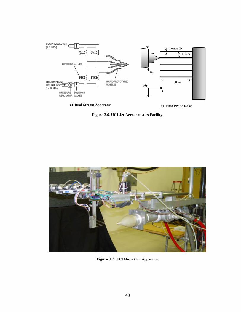
3.6 UCI Jet Aeroacoustics Facility. a) Dual-Stream Apparatus. b) Pitot-Probe Rake.
43
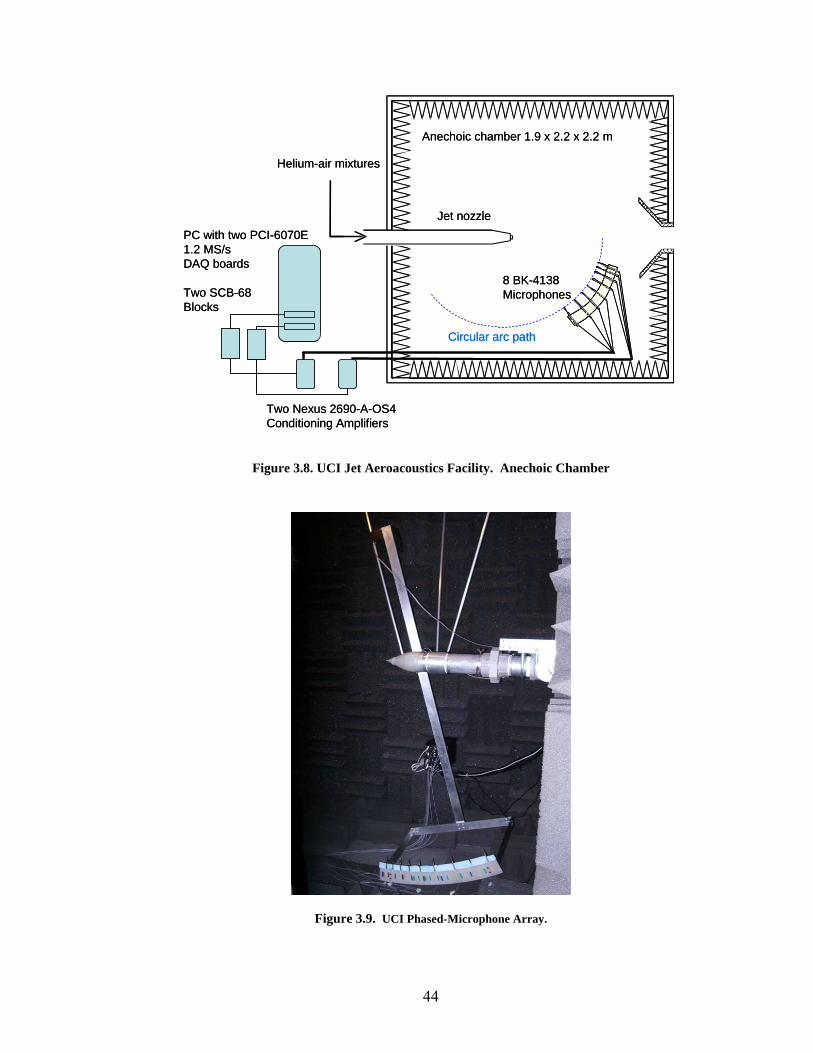
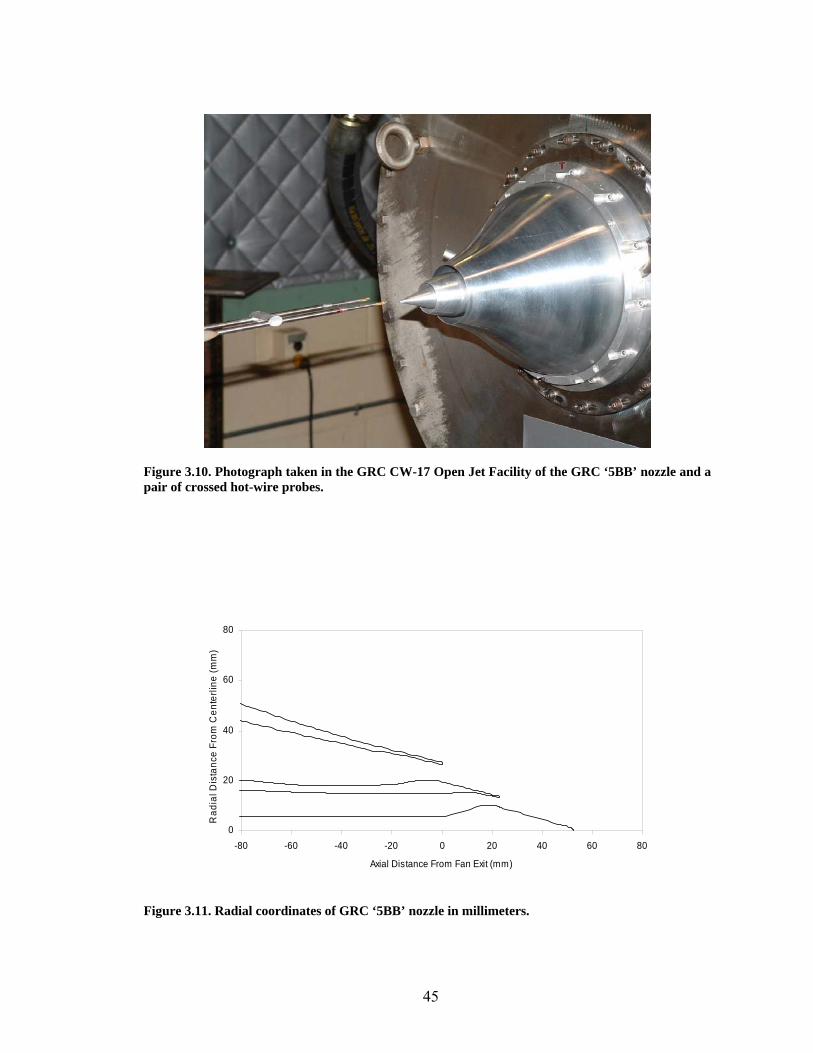
3.7 UCI Mean Flow Apparatus. 43 3.8 UCI Jet Aeroacoustics Facility. Anechoic Chamber 44 3.9 UCI Phased-Microphone Array. 44 3.10 Photograph taken in the GRC CW-17 Open Jet Facility of the GRC ‘5BB’
nozzle and a pair of crossed hot-wire probes.
45
3.11 Radial coordinates of GRC ‘5BB’ nozzle in millimeters. 45 3.12 Photographs taken in the GRC CW17 Open Jet Facility. GRC ‘5BB’
nozzle and a) W1 b) Pylon + Flap c) W2 + Cap1 d) W2 + Cap3.
46
3.13 Photograph taken in the GRC CW-17 Free Jet Facility of the GRC coannular nozzle and automated traversing mechanism.
46
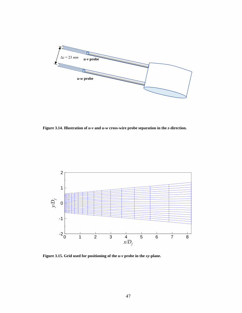
3.14 Illustration of u-v and u-w cross-wire probe separation in the z-direction. 47 3.15 Grid used for positioning of the u-v probe in the xy-plane. 47 3.16 Three regions of a coaxial jet (top). Mean velocity profiles (bottom)
measured at x/Df = 0.2,1, and 10 in a coaxial jet exhaust with secondary-to-primary velocity ratio 0.5.
48
3.17 Secondary shear layer mean velocity profiles. Values are non-dimensionalized for similarity.
49
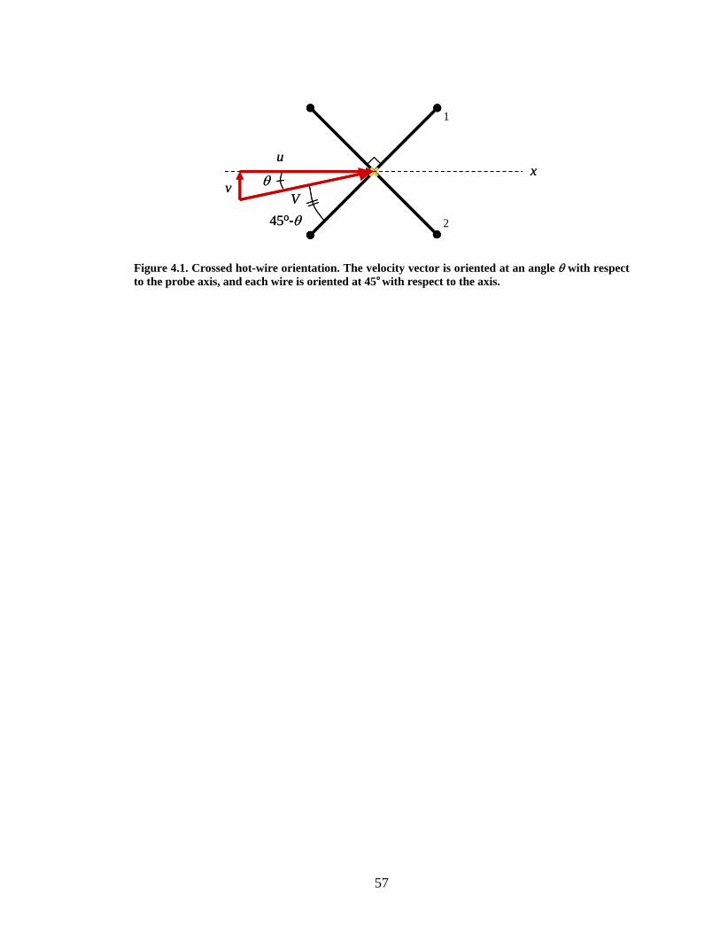
4.1 Crossed hot-wire orientation. The velocity vector is oriented at an angle θ with respect to the probe axis, and each wire is oriented at 45o with respect to the axis.
57
viii
5.1 Sound pressure level (SPL) measurements for an internal wedge in a nozzle with converging exit streamlines. Similar trends are observed at a) UCI and b) at NASA.
75
5.2
Sound pressure level (SPL) measurements for an internal wedge and nozzle with parallel exit streamlines. The wedge causes a noise increase.
75
5.3
Illustration showing hypothesis of deflection of flow in the nozzle with a) parallel geometry and b) with convergent geometry.
76
5.4
Mean flow measurements supporting the hypothesis in Fig. 5.3. Axial velocity isocontours of u(x,y,0)/Up and u(x0, y, z)/umax(x) taken at 4Df downstream of the plug tip. a) UCI ‘Classic’ and b) UCI ‘3BB’ nozzles.
76
5.5
Nozzle and internal-wedge configurations that produced the results in Fig.5.4. a) UCI ‘Classic’ coplanar and b) UCI ‘3BB’ nozzles.
76
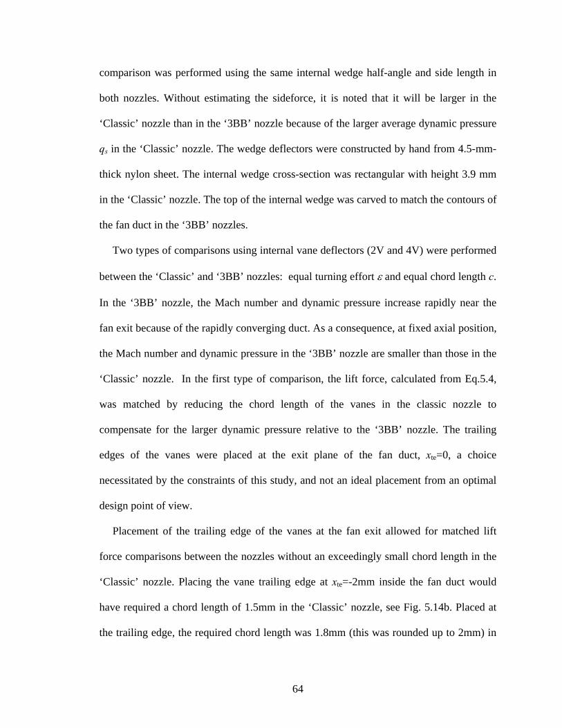
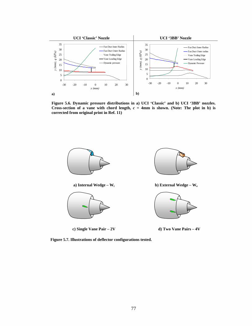
5.6
Dynamic pressure distributions in a) UCI ‘Classic’ and b) UCI ‘3BB’ nozzles. Cross-section of a vane with chord length, c = 4mm is shown. (Note: The plot in b) is corrected from original print in Ref. 11)
77
5.7
Illustrations of deflector configurations tested. 77
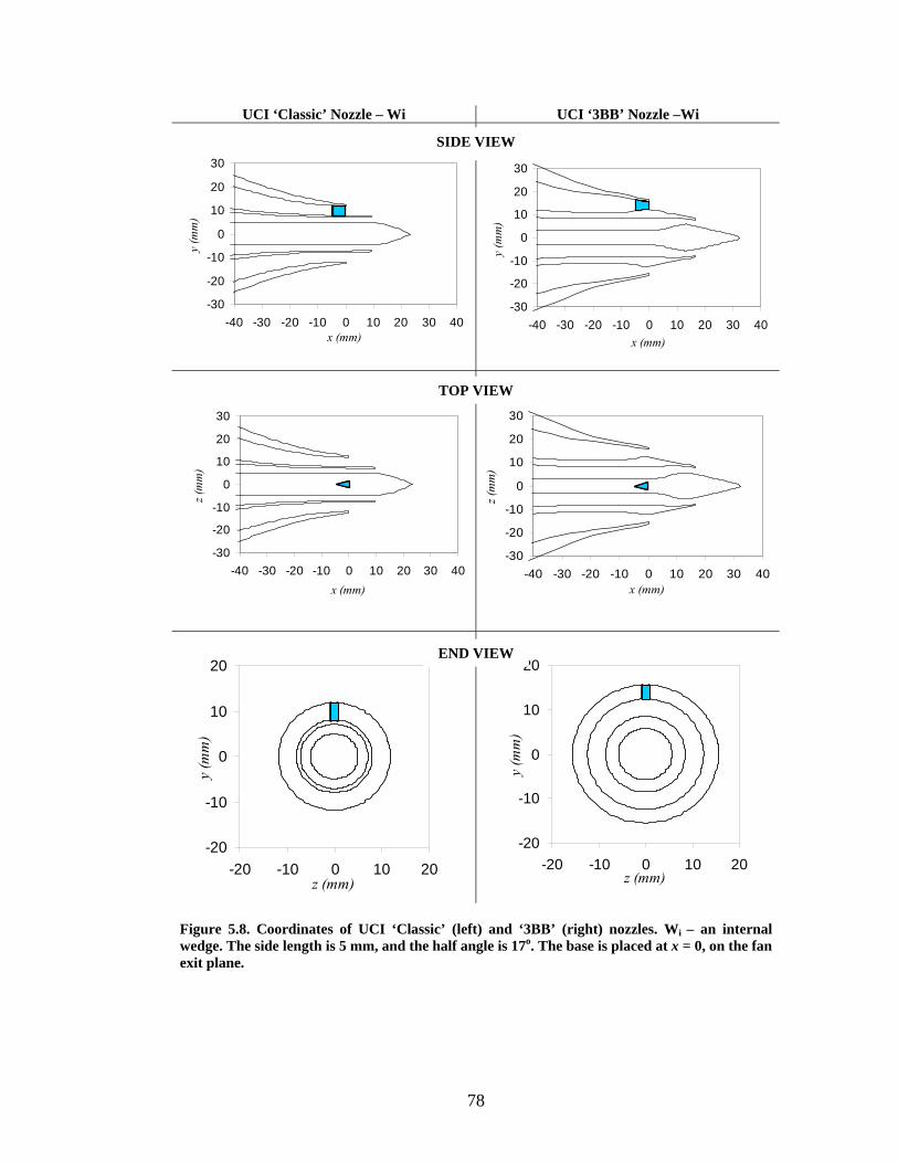
5.8
Coordinates of UCI ‘Classic’ (left) and ‘3BB’ (right) nozzles. Wi an internal wedge. The side length is 5 mm, and the half angle is 17o. The base is placed at x = 0, on the fan exit plane.
78
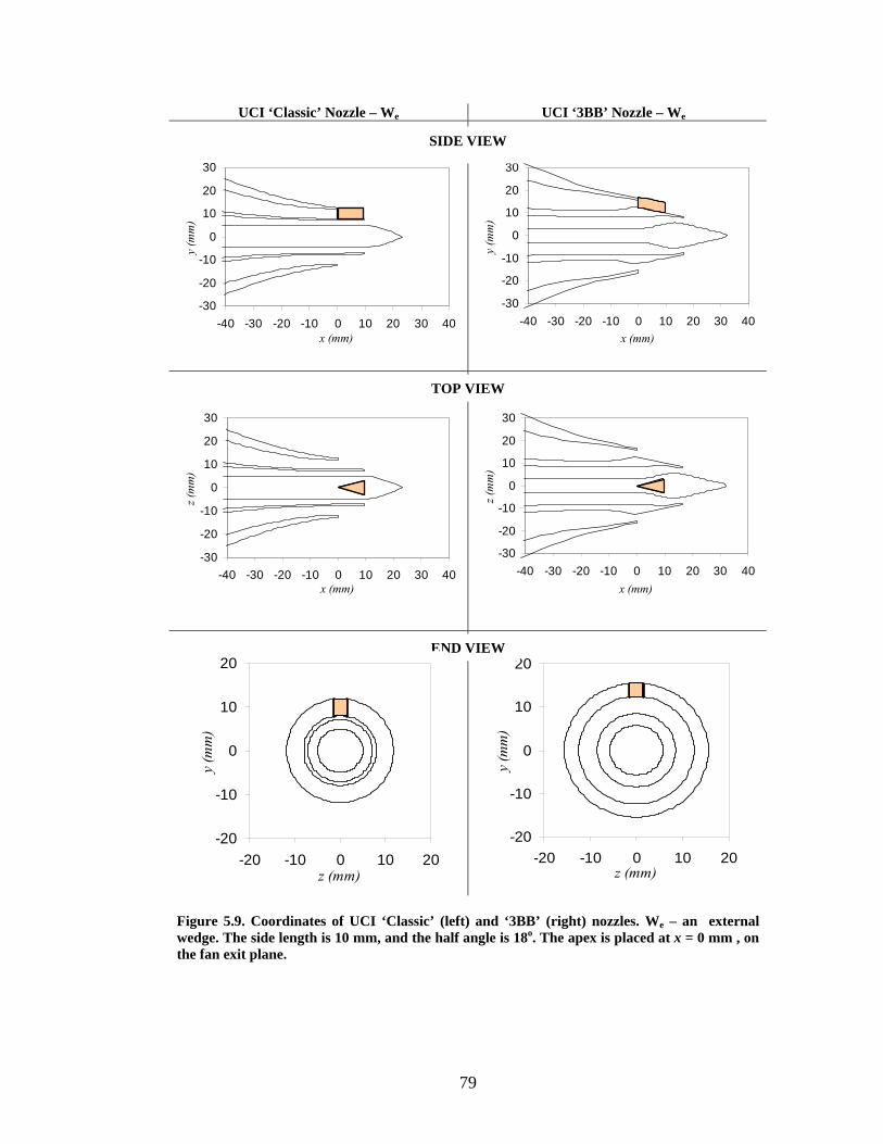
5.9
Coordinates of UCI ‘Classic’ (left) and ‘3BB’ (right) nozzles. We an external wedge. The side length is 10 mm, and the half angle is 18o. The apex is placed at x = 0 mm , on the fan exit plane.
79
5.10
Coordinates of UCI ‘Classic’ (left) and ‘3BB’ (right) nozzles. 2V a single pair of vanes. a) Equal turning effort comparison, c = 2 mm in the ‘Classic’ nozzle and c = 4mm in the ‘3BB’ nozzle. b) For the equal chord comparison, c = 4 mm in both nozzles. c) End views.
80
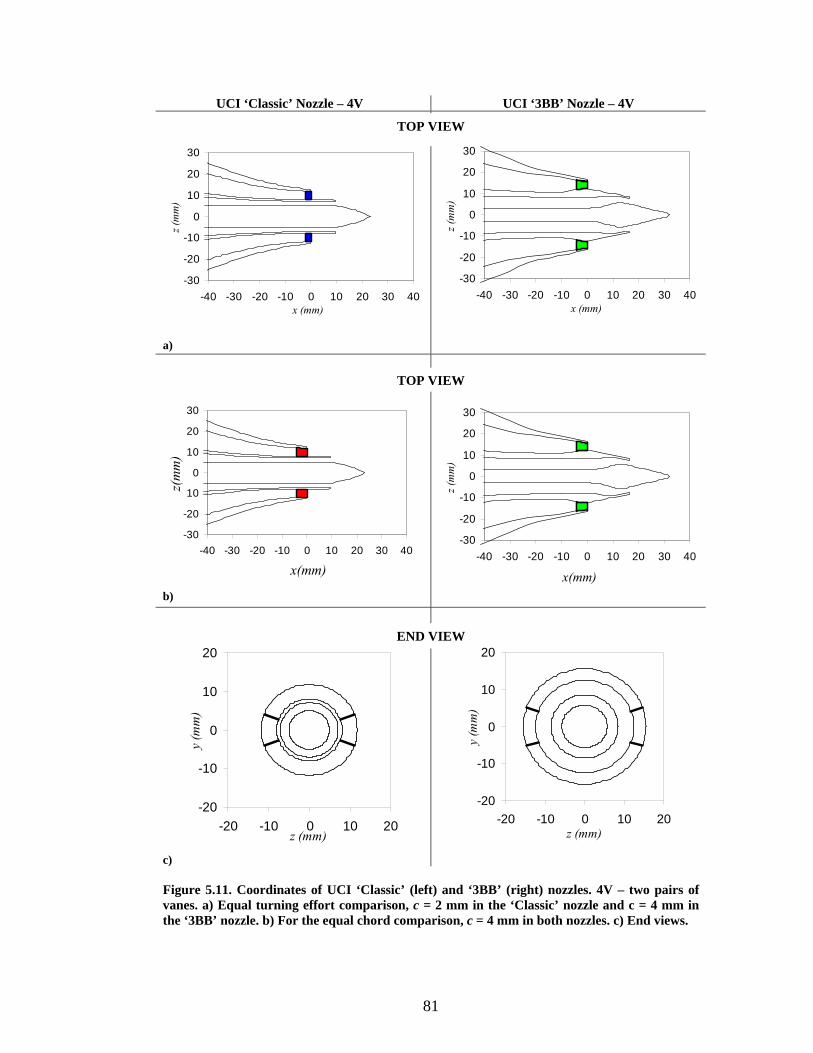
5.11
Coordinates of UCI ‘Classic’ (left) and ‘3BB’ (right) nozzles. 4V two pairs of vanes. a) Equal turning effort comparison, c = 2 mm in the ‘Classic’ nozzle and c = 4 mm in the ‘3BB’ nozzle. b) For the equal chord comparison, c = 4 mm in both nozzles. c) End views.
81
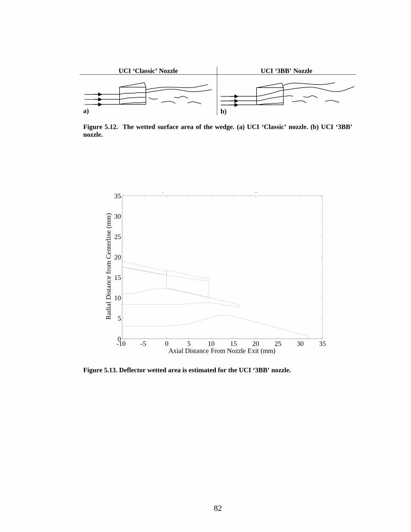
5.12
Wetted surface area of the wedge for a) ‘Classic’ and b) ‘3BB’ nozzles. 82
5.13 Deflector wetted area is estimated for the UCI ‘3BB’ nozzle. 82
5.14
Lift estimates for vane deflectors with trailing edge postion a) xte=0mm and b) xte =-2mm. 83
ix
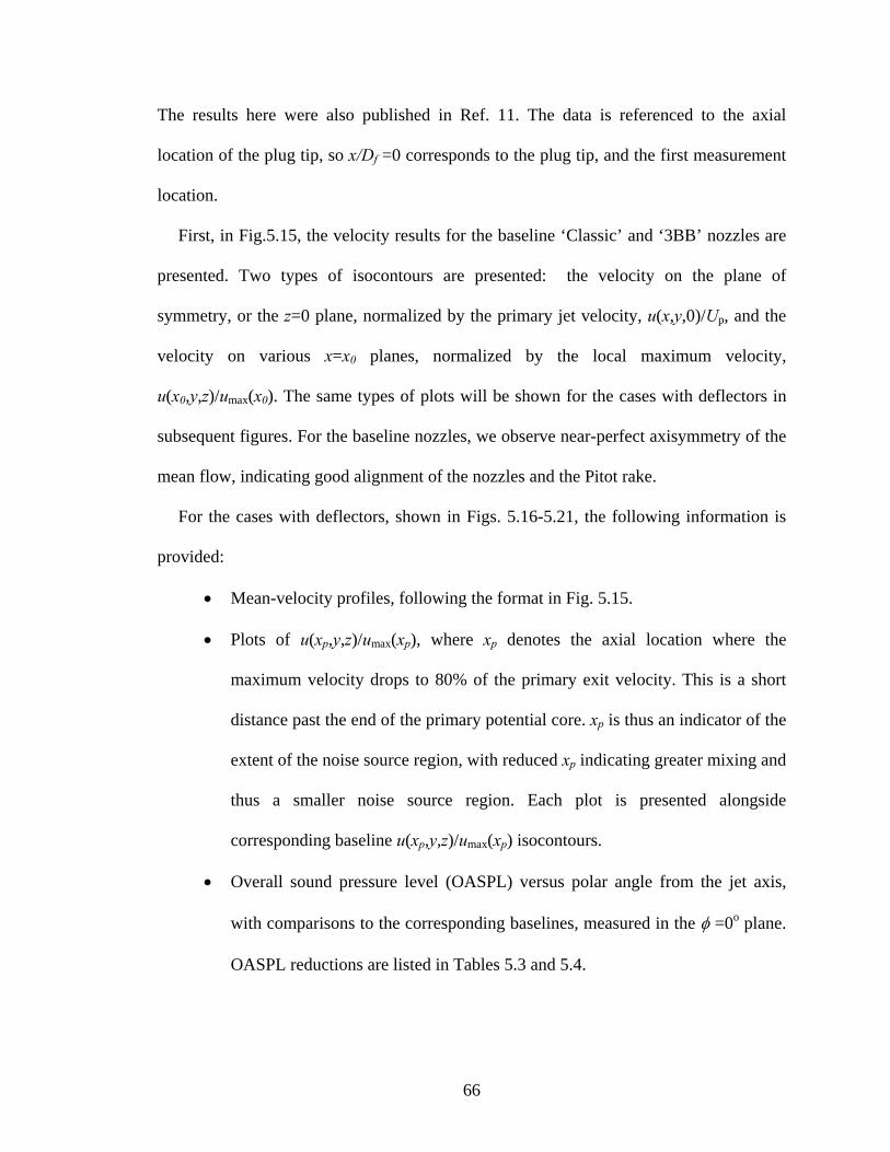
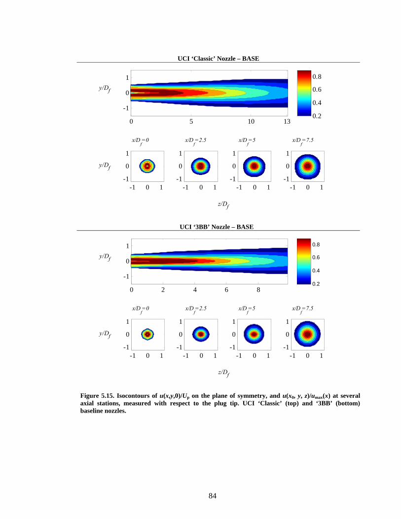
5.15
Isocontours of u(x,y,0)/Up on the plane of symmetry, and u(x0,y,z)/umax(x) at several axial stations, measured with respect to the plug tip. UCI ‘Classic’ (top) and ‘3BB’ (bottom) baseline nozzles.
84
5.16
UCI ‘Classic’ (left) and ‘3BB’ (right) nozzles with Wi (internal wedge). The measurements support the hypothesis in Fig. 5.3.
85
5.17
UCI ‘Classic’ (left) and ‘3BB’ (right) nozzles with We (external wedge). The measurements support the hypothesis in Fig. 5.3.
86
5.18
UCI ‘Classic’ (left) and ‘3BB’ (right) nozzles with 2V (pair of vanes.) Equal turning effort, ε.
87
5.19
UCI ‘Classic’ (left) and ‘3BB’ (right) nozzles with 2V (pair of vanes). Equal chord length, c.
88
5.20
UCI ‘Classic’ (left) and ‘3BB’ (right) nozzles with 4V (two pairs of vanes). Equal tuning effort, ε.
89
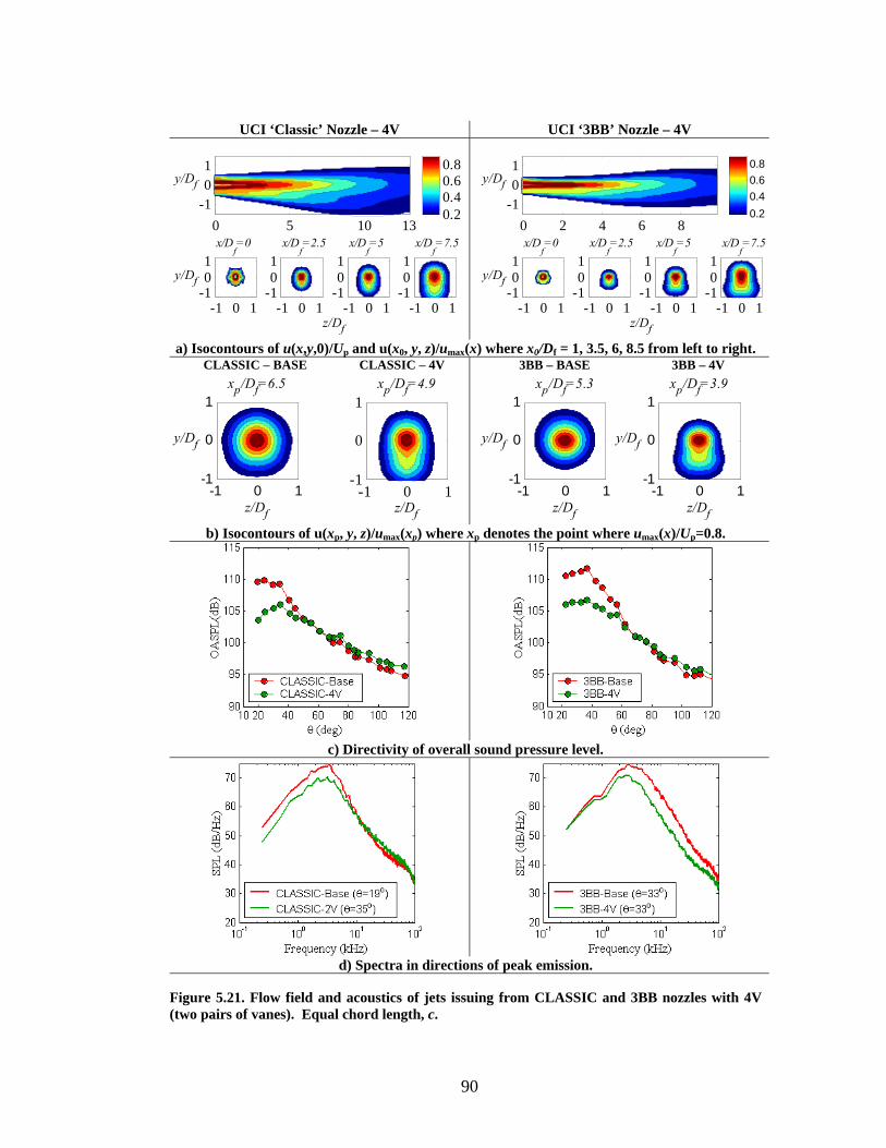
5.21
Flow field and acoustics of jets issuing from CLASSIC and 3BB nozzles with 4V (two pairs of vanes). Equal chord length, c.
90
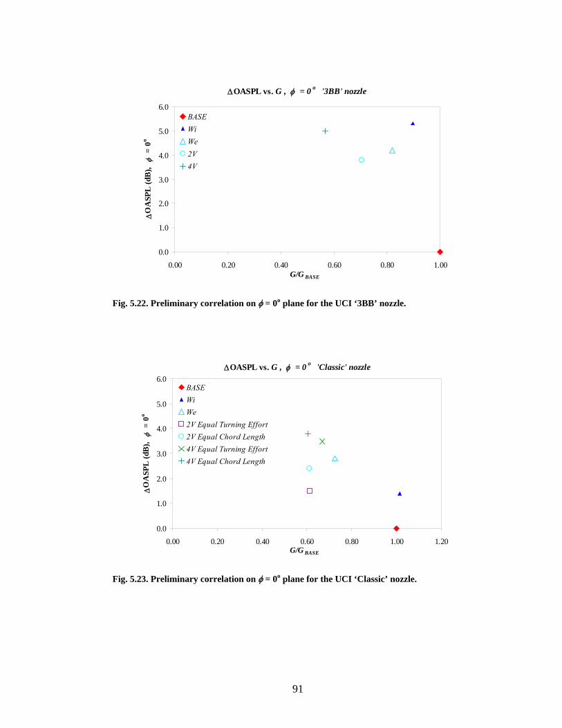
5.22 Preliminary correlation on φ = 0o plane for the UCI ‘3BB’ nozzle. 91
5.23 Preliminary correlation on φ = 0o plane for the UCI ‘Classic’ nozzle. 91
5.24 Preliminary correlation on φ = 0o plane for the UCI ‘3BB’ nozzle. For Wi and We, G is calculated using Eq.5.6. For 2V and 4V, Eq.5.5 is used.
92
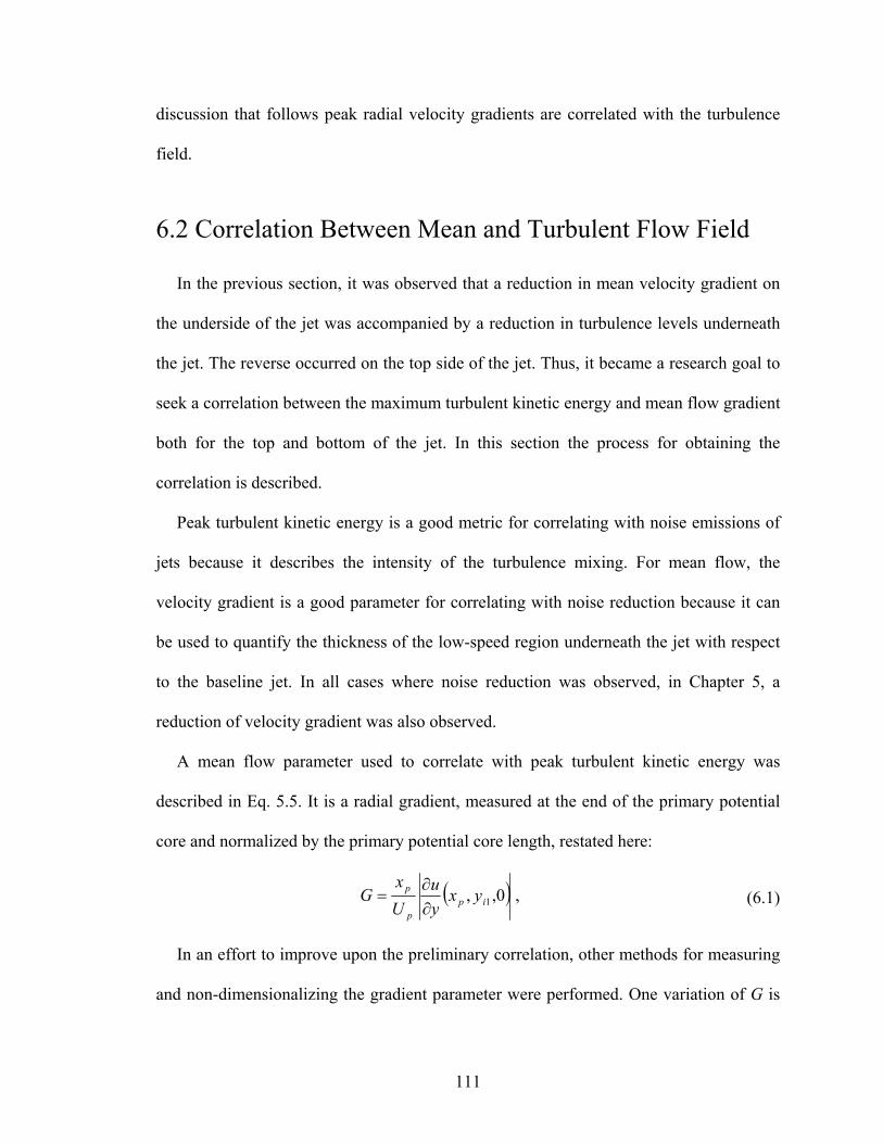
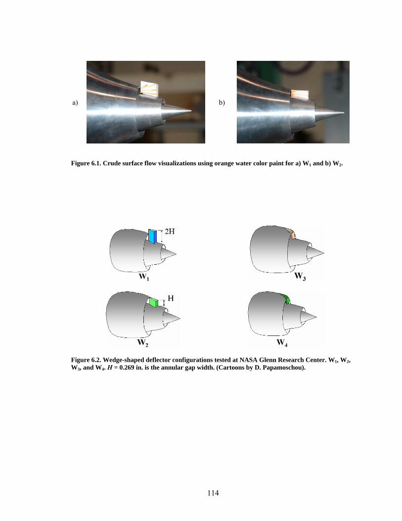
6.1 Crude surface flow visualizations using orange water color paint. a) W1. b) W2.
114
6.2 Wedge-shaped deflector configurations tested at NASA Glenn Research Center. W1, W2, W3, and W4.
114
6.3 Cross-section of a) W1, W2, and W3 and b) W4 c) Three caps (top views are shown).
115
6.4 W4 + pylon + external flap. Cap configurations tested.
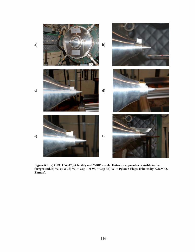
115 6.5 a) GRC CW-17 jet facility and ‘5BB’ nozzle. Hot-wire apparatus is
visible in the foreground. b) W1 c) W2 d) W2 + Cap 1 e) W2 + Cap 3 f) W4 + Pylon + Flaps.
116
6.6 Radial coordinates for the CW17 5BB nozzle with a) W1 b) W2 c) W3 d) W4.
117
x
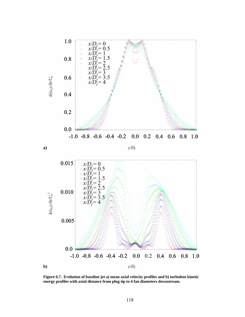
6.7 Evolution of baseline jet a) mean axial velocity profiles and b) turbulent
kinetic energy profiles with axial distance from plug tip to 4 fan diameters downstream.
118
6.8 Evolution of mean axial velocity profiles, u(x,y,0)/Up. Baseline jet.
119
6.9 Evolution of mean velocity gradient profiles, ∂u(x,y,0)/∂y · Df/Up. Baseline jet.
119
6.10 Evolution of mean axial velocity profiles, u(x,y,0)/Up. W1 overlaid with baseline jet.
120
6.11 Evolution of mean velocity gradient profiles, ∂u(x,y,0)/∂y·Df/Up. W1 overlaid with baseline jet.
120
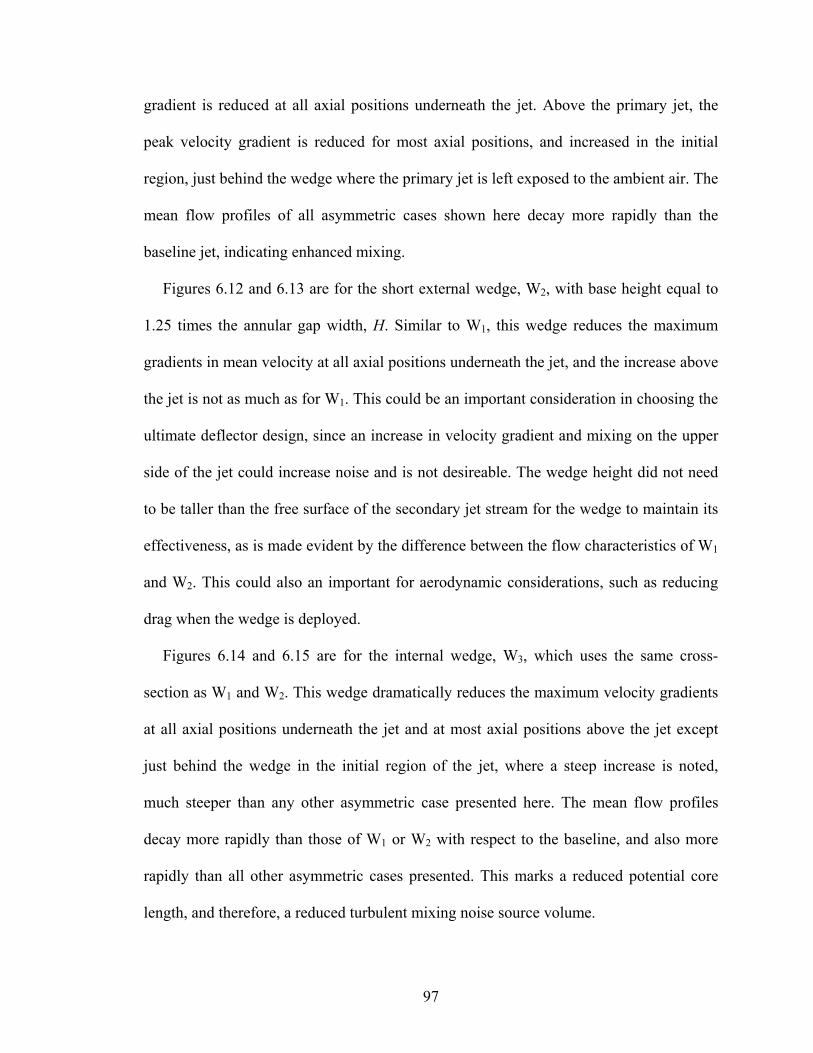
6.12 Evolution of mean axial velocity profiles, u(x,y,0)/Up. W2 overlaid with baseline jet.
121
6.13 Evolution of mean velocity gradient profiles, ∂u(x,y,0)/∂y·Df/Up. W2 overlaid with baseline jet.
121
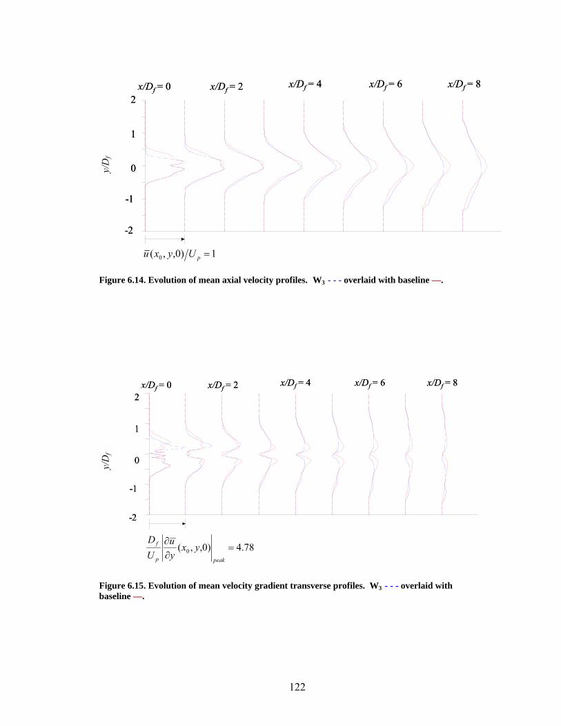
6.14 Evolution of mean axial velocity profiles, u(x,y,0)/Up. W3
overlaid with baseline jet .
122
6.15 Evolution of mean velocity gradient profiles, ∂u(x,y,0)/∂y·Df/Up. W3
overlaid with baseline jet.
122
6.16 Evolution of mean axial velocity profiles, u(x,y,0)/Up. W4
overlaid with baseline jet.
123
6.17 Evolution of mean velocity gradient profiles, ∂u(x,y,0)/∂y·Df/Up. W4
overlaid with baseline jet.
123
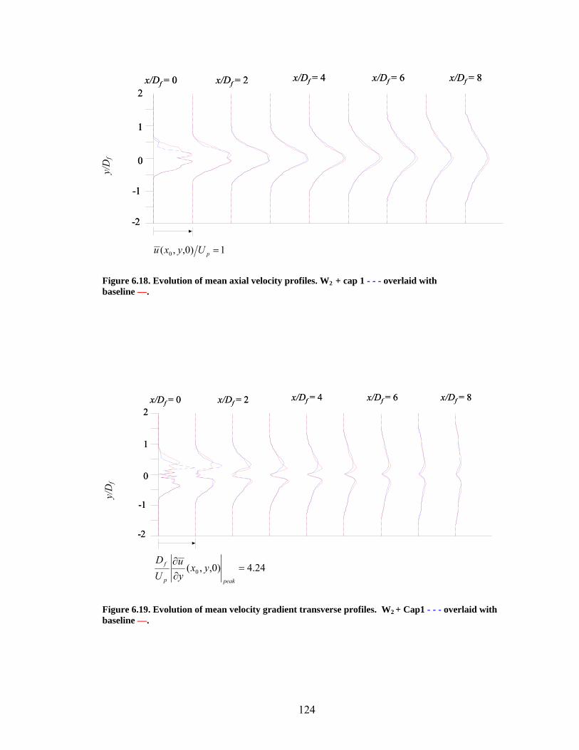
6.18 Evolution of mean axial velocity profiles, u(x,y,0)/Up. W2 +Cap1 overlaid with baseline jet.
124
6.19 Evolution of mean velocity gradient profiles, ∂u(x,y,0)/∂y·Df/Up. W2 + Cap1 overlaid with baseline jet. 124
6.20 Evolution of mean axial velocity profiles, u(x,y,0)/Up. W2
+ Cap2 overlaid with baseline jet.
125
6.21 Evolution of mean velocity gradient profiles, ∂u(x,y,0)/∂y·Df/Up. W2 + Cap2 overlaid with baseline jet.
125
xi
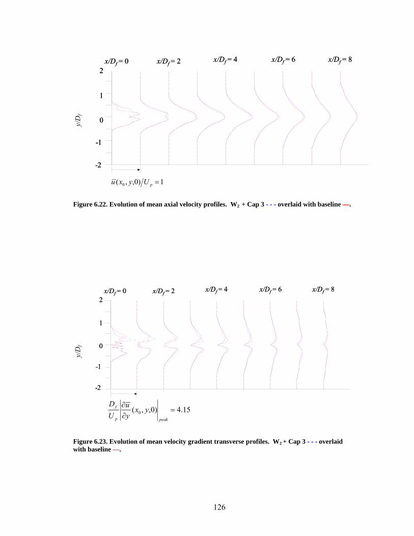
6.22 Evolution of mean axial velocity profiles, u(x,y,0)/Up. W2
+ Cap3 overlaid with baseline jet.
125
6.23 Evolution of mean velocity gradient profiles, ∂u(x,y,0)/∂y·Df/Up. W2 + Cap3 overlaid with baseline jet.
125
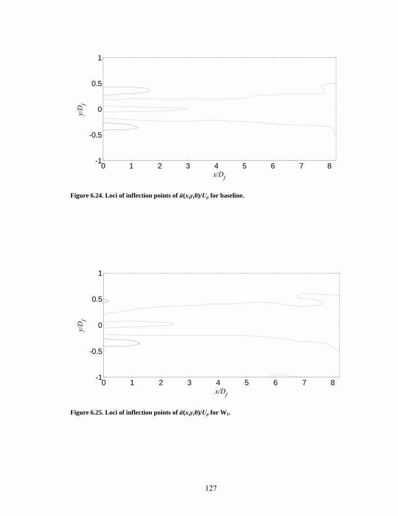
6.24 Locus of inflection points of u(x,y,0)/Up for baseline jet.
127 6.25 Locus of inflection points of u(x,y,0)/Up for W1.
127
6.26 Locus of inflection points of u(x,y,0)/Up for W2.
128 6.27 Locus of inflection points of u(x,y,0)/Up for W3.
128
6.28 Locus of inflection points of u(x,y,0)/Up for W4.
129 6.29 Locus of inflection points of u(x,y,0)/Up for W2
+ Cap1.
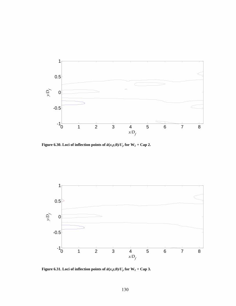
129 6.30 Locus of inflection points of u(x,y,0)/Up for W2
+ Cap2.
130 6.31 Locus of inflection points of u(x,y,0)/Up for W2
+ Cap3.
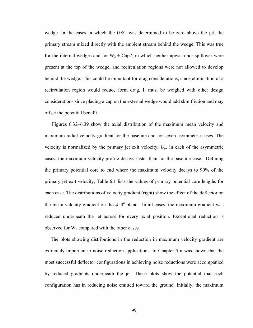
130 6.32 Axial distributions of a) maximum mean velocity u(x,y,0)/Up and
b) maximum radial velocity gradient ∂u(x,y,0)/∂y ·Df/Up , baseline jet.
131
6.33 Axial distributions of a) maximum mean velocity u(x,y,0)/Up and b) maximum radial velocity gradient ∂u(x,y,0)/∂y·Df/Up , W1 overlaid with baseline jet.
131
6.34 Axial distributions of a) maximum mean velocity u(x,y,0)/Up and b) maximum radial velocity gradient ∂u(x,y,0)/∂y ·Df/Up. W2 overlaid with baseline jet.
132
6.35 Axial distributions of a) maximum mean velocity u(x,y,0)/Up and b) maximum radial velocity gradient ∂u(x,y,0)/∂y ·Df/Up. W3 overlaid with baseline jet.
132
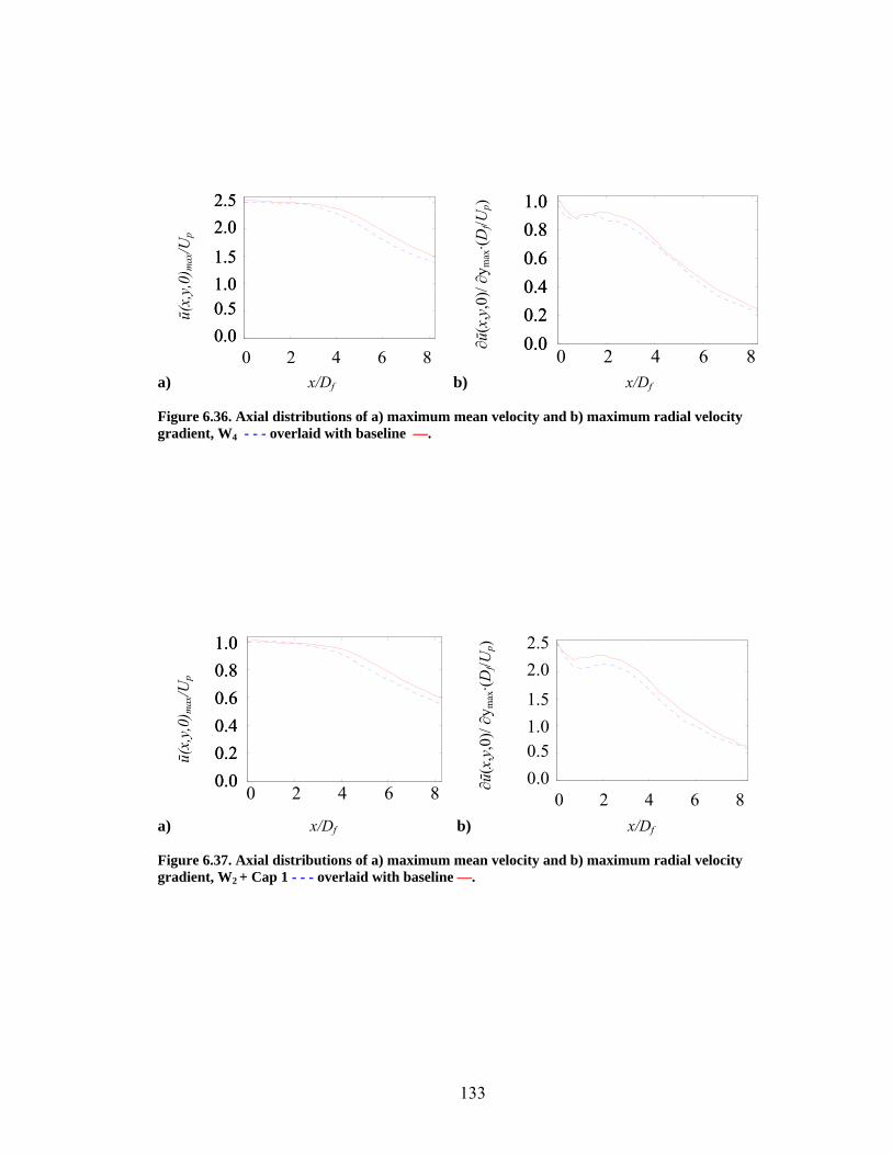
6.36 Axial distributions of a) maximum mean velocity u(x,y,0)/Up and b) maximum radial velocity gradient ∂u(x,y,0)/∂y ·Df/Up. W4 overlaid with baseline jet.
133
6.37 Axial distributions of a) maximum mean velocity u(x,y,0)/Up and b) maximum radial velocity gradient ∂u(x,y,0)/∂y·Df/U. W2 +Cap1 overlaid with baseline jet.
133
6.38 Axial distributions of a) maximum mean velocity u(x,y,0)/Up and b) maximum radial velocity gradient ∂u(x,y,0)/∂y·Df/Up. W2 +Cap2 overlaid with baseline jet.
134
6.39 Axial distributions of a) maximum mean velocity u(x,y,0)/Up and b) maximum radial velocity gradient ∂u(x,y,0)/∂y·Df/Up. W2 +Cap3 overlaid with baseline jet.
134
xii
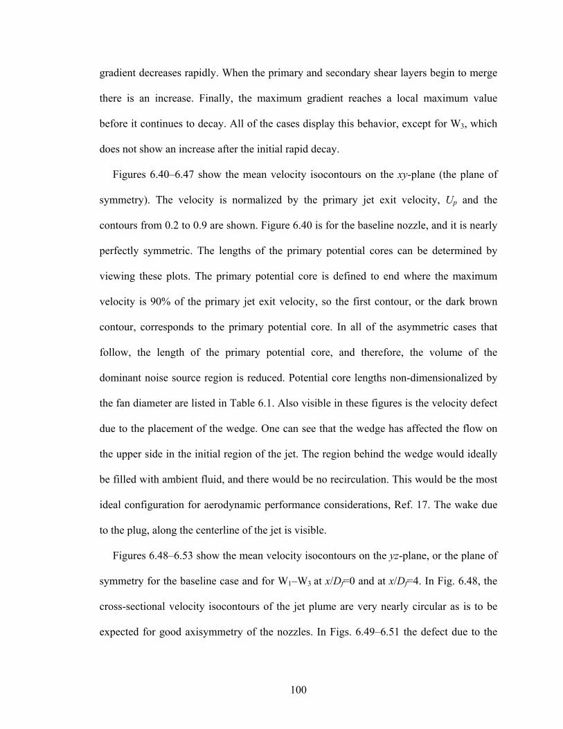
6.40 Mean axial velocity isocontours, u(x,y,0)/Up for the baseline jet.
135
6.41 Mean axial velocity isocontours, u(x,y,0)/Up for W1. 135
6.42 Mean axial velocity isocontours, u(x,y,0)/Up for W2. 135
6.43 Mean axial velocity isocontours, u(x,y,0)/Up for W3. 135
6.44 Mean axial velocity isocontours, u(x,y,0)/Up for W4. 136
6.45 Mean axial velocity isocontours, u(x,y,0)/Up for W2 + Cap1.
136
6.46 Mean axial velocity isocontours, u(x,y,0)/Up for W2 + Cap2.
136
6.47 Mean axial velocity isocontours, u(x,y,0)/Up for W2 + Cap3.
136
6.48 Mean axial velocity isocontours, u(x,y,0)/Up for the baseline jet. 137
6.49 Mean axial velocity isocontours, u(x,y,0)/Up for W1. 137
6.50 Mean axial velocity isocontours, u(x,y,0)/Up for W2. 138
6.51 Mean axial velocity isocontours, u(x,y,0)/Up for W3. 138
6.52 Mean axial velocity isocontours, u(x,y,0)/Up. a) W4 and b) W4 + Pylon.
139
6.53 Mean axial velocity isocontours, u(x,y,0)/Up. a) W4 + Pylon and b) W4 + Pylon + flaps.
139
6.54 Evolution of RMS axial velocity profiles, uRMS(x,y,0)/Up2.
Baseline jet
140
6.55 Evolution of turbulent kinetic energy profiles, k(x,y,0)/Up2.
Baseline jet.
140
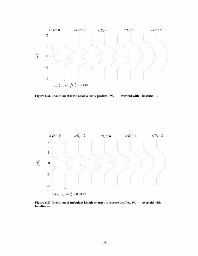
6.56 Evolution of RMS axial velocity profiles, uRMS(x,y,0)/Up. W1 overlaid with baseline jet.
141
6.57 Evolution of turbulent kinetic energy profiles, k(x,y,0)/Up2.
W1 overlaid with baseline jet.
141
6.58 Evolution of RMS axial velocity profiles, uRMS(x,y,0)/Up. W2 overlaid with baseline jet.
142
xiii
6.59 Evolution of turbulent kinetic energy profiles, k(x,y,0)/Up2.
W2 overlaid with baseline jet.
142
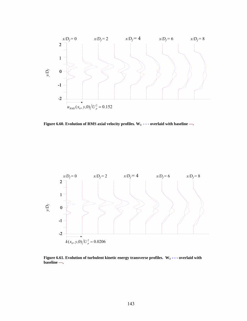
6.60 Evolution of RMS axial velocity profiles, uRMS(x,y,0)/Up. W3 overlaid with baseline jet.
143
6.61 Evolution of turbulent kinetic energy profiles, k(x,y,0)/Up2.
W3 overlaid with baseline jet.
143
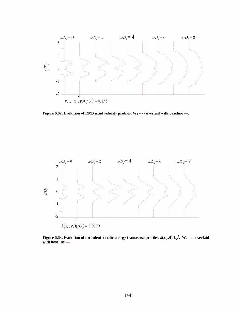
6.62 Evolution of RMS axial velocity profiles, uRMS(x,y,0)/Up. W4 overlaid with baseline jet.
144
6.63 Evolution of turbulent kinetic energy profiles, k(x,y,0)/Up2.
W4 overlaid with baseline jet.
144
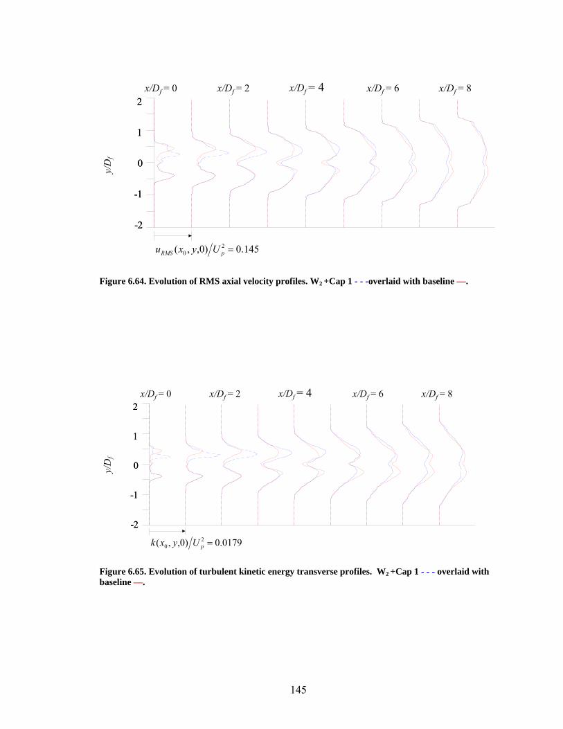
6.64 Evolution of RMS axial velocity profiles, uRMS(x,y,0)/Up . W2 + Cap1 overlaid with baseline jet.
145
6.65 Evolution of turbulent kinetic energy profiles, k(x,y,0)/Up2.
W2 + Cap1 overlaid with baseline jet.
145
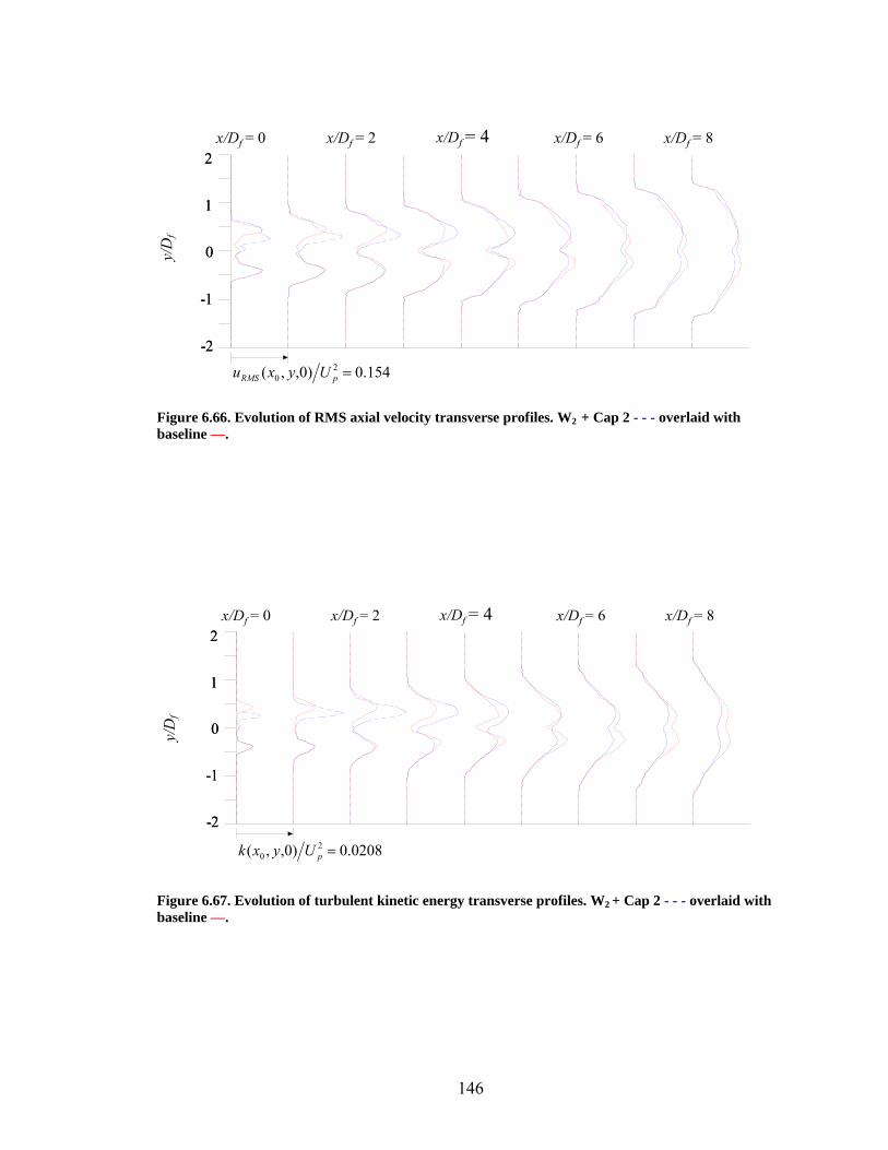
6.66 Evolution of RMS axial velocity profiles, uRMS(x,y,0)/Up. W2
+ Cap2 overlaid with baseline jet.
146
6.67 Evolution of turbulent kinetic energy profiles, k(x,y,0)/Up2.
W2 + Cap2 overlaid with baseline jet.
146
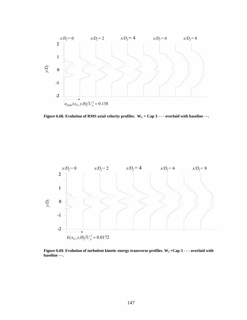
6.68 Evolution of RMS axial velocity profiles, uRMS(x,y,0)/Up. W2 + Cap3 overlaid with baseline jet.
147
6.69 Evolution of turbulent kinetic energy profiles, k(x,y,0)/Up2.
W2 + Cap3 overlaid with baseline jet.
147
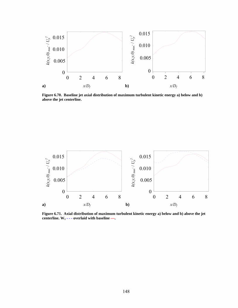
6.70
Baseline jet axial distribution of maximum turbulent kinetic energy a) below and b) above the jet centerline.
148
6.71 Axial distribution of maximum turbulent kinetic energy a) below and b) above the jet centerline. W1 overlaid with baseline jet.
148
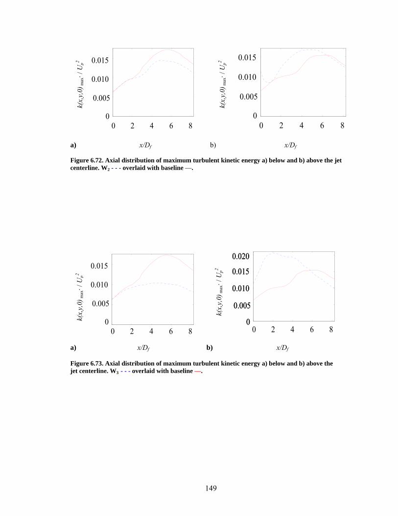
6.72 Axial distribution of maximum turbulent kinetic energy a) below and b) above the jet centerline. W2 overlaid with baseline jet.
149
6.73 Axial distribution of maximum turbulent kinetic energy a) below and b) above the jet centerline. W3
overlaid with baseline jet.
149
xiv
6.74 Axial distribution of maximum turbulent kinetic energy a) below and b) above the jet centerline. W4
overlaid with baseline jet.
150
6.75 Axial distribution of maximum turbulent kinetic energy a) below and b) above the jet centerline. W2+Cap1 overlaid with baseline jet.
150
6.76 Axial distribution of maximum turbulent kinetic energy a) below and b) above the jet centerline. W2+Cap2 overlaid with baseline jet.
151
6.77 Axial distribution of maximum turbulent kinetic energy a) below and b) above the jet centerline. W2+Cap3 overlaid with baseline jet.
151
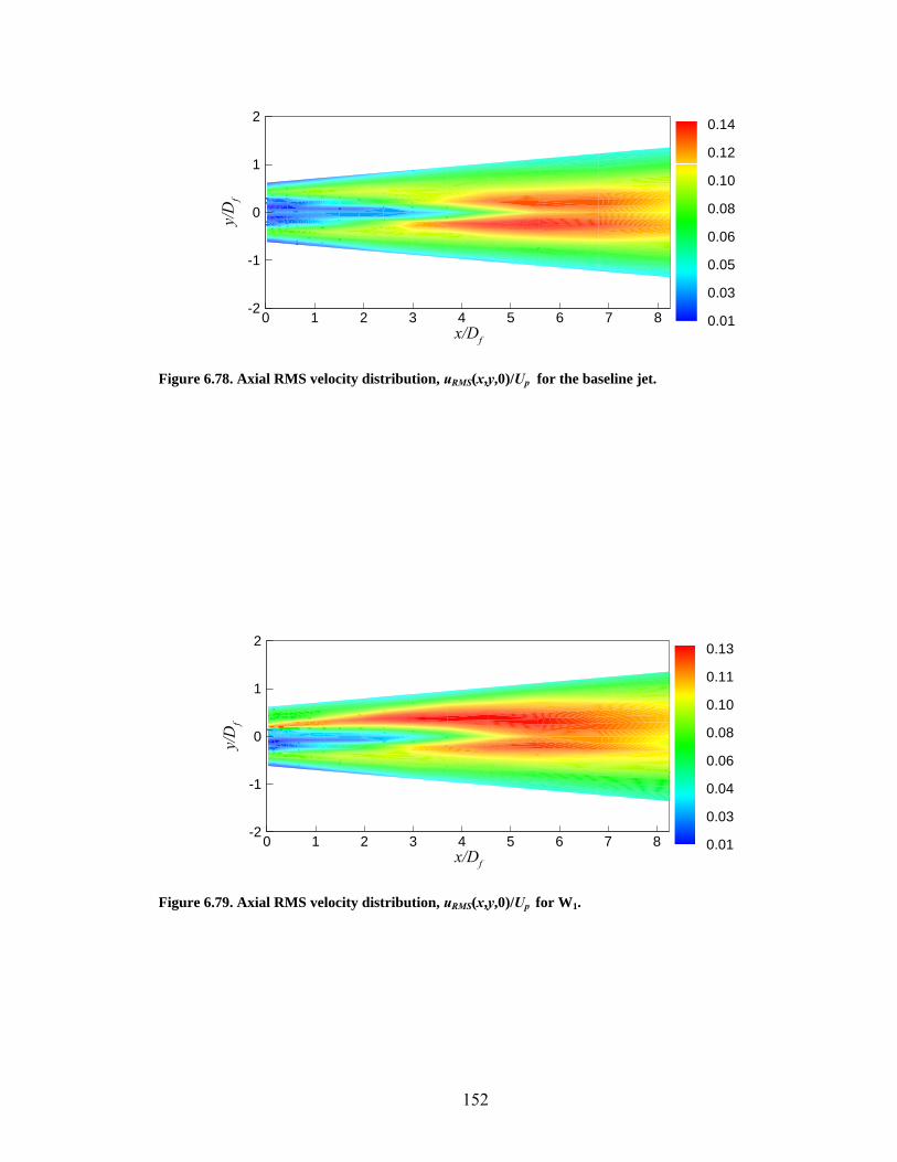
6.78 Axial RMS velocity distribution, uRMS(x,y,0)/Up for the baseline jet. 152
6.79 Axial RMS velocity distribution, uRMS(x,y,0)/Up for W1. 152
6.80 Axial RMS velocity distribution,, uRMS(x,y,0)/Up for W2. 153
6.81 Axial RMS velocity distribution, uRMS(x,y,0)/Up for W3. 153
6.82 Axial RMS velocity distribution, uRMS(x,y,0)/Up for W4. 154
6.83 Axial RMS velocity distribution, uRMS(x,y,0)/Up for W2 + Cap1.
154
6.84 Axial RMS velocity distribution, uRMS(x,y,0)/Up for W2 + Cap2.
155
6.85 Axial RMS velocity distribution, uRMS(x,y,0)/Up for W2 + Cap3.
155
6.86 Reynolds stresses a) ''vu (x,y,0)/Up2 and b) ''wu (x,y,0)/Up
2 for baseline jet. 156
6.87 Reynolds stresses a) ''vu (x,y,0)/Up2 and b) ''wu (x,y,0)/Up
2 for W1. 156
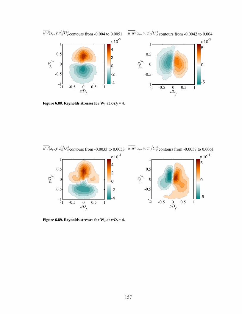
6.88 Reynolds stresses a) ''vu (x,y,0)/Up2 and b) ''wu (x,y,0)/Up
2 for W2. 157
6.89 Reynolds stresses a) ''vu (x,y,0)/Up2 and b) ''wu (x,y,0)/Up
2 for W3. 157
6.90 Reynolds stresses a) ''vu (x,y,0)/Up2 and b) ''wu (x,y,0)/Up
2 for W4. 158
6.91 Reynolds stresses a) ''vu (x,y,0)/Up2 and b) ''wu (x,y,0)/Up
2 for W2 +Cap1. 158
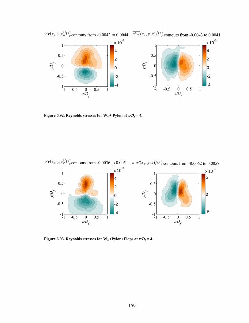
6.92 Reynolds stresses a) ''vu (x,y,0)/Up2 and b) ''wu (x,y,0)/Up
2 for W4+pylon. 159
6.93 Reynolds stresses a) ''vu (x,y,0)/Up2 and b) ''wu (x,y,0)/Up
2 for W4+pylon+flaps.
159
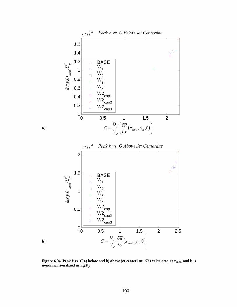
6.94 G vs. Peak k a) below and b) above jet centerline. G is calculated at xGSC, and it is non-dimensionalized using Df.
160
xv
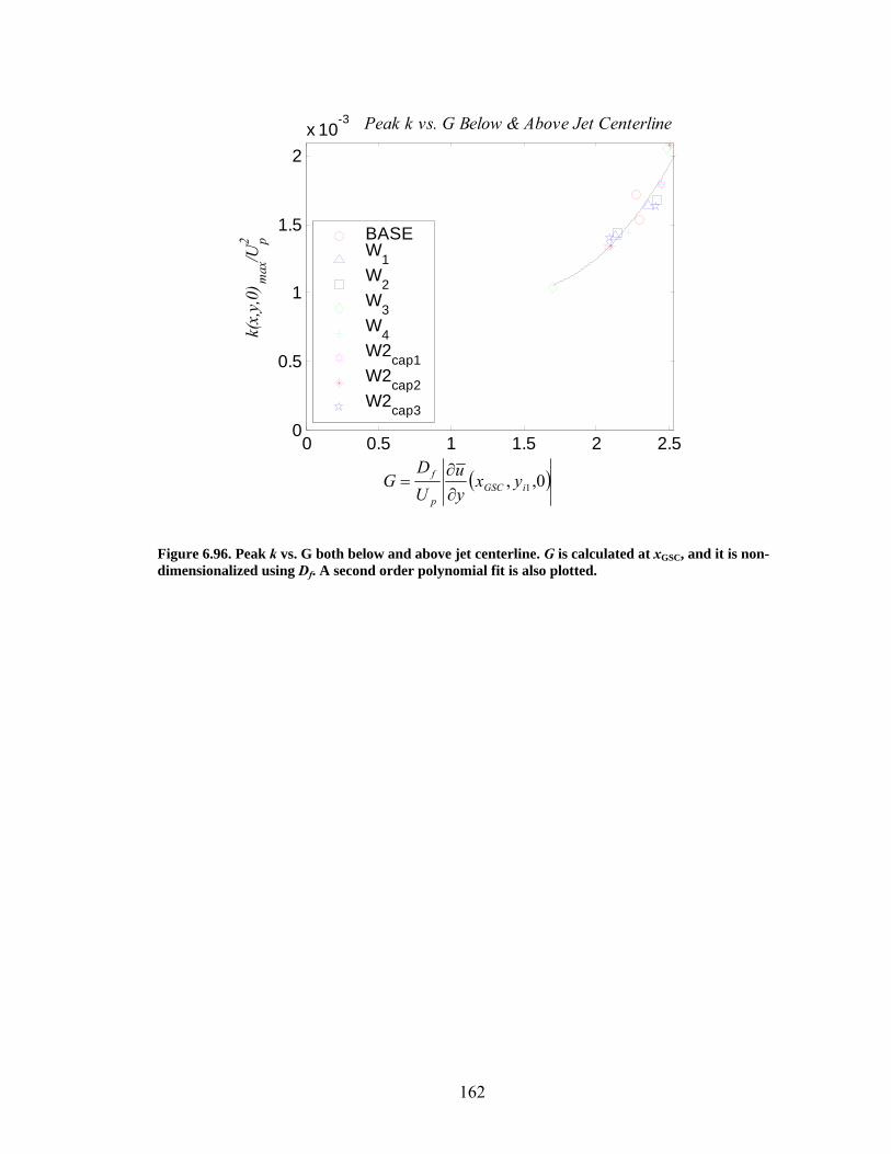
6.95 G vs. Peak k both below and above jet centerline. G is calculated at xGSC, and it is non-dimensionalized using Df. A second order polynomial fit is also plotted.
161
6.96 G vs. Peak k a) below and b) above jet centerline. G is calculated at xGSC, and it is non-dimensionalized using xp.
162
7.1 Computational grid for the axisymmetric configuration. 178
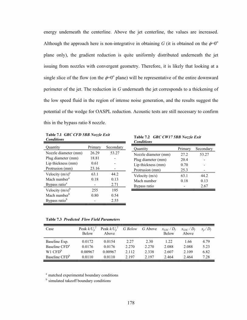
7.2 Computational grid for the asymmetric configuration, showing blocks above and behind wedge.
179
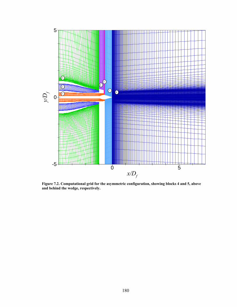
7.3 Computational grid for the asymmetric configuration, showing block on side of wedge.
180
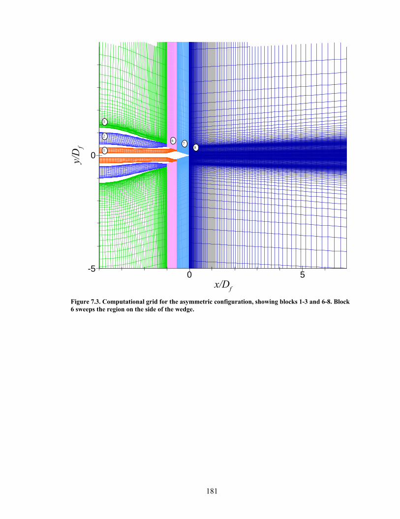
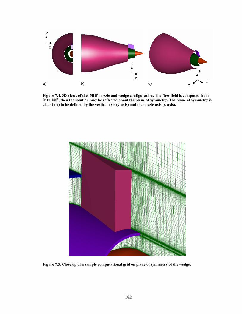
7.4 Close up of computational grid (on plane of symmetry) next to wedge-shaped deflector.
181
7.5 3D views of the ‘5BB’ nozzle and wedge configuration. Only 180o are necessary to model the entire flow field due to symmetry.
181
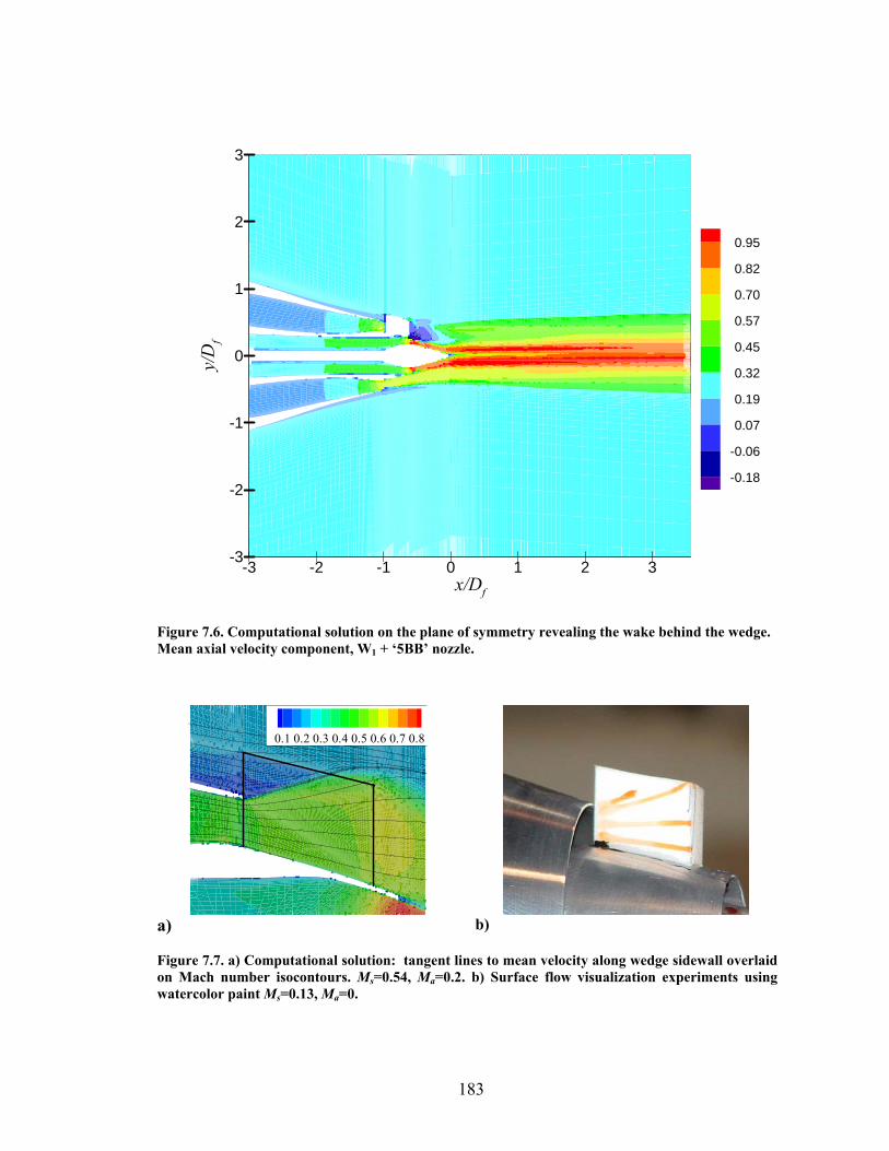
7.6 Computational solution on the plane of symmetry revealing the wake behind the wedge. Mean axial velocity component, W1 + ‘5BB’ nozzle.
182
7.7 a) Computational solution: tangent lines to mean velocity along wedge sidewall overlaid on Mach number isocontours. Ms=0.54, Ma=0.2. b) Surface flow visualization experiments using watercolor paint Ms=0.13, Ma = 0.
182
7.8 Evolution of baseline jet mean axial velocity profiles, u(x,y,0)/Up. 183
7.9 Evolution of baseline jet velocity gradient profiles, ∂u(x,y,0)/∂y·Df/Up. 183
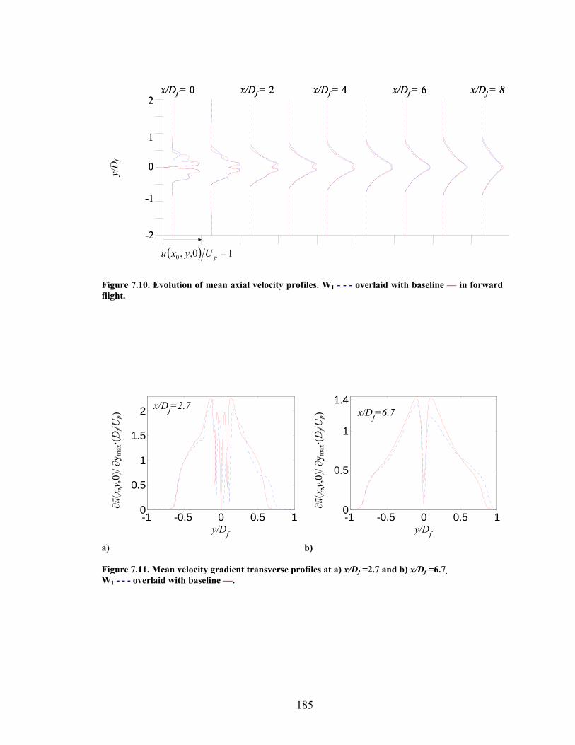
7.10 Evolution of mean axial velocity profiles, u(x,y,0)/Up. W1 overlaid with baseline.
184
7.11 Mean velocity gradient profiles, ∂u(x,y,0)/∂y·Df/Up. a) x/Df = 2.7 and b) x/Df = 6.7.
184
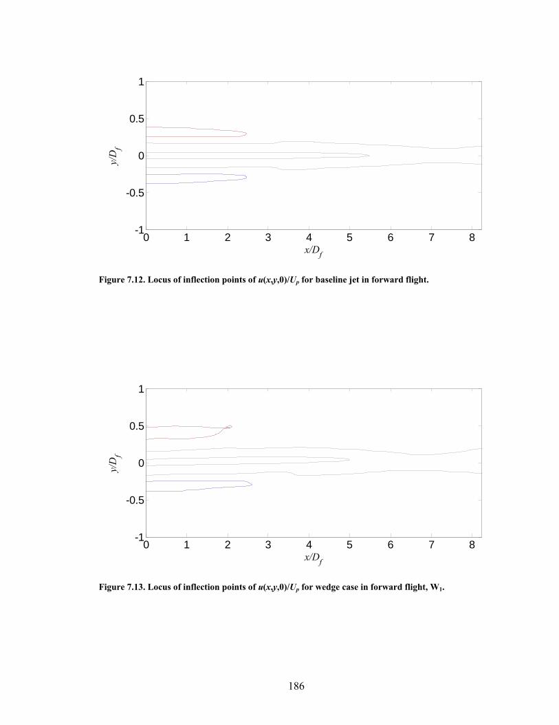
7.12 Locus of inflection points of u(x,y,0)/Up for baseline jet. 185
7.13 Locus of inflection points of u(x,y,0)/Up for W1. 185
7.14 Mean axial velocity isocontours, u(x,y,0)/Up for the baseline jet. 186
7.15 Mean axial velocity isocontours, u(x,y,0)/Up for W1. 186
xvi
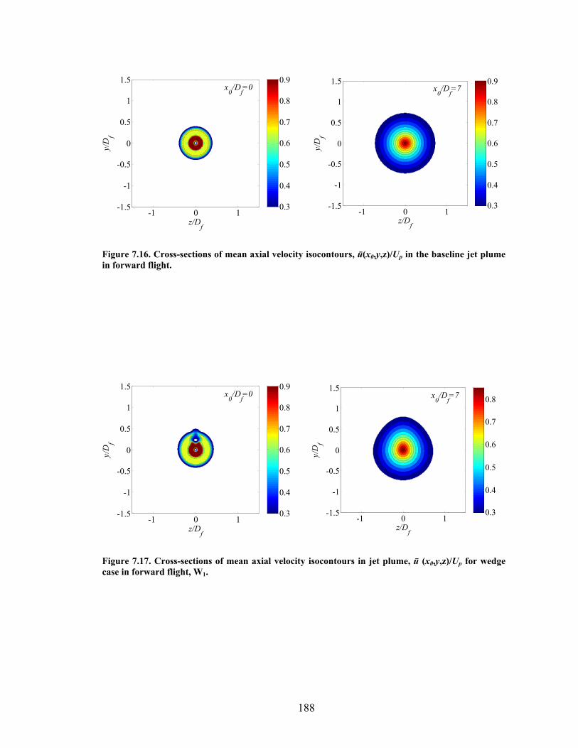
7.16 Cross-sections of mean axial velocity isocontours, u(x0,y,z)/Up for the baseline jet.
187
7.17 Cross-sections of mean axial velocity isocontours, u(x0,y,z)/Up for W1. 187
7.18 Axial distributions of maximum a) mean velocity u(x,y,0)/Up and b) radial velocity gradient ∂u(x,y,0)/∂y·Df/Up underneath the primary jet. W1 overlaid with baseline jet.
188
7.19 Axial distribution of maximum radial velocity gradient ∂u(x,y,0)/∂y·Df/Up, a) underneath the primary jet and b) above the primary jet. W1 overlaid with baseline jet.
188
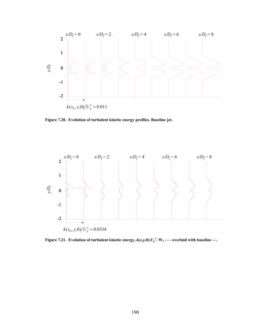
7.20 Evolution of baseline jet turbulent kinetic energy, k(x,y,0)/Up2.
189
7.21 Evolution of turbulent kinetic energy, k(x,y,0)/Up2. W1 overlaid with
baseline jet.
189
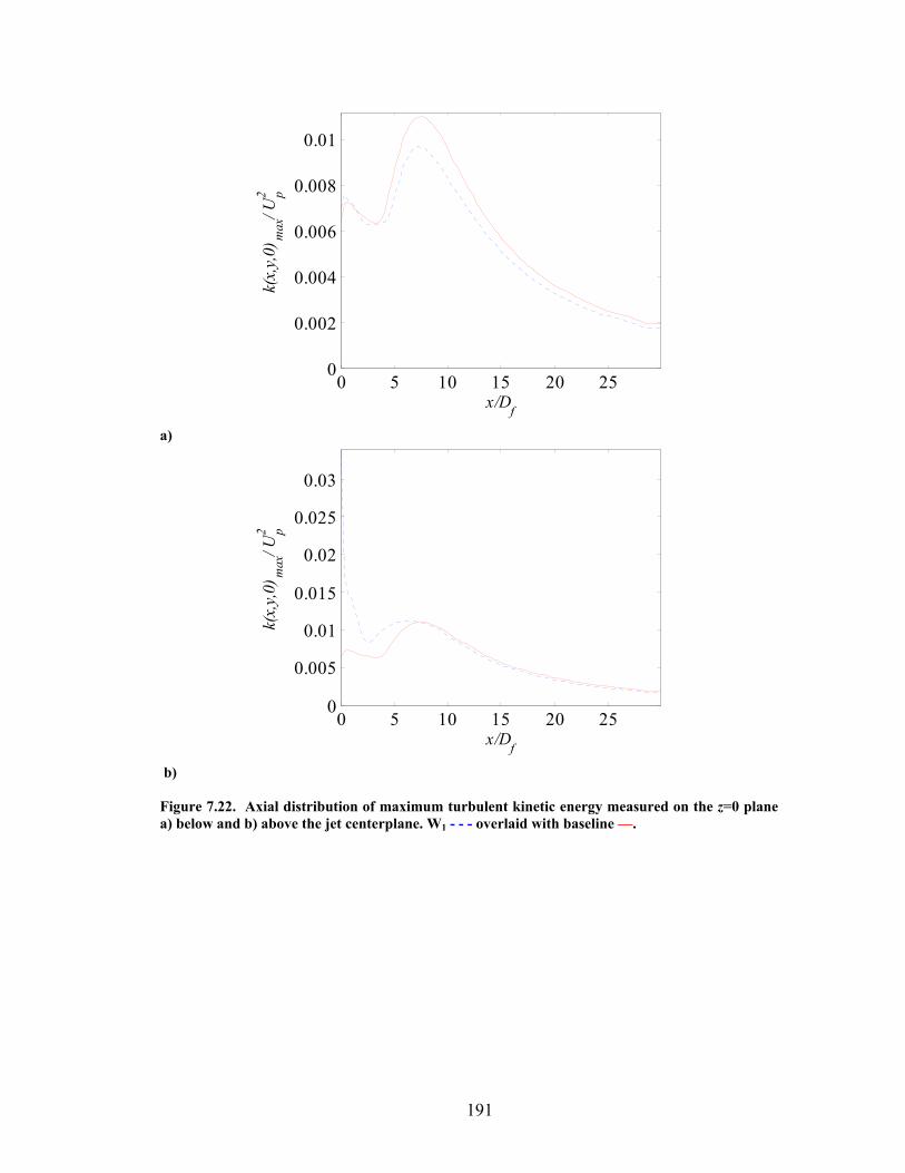
7.22 Axial distribution of maximum turbulent kinetic energy, k(x,y,0)/Up2.
a) below and b) above the jet centerline. W1 overlaid with baseline jet.
190
7.23 Distribution of turbulent kinetic energy k(x,y,0)/Up2 for the baseline jet.
191
7.24 Distribution of turbulent kinetic energy k(x,y,0)/Up2 for W1.
191
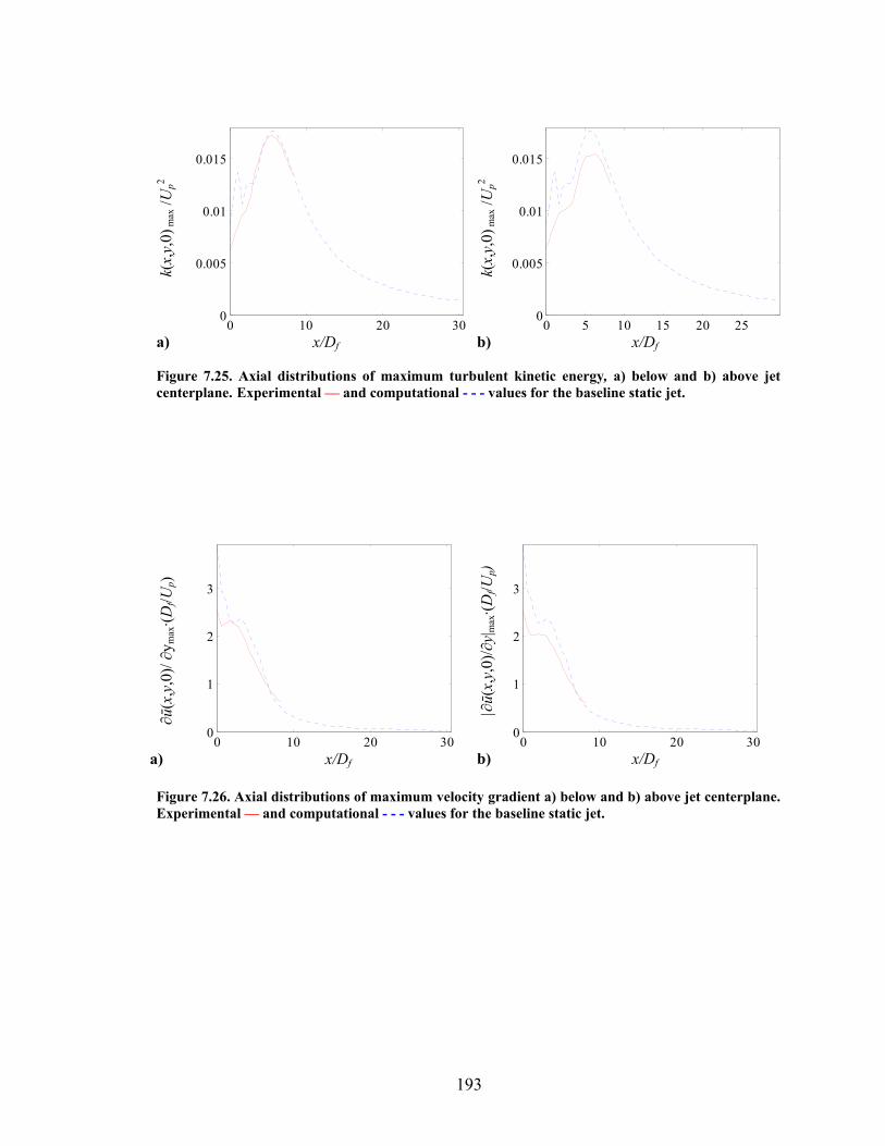
7.25 Axial distributions of maximum turbulent kinetic energy, k(x,y,0)/Up2, (a)
below and (b) above jet centerline. Experimental and computational values.
192
7.26 Axial distributions of maximum velocity gradient, ∂u(x,y,0)/∂y·Df/Up, (a) below and (b) above jet centerline. Experimental and computational values.
192
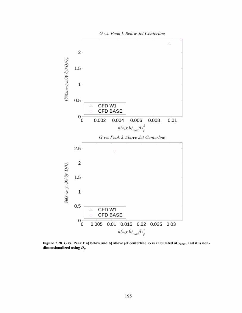
7.27 G vs. Peak k a) below and b) above jet centerline. G is calculated at xGSC, and it is non-dimensionalized using Df.
193
7.28 G vs. Peak k a) below and b) above jet centerline. G is calculated at xGSC, and it is non-dimensionalized using Df.
194
xvii
LIST OF TABLES Page
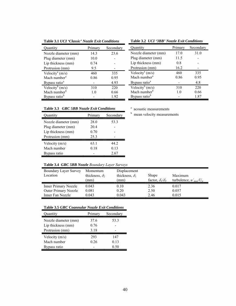
3.1. UCI ‘Classic’ Nozzle Exit Conditions 40
3.2. UCI ‘3BB’ Nozzle Exit Conditions 40
3.3. GRC 5BB Nozzle Exit Conditions 40
3.4. GRC 5BB Nozzle Boundary Layer Surveys 40
3.5. GRC Coannular Nozzle Exit Conditions 40
5.1. UCI ‘Classic’ Nozzle Exit Conditions 74
5.2.
UCI ‘3BB’ Nozzle Exit Conditions 74
5.3.
UCI ‘Classic’ Nozzle Deflector Configurations 74
5.4.
UCI ‘3BB’ Nozzle Deflector Configurations 74
6.1. GRC Flow Field Parameters 113
6.2. GRC Reynolds Stresses 113
7.1. GRC CFD 5BB Nozzle Exit Conditions 178
7.2. GRC CW17 5BB Nozzle Exit Conditions 178
7.3. Predicted Flow Field Parameters 178
xviii
LIST OF SYMBOLS Roman
a2D = two-dimensional lift curve slope
a = speed of sound
A = amplitude modulation function
 = Fourier transform of amplitude modulation function
B = wedge base
c = chord length of vane
CL = coefficient of lift (vane) or sideforce (wedge)
D = nozzle exit diameter
F = thrust
G = mean velocity radial gradient parameter
H = annular gap width (fan duct exit height)
k = turbulent kinetic energy, wavenumber
K = total kinetic energy
L = deflector lift or sideforce
l = side length of wedge
M = Mach number
p = pressure
q = dynamic pressure
r = shear layer velocity ratio
s = shear layer density ratio
S = wedge wetted area
xix
U = jet exit velocity
~u = total velocity vector in jet plume
'~u = fluctuating velocity vector in jet plume
~u = mean velocity vector in jet plume
u = mean axial velocity component in jet plume
u’ = fluctuating axial velocity component in jet plume
v’ = fluctuating vertical velocity component in jet plume
W = wedge-shaped deflector
w’ = fluctuating horizontal velocity component in jet plume
w = average vane span
x = axial position with respect to fan exit
Greek
α = vane angle of attack, wedge half angle
γ = specific heat ratio
δ = shear layer thickness
δ’ = shear layer growth rate
ε = deflector turning effort
η = similarity parameter, instability wave
θ = polar angle relative to jet axis
ρ = density
τ = shear stress
φ = azimuth angle relative to downward vertical
xx
ω = vorticity
Subscripts
a = ambient stream condition
c = convective
f = fan
GSC = generalized secondary core
p = primary (core) stream, potential core
le = leading edge of vane
s = secondary (bypass) stream
sym = symmetric
te = trailing edge of vane
∞ = ambient stream condition
0 = total (stagnation), fixed axial location
1 = fast moving stream
2 = slow moving stream
xxi
ACKNOWLEDGEMENTS
I wish to express my profound respect for and appreciation of my research advisor, Professor Dimitri Papamoschou. His expertise and physical intuition proved invaluable to this research effort. Through his dedication and demanding expectations, he has left a positive impact on my professional life. He is a genuinely kind and caring individual, and I am indebted to him for his helpful advice, encouragement, and friendship.
I am thankful to Dr. Khairul Zaman for his guidance and mentorship in fluid mechanics, and also for his help in conducting the crossed hot-wire measurements. I would like to express my thanks to Dr. Jim DeBonis for his expertise in computational fluid dynamics and grid generation, and for his time spent in obtaining the complementary solutions to the experimental investigation. I would like to extend my thanks to Dr. Stanley Birch for suggesting to me that I should test a pylon very early on, and for his kind and encouraging words. I would like to thank Professor Dennis McLaughlin for his mentorship in Aeroacoustics. Special thanks are due to Professor Robert Liebeck for encouragement and guidance well beyond the call of duty. Thanks to M. Leroy Spearman for many kind words and for sharing his enthusiasm with me about aeronautics. In addition, I am extremely thankful to all of the engineering professors and students who made life at UCI a unique experience. Their friendship and camaraderie provide energy and a competitive spirit that can inspire innovation in engineering. I am especially thankful to my committee members, Professors Feng Liu and William A. Sirignano, for their insight and special care with respect to reading my thesis. Funding for this research effort from NASA Glenn Research Center, Grant NAG-3-2345, monitored by Dr. Khairul B. Zaman and Dr. James Bridges, and the NASA Graduate Student Researchers Program (GSRP) Fellowship, are gratefully acknowledged. The Mechanical and Aerospace Engineering Departmental Fellowship, sponsored by the Graduate Assistance in Areas of National Need (GAANN) program, is also gratefully acknowledged.
xxii
ABSTRACT OF THE THESIS
Noise Reduction and Flow Characteristics in Asymmetric Dual-Stream Jets
by Rebecca Suzanne Shupe
Master of Science in Mechanical and Aerospace Engineering
University of California, Irvine 2007
Professor Dimitri Papamoschou, Chair
HIS research effort is motivated by the advent of asymmetric nozzle concepts for
directional suppression of jet noise from turbofan engines. The specific method addressed
is the fan flow deflection (FFD) technique, whereby aerodynamic devices deflect
downward the fan stream of the turbofan exhaust and thus create an asymmetry in the
plume of the jet exiting an otherwise coaxial nozzle. The asymmetry reduces jet noise
emissions in downward and sideward directions affecting airport communities. Flow field
and acoustic measurements were conducted to understand what flow quantities are
affected by the departure from symmetry and how their changes impact noise emission.
The experiments were complemented by computations that included the effect of forward
flight. It is found that FFD reduces the radial gradients of mean velocity, the turbulent
kinetic energy, and the Reynolds stress on the underside of the jet. A preliminary
correlation between downward velocity gradient and downward sound emission indicates
that velocity gradient reduction is an important ingredient for noise suppression using
FFD. Further, a correlation between the maximum radial gradient of the axial velocity
component and peak turbulent kinetic energy was obtained.
T
xxiii
In an additional related aspect of this work, the effect of baseline nozzle geometry on
efficacy of methods that create jet asymmetry was studied. A phenomenological
investigation between nozzles with parallel exit flow lines and converging exit flow lines
was conducted. Jets with uniformly reduced radial gradients below the centerplane were
found to be acoustically superior to jet plumes with focused or narrow gradient reduction.
1
Chapter 1 Introduction 1.1. Motivation
Today, a primary goal of the National Aeronautics and Space Administration’s
(NASA) Aeronautics Research Mission Directorate (AMRD) is the advancement of
aviation technology that will enable the United States to maintain a distinctly preeminent
role in industry. Aircraft noise emissions reduction has become a driving factor for
competitive aircraft design, as political and environmental laws have become more firm.
Additionally, takeoff noise reduction is a key challenge for developing future supersonic
jetliners. After careful planning and testing, successful implementation of innovative jet
noise reduction concepts in commercial turbofan engines and military aircraft engines
may be achieved for reduction of jet noise at both supersonic and subsonic jet exhaust
configurations.
The essence of this work arises from the need to improve the current understanding of
turbulent mixing noise and noise suppression in asymmetric dual-stream jets. The closure
problem of turbulence necessarily places limitations on noise predictions in jets using
computational methods. Solutions for high Reynolds number jets using Direct Numerical
2
Simulations (DNS) will not be feasible in the foreseeable future. Computational methods
such as Large Eddy Simulation (LES) and Reynolds Averaged Navier-Stokes (RANS)
use models that are promising, but as of yet cannot be relied upon for accurately
predicting noise emissions of dual-stream jets. As a consequence, applications involving
turbulent flows remain heavily reliant on empirical data for predictions. The work herein
is a first step in the aim to develop an empirical relation between key mean flow field
parameters and reduction in peak overall sound pressure level (OASPL). This correlation
is expected to improve computational predictions that will assist in the design of quiet
aircraft engine nozzle configurations.
1.2. The Turbofan Engine
The turbofan engine is the most efficient propulsion system for aircraft traveling at
high subsonic cruise speeds. Most commercial aircraft travel at a cruise Mach number of
M = 0.85 (564 mph, 35,000 ft altitude) so the turbofan engine is widely used. The
General Electric GE90 model, which is currently the world’s most powerful engine and is
used on the Boeing 777 airliner, is shown in Fig. 1.1. New composite material
technologies have been incorporated into the design of this engine adding to its improved
efficiency and power capabilities from previous models. The fan blades are made from
composite material, carbon-fiber reinforced epoxy, and the engineering process was
designed to make the material fibers completely free of defect, including wrinkles or
voids.
A turbofan engine has all of the same internal components as a turbojet engine, but it
is surrounded by a bypass duct. Figure 1.2 shows the main components. During subsonic
3
flight, the inlet section of the turbofan engine is designed to decrease the velocity of the
air that is brought into the engine. A fan accelerates the air through the fan duct. The ratio
of the mass of air that is routed through the bypass duct to the mass of air that is routed
through the core during a fixed time period is called the bypass ratio. With increased
bypass ratio, the engine becomes quieter and more efficient. Tradeoffs are drag due to an
increased cross-sectional area and increased weight. A compressor increases the pressure
of the air before it enters the combustion chamber. The air that passes through the core is
mixed with fuel, and chemical energy is converted to useful work after the air-fuel
mixture undergoes combustion in the burner. As the extremely hot gases leave the
combustion chamber, they expand through the turbine, causing the shaft to spin. The fan
and compressor are powered by the turbine shaft. The primary (core) jet exhaust is
characterized by very high speeds and temperatures, while the secondary (bypass) stream
has much lower speeds and is much cooler.
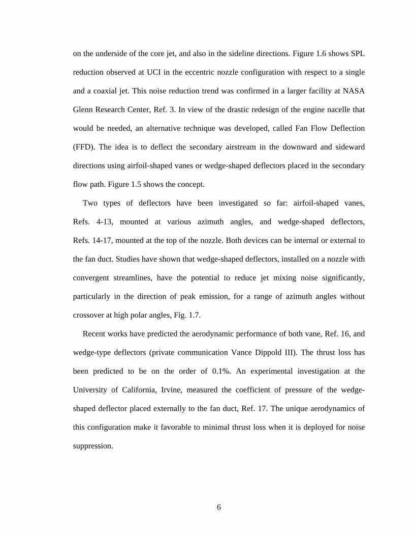
Turbofan engine noise consists of jet noise, fan noise, and core noise. Jet noise, the
focus of this study, is dominant during takeoff and climb when high thrust is required.
The fan noise component of engine noise is dominant on a landing approach when thrust
is reduced. Other noise sources are rotary machinery internal to the core engine and
pressure and temperature fluctuations inside the combustor. These sources lumped
together with fan noise that is propagated internally to the core engine, are referred to as
core noise. Figure 1.3 shows tone-corrected perceived noise level for jet noise relative to
other aircraft noise sources on takeoff and on landing. To date, the two primary
developments that have entered into service on commercial airliners to aid in reduction of
engine noise are acoustic linings for engine nacelles and increased bypass ratio engines,
4
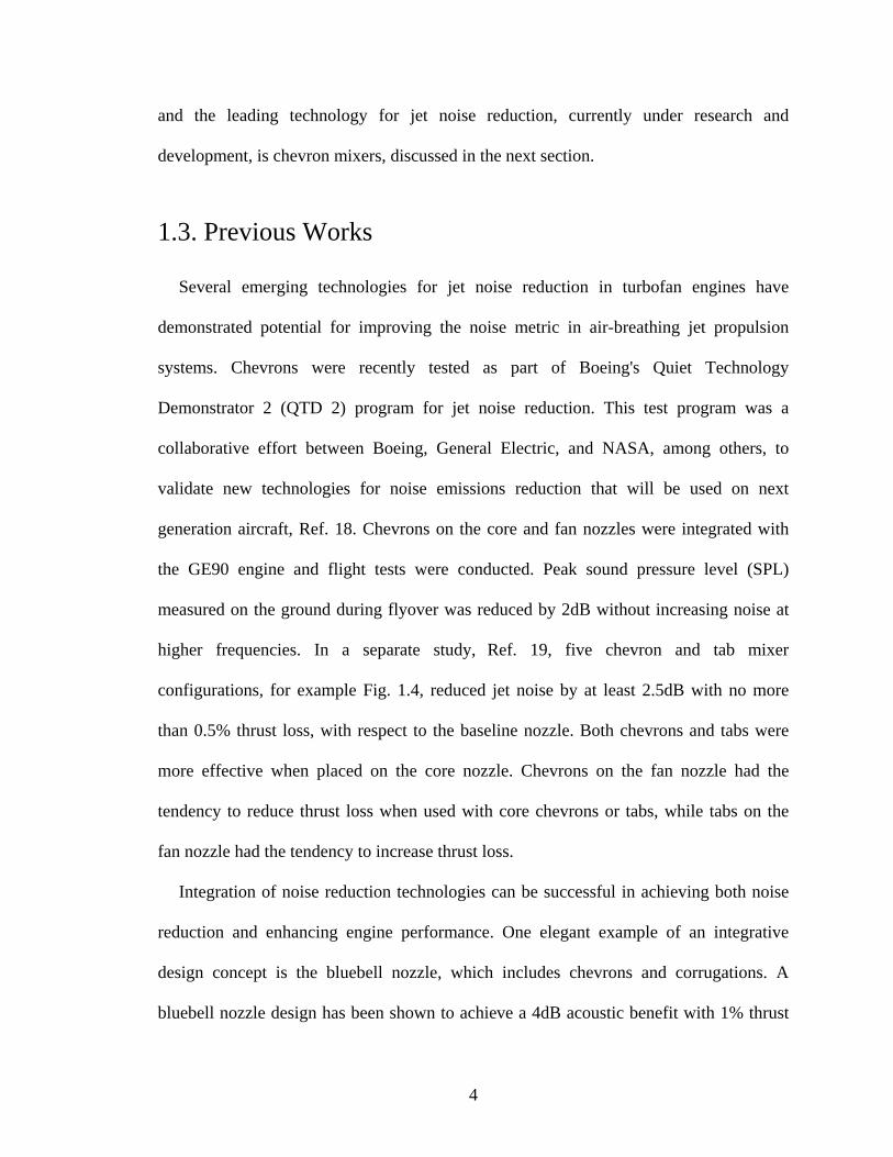
and the leading technology for jet noise reduction, currently under research and
development, is chevron mixers, discussed in the next section.
1.3. Previous Works
Several emerging technologies for jet noise reduction in turbofan engines have
demonstrated potential for improving the noise metric in air-breathing jet propulsion
systems. Chevrons were recently tested as part of Boeing's Quiet Technology
Demonstrator 2 (QTD 2) program for jet noise reduction. This test program was a
collaborative effort between Boeing, General Electric, and NASA, among others, to
validate new technologies for noise emissions reduction that will be used on next
generation aircraft, Ref. 18. Chevrons on the core and fan nozzles were integrated with
the GE90 engine and flight tests were conducted. Peak sound pressure level (SPL)
measured on the ground during flyover was reduced by 2dB without increasing noise at
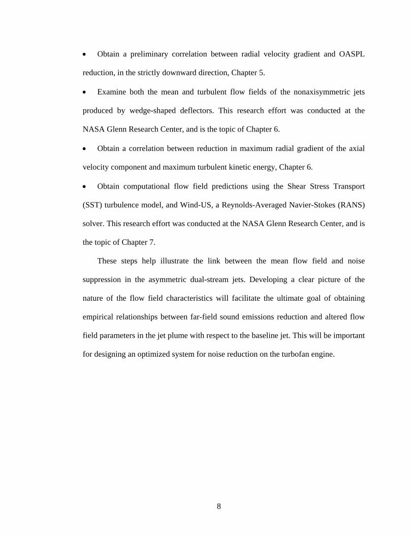
higher frequencies. In a separate study, Ref. 19, five chevron and tab mixer
configurations, for example Fig. 1.4, reduced jet noise by at least 2.5dB with no more
than 0.5% thrust loss, with respect to the baseline nozzle. Both chevrons and tabs were
more effective when placed on the core nozzle. Chevrons on the fan nozzle had the
tendency to reduce thrust loss when used with core chevrons or tabs, while tabs on the
fan nozzle had the tendency to increase thrust loss.
Integration of noise reduction technologies can be successful in achieving both noise
reduction and enhancing engine performance. One elegant example of an integrative
design concept is the bluebell nozzle, which includes chevrons and corrugations. A
bluebell nozzle design has been shown to achieve a 4dB acoustic benefit with 1% thrust
5
augmentation at supersonic exhaust conditions when compared to its round converging-
diverging baseline counterpart, Ref. 20.
As opposed to the traditional wing-mounted engine configuration, below the wing, a
straight-forward noise reduction solution is an over-the-wing-mounted engine
configuration. This results in a wing-shielding effect, inhibiting transmission of some of
the engine noise to the ground. Tests conducted in the 1970’s showed a 3dB reduction,
with respect to the traditional configuration, even though the wing chord length was not
large enough to cover the entire engine. A large aircraft would have the greatest potential
in making use of a wing-shielding benefit because its longer chord would shield more of
the noise sources. However, regions of intense turbulent mixing and noise production in
the jet plume occur at about 5 fan diameters downstream of the fan exit plane for a
bypass ratio 5 turbofan engine. It follows that a chord length of more than 12 m would be
required to shield the dominant noise sources of the jet for a turbofan engine with a 2.4 m
fan exit diameter. The Boeing 777 uses a mean aerodynamic chord length of 6.6 m.
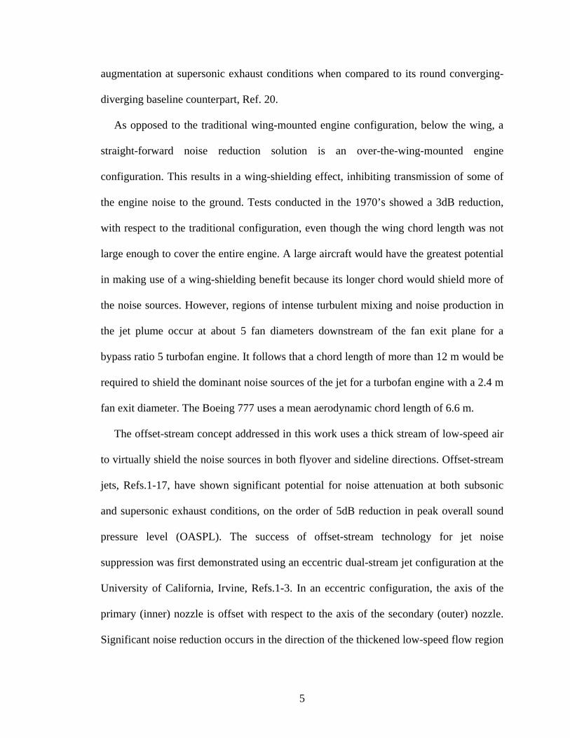
The offset-stream concept addressed in this work uses a thick stream of low-speed air
to virtually shield the noise sources in both flyover and sideline directions. Offset-stream
jets, Refs.1-17, have shown significant potential for noise attenuation at both subsonic
and supersonic exhaust conditions, on the order of 5dB reduction in peak overall sound
pressure level (OASPL). The success of offset-stream technology for jet noise
suppression was first demonstrated using an eccentric dual-stream jet configuration at the
University of California, Irvine, Refs.1-3. In an eccentric configuration, the axis of the
primary (inner) nozzle is offset with respect to the axis of the secondary (outer) nozzle.
Significant noise reduction occurs in the direction of the thickened low-speed flow region
6
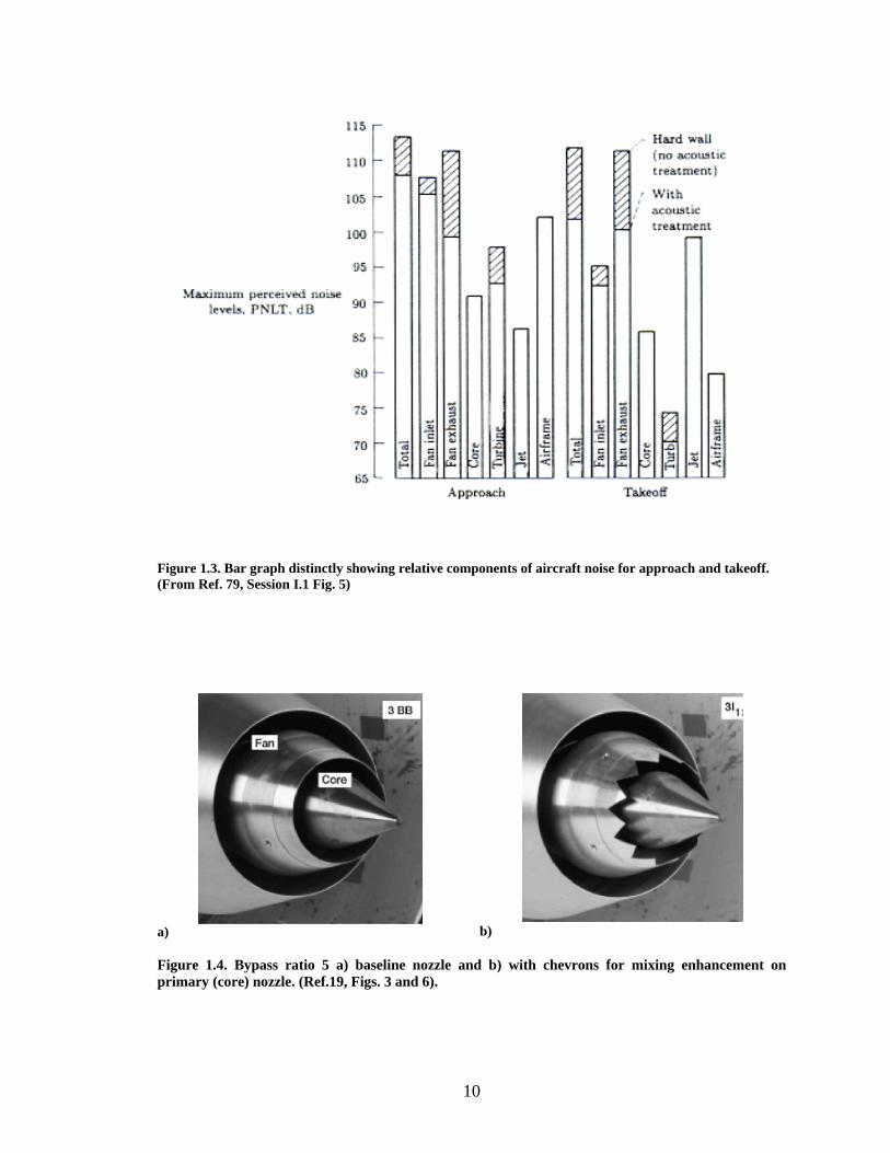
on the underside of the core jet, and also in the sideline directions. Figure 1.6 shows SPL
reduction observed at UCI in the eccentric nozzle configuration with respect to a single
and a coaxial jet. This noise reduction trend was confirmed in a larger facility at NASA
Glenn Research Center, Ref. 3. In view of the drastic redesign of the engine nacelle that
would be needed, an alternative technique was developed, called Fan Flow Deflection
(FFD). The idea is to deflect the secondary airstream in the downward and sideward
directions using airfoil-shaped vanes or wedge-shaped deflectors placed in the secondary
flow path. Figure 1.5 shows the concept.
Two types of deflectors have been investigated so far: airfoil-shaped vanes,
Refs. 4-13, mounted at various azimuth angles, and wedge-shaped deflectors,
Refs. 14-17, mounted at the top of the nozzle. Both devices can be internal or external to
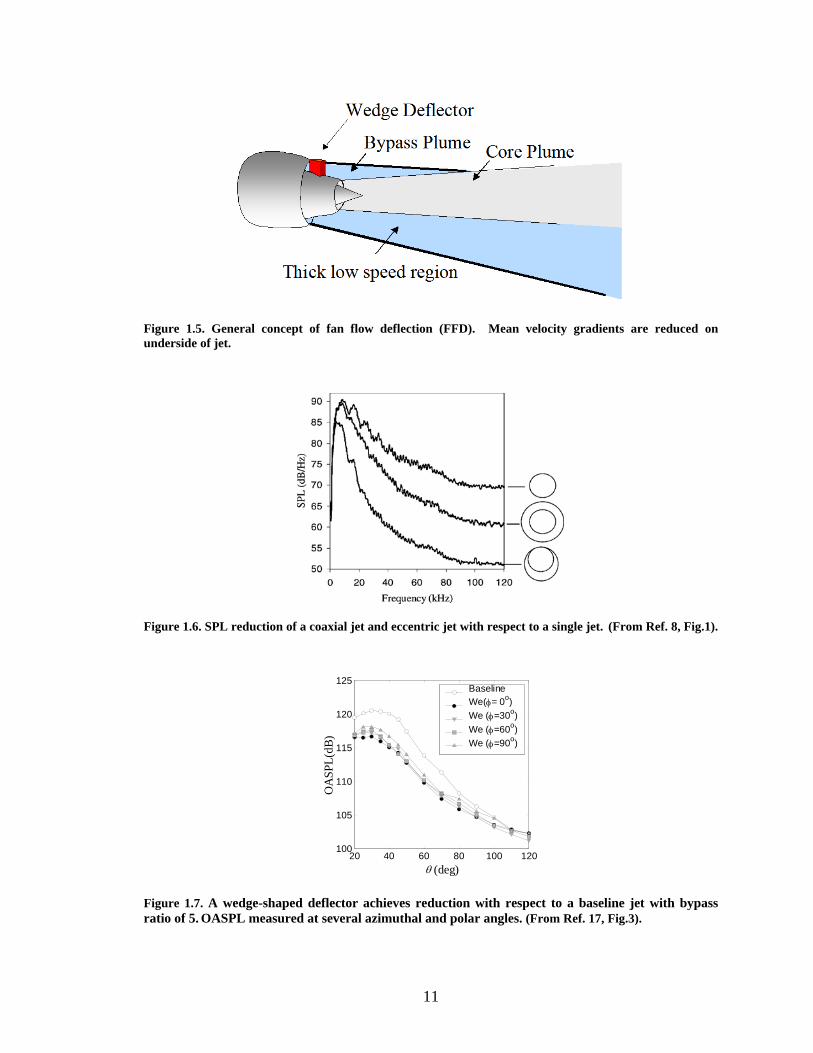
the fan duct. Studies have shown that wedge-shaped deflectors, installed on a nozzle with
convergent streamlines, have the potential to reduce jet mixing noise significantly,
particularly in the direction of peak emission, for a range of azimuth angles without
crossover at high polar angles, Fig. 1.7.
Recent works have predicted the aerodynamic performance of both vane, Ref. 16, and
wedge-type deflectors (private communication Vance Dippold III). The thrust loss has
been predicted to be on the order of 0.1%. An experimental investigation at the
University of California, Irvine, measured the coefficient of pressure of the wedge-
shaped deflector placed externally to the fan duct, Ref. 17. The unique aerodynamics of
this configuration make it favorable to minimal thrust loss when it is deployed for noise
suppression.
7
1.4. Program Objectives
At the University of California, Irvine, the jet aeroacoustics research group aims to
study the flow field of asymmetric dual-stream jets, and its relation to noise suppression
resulting from that symmetry. Novel concepts developed at the University of California,
Irvine have demonstrated noise reduction of peak OASPL in the downward and sideline
directions, across all frequencies in the downward direction. Consequently, it is desirable
to correlate the noise suppression resulting from these methods with the asymmetry in the
flow field characteristics of the dual-stream jets. The specific flow field characteristics
are reduced velocity gradients, Reynolds stresses, and peak turbulent kinetic energy.
The objectives addressed in this thesis entail the assessment of mean and turbulent
flow field characteristics that impact noise radiated to the far-field, and the development
of an empirical model correlating asymmetry in the flow field with noise suppression.
This model would enhance predictions for the design of acoustically superior engine
nozzle configurations. The primary tools of the investigation, discussed in detail in
subsequent chapters, encompass microphone noise measurements, mean and fluctuating
velocity field surveys, and computational simulations. Central to this research effort is the
analysis of the asymmetric dual-stream jet flow field characteristics including velocity
gradients and inflectional layers, Reynolds stresses, and turbulent kinetic energy.
The main objectives and results of this research effort are outlined as follows:
• Understand the effect of the baseline nozzle shape on the mean flow
characteristics of the jet and on the efficacy of fan flow deflectors (FFD) to suppress
noise. This research effort was conducted at the University of California Irvine, and is
the topic of Chapter 5.
8
• Obtain a preliminary correlation between radial velocity gradient and OASPL
reduction, in the strictly downward direction, Chapter 5.
• Examine both the mean and turbulent flow fields of the nonaxisymmetric jets
produced by wedge-shaped deflectors. This research effort was conducted at the
NASA Glenn Research Center, and is the topic of Chapter 6.
• Obtain a correlation between reduction in maximum radial gradient of the axial
velocity component and maximum turbulent kinetic energy, Chapter 6.
• Obtain computational flow field predictions using the Shear Stress Transport
(SST) turbulence model, and Wind-US, a Reynolds-Averaged Navier-Stokes (RANS)
solver. This research effort was conducted at the NASA Glenn Research Center, and is
the topic of Chapter 7.
These steps help illustrate the link between the mean flow field and noise
suppression in the asymmetric dual-stream jets. Developing a clear picture of the
nature of the flow field characteristics will facilitate the ultimate goal of obtaining
empirical relationships between far-field sound emissions reduction and altered flow
field parameters in the jet plume with respect to the baseline jet. This will be important
for designing an optimized system for noise reduction on the turbofan engine.
9
Figure 1.1. General Electric GE90 high bypass turbofan engine. Source: http://academic.csuohio.edu/cact/jet engine.png
Figure 1.2. Illustration showing main components of a turbofan engine.
Fan Duct
Engine Nacelle
Inlet/Diffuser
Fan Wedge-Shaped Noise Suppressor
BurnerCompressor Turbine
Primary Nozzle
Center Plug
Secondary Nozzle
10
Figure 1.3. Bar graph distinctly showing relative components of aircraft noise for approach and takeoff. (From Ref. 79, Session I.1 Fig. 5)
a)
b)
Figure 1.4. Bypass ratio 5 a) baseline nozzle and b) with chevrons for mixing enhancement on primary (core) nozzle. (Ref.19, Figs. 3 and 6).
11
Figure 1.5. General concept of fan flow deflection (FFD). Mean velocity gradients are reduced on underside of jet.
Figure 1.6. SPL reduction of a coaxial jet and eccentric jet with respect to a single jet. (From Ref. 8, Fig.1).
20 40 60 80 100 120100
105
110
115
120
125
OA
SPL(
dB)
θ (deg)
BaselineWe(φ= 0o)We (φ=30o)We (φ=60o)We (φ=90o)
Figure 1.7. A wedge-shaped deflector achieves reduction with respect to a baseline jet with bypass ratio of 5. OASPL measured at several azimuthal and polar angles. (From Ref. 17, Fig.3).
12
Chapter 2 Background
The focus of this work is on improving the current understanding of the physical
mechanism responsible for noise suppression in asymmetric subsonic and supersonic
dual-stream jet configurations. The jets under discussion here are referred to as
asymmetric because they have offset primary and secondary streams. The primary and
secondary streams represent the core and bypass exhausts, respectively, of turbofan
engines. Offset-stream nozzles include eccentric configurations and arrangements with
deflection of the fan stream. These configurations alter the mean flow field of the jet
plume, concentrating the low-speed fan flow underneath the core stream, thus reducing
downward and sideward noise emissions with respect to the baseline coaxial jet.
2.1. Physical Elements of the Coaxial Jet
In this section, a literature review is provided, outlining some of the basic physical
elements of axisymmetric coaxial dual-stream jets as they are relevant to jet noise
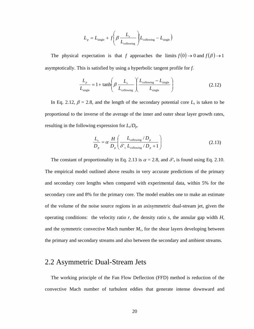
emissions. In the initial region of the jet, a primary shear layer and a secondary shear
layer exist, Fig. 2.1. The primary and secondary shear layers are formed between the
13
primary and secondary potential cores and between the secondary core and the ambient
fluid surrounding the jet, respectively. In the potential cores, the fluid is irrotational, and
the velocity is nearly uniform and equal to the nozzle exit velocities. The shear layers
work to mix the two core streams of fluid. Because of the difference in velocity between
the two streams, rotational motion is induced and turbulent eddies are formed in the shear
layers. At the end of the secondary core, the primary and secondary shear layers merge,
marking the beginning of the intermediate region of the jet, in Fig. 2.1. This is a very
important noise generation region because the primary jet is left exposed to the ambient,
and a single shear layer forms with a much higher velocity gradient than either of the two
shear layers in the initial region. The merging of the two shear layers makes it a complex
region to analyze. Analysis of the inflectional layers of the mean velocity is one way of
studying this complex region. The significance of the inflectional loci will be discussed
later in this chapter. Far downstream is the fully-developed region of the jet,
characterized by large turbulent eddies that span the entire plume. This region of the jet is
self-similar, and is characteristic of a single round jet, with Gaussian-like profiles, which
collapse onto one another when nondimensionalized properly. References 33-36 present a
wealth of experimental data from single and coaxial turbulent jets, both subsonic and
supersonic.
The primary and secondary axisymmetric shear layers, in the initial region of the jet,
are closely approximated by the turbulent planar shear layer, Fig. 2.2. Therefore,
empirical relations for the growth rate of the turbulent planar shear layer provide good
estimates for growth rates and potential core lengths in round jets. These are presented in
the following sections for the axisymmetric dual-stream jets. The spatial growth rate of a
14
shear layer is, sometimes referred to as a spreading rate, is the change in thickness with
position from a virtual origin, and it is constant for a fully developed, turbulent planar
shear layer:
.' constdxd
==δδ (2.1)
The growth rate will depend on the definition of thickness that is used. In the literature,
three common definitions include the pitot thickness, vorticity thickness, and the visual
thickness. One can predict the maximum radial gradient of the axial component of the
mean velocity, using the definition of the vorticity thickness. In the next section, the
convective Mach number is introduced. The convective Mach number of turbulent eddies
in the jet shear layer adjacent to the ambient has a direct impact on the noise emissions of
a dual-stream jet.
2.1.1 Convective Mach Number
The convective Mach number is best described as the Mach number felt by a
disturbance (instability wave or turbulent eddy) as it convects downstream in the shear
layer. The Mach number of the shear layer disturbance with respect to surrounding fluid
is important for consideration of Mach wave emissions. It is measured in a frame of
reference moving with the constant phase speed of the disturbance Uc. The definition is
as follows:
1
11 a
UUM cc
−= ,
2
22 a
UUM cc
−= (2.2)
where the subscript 1 makes reference to the fast moving freestream and the subscript 2
makes reference to the slow moving freestream, Fig. 2.2.
15
The so-called “symmetric” convective Mach number was first determined by
Bogdanoff, Ref. 21, and later by Papamoschou and Roshko, Refs. 22-23, by assuming
that the flow is brought to rest isentropically at a stagnation point between the large-scale
turbulent structures in the shear layer. There must be equality of pressure to maintain a
stable stagnation point, and the total pressures in the convective frame are assumed to be
equal on either side of the shear layer.
cc pp 0201 =
122
22
121
11
2
2
1
1
211
211
−−⎟⎠⎞
⎜⎝⎛ −
+=⎟⎠⎞
⎜⎝⎛ −
+γγ
γγ
γγcc MpMp
For 21 γγ = , it follows that 21 cc MM = , since the static pressure is balanced on either side
of the shear layer. The Mach number of either stream, called the symmetric convective
Mach number is
21
21
aaUUM csym +
−= (2.3)
At high compressibility, the convective Mach number cannot be assumed symmetric due
to entropy generation.
The convective Mach number is very important for noise emissions considerations,
because it is an indicator of the amount of energy that can be radiated to the acoustic far-
field. An analytical treatment is provided in Ref. 4 that yields insight into the physics
relevant to noise emissions reduction and it is summarized here. Using a parallel flow
approximation, the solution to the Rayleigh equation yields disturbances that amplify for
wavenumbers below a neutral value and decay for wavenumbers above the neutral value.
The growth or decay is exponential. Accounting for non-parallel, spatially-growing
16
mean flow, an initially-amplifying disturbance will saturate and decay with axial
distance. This can be expressed as a wave-packet η(x,t) with amplitude modulation
function A(x) of arbitrary units in length, Fig. 2.3. To simplify the analysis, a disturbance
with wave number of unity is considered. The disturbance is expressed as follows
( ) ( ) ( )tUxi cexAtx −= ˆ,η (2.4)
where Uc is the convective speed of the instability wave. Assuming the Fourier transform
exists for the amplitude modulation function, A(x), it can be written as a continuous
spectrum of cosines and sines by taking the inverse Fourier transform
( ) ( ) dkekAxA ikx∫∞
∞−
= ˆ21π
(2.5)
The wave packet can be expressed in Fourier space as
( ) ( ) ( )[ ]dkekAtx tUxki c−+∞
∞−∫= 1ˆ
21,π
η
and equivalently,
( ) ( ) dkekAtxt
kU
xik c⎥⎦
⎤⎢⎣
⎡ −∞
∞−∫ −= 1ˆ
21,π
η (2.6)
Since this result can be thought of as a continuous spectrum of waves with individual
phase-amplitudes Â(k-1)/2π, dimensionless phase-speeds Uc/k, and dimensionless phase-
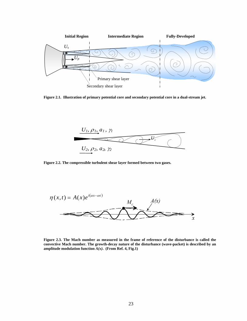
Mach numbers (recall a disturbance with a wavenumber of unity is assumed) mc = Uc/ka
= Mc/k, it follows that Mach wave emissions occur for the portion of the spectrum with
phase-speed greater than the speed of sound, Fig. 2.4. One can see that even if Mc is
subsonic there is a portion of the spectrum with supersonic phase-Mach numbers. By
reducing Mc, less energy will be radiated to the far-field as noise. Refer to Liepmann and
Roshko, Ref. 77, for a treatment of small perturbation theory and flow past a wave-
17
shaped wall. With this in mind, an aeroacoustician can reduce the convective speed of the
turbulent eddies in the dominant noise source region, near the end of the primary
potential core in a dual-stream jet, thereby reducing acoustic radiation to the far-field.
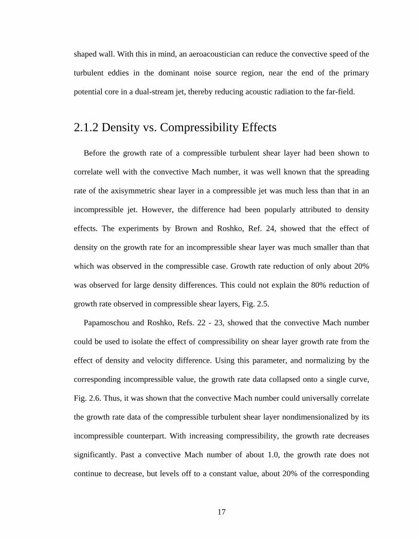
2.1.2 Density vs. Compressibility Effects
Before the growth rate of a compressible turbulent shear layer had been shown to
correlate well with the convective Mach number, it was well known that the spreading
rate of the axisymmetric shear layer in a compressible jet was much less than that in an
incompressible jet. However, the difference had been popularly attributed to density
effects. The experiments by Brown and Roshko, Ref. 24, showed that the effect of
density on the growth rate for an incompressible shear layer was much smaller than that
which was observed in the compressible case. Growth rate reduction of only about 20%
was observed for large density differences. This could not explain the 80% reduction of
growth rate observed in compressible shear layers, Fig. 2.5.
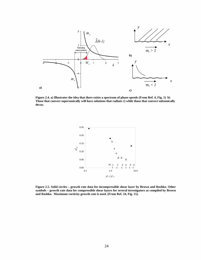
Papamoschou and Roshko, Refs. 22 - 23, showed that the convective Mach number
could be used to isolate the effect of compressibility on shear layer growth rate from the
effect of density and velocity difference. Using this parameter, and normalizing by the
corresponding incompressible value, the growth rate data collapsed onto a single curve,
Fig. 2.6. Thus, it was shown that the convective Mach number could universally correlate
the growth rate data of the compressible turbulent shear layer nondimensionalized by its
incompressible counterpart. With increasing compressibility, the growth rate decreases
significantly. Past a convective Mach number of about 1.0, the growth rate does not
continue to decrease, but levels off to a constant value, about 20% of the corresponding
18
incompressible value. The same general trend has been observed in several instability
analyses, Refs. 25 - 32.
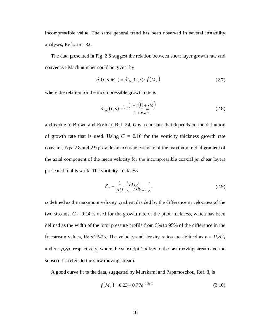
The data presented in Fig. 2.6 suggest the relation between shear layer growth rate and
convective Mach number could be given by
( )cincc MfsrMsr ⋅= ),('),,(' δδ (2.7)
where the relation for the incompressible growth rate is
( )( )sr
srCsrinc ++−
=1
11),('δ (2.8)
and is due to Brown and Roshko, Ref. 24. C is a constant that depends on the definition
of growth rate that is used. Using C = 0.16 for the vorticity thickness growth rate
constant, Eqs. 2.8 and 2.9 provide an accurate estimate of the maximum radial gradient of
the axial component of the mean velocity for the incompressible coaxial jet shear layers
presented in this work. The vorticity thickness
⎟⎠⎞⎜
⎝⎛
∂∂⋅
∆=
max
1y
UUωδ , (2.9)
is defined as the maximum velocity gradient divided by the difference in velocities of the
two streams. C = 0.14 is used for the growth rate of the pitot thickness, which has been
defined as the width of the pitot pressure profile from 5% to 95% of the difference in the
freestream values, Refs.22-23. The velocity and density ratios are defined as r = U2/U1
and s = ρ2/ρ1 respectively, where the subscript 1 refers to the fast moving stream and the
subscript 2 refers to the slow moving stream.
A good curve fit to the data, suggested by Murakami and Papamoschou, Ref. 8, is
( ) 25.377.023.0 cMc eMf −+= (2.10)
19
also shown in Fig. 2.6. The fit provides an empirical estimate of good quality for the
shear layer thickness growth rate as a function of the symmetric convective Mach number
in Eq. 2.3. In the next section it is used to estimate the potential core lengths of a coaxial
jet.
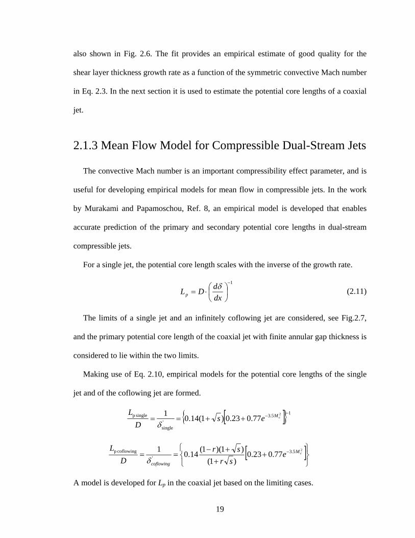
2.1.3 Mean Flow Model for Compressible Dual-Stream Jets
The convective Mach number is an important compressibility effect parameter, and is
useful for developing empirical models for mean flow in compressible jets. In the work
by Murakami and Papamoschou, Ref. 8, an empirical model is developed that enables
accurate prediction of the primary and secondary potential core lengths in dual-stream
compressible jets.
For a single jet, the potential core length scales with the inverse of the growth rate.
1−
⎟⎠⎞
⎜⎝⎛⋅=
dxdDLpδ (2.11)
The limits of a single jet and an infinitely coflowing jet are considered, see Fig.2.7,
and the primary potential core length of the coaxial jet with finite annular gap thickness is
considered to lie within the two limits.
Making use of Eq. 2.10, empirical models for the potential core lengths of the single
jet and of the coflowing jet are formed.
[ ]{ } 15.3'single
single p 2
77.023.0)1(14.01 −−++== cMesD
Lδ
[ ]⎭⎬⎫
⎩⎨⎧
++
+−== − 25.3
'coflowing p 77.023.0
)1()1)(1(14.01
cM
coflowing
esr
srD
Lδ
A model is developed for Lp in the coaxial jet based on the limiting cases.
20
( )singlecoflowingcoflowing
single LLL
LfLL s
p −⎟⎟⎠
⎞⎜⎜⎝
⎛+= β
The physical expectation is that f approaches the limits ( ) 00 →f and ( ) 1→βf
asymptotically. This is satisfied by using a hyperbolic tangent profile for f.
⎟⎟⎠
⎞⎜⎜⎝
⎛ −⎟⎟⎠
⎞⎜⎜⎝
⎛+=
single
singlecoflowing
coflowingsingle
tanh1L
LLL
LLL sp β (2.12)
In Eq. 2.12, β = 2.8, and the length of the secondary potential core Ls is taken to be
proportional to the inverse of the average of the inner and outer shear layer growth rates,
resulting in the following expression for Ls/Dp.
⎟⎟⎠
⎞⎜⎜⎝
⎛
+=
1/'/
coflowing
coflowing
ps
p
pp
s
DLDL
DH
DL
δα (2.13)
The constant of proportionality in Eq. 2.13 is α = 2.8, and δ’s is found using Eq. 2.10.
The empirical model outlined above results in very accurate predictions of the primary
and secondary core lengths when compared with experimental data, within 5% for the
secondary core and 8% for the primary core. The model enables one to make an estimate
of the volume of the noise source regions in an axisymmetric dual-stream jet, given the
operating conditions: the velocity ratio r, the density ratio s, the annular gap width H,
and the symmetric convective Mach number Mc, for the shear layers developing between
the primary and secondary streams and also between the secondary and ambient streams.
2.2 Asymmetric Dual-Stream Jets
The working principle of the Fan Flow Deflection (FFD) method is reduction of the
convective Mach number of turbulent eddies that generate intense downward and
21
sideward sound radiation. In a coaxial separate-flow turbofan engine, this is achieved by
tilting in the general downward direction, by a few degrees, the secondary (bypass)
plume relative to the primary (core) plume. Tilting of the secondary stream is possible by
means of fixed or variable deflectors installed near the exit of the fan duct. Figure 1.5
depicts the general concept. The wedge increases the volume of low speed flow between
the end of the generalized secondary core and the end of the primary potential core. This
can be thought of as effectively increasing the annular gap thickness on the underside of
the jet to target the dominant noise source region.
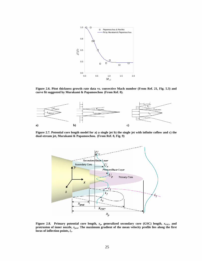
Mean flow surveys have shown that the misalignment of the two flows results in
reduction of the mean velocity gradients on the underside of the high-speed primary flow,
especially in the region near the end of the primary potential core which contains the
dominant noise sources. In addition to the reduction of mean velocity gradients at the end
of the primary potential core, an elongated generalized secondary core (GSC) on the
underside of the high-speed primary jet has been noted, Fig. 2.8. The secondary core
reduces the convective Mach number of the primary eddies, thus hindering their ability to
generate sound that travels to the downward acoustic far field.
One can estimate the distributions of convective Mach numbers of primary and
secondary eddies. One of the challenging aspects here is determining the velocity along
the inflection point defining the lower edge of the primary shear layer, us(x). See Fig. 2.8.
Measurements were performed by Papamoschou, Ref. 7. The following definitions
( ) ( )( )xa
xuxUM
s
scpcp
−= ,
( )∞
∞−=
aUxU
M cscs (2.14)
were used together with the Crocco-Busemann relation, to plot the convective Mach
number distributions of the primary and secondary eddies. A more balanced distribution
22
between the convective Mach numbers of the primary and secondary eddies (i.e., the
average of both primary and secondary eddy convective Mach numbers was lower for the
duration of their existence) was achieved using deflectors placed in the secondary flow
than by using eccentric nozzles. Analysis of experimental data collected from mean flow
surveys in the asymmetric dual-stream jets showed that by displacing some of the slow
moving fluid of the secondary stream from above the primary jet to the sides and
underneath the primary jet, the GSC was elongated underneath the jet and the primary
potential core was shortened. So, the longer the GSC, the more effective the asymmetric
configuration is in reducing the convective Mach number of the eddies in the primary
shear layer, and hence, in reducing noise emissions.
Figure 2.8 shows the important flow-field parameters as described in Ref. 7. The
length of the generalized secondary core (GSC) is determined by the loop formed
between the loci of inflection points of the transverse mean velocity profiles. Past the end
of the GSC, only one inflection point remains, and it persists into the far-field of the jet.
After the end of the GSC, the maximum gradient of the mean velocity profile exists along
this locus of inflection points, i1. As we shall see, the maximum radial gradient of the
mean velocity is an important parameter for noise considerations. For a coaxial jet, the
length of the GSC is approximately the same as the length of the secondary potential
core. For an asymmetric jet, the GSC underneath the primary jet is elongated and above
the primary jet it is shortened with respect to the coaxial jet.
23
Figure 2.1. Illustration of primary potential core and secondary potential core in a dual-stream jet.
U1, ρ1, a1 , γ1
U2, ρ2, a2, γ2
cU
Figure 2.2. The compressible turbulent shear layer formed between two gases.
Figure 2.3. The Mach number as measured in the frame of reference of the disturbance is called the convective Mach number. The growth-decay nature of the disturbance (wave-packet) is described by an amplitude modulation function A(x). (From Ref. 4, Fig.1)
Initial Region Intermediate Region Fully-Developed
Us
Up
Primary shear layer
Secondary shear layer
( )txiexAtx ωαη −= )(),(
24
b)
a) c)
Figure 2.4. a) Illustrates the idea that there exists a spectrum of phase-speeds (From Ref. 4, Fig. 1) b) Those that convect supersonically will have solutions that radiate c) while those that convect subsonically decay.
Figure 2.5. Solid circles – growth rate data for incompressible shear layer by Brown and Roshko. Other symbols – growth rate data for compressible shear layers for several investigators as compiled by Brown and Roshko. Maximum vorticity growth rate is used. (From Ref. 24, Fig. 15).
y
mc < 1 x
y
mc > 1 x
0.00
0.05
0.10
0.15
0.20
0.25
0.1 1.0 10.0
ρ 1 /ρ 2
δ'ω
1 2 3 4 5 6M1
25
0.0
0.3
0.5
0.8
1.0
0.0 0.5 1.0 1.5 2.0
M c1δ'
/ δ' 0
Papamoschou & RoshkoFit by Murakami & Papamoschou
Figure 2.6. Pitot thickness growth rate data vs. convective Mach number (From Ref. 21, Fig. 5.3) and curve fit suggested by Murakami & Papamoschou (From Ref. 8).
a) b) c) Figure 2.7. Potential core length model for a) a single jet b) the single jet with infinite coflow and c) the dual-stream jet, Murakami & Papamoschou. (From Ref. 8, Fig. 9)
Figure 2.8. Primary potential core length, xp, generalized secondary core (GSC) length, xGSC, and protrusion of inner nozzle, xprot. The maximum gradient of the mean velocity profile lies along the first locus of inflection points, i1.
26
Chapter 3 Experimental Program
The experimental program was part of a collaborative investigation between the
University of California Irvine (UCI) and NASA Glenn Research Center (GRC), aiming
toward the development and implementation of technology for noise suppression in
turbofan engines. The research objectives necessitated an experimental program that
encompassed noise and flow-field surveys of asymmetric dual-stream jets. Pitot-rake
experiments were conducted in the UCI Jet Aeroacoustics Laboratory, and hot-wire
experiments were conducted in the GRC Engine Research Building CW-17 Free Jet
Facility. The advantages of utilizing the NASA facility include the ability to resolve the
fluctuating velocity field and the opportunity to confirm trends observed at UCI in a
larger facility.
3.1 University of California, Irvine
The Jet Aeroacoustics Laboratory at the University of California Irvine has limited
flow capacity, and its facilities are suitable for conducting investigations of noise
emissions from small-scale models of turbofan engine nozzles. The nozzles used are
1/64th of the actual size. The experiments are run at room temperature, and realistic
27
exhaust conditions are simulated by using helium-air mixtures for the microphone noise
measurements. Mean velocity measurements are conducted using a Pitot-probe rake to
investigate the relationship between noise and flow field of the jets. The details of the
noise and flow measurements are provided here, and data analysis is in the next chapter.
3.1.1 UCI Nozzles
The UCI experiments (explained in Chapter 5) used two dual-stream nozzles, one with
rapidly converging exit streamlines, and one with nearly parallel exit streamlines,
Fig. 3.1. At nominal exhaust conditions both nozzles have a bypass ratio of
approximately 5. The motivation for this study was Ref. 14, in which minimal noise
reduction was observed when a wedge-shaped deflector was placed on a nozzle with
parallel exit flow lines at NASA Glenn Research Center, while at the same time, dramatic
noise reductions were being observed at UCI when the same type of deflector was placed
on a nozzle with converging streamlines. The UCI classic nozzle was selected because at
nominal exhaust conditions it has approximately the same bypass ratio as the UCI 3BB
nozzle. The two nozzles are described below. Both nozzles were made from epoxy resin
using rapid-prototyping methods. The nozzles were epoxied to a threaded aluminum pipe
fitting, shown in Fig. 3.2, taking care to keep the axes aligned.
The nozzle with parallel exit streamlines is called the UCI ‘Classic’ nozzle. This
nozzle is used in two configurations. One is in a coplanar arrangement where the exit of
the core nozzle is aligned with the exit of the fan nozzle. The second arrangement of the
UCI ‘Classic’ nozzle has an inner nozzle protrusion of 9.5-mm. The nozzle had been used
28
in past UCI experiments, before coordinates for realistic turbofan engine nozzles were
obtained, this is why it is referred to as the UCI ‘Classic’ nozzle.
The nozzle with convergent exit flow lines and a geometry that is representative of
actual separate-flow turbofan engines is referred to as the UCI ‘3BB’ nozzle throughout
the thesis. The nozzle was named ‘3BB’ because it was the third nozzle on the separate-
flow test program in the Aeroacoustic Propulsion Laboratory (AAPL) at NASA Glenn
Research Center, Ref. 37. The positions of the letters denote the configuration for the
core and fan nozzles, repsectively. ‘B’ means baseline. At UCI, the nozzle used is a
scaled-down version of the baseline separate-flow nozzle used on the Nozzle Acoustic
Test Rig (NATR). The coordinates of the NATR nozzle were divided by a factor of eight
to fit within the flow capacity of the UCI lab.
The nozzle assemblies includes three elements: secondary (fan) nozzle, primary (core)
nozzle, and center plug, Fig. 3.2b. Figures 3.1 and 3.2 show 3D views generated from the
stereolithography files for the nozzles. Figure 3.3 shows the radial coordinates of the
nozzles. Figure 3.4 shows a photograph of the nozzles with one pair of vanes installed.
Tables 3.1 and 3.2 list the nozzle exit conditions. The reader is referred to Ref. 10, for
further details of the UCI ‘3BB’ nozzle.
3.1.2 UCI Deflectors
The purpose of the airfoil-shaped vanes and wedge-shaped deflectors is to create
asymmetry in a dual-stream jet by imparting an aerodynamic force on the secondary
fluid, thereby diverting some of the secondary flow to the side and underneath the high-
speed primary jet. The deflector force creating the asymmetry, or deflector “turning
29
effort,” is quantitatively defined in Chapter 5. The asymmetry that results is in the form
of a thickened low speed fluid in the hemicylinder underneath the jet centerplane,
targeting the dominant noise sources near the end of the primary potential core. Figure
1.5 shows the concept.
All vanes were constructed by hand from strips of 0.35-mm thickness brass sheet
metal, cut to the desired chord width. The metal was folded at an angle so that there was
no sweepback upon installation, Fig. 3.5.a. The bending angle θ was equal to the surface
angle of the nozzle with respect to the centerline. Each vane in a pair was made to be a
mirror image of the other. Using the outer nozzle as a guide, the length of the vanes were
determined such that the vanes were full span upon installation. The leading edge was
generally about 1-mm longer in span than the trailing edge for the ‘3BB’ nozzle vanes.
The difference in leading edge and trailing edge span was less than 1-mm for the
‘Classic’ nozzle vanes because of the difference in the fan duct geometries. The base of
each vane was about 3-mm by 3-mm and was given slight curvature so that it could be
firmly attached to the nozzle surface, Fig. 3.5.b. Smooth electric tape (the thickness of the
electric tape was 0.18-mm) was used to give curvature to the leading edge of the vane.
Starting with a clean, smooth nozzle, the azimuth angles were measured from the ground
position; to assist with this, guide lines were drawn using pencil. The angle of attack was
carefully measured using specialized tooling developed specifically for the construction
of the vanes, and accuracy is estimated to within ±1° If the vanes were reused, they were
cleaned using acetone before installation, new tape was applied, and the vanes were
squared to ensure that camber, dihedral, or twist were not present. Using a drop of super
glue, the base of the vane was attached to the inner nozzle, at the desired trailing edge
30
position. The vanes were then examined under a magnifying lens to check symmetry, and
finally, the nozzle assembly, Fig. 3.2, was attached to the dual-stream apparatus,
described in the next section.
The wedge-shaped deflectors were cut out of 4.5-mm thick nylon sheet. The nylon
sheet was taken from flexible hosing, so it had curvature. This facilitated attachment of
the deflector to the nozzle. The same means are used to determine the half angle of the
wedge, as was used for the vane angle of attack. The sidewalls of the wedge were
vertical, and height of the wedge was approximately the same as the annular gap width of
the nozzle. The accuracy in cutting the wedge side length is estimated to be ± 0.5-mm.
For details of the aerodynamic forces of the deflectors, and how the forces differ
depending on which nozzle is used, and depending on choice of deflector leading edge
position, the reader is referred to Chapter 5.
3.1.3 UCI Noise Measurements
For acoustic simulation of hot jets, the nozzles were attached to the dual-stream
apparatus, shown in Fig. 3.6.a, and cold mixtures of helium and air are supplied to the
primary and secondary nozzles. Helium-air mixtures have been shown to simulate
reasonably well the acoustics of hot jets, Refs. 40-41. The exit flow conditions, listed in
Tables 3.1 and 3.2, matched the typical exit conditions of a turbofan engine with bypass
ratio 4.8 at takeoff setting. The Reynolds number of the jet, based on fan diameter, was
0.6 × 10⁶. For more information on the helium-air mixture matching method, the reader is
referred to Refs. 40 and 41.
31
The microphone phased array consists of eight 3.2-mm condenser microphones (Bruel
& Kjaer, Model 4138) arranged on a circular arc centered at the vicinity of the nozzle
exit. The polar aperture of the array is 30º and the array radius was 1m. The angular
spacing of the microphones is logarithmic. The entire array structure is rotated around its
center to place the array at the desired polar angle. Positioning of the array is done
remotely using a stepper motor. An electronic inclinometer displays the position of first
microphone. The arrangement of the microphones inside the anechoic chamber, and the
principal electronic components, are shown in Fig. 3.8. A photograph is shown in
Fig. 3.9. The microphones were connected, in groups of four, to two amplifier/signal
conditioners (Bruel & Kjaer, Model 4138) with low-pass filter set at 300 Hz and high-
pass filter set at 100 kHz. The four-channel output of each amplifier was sampled at 250
kHz per channel by a multi-function data acquisition board (National Instruments PCI-
6070E). Two such boards, one for each amplifier, were installed in a Pentium 4 personal
computer. National Instruments LabView software was used to acquire the signals. Even
though the array provides noise source location maps, in this study it was used only to
survey the far-field sound emitted by the jets. Only the downward azimuthal direction
was surveyed. The sound pressure level spectrum was corrected for actuator response,
free-field correction, and atmospheric absorption. The overall sound pressure level
(OASPL) was obtained by integrating the corrected spectrum. All acoustic data are
referenced to a distance of 100Df from the nozzle exit. For more details on the array
setup, the reader is referred to Ref. 42.
32
3.1.4 UCI Velocity Measurements
Pitot-pressure measurements were conducted and the mean velocity was calculated
using the equations presented in Chapter 4. The nozzles were attached to the dual-stream
apparatus, shown in Fig. 3.6.a. Compressed air was supplied to both the primary (core)
and secondary (fan) nozzles at room temperature. Velocity measurements cannot be
obtained using helium-air mixtures, because the concentration, and therefore the gas
constant would be unknown, Ref. 40. Since cold air is used to feed both streams, this
means that only the velocity ratio or the Mach number ratio at the jet exit can be matched
to a realistic turbofan exhaust. The velocity ratio was chosen to preserve some of the
important physics, and therefore the trends are also expected to be preserved. The exhaust
conditions are listed in Tables 3.1 and 3.2. The Reynolds number of the jet, based on fan
diameter, was 0.9×10⁶. Even though the velocities were lower than those of a realistic
turbofan exhaust, which was used in the acoustic tests, the trends of some of the essential
flow characteristics were expected to be preserved. The velocity ratio used was 0.7,
representative of the exhaust velocity ratio in turbofan engines, and it matched the
velocity ratio used in the acoustics tests.
A Pitot-probe rake, shown in Fig. 3.6.b and in Fig. 3.7, was used to survey the total
pressure in the jet plume. The rake consisted of five stainless steel tubes, each 70-mm
long, supported by a streamlined fitting. The tubes were mounted 10-mm apart and their
inner diameter is 1.0-mm, limiting the spatial resolution to 1.0-mm. The motion in the y-
direction was automated and the positioning in the x- and z-directions was manual.
11,000 data points are collected in the y-direction over a distance of 4Df. In the x-
direction, 25 data points were regularly spaced at intervals 0.42Df apart. For each axial
33
station, the rake traversed the plume in the y-direction a total of four times. Each time, the
rake was moved by a z-increment of 2.5-mm, i.e., one fourth of the probe spacing. This
resulted in 20 z-locations being surveyed for each axial position. The spatial resolution
was 2.5-mm in z and 1.0-mm in y.
The second probe from the top is the reference probe, and it is initially positioned at
the tip of the plug. The negative y-direction defines the direction of the ground (φ=0o).
The five probes of the rake were connected individually to five pressure transducers
(Setra Model 207). The transducers were mounted on the traverse assembly in order to
minimize the length of the tubing between each probe and transducer. This arrangement
allowed the response time of the probe-transducer system to be low enough to resolve the
steep gradients near the nozzle exit. The typical carriage speed was 10mm/s, and the
transducers were sampled each at 1000 samples per second by a National Instruments
analog-to-digital data acquisition board.
Mach number and velocity were computed from the total pressure measurements
assuming constant total temperature, equal to the ambient temperature, and uniform static
pressure, described in Chapter 4. Symmetry of the velocity field was assumed about the
plane z=0. Therefore, the region z≥0 and a small portion of the region z<0 were resolved.
Velocity data from the latter region were used to determine the true plane of symmetry of
u, which may differ slightly from the geometric plane z=0. The true plane of symmetry
was then used in mirror-imaging the velocity data.
34
3.2 NASA John H. Glenn Research Center (GRC)
In a complementary study to the UCI mean velocity measurements, hot-wire velocity
measurements were conducted in the CW-17 Free Jet Facility at NASA Glenn Research
Center to acquire the mean and RMS velocity fields using wedge-shaped deflectors. Due
to the stringent safety permits required to run at high pressures, only very low pressures
were approved, about one psig, at the time the experiments were performed. Therefore
the experiments were run at very low Mach number; the primary exit Mach number was
0.18, and the secondary Mach number was 0.13. The secondary-to-primary velocity ratio
of 0.7. Mean and turbulent flow-field surveys were acquired. Full pressure capabilities
(and therefore Mach number) were not restored to the facility upon completion of the
thesis, and noise measurements were not obtained. Details of the experiments are
provided in the sections that follow. Data analysis is provided in Chapter 4.
3.2.1 GRC Nozzle and Deflectors
It is practical to test replica aircraft engine nozzles that are also being tested by NASA
and industry with the aim of implementing them on efficient airliners. The bypass ratio 8
nozzle used at GRC was selected because it is representative of next generation high
bypass ratio turbofan engine nozzles. This nozzle, like the ‘3BB’ nozzle, has converging
exit geometry, and is referred to as the GRC ‘5BB’ nozzle throughout this document. It
was named ‘5BB’ because it was the fifth nozzle on the separate-flow test program in the
Aeroacoustic Propulsion Laboratory (AAPL) at NASA Glenn Research Center, Ref. 37.
The positions of the letters denote the configuration for the core and fan nozzles,
repsectively. ‘B’ means baseline. In the GRC CW-17 Open Jet Facility, the nozzle used
35
was a scaled-down version of the baseline separate-flow nozzle used on the Nozzle
Acoustic Test Rig (NATR). The coordinates of the NATR nozzle were divided by 4.67.
The Reynolds number of the jet, based on fan diameter, was 0.2 × 10⁶. Figure 3.10 shows
a photograph of the GRC ‘5BB’ Nozzle. Figure 3.11 shows the nominal radial
coordinates of the GRC ‘5BB’ nozzle. Table 3.3 lists the actual nozzle exit conditions.
The nominal bypass ratio is 8 when operated at realistic engine conditions. Ref. 12 also
uses this nozzle.
The alignment of the hot-wire probes and the jet axis was verified by taking mean y-
and z- velocity profiles at the nozzle exit and at a location far downstream of the nozzle
exit, 20Df. The alignment of the profiles provided information about how well aligned the
entire setup was. By measuring the shift of the location of the peak velocity, it was
determined that the probe was off-axis by about a tenth of a degree. The nozzle
axisymmetry was determined as precisely as possible by measuring the width of the
secondary annulus using a hole diameter gauge. It was possible to match the annular gap
width to within 0.005” of the values measured at three points around the nozzle. The
nozzle was left in place between baseline and external wedge experiments. The outer
nozzle was necessarily removed for installation of the internal wedges.
Several wedge deflector configurations and a pylon with an external half wedge on
either side were tested. Since the geometry of the internal pylon structure is likely to have
an impact on turbulent-mixing noise, internal wedge configurations were also examined
with the GRC ‘5BB’ nozzle. The wedges were fabricated from DuraForm® EX Plastic
and attached using epoxy. Photographs of the wedges and pylon with flaps are in Fig.
36
3.12. Further details of the wedge-shaped deflectors and pylon configuration design are
provided in Chapter 6.
3.2.2 GRC Velocity Measurements
Hot-wire experiments were conducted in the CW-17 Open Jet Facility open jet facility
at NASA Glenn Research Center, Fig. 3.13. The primary plenum chamber has a 0.76m.
diameter. Dual-stream coannular flow is achieved via a secondary plenum chamber
located just upstream of the nozzles. The secondary annular flow, supplied by four
equally spaced ports, is routed through contoured interior and screens to provide a
uniform velocity profile at the exit. Further details of this facility may be found in Ref.
38.
Separate centrifugal blowers were used to supply the primary and the secondary flows.
All results were obtained using cold air. This matched the UCI experiment. Also, using
the hot-wire technique, if there are temperature gradients in the jet, heat transfer from the
hot-wire probe is not strictly a function of velocity. Since air at room temperature was
used to supply the two streams, the total temperature everywhere was approximately the
same as ambient temperature, assuming a Prandtl number of unity. The facility had very
limited flow capacity, and a safety permit was obtained for operation at one psig. The
GRC ‘5BB’ nozzle exhaust conditions are listed in Table 3.3. Although the tests were
run at very low Mach number, Mp=0.18, and Ms=0.13, the secondary-to-primary velocity
ratio was 0.7, and thus, some of the fundamental fluid mechanics were expected to be
preserved. The velocity ratio also matched the UCI velocity measurements.
37
Two pairs of crossed hot-wires, illustrated in Fig. 3.14, were used to survey the mean
and fluctuating velocity components in the jet plume. One was in a u-v configuration, the
other in a u-w configuration. Only the normal velocity component to each wire can be
measured, so a single hot-wire cannot measure Reynolds stresses and turbulent kinetic
energy. The wires were spaced 1.0-mm apart, limiting the spatial resolution to 1.0-mm in
the y- and z- directions. The probes were mounted on a streamlined strut, visible in Fig.
3.13, and the positioning was automated under computer control in all three directions.
The two probes were located at the same y-location (vertical) and spaced apart from one
another by 23-mm in the z-direction (horizontal), Fig. 3.14. The step size in the z-
direction was chosen to be a submultiple of the separation distance so that a shift of the v-
array by an integral number of steps matched the corresponding w-array.
With axial distance, both spatial resolution and the sampling rate were decreased. Fig.
3.15 shows the grid used for data point spacing. Smaller grid intervals were used where
sharp spatial gradients exist in the initial region of the jet. An exponential function was
used to decrease the spatial resolution with axial distance. In the x-direction, 16 data
points were acquired, spanning 8.23Df. Grid spacing in the x-direction started with a
separation of 0.114Df or 6.1-mm between the first and second data points and ended with
a separation of 1.47Df between the last two data points. The first data point was taken
0.024Df from the tip of the nozzle center plug in x and 0.62Df from the jet centerline in y,
where the velocity was small. For each axial station, 19 data points were collected along
y, uniformly spaced. At each axial station, the grid spacing in y was adjusted so that the
outer data point formed an angle of 5.35º with the axis. The upstream-most position used
uniform intervals of 0.0715Df and the furthest position downstream used uniform
38
intervals of 0.157Df. This corresponds to a spatial resolution of 3.8-mm in y at the
upstream-most position and 8.3-mm in y at the downstream-most position.
Further downstream, where turbulent structures convect with lower frequencies, larger
sampling times were required. For distances upstream of 4.28Df, the sampling rate used
was 500 hz, and for distances downstream of 4.28Df from the plug tip, the sampling rate
used was 200 hz. The ensemble size was 2000. Thus, sampling times of 4s or 10s were
used depending on the axial location. At each data point, mean and RMS velocities were
sampled in all three directions. Reynolds stress u’v’ and u’w’ components were obtained.
In addition to the crossed wire surveys, a single wire was used separately to survey the
GRC ‘5BB’ nozzle exit boundary layers. The boundary layers were found to be
nominally laminar and their characteristics are listed in Table 3.4; here, location 1 refers
to the inner layer of the primary (core) nozzle, location 2 refers to the outer layer of the
primary (core) nozzle, and location 3 refers to the inner layer of the secondary (fan)
nozzle.
The calibration procedure used the coannular nozzle in order to produce a top-hat
velocity profile. The voltage of each probe was recorded and plotted against the
calculated velocity for several total pressures ranging from very low speeds, close to
zero, up to the highest velocity tested. The jet exit velocity was calculated based on the
total pressure supplied to the jet, using an assumption of isentropic expansion through the
nozzle, and knowledge of the total temperature and atmospheric pressure. A fourth order
polynomial was used to fit the calibration curve to the points.
In order to validate the setup, single hot-wire profiles were compared with crossed
hot-wire profiles. Mean velocity profiles measured in the initial, intermediate, and fully-
39
developed regions of a coaxial jet with secondary-to-primary velocity ratio 0.5 are shown
in Fig. 3.16. The mean velocity profiles measured using a single hot-wire probe agree
closely with the profiles measured using a pair of crossed hot-wire probes. Also
compared were mean velocity profiles that were obtained with the u-v probe and the u-w
probe. These are not shown, but it is noted that these comparisons displayed remarkable
agreement. The coannular nozzle exit conditions are listed in Table 3.5.
Also, mean velocity profiles were measured at two axial locations in the initial mixing
region of the jet, and compared with experimental data from Fig. 2 of Ko and Kwan, see
Fig. 3.17. It was desired to look at the similarity of the shear layer in the jet, as well as to
validate the experimental setup. The conventional similarity parameter was used, η=y/x,
where y is measured with respect to the lip of the secondary (fan) nozzle. The local mean
velocity ratio is taken with respect to the exit velocity of the secondary jet, Us.
Velocity (m/s) 293 147 Mach number 0.26 0.13 Bypass ratio - 0.50
41
UCI ‘Classic’ Nozzle – BASE UCI ‘3BB’ Nozzle – BASE
a)
b)
Figure 3.1. 3D views of UCI a) ‘Classic’ and b) ‘3BB’ nozzles.
UCI ‘3BB’ Nozzle – 2V
Figure 3.2. Solidworks model of entire assembly for the UCI ‘3BB’ nozzle: threaded aluminum fitting, fan nozzle, core nozzle, one pair of vanes, and center plug.
42
UCI ‘Classic’ Nozzle – BASE UCI ‘3BB’ Nozzle – BASE
-40 -30 -20 -10 0 10 20 30 400
10
20
30
40
50
60
xprotr. = 9.51 mm
Axial Distance From Nozzle Exit (mm)
Rad
ial D
ista
nce
from
Cen
terli
ne (m
m)
a)
-40 -30 -20 -10 0 10 20 30 400
10
20
30
40
50
60
Axial Distance From Nozzle Exit (mm)
Rad
ial D
ista
nce
from
Cen
terli
ne (m
m)
b) Figure 3.3. Radial coordinates of UCI a) ‘Classic’ and b) ‘3BB’ nozzles in millimeters.
UCI ‘Classic’ Nozzle – 2V UCI ‘3BB’ Nozzle – 2V
a)
b)
Figure 3.4. Photographs taken in the UCI Jet Aeroacoustics Laboratory with one pair of vanes in the UCI a) ‘Classic’ and b) ‘3BB’ nozzles.
a)
b)
Figure 3.5. a) Bending angle for zero sweepback and b) base curvature for secure attachment.
Figure 3.10. Photograph taken in the GRC CW-17 Open Jet Facility of the GRC ‘5BB’ nozzle and a pair of crossed hot-wire probes.
0
20
40
60
80
-80 -60 -40 -20 0 20 40 60 80
Axial Distance From Fan Exit (mm)
Rad
ial D
ista
nce
From
Cen
terli
ne (m
m)
Figure 3.11. Radial coordinates of GRC ‘5BB’ nozzle in millimeters.
46
a)
b)
c)
d)
Figure 3.12. Photographs taken in the GRC CW17 Open Jet Facility. GRC ‘5BB’ nozzle and a) W1 b) Pylon + Flap c) W2 + Cap 1 d) W2 + Cap 3.
Figure 3.13. Photograph taken in the GRC CW-17 Free Jet Facility of the GRC coannular nozzle and automated traversing mechanism.
47
Figure 3.14. Illustration of u-v and u-w cross-wire probe separation in the z-direction.
x/Df
y/D
f
0 1 2 3 4 5 6 7 8-2
-1
0
1
2
Figure 3.15. Grid used for positioning of the u-v probe in the xy-plane.
∆z = 23 mm
u-w probe
u-v probe
48
Figure 3.16. Three regions of a coaxial jet (top). Mean velocity profiles (bottom) measured at x/Df = 0.2,1, and 10 in a coaxial jet exhaust with secondary-to-primary velocity ratio 0.5.
Initial Region Interaction Region Fully-Developed
Us
Up
++ +
++
++
++
++
++ +
++
++
++
++
+
++ +
y/Df
U/U
p
-1.25 -1 -0.75 -0.5 -0.25 00
0.2
0.4
0.6
0.8
1 u-v probesingle probe
+
+
+ + ++
++
++
++
++
+
+
+
++ + + +
++
+
+
+
+
+
+
++ +
y/Df
U/U
p
-0.6 -0.4 -0.20
0.2
0.4
0.6
0.8
1
u-v probesingle probe
+
+x x x x x
x
x
x
xx x x x x x x x x
x
x
x
x x x x x x x x x x x
+ + +
+
+
+ + + + + +
+
++ + + + + +
y/Df
U/U
p
-0.6 -0.4 -0.20
0.2
0.4
0.6
0.8
1
u-v probesingle probe
x
+
x/Df = 0.2 x/Df = 1 x/Df = 10
49
Figure 3.17. Secondary shear layer mean velocity profiles. Values are non-dimensionalized for similarity.
The axial and transverse velocity components are u = Vcosθ and v = Vsinθ.
Combining with Eq.4.7, the velocity components are expressed based on the measured
(normal) components of each probe
( )2121
nn uuu += , ( )2121
nn uuv += (4.8)
The same procedure was used to determine u and w from the recorded voltages of the
second crossed hot-wire probe. The Savitsky-Golay filter explained in 4.1.1 is used to
smooth raw velocity data. The velocity components of Eq.4.8 represent total
instantaneous velocities and are functions of space and time. This means they consist of
an average and a fluctuating component. Due to the random nature of turbulent flows,
statistical tools are necessary to interpret the data in a meaningful fashion. These are
described in the next section.
4.2.2 Statistical Quantities
For a stationary ergodic process, the statistical quantities do not vary with time, and
several quantities of interest can be expressed by the equations presented in this section.
Many values can be measured in a flow field, such as velocity, pressure, or temperature.
We are interested in a turbulent process, for which these quantities have a mean and a
fluctuating component. The total turbulent velocity is a function of position in space and
time, ( )tzyxu ,,,~
. The fluctuating component, ( )tzyxu ,,,'~
, is the difference between the
total velocity and the average velocity, ( ) ( ) ( )zyxutzyxutzyxu ,,,,,,,,'~~~
−= . The mean
55
value, ( )zyxu ,,~
, is the average of many samples over a given time period. This quantity
is also called the first moment.
( ) ( )dttzyxuT
zyxuT
TT ∫
−∞→= ,,,
21lim,,
~~ (4.9)
The mean square, ψ2, is the average value of the squares of many individual samples over
a long period of time. This quantity is also called the second moment
( ) ( )dttzyxuT
zyxT
TT ∫
−∞→= ,,,
21lim,, 2
~
2ψ (4.10)
and the variance, σ2, or the second central moment is taken with respect to the mean
value, ( )zyxu ,,~
as follows
( ) ( ) ( )( ) dtzyxutzyxuT
zyxT
TT ∫
−∞→ −=
2
~~
2 ,,,,,21lim,,σ (4.11)
The root mean square (RMS), σ, is the square root of the variance. This value is often
used to describe the turbulence intensity. The turbulent kinetic energy (TKE) will be used
to describe the turbulence intensity in subsequent chapters. Its value is determined by
squaring the individual RMS components.
( ) ( )222
21,, zyxzyxk σσσ ++= (4.12)
In post-processing of the data, the turbulent kinetic energy can be approximated by
( ) ( )22 221,, zxzyxk σσ ⋅+≈
(4.13)
since the horizontal and transverse components are of the same order of magnitude. In
subsequent chapters, these statistical quantities are non-dimensionalized using either the
primary jet exit velocity Up or its square.
56
The skewness is the third central moment and the kurtosis is the fourth central
moment, but these are not presented here. For an excellent reference on statistical
engineering analysis, the reader is referred to Bendat and Piersol, Ref. 67.
The one-point velocity cross-correlations between the axial and vertical and the axial
and horizontal velocity components, u’v’ and u’w’ respectively, can be obtained using the
current hot-wire setup. These are directly related to the Reynolds stresses. In this work,
the term Reynolds stress is used synomonously with the cross-correlation defined below.
( ) ( ) ( )dttzyxvtzyxuT
zyxRT
TTuv ,,,',,,'
21lim,, ∫
−∞→=
( ) ( ) ( )dttzyxwtzyxuT
zyxRT
TTuw ,,,',,,'
21lim,, ∫
−∞→=
(4.14)
Commonly, the incompressible Reynolds stress definition includes density and a negative
sign as coefficients to the above definition, for example, Ref. 68.
57
45o-θ
θx
u
vV
45o-θ
θx
u
vV
Figure 4.1. Crossed hot-wire orientation. The velocity vector is oriented at an angle θ with respect to the probe axis, and each wire is oriented at 45o with respect to the axis.
1
2
58
Chapter 5 Effect of Nozzle Geometry on Jet Noise Reduction using Fan Flow Deflectors
Marginal noise reduction had been observed at UCI, after an internal wedge was
placed on the UCI ‘Classic’ nozzle, described in Chapter 3. Subsequently, the wedge was
discarded because it was thought to be inferior to vanes in noise suppression capability.
The wedge showed much improved efficacy when placed on a nozzle with realistic
(converging) exit geometry, such as the UCI ‘3BB’ nozzle, Refs.12-13. Subsequent
measurements taken at NASA GRC showed the same trends, Ref.14. Figure 5.1 shows
noise reduction achieved in the ‘3BB’ nozzle using an internal wedge deflector. On the
left is the UCI measurement and on the right is the GRC measurement. Figure 5.2 shows
the limited noise reduction observed when an internal wedge was placed on a nozzle with
parallel exit flow lines at NASA.
It was hypothesized that the convergent nozzle contours helped the wedge displace the
fluid in the downward and sideward directions, while the parallel exit contours limited
the fluid displacement strictly to the sideward direction. Figure 5.3 illustrates the
hypothesis. Mean flow measurements conducted at UCI confirmed the expected flow
59
behavior, Fig.5.4. Additionally, uniformly reduced velocity gradients were revealed
underneath the jet issuing from the ‘3BB’ nozzle.
The experiments conducted at UCI illuminated the relation between mean flow
gradient and noise reduction. By using two different nozzles, they augmented the
database for correlating the mean flow field with noise emissions. The noise and mean
flow fields for ten nozzle-deflector configurations are presented here, and important
trends are highlighted.
5.1 Nozzle-Deflector Comparisons
The baseline nozzles and deflector fabrication are described in Chapter 3.
Experiments covered two nozzle geometries, four deflector configurations, and two types
of comparisons using internal vanes: equal deflector turning effort, and equal chord
length. Comparisons at equal turning effort, to be defined below, were necessary to distill
the effect of nozzle geometry from the effect of deflection force.
5.1.1 UCI Nozzles
The nozzles used for the comparisons outlined here included one with parallel exit
streamlines and one with convergent exit streamlines, described in Chapter 3. The initial
measurements of Fig. 5.4 were taken using a coplanar configuration of the UCI ‘Classic’
nozzle and the UCI ‘3BB’ nozzle and internal wedge, Fig. 5.5. The nozzle coordinates
with deflector placement for all subsequent comparisons are shown in Figs. 5.11-5.14.
The UCI ‘Classic’ nozzle was tested with a protrusion of the core nozzle so that a one-
to-one comparison could be performed with the UCI ‘3BB’ Nozzle. Exit conditions are
60
listed in Tables 5.1 and 5.2. The principal difference between the two nozzles, as far as
deflector aerodynamics is concerned, is in the internal Mach number distribution. In the
nozzle with rapidly convergent exit streamlines, the Mach number decreases quickly
moving upstream of the fan exit, while in the nozzle with parallel streamlines, the Mach
number changes slowly in the vicinity of the nozzle exit. The Mach-area relation is used
to obtain the dynamic pressure distribution inside the nozzle fan ducts, Fig. 5.6.
5.1.2 Deflector Turning Effort, ε
In order to isolate the effect of nozzle geometry on the ability of fan flow deflectors to
reduce noise, it was necessary to conduct comparisons between deflectors on an “equal
turning effort” basis, meaning that the deflector force, normalized by the thrust of the
bypass stream, is approximately the same in both nozzles. The turning effort can be seen
as an overall deflection angle based on the force of the deflectors alone (i.e., without
considering any additional forces created by the nozzle surface). Its definition is
∑=
=N
ii
s
LF 1
1ε , (5.1)
where Li is the lift, or sideforce, generated by each deflector and N is the total number of
deflectors. Both nozzles produced approximately the same secondary (bypass) thrust Fs,
while the dynamic pressure distributions in the fan ducts of the two nozzles differ
drastically. Experiments were conducted using internal vanes with approximately
matched lift forces in the two nozzles, achieved by reducing the chord length of the vanes
in the UCI ‘Classic’ nozzle. The external wedge side forces were approximately matched
without altering the wedge geometry. The internal wedge forces were not matched,
61
however qualitative trends are not expected to change depending on the magnitudes of
the deflector forces. The equations in this section provided guidance for selection of the
deflector parameters.
Recent pressure coefficient measurements have been obtained for a wedge placed in a
compressible jet issuing from a rectangular nozzle, Ref. 17. This problem differs
significantly from the classic wedge problem because the top and base of the wedge are
in communication with ambient fluid. It is well worth noting that the drag force was
found to be about 75% less than a fully-immersed two-dimensional cylindrical wedge.
For the wedge placed in a finite thickness jet exhaust, one can reasonably assume
SqCL sLWe )(α= , (5.2)
where CL is a sideforce coefficient that depends only on the wedge half-angle α, qs is the
dynamic pressure at the nozzle exit, and S is the wetted area of the wedge. Given that qs
is the same for both nozzles, equal sideforce is achieved by wedges of equal half-angle
and wetted area.
For internal vanes, a computational study, Ref. 16, showed that the lift coefficient of
the vane airfoil (in that case a NACA 0012 section) approximately matched the lift
coefficient of the same airfoil in external flow if the reference conditions were taken at
the axial position of the leading edge of the vane. Reference conditions are taken at vane
leading edge. With this selection of reference conditions, the lift coefficient of the vane
airfoil is given by the familiar relation
αDL aC 2= , (5.3)
where a2D is the two-dimensional lift curve slope (typically 0.11 deg-1). Therefore, the
vane lift is
62
cwqaL leDV α2= , (5.4)
where w is the average vane span. Equations 5.2 and 5.4 provided guidance for the
design of deflectors that would allow comparisons at equal turning effort ε. Other
comparisons were performed on an equal chord length basis. Details of the deflector
designs are provided in the next section. The interested reader is referred to Shevell,
Anderson, and Liepmann and Roshko, Refs. 73, 75, and 77, for three excellent
aerodynamics texts.
5.1.3 Deflector Configurations
The deflector parameters were similar to those used in earlier exploratory studies,
Refs. 10-12. They do not represent optimal design configurations. Four configurations
were tested: internal wedge (Wi), external wedge (We), a single pair of internal vanes
(2V), and two pairs of internal vanes (4V). Figure 5.7 depicts the four configurations
tested. The deflector geometries are shown together with the nozzle coordinates in
Figs. 5.8-5.11. Tables 5.3 and 5.4 list the deflector parameters.
Both external wedges (We) were mounted at the top of the two nozzles (φ=180o) and
had the same half-angle. It was thus assumed that the sideforce coefficient, CL was the
same. In order for the sideward forces imparted by the wedges to be matched, the wetted
area, S, of the deflectors must be consistent between nozzles, Eq.5.2. Since the fan duct
thickness is 3.9 mm for the classic nozzle and 3.1 mm for the UCI 3BB nozzle, it was
thought that the wedge side lengths could be varied to match the wetted areas. This was
not necessary, however, since the wetted areas were estimated to be approximately the
same for a wedge that was 4.5 mm in height.
63
The wetted area of the external wedge (We) was estimated as follows: along the free
surface of the fluid passing over the wedge, the pressure is ambient. Assuming isentropic
flow, the Mach number is constant on the free surface. This means that the temperature
and therefore the density are also constant. It follows, from the continuity equation, that
the area filled by the flow must be constant. The surface of the ‘3BB’ nozzle downstream
of the fan duct exit is convergent, so the streamlines cannot remain parallel to the surface.
Fig. 5.12. shows the idea. A simple program was written to calculate the position of the
free surface when a wedge with half angle α = 17o is placed on the UCI ‘3BB’ nozzle.
The projection of the free surface of the fluid passing along the side of the wedge onto
the plane of symmetry is plotted in Fig.5.13. The outcome showed that the wetted area of
the wedge on the UCI ‘3BB’ nozzle for a wedge with half angle α = 18o and side length
l=10 mm is 37mm2. The wetted area for a wedge with the same half angle and side length
on the ‘Classic’ nozzle is rectangular assuming parallel flow lines, and it is 39mm2, a
difference of only about 5%. Altering the side length by 0.5 mm would have resulted in a
matched wetted area, but construction of the wedge-shaped deflector is very painstaking,
and the accuracy in making them was not better than ± 0.5 mm. Thus, the comparison
was performed using the same external wedge (We) geometry in both nozzles. This force
estimation procedure does not take into account the upwash that was noted in the flow
visualization experiments of Ref. 17. (Chapter 7 presents computational and experimental
surface flow data for an external wedge that are in contrast to the analysis here. However,
the estimate is still valid for matching force between nozzle geometries.)
Determining the turning effort provided by the internal wedge (Wi) is more
complicated because of the favorable pressure gradient inside the fan duct. This
64
comparison was performed using the same internal wedge half-angle and side length in
both nozzles. Without estimating the sideforce, it is noted that it will be larger in the
‘Classic’ nozzle than in the ‘3BB’ nozzle because of the larger average dynamic pressure
qs in the ‘Classic’ nozzle. The wedge deflectors were constructed by hand from 4.5-mm-
thick nylon sheet. The internal wedge cross-section was rectangular with height 3.9 mm
in the ‘Classic’ nozzle. The top of the internal wedge was carved to match the contours of
the fan duct in the ‘3BB’ nozzles.
Two types of comparisons using internal vane deflectors (2V and 4V) were performed
between the ‘Classic’ and ‘3BB’ nozzles: equal turning effort ε and equal chord length c.
In the ‘3BB’ nozzle, the Mach number and dynamic pressure increase rapidly near the
fan exit because of the rapidly converging duct. As a consequence, at fixed axial position,
the Mach number and dynamic pressure in the ‘3BB’ nozzle are smaller than those in the
‘Classic’ nozzle. In the first type of comparison, the lift force, calculated from Eq.5.4,
was matched by reducing the chord length of the vanes in the classic nozzle to
compensate for the larger dynamic pressure relative to the ‘3BB’ nozzle. The trailing
edges of the vanes were placed at the exit plane of the fan duct, xte=0, a choice
necessitated by the constraints of this study, and not an ideal placement from an optimal
design point of view.
Placement of the trailing edge of the vanes at the fan exit allowed for matched lift
force comparisons between the nozzles without an exceedingly small chord length in the
‘Classic’ nozzle. Placing the vane trailing edge at xte=-2mm inside the fan duct would
have required a chord length of 1.5mm in the ‘Classic’ nozzle, see Fig. 5.14b. Placed at
the trailing edge, the required chord length was 1.8mm (this was rounded up to 2mm) in
65
order to match the lift forces of in the two nozzles. Increasing the chord length in the
‘3BB’ nozzle had little effect on the lift force past c=4mm. Instead of varying the chord
length, the angle of attack could have been varied to match lift force. For vane deflectors
with chord lengths of 4mm, approximately matched lift forces would be achieved by
angles of attack less than 5o in the ‘Classic’ nozzle and 10o in the ‘3BB’ nozzle. It was
decided that placing the trailing edge position of the vanes at the fan exit, or xte=0mm,
was more practical from a fabrication standpoint in achieving the matched turning effort
than placing it at xte=-2mm based on the predictions. It was decided that the chord length
should be changed as opposed to angle of attack to provide downwash at a consistent
angle. This was thought to be a more consistent decision with the experimental necessity
to isolate the effect of the force provided by the nozzle from the force provided by the
deflector. Figure 3.4 shows photographs of the internal vane deflectors with c=2mm in
the ‘Classic’ nozzle, and c=4mm in the ‘3BB’ nozzle.
In the second type of comparison, the chord length of the vanes in the ‘Classic’ nozzle
matched the chord length of the vanes in the ‘3BB’ nozzle. The angle of attack, α =10o
was selected to achieve a large turning effort while avoiding flow separation. Azimuth
placement of the vanes was determined based on previous experiments that showed
significant noise suppression. The vane parameters are listed in Tables 5.3 and 5.4. Vane
fabrication is described in Chapter 3.
5.2 Noise and Mean Flow Measurements
Mean velocity and acoustic measurements were conducted in the Jet Aeroacoustics
Laboratory at the University of California, Irvine, for ten nozzle-deflector combinations.
66
The results here were also published in Ref. 11. The data is referenced to the axial
location of the plug tip, so x/Df =0 corresponds to the plug tip, and the first measurement
location.
First, in Fig.5.15, the velocity results for the baseline ‘Classic’ and ‘3BB’ nozzles are
presented. Two types of isocontours are presented: the velocity on the plane of
symmetry, or the z=0 plane, normalized by the primary jet velocity, u(x,y,0)/Up, and the
velocity on various x=x0 planes, normalized by the local maximum velocity,
u(x0,y,z)/umax(x0). The same types of plots will be shown for the cases with deflectors in
subsequent figures. For the baseline nozzles, we observe near-perfect axisymmetry of the
mean flow, indicating good alignment of the nozzles and the Pitot rake.
For the cases with deflectors, shown in Figs. 5.16-5.21, the following information is
provided:
• Mean-velocity profiles, following the format in Fig. 5.15.
• Plots of u(xp,y,z)/umax(xp), where xp denotes the axial location where the
maximum velocity drops to 80% of the primary exit velocity. This is a short
distance past the end of the primary potential core. xp is thus an indicator of the
extent of the noise source region, with reduced xp indicating greater mixing and
thus a smaller noise source region. Each plot is presented alongside
a acoustic measurements b mean velocity measurements
Table 5.3 UCI ‘Classic’ Nozzle Deflector Configurations Case Configuration ε ∆OASPL Wi α = 17o, l = 5 mm, xapex = -4.8 mm. - 1.4 We (equal ε) α = 18o, l = 10 mm, xapex = 0 mm. - 2.8 2V (equal ε) φ=90o, c = 2 mm, α = 10o, xte = 0 mm. 0.03 1.5 2V (equal c) φ =90o, c = 4 mm, α = 10o, xte = 0 mm. 0.06 2.4 4V (equal ε) φ =70o and φ =110o, c = 2mm, α = 10o, xte = 0 mm. 0.07 3.5 4V (equal c) φ =70o and φ =110o, c = 4mm, α = 10o, xte = 0 mm. 0.13 3.8
Table 5.4 UCI ‘3BB’ Nozzle Deflector Configurations Case Configuration ε ∆OASPL Wi α = 17o, l = 5 mm. - 5.3 We α = 18o, l = 10 mm. - 4.2 2V φ =90o, c = 4 mm, α = 10o, xte = 0 mm. 0.03 3.8 4V φ =70o and φ =110o, c = 4 mm, α = 10o, xte = 0 mm. 0.06 5.0
α = angle of attack for vane, half-angle for wedge c = chord length of vane airfoil l = length of side of wedge φ = azimuth angle measured from the downward vertical direction xte = axial location of trailing edge relative to exit of fan nozzle xapex = axial location of wedge apex relative to exit of fan nozzle
75
UCI ‘3BB’ Nozzle – BASE, Wi GRC ‘3BB’ Nozzle – BASE, Wi
f (Hz)
f (Hz)
Figure 5.1. Sound pressure level (SPL) measurements for an internal wedge in a nozzle with converging exit streamlines. Similar trends are observed at a) UCI and b) at NASA. (Fig. 5 of Ref. 14)
Figure 5.2. Sound pressure level (SPL) measurements for an internal wedge and nozzle with parallel exit streamlines. The wedge causes a noise increase. (Fig. 9 of Ref. 14)
76
Nozzle with Parallel Geometry Nozzle with Convergent Geometry
a)
b)
Figure 5.3. Illustration showing hypothesis of deflection of flow in the nozzle with a) parallel geometry and b) with convergent geometry. (Fig. 11 of Ref. 14)
UCI ‘Classic’ Nozzle UCI ‘3BB’ Nozzle
-1 0 1-1
0
1
y/Df
z/Df
x/Df=4
a)
-1 0 1-1
0
1
z/Df
x/Df=4
-1 0 1-1
0
1
y/Df
z/Df
x/Df=4
b)
-1 0 1-1
0
1
z/Df
x/Df=4
Figure 5.4. Mean flow measurements supporting the hypothesis in Fig. 5.3. Axial velocity isocontours of u(x,y,0)/Up and u(x0, y, z)/umax(x) taken at 4Df downstream of the plug tip. a) UCI ‘Classic’ and b) UCI ‘3BB’ nozzles.
UCI ‘Classic’ Nozzle – Wi UCI ‘3BB’ Nozzle – Wi
a)
b) Figure 5.5. Nozzle and internal-wedge configurations that produced the results in Fig.5.4. a) UCI ‘Classic’ coplanar and b) UCI ‘3BB’ nozzles.
77
UCI ‘Classic’ Nozzle UCI ‘3BB’ Nozzle
0
5
10
15
20
25
30
35
-30 -20 -10 0 10 20 30x (mm)
y (m
m),
q (k
Pa)
Fan Duct Inner Radius
Fan Duct Outer RadiusVane Trailing Edge
Vane Leading EdgeDynamic pressure
a)
0
5
10
15
20
25
30
35
-30 -20 -10 0 10 20 30
x (mm)
y (m
m),
q (k
Pa)
Fan Duct Inner Radius
Fan Duct Outer radiusVane Trailing Edge
Vane Leading EdgeDynamic Pressure
b)
Figure 5.6. Dynamic pressure distributions in a) UCI ‘Classic’ and b) UCI ‘3BB’ nozzles. Cross-section of a vane with chord length, c = 4mm is shown. (Note: The plot in b) is corrected from original print in Ref. 11)
a) Internal Wedge – Wi
b) External Wedge – We
c) Single Vane Pair – 2V
d) Two Vane Pairs – 4V
Figure 5.7. Illustrations of deflector configurations tested.
78
UCI ‘Classic’ Nozzle – Wi UCI ‘3BB’ Nozzle –Wi
Figure 5.8. Coordinates of UCI ‘Classic’ (left) and ‘3BB’ (right) nozzles. Wi – an internal wedge. The side length is 5 mm, and the half angle is 17o. The base is placed at x = 0, on the fan exit plane.
-20
-10
0
10
20
-20 -10 0 10 20z (mm)
y (m
m)
-20
-10
0
10
20
-20 -10 0 10 20z (mm)
y (m
m)
-30
-20
-10
0
10
20
30
-40 -30 -20 -10 0 10 20 30 40x (mm)
z (m
m)
-30
-20
-10
0
10
20
30
-40 -30 -20 -10 0 10 20 30 40x (mm)
y (m
m)
-30
-20
-10
0
10
20
30
-40 -30 -20 -10 0 10 20 30 40x (mm)
y (m
m)
SIDE VIEW
END VIEW
TOP VIEW
-30
-20
-10
0
10
20
30
-40 -30 -20 -10 0 10 20 30 40x (mm)
z (m
m)
79
UCI ‘Classic’ Nozzle – We UCI ‘3BB’ Nozzle – We
Figure 5.9. Coordinates of UCI ‘Classic’ (left) and ‘3BB’ (right) nozzles. We – an external wedge. The side length is 10 mm, and the half angle is 18o. The apex is placed at x = 0 mm , on the fan exit plane.
-30
-20
-10
0
10
20
30
-40 -30 -20 -10 0 10 20 30 40x (mm)
z (m
m)
-30
-20
-10
0
10
20
30
-40 -30 -20 -10 0 10 20 30 40x (mm)
z (m
m)
-30
-20
-10
0
10
20
30
-40 -30 -20 -10 0 10 20 30 40x (mm)
y (m
m)
-30
-20
-10
0
10
20
30
-40 -30 -20 -10 0 10 20 30 40x (mm)
y (m
m)
-20
-10
0
10
20
-20 -10 0 10 20z (mm)
y (m
m)
TOP VIEW
END VIEW
SIDE VIEW
-20
-10
0
10
20
-20 -10 0 10 20z (mm)
y (m
m)
80
UCI ‘Classic’ Nozzle – 2V UCI ‘3BB’ Nozzle – 2V
a)
b)
-20
-10
0
10
20
-20 -10 0 10 20z (mm)
y (m
m)
c)
-20
-10
0
10
20
-20 -10 0 10 20z (mm)
y (m
m)
Figure 5.10. Coordinates of UCI ‘Classic’ (left) and ‘3BB’ (right) nozzles. 2V – a single pair of vanes. a) Equal turning effort comparison, c = 2 mm in the ‘Classic’ nozzle and c = 4mm in the ‘3BB’ nozzle. b) For the equal chord comparison, c = 4 mm in both nozzles. c) End views.
-30
-20
-10
0
10
20
30
-40 -30 -20 -10 0 10 20 30 40x (mm)
z (m
m)
-30
-20
-10
0
10
20
30
-40 -30 -20 -10 0 10 20 30 40x (mm)
z (m
m)
TOP VIEW
TOP VIEW
END VIEW
-30
-20
-10
0
10
20
30
-40 -30 -20 -10 0 10 20 30 40x (mm)
z (m
m)
-30
-20
-10
0
10
20
30
-40 -30 -20 -10 0 10 20 30 40x (mm)
z (m
m)
81
UCI ‘Classic’ Nozzle – 4V UCI ‘3BB’ Nozzle – 4V
a)
b)
-20
-10
0
10
20
-20 -10 0 10 20z (mm)
y (m
m)
c)
-20
-10
0
10
20
-20 -10 0 10 20z (mm)
y (m
m)
Figure 5.11. Coordinates of UCI ‘Classic’ (left) and ‘3BB’ (right) nozzles. 4V – two pairs of vanes. a) Equal turning effort comparison, c = 2 mm in the ‘Classic’ nozzle and c = 4 mm in the ‘3BB’ nozzle. b) For the equal chord comparison, c = 4 mm in both nozzles. c) End views.
-30
-20
-10
0
10
20
30
-40 -30 -20 -10 0 10 20 30 40x (mm)
z (m
m)
-30
-20
-10
0
10
20
30
-40 -30 -20 -10 0 10 20 30 40x (mm)
z (m
m)
x(mm)
z(m
m)
-30
-20
-10
0
10
20
30
-40 -30 -20 -10 0 10 20 30 40x (mm)
z (m
m)
-30
-20
-10
0
10
20
30
-40 -30 -20 -10 0 10 20 30 40x (mm)
z (m
m)
x(mm)
TOP VIEW
TOP VIEW
END VIEW
82
UCI ‘Classic’ Nozzle UCI ‘3BB’ Nozzle
a)
b) Figure 5.12. The wetted surface area of the wedge. (a) UCI ‘Classic’ nozzle. (b) UCI ‘3BB’ nozzle.
-10 -5 0 5 10 15 20 25 30 350
5
10
15
20
25
30
35
Axial Distance From Nozzle Exit (mm)
Rad
ial D
ista
nce
from
Cen
terli
ne (m
m)
j g
Figure 5.13. Deflector wetted area is estimated for the UCI ‘3BB’ nozzle.
Vane Lift Force vs. Angle of Attack3BB Nozzle, XTE = 0mm, c = 4mmB45 Nozzle, XTE = 0mm, c = 4mm
,α = 10o
0 1 2 3 4 5 6 7 8 9 100
0.05
0.1
0.15
0.2
0.25
0.3
0.35
0.4
0.45
0.5
Angle of Attack α (degrees)
Lift
(lb)
Vane Lift Force vs. Angle of Attack3BB Nozzle, XTE = -2mm, c = 4mmB45 Nozzle, XTE = -2mm, c = 4mm
,α = 10o
-10 -9 -8 -7 -6 -5 -4 -3 -2 -1 00
0.02
0.04
0.06
0.08
0.1
0.12
0.14
0.16
0.18
0.2
xTE (mm)
Lift
(lb)
Vane Lift Force vs. Trailing Edge Position3BB Nozzle, c = 4mm, alpha = 10o
B45 Nozzle, c = 1.8mm, alpha = 10o
a)
-10 -9 -8 -7 -6 -5 -4 -3 -2 -1 00
0.02
0.04
0.06
0.08
0.1
0.12
0.14
0.16
0.18
0.2
xTE (mm)
Lift
(lb)
Vane Lift Force vs. Trailing Edge Position3BB Nozzle, c = 4mm, alpha = 10o
B45 Nozzle, c = 1.5mm, alpha = 10o
b)
Figure 5.14. Lift estimates for vane deflectors with trailing edge postion a) xte=0mm and b) xte =-2mm. – UCI ‘3BB’ nozzle -- UCI ‘Classic’ nozzle.
84
UCI ‘Classic’ Nozzle – BASE
0 5 10 13
-1
0
1
0.2
0.4
0.6
0.8
-1 0 1-1
0
1
y/Df
y/Df
x/Df=0
-1 0 1-1
0
1
x/Df=2.5
z/Df
-1 0 1-1
0
1
x/Df=5
-1 0 1-1
0
1
x/Df=7.5
UCI ‘3BB’ Nozzle – BASE
0 2 4 6 8
-1
0
1
0.2
0.4
0.6
0.8
-1 0 1-1
0
1
y/Df
y/Df
x/Df=0
-1 0 1-1
0
1
x/Df=2.5
z/Df
-1 0 1-1
0
1
x/Df=5
-1 0 1-1
0
1
x/Df=7.5
Figure 5.15. Isocontours of u(x,y,0)/Up on the plane of symmetry, and u(x0, y, z)/umax(x) at several axial stations, measured with respect to the plug tip. UCI ‘Classic’ (top) and ‘3BB’ (bottom)baseline nozzles.
85
UCI ‘Classic’ Nozzle – Wi UCI ‘3BB’ Nozzle – Wi
0 5 10 13-101
0.20.40.60.8
-1 0 1-101
y/Df
y/Df
x/Df=0
-1 0 1-101
x/Df=2.5
z/Df
-1 0 1-101
x/Df=5
-1 0 1-101
x/Df=7.5
0 2 4 6 8-101
0.20.40.60.8
-1 0 1-101
y/Df
y/Df
x/Df=0
-1 0 1-101
x/Df=2.5
z/Df
-1 0 1-101
x/Df=5
-1 0 1-101
x/Df=7.5
a) Isocontours of u(x,y,0)/Up and u(x0, y, z)/umax(x). CLASSIC – BASE
-1 0 1-1
0
1
y/Df
z/Df
xp/Df=6.5 CLASSIC – Wi
-1 0 1-1
0
1
y/Df
z/Df
xp/Df=5.6 3BB – BASE
-1 0 1-1
0
1
y/Df
z/Df
xp/Df=5.3 3BB – Wi
-1 0 1-1
0
1
z/Df
xp/Df=4.9
b) Isocontours of u(xp, y, z)/umax(xp) where xp denotes the point where umax(x)/Up=0.8.
c) Directivity of overall sound pressure level.
d) Spectra in directions of peak emission.
Figure 5.16. UCI ‘Classic’ (left) and ‘3BB’ (right) nozzles with Wi (internal wedge). The measurements support the hypothesis in Fig. 5.3.
86
UCI ‘Classic’ Nozzle – We UCI ‘3BB’ Nozzle – We
0 5 10 13-101
0.20.40.60.8
-1 0 1-101
y/Df
y/Df
x/Df=0
-1 0 1-101
x/Df=2.5
z/Df
-1 0 1-101
x/Df=5
-1 0 1-101
x/Df=7.5
0 2 4 6 8-101
0.20.40.60.8
-1 0 1-101
y/Df
y/Df
x/Df=0
-1 0 1-101
x/Df=2.5
z/Df
-1 0 1-101
x/Df=5
-1 0 1-101
x/Df=7.5
a) Isocontours of u(x,y,0)/Up and u(x0, y, z)/umax(x). CLASSIC – BASE
-1 0 1-1
0
1
y/Df
z/Df
xp/Df=6.5 CLASSIC – We
-1 0 1-1
0
1
z/Df
xp/Df=5.1 3BB – BASE
-1 0 1-1
0
1
y/Df
z/Df
xp/Df=5.3 3BB – We
-1 0 1-1
0
1
z/Df
xp/Df=4.5
b) Isocontours of u(xp, y, z)/umax(xp) where xp denotes the point where umax(x)/Up=0.8.
c) Directivity of overall sound pressure level.
d) Spectra in directions of peak emission.
Figure 5.17. UCI ‘Classic’ (left) and ‘3BB’ (right) nozzles with We (external wedge). The measurements support the hypothesis in Fig. 5.3.
87
UCI ‘Classic’ Nozzle – 2V UCI ‘3BB’ Nozzle – 2V
0 5 10 13-101
0.20.40.60.8
-1 0 1-101
y/Df
y/Df
x/Df=0
-1 0 1-101
x/Df=2.5
z/Df
-1 0 1-101
x/Df=5
-1 0 1-101
x/Df=7.5
0 2 4 6 8-101
0.20.40.60.8
-1 0 1-101
y/Df
y/Df
x/Df=0
-1 0 1-101
x/Df=2.5
z/Df
-1 0 1-101
x/Df=5
-1 0 1-101
x/Df=7.5
a) Isocontours of u(x,y,0)/Up and u(x0, y, z)/umax(x) where x0/Df = 1, 3.5, 6, 8.5 from left to right. CLASSIC – BASE
-1 0 1-1
0
1
y/Df
z/Df
xp/Df=6.5 CLASSIC – 2V
-1 0 1-1
0
1
z/Df
xp/Df=5 3BB – BASE
-1 0 1-1
0
1
y/Df
z/Df
xp/Df=5.3 3BB – 2V
-1 0 1-1
0
1
y/Df
z/Df
xp/Df=4.4
b) Isocontours of u(xp, y, z)/umax(xp) where xp denotes the point where umax(x)/Up=0.8.
c) Directivity of overall sound pressure level.
d) Spectra in directions of peak emission.
Figure 5.18. UCI ‘Classic’ (left) and ‘3BB’ (right) nozzles with 2V (pair of vanes.) Equal turning effort, ε.
88
UCI ‘Classic’ Nozzle – 2V UCI ‘3BB’ Nozzle – 2V
0 5 10 13-101
0.20.40.60.8
-1 0 1-101
y/Df
y/Df
x/Df=0
-1 0 1-101
x/Df=2.5
z/Df
-1 0 1-101
x/Df=5
-1 0 1-101
x/Df=7.5
0 2 4 6 8-101
0.20.40.60.8
-1 0 1-101
y/Df
y/Df
x/Df=0
-1 0 1-101
x/Df=2.5
z/Df
-1 0 1-101
x/Df=5
-1 0 1-101
x/Df=7.5
a) Isocontours of u(x,y,0)/Up and u(x0, y, z)/umax(x) where x0/Df = 1, 3.5, 6, 8.5 from left to right. CLASSIC – BASE
-1 0 1-1
0
1
y/Df
z/Df
xp/Df=6.5 CLASSIC – 2V
-1 0 1-1
0
1
z/Df
xp/Df=5.1 3BB – BASE
-1 0 1-1
0
1
y/Df
z/Df
xp/Df=5.3 3BB – 2V
-1 0 1-1
0
1
y/Df
z/Df
xp/Df=4.4
b) Isocontours of u(xp, y, z)/umax(xp) where xp denotes the point where umax(x)/Up=0.8.
c) Directivity of overall sound pressure level.
d) Spectra in directions of peak emission.
Figure 5.19. UCI ‘Classic’ (left) and ‘3BB’ (right) nozzles with 2V (pair of vanes). Equal chord length, c.
89
UCI ‘Classic’ Nozzle – 4V UCI ‘3BB’ Nozzle – 4V
0 5 10 13-101
0.20.40.60.8
-1 0 1-101
y/Df
y/Df
x/Df=0
-1 0 1-101
x/Df=2.5
z/Df
-1 0 1-101
x/Df=5
-1 0 1-101
x/Df=7.5
0 2 4 6 8-101
0.20.40.60.8
-1 0 1-101
y/Df
y/Df
x/Df=0
-1 0 1-101
x/Df=2.5
z/Df
-1 0 1-101
x/Df=5
-1 0 1-101
x/Df=7.5
a) Isocontours of u(x,y,0)/Up and u(x0, y, z)/umax(x) where x0/Df = 1, 3.5, 6, 8.5 from left to right. CLASSIC – BASE
-1 0 1-1
0
1
y/Df
z/Df
xp/Df=6.5 CLASSIC – 4V
-1 0 1-1
0
1
z/Df
xp/Df=4.6 3BB – BASE
-1 0 1-1
0
1
y/Df
z/Df
xp/Df=5.3 3BB – 4V
-1 0 1-1
0
1
y/Df
z/Df
xp/Df=3.9
b) Isocontours of u(xp, y, z)/umax(xp) where xp denotes the point where umax(x)/Up=0.8.
c) Directivity of overall sound pressure level.
d) Spectra in directions of peak emission.
Figure 5.20. UCI ‘Classic’ (left) and ‘3BB’ (right) nozzles with 4V (two pairs of vanes). Equal tuning effort, ε.
90
UCI ‘Classic’ Nozzle – 4V UCI ‘3BB’ Nozzle – 4V
0 5 10 13-101
0.20.40.60.8
-1 0 1-101
y/Df
y/Df
x/Df=0
-1 0 1-101
x/Df=2.5
z/Df
-1 0 1-101
x/Df=5
-1 0 1-101
x/Df=7.5
0 2 4 6 8-101
0.20.40.60.8
-1 0 1-101
y/Df
y/Df
x/Df=0
-1 0 1-101
x/Df=2.5
z/Df
-1 0 1-101
x/Df=5
-1 0 1-101
x/Df=7.5
a) Isocontours of u(x,y,0)/Up and u(x0, y, z)/umax(x) where x0/Df = 1, 3.5, 6, 8.5 from left to right. CLASSIC – BASE
-1 0 1-1
0
1
y/Df
z/Df
xp/Df=6.5 CLASSIC – 4V
-1 0 1-1
0
1
z/Df
xp/Df=4.9 3BB – BASE
-1 0 1-1
0
1
y/Df
z/Df
xp/Df=5.3 3BB – 4V
-1 0 1-1
0
1
y/Df
z/Df
xp/Df=3.9
b) Isocontours of u(xp, y, z)/umax(xp) where xp denotes the point where umax(x)/Up=0.8.
c) Directivity of overall sound pressure level.
d) Spectra in directions of peak emission.
Figure 5.21. Flow field and acoustics of jets issuing from CLASSIC and 3BB nozzles with 4V (two pairs of vanes). Equal chord length, c.
91
∆OASPL vs. G , φ = 0 o '3BB' nozzle
0.0
1.0
2.0
3.0
4.0
5.0
6.0
0.00 0.20 0.40 0.60 0.80 1.00G/G BASE
∆O
ASP
L (d
B),
φ =
0o
BASEWiWe2V4V
Fig. 5.22. Preliminary correlation on φ = 0o plane for the UCI ‘3BB’ nozzle.
Fig. 5.23. Preliminary correlation on φ = 0o plane for the UCI ‘Classic’ nozzle.
92
∆OASPL vs. G , φ = 0 o '3BB' nozzle
0.0
1.0
2.0
3.0
4.0
5.0
6.0
0.00 0.20 0.40 0.60 0.80 1.00G/G BASE
∆O
ASP
L (d
B),
φ =
0o
BASEWiWe2V4V
Fig. 5.24. Preliminary correlation on φ = 0o plane for the UCI ‘3BB’ nozzle. For Wi and We, G is calculated using Eq.5.6. For 2V and 4V, Eq.5.5 is used.
93
Chapter 6 Mean and Turbulent Flow Fields of Asymmetric Dual-Stream Jets
Hot-wire experiments conducted at NASA Glenn Research Center in the CW-17 Open
Jet Facility produced mean and turbulent velocity data for several asymmetric jet
configurations and a baseline symmetric configuration. It was desired to investigate the
mean flow gradient reduction, observed in the UCI experiments (Chapter 5), that was
achieved by a wedge-shaped deflector on a nozzle with convergent geometry, and the
relation to the turbulent flow field. Mean and turbulent velocity data are presented here.
In addition, a correlation between the mean and turbulent flow fields was obtained and it
is described here; specifically, a correlation is obtained between the maximum mean
velocity gradient in the vicinity of the peak turbulent kinetic energy.
In choosing the deflector configurations, the flow visualization experiments of Ref. 17
were considered, and an attempt to suppress upwash was made. Figure 6.1 shows similar
surface flow visualizations using water color paint. As is made evident by the streaklines
on the wedge surface, there is spillover at the top of the short wedge, while, there appears
to be minimal spillover at the top of the taller wedge. This aerodynamic effect will be
important for drag considerations. As pointed out in Chapter 5, a wedge that is in contact
94
with ambient fluid on the top and at its base has been demonstrated to have 75% less drag
than a traditional cylindrical wedge placed in a freestream with a recirculation region
forming behind it in the experiments of Ref. 17. Thus, it was desired to look at the effect
of upwash or suppressing the upwash on the ability of the deflectors to reduce gradients,
and therefore noise, in the downward direction.
The four base wedge configurations are depicted in Fig. 6.2. The subscripts 1 and 2
refer to the external wedges, and the subscripts 3 and 4 denote internal wedges. The tall
external wedge (W1) is twice the height of the annular gap width. The height of the
wedge was chosen to be much taller than the annular gap to prevent the air from flowing
over the wedge. The second wedge is shorter, starting at a height equal to the annular
gap, it flares upward ending with a height 1.25H. The cross-sections of the external
wedges are shown in Fig. 6.3a.
The third and fourth wedges are internal wedges. One of the internal wedges, (W3) has
a cross-section that matches that of the external wedges (W1 and W2). The other has a
cross-section corresponding to the internal portion of a pylon design, Fig. 6.3.b.
Figure 6.3.c. shows top views of the short wedge (W2) tested with caps of different cross-
sections. The caps were used to investigate the effect of suppressing upwash. Fig. 6.4a
illustrates the three caps placed on the wedge.
Since the pylon structure is likely to have an impact on turbulent-mixing noise, the
pylon ensemble is composed of three pieces: an internal component, terminating at the
fan exit plane (W4), an external component that is flush mounted against the internal
component (pylon), and two side-mounted half wedges (flaps), Fig. 6.4.b. The interior
portion of the pylon cross-section is a fast-diverging wedge, deep inside the fan duct,
95
with a half angle of 30o, with the sides becoming parallel close to the fan exit, Fig. 6.3b.
The distance from the apex to the base for all of the wedges is three times the annular gap
width, H. The half wedges have an angle of approximately 7o. Photographs of the
external wedge configurations on the GRC ‘5BB’ nozzle in the CW17 Open Jet Facility
are shown in Fig. 6.5, and a photograph of the pylon with flaps is shown in Fig. 6.5.f
6.1 Mean and Turbulent Flow Fields
Figure 6.7 shows the evolution of mean and turbulent kinetic energy velocity profiles
for the axisymmetric case from x/Df=0 to x/Df=4, referenced to the location of the plug
tip. Despite the painstaking effort to eliminate asymmetry from the nozzle upon
installation, the flow is evidently very sensitive to asymmetries present in the nozzle
geometry. The strong sensitivity of flow to asymmetries in geometry was first pointed out
by Birch et al., Ref. 46. As was noted in Chapter 3 the secondary annulus was matched to
within 0.005” at three different points using specialized tooling, namely a hole diameter
gauge. In Fig. 6.6.a, a thicker annulus is observed on the upper-side of the jet, and in
Fig. 6.6.b, lower peak turbulent kinetic energy values are observed on the upper-side of
the jet. On the underside of the jet, corresponding to the thinner annulus, higher peak
turbulent kinetic energy levels are observed for the “axisymmetric” baseline case.
6.1.1 Mean Velocity and Radial Velocity Gradient
Figures 6.8–6.23 show evolution of the mean velocity profiles and the radial velocity
gradient profiles for seven asymmetric configurations and for the baseline case.
Figures 6.8 and 6.9 show evolution of the baseline jet, and the profiles are nearly
96
symmetric. Transverse profiles at 8 axial positions referenced from the plug tip are
shown. The first four cases presented are for the wedge deflectors alone and the latter
three are for external wedges with caps. In the initial region of the jet, there are two
distinct streams, evident as bumps in the profile that have not yet been mixed with one
another. They are typically flat until they have been mixed. The primary stream is longer
because it represents the higher velocity stream. The two ‘shoulders’ on either side of the
primary stream correspond to the secondary flow, with slower velocity. There is a defect
in the middle of the primary stream because the center plug creates a wake flow region.
There are steep gradients surrounding the plug wake because a shear layer forms between
the wake flow and between the primary stream. Between the primary and secondary
streams, the primary mixing layer is characterized by steep mean velocity gradients.
Between the ambient and the secondary stream, the secondary mixing layer is also
characterized by steep gradients in the mean velocity. After the primary and secondary
shear layers merge, the secondary core is no longer distinguishable as two flat humps.
Soon, the effect of a secondary flow is no longer evident at all, marking the end of the
generalized secondary core (GSC), which was defined in Chapter 2. Past this complex
region, the behavior of the jet is characteristic of a single stream jet (sometimes referred
to as the simple region) and the mean velocity profiles have Gaussian-like distributions,
with one inflection point.
Figures 6.10 and 6.11 are for the tall external wedge, W1, with height equal to two
times the annular gap width, H. The effect of the wedge is to displace some of the low
speed flow from above and thicken the low speed region on the underside of the jet, or
equivalently, to reduce the peak velocity gradients underneath the jet. The peak velocity
97
gradient is reduced at all axial positions underneath the jet. Above the primary jet, the
peak velocity gradient is reduced for most axial positions, and increased in the initial
region, just behind the wedge where the primary jet is left exposed to the ambient air. The
mean flow profiles of all asymmetric cases shown here decay more rapidly than the
baseline jet, indicating enhanced mixing.
Figures 6.12 and 6.13 are for the short external wedge, W2, with base height equal to
1.25 times the annular gap width, H. Similar to W1, this wedge reduces the maximum
gradients in mean velocity at all axial positions underneath the jet, and the increase above
the jet is not as much as for W1. This could be an important consideration in choosing the
ultimate deflector design, since an increase in velocity gradient and mixing on the upper
side of the jet could increase noise and is not desireable. The wedge height did not need
to be taller than the free surface of the secondary jet stream for the wedge to maintain its
effectiveness, as is made evident by the difference between the flow characteristics of W1
and W2. This could also an important for aerodynamic considerations, such as reducing
drag when the wedge is deployed.
Figures 6.14 and 6.15 are for the internal wedge, W3, which uses the same cross-
section as W1 and W2. This wedge dramatically reduces the maximum velocity gradients
at all axial positions underneath the jet and at most axial positions above the jet except
just behind the wedge in the initial region of the jet, where a steep increase is noted,
much steeper than any other asymmetric case presented here. The mean flow profiles
decay more rapidly than those of W1 or W2 with respect to the baseline, and also more
rapidly than all other asymmetric cases presented. This marks a reduced potential core
length, and therefore, a reduced turbulent mixing noise source volume.
98
Figures 6.16 and 6.17 are for the internal wedge, W4, with a rapidly converging cross-
section deep inside the fan duct to nearly parallel sidewalls at the fan exit, see Fig. 6.3b.
This wedge results in reduction of peak velocity gradients underneath the jet and above
the jet, except just behind the wedge in the initial region of the jet, similar to those
observed in the case external wedge case, W1.
Figures 6.18 and 6.19 are for the external wedge, W2, with a rectangular cap to
suppress any upwash that may cause spillover at the top of the wedge. The rectangular
cap has a width equal to the wedge base width, B = 1.04 cm, and is referred to as Cap1.
Figs. 6.20 and 6.21 use a rectangular cap with width equal to twice the wedge base width,
Cap2, and Figs. 6.22 and 6.23 show results for the trapezoidal shaped cap, Cap3. The
results here are not too different from the results for the wedge alone, Figs. 6.12 and 6.13.
Figs. 6.24–6.31 show loci of inflection points for the same cases. Figure 6.24 shows
inflectional loci for the baseline case. The generalized secondary core (GSC) of a dual-
stream jet is defined by the loop formed by the second and third inflectional loci of the
mean velocity profile, Ref. 7 (not looking at the inflection points contributed by the
presence of the plug wake). The lengths of the GSC above and below the jet are listed in
Table 6.1 for each case. The length of the GSC is very important from a jet noise
standpoint. The primary potential core should not be left exposed to ambient, but covered
by the GSC, if possible. In all of the asymmetric cases presented here except W4, the
GSC is elongated on the underside of the jet (solid blue line) and reduced on the
upperside of the jet (solid red line) with respect to the baseline jet. In the case of W4
corresponding to the internal structure of the pylon, the GSC was shortened underneath
the jet. This may be a result of poor nozzle alignment after installation of this internal
99
wedge. In the cases in which the GSC was determined to be zero above the jet, the
primary stream mixed directly with the ambient stream behind the wedge. This was true
for the internal wedges and for W2 + Cap2, in which neither upwash nor spillover were
present at the top of the wedge, and recirculation regions were not allowed to develop
behind the wedge. This could be important for drag considerations, since elimination of a
recirculation region would reduce form drag. It must be weighed with other design
considerations since placing a cap on the external wedge would add skin friction and may
offset the potential benefit.
Figures 6.32–6.39 show the axial distribution of the maximum mean velocity and
maximum radial velocity gradient for the baseline and for seven asymmetric cases. The
velocity is normalized by the primary jet exit velocity, Up. In each of the asymmetric
cases, the maximum velocity profile decays faster than for the baseline case. Defining
the primary potential core to end where the maximum velocity decays to 90% of the
primary jet exit velocity, Table 6.1 lists the values of primary potential core lengths for
each case. The distributions of velocity gradient (right) show the effect of the deflector on
the mean velocity gradient on the φ=0o plane. In all cases, the maximum gradient was
reduced underneath the jet across for every axial position. Exceptional reduction is
observed for W3 compared with the other cases.
The plots showing distributions in the reduction in maximum velocity gradient are
extremely important to noise reduction applications. In Chapter 5 it was shown that the
most successful deflector configurations in achieving noise reductions were accompanied
by reduced gradients underneath the jet. These plots show the potential that each
configuration has in reducing noise emitted toward the ground. Initially, the maximum
100
gradient decreases rapidly. When the primary and secondary shear layers begin to merge
there is an increase. Finally, the maximum gradient reaches a local maximum value
before it continues to decay. All of the cases display this behavior, except for W3, which
does not show an increase after the initial rapid decay.
Figures 6.40–6.47 show the mean velocity isocontours on the xy-plane (the plane of
symmetry). The velocity is normalized by the primary jet exit velocity, Up and the
contours from 0.2 to 0.9 are shown. Figure 6.40 is for the baseline nozzle, and it is nearly
perfectly symmetric. The lengths of the primary potential cores can be determined by
viewing these plots. The primary potential core is defined to end where the maximum
velocity is 90% of the primary jet exit velocity, so the first contour, or the dark brown
contour, corresponds to the primary potential core. In all of the asymmetric cases that
follow, the length of the primary potential core, and therefore, the volume of the
dominant noise source region is reduced. Potential core lengths non-dimensionalized by
the fan diameter are listed in Table 6.1. Also visible in these figures is the velocity defect
due to the placement of the wedge. One can see that the wedge has affected the flow on
the upper side in the initial region of the jet. The region behind the wedge would ideally
be filled with ambient fluid, and there would be no recirculation. This would be the most
ideal configuration for aerodynamic performance considerations, Ref. 17. The wake due
to the plug, along the centerline of the jet is visible.
Figures 6.48–6.53 show the mean velocity isocontours on the yz-plane, or the plane of
symmetry for the baseline case and for W1–W3 at x/Df=0 and at x/Df=4. In Fig. 6.48, the
cross-sectional velocity isocontours of the jet plume are very nearly circular as is to be
expected for good axisymmetry of the nozzles. In Figs. 6.49–6.51 the defect due to the
101
wake of the wedge is apparent at x/Df=0, and at x/Df=4 the cross-sectional velocity
isocontours of the jet plume are pear-shaped. The pear-shaped contours were determined
to be acoustically superior to other shapes in the UCI experiments, as noted in Chapter 5.
Based on the results of the UCI experiments, the mean flow cross-sectional shape
suggests that the wedges may achieve a noise reduction in the ‘5BB’ nozzle, but acoustic
measurements are still required to confirm this, and they are also needed to determine by
how much the noise can be reduced. Note the augmented pear-shape in Fig. 6.51.b due to
the internal wedge W3 as compared to the pear-shapes in Figs. 6.49.b and 6.50.b due to
the external wedges. Figure 6.52a shows similar pear-shape in cross-sectional velocity
profile of the jet plume with internal wedge, W4.
Figures 6.52 and 6.53 show comparisons between the internal wedge, W4
corresponding to the internal pylon structure, and the external pylon structure and
external flaps. Figure 6.52 shows that there is not much change in the mean flow field
between W4 and W4 + pylon. This revealed that the internal portion of the pylon is
responsible for most of the deflection of the flow, and the external portion of the pylon
does not intrude much into the jet plume. Rather, it sits in the dead-flow region created by
W4. Figure 6.53 shows that the addition of external flaps alters the shape of the cross-
sectional mean velocity profile. It would be worthwhile to conduct an optimization for
flap angle by taking noise measurements. The flaps would be ideally deployed during
takeoff and retracted during flight.
102
6.1.2 Turbulence Field
Figures 6.54–6.69 show the evolution of the RMS axial velocity component and of the
turbulent kinetic energy for the baseline case and for seven asymmetric configurations.
Transverse profiles at 8 axial positions referenced from the plug tip are shown. Figures
6.54 and 6.55 are for the baseline case, and the profiles are nearly symmetric. The
maximum turbulence intensity occurs just past the end of the primary potential core,
around 5Df–6Df. The RMS profiles are qualitatively very similar to the turbulent kinetic
energy profiles because the axial component is the dominant component in the turbulent
kinetic energy. A larger view of the baseline profiles is shown in Fig. 6.7 up to x/Df=4.
Three distinct turbulence regions are notable in the initial region of the jet. In the wake
behind the plug, there is non-zero turbulence; the bump on y = 0 corresponds to this
turbulence region. The turbulence in the primary mixing region is noteable in Fig. 6.7,
and turbulence in the secondary mixing region is the outside peak. The profile never
reaches zero because the hot-wire probe never measures zero turbulence. This is a result
of the finite spacing between the crossed probes, making it difficult to measure accurate
values in regions where high spatial resolution is required. Downstream of the plug tip,
about 1.5–2Df, the two mixing layers are completely merged, and there is only one
turbulence peak radially outward from the jet centerline.
Figures 6.56 and 6.57 are for the tall external wedge, W1, with height equal to two
times the annular gap width, H. Similar to the velocity gradient, the peak turbulence
intensity is reduced at all axial positions underneath the jet. Above the primary jet, the
peak turbulence intensity is increased for most axial positions. A correlation is beginning
103
to appear between the effect that the wedge-deflectors have on the mean flow gradient
and on the turbulence intensity.
Figures 6.58 and 6.59 are for the short external wedge, W2, with base height equal to
1.25 times the annular gap width, H. Similar to W1, this wedge reduces the peak
turbulence intensity at all axial positions underneath the jet. Above the primary jet, the
peak turbulence intensity is slightly increased for most axial positions up to about x/Df=7.
Figures 6.60 and 6.61 are for the internal wedge, W3, with congruent cross-section to
W1 and W2. This wedge dramatically reduces the peak turbulence intensity at all axial
positions underneath the jet and significantly increases the values in the initial region of
the jet, up to about x/Df = 5.
Figures 6.62 and 6.63 are for the internal wedge, W4, with rapidly converging cross-
section deep inside the fan duct to nearly parallel sidewalls at the fan exit. This wedge
results in redistributions of turbulence intensity similar to W2.
Figures 6.64–6.69 are for the external wedge, W2, with caps. The caps are shown in
Figs. 6.3.b and 6.4.b. Figures 6.64 and 6.65 are for the external wedge, W2, with Cap1.
Figs. 6.66 and 6.67 are for W2, with Cap2, and Figs. 6.68 and 6.69 are for W2, with Cap3.
In these cases reduction in turbulence intensity, similar to W2, is observed underneath the
jet, while the behavior above the jet is similar to that of the internal wedge. Above the
primary jet, the peak turbulence intensity is increased up to about x/Df=5. The cap
appears to assist in reduction of the peak turbulent kinetic energy levels underneath the
jet, with the tradeoff being an increase on the upper side of the jet. The largest cap results
in increased levels of reduction, and the smallest cap results in minimal reduction
104
compared to W2 alone. Acoustic measurements are necessary to further assess the
potential benefits of having a cap.
Figures 6.70–6.77 show the axial distributions of maximum turbulent kinetic energy,
k, normalized by the primary jet exit velocity, Up2, above and below the jet centerline for
the baseline and for seven axymmetric configurations. Underneath the jet, the peak value
of k is always reduced with respect to the baseline symmetric configuration. Above the
jet centerline, the peak value of k is increased up to a given axial location, thereafter, it is
reduced. An important design consideration may be how much the turbulence levels can
be reduced on the underside of the jet without the compromise of an increase above the
jet. Increased turbulence above the jet could very well affect sideline noise emissions,
and it is a compromise that one must take into account when designing a wedge-shaped
deflector for noise-emissions reduction. Table 6.1 lists the values of peak k above and
below jet centerline for each case.
Figure 6.70 shows the axial distribution of the maximum turbulent kinetic energy for
the baseline jet above and below the centerline. The profiles are nearly symmetric with
respect to one another, about the jet centerline. The peak turbulence level occurs past the
end of the primary potential core, close to x/Df=6 on both sides. Between x/Df=2 and
x/Df=3 the maximum turbulent kinetic energy does not grow as rapidly as it does both
upstream and downstream of this location. This can also be seen in Fig. 6.7.b by
observing the peaks on either side of the jet centerline for x/Df=2–3.
Figure 6.71 shows the axial distribution of the maximum turbulent kinetic energy for
W1 overlaid with the baseline jet both above and below the centerline. The turbulent
kinetic energy is reduced underneath the jet for all axial locations, and the most
105
significant reduction occurs for the peak value. Above the jet centerline, the turbulent
kinetic energy is increased up to about x/Df=6.
Figure 6.72 shows the axial distribution of the maximum turbulent kinetic energy for
W2 overlaid with the baseline jet both above and below the centerline. Similar to W1,
reduction in turbulent kinetic energy underneath the jet is observed. The increase in the
initial region of the jet is less on the upperside of the jet centerline. This feature is a
consequence of the difference in wedge geometries. It would be interesting to look at
noise measurements on the sideline and see if this difference does indeed play a role in
sideline noise emissions.
Figure 6.73 shows the axial distribution of the maximum turbulent kinetic energy for
W3 overlaid with the baseline jet both above and below the centerline. Dramatic
reduction in peak levels is observed, much more than that which was observed due to the
external wedges. While the significant amount of reduction at first may look very
attractive, it is accompanied by a similarly dramatic increase in peak values of turbulent
kinetic energy above the jet centerline, which may offset any groundward emissions
reduction.
Figure 6.74 shows the axial distribution of the maximum turbulent kinetic energy for
W4 overlaid with the baseline jet both above and below the centerline. The distributions
are similar to those for W1. The internal wedge is not as attractive for noise emissions
reduction as the external wedge because it alters the mass flow rate and the bypass ratio.
For this reason, the external wedge is thought to be the most likely candidate as a fan
flow deflector for noise suppression.
106
Figures 6.75–6.77 show the axial distributions of the maximum turbulent kinetic
energy for W2 and caps overlaid with the baseline jet both above and below the
centerline. The distributions are similar to those for W2 below the jet centerline. Above
the jet centerline, the turbulence is increased at levels comparable to the internal wedge
(W3). The caps do not look like potentially good design solutions, not withstanding skin
friction that would add to thrust loss of the design. However, this is still speculative
without noise measurements.
Figures 6.78–6.85 show the RMS distributions of the axial velocity component on the
xy-plane for the baseline and for seven axymmetric configurations. uRMS(x,y,0) is
normalized by the primary jet exit velocity, Up. In Fig. 6.78, the baseline case is shown.
The turbulence intensity is slightly greater underneath the jet centerline. In this plot it is
possible to see both the primary and secondary cores. These are the regions of low
turbulence intensity. The peak turbulence intensity occurs just past the end of the primary
potential core.
Figure 6.79 and 6.80 are for the external wedges W1 and W2. They show similar
redistribution in turbulence intensity. The values underneath the jet are reduced
significantly, with an increase above the jet centerline. In Fig. 6.80 the increase in
turbulence intensity above the jet in the initial region is not as much as it is in Fig. 6.79.
Both show significant reduction underneath the jet, indicating their potential to reduce
noise in the downward direction.
Figure 6.81 is for the internal wedge with similar cross-section (W3). The
redistribution for this case is the most dramatic observed of all seven cases. The
turbulence intensity levels are reduced quite significantly on the underside of the jet, but
107
the reduction is accompanied by increased levels above the jet centerline. This wedge is
expected to reduce noise emissions in the downward direction when placed on a nozzle
with converging exit streamlines. It is not clear what impact the increased turbulence on
the upper side of the jet will have on noise emissions, if any.
Figure 6.82 is for internal wedge corresponding to the pylon structure (W4). The
redistribution is modest in comparison with (W3), and it is comparable to that of the first
two external wedge cases, in Figs. 6.79 and 6.80. Figs. 6.73-6.76 show similar
redistribuitions, and peak values are listed in Tables 6.1.
Figures 6.83–6.85 are for the short external wedge W2 with caps. Similar distributions
are observed beneath the jet centerline to the base external wedge (W2) while,
distributions similar to the internal wedge (W3) are observed above the jet, indicating that
some of the flow physics of the internal wedge are mimicked by the caps. The presence
of the caps increases turbulence on the upperside of the jet.
A very important turbulence parameter for noise considerations is Reynolds stress. In
fact, it has been stated in Ref. 48 that if one flow parameter should be chosen for code
validation, it should be peak shear stress because this is the parameter that governs the
turbulent mixing process. Figures 6.86–6.93 show isocontours of the ''vu and '' wu
components of the Reynolds stresses at x/Df=4. Isocontours are shown for the baseline
and for seven asymmetric configurations. The first four asymmetric configurations
correspond to the base wedge configurations (W1 – W4). Only one cap configuration is
presented here, that is for W2, with Cap1. Instead of the other two cap configurations,
Figs. 6.83 and 6.84 show pylon comparisons. One is for the baseline pylon alone (W4 +
pylon), and the other is for the pylon with flaps (W4 + pylon + flaps). As mentioned
108
above, the pylon ensemble is composed of three components. Peak values are listed in
Table 6.2, and stated in the text below.
For the baseline case, shown in Fig. 6.86, the profiles are nearly symmetric. The peak
''vu value above the jet is 0.0037, and below the jet is -0.0043. The peak '' wu positive
value is 0.0043, and the negative peak value is -0.0051. The sign of the Reynolds stress
depends upon the slope of the mean velocity profile, and it is positive on the positive axis
in both plots. The shape of the '' wu Reynolds stress contours are generally pear-shaped
for all of the axymmetric jet cases because of the coupling of the turbulence with mean
velocity.Figure 6.87 is for the tall external wedge (W1). The peak ''vu value above the jet
is 0.0057, a steep increase from the baseline. Below the jet, it is -0.0039, a reduction in
magnitude of about 10%. The peak '' wu positive value is 0.0042, and the negative peak
value is -0.0048, both reduced in magnitude from the baseline values. This is important
for suggesting the potential of the external wedge in comparison with the baseline to
reduce noise. Since the peak values occur near the axis, the reduction suggests that
sideline radial gradients are reduced. This means that it is likely that sideline noise
emissions will also be reduced using the external wedge. Note the characteristic pear-
shape formed by the two halves of the '' wu distribution, a feature to be noted in all
subsequent cases.
Figure 6.88 is for the short external (W2). The peak ''vu value above the jet is 0.0051,
much less of an increase from the baseline. Below the jet, it is -0.0040, a reduction in
magnitude of about 7%. The peak '' wu positive value is 0.0040, and the negative peak
value is -0.0041, both reduced significantly in magnitude from the baseline values, even
more than the reduction observed for the tall wedge. Looking at the balance of increase
109
on the top of the jet and the reduction underneath and on the side of the jet, the shorter
wedge looks to have more potential to reduce noise than does the tall wedge. Noise
measurements are needed to confirm this.
Figure 6.89 is for the internal wedge with matching cross-section (W3). The peak ''vu
value above the jet is 0.0053, increased from the baseline value by 36%. Below the jet,
however, a marked reduction is observed. It is -0.0033, a 26% decrease compared to the
baseline value of -0.0043. The peak '' wu positive value is 0.0061, and the negative peak
value is -0.0057, both steeply increasing in magnitude from the baseline values of 0.0043
and -0.0051. This behavior differs from the external wedge deflectors, both of which
reduced the '' wu values. Note, the augmented pear-shape formed by the two halves.
Figure 6.90 is for the internal wedge (W4). Similar behavior to the external wedges is
observed. The peak ''vu value above the jet is 0.0049, increased from the baseline value
by about 30%. Below the jet, the peak value is -0.0038, reduced by 12%. The peak '' wu
positive value is 0.0045, and the negative peak value is -0.0049, similar in magnitude to
the baseline values.
Figure 6.91 is for W2+Cap1. The peak ''vu value above the jet is 0.0048, increased
from the baseline value by about 26%. Below the jet, the peak value is -0.0040, a
reduction in magnitude of 7%. The peak '' wu positive value is 0.0040, and the negative
peak value is -0.0042, both decreased significantly in magnitude compared to the baseline
values, agreeing with the behavior of the external wedge deflector.
Figure 6.92 is for W4+pylon. The peak ''vu value above the jet is 0.0043, increased
from the baseline value by 15%. Below the jet, the peak value is -0.0042, reduced by 2%
110
The peak '' wu positive value is 0.0047 and the negative peak value is -0.0049 both
increased compared to the baseline values, and compared to the internal portion of the
pylon structure W4 alone. This shows that the external pylon used in these experiments
intruded somewhat into the flow, and it increased turbulence.
Figure 6.93 is for the entire pylon ensemble including flaps (W4+pylon+flaps). The
peak ''vu value above the jet is 0.0050, increased from the baseline pylon value of
0.0043. Below the jet, the peak value is -0.0036, a reduction in magnitude compared with
-0.0042. The peak '' wu values are 0.0056 and -0.0062 both steeply increased compared
with baseline pylon values. These results are similar to the behavior of the internal
wedge, (W3).
Peak Reynolds stresses occur where peak mean velocity gradients occur. The peak
''vu Reynolds stress component underneath the jet (measured in the region near the end
of the primary potential core) was reduced in all cases, as a consequence of the reduction
in maximum radial velocity gradient underneath the jet. In all cases, the peak ''vu
Reynolds stress component above the jet was increased, corresponding to the increase in
velocity gradient. In a few cases, for example, the external wedge-deflectors, the peak
'' wu Reynolds stress components were also reduced. This corresponds to a reduction in
mean velocity gradient in the z-direction (sideline direction), and this result is very
important to noise emissions. Ideally, the best design for reduced jet noise emissions in
the direction of the ground would not be accompanied by an increase in the sideline
direction. The external wedge looks very promising from this perspective, and the
sideline noise measurements shown in Fig. 1.7 already show its potential. In the
111
discussion that follows peak radial velocity gradients are correlated with the turbulence
field.
6.2 Correlation Between Mean and Turbulent Flow Field
In the previous section, it was observed that a reduction in mean velocity gradient on
the underside of the jet was accompanied by a reduction in turbulence levels underneath
the jet. The reverse occurred on the top side of the jet. Thus, it became a research goal to
seek a correlation between the maximum turbulent kinetic energy and mean flow gradient
both for the top and bottom of the jet. In this section the process for obtaining the
correlation is described.
Peak turbulent kinetic energy is a good metric for correlating with noise emissions of
jets because it describes the intensity of the turbulence mixing. For mean flow, the
velocity gradient is a good parameter for correlating with noise reduction because it can
be used to quantify the thickness of the low-speed region underneath the jet with respect
to the baseline jet. In all cases where noise reduction was observed, in Chapter 5, a
reduction of velocity gradient was also observed.
A mean flow parameter used to correlate with peak turbulent kinetic energy was
described in Eq. 5.5. It is a radial gradient, measured at the end of the primary potential
core and normalized by the primary potential core length, restated here:
( )0,, 1ipp
p yxyu
Ux
G∂∂
= , (6.1)
In an effort to improve upon the preliminary correlation, other methods for measuring
and non-dimensionalizing the gradient parameter were performed. One variation of G is
112
to on the axial location where the maximum gradient is obtained. For example, an
average of the maximum radial gradient between xp and xGSC could yield a good
correlation with peak turbulence. Several non-dimensionalizing schemes using the fan
diameter, Df, the primary potential core length, xp, and xp – xGSC, were considered. Also of
importance to noise is the primary jet velocity, so Up is used for non-dimensionalization.
Figure 6.94 shows the best correlations obtained. The mean radial gradient parameter
value, G, was obtained at the end of the generalized secondary core, xGSC, see Eq. 6.2.
Taking G at this location resulted in good correlations both above and below the jet
centerline. This correlation was instrumental in improving the noise correlation in
Fig.5.24, when normalizing by the primary potential core length, xp.
( )0,, 1iGSCp
p yxyu
Ux
G∂∂
= , (6.2)
The correlations above and below the jet are superimposed to form one curve in
Fig. 6.96. Because the baseline case was not perfectly symmetric, two points are obtained
for the baseline, one above, and one below the centerline. The least squares quadratic fit
displayed is 002955.0002621.0000884.0 2 +−= GGk .
Since the peak turbulent kinetic energy can be thought of as a measure of how intense
the turbulent mixing is, it is logical that it should also provide a measure for turbulent
mixing noise. Therefore, this correlation yields insight into the important mean flow
parameter that will yield a correlation with noise. This is important, since a large number
of experiments have been conducted at UCI for which there are only mean flow
measurements to be correlated with the noise measurements. The direct correlation
between the mean flow parameter measured at the end of the generalized secondary core
113
and the peak turbulent kinetic energy suggests that it may be possible to obtain a
correlation, a topic of future research.
In constructing correlations with the acoustics, the gradient parameter
( )0,, 1iGSCp
p yxyu
Ux
G∂∂
= , (6.3)
may be more physical because it includes the potential core length, xp. Figure 6.95 shows
that the correlation is very good. This parameter was used in Chapter 5 to provide a slight
improvement to the preliminary correlation between ∆OASPL and G on the φ=0o plane,
in Fig. 5.24. One of the remaining challenges in obtaining a robust correlation between
acoustics and mean flow is to extend the procedure to include the azimuthal variations of
Figure 6.1. Crude surface flow visualizations using orange water color paint for a) W1 and b) W2.
Figure 6.2. Wedge-shaped deflector configurations tested at NASA Glenn Research Center. W1, W2, W3, and W4. H = 0.269 in. is the annular gap width. (Cartoons by D. Papamoschou).
115
a)
b)
c)
Cap1
Cap 2
Cap 3
Figure 6.3. Cross-section of a) W1, W2, and W3 and b) W4 c) Three caps (top views are shown).
Figure 6.4. W4 + pylon + external flap. Cap configurations tested. (Pylon coordinates provided by Henry Haskins at NASA Langley).
30o
10.4mm
116
a) b)
c)
d)
e) f)
Figure 6.5. a) GRC CW-17 jet facility and ‘5BB’ nozzle. Hot-wire apparatus is visible in the foreground. b) W1 c) W2 d) W2 + Cap 1 e) W2 + Cap 3 f) W4 + Pylon + Flaps. (Photos by K.B.M.Q. Zaman).
117
a)
0
20
40
60
80
-80 -60 -40 -20 0 20 40 60 80x (mm)
y (m
m)
-40
-20
0
20
40
-40 -20 0 20 40
b)
0
20
40
60
80
-80 -60 -40 -20 0 20 40 60 80x (mm)
y (m
m)
-40
-20
0
20
40
-40 -20 0 20 40
c)
0
20
40
60
80
-80 -60 -40 -20 0 20 40 60 80x (mm)
y (m
m)
-40
-20
0
20
40
-40 -20 0 20 40
d)
0
20
40
60
80
-80 -60 -40 -20 0 20 40 60 80x (mm)
y (m
m)
-40
-20
0
20
40
-40 -20 0 20 40
Figure 6.6. Radial coordinates for the CW17 5BB nozzle with a) W1 b) W2 c) W3 d) W4.
118
ū(
x 0,y
,0)/U
p
a) y/Df
k(
x 0,y
,0)/U
p2
b) y/Df Figure 6.7. Evolution of baseline jet a) mean axial velocity profiles and b) turbulent kinetic energy profiles with axial distance from plug tip to 4 fan diameters downstream.
Figure 6.24. Loci of inflection points of ū(x,y,0)/Up for baseline.
0 1 2 3 4 5 6 7 8-1
-0.5
0
0.5
1
y/D
f
x/Df
Figure 6.25. Loci of inflection points of ū(x,y,0)/Up for W1.
128
0 1 2 3 4 5 6 7 8-1
-0.5
0
0.5
1
y/D
f
x/Df
Figure 6.26. Loci of inflection points of ū(x,y,0)/Up for W2.
0 1 2 3 4 5 6 7 8-1
-0.5
0
0.5
1
y/D
f
x/Df
Figure 6.27. Loci of inflection points of ū(x,y,0)/Up for W3.
129
0 1 2 3 4 5 6 7 8-1
-0.5
0
0.5
1y/
Df
x/Df
Figure 6.28. Loci of inflection points of ū(x,y,0)/Up for W4.
0 1 2 3 4 5 6 7 8-1
-0.5
0
0.5
1
y/D
f
x/Df
Figure 6.29. Loci of inflection points of ū(x,y,0)/Up for W2
+ Cap 1.
130
0 1 2 3 4 5 6 7 8-1
-0.5
0
0.5
1
y/D
f
x/Df
Figure 6.30. Loci of inflection points of ū(x,y,0)/Up for W2
+ Cap 2.
0 1 2 3 4 5 6 7 8-1
-0.5
0
0.5
1
y/D
f
x/Df
Figure 6.31. Loci of inflection points of ū(x,y,0)/Up for W2
+ Cap 3.
131
0 2 4 6 8 0.00.20.40.60.81.0
0.00.20.40.60.81.0
0 2 4 6 8 0.00.20.40.60.81.0
0.00.20.40.60.81.0
0 2 4 6 8 0.0
1.01.5
2.02.5
0.50.0
1.01.5
2.02.5
0.5
0 2 4 6 8 0.0
1.01.5
2.02.5
0.50.0
1.01.5
2.02.5
0.5
ū(
x,y,
0)m
ax/U
p
∂ū
(x,y
,0)/ ∂y
max
·(Df/U
p)
a) x/Df b) x/Df Figure 6.32. Axial distributions of a) maximum mean velocity and b) maximum radial velocity gradient, baseline jet.
ū(
x,y,
0)m
ax/U
p
∂ū
(x,y
,0)/
y max
·(Df/U
p)
a) x/Df b) x/Df Figure 6.33. Axial distributions of a) maximum mean velocity and b) maximum radial velocity gradient, W1 - - - overlaid with baseline ––.
132
0 2 4 6 8 0.00.20.40.60.81.0
0.00.20.40.60.81.0
ū(
x,y,
0)m
ax/U
p
∂ū(
x,y,
0)/ y
max
·(Df/U
p)
a) x/Df b) x/Df Figure 6.34. Axial distributions of a) maximum mean velocity and b) maximum radial velocity gradient, W2 - - - overlaid with baseline ––.
ū(x,
y,0)
max
/Up
∂ū(
x,y,
0)/ y
max
·(Df/U
p)
a) x/Df b) x/Df Figure 6.35. Axial distributions of a) maximum mean velocity and b) maximum radial velocity gradient, W3 - - - overlaid with baseline ––.
0 2 4 6 8 0.00.20.40.60.81.0
0.00.20.40.60.81.0
0 2 4 6 8 0.0
1.01.5
2.02.5
0.50.0
1.01.5
2.02.5
0.5
0 2 4 6 8 0.0
1.01.5
2.02.5
0.50.0
1.01.5
2.02.5
0.5
133
ū(
x,y,
0)m
ax/U
p
∂ū(
x,y,
0)/ ∂
y max
·(Df/U
p)
a) x/Df b) x/Df Figure 6.36. Axial distributions of a) maximum mean velocity and b) maximum radial velocity gradient, W4 - - - overlaid with baseline ––.
ū(x,
y,0)
max
/Up
∂ū(
x,y,
0)/ ∂
y max
·(Df/U
p)
a) x/Df b) x/Df Figure 6.37. Axial distributions of a) maximum mean velocity and b) maximum radial velocity gradient, W2 + Cap 1 - - - overlaid with baseline ––.
0 2 4 6 8 0.0
1.01.5
2.02.5
0.5
0 2 4 6 8 0.00.20.40.60.81.0
0.00.20.40.60.81.0
0 2 4 6 8 0.00.20.40.60.81.0
0.00.20.40.60.81.0
0 2 4 6 8 0.0
1.01.5
2.02.5
0.50.0
1.01.5
2.02.5
0.5
134
ū(x,
y,0)
max
/Up
∂ū(
x,y,
0)/ ∂
y max
·(Df/U
p)
a) x/Df b) x/Df Figure 6.38. Axial distributions of a) maximum mean velocity and b) maximum radial velocity gradient, W2 + Cap 2 - - - overlaid with baseline ––.
ū(
x,y,
0)m
ax/U
p
∂ū(
x,y,
0)/ ∂
y max
·(Df/U
p)
a) x/Df b) x/Df Figure 6.39. Axial distributions of a) maximum mean velocity and b) maximum radial velocity gradient, W2 + Cap 3 - - - overlaid with baseline ––.
0 2 4 6 8 0.0
1.01.5
2.02.5
0.5
0 2 4 6 8 0.0
1.01.5
2.02.5
0.5
0 2 4 6 8 0.00.20.40.60.81.0
0.00.20.40.60.81.0
0 2 4 6 8 0.0
1.01.5
2.02.5
0.50.0
1.01.5
2.02.5
0.5
135
Figure 6.40. Mean axial velocity isocontours, u(x,y,0)/Up for the baseline jet.
Figure 6.41. Mean axial velocity isocontours, u(x,y,0)/Up for W1.
Figure 6.42. Mean axial velocity isocontours, u(x,y,0)/Up for W2.
Figure 6.43. Mean axial velocity isocontours, u(x,y,0)/Up for W3.
0.2
0.4
0.6
0.8
0.2
0.4
0.6
0.8
0 1 2 3 4 5 6 7 8-1
-0.5
0
0.5
1
y/D
f
x/Df
u(x,y,0)/Up contours from 0.2 to 0.9GRC W3
0.2
0.4
0.6
0.8
0.2
0.4
0.6
0.8
0 1 2 3 4 5 6 7 8-1
-0.5
0
0.5
1
y/D
f
x/Df
u(x,y,0)/Up contours from 0.2 to 0.9GRC W2
0.2
0.4
0.6
0.8
0.2
0.4
0.6
0.8
0 1 2 3 4 5 6 7 8-1
-0.5
0
0.5
1
y/D
f
x/Df
u(x,y,0)/Up contours from 0.2 to 0.9GRC W1
0.2
0.4
0.6
0.8
0.2
0.4
0.6
0.8
0 1 2 3 4 5 6 7 8-1
-0.5
0
0.5
1
y/D
f
x/Df
u(x,y,0)/Up contours from 0.2 to 0.9GRC BASELINE 5BB
136
Figure 6.44. Mean axial velocity isocontours, u(x,y,0)/Up for W4.
Figure 6.45. Mean axial velocity isocontours, u(x,y,0)/Up for W2
+ Cap 1.
Figure 6.46. Mean axial velocity isocontours, u(x,y,0)/Up for W2
+ Cap 2.
Figure 6.47. Mean axial velocity isocontours, u(x,y,0)/Up for W2
+ Cap 3.
0.2
0.4
0.6
0.8
0.2
0.4
0.6
0.8
0 1 2 3 4 5 6 7 8-1
-0.5
0
0.5
1
y/D
f
x/Df
u(x,y,0)/Up contours from 0.2 to 0.9GRC W2cap2
0.2
0.4
0.6
0.8
0.2
0.4
0.6
0.8
0 1 2 3 4 5 6 7 8-1
-0.5
0
0.5
1
y/D
f
x/Df
u(x,y,0)/Up contours from 0.2 to 0.9GRC W2cap3
0.2
0.4
0.6
0.8
0.2
0.4
0.6
0.8
0 1 2 3 4 5 6 7 8-1
-0.5
0
0.5
1
y/D
f
x/Df
u(x,y,0)/Up contours from 0.2 to 0.9GRC W2cap1
0.2
0.4
0.6
0.8
0.2
0.4
0.6
0.8
0 1 2 3 4 5 6 7 8-1
-0.5
0
0.5
1
y/D
f
x/Df
u(x,y,0)/Up contours from 0.2 to 0.9GRC W4
137
-1 -0.5 0 0.5 1-1
-0.5
0
0.5
1
y/D
f
z/Df
0.2
0.4
0.6
0.8
-1 -0.5 0 0.5 1
-1
-0.5
0
0.5
1
y/D
f
z/Df
0.2
0.4
0.6
0.8
Figure 6.48. Mean axial velocity isocontours, u(x,y,0)/Up for the baseline jet at a) x/Df = 0 and at b) x/Df = 4.
-1 -0.5 0 0.5 1-1
-0.5
0
0.5
1
y/D
f
z/Df
0.2
0.4
0.6
0.8
-1 -0.5 0 0.5 1
-1
-0.5
0
0.5
1y/
Df
z/Df
0.2
0.4
0.6
0.8
Figure 6.49. Mean axial velocity isocontours, u(x,y,0)/Up for W1 at a) x/Df = 0 and b) x/Df = 4.
138
-1 -0.5 0 0.5 1-1
-0.5
0
0.5
1
y/D
f
z/Df
0.2
0.4
0.6
0.8
-1 -0.5 0 0.5 1
-1
-0.5
0
0.5
1
y/D
f
z/Df
0.2
0.4
0.6
0.8
Figure 6.50. Mean axial velocity isocontours, u(x,y,0)/Up for W2 at a) x/Df = 0 and b) x/Df = 4.
-1 -0.5 0 0.5 1-1
-0.5
0
0.5
1
y/D
f
z/Df
0.2
0.4
0.6
0.8
-1 -0.5 0 0.5 1
-1
-0.5
0
0.5
1y/
Df
z/Df
0.2
0.4
0.6
0.8
Figure 6.51. Mean axial velocity isocontours, u(x,y,0)/Up for W3 at a) x/Df = 0 and b) x/Df = 4.
139
-1 -0.5 0 0.5 1-1
-0.5
0
0.5
1
y/D
f
z/Df
0.2
0.4
0.6
0.8
a)
-1 -0.5 0 0.5 1-1
-0.5
0
0.5
1
y/D
f
z/Df
0.2
0.4
0.6
0.8
b)
Figure 6.52. Mean axial velocity isocontours, u(x,y,0)/Up for a) W4 and b) W4+Pylon at x/Df = 4.
-1 -0.5 0 0.5 1-1
-0.5
0
0.5
1
y/D
f
z/Df
0.2
0.4
0.6
0.8
a)
-1 -0.5 0 0.5 1-1
-0.5
0
0.5
1y/
Df
z/Df
0.2
0.4
0.6
0.8
b)
Figure 6.53. Mean axial velocity isocontours, u(x,y,0)/Up for a) W4 + Pylon and b) W4+Pylon+Flaps at x/Df = 4.
140
y/D
f
Figure 6.54. Evolution of the horizontal RMS velocity profiles. Baseline jet.
y/D
f
Figure 6.55. Evolution of turbulent kinetic energy transverse profiles. Baseline jet.
-2
2
0
1
-1
-2
2
0
1
-1
x/Df = 0 x/Df = 2 x/Df = 4 x/Df = 6 x/Df = 8
0172.0)0,,( 20 =pUyxk
x/Df
-2
2
0
1
-1
-2
2
0
1
-1
138.0)0,,( 20 =pRMS Uyxu
x/Df = 0 x/Df = 2 x/Df = 4 x/Df = 6 x/Df = 8fffff
x/Df
ffff
141
y/D
f
Figure 6.56. Evolution of RMS axial velocity profiles. W1 - - - overlaid with baseline ––.
y/D
f
Figure 6.57. Evolution of turbulent kinetic energy transverse profiles. W1 - - - overlaid with baseline ––.
x/Df
-2
2
0
1
-1
-2
2
0
1
-1
138.0)0,,( 20 =pRMS Uyxu
x/Df = 0 x/Df = 2 x/Df = 4 x/Df = 6 x/Df = 8
2
2
0
2
2
0
x/Df = 0 x/Df = 2 x/Df = 4 x/Df = 6 x/Df = 8
x/Df
22
0172.0)0,,( 20 =pUyxk
-2
2
0
1
-1
-2
2
0
1
-1
142
y/D
f
Figure 6.58. Evolution of RMS axial velocity profiles. W2 - - - overlaid with baseline ––.
y/D
f
Figure 6.59. Evolution of turbulent kinetic energy transverse profiles. W2 - - - overlaid with baseline ––.
x/Df
-2
2
0
1
-1
-2
2
0
1
-1
138.0)0,,( 20 =pRMS Uyxu
x/Df = 0 x/Df = 2 x/Df = 4 x/Df = 6 x/Df = 8
x/Df
-2
2
0
1
-1
-2
2
0
1
-1
x/Df = 0 x/Df = 2 x/Df = 4 x/Df = 6 x/Df = 8
0172.0)0,,( 20 =pUyxk
143
y/D
f
Figure 6.60. Evolution of RMS axial velocity profiles. W3 - - - overlaid with baseline ––.
y/D
f
Figure 6.61. Evolution of turbulent kinetic energy transverse profiles. W3
- - - overlaid with baseline ––.
x/Df
-2
2
0
1
-1
-2
2
0
1
-1
152.0)0,,( 20 =pRMS Uyxu
x/Df = 0 x/Df = 2 x/Df = 4 x/Df = 6 x/Df = 8
x/Df
-2
2
0
1
-1
-2
2
0
1
-1
x/Df = 0 x/Df = 2 x/Df = 4 x/Df = 6 x/Df = 8
0206.0)0,,( 20 =pUyxk
144
y/D
f
Figure 6.62. Evolution of RMS axial velocity profiles. W4
- - - overlaid with baseline ––.
y/D
f
Figure 6.63. Evolution of turbulent kinetic energy transverse profiles, k(x,y,0)/Up
2. W4 - - - overlaid
with baseline ––.
x/Df
-2
2
0
1
-1
-2
2
0
1
-1
138.0)0,,( 20 =pRMS Uyxu
x/Df = 0 x/Df = 2 x/Df = 4 x/Df = 6 x/Df = 8
x/Df
-2
2
0
1
-1
-2
2
0
1
-1
x/Df = 0 x/Df = 2 x/Df = 4 x/Df = 6 x/Df = 8
0179.0)0,,( 20 =pUyxk
145
y/D
f
Figure 6.64. Evolution of RMS axial velocity profiles. W2 +Cap 1 - - -overlaid with baseline ––.
y/D
f
Figure 6.65. Evolution of turbulent kinetic energy transverse profiles. W2 +Cap 1 - - - overlaid with baseline ––.
x/Df
-2
2
0
1
-1
-2
2
0
1
-1
145.0)0,,( 20 =pRMS Uyxu
x/Df = 0 x/Df = 2 x/Df = 4 x/Df = 6 x/Df = 8
x/Df
-2
2
0
1
-1
-2
2
0
1
-1
x/Df = 0 x/Df = 2 x/Df = 4 x/Df = 6 x/Df = 8
0179.0)0,,( 20 =pUyxk
146
y/D
f
Figure 6.66. Evolution of RMS axial velocity transverse profiles. W2
+ Cap 2 - - - overlaid with baseline ––.
y/D
f
Figure 6.67. Evolution of turbulent kinetic energy transverse profiles. W2 + Cap 2 - - - overlaid with baseline ––.
x/Df
-2
2
0
1
-1
-2
2
0
1
-1
x/Df = 0 x/Df = 2 x/Df = 4 x/Df = 6 x/Df = 8
0208.0)0,,( 20 =pUyxk
x/Df
-2
2
0
1
-1
-2
2
0
1
-1
154.0)0,,( 20 =pRMS Uyxu
x/Df = 0 x/Df = 2 x/Df = 4 x/Df = 6 x/Df = 8
147
y/D
f
Figure 6.68. Evolution of RMS axial velocity profiles. W2
+ Cap 3 - - - overlaid with baseline ––.
y/D
f
Figure 6.69. Evolution of turbulent kinetic energy transverse profiles. W2 +Cap 3 - - - overlaid with baseline ––.
x/Df
-2
2
0
1
-1
-2
2
0
1
-1
138.0)0,,( 20 =pRMS Uyxu
x/Df = 0 x/Df = 2 x/Df = 4 x/Df = 6 x/Df = 8
x/Df
-2
2
0
1
-1
-2
2
0
1
-1
x/Df = 0 x/Df = 2 x/Df = 4 x/Df = 6 x/Df = 8
0172.0)0,,( 20 =pUyxk
148
k(
x,y,
0) m
ax· /
Up2
k
(x,y
,0) m
ax· /
Up2
a) x/Df b) x/Df Figure 6.70. Baseline jet axial distribution of maximum turbulent kinetic energy a) below and b) above the jet centerline.
k(x,
y,0)
max
· / U
p2
k(x,
y,0)
max
· / U
p2
a) x/Df b) x/Df Figure 6.71. Axial distribution of maximum turbulent kinetic energy a) below and b) above the jet centerline. W1 - - - overlaid with baseline ––.
0 2 4 6 8 0
0.005
0.010
0.015
0 2 4 6 8 0
0.005
0.010
0.015
0 2 4 6 8 0
0.005
0.010
0.015
0 2 4 6 8 0
0.005
0.010
0.015
0 2 4 6 8
149
k(x
,y,0
) max
· / U
p2
k
(x,y
,0) m
ax· /
Up2
a) x/Df b) x/Df Figure 6.72. Axial distribution of maximum turbulent kinetic energy a) below and b) above the jet centerline. W2 - - - overlaid with baseline ––.
k(x
,y,0
) max
· / U
p2
k(
x,y,
0) m
ax· /
Up2
a) x/Df b) x/Df Figure 6.73. Axial distribution of maximum turbulent kinetic energy a) below and b) above the jet centerline. W3
- - - overlaid with baseline ––.
0 2 4 6 8 0
0.005
0.010
0.015
0 2 4 6 8 0
0.005
0.010
0.015
0 2 4 6 8 0
0.005
0.010
0.015
0 2 4 6 8 0
0.005
0.010
0.015
0.020
0
0.005
0.010
0.015
0.020
150
k(x,
y,0)
max
· / U
p2
k(x
,y,0
) max
· / U
p2
a) x/Df b) x/Df Figure 6.74. Axial distribution of maximum turbulent kinetic energy a) below and b) above the jet centerline. W4
- - - overlaid with baseline ––.
k(
x,y,
0) m
ax· /
Up2
k(
x,y,
0) m
ax· /
Up2
a) x/Df b) x/Df Figure 6.75. Axial distribution of maximum turbulent kinetic energy a) below and b) above the jet centerline. W2+Cap1 - - - overlaid with baseline ––.
0 2 4 6 8 0
0.005
0.010
0.015
0 2 4 6 8 0
0.005
0.010
0.015
0 2 4 6 8 0
0.005
0.010
0.015
0 2 4 6 8 0
0.005
0.010
0.015
151
k(
x,y,
0) m
ax· /
Up2
k(x,
y,0)
max
· / U
p2
a) x/Df b) x/Df Figure 6.76. Axial distribution of maximum turbulent kinetic energy a) below and b) above the jet centerline. W2 +Cap 2 - - - overlaid with baseline ––.
k(x
,y,0
) max
· / U
p2
k
(x,y
,0) m
ax· /
Up2
a) x/Df b) x/Df Figure 6.77. Axial distribution of maximum turbulent kinetic energy a) below and b) above the jet centerline. W2 + Cap 3 - - - overlaid with baseline ––.
0 2 4 6 8 0
0.005
0.010
0.015
0
0.005
0.010
0.015
0 2 4 6 8 0
0.005
0.010
0.015
0
0.005
0.010
0.015
0 2 4 6 8 0
0.005
0.010
0.015
0
0.005
0.010
0.015
0
0.005
0.010
0.015
0.020
0 2 4 6 8
152
x/Df
y/D
f
0 1 2 3 4 5 6 7 8-2
-1
0
1
2 0.14
0.12
0.10
0.08
0.06
0.05
0.03
0.01
Figure 6.78. Axial RMS velocity distribution, uRMS(x,y,0)/Up for the baseline jet.
x/Df
y/D
f
0 1 2 3 4 5 6 7 8-2
-1
0
1
2 0.13
0.11
0.10
0.08
0.06
0.04
0.03
0.01
Figure 6.79. Axial RMS velocity distribution, uRMS(x,y,0)/Up for W1.
153
x/Df
y/D
f
0 1 2 3 4 5 6 7 8-2
-1
0
1
2 0.13
0.11
0.10
0.08
0.06
0.05
0.03
0.01
Figure 6.80. Axial RMS velocity distribution, uRMS(x,y,0)/Up for W2.
x/Df
y/D
f
0 1 2 3 4 5 6 7 8-2
-1
0
1
2 0.15
0.13
0.11
0.09
0.07
0.05
0.03
0.00
Figure 6.81. Axial RMS velocity distribution, uRMS(x,y,0)/Up for W3.
154
x/Df
y/D
f
0 1 2 3 4 5 6 7 8-2
-1
0
1
2 0.13
0.12
0.10
0.08
0.06
0.04
0.03
0.01
Figure 6.82. Axial RMS velocity distribution, uRMS(x,y,0)/Up for W4.
x/Df
y/D
f
0 1 2 3 4 5 6 7 8-2
-1
0
1
2 0.15
0.13
0.11
0.09
0.07
0.05
0.03
0.01
Figure 6.83. Axial RMS velocity distribution, uRMS(x,y,0)/Up for W2
+ Cap 1.
155
x/Df
y/D
f
0 1 2 3 4 5 6 7 8-2
-1
0
1
2 0.15
0.13
0.11
0.09
0.07
0.05
0.03
0.01
Figure 6.84. Axial RMS velocity distribution, uRMS(x,y,0)/Up for W2
+ Cap 2.
x/Df
y/D
f
0 1 2 3 4 5 6 7 8-2
-1
0
1
2 0.14
0.12
0.10
0.08
0.06
0.05
0.03
0.01
Figure 6.85. Axial RMS velocity distribution, uRMS(x,y,0)/Up for W2
+ Cap 3.
156
Figure 6.86. Reynolds stresses for baseline jet at x/Df = 4.
Figure 6.87. Reynolds stresses for W1 at x/Df = 4.
( ) 20 ,,'' pUzyxvu
y/D
f
z/Df
x0/D
f=5
contours from -0.0043 to 0.0037BASELINE
-1 -0.5 0 0.5 1-1
-0.5
0
0.5
1
-4
-2
0
2
4
x 10-3
( ) 20 ,,'' pUzyxvu
y/D
f
z/Df
x0/D
f=5
contours from -0.0039 to 0.0057W1
-1 -0.5 0 0.5 1-1
-0.5
0
0.5
1
-4
-2
0
2
4
x 10-3
20 ),,('' pUzyxwu
y/D
f
z/Df
contours from -0.0051 to 0.0043
-1 -0.5 0 0.5 1-1
-0.5
0
0.5
1
-5
0
5x 10⁻³
20 ),,('' pUzyxwu
y/D
f
z/Df
contours from -0.0049 to 0.0043
-1 -0.5 0 0.5 1-1
-0.5
0
0.5
1
-5
0
5x 10⁻³
157
Figure 6.88. Reynolds stresses for W2 at x/Df = 4.
Figure 6.89. Reynolds stresses for W3 at x/Df = 4.
( ) 20 ,,'' pUzyxvu
y/D
f
z/Df
x0/D
f=5
contours from -0.004 to 0.0051W2
-1 -0.5 0 0.5 1-1
-0.5
0
0.5
1
-4
-2
0
2
4
x 10-3
( ) 20 ,,'' pUzyxvu
y/D
f
z/Df
x0/D
f=5
contours from -0.0033 to 0.0053W3
-1 -0.5 0 0.5 1-1
-0.5
0
0.5
1
-4
-2
0
2
4
x 10-3
20 ),,('' pUzyxwu
y/D
f
z/Df
contours from -0.0042 to 0.004
-1 -0.5 0 0.5 1-1
-0.5
0
0.5
1
-5
0
5x 10⁻³
20 ),,('' pUzyxwu
y/D
f
z/Df
contours from -0.0057 to 0.0061
-1 -0.5 0 0.5 1-1
-0.5
0
0.5
1
-5
0
5x 10⁻³
158
Figure 6.90. Reynolds stresses for W4 at x/Df = 4.
Figure 6.91. Reynolds stresses for W2 +Cap 1 at x/Df = 4.
( ) 20 ,,'' pUzyxvu
y/D
f
z/Df
x0/D
f=5
contours from -0.0038 to 0.0049W4
-1 -0.5 0 0.5 1-1
-0.5
0
0.5
1
-4
-2
0
2
4
x 10-3
y/D
f
z/Df
contours from -0.004 to 0.0048
-1 -0.5 0 0.5 1-1
-0.5
0
0.5
1
-4
-2
0
2
4
x 10-3
20 ),,('' pUzyxvu
20 ),,('' pUzyxwu
y/D
f
z/Df
contours from -0.0049 to 0.0046
-1 -0.5 0 0.5 1-1
-0.5
0
0.5
1
-5
0
5x 10⁻³
20 ),,('' pUzyxwu
y/D
f
z/Df
contours from -0.0043 to 0.0041
-1 -0.5 0 0.5 1-1
-0.5
0
0.5
1
-5
0
5x 10⁻³
159
Figure 6.92. Reynolds stresses for W4 + Pylon at x/Df = 4.
Figure 6.93. Reynolds stresses for W4 +Pylon+Flaps at x/Df = 4.
( ) 20 ,,'' pUzyxvu
y/D
f
z/Df
x0/D
f=5
contours from -0.0042 to 0.0044W4 + Pylon
-1 -0.5 0 0.5 1-1
-0.5
0
0.5
1
-4
-2
0
2
4
x 10-3
( ) 20 ,,'' pUzyxvu
y/D
f
z/Df
x0/D
f=5
contours from -0.0036 to 0.005W4 + Pylon + Flaps
-1 -0.5 0 0.5 1-1
-0.5
0
0.5
1
-4
-2
0
2
4
x 10-3
20 ),,('' pUzyxwu
y/D
f
z/Df
contours from -0.0043 to 0.0041
-1 -0.5 0 0.5 1-1
-0.5
0
0.5
1
-4
-2
0
2
4
x 10-3
20 ),,('' pUzyxwu
y/D
f
z/Df
contours from -0.0062 to 0.0057
-1 -0.5 0 0.5 1-1
-0.5
0
0.5
1
-5
0
5x 10⁻³
160
0 0.5 1 1.5 20
0.2
0.4
0.6
0.8
1
1.2
1.4
1.6
x 10-3
k(x,
y,0)
max
/Up2
Peak k vs. G Below Jet Centerline
BASEW1W2W3W4W2cap1W2cap2W2cap3
a) ( )⎟⎟⎠
⎞⎜⎜⎝
⎛∂∂
= 0,, 1iGSCp
f yxyu
UD
G
0 0.5 1 1.5 2 2.50
0.5
1
1.5
2x 10
-3
k(x,
y,0)
max
/Up2
Peak k vs. G Above Jet Centerline
BASEW1W2W3W4W2cap1W2cap2W2cap3
b) ( )0,, 1iGSCp
f yxyu
UD
G∂∂
=
Figure 6.94. Peak k vs. G a) below and b) above jet centerline. G is calculated at xGSC, and it is nondimensionalized using Df.
161
0 2 4 6 8 100
0.2
0.4
0.6
0.8
1
1.2
1.4
1.6
x 10-3
k(x,
y,0)
max
/Up2
Peak k vs. G Below Jet Centerline
BASEW1W2W3W4W2cap1W2cap2W2cap3
a) ( )⎟⎟⎠
⎞⎜⎜⎝
⎛∂∂
= 0,, 1iGSCp
p yxyu
Ux
G
0 2 4 6 8 100
0.5
1
1.5
2x 10
-3
k(x,
y,0)
max
/Up2
Peak k vs. G Above Jet Centerline
BASEW1W2W3W4W2cap1W2cap2W2cap3
b) ( )0,, 1iGSCp
p yxyu
Ux
G∂∂
=
Figure 6.95. Peak k vs. G a) below and b) above jet centerline. G is calculated at xGSC, and it is nondimensionalized using xp.
162
0 0.5 1 1.5 2 2.50
0.5
1
1.5
2x 10
-3
k(x,
y,0)
max
/Up2
Peak k vs. G Below & Above Jet Centerline
BASEW1W2W3W4W2cap1W2cap2W2cap3
( )0,, 1iGSCp
f yxyu
UD
G∂∂
=
Figure 6.96. Peak k vs. G both below and above jet centerline. G is calculated at xGSC, and it is non-dimensionalized using Df. A second order polynomial fit is also plotted.
Figure 7.1. Computational grid for the axisymmetric configuration, showing zones 1-6.
x/Df
y/D
f
0 5 100
5
10
15
1
2
3
4 6
5
180
Figure 7.2. Computational grid for the asymmetric configuration, showing blocks 4 and 5, above and behind the wedge, respectively.
x/Df
y/D
f
0 5-5
0
5
1
2
3
4
8 7
5
181
Figure 7.3. Computational grid for the asymmetric configuration, showing blocks 1-3 and 6-8. Block 6 sweeps the region on the side of the wedge.
x/Df
y/D
f
0 5-5
01
2
3
6
8 7
182
a)
b) c)
Figure 7.4. 3D views of the ‘5BB’ nozzle and wedge configuration. The flow field is computed from 0o to 180o, then the solution may be reflected about the plane of symmetry. The plane of symmetry is clear in a) to be defined by the vertical axis (y-axis) and the nozzle axis (x-axis).
Figure 7.5. Close up of a sample computational grid on plane of symmetry of the wedge.
y
x x
y
z
y
z
183
x/Df
y/D
f
-3 -2 -1 0 1 2 3-3
-2
-1
0
1
2
3
0.95
0.82
0.70
0.57
0.45
0.32
0.19
0.07
-0.06
-0.18
Figure 7.6. Computational solution on the plane of symmetry revealing the wake behind the wedge. Mean axial velocity component, W1 + ‘5BB’ nozzle.
0.1 0.2 0.3 0.4 0.5 0.6 0.7 0.8
a)
b)
Figure 7.7. a) Computational solution: tangent lines to mean velocity along wedge sidewall overlaid on Mach number isocontours. Ms=0.54, Ma=0.2. b) Surface flow visualization experiments using watercolor paint Ms=0.13, Ma=0.
184
y/D
f
Figure 7.8. Evolution of mean axial velocity profiles. Baseline jet in forward flight.
y
/Df
Figure 7.9. Evolution of mean velocity gradient transverse profiles. Baseline jet in forward flight.
Figure 7.12. Locus of inflection points of u(x,y,0)/Up for baseline jet in forward flight.
0 1 2 3 4 5 6 7 8-1
-0.5
0
0.5
1
y/D
f
x/Df
Figure 7.13. Locus of inflection points of u(x,y,0)/Up for wedge case in forward flight, W1.
187
Figure 7.14. Mean axial velocity isocontours, ū(x,y,0)/Up for the baseline jet in forward flight.
Figure 7.15. Mean axial velocity isocontours, ū(x,y,0)/Up for the wedge case, in forward flight W1.
0 5 10 15 20 25
-1
0
1
y/D
f
x/Df
p
0.4
0.6
0.8
0.4
0.6
0.8
0.4
0.6
0.8
0.4
0.6
0.8
0 5 10 15 20 25
-1
0
1
y/D
f
x/Df
p
188
-1 0 1-1.5
-1
-0.5
0
0.5
1
1.5
y/D
f
z/Df
x0/D
f=0
0.3
0.4
0.5
0.6
0.7
0.8
0.9
-1 0 1-1.5
-1
-0.5
0
0.5
1
1.5
y/D
f
z/Df
x0/D
f=7
0.3
0.4
0.5
0.6
0.7
0.8
0.9
Figure 7.16. Cross-sections of mean axial velocity isocontours, ū(x0,y,z)/Up in the baseline jet plume in forward flight.
-1 0 1-1.5
-1
-0.5
0
0.5
1
1.5
y/D
f
z/Df
x0/D
f=0
0.3
0.4
0.5
0.6
0.7
0.8
0.9
-1 0 1-1.5
-1
-0.5
0
0.5
1
1.5
y/D
f
z/Df
x0/D
f=7
0.3
0.4
0.5
0.6
0.7
0.8
Figure 7.17. Cross-sections of mean axial velocity isocontours in jet plume, ū (x0,y,z)/Up for wedge case in forward flight, W1.
189
ū(
x,y,
0)m
ax/U
p
0 5 10 15 20 250
0.2
0.4
0.6
0.8
1
∂ū(
x,y,
0)/ ∂
y max
·(Df/U
p)
0 5 10 15 20 250
5
10
15
20
a) x/Df b) x/Df Figure 7.18. Axial distributions of a) maximum mean velocity and b) maximum radial velocity gradient underneath primary jet W1 - - - overlaid with baseline ––.
∂ū
(x,y
,0)/ ∂y
max
·(Df/U
p)
0 10 20 300
.5
1
.5
2
.5
3
|∂ū(
x,y,
0)/ ∂
y|m
ax (D
f/Up)
0 10 20 300
1
2
3
4
5
a) x/Df b) x/Df Figure 7.19. Axial distribution of maximum radial velocity gradient not withstanding the large spike in the initial region due to the wake of the plug, a) underneath the primary jet and b) above the primary jet, W1 - - - overlaid with baseline ––.
190
y
/Df
Figure 7.20. Evolution of turbulent kinetic energy profiles. Baseline jet.
y
/Df
Figure 7.21. Evolution of turbulent kinetic energy, k(x,y,0)/Up
2. W1 - - - overlaid with baseline ––.
x/Df0334.0)0,,( 2
0 =pUyxk
-2
2
0
1
-1
-2
2
0
1
-1
x/Df = 0 x/Df = 2 x/Df = 4 x/Df = 6 x/Df = 8
011.0)0,,( 20 =pUyxk
-2
2
0
1
-1
-2
2
0
1
-1
x/Df = 0 x/Df = 2 x/Df = 4 x/Df = 6 x/Df = 8
191
0 5 10 15 20 250
0.002
0.004
0.006
0.008
0.01
x/Df
k(x,
y,0)
max
/ Up2
a)
0 5 10 15 20 250
0.005
0.01
0.015
0.02
0.025
0.03
x/Df
k(x,
y,0)
max
/ Up2
b) Figure 7.22. Axial distribution of maximum turbulent kinetic energy measured on the z=0 plane a) below and b) above the jet centerplane. W1 - - - overlaid with baseline ––.
192
x/Df
y/D
f
0 1 2 3 4 5 6 7 8 9 10-1
0
10.000 0.002 0.003 0.005 0.006 0.008 0.010 0.011
Figure 7.23. Distribution of turbulent kinetic energy k(x,y,0)/Up
2, for the baseline jet in forward flight.
x/Df
y/D
f
0 1 2 3 4 5 6 7 8 9 10-1
0
10.000 0.002 0.003 0.005 0.006 0.008 0.010 0.011
Figure 7.24. Distribution of turbulent kinetic energy k(x,y,0)/Up
2 for wedge case in forward flight, W1.
193
k(x,
y,0)
max
/Up2
0 10 20 300
0.005
0.01
0.015
k(x,
y,0)
max
/Up2
0 5 10 15 20 250
0.005
0.01
0.015
a) x/Df b) x/Df Figure 7.25. Axial distributions of maximum turbulent kinetic energy, a) below and b) above jet centerplane. Experimental –– and computational - - - values for the baseline static jet.
∂ū(
x,y,
0)/ ∂
y max
·(Df/U
p)
0 10 20 300
1
2
3
|∂ū
(x,y
,0)/∂
y| max
·(Df/U
p)
0 10 20 300
1
2
3
a) x/Df b) x/Df Figure 7.26. Axial distributions of maximum velocity gradient a) below and b) above jet centerplane. Experimental –– and computational - - - values for the baseline static jet.
194
(∂ū
(xG
SC,,y
i1,0
)/ ∂y
)·Df/U
p
0 0.002 0.004 0.006 0.008 0.01 0.012 0.014 0.0160
0.5
1
1.5
2
G measured at xGSC
k(x,y,0)max/Up2
G vs. Peak k Below Jet Centerline
BASEW1W2W3W4W2cap1W2cap2W2cap3CFD BASE
|∂ū
(xG
SC,,y
i1,0
)/ ∂y
|·Df/U
p
0 0.005 0.01 0.015 0.020
0.5
1
1.5
2
2.5 G measured at xGSC
k(x,y,0)max/Up2
G vs. Peak k Above Jet Centerline
BASEW1W2W3W4W2cap1W2cap2W2cap3CFD BASE
Figure 7.27. G vs. Peak k a) below and b) above jet centerline. G is calculated at xGSC, and it is non-dimensionalized using Df.
195
(∂ū
(xG
SC,,y
i1,0
)/ ∂y
)·Df/U
p
0 0.002 0.004 0.006 0.008 0.010
0.5
1
1.5
2
k(x,y,0)max/Up2
G vs. Peak k Below Jet Centerline
CFD W1CFD BASE
|∂ū
(xG
SC,,y
i1,0
)/ ∂y
|·Df/U
p
0 0.005 0.01 0.015 0.02 0.025 0.030
0.5
1
1.5
2
2.5
k(x,y,0)max/Up2
G vs. Peak k Above Jet Centerline
CFD W1CFD BASE
Figure 7.28. G vs. Peak k a) below and b) above jet centerline. G is calculated at xGSC, and it is non-dimensionalized using Df.
196
Chapter 8 Conclusions 8.1 Summary
Noise measurements and flow field surveys at the University of California, Irvine, and
at NASA Glenn Research Center were conducted in an effort to correlate noise reduction
resulting from asymmetry in dual-stream jets with asymmetries in flow field
characteristics such as reduced maximum radial velocity gradient, reduced peak turbulent
kinetic energy, and reduced peak Reynolds stresses, on the jet plane of symmetry. Pitot-
pressure surveys and hot-wire measurements revealed these reductions in the flow fields
for several asymmetric dual-stream jet configurations using the Fan Flow Deflection