UNIVERSITY OF CALIFORNIA, IRVINE Multivariate Hypothesis Tests for Statistical Optimization THESIS submitted in partial satisfaction of the requirements for the degree of MASTER OF SCIENCE in Computer Science by Anoop Korattikara Balan Dissertation Committee: Professor Max Welling, Chair Professor Alexander Ihler Professor Deva Ramanan 2011 c 2011 Anoop Korattikara Balan
Transcript
UNIVERSITY OF CALIFORNIA,IRVINE
Multivariate Hypothesis Tests for Statistical Optimization
THESIS
submitted in partial satisfaction of the requirementsfor the degree of
MASTER OF SCIENCE
in Computer Science
by
Anoop Korattikara Balan
Dissertation Committee:Professor Max Welling, Chair
4.1 Performance of Fisher Scoring(FSC) versus its sub-sampled version(FSC-SS) for Logistic Regression on the Cover Type dataset . . . . . . . . 21
4.2 Performance of Fisher Scoring(FSC) versus its sub-sampled version(FSC-SS) for Logistic Regression on the Poker Hands dataset . . . . . . . . 22
5.1 Performance of EM for LAD regression(LAD) versus its sub-sampledversion(LAD-SS) on the Cover Type dataset . . . . . . . . . . . . . . 30
5.2 Performance of EM for LAD regression(LAD) versus its sub-sampledversion(LAD-SS) on the Poker Hands dataset . . . . . . . . . . . . . 31
6.1 Performance Comparison of BPP versus its sub-sampled version(BPP-SS) on 3 real world data sets. . . . . . . . . . . . . . . . . . . . . . . 40
6.2 Performance of BPP versus its sub-sampled version(BPP-SS) on theAT&T data set. . . . . . . . . . . . . . . . . . . . . . . . . . . . . . . 41
v
ACKNOWLEDGMENTS
I would like to thank my thesis committee for their valuable feedback. In particular,I thank my advisor, Prof. Max Welling, for introducing me to research and for hisexcellent guidance and support throughout this work. I would like to thank students inProf. Welling’s research group, especially Levi Boyles, for many insightful commentsand useful discussions. And finally, thanks to my parents, for everything else.
This material is based upon work supported by the National Science Foundation underGrant No’s. 0447903, 0914783. The work in Chapter 6 was done in collaboration withProf. Haesun Park and Jingu Kim from Georgia Institute of Technology.
vi
ABSTRACT OF THE DISSERTATION
Multivariate Hypothesis Tests for Statistical Optimization
By
Anoop Korattikara Balan
Master of Science in Computer Science
University of California, Irvine, 2011
Professor Max Welling, Chair
Many machine learning problems involve minimizing an expected loss function de-fined with respect to some true underlying distribution of the data. However, inpractice, one works with an empirical loss function, defined over a finite dataset, thatis only an approximation of the expected loss. After the empirical loss function hasbeen defined, many practitioners often ignore the expected loss and tend to considerlearning as a mere mathematical optimization procedure. However, concentrating onminimizing the empirical loss function to high accuracy is wasteful, and often leadsto over-fitting. Motivated by such considerations and by treating learning as a sta-tistical procedure, we propose a stochastic optimization method that can be usedto speed-up a variety of iterative parameter estimation algorithms. In each itera-tion, our method computes using only just enough data to reliably take a single step.Thus in the early iterations, when our parameter estimates are far from their truevalues and we just need a general direction to move in parameter space, we computeparameter updates using only a very small subset of the data. Then as learning pro-ceeds, we use a frequentist hypothesis testing framework to adaptively increase thebatch size. Other than the obvious computational advantages, our method also helpsguard against over-fitting by stopping when the the hypothesis tests fail after usingall available data. In addition, our method has the advantage that there is only asingle interpretable parameter to tune. We apply these ideas to three learning prob-lems: parameter estimation in Generalized Linear Models, Least Absolute Deviationregression and Non-negative Matrix Factorization. As our experiments on many realworld datasets show, the proposed method significantly improves the performance ofthese algorithms, especially on large datasets.
1
Chapter 1
Introduction
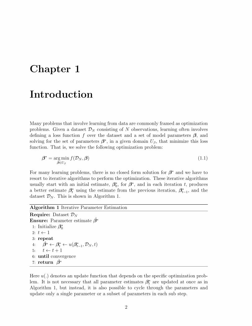
Many problems that involve learning from data are commonly framed as optimizationproblems. Given a dataset DN consisting of N observations, learning often involvesdefining a loss function f over the dataset and a set of model parameters β, andsolving for the set of parameters β∗, in a given domain Uβ, that minimize this lossfunction. That is, we solve the following optimization problem:
β∗ = arg minβ∈Uβ
f(DN ,β) (1.1)
For many learning problems, there is no closed form solution for β∗ and we have toresort to iterative algorithms to perform the optimization. These iterative algorithmsusually start with an initial estimate, β∗0, for β∗, and in each iteration t, producesa better estimate β∗t using the estimate from the previous iteration, β∗t−1, and thedataset DN . This is shown in Algorithm 1.
Here u(.) denotes an update function that depends on the specific optimization prob-lem. It is not necessary that all parameter estimates β∗t are updated at once as inAlgorithm 1, but instead, it is also possible to cycle through the parameters andupdate only a single parameter or a subset of parameters in each sub step.
2
Each update step β∗t ← u(β∗t−1,DN , t) can be viewed as moving our current estimateβ∗t−1 closer, through parameter space, to the true solution β∗. Very commonly inmachine learning, the number of observations N is very large, and evaluating theupdate function on a huge dataset in each iteration is computationally very expensive,or even impossible if N → ∞. Often these computations are wasteful: when ourestimate is far from β∗, the updates need not be very precise as we just need ageneral direction to move in parameter space. However, we need more precision inthe updates as we move closer to β∗.
To apply this idea to speed up learning, we first acknowledge the stochastic nature ofour data. We consider the N observations in DN as samples from a stochastic datagenerating process. If we had access to this generating process, we can constructinfinitely many datasets of size N that have similar statistical properties, and DN ,the dataset available to us, will be just one sample from this infinite pool of datasets.Our update function, u, is a quantity that depends on the particular dataset that wehave, and in certain cases, we can model the variability of u under different samplingsof the dataset. As N increases, this variability decreases since more information islikely to be shared between different draws of the dataset.
Hence, when our estimate β∗t−1 is far from β∗, and we do not need the updates tobe very precise, we can evaluate the update function using a subset DNt of DN withNt < N samples, to compute the new estimate as β∗t = u(β∗t−1,DNt , t). Usually inearly iterations our estimate is very far from β∗, and therefore the batch size Nt canbe very small. As learning proceeds and we move closer to β∗, we can increase Nt
and query more samples to increase the precision of our updates. Thus, we proposean ‘as needed’ approach that uses only just enough data and computation to make astep.
In every iteration t, we need a way of determining if the update computed using thecurrent mini-batch DNt is reliable enough, so that we can increase Nt when needed.If we can model the distribution of the updates under different draws of the mini-batch DNt , we can devise frequentist hypothesis tests to determine if at least theproposed update direction is correct with high probability. More precisely, we failthe hypothesis test if ρt, the probability that the proposed update direction is notwithin 90 degrees of the true update direction u(β∗t−1,DN , t)− β∗t−1, is higher than athreshold ρ∗. To calculate this probability, we first have to determine the pdf put ofthe proposed update u(β∗t−1,DNt , t) and compute:
ρt =
∫Ω
put(u)du where Ω = u :⟨u− β∗t−1, u(β∗t−1,DN , t)− β∗t−1
⟩< 0 (1.2)
Here, Ω represents proposed updates whose directions are significantly different fromthe true update direction. Note, that we do not actually compute the true updateu(β∗t−1,DN , t) in Eqn.(1.2), since it is the very computation that we are trying toavoid by using our sub-sampling scheme. Thus, in practice, we use u(β∗t−1,DNt , t) asan estimate of u(β∗t−1,DN , t). If ρt > ρ∗ and we fail the test, i.e. if we are not even
3
sure about the direction to move in parameter space, we have to increase our batchsize Nt by querying more samples and reduce the variability of the proposed updates.
This hypothesis testing framework also provides a natural stopping criterion for thealgorithm. If the hypothesis tests fail when Nt = N , we cannot try to decreasethe variability of our updates by querying more data points. Also, the fact that thehypothesis tests failed indicate that if we were to draw another dataset of size N fromthe generating process, there is substantial probability that the update direction willbe very different. At this point, if we were to continue learning, we would just beover-fitting to the particular dataset available to us. Therefore, all hypothesis testsfailing when Nt = N represents an automated and principled criterion to terminatelearning. The general structure of our algorithm is shown in Algorithm 2.
Algorithm 2 Iterative Parameter Estimation with Sub-Sampling
Require: Dataset DN , Threshold ρ∗
Ensure: Parameter Estimate β∗
1: Initialize β∗02: Initialize N1 N3: DN1 ← Sample N1 observations from DN4: t← 15: done← false6: repeat7: ut ← u(β∗t−1,DNt , t)8: Calculate put9: Calculate ρt as in Eqn. 1.210: if ρt ≤ ρ∗ then11: β∗ ← β∗t ← ut12: Nt+1 ← Nt
13: DNt+1 ← DNt14: else15: if Nt = N then16: done← true17: else18: β∗t ← β∗t−1
19: Nt+1 ← min(N, 2Nt)20: DNt+1 ← Sample Nt+1 observations from DN21: end if22: end if23: t← t+ 124: until done25: return β∗
The main challenge in applying this method is to determine put , the pdf of the updatefunction. Fortunately, for many machine learning algorithms, the update function in-volves sums or averages over data points. Thus, with sufficiently large batch sizes,
4
the Central Limit Theorem dictates that the update function will be normally dis-tributed, and we can fully specify put by estimating its mean and covariance usingthe current batch.
In the rest of the paper, we illustrate how this method can be used to significantlyoptimize three learning algorithms:
• A Fisher Scoring algorithm for parameter estimation in Generalized LinearModels (GLMs)
• An Expectation-Maximization (EM) algorithm for Least Absolution Devia-tion(LAD) Regression.
• The Block Principal Pivoting (BPP) algorithm, an active set type method whichis state-of-the-art for Non-Negative Matrix Factorization (NMF).
All of these methods are iterative algorithms and their update functions have a formsimilar to the solution of normal equations for least squares problems, i.e.
u(β∗t−1,DN , t) = (ATA)−1ATb (1.3)
It will be specified in later chapters what A and b represent for each of the abovealgorithms. The rest of this thesis is structured as follows. In chapter 2, we reviewrelated work. Then, in chapter 3, we develop a hypothesis testing framework for test-ing the reliability of updates having the form of Eqn. 1.3. We apply this hypothesistesting framework to optimize different learning algorithms in chapters 4, 5 and 6.Finally, we conclude in chapter 7.
5
Chapter 2
Related Work
Our method is related to Stochastic Approximation (SA) [17, 12, 18], a class of itera-tive algorithms that can be used to minimize a loss function using only noisy gradients.In SA, the updates at each step are multiplied with a gain value, that decreases overtime to ensure convergence. Thus, a key difference is that we systematically reducethe uncertainty in the updates by using larger and larger batches, whereas in SA,the effect of uncertainty is reduced by using smaller and smaller gain values. In SA,although it is easy to choose a gain sequence that ensures convergence, in general itrequires a lot of tuning to find the one that gives the best performance. In contrast,our method has a single interpretable parameter (the significance level for hypothesistests) and has a statistically principled stopping criterion.
Our ideas also have a close connection to the observations in [4] and [20]. Usuallyin learning problems, one is interested in minimizing an expected loss function withrespect to some true underlying distribution of the data. However, in practice, oneworks with an empirical loss function defined with respect to a finite dataset, thatis only an approximation of the expected loss. Therefore, it is wasteful to expendtoo much computational time in minimizing the empirical loss to very high accuracy.Additionally, as discussed in [4], when working with large datasets, methods thatapproximate updates at each step are often more effective. However, we are notaware of previous work where hypothesis tests are used to increase the batch size oras a stopping criterion.
6
Chapter 3
Hypothesis Testing
Let us consider applying our sampling strategy to iterative algorithms where theupdate function is of the form (ATA)−1ATb. We assume A ∈ RN×P and b ∈ RN×1,and that A and b are functions of the dataset DN and the parameter estimate fromthe previous iteration β∗t−1. If we denote the ith row of A by aTi and the ith componentof b by bi, we can write the P dimensional update function as:
uN = u(β∗t−1,DN , t) =
(1
N
N∑i=1
aiaTi
)−1(1
N
N∑i=1
aibi
)(3.1)
If N is very large, evaluating this update function in every iteration becomes verycostly. However, we can think of ai’s and bi’s as i.i.d instances of some random vari-ables a and b, and introduce the following stochastic generative process b = aTu + ε,where ε is an error term and u are the parameters of the model. Thus, the updatefunction in (3.1), uN , becomes the maximum likelihood estimate of the model param-eters, calculated from N observations, assuming that the errors ε are i.i.d normallydistributed random variables with zero mean and constant variance. In each iterationt, we can consider approximating the update function in (3.1) using a subset, DNt , ofthe full dataset, DN , with Nt < N samples of a and b:
uNt = u(β∗t−1,DNt , t) =
(1
Nt
Nt∑i=1
aiaTi
)−1(1
Nt
Nt∑i=1
aibi
)(3.2)
IfNt is sufficiently large for the Central Limit Theorem to take effect, and the followingassumptions hold:
1. No multicollinearity: Qaa = E[aaT ] is positive definite
2. Exogeneity: E[ε|a] = 0
3. Homoscedasticity: V ar[ε|a] = σ2
7
then the maximum likelihood estimator for u is known to be asymptotically normal[19]:
uNt ∼ N (µ,Σ) where Σ =Q−1
aaσ2
Nt
(3.3)
Here µ denotes the true value of the model parameters u. Note that the variance isinversely proportional to the number of samples Nt, i.e. the update is more precise ifcomputed from a large number of samples. We can approximate this distribution asuNt ∼ N (µt,Σt) by estimating its parameters from the subset DNt :
µt =
(1
Nt
Nt∑i=1
aiaTi
)−1(1
Nt
Nt∑i=1
aibi
)(3.4a)
Qaa,t =1
Nt − 1
Nt∑i=1
aiaiT (3.4b)
σ2t =
1
Nt − 1
Nt∑i=1
ε2i (3.4c)
Σt =Q−1
aa,tσ2t
Nt
(3.4d)
Estimating this distribution of the proposed approximate update, uNt , allows us todevise frequentist hypothesis tests to determine the reliability of this proposition. Asin (1.2), we compute ρt, the probability that the proposed updated direction is notwithin 90 degrees of the true update direction µ − β∗t−1 ≈ µt − β∗t−1. Denoting thepdf of the distribution N (µt,Σt) of the proposed update by put , we compute ρt as:
ρt =
∫Ω
put(u)du where Ω = u :⟨u− β∗t−1,µt − β∗t−1
⟩< 0 (3.5)
To compute ρt efficiently, consider a transformation of the co-ordinate system sothat β∗t−1 is at the origin and the true update direction, µt − β∗t−1, is along the firstco-ordinate axis. Under this transformation, the distribution of the proposed updatechanges as:
uNt ∼ N (µ′t,Σ′t) where µ′t = [‖µt − β∗t−1‖; 0P−1] and Σ′t = R−1ΣtR (3.6)
Here, 0P−1 represents a vector of P − 1 zeros and R is the rotation matrix thataligns the true update direction µt − β∗t−1 with the first co-ordinate axis. Now,consider a hyperplane passing through the origin and orthogonal to the first co-ordinate axis. This divides RP into two half spaces, RP
+ and RP−, containing the
positive and negative parts of the first co-ordinate axis respectively. Since the trueupdate direction is directed from the origin to the positive side of the first co-ordinateaxis, the region Ω that represents proposed update directions which differ by morethan 90 degrees from the true direction, is just RP
−. Now, ρt can be easily computed
8
0 2 4 6−1
0
1
2
3
4
5
Ω
µt
β*t−1
(a)
−2 −1 0 1 2 3 4 5−3
−2
−1
0
1
2
3
Ω
µt
β*t−1
(b)
Figure 3.1: Hypothesis testing: In 3.1a, the old estimate β∗t−1 and the distributionof the proposed update uNt are shown. The shaded region, Ω, represents proposedupdate direction which are not within 90 degrees of the true direction. 3.1b showshow transforming to an alternate coordinate system can help compute ρt efficiently.
from the marginal distribution of uNt [1], the first component of uNt . This distributionis just N (µ′t[1],Σ′t[1, 1]) and ρt = Φ(0) where Φ(.) is the CDF of the uNt [1]. This isshown in Figures 3.1a and 3.1b.
If ρt is greater than a threshold ρ∗, there is substantial probability that the proposedupdate direction is significantly different from the true direction, and we fail thehypothesis test. At this point, we have to increase the batch size to reduce thevariance in the updates so that they pass the hypothesis tests. If this is not possible,either due to unavailability of more data or because of computational limitations, weterminate learning so as to avoid over-fitting.
We will now write this hypothesis test as a procedure so that it can be easily referencedfrom later sections.
9
Procedure 3 HYPOTHESIS-TEST
Require: A ∈ RNt×P , b ∈ RNt×1, β∗t−1 ∈ RP×1, ρ∗
Ensure: pass1: µt ← (ATA)−1ATb
2: Qaa,t ←1
Nt − 1ATA
3: σ2t ←
1
Nt − 1‖Aβ∗t−1 − b‖2
2
4: Σt ←Q−1
aa,tσ2t
Nt5: µ′t ← [‖µt − β∗t−1‖; 0P−1]6: R← Rotation matrix s.t. R(µt − β∗t−1) = µ′t7: Σ′t ← R−1ΣtR8: ρt ← Φ(0) where Φ(.) is cdf of N (µ′t[1],Σ′t[1, 1])9: if ρt > ρ∗ then10: pass← false11: else12: pass← true13: end if14: return pass
10
Chapter 4
Generalized Linear Models
In this Chapter, we will show how the sub-sampling algorithm and hypothesis testingframework of Chapters 1 and 3 can be used to speed-up parameter estimation inGeneralized Linear Models (GLMs). In section 4.1, we give a brief introduction toGLMs. Section 4.2 reviews the Exponential Family of distributions, as they form animportant part of the theory of GLMs. Section 4.3 describes a Fisher scoring methodfor parameter estimation in GLMs. In Section 4.4, we show how our sub-samplingidea can be used to speed-up this Fisher scoring algorithm. Finally, in section 4.5,we present experimental results showing how our method optimizes Fisher scoring forparameter estimation in GLMs on 2 real world datasets.
4.1 Introduction
Generalized Linear Model (GLM)[15] is a flexible extension of the classical linearmodel for regression. Hence, we will first examine the classical linear model. In thismodel, we are given a dataset DN consisting of N statistical units, with the ith unitconsisting of a target variable yi and a set of P covariates denoted by the vectorxi ∈ RP×1. The classical linear model has the following 3 part specification:
1. Random Component : The targets yi are considered as realizations of randomvariables Yi, which are assumed to have independent normal distributions withconstant variance.
2. Systematic Component : The covariates are used to produce a linear predictorηi given by:
ηi = 〈xi,β〉 (4.1)
11
Here β ∈ RP×1 represents the unknown parameters of the model and the processof calculating them is called parameter estimation.
3. Link : The link between the random component and the systematic componentis specified as:
ηi = g(E[Yi]) (4.2)
where g(.) is the identity function.
GLMs allow the following 2 generalizations of the classical linear model:
1. In the random component, the distribution of Yi’s need not be normal, but canbe any distribution from the exponential family (see Section 4.2).
2. The link g(.) is not restricted to be the identity function, but can be any mono-tonic differentiable function.
We will briefly review the exponential family of distributions in the next section.
4.2 The Exponential Family
In GLMs, the random variables Yi’s are allowed to have any distribution from theexponential family, which has the following general form:
pY (y; θ, φ) = exp
yθ − r(θ)q(φ)
+ s(y, φ)
(4.3)
for some specific functions q(.), r(.) and s(.). Here, θ is usually the parameter ofinterest and is called the canonical parameter of the distribution. φ is known asthe dispersion parameter and in GLMs, it is the same for all observations. Theexpectation and variance of Y can be shown to be:
E[Y ] = µ = r′(θ) (4.4a)
Var[Y ] = r′′(θ)q(φ) (4.4b)
Note that the expression for variance contains the term r′′(θ) which is dependent onthe mean. This term when written as a function of the mean is called the variancefunction and is denoted by V (µ) = r′′(θ). Also, it is worth mentioning that a linkfunction g(.) for which η = g(µ) = θ is called the canonical link function of thedistribution.
We will now consider two illustrative examples of distributions from the exponentialfamily: the Normal distribution and the Bernoulli distribution.
12
4.2.1 Example 1: Normal distribution as an ExponentialFamily distribution
The pdf of a normally distributed random variable y is:
p(y;α, ω2) =1√
2πω2exp
−(y − α)2
2ω2
= exp
yα− (α2/2)
ω2− 1
2log 2πω2 − y2
2ω2
(4.5)
Comparing the coefficient of y in Eqns. 4.5 & 4.3, we see that θ = α and we chooseφ = ω. Now, we can see that the normal distribution belongs to the exponentialfamily with r(.), q(.) and s(.) defined as follows:
r(θ) =θ2
2(4.6a)
q(φ) = φ2 (4.6b)
s(y, φ) = −1
2log 2πφ2 − y2
2φ2(4.6c)
We can now calculate the expectation and variance of y as:
E[Y ] = µ = r′(θ) = θ = α (4.7a)
V ar[Y ] = r′′(θ)q(φ) = φ2 = ω2 (4.7b)
The variance function is given by,
V (µ) = r′′(θ) = 1 (4.8)
4.2.2 Example 2: Bernoulli distribution as an ExponentialFamily distribution
The pdf of a Bernoulli distributed random variable y is:
p(y;α) = αy(1− α)1−y
= exp
y log
(α
1− α
)+ log (1− α)
(4.9)
Comparing Eqns. 4.9 and 4.3, we have:
θ = log
(α
1− α
)or, equivalently: α =
1
1 + e−θ(4.10)
13
We can see that the Bernoulli distribution also belongs to the Exponential Familywith q(.), r(.) and s(.) defined as:
r(θ) = − log(1− α) = log(1 + eθ) (4.11a)
q(φ) = s(y, φ) = 1 (4.11b)
The expectation and variance of y are:
E[Y ] = µ = r′(θ) =1
1 + e−θ= α (4.12a)
V ar[Y ] = r′′(θ)q(φ) =e−θ
(1 + e−θ)2= α(1− α) (4.12b)
The variance function is given by,
V (µ) = r′′(θ) = µ(1− µ) (4.13)
4.3 Parameter Estimation using Fisher scoring
Once a particular generalized linear model has been selected by choosing a link func-tion and a distribution from the exponential family for the Yi’s, we have to calculatethe parameter vector β∗ ∈ RP×1 that makes the model best agree with the givendata. This is typically done by Maximum Likelihood Estimation, where we try tofind the β∗ which maximizes the following log likelihood:
`(β) =N∑i=1
yiθi − r(θi)
q(φ)+ s(yi, φ)
(4.14)
Note that ` depends on β through θ, since 〈xi,β〉 = ηi = g(µi) = g(r′(θi)). This max-imization can be performed using the Fisher scoring method, an iterative optimizationalgorithm (as in Algorithm 1) having the following update rule:
Here S(β) is the score function, the gradient of the log likelihood with respect toβ, and I(β) is the Fisher information matrix, the variance of the score. It can be
14
shown[15] that:
S(β) , ∇` =1
a(φ)
N∑i=1
W (µi)(yi − µi)g′(µi)xi (4.16)
where1
W (µi)= (g′(µi))
2V (µi) (4.17)
and
I(β) , −E [H(`)] =1
a(φ)
N∑i=1
W (µi)xixTi (4.18)
In Eqn. (4.16), the ∇ symbol represents the gradient operator and in Eqn. (4.18),H(`) represents the Hessian matrix of `. Also µ is a function of β although wehave not indicated it explicitly, in order to avoid clutter. From Eqn. (4.18), we cancalculate I(β)β as:
I(β)β =
(1
a(φ)
N∑i=1
W (µi)xixTi
)β =
1
a(φ)
N∑i=1
W (µi)ηixi =1
a(φ)
N∑i=1
W (µi)g(µi)xi
(4.19)
Using (4.16) and (4.19), we have:
I(β)β + S(β) =1
a(φ)
N∑i=1
g(µi) + (yi − µi)g′(µi)W (µi)xi (4.20)
It is convenient to introduce the following definitions: the design matrix X ∈ RN×P
whose ith row is xTi , the diagonal weighting matrix W(β) ∈ RN×N where Wii(β) =W (µi) and the vectors y,µ ∈ RN×1 whose ith components are yi and µi respectively.Additionally, we define the adjusted response vector, z(β) ∈ RN×1 as:
z(β) = g(µ) + (y − µ)g′(µ) (4.21)
This allows us to write:
I(β) =1
a(φ)XTW(β)X and I(β)β + S(β) =
1
a(φ)XTW(β)z(β) (4.22)
Using (4.22) and defining Wt = W(β∗t ) and zt = z(β∗t ), we can write the Fisherscoring update rule (4.15) as:
β∗t = (XTWt−1X)−1XTWt−1zt−1 (4.23)
Since the updates to the β∗ estimate are similar to the solution to a weighted leastsquares problem, and the weights Wt are recomputed in every iteration, this algorithm
15
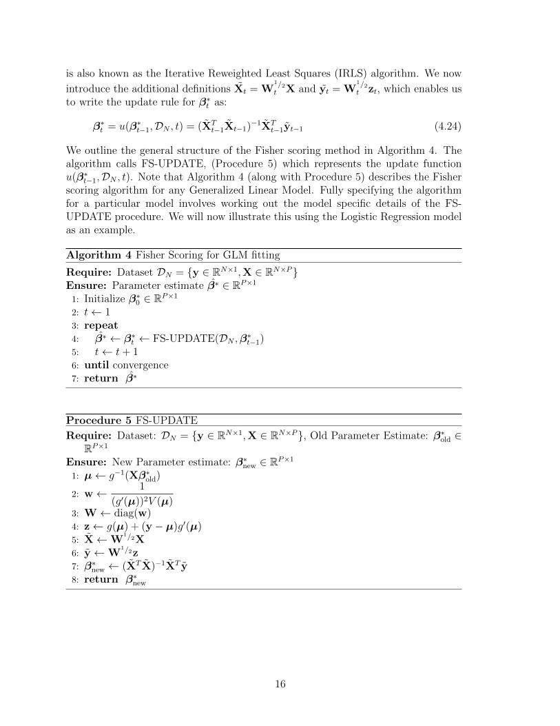
is also known as the Iterative Reweighted Least Squares (IRLS) algorithm. We now
introduce the additional definitions Xt = W1/2t X and yt = W
1/2t zt, which enables us
to write the update rule for β∗t as:
β∗t = u(β∗t−1,DN , t) = (XTt−1Xt−1)−1XT
t−1yt−1 (4.24)
We outline the general structure of the Fisher scoring method in Algorithm 4. Thealgorithm calls FS-UPDATE, (Procedure 5) which represents the update functionu(β∗t−1,DN , t). Note that Algorithm 4 (along with Procedure 5) describes the Fisherscoring algorithm for any Generalized Linear Model. Fully specifying the algorithmfor a particular model involves working out the model specific details of the FS-UPDATE procedure. We will now illustrate this using the Logistic Regression modelas an example.
4.3.1 Example: Fisher Scoring for Logistic Regression
Consider a GLM where the Yi’s have independent Bernoulli distributions and g(.)is the canonical link for the Bernoulli distribution i.e. g(.) is a function such thatg(µ) = θ. From Eqns. (4.10) and (4.12a), we have:
g(α) = log
(α
1− α
)and g−1(θ) =
1
1 + e−θ(4.25)
The random variable, Yi, representing the target, and the covariate vector, xi, arerelated as:
E[Yi] = µi = g−1(ηi) =1
1 + e−〈xi,β〉(4.26)
This is the familiar logistic regression model. We will now derive expressions for theweighting matrix, W, and the adjusted response vector, z, to fully specify the Fisherscoring algorithm for this model. First, from (4.25), we see that:
g′(α) =1
α(1− α)(4.27)
W is a diagonal matrix, with diagonal entries given by:
Wii = W (µi) ,1
(g′(µi))2V (µi)= µi(1− µi) (4.28)
Here, we have plugged in the definitions for g′(µi) and V (µi) from Eqns. (4.27) and(4.8) respectively. The adjusted response vector z can be calculated as:
z , g(µ) + (y − µ)g′(µ)
= Xβ + W−1(y − µ) (4.29)
We have used the fact that g(µ) = g(g−1(η)) = η = Xβ and g′(µi) =1
µi(1− µi)=
1
W (µi). Using the expressions for W and z, we describe the model specific update
function for logistic regression in Procedure 6 (FS-UPDATE-LOGISTIC).
Replacing the call to FS-UPDATE by FS-UPDATE-LOGISTIC in Algorithm 4, weobtain the Fisher scoring algorithm for logistic regression.
17
Procedure 6 FS-UPDATE-LOGISTIC
Require: Dataset: DN = y ∈ RN×1,X ∈ RN×P, Old Parameter Estimate: β∗old ∈RP×1
In this section, we will apply the ideas described in Chapters 1 and 3 to speed-upthe Fisher scoring algorithm. First, let us consider Procedure 5 (FS-UPDATE), theupdate function at each step of the Fisher scoring algorithm. It is easy to see that therunning time of this procedure is proportional to N , the number of statistical unitsin the dataset. Thus, when faced with large datasets, computing the true updatefunction in every step is very expensive.
Therefore, in the early iterations where our estimate is far from the true solutionand we just need a rough direction to move in parameter space, we can approximatethe update function using a mini-batch of statistical units. Since the updates are ofthe form (ATA)−1AT b, we can use the hypothesis testing framework (Procedure 3)developed in Chapter 3, to measure the reliability of these updates. If the hypothesistests fail and we are not even sure about the direction to move in parameter space, wegrow our mini-batch by adding more statistical units, so as to increase the precisionof our updates and pass the hypothesis tests. When the hypothesis tests fail afterusing all the data available to us, we stop learning so as to avoid over-fitting.
It is fairly straightforward to use the general skeleton of our sub-sampling method (Al-gorithm 2) along with Procedure 5 (FS-UPDATE) and Procedure 3 (HYPOTHESIS-TEST) to develop an optimized version of Fisher scoring. This is shown in Algorithm7.
18
Algorithm 7 Fisher Scoring for GLM fitting with Sub-Sampling
1: Initialize β∗02: Initialize N1 N3: y1,X1 ← Sample N1 statistical units from y,X4: t← 15: done← false6: repeat7: ut ← FS-UPDATE(yt,Xt,β∗t−1)8: htPassed← HYPOTHESIS-TEST(Xt,yt,β
∗t−1, ρ
∗)9: if htPassed then10: β∗ ← β∗t ← ut11: Nt+1 ← Nt
12: yt+1,Xt+1 ← yt,Xt13: else14: if Nt = N then15: done← true16: else17: β∗t ← β∗t−1
18: Nt+1 ← min(N, 2Nt)19: yt+1,Xt+1 ← Sample Nt+1 statistical units from y,X20: end if21: end if22: t← t+ 123: until done24: return β∗
4.5 Experiments
We compared the performance of the Fisher Scoring algorithm for Logistic regression(FSC) versus its sub-sampled version (FSC-SS) on 2 real world datasets from theUCI Machine Learning Repository [7]: the Poker Hands dataset and the Cover Typedataset. Both algorithms were implemented in MATLAB and all experiments wererun on a 2.2 GHz Core2 Duo, 3GB RAM machine running Windows 7.
The Cover Type dataset has 581012 observations, each with 54 cartographic at-tributes. Each observation represents a 30 × 30 meter cell of land and the goal isto predict its forest cover type. Out of the 54 attributes, we removed all binary at-tributes to avoid sparsity, since sparsity in the design matrix causes the normalityassumptions of the updates to fail and make the performance of our method un-predictable. We were left with a design matrix having 581012 observations with 10
19
attributes each, to which we added the usual ‘constant feature’ of ones. Although theoriginal task was to predict 1 out of 7 cover types, the task in our experiment wasto build a one-versus-all classifier for one of these types. Thus, we chose to build alogistic regression classifier to determine whether the cover type for a given patch ofland is ‘Ponderosa Pine’ or not. This gave us a dataset of 35754 positive instancesand 545258 negative instances which we randomly split into a training set, consistingof 90% of the total data, and a test set, consisting of the remaining 10%.
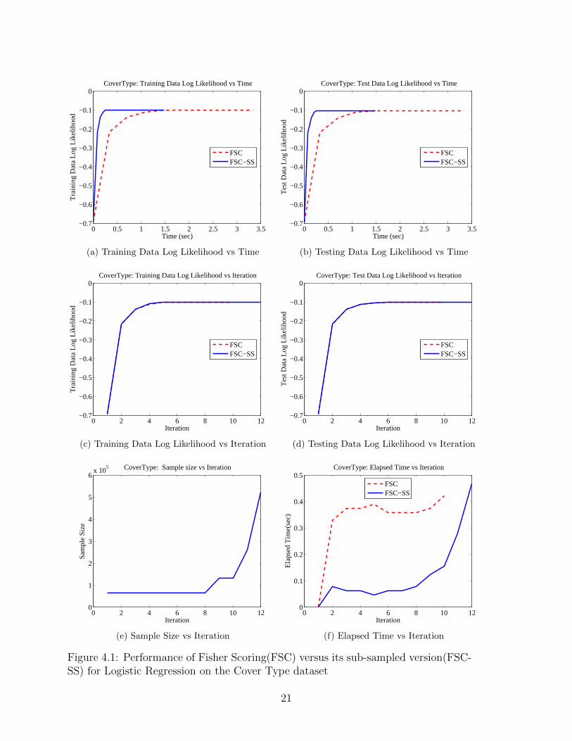
The performance of the FSC and FSC-SS algorithms on the cover type dataset areshown in Figure 4.1. For FSC-SS, we set the value of ρ∗t , the threshold for failing ahypothesis test, to be 0.01, and the initial sample size to be around 60000. We alsoadded an L2 regularization term with a weight of 0.01 for both the algorithms. In Fig-ures 4.1a and 4.1b, we show how quickly FSC-SS is able to increase the log likelihoodon the training and testing sets, as compared to the original FSC algorithm. Figures4.1c and 4.1d show how the log-likelihood increases as a function of iteration. Notethat the log-likelihood curves for both the algorithms are almost identical, supportingour intuition that we do not need to use all the available data in the earlier iterationsto compute very accurate updates. In Figure 4.1e, we show sample size for FSC-SSas a function of iteration, and in Figure 4.1f, we compare the amount of time takenin each iteration for both the algorithms. Figures 4.1e and 4.1f give a good picture ofhow the FSC-SS algorithm is able to save on computation as compared to the originalFSC algorithm.
Our next set of experiments was on the Poker Hands dataset. Each observation inthis dataset corresponds to a 5 card poker hand and the original task was to predictthe type of a given hand as one of 13 hand types. We used the original testingset consisting of 1,000,000 examples, which we randomly split into a training setcontaining 90 % of the observations and a testing set containing the rest. There were10 features for each observation, representing the suit and rank of each of the 5 cards,to which we added a constant feature of ones. As with the Cover Type dataset, thetask in this experiment was to build a one-versus-all classifier for deciding whether aparticular hand is a ‘Four of a Kind’ or not. This gave us a dataset consisting of 230positive examples and 999770 negative examples. We used the same settings as forthe experiments on the CoverType dataset. The performance of both the algorithmsis summarized in Figure 4.2, and is similar to that on the Cover Type dataset.
20
0 0.5 1 1.5 2 2.5 3 3.5−0.7
−0.6
−0.5
−0.4
−0.3
−0.2
−0.1
0CoverType: Training Data Log Likelihood vs Time
Time (sec)
Tra
inin
g D
ata
Log
Like
lihoo
d
FSCFSC−SS
(a) Training Data Log Likelihood vs Time
0 0.5 1 1.5 2 2.5 3 3.5−0.7
−0.6
−0.5
−0.4
−0.3
−0.2
−0.1
0CoverType: Test Data Log Likelihood vs Time
Time (sec)
Tes
t Dat
a Lo
g Li
kelih
ood
FSCFSC−SS
(b) Testing Data Log Likelihood vs Time
0 2 4 6 8 10 12−0.7
−0.6
−0.5
−0.4
−0.3
−0.2
−0.1
0CoverType: Training Data Log Likelihood vs Iteration
Iteration
Tra
inin
g D
ata
Log
Like
lihoo
d
FSCFSC−SS
(c) Training Data Log Likelihood vs Iteration
0 2 4 6 8 10 12−0.7
−0.6
−0.5
−0.4
−0.3
−0.2
−0.1
0CoverType: Test Data Log Likelihood vs Iteration
Iteration
Tes
t Dat
a Lo
g Li
kelih
ood
FSCFSC−SS
(d) Testing Data Log Likelihood vs Iteration
0 2 4 6 8 10 120
1
2
3
4
5
6x 10
5 CoverType: Sample size vs Iteration
Iteration
Sam
ple
Size
(e) Sample Size vs Iteration
0 2 4 6 8 10 120
0.1
0.2
0.3
0.4
0.5CoverType: Elapsed Time vs Iteration
Iteration
Ela
psed
Tim
e(se
c)
FSCFSC−SS
(f) Elapsed Time vs Iteration
Figure 4.1: Performance of Fisher Scoring(FSC) versus its sub-sampled version(FSC-SS) for Logistic Regression on the Cover Type dataset
21
0 2 4 6 8−0.7
−0.6
−0.5
−0.4
−0.3
−0.2
−0.1
0PokerHands: Training Data Log Likelihood vs Time
Time (sec)
Tra
inin
g D
ata
Log
Like
lihoo
d
FSCFSC−SS
(a) Training Data Log Likelihood vs Time
0 2 4 6 8−0.7
−0.6
−0.5
−0.4
−0.3
−0.2
−0.1
0PokerHands: Test Data Log Likelihood vs Time
Time (sec)
Tes
t Dat
a Lo
g Li
kelih
ood
FSCFSC−SS
(b) Testing Data Log Likelihood vs Time
0 5 10 15 20−0.7
−0.6
−0.5
−0.4
−0.3
−0.2
−0.1
0PokerHands: Training Data Log Likelihood vs Iteration
Iteration
Tra
inin
g D
ata
Log
Like
lihoo
d
FSCFSC−SS
(c) Training Data Log Likelihood vs Iteration
0 5 10 15 20−0.7
−0.6
−0.5
−0.4
−0.3
−0.2
−0.1
0PokerHands: Test Data Log Likelihood vs Iteration
Iteration
Tes
t Dat
a Lo
g Li
kelih
ood
FSCFSC−SS
(d) Testing Data Log Likelihood vs Iteration
0 5 10 15 200
1
2
3
4
5
6
7
8
9x 10
5 PokerHands: Sample size vs Iteration
Iteration
Sam
ple
Size
(e) Sample Size vs Iteration
0 5 10 15 200
0.1
0.2
0.3
0.4
0.5
0.6
0.7
0.8PokerHands: Elapsed Time vs Iteration
Iteration
Ela
psed
Tim
e(se
c)
FSCFSC−SS
(f) Elapsed Time vs Iteration
Figure 4.2: Performance of Fisher Scoring(FSC) versus its sub-sampled version(FSC-SS) for Logistic Regression on the Poker Hands dataset
22
Chapter 5
Least Absolute DeviationRegression
5.1 Introduction
Consider the classical linear regression model, introduced in Chapter 4, which has thefollowing generative model for the target, yi, given the covariate vector, xi ∈ RP×1,and conditioned on the model parameters, β ∈ RP×1 :
yi = xTi β + εi where εi ∼ N (0, σ2) (5.1)
Given a dataset DN consisting of N statistical units yi, xi, the goal in regression isto estimate the parameters β∗ which makes the model best agree with the given data.This is commonly done by Maximum Likelihood(ML) estimation where we try to findthe parameters which maximize the likelihood of the data. A crucial assumption ofthe classical linear regression model is that the errors εi are i.i.d. normally distributedrandom variables with zero mean and constant variance. However, the assumptionof constant variance of the error across observations is not often valid in real worlddatasets and makes the resulting ML solution very sensitive to outliers.
In Least Absolute Deviation (LAD) regression, we relax the classical linear regressionmodel by allowing the error εi to have different variances across observations. Thegenerative process for the LAD regression model is:
yi = xTi β +σ√2vi
εi where εi ∼ N (0, 1) (5.2)
Here, σ and β are the parameters of the model that has to be estimated from thedata. We consider εi to be standard normally distributed and the error σ√
2viεi is
allowed to have different variances across observations because of the dependence onvi. We assume that the vi’s are positive and independent of the εi’s. Also, we assume
23
that 12v2i
has a standard exponential distribution so that the pdf of vi is given by
pv(vi) = 1v3i
exp− 12v2i. From Eqn. (5.2) we see that the conditional distribution of
yi given xi and vi is:
py|v,x(yi|vi,xi;β, σ) =vi√πσ
exp
−(yi − xTi β)v2
i
σ2
(5.3)
Also, we can write down the joint distribution of yi and vi given xi as:
Note however that we do not observe the vi’s directly. Thus, to perform maximumlikelihood estimation of the parameters, we have to compute the conditional distri-bution of yi given xi by marginalizing out vi from equation Eqn. 5.4. This is ascale mixture of normal distributions and can be shown to be the Laplacian (doubleexponential) distribution[1], i.e.:
py|x(yi|xi;β, σ) =
∫ ∞0
py,v|x(yi, v|xi;β, σ)dv =
∫ ∞0
py|v,x(yi|v,xi;β, σ)pv(v)dv
=1√2σ
exp
−√
2|yi − xTi β|
σ
(5.5)
Now we can write down the log likelihood of the dataset DN as:
`(β, σ;DN) =N∑i=1
log py|x(yi|xi;β, σ) = −N log(√
2σ)−√
2
σ
N∑i=1
|yi − xTi β| (5.6)
Maximizing this log likelihood with respect to β is equivalent to minimizing∑N
i=1 |yi−xTi β|,i.e. the absolute value of prediction errors, and hence this is known as the LeastAbsolute Deviation regression model. However, maximizing the log likelihood in Eqn.(5.6) is hard and is typically performed using the Expectation-Maximization (EM)algorithm[16, 6].
We will now review the EM algorithm in Section 5.2. In Section 5.3, we describe theEM algorithm for parameter estimation in Least Absolute Deviation regression andshow that it is essentially an IRLS algorithm. Then, in Section 5.4, we will describehow our sub sampling method can be used to optimize this algorithm. Finally wepresent our experimental results on two real world datasets in Section 5.5
24
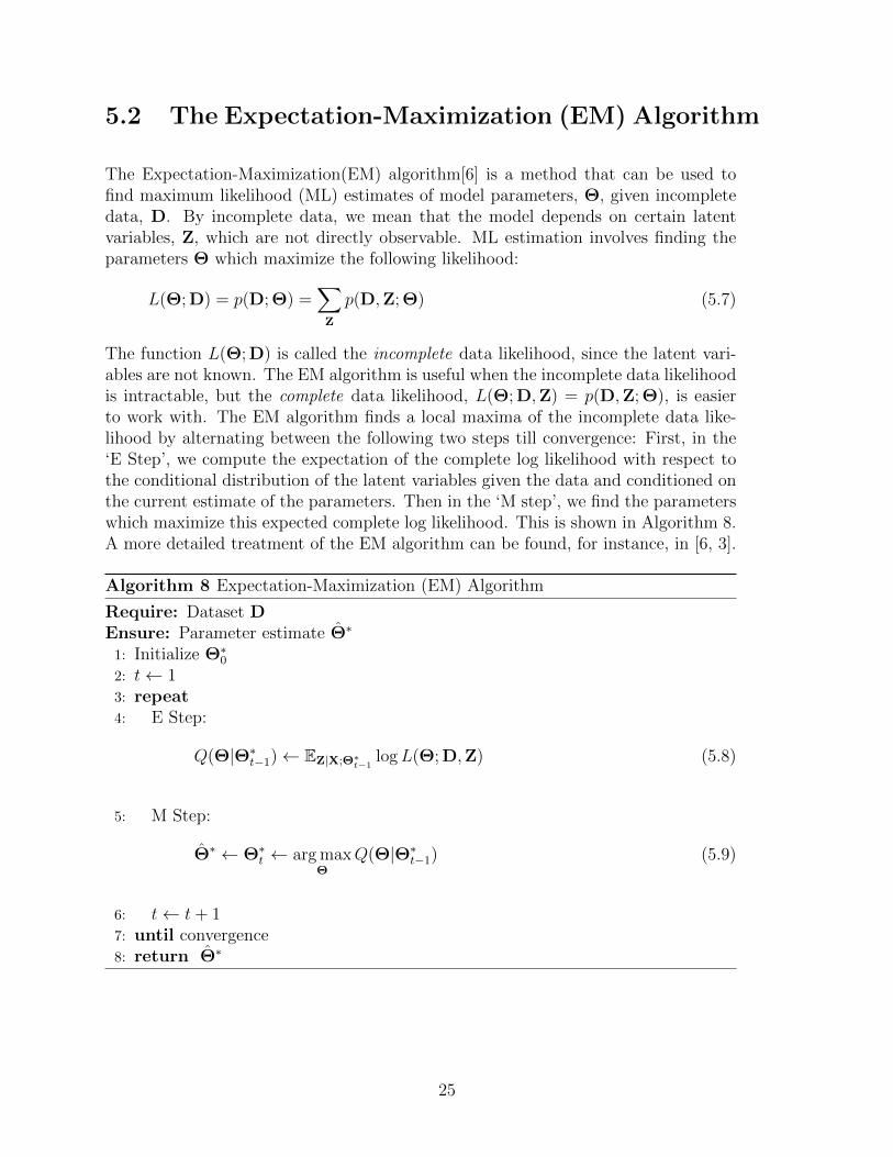
5.2 The Expectation-Maximization (EM) Algorithm
The Expectation-Maximization(EM) algorithm[6] is a method that can be used tofind maximum likelihood (ML) estimates of model parameters, Θ, given incompletedata, D. By incomplete data, we mean that the model depends on certain latentvariables, Z, which are not directly observable. ML estimation involves finding theparameters Θ which maximize the following likelihood:
L(Θ; D) = p(D; Θ) =∑
Z
p(D,Z; Θ) (5.7)
The function L(Θ; D) is called the incomplete data likelihood, since the latent vari-ables are not known. The EM algorithm is useful when the incomplete data likelihoodis intractable, but the complete data likelihood, L(Θ; D,Z) = p(D,Z; Θ), is easierto work with. The EM algorithm finds a local maxima of the incomplete data like-lihood by alternating between the following two steps till convergence: First, in the‘E Step’, we compute the expectation of the complete log likelihood with respect tothe conditional distribution of the latent variables given the data and conditioned onthe current estimate of the parameters. Then in the ‘M step’, we find the parameterswhich maximize this expected complete log likelihood. This is shown in Algorithm 8.A more detailed treatment of the EM algorithm can be found, for instance, in [6, 3].
We will now describe the EM algorithm for parameter estimation in LAD regression[16]. Here, the incomplete data D is the dataset DN consisting of N statistical unitsyi,xi, the parameters are Θ = β, σ and we consider the vi’s to be the hiddenvariables Z. If we have knowledge of the latent variables VN = viNi=1 in addition tothe dataset DN , we can write down the complete data log likelihood (using Eqn. 5.4)as:
`(β, σ;DN ,VN) =N∑i=1
log py,v|x(yi, vi|xi;β, σ) = −N log σ− 1
σ2
N∑i=1
(yi−xTi β)2v2i +C
(5.10)
Here C represents the terms that does not depend on the parameters β and σ. Now,in the E step of the tth iteration, we compute the expectation of this log likelihoodunder the conditional distribution of the latent variables VN given the data DN usingthe estimate of the parameters β∗t−1 and σ∗t−1. This is given by:
Q(β, σ|β∗t−1, σ∗t−1)←
N∑i=1
Evi|yi,xi;β∗t−1,σ
∗t−1
[log py,v|x(yi, vi|xi;β, σ)
](5.11)
= −N log σ − 1
σ2
N∑i=1
(yi − xTi β)2E[v2i |yi,xi;β∗t−1, σ
∗t−1] + C
It can be shown[16] that the conditional expectation of v2i is:
E[v2i |yi,xi;β∗t−1, σ
∗t−1] =
σ∗t−1√2|yi − xTi β
∗t−1|
(5.12)
Now, in theM step, we find the parameters β∗t , σ∗t which maximizeQ(β, σ|β∗t−1, σ∗t−1),
the expected complete log likelihood calculated in the E step. Maximizing this withrespect to β we have:
β∗t = u(β∗t−1,DN , t) = arg minβ
N∑i=1
wi(yi − xTi β)2
where wi = E[v2i |yi,xi;β∗t−1, σ
∗t−1] =
σ∗t−1√2|yi − xTi β
∗t−1|
(5.13)
The update for β∗t is a solution to a weighted least squares problem and can bealternately written as an IRLS update β∗t ← (XTWt−1X)−1XTWt−1y. Here X ∈RN×P represents the design matrix whose ith row is xTi , y ∈ RN×1 is a vector of targetswhose ith component is yi and Wt−1 is a diagonal matrix of weights with diagonalelements given by Wt−1[i, i] = wi. Note that the factor σ∗t−1/
√2 in Wt−1 cancels out
26
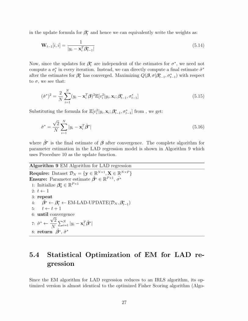
in the update formula for β∗t and hence we can equivalently write the weights as:
Wt−1[i, i] =1
|yi − xTi β∗t−1|
(5.14)
Now, since the updates for β∗t are independent of the estimates for σ∗, we need notcompute a σ∗t in every iteration. Instead, we can directly compute a final estimate σ∗
after the estimates for β∗t has converged. Maximizing Q(β, σ|β∗t−1, σ∗t−1) with respect
to σ, we see that:
(σ∗)2 =2
N
N∑i=1
(yi − xTi β)2E[v2i |yi,xi;β∗t−1, σ
∗t−1] (5.15)
Substituting the formula for E[v2i |yi,xi;β∗t−1, σ
∗t−1] from , we get:
σ∗ =
√2
N
N∑i=1
|yi − xTi β∗| (5.16)
where β∗ is the final estimate of β after convergence. The complete algorithm forparameter estimation in the LAD regression model is shown in Algorithm 9 whichuses Procedure 10 as the update function.
Since the EM algorithm for LAD regression reduces to an IRLS algorithm, its op-timized version is almost identical to the optimized Fisher Scoring algorithm (Algo-
27
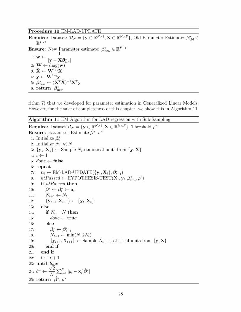
Procedure 10 EM-LAD-UPDATE
Require: Dataset: DN = y ∈ RN×1,X ∈ RN×P, Old Parameter Estimate: β∗old ∈RP×1
Ensure: New Parameter estimate: β∗new ∈ RP×1
1: w← 1
|y −Xβ∗old|2: W← diag(w)3: X←W
1/2X4: y←W
1/2y5: β∗new ← (XT X)−1XT y6: return β∗new
rithm 7) that we developed for parameter estimation in Generalized Linear Models.However, for the sake of completeness of this chapter, we show this in Algorithm 11.
Algorithm 11 EM Algorithm for LAD regression with Sub-Sampling
1: Initialize β∗02: Initialize N1 N3: y1,X1 ← Sample N1 statistical units from y,X4: t← 15: done← false6: repeat7: ut ← EM-LAD-UPDATE(yt,Xt,β∗t−1)8: htPassed← HYPOTHESIS-TEST(Xt,yt,β
∗t−1, ρ
∗)9: if htPassed then10: β∗ ← β∗t ← ut11: Nt+1 ← Nt
12: yt+1,Xt+1 ← yt,Xt13: else14: if Nt = N then15: done← true16: else17: β∗t ← β∗t−1
18: Nt+1 ← min(N, 2Nt)19: yt+1,Xt+1 ← Sample Nt+1 statistical units from y,X20: end if21: end if22: t← t+ 123: until done
24: σ∗ ←√
2
N
∑Ni=1 |yi − xTi β
∗|
25: return β∗, σ∗
28
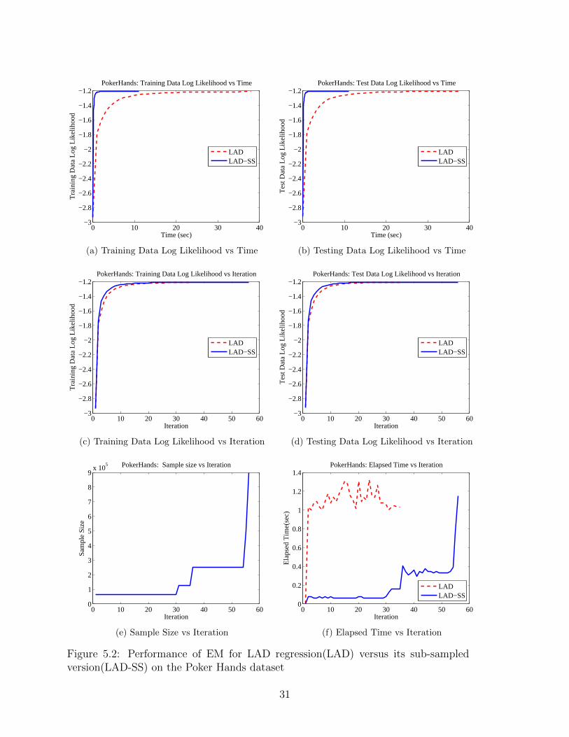
5.5 Experiments
As with the Fisher Scoring algorithm, we compared the performance of the EM algo-rithm for Least Absolute Deviation regression(LAD) versus its sub-sampled version(LAD-SS) on two real world datasets from the UCI Machine Learning Repository[7]: the Poker Hands dataset and the Cover Type dataset. Both algorithms wereimplemented in MATLAB and all experiments were run on a 2.2 GHz Core2 Duo,3GB RAM machine running Windows 7.
For a description of the datasets, please refer Section 4.5 of Chapter 4. In thisexperiment, instead of building a one-versus-all classifier as in Chapter 4, the taskwas to predict the the cover type as 1 of 7 types or the poker hand as 1 of 13 types,which we treated as a regression problem. For LAD-SS, we set the value of ρ∗t , thethreshold for failing a hypothesis test, to be 0.001, and the initial sample size to bearound 60000. The performance of both algorithms are shown in Figures 5.1 and 5.2.The results are very similar to those for the Fisher scoring algorithm (see 4.5).
29
0 2 4 6 8 10 12−4
−3.5
−3
−2.5
−2
−1.5
−1CoverType: Training Data Log Likelihood vs Time
Time (sec)
Tra
inin
g D
ata
Log
Like
lihoo
d
LADLAD−SS
(a) Training Data Log Likelihood vs Time
0 2 4 6 8 10 12−4
−3.5
−3
−2.5
−2
−1.5
−1CoverType: Test Data Log Likelihood vs Time
Time (sec)
Tes
t Dat
a Lo
g Li
kelih
ood
LADLAD−SS
(b) Testing Data Log Likelihood vs Time
0 5 10 15 20 25−4
−3.5
−3
−2.5
−2
−1.5
−1CoverType: Training Data Log Likelihood vs Iteration
Iteration
Tra
inin
g D
ata
Log
Like
lihoo
d
LADLAD−SS
(c) Training Data Log Likelihood vs Iteration
0 5 10 15 20 25−4
−3.5
−3
−2.5
−2
−1.5
−1CoverType: Test Data Log Likelihood vs Iteration
Iteration
Tes
t Dat
a Lo
g Li
kelih
ood
LADLAD−SS
(d) Testing Data Log Likelihood vs Iteration
0 5 10 15 20 250
1
2
3
4
5
6x 10
5 CoverType: Sample size vs Iteration
Iteration
Sam
ple
Size
(e) Sample Size vs Iteration
0 5 10 15 20 250
0.1
0.2
0.3
0.4
0.5
0.6
0.7
0.8CoverType: Elapsed Time vs Iteration
Iteration
Ela
psed
Tim
e(se
c)
LADLAD−SS
(f) Elapsed Time vs Iteration
Figure 5.1: Performance of EM for LAD regression(LAD) versus its sub-sampledversion(LAD-SS) on the Cover Type dataset
30
0 10 20 30 40−3
−2.8
−2.6
−2.4
−2.2
−2
−1.8
−1.6
−1.4
−1.2PokerHands: Training Data Log Likelihood vs Time
Time (sec)
Tra
inin
g D
ata
Log
Like
lihoo
d
LADLAD−SS
(a) Training Data Log Likelihood vs Time
0 10 20 30 40−3
−2.8
−2.6
−2.4
−2.2
−2
−1.8
−1.6
−1.4
−1.2PokerHands: Test Data Log Likelihood vs Time
Time (sec)
Tes
t Dat
a Lo
g Li
kelih
ood
LADLAD−SS
(b) Testing Data Log Likelihood vs Time
0 10 20 30 40 50 60−3
−2.8
−2.6
−2.4
−2.2
−2
−1.8
−1.6
−1.4
−1.2PokerHands: Training Data Log Likelihood vs Iteration
Iteration
Tra
inin
g D
ata
Log
Like
lihoo
d
LADLAD−SS
(c) Training Data Log Likelihood vs Iteration
0 10 20 30 40 50 60−3
−2.8
−2.6
−2.4
−2.2
−2
−1.8
−1.6
−1.4
−1.2PokerHands: Test Data Log Likelihood vs Iteration
Iteration
Tes
t Dat
a Lo
g Li
kelih
ood
LADLAD−SS
(d) Testing Data Log Likelihood vs Iteration
0 10 20 30 40 50 600
1
2
3
4
5
6
7
8
9x 10
5 PokerHands: Sample size vs Iteration
Iteration
Sam
ple
Size
(e) Sample Size vs Iteration
0 10 20 30 40 50 600
0.2
0.4
0.6
0.8
1
1.2
1.4PokerHands: Elapsed Time vs Iteration
Iteration
Ela
psed
Tim
e(se
c)
LADLAD−SS
(f) Elapsed Time vs Iteration
Figure 5.2: Performance of EM for LAD regression(LAD) versus its sub-sampledversion(LAD-SS) on the Poker Hands dataset
31
Chapter 6
Non-Negative Matrix Factorization
6.1 Introduction
Non-negative Matrix Factorization (NMF) is a popular dimensionality reduction tech-nique that has many useful applications in machine learning and data mining. NMFis typically applied to high dimensional data where each element is non-negative andit provides a low rank approximation formed by factors whose elements are themselvesnon-negative. Unlike other dimensionality reduction techniques, the non-negativityconstraints in NMF typically lead to a ”sum of parts” decomposition of objects. NMFhas been applied successfully to a variety of tasks in fields such as computer vision,audio analysis, text mining, spectral analysis and bioinformatics.
NMF can be formulated mathematically as follows. Given an input matrix X ∈ RR×S
where each element is nonnegative and an integer K < minR, S, NMF aims tofind two factors W∗ ∈ RR×K and H∗ ∈ RK×S with nonnegative elements such thatX ≈ W∗H∗. The factors W∗ and H∗ are commonly found by solving the followingnon-convex optimization problem:
W∗,H∗ = arg minW,H≥0
f(W,H) = ‖X−WH‖2F (6.1)
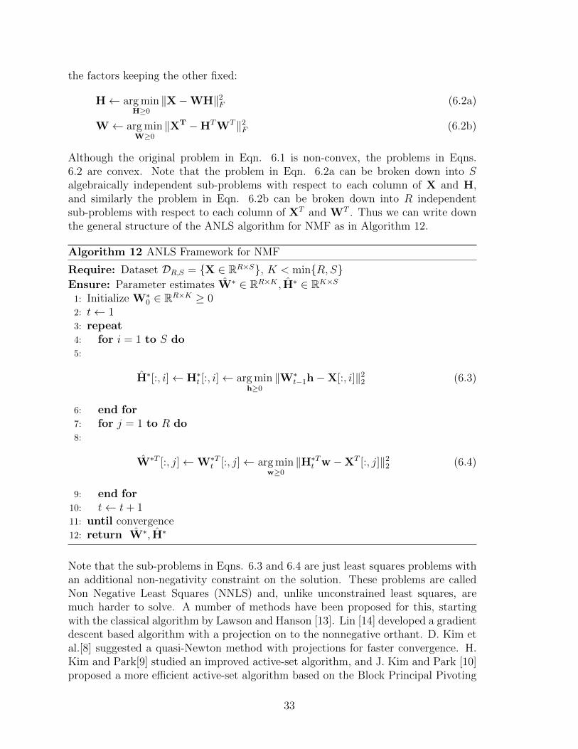
There are no closed form solutions for W∗,H∗ and one has to resort to iterativemethods to solve for these factors. Algorithms based on the Alternating Non-negativeLeast Squares (ANLS) framework have been found to be very efficient for this problemand has convergence properties provided by a block coordinate descent argument[2].ANLS is a simple alternating minimizing scheme that iteratively optimizes each of
32
the factors keeping the other fixed:
H← arg minH≥0
‖X−WH‖2F (6.2a)
W← arg minW≥0
‖XT −HTWT‖2F (6.2b)
Although the original problem in Eqn. 6.1 is non-convex, the problems in Eqns.6.2 are convex. Note that the problem in Eqn. 6.2a can be broken down into Salgebraically independent sub-problems with respect to each column of X and H,and similarly the problem in Eqn. 6.2b can be broken down into R independentsub-problems with respect to each column of XT and WT . Thus we can write downthe general structure of the ANLS algorithm for NMF as in Algorithm 12.
Algorithm 12 ANLS Framework for NMF
Require: Dataset DR,S = X ∈ RR×S, K < minR, SEnsure: Parameter estimates W∗ ∈ RR×K , H∗ ∈ RK×S
1: Initialize W∗0 ∈ RR×K ≥ 0
2: t← 13: repeat4: for i = 1 to S do5:
H∗[:, i]← H∗t [:, i]← arg minh≥0
‖W∗t−1h−X[:, i]‖2
2 (6.3)
6: end for7: for j = 1 to R do8:
W∗T [:, j]←W∗Tt [:, j]← arg min
w≥0‖H∗Tt w −XT [:, j]‖2
2 (6.4)
9: end for10: t← t+ 111: until convergence12: return W∗, H∗
Note that the sub-problems in Eqns. 6.3 and 6.4 are just least squares problems withan additional non-negativity constraint on the solution. These problems are calledNon Negative Least Squares (NNLS) and, unlike unconstrained least squares, aremuch harder to solve. A number of methods have been proposed for this, startingwith the classical algorithm by Lawson and Hanson [13]. Lin [14] developed a gradientdescent based algorithm with a projection on to the nonnegative orthant. D. Kim etal.[8] suggested a quasi-Newton method with projections for faster convergence. H.Kim and Park[9] studied an improved active-set algorithm, and J. Kim and Park [10]proposed a more efficient active-set algorithm based on the Block Principal Pivoting
33
method.
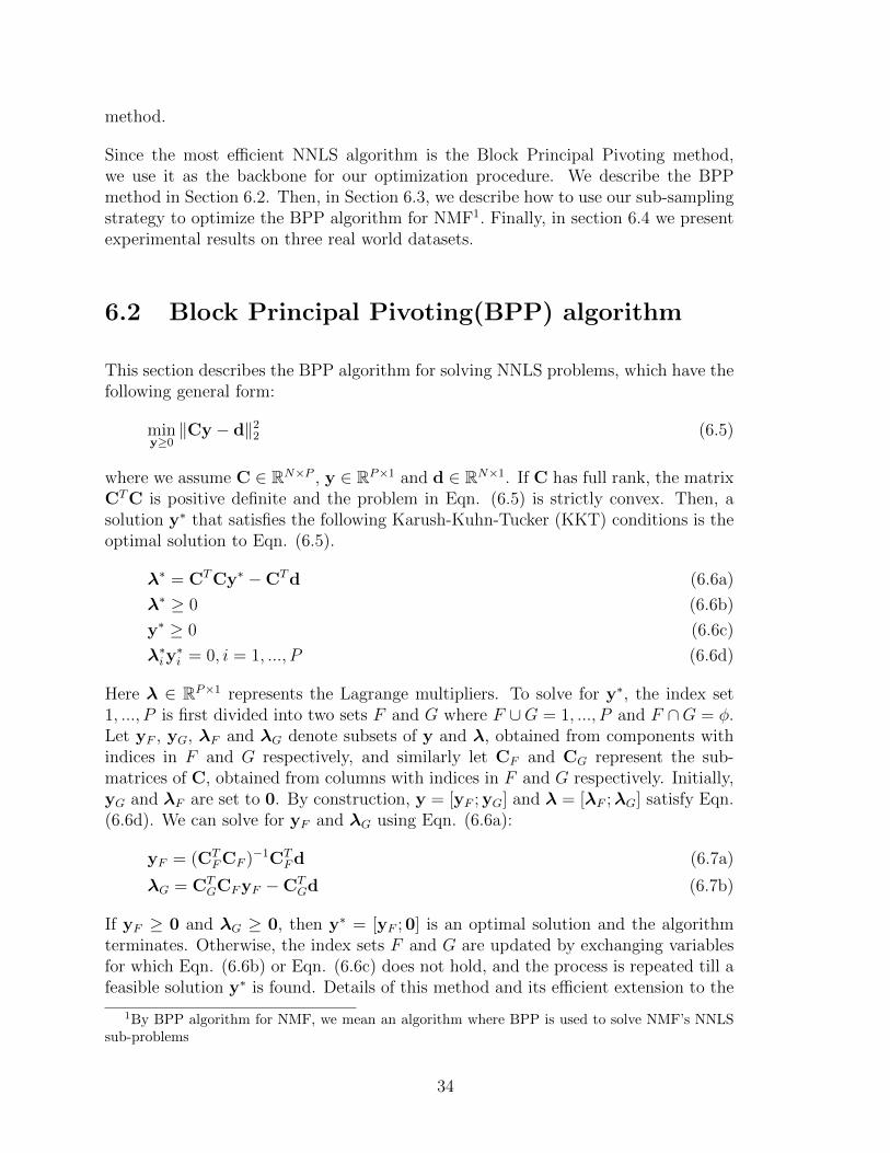
Since the most efficient NNLS algorithm is the Block Principal Pivoting method,we use it as the backbone for our optimization procedure. We describe the BPPmethod in Section 6.2. Then, in Section 6.3, we describe how to use our sub-samplingstrategy to optimize the BPP algorithm for NMF1. Finally, in section 6.4 we presentexperimental results on three real world datasets.
6.2 Block Principal Pivoting(BPP) algorithm
This section describes the BPP algorithm for solving NNLS problems, which have thefollowing general form:
miny≥0‖Cy − d‖2
2 (6.5)
where we assume C ∈ RN×P , y ∈ RP×1 and d ∈ RN×1. If C has full rank, the matrixCTC is positive definite and the problem in Eqn. (6.5) is strictly convex. Then, asolution y∗ that satisfies the following Karush-Kuhn-Tucker (KKT) conditions is theoptimal solution to Eqn. (6.5).
λ∗ = CTCy∗ −CTd (6.6a)
λ∗ ≥ 0 (6.6b)
y∗ ≥ 0 (6.6c)
λ∗iy∗i = 0, i = 1, ..., P (6.6d)
Here λ ∈ RP×1 represents the Lagrange multipliers. To solve for y∗, the index set1, ..., P is first divided into two sets F and G where F ∪G = 1, ..., P and F ∩G = φ.Let yF , yG, λF and λG denote subsets of y and λ, obtained from components withindices in F and G respectively, and similarly let CF and CG represent the sub-matrices of C, obtained from columns with indices in F and G respectively. Initially,yG and λF are set to 0. By construction, y = [yF ; yG] and λ = [λF ;λG] satisfy Eqn.(6.6d). We can solve for yF and λG using Eqn. (6.6a):
yF = (CTFCF )−1CT
Fd (6.7a)
λG = CTGCFyF −CT
Gd (6.7b)
If yF ≥ 0 and λG ≥ 0, then y∗ = [yF ; 0] is an optimal solution and the algorithmterminates. Otherwise, the index sets F and G are updated by exchanging variablesfor which Eqn. (6.6b) or Eqn. (6.6c) does not hold, and the process is repeated till afeasible solution y∗ is found. Details of this method and its efficient extension to the
1By BPP algorithm for NMF, we mean an algorithm where BPP is used to solve NMF’s NNLSsub-problems
34
case of multiple d’s (as in Eqns. (6.2)) can be found in [10].
From now, we will write BPP-SOLVE to represent a procedure that takes in asinput C ∈ RN×P , d ∈ RN×1 and uses the BPP algorithm to produce output y∗ =arg miny≥0 ‖Cy− d‖2
2. For instance, we can write steps 5 and 8 of Algorithm 12 as:
Replacing steps 5 and 8 of Algorithm 12 with the calls to BPP-SOLVE as shownabove gives us the BPP algorithm for NMF.
6.3 Statistical Optimization of the NMF BPP al-
gorithm
Now, we will describe how our sub-sampling method can be used to optimize theNMF BPP algorithm for large input matrices [11]. Note that in every iteration ofANLS, we make a large number of calls to the BPP-SOLVE procedure to solve theR + S NNLS problems. Also, each call to BPP-SOLVE computes CT
FCF and CTFd
to solve for y∗ and can be very expensive for large input matrices. Thus, we cansignificantly optimize the NMF BPP algorithm if we can reduce the number of callsto BPP-SOLVE and reduce the computational cost of BPP-SOLVE. Our sub-samplingmethod can achieve both of these optimizations.
Before explaining our optimization method in detail, we will first give a quick overview.In the initial iterations of ANLS, the estimates of the optimal factors W∗ and H∗ arefar from their true values. Therefore, instead of using BPP-SOLVE with all the avail-able data to estimate the updates to W∗ and H∗, we can approximate the updatesusing a small subset of the available data. Since these updates (see Eqn. (6.7a)) havethe form (ATA)−1ATb, we can use the hypothesis testing framework of Chapter 3 todetermine the reliability of these updates. As learning proceeds, and our estimatesof W∗ and H∗ move closer to their true solution, more precision is needed in theupdates and hence the hypothesis tests fail. When this happens, we can increase thesample size used to compute the updates, so that the updates become more preciseand pass the hypothesis tests. Finally, we stop optimizing when the hypothesis testsfail while using all the data.
Now we will explain this in more detail. In each iteration t, instead of using allavailable data to accurately compute H∗t [:, i] as in Eqn. (6.3), we will approximateH∗t [:, i] using only NH
t rows of W∗t−1 and the corresponding NH
t components of X[:, i].Similarly, instead of computing W∗T
t [:, j] as in Eqn. (6.4), we will approximate it usingNWt rows of H∗Tt and the corresponding components of XT [:, j]. Thus, we will replace
35
the calls shown in Eqns. (6.8) as follows:
H∗[:, i]← H∗t [:, i]← BPP-SOLVE(W∗t−1[1:NH
t , :],X[1:NHt , i]) (6.9a)
W∗T [:, j]←W∗Tt [:, j]← BPP-SOLVE(H∗Tt [1:NW
t , :],XT [1:NWt , j]) (6.9b)
Since, the updates (Eqn. (6.7a)) computed using BPP-SOLVE have a form similarto the solution to a least square problem, the updates produced by the calls to BPP-SOLVE shown in Eqns. (6.9) are a valid approximation of the true updates (Eqns.(6.8)). We test the reliability of updates using Procedure 3 (HYPOTHESIS-TEST)and if the updates to H∗t [:, i] or W∗T
t [:, j] fail these tests, we increase NHt or NW
t
respectively, for the next iteration.
In practice, we will not test updates for all columns of H∗ (or W∗T ). Instead we willpick a representative sample of M columns of H∗ (or W∗T ), and if the updates to theseM columns pass the hypothesis tests, we will deem the sample size, NH
t (or NWt ),
as providing necessary accuracy to compute updates to all columns of H∗ (or W∗T ).We keep the value of M fixed throughout the optimization procedure, and we havechosen M = 10 in all our experiments. In theory, one should apply a correction formultiple hypothesis testing. For instance, the Bonferroni correction simply divides thesignificance level by the number of tests performed. However, these considerations arerequired only if a principled stopping criterion is desired. In practice, the significancelevel is often a tuning parameter to optimize the computational efficiency of thealgorithm. Also, note that the update calculated by BPP-SOLVE is y∗ = [yF ; 0]where yF has the form (ATA)−1ATb. We perform our hypothesis testing only onyF , the components of y∗ corresponding to the index set F . Thus, we introduce amodified version of the hypothesis test in Procedure 13 (HTEST-NMF).
Procedure 13 HTEST-NMF
Require: A ∈ RNt×P , B ∈ RNt×Q, Y∗t−1 ∈ RP×Q, ρ∗, MEnsure: pass1: pass← true2: Choose M indices q1, ..., qM in 1...Q3: for i = 1 to M do4: y∗t , F ← BPP-SOLVE(A,B[:, qi])5: pass← HYPOTHESIS-TEST(A[:, F ],B[:, qi]),Y
∗t−1[F, qi], ρ
∗)6: if not pass then7: break8: end if9: end for10: return pass
In addition to reducing the size of NNLS problems and making each call to BPP-SOLVE faster, our sub-sampling method also reduces the number of NNLS problemsto be solved, i.e. it also decreases the number of calls to BPP-SOLVE. To see this,consider the for loop in steps 4 to 6 of Algorithm 12, which makes S calls to BPP-
36
SOLVE to solve for each column of H∗t in iteration t. However, in the next stepof iteration t, using our sub-sampling method, we just need NW
t columns of H∗t toestimate the rows of W∗
t . Thus, we need to solve for only NWt columns of H∗t in
the tth iteration. Similarly, in iteration t, we just need to solve for NHt+1 columns of
W∗t instead of solving for all R columns as in steps 7 to 9 . Since NW
t S andNHt+1 R in the initial iterations, the reduced number of calls to BPP-SOLVE yield
very significant savings.
As mentioned in previous chapters, the sub-sampling method also provides us with anautomatic and principled stopping criterion. In the case of NMF, we stop optimizingwhen the updates to at least one of the factors fail while using all the available data.The complete algorithm is shown in Algorithm 14.
6.4 Experiments
We compared the performance of the original Block Principal Pivoting (BPP) algo-rithm to BPP using our Sub-Sampling scheme (BPP-SS) on three real world datasets:the AT&T dataset of faces2, the MNIST dataset of handwritten digits 3 and a datasetof HOG [5] features extracted from the INRIA pedestrian detection dataset 4. Bothalgorithms were implemented in MATLAB. The experiments on the AT&T facesdataset were executed on a 2.2 GHz Core2 Duo, 3GB RAM machine running Win-dows 7 whereas the MNIST and HOG dataset experiments were run on a 2.93GHz 4Intel(R) Xeon(R) X5570, 96GB RAM cluster node running Linux 2.6.
For all datasets, we started out with a sample size around 500 and chose the threshold,ρ∗, for failing a hypothesis test to be 0.4. We always performed M = 10 testsat every iteration of the algorithm. For BPP-SS, we stopped the algorithm whenthe hypothesis tests failed with the full dataset. We calculated the relative error or“residual” for BPP-SS as ‖X−W∗H∗‖F/‖X‖F and used this as the stopping criterionfor the BPP algorithm. We have verified that our stopping criterion resulted in verysimilar (in fact slightly smaller) residuals as the ones reported in [10]. We ran 10trials on each dataset using the same initial value of W0 for both algorithms in anyparticular trial. We measured the the residual, the average running time of bothalgorithms and its standard deviation. For each trial, we measured the speed-upfactor as the ratio between the running time of BPP with respect to that of BPP-SS.Note that because the algorithms may converge to different local minima for differenttrials, the variation of the running times of BPP or BPP-SS between trials is high andthe only good comparison is the mean paired speed-up and its standard deviation.Note that since we are measuring the speed-up ratio, the mean and standard deviationrefer to the geometric mean and geometric standard deviation respectively.
For tuning our parameters and initial testing, our first experiments were on the AT&Tdatabase of faces which consists of 400 face images of 40 different people with 10images per person. Each face image has 92×112 pixels and we obtained a 10304×400matrix. The average performance of both algorithms are shown in Figure 6.1a fordifferent values of K. We show the residuals over time for K =16 and 81 in Figures6.2a and 6.2b respectively. Note that the residual can go up for BPP-SS when weincrease the sample size, since we also introduce more NNLS sub-problems to besolved. We show how the sample size NH
t , i.e. the number of rows of W∗t used to
solve for H∗t , increases in Figures 6.2c and 6.2d. In Figures 6.2e and 6.2f, the timetaken per iteration is shown. Note the spike in processing time, when the sample sizeis increased.
Our next set of experiments was on the MNIST database of handwritten digits. Weused 60000 images of handwritten digits, each 28 × 28 pixels, giving a 60000 × 784matrix. Results are shown in Figure 6.1b. Our final experiments were on a datasetconsisting of HOG features of over 5 million windows from the INRIA pedestriandetection dataset. Each scanning window was divided into 14 × 6 cells of 8 × 8pixels and each cell was represented by a gradient orientation histogram using 13bins resulting in a 1092 element vector per window. We used only a 1 million subsetof windows giving a 1, 000, 000 × 1092 matrix, because of memory constraints. Thisis an extremely large dataset which allowed the BPP-SS algorithm to achieve verysignificant speed-ups over the BPP algorithm (Figure 6.1c ).
Our experiments on these three real world datasets clearly demonstrate that the pro-posed sub-sampling method significantly improves the NMF Block Principal Pivotingalgorithm, especially on large datasets.
39
k Residual Running Time (sec) Speed UpBPP BPP-SS Mean
Figure 6.1: Performance Comparison of BPP versus its sub-sampled version(BPP-SS)on 3 real world data sets.
40
0 10 20 30 40 500.185
0.19
0.195
0.2
0.205
0.21
0.215
0.22Residual vs Time, k = 16
Time (secs)
Res
idua
l
BPP−SSBPP
(a) Residual vs Time, k = 16
0 100 200 300 400 5000.12
0.125
0.13
0.135
0.14
0.145
0.15
0.155Residual vs Time, k = 81
Time (secs)
Res
idua
l
BPP−SSBPP
(b) Residual vs Time, k = 16
0 10 20 30 40 500
2000
4000
6000
8000
10000
12000Sample Size vs Iterations, k = 16
Iterations
Sam
ple
Size
(c) Sample Size vs Iterations, k = 16
0 20 40 60 80 100 1200
2000
4000
6000
8000
10000
12000Sample Size vs Iterations, k = 81
Iterations
Sam
ple
Size
(d) Sample Size vs Iterations, k = 81
0 10 20 30 40 50 60 70 800
0.5
1
1.5Elapsed Time per Iteration, k = 16
Iterations
Ela
psed
Tim
e(se
cs)
BPP−SSBPP
(e) Elapsed Time per Iteration, k = 16
0 20 40 60 80 100 1200
5
10
15
20
25Elapsed Time vs Iterations, k = 81
Iterations
Ela
psed
tim
e(se
cs)
BPP−SSBPP
(f) Elapsed Time per Iteration, k = 81
Figure 6.2: Performance of BPP versus its sub-sampled version(BPP-SS) on theAT&T data set.
41
Chapter 7
Conclusion
We argued that statistical estimation should not be considered as a mere mathe-matical optimization procedure once the loss function has been chosen. Instead, oneshould treat learning as a statistical procedure, acknowledging the fact that the lossfunction is a stochastic quantity which fluctuates under resampling the dataset fromits generating process.
We proposed a general stochastic optimization method that can be used to speed-upa variety of iterative estimation problems. In each iteration, our method computes byusing only just enough data to reliably take a single step. Thus, in early iterations,when we are far from the true solution, only a few datapoints are needed to tell usthe general direction to move in parameter space. However, as we proceed towardsconvergence, more precision is required in the updates. The optimal batch size ineach iteration is determined using frequentist hypothesis tests which check whetherthe proposed update direction is correct with high probability. If the hypothesis testsfail, it is an indication that more precision is needed in the updates and the batchsize is increased. Thus, we proposed an “as needed” approach to computation.
Our method, besides speeding up learning by sub-sampling the data, also has theadvantage of an automatic and principled stopping criterion. When all hypothesistests fail and we cannot increase the sample size, either due to unavailability of moredata or due to computational limitations, we terminate learning. This is a statisticallyprincipled stopping criterion because, at this point, another dataset drawn from thetrue underlying distribution of the data might propose a significantly different updatedirection. Another important advantage of our method is that we have only a singleinterpretable parameter: the significance level of the hypothesis tests. Also, ourmethod is orthogonal to many other speed-up methods developed in the optimizationliterature and can often be effectively combined with them.
The method crucially depends on the central limit theorem and we have indeed ob-served that the method fails when such central limit tendencies are absent. This
42
appears to be the case when the data-matrix is very sparse. Another example wherewe have noticed our algorithm to fail is Non-negative Tensor Factorization. In thiscase, the reshaping of the tensor at every iteration induces complicated dependenciesand non-Gaussian behavior (presumably due to the multiplication of random vari-ables). However, despite the above exceptions, many interesting learning algorithmsexist to which our ideas can be applied.
Experiments on real world datsets showed that our method works well in practiceand can highly speed-up many learning algorithms, especially on large datasets. Forexample, we were able to speed-up the state of the art Non-negative Matrix Factor-ization algorithm by a factor of 4-5.
43
Bibliography
[1] D. Andrews and C. Mallows. Scale mixtures of normal distributions. Journal ofthe Royal Statistical Society. Series B (Methodological), 36(1):99–102, 1974.
[2] D. P. Bertsekas. Nonlinear programming. Athena Scientific, Belmont, Mass,1999.
[3] C. Bishop. Pattern recognition and machine learning, volume 4. Springer NewYork, 2006.
[4] L. Bottou and O. Bousquet. Learning using large datasets. Mining MassiveDataSets for Security, NATO ASI Workshop Series, 2008.
[5] N. Dalal and B. Triggs. Histograms of oriented gradients for human detection.In IEEE Computer Society Conference on Computer Vision and Pattern Recog-nition, pages 886–893, 2005.
[6] A. Dempster, N. Laird, D. Rubin, et al. Maximum likelihood from incompletedata via the EM algorithm. Journal of the Royal Statistical Society. Series B(Methodological), 39(1):1–38, 1977.
[7] A. Frank and A. Asuncion. UCI Machine Learning Repository, 2010.
[8] D. Kim, S. Sra, and I. Dhillon. Fast newton-type methods for the least squaresnonnegative matrix approximation problem. In Proceedings of the 2007 SIAMInternational Conference on Data Mining, 2007.
[9] H. Kim and H. Park. Nonnegative matrix factorization based on alternatingnonnegativity constrained least squares and active set method. SIAM Journalon Matrix Analysis and Applications, 30(2):713–730, 2008.
[10] J. Kim and H. Park. Toward faster nonnegative matrix factorization: A new al-gorithm and comparisons. In Proceedings of the 2008 Eighth IEEE InternationalConference on Data Mining (ICDM), pages 353–362, 2008.
[11] A. Korattikara, L. Boyles, M. Welling, J. Kim, and H. Park. Statistical Opti-mization of Non-Negative Matrix Factorization. In AISTATS, 2011.
[12] H. Kushner and G. Yin. Stochastic approximation and recursive algorithms andapplications. Springer Verlag, 2003.
44
[13] C. L. Lawson and R. J. Hanson. Solving Least Squares Problems. Society forIndustrial and Applied Mathematics, 1995.
[15] P. McCullagh and J. Nelder. Generalized linear models. Chapman & Hall, CRC,1999.
[16] R. Phillips. Least absolute deviations estimation via the EM algorithm. Statisticsand Computing, 12(3):281–285, 2002.
[17] H. Robbins and S. Monro. A stochastic approximation method. The Annals ofMathematical Statistics, 22(3):400–407, 1951.
[18] J. Spall. Introduction to stochastic search and optimization: estimation, simula-tion, and control. John Wiley and Sons, 2003.
[19] M. Verbeek. A Guide to Modern Econometrics. John Wiley and Sons, 2000.
[20] B. Yu. Embracing statistical challenges in the information technology age. Tech-nometrics, American Statistical Association and the American Society for Qual-ity, 49:237–248, 2007.
45
Appendices
A Notation (and abuse thereof)
We will represent vectors using bold lowercase symbols (e.g. v) and matrices usingbold uppercase symbols (e.g. M).We will denote the ith element of a vector v ∈ RN×1
by vi. If a vector has other subscripts, say, for instance, if vt represents a vectorcalculated at time t, we will use vt[i] to represent the ith element of vt. Occasionally,we use a ‘MATLAB like’ notation for indexing vectors. If P is a list of indices, thenv[P ] represents a |P |×1 vector composed of elements of v with indices in P . v[a : b],where a and b are two integers in [1, N ], represents a vector formed from a subset ofelements of v with indices ranging from a to b. If a and b are not specified, they areassumed to be 1 and N respectively, i.e. v[:] represents the whole vector v. Similarconventions are also used for matrix indexing.
We will use the notation diag(v) to represent the diagonal matrix D ∈ RN×N suchthat Dii = vi for i = 1...N . 1 or 0 represents a vector or matrix whose elements areall 1 or 0, respectively. The dimensions of 1 or 0 will be specified, if not clear fromthe context. If h(.) is a function that takes a scalar argument and v ∈ RN×1, thenwe abuse notation slightly and write h(v) ∈ RN×1 to represent the vector obtainedby applying h(.) to each component of v separately. Similarly, 1/v ∈ RN×1 representsthe vector obtained by taking the reciprocals of each component of v. For two vectorsv,w ∈ RN×1, the product vw denotes the vector of element-wise products.