It is easy to see that the reactor geometry and the fluid flow rates, therefore, the
fluid dynamics of the total system, are the same for both compounds ; the
interfacial area, along with the bubble coalescence and physical properties of
the phases are the same for each compound ; and the presence of a solid phase
should also have the same effect on both compounds, unless there is mass
transfer enhancement due to simultaneous depletion in one of the phases, i .e .
fast chemical reactions .
Therefore, the ratio of two liquid film mass transfer coefficients (often called 'Y
for the ratio between VOC's and 02 mass transfer coefficients) reduces to :
'I1= kLaA
DLAkLaB - f\DLB
When the liquid film resistance dominates (K La = kLa), then only the ratio of
the liquid diffusion coefficients affects the ratio of the overall mass transfer
coefficients for the simultaneous transfer of two compounds in one system .
As discussed in Section 2 .1 .1, the assumption that the liquid side dominates de-
pends on the ratio of the film coefficients kGa/kLa. In work on volatilization
from natural bodies of water, Mackay and Leinonen (1975) report typical
21
kGa/kLa ratios range from 50-300. Assuming kc;a/kLa = 200, the resistances be-
come approximately equal when H, = 0 .005 and the liquid side resistance dom-
inates (kLa/KLa = 0.95) for H, > 0.10. This is valid for natural bodies of water,
the system for which the film coefficients were determined . For engineered
systems with much more turbulence, i .e. surface and bubble aeration, Munz
and Roberts (1984) found kca/kLa to be closer to 20 and Hsieh (1990) found a
ratio of 6. In such systems, the compounds must be more volatile (H e > 0.95, or
3.17 respectively) in order to assume the liquid side resistance dominates. Only
very volatile compounds fulfill this requirement .
If we consider an example for toluene :
The requirement that kLa << HckGa is not fulfilled, in fact, k La - I-L kGa. There-
fore, the assumption that liquid side resistance dominates is not valid here .
Looking at a hypothetical case where k Ga remains constant, but kLa increases
ten-fold, we find that KLa = 0.00052 s -1 . Thus, a ten-fold increase in k La results
in only a doubling of K La when Hc-kGa is on the same order of magnitude as
kLa.
22
Given : KLavoc = 0.00025 s"1
kc;a/kLa = 6
He = 0.24
subst.in eqn 5 : 1/0.00025 =1 /x + 1 / (0.24 - y)
where:
then:
6x = y
kLa = 0.00042 s"1 and ka = 0.00252 s - '
and : Hckra = 0.24 * 0.00252 = 0.00060 s - '
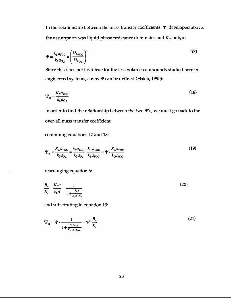
In the relationship between the mass transfer coefficients, 'P, developed above,
the assumption was liquid phase resistance dominates and K La = kLa
kavoc DLVOC n
T = kLao2 = DLO,
Since this does not hold true for the less volatile compounds studied here in
engineered systems, a new W can be defined (Hsieh, 1990) :
,h KLavocm _
kLao2
In order to find the relationship between the two 'F's, we must go back to the
over-all mass transfer coefficient :
combining equations 17 and 18 :
KLavoc kavoc KLavoc
KLavockLao2 kLao2 kavoc
kavoc
rearranging equation 6 :
RL KLa
1RT kLa 1 + k`a
kGa „HH
and substituting in equation 19 :
T+ HekGƒvoc
23
(20)
The over-all mass transfer coefficient, K Lavoc, will be used to denote the mea-
sured VOC mass transfer coefficients in the following sections, while for the
oxygen mass transfer coefficients, the film coefficient kLa 2 will be used to
emphasize the difference .
In summary, if the liquid side resistance dominates for VOC transfer, then the
ratio between the over-all mass transfer coefficients for oxygen and the VOC's
CI') should remain approximately constant as power density varies and pro-
portional to the ratio of the diffusion coefficients raised to a power n. If both
gas and liquid side resistance play a role, then the ratio of the over-all mass
transfer coefficients will vary as power density varies, because of its depen-
dence on the ratio of liquid side to total resistance .
To illustrate the possible variation in 'I' just due to the variation in the expo-
nent n predicted by the three common theories, from (DLvoc/Dw2) 1-0 to
(DLvoc/DLo2) 0-5 , the calculated 'I' for the three compounds used in this study
are listed in Table 2 . Since the Wilke-Chang correlation used to calculate the
diffusion coefficients is only considered valid within • 15%, the possible varia-
tion in 'P due to the error in the VOC diffusion coefficient is also listed . For ex-
ample, (DLvoc/DLO2) for toluene is 0.42. The possible range of 'P due to a
change in the exponent n from 1 .0 to 0.5 and the • 15% error in DLTOL is
0.36-0.70 .
24
Table 2. Variation in 'If according to mass transfer theories .
2.1.5 Volatilization in engineered systems
In surface aeration studies on the relationship between the oxygen and organic
compound mass transfer coefficients in clean water for six volatile chlorinated
hydrocarbons, Roberts et al.(1984a) found the ratio of the two mass transfer co-
efficients to be constant, 'P - 0.6, and independent of power input over the
range of P/V = 0.8 to 320 W/m3. They also ran the experiments in filtered
secondary effluent from a wastewater treatment plant and found the ratio re-
mained the same. Comparing the mass transfer coefficients for the clean water
to those for the filtered secondary effluent, they found a,,oc = 0.89, while a02 =
0.77, and they both increased with increasing power input.
Roberts et al. (1984) also made bubble column experiments to simulate diffused
aeration basins . The column had a diameter of 22 .5 cm with the liquid height
varying from 35 to 60 cm . They found that for all but the most volatile com-
pound, CC1 2F2 , the gas phase was substantially saturated upon exiting the col-
umn. Using the differential gas phase mass balance and integrating over the
height of the column, they developed a model to estimate the mass transfer
25
THEORY Two-film Surface renewal
Compound exponent (n) = 1 .0 0.5
% error -15% 'P +15% -15% 'P +15%
DCM 0.51 0.60 0.69 0.72 0.78 0.83
Toluene 0.36 0.42 0.49 0.60 0.65 0.70
1,2-DCB 0.34 0.40 0.46 0.58 0.63 0.68
coefficient when gas phase saturation is negligible, or the Henry's constant
when saturation is complete, or either k La or H, (if the other is known) for the
intermediate range of gas phase saturation .
Truong and Blackburn (1984) investigated the volatilization of several volatile
as well as non-volatile compounds in a bubble column . Various contaminants
were added to tap water: surfactants, an oil phase, a pulp mill wastewater, and
nonviable biomass to investigate their effect on volatilization . In analyzing
their work, Allen et al.(1986) found that the Henry's constant for benzene cal-
culated from their experimental data was comparable to values reported in the
literature, suggesting that equilibrium for the organic compounds was reached
in their apparatus . Therefore, a true mass transfer coefficient was not measured
in their experiments and the relationship between the mass transfer coefficients
cannot be checked with their data .
26
2.2 Driving force
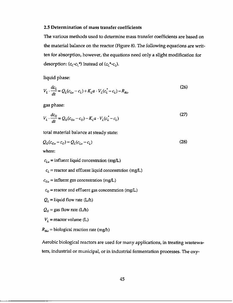
Before considering how mass transfer coefficients are measured, we have to first
delve deeper into the mass transfer theory and discuss the driving force . The
driving force is the difference in the concentration of the compound in the phase
itself and at the interface. As discussed above, the driving force can be defined
in either phase, and if the Henry's absorption isotherm is linear for desorption :
m =KLa(cL-c;)
since :
CG CGHC _- _;
CL CL
In a mass transfer apparatus if the receiving phase reaches the equilibrium
concentration, e.g., in volatilization if the gas becomes saturated such that
(cL-cL')=0, a mass transfer coefficient can no longer be used to calculate the mass
transfer rate. For the case of nonsteady state with a saturated gas phase, the
mass transfer rate can be calculated from:
d cLVL
dt=-QG „ CL „ He
since : CG = CG = CLAHC
where: QG = gas flow rate
VL = reactor volume
Mackay et al. (1979) suggests calculating Henry's constants with this equation
from data collected in a bubble column . Figure 6 illustrates the rapid approach
to equilibrium for air bubbles rising in a benzene/water solution (Allen et al .,
1986) .
(22)
(23)
27
0
100
80
20
A
4,
40
A.
Bubble size
0.1 cm0
0.3 cmA
1 .0 cmO
Liquid depth (cm)Figure 6. Approach to equilibrium as a function of liquid depth for benzene ab-
sorbed during bubble rise in water (Allen et al ., 1986)
Since a mass transfer coefficient can only be measured in phases not at equilib-
rium, care must be taken to insure that samples of the gas and liquid phases col-
lected for the evaluation of KLavoc are not saturated. The experimental ratio of
the KLa's cannot be constant for varying operating conditions if one of them is
measured incorrectly, i .e with the phases in equilibrium .
2.2.1 Equilibrium concentration - c*
Bringing in the equilibrium concentration (c*), we introduce a source of error in
the calculation of the driving force . This applies to both oxygen and VOC's .
The correction of c* for the change in the oxygen saturation concentration in
contaminated water is often made with an empirical factor, the beta factor . The
beta factor has been defined as :
28
where:
c;, = oxygen saturation concentration in wastewater
cTP = oxygen saturation concentration in tap water
The beta factor has been found to be correlated to the total dissolved solids
content of the water. Another common problem in determining c* for oxygen is
correctly accounting for hydrostatic pressure . In CFSTR's used in this study,
this effect is negligible, but can be quite significant in deep diffused aeration
systems. Campbell et al. (1976) present a good review of the problem .
In calculating the equilibrium concentration for VOC's, the error caused by
using an inappropriate Henry's constant can be significant since the relation-
ship cj=c c;/Hc is used. The determination of the Henry's constant in clean
water is difficult and the difference in values found by various investigators
can be large. Mackay and Shiu (1981) reviewed published Henry's constants
for environmentally relevant compounds and found that considerable discre-
pancies exist in the literature, even for fairly common compounds . The use of a
Henry's constant obtained for a substance dissolved in a pure water in the
calculations for a heavily contaminated water can lead to false estimates of the
mass transfer rate . Two methods are commonly used for measuring Henry's
constants, the bubble column as mentioned previously, and the equilibrium
partitioning in closed systems (EPICS) method (Lincoff and Gossett, 1984) as
described in Section 3 .5.
(24)
29
For six chlorinated volatile organic compounds, Roberts et al . (1984b) found
differences of up to 50% between the H, found for filtered effluent from a
wastewater treatment plant and for clean water in measurements in a bubble
column. If we write the beta factor defined above for oxygen in terms of Hen-
ry's constants, we find :
C;W CG/H~wk, HcTP
CTP CG/HcTP HcWW
(25)
Using this definition and the values of H,, reported by Roberts et al . for volatile
chlorinated hydrocarbons, beta factors for the filtered secondary wastewater
used in the study can be calculated that range from 0 .62 for chloroform to 0 .99
for carbon tetrachloride. They did not report a beta factor for oxygen. Accept-
ing these values for the moment, and considering the wide range of beta
factors found for the various compounds in the same waters : 0.62-0.99, it seems
that the oxygen beta factor cannot be used to adjust for changes in H e for other
compounds.
Yuteri et al . (1987) investigated the effect of additives in distilled water on Hen-
ry's constants for trichloroethylene (TCE) and toluene using the EPICS method .
They found differences in the Henry's constant for TCE of -+15% when the
ionic strength of the water was increased and --15%a when surfactants were
added. In experiments with natural waters, they found the H, for toluene var-
ied as much as 24%, but there was no apparent trend with alkalinity, pH, or
TOC. They warn that unpredictable deviations from the pure water values of
the Henry's constants should be expected in contaminated water because of
30
such molecular phenomena as association, solvation, and salting-out . In con-
sidering the significance of these variations, one must keep in mind that their
comparison of their H', data for 15 compounds in distilled water with other
published experimental values shows deviations of up to 30% .
Lincoff and Gossett (1984), in comparing the two methods, found that the Hen-
ry's constants from the EPICS method was consistently higher than the bubble
column results (-14%). An interesting explanation for this may be the equation
proposed by Lord Kelvin in 1871 relating the change in vapor pressure with
drop curvature as a function of surface tension . The interface for the EPICS
method is a plane surface and the interface for the bubble column is spherical .
If we consider that the vapor pressure of a small drop of liquid is greater than
that of a liquid with a plane surface and that the vapor pressure inside a
bubble surrounded by bulk liquid is less than that at a plane surface, then theo-
retically, Hcdlop > Hcp,ane > Hcb„bb,e. Padday (1969a) explains this by supposing
that the attraction forces on a molecule in a convex surface are less than those
at a plane surface. The attraction is diminished because, on the average, there
are fewer molecules in the immediate vicinity to contribute to the total attrac-
tion. In a similar way, the vapor pressure at a concave surface is less than that
at a plane surface because the number of molecules contributing to the total
attraction is greater at a concave than at a plane surface . Therefore, theoreti-
cally, a compound is more volatile in surface aeration than in fine bubble aera-
tion. The question, of course, is the magnitude of this difference . Looking at the
values of Henry's constants gathered by Yuteri et al . (1987) from the literature,
there is no clear trend in the values from the two methods ; the variation in the
same method used by various researchers is sometimes greater than the varia-
31
lion between the two .
2.3 Surface tension
Many studies of the effect of surfactants on mass transfer have found mass
transfer to decrease with decreasing surface tension . Reports of increased mass
transfer have also been made . In order to understand the effect of surfactants
on mass transfer, we have to understand the general concept of surface tension .
This is discussed below, as well as the factors affecting surface tension, followed
by a discussion of literature results relevant to the effect of surface tension on
mass transfer .
Surface molecules possess energy in excess of the energy they already possess in
the bulk liquid state. In order to create new surface, work has to be done on the
system to overcome the excess energy. This surface free energy equals the sur-
face tension of a pure liquid .
Padday (1969a) presents an interesting review of the historical development of
surface tension starting from Leonardo da Vinci's observation of capillarity to
the present day theoretical and experimental results . Studying the historical de-
velopment helps understand the theory of surface tension. The following table
summarizes some of the historical highlights .
That contaminants, such as soap and grease, lower the surface tension of water
has been known since the first measurements were made with capillary tubes ; it
took much longer before it was discovered that the addition of inorganic elec-
trolytes increased the surface tension of water . This phenomenon, however, is
not of interest in this work, because such large quantities are required that
32
Table 3. Historical development of the theory of surface tension .
increases in surface tension due to salts in wastewater applications are not ex-
pected. The discussion here will be limited to the effect of surface active agents
on surface tension . Various methods exist to measure surface tension ; Padday
(1969b) and Masutani (1988) present good reviews of the methods .
The addition of organic liquids or surface-active agents lowers the surface ten-
sion of water. The ability of an organic molecule to lower the surface tension is
due to its tendency to adsorb at the liquid /air interface, orienting itself with the
33
Leonardo da Vinci (1452 -observed and recorded rise of liquid in a tube of-1519) small bore
Sir Isaac Newton 1721
-explained rise of liquid in a capillary tube as theproduct of cohesive and adhesive forces .
-recognized that the forces were intermolecular inorigin and that mutual attraction gave rise to apressure inside the liquid .
J.A. von Segner 1751
-proposed the first theory of capillarity :cohesive forces create a pressure which is re-sisted by a uniform tension in the surface (sur-face tension) .
-surface tension denoted the resence of a con-tractile skin at the surface ofpa liquid .
Thomas Young
P.S. de Laplace
1804 -proposedwithsion,than
1805
-thesurfaceposed
particles of matter act on one anothertwo kinds of forces, attraction and repul-the former acting over greater distancesthe latter .
attraction force gives rise to a pressure onparticles: the surface tension as pro-
by von Segner .J.D. van der Waals 1899 -showed existence of physical forces of attraction
between molecules .
Lord Rayleigh 1902 -related the physical forces of attraction to surfacetension.
J. Willard Gibbs 1906 -developed quantitative thermodynamic relation-ships between the energetics of surface forma-tion and intensive properties of the liquid .
hydrophobic group at the air interface and the hydrophilic group in the water
phase. Characteristic of surface-active agents is their ability to lower the surface
tension at relatively low bulk concentrations by adsorbing strongly at the sur-
face .
2.3.1 Effect on mass transfer
Surfactants can affect mass transfer in two ways, changing the interfacial area
or the mass transfer coefficient k L. A small amount of a surfactant can poten-
tially cause a large change in interfacial area . Bubbles break away from an ori-
fice when the ascending force is greater than the force due to surface tension ;
therefore, a decrease in surface tension can reduce the size of primary bubbles,
increasing the interfacial area . Bubble coalescence is also hindered by surfac-
tants, thereby, preserving the increase in interfacial area . This phenomena is
discussed more thoroughly in Section 2 .4 .
Two theories are commonly used to explain the effect of surfactants on the
mass transfer coefficient : the barrier effect and the hydrodynamic effect . In the
barrier theory, the presence of the surfactants at the phase interface creates an
additional resistance to mass transfer due to diffusion through the surfactant
layer .
In studies of the effect of surfactants on the absorption of SO2 in water in a
stirred system, Springer and Pigford (1970) found that surface films of a solu-
ble surfactant (sodium lauryl sulfonate) showed no barrier effect, though the
insoluble 1-hexadecanol surface film showed definite resistance . Llorens et
al.(1988) in studying CO2 absorption into solutions of various surfactants in a
wetted area column determined that the barrier effect was insignificant com-
34
pared to the hydrodynamic effect .
The hydrodynamic theory is based on two limiting cases . Considering a bubble
in a pure water/gas system, the bubble behaves like a fluid sphere; it has a
moving interface, retarded only by the viscosity of the gas, with a strong inter-
nal recirculation of the gas . Addition of surfactants retards the interface motion
because surfactants have a strong tendency to adsorb on the bubble interface,
accumulating at the bottom of the bubble . At high surfactant concentrations
the bubble is thought to behave like a solid sphere, a Ping-pong ball with a
rigid interface and no internal gas recirculation .
The mathematical model developed by Andrews et. al (1988) illustrates the hy-
drodynamic theory. Their model describes the hydrodynamics and mass trans-
fer of bubbles rising through contaminated liquids using boundary layer and
wake type hydrodynamics . The model divides the bubble into an upper
boundary layer region where surfactant adsorbs and a lower wake region from
where it desorbs. The model includes the mass transfer of surfactant from the
liquid to the upper part of the bubble, its transfer around the interface by inter-
facial motion and diffusion, its desorption from the bottom of the bubble and
the effect of these processes on the interfacial tension gradient in the boundary
layer region. The results from the model only apply strictly for surfactant con-
centrations greater than the concentration that causes interface saturation ; thus,
the model may not be valid for very low surfactant concentrations .
The model predicts that at "low" surfactant concentrations the high concentra-
tion gradients produce large gradients of interfacial tension, which keeps the
bubble interface almost immobile. Conversely, at surfactant concentrations
35
J~.
J
0"'1 ~~
36
a. fluid sphere hydrodynamics b. solid sphere hydrodynamics
c. large wake hydrodynamicsno surfactants
"low" surfactant concentration
"high" surfactant concentration
Figure 7. Change in bubble surfactant layer in the two hydrodynamic regimes .
above those required to make a bubble behave as a solid sphere (solid-sphere
hydrodynamics), the gradients of adsorbed surfactant and interfacial tension
are small so the interface is mobile (Figure 7) .
They introduced a third hydrodynamic regime to describe this phenomena : the
"large-wake" hydrodynamics, associated with the saturation of the interface in
the wake region with surfactant. In this regime increasing the surfactant con-
centration increases the mobility of the interface in the boundary region so the
boundary layer is thinner and the local mass transfer coefficients are
correspondingly larger . At the same time the boundary layer occupies less of
the total surface area of the bubble . Therefore, between the two hydrodynamic
regimes the mass transfer coefficient from the bubble goes through a maximum
and then declines . This maximum has been observed experimentally (Ziemin-
ski, et al ., 1967) with bubbles in a water/air system with low molecular weight
surfactants (carboxylic acids and alcohols) . With high molecular weight
surfactants, normally only the decline in k L with a leveling off at high surfac-
tant concentrations has been observed. Their explanation is the transition from
fluid-sphere to solid-sphere to "large-wake" hydrodynamics happens in such a
narrow range of surfactant concentrations that a maximum is not detectable .
In studying the mass transfer of acetone across a plane interface in a liquid/li-
quid system (water/carbon tetrachloride), Ollenik and Nitsch (1981) found that
below the critical micelle concentration (cmc) of dodecyl sodium sulfate the
interface was almost rigid and kL fell to approximately one third the value in
clean water. As the surfactant concentration neared the cmc, they observed an
increase in interfacial velocities and k L. Above the cmc, the values of k L and in-
terfacial velocity reached those of clean water . Assuming that the results from
a liquid/liquid system are extrapolatable to liquid/gas systems, it is possible
that this recovery corresponds to the maximum predicted by the bubble model
of Andrews et al.(1988). In their model, k L goes through a maximum as surfac-
tant concentration increases because the two trends, the decrease in surface
tension gradient and the decrease in surface area due to accumulation of
surfactants in the bubble wake, cause opposite effects on mass transfer . In a
system with a plane interface the decrease in the boundary layer due to accu-
mulation of surfactants is reduced, so that k L steadily increases due to the de-
crease in surface tension gradient and the resulting increase in interface mobil-
ity as discussed above .
Lee, Tsao, and Wankat (1980) investigated the hydrodynamic effect of surfac-
tants using an oxygen ultra-microprobe. They studied the effect of sodium lau-
ryl sulfate, bovine serum albumin, and glucose oxidase on oxygen transfer and
37
found kL to decrease with increased surfactant concentration at a constant
power input. However, the hydrodynamic effect decreased with increase in
impeller speed .
The adsorption of surface active agents at the surface is time dependent . In
aqueous solutions, a freshly formed surface possesses a higher surface tension
than the value at equilibrium. Reports of the time required to reach equilib-
rium surface tension vary according to the surface active agent, from 0 .01 s to
many hours. The time required for the compound to migrate to the surface
depends partly on the size of the molecule, its polarity, and the free energy of
the surface (Addison, 1944) . In studies of n-alcohols, Addison (1945) showed
that the migrational velocity increases with chain length . He also found that at
very low concentrations the migrational velocity decreases with decreasing
concentration .
The difference between the dynamic and static surface tension may explain the
dependence of mass transfer on power input . In discussing their results, Lee et
al.(1980) point out that the common assumption that the surfactants recover
their equilibrium surface tension immediately after the disruption by the ed-
dies approaching the surface is an oversimplification . In reality, there may be a
time lag before the surfactant recovers its equilibrium surface tension . If so, it is
not the static but the dynamic value of surface tension that is responsible for
the hydrodynamic effect . This dynamic surface tension is expected to depend
on the properties of the surfactant. Springer and Pigford (1970) postulated that
the dynamic surface tension is related with the time constant of recovery to
equilibrium for a given surfactant, and stated that a surfactant with a fast re-
covery time exhibits the hydrodynamic effect even at high liquid turbulence .
38
Attempts to correlate equilibrium or static surface tension with mass transfer
coefficients have been made with limited success (Stenstrom and Gilbert, 1981) .
This lead Masutani (1991) to investigate the relationship between k LaO2 and dy-
namic surface tension. She studied the effect of two anionic surfactants on oxy-
gen transfer in a tank with fine bubble diffusers . The maximum bubble pres-
sure method was used to measure the change in surface tension with time and
the Du Nouy ring method for the static surface tension values . She was able to
develop a correlation for kLaO2 as a function of the air flow rate, dynamic sur-
face tension, and static surface tension .
A model proposed by Koshy et al. (1988) for drop breakage and mass transfer
in liquid/liquid systems offers insight into the dynamic/static surface tension
effects. The model can help explain gas/liquid transfer as well . When a pres-
sure fluctuation due to an eddy is experienced by a drop across its diameter,
the drop starts deforming . The deformation most probably starts by the
formation of a depression on the drop interface and this depression propagates
resulting in breakage . When the surfactants are present at the interface, the
pressure fluctuation, besides causing depression at the interface, also removes
the adsorbed surfactant molecules thereby exposing a fresh interface . This
fresh interface has dynamic interfacial tension which is higher than the static
interfacial tension. Thus, at the base of the depression, the interfacial tension is
higher. This difference in interfacial tension causes a flow towards the base and
this adds to the flow already taking place due to the pressure fluctuation . Thus
internal recirculation of the drop is generated due to the difference in dynamic
and static interfacial tension . This in turn increases the mass transfer between
the drop and its surroundings .
39
The effect of increasing power input can be explained based on this model .
Since the effect of surfactants is to reduce the internal recirculation of a bubble
and to dampen turbulence, the increase in surface renewal of the bubble inter-
face due to increased turbulence, not only increases transfer by removing the
barrier, but also through the increased interfacial turbulence caused by the
difference in the dynamic and static surface tension at the point where the sur-
face is renewed .
2.4 Coalescence
Mass transfer is affected by the coalescence behavior of the bubbles because of
the decrease in interfacial area that occurs when the bubbles coalesce . As seen in
the development of equation 9 in Section 2 .1 .2, a term describing bubble coales-
cence is needed for the correlation of the mass transfer coefficient, however,
none is yet available. Therefore, separate correlations are made for coalescing
and non-coalescing systems. Water/air is a coalescing system . Addition of elec-
trolytes to water hinders bubble coalescence and increases the volumetric mass
transfer coefficient. Organic compounds, such as surfactants, acids and alcohols,
also affect coalescence, generally hindering it and thereby, increasing the volu-
metric mass transfer coefficient .
Osorio (1985) studied the influence of ionic strength with the steady state hydra-
zine method. He found kLaO2 increased with increased ionic strength up to a
concentration of 0 .2 mol/L NaCl where it then plateaus off with increased NaCl
addition. He called this the region of complete coalescence inhibition . The a
value was approximately 1 .5. He also studied the effect of iso-propanol on mass
transfer, for the same energy input and superficial gas velocities, a "small"
amount of iso-propanol (0.04 mol/L) caused more than a two-fold increase in
40
kLaO2 (a =-2-2.5) . Although he said coalescence in the salt solution of 0 .2 mol/L
was completely inhibited, he based this increase due to iso-propanol on the al-
most completely inhibited coalescence. Here it is possible that the amount of
iso-propanol was large enough that the primary bubble size was decreased by
the reduction in surface tension, although the surface tension was only reduced
1 .5% .
The effect of coalescence inhibition on k La depends on the type of aerator, the
greater the possibility of coalescence, the greater the effect. Zlokarnik (1978)
found a strong dependence of salt concentration on the increase in k LaO2, stron-
ger than other published results, ((x =5-7), which he explained on the basis of his
stirrer type (a self-aspirating stirrer) which produced very fine bubbles . Once
fine bubbles are formed they do not easily coalesce. Zieminski and Hill (1962)
developed a system which exploited this observation to increase oxygen trans-
fer with a very low organic concentration. They introduced a concentrated solu-
tion of 4-methyl-2-pentanol continuously at the surface of the porous plate dif-
fuser, and thus, compared to a system with the same bulk liquid concentration,
achieved a higher oxygen transfer .
Keitel and Onken (1982) studied coalescence inhibition with n-alcohols, ali-
phatic mono-carboxylic acids, ketones, bivalent alcohols . They found that the
compounds reduced the surface tension and with a certain concentration level
caused coalescence inhibition . This concentration is lower for carboxylic acids
than for alcohols and ketones . The presence of a second OH group pushes the
concentration level necessary higher. Increasing chain length in a homologous
group decreases concentration level necessary .
41
Drogaris and Weiland (1983) studied the coalescence frequency and coalescence
times of bubble pairs in the presence of n-alcohols and carboxylic acids. They
found that if the contact time between two bubbles is larger than the coalescence
time, the bubbles coalesce . Since different reactors have different available con-
tact times, the degree of coalescence inhibition produced by a certain concentra-
tion of an organic compound depends on the type of reactor and aerator used .
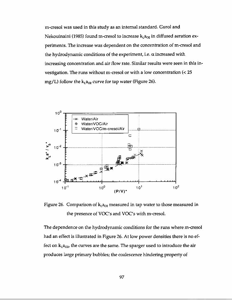
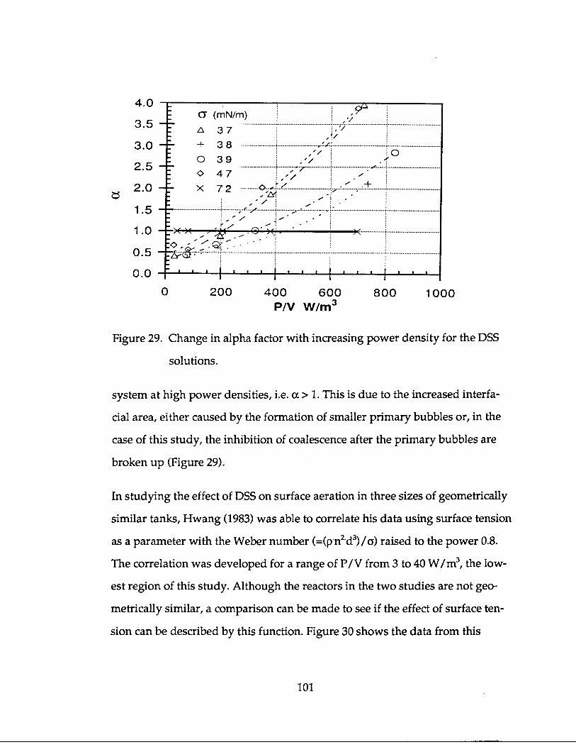
Gurol and Nekouinaini (1985) investigated the effects of various organics on the
characteristics of oxygen transfer from air bubbles to water, (acetic acid, 8 phe-
nols, tertiary butyl alcohol, toluene and chlorobenzene) . They used a bubble col-
umn with a glass frit or capillary to introduce the air . The effects of gas flow
rate, pH, and ionic strength were also examined .
Values of kLa in the presence of phenolic compounds, acetic acid and tertiary
butyl alcohol were consistently higher than those measured in pure water . Tolu-
ene and chlorobenzene (0 .4mM = 36.8 mg/L toluene) did not affect the kLa. The
type of substitution on the phenol molecule made a significant difference on the
magnitude of a . Their attempt to correlation their a values for the phenolic com-
pounds at pH 2.5 with the octanol-water partition coefficient (K ow) showed the
general trend that the more hydrophobic the compound (higher Kow), the
higher the a value . The effect of acetic acid on kLaO2 could not be explained with
this. The pH also had an influence on the change in kLa for the organics that de-
protonate: the protonated form of the molecule showed a much larger effect .
Above pH 7 acetic acid had little to no effect on a . Because of the higher pKa of
m-cresol, its affect on kLaO2 decreased only after -pH 9 was reached (a=2.5, 21 .6
mg/L).
42
Because bubbles coalesce more rapidly at high gas flow rates in a water/air sys-
tem, the presence of substances that suppress coalescence becomes more impor-
tant the higher the flow rate: a increased with an increase in QG. As already dis-
cussed above, an increase in ionic strength increased kLaO2. They found ions and
organics have additive effect. This is probably due to the concept of total
coalescence inhibition, which was not yet reached by the addition of salts, so
kLaO2 increased until the complete inhibition was achieved .
In order to investigate whether the increase in k LaO2 was due to coalescence or
surface tension variations, Gurol and Nekouinaini (1985) studied the behavior
of single bubbles in the presence of the organics . In experiments in which
bubble coalescence was prevented by non-frequent formation of bubbles, nei-
ther kLaO2 nor bubble size was affected by the organics . Measurements with a
tensiometer (Du Nouy ring method) showed no significant change in surface
tension due to the presence of the organics in the concentration ranges studied .
They studied the effect of a surfactant in the system. The typical behavior of sur-
factants was seen-first k LaO2 decreased with concentration (up to a =69 mN/m)
then it recovered (after a =62 mN/m) and increased to a=1 .3 as the
concentration increased . (a =72.8->56 mN/m). They found the presence of both
a surfactant and an organic compound have an additive effect .
2.4.1 Increased coalescence
Certain compounds in very low concentrations can cause a large increase in
coalescence. Zlokarnik (1980) reported experimental results with a nonionic
surfactant that is often used as an antifoam agent . He found that certain anti-
foamers at concentrations as low as 3 mg/L can reduce the oxygen transfer to
43
half that found in pure water . In experiments with biomass, he found an a
value of 0 .5. He postulated that the activated sludge flocs act as "crystallization
seeds", promoting bubble coalescence and, thus decreasing the oxygen trans-
fer. In comparison, in experiments with 6 g/L cellulose and 6 g/L activated
carbon in pure water, the finely dispersed solids alone did not strongly
promote coalescence .
In diffused aeration systems increases in air flow rate can sometimes reduce
the volumetric mass transfer coefficient, because the increased gas flow and re-
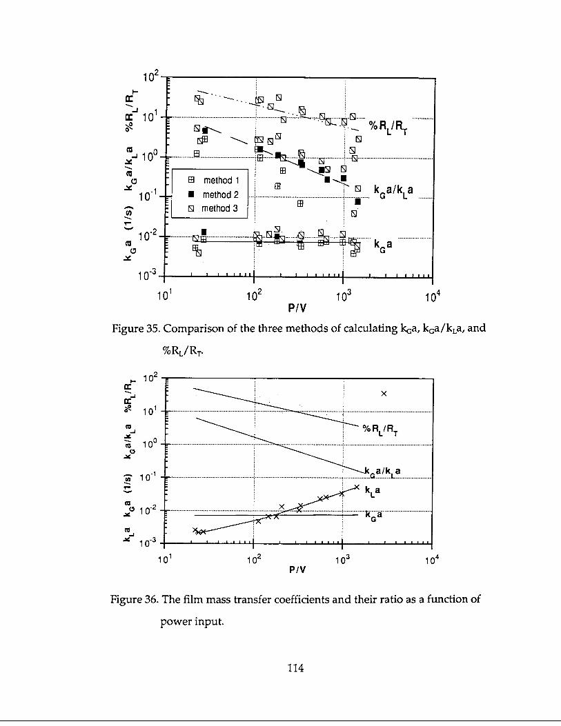
Figure 45. Comparison of the vales of kca, kGa/kLa, and %RL/RT measured in
tap water and the DSS solution .
Figure 46. Comparison of T . in tap water and in the DSS solution .
128
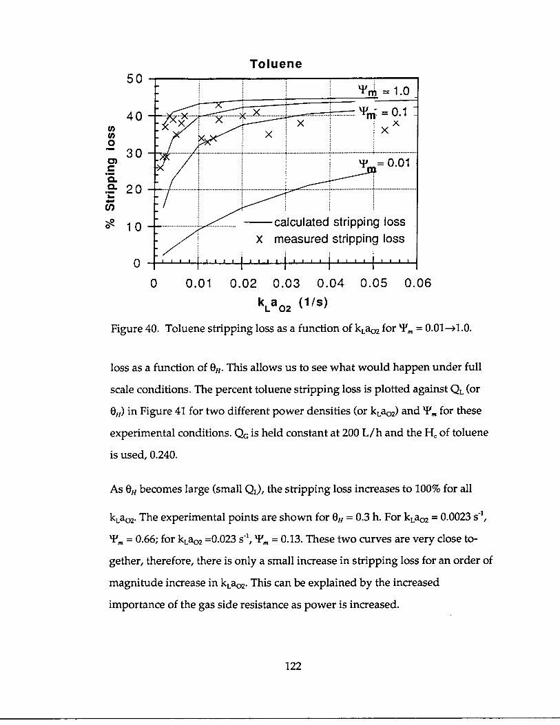
4.2.3 Application of results
The relationship KLavoc ='F*kLaO2 is being used to estimate stripping losses for
compounds of medium and low volatility in wastewater treatment processes .
As discussed in the previous sections, the mass transfer of semi-volatile com-
pounds is not controlled by liquid side resistance, but is a function of resistance
in both phases, so that'. <'F; therefore, the predicted VOC emissions using
this technique are being overestimated .
When upgrading aeration systems it is important to consider the effects of gas
side resistance on VOC emissions . If k Ga/kLa is decreased (i.e . the turbulence is
increased due to increased power density or increased gas flow) 'F. decreases,
and VOC emissions can remain unchanged, even though the oxygen transfer
rates are increased . If the method of aeration is changed, each method must be
evaluated in terms of kGa/kLa and 'F. in order to compare VOC emissions .
Subsurface aeration systems, such as the one used in this study, have lower
kc;a/kLa ratios than surface aerators for the same oxygen mass transfer coeffi-
cients (Hsieh, 1991), so that 'F. <<'F for subsurface aerators, resulting in lower
VOC emissions. Care should be exercised with free surfaces, weirs, and other
high kGa/kLa aeration devices .
VOC emissions from a reactor are also very dependent on the hydraulic reten-
tion time. The use of a process with a shorter hydraulic retention time and
higher oxygen mass transfer coefficient is preferable to a process with a longer
hydraulic retention time and lower oxygen mass transfer coefficient .
129
5 Conclusions
Volatilization, the mass transfer of chemicals from water to air, is an important
phenomenon to be considered when accessing the effectiveness of an activated
sludge process in treating wastewater high in volatile organic compounds
(VOC's). The aeration process can remove volatile compounds and less volatile
but not easily biodegraded compounds by the stripping effect . Volatilization can
also occur in other activated sludge unit processes, though theoretically the
major source of VOC emissions is the aeration process . This study investigated
the quantification of the simultaneous mass transfer of oxygen and volatile or-
ganic compounds in an aerated stirred tank reactor .
The mass transfer coefficients of oxygen and three VOC's, toluene, dichlorome-
thane, and 1,2-dichlorobenzene, were determined in three water systems : tap
water, tap water with an anionic surfactant, dodecyl sodium sulfate (DSS), and
tap water with biomass (oxygen only). A steady state method was chosen as the
appropriate method for studying the simultaneous mass transfer of oxygen and
VOC's in a stirred tank reactor . Experiments were made to span the range of
mass transfer coefficients found in both municipal and industrial wastewater
treatment processes .
Water/Air
The experimental kLaO2 values were compared to published correlations, which
describe the relationship between power input, superficial gas velocity and k La.
Comparison of this study's results to correlations made from data measured with
methods designed to avoid errors associated with gas phase depletion shows
good agreement .
130
Analysis of the results using dimensional analysis, k La* as a function of (P/ V) 3
and vs* ', showed that the results can be separated into two power regions, with
a=0.64 for 20-200 W/m3, and a=1 .0 for >200 W/m3; b=1 .0 for both regions. The
mass transfer process in the low power range (20-200 W/m) in the stirred tank
reactor is not well described by the superficial velocity . Using bubble velocities
and bubble retention time could possibly improve the correlation .
Water/VOC/Air
The addition of the three VOC's studied, toluene, dichloromethane, and 1,2-dich-
lorobenzene, to the tap water had no effect on k LaO2 at the concentrations used .
However, the addition of m-cresol as an internal standard at concentrations >25
mg/L inhibited bubble coalescence, which became important at the higher
power densities and increased kLaO2 dramatically .
Ratios of k Ga/kLa measured in the stirred tank reactor were low, ranging from
0.1 to 5. As power density increased, k Ga/kLa decreased. The gas film mass trans-
fer coefficient, kc;a, was found to be constant over the range of power densities
investigated .
KLaVOC increased initially as power density increased and then became constant
(_ He kGa), because both gas and liquid side resistance become important for com-
pounds with lower volatility (HH < 1) under the experimental conditions studied .
The increase was a function of the Henry's constant, H H . The KLa for toluene, the
most volatile compound, increased the most .
The stripping losses of the VOC's became independent of power, because KLavOC
approached a constant as power increased . Stripping loss becomes controlled by
the retention time, not by P/V. The range of power densities where K La and
1 31
stripping loss become independent depended on the He of the compound and the
value of kGa, i.e. for toluene (H,=0.24), at P/V>400 W/m3, and for dichlorome-
thane (K=0.105), at P/V>100 W/m3.
The ratio of the two mass transfer coefficients, K LaV /kLaO2 (Tm), decreased over
the range of power studied (20-2820 W/m); KLavoc approached a constant and
kLao2 increased with power. T. can be calculated for a system from the Henry's
constant and the ratio of kca/kLa.
Water/DSS/VOC/Air
The effect of an anionic surfactant (DSS) on mass transfer varied according to the
hydrodynamic conditions in the reactor .
In the moderately turbulent region both mass transfer coefficients were reduced
in the presence of DSS due to the dampening of interfacial turbulence by the ad-
sorbed layer of surfactant on the bubble/water interface. As power increased,
both mass transfer coefficients recovered to the values found in tap water; the
increased turbulence caused increased surface renewal at the bubble/water in-
terface, thereby annulling the effect of the surfactant . Therefore, in this region,
WPDSS 'FmTP
In the highly turbulent region, k Lao2 increased significantly, following the curve
of the Water/VOC/Air experiments in which coalescence was inhibited by m-
cresol. The inhibition of coalescence by the surfactant, as in the case of m-cresol,
increased the interfacial area . The VOC mass transfer coefficients recovered to
132
the values found in tap water . No further increase was seen because of the im-
portance of the gas phase resistance, as discussed above . Therefore, 'F,‚Dss < T.TP
due to the increase in k LaO2 .
Water/Biomass/Air
The oxygen mass transfer coefficient was measured in the presence of biomass .
The kLaO2 values were reduced at the lower to medium power densities, recover-
ing only at very high power densities. The mixed liquor was characterized in
terms of surface tension, suspended solids, and TOC. A comparison of the effect
of surfactant at this surface tension and the effect of the biomass showed that sur-
face tension alone was not enough to describe the changes in k LaD2 .
133
6 References
Addison, C .C. (1944). "The properties of freshly formed surfaces . Part III. Themechanism of adsorption, with particular reference to the octyl alcohol-watersystem," J.Chem.Soc ., 477-480 .
Addison, C.C. (1945). 'The properties of freshly formed surfaces . Part IV. The in-fluence of chain length and structure on the static and the dynamic surfacetensions of aqueous-alcoholic solutions," J.Chem.Soc ., 98-106.
Allen, C.C., D.A. Green, J.B. White, and J.B. Coburn (1986) . "Preliminary assess-ment of air emissions from aerated waste treatment systems at hazardouswaste treatment storage and disposal facilities," US EPA, Hazardous WasteEngineering Research Laboratory, Office of Research and Development, Cin-cinnati, Ohio .
Andrews, G.F., R. Fike, and S. Wong (1988). "Bubble hydrodynamics and masstransfer at high Reynolds number and surfactant concentration," Chemical En-
gineering Science, Vol.43, No.7,1467-1477 .
ASCE, ASCE Standard (1984) . "Measurement of oxygen transfer in clean water,"ISBN 0-87262-430-7, New York .
Baillod, C.R., W.L. Paulson, J.J. McKeown, and H.J. Campbell,Jr . (1986) . "Accu-racy and precision of plant scale and shop clean water oxygen transfer tests,"J. Water Pollut. Control Fed., Vol.58, No.4, 290-299.
Berglund, R.L., G.M. Whipple, J.L. Hansen, G.M. Alsop, T.W. Siegrist, B.E .Wilker, and C.R. Dempsey (1985). "Fate of low solubility chemicals in a petro-leum chemical wastewater treatment facility," Presented at the National Meet-ing of the AICHE .
Bird, R.B., W.E. Stewart, and E.N. Lightfoot (1960) . Transport Phenomena, JohnWiley and Sons, Inc., New York.
Blackburn, J.W., W.L. Troxler, K .N. Truong, R.P. Zink, S .C. Meckstroth, J.R. Flo-rance, A. Groen, G .S. Sayler, R.W Beck, R.A. Minear, A . Breen, and O . Yagi(1985) . "Organic chemical fate prediction in activated sludge processes,"EPA-600/2-85/102 US EPA, Cincinnati, Ohio .
1 34
Brown, L.C . and C.R. Baillod (1982). "Modeling and interpreting oxygen transferdata," J.Env.Eng.Div., ASCE, Vol.108, No.4, 607-628.
Campbell, H.J ., R.O. Ball, and J.H. O'Brien (1976). "Aeration testing and design -a critical review," 8th Mid-Atlantic Industrial Waste Conference, university ofDelaware, January 13,1976,1-35.
Chang, D.P.Y., E.D. Schroeder, and R .L. Corsi (1987) . "Emissions of volatile andpotentially toxic organic compounds from sewage treatment plants and col-lection systems," Report California Air Resources Board .
Chapman, C.M., L.G. Gilibaro, and A.W. Nienow (1982). "A dynamic responsetechnique for the estimation of gas-liquid mass transfer coefficients in astirred vessel," Chemical Engineering Science, Vol.37, No.6, 891-896 .
Corsi, R.L., E.D. Schroeder, and D.P.Y. Chang (1989) . "Discussion of estimatingvolatile organic compound emissions from publicly owned treatment works,"J. Water Pollut. Control Fed ., Vol.61, No.1, 95-96.
Danckwerts, P.V. (1951) . "Significance of liquid-film coefficient in gas absorp-tion," Ind.Eng.Chem ., Vol.43, No.6,1460-1467 .
Dang, N.D.P., D.A. Karrer, and I.J. Dunn (1977) . Biotechnol.Bioeng., Vol.19, 853 .
Dixon, G., and B. Bremen (1984) . "Technical background and estimation methodsfor assessing air releases from sewage treatment plants," Versar, Inc ., Memo-randum.
Drogaris, G. and P. Weiland (1983) . "Coalescence behavior of gas bubbles inaqueous solutions of n-alcohols and fatty acids," Chemical Engineering Science,
Vol.38, No.9,1501-1506 .
Eckenfelder, W.W. and D.L. Ford (1968) . "New concepts in oxygen transfer andaeration," Advances in Water Ouality Improvements, Ed. by Gloyna, E.F. andW.W. Eckenfelder, Univ . of Texas Press, 215-236 .
Figueiredo, M.M.L. and P.H. Calderbank (1979) . '"The scale-up of aerated mixingvessels for specified oxygen dissolution rates," Chemical Engineering Science,Vol.34, No. 11, 1333-1338.
135
Gibilaro, L.G., S.N. Davies, M. Cooke, P.M. Lynch, and J.C. Middleton (1985) ."Initial response analysis of mass transfer in a gas sparged stirred vessel,"Chemical Engineering Science, Vol.40, No.10, 1811-1816 .
Gurol, M.D. and S. Nekouinaini (1985). Effect of organic substances on masstransfer in bubble aeration . J. Water Pollut. Control Fed ., Vol.57, No.3, 235-240 .
Higbie, R. (1935). 'The rate of absorption of a pure gas into a still liquid duringshort periods of exposure," Trans. AIChE, Vol.31, 365-388 .
Hsieh, C.C. (1990). "Estimating volatilization rates and gas/liquid mass transfercoefficients in aeration systems," Ph .D. Prospectus, University of California,Los Angeles .
Hwang, H.J., and M.K. Stenstrom (1979) . "Effects of surface active agents on oxy-gen transfer," Water Resources Program, Report 79-2, University of California,Los Angeles .
Hwang, H.J. (1983). "Comprehensive studies of oxygen transfer under nonidealconditions," Dissertation, University of California, Los Angeles .
Ihme, F. (1975) . "Leistungsbedarf and Verformung der Fluessigkeitsoberflaechebeim Ruehren newtonischer Fluessigkeiten mit Turbinenblatt- and Anker-ruehrern," Dissertation, Technical University Berlin.
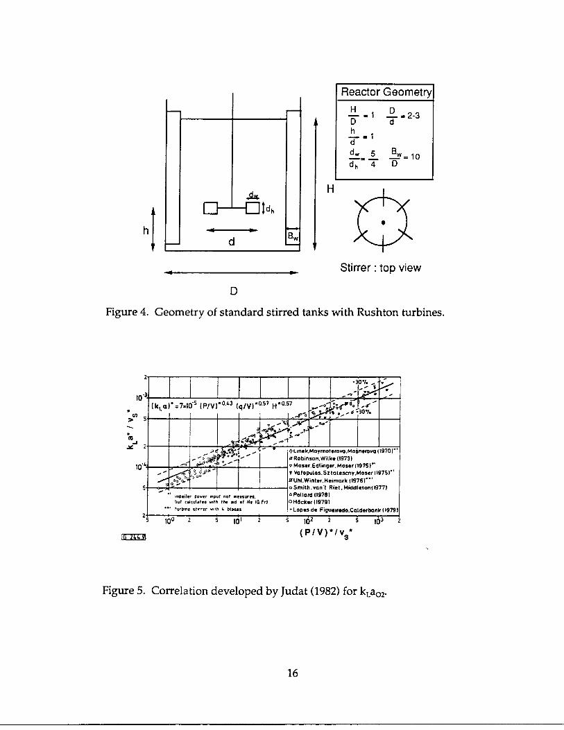
Judat, H., (1982) . "Gas/liquid mass transfer in stirred vessels-a critical review",German Chemical Engineering, Vol.5, 357-363 .
Kapartis, N. (1991) . "Einfluss der Biomasse auf die Desorptionsgeschwindigkeitfluechtiger Substrate in beluefteten Ruehrreaktoren," Diplomarbeit, Tech-nische Universitaet Berlin .
Keitel G. and U. Onken (1982). "Zur Koaleszenzhemmung durch Elektrolyte andorganische Verbindungen in waessrigen Gas/Fluessigkeits-Dispersionen,"Chemie Ingenieur Technik, Vol.54, No.3, 262-263 .
Kincannon, D.F., A. Weinert, R. Padorr, and E.L. Stover (1983) . "Predicting treat-ability of multiple organic priority pollutant wastewaters from single-
1 36
pollutant treatability studies," Proceedings 37th Industrial Waste Conf ., May1982, Purdue University, J. Bell, Ed ., Ann Arbor Science, Ann Arbor,Michigan, 640-650 .
Kincannon, D.F. and E.L. Stover (1983) . "Determination of activated sludge bioki-netic constants for chemical and plastic industrial wastewater," EPA-600/2-83-073A, US EPA, Cincinnati, Ohio .
Koshy, A., T.R. Das, and R. Kumar (1988). "Effect of surfactants on drop breakagein turbulent liquid dispersions," Chemical Engineering Science, Vol.43, No.3,649-654.
Khudenko, B.M., and A. Garcia-Pastrana (1987) . "Temperature influence on ab-sorption and stripping processes," Wat.Sci.Tech ., Vol.19, 877-888.
Lee, Y.H., G.T. Tsao, and P.C. Wankat (1980) . "Hydrodynamic effect of surfac-tants on gas-liquid oxygen transfer," AIChE J, Vol.26 No.6,1008-1012.
Lewis, W.K. and W.G. Whitman (1924). "Principles of gas absorption,"Ind.Eng.Chem ., Vol.16, No.3,1215-1220.
Lincoff, A.H. and J.M. Gossett (1984) . 'The determination of Henry's constant forvolatile organics by equilibrium partitioning in closed systems," in Gas Trans-fer at Water Surfaces, W. Brutsaert and G.H. Jirka (eds.), D. Reidel PublishingCo., 17-25 .
Linek, V., J. Mayrhoferova, and J . Mosnerova (1970) . "The influence of diffusivityon liquid phase mass transfer in solutions of electrolytes," Chemical Engineer-
ing Science, Vol.25, 1033-1045 .
Linek, V., P. Benes, V . Vacek, and F. Hovorka (1982). "Analysis of differences inkLa values determined by steady-state and dynamic methods in stirred tanks,"The Chemical Engineering Journal, 25 (1982) 77-88.
Linek, V., V. Vacek, and P. Benes, (1987) . "A critical review and experimental ver-ification of the correct use of the dynamic method for the determination of ox-ygen transfer in aerated agitated vessels to water, electrolyte solutions andviscous liquids," The Chemical Engineering Journal, Vol.34,11-34 .
Llorens, J ., C. Mans, and J . Costa (1988) . "Discrimination of the effects of surfac-tants in gas absorption," Chemical Engineering Science, Vol.43, No.3, 443-450
137
Mackay, D. and P.J. Leinonen (1975). "Rate of evaporation of low solubility con-taminants from water bodies to atmosphere," Environmental Science and Tech-
nology, Vol.9, No.13,1178-? .
Mackay, D., W.Y. Shiu, and R.P. Sutherland (1979) . "Determination of air-waterHenry's law constants for hydrophobic pollutants," Environmental Science and
Technology, Vol.13, No.3, 333-337.
Mackay, D. and W.Y. Shiu (1981) . "A critical review of Henry's law constants forchemicals of environmental interest," J.Phys.Chem.Ref.Data, Vol .10, No.4,1175-1199 .
Mancy, K.H. and D.A. Okun (1960). "Effects of surface active agents on bubbleaeration," J. Water Pollut. Control Fed., Vol.32, No.4, 351-364.
Mancy, K.H. and D.A. Okun (1965). "Effects of surface active agents on bubbleaeration," J. Water Pollut. Control Fed., Vol.37, No.2, 212-227.
Masutani, G .K. (1988). "Dynamic surface tension effects on oxygen transfer in ac-tivated sludge," Dissertation, University of California, Los Angeles .
Masutani, G .K. and M.K. Stenstrom (1991) . "Dynamic surface tension effects onoxygen transfer," J.Env.Eng.Div., ASCE, Vol.117, No.1, 126-142.
Matter-Mueller, C ., W. Gujer, and W. Giger (1981), "Transfer of volatile sub-stances from water to the atmosphere," Water Research, Vol.15,1271 .
Mueller, J.S. and H.D. Stensel (1990) . "Biologically enhanced oxygen transfer inthe activated sludge process," J. Water Pollut. Control Fed ., Vol.62, No.2,193-203 .
Munz, C. and P.V. Roberts (1984) . "The ratio of gas phase to liquid phase masstransfer coefficients in gas-liquid contacting processes," in Gas Transfer atWater Surfaces, W. Brutsaert and G .H. Jirka (eds.), D. Reidel Publishing Co .,35-45 .
Nagata, S . (1975) . Mixing: Principles and applications . Halstead Press, New York.
Ollenik, R. and W. Nitsch (1981) . "Einfluss von Tensiden auf Stroemung andStoffuebergang in einer Fluessig/fluessig-Kanalstroemung," Berichte der Bun-
Osorio, C. (1985). "Untersuchung des Einflusses der Fluessigkeitseigenschaftenauf den Stoffuebergang Gas/Fluessigkeit mit der Hydrazin-oxidation," Dis-sertation, Universitaet Dortmund, 1-109 .
Padday, J .F. (1969a) . "Surface tension. Part I. The theory of surface tension," Sur-
face and Colloid Science, Vol.1, 39-99.
Padday, J .F. (1969b). "Surface tension . Part II. The measurement of surface ten-sion," Surface and Colloid Science, Vol.1,101-153 .
Philichi, T .L. and M.K. Stenstrom (1989) . 'The effects of dissolved oxygen probelag on oxygen transfer parameter estimation," J. Water Pollut . Control Fed., Vol
61, No.1, 83-86.
Rathbun, R.E., W.S. Doyle, D .J. Shultz, and D.Y. Tai (1978) . "Laboratory studies ofgas tracers for reaeration," J.Env.Eng.Div., ASCE, Vol.104, No.2, 215-229 .
Redmon, D., W.C. Boyle, and L. Ewing (1983) . "Oxygen transfer efficiency mea-surements in mixed liquor using off-gas techniques," J. Water Pollut . Control
Fed., Vol.55, No. 11, 1338-1347 .
Roberts, P.V., and P.G. Daendilker (1983) . "Mass transfer of volatile organic con-taminants from aqueous solution to the atmosphere during surface aeration,"Environmental Science and Technology, Vol.17, No.8,1983, 484489 .
Roberts, P.V., C. Munz, and P. Daendliker (1984a) . "Modeling volatile organicsolute removal by surface and bubble aeration," J. Water Pollut . Control Fed .,
Vol 56,157-163 .
Roberts, P.V., C. Munz, P . Daendliker, and C. Matter-Mueller (1984b) . "Volatil-ization of organic pollutants in wastewater treatment- model studies," EPA-600/S2-84-047, US EPA, Cincinnati, Ohio.
Sherwood, T.K., R.L. Pigford, and C.R. Wilke (1975) . Mass Transfer, McGraw-Hill, New York .
Smith, J.H., D.C. Bomberger, and D .L. Haynes (1981) . "Volatilization rates of in-termediate and low volatility chemicals from water," Chemosphere, Vol.10,No.3, 281-289 .
139
Smith, J.H., D. Mackay, and C .W.K. Ng (1983a) . "Volatilization of pesticides fromwater." Residue Reviews, Vol 85, Springer-Verlag, New York, Inc ., 73-88 .
Smith, J.H., D.C. Bomberger, and D .L. Haynes (1983b). "Prediction of the volatil-ization rates of high volatility chemicals from natural water bodies," Environ-mental Science and Technology, Vol.14, No. 11, 1332-1337.
Spalding, D .B, (1963) . Convective Mass Transfer, Edward Arnold Publishers Ltd .,London.
Springer, T.G. and R.L. Pigford (1970) . "Influence of surface turbulence and sur-factants on gas transport through liquid interfaces," Ind.Eng.Chem., Fundam.,Vol.9, No.3, 458-465 .
Stenberg, O. and B. Andersson (1988). "Gas-liquid mass transfer in agitated ves-sels. II. Modeling of gas-liquid mass transfer ." Chemical Engineering Science,Vol.43, No.3, 725-730 .
Stenstrom, M.K. and R.G . Gilbert (1981). "Review Paper: Effects of alpha, beta,and theta factor upon the design, specification and operation of aeration sys-tems," Water Research, Vol. 15, 643-654 .
Treybal, R .E. (1968) . Mass Transfer Operations, 2.Ed., McGraw-Hill, New York .
Truong, K.N. and J.W. Blackburn (1984) . "The stripping of organic chemicals inbiological treatment processes," Environ.Prog., Vol 3, No 3,143-152 .
US Environmental Protection Agency (1982) . "Fate of priority pollutants in pub-licly owned treatment works, Vol 1 .," EPA-440/1-82/303, US EPA, Office ofwater regulations and standards, Washington, D .C.
Van Dierendonck, L.L., J.M.H. Fortuin, and D. Venderbos (1968). "The specificcontact area in gas-liquid reactors," Chem.Reaction Eng.Symp., 205-213 .
Verscheuren, K. (1977) . Handbook of Environmental Data on Organic Chemicals,Van Nostrand Reinhold Co., New York .
140
Versteeg, G.F ., P.M.M. Blauwhoff, and W.P.M. van Swaaij (1987) . 'The effect ofdiffusivity on gas-liquid mass transfer in stirred vessels . Experiments at atmo-spheric and elevated pressures," Chemical Engineering Science, Vol.42,1103-1119 .
Wiesmann, U . (1988). Lecture notes, Chemical Engineering Department, Techni-cal University Berlin .
Yuteri, C ., D.F. Ryan, J .J. Callow, and M.D. Gurol (1987) . "The effectof chemical composition of water on Henry's law constant," J. Water Pollut .
Control Fed., Vol.59, No. 11, 950-956 .
Zieminski, S.A., R.L. Hill (1962) . "Bubble aeration of water in the presence ofsome organic compounds," J.Chem.Eng.Data, Vol.7, No.1, 51-54.
Zieminski, S.A., M.M. Caron, and R.B. Blackmore (1967) . "Behavior of air bubblesin dilute aqueous solutions," Ind.Eng.Chem., Fundam ., Vol.6, No.2, 233-242 .
Zlokarnik, M. (1978). "Sorption characteristics for gas-liquid contacting in mixingvessels," Advances in Biochemical Engineering, Vol.8,133-151 .
Zlokarnik, M. (1980). "Koaleszenzphaenomene im System gasfoermig/fluessigand deren Einfluss auf den 02Eintrag bei der biologischen Abwasserreini-gung," Korrespondenz Abwasser, Vol.27, No.11, 728-734 .
141
Appendix
Power input correlation
The power input into the reactor was calculated using the following correlation
from Judat (1976) . The correlation is valid for the water/air system with