95
Introductory QED and QCD RAL Summer School September 2007 David J. Miller University of Glasgow Recommended Text: Quarks & Leptons by F. Halzen and A. Martin
| Date post: | 22-Apr-2018 |
| Category: |
Documents |
| Upload: | hoangtuyen |
| View: | 220 times |
| Download: | 3 times |

Introductory QED and QCD
RAL Summer SchoolSeptember 2007
David J. MillerUniversity of Glasgow
Recommended Text: Quarks & Leptons by F. Halzen
and A. Martin

2
Rough outline of topics
Non-relativistic Quantum MechanicsThe Schrodinger equation
Relativistic Quantum MechanicsThe Klein-Gordon Equation, The Dirac Equation, Angular Momentum and Spin, Symmetries of the Dirac Equation
Quantum ElectrodynamicsClassical Electromagnetism, The Dirac Equation in an electromagnetic field
Scattering and Perturbation TheoryThe QED Feynman rules, cross-sections, crossing symmetry, identical particles, the fermion propagator, decay rates
Quantum ChromodynamicsQuarks, gluons and color, renormalisation, running couplings
3
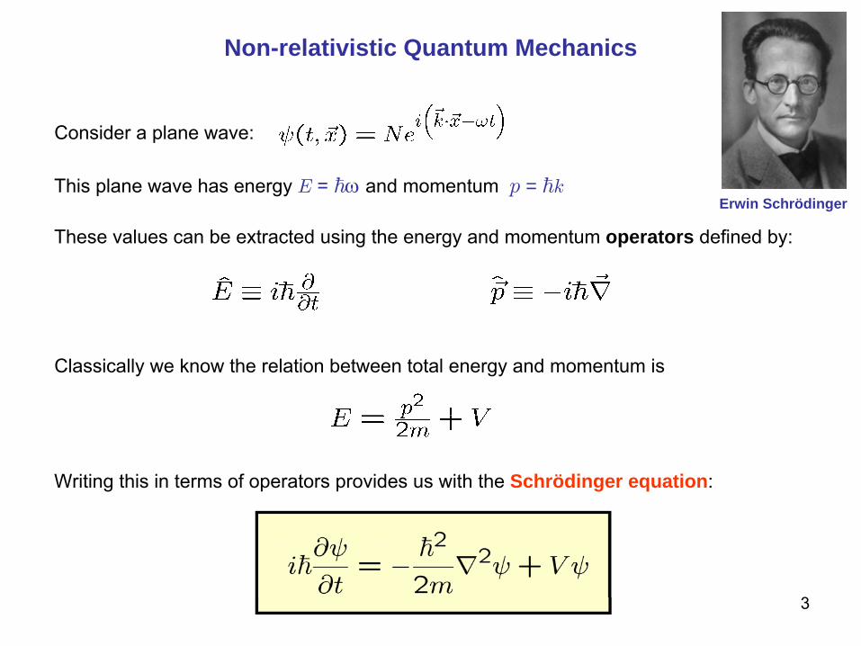
Non-relativistic Quantum Mechanics
Consider a plane wave:
This plane wave has energy E
= ~ω
and momentum p
= ~k
These values can be extracted using the energy and momentum operators defined by:
Classically we know the relation between total energy and momentum is
Writing this in terms of operators provides us with the Schrödinger equation:
Erwin Schrödinger
4
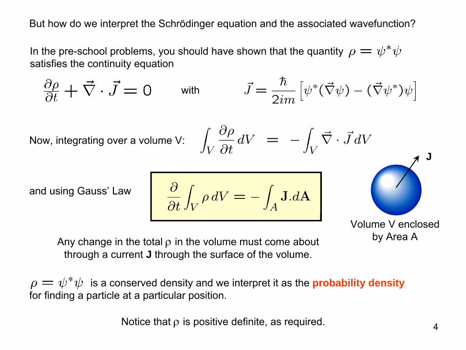
In the pre-school problems, you should have shown that the quantity satisfies the continuity equation
But how do we interpret the Schrödinger equation and the associated wavefunction?
with
Now, integrating over a volume V:
Volume V enclosed by Area A
J
and using Gauss’
Law
Any change in the total ρ
in the volume must come about through a current J through the surface of the volume.
is a conserved density and we interpret it as the probability density for finding a particle at a particular position.
Notice that ρ
is positive definite, as required.

5
Relativistic Quantum Mechanics
The Schrödinger Equation only describes particles in the non-relativistic limit. To describe the particles at particle colliders we need to incorporate special relativity.
Let’s have a quick review of special relativity
We construct a position four-vector as
An observer in a frame S0
will instead observe a four-vector where denotes a Lorentz transformation.
e.g. under a Lorentz boost by v in the positive x direction:

6
The quantity xμxμ
is invariant under a Lorentz transformation
where is the metric tensor of Minkowski
space-time.
A particle’s four-momentum is defined by where is proper time,
the time in the particle’s own rest frame. Proper time is related to an observer’s time via
Its four-momentum’s time component is the particle’s energy, while the space components are its three-momentum
and its length is an invariant, its
mass:
note the definition of a covector
⇔

7
Finally, I define the derivative
Note that you will sometimes use the vector expression
Watch the minus sign!
For simplicity, from now on I will use natural units. Instead of writing quantities in terms of kg, m and s, we could write them in terms of c, ~
and eV:
c = 299 792 458 ms-1
~
= 6.582 118 89(26) ×
10-16
eV
s1 eV
= 1.782 661 731(70) c2
kg
So any quantity with dimensions kga
mb
sc
can be written in units of eVα
~β
cγ
with,
Then we omit ~
and c in our quantites
(you can work them out from the dimensions).
transforms as
so

8
The Klein-Gordon Equation
The invariance of the four-momentum’s length provides us with a relation between energy, momentum and mass:
(We have set V=0 for simplicity.)
( ∂2
≡
∂μ
∂μ
is sometimes written as or 2 )
Oskar Klein
This has plane-wave solutions
normalization
Replacing energy and momentum with , gives the Klein-Gordon equation:
Alternatively, in covariant notation:
with gives

9
This is the relativistic wave equation for a spin zero particle, which conventionally is denoted φ. Under a Lorentz transformation the Klein-Gordon operator is invariant:
with So(Lorentz trans. preserve the norm)
real (since is real)
Under continuous Lorentz transformations, S must be the same as for the identity, ie. S = 1
If S = 1, then φ
is a scalar
If S = -1, then φ
is a pseudoscalar
But for a parity inversion it can take either sign

10
Since φ
is invariant, then |φ|2
does not change with a Lorentz transformation.
This is at odds with our previous interpretation of |φ|2
as a probability density, since densities do change with Lorentz transformations (the probability P = ρV = constant).
One possible choice is:
(this is the same current as before, just with a different normalisation)
As a four-vector,
We need new definitions for the density ρ
and current J which satisfy the continuity equation
or, convariantly, with
11
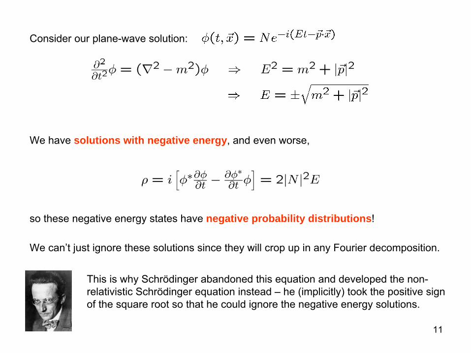
Consider our plane-wave solution:
We have solutions with negative energy, and even worse,
so these negative energy states have negative probability distributions!
We can’t just ignore these solutions since they will crop up in any Fourier decomposition.
This is why Schrödinger abandoned this equation and developed the non-
relativistic Schrödinger equation instead –
he (implicitly) took the positive sign of the square root so that he could ignore the negative energy solutions.

12
Feynman-Stuckelberg Interpretation
You will see in your QFT course that positive energy states must
propagate forwards in time in order to preserve causality.
Feynman and Stuckelberg
suggested that negative energy states propagate backwards in time.
If the field is charged, we may reinterpret as a charge density, instead of a probability density:
If E < 0, just move the sign into the time:
Particles flowing backwards in time are then reinterpreted as anti-particles flowing forwards in time.
Now ρ
= j0, so for a particle of energy E:
while for an anti-particle of energy E:
which is the same as the charge density for an electron of energy -E

13
In reality, we only ever see the final state particles, so we must include these anti-particles anyway.
Quantum mechanics does not adequately handle the creation of particle—anti-particle pairs out of the vacuum. For that you will need Quantum Field Theory.
positive energy state flowing forwards in time
time
spac
e
negative energy state flowing backwards in time
≡positive energy anti-particle state
flowing forwards in time

14
The particle (or charge) density allows us to normalize the KG solutions in a box.
Normalization of KG solutions
So if we normalize to 2E
particles per unit volume, then N
= 1
Notice that this is a covariant choice. Since the number of particles in a box should be independent of reference frame, but the volume of the box changes with a Lorentz boost, the density must also change with a boost. In fact, the density is the time component of a four-vector j0.
so in a box of volume V the number of particles is:

15
The Dirac Equation
The problems with the Klein-Gordon equation all came about because of the square root required to get the energy:
Dirac tried to get round this by finding a field equation which was linear in the operators.
All we need to do is work out and
Paul Dirac

16
So, comparing with we must have:
Now, we have where i
and j
are summed over 1 ,2,3
and are anti-commuting objects – not just numbers!

17
These commutation relations define α
and β. Anything which obeys these relations will do. One possibility, called the Dirac representation, is the 4×4 matrices:
2×2 matrices
where σi
are the usual Pauli matrices:
Since these act on the field ψ, ψ
itself must now be a 4 component vector, known as a spinor.

18
We can write this equation in a four-vector form by defining a new quantity γμ:
The anti-commutation relations become:
And the Dirac Equation is: (with )
Often is written as

19
Does the Dirac Equation have the right properties?
Is the probability density positive definite?
A appropriate conserved quantity is now with
In four-vector notation,
( Note )with
Clearly always!
20
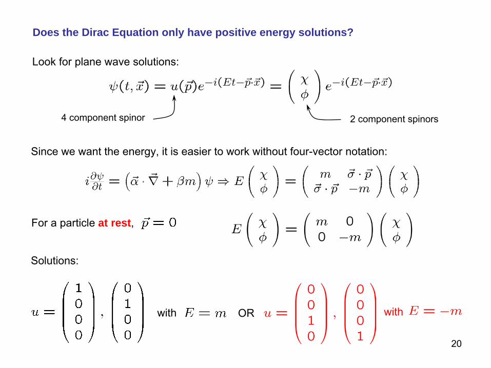
Does the Dirac Equation only have positive energy solutions?
Since we want the energy, it is easier to work without four-vector notation:
Look for plane wave solutions:
4 component spinor 2 component spinors
For a particle at rest,
Solutions:
with withOR

21
Dirac got round this by using the Pauli Exclusion principle.
He reasoned that his equation described particles with spin (e.g. electrons) so only two particles can occupy any particular energy level (one spin-up, the other spin-down).
E=0
Dira
c S
ea
…
Ene
rgy
If all the energy states with E<0 are already filled, the electron can’t fall
into a negative energy state.
…
Moving an electron from a negative energy state to a positive one leaves a
hole which we interpret as an anti-particle.
Note that we couldn’t have used this argument for bosons (no exclusion principle) so the Feynman-Stuckleberg interpretation is more useful.
Oops! We still have negative energy solutions!

22
A General Solution
We need to choose a basis for our solutions. Choose,
Check these are compatible:
since

23
Conventions differ here: sometimes the
order is inverted
Positive Energy Solutions, E > 0, are
[Normalization choice (see next slide)]
Typically, we write this in terms of the antiparticle’s energy and momentum:
Antiparticle spinor, normalised to make
Negative Energy Solutions, E < 0, are

24
Normalization of solutions
Notice the normalization choice made for the spinors.
So a covariant normalization is
unitvolume
Just like for the KG equation, we can choose to have 2E particles per unit volume
But
Occasionally, I will instead normalize spinors
to 2E
particles per volume V
Then
and only set V
=1 at the end.

25
Orthagonality and completeness
With the normalization of 2E
particles per unit volume, it is rather obvious that:
This is a statement of orthogonality.
Less obvious, but easy to show, are the completeness relations:

26
Angular Momentum and Spin
The angular momentum of a particle is given by .
If this commutes with the Hamiltonian then angular momentum is conserved.
So the quantity is conserved!
This is not zero, so is not conserved!
But, if we define
then

27
is the orbital angular momentum, whereas is an intrinsic angular momentum
Notice that our basis spinors
are eigenvectors of
with eigenvalues
Note that an E < 0 electron with spin ≡
an E > 0 positron with spin
This is why we switched the labelling of the anti-particles earlier.

28
Helicity of massless fermions
If the mass is zero, our wave equation becomes
These two component spinors, called Weyl spinors, are completely independent, and can even be considered as separate particles!
Notice that each is an eigenstate
of the operator with eigenvalues
for massless
state
Writing then we find the equations decouple
and

29
For the full Dirac spinor, we define the Helicity operator as
This is the component of spin in the direction of motion.
Since an antiparticle has opposite momentum it will have opposite helicity.
left handed particle right handed antiparticle
A particle with a helicity
eigenvalue
is right handed
A particle with a helicity
eigenvalue
is left handed
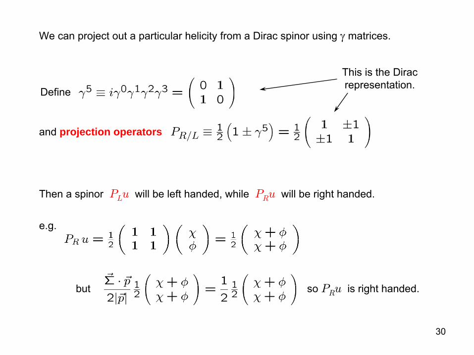
30
We can project out a particular helicity
from a Dirac spinor
using γ
matrices.
Then a spinor
PL
u
will be left handed, while PR
u
will be right handed.
Define
and projection operators
This is the Dirac representation.
e.g.
but so PR
u
is right handed.

31
We can make this more explicit by using a different representation of the γ
matrices.
Now
The left-handed Weyl
spinor
sits in the upper part of the Dirac spinor, while the right handed Weyl
spinor
sits in the lower part.
e.g.
The chiral representation (sometimes called the Weyl representation) is:
32
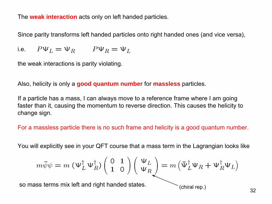
Since parity transforms left handed particles onto right handed ones (and vice versa),
i.e.
the weak interactions is parity violating.
Also, helicity
is only a good quantum number for massless particles.
If a particle has a mass, I can always move to a reference frame
where I am going faster than it, causing the momentum to reverse direction. This causes the helicity
to change sign.
For a massless
particle there is no such frame and helicity
is a good quantum number.
The weak interaction acts only on left handed particles.
You will explicitly see in your QFT course that a mass term in the Lagrangian
looks like
so mass terms mix left and right handed states. (chiral
rep.)

33
Symmetries of the Dirac Equation
The Lorentz Transformation
How does the field behave under a Lorentz transfromation?
( γμ
and m are just numbers and don’t transform)
Premultiply
by :
This notation differs in different texts. e.g. Peskin
and Schroeder would write
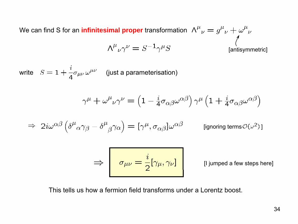
34
We can find S for an infinitesimal proper transformation
[antisymmetric]
This tells us how a fermion field transforms under a Lorentz boost.
write (just a parameterisation)
[ignoring terms ]
[I jumped a few steps here]

35
The adjoint
transforms as
[since for the explicit form of S
derived above]
So is invariant.
And so our current is a four-vector.
scalar
pseudoscalar
vector
axial vector
tensor
Common fermion bilinears:

36
Can you derive the parity transformations of the bilinears
given on the last slide?
You should see that η drops out, so there is no loss of generality setting η = 1
Parity
A parity transformation is an improper Lorentz transformation described by
Again , so and
Since commutes with itself (trivially) and anticommutes
with , a suitable choice is

37
Charge Conjugation
Another discrete symmetry of the Dirac equation is the interchange of particle and anti-
particle.
Therefore we need C
such that
Premultiply
by and the Dirac equation becomes:
used and
Take the complex conjugate of the Dirac equation:

38
The form of C changes with the representation of the γ-matrices. For the Dirac representation a suitable choice is
How does this transformation affect the stationary solutions?
We have mapped particle states onto antiparticle states, as desired.
etc

39
Time Reversal
A naive transformation of the wavefunction
is not sufficient for time reversal. Since the momentum of a particle, is a rate of change, it too must change sign.
We must (again!) make a complex conjugation:
Take complex conjugation of Dirac Equation, switch and pre-multiply by T:
Changing the momentum direction and time for a plane wave gives:

40
Need:
A suitable choice is:

41
CPT
For the discrete symmetries, we have shown:
Doing all of these transformations gives us
So if is an electron, is a positron travelling backwards in space-time multiplied by a factor .
This justifies the Feynman-Stuckleberg interpretation!
42
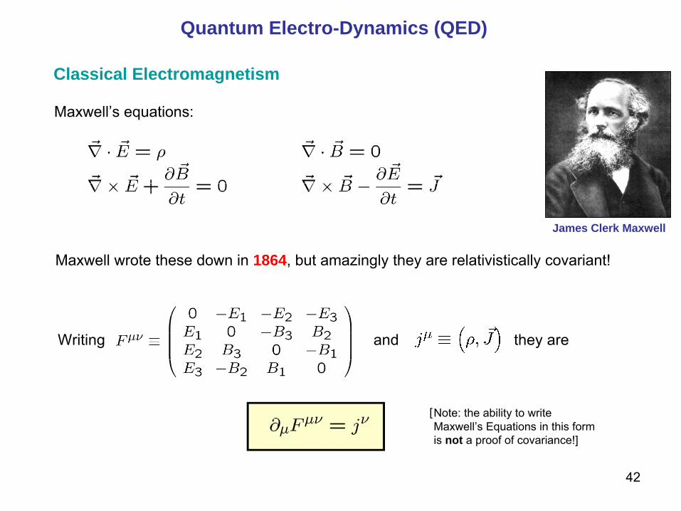
Quantum Electro-Dynamics (QED)
Maxwell’s equations:
Maxwell wrote these down in 1864, but amazingly they are relativistically
covariant!
James Clerk Maxwell
Classical Electromagnetism
Note: the ability to write Maxwell’s Equations in this form is not a proof of covariance!]
[
Writing and they are

43
Maxwell’s equations can also be written in terms of a potential Aμ
Writing
we have
Choose λ
such that
This is a gauge transformation, and the choice is know as the Lorentz gauge.
In this gauge:
Now, notice that I can change Aμ
by a derivative of a scalar and leave Fμ ν
unchanged

44
The wave equation with no source, has solutions
with
So has only 3 degrees of freedom (two transverse d.o.f. and one longitudinal d.o.f.)
The Lorentz condition
We still have some freedom to change Aμ, even after our Lorentz gauge choice:
is OK, as long as
Usually we choose such that . This is known as the Coulomb gauge.
So only two polarisation states remain (both transverse).
polarisation vector with 4 degrees of freedom

45
The Dirac Equation in an Electromagnetic Field
So far, this has been entirely classical. So how do we incorporate electromagnetism into the quantum Dirac equation?
We do the ‘obvious’
thing and replace the momentum operator
charge of the electron = -e
Beware:
conventions differ, e.g. Halzen
and Martin have
while Peskin
& Schroeder have as above
Then
Dμ
is called the Covariant Derivative, and the Dirac Equation in an electromagnetic field becomes
Often we write

46
The Magnetic Moment of the Electron
We saw that the interaction of an electron with an electromagnetic field is given by
Writing as before,
Coulomb gauge ⇒ A0=0
Also,
andSo
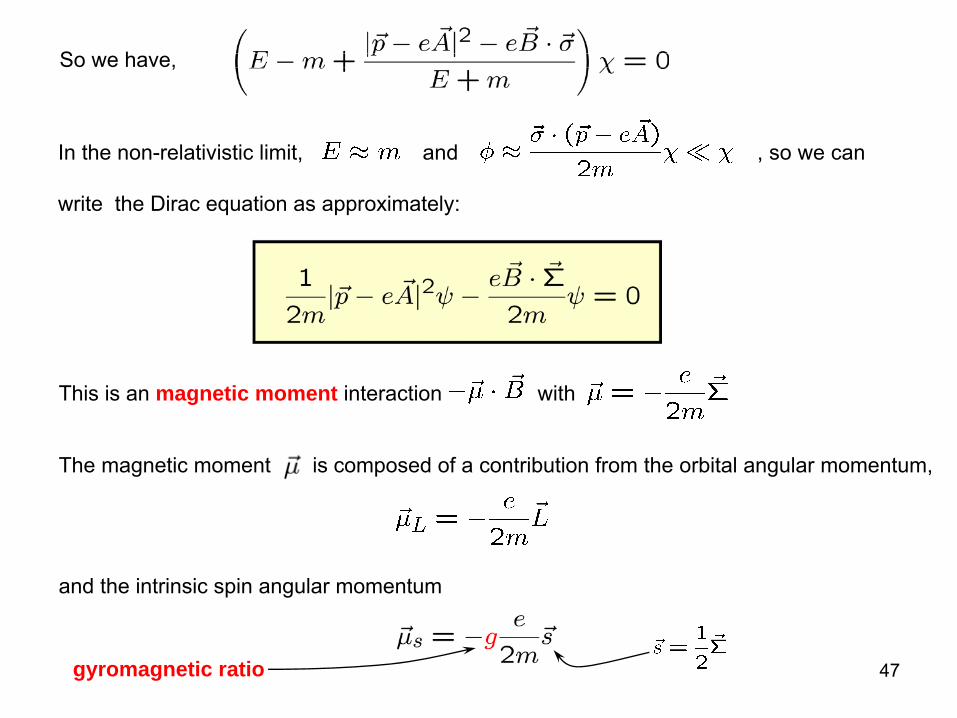
47
So we have,
This is an magnetic moment interaction with
The magnetic moment is composed of a contribution from the
orbital angular momentum,
and the intrinsic spin angular momentum
gyromagnetic ratio
In the non-relativistic limit, and , so we can
write the Dirac equation as approximately:

48
The Dirac equation predicts a gyromagnetic
ratio g = 2
We can compare this with experiment: gexp = 2.0023193043738 ±
0.0000000000082
The muon’s
magnetic moment is more interesting because it is more sensitive to new physics.
The discrepancy of g-2 from zero is due to radiative corrections
The electron can emit a photon, interact, and reabsorb the photon.
If one does a more careful calculation, including these effects,
QED predicts:
Theory:
Experiment:
excellent agreement!

49
Now we have the Dirac equation in an Electromagnetic field we can calculate the scattering of electrons (via electromagnetism) .
We will assume that the coupling e
is small, and that far away from the interaction, i.e. outside the shaded area, the electrons are free particles.
γ
a
b
c
d
Scattering and Perturbation theory
The Dirac Equation (in a field) can be written:
with
c.f. the Schrödinger equation in a potential V [Remember γ0γ0
= 1 ]
50
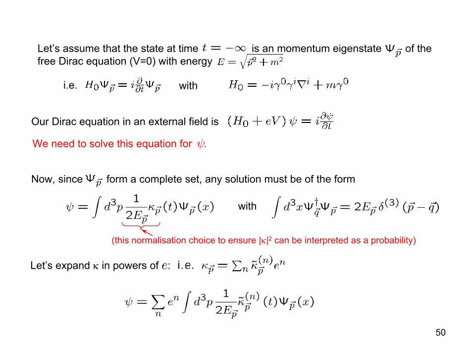
Let’s assume that the state at time is an momentum eigenstate
of the free Dirac equation (V=0) with energy
i.e. with
Our Dirac equation in an external field is
We need to solve this equation for .
Let’s expand κ
in powers of e:
Now, since form a complete set, any solution must be of the form
with
(this normalisation choice to ensure |κ|2
can be interpreted as a probability)

51
Let’s stick this in and see what we get:
To order e1:
We can now extract using the orthogonality
of :
cancel
To order e0:
Equate order by order in en

52
But at time the initial state is ,
Integrate over t:
zero
By time the interaction has stopped. The probability of finding the system in a state
is given by to order e1
with:

53
Explicitly putting in our gives
OK, so now we know the effect of the field Aμ
on the electron, but what Aμ
does the other electron produce to cause this effect?
a c
b d

54
Putting this all together:
a
b
c
d
q
forces momentum conservation

55
Feynman Diagrams: The QED Feynman RulesWe can construct transition amplitudes simply by associating a mathematical expression with the diagram describing the interaction.
• for each incoming electron• for each outgoing electron• for each incoming positron• for each outgoing positron
• for each incoming photon
• for each outgoing photon
• for each internal photon
• for each internal electron
• for each vertex
p
Remember that γ-matrices and spinors
do not commute, so be careful with the order in spin lines. Write left to right, against
the fermion flow.
Richard Feynman
For each diagram, write:
p

56
2 details:
•
Closed loops:
Integrate over loop momentum and include an extra factor of -1 if it is a fermion loop.
•
Fermi Statistics: If diagrams are identical except for an exchange of electrons, include a relative –
sign.
k
p1
p2
p3
p4
p1
p2
p3
p4
–
These rules provide , and the transition amplitude is
The probability of transition from initial to final state is

57
An example calculation:
k
p0
k0
p
e- e-
μ- μ-
This is what we had before.
To get the total probability we must square this, average over initial spins, and
sum over final spins.
But
58
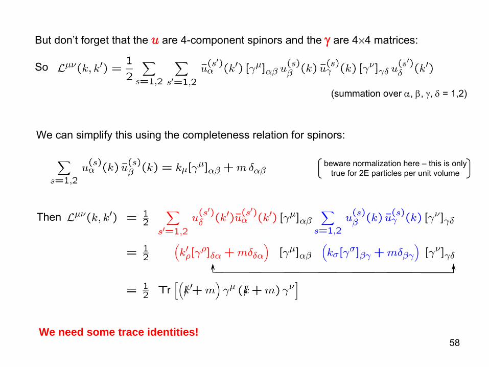
(summation over α, β, γ, δ
= 1,2)
But don’t forget that the u
are 4-component spinors
and the γ
are 4×4 matrices:
So
We need some trace identities!
We can simplify this using the completeness relation for spinors:
beware normalization here –
this is only true for 2E particles per unit volume
Then

59
Trace Identities
[This is true for any odd number of γ-matrices]
be careful with this one!
Using these identities:
So

60
If we are working at sufficiently high energies, then and we may ignore the masses.
Often this is written in terms of Mandlestam Variables, which are defined:
[Note that ]
Then

61
Cross-sectionsSo we have but we are not quite there yet –
we need to turn this into a cross-section.
Recall
⇒
since
But we need the transition probability per unit time and per unit volume is:

62
The cross-section is the probability of transition per unit volume, per unit time
×
the number of final states / initial flux.
This must also be true for a collider, where A and B are both moving, since the lab frame and centre-of-mass frame are related by a Lorentz boost.
Initial Flux
In the lab frame, particle A, moving with velocity , hits particle B, which is stationary.
A B
The number of particles like A in the beam, passing through volume V per unit time is
The number of particles like B per volume V in the target is
So the initial flux in a volume V is
But we can write this in a covariant form:

63
# final states
How many states of momentum can we fit in a volume V?
In order to not have any particle flow through the boundaries of
the box, we must impose periodic boundary conditions.
so the number of states between px
and px
+dpx
is
L
So in a volume V we have
But there are 2EV
particles per volume V, so
# final states per particle =
Note that so this is covariant!

64
Putting all this together, the differential cross-section is:
where the Flux F
is given by,
and the Lorentz invariant phase space is,
momentum conservation on-shell conditions integration measure

65
In the
centre-of-mass, this becomes much simpler
This frame is defined by and Remember
So and
with
Then the Flux becomes
66
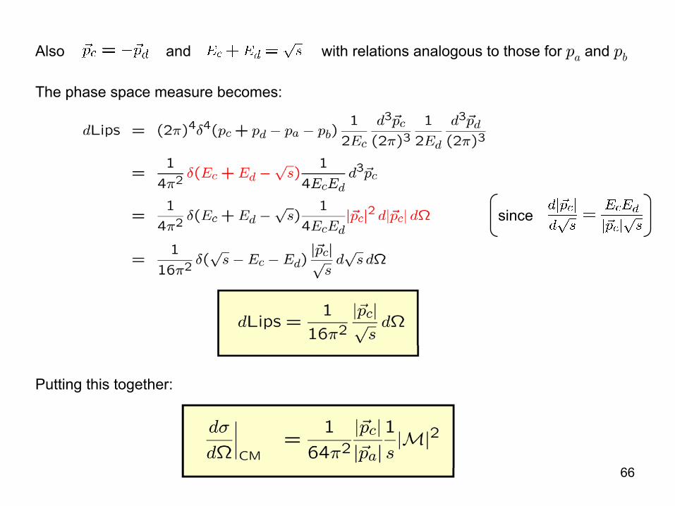
Also and with relations analogous to those for pa
and pb
since
The phase space measure becomes:
Putting this together:
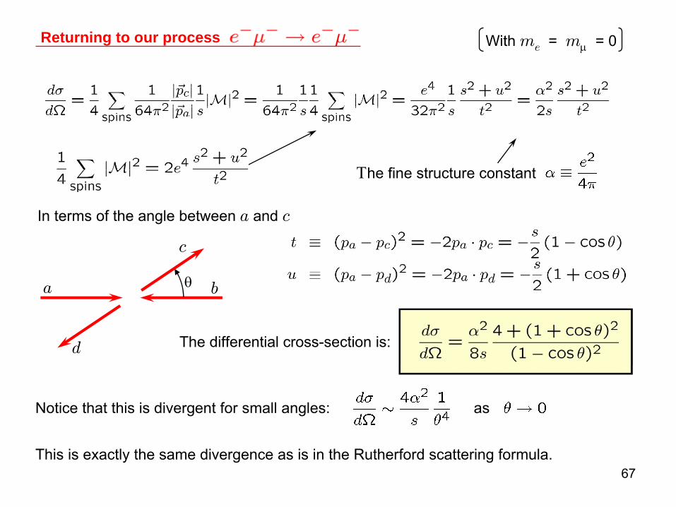
67
Returning to our process With me
= mμ
= 0
Τhe fine structure constant
θa b
c
d
In terms of the angle between a
and c
The differential cross-section is:
Notice that this is divergent for small angles: as
This is exactly the same divergence as is in the Rutherford scattering formula.

68
Crossing symmetry
Generally, in a Feynman diagram, any incoming particle with momentum p
is equivalent to an outgoing antiparticle with momentum –p.
crossing
This lets us use our result for e-
μ-
→ e-
μ-
to easily calculate the differential cross-section for e+e-
→ μ+μ-.
crossing
i.e.

69
e+
e-
μ+
μ-
Be careful not to change the s
from flux and phase space!
⇒
Writing θ
as the angle between the e-
and μ-,
as before
The total cross-section is
⇒ Notice the singularity is gone!

70
Identical particles in initial or final state
So far, in the reactions we have looked at, the final state particles have all been distinguishable. form one another. If the final state particles are
identical, we have additional Feynman diagrams.
pc
and pd
interchangedinterchange of identical fermions ⇒ minus sign
e.g. e-
e-
→ e-
e-
p1
p2
p3
p4
e-
e-
e-
e-
[See Feynman rules]
p1
p2
p3
p4e-
e- e-
e-

71
Since the final state particles are identical, these diagrams are indistinguishable and must be summed coherently.
We have interference between the two contributions.

72
Compton Scattering and the fermion propagator
Compton scattering is the scattering of a photon with an electron.
e-e- e-e-
γ γ γγ
+
I just quoted the Feynman rule for the fermion propagator, but where did it come from?
Let’s go back to the photon propagator first.
Recall the photon propagator is
The is the inverse of the photon’s wave equation:

73
The gμν
is coming from summing the photon polarization vectors over spins:
this is for virtual photons
So, the photon propagator is then
For a massless fermion propagator we follow the same procedure
The massless
fermion spin sum is
so the massless
fermion propagator is
sometimes written

74
But what about massive propagators?
= + + + ….
Lets think about a massive scalar propagator since it is easier (we can forget the spin-sum).
We can consider the mass term as a perturbation on the ‘free’
(i.e. massless) theory.
with
So the massive scalar propagator is

75
The Klein-Gordon equation leads to a propagator
The same procedure on the Dirac equation gives a propagator
More precisely, the propagator is the momentum space Fourier transform of the wave equation’s Greens function
Green’s function S
obeys:
Writing , and pre-multiplying by
gives
⇒
More details in your QFT course!

76
So now we are armed with enough information to calculate Compton Scattering
+
Putting in the Feynman rules, and following through, with me
= 0
Can you reproduce this?
You will need to use

77
Decay Rates
So far we have only looked at 2 → 2 processes, but what about decays?
A decay width is given by:
This replaces the Flux.
# of decay particles per unit volume
For a decay we have
# final states
⇒

78
In the rest frame of particle a:
ab
c The decay is back-to-back
with
But

79
Remember, to get the total decay rate, you need to sum over all possible decay processes.
The inverse of the total width will give the lifetime of the particle:
If the number of particles = Na
then,
80
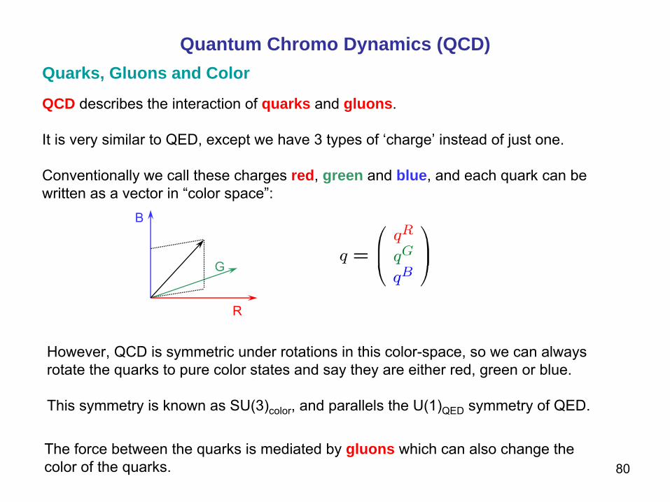
Quantum Chromo Dynamics (QCD)
QCD describes the interaction of quarks and gluons.
It is very similar to QED, except we have 3 types of ‘charge’
instead of just one.
Conventionally we call these charges red, green and blue, and each quark can be written as a vector in “color
space”:
The force between the quarks is mediated by gluons which can also change the color
of the quarks.
However, QCD is symmetric under rotations in this color-space, so we can always rotate the quarks to pure color
states and say they are either red, green or blue.
This symmetry is known as SU(3)color
, and parallels the U(1)QED
symmetry of QED.
Quarks, Gluons and Color
R
G
B

81
Since we have 3 different sorts of quark (red, green and blue), to connect them
all together we naϊvely
need 3 ×
3 = 9 different gluons.
Since we are connecting together quarks of different color, the gluons
must be colored
too.
B B
particle flow color
flow
B
R
R
R
RB_
≡
Since QCD is symmetric to rotations in color-space, the first 8 of these must have related couplings. However, the last one is a color
singlet, so in principle can have an arbitrary coupling. In QCD, its coupling is zero.
⇒ We have 8 gluons
So, for example, we could have gluons:
three orthogonal combinations of
Conventionally these last 3 are

82
In order to transform one quark color-vector onto another, we need eight 3×3 matrices.
These matrices are generators of the SU(3) group and obey the SU(3) algebra,
SU(3) structure constants
For example to turn a red quark into a blue quark we need a gluon represented by
i.e.
The above matrix is not a very convenient choice (it is actually
a ladder operator). Instead we normally write TA
in terms of the Gell-Mann λ
matrices.
are conventionally normalised by and are traceless.
Hence the removal of

83
The Gell-Mann matrices are:
Notice there are only 2 diagonal Gell-Mann matrices.

84The full QCD Feynman rules will be given to you in the Standard Model course.
At a vertex between quark and gluons we need to include a factor
b c
A α
i j
The gluons also carry color, so we must also include a gluon-gluon interaction. This is given by
A
B
C
α γ
β
p2
p1 p3

85
Renormalisation
When we calculate beyond leading order in our perturbative
expansion, we will find that we have diagrams with loops in them.
For example, the corrections to our e+e-
→ μ+μ-
would include the diagram
kp p
k
+ p
This integral is infinite!
But momentum conservation at all vertices leaves the momentum flowing around the loop unconstrained! We need to integrate over this loop momentum, and find a result containing
86
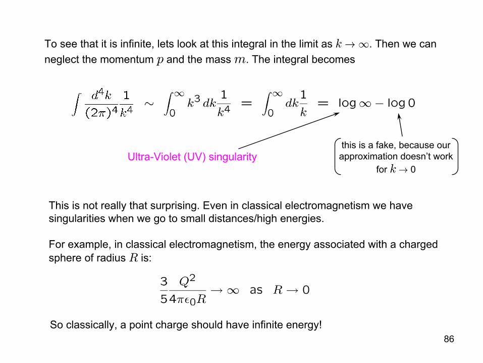
To see that it is infinite, lets look at this integral in the limit as k
→∞. Then we can neglect the momentum p
and the mass m. The integral becomes
This is not really that surprising. Even in classical electromagnetism we have singularities when we go to small distances/high energies.
For example, in classical electromagnetism, the energy associated with a charged sphere of radius R
is:
So classically, a point charge should have infinite energy!
Ultra-Violet (UV) singularitythis is a fake, because our approximation doesn’t work
for k
→ 0

87
Our theories such as QED and QCD make predictions of physical quantities. While infinities may make the theory difficult to work with, there is no real problem as long as our predictions
of physical quantities are finite and match experiment.
Are infinities really a problem?
In order for the physically measured mass to be finite, the ‘bare mass’ must be infinite and cancel the divergence from the loop. But this is OK, since m0
is not measurable, only m is.
We absorb infinities into unmeasurable
bare quantities.
To understand this, lets think about the one-loop calculation of the electron mass
We find, that in both QED and QCD, that our physical observables
are finite: they are renormalizable theories.
Gerardus 't Hooft
Martinus Veltman
+ +=
finite

88
In reality, what we are doing is measuring differences between quantities.
Since the loop contains a dependence on the momentum scale, Q, the mass changes with probed energy. The difference between two masses at different scales is:
+ +=Q2
infinities are the same in both m1
’s ⇒ finite
The difference between the masses is finite.

89
Both philosophies, absorption or subtraction of singularities, are doing the same thing. We replace the infinite bare quantities in the Lagrangian
with finite physical ones. This is called renormalization.
The beauty of QED (and QCD) is that we don’t need to do this for every observable (which would be rather useless). Once we have done it for certain observables, everything is finite! This is a very non-trivial statement. We say that QED and QCD are renormalizable.
In QED we choose to absorb the divergences into:
electroncharge electron
masselectron
wave-function
photon wave-function
Instead of writing observables in terms of the infinite bare quantities , we write them in terms of the measurable ‘renormalized’
quantities .
In order to do this, we must first regularize the divergences in our integrals.

90
Regularization by a Momentum cut-off
The most obvious regularization is to simply forbid any momenta above an scale Λ. Then, the integral becomes
The UV divergence has been regularized (remember the infra-red divergence here, log 0, is fake). This isn’t very satisfactory though, since this breaks gauge invariance.
Dimensional Regularization
The most usual way to regulate the integrals is to work in dimensions rather than 4 dimensions.
we have increased the power of k
in the denominator, making the integral finite

91
More precisely, our original integral (ignoring masses for simplicity) gives:
finite divergent as
Also notice the renormalization scale Q.
Notice that it is rather arbitrary which bit one wants to absorb
or subtract off.
One could subtract off only the pole in ², i.e. for the above integral.
This is known as the Minimal Subtraction, denoted MS.
[Euler-Mascheroni
Constant]
This choice is known as
MS
Alternatively we could have removed some of the finite terms too,
e.g.

92
Running couplings
How does the QED coupling e
change with quantum corrections?
these cancel, due to a Ward Identity
Writing this is
= ++ + + …+
I can include some extra loops by….
= ++ + …+

93
In terms of , we find
cut-off
The QED coupling changes with energy.
but since this was general, I could have chosen to evaluate my coupling at a different scale
e.g.
I can use this second equation to eliminate α0
(which is infinite) from my first equation.

94
We can do the same thing for QCD, except we have some extra diagrams
e.g. We find,
where Nc
= # of colors
= 3Nf
= # of active flavors
At higher orders in perturbation theory we will have more contributions. The complete evolution of the coupling is described by the beta function

95
For . the QCD and QED couplings run in the opposite direction.
At low energies QCD becomes strong enough to confine quarks inside hadrons.(The β
function is not proof of this!)
At high energies QCD is asymptotically free, so we can use perturbation theory.
QED
absurdlyhigh energy
Asymptotic freedom
QCD
confinement


