University of Groningen

Dynamics and geometry near resonant bifurcationsBroer, Hendrik; Holtman, Sijbo J.; Vegter, Geert; Vitolo, Renato

Published in:Regular & chaotic dynamics

DOI:10.1134/S1560354710520023

IMPORTANT NOTE: You are advised to consult the publisher's version (publisher's PDF) if you wish to cite fromit. Please check the document version below.

Document VersionPublisher's PDF, also known as Version of record

Publication date:2011

Link to publication in University of Groningen/UMCG research database

Citation for published version (APA):Broer, H., Holtman, S. J., Vegter, G., & Vitolo, R. (2011). Dynamics and geometry near resonantbifurcations. Regular & chaotic dynamics, 16(1-2), 39-50. DOI: 10.1134/S1560354710520023

CopyrightOther than for strictly personal use, it is not permitted to download or to forward/distribute the text or part of it without the consent of theauthor(s) and/or copyright holder(s), unless the work is under an open content license (like Creative Commons).

Take-down policyIf you believe that this document breaches copyright please contact us providing details, and we will remove access to the work immediatelyand investigate your claim.

Downloaded from the University of Groningen/UMCG research database (Pure): http://www.rug.nl/research/portal. For technical reasons thenumber of authors shown on this cover page is limited to 10 maximum.

Download date: 28-05-2018

ISSN 1560-3547, Regular and Chaotic Dynamics, 2011, Vol. 16, Nos. 1–2, pp. 39–50. c© Pleiades Publishing, Ltd., 2011.

Dynamics and Geometry Near Resonant Bifurcations

Henk W. Broer1*, Sijbo J. Holtman1**, Gert Vegter1***, and Renato Vitolo2****

1Johann Bernoulli Institute for Mathematics and Computer ScienceUniversity of Groningen, P.O. Box 407, 9700 AK Groningen, The Netherlands

2College of Engineering, Mathematics and Physical Sciences,University of Exeter, North Park Road, Exeter EX4 4QF, UK

Received April 04, 2010; accepted June 21, 2010

Abstract—This paper provides an overview of the universal study of families of dynamicalsystems undergoing a Hopf–Neımarck–Sacker bifurcation as developed in [1–4]. The focus is onthe local resonance set, i.e., regions in parameter space for which periodic dynamics occurs. Aclassification of the corresponding geometry is obtained by applying Poincare–Takens reduction,Lyapunov–Schmidt reduction and contact-equivalence singularity theory, equivariant under anappropriate cyclic group. It is a classical result that the local geometry of these sets in the non-degenerate case is given by an Arnol’d resonance tongue. In a mildly degenerate situation a morecomplicated geometry given by a singular perturbation of a Whitney umbrella is encountered.Our approach also provides a skeleton for the local resonant Hopf–Neımarck–Sacker dynamicsin the form of planar Poincare–Takens vector fields. To illustrate our methods a leading exampleis used: A periodically forced generalized Duffing–Van der Pol oscillator.

MSC2010 numbers: 37G15, 37G40, 34C25, 34C29

DOI: 10.1134/S1560354710520023

Keywords: periodically forced oscillator, resonant Hopf–Neımarck–Sacker bifurcation, geometricstructure, Lyapunov–Schmidt reduction, equivariant singularity theory

1. INTRODUCTION

This paper reviews the study of resonant Hopf–Neımarck–Sacker (HNS) bifurcations in familiesof continuous and discrete dynamical systems as presented in [1–4]. The main topic is a novelprocedure to detect such bifurcations for the well-known non-degenerate and a mildly degeneratesituation. Especially the investigation of the mildly degenerate resonant HNS bifurcation goesbeyond known results, since it corresponds to a “next case” in the general program for recognizingbifurcations, cf. [5, 6]. Moreover, by considering Poincare–Takens normal form vector field familieswe show that given the degeneracy the local bifurcation diagram is approximately known.

Leading example. Continuous systems that typically give rise to resonant HNS bifurcationsare given by, e.g., coupled oscillators, cell-networks, high dimensional autonomous systems,and periodically forced oscillators. To fix thoughts we consider an example of the latter type:A periodically forced generalized Duffing–Van der Pol oscillator [7, 8] given by

u + (ν1 + ν3u2)u + ν2u + ν4u

3 + u5 = ε(1 + u6) cos(2πt), (1.1)

where u ∈ R, t ∈ R, ε is a small positive real constant and ν = (ν1, ν2, ν3, ν4) ∈ R4 is a multi-

parameter. We note that a necessary requirement for (1.1) to exhibit resonance is that ν1 < 0 andν2 > 0. Furthermore, including the terms of degree 5 and 6 in u turns out to be one of the simplestgeneralizations of the standard Duffing–Van der Pol oscillator ensuring that (1.1) does not exhibit

*E-mail: H.W.Broer@rug.nl**E-mail: S.J.Holtman@rug.nl

***E-mail: G.Vegter@rug.nl****E-mail: R.Vitolo@exeter.ac.uk

39

40 BROER et al.

too degenerate resonance phenomena. Both Duffing and Van der Pol type oscillators originate fromelectrical circuits [9, 10].

Resonance. We speak of resonance when a dynamical system contains interacting oscillatorysubsystems with rationally related frequencies. To obtain an appropriate form for investigatingresonant dynamics in the Duffing–Van der Pol family, we rewrite (1.1) in system form,

⎧⎪⎪⎪⎨

⎪⎪⎪⎩

u = v,

v = −(ν1 + ν3u2)v − ν2u − ν4u

3 − u5 + ε(1 + u6) cos(2πt),

t = 1,

(1.2)

where (u, v, t) ∈ R2 × R/Z. For ε = 0 and without the t-component the system has an equilibrium

at (u, v) = (0, 0). Since t runs over a circle, including the t-component causes this equilibrium tobecome a periodic evolution of (1.2) that goes through (u, v, t) = (0, 0, 0), see Fig. 1. To study thedynamics near this periodic evolution we focus on a section of state space with a constant t-valueand on the corresponding discrete dynamics induced by the period-1-map, or Poincare map, Pν

of the flow of (1.2). The periodic evolution of (1.2) leads to a fixed point of Pν , which for smallpositive values of ε is given by (u, v) = (0, 0) + O(ε). Since system (1.1) consists of two oscillatorysubsystems, given by the periodic forcing and the Duffing–Van der Pol oscillator, we expect thatresonant dynamics occurs for certain ν-values. For Pν this phenomenon shows itself as q-periodicorbits near the fixed point, see Fig. 1. The evolution of (1.2) that gives rise to such periodic orbitsare called subharmonics of order q. As the q-periodic orbits are typically situated on an invariantcircle, the corresponding subharmonics close after going p times around in a direction transversalto the t-direction and q times around in the t-direction on an invariant torus. In this case we speakof p : q-resonance.

We are especially interested in resonance sets, i.e., regions in parameter space for which q-periodic orbits of the Poincare map occur. On the boundary of these sets the number of theseorbits typically changes through a saddle-node bifurcation. Depending on the degeneracy severalgeometries are possible for the resonance set.

v

u

t

Fig. 1. Left: Sketch of (u, v, t) state space showing a section with t constant, a periodic evolution (thickcurve) and a subharmonic of order 7 (thin curve). Right: Sketch of the section with t constant in the leftpanel, indicating a fixed point and a 7-periodic orbit of the Poincare map Pν on an invariant circle.

1.1. Classical Non-degenerate Resonance

Our approach recovers that the simplest resonance scenario is given by the weakly resonant(q � 5) non-degenerate case. In this situation the resonance set is formed by a well-known tongueshaped region, the so-called Arnol’d resonance tongue [5]. Upon passage of the correspondingboundaries a pair of subharmonics appears or merges in state space, see Fig. 2. The tip of the tongue

REGULAR AND CHAOTIC DYNAMICS Vol. 16 Nos. 1–2 2011

DYNAMICS AND GEOMETRY NEAR RESONANT BIFURCATIONS 41

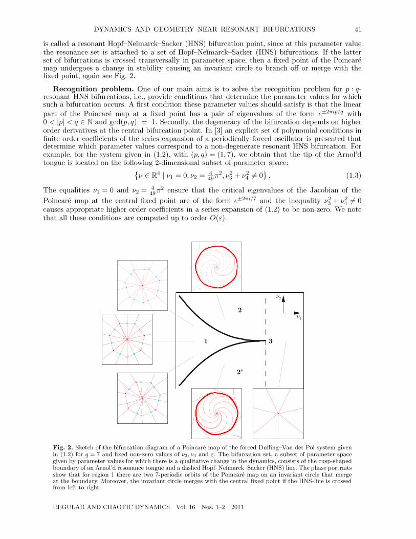
is called a resonant Hopf–Neımarck–Sacker (HNS) bifurcation point, since at this parameter valuethe resonance set is attached to a set of Hopf–Neımarck–Sacker (HNS) bifurcations. If the latterset of bifurcations is crossed transversally in parameter space, then a fixed point of the Poincaremap undergoes a change in stability causing an invariant circle to branch off or merge with thefixed point, again see Fig. 2.

Recognition problem. One of our main aims is to solve the recognition problem for p : q-resonant HNS bifurcations, i.e., provide conditions that determine the parameter values for whichsuch a bifurcation occurs. A first condition these parameter values should satisfy is that the linearpart of the Poincare map at a fixed point has a pair of eigenvalues of the form e±2πip/q with0 < |p| < q ∈ N and gcd(p, q) = 1. Secondly, the degeneracy of the bifurcation depends on higherorder derivatives at the central bifurcation point. In [3] an explicit set of polynomial conditions infinite order coefficients of the series expansion of a periodically forced oscillator is presented thatdetermine which parameter values correspond to a non-degenerate resonant HNS bifurcation. Forexample, for the system given in (1.2), with (p, q) = (1, 7), we obtain that the tip of the Arnol’dtongue is located on the following 2-dimensional subset of parameter space:

{ν ∈ R

4 | ν1 = 0, ν2 = 449π2, ν2

3 + ν24 �= 0

}. (1.3)

The equalities ν1 = 0 and ν2 = 449π2 ensure that the critical eigenvalues of the Jacobian of the

Poincare map at the central fixed point are of the form e±2πi/7 and the inequality ν23 + ν2

4 �= 0causes appropriate higher order coefficients in a series expansion of (1.2) to be non-zero. We notethat all these conditions are computed up to order O(ε).

�1

�2

1

2

2’

3

Fig. 2. Sketch of the bifurcation diagram of a Poincare map of the forced Duffing–Van der Pol system givenin (1.2) for q = 7 and fixed non-zero values of ν3, ν4 and ε. The bifurcation set, a subset of parameter spacegiven by parameter values for which there is a qualitative change in the dynamics, consists of the cusp-shapedboundary of an Arnol’d resonance tongue and a dashed Hopf–Neımarck–Sacker (HNS) line. The phase portraitsshow that for region 1 there are two 7-periodic orbits of the Poincare map on an invariant circle that mergeat the boundary. Moreover, the invariant circle merges with the central fixed point if the HNS-line is crossedfrom left to right.

REGULAR AND CHAOTIC DYNAMICS Vol. 16 Nos. 1–2 2011

42 BROER et al.

Central questions. The dynamics of the forced Duffing–Van der Pol system described aboveoccurs in all generic 2-parameter families of smooth (Poincare) maps undergoing a non-degenerateresonant HNS bifurcation. This is a classical result, so we are more interested in a next casecorresponding to mildly degenerate weakly resonant (q � 7) HNS bifurcations. This situation isencountered in generic 4-parameter families. To be more precise, the main part of the current workdeals with the following central questions:

1. How to detect, or recognize, a mildly degenerate resonant HNS bifurcation in a given familyof smooth (Poincare) maps?

2. What is the generic local geometry of the resonance set attached to a mildly degenerateresonant HNS bifurcation?

3. What is the generic local bifurcation diagram near a mildly degenerate resonant HNSbifurcation?

We note that the resonance set only gives information on bifurcations of q-periodic orbits of maps,while the bifurcation set also incorporates other types of bifurcations involving, e.g., invariant circlesand stable and unstable manifolds.

To solve the first two central questions we apply Lyapunov–Schmidt reduction, which mapsa family of maps near p : q-resonance to a family of Zq-equivariant maps, such that the zeros ofthe latter family correspond to periodic orbits of the former family. Then Zq-equivariant contact-equivalence singularity theory is utilized to obtain recognition conditions and the geometry of theresonance set for the mildly degenerate case. To answer the third central question we apply thePoincare–Takens normal form procedure, which provides an approximating family of vector fieldsfor the family of (Poincare) maps. The dynamics of the latter family is investigated by studyingthe vector field family using (numerical) methods from bifurcation theory.

1.2. Mildly Degenerate Resonance

We continue discussing mildly degenerate resonant HNS bifurcations in the Duffing–Van der Polfamily given in (1.2). In particular, we focus on a 1 : 7-resonance, since this is the strongest mildlydegenerate weak resonance. We note that the geometry and dynamics described here is generic and,therefore, occurs in all families of smooth (Poincare) maps undergoing a mildly degenerate HNSbifurcation.

Recognition problem. We start with the solution of the recognition problem. By usingthe tools presented in [3], which amounts to checking a set of polynomial conditions in finiteorder coefficients of a series expansion of (1.2), we arrive at the following result. System (1.1)undergoes a mildly degenerate 1 : 7-resonant HNS bifurcation for the following 0-dimensional subsetof parameter space:

{ν ∈ R

4 | ν1 = 0, ν2 = 449π2, ν3 = 0, ν4 = 0

}. (1.4)

This set is computed up to order O(ε). The difference with the recognition conditions for thenon-degenerate case given in (1.3) is that here both ν3 and ν4 are equal to 0.

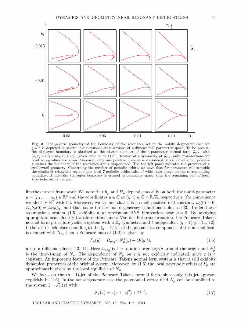
The boundary of the resonance set attached to the parameter value given in (1.4) is diffeomorphicto the discriminant set of a 4-parameter normal form family, see the next section. To display thegeometry of this set we take 2-dimensional cross-sections of parameter space, see Fig. 3, whichindicates the presence of cusps and a swallowtail. The normal form family also provides a skeletonfor the local dynamics. To understand this we first explain the Poincare–Takens normal formprocedure.

Poincare–Takens normal form. The Duffing–Van der Pol system given in (1.2) is of theappropriate form to apply Poincare–Takens reduction. In fact, every system of the form

⎧⎨

⎩

y = hμ(y) + εHμ(y, t),

t = 1(1.5)

REGULAR AND CHAOTIC DYNAMICS Vol. 16 Nos. 1–2 2011

DYNAMICS AND GEOMETRY NEAR RESONANT BIFURCATIONS 43

τ2

τ1−0.05 −0.03 −0.01 0.01

0

−0.01

−0.015σ1

σ2

Fig. 3. The generic geometry of the boundary of the resonance set in the mildly degenerate case forq = 7 is depicted in several 2-dimensional cross-sections of 4-dimensional parameter space. To be precise,the displayed boundary is obtained as the discriminant set of the 4-parameter normal form Gσ,τ , with(σ, τ ) = (σ1 + iσ2, τ1 + iτ2), given later on in (1.8). Because of a symmetry of Gσ,τ , only cross-sections forpositive τ2-values are given. Moreover, only one positive τ1-value is considered, since for all small positiveτ1-values the boundary of the resonance set is cusp-shaped. The top left panel indicates the presence of aswallowtail-geometry. Concerning the number of periodic orbits, we have that for parameter values insidethe displayed triangular regions four local 7-periodic orbits exist of which two merge on the correspondingboundary. If next also the outer boundary is crossed in parameter space, then the remaining pair of local7-periodic orbits merges.

fits the current framework. We note that hμ and Hμ depend smoothly on both the multi-parameterμ = (μ1, . . . , μn) ∈ R

n and the coordinates y ∈ C or (y, t) ∈ C × R/Z, respectively (for conveniencewe identify R

2 with C). Moreover, we assume that ε is a small positive real constant, h0(0) = 0,Dyh0(0) = 2πip/q, and that some further non-degeneracy conditions hold, see [3]. Under theseassumptions system (1.5) exhibits a p : q-resonant HNS bifurcation near μ = 0. By applyingappropriate near-identity transformations and a Van der Pol transformation, the Poincare–Takensnormal form procedure yields a system with a Zq-symmetric and t-independent (q − 1)-jet [11, 12].If the vector field corresponding to the (q − 1)-jet of the planar first component of this normal formis denoted with Nμ, then a Poincare map of (1.2) is given by

Pμ(y) = Ωp/q ◦ N1μ(y) + O(|y|q), (1.6)

up to a diffeomorphism [13, 14]. Here Ωp/q is the rotation over 2πp/q around the origin and N1μ

is the time-1-map of Nμ. The dependence of Nμ on ε is not explicitly indicated, since ε is aconstant. An important feature of the Poincare–Takens normal form system is that it still exhibitsdynamical properties of the original system. Moreover, by (1.6) the local q-periodic orbits of Pμ areapproximately given by the local equilibria of Nμ.

We focus on the (q − 1)-jet of the Poincare–Takens normal form, since only this jet appearsexplicitly in (1.6). In the non-degenerate case the polynomial vector field Nμ can be simplified tothe system z = Fσ(z) with

Fσ(z) = z(σ + |z|2) + zq−1, (1.7)

REGULAR AND CHAOTIC DYNAMICS Vol. 16 Nos. 1–2 2011

44 BROER et al.

Table 1. Relations between the dynamics of vector fields determined by Fσ given in (1.7) or Gσ,τ

given in (1.8) and corresponding Poincare maps they approximate. The first five rows give the relationsbetween local dynamical properties, while the latter two rows give generically expected relationsbetween more global features.

Approximating vector field Poincare map

equilibrium fixed point

q different equilibria invariant under Ωp/q q-periodic orbit

(degenerate) Hopf bifurcation (degenerate) HNS bifurcation

saddle-node bif. of q different equilibria saddle-node bif. of q-periodic orbit

cusp bif. of q different equilibria cusp bifurcation of q-periodic orbit

homoclinic connection homoclinic tangle

heteroclinic connection heteroclinic tangle

where σ = σ1 + iσ2 ∈ C, by a locally diffeomorphic transformation of state space and a submersivereparametrization of the multi-parameter. In the mildly degenerate case Nμ can be simplified tothe system z = Gσ,τ (z) with

Gσ,τ (z) = z(σ + τ |z|2 + |z|4) + zq−1, (1.8)

where (σ, τ) = (σ1 + iσ2, τ1 + iτ2) ∈ C2. For details see the next section. We note that the systems

z = Fσ(z) and z = Gσ,τ (z) may not be structurally stable.Local dynamical features of a Poincare map only depend on a finite order jet, so all such features

of (1.5), see Table 1, are determined by Fσ , if the system is non-degenerate, and by Gσ,τ , if the systemis mildly degenerate. On the other hand, more global phenomena, like heteroclinic connections, donot translate one-to-one between maps and approximating vector fields, since such dynamics alsodepends on higher order terms. Nevertheless, parameter values for which homoclinic or heteroclinicconnections occur generically do turn into open regions corresponding to homoclinic or heteroclinictangles, see [5, 6, 15].

Remarks.

1. By computing a Poincare map for (1.5), utilizing the Poincare–Takens normal form procedure,we encounter a “simple” approximating planar Zq-symmetric vector field Nμ of which thebifurcation diagram provides topological information on the dynamics of the original system.

2. We can also consider the procedure the other way around: For a given family of planardiffeomorphisms undergoing a resonant bifurcation, the normal form Nμ provides a vectorfield approximation. The latter point of view is useful for studying the dynamics in familiesof diffeomorphisms near resonance.

3. The form (1.5) also appears when periodic evolutions of autonomous systems are studiedusing center manifold reduction [6].

Bifurcation diagram of z = Gσ,τ (z). The bifurcation diagram of z = Fσ(z) is already given inFig. 2. So we proceed with briefly demonstrating the complexity of the bifurcation diagram in themildly degenerate case by considering an interesting 2-dimensional cross-section of the bifurcationset corresponding to z = Gσ,τ (z) for q = 7. More specifically, Fig. 4 displays such a section for(τ1, τ2) = (−0.1, 0). The following codimension 1 bifurcation curves occur:

1. The curve Ho of Hopf bifurcations. Crossing this curve transversally from σ1 < 0 to σ1 > 0causes the central equilibrium to loose stability.

REGULAR AND CHAOTIC DYNAMICS Vol. 16 Nos. 1–2 2011

DYNAMICS AND GEOMETRY NEAR RESONANT BIFURCATIONS 45

-0.006

-0.004

-0.002

0

0.002

0.004

0.006

-0.001 0 0.001 0.002 0.003

1 23

45

6

7

9

10

11

1213

15

16

σ1

σ2

Ho

(A2)1

L−

L+

-0.002

-0.001

0

0.001

0.002

0 0.001 0.002 0.003

1

2

3

4

56

7

11

12

13

σ1

σ2

Ho(A2)1

L−

L+

H−1

H+1

DH−

DH+

(A2)3(A2)4

(A2)5

-0.0002

-0.00019

-0.00018

-0.00017

-0.00016

0.00213 0.00214 0.00215

2

3

7

8

σ1

σ2

(A3)+2

H−1

(A2H)−1

(A2H)−2

(A2)4

(A2)5

H−2

Fig. 4. Bifurcation set of the planar Poincare–Takens normal form system z = Gσ,τ(z) given in (1.8) forτ = (−0.1, 0) and q = 7, with two subsequent magnifications in the (σ1, σ2)-parameter plane near interestingregions. See Section 1.2 for the meaning of the symbols. The curves of type A2 are fatter to facilitate theidentification of the resonance set.

2. The curves (A2)k, with k = 1, . . . , 5, of saddle-node bifurcations of equilibria.

3. The curves L± of saddle-node bifurcations of limit cycles.

4. The curves H±1,2 of heteroclinic bifurcations of equilibria. The heteroclinic connections taking

place for parameter values on the curves H±1 form heteroclinic cycles [6, Section 9.5].

Moreover, the following codimension 2 bifurcation points occur:

1. The points A±3 of cusp bifurcations of equilibria.

2. The points DH± of degenerate heteroclinic bifurcations of equilibria, where the curves L±

are attached to the curves H±1 .

3. The points (A2H)±1,2 of degenerate heteroclinic bifurcations of equilibria. At (A2H)±1 twocurves of heteroclinic bifurcations are attached to an A2 curve. At (A2H)±2 the curves H±

2end on (A2)4.

REGULAR AND CHAOTIC DYNAMICS Vol. 16 Nos. 1–2 2011

46 BROER et al.

-0.4

-0.2

0

0.2

0.4

-0.4 -0.2 0 0.2 0.4

Region 1 -0.00025,-0.001,0

-0.4

-0.2

0

0.2

0.4

-0.4 -0.2 0 0.2 0.4

Region 2 0.001,-0.001,0

-0.4

-0.2

0

0.2

0.4

-0.4 -0.2 0 0.2 0.4

Region 3 0.0029,-0.001,0

-0.4

-0.2

0

0.2

0.4

-0.4 -0.2 0 0.2 0.4

Region 4 0.00228,-0.00195,0

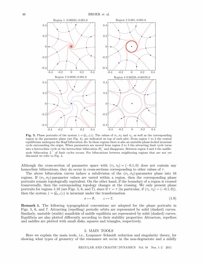
Fig. 5. Phase portraits of the system z = Gσ,τ(z). The values of σ1, σ2 and τ2, as well as the correspondingregion in the parameter plane (see Fig. 4), are indicated on top of each plot. From region 1 to 2 the centralequilibrium undergoes the Hopf bifurcation Ho. In these regions there is also an unstable phase-locked invariantcycle surrounding the origin. When parameters are moved from region 2 to 3 the attracting limit cycle turnsinto a heteroclinic cycle at the heteroclinic bifurcation H−

1 and disappears. Between region 3 and 4 the saddle-

node bifurcation L− of limit cycles occurs. For bifurcations between neighboring regions that are not yetdiscussed we refer to Fig. 4.

Although the cross-section of parameter space with (τ1, τ2) = (−0.1, 0) does not contain anyhomoclinic bifurcations, they do occur in cross-sections corresponding to other values of τ .

The above bifurcation curves induce a subdivision of the (σ1, σ2)-parameter plane into 16regions. If (σ1, σ2)-parameter values are varied within a region, then the corresponding phaseportraits remain topologically equivalent. On the other hand, if the boundary of a region is crossedtransversally, then the corresponding topology changes at the crossing. We only present phaseportraits for regions 1-10 (see Figs. 5, 6, and 7), since if τ = τ (in particular, if (τ1, τ2) = (−0.1, 0)),then the system z = Gσ,τ (z) is invariant under the transformation

σ �→ σ, z �→ z. (1.9)

Remark 1. The following typographical conventions are adopted for the phase portraits inFigs. 5, 6, and 7. Attracting (repelling) periodic orbits are represented by solid (dashed) curves.Similarly, unstable (stable) manifolds of saddle equilibria are represented by solid (dashed) curves.Equilibria are also plotted differently according to their stability properties: Attractors, repellorsand saddles are plotted with small disks, squares and triangles, respectively.

2. MAIN TOOLSHere we explain the main tools, i.e., Lyapunov–Schmidt reduction and singularity theory, for

showing what types of geometry of the resonance set occur in the non-degenerate and a mildly

REGULAR AND CHAOTIC DYNAMICS Vol. 16 Nos. 1–2 2011

DYNAMICS AND GEOMETRY NEAR RESONANT BIFURCATIONS 47

-0.4

-0.2

0

0.2

0.4

-0.4 -0.2 0 0.2 0.4

Region 5 0.00228,-0.00234,0

-0.4

-0.2

0

0.2

0.4

-0.4 -0.2 0 0.2 0.4

Region 6 0.0031,-0.0021,0

-0.4

-0.2

0

0.2

0.4

-0.4 -0.2 0 0.2 0.4

Region 7 0.00198,-0.0001,0

-0.4

-0.2

0

0.2

0.4

-0.4 -0.2 0 0.2 0.4

Region 8 0.0021443,-0.0001872,0

Fig. 6. Continuation of Fig. 5. For region 8, two subsequent magnifications near one of the saddles have beenadded in the boxes. Between regions 5 and 6 there is the saddle-node bifurcation L− of limit cycles. Changingparameters from region 7 to regions 8 causes the “inner cycle” and “outer cycle” in region 7 to be broken upby the heteroclinic bifurcation H−

2 . For bifurcations between neighboring regions that are not yet discussedwe refer to Fig. 4.

-0.4

-0.2

0

0.2

0.4

-0.4 -0.2 0 0.2 0.4

Region 9 -0.0008,-0.006,0

-0.4

-0.2

0

0.2

0.4

-0.4 -0.2 0 0.2 0.4

Region 10 -0.0008,-0.005555,0

Fig. 7. Continuation of Fig. 6. Phase portraits for regions 11–16 are not included because, due to the symmetryin (1.9), up to mirroring in the x-axis they are the same as the phase portraits for regions 2, 4, 5, 8, 9 and10, respectively. Moving parameters from region 10 to region 9 the saddle-node bifurcation (A2)1 between twosets of Z7-symmetric equilibria occurs. For bifurcations between neighboring regions that are not yet discussedwe refer to Fig. 4.

REGULAR AND CHAOTIC DYNAMICS Vol. 16 Nos. 1–2 2011

48 BROER et al.

degenerate case. Moreover, we provide the solution of the accompanying recognition problem. Tothis end we focus on the general setting of resonant families of diffeomorphisms.

2.1. Lyapunov–Schmidt Reduction

Our method to determine resonance sets for discrete systems proceeds as follows. Obtainparameter values for which a family of smooth diffeomorphisms Pμ : R

m → Rm, with 2 � m ∈ N

and μ near 0 ∈ Rn, has q-periodic orbits, i.e., solve the equation P q

μ(x) = x. Utilizing a methoddue to Vanderbauwhede [16], we can solve for such orbits by Lyapunov–Schmidt reduction. Moreprecisely, a q-periodic orbit consists of q points x1, . . . , xq, where

Pμ(x1) = x2, . . . , Pμ(xq−1) = xq, Pμ(xq) = x1.

These orbits are the zeros of the family Pμ : (Rm)q → (Rm)q given by

Pμ(x1, . . . , xq) = (Pμ(x1) − x2, . . . , Pμ(xq) − x1).

This map is Zq-equivariant. More specifically, if we define ξ : (Rm)q → (Rm)q, which generates aZq-action on (Rm)q, as follows,

ξ(x1, . . . , xq) = (x2, . . . , xq, x1),

then

ξ ◦ Pμ = Pμ ◦ ξ.

Notice that by considering Pμ the Zq-symmetry of q-periodic points of Pμ has become a fullsymmetry.

Assuming that Pμ(0) = 0 and that the map DxP0(0) has only two critical eigenvalues of theform e±2πip/q implies that the kernel of DyP0(0), with y = (x1, . . . , xq), is 2-dimensional. Hence,the implicit function theorem cannot be used to solve Pμ(y) = 0 near μ = 0. However, Lyapunov–Schmidt reduction allows us to reduce the latter equation to finding zeros of a reduced map fromR

2 to R2. Identifying R

2 with C, we need to obtain the zeros of a reduced family Gμ : C → C withGμ(0) = 0 and DzG0(0) = 0. This family also inherits the symmetry of Pμ, i.e., let ω be a criticaleigenvalue of DxP0(0), then

Gμ(ωz) = ωGμ(z).

As ω generates an action of the group Zq on C, we have that Gμ is Zq-equivariant. Due to thissymmetry and the property that G0 has a singular zero at z = 0, Zq-equivariant contact-equivalencesingularity theory provides a natural setting for the study of Gμ.

2.2. Zq-equivariant Contact-equivalence Singularity Theory

In this subsection we derive normal forms for the families Gμ by applying singularity theory. Tobegin with, we present a standard form for a family of planar Zq-equivariant smooth (non-analytic)germs, which is given by

Gμ(z) = Kμ(u, v)z + Lμ(u, v)zq−1, (2.1)

where u = |z|2, v = zq + zq and Kμ, Lμ are uniquely defined complex-valued Zq-invariant mapgerms [1].

Contact-equivalence Contact-equivalence singularity theory approaches the study of zeros ofa family by implementing coordinate changes that transform the family to a “simple” normal formand then solve the normal form equation. To make this precise we introduce n-parameter Zq-contact-equivalence transformations, which are given by a pair of the form (Sμ, Zμ), where Sμ : C → C\{0}is a smooth map germ satisfying S0(z) = 1 and Sμ(ωz)ω = ωS(z), with ω = e2πip/q, and Zμ : C → C

is a Zq-equivariant diffeomorphism germ, with Z0(z) = z. We call the two planar Zq-equivariant

REGULAR AND CHAOTIC DYNAMICS Vol. 16 Nos. 1–2 2011

DYNAMICS AND GEOMETRY NEAR RESONANT BIFURCATIONS 49

families Hμ and Gμ Zq-contact-equivalent if there is a Zq-contact-equivalence transformation(Sμ, Zμ), such that

Hμ(z) = Sμ(z)Gμ(Zμ(z)).

It follows that contact-equivalences preserve the zeros of a map up to a diffeomorphism.

Recognition conditions. Now we are in the position to characterize two classes of Zq-equivariant families. The non-degenerate case corresponds to families of which only the linear partbecomes zero for μ = 0, while in the mildly degenerate case all coefficients of terms up to third orderbecome zero for μ = 0. More specifically, consider (2.1), with K0(0, 0) = 0, since DzG0(0) = 0 for theLyapunov–Schmidt reduced function, and L0(0, 0) �= 0, which we impose to avoid high degeneracies,then the following results hold.

1. If DuK0(0, 0) �= 0, q � 5 and if

μ �→ (Re(Kμ(0, 0)), Im(Kμ(0, 0))) (2.2)

is a submersion at μ = 0, then Gμ is Zq-contact-equivalent to the normal form for the non-degenerate case given by Fσ(μ) in (1.7). Here the notation σ(μ) indicates that besides acontact-equivalence transformation also a smooth submersive reparametrization of parameterspace is needed to obtain the normal form.

2. If DuK0(0, 0) = 0, D2uK0(0, 0) �= 0, q � 7 and if

μ �→ (Re(Kμ(0, 0)), Im(Kμ(0, 0)),Re(DuKμ(0, 0)), Im(DuKμ(0, 0))) (2.3)

is a submersion at μ = 0, then Gμ is Zq-contact-equivalent to the normal form for the mildlydegenerate case given by Gσ(μ),τ(μ) in (1.8). Here the notation σ(μ) and τ(μ) indicates thatagain a smooth submersive reparametrization of parameter space is needed to obtain thenormal form.

Remarks.

1. The latter recognition conditions on Kμ and Lμ distinguishing between the non-degenerateand mildly degenerate case can also be applied to the Zq-equivariant (q − 1)-jet of thePoincare–Takens normal form vector field of the previous section.

2. The normal forms Fσ and Gσ,τ are universal unfoldings of the degenerate germs F0 and G0,0

respectively. This means that every Zq-equivariant parameter dependent deformation of F0 isZq-contact-equivalent to Fσ up to a reparametrization of parameter space and, additionally,the number of parameters is minimal for this property to be satisfied. This minimal numberof parameters is the codimension of F0. The same relations hold between G0,0 and Gσ,τ .

3. Gradual violation of degeneracy conditions, like L0(0, 0) �= 0, gives rise to a familiar endlesssequence of cases with ever higher codimension.

Resonance sets. Finally, we are in the position to determine the geometry of generic resonancesets. To this end we consider the corresponding boundaries, which are given by parameter values forwhich the number of q-periodic orbits of Pμ, or zeros of Gμ, changes. These changes occur when Gμ

has a singular zero, i.e., for parameter values on the discriminant set of Gμ given by

{μ ∈ Rn | there exists a z such that Gμ(z) = 0 and det(DzGμ(z)) = 0}.

We observe that discriminant sets are preserved by contact-equivalences. Hence, in the non-degenerate case the boundary of the resonance set is diffeomorphic to the Cartesian product of R

n−2

and the discriminant set of Fσ. In the mildly degenerate case the boundary is diffeomorphic to theCartesian product of R

n−4 and the discriminant set of Gσ,τ .

REGULAR AND CHAOTIC DYNAMICS Vol. 16 Nos. 1–2 2011

50 BROER et al.

3. CONCLUSION AND FUTURE WORK

The main aim of the current paper is presenting a novel practical procedure to detect non-degenerate and mildly degenerate Hopf–Neımarck–Sacker bifurcations in families of periodicallyforced oscillators. In particular, the mildly degenerate situation forms a “next case” in the generalprogram for recognizing bifurcations, cf. [6]. We also explain how recognition conditions for HNSfamilies determine the local geometry of the resonance set attached to the central resonant HNSbifurcation point. As an illustration, the results are applied in a leading example: A generalizedDuffing–Van der Pol oscillator.

Moreover, we show that the resonance set, up to a small diffeomorphic distortion, forms only asmall part of a more complicated bifurcation set, which is obtained using a Poincare–Takens normalform vector field approximation of the family of diffeomorphisms. The 2-dimensional tomograms ofparameter space investigated for this family of vector fields demonstrate a rich variety of bifurcationsincluding (degenerate) Hopf, homoclinic, heteroclinic and Bogdanov–Takens bifurcations. A morecomplete study of the bifurcation set of both the mildly degenerate universal family and thecorresponding vector field approximation remain future work.

An interesting extension of the current paper is formulating the recognition conditions forfamilies of vector fields with a periodic orbit in R

k, where k � 3, without assuming the reductionto the center manifold has been performed already, cf. [6].

REFERENCES1. Broer, H., Golubitsky, M., and Vegter, G., The Geometry of Resonance Tongues: A Singularity Approach,

Nonlinearity, 2003, vol. 16, pp. 1511–1538.2. Broer, H., Holtman, S., and Vegter, G., Recognition of the Bifurcation Type of Resonance in Mildly

Degenerate Hopf–Neımark–Sacker Families, Nonlinearity, 2008, vol. 21, pp. 2463–2482.3. Broer, H., Holtman, S., and Vegter, G., Recognition of Resonance Type in Periodically Forced Oscillators,

Physica D, 2010, vol. 239, pp. 1627–1636.4. Broer, H., Holtman, S., and Vegter, G., and Vitolo, R., Geometry and Dynamics of Mildly Degenerate

Hopf–Neımarck–Sacker Families Near Resonance, Nonlinearity, 2009, vol. 22, pp. 2161–2200.5. Arnol’d, V.I., Geometrical Methods in the Theory of Ordinary Differential Equations, Berlin: Springer,

1982.6. Kuznetsov, Y., Elements of Applied Bifurcation Theory, Applied Mathematical Sciences, vol. 112, Berlin,

New-York: Springer, 1995.7. Broer, H., Naudot, V., Roussarie, R., Saleh, K., and Wagener, F., Organising Centres in the Semi-global

Analysis of Dynamical Systems, Int. J. Appl. M. Stat., 2007, vol. 12, no. D07, pp. 7–36.8. Siewe, M., Kameni, F., and Tchawona, C., Resonant Oscillation and Homoclinic Bifurcation in a Φ6-van

der Pol Oscillator, Chaos, Solitons and Fractals, 2004, vol. 24, no. 4, pp. 841–853.9. Duffing, G., Erzwungene schwingungen bei veranderlicher eigenfrequenz, Braunschweig: F. Vieweg u.

Sohn 1918.10. van der Pol, B. and van der Mark, J., Frequency Demultiplication, Nature, 1927, vol. 120, pp. 363–364.11. Broer, H., Golubitsky, M., and Vegter, G., Geometry of Resonance Tongues, in Singularity Theory.

Proceedings of the 2005 Marseille Singularity School and Conference, Hackensack, NJ: World Sci. Publ.,2007, pp. 327–356.

12. Broer, H., and Vegter, G., Generic Hopf–Neımarck–Sacker Bifurcations in Feed-forward Systems,Nonlinearity, 2008, vol. 21, pp. 1547–1578.

13. Takens, F., Forced Oscillations and Bifurcations, in Applications of global analysis, I (Sympos., UtrechtState Univ., Utrecht, 1973), Comm. Math. Inst. Rijksuniv. Utrecht, No. 3-1974, Utrecht: Math. Inst.Rijksuniv. Utrecht, 1974, pp. 1–59.

14. Takens, F., Singularities of Vector Fields, Publ. Math. IHES, 1974, vol. 42, pp. 48–100.15. Guckenheimer, J. and Holmes, P., Nonlinear Oscillations, Dynamical Systems, and Bifurcations of

Vector Fields, New York: Springer, 1983.16. Vanderbauwhede, A., Branching of Periodic Solutions in Time-reversible Systems, in Geometry and

Analysis in Non-linear Dynamics, H. Broer and F. Takens, Eds., Pitman Research Notes in Mathematics,vol. 222, Pitman London, 1992, pp. 97–113.

REGULAR AND CHAOTIC DYNAMICS Vol. 16 Nos. 1–2 2011