University of Groningen Nonlocal Field theories: Theoretical and Phenomenological Aspects Buoninfante, Luca DOI: 10.33612/diss.99349099 IMPORTANT NOTE: You are advised to consult the publisher's version (publisher's PDF) if you wish to cite from it. Please check the document version below. Document Version Publisher's PDF, also known as Version of record Publication date: 2019 Link to publication in University of Groningen/UMCG research database Citation for published version (APA): Buoninfante, L. (2019). Nonlocal Field theories: Theoretical and Phenomenological Aspects. University of Groningen. https://doi.org/10.33612/diss.99349099 Copyright Other than for strictly personal use, it is not permitted to download or to forward/distribute the text or part of it without the consent of the author(s) and/or copyright holder(s), unless the work is under an open content license (like Creative Commons). The publication may also be distributed here under the terms of Article 25fa of the Dutch Copyright Act, indicated by the “Taverne” license. More information can be found on the University of Groningen website: https://www.rug.nl/library/open-access/self-archiving-pure/taverne- amendment. Take-down policy If you believe that this document breaches copyright please contact us providing details, and we will remove access to the work immediately and investigate your claim. Downloaded from the University of Groningen/UMCG research database (Pure): http://www.rug.nl/research/portal. For technical reasons the number of authors shown on this cover page is limited to 10 maximum. Download date: 14-02-2022
Transcript
University of Groningen
Nonlocal Field theories: Theoretical and Phenomenological AspectsBuoninfante, Luca
DOI:10.33612/diss.99349099
IMPORTANT NOTE: You are advised to consult the publisher's version (publisher's PDF) if you wish to cite fromit. Please check the document version below.
Document VersionPublisher's PDF, also known as Version of record
Publication date:2019
Link to publication in University of Groningen/UMCG research database
Citation for published version (APA):Buoninfante, L. (2019). Nonlocal Field theories: Theoretical and Phenomenological Aspects. University ofGroningen. https://doi.org/10.33612/diss.99349099
CopyrightOther than for strictly personal use, it is not permitted to download or to forward/distribute the text or part of it without the consent of theauthor(s) and/or copyright holder(s), unless the work is under an open content license (like Creative Commons).
The publication may also be distributed here under the terms of Article 25fa of the Dutch Copyright Act, indicated by the “Taverne” license.More information can be found on the University of Groningen website: https://www.rug.nl/library/open-access/self-archiving-pure/taverne-amendment.
Take-down policyIf you believe that this document breaches copyright please contact us providing details, and we will remove access to the work immediatelyand investigate your claim.
Downloaded from the University of Groningen/UMCG research database (Pure): http://www.rug.nl/research/portal. For technical reasons thenumber of authors shown on this cover page is limited to 10 maximum.
Einstein's theory of general relativity (GR) has been tested to a very highprecision in the infrared (IR) regime, i.e. at large distances and late times.Despite its great achievements, there are still open questions which suggestthat GR is incomplete in the ultraviolet (UV) regime. From a classical point ofview GR suers from the presence of black hole and cosmological singularities;while from a quantum point of view GR lacks of predictability in the UV regime,being not perturbatively renormalizable.
One of the most straightforward attempt aimed to complete Einstein's GRin the ultraviolet (or short-distance) regime was to introduce quadratic cur-vature terms in the gravitational action besides the Einstein-Hilbert term, asfor example R2 and RµνRµν . Such an action turns out to be power countingrenormalizable, but suers from the presence of a massive spin-2 ghost degreeof freedom, which causes classical Hamiltonian instabilities and breaks the uni-tarity condition at the quantum level.
Recently, it has been pointed out that a possible way to ameliorate the is-sue of ghost is to go beyond nite order derivative theories, and to modify theEinstein-Hilbert action by introducing dierential operators made up of inniteorder covariant derivatives, thus giving up the locality principle. In fact, by gen-eralizing the Einstein-Hilbert action with quadratic curvature terms made up ofnonlocal (i.e. non-polynomial) operators, one can formulate a quantum theoryof gravity which is unitary and that shows an improved ultraviolet behaviour.The nonlocal dierential operators are required to be made up of exponential ofentire functions in order to avoid the presence of ghost-like degrees of freedomin the graviton propagator and preserve the unitarity condition.
In this Thesis, we investigate some fundamental aspect of nonlocal (innitederivative) eld theories, like causality, unitarity and renormalizability. We alsoshow how to dene and compute scattering amplitudes for a nonlocal scalarquantum eld theory, and how they behave for a large number of interactingparticles. Subsequently, we discuss the possibility to enlarge the class of sym-metries under which a local Lagrangian is invariant by means the introductionof non-polynomial dierential operators.
Furthermore, we move to the gravity sector. After showing how to con-struct a ghost-free higher derivative theory of gravity, we will nd a linearizedmetric solution for a (neutral and charged) point-like source, and show thatit is nonsingular. By analysing all the curvature tensors one can capture andunderstand the physical implications due to the nonlocal nature of the gravi-tational interaction. In particular, the Kretschmann invariant turns out to benon-singular, while all the Weyl tensor components vanish at the origin mean-ing that the metric tends to be conformally-at at r = 0. Similar features canbe also found in the case of a Delta Dirac distribution on a ring for which noKerr-like singularity appears. Therefore, nonlocality can regularize singularities
by smearing out point-like objects. At the full non-linear level, we show thatthe Schwarzschild metric cannot be a full metric solution valid in the entirespacetime, but it can be true only in some subregion, for instance in the largedistance regime where there is vacuum.
Finally, we also discuss some phenomenological implications in the contextof ultra-compact objects (UCOs), in which ghost-free innite derivative gravitycan be put on test and constrained.
All the obtained results appear to be relevant for the follow up research. Wealso emphasize that, besides the conceptual signicance of our results, we alsodeveloped new frameworks in which testability of nonlocal interaction mightbecome more feasible in future experiments.
Publication List
This is the list of the publications on which the present PhD Thesis is basedon.
P1 L. Buoninfante, A. S. Koshelev, G. Lambiase and A. MazumdarClassical properties of non-local, ghost- and singularity-free gravityJCAP 1809, no. 09, 034 (2018)arXiv:1802.00399
P2 L. Buoninfante, A. S. Koshelev, G. Lambiase, J. Marto and A. MazumdarConformally-at, non-singular static metric in innite derivative gravityJCAP 1806, no. 06, 014 (2018)arXiv:1804.08195
P3 L. Buoninfante, G. Lambiase and A. MazumdarGhost-free innite derivative quantum eld theoryNucl. Phys. B 944, 114646 (2019)arXiv:1805.03559
P4 L. Buoninfante, G. Harmsen, S. Maheshwari and A. MazumdarNonsingular metric for an electrically charged point-source in ghost-freeinnite derivative gravityPhys. Rev. D 97, no. 8, 104006 (2018)arXiv:1804.09624
P5 L. Buoninfante, A. S. Cornell, G. Harmsen, A. S. Koshelev, G. Lambiase,J. Marto and A. MazumdarTowards nonsingular rotating compact object in ghost-free innite deriva-tive gravityPhys. Rev. D 98, no. 8, 084009 (2018)arXiv:1807.08896
P6 L. Buoninfante, A. Ghoshal, G. Lambiase and A. MazumdarTransmutation of nonlocal scale in innite derivative eld theoriesPhys. Rev. D 99, no. 4, 044032 (2019)arXiv:1812.01441
P7 L. Buoninfante, G. Lambiase and M. YamaguchiNonlocal generalization of Galilean theories and gravityPhys. Rev. D 100, no. 2, 026019 (2019)arXiv:1812.10105
P8 L. Buoninfante and A. MazumdarNonlocal star as blackhole mimicker
Phys. Rev. D 100, no. 2, 024031 (2019)arXiv:1903.01542
P9 L. Buoninfante, A. Mazumdar and J. PengNonlocality amplies echoesSubmitted, 2019arXiv:1906.03624
P10 L. BuoninfanteLinearized metric solutions in ghost-free nonlocal gravityJ. Phys. Conf. Ser. 1275, no. 1, 012042 (2019)DOI: 10.1088/1742-6596/1275/1/012042
During my PhD I also published or submitted the following papers, whosecontents are not part of this Thesis.
P11 L. Buoninfante and G. Lambiase,Cosmology with bulk viscosity and the gravitino problemEur. Phys. J. C 77, no. 5, 287 (2017)arXiv:1610.01827
P12 L. Buoninfante, G. Lambiase and A. MazumdarQuantum solitonic wave-packet of a meso-scopic system in singularity freegravityNucl. Phys. B 931, 250 (2018)arXiv:1708.06731
P13 L. Buoninfante, G. Lambiase and A. MazumdarQuantum spreading of a self-gravitating wave-packet in singularity freegravityEur. Phys. J. C 78, no. 1, 73 (2018)arXiv:1709.09263
P14 L. Buoninfante, G. Lambiase, L. Petruzziello and An. StabileCasimir eect in quadratic theories of gravityEur. Phys. J. C 79, no. 1, 41 (2019)arXiv:1811.12261
P15 L. Buoninfante, G.G. Luciano and G. PetruzzielloGeneralized Uncertainty Principle and Corpuscular GravityEur. Phys. J. C 79, no. 8, 663 (2019)arXiv:1903.01382
P16 L. Buoninfante, G. G. Luciano, L. Petruzziello and L. SmaldoneNeutrino oscillations in extended theories of gravity
This is the rst time I write a section on "Acknowledgements" in a Thesiswork or anywhere else, indeed I did it neither for my master's thesis nor formy bachelor's one. So, please, try to understand that I am not an expert and,therefore, I might follow unconventional ways.
Ah by the way, here I assume that you are reading this now 5th November2019, the day of my PhD defence...So, let's start!
First of all, I will start and end my Acknowledgements by expressing mygratitude and my innite love to the most important people in my life: My DadRemo, My Mum Giuseppina and My Brother Carletto. I have so much to saythat a standard lifetime would not be enough, but there are a couple of things(maybe more) which I really need to and want to tell you. If Nature would giveme the opportunity to select and choose two parents and a brother, I would notbe able to nd anything better than you in this or any other Universe. Youare not just parents and brother for me, but my Best Friends. You have beenalways present, always available and ready to help and give me any kind ofsupport and unique advices. From you I have learned and will keep learning somuch about life. Papà and Mamma, You gave me the Best Thing any humanbeing can dream of: FAMILY. Not only you thought me what the meaning andthe importance hidden in the word "family" are, but you also showed me andgave me the possibility to fully embrace and live such a supreme gift!
Carletto (Fratmo), sometime it's dicult to express in words a real feeling,because it can be so strong that one would feel too emotional and lose thecapacity to do it. Well, this is the right moment and right place to tell youthat you occupy the most special part of my heart. Since you were born a verypowerful connection was also established between you and me. I really don'thave any words to explain this concept, probably no existing words can do so.What I can say is that when you are sad I am sad, when you are happy I amhappy. I don't know if I have been a good older brother so far, but I want youto know that I have always tried to do my best and I would give my life for you.
One can think that I have been very lucky for having lived a life surroundedby such beautiful people...but wait, what my parents also thought me is thatFAMILY has no limit, and yes I have been even more lucky than what you canexpect...almost four years ago I met you, my love Elizabeth. Like my parentsare not just parents, you are not just my girlfriend but you can be everything asyou have shown in any kind of moments since I met you: you have been my bestlove, my best friend, my best enemy, my best half, my best partner in crime, mybest guidance, my best trusted person, my best pain in the a...(neck), my bestinspiration, my best Spanish and also English teacher, my best whatever you
can add... In so little time you became part of my FAMILY, everyone aroundme likes you. I have already told you this many times but you never believeme, so I will repeat it again: from you I have learned so much, you are one ofthe strongest and smartest person I have ever met, you are a real ghter, andI respect you so much. PhD life sometime can be very stressful and a lot ofpatience is required, not only from the PhD students but also from the peopleclose to them. And yes, you have been the only person who has been reallypresent in each moment and always understood my feelings and tried to helpme oering all your best. You know what I mean so I don't need to say anythingelse about this but just THANKS! I promise that I will do my best to make allour dreams to come true. Also for you I have so many other things to say, butI will continue to tell you more things with calm tonight...
Before going ahead I need to say that in my family nest there is anotherlovely person which has contributed to make my life more complete, she isGiusy, my brother's love. Giusy, rst of all I would like to thank you for makingmy brother happy, because this makes happy me too, you cannot even imaginehow valuable it is. Secondly, I want to tell you that wherever I go I will alwaysbring with me that special gift you and my brother gave me. It is not just anormal gift, but it contains a very deep meaning from which I get strength incertain moments, especially when I am far away from you. Thanks Cognatina!
Nonno e Nonna, of course I haven't forgotten about you...but since peoplehere might get fed up with so much love coming out of this page, I will comeback to you very soon...
So far I have mentioned the word "PhD" a couple of times, but if I had thepossibility to learn about this word and work as a PhD student is especiallythanks to my two supervisors Prof. Gaetano Lambiase and Prof. AnupamMazumdar.
Gaetano, I met you during my rst year of master's, and just attending yourlectures on Theoretical Physics I fell even more in love with physics; basically,you naturally pushed me towards you. I would really like to tell you that youhave been not just a supervisor but also a friend from which I had the possibilityto learn and understand so many things, not only a lot of physics but also aboutlife in general. You have been an excellent guidance in many dicult moments,always up for very good advices. You made my PhD life very easy and enjoyable,giving me all the freedom I wanted, thus teaching me that the rst rule in orderto be a researcher is to be free and open minded. Many thanks for sharing yourdeep knowledge, your intuition and your wisdom with me during these threeyears of PhD.
Anupam, I met you during my master's thesis project and since then wenever stopped our intense physics discussions. Thanks to you I had the possi-bility to start my journey as a researcher in theoretical physics and to touch
for the rst time aspects of quantum gravity. I would like to thank you forgiving me the possibility to realize many things about scientic research in ourphysics community. Moreover, by working with you I had the possibility to meetmany physicists, and also collaborators, which I would have probably never metwithout you.
Gaetano and Anupam, many thanks for giving me the possibility to be partof a Double PhD program, I am sure that such an experience will be fundamentalfor my future career as a researcher.
I acknowledge University of Salerno and Istituto Nazionale di Fisica Nucleare(INFN) for nancial support thanks to which I had the opportunity to traveland attend many schools, workshops and conferences.
I would like also to thank all my other scientic collaborators from which Ihave beneted lots of fruitful discussions, they are: Prof. Masahide Yamaguchi,Prof. Joao Marto, Dr. Alexey Koshelev, Shubham Maheshwari, Sravan Kumar,Gerhard Harmsen, Antonio Stabile, Antonio Capolupo, Luciano Petruzziello,Gaetano Giuseppe Luciano and Luca Smaldone (I will come back to you soonguys...).
It is my pleasure to thank the four members of the Assessment Committeefor reading, evaluating, giving useful comments and approving my PhD The-sis. They are Prof. Valeri Frolov, Prof. Elisabetta Pallante, Prof. SalvatoreCapozziello and Prof. Salvatore De Pasquale.
I have already said that sometime PhD life can be hard, tiring, boring andso on. But fortunately, I have always had several sources of strength whichhave helped me to relax and enjoy life as usual. One of the best source comesfrom my Old Friends: Luigi, Paolo, Raaele and Stefano. Amici, I really wantyou to know that like my parents are not just parents, and my girlfriend is notjust girlfriend, you are not just friends but I consider you Brothers. With youI feel so comfortable, I can do, behave and say anything I want, I never feeljudged and I know that anytime you tell me o is because there is a real reason.Everyday I can learn new things from you, and I really like the way we behavewith each other. We are very solid and tight to each other and always up todefend any of us if some diculty arise. I hope with all my heart that OurFriendship will never end because my life wouldn't be the same without you.
Of course, it is my duty to reserve a special treatment for you Raaele.Yes, I have to...you know? You have been the only friend who has been alwayspresent during all my thesis's defences: bachelor's, master's and now PhD's. Istill remember that for the other two you were the one coming to pick me upwith your car, you cannot even imagine how valuable it was for me and howvaluable it is the fact that you are here in Groningen. Bro, there is somethingspecial between you and me, we know, it doesn't matter how far we are, or how
often we speak, nothing can change our relationship. With one big THANKYOU I would like to express my strong feelings and all my gratitude to you.
There are also other special people who I must thank for their continuouspresence and love they have shown to me: Luana, Danila, Fabio and Ferdinando.Then, I special acknowledgement goes to Generoso who is the best mathemati-cian I have ever met and thanks to him and his beautiful explanation I learnedsomething about Einstein's Special Reltivity for the rst time at high school.He has been the one who made fall in love for physics. Gene, I am not sure ifit was something good or bad, but in any case I must thank you!
Let us now go through my experience at University of Salerno and Universityof Groningen.
Salerno has been the place where I started my studies, I did my bachelor'sand master's, and I am now also nishing my PhD. Of course, it is my duty tothank all my professors and university's friends who have contributed a lot inthese unforgettable 8 years. A special thank goes to my General Relativity'sprofessor, Prof. Gaetano Vilasi. From you I have learned few interesting things,and one sentence I will never forget is: "You don't need to know a lot, what isimportant is to know little but extremely well."
Before jumping to the PhD experience, let me say that during my studies Imet beautiful people with whom I shared so many special moments: Luciano andFrancesco (bestia and zuzzus, when are going to work on a project together?),Francesca, Melly, Simone, Marco (Prsso), Mariateresa and Ofelia (ragazze, wehad so much fun together, I miss those moments so much!).
Luciano and Francesco, I am really grateful to you for our student's experi-ence together. Let us also remind us how it was when we met again in Triesteduring our rst year of PhD...we had so much fun in Muggia...that's why I can-not forget my dear Diksha and Francesco S., thank you guys for all the fun weshared! Since we are mentioning people from SISSA, let me take this opportu-nity to thank Costantino for sending me the LaTeX format I used for this PhDthesis, I haven't found a better one so far, so thanks a lot.
People, you cannot even imagine how fun and enjoyable doing the PhD inSalerno has been. The Theoretical Physics group in Salerno has been the perfectplace where to conduct research and enjoy discussions with colleagues/friends.Gaetano, Massimo, my big Mastro and friend Antonio S., Antonio C., Luciano,GPL and Big Smald, working with you has been a real pleasure and I reallyhope that both friendship and collaboration will never end. Luciano and GPL,my dear Piscatori 'e Pusilleco, we have always understood each other very welland been always available for each other. The feelings that I have felt duringthese three years together cannot be described in few lines, so what I can sayfor now is: thank you very much to have been perfect colleagues and friends.
Moreover, I will never forget all the conversations and stories about gossip
that we had with Antonio C., it was so funny to see when Gaetano showed histotal unawareness about those striking facts....Thanks Guys!
I would like to thank all my oce mates for making our oce(s), or whateverit is, a kind of home in which we have spent most of the time during week-days. First oce: Luciano, Alfonso, Alex, Onofrio and Giuseppe, and also ourBrasilian friend Victor who was a visitor during my rst year of PhD. SecondOce: GPL, Big Smald, Enrico and Aniello. Gianpaolo, Enver and Marco,thanks to you too guys for all the chats and coees we shared.
It's my pleasure to thank our great Modestino, his nice family and his restau-rant with all the amazing food who gave us the right energy to work and doresearch during many days.
Moreover, I would like to thank all the people I met at LACES (my rstPhD school) and Erice School, for the physics discussions and all the fantasticmoments of fun we shared. I special thanks goes to my dear Alberto Merlano.
Now it is my great pleasure to thank my football team at Salerno University:CRAL-Salerno. It has been an amazing experience being part of this team, andI really hope one day I can be back at Salerno University and still play withyou. All our trainings at 14:30 on Tuesdays and Thursdays were also a perfectway to take a break from research and relax enjoying football with good friends.The three national tournaments we did together will be unforgettable for therest of my life. A special mention goes to my dear Rocco called Cinghialotto, Iam honoured to have met and gotten a friend like you.
Let's now y to Netherlands. The rst person I would like to thank is Janfor being a very good friend and never making me feel alone in Groningen. Iwill never forget all our romantic dinners at Lambik, which I also must thankfor giving us the right atmosphere each Friday night. Man, many thanks forbeing always honest, sincere and available for me. Thanks for having translatedthe abstract of my Thesis in Dutch. I really hope we will never lose each other.
Shubham, you have been the rst person I met when I started my PhDadventure in Groningen; I still remember when we went together to universityon the rst day. It has been super nice to share my oce with you. Sravan, I metyou during my last year of PhD, but it is like we have known each other for longtime. Since we met we had so much fun going deep inside and (fortunately) alsodeep far away. Guys, many thanks for sharing physics discussions and especiallyso much fun and jokes together.
Aysigul, I would like to thank you for your presence and for making mytime in Groningen more enjoyable. It has been very nice discussing with you onany kind of topic, going from PhD diculties, society, art and life in general.Watching movies together has been very relaxing. I am sure that even if longdistances will separate us, our friendship will keep solid.
It is my pleasure to thank also my dear Ceyda, Gerhard, Perseas and all the
other PhD students, Post-Docs and professors I have met during my experiencein Groningen.
Of course, I cannot forget to thank my dear Rick and Natalia, who havebeen my rst Dutch friends I have met already when I came to Groningen formy master's thesis, four years ago. At that time I have also met my Italianfriend Stefano with whom I have always kept in contact. A thanks also goesto Mustafà with whom I shared his apartment for almost ten months; Man, Ireally felt comfortable with you, thanks.
Finally, I can now come back to my family and start thanking my lovelygrandparents Nonna Assunta, Nonno Mario and Nonna Felicetta.
Nonna Assunta, for obvious reasons we haven't been able to communicateso much, but I would really like to tell you that anytime you smile to me, youreally make my day!
Nonno Mario and Nonna Felicetta, you are the wisest people I have evermet in all my life. What I have learned from your words, your stories andyour advices has no price; none in Earth could have taught me so profoundand precious things. I cannot use the word "thanks" because it would not beenough to pay back what you have done for me in all these years. Nonno, inthis three years of PhD not only I have learned something about "nonlocal eldtheories"..., but thanks to you I nally learned how to make real good wine andthis is something I wouldn't have been able to learn without you. Moments inwhich we play cards, watch football, discuss about your past experiences are soenjoyable that I would replace them with nothing else in this world. Nonna,you have been a second mum for me, you gave and are still giving me a verygood education, and taught me how to behave since I was a kid. The only thingI regret is that I have never tried to learn how to cook the way you do, not evenone percent of it. You, together with my mum, cook the best food I have evereaten, it's AMAZING!
I have so many relatives that there is no space to thank each of them, butof course I can just say thank you to all my uncles, aunts and all my cousins.Paolo, Cugì, what a shame you are not here, I miss you! Moreover, I needto reserve a special acknowledgement for my uncle Salvatore, my uncle Lucaand my aunt Annamaria for coming to Groningen to attend my defence; manythanks Zii!
I don't know if you managed to read all of it and reached to this point, butI truly believe that now it is time to end this long "section," and of course Iwill do it with the people who have been with me since I was a kid, that is myFAMILY. Papà and Mamma, you are my Idols, thanks for everything you didsince I was born! Carlé, I admire you so much, and I want you to know thatyou are the most important person in my life. GRAZIE FAMIGLIA!
Sono sempre andato a letto cinque minuti più tardi degli altri,per avere cinque minuti in più da raccontare
Franco Califano
List of Acronyms
AdS anti-de Sitter
dS de Sitter
EOM Equation(s) of motion
GR General relativity
IDG Innite derivative gravity
IR Infrared
QCD Quantum chromodynamics
QFT Quantum eld theory
QNF Quasi-normal frequencies
QNM Quasi-normal mode
SFT String eld theory
SUGRA Supergravity
UV Ultraviolet
Conventions and Notations
In this Thesis we adapt all our conventions to the mostly plus metric signature(−+ ++). Moreover, unless otherwise specied, we work in Natural units:c = ~ = 1. We shall use the index 0 for the temporal coordinate, and theother indices 1, 2, 3 for the spatial coordinates. Then, latin indices i, j, k, l etcgenerally run over three spatial coordinate labels, usually, 1, 2, 3 or x, y, z. Greekindices µ, ν, ρ, σ etc generally run over the four coordinate labels in a generalcoordinate system.
Note that in this thesis we shall frequently suppress the indices, especiallywhen we work with the spin projector operators. Thus, for instance, P2
µνρσ willbe just written as P2, and in the same way also in the formulas that containthe spin projector operators there will be a suppression of the indices.
Let us introduce a notation for the expressions containing either symmetricor antisymmetric terms. The indices enclosed in parentheses or brackets sat-isfy, respectively, the properties of symmetry or antisymmtery dened by thefollowing rules:
T(µν) =Tµν + Tµν
2and T[µν] =
Tµν − Tµν2
.
The adopted conventions for the curvature tensors are the following. TheChristoel symbol is dened as:
Γρµν =1
2gρλ (∂µgλν + ∂νgµλ − ∂λgµν) ;
the Riemann tensor components read:
Rαµρν = ∂ρΓαµν − ∂νΓαρµ + ΓαρρΓ
ρµν − ΓανρΓ
ρρµ;
the Ricci tensor, Rµν = Rαµαν = gαρRαµρν :
Rµν = ∂αΓαµν − ∂νΓαµα + ΓαµνΓβαβ − ΓαµβΓβνα;
while, the Ricci scalar R = Rµµ = gµνRµν .By lowering the upper index with the metric tensor we can obtain the com-
pletely covariant Riemann tensor:
Rµνρσ =1
2(∂ν∂ρgµσ + ∂µ∂σgνρ − ∂σ∂νgµρ − ∂µ∂ρgνσ)
+gαβ(ΓανρΓ
βµσ − ΓασνΓβµρ
).
Moreover, the d'Alembertian operator is dened as = gµν∇µ∇ν .Let us now introduce the linearized forms of the above curvature tensors
around Minkowskias as we shall frequently use them. By perturbing aroundthe Minkowski background,
gµν(x) = ηµν + hµν(x),
the curvature tensors up to linear order read
Rµνρσ =1
2(∂ν∂ρhµσ + ∂µ∂σhνρ − ∂σ∂νhµρ − ∂µ∂ρhνσ) ,
Rµν =1
2
(∂ρ∂νh
ρµ + ∂ρ∂µh
ρν − ∂µ∂νh−hµν
),
R = ∂µ∂νhµν −h.
Moreover, we can also dened the traceless Riemann tensor also known as Weyltensor:
Cµνρσ = Rµνρσ +R6
(gµρgνσ − gµσgνρ)
−1
2(gµρRνσ − gµσRνρ − gνρRµσ + gνσRµρ) .
The usual form of the eld equation for General Relativity is given by
Gµν ≡ Rµν −1
2gµνR = κ2Tµν ,
whereGµν = Rµν+gµνR/2 is the Einstein tensor and Tµν the energy-momentum(or stress-energy) tensor. In SI units the coupling is given by κ = 8πG/c4, wherethe value of the Newton constant is G = 6.67 × 10⁻⁸ g−1 cm3 s−2. In Naturalunits, since c = 1 = ~, one has κ2 = 8πG. Often it is useful to display thePlanck mass in the gravitational eld equations. Indeed, the Planck mass isdened as
mp :=
√~cG' 1.2× 10¹⁹ GeV/c2 = 2.2× 10⁻⁸ kg
and in natural units G = 1/M2p . To get rid of the 2π factor is useful to introduce
the reduced Planck mass that is dened as
Mp :=
√~c
8πG' 2.4× 10¹⁸ GeV/c2 = 4.3× 10⁻⁹ kg.
Therefore, the coupling constant in Natural units turns out to be equal to
κ =1
Mp,
and the Einstein equations turn out to be expressed in terms of the reducedPlanck mass.
Albert Einstein's General Relativity (GR) since 1916 has become the widelyaccepted theory of gravity and has been tested to a very high precision in theinfrared (IR) regime, i.e. at large distances and time scales. A vast amountof observational data [1] have made GR the best current theory to describeclassical aspects of the gravitational interaction. Remarkably, the recent obser-vation of gravitational waves (GW) emission from merging of compact objectshas given an additional powerful conrmation of its predictions, even after onehundred years from its formulation. Despite the great success, there still remainfundamental questions with no answer. At the classical level, Einstein's theoryis plagued by the presence of cosmological and black hole singularities whichmake the theory incomplete at short distances [2, 3]. Moreover, at the quantumlevel GR lacks of predictability in the ultraviolet (UV), indeed it turns out tobe perturbatively non-renormalizable. In 1972, 't Hooft and Veltman [4] calcu-lated the one-loop eective action of Einstein's theory and found that gravitycoupled to a scalar eld is non-renormalizable, but also showed how to intro-duce counter-terms to make pure GR nite at one-loop. The crucial result wasonly obtained several years later by Goro and Sagnotti [5] and van de Ven [6],who showed the existence of a two loops divergent term cubic in the Riemanntensor.
The theory of GR is described by the simple Einstein-Hilbert action:
S =1
2κ2
∫d4x√−gR,
where R is the Ricci scalar and the coupling κ =√
8πG = 1/Mp has the dimen-sion of mass inverse. One can prove that such an action is non-renormalizable
3
4
by making a power-counting of the coupling constant dimension in front of theinteraction terms. First, since we want to work in the realm of standard per-turbative quantum eld theory (QFT), we need to expand the action in Eq.(1)around Minkowski:
gµν(x) = ηµν + κhµν(x),
so that we obtain
S =1
4
∫d4xhµνOµνρσ hρσ +O(κh3),
where Oµνρσ is the kinetic operator, while O(κh3) takes into account higherorder interaction terms in the perturbation. We can immediately notice thatall the interaction terms are multiplied by powers of κ which has the dimensionof a mass inverse, and this implies that such an action is non-renormalizable bypower-counting.
This feature of the theory is also reected on the UV behavior of loop-integrals. Indeed, if we compute the supercial degree of divergence in fourdimensions we obtain [7]:
D = 2L+ 2,
which tells us that the degree of divergence increases with the number of loops.In fact, one can always implement a renormalization prescription but an innitenumber of counter-terms are needed, namely an innite number of couplings.However, any experiment can never determine the value of an innite numberof parameters, therefore GR's predictability is spoiled at high energy.
In the past there have been several attempts aimed to resolve this problem.Some of them are based on standard tools of QFT, while others attempts arerely on dierent physical principles and alternative mathematical frameworks.Let us list some of them.
The most straightforward and conservative attempt is to generalize theEinstein-Hilbert action by introducing local operators made up of higherorder terms in the curvatures and to use tools of standard perturbativeQFT. In 1977, Stelle proved that a theory described by an action includ-ing the Einstein-Hilbert term plus quadratic curvature terms like R2 andRµνRµν ,1
S =1
2κ2
∫d4x√−g(R+ αR2 + βRµνRµν
)1Note that the Riemann tensor squared does not appear in Stelle's action because it can
be rewritten in terms of the Ricci scalar squared and Ricci tensor squared by means the socalled Euler characteristic:
RµνρσRµνρσ − 4RµνRµν +R2 = div,
where div stands for total covariant derivative.
5
is perturbatively renormalizable [8, 9]. However, the same action is plaguedby the presence of an additional massive spin-2 ghost degree of freedomwhich causes classical Ostrogradsky instabilities by making the Hamilto-nian unbounded from below [10], while at the quantum level it breaks theunitarity condition. Indeed, by expanding the action in Eq.(1) aroundMinkowski, we can compute the propagator whose spin-2 part reads
Πµνρσ(k) = ΠGR,µνρσ −P2µνρσ
k2 +m22
,
where ΠGR is the massless spin-2 graviton propagator of GR, while thesecond term is the so called Weyl ghost with mass m2
2. Hence, at the per-turbative level, there is a conict between unitarity and renormalizabilitywhich seem to be incompatible in both Einstein's GR and quadratic cur-vature gravity. Despite the presence of such an unhealthy degree of free-dom, such a theory can be still considered predictive as an eective eldtheory whose validity is accurate at energy scales lower than the cut-orepresented by the mass of the ghost [11, 12]. Another important achieve-ment of quadratic gravity can be found in the Starobinski-model of ina-tion [13, 14], which is able to suitably explain the current data; dierentlyfrom the model of Stelle, here only the term R2 shows up in the quadraticpart of the action. It is also worthwhile to highlight that gravitationalactions with quadratic curvature corrections were taken into account inseveral dierent frameworks (see for example Refs. [15, 16, 17, 18]).
An alternative class of attempts was based on the introduction of new par-ticles and new symmetries, going beyond GR and the standard model ofparticles. The most important examples in this class are supergravity the-ories (SUGRA), whose pioneers are Freedman, Ferrara and van Nieuwen-huizen [19]. Supersymmetric theories are very special because the balanceof bosonic and fermionic degrees of freedom leads to cancellation of di-vergences in loop diagrams and indeed even the simplest SUGRAs do nothave the two-loop divergence that is present in GR; in particular, N = 8SUGRA has been shown to be nite up to ve loops [20, 21]. However,besides the improved quantum behavior, these theories have other kind ofeither theoretical and experimental diculties that thwarted this hope.
A third possibility is that the non-renormalizability is an intrinsic pathol-ogy of the perturbative approach, and not of gravity itself. There havebeen more than one way of implementing this idea. The Hamiltonian ap-proach to quantum gravity can be viewed as falling in this broad category,
2See Appendix A for more details on ghosts and unitarity and Appendix C for the deni-tion of the spin projector operator P2.
6
like loop quantum gravity [22, 23, 24]. A more recent non-perturbative ap-proach to quantize gravity is based on the asymptotic safety scenario inwhich it has been argued that there exist a UV xed point in a region ofthe parameters space where the couplings are not small [25, 7]. Therefore,GR would be renormalizable from a non-perturbative point of view. Alsofor this approach a lot of work is still needed, indeed the unitarity problemis still open.
Furthermore, a very popular attempt which is not based on the principlesof quantum eld theory is given by String Theory [26, 27], whose mainaim is to construct an unied quantum framework of all interaction. Thequantum aspect of the gravitational eld only emerges in a certain limitin which the dierent interactions can be distinguished from each other.All particles have their origin in excitations of fundamental strings. Thefundamental scale is given by the string length which is supposed to be ofthe order of the Planck length Lp = 1/Mp .
In this Thesis we mainly focus on the rst category of attempts and try toattack the problem of unitarity and renormalizablity by questioning the mainprinciples of standard QFT. Any standard QFT (like the standard model of par-ticles) is based on the principles of locality (polynomial Lagrangians), causality,unitarity and renormalizability. Moreover, the quantization of the theory andthe denition of quantum scattering amplitudes is based on the Feynman iε-prescription. We may ask whether we can give up some of these key ingredientsand be able to formulate a consistent theory of quantum gravity compatiblywith the standard model. There is still no denite answer to this fundamentalquestion, but there have been very interesting recent works along this direction,which we now list.
Lee-Wick theories of gravity: are a class of higher (than four) derivativetheories of gravity which have been shown to be both super-renormalizableand unitary. The simplest case is sixth order gravity whose Lagrangiancontains sixth order dierential operators, like for instance RR andRµνRµν , besides the Einstein-Hilbert term; see Refs.[28, 29, 30]. Inthis case, one can easily notice that all the couplings have the dimen-sion of a mass which means they are super-renormalizable by power-counting. Moreover, the spin-2 part of the graviton propagator does nothave any extra real massive pole, but a pairs of complex conjugate poles.In Refs.[31, 32, 30, 33] a new quantization prescription alternative to theFeynman one was introduced, and it was shown that the optical theo-rem holds true at all order in perturbation theory. However, althoughthe S-matrix seems to be well dened at the quantum level, it is still notclear whether the presence of this kind of higher derivatives, with complexconjugate poles, can cause Hamiltonian instabilities at the classical level.
7
Fourth order gravity with fakeons: this is the only example of strictlyrenormalizable and unitary theory of quantum gravity [30, 34, 35, 36]. In-deed, as already mentioned above, fourth order gravity is renormalizableby power-counting but non-unitarity if the standard Feynman quantiza-tion prescription is implemented. However, the authors in Refs.[30, 34,35, 36] have shown that it is still possible to make the theory unitaryby implementing a new quantization prescription under which the Weylghost is converted into a fake degree of freedom (fakeon), so that the op-tical theorem can be preserved to all orders in perturbation theory. Alsoin this case, through this new prescription, one is able to construct a welldened S-matrix for quantum gravity, but at the classical level is still notcompletely clear how to avoid the Ostrogradsky instability without usingperturbative tools.
Nonlocal eld theories: are based on giving up one of the key principlesof standard QFT, i.e. locality. In fact, it consist in generalizing theEinstein-Hilbert action by including higher order curvature terms madeup of nonlocal (i.e. non-polynomial) analytic dierential operators whosepeculiar form is crucial in order to make the graviton propagator ghost-freearound any background and ameliorate the UV behavior of amplitudes andloop integrals [37, 38, 39, 40, 41, 42]. These ghost-free nonlocal theoriesare also known as innite derivative theories of gravity (IDG), since non-polynomial operators are usually made up of innite order derivatives.This alternative approach can be useful not only at the quantum level butalso classically, indeed no extra unhealthy degree of freedom is present inthe physical spectrum.
In this Thesis we focus on this last approach to quantum gravity and discussmany of its aspects not only in relation to the gravitational sector, but also ina more general context of QFT. Let us now go through the history of nonlocal(innite derivative) and introduce its main ingredients.
From local to nonlocal Lagrangians
In standard local eld theory, Lagrangians are constructed in terms of polyno-mials of elds and polynomials of derivatives of elds since one is interested inobservables at low energies, therefore, the order of derivatives is always nite:
L ≡ L(φ, ∂φ, ∂2φ, . . . , ∂nφ
),
where n is a positive nite integer and φ(x), in principle, can be any kind oftensorial eld. Instead, a nonlocal Lagrangian is a function which can be alsomade up of non-polynomial dierential operators, like for instance
L ≡ L(φ, ∂φ, ∂2φ, . . . , ∂nφ,
1
φ, ln
(/M2
s
)φ, e/M
2s φ, . . .
),
8
where the non-polynomial operators contain innite order covariant derivatives;Ms is the energy scale of nonlocality beyond which new physics should manifestand observables at high energy can be computed, and it is mathematicallyneeded to make the arguments of logarithm and exponential dimensionless. Forexample, in the case of the exponential of the d'Alembertian, we can write theoperator:
e/M2s =
∞∑n=0
1
n!
(M2s
)n,
where the derivative order n goes up to innity. In terms of Taylor expansionsit seems that we have to provide the full function (and thus nonlocal informa-tion) when an innite number of derivatives is present. This is in contrast witha standard two derivative theory for which only the eld and its rst deriva-tive (and thus rather local information) are needed. By thinking in terms ofdiscrete derivatives one can explicitly see why innite order derivative operatorare nonlocal in nature: to dene the discrete version of the rst derivative weneed to know the function on two adjacent lattice points, to dene the secondderivative on three and to dene the n-th derivative on n + 1 lattice points,while for innite order derivatives one needs to know the function on an inniteset of lattice points. Thus, the higher the derivative order is, the more nonlocalthe information required to know the system is. However, although the deriva-tive order is innite, one can show that for some specic choice of the nonlocaloperator the number of independent solutions of an innite order dierentialequation can be still nite [43, 44].
Generally, nonlocality can be thought at least in two dierent ways: (i) asdiscretization of the spacetime; (ii) or purely related to the interaction in sys-tems dened in a continuum spacetime. In the case (i) there would be a minimallength scale given by the size of the unit cell in such a discrete background, andit is often identied with the Planck length, Lp = 1/Mp . As for (ii), the nonlo-cality does not aect the kinematics at the level of free theory, but it becomesrelevant only when dynamics is considered. In other words, in the free-theorythis kind of nonlocality would not play any role, but it would become relevantas soon as the interaction is switched on. In this regard, we will be investigatingthe latter scenario, where we will consider a continuum spacetime and introducenonlocality through non-polynomial dierential operators into either the kineticoperator and/or the interaction vertex.
First attempts along (ii) trace back in the fties, when people were stillfacing the problem of UV divergences in QFT and renormalization was still notvery well understood. Thus, an alternative possibility to deal with divergenceswas the introduction of nonlocal interactions with the aim to regularize thetheory and make it nite in the UV [45, 46, 47]. Subsequently, they were alsostudied from a pure axiomatic point of view [48]. In 1987 Krasnikov constructeda nonlocal Lagrangian for gauge theories and made some progress towards a
9
super-renormalizable and unitary nonlocal theory of quantum gravity. In 1989Kuz'min [38] continued and extended the previous works and computed the one-loop eective action for a nonlocal quadratic theory of gravity.3 In Refs.[49, 50,51, 39] further studies were made in relation to both niteness of loop integralsand unitarity of higher derivative theories. It was noticed that by workingwith innite order derivatives, and in particular using exponentials of entirefunctions, one could construct a ghost-free propagator as, for instance,
Π(k) =eγ(−k2)
k2 +m2,
where γ(−k2) is an entire function, i.e. a function with no poles in the complexplane. Note that this kind of nonlocality refers to analytic dierential operatorsfor which a Taylor expansion around = 0 can be dened, but in literatureother possibilities involving non-analytic operators, like 1/ and ln(), havebeen explored; see for instance Refs.[52, 53, 54, 55, 56, 57]. Nonlocal eldtheories constructed in terms of analytic dierential operators are often calledinnite derivative eld theories.
In 2005 the authors in Ref.[40] used this kind of analytic non-polynomialoperators and made a more detailed investigation of nonlocal actions in thecontext of gravity. In particular, they noticed that nonlocality not only canhelp to make the theory unitary and to ameliorate high energy behavior of loopintegrals, but also to resolve classical singularities. Indeed, exact non-singularbouncing solutions were found; see also Refs.[58, 59, 60, 61] for further progressesalong this direction. In a gravitational context, the graviton propagator under-goes a similar generalization as in Eq.(1), for example the simplest IDG actioncan give a propagator around Minkowski which is the GR propagator multi-plied by an exponential of an entire function. Further relavant studies weremade in Refs.[41, 42], in which non-singular spherically symmetric solutionswere obtained in the linearized regime around Minkowski. Very interestingly, inRefs.[41, 62, 63] the most general quadratic ghost-free actions were constructedaround any maximally symmetric backgrounds, i.e. Minkowski, de Sitter (dS)and anti-de Sitter (AdS). IDG in three dimensions has been recently studied,in both massless and massive cases [64]; see also Refs.[65, 66, 67] for details onthree-dimensional local massive gravity.
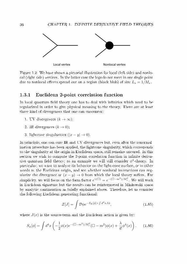
One of the main physical implications due to nonlocal interactions is theresolution of singularities. For instance, one can straightforwardly show thatinnite order dierential operators acting on a Delta source can yield a non-pointsupport, i.e. can map a point-like object into an extended one whose size is givenby the nonlocal length scale Ls = 1/Ms . Indeed, at the classical level it wasshown that in IDG full non-linear bouncing solutions can be found in the context
3It is still not clear to the physics community whether the computations in Ref.[38] arecorrect, indeed further investigations are still required.
10
of cosmology [40, 58, 59, 60, 61]. Moreover, nonlocal gravitational interactionmay also be useful to solve black hole singularities; so far exact non-singularspherically symmetric solutions have been found in the linearized regime bothin static [68, 69, 41] and dynamical [70, 71, 72] scenarios. Further investigationshave been made in Refs.[42, 73, 63, 74, 75, 76, 77, 78, 79, 80, 81, 82, 83].Moreover, IDG can also address the horizon problem in black hole physics: ithas been argued that nonlocal eects can spread out up to the horizon scale sothat the size of the nonlocal region always engulfs the Schwarzschild radius, thuspreventing the formation of any horizon [75, 78, 84]. In fact, recently horizonlesscompact solutions have been discussed in IDG, where the gravitational systemis assumed to be made up of a very large number of constituents interactingnonlocally [84]. Such systems are known as nonlocal stars.
At a quantum level there are hints that the UV behavior of the theory isameliorated by the presence of exponential of entire functions [38, 39, 42, 85, 86,87, 88]; however a lot of work has to be done especially in the gravity sector. Infact, by making a simple power counting, one can straightforwardly show thatthe supercial degree of divergence of loop integrals in IDG is given by [42, 86]
D = 1− L,
which would seem to imply that for L > 1 all loop integrals should be nite.However, the power counting argument is not sucient since we now have todeal with nonlocal Lagrangian for which the structure of the counter-termsmay be very complicated and not simply given by polynomials. Therefore, inIDG we cannot apply the usual theorems on renormalizability of standard localQFT and further investigations are needed. It is worthwhile mentioning that inRefs.[42, 85, 89] it has been claimed that by choosing peculiar nonlocal operatorswhich behave polynomially in the UV a super-renormalizable IDG theory can beproven to exist. Moreover, in Ref.[86] it was proposed an alternative approachto renormalization where all bare propagators were replaced by the dressed ones.
There have been attempts to construct a model with innite derivative Higgs[90] and fermions [87], which indeed ameliorates the UV aspects by making theβ-function to vanish at high energies [91, 90]. It has also been argued that inpresence of multi-particle interaction, the nonlocal scale Ms can be transmutedfrom the UV to the IR depending on the number of particles involved in thescattering process [92]. Innite derivative Lagrangians were also studied in thecontext of thermal eld theory [93, 94, 95, 96], inationary cosmology [97, 98,99, 100, 101, 102], supersymmetry [103, 104] and applied to the study of theCasimir eect in curved background [105]. Moreover, a nonlocal modicationof the Schrödinger equation has been analyzed in Refs.[106, 107, 108, 109].
Furthermore, the appearance of nonlocality in string theory is very wellknown. In particular, in string eld theory (SFT), which has lots of similaritywith a nonlocal QFT, vertices of the following form arise [110, 111, 112, 68, 69,
11
113]:
V (φ) ∼(ecα′φ)3
where c ∼ O(1) is a dimensionless constant that can change depending onwhether one considers either open or closed string [113], and α′ is the so calleduniversal Regge slope. In fact, by discretizing the string functional integral asa sum over all lattices and using the large-N expansion to dene surfaces onthese lattices, one can dene a continuum limit [114] which produces a nonlocalscalar eld action with a Gaussian behavior (e−α
′k2) either in the propagator orin the vertex [115, 116]. Such a method in string theory was also thought as anon-perturbative approach to connement in quantum chromodynamics (QCD)[114]; see Ref.[117] for a recent review on QCD.
This Thesis is motivated by the success of innite derivative eld theoriesuntil now and by the possibility to solve fundamental open questions, like aconsistent formulation of a quantum theory of the gravitational interaction.
Organization of the Thesis
The goal of this Thesis it to study dierent aspects of innite derivative eldtheories ranging from fundamental eld theoretical problems to aspects of in-nite derivative gravity. After a deep and quite complete theoretical analysis,we will discuss some phenomenological aspects of nonlocal interaction.
Chapter 1: We make a very general study of Lorentz-invariant innite deriva-tive eld theories by working with a real scalar eld for simplicity. We an-alyze fundamental aspects like propagator, causality, unitarity and renor-malizabity. In particular, we explicitly show that the presence of nonlocal-ity implies violation of microcausality. Moreover, we show that the scaleof nonlocality depends on the number of interacting particles, meaningthat the size of the region on which nonlocal interaction takes place is notxed but dynamical. We also investigate the possibility to enlarge theclass os symmetries under which a local Lagrangian is invariant, by usingnon-polynomial dierential operators.
Chapter 2: We introduce innite derivative gravity and show how the presenceof nonlocal operators in the gravitational action can make the propagatorghost-free and preserve perturbative unitarity. We study the linear regimearound Minkowski background and nd spacetime solutions for a neutraland an electrically charged point-like source, and for a rotating ring, show-ing how nonlocality can regularize the singularities from which Einstein'sGR suers. Subsequently, we move towards the non-linear regime anddiscuss the main feature of nonlocality. In particular, we show that theSchwarzschild metric cannot be a full solution in IDG.
12
Chapter 3: We study the possibility to extract some phenomenology in re-lation with the physics of horizonless ultra-compact objects. First, wediscuss how nonlocal interaction can help to prevent the formation of ahorizon in astrophysical scenarios and to form very compact objects whoseradius is slightly larger than the Schwarzschild radius. Secondly, we an-alyze the interaction between waves and potential barriers in presence ofnonlocality. As an example, we consider a double delta potential whichcan mimic the two photon spheres of a wormhole, or the two potentialbarriers at the photon sphere and at the surface of a an ultra-compactobject. Especially, we show how nonlocality modify the behavior of quasinormal modes and echoes.
Chapter 4: We summarize the main results obtained in this work and discussthe outlook.
Appendix: In Appendix A we shortly review the concepts of unitarity andghost, and theirs main implications. We show why higher derivative eldtheories, like fourth order gravity, are pathological. In Appendix B weshow explicitly the steps of the computation of some Green functions ininnite derivative eld theory. In Appendix C we review the formalism ofthe spin projector operators which are very useful to compute the gravitonpropagator and nd the relevant degrees of freedom of the theory aroundMinkowski background.
1Infinite derivative field theories
In this Chapter we investigate classical and quantum aspects of Lorentz-invariantinnite derivative eld theories whose Lagrangians contain analytic form factorsmade up of innite order derivatives. We will treat the simplest case of a scalareld.
This chapter is mainly based on P3, P6, P7 and is organized as follows.In Section 1.1, we will introduce the action for a real scalar eld and analyzeinto details the structure of the propagator, and emphasize that nonlocalityis important only when the interactions are switched on. We will see how toperform calculations with operators involving derivatives of innite orders. InSection 1.2, we will show that nonlocality leads to a violation of causality in aspace-time region whose size is given by the scale of nonlocality Ls = 1/Ms.Wewill show that the retarded Green function becomes acausal due to nonlocalityand as a consequence also local commutativity is violated. In Section 1.3, wewill discuss quantum scattering amplitudes also in relation to unitarity. We willconsider some simple computations of correlators and amplitudes in Euclideanspace and how to analytically continue back to Minkowski. In particular, wewill show that the Euclidean 2-point correlation function is non-singular at theEuclidean origin, unlike the local case. In Subsection 1.3.5 we will discuss thebehavior of scattering amplitudes when a very large of interacting particles areinvolved. In Section 1.4 we will consider the possibility to enlarge the classof symmetries under which a local Lagrangian is invariant by means nonlocalgeneralizations.
13
14 CHAPTER 1. INFINITE DERIVATIVE FIELD THEORIES
1.1 Innite derivative actions
We now wish to introduce a Lorentz-invariant innite derivative eld theory fora real scalar eld φ(x) by an action:
S =1
2
∫d4xd4yφ(x)K(x− y)φ(y)−
∫d4xV (φ(x)), (1.1)
where the operator K(x− y) in the kinetic term makes explicit the dependenceon the eld variables at nite distances x−y, signaling the presence of a nonlocalnature; the second contribution to the action is a standard local potential term.We can rewrite the kinetic term as follows
SK =1
2
∫d4xd4yφ(x)K(x− y)φ(y)
=1
2
∫d4xd4yφ(x)
∫d4k
(2π)4F (−k2)eik·(x−y)φ(y)
=1
2
∫d4xd4yφ(x)F ()
∫d4k
(2π)4eik·(x−y)φ(y)
=1
2
∫d4xφ(x)F ()φ(x),
(1.2)
where F (−k2) is the Fourier transform of K(x−y), and we have used the integralrepresentation of the Dirac delta,
∫d4k
(2π)4 eik·(x−y) = δ(4)(x− y). From Eq.(1.2)
note that the operator K(x− y) has the following general form [118]:
K(x− y) = F ()δ(4)(x− y). (1.3)
Note that the action in Eqs.(1.1,1.2) is manifestly Lorentz invariant, thus it ispossible to dene a divergenceless stress-energy momentum tensor [119]. Notethat is dimensionful, and strictly speaking we should write/M2
s . For brevity,we will suppress Ms in the denition of the form factors from now on. Furthernote that the action without the potential has no nonlocality. The homogeneoussolution obeys the local equations of motion.
In what follows we will not refer to the operator K(x− y) anymore, but wewill speak in terms of F ().
1.1.1 Choice of form factor and degrees of freedom
So far we have not required any property for the form factor F (), other thanbeing Lorentz invariant; however it has to satisfy special conditions in order todene a consistent quantum eld theory, in particular absence of ghosts at thetree level; see also Appendix A for a general discussion on unitarity and ghosts.We will restrict the class of operators by demanding F () to be an entire
1.1. INFINITE DERIVATIVE ACTIONS 15
analytic function1. We can now apply the Weierstrass factorization-theorem forentire functions, so that we can write:
F () = e−γ()N∏i=1
(−m2i ), (1.5)
where γ() is also an entire function, N can be either nite or innite and itis related to the number of zeros of the entire function F (). From a physicalpoint of view, 2N counts the number of poles in the propagator that is denedas the inverse of the kinetic operator in Eq.(1.5). The exponential function doesnot introduce any extra degrees of freedom and it is suggestive of a cut-o factorthat could improve the UV-behavior of loop-integrals in perturbation theory,moreover it contains all information about the innite-order derivatives:
e−γ() =
∞∑n=0
γnn!n, (1.6)
where γn ≡ ∂(n)e−γ()/∂n∣∣=0
. By inverting the kinetic operator in Eq.(1.5), we obtain the propagator that in momentum space reads 2
Π(k) = eγ(−k2)N∏i=1
−ik2 +m2
i
. (1.7)
One can immediately notice that if N > 1 ghosts appear. Indeed, we candecompose the propagator in Eq.(1.7) as
eγ(−k2)N∏i=1
1
k2 +m2i
= eγ(−k2)N∑i=1
cik2 +m2
i
, (1.8)
where the coecients ci contain the sign of the residues of the propagator ateach pole; then by multiplying with e−γ(−k2)k2, and taking the limit k2 → ∞,
1Let us remind that an entire function is a complex-valued function that is holomorphic atall nite points in the whole complex plane. It is worthwhile to mention that in literature thereare also examples of eld theory where the operator is a non-analytic function. For instance,from quantum correction to the eective action of quantum gravity non-analytic terms likeR(µ2/)R and Rln(/µ2)R emerge [52, 53, 54, 55]. Moreover, in causal-set theory [56, 57],the Klein-Gordon operator for a massive scalar eld is modied as follows
F (+m2) = +m2 −3L2
p
2π√
6(+m2)2
[3γE − 2 + ln
(3L4
p(+m2)2
2π
)]+ · · · , (1.4)
where γE = 0.57721... is the Euler-Mascheroni constant and p is the appropriate length scale;note also the presence of branch cuts once analyticity is given up.
2We adopt the convention in which the propagator in the Minkowski signature is denedas the inverse of the kinetic term times the imaginary unit "i".
16 CHAPTER 1. INFINITE DERIVATIVE FIELD THEORIES
we obtain
0 =
N∑i=1
ci, (1.9)
which means that at least one of the coecients ci must be negative in order tosatisfy the equality in Eq.(1.9), i.e., at least one of the degrees of freedom mustbe ghost like. We will focus on the case N = 1, so that tree level unitarity willbe preserved and no ghosts whatsoever will be present in the physical spectrumof the theory.
Let us now x the function γ() in the exponential. As we have alreadymentioned, it has to be an entire function, moreover it has to recover the lo-cal Klein-Gordon operator, i.e. two-derivatives dierential operator, in the IRregime, /M2
s → 0. In this Thesis we will mainly consider polynomial functionsof , in particular we will study the simplest operator
γ() =(−+m2)n
M2ns
=⇒ F () = e(−+m2)n
M2ns (−m2), (1.10)
where n is a positive integer and we have explicitly reinstated Ms.In literature also other kind of entire functions have been deeply studied,
see for instance Refs.[39, 42, 74]3. In particular, in Refs.[39] was introduced thefollowing entire function
γ() = Γ(0, p2()
)+ γE + log
(p2()
), (1.11)
where Γ(0, z) is the incomplete gamma-function and p() is any polynomial of . This last operator is very suitable to construct renormalizable gauge theoriessince it assumes a polynomial behavior in the UV, such that the counter-termsare still local operators and all renormalization techniques of standard localquantum eld theory can be still applied [39, 42, 85, 91, 89]. However, workingwith the entire functions in Eq.(1.10) will be sucient to understand which arethe main features and physical implications due to nonlocality.
1.1.2 Field redeniton and nonlocal interaction
The innite derivative eld theory introduced in Eqs.(1.1) and (1.2) shows amodication in the kinetic term. However, note that we can also dene aninnite derivative eld theory where the kinetic operator corresponds to theusual local Klein-Gordon operator by making the following eld re-denition:
φ(x) = e−12γ()φ(x) =
∫d4yF(x− y)φ(y), (1.12)
3In Section 1.4 we will study a slightly dierent type of form factors which can admitextra complex conjugate poles but still giving a ghost-free propagator at the tree level.
1.1. INFINITE DERIVATIVE ACTIONS 17
where F(x − y) := e−12γ()δ(4)(x − y) is the kernel of the dierential operator
e−12γ(). By inserting such a eld redenition into the action in Eq.(1.1), we
obtain an equivalent action that we can still name by S:
S =1
2
∫d4xφ(x)(−m2)φ(x)−
∫d4xV
(e
12γ()φ(x)
). (1.13)
From Eq.(1.13) it is evident that now the form factor e12γ() appears in the
interaction term and that nonlocality only plays a crucial rule when the inter-action is switched on as the free-part is just the standard local Klein-Gordonkinetic term. Such a feature of nonlocality is relevant only at the level of inter-action, this will become more clear below, when we will discuss homogeneous(without interaction-source), and inhomogeneous (with interaction-source) eldequations.
1.1.3 Homogeneous solution: Wightman function
We can now determine the eld equation for a free massive scalar eld by varyingthe kinetic action in Eq.(1.2) in the case of N = 1 degree of freedom and weobtain
F ()φ(x) = 0⇐⇒ e−γ()(−m2)φ(x) = 0, (1.14)
that is a homogeneous dierential equation of innite order. One of the rstquestion one needs to ask is how to formulate the Cauchy problem correspondingto Eq.(1.14) or, in other words, whether we really need to assign an innitenumber of initial conditions in order to nd a solution; if this is the case we wouldlose physical predictability as we would need an innite amount of informationto uniquely specify a physical conguration. Fortunately, as pointed out inRef.[43, 44], what really xes the number of independent solutions is the polestructure of the inverse operator F−1(). For instance, as for Eq.(1.14) we havetwo poles solely given by the Klein-Gordon operator −m2, which implies thatthe number of initial conditions and independent solutions is also two.
In particular, note that the equality (−m2)φ(x) = 0 also solves Eq.(1.14),namely the two independent solutions of Eq.(1.14) are given by the same twoindependent solutions of the standard local Klein-Gordon equation 4:
φ(x) =
∫d3k
(2π)3
1√2ω~k
(a~ke
ik·x + a∗~ke−ik·x
), (1.15)
4The normalization factor 1(2π)3
√2ω~k
in the eld-decomposition Eq.(1.15) is consis-
tent with the following conventions for the creation operator a†~k|0〉 = 1√
2ω~k|~k〉, for the
states-product 〈~k|~k′〉 = 2ω~k(2π)3δ(3)(~k − ~k′) and for the identity in the Fock space I =∫d3k
(2π)31
2ω~k|~k〉〈~k|. With such conventions, the canonical commutation relation for free-elds
reads [φ(x), π(y)]x0=y0 = δ(3)(~x− ~y), where π(y) is the conjugate momentum to φ(y).
18 CHAPTER 1. INFINITE DERIVATIVE FIELD THEORIES
where k ·x = −ω~kx0 +~k ·~x, with ω~k =√~k2 +m2. The coecients a~k and a
∗~kare
xed by the initial conditions and once a quantization procedure is applied theybecome the usual creation and annihilation operators satisfying the followingcommutation relations:
[a~k, a†~k′
] = (2π)3δ(3)(~k − ~k′), [a†~k, a†~k′
] = 0 = [a~k, a~k′ ]. (1.16)
Furthermore, let us remind that the Wightman function is dened as a solutionof the homogeneous dierential equation Eq.(1.14), thus from the above consid-erations it follows that it is not aected by the innite derivative modication.
Indeed, in a local eld theory the Wightman function is found by solvingthe homogeneous Klein-Gordon equation, and reads 5
WL(x− y) =
∫d4k
(2π)3θ(k0)δ(4)(k2 +m2)eik·(x−y). (1.17)
The corresponding innite derivative Wightman function would be dened byacting on Eq.(1.17) with the operator eγ(). However, because of the Lorentz-invariance of the operator eγ(), with γ() being an entire analytic function,Eq.(1.17) will only depend on k2 in momentum space. Therefore, given theon-shell nature of WL(x− y) through the presence of δ(4)(k2 +m2), one has6
W (x− y) = eγ()WL(x− y)
= eγ(m2)
∫d4k
(2π)3θ(k0)δ(4)(k2 +m2)eik·(x−y).
(1.18)
The exponential operator only modies the local Wightman function by an over-all constant factor eγ(m2) that can be appropriately normalized to 1: eγ(m2) = 1.For instance, in the case of exponential of polynomials, as in Eq.(1.10), one hase−(−k2−m2)n/M2n
s = 1, once we go on-shell, k2 = −m2. Thus, innite derivativesdo not modify the Wightman function. It is also clear that the commutationrelations between the two free-elds evaluated at two dierent space-time pointswill not change:
〈0 |[φ(x), φ(y)]| 0〉 = W (x− y)−W (y − x)
= WL(x− y)−WL(y − x).(1.19)
Let us remind that for a massive scalar eld, one has:
〈0 |[φ(x), φ(y)]| 0〉 = − i
2π2
1
r
∞∫0
d|~k| |~k|sin(
√~k2 +m2t)sin(|~k|r)√~k2 +m2
≡ i∆(t, r)
(1.20)5Whenever there is a confusion, we will label the local quantities with a subscript L.6Note that Wightman function for the free-theory can get modied in eld theories with
non-analytic form factors, see Refs. [56, 57], in our scenario this is not the case.
1.1. INFINITE DERIVATIVE ACTIONS 19
where we have dened t = x0 − y0 and ~r = ~x− ~y; ∆(t, r) is called Pauli-Jordanfunction. The above integral can be calculated, and in the massive case this isgiven by [120]:
∆(t, r) = − 1
2πε(t)δ(ρ) +
m
4π√ρθ(ρ)ε(ρ)J1(m
√ρ), (1.21)
where ρ := t2 − r2, ε(t) = θ(t) − θ(−t), and J1 is the Bessel function of therst kind. It is clear that ∆(t, r) has support only within the past and futurelightcones, indeed it vanishes for space-like separations (ρ < 0). When m = 0,one has
∆(t, r)|m=0 = − 1
2πε(t)δ(ρ)
=1
4πr[δ(t+ r)− δ(t− r)] ,
(1.22)
which has support only on the lightcone surface. By dening the lightconecoordinates u = t − r and v = t + r, the massless elds are parametrized byu = 0 = v, as indicated by the Dirac deltas in Eq.(1.22), so it follows that thecommutation relations in Eqs.(1.21),(1.22) dene the lightcone structure of thetheory, which is not modied by innite derivatives 7.
1.1.4 Inhomogeneous solution: propagator
From the previous considerations it is very clear that nonlocality in innitederivative theories is not relevant at the level of free-theory, but it will play acrucial role when interactions are included. In fact, in presence of the potential
7It is worth mentioning that there are examples of eld theories where the commutationrelations for free-elds are modied by the presence of a minimal length-scale. For instance, ithappens in non-commutative geometry [121] and causal-set theory [56, 57]. In the latter theform factor F (k), not only depends on the invariant k2, but also on the sign of k0 signalingthe presence of branch-cuts in the Wightman function due to non-analyticity. Furthermore,modied commutation relations may emerge in theories were Lorentz-invariance is broken.Let us consider a very simple pedagogical example where the form factor explicitly breaks
Lorentz-invariance: F (∇2) = e−∇2/M2
s , where ∇2 ≡ δij∂i∂j is the spatial Laplacian, or in
momentum space F (~k2) = e~k2/M2
s . In such a case it is easy to show that the commutatorbetween two free massless scalar elds assumes the following form:
〈0 |[φ(x), φ(y)]| 0〉 = −i
2π2
1
r
∞∫0
d|~k|e−~k2/M2
s sin(|~k|t)sin(|~k|r)
=iMs
8π3/2
[e−
14M2s (r+t)
2− e−
14M2s (r−t)
2].
(1.23)
It is evident from Eq.(1.23) that the commutator for massless free elds is dierent from zeroeither inside and outside the lightcone on a region of size ∼ 1/Ms around the lightcone surfaceu = 0 = v.
20 CHAPTER 1. INFINITE DERIVATIVE FIELD THEORIES
term the eld equation is given by
e−γ()(−m2)φ(x) =∂V (φ)
∂φ(x), (1.24)
and in this case the general solution cannot be simply found by solving the localKlein-Gordon equation, but the exponential operator e−γ() will play a crucialrole. Hence, solutions of the inhomogeneous eld equation will feel the nonlocalmodication. The simplest example of inhomogeneous equation is the one witha delta source δ(4)(x−y) = δ(x0−y0)δ(3)(~x−~y), whose solution corresponds tothe propagator of the theory. In Minkowski signature, the propagator Π(x− y)satises the following dierential equation:
e−γ(x)(x −m2)Π(x− y) = iδ(4)(x− y), (1.25)
whose solution can be expressed as
Π(x− y) =
∫d4k
(2π)4
−ieγ(−k2)
k2 +m2 − iεeik·(x−y), (1.26)
where
Π(k) = − ieγ(−k2)
k2 +m2 − iε, (1.27)
is the Fourier transform of the propagator in Minkowski signature. We nowwish to explicitly show that the propagator in Eq.(1.26) can not be identiedwith the time-ordered product of two elds, Π(x− y) 6= 〈0 |T (φ(x)φ(y))| 0〉 . Aswe have already seen for the Wightman function, the quantity Π(x− y) can beexpressed in terms of the local one, ΠL(x− y), by acting on the latter with theoperator eγ(x):
where we have used the fact that the local propagator ΠL(x−y) corresponds tothe time-ordered product between two elds φ(x) and φ(y). Because of the time-derivative component of the d'Alembertian in the exponential function γ(x),it is clear that the propagator cannot maintain the same causal structure of theFeynman propagator of the standard local eld theory.
We now want to nd the explicit form of the propagator in the coordinate-space, and in order to do so we need to understand how to deal with the dier-ential operators of innite order. By using the identity 8
nx = (−∂2x0 +∇2
~x)n
=
n∑p=0
(n
p
)(−∂2
x0
)(p) (∇2~x
)(n−p),
(1.29)
8The identity in Eq.(1.29) holds in at spacetime as [∂2x0,∇2
~x] = 0. In curved spacetime onehas to deal with covariant derivatives and = gµν∇µ∇ν , so that the simple decompositionin Eq.(1.29) is not possible.
1.1. INFINITE DERIVATIVE ACTIONS 21
and the generalized Leibniz product-rule,
∂(2p)x0
[g(x0)h(x0)
]=
2p∑q=0
(2p
q
)∂
(q)x0 g(x0)∂
(2p−q)x0 h(x0), (1.30)
we can manipulate the expression in the last line of Eq.(1.28) and obtain:
eγ(x)[θ(x0 − y0)WL(x− y)
]=
∞∑n=0
γnn!nx[θ(x0 − y0)WL(x− y)
]=
∞∑n=0
γnn!
n∑p=0
(n
p
)(−∂2
x0
)(p) [θ(x0 − y0)
(∇2~x
)(n−p)WL(x− y)
]= θ(x0 − y0)W (x− y) +
∞∑q=1
∞∑n=0
γnn!
n∑p=0
(n
p
)(2p
q
)iqθ(2p− q)∂(q−1)
x0 δ(x0 − y0)
×∫
d3k
(2π)3
eik·(x−y)
2ω~k(−~k2)n−pω2p−q
~k,
(1.31)where in the last equality we have introduced the step-function θ(2p − q), sothat we can extend the summation over q up to innity. We can now note thatthe identity
1
q!
∂(q)eγ(−k2)
∂k0(q)=
1
q!
∞∑n=0
γnn!
∂(q)((k0)2 − ~k2)n
∂k0(q)
=1
q!
∞∑n=0
γnn!
n∑p=0
(n
p
)∂(q)(k0)2p
∂k0(q)(−~k2)n−p
=
∞∑n=0
γnn!
n∑p=0
(n
p
)(2p
q
)θ(2p− q)(k0)2p−q(−~k2)n−k.
(1.32)
allows us to rewrite Eq.(1.31) as follows:
eγ(x)[θ(x0 − y0)WL(x− y)
]= θ(x0 − y0)W (x− y)
+i
∞∑q=1
iq−1
q!∂
(q−1)x0 δ(x0 − y0)
∫d3k
(2π)3
eik·(x−y)
2ω~k
∂(q)eγ(−k2)
∂k0(q)
∣∣∣∣∣k0=ω~k
.
(1.33)Following the same steps for the second term in Eq.(1.28), one has
eγ(x)[θ(y0 − x0)WL(y − x)
]= θ(y0 − x0)W (y − x)
−i∞∑q=1
iq−1
q!∂
(q−1)x0 δ(x0 − y0)
∫d3k
(2π)3
eik·(y−x)
2ω~k
∂(q)eγ(−k2)
∂k0(q)
∣∣∣∣∣k0=ω~k
.
(1.34)
22 CHAPTER 1. INFINITE DERIVATIVE FIELD THEORIES
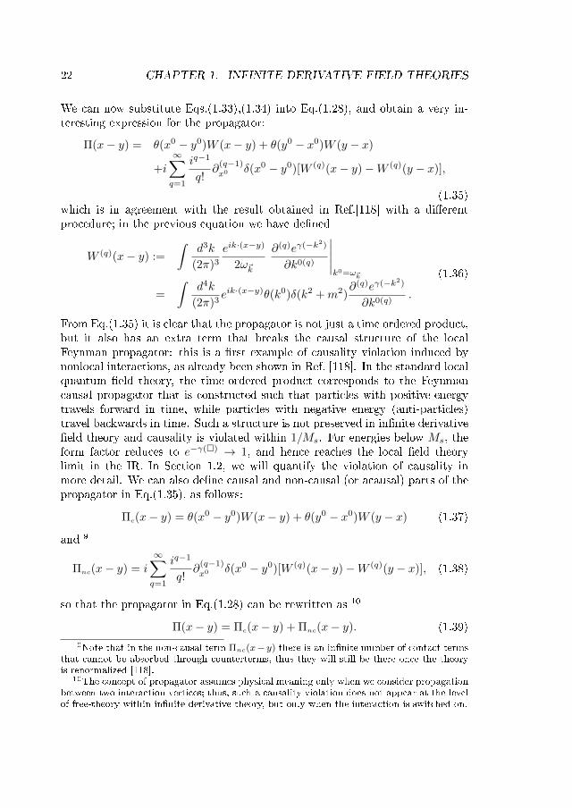
We can now substitute Eqs.(1.33),(1.34) into Eq.(1.28), and obtain a very in-teresting expression for the propagator:
(1.35)which is in agreement with the result obtained in Ref.[118] with a dierentprocedure; in the previous equation we have dened
W (q)(x− y) :=
∫d3k
(2π)3
eik·(x−y)
2ω~k
∂(q)eγ(−k2)
∂k0(q)
∣∣∣∣∣k0=ω~k
=
∫d4k
(2π)3eik·(x−y)θ(k0)δ(k2 +m2)
∂(q)eγ(−k2)
∂k0(q).
(1.36)
From Eq.(1.35) it is clear that the propagator is not just a time ordered product,but it also has an extra term that breaks the causal structure of the localFeynman propagator: this is a rst example of causality violation induced bynonlocal interactions, as already been shown in Ref. [118]. In the standard localquantum eld theory, the time-ordered product corresponds to the Feynmancausal propagator that is constructed such that particles with positive-energytravels forward in time, while particles with negative energy (anti-particles)travel backwards in time. Such a structure is not preserved in innite derivativeeld theory and causality is violated within 1/Ms. For energies below Ms, theform factor reduces to e−γ() → 1, and hence reaches the local eld theorylimit in the IR. In Section 1.2, we will quantify the violation of causality inmore detail. We can also dene causal and non-causal (or acausal) parts of thepropagator in Eq.(1.35), as follows:
so that the propagator in Eq.(1.28) can be rewritten as 10
Π(x− y) = Πc(x− y) + Πnc(x− y). (1.39)
9Note that in the non-causal term Πnc(x− y) there is an innite number of contact termsthat cannot be absorbed through counterterms, thus they will still be there once the theoryis renormalized [118].
10The concept of propagator assumes physical meaning only when we consider propagationbetween two interaction vertices; thus, such a causality violation does not appear at the levelof free-theory within innite derivative theory, but only when the interaction is switched on.
1.2. CAUSALITY 23
Since for free-elds W (x− y) = WL(x− y), one has Πc(x− y) = ΠL(x− y).
1.2 Causality
In this Section we will explicitly show that the presence of nonlocal interactionsviolate causality in a region whose size is given by ∼ 1/Ms in coordinate space,and for momenta k2 > M2
s in momentum space.
1.2.1 A brief reminder
Let us consider a real scalar eld φ(x0, ~x) that evolves by means of a dierentialoperator F () in presence of a source j(x0, x), so that it satises the followingdierential equation:
F ()φ(x0, ~x) = −j(x0, ~x). (1.40)
A formal solution to Eq. (1.40) is given by
φ(x0, ~x) = φo(x0, ~x) + i
∫dy0d3yG(x0 − y0, ~x− ~y)j(y0, ~y), (1.41)
where φo(x0, ~x) is the solution of the homogeneous equation, and G(x0−y0, ~x−~y) is the Green function of the dierential operator F (), dened by
A system whose evolution is governed by Eq. (1.40) is said to be causal if thecorresponding Green function G(x0, ~x) can be chosen, such that
G(x0, ~x) = 0 , if x0 < 0. (1.43)
The statement in Eq. (1.43) means that a physical system cannot respond to aninteraction-source before the source was turned on 11. The previous denitionof causal response holds for both relativistic and non-relativistic systems. Astronger version of the condition in Eq.(1.43) is given by the concept of sub-luminality [122], which is a property that has to be satised by any relativisticsystem. A physical system is said to be sub-luminal, if the Green functionG(x0, ~x) is causal and also vanishes outside the light cone, i.e.
G(x0, ~x) = 0 , if x0 < |~x|. (1.44)
By causality we will also refer to the concept of sub-luminality, namely a causalsystem will be characterized by a vanishing Green function for space-like sep-arations. Such a Green function is often indicated with a subscript "R" due
11Note that such a denition of causality in terms of the Green function, not only holds forclassical elds, but also for the expectation value of quantum elds in presence of a source,〈φ(x)〉j .
24 CHAPTER 1. INFINITE DERIVATIVE FIELD THEORIES
to its retarded behavior, and we will use the symbol GL,R in the case of thestandard local eld theory. Another denition of causality is given through thecommutator of two elds evaluated in two dierent space-time points. Froma physical-measurement point of view, to preserve causality, we would requirethat the commutator of the two observables has to vanish outside the lightcone,i.e. for space-like separations. For a real scalar eld, such a property can beformulated in the following way 12:
[φ(x), φ(y)] = 0 , if (x− y)2 > 0. (1.45)
When two observables commute, it means that they can be measured simultane-ously, i.e. namely one measurement cannot inuence the other. If the conditionin Eq.(1.45) is violated, there would be correlations between the two measure-ments performed at two dierent spacetime points with space-like separation,implying transmission of information at a speed faster than light, thus violatingcausality. The property in Eq.(1.45) is called local commutativity, or sometimemicrocausality.
Note that the two conditions of causality given in terms of the Green func-tion, see Eq. (1.44), and local commutativity, see Eq. (1.45), are closely relatedin local eld theory. Let us consider a Hamiltonian interaction between a realscalar eld φ(x) and a source j(x), Hint =
∫d3xjφ. Consider an initial cong-
uration with a vacuum state at a time y0 = −∞ and then switch on the sourceat a later time. The expectation value of φ at a spacetime point (x0, ~x), withx0 > y0, can be calculated in the interaction picture, and it is given by [122]
(1.46)where the dots stand for higher order contributions in the interaction-sourceterm. By comparing Eq.(1.41) with Eq.(1.46) we can identify φo(x) = 〈φ(x)〉j=0,and also note that in local eld theory, the expectation value of the commuta-tor between the two elds is related to the retarded Green function through thefollowing relation:
Hence, if the commutator vanishes for space-like separations, the interaction-source can only generate non-zero modes inside its future lightcone, and thusthe denition of causality given in terms of the Green function is consistent
12Let us remind that in the mostly positive metric signature (x− y)2 > 0 stands for space-like separation and (x − y)2 < 0 for time-like separation. In the mostly negative conventionwe would have had the opposite situation.
1.2. CAUSALITY 25
with the local commutativity condition. For completeness, we can also writethe analog of Eq.(1.47) for the advanced Green function:
We have already given an example of causality violation in Section 1.1, where wehave shown that the propagator is not simply given by a time-ordered product,but it has an extra non-causal term which becomes relevant inside the nonlocalregion. We now want to show that the presence of nonlocal interactions leadsinevitably to a violation of causality inside the region ∼ 1/Ms. In particular,we wish to show explicitly that the nonlocal analog of the retarded Green func-tion, eγ()[GL,R(x0, ~x)], is not vanishing outside the light-cone. We will simplyindicate the nonlocal analog of the retarded Green function with the symbolGR, meaning that it is a nonlocal quantity, while in presence of the subscript"L" we would refer to local quantities.
Let us remind that in local quantum eld theory the retarded Green functionis dened in terms of its Fourier transform as
− iGL,R(x− y) =
∫CR
d4k
(2π)4
eik·(x−y)
(k0)2 − ~k2 −m2, (1.49)
where the integration contour CR is given by the real axis where both the poles:
±ω~k = ±√~k2 +m2 are avoided from above with two semi-circles. By evaluating
the integral in Eq.(1.49) in the massless case, one obtains the retarded Greenfunction in coordinate space:
− iGL,R(x− y) =1
2πθ(t)δ(ρ) =
1
4πrδ(t− r), (1.50)
where t = x0 − y0, ~r = ~x− ~y and ρ = t2 − r2. From Eq.(1.50) it is obvious thatthe retarded propagator is vanishing outside the light-cone, i.e. in the regiont < r.
We now want to treat the case of innite derivative eld theory and explicitlysee that the retarded Green function shows an acausal behavior due to nonlocalinteractions. By following the steps in Eqs.(1.33) and (1.34) together withEq.(1.47), one can write the nonlocal retarded Green function as follows
Note the presence of the acausal (non-causal) term Πnc introduced in Eq.(1.38).In particular, we will consider form factors with polynomial exponents as inEq.(1.10), and for this specic choice we will see which is the form of Πnc.
26 CHAPTER 1. INFINITE DERIVATIVE FIELD THEORIES
First of all, note that such form factors are divergent at innity along somedirections in the complex plane k0: for example, it can happen that they divergeat −∞ and +∞ along the real axis making it impossible to compute the inte-gral in Eq.(1.50) in Minkowski signature. These kind of divergences make alsoimpossible to dene the usual Wick-rotation; this is one of the mathematicalreason why in innite derivative eld theory one has to dene all amplitudesin the Euclidean space, and in the end of the calculation go back to Minkowskisignature by making an appropriate analytic continuation. Below we will givea more detailed discussion about this last observation.
However, in the case of the exponential choice in Eq.(1.10) with even powersn the nonlocal form factor does not diverge along the real axis at innity, andwe can still compute the principal value of the integral in Minkowski signature.Therefore, in this subsection we will consider the following form factors:
e−γ() = e
(M2s
)2n
(1.52)
and we will work in the massless case for simplicity, m = 0. The aim is tocompute the following integral:
− iGR(x− y) =
∫CR
d4k
(2π)4
e−(k2
M2s
)2n
eik·(x−y)
(k0)2 − ~k2. (1.53)
The integral in Eq.(1.53) can be split into its principal value plus the contribu-tion coming from the two semi-circles that avoid the two poles from above:
− iGR = IPV + I2C , (1.54)
where I2C can be calculated by using the residue theorem, and one can easilyshow that is equal to
I2C =1
8πr[δ(t− r)− δ(t+ r)] =
1
4πε(ρ)δ(ρ). (1.55)
As for the principal value, one has
IPV =1
16iπ3
1
r
∞∫−∞
kdk P.V.
∞∫−∞
dk0 e−(−k20+k2
M2s
)2n
k20 − k2
(ei(kr−k
0t) − e−i(kr+k0t)),
(1.56)where k ≡ |~k| and ω~k = k, as we are working in the massless case. Note thatall information about nonlocality is contained in the principal value IPV , whileI2C is just a local contribution as it is evaluated at the residues, i.e. on-shell.
1.2. CAUSALITY 27
0 2 4 6 8 10 12 14
0.0000
0.0005
0.0010
0.0015
0.0020
0.0025
0.0030
|ρ| 1/2= |x-y|
iGR
2n=2
2n=4
2n=8
2n=10
Figure 1.1: In this plot we have shown the behavior of the nonlocal analog of theretarded Green function as a function of the space-like distance |ρ|1/2 = |x− y|,ρ < 0, for several values of the power in the exponent: 2n = 2 (continuous thickblue line), 2n = 4 (dashed orange line), 2n = 8 (dotted red line) and 2n = 10(continuous thin green line). The rst two cases can be computed analyticallyand expressed in terms of the Meijer-G functions (see Eq.(1.58) for the case2n = 2), while the last two cases have been obtained numerically. We have setMs = 1 as we are only interested in the qualitative behavior of the functions. Itis evident that for small distances nonlocality is relevant and we have an acausalbehavior, but as soon as |ρ|1/2 increases nonlocality becomes less important andthe Green function tends to a zero value recovering the local result, as expected.The oscillation-eects induced by nonlocality increase with the power 2n.
After some manipulations, one can show that the principal value in Eq.(1.56)can be recast in the following form 13:
IPV =1
π3
∂
∂ρ
ε(ρ)
∞∫0
dζ
ζe− ζ4n
M4ns ρ2n
[K0(ζ) +
π
2Y0(ζ)
] , (1.57)
where ε(ρ) is equal to +1 if ρ > 0 (time-like separation), while it is −1 if ρ < 0(space-like separation); Y0 and K0 are Bessel functions of the second kind andthe modied Bessel function, respectively.
We can now nd an explicit form for the integral in Eq.(1.57), for examplewe can consider the power 2n = 2. In such a case the integral can be computed
13See Appendix B for all the details of the calculation.
28 CHAPTER 1. INFINITE DERIVATIVE FIELD THEORIES
and expressed in terms of the Meijer-G functions [123], so that the acausalGreen function in Eq.(1.53),(1.54) reads
−iGR(ρ) =1
4πε(ρ)δ(ρ) +
1
2π4
ε(ρ)
ρ
G4,1
2,5
(00, 0, 1
2 ,12
∣∣∣∣∣M4s ρ
2
256
)
+2π2G4,13,6
(0,− 1
4 ,14
0, 0, 12 ,
12 ,−
14 ,
14
∣∣∣∣∣M4s ρ
2
256
).
(1.58)
From Eq.(1.58) it follows that the Green function GR is not vanishing for space-like separation (ρ < 0). In Fig. 1.1 we have plotted such a Green function forρ < 0 so that it is very clear that it assumes values dierent from zero, but forlarge value of ρ, i.e. for M2
s ρ → ∞, GR → 0, as expected. Thus, the violationof causality is restricted to the spacetime region of size approximatively givenby ∼ 1/Ms.
In the limit M2s ρ→∞ the integral in Eq. (1.57) reduces to:
limM2s ρ→∞
IPV =1
8πr[δ(t+ r) + δ(t− r)], (1.59)
so that the sum of the two contributions I2C + IPV would recover the localresult in Eq.(1.50).
It is worth mentioning that for other values of 2n the integral in Eq.(1.57)also shows an acausal behavior, for example we have checked that in the case2n = 4 the integral can be still expressed as a combination of Meijer-G func-tions; for larger values of 2n one can proceed numerically. In Fig. 1.1 we havealso shown the behavior of the acausal Green function for 2n = 4, 8, 10. More-over, the same procedure that we have used above can be used to compute thenonlocal analog of the advanced Green function, and it will lead to an oppositesituation in which GA will be non-vanishing for time-like separations.
1.2.3 Acausality for nonlocally interacting elds
We now wish to show that, due to the acausal feature of the Green functions,nonlocal interaction also implies the presence of acausality in the evolution ofthe elds; in particular we will see that the elds can depend acausally uponthe initial data. Let us consider the Lagrangian for a real scalar eld φ(x) witha quartic interaction 14 as an example:
L =1
2φ(x)(−m2)φ(x)− λ
4!
(e
12γ()φ(x)
)4
, (1.60)
14We could have considered any kind of interaction, but as an example we have chosen φ4.Moreover, we are working in the case in which the kinetic term is the standard Klein-Gordonoperator and the interaction term is modied by the introduction of a form factor; of coursethe results would be the same if we considered nonlocal kinetic operator and local interactionvertices.
1.2. CAUSALITY 29
with corresponding eld equations given by
(−+m2)φ(x) = − λ3!e
12γ()
(e
12γ()φ(x)
)3
, (1.61)
where λ is a dimensionless coupling constant. The eld equation in Eq.(1.61)can be solved perturbatively by continuous iterations; the zeroth and rst orderare given by:
(−+m2)φ(0)(x) = 0,
(−+m2)φ(1)(x) = − λ3!e
12γ()
(e
12γ()φ(0)(x)
)3
,(1.62)
where the zeroth order is nothing but the homogeneous Klein-Gordon equation,whose local solutions are given by the free-eld decomposition in Eq.(1.15), thatwe rewrite for clarity:
φ(0)(x0, ~x) =
∫d3k
(2π)3
1√2ω~k
(a~ke−iω~kx
0+i~k·~x + a∗~keiω~kx
0−i~k·~x). (1.63)
Note that the Fourier-transform of the eld φ(0)(x0, ~x) with respect to the spatialcoordinate ~x, φ(0)(x0,~k), can be expressed in terms of the initial eld congu-
ration, φ(0)(0,~k) and ˙φ(0)(0,~k), as follows 15
φ(0)(x0,~k) = φ(0)(0,~k)cos(ω~kx0) +
˙φ(0)(0,~k)
sin(ω~kx0)
ω~k, (1.64)
so that the free-eld in Eq. (1.63) can be rewritten as
φ(0)(x0, ~x) =
∫d3k
(2π)3ei~k·~x(φ(0)(0,~k)cos(ω~kx
0) +˙φ(0)(0,~k)
sin(ω~kx0)
ω~k
).
(1.65)Let us now compute the variation of the free-eld with respect to an initial
eld-conguration φ(0)(y), with y ≡ (0, ~y), such that the distance between xand y is space-like, (x− y)2 > 0 (or, equivalently, |~x− ~y| > x0):
δφ(0)(x0, ~x)
δφ(0)(0, ~y)=
∫d3k
(2π)3e−ik·(~x−~y)cos(ω~kx
0) = −∆(x0, ~x− ~y), (1.66)
δφ(0)(x0, ~x)
δφ(0)(0, ~y)=
∫d3k
(2π)3e−ik·(~x−~y) sin(ω~kx
0)
ω~k= −∆(x0, ~x− ~y), (1.67)
where we have used
φ(0)(0,~k) =
∫d3x′e−i
~k·~x′φ(0)(0, ~x′) andδφ(0)(0, ~x′)
δφ(0)(0, ~y)= δ(3)(~x′ − ~y).
15Note that the symbol " · " means derivative with respect to x0.
30 CHAPTER 1. INFINITE DERIVATIVE FIELD THEORIES
Note that we have obtained the Pauli-Jordan function as a result of the func-tional dierentiation. As we have already emphasized, ∆(x0, ~x − ~y) has onlysupport inside the lightcone, and the same holds for its time-derivative; thusfor space-like separations they vanish and causality is preserved at the level offree-theory.
Let us now consider the rst order in perturbation, i.e. the dierentialequation in the second line of Eq.(1.63). The solution φ(1)(x) is given by thesum of the homogeneous and the particular solutions, which we can indicate byφ
(1)o (x) and φ(1)
p (x), respectively:
φ(1)(x) = φ(1)o (x) + φ(1)
p (x), (1.68)
where the particular solution has the physical information about the nonlocalinteraction. The homogeneous solution, φ(1)
o (x), satises the same equation ofφ(0)(x), while the particular solution can be formally expressed in terms of theGreen function as in Eq.(1.41):
φ(1)p (x0, ~x) =
iλ
3!
∫dx′0d3x′e
12γ(x′ )[GL,R(x0 − x′0, ~x− ~x′)]
(φ(0)(x′0, ~x′)
)3
,
(1.69)where we have used the fact that e
12γ()φ(0)(x) = φ(0)(x), at the zeroth order we
have a free-eld eld propagation - satisfying the homogeneous Klein-Gordonequation, and we have also made use of the kernel representation of the expo-nential dierential operator:
e12γ(x)g(x) =
∫d4ye
12γ(y)δ(4)(x− y)g(y).
All information about the presence of nonlocal interactions is contained in theparticular solution; thus let us now calculate, as done for the zeroth order inEqs.(1.66) and (1.67), the variation of the eld φ(1)
p (x0, ~x) with respect an initialeld conguration φ(0)(0, ~y), φ(0)(0, ~y)16:
δφ(1)p (x0, ~x)
δφ(0)(0, ~y)= − iλ
2
∫dx′0d3x′e
12γ(x′ )[GL,R(x0 − x′0, ~x− ~x′)]
×∆(x′0, ~x′ − ~y)(φ(0)(x′0, ~x′)
)2
,
(1.70)
δφ(1)p (x0, ~x)
δφ(0)(0, ~y)= − iλ
2
∫dx′0d3x′e
12γ(x′ )[GL,R(x0 − x′0, ~x− ~x′)]
×∆(x′0, ~x′ − ~y)(φ(0)(x′0, ~x′)
)2
.
(1.71)
16A similar computation was also done, for example, in Ref. [111] in the case of scalar eld
with cubic interaction, [e/M2s φ(x)]3, that can represent the interaction vertex for a dilaton
eld in string eld theory.
1.2. CAUSALITY 31
The action of the dierential operator on the local Green function in the in-tegrals in Eqs.(1.70) and (1.71) makes the interacting eld φ
(1)p depending
acausally upon the initial data: in fact, the integrals in Eq.(1.70) and (1.71)are not vanishing for space-like separations |~x − ~y| > x0 due to the non-zerocontribution coming from the integration-region x′0 < |~x′| as the functione
12γ(x′ )[GL,R(x′0, ~x′)] exhibits an acausal behavior, i.e. it is non-vanishing
for the space-like separations x′0 < |~x′|, as previously shown for the caseγ() = (− + m2)n/M2n
s . Indeed, more explicitly one has the following sit-uations.
In the local case, γ() = 0, the integrals in Eqs.(1.70),(1.71) get non-vanishing contributions coming from the integration region on which boththe retarded Green function and the Pauli-Jordan function are non-zero.Such a region is dened by the following two inequalities: x0 − x′0 ≥|~x − ~x′|, x′0 ≥ |~x′ − ~y|. Moreover, since the initial time condition isy0 = 0 and we are looking at the future evolution by means the nonlocalanalog of the retarded Green function, the following inequality has to hold:x0 > x′0 > 0. We can now ask if the eld φ(1)
p (x) depends acausally uponthe initial spacetime conguration (0, ~y). One can easily show that byputting together the above inequalities, we obtain
x0 ≥ |~x− ~y|, (1.72)
which implies that for space-like separation, x0 < |~x − ~y|, the integralsin Eqs. (1.70),(1.71) are vanishing. Thus, in local eld theory the eldevolution turns out to be causal.
In the case of nonlocal interactions, γ() 6= 0, the Green function GRshows an acausal behavior, i.e. it is non-vanishing for space-like separa-tions, thus we can not use the rst inequality x0 − x′0 ≥ |~x− ~x′|, x′0 ≥|~x′ − ~y|, as done above for the local case. It follows that for space-likeseparation x0 < |~x − ~y| the functional derivatives in Eqs.(1.70),(1.71) donot vanish and the eld can depend acausally on the initial data.
The acausal behavior is conned to a region of size ∼ 1/Ms, as it would be moreexplicit once a specic choice for the form factor is made.
1.2.4 Local commutativity violation
We have shown that the presence of nonlocal interaction implies an acausalbehavior of the Green functions, which in turn makes the interacting eldsdepending acausally upon the initial data. However, we have not investigatedyet whether also the commutator between interacting elds is modied in sucha way that the local commutativity condition is also violated. In Section 1.1.3,
32 CHAPTER 1. INFINITE DERIVATIVE FIELD THEORIES
we have shown that the commutator for free-elds is not modied by innitederivatives, maintaining the same structure of the local theory. We now want toshow that local commutativity is violated when nonlocal interaction is switchedon.
Let us still consider the nonlocal φ4-theory as an example, i.e. the La-grangian in Eq.(1.60), and let us compute the commutator between two interact-ing elds by using the perturbative eld solution φ(x) = φ(0)(x)+φ(1)(x)+O(λ2)introduced in the previous subsection. The commutator between two interactingelds up to order O(λ2) is given by
Note that [φ(0)(x), φ(0)(y)] obeys local commutativity as φ(0) is not aectedby nonlocality, see Eqs.(1.62),(1.22). Moreover, from Eq.(1.68) we know thatφ(1) = φ
(1)o +φ
(1)p , where φ(1)
o is also not aected by nonlocality being a homoge-neous solution; thus all the information about the nonlocal modication of thecommutator are taken into account by the terms involving φ(1)
p . The second andthird terms contributing to the commutator in Eq.(1.73) are of the followingform:
[φ(0)(x), φ(1)(y)] ∼ iλ
3!
∫d4y′e
12γ(y′ )[GL,R(y−y′)]
(φ(0)(y′)
)2
[φ(0)(x), φ(0)(y′)].
(1.74)
In the local case, γ() = 0, the integral in Eq.(1.74) gets a non-vanishingcontribution when the following two inequalities are satised:
y0 − y′0 ≥ |~y − ~y′|, y′0 ≥ |~y′ − ~x| (1.75)
where we have taken x0 = 0 without any loss of generality. We can nownotice that, by choosing y0 > x0 = 0, the last two inequalities togetherimply
y0 ≥ |~y − ~x|, (1.76)
which means that the commutator in Eq.(1.74) gets non-vanishing contri-butions only for either time-like or null separations, in local eld theory.
In the case of nonlocal interaction, γ() 6= 0, the rst inequality inEq.(1.75) can not be used as the Green function is acausal and gives anon-vanishing contribution also for space-like separations. As a result, thecommutator in Eq.(1.74) will be non-vanishing for space-like separations.
1.3. AMPLITUDES 33
The same scenario also holds for the fourth term in Eq.(1.73), whose expressionis of the following form:
[φ(1)(x), φ(1)(y)] ∼(iλ
3!
)2∫d4xd4ye
12γ(x′ )[GL,R(x− x′)]e 1
2γ(y′ )[GL,R(y − y′)]
×(φ(0)(y′)
)2 (φ(0)(x′)
)2
[φ(0)(x′), φ(0)(y′)].
(1.77)
In the local case, γ() = 0, the integral in Eq.(1.77) gets a non-vanishingcontribution when the following three inequalities are satised:
For simplicity, we can take y0 > x0 = 0, without any loss of generality,and we can notice that all together the inequalities in Eq.(1.78) imply
y0 ≥ |~x− ~y|, (1.79)
which means that the commutator in Eq.(1.77) gets non-vanishing contri-butions only for either time-like or null separations, in local eld theory.
In the case of nonlocal interaction, γ() 6= 0, the rst two inequalities inEq.(1.78) can not be used as the Green functions are acausal and give non-vanishing contributions also for space-like separations. As a result, thecommutator in Eq.(1.77) will be non-vanishing for space-like separation,meaning a violation of the local commutativity condition.
Note that we have only considered the commutator up to quadratic order in thecoupling constant, but it is clear that local commutativity will be also violatedat higher order in perturbation theory.
In order to quantify the degree of local commutativity violation we need toperform the computation by specifying an explicit form for the Green functionand the Pauli-Jordan function to see how the integrals in Eqs.(1.74,1.77) behavesfor space-like separation; but it will be subject of future works.
1.3 Amplitudes
From a physical point of view the presence of acausal eects means that thereis no concept of Minkowski spacetime in the nonlocal region, nonlocality is suchthat we can not dene the usual concepts of space and time. We can not deneclock and rulers to make any kind of measurements inside 1/Ms. For this reason,dening physical quantities in Minkowski signature in such a region would notmake sense from a physical point of view, but the appropriate way to proceed
34 CHAPTER 1. INFINITE DERIVATIVE FIELD THEORIES
would be to dene Euclidean amplitudes and Euclidean correlators. Indeed, inEuclidean space we do not have any concept of real time, all Euclidean distancesare space-like by denition.
Such a physical argument also has a mathematical counterpart. As we havealready briey mentioned in the previous subsections, in innite derivative eldtheory the form factors introduce some ambiguities when performing calcula-tions of integrals in momentum space. For example, the exponential form factorswith polynomial exponents introduced in Eq.(1.10) can always appear in loop-integral and amplitudes in the form e−(k2/Ms)
n
where n is a positive integer. Forexample, for the calculation of either propagator or any other Green functions,one has to deal with integrals of the following type:
I(x) =
∞∫−∞
dk0 e−(−k20+~k2
M2s
)ne−ik
0x0+i~k·~x
k20 − ω2
~k
. (1.80)
It is easy to understand that the presence of the form factor gives divergentcontributions along certain directions in the complex plane k0; for instance, wecan consider as examples n = 1 and n = 2.
In the case n = 1 one has:
ek20−
~k2
M2s e−ik
0x0+i~k·~x ∼ eRe2(k0)
M2s e
Im(k0)x0
M2s e
− Im2(k0)
M2s , (1.81)
which diverges at innity along the directions belonging to the region|Re(k0)| > |Im(k0)|, while it converges to zero along the directions suchthat |Re(k0)| ≤ |Im(k0)|.
In the case n = 2, the relevant contribution at innity is given by:
e− (−k20+~k2)2
M4s e−ik
0x0+i~k·~x ∼ e−Re4(k0)
M4s e
− Im4(k0)
M4s e
6Im2(k0)Re2(k0)
M4s , (1.82)
that only diverges along the directions Im(k0) = ±Re(k0), while in therest of the complex plane it approaches to zero at innity.
Note that such divergences in most of the cases it makes impossible to calcu-late integrals in Minkowski signature, for example the usual Feynman contourprescription does not work anymore, because the contribution coming from thesemi-circle in either the lower or the upper half of the complex plane receive aninnite contribution at innity. It implies that the usual Wick-rotation cannotbe dened. Therefore, one has to be careful when defying scattering ampli-tudes. For instance, by starting in Minkowski signature the optical theorem isnot satised and unitarity seems to be lost [124].
1.3. AMPLITUDES 35
However, one can show that by defying all amplitudes in Euclidean space andthen making an appropriate analytical continuation of the external momentato Minkowski, the theory turns out to be unitary [125, 124, 126, 127]. Theimportant property of such exponential form factors is that they always go tozero along the imaginary axis I directions, Im(k0)→ ±∞, so that amplitudes inEuclidean signature are well dened and each loop integral can be legitimatelycomputed on the integration domain I×R3 . Subsequently, these amplitudes areanalytically continued to real and positive external energies by means of a newprescription such that no Wick rotation is performed by the integration contouris deformed in a nite region of the complex plane; see Refs.[125, 127, 126] formore details.
As mentioned above, in the region of nonlocality < 1/Ms, or in momen-tum space, for momenta k2 > M2
s , we cannot dene any classical concept ofspacetime point, but vertices are smeared out such that the external legs andinternal lines do not join in one point but they overlap in a region of size 1/Ms.The crucial role is played by the acausal term Πnc dened in Eq.(1.38), whichimplies causality violation in the vertices. In momentum space Πnc reads [118]:
Πnc(k) =
∫d4xΠnc(x)e−ik·x
= i
∞∑q=1
1
q!
1
2ω~k
∂(q)eγ(−k2)
∂k0(q)
∣∣∣∣∣k0=ω~k
(k0 − ω~k)q−1 − ∂(q)eγ(−k2)
∂k0(q)
∣∣∣∣∣k0=−ω~k
(k0 + ω~k)q−1
,(1.83)
and it is evident that it has no poles and has no absorptive components, namelyit is not made of on-shell intermediate states, but it is purely o-shell; indeed,it can be seen as a nonlocal vertex: Πnc(k) = iV (k). Thus, in momentum spacethe nonlocal propagator in Eq.(1.39) reads:
Π(k) = Πc(k) + iV (k), (1.84)
where Πc(k) is causal and V (k) tends to zero for k2 M2s , but would be
relevant for k2 ≥ M2s . Note that the nonlocal acausal part of the propagator,
iV (k), is made of innite derivatives and this is the main cause of the smearingof the vertices, which are not point-like anymore. Thus, from Eqs.(1.83,1.84)it is now more clear that in innite derivative eld theories nonlocality andacausality manifest as o-shell eects.
In the standard local quantum eld theory all internal lines of a Feynmandiagram are seen as o-shell, while in innite derivative quantum eld theorythe degree of "o-shellness" increases as also the vertices become nonlocal. Inparticular, there is no energy and momentum conservation in one single point,as legs and internal lines overlap on a smeared region of size 1/Ms, or in termsof momentum,Ms. See Fig. 1.2 for an illustration of local and nonlocal vertices.
36 CHAPTER 1. INFINITE DERIVATIVE FIELD THEORIES
Local vertex Nonlocal vertex
Figure 1.2: We have shown a pictorial illustration for local (left side) and nonlo-cal (right side) vertices. In the latter case the legs do not meet in one single pointdue to nonlocal eects spread out on a region (black blob) of size Ls = 1/Ms .
1.3.1 Euclidean 2-point correlation function
In local quantum eld theory one has to deal with innities which need to beregularized in order to give physical meaning to the theory. There are at leastthree kind of divergences that one can encounter:
1. UV divergences (k →∞);
2. IR divergences (k → 0);
3. lightcone singularities (|x− y| → 0).
In principle, one can cure IR and UV divergences but, even after the renormal-ization procedure has been applied, the lightcone singularity, which correspondsto the singularity at the origin in Euclidean space, still remains uncured. In thissection we wish to compute the 2-point correlation function in innite deriva-tive quantum eld theory; as an example we will still consider φ4-theory. Inparticular, we want to analyze its behavior on the light-cone surface, or in otherwords at the Euclidean origin, and see whether nonlocal interactions can reg-ularize the divergence at (x − y) → 0 from which the local theory suers. Forsimplicity, we will focus on the form factor eγ() = e−(−m2)/M2
s . We will workin Euclidean signature but the results can be reinterpreted in Minkowski spaceby analytic continuation as briey explained above. Therefore, let us considerthe following Euclidean generating functional:
Z[J ] =
∫Dφe−SE [φ]+
∫d4xJφ, (1.85)
where J(x) is the source-term and the Euclidean action is given by:
SE[φ] =
∫d4x
(−1
2φ(x)e−(−m2)/M2
s (−m2)φ(x) +λ
4!φ4(x)
). (1.86)
1.3. AMPLITUDES 37
The functional in Eq.(1.86) can be rewritten in the following way:
Z[J ] = e−λ4!
∫d4x[ δ
δJ(x) ]4
Z0[J ] = e−λ4!
∫d4x[ δ
δJ(x) ]4
e12
∫d4xd4yJ(x)Π(x−y)J(y),
(1.87)where Z0[J ] is the free generating functional and Π(x − y) is the propagatorin the Euclidean space where, now, k ≡ (k4,~k) stands for the Euclidean mo-mentum, with k4 = −ik0, and x ≡ (x4, ~x) for the Euclidean coordinate, withx4 = ix0. We are interested in computing the 2-point correlation function thatis dened as
G(x− y) :=δ2Z[J ]
δJ(x)δJ(y)
∣∣∣∣J=0
. (1.88)
By expanding the exponential in Eq.(1.87), we can compute perturbatively thecorrelator G(x− y); for instance up to the rst order in λ, we obtain:
G(x− y) = Π(x− y)− λ
2Π(0)
∫d4zΠ(x− z)Π(z − y) +O(λ2), (1.89)
where at zeroth order we have the free-propagator, while at the rst order atadpole contribution.
Let us start by analyzing the zeroth order of the perturbative expansion inEq.(1.89), i.e. the Euclidean propagator, in both massless and massive case.
In the massless case the Euclidean 2-point function at zeroth order reads:
Π(x− y)|m=0 =
∫d4k
(2π)4
e−k2/M2
s eik·(x−y)
k2=
1− e−M2s (x−y)2
4
4π2(x− y)2. (1.90)
First of all, note that in the limit M2s (x− y)2 →∞, we recover the local
massless propagator, ΠL(x− y)|m=0 = 14π2(x−y)2 . More importantly, in
the limit in which nonlocality becomes relevant, i.e. M2s (x − y)2 → 0,
unlike in the local case the massless propagator in Eq.(1.90) does notdiverge but it tends to a nite constant value:
Π(0)|m=0 =M2s
16π2. (1.91)
The result in Eq.(1.91) is extremely important for what concerns the UVbehavior of the theory. The quantity Π(0)|m=0 appears as a coecientof the perturbative series in Eq.(1.89), and in local eld theory the renor-malization problem arises because of the presence of divergent coecients.Thus, we have seen a rst concrete example of how nonlocal interactioncan improve the UV behavior of the theory. In particular, φ4-theory withnonlocal interaction becomes nite as discussed in Ref.[87, 86].
38 CHAPTER 1. INFINITE DERIVATIVE FIELD THEORIES
As for the massive propagator, by using again the Schwinger parametriza-tion for 1/(k2 +m2), we can write
Π(x− y) =
∫d4k
(2π)4
e−(k2+m2)/M2s eik·(x−y)
k2 +m2=
m2
16π2
∞∫m2
M2s
dse−se−
m2(x−y)24s
s2.
(1.92)Although the integral in Eq.(1.92) cannot be solved in terms of elementaryfunctions as in the massless case (Eq.(1.90)), it can be expressed in termsof the so called cylindrical incomplete function of Sonine-Schlaei:
Π(x− y) = − 1
4π
m
|x− y|S1
(−m
2
M2s
,−∞; im|x− y|), (1.93)
where the Sonine-Schlaei function is dened as [128]
Sν(−p,−q; iz) :=e−
iπν2
2πi
(z2
)ν q∫p
dt t−ν−1e−t−z2
4t .
We can study the limit (x−y)→ 0, and note that the massive propagatoris non-singular at the Euclidean origin. Indeed, in this limit the integralin Eq.(1.92) gives
Π(0) =M2s e−m2
M2s
16π2
[1 + e
m2
M2s Ei
(−m
2
M2s
)], (1.94)
where
Ei(x) := −∫ ∞−x
dte−t
t
is the so called exponential-integral function.
First-order correction O(λ)
So far we have learnt that at the zeroth order in the perturbative expansionin Eq.(1.89) the 2-point correlation function is regular at the Euclidean ori-gin unlike in the local case where singularities are present. We now want tostudy the rst order correction (tadpole) in Eq.(1.89) and see whether such aregularization property is maintained.
In the massive case, one can check numerically that the rst order correc-tion is non-singular at the Euclidean origin.
1.3. AMPLITUDES 39
In the massless case, the rst order correction to the 2-point Euclideancorrelator is singular at the origin, as we will now show with an explicitcalculation. However, this can be made non-singular by dressing the prop-agator; see below.
At the rst order in perturbation theory, by going to polar coordinates in 4-dimensions, d4k = k3 sinθ sin2αdk dθ dα dϕ , the 2-point function for the mass-less case can be expressed as
G(1)(x− y)∣∣m=0
= −λ2
Π(0)|m=0
∫d4z Π(x− z)|m=0 Π(z − y)|m=0
= −λ2
Π(0)|m=0
1
4π2|x− y|
∞∫0
dke− 2k2
M2s J1(k|x− y|)
k2.
(1.95)First of all, note that the integral in Eq.(1.95) has an IR divergence, as we cansee more explicitly by introducing an IR cut-o L:
G(1)(x− y)|m=0 = −λ2
Π(0)|m=0
− 1
2π2
1
M2s (x− y)2
(1− e−
M2s (x−y)2
8
)+
1
16π2Ei
(−M
2s (x− y)2
8
)+ lim
L→∞
[1
4π2
L
|x− y|
(1− e−
|x−y|4L
)− 1
16π2Ei
(−|x− y|
4L
)].
(1.96)It is obvious that in the limit L→∞, the IR divergence comes from
limL→∞
Ei
(−|x− y|
4L
)=∞. (1.97)
Note that the IR divergence comes together with the singularity at the Euclideanorigin (or lightcone singularity in Minkowski signature) in the massless case -the correlator at the rst order in λ in Eq.(1.96) also diverges for |x− y| → 0.17
We have seen that the rst order correction seems to suggest that nonlocalityis not sucient to regularize the singularity of the 2-point correlation functionin the massless case. However, as we will show below, if we consider the fullcorrelator, namely taking into account all the quantum perturbative correctionsthrough the so called dressed propagator, then we will see that the physical 2-point function becomes regular at the origin.
17The singularity at the Euclidean origin will also appear for any power of thed'Alembertian n, with any n; indeed, it is purely related to the infrared divergence thatone has in the massless case. It so happens that infrared divergence and singularity at theEuclidean origin (or lightcone singularity) are mixed.
40 CHAPTER 1. INFINITE DERIVATIVE FIELD THEORIES
0 2 4 6 80.000
0.001
0.002
0.003
0.004
|x-y|
2-pointcorrelationfunction
Massless
Massive
Figure 1.3: In this plot we have shown the behavior of the dressed 2-pointcorrelation function obtained by solving numerically the integral in Eq.(1.100).The blue-line represent the massless case, while the orange line represents themassive case with m = 1. We have set Ms = 1 for simplicity, as we are onlyinterested in the qualitative behavior around the origin. We can notice that for|x−y| → 0 the correlators tend to a nite value that of course dier for masslessand massive cases.
Dressed 2-point correlation function
Let us consider the Fourier transform G(k) of the correlator in Eq.(1.89), inthe more general case of massive scalar eld and then we will also specializeto the massless case. It is well known that once one takes into account all theperturbative corrections to the 2-point correlation function in momentum spaceone obtains the so called dressed-propagator that can be expressed in terms ofthe self-energy Σ(k). Thus, we have [87]
G(k) = Π(k)
∞∑n=0
(−1)n [Σ(k)Π(k)]n
=Π(k)
1 + Σ(k)Π(k)
=e− k
2+m2
M2s
k2 +m2 + Σ(k)e− k2+m2
M2s
.
(1.98)
The self-energy at 1-loop is independent on the external momenta (tad-pole),
1.3. AMPLITUDES 41
and reads:
Σ = λ
∫d4p
(2π)4
e− (p2+m2)
M2s
p2 +m2, (1.99)
The integral in Eq.(1.99) turns out to be nite in both massless and massivecases; in fact it has the same expression of the Euclidean propagator evaluated atthe origin in Eqs.(1.91) and (1.94) for massless and massive cases, respectively.
We are interested in the coordinate-space dressed-correlator, so we need toconsider the following Fourier transform:
G(x− y) =
∫d4k
(2π)4
e− k
2+m2
M2s eik·(x−y)
k2 +m2 + Σ(k)e− k2+m2
M2s
=1
4π2|x− y|
∞∫0
k2J1(k|x− y|)dk
ek2+m2
M2s (k2 +m2) + Σ(k)
.
(1.100)
The integral in Eq.(1.100) cannot be solved analytically, but we can calculate itnumerically, and we note that the full 2-point correlation function is non-singularat the Euclidean origin for both massive and massless cases. In Fig.1.3, we haveshown the numerical solutions of the integral in Eq.(1.100) for both massive andmassless cases.
1.3.2 s- and t-channels
We now wish to discuss an open problem of innite derivative eld theorieswhich is related to an apparent divergent behavior of scattering amplitudes. Wewill propose a possible solution to this issue even though deeper investigationsare need for a denite resolution.
Some ambiguities may appear when working with amplitudes with the ex-ponentials of the kind e−(p2/M2
s )n :
1. e−(p2/M2s )2n : tree level amplitudes with even power of the exponent would
be always exponentially suppressed for both time-like and space-like mo-mentum exchange;
2. e−(p2/M2s )2n+1
: tree level amplitudes with odd power of the exponent wouldbe exponentially suppressed only for space-like momentum exchange, butthey blow up for time-like exchange, i.e. for p2 < 0.
As a consequence, for both even and odd powers the tree level scattering ampli-tudes turn out to be exponentially suppressed in the case of t- and u-channels,while the s-channel amplitude is exponentially suppressed only for even pow-ers, but it blows up for odd powers as in this case the momentum exchange
42 CHAPTER 1. INFINITE DERIVATIVE FIELD THEORIES
is time-like, giving a positive exponent in the exponential which causes thedivergence for high energies. Such a divergent behavior appears when the am-plitude is made of an internal propagator that connects two cubic vertices (e.g.φ3-theory).
This unstable behavior should be only apparent and a resolution that goesbeyond standard local quantum eld theory techniques may be found, indeedhere we present an attempt. Note that such divergences only manifest at thelevel of the bare propagator, i.e. at the tree level. In fact, once all quantum cor-rections are taken into account through the dressed propagator, all the scatteringamplitudes become exponentially suppressed, thus physically well-dened; seealso Ref. [129] for analogue discussions, where the tree level scattering ampli-tudes were computed, and also the dressed vertices and the dressed propagator.
Let us explicitly show that by correctly dressing the propagator no ambiguitywould arise. For simplicity, we will consider the case of λφ3-theory with anonlocal kinetic operator, and work in the massless case. A generic tree levelscattering amplitude will be given by:
Mn ∼ λ2 e−(p2/M2
s )n
p2. (1.101)
Once we dress the propagator, we obtain (see Eq.(1.98))
Mn ∼ λ2 e−(p2/M2s )n
p2 + Σn(p)e−(p2/M2s )n
, (1.102)
where the self-energy Σn(p) for λφ3-theory, for example at 1-loop, reads
Σn(p) = λ2
∫dk4
(2π)4
e−(k2/M2s )ne−((k−p)2/M2
s )n
k2(k − p)2, (1.103)
which for even powers of n turns out to be always exponentially suppressed forany value of p2, while for odd powers of n can blow up for time-like momenta,p2 < 0. Note that, generally, integrals of the type in Eq.(1.103) can blow upfor some values of the integration variable k; however, by working in Euclideansignature, k0 = ik4 and p0 = ip4, the integrals can be computed, and after thecomputation is made the momentum p can be analytically continued back toMinkowski signature, p4 = −ip0; see for example for discussions Refs.[125, 87].
Let us analyze t-channel and s-channel, for both even and odd powers.
Even powers 2n
Note that in the case of even powers, e−(p2/M2s )2n , the high energy behavior of
the scattering amplitudes is the same for both bare and dressed propagator. In-deed, in the UV regime, p2/Ms →∞ we have the following asymptotic behavior
1.3. AMPLITUDES 43
for the dressed amplitude in Eq.(1.102) with even powers:
M2n ∼ e−(p2/M2s )2n , (1.104)
as Σ2n(p) e−(p2/M2s )2n → 0 for p2/M2
s →∞. Moreover, the asymptotic behavioris also the same for both t- and s-channels, as the even power, 2n, does notdistinguish between space-like and time-like momentum exchange: (±p2)2n =(p2)2n.
Thus, we have shown that in both cases of bare and dressed propagator, ands- and t-channels, the asymptotic behaviors of the scattering amplitudes are thesame for even powers (2n) of the d'Alembertian.
Odd powers 2n+1
We now want to address the case of odd powers, e−(p2/M2s )2n+1
. Let us distin-guish the cases of t-channel and s-channel.
t-channel scattering: In the case of t-channel scattering, the momentumexchange is space-like, k2 > 0, and the asymptotic behavior for high ener-gies turns out to be the same for both bare and dressed propagator, as italso happens for the case of even power. Indeed, for space-like momentumexchange, for p2/M2
s →∞, we have:
M2n+1 ∼ e−(p2/M2s )2n+1
, (1.105)
as Σ2n+1(p)e−(p2/M2s )2n+1 → 0.
s-channel scattering: In the case of s-channel scattering, the momen-tum exchange is time-like, p2 < 0, and it is clear that for high energy thepropagator blows up. However, as we have already emphasized, nonlocal-ity is inherently o-shell, and as such quantum eects are not negligibleand what is physically meaningful is the dressed propagator in the regionof nonlocality, p2 > M2
s .
By dressing the propagator, it so happens that for high energy the am-plitude has the same asymptotic behavior as for the t-channel, with thesame exponential suppression, as one would expect for consistency. Wewill show this by making an explicit calculation for the simplest case n = 1.In this case the s-channel amplitude with dressed propagator is given by:
M1 ∼ λ2 e−p2/M2
s
p2 + Σ1(k)e−p2/M2
s. (1.106)
Note that the self-energy Σ1(k) at 1-loop can be explicitly computedby performing the integration in Euclidean space and then analytically
44 CHAPTER 1. INFINITE DERIVATIVE FIELD THEORIES
continuing back to Minkowski the momentum p; indeed by using theSchwinger parameterization we obtain:
Σ1(p) =λ2
16π2
∞∫1M2s
dt1
∞∫1M2s
dt2e−p
2 t1t2t1+t2
(t1 + t2)2
=λ2
16π2
[2M2
s
p2
(e−p
2/2M2s − e−p
2/M2s
)+ Ei
(− p2
2M2s
)− Ei
(− p2
M2s
)],
(1.107)which in the high energy regime goes to zero for space-like momentumexchange, while diverges for time-like exchange. In particular, the asymp-totic behavior of the self-energy for p2/M2
s →∞ is given by:
Σ1(p) ∼ e−p2/M2
s . (1.108)
It is now clear that the interplay between the divergences of the self-energy and the bare propagator, for time-like exchange, is such that thefully dressed s-channel scattering amplitude turns out to be exponentiallysuppressed in the UV regime, showing the same behavior as in the case ofthe t-channel. Indeed, the asymptotic behavior of the s-channel amplitudein Eq.(1.106) is given by
M1 ∼ λ2 e−p2/M2
s
p2 + λ2e−p2/M2
s · e−p2/M2s∼ ep
2/M2s , (1.109)
which is exponentially suppressed in the UV regime, p2/M2s → −∞, with
p2 < 0.
Therefore, we have shown that all scattering amplitudes in φ3-theory, forany kind of channel,18 and for any power n of the d'Alembertian, are physicallywell-dened and have exactly the same UV behavior, once the propagator isconsistently dressed. However, a more general study is needed to include morecomplicated theories and understand whether the dressing procedure can alwayshelp to cure the s-channel divergence for form factors with odd powers of thed'Alembertian.
Note that our procedure and result rely on the fact that we can dene thedressed propagator by summing up the geometric series in Eq.(1.98). However,the geometric series converges if and only if |Π(p)Σ(p)| < 1, and such a conditionis always satised if we dene the series in the Euclidean signature where themomenta are space-like, and only after we allow the momenta to be also time-like by performing analytic continuation.
18Note that the case of u-channel is similar to the t-channel where the momentum exchangeis space-like.
1.3. AMPLITUDES 45
Furthermore, in the case of 1-loop or multi-loops amplitudes, we still havenite results, for example, quartic interaction with propagators that are ex-ponentially suppressed was considered in Ref.[87], where scattering amplitudes(φφ → φφ) and cross sections were computed. One can also consider loop-amplitudes for decay of unstable particles (φ→ ψψ), but in this case, althoughthere is no UV divergence, the amplitudes blow up for some values of the in-tegration variables. However, such divergent integrals can be regularized withappropriate prescriptions and are still physically meaningful [125, 130, 126].
1.3.3 Unitarity
A quantum eld theory is unitarity if and only if the S-matrix satises theunitarity condition (see Appendix A):
S†S = 1, (1.110)
which, by introducing the amplitude T such that S = 1 + iT, can be alsoexpressed as
2Im T = T †T > 0. (1.111)
The last relation is also known as optical theorem and one of its implicationis that the imaginary part of any amplitude T has to be always positive. Asalready mentioned above and discussed in details in Appendix A, higher deriva-tive theories suer from the presence of unhealthy degrees of freedom which canbreak the unitarity condition at the tree level. We will now show that, instead,when considering innite order derivatives this is not the case and unitarity canbe preserved.
Let us consider the nonlocal propagator in Eq.(1.27) and the associatedamplitude:
T = iΠ(k) =eγ(−p2)
p2 +m2 − iε. (1.112)
If we compute the imaginary part of this amplitude we obtain:
Im T =eγ(−p2)ε
(p2 +m2)2 + ε2
= πδ(4)(p2 +m2)
≡ Im Res (iΠ(p))p2=−m2 ,
(1.113)
which is positive if and only if the residue of the propagator is positive; togo from the second to the third line we have taken the limit ε → 0 andthe normalization eγ(m2) = 1 . In the simple case of a scalar eld we obtain:Im Res (iΠ(p))p2=−m2 = πδ(4)(p2 + m2) > 0, i.e. the unitarity condition ispreserved at the tree level.
46 CHAPTER 1. INFINITE DERIVATIVE FIELD THEORIES
In Refs.[125, 130, 126] the optical theorem and the Cutkosky rules [131] wereproven at all order in perturbation theory, therefore nonlocal (innite derivative)eld theories respect perturbative unitarity. It is also worthwhile mentioningthat the largest time equation technique cannot be used in this case to proveunitarity, indeed one of its main assumptions is that the propagator has a timeordered structure and that the vertexes are polynomials of the momenta [132].
1.3.4 Unitarity and dressed propagator
The concept of dressed propagator has been very useful to obtain a singularity-free Euclidean correlator and to make the amplitudes well dened. We nowwish to point out that the presence of extra poles in the dressed propagator isharmless, as far as perturbative unitarity is concerned [132]. Indeed, in quantumeld theory what is needed to prove perturbative unitarity are bare propagatorsand bare vertexes, in terms of which higher loop amplitudes are constructed19.However, it is interesting to understand which is the pole structure of the dressedpropagator and whether the presence of innite massive complex poles maycreate some instabilities. As an example we will consider a massless scalar eldin φ3- and φ4-theory, with the simplest choice γ() = /M2
s .In the case of the dressed propagator, the pole structure is described by the
following equation (see Eqs.(1.98,1.106)):
p2 + Σ(p)e−p2/M2
s = 0. (1.114)
Innite massive complex conjugate poles
As a rst example, let us consider the φ4-theory for which the self-energy at1-loop is just a constant, so that one has the simple complex equation
z = cez, (1.115)
where −p2/M2s =: z = x + iy and c is a nite positive constant. We can now
study the complex equation in Eq.(1.115) and understand how many and whichkind of solutions it has.
First all note that Eq.(1.115) can have at most two real solutions, whenthe line z = x intersects the exponential cez = cex.We can check that oneof the solution can be associated to the usual shifted mass value, while
19As a more familiar example we can think of quantum electrodynamics, which is unitaryat the perturbative level. At the same time, it also known that by dressing the propagator anextra ghost-like pole emerges, which is related to the Landau pole. Analogously in GR, whendressing the graviton propagator by taking into account matter contributions, innite pairsof complex conjugate poles appear [133]. However, such a more complicated pole structure ofthe dressed propagator does not spoil perturbative unitarity.
1.3. AMPLITUDES 47
the second one comes with a negative residue, whose mass value is largerthan the scale of nonlocality, (x = −p2/M2
s > 1). Moreover, the smalleris c, which is related to the coupling constant, the larger will be the massof this ghost-mode beyond the scale of nonlocality20.
Secondly, we can check whether there are any massive complex poles. Bydecomposing z in real and imaginary components, we obtain two equationscoming from the real and imaginary parts of Eq.(1.115):
x = −cexcosy,y = −cexsiny,
(1.116)
which can be rewritten as
x =y
tany, y = −cey/tanysiny. (1.117)
We note that this system of two equations has an innite number of so-lutions, which means that the dressed propagator has an innite numberof massive complex poles. Moreover, by studying the system of equationsin Eq.(1.117) we can easily understand that if x + iy is a solution, alsoits complex conjugate, x − iy, will be a solution as the equations areunchanged under the transformation y → −y.
Note that also in the case of φ3-theory, in which the structure of the 1-loopself-energy is more complicated, see Eq.(1.107), one has a similar scenario withinnite complex conjugate poles.
Unitarity with innite complex conjugate poles
The amplitude with an internal dressed propagator in Minkowski space reads:
T = iG(p) =e−p
2/M2s
p2 − iΣ(p)e−p2/M2
s, (1.118)
Γ ∼ Σ(p)e−p2/M2
s is related to the width of the particle. If we now compute theimaginary part of Eq.(1.118) we obtain:
Imλ2G(p)
= Im
e−p
2/M2s
p2 − iΣ(p)e−p2/M2
s
=
e−2p2/M2sΣ(p)
p4 + Σ2(p)e−2p2/M2s. (1.119)
Note that the sign in Eq.(1.119) is determined by the sign of Σ(p). First ofall, we can observe that for φ4-theory the self-energy at 1-loop is a positive
20See Ref.[134] for a similar real particle spectrum beyond the scale of nonlocality but inthe context of Higgs mechanism.
48 CHAPTER 1. INFINITE DERIVATIVE FIELD THEORIES
constant, see the subsection 1.3.1, so that the imaginary part of the dressedpropagator is positive too. Furthermore, we can also perform the same checkfor a non-constant self-energy (Σ(p) 6= c). For instance in the case of φ3-theorywe need to consider the 1-loop expression in Eq.(1.107) which can be checkedto be always positive for any value of p.
Therefore, we have shown that also for a dressed propagator the imaginarypart can be still positive consistently with the optical theory, despite the pres-ence of extra poles.
1.3.5 Transmutation of nonlocal scale
In this Subsection we will study the behavior of scattering amplitudes involvinga very large number of interacting particles [92]. We will consider a simplemodel with nonlocal kinetic term and φ3 local interaction potential, and work inEuclidean signature. Subsequently, we will also comment on more complicatedand realistic Lagrangians.
Let us consider an innite derivative massless scalar eld with cubic interac-tion and form factor eγ(s) = e(−/Ms)
n
. The corresponding Euclidean actionreads
S =
∫d4x
(1
2φ(x)e(−s/M2
s )nφ(x) +λ
3!φ3(x)
), (1.120)
where λ being the coupling constant, and the Euclidean bare propagator is givenby
Π(p) =e−(p2/M2
s )n
p2, (1.121)
which is exponentially suppressed in the UV regime, p2 M2s , with p2 =
(p4)2 + ~p2 > 0 being the squared of the 4-momentum in an Euclidean signaturep ≡ (ip4, ~p). The bare vertex is just a constant:
V (k1, k2, k3) = λ. (1.122)
N-point scattering amplitude
We now want to computeN -point amplitudes,MN , for the action in Eq.(1.120).Let us consider n = 1 to start with, and then we will generalize to generic powersof . A generic tree level N -point amplitude for the action in Eq.(1.120) willbe made up of N external legs, N − 2 vertices and N − 3 internal propagators;see Fig. 1.4. The simplest scattering amplitude we can construct is a 4-pointdiagram:
M4 = λ2 e−p2/M2
s
p2, (1.123)
1.3. AMPLITUDES 49
Figure 1.4: 6-point amplitude for scalar cubic interaction.
with p being the sum of the two ingoing (or, equivalently, outgoing) momenta,p1 + p2 = p3 + p4 ≡ p. Similarly, by increasing the number of external legs to 6,we can consider a 6-point amplitude 21 as in Fig. 1.4, where our convention isthat all pi with i = 1, 2, 3, 4 are ingoing, while p5 and p6 are outgoing momenta.From the conservation law of the total 4-momentum, we have:
p1 + p2 + p3 + p4 = p5 + p6. (1.124)
The 6-point amplitude in the UV regime then reads:
thus, the amplitude in Eq.(1.125) is roughly given by
M6 ∼λ4
(2!)2
e−(2(1)2+22)p2/M2s
p6=
λ4
(2!)2
e−6p2/M2s
p6, (1.127)
where we have neglected the terms such as (p43)2 and 2p4
3|p| since 2p2 > (p43)2,
2p43|p|, and this approximation becomes even more justied for a very large num-
ber of external legs, i.e. when N 1 ; see below. By adding two extra externallegs, p7 and p8, and making similar choices as in Eq.(1.126) and neglecting thecross-terms, one can see that the 8-point scattering amplitude will behave as
M8 ∼λ6
(3!)2
e−(2(12+22)+32)p2/M2s
p10=
λ6
(3!)2
e−19p2/M2s
p10. (1.128)
21In principle, we can also consider more complicated diagrams, but in the large N limitall the correct features related to the exponential form factors can be captured universally.
50 CHAPTER 1. INFINITE DERIVATIVE FIELD THEORIES
By inspecting Eqs. (1.127, 1.128), it is clear that by increasing the number ofexternal legs, the scattering amplitude becomes even more exponentially sup-pressed. We can now easily nd the expression for an N -point scattering am-plitude, which will be roughly given by22
MN = V (p1, p2, p1 + p2)
N−2∏i=2
Π(p1 + · · ·+ pi)
×N−3∏j=2
V (p1 + · · ·+ pj , pj+1, p1 + · · ·+ pj+1)
×V (p1 + · · ·+ pN−2, pN−1, pN )
∼ λN−2
[(N − 2)/2]!2e−2
N−22∑l=1
l2− 12 (N−2
2 )2
p2/M2s
p2(N−3),
(1.129)
where now the conservation law of the 4-momenta in Eq.(1.124) and the choicein Eq.(1.126) generalize to
p1 + p2 + · · ·+ pN−2 = pN−1 + pN , (1.130)
|pi + pi+1| ≡ |p|, ~pi = −~pi+1, i = 1, . . . , N − 3; (1.131)
and we have used the relation
2j2p2 (p42j+1)2, 2p4
2j+1jp, (1.132)
to neglect terms like (p42j+1)2 and 2p4
2j+1jp, as j 1. Note that the second setof equalities in Eq.(1.131) corresponds to the choice of the centre of mass framefor N − 2 incoming particles; indeed, for two incoming particles we would onlyhave ~p1 = −~p2 and recover the usual relation between the spatial part of thetwo incoming momenta in the case of a 4-point scattering amplitude.
The numeric series in Eq.(1.129) can be summed up and in the limit N 1reads:
N−22∑l=1
l2 =N(N − 1)(N − 2)
12
N1−−−→ N3; (1.133)
therefore, for a large number of interacting particles the N -point amplitude inEq.(1.129) shows the following behavior:
MN ∼ λ′e−N
3p2/M2s
p2(N−3)= λ′
e−P2/M2
eff
p2(N−3), (1.134)
22The formula in Eq.(1.129) is valid for N even, but the analog formula for N odd can beeasily derived. However, in the large N limit the results are the same and do not depend onthe parity of the number of legs.
1.3. AMPLITUDES 51
Figure 1.5: The dashed blob represents the region in which the nonlocal inter-action takes place. The larger is the number of interacting particles, the largerwill be the nonlocal region in coordinate space and time.
where we have dened λ′ := λN−2/[(N − 2)/2]!2 , while in the last step we haveintroduced the total momentum P = Np and the eective scale
Meff =Ms√N. (1.135)
Hence, from Eqs.(1.134, 1.135) we have obtained that by increasing the num-ber of external legs, or in other words the number of interacting particles, thescattering amplitude becomes more exponentially suppressed. This feature canbe understood as follows: there is a transmutation of scale under which the fun-damental scale of nonlocality Ms shifts towards lower energies, i.e. Meff Ms
when N 1. In this process, the nonlocal length and time scales can be mademuch larger than the original scale of nonlocality, i.e. Ls = M−1
s →√NLs,
therefore its aect can be felt in the IR. In other words, for larger is the num-ber of interacting particles, the larger will be the spacetime region on whichnonlocal interaction takes place; see Fig. 1.5 for an illustration.
The above calculations have been performed for the form factor e−/M2s , i.e.
with n = 1. We can generalize straightforwardly the previous results to genericpowers n of the d'Alembertian, such as e(−/M2
s )n :
MN ∼ λ′e−2
N−22∑l=1
l2n− 12 (N−2
2 )2n
p2n/M2ns
p2(N−3). (1.136)
The numeric series in Eq.(1.136) can be expressed in terms of the Faulhaber
52 CHAPTER 1. INFINITE DERIVATIVE FIELD THEORIES
formula which is given by [135]
N−22∑l=1
l2n =1
2n+ 1
2n∑i=0
(−1)i(
2n+ 1
i
)Bi ·
(N
2− 1
)2n+1−i
, (1.137)
where Bi is the so called Bernoulli number. The expression in Eq.(1.137) seemsrather complicated, but fortunately we are only interested in the limit N 1,which gives
N−22∑l=1
l2nN1−−−→ N2n+1. (1.138)
Hence, theN -point scattering amplitude for generic powers n of the d'Alembertianwill behave as
MN ∼ λ′e−(N2n+1)p2n/M2n
s
p2(N−3)= λ′
e−p2n/M2n
eff
p2(N−3), (1.139)
where in this more general case the eective nonlocal scale is dened as:
Meff =Ms
N2n+12n
=Ms
N1+1/2n. (1.140)
We can immediately notice that in the case n = 1 we consistently recover thecase with e−/M
2s studied above.
Our study has been made for the simple scalar action in Eq.(1.120) but theanalysis becomes more complicated for other kind of models. For instance, in thecase of gravity we would expect the presence of exponential operators both in thepropagator and in the vertex. In this case, one way to make the amplitude wellbehaved at all energy scales is to dress both propagators and vertexes as it wasimplemented in Ref.[92]. However, a more general and rigorous investigationhas been still work out and will be subject of future works.
1.4 Enlarging (local) symmetries
In the previous Section we have studied a very peculiar property of some non-polynomial Lagrangians according to which the eect of nonlocality becomesmore relevant when more particles are involved in a scattering process. In thisSection, we will discuss another interesting novel feature related to the possibil-ity to enlarge the class of symmetries under which a Lagrangian is invariant onceinnite derivative generalization are introduced. We will show that at least fora simple example it works and leave more general possibilities for future [136].
1.4. ENLARGING (LOCAL) SYMMETRIES 53
The symmetry class we wish to generalize through nonlocal operators is theso called Galilean symmetry in Minkowski spacetime, which is dened by thefollowing transformation:
φ(x)→ φ(x) + bµxµ + a, where bµ, a (1.141)
is a family of ve constant parameters which generate the whole Galilean sym-metry. Lagrangians invariant under the above transformations can be con-structed, in terms of a massless scalar eld φ(x), where only specic derivativeself-interactions are present. For example, the following Lagrangian exhibitssuch a symmetry [137]:
L =1
2φφ− 1
2Λ3φ∂µφ∂
µφ+ · · · (1.142)
where Λ can be, for example, a cut-o energy scale above which an eective eldtheory description may break down. A more general form of the Lagrangian inEq. (1.142) can be found in Ref. [137].
We now wish to understand whether we can enlarge the Galilean symmetrywhile working with nonlocal dierential operators. In order to satisfy such a(local) symmetry, we need to construct other nonlocal operators which are dif-ferent from the ones considered so far. Further note that second order derivativeoperators, containing terms like the ones in Eq. (1.142), are always invariantunder the Galilean transformation. It is easy to understand that if φ is in-variant under the Galilean transformation, then any power nφ will be alsoinvariant, which in turn implies that the following nonlocal operator is alsoinvariant under the Galilean transformation:
Oφ ≡(e−/M
2s − 1
)φ =
∞∑n=1
1
n!
(− M2s
)nφ , (1.143)
which is slightly dierent from the dierential operators in Eq.(1.10).The question to ask is the following - is there any function ψ(x), such that
the transformation φ(x)→ φ(x) + ψ(x), leaves invariant the nonlocal operatorin Eq. (1.143), but not the local one? Or, in other words, can we nd a function
ψ(x) such that(e−/M
2s − 1
)ψ = 0, but ψ 6= 0? The answer is yes .
Let us nd solutions to the following nonlocal dierential equation:(e−/M
2s − 1
)ψ(x) = 0⇐⇒ e−/M
2sψ(x) = ψ(x), (1.144)
which also means to nd the eigenfunctions ψ of the operator e−/M2s of unit
eigenvalue. First of all, note that the following property holds
e−/M2s = e−/M
2s+i2πk ≡ eθ2 , (1.145)
54 CHAPTER 1. INFINITE DERIVATIVE FIELD THEORIES
where k is an integer number and we have dened the dierential operatorθ2 := −/M2
s +i2πk.We can show that the solutions of the dierential equationθ2ψ(x) = 0 are given by [136]:
ψk(x) =B√k
sinh
(√k
Bbµx
µ
)+ ae−
√kB bµx
µ
. (1.146)
where the integration constants have been xed by demanding to recover theGalilean shift symmetry in Eq. (1.141) for k = 0, in particular B =
√bµbµ/((1+
i)√πMs).Hence, we have explicitly shown that by working with the nonlocal, in-
nite derivative operator introduced in Eq. (1.143), we can enlarge the Galileanshift symmetry which now becomes a subclass of a wider class described by
φ(x)→ φ(x) + ψk(x), where bµ, a, k (1.147)
is a family of six parameters, so that the Galilean transformations correspondto the subfamily bµ, a, 0 .
1.4.1 A nonlocal Galilean model
The tree level Lagrangians in local Galilean theories are free from any kindof instabilities as the corresponding eld equations turn out to be of secondorder in the derivatives [137]. However, as shown in Ref.[138, 139], quantumcorrections can introduce new higher derivative terms like φ2φ, φ3φ andφ4φ, which cause classical instabilities and unitarity violation, since ghostmodes are introduced.
Nonlocal generalizations of Galilean theories can avoid any ghost degrees offreedom, not only at the tree level but also when quantum loop corrections aretaken into account, due to their improved UV behavior. As an example, we canconsider the following nonlocal model:
LNL = −M2s
2φ(e−/M
2s − 1
)φ
−λM3s
2
(e/M
2s − 1
)φ
(e/M
2s − 1
)
∂µφ
(e/M
2s − 1
)
∂µφ,
(1.148)
where λ is a dimensionless coupling constant and the corresponding (Euclidean)propagator reads
Π(p) =1
M2s
(ep
2/M2s − 1
) , (1.149)
1.4. ENLARGING (LOCAL) SYMMETRIES 55
while the vertex is given by
V (k1, k2, k3) = λM3s
(e−k
21/M
2s − 1
)(e−k
22/M
2s − 1
)(e−k
23/M
2s − 1
)×(k1 · k2
k21k
22
+k1 · k3
k21k
23
+k2 · k3
k22k
23
).
(1.150)Very interestingly, in the low energy regime, M2
s , the action in Eq.(1.148)reduces to some version of local Galilean actions with the cubic term in Eq.(1.142)plus higher order terms including the 1-loop quantum corrections found inRef.[138, 139]; for instance, by expanding up to O(1/M6
s ) we obtain:
LNL =1
2φφ− 1
4M2s
φ2φ− λ
2M3s
φ∂µφ∂µφ+
1
12M4s
φ3φ
− λ
M5s
φ∂µφ∂µφ− 1
24M6s
φ4φ+O(1/M7s ),
(1.151)
and if we truncate the series at a certain order in the expansion the nonlocal scaleMs assumes the meaning of a cut-o scale. Therefore, the action in Eq. (1.148)can represent a ghost-free UV completion of the local cubic Galilean actionconsidered in Eq.(1.142); we will now clarify it with a 1-loop computation.
The presence of the exponentials in both propagator and interaction vertexameliorates the UV behavior of the theory not only at the tree level but also athigher loop orders. The power counting arguments gives the following supercialdegree of divergence which turns out to be always negative: D = −I, whereI is the number of internal propagators. This is a good hint in favor of theniteness of loop integrals for the model in Eq.(1.148) and we can explicitlyshow this feature by computing as an example the self-energy Σ(p) at 1-loop(bubble diagram),
Σ(1)(p) =
∫d4k
(2π)4Π(k)Π(p− k)V 2(k, p− k, p)
= λ2M2s
(e−p
2/M2s − 1
)2∫
d4k
(2π)4
(e−k
2/M2s − 1
)2 (e−(p−k)2/M2
s − 1)2
(ek
2/M2s − 1
) (e(p−k)2/M2
s − 1)
×(k · (p− k)
k2(p− k)2+k · pk2p2
+p · (p− k)
p2(p− k)2
)2
,
(1.152)whose behavior in the UV regime is given by
Σ(1)(p)UV−−→ λ2M2
s
(e−p
2/M2s − 1
)2
e−p2/M2
s
∫d4k
(2π)4
e−2k2/M2s
k2, (1.153)
where the factor 2 in the exponent is in agreement with the power countingargument: D = −2. From Eq.(1.153) we can notice that the loop integral is
56 CHAPTER 1. INFINITE DERIVATIVE FIELD THEORIES
exponentially suppressed at high energy and does not need to be renormalized.Therefore, for the model in Eq.(1.148) we would expect no ghost degrees offreedom to emerge when quantum loop corrections are taken into account, unlikethe local case studied in Ref.[138, 139].
Propagator and tree level unitarity
The pole structure of the propagator in Eq.(1.149) is more complicated thanthe ones seen so far, besides the usual real massless pole at p2 = 0, we nowhave an innite number of complex conjugate poles. Indeed, the denominatorin Eq.(1.149) vanishes for p2 = i2πM2
s ` where ` is an integer number: ` = 0corresponds to the only real massless pole, while each value of ` 6= 0 is associatedwith two complex poles, whose conjugates are the ones corresponding to theopposite integer −`.
The pole structure becomes more explicit by rewriting the momentum spacepropagator in Eq.(1.149) as follows [136]
Π(p) =e−p
2/2M2s
p2+ e−p
2/2M2s
∞∑`=1
(−1)`(
1
p2 + i2πM2s `
+1
p2 − i2πM2s `
),
(1.154)where we have used the following identity
1
sin(iz/2)=
2
i
∞∑`=−∞
(−1)`1
z + i2π`. (1.155)
Note that the presence of complex poles, in general, may spoil perturbativeunitarity, in such a way that predictability would be lost at the quantum level.However, we can show, at least at tree level, that the model in Eq. (1.148) ishealthy. As alredy discussed above for other operators, the unitarity conditionimplies that the imaginary part of the propagator has to be positive. If wecompute the imaginary part of the propagator in Eq.(1.149) we obtain [136]
Im Π(p)= e−p2/2M2
s Im
1
p2 − iε+
∞∑`=1
(−1)`(
1
p2 + i2πM2s `
+1
p2 − i2πM2s `
)
=e−p
2/2M2s ε
p4 + ε2
= πδ(4)(p2) > 0,(1.156)
where the innite complex poles do not contribute to the imaginary part ofthe propagator due to the fact that they appear in conjugate pairs, and in thelast step we have taken the limit ε → 0. This implies that the propagator inEqs.(1.149,1.154) satises the tree level unitarity condition.
1.4. ENLARGING (LOCAL) SYMMETRIES 57
Hence, we have showed that by working with nonlocal actions it is possibleto enlarge the Galilean shift symmetry. Indeed, we have found a new class oftransformations, Eq. (1.147), under which our nonlocal actions are invariant,and such a wider class includes the Galilean shift symmetry as a subclass. Atthe same time, we have been also able to enlarge the class of nonlocal operatorswhich make the propagator ghost-free, without restricting ourself to exponen-tial of entire functions, which we introduced in the previous sections. However,further studies aimed to show that for the model in Eq.(1.148) the optical the-orem holds at all order in perturbation theory will be subject of future works.Note that in Refs.[31, 32, 30], perturbative unitarity was proved for Lee-Wicktheories which are local higher derivative theories with a nite number of com-plex conjugate poles, and these results, or their generalization to innite pairsof complex conjugate poles, might be useful in our case.
Furthermore, the question on the possibility to enlarge symmetries of localLagrangian through innite derivative operators remains still open, indeed wehave only showed a very simple example which might be very unique.
58 CHAPTER 1. INFINITE DERIVATIVE FIELD THEORIES
2Infinite derivative gravity
Einstein's GR turns out to be perturbatively non-renormalizable, while byadding quadratic curvature terms to the Einstein-Hilbert action one obtainsa renormalizable theory of gravity which, however, lacks of predictability due tothe lost of unitarity caused by the presence of a ghost in the physical spectrum.In this Chapter we study the most general quadratic curvature action which ismade up of higher order dierential operators, and show that it is possible tochoose peculiar non-polynomial operators that make the propagator ghost-freearound Minkowski background.
In Section 2.1 we introduce the action and the eld equations. By linearizingaround Minkowski background, we compute the graviton propagator. In Section2.2 we nd linearized metric solutions in several cases. In Section 2.3 we movetowards the non-linear regime and show how nonlocality can help to resolvecurvature singularities.
This Chapter is mostly based on P1, P2, P4, P5.
2.1 Quadratic curvature action
The most general gravitational action in the curvature, parity-invariant andtorsion-free can be written in a compact form as follows [41]:
S =1
2κ2
∫d4x√−gR+Rµ1ν1λ1σ1
Dµ1ν1λ1σ1
µ2ν2λ2σ2Rµ2ν2λ2σ2
, (2.1)
where κ =√
8πG, R······ stands for any curvature tensor, like Ricci scalar, Riccitensor and Riemann tensor, while D must be a covariant dierential operatorcontaining only covariant derivatives and the metric tensor gµν . In Refs.[41, 62,
59
60 CHAPTER 2. INFINITE DERIVATIVE GRAVITY
63] it was shown that up to linear order in perturbation around any maximallysymmetric background, i.e. Minkowski, dS and AdS, the action in Eq.(2.1)reduces to a simpler form:
S =1
2κ2
∫d4x√−gR+
1
2(RF1()R+RµνF2()Rµν
+RµνρσF3()Rµνρσ) ,(2.2)
where the form factors Fi() are analytic operators of the d'Alembertian andcan be either local (polynomial) or nonlocal (non-polynomial)1:
Fi() =
N∑n=0
fi,nn, i = 1, 2, 3 . (2.3)
We will show examples for both cases of positive and negative powers of ,namely n ≥ 0 or n < 0 which correspond to ultraviolet or infrared modicationsof Einstein's GR, respectively. Note that, ifN is nite (<∞) and n > 0 the formfactors are polynomial functions and we have a local theory of gravity of order2N + 4 in derivatives, whereas if N = ∞ the form factors are non-polynomialfunctions, namely we have a nonlocal theory of gravity.
The action in Eq.(2.2) can be also written in the Weyl basis in which theRiemann tensor is replaced by the Weyl tensor:
S =1
2κ2
∫d4x√−gR+
1
2(RF1()R+RµνF2()Rµν
+CµνρσF3()Cµνρσ) ,(2.4)
where the new form actors Fi() are related to Fi() by the following relations:
F1() = F1() +1
3F3(), F2() = F2() + 2F3(), F3() = F3().
(2.5)Since the two actions above are equivalent and related by the simple lineartransformations in Eq.(2.5), to derive the EOM we can variate the action inEq.(2.4) as the Weyl tensor is less cumbersome than the Riemann tensor. Thefull derivation of the EOM can be found in Refs.[73, 140] where it was shown
1Each form factor also depends on at least one new physical scale Ms, indeed to be moreprecise we should write Fi(/M2
s ) . However, to make the notation less heavy we just writeFi() .
2.1. QUADRATIC CURVATURE ACTION 61
that:
Eµν = (1 + 2F1()R)Gµν +1
2δµνRF1()R− 2 (∇µ∂ν − δµν)F1()R
− Ωµ1 ν +1
2δµν (Ω σ
1σ + Ω1) + 2RµσF2()Rνσ
− 1
2δµνRσρF2()Rρσ − 2∇σ∇µF2()Rσν +F2()Rµν
+ δµν∇α∇β(F2()Rαβ)− Ωµ2ν +1
2δµν (Ω σ
2σ + Ω2)− 2∆µ2ν
− 1
2δµν CαβλσF3()Wαβλσ + 2CµαβσF3()Cαβσν − Ωµ3ν
− 2(Rαβ + 2∇α∇β)(F3(s)Cµ αβν ) +
1
2δµν (Ω σ
3σ + Ω3)− 4∆µ3ν
= κ2Tµν , (2.6)
where Gµν = Rµν − 12δµνR is the Einstein tensor, Tµν = −(2/
√−g)δSm/δg
νµ is the
stress-energy tensor dened in terms of the matter action Sm and
Ωµ1ν =1
M2s
∞∑n=1
f1n
n−1∑l=0
∂µR(l)∂νR(n−l−1), Ω1 =
∞∑n=1
f1n
n−1∑l=0
R(l)R(n−l),
Ωµ2ν =1
M2s
∞∑n=1
f2n
n−1∑l=0
Rα;µ(l)β Rβ(n−l−1)
α;ν , Ω2 =
∞∑n=1
f2n
n−1∑l=0
Rα(l)β Rβ(n−l)
α ,
∆µ2ν =
1
M2s
∞∑n=1
f2n
n−1∑l=0
[Rβ(l)σ R(µσ (n−l−1)
;ν) −Rβ(l)σ;νRµσ(n−l−1)];β ,
Ωµ3ν =1
M2s
∞∑n=1
f3n
n−1∑l=0
Cα(l)βλσ;νC
βλσ;µ(n−l−1)α , Ω3 =
∞∑n=1
f3n
n−1∑l=0
Cα(l)βλσC
βλσ(n−l)α ,
∆µ3ν =
1
M2s
∞∑n=1
f3n
n−1∑l=0
[Cλβ(l)σαC
µσα(n−l−1)λ;ν − Cλβ (l)
σα;νCµσα(n−l−1)λ ];β .
(2.7)The notation R(l) ≡ lR is used for the curvature tensors and their covariantderivatives.
Taking the trace of Eq.(2.6), we obtain
E = − (1− 6F1(s))R+(F2(s)R) + 2∇µ∇ν(F2(s)Rµν)
+(Ω σ1σ + 2Ω1) + (Ω σ
2σ + 2Ω2) + (Ω σ3σ + Ω3)− 2∆ σ
2σ − 4∆ σ3σ
= κ2T ,
(2.8)
where E ≡ δνµEµν and T ≡ δµνT νµ .
62 CHAPTER 2. INFINITE DERIVATIVE GRAVITY
The EOM above are very cumbersome and nding exact non-linear solutionsis very challenging. Indeed, so far exact non-trivial vacuum solutions have beenonly found in the context of cosmology [40, 58, 59, 60, 101]. We will now workin the linearized regime around Minkowski background analytic solutions canbe found.
2.1.1 Linearized action and propagator
Let us consider linear perturbation around the Minkowski spacetime:
gµν = ηµν + κhµν , (2.9)
where hµν is the metric perturbation. By working in the linear regime aroundMinkowski we can further simplify then in Eq.(2.2), by using the fact thatthe relevant contribution is of the order O(h2), and in such a regime the termRµνρσF3()Rµνρσ in Eq.(2.2) or, equivalently, the term CµνρσF3()Cµνρσ inEq.(2.4), can be neglected. In fact, since the following identity holds true
RµνρσnRµνρσ = 4RµνnRµν −RnR+O(R3) + div , (2.10)
where div stands for total derivative, up to order O(h2) we can always replacethe Riemann square contributions by combinations of Ricci scalar and Riccitensor square, indeed O(R3) only contributes at order O(h3). Hence, by workingin the linearized regime we are allowed to set F3() = 0 without any loss ofgenerality.
Therefore, the quadratic gravitational action in Eq.(2.2) up to order O(h2)reads [41]:
S(2) =1
4
∫d4x
1
2hµνf()hµν − hσµf()∂σ∂νh
µν + hg()∂µ∂νhµν
−1
2hg()h+
1
2hλσ
f()− g()
∂λ∂σ∂µ∂νh
µν
,
(2.11)where h ≡ ηµνhµν denes the trace and
f() ≡ 1 +1
2F2(),
g() ≡ 1− 2F1()− 1
2F2() .
(2.12)
Note that, the linearized action in Eq.(1) can be also recast as
S(2) =1
4
∫d4xhµνOµνρσhρσ, (2.13)
2.1. QUADRATIC CURVATURE ACTION 63
where Oµνρσ = Oνµρσ = Oνµσρ = Oρσµν is the kinetic operator of the gravitoneld and is dened as [141]
Oµνρσ ≡ 1
4(ηµρηνσ + ηµσηνρ) f()− 1
2(ηµρ∂ν∂σ + ηµσ∂ν∂ρ) f()
−1
2ηµνηρσg()+
1
2(ηµν∂ρ∂σ + ηρσ∂µ∂ν) g()
+1
2
f()− g()
∂µ∂ν∂ρ∂σ.
(2.14)By variating the action in Eq.(2.11) with respect to the eld hµν we can obtainthe corresponding linearized eld equations:
f()(hµν − ∂σ∂νhσµ − ∂σ∂µhσν
)+ g() (ηµν∂ρ∂σh
ρσ + ∂µ∂νh− ηµνh)
+f()− g()
∂µ∂ν∂ρ∂σh
ρσ = −2κ2Tµν ,
(2.15)where now
Tµν ' 2δSmδhµν
, (2.16)
which satises the conservation law ∂µTµν = 0 consistently with the Bianchiidentity.
Propagator
We can compute the momentum space propagator for the eld hµν by invertingthe kinetic operator in Eq.(2.14). Note that, being gravity a gauge theoryfor a two-rank symmetric tensor, one has to introduce a gauge xing term inorder to make the kinetic operator invertible. One can show that the gaugeindependent part of the graviton propagator around Minkowski is given by[37, 39, 41, 142, 141]
iΠµνρσ(k) =i
fΠGR,µνρσ(k) +
3
2
f − g(f − 3g)k2
P0s,µνρσ, (2.17)
where
iΠGR,µνρσ(k) =P2µνρσ
k2−P0s,µνρσ
2k2(2.18)
is the GR graviton propagator, and the functions f and g in momentum spacedepends on k2 . P2
µνρσ and P0s,µνρσ are the so called spin-2 and spin-0 projector
operators [143, 142, 141], respectively; see Appendix C for their denition andmore details. Notice that the graviton propagator in GR has six degrees offreedom o-shell, ve coming from the spin-2 and one from the spin-0 . The
64 CHAPTER 2. INFINITE DERIVATIVE GRAVITY
scalar component has a minus sign in front which means it is a ghost. One canshow that it is a good ghost (see Appendix A) and it is needed to cancel thelongitudinal component with helicity 0 of the spin-2 when going on-shell. Infact, by imposing the on-shell condition and gauge invariance, we remain onlywith the ±2 helicities. However, in higher derivative theories of gravity morephysical degrees of freedom can appear.
2.1.2 Several applications
Let us now consider several gravitational theories and see the correspondingform of the propagator, which can be done by making specic choices for thefunctions f(−k2) and g(−k2) in Eq.(2.17). We will suppress the indexes tomake the notation less heavy.
General Relativity
The choiceF1 = F2 = 0 =⇒ f = g = 1 (2.19)
givesiΠ(k) = iΠGR(k), (2.20)
which recovers the graviton propagator of GR in Eq.(2.18). The only pole ofthe propagator is k2 = 0 and describes a massless transverse spin-2 particle.Einstein's GR is unitarity but non-renormalizable.
F (R)theory
The F (R) gravity is actually a family of theories, each one dened by a dierentfunction of the Ricci scalar. The general action is
S =1
2κ2
∫d4x√−gF (R). (2.21)
Since we are interested in computing the propagator around Minkowski, theexpansion up to second order in the curvature is sucient:
F (R) = F (0) + F ′(0)R+1
2F ′′(0)R2 + · · · . (2.22)
The zero order term identies with the cosmological constant, and the rst orderterm should reduce to the Einstein-Hilbert term in a healthy theory, F ′(0) = 1.By neglecting the cosmological constant term, the corresponding choice for thenon-polynomial dierential operators in Eq.(2.12) is
F1 = F ′′ ≡ α, F2 = 0 =⇒ f = 1 , g = 1− 2α . (2.23)
2.1. QUADRATIC CURVATURE ACTION 65
Therefore, gauge independent part of propagator (2.17) reads
iΠ(k) = iΠGR +1
2
P0s
k2 +m20
, (2.24)
where m0 ≡ (3α)−1/2 is the mass of the spin-0 part, which is an additionaldegree of freedom besides the massless spin-2. This extra mode is not a ghostand neither a tachyonic as long as α = F ′′(0) > 0. F (R)-theories are unitarybut non-renormalizable.
Fourth order gravity
The gravitational action is dened by
S =1
2κ2
∫d4x√−gR+
1
2
(αR2 + βRµνRµν
), (2.25)
which implies
F1 = α , F2 = β =⇒ f = 1 +1
2β, g = 1− 2α− 1
2β . (2.26)
The propagator is given by
iΠ(k) = iΠGR +1
2
P0s
k2 +m20
− P2
k2 +m22
, (2.27)
where m2 = 2 (−β)−1/2 and m0 = (3α+ β)
−1/2, with β < 0 in order to avoid
the presence of tachyonic instabilities, are the masses of the healthy spin-0 com-ponent and massive spin-2 ghost mode, respectively. The latter cause classicaland quantum instabilities; see Appendix A for a proof. The action in Eq.(2.25)describes a renormalizable but non-unitarity theory.
Sixth order gravity
As last example of nite higher order derivatives, we consider an action whosederivative order is six. It is given by
S =1
2κ2
∫d4x√−gR+
α
2RR
, (2.28)
so that the functions in Eq.(2.12) read
F1 = α , F2 = 0 =⇒ f = 1, g = 1− 2α2 . (2.29)
In this case the propagator in Eq.(2.17) gives
iΠ(k) = iΠGR +3
2
1− 2αk4
(1− 6αk4)k2P0s , (2.30)
66 CHAPTER 2. INFINITE DERIVATIVE GRAVITY
which possesses a pair of complex poles, k2 = ±(6α)−1/2 besides the masslessspin-2 graviton. Such a gravitational theory belongs to the wide class of Lee-Wick gravity theories which are super-renormalizable and the unitary can bestill preserved by implementing an alternative quantization prescription to theFeynman one [28, 29, 30].
2.1.3 Ghost-free higher derivative gravity
So far we have only seen examples of nite order theories of gravity. We willnow show that it is possible to introduce non-polynomial form factors such thatthe graviton propagator in Eq.(2.17) turns out to be ghost-free. In fact, byimposing
with γ1(−k2) and γ2(−k2) being two entire functions, the propagator becomes
iΠ(k) =i
eγ1(−k2)ΠGR(k) +
3
2
f − geγ2(−k2)(k2 +m2
0)k2P0s , (2.32)
which only possesses the poles k2 = 0 and k2 = −m20 and no massive spin-2
ghost degree of freedom. From Eq.(2.31) we can derive
f(−k2) = eγ1(−k2), g(−k2) =1
3
[eγ1(−k2) − eγ2(−k2)(k2 +m2
0)], (2.33)
which implies
F1() =2− [f() + g()]
=
2−eγ1() + 1
3
[eγ1() + eγ2()(−+m2
0)]
,
F2() = 2f()− 1
= 2
eγ1() − 1
.
(2.34)Note that we can also impose a further condition such that only the masslessspin-2 graviton propagates. Indeed, by imposing
f = g =⇒ F1 = −1
2F2, (2.35)
the propagators reads
iΠ(k) =i
f(−k2)ΠGR(k) =
i
eγ1(−k2)ΠGR(k), (2.36)
which only possesses the pole k2 = 0 .
2.2. LINEARIZED METRIC SOLUTIONS 67
As already mentioned above, the key role is played by the functions γ1 and γ2
which are entire so that the exponentials do not introduce any new pole besidesthe standard healthy ones. Therefore, we have seen an explicit example of hownonlocality can help to resolve the ghost problem by means the introduction ofnon-polynomial dierential operators in the action.
Below, when considering physical applications, we will mainly work with therelations in Eq.(2.35) and with the simplest choice for the entire function:
eγ1(−k2) = ek2/M2
s ⇐⇒ eγ1() = e−/M2s , (2.37)
which together with Eq.(2.35) corresponds to the following gravitational action:
S =1
2κ2
∫d4x√−g
R+Gµν
e−/M2s − 1
Rµν
. (2.38)
Working in this simpler case will allow us to make exact analytic computationsand get physical insights on features of nonlocal gravitational interaction.
Furthermore, this class of non-polynomial ghost-free higher derivative theo-ries of gravity, being nonlocal, are also known as innite derivative theories ofgravity (IDG).
2.2 Linearized metric solutions
We are now interested in nding linearized stationary metric solutions for aslowly rotating source in the weak-eld regime. We will rst present a verygeneral method which applies to any kind of spacetime metric and any kind ofhigher derivative theory of gravity, and subsequently we will specify to IDG.
where ~r ≡ (x, y, z) is the isotropic radial coordinate, r =√x2 + y2 + z2 and
dr2 + r2dΩ2 = dx2 + dy2 + dz2, while h00 = −2Φ, hij = −2Ψδij and hi = h0i
are the metric potentials generated by a non-diagonal stress-energy tensor Tµν .In particular, we assume that the source is pressureless, T ≡ ηµνTµν ' −T00,therefore the non-vanishing components are given by T00 = ρ(r) and T0i, i.e.the source is modelled as a rotating dust of density ρ(r).
By making the assumption of stationary source, ' ∇2, and using the00-component and the trace of the linearized eld equations in Eq.(2.15), onecan show that the metric potentials in Eq.(2.39) are solutions of the following
68 CHAPTER 2. INFINITE DERIVATIVE GRAVITY
dierential equations:
f(∇2)[f(∇2)− 3g(∇2)]
f(∇2)− 2g(∇2)∇2Φ(r) = 8πGT00(r) ,
f(∇2)[f(∇2)− 3g(∇2)]
g(∇2)∇2Ψ(r) = −8πGT00(r) ,
f(∇2)∇2h0i(r) = −16πGT0i(r) ,
(2.40)
where f ≡ f(∇2), g ≡ g(∇2) are now functions of the Laplacian operator. Wecan notice that the non-diagonal components of the metric are only modiedthrough the function f(∇2), which means that only if F2() 6= 0 the quadraticpart of the action will induce modication on the non-diagonal part of themetric; see the rst expression in Eq.(2.12).
General solution
The dierential equations in Eq.(2.40) can be formally solved by nding theGreen function and using the method of Fourier transform. Indeed, fromEq.(2.40) we obtain:
Φ(r) = −2G
∫d3r′G1(~r − ~r′)T00(~r′) , (2.41)
Ψ(r) = 2G
∫d3r′G2(~r − ~r′)T00(~r′) , (2.42)
h0i(r) = 4G
∫d3r′G3(~r − ~r′)T0i(~r
′) , (2.43)
where the integration region is dened by the volume of the gravitational source,while G`(~r − ~r′) with ` = 1, 2, 3 are the Green functions which eventually willonly depend on the modulus |~r − ~r′| and are dened by
where · · · " stand for higher order multipole contributions and G`(r) can becomputed as (see Eqs. (2.44),(2.45) and (2.46))
G1(r) = 4π
∫d3k
(2π)3
1
k2
f − 2g
f(f − 3g)ei~k·~r =
2
π
1
r
∞∫0
dkf − 2g
f(f − 3g)
sinkr
k, (2.48)
G2(r) = 4π
∫d3k
(2π)3
1
k2
f − 2g
gei~k·~r =
2
π
1
r
∞∫0
dkg
f(f − 3g)
sinkr
k, (2.49)
G3(r) = 4π
∫d3k
(2π)3
1
f k2ei~k·~r =
2
π
1
r
∞∫0
dk1
f
sinkr
k. (2.50)
Let us rst consider the diagonal components Φ and Ψ and subsequentlythe cross term h0i. By using the multipole expansion in Eq.(2.47), the rstnon-vanishing contributions for the diagonal components are
Φ(r) = −GG1(r)
∫d3r′T00(~r′) = −GmG1(r) , (2.51)
Ψ(r) = GG2(r)
∫d3r′T00(~r′) = GmG2(r) , (2.52)
where we have dened the mass of the system as
m =
∫d3r′T00(~r′) . (2.53)
As for the non-diagonal components, we can proceed as done for the diagonalpart but the rst non-vanishing contribution will come from the dipole in themultipole expansion. Indeed, we can rewrite the solution in Eq.(2.43) as
h0i(r) = 4GG3(r)
∫d3r′T0i(~r
′)− 4G
r
∂G3(r)
∂rxj
∫d3r′x′jT0i(~r
′)
= −2G
r
∂G3(r)
∂r(~r ∧ ~J)i ,
(2.54)
where we have used the property∫d3r′T0i(~r
′) = 02 and introduced the angularmomentum of the source which is dened as
J i =
∫d3r′εijkT0j(~r
′)x′k ⇐⇒∫d3r′T0i(~r
′)x′j =1
2εijkJ
k . (2.55)
2Note that this relation is a consequence of the continuity equation ∂µTµν = 0. Indeed,one can easily show that∫
d3r′Tµi(~r′) =
∫d3r′Tµk(~r′)δik =
∫d3r′Tµk(~r′)
∂x′i
∂x′k= −
∫d3r′
(∂′kT
µk(~r′))x′i = 0.
70 CHAPTER 2. INFINITE DERIVATIVE GRAVITY
Hence, we have found a formal expression for the cross-term in the metricin Eq.(2.39). By choosing the direction of angular momentum along the z-axis, ~J = Jz, and making the coordinate transformations x = r sinθ cosϕ andy = r sinθ sinϕ, we can write
2~h · d~rdt = −4J
r
∂G3(r)
∂r(~r ∧ ~J)i dx
idt
= −4J
r
∂G3(r)
∂r(y dx− x dy) dt
= 4Jr∂G3(r)
∂rsin2θ dϕ dt
≡ 2χ(r) sin2θ dϕ dt ,
(2.56)
where we have dened
χ(r) ≡ 2J r∂G3(r)
∂r. (2.57)
Therefore, the spacetime metric in Eq.(2.39) can be recast in the form
where the metric potentials Φ, Ψ and χ can be found by using the expressionsin Eqs.(2.41,2.42,2.57). Note that in Einstein's GR we have f = g = 1 whichimplies G1(r) = −G2(r) = G3(r) = 1/r, thus recovering the weak-eld limit ofthe metric potentials for the Kerr metric, i.e the metric in Eq.(2.58) will beLense-Thirring [144].
2.2.1 Static point-like source
We now specialize the above framework to the case of IDG theories, in par-ticular we will work with the choice of the form factors in Eqs.(2.35,2.37) andnd solutions for several types of stress-energy tensors. In this case, the eldequations (2.40) become
e−∇2/M2
s ∇2Φ(r) = 8πGT00(r) ,
e−∇2/M2
s ∇2Ψ(r) = −8πGT00(r) ,
e−∇2/M2
s ∇2h0i(r) = −16πGT0i(r) .
(2.59)
For a neutral static point-like source, the stress energy tensor is given by
Tµν = mδ0µδ
0νδ
(3)(~r), (2.60)
so that the modied Poisson equations (2.59) reduce to
e−∇2/M2
s∇2Φ = e−∇2/M2
s∇2Ψ = 4πmδ(3)(~r), (2.61)
2.2. LINEARIZED METRIC SOLUTIONS 71
implying that the two metric potentials are equal, Φ = Ψ. Note that we haveto deal with a dierential equation of innite order due to the presence ofthe exponential operator e−∇
2/M2s ; however it can be easily solved by going to
Fourier space and then anti-transforming back to coordinate space as shownabove. Indeed, by following the steps in Eqs.(2.51,2.52) we obtain:
Φ(r) = Ψ(r) −4πGm
∫d3k
e−k2/M2
s
k2ei~k·~r
= −2Gm
π
1
r
∞∫0
dksin(kr)
ke−k
2/M2s
= −Gmr
Erf
(Msr
2
),
(2.62)
where
Erf(x) :=2√π
x∫0
e−t2
dt, (2.63)
is the so called error-function.Very interestingly, the gravitational potential in Eq.(2.62) is non-singular at
r = 0, indeed it tends to the nite constant value Φ(0) = 2GmMs/√π; while
for large distances we recover the 1/r behavior of the Newtonian potential, asexpected. Note that the linearized regime is valid as long as the inequality
2GmMs√π
< 1 (2.64)
holds true. It is worthwhile mentioning that non-singular time-dependent solu-tions in a dynamical scenario were obtained in Refs.[71, 70].
From a physical point of view, nonlocality is able to regularize the singularityat the origin, indeed the point-like source at r = 0 is smeared out on a region ofsize 1/Ms due to the presence of innite order derivative. Not only the linearizedmetric potentials but also all the linearized curvature invariants turn out to benon-singular. For instance, the expression for the Ricci scalar is given by
R =e−
M2s r
2
4 GmM3s√
π, (2.65)
while the Kretschmann invariant reads
K =e−
M2s r
2
2 G2m2
3πr6
5M6
s r6 + 4
[6Msr +M3
s r3 − 6
√πe
M2s r
2
4 Erf
(Msr
2
)]2,
(2.66)
72 CHAPTER 2. INFINITE DERIVATIVE GRAVITY
and one can easily show that both curvatures tend to nite values in the limitr → 0 . Furthermore, at r = 0 the metric becomes conformally-at, since allthe components of the Weyl tensor vanish at the origin; see Ref.[76] for moredetails.
Let us now consider the case of a static electric charge as a gravitational sourceand nd the corresponding metric potentials. The stress-energy tensor in thiscase is given by electro-magnetic one which reads
Tµν =1
4π
(ηρνFµσF
ρσ − 1
4ηµνFρσF
ρσ
), (2.67)
where Fµν = ∂µAν−∂νAµ is the electro-magnetic eld strength dened in termsof the potential-vector Aµ. In the simplest case of an electric charge, only thecomponents related to the electric eld are non-vanishing:
F10 = −F01 = Er and Er =Q
r2, (2.68)
with Er being the radial component of the electric eld. Given the stress-energytensor in Eq.(2.67) with the components in Eq.(2.68), the innite derivativedierential equations in Eq. (2.59) become [79]:
e−∇2/M2
s∇2Φ =GQ2
r4,
e−∇2/M2
s∇2Ψ =GQ2
2r4.
(2.69)
Also in this case we can solve the modied Poisson equations by using theFourier transform method. By making the eld redenitions Φ := e−∇
2/M2sΦ,
Ψ := e−∇2/M2
sΨ, we obtain the following two solutions from Eq. (2.69):
Φ(r) = −C1
r+GQ2
2r2+ C2
Ψ(r) = −C1
r+GQ2
4r2+ C2,
(2.70)
where we x C1 = Gm by requiring that we want to recover the static neutralcase in Eq. (2.62) when Q = 0, and C2 = 0 since we want asymptotic atness(for r −→∞). We can now go back to the elds Φ and Ψ, which are given by
Φ(r) = −Gme∇2/M2
s
(1
r
)+GQ2
2e∇
2/M2s
(1
r2
),
Ψ(r) = −Gme∇2/M2
s
(1
r
)+GQ2
4e∇
2/M2s
(1
r2
).
(2.71)
2.2. LINEARIZED METRIC SOLUTIONS 73
By using the fact that 4π/k2 is the Fourier transform of 1/r, we can write
e∇2/M2
s
(1
r
)=
∫d3k
(2π)3
4π
k2e−k
2/M2s ei
~k·~r
=2
π
∫ ∞0
dksin (kr)
kre−k
2/M2s
=1
rErf
(Msr
2
),
(2.72)
which gives the neutral part of the potentials; then, by using the Fourier trans-form 2π2
k sign(k) of 1/r2, we can write
e∇2/M2
s
(1
r2
)=
∫d3k
(2π)3
2π2
ksign(k)e−k
2/M2s ei
~k·~r
=
∫ ∞0
dksin (kr)
re−k
2/M2s
=Ms
rF
(Msr
2
),
(2.73)
where
F(x) := e−x2
x∫0
et2
dt (2.74)
is the so called Dawson function. Therefore, the two metric potentials in Eq.(2.71) read [79]
Φ(r) = −Gmr
Erf
(Msr
2
)+GQ2Ms
2rF
(Msr
2
),
Ψ(r) = −Gmr
Erf
(Msr
2
)+GQ2Ms
4rF
(Msr
2
).
(2.75)
As expected, for large distances Msr 1, we recover the metric potentials ofthe linearized Reissner-Nordström metric of GR [79], while in the limit r → 0the two metric potentials tend to nite values, Φ(0) = −GmMs/
√π+GQ2M2
s /4and Ψ(0) = −GmMs/
√π+GQ2M2
s /8, as can be easily checked. The same reg-ularized behavior can be shown for all linearized curvature invariants; in par-ticular, the Weyl tensor vanishes implying that the metric is conformally-at atthe origin [79], as it also happens for the case of a neutral source. Therefore, alsofor a point-like electric charge nonlocality is able to regularize the singularityat r = 0.
The linearized regime holds all the way from r =∞ up to r = 0, as long asthe inequalities 2|Φ(0)|, 2|Ψ(0)| < 1 are satised, which means mMs < M2
p and|Q|Ms < Mp, where we have neglected constant factors of order one [79].
74 CHAPTER 2. INFINITE DERIVATIVE GRAVITY
2.2.3 Stationary rotating ring
We now aim to determine the spacetime metric generated by a Dirac Deltadistribution on a ring and show how nonlocality can regularize Kerr-like ringsingularities. It is well known that the Kerr metric suers from the presenceof a ring singularity which in Boyer-Lindquist coordinates is described by theequation r2 + a2cos2ϑ = 0, or in Cartesian coordinates by z = 0, x2 + y2 = a2,where a is the radius of the ring [3].
To mimic such a ring distribution, we consider a ring of radius a rotatingwith constant angular velocity ω, described by following stress-energy tensor:
T00 = mδ(z)δ(x2 + y2 − a2)
π, T0i = T00vi, (2.76)
where vi is the tangential velocity and its magnitude is related to the angularvelocity through the relation v = ω a; moreover, by assuming that the rotationhappens around the z-axis, we can write vx = −y ω, vy = xω and vz = 0.The stress-energy tensor in Eq.(2.76) will source the following linearized non-diagonal metric in Eq.(2.39), in which the coordinate r is the isotropic radiuswhich should not be confused with the Boyer-Lindquist radial coordinate intro-duced above. By still following the general method introduced above, we cannotice that the metric components in Eq.(2.39) can be found by solving thefollowing set of decoupled innite order dierential equations [80]:
e−∇2/M2
s∇2Φ(~r) = e−∇2/M2
s∇2Ψ(~r) = 4Gmδ(z)δ(x2 + y2 − a2),
e−∇2/M2
s∇2h0x(~r) = −16Gmω yδ(z)δ(x2 + y2 − a2),
e−∇2/M2
s∇2h0y(~r) = 16Gmω xδ(z)δ(x2 + y2 − a2).(2.77)
Note that, by going to cylindrical coordinates, we can Fourier transform thestress-energy tensor components as follows [80]:
F [δ(z)δ(x2 + y2 − a2)] =
∞∫−∞
dzδ(z)eikzz∞∫
0
dρρδ(ρ2 − a2)
2π∫0
dϕeikxρcosϕeikyρsinϕ
= π
∞∫0
d(ρ2)δ(ρ2 − a2)I0
(iρ√k2x + k2
y
)= πI0
(ia√k2x + k2
y
),
(2.78)
2.2. LINEARIZED METRIC SOLUTIONS 75
F [δ(z)δ(x2+y2−a2)] =
∞∫−∞
dzδ(z)eikzz∞∫
0
dρρ2δ(ρ2 − a2)
2π∫0
dϕeikxρcosϕeikyρsinϕcosϕ
=πkx√k2x + k2
y
∞∫0
d(ρ2)ρδ(ρ2 − a2)I1
(iρ√k2x + k2
y
)=πa
kx√k2x + k2
y
I1
(ia√k2x + k2
y
),
(2.79)and
F [yδ(z)δ(x2 + y2 − a2)] = πaky√k2x + k2
y
I1
(ia√k2x + k2
y
), (2.80)
where F [· · · ] stands for the Fourier transform operation, I0 and I1 are twoModied Bessel functions. For simplicity, let us only consider the plane z = 0and work with the cylindrical radial coordinate ρ =
√x2 + y2, as we know that
in GR the ring singularity lies in the x-y plane. Therefore, by anti-transformingto coordinate space, the metric potentials will be given by [80]
Φ(ρ) = Ψ(ρ) = −Gm∞∫
0
dζI0 (iaζ) I0 (iζρ) Erfc
(ζ
Ms
), (2.81)
h0x(x, y) = 4Gmω ay
ρH(ρ), h0y(x, y) = −4Gmω a
x
ρH(ρ), (2.82)
with
H(ρ) :=
∞∫0
dζI1(iaζ)I1(iζρ)Erfc
(ζ
Ms
), (2.83)
which in the limit Ms →∞ reduce to GR case.The above three integrals cannot be solved analytically but we can do it
numerically as shown in Fig. 2.1. We can explicitly see that in GR the metricpotentials suers from the presence of a ring singularity at ρ = a, while in IDGsuch a singularity is regularized. Also in this case, one can show that all thecurvature invariants are non-singular in the entire spacetime and that the Weyltensor vanishes at r = 0.
Multipole expansion
We now wish to determine the generic form of the metric in IDG outside therotating source, without assuming any large distance limit; we will follow allthe steps above that brought us to the metric form in Eq.(2.58).
76 CHAPTER 2. INFINITE DERIVATIVE GRAVITY
0 1 2 3 4 5 6 7-2.0
-1.5
-1.0
-0.5
0.0
ρ=(x2+y2)1/2
2Φ GR
IDG
Multipole expansion in IDG
0 1 2 3 4 5 6 7-0.8
-0.6
-0.4
-0.2
0.0
ρ=(x2+y2)1/2
H GRIDGMultipole expansion in IDG
Figure 2.1: In this plot we have shown the behavior of the components −h00 andh0i ∼ H as functions of the cylindrical radius ρ, in both cases of IDG (orangeline) and IDG (blue line). We have set Ms = 1, G = 1, m = 0.5 and a = 1.It is clear that, while the metric potentials in GR have a singularity for ρ = a,they turn out to be regular in IDG. We have also compared with the multipoleexpansion result in IDG (dashed red line).
Let us expand in multipole the potential Erf (Ms|~r − ~r′|/2) /|~r − ~r′| :
1
|~r − ~r′|Erf
(Ms|~r − ~r′|
2
)=
1
rErf
(Msr
2
)+
[1
r3Erf
(Msr
2
)− Ms√
πr2e−
M2s r
2
4
] 3∑j=1
xjx′j + · · · .
(2.84)Such a multipole expansion holds true for r > r′ ∼ a, which means outside thesource. By using Eq.(2.84) we can now compute the h0i components
h0i(~r) = 4G
∫d3r′
T0i(~r′)
|~r − ~r′|Erf
(Ms|~r − ~r′|
2
)= 2G
[1
r3Erf
(Msr
2
)− Ms√
πr2e−
M2s r
2
4
](~r × ~J)i .
(2.85)
We can move from Cartesian to isotropic coordinates, so that the dϕdt compo-nent of the metric will be given by:
2~h · d~xdt = −4GJ
[1
rErf
(Msr
2
)− Ms√
πe−
M2s r
2
4
]sin2θdϕdt. (2.86)
Moreover, by expressing J = Iω = ma2ω and imposing |h0i| ∼ GmM2sωa
2 < 1,we can notice that the slow rotation regime means ω < 1/a.
Therefore, the linearized spacetime metric in Eq.(2.58) outside the source,
2.3. TOWARDS NON-LINEAR SOLUTIONS 77
r > a, in the case of IDG reads:
ds2 = −[1− 2Gm
rErf
(Msr
2
)]dt2 +
[1 +
2Gm
rErf
(Msr
2
)](dr2 + r2dΩ2)
−4GJ
[1
rErf
(Msr
2
)− Ms√
πe−
M2s r
2
4
]sin2θdϕdt.
(2.87)From Fig. 2.1, it is very clear that the metric constructed by using the multipoleexpansion is a very good approximation to describe the spacetime outside thesource, r > a; while in the regime Msr 2, we recover the GR predictions,indeed Eq.(2.87) reduces to the Lense-Thirring metric [144]3.
Note that, the linearized regime holds from r = ∞ all the way up to r =0 as long as the inequalities 2|Φ| < 1 and |h0i| < 1 are satised for any r,which, by neglecting constant factors of order one, also means GmMs < 1 andGmM2
sωa2 < 1, respectively [80].
2.3 Towards non-linear solutions
So far we have found linearized metric solutions for several congurations. Inthis Section we wish to move towards the full non-linear regime and understandwhether nonlocality can resolve singularities for spherical symmetric solutionsalso when the linearized approximation does not hold. In such a case one shoulddeal with the full set of EOM in Eq.(2.6) which are highly nonlocal due to thepresence of innite order covariant derivatives. Exact solutions have been onlyobtained in cosmology were non-singular bouncing solutions were shown to exist[40, 58, 145], while no non-linear spherical symmetric metric solution has beenfound so far.
Here, to get some physical insights on the role of nonlocality, we do notfollow a brute force approach but we ask whether the Schwarzschild metricof Einstein's GR can be a full solution also in IDG. Before doing so, let usrecall some general aspects of the Schwarzschild metric which, usually, are notsuciently emphasized.
3Recall that the Lense-Thirring metric represents the weak-eld and slow-rotation limitof the Kerr metric [144]:
ds2 = −(
1−2Gm
r
)dt2 −
4GJ
rsin2θ dtdϕ+
(1 +
2Gm
r
)(dr2 + r2dΩ2). (2.88)
78 CHAPTER 2. INFINITE DERIVATIVE GRAVITY
2.3.1 A brief remark on Schwarzschild metric
First of all, let us recall the Schwarzschild metric for clarity,
It is usually stated that the Schwarzschild metric is a vacuum solution (T µν ) = 0
everywhere) of the Einstein EOM, or in other words, that it is a Ricci atsolution, R µ
ν , but this is not correct. Indeed, as rigorously shown in Refs.[146,147], strictly speaking the Schwarzschild metric is vacuum everywhere exceptat r = 0 where a Dirac delta is sitting and plays the role of stress-energy tensorfor the such a metric solution.
We can easily understand this feature by looking at components of the Ein-stein EOM when the metric in Eq.(2.89) is plugged in. For instance, the (22)-component is roughly given by
∇2Φ(r) ∼ ∇2
(1
r
)∼ T22, (2.90)
where ∇2 = ∂2r + 2
r∂r is the radial component of the Laplacian. It is clearthat if we consider vacuum everywhere, T22 = 0, then Eq.(2.90) would not betrue at r = 0 since the left-hand side diverges while the right-hand side is zero.In fact, Eq.(2.90) would hold for any value of r only when T22 ∼ δ(3)(~r) , sothat at r = 0 the left-hand side and the right-hand side assume consistentlythe same divergent value. Therefore, the true singular Schwarzschild metric isnot a vacuum solution, but it is a solution of the Einstein EOM sourced by apoint-like Dirac delta source at the origin.
The same feature also occurs for the other components of the Einstein EOM.Indeed, by using the theory of distributions one can rigorously show the stress-energy tensor for the Schwarzschild metric is given by [146, 147]
T µν = diag
(−mδ(3)(~r),−mδ(3)(~r),
m
2δ(3)(~r),
m
2δ(3)(~r)
). (2.91)
It is worth emphasizing that a more complicated stress-energy tensor can beconstructed in the case of the Kerr-Newman family [147].
2.3.2 Nonlocality and singularity resolution
The form of the stress-energy tensor in Eq.(2.91) is crucial in order to under-stand whether Schwarzchild is still a vacuum (i.e. except at r = 0) in both casesof nite and innite order higher derivative theories of gravity.
It has been known that a nite number of spatial derivatives acting on aDirac delta distribution still yields a point-like source [9, 148]. Would one repeat
2.3. TOWARDS NON-LINEAR SOLUTIONS 79
the same argument mathematically for any local theory of gravity, includingquadratic curvature Stelle's gravity [8, 9], one would obtain in the right handside of the EOM, a schematic form of δ(r) + δ′(r), which is still a point-likesource, but a bit less conventional one. Going further, more but nite numberof derivatives will generate a nite series like
δ(r) + δ′(r) + δ′′(r) + · · ·+ δ(N)(r), (2.92)
for some nite N . As long as N is nite we will still have a point-like sourceand the singular Schwarzschild metric is still a valid solution, even at r = 0 .
However, if we continue up to the innite order in derivatives, then onewould obtain a series with innitely many terms. By consulting the theoryof distributions in this subtle case one can easily nd out (see the book byVladimirov [149]) that a series of innitely many terms with derivatives actingon the Dirac delta distribution corresponds to a function with a non-point sup-port. To see this explicitly, let us consider the following distribution eα∂
2xδ(x)
on a real axis, where α is a constant. By employing the Fourier transform, weobtain:
eα∂2xδ(x) =
1
2πeα∂
2x
∫dkeikx =
1
2π
∫dke−αk
2
eikx =1√4πα
e−x2
4α , (2.93)
which is manifestly a regular function with a non-point support. We have seenthis argument before in Refs. [69, 40, 41] that an innite tower of derivativescan smear the singular behavior of a Dirac delta mass distribution4. The usualnotion of vacuum solution, that applies for the Schwarzschild metric in GR,does not apply in IDG, where nonlocality smears out the point-like source on aregion of size ∼ 1/Ms.
Although the singular Schwarzschild metric in Eq.(2.89) cannot be a fullsolution of the EOM (2.6) with a point-like source, in principle, there can existsome complicated non-point source which can support it as a full non-linearsolution. We argue that this is not the case, namely that nonlocality does notadmit the 1/r metric potential as a full solution valid in the entire spacetime.We will now show an argument in favor of such a statement by working in thelinearized regime.
4For example the gravitational potential in Eq.(2.62) is a solution of the modied Poisson
equation e−∇2/M2
s∇2Φ(r) = 4πGmδ(3)(r), which can be also rewritten as
∇2Φ(r) = 4πGme∇2/M2
s δ(3)(r) =GmM3
s
2√π
e−M2s r
2
4 .
We can notice that the presence of innite order derivatives has smeared out the Dirac deltasource and produced a Gaussian-like distribution which has a non-point support.
80 CHAPTER 2. INFINITE DERIVATIVE GRAVITY
Hint from the linearized regime
In the linearized regime around Minkowski the modied Poisson equation forthe gravitational potential would be roughly given by:
[1−F(∇2)∇2]∇2Φ(r) = 4πGρ(r). (2.94)
In fourth order gravity we have a constant form factor F() = −α, with α > 0,from which it is clear that there always exists a source which generates theSchwarzschild solution, Φ(r) ∼ 1/r, and such a source is given by
ρ(r) =1
4πG[1 + α∇2]∇2
(−Gm
r
)= − m
2πr[δ′(r) + α δ′′′(r)] (2.95)
which is not positive dened [9]. A similar scenario will also hold for any localhigher derivative theory of gravity: for any gravitational theory with poly-nomial form factor F there exist always a source which generates a the 1/rSchwarzschild singularity. For instance, in sixth order gravity, F() = −α,the 1/r potential is generated by the density ρ(r) = −m/(2πr)[δ′(r)+α δ(5)(r)].
In ghost-free IDG, the form factor is a non-polynomial function, thereforeone has innite order derivatives acting on 1/r, or in other words, by looking atthe full eld equations they will act on the Schwarzschild curvature R ∼ δ(3)(~r).Unlike the local scenario in which we have a nite number of terms, nonlocaldierential operators would generated a complicated expression on the left-handside involving innite order derivatives of the Dirac delta, thus yielding a non-point support.
A-priori the Schwarzschild metric could be still a solution but coupled toa source which is not point-like. However, we argue that in IDG there existno source which can couple to the Schwarzschild metric. By looking at themodied Poisson equation in Eq.(2.94) with the function in Eq.(2.37) and usingthe method of Fourier transform, we obtain:
ρ(r) =1
4πGe−∇
2/M2s
(−Gm
r
)=
1
2π2r
∞∫0
dk k sin(k r) e+k2/M2s =∞. (2.96)
From the last equation, we can notice that, at least in the linear regime, it is im-possible to dene any source ρ(r) which can generated the Schwarzschild metricwith 1/r behaviour. In fact, the only option could be ρ(r) ∼ e−∇2/M2
s δ(~r), butit turns out that it cannot be mathematically dened since e−∇
2/M2s δ(~r) =∞.
Hence, nonlocality through innite order derivatives does not allow theSchwarzschild metric as an exact full solution, but it can be solution only insome region of the spacetime, for instance in the local regime when rMs 1 ,which means at large distances far away from the origin [78].
2.3. TOWARDS NON-LINEAR SOLUTIONS 81
A rigorous and satisfactory treatment for full non-linear spherically sym-metric solutions is still lacking. Such a program is challenging but at the sametime very attractive, and it will subject of future works.
82 CHAPTER 2. INFINITE DERIVATIVE GRAVITY
3Phenomenological implications
We wish to study some phenomenological aspects of nonlocal (innite deriva-tive) eld theories, which have been already applied to many several contextsso far. It is worthwhile highlighting that the rst application was related tothe problem of singularity resolution in cosmology [40], which was also one ofthe initial motivation to introduce innite derivative actions. Many eorts werealso made to understand how nonlocality aects the inationary scenario andcorrections to the power spectrum were computed [59, 97, 98, 150, 100, 101].Moreover, interesting contributions were also made in the context of thermaleld theory [93, 94, 95].
In this Chapter, we work in the astrophysical context of ultra-compact ob-jects (UCOs) and show which are the main physical implications due to nonlo-cal interactions. In Section 3.1, we study nonlocal gravitational interaction andshow how in this case nonlocality can help to prevent the formation of a hori-zon and, thus, supporting the existence of horizonless UCOs as metric solutions.Instead, in Section 3.2, as a second application, we study nonlocal eld theoryin at space and ask how innite order derivatives can aect the dynamics ofa scalar wave interacting with a double delta potential. The two Dirac deltascan be used to model either the two symmetric photon spheres of a wormhole[151], or to mimic the two potential barriers at the surface and at the photonsphere of an UCO, located at 2Gm(1 + ε) and 3Gm, respectively, with ε < 0.5[152]. We also compute the echoes and compare with the case of local physicsin order to extract insights on nonlocal interaction.
These two Sections are based on P8 and P9, respectively.
83
84 CHAPTER 3. PHENOMENOLOGICAL IMPLICATIONS
3.1 Nonlocal star as a black hole mimicker
In Section 2.2.1 we have computed the linearized spacetime metric for a point-like source and highlighted the regularizing feature of nonlocality. Indeed, thenonlocal nature of spacetime is able to smear out the Dirac delta source turningit into an extended object of size 1/Ms .We have also noticed that the linearizedregime can be trusted as long as the inequality in Eq.(2.64) is valid. Such aninequality can be also recast as
rnl > rsch2√π, rnl ∼
2
Ms, rsch = 2Gm, (3.1)
which tells us that the radius rnl always engulfs the Schwarzschild radius, namelythe nonlocal region on which the smearing eects happen extends even beyondthe horizon. Indeed, this feature of nonlocality is the key ingredient to avoidhorizons.
Classically, Ms (or Ls) is a fundamental parameter (smaller or equal to thePlanck mass Mp), thus there always exists a critical value of the mass abovewhich the inequality does not hold. Therefore, the natural question to ask iswhether there exists any mechanism such that the inequality (3.1) can remainvalid in the entire spacetime and for any large value of the mass m. To nd ananswer to this question we need to understand how nonlocality behaves when alarge number of particles interact nonlocally through gravity. We will constructa quantum framework in which such a mechanism can exist.
3.1.1 Horizon avoidance
In Section 1.3.5 we studied a nonlocal scalar eld with cubic interaction andshown that when N particles interact, an eective nonlocal scale emerges. Themain feature was that, given two bosons the nonlocal interaction will happenon a region of size Ls = 1/Ms; while if the number of interacting particles is N( 1) then the spacetime region on which the nonlocal interaction manifests islarger and given by
Leff =√NLs (3.2)
or, in terms of energyMeff = Ms/√N ; see Eq.(1.135). Thus, the nonlocal scale
is not xed but dynamical and depends on the number of interacting particles.Note that a similar scaling behavior was also obtained in Ref.[75] from a dierentpoint of view by demanding that the gravitational entropy of a self-gravitatingsystem preserves the area-law.
This result has been obtained only for a scalar toy model. We now assumethat similar features are also true for a full nonlocal theory of gravity, eventhough a full rigorous treatment for the graviton eld is still missing and willbe subject of future investigations.
3.1. NONLOCAL STAR AS A BLACK HOLE MIMICKER 85
Hence, we understood the scaling behavior ofMs for a system of N interact-ing particles. We now wish to nd the scaling for the massm of the gravitationalsystem, thus we will be then able to understand how the inequality (3.1) changesby increasing the mass of the gravitational source.
Let us assume that our gravitational system is made up of N nonlocal con-stituents which can be seen as building blocks. Each quanta bring an energy(or eective mass), Eg, and so a wave-length
λg =1
Eg. (3.3)
Each individual constituent feels nonlocal interaction if and only λg ∼ Ls,while for wave-lengths λg > Ls the self-gravitational interaction is just local.Therefore, each of them is characterized by a wave-length of the order of thefundamental scale of nonlocality:
λg ∼ Ls ∼M−1s , or equivalently, Eg ∼Ms . (3.4)
Moreover, the total mass of the system is given by:
m = NEg . (3.5)
Note that, Eq.(3.2) together with Eq.(3.4) tell us that the wave-length of eachconstituent increases with N showing a collective behavior typical of a conden-sate. Therefore, the following scaling behavior for each quanta holds:
λg ∼√NLs ∼ Leff . (3.6)
While, in terms of the mass, each quanta becomes softer
Eg ∼Ms√N. (3.7)
Note that the quantity in Eq.(3.6) corresponds to the size of the system, which isapproximatively given by Leff =
√NLs. From Eq.(3.7) we can now understand
that the total mass of the graviton condensate in Eq.(3.5) reads
m = NEg ∼ NMs√N
=√NMs. (3.8)
Knowing the expressions of the total mass and the eective nonlocal scale, seeEq.(3.8) and Eq.(1.135) (or, (3.2)), we nd that the inequality 2|Φ| < 1, alwaysholds true. Indeed, we have:
mMeff ∼√NMs
Ms√N
= M2s < M2
p . (3.9)
86 CHAPTER 3. PHENOMENOLOGICAL IMPLICATIONS
Increasing the mass of a gravitational system also means increasing the numberof interacting quanta, which in turn means shifting the nonlocal energy scaletowards the infrared regime, in such a way that the inequality in Eq.(3.1) isalways satised for any value of the mass. This should be seen as a comple-mentary principle for nonlocal systems. Hence, by relying on such a quantumframework, it is possible to show that horizonless objects can exist in IDG, andthey are also known as nonlocal stars [84].
It is worthwhile mentioning that in this Thesis work we only consider astatic scenario and do not discuss how such a nonlocal star can be formed ina dynamical process, namely whether the collapse can be avoided. We believethat nonlocal interaction can play a crucial role to stop the collapse and preventthe formation of curvature singularities. Indeed, in our quantum nonlocal modelthe number of gravitons can be very large compared to the number of baryons sothat the self-gravitational interaction can be strong enough to win the attractivegravitational force between baryons1. We can understand this by showing therelation between the number of gravitons N and the number of baryons NB .The total mass of the system can be written as m = mBNB , with mB beingthe mass of each single baryon, which we assume to have all the same mass forsimplicity. Moreover, from Eq.(3.8) we also know that m =
√NMs, therefore
we obtain the following relation:
N = N2B
(mB
Ms
)2
. (3.10)
As an example, let us consider a solar mass compact object, m ∼ 1038Mp, madeup of neutrons, mB ∼ 10−19Mp, whose number is NB ∼ 1057 . From Eq.(3.10)we can immediately notice that the number of gravitons is N ∼ 1076(Mp/Ms)
2
and, since Ms ≤ Mp by denition, one has N NB ; for instance if Ms ∼ Mp
we get N/NB ∼ 1019 1 . However, a deeper and more satisfactory study ofgravitational collapse in presence of nonlocality is still missing and will be partof future works.
3.1.2 Compactness
The spacetime metric for a nonlocal star can be modelled as follows. We haveseen that the inside of the star is a non-vacuum region in which nonlocal inter-actions among the constituents take place, in such a way that the overall metricpotential 2|φ| remains bounded by one. While, outside we have a vacuum re-gion whose spacetime geometry is well described by the Schwarzschild metric.
1See Ref.[153] and references therein for discussions on black holes as condensates of softgravitons.
3.1. NONLOCAL STAR AS A BLACK HOLE MIMICKER 87
Therefore, we can construct the metric for a nonlocal star as follows [75, 78]:
ds2 = −(1 + 2Φ)dt2 +dr2
1 + 2Ψ(r)+ r2dΩ2, (3.11)
where2
Φ(r) =
−Gm
rErf
(r
rnl
), r . rnl,
−Gmr, r > rnl,
(3.12)
and
Ψ(r) =
−Gm
rErf
(r
rnl
)+
2Gme−r2/r2nl
√πrnl
, r . rnl,
−Gmr, r > rnl,
(3.13)
where the radius of the nonlocal star is approximatively given by rnl ∼ 2Leff .For such a metric all curvature invariants are non-singular, and it approachesconformal-atness in the limit r → 0 [76, 78]. Moreover, for the inside metricthe Birkho thereom is violeted, Φ 6= Ψ. Note that, the metric potential Φ isnon-vanishing at r = 0 meaning a net distinction between the nonlocal star andgravastar [154, 155] metrics, indeed the latter has a de Sitter core.
Note that, we can now recast in inequality in Eq.(3.1) as follows:
rnl ∼ 2Leff = rsch(1 + ε) & 2Gm2√π. (3.14)
whereε & 0.128 , (3.15)
which is saturated in the most compact scenario, i.e. ε ' 0.128. From theinequality in Eq.(3.14), we can understand that the radius of a nonlocal staralways engulfs the Schwarzschild radius, which implies that there is no horizonfor any value of the mass parameter. A Similar situation arises in the fuzz-ballscenario, which has been constructed in a stringy scenario; for a review seeRef. [156, 157].
Let us dene the following function
µ := 1− rsch
rnl=
ε
1 + ε, (3.16)
2Note that the metric potentials in Eqs.(3.12,3.13) are discontinuous at r = rnl. However,there is no sharp boundary between nonlocal and local regimes, but the metric has to besmooth all the way from r = ∞ to r = 0; therefore, a more rigorous description should beable to take into account this issue in such a way that the there exist two metric potentialswhich continuously interpolate between the inner and outer regions.
88 CHAPTER 3. PHENOMENOLOGICAL IMPLICATIONS
which measures the compactness of a nonlocal star. For a black hole we haveε = 0, which implies µbh = 0. In the case of the most compact nonlocal star, i.e.ε ' 0.128, the compactness parameter is equal to µnl ' 0.11, or in other wordsrsch/rnl '
√π/2 ' 0.886... . A very intriguing fact is that the compactness
of a nonlocal star is of the same order of the Buchdahl limit [158] which is8/9 ' 0.888... and was derived by Buchdahl by assuming a constant densityinterior. Indeed, for a nonlocal star when we take the limit r → 0, the metricapproaches conformal atness with constant metric potentials or, equivalently,the eective Gaussian density source becomes constant in good approximationclose to the origin.
Let us distinguish several possibilities:
Nonlocal star as an UCO: For a suciently compact nonlocal star wecan have
rnl = 2Gm(1 + ε) < 3Gm, 0.128 . ε . 0.5 , (3.17)
which means that it can possess a photon sphere, and can be seen as a newkind of UCO. In this case, the properties of a nonlocal star can be probedby studying the ringdown phase. Indeed, after the merging process of twosuciently compact objects there is a fraction of waves which will be ableto cross the photon sphere, but there will also be a fraction of them whichwill interact with the photon sphere and travel back towards the centralobject. Since there is no horizon the waves can interact with the surfaceand travel back. This periodic behavior of a small fraction of gravitationalwaves would produce echoes in the wave-form signal [152, 159, 160, 161].
Echoes after ringdown phase: In Ref.[159], an interesting distinctionwas made in the class of ultracompact objects, by distinguishing the socalled ClePhOs (Clean Photon sphere) from the non-ClePhOs. The maindierence between these two kind of objects is that for the former echoesare produced at later times, and can be more easily distinguished by therest of the wave-form by future LIGO/VIRGO observatories. ClePhOshave a radius
R = rsch(1 + ε), ε . 0.0165.
From Eqs.(3.14,3.15), we can now understand that the nonlocal star is aparticular class of ultracompact object which does not belong to the classof ClePhOs, since in its most compact case we have ε = 0.128 > 0.01665.
Nonlocal star as a dark giant star: When
ε > 0.5,
the radius of the nonlocal star is such that it engulfs the photon sphere,i.e. rnl > 3Gm, so that no light ring would be present. Such a gravita-tionally bound system would be very similar to a dark giant star and they
3.1. NONLOCAL STAR AS A BLACK HOLE MIMICKER 89
will hardly radiate, which will become evident when discussing the lifetime of a nonlocal star and the number of quantum states such an objectpossesses, see below. In terms of compactness, they will be very similarto a neutron [162], or a boson star [163].
3.1.3 Absorption coecient
We now wish to obtain an estimation of the absorption coecient of a nonlocalstar in the most compact case, ε ' 0.128.We can do it by studying the dynamicsof the system composed by the compact object and the accretion disk, see [164],and using the experimental bounds on the exchanged uxes of energies Mdisk
and E. The former describes the amount of infalling matter coming from theaccretion disk and going inside the central object per unit time, while the lattercorresponds to the emitted energy from the compact object per unit of time. Wecan immediately notice that a classical black hole is characterized by Ebh = 0,as nothing can escape outside beyond the horizon.
First, note that one can compute which is the solid angle ∆Ω under whichparticles coming out of the compact object can escape at innity, and it isproportional to the parameter ε, see [159]:
∆Ω
2π=
27
8ε+O(ε2). (3.18)
The last equation tells us that the more compact the object is, the more deectedthe geodesics are, i.e. the more black the central object appears. This result iscrucial in order to study the scenario in which a compact object is surroundedby an accretion disk.
Let us now introduce the following fundamental quantities for a nonlocalstar [160]:
κ is the absorption coecient and measures the amount of energy that islost inside the nonlocal star.
γ is the elastic reection coecient which measures the fraction of energythat reaches and interact elastically with the surface of the nonlocal star,and then is reected back.
γ is the inelastic reection coecient which measures the fraction of en-ergy which is reected after inelastic interaction with the surface, i.e. theportion of energy that goes inside the nonlocal star and subsequently isre-emitted.
Note that the following relation holds: γ = 1− κ− γ. For a classical blac kholewe have: κbh = 1, γbh = γbh = 0. See also Ref.[160], for the denition of otherfundamental parameters characterizing compact objects.
90 CHAPTER 3. PHENOMENOLOGICAL IMPLICATIONS
In the case of a compact object the ux of emitted energy can be non-vanishing, indeed the following relation holds true [160]:
E
Mdisk
' (1− κ− γ)(1− γ)∆Ω/2π
κ+ (1− κ− γ)∆Ω/2π. (3.19)
Very interestingly, the quantity in Eq.(3.19) can be constrained throughastronomical observations; indeed, one can put the following upper bound [160]:
(1− κ− γ)(1− γ)∆Ω/2π
κ+ (1− κ− γ)∆Ω/2π. O(10−2). (3.20)
We are mainly interested in obtaining a direct bound on the absorption coef-cient, but the way Eq.(3.20) is written would only allow us to constrain thecombination of the two parameters κ and γ. However, we will still have to useone of the main features due to nonlocality, namely that it does not have a hardsurface due to nonlocality which weakens the interactions, thus the correspond-ing elastic reection coecient is very close to zero, γ ≈ 0. However, there isstill a non-vanishing inelastic reection coecient which measures the fractionof infalling quanta which can come out again and escape from the nonlocal star,but we expect it to be very small by virtue of our previous results.
Therefore, for a nonlocal star Eq.(3.20) becomes
(1− κ)∆Ω/2π
κ+ (1− κ)∆Ω/2π. O(10−2), (3.21)
from which, by using the formula Eq.(3.18) and working in the most compactcase, ε ' 0.128, we get a direct bound on the absorption coecient:
0.977 . κ . 1. (3.22)
This result is consistent with the discussions on life time, entropy and numberof states made above, indeed as expected the value of the absorption coecientof a nonlocal star is very close to unity. As a consequence, since γ ≈ 0, we alsoobtain an upper bound on the inelastic reection coecient:
0 . γ . 0.023, (3.23)
which turns out to be very small, consistently with our expectations.Let us summarize the main results of this Section. We have provided a quan-
tum mechanical framework in which non-singular, horizonless compact objectscan exist. The gravitational interaction weakens due to the presence of nonlocalform factors made up of innite order covariant derivatives. For the simplestchoice of an entire function, which appears in the graviton propagator, it ispossible to avoid any curvature singularity and event horizon, provided that the
3.2. NONLOCALITY AS AN AMPLIFIER OF ECHOES 91
complementarity relation holds, mMeff ∼ M2s < M2
p . We wish to emphasizethat we have only worked with a scalar toy model for which the complementar-ity relation can be shown to be true; see Subsection 1.3.5. In fact, one shouldstudy the full gravitational action and compute scattering amplitudes betweengravitons. This is very challenging and further investigations will be subject offuture works.
3.2 Nonlocality as an amplier of echoes
In this Section we wish to provide a neat smoking gun signature for nonlocalinteractions, which is independent of the nonlocal star picture introduced above.We study the propagation of waves for a nonlocal massless scalar eld coupledto two Dirac delta potential barriers in one spatial dimension. We work out thequasi-normal modes (QNMs) and the echoes of an initial incoming pulse andmake the comparison with the local case. Our analysis allows to make a verypowerful analogy in astrophysics. Despite the simplicity of the model, we areable to capture the main features of nonlocality which turn out to be universaland we believe also to hold in a more realistic astrophysical scenarios.
3.2.1 Nonlocal scalar eld with double delta potential
Let us consider a nonlocal massless scalar eld Φ interacting with a potentialV in 1 + 1 dimensions with a nonlocal operator given by an exponential of anentire function
[F ()− V ]Φ = 0 , F () = e−L2s ; (3.24)
we will work with the simplest kinetic operator above but other choices are alsopossible [39, 42, 74, 81]. In Eq.(3.24), Ls is the fundamental length scale ofnonlocality below which new physics should manifest and = −∂2
t + ∂2x is the
at d'Alembertian operator. By separating the time and spatial variables withthe ansatz Φ(t, x) = e−iωtψ(x), Eq.(3.24) becomes [106][
e−L2s(∂
2x+ω2)(∂2
x + ω2)− V (x)]ψ(x) = 0 , (3.25)
which is a nonlocal version of the Schrödinger equation. For general potentialbarriers, V (x) is assumed to be positive and to satisfy V (x) → 0 as x → ±∞,so that the general solution of ψ(x) has the form
ψ(x) =
Aeiωx +Be−iωx, x→ −∞,Ceiωx, x→ +∞.
(3.26)
The reection and transmission coecients, R and T respectively, are denedas
R =B
A, T =
C
A, |R|2 + |T |2 = 1 . (3.27)
92 CHAPTER 3. PHENOMENOLOGICAL IMPLICATIONS
For a general potential Eq.(3.25) may not be easily solvable, but there existanalytic solution in some cases. Here, we assume a symmetric double Diracdelta potentials
V (x) = λδ(x+ a) + λδ(x− a) . (3.28)
Note that a single Dirac delta potential in nonlocal theory was rst studied in[106]. The nonlocal Schrödinger equation (3.25) with the potential (3.28) canbe solved analytically by using the Lippmann-Schwinger method [165]
ψ(x) = ψ0(x)−∫ ∞−∞
dx′G(x, x′)V (x′)ψ(x′) (3.29)
whereG(x, x′) is the Green function dened through the equation e−L2s(∂
2x+ω2)(∂2
x+ω2)G(x, x′) = −δ(x− x′), and reads [106]
G(z) =i
4ω[eiωzY(z) + e−iωzY(−z)]
with Y(z) = 1 + erf
(iωLs +
z
2Ls
),
(3.30)
which in the limit Ls → 0 reduces to the local Green function G0(z) = i2ω e
iω|z| ,as expected. The Green function turns out to be symmetric, G(x, x′) = G(x′, x),and depends only on the variable z = x − x′ : G(x, x′) ≡ G(z), G(z) = G(−z) .Hence, by using the Lippmann-Schwinger equation (3.29), the solution for thesymmetric double delta in (3.28) can be shown to be
ψ(x) = eiωx − λ2∑
j,k=1
G(x− ak)Φ−1kj e
iωaj , (3.31)
where
Φkj =
1 +
iλj2ω
[1 + erf(iωLs)], k = j;
iλj4ω
[ei2ωaY(2a)+e−i2ωaY(−2a)], k 6= j ,(3.32)
and we have dened a1 = a, a2 = −a . By assuming that the incoming wavecomes from the left, we can nd the reection and transmission coecients forthe solution in Eq.(3.32) by identifying the coecients in front of e−iωx whenx a and of eiωx when x a , respectively; they are given by
R=− 2[−2ωλ i+1+erf(iωLs)]cos(2ωa)−[1+erf(iωLs+aLs
)]e2iωa−[1+erf(iωLs− aLs
)]e−2iωa
[−2ωλ i+1+erf(iωLs)]2− 14[1+erf(iωLs+
aLs
)]e2iωa+[1+erf(iωLs− aLs
)]e−2iωa2 ,
T = 1− 2[−2ωλ i+1+erf(iωLs)]−[1+erf(iωLs+aLs
)]e2iωa+[1+erf(iωLs− aLs
)]e−2iωa cos(2ωa)
[−2ωλ i+1+erf(iωLs)]2− 14[1+erf(iωLs+
aLs
)]e2iωa+[1+erf(iωLs− aLs
)]e−2iωa2 ,
(3.33)and one can easily check that |R|2 + |T |2 = 1.
3.2. NONLOCALITY AS AN AMPLIFIER OF ECHOES 93
-300 -200 -100 0 100 200 3000.0
0.5
1.0
1.5
2.0
2.5
Re(ω)
-Im
(ω)
NonlocalLocal
-300 -200 -100 0 100 200 3000.0
0.5
1.0
1.5
2.0
2.5
3.0
Re(ω)
-Im
(ω)
NonlocalLocal
Figure 3.1: We have shown the behaviour of the real part of the QNFs Wn asa function of the negative imaginary part ω′n for both local (black line) andnonlocal (orange line) cases; the latter was obtained by solving numericallyEq.(3.35). In the left panel we have set a = 1, Ls = 0.01 and λ = 10, while inthe right panel a = 1, Ls = 0.01 and λ = 50 .
3.2.2 Quasi-normal modes
The poles of R and T describe the QNMs of the system, which satisfy theboundary condition such that there is no incoming wave at innity, i.e. ψ →e−iωx as x→ −∞ and ψ → eiωx as x→ +∞ [166]. In a realistic astrophysicalframework, the quantities in Eq.(3.33) are crucial for understanding the eectof nonlocality in the UCOs. We can check that the poles of the reection andtransmission coecients are given by the equations
2[−2ωλ i+ 1 + erf(iωLs)] = ±
[1 + erf(iωLs + aLs
)]e2iωa
+[1 + erf(iωLs − aLs
)]e−2iωa,
(3.34)
whose roots are of the type ωn =Wn−iω′n and are called quasi-normal frequen-cies (QNFs). Note that for ω with a negative imaginary part, the time dependentpiece e−iωt behaves like a damped oscillation: the real part gives the energy car-ried by the wave and the imaginary part (inverse) gives the time scale over whichthe wave decays after interacting with the potential barrier. It is worthwhilementioning that in the limit, a = 0, we recover the quasi-normal condition fora single Dirac delta potential with strength 2λ, i.e. 1 − iω/λ + erf(iωLs) = 0[106]; while in the limit Ls = 0 , Eq.(3.34) reduces to the well known local case,1− i2ω/λ = ±e2iωa .
Generally, Eq.(3.34) cannot be solved, but we can simplify it and obtain ananalytic solution by working in a specic regime which turns out to be the mostinteresting one from a physical point of view. Since we expect the fundamentalscale of nonlocality Ls to be always smaller than the distance between thesurface and the photon sphere of a UCO, see [152, 84], it is sensible to require
94 CHAPTER 3. PHENOMENOLOGICAL IMPLICATIONS
a Ls . Moreover, when studying the QNMs and the echoes produced by aninitial pulse (see also below) the low frequencies are the most relevant onesas they correspond to longer damping times, therefore we can also impose theinequality |ω|Ls < a/Ls . In such limits, erf(iωLs + a/Ls)→ 1 and erf(iωLs −a/Ls)→ −1 , so that Eq.(3.34) reduces to
1− i2ωλ
+ erf(iωLs) = ±e2iωa, (3.35)
which in the limit |ω|Ls 1 can be further simplied since erf(iωLs) ≈2√πiωLs . Indeed, in this regime we can nd an analytic expression for the QNMs
in terms of the Lambert W function:
ωn = i
[Wn(±αaeαa)
2a− α
2
],
1
α=
1
λ− Ls√
π. (3.36)
Furthermore, we can solve numerically Eq.(3.35) and study the behaviour of thereal part of the QNMs, Re(ω) = Wn , as a function of the negative imaginarypart −Im(ω) = ω′n . From Fig. 3.1, we can see that nonlocal eects make theimaginary part of the QNFs smaller, i.e. the damping time is longer. The curvecorresponding to the nonlocal case is always below the local one in the lowfrequency regime as shown in the Fig. 3.1. The closer the ring-down energyWn is to the energy scale 1/Ls ≡ Ms, the more relevant nonlocality is. Thismeans the more obvious becomes the dierence between the imaginary partsbetween local and nonlocal. Only for Ls → 0 the two curves coincide. Moreover,when the strength of the delta potential λ & 1/Ls ≡ Ms , the damping issmaller. Therefore, a crucial implication due to nonlocality is that low frequencywaves survive a longer life-time as compared to the local case. This feature wasexpected since it is known that nonlocality weakens the interaction [87, 88].Furthermore, when WnLs ∼ O(1), we can also notice the presence of a turningpoint after which the damping time decreases. This property is mathematicallyrelated to the structure of the error function with complex argument but it isnot relevant from a physical point of view since it will only describe short-livedwaves with energies WnLs 1 .
3.2.3 Echoes
So far we have learned that nonlocal eects weaken the interaction betweenwave and potential barriers, and as a consequence the time scales over which atransmitted wave decays turn out to be longer than the local case. We now wishto use the spectral features of the QNMs and study the consequences inducedby nonlocality on the echoes production. In order to do so we need to work inthe time domain where the form of the wave can be cast as an innite linear
3.2. NONLOCALITY AS AN AMPLIFIER OF ECHOES 95
combination of QNMs [151, 167]:
Ψ(t) =
∞∑n=−∞
cne−iωnt , (3.37)
which in a more realistic scenario can represent the signal produced at the pho-ton sphere after relaxation. Because the oscillation period of the real partsof the QNMs is Re(ωn+1 − ωn) ' π/2a , which is the same also in the localcase, and since Im(ωn) Re(ωn), the function Ψ(t) is in good approximationperiodic, with period T = 4a . This means that the primary signal is repro-duced periodically, as it can be reected by the second potential barrier (UCO'ssurface), thus giving rise to echoes.
This feature allows us to express the coecients cn as a Fourier transformof the rst echo, Ψ
(0)1stecho(t),
cn =1
4a
∫ 4a
0
dtΨ(0)1stecho(t)eiωnt . (3.38)
We can choose the rst echo as a Gaussian wave packet of the form
Ψ(0)1stecho(t) = e−iω0(t−t0)e−(t−t0)2/2τ2
, (3.39)
where ω0 is the leading frequency of the primary signal. Assuming that τ 2awe can obtain an approximation for the coecients cn of the subsequent echoesby computing the integral in Eq.(3.38) [151]
cn '√π
2
τ
2aexp
[iωnt0 −
τ2
2(ωn − ω0)2
]. (3.40)
Hence, we can now use Eq.(3.37) with the coecients given in Eq.(3.40) toplot the time dependent prole of the signal, see Fig. 3.2 Note that, becauseonly the long-lived QNMs (QNFs with small negative imaginary part) led to theechoes in the late time [168], thus it is also sucient to analyze these resultsusing Eq.(3.36).
Let us capture the salient features of our analysis. In the regime λ 1/Ls ≡ Ms, we have already seen that the QNMs are very similar to the localcase, therefore the same applies for the echoes. It means that when the heightof the potential barriers is below the energy scale 1/Ls ≡Ms, nonlocality doesnot play a relevant role, i.e. the echoes are almost the same as the local case.However, when the height of the potential barrier is either comparable or largerthan the nonlocal energy scale, i.e. λ & Ms, the damping time of the nonlocalcase is much longer at low frequency. So a very distinct dierence arises betweenlocal and nonlocal cases. As shown in Fig. 3.2, the amplitudes of the late timeechoes are amplied with respect to the local ones, meaning that nonlocality
96 CHAPTER 3. PHENOMENOLOGICAL IMPLICATIONS
8.0 8.5 9.0 9.5 10.0-0.4
-0.2
0.0
0.2
0.4
0 5 10 15
-1.0
-0.5
0.0
0.5
1.0
time t
Ψ(t)
NonlocalLocal
Figure 3.2: We have plotted the behaviour of the signal in Eq.(3.37), withcoecients (3.40), which describes the evolution of the echoes produced at axed spatial point, for both local (black line) and nonlocal (orange line) cases.We have chosen t0 = 1, τ = 0.25, and set a = 1, λ = 50, Ls = 0.01 .
acts as an amplier. Actually, we can adjust the degree of amplication byadjusting the height of the potential λ. Such a behavior is consistent with thefact that the nonlocal interaction makes the life-times of the waves longer [84],which means they are less damped in time, therefore the echo signal is moreamplied. The presence of a smaller damping scale also implies that in theprocess of transmission less energy is dissipated when the interaction betweenthe wave and the potential barrier is nonlocal, therefore the echoes are louder.Therefore, nonlocal eects can be amplied in presence of double delta potentialbarriers, which can be experimentally probed.
This analysis has been made in the simple case of at background but futurestudies are needed to take into account the presence of a curvature and of a morerealistic eective potential, but we believe that the essence will be very similarto what we have presented here. The key smoking-gun signature will be thepresence of a smaller damping scale and the amplication of echoes, which is adistinctive feature of nonlocality and is surely absent in a local theory.
It is worthwhile mentioning that this kind of nonlocal eects could be cap-tured in models of condensate matter system, in which the reection and trans-mission properties of quantum mechanical barriers can be potentially testedin a table-top experiment. For a dierent application, see also Ref.[169] werenonlocal eects on quantum mechanical oscillators were studied.
4Conclusions and Outlook
In this Thesis we have studied classical and quantum aspects of Lorentz invari-ant nonlocal (innite derivative) eld theories. Let us briey summarize andhighlight the obtained results and the analyzed relevant properties.
In Chapter 1, we showed that the action can be made nonlocal by intro-ducing Lorentz invariant analytic form factors either in the kinetic operatorand/or in the interaction vertex. We demonstrated that in order to not intro-duce any ghost-like degree of freedom, we need to demand the form factors tobe exponentials of entire functions; in particular, we considered exponentialsof polynomials of ; see Eq.(1.10). One rst feature we noticed is that thenonlocal propagator is not simply dened in terms of a time-ordered productbut it is made of an acausal contribution, unlike in local theory. Moreover, thenonlocal analog of the retarded Green function assumes an acausal behavior,indeed it is non-vanishing for space-like separations. As a consequence, also thelocal commutativity condition is violated in presence of nonlocal interaction.Therefore, in the nonlocal region, we cannot dene any concept of space andtime due to the presence of acausal eects. Such a statement is also mathemat-ically justied by the fact that amplitudes are ill-dened with the Minkowskisignature due to the presence of the exponential operators, which can divergealong some direction in the complex plane, making it impossible to dene theusual Wick-rotation. For this reasons, the recipe to follow is to dene the the-ory in the Euclidean space, where all the amplitudes can be well-dened, andafter having performed the computations, we can analytically continue back theexternal momenta to the Minkowski signature with the prescription describedin Ref.[125, 126, 127]. We have also emphasized that nonlocality and acausalitymanifest as o-shell phenomena.
Subsequently, we showed that the optical theoreom, and so the unitarity
97
98 CHAPTER 4. CONCLUSIONS AND OUTLOOK
condition, are preserved in nonlocal scalar eld theory. We also consideredN ( 1) particles interacting in a scattering process and for a simple scalarmodel with cubic interaction we showed that the scale of nonlocality Ms shiftstowards the IR regime by increasing the number of interacting particles. Itmeans that the larger N is, the bigger the size of the region on which thenonlocal interaction takes place is. Moreover, we computed the Euclidean 2-point correlation function, and showed that it is non-singular at the Euclideanorigin.
Another intriguing aspect we have discussed is the possibility to enlarge theclass of symmetries under which a local Lagrangian is invariant by introducingnon-polynomial dierential operators. We managed to do it in the case of theGalilean shift symmetry but a more general investigation is needed in future.
In Chapter 2, we built a ghost-free higher derivative theory of gravity by us-ing exponentials of entire functions as done for the simpler case of a scalar eld.We computed the propagator which can be made ghost-free, and found severallinearized spacetime metric solutions around Minkowski background. One ofthe physical implication of nonlocal gravitational interaction is the resolution ofcurvature singularities through the action of innite order derivatives. Indeed,for the cases of neutral and electrically charged point-like sources we noticedthat no singularity appears at r = 0, and for a stationary rotating ring that noKerr-like singularity is present. Subsequently, we moved towards the non-linearregime and showed that also in this case nonlocality can play a crucial role, in-deed in IDG the Schwarzschild metric cannot be a full non-linear solution, butcan be only valid in the large distance regime, Msr 1 and has to interpolatewith a non-singular core in the regime Ms 1 .
In Chapter 3, we have discussed two phenomenological applications of non-local (innite derivative) eld theories. The rst refers to nonlocal gravitationalinteraction, in particular to the possibility to form horizonless compact objectsin IDG. Indeed, we built a quantum framework in which the mass and the nonlo-cal scale of a system made up of N quanta scale in such a way that the inequality2|Φ| < 1 is always satised in the entire spacetime and for any value of the mass,thus preventing the formation of any horizon. We also studied some physicalproperties like compactness and absorption coecient. As a second application,we have considered a scalar eld interacting nonlocally with a double delta po-tential in at spacetime. We computed transmission and reection coecients,and afterwords we worked out the QNMs and the echoes. Since nonlocalityweakens the interaction, it was possible to show that the damping time of thewave through the barrier is larger and the echoes turn out to be amplied ascompared to the local case. Despite its simplicity, this model can be very usefulin an astrophysical context to mimic the interaction of gravitational waves withthe two photon spheres of a wormhole, or the two potential barriers located atthe surface and at the photon sphere of a UCO. Therefore, nonlocality works
99
as an amplier and this feature might represent a smoking-gun signature ofnonlocal interaction in future experiments.
Open issues
Although nonlocal (innite derivative) eld theories have been showing manyinteresting features, there are still several open questions which still need to beproperly addressed.
Systematic methods to proof macrocausality 1 at the level of the S-matrix(Bogolyubov's causality condition [120]) have not been developed yet. Inlocal quantum eld theory, it is well known that the causality can bealso proven by using the largest time equation [132]. Such an approachstrongly relies on two crucial hypothesis: (i) the propagator has a time-ordered structure, (ii) vertices are local. It is clear that when the principleof locality is given up at the level of interaction, and innite derivativeare introduced, the largest time equation cannot be consistently used, asthe propagator is not simply a time-ordered product and the interactionvertices become nonlocal.
All the theorems on renormalizability of local eld theories rely on thecrucial assumptions of polynomial counter-terms, which follows from thelocality of the Lagrangian [170]. It is clear that similar theorems do notexist in nonlocal eld theory since the basic assumption of locality is nowmissing. For instance, the usual power-counting argument is not sucientin this case due to the presence of exponentials in the propagators and/orin the vertices. Therefore, new smart ideas are needed.
While in nonlocal scalar eld theory all amplitudes can be well dened, inthe case of gravity some ambiguities can appear at the tree level. Indeed,in IDG the exponentials of entire functions appear both in the kineticand in the interaction terms, which means that in a scattering amplitudethere can be both suppressed and enhanced nonlocal contributions. Bydoing a simple power-counting, one can show that the supercial degreeof divergence of a tree level diagram in Euclidean space is given by thedierence of number of vertices and number of internal propagators: D =V − I . This formula means that anytime V > I the amplitude divergesat high energies. A new attempt to solve this problem was worked out inRef.[86] in which both bare propagators and bare vertices were replacedby the dressed ones in order to make all loop integrals convergent.
1Macrocausality is a generalization of the concept of causality in which one can have thepresence of acausal eects at microscopic scales (t, r ≤ 1/Ms), but physics is still causal onmacroscopic scales (t, r 1/Ms).
100 CHAPTER 4. CONCLUSIONS AND OUTLOOK
As already discussed in this Thesis, nonlocality can help to regularize sin-gularities from which the local theory suers. This has been shown inthe linearized regime but it still not clear whether such a feature holdsuniversally and, so, if applies to the non-linear level too. No exact spher-ically symmetric solution has been found so far in the non-linear regime,therefore a complete satisfactory picture is still lacking.
Another serious issue of innite derivative eld theories is the huge arbi-trariness in the choice of the entire function γ() . In principle, any kindof entire function is suitable, since all of them would give a ghost-freepropagator. At the moment, it is still not clear how to choose and/ordiscriminate among this innite class of entire functions. However, it isworthwhile emphasizing that at least in string theory only one type is re-current, namely γ() = α′ . Indeed, by identifying the string functionalintegral over the worldsheet metrics with a sum over all lattices and usingthe large-N expansion to dene surfaces on these lattices, one can denea continuum limit [114] yielding a string eld theory action with Gaussianbehaviors (e−α
′k2) either in the propagator or in the vertex [115, 116].
To conclude, it is still not very clear how to tackle these problems and nddenite answers to these questions. However, the very interesting results ob-tained so far motivate a better understanding of how to address these issues.Such a program is extremely challenging but equally attractive, therefore in-nite derivative eld theories will deserve and surely undergo further and deeperfuture investigations.
AUnitarity and ghosts
In this Appendix we give the concept of unitarity and study the conditionsunder which it is preserved in a generic (either local or nonlocal) quantumeld theory. We will also give the denition of ghost degree of freedom anddistinguish between good and bad ghosts.
A.1 Unitarity and optical theorem
In a physical quantum theory, we expect that the sum of all probabilities isequal to 1. This means that the norm of a state |α〉 at time t = 0 should be thesame at a later time t :
〈α, t = 0|α, t = 0〉 = 〈α, t|α, t〉 , (A.1)
which also implies that the Hamiltonian should be Hermitian, H† = H, since
|α, t〉 = eiHt |α, t = 0〉 . (A.2)
The S-matrix is dened asS := eiHt, (A.3)
and from Eqs.(A.1,A.2) it follows that the operator S has to be unitary:
S†S = 1. (A.4)
Therefore, the unitarity of the S-matrix is equivalent to conservation of proba-bility.
Let us write the S-matrix as
S = 1 + iT, (A.5)
101
102 APPENDIX A. UNITARITY AND GHOSTS
where T is called transfer matrix and its elements are dened as
〈α |T |β〉 = (2π)4δ4(pα − pβ)M(α→ β), (A.6)
withM(α→ β) being the scattering amplitude. The matrix T is not hermitian,in fact from Eq.(A.5) we have
1 = S†S =(1− iT †
)(1 + iT ) (A.7)
=⇒ 2Im T = T †T, (A.8)
that is an equivalent to Eq.(A.4) and is well known as optical theorem.Let us now suppose we can construct a Fock space W around Minkowski
spacetime and consider the states |α〉 , |β〉 ∈ W as in- and out-states, respec-tively. Therefore, by using the completeness relation
1 =∑|n〉∈W
|n 〉〈n| , (A.9)
we can recast Eq.(A.8) as follows:
〈α |(−i)T |β〉+⟨α∣∣iT †∣∣β⟩ =
∑|n〉∈W
⟨α∣∣T † |n〉 〈n|T ∣∣β⟩ . (A.10)
Note that the relation in Eq.(A.10) must hold order by order in perturbationtheory. While the left hand side is matrix elements, the right hand side is matrixelements squared: this means that at order λ2 in some coupling the left handside must be a loop to match a tree level calculation on the right hand side.Thus, the imaginary parts of loop amplitudes can be fully determined once weknow the tree level amplitudes; in particular, without loops unitarity would beviolated.
A.2 Ghost elds
In this Section we give the denition of ghost eld and study its implicationsboth at the classical level and at the quantum level. We will only consider ascalar eld for simplicity but the results also hold for vector and tensor eld.
Let us consider the following Lagrangian:
L = −a2∂µφ∂
µφ− b
2m2φ2, (A.11)
where a = ±1 and b = ±. The momentum conjugate to φ is dened by
π :=∂L
∂(∂0φ)= a∂0φ ≡ aφ, (A.12)
A.2. GHOST FIELDS 103
We can obtain the Hamiltonian density by performing the following Legendretransformation
H = πφ− L
= πφ− a
2∂µφ∂
µφ+b
2m2φ2
=a
2
(φ2 + (∇φ)2
)+b
2m2φ2
(A.13)
while the Hamiltonian reads
H =
∫d3x
[a
2
(φ2 + (∇φ)2
)+b
2m2φ2
]. (A.14)
We can distinguish the following scenarios [171]:
a = b = +1 : the Hamiltonian is positive semi-denite and thereforebounded from below;
a = b = −1 : the Hamiltonian is negative semi-denite and thereforebounded from above;
a = −b : the Hamiltonian is indenite and so it is not bounded eitherfrom below or from above.
If a = b = −1, the eld φ is called ghost eld; if a = +1 and b = −1 one hasa tachyon eld; while, if a = −1 and b = +1 it is called tachyonic ghost eld.More generally one gives the following denition:
A ghost eld is dened as a eld which has negative kinetic energy.
In what follows we shall see what happens if ghosts are present in the La-grangian. At the classical level the presence of ghost could cause instabilities ofthe vacuum since the energy is not bounded from below, while at the quantumlevel they correspond to states with negative norm and could violate the unitar-ity condition. However, the presence of ghost does not always violate fundamen-tal principles. In fact, we have to distinguish good ghosts from bad ghosts. Agood ghost does not violate any fundamental principles since they never appearas observable physical state. An example of good ghost appears in Electrody-namics where the time component of the four-vector Aµ has a negative kineticterm. The associated states do not belong to the physical spectrum but theyare very important because are necessary to cancel out the longitudinal compo-nent of the vector eld. Another example is given by the Faddeev-Popov ghostin gauge theories which were introduced to maintain the consistency betweengauge invariance and path integral formulation and, as Feynman noticed, theywere necessary to preserve unitarity. It is remarkable, doubtless of profound
104 APPENDIX A. UNITARITY AND GHOSTS
signicance, that good ghosts solve, simultaneously, the problem of unitarityand gauge invariance [172]. Moreover, we have also seen an example of goodghost in GR graviton propagator, where we have a scalar graviton componentthat behave as a good ghost. Instead, a bad ghost does violate fundamentalprinciples because it is associated with physical particles. Examples are thePauli-Villars ghost that was introduced to regularize loop-integrals in quantumeld theory, and the Weyl ghost in fourth order gravity which we have deeplystudied in this Thesis.
A.2.1 Ghosts at the classical level
If a Hamiltonian is unbounded from below (like in the cases a = b = −1 anda = −b) instabilities can emerge in the system. However, if a ghost eld φ is free,namely if interactions are absent, one can easily see that the system will be stillstable as the energy is conserved, independently of its sign. In fact, any constantthat multiplies a (classical) Lagrangian does not change the physics, since itdoes not appear in the equations of motion. Thus, the choices a = b = +1 anda = b = −1 are completely equivalent at the free level. Translating the previouswords in formula, the eld equation for the Lagrangian (A.4) is given by(
−a+ bm2)φ(x) = 0. (A.15)
Thus, in the cases a = b = +1 and a = b = −1 the eld equations coincide. Inmomentum space the last equation becomes(
Unlike ghosts, tachyons can cause troubles even when there is no interaction.First, we can easily verify that for a = −b we have a tachyonic solution. Infact, Eq.(A.16)) gives (k0)2 − ~k2 = −m2 > 0 that implies m2 < 0, i.e. complexmasses. If we now consider the following Fourier decomposition
φ(~x, t) =
∫d3k
(2π)3φ~k(t)ei
~k·~x, (A.17)
we obtain that, for a = b = ±1, every mode φ~k(t) evolves independently fromthe others and satises the equation
φ~k(t) +(m2 + ~k2
)φ~k(t) = 0, (A.18)
which exhibits oscillatory solutions of frequency given by ω(~k) =√m2 + ~k2.
A small perturbation at t = t0 from the conguration φ = 0 is described bysmall Fourier coecients φ~k(t0), and the oscillatory behavior ensures that thereis no exponential enhancement, i.e. the perturbation remains small for t > t0.
A.2. GHOST FIELDS 105
Instead, if a = −b, the frequency ω(~k) =√~k2 −m2 turns out to be imaginary
when ~k2 < m2 and so the Fourier modes suer from an exponential growth,implying the presence of a tachyonic instability in the theory.
Let us now switch the interaction on and consider the following Lagrangian:
L =a
2∂µφ∂
µφ− a
2m2φφ
2 +1
2∂µψ∂
µψ − 1
2m2ψψ
2 − Vint(φ, ψ), (A.19)
where for simplicity the potential Vint is assumed to be independent of eldderivative, but only depends on the two elds φ, ψ, and admits the solutionφ = ψ = 0 as a local minimum. By performing the Legendre transformation wecan also obtain the corresponding Hamiltonian:
H =a
2
(φ2 + (∇φ)2
)+a
2m2φ2 +
1
2
(φ2 + (∇φ)2
)+
1
2m2φ2 +Vint(φ, ψ). (A.20)
Note that, if Vint(φ, ψ) = 0, the conguration φ = ψ = 0 is still stable indepen-dently of the sign of a. The stability is preserved as the energy conservation lawcan be applied separately for the two non-interacting elds φ and ψ. However,we have to point out that already at this level there is a dierence between thecases a = +1 and a = −1. Although the system is stable, the choice a = −1corresponds to an innite number of dierent states with zero energy which can-not be associated to small perturbations of the vacuum (minimum) φ = ψ = 0.In the case Vint(φ, ψ) 6= 0, the minimum conguration is still a solution of theeld equation and one can show that the Hamiltonian can be bounded from be-low for constant values of the dynamical elds. Since now the interaction termis non-vanishing, the congurations cannot have zero energy anymore. How-ever, by perturbing the vacuum conguration, one can construct states withenergy values very close to zero. Therefore, if a = −1, the available volumeof the momentum space turns out to be innite with an innite number of ex-cited states. Thus, since for entropy reasons the total energy is redistributedinto the largest possible class of states, the decay towards these excited statesis extremely favoured, and this can be summarized saying that the system isunstable for small oscillations [171].
As we will see below a Lagrangian of the type in Eq.(A.19) with a = −1is equivalent to a Lagrangian containing higher order derivatives. In 1850,Ostrogradsky demonstrated a theorem in which he states that the Hamiltonianof a non-degenerate higher derivative theory is unbounded from below, andalso from above, so instabilities are present [10, 173]. For this reason, theclassical instability due to the presence of a negative kinetic term is also calledOstrogradsky instability.
106 APPENDIX A. UNITARITY AND GHOSTS
A.2.2 Ghosts at the quantum level
Let us compute the propagator for the Lagrangian in Eq.(A.4) with the ghostchoice for the coecients, a = b = −1 :
Π(k) =i
k2 +m2 − iε, (A.21)
which turns out to have a minus sign of dierence with respect to an ordinary(healthy) propagator; see Eq.(1.27).
We now want to show the physical implications due to the presence of aghost at the quantum level.
Optical theorem violation
We will now show that the presence of ghost degrees of freedom violates the op-tical theorem. From Eq.(A.8) it follows that the imaginary parts of amplitudesin a generic quantum eld theory have to be positive, but this is not the casefor a ghost. Indeed, by dening the tree level amplitude T = iΠ(k) we obtain
Im T =ε
(k2 +m2)2 + ε2
= −πδ(4)(k2 +m2)
≡ Im Res (iΠ(k))k2=−m2 ,
(A.22)
which means that the residue is negative, Im Res (Π(k))k2=−m2 < 0, thereforeit is in contradiction with the optical theorem1.
One could think that a possible way out is to restrict the Fock space only tothe in- and out-states |α〉 , |β〉 which are physical. However, this strategy wouldnot help since in Eq.(A.10) the completeness relation would introduce anywaythe full set of states through |n〉 . Therefore, in presence of ghost states onecannot prove the identity S†S = 1, but only establish a dierent relation whichis called pseudo-unitarity equation and reads:
〈α |(−i)T |β〉+⟨α∣∣iT †∣∣β⟩ =
∑|n〉∈W
⟨α∣∣T † |n〉 (−1)σn 〈n|T
∣∣β⟩ , (A.23)
1Let us remark that our conclusions rely on the fact that we are using the Feynmanprescription to quantize the theory, indeed we are shifting the denominator of the propagatorby −iε. We would like to emphasize that alternative quantization prescriptions may givedierent results. For instance, if we consider iε (Dyson prescription) instead of −iε, thewould be ghost becomes healthy while the would be standard degree of freedom becomesunhealthy. However, generally the latter prescription violates macro-causality and does notdene a physical theory. We would also like to mention that recently a new quantizationprescription has been introduced in order to solve the problem of the Weyl ghost, and ingeneral of ghosts in any higher derivative theory, where the ghost is converted in a fake degreeof freedom; see Refs.[31, 32, 33, 30, 34, 35, 36] for more details.
A.2. GHOST FIELDS 107
where σn = 1 for physical states and σn = −1 for unphysical states. Therefore,in presence of ghost states we can prove the pseudo-unitarity equation whichdoes not imply the optical theorem.
Unbounded probabilities
We will now show another implications due to the presence of ghost elds,namely of negative residues in the propagator. From the path integral formula-tion of the quantum eld theory we know that the vacuum-vacuum transitionamplitude in the presence of a source J corresponds to the generating functionZ0[J ], where the subscript 0 means that we are dealing with the free theory[172]:
Z0[J ] =⟨0,∞|0,−∞
⟩J= exp
i
∫d4x
∫d4yJ(x)Π(x− y)J(y)
,
(A.24)
with the normalization choice Z0[0] = 1.Now, we want to recast the integrals in Eq.(A.24) in terms of its Fourier
transform. Indeed, by using the relations
Π(x− y) =
∫d4k
(2π)4Π(k)eik·(x−y) =
∫d4k
(2π)4
1
k2 +m2eik·(x−y),
J(x) =
∫d4k1
(2π)4J(k1)eik1·x,
J(y) =
∫d4k2
(2π)4J(k2)eik2·y;
(A.25)
and the momentum space representation the Dirac delta in four dimensions,
δ(4)(k+k1) =
∫d4x
(2π)4e−i(k+k1)·x, δ(4)(k−k2) =
∫d4y
(2π)4e−i(k−k2)·x, (A.26)
we obtain (up to 2π factors)∫d4x
∫d4yJ(x)Π(x− y)J(y) ∼
∫d4kJ(−k)Π(k)J(k). (A.27)
Thus, the vacuum-vacuum amplitude in the presence of a source J becomes⟨0,∞|0,−∞
⟩J ∼ exp
i
∫d4kJ(−k)Π(k)J(k)
. (A.28)
We can write the integral over k as∫d4kJ(−k)Π(k)J(k) =
∫d3k
[∫dk0J(−k)Π(k)J(k)
](A.29)
108 APPENDIX A. UNITARITY AND GHOSTS
and calculate rst the one dimensional integral over k0 by using Cauchy's residuetheorem:∫
d4kJ(−k)Π(k)J(k) =
∫d3k
[2πiRes J(−k)Π(k)J(k)k2=−m2
]. (A.30)
Hence, Eq.(A.28)) can be recast as⟨0,∞|0,−∞
⟩J ∼ exp
i
∫d3k
[2πRes J(−k)iΠ(k)J(k)k2=−m2
]. (A.31)
The integrand represents the current-current amplitude in momentum space:A(k) = J(−k)iΠ(k)J(k). We can immediately notice that the sign of the imag-inary part of the residue is crucial 2: if it is positive we obtain a negativeexponent in Eq.(A.31), while if it is negative the exponential will be positiveallowing the vacuum-vacuum amplitude to be greater than 1.
The quantity⟨0,∞|0,−∞
⟩Jis the transition amplitude to go from the initial
|0,−∞⟩to the nal state |0,∞
⟩. The probability to nd the system in the initial
state is given by P, which has to be less than 1, (P < 1); while the probabilityto transit to the nal state is given by 1−P and it has to be less than one too.Therefore, if the imaginary part of the residue in Eq.(A.31) is negative, then weobtain 1−P > 1 =⇒ P < 0, i.e. as a result we get negative probabilities whichalso implies unitarity violation.
A.3 Ghosts in higher derivative theories
We have already mentioned that higher derivative eld theories suer from thepresence of ghost degrees of freedom. We now wish to make a more systematicstudy.
Let us consider a scalar eld with fourth derivative Lagrangian given by
L =1
2φ(−m2
1
) (−m2
2
)φ, (A.32)
with masses m1 and m2 ; let us assume m2 > m1. By dening two new elds[174]
ψ1 =
(−m2
2
)φ√
(m22 −m2
1), ψ2 =
(−m2
1
)φ√
(m22 −m2
1), (A.33)
the Lagrangian in Eq.(A.32) can be recast as
L =1
2ψ1
(−m2
1
)ψ1 −
1
2ψ2
(−m2
2
)ψ2, (A.34)
2Note that if the integrand 2πiRes J(−k)Π(k)J(k)k2=−m2 is positive (negative), the
integral∫d3k[2πiRes iJ(−k)Π(k)J(k)k2=−m2 ] will be positive (negative) too.
A.4. FOURTH ORDER GRAVITY 109
where the term corresponding to the eld ψ2 has the wrong sign, i.e. it is a ghosteld. Thus, we have two degrees of freedom among which one is unhealthy. Weare considering a theory without interaction but, naturally, the study can beextend to Lagrangians with interaction potential Vint(φ) ≡ Vint(φ1, φ2).
We can also compute the momentum space propagator which reads:
Π(k) =−i
(k2 +m21)(k2 +m2
2)
=−i
(m22 −m2
1)
(1
k2 +m21 − iε
− 1
k2 +m22 − iε′
),
(A.35)
where we have introduced two innitesimal shifts ε and ε′ as the Feynman pre-scription has to be applied to both components of the propagator. Therefore, itis clear that the higher derivative propagator can be equivalently recast as thedierence of the two propagators for ψ1 and ψ2, among which the latter corre-sponds to a negative residue, i.e. it is responsible for Hamiltonian instabilities3
and violation of unitarity . Indeed, its imaginary part is not positive denite:
Im iΠ(k) =π
(m22 −m2
1)
[δ(4)(k2 +m2
1)− δ(4)(k2 +m22)]. (A.36)
We can also consider the case in which one has only one massive eld withmass m, while the other is massless. Moreover, an interesting case is when thetwo masses are equals m1 = m2 = m. In this case the propagator as a doublepole:
Π(k) =−i
(k2 +m2 − iε)2. (A.37)
Also in this case we have one healthy degree of freedom and one ghost, indeedthe double pole can be represented as the convergence of two simple poles withopposite residues. We can introduce a small positive parameter ε, which has tobe sent to zero at the end, and dene the two masses m1 = m and m2 = m+ ε .Thus, we can now follow the same steps as in Eqs.(A.35,A.36) and reach similarconclusions.
A.4 Fourth order gravity
In this Section we wish to consider the case of fourth order gravity and explicitlyshow that the presence of the massive spin-2 Weyl ghost cause instabilities andbreak unitarity. To do so we will compute the residue of a tree level amplitudeand show that it is not positive denite.
3See also Refs.[175, 176], in which the authors show a method to avoid Hamiltonianinstabilities in higher derivative eld theories by introducing new variables.
110 APPENDIX A. UNITARITY AND GHOSTS
The action for fourth order gravity is
S =1
2κ2
∫d4x√−gR+
1
2
(αR2 + βRµνRµν
). (A.38)
By linearizing around Minkowski we can compute the propagator, whose gaugeindependent part reads
iΠ(k) =P2[
1 + 14βk
2]k2
+P0s
[−2− (3α+ β) k2] k2, (A.39)
which, by playing with the fractions, can be also written as
iΠ(k) =1
k2
(P2 − P
0s
2
)+
1
2
P0s
k2 +m20
− P2
k2 +m22
(A.40)
where m2 = 2 (−β)−1/2 and m0 = (3α+ β)
−1/2. The rst piece,
iΠGR(k) =1
k2
(P2 − P
0s
2
), (A.41)
is the GR graviton propagator corresponding to the Hilbert-Einstein linearizedaction, while the second and the third terms in correspond to a healthy massivescalar degree of freedom with mass m0 and to a massive spin-2 ghost with massm2 , respectively.
Let us consider the amplitude
A = T ∗µν(k)Πµνρσ(k)T ρσ(k) = AGR +A2 +A0, (A.42)
whereAGR = T ∗µνΠGR(k)µνρσ(k)T ρσ(k),
A2 = −T ∗µν(k)(−i)P2
µνρσ
k2 +m22
T ρσ(k),
A0 = T ∗µν(k)1
2
(−i)P0s, µνρσ
k2 +m20
T ρσ(k).
(A.43)
We need to calculate the imaginary part of the residue of the full amplitude in(A.42), that corresponds to the sum of the residue of the three amplitudes in(A.43). By using the denition of the spin projector operators P2 and P0
where we have dened f = fii , |f |2 = f∗iifjj and |fij |2 =∑ij f∗ijfij . From a
physical point of view we consider T > 0, which implies fii < 0 [141]. Sincethe source Tµν(k) is arbitrary, its Fourier modes (i.e. the coecients a(k),b(k), . . .) can be freely chosen and we can make choices such that only one ofthe three residues contributes at a time. Then, we notice that the masslessand the massive scalar poles (rst and second lines in (A.47)) are well denedphysical state. While, if we choose the source Tµν(k) such that only the polem2
2 contributes one can see that the second line in Eq.(A.47)) is not positivedened. For example, if |ci(m2)|2 − |ei(m2)|2 > 0 and a(m2) − d(m2) > 0 weget
Im
Resk2=−m22A2
< 0 (A.48)
which violates the unitarity condition at tree level. We could imagine to makespecial choices for the coecients in the source expansion (A.45) to obtain a
112 APPENDIX A. UNITARITY AND GHOSTS
positive value for the sum of the three residues and so a ghost-free theory4.However, in this way we would restrict Tµν(k) by hand to get a ghost-free sumand it does not mean that the theory is healthy because interactions can alwaysgenerate the Tµν(k)-congurations that have not been considered.
Hence, we have shown that the Weyl ghost in fourth order gravity is a badghost, indeed it does not satisfy the optical theorem.
4Keep in mind that with the nomenclature "ghost-free" we refer to a theory free from"bad" ghosts.
BAcausal Green function computation
We now want to show the computation that leads to the expression in Eq.(1.58)for the acausal Green function in innite derivative eld theory. In particular,we want to compute the principal-value integral in Eq. (1.56) that we recall forclarity:
IPV =1
16iπ3
1
r
∞∫−∞
kdk P.V.
∞∫−∞
dk0 e−(−k20+k2
M2s
)2n
k20 − k2
(ei(kr−k
0t) − e−i(kr+k0t)),
(B.1)where, let us remind that k ≡ |~k| and ω~k = k, as we are working with themassless case.
Since we are interested in the modication of the local retarded Green func-tion we will consider the case t > 01. To compute IPV we need to considerseveral cases corresponding to dierent regions of the planes t-r and k0-k. Asfor the plane t-r we have to distinguish 2:
By moving to the new integration variables R, β we get a Jacobian factor |R|so that the integral in Eq.(B.1) in the case 1. (ρ > 0) reads
IPV =i
16π3r
∞∫−∞
dRdβe−R4n/M4n
s|R|R
sinhβ
[e−iRρ
1/2cosh(β−α) − e−iRρ1/2cosh(β+α)
]− coshβ
[eiRρ
1/2sinh(β−α) − e−iRρ1/2sinh(β+α)
]= − 1
8π3r
∞∫−∞
dRdβe−R4n/M4n
s|R|R
sinhβsin
(Rρ1/2cosh(β + α)
)−coshβsin
(Rρ1/2sinh(β + α)
).
(B.2)Dening the new integration variable θ = β + α, the integral in Eq.(B.2) be-comes:
IPV =1
8π3ρ1/2
∞∫−∞
dRdθe−R4n/M4n
s|R|R
coshθsin
(Rρ1/2coshθ
)−sinhθsin
(Rρ1/2sinhθ
)= − 1
π3
∂
∂ρ
∞∫0
dR
Re−R
4n/M4ns
∞∫0
dθ
cos(Rρ1/2coshθ
)− cos
(Rρ1/2sinhθ
).
(B.3)The integrals in θ-variable can be expressed in terms of Bessel functions [178]:
∞∫0
dθcos(Rρ1/2sinhθ
)= K0(Rρ1/2),
∞∫0
dθcos(Rρ1/2coshθ
)= −π
2Y0(Rρ1/2);
(B.4)
115
then, by introducing the dimensionless variable ζ = Rρ1/2, the principal-valueintegral in Eq.(B.3) becomes
IPV =1
π3
∂
∂ρ
∞∫0
dζ
ζe− ζ4n
M4ns ρ2n
[K0(ζ) +
π
2Y0(ζ)
]. (B.5)
The last result holds for the case 1. when ρ > 0, but we can also take intoaccount the case 2., when ρ < 0, by considering the following expression:
IPV =1
π3
∂
∂ρ
ε(ρ)
∞∫0
dζ
ζe− ζ4n
M4ns ρ2n
[K0(ζ) +
π
2Y0(ζ)
] , (B.6)
where the function ε(ρ) is equal to +1 if ρ > 0 (time-like separation), while it is−1 if ρ < 0 (space-like separation). The result in Eq.(B.6) corresponds to theintegral in Eq.(1.57).
The integral in Eq.(B.6) can be computed analytically for 2n = 2 and canbe expressed in terms of the Meijer-G functions [123]; indeed for space-likeseparation (ρ < 0) one has
IPV =1
π3
∂
∂ρ
∞∫
0
dζ
ζe− ζ4
M4s ρ
2
[K0(ζ) +
π
2Y0(ζ)
]=
2
π3M4s ρ
3
∞∫
0
dζe− ζ4
M4s ρ
2 ζ3[K0(ζ) +
π
2Y0(ζ)
]=
1
2π4
1
ρ
G4,1
2,5
(00, 0, 1
2 ,12
∣∣∣∣∣M4s ρ
2
256
)
+2π2G4,13,6
(0,− 1
4 ,14
0, 0, 12 ,
12 ,−
14 ,
14
∣∣∣∣∣M4s ρ
2
256
),
(B.7)
which explains the expression in Eq.(1.58) for the acausal retarded Green func-tion GR.
116 APPENDIX B. ACAUSAL GREEN FUNCTION COMPUTATION
CSpin projector operators decomposition
C.1 Tensor decomposition
In this appendix we introduce the formalism of the spin projector operatorswhich we used in Chapter 2 to compute the graviton propagator around theMinkowski background. First, we will study the tensor representations of theLorentz Group, especially the irreducible tensor representations under SO(3);then we will construct the projector operators through which we can decom-pose four-vector and two-rank tensors. As for the tensor representation we willclosely follow the treatment in Ref.[179], while for the spin projector operatorsRefs.[143, 142] and especially Ref.[141].
C.1.1 Lorentz tensor representation
Let us consider a two-rank tensor ϕµν with two contravariant indices in Minkowskispace. By denition ϕµν is an object that under Lorentz transformations trans-forms as
ϕ′µν = ΛµρΛνσϕρσ. (C.1)
Tensors are examples of representations of the Lorentz group. For instance ageneric two-rank tensor ϕµν has 16 components and (C.1) shows that these com-ponents transform among themselves, i.e. they form a basis for a 16-dimensionalrepresentation of the Lorentz group.In Group Theory the irreducible representations of any group turn out to bevery important; for example, they are very useful when we want to decom-pose a tensor object in its several spin components. We can notice that the16-dimensional representation, we have just introduced, is reducible in dierent
117
118 APPENDIX C. SPIN PROJECTOR OPERATORS DECOMPOSITION
irreducible parts. First of all we easily understand that if ϕ is symmetric (an-tisymmetric) then also ϕ′ will be symmetric (antisymmetric), so the symmetricand antisymmetric parts of a tensor ϕµν do not mix, and the 16-dimensionalrepresentation is for sure reducible into a 6-dimensional antisymmetric repre-sentation ψµν and a 10-dimensional symmetric representation hµν . One canexplicitly see this decomposition in symmetric and antisymmetric parts in thefollowing way:
ϕµν = hµν + ψµν ,
hµν :=
1
2(ϕµν + ϕνµ)
ψµν :=1
2(ϕµν − ϕνµ)
. (C.2)
Furthermore, the trace of a symmetric tensor can be also isolated. Indeed, it isinvariant under Lorentz transformation:
h′ = ηµνh′µν = ηµνΛµρΛνσh
ρσ = ηρσhρσ = h; (C.3)
so a traceless tensor remains traceless after a Lorentz transformation, and thusthe 10-dimensional symmetric representation decomposes into a 9-dimensionalirreducible symmetric traceless representation and a 1-dimensional scalar rep-resentation. In formula this means that
hTµν := hµν − 1
4ηµνh, h = ηµνh
µν , (C.4)
where the apex "T" means "traceless", in fact ηµνhTµν = h− 44h = 0.
In representation theory the following notation is commonly used: an irreduciblerepresentation is denoted by its dimensionality (the number of components),written in boldface. Thus the scalar representation is denoted as 1, the four-vector representation as 4, the antisymmetric representation as 6 and the trace-less symmetric representation as 9.
The tensor representation (C.1) sees the action of two Lorentz matrices.It means that the representation (C.1) is a tensor product of two four-vectorrepresentations, namely each of two contravariant indices of ϕµν transformsseparately as a four-vector index. The tensor product of two representation isdenoted by the symbol ⊗. Since we have found that a two-rank tensor can bedecomposed into the direct sum of three irreducible representations, denotingthe direct sum by ⊕, we can express the irreducible representation in terms ofthe dimensionality introduced above:
4⊗ 4 = 1⊕ 6⊕ 9. (C.5)
Analogously one can obtain the tensor decomposition into irreducible partswhen more than two indices are present. The most general irreducible repre-sentation of the Lorentz group are found starting from a generic tensor with an
C.1. TENSOR DECOMPOSITION 119
arbitrary number of indices, removing rst all traces, and then symmetrizingor antisymmetrizing over all pairs of indices. Note also that, by raising andlowering the indices with the Minkowski metric tensor ηµν , we can always re-strict to contravariant tensors. Thus, for instance, V µ and Vµ are equivalentrepresentations.
All tensor representations are in a sense derived from the four-vector rep-resentation, since the transformation law of a tensor is obtained by applyingseparately on each Lorentz index the matrix Λµν that denes the transformationlaw of a four-vector. This means that tensor representations are tensor prod-ucts of four-vector representations and for this reason, the four-vectors play afundamental role.
C.1.2 Decomposition of Lorentz tensors under SO(3)
We know how a tensor behaves under a generic Lorentz transformation. Now,we are going to focus particularly on the transformation properties of a tensorunder the SO(3) rotation subgroup, and we can therefore ask what is the angularmomentum j of the various tensor representations. We will be able to decomposea generic two-rank tensor in terms of its spin components.
Let us recall that the representations of SO(3) are labeled by an index jwhich assumes integer values j = 0, 1, 2 . . . ; while the dimension of the repre-sentation, labeled by j, is dened by 2j + 1. Then within each representation,there are 2j+ 1 states labeled by jz = −j, . . . , j. Note that for SO(3) it is morecommon to denote the representation as j, i.e. to label it with the associatedangular momentum rather than with the dimension of the representation, 2j+1.Hence in this notation, 0 is the scalar (singlet, spin-0), 1 is a triplet (spin-1)with components jz = −1, 0, 1, while 2 is a representation of dimension 5 (spin-2), and so on with higher dimensionality.A Lorentz scalar is of course also scalar under rotations, so it has j = 0. A four-vector V µ = (V0, ~V ) is an irreducible representation of the Lorentz group, sincea generic Lorentz transformation mixes all four components, but under SO(3)
it is reducible. Indeed, spatial rotations do not mix V 0 with ~V : V 0 is invariantunder spatial rotations, so it has j = 0, while the three spatial components V i
form an irreducible 3-dimensional representations of SO(3), with j = 1.By adopting the above convention according to which the representations
are indicated by the associated angular momentum, the decomposition of afour-vector into the direct sum of a scalar and a spin-1 representation underSO(3) can be written as
V µ ∈ 0⊕ 1. (C.6)
While in terms of their dimensions we should write
V µ ∈ 4 = 1⊕ 3. (C.7)
120 APPENDIX C. SPIN PROJECTOR OPERATORS DECOMPOSITION
Now we would like to understand which are the spin components of a two-ranktensor ϕµν , i.e. what angular momenta appear. By denition we know thatϕµν transforms as the tensor product of two four-vector representations. Since,from a point of view of SO(3), a four-vector decomposes as 0 ⊕ 1, a generictwo-rank tensor has the following decomposition in angular momenta
In (C.8) we have used the usual rule to compose angular momenta, accordingto which the composition of two angular momentum j1 and j2 is given by allangular momentum between |j1 − j2| and j1 + j2 :
0⊗ 0 = 0, 0⊗ 1 = 1⊗ 0 = 1, 1⊗ 1 = 0⊕ 1⊕ 2. (C.9)
Thus, under the rotation group SO(3), ϕµν decomposes as two spin-0 represen-tations, three spin-1 representations and one spin-2 representation. It would beinteresting to see how these representations are shared between the symmetrictraceless, the trace and the antisymmetric part of the tensor ϕµν , since theseare irreducible Lorentz representations. So, let us see how these two dierentirreducible decompositions match to each other. The trace is a Lorentz scalar,so it is in particular scalar under SO(3) and therefore is a 0 representation.An antisymmetric tensor ψµν has six components, which can be written as thedirect sum of the two three-vectors ψ0i and 1
2εijkψjk. These are two spatial
vectors (two triplets) and so1
ψµν ∈ 1⊕ 1. (C.10)
Since we have identied the trace h with 0 and ψµν with 1⊕ 1, by comparing(C.5) and (C.8) we can see that the nine components of a symmetric tracelesstensor hTµν decompose, under the subgroup SO(3), as
hTµν ∈ 0⊕ 1⊕ 2. (C.11)
We have seen that a generic two-rank tensor can be written as a tensor productof two four-vectors. So let us observe that when we write ϕµν as (0⊕1)⊗(0⊕1),the rst 0 corresponds to taking the index µ = 0, the rst 1 corresponds totaking the index µ = i, and similarly for the second factor (0⊕1) and the indexν. Therefore in equation (C.8) we have the following correspondence:
0⊗ 0→ ϕ00, 0⊗ 1→ ϕ0i, 1⊗ 0→ ϕi0, 1⊗ 1→ ϕij .
1In Electrodynamics one has an important example of antisymmetric tensor, i.e the tensoreld Fµν = ∂µAν − ∂νAµ. In this case the two vectors are Ei = −F 0i and Bi = − 1
2εijkF jk,
i.e. the electric and magnetic elds.
C.2. SPIN PROJECTOR OPERATORS 121
It is clear that, under spatial rotations SO(3), ϕ00 behaves like a scalar, whileϕ0i and ϕi0 like spatial vectors. As for the spatial componentsϕij , its antisym-metric part ψij = 1
2
(ϕij − ϕji
)has only three independent component and so it
turns out to be a spatial vector, giving a 3-dimensional representation 1; whileits symmetric part can be separated into its trace, which gives the second 0representation, and the traceless symmetric part, which must have2 j = 2.
In general, a symmetric tensor with N indices contains angular momentumup to j = N. In four dimensions, higher antisymmetric tensors with four in-dices, ϕµνρσ, has only one independent component ϕ0123, so it must be a Lorentzscalar. An antisymmetric tensor with three indices, ϕµνρ, has 4×3×2
3! = 4 com-ponents and it has the same transformation properties of a four-vector.
C.2 Spin projector operators
So far we have seen how to decompose a generic two-rank tensor (or moregenerally a N -rank tensor) into scalar, vector and tensor components. At thispoint one question that we can ask could be: can we dene a complete set ofprojector operators through which the tensor ϕµν can be projected along itsscalar, vector and tensor components? The answer is yes as we will now show.
Furthermore, we are going to introduce a basis in the space of four-ranktensor operators Oµνρσ appearing in a given parity-invariant Lagrangian
L =1
2ϕµνOµνρσϕρσ, (C.12)
whose eld equations in presence of a source Jµν read
Oµνρσϕρσ = λJµν , (C.13)
where λ a coupling constant.Note that in the case of the quadratic theories of gravity studied in the
Chapter 2 we have deal with the symmetric tensor eld ϕµν → hµν and thesymmetric stress-energy tensor Jµν → Tµν , while the coupling constant is givenby λ→ κ and the operator Oµνρσ is symmetric in all its four indexes Oµνρσ =Oνµρσ = Oµνσρ = Oρσµν .
Let us start by discussing how decompose a four-vector and subsequentlywe will generalize to two-rank tensors.
2In General Relativity an important example is given by the physical graviton. It can bedescribed by a traceless symmetric spatial tensor (transverse to the propagation direction)corresponding to spin-2.
122 APPENDIX C. SPIN PROJECTOR OPERATORS DECOMPOSITION
C.2.1 Four-vector decomposition
A generic four-vector V µ can be decomposed along its transverse and lon-gitudinal components, under the SO(3) representation of the Lorentz groupV µ ∈ 0⊕ 1, in terms of a set of two projectors, θ, ω :
Vµ = θµνVν + ωµνV
ν , (C.14)
where the operators θµν and ωµν are dened as
θµν = ηµν −∂µ∂ν
, ωµν =∂µ∂ν
(C.15)
or in momentum space
θµν = ηµν −kµkνk2
, ωµν =kµkνk2
. (C.16)
It is easy to show that the following properties hold3
θµν + ωµν = ηµν , θµνθνρ = θµρ, ωµνω
νρ = ωµρ, θµνω
νρ = 0, (C.17)
which means that the set θ, ω is complete and orthogonal. Note also that θand ω project along the transverse and longitudinal components, respectively:
kµθµν = 0, kµωµν = kν . (C.18)
Furthermore, we notice that the transverse component has spin-1 and the lon-gitudinal one spin-0 by calculating the trace of the two projectors:
ηµνθµν = 3 = 2(1) + 1 (spin-1),
ηµνωµν = 1 = 2(0) + 1 (spin-0).(C.19)
C.2.2 Two-rank tensor decomposition
Let us now to implement an analogue decomposition in the case of a two-ranktensor. We know that a two-rank tensor can be seen as a tensor product of twofour-vectors, so we can nd the projector operators for ϕµν by decomposingeach index separately:
ϕµν ≡ V µ ⊗ Uν . (C.20)
Moreover, we know that we can decompose ϕµν in its symmetric and antisym-metric parts as done in (C.2), so one can study the two sectors separately.
3As we have already said more times, we shall often write the projectors suppressing theindices.
C.2. SPIN PROJECTOR OPERATORS 123
Symmetric decomposition
Let us start with the symmetric part: hµν ∈ 0 ⊕ 0 ⊕ 1 ⊕ 2. By treating hµνas a symmetric tensor product of two four-vectors, the decomposition can beperformed as follow:
hµν = (θµρ + ωµρ) (θνσ + ωνσ)hρσ
= (θµρθνσ + θµρωνσ + ωµρθνσ + ωµρωνσ)hρσ
=1
2(θµρθνσ + θµσθνρ)h
ρσ − 1
3θµνθρσh
ρσ
+1
3θµνθρσh
ρσ + ωµνωρσhρσ
+1
2(θµρωνσ + θµσωνρ + θνρωµσ + θνσωµρ)h
ρσ.
(C.21)
We can now dene the following projectors: 4
P2µνρσ =
1
2(θµρθνσ + θµσθνρ)−
1
3θµνθρσ,
P1m,µνρσ =
1
2(θµρωνσ + θµσωνρ + θνρωµσ + θνσωµρ) ,
P0s, µνρσ =
1
3θµνθρσ, P0
w, µνρσ = ωµνωρσ.
(C.22)
The setOi ≡
P2,P1
m,P0s ,P0
w
, i = 1, 2, 3, 4, (C.23)
forms a complete set of spin projector operators in terms of which a symmetrictwo-rank tensor can be decomposed. In fact, one can easily verify that
OiOj = δijOi, O1 +O2 +O3 +O4 = 1, (C.24)
or in terms of Ps
PiaPjb = δijδabPia, P2 + P1
m + P0s + P0
w = 1. (C.25)
Note that we are suppressing the indexes for simplicity, but we mean we shouldwrite OiµναβO
jαβρσ = δijOiµνρσ or Pia, µναβPib, αβρσ = δijδabPia, µνρσ. The second
property of (C.24) (or (C.25)) has been already showed when we constructed
4We are labeling the spin-1 projector operator also with the apex m to distinguish it fromthe spin-1 of the anti-symmetric sector. However, when working only with the symmetricpart no ambiguity can arise and we can just use P1, as it has been done in Chapter 2.
124 APPENDIX C. SPIN PROJECTOR OPERATORS DECOMPOSITION
and dened the set of operators in (C.21), but we can also show it explicitly:(P2 + P1
m + P0s + P0
w
)µνρσ
=1
2(θµρθνσ + θµσθνρ) + ωµνωρσ
+1
2(θµρωνσ + θµσωνρ + θνρωµσ + θνσωµρ)
=1
2(ηµρηνσ + ηνρηµσ) +
1
2ηνρωµσ +
1
2ηνσωµρ
−1
2ηνσωµρ −
1
2ηνρωµσ
=1
2(ηµρηνσ + ηνρηµσ) = 1µνρσ.
(C.26)Hence, we have found a complete set of projector operators to decompose hµν :
hµν = P2µνρσh
ρσ + P1m,µνρσh
ρσ + P0s, µνρσh
ρσ + P0w, µνρσh
ρσ
=(P2 + P1
m + P0s + P0
w
)µνρσ
hρσ.(C.27)
Note that in order to form a basis in the space of symmetric four-rank tensors,the four operators we have introduced in Eq.(C.23) are not enough. In fact, thefull basis has to contain ve independent elements so that one can expand anyof the following ve independent operators:
kµkνkρkσ, kµkνηρσ, kµkρηνσ
ηµνηρσ, ηνσηνσ.(C.28)
Therefore, we need to introduce one more operator which is dened as:
P×µνρσ = P0sw, µνρσ + P0
ws, µνρσ, (C.29)
where
P0sw, µνρσ =
1√3θµνωρσ, P0
ws, µνρσ =1√3ωµνθρσ. (C.30)
are two operators that mix the two scalar components s and w5.The orthogonality relations in (C.25) can be extended to the operators P0
sw
and P0ws, so that we obtain (when a 6= b and c 6= d)
PiaPjb = δijδabPja, P0
abPic = δi0δbcPiab,
PicP0ab = δi0δacP0
ab, P0abP0
cd = δadδbcP0a ,
(C.31)
5Note that P0sw and P0
sd are not projectors, as it becomes very clear by looking at theorthogonality relations in Eq.(C.31). Often we will make an abuse of nomenclature by referringto them as projectors.
C.2. SPIN PROJECTOR OPERATORS 125
where i, j = 2, 1, 0 and a, b, c, d = m, s,w, absent 6. Hence, the setP2,P1
m,P0s ,P0
w,P0sw,P0
ws
(C.32)
forms a basis of symmetric four-rank tensors. We can also verify that P2 istraceless and transverse, in fact:
ηµνP2µνρσh
ρσ =
[1
2(ηµνθµρθνσ + ηµνθµσθνρ)−
1
3ηµνθµνθρσ
]hρσ
=
[1
2
(θνρθνσ + θνσθνρ
)− 1
3(4− 1) θρσ
]hρσ
=
[1
2(θρσ + θρσ)− θρσ
]hρσ = 0
(C.33)
Moreover,
kµP2µνρσh
ρσ =
[1
2(kµθµρθνσ + kµθµσθνρ)−
1
3kµθµνθρσ
]hρσ = 0, (C.34)
where we have used kµθµρ = kµθµσ = kµθµν = 0 .
Antisymmetric decomposition
Let us now work on the antisymmetric part ψµν ∈ 1⊕1. By proceeding as donefor the symmetric part, we get:
ψµν = (θµρ + ωµρ) (θνσ + ωνσ)ψρσ
= (θµρθνσ + θµρωνσ + ωµρθνσ + ωµρωνσ)ψρσ
=1
2(θµρθνσ − θµσθνρ)ψρσ
+1
2(θµρωνσ − θµσωνρ − θνρωµσ + θνσωµρ)ψ
ρσ
(C.35)
We can dene the spin projector operators for the antisymmetric part as follow:
P1b, µνρσ =
1
2(θµρθνσ − θµσθνρ) ,
P1e, µνρσ =
1
2(θµρωνσ − θµσωνρ − θνρωµσ + θνσωµρ) .
(C.36)
Thus, we obtainψµν = P1
b, µνρσψρσ + P1
e, µνρσψρσ
=(P1b + P1
e
)µνρσ
ψρσ(C.37)
6Note that the projector P2 does not have any lower index, so it can happen that a, b, c, dare absent.
126 APPENDIX C. SPIN PROJECTOR OPERATORS DECOMPOSITION
The setP1b ,P1
e
is complete and allow us to project every antisymmetric ten-
sor along its two vector components. Observe that the letters b and e refer tomagnetic spin-1 and electric spin-1, respectively, in analogy with electrodynam-ics where the same happens with the antisymmetric tensor Fµν = ∂µAν−∂νAµ.Note that, in the antisymmetric case, the completeness relation is given by(
P1b + P1
e
)µνρσ
=1
2(ηµρηνσ − ηµσηνρ) . (C.38)
Full decomposition
We are now able to decompose any two-rank tensor ϕµν along the spin compo-nents corresponding to the irreducible representations of the group SO(3),
ϕµν ∈ 1⊕ 1⊕ 0⊕ 0⊕ 1⊕ 2, (C.39)
in terms of the spin projector operators. Indeed, we can extend the symmetricsetP2,P1
m,P0s ,P0
w
by including the antisymmetric part
P1b ,P1
e
:
Oi ≡P2,P1
m,P0s ,P0
w,P1b ,P1
e
, i = 1, 2, 3, 4, 5, 6, (C.40)
so that any two-rank tensor can be decomposed as
ϕµν = P2µνρσϕ
ρσ + P1m,µνρσϕ
ρσ + P0s, µνρσϕ
ρσ
+P0w, µνρσϕ
ρσ + P1b, µνρσϕ
ρσ + P1e, µνρσϕ
ρσ
=(P2 + P1
m + P0s + P0
w + P1b + P1
e
)µνρσ
ϕρσ.
(C.41)
To form a basis in terms of which we can expand any four-rank tensor we needto introduce other two operators that mix the spin-1 components:
P1me, µνρσ =
1
2(θµρωνσ − θµσωνρ + θνρωµσ − θνσωµρ) ,
P1em, µνρσ =
1
2(θµρωνσ + θµσωνρ − θνρωµσ − θνσωµρ) ,
(C.42)
which nally complete the basis:P2,P1
m,P0s ,P0
w,P1e ,P1
b ,P0sw,P0
ws,P1em,P1
me
. (C.43)
It easy to show that the following orthogonal relations hold (when a 6= b andc 6= d)
PiaPjb = δijδabPja, P0
abPic = δi0δbcPiab,
PicP0ab = δi0δacP0
ab, P0abP0
cd = δadδbcP0a ,
(C.44)
C.2. SPIN PROJECTOR OPERATORS 127
where i, j = 2, 1, 0 and a, b, c, d = m, s,w, b, e, absent. Hence, the introductionof the four operators7 P0
ws,P0sw,P1
em,P1me is important to satisfy the relations
(C.44) that dene the algebra of the operators. Note that for the full de-composition the completeness relations takes into account both symmetric andantisymmetric part, and it is given by(
P2 + P1m + P0
s + P0w + P1
b + P1e
)µνρσ
=1
2(ηµρηνσ + ηµσηνρ)
+1
2(ηµρηνσ − ηµσηνρ)
= ηµρηνσ.
(C.46)
We can also nd the spin value of each spin projector operator by contract-ing with the identity matrix 1µνρσ which in the symmetric case is given by12 (ηµρηνσ + ηµσηνρ), while in the antisymmetric case by 1
2 (ηµρηνσ − ηµσηνρ).Indeed, the following relation hold:
1µνρσPjµνρσ = 2(j) + 1, (C.47)
where j is the spin associated to the spin projector operator Pj . Hence we caneasily verify that:
ηµρηνσP2µνρσ = 5 = 2(2) + 1 (spin-2),
ηµρηνσP1m,µνρσ = 3 = 2(1) + 1 (spin-1),
ηµρηνσP0s, µνρσ = 1 = 2(0) + 1 (spin-0),
ηµρηνσP0w, µνρσ = 1 = 2(0) + 1 (spin-0),
ηµρηνσP1b, µνρσ = 3 = 2(1) + 1 (spin-1),
ηµρηνσP1e, µνρσ = 3 = 2(1) + 1 (spin-1).
(C.48)
Note that the relations in Eq.(C.48) do not hold for the operators P0sw, P0
ws, P1me,
P1em because they are not projectors as we have already pointed out. Moreover,
7No operators which connect electric and magnetic spin-1 spaces (P1eb and P1
be), noroperators which connect the third pair of spin-1 spaces (P1
bm and P1mb) exist; let us understand
why. The four-rank tensor operators we are dealing with can be part of a Lagrangian andeld equations, for instance,
L =1
2ϕµνOµνρσϕρσ . (C.45)
If the Lagrangian is invariant under parity transformations the presence of such transitionoperators is excluded. While, in a parity-violating scenario terms like εµνρσϕµνϕρσ orεµνρσϕµν∂ρψσ would be present in the Lagrangian and so the operators P1
eb,P1be,P
1mb and
P1bm would appear. See Ref.[143] for more details.
128 APPENDIX C. SPIN PROJECTOR OPERATORS DECOMPOSITION
they tell us that (C.27) corresponds to the decomposition of a symmetric two-rank tensor in terms of one spin-2, one spin-1 and two spin-0 components underthe SO(3) representation of the Lorentz group, i.e. hµν ∈ 0⊕ 0⊕ 1⊕ 2; while(C.37) corresponds to the decomposition of an antisymmetric tensor in termsof two spin-1 components, i.e. hµν ∈ 1⊕ 1 .
The basis (C.43) is important, for instance, when we want to determine thepropagator associated to any Lagrangian. We have used only the symmetricspace in this Thesis, but generally we can have Lagrangians that require theuse of the complete set of operators [143]:
Oi ≡P2,P1
m,P0s ,P0
w,P1b ,P1
e ,P0ws,P0
sw,P1em,P1
me
, i = 1, . . . , 10; (C.49)
which allows us to write
L =1
2ϕµνOµνρσϕρσ
=1
2ϕµν
(10∑i=1
CiOi, µνρσ)ϕρσ,
(C.50)
or, in other words, we can say that the operator space of the eld equations canbe spanned as
Oµνρσϕρσ = λJµν
⇐⇒
(10∑i=1
CiOi, µνρσ)ϕρσ = λ
(6∑i=1
CiOi, µνρσ)Jρσ,
(C.51)
where the coecients Ci depends the specic Lagrangian theory we are consid-ering.
Bibliography
[1] C. M. Will, Living Rev. Rel. 17, 4 (2014), arXiv:1403.7377 [gr-qc] .
[2] S. W. Hawking and R. Penrose, Proc. Roy. Soc. Lond. A314, 529 (1970).
[3] S. W. Hawking and G. F. R. Ellis, The Large Scale Structure of Space-Time, Cambridge Monographs on Mathematical Physics (Cambridge Uni-versity Press, 2011).
[4] G. 't Hooft and M. J. G. Veltman, Ann. Inst. H. Poincare Phys. Theor.A20, 69 (1974).
[5] M. H. Goro and A. Sagnotti, Phys. Lett. 160B, 81 (1985).
[6] A. E. M. van de Ven, Conference on Strings and Symmetries Stony Brook,New York, May 20-25, 1991, Nucl. Phys. B378, 309 (1992).
[7] R. Percacci, An Introduction to Covariant Quantum Gravity and Asymp-totic Safety , 100 Years of General Relativity, Vol. 3 (World Scientic,2017).
[8] K. S. Stelle, Phys. Rev. D16, 953 (1977).
[9] K. S. Stelle, Gen. Rel. Grav. 9, 353 (1978).
[10] M. Ostrogradsky, Mem. Acad. St. Petersbourg 6, 385 (1850).
[11] J. F. Donoghue, Phys. Rev. Lett. 72, 2996 (1994), arXiv:gr-qc/9310024[gr-qc] .
[12] J. F. Donoghue, Phys. Rev.D50, 3874 (1994), arXiv:gr-qc/9405057 [gr-qc].
[13] A. A. Starobinsky, Phys. Lett. B91, 99 (1980).
[14] A. A. Starobinsky, in *Moscow 1981, Proceedings of the second seminarQuantum Theory of Gravity*, 58-72 (1981).
[15] S. Capozziello and M. De Laurentis, Phys. Rept. 509, 167 (2011),arXiv:1108.6266 [gr-qc] .
[16] S. Capozziello and G. Lambiase, Gen. Rel. Grav. 32, 295 (2000), arXiv:gr-qc/9912084 [gr-qc] .
[17] G. Lambiase, M. Sakellariadou, and A. Stabile, JCAP 1312, 020 (2013),arXiv:1302.2336 [gr-qc] .
[18] S. Capozziello, G. Lambiase, M. Sakellariadou, and A. Stabile, Phys.Rev. D91, 044012 (2015), arXiv:1410.8316 [gr-qc] .
[19] D. Z. Freedman, P. van Nieuwenhuizen, and S. Ferrara, Phys. Rev. D13,3214 (1976).
[20] Z. Bern, J. J. M. Carrasco, W.-M. Chen, H. Johansson, R. Roiban, andM. Zeng, Phys. Rev. D96, 126012 (2017), arXiv:1708.06807 [hep-th] .
[21] Z. Bern, J. J. Carrasco, W.-M. Chen, A. Edison, H. Johansson, J. Parra-Martinez, R. Roiban, and M. Zeng, Phys. Rev. D98, 086021 (2018),arXiv:1804.09311 [hep-th] .
[22] A. Ashtekar, Phys. Rev. Lett. 57, 2244 (1986).
[23] A. Ashtekar, Phys. Rev. D36, 1587 (1987).
[24] C. Rovelli and L. Smolin, Nucl. Phys. B331, 80 (1990).
[25] M. Niedermaier and M. Reuter, Living Rev. Rel. 9, 5 (2006).
[26] M. B. Green, J. H. Schwarz, and E. Witten, Superstring Theory Vol. 1 ,Cambridge Monographs on Mathematical Physics (Cambridge UniversityPress, 2012).
[27] M. B. Green, J. H. Schwarz, and E. Witten, Superstring Theory Vol. 2 ,Cambridge Monographs on Mathematical Physics (Cambridge UniversityPress, 2012).
[28] L. Modesto and I. L. Shapiro, Phys. Lett. B755, 279 (2016),arXiv:1512.07600 [hep-th] .
[48] G. V. Emov, Commun. Math. Phys. 5, 42 (1967).
[49] J. W. Moat, Phys. Rev. D41, 1177 (1990).
[50] D. Evens, J. W. Moat, G. Kleppe, and R. P. Woodard, Phys. Rev. D43,499 (1991).
[51] G. Kleppe and R. P. Woodard, Nucl. Phys. B388, 81 (1992), arXiv:hep-th/9203016 [hep-th] .
[52] A. O. Barvinsky, Phys. Lett. B572, 109 (2003), arXiv:hep-th/0304229[hep-th] .
[53] S. Deser and R. P. Woodard, Phys. Rev. Lett. 99, 111301 (2007),arXiv:0706.2151 [astro-ph] .
[54] E. Belgacem, Y. Dirian, S. Foa, and M. Maggiore, JCAP 1803, 002(2018), arXiv:1712.07066 [hep-th] .
[55] R. P. Woodard, International Conference on Quantum Gravity Shen-zhen, Guangdong, China, March 26-28, 2018, Universe 4, 88 (2018),arXiv:1807.01791 [gr-qc] .
[56] S. Aslanbeigi, M. Saravani, and R. D. Sorkin, JHEP 06, 024 (2014),arXiv:1403.1622 [hep-th] .
[57] A. Belenchia, D. M. T. Benincasa, and S. Liberati, JHEP 03, 036 (2015),arXiv:1411.6513 [gr-qc] .
[58] T. Biswas, T. Koivisto, and A. Mazumdar, JCAP 1011, 008 (2010),arXiv:1005.0590 [hep-th] .
[59] T. Biswas, A. S. Koshelev, A. Mazumdar, and S. Yu. Vernov, JCAP1208, 024 (2012), arXiv:1206.6374 [astro-ph.CO] .
[60] A. S. Koshelev and S. Yu. Vernov, Supersymmetries and Quantum Sym-metries. Proceedings, 9th International Workshop (SQS'2011), Phys. Part.Nucl. 43, 666 (2012), arXiv:1202.1289 [hep-th] .
[61] A. S. Koshelev, J. Marto, and A. Mazumdar, (2018), arXiv:1803.07072[gr-qc] .
[62] T. Biswas, A. S. Koshelev, and A. Mazumdar, Phys. Rev. D95, 043533(2017), arXiv:1606.01250 [gr-qc] .
[63] T. Biswas, A. S. Koshelev, and A. Mazumdar, Fundam. Theor. Phys.183, 97 (2016), arXiv:1602.08475 [hep-th] .
[64] A. Mazumdar and G. Stettinger, (2018), arXiv:1811.00885 [hep-th] .
[65] E. A. Bergshoe, O. Hohm, and P. K. Townsend, Phys. Rev.D79, 124042(2009), arXiv:0905.1259 [hep-th] .
[66] E. A. Bergshoe, O. Hohm, and P. K. Townsend, Phys. Rev. Lett. 102,201301 (2009), arXiv:0901.1766 [hep-th] .
[67] E. A. Bergshoe, O. Hohm, and P. K. Townsend, in On recent develop-ments in theoretical and experimental general relativity, astrophysics andrelativistic eld theories. Proceedings, 12th Marcel Grossmann Meeting onGeneral Relativity, Paris, France, July 12-18, 2009. Vol. 1-3 (2009) pp.23292331.
[68] A. A. Tseytlin, Phys. Lett. B363, 223 (1995), arXiv:hep-th/9509050 [hep-th] .
[69] W. Siegel, (2003), arXiv:hep-th/0309093 [hep-th] .
[70] V. P. Frolov, Phys. Rev. Lett. 115, 051102 (2015), arXiv:1505.00492 [hep-th] .
[71] V. P. Frolov, A. Zelnikov, and T. de Paula Netto, JHEP 06, 107 (2015),arXiv:1504.00412 [hep-th] .
[72] V. P. Frolov and A. Zelnikov, Phys. Rev. D93, 064048 (2016),arXiv:1509.03336 [hep-th] .
[73] T. Biswas, A. Conroy, A. S. Koshelev, and A. Mazumdar, Class. Quant.Grav. 31, 015022 (2014), [Erratum: Class. Quant. Grav.31,159501(2014)],arXiv:1308.2319 [hep-th] .
[74] J. Edholm, A. S. Koshelev, and A. Mazumdar, (2016), arXiv:1604.01989[gr-qc] .
[75] A. S. Koshelev and A. Mazumdar, (2017), arXiv:1707.00273 [gr-qc] .
[76] L. Buoninfante, A. S. Koshelev, G. Lambiase, and A. Mazumdar, JCAP1809, 034 (2018), arXiv:1802.00399 [gr-qc] .
[77] A. S. Koshelev, J. Marto, and A. Mazumdar, Phys. Rev. D98, 064023(2018), arXiv:1803.00309 [gr-qc] .
[78] L. Buoninfante, A. S. Koshelev, G. Lambiase, J. Marto, and A. Mazum-dar, JCAP 1806, 014 (2018), arXiv:1804.08195 [gr-qc] .
[79] L. Buoninfante, G. Harmsen, S. Maheshwari, and A. Mazumdar, Phys.Rev. D98, 084009 (2018), arXiv:1804.09624 [gr-qc] .
[80] L. Buoninfante, A. S. Cornell, G. Harmsen, A. S. Koshelev, G. Lam-biase, J. Marto, and A. Mazumdar, Phys. Rev. D98, 084041 (2018),arXiv:1807.08896 [gr-qc] .
[81] J. Boos, V. P. Frolov, and A. Zelnikov, Phys. Rev. D97, 084021 (2018),arXiv:1802.09573 [gr-qc] .
[133] X. Calmet, R. Casadio, A. Yu. Kamenshchik, and O. V. Teryaev, Phys.Lett. B774, 332 (2017), arXiv:1708.01485 [hep-th] .
[134] M. N. Hashi, H. Isono, T. Noumi, G. Shiu, and P. Soler, (2018),arXiv:1805.02676 [hep-th] .
[135] J. H. Conway and R. Guy, The Book of Numbers (1996).
[136] L. Buoninfante, G. Lambiase, and M. Yamaguchi, (2018),arXiv:1812.10105 [hep-th] .
[137] A. Nicolis, R. Rattazzi, and E. Trincherini, Phys. Rev. D79, 064036(2009), arXiv:0811.2197 [hep-th] .
[138] T. de Paula Netto and I. L. Shapiro, Phys. Lett. B716, 454 (2012),arXiv:1207.0534 [hep-th] .
[139] N. Brouzakis, A. Codello, N. Tetradis, and O. Zanusso, Phys. Rev. D89,125017 (2014), arXiv:1310.0187 [hep-th] .
[140] A. Conroy, T. Koivisto, A. Mazumdar, and A. Teimouri, Class. Quant.Grav. 32, 015024 (2015), arXiv:1406.4998 [hep-th] .
[141] L. Buoninfante, (2016), arXiv:1610.08744 [gr-qc] .
[142] T. Biswas, T. Koivisto, and A. Mazumdar, in Proceedings, BarcelonaPostgrad Encounters on Fundamental Physics (2013) pp. 1324,arXiv:1302.0532 [gr-qc] .
[143] P. Van Nieuwenhuizen, Nucl. Phys. B60, 478 (1973).
[144] J. Lense and H. Thirring, Phys. Z. 19, 156 (1918).
[145] A. S. Koshelev and S. Yu. Vernov, Proceedings, 10th Supersymmetries andQuantum Symmetries (SQS'2013), Phys. Part. Nucl. Lett. 11, 960 (2014),arXiv:1406.5887 [gr-qc] .
[146] H. Balasin and H. Nachbagauer, Class. Quant. Grav. 10, 2271 (1993),arXiv:gr-qc/9305009 [gr-qc] .
[147] H. Balasin and H. Nachbagauer, Class. Quant. Grav. 11, 1453 (1994),arXiv:gr-qc/9312028 [gr-qc] .
[148] H. Lü, A. Perkins, C. N. Pope, and K. S. Stelle, Phys. Rev. D92, 124019(2015), arXiv:1508.00010 [hep-th] .
[149] V. S. Vladimirov, Generalized Functions in Mathematical Physics (MirPublishers. Moscow, 1979).
[150] A. S. Koshelev, K. Sravan Kumar, and P. Vargas Moniz, Phys. Rev.D96,103503 (2017), arXiv:1604.01440 [hep-th] .
[151] P. Bueno, P. A. Cano, F. Goelen, T. Hertog, and B. Vercnocke, Phys.Rev. D97, 024040 (2018), arXiv:1711.00391 [gr-qc] .
[152] V. Cardoso, S. Hopper, C. F. B. Macedo, C. Palenzuela, and P. Pani,Phys. Rev. D94, 084031 (2016), arXiv:1608.08637 [gr-qc] .
[153] R. Casadio, A. Giugno, and A. Giusti, Phys. Lett. B763, 337 (2016),arXiv:1606.04744 [hep-th] .
[154] P. O. Mazur and E. Mottola, (2001), arXiv:gr-qc/0109035 [gr-qc] .
[155] P. O. Mazur and E. Mottola, Proc. Nat. Acad. Sci. 101, 9545 (2004),arXiv:gr-qc/0407075 [gr-qc] .
[156] S. D. Mathur, The quantum structure of space-time and the geometricnature of fundamental interactions. Proceedings, 4th Meeting, RTN2004,Kolymbari, Crete, Greece, September 5-10, 2004, Fortsch. Phys. 53, 793(2005), arXiv:hep-th/0502050 [hep-th] .
[157] S. D. Mathur, Gen. Rel. Grav. 51, 24 (2019), arXiv:1703.03042 [hep-th] .
[158] H. A. Buchdahl, Phys. Rev. 116, 1027 (1959).
[159] V. Cardoso and P. Pani, Nat. Astron. 1, 586 (2017), arXiv:1709.01525[gr-qc] .
[160] R. Carballo-Rubio, F. Di Filippo, S. Liberati, and M. Visser, Phys. Rev.D98, 124009 (2018), arXiv:1809.08238 [gr-qc] .
[161] V. Cardoso and P. Pani, Living Rev. Rel. 22, 4 (2019), arXiv:1904.05363[gr-qc] .
[162] F. Özel and P. Freire, Ann. Rev. Astron. Astrophys. 54, 401 (2016),arXiv:1603.02698 [astro-ph.HE] .
[163] F. E. Schunck and E. W. Mielke, Class. Quant. Grav. 20, R301 (2003),arXiv:0801.0307 [astro-ph] .
[164] M. A. Abramowicz and P. C. Fragile, Living Rev. Rel. 16, 1 (2013),arXiv:1104.5499 [astro-ph.HE] .
[165] B. A. Lippmann and J. Schwinger, Phys. Rev. 79, 469 (1950).
[166] P. Boonserm and M. Visser, JHEP 03, 073 (2011), arXiv:1005.4483 [math-ph] .
[167] Z. Mark, A. Zimmerman, S. M. Du, and Y. Chen, Phys. Rev. D96,084002 (2017), arXiv:1706.06155 [gr-qc] .
[168] N. Oshita and N. Afshordi, Phys. Rev. D99, 044002 (2019),arXiv:1807.10287 [gr-qc] .
[169] A. Belenchia, D. M. T. Benincasa, S. Liberati, F. Marin, F. Marino, andA. Ortolan, Phys. Rev. Lett. 116, 161303 (2016), arXiv:1512.02083 [gr-qc].
[170] J. C. Collins, Renormalization, Cambridge Monographs on MathematicalPhysics, Vol. 26 (Cambridge University Press, Cambridge, 1986).
[171] F. Sbisà, Eur. J. Phys. 36, 015009 (2015), arXiv:1406.4550 [hep-th] .
[172] L. H. Ryder, Quantum eld theory (1985).
[173] R. P. Woodard, Scholarpedia 10, 32243 (2015), arXiv:1506.02210 [hep-th].
[174] S. W. Hawking and T. Hertog, Phys. Rev.D65, 103515 (2002), arXiv:hep-th/0107088 [hep-th] .
[175] R. Klein and D. Roest, JHEP 07, 130 (2016), arXiv:1604.01719 [hep-th] .
[176] M. Crisostomi, R. Klein, and D. Roest, JHEP 06, 124 (2017),arXiv:1703.01623 [hep-th] .
[177] A. Accioly, A. Azeredo, and H. Mukai, J. Math. Phys. 43, 473 (2002).
[178] G. N. Watson, A treatise on the Theory of Bessel functions (1995).
[179] M. Maggiore, A Modern introduction to quantum eld theory (2005).