University of Groningen Quantum Computer Emulator de … · We illustrate the use of the quantum...

University of Groningen

Quantum Computer Emulatorde Raedt, Hans; Hams, A.H; Michielsen, K.F L; De Raedt, K.

Published in:Computer Physics Communications

DOI:10.1016/S0010-4655(00)00132-6

IMPORTANT NOTE: You are advised to consult the publisher's version (publisher's PDF) if you wish to cite fromit. Please check the document version below.

Document VersionPublisher's PDF, also known as Version of record

Publication date:2000

Link to publication in University of Groningen/UMCG research database

Citation for published version (APA):de Raedt, H. A., Hams, A. H., Michielsen, K. F. L., & De Raedt, K. (2000). Quantum Computer Emulator.Computer Physics Communications, 132(1-2), 1 - 20. DOI: 10.1016/S0010-4655(00)00132-6

CopyrightOther than for strictly personal use, it is not permitted to download or to forward/distribute the text or part of it without the consent of theauthor(s) and/or copyright holder(s), unless the work is under an open content license (like Creative Commons).

Take-down policyIf you believe that this document breaches copyright please contact us providing details, and we will remove access to the work immediatelyand investigate your claim.

Downloaded from the University of Groningen/UMCG research database (Pure): http://www.rug.nl/research/portal. For technical reasons thenumber of authors shown on this cover page is limited to 10 maximum.

Download date: 06-06-2018

https://doi.org/10.1016/S0010-4655(00)00132-6

https://www.rug.nl/research/portal/nl/publications/quantum-computer-emulator(05272037-8a4c-4561-aa03-052366fd0072).html

Computer Physics Communications 132 (2000) 1–20www.elsevier.nl/locate/cpc

Quantum Computer Emulator

Hans De Raedta,∗, Anthony H. Hamsa, Kristel Michielsenb, Koen De Raedtca Institute for Theoretical Physics and Materials Science Centre, University of Groningen, Nijenborgh 4, NL-9747 AG Groningen,

The Netherlandsb Laboratory for Biophysical Chemistry, University of Groningen, Nijenborgh 4, NL-9747 AG Groningen, The Netherlands

c European Marketing Support, Vlasakker 21, B-2160 Wommelgem, Belgium

Received 8 November 1999; received in revised form 28 January 2000

Abstract

We describe a Quantum Computer Emulator for a generic, general purpose Quantum Computer. This emulator consists ofa simulator of the physical realization of the quantum computer and a graphical user interface to program and control thesimulator. We illustrate the use of the quantum computer emulator through various implementations of the Deutsch–Jozsa andGrover’s database search algorithm. 2000 Elsevier Science B.V. All rights reserved.

PACS:03.67.Lx; 05.30.-d; 89.80.+h; 02.70Lq

1. Introduction

Recent progress in the field of quantum information processing has opened new prospects to use quantummechanical phenomena for processing information. The operation of elementary quantum logic gates using iontraps, cavity QED, and NMR technology has been demonstrated. A primitive Quantum Computer (QC) [1–4] andsecure quantum cryptographic systems have been build [5–7]. Recent theoretical work has shown that a QC hasthe potential of solving certain computationally hard problems such as factoring integers and searching databasesmuch faster than a conventional computer [8–13].

The fact that a QC might be more powerful than an ordinary computer is based on the notion that a quantumsystem can be in any superposition of states and that interference of these states allows exponentially manycomputations to be done in parallel [14]. This intrinsic parallelism might be used to solve other difficult problemsas well, such as, for example, the calculation of the physical properties of quantum many-body systems [15–18].In fact, part of Feynman’s original motivation to consider QC’s was that they might be used as a vehicle to performexact simulations of quantum mechanical phenomena [19].

Just as simulation is an integral part of the design process of each new generation of microprocessors, software toemulate the physical model representing the hardware implementation of a quantum processor may prove essential.

∗ Corresponding author.E-mail addresses:[email protected] (H. De Raedt), [email protected] (A.H. Hams), [email protected]

(K. Michielsen).

0010-4655/00/$ – see front matter 2000 Elsevier Science B.V. All rights reserved.PII: S0010-4655(00)00132-6

2 H. De Raedt et al. / Computer Physics Communications 132 (2000) 1–20

In contrast to conventional digital circuits (which may be build using vacuum tubes, relays, CMOS, etc.) wherethe internal working of each basic unit is irrelevant for the logical operation of the whole machine (but extremelyrelevant for the speed of operation and the cost of the machine of course), in a QC the internal quantum dynamicsof each elementary constituent is a key ingredient of the QC itself. Therefore it is essential to incorporate into asimulation model, the physics of the elementary units that make up the QC.

Theoretical work on quantum computation usually assumes the existence of units that perform highly idealizedunitary operations. However, in practice these operations are difficult to realize: Disregarding decoherence, ahardware implementation of a QC will perform unitary operations that are more complicated than those consideredin most theoretical work. Therefore it is important to have theoretical tools to validate designs of physicallyrealizable quantum processors.

This paper describes a Quantum Computer Emulator (QCE) to emulate various hardware designs of QC’s.The QCE simulates the physical processes that govern the operation of the hardware quantum processor, strictlyaccording to the laws of quantum mechanics. The QCE also provides an environment to debug and executequantum algorithms (QA’s) under realistic experimental conditions. This is illustrated for several implementationsof the Deutsch–Jozsa [20,21] and Grover’s database search algorithm [12,13] on QC’s using ideal and morerealistic units, such as those used in the 2-qubit NMR QC [3,4]. Elsewhere [18] we present results of aQA to compute the thermodynamic properties of quantum many-body systems obtained on a 21-qubit hard-coded version of the QCE. The QCE software runs in a W98/NT4 environment and may be downloaded fromhttp://rugth30.phys.rug.nl/compphys/qce.htm.

2. QCE: Quantum Computer Emulator

Generically, hardware QC’s are modeled in terms of quantum spins (qubits) that evolve in time according to thetime-dependent Schrödinger equation (TDSE)

i∂

∂t

∣∣Φ(t)⟩=H(t)∣∣Φ(t)⟩, (1)

in units such thath= 1 and where∣∣Φ(t)⟩= a(↓,↓, . . . ,↓; t) |↓,↓, . . . ,↓〉+ a(↑,↓, . . . ,↓; t) |↑,↓, . . . ,↓〉 + · · ·+ a(↑,↑, . . . ,↑; t) |↑,↑, . . . ,↑〉, (2)

describes the state of the whole QC at timet . The complex coefficientsa(↓,↓, . . . ,↓; t), . . . , a(↑,↑, . . . ,↑; t)completely specify the state of the quantum system. The time-dependent HamiltonianH(t) takes the form [22]

H(t)=−L∑

j,k=1

∑α=x,y,z

Jj,k,α(t)Sαj S

αk

−L∑j=1

∑α=x,y,z

(hj,α,0(t)+ hj,α,1(t)sin(fj,αt + ϕj,α)

)Sαj , (3)

where the first sum runs over all pairsP of spins (qubits),Sαj denotes theαth component of the spin-1/2 operatorrepresenting thej th qubit,Jj,k,α(t) determines the strength of the interaction between the qubits labeledj andk, hj,α,0(t) andhj,α,1(t) are the static (magnetic) and periodic (RF) field acting on thej th spin, respectively. Thefrequency and phase of the periodic field are denoted byfj,α andϕj,α . The number of qubits isL and the dimensionof the Hilbert spaceD = 2L.

Hamiltonian (3) is sufficiently general to capture the salient features of most physical models of QC’s.Interactions between qubits that involve different spin components have been left out in (3) because we are not

H. De Raedt et al. / Computer Physics Communications 132 (2000) 1–20 3

aware of a candidate technology of QC where these would be important. Incorporating these interactions requiressome trivial additions to the QCE program.

A QA for QC model (3) consists of a sequence of elementary operations which we will call micro instructions(MIs) in the sequel. They are not exactly playing the same role as MIs do in digital processors, they merelyrepresent the smallest units of operation the quantum processor can carry out. The action of a MI on the state|Ψ 〉of the quantum processor is defined by specifying how long it acts (i.e. the time interval it is active), and the valuesof all theJ ’s andh’s appearing in (3). TheJ ’s andh’s are fixed during the operation of the MI. A MI transformsthe input state|Ψ (t)〉 into the output state|Ψ (t + τ )〉 whereτ denotes the time interval during which the MI isactive. During this time interval the only time-dependence ofH(t) is through the sinusoidal modulation of thefields on the spins.

Procedures to construct unconditionally stable, accurate and efficient algorithms to solve the TDSE of awide variety of continuum and lattice models have been reviewed elsewhere [23–26]. A detailed account of theapplication of this approach to two-dimensional quantum spin models can be found in [27]. Here we limit ourselvesto a discussion of the basic steps in the construction of an algorithm to solve the TDSE for an arbitrary model of thetype (3). According to (2) the time evolution of the QC, i.e. the solution of TDSE (1), is determined by the unitarytransformationU(t + τ, t)≡ exp+(−i

∫ t+τt

H (u)du), where exp+ denotes the time-ordered exponential function.Using the semi-group property ofU(t + τ, t) we can write

U(t + τ, t)=U(t +mδ, t + (m− 1)δ) · · ·U(t + 2δ, t + δ)U(t + δ, t), (4)

whereτ =mδ (m> 1). In general the first step is to replace eachU(t + (n+1)δ, t +nδ) by a symmetrized Suzukiproduct-formula approximation [23,29]. For the case at hand a convenient choice is (other decompositions [27,30]work equally well but are somewhat less efficient for our purposes):

U(t + (n+ 1)δ, t + nδ)≈ U (t + (n+ 1)δ, t + nδ), (5a)

U(t + (n+ 1

)δ, t + nδ)= e−iδHz(t+(n+1/2)δ)/2e−iδHy(t+(n+1/2)δ)/2

×e−iδHx(t+(n+1/2)δ)e−iδHy(t+(n+1/2)δ)/2

×e−iδHz(t+(n+1/2)δ)/2, (5b)

where

Hα(t)=−L∑

j,k=1

Ji,j,αSαj S

αk

−L∑j=1

(hj,α,0+ hj,α,1 sin(fj,αt + ϕj,α)

)Sαj ; α = x, y, z. (6)

Note that in (6) we have omitted the time dependence of theJ ’s and theh’s to emphasize that these parameters arefixed during the execution of a particular MI.

EvidentlyU(t + τ, t) is unitary by construction, implying that the algorithm to solve the TDSE is uncondition-ally stable [23]. It can be shown that‖U(t + τ, t)− U(t + τ, t)‖ 6 cδ3, implying that the algorithm is correct tosecond order in the time-stepδ [23]. If necessary,U(t + τ, t) can be used as a building block to construct higher-order algorithms [31–33]. In practice it is easy to find reasonable values ofm such that the results obtained nolonger depend onm (andδ). Then, for all practical purposes, these results are indistinghuisable from the exactsolution of the TDSE (1).

As already indicated above, as basis states{|φn〉} we take the direct product of the eigenvectors of theSzj (i.e.

spin-up|↑〉j and spin-down|↓〉j ). In this basis e−iδHz(t+(n+1/2)δ)/2 changes the input state by altering the phase ofeach of the basis vectors. AsHz is a sum of pair interactions it is trivial to rewrite this operation as a direct productof 4× 4 diagonal matrices (containing the interaction-controlled phase shifts) and 4× 4 unit matrices. Hence the


computation of exp(−iδHz(t + (n+ 1/2)δ)/2)|Ψ 〉 has been reduced to the multiplication of two vectors, element-by-element. The QCE carries outO(P2L) operations to perform this calculation but a real QC operates on allqubits simultaneously and would therefore only needO(P ) operations.

Still working in the same representation, the action of e−iδHy(t+(n+1/2)δ)/2 can be written in a similar mannerbut the matrices that contain the interaction-controlled phase-shift have to be replaced by non-diagonal matrices.Although this does not present a real problem it is more efficient and systematic to proceed as follows. Let usdenote byX (Y) the rotation byπ/2 of all spins about thex (y)-axis. As

e−iδHy(t+(n+1/2)δ)/2=XX †e−iδHy(t+(n+1/2)δ)/2XX †

=Xe−iδH ′z(t+(n+1/2)δ)/2X †, (7)

it is clear that the action of e−iwδHy(t+(n+1/2)δ)/2 can be computed by applying to each qubit, the inverse ofXfollowed by an interaction-controlled phase-shift andX . The prime in (7) indicates thatJi,j,z, hi,z,0, hi,z,1 andfi,z in Hz(t + (n+ 1/2)δ) have to be replaced byJi,j,y , hi,y,0, hi,y,1 andfi,y , respectively. A similar procedureis used to compute the action of e−iδHx(t+(n+1/2)δ): We only have to replaceX by Y . The operation counts fore−iδHx(t+(n+1/2)δ) (or e−iδHy(t+(n+1/2)δ)/2) areO((P + 2)2L) andO(P + 2) for the QCE and QC, respectively.On a QC the total operation count per time-step isO(3P + 4).

The operation count of the algorithm described above (and variations of it, see, e.g., [27]) increases linearlywith the dimensionD of the Hilbert space, and cannot be improved in that sense (although there may be room forreducing the prefactor by more clever programming). On the other hand one might be tempted to think that forsmallD the cost of an exact diagonalization of the time-dependent Hamiltonian (3) at each time-stepτ may becompensated for by absence of intermediate time-stepsδ. For the problem at hand this is unlikely to be the case:The sinusoidal terms in (3) require the use of a time-step that is much smaller than the time-step that guarantees ahigh accuracy of the Suzuki product formula. Therefore in practice for time-dependent Hamiltonian (3),δ = τ sothat disregarding implementation issues, the running time of the algorithm is very close to the theoretical limit.

3. Graphical user interface

The QCE consists of a QC simulator, described above, and a graphical user interface (GUI) that controls theformer. The GUI considerably simplifies the task of specifying the MIs (i.e. to model the hardware) and to executequantum programs (QPs). The QCE runs in a Windows 98/NT environment. Using the GUI is very much likeworking with any other standard MS-Windows application. The maximum number of qubits in the version of theQCE that is available for distribution is limited to eight. The QCE is distributed as a self-installing executable,containing the program, documentation, and all the QPs discussed in this paper. These QPs also illustrate the useof the GUI itself.

Some of the salient features of the GUI of the QCE are shown in Figs. 1–4. The main window contains a windowthat shows the set of MIs that is currently active and several other windows (limited to 10) that contain QPs. Helpon a button appears when the mouse moves over the button, a standard Windows feature.

Writing a QA on the QCE from scratch is a two-step process. First one has to specify the MIs, taking into accountthe particular physical realization of the QC that one wants to emulate. The “MI” window offers all necessary toolsto edit (see Fig. 2) and manipulate (groups of) MIs. The second step, writing a QP, consists of dragging anddropping MIs onto a “QP” window.

Each MI set has two reserved MIs: A break point (allowing the QP to pause at a specified point) and a MI toinitialize the QC. Normally the latter is the first instruction in a QP. Each QP window has a few buttons to controlthe operation of the QC.

The results of executing a QP appear in color-coded form at the bottom of the corresponding program window.For each qubit the expectation value of the three spin components are shown:Qαj ≡ 1/2−〈Sαj 〉 (α = x, y, z), green


corresponds to 0, red to 1. Usually only one row of values (thez-component) will be of interest. Optionally theQCE will generate text files with the numerical results for further processing.

The QCE supports the use of QPs as MIs (see Figs. 3, 4). QPs can be added to a particular MI set throughthe button labeled “QP”. During execution, a QP that is called from another QP will call either another QP or agenuine MI from the currently loaded set of MIs. The QCE will skip all initialization MIs except for the first one.This facilitates the testing of QPs that are used as sub-QPs. A QP calling a MI that cannot be found in the currentMI set will generate an error message and stop.

4. Applications

Our aim is to illustrate how to use the QCE to simulate the QC implemented using NMR techniques [1–4].A classical coin has been used to decide which of the two realizations (i.e. [1,2] or [3,4]) to take as an example.In the NMR experiments [3,4] the two nuclear spins of the (1H and13C atoms in a carbon-13 labeled chloroform)molecule are placed in a strong static magnetic field in the+z direction. In the absence of interactions with otherdegrees of freedom this spin-1/2 system can be modeled by the Hamiltonian

H =−J1,2,zSz1Sz2− h1,z,0S

z1 − h2,z,0S

z2, (8)

whereh1,z,0/2π ≈ 500 MHz,h2,z,0/2π ≈ 125 MHz, andJ1,2,z/2π ≈−215 Hz [3]. It is amusing to note that themost simple spin-1/2 system, i.e. the Ising model, can be used for quantum computing [34–38].

In the chloroform molecule the antiferromagnetic interaction between the spins is much weaker than the couplingto the external field and (8) is a diagonal matrix with respect to the basis states chosen, the ground state of (8) isthe state with the two spins up. Following [3] we denote this state by|00〉 = |0〉⊗ |0〉 =|↑↑〉, i.e. the state with spinup corresponds to a qubit|0〉. A state of theN -qubit QC will be denoted by|x1x2 . . . xN 〉 = |x1〉 ⊗ |x2〉 . . . |xN 〉.

It is expedient to write the TDSE for this problem in frames of reference rotating with the nuclear spin. Formallythis is accomplished by substituting in (1)∣∣Φ(t)⟩= eit (h1,z,0S

z1+h2,z,0S

z2)∣∣Ψ (t)⟩, (9)

so that in the absence of RF-fields the time evolution ofΨ (t) is governed by the HamiltonianH =−J1,2,zSz1Sz2.

This transformation removes from the sequence of elementary operations, phase factors that are irrelevant for thevalue of the qubits. Indeed, as the expectation value of a qubit is related to the expectation value of thez componentof the spin:

Qj ≡Qzj = 12 −

⟨Φ(t)

∣∣Szi ∣∣Φ(t)⟩, (10a)

and ⟨Φ(t)

∣∣Szj ∣∣Φ(t)⟩= ⟨Ψ (t)∣∣e−it (h1,z,0Sz1+h2,z,0S

z2)Szje

it (h1,z,0Sz1+h2,z,0S

z2)∣∣Ψ (t)⟩

= ⟨Ψ (t)∣∣Szj ∣∣Ψ (t)⟩. (10b)

From (10) it is clear that transformation (9) has no net effect. This is not the case for the expectation values of thex or y component of the spins: The phase factors induce an oscillatory behavior, reflecting the fact that the spinsare rotating about thez-axis (see (A.17) for an example). In the following it is implicitly assumed that the basisstates of the spins refer to states in the corresponding rotating frame.

We now discuss the implementation on the QCE of two QA’s that have been tested on an NMR QC [1–4].

4.1. Deutsch–Jozsa algorithm

This QA [20,39] and its refinement [21] provide illustrative examples of how the intrinsic parallelism of a QCcan be exploited to solve certain decision problems.


Table 1Input and output values ofconstant(f1(x), f2(x)) andbalancedfunctions (f3(x), f4(x)) of one input bitx

x f1(x) f2(x) f3(x) f4(x)

0 0 1 0 1

1 0 1 1 0

Table 2Input and output values ofconstant(f1(x), f2(x)) andbalancedfunctions (f3(x), f4(x), f5(x)) of three input bitsx = {x1, x2, x3}. Note thatf4(x) only depends onx2 and is therefore rather triviallybalanced

x1 x2 x3 f1(x1, x2, x3) f2(x1, x2, x3) f3(x1, x2, x3) f4(x1, x2, x3) f5(x1, x2, x3)

0 0 0 0 1 0 0 0

1 0 0 0 1 0 0 1

0 1 0 0 1 0 1 1

1 1 0 0 1 1 1 0

0 0 1 0 1 0 0 1

1 0 1 0 1 1 0 0

0 1 1 0 1 1 1 0

1 1 1 0 1 1 1 1

Consider a functionf = f (x1, x2, . . . , xN)= 0,1 that transforms theN bits {xn = 0,1} to one output bit. Thereare three classes of functionsf : Constantfunctions, returning 0 or 1 independent of the input{xn}, balancedfunctions that givef = 0 for exactly half of the 2N possible inputs andf = 1 for the remaining inputs, andotherfunctions that do not belong to one of the two other classes. Some examples ofconstantandbalancedfunctionsare given in Tables 1 and 2.

The Deutsch–Jozsa (D-J) algorithm allows a QC to decide whether a function isconstantor balanced, given theadditional piece of information that functions of the typeotherwill not be fed into the QC. For a function of oneinput variable the D-J problem is equivalent to the problem of deciding if a coin is fair (has head and tail) or fake(e.g., two heads). In the case of the coin we would have to look at both sides to see if it is fair. A QC can make adecision by looking only once (at the two sides simultaneously).

In the NMR experiment the two qubits of the QC (i.e. the two nuclear spins of the chloroform molecule) areused during the execution of the D-J algorithm although in principle only one qubit would do [21]. However ouraim is to simulate the NMR-QC experiment and therefore we will closely follow Ref. [3]. Accordingly the firstqubit is considered as the input variable, the other one serves as work space.

Before the actual calculation starts the QC has to be initialized. This amounts to setting each of the two qubits to|0〉. On the QCE this is accomplished by the MI “Initialize”, a reserved MI name in the QCE (see above). The firststep in the D-J algorithm is to prepare the QC by putting the first qubit in the state(|0〉 + |1〉)/√2 and the secondone in(|0〉 − |1〉)/√2 [3]. This can be done by performing two rotations:

Prepare⇔ Y 2Y1, (11)

whereYj represents the operation of rotatingclock-wise the spinj by π/2 along they-axis, andYj its inverse(see Appendix A). In this paper we adopt the convention that all expressions like (11) have to be read fromrightto left.

The next step is to compute the functionf (x). Following [3] the twoconstantand twobalancedfunctions listedin Table 1 can be implemented by the sequences


f1(x)⇔ F1=X2X2I (π/2)X2X2I (π/2), (12a)

f2(x)⇔ F2= I (π/2)X2X2I (π/2), (12b)

f3(x)⇔ F3= Y1X1Y 1X2Y 2I (π)Y2, (12c)

f4(x)⇔ F4= Y1X1Y 1X2Y 2I (π)Y2, (12d)

whereXj denotes theclock-wise rotation of spinj by π/2 along thex-axis,Xj the inverse operation andI (a)≡ e−iaS

z1Sz2 represents the time evolution due toH itself. In Table 3 we show the result of letting the sequences

(12) act on the basis states. It is clear that they have the desired properties. Note that prefactors have no physicalrelevance (they drop out when we compute expectation values) and thatF1 is a rather complicated version of theidentity operation.

Finally there is a read-out operation which corresponds to the inverse of the “Prepare”:

ReadOut⇔ Y 1Y2. (13)

Note that there is some flexibility in the choice of these sequences. For instance to “Prepare” we could have usedWalsh–Hadamard (WH) transformationsW1W2 as well.

Upto this point the D-J algorithm has been written as a sequence of unitary operations that perform specific tasks.Now we consider two different implementations of these unitary transformations: The first one will be physical,i.e. we will use the QCE to simulate the NMR-QC experiment itself. The second will be “computer-science” like,i.e. we will use highly idealized, nonrealizable rotations.

NMR uses radiofrequency electromagnetic pulses to rotate the spins [40,41]. By tuning the frequency of the RF-field to the precession frequency of a particular spin, the power of the applied pulse (= intensity times duration)controls how much the spin will rotate. The axis of the rotation is determined by the direction of the appliedRF-field (see [40,41] or Appendix A). A possible choice of the model parameters, corresponding to the actualexperimental values of these parameters, is given in Table 4. For simplicity all frequencies have been normalizedwith respect to the largest one (i.e. 500 MHz in the experiments [3,4]). Also note that it is convenient to expressexecution times in units of 2π , the default setting in the QCE.

The results of running the QCE with the MIs simulating the NMR experiment are summarized in Fig. 1. The firstqubit (Qj = 1/2−〈Szj 〉) unambiguously tells us that the functionsf1(x) andf2(x) are constant and thatf3(x) andf4(x) are balanced. Clearly the QCE qualitatively reproduces the experimental results. In the D-J algorithm thefinal state of the second qubit is irrelevant. In the final state the numerical value of qubit 1, is only approximatelyzero or one (see Table 5). This is a direct consequence of the fact that we are simulating a genuine physical system.

In an NMR experiment, application of a RF-pulse affects all spins in the sample. Although the response of a spinto the RF-field will only be large when this spin is at resonance, the state of the spins that are not in resonance willalso change. These unitary transformations not necessarily commute with the sequence of unitary transformationsthat follow and may therefore affect the final outcome of the whole computation. Furthermore the use of a time-dependent external field to rotate spins is only an approximation to the simple rotations envisaged in theoreticalwork (see Appendix A). This definitely has an effect on the expectation values of the spin operators.

Table 3Results of letting the sequencesF1, . . . ,F3 (see(12)) transform the four basis states. Inspection of the outputs demonstrated that these sequencesimplement theconstantor balancedfunctions of Table 1

x |Ψ 〉 F1|Ψ 〉 F2|Ψ 〉 F3|Ψ 〉 F4|Ψ 〉0 |00〉 −|00〉 i|01〉 e−iπ/4|00〉 −e+iπ/4|01〉1 |10〉 −|10〉 i|11〉 −e−iπ/4|11〉 e+iπ/4|10〉2 |01〉 −|01〉 i|00〉 e−iπ/4|01〉 −e+iπ/4|00〉3 |11〉 −|11〉 i|10〉 −e−iπ/4|10〉 e+iπ/4|11〉


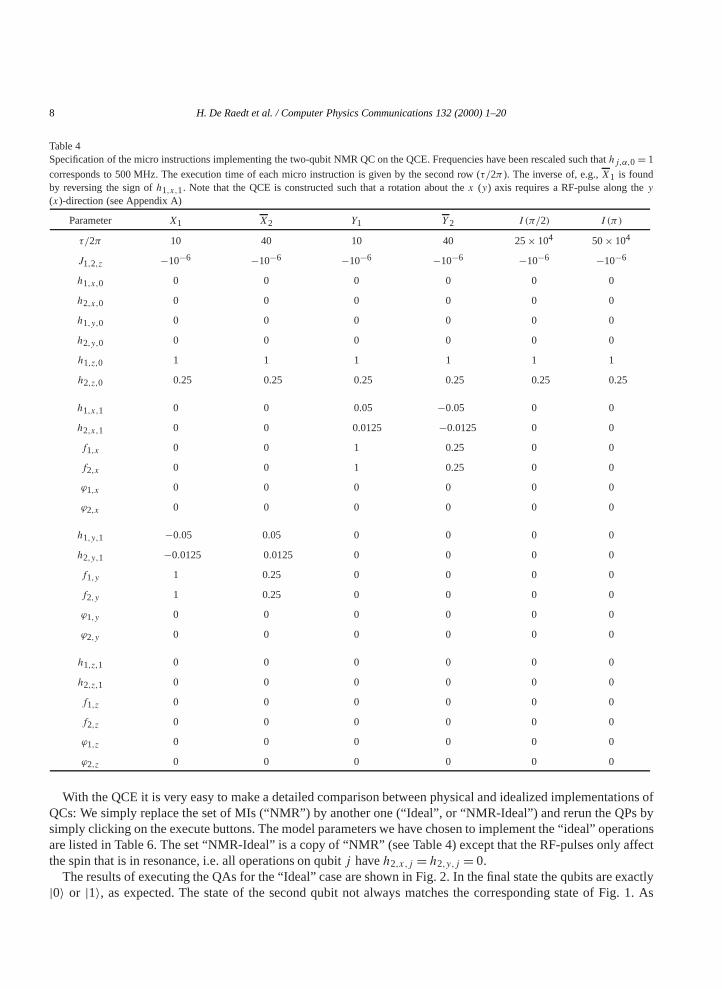
Table 4Specification of the micro instructions implementing the two-qubit NMR QC on the QCE. Frequencies have been rescaled such thathj,α,0= 1

corresponds to 500 MHz. The execution time of each micro instruction is given by the second row (τ/2π ). The inverse of, e.g.,X1 is foundby reversing the sign ofh1,x,1. Note that the QCE is constructed such that a rotation about thex (y) axis requires a RF-pulse along they(x)-direction (see Appendix A)

Parameter X1 X2 Y1 Y 2 I (π/2) I (π)

τ/2π 10 40 10 40 25× 104 50× 104

J1,2,z −10−6 −10−6 −10−6 −10−6 −10−6 −10−6

h1,x,0 0 0 0 0 0 0

h2,x,0 0 0 0 0 0 0

h1,y,0 0 0 0 0 0 0

h2,y,0 0 0 0 0 0 0

h1,z,0 1 1 1 1 1 1

h2,z,0 0.25 0.25 0.25 0.25 0.25 0.25

h1,x,1 0 0 0.05 −0.05 0 0

h2,x,1 0 0 0.0125 −0.0125 0 0

f1,x 0 0 1 0.25 0 0

f2,x 0 0 1 0.25 0 0

ϕ1,x 0 0 0 0 0 0

ϕ2,x 0 0 0 0 0 0

h1,y,1 −0.05 0.05 0 0 0 0

h2,y,1 −0.0125 0.0125 0 0 0 0

f1,y 1 0.25 0 0 0 0

f2,y 1 0.25 0 0 0 0

ϕ1,y 0 0 0 0 0 0

ϕ2,y 0 0 0 0 0 0

h1,z,1 0 0 0 0 0 0

h2,z,1 0 0 0 0 0 0

f1,z 0 0 0 0 0 0

f2,z 0 0 0 0 0 0

ϕ1,z 0 0 0 0 0 0

ϕ2,z 0 0 0 0 0 0

With the QCE it is very easy to make a detailed comparison between physical and idealized implementations ofQCs: We simply replace the set of MIs (“NMR”) by another one (“Ideal”, or “NMR-Ideal”) and rerun the QPs bysimply clicking on the execute buttons. The model parameters we have chosen to implement the “ideal” operationsare listed in Table 6. The set “NMR-Ideal” is a copy of “NMR” (see Table 4) except that the RF-pulses only affectthe spin that is in resonance, i.e. all operations on qubitj haveh2,x,j = h2,y,j = 0.

The results of executing the QAs for the “Ideal” case are shown in Fig. 2. In the final state the qubits are exactly|0〉 or |1〉, as expected. The state of the second qubit not always matches the corresponding state of Fig. 1. As


Fig. 1. Picture of the Quantum Computer Emulator showing a window with a set of micro instructions implementing an NMR quantum computerand windows with four Deutsch–Jozsa programs (d-j1,. . . , d-j4), one for each function(f1(x), . . . , f4(x)) listed in Table 1. The final state ofthe QC, i.e. the expectation value of the qubits (spin operators), is shown at the bottom of each program window(green= |0〉, red= |1〉). Thenumerical values appear if the cursor moves over the qubit area.

Table 5Final state of the QC after running the D-J algorithm for the case of the ideal QC (Q1,Q2, see Table 5) and the NMR-QC (Q1, Q2, see Table 4).The results (Q1, Q2) have been obtained by modifying the NMR MI’s such that the RF-pulses only affect the spin that is in resonance. The lasttwo rows show the results of running the refined version [21] of the D-J algorithm.Q1: Ideal operationsQ1: NMR implementation

f1(x) f2(x) f3(x) f4(x)

Q1 0.000 0.000 1.000 1.000

Q2 0.000 0.000 0.000 0.000

Q1 0.169 0.064 0.867 0.867

Q2 0.999 1.000 0.001 0.002

Q1 0.000 0.000 0.998 0.998

Q2 1.000 1.000 0.001 0.001

Q1 0.000 0.000 1.000 1.000

Q1 0.000 0.000 0.995 0.996

mentioned above this is due to the approximate nature of the operations used in the NMR case, but as the finalstate of the second qubit is irrelevant for the D-J algorithm there is no problem. In Table 5 we collect the numericalvalues of the qubits as obtained by running the D-J algorithm on the NMR and ideal QC. It is clear in that all casesthe D-J algorithm gives the correct answer.


Table 6Specification of the micro instructions implementing a mathematically perfect two-qubit QC on the QCE. The execution time of each microinstruction is given by the second row (τ/2π ). The inverse of, e.g.,X1 is found by reversing the sign ofh1,x,0. Model parameters omitted arezero for all micro instructions

Parameter X1 X2 Y1 Y 2 I (π/2) I (π)

τ/2π 0.25 0.25 0.25 0.25 25× 104 50× 104

J1,2,z 0 0 0 0 −10−6 −10−6

h1,x,0 +1 0 0 0 0 0

h2,x,0 0 −1 0 0 0 0

h1,y,0 0 0 +1 0 0 0

h2,y,0 0 0 0 −1 0 0

Fig. 2. Picture of the Quantum Computer Emulator showing a window with a set of micro instructions implementing an ideal quantum computerand windows with four Deutsch–Jozsa programs (d-j1,. . . , d-j4), one for each function (f1(x), . . . , f4(x)) listed in Table 1. Also shown is awindow for editing micro instructions, which appears by double-clicking on a micro instruction(X2 in this example). The final state of thequantum computer, i.e. the expectation value of the qubits (spin operators), is shown at the bottom of each program window(green= |0〉,red= |1〉). In this ideal case the expectation values are either zero or one.

4.2. Collins–Kim–Holton algorithm

From the description of the D-J algorithm of one variable [3, Fig. 1] it is evident that the second qubit isredundant because the function call (step T2 in [3]) leaves the state of the second qubit, i.e. the work space,


untouched. A refined version of the D-J algorithm (for an arbitrary number of qubits) that does not require a bit forthe evaluation of the function is given in [21]. For one variable, the QC has to compute the function

fj ⇔1∑x=0

(−1)fj (x)|x〉. (14)

Following [21] this may be accomplished via anf controlled gate defined by

Uf |x〉 = (−1)f (x)|x〉. (15)

Accordingly, once choice (there are several) of the set of sequences that implements the refined version of the D-Jalgorithm reads:

Prepare⇔ Y 1, (16a)

f1(x)⇔ F1=W1W1, (16b)

f2(x)⇔ F2=X1X1, (16c)

f3(x)⇔ F3= Y 1X1Y1Y 1X1Y1, (16d)

f4(x)⇔ F4= Y1X1Y 1Y1X1Y 1, (16e)

ReadOut⇔ Y 1. (16f)

The results of running these QPs on the QCE are given in Table 6. It is clear that the refined version performs asexpected.

4.3. Grover’s database search algorithm

On a conventional computer finding a particular entry in an unsorted list ofN elements requires of the orderof N operations. Grover has shown that a QC can find the item using onlyO

√N attempts [11,12]. Consider the

extremely simple case of a database containing four items and functionsgj (x), j = 0, . . . ,3, that upon query ofthe database return minus one ifx = j and plus one ifx 6= j . Assuming a uniform probability distribution for theitem to be in one of the four locations, the average number of queries required by a conventional algorithm is 9/4.With Grover’s QA the correct answer can be found in a single query (this result only holds for a database with 4items). Grover’s algorithm for the four-item database can be implemented on a two-qubit QC.

The key ingredient of Grover’s algorithm is an operation that replaces each amplitude of the basis states in thesuperposition by two times the average amplitude minus the amplitude itself. This operation is called “inversionabout the mean” and amplifies the amplitude of the basis state that represents the searched-for item. To see how thisworks it is useful to consider an example. Let us assume that the item to search for corresponds to, e.g., number 2(g2(0)= g2(1)= g2(3)= 1 andg2(2)=−1). Using the binary representation of integers with the order of the bitsreversed, the QC is in the state (up to an irrelevant phase factor as usual)

|Ψ 〉 = 12

(|00〉 + |10〉 − |01〉 + |11〉). (17)

We return to the question of how to prepare this state below. The operatorD that inverts states like (17) abouttheir mean reads

D = 1

2

−1 1 1 1

1 −1 1 11 1 −1 11 1 1 −1

;|00〉|10〉|01〉|11〉

(18)

The mean amplitude of (17) is 1/4 and we find that

D|Ψ 〉 = |01〉, (19a)


i.e. the correct answer, and

D2|Ψ 〉 = 12

(|00〉 + |10〉 + |01〉 + |11〉), (19b)

D3|Ψ 〉 =−12

(|00〉 + |10〉 − |01〉 + |11〉)=−|Ψ 〉, (19c)

showing that (in the case of 2 qubits) the correct answer (i.e. the absolute value of the amplitude of|10〉 equal toone) is obtained after 1,4,7, . . . iterations. In general, for more than two qubits, more than one application ofD isrequired to get the correct answer. In this sense the 2-qubit case is somewhat special.

The next task is to express the preparation and query steps in terms of elementary rotations. For illustrativepurposes we stick to the example used above. Initially we set the QC in the state|00〉, i.e. the state with both spinsup [42] and then transform|00〉 to the linear superposition (17) by a two-step process. First we set the QC in theuniform superposition state|U〉:

Prepare⇔ |U〉 ≡W2W1|00〉 = −12

(|00〉 + |10〉 + |01〉 + |11〉), (20)

where

Wj =XjXjY j =−XjXjY j = i√2

(1 11 −1

)j

, (21)

is the WH transform on qubitj which transforms|0〉 to i(|0〉 + |1〉)/√2 (see Appendix A). The transformationthat corresponds to the application ofg2(x) to the uniform superposition state is

F2=

1 0 0 00 1 0 00 0 −1 00 0 0 1

;|00〉|10〉|01〉|11〉

(22)

This transformation can be implemented by first letting the system evolve in time:

I (π)|U〉 = e−iπSz1Sz2[1

2(|00〉 + |10〉 + |01〉 + |11〉)]= 1

2

(e−iπ/4|00〉 + e+iπ/4|10〉 + e+iπ/4|01〉 + e−iπ/4|11〉). (23)

For the NMR-QC based on Hamiltonian (8) this means letting the system evolve in time (without applying pulses)for a time τ0 = −π/J1,2,z (recall J1,2,z < 0). Next we apply a sequence of single-spin rotations to change thefour phase factors such that we get the desired state. The two sequencesYXY andYXY (see Appendix B) areparticularly useful for this purpose. We find

Y1X1Y 1Y2X2Y 2[1

2

(e−iπ/4|00〉 + e+iπ/4|10〉 + e+iπ/4|01〉 + e−iπ/4|11〉)]

= 12

(e−iπ/4|00〉 + e−iπ/4|10〉 + e+3iπ/4|01〉 + e−iπ/4|11〉)

= e−iπ/4

2

(|00〉 + |10〉 − |01〉 + |11〉). (24)

Combining (23) and (24) we can construct the sequenceGj that transforms the uniform superposition|U〉 to thestate that corresponds togj (x):

F0= Y1X1Y 1Y2X2Y 2I (π), (25a)

F1= Y1X1Y 1Y2X2Y 2I (π), (25b)

F2= Y1X1Y 1Y2X2Y 2I (π), (25c)

F3= Y1X1Y 1Y2X2Y 2I (π). (25d)


The remaining task is to express the operation of inversion about the mean, i.e. the matrixD (see (18)), by asequence of elementary operations. It is not difficult to see thatD can be written as the product of a WH transform,a conditional phase shiftP and another WH transform:

D =W1W2PW1W2

=W1W2

1 0 0 00 −1 0 00 0 −1 00 0 0 −1

W1W2. (26a)

The same approach that was used to implementg2(x) also works for the conditional phase shiftP (=−F0) andyields

P = Y1X1Y 1Y2X2Y 2I (π). (27)

The complete sequenceUj reads

Uj =W1W2PW1W2Fj . (28)

Fig. 3. Picture of the Quantum Computer Emulator showing a window with a set of micro instructions for a two-qubit NMR quantum computerand windows with quantum programs implementing Grover’s database search for the four different casesg0(x) (g0), . . . , g3(x) (g3). Thisexample also shows the use of quantum programs as micro instructions in other quantum programs. The final state of the QC, i.e. two qubitsshown at the bottom of each program, gives the location (in binary representation) of the item in the database. Note that for the case g1 we wereusing single-step mode to execute the program and stopped at f1.


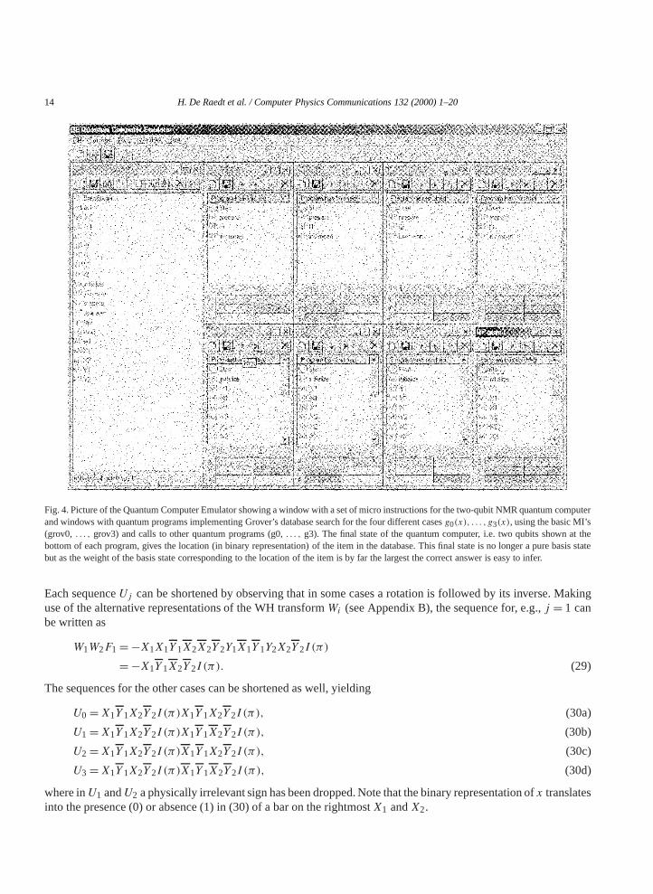
Fig. 4. Picture of the Quantum Computer Emulator showing a window with a set of micro instructions for the two-qubit NMR quantum computerand windows with quantum programs implementing Grover’s database search for the four different casesg0(x), . . . , g3(x), using the basic MI’s(grov0, . . . , grov3) and calls to other quantum programs (g0,. . . , g3). The final state of the quantum computer, i.e. two qubits shown at thebottom of each program, gives the location (in binary representation) of the item in the database. This final state is no longer a pure basis statebut as the weight of the basis state corresponding to the location of the item is by far the largest the correct answer is easy to infer.

Each sequenceUj can be shortened by observing that in some cases a rotation is followed by its inverse. Makinguse of the alternative representations of the WH transformWi (see Appendix B), the sequence for, e.g.,j = 1 canbe written as

W1W2F1=−X1X1Y 1X2X2Y 2Y1X1Y 1Y2X2Y 2I (π)

=−X1Y 1X2Y 2I (π). (29)

The sequences for the other cases can be shortened as well, yielding

U0=X1Y 1X2Y 2I (π)X1Y 1X2Y 2I (π), (30a)

U1=X1Y 1X2Y 2I (π)X1Y 1X2Y 2I (π), (30b)

U2=X1Y 1X2Y 2I (π)X1Y 1X2Y 2I (π), (30c)

U3=X1Y 1X2Y 2I (π)X1Y 1X2Y 2I (π), (30d)

where inU1 andU2 a physically irrelevant sign has been dropped. Note that the binary representation ofx translatesinto the presence (0) or absence (1) in (30) of a bar on the rightmostX1 andX2.


Table 7Final state of the QC after running the Grover’s database search algorithm for the case of the ideal QC (Q1,Q2, see Table 5) and the NMR-QC(Q1, Q2, see Table 4)

g0(x) g1(x) g2(x) g3(x)

Q1 0 1 0 1

Q2 0 0 1 1

Q1 0.028 0.966 0.037 0.955

Q2 0.163 0.171 0.836 0.830

As before, our aim is to use the QCE to simulate the NMR-QC experiment [4]. For the D-J algorithm we alreadyspecified the physical parameters for the elementary operations and we will make use of the same set of MI’s here.In Figs. 3 and 4 we show the QCE after running the four casesg0(x), . . . , g3(x) using the NMR (Fig. 4) MI’s. Thenumerical values of the qubits in the final state are given in Table 7, for the ideal and NMR QC. In both cases theQA performs as it should. In the ideal case, the final state of the QC is exactly equal to|x〉 (binary representation ofintegers). Using RF-pulses instead of ideal transformations to performπ/2 rotations leads to less certain answers:The final state is no longer a pure basis state but some linear superposition of the four basis states. What is beyonddoubt though is that in all cases the weight of|x〉 is by far the largest. Hence the QC returns the correct answer.

5. Summary

We have described the internal operation of QCE, a software tool for simulating hardware realizations ofquantum computers. The QCE simulates the physical (quantum) processes that govern the operation of thehardware quantum processor by solving the time-dependent Schrödinger equation. The use of the QCE has beenillustrated by several implementations of the Deutsch–Jozsa and Grover’s database search algorithm, on QCs usingideal and more realistic units, such as those of 2-qubit NMR-QCs. Currently the QCE is used to study the stabilityof quantum computers in relation to the non-idealness of realizable elementary operations [43].

Acknowledgements

Generous support from the Dutch “Stichting Nationale Computer Faciliteiten (NCF)” is gratefully acknowl-edged.

Appendix A. Spin-1/2 algebra

Here we present a collection of standard results on spin-1/2 systems which are used in the paper and are takenfrom [41]. We begin with some notation.

The two basis states spanning the Hilbert space of a two-state quantum system are usually denoted by

|↑〉 ≡(

10

), |↓〉 ≡

(01

). (A.1)

The three components of the spin-1/2 operatorES acting on this Hilbert space are defined by

Sx = h2

(0 11 0

), Sy = h

2

(0 −ii 0

), Sz = h

2

(1 00 −1

). (A.2)


By convention the representation (A.2) is chosen such that|↑〉 and|↓〉 are eigenstates ofSz with eigenvalues+h/2and−h/2, respectively.

From (A.2) it is clear that(Sx)2= (Sy)2= (Sz)2= h2/4 so that

cos

(ϕSα

h

)= cos

(ϕ

2

)(1 00 1

), (A.3a)

and

sin

(ϕSα

h

)= 2

hsin

(ϕ

2

)Sα. (A.3b)

The commutation relations between the three spin-components read

[Sα,Sβ ] = ihεαβγ Sγ , (A.4)

where[A,B] ≡AB −BA, εαβγ is the totally antisymmetric unit tensor (εxyz = εyzx = εzxy = 1, εαβγ =−εβαγ =−εγβα =−εαγβ , εααγ = 0) and the summation convention is assumed.

Rotation of the spin about an angleϕ around the axisβ gives

Sα(ϕ,β)≡ eiϕSβ/hSαe−iϕSβ /h = Sα cosϕ + εαβγ Sγ sinϕ. (A.5)

Of particular interest to quantum computing are rotations aboutπ/2 around thex- andy-axis defined by

X ≡ eiπSx/2h = 1√

2

(1 i

i 1

), (A.6a)

and

Y ≡ eiπSy/2h = 1√

2

(1 1−1 1

). (A.6b)

The inverse of a rotationZ will be denoted asZ and if more than one spin is involved a subscript will beattached. With our convention〈↑|YSxY |↑〉 = −1/2 so that a positive angle corresponds to a rotation in the clock-wise direction.

Another basic operation is the Walsh–Hadamard transformW which rotates the state|↑〉 into (|↓〉 + |↑〉)/√2(up to an irrelevant phase factor), i.e. the uniform superposition state. In terms of elementary rotations the Walsh–Hadamard transform reads

W =X2Y = YX2=−X2Y =−YX2= i√

2

(1 11 −1

). (A.7)

For example,

W |↑〉 =W(

10

)= i√

2

(11

). (A.8)

We now consider the time evolution of a single spin subject to a constant magnetic field along thez-axis and aRF-field along thex-axis, i.e. the elementary model of NMR. The TDSE reads

ih∂

∂t

∣∣Φ(t)⟩=−[H0Sz +H1S

x sinωt]∣∣Φ(t)⟩, (A.9)

where|Φ(t = 0)〉 is the initial state of the two-state system and we have set the phase in (3) to zero for notationalconvenience. Substituting|Φ(t)〉 = eitω0S

z/h|Ψ (t)〉 yields

ih∂

∂t

∣∣Ψ (t)⟩=−[(H0−ω0)Sz +H1S

x sinωt cosω0t +H1Sy sinωt sinω0t

]∣∣Ψ (t)⟩, (A.10)


which upon choosingω0=H0 can be written as

ih∂

∂t

∣∣Ψ (t)⟩=−H1[Sx sinωt cosH0t + Sy sinωt sinH0t

]∣∣Ψ (t)⟩. (A.11)

At resonance, i.e.ω =H0, we find

ih∂

∂t

∣∣Ψ (t)⟩=−H1

2

[Sy + Sx sin2H0t − Sy cos2H0t

]∣∣Ψ (t)⟩. (A.12)

Assuming that the effects of the higher harmonic terms (i.e. the terms in sin2H0t and cos2H0t) are small [41] weobtain

ih∂

∂t

∣∣Ψ (t)⟩≈−H1

2Sy∣∣Ψ (t)⟩, (A.13)

which is easily solved to give∣∣Ψ (t)⟩≈ eitH1Sy/2h

∣∣Ψ (t = 0)⟩, (A.14)

so that the overall action of an RF-pulse of durationτ can be written as∣∣Φ(t + τ )⟩≈ eiτH0Sz/heiτH1S

y/2h∣∣Φ(t)⟩. (A.15)

From (A.15) it follows that application of an RF-pulse of “power”τH1= π will have the effect of rotating the spinby an angle ofπ/2 about they-axis. For example,

eiτH0Sz/heiπS

y/2h|↑〉 = eiτH0Sz/h

[cos

π

4

(1 00 1

)+ i sin

π

4

(0 −ii 0

)](10

)= 1√

2eiτH0S

z/h

(1−1

)= 1√

2

(eiτH0/2

−e−iτH0/2

). (A.16)

In this rotated state the expectation values of the spin components are given by

〈↑|e−iπSy/2he−iτH0Sz/hSxeiτH0S

z/heiπSy/2h|↑ =−hcosτH0, (A.17a)

〈↑|e−iπSy/2he−iτH0Sz/hSyeiτH0S

z/heiπSy/2h|↑ =−hsinτH0, (A.17b)

〈↑|e−iπSy/2he−iτH0Sz/hSzeiτH0S

z/heiπSy/2h|↑ = 0, (A.17c)

showing that the time of the RF-pulse also affects the projection of the spin on thex- andy-axis.It is instructive to derive the TDSE that corresponds to approximation (A.15). Taking the derivative of (A.15)

with respect tot we obtain

ih∂

∂t

∣∣Φ(t)⟩=−H0Sz − H1

2

[Sx sinH0t + Sy cosH0t

]∣∣Φ(t)⟩, (A.18)

telling us that the approximate solution (A.15) is the exact solution for an RF-field rotating in space [41]. The factthat the application of an RF-pulse does notexactlycorrespond to a simple rotation in spin space may well beimportant for applications of NMR techniques to QC’s.

Finally we note that our choice of using “sinωt” instead of “cosωt” [41] to couple the spin to the RF-fieldmerely leads to a phase shift. In the former case rotating the spin around thex-axis requires a pulse along they-axis, whereas in the latter the pulse should be applied along thex-axis [41].


Appendix B. Basic operations

Below we list a number of identities that are useful to compute by hand the action of the sequences appearingabove. The convention adopted in this paper is that

|0〉 = |↑〉 =(

10

); |1〉 = |↓〉 =

(01

). (B.1)

A straightforward calculation yields:

X|0〉 = 1√2

(|0〉 + i|1〉), X|1〉 = 1√2

(i|0〉 + |1〉), (B.2a)

X|0〉 = 1√2

(|0〉 − i|1〉), X|1〉 = 1√2

(−i|0〉 + |1〉), (B.2b)

Y |0〉 = 1√2

(|0〉 − |1〉), Y |1〉 = 1√2

(|0〉 + |1〉), (B.3a)

Y |0〉 = 1√2

(|0〉 + |1〉), Y |1〉 = 1√2

(−|0〉 + |1〉), (B.3b)

Y

[1√2(|0〉 − |1〉)

]=−|1〉, Y

[1√2(|0〉 + |1〉)

]= |0〉, (B.4a)

Y

[1√2(|0〉 − |1〉)

]= |0〉, Y

[1√2(|0〉 + |1〉)

]= |1〉, (B.4b)

XX|0〉 = i|1〉, XX|1〉 = i|0〉, (B.5a)

YY |0〉 = −|1〉, YY |1〉 = |0〉, (B.5b)

XY |0〉 = e−iπ/4√2

(|0〉 − |1〉), XY |1〉 = e+iπ/4√2

(|0〉 + |1〉), (B.6a)

XY |0〉 = e+iπ/4√2

(|0〉 − |1〉), XY |1〉 = e−iπ/4√2

(|0〉 + |1〉), (B.6b)

XY |0〉 = e+iπ/4√2

(|0〉 + |1〉), XY |1〉 = e−iπ/4√2

(−|0〉 + |1〉), (B.6c)

X Y |0〉 = e−iπ/4√2

(|0〉 + |1〉), X Y |1〉 = e+iπ/4√2

(−|0〉 + |1〉), (B.6d)

YXY |0〉 = e+iπ/4|0〉, YXY |1〉 = e−iπ/4|1〉, (B.7a)

YXY |0〉 = e−iπ/4|0〉, YXY |1〉 = e+iπ/4|1〉, (B.7b)

YXY |0〉 = e+iπ/4|1〉, YXY |1〉 = −e−iπ/4|0〉, (B.7c)

YX Y |0〉 = e−iπ/4|0〉, YX Y |1〉 = e+iπ/4|1〉, (B.7d)

W =X2Y = YX2=−X2Y =−YX2

, (B.8a)

W |0〉 = i√2

(|0〉 + |1〉), W |1〉 = i√2

(|0〉 − |1〉), (B.8b)

W2|0〉 = −|0〉, W2|1〉 = −|1〉. (B.8c)


References

[1] J.A. Jones, M. Mosca, Implementation of a quantum algorithm on a nuclear magnetic resonance quantum computer, J. Chem. Phys. 109(1998) 1648–1653.

[2] J.A. Jones, M. Mosca, R.H. Hansen, Implementation of a quantum search algorithm on a quantum computer, Nature (London) 393 (1998)344–346.

[3] I.L. Chuang, L.M.K. Vandersypen, X. Zhou, D.W. Leung, S. Lloyd, Experimental realization of a quantum algorithm, Nature 393 (1998)143–146.

[4] I.L. Chuang, N. Gershenfeld, M. Kubinec, Experimental implementation of Fast Quantum Searching, Phys. Rev. Lett. 80 (1998) 3408–3411.

[5] C. Bennett, G. Brassard, The dawn of a new era for quantum cryptography: The experimental prototype is working, SIGACT News 20(1989) 78–82.

[6] C. Bennett, F. Bessette, G. Brassard, L.G. Salvail, J. Smolin, Experimental quantum cryptography, J. Cryptology 5 (1992) 3–28.[7] A. Ekert, J. Rarity, P. Tapster, G. Palma, Practical quantum cryptography based on two-photon interferometry, Phys. Rev. Lett. 69 (1992)

1293–1295.[8] P. Shor, Algorithms for quantum computation: Discrete logarithms and factoring, in: Proc. 35th Annu. Symp. Foundations of Computer

Science 124, S. Goldwasser (Ed.) (IEEE Computer Soc., Los Alamitos, CA, 1994).[9] I.L. Chuang, R. Laflamme, P.W. Shor, W.H. Zurek, Quantum computers, factoring and decoherence, Science 230 (1995) 1663–1665.

[10] A.Yu. Kitaev, Quantum measurements and the Abelian stabiliser problem, e-print quant-ph/9511026.[11] L.K. Grover, A fast quantum mechanical algorithm for database search, in: Proc. 28th Annual ACM Symposium of Theory of Computing

(ACM, Philadelphia, 1996).[12] L.K. Grover, Quantum computers can search arbitrary large databases by a single query, Phys. Rev. Lett. 79 (1997) 4709–4712.[13] L.K. Grover, Quantum computers can search rapidly by using almost any transformation, Phys. Rev. Lett. 80 (1998) 4329– 4332.[14] D. Aharonov, Quantum computation, e-print quant-ph/9812037.[15] N.J. Cerf, S.E. Koonin, Monte Carlo simulation of quantum computation, Math. Comput. Simulation 47 (1998) 143–152.[16] C. Zalka, Simulating quantum systems on a quantum computer, Proc. Roy. Soc. London A 454 (1998) 313–322.[17] B.M. Terhal, S.P. DiVincenzo, On the problem of equilibration and the computation of correlation functions on a quantum computer,

e-print quant-ph/9810063.[18] H. De Raedt, A.H. Hams, K. Michielsen, S. Miyashita, K. Saito, Quantum statistical mechanics on a quantum computer, Prog. Theor.

Phys. (in press), e-print quant-ph/9911037.[19] R.P. Feynman, Simulating physics with computers, Int. J. Theor. Phys. 21 (1982) 467–488.[20] D. Deutsch, R. Jozsa, Rapid solution of problems by quantum computation, Proc. Roy. Soc. London A 439 (1992) 553–558.[21] D. Dollins, K.W. Kim, W.C. Holton, Deutsch–Jozsa algorithm as a test of quantum computation, Phys. Rev. A 58 (1998) R1633–R1636.[22] We use a notation that closely resembles the symbols in the QCE’s graphical user interface.[23] H. De Raedt, Product formula algorithms for solving the time-dependent Schrödinger equation, Comput. Phys. Rep. 7 (1987) 1–72.[24] H. De Raedt, K. Michielsen, Algorithm to solve the time-dependent Schrödinger equation for a charged particle in an inhomogeneous

magnetic field: application to the Aharonov–Bohm effect, Comput. in Phys. 8 (1994) 600–607.[25] H. De Raedt, Quantum dynamics in nano-scale devices, in: Computational Physics, K.-H. Hoffmann, M. Schreiber (Eds.) (Springer, Berlin,

1996) pp. 209–224.[26] H. De Raedt, Computer simulation of quantum phenomena in nano-scale devices, in: Annual Reviews of Computational Physics IV,

D. Stauffer (Ed.) (World Scientific, Singapore, 1996).[27] P. de Vries, H. De Raedt, Solution of the time-dependent Schrödinger equation for two-dimensional spin-1/2 Heisenberg systems, Phys.

Rev. B 7 (1993) 7929–7937.[28] J. Huyghebaert, H. De Raedt, Product formula methods for time-dependent Schrödinger problems, J. Phys. A: Math. Gen. 23 (1990) 5777.[29] M. Suzuki, General decomposition theory of ordered exponentials, Proc. Japan Acad. 69, Ser. B (1993) 161–166.[30] M. Suzuki, S. Miyashita, A. Kuroda, Monte Carlo simulation of quantum spin systems. I, Prog. Theor. Phys. 58 (1977) 1377–1387.[31] H. De Raedt, B. De Raedt, Applications of the generalized trotter formula, Phys. Rev. A 28 (1983) 3575–3580.[32] M. Suzuki, Decomposition formulas of exponential operators and Lie exponentials with some applications to quantum mechanics and

statistical physics, J. Math. Phys. 26 (1985) 601–612.[33] M. Suzuki, General nonsymetric higher-order decomposition of exponential operators and symplectic integrators, J. Phys. Soc. Jpn. 61

(1995) 3015–3019.[34] S. Lloyd, Science 261 (1993) 1569.[35] G.P. Berman, G.D. Doolen, D.D. Holm, V.I. Tsifrinovich, Quantum computer on a class of one-dimensional Ising systems, Phys. Lett. A

193 (1994) 444–450.[36] G.P. Berman, G.D. Doolen, R. Mainieri, V.I. Tsifrinovich, Introduction to Quantum Computers. (World Scientific, Singapore, 1998).[37] G.P. Berman, G.D. Doolen, V.I. Tsifrinovich, Quantum computation as a dynamical process, e-print quant-ph/9904105.[38] G.P. Berman, G.D. Doolen, G.V. López, V.I. Tsifrinovich, Quantum computation as a dynamical process, e-print quant-ph/9909027.


[39] R. Cleve, A. Ekert, C. Macciavello, M. Mosca, Quantum algorithms revisited, Proc. Roy. Soc. London. A 454 (1998) 339–354.[40] C.P. Slichter, Principles of Magnetic Resonance (Springer, Berlin, 1990).[41] G. Baym, Lectures on Quantum Mechanics (W.A. Bejamin, Reading, MA, 1974).[42] We follow the convention used earlier in this paper, i.e. the one used in [3] and therefore deviate from the notation used in [4].[43] H. De Raedt, A.H. Hams, K. Michielsen, S. Miyashita, K. Saito, Quantum spins dynamics and quantum computation, J. Phys. Soc. Jpn.

(in press), e-print quant-ph/9911038.

Date post:	19-Apr-2018
Category:	Documents
Upload:	vandieu
View:	215 times
Download:	1 times

University of Groningen Quantum Computer Emulator de … · We illustrate the use of the quantum...

Documents