University of Groningen Water impact on offshore structures - a numerical study Kleefsman, Kornelia Marchien Theresa IMPORTANT NOTE: You are advised to consult the publisher's version (publisher's PDF) if you wish to cite from it. Please check the document version below. Document Version Publisher's PDF, also known as Version of record Publication date: 2005 Link to publication in University of Groningen/UMCG research database Citation for published version (APA): Kleefsman, K. M. T. (2005). Water impact on offshore structures - a numerical study. s.n. Copyright Other than for strictly personal use, it is not permitted to download or to forward/distribute the text or part of it without the consent of the author(s) and/or copyright holder(s), unless the work is under an open content license (like Creative Commons). The publication may also be distributed here under the terms of Article 25fa of the Dutch Copyright Act, indicated by the “Taverne” license. More information can be found on the University of Groningen website: https://www.rug.nl/library/open-access/self-archiving-pure/taverne- amendment. Take-down policy If you believe that this document breaches copyright please contact us providing details, and we will remove access to the work immediately and investigate your claim. Downloaded from the University of Groningen/UMCG research database (Pure): http://www.rug.nl/research/portal. For technical reasons the number of authors shown on this cover page is limited to 10 maximum. Download date: 12-03-2022
Transcript
University of Groningen
Water impact on offshore structures - a numerical studyKleefsman, Kornelia Marchien Theresa
IMPORTANT NOTE: You are advised to consult the publisher's version (publisher's PDF) if you wish to cite fromit. Please check the document version below.
Document VersionPublisher's PDF, also known as Version of record
Publication date:2005
Link to publication in University of Groningen/UMCG research database
Citation for published version (APA):Kleefsman, K. M. T. (2005). Water impact on offshore structures - a numerical study. s.n.
CopyrightOther than for strictly personal use, it is not permitted to download or to forward/distribute the text or part of it without the consent of theauthor(s) and/or copyright holder(s), unless the work is under an open content license (like Creative Commons).
The publication may also be distributed here under the terms of Article 25fa of the Dutch Copyright Act, indicated by the “Taverne” license.More information can be found on the University of Groningen website: https://www.rug.nl/library/open-access/self-archiving-pure/taverne-amendment.
Take-down policyIf you believe that this document breaches copyright please contact us providing details, and we will remove access to the work immediatelyand investigate your claim.
Downloaded from the University of Groningen/UMCG research database (Pure): http://www.rug.nl/research/portal. For technical reasons thenumber of authors shown on this cover page is limited to 10 maximum.
To perform realistic simulations of green water and bow impact loading, the method hasto be extended with wave generation options. There are different ways to create a wavefield in a computational program:
• Prescribe a wave at the inflow boundary using theory, for example Stokes theory ora superposition of linear waves.
• Use a wave maker, which can be modelled as a moving object.
• Use another calculation method, which calculates kinematics away from an objectthat will be prescribed at the domain boundaries.
In this chapter the implementation and validation of the first option will be described,whereas the third option is used in the next chapter. The waves considered are longcrested waves, so the incoming wave is two-dimensional of shape. Of course, when anobject is present, the wave will be disturbed and three-dimensional aspects become im-portant. At the boundary of the domains appropriate conditions are needed to let thewave travel in and out of the domain in an undisturbed way. Therefore, at the inflowboundary fluid wave kinematics will be prescribed according to wave description theories.The undisturbed wave will be prescribed, so the disturbance due to wave diffraction on anobject is not taken into account. At the outflow boundary conditions should be imposed,such that the wave can leave the domain undisturbedly. Determining these conditions isdifficult, because no information about the wave is present near the outflow boundary.
After describing the wave theories and conditions at the outflow boundary, attentionwill be paid to possible energy dissipation due to the upwind discretisation of the convec-tive terms. Also the influence of the treatment of the free surface on wave propagation,like the choice for free surface velocities and the displacement algorithm, is investigated.
To validate the numerical model, simulations have been performed, which can bechecked against theory or experiments. First, results will be shown of two-dimensionalwave simulations without the presence of an object. Further, a spar platform has beenput into the flow. Forces and wave heights have been calculated, which can be comparedwith experimental results. Finally, as the most demanding test case, green water on thebow of a moving FPSO is simulated.
84 Chapter 3. Wave generation and propagation
3.2 Wave definition
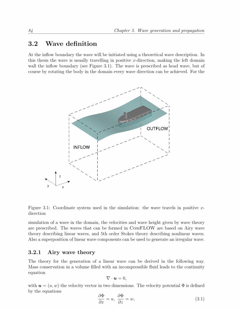
At the inflow boundary the wave will be initiated using a theoretical wave description. Inthis thesis the wave is usually travelling in positive x-direction, making the left domainwall the inflow boundary (see Figure 3.1). The wave is prescribed as head wave, but ofcourse by rotating the body in the domain every wave direction can be achieved. For the
Figure 3.1: Coordinate system used in the simulation: the wave travels in positive x-direction
simulation of a wave in the domain, the velocities and wave height given by wave theoryare prescribed. The waves that can be formed in ComFLOW are based on Airy wavetheory describing linear waves, and 5th order Stokes theory describing nonlinear waves.Also a superposition of linear wave components can be used to generate an irregular wave.
3.2.1 Airy wave theory
The theory for the generation of a linear wave can be derived in the following way.Mass conservation in a volume filled with an incompressible fluid leads to the continuityequation
∇ · u = 0,
with u = (u, w) the velocity vector in two dimensions. The velocity potential Φ is definedby the equations
∂Φ
∂x= u,
∂Φ
∂z= w, (3.1)
3.2 Wave definition 85
with x and z the horizontal and vertical coordinate, respectively. Substituting Φ into thecontinuity equation leads to a Laplace equation for the velocity potential:
∂2Φ
∂x2+
∂2Φ
∂z2= 0.
When assuming the water surface slope very small, the potential is written as a sine withan amplitude depending on the water depth
Φ(x, z, t) = P (z) sin(ωt− kx + φ), (3.2)
where t is the time, k the wave number, and φ the phase angle. P (z) can be determinedby substituting Equation (3.2) into the Laplace equation and solving the differentialequation for P (z), which finally results in
Φ(x, z, t) = (C1ekz + C2e
−kz) sin(ωt− kx + φ). (3.3)
The constants C1 and C2 can be determined using the boundary conditions at the seabed and the free surface. At the sea bed a no-leak condition holds, which is given by
∂Φ
∂z= 0 at z = −h.
Substituting this boundary condition into Equation (3.3) reduces the two unknowns toone:
The unknown constant C can be determined by using the free surface dynamic boundarycondition that is deduced from the Bernoulli equation, taking into account the smallwave steepness. The condition at the free surface is linearised around the calm waterlevel (z = 0), which leads to
∂Φ
∂t+ gζ = 0 for z = 0.
The free surface elevation ζ can be derived from this equation after substitution of thevelocity potential, resulting in
ζ(x, t) = ζa cos(ωt− kx) with ζa = −ω
gC cosh(kh).
Rewriting the expression for ζa, the constant C can be determined as C = − ζagω
1cosh(kh)
.
Substituting this into Equation (3.4) leads to the final expression for the velocity potential
Φ(x, z, t) = −ζag
ω
cosh(k(z + h))
cosh(kh)sin(ωt− kx + φ). (3.5)
The linearised free surface kinematic boundary condition given by
∂z
∂t+
1
g
∂2Φ
∂t2= 0 for z = 0
86 Chapter 3. Wave generation and propagation
leads to the dispersion relation, which connects the wave number and frequency in thefollowing way:
k tanh(kh) =ω2
g.
For deep water, the dispersion relation reduces to k = ω2/g.The velocity vector u = (u, w) can now be determined using the definition of the
velocity potential given in Equation (3.1)
u(t, x, z) =ζagk
ωcos(ωt− kx + φ)
cosh(k(z + h))
cosh(kh), (3.6)
w(t, x, z) = −ζagk
ωsin(ωt− kx + φ)
sinh(k(z + h))
cosh(kh). (3.7)
As stated before, linear theory can only be applied to very low waves. According to LeMehaute [61], the range of suitability of linear theory in deep water is H/λ < 0.0062,with H the wave height and λ the wavelength.
Linear wave theory can also be used to generate irregular seas, because the superpo-sition principle can be applied. Given vectors of frequencies, amplitudes and phases, alinear wave can be built as the sum of the individual components.
3.2.2 Wave kinematics above the calm water level
Since linear wave theory is only valid up to the calm water level and velocities are neededup to the free surface, some kind of stretching technique has to be used above the calmwater level. In this method Wheeler stretching has been used as a commonly acceptedmethod, which is easy to implement. In the Wheeler stretching technique the negativez-axis has been extended from the actual instantaneous free surface elevation to the seabed. This has been done by replacing z in the right-hand-side of Equations (3.6) and(3.7) by
z′ =h
h + ζz + h (
h
h + ζ− 1)
where
• z′ is the computational vertical coordinate −h ≤ z′ ≤ 0;
• z is the actual vertical coordinate −h ≤ z ≤ ζ.
3.2.3 5th order Stokes theory
For steeper waves, where in general the crests become higher and the troughs flatter,linear theory does no longer hold. To describe nonlinear waves, a solution to potentialtheory is used. The solution is represented by Fourier series, and the coefficients in theseseries can be written as perturbation expansions with parameter Ak. Here, k is thewave number, which can be written in terms of the wave length k = 2π/λ, and A is theamplitude of the wave at lowest order. The terms in the perturbation expansion can befound by satisfying boundary conditions on the free surface, and solving the resulting set
3.3 Treatment of open boundaries 87
of ordered equations. The expansion of the series can be done, in theory, infinitely far,but in practice, the 5th order solution is already very complicated.
Details about how to implement the 5th order Stokes solution can be found in [83],where the sign correction described by [25] should be taken into account.
3.3 Treatment of open boundaries
Domain walls in wave simulations at open sea need to permit fluid flow in and out.Therefore, as pictured in Figure 3.1, at least an inflow boundary is needed where thewave is generated, and an outflow boundary opposite to the inflow boundary wherethe wave leaves the domain. In the current method the waves, which are long crested,usually travel in the positive x-direction. Because of the two-dimensional shape, the sideboundaries can often be closed walls; when positioned far enough from the structure theydo not influence the wave field in the close surroundings of the structure. When the wavesare highly distorted, such that side walls are severely influencing the flow, also outflowboundary conditions can be used at the side walls.
In Figure 3.2 a cross-section of one row of cells is shown with the positions of thevelocities at the inflow and outflow boundaries. At the inflow boundary the velocities andVOF function in the column of cells directly left of the domain boundary are prescribed(a Dirichlet boundary condition). This way, the horizontal inflow velocity is positionedat the domain boundary, and no pressure is needed in the inflow cells. For the outflowboundary the horizontal velocity is shifted to one cell width away of the actual domainboundary. Therefore, also a pressure is needed in the outflow cells, so velocities, pressureand VOF function need to be determined at the outflow boundary (using a Neumann-type outflow condition). In the previous section the wave descriptions have been given,from which velocities and wave height at the inflow boundary are derived. The remainderof this section deals with the outflow boundary.
inflow domain outflow
poutuin uout
vin vout
Figure 3.2: Position of velocities at the inflow boundary, and velocities and pressure atthe outflow boundary
3.3.1 Overview outflow boundary conditions
A very important aspect of wave simulation is to determine the conditions at the outflowboundaries. If the wave is developing inside the domain, it should flow out of the domain
88 Chapter 3. Wave generation and propagation
as if there was no boundary. Otherwise, the wave will reflect from the boundaries intothe domain, which disturbs the simulation.
An overview of outflow boundary conditions that prevent wave reflections is given byGivoli [30]. He describes three classes of outflow boundary conditions.
• The first class consists of special procedures for the numerical solution of wave prob-lems in unbounded domains, that involve an artificial boundary but not the directuse of a non-reflecting boundary condition. Cerjan et al. [11] and others presentedwhat can be termed a ’filtering scheme’. In this scheme, the amplitudes of thedisplacements are gradually reduced in a strip of nodes adjacent to the boundary.Thus, the solution is artificially damped in the vicinity of the boundary. Anotherkind of dissipation zone was used by [95], where an extra damping pressure wasadded to the free surface, which opposes the vertical wave velocity. A disadvantageof such damping zones is the increase of computational cells out of which the damp-ing zone exists. Especially, in three dimensions many computational cells have tobe added outside the real computational domain.
• In the second class, which is the largest one, local non-reflecting boundary conditions(NRBCs) based on the scalar wave equation are used. There exist many variationsin local NRBCs, every problem in different types of fields (acoustics, gas dynamics,hydrodynamics, ...) uses NRBCs that works best for that particular problem. Acomparison of different boundary conditions derived from the discretisation of themulti-dimensional wave equation is given by [42].The widely used NRBC of Sommerfeld [84] is a discretisation of the one-dimensionalscalar wave equation with an a priori chosen wave velocity. A variation hereof wasintroduced by Orlanski [71], who calculated the wave velocity for every grid pointand used that velocity in the discretised wave equation. The advantage of thismethod is that no information is needed of the flow beforehand.
• Finally, non-reflecting boundary conditions are considered that are non-local intime or space or both. These NRBCs have the disadvantage that many time levelsshould be stored in memory.
In the following sections a discussion of the Sommerfeld and Orlanski boundary conditionsis given. The implementation of a general non-reflecting boundary condition is described,and the damping zone used by [95] is introduced.
3.3.2 Non-reflecting boundary conditions
Boundary conditions based on the wave equation
One way to prevent waves reflecting from the outflow boundary is to use a non-reflectingboundary condition. In case of waves most of the existing boundary conditions are basedon the wave equation [42]
∂φ
∂t+ c
∂φ
∂x= 0, (3.8)
where φ is any quantity that travels wave-like as velocity or pressure, and c the wave ve-locity. In Equation (3.8) the direction of the wave is in the x-direction. In the Sommerfeld
3.3 Treatment of open boundaries 89
boundary condition [84] the wave velocity is chosen a priori, which is easy when regularwaves are simulated. In that case, the Sommerfeld condition gives very good results aswill be shown later. When irregular waves are considered, or when the regular wavesare deformed due to the presence of an object, the method does not give very accurateresults, since only one wave velocity can be chosen. For those situations, Orlanski [71]developed a method where the wave velocity is not chosen a priori, but is calculated everytime step based on the local wave kinematics near the outflow boundary. The problemwith this method is to determine the wave velocity accurately. To calculate c, first thewave equation is discretised using finite differences in cells close to the outflow boundarywhere the condition will be imposed. The wave equation is discretised for the horizontalvelocity in every level of cells in the water depth. The c is then calculated as the mean ofthe approximated wave velocities in every level in the water depth. In Figure 3.3 the cal-culated wave velocity is shown for a regular wave with an actual wave velocity of 22.6 m/sduring one wave period. The calculated wave velocity is not constant at all, but oscillatesaround the theoretical value. The jump that occurs around 7.2 s is present because therethe crest of the wave travels through the outflow boundary resulting in ∂u/∂x = 0. Thiscan cause the wave velocity to jump from minus infinity to plus infinity. In this region,the wave velocity is adapted, such that these extreme values are not used in the outflowboundary conditions. In an investigation of wave propagation using Orlanski’s methodat the outflow boundary, it turned out that the results were not very accurate, so thismethod is not used in the simulations shown in this thesis.
Figure 3.3: Calculated wave velocity using a finite difference approximation of the waveequation
The implementation of a non-reflecting boundary condition
At the outflow boundary conditions for pressure and velocity are needed. When usinga Sommerfeld boundary condition, for the velocities at the outflow boundary, the waveequation Equation (3.8) is discretised using finite differences in the following way
φn+1e − φn
e
δt+ c
φne − φn
c
δxe
= 0,
90 Chapter 3. Wave generation and propagation
where the notation is explained in Figure 3.4 and φ is used for the velocity components.From this equation the velocities at the outflow boundary un+1
e , vn+1e and wn+1
e follow.
pw pc pe
ps
pn
uc ue
δxc δxe
domain outflow
Figure 3.4: Configuration of cells near the outflow boundary
For the calculation of the pressure in the outflow cell the procedure is somewhat morecomplicated, since the pressure appears in the Poisson equation that is solved using aniterative method. To avoid an iteration in the outflow cell, the boundary condition issubstituted in the equation for the interior pressure cell pe, such that the equation forthe pressure in the outflow cell is not needed. At the end of the iterations the pressurein the outflow cell is updated using the pressure in the interior cell. This procedure iselaborated for a general outflow boundary condition
α∂p
∂x+ βp = αA + βp0.
Here, the Neumann condition can be recognised for (α, β) = (1, 0) and the Dirichletcondition for (α, β) = (0, 1). The Sommerfeld condition is obtained when taking α = c,β = 1/δt, A = 0 and p0 = pn
e . This equation is discretised using finite differences
αpe − pc
δxpe
+ βpe = αA + βp0,
with δxpe = (δxe + δxc)/2. From this equation the pressure in the outflow cell pe can besolved
pe =α
α + βδxpe
pc +αAδxpe + βp0δxpe
α + βδxpe
. (3.9)
The discretised Poisson equation for the interior pressure pc can be written as (for notationsee Figure 3.4)
Ccpc + Cwpw + Cepe + Cnpn + Csps = RHS.
The coefficients Cc to Cs contain squared grid sizes and the right-hand-side RHS con-tains the divergence of the contributions from convection, diffusion and external forces
3.3 Treatment of open boundaries 91
(Equation (2.18)). In this equation the outflow pressure given by Equation (3.9) can besubstituted resulting in
The matrix containing the coefficients remains diagonal dominant when α, β ≥ 0. Afterthe pressure in the interior of the domain is solved from the Poisson equation, the pressurein the outflow cell is updated using Equation (3.9).
3.3.3 Dissipation zone: pressure damping at the free surface
Instead of using a non-reflecting boundary condition, a dissipation zone can be usedwhere the wave is damped. In the current method, for the damping inside the dissipationzone a pressure term has been added to the free surface pressure. Physically, this canbe interpreted as the air acting like a damper on the wave. The pressure added tothe atmospheric pressure term at the free surface is chosen as a function of the verticalvelocity at the free surface:
pdamp(t, x, ζ) = α(x) w(t, x, ζ).
The damping function α(x) should be chosen such that the wave is damped completely,and the wave should not reflect at the start of the damping zone. A polynomial form forthe function α(x) is used by [95], and [62] concludes in his report that a linear function issuitable for the purposes of wave simulation. If a linear damping function α(x) = ax + bis used, two constants a and b have to be chosen. Here, a is the slope of the dampingfunction, which determines the rate of the damping. The constant b has to be chosen suchthat the damping function is zero at the start of the dissipation zone. The slope of thedamping function is determined by the characteristics of the wave that is to be damped.Meskers [62] shows in his report how the slope and the length of the dissipation zone canbe determined after choosing the total reflection that is allowed. In Figure 3.5 the result isshown. For a number of allowed reflection factors the slope and length of the dissipationzone are plotted. For regular waves, the following steps have to be taken to determinethe slope and length of the dissipation zone. First, choose the amount of reflection (rtot)that can be permitted. This amount of reflection is calculated theoretically, and is onlyvalid for a perfectly regular wave [62]. Then, given the wave frequency and reflectioncoefficient, determine the length of the numerical beach using the curved lines. At theleft coordinate axis, the accompanying values are placed. Finally, determine the slope ofthe numerical beach, using the straight lines with the values of the right coordinate axis.
Besides the choice of the function α(x), there also are some different possibilitiesfor the closing wall of the domain, by which we mean the wall opposite of the inflowboundary.
• In the first option the wave is damped completely, the closing wall of the domainis a solid wall, no water is flowing out.
• In the second option the wave is damped towards its analytical form. So a ’perfect’wave is formed at the end of the domain. The closing wall is an outflow boundary,
92 Chapter 3. Wave generation and propagation
Figure 3.5: Combination of required length and slope of the dissipation zone for a certainallowed amount of reflection (from [62])
at which the analytical velocities are prescribed. This works very nicely in the caseof wave propagation simulations without an object that disturbs the wave.
• In [95] and [62] a combination of the dissipation zone with a Sommerfeld boundarycondition is used. In this case, the closing wall is an outflow boundary wherea Sommerfeld boundary condition has been applied. The Sommerfeld boundarycondition is tuned for the smallest frequencies of the wave in the domain, whereasthe dissipation function is tuned for the larger frequencies.
In the current model we aim for the most general solution, so damping towards zero (thefirst option) is used. The wave is only damped in the travelling direction, whereas thetangential sides of the domain are solid walls, which have been placed at such a distancethat the simulation results are not influenced by them.
When applying this to a rather high wave, some problems arise. The water level inthe domain increases linearly in time, which is due to the fact that the net amount ofwater flowing into the domain at the inflow boundary is positive over one period and notzero, the so-called Stokes drift [22]. This is shown in Figure 3.6, where the results of awave simulation are shown with a period of 14.44 s, a wave height of 32.6 m, a wavelengthof 325 m and the water depth is 600 m. In the left of the figure the amount of waterflowing into the domain is shown. Clearly, the integral over one period is not zero butpositive. Because there is a solid wall at the end of the domain, the total amount of wateris determined by the in- and outlet at the inflow boundary only, which causes the waterlevel to increase linearly in time as is shown in the right of the figure. Because the waveis quite high, there is a very large increase of the water level, which is directly reflected
3.3 Treatment of open boundaries 93
Figure 3.6: Left: Amount of water flowing into the domain; right: total amount of waterin the domain
Figure 3.7: Wave elevation (top) and difference in wave elevation between theory andsimulation (bottom) without outflow boundary (left) and with an outflow boundary wherehydrostatic pressure is prescribed (right)
in the mean of the wave elevation as can be seen in the left of Figure 3.7. There arealso some problems near the inflow boundary, where the wave is disturbed. Due to thereflections from the outflow boundary and the rise of the water level, the velocities andwater height in the interior of the computational domain do not fit to the analyticallyprescribed velocities at the inflow boundary any more.
There are several ways to solve this increase of water problem. One way is to determinethe net inflow and add an outflow boundary where this amount of fluid is forced out ofthe domain. A disadvantage of this method is, that it can only be applied to regularwaves in a nice way, in which case it is known how much fluid should flow out of thedomain at what time, due to the regularity.
A more flexible method has been found by changing the solid wall at the end of thedomain into an outflow boundary, where hydrostatic pressure is prescribed. In a perfectsituation, the water height at the end of the domain always equals the calm water levelbecause of the damping of the wave. The fluid simulation will always try to maintainthat level when the hydrostatic pressure for a water level equal to the water depth isprescribed at the outflow boundary. This method has been adopted in the dashed linein the right of Figure 3.6 and in the right of Figure 3.7. Instead of the linear increase
94 Chapter 3. Wave generation and propagation
of water, a fluctuation of the water volume around the initial amount of water can beobserved. The fluctuation is due to some reflections, which can be concluded from thefact that the period of the fluctuation is 8 wave periods, which means that the reflectedwave travels 8 wavelengths before it reaches the starting position, the outflow boundary,again. In a domain consisting of 4 wavelengths, this is exactly 8 wavelengths (back andforth in the domain). The increase and decrease of the total water level during 8 periodsis less than 0.5%.
3.4 Free surface velocities
In Section 2.3.10 the treatment of the velocities in the neighbourhood of the free surfaceis explained. It was concluded that special care has to be taken for the determination ofSE-velocities, which are velocities at the cell face between a surface cell and an emptycell. In Section 2.3.10 two methods are described, of which a combination is used inComFLOW. In the first method SE-velocities are defined by demanding conservationof mass in an S-cell. This means that the total flux through the cell faces of the S-cellshould be zero. One problem of this method, which is the origin of instabilities, hasalready been described in Section 2.3.10.
Another disadvantage of this method is the inaccuracy in wave simulations as will beshown here. This was already noticed by Chan et al. [13], who used an extrapolation ofthe velocity field instead. The inaccurate prediction of an SE-velocity in case of a wavesimulation can be understood from Figure 3.8. In the right of the figure the horizontalvelocity has been shown as function of the vertical coordinate. The theoretical valuesof the horizontal velocity in the neighbourhood of the free surface are indicated by thesolid line. To satisfy div(u) = 0 in the central S-cell, the SE-velocity uSE is copied fromthe left neighbour velocity (and the vertical velocity of this S-cell vSE is copied from thelower cell face). Due to the coarseness of the grid, this neighbour velocity is about one ormore meters left of the SE-velocity resulting in an inaccurate prediction of uSE sketchedby the dashed arrow in Figure 3.8.
F F F
F F S
S S E
uFF
uFS
uSE
z
u
incorrect uSE
theoretical uSE
uFS
uFF
Figure 3.8: Inaccurate prediction of uSE in a wave simulation when method 1 is used
In the second method for SE-velocities it is proposed to determine the velocities bychoosing a direction, from which all SE-velocities in an S-cell are extrapolated. This di-rection is chosen as the direction where most fluid is present, so the coordinate directionthat is ’most normal’ to the free surface. In the case of waves, this is mostly the negative
3.5 Wave propagation using different VOF methods 95
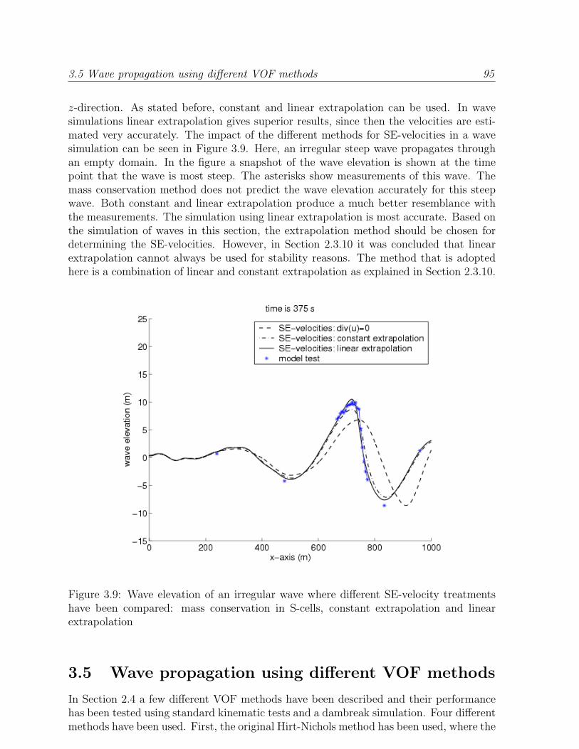
z-direction. As stated before, constant and linear extrapolation can be used. In wavesimulations linear extrapolation gives superior results, since then the velocities are esti-mated very accurately. The impact of the different methods for SE-velocities in a wavesimulation can be seen in Figure 3.9. Here, an irregular steep wave propagates throughan empty domain. In the figure a snapshot of the wave elevation is shown at the timepoint that the wave is most steep. The asterisks show measurements of this wave. Themass conservation method does not predict the wave elevation accurately for this steepwave. Both constant and linear extrapolation produce a much better resemblance withthe measurements. The simulation using linear extrapolation is most accurate. Based onthe simulation of waves in this section, the extrapolation method should be chosen fordetermining the SE-velocities. However, in Section 2.3.10 it was concluded that linearextrapolation cannot always be used for stability reasons. The method that is adoptedhere is a combination of linear and constant extrapolation as explained in Section 2.3.10.
Figure 3.9: Wave elevation of an irregular wave where different SE-velocity treatmentshave been compared: mass conservation in S-cells, constant extrapolation and linearextrapolation
3.5 Wave propagation using different VOF methods
In Section 2.4 a few different VOF methods have been described and their performancehas been tested using standard kinematic tests and a dambreak simulation. Four differentmethods have been used. First, the original Hirt-Nichols method has been used, where the
96 Chapter 3. Wave generation and propagation
interface is implicitly reconstructed in a piecewise constant manner. To avoid flotsam andjetsam and to take care of mass conservation, a local height function has been introduced.A more sophisticated method for the displacement of the free surface is the method ofYoungs [98]. The free surface is reconstructed using piecewise linear elements and thedisplacement is based on this reconstruction. Youngs’ method has also been used incombination with the local height function to ensure perfect mass conservation. In allsimulations in this section, the extrapolation method for free surface velocities has beenused.
First, the different VOF methods are tested on the propagation of a regular wave. Thewave has a period of 14.44 seconds and a length of 325 meter. The wave height is 10.14meter and the water has a depth of 600 meter. At the outflow boundary a Sommerfeldcondition is used. Figure 3.10 shows the resulting free surface profile after a simulationtime of four wave periods. Also the error in the calculated free surface profile comparedto the theoretical solution is shown, calculated by
Ew(x) = |η(x)− ηth(x)|/H,
where η is the calculated wave elevation, ηth the theoretical wave elevation, and H thewave height. From the resulting error Ew, plotted in the bottom of Figure 3.10, it can be
Figure 3.10: Wave elevation (up) and difference in wave elevation between Stokes 5thorder theory and simulation (down) for different VOF methods: Hirt-Nichols and Youngswithout and with a local height function
concluded that Youngs’ method gives more accurate results in a regular wave simulationthan Hirt-Nichols’ method. Youngs without a local height function is best in the interiorof the domain, but has a larger error at the outflow boundary than Youngs with a local
3.5 Wave propagation using different VOF methods 97
height function. No reason has been found for this behaviour. In all four simulationsrelatively little mass was lost. When examining the total amount of water in an areaof 30 m high around the calm water level, all four methods have mass loss within 0.5%of the amount of water in that area. The calculation times of the four simulations arecomparable. The factor between the calculation times of Youngs and Hirt-Nichols is 1.2.Youngs method does not take much extra calculation time in this simulation, since theinterface reconstruction is only performed in a small percentage of the total number ofcells (in average in 130 of the 6000 cells a reconstruction is made).
The four different VOF methods are also used in the propagation of a steep wave event.The wave event is taken from an experiment at MARIN, to be more precise experiment114002, which is described in Section 3.6.2. The wave is generated at the inflow boundaryby prescribing a superposition of linear wave components derived from Fourier analysis ofthe measured wave elevation in the experiment. Figure 3.11 shows the wave elevation atthe position and time point where the wave is high and steep. Youngs’ method without
Figure 3.11: Wave elevation of a steep wave event using the four different VOF methods:Hirt-Nichols’ VOF and Youngs’ VOF with and without a local height function
a local height function results in the highest wave and gives the best agreement with themeasurement. Hirt-Nichols with and without local height function give similar results,both are pretty good, but the wave crest is a bit flattened compared to the experiment.Youngs with a local height function performs worst, which is remarkable considering thegood performance of this method in Section 2.4. The explanation for this result has notyet been discovered.
To conclude, Youngs’ method performs best in wave simulations, its results are mostaccurate. A problem arises when combining Youngs’ method with a local height functionin the steep wave event shown in this section. So, this combination should only be used
98 Chapter 3. Wave generation and propagation
with care until this problem is solved. Unfortunately, due to the choice of free surfacevelocities that are extrapolated, Youngs’ method without local height function can causeloss of mass as shown in the dambreak simulation in Section 2.4.9. But in a simulationwith a very smooth free surface as in the wave simulations, only a very small amount ofwater is lost using Youngs’ method. So, for wave simulations, Youngs’ method withoutlocal height function can be used without problem. But when performing a more violentsimulation with a much distorted free surface, mass can be lost as shown in the section justmentioned. Mass can be perfectly conserved using Youngs’ method, when it is combinedwith div(u) = 0 in surface cells. But using div(u) = 0 for the determination of freesurface velocities results in inaccurate wave simulations as shown in Section 3.4 and cancause instabilities in the computations. Therefore, this option should not be used. Thesafest way is to use Hirt-Nichols’ method with local height function, but this can be abit less accurate.
In the remainder of this chapter Hirt-Nichols’ method combined with the local heightfunction is used for the displacement of the free surface.
3.6 Validation of wave propagation
For the validation of wave propagation in ComFLOW several tests have been performed.Firstly, two-dimensional wave propagation without an object in the flow has been inves-tigated. Attention has been paid to reflections at the outflow boundary, the influence ofthe artificial viscosity present due to the upwind discretisation and the size of the gridand time step necessary for an accurate simulation of waves. Especially, steep and highwaves, which are the most important waves in green water and wave impact calculations,have been studied.
Secondly, simulations have been performed of wave loading on a spar platform. Thewaves are regular, very long and quite low. The simulation results have been comparedwith experimental results that have been provided by the Maritime Research InstituteNetherlands (MARIN).
A very extensive study of two-dimensional wave propagation without an object in theflow has been performed by Meskers [62]. Some of the most important results will beshown here also. In this section attention will be paid to the number of cells and the timestep that are needed for an accurate description of the wave. The simulations have beenperformed and compared with both the linear and the 5th order Stokes theory. Also, theinfluence of the artificial viscosity has been studied by performing a simulation of manywavelengths during many periods. The next section is devoted to higher and steeperwaves. These waves have been studied by simulating a design wave, which is a kind ofmean shape of a wave in a linear random sea-state of which the power spectrum is given.
In this section a study of the necessary number of grid points and time steps for anaccurate wave simulation is presented. Also a comparison of the use of a Sommerfeldboundary condition with a damping zone is made. The simulations have been performedfor one example of a wave, which is one of the characteristic waves in an FPSO field with
3.6 Validation of wave propagation 99
Fig. H (m) # cells/λ # cells/H # dt/T theory outflow
Table 3.1: Characteristics of simulations run to investigate the propagation of two-dimensional regular waves
a water depth of 600 meter. This wave has a period of 14.44 seconds, resulting in a wavelength of 325 meter. The wave height is varied between 10.14 and 20.28 meter. Fromthe conclusions of Meskers in [62] we see that the characteristic parameter settings thathave shown to give an accurate simulation of this example wave can also be used for deepwater waves with different periods and wavelengths.
In the simulations of the wave shown in this thesis, a few numerical parameters havebeen varied, namely the number of time steps per period, the number of cells per wave-length, and the number of cells in the wave height. The results have been presented asthe resulting wave elevation after a simulation time of four periods. The domain consistsof four wavelengths in case of using a damping zone, of which two wavelengths are used asdamping zone. The domain consists of two wavelengths when the Sommerfeld boundarycondition is used.
In Table 3.1 an overview is given of the simulation characteristics, of which the resultsare shown in Figures 3.12 to 3.16.
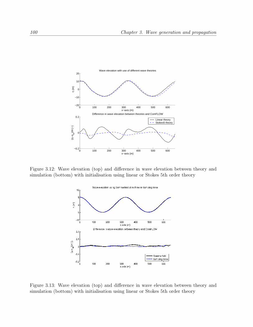
In Figure 3.12 Airy wave theory and 5th order Stokes theory have been used for theinitial condition and the inflow boundary condition. In the lower picture the differencebetween the simulation and linear theory and Stokes 5th order theory, respectively, hasbeen shown. Clearly, the 5th order Stokes results are much better than the linear Airywave results, which is consistent with the fact that H/λ equals 0.06, outside the validityregion of linear theory [61].
Figure 3.13 shows results of two simulations with different outflow methods. First,the Sommerfeld outflow boundary condition is used that is based on the wave equation.Second, a damping zone is added as in the other simulations in this section. Both methodsgive similar results. The Sommerfeld boundary condition lets the wave flow out of thedomain properly without much disturbance in the domain. The advantage of using theSommerfeld condition over a damping zone is the number of grid cells that need to beused. In this simulation, the number of grid cells in the simulation using a damping zoneis twice as large as the number of grid cells in the Sommerfeld simulation. On the otherhand, the Sommerfeld condition can only be used in case of regular waves that are nottoo much disturbed. Further, the wave velocity should be given a priori, which is onlypossible when the wave characteristics are known.
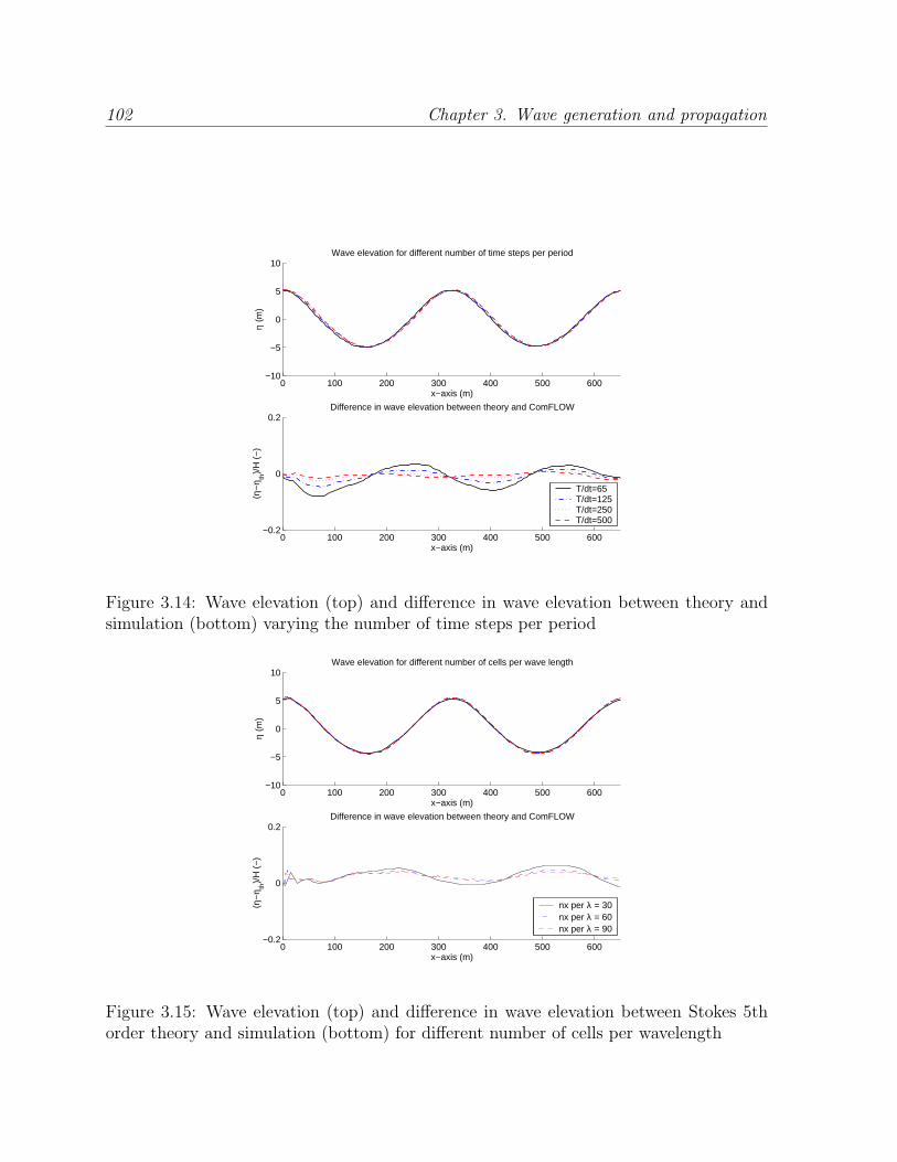
In Figure 3.14 the number of time steps per period has been altered. From the figureit can be seen that more time steps per period results in a more accurate wave simulation.The difference between 250 and 500 time steps per period is not very large. From this itis concluded that 250 time steps per period is enough for an accurate simulation result.
100 Chapter 3. Wave generation and propagation
0 100 200 300 400 500 600−20
−10
0
10
20Wave elevation with use of different wave theories
x−axis (m)
η (m
)
0 100 200 300 400 500 600−0.2
0
0.2
x−axis (m)
(η−
η th)/
H (
−)
Difference in wave elevation between theories and ComFLOW
Linear theoryStokes5 theory
Figure 3.12: Wave elevation (top) and difference in wave elevation between theory andsimulation (bottom) with initialisation using linear or Stokes 5th order theory
Figure 3.13: Wave elevation (top) and difference in wave elevation between theory andsimulation (bottom) with initialisation using linear or Stokes 5th order theory
3.6 Validation of wave propagation 101
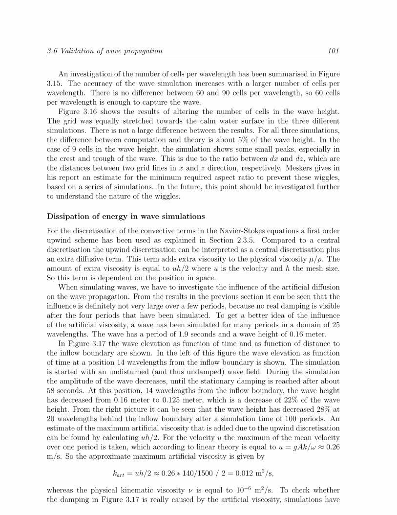
An investigation of the number of cells per wavelength has been summarised in Figure3.15. The accuracy of the wave simulation increases with a larger number of cells perwavelength. There is no difference between 60 and 90 cells per wavelength, so 60 cellsper wavelength is enough to capture the wave.
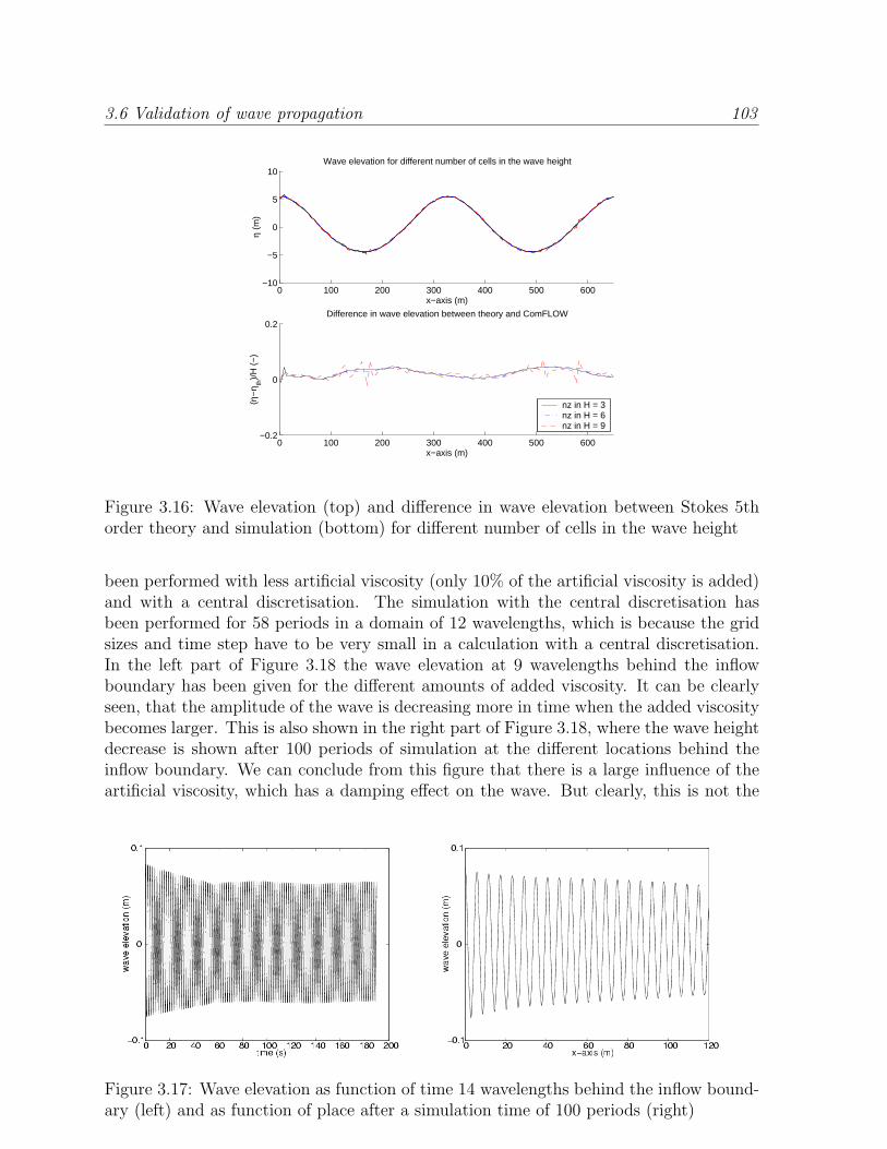
Figure 3.16 shows the results of altering the number of cells in the wave height.The grid was equally stretched towards the calm water surface in the three differentsimulations. There is not a large difference between the results. For all three simulations,the difference between computation and theory is about 5% of the wave height. In thecase of 9 cells in the wave height, the simulation shows some small peaks, especially inthe crest and trough of the wave. This is due to the ratio between dx and dz, which arethe distances between two grid lines in x and z direction, respectively. Meskers gives inhis report an estimate for the minimum required aspect ratio to prevent these wiggles,based on a series of simulations. In the future, this point should be investigated furtherto understand the nature of the wiggles.
Dissipation of energy in wave simulations
For the discretisation of the convective terms in the Navier-Stokes equations a first orderupwind scheme has been used as explained in Section 2.3.5. Compared to a centraldiscretisation the upwind discretisation can be interpreted as a central discretisation plusan extra diffusive term. This term adds extra viscosity to the physical viscosity µ/ρ. Theamount of extra viscosity is equal to uh/2 where u is the velocity and h the mesh size.So this term is dependent on the position in space.
When simulating waves, we have to investigate the influence of the artificial diffusionon the wave propagation. From the results in the previous section it can be seen that theinfluence is definitely not very large over a few periods, because no real damping is visibleafter the four periods that have been simulated. To get a better idea of the influenceof the artificial viscosity, a wave has been simulated for many periods in a domain of 25wavelengths. The wave has a period of 1.9 seconds and a wave height of 0.16 meter.
In Figure 3.17 the wave elevation as function of time and as function of distance tothe inflow boundary are shown. In the left of this figure the wave elevation as functionof time at a position 14 wavelengths from the inflow boundary is shown. The simulationis started with an undisturbed (and thus undamped) wave field. During the simulationthe amplitude of the wave decreases, until the stationary damping is reached after about58 seconds. At this position, 14 wavelengths from the inflow boundary, the wave heighthas decreased from 0.16 meter to 0.125 meter, which is a decrease of 22% of the waveheight. From the right picture it can be seen that the wave height has decreased 28% at20 wavelengths behind the inflow boundary after a simulation time of 100 periods. Anestimate of the maximum artificial viscosity that is added due to the upwind discretisationcan be found by calculating uh/2. For the velocity u the maximum of the mean velocityover one period is taken, which according to linear theory is equal to u = gAk/ω ≈ 0.26m/s. So the approximate maximum artificial viscosity is given by
kart = uh/2 ≈ 0.26 ∗ 140/1500 / 2 = 0.012 m2/s,
whereas the physical kinematic viscosity ν is equal to 10−6 m2/s. To check whetherthe damping in Figure 3.17 is really caused by the artificial viscosity, simulations have
102 Chapter 3. Wave generation and propagation
0 100 200 300 400 500 600−10
−5
0
5
10Wave elevation for different number of time steps per period
x−axis (m)
η (m
)
0 100 200 300 400 500 600−0.2
0
0.2
x−axis (m)
(η−
η th)/
H (
−)
Difference in wave elevation between theory and ComFLOW
T/dt=65T/dt=125T/dt=250T/dt=500
Figure 3.14: Wave elevation (top) and difference in wave elevation between theory andsimulation (bottom) varying the number of time steps per period
0 100 200 300 400 500 600−10
−5
0
5
10Wave elevation for different number of cells per wave length
x−axis (m)
η (m
)
0 100 200 300 400 500 600−0.2
0
0.2
x−axis (m)
(η−
η th)/
H (
−)
Difference in wave elevation between theory and ComFLOW
nx per λ = 30nx per λ = 60nx per λ = 90
Figure 3.15: Wave elevation (top) and difference in wave elevation between Stokes 5thorder theory and simulation (bottom) for different number of cells per wavelength
3.6 Validation of wave propagation 103
0 100 200 300 400 500 600−10
−5
0
5
10Wave elevation for different number of cells in the wave height
x−axis (m)
η (m
)
0 100 200 300 400 500 600−0.2
0
0.2
x−axis (m)
(η−
η th)/
H (
−)
Difference in wave elevation between theory and ComFLOW
nz in H = 3nz in H = 6nz in H = 9
Figure 3.16: Wave elevation (top) and difference in wave elevation between Stokes 5thorder theory and simulation (bottom) for different number of cells in the wave height
been performed with less artificial viscosity (only 10% of the artificial viscosity is added)and with a central discretisation. The simulation with the central discretisation hasbeen performed for 58 periods in a domain of 12 wavelengths, which is because the gridsizes and time step have to be very small in a calculation with a central discretisation.In the left part of Figure 3.18 the wave elevation at 9 wavelengths behind the inflowboundary has been given for the different amounts of added viscosity. It can be clearlyseen, that the amplitude of the wave is decreasing more in time when the added viscositybecomes larger. This is also shown in the right part of Figure 3.18, where the wave heightdecrease is shown after 100 periods of simulation at the different locations behind theinflow boundary. We can conclude from this figure that there is a large influence of theartificial viscosity, which has a damping effect on the wave. But clearly, this is not the
Figure 3.17: Wave elevation as function of time 14 wavelengths behind the inflow bound-ary (left) and as function of place after a simulation time of 100 periods (right)
104 Chapter 3. Wave generation and propagation
only reason for dissipation of energy in the wave simulations. Although in the centraldiscretisation no artificial viscosity is present, the wave has been damped much morethan it should be according to the physics. This is due to the boundary conditions andthe displacement of the free surface that sometimes are chosen to be a bit dissipative toget a stable solution.
Summarising, for wave simulation in a very long domain, where many periods aresimulated, a clear damping is visible. This dissipation of energy is for a great deal dueto the artificial viscosity that is added when using an upwind discretisation. But anotherpart of the energy dissipation is coming from the treatment of the boundaries and thefree surface. Although an energy preserving discretisation is used (see [26]), some energyis lost in other parts of the algorithm. The loss of energy is only a few percent in asmall domain when not that many periods are simulated. So for the applications of waveloading on ships, the influence will not be very significant.
Figure 3.18: Left: wave elevation at 10 wavelengths behind the inflow boundary; right:decrease of wave height after a simulation time of 100 periods at different distances fromthe inflow boundary
For the validation of irregular steep or high waves, waves generated on basis of Newwavetheory have been used [90]. Such a wave event has been developed as a mean wave shapeof a high wave in a given linear random sea-state. The wave is modelled by a superpositionof linear waves, and thus is a linear wave. Of course high waves are not linear of form,and therefore, mostly some nonlinear corrections are being made to the waves. The wavesare sometimes used as a design wave, because they have the nice feature that the positionand time of the largest impact can be predicted beforehand.
At MARIN these design waves have been used in the experimental program of theSafeFLOW project to get a better understanding of wave slamming. Before the experi-ments with a vessel in the waves is performed, the waves have been calibrated in the basinwithout the presence of a vessel. The measurements of this undisturbed wave elevationhave been used to compare our numerical method with. The characteristics of the waveevents are described in Table 3.2 with Hm0 the significant wave height and T0 the peakperiod.
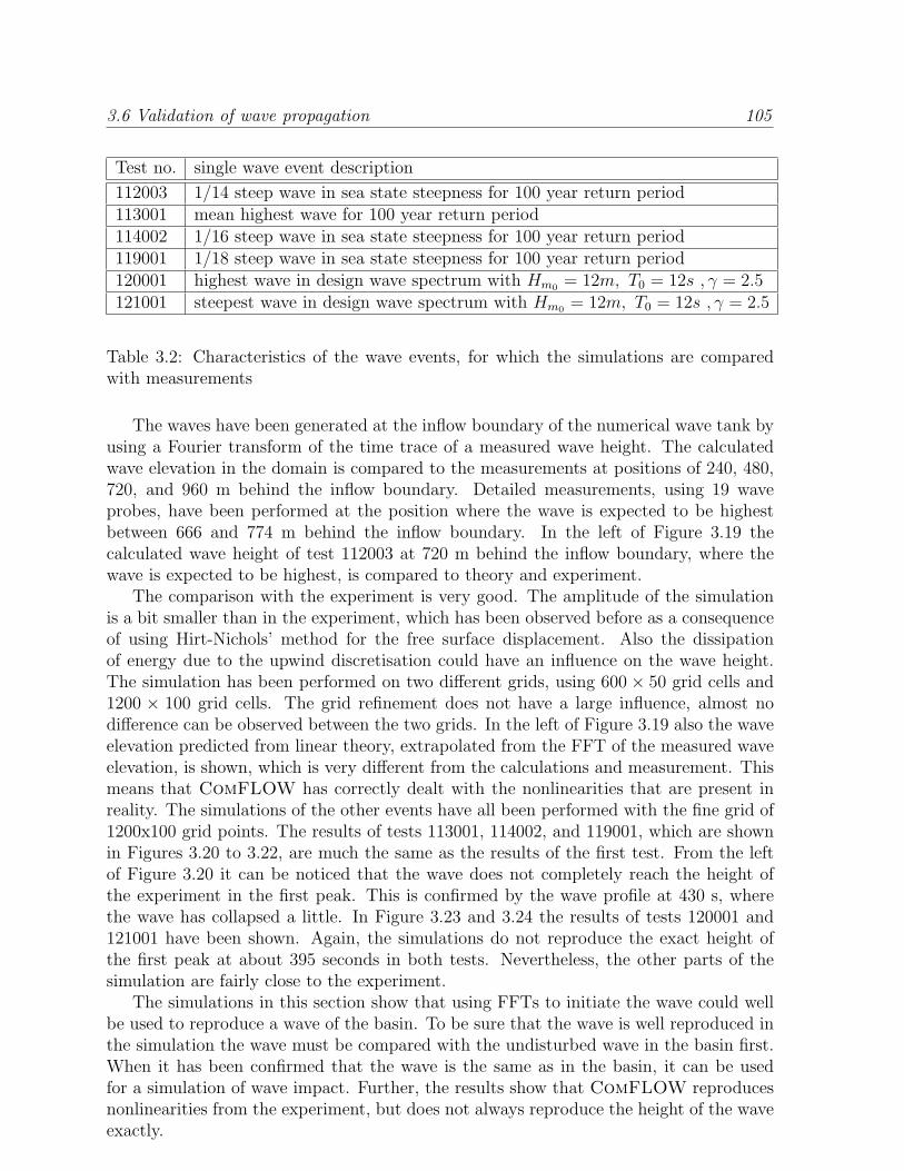
3.6 Validation of wave propagation 105
Test no. single wave event description
112003 1/14 steep wave in sea state steepness for 100 year return period113001 mean highest wave for 100 year return period114002 1/16 steep wave in sea state steepness for 100 year return period119001 1/18 steep wave in sea state steepness for 100 year return period120001 highest wave in design wave spectrum with Hm0 = 12m, T0 = 12s , γ = 2.5121001 steepest wave in design wave spectrum with Hm0 = 12m, T0 = 12s , γ = 2.5
Table 3.2: Characteristics of the wave events, for which the simulations are comparedwith measurements
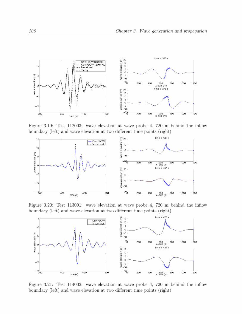
The waves have been generated at the inflow boundary of the numerical wave tank byusing a Fourier transform of the time trace of a measured wave height. The calculatedwave elevation in the domain is compared to the measurements at positions of 240, 480,720, and 960 m behind the inflow boundary. Detailed measurements, using 19 waveprobes, have been performed at the position where the wave is expected to be highestbetween 666 and 774 m behind the inflow boundary. In the left of Figure 3.19 thecalculated wave height of test 112003 at 720 m behind the inflow boundary, where thewave is expected to be highest, is compared to theory and experiment.
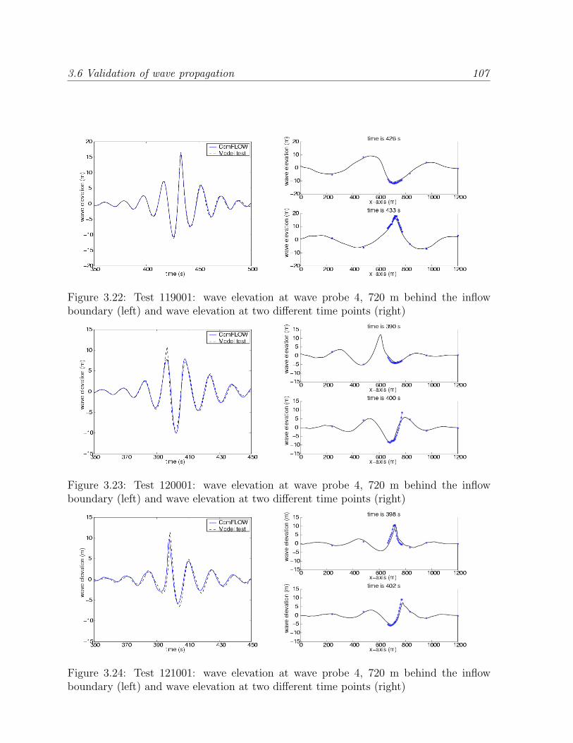
The comparison with the experiment is very good. The amplitude of the simulationis a bit smaller than in the experiment, which has been observed before as a consequenceof using Hirt-Nichols’ method for the free surface displacement. Also the dissipationof energy due to the upwind discretisation could have an influence on the wave height.The simulation has been performed on two different grids, using 600× 50 grid cells and1200 × 100 grid cells. The grid refinement does not have a large influence, almost nodifference can be observed between the two grids. In the left of Figure 3.19 also the waveelevation predicted from linear theory, extrapolated from the FFT of the measured waveelevation, is shown, which is very different from the calculations and measurement. Thismeans that ComFLOW has correctly dealt with the nonlinearities that are present inreality. The simulations of the other events have all been performed with the fine grid of1200x100 grid points. The results of tests 113001, 114002, and 119001, which are shownin Figures 3.20 to 3.22, are much the same as the results of the first test. From the leftof Figure 3.20 it can be noticed that the wave does not completely reach the height ofthe experiment in the first peak. This is confirmed by the wave profile at 430 s, wherethe wave has collapsed a little. In Figure 3.23 and 3.24 the results of tests 120001 and121001 have been shown. Again, the simulations do not reproduce the exact height ofthe first peak at about 395 seconds in both tests. Nevertheless, the other parts of thesimulation are fairly close to the experiment.
The simulations in this section show that using FFTs to initiate the wave could wellbe used to reproduce a wave of the basin. To be sure that the wave is well reproduced inthe simulation the wave must be compared with the undisturbed wave in the basin first.When it has been confirmed that the wave is the same as in the basin, it can be usedfor a simulation of wave impact. Further, the results show that ComFLOW reproducesnonlinearities from the experiment, but does not always reproduce the height of the waveexactly.
106 Chapter 3. Wave generation and propagation
Figure 3.19: Test 112003: wave elevation at wave probe 4, 720 m behind the inflowboundary (left) and wave elevation at two different time points (right)
Figure 3.20: Test 113001: wave elevation at wave probe 4, 720 m behind the inflowboundary (left) and wave elevation at two different time points (right)
Figure 3.21: Test 114002: wave elevation at wave probe 4, 720 m behind the inflowboundary (left) and wave elevation at two different time points (right)
3.6 Validation of wave propagation 107
Figure 3.22: Test 119001: wave elevation at wave probe 4, 720 m behind the inflowboundary (left) and wave elevation at two different time points (right)
Figure 3.23: Test 120001: wave elevation at wave probe 4, 720 m behind the inflowboundary (left) and wave elevation at two different time points (right)
Figure 3.24: Test 121001: wave elevation at wave probe 4, 720 m behind the inflowboundary (left) and wave elevation at two different time points (right)
108 Chapter 3. Wave generation and propagation
3.6.3 Regular wave loading on a spar platform
For the validation of wave loading, simulations have been performed of regular waveloading on a spar platform. A spar platform is a floating structure for drilling and theproduction of crude oil in the ocean. Typically, a spar is a long cylindrical steel structurewith 30-50 meters in diameter and 200 meters in length. In Figure 3.25 a schematicpicture and a photo of the Genesis spar platform are shown.
Figure 3.25: Left: schematic picture of a spar buoy, taken from http://www.ae.ic.ac.uk/;right: photo of the Genesis platform, taken from http://www.offshore-technology.com/
At MARIN experiments with a spar have been performed, where the spar was fixedwhile regular waves hit the structure. In full scale the spar has a total length of 220 mand a diameter of 35 m, the draft is 200 m in a water depth of 290.35 m. The spar hasbeen divided into three horizontal segments, on which forces have been measured (seeFigure 3.26).
Figure 3.26: Configuration of the sparbuoy, which is divided into 3 segments: thepart above the calm water surface, the part12 meter below the calm water surface andthe remainder
The characteristics of the waves used in the simulations that have been performedare given in Table 3.3. The spar buoy has been placed at a distance of one wavelengthbehind the inflow boundary. About 100 m behind the cylinder, a dissipation zone of onewavelength has been added to prevent the wave from reflecting into the domain.
3.6 Validation of wave propagation 109
Test No. frequency period wave height wavelength
101 0.26 rad/s 24.17 s 10.77 m 866 m201 0.26 rad/s 24.17 s 23.62 m 866 m001 0.48 rad/s 13.09 s 10.91 m 274 m
Table 3.3: Wave characteristics of simulations of loading on a spar platform
The simulations of wave tests 101 and 102 have been performed on a grid with about60 cells per wavelength, 15 cells in the transverse direction and 52 cells along the totalheight of the domain. The grid is stretched in the z-direction towards the calm waterlevel. The wave in these tests is the same, except that the wave height in test 201 isabout two times as large. The results of test 101 are shown in Figure 3.27 to 3.29.
Figure 3.27: Test 101: Wave height 300 meter in front of the spar (left) and pressure(middle) and wave height (right) at the left of the spar
Figure 3.28: Test 101: Total force on the spar in the three coordinate directions: hori-zontal (left), transverse (middle) and vertical (right)
The global impression of the results is that there is a good agreement between thesimulation and the model test. In the left of Figure 3.27 the wave height at about 300meter in front of the spar has been shown. The comparison between the experiment andthe simulation is satisfying. No phase difference is present and the amplitude of the waveis very much the same except for the trough of the wave, which is a bit flatter in thesimulation. In the other two pictures of Figure 3.27 the wave height and pressure at theside of the spar is plotted. The results give the same impression as in the previous figure.The wave is not disturbed by the spar, which is a logical result when comparing the verylarge wavelength to the diameter of the spar.
110 Chapter 3. Wave generation and propagation
Figure 3.29: Test 101: Horizontal force on the three different segments of the spar: uppersegment (left), mid segment (middle) and lower segment (right)
In Figure 3.28 the measured forces on the center of gravity of the spar platformhave been compared to the calculated forces. The horizontal force, which is the force inthe direction of the wave, has the largest amplitude and shows a very good agreement.The force in the transverse direction is and should be very small because of symmetrycharacteristics. In the vertical force a clear difference is observed between the measuredand calculated amplitude, which cannot be explained at the moment.
The calculated forces on the different segments, which are shown in Figure 3.29, arein good agreement with the measurements. The force on the lower segment is almostequal to the total force on the spar. The upper segment lies above the calm water level,so this segment comes completely out of the water every period, where the force equalszero. The non sinusoidal form of the force on the mid segment is also due to the fact thatthe wetness of the segment is not constant throughout a period.
Figure 3.30: Test 201: Wave height 300 meter in front of the spar (left) and horizontalforce on the upper segment (right)
The results of test 201 are much the same as the results presented for test 101. Toget a good idea of the agreement between this model test and the simulation, the waveheight 300 meter in front of the spar and the forces on the different segments are shownin Figures 3.30 and 3.31. The wave is really flatter in the troughs, which is also reflectedin the horizontal force on the upper and mid segments where the simulation results showa smaller amplitude of the force. The horizontal force on the lower segment is in goodagreement with the experimental data.
The third wave loading simulation that has been performed, deals with a much shorter
3.6 Validation of wave propagation 111
Figure 3.31: Test 201: Horizontal force on the mid segment (left) and on the lowersegment (right)
(and more realistic) wave. In this case, the influence of the spar on the wave is notnegligible as it was in the previous cases. This is also shown in the results of the simulationof this wave (with the same number of grid cells per wavelength), of which the wave heightat the front of the spar and the total horizontal force on the spar are shown in Figure3.32 (coarse grid). Many more cells are needed around the spar, therefore also stretchingin x and y direction is applied in the mid and fine grid of Figure 3.32. The fine gridhas about 3.5 times more grid cells in the neighbourhood of the spar than the coarsegrid. From Figure 3.32 it can be concluded that the fine grid reproduces the model testvery well, whereas the other grids are not accurate enough. In Figure 3.33 time traces ofthe horizontal forces on the upper and mid segment of the spar have been shown. Bothgraphs show a rather good agreement with the experiment.
3.6.4 Green water on the deck of a moving FPSO
A very demanding test case for the current simulation method is the calculation of loadsdue to green water on the deck of a moving FPSO (Floating Production Storage andOffloading vessel). For validation, an experiment performed at MARIN has been used.Measurements were done of the wave in front of the FPSO, relative wave heights in theneighbourhood of the FPSO, water heights and pressures at the deck of the FPSO andthe pressure at some places at a deck structure. The FPSO has a total length of 260 meterand is 47 meter wide. The draft is 16.5 meter, the total height of the deck at the foreside of the FPSO is 25.6 meter. There is a bulwark extension of 1.4 meter. At the decka box-like structure has been placed, at which forces and pressures have been measured.The bow has a fully elliptical shape without flare. The wave has a period of 12.9 secondsand the wave length is 260 meter, equal to the length of the FPSO. The wave amplitudeis 6.76 meter. To be sure that the same wave has been used in the experiment and inthe simulation, the wave measurement 230 meter in front of the bow of the vessel hasbeen used to initiate the wave at the inflow boundary. The signal from the wave probehas been decomposed in linear components that are prescribed at the inflow boundary.The motion of the ship is prescribed using the measurements of the experiment. Thesimulation has been performed with only half of the FPSO in a relatively small domainaround the bow of the vessel. A grid with 100 × 60 × 80 grid points has been used,
112 Chapter 3. Wave generation and propagation
Figure 3.32: Test 001: Comparison of different grids: wave height at the front of the spar(left) and horizontal force on the total spar (right)
Figure 3.33: Test 001: Horizontal force on the upper segment (left) and on the midsegment (right) using the fine grid
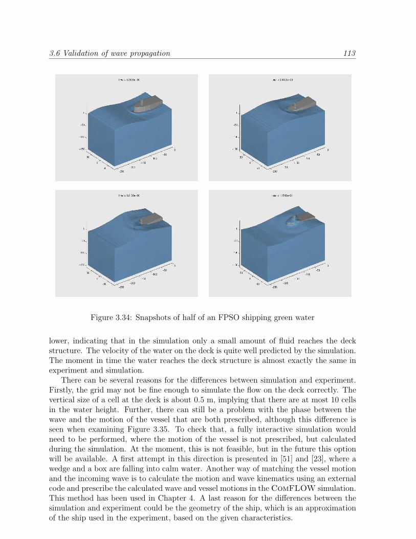
resulting in a calculation time of about 4.5 hours. In Figure 3.34 some snapshots of thesimulation are shown during the first period of the simulation. The large wave is buildingin front of the vessel, after which it starts to flow onto the deck. The water flows off thedeck when the ship is straightening.
In Figure 3.35 the relative wave height in front of the vessel is shown. In both picturesthere is a good agreement, such that it can be concluded that the motion of the vesselrelative to the wave motion does not differ much in simulation and experiment. Thewater height on the deck of the vessel has been compared in Figure 3.36. When the waterhas just flowed onto the deck (left figure), the agreement between the experiment andthe simulation is reasonable. The moment in time the wave probe gets wet is almost thesame. But in the first periods, the water height is somewhat higher in the simulation,whereas the total time the water hits the wave probe is shorter. Closer to the deckstructure, in the right of Figure 3.36, the total amount of water passing the wave probeis much smaller in the simulation. This same behaviour can be seen from the pressureon the deck and the deck structure. Whereas the pressure at the deck just behind thefore point of the FPSO agrees reasonably well, the pressure at the deck structure is much
3.6 Validation of wave propagation 113
Figure 3.34: Snapshots of half of an FPSO shipping green water
lower, indicating that in the simulation only a small amount of fluid reaches the deckstructure. The velocity of the water on the deck is quite well predicted by the simulation.The moment in time the water reaches the deck structure is almost exactly the same inexperiment and simulation.
There can be several reasons for the differences between simulation and experiment.Firstly, the grid may not be fine enough to simulate the flow on the deck correctly. Thevertical size of a cell at the deck is about 0.5 m, implying that there are at most 10 cellsin the water height. Further, there can still be a problem with the phase between thewave and the motion of the vessel that are both prescribed, although this difference isseen when examining Figure 3.35. To check that, a fully interactive simulation wouldneed to be performed, where the motion of the vessel is not prescribed, but calculatedduring the simulation. At the moment, this is not feasible, but in the future this optionwill be available. A first attempt in this direction is presented in [51] and [23], where awedge and a box are falling into calm water. Another way of matching the vessel motionand the incoming wave is to calculate the motion and wave kinematics using an externalcode and prescribe the calculated wave and vessel motions in the ComFLOW simulation.This method has been used in Chapter 4. A last reason for the differences between thesimulation and experiment could be the geometry of the ship, which is an approximationof the ship used in the experiment, based on the given characteristics.
114 Chapter 3. Wave generation and propagation
Figure 3.35: Relative wave height 30 meter (left) and 5 meter (right) in front of the FPSO
Figure 3.36: Water height on the deck of the FPSO: at the fore side of the bow (left) andnear the deck structure (right)
Figure 3.37: Left: pressure on the deck of the FPSO; right: pressure at the deck structure