University of Hawai`i at Mānoa Department of Economics ...

University of Hawai`i at Mānoa

Department of Economics Working Paper Series

Saunders Hall 542, 2424 Maile Way,

Honolulu, HI 96822 Phone: (808) 956 -8496

www.economics.hawaii.edu

Working Paper No. 14-23

Who is to Blame: Foreign Ownership or Foreign Funding?

By

Inessa Love

Roberto Rocha Erik Feyen

Samuel Munzele Maimbo Raquel Letelier

September 2014


Inessa Love, Roberto Rocha, Erik Feyen, Samuel Munzele Maimbo, and Raquel Letelier1

JEL Classification: G01, G21, F36. Key words: Global financial crisis, bank credit, foreign banks, funding models.

1 Inessa Love is an Associate Professor at the University of Hawaii ([email protected]), Roberto Rocha is a Senior Advisor in the World Bank’s Financial System Department ([email protected]), Erik Feyen is a Lead Financial Economist in the World Bank’s Financial Systems Department ([email protected]), Samuel Munzele Maimbo is a Lead Financial Sector Specialist in the World Bank's Europe and Central Asia Department ([email protected]) and Raquel Letelier is a Financial Analyst in the World Bank’s Europe and Central Asia Department ([email protected]). We thank María Soledad Martínez Pería, Stijn Claessens, participants of the June 2013 World Bank ECA region retreat, participants of the University of Hawaii seminar and participants of the 2014 FIRS conference for useful comments and suggestions.

mailto:[email protected]






Abstract

We investigate whether the credit contraction that followed the global financial crisis is due to high foreign ownership or high reliance on foreign finding. We apply panel vector autoregressions to quarterly data for 41 countries and find that domestic credit growth is highly sensitive to cross-border funding shocks around the world. However, high foreign ownership per se does not appear to increase the sensitivity of credit to foreign funding shocks. Rather, the sensitivity is higher in countries with high reliance on foreign funding and high loan-to-deposit ratios. These findings have important policy implications for many countries involved in cross-border funding.

JEL Classification: G01, G21, F36. Key words: Global financial crisis, bank credit, foreign banks, funding models.

3

I. Introduction

Although most countries across the world experienced a severe contraction of credit

during the recent global financial crisis, the Eastern Europe and Central Asia (ECA) region was

hit harder than most of the developing countries. One possible reason for the severe decline lies

in close economic and financial links with Western Europe, including a high degree of foreign

ownership (i.e. foreign equity) and greater reliance on foreign funding (i.e. foreign liabilities) in

the banking sector. The credit crunch was generally driven by foreign banks, as they initiated

efforts to repair their balance sheets and retrench to home markets. The concerted policy

response, including the Vienna Initiative, succeeded in mitigating a severe credit contraction in

the participating countries (de Haas et al, 2012). However, these events triggered a renewed

debate about the benefits and costs associated with the presence of foreign banks, cross-border

finance, and financial integration. We use the special case of ECA countries to provide new

evidence on the relative role that foreign ownership and foreign funding play in the transmission

of global financial crises.

Previous research has established that foreign banks have much to contribute to financial

sector development (see Claessens and Van Horen, 2014, for a comprehensive review of the

literature).2 However, as the global financial crisis has made clear, their presence can also have

large destabilizing impacts (Mishkin, 2007). Recent research shows that foreign banks drove the

2 Specifically, foreign banks can accelerate financial development by lowering the cost of financial intermediation, increasing the quality of and access to financial services (Giannettia and Ongena, 2012), increasing competition in the host country, bringing in up-to-date technology to the market, introducing new, more diversified products and services, and pressing regulators to reform and modernize the regulation and supervision of financial systems. Allen et al (2012) also discuss costs and benefits of cross-border banking in detail.

4

credit boom in ECA before the crisis and exacerbated the credit contraction after the crisis.3

Even the US branches of foreign banks were significantly affected (Cetorelli and Goldberg,

2012). Concerned about their potentially destabilizing impact, many countries are reconsidering

the merits of limits on foreign bank ownership.4

Despite the widespread agreement that foreign banks have amplified the transmission of

the global shocks to host countries, the evidence appears more nuanced and there is significant

heterogeneity among the foreign banks. For example, foreign banks that focused on deposit-

based funding contracted lending less than domestic banks during the crisis (Claessens and Van

Horen, 2013, Ongena et al 2012). Also, foreign banks which were more integrated into a network

of domestic co-lenders reduced lending less during the crisis (De Haas and Van Horren, 2013).

Kapan and Minoiu (2013) show that banks with stronger balance sheets were better able to

maintain lending during the crisis, while those more dependent on market funding—which is

typically shorter term and more fickle—reduced the supply of credit more than other banks.

Cerutti and Claessens (2013) point that market-based measures of vulnerabilities of banking

systems to shocks were more important than accounting based measures in explaining bank

deleveraging. In addition, Choi, Gutierrez, and Martinez Peria (2013) find that banks with better

capitalized parents were more stable in their lending.

These findings suggest that the type of bank funding models, along with the regulatory

standards and supervisory arrangements, maybe more important for stability than foreign

ownership per se. Foreign banks can finance their operations predominantly with local deposit-

3 Cetorelli and Goldberg (2011), de Haas and Van Lelyveld (2014), de Haas et al (2012), Cull and Martinez Peria (2012), Popov and Udell (2012), Feyen and González del Mazo (2013), Impavido et al (2013). 4 For example, Indonesia and Namibia have imposed new restrictions on foreign banks in 2013.

5

based funding, as they do in most Latin American countries, or with the foreign funding from

their parent banks or cross-border wholesale funding sources, as in most ECA countries. Casual

observation suggests that the source of funding played an important role during the recent crisis.

For example, some Eastern European countries with a high degree of foreign ownership but less

reliance on foreign funding seem to have been less affected (e.g. Czech Republic, Slovakia),

while other countries with a lower degree of foreign ownership but strong reliance on cross-

border funding were highly affected (e.g. Kazakhstan and the Ukraine). It is important for

policymakers to know whether the destabilizing impact of foreign banks depends on the origin of

bank funding (i.e. liabilities) or the origin of bank ownership (i.e. equity).

While other authors have argued that cross-border funding is one of the main channels of

transmission of global crises, earlier studies cited above lacked the direct measures of reliance on

foreign funding because they used bank-level data, mostly from Bankscope database, which does

not include information on the origin of bank liabilities.5 Thus, the previous research has not

been able to directly pinpoint the foreign funding channel as the culprit of the foreign-bank

induced credit crunch.

In this paper we provide direct evidence on the impact of foreign funding on credit

growth, which has immediate implications for the regulatory debate on cross border banking. We

make several contributions to the ongoing research efforts to disentangle the role of foreign

ownership and foreign funding in the transmission of the global financial crisis. First, we use

precise measures of a country’s reliance on foreign funding using data on foreign liabilities of

5 While some previous authors use the ratio of deposits to assets to proxy for the levels of foreign funding, this variable is crude and does not accurately measure the exposure to foreign funding, and thus have only indirect relevance for the policy debate.

6

the banking system. Second, we compare how factors affecting credit growth were different in

ECA vs. other regions. Third, we follow a different methodology – Panel Vector Autoregression

(PVAR) – allowing us to examine the dynamic relationship between funding structures and

credit growth over time.

There are several advantages in using PVAR methodology to study the importance of

different factors in explaining credit growth. First, in VAR, all variables are treated as

endogenous and interdependent so all the feedback effects are explicitly included in the model.

Thus, VARs are designed to explicitly address the endogeneity problem, which is a serious

challenge in studying the empirical relationships between credit growth and funding sources.

Second, unlike single country VARs that need long time series for efficiency, PVARs can be

used with relatively short time-series. This is important for our study since the quarterly data on

foreign liabilities are only available for about 10 years. Third, the PVAR methodology can

distinguish between the short-term impacts of each of the factors based on the impulse-response

functions and the long-term cumulative impacts of shocks based on variance decompositions.

Fourth, as in any panel-based method, PVAR allows us to control for country- and year- fixed

effects. Country-fixed effects will capture time-invariant country characteristics that can explain

credit growth, such as institutions, the rule of law, the quality and depth of credit information and

other relatively static features of the business environment. Year-fixed effects capture global

shocks affecting finance and growth, such as the effect of the global financial crisis that is

common for all countries in the same time period. Fifth, the VAR model can distinguish whether

demand (e.g. GDP) or supply (e.g. foreign liabilities and deposits) factors drove the decline of

the private credit, which is important because all these variables deteriorated simultaneously

7

during the crisis. Thus, PVAR is a methodology that is very well-suited to the questions this

study aims to address.

Our results can be summarized as follows. We apply PVARs to a global panel that

consists of quarterly data for 41 countries in ECA, Asia, Latin America, and the Middle East and

Africa for the period 2000-2011. We document four main findings. First, we find that private

credit growth is highly sensitive to cross-border funding shocks around the world. Second, we

find that this relationship is significantly stronger in the average ECA country compared to the

rest of our sample. Specifically, the response is 72% higher in the initial period and about three

times higher after one quarter. Third, we show that countries with high loan-to-deposit ratios and

high reliance on foreign funding exhibit a stronger response of private credit to foreign funding

shocks. However, foreign ownership per se does not lead to different response in our sample of

countries. Fourth, we show more directly that high loan-to-deposit ratios and high foreign

funding are able to explain the differences between ECA and the rest of the world, while high

foreign ownership by itself is insufficient to explain these differences.

Taken together, our findings suggest that funding model differences were at the heart of

ECA’s protracted post-crisis credit growth contraction, not its high prevalence of foreign bank

ownership. These finding have important policy implications. Rather than trying to curtail and

scale back foreign bank presence, this paper suggests regulators ought to focus on business

models of local affiliates of international banks and the regulation of cross-border funding. We

discuss policy implications in more detail in the conclusions of the paper.

8

II. Data

We compile a panel database with quarterly data covering 41 countries in various regions

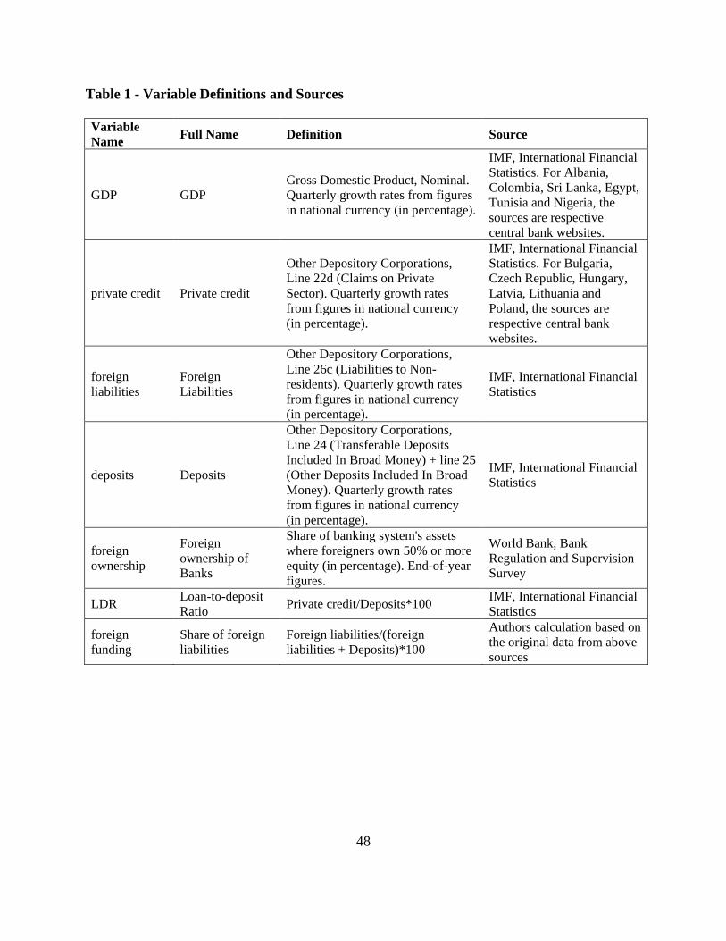
with about 11 years of data available for most countries. Table 1 provides a description of the

variables and sources. We have two sets of variables: the time series variables are used for the

panel VAR and the cross-country variables are used for sample splits. We describe each of these

sets of variables in detail below.

II.1. Panel VAR Variables

There four main variables in our PVAR model, which are taken from the IMF’s

International Financial Statistics (IFS): private credit, foreign liabilities, GDP, and deposits. For

most of the countries in our sample these variables are available quarterly starting with Q2, 2001

and ending with Q4, 2011.6 The private credit variable measures the quarter-on-quarter real

growth rate of private credit. Private credit isolates credit issued to the private sector and

therefore excludes credit issued to governments, government agencies, and public enterprises.

Private credit also excludes credits issued by central banks. The foreign liabilities variable

measures the quarter-on-quarter real growth rate of foreign liabilities. These liabilities include

claims of non-residents on the domestic banking system which include deposits, securities, loans,

financial derivatives and other liabilities. GDP is the quarter-on-quarter, seasonality-adjusted

growth rate of real GDP. The deposits variable measures quarter-on-quarter real growth rate of

6 Some countries have shorter series due to data availability, details available on request.

9

bank deposits, consisting of the domestic time, savings, and demand deposits of deposit money

banks. All variables are denominated in local currency.

For all variables we first calculate quarter-on-quarter nominal growth rates. Then we

construct real growth rates by subtracting the quarter-on-quarter percent change in the CPI

index.7 Thus, our main PVAR variables are expressed in growth rates, which ensures their

stationarity.

Table 2A shows that the mean real quarterly growth rates of foreign liabilities were

higher than those of private credit and deposits, and its standard deviation was considerably

higher, by a factor of three or larger. This result reveals the major weakness of foreign funding –

its volatility in periods of crisis. The mean growth rates of foreign liabilities and private credit

were much higher in the case of ECA countries, relative to Non-ECA countries, reflecting the

greater reliance of the ECA region on foreign funding and the key role played by cross-border

finance in ECA’s pre-crisis credit boom. Interestingly, the standard deviation of foreign

liabilities in the ECA and non-ECA regions are similar, revealing that countries in the two

regions are potentially exposed to the same volatility in periods of crisis, but ECA countries are

much more exposed, given their greater reliance on foreign funding. This result will be further

explored in Section V.

II.2. Sample Split Variables

7 We have also used GDP deflator to adjust GDP growth rates, but it had less coverage. All our results hold using the GDP deflator, however the GDP results become slightly less significant perhaps because of the added noise. In addition, we removed significant country-specific seasonality in GDP growth rates. To do that we regressed real GDP growth rates on country-specific quarter dummies and subtracted the predicted values.

10

One of the objectives of this paper is to understand what drives the differences in the

response of private credit to other PVAR variables between ECA and the rest of the world. In

doing so, we use three variables hypothesized to explain these differences: the loan-to-deposit

ratio (LDR), foreign ownership, and foreign funding. LDR is calculated as the ratio of private

credit to deposits, both variables were defined above. LDR proxies the extent to which domestic

bank credit is funded by domestic deposits. An LDR in excess of 100 percent implies that credit

has been financed with other sources of funding such as unsecured wholesale funding in the

international or domestic interbank markets. These types of funding are typically short-term and

highly sensitive to market conditions in contrast with (retail) deposits which are usually much

more stable. The foreign funding measure is a proxy of the banking system’s reliance on foreign

sources of funding relative to total funding. It is calculated as the ratio of foreign liabilities to the

sum of foreign liabilities and deposits, which roughly represents total debt funding. Lastly,

foreign ownership measures the fraction of banking system assets that are majority-owned by

non-residents. These data are taken from the World Bank’s Bank Regulation and Supervision

Survey.

To gauge the impact of these variables, we split the sample based on their pre-crisis

values.8 Table 2B reports the pre-crisis country averages for our three sample-split variables

broken for ECA and non-ECA countries. Table 2B shows that LDR, foreign funding and foreign

ownership are significantly higher in ECA countries, relative to non-ECA countries. However,

the standard deviations also suggest that there is substantial variation across countries within

8 We use 2007:Q4 values for LDR and foreign funding. We use the closest available observation for foreign ownership, which is 2008 for most countries.

11

each of the two regions. This is an important result that will also be further explored in Section

V.

III. Trends and descriptive statistics

For our graphical analysis we break down the ECA region into the Commonwealth of

Independent States (CIS) and the Central, Eastern and Southeastern Europe region (CESEE).

Many countries in both samples enjoyed a credit boom prior to the global financial crisis, the

CIS growing by 50-60% per year while the CESEE growing at 30%-40% between 2005 and

mid-2008 (Figure 1, Panel A). Among other regions, only the Gulf Cooperation Council (GCC)

countries grew at a similar pace, while the non-GCC countries in the Middle East and North

Africa (MENA) region, and the Latin American and Asia regions showed moderate rates of

credit growth during that period.

Deposit growth rates in these economies were also growing at high rates (Panel B),

although lower than the rates of credit growth, as reflected in the growing loan-to-deposit ratios

(Panel F). Loan-to-deposit ratios in the CIS went as high as 170% before the crisis, and

continued to increase even after the crisis, reaching almost 180% at its peak in mid-2009.

CESEE reached its maximum ratio in early 2009, with levels of 140%, while GCC went as high

as 125% around the same period. Conversely, other emerging regions showed more steady

levels, and in the case of non-GCC and Emerging Asian countries, always below 100%.

These trends can be largely explained by differences in banking models across regions.

While LAC, non-GCC and Asia financed their credit growth with local deposits (keeping their

12

loan-to-deposit ratios under 100%), CESEE, CIS and GCC countries were heavily reliant on

foreign borrowing. Figure 1, Panel D displays the share of foreign liabilities to total liabilities

(i.e. it is the foreign funding measure described above) and shows the different paths these

regions followed. While foreign liabilities in LAC, non-GCC and Asia were in the range of 10%-

20% of total liabilities, foreign borrowing in CESEE, CIS and GCC increased prior to the crisis,

exceeding on average 40% of total liabilities in early 2008.

The ECA region is generally known for the dominant presence of foreign ownership in

comparison with emerging peers, but this is only true for the CESEE countries (Panel G). By

2008, 80% of the banking system in CESEE was in foreign hands, a figure that barely surpassed

40% in LAC and 30% in other emerging regions. The levels of foreign ownership were lower in

the large CIS countries, especially in countries like Russia and the Ukraine, where foreign banks

accounted for less than 20% of total assets.

After the onset of the crisis in 2008, credit experienced a significant slowdown in all

emerging regions. This was more acutely felt in those regions where credit had been increasing

at a rapid pace and GDP contracted heavily in 2009, such as CESEE and CIS (Panel C). As a

consequence of the credit crunch, these regions witnessed an increasing deterioration in asset

quality, as shown by the ratio of nonperforming loans to total loans (Panel E).9

III.1. Correlations

9 High NPLs in CIS are exacerbated by Kazakhstan, which experienced a housing market collapse, leading to a deterioration in the quality of banks’ assets, who were large investors in the real estate market.

13

Panel A of Table 3 presents the correlations between our PVAR variables for the full

sample, as well as separate correlations for ECA and the rest of the sample (“non-ECA”). As

expected, the correlation between deposits and private credit is high in all samples. We also

observe that foreign liabilities are correlated with private credit (0.40). However, this correlation

is almost twice as high in ECA compared to non-ECA (0.50 vs. 0.23). This suggests credit in the

ECA region could be much more vulnerable to foreign funding shocks than in the rest of the

world, a hypothesis we formally test with PVARs in Section V.

Panel B of Table 3 displays the correlations for the sample split variables. It illustrates the

different funding model in ECA reflected in the high correlation between foreign funding and

LDR in ECA, but the absence of such correlation in the non-ECA region. Indeed, many banks in

ECA funded their operations by attracting foreign funding to supplement domestic deposits in

order to sustain high credit growth, resulting in elevated loan-to-deposit ratios. The correlations

suggest this practice was not as widespread in non-ECA countries.

While foreign funding and foreign ownership are positively correlated, the correlation is

not very high: 0.35 in the full sample and near zero in ECA (Table 3, panel B). The positive

correlation is expected, as foreign owned banks often obtain funding from parent banks and have

better access to international funding markets. However, in ECA there are many cases of

countries with high levels of foreign liabilities but low levels of foreign ownership and vice

versa. For example, Kazakhstan and Ukraine had relatively low levels of foreign ownership, but

high levels of foreign liabilities, while Czech Republic and Slovakia had high levels of foreign

ownership (around 90 percent of assets) but limited reliance on foreign funding (around 10

percent of liabilities). These correlations suggest that many domestically-owned banks in ECA,

especially those in CIS, relied to a significant extent on foreign funding.

14

III.2. T-tests: Is ECA Different from the Rest of the World?

In this section we test whether the patterns discussed above are statistically significant.

Our main focus is on the differences between ECA and the rest of the world (i.e. non-ECA).

Therefore, we split our sample into an ECA and non-ECA subsample and run basic mean

comparison t-tests. Specifically, we track the evolution of our variables before (2005-07), during

(2008-2009), and after (2010-2011) the global financial crisis hit.

Table 4 presents the results. Panel A documents the ECA vs. non-ECA differences for the

PVAR variables: private credit, foreign liabilities, GDP, and deposits. We observe that in the

pre-crisis period, ECA was significantly different from the rest of the sample in terms of the

growth of foreign liabilities, private credit, and deposits. The real rate of growth of foreign

liabilities and private credit for ECA was more than double relative to non-ECA: 10.06% vs.

3.64% for foreign liabilities and 7.87% vs. 3.15% for private credit. These differences are

statistically significant and highlight the distinctiveness of the ECA cross-border, wholesale

funding model which consists of rapid private credit growth sustained by inflows of foreign

funding. The resulting ECA credit boom is demonstrated by higher average real deposit growth

(5.42% vs. 2.65%), but it did not result in significant differences in real GDP growth (0.95% vs.

0.51%).

Next, we study the PVAR variables during the peak of the crisis in 2008-2009. During

this period, GDP growth fell significantly more in ECA compared to non-ECA (-1.86% vs. -

15

0.51%), while the private credit growth was still significantly higher in ECA (2.15% vs. 1.45%).

Yet, deposit growth differences are not statistically significant. The difference for foreign

liabilities was not statistically significant in this period (even though the means are still higher

for ECA, there was substantial variation within the region). This may point to the lag in adjusting

banks operations, which squares well with our ordering of the foreign liabilities as first (i.e. the

variable that responds to all others with a lag).

In the immediate post-crisis years (2010-2011), many non-ECA countries had started

their recovery as evidenced by the return of positive growth in foreign liabilities, private credit,

and deposits. In contrast, foreign liabilities and credit growth were significantly lower in ECA,

reflecting the onset of the EU’s sovereign and banking crisis, which had protracted effects on

cross-border lending.. The continuation of the crisis in the EU is also reflected in the lower GDP

and deposit growth rates in ECA, although the differences are not statistically significant. These

findings suggest that non-ECA countries have recovered faster from the impact of the crisis.

Given such distinctive differences in the impact of the global crisis and the path of

recovery in ECA vs. non-ECA economies, we seek to understand what key pre-crisis features of

financial systems in ECA could be responsible for such differences. As discussed, we

hypothesize the differences could be attributed to dissimilarities in the funding model and/or the

extent of foreign ownership. Therefore, to gauge funding model differences we perform t-tests

on LDR, foreign ownership and foreign funding. Table 4, Panel B shows the results.

The average LDR in ECA is significantly higher than in non-ECA (126.4% vs. 98.4%).

Since ECA’s LDR exceeds 100% by a wide margin, ECA had to fund its liquidity gap with other

wholesale sources, which are typically regarded as less stable than retail deposits. These

wholesale sources were often of foreign nature in ECA as evidenced by the fact that foreign

16

funding was twice as high ECA compared to non-ECA (31.9% vs. 15.8%). While these foreign

sources of funding can act as stabilizers when stress originates from the domestic financial sector

(e.g. De Haas and Van Lelyveld, 2014, they can also function like conduits of foreign financial

stress. The ECA funding model contrasts sharply with the one of foreign bank affiliates in Latin

America which typically source their funding in domestic markets—mostly retail deposits—

which impedes excessive credit expansion and the transmission of foreign stress.

At the same time, we find that foreign ownership is also very high in ECA. In the average

non-ECA country, 31.4% of banking assets are majority-owned by non-residents compared to

66.7% in the average ECA country.

While ECA has high averages of all three ratios, not all countries have equally high

foreign bank ownership and high foreign funding dependence, as we discussed above. We use

this variation to assess which of these two factors is responsible for the differences in credit

growth in our PVAR analysis below.

IV. Methodology

PVARs combine the advantages of the traditional Vector Autoregression (VAR) with the

advantages of panel-data models. Basic VARs allow for the simultaneous analysis of the

evolution of a system of endogenous variables. Moreover, the PVAR allows us to separately

study demand and supply factors to better understand the evolution of private credit. The prime

benefit of VARs is that the dynamic impact of orthogonal shocks can be evaluated—i.e. the

isolated impact of a shock of one variable on the system over time, keeping the shocks of the

other variables equal to zero.

17

The PVAR technique is particularly suitable for our purposes because we seek to model

the evolution of a system of our four variables of interest—private credit, foreign liabilities,

GDP, and deposits—in a set of countries which significantly differ along various dimensions

such as the development of their financial and economic systems, financial regulation and

supervisory effectiveness, and exchange rate regimes. These unobservable country-specific

differences are captured with country fixed effects in our model.

Moreover, these countries are faced with common exposures such as the global cycle,

global risk appetite, key interest rates, extraordinary measures of large central banks, and other

global financial and economic shocks. Controlling for these common exposures is also important

because our sample includes the period of the global financial crisis during which financial stress

rapidly spilled over to other parts of the world significantly increasing the size of common risk

factors. These common time shocks are captured with time fixed effects in our model.

The structure of our baseline PVAR model can be written in reduced form as follows:

Ζit = Γ0 + Γ1 Ζit-1 + fi + dt +eit (1)

where Ζit is a vector of our four variables for quarter t and country i and modeled as a

function of the first-order lags of all variables in the system. The fi and dt terms are country fixed

effects and time fixed effects respectively.

The country fixed effects present an estimation challenge which arises in any model

which includes lags of the dependent variables: the fixed effects are correlated with the

regressors and therefore the mean-differencing procedure commonly used to eliminate fixed

effects would create biased coefficients. Our PVAR implementation follows Love and Zicchino

18

(2006).10 Specifically, to remove fixed effects we use forward mean-differencing, also referred to

as the `Helmert procedure' (see Arellano and Bover, 1995).11 This procedure removes only the

forward mean, i.e. the mean of all the future observations available for each firm-year. This

transformation preserves the orthogonality between transformed variables and lagged regressors,

which allows us to use lagged regressors as instruments and estimate the coefficients by system

Generalized Method of Moments (GMM).12 The time-fixed effects are removed by time-

differencing all the variables prior to GMM estimation, which is equivalent to putting time

dummies in the system. Finally, to minimize the influence of outliers, we winsorize all variables

by replacing the data below/above the 1st/99th percentile with the value of the 1st/99th percentile.13

The PVARs allow us to model the impact of an isolated shock or innovation of a single

variable on the whole system over time, while setting the innovations of all other variables equal

to zero. This produces so-called impulse-response functions, which take into consideration the

estimated coefficients matrix (given by Γ1 in equation 1), as well as the correlation of residuals

across equations (i.e. e’e).

However, the errors across the variables in the system are typically correlated which

inhibits the attribution of the impact of an innovation of a single variable to that variable only. To

isolate the impact of innovations, it is necessary to decompose the residuals in such a way that

they become orthogonal. The common solution is to adopt a particular variable ordering which

10 More recently, Love and Turk Ariss (2014) have used the same PVAR estimation methodology to evaluate the impact of macroeconomic shocks on bank loan portfolio quality in Egypt. 11 The forward mean differencing is an alternative to first differencing. It is preferable because it preserves more data, preserves the variance, and does not induce first order autocorrelation, which then need to be corrected for as in the case of first differencing. 12 In our case the model is “just identified” because the number of regressors equals the number of instruments, therefore system GMM is mathematically equivalent to equation-by-equation 2SLS. Also, there are no overidentifying restrictions because the number of instruments is equal to the number of variables in the model. 13 We choose to winsorize the data to avoid a significant reduction in our sample size by dropping these outliers. However, our results are robust to excluding these observations from the system (results available upon request).

19

assumes that variables that come earlier in the order affect all following variables

contemporaneously, while variables that come later affect previous variables only with a lag.

While all the variables are treated as endogenous, the ordering only affects the timing of the

responses as the variables that come later in the ordering have a delayed response on the

variables that come earlier in the ordering. In other words, the correlation between the residuals

of two variables is allocated to the variable that comes first in the ordering. The ordering can

therefore have implications for the shape of impulse-response functions and for variance

decompositions. This procedure is known as a Choleski decomposition of the variance-

covariance matrix of residuals and is equivalent to transforming the system into a “recursive''

VAR for identification purposes (see Hamilton (1994) for the derivations and discussion of

impulse-response functions).

In our baseline model, we assume the following ordering: foreign liabilities, GDP,

deposits and private credit. We place foreign liabilities first since it is to a large extent driven by

external supply factors such as global risk appetite, parent bank health, economic conditions in a

home country, and global funding markets. This assumption implies that foreign liabilities affect

all other variables contemporaneously. In contrast, the other variables can only affect foreign

liabilities with a 1-quarter lag. This is a reasonable assumption since reversing the flow of

foreign liabilities is likely to take some time.

We place private credit last in the order because arguably private credit can react to all

other factors quickly, i.e. in the same quarter; however, the private credit only affects other

variables with a 1-quarter lag. Indeed, typically there is a delay between loan origination and

loan deployment, so an impact on other variables can only be expected with a lag.

20

Having established foreign liabilities and private credit as first and last in the order,

respectively, in our baseline model we put GDP second, followed by deposits. Our rationale is

that GDP has a more immediate impact on deposits as money demand responds more quickly to

changes in GDP, while changes in deposits are likely to affect GDP only with a lag. However,

the alternative ordering in which deposits enter second and GDP third produces qualitatively

similar results (available on request).

To analyze the impulse-response functions we need an estimate of their confidence

intervals. Following Hamilton (1994) we calculate confidence intervals with Monte Carlo

simulations.14

Finally, we also employ variance decompositions to understand the cumulative impact of

the shock of a particular variable on the system. Variance decompositions show the percent of

the total variation in one variable that is explained by the shock of another variable after a certain

amount of time. They therefore provide an indication of the magnitude of the total effect one

variable exerts on another. We report the total effect accumulated over 10 quarters, but longer

time horizons produced equivalent results since after 10 quarters the effect of a shock has mostly

worked its way through the system (and most impulse responses have converged to zero in our

estimations).

14 Specifically, we randomly generate a draw of coefficients Γ0 and Γ1 from Equation (1) using the model estimations and the variance-covariance matrix and re-calculate the impulse-responses. We repeat this procedure 200 times and then generate the 5th and 95th percentiles of this distribution which we use as confidence intervals.

21

V. Empirical Results

V.1. The Baseline Model for the Entire Sample

Our baseline PVAR models the interaction between private credit, foreign liabilities,

GDP, and deposits using Generalized Method of Moments (GMM) estimations for our entire

sample of 41 countries. The baseline model will provide a good idea of the basic interactions

between the variables for an average country and help us interpret the findings when we start

splitting the sample.

We report the coefficient estimates of our reduced form PVAR models for the full

sample, and the ECA and non-ECA subsamples in Table 5. Since our main focus is to isolate

how shocks to one variable affect another variable, we don’t focus on the coefficient estimates

and instead turn our attention to the impulse-response functions, which take into account the

coefficients, as well as the variance-covariance matrix of the errors.

Figure 2 shows 16 impulse-response functions for our baseline model. Each row

corresponds to a particular variable and shows 4 impulse-response functions which display how

this variable responds to an isolated shock of each of the variables in the system (i.e. including

the variable itself). Each response is traced for 6 periods (i.e. 1.5 years) after which the shock has

mostly worked its way through the system and any residual impact is minimal. For example, the

graph in row 1, column 4 reports the response of foreign liabilities to a shock in private credit

and the graph in row 4, column 1 reports the response of private credit to a shock in foreign

liabilities. Because private credit comes later in the ordering, its impact on foreign liabilities is

delayed by one period (and hence there is no effect at time zero), while the impact of foreign

22

liabilities on private credit is immediate and positive at time zero. Each graph shows the point

estimates of the impulse-response function (the middle line) as well as the 5% and 95%

confidence bounds (the top and the bottom lines) based on Monte Carlo simulations. The

response is statistically significant if the confidence interval does not include the zero line.

Given our research objective to explain the behavior of private credit, we focus on row 4

which displays how private credit responds to various shocks. The same point estimates of the

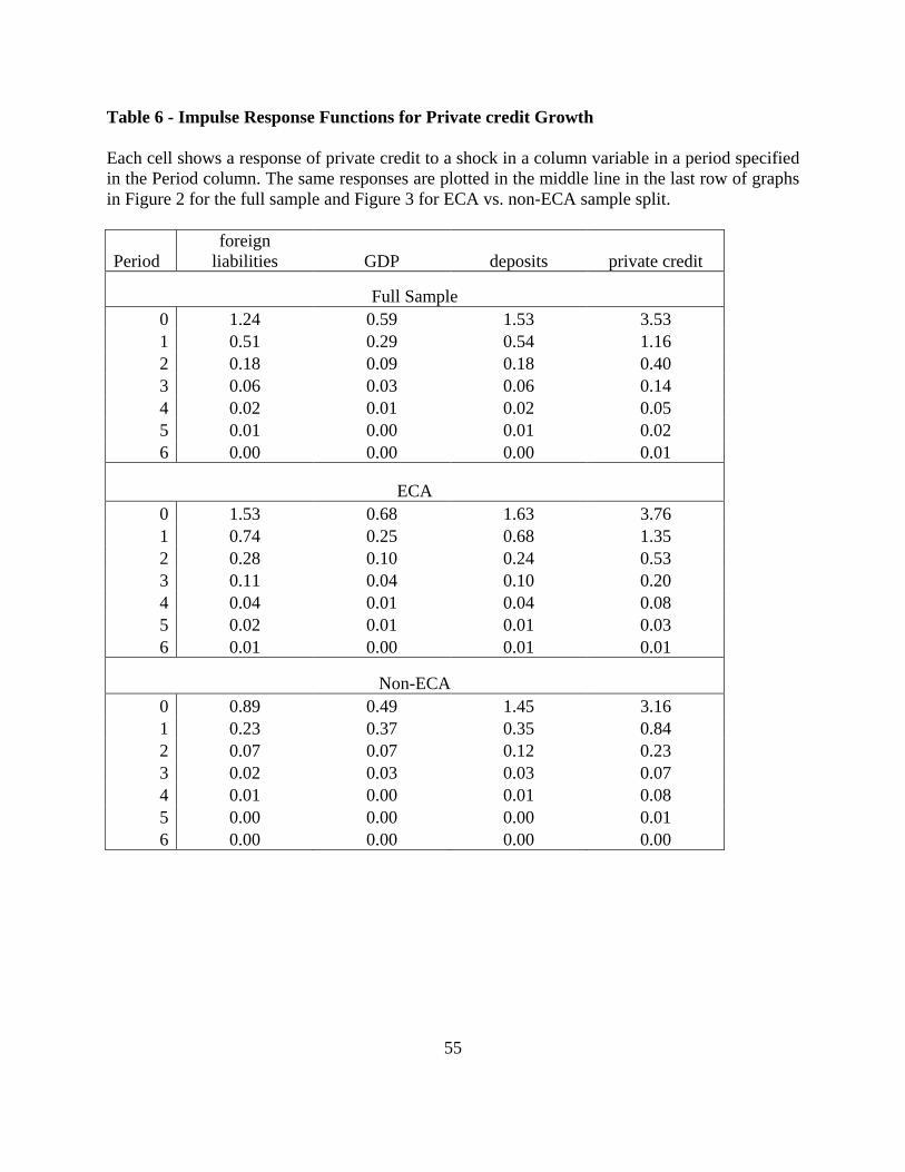
impulse responses plotted on the Figure 2 (i.e. the middle line) are also reported in Table 6. We

document a significantly positive response of private credit to a shock in foreign liabilities. A

one standard deviation shock in foreign liabilities results in a 1.24% increase in private credit

growth at time zero which is large given that average private credit growth in our entire sample

is 3.2% and its standard deviation is 5.12% (see Table 2). This is a key result which we will

study further in order to understand response differences in ECA vs. non-ECA countries.

We also find a positive response of private credit to GDP, which in our model captures

the demand for credit. This response is also statistically significant, but somewhat smaller in

magnitude: 0.59% at time zero. Finally, we observe a positive and significant response of private

credit to a deposits shock: 1.53% at time zero. Thus, we conclude that all our supply and

demand factors are significant drivers of private credit.15

Other impulse-response functions in Figure 2 show interesting and intuitive results that

are statistically significant. For example, foreign liabilities respond positively to a private credit

shock (row 1, column 4) suggesting that a sudden increase in credit can be funded by foreign

liabilities which can typically be attracted on short notice. At the same time, deposits also

15 Takáts (2010) finds that both demand and supply factors contributed to the fall in gredit during the crisis, but the impact of supply factors was stronger.

23

respond positively to a private credit shock (row 3, column 4) but the magnitude is smaller than

for foreign liabilities, arguably because it is more difficult to significantly raise deposits in the

short term. Together, these findings imply that foreign sources of funding can be useful to

temporarily fill domestic funding gaps. We also find that a foreign liabilities shock has a positive

impact on deposits (row 3, column 1) which implies that banks pursue deposit growth when

foreign funding increases, possibly to avoid a relative over-reliance on foreign funding.

Alternatively, an increase in deposits could be due to the perception that better performing banks

are able to attract foreign funding. We also confirm that a private credit shock boosts GDP which

is expected since private credit typically expands consumption and investment. This corroborates

with results of the finance and growth literature (e.g. Levine, 2005).

While impulse-response functions show the short-term response of each variable to a

shock in another variable, the long-term cumulative impact of a shock is captured by the variance

decompositions. Table 7, Panel A displays the variance decomposition for our baseline model.

Each cell in the table shows what percent of variation in the row variable is explained by the

column variable after the 10 quarters, i.e. 2.5 years. Note that for all variables their own shocks

explain most of the variance (i.e. the diagonal of Table 7, Panel A contains the largest values).

Row 4 of Table 7, Panel A reports that a foreign liabilities shock explains a relatively

large part of the variance in private credit (9.7%). The deposits shocks explain an even larger

portion of the variance (14.2%), while a shock to GDP explains relatively little variance at 2.4%.

Taken together, our PVAR model explains a substantial portion of the variation in private credit

(i.e. 26.2% is explained by other variables and 73.8% is explained by its own shocks). While our

model explains smaller portion of the variation in the other variables, it works reasonably well to

fulfill our main objective, which is to explain the behavior of private credit.

24

Before we proceed with our sample splits, we conduct various robustness checks to our

baseline model (results of these additional tests are available on request). First, we include an

additional lag of all variables in the model and find that our results are robust, even with

decreasing degrees of freedom.16 Second, we change the ordering of the variables where we

interchange deposits and GDP and find our main results still hold. Finally, we find that dropping

large outliers (i.e. extreme observations above 99th percentile and below 1st percentile) rather

than winsorizing the data does not affect the results. Therefore, in the remainder of this paper, we

use the ordering of the baseline model and include 1 lag only.

V.2. Sample Splits: Is ECA Different from the Rest of the World?

In this section we formally test whether private credit in the ECA region responded

differently compared to the rest of the world. To do that, we split our full sample into ECA and

non-ECA subsamples and run separate PVARs for each subsample. The two subsamples are

roughly equal in size: (ECA: 22 countries, 947 observations; non-ECA: 19 countries, 820

observations). Figure 3 presents the results. For space considerations, we only present impulse-

response functions and variance decompositions for private credit, our key variable. In other

words, only the fourth row of graphs from Figure 2 is presented for the split samples. The first

and second rows in Figure 3 show the private credit responses to shocks of all four variables for

the ECA and non-ECA subsamples, respectively. Both rows exhibit very similar patterns to our

16 Adding an additional lag to the model significantly increases the number of coefficients that have to be estimated – i.e. from 16 in our baseline model to 32 – and reduces the number of observations from 1,591 in the baseline model to 1,554 because one year of data is lost. The loss in degrees of freedom is particularly relevant for models for subsamples.

25

baseline findings and confirm our key result: the significant and positive response of private

credit to a foreign liabilities shock. We also observe positive and significant responses in both

samples to GDP and deposits shocks.

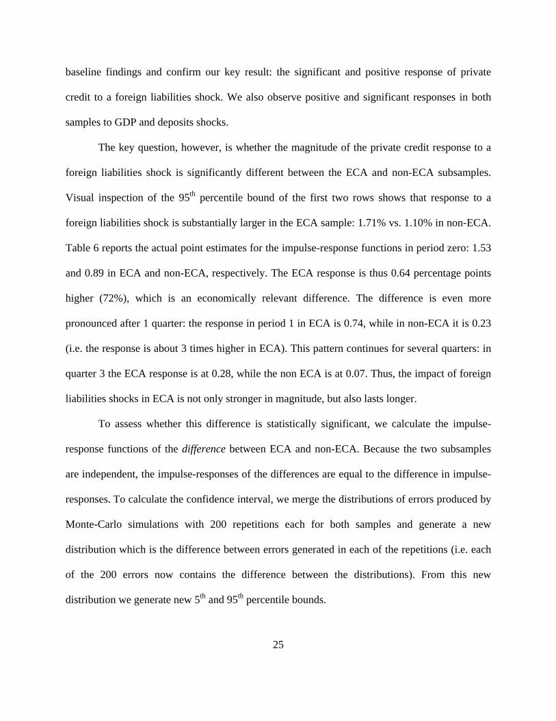
The key question, however, is whether the magnitude of the private credit response to a

foreign liabilities shock is significantly different between the ECA and non-ECA subsamples.

Visual inspection of the 95th percentile bound of the first two rows shows that response to a

foreign liabilities shock is substantially larger in the ECA sample: 1.71% vs. 1.10% in non-ECA.

Table 6 reports the actual point estimates for the impulse-response functions in period zero: 1.53

and 0.89 in ECA and non-ECA, respectively. The ECA response is thus 0.64 percentage points

higher (72%), which is an economically relevant difference. The difference is even more

pronounced after 1 quarter: the response in period 1 in ECA is 0.74, while in non-ECA it is 0.23

(i.e. the response is about 3 times higher in ECA). This pattern continues for several quarters: in

quarter 3 the ECA response is at 0.28, while the non ECA is at 0.07. Thus, the impact of foreign

liabilities shocks in ECA is not only stronger in magnitude, but also lasts longer.

To assess whether this difference is statistically significant, we calculate the impulse-

response functions of the difference between ECA and non-ECA. Because the two subsamples

are independent, the impulse-responses of the differences are equal to the difference in impulse-

responses. To calculate the confidence interval, we merge the distributions of errors produced by

Monte-Carlo simulations with 200 repetitions each for both samples and generate a new

distribution which is the difference between errors generated in each of the repetitions (i.e. each

of the 200 errors now contains the difference between the distributions). From this new

distribution we generate new 5th and 95th percentile bounds.

26

Figure 3, row 3 presents the result of the difference in impulse responses (“Sample:

Difference”). Row 3, column 1 confirms the difference in responses of private credit to foreign

liabilities shock is indeed significant (i.e. the zero line is outside of the confidence interval).

Other impulse-response functions in row 3 show that private credit does not behave differently in

ECA in response to a GDP shock, while there is a slightly larger response to a deposits shock

after 1 period.

Lastly, we compute the variance decompositions in the ECA and non-ECA subsamples to

study the cumulative longer-term impact of various shocks on private credit. Table 7, Panel B

reports the results. To save space, we only report the decompositions for the private credit

variable. The first row is the baseline decomposition for the whole sample, replicated from Panel

A. The second and third rows show the decompositions for the ECA and non-ECA subsamples,

respectively. A foreign liabilities shock explains 6.0% of the private credit variation in non-ECA

countries and 12.9% of the variation in the ECA subsample, which is more than twice as large.

These findings establish the second of our key results: private credit in ECA has been more

heavily influenced by shocks to foreign liabilities.

V.3. Further Sample Splits: Explaining Differences in Private credit Responses

After establishing that private credit is significantly more responsive to foreign liabilities

shocks in ECA compared to non-ECA countries, this section seeks to identify the factors that

could drive the difference. As discussed earlier, the banking sector in ECA is markedly different

from those in non-ECA countries along our sample split variables: ECA countries exhibit

27

significantly higher foreign ownership, higher reliance on foreign funding and higher LDR

ratios.

To determine which of these factors can explain the differential responses of private

credit to foreign funding shocks, we perform sample splits using each of the three sample-split

variables one at a time. In each case we split the whole sample in two subsamples of equal size

based on the median value of the variable in question. The sample-split approach is similar to

interacting each of the factors with the responsiveness of private credit to foreign liabilities.17

First, we test whether LDR is driving the response differences. We calculate the pre-crisis

median LDR ratio in our full sample using data from the fourth quarter of 2007. We then split

the full sample into high and low LDR subsamples of equal size based on the median and rerun

our baseline model for each sample. The impulse-response results are presented in Figure 4 and

the variance decompositions are presented in Table 7, Panel B. We find that the difference

between the response of private credit to a foreign liabilities shock in both high LDR and low

LDR samples is positive and statistically significant.18 The variance decomposition shows that in

the high LDR subsample, a foreign liabilities shock explains 14.1% of the variation in private

credit, while it explains only 5.6% of the variation in the low LDR sample. This finding suggests

that high LDRs are associated with a stronger response of private credit to foreign funding

shocks. While this does not present a direct proof, this finding suggests that high LDRs are at

least partially responsible for higher response of private credit to foreign funding shocks in ECA.

17 Note that such interactions cannot be modeled directly in a VAR setting. 18 The significance is at about 5% in period 1 because the bottom 5th percentile line is touching the zero line, while it is stronger in periods 0 and period 2 and 3.

28

Next, we perform another sample split to test whether foreign funding dependence is

driving the difference. Similarly, we use pre-crisis foreign funding values for all countries from

the fourth quarter of 2007 and split the sample into high and low foreign funding subsamples.

The impulse-response results are presented in Figure 5 and the variance decompositions are

presented in Table 7, Panel B. We find that the response of private credit to a foreign liabilities

shock is significantly higher in the high foreign funding sum-sample. The variance

decompositions show that in the high foreign funding subsample a foreign liabilities shock

explains 12.9% of the variation in private credit, while it only explains 6.9% in the low foreign

funding subsample. These results suggest that high reliance of countries on foreign funding is

associated with stronger response of private credit to foreign funding. Again, the results are in

line with the hypothesis that high reliance on foreign funding is responsible for explaining the

difference between the ECA and non-ECA samples.

Lastly, we split our full sample using foreign ownership. Based on the latest pre-crisis

data, we create high and low foreign ownership subsamples. The impulse-response results are

presented in Figure 6 and the variance decompositions are presented in Table 7, Panel B. We

find that the difference between the responses of private credit to a foreign liabilities shock in the

high and low foreign ownership samples are not statistically significant (row 3). This is in

contrast to previous findings of sample splits on LDR and foreign funding. The variance

decompositions show that in the high foreign ownership subsample a foreign liabilities shock

explains 10.0% of the variation in private credit while it explains 9.1% in the low foreign

ownership subsample. These two values are not materially different here, while there was

substantial difference in the two previous sample splits. These results suggest that in the whole

29

sample foreign ownership is not associated with a stronger response of private credit to foreign

liabilities.

Taken together, our findings suggest that high LDR and high foreign funding in ECA are

associated with stronger response of private credit to foreign funding shocks, while high foreign

ownership does not appear to drive this difference. These results suggest that ECA funding

model is at the heart of ECA’s vulnerability to external financial shocks rather than the strong

presence of foreign banks in the region per se. However, while these results are suggestive of the

reasons for why ECA is different, they do not directly demonstrate this because we have used

our whole sample to do the sample splits. In the next section we present a more direct evidence

to explain the differences between ECA and non-ECA.

V.4. What factors explain differences of ECA and the rest of the world?

In this section we provide more direct evidence on the factors that drive the differences in

ECA and the rest of the world. While all three factors – LDR, foreign funding and foreign

ownership – are higher in ECA, not all factors are present in all countries, as we discussed above.

This allows us to investigate which of the three factors is driving the difference between ECA

and non-ECA in terms of the measured response of private credit to foreign funding shocks.

The intuition for our procedure is as follows. We create a “truncated ECA sample” which

is constructed to resemble to the non-ECA sample in one of the three indicators, without

restricting the other two factors. For example, we make a “truncated ECA sample” by removing

from ECA sample countries with extra high LDR. In practice, we drop countries with LDR that

is higher than the median LDR in ECA. This “truncated ECA sample” is more similar to the rest

30

of the world based on average LDR because the highest LDR countries are now removed. Then,

we run our PVARs on this “truncated ECA sample” and compare the results with the non-ECA

sample. If we still find the difference between ECA and the rest of the world, we conclude that

the specific factor (i.e. LDR) is not driving such difference (because now ECA is similar to non-

ECA based on this factor). If, however, we no longer find a difference between ECA and non-

ECA, we conclude that this factor was indeed responsible for the observed difference between

ECA and non-ECA. This procedure provides a more direct test of which factors are responsible

for the differences between ECA and non-ECA in our PVAR framework, which is less flexible

than a simple regression framework (i.e. we cannot implement the interaction terms directly

because of the lag structure).

First, we remove from the ECA sample countries that are high on LDR. We use the

median LDR in ECA (pre-crisis) to make this truncated sample. Table 4, Panel C reports the t-

tests for comparison of this “truncated ECA” sample and non-ECA sample. The t-test shows that

truncated ECA sample is not significantly different from non-ECA sample based on average

LDR ratios. Figure 7 presents the differences between ECA and non-ECA samples in the

impulse responses of the response of private credit to foreign liabilities shock. The graph in

Panel Ashows that there is no longer a significant difference between ECA and non-ECA

samples. Thus, LDR appears to be a factor responsible for observed differences between the

(full) ECA sample and non-ECA sample.

Second, we remove from the ECA sample countries that are high on foreign funding.

Again, we use the median foreign funding in ECA (pre-crisis) to make this truncated sample.

The resulting sample contains ECA countries with relatively low foreign funding. However, even

the “relatively low” foreign funding countries in ECA still have significantly higher foreign

31

funding: 20% in the truncated ECA sample, vs. 11% in the non-ECA sample. This difference is

statistically significant (Table 4, Panel C). Ideally, we would like the truncated ECA sample to

not be statistically different from non-ECA sample. However, while not “ideal”, this truncated

ECA sample stacks the cards toward finding the differential impact in the truncated ECA sample

(which still is relatively high on foreign funding) and the non-ECA sample. In other words, this

sample is biased toward finding the statistically significant differences in impulse responses. We

then compare such truncated ECA sample with the rest of the world. Graph in Panel B in Figure

7 shows that the difference between the truncated ECA and the rest of the world is not

significantly different from zero. This suggests that very high foreign funding is indeed a factor

that explains the difference between the (full) ECA sample and the non-ECA sample.

Third, we remove from the ECA sample countries that are high on foreign ownership.

Again, we use the median foreign ownership in ECA (pre-crisis) to make this truncated sample.

This truncated sample is not significantly different in the average foreign ownership than non-

ECA sample (Table 4, Panel C). The results in Panel C in Figure 7 show that there still is a

significant difference between truncated ECA sample and non-ECA sample. Thus, even after

removing half of the ECA sample with highest foreign ownership the remaining sample still

shows a significant difference in impulse-responses relative to non-ECA countries. Before we

make a final conclusion, we note that the truncated ECA sample still has a relatively high foreign

ownership. The average foreign ownership in the truncated sample is 39%, while it is 33% in the

rest of the world. However, this difference is not statistically significant (Table 4, Panel C).

Nevertheless, to be sure, we perform even a stricter test. We drop four remaining high foreign

ownership countries (Serbia, 75%, Latvia, 68%, Poland 68% and Armenia 60%). In other words,

we removed from ECA sample any country with foreign ownership above 51%. This further

32

truncated sample (referred to as “foreign ownership 2” in Table 4, Panel C) has the average

foreign ownership of 23%, which is way below the average foreign ownership in the non-ECA

sample (i.e. 33%), although t-test shows that this difference is not statistically significant.

Finally, we compare the behavior of this restricted sample with the non-ECA sample. Again, we

find the two samples show statistically significantly different responses of private credit to

foreign ownership (Panel D). In other words, even when the ECA looks statistically the same in

terms of average foreign ownership as our non-ECA sample, there is still a significant difference

in the responses of private credit to foreign funding shocks. Therefore, we conclude that foreign

ownership does not appear to be the factor that is driving the difference between (full) ECA and

non-ECA samples.

To summarize the results of this section, we show that removing from the ECA sample

countries with very high foreign funding or very high LDR makes the “remaining

ECA” sample to be similar to the rest of the world in the response of private credit to foreign

funding shocks. This suggests that high foreign funding and high LDR are indeed the factors that

are driving the observed differences between (full) ECA and non-ECA samples. However, high

foreign ownership is not driving these differences because even when high foreign ownership

countries are removed from the ECA sample and the “remaining ECA” has lower average

foreign ownership than non-ECA sample, there is still a significant difference in the responses of

private credit to foreign funding shocks. These results provide more direct evidence that high

foreign funding and high LDR ratios were they key factors explaining higher sensitivity of

private credit to foreign funding shocks in ECA, while high foreign ownership per se was not the

main culprit.

33

VI. Summary and Policy Implications

By applying PVARs to a global country panel database, we show that growth in bank

credit to the domestic private sector is highly sensitive to cross-border funding shocks around the

world. We find that this relationship is significantly stronger in the average ECA country where

the response is larger and lasts longer compared to the average country in the rest of the world.

At the same time, we show that foreign ownership per se does not explain the different credit

responses in our sample of countries. Instead, our results indicate stronger responses in countries

with high loan-to-deposit ratios and stronger reliance on foreign funding. Higher loan-to-deposit

ratios make banks more vulnerable to general wholesale funding shocks while high reliance on

foreign funding specifically implies exposure to more volatile cross-border financing flows and

sensitivity to foreign shocks. Taken together, our findings therefore suggest that funding model

differences with the rest of the world were at the heart of ECA’s post-crisis credit growth

contraction, and that this contraction was not simply due to the high prevalence of foreign bank

ownership in the region.

Our findings provide an illustration of the potential downside risks of financial opening

or financial integration in the absence of adequate regulatory and supervisory frameworks. The

easy access to parent funding and direct wholesale borrowings abroad exposed many ECA

countries to substantial funding risks which materialized when cross-border flows were

interrupted by the global crisis and parent bank health deteriorated. The sudden slowdown of the

34

pace of funding contributed to a sharp slowdown of bank credit and GDP growth, as well as an

accumulation of non-performing loans in many countries.19

The “Spanish model”, in which standalone bank subsidiaries are fully funded locally, is

likely to be an extreme solution for a region that shares a common market and a regulatory

framework.20 Thus, eradicating cross-border funding altogether and promoting a fully

domestically funded subsidiary model also appears suboptimal as it may lead to costly pockets of

inert liquidity and capital within banking groups. The important question therefore is what

regulatory and supervisory approaches would allow ECA countries to reap most of the benefits

of financial integration in the coming years, while mitigating the risks.

The full implementation of Basel III may contribute to the achievement of such an

objective as it is expected to boost capital and liquidity and also promote more stable funding

through the Net Stable Funding Ratio (NSFR). The Basel III approach also opens room for the

introduction of additional capital charges on banks with domestic and regional systemic

importance, such as Western European banks with a network of subsidiaries in the ECA region.

However, the extent to which Basel III will effectively address the problems identified in the

crisis remains to be seen.

There are other complementary measures that could also contribute to the achievement of

this objective. For example, in 2012 Austrian regulators introduced a cap of 110 percent on the

loan-to-deposit ratios of all subsidiaries of Austrian parent banks (see Austrian Financial Market

Authority and Austrian National Bank (2012)). The approach of Austrian regulators does imply

19 The credit boom exposed ECA countries to other risks as well, including credit, interest rate, and exchange rate risks in their consumer, mortgage and SME portfolios. 20 Fiechter et al (2011) discuss the choice between branches and subsidiaries and the implications for financial stability and Martel et al (2012) discuss business models of international banks in more detail.

35

some flexibility relative to the “Spanish model”, although it was still met with reservations by

many host regulators and parent banks when it was introduced.

Therefore, home and host regulators in Europe still face the challenge of designing an

effective regulatory framework for cross-border banking in the coming years. Such a framework

may include supplements to Basel III to prevent the funding and credit growth excesses of the

past decade and the risk of another crisis, while allowing banking institutions to benefit from the

centralized management of capital, liquidity, and funding. Additional measures can be taken by

either home or host authorities, imposed at either the parent or subsidiary level. European

authorities may also consider if specific supervisory guidance on cross-border funding is needed.

Meeting this challenge will be important for ECA countries, especially smaller ones that face

more constraints to develop local capital markets, and that may continue depending relatively

more on parent and other sources of cross-border bank funding.

36

References

Allen, F., T. Beck, E. Carletti, P. Lane, D. Schoenmaker, W. Wagner, 2011, “Cross

Border Banking in Europe: Implications for Financial Stability and Macroeconomic Policies”,

Center for Economic Policy Research, London, UK.

Austrian Financial Monetary Authority (AFMA) and Austrian National Bank

(ANB), 2012, “Background note on the strengthening of the sustainability of the business

models of large internationally active Austrian banks”. Vienna.

Choi, M., E. Gutierrez, and M. Martinez-Perias, 2013, "Dissecting foreign bank

lending behavior during the 2008-2009 crisis”. Manuscript. The World Bank.

Cerutti, Eugenio and Stijn Claessens, 2014, The Great Cross-Border Bank

Deleveraging: Supply Side Characteristics, IMF working paper.

Cetorelli, N., and L. Goldberg, 2011, “Global Banks and International Shock

Transmission: Evidence from the Crisis.” IMF Economic Review, Vol. 59, pp. 41-76.

Nicola Cetorelli & Linda S. Goldberg, 2012. "Follow the Money: Quantifying

Domestic Effects of Foreign Bank Shocks in the Great Recession," American Economic Review,

American Economic Association, vol. 102(3), pages 213-18, May.

Claessens, S., and N. van Horen, 2014, “Foreign banks: Trends and Impact” Journal of

Money, Credit and Banking. 46(1), 295–326.

37

Claessens, S., and N. van Horen, 2013, “Impact of Foreign Banks,” The Journal of

Financial Perspectives, 1(1), pp. 29-42.

Cull, R., and M. S. Martinez Peria, 2012, “Bank ownership and lending patterns during

the 2008-2009 financial crisis: evidence from Latin America and Eastern Europe,” World Bank

Policy Research Working Paper, No. 6195.

De Haas, R., and I. Van Lelyveld, 2014, “Multinational banks and the global financial

crisis: weathering the perfect storm,” Journal of Money, Credit and Banking, 46(s1), 333-364,

02.

De Haas, R., and N. van Horen, 2013, “Running for the exit? International bank lending

during a financial crisis,” Review of Financial Studies, 26 (1): 244-285.

De Haas, R., Y. Korniyenko, E. Loukoianova, and A. Pivovarsky, 2012, “Foreign

banks and the Vienna initiative: turning sinners into saints?” IMF Working Paper WP/12/117

(April).

Feyen, E. and I. González del Mazo, 2013, “European bank deleveraging and global

credit conditions: Implications of a multi-year process on long-term finance and beyond”, World

Bank Policy Research Working Paper 6388 (March).

Fiechter, J., I. Ötker-Robe, A. Ilyina, M. Hsu, A. Santos, and J. Surti, 2011,

“Subsidiaries or Branches: Does One Size Fits All?” IMF Staff Discussion Note SDN 11/04

(March).

38

Giannettia, M., and S. Ongena, 2012, “Lending by example: direct and indirect effects

of foreign banks in emerging markets,” Journal of International Economics, 86, 167-180.

Hamilton, J. D., 1994, Time Series Analysis, Princeton University Press.

Impavido, G., H. Rudolph, and L. Ruggerone, 2013, “Bank funding in Central, Eastern

and Southern Europe post Lehman: A new normal?” IMF Working Paper WP/13/148 (June).

Kapan, T., and C. Minoiu, 2013, “Balance sheet strength and bank lending during the

global financial crisis”, IMF Working Paper WP/13/102.

Levine, R., 2005, Finance and Growth: Theory and Evidence. in P. Aghion and S.

Durlauf (Eds.). Handbook of Economic Growth. The Netherlands: Elsevier Science.

Love, I., and L. Zicchino, 2006, “Financial development and dynamic investment

behavior: Evidence from panel vector autoregression.” The Quarterly Review of Economics and

Finance 46, 190-210.

Love, I. and Turk Ariss, R., 2014, Macro-financial linkages in Egypt: A panel analysis

of economic shocks and loan portfolio quality. Journal of International Financial Markets,

Institutions and Money 28, 158–181.

Martel, M., A van Rixtel, and E. Mota, 2012, “Business models of international banks

in the wake of the 2007-2009 global financial crisis”, Banco de España Revista de Estabilidad

Financiera, No. 22, pp. 19-121.

39

Mishkin, F. S., 2007, “Is financial globalization beneficial?” Journal of Money, Credit

and Banking, 39, 259-294.

Ongena, S., J. L. Peydro, and N. van Horen, 2012, “Shocks abroad, pain at home?

Bank-firm level evidence on financial contagion during the 2007-2009 crisis,” Mimeo, Tilburg

University, Universitat Pompeu Fabra, De Nederlandsche Bank

Popov, A., and G. Udell, 2012, “Cross-border banking, credit access and the financial

crisis,” Journal of International Economics, 87, 147-161.

Takáts, E., 2010, “Was it Credit Supply? Cross-border bank lending to emerging market

economies during the financial crisis”. BIS Quarterly Review, June.

40

Figure 1 – Financial Sector Trends

Panel A: Annual credit growth (regional average, %)

Panel B: Annual deposit growth (regional average, %)

Panel C: Annual GDP growth (regional average, %)

Panel D: Foreign liabilities to total liabilities (regional average, %)

Source: IMF, International Financial Statistics

CESEE: Central, Eastern and Southeastern Europe, CIS: Commonwealth of Independent States, LAC: Latin America and Caribbean, GCC: Gulf Coast Countries.

-20-10

0102030405060708090

2003

M1

2003

M7

2004

M1

2004

M7

2005

M1

2005

M7

2006

M1

2006

M7

2007

M1

2007

M7

2008

M1

2008

M7

2009

M1

2009

M7

2010

M1

2010

M7

2011

M1

2011

M7

2012

M1

2012

M7

CESEE CIS LAC7ASIA GCC NON-GCC

0

10

20

30

40

50

60

70

2003

M1

2003

M7

2004

M1

2004

M7

2005

M1

2005

M7

2006

M1

2006

M7

2007

M1

2007

M7

2008

M1

2008

M7

2009

M1

2009

M7

2010

M1

2010

M7

2011

M1

2011

M7

2012

M1

2012

M7


-10

-5

0

5

10

15

2000

2001

2002

2003

2004

2005

2006

2007

2008

2009

2010

2011


0

10

20

30

40

5020

02M

120

02M

820

03M

320

03M

1020

04M

520

04M

1220

05M

720

06M

220

06M

920

07M

420

07M

1120

08M

620

09M

120

09M

820

10M

320

10M

1020

11M

520

11M

1220

12M

7


41

Figure 1 – Financial Sector Trends, cont

Panel E: Nonperforming loans to total loans (regional average, %)

Panel F: Loan-to-deposit ratio (regional average, %)

Source: IMF, Global Financial Stability Report

Panel G: Asset share of foreign-owned banks (regional average, %)

Source: World Bank, World Development Indicators

02468

101214161820

2005 2006 2007 2008 2009 2010 2011 2012CESEE CIS LAC7ASIA GCC NON-GCC

60

80

100

120

140

160

180

200

2002

M1

2002

M8

2003

M3

2003

M10

2004

M5

2004

M12

2005

M7

2006

M2

2006

M9

2007

M4

2007

M11

2008

M6

2009

M1

2009

M8

2010

M3

2010

M10

2011

M5

2011

M12

2012

M7


0

10

20

30

40

50

60

70

80

90

2001 2005 2008 2009 2010

CESEE CIS LAC7 ASIA GCC NON-GCC

42

Figure 2 - Baseline Panel Vector Autoregression Model

The figure displays impulse-response functions of the baseline 1-lag PVAR model which is based on 4 variables: foreign liabilities, GDP, deposits, and private credit.

Impulse-responses for 1 lag VAR of foreign gdp deposits privcred

Errors are 5% on each side generated by Monte-Carlo with 200 reps

response of foreign to foreign shocks

(p 5) foreign foreign (p 95) foreign

0 60.0000

13.0499

response of foreign to gdp shocks

(p 5) gdp gdp (p 95) gdp

0 6-0.2578

0.7748

response of foreign to deposits shocks

(p 5) deposits deposits (p 95) deposits

0 6-0.0958

0.9718

response of foreign to privcred shocks

(p 5) privcred privcred (p 95) privcred

0 60.0000

2.6618

response of gdp to foreign shocks


0 6-0.0386

0.3698

response of gdp to gdp shocks


0 6-0.7137

3.5696

response of gdp to deposits shocks


0 6-0.0598

0.3324

response of gdp to privcred shocks


0 6-0.1227

0.1805

response of deposits to foreign shocks


0 6-0.1382

0.9000

response of deposits to gdp shocks


0 6-0.0517

0.8376

response of deposits to deposits shocks


0 6-0.2645

4.1138

response of deposits to privcred shocks


0 60.0000

0.6323

response of privcred to foreign shocks


0 60.0000

1.4147

response of privcred to gdp shocks


0 60.0000

0.7420

response of privcred to deposits shocks


0 60.0000

1.6568

response of privcred to privcred shocks


0 60.0000

3.6137

43

Figure 3 - ECA vs. Non-ECA Sample Split

The figure shows impulse-response functions of private credit due to various shocks. The first and second rows provide the functions for the ECA and non-ECA subsamples, respectively. The third row provides the difference functions between these subsamples. The shocks are as follows: “foreign” is foreign liabilities, “gdp” is GDP, “deposits” is deposits, and “privcred” denotes private credit itself.

0.00

141.

7141

0 2 4 6s

response to foreign shock

-0.0

383

0.90

46

0 2 4 6s

response to gdp shock

0.00

151.

8292

0 2 4 6s

response to deposits shock

0.00

343.

8968

0 2 4 6s

response to privcred shock

Sample: ECA

-0.0

386

1.09

91

0 2 4 6s


0.00

000.

6474

0 2 4 6s


0.00

011.

6221

0 2 4 6s


0.00

023.

2902

0 2 4 6s


Sample: nonECA

0.00

060.

9092

0 2 4 6s


-0.5

024

0.47

62

0 2 4 6s


-0.0

956

0.77

59

0 2 4 6s


0.00

040.

9332

0 2 4 6s


Sample: Difference

Split by Region: ECA vs. non ECA

44

Figure 4- Sample Split by High and Low Loan-to-Deposit Ratios

The figure shows impulse-response functions of private credit due to various shocks. The first and second rows provide the functions for the high LDR and low LDR subsamples, respectively. The split is based on the median value (see text for details). The third row provides the difference functions between these subsamples. The shocks are as follows: “foreign” is foreign liabilities, “gdp” is GDP, “deposits” is deposits, and “privcred” denotes private credit itself.

0.00

121.

8003

0 2 4 6s


-0.0

657

0.70

93

0 2 4 6s


0.00

101.

8362

0 2 4 6s


0.00

303.

7621

0 2 4 6s


Sample: High

0.00

001.

0837

0 2 4 6s


0.00

010.

9716

0 2 4 6s


0.00

011.

5592

0 2 4 6s


0.00

023.

4692

0 2 4 6s


Sample: Low

-0.1

082

1.02

53

0 2 4 6s


-0.5

235

0.23

21

0 2 4 6s


-0.2

453

0.58

99

0 2 4 6s


-0.0

050

0.91

52

0 2 4 6s


Sample: Difference

Split by LDR

45

Figure 5 - Sample Split by High and Low Foreign funding Dependence

The figure shows impulse-response functions of private credit due to various shocks. The first and second rows provide the functions for the high foreign funding and low foreign funding subsamples, respectively. The split is based on the median value (see text for details). The third row provides the difference functions between these subsamples. The shocks are as follows: “foreign” is foreign liabilities, “gdp” is GDP, “deposits” is deposits, and “privcred” denotes private credit itself.

0.00

101.

8338

0 2 4 6s


-0.1

518

0.88

94

0 2 4 6s


0.00

131.

9543

0 2 4 6s


0.00

274.

0131

0 2 4 6s


Sample: High

0.00

011.

1422

0 2 4 6s


0.00

020.

7132

0 2 4 6s


0.00

021.

5497

0 2 4 6s


0.00

053.

2686

0 2 4 6s


Sample: Low

-0.0

062

0.91

20

0 2 4 6s


-0.6

834

0.40

17

0 2 4 6s


-0.0

005

0.81

95

0 2 4 6s


-0.0

223

0.89

41

0 2 4 6s


Sample: Difference

Split by Foreign Share

46

Figure 6 - Sample Split by High and Low Foreign ownership

The figure shows impulse-response functions of private credit due to various shocks. The first and second rows provide the functions for the high foreign ownership and low foreign ownership subsamples, respectively. The split is based on the median value (see text for details). The third row provides the difference functions between these subsamples. The shocks are as follows: “foreign” is foreign liabilities, “gdp” is GDP, “deposits” is deposits, and “privcred” denotes private credit itself.

0.00

061.

4061

0 2 4 6s


-0.3

446

0.95

03

0 2 4 6s


0.00

061.

7090

0 2 4 6s


0.00

173.

6034

0 2 4 6s


Sample: High

0.00

031.

4548

0 2 4 6s


0.00

060.

8628

0 2 4 6s


0.00

041.

6842

0 2 4 6s


0.00

133.

7035

0 2 4 6s


Sample: Low

-0.3

223

0.61

24

0 2 4 6s


-1.0

378

0.57

88

0 2 4 6s


-0.2

392

0.54

98

0 2 4 6s


-0.5

414

0.29

33

0 2 4 6s


Sample: Difference

Split by Foreign ownership

47

Figure 7. Truncated ECA sample vs. non-ECA

The graphs show differences in responses of private credit to foreign liabilities in truncated ECA samples vs. the rest of the sample. Each truncated ECA sample is constructed by removing from the ECA sample countries above the median for each of the three characteristic (one at a time): foreign ownership, foreign funding and LDR. The graph in column 2, row 2 removes additional 4 countries which have foreign ownership above 51%.

Panel A: ECA without high LDR versus non-ECA

Panel B. ECA without high foreign funding vs. non-ECA

ECA without high foreign funding versus non-ECA

Panel C. ECA without high foreign ownership versus non-ECA

Panel D. ECA without high foreign ownership (above 51%) versus non-ECA

-0.40

-0.20

0.00

0.20

0.40

0.60

0.80

0 1 2 3 4 5 6Period

5th percentileimpulse95th percentile

0.00

0.20

0.40

0.60

0.80

1.00

1.20

1.40

1.60

0 1 2 3 4 5 6Period

5th percentile

impulse

95th percentile

-0.50

0.00

0.50

1.00

1.50

2.00

0 1 2 3 4 5 6

Period

5th percentile

impulse

95th percentile

-0.40

-0.20

0.00

0.20

0.40

0.60

0.80

1.00

0 1 2 3 4 5 6

Period

5th percentileimpulse95th percentile

48

Table 1 - Variable Definitions and Sources

Variable Name Full Name Definition Source

GDP GDP Gross Domestic Product, Nominal. Quarterly growth rates from figures in national currency (in percentage).

IMF, International Financial Statistics. For Albania, Colombia, Sri Lanka, Egypt, Tunisia and Nigeria, the sources are respective central bank websites.

private credit Private credit

Other Depository Corporations, Line 22d (Claims on Private Sector). Quarterly growth rates from figures in national currency (in percentage).

IMF, International Financial Statistics. For Bulgaria, Czech Republic, Hungary, Latvia, Lithuania and Poland, the sources are respective central bank websites.

foreign liabilities

Foreign Liabilities

Other Depository Corporations, Line 26c (Liabilities to Non-residents). Quarterly growth rates from figures in national currency (in percentage).

IMF, International Financial Statistics

deposits Deposits

Other Depository Corporations, Line 24 (Transferable Deposits Included In Broad Money) + line 25 (Other Deposits Included In Broad Money). Quarterly growth rates from figures in national currency (in percentage).

IMF, International Financial Statistics

foreign ownership

Foreign ownership of Banks

Share of banking system's assets where foreigners own 50% or more equity (in percentage). End-of-year figures.

World Bank, Bank Regulation and Supervision Survey

LDR Loan-to-deposit Ratio Private credit/Deposits*100 IMF, International Financial

Statistics

foreign funding

Share of foreign liabilities

Foreign liabilities/(foreign liabilities + Deposits)*100

Authors calculation based on the original data from above sources

49

Table 2A - Summary Statistics for Quarterly PVAR Variables

All variables are expressed as quarterly real growth rates (%).

i) Full sample

FOREIGN LIABILITIES PRIVATE CREDIT GDP DEPOSITS

N 1,767 1,767 1,767 1,767 mean 3.86 3.23 -0.01 2.62 Sd 13.66 5.12 3.53 4.67 p1 -28.10 -10.72 -11.05 -9.80 p25 -4.42 0.11 -1.55 -0.10 p50 2.36 2.66 0.07 2.08 p75 9.97 6.00 1.71 4.85 p99 52.40 19.42 9.21 16.70

ii) ECA


N 947 947 947 947 mean 5.75 4.55 -0.05 3.41 Sd 14.07 5.78 4.18 5.42 p1 -29.13 -10.79 -13.67 -10.61 p25 -2.99 0.61 -1.82 -0.07 p50 4.37 4.56 0.06 2.82 p75 12.43 8.18 2.05 6.59 p99 55.20 20.31 10.55 20.50

iii) Non-ECA


N 820 820 820 820 mean 1.68 1.71 0.03 1.70 Sd 12.84 3.70 2.60 3.40 p1 -27.09 -9.55 -7.31 -7.26 p25 -5.72 -0.33 -1.28 -0.18 p50 -0.13 1.61 0.08 1.67 p75 7.12 3.60 1.40 3.56 p99 43.67 11.36 6.48 10.30

50

Table 2B - Summary Statistics for Split Variables

All variables are expressed as percentages (%).

i) Full sample

LDR FOREIGN FUNDING

FOREIGN OWNERSHIP

N 41 41 41 mean 115.10 0.22 50.02 p50 99.58 0.17 51 Sd 48.96 0.16 31.47

ii) ECA

LDR FOREIGN FUNDING

FOREIGN OWNERSHIP

N 22 22 22 mean 127.22 0.32 64.64 p50 115.5 0.28 79.61 Sd 47.30 0.16 31.48

iii) Non-ECA

LDR FOREIGN FUNDING

FOREIGN OWNERSHIP

N 19 19 19 mean 101.07 0.11 33.09 p50 83.53 0.10 29.93 Sd 48.27 0.06 21.94

51

Table 3 - Correlations

Panel A. PVAR Variables

foreign

liabilities GDP deposits private credit Full Sample

foreign liabilities 1

GDP 0.05 1

deposits 0.24 0.18 1 private credit 0.40 0.16 0.51 1

ECA foreign liabilities 1

GDP 0.05 1


non ECA foreign liabilities 1

GDP 0.06 1


Bold numbers indicate statistical significance at 5%.

Panel B. Sample Split Variables

foreign ownership foreign funding LDR Full Sample

foreign ownership 1 foreign funding 0.35 1

LDR 0.08 0.54 1 ECA

foreign ownership 1 foreign funding -0.06 1

LDR -0.12 0.96 1 non ECA

foreign ownership 1 foreign funding 0.30 1

LDR -0.11 -0.02 1

Bold numbers indicate statistical significance at 5%.

52

Table 4 - Mean Tests for ECA vs. Non-ECA

Reported are means and t-tests for differences in means between ECA and non-ECA countries. Variables are quarterly growth rates (%). T-test significance is indicated by stars: ***, ** and * represent 1%, 5% and 10% respectively.

Panel A: Key Differences for PVAR Variables (growth rates in %)

Sample: Non-ECA Sample: ECA

N(1) Mean(1) N(2) Mean(2) T-test Significance

Years 2005-2007 foreign liabilities 300 3.64 286 10.06 *** GDP 239 0.51 263 0.95 ** deposits 312 2.65 286 5.42 *** private credit 312 3.15 286 7.87 ***

Years 2008-2009 foreign liabilities 214 0.74 192 2.33

GDP 160 -0.51 176 -1.86 *** deposits 222 1.59 192 1.34

private credit 222 1.45 192 2.15 *

Years 2010-2011 foreign liabilities 214 3.62 192 -0.02 *** GDP 159 0.09 176 -0.11

deposits 222 1.81 192 1.59 private credit 222 2.19 192 0.67 ***

53

Panel B: Key Differences for Sample Split Variables

Variables are measured at pre-crisis levels: 2007 Q4 for LDR and Foreign funding and 2008 for foreign ownership.

Sample: Non-ECA Sample: ECA

Variable N(1) Mean(1) N(2) Mean(2) T-test Significance

LDR 19 101% 22 127% ** foreign funding 19 11% 22 32% *** foreign ownership 19 33% 22 65% ***

Panel C: Key Differences for Sample Split Variables for truncated ECA sample

Variables are measured at pre-crisis levels: 2007 Q4 for LDR and Foreign funding and 2008 for foreign ownership. Truncated ECA sample is constructed by removing from ECA sample countries above the median for each of the indicator one at a time. The “foreign ownership 2” sample is truncated further to remove 4 more countries with high foreign ownership: (Serbia, 75%, Latvia, 68%, Poland 68% and Armenia 60%), in effect it removes all countries with foreign ownership above 51%.

Sample: Non-ECA Sample:

truncated ECA

Variable N(1) Mean(1) N(2) Mean(2) T-test Significance

LDR 19 101% 11 92% foreign funding 19 11% 11 20% ***

foreign ownership 19 33% 11 39% foreign ownership 2 19 33% 7 23%

54

Table 5 - GMM Estimates of the Reduced-Form PVAR Models

This table reports system estimates in which each of the dependent variables is regressed on the lags of the other variables in the system, estimated by system GMM in which the original variables are transformed using forward orthogonal deviations. The instruments are lags of the untransformed variables as described in text. All variables enter as real quarterly growth rates.

Dependent Variable: foreign liabilities GDP deposits private credit Coef T-stat Coef T-stat Coef T-stat Coef T-stat

Full Sample L.FOREIGN 0.01 0.33 0.02 2.01 0.00 -0.33 0.00 0.72 L.GDP -0.01 -0.10 -0.14 -3.28 0.05 1.38 0.03 0.78 L.deposits -0.14 -1.44 0.04 1.41 -0.05 -1.39 0.01 0.23 L.CREDIT 0.61 5.95 0.01 0.49 0.12 3.44 0.33 8.89

ECA L.FOREIGN 0.00 0.01 0.02 1.90 0.00 -0.24 0.01 0.89 L.GDP -0.02 -0.13 -0.15 -2.61 0.03 0.64 -0.00 -0.06 L.deposits -0.18 -1.54 0.03 0.76 -0.04 -0.77 0.02 0.40 L.CREDIT 0.69 4.83 -0.01 -0.38 0.09 1.74 0.36 7.10

Non ECA L.FOREIGN 0.02 0.44 0.00 0.63 0.00 -0.12 0.00 -0.08 L.GDP 0.00 0.00 -0.12 -2.56 0.11 2.41 0.10 2.03 L.deposits -0.05 -0.28 0.07 2.52 -0.09 -1.66 -0.01 -0.18 L.CREDIT 0.47 3.30 0.05 1.87 0.19 4.14 0.27 4.93

55

Table 6 - Impulse Response Functions for Private credit Growth

Each cell shows a response of private credit to a shock in a column variable in a period specified in the Period column. The same responses are plotted in the middle line in the last row of graphs in Figure 2 for the full sample and Figure 3 for ECA vs. non-ECA sample split.

Period foreign

liabilities GDP deposits private credit

Full Sample 0 1.24 0.59 1.53 3.53 1 0.51 0.29 0.54 1.16 2 0.18 0.09 0.18 0.40 3 0.06 0.03 0.06 0.14 4 0.02 0.01 0.02 0.05 5 0.01 0.00 0.01 0.02 6 0.00 0.00 0.00 0.01

ECA 0 1.53 0.68 1.63 3.76 1 0.74 0.25 0.68 1.35 2 0.28 0.10 0.24 0.53 3 0.11 0.04 0.10 0.20 4 0.04 0.01 0.04 0.08 5 0.02 0.01 0.01 0.03 6 0.01 0.00 0.01 0.01

Non-ECA 0 0.89 0.49 1.45 3.16 1 0.23 0.37 0.35 0.84 2 0.07 0.07 0.12 0.23 3 0.02 0.03 0.03 0.07 4 0.01 0.00 0.01 0.08 5 0.00 0.00 0.00 0.01 6 0.00 0.00 0.00 0.00

56

Table 7. Variance Decompositions

Panel A. Baseline PVAR Model

Each cell shows the percent of variation in the row variable explained by a shock of the column variable after 10 quarterly periods.

foreign


Baseline Model foreign liabilities 96.7% 0.0% 0.1% 3.1% GDP 0.5% 99.2% 0.2% 0.0% deposits 3.2% 3.0% 92.6% 1.2% private credit 9.7% 2.4% 14.2% 73.8%

Panel B. Variance Decomposition for Private credit Growth in Various Sample Splits

Each cell reports the percent of variance in private credit explained after 10 quarters by a shock to the column variable.

Obs foreign


Full Sample 1,767 9.7% 2.4% 14.2% 73.8%

ECA 947 12.9% 2.3% 13.9% 70.9%

Non-ECA 820 6.0% 2.6% 15.7% 75.6%

High LDR 895 14.1% 1.6% 13.9% 70.5% Low LDR 872 5.6% 4.8% 13.2% 76.3%

High foreign funding 799 12.9% 1.9% 14.7% 70.4% Low foreign funding 968 6.9% 3.8% 13.8% 75.5%

High foreign ownership 886 10.0% 3.0% 15.2% 71.8% Low foreign ownership 881 9.1% 3.0% 12.8% 75.2%

Date post:	16-Oct-2021
Category:	Documents
Upload:	others
View:	1 times
Download:	0 times

University of Hawai`i at Mānoa Department of Economics ...

Documents