University of Innsbruck

University of Innsbruck

Institute of Computer Science

Intelligent and Interactive Systems

On the Missing Value Problem Using Kernels

Chris [email protected]

M.Sc. ThesisSupervisor: Sandor Szedmak

[email protected] November 2016

In memory of my father, Jimmy.

ii

Abstract

Machine learning tasks lurk wherever large amounts of data are of concern. Not only computerscience applications such as social networks or webshops but also problems occurring in areaslike life science or economics give rise for different machine learning tasks such as object classifi-cation, item recommendation or the prediction of unknown relationships. Despite the variety ofthese tasks, their underlying optimization problems are often similar and can be cast as specialcases of the missing value problem, in which the missing values of a table are inferred using theobserved ones.This thesis aims to illuminate the theoretical foundations required to understand such prob-lems ranging from the formalization to the solution of the corresponding optimization problems.In order to do so, the application of kernel methods to learning tasks of increasing difficulty,starting with classical and ending with structured-output learning tasks, is investigated. Theimplicit knowledge given by the data is modeled by a linear operator between Hilbert spaces, inwhich the input and output data are represented. Utilizing the notion of reproducing kernels,the resulting hypothesis spaces are accessible in an elegant way. Different learning tasks can becharacterized by loss functions measuring the quality of a certain hypothesis with respect to thetask. Given a loss function and a hypothesis space, a hypothesis is found by regularized riskminimization.In the end, the previous efforts culminate in a learning framework capable of handling the miss-ing value problem for structured objects. This thesis shows that the application of the kerneltrick allows for the solution of various learning tasks in a unified and efficient way.

iii

iv

Acknowledgments

I would first like to thank my thesis supervisor Sandor Szedmak of the Aalto university. Sandorwas a very patient supervisor, who spent a lot of time and effort in answering my questions, ofwhich I had a lot. He gave me absolute freedom over the topic and contents of my thesis, whichmade writing my master thesis a refreshing and challenging experience.

I would also like to thank Senka Krivic for providing me with as many datasets and exampletasks as I wanted, and Roswitha Kathrein for proofreading my thesis.

Finally, I must express my gratitude to my family and my girlfriend without whose uncondi-tional support this thesis never would have been completed.

Thank you!

v

vi

Contents

Abstract iii

Acknowledgments v

Contents vii

Nomenclature xi

List of Figures xv

List of Tables xvii

Declaration xix

1 Introduction 1

2 Machine Learning 32.1 Background . . . . . . . . . . . . . . . . . . . . . . . . . . . . . . . . . . . . . . . . . . 3

2.1.1 Types of Problems and Tasks . . . . . . . . . . . . . . . . . . . . . . . . . . . 32.1.2 The Missing Value Problem . . . . . . . . . . . . . . . . . . . . . . . . . . . . 32.1.3 The Learning Task . . . . . . . . . . . . . . . . . . . . . . . . . . . . . . . . . 4

2.2 Learning Algorithms . . . . . . . . . . . . . . . . . . . . . . . . . . . . . . . . . . . . . 62.2.1 Linear Classification . . . . . . . . . . . . . . . . . . . . . . . . . . . . . . . . 62.2.2 Feature Space and Hypothesis Space . . . . . . . . . . . . . . . . . . . . . . . 92.2.3 Learning Linear Classifiers . . . . . . . . . . . . . . . . . . . . . . . . . . . . . 122.2.4 Linear Regression . . . . . . . . . . . . . . . . . . . . . . . . . . . . . . . . . . 13

2.3 Risk Minimization . . . . . . . . . . . . . . . . . . . . . . . . . . . . . . . . . . . . . . 172.3.1 Empirical Risk Minimization . . . . . . . . . . . . . . . . . . . . . . . . . . . 182.3.2 Regularization . . . . . . . . . . . . . . . . . . . . . . . . . . . . . . . . . . . . 20

2.4 The Support Vector Machine . . . . . . . . . . . . . . . . . . . . . . . . . . . . . . . . 212.4.1 Linearly Separable Case . . . . . . . . . . . . . . . . . . . . . . . . . . . . . . 222.4.2 Non-linearly Separable Case . . . . . . . . . . . . . . . . . . . . . . . . . . . . 222.4.3 Solving the Constrained Optimization Problem . . . . . . . . . . . . . . . . 23

Appendix 292.A Constrained Optimization . . . . . . . . . . . . . . . . . . . . . . . . . . . . . . . . . 29

2.A.1 The Problem . . . . . . . . . . . . . . . . . . . . . . . . . . . . . . . . . . . . . 292.A.2 The Lagrangian Function . . . . . . . . . . . . . . . . . . . . . . . . . . . . . 292.A.3 The Lagrangian dual function . . . . . . . . . . . . . . . . . . . . . . . . . . . 302.A.4 Linear approximation interpretation . . . . . . . . . . . . . . . . . . . . . . . 30

vii

2.A.5 Weak and Strong Duality . . . . . . . . . . . . . . . . . . . . . . . . . . . . . 312.A.6 Karush-Kuhn-Tucker Optimality Conditions . . . . . . . . . . . . . . . . . . 32

3 Kernel Methods 333.1 Motivation . . . . . . . . . . . . . . . . . . . . . . . . . . . . . . . . . . . . . . . . . . . 333.2 The Kernel Trick . . . . . . . . . . . . . . . . . . . . . . . . . . . . . . . . . . . . . . . 35

3.2.1 When Can the Kernel Trick Be Applied? . . . . . . . . . . . . . . . . . . . . 353.2.2 Summary and Outlook . . . . . . . . . . . . . . . . . . . . . . . . . . . . . . . 39

4 A Glance at Kernel Theory 414.1 Terminology - Kernel . . . . . . . . . . . . . . . . . . . . . . . . . . . . . . . . . . . . 414.2 Reproducing Kernel Hilbert Spaces (RKHS) . . . . . . . . . . . . . . . . . . . . . . 41

4.2.1 Outline . . . . . . . . . . . . . . . . . . . . . . . . . . . . . . . . . . . . . . . . 414.2.2 Recap & Important Properties of Hilbert Spaces . . . . . . . . . . . . . . . 424.2.3 Functional Analysis perspective . . . . . . . . . . . . . . . . . . . . . . . . . . 474.2.4 Positive Definite Kernels . . . . . . . . . . . . . . . . . . . . . . . . . . . . . . 494.2.5 Feature Space Mappings . . . . . . . . . . . . . . . . . . . . . . . . . . . . . . 524.2.6 Mercer Theorem - a Fourth View . . . . . . . . . . . . . . . . . . . . . . . . . 55

4.3 RKHS and Regularized Risk Minimization . . . . . . . . . . . . . . . . . . . . . . . 56

5 Structured Output Learning 595.1 Introduction . . . . . . . . . . . . . . . . . . . . . . . . . . . . . . . . . . . . . . . . . . 595.2 Background . . . . . . . . . . . . . . . . . . . . . . . . . . . . . . . . . . . . . . . . . . 60

5.2.1 The Intuitive Approach . . . . . . . . . . . . . . . . . . . . . . . . . . . . . . 605.2.2 The General Approach . . . . . . . . . . . . . . . . . . . . . . . . . . . . . . . 615.2.3 Learning with Joint Feature Maps . . . . . . . . . . . . . . . . . . . . . . . . 625.2.4 Designing Joint Kernels . . . . . . . . . . . . . . . . . . . . . . . . . . . . . . 63

5.3 Structured Support Vector Machine . . . . . . . . . . . . . . . . . . . . . . . . . . . 645.3.1 Linearly Separable Case . . . . . . . . . . . . . . . . . . . . . . . . . . . . . . 645.3.2 Non-linearly Separable Case . . . . . . . . . . . . . . . . . . . . . . . . . . . . 665.3.3 Arbitrary Loss Function . . . . . . . . . . . . . . . . . . . . . . . . . . . . . . 665.3.4 Simplifications . . . . . . . . . . . . . . . . . . . . . . . . . . . . . . . . . . . . 68

5.4 Maximum Margin Regression . . . . . . . . . . . . . . . . . . . . . . . . . . . . . . . 695.4.1 Problem Formulation . . . . . . . . . . . . . . . . . . . . . . . . . . . . . . . . 695.4.2 Kernel Version . . . . . . . . . . . . . . . . . . . . . . . . . . . . . . . . . . . . 70

Appendix 755.A The Tensor Product . . . . . . . . . . . . . . . . . . . . . . . . . . . . . . . . . . . . . 75

6 Structured Object Imputation 776.1 Introduction . . . . . . . . . . . . . . . . . . . . . . . . . . . . . . . . . . . . . . . . . . 776.2 Background . . . . . . . . . . . . . . . . . . . . . . . . . . . . . . . . . . . . . . . . . . 78

6.2.1 Problem Statement . . . . . . . . . . . . . . . . . . . . . . . . . . . . . . . . . 786.2.2 Intuitive Approach . . . . . . . . . . . . . . . . . . . . . . . . . . . . . . . . . 796.2.3 Relational Learning Perspective . . . . . . . . . . . . . . . . . . . . . . . . . 796.2.4 Feature Representation . . . . . . . . . . . . . . . . . . . . . . . . . . . . . . . 80

6.3 Relational Learning Using MMR . . . . . . . . . . . . . . . . . . . . . . . . . . . . . 816.3.1 Problem Formulation . . . . . . . . . . . . . . . . . . . . . . . . . . . . . . . . 816.3.2 Kernel Version . . . . . . . . . . . . . . . . . . . . . . . . . . . . . . . . . . . . 826.3.3 Solving the Optimization Problem Using Frank-Wolfe . . . . . . . . . . . . 83

viii

6.4 Maximum Margin Multi Valued Mappings (MMMVM) . . . . . . . . . . . . . . . . 876.4.1 Notation . . . . . . . . . . . . . . . . . . . . . . . . . . . . . . . . . . . . . . . 876.4.2 Defining the Swarm of Learners . . . . . . . . . . . . . . . . . . . . . . . . . . 886.4.3 Kernel Version . . . . . . . . . . . . . . . . . . . . . . . . . . . . . . . . . . . . 896.4.4 Solving the Optimization Problem Using Frank-Wolfe . . . . . . . . . . . . 91

6.5 Application Example - Missing Edges in Multiplex Networks . . . . . . . . . . . . 946.5.1 Details about the Dataset . . . . . . . . . . . . . . . . . . . . . . . . . . . . . 946.5.2 Application of the MMR & MMMVM . . . . . . . . . . . . . . . . . . . . . . 946.5.3 Experimental Setup and Results . . . . . . . . . . . . . . . . . . . . . . . . . 96

Appendix 996.A The Frank-Wolfe Algorithm . . . . . . . . . . . . . . . . . . . . . . . . . . . . . . . . 99

6.A.1 Problem Statement . . . . . . . . . . . . . . . . . . . . . . . . . . . . . . . . . 996.A.2 Algorithm . . . . . . . . . . . . . . . . . . . . . . . . . . . . . . . . . . . . . . . 996.A.3 Computational Complexity . . . . . . . . . . . . . . . . . . . . . . . . . . . . 100

7 Conclusion 101

Bibliography 103

ix

x

Nomenclature

⟨⋅, ⋅⟩H inner product in corresponding to the Hilbert space H

⟨⋅, ⋅⟩Frobenius the Frobenius inner product

γ(w) the generalization of the SVM margin to the structured-output case

d(w,X) the margin of the hyperplane parametrized by w with respect to the set of pointsX ⊂H, where H is a Hilbert space

H′ the topological dual space of a Hilbert space H, which contains linear and continuousforms

Hφ Hilbert space corresponding to the feature space mapping φ

S orthogonal complement of a subspace S of a Hilbert space

V ⊗W the tensor product of the vector spaces V and W

X input space

Y output space

Z input-output space

A learning algorithm

Cw a compatibility function that measures the compatibility of elements of different sets,parametrized by w

H hypothesis space

Hφ ∶= g ∶ X → R ∶ g = f φ, f ∈H∗φ and feature space mapping φ

Hk ∶= g ∶ X → R ∶ g = ∑ni=1 αik(xi, ⋅), for n ∈ N, x1, . . . , xn ∈ X , α1, . . . αn ∈ R and k is a kernel function

L2(M) the space of square-integrable functions defined on the setM

z training sample

∇f the gradient of the function f

φ(⋅) feature space mapping

φ(x) feature vector of input point x

φi(x) i-th feature of the feature vector of input point x

xi

Br(x) open ball with radius r around x

c(⋅, ⋅) loss function

c01(⋅, ⋅) zero one loss function

chinge the hinge loss function

csq(⋅, ⋅) squared loss function

J a joint kernel function defined on the Cartesian product of several sets

kX positive definite kernel function defined on the set X

l2(K) the space of square-summable sequences over the field K

Lx the evaluation functional over a Hilbert space of functions H for the point x ∈ X

R[⋅] risk functional

Remp[⋅; z] empirical risk functional with respect to the sample z

Rreg[⋅; z] regularized empirical risk functional with respect to the sample z

v ⊗w the tensor product of the vectors v and w

y∗(x) the solution of the pre-image problem of a structured-output method for the point x

Linear Algebra

⟨⋅, ⋅⟩ inner product

H Hilbert space

P(w,b) affine hyperplane parametrized by normal vector w and bias b

d(w,b)(x) signed distance between point x and hyperplane P(w,b)

DH(⋅, ⋅) the metric induced by the inner product in H

Probability Theory

∫ ⋅dµ Lebesgue integral with respect to the measure µ

E(X ,Y)[⋅] expected value of a function with respect to the joint input-output probability distri-bution

P(X ,Y) joint probability distribution on X ×Y

PX a probability measure on X such that the triple (X ,X ,PX ) is a probability space

PZ joint probability distribution on X ×Y

Abbreviations

i.i.d. independently and identically distributed

MMMVM Maximum Margin Multi Valued Mappings

MMR Maximum Margin Regression

xii

p.d. kernel positive definite kernel

r.k. reproducing kernel

RKHS reproducing kernel Hilbert space

SVM Support Vector Machine

xiii

xiv

List of Figures

2.1 An overview of the different learning problems. . . . . . . . . . . . . . . . . . . . . . 42.2 Classification of non-linearly separable data by choosing non-linear basis func-

tions. Figure (a) depicts the training sample in the input space, clearly thesample is not linearly separable. Figure (b) depicts feature vectors of the datapoints, computed by φ ∶ R2 → R3 ∶ (x, y) ↦ (x2,

√2xy, y2), and a separating hy-

perplane. In Figure (c) the image of R2 under φ φ(R2) ⊂ R3 is visualized by theyellow cone. Considering planes in R3 corresponds to considering conic sectionsin R2. The conic section corresponding to the separating hyperplane in Figure(b) is the blue ellipse in Figure (a) and (c). . . . . . . . . . . . . . . . . . . . . . . . 11

2.3 Linear regression using a line. In the upper left corner there is the training data,in the upper right corner the minimizer of the least squares error (red) and in thelower left corner there is the function (blue) used to generate the training data.The training data was generated by evaluating a polynomial function and addingGaussian noise. . . . . . . . . . . . . . . . . . . . . . . . . . . . . . . . . . . . . . . . . 16

2.4 Linear regression using polynomials of increasing degree (red). The training datapoints (green) were generated by evaluating a polynomial function (blue) andadding Gaussian noise. . . . . . . . . . . . . . . . . . . . . . . . . . . . . . . . . . . . 25

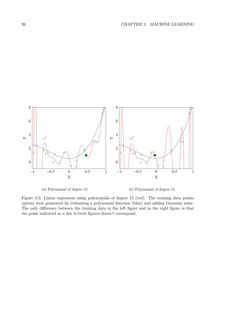
2.5 Linear regression using polynomials of degree 15 (red). The training data points(green) were generated by evaluating a polynomial function (blue) and addingGaussian noise. The only difference between the training data in the left figureand in the right figure is that the point indicated as a dot in both figures doesn’tcorrespond. . . . . . . . . . . . . . . . . . . . . . . . . . . . . . . . . . . . . . . . . . . 26

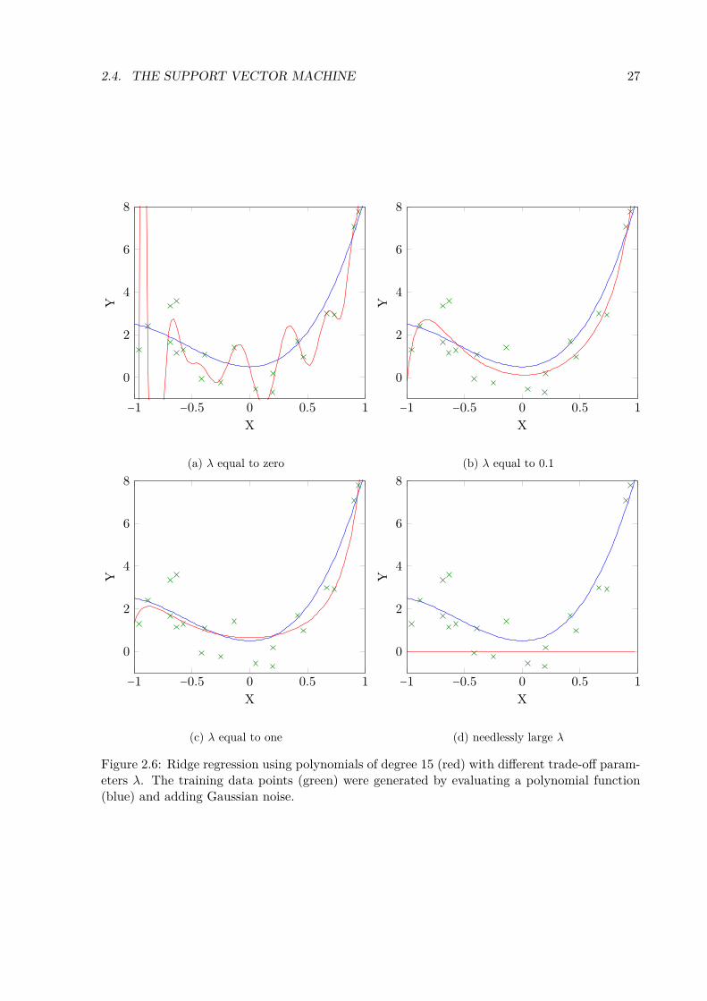
2.6 Ridge regression using polynomials of degree 15 (red) with different trade-offparameters λ. The training data points (green) were generated by evaluating apolynomial function (blue) and adding Gaussian noise. . . . . . . . . . . . . . . . . 27

2.7 Several elements of the version space are illustrated in different colors. All ofthem minimize the empirical risk with the zero-one loss, however intuitively wewould tend to choose a hypothesis similar to the red, blue or purple one. Thered line is the one that satisfies the maximum margin property. The illustrationis derived from an illustration by Yifan. . . . . . . . . . . . . . . . . . . . . . . . . . 28

2.8 The hyperplane with the maximum margin in a two dimensional example. Intwo dimensions the hyperplane corresponds to a line. For simplicity reasons thefeature space mapping φ(x) = (x,1)′ and the weight vector w = (w, b)′ resultingin ⟨(w, φ(x))⟩ = wx + b are used. The dotted lines illustrate the boundaries ofthe margin, which are set to one and minus one, respectively. The illustration istaken from Yifan. . . . . . . . . . . . . . . . . . . . . . . . . . . . . . . . . . . . . . . . 28

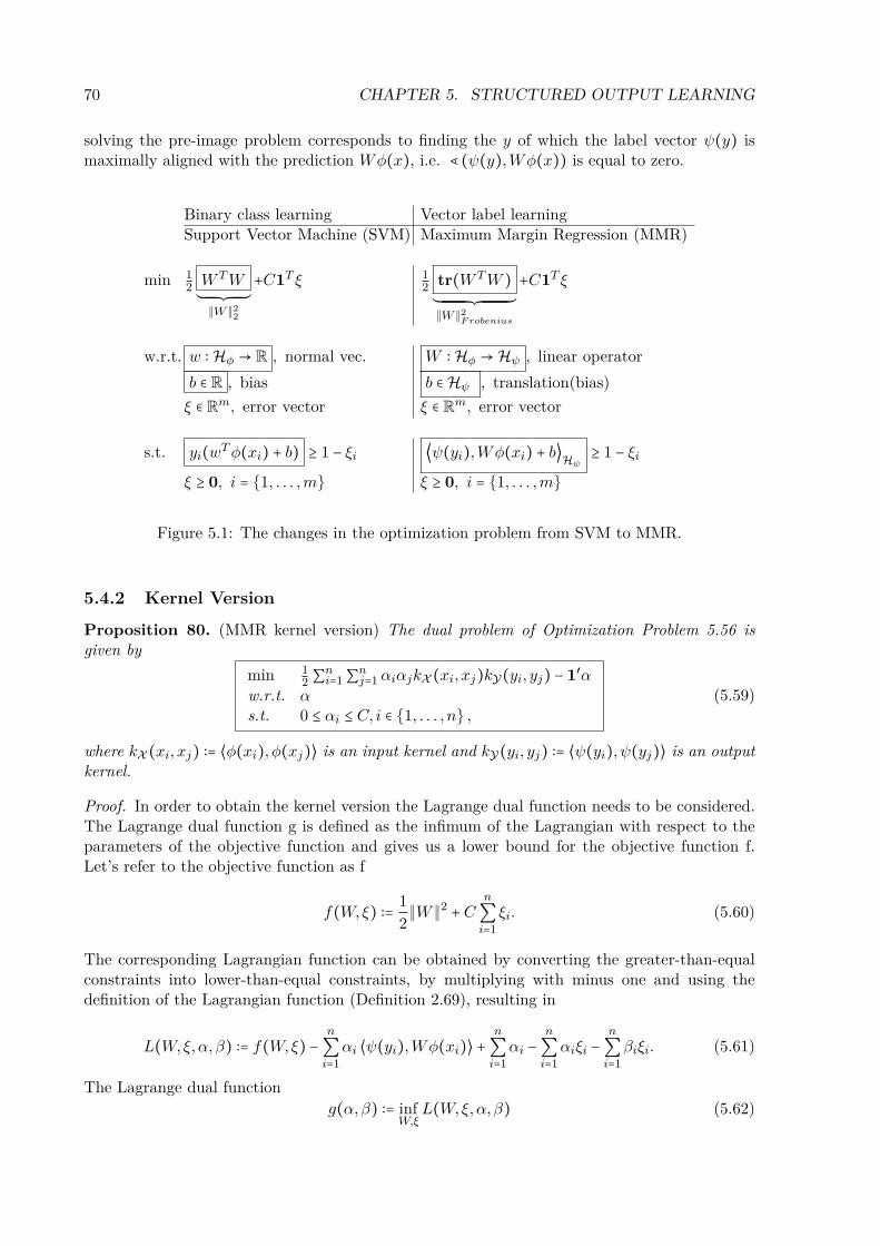
4.1 Different perspectives on reproducing kernel Hilbert spaces. . . . . . . . . . . . . 42

5.1 The changes in the optimization problem from SVM to MMR. . . . . . . . . . . . 70

xv

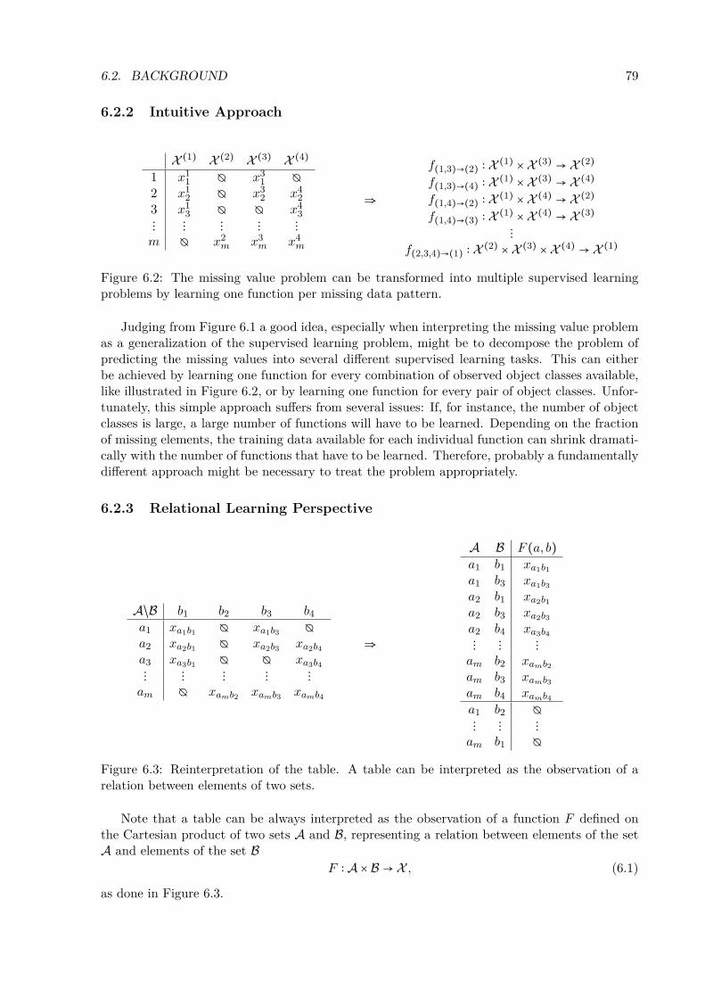
6.1 The missing value problem. . . . . . . . . . . . . . . . . . . . . . . . . . . . . . . . . . 786.2 The missing value problem can be transformed into multiple supervised learning

problems by learning one function per missing data pattern. . . . . . . . . . . . . . 796.3 Reinterpretation of the table. A table can be interpreted as the observation of a

relation between elements of two sets. . . . . . . . . . . . . . . . . . . . . . . . . . . 796.4 Content based and relational features illustrated in the example of a movie rec-

ommendation system. The rows correspond to movies and the columns to users.Every user is characterized by content based features like age or gender and byrelational features like the set of ratings made by the user. Movies are character-ized analogously, for every movie there are content based features like the genreor subgenre of the movie and relational features like the set of ratings obtainedby the movie. . . . . . . . . . . . . . . . . . . . . . . . . . . . . . . . . . . . . . . . . . 81

6.1 A layer-wise depiction of a subset of the multiplex network. The red circlescorrespond to objects and colored edges to different interaction types. . . . . . . . 95

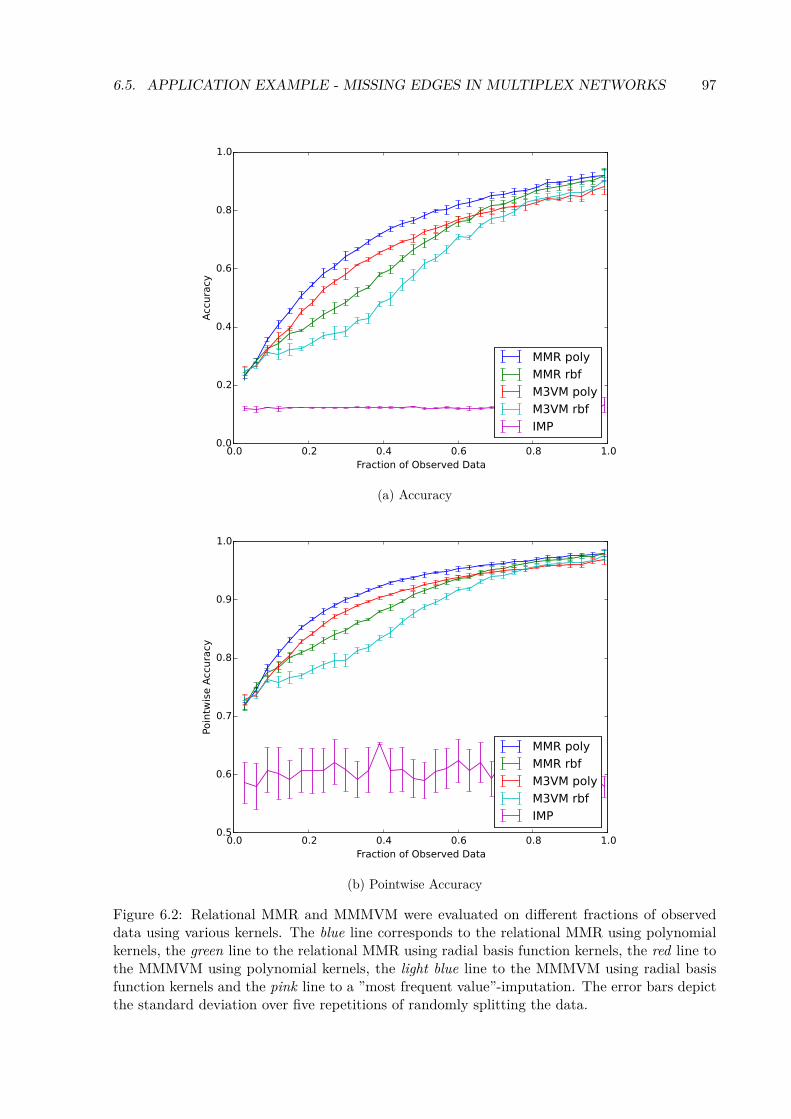
6.2 Relational MMR and MMMVM were evaluated on different fractions of observeddata using various kernels. The blue line corresponds to the relational MMRusing polynomial kernels, the green line to the relational MMR using radial basisfunction kernels, the red line to the MMMVM using polynomial kernels, the lightblue line to the MMMVM using radial basis function kernels and the pink line toa ”most frequent value”-imputation. The error bars depict the standard deviationover five repetitions of randomly splitting the data. . . . . . . . . . . . . . . . . . . 97

xvi

List of Tables

2.1 Types of learning problems based on the structure of the output space. . . . . . . 6

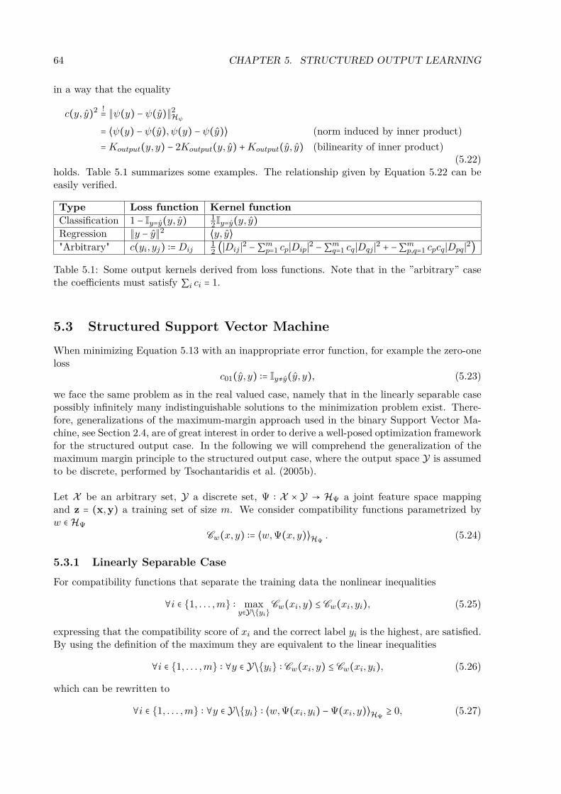
5.1 Some output kernels derived from loss functions. Note that in the ”arbitrary”case the coefficients must satisfy ∑i ci = 1. . . . . . . . . . . . . . . . . . . . . . . . . 64

xvii

xviii

Declaration

By my own signature I declare that I produced this work as the sole author, working indepen-dently, and that I did not use any sources and aids other than those referenced in the text.All passages borrowed from external sources, verbatim or by content, are explicitly identified assuch.

Signed: . . . . . . . . . . . . . . . . . . . . . . . . . . . . . . . . . . . . . . . . . . . . . . . . . . . . . . . . . .Date: . . . . . . . . . . . . . . . . . . . . . . .

xix

xx

Chapter 1

Introduction

In the age of multimedia machine learning has gained popularity, the internet is flooded bydata such as images, movies and texts. Despite the flood of data, knowledge still presents ascarce resource. In a certain sense, machine learning aims at closing the gap between dataand knowledge. Informally, one could define machine learning as the process of finding ways tounderstand data, which is in most cases coupled to a task. In this context, the knowledge orthe understanding of the data is usually modeled as a function and the task is used to definea performance measure. Therefore, given data and a task, the objective of a machine learningalgorithm is to find a function that optimally solves the task with respect to a performancemeasure. Additionally, the learned function should improve - with respect to the performancemeasure - with an increasing amount of data available and be able to generalize to unseen data.This definition of machine learning is consistent with the one of Mitchell (1997).

Depending on the type of data and the performance measure three broad categories aredistinguished: supervised, unsupervised and reinforcement learning (Bishop, 2006). This thesisis mainly concerned with supervised learning. In supervised learning tasks the objective is tofind a functional relationship connecting elements of an input set with elements of an outputset, based on a given training sample comprised by input/output pairs. Typical supervisedlearning tasks are classification and regression, where the input space is an arbitrary set andthe output spaces are a discrete set and a metric space (e.g. the real numbers) respectively. Ifthe output space also is a more or less arbitrary set comprised by complex (structured) objects,then according to Bakir et al. (2007), Tsochantaridis et al. (2005b), Nowozin and Lampert (2011)and Weston et al. (2007) we talk about structured output learning. Related to the high costsof extensive labeling of large datasets it is of interest to also consider training samples withincomplete labeling, i.e. for some input objects the corresponding output objects are unknown.In that situation we talk about weakly supervised learning. One can go even further and omitthe distinction between input and output space and learn relations between an arbitrary numberof sets, which leads us to the missing value problem (Little and Rubin, 1986).

Without much effort it is observable that supervised learning problems can always be castas weakly supervised learning problems, which can be always cast as missing value problems.Therefore, if the missing value problem was solved, the weakly supervised and the supervisedlearning problem would be solved as well. If all variables lived in a field, e.g. the real numbers, wewould talk about the matrix completion problem. Unfortunately, according to Johnson (1990),the matrix completion problem and consequently the missing value problem are not solvablewithout further assumptions.

The goal of this thesis is to incrementally develop a framework that is capable of solving themissing value problem under certain assumptions. In order to do so, we first study classificationand regression tasks in Chapter 2 and show a possible solution by risk minimization using

1

2 CHAPTER 1. INTRODUCTION

suitable input representations, i.e. Hilbert spaces. Secondly, we show that a certain class ofhypothesis spaces – more precisely, reproducing kernel Hilbert spaces of real valued functions– can be used implicitly and efficiently by considering so-called kernel functions in Chapters 3and 4. In Chapter 5 all the previously introduced concepts are combined in order to addressthe structured output learning task. Chapter 6 illuminates the missing value problem from therelation learning perspective and concludes with a framework capable of addressing the missingvalue problem, which is demonstrated by its application on an affordance learning dataset.Eventually, Chapter 7 is going to present the conclusion of the thesis.

Chapter 2

Machine Learning

In this chapter the fundamentals of machine learning required to understand the remainingthesis are introduced. For a more extensive overview please have a look at Bishop (2006) andfor a more specific self-contained introduction please have a look Herbrich (2001). This chapteris largely based on Herbrich (2001).

2.1 BackgroundAs machine learning is a broad field, in which many research areas overlap, this section willbriefly summarize the basic concepts and notations relevant for this thesis.

2.1.1 Types of Problems and Tasks

Machine learning problems are classified into three broad categories by means of the data avail-able and in terms of the nature of the feedback signal, namely:

• Supervised learning: Given a sample of input-output pairs, the objective is to find afunction mapping any input to an output in order to minimize the disagreement withfuture input/output observations. The inputs could for instance be images of certainobjects and the outputs the class labels of the objects depicted.

• Unsupervised learning: Given data sample, the objective is to find the structure underlyingthe data which for instance could be captured by the probability distribution of the dataor simply a more compact representation of the data.

• Reinforcement learning: Given a situation, the objective is to find the best action in orderto reach a certain goal. In contrast to the supervised learning task, here the optimal actionis not available during the training phase. Instead, the learner has to gain informationabout the quality of actions by the rewards it gets. There are many ways to designdifferent reward functions - particularly, it is not necessary that every action is rewardedindividually. To incorporate a variety of reward functions it is common practice to choosethe actions that maximize the expected value of the reward function.

Despite the fact that the objectives of the different learning categories seem different at firstglance, the underlying task in all of them is to generalize from data.

2.1.2 The Missing Value Problem

Due to the fact that in some cases it is costly to obtain a large sample of annotated data points, itmakes sense to consider learning problems that contain data points with missing output values,

3

4 CHAPTER 2. MACHINE LEARNING

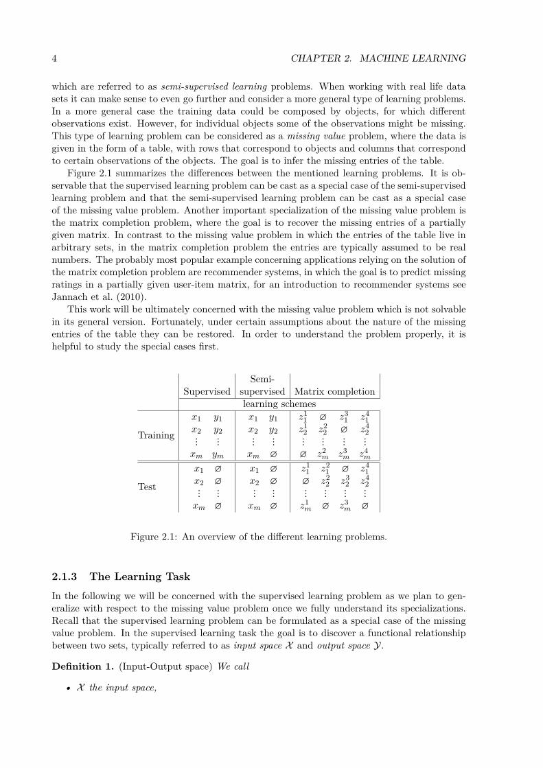
which are referred to as semi-supervised learning problems. When working with real life datasets it can make sense to even go further and consider a more general type of learning problems.In a more general case the training data could be composed by objects, for which differentobservations exist. However, for individual objects some of the observations might be missing.This type of learning problem can be considered as a missing value problem, where the data isgiven in the form of a table, with rows that correspond to objects and columns that correspondto certain observations of the objects. The goal is to infer the missing entries of the table.

Figure 2.1 summarizes the differences between the mentioned learning problems. It is ob-servable that the supervised learning problem can be cast as a special case of the semi-supervisedlearning problem and that the semi-supervised learning problem can be cast as a special caseof the missing value problem. Another important specialization of the missing value problem isthe matrix completion problem, where the goal is to recover the missing entries of a partiallygiven matrix. In contrast to the missing value problem in which the entries of the table live inarbitrary sets, in the matrix completion problem the entries are typically assumed to be realnumbers. The probably most popular example concerning applications relying on the solution ofthe matrix completion problem are recommender systems, in which the goal is to predict missingratings in a partially given user-item matrix, for an introduction to recommender systems seeJannach et al. (2010).

This work will be ultimately concerned with the missing value problem which is not solvablein its general version. Fortunately, under certain assumptions about the nature of the missingentries of the table they can be restored. In order to understand the problem properly, it ishelpful to study the special cases first.

Semi-Supervised supervised Matrix completion

learning schemes

Training

x1 y1x2 y2⋮ ⋮xm ym

x1 y1x2 y2⋮ ⋮xm ∅

z11 ∅ z3

1 z41

z12 z2

2 ∅ z42

⋮ ⋮ ⋮ ⋮∅ z2

m z3m z4

m

Test

x1 ∅x2 ∅⋮ ⋮xm ∅

x1 ∅x2 ∅⋮ ⋮xm ∅

z11 z2

1 ∅ z41

∅ z22 z3

2 z42

⋮ ⋮ ⋮ ⋮z1m ∅ z3

m ∅

Figure 2.1: An overview of the different learning problems.

2.1.3 The Learning Task

In the following we will be concerned with the supervised learning problem as we plan to gen-eralize with respect to the missing value problem once we fully understand its specializations.Recall that the supervised learning problem can be formulated as a special case of the missingvalue problem. In the supervised learning task the goal is to discover a functional relationshipbetween two sets, typically referred to as input space X and output space Y.

Definition 1. (Input-Output space) We call

• X the input space,

2.1. BACKGROUND 5

• Y the output space,

• Z ∶= X ×Y the joint input-output space

of the learning problem.

The learning of a relationship between inputs and outputs is based on the realization ofa sample of several input-output pairs, which are assumed to be drawn independently andidentically distributed (i.i.d.) from an unknown probability distribution. In machine learningliterature the realization of the sample is often directly referred to as the sample. Therefore, wewill stick to this terminology unless the context suggests the more precise statistical terminology.

Definition 2. (Training sample) Given an input-output space Z and a probability measure PZover Z, we call the m-tuple

z ∶= (z1, . . . , zm) ∈ Zm, (2.1)drawn i.i.d. from PZ , a training sample of size m. Additionally we call the pairs zi = (xi, yi)for i ∈ 1, . . . ,m training examples and define x as (x1, . . . , xm) and y as (y1, . . . , ym). We usez and (x,y) exchangeable.

To sum up, based on a training sample we aim to learn a functional relation between inputand output space. Theoretically, this relation could be any function. Unfortunately, consideringall possible functions from X to Y would result in an infeasible optimization problem, becauseYX is simply too large. Therefore, typically only a subspace of YX , a so-called hypothesis space,is considered.

Definition 3. (Function space) Let YX denote the set containing all functions from X to Y

YX ∶= f ∣f ∶ X → Y. (2.2)

A subset KK ⊆ YX (2.3)

of YX is called function space. The reason for this nomenclature originates from the fact thatin many applications the subset of functions is a topological space, a vector space or both. Forexample when Y is a field YX is a vector space.

Definition 4. (Hypothesis space) The function space

H ⊆ YX , (2.4)

that is considered when solving an optimization problem, is called hypothesis space and an ele-ment h ∈ H is called hypothesis.

The above definitions allow for a formulation of a more concise definition of the learningproblem:

Definition 5. (Learning problem) Given an input space X , an output space Y, a trainingsample z = (x,y) = ((x1, y1), . . . , (xm, ym)) ∈ (X × Y)m of size m ∈ N drawn i.i.d. from anunknown distribution PZ and a hypothesis space H , the learning problem is to find the unknownfunctional relation h ∶ X → Y ∈ H between objects x ∈ X and targets y ∈ Y based on the trainingsample. Depending on the structure of the output space different types of learning problems aredistinguished, see Table 2.1 for an overview.

At this point we did not introduce a methodology to evaluate the quality of a given hypothe-sis. However, in order to address the learning problem from an optimization point of view this ismandatory. In the next section of this chapter we are going to study classical machine learningproblems in order to get an intuition about evaluating the quality of given hypotheses.


Output space Y Typefinite set classification learningordered space preference learningmetric space function learningcontains structured objects structured output learning

Table 2.1: Types of learning problems based on the structure of the output space.

2.2 Learning Algorithms

A learning algorithm is an algorithm that is intended to solve a learning problem by utilizingdata. Additionally, learning algorithms should perform the better the more data is available.The objective of a learning algorithm is the selection of a function from the hypothesis space.

Definition 6. (Learning algorithm) Given an input space X , an output space Y and a hypothesisspace H ⊆ YX , a learning algorithm A is a mapping

A ∶∞

⋃n=1

(X ×Y)n →H . (2.5)

So far, it is not clear how the selection of an element of the hypothesis space is performed,however, it is obvious that for a proper selection a quality measure is required. The qualitymeasure is typically partially imposed by the task and partially a design choice. A closer lookat the classification and regression problem leads to the analysis of the connection between taskand quality measure.

2.2.1 Linear Classification

In this section the basics of linear classifiers will be introduced and their relevance illustrated inan example.

Binary Classification

The simplest classification problem is the binary classification problem. In the following, let Vbe a Euclidean vector space over the field of real numbers.

Definition 7. (Binary classification problem) Given a sample z = (x,y) = ((x1, y1), . . . , (xm, ym)) ∈(X × Y)m of size m ∈ N, where the inputs xi ∈ X are elements of an arbitrary set and thetarget values yi ∈ −1,1 correspond to binary class labels, the objective is to find a functionf ∶ X → Y ∈ YX , that for any x ∈ X assigns the corresponding class label.

If the input space X is a Euclidean vector space, the binary classification problem might beaddressed by looking for hyperplanes.

Definition 8. (Linear hyperplane) A linear hyperplane in a d-dimensional vector space V is alinear subspace of dimension d − 1 and is characterized by

Pw ∶= x ∈ V ∶ ⟨w,x⟩ = 0 for w ∈ V,

where w ∈ V and x ∈ V a d-dimensional vectors and w is referred to as a normal vector of thelinear hyperplane.

2.2. LEARNING ALGORITHMS 7

Definition 9. (Affine hyperplane) An affine hyperplane in a d-dimensional vector space V isan affine subspace of dimension d − 1 and is characterized by

P(w,b) ∶= x ∈ V ∶ ⟨w,x⟩ = b for w ∈ V,

where w ∈ V and x ∈ V a d-dimensional vectors and w is referred to as a normal vector of theaffine hyperplane.

In the machine learning literature it frequently occurs that affine hyperplanes are referredto as linear hyperplanes.

Remark 10. (Distance from a point to a hyperplane) The signed distance between a pointv ∈ V and a hyperplane P(w,b) is given by the length of the projection of a vector from any pointx0 ∈ P(w,b) to v, given by v − x0, onto the normal vector of the hyperplane w

d(w,b) ∶ V → R ∶ x↦ ⟨w,x⟩ − b∥w∥2

. (2.6)

Every hyperplane naturally separates its corresponding vector space into two subspaces.

Remark 11. (Half-spaces) In a vector space V over the field of real numbers an affine hyperplanePw separates the space into two half-spaces, which are given by

V+ ∶= x ∈ V ∶ ⟨w,x⟩ > b

andV− ∶= x ∈ V ∶ ⟨w,x⟩ < b ,

where w,x ∈ V and b ∈ R. A hyperplane separating two classes in a classification scenario iscalled separating hyperplane.

Therefore, to define a linear classifier it is sufficient to find a hyperplane that separates theinput space, in such a way that one half contains all the data points with class label one andthe other half contains all data points with label minus one.

Definition 12. (Binary linear classifier) Given an affine hyperplane P(w,b) ⊂ V a binary linearclassifier h ∶ V → −1,1 can be obtained by considering

h(x) ∶= sign(⟨w,x⟩ − b) for x ∈ X ,

which is equal to one if x ∈ V+ and minus one if x ∈ V−.

If a hyperplane that agrees with the data sample exists, the sample will be linearly separable.

Definition 13. (Linear separability) Let X be a Euclidean vector space. A data-set z = (x,y) ∈(X × −1,1)m is called linearly separable if a linear classifier h exists that satisfies

(x, y) ∈ z ∶ h(x) ≠ y = ∅.

Meaning that it correctly classifies each item of the training set.


Multi-class Classification

After having introduced binary linear classifiers, we new have the tools to address the binaryclassification task. However, in practice often more than two classes are of interest.

Definition 14. (Multi-class classification problem) Given a sample z = (x,y) = ((x1, y1), . . . , (xm, ym)) ∈(X × Y)m of size m ∈ N, where the inputs xi ∈ X can have arbitrary structure and the targetvalues yi ∈ 1, . . . , k correspond to class labels, the objective is to find a function f ∶ X → Y ∈ YXthat for a x ∈ X assigns the corresponding class label y ∈ Y.

In the following example we will motivate the choice of linear classifiers and introduce oneway to address the multi-class classification problem.

Example 15. (Classification learning example) Given a sample (x,y) = ((x1, y1), . . . , (xm, ym))of object-label pairs, where Y = 1, . . . , k, we are looking for a function h ∶ X → Y that assigns aclass label y ∈ Y to an object x ∈ X . Ideally, h should assign identical class labels to objects thatare very similar. When talking about similarity between objects, it is useful to work with metricspaces. In this example X is assumed to be a Euclidean vector space. Arbitrary input spacescan be handled by mapping them into metric spaces. One simple classifier showing the desiredbehavior is the nearest neighbor classifier

hNN ∶ X → Y ∶ x↦ ynn, where nn = arg mini∈1,...,m

∥x − xi∥, (2.7)

which assigns the label of the closest training point to the point of interest. Unfortunately usinga nearest neighbor classifier requires the storage of the whole training set, which can require asignificant amount of storage. Therefore, it would be favorable to use a parametric function tomodel the classifier in order to overcome this drawback. The simplest parametric functions withthe desired behavior are linear ones

f(⋅;w) ∶ X → R ∶ x↦ ⟨w,x⟩ = w′x. (2.8)

The fact that linear functions map similar points to similar function values can be easily derivedby considering

∣f(x) − f(x)∣ = ∣ ⟨w,x⟩ − ⟨w, x⟩ ∣= ∣ ⟨w,x − x⟩ ∣≤ ∥w∥∥x − x∥,

where the last inequality is the Cauchy-Schwarz inequality. The difference between the functionvalues evaluated at two points is proportional to the distance between the points with the constantfactor ∥w∥. A linear binary classifier can be obtained by taking the sign of a linear function

hlin(⋅;w) ∶ X → Y ∶ x↦ sign(f(x;w)).

In order to build a classifier for more than two classes, as required in our case, a simple construc-tion is to first learn k 1-vs-all classifiers h1, . . . , hk, where a positive sign of hi(x) correspondsto "x is member of class i". The linear functions learned can be used to construct a multiclassclassifier

hmulti ∶ X → Y ∶ x↦ arg maxi∈1,...,k

fi(x).

Therefore, using parametric linear classifiers enables to drastically reduce the amount of storageinstead of storing the whole training set. That way, only the storage of k parameter vectors isrequired, while the property that similar points are mapped to similar class labels is preserved.

In Chapter 5, a more sophisticated learning framework with the ability to address the multi-class classification problem is introduced.


2.2.2 Feature Space and Hypothesis Space

Unfortunately, real world problems are often more complex. This occurs, for instance, whenthe data is not linearly separable in the input space or when the input space X is an arbitraryset without the notion of an inner product and the other nice properties of Euclidean vectorspaces. When working with not linearly separable data the classifiers introduced so far arelikely to perform poorly. Even more so, if X is an arbitrary set they might not be able to beused directly. Therefore, it is common to map the input space to a Euclidean space or - moregenerally - to a Hilbert space. In a Hilbert space, we have an inner product and therefore areable to work with linear forms the same way we did in Euclidean vector spaces.

Definition 16. (Hilbert space) A Hilbert space is a vector space H over the field K togetherwith an inner product ⟨⋅, ⋅⟩ ∶H ×H → K that for all x, y, z ∈H and a ∈ K satisfies

1. Conjugate symmetry:⟨x, y⟩ = ⟨y, x⟩

2. Linearity in the first argument:

⟨ax, y⟩ = a ⟨x, y⟩ and ⟨x + y, z⟩ = ⟨x, z⟩ + ⟨y, z⟩

3. Positive-definiteness:⟨x,x⟩ ≥ 0 and ⟨x,x⟩ = 0⇒ x = 0.

Note that if K = R conjugate symmetry is equivalent to symmetry. Thus, the linearity in thefirst argument implies bilinearity. Additionally a Hilbert space H is a complete metric space withrespect to the metric DH induced by the inner product

DH ∶H ×H → [0,∞) ∶ (x, y)↦ ∥x − y∥ ∶=√

⟨x − y, x − y⟩. (2.9)

We don’t need the concept of completeness in the scope of this chapter, but it will be detailed inChapter 4.

Furthermore, the notion of Hilbert spaces allows us to consider diverse hypothesis spacesthat are easy to handle, for example the space of polynomials.

Definition 17. (Basis function) A basis function is an element of a basis of a function space.Analogously to the representations of vectors in a vector space in terms of a linear combination ofbasis vectors, it is possible to represent every function in a function space by a linear combinationof the basis functions of that space.

It is not trivially possible to work with arbitrary shaped data points; still, one way to do sois to perform a mapping of the data into a Hilbert space, referred to as feature space.

Definition 18. (Feature space mapping) We call a mapping φ from the input space X to aHilbert space Hφ a feature space mapping and Hφ a feature space. One way of defining such amapping is using a set of basis functions φ1, . . . , φi, . . . resulting in

φ ∶ X →Hφ ∶ x↦ (φ1(x), . . . , φi(x), . . . )′. (2.10)

The feature space can be infinite dimensional which is indicated by the dots (φ1(x), . . . , φi(x), . . . ).The image φ(x) of an input x ∈ X under φ is often referred to as feature vector, of which thecomponents are called features. The term basis function for the component functions of the fea-ture space mapping relates to the fact, that the dual space of the feature space, namely the spaceof linear forms f ∶Hφ → R, is isomorphic to the function space spanned by the basis functions. Alinear form in the feature space corresponds to a possibly nonlinear function in the input space.


Remark 19. (A new hypothesis space) Feature space mappings allow us to work with a powerfulfamily hypothesis spaces, namely the ones obtained by considering linear forms from featurespaces to R

H∗φ = f ∶Hφ → R ∶ f is linear. (2.11)

By the composition of the corresponding feature space mapping and those linear forms we obtaina hypothesis space of possibly non-linear functions

H = g ∶ X → R ∶ g = f φ, f ∈H∗φ and feature space mapping φ. (2.12)

Remark 20. (Convenient notation) Additionally, the notion of feature space mapping allowsus to omit the bias term when working with linear models, since it can be assumed that oneof the basis functions φi is equal to one. Therefore, ⟨w,x⟩ − b can be written as ⟨⟨w, φ(x)⟩⟩,where w ∶= (w′,−b)′ is the concatenation of the old parameter vector w and the bias term andφ(x) ∶= (x,1)′.

Non-linearly Separable Data

If the input space X is already a Hilbert space but the given data is not linearly separable, itis possible to improve the separability of the data by wisely choosing a feature mapping. Recallthat binary linear classifiers were obtained by considering the signs of linear forms on the inputspace.

After finding a mapping from the input space to a Hilbert space φ ∶ X →Hφ it is possible todefine binary linear classifiers in exactly the same fashion

hw ∶ X → −1,1 ∶ x↦ sign(⟨w,φ(x)⟩Hφ) where w ∈Hφ.

The pre-image of the separating hyperplane Pw in the feature space under the feature map φ,denoted by φ−1(Pw) corresponds to a non-linear decision surface or decision boundary in theinput space, where the non-linearity is determined by the choice of the basis functions of thefeature mapping.

Definition 21. (Decision surface) Given an input space X a feature map φ a binary linearclassifier hw and the corresponding separating hyperplane Pw ⊂ Hφ, then the pre-image of Pwunder the feature map φ

φ−1(Pw) = x ∈ X ∶ φ(x) ∈ Pw

= x ∈ X ∶ ⟨w,φ(x)⟩Hφ = 0= x ∈ X ∶ hw(x) = 0 ,

is referred to as decision surface or decision boundary.

The following example is intended to provide a basic idea about the way in which the choiceof basis functions affects the non-linearities used for classification.

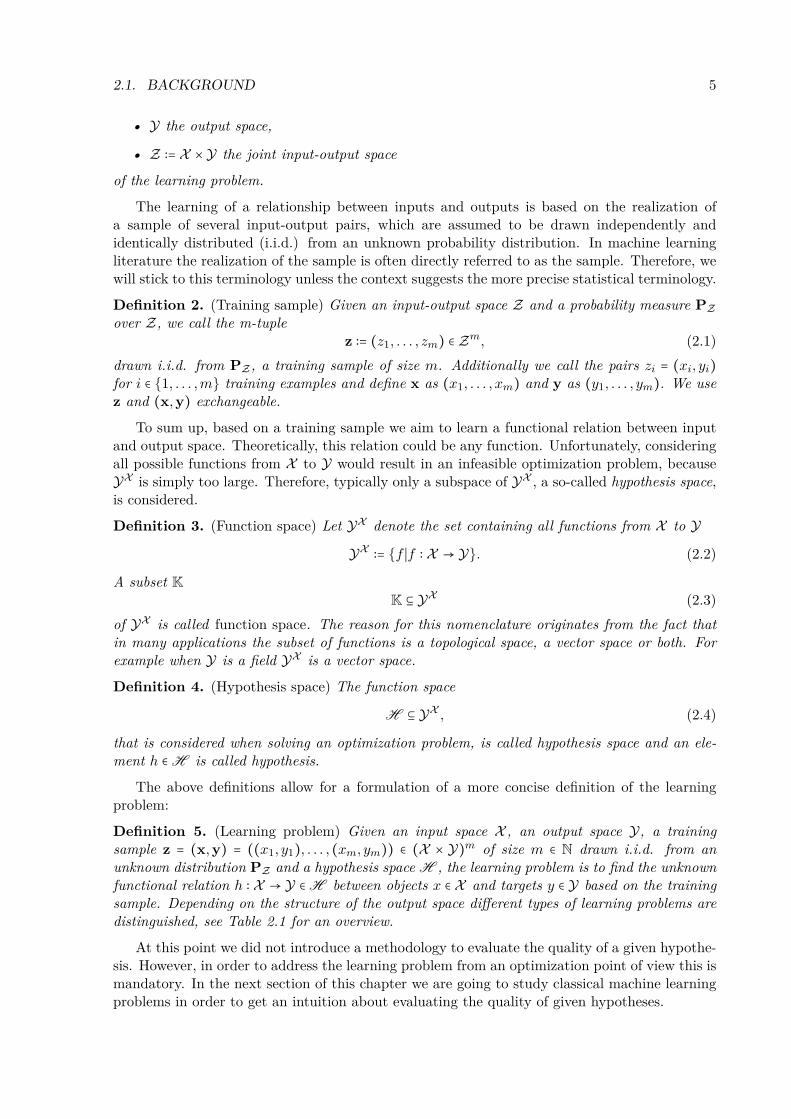
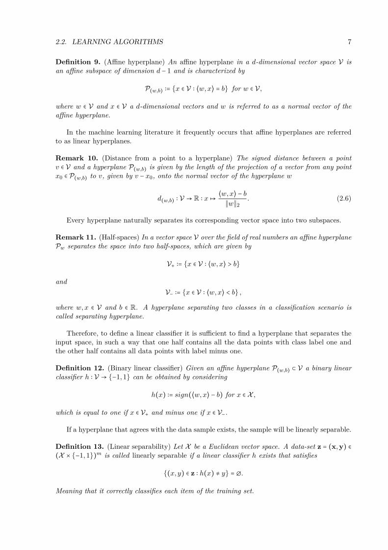
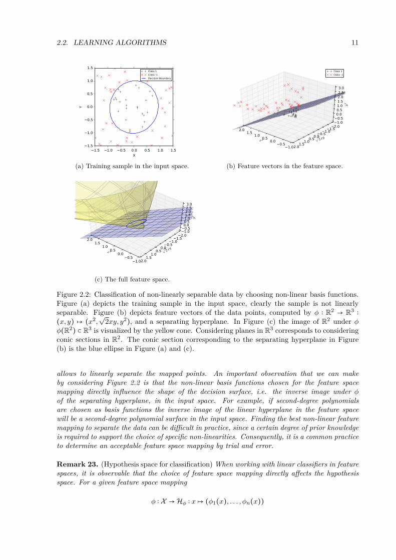
Example 22. (Non-linear classification)Figure 2.2 illustrates a situation as stated previously, where - in the input space - the two

classes of points cannot be separated by a linear function. However, they can be separated bya nonlinear function, for example a circle with its center at (0,0) and a radius of length one.This observation suggests to use quadratical monomials as non linear basis functions, the featurespace mapping given by

φ ∶ R2 → R3 ∶ (x, y)↦ (x2,√

2xy, y2) (2.13)


(a) Training sample in the input space. (b) Feature vectors in the feature space.

(c) The full feature space.

Figure 2.2: Classification of non-linearly separable data by choosing non-linear basis functions.Figure (a) depicts the training sample in the input space, clearly the sample is not linearlyseparable. Figure (b) depicts feature vectors of the data points, computed by φ ∶ R2 → R3 ∶(x, y) ↦ (x2,

√2xy, y2), and a separating hyperplane. In Figure (c) the image of R2 under φ

φ(R2) ⊂ R3 is visualized by the yellow cone. Considering planes in R3 corresponds to consideringconic sections in R2. The conic section corresponding to the separating hyperplane in Figure(b) is the blue ellipse in Figure (a) and (c).

allows to linearly separate the mapped points. An important observation that we can makeby considering Figure 2.2 is that the non-linear basis functions chosen for the feature spacemapping directly influence the shape of the decision surface, i.e. the inverse image under φof the separating hyperplane, in the input space. For example, if second-degree polynomialsare chosen as basis functions the inverse image of the linear hyperplane in the feature spacewill be a second-degree polynomial surface in the input space. Finding the best non-linear featuremapping to separate the data can be difficult in practice, since a certain degree of prior knowledgeis required to support the choice of specific non-linearities. Consequently, it is a common practiceto determine an acceptable feature space mapping by trial and error.

Remark 23. (Hypothesis space for classification) When working with linear classifiers in featurespaces, it is observable that the choice of feature space mapping directly affects the hypothesisspace. For a given feature space mapping

φ ∶ X →Hφ ∶ x↦ (φ1(x), . . . , φn(x))


the corresponding hypothesis space H ⊂ YX is

H = h ∈ YX ∶ h(x) = sign(f(x)), x ∈ X , f ∈H∗φ

= h ∈ YX ∶ h(x) = sign(⟨w,φ(x)⟩), x ∈ X ,w ∈Hφ

= h ∈ YX ∶ h(x) = sign(n

∑i=1wiφi(x)), x ∈ X ,w ∈Hφ .

Arbitrary Input Space

If the only requirement for the input space X is to be a set it will - per definition - not bepossible to define a linear form which is a linear function from a vector space to its field ofscalars directly on the input space. Therefore, the mapping of the data into a Hilbert space isrequired in order to work with linear forms or subsequently with linear classifiers. Since linearclassifiers are similarity based, one desired property for a feature space mapping φ ∶ X → Hφ isthat the images of similar objects under the feature mapping are close. If the only informationavailable about the input space is that it is a set, no notion of similarity in the input space willexist. Therefore, in that case it is impossible to quantify the goodness of a corresponding featurespace mapping. Fortunately, the objects of interest in practice, for example images, texts, DNAsequences, time series and so on, typically have certain additional structure that enables at leastan empirical notion of similarity between them. However, by now it should be observable thatthe choice of a proper feature space mapping can be tricky.

Additionally, the interpretation of the basis functions φi as non-linearities that can enhanceclassification performance cannot be used directly, instead the images of inputs x ∈ X underthe feature space mapping φ(x) should be thought of as representers of the inputs. In order toresolve remaining unclarities consider the following example, in which the input space is not aHilbert space.

Example 24. (String classification) Let X = Σ∗ be the set of strings of arbitrary length over thealphabet Σ, for more information about strings and substrings we refer to Hopcroft and Ullman(1990). Obviously, Σ∗ is not a Hilbert space, therefore, in order to use linear classifiers it isnecessary to find a feature mapping φ from Σ∗ to Hφ. As stated above, it would be desirable ifsimilar strings get mapped to similar representations. Intuitively, two strings are similar if theyshare common sub-strings. Motivated by that notion of similarity a natural choice of a basisfunction would be an indicator function for a certain substring

φb ∶ Σ∗ → R ∶ v ↦⎧⎪⎪⎨⎪⎪⎩

1, if v contains b0, else

, where b ∈ Σ∗. (2.14)

Therefore, for a given lexicon (b1, . . . , bd) of substrings one possible feature space mapping withthe desired property could be

φ ∶ Σ∗ → Rd ∶ v ↦ (φb1 , . . . , φbd). (2.15)

Of course, there are more sophisticated ways to represent strings, as in Lodhi et al. (2002) wherea feature space generated by considering the number of occurrences of all subsequences of lengthk weighted by their length is used.

2.2.3 Learning Linear Classifiers

After defining linear classifiers the only open question remaining is how to find the best one fora given task. Ideally, for a given i.i.d. sample z = (x,y) = ((x1, y1), . . . , (xm, ym)) we would like


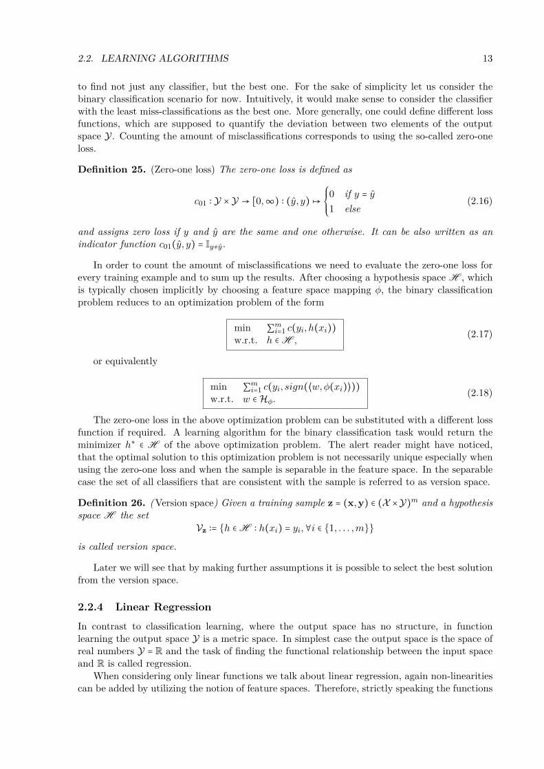
to find not just any classifier, but the best one. For the sake of simplicity let us consider thebinary classification scenario for now. Intuitively, it would make sense to consider the classifierwith the least miss-classifications as the best one. More generally, one could define different lossfunctions, which are supposed to quantify the deviation between two elements of the outputspace Y. Counting the amount of misclassifications corresponds to using the so-called zero-oneloss.

Definition 25. (Zero-one loss) The zero-one loss is defined as

c01 ∶ Y ×Y → [0,∞) ∶ (y, y)↦⎧⎪⎪⎨⎪⎪⎩

0 if y = y1 else

(2.16)

and assigns zero loss if y and y are the same and one otherwise. It can be also written as anindicator function c01(y, y) = Iy≠y.

In order to count the amount of misclassifications we need to evaluate the zero-one loss forevery training example and to sum up the results. After choosing a hypothesis space H , whichis typically chosen implicitly by choosing a feature space mapping φ, the binary classificationproblem reduces to an optimization problem of the form

min ∑mi=1 c(yi, h(xi))w.r.t. h ∈ H ,

(2.17)

or equivalently

min ∑mi=1 c(yi, sign(⟨w,φ(xi)⟩))w.r.t. w ∈Hφ.

(2.18)

The zero-one loss in the above optimization problem can be substituted with a different lossfunction if required. A learning algorithm for the binary classification task would return theminimizer h∗ ∈ H of the above optimization problem. The alert reader might have noticed,that the optimal solution to this optimization problem is not necessarily unique especially whenusing the zero-one loss and when the sample is separable in the feature space. In the separablecase the set of all classifiers that are consistent with the sample is referred to as version space.

Definition 26. (Version space) Given a training sample z = (x,y) ∈ (X ×Y)m and a hypothesisspace H the set

Vz ∶= h ∈ H ∶ h(xi) = yi,∀i ∈ 1, . . . ,m

is called version space.

Later we will see that by making further assumptions it is possible to select the best solutionfrom the version space.

2.2.4 Linear Regression

In contrast to classification learning, where the output space has no structure, in functionlearning the output space Y is a metric space. In simplest case the output space is the space ofreal numbers Y = R and the task of finding the functional relationship between the input spaceand R is called regression.

When considering only linear functions we talk about linear regression, again non-linearitiescan be added by utilizing the notion of feature spaces. Therefore, strictly speaking the functions


of interest are only linear in the feature space. More precisely, given a feature space mappingφ, the hypothesis space H is the space of linear forms from Hφ to R, also referred to as dualspace H∗

φ of Hφ. Traditionally, the loss function used for regression is the squared loss.

Definition 27. (Squared loss) The squared loss is defined as

csq ∶ Y ×Y → [0,∞) ∶ (y, y)↦ ∥y − y∥22,

where ∥x∥22 is defined as x2 for x ∈ R.

This particular choice of loss function can be motivated probabilistically. In the classicalregression model the i’th observation is assumed to have the following form

yi = wxi + b + εi, (2.19)

where i ∈ 1, . . . , n and εi is the realization of a normally, independently and identically dis-tributed sample E1, . . . ,En, with E[E1] = 0 and V ar[E1] = σ2. Therefore, the random variablesYi = wxi + b +Ei are distributed normally Yi ∼ N (wxi + b, σ2) with the density

f(y;wxi − b, σ2) = 1√2φσ2

exp(−12(y −wxi − b

σ)

2) (2.20)

for i ∈ 1, . . . , n. In statistics a common practice for parameter estimation is to maximize thelikelihood function. Since our random variables are independent the likelihood function L(w, b)is

L(w, b) =n

∏i=1f(yi;wxi − b, σ2)

=⎛⎝

1√2φσ2

⎞⎠

n

exp(n

∑i=1

−12(yi −wxi − b

σ)

2) .

(2.21)

When working with normal distributions the maximization of the likelihood function can besimplified by considering the logarithm of the likelihood function

ln(L(w, b)) = −n2ln(2πσ2) − 1

2σ2

n

∑i=1

(yi −wxi − b)2 . (2.22)

The maximization of ln(L(w, b)) with respect to w and b is achieved, when the sum of squaredlosses ∑ni=1 (yi −wxi − b)

2 is minimized. Therefore, after choosing a reasonable feature space Hφ,the optimization problem to solve becomes

min ∑mi=1 csq(yi, ⟨w,φ(xi)⟩)w.r.t. w ∈Hφ.

(2.23)

Since the squared loss function is differentiable and convex, the sum of convex functions isconvex and the sum of differentiable functions is differentiable, a closed form solution for thelinear regression problem can be obtained by setting the derivative of the objective function tozero.

Example 28. (Linear regression with a straight line) Let’s find the optimal weight vector for asimple example, where X is R, Y is R and φ(x) = (1, x)′. Given an i.i.d. sample of observations(xi, yi)mi=1 ∈ (R ×R)m, we are looking for the linear function that minimizes the sum of squareserror E

minw∈Hφ

E(w1,w2) ∶=12m

∑i=1

(w1 +w2xi − yi)2, (2.24)


where we added the factor 12 to make the solution prettier. Therefore, we set the derivatives of

the error function E with respect to w1

∂E

∂w1(w1,w2) =

m

∑i=1

(w1 +w2xi − yi) != 0 (2.25)

and to w2∂E

∂w2(w1,w2) =

m

∑i=1

(w1 +w2xi − yi)xi != 0 (2.26)

to zero. From Equation 2.25 we obtain

w1 =1m

m

∑i=1yi −w2xi, (2.27)

by splitting up the sum into ∑mi=1w1 + ∑mi=1 (w2xi − yi) and solving for w1. Let’s denote theaverage 1

mxi by x and 1myi by y. Substituting Equation 2.27 into Equation 2.26, yields

0 =m

∑i=1

(y −w2x +w2xi − yi)xi

= w2m

∑i=1

(xi − x)xi +m

∑i=1

(y − yi)xi,(2.28)

which is equivalent tow2 =

∑mi=1 (yi − y)xi∑mi=1 (xi − x)xi

. (2.29)

If our goal was only the determination of the optimal parameters we would be done here. How-ever, with slight refinements of this expression a meaningful representation can be derived. Inorder to do so, let us consider the enumerator and the denominator individually. The enumeratorcan be rewritten by first adding and subtracting xyi to every summand

m

∑i=1

(yixi − yxi) =m

∑i=1

(yixi − yxi − xyi + xyi). (2.30)

By pulling x and y out of the sums and utilizing x = 1mxi and y =

1myi

m

∑i=1yixi −myx −mxy +mxy =

m

∑i=1yixi −

m

∑i=1yx −

m

∑i=1xy +

m

∑i=1xy (2.31)

is obtained, which is equivalent tom

∑i=1

(yixi − yxi) =m

∑i=1

(xi − x)(yi − y) (2.32)

Analogously the denominator can be transformed into ∑mi=1 (xi − x)2. Therefore we get the fol-lowing expression for w2

w2 =∑mi=1 (xi − x)(yi − y)∑mi=1 (xi − x)2 , (2.33)

which is closely related to the Pearson correlation, see Pearson (1895) for further details. Theexpression in the enumerator of w2 is called empirical covariance, since the denominator is al-ways positive, the empirical covariance alone determines the sign of the slope of the regressionline. Figure 2.3 shows the type of regression line we just derived in a toy example. The train-ing data was generated by perturbing point evaluations of a polynomial function with normallydistributed noise in the target component. The Figure contains plots of the training data, theregression line and also the ground truth polynomial.


−1 −0.5 0 0.5 1

0

2

4

6

8

X

Y

(a) Training data

−1 −0.5 0 0.5 1

0

2

4

6

8

XY

(b) Regression line

−1 −0.5 0 0.5 1

0

2

4

6

8

X

Y

(c) Ground truth

Figure 2.3: Linear regression using a line. In the upper left corner there is the training data, inthe upper right corner the minimizer of the least squares error (red) and in the lower left cornerthere is the function (blue) used to generate the training data. The training data was generatedby evaluating a polynomial function and adding Gaussian noise.

It’s observable that the regression line in Figure 2.3 (b) does not look like a very goodestimate of the polynomial function. In order to fit the underlying polynomial function betterit could be beneficial to increase the degree of the regression polynomial that we want to fit.Instead of a polynomial of degree one, which is a line, polynomials of arbitrary degree can beutilized by adjusting the feature space mapping accordingly.

Example 29. (Linear regression with a polynomial) When X is R and Y is R like in theprevious example it is sufficient to change the feature mapping φ to

φ ∶ R→ R(n+1) ∶ x↦ (x0, x1, . . . , xn) (2.34)

2.3. RISK MINIMIZATION 17

in order to use polynomials of degree n. The resulting optimization problem is

minw∈Hφ

E(w) ∶= 12m

∑i=1

(yi −n

∑j=0

wjxji )

2 (2.35)

and can be solved analogously by setting the derivative with respect to w equal to zero. Figure 2.4illustrates regression polynomials of different degrees. With an increasing degree the regressionpolynomial converges closer and closer to the training points, in other words, the least squareserror becomes smaller the higher the degree of the regression polynomial gets. Nevertheless, thedeviation between ground truth and regression polynomials obviously increases with the degree ofthe polynomials considered. This problem is called overfitting. In the next section we shall seeone possibility to deal with overfitting.

2.3 Risk MinimizationAs we have seen in the classification and regression task, different trains of thoughts lead usto almost identically looking optimization problems. Considering the resulting optimizationproblems of both tasks, the only observable differences are to be found in the choice of hypothesisspace and loss functions. In this chapter we are going to introduce a framework that is capableof handling all supervised learning problems, namely, the risk minimization framework. So far,we have already worked with several loss functions without describing explicitly what a lossfunction should look like in general. Clearly, it should be possible to interpret the loss functionas a measure of discrepancy in the output space. In further consequence, a loss function shouldallow us to determine the quality of a prediction. The higher the value of the loss functionevaluated at a predicted output and the corresponding true output the worse the quality of theprediction.

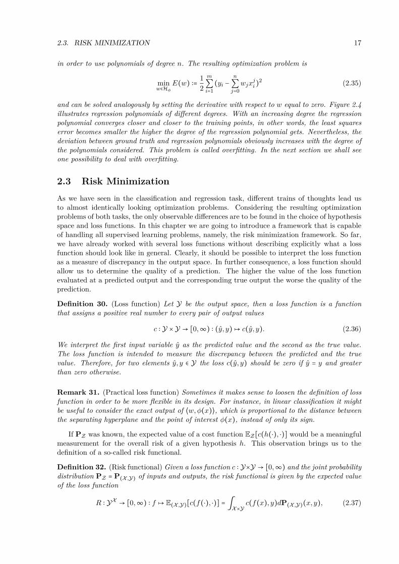
Definition 30. (Loss function) Let Y be the output space, then a loss function is a functionthat assigns a positive real number to every pair of output values

c ∶ Y ×Y → [0,∞) ∶ (y, y)↦ c(y, y). (2.36)

We interpret the first input variable y as the predicted value and the second as the true value.The loss function is intended to measure the discrepancy between the predicted and the truevalue. Therefore, for two elements y, y ∈ Y the loss c(y, y) should be zero if y = y and greaterthan zero otherwise.

Remark 31. (Practical loss function) Sometimes it makes sense to loosen the definition of lossfunction in order to be more flexible in its design. For instance, in linear classification it mightbe useful to consider the exact output of ⟨w,φ(x)⟩, which is proportional to the distance betweenthe separating hyperplane and the point of interest φ(x), instead of only its sign.

If PZ was known, the expected value of a cost function EZ[c(h(⋅), ⋅)] would be a meaningfulmeasurement for the overall risk of a given hypothesis h. This observation brings us to thedefinition of a so-called risk functional.

Definition 32. (Risk functional) Given a loss function c ∶ Y×Y → [0,∞) and the joint probabilitydistribution PZ = P(X ,Y) of inputs and outputs, the risk functional is given by the expected valueof the loss function

R ∶ YX → [0,∞) ∶ f ↦ E(X ,Y)[c(f(⋅), ⋅)] = ∫X×Y

c(f(x), y)dP(X ,Y)(x, y), (2.37)


where ∫ ⋅dµ denotes the Lebesgue integral with respect to the measure µ. In this case µ is definedas the joint probability distribution of the input-output space P(X ,Y). For the construction andproperties of the Lebesgue integral we refer to Geiss and Geiss (2014). Note that for evaluationsof functionals we use square brackets R[f].

After choosing a hypothesis space and a cost function, learning reduces to an optimizationproblem of the form

min R[h]w.r.t. h ∈ H .

(2.38)

Unfortunately, this elegant approach is not directly applicable in most real world scenarios,since the probability distribution of the data is typically unknown. Instead, the only informationavailable is an independent and identically distributed sample of the form ((x1, y1), . . . , (xm, ym)) ∈(X ×Y)m.

2.3.1 Empirical Risk Minimization

The question that demands to be answered now is how to estimate P(X ,Y) given an i.i.d. sample((x1, y1), . . . , (xm, ym)) ∈ (X × Y)m. For simplicity reasons let’s assume that X ⊆ Rd and thatY ⊆ Rk. If the sample is sufficiently large the obvious answer to that question will be to use theempirical distribution

Pm(⋅; (x,y)) ∶ B(Rd ×Rk)→ [0,1] ∶ (A,B)↦ 1m

m

∑i=1δ(xi,yi)(A,B), (2.39)

where

δ(x,y)(A,B) =⎧⎪⎪⎨⎪⎪⎩

1 if x ∈ A and y ∈ B0 else

(2.40)

is a Dirac measure, (A,B) ∈ B(Rd ×Rk) are Borel sets, i.e. sets that can be formed from opensets through countable unions and intersections, and B(Rd ×Rk) denotes the Borel σ-algebra ofRd ×Rk, which is the smallest σ-algebra containing all open sets in Rd ×Rk.

According to the Glivenko-Cantelli theorem, see Glivenko and Cantelli (1933), the empiricaldistribution converges to the real probability distribution with an increasing amount of sampleitems almost certainly. The convergence towards the real probability distribution suggests thatfor large training sets the empirical distribution is a good estimate of the real distribution, whichmotivates the definition of the empirical risk functional. By estimating the joint probabilitydistribution with the empirical distribution, the integral of the cost function reduces to a sumof cost function evaluations

Remp[f ; z] ∶= Em[c(f(⋅), ⋅)] = ∫X×Y

c(f(x), y)dPm(x, y; (x,y))

= ∫X×Y

c(f(x), y)d( 1m

m

∑i=1δ(xi,yi)(x, y)) (by definition of Pm)

= 1m

m

∑i=1∫X×Y

c(f(x), y)dδ(xi,yi)(x, y) (by definition of ∫ )

= 1m

m

∑i=1c(f(xi), yi) (property of the Dirac measure).

(2.41)This leads to the following definition of the empirical risk functional.

2.3. RISK MINIMIZATION 19

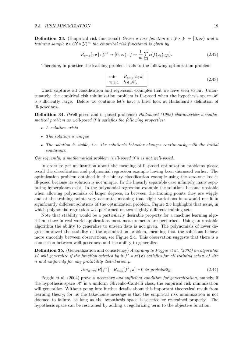
Definition 33. (Empirical risk functional) Given a loss function c ∶ Y × Y → [0,∞) and atraining sample z ∈ (X ×Y)m the empirical risk functional is given by

Remp[⋅; z] ∶ YX → [0,∞) ∶ f ↦ 1m

m

∑i=1c(f(xi), yi). (2.42)

Therefore, in practice the learning problem leads to the following optimization problem

min Remp[h; z]w.r.t. h ∈ H ,

(2.43)

which captures all classification and regression examples that we have seen so far. Unfor-tunately, the empirical risk minimization problem is ill-posed when the hypothesis space His sufficiently large. Before we continue let’s have a brief look at Hadamard’s definition ofill-posedness.Definition 34. (Well-posed and ill-posed problems) Hadamard (1902) characterizes a mathe-matical problem as well-posed if it satisfies the following properties:

• A solution exists

• The solution is unique

• The solution is stable, i.e. the solution’s behavior changes continuously with the initialconditions.

Consequently, a mathematical problem is ill-posed if it is not well-posed.In order to get an intuition about the meaning of ill-posed optimization problems please

recall the classification and polynomial regression example having been discussed earlier. Theoptimization problem obtained in the binary classification example using the zero-one loss isill-posed because its solution is not unique. In the linearly separable case infinitely many sepa-rating hyperplanes exist. In the polynomial regression example the solutions become unstablewhen allowing polynomials of larger degrees, in between the training points they are wigglyand at the training points very accurate, meaning that slight variations in z would result insignificantly different solutions of the optimization problem. Figure 2.5 highlights that issue, inwhich polynomial regression was performed on two slightly different training sets.

Note that stability would be a particularly desirable property for a machine learning algo-rithm, since in real world applications most measurements are perturbed. Using an unstablealgorithm the ability to generalize to unseen data is not given. The polynomials of lower de-gree improved the stability of the optimization problem, meaning that the solutions behavemore smoothly between observations, see Figure 2.4. This observation suggests that there is aconnection between well-posedness and the ability to generalize.Definition 35. (Generalization and consistency) According to Poggio et al. (2004) an algorithmA will generalize if the function selected by it f∗ = A (z) satisfies for all training sets z of sizen and uniformly for any probability distribution µ

limn→∞∣R[f∗] −Remp[f∗,z]∣ = 0 in probability. (2.44)

Poggio et al. (2004) prove a necessary and sufficient condition for generalization, namely, ifthe hypothesis space H is a uniform Glivenko-Cantelli class, the empirical risk minimizationwill generalize. Without going into further details about this important theoretical result fromlearning theory, for us the take-home message is that the empirical risk minimization is notdoomed to failure, as long as the hypothesis space is selected or restrained properly. Thehypothesis space can be restrained by adding a regularizing term to the objective function.


2.3.2 Regularization

If the hypothesis space in empirical risk minimization is sufficiently discriminative, an unavoid-able problem that occurs is the problem of overfitting. In order to fully understand the magnitudeof this problem, think of a training sample of the following shape

((x1, y1), . . . , (xm, ym)) ∈ (R ×R)m with xi ≠ xj for i ≠ j ∈ 1, . . . ,m . (2.45)

If the hypothesis space contains polynomials of degree m − 1, it will contain at least one func-tion that minimizes every reasonable loss function evaluated at the training set, namely, theinterpolating polynomial given by the Lagrange formula

p(x) ∶=m

∑i=1yi

m

∏k=1,k≠i

x − xkxi − xk

. (2.46)

However, polynomials of high degree are known to be rather poor interpolants in terms of theirbehavior between interpolated points, where they are typically wiggly. Additionally, a smallchange in the training sample can have a big impact on the interpolating function. Similarly,if the hypothesis space is complex enough there will always be a minimizer strongly dependenton the training sample. When doing interpolation one way around this is to consider moresophisticated interpolation methods like the spline interpolation.

Another more practical way in machine learning is the method of regularization, i.e. toconstrain the solution to be less complex. Remember that in machine learning problems wedon’t want to interpolate, instead, we want to learn a function that generalizes to the wholeinput space. When learning polynomials this would mean to prefer polynomials of smallerdegree. More generally, instead of minimizing the empirical risk functional, given by Equation2.41, the regularized risk functional is minimized.

Definition 36. (Regularized risk functional) Given a hypothesis space H and a training samplez ∈ (X ×Y)m the regularized risk functional is given by

Rreg[.; z] ∶ H → [0,∞) ∶ f ↦ Remp[f ; z] + λΩ(∥f∥H ),

where λ ∈ [0,∞) can be thought of as a trade-off parameter that controls the impact of theregularization functional Ω∥ ⋅∥H ∶ H → R, where Ω is a strictly monotonic increasing function.The idea of the regularization is to restrict the space of solutions to a compact subset of thehypothesis space. Therefore, the essential requirement for any regularization functional Ω is thatf ∈ H ∶ Ω(∥f∥H ) ≤ ε ⊆ H is compact for each positive number ε > 0, see Herbrich (2001).When using Ω(∥f∥H ) = ∥f∥2

H we talk about the well-known Tikhonov regularization introducedby Tikhonov and Arsenin (1977).

Resulting in the following optimization problem

min Rreg[f,z]w.r.t. f ∈ H .

(2.47)

As a concluding example of this section the so-called Tikhonov regularization is applied tothe linear regression task using polynomial basis functions.

Example 37. (Regularized polynomial regression) Recall that despite decreasing the empiricalrisk, increasing the degree of the regression polynomial resulted in rather poor regression polyno-mials. When considering Figure 2.4 it is observable that with an increasing degree the regression

2.4. THE SUPPORT VECTOR MACHINE 21

polynomial wiggles between the training instances. Let’s examine how the extension of the ob-jective function by a regularizing term affects the solution of the regression problem. Let X beR, Y be R and the feature space mapping φ(x) be (1, x, x2, . . . , xd) like in the previous example.Hypotheses can be represented by an inner product in the feature space fw(⋅) ∶= ⟨w, ⋅⟩. For re-gression one of the most popular forms of regularization is the so-called Tikhonov regularization,named after Tikhonov and Arsenin (1977), which is also known as ridge regression in statistics.In Tikhonov regularization the regularizing term takes the form

Ω ∥Γ ⋅ ∥2 ∶ H → [0,∞) ∶ fw ↦ ∥Γw∥22, (2.48)

where the squared Euclidean norm of the parameter vector w, transformed by the so-calledTikhonov matrix Γ, is computed. Originally the Tikhonov regularization objective function takesthe following form

min 12 ∑

mi=1 (yi − ⟨w,φ(xi)⟩) + ∥Γw∥2

2w.r.t. fw ∈ H ,

(2.49)

where the squared loss is used as loss function and the regularizing term is simply added to theexpected risk. For the sake of simplicity we consider diagonal matrices of the form Γ = λId in thisexample. This is referred to as l2-regularization in the literature. Using the absolute homogeneityof the norm and considering only λ > 0 the objective function becomes

min 12 ∑

mi=1 (yi −∑dj=0wjx

ji )2 + λ∥w∥2

2w.r.t. fw ∈ H ,

(2.50)

where the regularization term prefers weight vectors with low coefficients or in other wordspolynomials of low degree. The factor λ can be thought of as a trade-off parameter, which steersthe amount of regularization. Obviously, the old objective function can be restored by setting λ = 0and the larger λ becomes the less is the relevance of the training data. Figure 2.6 depicts howdifferent choices of lambda influence the solution of the optimization problem. It is observablethat the solutions obtained with reasonable choices of λ, - see Figure 2.6 (b) and (c) - generalizebetter to unseen data points than the solution obtained without regularization, Figure 2.6 (a).Applied in real world problems the trade-off parameter λ can be estimated by cross-validation.

The ridge regression example empirically showed that regularization can improve the qualityof the solution by restricting the hypothesis space in a proper way.

2.4 The Support Vector MachineThe probably most important machine learning method for classification is the Support VectorMachine (SVM) introduced by Cortes and Vapnik (1995). Recall that the classification problemusing the zero-one loss is ill-posed, since there are infinitely many indistinguishable solutions inthe linear separable case. We called the set of all classifiers agreeing with the training set theversion space. The question is which hypothesis to select from the version space. To find ananswer to this question consider Figure 2.7, where a subset of the version space is illustratedfor an example dataset. Based on the zero-one loss all the hypotheses are the same, despite thefact that we would probably choose one of them with a large margin to the training instancesof both classes. Cortes and Vapnik (1995) utilized that simple idea, referred to as maximummargin principle, to determine which hypothesis in the version space is the best one. To sumup, the solution with the maximum margin to the instances of both classes is assumed to be thebest one. We define the margin for a given training set the following way.


Definition 38. (Margin) For a set of points X ∶= x1, . . . , xn living in a Hilbert space H and ahyperplane P(w,b) ⊂H the margin d is defined as the distance from the hyperplane to it’s closestpoint x ∈X

d(w,X) ∶= minx∈X

∣ ⟨w,x⟩ ∣∥w∥2

, (2.51)

where ∣⟨w,x⟩∣∥w∥2

is the projection of x to the normal vector of the hyperplane w.

2.4.1 Linearly Separable Case

Let’s for the sake of simplicity assume that the training set z = (x,y) of size n is linearlyseparable in the feature space Hφ induced by φ and that Y is −1,1. In the linearly separablecase the inequation yi ⟨w,φ(xi)⟩ ≥ 0 holds for all i ∈ 1, . . . , n. Therefore, we can get rid of themodulus in ∣ ⟨w,φ(xi)⟩ ∣ by multiplying ⟨w,φ(xi)⟩ with yi. The problem of finding the separatinghyperplane with the largest margin can be written as a constrained optimization problem

maxw mini yi⟨w,φ(xi)⟩∥w∥2

w.r.t. w ∈Hφ, xi ∈ x, for i ∈ 1, . . . , ns.t. yi ⟨w,φ(xi)⟩ ≥ 0, for i ∈ 1, . . . , n,

(2.52)

where the objective is to maximize the margin between the hyperplane and the training set, insuch a way that there is no disagreement. At first glance, the optimization problem given byEquation 2.52 seems hard, since for every choice of w the closest training point to the hyperplanemight be different.

The problem can be significantly simplified by defining yi ⟨w,φ(xi)⟩ as one for points φ(x) ∈Hφ that lie on the boundaries of the margin. Figure 2.8 visualizes the resulting situation. Asa consequence for all training points xi, with i ∈ 1, . . . , n, the equation yi ⟨w,φ(xi)⟩ ≥ 1 issatisfied. This can be achieved without loss of generality, since it is always possible to adjustthe feature space mapping in such a way that the boundary equations are satisfied. Therefore,the optimization problem to solve changes to

max 1∥w∥2

w.r.t. w ∈Hφ,s.t. yi ⟨w,φ(xi)⟩ ≥ 1, for i ∈ 1, . . . , n,

(2.53)

which is equivalent to

min 12∥w∥2

2w.r.t. w ∈Hφ,s.t. yi ⟨w,φ(xi)⟩ ≥ 1, for i ∈ 1, . . . , n.

(2.54)

The resulting optimization problem is a quadratic optimization problem with linear con-straints and is solvable with the use of so-called Lagrangian multipliers, which are introduced inAppendix 2.A. Before considering the Lagrangian dual problem let’s think about the non-linearlyseparable case.

2.4.2 Non-linearly Separable Case

If the training set z = (x,y) is not linearly separable in the feature space Hφ, training pointsthat lie on the wrong side of the margin, i.e.

∃(x, y) ∈ z ∶ y ⟨w,x⟩ < 1, (2.55)


will exist.Therefore, the optimization problem needs to be adjusted to that situation in order to make

it solvable. One popular method to account for points that are possibly on the wrong side ofthe margin, namely the usage of so-called slack variables. Cristianini and Shawe-Taylor (2000)outline the usage of slack variables in the context of the SVM and Tsochantaridis et al. (2005a)discuss a variety of different types of slack variables linked to specific tasks.

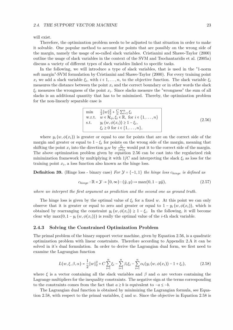
In the following, we will introduce a type of slack variables, that is used in the "1-normsoft margin"-SVM formulation by Cristianini and Shawe-Taylor (2000). For every training pointxi we add a slack variable ξi, with i ∈ 1, . . . , n, to the objective function. The slack variable ξimeasures the distance between the point xi and the correct boundary or in other words the slackξi measures the wrongness of the point xi. Since slacks measure the "wrongness" the sum of allslacks is an additional quantity that has to be minimized. Thereby, the optimization problemfor the non-linearly separable case is

min 12∥w∥2

2 + Cn ∑

ni=1 ξi

w.r.t. w ∈Hφ, ξi ∈ R, for i ∈ 1, . . . , ns.t. yi ⟨w,φ(xi)⟩ ≥ 1 − ξi,

ξi ≥ 0 for i ∈ 1, . . . , n,

(2.56)

where yi ⟨w,φ(xi)⟩ is greater or equal to one for points that are on the correct side of themargin and greater or equal to 1 − ξi for points on the wrong side of the margin, meaning thatshifting the point xi into the direction yiw by ξi

∥w∥2would put it to the correct side of the margin.

The above optimization problem given by equation 2.56 can be cast into the regularized riskminimization framework by multiplying it with 1/C and interpreting the slack ξi as loss for thetraining point xi, a loss function also known as the hinge loss.

Definition 39. (Hinge loss - binary case) For Y = −1,1 the hinge loss chinge is defined as

chinge ∶ R ×Y → [0,∞) ∶ (y, y)↦max(0,1 − yy), (2.57)

where we interpret the first argument as prediction and the second one as ground truth.

The hinge loss is given by the optimal value of ξi for a fixed w. At this point we can onlyobserve that it is greater or equal to zero and greater or equal to 1 − yi ⟨w,φ(xi)⟩, which isobtained by rearranging the constraint yi ⟨w,φ(xi)⟩ ≥ 1 − ξi. In the following, it will becomeclear why max(0,1 − yi ⟨w,φ(xi)⟩) is really the optimal value of the i-th slack variable.

2.4.3 Solving the Constrained Optimization Problem

The primal problem of the binary support vector machine, given by Equation 2.56, is a quadraticoptimization problem with linear constraints. Therefore according to Appendix 2.A it can besolved in it’s dual formulation. In order to derive the Lagrangian dual form, we first need toexamine the Lagrangian function

L(w, ξ, β,α) = 12∥w∥2

2 +Cn

∑i=1ξi −

n

∑i=1βiξi −

n

∑i=1αi(yi ⟨w,φ(xi)⟩ − 1 + ξi), (2.58)

where ξ is a vector containing all the slack variables and β and α are vectors containing theLagrange multipliers for the inequality constraints. The negative sign at the terms correspondingto the constraints comes from the fact that a ≥ b is equivalent to −a ≤ −b.

The Lagrangian dual function is obtained by minimizing the Lagrangian formula, see Equa-tion 2.58, with respect to the primal variables, ξ and w. Since the objective in Equation 2.58 is


a convex function with respect to w and ξ its minimum can be found by setting the gradientswith respect to w and ξ,

∂L

∂w(w, ξ, β,α) = w −

n

∑i=1αiyiφ(xi) != 0 (2.59)

and∂L

∂ξi(w, ξ, β,α) = C1 − β − α != 0, for i ∈ 1, . . . , n (2.60)

to zero. From Equation 2.59 follows that

w =n

∑i=1αiyiφ(xi) (2.61)

and from Equation 2.60 follows thatβ = C1 − α. (2.62)

Additionally, the remaining Karush-Kuhn-Tucker (KKT) conditions, namely the KKT com-plementarity conditions

αi(yi ⟨w,φ(xi)⟩ − 1 + ξi) = 0(αi −C)ξi = 0 (using βi = C − αi)

(2.63)

must be satisfied.Remark 40. (Hinge loss) The KKT conditions legitimate the definition of the hinge loss, seeEquation 2.57. When the i-th boundary constraint, yi ⟨w,φ(xi)⟩ − 1 + ξi ≥ 0, is active, i.e.αi > 0, then ξi must be equal to 1 − yi ⟨w,φ(xi)⟩ and αi must be equal to C and when the i-thboundary constraint is inactive, i.e. αi = 0, then ξ must be equal to zero in order to satisfy thecomplementarity conditions, given by Equation 2.63.

By substituting Equation 2.61 and Equation 2.62 back into the Lagrange formula 2.58 theLagrangian dual function g

g(α) = 12∥n

∑i=1αiyiφ(xi)∥2

2+Cn

∑i=1ξi−

n

∑i=1

(C − αi)ξi−n

∑i=1αi(yi ⟨

n

∑j=1

αjyjφ(xj), φ(xi)⟩ − 1 + ξi) (2.64)

is obtained. The expression for g can be simplified by using the identity ∥a∥22 = ⟨a, a⟩, for a ∈Hφ,

and the bilinearity of the inner product, resulting in

g(α) = 12

n

∑i,j=1

αiαjyiyj ⟨φ(xi), φ(xj)⟩−n

∑i,j=1

αiαjyiyj ⟨φ(xi), φ(xj)⟩+n

∑i=1αi+

n

∑i=1

(C − αi −C + αi)ξi.

(2.65)After grouping the terms we get

g(α) = −12

n

∑i,j=1

αiαjyiyj ⟨φ(xi), φ(xj)⟩ +n

∑i=1αi. (2.66)

Since the Lagrange dual function g, given by Equation 2.66, provides a lower bound on theoptimal value of the optimization problem it needs to be maximized in order to find the bestpossible lower bound. Maximizing the dual function is equivalent to minimizing its negative

min 12 ∑

ni,j=1 αiαjyiyj ⟨φ(xi), φ(xj)⟩ −∑ni=1 αi

w.r.t. αi ∈ R, for i ∈ 1, . . . , ns.t. 0 ≤ αi ≤ C, for i ∈ 1, . . . , n ,

(2.67)

where the box-constraints for αi come from the KKT conditions and Equation 5.70, since αi ≥ 0,βi ≥ 0 and αi = C − βi imply that αi ≤ C for i ∈ 1, . . . , n.


−1 −0.5 0 0.5 1

0

2

4

6

8

X

Y

(a) Polynomial of degree one

−1 −0.5 0 0.5 1

0

2

4

6

8

X

Y(b) Polynomial of degree three

−1 −0.5 0 0.5 1

0

2

4

6

8

X

Y

(c) Polynomial of degree five

−1 −0.5 0 0.5 1

0

2

4

6

8

X

Y

(d) Polynomial of degree ten

−1 −0.5 0 0.5 1

0

2

4

6

8

X

Y

(e) Polynomial of degree 15

Figure 2.4: Linear regression using polynomials of increasing degree (red). The training datapoints (green) were generated by evaluating a polynomial function (blue) and adding Gaussiannoise.


−1 −0.5 0 0.5 1

0

2

4

6

8

X

Y

(a) Polynomial of degree 15

−1 −0.5 0 0.5 1

0

2

4

6

8

X

Y

(b) Polynomial of degree 15

Figure 2.5: Linear regression using polynomials of degree 15 (red). The training data points(green) were generated by evaluating a polynomial function (blue) and adding Gaussian noise.The only difference between the training data in the left figure and in the right figure is thatthe point indicated as a dot in both figures doesn’t correspond.


−1 −0.5 0 0.5 1

0

2

4

6

8

X

Y

(a) λ equal to zero

−1 −0.5 0 0.5 1

0

2

4

6

8

X

Y

(b) λ equal to 0.1

−1 −0.5 0 0.5 1

0

2

4

6

8

X

Y

(c) λ equal to one

−1 −0.5 0 0.5 1

0

2

4

6

8

X

Y

(d) needlessly large λ

Figure 2.6: Ridge regression using polynomials of degree 15 (red) with different trade-off param-eters λ. The training data points (green) were generated by evaluating a polynomial function(blue) and adding Gaussian noise.


y

x

Figure 2.7: Several elements of the version space are illustrated in different colors. All of themminimize the empirical risk with the zero-one loss, however intuitively we would tend to choosea hypothesis similar to the red, blue or purple one. The red line is the one that satisfies themaximum margin property. The illustration is derived from an illustration by Yifan.

y

x

w⋅ x+ b= 0w

⋅ x+ b= 1

w⋅ x+ b= −

1

2∥w∥

b∥w∥

w

Figure 2.8: The hyperplane with the maximum margin in a two dimensional example. Intwo dimensions the hyperplane corresponds to a line. For simplicity reasons the feature spacemapping φ(x) = (x,1)′ and the weight vector w = (w, b)′ resulting in ⟨(w, φ(x))⟩ = wx + b areused. The dotted lines illustrate the boundaries of the margin, which are set to one and minusone, respectively. The illustration is taken from Yifan.

Appendix

2.A Constrained Optimization

In this section the Karush-Kuhn-Tucker theory is briefly summarized, the material mainly istaken from the Convex Optimization textbook of Boyd and Vandenberghe (2004), where furtherdetails and proofs can be found.

2.A.1 The Problem

The goal of this chapter is to solve an optimization problem with respect to certain constraints

min f(x)w.r.t. x ∈ Rns.t. gi(x) ≤ 0, i = 1, . . . ,m,

hj(x) = 0, j = 1, . . . , p.

(2.68)

Example 41. Problems of this shape naturally occur in many scenarios, imagine for examplethat you would like to build a windmill at a given contour line of a mountain. Obviously thestrength of the wind can vary at different locations and therefore it would be beneficial to choosethe location on the contour line with the largest wind strength. In this scenario the variable ofinterest x ∈ R3 would correspond to a position in space, the objective function would be a functionf ∶ R3 → R, that gives the wind strength at a given position and the constraint could be anotherfunction h ∶ R3 → R,that is zero if and only if the current position is located on the contour lineof interest. Since Optimization Problem 2.68 is stated as a minimization problem it the sign ofthe objective function has to be reversed in order to maximize the wind strength, resulting in

min −f(x)w.r.t. x ∈ R3

s.t. h(x) = 0..

2.A.2 The Lagrangian Function

Definition 42. (Lagrange function) For Optimization Problem 2.68, the Lagrange function

L(x,λ, ν) ∶= f(x) +m

∑i=1λigi(x) +

p

∑j=1

νjhj(x) (2.69)

is obtained by adding a linear combination of the constraints to the objective function. Thelinear factors are often referred to as Lagrange multipliers in honor of "Joseph-Louis de La-grange".

29


When having a look at the gradient of the Lagrange function

∇L(x,λ, ν) =⎛⎜⎝

∂L∂x (x,λ, ν)g(x)h(x)

⎞⎟⎠, (2.70)

where g ∶ Rn → Rm is a vector valued function with the inequality constraints as componentfunctions and h ∶ Rn → Rp is a vector valued function with the equality constraints as componentfunctions. By setting the gradient of the Lagrange function to zero it is guarantied, that theequality constraints are fulfilled. To ensure the validity of the inequality constraints additionalconditions, referred to as Karush-Kuhn-Tucker (KKT) conditions, are necessary. The KKT con-ditions are named after Kuhn (1982) and Kuhn and Tucker (1951) and are used to generalize theLagrange multiplier formalism to constraint optimization problems with inequality constraints.After adding the KKT conditions, the optimization problem is

maxλ,ν minxL(x,λ, ν)s.t. λi ≥ 0, i = 1, . . . ,m,

λigi(x) = 0, i = 1, . . . ,m,(2.71)

which is referred to as the dual problem. We shall see in the remainder of this chapter why thedual problem takes this form.

2.A.3 The Lagrangian dual function

Definition 43. (Lagrange dual function) The Lagrange dual function is defined as the infimumof the Lagrange function with respect to the primal variable

D ∶ Rm ×Rp → R ∶ (λ, ν)↦ infxL(x,λ, ν). (2.72)

As we shall see in the next section the Lagrange dual function provides a lower bound of theoptimal solution.

2.A.4 Linear approximation interpretation

If the optimization problem would be unconstrained and the objective function differentiableit would be straightforward to examine the function’s extrema, by setting the gradient to zeroand analyzing the definiteness of the hessian matrix. Motivated by that thought OptimizationProblem 2.68 can be transformed to an unconstrained optimization problem,

min f(x) +∑mi=1 I−(gi(x)) +∑pj=1 I0(hj(x))

w.r.t. x ∈ Rn, (2.73)

where the indicator functions

I0 ∶ R→ R ∶ u↦⎧⎪⎪⎨⎪⎪⎩

0 if u = 0∞ else

(2.74)

and

I− ∶ R→ R ∶ u↦⎧⎪⎪⎨⎪⎪⎩

0 if u ≤ 0∞ else

(2.75)

are used to exclude unwanted results, by punishing them infinitely hard. If the constraintsare fulfilled the indicator functions output zero, and therefore are not affecting the objective

2.A. CONSTRAINED OPTIMIZATION 31

function at all. However if a point violates a constraint the corresponding indicator functionadds a penalty (+∞) to the objective. As a consequence points violating the constraints arenot considered when looking for the minimum. Linearly approximating the indicator functionsyields the Lagrangian function

L(x,λ, ν) = f(x) +∑mi=1 λigi(x) +∑pj=1 νjhj(x). (2.76)

In a certain sense the previously hard punishment of unwanted solutions now turned intoa soft one. Assuming λ > 0 for inequality constraints the punishment is zero when gi(x) = 0,larger than zero when gi(x) > 0 and smaller than zero when gi(x) < 0. Consequently solutionsinside of the compactum, parametrized by gi, with a margin to the boundary are preferred usingthe soft formulation. Similar considerations can be made for equality constraints, which can berewritten in terms of inequality constraints

hi(x) = 0 ⇐⇒ hi(x) ≤ 0 ∧ hi(x) ≥ 0. (2.77)

Therefore, the Lagrange function can be written as

f(x) +m

∑i=1λigi(x) +

p

∑j=1

αjhj(x) −p

∑j=1

βjhj(x), (2.78)

where α > 0 and β > 0 are the Lagrange multipliers for the inequality constraints correspondingto the equality constrain. Obviously the equation ν = α−β holds, meaning that ν can be any realnumber, which is not particularly satisfying when thinking of νjhj(x) as approximations of thepenalty terms. Nevertheless the linear approximations underestimate the indicator functions,since λiu ≤ I−(u) and νju ≤ I0(u) hold for all u. As a consequence, the expression

maxλ,ν minxL(x,λ, ν), (2.79)

gives the best lower bound on the optimal value of the original problem. The function D(λ, ν) =minxL(x,λ, ν) is called the Lagrange dual function of the problem.

2.A.5 Weak and Strong Duality

One question that naturally rises is how good the best lower bound obtained from the dualproblem can be. Let p∗ denote the optimal value of the Optimization Problem 2.68, in thiscontext usually called primal problem, and let d∗ denote the best lower bound on p∗ that canbe obtained from D, then a property which is called weak duality, namely

d∗ ≤ p∗, (2.80)

always holds. If the equalityd∗ = p∗ (2.81)

holds, we speak of strong duality. Slater’s theorem, introduced by Slater (2014), provides asufficient condition for strong duality to hold. Namely, if the primal problem is convex andstrictly feasible, such that

∃x0 ∈ Rn ∶ gi(x0) < 0, hj(x0) = 0 for i = 1, . . . ,m and j = 1, . . . , p, (2.82)

where the inequality constraints g1, . . . , gm are convex and the equality constraints h1, . . . , hp areaffine functions, strong duality will hold.


2.A.6 Karush-Kuhn-Tucker Optimality Conditions

For differentiable functions f, g1, . . . , gm, h1, . . . , hm any pair primal and dual optimal points x∗and (λ∗, ν∗) with strong duality, i.e. a duality gap f(x∗)−D(λ∗, ν∗) equal to zero, must satisfy

∇f(x∗) +m

∑i=1λi∇gi(x∗) +

p

∑j=1

νj∇hj(x∗) = 0, (2.83)

since x∗ minimizes the Lagrange function L(x,λ∗, ν∗) over x. Therefore, following conditions

gi(x∗) ≤ 0, i = 1, . . . ,mhi(x∗) = 0, i = 1, . . . , p

λi ≥ 0, i = 1, . . . ,mλigi(x∗) = 0, i = 1, . . . ,m

∇f(x) +m

∑i=1λi∇gi(x) +

p

∑j=1

νj∇hj(x) = 0,

(2.84)

which are called Karush-Kuhn-Tucker conditions, must hold for any pair of primal and dualoptimal points.

Chapter 3

Kernel Methods

3.1 Motivation

We have seen that machine learning methods work well in the linear separable case. However,as far as the real world’s problems are concerned, we cannot rely on the linear separability of thedata. In fact, we cannot even generally assume that the data is represented in a Hilbert space.We have already seen that one way to deal with non-linear separable and abstract data is toembed it into a Hilbert space, usually referred to as feature space. Thereby, implicitly a differenthypothesis space is utilized, within which the embedded data points are possibly separable. Sofar, we rarely had to clarify explicitly which particular feature space mapping we used, despitethe fact that in practice - for the solution of a problem - this is a mandatory step. Unfortunately,the choice of a feature space mapping can be difficult, particularly when working with abstractobjects. Even when working with vector valued data the embedding into the feature space canbe a non-linear function and the feature space can be high dimensional. Even when leaving thechoice of feature space aside, the embedding into the feature space and the calculations in thefeature space are often computationally expensive.

Recently, kernel methods gained a lot of attention since they provide a tool to use theadvantages of using high dimensional feature spaces, while avoiding the computational costs ofembedding the data. The following example is intended to provide a better understanding ofthe problem.

Example 44. (Kernel classifier) Let the input space X be a non-empty set, z ∈ (X × Y)m atraining sample and φ ∶ X → Hφ a feature space mapping. In the previous chapter we saw thatlinear classifiers depend on the evaluation of a linear form

f ∶ X → R ∶ x↦ ⟨w,φ(x)⟩ .

Let’s assume for now that w has a representation of the form

w =m

∑i=1γiφ(xi), (3.1)

in which γ ∈ Rm, like in the SVM example in Equation 2.61, where γi would be yiαi. Then,by using the representation of w given by Equation 3.1 and the bilinearity of the inner product,an evaluation of a linear form can be written as a linear combination of inner products between

33

34 CHAPTER 3. KERNEL METHODS

training points and the point of interest

f(x) = ⟨w,φ(x)⟩

= ⟨m

∑i=1γiφ(xi), φ(x)⟩

=m

∑i=1γi ⟨φ(xi), φ(x)⟩ .

(3.2)

Therefore, if we knew how to compute the inner product in the feature space for pairs of elementsof the input space, i.e. if we knew how to compute k(x, x) ∶= ⟨φ(x), φ(x)⟩, the explicit featuremapping φ would not be necessary in order to evaluate linear classifiers. The function k ∶ X×X →R is called kernel function.

As seen in the previous example, a kernel function corresponds to an inner product in afeature/inner-product space. Therefore, if the problem admits a representation where datapoints only enter via inner products in the feature space and the kernel function of that featurespace is known, the utilization of the benefits provided by the feature space by evaluating theinner products directly via the kernel function will be possible. In many cases it is compu-tationally more efficient to evaluate the kernel function directly than to embed the data andconsecutively compute the inner product between the embedded data points. The followingexample is intended to provide a better idea of the magnitudes of the computational benefits.

Example 45. (Polynomial kernel) To separate the data depicted in Figure 2.2 a feature spacewith quadratic basis functions was used. Obviously, the last time when we considered this exampleprior knowledge about the classes influenced the choice of basis functions of the feature space.Typically, we don’t have prior knowledge about the classes in real world applications, which iswhy it would make sense to include additional basis functions in order to solve more generaltasks. Intuitively, one could include linear basis functions and also basis functions in the formof polynomials of higher degree. This considerations ultimately lead to the space of polynomials ofa certain degree, which we will see later in this chapter. For now consider polynomials of degreetwo with two dimensional inputs. One possible feature space mapping in order to represent suchpolynomials is

φ ∶ R2 → R6 ∶ (x, y)↦ (x2, y2,√

2xy,√

2x,√

2y,1)′, (3.3)

where the coefficients of x, y and xy are chosen equal√

2 for mathematical convenience. Evenin this small scale example a quick growth of the dimensionality required to represent the datais visible, if the dimensionality of the input data was increased from two to n ≥ 2, i.e.

φn((x1, . . . , xn)′) =(x2

1, . . . , x2n

´¹¹¹¹¹¹¹¹¹¹¹¹¹¹¹¹¹¹¹¸¹¹¹¹¹¹¹¹¹¹¹¹¹¹¹¹¹¹¹¶n

,√

2x1x2, . . . ,√

2x1xn´¹¹¹¹¹¹¹¹¹¹¹¹¹¹¹¹¹¹¹¹¹¹¹¹¹¹¹¹¹¹¹¹¹¹¹¹¹¹¹¹¹¹¹¹¹¹¹¹¹¹¹¹¹¹¹¹¹¹¹¹¹¸¹¹¹¹¹¹¹¹¹¹¹¹¹¹¹¹¹¹¹¹¹¹¹¹¹¹¹¹¹¹¹¹¹¹¹¹¹¹¹¹¹¹¹¹¹¹¹¹¹¹¹¹¹¹¹¹¹¹¹¹¹¹¶

n−1

,√

2x2x3, . . . ,√

2x2xn´¹¹¹¹¹¹¹¹¹¹¹¹¹¹¹¹¹¹¹¹¹¹¹¹¹¹¹¹¹¹¹¹¹¹¹¹¹¹¹¹¹¹¹¹¹¹¹¹¹¹¹¹¹¹¹¹¹¹¹¹¹¸¹¹¹¹¹¹¹¹¹¹¹¹¹¹¹¹¹¹¹¹¹¹¹¹¹¹¹¹¹¹¹¹¹¹¹¹¹¹¹¹¹¹¹¹¹¹¹¹¹¹¹¹¹¹¹¹¹¹¹¹¹¹¶

n−2

, . . . ,√

2xn−1xn´¹¹¹¹¹¹¹¹¹¹¹¹¹¹¹¹¹¹¹¹¸¹¹¹¹¹¹¹¹¹¹¹¹¹¹¹¹¹¹¹¹¹¶

1´¹¹¹¹¹¹¹¹¹¹¹¹¹¹¹¹¹¹¹¹¹¹¹¹¹¹¹¹¹¹¹¹¹¹¹¹¹¹¹¹¹¹¹¹¹¹¹¹¹¹¹¹¹¹¹¹¹¹¹¹¹¹¹¹¹¹¹¹¹¹¹¹¹¹¹¹¹¹¹¹¹¹¹¹¹¹¹¹¹¹¹¹¹¹¹¹¹¹¹¹¹¹¹¹¹¹¹¹¹¹¹¹¹¹¹¹¹¹¹¹¹¹¹¹¹¹¹¹¹¹¹¹¹¹¹¹¹¹¹¹¹¹¹¹¹¹¹¹¹¹¹¹¹¹¹¹¹¹¹¹¹¹¹¹¹¹¹¹¹¹¹¹¹¹¹¹¹¹¹¹¹¹¹¹¹¹¹¹¹¹¹¹¹¹¹¹¹¹¹¹¹¹¹¹¹¹¹¹¹¹¹¹¹¹¹¹¹¹¹¹¹¹¹¹¹¹¹¹¹¹¹¹¹¹¹¹¹¹¹¹¹¹¹¹¹¹¸¹¹¹¹¹¹¹¹¹¹¹¹¹¹¹¹¹¹¹¹¹¹¹¹¹¹¹¹¹¹¹¹¹¹¹¹¹¹¹¹¹¹¹¹¹¹¹¹¹¹¹¹¹¹¹¹¹¹¹¹¹¹¹¹¹¹¹¹¹¹¹¹¹¹¹¹¹¹¹¹¹¹¹¹¹¹¹¹¹¹¹¹¹¹¹¹¹¹¹¹¹¹¹¹¹¹¹¹¹¹¹¹¹¹¹¹¹¹¹¹¹¹¹¹¹¹¹¹¹¹¹¹¹¹¹¹¹¹¹¹¹¹¹¹¹¹¹¹¹¹¹¹¹¹¹¹¹¹¹¹¹¹¹¹¹¹¹¹¹¹¹¹¹¹¹¹¹¹¹¹¹¹¹¹¹¹¹¹¹¹¹¹¹¹¹¹¹¹¹¹¹¹¹¹¹¹¹¹¹¹¹¹¹¹¹¹¹¹¹¹¹¹¹¹¹¹¹¹¹¹¹¹¹¹¹¹¹¹¹¹¹¹¹¹¹¹¹¶

(n+1)n2

,√

2x1, . . . ,√

2xn´¹¹¹¹¹¹¹¹¹¹¹¹¹¹¹¹¹¹¹¹¹¹¹¹¹¹¹¹¹¹¹¹¹¹¹¹¹¹¹¹¹¹¹¸¹¹¹¹¹¹¹¹¹¹¹¹¹¹¹¹¹¹¹¹¹¹¹¹¹¹¹¹¹¹¹¹¹¹¹¹¹¹¹¹¹¹¹¹¶

n

, 1®1

),

(3.4)the dimensionality of the second-degree polynomial feature space would increase to 1+n+ (n+1)n

2 ,one dimension for the constant term, n dimensions for the linear terms and (n+1)n

2 dimensionsfor the quadratic terms. This trend continues when increasing the degree of the polynomial,resulting in high dimensional feature spaces, where computations are costly. In contrast to that,the evaluation of the kernel function corresponding to those feature spaces can be performed effi-ciently. In the example at hand focusing on the second-order polynomial space the corresponding

3.2. THE KERNEL TRICK 35

kernel function is

k(u, v) = ⟨φ(u), φ(v)⟩= (x2

1, y21,

√2x1y1,

√2x1,

√2y1,1) ⋅ (x2

2, y22,

√2x2y2,

√2x2,

√2y2,1)′

= x21x

22 + y2

1y22 + +2x1x2y1y2 + 2x1x2 + 2y1y2 + 1

= 1 + 2x1x2 + 2y1y2 + x21x

22 + 2x1x2y1y2 + y2

1y22 (rearrangement of terms)

= 1 + 2 ⟨u, v⟩ + ⟨u, v⟩2 (by definition of u & v)= (⟨u, v⟩ + 1)2 (binomial equation),

(3.5)where u = (x1, y1)′ and v = (x2, y2)′ and instead of 1+n+ (n+1)n

2 multiplications, that are necessaryfor the computation of the inner product in the feature space, only n + 1 multiplications arerequired for the direct evaluation of the corresponding kernel function. In our example n wasequal to two.

At this point, it is worth pointing out that considering the kernel version of machine learningproblems can be seen as a computational trick in a certain sense, which might be one of thereasons why in the literature (Shawe-Taylor and Cristianini, 2004; Herbrich, 2001) the processof transforming an algorithm into its kernel form is known as the kernel trick. Using kernelmethods not only high dimensional feature spaces can be utilized but also infinite dimensionalones, as we will see when having a look at Gaussian kernels. To make a long story short, thegoal of this chapter is to utilize kernel functions in order to access the hypothesis spaces inducedby feature space mappings in a computationally more efficient way.

3.2 The Kernel Trick

As previously mentioned, the kernel function belonging to a non-linear feature space Hφ is givenby

k(x, y) = φ(x)′φ(y) = ⟨φ(x), φ(y)⟩ , (3.6)

which corresponds to the inner product in that feature space. If it is possible to rewrite analgorithm in such a way that the input vectors only enter via inner products, the latter will bereplaced by arbitrary kernel functions - a process which is known as the kernel trick.

3.2.1 When Can the Kernel Trick Be Applied?

The Real Valued Case

The kernel trick is applicable to quadratic programming problems with linear constraints. Con-sequently, the optimization problems of many linear parametric models

min 12w

′Qw + c′dw.r.t. w ∈Hφ, d ∈ R∣I∪J ∣,s.t. yi ⟨w,φ(xi)⟩ − fi(d) = 0, for i ∈ I

yj ⟨w,φ(xj)⟩ − gj(d) ≥ 0, for j ∈ J ,

(3.7)

where a training sample z of size n is considered, I,J are subsets of 1, . . . , n, φ is a featurespace mapping from X to Hφ, Q is symmetric linear operator from Hφ to Hφ, c and d are vectorsin R∣I∪J ∣ and fi for i ∈ I and gj for j ∈ J are differentiable functions from R∣I∪J ∣ to R, allowfor the application of the kernel trick.


In order to derive the kernel representation of the optimization problem, consider the corre-sponding Lagrange function

L(w,d,α, β) = 12w′Qw + c′d +∑

i∈I

αi(⟨w,φ(xi)⟩ − fi(d)) − ∑j∈J

βj(⟨w,φ(xj)⟩ − gj(d)). (3.8)

Note that there is no co-occurrence of feature vectors φ(x), with x ∈ X , and the primal parameterd. As a consequence, the optimization for the parameter d has no impact on the applicabilityof the kernel trick. Therefore, we only need to consider the derivatives with respect to w inorder to figure out whether the kernel trick is applicable. When considering the gradient of theLagrange function with respect to w, the primal variable w occurs only linearly

∂L

∂w(w,d,α, β) = Qw +∑

i∈I

αiφ(xi) − ∑j∈J

βjφ(xj). (3.9)

Setting the gradient with respect to the primal variable to zero and solving for the primalvariable yields

w = Q−1(−∑i∈I

αiφ(xi) + ∑j∈J

βjφ(xj))

=∶ Q−1 ∑i∈K

γiφ(xi), with K ∶= I ∪J ,(3.10)

and substituting it back into the Lagrange function will yield a Lagrangian dual problem inwhich the kernel trick is applicable. When substituting Equation 3.10 into w′Qw we get

w′Qw = (Q−1 ∑i∈K

γiφ(xi))′

Q(Q−1 ∑i∈K

γiφ(xi))

= (∑i∈K

γiφ(xi)′(Q−1)′)(∑i∈K

γiφ(xi)) (transpose and QQ−1 = id)

= (∑i∈K

γiφ(xi)′Q−1)(∑i∈K

γiφ(xi)) (symmetry of Q−1)

(3.11)

since the inverse of a symmetric operator Q−1 is a symmetric operator. According to the spectraltheorem the symmetric operator Q−1 can be written as (Q−1) 1

2 (Q−1) 12 , yielding

w′Qw = (∑i∈K

γiφ(xi)′(Q−1)12 )((Q−1)

12 ∑i∈K

γiφ(xi)) (by Q−1 = (Q−1)12 (Q−1)

12 )

= ⟨∑i∈K

γi((Q−1)12 )′φ(xi),∑

i∈K

γi(Q−1)12φ(xi)⟩ (by φ(xi)′(Q−1)

12 = ((Q−1)

12 )′φ(xi))

= ⟨∑i∈K

γi(Q−1)12φ(xi),∑

i∈K

γi(Q−1)12φ(xi)⟩ (by (Q−1)

12 = Pdiag(

√λ1, . . . ,

√λd)P ′)

= ∑i,j∈K

γiγj ⟨(Q−1)12φ(xi), (Q−1)

12φ(xj)⟩ (bilinearity of inner product),

(3.12)which is a linear combination of inner products in the feature space induced by (Q−1) 1

2 φ.


Similarly substituting Equation 3.10 into ∑i∈I αiw′φ(xi) − fi(d) yields

∑i∈I

αi(w′φ(xi) − fi(d)) =∑i∈I

αi((Q−1 ∑j∈K

γjφ(xj))′φ(xi) − fi(d))

=∑i∈I

αi((∑j∈K

γjφ(xj)′)(Q−1)′φ(xi) − fi(d)) (transpose)

=∑i∈I

αi((∑j∈K

γjφ(xj)′)Q−1φ(xi) − fi(d)) (symmetry of Q−1)

=∑i∈I

∑j∈K

(αiγjφ(xj)′Q−1φ(xi)) −∑i∈I

αifi(d) (distributivity)

=∑i∈I

∑j∈K

αiγj ⟨(Q−1)12φ(xi), (Q−1)

12φ(xj)⟩ −∑

i∈I

αifi(d) (similar to Equation 3.12),

(3.13)which is a linear combination of inner products in the feature space induced by (Q−1) 1

2 φ. Thesubstitution for ∑i∈J βiw′φ(xi) − gi(d) works analogously.

We have already seen a concrete example clarifying the statements above, namely the dualproblem of the binary support vector machine given by Equation 2.67 which depends only oninner products in the feature space and thereby allows the application of the kernel trick. Inorder to obtain the corresponding primal optimization problem Q is set to the identity mapping,J is set to 1, . . . , n, I is set to ∅, c is set to 1Cn and gj(d) is set to 1 − dj . An alternativeframework that is capable of transforming general linear programming problems into their kernelform was introduced by Mangasarian (2006).

Beyond the Real Valued Case

Of course, the kernel trick is not limited to the real valued learning problems. Prior to furtherinvestigations concerning theoretical details of the kernel formulation of real valued learningproblems, a brief look at the kernel version of the regularized multivariate linear regression willshed more light on the issue. In the following we will encounter various additional exampleswith more complex output spaces.Example 46. (Linear Kernel Regression1): In the multivariate case of the linear regressionproblem with regularization the input space X is a d-dimensional R-vector space and the outputspace Y is a k-dimensional R-vector space. Given a set of observations

(xi, yi)Ni=1 ∈ (X ×Y)N (3.14)

we are looking for a linear function

f ∶ X → Y ∶ x↦Wx, (3.15)

parametrized by a the k × d matrix W, that minimizes the sum-of-squares error

minW

12N

∑i=1

∥yi −Wxi∥2 + C2∥W∥2

Frobenius. (3.16)

Looking at the objective function at hand it is not trivial to formulate the Lagrangian dual.However, substituting yi −Wxi with ξi and adding equality constraints of the form ξi = yi −Wxito the optimization problem

min 12 ∑

Ni=1 ∥ξi∥2 + C

2 ∥W∥2Frobenius

w.r.t. W ∶ X → Y, ξ ∈ Ys.t. ξi = yi −Wxi, i ∈ 1 . . .N

(3.17)

1Similar examples are considered by Saunders et al. (1998) and Cortes et al. (2006).


does the trick. As a consequence, the linear regression problem can be considered from a con-strained optimization perspective, where the Lagrangian dual form can be derived. The Lagrangefunction of the constrained optimization problem is

L(W, ξ,A) = 12N

∑i=1

∥ξi∥2 + C2∥W∥2

Frobenius +N

∑i=1α′i(Wxi − yi + ξi), (3.18)

where A is a k × N matrix with columns α1, . . . , αN . In order to obtain the Lagrangian dualfunction the gradients of the Lagrangian with respect to the primal variables

∂L

∂W(W, ξ,A) = CW +

N

∑i=1αix

′i

!= 0 (3.19)

and∂L

∂ξi(W, ξ,A) = ξi + αi != 0 (3.20)

are set to zero. From Equation 3.19 follows that

W = − 1C

N

∑i=1αix

′i (3.21)

and from Equation 3.20 follows thatξi = −αi. (3.22)

By substituting Equation 3.21 and Equation 3.22 back into the Lagrange formula, given by Equa-tion 3.18, the Lagrangian dual function is obtained. The substitution of the expression for Winto the Frobenius norm is considered separately before performing the substitution into the La-grange function and yields

∥ − 1C

N

∑i=1αix

′i∥2Frobenius = ⟨− 1

C

N

∑i=1αix

′i,−

1C

N

∑j=1

αjx′j⟩Frobenius

= 1C2

N

∑i=1

N

∑j=1

⟨αix′i, αjx′j⟩Frobenius (bilinearity of inner product)

= 1C2

N

∑i=1

N

∑j=1

tr((αix′i)′αjx′j) (definition of Frobenius inner product)

= 1C2

N

∑i=1

N

∑j=1

tr(xiα′iαjx′j) (transpose)

= 1C2

N

∑i=1

N

∑j=1

α′iαjtr(xix′j) (α′i ⋅ αjis a scalar & linearity of trace)

= 1C2

N

∑i=1

N

∑j=1

α′iαj ⟨xi, xj⟩ (tr(xy’) = tr(x’y)),

(3.23)in which ∥A∥Frobenius = tr(A′A) denotes the Frobenius norm and ⟨A,B⟩Frobenius ∶= ∑i,j AijBijthe Frobenius inner product.


Similarly by substituting the new expression for W into ∑Ni=1 α′iWxi

N

∑i=1α′i(−

1C

N

∑j=1

αjx′j)xi = −

1C

N

∑i=1

N

∑j=1

α′iαjx′jxi

= − 1C

N

∑i=1

N

∑j=1

α′iαj ⟨xi, xj⟩(3.24)

is obtained. Substituting everything back into the Lagrange formula given by Equation 3.18 yields

g(A) = −12N

∑i=1

∥αi∥2 + 12C

N

∑i=1

N

∑j=1

α′iαj ⟨xi, xj⟩ −1C

N

∑i=1

N

∑j=1

α′iαj ⟨xi, xj⟩

= −12N

∑i=1

∥αi∥2 − 12C

N

∑i=1

N

∑j=1

α′iαj ⟨xi, xj⟩ ,(3.25)

where the kernel trick can be applied. As a result, we end up the dual function

g(A) = −12N

∑i=1

∥αi∥2 − 12C

N

∑i=1

N

∑j=1

α′iαjk(xi, xj). (3.26)

Since the Lagrange dual function g, given by Equation 3.25, provides a lower bound on theoptimal value of the optimization problem, it needs to be maximized in order to find the bestpossible lower bound. Maximizing the dual function is equivalent to minimizing its negative

min 12 ∑

Ni=1 ∥αi∥2 + 1

2C ∑Ni=1∑Nj=1 α

′iαjk(xi, xj)

w.r.t. αi ∈ Y, i ∈ 1 . . .N . (3.27)

3.2.2 Summary and Outlook

For many machine learning algorithms the kernel trick is applicable. It allows for the access tothe hypothesis space given by the composition of the feature space mapping φ ∶ X → Hφ andlinear forms from Hφ to R,

Hφ ∶= g ∶ X → R ∶ g = f φ, f ∈H∗φ and feature space mapping φ, (3.28)

without the need of an explicit representation of the feature space mapping, namely by consid-ering

Hk ∶= g ∶ X → R ∶ g =n

∑i=1αik(xi, ⋅), for n ∈ N, x1, . . . , xn ∈ X , α1, . . . αn ∈ R and k is a kernel function,

(3.29)where k(x, y) ∶= ⟨φ(x), φ(y)⟩. It is to be noted that this is a non-trivial statement, which has sofar only been motivated by examples. In the following, additional work will be put into showingthat the equivalence

Hφ⇔Hk (3.30)

holds.


Chapter 4

A Glance at Kernel Theory

This chapter is meant to introduce some of the theorems that build the theoretic foundation ofkernel methods, how they are used in the machine learning context, respectively. We revise thetheoretical foundation of the kernel trick and the usage of the resulting hypothesis spaces in thescope of the regularized risk minimization framework. Most of the material is based on reviewsabout reproducing kernel Hilbert spaces by Hofmann et al. (2006) and Wahba (2003) and thestatistical learning course notes of Poggio and Rosasco (2015).

4.1 Terminology - Kernel

The type of functions that are referred to as kernel functions in the context of machine learningwere initially examined by mathematicians, like Hilbert (1904), Mercer (1909) and Aronszajn(1950), in the first half of the 20th century in the scope of integral calculus. Hilbert (1989) usedthe German term ’Kern’ for complete quadratic forms that characterize linear integral equationsof the form

φ(s) = f(s) + ∫b

ak(s, t)φ(t)dt, (4.1)

where the goal is to find the unknown function φ given an inhomogeneity function f and a’Kern’ k. In the German language the term ’Kern’ - comparable to the English word core -refers to the innermost part of an object or organism such as a fruit. The ’Kern’ is the mostcentral and essential part of the fruit since it is fully determined by its ’Kern’ carrying thenecessary information and ability for reproduction. Similarly, the ’Kern’ of an integral equationrepresents its most central part, leaving the inhomogeneity aside - the ’Kern’ fully determinesits solution. In the machine learning context the kernel function (’Kern’) can be thought of asthe most central part of a kernel method as well, since the choice of kernel function determinesthe hypothesis space used. Despite the fact that the ’Kern’ serves different purposes in the fruit,the integral equation and the kernel method, it determines the whole system.

4.2 Reproducing Kernel Hilbert Spaces (RKHS)

4.2.1 Outline

In the following, different perspectives on a rich family of hypothesis spaces, so-called reproducingkernel Hilbert spaces (RKHS) as illustrated in Figure 4.1, are going to be studied. First amathematical definition will be introduced followed by a demonstration showing the one to onecorrespondence between RKHS and positive definite kernels. In addition, the equivalence of Hφ

and Hk, given by Equation 3.28 and Equation 3.29, is going to be shown.

41

42 CHAPTER 4. A GLANCE AT KERNEL THEORY

Reproducing Ker-nel Hilbert Spaces

Positivedefinitekernels

Featuremaps

Functionalanalysis

Figure 4.1: Different perspectives on reproducing kernel Hilbert spaces.

4.2.2 Recap & Important Properties of Hilbert Spaces

Before looking at the theorems that provide theoretical justification for the kernel trick, somemathematical definitions and results of relevance, taken from Rudin (2006), Wagner (2004) andHell and Neumann (2012), are going to be revised.

Function space In Chapter 2 we introduced the notion of function space as a set of functionsfrom set X to set Y, see Definition 3. Function spaces are often also vector spaces.

Hypothesis space The function space considered when solving a learning task is referred toas hypothesis space, see Definition 4.

Hilbert space K-Vector spaces with an inner product, that are complete with respect to themetric induced by their inner product, are so-called Hilbert spaces, see Definition 16. Forsimplicity it is to be assumed that the field of real numbers, i.e. K ∶= R, will be usedwithout exception.

Dual space So far function spaces spanned by linear forms on Hilbert spaces called featurespaces were used, see Definition 18. The space spanned by the linear forms from a Hilbertspace H to R

H∗ = f ∶H → R, (4.2)is called dual space. We will see that for the topological dual space H′ of a Hilbert spaceis a Hilbert space with point-wise addition, point-wise scalar multiplication and an innerproduct.

In a Hilbert space of functions we are allowed to add functions, multiply them with scalarswithout leaving the Hilbert space. Additionally, thanks to the inner product associated with the

4.2. REPRODUCING KERNEL HILBERT SPACES (RKHS) 43

Hilbert space, we can talk about both orthogonality and distances, since angles and distancesare closely related to inner products. In order to study the connections between Hilbert spaces,positive definite kernels and feature spaces, some additional properties of Hilbert spaces arerequired, for instance the that Hilbert spaces are topological spaces.

Topological spaces

Earlier, the choice of linear functions on finite dimensional vector spaces as hypothesis functionswas partially motivated by the fact that linear functions on vector spaces are always continuous.In the infinite dimensional spaces a more general concept of continuity is required.

Definition 47. (Topological space) The pair (X ,T ), where X is a set and T is a collectionof subsets of X satisfying the axioms:

1. X ∈ T and ∅ ∈ T ,

2. for all sequences (Ai)i∈N ∈ T N holds that ⋃i∈NAi ∈ T ,

3. for all finite sequences (Ai)Ni=1 holds that ⋂Ni=1Ai ∈ T ,

is called topological space. The collection of sets T is called topology and defines which subsetsare open or closed.

Definition 48. (Open subset & closed subset) A subset S ⊂ X of a topological space (X ,T ) isopen if S ∈ T and closed if X /S ∈ T .

Definition 49. (Topological subspace) A subset S of a topological space (X ,T ) is a topologicalspace equipped with the subspace topology

TS ∶= S ∩O ∶ O ∈ T . (4.3)

This abstract definition of open and closed subsets leads to a more abstract definition ofcontinuity.

Definition 50. (Continuous function) Let (X ,TX ) and (Y,TY) be topological spaces, then afunction f

f ∶ X → Y (4.4)

is continuous iff pre-images of open subsets of Y under f are open subsets of X , i.e.

∀OY ∈ TY ∶ f−1(OY) ∈ TX . (4.5)

Example 51. (Standard topology on Rd) The standard topology T on Rd is defined utilizingthe notion of open balls. An open ball of radius r around the point x ∈ X is defined as

Br(x) ∶= y ∈ Rd ∶ ∥x − y∥ < r, (4.6)

where ∥ ⋅ ∥ is a norm on Rd. Consequently, an open subset O of Rd is characterized by the factthat for every point x ∈ O there exists an ε > 0 such that the ball Bε(x) is a subset of O. Theset of all open subsets, defined this way, is called the standard topology on Rd.


Metric spaces

Definition 52. (Metric space) The pair (X , d), where X is a set and d is a metric, i.e. afunction from X ×X → R satisfying

1. d(x, y) ≥ 0 (non-negativity),

2. d(x, y) = 0⇔ x = y (identity of indiscernibles),

3. d(x, y) = d(y, x) (symmetry),

4. and d(x, z) ≤ d(x, y) + d(y, z) (triangle inequality),

is called metric space.

The reasoning applied in Example 51 can be extended to metric spaces (X , d), where openballs are defined using the metric d

Br(x) ∶= y ∈ X ∶ d(x, y) < r. (4.7)

Accordingly, the metric of a metric space induces a topology. As a consequence, Hilbert spacesare topological spaces as well, since the inner-product induces a norm and this norm induces ametric, which induces a topology.

Definition 53. (Complete metric space) A metric space (X , d) is complete iff the limit x ∶=limn→∞ xn of every Cauchy sequence (xi)i∈N ∈ XN, i.e. every sequence (xi)i∈N ∈ XN satisfying

∀ε > 0 ∶ ∃N ∈ N such that ∀n,m ∈ N with m > N and n > N ∶ d(xm, xn) < ε, (4.8)

is contained in X .

Theorem 54. (Complete subspace) A closed subspace of a complete space is a complete sub-space.

Proof. The interested reader is referred to Rudin (2006).

Hilbert spaces

The notion of Hilbert spaces combines the topological structure with the structure of innerproduct spaces. At this point it is necessary to recall the definition of Hilbert spaces.

Definition 55. (Hilbert space) A Hilbert space H is an inner-product space, which is completewith respect to the metric induced by it’s inner-product.

Example 56. (Examples of Hilbert spaces) The following spaces are Hilbert spaces:

1. l2, the space of square-summable sequences

l2(R) ∶= (xi)i∈N ∈ RN ∶∞

∑i=1

∣xi∣2 <∞ (4.9)

with the inner product

⟨x, y⟩l2 ∶=∞

∑i=1xiyi. (4.10)


2. L2, the space of square-integrable functions

L2(R) ∶= f ∈ RR ∶ ∫∞

−∞∣f(x)∣2dx <∞/g ∈ RR ∶ ∫

∞

−∞∣g(x)∣2dx = 0 (4.11)

with the inner product⟨f, g⟩L2 ∶= ∫

∞

−∞f(x)g(x)dx. (4.12)

3. Any finite dimensional Euclidean vector space with the corresponding scalar product.

The interested reader may verify that the listed examples are Hilbert spaces, by checking theHilbert space properties.

Definition 57. (Topological dual space) The space spanned by linear and continuous froms ona Hilbert space H is referred to as the topological dual space H′. Clearly, the relation H′ ⊂ H∗

holds.

With the properties of the inner product the complement of a subspace can be uniquelydefined.

Definition 58. (Orthogonal complement) For a subspace S of a Hilbert space H the orthogonalcomplement is defined as

S ∶= x ∈H ∶ ∀y ∈ S ∶ ⟨x, y⟩H = 0. (4.13)

The orthogonal complement is always closed.

Theorem 59. (S ⊕ S ≃H) Let H be a Hilbert space and S be a subspace of H, then

⊕ ∶ S × S →H ∶ (x, y)↦ x + y, (4.14)

defines an isomorphism.

Proof. The proof is not particularly interesting for this thesis. It basically needs to be shown,that the function ⊕ is bijective and continuous. The interested reader can find the proof inWagner (2004).

Utilizing the definitions and results introduced so far, we can prove a theorem that will turnout to be important in the following.

Theorem 60. (Riesz representation theorem) Let H be a Hilbert space, not necessarily a Hilbertspace of functions. The mapping ψ defined as

ψ ∶H →H′ ∶ x↦ ⟨x, ⋅⟩H (4.15)

is an isomorphism, i.e. ψ is bijective and continuous.

Proof. The ideas of the following proof were taken from Wagner (2004). In order to show thatψ defines an isomorphism between H and H∗, we only need to prove that ψ exists and that itis bijective, since the linearity follows from the bilinearity of the inner product.

Well-posedness: From

∣ψ(x)(y)∣ = ∣ ⟨x, y⟩H ∣ (by definition)≤ ∥x∥H∥y∥H (Cauchy-Schwarz inequality),

(4.16)


for x, y ∈H, follows

∥ψ(x)∥ ∶= sup∥y∥H≤1

∣ψ(x)(y)∣ (operator norm)

= sup∥y∥H≤1

∣ ⟨x, y⟩H ∣ (definition of ψ)

≤ sup∥y∥H≤1

∣∥x∥H∥y∥H∣ (Cauchy-Schwarz inequality)

= ∥x∥H <∞

(4.17)

and thereby the existence of ψ(x) for all x ∈H.

Injectivity: In order to show that ψ is injective, we show that it is an isometric functional, i.e.for all x ∈H the property ∥ψ(x)∥ = ∥x∥H holds. From Equation 4.17 we already know an upperbound for ∥ψ(x)∥, namely ∥x∥H. If we manage to show that the lower bound of ∥ψ(x)∥ is also∥x∥H for all x ∈ H, we will know that ψ is isometric. The case x = 0 is simple, from Equation4.17 and the properties of the norm, in particular from ∥ ⋅ ∥ ≥ 0, follows that ∥ψ[0]∥ = 0. Ifx ∈H/0,

∥ψ(x)∥ = sup∥y∥H≤1

∣ ⟨x, y⟩H ∣ (definition of ψ)

≥ ∣⟨x, x

∥x∥H⟩H∣ (supremum property)

= ⟨x,x⟩2H

∥x∥H= ∥x∥H (absolute homogenity)

= ∥x∥2H

∥x∥H= ∥x∥H (norm induced by inner product)

(4.18)

will hold. Therefore, ψ is an isomeric functional, since Equation 4.17 and Equation 4.18 imply∥x∥H ≤ ∥ψ(x)∥ ≤ ∥x∥H, which is equivalent to ∥ψ(x)∥ = ∥x∥H.

Surjectivity: To prove the surjectivity of ψ we need to show that ψ(H) = H′ or equiva-lently that for every f ∈ H′ there exists a x ∈ H, with ψ(x) = f . The case f = 0 is trivial, it iseasy to check that ψ(0) = 0. If f ∈H′/0,

ker(f) = x ∈H ∶ f(x) = 0 ⊆H (4.19)

is a complete subspace of H. By Theorem 59 an element x ∈ (ker(f))/0 exists. For allx ∈ (ker(f)) the inequality f(x) ≠ 0 holds. Next, we are going to exploit that the functionsf ∈H′ are linear to construct elements of ker(f). To do that, consider the following derivation

0 = f(y) − f(y) (Trick 17)

= f(y) − f(y)f(x)²∈R

f(x) (Trick 17)

= f(y − f(y)f(x)x) (R linearity of f),

(4.20)

where y ∈ H. From Equation 4.20 follows y − f(y)f(x)x ∈ ker(f) for all y ∈ H. Now, since we have

managed to construct an element of ker(f) which depends on f(y), we utilize the fact that a x


is an element of (ker(f)) in order to obtain a representation of f(y). Thus, the inner product

0 = ⟨ x®∈(ker(f))

, y − f(y)f(x)x

´¹¹¹¹¹¹¹¹¹¹¹¹¹¹¹¹¹¹¹¹¸¹¹¹¹¹¹¹¹¹¹¹¹¹¹¹¹¹¹¹¹¶∈ker(f)

⟩

H

(by definition 58)

= ⟨x, y⟩ − ⟨x, f(y)f(x)x⟩

H

(linearity of inner product)

= ⟨x, y⟩ − f(y)f(x) ⟨x,x⟩H (linearity of inner product),

(4.21)

which is equivalent to

f(y) = ⟨x, y⟩H∥x∥2 f(x) (norm induced by inner product)

= ⟨xf(x)∥x∥2 , y⟩H (linearity of inner product),(4.22)

has to be considered. Equation 4.22 implies that

ψ(xf(x)∥x∥2 ) = f. (4.23)

As a consequence, the above procedure allows for finding an element ψ−1(f) ∈H for every f ∈H′,meaning that ψ is surjective.

Remark 61. (Dual of a Hilbert space) One direct implication of the Riesz representation the-orem (Theorem 60) is that the dual of a Hilbert space H is a Hilbert space, with point-wiseaddition, point-wise scalar multiplication and the inner product

⟨⋅, ⋅⟩H′ ∶H′ ×H′ → R ∶ (f, g)↦ ⟨ψ−1(f), ψ−1(g)⟩H, (4.24)

where ψ is the isomorphism defined by Riesz representation theorem. The function, given by Def-inition 4.24, inherits all properties from the inner product of H and therefore is an inner productitself. Additionally, the completeness of H is inherited. We are going to use this observationwhen we consider Hφ later in this section.

4.2.3 Functional Analysis perspective

If not stated otherwise, let X be an arbitrary set and H a Hilbert space of real-valued functionson X in the following. The notion of Hilbert spaces allows for working with functions in thesame way as with vectors. The similarity between vectors and functions can be further increasedby considering functions that can be defined point-wisely. A vector v ∈ Rn for example can beinterpreted as a point-wise function from a subset of N to it’s field R, namely

v ∶ 1, . . . , n ⊆ N→ R ∶ i↦ vi. (4.25)

In order to study spaces of point-wise functions we define evaluation functionals. If theevaluation functionals are bounded we will be in a similar situation as in vector spaces.

Definition 62. (Evaluation functional) An evaluation functional over the Hilbert space of func-tions H is a linear functional that evaluates a function f ∈H at a point x ∈ X ,

Lx ∶H → R ∶ f ↦ f(x). (4.26)


Evaluation functionals are elements of the dual space of H, since they are linear functionalsfrom H to R.

Definition 63. (Reproducing kernel Hilbert space - RKHS) Let Lx denote the evaluation func-tional for the point x ∈ X . According to Akhiezer and Glazman (1993), we call a Hilbert spaceof functions H a reproducing kernel Hilbert space (RKHS) if all evaluation functionals Lx arecontinuous or, equivalently, if for all x ∈ X , Lx is a bounded operator, i.e.

∀x ∈ X ∶ Lx ∈H′ ∶ ∃M > 0 ∶ ∀f ∈H ∶ ∣Lx[f]∣ ≤M∥f∥H. (4.27)

In the following, we will learn a more intuitive, however equivalent, way to characterizeRKHS.

Definition 64. (Reproducing kernel) A reproducing kernel (r.k.) is a function k ∶ X ×X → R,which satisfies the properties:

1. k(⋅, x) ∈H for any x ∈ X and

2. the reproducing property, namely ∀f ∈H ∶ ∀x ∈ X ∶ f(x) = ⟨f, k(⋅, x)⟩H .

Every Hilbert space with a r.k. is a RKHS.

Theorem 65. (RKHS and r.k.) For a Hilbert space of real-valued functions H the followingstatements are equivalent:

1. H has a reproducing kernel.

2. H is a reproducing kernel Hilbert space.

Proof. The following proof is similar to the one by Tan (2014).(1.) ⇒ (2.): Let k denote the reproducing kernel of H. Then, for an arbitrary x ∈ X ,

consider the evaluation functional Lx. We want to show that Lx is bounded, therefore weconsider ∣Lx[f]∣ for an arbitrary function f ∈H. The statement follows from the derivation

∣Lx[f]∣ = ∣f(x)∣ (by definition)= ∣ ⟨f, k(⋅, x)⟩H ∣ (reproducing property, Def. 64)≤ ∥f∥H ∥k(⋅, x)∥H

´¹¹¹¹¹¹¹¹¹¹¹¹¹¹¹¹¹¹¹¸¹¹¹¹¹¹¹¹¹¹¹¹¹¹¹¹¹¹¹¶=∶M>0

(Cauchy-Schwarz inequality).(4.28)

H is a RKHS, i.e. all evaluation functionals are bounded operators, since f ∈H and x ∈ X werechosen arbitrarily and the fact that M does not depend on f .

(2.) ⇒ (1.): Let H be a RKHS, then we know that for every point x ∈ X the evaluationfunctional Lx is bounded and an element of H′. Therefore the isomorphism H ≃H′, defined bythe Riesz representation theorem (Theorem 60), allows us to find an element kx ∈H with

Lx = ⟨kx, ⋅⟩H (4.29)

for every x ∈ X . Elements of H are functions from X to R by definition and therefore kx(y) canbe written as

kx(y) = Ly[kx] = ⟨ky, kx⟩H . (4.30)Subsequently, using the symmetry of the inner product for a mathematically convenient notation,we can define a function

k ∶ X ×X → R ∶ (x, y)↦ ⟨kx, ky⟩H , (4.31)that satisfies


1. k(⋅, x) ∈H for any x ∈ X and

2. the reproducing property, namely ∀f ∈H ∶ ∀x ∈ X ∶ f(x) = ⟨f, k(⋅, x)⟩H .

Consequently k is a reproducing kernel.

The uniqueness of the r.k. corresponding to a RKHS can be shown without much additionaleffort.

Theorem 66. (Unique correspondence) If for a Hilbert space H a r.k. exists, it will be unique.

Proof. Let k and k be reproducing kernels of a Hilbert space H, by exploiting the symmetryand reproducing property of k and k, the identity k = k, can be shown. The derivation

k(x, y) = ⟨k(⋅, y), k(⋅, x)⟩H

(Definition 64)= ⟨k(⋅, x), k(⋅, y)⟩

H(symmetry of inner product)

= k(y, x) (Definition 64)= ⟨k(⋅, y), k(⋅, x)⟩

H(Definition 64)

= k(x, y) (symmetry i.p. & Def. 64),

(4.32)

which is obtained by repeatedly applying of the reproducing properties of k and k and thesymmetry of the inner product, is true for all x, y ∈ X . Thus, Derivation 4.32 proves thestatement k = k.

4.2.4 Positive Definite Kernels

After seeing the appealing properties of reproducing kernel Hilbert spaces, we would like toaccess them in a convenient way. Therefore, we study a class of bivariate functions, namelypositive definite kernels, and show that there is a one-to-one correspondence between positivedefinite kernels and RKHSs.

Definition 67. (Positive definite kernel) A symmetric function k ∶ X ×X → R is called a positivedefinite kernel (p.d.) on X if

∀n ∈ N, x1, . . . , xn ∈ X , c1, . . . , cn ∈ R ∶n

∑i,j=1

cicjk(xi, xj) ≥ 0 (4.33)

holds. Positive definite kernels are often referred to as Mercer kernels, because Mercer alsoconsidered positive definite kernels in Mercer (1909).

The following theorem connects RKHSs and p.d. kernels.

Theorem 68. (Moore-Aronszajn Theorem) Aronszajn (1950) has shown that

1. for every RKHS, a corresponding p.d. kernel exists and

2. that for every p.d. kernel k on X ×X , a (unique) RKHS exists.

Proof. (1.): For a RKHS H we have already got to know a good candidate function that couldbe a p.d. kernel, namely the reproducing kernel function

k ∶ X ×X → R ∶ ⟨kx, ky⟩H , (4.34)


where kx is the element in H with Lx = ⟨kx, ⋅⟩H. k is symmetric, by definition, because everyinner product is symmetric, when the corresponding field is R. Let n be a natural number,x1, . . . , xn ∈ X and c1, . . . , cn ∈ R, then the positive definiteness follows from the derivation

n

∑i,j=1

cicjk(xi, xj) =n

∑i,j=1

cicj ⟨kxi , kxj ⟩H (Equation 4.34)

= ⟨n

∑i=1cikxi ,

n

∑j=1

cjkxj⟩H

(bilinearity of inner product)

≥ 0 (p.d. of inner product).

(4.35)

Therefore, the reproducing kernel k, defined by Equation 4.34 is a symmetric, positive definitekernel.

(2.): Now we want to proof that - given a p.d. kernel k - we can construct a RKHS. Theconstruction used will be similar to the one by Hofmann et al. (2006). Note that for every x ∈ Xthe function k(⋅, x) has domain X and range R. So far, we have always considered RKHSs offunctions from X to R. It is obvious that the set

Hpd ∶= n

∑i=1αik(⋅, xi) ∶ n ∈ N, α1, . . . , αn ∈ R and x1, . . . , xn ∈ X (4.36)

only contains functions from X to R. It is straightforward to prove that Hpd is a R-vector space,by checking the vector space axioms. We skip this part and claim that the vector space axiomsfollow from the linearity of the sum. In order to make Hpd a Hilbert space, we need an innerproduct. It can be shown that the function

⟨⋅, ⋅⟩Hpd ∶Hpd ×Hpd → R ∶ (f, g)↦m

∑i=1

n

∑j=1

αiβjk(xi, xj), (4.37)

for f and g in Hpd, with the representations

f =m

∑i=1αik(⋅, xi), where m ∈ N, α1, . . . , αn ∈ R and x1, . . . , xm ∈ X (4.38)

and

g =n

∑j=1

βjk(⋅, xj), where n ∈ N, β1, . . . , βn ∈ R and x1, . . . , xn ∈ X , (4.39)

defines an inner product on Hpd. Most inner product axioms can be checked quickly:

1. ⟨⋅, ⋅⟩Hpd is symmetric, because the multiplication and addition in R are commutative andk is symmetric.

2. The bilinearity of ⟨⋅, ⋅⟩Hpd also follows from the distributivity of multiplication and additionin R.

3. The positive definiteness, i.e. ⟨f, f⟩Hpd ≥ 0 for all f ∈Hpd follows directly from the positivedefiniteness of k.

It remains to be shown that ⟨f, f⟩Hpd = 0 implies f = 0, which would be straightforward if k


would have the reproducing property. If k was a reproducing kernel, the derivation

0 ≤ f(x)2 (Trick 17)= ⟨f, k(⋅, x)⟩2

Hpd(reproducing property, Def. 64)

= (∥f∥Hpd∥k(⋅, x)∥Hpd)2 (Cauchy-Schwarz inequality)= ⟨f, f⟩Hpd ⟨k(⋅, x), k(⋅, x)⟩Hpd (norm induced by inner product)= ⟨f, f⟩Hpd k(x,x)

´¹¹¹¹¹¹¹¹¸¹¹¹¹¹¹¹¹¶>0 for some x

(reproducing property, Def. 64)

(4.40)

would imply that f(x) = 0 only if ⟨f, f⟩ = 0, for all x ∈ X .In order to complete the proof that Hpd is a Hilbert space, the completeness of Hpd with

respect to the metric induced by ⟨⋅, ⋅⟩Hpd remains to be shown. According to Definition 53, ametric space M is complete if every Cauchy sequence in M converges in M. Let (fi)i∈N be aCauchy sequence in Hpd, then, by Equation 4.40, we have that

(fr(x) − fs(x))2 ≤ ∥fr − fs∥2Hpd

k(x,x),∀r, s ∈ N and x ∈ X . (4.41)

Therefore, (fi)i∈N converges to a real-valued function on X and adding the limits of all Cauchysequences and extending the definition of the inner product accordingly would complete Hpd 1.

Finally, we will show that k is really a reproducing kernel of Hpd, then, by Theorem 65, wewill know that Hpd is a reproducing kernel Hilbert space. First, we note that

⟨k(⋅, x), k(⋅, y)⟩Hpd = k(x, y) (4.42)

for x and y in X . Next we consider f(x) for an arbitrary f ∈H,

f(x) =m

∑i=1αik(x,xi) (Equation 4.38)

=m

∑i=1αi ⟨k(⋅, x), k(⋅, xi)⟩Hpd (Equation 4.42)

= ⟨k(⋅, x),m

∑i=1αik(⋅, xi)⟩

Hpd


= ⟨k(⋅, x), f⟩Hpd (Definition 4.37).

(4.43)

According to Equation 4.34, k satisfies the reproducing property. Additionally, k(⋅, x) is anelement of Hpd for all x ∈ X . Therefore the p.d. kernel k ∶ X ×X → R is a reproducing kernel ofHpd.

Theorem 68 allows for the convenient access and construction of reproducing kernel Hilbertspaces.

Remark 69. (Construction of RKHS) Every operation on and between p.d. kernels that pre-serves their positive definiteness results in another p.d. kernel, which corresponds to a differentRKHS. For the p.d. kernels

k1 ∶ A ×A↦ R (4.44)

andk2 ∶ B × B ↦ R, (4.45)

1For an extensive version of this step please have a look at Hofmann et al. (2006).


defined on the sets A and B, the point-wise addition and multiplication of the p.d. kernels,

k+ ∶ (A × B) × (A × B)↦ R ∶ ((a1, b1), (a2, b2))↦ k1(a1, a1) + k2(b1, b2) (4.46)

andk∗ ∶ (A × B) × (A × B)↦ R ∶ ((a1, b1), (a2, b2))↦ k1(a1, a1) ∗ k2(b1, b2), (4.47)

yield p.d. kernels defined on the Cartesian product of the sets A×B. Therefore, using the point-wise addition or multiplication of p.d. kernels RKHSs for almost arbitrary input spaces can beobtained2.

4.2.5 Feature Space Mappings

Feature space mapping A feature space mapping φ from X to a Hilbert space Hφ is definedby a set of component functions φ1, . . . φd ∈ RX , sometimes called a dictionary, whered ∈ N ∪∞.

When we studied the kernel trick we have derived positive definite kernels from feature mapsφ, namely by considering inner products in feature space.

Proposition 70. (Feature map ⇒ p.d. kernel) For every feature map φ ∶ X →Hφ the bivariatefunction

k ∶ X ×X → R ∶ (x, y)↦ ⟨φ(x), φ(y)⟩Hφ (4.48)

is a p.d. kernel.

Proof. The function given by Equation 4.48 is symmetric, by the definition of the inner product,and positive definite, since

n

∑i,j=1

cicjk(xi, xj) =n

∑i,j=1

cicj ⟨φ(xi), φ(xj)⟩Hφ (Definition 4.48)

= ⟨n

∑i=1ciφ(xi),

n

∑j=1

cjφ(xj)⟩Hφ


>= 0 (p.d. of inner product)

(4.49)

holds for all n ∈ N, x1, . . . , xn ∈ X and c1, . . . , cn ∈ R.

As a consequence of Theorem 70, a unique RKHS exists by the Moore-Aronszajn Theorem68. Earlier, in Equation 3.29, we denoted that space as Hk. Additionally, it is easy to see thatthe mapping

φ ∶ X →H ∶ x↦ k(⋅, x) (4.50)

is a feature space mapping, for a reproducing kernel k with RKHS H.

In order to close the loop and to ultimately prove that the kernel trick is legit, it only re-mains to be shown that the hypothesis space of linear functions in the feature space Hφ andthe RKHS Hk are equivalent.

2A the proof of the positive definiteness of k+ and k∗ and a list of other operations that preserve the positivedefiniteness of kernels are given by Bishop (2006).


Proposition 71. (Hφ is a RKHS) Given a feature space mapping φ ∶ X →Hφ the set

Hφ = g ∶ X → R ∶ g = f φ, f ∈H′φ

= g ∶ X → R ∶ g = ⟨w,φ(⋅)⟩Hφ , with w = ψ−1(f) and f ∈H′φ

(Theorem 60)(4.51)

is a RKHS.Proof. By definition of the feature space mapping φ (Definition 18), Hφ is a Hilbert space.According to Remark 61, the dual of a Hilbert space is a Hilbert space. Therefore H′

φ is aHilbert space. Elements of Hφ are compositions of φ and functions H′

φ, i.e. g ∈ Hφ can bewritten as f φ, with f ∈H′

φ. Together with the addition,

+ ∶ Hφ ×Hφ →Hφ ∶ (g, g)↦ (f + f) φ, (4.52)

the scalar multiplication⋅ ∶ R ×Hφ →Hφ ∶ (λ, g)↦ (λf) φ (4.53)

and the inner product

⟨⋅, ⋅⟩Hφ∶ Hφ ×Hφ → R ∶ (g, g)↦ ⟨f, f⟩

H′φ

, (4.54)

where g = f φ and g = f φ, the space Hφ is a Hilbert space. Again instead of checking allvector space axioms, we claim that the defined addition, Equation 4.52, and scalar multiplication,Equation 4.53, inherit the linear structure from the addition and scalar multiplication in H′

φ.Analogously, we claim that the inner product properties are inherited from the inner product inH′φ.In order to show that Hφ is a RKHS, we check whether the evaluation functionals are

bounded, i.e. whether

∀x ∈ X ∶ Lx ∈ H ′φ ∶ ∃M > 0 ∶ ∀g ∈ Hφ ∶ ∣Lx[g]∣ ≤M∥g∥Hφ

(4.55)

is satisfied. For an arbitrary element x ∈ X and an arbitrary f ∈ Hφ consider

∣Lx[g]∣ = ∣g(x)∣ (Definition 62)= ∣f(φ(x))∣ (Definition 3.28)

= ∣⟨w,φ(x)⟩Hφ ∣ (Equation 4.51)

≤ ∥w∥Hφ ∥φ(x)∥Hφ´¹¹¹¹¹¹¹¹¹¹¹¹¹¹¹¹¹¸¹¹¹¹¹¹¹¹¹¹¹¹¹¹¹¹¹¹¶

=∶M

(Cauchy-Schwarz inequality)

=M∥ψ−1(f)∥Hφ (Theorem 60)=M∥f∥H′

φ(Remark 61)

=M∥g∥Hφ(Definition 4.54),

(4.56)

which implies that every evaluation functional is bounded.

Proposition 72. (Hk⇔Hφ) Given a feature space mapping φ ∶ X →Hφ the RKHS

Hφ = g ∶ X → R ∶ g = f φ, f ∈H′φ (4.57)

and the RKHS Hk

Hk = g ∶ X → R ∶ g =n

∑i=1αik(xi, ⋅), for n ∈ N, x1, . . . , xn ∈ X , α1, . . . αn ∈ R, (4.58)

corresponding to the p.d. kernel k ∶= ⟨φ(⋅), φ(⋅)⟩Hφ, are equivalent.


Proof. The equivalence of two sets can be proved by showing that they contain each other. Let’sstart with the simple direction.

"⊂": We consider g ∈ Hk, with the representation

g =n

∑i=1αik(⋅, xi), (4.59)

where n ∈ N, αi ∈ R and xi ∈ X for i ∈ 1, . . . , n. By using the definition of k and the bilinearityand symmetry of the inner product,

g =n

∑i=1αik(⋅, xi)

=n

∑i=1αi ⟨φ(⋅), φ(xi)⟩Hφ (Equation 4.48)

= ⟨φ(⋅),n

∑i=1αiφ(xi)⟩Hφ (bilinearity of inner product)

= ⟨n

∑i=1αiφ(xi)

´¹¹¹¹¹¹¹¹¹¹¹¹¹¹¹¹¹¹¹¹¹¸¹¹¹¹¹¹¹¹¹¹¹¹¹¹¹¹¹¹¹¹¹¹¶∈Hφ

, φ(⋅)⟩Hφ (symmetry of the inner product),

(4.60)

we observe that g ∈ Hφ. g was chosen arbitrarily, which implies Hk ⊂ Hφ."⊃": Now we consider h ∈ Hφ of the form

h = ⟨w,φ(⋅)⟩ , (4.61)

in which w ∈Hφ. Because Hφ is a Hilbert space, w can be represented as linear combination

w =m

∑j=1

βjvj , (4.62)

in which v1, . . . , vm are elements of Hφ. Given that every vj ∈ Hφ can be written as vj = φ(xj)for j ∈ 1, . . . ,m, the statement Hφ ⊂ Hk follows from Derivation 4.60.

All in all we have shown that every RKHS has a unique reproducing kernel and that theequivalence chain ”reproducing kernel ⇔ positive definite kernel ⇔ kernel defined by featuremap” holds. In addition, we proved an alternative equivalent way from feature space mappingto RKHS, namely by considering linear hyperplanes in the feature space. Hence, all threeperspectives illustrated in Figure 4.1 are equivalent.

Due to of the correspondence between kernels and inner products in feature spaces, kernelfunctions are often interpreted as similarity functions. The inner-product is closely related tothe angle between the two vectors of interest

cos(α) = ⟨u, v⟩∥u∥∥v∥ , (4.63)

where u and v are elements of the inner-product space and α denotes the angle between them.Looking at corresponding kernel function

k(u, v) = cos(α)∥u∥∥v∥ (4.64)

from that point of view reveals that the kernel function reaches its maximal value when theangle between the two vectors is equal to zero, in other words when the cosine of the angle isequal to one.


4.2.6 Mercer Theorem - a Fourth View

Let’s briefly consider another way to find a feature map corresponding to a p.d. kernel, namelythe ”integral equations”-way. As a side effect we thereby show that the mapping x ↦ k(⋅, x)defined in Section 4.2.5 is not unique. According to the Mercer Theorem for every positivedefinite kernel, a feature space/RKHS can be found. Recall the concept of linear maps.

Definition 73. (Linear map) A linear map f is a mapping f ∶ V → W between two K-vectorspaces V and W that fulfills the following properties: Let x, y ∈ V and λ ∈K.

1. f(x + y) = f(x) + f(y)

2. f(λx) = λf(x)

3. f(0) = 0

In the case that V =W the map is called linear operator or endomorphism of V.

The following version of the Mercer theorem is taken form Gu (2008).

Theorem 74. (Mercer Theorem) Suppose k is a continuous symmetric non-negative definitekernel and

Tk ∶ L2([a, b])→ L2([a, b]) ∶ φ↦ ∫[a,b]

k(⋅, s)φ(s)ds (4.65)

is a linear operator on functions. Then there is an orthonormal basis (e1, . . . , ek) of L2 [a, b]consisting of eigenfunctions ei∞i=1 of Tk such that the corresponding sequence of eigenvaluesλ1, . . . , λk is nonnegative. The eigenfunctions corresponding to non-zero eigenvalues are contin-uous on [a, b] and k has the representation

k(s, t) =∞

∑i=1λiei(s)ei(t) (4.66)

where the convergence is absolute and uniform.

Informally, the Mercer Theorem states that for every positive definite kernel a feature spacecan be found, namely by spectral decomposition of Tk. Despite the fact that in practice thebasis representation of the RKHS used in the Mercer Theorem is not the one of choice, theMercer theorem delivers the theoretical foundation or legitimation of the kernel trick. In acertain sense in the machine learning context the Mercer theorem can be seen as a moralisticone, guaranteeing that the kernel trick is a legit operation. Utilizing the result of the Mercertheorem a feature map

φ ∶ X → L2[a, b] ∶ x↦ (√λ1e1(x), . . . ,

√λkek(x))

can be found.

Mercer Theorem Finite Dimensional Analog

For an easier understanding of the underlying idea behind the Mercer theorem it can be helpfulto consider it in a finite dimensional case. Let X be Rn with the basis ⟨x1, . . . , xn⟩, then thekernel function k becomes a matrix Kij = k(xi, xj) and functions φ ∶ X → R ∈ RX become rows(φ1, . . . , φn) ∈ R1xn. Consequently the application of a linear operator becomes a matrix vectormultiplication

Tk[φ] ∶ RX → RX ∶Kφ′.


In order to emphasize the similarity with the general case of the Mercer theorem it makes senseto consider

Tk[φ]i =n

∑s=1

Kisφs.

Since K is a symmetric positive definite matrix the spectral theorem can be applied todiagonalize it

K = Pdiag(λ1, ...λn)P ′.

ThereforeKij = (Pdiag(λ1, ...λn)P ′)ij

=n

∑t=1λtPtiPtj .

To sum up by exploiting the fact that every symmetric positive definite matrix is a normalmatrix (K ′K = KK′) a orthonormal basis of X , where K can be diagonalized, can be foundby application of the spectral theorem for normal functions. After the diagonalization step it isstraightforward to find a feature map

ψ ∶ X → RX ∶ x↦ (√λ1P1−x, . . . ,

√λnPn−x),

for which the propertyk(x, y) = ⟨ψ(x), ψ(y)⟩ , x, y ∈ X

holds.

4.3 RKHS and Regularized Risk MinimizationSo far, we have considered the whole input space X as known, however, this is not the case inmost machine learning problems. Typically, only a small fraction of the whole space, namelythe training set, is known. At this point the question, whether the known subset of the wholespace is sufficient to represent the optimal solution of the machine learning problem, whichcan be characterized by a loss function and a regularized risk functional, rises naturally andis answered by the representer theorem. The representer theorem basically states that - undercertain conditions - the training data points are sufficient to represent the optimal solution ofthe machine learning problem. Therefore, the representer theorem can be utilized to determinewhether a kernel version of certain machine learning problems exists or not.

Theorem 75. (Representer Theorem) If the hypothesis space H is the RKHS defined by a p.d.kernel k, then each minimizer f∗ ∈H of the regularized risk functional

Rreg[f ; z] ∶= 1m

m

∑i=1c(f(xi), yi) + λΩ(∥f∥H), (4.67)

where z = (x,y) is a training set of size m, c ∶ R × Y → [0,∞) a loss function, λ > 0 a trade-offparameter and Ω a strictly monotonic increasing function, admits a representation of the form

f∗ =m

∑i=1αik(⋅, xi). (4.68)

Proof. Let S denote the subspace given by the span of kernel evaluations at training points

S ∶= m

∑i=1αik(⋅, xi) ∶ α1, . . . , αm ∈ R. (4.69)

4.3. RKHS AND REGULARIZED RISK MINIMIZATION 57

In order to proof the representer theorem we consider the isomorphism between S ⊕ S andH given by Theorem 59. Consequently, every element f ∈ H can be represented as a linearcombination of kernel evaluations at the training points and an orthogonal part

f =m

∑i=1βik(⋅, xi)

´¹¹¹¹¹¹¹¹¹¹¹¹¹¹¹¹¹¹¹¹¹¹¹¹¹¹¸¹¹¹¹¹¹¹¹¹¹¹¹¹¹¹¹¹¹¹¹¹¹¹¹¹¹¹¶∈S

+ g®∈S

, (4.70)

where β1, . . . , βm ∈ R. It is easy to see that every function evaluation at a training point x ∈ x isindependent of the orthogonal part, i.e.

f(x) = ⟨m

∑i=1βik(⋅, xi) + g, k(⋅, x)⟩

H

(reproducing property, Def. 64)

= ⟨m

∑i=1βik(⋅, xi), k(⋅, x)⟩

H

+ ⟨g, k(⋅, x)⟩H´¹¹¹¹¹¹¹¹¹¹¹¹¹¹¹¹¹¹¹¹¹¹¹¹¹¹¸¹¹¹¹¹¹¹¹¹¹¹¹¹¹¹¹¹¹¹¹¹¹¹¹¹¹¹¶

=0


= ⟨m

∑i=1βik(⋅, xi), k(⋅, x)⟩

H

(g ∈ S and k(⋅, x) ∈ S).

(4.71)

Considering ∥f∥H yields Ω(∥∑mi=1 βik(⋅, xi)∥H) ≤ Ω(∥f∥H), since

∥f∥H = ∥m

∑i=1βik(⋅, xi) + g∥H (Equation 4.70)

=¿ÁÁÀ⟨

m

∑i=1βik(⋅, xi) + g,

m

∑i=1βik(⋅, xi) + g⟩

H

(norm induced by inner product)

=¿ÁÁÁÁÁÀ

∥m

∑i=1βik(⋅, xi)∥2

H+ 2 ⟨

m

∑i=1βik(⋅, xi), g⟩

H´¹¹¹¹¹¹¹¹¹¹¹¹¹¹¹¹¹¹¹¹¹¹¹¹¹¹¹¹¹¹¹¹¹¹¹¹¹¹¹¹¹¹¹¹¹¹¹¹¹¹¸¹¹¹¹¹¹¹¹¹¹¹¹¹¹¹¹¹¹¹¹¹¹¹¹¹¹¹¹¹¹¹¹¹¹¹¹¹¹¹¹¹¹¹¹¹¹¹¹¹¹¶

=0

+∥g∥2H


=¿ÁÁÀ∥

m

∑i=1βik(⋅, xi)∥2

H+ ∥g∥2

H(orthogonal complement)

≥¿ÁÁÀ∥

m

∑i=1βik(⋅, xi)∥2

H(∥g∥2

H ≥ 0)

= ∥m

∑i=1βik(⋅, xi)∥H

(4.72)and Ω is a strictly monotonic increasing function. Hence every minimizer f∗ of the regularizedrisk functional Rreg[⋅; z] must live in S.


Chapter 5

Structured Output Learning

5.1 Introduction

Up to this point we mainly have considered real valued machine learning problems like classi-fication and regression. We have studied methods that can handle those problems pretty well,namely the SVM for classification and a regularized version of regression. Both methods owepart of their success to the fact that non-linear hypothesis spaces can be utilized implicitly andefficiently thanks to the kernel trick.

Recently, driven by the requirements imposed by practical learning tasks as, for instance,learning tasks related to natural language processing or computational biology, a new stream ofmachine learning methods, the so-called structured output learning or structured output pre-diction methods, emerged. Many structured learning tasks involve labeling a set of inter-relatedinstances. Popular example tasks are optical character recognition, part-of-speech tagging orsemantic image segmentation. In optical character recognition and part-of-speech tagging a se-quence of input objects x = (x1, . . . , xt), to be more accurate a sequence of images of charactersand a sequence of words, is given and a label sequence of equal length y = (y1, . . . , yt), one char-acter per image and one word category per word, is required. Clearly, in both cases there aredependencies within the output structure: in optical character recognition certain characters aremore likely to occur next to other characters and in part-of-speech tagging the rules of grammarenforce certain correlations on the word categories. Similarly, in semantic image segmentationa semantic label has to be assigned to every pixel of the image and frequently the assumptionis made, that close by pixels tend to have the same label. Tsochantaridis et al. (2005b) summa-rize cases, where the outputs describe a configuration over components, as structured learningproblems with macro-labels. However, the macro-label case doesn’t cover all structured outputproblems. For example, in semantic parsing for a given sequence of words a corresponding parsetree or in classification with taxonomies for an input a the corresponding path in a taxonomytree is required.

Although there is no concise definition of structured output learning in the main literatureto the best of my knowledge, the key observation that has to be made is that in every structuredoutput learning task the outputs possess a certain kind of structure, i.e. various dependenciesbetween the components that compose the outputs exist.

It is well known that naive solutions, involving the decomposition of the structured learningtask into independent scalar-valued tasks, fail to produce viable solutions. In many cases this iscaused by the cardinality of the output set. For example, if we have an alphabet Σ and macro-labels of the shape y ∈ Σt, the naive solution, i.e. to solve ∣Σ∣t independent 1-vs-all classificationtasks, will be infeasible if the number ∣Σ∣t is sufficiently large. Even if the resulting problem isfeasible the results might be poor in case there is a certain degree of correlation between the

59

60 CHAPTER 5. STRUCTURED OUTPUT LEARNING

outputs.Despite the fact that graphical models 1 provide a framework to incorporate dependencies

of various kinds, we will proceed with the ”kernel methods” line of thinking and consider exten-sions of the binary SVM to the structured output case, by utilizing and extending the conceptsthat enabled us to work with arbitrary inputs. More precisely, we will consider so-called dis-criminant or compatibility functions that measure the compatibility between inputs and outputsas hypothesis functions, by approximating them linearly in a joint feature space into which theinput-output pairs are embedded. Inference corresponds to maximizing the learned discriminantfunction with respect to the output variable. In order to learn discriminant functions we willhave a look at the generalization of the binary SVM performed by Tsochantaridis et al. (2005b)and at simplifications.

5.2 Background

In structured output learning problems the objective is to find a function

f ∶ X → Y, (5.1)

that associates an element of an arbitrary input set X with an element of an structured outputset Y. In the supervised learning scenario that function should minimize a risk functional

R[f] = ∫X×Y

c(f(x), y)dP(X ,Y)(x, y) (5.2)

or in most practical cases a regularized empirical risk functional

Rreg[f ; z] = 1m

m

∑i=1c(f(xi), yi) + λΩ(∥f∥H), (5.3)

where c is a loss function, z is a training set of size m and Ω(∥f∥H) a regularizing term.In the following we are examining the two different ways of designing suitable hypothesis

functions that dominate the literature.

5.2.1 The Intuitive Approach

Continuing the line of thinking that we have used so far, namely to represent the arbitrary inputsby feature vectors which are elements of a Hilbert space and to consider linear operators withinthat, it would be intuitive to define an analogon to the feature space in order to represent theelements of the output set, let’s say a label space, and consequently, to consider linear operatorsbetween the feature space and the label space. Let φ be a feature space mapping, ψ be a labelspace mapping and Hφ and Hψ the Hilbert spaces induced by φ and ψ, respectively; then sucha linear operator would be

F ∶Hφ →Hψ ∶ φ(x)↦ F (φ(x)). (5.4)

In the finite dimensional case F can be expressed by a matrix-vector multiplication

F (φ(x)) ∶=Wφ(x). (5.5)

In case this has not become clear, please have a look at the following example.1The interested reader is referred to Taskar et al. (2003), who combine the principles of the SVM and graphical

models in an impressive way in order to get the best of both worlds.

5.2. BACKGROUND 61

Example 76. (Linear mapping) If Hφ ∶= Rn and Hψ ∶= R, a the row vector w′ ∈ R1×n definesthe linear map Rn → R ∶ x ↦ w′x. Analogously, if Hφ ∶= Rn and Hψ ∶= Rm, a linear map fromRn to Rm is defined by a matrix W ∈ Rm×n ∶ Rn → Rm ∶ x↦Wx.

An important observation that has to be made here, is that even if the optimal label vectorin Hψ is found for a certain input x ∈ X using F , the corresponding element of the output setwill still be unknown. Therefore in order to obtain an actual prediction for an input x ∈ X thepre-image problem

y∗(x) = arg miny∈Y

∥F (φ(x)) − ψ(y)∥Hψ (5.6)

needs to be solved. Hence, for every prediction the whole output set needs to be considered inorder to find the most similar output to the predicted label vector F (φ(x)). Accordingly, thefunctions of interest take the form

f ∶ X → Y ∶ x↦ arg miny∈Y

∥F (φ(x)) − ψ(y)∥Hψ . (5.7)

The necessity of the solution of this pre-image problem makes structured output learning sig-nificantly harder than the real valued learning problems. One of the earliest implementationsof such a scheme is the so-called Kernel Dependency Estimation introduced by Weston et al.(2002), where a linear mapping between a feature space induced by a similarity kernel and alabel space induced by a loss function kernel is learned. Similarly, in the Maximum MarginRegression proposed by Szedmak et al. (2005) and in the extension of the Minimal Norm In-terpolation made by Micchelli and Pontil (2005) separate representation spaces for inputs andoutputs are considered. Despite this being an intuitive and straightforward approach to modelthe problem, the majority of the structured learning work focuses on a slightly more generalapproach.

5.2.2 The General Approach

Instead of considering separate representation spaces for inputs and outputs in the generaliza-tions of the SVM by Tsochantaridis et al. (2005b) and Weston et al. (2007) and in the JointKernel Support Estimation introduced by Lampert and Blaschko (2009) a joint feature spaceconsidered. In order to understand why the joint feature space makes sense, we look at Equation5.6 in more detail. Analogously to Weston et al. (2007) we consider normalized outputs only, i.e.∥ψ(y)∥Hψ = 1 for all y ∈ Y, in order to guarantee the well-posedness of the pre-image problem.A simple derivation

y∗(x) = arg miny∈Y

∥F (φ(x)) − ψ(y)∥Hψ´¹¹¹¹¹¹¹¹¹¹¹¹¹¹¹¹¹¹¹¹¹¹¹¹¹¹¹¹¹¹¹¹¹¹¹¹¹¹¹¹¹¹¹¹¹¹¹¹¹¹¹¹¹¹¹¹¹¹¹¹¹¸¹¹¹¹¹¹¹¹¹¹¹¹¹¹¹¹¹¹¹¹¹¹¹¹¹¹¹¹¹¹¹¹¹¹¹¹¹¹¹¹¹¹¹¹¹¹¹¹¹¹¹¹¹¹¹¹¹¹¹¹¹¶

≥0

= arg miny∈Y

∥F (φ(x)) − ψ(y)∥2Hψ

(strict monotony of ⋅2)

= arg miny∈Y

⟨F (φ(x)) − ψ(y), F (φ(x)) − ψ(y)⟩Hψ (norm induced by inner product)

= arg miny∈Y

∥F (φ(x))∥2Hψ

´¹¹¹¹¹¹¹¹¹¹¹¹¹¹¹¹¹¹¹¹¹¹¹¹¹¹¹¹¹¹¹¹¹¸¹¹¹¹¹¹¹¹¹¹¹¹¹¹¹¹¹¹¹¹¹¹¹¹¹¹¹¹¹¹¹¹¹¹¶const.

−2 ⟨F (φ(x)), ψ(y)⟩Hψ + ∥ψ(y)∥2Hψ

´¹¹¹¹¹¹¹¹¹¹¹¹¹¹¹¹¹¹¸¹¹¹¹¹¹¹¹¹¹¹¹¹¹¹¹¹¹¹¶=1

(bilinearity of the inner product)

= arg maxy∈Y

⟨F (φ(x)), ψ(y)⟩Hψ (normalized outputs),

(5.8)shows not only that the solution to the pre-image problem is the y ∈ Y aligned with F (φ(x)),but also illuminates the problem from a different angle. The expression ⟨F (φ(x)), ψ(y)⟩Hψ can


be interpreted as a bilinear similarity or compatibility function

C ∶Hφ ×Hψ → R ∶ (φ(x), ψ(y))↦ ⟨F (φ(x)), ψ(y)⟩Hψ , (5.9)

since the function F is linear and the inner product is bilinear. As we know from Appendix 5.Aa linear compatibility function

C ∶Hφ ⊗Hψ → R, (5.10)

that satisfies the property C(φ(x) ⊗ ψ(y)) = C(φ(x), ψ(y)) for all φ(x) ∈ Hφ and ψ(y) ∈ Hψ,can be found by considering the tensor product of Hφ and Hφ. Therefore, the back projectioninvolved in the pre-image problem can be interpreted as a maximization of a compatibilityfunction, which is approximated linearly in a joint representation space HΨ, where HΨ is definedas the tensor product of Hφ and Hφ in the above example. As suggested by it’s name, thecompatibility function measures the compatibility of input-output pairs, i.e. evaluated at aninput and the corresponding output the compatibility function should be maximal. Note thatthe tensor product of Hφ and Hψ is a rather simple example for a joint feature space. In generalcompatibility functions that are linear in an arbitrary joint feature space

C ∶ X ×Y → R ∶ (x, y)↦ ⟨w,Ψ(x, y)⟩HΨ, (5.11)

where Ψ is a joint feature space mapping from X ×Y to a Hilbert space HΨ, are of interest. Asa consequence, hypothesis functions that can be expressed in this fashion take the form

f ∶ X → Y ∶ x↦ arg maxy∈Y

C (x, y), (5.12)

and are a true generalization of the ones in Equation 5.7. Additionally, the linear compatibilityfunction on a joint feature space captures the prediction functions that originate from graphicalmodel based approaches, see Nowozin and Lampert (2011). When a graphical model is used forprediction usually a so-called energy function is minimized. The corresponding compatibilityfunction is obtained by taking the negative of the energy function.

5.2.3 Learning with Joint Feature Maps

Learning a function f of the shape given by Equation 5.12 corresponds to finding a suitablecompatibility function C , namely the minimizer of

Rreg[f ; z] = 1m

m

∑i=1c(f(xi), yi) + λΩ(∥f∥H)

= 1m

m

∑i=1c(arg max

y∈YC (xi, y), yi) + λΩ(∥C ∥HΨ).

(5.13)

According to Theorem 71, compatibility functions given by Equation 5.11 live in a reproduc-ing kernel Hilbert space HΨ since they are linear forms on a Hilbert space HΨ and X × Y is aset. Therefore, thanks to the reproducing property every evaluation of a compatibility functionC (x, y) can be represented by means of a reproducing kernel

J ∶ (X ×Y) × (X ×Y)→ R ∶ ((x, y), (x, y))↦ ⟨Ψ(x, y),Ψ(x, y)⟩HΨ, (5.14)

namely by considering the inner product

C (x, y) = ⟨C , J(⋅, (x, y))⟩HΨ. (5.15)

5.2. BACKGROUND 63

The reproducing kernels corresponding to joint feature spaces like the one given by Equation5.14 are often referred to as joint kernel functions.

Combining the above observations and following the same argumentation as in the represen-ter theorem (Theorem 75), it is straightforward to derive2 that the compatibility function C ∗

corresponding to the the minimizer f∗ of Equation 5.13 admits a representation of the form

C ∗ =m

∑i=1∫Yβi(y)J(⋅, (xi, y))dµ(y), (5.16)

where µ is a measure on Y. Typically, in the discrete case the counting measure and in thecontinuous case the Lebesgue measure is used yielding

C ∗ =m

∑i=1∑y∈Y

βiyJ(⋅, (xi, y)) (5.17)

andC ∗ =

m

∑i=1∫Yβi(y)J(⋅, (xi, y))dλ(y) (5.18)

respectively. To make a long story short, using the notion of joint feature spaces allows forreusing most of the kernel theory introduced in Chapter 4 in a natural way. As a consequence,joint feature spaces with an easily computable scalar product are particularly interesting.

5.2.4 Designing Joint Kernels

There are various ways of designing the joint kernel functions used for structured learningalgorithms. Similar to the kernels used for the real-valued problems, joint kernels can be eitherdefined as the inner product induced by the joint feature map Ψ ∶ X × Y → HΨ or directly byspecifying J((x, y), (x, y)). It is important to note that prior knowledge about the task – suchas input-input, input-output and output-output correlations – can be included by designing thejoint kernel appropriately3.

One straightforward way of designing joint kernels is to make use of Proposition 21 ofTsochantaridis et al. (2005b), which states that the inner product in a joint feature space HΨof the form Hφ ⊗Hψ can be written as

⟨Ψ(x, y),Ψ(x, y)⟩HΨ= ⟨φ(x), φ(x)⟩Hφ ⟨ψ(y), ψ(y)⟩Hψ . (5.19)

Therefore joint kernel evaluations can be defined as the product of input kernel and outputkernel evaluations.

J((x, y), (x, y)) ∶=Kinput(x, x)Koutput(y, y). (5.20)

We already know several input kernels, therefore the final remaining issue is the definition ofsuitable output kernels.

Weston et al. (2002) present an elegant way of transforming certain types of loss functionsinto output kernels, namely by choosing the output kernel

Koutput(y, y) ∶= ⟨ψ(y), ψ(y)⟩Hψ (5.21)

2The interested reader is referred to Lafferty et al. (2004), who perform a similar derivation in order to proofa variation of the Representer Theorem for Conditional Random Fields.

3Weston et al. (2007) show how to incorporate those correlations, when designing the joint kernel.


in a way that the equality

c(y, y)2 != ∥ψ(y) − ψ(y)∥2Hψ

= ⟨ψ(y) − ψ(y), ψ(y) − ψ(y)⟩ (norm induced by inner product)=Koutput(y, y) − 2Koutput(y, y) +Koutput(y, y) (bilinearity of inner product)

(5.22)holds. Table 5.1 summarizes some examples. The relationship given by Equation 5.22 can beeasily verified.

Type Loss function Kernel functionClassification 1 − Iy=y(y, y) 1

2Iy=y(y, y)Regression ∥y − y∥2 ⟨y, y⟩"Arbitrary" c(yi, yj) ∶=Dij

12 (∣Dij ∣2 −∑mp=1 cp∣Dip∣2 −∑mq=1 cq ∣Dqj ∣2 + −∑mp,q=1 cpcq ∣Dpq ∣2)

Table 5.1: Some output kernels derived from loss functions. Note that in the ”arbitrary” casethe coefficients must satisfy ∑i ci = 1.

5.3 Structured Support Vector MachineWhen minimizing Equation 5.13 with an inappropriate error function, for example the zero-oneloss

c01(y, y) ∶= Iy≠y(y, y), (5.23)

we face the same problem as in the real valued case, namely that in the linearly separable casepossibly infinitely many indistinguishable solutions to the minimization problem exist. There-fore, generalizations of the maximum-margin approach used in the binary Support Vector Ma-chine, see Section 2.4, are of great interest in order to derive a well-posed optimization frameworkfor the structured output case. In the following we will comprehend the generalization of themaximum margin principle to the structured output case, where the output space Y is assumedto be discrete, performed by Tsochantaridis et al. (2005b).

Let X be an arbitrary set, Y a discrete set, Ψ ∶ X × Y → HΨ a joint feature space mappingand z = (x,y) a training set of size m. We consider compatibility functions parametrized byw ∈HΨ

Cw(x, y) ∶= ⟨w,Ψ(x, y)⟩HΨ. (5.24)

5.3.1 Linearly Separable Case

For compatibility functions that separate the training data the nonlinear inequalities

∀i ∈ 1, . . . ,m ∶ maxy∈Y/yi

Cw(xi, y) ≤ Cw(xi, yi), (5.25)

expressing that the compatibility score of xi and the correct label yi is the highest, are satisfied.By using the definition of the maximum they are equivalent to the linear inequalities

∀i ∈ 1, . . . ,m ∶ ∀y ∈ Y/yi ∶ Cw(xi, y) ≤ Cw(xi, yi), (5.26)

which can be rewritten to

∀i ∈ 1, . . . ,m ∶ ∀y ∈ Y/yi ∶ ⟨w,Ψ(xi, yi) −Ψ(xi, y)⟩HΨ≥ 0, (5.27)

5.3. STRUCTURED SUPPORT VECTOR MACHINE 65

by Definition 5.24 and the bilinearity of the inner product. In order to obtain a unique w,satisfying Property 5.27, the one with the largest margin is selected. Tsochantaridis et al.(2005b) generalizes definition of the margin introduced by Vapnik (1998) (Definition 38) to thestructured output case by considering the minimal difference between the correct score and theclosest runner up

γ(w) ∶= mini∈1,...,m,y∈Y/yi

Cw(xi, yi) −Cw(xi, y)

= mini∈1,...,m,y∈Y/yi

⟨w,Ψ(xi, yi) −Ψ(xi, y)⟩ .(5.28)

Remark 77. (Generalization of the margin) It is straightforward to verify, that Expression5.28 is a generalization of the expression for the margin in the binary case in Definition 38, byconsidering the scoring function

Cw(x, y) ∶= y ⟨w,φ(x)⟩ . (5.29)

By substituting this scoring function into Expression 5.28 we get

γ(w) = mini∈1,...,m,y∈Y/yi

C (xi, yi) −C (xi, y)


yi ⟨w,φ(xi)⟩ − y ⟨w,φ(xi)⟩ (Definition 5.29)


(yi − y) ⟨w,φ(xi)⟩ (bilinearity of the inner product).

(5.30)

The observation that in the linear separable case (yi − y) ⟨w,φ(xi)⟩ is equal to 2∣ ⟨w,φ(xi)⟩ ∣,which is the distance between φ(xi) and the hyperplane multiplied by a constant, concludes theverification.

Using Definition 5.28, maximizing the margin in the linear separable case results in theoptimization problem

max γ(w)w.r.t. w ∈ w ∈HΨ ∶ ∥w∥HΨ = 1,s.t. ∀y ∈ Y/yi ∶ ⟨w,Ψ(xi, yi) −Ψ(xi, y)⟩HΨ

≥ γ(w),for i ∈ 1, . . . ,m.

(5.31)

Note that without the normalization of w the maximization problem would not be well defined.The Optimization Problem 5.31 can be rewritten into a convex quadratic programming

problem by considering the constraints

⟨w,Ψ(xi, yi) −Ψ(xi, y)⟩HΨ≥ γ(w)⇔

⟨ w

γ(w) ,Ψ(xi, yi) −Ψ(xi, y)⟩HΨ

≥ 1⇔

⟨v,Ψ(xi, yi) −Ψ(xi, y)⟩HΨ(v ∶= w

γ(w))

(5.32)


and noting that γ(w) is maximized when ∥v∥2HΨ

is minimized, because of the relationship

∥v∥2HΨ = ∥ w

γ(w)∥2HΨ

= 1γ(w)2 ∥w∥2

HΨ (absolute homogeneity of the norm)

= 1γ(w)2 (∥w∥HΨ = 1).

(5.33)

The resulting quadratic programming problem is

min ∥v∥2HΨ

w.r.t. v ∈HΨ,s.t. ∀y ∈ Y/yi ∶ ⟨v,Ψ(xi, yi) −Ψ(xi, y)⟩HΨ

≥ 1,for i ∈ 1, . . . ,m.

(5.34)

Remark 78. (Continuous outputs) Weston et al. (2007) generalize the structured SVM tocontinuous output spaces, by adjusting the constraints from Optimization Problem 5.34 to

∀i ∈ 1, . . . ,m ∶ ∀y ∈ Y ∶ ∥yi − y∥ ≥ ε ∶ ⟨v,Ψ(xi, yi) −Ψ(xi, y)⟩HΨ≥ ε

2

2. (5.35)

5.3.2 Non-linearly Separable Case

When the training set z is not linearly separable slack variables can be introduced to account forthe errors analogously as it has been performed in binary SVM. There are several different waysof using slack variables, for example one could either use one slack variable per linear constraintor one slack variable per non-linear constraint. Tsochantaridis et al. (2005b) focus on the latterapproach. Adding a penalty term for the slacks to the objective and adjusting the constraints,leads to the optimization problem

min ∥v∥2HΨ

+ Cm ∑

mi=1 ξi

w.r.t. v ∈HΨ, ξ ∈ Rm,s.t. ∀y ∈ Y/yi ∶ ⟨v,Ψ(xi, yi) −Ψ(xi, y)⟩HΨ

≥ 1 − ξi,ξi ≥ 0, for i ∈ 1, . . . ,m,

(5.36)

where C controls the trade-off between margin maximization and training error minimization.

5.3.3 Arbitrary Loss Function

Despite the fact that in the linear separable case many loss functions, i.e. loss functions thatsatisfy c(y, y) = 0, don’t lead to a well posed optimization problem, there is a second difficultythat arises when minimizing Equation 5.13, namely that c(arg maxy∈Y Cw(xi, y), yi) is not con-tinuous with respect to w. In the current setting f(x) ∶= arg maxy∈Y Cw(x, y) maps into thediscrete space Y, as a result c(arg maxy∈Y Cw(xi, y), yi) is a piecewise constant function withrespect to w.

Tsochantaridis et al. (2005b) present two intuitive approaches to augment the maximummargin learning framework, described by Optimization Problem 5.36, with arbitrary loss func-tions. One involves rescaling the slack variables and the other rescaling the margin. The sumover the optimal values for the slack variables of the corresponding optimization problems, pro-vide upper-bounds for the empirical risk of the loss function, see Proposition 1 and Proposition2 of Tsochantaridis et al. (2005b). We briefly outline the slack rescaling approach.

5.3. STRUCTURED SUPPORT VECTOR MACHINE 67

Slack rescaling

The underlying idea of the slack rescaling approach is that the penalty for the violation of amargin constraint f(xi) ≠ yi should scale with the corresponding loss c(f(xi), yi). The am-plification of the penalty ξi by the factor c(f(xi), yi) is accomplished by scaling ξi in marginconstraints with the inverse loss, which yields

min ∥v∥2HΨ

+ Cm ∑

mi=1 ξi


≥ 1 − ξic(y,yi)

,

ξi ≥ 0, for i ∈ 1, . . . ,m.

(5.37)

By considering the dual problem of Optimization Problem 5.37 and thereby noting that theoptimal slacks are given by

ξ∗i = max0,maxy≠yi

c(y, yi)(1 − ⟨v,Ψ(xi, yi) −Ψ(xi, y)⟩HΨ) (5.38)

it is straightforward to show that the inequality

1m

m

∑i=1c(f(xi), yi) ≤

1m

m

∑i=1ξ∗i (5.39)

holds, namely by showing that every summand on the left is bounded by the one on the right.The case, where f(xi) = yi, meaning that c(f(xi), yi) = 0, is trivial, since ξi ≥ 0 per definition.When f(xi) ≠ yi holds on the other hand, then ⟨v,Ψ(xi, yi) −Ψ(xi, f(xi))⟩ ≤ 0 and since f(xi)is defined as arg maxy∈Y ⟨v,Ψ(xi, y)⟩HΨ

the equality

ξ∗i = c(f(xi), yi)(1 − ⟨v,Ψ(xi, yi) −Ψ(xi, f(xi))⟩HΨ´¹¹¹¹¹¹¹¹¹¹¹¹¹¹¹¹¹¹¹¹¹¹¹¹¹¹¹¹¹¹¹¹¹¹¹¹¹¹¹¹¹¹¹¹¹¹¹¹¹¹¹¹¹¹¹¹¹¹¹¹¹¹¹¹¹¹¹¹¹¹¹¹¹¹¹¹¹¹¹¹¹¹¹¹¹¹¹¹¹¹¹¹¹¹¹¹¹¹¸¹¹¹¹¹¹¹¹¹¹¹¹¹¹¹¹¹¹¹¹¹¹¹¹¹¹¹¹¹¹¹¹¹¹¹¹¹¹¹¹¹¹¹¹¹¹¹¹¹¹¹¹¹¹¹¹¹¹¹¹¹¹¹¹¹¹¹¹¹¹¹¹¹¹¹¹¹¹¹¹¹¹¹¹¹¹¹¹¹¹¹¹¹¹¹¹¹¹¹¶

≤0

) (5.40)

holds. Thus ξ∗ic(f(xi),yi)

≥ 1, which is equivalent to ξ∗i ≥ c(f(xi), yi). Therefore, using the slackrescaling approach in order to incorporate arbitrary loss functions in the maximum marginframework, leads to the thought of exchanging the badly-behaving loss function with a well-behaving one.

Margin rescaling

Alternatively, the margin can be rescaled instead of the slack variables, resulting in

min ∥v∥2HΨ

+ Cm ∑

mi=1 ξi


≥ c(y, yi) − ξi,ξi ≥ 0, for i ∈ 1, . . . ,m.

(5.41)

The average over the optimal slacks of Optimization Problem 5.41 provides an upper bound tothe empirical risk as well, see Tsochantaridis et al. (2005b) Proposition 2. Note that instead ofthe constraints

∀y ∈ Y/yi ∶ ⟨v,Ψ(xi, yi) −Ψ(xi, y)⟩HΨ≥ c(y, yi) − ξi (5.42)

the constraints∀y ∈ Y ∶ ⟨v,Ψ(xi, yi) −Ψ(xi, y)⟩HΨ

≥ c(y, yi) − ξi (5.43)can be considered, since ⟨v,Ψ(xi, yi) −Ψ(xi, yi)⟩HΨ

is equal to zero and thereby greater or equal−ξi.


5.3.4 Simplifications

Optimization Problem 5.34 is hard to solve, not least because of a training set of size m and anoutput space of size ∣Y ∣, the number of constraints is m(∣Y ∣ − 1). In order to solve the problemefficiently, typically a variety of assumptions are made. Among others, the strongest assumptionthat is made for example by Tsochantaridis et al. (2005b) to solve the problem efficiently, is theexistence of an algorithm that solves the pre-image problem in polynomial time. Corollary 1 ofProposition 1 of Gärtner and Vembu (2009) shows that for a large class of output set - hypothesisspace pairs (Y,H ) this assumption is violated.

This result suggests to put effort into simplifying the problem. For example Gärtner andVembu (2009) considered hypotheses that are linear in a tensor product space together with out-put sets for which ∣Y ∣,∑y∈Y ψ(y) and ∑y∈Y ψ(y)ψ(y)′ can be computed efficiently. Alternatively,similar optimization problems, that carry the spirit of maximum margin learning but are moreefficient to solve, can be derived by relaxing the constraints of the structured SVM optimizationproblems.

Example 79. (Relaxation of the Constraints)Let Y = −1,+1n, Ψ(xi, y) be defined as φ(xi)⊗ y and c(y, y) be the Hamming distance

c(y, y) =n

∑i=1

I(y≠y)(y, y). (5.44)

The Structured SVM constraints of Optimization Problem 5.41 can be written as

⟨v,Ψ(xi, yi) −Ψ(xi, y)⟩HΨ≥ c(yi, y) − ξi,∀i ∈ 1, . . . ,m, y ∈ Y. (5.45)

If the constraints in Optimization Problem 5.45 are satisfied, the constraints

⟨v,Ψ(xi, yi) −Ψ(xi, y)⟩HΨ≥ c(yi,y)

Ci− ξi,∀i ∈ 1, . . . ,m, y ∈ Y, (5.46)

where Ci is a positive constant will be satisfied as well. In the following we will consider theaverage over all constraints, therefore choosing

Ci ∶= ∑y∈Y

c(yi, y) =n

2(5.47)

will lead to a simpler expression. When averaging over the constraints with respect to the domainY the first term becomes

∑y∈Y ⟨v,Ψ(xi, yi)⟩HΨ/∣Y ∣ = ⟨v,Ψ(xi, yi)⟩HΨ

, (5.48)

the second term vanishes

∑y∈Y

⟨v,Ψ(xi, y)⟩HΨ/∣Y ∣ = ∑

y∈Y

⟨v, y ⊗ φ(xi)⟩HΨ/∣Y ∣ (assumption)

= ⟨v, (1/∣Y ∣)∑y∈Y

y ⊗ φ(xi)⟩HΨ


= ⟨v, (∑y∈Y

y/∣Y ∣)⊗ φ(xi)⟩HΨ

(bilinearity of tensor product)

= ⟨v,0⊗ φ(xi)⟩HΨ(symmetry of Y)

= 0

(5.49)

because ∑y∈Y y = 0, for the Hamming distance we have

∑y∈Y c(yi,y)n/2 /∣Y ∣ = 1 (5.50)

5.4. MAXIMUM MARGIN REGRESSION 69

and for the slack we get∑y∈Y ξi/∣Y ∣ = ξi. (5.51)

Putting together these terms will leads to the same constraints as in the optimization problemof the Maximum Margin Regression, introduced by Szedmak et al. (2005), where the constraintsare given by

⟨yi, vφ(xi)⟩HΨ≥ 1 − ξi,∀i ∈ 1, . . . ,m, (5.52)

because of the equality⟨v, yi ⊗ φ(xi)⟩HΨ

= ⟨yi, vφ(xi)⟩HΨ. (5.53)

It is worth pointing out, that Szedmak et al. (2005) derived the same optimization problem bygeneralizing the binary SVM in a geometrical sense.

5.4 Maximum Margin RegressionThe maximum margin regression (MMR), introduced by Szedmak et al. (2005), can be seen as ageometrical generalization of the two-class support vector machine to structured output spaces.Astikainen et al. (2008) use the MMR method in order to predict enzyme functions and Xionget al. (2015) use it for image annotation.

5.4.1 Problem Formulation

In the binary SVM the objective is to find the hyperplane with the maximum margin. Thishyperplane is parametrized by a linear form in the feature space. In order to consider structuredoutputs the outputs can be mapped into a label space. Both the feature space Hφ and the labelspace Hψ are Hilbert spaces. As a consequence instead of a linear form

hw ∶Hφ → R ∶ φ(x)↦ w′φ(x) (5.54)

a linear map hW from the feature space into the label space

hW ∶Hφ →Hψ ∶ φ(x)↦Wφ(x) (5.55)

is required. After introducing the generalization of our linear function hw in the form of alinear mapping hW the objective and the remaining constraints of the binary SVM optimizationproblem can be rewritten correspondingly. In the objective an operator norm has to be usedin place of the vector norm and the constraints can be generalized using the properties of theoutput Hilbert space Hψ. Figure 5.1 summarizes these changes. Omitting the bias term, theresulting optimization problem is

min ∥W ∥2Frobenius +C∑mi=1 ξi

w.r.t. W ∶Hφ →Hψ, ξ ∈ Rm,s.t. ⟨ψ(yi),Wφ(xi)⟩Hψ ≥ 1 − ξi,

ξi ≥ 0, for i ∈ 1, . . . ,m.

(5.56)

In order to predict, the pre-image problem

y∗ = arg maxy∈Y

⟨ψ(y),Wφ(x)⟩Hψ (5.57)

has to be solved. Because of the relationship between the inner product of two vectors u and vand the angle between them

cos(∢(u, v)) = ⟨u, v⟩∥u∥∥v∥ , (5.58)


solving the pre-image problem corresponds to finding the y of which the label vector ψ(y) ismaximally aligned with the prediction Wφ(x), i.e. ∢(ψ(y),Wφ(x)) is equal to zero.

Binary class learning Vector label learningSupport Vector Machine (SVM) Maximum Margin Regression (MMR)

min 12 W TW´¹¹¹¹¹¹¹¹¹¹¹¸¹¹¹¹¹¹¹¹¹¹¹¹¶

∥W ∥22

+C1T ξ 12 tr(W TW )´¹¹¹¹¹¹¹¹¹¹¹¹¹¹¹¹¹¹¹¹¹¹¹¹¹¹¹¸¹¹¹¹¹¹¹¹¹¹¹¹¹¹¹¹¹¹¹¹¹¹¹¹¹¹¹¹¶∥W ∥2

Frobenius

+C1T ξ

w.r.t. w ∶Hφ → R , normal vec. W ∶Hφ →Hψ , linear operatorb ∈ R , bias b ∈Hψ , translation(bias)ξ ∈ Rm, error vector ξ ∈ Rm, error vector

s.t. yi(wTφ(xi) + b) ≥ 1 − ξi ⟨ψ(yi),Wφ(xi) + b⟩Hψ ≥ 1 − ξiξ ≥ 0, i = 1, . . . ,m ξ ≥ 0, i = 1, . . . ,m

Figure 5.1: The changes in the optimization problem from SVM to MMR.

5.4.2 Kernel Version

Proposition 80. (MMR kernel version) The dual problem of Optimization Problem 5.56 isgiven by

min 12 ∑

ni=1∑nj=1 αiαjkX (xi, xj)kY(yi, yj) − 1′α

w.r.t. αs.t. 0 ≤ αi ≤ C, i ∈ 1, . . . , n ,

(5.59)

where kX (xi, xj) ∶= ⟨φ(xi), φ(xj)⟩ is an input kernel and kY(yi, yj) ∶= ⟨ψ(yi), ψ(yj)⟩ is an outputkernel.

Proof. In order to obtain the kernel version the Lagrange dual function needs to be considered.The Lagrange dual function g is defined as the infimum of the Lagrangian with respect to theparameters of the objective function and gives us a lower bound for the objective function f.Let’s refer to the objective function as f

f(W,ξ) ∶= 12∥W ∥2 +C

n

∑i=1ξi. (5.60)

The corresponding Lagrangian function can be obtained by converting the greater-than-equalconstraints into lower-than-equal constraints, by multiplying with minus one and using thedefinition of the Lagrangian function (Definition 2.69), resulting in

L(W,ξ,α, β) ∶= f(W,ξ) −n

∑i=1αi ⟨ψ(yi),Wφ(xi)⟩ +

n

∑i=1αi −

n

∑i=1αiξi −

n

∑i=1βiξi. (5.61)

The Lagrange dual functiong(α,β) ∶= inf

W,ξL(W,ξ,α, β) (5.62)


provides a lower bound on the objective function g(α,β) ≤ f(W,ξ). The infimum can be foundby setting the derivatives with respect to W

∂L

∂W

!= 0 (5.63)

and ξ∂L

∂ξ

!= 0 (5.64)

to zero.When using the Frobenius norm ∥W ∥2 = tr(W ′W ), the derivative with respect toW becomes

∂L

∂W=W −

n

∑i=1αiψ(yi)φ(xi)′, (5.65)

because of the identities∂tr(W ′W )

∂W= 2W (5.66)

and∂ ⟨ψ(yi),Wφ(xi)⟩

∂W= ∂ψ(yi)

′Wφ(xi)∂W

= ψ(yi)φ(xi)′. (5.67)

Therefore, W can be expressed in terms of α

W =n

∑i=1αiψ(yi)φ(xi)′. (5.68)

The derivative with respect to ξ is

∂L

∂ξ= C1 − α − β. (5.69)

By rearranging the terms the following expression is obtained for β

β = C1 − α. (5.70)The Lagrange dual function now can be written explicitly by substituting Equation 5.68 andEquation 5.70 into Equation 5.61. Without further simplifications the following expression isobtained

g(α,β) =12tr((

n

∑i=1αiψ(yi)φ(xi)′)

′

(n

∑i=1αiψ(yi)φ(xi)′))

+C1′ξ −n

∑i

αi ⟨ψ(yi),(n

∑i=1αiψ(yi)φ(xi)′)φ(xi)⟩

+ 1′α − α′ξ −C1′ξ + α′ξ,

(5.71)

where the terms containing ξ cancel. The dual function can be further simplified by unfoldingthe matrix multiplications inside the trace and inside the inner product. Let’s consider the partwith the trace first. Assuming that the dimensionality of the feature space Hφ is d and thedimensionality of the output space Hψ is k, the shape of W is k × d. Therefore, the trace ofW ′W is

tr(W ′W ) =d

∑v=1

(W−v)′W−v, (5.72)


where W−v denotes the v-th column of W , which is equal to

W−v =n

∑i=1αi

⎛⎜⎝

ψ(yi)1φ(xi)v⋮

ψ(yi)kφ(xi)v

⎞⎟⎠. (5.73)

Substituting Equation 5.73 into Equation 5.72 and performing the vector multiplication we get

tr(W ′W ) =d

∑v

k

∑u

⎛⎝n

∑i=1αiψ(yi)uφ(xi)v ⋅

n

∑j

αjψ(yj)uφ(xj)v⎞⎠. (5.74)

By making use of the commutativity of the sum a+ b = b+a and the distributive law a ⋅ b+a ⋅ c =a ⋅ (b + c) the following expression can be obtained

tr(W ′W ) =n

∑i=1

n

∑j

αiαj (k

∑u

ψ(yi)uψ(yj)u ⋅d

∑v

φ(xi)vφ(xj)v)

=n

∑i=1

n

∑j

αiαj ⟨φ(xi), φ(xj)⟩ ⟨ψ(yi), ψ(yj)⟩,(5.75)

where the the inputs and the outputs only enter via inner-products. The simplification of theremaining part of the formula is similar

n

∑i=1αi ⟨ψ(yi),(

n

∑i=1αiψ(yi)φ(xi)′)φ(xi)⟩ (inner-product and matrix-multiplication)

=n

∑i=1αi

⎛⎝k

∑u

ψ(yi)u ⋅d

∑v

φ(xi)v ⋅n

∑j

αjψ(yj)uφ(xj)v⎞⎠

(commutativity and distributivity)

=n

∑i=1

n

∑j

αiαj (k

∑u

ψ(yi)uψ(yj)u ⋅d

∑v

φ(xi)vφ(xj)v) (definition of inner-product)

=n

∑i=1

n

∑j

αiαj ⟨φ(xi), φ(xj)⟩ ⟨ψ(yi), ψ(yj)⟩.

(5.76)Putting Equation 5.75 and Equation 5.76 back into Equation 5.71 results in

g(α) = −12

n

∑i=1

n

∑j=1

αiαj ⟨φ(xi), φ(xj)⟩ ⟨ψ(yi), ψ(yj)⟩ + 1′α, (5.77)

where the parameter β does not occur any longer. Since the dual is a lower bound on the objectivefunction f , it has to be maximized in order to find the best α. Maximizing g is equivalent tominimizing (−1)g(α), resulting in the Optimization Problem 5.59, where the box-constraints forαi come from the Karush-Kuhn-Tucker conditions (Boyd and Vandenberghe, 2004) and fromEquation 5.70, since αi ≥ 0, βi ≥ 0 and αi = C − βi imply that αi ≤ C for i ∈ 1, . . . , n.

Proposition 81. (MMR predictor) The pre-image problem of the MMR takes the form

y∗(x) = arg maxy∈Y

n

∑i=1αikX (xi, x)kY(yi, y) (5.78)


Proof. Substituting the parametrization of the learned mappings, given by Equation 5.68, intothe Pre-image Problem 5.57 and using the bilinearity of the inner product yields

y∗(x) = arg maxy∈Y

⟨ψ(y),Wφ(x)⟩ (Pre-image Problem 5.57)

= arg maxy∈Y

⟨ψ(y),n

∑i=1αiψ(yi)φ(xi)′φ(x)

´¹¹¹¹¹¹¹¹¹¹¹¹¹¹¹¹¹¹¹¹¹¹¹¸¹¹¹¹¹¹¹¹¹¹¹¹¹¹¹¹¹¹¹¹¹¹¹¶=⟨φ(xi),φ(x)⟩

⟩ (Equation 5.68)

= arg maxy∈Y

n

∑i=1αi ⟨φ(xi), φ(x)⟩ ⟨ψ(y), ψ(yi)⟩ (bilinearity i.p.).

(5.79)

The application of the kernel trick on the last line of Derivation 5.79 leads to Equation 5.78,which closes the proof.


Appendix

5.A The Tensor Product

Without going into too much math, we will introduce the tensor product as a powerful tool,that enables us to work with multilinear functions as if they were linear functions.

Definition 82. (Multilinear function) Let n be in N and V1, . . . ,Vn,W be K-vector spaces. Afunction f ∶ V1 × ⋅ ⋅ ⋅ × Vn →W is called multilinear, if the functions

fi ∶ Vi →W ∶ vi ↦ f(v1, . . . , vi, . . . , vn) (5.80)

are linear for all i ∈ 1, . . . , n and all fixed (n − 1)-tuples

(v1, . . . , vi−1, vi+1, . . . , vn) ∈ V1 × ⋅ ⋅ ⋅ × Vi−1 × Vi+1 × ⋅ ⋅ ⋅ × Vn. (5.81)

If n is equal to two we will call a multilinear function bilinear.

For the sake of simplicity we consider bilinear functions for now.

Definition 83. (Tensor product) Let V1 and V2 be K-vector spaces. The tensor product V1⊗V2of V1 and V2 is a K-vector space, for which a bilinear mapping ⊗ ∶ V1 ×V2 → V1 ⊗V2 exists, thatfulfills the universal property:

For every bilinear mapping b from V1 × V2 to a K-vector space W

b ∶ V1 × V2 →W, (5.82)

an uniquely determined linear mapping b from V1 ⊗ V2 to W exists

b ∶ V1 ⊗ V2 →W, (5.83)

such that the equalityb(v1 ⊗ v2) = b(v1, v2), (5.84)

where v1 ⊗ v2 ∶= ⊗(v,w), holds for all v1 ∈ V1 and v2 ∈ V2.

The tensor product space and the corresponding bilinear mapping can be constructed invarious ways4. The resulting vector space is uniquely determined up to isomorphisms. Addi-tionally, the definition and construction for the tensor product of more than two vector spacescan be performed analogously.

As illustrated in the following example, in the tensor product space a for every bilinear forma linear form can be found.

4For the construction of the tensor product we refer the reader to Halmos (1974).

75


Example 84. (The Kronecker product) For finite dimensional vector spaces Rm and Rn, amatrix A ∈ Rm×n exists for every bilinear form b ∶ Rm ×Rn → R with

b(x, y) = x′Ay, for all x ∈ Rm and y ∈ Rn. (5.85)

Let m be equal to three, n be equal to two and b the bilinear form defined by the matrix B ∈ R3×2

b(⎛⎜⎝

v1v2v3

⎞⎟⎠,(w1w2

)) = (v1 v2 v3)⎛⎜⎝

B11 B12B21 B22B31 B32

⎞⎟⎠(w1w2

) , (5.86)

for v ∈ R3 and w ∈ R2. By the definition of the matrix multiplication b(v,w) can be written as asummation

b(v,w) =3∑i=1vi

2∑j=1

Bijwj . (5.87)

Using the distributivity of multiplication and addition and the commutativity of the multiplicationin R, b(v,w) can be written as

b(v,w) =3∑i=1

2∑j=1

Bijviwj , (5.88)

which already indicates, that at least one vector space that is isomorphic to the tensor productspace of R3 and R2 exists, namely a subspace of R3×2. The bilinear function ⊗, that maps R3×R2

to that space, is called Kronecker product and defined as

⊗ ∶ Rm×n ×Rp×r ∶ (A,B)↦ Aij ⋅B,i ∈ 1 . . .m , j ∈ 1 . . . n .

(5.89)

The Kronecker product of v ∈ R3 and w ∈ R2 is

v ⊗w =⎛⎜⎝

v1w1 v1w2v2w1 v2w2v3w1 v3w2

⎞⎟⎠, (5.90)

which is an element of R3×2. As a consequence, the linear function b corresponding to b caneasily be specified

b ∶ R3 ⊗R2 → R ∶ v ⊗w ↦ ⟨B,v ⊗w⟩Frobenius , (5.91)

where v ∈ R3, w ∈ R2 and ⟨⋅, ⋅⟩Frobenius is the Frobenius inner product.

Chapter 6

Structured Object Imputation

6.1 Introduction

Imputation terms the process of filling up missing data in a data set, for example in a datamatrix of a statistical survey. In statistics imputation has been an important topic for decades.One of the reasons for the importance of imputation in statistics is that many tools of statisticaldata analysis, for example statistical tests, factor analysis, regression analysis and all the othermachine learning methods that we have seen so far, require the data set to be complete to acertain extend.

According to Enders (2010), traditional imputation methods range from simple approacheslike Listwise Deletion, where instances with missing attributes are omitted, Arithmetic MeanImputation, where the mean of the corresponding attribute is imputed, Hot-Deck Imputation,where the latest observed value of the corresponding attribute is imputed, to more sophisticatedapproaches like Regression Imputation, where for every configuration of missing and observedattributes, so-called missing data patterns, a regression function is computed, and Stochas-tic Regression Imputation, which is an extension of Regression Imputation. State-of-the-artapproaches go one step further and are mostly based on Maximum Likelihood and Bayesianformulations.

Machine learning methods for the imputation of discrete values based on various classifiersexist as well, for instance Rahman and Davis (2013) compare a classification based imputationapproach using different classifiers with Arithmetic Mean Imputation. More recently Kidambiet al. (2013) formulated the Missing Value Imputation problem as a Structured Output Problem.The rows of a discrete valued data matrix with missing entries are considered as structuredobjects, which are composed of inter-related variables, namely the missing and observed entries ofthe row. In order to impute the missing values a procedure is proposed, that starting from a ModeImputation iteratively improves the imputed values by re-predicting them using a generalizationof a multi-class SVM.

The nature of the missing value problem complicates the usage of standard machine learningmethods like regression, classification and structured prediction, since depending on the amountof variables a large number of missing data patterns has to be addressed and the fraction anddistribution of the missing values together with the amount of interrelation between them haveto be considered. Additionally, the approaches by Kidambi et al. (2013) and Rahman andDavis (2013) both suffer from their iterative nature, because the iterations are computationallyexpensive, i.e. every iteration involves a training and a prediction step.

For missing data problems, in which the data table obeys certain rules, collaborative filtering

77

78 CHAPTER 6. STRUCTURED OBJECT IMPUTATION

techniques1 are widely applied. An example might be the recommender system problems, wherethe data table describes user behavior in terms of user-item interactions. Even though in generalthe data table for a collaborative filtering problem does not necessarily have to connect usersto items, but objects to other objects instead, we stick to the user-item terminology for betterreadability. The base assumption underlying collaborative filtering techniques is that userssharing their opinion on some items are likely to share their opinion on other items as well,which is basically a reformulation of the base assumption of machine learning, namely thatsimilar inputs shall lead to similar outputs. Therefore, collaborative filtering approaches can bebroken down to a similarity measure that allows to identify users with a similar opinion and amechanism to combine the opinions found that way.

We would like to present an efficient alternative, the work of Szedmak et al. (2014a), whichhandles the mentioned difficulties in an elegant way while preserving a high extend of generality.The different missing data patterns occurring can be handled simultaneously by reinterpretingthe data table appropriately. Large scale datasets can be handled efficiently by distributingthe workload among several learners. Additionally, the missing entries of the table may bestructured objects.

6.2 Background

6.2.1 Problem Statement

Data table examplex11 ∅ x13 ∅x21 ∅ x23 x24x31 ∅ ∅ x34⋮ ⋮ ⋮∅ xm2 xm3 xm4.

∅missing items

Figure 6.1: The missing value problem.

At the end of the day all missing value problems can be broken down to the same task:Given a partially observed table, like the one in Figure 6.1, fill in the missing values.

The differences between collaborative filtering problems and statistical imputation problemsorigin from the procedure underlying the generation of the table. In the collaborative filteringproblem the rows of the table correspond to users, the columns to items and the entries capturea relation between users and items, and in many statistical imputation problems the rows of thetable correspond to instances (e.g. participants of a survey), the columns to experiments carriedout on the instances (e.g. different questions of that survey) and the entries contain the resultsof the experiments carried out on an instance (e.g. the answer a user gave to a question). Whenconsidering the missing value problem as an extension of the supervised learning problem, inwhich no explicit distinction between input and output variables is made and the missing valuescan occur anywhere, the rows can be interpreted as instances, the columns as different objectclasses (e.g. image, textual description, class label) and the entries as the descriptions of theinstances in terms of the different object classes.

1For more detailed information we refer the interested reader to Su and Khoshgoftaar (2009).

6.2. BACKGROUND 79

6.2.2 Intuitive Approach

X (1) X (2) X (3) X (4)

1 x11 ∅ x3

1 ∅2 x1

2 ∅ x32 x4

23 x1

3 ∅ ∅ x43

⋮ ⋮ ⋮ ⋮ ⋮m ∅ x2

m x3m x4

m

⇒

f(1,3)→(2) ∶ X (1) ×X (3) → X (2)

f(1,3)→(4) ∶ X (1) ×X (3) → X (4)

f(1,4)→(2) ∶ X (1) ×X (4) → X (2)

f(1,4)→(3) ∶ X (1) ×X (4) → X (3)

⋮f(2,3,4)→(1) ∶ X (2) ×X (3) ×X (4) → X (1)

Figure 6.2: The missing value problem can be transformed into multiple supervised learningproblems by learning one function per missing data pattern.

Judging from Figure 6.1 a good idea, especially when interpreting the missing value problemas a generalization of the supervised learning problem, might be to decompose the problem ofpredicting the missing values into several different supervised learning tasks. This can eitherbe achieved by learning one function for every combination of observed object classes available,like illustrated in Figure 6.2, or by learning one function for every pair of object classes. Unfor-tunately, this simple approach suffers from several issues: If, for instance, the number of objectclasses is large, a large number of functions will have to be learned. Depending on the fractionof missing elements, the training data available for each individual function can shrink dramati-cally with the number of functions that have to be learned. Therefore, probably a fundamentallydifferent approach might be necessary to treat the problem appropriately.

6.2.3 Relational Learning Perspective

A/B b1 b2 b3 b4a1 xa1b1 ∅ xa1b3 ∅a2 xa2b1 ∅ xa2b3 xa2b4

a3 xa3b1 ∅ ∅ xa3b4

⋮ ⋮ ⋮ ⋮ ⋮am ∅ xamb2 xamb3 xamb4

⇒

A B F (a, b)a1 b1 xa1b1

a1 b3 xa1b3

a2 b1 xa2b1

a2 b3 xa2b3

a2 b4 xa3b4

⋮ ⋮ ⋮am b2 xamb2am b3 xamb3am b4 xamb4a1 b2 ∅⋮ ⋮ ⋮am b1 ∅

Figure 6.3: Reinterpretation of the table. A table can be interpreted as the observation of arelation between elements of two sets.

Note that a table can be always interpreted as the observation of a function F defined onthe Cartesian product of two sets A and B, representing a relation between elements of the setA and elements of the set B

F ∶ A × B → X , (6.1)

as done in Figure 6.3.


By reinterpreting the data table that way, the missing value problem can be formulated asa supervised learning problem. Let D ⊂ A × B denote the pairs (a, b) for which xab is observed,i.e.

D ∶= (a, b) ∈ A × B ∶ xab ∈ X and xab ≠ ∅, (6.2)

where we denote missing entries in the table by ∅. Accordingly, the training set can be definedas

((a, b), xab) ∈ (A × B) ×X ∶ (a, b) ∈ D (6.3)

and the test set as

((a, b), ∅) ∈ (A × B) × (X ∪ ∅) ∶ (a, b) ∈ (A × B)/D. (6.4)

Depending on the nature of X any suitable learning algorithm, i.e. a learning algorithm thatcan learn a function between the sets A×B and X , can be chosen. For example in recommendersystems the elements of X frequently is a subset of the natural numbers representing ratingsand the objective of the learning task is to learn the "user-rates-item" relation, but in generalthe elements of X can also be binary, categorical, real valued, vector valued or structured,representing a relation indicating whether there is a connection, a connection of a certain type,corresponding to a probability measure, a vector valued measure or to something even fancier,respectively. In the following we will consider a structured learning method to learn the relations,since it can capture the simpler cases as well.

Learning a n-ary Relation

Using the structured learning framework, learning a X -valued n-ary relation between the setsA1, . . . ,An

F ∶ A1 ×⋯ ×An → X , (6.5)

can be performed by finding a compatibility function in a joint representation space HΨ

Cw ∶ A1 ×⋯ ×An ×X → R ∶ (a1, . . . , an, x)↦ ⟨w,Ψ(a1, . . . , an, x)⟩ . (6.6)

Consequently, the evaluation of the learned relation becomes

F (a1, . . . , an) ≈ arg maxx∈X

Cw(a1, . . . , an, x). (6.7)

6.2.4 Feature Representation

A feature representation in the spirit of collaborative filtering methods, where objects are de-scribed purely by their associated entries of the table, typically has the form

φ(relational)A

∶ A→Hφ(relational)A

∶ a↦ φ ((xab)(a,b)∶b∈B) . (6.8)

Note that φ ∶∏b∈BX ↦Hφ(relational)Ais a mapping from a tuple, in this case representing a row, to

a Hilbert space. In addition, features of the objects themselves, so-called contend-based features

φ(content−based)A

∶ A→Hφ(content−based)A

, (6.9)

can be considered. Figure 6.4 highlights the difference between content-based features, whichcan be thought of as intrinsic properties of the objects, and relational features, which can bethought of as interactions between object pairs.

6.3. RELATIONAL LEARNING USING MMR 81

age,gender,.. .

(15,m

ale,. .

. )(32,fem

ale,. .

. )

(45,fem

ale,. .

. )(25,m

ale,. .

. )

genre,subgenre,. . . A/B b1 b2 . . . bn−1 bn(sports, extreme, . . . ) a1 xa1b1 ∅ . . . xa1bn−1 ∅(action, comedy, . . . ) a2 xa2b1 ∅ . . . xa2bn−1 xa2bn

(action, thriller, . . . ) a3 xa3b1 ∅ . . . ∅ xa3bn

⋮ ⋮ ⋮ ⋮ ⋮(crime, drama, . . . ) am ∅ xamb2 . . . xambn−1 xambn

Figure 6.4: Content based and relational features illustrated in the example of a movie recom-mendation system. The rows correspond to movies and the columns to users. Every user ischaracterized by content based features like age or gender and by relational features like the setof ratings made by the user. Movies are characterized analogously, for every movie there arecontent based features like the genre or subgenre of the movie and relational features like theset of ratings obtained by the movie.

Both feature representations can be combined, in the collaborative filtering literature meth-ods using such a feature representation are referred to as hybrid methods. One way to combinethe feature representation is to use the tensor product

φ(hybrid)A

∶ A→Hφ(content−based)A

⊗Hφ(relational)A

. (6.10)

A feature representation for the objects indexing the columns can be defined analogously. Lastly,a feature space mapping

ψ ∶ X →Hψ (6.11)

for the entries themselves is necessary in the general case.After specifying the feature representations the learning procedure needs to find a bilinear

mapping, or, using the tensor product representation, a linear mapping from the feature repre-sentation of objects indexing the rows and the objects indexing the columns to the representationof the relation.

6.3 Relational Learning Using MMR

6.3.1 Problem Formulation

Let’s assume that suitable Hilbert space mappings for the elements of the sets A, B and Xare given by φA, φB, and ψ. Recall that using the MMR formalism learning the compatibilityfunction

Cw ∶ A × B ×X → R ∶ (a, b, x)↦ ⟨w,φA(a)⊗ φB(b)⊗ ψ(x)⟩ (6.12)

is performed by finding a linear mapping between the two spaces HφA ⊗HφB and Hψ. Thislinear mapping can be seen as linear approximation of the X -valued relation

F ∶ A × B → X , (6.13)


by writing the multilinear approximation of the relation

F ∶HφA ×HφB →Hψ, (6.14)

as the corresponding linear function in the tensor product space

˜F ∶HφA ⊗HφB →Hψ ∶ φA(a)⊗ φB(b)↦W (φA(a)⊗ φB(b)). (6.15)

Remark 85. (Learning n-ary relations) Practically the same learning scheme can be appliedwhen learning a X -valued n-ary relation between the sets A1, . . . ,An

F ∶ A1 ×⋯ ×An → X . (6.16)

Given that φA1 , . . . , φAn are the corresponding feature space mappings, the multilinear approxi-mation of the relation becomes

F ∶HφA1×⋯ ×HφAn →Hψ, (6.17)

for which a linear mapping from the tensor product HφA1⊗⋯⊗HφAn to Hψ

˜F ∶HφA1⊗⋯⊗HφAn →Hψ ∶ φA1(a1)⊗⋯⊗ φAn(an)↦W (φA1(a1)⊗⋯⊗ φAn(an)) (6.18)

exists.

Therefore, after a proper problem formulation the MMR is used to find the linear mapping˜F . For binary relations the resulting optimization problem is

min ∥W ∥2Frobenius +C∑Oi=1 ξi

w.r.t. W ∶HφA ⊗HφB →Hψ, ξ ∈ RO,s.t. ⟨ψ(xaibi),W (φA(ai)⊗ φB(bi))⟩Hψ ≥ 1 − ξi,

ξi ≥ 0, for i ∈ 1, . . . ,O,

(6.19)

where the set xa1b1 , . . . , xaObO denotes all the observed entries of the table.


In the following let kA(ai, aj) ∶= ⟨φA(ai), φA(aj)⟩, kB(bi, bj) ∶= ⟨φB(bi), φB(bj)⟩ and kX (xi, xj) ∶=⟨ψ(xi), ψ(xj)⟩ denote the kernels corresponding to the representation spaces.

Proposition 86. (Relational-MMR kernel version) The dual problem of Optimization Problem6.19 is given by

min 12 ∑

Oi=1∑Oj=1 αiαjkA(ai, aj)kB(bi, bj)kX (xi, xj) − 1′α

w.r.t. αs.t. 0 ≤ αi ≤ C, i ∈ 1, . . . ,O .

(6.20)

Proof. The proof is identical to the proof of Proposition 80. Additionally, the Identity 5.19 wasused to obtain

kA×B((ai, bi), (aj , bj)) = ⟨φA(ai)⊗ φB(bi), φA(aj)⊗ φB(bj)⟩ (by definition)= ⟨φA(ai), φA(aj)⟩ ⟨φB(bi), φB(bj)⟩ (Identity 5.19)= kA(ai, aj)kB(bi, bj) (by definition).

(6.21)


Proposition 87. (Relational-MMR predictor) The pre-image problem of the relational-MMRtakes the form

x∗(a, b) = arg maxx∈X

O

∑i=1αikA(ai, a)kB(bi, b)kX (xi, x) (6.22)

Proof. The parametrization of the learned mappings takes the form

W =O

∑i=1αi(φA(ai)⊗ φB(bi)⊗ ψ(xi)), (6.23)

yielding the prediction function


⟨ψ(x),W (φA(a)⊗ φB(b))⟩ (pre-image problem)

= arg maxx∈X

⟨ψ(x),(O

∑i=1αi(φA(ai)⊗ φB(bi)⊗ ψ(xi))) (φA(a)⊗ φB(b))⟩ (Equation 6.23)

= arg maxx∈X

O

∑i=1αi ⟨ψ(x), (φA(ai)⊗ φB(bi)⊗ ψ(xi))(φA(a)⊗ φB(b))⟩ (bilinearity i.p.)

= arg maxx∈X

O

∑i=1αi ⟨ψ(x), ψ(xi)(φA(ai)⊗ φB(bi))′(φA(a)⊗ φB(b))⟩ (Kronecker product)

= arg maxx∈X

O

∑i=1αi ⟨ψ(x), ψ(xi) ⟨φA(ai)⊗ φB(bi), φA(a)⊗ φB(b)⟩⟩ (u′v = ⟨u, v⟩)

= arg maxx∈X

O

∑i=1αi ⟨φA(ai)⊗ φB(bi), φA(a)⊗ φB(b)⟩ ⟨ψ(x), ψ(xi)⟩ (bilinearity i.p.)

= arg maxx∈X

O

∑i=1αikA(ai, a)kB(bi, b)kX (xi, x) (kernel trick)

(6.24)evaluated on the pair (a, b).

The view on kernel functions as similarity functions, e.g. motivated by Equation 4.64, allowsan intuitive interpretation of the prediction function


O

∑i=1αi kA(ai, a)

´¹¹¹¹¹¹¹¹¹¹¹¹¹¹¹¸¹¹¹¹¹¹¹¹¹¹¹¹¹¹¹¹¶row score

kB(bi, b)´¹¹¹¹¹¹¹¹¹¹¹¹¹¸¹¹¹¹¹¹¹¹¹¹¹¹¹¶

column score

kX (xi, x)´¹¹¹¹¹¹¹¹¹¹¹¹¹¹¹¹¸¹¹¹¹¹¹¹¹¹¹¹¹¹¹¹¹¹¶entry score

. (6.25)

The optimizer of the pre-image problem x∗ maximizes the weighted combination of the agree-ment with all observed entries of the table where the agreement with entries of similar rows andcolumns is emphasized due to the row- and column-kernels.

6.3.3 Solving the Optimization Problem Using Frank-Wolfe

Optimization Problem 6.20, the dual problem of the MMR, is a constrained quadratic optimiza-tion problem. Since the optimization only depends on the dual parameter vector α ∶= (α1,⋯, αO)′the objective function

g(α) = 12O

∑i=1

O

∑j=1

αiαj kA(ai, aj)kB(bi, bj)kX (xi, xj)´¹¹¹¹¹¹¹¹¹¹¹¹¹¹¹¹¹¹¹¹¹¹¹¹¹¹¹¹¹¹¹¹¹¹¹¹¹¹¹¹¹¹¹¹¹¹¹¹¹¹¹¹¹¹¹¹¹¹¹¹¹¹¹¹¹¹¹¹¹¹¹¹¹¹¹¹¹¹¹¹¹¹¹¹¹¹¹¹¹¹¹¹¹¹¸¹¹¹¹¹¹¹¹¹¹¹¹¹¹¹¹¹¹¹¹¹¹¹¹¹¹¹¹¹¹¹¹¹¹¹¹¹¹¹¹¹¹¹¹¹¹¹¹¹¹¹¹¹¹¹¹¹¹¹¹¹¹¹¹¹¹¹¹¹¹¹¹¹¹¹¹¹¹¹¹¹¹¹¹¹¹¹¹¹¹¹¹¹¹¹¶

=∶Kij

− 1′α (6.26)


can be written compactly by using vector- and matrix multiplications

g(α) = 12O

∑i=1

O

∑j=1

αiKijαj − 1′α (Equation 6.26)

= 12α′Kα − 1′α (matrix-vector multiplication).

(6.27)

Therefore, Optimization Problem 6.20 can be equivalently written as

min 12α

′Kα − 1′α =∶ g(α)w.r.t. α ∈ R∣D∣

s.t. 0 ≤ αi ≤ C, i ∈ 1, . . . ,O .(6.28)

Requirements

The objective function g is a convex differentiable function and the constraints restrict thedomain of the optimization problem to an O-dimensional hypercube [0,C]O, which is a convexcompact subset of RO.

In order to recognize that g is a convex function, the fact that K is a symmetric positivesemidefinite matrix and Proposition 88 are used. The symmetry and positive semidefiniteness ofthe matrix K follow from the symmetry and positive semidefiniteness of the joint kernel functionk((ai, bi, xi), (aj , bj , xj)) = kA(ai, aj)kB(bi, bj)kX (xi, xj) comprising its entries.

Proposition 88. (Convexity of quadratic form) For a symmetric positive semidefinite (p.s.d.)matrix Q ∈ Rn×n the function

h(x) ∶= 12x′Qx + c′x (6.29)

is convex.

Proof. The function h is convex if the inequality

h(tx + (1 − t)y) ≤ th(x) + (1 − t)h(y) (6.30)

holds for all x, y ∈ Rn and for all t ∈ [0,1]. By the expansion of Definition 6.29 in Inequality6.30, we get12(tx+ (1− t)y)′Q(tx+ (1− t)y)+ c′(tx+ (1− t)y) ≤ t(1

2x′Qx+ c′x)+ (1− t)(1

2y′Qy + c′y), (6.31)

where it is easy to observe that the linear terms cancel each other.Therefore, consideration of the left hand side of Inequality 6.31 and estimation from above

with the right hand side12(tx + (1 − t)y)′Q(tx + (1 − t)y)

= 12(y + t(x − y))′Q(y + t(x − y))

= 12(y′Qy + t(x − y)′Qy + ty′Q(x − y) + t2(x − y)′Q(x − y)) (bilinerity of i.p.)

= 12y′Qy + t(x − y)′Qy + 1

2t2®≥t

(x − y)′Q(x − y)´¹¹¹¹¹¹¹¹¹¹¹¹¹¹¹¹¹¹¹¹¹¹¹¹¹¹¹¹¹¹¹¹¹¹¹¹¹¹¹¹¹¹¹¹¸¹¹¹¹¹¹¹¹¹¹¹¹¹¹¹¹¹¹¹¹¹¹¹¹¹¹¹¹¹¹¹¹¹¹¹¹¹¹¹¹¹¹¹¹¶

≥0

(symmetry of Q & i.p.)

≥ 12y′Qy + t(x − y)′Qy + 1

2t(x − y)′Q(x − y) (p.s.d. of Q)

= 12(1 − t)y′Qy + 1

2tx′Qx (symmetry of Q & i.p.)

(6.32)


yields the convexity of h.

Consequently, the requirements of the Frank-Wolfe algorithm, see Appendix 6.A, which isan iterative algorithm designed to solve constrained optimization problems, are satisfied and itcan be applied.

Solution of the Linear Sub-problem

The only thing missing for the application of the Frank-Wolfe algorithm is the solution of thelinear sub-problem

min ⟨Kα − 1, s⟩ = ∇g(α)′sw.r.t. s ∈ R∣D∣

s.t. 0 ≤ si ≤ C, i ∈ 1, . . . , ∣D∣ ,(6.33)

which is required in every step.For the proof of the following proposition we need the supremum norm and the 1-norm,

which is a special case of the p-norm.

Definition 89. (Supremum norm) The supremum norm of a vector in Rd is defined as

∥ ⋅ ∥∞ ∶ Rd ↦ [0,∞) ∶ x↦ supi∈1,...,d

∣xi∣. (6.34)

Definition 90. (p-norm) For 1 ≤ p <∞ the p-norm of a vector in Rd is defined as

∥ ⋅ ∥p ∶ Rd ↦ [0,∞) ∶ x↦ (d

∑i=1

∣xi∣p)1p

. (6.35)

Proposition 91. (MMR sub-problem solution) The i-th component of a minimizer s∗ of Opti-mization Problem 6.33 is

s∗i =C

2− sign((∇g(α))i)

C

2=⎧⎪⎪⎪⎪⎨⎪⎪⎪⎪⎩

0 , for (∇g(α))i > 0C , for (∇g(α))i < 0C/2 , for (∇g(α))i = 0,

(6.36)

in which sign denotes the signum function. Note that in the case (∇g(α))i = 0 the i-th componentof s∗ is not uniquely determined.

Proof. In order to prove Equation 6.33 it suffices to realize that the constrained domain

M ∶= α ∈ R∣D∣ ∶ ∀i ∈ 1, . . . , ∣D∣ ∶ 0 ≤ αi ≤ C (6.37)

shifted by the vector 1−C2 is a multiple of the unit ball of the supremum norm, i.e.

M − 1C2= β ∈ R∣D∣ ∶ β = α − 1C

2, α ∈M

= β ∈ R∣D∣ ∶ ∀i ∈ 1, . . . , ∣D∣ ∶ −C2≤ βi ≤

C

2

= β ∈ R∣D∣ ∶ ∥β∥∞ ≤ C2 (Definition 6.34)

=∶ B∞C2(0),

(6.38)


and to follow the steps of the proof for optimization over the lp-ball by Jaggi (2012).The first equality in Derivation 6.38 implies that for every element s ∈M there is an element

t ∈ B∞C2(0) with s = t+1C2 . Therefore, the minimization of ⟨∇g(α), s⟩ w.r.t. s ∈M can be written

as minimization of ⟨∇g(α), t + 1C2 ⟩ w.r.t. t ∈ B∞C2(0) which doesn’t depend on ⟨∇g(α),1C2 ⟩.

After omitting ⟨∇g(α),1C2 ⟩, changing the minimization problem into a maximization problemand defining u as −∇g(α), Optimization Problem 6.33 can be equivalently rewritten as

max ⟨u, t⟩w.r.t. t ∈ B∞

C2(0). (6.39)

The estimation from above using the Hölder’s inequality2 yields

⟨u, t⟩ ≤∣D∣

∑i=1

∣uiti∣ (triangle inequality)

≤ ∥u∥1∥t∥∞ (Hölder’s inequality)

≤ ∥u∥1 ⋅C

2(for t ∈ B∞

C2(0)).

(6.40)

The derivation

∥u∥1 ⋅C

2=

∣D∣

∑i=1

∣ui∣C

2(Definition 6.35)

=∣D∣

∑i=1uisign(ui)

C

2(Definition of ∣ ⋅ ∣)

(6.41)

and back-substitution of u leads to the following representation for the maximizer

t∗i ∶= sign(−(∇g(α))i)C

2. (6.42)

Consequently, s∗ ∈M is given by Equation 6.36.

Computational Complexity

Typically, the cardinality of the observed sub-domain is large, even for sparsely filled data tables.A one thousand times one thousand table has one million entries and in practice data tablesare much larger than that. For example, the Netflix Price Dataset published by Bennett et al.(2007) contains information about 480,189 rows (users) and 17,770 columns (movies) in the formof 2,817,131 (user, movie, rating) triplets.

Therefore, a constrained quadratic optimization problem, parametrized by a very large ma-trix needs to be solved. According to Appendix 6.A, the computational costs for achieving thatthe error between the k-th iterate and the optimal solution α∗ is in O( 1

k), i.e.

∣g(α(k)) − g(α∗)∣ ∈ O(1k), (6.43)

are k Frank-Wolfe iterations. The computational costs of one iteration are dominated by thecomputation of the gradient ∇g(α(k)) and the solution of the linear sub-problem.

The gradient of the objective function g is

∇g(α) =Kα − 1, (6.44)2For further details and the proof of the Hölder inequality, we refer the interested reader to Trèves (1967).

6.4. MAXIMUM MARGIN MULTI VALUED MAPPINGS (MMMVM) 87

therefore, its computation corresponds roughly to a matrix-vector multiplication, which costsare in O(O2). Using Proposition 91, the computational costs of the linear sub-problem are inO(O). As a consequence, the computational complexity of one iteration is O(O2), which is toolarge for many practical applications.

6.4 Maximum Margin Multi Valued Mappings (MMMVM)The MMMVM, developed by Sandor Szedmak, is a structured output method that addressesmissing value problems by interpreting the data table as the observation of a potentially ”struc-tured object valued”-relation. In order to overcome the computational problems occurring, ifa structured output method is naively applied to the task of learning a relation, a swarm ofweakly coupled learners is introduced. In addition to the computational benefits, the utilizationof a swarm of learners instead of one single learner allows for the exploitation of local trends.

The underlying idea stems from manifolds, where the potentially complex structure of amanifold can be described by an atlas consisting of several charts, i.e. mappings from subsetsof the manifold to a hyperplane. For a smooth manifold those charts agree on overlaps. Whenlearning a relation from a partially observed table we are in a similar situation. Assuming thedata lives on a manifold, the learning task could be solved by finding the inverse mapping forevery mapping in the atlas. In practice, we don’t have an atlas, which is why this approachcannot be applied directly. However, if the learners are simply assigned to subsets of the domain,for example to the rows or the columns, and forced to agree on overlapping areas of their domainswe will be in a similar situation.

Ghazanfar et al. (2011) and Ghazanfar et al. (2012) build a recommender system basedon the MMMVM. Szedmak et al. (2014b) utilize the MMMVM to learn affordances of actionsapplied to pairs of objects, for instance the outcome of a stack-action applied to pairs of objectsis learned. Krivić et al. (2015) demonstrate the correspondence between relations and graphsby using the MMMVM to learn missing edges in partially-known graphs.

6.4.1 Notation

For mathematical convenience let Da− and D−b denote the set of observed columns in the rowindexed by a ∈ A and the set of observed rows in the column indexed by b ∈ B respectively,

Da− ∶= b ∈ B ∶ (a, b) ∈ D (6.45)

andD−b ∶= a ∈ A ∶ (a, b) ∈ D. (6.46)

Note that D can be written asD = (a, b) ∈ A × B ∶ a ∈ A and b ∈ Da−= (a, b) ∈ A × B ∶ b ∈ B and a ∈ D−b.

(6.47)

Additionally for a vector v in R∣D∣, let

va ∶= (vab)′b∈Da− (6.48)

denote the part of the vectorv ∶= (va)′a∈A (6.49)

corresponding to Da− andvb ∶= (vab)′a∈Db− (6.50)

denote the part of v corresponding to Db−.


6.4.2 Defining the Swarm of Learners

One way to overcome the difficulties that arise, when applying MMR directly to the relationaldataset, is to distribute the available data among various cooperating learners. A properlyconfigured swarm of learners can capture complicated data manifolds, while preserving compu-tational efficiency.

For example we could attach one learner to each row, i.e.

Fa ∶HφB →Hψ ∶ φB(b)↦Wa(φA(a)⊗ φB(b)),∀a ∈ A ∶ ∃b ∈ B s.t. (a, b) ∈ D. (6.51)

The learner Fa takes the feature representation of a column φB(b) ∈ HφB and maps it to anelement in the label space Wa(φA(a)⊗φB(b)) ∈Hψ corresponding to the entry xab in the table.Without further modifications the resulting swarm of learners would be independent, meaningthat the prediction Fa(φB(b)) for entry xab and the prediction Fa′(φB(b)) for entry xa′b wouldnot affect each other. Although computational efficiency is gained that way an important sourceof information is lost.

For many practical applications the predictions Fa(φB(b)) and Fa′(φB(b)) should influenceeach other. Just think of the Netflix Price dataset mentioned earlier. Clearly, in many cases therating of movie b by user a tells us about something about the rating of movie b by user a′. Ifmovie b is a brilliant movie it will be likely that both ratings xab and xa′b are high. Similarly,if movie b is bad it will be likely that both ratings are low. In other words, it is fair to assumethat ratings of the same movie are consistent with each other to a certain degree.

In order to incorporate this kind of interaction between the learners an appropriate couplingrule has to be applied. Szedmak et al. (2015) couple the learners by forcing them to sharethe same slack. Following that line, one slack variable for every column with observed entries,instead of having one slack variable for every observed entry in the table, is used. The resultingoptimization problem is

min ∑a∈A ∥Wa∥2Frobenius +C∑b∈B ξb

w.r.t. Wa ∶HφA ⊗HφB →Hψ, ξ ∈ R∣B∣,

s.t. ⟨ψ(xab),Wa(φA(a)⊗ φB(b))⟩Hψ ≥ 1 − ξb, for a ∈ A and b ∈ Da−,ξb ≥ 0, for b ∈ B.

(6.52)

This way the predictions of the learners cannot vary independently for shared columns, sincefor a fixed column b ∈ B the optimization problem requires the slack ξb attached to it to beminimized and that the inequalities

∀a ∈ A ∶ ⟨ψ(xab),Wa(φA(a)⊗ φB(b))⟩Hψ ≥ 1 − ξb⇔ ∀a ∈ A ∶ ξb ≥ 1 − ⟨ψ(xab),Wa(φA(a)⊗ φB(b))⟩Hψ

´¹¹¹¹¹¹¹¹¹¹¹¹¹¹¹¹¹¹¹¹¹¹¹¹¹¹¹¹¹¹¹¹¹¹¹¹¹¹¹¹¹¹¹¹¹¹¹¹¹¹¹¹¹¹¹¹¹¹¹¹¹¹¹¹¹¹¹¹¹¹¹¹¹¹¹¹¹¹¹¹¹¹¹¹¹¹¹¹¹¹¹¹¹¹¹¹¹¹¹¹¹¹¹¹¹¹¹¹¹¹¹¹¹¹¹¹¹¹¹¸¹¹¹¹¹¹¹¹¹¹¹¹¹¹¹¹¹¹¹¹¹¹¹¹¹¹¹¹¹¹¹¹¹¹¹¹¹¹¹¹¹¹¹¹¹¹¹¹¹¹¹¹¹¹¹¹¹¹¹¹¹¹¹¹¹¹¹¹¹¹¹¹¹¹¹¹¹¹¹¹¹¹¹¹¹¹¹¹¹¹¹¹¹¹¹¹¹¹¹¹¹¹¹¹¹¹¹¹¹¹¹¹¹¹¹¹¹¹¹¹¶error by learner Fa

(6.53)

are satisfied. Therefore, in order to minimize ξb the errors have to be uniformly minimized.

Remark 92. (Utilizing local trends) Due to the fact, that learners are assigned to rows andconstraints to the columns it an be useful to reorganize the table before applying the MMMVM.For example, in an image reconstruction task one could like to utilize the local smoothness ofpixel values. In order to do so one learner could be assigned to every image patch and oneconstraint to every intensity interval.

In general, two separating partitions of A × B are required, i.e. two collections of subsets ofA × B R and C satisfying


1. ⋃R∈RR = A × B,

2. ⋃C∈C C = A × B,

3. ∀R ∈ R,C ∈ C ∶R ∩ C contains at most one element and

4. ∀(a, b) ∈ A × B ∶ ∃! (R,C) ∈ R ×C with R ∩ C = (a, b).

Utilizing those two separating partitions a new table with one row per subset R ∈ R and onecolumn per subset C ∈ C can be obtained. The entry in row R ∈ R and column C ∈ C for whichthe equality R ∩ C = (a, b) holds is xab.


In the following let kA(ai, aj) ∶= ⟨φA(ai), φA(aj)⟩, kB(bi, bj) ∶= ⟨φB(bi), φB(bj)⟩ and kX (xi, xj) ∶=⟨ψ(xi), ψ(xj)⟩ denote the kernels corresponding to the representation spaces.

Proposition 93. (MMMVM kernel version) The dual problem of Optimization Problem 6.52 isgiven by

min 12 ∑a∈A∑b,b′∈Da− αabαab′kA(a, a)kB(b, b

′)kX (xab, xab′) −∑(a,b)∈D αabw.r.t. αab ∈ R for (a, b) ∈ Ds.t. ∑a∈D−b αab ≤ C, for b ∈ B

αab ≥ 0, for (a, b) ∈ D.

(6.54)

Proof. In order to obtain the kernel version the Lagrange dual function needs to be considered.The Lagrange dual function g is defined as the infimum of the Lagrangian with respect to theparameters of the objective function and gives us a lower bound for the objective function f.Let’s refer to the objective function as f

f(W,ξ) ∶= 12 ∑a∈A

∥Wa∥2Frobenius +C∑

b∈B

ξb, (6.55)

whereW denotes the tuple (Wa)a∈A. The corresponding Lagrangian function can be obtained byconverting the greater-than-equal constraints into lower-than-equal constraints, by multiplyingwith minus one and using the definition of the Lagrangian function (Definition 2.69), resultingin

L(W,ξ,α, β) ∶= f(W,ξ) − ∑(a,b)∈D

αab (⟨ψ(xab),Wa(φA(a)⊗ φB(b)⟩ − 1 + ξb) −∑b∈B

βbξb. (6.56)

The Lagrange dual functiong(α,β) ∶= inf

W,ξL(W,ξ,α, β) (6.57)

provides a lower bound on the objective function g(α,β) ≤ f(W,ξ). The infimum can be foundby setting the derivatives with respect to W and ξ to zero:

∂L

∂Wa

!= 0,∀a ∈ A (6.58)

∂L

∂ξ

!= 0 (6.59)


When using the Frobenius norm ∥Wa∥2Frobenius = tr(W ′

aWa), the derivative with respect toWa becomes

∂L

∂Wa=Wa − ∑

(a,b)∈D

αabψ(xab)(φA(a)⊗ φB(b))′, (6.60)

because of the already known derivation rules

∂tr(W ′aWa)

∂Wa= 2Wa (6.61)

and∂ ⟨ψ(xab),Wa(φA(a)⊗ φB(b)⟩

∂Wa= ψ(xab)(φA(a)⊗ φB(b))′. (6.62)

Therefore, Wa can be expressed in terms of α

Wa = ∑(a,b)∈D

αabψ(xab)(φA(a)⊗ φB(b))′. (6.63)

The derivative with respect to ξb is

∂L

∂ξb= C − ∑

a∈D−b

αab − βb. (6.64)

By rearranging the terms and using the fact that βb ≥ 0, the Lagrange function is minimizedwith respect to ξb when the inequality

∑a∈D−b

αab = C − βb®≥0

≤ C (6.65)

is satisfied. The Lagrange dual function now can be written explicitly by substituting Equation6.63 and Equation 6.65 into Equation 6.56. After simplification we obtain

g(α) = −12 ∑a∈A

∑b,b′∈Da−

αabαab′ ⟨φA(a)⊗ φB(b), φA(a)⊗ φB(b′)⟩ ⟨ψ(xab), ψ(xab′)⟩ + ∑(a,b)∈D

αab,

(6.66)where the parameter β does not occur any longer. Since the dual is a lower bound on theobjective function f it has to be maximized to find the best α, which is equivalent to minimizing(−1)g(α), resulting in the Optimization Problem 6.54.

Proposition 94. (MMMVM Predictor) The MMMVM prediction function takes the form


∑b′∈Da−

αab′kB(b′, b)kX (xab′ , x). (6.67)

Proof. Expression 6.67 is obtained by substituting Wa with Expression 6.63 in


⟨ψ(x),Wa(φA(a)⊗ φB(b))⟩ . (6.68)

After performing analogous simplifications as in Derivation 6.24 the identity


∑b′∈Da−

αab′kA(a, a)kB(b′, b)kX (xab′ , x) (6.69)

is obtained. Omitting kA(a, a), which is a constant term with respect to x and thereby does notinfluence the maximization, results in Expression 6.67.


Again the prediction function admits an intuitive interpretation


∑b′∈Da−

αab′ kB(b′, b)´¹¹¹¹¹¹¹¹¹¹¹¹¸¹¹¹¹¹¹¹¹¹¹¹¹¹¶

column score

kX (xab′ , x)´¹¹¹¹¹¹¹¹¹¹¹¹¹¹¹¹¹¹¹¹¹¹¹¸¹¹¹¹¹¹¹¹¹¹¹¹¹¹¹¹¹¹¹¹¹¹¹¶entry score

. (6.70)

The optimizer of the pre-image problem x∗ maximizes the weighted combination of the agree-ment with all observed entries in the same row, where the agreement with entries of similarcolumns is emphasized due to the column-kernels.

Additionally, the fact that the prediction of an element in row a only depends on the partof α corresponding to the learner assigned to that row allows every row to follow an individualtrend. This property is particularly appealing, when applying the MMMVM on a collaborativefiltering type of problem, where the rows could correspond to users for instance.

6.4.4 Solving the Optimization Problem Using Frank-Wolfe

Let’s have a look at Optimization Problem 6.54, the dual problem of the MMMVM, and compareit to Optimization Problem 6.20. First of all, we simplify the expression consisting of the nestedsums in the objective function of Optimization Problem 6.54

∑a∈A

∑b,b′∈Da−

αabαab′kA(a, a)kB(b, b′)kX (xab, xab′)

= ∑a∈A

kA(a, a) ∑b,b′∈Da−

αabαab′ kB(b, b′)kX (xab, xab′)´¹¹¹¹¹¹¹¹¹¹¹¹¹¹¹¹¹¹¹¹¹¹¹¹¹¹¹¹¹¹¹¹¹¹¹¹¹¹¹¹¹¹¹¹¹¹¹¹¹¹¹¹¹¹¹¹¹¹¹¹¹¹¸¹¹¹¹¹¹¹¹¹¹¹¹¹¹¹¹¹¹¹¹¹¹¹¹¹¹¹¹¹¹¹¹¹¹¹¹¹¹¹¹¹¹¹¹¹¹¹¹¹¹¹¹¹¹¹¹¹¹¹¹¹¹¹¶

=∶Kabb′

(pull out kA(a, a))

= ∑a∈A

kA(a, a) ∑b,b′∈Da−

αabKabb′αab′ (substitution)

= ∑a∈A

kA(a, a) α′aKaαa (matrix-vector mult.),

(6.71)

where Ka ∈ R∣Da−∣×∣Da−∣ captures all the kernel evaluations associated to learner Wa and αadenotes the corresponding vector of dual parameters (αab)′b∈Da− . Note that kA(a, a) only actsas a scaling factor, for mathematical convenience we assume normalized feature vectors in thefollowing, i.e.

∀a ∈ A ∶ 1 != ∥φA(a)∥22 (= kA(a, a)). (6.72)

After using some linear algebra, the nested sums can be written as

∑a∈A

kA(a, a) α′aKaαa

= ∑a∈A

α′aKaαa (∀a ∈ A ∶ kA(a, a) = 1)

= α′Kα,

(6.73)

where α ∈ R∣D∣ is defined as the concatenation of all αa’s

α ∶= (αa)′a∈A (6.74)

and K ∈ R∣D∣×∣D∣ is defined as a block-diagonal matrix containing the matrices Ka, for a ∈ A,in the diagonal

K ∶=

⎛⎜⎜⎜⎜⎜⎜⎝

Ka1 0 0 ⋯ 00 Ka2 0 ⋯ 00 0 ⋱ 0⋮ ⋮ ⋱ ⋮0 0 ⋯ ⋯ Ka∣A∣

⎞⎟⎟⎟⎟⎟⎟⎠

. (6.75)


Note that in Equation 6.75 we wrote A as a1, . . . , a∣A∣ and additionally, the zeros are matricesof proper dimension filled with zeros, for instance the first zero-matrix in the first row is ofdimension ∣Da1−∣ × ∣Da2−∣.

Therefore, Optimization Problem 6.54 can be equivalently written as

min 12α

′Kα − 1′α =∶ g(α)w.r.t. α ∈ R∣D∣

s.t. ∑a∈D−b αab ≤ C, for b ∈ Bαab ≥ 0, for (a, b) ∈ D.

(6.76)

Requirements

The objective function g is of the same type as the one in Optimization Problem 6.28. Thus,it is a convex differentiable function and according to the following proposition the constraintsrestrict the domain to a compact convex set.

Proposition 95. (Compactness and convexity of the domain) Let M denote the restricteddomain

M ∶= α ∈ R∣D∣ ∶ αab ≥ 0, for (a, b) ∈ D and ∑a∈D−b

αab ≤ C, for b ∈ B. (6.77)

M is a compact convex subset of R∣D∣.

Proof. The compactness ofM follows from the relation

M ⊂ [0,C]∣D∣, (6.78)

because [0,C]∣D∣ is compact and subsets of compact sets are compact.A short derivation shows the convexity of the domain. M is convex if the property

∀α, α ∈M ∶ ∀t ∈ [0,1] ∶ (1 − t)α + tα ∈M (6.79)

is satisfied.Consider arbitrary α, α ∈M. Obviously, the property

∀t ∈ [0,1] ∶ ((1 − t)α + tα)ab ≥ 0 (6.80)

holds, since the inequalities t ≥ 0, (1 − t) ≥ 0, αab ≥ 0 and αab ≥ 0 hold. Additionally, for allt ∈ [0,1] and for all b ∈ B the inequality

∑a∈D−b

((1 − t)α + tα)ab ≤ C (6.81)

holds, because of the simple derivation

∑a∈D−b

((1 − t)α + tα)ab = (1 − t) ∑a∈D−b

αab + t ∑a∈D−b

αab ≤ (1 − t)C + tC = C. (6.82)

Consequently, the requirements of the Frank-Wolfe algorithm are fulfilled and it can beapplied.


Solution of the Linear Sub-problem

Step 1 of the Frank-Wolfe Algorithm 1 requires the solution of the linear sub-problem

min ⟨Kα − 1, s⟩ = ∇g(α)′sw.r.t. s ∈ R∣D∣

s.t. ∑a∈D−b sab ≤ C, for b ∈ Bsab ≥ 0, for (a, b) ∈ D.

(6.83)

Proposition 96. (MMMVM sub-problem solution) Szedmak et al. (2015) show that the mini-mizer s∗ of Optimization problem 6.83 can be obtained by setting

(s∗b )i =⎧⎪⎪⎨⎪⎪⎩

C if i = arg mink∈1,...,∣D−b∣(∇g(α))k and (∇g(α))k < 0,0 otherwise

(6.84)

for all i ∈ 1, . . . , ∣D−b∣ and for all b in B.

Proof. Thanks to the linearity of ⟨∇g(α), ⋅⟩ and the nature of its constraints, OptimizationProblem 6.83 can be split up into independent sub-problems.

Rewriting the objective function ∇g(α)′s utilizing Notation 6.50 yields

∇g(α)′s = ∑(a,b)∈D

(∇g(α))absab (per definition)

=∑b∈B

∑a∈D−b

(∇g(α))absab (Equation 6.47)

=∑b∈B

⟨(∇g(α))b, sb⟩ (definition i.p.).

(6.85)

Putting the result of Derivation 6.85 back into Optimization Problem 6.83 leads to the opti-mization problem

min ∑b∈B ⟨(∇g(α))b, sb⟩w.r.t. s ∈ R∣D∣

s.t. ⟨1, sb⟩ ≤ C, for b ∈ Bsab ≥ 0, for (a, b) ∈ D,

(6.86)

in which every summand can be considered individually as there are no dependencies betweenthem. Therefore, solving Optimization Problem 6.83 is equivalent to solving the optimizationproblem

min ⟨(∇g(α))b, sb⟩w.r.t. sb ∈ R∣D−b∣

s.t. ⟨1, sb⟩ ≤ C,sab ≥ 0, for a ∈ D−b

(6.87)

for all b in B independently. According to Szedmak et al. (2015) the solution of OptimizationProblem 6.87 is given by Equation 6.84, which seems intuitive as it emphasizes the most negativecomponent of the part of the gradient corresponding to the constraint b as much as possible.

Computational Complexity

In contrast to Optimization Problem 6.28, in which the complexity of Frank-Wolfe iteration wasO(∣D∣2), the matrix parameterizing Optimization Problem 6.76 is a block-diagonal matrix. The


combination of the block-diagonal structure of K with the sparsity of the optimal solution ofthe linear sub-problem allows for an efficient computation of the gradient.

Szedmak et al. (2015) show that the complexity of the gradient computation can be reducedto linear complexity, i.e. to O(∣D∣) operations, by using the update rule

(∇g(α(k)))a ∶= γKas∗a + (1 − γ)(∇g(α(k−1)))a, (6.88)

and that s∗ can be computed in linear time. The estimate for the complexity of the gradientcomputation is obtained by bounding the size of the Ka blocks in a clever way.

Therefore, the worst-case computational complexity of one Frank-Wolfe iteration is O(∣D∣),which is a significant improvement compared to the O(∣D∣2) complexity of the relational MMR.

6.5 Application Example - Missing Edges in Multiplex Net-works

”A multiplex network is a graph defined over a set of nodes linked by different typesof relations.” (Pujari and Kanawati, 2015)

In this section a sub-problem of a robot planning task, in which a robot needs to plan itsactions to achieve a specific goal, is considered. Such a goal could be to build a tower of maximumheight composed of a subset of objects in the environment. In order to plan its actions, the robotneeds information about its environment, in particular how it can interact with pairs of objects.These possible interactions between the robot and the pairs of objects are called affordances. Anexample of an affordance for the ”stack action” of a robot could be: ”objecti can be stacked onobjectj”. Therefore, the objective of the robot’s machine learning module is to infer the missingaffordances of a partially known affordance table.

6.5.1 Details about the Dataset

The dataset contains affordances for all pairs of a set of 82 objects. For every object pair thereare four different types of affordances. One of these could correspond to the ”stack-ability ofobjects” and could have the manifestations: ”object1 can be placed on object2”,”object2 can beplaced on object1” and ”object1 and object2 cannot be stacked”3. Three of the affordance typeshave three different manifestations and the remaining one has four different manifestations. Asa result, the output space of interest contains 33 ⋅ 41 = 108 different affordance vectors.

The described dataset can be interpreted as a multiplex network, in which nodes correspondto objects and edges to affordances between them. Figure 6.1 shows a layer-wise depiction of asub-network composed by ten objects.

6.5.2 Application of the MMR & MMMVM

In order to address the learning problem with the relational MMR or the MMMVM, the mul-tiplex network is represented as a vector valued table. The entries of the table are interpretedas structured objects. In this example the sets indexing the rows A and the columns B areidentical, namely, A = B = Object1, . . . ,Object82 and the entries of the table are elements ofX which is a subset of R4.

The only requirement for the application of the relational MMR and MMMVM is the choice ofkernel functions and the penalty parameter C. For the sake of simplicity normalized polynomial

3Unfortunately, this information is not available for us.

6.5. APPLICATION EXAMPLE - MISSING EDGES IN MULTIPLEX NETWORKS 95

(a) Layer 1 (b) Layer 2

(c) Layer 3 (d) Layer 4

Figure 6.1: A layer-wise depiction of a subset of the multiplex network. The red circles corre-spond to objects and colored edges to different interaction types.

kpoly(x, y) =(⟨x, y⟩ + b)p√

(⟨x,x⟩ + b)p ⋅ (⟨y, y⟩ + b)p(6.89)

and radial basis function kernels

krbf(x, y) = e−∥x−y∥2

2σ2 , (6.90)

in which ⟨⋅, ⋅⟩ is the scalar product of Rd and ∥ ⋅ ∥ the corresponding norm, are considered.As a consequence, the kernel functions

kX (x1, x2) ∶= kt(x1, x2), (6.91)

kA(a1, a2) ∶= kt(ra1 , ra2) (6.92)

andkB(b1, b2) ∶= kt(cb1 , cb2), (6.93)

in which ra ∶= (xab)b∈Da− is the concatenation of all vectors in row a, cb ∶= (xab)a∈D−b is theconcatenation of all vectors in column b and t is a placeholder for poly or rbf , are obtained.The remaining parameters b, p, σ and C can be found by cross-validation or simply by trial anderror.


6.5.3 Experimental Setup and Results

The relational MMR and the MMMVM were applied on different fractions of the table in orderto predict the missing entries. Fractions ranging from three percent to 99 percent of the entrieswere considered. Each random split into observed and missing entries was repeated five times.

Figure 6.2 depicts the comparison of the relational MMR and the MMMVM using polynomialand radial basis function kernels. For the polynomial row and column kernels the parametersb = 1 and p = 15 and for the polynomial entry kernels the parameters b = 1 and p = 4 wereused. For the radial basis function row, column and entry kernels the parameter σ = 1 was used.Additionally, as a baseline method a mode imputation was used.

Two performance measures were considered:

• Accuracy - the fraction of correctly predicted affordance vectors.

• Pointwise Accuracy - the fraction of correctly predicted affordance vector entries.

It is to be noted, that in this comparison all four methods behave similarly. This observationbecomes particularly clear considering the pointwise accuracy plot. Nevertheless, for the param-eters used the polynomial kernels worked slightly better than the radial basis function kernels.Equally, the relational MMR behaved slightly better than the MMMVM. Using the polyno-mial kernels for both the relational MMR and the MMMVM already twenty percent of theedges suffice to recover more than eighty percent of the missing missing edges in the multiplexnetwork.

6.5. APPLICATION EXAMPLE - MISSING EDGES IN MULTIPLEX NETWORKS 97

(a) Accuracy

(b) Pointwise Accuracy

Figure 6.2: Relational MMR and MMMVM were evaluated on different fractions of observeddata using various kernels. The blue line corresponds to the relational MMR using polynomialkernels, the green line to the relational MMR using radial basis function kernels, the red line tothe MMMVM using polynomial kernels, the light blue line to the MMMVM using radial basisfunction kernels and the pink line to a ”most frequent value”-imputation. The error bars depictthe standard deviation over five repetitions of randomly splitting the data.


Appendix

6.A The Frank-Wolfe Algorithm

6.A.1 Problem Statement

For a compact convex subset D of a vector space and a convex differentiable real-valued functionf ∶ D → R the conditional gradient algorithm developed by Frank and Wolfe (1956) solves theoptimization problem

min f(x)w.r.t. x ∈ D. (6.94)

6.A.2 Algorithm

The underlying idea of the optimization procedure is to utilize the fact that the local error ofthe linear Taylor approximation centered at the point x

f(x) = f(x) +∇f(x)′(x − x) + O(∥x − x∥2)´¹¹¹¹¹¹¹¹¹¹¹¹¹¹¹¹¹¹¹¹¹¹¹¹¹¹¹¸¹¹¹¹¹¹¹¹¹¹¹¹¹¹¹¹¹¹¹¹¹¹¹¹¹¹¹¹¶error magnitude

(6.95)

is small.Therefore, in order to solve Optimization Problem 6.94 an element x(k) of D is iteratively movedtowards the minimizer s∗ of the optimization problem

min f(x(k)) +∇f(x(k))′(s − x(k))w.r.t. s ∈ D, (6.96)

i.e. x(k+1) ∶= x(k) + γ(s∗ − x(k)). Note that the terms without dependency on s can be omitted,resulting in the linear programming problem

min ∇f(x(k))′sw.r.t. s ∈ D. (6.97)

Linear programming problems are well studied and general purpose solvers such as the simplexmethod introduced by Dantzig (1951) exist.

In summary, the above considerations lead to Algorithm 1, in which different step-size de-

99


termination policies such as a line search for the optimal step-size would work as well.Algorithm 1: Frank and Wolfe (1956)Let x(0) ∈ Dfor k ∈ 0, . . . ,K − 1 do

1. Find direction:s∗ ∶= arg mins∈D ⟨∇f(x(k)), s⟩

2. Determine step-size:γ ∶= 2

k+2

3. Update:xk+1 ∶= x(k) + γ(s∗ − x(k))

end.

6.A.3 Computational Complexity

According to Frank and Wolfe (1956) and Jaggi (2012), the iterates x(k) of Algorithm 1 satisfy

∣f(x(k)) − f(x∗)∣ ∈ O(1k), (6.98)

in which x∗ denotes the optimal solution for Optimization Problem 6.94.Therefore, the sole unknown for the determination of the computational complexity of theFrank-Wolfe algorithm is the cost of one iteration. In Algorithm 1 the cost of one iteration isdominated by the computation of the gradient and the solution of the linear sub-problem, sincethe determination of the step-size and the update of the iterate are trivial operations.

Chapter 7

Conclusion

We have seen that the kernel trick is a powerful tool that allows for the solution of learningproblems of various generalities in a uniform way. For example, the dual problem of the MMR isidentical to the one of the SVM, except for the fact that in the MMR a more general output ker-nel than a linear one can be used. Thanks to the connections between reproducing kernel Hilbertspaces (RKHS), positive definite kernels and feature space mappings a rich toolset for the designof reproducing kernels and, in further consequence, for the choice of hypothesis spaces has beenobtained. In addition, we have derived the representer theorem for the real valued case, whichstates that the optimal solution of the regularized risk minimization problem using a RKHS ashypothesis space can be represented exclusively in terms of the training data, and informallyextended it to the structured output case by utilizing the notion of joint kernels. Therefore,potentially infinite dimensional hypothesis functions admit a finite dimensional representation.Furthermore, we have addressed the missing value problem using the same techniques, by rein-terpreting and thereby reformulating it as a supervised learning problem. Additionally, theproposed reformulation allows for the avoidance of problems – in particular, the problem ofmultiple missing value patterns – occurring when directly approaching the missing value prob-lem and for seamless extension to the structured object valued case.Since the missing value problem is a very general problem, it is of high relevance for variousfields. For instance, in the pharmaceutical analysis of medicaments significant financial sav-ings are achieved by predicting interactions between molecules, and thereby identifying pairs ofmolecules, for which an expensive measuring procedure is worthwhile. In this thesis an analo-gous problem, namely the problem of predicting object pair affordances in the scope of a robotlearning task has been studied, and the proposed kernel methods have achieved decent results.Already with a small fraction of observed interactions most of the unknown interactions havebeen predicted correctly. In order to identify the ”hard cases”, i.e. the pairs of objects – oranalogously the pairs of molecules – for which the a measurement would be worthwhile, a mea-surement of certainty about a prediction is necessary. One way to include such a measure intothe proposed kernel methods, is to map the output space into a probabilistic one, and to usethe probability of an output as its certainty.Bearing in mind that in this thesis only finite output spaces have been considered, the solutionof the pre-image problems required in the prediction step has been trivial. However, in manypractical applications this is not the case. Therefore, further research towards more generalstructured output spaces, in particular infinite dimensional ones would be interesting in orderto obtain a general learning framework. Despite this weakness, we have revised a fairly generallearning framework, namely the MMMVM.

We live in a time, in which despite the flood of data, knowledge has remained a scarceresource. Understanding machine learning methods on a low level could help to shrink this gap

101

102 CHAPTER 7. CONCLUSION

between data and knowledge. Of course, in that process machine learning methods should berather regarded as helpful tool than as panacea, since there is a difference between separatingand understanding the data. Researchers of the corresponding fields may be able to gain insightsabout their research question, by investigating which aspects of the data were the separatingones for a decently working machine learning algorithm applied on a related task.

Bibliography

N.I. Akhiezer and I.M. Glazman. Theory of Linear Operators in Hilbert Space. Dover Bookson Mathematics. Dover Publications, 1993. ISBN 9780486677484. URL https://books.google.de/books?id=GTWMqiuvOAQC.

N. Aronszajn. Theory of reproducing kernels. Transactions of the American MathematicalSociety, 68(3):337–404, 1950. URL http://dx.doi.org/10.2307/1990404.

K. Astikainen, L. Holm, E. Pitkänen, S. Szedmak, and J. Rousu. Towards structured outputprediction of enzyme function. In BMC Proceedings, 2(Suppl 4):S2. 2008.

Gükhan H. Bakir, Thomas Hofmann, Bernhard Schölkopf, Alexander J. Smola, Ben Taskar, andS. V. N. Vishwanathan. Predicting Structured Data (Neural Information Processing). TheMIT Press, 2007. ISBN 0262026171.

James Bennett, Stan Lanning, and Netflix Netflix. The netflix prize. In In KDD Cup andWorkshop in conjunction with KDD, 2007.

Christopher M. Bishop. Pattern Recognition and Machine Learning (Information Science andStatistics). Springer-Verlag New York, Inc., Secaucus, NJ, USA, 2006. ISBN 0387310738.

Stephen Boyd and Lieven Vandenberghe. Convex Optimization. Cambridge University Press,New York, NY, USA, 2004. ISBN 0521833787.

Corinna Cortes and Vladimir Vapnik. Support-vector networks. Mach. Learn., 20(3):273–297,September 1995. ISSN 0885-6125. doi: 10.1023/A:1022627411411. URL http://dx.doi.org/10.1023/A:1022627411411.

Corinna Cortes, Mehryar Mohri, and Jason Weston. A general regression framework for learningstring-to-string mappings. 2006.

N. Cristianini and J. Shawe-Taylor. An introduction to Support Vector Machines and otherkernel-based learning methods. Cambridge University Press, 2000.

G. B. Dantzig. Maximization of a Linear Function of Variables Subject to Linear Inequalities,in Activity Analysis of Production and Allocation, chapter XXI. Wiley, New York, 1951.

C.K. Enders. Applied Missing Data Analysis. Methodology in the social sciences. Guilford Press,2010. ISBN 9781606236390. URL https://books.google.at/books?id=MN8ruJd2tvgC.

Marguerite Frank and Philip Wolfe. An algorithm for quadratic programming. Naval ResearchLogistics Quarterly, 3(1-2):95–110, 1956. ISSN 1931-9193. doi: 10.1002/nav.3800030109. URLhttp://dx.doi.org/10.1002/nav.3800030109.

103

https://books.google.de/books?id=GTWMqiuvOAQC

https://books.google.de/books?id=GTWMqiuvOAQC

http://dx.doi.org/10.2307/1990404

http://dx.doi.org/10.1023/A:1022627411411

http://dx.doi.org/10.1023/A:1022627411411

https://books.google.at/books?id=MN8ruJd2tvgC

http://dx.doi.org/10.1002/nav.3800030109

104 BIBLIOGRAPHY

Thomas Gärtner and Shankar Vembu. On structured output training: hard cases andan efficient alternative. Machine Learning, 76(2):227–242, 2009. ISSN 1573-0565. doi:10.1007/s10994-009-5129-3. URL http://dx.doi.org/10.1007/s10994-009-5129-3.

Christel Geiss and Stefan Geiss. An introduction to probability theory, 2014. URL https://www.jyu.fi/maths/en/research/stochastics/lecture-notes-for-stochastics-1/probability-1.pdf.

Mustansar Ali Ghazanfar, Sandor Szedmak, and Adam Prugel-Bennett. Incremental kernelmapping algorithms for scalable recommender systems. In Proceedings of the 2011 IEEE23rd International Conference on Tools with Artificial Intelligence, ICTAI ’11, pages 1077–1084, Washington, DC, USA, 2011. IEEE Computer Society. ISBN 978-0-7695-4596-7. doi:10.1109/ICTAI.2011.183. URL http://dx.doi.org/10.1109/ICTAI.2011.183.

Mustansar Ali Ghazanfar, Adam PrüGel-Bennett, and Sandor Szedmak. Kernel-mapping rec-ommender system algorithms. Inf. Sci., 208:81–104, November 2012. ISSN 0020-0255. doi:10.1016/j.ins.2012.04.012. URL http://dx.doi.org/10.1016/j.ins.2012.04.012.

Valery Glivenko and Francesco Cantelli. Sulla determinazione empirica della legge di probabilita.Giornale dell’Istituto Italiano degli Attuari, (Bd. 4):221–424, 1933. ISSN 0021-2482. URLhttps://books.google.at/books?id=QPaFAAAAIAAJ.

Chunhui Gu. Reproducing kernel hilbert spaces, 2008. URL http://people.eecs.berkeley.edu/~bartlett/courses/281b-sp08/7.pdf.

Jacques Hadamard. Sur les problèmes aux dérivés partielles et leur signification physique. Prince-ton University Bulletin, 13:49–52, 1902.

Paul R. Halmos. Finite-Dimensional Vector Spaces. 1974. ISBN 0-387-90093-4. Reprint of theSecond edition published by Van Nostrand, Princeton, NJ, 1958.

Tobias Hell and Lukas Neumann. Topologie und funktionalanalysis, 2012. URL https://numerical-analysis.uibk.ac.at/images/User-Data/Tobias-Hell/Analysis4SS12.pdf.

Ralf Herbrich. Learning Kernel Classifiers: Theory and Algorithms. MIT Press, Cambridge,MA, USA, 2001. ISBN 026208306X.

David Hilbert. Grundzüge einer allgemeinen theorie der linearen integralrechnungen. (erste mit-teilung). Nachrichten von der Gesellschaft der Wissenschaften zu GÃűttingen, Mathematisch-Physikalische Klasse, 1904:49–91, 1904. URL http://eudml.org/doc/58572.

David Hilbert. Grundzüge einer allgemeinen theorie der linearen integralgleichungen. InA. Pietsch, editor, Integralgleichungen und Gleichungen mit unendlich vielen Unbekannten,volume 11 of Teubner-Archiv zur Mathematik, pages 8–171. Vieweg+Teubner Verlag, 1989.ISBN 978-3-322-00681-3. doi: 10.1007/978-3-322-84410-1_1. URL http://dx.doi.org/10.1007/978-3-322-84410-1_1.

Thomas Hofmann, Bernhard Schölkopf, and Alexander J. Smola. A review of kernel methodsin machine learning, 2006.

John E. Hopcroft and Jeffrey D. Ullman. Introduction To Automata Theory, Languages, AndComputation. Addison-Wesley Longman Publishing Co., Inc., Boston, MA, USA, 1st edition,1990. ISBN 020102988X.

http://dx.doi.org/10.1007/s10994-009-5129-3

https://www.jyu.fi/maths/en/research/stochastics/lecture-notes-for-stochastics-1/probability-1.pdf



http://dx.doi.org/10.1109/ICTAI.2011.183

http://dx.doi.org/10.1016/j.ins.2012.04.012

https://books.google.at/books?id=QPaFAAAAIAAJ

http://people.eecs.berkeley.edu/~bartlett/courses/281b-sp08/7.pdf

http://people.eecs.berkeley.edu/~bartlett/courses/281b-sp08/7.pdf

https://numerical-analysis.uibk.ac.at/images/User-Data/Tobias-Hell/Analysis4SS12.pdf

https://numerical-analysis.uibk.ac.at/images/User-Data/Tobias-Hell/Analysis4SS12.pdf

http://eudml.org/doc/58572

http://dx.doi.org/10.1007/978-3-322-84410-1_1

http://dx.doi.org/10.1007/978-3-322-84410-1_1

BIBLIOGRAPHY 105

Martin Jaggi. Revisiting Frank-Wolfe: Projection-Free Sparse Convex Optimization. submitted,2012.

Dietmar Jannach, Markus Zanker, Alexander Felfernig, and Gerhard Friedrich. RecommenderSystems: An Introduction. Cambridge University Press, New York, NY, USA, 1st edition,2010. ISBN 0521493366, 9780521493369.

C. R. Johnson. Matrix Completion Problems: A Survey. 1990.

Rahul Kidambi, Vinod Nair, Sundararajan Sellamanickam, and S. Sathiya Keerthi. A structuredprediction approach for missing value imputation. CoRR, abs/1311.2137, 2013. URL http://arxiv.org/abs/1311.2137.

Senka Krivić, Sandor Szedmak, Hanchen Xiong, and Justus Piater. Learning missing edges viakernels in partially-known graphs. In European Symposium on Artificial Neural Networks,Computational Intelligence and Machine Learning, 2015. URL https://iis.uibk.ac.at/public/papers/Krivic-2015-ESANN.pdf.

H. W. Kuhn and A. W. Tucker. Nonlinear programming. In Proceedings of the Second Berke-ley Symposium on Mathematical Statistics and Probability, pages 481–492, Berkeley, Calif.,1951. University of California Press. URL http://projecteuclid.org/euclid.bsmsp/1200500249.

Harold W. Kuhn. Nonlinear programming: a historical view. ACM Sigmap Bulletin, pages 6–18,1982. doi: 10.1145/1111278.1111279.

John Lafferty, Xiaojin Zhu, and Yan Liu. Kernel conditional random fields: Representationand clique selection. In Proceedings of the Twenty-first International Conference on MachineLearning, ICML ’04, pages 64–, New York, NY, USA, 2004. ACM. ISBN 1-58113-838-5. doi:10.1145/1015330.1015337. URL http://doi.acm.org/10.1145/1015330.1015337.

Christoph H. Lampert and Matthew B. Blaschko. Structured prediction by joint kernel supportestimation. Mach. Learn., 77(2-3):249–269, December 2009. ISSN 0885-6125. doi: 10.1007/s10994-009-5111-0. URL http://dx.doi.org/10.1007/s10994-009-5111-0.

Roderick J A Little and Donald B Rubin. Statistical Analysis with Missing Data. John Wiley& Sons, Inc., New York, NY, USA, 1986. ISBN 0-471-80254-9.

Huma Lodhi, Craig Saunders, John Shawe-Taylor, Nello Cristianini, and Chris Watkins.Text classification using string kernels. J. Mach. Learn. Res., 2:419–444, March 2002.ISSN 1532-4435. doi: 10.1162/153244302760200687. URL http://dx.doi.org/10.1162/153244302760200687.

Olvi L. Mangasarian. Exact 1-norm support vector machines via unconstrained convex differ-entiable minimization. JOURNAL OF MACHINE LEARNING RESEARCH, 7:1517–1530,2006.

J. Mercer. Functions of positive and negative type, and their connection with the theory ofintegral equations. Philosophical Transactions of the Royal Society of London A: Mathemat-ical, Physical and Engineering Sciences, 209(441-458):415–446, 1909. ISSN 0264-3952. doi:10.1098/rsta.1909.0016.

Charles A. Micchelli and Massimiliano A. Pontil. On learning vector-valued functions. NeuralComput., 17(1):177–204, January 2005. ISSN 0899-7667. doi: 10.1162/0899766052530802.URL http://dx.doi.org/10.1162/0899766052530802.

http://arxiv.org/abs/1311.2137

http://arxiv.org/abs/1311.2137

https://iis.uibk.ac.at/public/papers/Krivic-2015-ESANN.pdf

https://iis.uibk.ac.at/public/papers/Krivic-2015-ESANN.pdf

http://projecteuclid.org/euclid.bsmsp/1200500249

http://projecteuclid.org/euclid.bsmsp/1200500249

http://doi.acm.org/10.1145/1015330.1015337

http://dx.doi.org/10.1007/s10994-009-5111-0

http://dx.doi.org/10.1162/153244302760200687

http://dx.doi.org/10.1162/153244302760200687

http://dx.doi.org/10.1162/0899766052530802

106 BIBLIOGRAPHY

Thomas M. Mitchell. Machine Learning. McGraw-Hill, Inc., New York, NY, USA, 1 edition,1997. ISBN 0070428077, 9780070428072.

Sebastian Nowozin and Christoph H. Lampert. Structured learning and prediction in computervision. Found. Trends. Comput. Graph. Vis., 6(3–4):185–365, March 2011. ISSN1572-2740. doi: 10.1561/0600000033. URL http://dx.doi.org/10.1561/0600000033.

Karl Pearson. Notes on regression and inheritance in the case of two parents. pages 240–242,1895. URL https://books.google.at/books?id=60aL0zlT-90C.

Tomaso Poggio and Lorenzo Rosasco. Machine learning: a regularization approach, mit-9.520lectures notes, 2015.

Tomaso Poggio, Ryan Rifkin, Sayan Mukherjee, and Partha Niyogi. General conditions forpredictivity in learning theory. Nature, 428(6981):419–422, Mar 2004. ISSN 0028-0836. doi:10.1038/nature02341. URL http://dx.doi.org/10.1038/nature02341.

Manisha Pujari and Rushed Kanawati. Link prediction in multiplex networks. Networks andHeterogeneous Media, 10(1):17–35, 2015. ISSN 1556-1801. doi: 10.3934/nhm.2015.10.17. URLhttp://aimsciences.org/journals/displayArticlesnew.jsp?paperID=10837.

M. Mostafizur Rahman and Darryl N. Davis. Fuzzy unordered rules induction algorithm usedas missing value imputation methods for k-mean clustering on real cardiovascular data, 2013.

W. Rudin. Functional Analysis. International series in pure and applied mathematics. McGraw-Hill, 2006. ISBN 9780070619883. URL https://books.google.de/books?id=l7XFfDmjp5IC.

Craig Saunders, Alexander Gammerman, and Volodya Vovk. Ridge regression learning algorithmin dual variables. In Proceedings of the Fifteenth International Conference on Machine Learn-ing, ICML ’98, pages 515–521, San Francisco, CA, USA, 1998. Morgan Kaufmann PublishersInc. ISBN 1-55860-556-8. URL http://dl.acm.org/citation.cfm?id=645527.657464.

John Shawe-Taylor and Nello Cristianini. Kernel Methods for Pattern Analysis. CambridgeUniversity Press, New York, NY, USA, 2004. ISBN 0521813972.

Morton Slater. Lagrange multipliers revisited. In Giorgio Giorgi and Tinne Hoff Kjeldsen,editors, Traces and Emergence of Nonlinear Programming, pages 293–306. Springer Basel,2014. ISBN 978-3-0348-0438-7. doi: 10.1007/978-3-0348-0439-4_14. URL http://dx.doi.org/10.1007/978-3-0348-0439-4_14.

Xiaoyuan Su and Taghi M. Khoshgoftaar. A survey of collaborative filtering techniques. Adv. inArtif. Intell., 2009:4:2–4:2, January 2009. ISSN 1687-7470. doi: 10.1155/2009/421425. URLhttp://dx.doi.org/10.1155/2009/421425.

S. Szedmak, J. Shawe-Taylor, and E. Parado-Hernandez. Learning via linear operators: Max-imum margin regression. In PASCAL Research Reports, http://eprints.pascal-network.org/.2005.

S. Szedmak, E. Ugur, and J. Piater. Knowledge propagation and relation learning for predictingaction effects. In Intelligent Robots and Systems (IROS 2014), 2014 IEEE/RSJ InternationalConference on, pages 623–629, Sept 2014a. doi: 10.1109/IROS.2014.6942624.

http://dx.doi.org/10.1561/0600000033

https://books.google.at/books?id=60aL0zlT-90C

http://dx.doi.org/10.1038/nature02341

http://aimsciences.org/journals/displayArticlesnew.jsp?paperID=10837

https://books.google.de/books?id=l7XFfDmjp5IC

http://dl.acm.org/citation.cfm?id=645527.657464

http://dx.doi.org/10.1007/978-3-0348-0439-4_14

http://dx.doi.org/10.1007/978-3-0348-0439-4_14

http://dx.doi.org/10.1155/2009/421425

BIBLIOGRAPHY 107

Sandor Szedmak, Emre Ugur, and Justus Piater. Knowledge Propagation and Relation Learningfor Predicting Action Effects. In IEEE/RSJ International Conference on Intelligent Robotsand Systems, pages 623–629. IEEE, 09 2014b. doi: 10.1109/IROS.2014.6942624. URL https://iis.uibk.ac.at/public/papers/Szedmak-2014-IROS.pdf.

Sandor Szedmak, Senka Krivić, and Hanchen Xiong. Learning Interrelations via IncompleteMultivalued Mappings. 2015.

Xin Lu Tan. Notes on reproducing kernel hilbert space. 2014.

B. Taskar, C. Guestrin, and D. Koller. Max-margin markov networks. In NIPS 2003. 2003.

A.N. Tikhonov and V.I.A. Arsenin. Solutions of ill-posed problems. Scripta series in mathe-matics. Winston, 1977. ISBN 9780470991244. URL https://books.google.at/books?id=ECrvAAAAMAAJ.

François Trèves. Topological vector spaces, distributions and kernels. New York-London: Aca-demic Press 1967. XVI, 565 p. (1967)., 1967.

I. Tsochantaridis, T. Joachims, T. Hofmann, and Y. Altun. Large margin methods for structuredand interdependent output variables. Journal of Machine Learning Research (JMLR), 6(Sep):1453–1484, 2005a.

Ioannis Tsochantaridis, Thorsten Joachims, Thomas Hofmann, and Yasemin Altun. Large mar-gin methods for structured and interdependent output variables. J. Mach. Learn. Res., 6:1453–1484, December 2005b. ISSN 1532-4435. URL http://dl.acm.org/citation.cfm?id=1046920.1088722.

V. Vapnik. Statistical Learning Theory. Wiley, 1998.

Peter Wagner. Skriptum zur vorlesung funktionenanalysis, 2004.

Grace Wahba. Reproducing kernel hilbert spaces-two brief reviews. 2003. URL http://www.stat.wisc.edu/techreports/tr1079.pdf.

Jason Weston, Olivier Chapelle, André Elisseeff, Bernhard Schölkopf, and Vladimir Vapnik.Kernel Dependency Estimation. In Suzanna Becker, Sebastian Thrun, Klaus Obermayer,Suzanna Becker, Sebastian Thrun, and Klaus Obermayer, editors, NIPS, pages 873–880. MITPress, 2002. ISBN 0-262-02550-7. URL http://dblp.uni-trier.de/rec/bibtex/conf/nips/WestonCESV02.

Jason Weston, Gökhan Bakir, Olivier Bousquet, Tobias Mann, William Stafford Noble, andBernhard Schölkopf. Joint kernel maps. In Gökhan H. Bakir, Thomas Hofmann, BernhardSchölkopf, Alexander J. Smola, Ben Taskar, and S. V. N. Vishwanathan, editors, PredictingStructured Data (Neural Information Processing), chapter 4, pages 80–96. The MIT Press,2007. ISBN 0262026171.

Hanchen Xiong, Sandor Szedmak, and Justus Piater. Scalable, Accurate Image Annotation withJoint SVMs and Output Kernels. Neurocomputing, 2015. URL https://iis.uibk.ac.at/public/papers/Xiong-2015-NEUCOM.pdf. To appear.

Peng Yifan. Illustration of the maximum margin hyperplane. http://blog.pengyifan.com/tikz-example-svm-trained-with-samples-from-two-classes/. Accessed: 2015-12-11.

https://iis.uibk.ac.at/public/papers/Szedmak-2014-IROS.pdf

https://iis.uibk.ac.at/public/papers/Szedmak-2014-IROS.pdf

https://books.google.at/books?id=ECrvAAAAMAAJ

https://books.google.at/books?id=ECrvAAAAMAAJ



http://www.stat.wisc.edu/techreports/tr1079.pdf

http://www.stat.wisc.edu/techreports/tr1079.pdf

http://dblp.uni-trier.de/rec/bibtex/conf/nips/WestonCESV02

http://dblp.uni-trier.de/rec/bibtex/conf/nips/WestonCESV02

https://iis.uibk.ac.at/public/papers/Xiong-2015-NEUCOM.pdf

https://iis.uibk.ac.at/public/papers/Xiong-2015-NEUCOM.pdf

http://blog.pengyifan.com/tikz-example-svm-trained-with-samples-from-two-classes/

http://blog.pengyifan.com/tikz-example-svm-trained-with-samples-from-two-classes/

Date post:	28-Dec-2021
Category:	Documents
Upload:	others
View:	1 times
Download:	0 times

University of Innsbruck

Documents