Page 1
UNIVERSITY OF NAIROBI
SCHOOL OF ENGINEERING
DEPARTMENT OF ELECTRICAL AND INFORMATION
ENGINEERING
POWER LOSS REDUCTION BY PV-PQ BUSES CONVERSION
PROJECT INDEX: 43
BY
KABUTHA SAMUEL GACHIHI
F17/28954/2009
SUPERVISOR: MR. P. M. MUSAU
EXAMINER: MR.S.L. OGABA
PROJECT REPORT SUBMITTED IN PARTIAL FULFILLMENT OF
THE
REQUIREMENT FOR THE AWARD OF THE DEGREE
OF
BACHELOR OF SCIENCE IN ELECTRICAL AND ELECTRONIC
ENGINEERING OF THE
UNIVERSITY OF NAIROBI 2015
DATE SUBMITTED: April 24, 2015
Page 2
ii
DECLARATION OF ORIGINALITY
NAME OF STUDENT: KABUTHA SAMUEL GACHIHI
REGISTRATION NUMBER: F17/28954/2009
COLLEGE: Architecture and Engineering
FACULTY/SCHOOL/INSTITUTE: Engineering
DEPARTMENT: Electrical and Information Engineering
COURSE NAME: Bachelor of Science in Electrical and Electronic Engineering
TITLE OF WORK: POWER LOSS REDUCTION BY PV-PQ BUSES
CONVERSION
1) I understand what plagiarism is and I am aware of the university policy in this regard.
2) I declare that this final year project report is my original work and has not been submitted
elsewhere for examination, award of a degree or publication. Where other people‟s work or
my own work has been used, this has properly been acknowledged and referenced in
accordance with the University of Nairobi‟s requirements.
3) I have not sought or used the services of any professional agencies to produce this work.
4) I have not allowed, and shall not allow anyone to copy my work with the intention of
passing it off as his/her own work.
5) I understand that any false claim in respect of this work shall result in disciplinary action,
in accordance with University anti-plagiarism policy
Signature:…………………………………………………………………………
Date:…………………………………………………………………………….
Page 3
iii
DEDICATION
I dedicate this work to my beloved parents.
Page 4
iv
CERTIFICATION
It is certified that KABUTHA SAMUEL GACHIHI REGISTRATION No. F17/28954/2009,
student at University of Nairobi, Department of Electrical and Information Engineering, has
submitted the project entitled “POWER LOSS REDUCTION BY PV-PQ BUSES
CONVERSION‟‟ under my guidance towards partial fulfillment of the requirements for the
award of the undergraduate degree of BSC in Electrical and Electronic Engineering.
This is a record of project work carried out by him under my guidance and supervision. His work
is found to be outstanding and has not been done earlier.
I wish him success in all his endeavors.
Mr. MOSES P MUSAU
Electrical and Information Engineering
University of Nairobi
Signature: ……………………………………………………………
Date: ………………………………………………………………….
Page 5
v
ACKNOWLEDGEMENT
I wish to appreciate the Almighty God for His amazing grace throughout my life. His love and
guidance has propelled me to this far.
I appreciate my parents and my siblings for their love and support.
I extend my gratitude and thanks to my guides‟ MR. MOSES MUSAU, for his constant support
and motivation throughout the course of my project besides him being great mentor. I am
indebted to him for always being there to help me shape the problem and provide insights
towards the solution.
I would also like to appreciate Miss. Peris Njeri Kiarie for her constant encouragement
throughout the course of this work.
Page 6
vi
ABSTRACT
The focus of this project is to develop a load flow program based on Gauss Seidel load flow
method and use it for effective PV-PQ buses conversion to prove power loss reduction.
MATLAB software is used as a programming platform. IEEE 14-bus system test network was
used for input data.
Load flow study is the analysis of a network under steady state operation subjected to inequality
constraints in which the system operates. Load flow analysis is the backbone of power system
analysis and design. They are necessary for planning, operation, economic scheduling and
exchange of power between utilities. The principal information of power flow analysis is to find
the magnitude and phase angle of voltage at each bus and the real and reactive power flows in
each transmission lines. Therefore, load flow analysis is an important tool involving numerical
analysis applied to a power system.
In this analysis, iterative techniques are used because there are no known analytical methods to
solve the non-linear load flow problem. This iterative techniques includes; Gauss Siedel (GS),
Newton Raphson (NR), Decoupled Load Flow (DFL) method and Fast Decoupled Load Flow
(FDLF) method.
Gauss Seidel load flow method is chosen for this power flow analysis; system losses reduced
from 5.0345MW & 26.303 MVAR to 2.838 MW & 10.715 MVAR for the 14 bus system
following PV –PQ buses conversion. Similarly, for the 30 bus system following PV –PQ buses
conversion system losses have reduced from 4.488 MW & 24.736 MVAR to 1.685 MW &
6.975 MVAR.
Page 7
vii
Contents DECLARATION OF ORIGINALITY ............................................................................................... ii
DEDICATION...................................................................................................................................... iii
CERTIFICATION ............................................................................................................................... iv
ACKNOWLEDGEMENT .................................................................................................................... v
ABSTRACT .......................................................................................................................................... vi
LIST OF FIGURES ................................................................................................................... xi
LIST OF TABLES .............................................................................................................................. xii
LIST OF ABBREVIATION .............................................................................................................. xiii
CHAPTER.1 ........................................................................................... Error! Bookmark not defined.
INTRODUCTION .................................................................................. Error! Bookmark not defined.
1.1 What is Power Loss ....................................................................... Error! Bookmark not defined.
1.2 Power Systems Losses .................................................................................................................. 1
1.2.1 Causes of Power Losses ............................................................................................................. 1
1.2.2 Measures for Reducing Technical Power Losses....................................................................... 2
1.3 What is a Bus in Power Systems ................................................................................................... 2
1.4 Classification of Buses .................................................................................................................. 2
1.4.1 Load Bus .................................................................................................................................... 3
1.4.2 Generator Bus ............................................................................................................................ 3
1.4.3 Slack Bus ................................................................................................................................... 3
1.4.3.1 Importance of Slack Bus ......................................................................................................... 4
1.4.4 Voltage-Controlled Buses .......................................................................................................... 4
1.5 Bus Conversion ............................................................................................................................. 5
1.6 Survey of Earlier Work ................................................................................................................. 5
Page 8
viii
1.6.1 Power Loss Reduction by Distributing the Slack Bus ................................................................. 6
1.6.2 Power Loss Reduction by the Slack-PV Buses Conversion ......................................................... 6
1.7 Problem Statement ....................................................................................................................... 6
1.8 Objectives...................................................................................................................................... 7
Organization of Report ....................................................................................................................... 7
CHAPTER 2 .......................................................................................................................................... 8
BACKGROUND AND LITERATURE REVIEW ............................................................................. 8
2.1 Load Flow Studies ....................................................................................................................... 8
2.2 Constraints on the Load Flow Solution ......................................................................................... 8
2.3 Solution to Load Flow .................................................................................................................. 9
2.4 Importance of Load Flow Studies ................................................................................................. 9
2.5 Load Flow Analysis .................................................................................................................... 10
2.5.1 Type of Variables and Limits ................................................................................................... 10
2.5.1.1 Type of Variables .................................................................................................................. 10
2.5.1.2 Variables Limits .................................................................................................................... 11
2.5.1.3 System Balance Equations .................................................................................................... 11
2.6 Load Flow Problem Formulation ................................................................................................ 11
2.6.1 Mathematical Formulation of the Problem .............................................................................. 11
2.6.2 General Rules For Assembling Admittance Matrix ................................................................. 13
2.7 Application of Numerical Technique to Solve the Load Flow Problem ..................................... 14
2.7.1 Properties of Load Flow Solution Method ............................................................................... 14
2.8 Development of Load Flow Equations ....................................................................................... 15
2.8.1 Iterative Methods ..................................................................................................................... 15
2.8.1.1 Gauss Iterative Method ......................................................................................................... 16
2.8.1.2Gauss-Seidel Iterative Method .............................................................................................. 16
2.8.1.2.1 Algorithm for Load Flow Solution using GS ..................................................................... 17
2.8.1.2.2 Line Flows . ....................................................................................................................... 19
2.8.1.2.3 AlgorithmModification when PV buses are present .......................................................... 20
2.8.1.2.4 Acceleration of Convergence for the GS ........................................................................... 22
2.9 Newton-Raphson Method ........................................................................................................... 22
2.10 Decoupled Newton Method ...................................................................................................... 26
2.11 Fast Decoupled Load Flow Method .......................................................................................... 27
Page 9
ix
2.12 Comparison of Load Flow Solution Method ............................................................................ 30
CHAPTER 3 ........................................................................................................................................ 31
METHOGOLOGY ............................................................................................................................. 31
3.1. Formulation of PV-PQ Switching Logic ................................................................................... 31
3.2 Computational Pseudocode for GS Load Flow Method ............................................................. 32
3.3 Flow Chart .................................................................................................................................. 35
3.4 IEEE 14 bus Test Case ............................................................................................................... 36
3.5Load Flow Data ............................................................................................................................ 37
3.5.1 Bus Data ................................................................................................................................... 37
3.5.2 Line Data .................................................................................................................................. 38
3.5.3 Transformer Data ..................................................................................................................... 39
3.6 Assembling Load Flow MATLAB data ...................................................................................... 40
3.7 Running the MATLAB Code ...................................................................................................... 40
CHAPTER 4 ........................................................................................................................................ 41
RESULTS AND ANALYSIS ............................................................................................................. 41
4.1 Results ,Analysis and Discussion ............................................................................................... 41
4.1.1 Normal GS Power Flow Results with no Buses Conversion ...... Error! Bookmark not defined.
4.1.2 GS Power Flow Results with PV-PQ buses Conversion ........................................................ 43
4.2Performance Analysis .................................................................................................................. 45
4.3Comparison of the Results ........................................................................................................... 46
4.4Charts And Graphs ....................................................................................................................... 47
4.4.1Voltage Profile ......................................................................................................................... 47
4.4.2Line Losses ............................................................................................................................... 48
4.5GS Power FlowResults And Analysis for IEEE 30 bus System .................................................. 50
CHAPTER 5 ........................................................................................................................................ 51
CONCLUSION AND RECOMMENDATIONS .............................................................................. 51
5.1Conclusion ................................................................................................................................... 51
5.2Recommendations for Further Work ........................................................................................... 51
REFERENCES .................................................................................................................................... 52
Page 10
x
APPENDIX .......................................................................................................................................... 54
Page 11
xi
LIST OF FIGURES Figure 2.1: -Representation of A Line Flow.................................................................................. 19
Figure 3.1: Gauss-Seidel Load Flow Chart........................................................................................ 35
Figure 3.2: IEEE-14 Bus Systems …................................................................................................... 36
Figure 3.3: A Diagram of a Two-Winding Transformer Circuit......................................................... 39
Figure 4.1: Voltage Profile Comparison for the Cases 1 And 2........................................................ 48
Figure 4.2: Active Power Line Losses Comparison Over Different Lines for Cases 1and 2............... 49
Figure 4.3: Reactive Power Line Losses Comparison Over Different Lines for Cases 1and 2............ 49
Page 12
xii
LIST OF TABLES Table 2.1: Summary of Bus Classification.............................................................................. 5
Table 3.1: Bus Data............................................................................................................... 37
Table 3.2: Line Data.............................................................................................................. 38
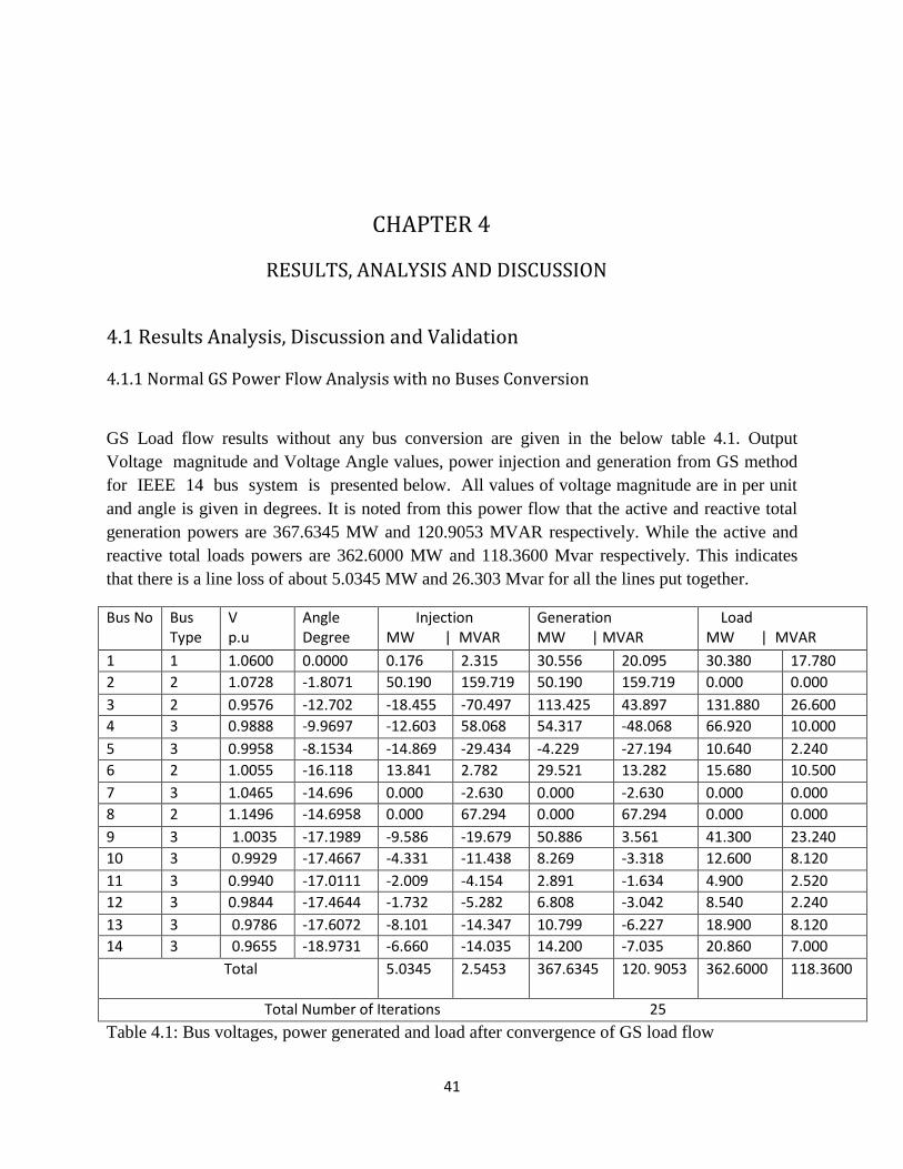
Table 4.1: Bus voltages, power generated and load after convergence of GS load flow…….41
Table 4.2: Real and Reactive Power flow over different lines and Losses………………….42
Table 4.3: Bus voltages, power generated and load after convergence of GS load flow
with PV to PQ buses conversion……………………………….…………………………………….…43
Table 4.4: Real and Reactive Power flow over different lines and Losses after PV to PQ
buses conversion……………………………………………………………..….44
Table 4.5: Comparison of Line Losses Before And After Buses Conversion ……………..47
Table 4.6: Power flow results for the 30 bus system………………………………………..50
Page 13
xiii
LIST OF ABBREVIATIONS GS Gauss-Seidel Load Flow Method
NR Newton Raphson Method
DLF Decoupled Load Flow
FDLF Fast Decoupled Load Flow
IEEE Institute of Electrical and Electronics Engineering
MATLAB Matrix Laboratory
MVA Mega Voltage Ampere
MVAR Reactive Power in Mega watts
MW Real power in Mega Watts
P.U Per Unit
P-V Voltage Controlled Bus or Generator
P-Q Load Bus
kV Kilo Voltage
DTs Distribution Transformers
Page 15
1
CHAPTER 1
INTRODUCTION
In an ideal business the cost of production should always be at the decreasing scale without
sacrificing the quality of product and services. It is not different in the power system the main
idea is to maintain the cost of producing energy low while maintaining quality and constant
output.
However, challenges are encountered in power system, these challenges include power losses
economics dispatch. A loss in energy has effect of reducing the amount of energy ready for
consumption. This has effect of increasing cost of maintaining constant supply of energy. It‟s
from this background there arises need for inverting ways to cut energy losses.
1.1 What is power loss? Power loss is defined as deficiency of energy at consumers‟ end in comparison to the generation
end. If the energy summation at the consumers point does not add-up to the figure that was
generated initially then we say power loss has occurred.
In power system there is not even a single power system that does not encounter power losses.
Power losses occur at all points including generation, transmission and distribution. Power loss
can account up to 30% of the generated value [5].
1.2 Power System Losses Energy losses occur in the process of supplying electricity to consumers due to technical and
commercial losses. The technical losses are due to energy dissipated in the conductors and
equipment used for transmission, transformation, sub- transmission and distribution of power.
These technical losses are inherent in a system and can be reduced to an optimum level.
The commercial losses are caused by pilferage, defective meters, and errors in meter reading
and in estimating unmetered supply of energy [4].
1.2.1 Causes of Power Losses. The major causes reason for high technical losses in our power systems are;
Inadequate investment and planning on transmission and distribution particularly in
sub-transmission and distribution centers. While there is desire to match the expanding
need for power, lack of sufficient distribution system has resulted in overloading of the
distribution system.
Long high voltage and medium distance transmission lines and distribution lines in the
magnitude of 400KV where high voltage drops occur.
Page 16
2
Improper load management-Most loads are inductive instead of capacitive which would
help improve power factor. This inductive load draw lagging current which give a
lagging power factor and thus power loss.
Inadequate reactive power compensation [5, 4].
1.2.2 Measures for reducing technical power losses Compilation of data regarding existing loads, operating conditions, forecast of expected
loads using methods such load flow analysis. Mapping of complete primary and
secondary transmission system clearly depicting the various parameters such as
conductor size line lengths, losses along each conductor and formulating methods to
reduce these losses etc.
Identifying of the weakest areas in the transmission and distribution system and
strengthening /improving them so as to draw the maximum benefits of the limited
resources.
Reducing the length of Long Transmission lines by addiction of distribution sub-stations
to cater for the additional distribution transformers (DTs).
Installation of lower capacity distribution transformers at each consumer premises instead
of cluster formation and substitution of DTs with those having lower or no load losses
such as amorphous core transformers. Or installation of shunt capacitors for improvement
of power factor.
Carrying out detailed distribution system studies considering the expected load
development during the next 8-10 years. Preparation of long-term plans for phased
strengthening and improvement of the distribution systems along with associated
transmission system [4].
1.3 What is a Bus in Power System? In power engineering a bus is a node at which one or many lines, one or many loads
and generators are connected point , and it is usually associated with four quantities; real
generated power and reactive generated power ( ),real demanded power ,
and reactive demanded power , voltage magnitude | |and its phase angle [22].
This bus may or may not correspond to the physical bus bars in substation [5].
1.4 Classification of Buses
In a load flow solution, two out of the four quantities associated with a bus, are specified and the
unspecified two are required to be obtained through the solution of the load flow non-linear
equations [1, 2].
Depending upon which quantities have been specified, the buses are classified into following
three categories;
Page 17
3
1.4.1 LOAD BUS
This is a bus without any generators connected to it, both real power generated and reactive
power generated are zero and the real power and reactive power drawn from the
system by the load (negative inputs into the system) are known from historical record, load
forecast, or measurement.
All buses having no generators are load buses or the bus connected to load is a load bus. Quite
often in practice only real power is known and the reactive power is then based on an assumed
power factor such as 0.85 or higher [2].
Load bus is never connected to a generator; however, the power output of some generators is
constant or cannot be adjusted under the particular operation conditions. The corresponding bus
connected to such bus will also be referred as load bus [1, 3, 8].
Load bus is also known as P-Q bus because the scheduled values; negative inputs into the system
( ) are known and mismatches ( ) can be defined [2].
This bus is also called power controlled bus [16].
1.4.2 GENERATOR BUS
This is a bus at which the real power corresponding to generator ratings and voltage
magnitude | | corresponding to generator voltage; are specified and the real power drawn
from the system by the load is zero hence known.
It is required to find out the reactive power drawn and the phase angle of the bus voltage
[1].
This bus is also called Voltage Controlled bus or P-V bus because a bus of the system at which
the voltage magnitude can be kept constant is said to be voltage controlled.
At each bus to which there is a generator connected, the megawatt generation can be controlled
by adjusting the prime mover, and the voltage magnitude can be controlled by adjusting the
generator excitation.
Therefore, at each generator bus we may properly specify and thus the name P-V bus.
Certain buses without generators may have voltage control capability; such buses are also
designated voltage- controlled buses at which the real power generation is simply zero [2, 3, 5].
1.4.3 SLACK BUS
This is a bus in which voltage magnitude Vi and phase angle i are specified ,also known as V
bus. A bus used to balance the active |P| and reactive |Q| powers in the system while performing
load flow studies in electrical power systems. From the load flow solution one is expected to find
real power |P| and reactive power |Q|. At this bus the phase angle is usually set at zero. The slack
bus is usually designated as bus 1 .In most power systems there is only one slack bus, but there
can be more than one slack bus in a given power system scheme(distributed slack bus). It serves
Page 18
4
as the reference while performing load flow analysis. This bus is also called Swing Bus or
Reference Bus [1, 3, 5].
Slack bus is used to provide system losses by emitting or absorbing active/reactive power
to/from the system. While this definition of the load flow problem is appropriate for a
deterministic solution, it has an inherent drawback when dealing with uncertain input variables:
the slack bus must absorb all uncertainties arising from the system and thus, will have the widest
nodal power possibility (probability) distributions in the system. If even moderate amounts of
uncertainty are allowed in a large system, the resulting distributions will frequently contain
values well beyond the generating margins of the slack generator.
If a slack bus is not specified, then a generator bus with maximum real power will be chosen as
the Slack bus so that the variations in real and reactive powers of the slack bus to be a small
percentage of its generating capacity during the iteration process, and from this background a
slack bus is a generator bus [19].
1.4.3.1 The Importance of Slack bus Since the grid is interconnected and the phase angle plays a crucial role in load
flow, one bus must remain at a virtual reference zero degrees, so that the other
buses can be related with respect to this bus.
The line losses in the system aren‟t calculated till the end of the iteration. The
deficit in the power injection and power demand is the loss of the system.
This extra power must be accommodated in the load flow for the next iteration.
Hence the slack bus accepts this extra burden on itself and balances the system. So
at this bus the voltage magnitude and phase angle is specified and the real and
reactive power is calculated.
A slack bus is also required from the nodal admittance matrix point of view.
Without a slack bus, the matrix will be singular and can‟t be handled. By
introducing a slack bus, one row and column is eliminated and thus the system
turns non-singular [2].
1.4.4 VOLTAGE-CONTROLLED BUSES Generally the PV buses and the voltage-controlled buses are grouped together but these buses
have physical difference. The voltage-controlled bus has also voltage control capabilities, and
uses a tap-adjustable transformer and/or a static VAR compensator instead of a generator. Hence,
at these buses. Thus at these buses.
The known are real power , reactive power , and voltage magnitude | |.The voltage angle is
an unknown parameter [19].
Page 19
5
Bus Type Specified Variables Unknown Variables
Slack or reference bus | |
Generator or PV bus | |
Load or PQ bus | | | | | |
Table 2.1: Summary of Bus Classification
1.5 Bus Conversion Bus conversion is a process of assigning new bus specification while the previous bus
specifications are dropped or are relaxed. In electrical power systems any bus has predefined
specifications, and unknown specifications which have the extent to which the specification can
vary (variable limits). If for a certain bus, the specifications are changed it affect the bus
treatment and thus its conversion.
In static analysis of power system the reactive power outputs of generators and switchable shunts
are modeled to vary instantaneously within their physical limits to maintain some buses‟ voltage
magnitudes. These buses are called voltage regulated buses.
In power flow computation, if the voltage magnitude of a bus can be regulated by the automatic
voltage regulator of generator or the continuously-switchable shunt, its type may be switched
between PV and PQ. Generally speaking, if the type of a bus is PV, which means the real power
injection and voltage magnitude of a bus are fixed while its reactive power injection and voltage
phase angle are free. When its reactive power injection reaches its upper or lower limit, the type
of this bus becomes PQ, which means that the real and reactive power injections are fixed while
the voltage phase angle and magnitude are free.
The process of power flow computation is mathematically an iterative solution process of a set of
non-linear algebraic equations. The type identification of voltage controlled bus is done between
two iterations [21].
1.6 Survey of Earlier Work For proper planning and operation of power system, economic scheduling of generating units and
to achieve power through tie line as per agreement, power flow analysis is a must. It is
performed to have clear knowledge regarding bus voltage magnitude and angle and line flows. A
number of methodology are being used all over the world for power flow analysis in order to
assist reduce power losses in a system this include
Power loss reduction by distributing the slack bus.
Power loss reduction by slack- PV buses conversion.
Page 20
6
1.6.1 Power loss reduction by distributing the slack bus
The traditional power flow with a single slack bus model, one generator bus is selected to be the
voltage phase angle reference and this is assumed to balance the real power mismatch due
to uncertain system real power loss. However, there is no slack bus in actual power
systems especially with distributed generation. Thus, single slack bus model significantly
distort computed power flows. Thus with the increased penetration of distributed generation
into the power distribution system, the traditional load flow analysis that assumes a single
slack bus has become impractical.
The existing literature focuses on slack bus placement taking only real power losses into
account. Thus a distributed slack bus model taking into consideration both real and reactive
power losses is of paramount importance [16].
With the basic understanding of slack bus where voltage magnitude and phase angle of the
voltage are known while the power is unknown, if after load flow analysis it‟s designed that the
excess load (or generation) get assigned to a chosen number of generator buses that will share the
load in a predetermined manner. This relieves slack bus production to PV buses, which is
referred as distributing a slack bus. Load flow analysis usually proves transmission losses for
such system have been reduced compared to the case of single slack bus model [1, 2, 7].
1.6.2 Power loss reduction by slack- PV buses conversion. The basic understanding of Slack bus is voltage magnitude and phase angle of the voltage are
known while the power is unknown, if after load flow analysis, the Slack bus power generation
(or consumption) extends beyond its predefined limits; it is fixed at the violated limits. The
other PV bus‟s active power generation (or consumption) then must be relaxed in order to be
able to solve the load flow problem. The PV bus to choose seems to be a matter of preference,
but it is logical to pick the one that has the highest margin from the current production
(consumption) to either its lower or upper limit, depending on which limit was violated at the
slack bus. With the choice of a PV bus to relax, it is now possible to redefine the load flow
problem by swapping only the equation for the real power at the chosen PV bus with the
equation for the slack bus real power, without changing the unknown state variables. In other
words, the slack bus becomes a PV bus [1, 2, 7].
In another approach, one can relax the voltage angle of the slack bus and declare the voltage
angle of the PV bus with relaxed real power as the reference (i.e. known).This will result in a
complete slack to PV bus and PV to slack bus conversion [1, 7, 10].
1.7 Problem Statement The main goal of this project is to understand the theory of load flow analysis and buses
conversion processes for 14 and 30 buses power system with effective power loss reduction. And
develop a reliable and effective program based on Gauss Seidel Method with MATLAB software
as a programming platform. IEEE standard 14 buses, to be used for test validation.
Page 21
7
1.8 Objectives The objectives of carrying out this project is :
1. To understand the Gauss Seidel load flow method and use it for effective PV-PQ buses
conversion to prove power loss reduction.
2. To develop a Gauss-Seidel load flow program inclusive of buses conversion capability
using Matlab platform.
Organization of Report In Chapter 1 the definition of Power Loss and various measures that can be employed to solve
the power loss problem have been discussed. Definition of a bus in power system, buses
classification and buses conversion procedure, including the method which will be used to
convert buses in this project. Survey of earlier of works has been covered here. It also covers the
problem statement, objective of the project.
In Chapter 2 discussion of the literature review is covered.
In Chapter 3, PV-PQ buses conversions problem formulation based on GS method is discussed.
Formulation of pseudocode and Flow chart are also covered.
In Chapter 4 will discuss the results of the project.
In Chapter 5 will present the challenges, conclusions and recommendations for further work on
the topic.
Page 22
8
CHAPTER 2
BACKGROUND AND REVIEW OF LITERATURE
2.1 Load flow Studies Load flow solution is a solution of the network under steady state condition subject to certain
inequality constraints under which the system operates. These constraints can be in form of load
voltages, reactive power generation of the generators, the tap setting of a tap change under load
transformer [13].
The load flow solution gives nodal voltages and phase angles and hence the power injection at all
the buses and power flows through interconnection power channels [1, 8].
Load flow solution is essential for designing a new power system and for planning extension of
the existing one for increased load demand.
Different steady state solutions can be obtained, for different operating conditions, to help in
planning, design and operation of the power system. The solution also gives the initial conditions
of the system when the transient behavior of the system is to be studied.
The mode of operation of power system, either, symmetrical or unsymmetrical dictates
operational features of the power system. Symmetrical steady state is the most important mode
of operation; however, three major problems are encountered in this mode; Load Flow problem,
Optimal Load Scheduling problem and System Control Problem [5, 6].
Generally, load flow studies are limited to the transmission system, which involves bulk power
transmission [13].
2.2 Constraints on load flow solution The constraints placed on the load flow solutions could be: The Kirchhoff‟s relations holding
well, Capability limits of reactive power sources, Tap-setting range of tap-changing
transformers, Specified power interchange between interconnected systems, Selection of initial
values, Acceleration factor and Convergence limit [6].
For optimal operation of an electrical power system requires that; Generation must supply the
load plus losses, The bus voltage magnitudes must remain close to rated values, generators must
Page 23
9
operate within specified real and reactive power limits and that transmission lines and
transformers should not be overloaded for long periods [2].
2.3 Solution to Load flow Load flow analysis is performed extensively both for system planning purposes, to analyze
alternative plans of future systems operation and to evaluate different operating conditions of
existing systems.
In load flow analysis, it is normal to assume that the system is balanced and that the network is
composed of constant, linear, lumped-parameter branches. In the most basic form of the power
flow, transformer taps are assumed to be fixed. This assumption is relaxed in commercial
load flow [1].
Therefore, nodal analysis is generally used to describe the network. However, because the
injection and demand at bus bars, it is generally specified in terms of real and reactive power, the
overall problem is nonlinear. Accordingly, the load flow problem is a set of simultaneous
nonlinear algebraic equations. Numerical techniques are required to solve this set of equations
[2].
The traditional solution finding methodology of the load-flow problems follow an iterative
process, which start by assigning estimated values to the unknown bus voltages and angles and
calculating a new value for each bus voltage and angle from the estimated values at the other
buses. A new set of values for voltage and angle are thus obtained for each bus and are used to
calculate the next set of bus voltages and angles in a sequential algorithm. The iterative process
is repeated until the changes at each bus are less than the specified tolerance value,
(0.00001<ε<0.0001).
However, the load distribution network is a complex system and exhibits lots computational
procedure hence time consuming. Secondly, there are losses in electrical network distribution
hence quantification and minimization of losses is important because it will determine the
economic operation of the power system [15].
2.4 Importance of load flow studies Load flow studies are performed in major areas of power system development and operation
because of the following rationale;
1. Load flow analysis is necessary for planning, economic scheduling, and control of an
existing system as well as planning its future expansion.
Page 24
10
2. Load-flow studies are performed to determine the steady-state operation of an electric
power system. It calculates the voltage drop on each feeder, the voltage at each bus, and
the power flow in all branch and feeder circuits [13].
3. A load flow analysis allows identification of real and reactive power flows, voltage
profiles, power factor and any overloads in the network. This allows the engineer to
investigate the performance of the network under a variety of operating conditions [9].
4. The Economic Operation: As loads change throughout the day there is a need to
determine the best generating pattern to minimize costs of operation and provide the best
voltage regulation.
5. Determine if system voltages remain within specified limits under various contingency
conditions, and whether equipment such as transformers and conductors are
overloaded [13, 3].
2.5 Load flow Analysis The different types of information selected as input and output are grouped as follows.
Input data is divided into: Generator data, Bus data, Transformer data, Line data and Load data.
Output data are divided into Load and Losses data.
The bus type classification are dependent on the bus data specified .This data is included with
every load flow output file in order to document the system, load configuration that the solution
applies for [15, 18].
2.5.1 Types of Variables and limits
2.5.1.1 Type of variables
Control variables – These are the adjustable independent parameters used to manipulate
some state variables. Power injected by generator real power Pi and reactive power Qi
or the corresponding voltage magnitude |Vi| are controllable (excepting in slack bus) [1,
18].
Non-control variables - Power drawn from the generator and reactive power are
non-controllable.
State variables –Variables defining state of system; Voltage magnitude |Vi| and Power
angle .
2.5.1.2 Variable limits For Static Load Flow Equation (SLFE) solution to have practical significance, all the
state and control variables must lie within specified practical limits. The limits are
dictated by specifications of power system hardware and operating constraints [1].
If the system limits criteria are violated then for instance the bus properties are altered
significantly. These limit criteria are as follows;
(i)Voltage magnitude |Vi| must satisfy the inequality
Page 25
11
| |min | | | |max (2.1)
The power system equipment is designed to operate at fixed voltages with allowable
variations of ± (5−10) % of the rated values.
(ii) Power angle (state variables) must satisfy the inequality constraint
| | | | | | (2.2)
This constraint limits the maximum permissible power angle of transmission line
connecting buses and and is justifiable by considerations of system stability
(iii) Owing to physical limitations of P and/or Q generation sources, Pi , and Qi are
constrained as follows
| | | | | |
| | | | | |
2.5.1. 3System balance Equations For any given power system there must be a power balance, the total generation of real and
reactive power must equal the total load demand plus losses, i.e.
∑ ∑
∑ ∑
Where stand for the system real and reactive power loss, respectively. This leads to
optimal sharing of active and reactive power generation between sources [18].
2.6 Load Flow Problem Formulation
The solution to the load flow problem requires two main steps; mathematical formulation of the
problem and application of numerical technique to solve the problem.
2.6.1 Mathematical Formulation of the Problem The following steps are critical in formulation of the problem;
Page 26
12
The complex power injected by the source into the bus of a power system is
Where
the voltage at the bus and with respect to ground and
is the source current injected into the bus.
The load flow problem is handled more conveniently by use of rather than .Therefore, taking
the complex conjugate of Eqn. (2.7), hence
Substituting for;
∑
then from Eqn. (2.8),we can write
(∑
)
Equating real and imaginary parts
{ ∑
}
{ ∑
}
In polar form
| | | |
| | | |
| |
Substituting for ,
| | ∑| |
| |
Page 27
13
Or
| | ∑| | | |
Or
| | ∑| | | |
Or
| | ∑ | | | | { }
(2.10f)
Separating the Real and reactive powers of the above equation can be expressed as
| |∑| || |
| |∑| || |
2.6.2 General Rules for Assembling Admittance Matrix [ ] The load flow equations are easily solved using nodal admittance matrix. It‟s advantageous to
use admittance matrix because it has characteristics that favor computational process. These
characteristics of [ ] are;
i. The nodal admittance matrix is a sparse matrix-a few numbers of elements are
non-zero.
ii. The nodal admittance matrix is a symmetric matrix along the leading diagonal;
the computer need store the upper triangular nodal admittance matrix only [1, 3,
5].
If the interconnection between the various buses of a given power system, and the admittance
value for each interconnecting circuit are known the admittance matrix may be built as follows;
i. The diagonal element (self-admittance ) of each node is the algebraic sum of
the admittance connected to it
Page 28
14
ii. The off-diagonal element (mutual admittance) is the negated admittance
between the nodes . If there is no line between buses this term is
zero.
iii. [5, 19, 20].
2.7 Application of Numerical Technique to Solve the Problem The various method of load flow analysis include ;Gauss‟s Iterative Method, Gauss-Seidel
Method, Newton-Raphson Method, Decoupled Load Flow Method. The most successful
methods of load flow solution are based on the admittance matrix [ ] representation of a
system The admittance matrix use is favored because is sparse hence necessity low storage [13].
The Gauss-Seidel (GS) method is an iterative algorithm for solving a set of non-linear algebraic
equations. This method solves the power-flow equations in rectangular (complex variable)
coordinates until differences in bus voltages from one iteration to another are sufficiently
small.GS method is based on bus admittance equations [2].
The Newton-Raphson method (NR) was developed this time ,it uses the admittance matrix
and was found very useful because the number of iterations involved is less; thus the load
flow solution is achieved quicker. This method solves the power-flow equations in polar
coordinates. The number of iterations is also not much dependent on the size of the
system involved. As compared to GS method, NR method has a faster convergence rate [10].
For very large scale power transmission system, Decoupled Load Flow (DLF) has been
found to be an alternative strategy for improving the computational efficiency and reducing
computer storage requirements. This method uses an approximate version of NR procedure. The
DLF requires more iterations than NR method, but, requires considerably less time per iterations
and thus power flow solution is obtained rapidly. This technique is very useful tool in
contingency analysis where numerous outages are to be simulated or when a power flow
solution is required for line control [13].
2.7.1 Properties of load flow solution method When choosing a suitable load flow analysis numerical technic, a compromise has to be reached
since every method has its pros and cons. However, a good method should have some salient
properties such as follows;
High computational speed.
Low computer storage need.
Versatility; an ability on the part of load flow to handle conventional and special
operational condition .
Reliability of solution.
Page 29
15
Simplicity [19, 20].
2.8 Development of Load Flow Equations The nodal current equations derived earlier can be written as
∑
∑
Or
∑
Now
Or
Substituting for in equation (2.13b)
[
∑
]
has been substituted by the real and reactive powers because normally in a power system these
quantities are specified.
2.8.1 Iterative Methods Equations (2.14) are the load flow equations where bus voltages are the variables. It can be seen
that the load flow equations are non-linear and they can be solved by an iterative method.
The iterative methods are
i. Gauss‟s method,
ii. Gauss-Seidel method.
Page 30
16
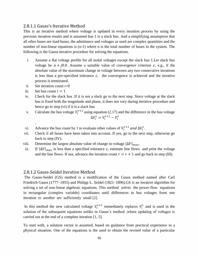
2.8.1.1 Gauss’s Iterative Method This is an iterative method where voltage is updated in every iteration process by using the
previous iteration results and is assumed bus 1 is a slack bus. And a simplifying assumption that
all other buses are load buses, the admittance and voltages as used are complex quantities and the
number of non-linear equations is (n-1) where n is the total number of buses in the system. The
following is the Gauss iterative procedure for solving the equations.
i. Assume a flat voltage profile for all nodal voltages except the slack bus 1.Let slack bus
voltage be Assume a suitable value of convergence criterion , e.g., if the
absolute value of the maximum change in voltage between any two consecutive iterations
is less than a pre-specified tolerance the convergence is achieved and the iterative
process is terminated.
ii. Set iteration count r=0
iii. Set bus count
iv. Check for the slack bus .If it is not a slack go to the next step. Since voltage at the slack
bus is fixed both the magnitude and phase, it does not vary during iterative procedure and
hence go to step (vi) if it is a slack bus
v. Calculate the bus voltage using equation (2.17) and the difference in the bus voltage
.
vi. Advance the bus count by 1 to evaluate other values of
vii. Check if all buses have been taken into account. If yes, go to the next step, otherwise go
back to step (IV).
viii. Determine the largest absolute value of change in voltage | |
ix. If | | is less than a specified tolerance , estimate line flows and print the voltage
and the line flows. If not, advance the iteration count and go back to step (III).
2.8.1.2 Gauss-Seidel Iterative Method The Gauss-Seidel (GS) method is a modification of the Gauss method named after Carl
Friedrich Gauss (1777–1855) and Philipp L. Seidel (1821–1896).GS is an iterative algorithm for
solving a set of non-linear algebraic equations. This method solves the power-flow equations
in rectangular (complex variable) coordinates until differences in bus voltages from one
iteration to another are sufficiently small [2].
In this method the new calculated voltage immediately replaces
and is used in the
solution of the subsequent equations unlike in Gauss‟s method ,where updating of voltages is
carried out at the end of a complete iteration [1, 5].
To start with, a solution vector is assumed, based on guidance from practical experience in a
physical situation. One of the equations is the used to obtain the revised value of a particular
Page 31
17
variable by substituting in it the present values of the remaining values. The solution vector is
immediately updated in respect of these variables. The process is then repeated for all the
variables thereby completing iteration. The iterative process is repeated till the solution vector
converges within prescribed accuracy. The convergence is quite sensitive to the starting values
assumed. Fortunately, in load flow study a starting vector close to the final solution can be easily
identified with previous experience.
To explain how the GS method is applied to obtain the load flow solution, let it be assumed that
all the buses other than the slack bus are PQ buses. We shall see later that the method can be
easily adopted to include PV buses as well. The slack bus voltage being specified, there are (n-1)
bus voltages starting values of whose magnitudes and angles are assumed. These values are then
updated through an iterative process. During the course of iteration, the revised voltage at the
bus is obtained using eqn. (2.14); i.e.
[
∑
]
The voltages substituted in the right hand side of Eqn. (2.15) are the most recently calculated
(updated) values for the corresponding buses. During each iteration voltage at buses
are sequentially updated through use of Eqn. (2.15). , the slack bus
voltage being fixed is not required to be updated. Iterations are repeated till no bus voltage
magnitude changes by more than a prescribed value during iteration. The computation process is
then said to converge to a solution [1].
The general load flow equation for (r+1) iteration resultant from GS method will be as given
below
[
∑
∑
]
The second term on the R.H.S of the above equation is clear because the voltage prior to bus i
should correspond to the value as calculated during the current iteration [5].
2.8.1.2.1 Algorithm for Load Flow Solution using GS Consider the case where all buses other than the slack are PQ buses. The steps of a
computational algorithm are given below:
1. With the load profile known at each bus (i.e. ) allocate .
.While active and reactive generations are allocated to the
Page 32
18
slack bus, these are permitted to vary during iterative computation. This is necessary as
voltage magnitude and angle are specified at this bus (only two variables can be specified
at any bus).With this step, bus injections ( ) are known at all buses other than the
slack bus.
2. Assembly of bus admittance matrix ; with the line and shunt admittance data
stored in the computer, , is assembled by using the rule for self and mutual
admittances.
3. Iterative computation of bus voltages ( ): To start the iterations a set of
initial voltage values is assumed. Since, in a power system the voltage spread is not too
wide, it is normal practice to use a flat voltage start, that is, initially all voltages are set
equal to (1+j0.00) except the voltage of the slack bus which is fixed. It should be
noted that (n -1) equations (2.15) in complex numbers are to be solved iteratively
for finding(n-1) complex voltages . If complex number operations are
not available in a computer, equation (2.15) can be converted into 2(n- 1) equations
in real unknowns ( | | ) by writing
| |
A significant reduction in the computer time can be achieved by performing in advance
all the arithmetic operations that do not change with iterations.
Define
Similarly let
And
With these simplifications the voltage equation (2.16) for iteration becomes
[
∑
∑
]
Page 33
19
For the th iteration, the updated values of are used for
the rest of voltages previous values, i.e are used.
The iterative process is continued till the change in magnitude of bus voltage,
| | |
|, between two consecutive iterations is less than a certain
tolerance limit for all buses voltages;
| | |
|
The limits of voltage magnitude can be checked and fixed as
{
| | | | | |
| |
| | | |
| | | | | | | |
}
4 Computation of slack bus power(since at the slack bus, voltage magnitude and voltage
angle are specified or known, and real power and reactive power are to be
calculated): Substitution of all bus voltages computed in step 3 along with equation
(2.9) yields
5 Computation of line flows and line losses: this is the last step in the load flow analysis
wherein the power flows on the various lines of the network are computed [1, 5,
19].
2.8.1.2.2 Line power flows Consider the lines connecting buses . The line and the transformers at each end can be
represented by a circuit with series admittance and two shunt admittances as
shown in Fig (2.0)
Fig.2.1: -representation of a line and transformers connected between two buses
Page 34
20
The current field fed by bus into the line can be expressed as
Where
Then equation (2.22) now is rewritten as
The power fed into the line from bus is
And
Therefore
Similarly, power fed into the line from bus k is
The power loss in the line is the sum of the power flows determined from equation
(2.27a) and (2.27b).
The total transmission loss can be computed by summing all the line flows of the power
system.
∑
Where
The slack bus power can also be found by summing the flows on the lines terminating at the
slack bus.
2.8.1.2.3 Algorithm Modification When PV Buses Are Also Present At the PV buses | | are specified and are the unknowns to be determined.
Therefore, the values of are to be updated in every GS iteration through appropriate bus
equations. This is accomplished in the following steps for the bus.
1. From equation (2.10b)
{ ∑
}
Page 35
21
The revised value of is obtained from the above equation by substituting most updated
values of voltages on the right hand side. In fact, for the iteration one can
write from the above equation
{
∑
∑
}
Limits of reactive power are checked and fixed as given below
{
2. The revised value of is obtained from Eqn. (2.20) immediately following step 1. Thus
[
∑ ∑
]
Where
The algorithm for PQ buses remains unchanged.
The physical limitations of Q generation require that Q demand at any bus must be in the
range if at any stage during the computation, Q at any bus goes outside
these limits, it is fixed at and the bus voltage description is dropped, that is
the bus now is treated as PQ bus. Thus step 1 branch out to step 3.
3. If
, and treat bus as a PQ bus.
Compute
from equations (2.33) and (2.20), respectively.
Page 36
22
In this case it is assumed that out of n buses, the first bus is a slack bus, then 2, 3, …, m
are PV buses and the remaining m+1, …, n are PQ buses [1].
2.8.1.2.4 Acceleration of convergence Convergence in the GS method can be sometimes be speeded up by the use of the
acceleration factor, since the method is slow and it requires a large number of iterations before a
solution is obtained. The process of convergence can be speeded up if the voltage correction
during consecutive iteration process is modified to
where is known as the acceleration factor and is a real number.
A suitable value of B for any system can be obtained by running trial load flows. A generally
recommended value is set at 1.6 and cannot exceed 2 if convergence has to occur. Wrong choice
of might indeed slow-down convergence or even cause the method to divergence [1, 5, 2].
2.9 Newton Raphson The Newton-Raphson (NR) method is a powerful method of solving non-linear algebraic
equations.NR method is a successive approximation procedure based on an initial estimate of the
one-dimensional equation given by series expansion.
The NR method using the bus admittance matrix in either first or second –order expansion of
Taylor series has been voted as a best solution for the reliability and the rapid convergence. It is
most suitable for very large power system. Its only drawback is the large requirement of
computer memory which has been overcome through a compact storage scheme.
Its convergence is speeded up considerably by performing the first iteration through the GS
method and using the values obtained for starting the NR iteration. [1, 18].
To introduce this method start by formulating a non-linear equation with single variable; which
can be expressed as
For solving this equation, select an initial value The difference between the initial value and
the final solution will be .Then is the solution of non-linear equation (2.35) ,
that is,
Expanding the above equation with the Taylor series, we get
Page 37
23
Where are the derivatives of the function . If the difference is
very small (meaning that the initial value is close to the solution of the function), the terms of
the second and higher derivatives can be neglected. Thus equation (2.37) becomes a linear
equation as below:
Then we can get
The new solution will be
Since equation (2.38) is an approximate equation, the value of ( ) is also an approximation.
Thus the solution is not a real answer. Further iterations are needed. The iteration equation is
The iteration can be stopped if one of the following conditions is met:
| | | |
where which are the permitted convergence precision, are small positive numbers.
Expanding equation (2.41) in Taylor series around the initial guess and neglecting the terms of
second and higher derivatives, we get
|
|
+…+
|
|
|
+…+
|
(2.43)
…………….
|
|
+…+
|
Page 38
24
Equation (2.43) can also be written in matrix form from which we can get {
}.
Then the new solution can be obtained. The iteration equation can be written as follows:
[
]
[
|
|
|
|
|
|
|
|
| ]
[
]
Equations (2.44) and (2.45) can be expressed as
( )
Where is an matrix and called a Jacobian matrix.
The Power Flow non-linear equations derived above under NR method, can be solved in either
Polar Coordinate System or Rectangular Coordinate System.
If the bus voltage in equation (2.9) is expressed with a polar coordinate system, the complex
voltage and real and reactive powers can be written as;
∑
∑
where which is the angle difference between bus .
Page 39
25
Newton Method: If the bus voltage in equation (2.9) is expressed with a rectangular coordinate
system, the complex voltage and real and reactive powers can be written as
∑ ∑( )
∑ ∑( )
Assuming that buses 1 ∼m are PQ buses, buses m + 1 ∼ n −1 are PV buses and the bus is
the slack bus. The | | are given in the slack bus, and
the magnitude of the PV bus voltage are also given. Then, bus voltage angles
are unknown, and magnitudes of voltage are unknown. For each PV or PQ bus we have the
following real power mismatch equation:
In polar form;
∑
Or,
In rectangular form;
∑ ∑( )
Similarly the reactive powers mismatch equation for each PQ bus is:
In polar form;
∑
In rectangular form
Page 40
26
∑ ∑( )
Where are the calculated real and reactive power buses injections respectively.
According to the Newton method, the power flow equations (2.57) and (2.58) can be expanded
into Taylor series and the following first - order approximation can be obtained.
[
] [
⁄]
Or
[
] [
] [
⁄]
Where
[
]
And
[
⁄]
[ ] [
]
The elements of the Jacobian matrix are the function of bus voltage, which will be updated
through iterations. The element of the sub-matrix of the Jacobian matrix in equation (2.61) is
related to the corresponding element in bus admittance matrix if this .
Therefore, the Jacobian matrix in equation (2.61) is also a sparse matrix that is the same as the
bus admittance matrix this certainly simplifies the calculation and results in smaller computation
time [1, 3].
2.10 Decoupled Newton Method An intrinsic characteristic of any practical electric power system operating in steady state is
strong inter-reliance between real power and bus voltage angles and between reactive powers
and voltage magnitudes. The property of feeble coupling between variables
results in developing Decoupled Load Flow (DLF) method.
Page 41
27
are solved separately. In the view of above equations (2.59) and (2.60) can be
modified as given below
[
]
[
]
[
]
[
] [
] [
]
∑
∑
Where
(2.65a)
[ ]
[ ]
Equation (2.64a) is solved to get . The updated is then used to solve equation (2.64b) to get
2.11 Fast Decoupled Load Flow The Fast Decoupled Load Flow (FDLF) was developed by B. Scott in 1974. The assumptions
which are valid in normal power system operation are as follows:
Page 42
28
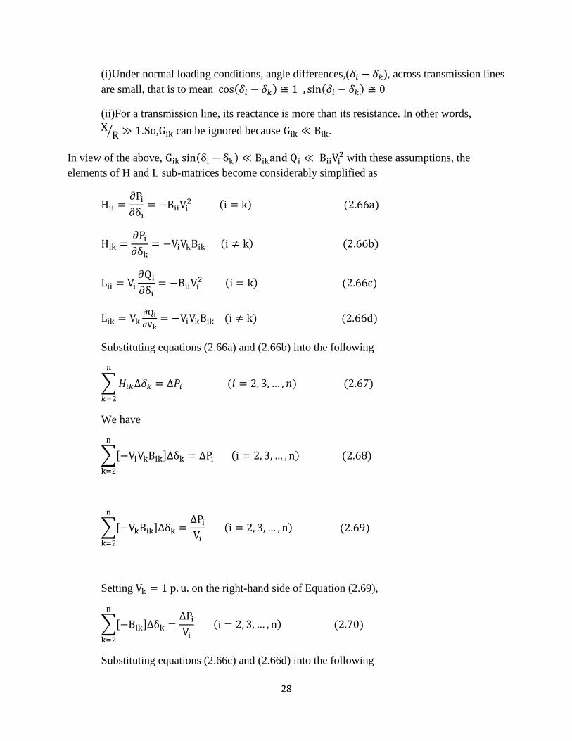
(i)Under normal loading conditions, angle differences,( ), across transmission lines
are small, that is to mean
(ii)For a transmission line, its reactance is more than its resistance. In other words,
⁄ .So, can be ignored because .
In view of the above, with these assumptions, the
elements of H and L sub-matrices become considerably simplified as
Substituting equations (2.66a) and (2.66b) into the following
∑
We have
∑[ ]
∑[ ]
Setting on the right-hand side of Equation (2.69),
∑[ ]
Substituting equations (2.66c) and (2.66d) into the following
Page 43
29
∑
∑ [ ]
Or
∑ [ ]
Setting on the right-hand side of Equation (2.72a),
∑[ ]
Above equations can be written in matrix form as
[ ][ ] [
]
[ ][ ] [
]
Where
is the matrix having elements
is the matrix having elements
Further simplification of the FDLF can be achieved by:
1. Omitting the elements of [B‟] that predominately affect reactive power
flows, i.e. shunt reactance and transformer off-nominal in-phase taps.
2. Omitting from [B”] the angle shifting effect of the phase shifter that
predominately affects reactive power flows.
3. Ignoring the series resistance in calculating the elements of [B‟], this then
becomes the dc approximation of the power flow matrix.
Page 44
30
Equations (2.73) and (2.74) are solved alternatively, always employing the most recent voltage
values.
2.12 Comparison of Load flow Solution Methods.
Since the Gauss-Seidel is undoubtedly superior to Gauss method, the comparison is restricted
only between G-S method and the Newton-Raphson method and that too when Y bus matrix is
used for problem formulation. From the view point of memory requirements, polar coordinates
are preferred for solution based on N-R method and rectangular coordinates for the G-S method.
The time taken to perform an iteration of the computation is relatively smaller in case of G-S
method as compared to N-R method but the number of iterations required by G-S method for a
particular system is greater as compared to N-R method. The number of iteration increase with
increase in size of the system.
In the case of N-R method, the number of iteration is more or less independent of the size of the
system and varies between 3 or 5 iterations. The convergence characteristics of N-R method are
not affected by the selection of a particular bus may result in poor convergence.
The main advantage of G-S method as compared to N-R method is its ease in programming and
most efficient use of core memory. Nevertheless, for very large systems N-R method is found to
be more efficient and practical from point of view of computational time and convergence
characteristics. Even though N-R method can solve most of the practical problems, it may fail in
respect of some ill-conditioned problem where other advanced mathematical programming
techniques like the non-linear programming techniques can be used.
Page 45
31
CHAPTER 3
METHODOLOGY
3.1 Description of PV-PQ Switching Logic Mathematically two tasks need to be done in power flow computation. One is to decrease the
mismatches to a very small value through an iterative process. Another is the type identification
of the buses.
After power flow iteration, for a voltage controlled bus , compute value of its reactive power
injection by solving:
{
∑
∑
}
And for the load bus, after power flow iteration the computation for voltage magnitude and
its load angle can be solved by:
[
∑
∑
]
Simplified as;
[
∑
∑
]
[
∑ ∑
]
Page 46
32
There are two possibilities for each PQ & PV bus:
1. Bus i is a PQ bus in the previous iteration and its calculated voltage magnitude ,
compare it with its upper and lower limits.
If then it is switched to PV and set
.
If then this bus is switched to PV and set
.
If , then this bus remains a PQ bus .
2. Bus i is a PV bus in the previous iteration compare its calculated reactive power
with its upper and lower limits.
If then it is switched to PQ and set
.
If then this bus is switched to PQ and set
.
If , then this bus remains a PV bus [1, 2, 21].
3.2 Computational Pseudocode for Gauss-Seidel load flow method
1. Read data
n (number of buses); m(number of PQ buses).
for slack bus, for PQ and PV buses.
for PQ buses, for PV buses.
for PQ buses.
for PV buses. ( step length), R (number of
iterations), (convergence tolerance).
2. Form the
3. Assume initially
| |
4. Set iteration count | |
5. Set bus count
6. If BUS is PQ-bus then
6.1 Compute from equation (2.22) as
[
∑
]
6.2 Update the voltage according to equation (2.39b) as
6.3 Check the limits of the and set according to
Page 47
33
{
| | | | | |
| |
| | | |
| | | | | | | |
}
6.4 Compute if | | | | | |
6.5 Assign new voltage to old
7. If BUS is the PV-bus then
7.1 Compute for PV bus using equation (2.36)
{
∑
}
7.2 Check the limits of and set according to
{
If no limit is violated then set
If any limit is violated then set
7.3 Compute the voltage angle for the PV bus using equation (2.23)
[
∑
∑
]
7.4 Update the voltage according to equation (2.39b) as
7.5 If then
(
)
7.6 Assign new voltage to old
8. Increment the bus count
9. Check that all voltages of PQ and PV buses have been modified if then GOTO step
6 and repeat.
10. Check convergence
Page 48
34
If | | then GOTO step 5 and repeat
11. Compute powers on slack bus
{ ∑
}
12. Calculate line flows using equations (2.34a)and (2.34b)
Page 49
35
3.3 Flow Chart
Figure 3.1: Gauss-Seidel Flow Chart with PV-PQ buses conversion [3, 4, 5].
Page 50
36
3.4 IEEE 14 Bus Test Network
The 14 bus system consists of five synchronous machines with IEEE type; 1 exciter, four of
which are synchronous compensators used only for reactive power support. There are nine load
buses in the system totaling to 259MW and 81.3 MVAR. The dynamic and static data of the
system can be found. The system is widely used for voltage stability as well as low frequency
oscillatory stability analysis.
Figure 3.2: IEEE 14 bus system [16]
Page 51
37
3.5 Load Flow Data
3.5.1 Bus data
The bus data provided for the IEEE-14bus system is given in the table 3.1 below.
Bus
No
Bus
code
Volt.
Mag.
Angle
Deg.
Load Generator
MW MVAR MW MVAR
1 1 1.060 0 0 0 232.4 -16.9 0 0 1.0600 1.0600
2 2 1.045 0 21.7 12.7 40 42.4 -40 50 1.0105 1.0450
3 2 1.01 0 131.88 94.2 19 23 0 40 0.9645 1.0100
4 3 1 0 66.92 47.8 -3.9 0 0 0 0.9583 1.0330
5 3 1 0 10.64 7.6 1.6 0 0 0 0.9649 1.0328
6 2 1.07 0 15.68 11.2 7.5 12.2 -6 24 1.0094 1.0700
7 3 1 0 0 0 0 0 0 0 0.9904 1.0762
8 2 1.09 0 0 0 0 17.4 -6 24 1.0314 1.0900
9 3 1 0 29.5 16.6 0 0 0 0 0.9920 1.0797
10 3 1 0 9 5.8 0 0 0 0 1.0013 1.0746
11 3 1 0 3.5 1.8 0 0 0 0 1.0189 1.0709
12 3 1 0 6.1 1.6 0 0 0 0 0.9843 1.0638
13 3 1 0 13.5 5.8 0 0 0 0 0.9902 1.0638
14 3 1 0 14.9 5 0 0 0 0 0.9581 1.0633
Table 3.1: Bus Data
Limits of the MVAR demand must be specified. The 14 bus test system being used has
four generator buses 2, 3, 6 and 8. Apart from bus number 8, the rest of the generator
buses have loads tapped from them. To identify the P-V buses from the rest of the bus
types in the system given, they are coded 2.
PQ this type means to be used for load buses. The loads are entered positive in inputting
megawatts and MVAR; negative in outputting megawatts and MVAR by the power
system. For this bus, initial voltage estimations must be specified. This is usually 1 and 0
for voltage magnitude and phase angle, respectively. The system has nine P-Q buses 4, 5,
7, 9-14. They are coded 3.
The bus data table 3-1 provides information on;
The value of the loads that are tapped from the system and to which buses
they are connected to.
The capacity of the generators that supply the system and to which buses
they are connected to.
The voltage magnitude and phase angles at the buses.
Page 52
38
The maximum and minimum reactive power limits for the generators.
Amount of injected MVAR at the buses
3.5.2 Line data The line data table 3.2 below provides the values for the resistance, reactance and half susceptance in Per
Unit of the transmission lines connecting the buses in the system.
This information is necessary for building the matrix.
Other information provided is the tap settings of the transformers connected between the lines. Two-
winding transformer or three-winding transformer data is included in last column of line data structure.
At each line a 1 is entered to represent a case where no transformers on this transmission line are
included.
Sending end
bus
Receiving end
bus
Resistance(r)
Per Unit
Reactance(x)
Per Unit
Half
Susceptance(B/2)
Per Unit
Transformer
Tap (a)
1 2 0.01938 0.05917 0.0264 1
2 3 0.04699 0.19797 0.0219 1
2 4 0.05811 0.17632 0.0187 1
1 5 0.05403 0.22304 0.0246 1
2 5 0.05695 0.17388 0.017 1
3 4 0.06701 0.17103 0.0173 1
4 5 0.01335 0.04211 0.0064 1
5 6 0 0.25202 0 0.932
4 7 0 0.20912 0 0.978
7 8 0 0.17615 0 1
4 9 0 0.55618 0 0.969
7 9 0 0.11001 0 1
9 10 0.03181 0.0845 0 1
6 11 0.09498 0.1989 0 1
6 12 0.12291 0.25581 0 1
6 13 0.06615 0.13027 0 1
9 14 0.12711 0.27038 0 1
10 11 0.08205 0.19207 0 1
12 13 0.22092 0.19988 0 1
13 14 0.17093 0.34802 0 1
Table 3.2: Line data
The network of the medium power system network has its transmission lines modeled in standard π (Pi)
model. The impedance of a line is represented as a series impedance Z the line charging effects are
divided between the two shunt arms each with an admittance of ⁄ [2].
The Admittance Y is made up of a Conductance G and Susceptance B.
Such that
Page 53
39
3.5.3 Transformer Data Two-winding transformer or three-winding transformer data is included in last column of line
data. At each line, 1 must be entered in this column due to no transformers on that particular
transmission line. The lines may be entered in any sequence or order with the only restriction
being that if the entry is a transformer, the left bus number is defined as the tap side of the
transformer.
For a two-winding transformer, which is the also basic component of three-winding
transformer, represented by the equivalent PI circuit shown in figure 3.2.
The transformer tap ratio is setting as 1:k . The branch admittance elements can be calculated
from its PI equivalent circuit.
Figure 3.2: Diagram of a two-winding transformer circuit [16].
The branch self-admittance of bus is obtained by the following equation
The branch self-admittance of bus j is obtained by the following equation.
Page 54
40
The algorithm discussed in section 3.2 was implemented using a MATLAB code. The load flow
input data was borrowed from IEEE 14 bus and 30 bus systems.
Two different analysis were conducted on the three input bus systems, namely,
1. Ordinary G-S Load flow to serve as the reference case.
2. Gauss-Seidel Load flow with PV to PQ buses conversion.
There are several ways or steps for carrying out the GS load flow analysis, the most important is
outlined in the steps as below;
1) Assembling of load flow MATLAB data. (IEEE Data was used)
2) Running the MATLAB assembled code.
3.6 Assembling load flow MATLAB data. The bus data and the line data input were assembled on a MATLAB . A matrix composed
of 14 rows and 11 columns was used to input bus data and a matrix composed of 20 rows and 6 columns
was used to input line data with the input vectors oriented column wise.
To introduce this data to MATLAB workspace the following command were used to call the
functions:
Ybus = ybusppg( ); % Calling program "ybusppg.m" to get Y-Bus.
busdata = busdata14(); % Calling "busdata14.m" for busdata.
This two command functions will input the data that will be analyzed by the written MATLAB code.
3.7 Running the MATLAB code. After all the containing MATLAB data are in the current path of workspace directory, the run
button on the toolbar menu was clicked to simulate the code. The output results obtained from the
workspace were tabulated on the Tables.
Page 55
41
CHAPTER 4
RESULTS, ANALYSIS AND DISCUSSION
4.1 Results Analysis, Discussion and Validation
4.1.1 Normal GS Power Flow Analysis with no Buses Conversion
GS Load flow results without any bus conversion are given in the below table 4.1. Output
Voltage magnitude and Voltage Angle values, power injection and generation from GS method
for IEEE 14 bus system is presented below. All values of voltage magnitude are in per unit
and angle is given in degrees. It is noted from this power flow that the active and reactive total
generation powers are 367.6345 MW and 120.9053 MVAR respectively. While the active and
reactive total loads powers are 362.6000 MW and 118.3600 Mvar respectively. This indicates
that there is a line loss of about 5.0345 MW and 26.303 Mvar for all the lines put together.
Bus No Bus Type
V p.u
Angle Degree
Injection MW | MVAR
Generation MW | MVAR
Load MW | MVAR
1 1 1.0600 0.0000 0.176 2.315 30.556 20.095 30.380 17.780
2 2 1.0728 -1.8071 50.190 159.719 50.190 159.719 0.000 0.000
3 2 0.9576 -12.702 -18.455 -70.497 113.425 43.897 131.880 26.600
4 3 0.9888 -9.9697 -12.603 58.068 54.317 -48.068 66.920 10.000
5 3 0.9958 -8.1534 -14.869 -29.434 -4.229 -27.194 10.640 2.240
6 2 1.0055 -16.118 13.841 2.782 29.521 13.282 15.680 10.500
7 3 1.0465 -14.696 0.000 -2.630 0.000 -2.630 0.000 0.000
8 2 1.1496 -14.6958 0.000 67.294 0.000 67.294 0.000 0.000
9 3 1.0035 -17.1989 -9.586 -19.679 50.886 3.561 41.300 23.240
10 3 0.9929 -17.4667 -4.331 -11.438 8.269 -3.318 12.600 8.120
11 3 0.9940 -17.0111 -2.009 -4.154 2.891 -1.634 4.900 2.520
12 3 0.9844 -17.4644 -1.732 -5.282 6.808 -3.042 8.540 2.240
13 3 0.9786 -17.6072 -8.101 -14.347 10.799 -6.227 18.900 8.120
14 3 0.9655 -18.9731 -6.660 -14.035 14.200 -7.035 20.860 7.000
Total
5.0345
2.5453 367.6345 120. 9053 362.6000 118.3600
Total Number of Iterations 25
Table 4.1: Bus voltages, power generated and load after convergence of GS load flow
Page 56
42
From bus
To bus P MW
Q Mvar From bus
To bus P MW Q Mvar Line Losses
Active||Reactive
1 2 -6.808 -20.786 2 1 6.89 21.038 0.083 0.252
1 5 6.984 28.831 5 1 -6.561 -27.084 0.423 1.747
2
3
14.031
59.114
3
2
-12.524
-52.765
1.507
6.349
2 4 15.202 46.127 4 2 14.011 42.514 1.191 3.613
2 5 14.066 42.947 5 2 -13.056 -39.862 1.011 3.085
3 4 -5.931 -15.137 4 3 6.124 15.63 0.193 0.493
4 5 -4.715 -14.873 5 4 4.748 14.977 0.033 0.105
4 7 0 -27.887 7 4 0 29.513 0 1.627
4 9 0 -2.695 9 4 0 2.735 0 0.04
5 6 0 -4.111 6 5 0 4.151 0 0.04
6 11 2.25 4.713 11 6 -2.225 -4.659 0.026 0.054
6 12 3.226 6.714 12 6 -3.158 -6.573 0.067 0.14
6 13 8.365 16.473 13 6 -8.141 -16.033 0.223 0.44
7 8 0 -61.258 8 7 0 67.294 0 6.036
Total Losses 5.034 26.303
Table 4.2 Real and Reactive Power flow over different lines and Losses.
Page 57
43
4.1.2 GS Power Flow with PV to PQ Buses conversion
GS Load flow results with PV to PQ bus conversion is as follows table 4.3; from this power flow
results it is noted that the active and reactive total generation powers are 365.4376 MW and
104.4068 MVAR respectively. The total active and reactive load powers are as in previous case
that is 362.6 MW and 118.36 MVAR respectively. This indicate a total line losses of 2.838MW
and 10.715 MVAR .
Bus No
Bus Type
V Angle Injection Generation Load
p.u Degree MW MVAR MW MVAR MW MVAR
1 1 1.06 0 15.068 47.926 45.448 65.706 30.38 17.78
2 2 1.045 0 15.686 43.489 15.686 43.489 0 0
3 2 1.01 0 0.806 -7.492 132.686 19.108 131.88 26.6
4 3 0.986 -5.2046 -20.289 -56.945 46.631 -46.945 66.92 10
5 3 0.9945 -4.7128 -9.394 -27.509 1.246 -25.269 10.64 2.24
6 2 1.039 -12.6359 21.156 31.320 36.836 41.820 15.68 10.5
7 3 1.0088 -9.982 0 -2.602 0 -2.602 0 0
8 2 1.0491 -9.9823 0 23.998 0 23.998 0 0
9 3 0.9868 -12.5478 3.327 -17.749 44.627 5.491 41.3 23.24
10 3 0.985 -12.9973 -4.668 -11.139 7.932 -3.019 12.6 8.12
11 3 1.0066 -12.9914 -2.287 -3.782 2.613 -1.262 4.9 2.52
12 3 1.0148 -13.8666 -1.440 -5.715 7.100 -3.475 8.54 2.24
13 3 1.0056 -13.88 -8.376 -13.770 10.524 -5.650 18.9 8.12
14 3 0.9679 -14.7139 -6.751 -13.983 14.109 -6.983 20.8 7
Total 2.8376 -13.9532 365.4376 104.4068 362.6 118.36
Total Number of Iterations 21
Table 4.3: Bus voltages, power generated and load after convergence of GS load flow on PV to
PQ buses conversion.
Page 58
44
Table 4.4 Real and Reactive Power flows over different lines and Losses on PV to PQ buses
conversion.
From bus
To bus P MW Q MVar From bus
To bus P MW Q MVar Losses
Active Reactive
1 2 7.949 24.268 2 1 -7.836 -23.925 0.112 0.343
1 5 7.119 29.388 5 1 -6.679 -27.573 0.44 1.815
2 3 4.151 17.49 3 2 -4.012 -16.904 0.139 0.586
2 4 10.399 31.554 4 2 -9.812 -29.772 0.587 1.782
2 5 8.971 27.391 5 2 -8.538 -26.068 0.433 1.323
3 4 4.819 12.299 4 3 -4.704 -12.006 0.115 0.293
4 5 -5.773 -18.209 5 4 5.823 18.367 0.05 0.158
4 7 0 -10.997 7 4 0 11.251 0 0.254
4 9 0 -0.149 9 4 0 0.149 0 0
5 6 0 -18.816 6 5 0 19.657 0 0.841
6 11 6.575 13.768 11 6 -6.37 -13.339 0.205 0.429
6 12 3.84 7.991 12 6 -3.75 -7.805 0.09 0.186
6 13 10.742 21.155 13 6 -10.397 -20.475 0.345 0.679
7 8 0 -23.076 8 7 0 23.998 0 0.922
Total Losses 2.838 10.715
Page 59
45
4.2 Performance Analysis
For analysis of line flows, bus 1 and 2 were considered. The current flowing through line 1-2
was calculated and the corresponding real and reactive power flow was obtained. The real and
reactive losses were also determined. The current flowing between the buses i and k can be
written as
Therefore the complex leaving bus is given by
Similarly the complex power entering bus is
Therefore the loss in the line segment
The real power flow over different lines is listed in Table 4.2 for GS load flow analysis before
bus conversion and Table 4.4 after PV to PQ bus conversion. The two tables also give the
loss along various segments. It can be seen that all the losses add up to 5.034MW, which is the
net difference between power generation and load for normal GS analysis. Similarly the
losses add up to 2.838MW for GS analysis with PV to PQ buses conversion. Finally we can
compute the line drops in a similar way. This drop is given by
However, the effect of line charging was considered separately
Consider the line segment 1-2. The voltage of bus-1 is per unit while that of
bus-2 is per unit .Then we can get
Therefore the complex power dispatched from bus-1 is
Where the negative signal indicates the power is leaving bus-1. The complex power received
at bus-2 is
Page 60
46
Therefore out of a total amount of 6.808 MW of real power is dispatched from bus-1 over the
line segment 1-2, 6.89 MW reaches bus-2. This indicates that the drop in the line segment
is0.083MW.
Where is resistance of the line segment 1-2. Therefore we can also use this method to
calculate the
line loss. Now the reactive drop in the line segment 1-2 is
We also get this quantity by subtracting the reactive power absorbed by bus-2 from that
supplied by bus-1. The above calculation however does not include the line charging. Note that
since the line is modeled by an equivalent- pi, the voltage across the shunt capacitor is the bus
voltage to which the shunt capacitor is connected. Therefore the current flowing through line
segment is not the current leaving bus-1 or entering bus-2 - it is the current flowing in between
the two charging capacitors. Since the shunt branches are purely reactive, the real power flow
does not get affected by the charging capacitors. Each charging capacitor is assumed to inject a
reactive power that is the product of the half line charging admittance and square of the
magnitude of the voltage of that at bus. The half-line charging admittance of this line is 0.0264.
Therefore line charging capacitor will inject at bus-1
| |
Similarly the reactive power injected at bus -2 is
| |
4.3 Comparison of Results Let „1‟ denotes GS load flow analysis with no bus conversion while „2‟ denotes GS load flow
analysis on PV to PQ buses conversion. It‟s noted from Table 4.5 column 2 and 6, buses number
6 and 8 have been converted from type 2 to type 3 which is PV (generator bus) to PQ (load bus).
The system losses reduce by approximately 51.5%, which is quite significant margin.
Page 61
47
COMPARISON OF LINE LOSSES BEFORE (1) AND AFTER BUSES CONVERSION (2)
GS LOAD FLOW ANALYSIS GS LOAD FLOW ANALYSIS ON PV TO PQ CONVERSION
Bus No
Bus Type 1
Losses 1
Bus No
Bus Type 2
Losses 2
Active 1 Line Losses
Reactive 1 Line Losses
Active 2 Line Losses
Reactive 2 Line Losses
1 1 0.083 0.252 1 1 0.112 0.343
2 2 0.423 1.747 2 2 0.44 1.815
3 2 1.507 6.349 3 2 0.139 0.586
4 3 1.191 3.613 4 3 0.587 1.782
5 3 1.011 3.085 5 3 0.433 1.323
6 2 0.193 0.493 6 3 0.115 0.293
7 3 0.033 0.105 7 3 0.05 0.158
8 2 0 1.627 8 3 0 0.254
9 3 0 0.04 9 3 0 0
10 3 0 0.04 10 3 0 0.841
11 3 0.026 0.054 11 3 0.205 0.429
12 3 0.067 0.14 12 3 0.09 0.186
13 3 0.223 0.44 13 3 0.345 0.679
14 3 0 6.036 14 3 0 0.922
TOTAL 5.034 26.303
TOTAL
2.838 10.715
Table 4.5 Comparison of Line Losses before and after Buses Conversion
4.4 Charts and Graphs
4.4.1 Voltage Profile To illustrate the difference in the voltage magnitudes on the various lines of the IEEE 14 bus
system, on the two cases (GS load flow analysis when there is no buses conversion lets refer this
as case 1 and after PV to PQ buses conversion refer it as case 2). Figure 4.1 shows the voltage
magnitudes in per unit of all the 14 buses. The voltage magnitudes prove to remain fairly
constant at 1p.u with a slight increase at bus 8 to approximately 1.1p.u in both cases.
Page 62
48
Figure 4.1 Voltage profile comparison for cases 1 and 2.
4.4.2 Line Losses The power flows in each line were determined for the two different cases 1 and 2. The plot below
provides a measure of the comparison of power flows and hence the line losses. Figures (4.2) and (4.3)
show the comparison of active line losses and reactive line losses respectively. Clearly case 1 has the
highest losses for both the active and reactive losses, with bus number 3 depicting maximum losses. Case
2 which is on PV to PQ buses conversion of bus numbers 6 and 8, the line losses in all buses remain fairly
equal at approximately 0.2 MW for active power losses and 2 Mvar for the reactive power losses.
0
0.2
0.4
0.6
0.8
1
1.2
1.4
1 2 3 4 5 6 7 8 9 10 11 12 13 14
Voltage magnitudes
Bus Numbers
Voltage Profile Comparison
V1 p.u V2 p.u
Page 63
49
Figure 4.2: A comparison of active power (MW) line losses over different lines for cases 1and 2
Figure 4.3: A comparison of reactive power (Mvar) line losses over different lines for cases 1
and 2
1 2 3 4 5 6 7 8 9 10 11 12 13 14
Active 1 line losses 0.083 0.423 1.507 1.191 1.011 0.193 0.033 0 0 0 0.026 0.067 0.223 0
Active 2 line losses 0.112 0.44 0.139 0.587 0.433 0.115 0.05 0 0 0 0.205 0.09 0.345 0
0
0.2
0.4
0.6
0.8
1
1.2
1.4
1.6
Act
ive
Lin
e lo
sse
s in
MW
Comparison of Active power line losses
Active 1 line losses Active 2 line losses
1 2 3 4 5 6 7 8 9 10 11 12 13 14
Reactive 1 line losses 0.2521.7476.3493.6133.0850.4930.1051.627 0.04 0.04 0.054 0.14 0.44 6.036
Reactive 2 line losses 0.3431.8150.5861.7821.3230.2930.1580.254 0 0.8410.4290.1860.6790.922
0
1
2
3
4
5
6
7
Re
acti
ve li
ne
Lo
sse
s in
MV
ar
Comparison of reactive power line losses
Reactive 1 line losses Reactive 2 line losses
Page 64
50
4.5 GS Power Flow Results and Analysis for 30 IEEE bus System. Load flow analysis was carried out for IEEE 30 bus test system, output total power generation
and injection values are presented below in summary. A similar GS load analysis on PV-PQ
buses conversion was carried out, proved as well to have significantly reduced power losses by
approximately 67.1%.
From table 4.6 it is notable that the system losses have reduced from 4.488 MW to 1.685 MW
for the active power and 24.736 MVAR to 6.975 MVAR for the reactive power.
Important to be noted also is that the number of iterations reduced on PV-PQ buses conversion
from 58 to 26 iterations. The number of iterations and thus computational time for voltage
magnitudes and angles increased as the number of buses increases, the 14 bus system took 25
iterations while 30 bus system took 58 iterations.
GS POWER FLOW ANALYSIS 30 BUS SYSTEM GS POWER FLOW ANALYSIS ON PV-PQ BUS CONVERSION FOR 30 BUS SYSTEM
TOTAL INJECTION
TOTAL GENERATION TOTAL LOAD
TOTAL INJECTION
TOTAL GENERATION TOTAL LOAD
MW MVAR MW MVAR MW MVAR MW MVAR MW MVAR MW MVAR
4.49 -23.44 287.9 102.76 283 126 1.685 -40 285.085 86.197 283 126
TOTAL SYSTEM LINE LOSSES TOTAL SYSTEM LINE LOSSES
4.488 MW 24.736 MVAR 1.685 MW 6.975 MVAR
Table 4.6 Power flow results for the 30 bus system
Page 65
51
CHAPTER 5
CONCLUSION AND RECOMMENDATION
5.1 CONCLUSION The G-S load flow method was successfully designed and implemented to solve Load flow
problem. The Gauss-Seidel Load flow method on no bus conversion and on PV-PQ bus
conversion, for determining the effect of buses conversion on power flows of the IEEE-14 bus
and 30 bus systems was carried out. The comparison of results for the two cases of IEEE 14 and
30 bus test networks, clearly shows that the system losses reduced significantly. The proposed
PV-PQ bus conversion indeed proved capable of obtaining optimum solution efficiently with
minimum system losses. The Voltage magnitude and corresponding angles of a 14 bus system
were observed for different values of Reactance loading and the findings has been presented.
Line flows are also calculated. It is therefore easy to calculate the system losses from these
flows. Tables 4.1, 4.2, 4.3 and 4.4 indicate that the line losses reduced from 5.0345MW &
26.303 MVAR to 2.838 MW & 10.715 MVAR for the 14 bus system.
From table 4.6 it is notable that the system losses have reduced from 4.488 MW & 24.736
MVAR to 1.685 MW & 6.975 MVAR for the 30 bus system. It is seen that number of
iterations and hence computational time for convergence is less on PV to PQ conversion for
both IEEE 14 bus and 30 bus.
Load-flow studies are important for planning future expansion of power systems as well as in
determining the best operation of existing systems. From the findings, it is concluded that
conversion of a number of PV buses to PQ buses is an effective way of reducing power losses in
small and medium size power systems. Therefore, a successful case of design, development and
implementation of Power Loss Reduction by PV-PQ Buses Conversion MATLAB based has
therefore been presented.
5.2Recommendations for Further Work Further works that may be done with regards to this study are:
1. Improvements would be made on the information about the contingency analysis into the
power system networks as well as control measures and load demand patterns so as to
obtain a more representative load flow analysis of a physical system.
2. Distance between various buses to be incorporated so as to study their effects on line
flow losses.
3. Load flow specialization- the load flow approach such as bus conversion or use of one
load flow method for the peak periods and another approach methodology for the normal
periods can also be studied.
Page 66
52
REFERENCE
[1] D. K. &. I. Nagrath, Modern Power System Analysis, New Delhi: Tata Mc Graw Hill, 2003, pp.
184-228.
[2] J. John J Grainger & William D Stevenson, “Power system analysis” Singapore McGraw Hill
1994, p.p 329-374
[3] J Zhu “Optimization of Power System Operation”, Hoboken New Jersey John Wiley and Son. Inc
2009 p.p 9-41
[4] M.S Bhalla, “Transmission and Distribution losses” (Power),2001 pp1-5
[5] C.L Wadhwa “Electrical Power Systems,” sixth Edition New Age International Publishers 2010 p.p
592-620
[6] Mohamed E. El-Hawary “Introduction to Electrical Power Systems”2008 John Wiley & Sons
ISBN 978-0470-40863-6 p.p 305-312
[7] A. Dimitrovski & K. Tomsovic “Slack bus Treatment in load flow solutions with Uncertain
Nodal Powers “ Iowa Sept 2004 p.p 2-6
[8]S.A Nasar, “Electrical Power Systems”, New York McGraw Hill 1990 p.p 119 -133
[9] Brain Hardy ,” Transmission and Distribution Electrical Engineering” 3rd
Edition Elsevier 1996
[10] Anurag Mohapatra, “Distributed Slack Bus for Economic Load Dispatch” National Institute of
Technology, Rourkela
2012 pp2-4.
[11] J.D Glover & J.O Thomas ,“Power system Analysis and Design “ Fifth Edition Global
Engineering 2012
[12] C.L Wadhwa, “Power Flow Analysis” 2011 pp 2-9
[13] K.K Samson, “Decoupled Load Flow Study Method” University of Nairobi 2014
[14] D.S.S Reddy, “Power System Analysis”, New Delhi Laxmi 1997
[15] I. A. Hisken, “Power Flow Analysis”, Nov.6.2003.
[16] P.M Musau & N.O Abungu” Distributed Slack Bus Model for a Wind-Based Distributed
Generation using Combined Participation Factors” , ISSN 2250-2459, Volume 2, Issue 10, October
2012
[17] P.M Musau, “Power Loss Reduction in the Distribution System with a Wind Based Distributed
Generation “,University of Nairobi Feb 2014
[18] M.B.I Shahimi Mohamad “Power Flow Analysis Software using Mat lab”, University Malaysia
Page 67
53
Pahang
[19] D.P.Kothari &J.S Dhillon, ”Power System Optimization”
[20] D. Das, "Electrical Power System," New Age International (P)
ISBN (13) : 978-81-224-2515-4 Department of Electrical Engineering Indian Institute of
Technology pp. 147-184
[21] J. Zhao, C. Hsiao-Dong , L. Hua , Ping Ju “On PV-PQ Bus Type Switching Logic In Power Flow
Computation” 16th PSCC, Glasgow, Scotland, July 14-18, 2008
[22] S. Bhuyan, Sanjib.H & Aroop.B,” Power Analysis on IEEE Flow A 57 bus System
using MATLAB”
[23] P. Srikanth, O. Rajendra, A. Yesuraj, M. Tilak & K.Raja “Load Flow Analysis Of IEEE-14 Bus
System Using MATLAB”
Page 68
54
APPENDIXES
Clear all;
Clear variables
BaseMVA = 100;
ybus = ybusppg();
busdata = busdata30();
rect2pol = rect2pol();
bus = busdata(:,1);
type = busdata(:,2);
V = busdata(:,3);
angle = busdata(:,4);
GenMW = busdata(:,5)/BaseMVA;
GenMVAR = busdata(:,6)/BaseMVA;
LoadMW = busdata(:,7)/BaseMVA;
LoadMVAR = busdata(:,8)/BaseMVA;
Qmin = busdata(:,9)/BaseMVA;
Qmax = busdata(:,10)/BaseMVA;
Vmin = busdata(:,11)/BaseMVA;
Vmax = busdata(:,12)/BaseMVA;
nbus = max(bus);
P = GenMW - LoadMW;
Q = GenMVAR - LoadMVAR;
slack = find(type == 1);
pv = find ( type == 2 );
pq = find ( type == 3);
Npv = length (pv);
Npq = length (pq);
linedata = linedata30();
fb = linedata(:,1);
tb = linedata(:,2);
nl = length(fb);
Iik = zeros(nbus,nbus);
Sik = zeros(nbus,nbus);
Si = zeros(nbus,1);
Vprev = V;
toler = 1;
iter = 1;
acc = 1.6;
for m=2:nbus
Vprev(m)=1;
end
while (toler > 0.00001)
for i = 2:nbus
sumyv = 0;
for k = 1:nbus
if i ~= k
sumyv = sumyv + ybus(i,k)* V(k);
end
end
%---------------------------Computing Qi for PV
bus-----%
if type(i) == 2
Q(i) = -imag(conj(V(i))*(sumyv +
ybus(i,i)
V(i) = (1/ybus(i,i))*((P(i)-
1i*Q(i))/conj(V(i)) - sumyv);
V(i) = Vprev(i)+acc*(V(i)-Vprev(i))
;%Update voltage
angle(i) = atan(imag(V(i))./real(V(i)));
% Checking for Qi Violation this will apply PV
to PQ%
if (Q(i) >= Qmax(i))
Q(i)=Qmax(i);
type(i) = 3;
if (Q(i) <= Qmin(i))
Q(i) = Qmin(i);
type(i) = 3;
else
Q(i)=Q(i);
%------ Updating new Voltages for PV buses----
-%
if type(i) == 2
V(i) = (1/ybus(i,i))*((P(i)-
1i*Q(i))/conj(V(i)) - sumyv);
V(i) = Vprev(i)+acc*(V(i)-Vprev(i))
;%Updating voltage
% angle(i) = atan(imag(V(i))./real(V(i)));
V(i) = pol2rect(abs(Vprev(i)),
angle(V(i)));revised angle
end
%end
%end
end
% -------------------Computing Vi for PQ bus-----
-------------------------%
if type(i) == 3 % If bus Identified as PQ
Compute Vi
V(i) = (1/ybus(i,i))*((P(i)-
1i*Q(i))/conj(V(i)) - sumyv);
V(i) = Vprev(i)+acc*(V(i)-Vprev(i)) ;
%Update by an acceleration factor.
%angle(i) = atan(imag(V(i))./real(V(i)));
Page 69
2
V(i) = rect2pol(abs(Vprev(i)), angle(V(i)));
% Checking for Vi Violation this will ap PQ to
PV.
if (V(i) >= Vmax(i))
V(i)=Vmax(i);
type(i) = 2;
if (V(i) <= Vmin(i))
V(i) = Vmin(i);
type(i) = 2;
else
V(i)=V(i);
end
end
end
end
iter = iter + 1; % Increment iteration count.
toler = max(abs(abs(V) - abs(Vprev))); %
Calculate tolerance.
Vprev=V; % Vprev is required for next
iteration.
%end
end
iter;
V ;
disp (V)
V = abs(V);
angle = 180/pi*angle;
sum2=0;
for i=1:nbus
sum2=sum2+ybus(1,i)*V(i);
end
S=conj(V(1))*sum2;
P(1)=real(S);
Q(1)=-imag(S);
% Bus Current Injections...I = ybus*V;
%Line Current Flows..
for m = 1:nl
p = fb(m); q = tb(m);
Iik(p,q) = -(V(p) - V(q))*ybus(p,q);
Iik(q,p) = -Iik(p,q);
%disp(Iik) %%Note Iik is very sparse
end
% Line Power Flows..
for m = 1:nbus
for n = 1:nbus
if m ~= n
Sik(m,n) = V(m)*conj(Iik(m,n))*BaseMVA;
%Subsequently Sik is sparse
end
end
end
Sik = sparse(Sik);
Pik = real(Sik);
Qik = imag(Sik);
% Line Losses.
Lik = zeros(nl,1);
for m = 1:nl
p = fb(m); q = tb(m);
Lik(m) = Sik(p,q) + Sik(q,p); %power loss in (i-
k)th line Lpik=Sik+Ski
end
Lpik = real(Lik); %Active power loss
Lqik = imag(Lik); %Reactive power loss
% Bus Power Injections.
for i = 1:nbus
for k = 1:nbus
Si(i) = Si(i) + conj(V(i))*
V(k)*ybus(i,k)*BaseMVA;
end
end
Pi = real(Si); %Active power injection
Qi = -imag(Si); %Reactive power injection
Pload=LoadMW*BaseMVA;
Qload=LoadMVAR*BaseMVA;
Pg=Pi+Pload; %Active power generation
Qg=Qi+Qload; %Reactive power
generation