Page 1
I
UNIVERSITY OF NAPLES FEDERICO II Department of Structures
for Engineering and Architecture
Ph.D. Programme in Materials and Structures
XXVI Cycle
VINCENZO GIAMUNDO
Ph.D. Thesis
SEISMIC ASSESSMENT AND RETROFIT OF
HISTORICAL MASONRY BARREL VAULTS
TUTORS: PROF. GIAN PIERO LIGNOLA
PROF. GAETANO MANFREDI
2014
Page 3
III
“Per aspera sic itur ad astra”
Seneca, Hercules furens, act II, v.437
Page 4
IV
Acknowledgements
Before all, I would like to express my deepest gratitude to Prof. Gian Piero Lignola.
I am very grateful to him for his encouragement, interest, stimulus and guidance. It was
mainly due to his initiatives, valuable instructions and constant help that the
development of this work has been possible. Special thanks go to both Prof. Gaetano
Manfredi and Prof. Andrea Prota for giving me the chance to be part of such
outstanding research group. I would like to thank Prof. Stephen Garrity for his support
and precious advices during my time spent at the University of Leeds.
Furthermore, I would like to acknowledge all the people with whom I collaborated
during these years, in particular: Prof. Edoardo Cosenza, Prof. Giuseppe Maddaloni,
Prof. Francesca da Porto, Prof. Yong Sheng, Dr. Vasilis Sarhosis, Prof. Gianluigi
De Martino and Prof. Renata Picone.
I would like to acknowledge past and present PhD colleagues and all the members of
staff at the Department of Structures for Engineering and Architecture at the University
of Naples Federico II. In particular my officemates: Alberto Zinno, Andrea Calabrese,
Anna Bozza, Claudio D’Ambra, Concetta Onorii, Daniele Losanno, Giancarlo
Ramaglia and Loredana Napolano. Thank you guys for your precious help!
I wish to express my gratitude to my friends: Barbara Polidoro, Carmine Galasso,
Antonio Bilotta, Fabio Petruzzelli, Eugenio Chioccarelli, Raffaele Frascadore, Michele
Franzese, Michele di Donato, Emiliano and Peppe Petix who directly or indirectly
helped me during this period. I would also like to thank my colleagues and friends at
the University of Leeds whom provided friendly cooperation and useful discussions
throughout my time in Leeds; I would particularly like to mention: Abdulrahman
Bashawri, Rachel Albinson, Guy Brackenbury, Omar Alzayani, Kalhed, Laura Davis,
Silvia Purin, Alessia Perego, Liting Lin, Anton Dmitriev, Marion Goemans and
Chin Wei Lim.
Special thanks are due to my family for their constant support, love, and
encouragement. Finally, I would like to thank Silvia for her sacrifice and for having
shared my successes and disappointments. Without their full support and
encouragement, this thesis would not have been completed.
Vincenzo Giamundo
Page 5
1
Abstract
Recent earthquakes in Italy highlighted the extreme vulnerability of historical
buildings. Masonry vaults, which represent artistic valuable elements, have
been recognised as the most vulnerable elements of such buildings. Therefore,
the knowledge of their seismic performances, as well as potential retrofit
techniques, meets the need to protect cultural heritage buildings which are
prone to natural hazards. Vault dynamic behaviour is generally studied
according to simplified methods or, as an alternative, to complex Finite
Element (FE) analyses. However, a deep knowledge of their dynamic behaviour
is still lacking from an experimental point of view. In order to investigate the
seismic behaviour of masonry vaults, shaking table tests have been performed
of a full scale masonry barrel vault. After the tests, the vault has been retrofitted
by means of mortar joint repointing, grout injections and Inorganic Matrix FRP
Grid (IMG). Then shaking table tests have been performed on the retrofitted
vault. By means of the experimental tests outcomes, reliable numerical models
able to predict the dynamic behaviour of the masonry vault (before and after the
retrofit) have been developed. This aspect is relevant for studying
characteristics which cannot be investigated by means of the experimental test
monitoring. In this thesis a comprehensive overview of the main results of the
experimental tests is reported. The unreinforced vault exhibits a good seismic
behaviour, showing very slight damage up to a horizontal acceleration of about
4.8 m/s2 (measured at the keystone location). The retrofit resulted in a
significant increase of both stiffness and capacity. Indeed, very slight damages
only after the last test (performed with an achieved PGA of 11.70 m/s2) were
detected on the retrofitted vault. However the retrofit did not drastically change
the global dynamic behaviour of the vault.
KEYWORDS: •Seismic Assessment •Masonry Vaults •Seismic Retrofit •Dynamic
Tests •FEM Analysis.
Page 6
Table of Contents
______________________________________________________________________________________________________________________________
1
Table of Contents
Abstract ............................................................................................................... 1
Table of Contents ............................................................................................... 1
List of Tables ...................................................................................................... 4
List of Figures ..................................................................................................... 5
Introduction .............................................................................. 10 Chapter 1
1.1. General context .................................................................................................. 10
1.2. Research significance ......................................................................................... 13
1.3. Outline of the thesis ........................................................................................... 14
Literature review ...................................................................... 15 Chapter 2
2.1 Brief historical overview of the masonry curved elements .......................... 16
2.2 Arch static analysis methods ........................................................................ 19
2.2.1 Equilibrium methods ........................................................................................... 19
2.3 Arch dynamic analysis methods ................................................................... 25
2.3.1 Finite Element Method (FEM) analysis .............................................................. 26
2.4 Retrofit of historical buildings ..................................................................... 27
2.4.1 Retrofit of vaulted structures............................................................................... 28
2.4.2 Overview on the main retrofit techniques for the vaults ..................................... 30
2.4.2.1 Innovative retrofit techniques......................................................................... 38
2.5 Experimental studies .................................................................................... 44
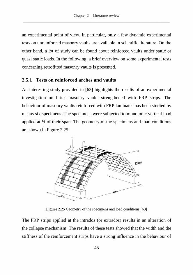
2.5.1 Tests on reinforced arches and vaults ................................................................. 45
Experimental tests: unreinforced vault.................................. 52 Chapter 3
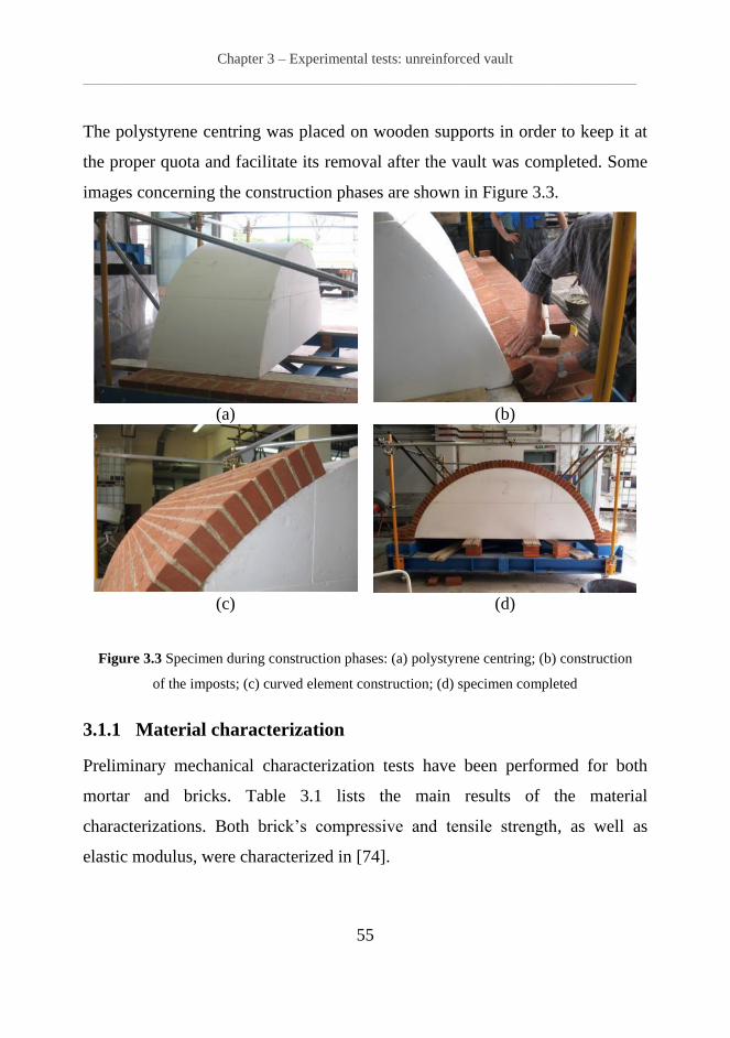
3.1 Specimen ...................................................................................................... 53
3.1.1 Material characterization .................................................................................... 55
Page 7
Table of Contents
______________________________________________________________________________________________________________________________
2
3.2 Experimental facilities ................................................................................. 58
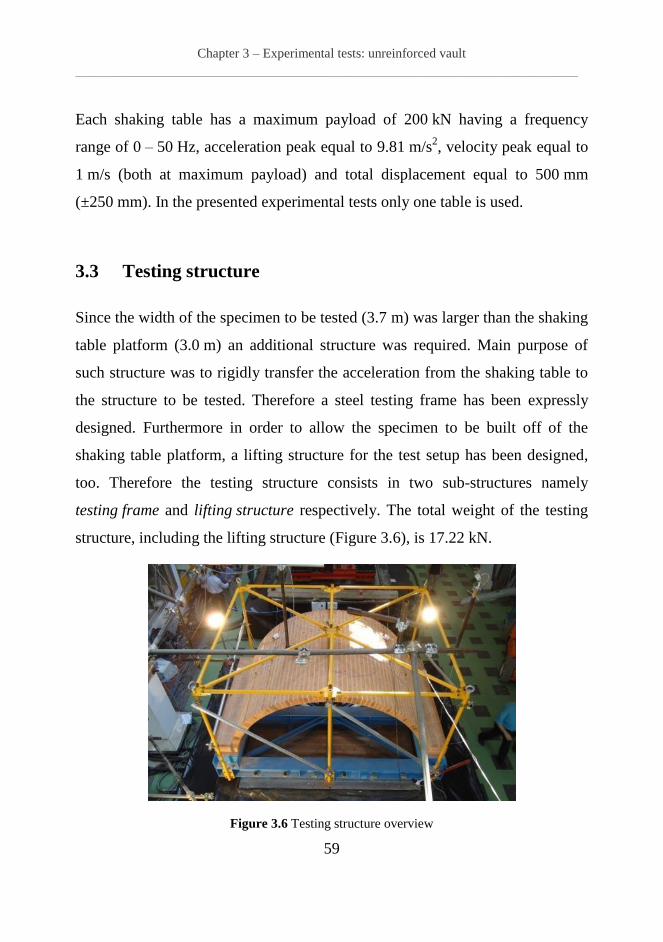
3.3 Testing structure ........................................................................................... 59
3.3.1 Testing frame design ........................................................................................... 60
3.3.2 Lifting structure design ....................................................................................... 70
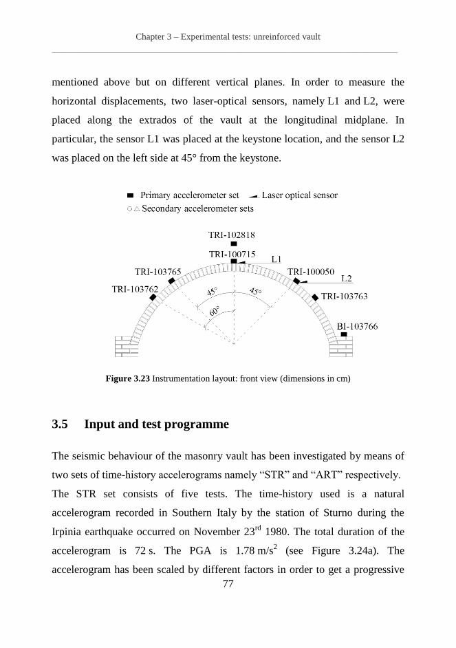
3.4 Instrumentation ............................................................................................ 75
3.5 Input and test programme ............................................................................. 77
3.6 Outcomes of the shaking table tests ............................................................. 81
3.6.1 RND test results (Dynamic identification) .......................................................... 81
3.6.2 STR test results (Sturno earthquake) .................................................................. 82
3.6.3 ART test results (artificial earthquake) ............................................................... 88
3.7 Conclusions .................................................................................................. 96
Experimental tests: retrofitted vault ...................................... 97 Chapter 4
4.1 Specimen retrofit .......................................................................................... 98
4.2 Instrumentation .......................................................................................... 102
4.3 Input and test programme ........................................................................... 103
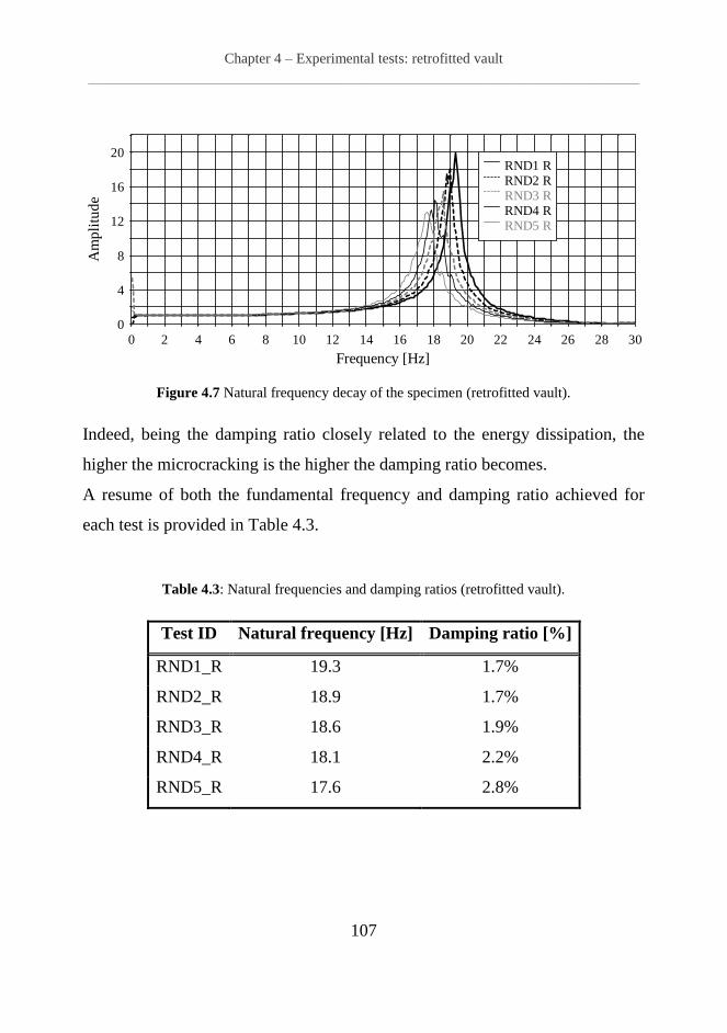
4.4 Outcomes of the shaking table tests ........................................................... 106
4.4.1 RND_R test results (Dynamic identification) ................................................... 106
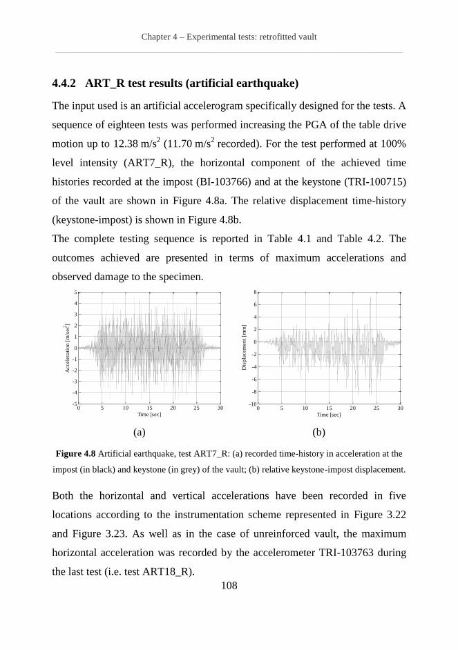
4.4.2 ART_R test results (artificial earthquake) ........................................................ 108
4.5 Outcomes comparison: retrofitted/unreinforced vault ............................... 119
4.5.1 Dynamic characteristics .................................................................................... 119
4.5.2 Maximum acceleration profiles ........................................................................ 122
4.5.3 Dynamic amplification profiles ........................................................................ 124
4.6 Conclusions ................................................................................................ 126
Numerical modelling .............................................................. 128 Chapter 5
5.1 FE Models .................................................................................................. 129
Page 8
Table of Contents
______________________________________________________________________________________________________________________________
3
5.1.1 Modelling of the retrofit interventions .............................................................. 134
5.2 Calibration of the model............................................................................. 137
5.2.1 Calibration of the interface stiffness ................................................................. 137
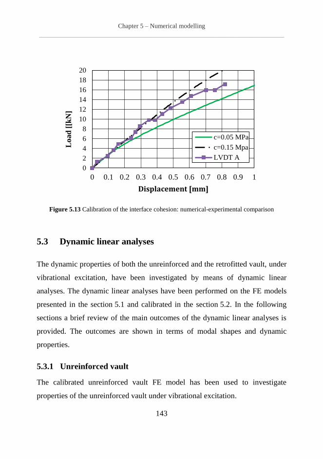
5.2.2 Calibration of the interface cohesion ................................................................ 139
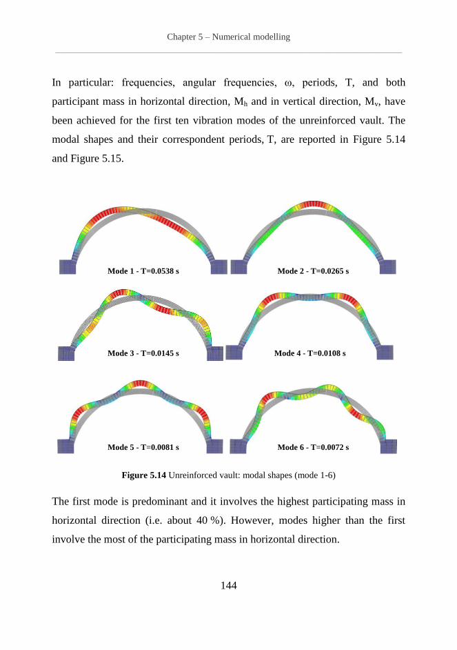
5.3 Dynamic linear analyses ............................................................................ 143
5.3.1 Unreinforced vault ............................................................................................ 143
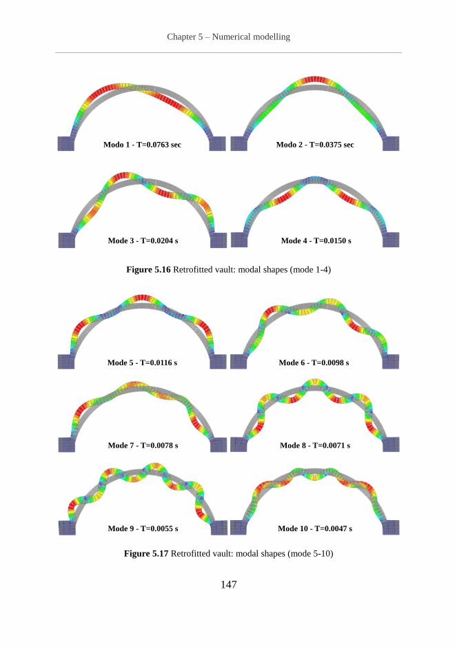
5.3.2 Retrofitted vault ................................................................................................ 146
5.4 Static nonlinear analyses ............................................................................ 149
5.4.1 Unreinforced vault ............................................................................................ 149
5.4.2 Retrofitted vault ................................................................................................ 152
5.5 Dynamic nonlinear analyses ...................................................................... 155
5.5.1 Rayleigh damping coefficients.......................................................................... 156
5.5.2 Input signals ...................................................................................................... 159
5.5.3 Unreinforced vault: experimental-numerical comparison ................................. 162
5.5.4 Retrofitted vault: experimental-numerical comparison ..................................... 164
5.6 Influence of the damage on the numerical results ...................................... 167
5.6.1 ART7: experimental-numerical comparison ..................................................... 168
5.6.2 ART7_R: experimental-numerical comparison ................................................ 170
5.6.3 Parametric analyses (damping influence) ......................................................... 172
5.7 Conclusions ................................................................................................ 175
Conclusions ............................................................................. 177 Chapter 6
References ....................................................................................................... 181
Appendix A ..................................................................................................... 188
Appendix B ..................................................................................................... 193
Appendix C ..................................................................................................... 195
Page 9
List of Tables
______________________________________________________________________________________________________________________________
4
List of Tables
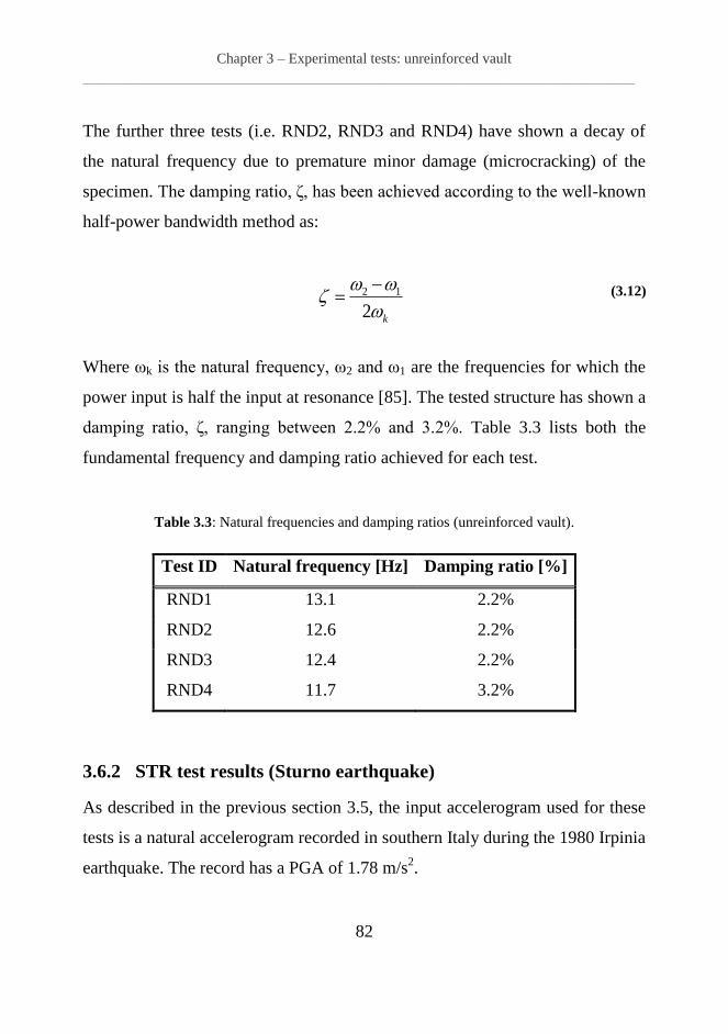
Table 3.1: Material mechanical properties. ................................................................................. 56 Table 3.2: Experimental test programme (unreinforced vault). .................................................. 80 Table 3.3: Natural frequencies and damping ratios (unreinforced vault).................................... 82
Table 3.4: STR test results: horizontal maximum accelerations. ................................................ 85
Table 3.5: STR test results: vertical maximum accelerations. .................................................... 85
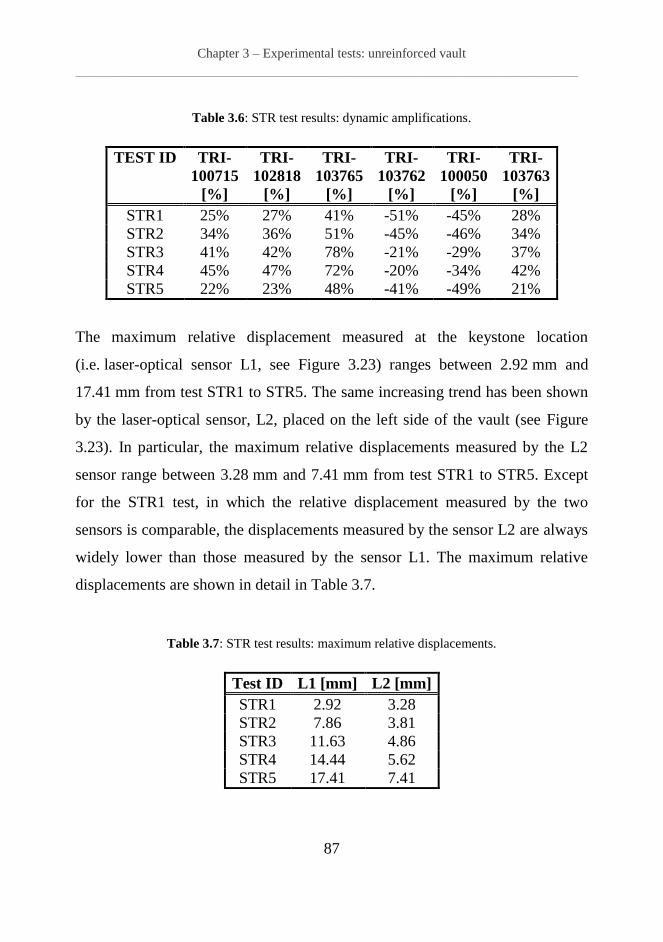
Table 3.6: STR test results: dynamic amplifications. ................................................................. 87 Table 3.7: STR test results: maximum relative displacements. .................................................. 87
Table 3.8: ART test results: horizontal maximum accelerations. ............................................... 90 Table 3.9: ART test results: vertical maximum accelerations. ................................................... 91 Table 3.10: ART test results: dynamic amplifications. ............................................................... 92
Table 3.11: ART test results: maximum relative displacements. ................................................ 93 Table 4.1: Experimental test programme pt. 1 (retrofitted vault). ............................................ 104
Table 4.2: Experimental test programme pt. 2 (retrofitted vault). ............................................ 105
Table 4.3: Natural frequencies and damping ratios (retrofitted vault). ..................................... 107
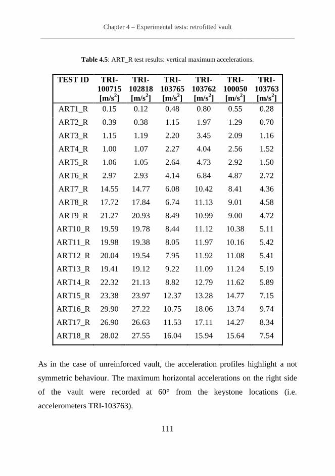
Table 4.4: ART_R test results: horizontal maximum accelerations. ......................................... 110 Table 4.5: ART_R test results: vertical maximum accelerations. ............................................. 111
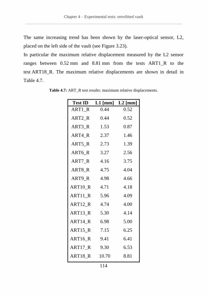
Table 4.6: ART_R test results: dynamic amplifications. .......................................................... 113 Table 4.7: ART_R test results: maximum relative displacements. ........................................... 114 Table 5.1: Interface elements properties ................................................................................... 133
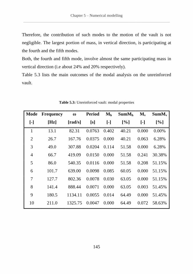
Table 5.2: IMG mechanical properties ..................................................................................... 136 Table 5.3: Unreinforced vault: modal properties ...................................................................... 145 Table 5.4: Retrofitted vault: modal properties .......................................................................... 148
Table 5.5: Unreinforced vault: Rayleigh coefficients ............................................................... 158
Table 5.6: Retrofitted vault: Rayleigh coefficients ................................................................... 158
Page 10
List of Figures
______________________________________________________________________________________________________________________________
5
List of Figures
Figure 1.1 Example of vaults damaged: (a) Emilia-Romagna Earthquake (2012) [2]; (b), (c) and
(d) L’Aquila earthquake (2009) [2, 3]; ....................................................................................... 11 Figure 2.1 Arch as a subdivision of stone beams into smaller single elements [10] ................... 16
Figure 2.2 Arches in Roman architecture: (a) Colosseum; (b) Segovia’s aqueduct ................... 17
Figure 2.3 Vaulted structure in Romanesque architecture [12] .................................................. 17
Figure 2.4 Gothic architecture: (a) Cathedral; (b) Flying buttress .............................................. 18 Figure 2.5 Forces through arches [18] ........................................................................................ 20
Figure 2.6 Sketch of the thrusts in a generic masonry arch ........................................................ 21 Figure 2.7 Hanging chain (catenaria) .......................................................................................... 22 Figure 2.8 Graphical method by Snell [32] ................................................................................ 23
Figure 2.9 Graphical methods by Huerta [30] ............................................................................ 24 Figure 2.10 Masonry arch model under horizontal load [36] ..................................................... 25
Figure 2.11 Typical four hinges mechanism due to vertical load [49]........................................ 30
Figure 2.12 Example of ordinary buttresses [50] ........................................................................ 31
Figure 2.13 Typologies of buttress through the history: (a), (b), (c), (d) ordinary buttress; (e)
flying buttress [12] ...................................................................................................................... 32
Figure 2.14 Tying scheme for a two span vaulted ceiling [50] ................................................... 33 Figure 2.15 Examples of curved element retrofit by means of ties of ties: (a) steel; (b) wood .. 34 Figure 2.16 Reinforced concrete jacketing at the extrados of the vault ...................................... 36
Figure 2.17 Examples of grout injections [53] ........................................................................... 36 Figure 2.18 Mortar joint repointing process: (a) Joint after cleaning; (b) detail of the joint depth;
(c) joint’s repointing; (d) after intervention [56]. ....................................................................... 37
Figure 2.19 Detail of the anchorage of the cable to the extrados [57] ........................................ 39
Figure 2.20 Force interaction between the cable (in tension) and the vault (in compression): (a)
reinforcement at the extrados; (b) reinforcement at the intrados [58] ......................................... 39
Figure 2.21 Bed joint NSM reinforcement for a masonry representative element [61] .............. 40
Figure 2.22 Possible retrofit layouts for barrel vaults [62] ......................................................... 41 Figure 2.23 Debonding in curved structures [62] ....................................................................... 42 Figure 2.24 IMG retrofit system scheme .................................................................................... 43 Figure 2.25 Geometry of the specimens and load conditions [63].............................................. 45 Figure 2.26 Reinforcement configuration [68] ........................................................................... 46
Figure 2.27 Extrados of the vault after the intervention [46] ...................................................... 47
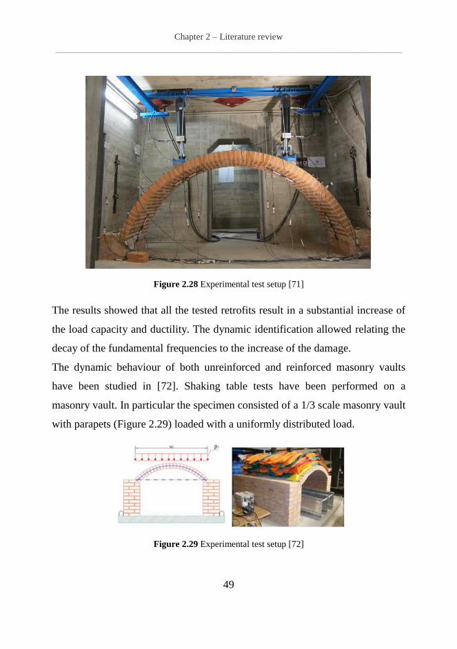
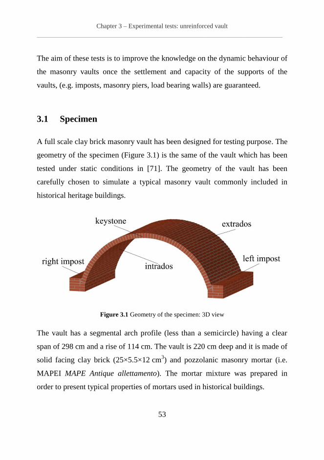
Figure 2.28 Experimental test setup [71] .................................................................................... 49 Figure 2.29 Experimental test setup [72] .................................................................................... 49 Figure 2.30 Experimental test setup [73] .................................................................................... 50 Figure 3.1 Geometry of the specimen: 3D view ......................................................................... 53
Page 11
List of Figures
______________________________________________________________________________________________________________________________
6
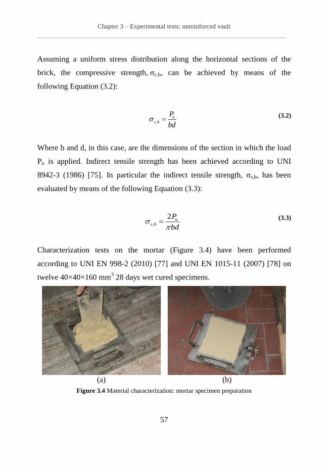
Figure 3.2 Geometry of the specimen: plan and section views (dimension in cm)..................... 54 Figure 3.3 Specimen during construction phases: (a) polystyrene centring; (b) construction of
the imposts; (c) curved element construction; (d) specimen completed ..................................... 55
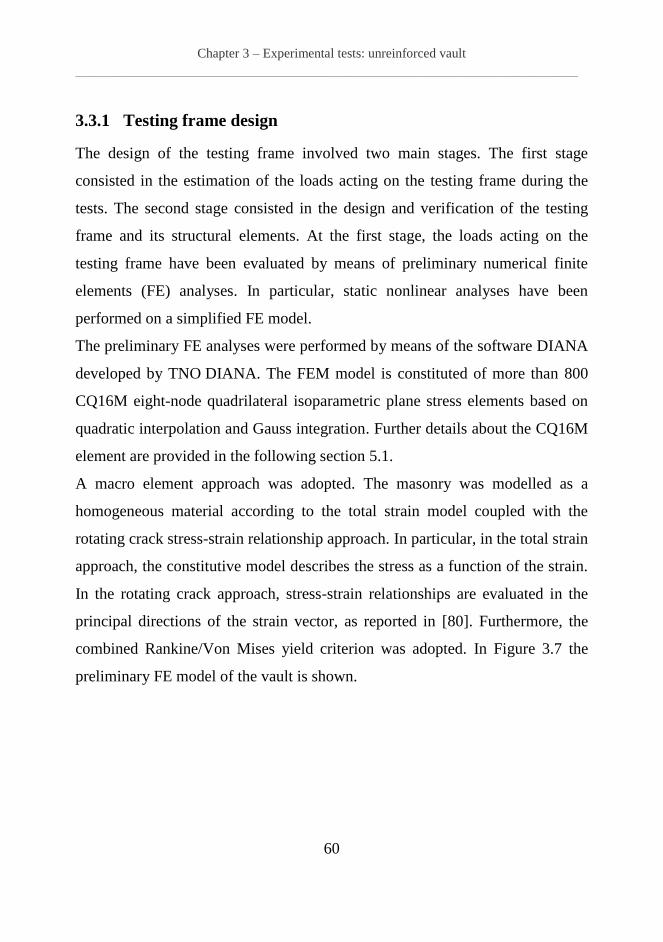
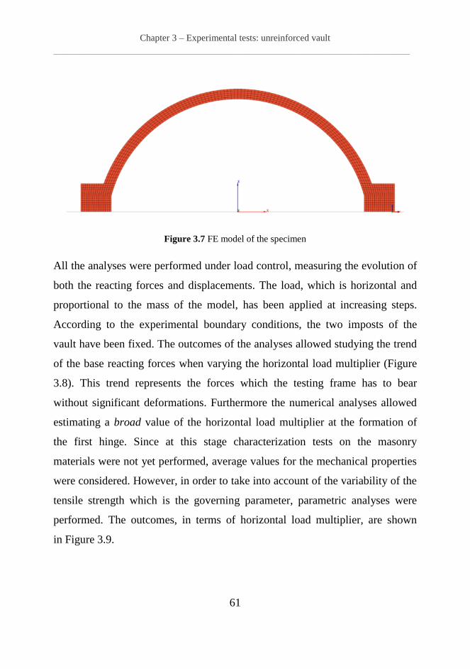
Figure 3.4 Material characterization: mortar specimen preparation ........................................... 57 Figure 3.5 Earthquake simulator system (ESS) scheme ............................................................. 58 Figure 3.6 Testing structure overview ........................................................................................ 59 Figure 3.7 FE model of the specimen ......................................................................................... 61 Figure 3.8 Static nonlinear analyses results: horizontal load multiplier-base reacting forces
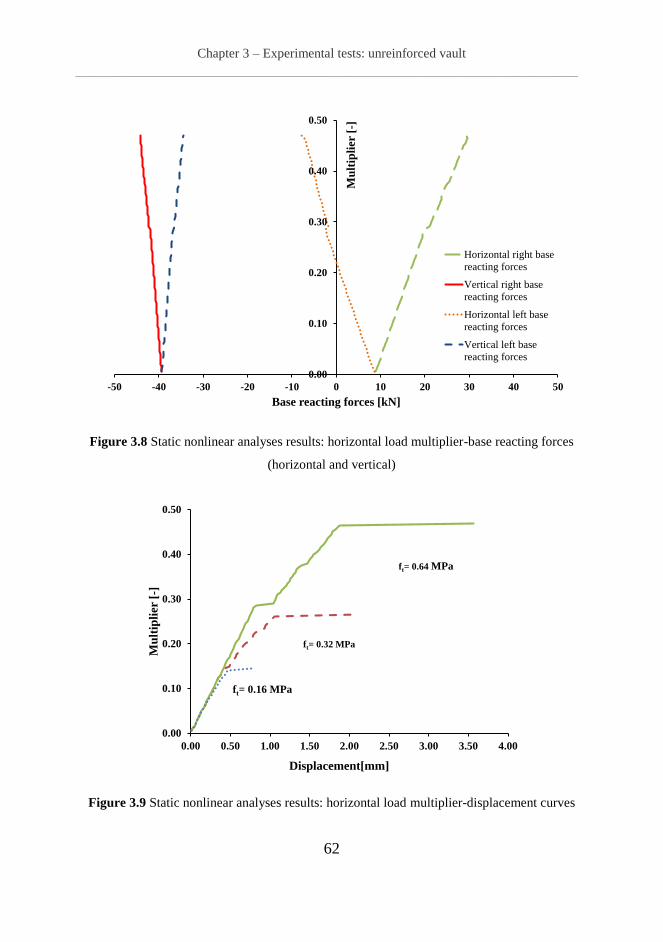
(horizontal and vertical) .............................................................................................................. 62
Figure 3.9 Static nonlinear analyses results: horizontal load multiplier-displacement curves .... 62 Figure 3.10 Geometry of the steel plane frame (plan and laterals view) .................................... 63
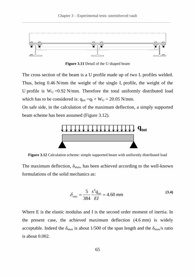
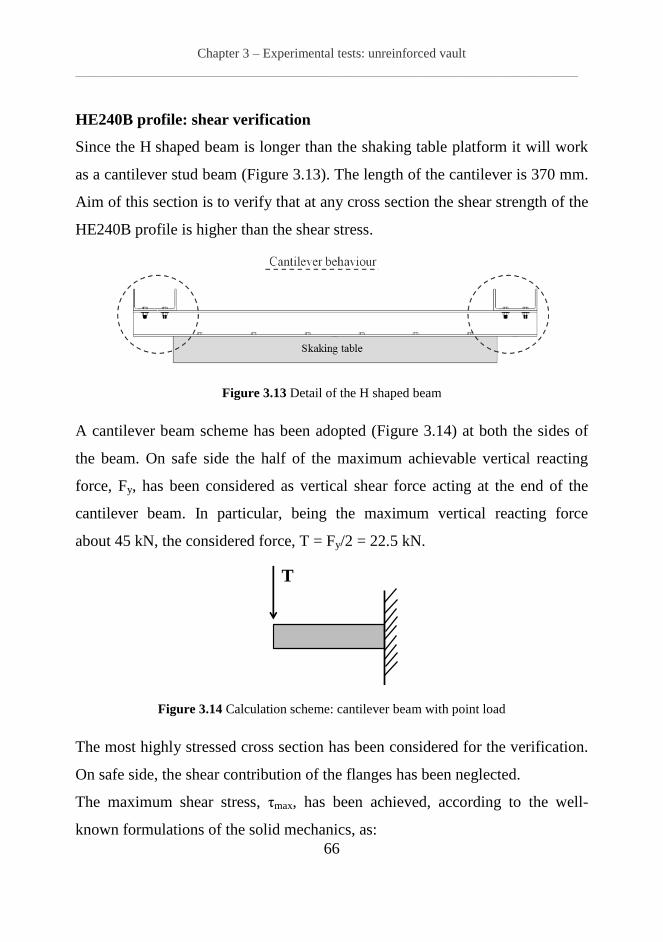
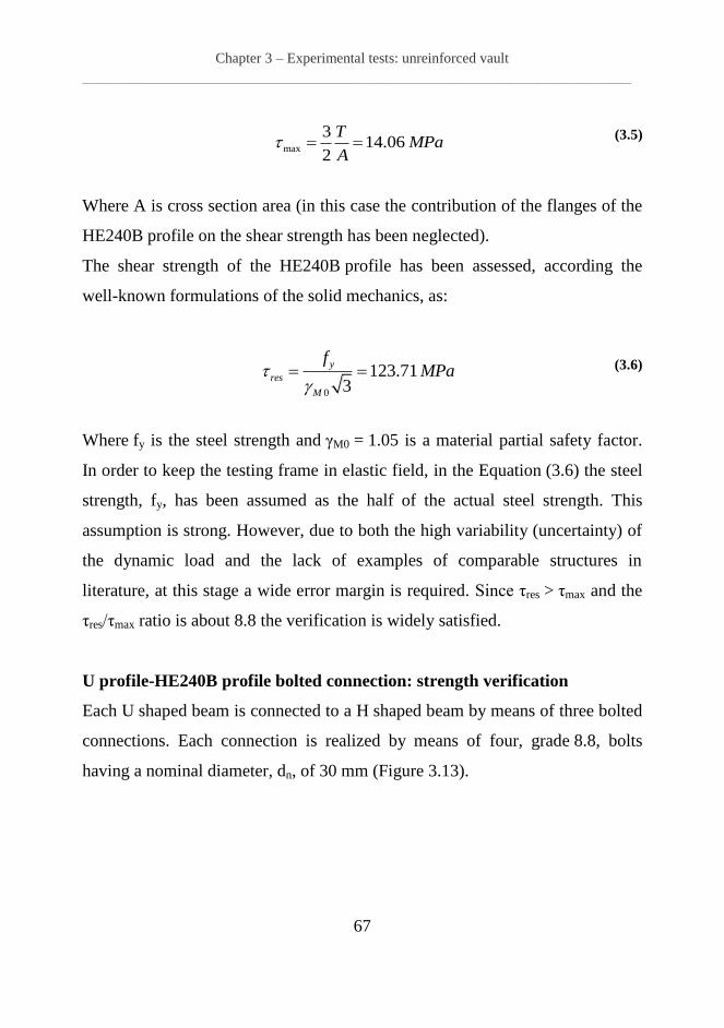
Figure 3.11 Detail of the U shaped beam ................................................................................... 65 Figure 3.12 Calculation scheme: simple supported beam with uniformly distributed load ........ 65 Figure 3.13 Detail of the H shaped beam ................................................................................... 66
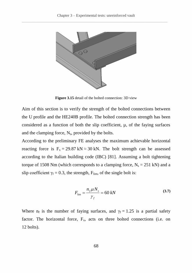
Figure 3.14 Calculation scheme: cantilever beam with point load ............................................. 66 Figure 3.15 detail of the bolted connection: 3D view ................................................................. 68
Figure 3.16 Force acting on the single bolted connection .......................................................... 69
Figure 3.17 Bolt holes spacing reference scheme ....................................................................... 69
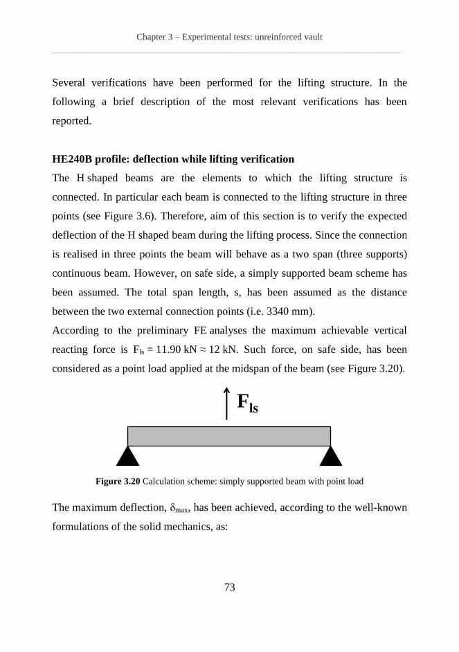
Figure 3.18 Connections between the lifting structure and the testing frame ............................. 71 Figure 3.19 FEM model of the lifting/moving system ................................................................ 72 Figure 3.20 Calculation scheme: simply supported beam with point load ................................. 73
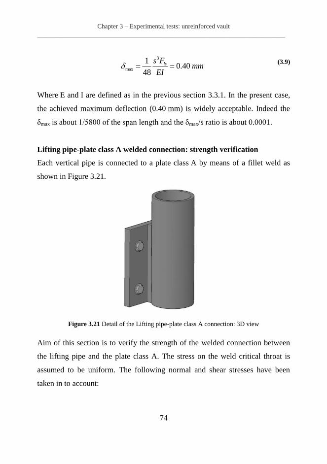
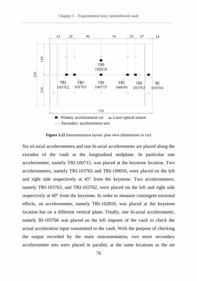
Figure 3.21 Detail of the Lifting pipe-plate class A connection: 3D view ................................. 74 Figure 3.22 Instrumentation layout: plan view (dimensions in cm) ........................................... 76
Figure 3.23 Instrumentation layout: front view (dimensions in cm) ........................................... 77 Figure 3.24 Time-history accelerograms at 100% intensity: (a) STR; (b) ART; ........................ 78 Figure 3.25 Time-history accelerograms at 100%: (a) FFT STR; (b) FFT ART. ....................... 79
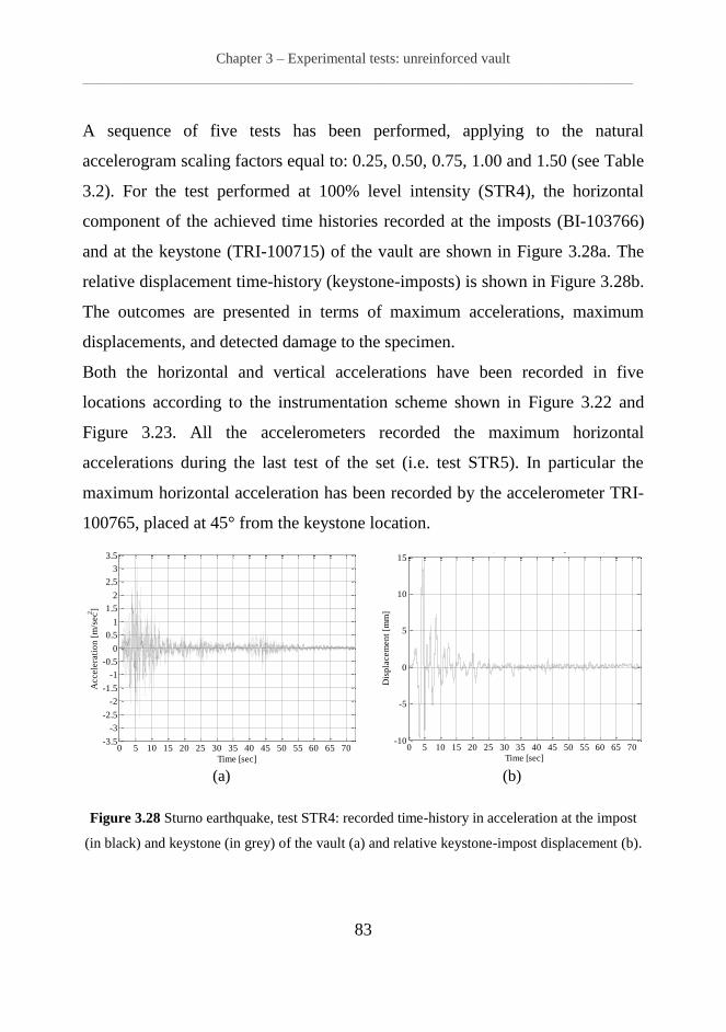
Figure 3.26 Test setup and specimen: shaking direction (unreinforced vault). .......................... 80 Figure 3.27 Natural frequency decay of the specimen (unreinforced vault). .............................. 81 Figure 3.28 Sturno earthquake, test STR4: recorded time-history in acceleration at the impost
(in black) and keystone (in grey) of the vault (a) and relative keystone-impost displacement (b).
.................................................................................................................................................... 83 Figure 3.29 STR: Maximum acceleration profiles (values expressed in m/s
2). .......................... 84
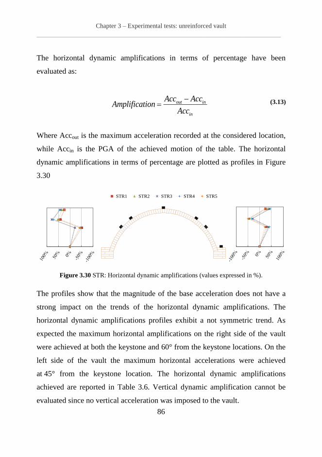
Figure 3.30 STR: Horizontal dynamic amplifications (values expressed in %). ........................ 86 Figure 3.31 Artificial earthquake, test ART7: (a) recorded time-history in acceleration at the
impost (in black) and keystone (in grey) of the vault; (b) relative keystone-impost displacement.
.................................................................................................................................................... 88
Figure 3.32 ART: Maximum acceleration profiles (values expressed in m/s2). ......................... 89
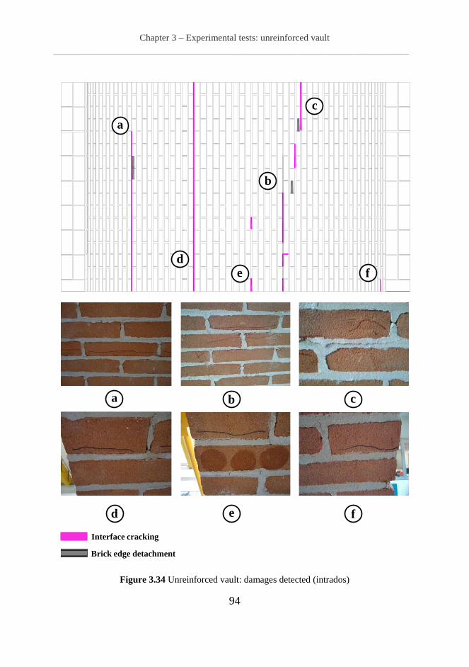
Figure 3.33 ART: Horizontal dynamic amplifications (values expressed in %). ........................ 91 Figure 3.34 Unreinforced vault: damages detected (intrados) .................................................... 94
Page 12
List of Figures
______________________________________________________________________________________________________________________________
7
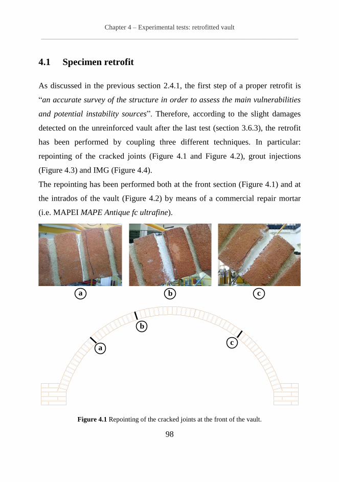
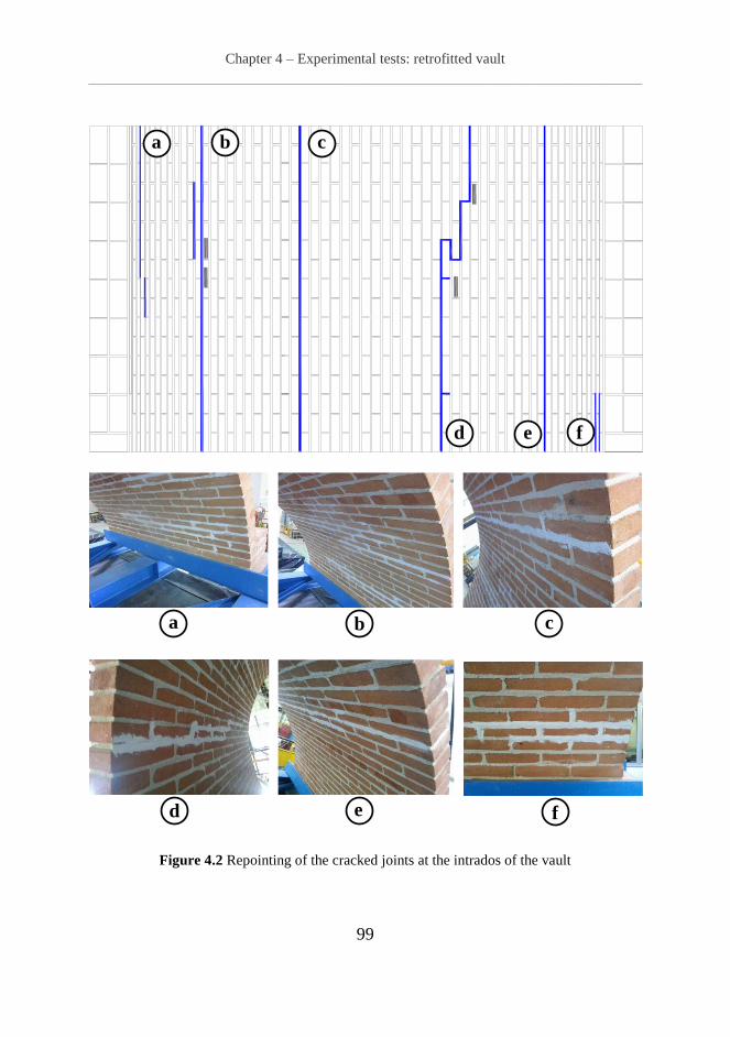
Figure 3.35 Unreinforced vault: damages detected (extrados) ................................................... 95 Figure 4.1 Repointing of the cracked joints at the front of the vault. ......................................... 98 Figure 4.2 Repointing of the cracked joints at the intrados of the vault ..................................... 99
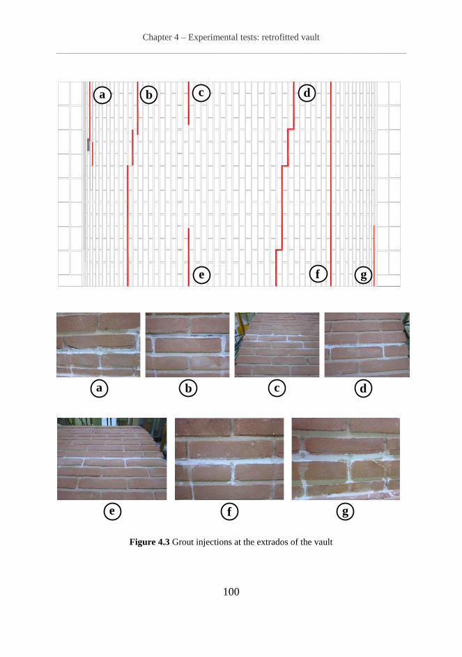
Figure 4.3 Grout injections at the extrados of the vault ............................................................ 100 Figure 4.4 IMG system at the extrados of the vault .................................................................. 101 Figure 4.5 Resume of the retrofit process: (a) Repointing of the cracked joints at the intrados;
(b) Grout injections at the extrados; (c) Grid installing layer at the extrados. .......................... 102 Figure 4.6 Test setup and specimen: shaking direction (retrofitted vault). ............................... 103
Figure 4.7 Natural frequency decay of the specimen (retrofitted vault). .................................. 107
Figure 4.8 Artificial earthquake, test ART7_R: (a) recorded time-history in acceleration at the
impost (in black) and keystone (in grey) of the vault; (b) relative keystone-impost displacement.
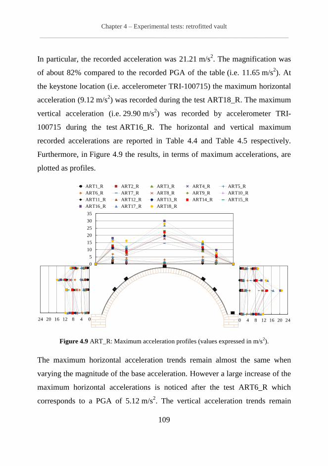
.................................................................................................................................................. 108 Figure 4.9 ART_R: Maximum acceleration profiles (values expressed in m/s
2). ..................... 109
Figure 4.10 ART_R: Horizontal dynamic amplifications (values expressed in %). ................. 112
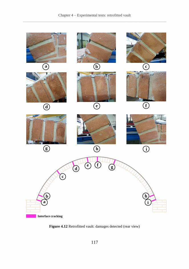
Figure 4.11 Retrofitted vault: damages detected (front view). ................................................. 116 Figure 4.12 Retrofitted vault: damages detected (rear view) .................................................... 117
Figure 4.13 Retrofitted vault: damages detected (intrados) ...................................................... 118
Figure 4.14 Natural frequency comparison: retrofitted vault/unreinforced vault ..................... 120
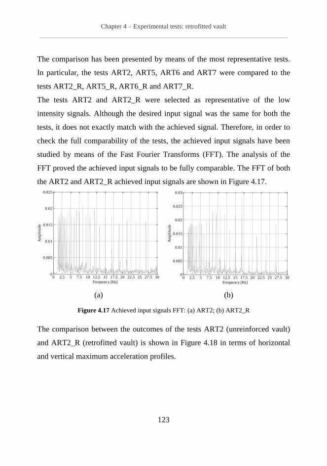
Figure 4.15 Comparison: frequency decay-achieved PGA trends ............................................ 121 Figure 4.16 Comparison: damping ratios-achieved PGA trends............................................... 122 Figure 4.17 Achieved input signals FFT: (a) ART2; (b) ART2_R ........................................... 123
Figure 4.18 Maximum acceleration profiles comparison: ART2-ART2_R (values expressed in
m/s2) .......................................................................................................................................... 124
Figure 4.19 Dynamic amplification profiles comparison: ART2-ART2_R (values expressed in
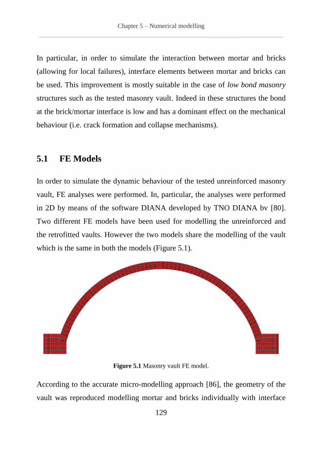
%). ............................................................................................................................................ 125 Figure 5.1 Masonry vault FE model. ........................................................................................ 129
Figure 5.2 Masonry vault FE model: detail of the adopted mesh. ............................................ 130 Figure 5.3 CQ16M element [80] ............................................................................................... 131 Figure 5.4 CL12I element: (a) topology; (b) displacement [80] ............................................... 131
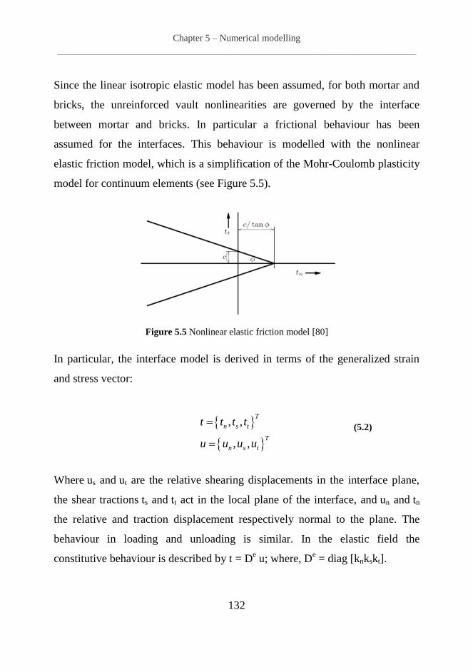
Figure 5.5 Nonlinear elastic friction model [80]....................................................................... 132
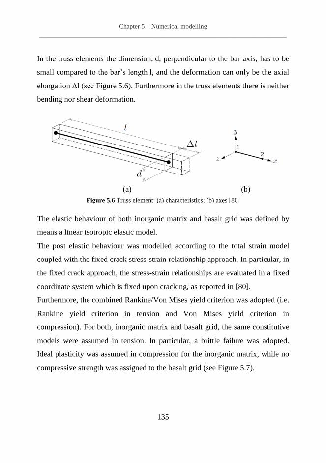
Figure 5.6 Truss element: (a) characteristics; (b) axes [80] ...................................................... 135 Figure 5.7 IMG constitutive models adopted: (a) grid; (b) matrix............................................ 136 Figure 5.8 Calibration of the interface stiffness: interface stiffness-natural frequency curve .. 138 Figure 5.9 Vertical load test: instrumentation and load layout ................................................. 140 Figure 5.10 Vertical load test: (a) loading phase; (b) maximum load ....................................... 140
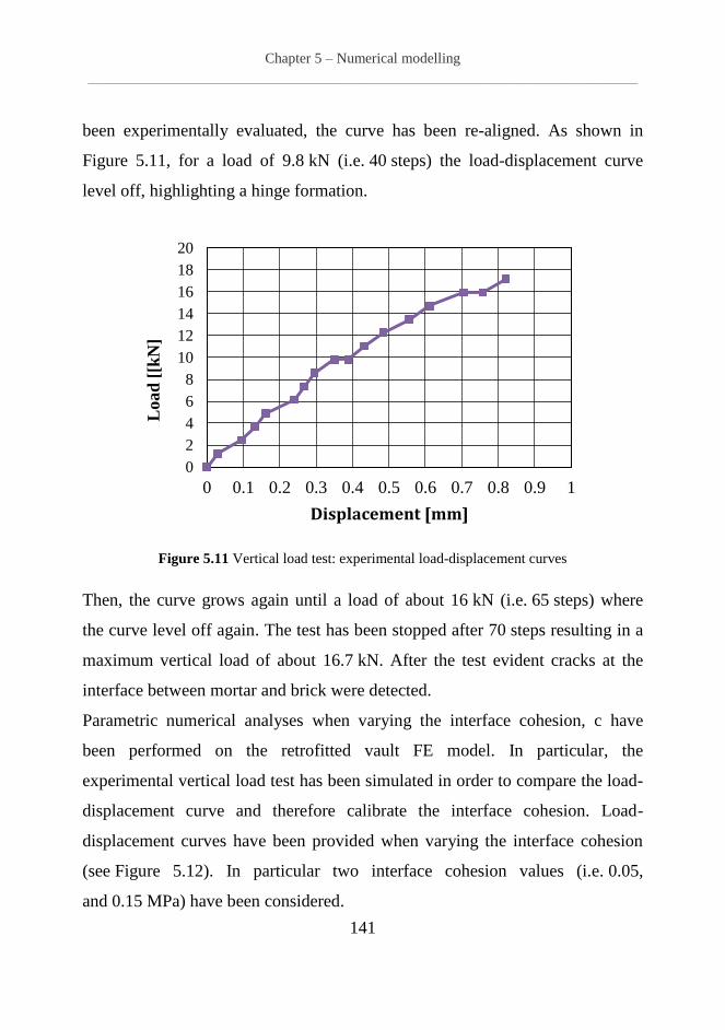
Figure 5.11 Vertical load test: experimental load-displacement curves ................................... 141
Figure 5.12 Calibration of the interface cohesion: numerical load-displacement curves ......... 142 Figure 5.13 Calibration of the interface cohesion: numerical-experimental comparison ......... 143 Figure 5.14 Unreinforced vault: modal shapes (mode 1-4) ...................................................... 144
Page 13
List of Figures
______________________________________________________________________________________________________________________________
8
Figure 5.15 Unreinforced vault: modal shapes (mode 5-10) .................................................... 146 Figure 5.16 Retrofitted vault: modal shapes (mode 1-4) .......................................................... 147 Figure 5.17 Retrofitted vault: modal shapes (mode 5-10) ........................................................ 147
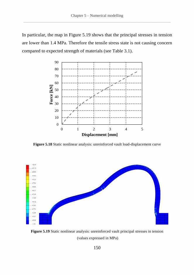
Figure 5.18 Static nonlinear analysis: unreinforced vault load-displacement curve ................. 150 Figure 5.19 Static nonlinear analysis: unreinforced vault principal stresses in tension (values
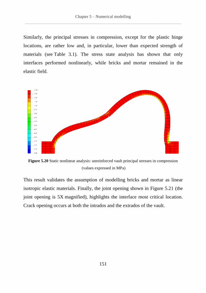
expressed in MPa)..................................................................................................................... 150 Figure 5.20 Static nonlinear analysis: unreinforced vault principal stresses in compression
(values expressed in MPa) ........................................................................................................ 151
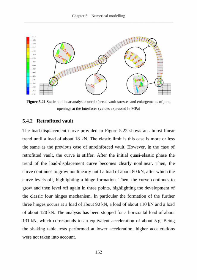
Figure 5.21 Static nonlinear analysis: unreinforced vault stresses and enlargements of joint
openings at the interfaces (values expressed in MPa) ............................................................... 152 Figure 5.22 Static nonlinear analysis: retrofitted vault load-displacement curve ..................... 153
Figure 5.23 Static nonlinear analysis: retrofitted vault principal stresses in tension (values
expressed in MPa)..................................................................................................................... 154 Figure 5.24 Static nonlinear analysis: retrofitted vault principal stresses in compression (values
expressed in MPa)..................................................................................................................... 154 Figure 5.25 Static nonlinear analysis: retrofitted vault stresses and stresses and enlargements of
joint openings at the interfaces (values expressed in MPa) ...................................................... 155
Figure 5.26 Variation of damping ratio with natural frequency ............................................... 159
Figure 5.27 ART2: (a) time-history accelerogram; (b) elastic spectrum .................................. 160 Figure 5.28 ART7: (a) time-history accelerogram; (b) elastic spectrum .................................. 160 Figure 5.29 ART2_R: (a) time-history accelerogram; (b) elastic spectrum .............................. 161
Figure 5.30 ART7_R: (a) time-history accelerogram; (b) elastic spectrum .............................. 161 Figure 5.31 ART15_R: (a) time-history accelerogram; (b) elastic spectrum ............................ 161
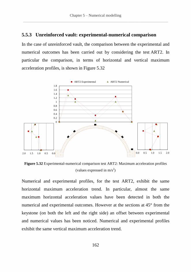
Figure 5.32 Experimental-numerical comparison test ART2: Maximum acceleration profiles
(values expressed in m/s2)......................................................................................................... 162
Figure 5.33 Experimental-numerical comparison test ART2: Dynamic amplification profiles
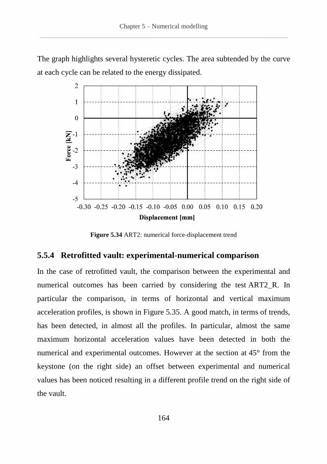
(values expressed in %). ........................................................................................................... 163 Figure 5.34 ART2: numerical force-displacement trend .......................................................... 164 Figure 5.35 Experimental-numerical comparison test ART2_R: Maximum acceleration profiles
(values expressed in m/s2)......................................................................................................... 165
Figure 5.36 Experimental-numerical comparison test ART2_R: Dynamic amplification profiles
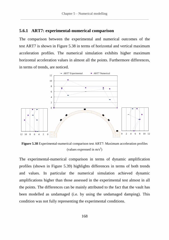
(values expressed in %). ........................................................................................................... 165 Figure 5.37 ART2_R: numerical force-displacement trend ...................................................... 166 Figure 5.38 Experimental-numerical comparison test ART7: Maximum acceleration profiles
(values expressed in m/s2)......................................................................................................... 168
Figure 5.39 Experimental-numerical comparison test ART7: Dynamic amplification profiles
(values expressed in %). ........................................................................................................... 169 Figure 5.40 ART7: numerical force-displacement trend .......................................................... 169
Page 14
List of Figures
______________________________________________________________________________________________________________________________
9
Figure 5.41 Experimental-numerical comparison test ART7_R: Maximum acceleration profiles
(values expressed in m/s2)......................................................................................................... 170
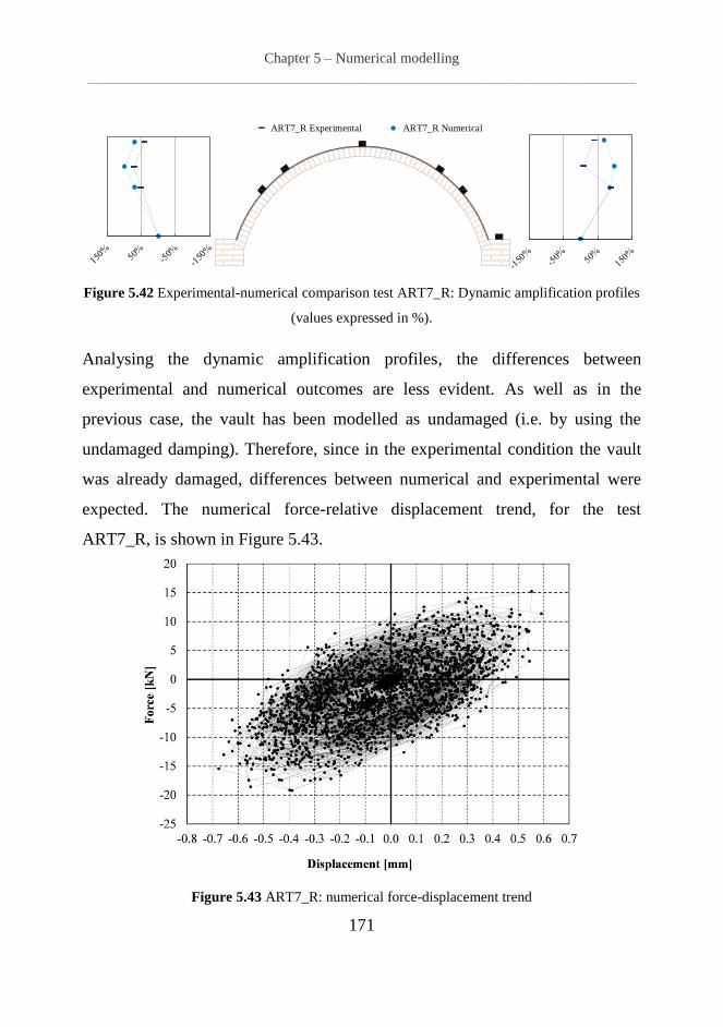
Figure 5.42 Experimental-numerical comparison test ART7_R: Dynamic amplification profiles
(values expressed in %). ........................................................................................................... 171 Figure 5.43 ART7_R: numerical force-displacement trend ...................................................... 171 Figure 5.44 ART15_R: experimental (in black) and numerical 2.8% damping (in grey) ......... 173 Figure 5.45 ART15_R: experimental (in black) and numerical 5% damping (in grey) ............ 173 Figure 5.46 ART15_R: experimental (in black) and numerical 10% damping (in grey) .......... 173
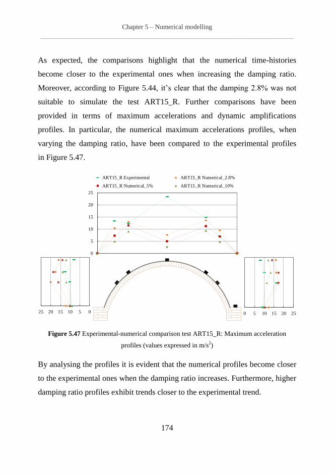
Figure 5.47 Experimental-numerical comparison test ART15_R: Maximum acceleration
profiles (values expressed in m/s2) ........................................................................................... 174
Figure 5.48 Experimental-numerical comparison test ART15_R: Dynamic amplification
profiles (values expressed in %) ............................................................................................... 175
Page 15
Chapter 1 - Introduction
______________________________________________________________________________________________________________________________
10
Chapter 1
Introduction
1.1. General context
Masonry is the generic term for a composite material made of a large number of
separate small elements bonded together by some binding filler in many
different arrangements. The quality of the bond, materials used, workmanship
and the masonry textures significantly affect the mechanical performance of the
overall masonry structure. For these reasons, the prediction of masonry
behaviour is generally extremely hard.
Masonry constructions were widespread in the ancient world, and masonry is
one of the most used materials in ancient times. Furthermore the most of the
European cultural heritage buildings are constituted by masonry. Despite their
past and present spread, and their long existence, masonry constructions are
prone to damage under seismic actions. Moreover, a relevant part of these
buildings are located in areas of high seismic risk.
Page 16
Chapter 1 - Introduction
______________________________________________________________________________________________________________________________
11
Recent earthquakes in Italy (Umbria and Marche,1997-1998; L’Aquila, 2009;
Emilia Romagna, 2012) have produced significant damages to several historical
and cultural heritage sites [1]. In many of these historical buildings the vertical
masonry elements were connected by means of curved elements, such as arches
or vaults. The inspections of the damaged building, after the earthquakes
(e.g. San Paolo Cathedral in Mirabello, San Francesco church complex in
Assisi, Estense Fortress in Finale Emilia [1]), have shown that masonry arches
and vaults are the most critical elements in the seismic vulnerability of such
structures (Figure 1.1).
Figure 1.1 Example of vaults damaged: (a) Emilia-Romagna Earthquake (2012) [2];
(b), (c) and (d) L’Aquila earthquake (2009) [2, 3];
(a) (b)
(c) (d)
Page 17
Chapter 1 - Introduction
______________________________________________________________________________________________________________________________
12
Therefore, the preservation and, in particular, the retrofit of curved masonry
structural elements is a crucial structural issue.
Recent developments in materials, manufacturing, mechanics and design of
composite materials allowed the growth of such materials as retrofit of masonry
elements.
In the last years the most of composites strengthening research has involved
fibre reinforced polymers (FRP). However, resin-based composites have shown
several drawbacks such as: inappropriate bond to existing masonry substrates,
flammability, sensitivity to high temperatures and moisture permeability [4].
Such problems can be overcome by innovative applications which involve
inorganic matrix composite grids (IMG). Cement based matrixes are, indeed,
highly compatible to the masonry substrate in terms of bond, moisture
permeability, and thermal properties preventing therefore the main critical
issues [5]. These retrofit techniques applied to masonry elements have
demonstrated to significantly improve the stiffness, ductility and the ultimate
strength, preventing the element from a brittle collapse [6-8].
So far, however comprehensive knowledge on the effectiveness of such retrofit
applied to masonry vault elements under dynamic load is still lacking.
In this thesis, the dynamic behaviour of both unreinforced and retrofitted
masonry vault elements has been investigated. The vault has been retrofitted by
means of mortar joint repointing, grout injections and IMG. Moreover, the
experimental data allowed developing reliable numerical models able to predict
the dynamic behaviour of masonry vault (before and after the retrofit).
Page 18
Chapter 1 - Introduction
______________________________________________________________________________________________________________________________
13
1.2. Research significance
Masonry is the simplest construction material. Despite its straightforwardness,
however, the seismic behaviour of masonry structures is hard to predict. In
many masonry buildings, the vertical elements are connected by means of
curved elements, such as arches or barrel vaults. Furthermore the vaults
represent an artistic valuable element in the historical heritage buildings.
Consequently, the understanding of their seismic performance, as well as
potential retrofit techniques, meets also the need to protect cultural heritage
buildings against earthquakes. Nowadays, however, a better knowledge on the
dynamic behaviour of masonry vaulted elements is still a need. These
motivating factors provide the purposes of this thesis, which are:
improving the knowledge on the dynamic behaviour of masonry vaulted
elements;
studying the impact of innovative retrofit techniques such as IMG on the
dynamic behaviour of masonry vaulted elements;
developing reliable numerical models able to predict the dynamic
behaviour of masonry vaults (before and after the retrofit)
In order to achieve this goal a multi-scale approach has been adopted. Both
experimental shaking table tests and numerical analyses have been performed
on the vault before and after the retrofit. In order to calibrate the numerical
models, further experimental vertical load tests been performed.
Page 19
Chapter 1 - Introduction
______________________________________________________________________________________________________________________________
14
1.3. Outline of the thesis
The thesis has been structured into 5 chapters, included the Chapter 1, which
briefly introduces to the general context and states the objectives and strategies
adopted to achieve them. Chapter 2 provides for a review the previous
researches by means of an accurate literature review. In particular the following
aspects have been treated: static and dynamic analysis methods; retrofit
techniques for historical vaulted structures; previous experimental studies on
the theme. In the Chapter 3 the experimental shaking table tests on the
unreinforced vault have been presented. In particular, specimen characteristics,
test setup design, monitoring instrumentation and seismic inputs have been
described. The test outcomes have been presented in terms of: relative
displacement, maximum acceleration and dynamic amplification profiles and
time histories. Chapter 4 deals with the experimental shaking table tests on the
retrofitted vault. In particular, specimen retrofit, monitoring instrumentation
and seismic inputs have been described. Furthermore, a comparison between
the test outcomes of reinforced and retrofitted vault has been provided. Both the
test and the outcomes of comparisons have been presented in terms of: relative
displacement, maximum acceleration and dynamic amplification profiles and
time histories. In the Chapter 5 is presented the finite elements modelling of the
tested specimens (i.e. both unreinforced and retrofitted vaults). Micro-
modelling approach has been adopted and the nonlinear characteristics of the
vault have been calibrated by means of experimental tests. Dynamic linear,
static nonlinear and dynamic nonlinear analyses have been performed in order
to validate the numerical models. Furthermore, the influence of the damping
parameters has been investigated.
Page 20
Chapter 2 – Literature review
______________________________________________________________________________________________________________________________
15
Chapter 2
Literature review
Vaults are spatial three-dimensional structures which were usually built in order
to provide a space with a ceiling or roof. In the history several types of vaults
have been built. The simplest type of vault is the “barrel vault” which consists
of a continuous ongoing series of semi-circular arches. Barrel vaults can be
schematized as sum of series of elementary arches (neglecting potential mutual
interaction between the arches). Thus the structural analysis of barrel vaults is
practically a problem which can be solved by studying the elementary arch in
its own plane [9]. Therefore, the methods developed for the arches can be
expanded to three dimensions, in order to study behaviour of the barrel vaults.
Masonry arches have been studied for many centuries and several methods and
tools have been developed to understand their behaviour. In the following
sections a brief overview on the historical evolution of the masonry curved
elements has been provided. Then the mechanical and analytical methods
adopted to study the arch behaviour have been addressed.
Page 21
Chapter 2 – Literature review
______________________________________________________________________________________________________________________________
16
2.1 Brief historical overview of the masonry curved elements
The use of arches and vaults is thousand years old. It exists in nature as a
consequence of natural lack of tensile strength of the stones. Several theories
have been formulated on how this type of structure has started to be used in
architecture. Probably it has conceived as a refinement of support stone
elements [10], or as a subdivision of stone beams into smaller single
elements (Figure 2.1)
Figure 2.1 Arch as a subdivision of stone beams into smaller single elements [10]
Primitive examples of curved masonry elements date back to the prehistory.
Stone arches appeared in Babylon about 6,000 years ago. The first small-span
vaults, dated back about 5,000 years ago, are clear in Mesopotamic burial
chambers [10, 11]. Several examples of vaults were also found in Sumerians
and Old Egyptians architecture. A step forward in the development of curved
elements was done during the time of the Roman Empire. In this time the
placement of the stones was improved and the mortar started to be used. These
improvements allowed the construction of wide-span vaults. Roman bridges,
amphitheatres and aqueducts are clear example of the considerable usage of
curved masonry elements in the Roman architecture (Figure 2.2).
Page 22
Chapter 2 – Literature review
______________________________________________________________________________________________________________________________
17
(a) (b)
Figure 2.2 Arches in Roman architecture: (a) Colosseum; (b) Segovia’s aqueduct
After the Roman Empire fall, the use of curved masonry elements was
remarkable in the Byzantine architecture, where new arch typologies were
developed (i.e. lancet and ogee arches). Later, during the Middle Age, in the
Romanesque architecture the use of round arches and barrel vaults was massive
once again (Figure 2.3).
Figure 2.3 Vaulted structure in Romanesque architecture [12]
Page 23
Chapter 2 – Literature review
______________________________________________________________________________________________________________________________
18
The use of vaulted structures was largely adopted in the Gothic architecture as
well. In this historic period the use of curved masonry elements allowed the
perfect integration of architectural and structural functions. In particular the
main innovations of the use of curved masonry elements in Gothic architecture
were: the use of flying buttress and the use of the pointed arch (Figure 2.4).
(a) (b)
Figure 2.4 Gothic architecture: (a) Cathedral; (b) Flying buttress
During the Renaissance, symmetry, proportion, geometry and the regularity of
parts were the main architectural points, and the application of circular
segments became very popular. In the 19th
centuries, due to the gradual
introduction of iron and then steel, to be followed by reinforced concrete the
decline of the use of masonry structures has started. Nowadays masonry
constructions do not have a central role in the building trade. However their
preservation and retrofit represents a challenging structural matter.
Page 24
Chapter 2 – Literature review
______________________________________________________________________________________________________________________________
19
2.2 Arch static analysis methods
A large amount of literature has been published on the arch static analysis. It
represents a solid base to the proper study of the arch behaviour. Since the
dynamic effects are neglected, these methods are not as accurate as the modern
dynamic methods are. On the other hand, they are practical and they can be
applied when high computational power is not available. Therefore, these
methods represent a good compromise between the approximation and
computational expense.
2.2.1 Equilibrium methods
The static behaviour of masonry structures can be studied according to three
simple key assumption proposed in the 1730 by Couplet [13, 14]:
masonry has no tensile strength;
sliding failure does not occur;
stresses are so low that masonry compressive strength can effectively be
considered unlimited.
Each one of these assumptions could not be strictly true. Therefore it must be
hedged with qualifications and it must, in any case, be tested [14].
However, for historical masonry structures, the Couplet assumptions are largely
acceptable in the most of the cases. Thus, they still provide the basic principles
used for the masonry structural analysis [14, 15]. The analysis methods based
on this assumptions are usually known as “equilibrium methods” [16]. Since the
main field of application of these methods are the pure compression structures,
they are particularly suitable, for the structural analysis of arches and vaults.
The arch is the fundamental structural element in the masonry architecture [17].
However, it is worth to briefly introduce the basic concepts of the arch
Page 25
Chapter 2 – Literature review
______________________________________________________________________________________________________________________________
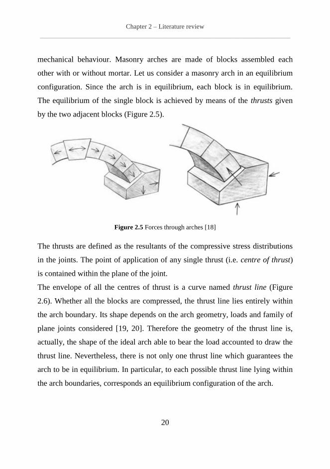
20
mechanical behaviour. Masonry arches are made of blocks assembled each
other with or without mortar. Let us consider a masonry arch in an equilibrium
configuration. Since the arch is in equilibrium, each block is in equilibrium.
The equilibrium of the single block is achieved by means of the thrusts given
by the two adjacent blocks (Figure 2.5).
Figure 2.5 Forces through arches [18]
The thrusts are defined as the resultants of the compressive stress distributions
in the joints. The point of application of any single thrust (i.e. centre of thrust)
is contained within the plane of the joint.
The envelope of all the centres of thrust is a curve named thrust line (Figure
2.6). Whether all the blocks are compressed, the thrust line lies entirely within
the arch boundary. Its shape depends on the arch geometry, loads and family of
plane joints considered [19, 20]. Therefore the geometry of the thrust line is,
actually, the shape of the ideal arch able to bear the load accounted to draw the
thrust line. Nevertheless, there is not only one thrust line which guarantees the
arch to be in equilibrium. In particular, to each possible thrust line lying within
the arch boundaries, corresponds an equilibrium configuration of the arch.
Page 26
Chapter 2 – Literature review
______________________________________________________________________________________________________________________________
21
Figure 2.6 Sketch of the thrusts in a generic masonry arch
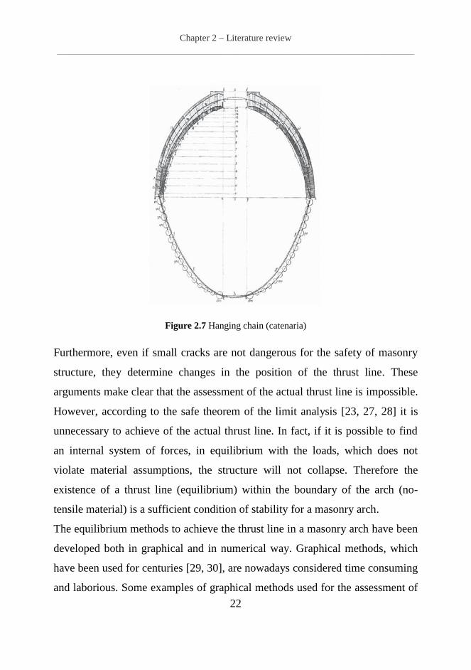
Given an arbitrary masonry arch, ideally inverting his curvature (Figure 2.7),
the compression forces will become tension forces.
Thus the blocks constituent the arch, will hang like a chain [21, 22]. Therefore,
according to Heyman [23] is possible to re-assert the previous statements as
“…none but the catenaria is the figure of a true legitimate arch, or fornix. And
when an arch of any other figure is supported, it is because in its thickness some
catenaria is included”.
The solution of the equilibrium problem is not unique. Infinite thrust lines or
catenaries can lie within the arch boundaries. The arch is, indeed, a hyperstatic
structure. Thus the equilibrium equations are not enough to give the solution. In
order to achieve the actual thrust line, statements about both material properties
and boundary condition are required. Appling the elastic analysis (equilibrium,
congruence and compatibilities equations) it is possible to achieve the stresses
in the arch [23-26]. However, the resultant equation system found applying the
elastic analysis is highly sensitive to small changes in boundary conditions (i.e.
hinges formation) [14, 17].
Page 27
Chapter 2 – Literature review
______________________________________________________________________________________________________________________________
22
Figure 2.7 Hanging chain (catenaria)
Furthermore, even if small cracks are not dangerous for the safety of masonry
structure, they determine changes in the position of the thrust line. These
arguments make clear that the assessment of the actual thrust line is impossible.
However, according to the safe theorem of the limit analysis [23, 27, 28] it is
unnecessary to achieve of the actual thrust line. In fact, if it is possible to find
an internal system of forces, in equilibrium with the loads, which does not
violate material assumptions, the structure will not collapse. Therefore the
existence of a thrust line (equilibrium) within the boundary of the arch (no-
tensile material) is a sufficient condition of stability for a masonry arch.
The equilibrium methods to achieve the thrust line in a masonry arch have been
developed both in graphical and in numerical way. Graphical methods, which
have been used for centuries [29, 30], are nowadays considered time consuming
and laborious. Some examples of graphical methods used for the assessment of
Page 28
Chapter 2 – Literature review
______________________________________________________________________________________________________________________________
23
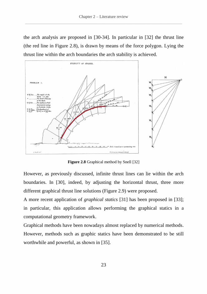
the arch analysis are proposed in [30-34]. In particular in [32] the thrust line
(the red line in Figure 2.8), is drawn by means of the force polygon. Lying the
thrust line within the arch boundaries the arch stability is achieved.
Figure 2.8 Graphical method by Snell [32]
However, as previously discussed, infinite thrust lines can lie within the arch
boundaries. In [30], indeed, by adjusting the horizontal thrust, three more
different graphical thrust line solutions (Figure 2.9) were proposed.
A more recent application of graphical statics [31] has been proposed in [33];
in particular, this application allows performing the graphical statics in a
computational geometry framework.
Graphical methods have been nowadays almost replaced by numerical methods.
However, methods such as graphic statics have been demonstrated to be still
worthwhile and powerful, as shown in [35].
Page 29
Chapter 2 – Literature review
______________________________________________________________________________________________________________________________
24
Figure 2.9 Graphical methods by Huerta [30]
Numerical methods can be applied to assess both the stability and the seismic
behaviour. In the case of seismic assessment all the equilibrium numerical
methods simulate the ground motion effects by means of a constant horizontal
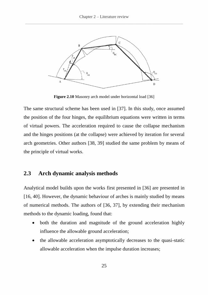
force. In [36] the problem of the masonry arch under seismic, load has been
studied by modelling the arch as a single degree of freedom (SDOF) system.
The system consisted of a rigid body made up of three hinged bars and four
hinges as shown in Figure 2.10. Once assumed the position of the four hinges,
the equation of motion were derived by means of Hamilton’s Principle and
Lagrange equations for SDOF rigid body systems. The minimum acceleration
required activating the collapse mechanism and the correspondent mechanism
were achieved by iteration.
Page 30
Chapter 2 – Literature review
______________________________________________________________________________________________________________________________
25
Figure 2.10 Masonry arch model under horizontal load [36]
The same structural scheme has been used in [37]. In this study, once assumed
the position of the four hinges, the equilibrium equations were written in terms
of virtual powers. The acceleration required to cause the collapse mechanism
and the hinges positions (at the collapse) were achieved by iteration for several
arch geometries. Other authors [38, 39] studied the same problem by means of
the principle of virtual works.
2.3 Arch dynamic analysis methods
Analytical model builds upon the works first presented in [36] are presented in
[16, 40]. However, the dynamic behaviour of arches is mainly studied by means
of numerical methods. The authors of [36, 37], by extending their mechanism
methods to the dynamic loading, found that:
both the duration and magnitude of the ground acceleration highly
influence the allowable ground acceleration;
the allowable acceleration asymptotically decreases to the quasi-static
allowable acceleration when the impulse duration increases;
Page 31
Chapter 2 – Literature review
______________________________________________________________________________________________________________________________
26
the acceleration impulse required to let the arch collapse, almost
increase by the square root of the arch radius;
It is worth noting that none of the authors validated experimentally their
modelling. However the main results of their findings are rational. An
alternative to these methods is the Numerical finite elements method (FEM).
FEM is, nowadays, one of the mainly used methods for the arch dynamics
assessment. FEM analysis is, indeed, a powerful tool for the assessment of both
dynamic linear and dynamic nonlinear response of the arches.
2.3.1 Finite Element Method (FEM) analysis
The FEM in the past was used to study masonry arch behaviour, mainly by
means of static linear elastic analyses. The arch was usually modelled by means
of one-dimensional elements (i.e. beam elements) [41, 42]. The FEM modelling
techniques have been gradually refined and improved. Thus nowadays FEM is
typically applied to study the dynamic behaviour of arches by means of both
linear and nonlinear dynamic analyses.
In particular, FEM linear dynamic analyses are performed to study the
fundamental dynamic properties (e.g. fundamental frequency, damping) and the
steady-state dynamic response. By means of linear dynamic analyses is possible
to assess the strass state, thus the location in which the cracking might occur.
However, since masonry is a complex nonlinear material, in order to perform an
accurate dynamic analysis, its nonlinear behaviour should be considered.
The nonlinear dynamic analysis is the more accurate approach to numerically
assess the seismic response of a structure. In particular nonlinear dynamic
analyses are performed in order to assess the evolution of stresses and strains in
the time domain.
Page 32
Chapter 2 – Literature review
______________________________________________________________________________________________________________________________
27
Both material nonlinearities and stress redistribution due to cracking are
accounted. However, the results obtained are highly sensitive to the seismic
input adopted for the analyses. Several examples of application of dynamic
nonlinear analysis can be found in literature [43, 44].
2.4 Retrofit of historical buildings
Recent seismic events which affected the historical heritage buildings in Italy
remarked the importance of a proper seismic retrofit intervention. Retrofit of
historical masonry buildings is not an easy task. Indeed common retrofit
techniques cannot be arbitrarily applied to historical buildings. On this matter
the International council on monuments and sites (ICOMOS), which offers
advice to UNESCO on World heritage sites, provided important
recommendations [45]. Few of these recommendations are resumed in the
following bulleted list (references to the ICOMOS recommendation articles are
reported).
The restoration of monuments must have recourse to all the techniques
which can contribute to the safeguarding of the architectural
heritage. (Article 2)
The intention in conserving and restoring monuments is safeguard them
no less as works of art, than as historical evidence. (Article 3)
Where traditional techniques prove inadequate, the restoration of a
monument can be achieved by the use of any modern techniques of
construction, the efficacy of which has been shown by scientific data
and proved by experience. (Article 10)
Page 33
Chapter 2 – Literature review
______________________________________________________________________________________________________________________________
28
The valid contributions of all periods to the building of a monument
must be respected, since unity of style is not the aim of a restoration.
When a building includes the superimposed work of different periods,
the revealing of the underlying state can only be justified in exceptional
circumstances. (Article 11)
Replacements of missing parts must integrate harmoniously with the
whole, but at the same time must be distinguishable from the original, so
that the restoration does not falsify the artistic or historical
evidence. (Article 12)
Therefore, depending on the cultural relevance of the studied building, the final
choice could be either a stronger or a softer retrofit intervention.
For instance, for a highly vulnerable building, without any artistic value, the
replacement of deficient structural elements could be a quick and efficient
solution. Otherwise, if the same building would have a high artistic value, the
same solution could even not to be feasible. In particular, according to [45] any
retrofit intervention should be minimal and easily recognisable, in order to
prevent any potential fabrication of the historical meaning of the building.
2.4.1 Retrofit of vaulted structures
As discussed in the previous Chapter 1, vaults are among the more vulnerable
elements in historical masonry building. The damage of the vaults can be
induced by several reasons, such as: variations in the acting loads, instability of
the piers, and material degradation. The unexpected variation of either
horizontal or vertical loads (or a combination of both) is among the more
common cause of damage of vaults. The variation in the horizontal load
frequently is due to a seismic event. Otherwise, the variation of vertical loads
Page 34
Chapter 2 – Literature review
______________________________________________________________________________________________________________________________
29
often is due to a change of use of the structure. For instance, some historical
buildings become museum, bearing loads which were not expected in the
original design phase. The instability of the piers can be due to either
subsidence of the foundation soil or changing in the pier constraint conditions.
Furthermore, the mechanical behaviour of the vaults can be strongly influenced
by the degradation of its constituent materials. For instance, an aggressive
environment can lead to a reduction of the mechanical performances of
materials such as: clay, tuff, or natural stones. Such materials are commonly
used in vault construction. However, vaults geometry allows the distribution of
the strains along the joints preventing significant cracking in the masonry units.
Therefore, rather than the lack of strength, their collapse is generally due to the
inability of the structure to follow the displacement of the piers [46].
A retrofit intervention should be able to provide its strengthening action only in
case of changing of boundary conditions. Indeed, such intervention allows
retrofitting the vault without changing its constitutive global response.
Inappropriate retrofit interventions could even lead to an increase of the
vulnerability of the retrofitted building.
A proper retrofit intervention starts with an accurate survey of the structure in
order to assess the main vulnerabilities and potential instability sources. The
survey has to take into account of: material and geometrical properties, crack
patterns and degradation. According to [47, 48] the instability sources can be
sort as follow:
pier failure;
vault spontaneous collapse;
pier failure mixed with vault spontaneous collapse.
Page 35
Chapter 2 – Literature review
______________________________________________________________________________________________________________________________
30
However, often the assessment of the instability sources is not straightforward.
Indeed, it requires a strong knowledge and experience on masonry structural
analysis together with a deep knowledge of the analysed structure.
Several simultaneous instability sources could coexist in the same structure
making hard their recognition.
The analysis of damaged vaults shows that frequently the damages are restricted
only in few locations which can be assumed as plastic hinges. The collapse
mechanism will occur with the formation of the fourth plastic hinge (Figure
2.11). Traditional retrofit interventions on vaulted structures are based on the
basic idea of improving the strength of the structure. Otherwise innovative
retrofit techniques are based on the idea of improving both the capacity and the
ductility of the structure, without increasing its mass and stiffness.
Figure 2.11 Typical four hinges mechanism due to vertical load [49]
2.4.2 Overview on the main retrofit techniques for the vaults
In the following a brief overview on the main retrofit techniques adopted for
masonry vaults is provided. The aim of the following overview is to present a
list of such systems. For each system a brief description and a review of both
the main values and weaknesses is provided.
Page 36
Chapter 2 – Literature review
______________________________________________________________________________________________________________________________
31
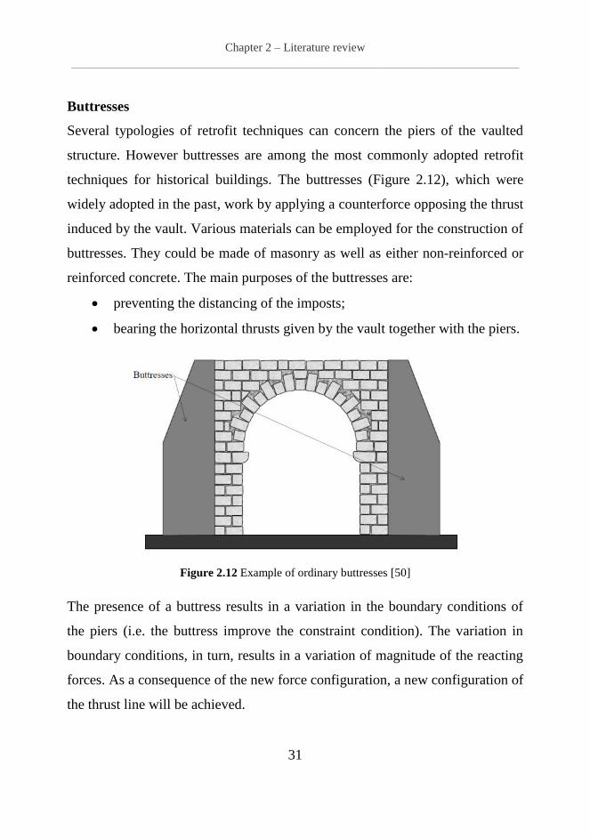
Buttresses
Several typologies of retrofit techniques can concern the piers of the vaulted
structure. However buttresses are among the most commonly adopted retrofit
techniques for historical buildings. The buttresses (Figure 2.12), which were
widely adopted in the past, work by applying a counterforce opposing the thrust
induced by the vault. Various materials can be employed for the construction of
buttresses. They could be made of masonry as well as either non-reinforced or
reinforced concrete. The main purposes of the buttresses are:
preventing the distancing of the imposts;
bearing the horizontal thrusts given by the vault together with the piers.
Figure 2.12 Example of ordinary buttresses [50]
The presence of a buttress results in a variation in the boundary conditions of
the piers (i.e. the buttress improve the constraint condition). The variation in
boundary conditions, in turn, results in a variation of magnitude of the reacting
forces. As a consequence of the new force configuration, a new configuration of
the thrust line will be achieved.
Page 37
Chapter 2 – Literature review
______________________________________________________________________________________________________________________________
32
By analysing the load distributions inside the buttress it is clear that the loads
are mostly located in the upper part of the buttress. In particular the analyses
showed that the buttress works just like an arch. For this reason, in the ancient
architecture (mostly in the gothic period), instead of the ordinary buttresses the
flying buttresses were often adopted. In Figure 2.13 a brief illustrated overview
of the main typologies of buttress through the history is reported. Nevertheless,
despite its past wide spread, this strengthening technique, could not to be
feasible for historical building. Indeed, the buttresses have a high shape factor
which results in a high visual impact.
Figure 2.13 Typologies of buttress through the history: (a), (b), (c), (d) ordinary buttress; (e)
flying buttress [12]
Ties
The ties (Figure 2.14) are the simplest way to counterbalance the thrust of the
vault without imposing it to the piers. Their main purpose is, therefore,
preventing the distancing between the imposts. Retrofit interventions by means
Page 38
Chapter 2 – Literature review
______________________________________________________________________________________________________________________________
33
of ties were widely adopted in the past; however they are still widely adopted.
Ties are mostly built up of either steel or wood (Figure 2.15); nevertheless
usually the selection of the proper material is depending on the environment
aggressiveness.
Figure 2.14 Tying scheme for a two span vaulted ceiling [50]
Tie retaining system can be passive (no pre-tensioned) or active (pre-tensioned).
The former starts to work only once a relative displacement between the piers
occur. Conversely, the latter does not need a relative displacement between the
piers to start working. Tie dimensional design is crucial; it should be performed
with regard to prevent any damage to the piers masonry due to the traction of
the tie.
Compared to buttresses, ties certainly have a lower visual impact. However,
depending on their positioning, they could potentially obstruct the view of
artistic elements such as painting and frescoes located at the intrados of the
vault. Depending on either architectural or structural reasons, ties can be
applied both at intrados and extrados. From a structural point of view, ties
located at the intrados have shown to be more effective in contrasting vault’s
thrust [51]. On the other hand ties located at the extrados, having a lower visual
impact, could be a more suitable solution for historical buildings. In this case,
Page 39
Chapter 2 – Literature review
______________________________________________________________________________________________________________________________
34
flexural forces acting on the portion of pier between the tie and the pier have to
be taken into account.
(a) (b)
Figure 2.15 Examples of curved element retrofit by means of ties of ties: (a) steel; (b) wood
In order to improve the flexural capacity of the piers post-tensioned ties can be
applied in vertical. Usually this intervention is adopted when the vertical load is
not sufficient to guarantee the stability of the piers. Frequently post-tensioned
vertical ties are combined with horizontal ties. In this case, the anchorage of the
vertical ties has to be at a higher quota compared to the horizontal ties location.
This expedient allows the proper distribution of the stresses due to the
tensioning of the vertical ties.
In addition to the retrofit intervention on the piers, several typologies of retrofit
intervention can concern the vault itself. It is worth remarking that the
conservation of any artistic/historical element, such as frescoes, paints or
decorations, on the vault is the governing factor in the selection of the retrofit
solution. However, when the vault itself is clearly damaged (e.g. cracking at
either the intrados or the extrados), these interventions could be crucial for the
Page 40
Chapter 2 – Literature review
______________________________________________________________________________________________________________________________
35
safety of the structure. In the following the main typologies of retrofit
intervention on the vault are briefly presented.
Dead load reduction
An alternative solution to reduce the thrusts of the vault on the piers is to reduce
the dead loads. Reducing the dead loads acting on the vault, results in
improving the capacity of the vault to bear live loads. Basically the filling
material (which is usually made up of earth) is replaced with a lighter material
such as hollow bricks. Studies show that by means of this solution it is possible
to reduce the dead loads of about 50% [52]. It is crucial during the intervention
design phase, checking whether the new thrust line lies within the arch bounds
or not. In order to achieve the new thrust line both the new dead and the new
live loads have to be taken into account.
Reinforced concrete jacket
A solution frequently adopted, is the creation of a reinforced concrete jacket at
the extrados of the vault (Figure 2.16). This solution sometimes is coupled with
the previous discussed intervention of reduction of the dead load. In fact it is
used in case in which the thrust line, due to the new loads, does not lie within
the arch bounds. In order to let the reinforced concrete jacket works together
with the old masonry vault, metal connectors between the two structures, have
to be installed. The reinforced concrete jacketing improves both stiffness and
strength of the vault. On the other hand, the high self-weight of the jacket may
cause damages on both the structures and the foundations.
Page 41
Chapter 2 – Literature review
______________________________________________________________________________________________________________________________
36
Figure 2.16 Reinforced concrete jacketing at the extrados of the vault
Furthermore the increase in mass due to the jacket could become
disadvantageous, especially in case of earthquakes.
Grout injection
In recent years, the use of the grout injection as a retrofit technique is became
common for curved masonry elements. The grout injections consist in filling:
cracks, void, collar joints, or cavities within masonry (Figure 2.17). Usually the
mixture injected is cement based. However the mixture composition depends on
the characteristics of both the masonry and the crack to be filled.
Figure 2.17 Examples of grout injections [53]
For instance cement-based grout is frequently used in the case of wide cracks
[54]; while epoxy resin or cement fluid hydraulic binder are used in the case of
Page 42
Chapter 2 – Literature review
______________________________________________________________________________________________________________________________
37
small cracks (less than 2 mm). The grout injection prevents the crack spread
and improves the overall behaviour of the masonry [55]. Moreover, since the
grout injection does not alter the aesthetic features of the retrofitted element, it
is particularly suitable for historic buildings.
Mortar joint repointing
Mortar joint repointing is one of the basic procedures in the refurbishment of
masonry elements. It consists in removing damaged (or deteriorated) mortar
from masonry joints and replacing it with new mortar. In Figure 2.18 is
reported the typical repointing process. Repointing allows improving the
strength and the stiffness of masonry [56] and it reduces the water effect.
Usually the mortar joint repointing is coupled with other retrofit techniques
such as grout injection or near surfaces mounted reinforcements.
Figure 2.18 Mortar joint repointing process: (a) Joint after cleaning; (b) detail of the joint
depth; (c) joint’s repointing; (d) after intervention [56].
An efficient repointing retrofit starts with the assessment of the existing
materials. Such knowledge is crucial in the selection of the mortar to be used
for the repointing intervention. Indeed, the selection of the mortar is critical to
the long-term durability and performance of the intervention. In particular, the
new mortar has to be durable and compatible with existing masonry. If the
mortar is too strong or too stiff than the adjacent materials, it can even damage
the masonry units reducing the durability of the intervention.
Page 43
Chapter 2 – Literature review
______________________________________________________________________________________________________________________________
38
Moreover, both the old mortar removing and cleaning operations are crucial as
well. Improper joint preparation frequently results in falling out of the repointed
joint within a few years. Otherwise a proper repointing intervention can last
between 25 and 30 years.
2.4.2.1 Innovative retrofit techniques
The raising awareness for the preservation of historical buildings, together with
the development in the innovative materials technologies, has supported the
growth of innovative retrofit techniques. Traditional retrofit techniques are
based on the idea of improving the strength of the structure. Otherwise the
approach of innovative techniques is based on the idea of improving both
capacity and ductility. The choice among solutions traditional or innovative is
controversial. However, depending on the specific case, innovative techniques
can either coexist with the traditional techniques, or be used as their alternative.
In the following a brief overview of the main innovative retrofit techniques for
vaults and curved elements is presented.
Reinforced arch method (RAM)
The Reinforced Arch Method (RAM) is often presented as an innovative
alternative to the reinforced concrete jacket. It consist in a distributed
reinforcement, applied to the extrados (or the intrados) of the vault. The basic
concept of this retrofit intervention (introduced for the first time in [57, 58] is to
modify the distribution of loads acting on the arch in order to let the thrust line
lie within the arch bounds. Therefore this intervention is suitable to be coupled
with the reduction of the dead loads. Both steel and FRP reinforcing cables can
be used as a tensile resistant reinforcement. The installation of the RAM is
Page 44
Chapter 2 – Literature review
______________________________________________________________________________________________________________________________
39
made up by means of post-tensioned cable yarns fixed to the extrados of the
vault as shown in the Figure 2.19.
Figure 2.19 Detail of the anchorage of the cable to the extrados [57]
The cables can be fixed at both the intrados and the extrados. However, due to
the necessity of cable deviator, the installation at the intrados could be difficult.
The post-tensioned cables application results in a radial distribution of forces on
the vault. In Figure 2.20 is reported the force interaction scheme in both the
cases of reinforcement at the extrados and reinforcement at the intrados.
Figure 2.20 Force interaction between the cable (in tension) and the vault (in compression): (a)
reinforcement at the extrados; (b) reinforcement at the intrados [58]
Page 45
Chapter 2 – Literature review
______________________________________________________________________________________________________________________________
40
The RAM improves the seismic behaviour of the vault. In fact, it improves both
capacity and ductility of the vault, without increasing its mass and stiffness.
Near Surface Mounted (NSM) reinforcement
The near surface mounted (NSM) reinforcement consists in installing FRP or
stainless steel reinforcing bars in a groove cut into the surface of the
masonry [59, 60]. Depending on the desired strengthening (i.e. either flexural or
shear) the location of the bar application can change. For instance, in the case of
flexural strengthening, bars are vertically applied. Otherwise, in the case of
shear strengthening, bars are inserted horizontally in the masonry bed joints
(see Figure 2.21).
Figure 2.21 Bed joint NSM reinforcement for a masonry representative element [61]
NSM reinforcement in masonry curved elements improves the load carrying
capacity, reduces the hinge formations and reduced the crack development [59].
Low aesthetic impact and easy installation are among the values of this retrofit
technique. Furthermore the NSM reinforcement provides no mass improvement
which is crucial in seismic retrofit. Experimental and theoretical studies show
the effectiveness of this retrofit technique.
Page 46
Chapter 2 – Literature review
______________________________________________________________________________________________________________________________
41
FRP laminates/fabric
Another innovative solution for the retrofit of vaults is the use of FRP
laminates. The FRP laminates can be installed at the extrados, at the intrados or
at both the intrados and the extrados of the vault. Figure 2.22 shows the three
possible retrofit layouts for barrel vaults.
Figure 2.22 Possible retrofit layouts for barrel vaults [62]
However, the installation at the intrados is not always possible. For instance, in
the case of historical buildings, the presence of valuable stuccoes and frescoes,
preclude the chance of removing the plaster. Thus the reinforcement can be
only installed at the extrados. On the other hand, whether valuable tiles or
floorings, which cannot be removed, are present, the chance of retrofit at the
extrados is precluded. However, it is worth remarking that, due to tensile
stresses normal to the reinforcement (Figure 2.23), the application of FRP
laminates at the intrados is the most critical with respect to the debonding
failure. The basic concept of the retrofit with FRP is to prevent the hinge
mechanism and, therefore, the brittle collapse. This result is achieved moving
the failure mechanism from brittle to ductile, by improving the energy
3rd layout
Strips placed at
the intrados only
1st layout
Strips placed at
the extrados only
2nd layout
Strips placed at
both extrados
and intrados
Page 47
Chapter 2 – Literature review
______________________________________________________________________________________________________________________________
42
dissipation. Several experimental tests [63, 64] showed the effectiveness of
retrofit with FRP in preventing the hinge formations. Then, according to [62] in
the case of retrofit with FRP the main potential failure modes are: debonding,
FRP rupture, crushing and sliding.
Figure 2.23 Debonding in curved structures [62]
The debonding failure is the main critical issue of the retrofit with FRP. It is
mostly due to the curvature of vaults coupled with both the peeling stresses and
normal axial forces at the FRP fibre plane. However, the application of
longitudinal quadriaxial strips provides anchoring to former transverse strips
preventing the debonding failure.
If a proper FRP anchorage is provided, the FRP rupture is possible.
Nevertheless, whether the original failure is governed by shear failure or
crushing of the masonry, the effectiveness of the FRP retrofit is not granted.
Crushing failure as well as sliding failure is related to the load pattern. The
former is achieved when the thrust line is very close to the bounds of the arch.
In particular it is due to either load pattern variations or increases in flexural
forces. The latter is usually achieved for highly non-symmetric loads. In order
to reduce sliding issues, the masonry substrate preparation (usually by means of
Page 48
Chapter 2 – Literature review
______________________________________________________________________________________________________________________________
43
thin layer of fibre reinforced mortar) is crucial. The same issues discussed in the
case of FRP laminates can be repeated in the case of FRP fabric. In the case of
vault retrofit, the fabric is commonly preferred to the laminates due to its ability
to fit curved geometries.
Inorganic Matrix composite Grids (IMG)
As discussed in the previous section the use of FRP laminates (fabric) in
masonry structural retrofit has shown to be effective. However, this technique
has shown a number of problems. In particular, the main problems are:
insufficient vapour permeability, low performances at high temperatures
(flammability), lack of bond between resins and masonry substrates, no
reversibility [5]. By means of inorganic matrix composite grid (IMG) such
issues can be overcame. IMG retrofit is an innovative retrofit technique based
on inorganic matrixes. In particular the inorganic matrix (e.g. cement based
matrix) replaces the traditional epoxy resin of the classic FRP system (see
Figure 2.24 ).
Figure 2.24 IMG retrofit system scheme
Page 49
Chapter 2 – Literature review
______________________________________________________________________________________________________________________________
44
The main advantage of inorganic cement based matrixes is the high physical
and chemical compatibility with the masonry substrate. Thus usually premature
debonding failure does not occur. Furthermore, due to its continuous nature, the
IMG is particularly suitable for curved masonry elements such as arches and
vaults. Several experimental tests show [4, 5] that the IMG strengthening
systems increase the load-bearing capacity of masonry elements.
An issue related to the IMG system can be found in the installation phase. In
fact the IMG system should be installed at temperatures ranging between 5°C
and 35°C. The installation at higher temperatures results in a sensitive decrease
in the mortar workability. Otherwise, the installation at lower temperatures
results in setting slow down.
It is worth noting that, being innovative this technique, there is still not a widely
adopted name. Therefore in the literature, it is usually identified with several
different acronyms generating possible misunderstandings. For instance some
of the more frequent acronyms are: fibre reinforced cementitious mortar
(FRCM), fibre reinforced cementitious matrix (FRCM) and cementitious matrix
grid (CMG).
2.5 Experimental studies
The seismic behaviour of masonry vaults is strongly affected by the global
behaviour of the structure in which they are inserted. On the other hand the role
of structural components testing is fundamental [65]. Vault’s dynamic
behaviour is generally treated by means of either simplified mechanism
methods or complex computational analysis [40, 66, 67]. Even so, detailed
knowledge on the dynamic behaviour of the vault elements is still lacking from
Page 50
Chapter 2 – Literature review
______________________________________________________________________________________________________________________________
45
an experimental point of view. In particular, only a few dynamic experimental
tests on unreinforced masonry vaults are available in scientific literature. On the
other hand, a lot of study can be found about reinforced vaults under static or
quasi static loads. In the following, a brief overview on some experimental tests
concerning retrofitted masonry vaults is presented.
2.5.1 Tests on reinforced arches and vaults
An interesting study provided in [63] highlights the results of an experimental
investigation on brick masonry vaults strengthened with FRP strips. The
behaviour of masonry vaults reinforced with FRP laminates has been studied by
means six specimens. The specimens were subjected to monotonic vertical load
applied at ¼ of their span. The geometry of the specimens and load conditions
are shown in Figure 2.25.
Figure 2.25 Geometry of the specimens and load conditions [63]
The FRP strips applied at the intrados (or extrados) results in an alteration of
the collapse mechanism. The results of these tests showed that the width and the
stiffness of the reinforcement strips have a strong influence in the behaviour of
Page 51
Chapter 2 – Literature review
______________________________________________________________________________________________________________________________
46
the vault. Vaults strengthened at the extrados showed possible brittle failure;
while vaults strengthened at the intrados showed a ductile failure mechanism.
This is due to the detachment of the fibre perpendicularly to the masonry
interface. The failure involves a limited area, thus the strips can still prevent the
collapse.
In [68] a study on the dynamic behaviour of masonry barrel vaults is presented.
Vault dynamic behaviour has been investigated in the cases of unreinforced
vault, damaged unreinforced vault and retrofitted vault. The vault has been
retrofitted by means of GFRP strips (at the extrados). In Figure 2.26 is shown
the reinforcement configuration.
Figure 2.26 Reinforcement configuration [68]
The results of experimental tests showed a good dynamic behaviour in both the
cases of undamaged and damaged vault. After the retrofit the vault showed a
dynamic behaviour similar to the undamaged vault.
A contribution to the investigation of the effectiveness of the IMG as seismic
retrofit of vaults is found in [46]. In particular in this study the retrofit is based
on steel cords embedded in an inorganic cement based matrix (i.e. steel
Page 52
Chapter 2 – Literature review
______________________________________________________________________________________________________________________________
47
reinforced grout). The research consists in the retrofit of the vaults for the case
study of Jacobilli building which is a clustered complex in the historical centre
of Foligno (Italy). The building was seriously damaged by the Umbria-Marche
earthquake (1997). Therefore, in order to improve the strength of the cloister
vaults included in the building against earthquake, two systems have been
adopted. A couple of prestressed steel reinforced grout (SRG) strips and a
reticular system made of transversal and longitudinal prestressed SRG
laminates. The reinforcements have been applied at the extrados of the vault
(see Figure 2.27).
Figure 2.27 Extrados of the vault after the intervention [46]
The study remarks that the retrofit can modify the failure mode of the masonry
vault preventing the formation of the fourth hinge. Furthermore the retrofit
significantly increases the load carrying capacity of the vault.
Another application of IMG on curved masonry elements is provided in [69]. In
particular laboratory tests were carried out on seven semicircular brick arches
which underwent repair and retrofit.
Page 53
Chapter 2 – Literature review
______________________________________________________________________________________________________________________________
48
The experimental tests on models showed that in all the cases the use of Fibre
Reinforced Cementitious Matrix (FRCM) reinforcement significantly enhances
the load-bearing capacity of the brick arches (vaults). In particular, the
cementitious matrix has ensured a good capacity for distribution of stresses on
the masonry support.
A comparison between the experimental performances of FRP strips and IMG
is provided in [70]. The tests were carried out on two arch specimens. The first
specimen has been retrofitted with carbon FRP (CFRP). The second specimen
has been retrofitted with glass fibre reinforced cement matrix (GFRCM). The
reinforcements have been applied on the whole surface at the intrados of the
arches. The experimental results showed that, under seismic load, the GFRCM
performed better. Furthermore the specimen retrofitted with GFRCM showed a
failure mechanism similar to an unreinforced arch. Conversely the failure
mechanism for the specimen retrofitted with CFRP strips was different. In
particular, due to delamination, a highly brittle collapse occurred.
A further contribution on the study of reinforced vaults is found in [71] which
studied the IMC for masonry vaults by means of experimental tests. In
particular the influence of the retrofit has been studied by comparing the results
achieved for different kinds of retrofit. Both the static and the dynamic
behaviour of the retrofitted vaults were studied. The specimens were retrofitted
with five different systems. In particular: SRG, basalt textile reinforced mortar
(BTRM), steel reinforced polymers (SRP), CFRP and reinforced transverse
vertical diaphragms (RTVD). The specimens were subjected to both monotonic
and cyclic vertical load applied at ¼ of their span (Figure 2.28).
Page 54
Chapter 2 – Literature review
______________________________________________________________________________________________________________________________
49
Figure 2.28 Experimental test setup [71]
The results showed that all the tested retrofits result in a substantial increase of
the load capacity and ductility. The dynamic identification allowed relating the
decay of the fundamental frequencies to the increase of the damage.
The dynamic behaviour of both unreinforced and reinforced masonry vaults
have been studied in [72]. Shaking table tests have been performed on a
masonry vault. In particular the specimen consisted of a 1/3 scale masonry vault
with parapets (Figure 2.29) loaded with a uniformly distributed load.
Figure 2.29 Experimental test setup [72]
Page 55
Chapter 2 – Literature review
______________________________________________________________________________________________________________________________
50
The specimen was built on a reinforced concrete slab connected to the shaking
table. The specimen was monitored by linear variable differential transformer
(LVDT) and accelerometers. Two accelerograms (one natural and one artificial)
have been imposed to the structure without producing any significant damage to
the specimen. In order to achieve the failure, a sine sweep action (having
acceleration equal to 0.5 g) have been imposed to the structure. The collapse
started due to relative displacements in the mortar beds near the abutments and
was due to the formation of five hinges.
The investigation of uncertain features of the masonry vault seismic response
has been proposed in [73]. On this purpose experimental tests on mono-
directional shaking table have been performed.
The specimens were arches made of tuff bricks resting on two piers which
continue over the imposts. Furthermore some steel ties were placed between the
wing walls. A sketch of the specimen is provided in Figure 2.30.
Figure 2.30 Experimental test setup [73]
The test consisted in two phases. The first phase was performed by means of
the same dynamic signal (which reproduces a natural earthquake) scaled at
progressively increasing intensities. In the second phase an overload was
Page 56
Chapter 2 – Literature review
______________________________________________________________________________________________________________________________
51
imposed on the top of the arches. The specimens were monitored by
accelerometers (applied on the arch) and transducers (applied at the external
sides of the piers). The collapse was not reached in the first phase. Then the
collapse was reached in the second phase. By the comparison of the outcomes
of the two phases it was evident that the static degradation was faster than the
dynamic one. However this result is probably due to the previous damages
occurred.
Page 57
Chapter 3 – Experimental tests: unreinforced vault
______________________________________________________________________________________________________________________________
52
Chapter 3
Experimental tests: unreinforced vault
The experimental programme presented in this chapter aims to investigate the
dynamic behaviour of a masonry vault subjected to a dynamic base excitation.
In particular dynamic shaking table tests on a full scale masonry barrel vault
have been performed at the Laboratory of the Department of Structures for
Engineering and Architecture (University of Naples “Federico II”).
A comprehensive overview of the results of the shaking table tests is presented
and discussed. The presented experimental activity is part of a wider research
project which involves the University of Naples “Federico II”, University of
Padova, STRESS S.c.ar.l, Veneto Nanotech s.p.a., Regional Center of
Assistance for Economic Cooperation Artisan, CETMA Consortium,
Consortium TRE and SIPRE s.r.l. In the presented experimental tests the vault
is tested without any vertical load acting at the extrados. This load condition is
suitable, for instance, to simulate typical historical vaulted roof. Furthermore,
the vault’s imposts are constrained on the shaking table. Therefore the outcome
represents the behaviour of the vault itself.
Page 58
Chapter 3 – Experimental tests: unreinforced vault
______________________________________________________________________________________________________________________________
53
The aim of these tests is to improve the knowledge on the dynamic behaviour of
the masonry vaults once the settlement and capacity of the supports of the
vaults, (e.g. imposts, masonry piers, load bearing walls) are guaranteed.
3.1 Specimen
A full scale clay brick masonry vault has been designed for testing purpose. The
geometry of the specimen (Figure 3.1) is the same of the vault which has been
tested under static conditions in [71]. The geometry of the vault has been
carefully chosen to simulate a typical masonry vault commonly included in
historical heritage buildings.
Figure 3.1 Geometry of the specimen: 3D view
The vault has a segmental arch profile (less than a semicircle) having a clear
span of 298 cm and a rise of 114 cm. The vault is 220 cm deep and it is made of
solid facing clay brick (25×5.5×12 cm3) and pozzolanic masonry mortar (i.e.
MAPEI MAPE Antique allettamento). The mortar mixture was prepared in
order to present typical properties of mortars used in historical buildings.
Page 59
Chapter 3 – Experimental tests: unreinforced vault
______________________________________________________________________________________________________________________________
54
The vault is fixed on two imposts made of the same masonry material. Further
geometrical details are provided in (Figure 3.2).
Figure 3.2 Geometry of the specimen: plan and section views (dimension in cm)
The specimen was built up on a steel beam system which is part of the testing
structure (further information about the technical characteristics of the testing
structure will be discussed in the following section 3.3). Since the vault is not
self-supporting, until the keystone bricks were positioned, a polystyrene
centring has been used as a temporary support (Figure 3.3a).
Page 60
Chapter 3 – Experimental tests: unreinforced vault
______________________________________________________________________________________________________________________________
55
The polystyrene centring was placed on wooden supports in order to keep it at
the proper quota and facilitate its removal after the vault was completed. Some
images concerning the construction phases are shown in Figure 3.3.
(a) (b)
(c) (d)
Figure 3.3 Specimen during construction phases: (a) polystyrene centring; (b) construction
of the imposts; (c) curved element construction; (d) specimen completed
3.1.1 Material characterization
Preliminary mechanical characterization tests have been performed for both
mortar and bricks. Table 3.1 lists the main results of the material
characterizations. Both brick’s compressive and tensile strength, as well as
elastic modulus, were characterized in [74].
Page 61
Chapter 3 – Experimental tests: unreinforced vault
______________________________________________________________________________________________________________________________
56
In particular, according to UNI 8942-3 (1986) [75], three point bending tests
have been performed. In these tests the brick is placed on two supports. Then
given the distance, l, between the two supports, (typically l = 200 mm), the
actuator applies a force in the middle of the two supports (l/2).
Table 3.1: Material mechanical properties.
Property Brick [MPa] Mortar [MPa]
Compressive strength 19.8 10.1
Flexural strength 3.7 -
Splitting tensile strength 2.5 -
Tensile strength - 2.4
Elastic Modulus 5756 1452
Therefore the flexural strength, σf,b, is achieved by applying the well-known
Navier’s formulation (simple bending case). In particular in this case the
following Equation (3.1) has been used:
, 2
3
2
uf b
P l
bh (3.1)
Where b and h are the dimensions of the brick’s cross section, and Pu is the
ultimate achieved load.
Compression tests on the bricks have been performed as well. In particular,
according to EN 772-1 (2002) [76], the compression force on the two faces of
the specimen have to be applied by means of suitable actuators.
Page 62
Chapter 3 – Experimental tests: unreinforced vault
______________________________________________________________________________________________________________________________
57
Assuming a uniform stress distribution along the horizontal sections of the
brick, the compressive strength, σc,b, can be achieved by means of the
following Equation (3.2):
,u
c b
P
bd (3.2)
Where b and d, in this case, are the dimensions of the section in which the load
Pu is applied. Indirect tensile strength has been achieved according to UNI
8942-3 (1986) [75]. In particular the indirect tensile strength, σs,b, has been
evaluated by means of the following Equation (3.3):
,
2 us b
P
bd
(3.3)
Characterization tests on the mortar (Figure 3.4) have been performed
according to UNI EN 998-2 (2010) [77] and UNI EN 1015-11 (2007) [78] on
twelve 40×40×160 mm3 28 days wet cured specimens.
(a) (b)
Figure 3.4 Material characterization: mortar specimen preparation
Page 63
Chapter 3 – Experimental tests: unreinforced vault
______________________________________________________________________________________________________________________________
58
In order to achieve the elastic modulus, several tests were performed according
to UNI 6556 (1976) [79]. The elastic modulus reported in Table 3.1 has been
achieved as average of the elastic modulus achieved in these tests.
3.2 Experimental facilities
Shaking table tests have been performed in order to investigate the seismic
behaviour of the brick masonry vault. The tests have been carried out at the
laboratory of the Department of Structures for Engineering and Architecture of
the University of Naples Federico II.
The tests have been performed by means of an earthquake simulator
system (ESS). In particular the ESS consists of two square shaking
tables (3×3 m2). Each table is characterized by two degrees of freedom in the
two horizontal directions. In Figure 3.5 a scheme of the EES is provided.
Figure 3.5 Earthquake simulator system (ESS) scheme
Page 64
Chapter 3 – Experimental tests: unreinforced vault
______________________________________________________________________________________________________________________________
59
Each shaking table has a maximum payload of 200 kN having a frequency
range of 0 – 50 Hz, acceleration peak equal to 9.81 m/s2, velocity peak equal to
1 m/s (both at maximum payload) and total displacement equal to 500 mm
(±250 mm). In the presented experimental tests only one table is used.
3.3 Testing structure
Since the width of the specimen to be tested (3.7 m) was larger than the shaking
table platform (3.0 m) an additional structure was required. Main purpose of
such structure was to rigidly transfer the acceleration from the shaking table to
the structure to be tested. Therefore a steel testing frame has been expressly
designed. Furthermore in order to allow the specimen to be built off of the
shaking table platform, a lifting structure for the test setup has been designed,
too. Therefore the testing structure consists in two sub-structures namely
testing frame and lifting structure respectively. The total weight of the testing
structure, including the lifting structure (Figure 3.6), is 17.22 kN.
Figure 3.6 Testing structure overview
Page 65
Chapter 3 – Experimental tests: unreinforced vault
______________________________________________________________________________________________________________________________
60
3.3.1 Testing frame design
The design of the testing frame involved two main stages. The first stage
consisted in the estimation of the loads acting on the testing frame during the
tests. The second stage consisted in the design and verification of the testing
frame and its structural elements. At the first stage, the loads acting on the
testing frame have been evaluated by means of preliminary numerical finite
elements (FE) analyses. In particular, static nonlinear analyses have been
performed on a simplified FE model.
The preliminary FE analyses were performed by means of the software DIANA
developed by TNO DIANA. The FEM model is constituted of more than 800
CQ16M eight-node quadrilateral isoparametric plane stress elements based on
quadratic interpolation and Gauss integration. Further details about the CQ16M
element are provided in the following section 5.1.
A macro element approach was adopted. The masonry was modelled as a
homogeneous material according to the total strain model coupled with the
rotating crack stress-strain relationship approach. In particular, in the total strain
approach, the constitutive model describes the stress as a function of the strain.
In the rotating crack approach, stress-strain relationships are evaluated in the
principal directions of the strain vector, as reported in [80]. Furthermore, the
combined Rankine/Von Mises yield criterion was adopted. In Figure 3.7 the
preliminary FE model of the vault is shown.
Page 66
Chapter 3 – Experimental tests: unreinforced vault
______________________________________________________________________________________________________________________________
61
Figure 3.7 FE model of the specimen
All the analyses were performed under load control, measuring the evolution of
both the reacting forces and displacements. The load, which is horizontal and
proportional to the mass of the model, has been applied at increasing steps.
According to the experimental boundary conditions, the two imposts of the
vault have been fixed. The outcomes of the analyses allowed studying the trend
of the base reacting forces when varying the horizontal load multiplier (Figure
3.8). This trend represents the forces which the testing frame has to bear
without significant deformations. Furthermore the numerical analyses allowed
estimating a broad value of the horizontal load multiplier at the formation of
the first hinge. Since at this stage characterization tests on the masonry
materials were not yet performed, average values for the mechanical properties
were considered. However, in order to take into account of the variability of the
tensile strength which is the governing parameter, parametric analyses were
performed. The outcomes, in terms of horizontal load multiplier, are shown
in Figure 3.9.
Page 67
Chapter 3 – Experimental tests: unreinforced vault
______________________________________________________________________________________________________________________________
62
Figure 3.8 Static nonlinear analyses results: horizontal load multiplier-base reacting forces
(horizontal and vertical)
Figure 3.9 Static nonlinear analyses results: horizontal load multiplier-displacement curves
0.00
0.10
0.20
0.30
0.40
0.50
-50 -40 -30 -20 -10 0 10 20 30 40 50
Mu
ltip
lier
[-]
Base reacting forces [kN]
Horizontal right base
reacting forces
Vertical right base
reacting forces
Horizontal left base
reacting forces
Vertical left base
reacting forces
0.00
0.10
0.20
0.30
0.40
0.50
0.00 0.50 1.00 1.50 2.00 2.50 3.00 3.50 4.00
Mu
ltip
lier
[-]
Displacement[mm]
ft= 0.64 MPa
ft= 0.32 MPa
ft= 0.16 MPa
Page 68
Chapter 3 – Experimental tests: unreinforced vault
______________________________________________________________________________________________________________________________
63
Due to the high variability of the mechanical parameters, all the results
achieved at this stage have to be considered as approximate values. Therefore at
the design and verification stage partial safety factors were adopted. According
to the outcomes of the FE analyses performed at the previous stage, the testing
frame has been designed. In particular, the testing frame is a steel plane frame
constituted of three H shaped beams (HE240B profile in Figure 3.10) bolted on
the shaking table platform. Two U shaped beams (welded U profiles in Figure
3.10) are bolted on the main H shaped beams, forming a two span beam
scheme. The structure has a symmetric K-bracing system in order to prevent the
buckling and to increase the in-plane stiffness of the plane frame. The bracing
system is constituted of six steel U shaped beams (UPN100 profile in Figure
3.10). A sketch of the complete steel plane frame is provided in Figure 3.10.
Figure 3.10 Geometry of the steel plane frame (plan and laterals view)
Page 69
Chapter 3 – Experimental tests: unreinforced vault
______________________________________________________________________________________________________________________________
64
The bracing system trusses are linked to the plane frame by means of bolted
connections. The overall dimensions of the plane frame are 3.7×2.6 m2. The
total weight of the testing frame is 12.5 kN. During the testing frame design the
main purpose was to prevent any possible influence, of the frame deformability,
on the test results. Therefore the testing frame has been designed to be rigid in
order to prevent any significant deformation, and it has been verified in the
elastic field. Furthermore all the testing frame structural elements have been
verified under the following assumptions:
Material isotropic and perfectly homogeneous.
Material in elastic field (the Hook’s law is valid).
The cross section remains flat (before and after bending).
The elastic modulus is the same in tension and compression.
Several verifications have been performed for the testing frame. In the
following a brief description of the most relevant verifications has been
reported.
U profile (welded): deflection verification
Aim of this section is to verify the deflection of the U shaped two span
(three supports) continuous beam (Figure 3.11). The length of each span is
1176 mm. According to the preliminary FE analyses the maximum vertical
reacting force is Fy = 44.8 kN ≈ 45 kN. This force can be smeared on the total
span length, s, (2352 mm) achieving a uniformly distributed load
qf = 19.13 N/mm.
Page 70
Chapter 3 – Experimental tests: unreinforced vault
______________________________________________________________________________________________________________________________
65
Figure 3.11 Detail of the U shaped beam
The cross section of the beam is a U profile made up of two L profiles welded.
Thus, being 0.46 N/mm the weight of the single L profile, the weight of the
U profile is WU =0.92 N/mm. Therefore the total uniformly distributed load
which has to be considered is: qtot =qf + WU = 20.05 N/mm.
On safe side, in the calculation of the maximum deflection, a simply supported
beam scheme has been assumed (Figure 3.12).
Figure 3.12 Calculation scheme: simple supported beam with uniformly distributed load
The maximum deflection, δmax, has been achieved according to the well-known
formulations of the solid mechanics as:
4
max
54.60
384
tots qmm
EI
(3.4)
Where E is the elastic modulus and I is the second order moment of inertia. In
the present case, the achieved maximum deflection (4.6 mm) is widely
acceptable. Indeed the δmax is about 1/500 of the span length and the δmax/s ratio
is about 0.002.
qtot
Page 71
Chapter 3 – Experimental tests: unreinforced vault
______________________________________________________________________________________________________________________________
66
HE240B profile: shear verification
Since the H shaped beam is longer than the shaking table platform it will work
as a cantilever stud beam (Figure 3.13). The length of the cantilever is 370 mm.
Aim of this section is to verify that at any cross section the shear strength of the
HE240B profile is higher than the shear stress.
Figure 3.13 Detail of the H shaped beam
A cantilever beam scheme has been adopted (Figure 3.14) at both the sides of
the beam. On safe side the half of the maximum achievable vertical reacting
force, Fy, has been considered as vertical shear force acting at the end of the
cantilever beam. In particular, being the maximum vertical reacting force
about 45 kN, the considered force, T = Fy/2 = 22.5 kN.
Figure 3.14 Calculation scheme: cantilever beam with point load
The most highly stressed cross section has been considered for the verification.
On safe side, the shear contribution of the flanges has been neglected.
The maximum shear stress, τmax, has been achieved, according to the well-
known formulations of the solid mechanics, as:
T
Page 72
Chapter 3 – Experimental tests: unreinforced vault
______________________________________________________________________________________________________________________________
67
max
314.06
2
TMPa
A (3.5)
Where A is cross section area (in this case the contribution of the flanges of the
HE240B profile on the shear strength has been neglected).
The shear strength of the HE240B profile has been assessed, according the
well-known formulations of the solid mechanics, as:
0
123.713
y
res
M
fMPa
(3.6)
Where fy is the steel strength and γM0 = 1.05 is a material partial safety factor.
In order to keep the testing frame in elastic field, in the Equation (3.6) the steel
strength, fy, has been assumed as the half of the actual steel strength. This
assumption is strong. However, due to both the high variability (uncertainty) of
the dynamic load and the lack of examples of comparable structures in
literature, at this stage a wide error margin is required. Since τres > τmax and the
τres/τmax ratio is about 8.8 the verification is widely satisfied.
U profile-HE240B profile bolted connection: strength verification
Each U shaped beam is connected to a H shaped beam by means of three bolted
connections. Each connection is realized by means of four, grade 8.8, bolts
having a nominal diameter, dn, of 30 mm (Figure 3.13).
Page 73
Chapter 3 – Experimental tests: unreinforced vault
______________________________________________________________________________________________________________________________
68
Figure 3.15 detail of the bolted connection: 3D view
Aim of this section is to verify the strength of the bolted connections between
the U profile and the HE240B profile. The bolted connection strength has been
considered as a function of both the slip coefficient, µ, of the faying surfaces
and the clamping force, Ns, provided by the bolts.
According to the preliminary FE analyses the maximum achievable horizontal
reacting force is Fx = 29.87 kN ≈ 30 kN. The bolt strength can be assessed
according to the Italian building code (IBC) [81]. Assuming a bolt tightening
torque of 1508 Nm (which corresponds to a clamping force, Ns = 251 kN) and a
slip coefficient γf = 0.3, the strength, Flim, of the single bolt is:
lim 60f s
f
n NF kN
(3.7)
Where nf is the number of faying surfaces, and γf = 1.25 is a partial safety
factor. The horizontal force, Fx, acts on three bolted connections (i.e. on
12 bolts).
Page 74
Chapter 3 – Experimental tests: unreinforced vault
______________________________________________________________________________________________________________________________
69
Thus the total resistant force of the single connection is 240 kN while the force
loading the single connection is Fx/3 = 10 kN. Therefore the verification is
satisfied. A simplified scheme of the force acting on a single bolted connection
is provided in Figure 3.16.
Figure 3.16 Force acting on the single bolted connection
U profile-HE240B profile bolted connection: bearing strength verification
Aim of this section is to verify the bolted connections between the U profile and
the HE240B profile against the bearing failure at bolt holes. The nominal
diameter of the bolts is 30 mm. The thickness of the thinnest plate involved in
the connection (i.e. the U profile) is t = 15 mm. The spacing between the bolt
holes are: p1 = 150 mm and e1 = 45 mm. Where the dimensions p1 and e1, are
defined as shown in figure.
Figure 3.17 Bolt holes spacing reference scheme
1
3xF
Page 75
Chapter 3 – Experimental tests: unreinforced vault
______________________________________________________________________________________________________________________________
70
According to the Eurocode 3 (EC3) [82] the bearing strength, Fb, can be
assessed as:
2
2.5 183.33b y n
b
M
f d tF kN
(3.8)
Where αb is defined as the min (p1/3dn-1/4; fub/fy; 1) which in this case is 1,
fub is the bolt ultimate strength and γM2 = 1.35 is a partial safety factor. Being
the expected maximum horizontal force Fx = 30 kN the verification is satisfied.
3.3.2 Lifting structure design
The lifting structure has been realised by means of steel pipes. Two different
thicknesses for the pipes have been used. In particular, the vertical pipes used to
link the lifting structure to the steel testing frame are 10 mm thick, while all the
other pipes have a thickness of 3 mm. All the joints between the pipes are
realised using a commercial pipe connection system commonly used for
scaffolding structures. The lifting structure is connected to the testing frame by
means of steel plates. In particular each vertical steel pipe is welded onto a steel
plate (namely plate class A). The plate class A is bolted onto another plate
(namely plate class B). The plate class B is welded to the testing frame (onto
the web of the HE240B) by means of another plate (namely plate class C). Two
further plates are welded between the plates class B, C and the HE240B profile
in order to stiffen the plate class C. A sketch of the connection between the
lifting structure and the testing frame is provided in Figure 3.18.
Page 76
Chapter 3 – Experimental tests: unreinforced vault
______________________________________________________________________________________________________________________________
71
Figure 3.18 Connections between the lifting structure and the testing frame
Numerical FEM analyses have been performed by means of the software
SAP2000 developed by CSI [83] in order to simulate the lifting procedure and
achieve the axial forces. Each pipe of the lifting structure has been modelled as
an elastic truss element (see Figure 3.19). The lifting force (i.e. 41.50 kN) has
been achieved as the sum of the total weight of the testing structure including
the lifting structure (i.e. 17.22 kN) and the total weight of the specimen
(i.e. 24.28 kN).
The maximum axial loads achieved in tension and in compression are:
24.50 kN and 22.10 kN respectively. The maximum vertical reacting force
achieved, Fly, is 11.90 kN.
A B
C
A C
B
A
Page 77
Chapter 3 – Experimental tests: unreinforced vault
______________________________________________________________________________________________________________________________
72
Figure 3.19 FEM model of the lifting/moving system
The main design purpose was to prevent any possible damage to the specimen
while lifting (or moving). Therefore the lifting structure has been designed to be
rigid in order to prevent any significant deformation, and it has been verified in
the elastic field. Furthermore all the lifting structure elements have been
verified under the following assumptions:
Material isotropic and perfectly homogeneous.
Material in elastic field (the Hook’s law is valid).
The cross section remains flat (before and after bending).
The elastic modulus is same in tension and compression.
Page 78
Chapter 3 – Experimental tests: unreinforced vault
______________________________________________________________________________________________________________________________
73
Several verifications have been performed for the lifting structure. In the
following a brief description of the most relevant verifications has been
reported.
HE240B profile: deflection while lifting verification
The H shaped beams are the elements to which the lifting structure is
connected. In particular each beam is connected to the lifting structure in three
points (see Figure 3.6). Therefore, aim of this section is to verify the expected
deflection of the H shaped beam during the lifting process. Since the connection
is realised in three points the beam will behave as a two span (three supports)
continuous beam. However, on safe side, a simply supported beam scheme has
been assumed. The total span length, s, has been assumed as the distance
between the two external connection points (i.e. 3340 mm).
According to the preliminary FE analyses the maximum achievable vertical
reacting force is Fls = 11.90 kN ≈ 12 kN. Such force, on safe side, has been
considered as a point load applied at the midspan of the beam (see Figure 3.20).
Figure 3.20 Calculation scheme: simply supported beam with point load
The maximum deflection, δmax, has been achieved, according to the well-known
formulations of the solid mechanics, as:
Fls
Page 79
Chapter 3 – Experimental tests: unreinforced vault
______________________________________________________________________________________________________________________________
74
3
max
10.40
48
lss Fmm
EI
(3.9)
Where E and I are defined as in the previous section 3.3.1. In the present case,
the achieved maximum deflection (0.40 mm) is widely acceptable. Indeed the
δmax is about 1/5800 of the span length and the δmax/s ratio is about 0.0001.
Lifting pipe-plate class A welded connection: strength verification
Each vertical pipe is connected to a plate class A by means of a fillet weld as
shown in Figure 3.21.
Figure 3.21 Detail of the Lifting pipe-plate class A connection: 3D view
Aim of this section is to verify the strength of the welded connection between
the lifting pipe and the plate class A. The stress on the weld critical throat is
assumed to be uniform. The following normal and shear stresses have been
taken in to account:
Page 80
Chapter 3 – Experimental tests: unreinforced vault
______________________________________________________________________________________________________________________________
75
)2
)
ls
ls b
x
Fa
ah
F Lb y
I
(3.10)
Where a = b/3 is the throat, b is the welded plate thickness, h is the height of the
weld, Lb is the distance between the weld and the force Fls, Ix is the second
order moment of inertia (about the neutral axis x) and y is the perpendicular
distance to the neutral axis.
According to the EC3 [82] the verification of the weld strength is satisfied if the
following conditions are verified:
2 2 2) 13.08 196.07
) 17.84 166.66
y
w Mw
y
Mw
fa MPa MPa
Fb MPa MPa
(3.11)
Where βw = 0.85 is a coefficient related to steel typology and γMW = 1.35 is a
partial safety factor. It is worth noting that, due to the geometrical configuration
of the weld, in this case τ||.is equal to zero.
3.4 Instrumentation
The monitoring of the vault has been achieved by means of seven
accelerometers and two laser-optical displacement sensors. In Figure 3.22 and
Figure 3.23 the positions of the sensors are indicated.
Page 81
Chapter 3 – Experimental tests: unreinforced vault
______________________________________________________________________________________________________________________________
76
Figure 3.22 Instrumentation layout: plan view (dimensions in cm)
Six tri-axial accelerometers and one bi-axial accelerometer are placed along the
extrados of the vault at the longitudinal midplane. In particular one
accelerometer, namely TRI-100715, was placed at the keystone location. Two
accelerometers, namely TRI-103765 and TRI-100050, were placed on the left
and right side respectively at 45° from the keystone. Two accelerometers,
namely TRI-103763, and TRI-103762, were placed on the left and right side
respectively at 60° from the keystone. In order to measure contingent torsional
effects, an accelerometer, namely TRI-102818, was placed at the keystone
location but on a different vertical plane. Finally, one bi-axial accelerometer,
namely BI-103766 was placed on the left imposts of the vault to check the
actual acceleration input transmitted to the vault. With the purpose of checking
the output recorded by the main instrumentation, two more secondary
accelerometer sets were placed in parallel, at the same locations as the set
Page 82
Chapter 3 – Experimental tests: unreinforced vault
______________________________________________________________________________________________________________________________
77
mentioned above but on different vertical planes. In order to measure the
horizontal displacements, two laser-optical sensors, namely L1 and L2, were
placed along the extrados of the vault at the longitudinal midplane. In
particular, the sensor L1 was placed at the keystone location, and the sensor L2
was placed on the left side at 45° from the keystone.
Figure 3.23 Instrumentation layout: front view (dimensions in cm)
3.5 Input and test programme
The seismic behaviour of the masonry vault has been investigated by means of
two sets of time-history accelerograms namely “STR” and “ART” respectively.
The STR set consists of five tests. The time-history used is a natural
accelerogram recorded in Southern Italy by the station of Sturno during the
Irpinia earthquake occurred on November 23rd
1980. The total duration of the
accelerogram is 72 s. The PGA is 1.78 m/s2 (see Figure 3.24a). The
accelerogram has been scaled by different factors in order to get a progressive
Page 83
Chapter 3 – Experimental tests: unreinforced vault
______________________________________________________________________________________________________________________________
78
PGA increase (0.25, 0.50, 0.75, 1.00 and 1.50). Consequently, the test sequence
in terms of PGA was the following: 0.44, 0.89, 1.33, 1.78 and 2.67 m/s2.
The ART set consists of seven tests. The time-history used as base is an
artificial accelerogram obtained from a non-stationary broadband random
excitation having an energy content ranging from 1 to 30 Hz. The drive signal
composition is obtained as multiple-frequency random excitations. The total
duration of the accelerogram is 30 s. The accelerogram has a PGA of
4.50 m/s2 (see Figure 3.24b).
Figure 3.24 Time-history accelerograms at 100% intensity: (a) STR; (b) ART;
The time-history is scaled by different factors in order to get a progressive PGA
increase (0.10, 0.20, 0.30, 0.40, 0.50, 0.75, 1.00). Consequently, the test
sequence in terms of PGA was the following: 0.45, 0.90, 1.35, 1.80, 2.25, 3.38,
and 4.50 m/s2. The two sets of time-history accelerograms cover two different
frequency ranges being the STR mainly limited to 15 Hz, while the second
ART is up to 30 Hz (Fast Fourier Transforms, FFT, in Figure 3.25a and b).
1
(a) (b)
2
0 5 10 15 20 25 30 35 40 45 50 55 60 65 70-5
-4
-3
-2
-1
0
1
2
3
4
5
Time [sec]
Accele
rati
on
[m
/sec2
]
STR test (desired time/acceleration)
0 2.5 5 7.5 10 12.5 15 17.5 20 22.5 25 27.5 30-5
-4
-3
-2
-1
0
1
2
3
4
5
Time [sec]
Accele
rati
on
[m
/sec2
]ART test (desired time/acceleration)
Page 84
Chapter 3 – Experimental tests: unreinforced vault
______________________________________________________________________________________________________________________________
79
Figure 3.25 Time-history accelerograms at 100%: (a) FFT STR; (b) FFT ART.
Preliminarily, a set of random accelerograms were performed on dynamic
identification purpose (natural frequency and damping). The random set,
namely “RND” was performed by means of four tests. In particular, an input
random accelerogram scaled at different PGA levels (0.25, 0.50, 0.75 and
1.00 m/s2) was used as the input. The total duration of the random vibration is
60 s. Table 3.2 lists the complete experimental test programme.
It is worth noting that the desired PGA does not exactly match with the
achieved PGA (actual value of the maximum acceleration transmitted at the
specimen by the shaking table motion). This aspect may be crucial for
experimental tests on shaking table especially on specimens made of brittle
material like masonry. For this reason, the procedure described in [84],
concerning the optimisation of the drive motion to predict the signal recorded at
desired locations, i.e. on the keystone, using a compensation procedure, has
been taken into account in the experimental programme.
All the tests of the experimental program are unidirectional with the shaking
movement applied in the transversal direction of the vault (Figure 3.26).
(a) (b)
1
0 5 10 15 20 25 300
0.005
0.01
0.015
0.02
0.025
0.03
0.035
Frequency [Hz]
Am
pli
tud
e
FFT -Ch 18: Acc.100715 (Y) [m/s2]
0 5 10 15 20 25 300
0.02
0.04
0.06
0.08
0.1
0.12
0.14
0.16
Frequency [Hz]
Am
pli
tud
e
FFT -Ch 18: Acc.100715 (Y) [m/s2]
Page 85
Chapter 3 – Experimental tests: unreinforced vault
______________________________________________________________________________________________________________________________
80
Table 3.2: Experimental test programme (unreinforced vault).
Test ID Scale factor Desired PGA [m/s2] Achieved PGA [m/s
2]
RND1 0.25 0.25 0.26
RND2 0.50 0.50 0.52
RND3 0.75 0.75 0.89
RND4 1.00 1.00 1.29
STR1 0.25 0.44 0.53
STR2 0.50 0.89 1.04
STR3 0.75 1.33 1.54
STR4 1.00 1.78 2.13
STR5 1.50 2.67 3.52
ART1 0.10 0.45 0.39
ART2 0.20 0.90 0.85
ART3 0.30 1.35 1.27
ART4 0.40 1.80 1.81
ART5 0.50 2.25 2.30
ART6 0.75 3.38 3.24
ART7 1.00 4.50 4.67
Figure 3.26 Test setup and specimen: shaking direction (unreinforced vault).
Page 86
Chapter 3 – Experimental tests: unreinforced vault
______________________________________________________________________________________________________________________________
81
3.6 Outcomes of the shaking table tests
The main results of the experimental tests are described in the following
sections. The outcomes are grouped by test set, according to the set naming
defined in the previous section 3.5.
3.6.1 RND test results (Dynamic identification)
The natural frequency and the damping ratio have been evaluated by means of a
dynamic identification procedure. Using a random time-history in acceleration
as input signal, a sequence of four shakings has been performed scaling the
signal from a PGA of 0.25 m/s2 to 1.0 m/s
2. It’s worth noting that a low
intensity signal has been used in the dynamic identification phase to prevent
premature damage on the specimen. The natural frequency has been assessed
according to the transfer curve method. The decay of the natural frequency
evidenced by the transfer function amplitude is shown in Figure 3.27.
Figure 3.27 Natural frequency decay of the specimen (unreinforced vault).
The first shaking at a PGA of 0.25 m/s2 (RND1) provided a natural frequency
of about 13.1 Hz. That result remarks the high stiffness of the vault.
0 1 2 3 4 5 6 7 8 9 10 11 12 13 14 15 16 17 18 19 20
Frequency [Hz]
0
2
4
6
8
10
12
14
Am
pli
tud
e
RND1RND1RND2RND2RND3RND3RND4RND4RND1RND1X
RND1
RND1RND2RND2X
RND2
RND2RND3RND3X
RND3
RND3RND4RND4X
RND4
RND4
W4: FDT
Page 87
Chapter 3 – Experimental tests: unreinforced vault
______________________________________________________________________________________________________________________________
82
The further three tests (i.e. RND2, RND3 and RND4) have shown a decay of
the natural frequency due to premature minor damage (microcracking) of the
specimen. The damping ratio, ζ, has been achieved according to the well-known
half-power bandwidth method as:
2 1
2 k
(3.12)
Where ωk is the natural frequency, ω2 and ω1 are the frequencies for which the
power input is half the input at resonance [85]. The tested structure has shown a
damping ratio, ζ, ranging between 2.2% and 3.2%. Table 3.3 lists both the
fundamental frequency and damping ratio achieved for each test.
Table 3.3: Natural frequencies and damping ratios (unreinforced vault).
Test ID Natural frequency [Hz] Damping ratio [%]
RND1 13.1 2.2%
RND2 12.6 2.2%
RND3 12.4 2.2%
RND4 11.7 3.2%
3.6.2 STR test results (Sturno earthquake)
As described in the previous section 3.5, the input accelerogram used for these
tests is a natural accelerogram recorded in southern Italy during the 1980 Irpinia
earthquake. The record has a PGA of 1.78 m/s2.
Page 88
Chapter 3 – Experimental tests: unreinforced vault
______________________________________________________________________________________________________________________________
83
A sequence of five tests has been performed, applying to the natural
accelerogram scaling factors equal to: 0.25, 0.50, 0.75, 1.00 and 1.50 (see Table
3.2). For the test performed at 100% level intensity (STR4), the horizontal
component of the achieved time histories recorded at the imposts (BI-103766)
and at the keystone (TRI-100715) of the vault are shown in Figure 3.28a. The
relative displacement time-history (keystone-imposts) is shown in Figure 3.28b.
The outcomes are presented in terms of maximum accelerations, maximum
displacements, and detected damage to the specimen.
Both the horizontal and vertical accelerations have been recorded in five
locations according to the instrumentation scheme shown in Figure 3.22 and
Figure 3.23. All the accelerometers recorded the maximum horizontal
accelerations during the last test of the set (i.e. test STR5). In particular the
maximum horizontal acceleration has been recorded by the accelerometer TRI-
100765, placed at 45° from the keystone location.
Figure 3.28 Sturno earthquake, test STR4: recorded time-history in acceleration at the impost
(in black) and keystone (in grey) of the vault (a) and relative keystone-impost displacement (b).
(a) (b)
1
0 5 10 15 20 25 30 35 40 45 50 55 60 65 70-3.5
-3
-2.5
-2
-1.5
-1
-0.5
0
0.5
1
1.5
2
2.5
3
3.5
Time [sec]
Accele
rati
on
[m
/sec2
]
STR4 test: keystone/base recorded acceleration time history )
0 5 10 15 20 25 30 35 40 45 50 55 60 65 70-10
-5
0
5
10
15
Time [sec]
Dis
pla
cem
en
t [m
m]
STRN4 test (recorded time/displacement)
Page 89
Chapter 3 – Experimental tests: unreinforced vault
______________________________________________________________________________________________________________________________
84
This acceleration of 5.21 m/s2 has a dynamic magnification of about 48%
compared to the PGA of the achieved shaking table motion (i.e. 3.52 m/s2).
At the keystone location (i.e. accelerometer TRI-100715) the maximum
recorded acceleration is 4.28 m/s2 with a dynamic magnification of about 22%
compared to the recorded shaking table PGA (i.e. 3.52 m/s2).
Furthermore, since the difference between the values of the accelerations
recorded by the two accelerometers, at the keystone location (i.e. TRI-100715
and TRI-102818), is small (it ranges between 1% and 2%), the torsional effects
can be considered negligible. The maximum vertical acceleration, equal to
5.06 m/s2, has been recorded during the test STR5 by the accelerometer TRI-
103762 (see Figure 3.22 and Figure 3.23). In Figure 3.29 the results, in terms of
maximum accelerations, are plotted as profiles.
Figure 3.29 STR: Maximum acceleration profiles (values expressed in m/s2).
The profiles show that the trends of the maximum accelerations (horizontal and
vertical) do not change when varying the magnitude of the base acceleration.
Furthermore the maximum acceleration profiles highlight a not symmetric
0 1 2 3 4 5 60123456
0
1
2
3
4
5
6
STR1 STR2 STR3 STR4 STR5
Page 90
Chapter 3 – Experimental tests: unreinforced vault
______________________________________________________________________________________________________________________________
85
dynamic behaviour. In particular the maximum horizontal accelerations on the
right side of the vault were recorded at both the keystone and 60° from the
keystone locations (i.e. accelerometers TRI-103763 and TRI-100715).
Otherwise, on the left side of the vault the maximum horizontal accelerations
were recorded at 45° from the keystone location (i.e. accelerometer TRI-
103765). The horizontal and vertical maximum recorded accelerations are
reported in Table 3.4 and Table 3.5 respectively.
Table 3.4: STR test results: horizontal maximum accelerations.
TEST ID TRI-
100715
[m/s2]
TRI-
102818
[m/s2]
TRI-
103765
[m/s2]
TRI-
103762
[m/s2]
TRI-
100050
[m/s2]
TRI-
103763
[m/s2]
STR1 0.66 0.67 0.75 0.26 0.29 0.68
STR2 1.39 1.41 1.57 0.57 0.56 1.39
STR3 2.17 2.19 2.74 1.21 1.09 2.11
STR4 3.08 3.13 3.66 1.69 1.40 3.02
STR5 4.28 4.33 5.21 2.06 1.79 4.27
Table 3.5: STR test results: vertical maximum accelerations.
TEST ID TRI-
100715
[m/s2]
TRI-
102818
[m/s2]
TRI-
103765
[m/s2]
TRI-
103762
[m/s2]
TRI-
100050
[m/s2]
TRI-
103763
[m/s2]
STR1 0.18 0.24 0.28 0.78 0.66 0.14
STR2 0.14 0.25 0.57 1.60 1.28 0.28
STR3 0.32 0.45 1.21 2.82 1.97 0.60
STR4 0.98 1.21 1.70 3.77 2.85 0.78
STR5 1.14 1.19 2.56 5.06 3.87 1.04
Page 91
Chapter 3 – Experimental tests: unreinforced vault
______________________________________________________________________________________________________________________________
86
The horizontal dynamic amplifications in terms of percentage have been
evaluated as:
out in
in
Acc AccAmplification
Acc
(3.13)
Where Accout is the maximum acceleration recorded at the considered location,
while Accin is the PGA of the achieved motion of the table. The horizontal
dynamic amplifications in terms of percentage are plotted as profiles in Figure
3.30
Figure 3.30 STR: Horizontal dynamic amplifications (values expressed in %).
The profiles show that the magnitude of the base acceleration does not have a
strong impact on the trends of the horizontal dynamic amplifications. The
horizontal dynamic amplifications profiles exhibit a not symmetric trend. As
expected the maximum horizontal amplifications on the right side of the vault
were achieved at both the keystone and 60° from the keystone locations. On the
left side of the vault the maximum horizontal accelerations were achieved
at 45° from the keystone location. The horizontal dynamic amplifications
achieved are reported in Table 3.6. Vertical dynamic amplification cannot be
evaluated since no vertical acceleration was imposed to the vault.
0
1
2
3
4
5
6
STR1 STR2 STR3 STR4 STR5
Page 92
Chapter 3 – Experimental tests: unreinforced vault
______________________________________________________________________________________________________________________________
87
Table 3.6: STR test results: dynamic amplifications.
TEST ID TRI-
100715
[%]
TRI-
102818
[%]
TRI-
103765
[%]
TRI-
103762
[%]
TRI-
100050
[%]
TRI-
103763
[%]
STR1 25% 27% 41% -51% -45% 28%
STR2 34% 36% 51% -45% -46% 34%
STR3 41% 42% 78% -21% -29% 37%
STR4 45% 47% 72% -20% -34% 42%
STR5 22% 23% 48% -41% -49% 21%
The maximum relative displacement measured at the keystone location
(i.e. laser-optical sensor L1, see Figure 3.23) ranges between 2.92 mm and
17.41 mm from test STR1 to STR5. The same increasing trend has been shown
by the laser-optical sensor, L2, placed on the left side of the vault (see Figure
3.23). In particular, the maximum relative displacements measured by the L2
sensor range between 3.28 mm and 7.41 mm from test STR1 to STR5. Except
for the STR1 test, in which the relative displacement measured by the two
sensors is comparable, the displacements measured by the sensor L2 are always
widely lower than those measured by the sensor L1. The maximum relative
displacements are shown in detail in Table 3.7.
Table 3.7: STR test results: maximum relative displacements.
Test ID L1 [mm] L2 [mm]
STR1 2.92 3.28
STR2 7.86 3.81
STR3 11.63 4.86
STR4 14.44 5.62
STR5 17.41 7.41
Page 93
Chapter 3 – Experimental tests: unreinforced vault
______________________________________________________________________________________________________________________________
88
In order to detect damages to the vault, after each test, the specimen has been
inspected. However even after the last test (i.e. test STR5) the specimen
damages were not relevant. In particular very slight cracking, at the interface
between mortar and brick, has been observed.
3.6.3 ART test results (artificial earthquake)
As described in the previous section 3.5, the input used is an artificial
accelerogram specifically designed for the tests. A sequence of seven tests was
performed increasing the PGA of the table drive motion up to 4.50 m/s2
(4.67 m/s2 recorded). For the test performed at 100% level intensity (ART7),
the horizontal component of the achieved time histories recorded at the impost
(BI-103766) and at the keystone (TRI-100715) of the vault are shown in Figure
3.31a. The relative displacement time-history (keystone-impost) is shown in
Figure 3.31b.
(a) (b)
Figure 3.31 Artificial earthquake, test ART7: (a) recorded time-history in acceleration at the
impost (in black) and keystone (in grey) of the vault; (b) relative keystone-impost displacement.
0 5 10 15 20 25 30-5
-4
-3
-2
-1
0
1
2
3
4
5
Time [sec]
Accele
rati
on
[m
/sec2
]
ART7 test: keystone/base recorded acceleration time history
0 5 10 15 20 25 30-10
-8
-6
-4
-2
0
2
4
6
8
Time [sec]
Dis
pla
cem
en
t [m
m]
ARTF74 test (recorded time/displacement)
Page 94
Chapter 3 – Experimental tests: unreinforced vault
______________________________________________________________________________________________________________________________
89
The complete testing sequence is reported in Table 3.2. The outcomes are
presented in terms of maximum accelerations, maximum displacements, and
detected damage to the specimen.
Both the horizontal and vertical accelerations have been recorded in five
locations according to the instrumentation scheme represented in Figure 3.22
and Figure 3.23.
The maximum horizontal acceleration was recorded by the accelerometer TRI-
103763 during the last test (i.e. test ART7). The recorded acceleration was
7.64 m/s2. The magnification was of about 64% compared to the recorded PGA
of the table (i.e. 4.67 m/s2). At the keystone location (i.e. accelerometer TRI-
100715) the maximum acceleration was recorded during the test ART7. The
recorded acceleration was 4.80 m/s2 having a dynamic magnification of about
3% compared to the recorded PGA (i.e. 4.67 m/s2). The maximum vertical
accelerations were recorded by all the accelerometers during the last test of the
set (i.e. test ART7). In particular the maximum vertical acceleration was
7.51 m/s2 and it is recorded by the accelerometer TRI-103762. In Figure 3.32
the results, in terms of maximum accelerations, are plotted as profiles.
Figure 3.32 ART: Maximum acceleration profiles (values expressed in m/s2).
0 1 2 3 4 5 6 7 8012345678
012345678
ART1 ART2 ART3 ART4
ART5 ART6 ART7
Page 95
Chapter 3 – Experimental tests: unreinforced vault
______________________________________________________________________________________________________________________________
90
The profiles show that the trends of the maximum accelerations (horizontal and
vertical) do not change when varying the magnitude of the base acceleration
(except for the last ART7 test). In the ART7 test the maximum vertical
acceleration profile show a sharp change in the trend (compared with the
previous tests). A possible reason for this sharp change is a damage localised at
that location.
As in the previous tests (i.e. STR), the acceleration profiles highlight a not
symmetric dynamic behaviour. In particular the maximum horizontal
accelerations on the right side of the vault were recorded at both the keystone
and 60° from the keystone locations (i.e. accelerometers TRI-103763 and TRI-
100715). Otherwise, on the left side of the vault the maximum horizontal
accelerations were recorded at 45° from the keystone location (i.e.
accelerometer TRI-103765). The horizontal and vertical maximum recorded
accelerations are reported in Table 3.8 and Table 3.9 respectively.
Table 3.8: ART test results: horizontal maximum accelerations.
TEST ID TRI-
100715
[m/s2]
TRI-
102818
[m/s2]
TRI-
103765
[m/s2]
TRI-
103762
[m/s2]
TRI-
100050
[m/s2]
TRI-
103763
[m/s2]
ART1 0.61 0.62 0.80 0.45 0.33 0.59
ART2 1.24 1.25 1.70 1.01 0.73 1.38
ART3 1.90 1.94 2.67 1.68 1.10 1.94
ART4 2.62 2.66 3.29 2.27 1.39 2.64
ART5 3.07 3.06 4.04 2.99 1.63 3.25
ART6 3.96 4.08 4.90 3.43 2.53 5.11
ART7 4.80 4.83 6.74 4.82 4.54 7.64
Page 96
Chapter 3 – Experimental tests: unreinforced vault
______________________________________________________________________________________________________________________________
91
Table 3.9: ART test results: vertical maximum accelerations.
TEST ID TRI-
100715
[m/s2]
TRI-
102818
[m/s2]
TRI-
103765
[m/s2]
TRI-
103762
[m/s2]
TRI-
100050
[m/s2]
TRI-
103763
[m/s2]
ART1 0.17 0.23 0.50 0.77 0.60 0.24
ART2 0.32 0.49 1.14 1.59 1.12 0.51
ART3 0.80 0.99 1.75 2.49 1.78 0.80
ART4 1.24 1.48 2.31 3.74 2.36 1.05
ART5 1.70 1.68 2.74 4.69 2.84 1.44
ART6 2.97 3.27 3.48 4.79 4.39 1.82
ART7 5.98 5.86 4.61 7.51 6.18 3.03
The horizontal dynamic amplifications, evaluated as shown in the
Equation (3.13), are plotted as profiles in terms of percentage in Figure 3.33.
Figure 3.33 ART: Horizontal dynamic amplifications (values expressed in %).
According to the dynamic amplification profiles, the magnitude of the input
acceleration does not have a strong impact on the trends of the horizontal
dynamic amplifications. The horizontal dynamic amplifications profiles exhibit
a not symmetric trend.
As expected the maximum horizontal amplifications on the right side of the
vault were achieved at both the keystone and 60° from the keystone locations.
On the left side of the vault the maximum horizontal accelerations were
02468
1012141618
ART1 ART2 ART3 ART4
ART5 ART6 ART7
Page 97
Chapter 3 – Experimental tests: unreinforced vault
______________________________________________________________________________________________________________________________
92
achieved at 45° from the keystone location. The horizontal dynamic
amplifications achieved are reported in Table 3.10.
Table 3.10: ART test results: dynamic amplifications.
TEST ID TRI-
100715
[%]
TRI-
102818
[%]
TRI-
103765
[%]
TRI-
103762
[%]
TRI-
100050
[%]
TRI-
103763
[%]
ART1 55% 59% 105% 15% -15% 51%
ART2 47% 47% 100% 19% -14% 63%
ART3 50% 53% 110% 33% -13% 53%
ART4 45% 47% 82% 26% -23% 46%
ART5 34% 33% 76% 30% -29% 41%
ART6 22% 26% 51% 6% -22% 58%
ART7 3% 3% 44% 3% -3% 64%
The maximum relative displacement measured at the keystone location
(i.e. laser-optical sensor L1, see Figure 3.23) ranges between 1.35 mm and
8.57 mm from test ART1 to ART7. The same increasing trend has been shown
by the laser-optical sensor, L2, placed on the left side of the vault (see Figure
3.23). In particular the maximum relative displacement measured by the L2
sensor ranges between 0.70 mm and 11.12 mm from tests ART1 to ART7.
Except for the last test (i.e. ART7) in which the displacement measured by the
sensor L1 is lower than the one measured by the sensor L2, the key section
always shows a relative displacement larger than the side of the vault. The
maximum relative displacements are shown in detail in Table 3.11
Page 98
Chapter 3 – Experimental tests: unreinforced vault
______________________________________________________________________________________________________________________________
93
Table 3.11: ART test results: maximum relative displacements.
Test ID L1 [mm] L2 [mm]
ART1 1.35 0.70
ART2 2.03 1.06
ART3 2.86 1.74
ART4 3.77 2.25
ART5 3.98 2.36
ART6 5.50 3.00
ART7 8.57 11.12
In order to detect damages to the vault, after each test, the specimen has been
inspected. Only after the last test (i.e. test ART7) slight damages were
observed. However, evident cracking at the interface between mortar and brick
has been observed at both intrados and the extrados of the vault. In particular,
as shown in Figure 3.34, at the intrados, interface cracking occurred, in a few
joints, along its entire depth. Interface cracking occurred at the extrados as well.
However, at the extrados, the cracking has involved a larger number of joints.
Due to excessive local compressive stress concentrations, few minor
detachments of the brick edges have been observed.
In the following figures a comprehensive overview on the damages observed is
provided. In particular, Figure 3.34 and Figure 3.35, show the damages at the
intrados and at the extrados of the vault respectively.
Page 99
Chapter 3 – Experimental tests: unreinforced vault
______________________________________________________________________________________________________________________________
94
Figure 3.34 Unreinforced vault: damages detected (intrados)
Interface cracking
Brick edge detachment
a
a
b c
b
c
d e f
d
e f
Page 100
Chapter 3 – Experimental tests: unreinforced vault
______________________________________________________________________________________________________________________________
95
Figure 3.35 Unreinforced vault: damages detected (extrados)
a b c
d e f g
a b c
d e f g
Interface cracking
Brick edge detachment
Page 101
Chapter 3 – Experimental tests: unreinforced vault
______________________________________________________________________________________________________________________________
96
3.7 Conclusions
The dynamic behaviour of the masonry vault has been investigated by means of
shaking table tests. In particular, two sets of time-history accelerograms (natural
and artificial) have been used as input signal. Preliminarily, a set of random
accelerograms were performed on dynamic identification purpose. The results
of the shaking tests have been presented in terms of dynamic characteristics
(natural frequency and damping ratio), maximum accelerations, maximum
displacements, time histories and observed damage to the specimen.
In the case of unreinforced vault, a natural frequency of 13.1 Hz and a damping
ratio ranging between 2.2% and 3.2% have been evaluated. The outcomes, in
terms of accelerations measured on the structure, highlighted a dynamic
amplification of the base horizontal excitation. Furthermore, although the
shaking is applied only in the horizontal direction, significant vertical
accelerations have been detected. The tested structure exhibits good seismic
behaviour, showing very slight damage only after the last test performed with
an achieved PGA of 4.67 m/s2. In particular, cracking at the interface between
mortar and brick has been observed at both the intrados and the extrados of the
vault.
Page 102
Chapter 4 – Experimental tests: retrofitted vault
______________________________________________________________________________________________________________________________
97
Chapter 4
Experimental tests: retrofitted vault
Since the previous shaking table tests (see Chapter 3) resulted in a slight
damage of the vault, it was possible to retrofit the vault. Then shaking table
tests have been performed on the retrofitted vault.
The experimental programme presented in this chapter aims to investigate the
behaviour of a retrofitted masonry vault subjected to a dynamic base excitation.
Furthermore, in the cases of comparable dynamic input, a comparison with the
previous unreinforced vault tests allowed to investigate the effect of the retrofit.
A comprehensive overview of the results of the shaking table tests is presented
and discussed. As well as in the previous tests (see Chapter 3), the vault has
been tested without any vertical load acting at the extrados. Furthermore the
vault is constrained on the shaking table. Therefore the outcome represents the
behaviour of the retrofitted vault once the settlement and capacity of the
supports of the vaults, (e.g. imposts, masonry piers, load bearing walls) is
guaranteed.
Page 103
Chapter 4 – Experimental tests: retrofitted vault
______________________________________________________________________________________________________________________________
98
4.1 Specimen retrofit
As discussed in the previous section 2.4.1, the first step of a proper retrofit is
“an accurate survey of the structure in order to assess the main vulnerabilities
and potential instability sources”. Therefore, according to the slight damages
detected on the unreinforced vault after the last test (section 3.6.3), the retrofit
has been performed by coupling three different techniques. In particular:
repointing of the cracked joints (Figure 4.1 and Figure 4.2), grout injections
(Figure 4.3) and IMG (Figure 4.4).
The repointing has been performed both at the front section (Figure 4.1) and at
the intrados of the vault (Figure 4.2) by means of a commercial repair mortar
(i.e. MAPEI MAPE Antique fc ultrafine).
Figure 4.1 Repointing of the cracked joints at the front of the vault.
a b c
a
b
c
Page 104
Chapter 4 – Experimental tests: retrofitted vault
______________________________________________________________________________________________________________________________
99
Figure 4.2 Repointing of the cracked joints at the intrados of the vault
a b c
d e f
a b c
d e f
Page 105
Chapter 4 – Experimental tests: retrofitted vault
______________________________________________________________________________________________________________________________
100
Figure 4.3 Grout injections at the extrados of the vault
a b c d
e f g
a b c d
e f g
Page 106
Chapter 4 – Experimental tests: retrofitted vault
______________________________________________________________________________________________________________________________
101
The deteriorated or distressed mortar has been carefully removed from the
joints, taking care to prevent damages to the nearest bricks. Once the old mortar
had been removed, the whole involved surfaces have been accurately cleaned
from mortar dust and debris. Then the repointing phase has been performed by
pressing the repair mortar into the joints (in three successive layers).
The grout injections have been performed at the extrados of the vault (Figure
4.3). In particular, at the cracked locations, holes have been drilled at the
extrados of the vault with a spacing of 12 cm. Since the cracks were not wide, a
cement-free fluid hydraulic binder has been used as mixture for the injections.
Figure 4.4 IMG system at the extrados of the vault
The IMG system has been installed at the extrados of the vault (Figure 4.4). In
particular, a first layer 5 mm thick of mortar has been applied to the extrados of
the vault. While the mortar was still fresh, an alkali-resistant primed basalt fibre
grid has been applied onto the mortar layer. Since the vault is 220 cm deep, two
sheets of grid have been jointed in order to cover the entire extrados. Therefore,
the installation of the grids has been performed taking care to overlap at the
least by 5 cm all the joints.
Page 107
Chapter 4 – Experimental tests: retrofitted vault
______________________________________________________________________________________________________________________________
102
Once the grid was perfectly bonded to the first mortar layer, a second layer,
entirely covering the grid, has been applied. The mortar used for both the layers
was a two-component premixed mortar made of: natural hydraulic lime (NHL),
Eco-Pozzolan, natural sand, special additives and synthetic polymers in
aqueous dispersion (i.e. MAPEI Planitop HDM restauro). The grid used was a
basal grid (250 g/m3) having a tensile strength ftg = 3000 MPa and elastic
modulus Eg = 89 GPa. A photographic resume of the whole retrofit process has
been provided in Figure 4.5.
Figure 4.5 Resume of the retrofit process: (a) Repointing of the cracked joints at the intrados;
(b) Grout injections at the extrados; (c) Grid installing layer at the extrados.
4.2 Instrumentation
The monitoring of the retrofitted vault has been achieved with the use of seven
accelerometers (six tri-axial accelerometers and one bi-axial accelerometer) and
two laser-optical displacement sensors. The outputs recorded by the main
instrumentation have been validated by means of two more secondary
accelerometer sets. On comparison purpose all the sensors, namely: TRI-
100715, TRI-103765, TRI-100050, TRI-103763, TRI-103762, TRI-102818, BI-
103766, L1 and L2, have been installed in the same geometrical configuration
(a) (b) (c)
Page 108
Chapter 4 – Experimental tests: retrofitted vault
______________________________________________________________________________________________________________________________
103
adopted in the previous tests (see section 3.4). A comprehensive scheme of the
sensor position is provided in Figure 3.22 and Figure 3.23.
4.3 Input and test programme
The seismic behaviour of the retrofitted masonry vault has been investigated by
means of one set of time-history accelerograms namely “ART_R”. The ART_R
set consists of eighteen tests, each one having a total duration of 30 s. The time-
history used is the same artificial accelerogram used in the previous tests (see
section 3.5) having a PGA of 4.50 m/s2 (Figure 3.24b). All the tests of the
experimental programme are unidirectional with the shaking movement applied
in the transversal direction of the vault (Figure 4.6).
Figure 4.6 Test setup and specimen: shaking direction (retrofitted vault).
Page 109
Chapter 4 – Experimental tests: retrofitted vault
______________________________________________________________________________________________________________________________
104
As well as in the previous tests on the unreinforced vault, the time-history has
been scaled by different factors in order to get a progressive PGA increase.
In particular the scale factors adopted are: 0.10, 0.20, 0.30, 0.40, 0.50, 0.75,
1.00, 1.10, 1.20, 1.30, 1.40, 1.50, 1.60, 1.80, 2.00, 2.20, 2.50, and 2.75.
Consequently, the test sequence in terms of PGA was the following: 0.45, 0.90,
1.35, 1.80, 2.25, 3.38, 4.50, 4.95, 5.40, 5.85, 6.30, 6.75, 7.20, 8.10, 9.00, 9.90,
11.25 and 12.38 m/s2. The ART_R set of time-history accelerograms cover
frequency ranging up to 30 Hz (see the FFT in Figure 3.11d).
Preliminarily, a set of random accelerograms were performed on dynamic
identification purpose (natural frequency and damping). The random set,
namely “RND_R” was performed by means of five tests. In particular, an input
random accelerogram scaled at different PGA levels (0.25, 0.50, 0.75, 1.00
and 1.25 m/s2) was used as the input. The total duration of the random vibration
is 60 s. It is worth remarking that, for the reasons discussed in the previous
section 3.5, the procedure described in [84], concerning the optimisation of the
drive motion has been taken into account in the present experimental
programme as well. Although the ART_R set include more tests than the
previous ART set (see section 3.5), on comparison purpose, each test of the
ART set has a corresponding (same input signal) test in the ART_R set. Table
4.1 and Table 4.2 list the complete experimental test programme.
Table 4.1: Experimental test programme pt. 1 (retrofitted vault).
Test ID Scale factor Desired PGA [m/s2] Achieved PGA [m/s
2]
RND1_R 0.25 0.25 0.28
RND2_R 0.50 0.50 0.56
RND3_R 0.75 0.75 0.88
RND4_R 1.00 1.00 1.19
RND5_R 1.25 1.25 1.51
Page 110
Chapter 4 – Experimental tests: retrofitted vault
______________________________________________________________________________________________________________________________
105
Table 4.2: Experimental test programme pt. 2 (retrofitted vault).
Test ID Scale factor Desired PGA [m/s2] Achieved PGA [m/s
2]
ART1_R 0.10 0.45 0.42
ART2_R 0.20 0.90 0.97
ART3_R 0.30 1.35 1.38
ART4_R 0.40 1.80 1.69
ART5_R 0.50 2.25 2.23
ART6_R 0.75 3.38 3.55
ART7_R 1.00 4.50 5.12
ART8_R 1.10 4.95 6.14
ART9_R 1.20 5.40 6.35
ART10_R 1.30 5.85 6.15
ART11_R 1.40 6.30 7.88
ART12_R 1.50 6.75 8.30
ART13_R 1.60 7.20 6.93
ART14_R 1.80 8.10 8.32
ART15_R 2.00 9.00 9.17
ART16_R 2.20 9.90 9.59
ART17_R 2.50 11.25 10.70
ART18_R 2.75 12.38 11.70
Page 111
Chapter 4 – Experimental tests: retrofitted vault
______________________________________________________________________________________________________________________________
106
4.4 Outcomes of the shaking table tests
The main results of the experimental tests are described in the following
sections. The outcomes are grouped by test set, according to the set naming
defined in the previous section 4.3.
4.4.1 RND_R test results (Dynamic identification)
The natural frequency and the damping ratio have been evaluated by means of a
dynamic identification procedure. Using a random time-history in acceleration
as input signal, a sequence of five shakings has been performed scaling the
signal from a PGA of 0.25 m/s2 to 1.25 m/s
2.
It’s worth noting that a low intensity signal has been used in the dynamic
identification phase to prevent premature damage on the specimen.
The natural frequency has been assessed according to the transfer curve
method. The first shaking (RND1_R) at PGA of 0.25 m/s2 provided a natural
frequency of about 19.3 Hz. The achieved result highlights the improvement of
stiffness given by the retrofit (coupled to a negligible mass increase). The
further four tests (i.e. RND2_R, RND3_R, RND4_R and RND5_R) have shown
a decay of the natural frequency due to premature minor damage
(microcracking) of the specimen.
The decay of the natural frequency evidenced by the Transfer Function
amplitude is shown in Figure 4.7.
The damping ratio, ζ, has been achieved according to the well-known half-
power bandwidth method (section 3.6.1). The retrofitted vault has shown a
damping ratio, ζ, ranging between 1.7% and 2.8%. The damping ratio increases
with the intensity of the signal. This result is expected and it is due to the
microcracking of the specimen.
Page 112
Chapter 4 – Experimental tests: retrofitted vault
______________________________________________________________________________________________________________________________
107
Figure 4.7 Natural frequency decay of the specimen (retrofitted vault).
Indeed, being the damping ratio closely related to the energy dissipation, the
higher the microcracking is the higher the damping ratio becomes.
A resume of both the fundamental frequency and damping ratio achieved for
each test is provided in Table 4.3.
Table 4.3: Natural frequencies and damping ratios (retrofitted vault).
Test ID Natural frequency [Hz] Damping ratio [%]
RND1_R 19.3 1.7%
RND2_R 18.9 1.7%
RND3_R 18.6 1.9%
RND4_R 18.1 2.2%
RND5_R 17.6 2.8%
0 2 4 6 8 10 12 14 16 18 20 22 24 26 28 30
Frequency [Hz]
0
4
8
12
16
20
Am
pli
tud
e
RND1 RRND1 RRND2 RRND2 RRND3 RRND3 RRND4 RRND4 RRND5 RRND5 RRND1 RRND1 RX
RND1 R
RND1 RRND2 RRND2 RX
RND2 R
RND2 RRND3 RRND3 RX
RND3 R
RND3 RRND4 RRND4 RX
RND4 R
RND4 RRND5 RRND5 RX
RND5 R
RND5 R
Page 113
Chapter 4 – Experimental tests: retrofitted vault
______________________________________________________________________________________________________________________________
108
4.4.2 ART_R test results (artificial earthquake)
The input used is an artificial accelerogram specifically designed for the tests. A
sequence of eighteen tests was performed increasing the PGA of the table drive
motion up to 12.38 m/s2 (11.70 m/s
2 recorded). For the test performed at 100%
level intensity (ART7_R), the horizontal component of the achieved time
histories recorded at the impost (BI-103766) and at the keystone (TRI-100715)
of the vault are shown in Figure 4.8a. The relative displacement time-history
(keystone-impost) is shown in Figure 4.8b.
The complete testing sequence is reported in Table 4.1 and Table 4.2. The
outcomes achieved are presented in terms of maximum accelerations and
observed damage to the specimen.
(a) (b)
Figure 4.8 Artificial earthquake, test ART7_R: (a) recorded time-history in acceleration at the
impost (in black) and keystone (in grey) of the vault; (b) relative keystone-impost displacement.
Both the horizontal and vertical accelerations have been recorded in five
locations according to the instrumentation scheme represented in Figure 3.22
and Figure 3.23. As well as in the case of unreinforced vault, the maximum
horizontal acceleration was recorded by the accelerometer TRI-103763 during
the last test (i.e. test ART18_R).
0 5 10 15 20 25 30-5
-4
-3
-2
-1
0
1
2
3
4
5
Time [sec]
Accele
rati
on
[m
/sec2
]
ART7 test: keystone/base recorded acceleration time history
0 5 10 15 20 25 30-10
-8
-6
-4
-2
0
2
4
6
8
Time [sec]
Dis
pla
cem
en
t [m
m]
ARTF74 test (recorded time/displacement)
Page 114
Chapter 4 – Experimental tests: retrofitted vault
______________________________________________________________________________________________________________________________
109
In particular, the recorded acceleration was 21.21 m/s2. The magnification was
of about 82% compared to the recorded PGA of the table (i.e. 11.65 m/s2). At
the keystone location (i.e. accelerometer TRI-100715) the maximum horizontal
acceleration (9.12 m/s2) was recorded during the test ART18_R. The maximum
vertical acceleration (i.e. 29.90 m/s2) was recorded by accelerometer TRI-
100715 during the test ART16_R. The horizontal and vertical maximum
recorded accelerations are reported in Table 4.4 and Table 4.5 respectively.
Furthermore, in Figure 4.9 the results, in terms of maximum accelerations, are
plotted as profiles.
Figure 4.9 ART_R: Maximum acceleration profiles (values expressed in m/s2).
The maximum horizontal acceleration trends remain almost the same when
varying the magnitude of the base acceleration. However a large increase of the
maximum horizontal accelerations is noticed after the test ART6_R which
corresponds to a PGA of 5.12 m/s2. The vertical acceleration trends remain
0
5
10
15
20
25
30
35
ART1_R ART2_R ART3_R ART4_R ART5_R
ART6_R ART7_R ART8_R ART9_R ART10_R
ART11_R ART12_R ART13_R ART14_R ART15_R
ART16_R ART17_R ART18_R
04812162024 0 4 8 12 16 20 24
Page 115
Chapter 4 – Experimental tests: retrofitted vault
______________________________________________________________________________________________________________________________
110
almost the same until the test ART6_R (5.12 m/s2) then a different trend is
noticed. Therefore the maximum acceleration trends can be divided into two
groups. The first group includes the tests until the ART6_R (5.12 m/s2), while
the second group includes all the other tests (i.e. until the test ART18_R which
corresponds to a PGA of 11.70 m/s2).
Table 4.4: ART_R test results: horizontal maximum accelerations.
TEST ID TRI-
100715
[m/s2]
TRI-
102818
[m/s2]
TRI-
103765
[m/s2]
TRI-
103762
[m/s2]
TRI-
100050
[m/s2]
TRI-
103763
[m/s2]
ART1_R 0.65 0.65 0.75 0.50 0.36 0.63
ART2_R 1.56 1.57 1.90 1.24 1.01 1.50
ART3_R 2.72 2.74 3.21 2.04 1.84 2.63
ART4_R 3.28 3.24 3.78 2.69 1.94 3.05
ART5_R 3.92 3.90 4.23 2.71 2.18 3.67
ART6_R 5.77 5.81 7.10 4.82 4.04 5.05
ART7_R 7.20 7.11 8.79 7.81 5.56 9.73
ART8_R 6.83 6.97 9.36 6.08 7.58 11.67
ART9_R 6.62 6.88 10.95 6.99 7.22 11.20
ART10_R 6.60 6.47 10.58 8.02 7.05 11.55
ART11_R 6.55 6.42 11.07 7.52 7.82 13.73
ART12_R 6.54 6.95 11.33 8.43 8.15 13.22
ART13_R 6.75 7.10 11.60 8.33 8.17 13.58
ART14_R 7.57 7.96 12.03 8.36 8.60 13.66
ART15_R 7.96 8.08 12.69 10.23 10.08 16.30
ART16_R 8.62 8.70 13.93 11.12 11.05 20.48
ART17_R 8.86 8.85 14.94 10.99 14.03 16.83
ART18_R 9.12 9.15 15.85 11.30 13.18 21.21
Page 116
Chapter 4 – Experimental tests: retrofitted vault
______________________________________________________________________________________________________________________________
111
Table 4.5: ART_R test results: vertical maximum accelerations.
TEST ID TRI-
100715
[m/s2]
TRI-
102818
[m/s2]
TRI-
103765
[m/s2]
TRI-
103762
[m/s2]
TRI-
100050
[m/s2]
TRI-
103763
[m/s2]
ART1_R 0.15 0.12 0.48 0.80 0.55 0.28
ART2_R 0.39 0.38 1.15 1.97 1.29 0.70
ART3_R 1.15 1.19 2.20 3.45 2.09 1.16
ART4_R 1.00 1.07 2.27 4.04 2.56 1.52
ART5_R 1.06 1.05 2.64 4.73 2.92 1.50
ART6_R 2.97 2.93 4.14 6.84 4.87 2.72
ART7_R 14.55 14.77 6.08 10.42 8.41 4.36
ART8_R 17.72 17.84 6.74 11.13 9.01 4.58
ART9_R 21.27 20.93 8.49 10.99 9.00 4.72
ART10_R 19.59 19.78 8.44 11.12 10.38 5.11
ART11_R 19.98 19.38 8.05 11.97 10.16 5.42
ART12_R 20.04 19.54 7.95 11.92 11.08 5.41
ART13_R 19.41 19.12 9.22 11.09 11.24 5.19
ART14_R 22.32 21.13 8.82 12.79 11.62 5.89
ART15_R 23.38 23.97 12.37 13.28 14.77 7.15
ART16_R 29.90 27.22 10.75 18.06 13.74 9.74
ART17_R 26.90 26.63 11.53 17.11 14.27 8.34
ART18_R 28.02 27.55 16.04 15.94 15.64 7.54
As in the case of unreinforced vault, the acceleration profiles highlight a not
symmetric behaviour. The maximum horizontal accelerations on the right side
of the vault were recorded at 60° from the keystone locations (i.e.
accelerometers TRI-103763).
Page 117
Chapter 4 – Experimental tests: retrofitted vault
______________________________________________________________________________________________________________________________
112
Otherwise, on the left side of the vault the maximum horizontal accelerations
were recorded at 45° from the keystone location (i.e. accelerometer TRI-
103765). The horizontal dynamic amplifications, evaluated as shown in the
Equation (3.13), are plotted as profiles in terms of percentage in Figure 4.10.
Figure 4.10 ART_R: Horizontal dynamic amplifications (values expressed in %).
In terms of dynamic amplifications it is not possible to divide the profiles into
two groups. In fact, the dynamic amplification profiles highlight that the
magnitude of the base acceleration does not have a strong impact on the trends
of the horizontal dynamic amplifications. The horizontal dynamic amplification
profiles exhibit a not symmetric trend. As expected the maximum horizontal
amplifications on the right side of the vault were achieved at both the keystone
and 60° from the keystone locations. On the left side of the vault the maximum
horizontal accelerations were achieved at 45° from the keystone location. The
horizontal dynamic amplifications achieved are reported in Table 4.6.
0
5
10
15
20
25
30
35
ART1_R ART2_R ART3_R ART4_R ART5_RART6_R ART7_R ART8_R ART9_R ART10_RART11_R ART12_R ART13_R ART14_R ART15_RART16_R ART17_R ART18_R
Page 118
Chapter 4 – Experimental tests: retrofitted vault
______________________________________________________________________________________________________________________________
113
Table 4.6: ART_R test results: dynamic amplifications.
TEST ID TRI-
100715
[%]
TRI-
102818
[%]
TRI-
103765
[%]
TRI-
103762
[%]
TRI-
100050
[%]
TRI-
103763
[%]
ART1_R 53.5% 53.9% 77.2% 18.2% -14.4% 49.5%
ART2_R 60.2% 61.1% 95.6% 27.8% 3.5% 54.4%
ART3_R 97.1% 98.3% 132.8% 48.0% 32.9% 90.5%
ART4_R 94.2% 92.3% 124.3% 59.2% 14.8% 81.0%
ART5_R 75.8% 74.8% 89.8% 21.7% -2.2% 64.7%
ART6_R 62.9% 63.9% 100.2% 36.0% 13.8% 42.5%
ART7_R 40.6% 38.8% 71.6% 52.4% 8.6% 89.9%
ART8_R 11.2% 13.5% 52.4% -1.0% 23.3% 90.0%
ART9_R 4.2% 8.3% 72.5% 10.1% 13.7% 76.3%
ART10_R 7.3% 5.3% 72.0% 30.4% 14.6% 87.8%
ART11_R -16.9% -18.4% 40.5% -4.5% -0.7% 74.3%
ART12_R -21.2% -16.2% 36.5% 1.5% -1.8% 59.3%
ART13_R -2.7% 2.3% 67.3% 20.1% 17.8% 95.8%
ART14_R -9.0% -4.3% 44.6% 0.5% 3.3% 64.1%
ART15_R -13.2% -11.9% 38.4% 11.5% 9.9% 77.7%
ART16_R -10.1% -9.3% 45.3% 15.9% 15.2% 113.6%
ART17_R -16.9% -17.0% 40.0% 3.0% 31.6% 57.8%
ART18_R -21.7% -21.5% 36.1% -3.0% 13.1% 82.1%
The maximum relative displacement measured at the keystone location (i.e.
laser-optical sensor L1, see Figure 3.23) ranges between 0.44 mm and
10.70 mm from the test ART1_R to the test ART18_R.
Page 119
Chapter 4 – Experimental tests: retrofitted vault
______________________________________________________________________________________________________________________________
114
The same increasing trend has been shown by the laser-optical sensor, L2,
placed on the left side of the vault (see Figure 3.23).
In particular the maximum relative displacement measured by the L2 sensor
ranges between 0.52 mm and 8.81 mm from the tests ART1_R to the
test ART18_R. The maximum relative displacements are shown in detail in
Table 4.7.
Table 4.7: ART_R test results: maximum relative displacements.
Test ID L1 [mm] L2 [mm]
ART1_R 0.44 0.52
ART2_R 0.44 0.52
ART3_R 1.53 0.87
ART4_R 2.37 1.46
ART5_R 2.73 1.39
ART6_R 3.27 2.56
ART7_R 4.16 3.75
ART8_R 4.75 4.04
ART9_R 4.98 4.66
ART10_R 4.71 4.18
ART11_R 5.96 4.09
ART12_R 4.74 4.00
ART13_R 5.30 4.14
ART14_R 6.98 5.00
ART15_R 7.15 6.25
ART16_R 9.41 6.41
ART17_R 9.30 6.53
ART18_R 10.70 8.81
Page 120
Chapter 4 – Experimental tests: retrofitted vault
______________________________________________________________________________________________________________________________
115
In the first two tests (i.e. ART1_R and ART2_R) the displacement measured by
the sensor L1 is lower than the one measured by the sensor L2. Otherwise, in all
the other tests, the key section always shows a relative displacement larger than
the side of the vault. In order to detect vault damages, after each test, the
specimen has been inspected. After the last test (i.e. test ART18_R) slight
damages were observed. In the following Figure 4.11, Figure 4.12 and Figure
4.13 a comprehensive overview on the damages observed is provided.
It is worth noting that, during the tests was evident a mechanism of opening and
closing of the cracks. The presence of the IMG prevented the cracking at the
extrados of the vault. However, evident cracking at the interface between
mortar and brick at the intrados of the vault has been observed.
In particular, as shown in Figure 4.13, at the intrados, interface cracking
occurred, in a few joints, along its entire depth. This outcome remarks that for
such curved masonry structures the weak element is the interface. Due to
excessive local compressive stress concentrations, few minor detachments of
the brick edges have been observed at the intrados.
Page 121
Chapter 4 – Experimental tests: retrofitted vault
______________________________________________________________________________________________________________________________
116
Figure 4.11 Retrofitted vault: damages detected (front view).
a b c
d e f
a
b
c d
e
f
Interface cracking
Page 122
Chapter 4 – Experimental tests: retrofitted vault
______________________________________________________________________________________________________________________________
117
Figure 4.12 Retrofitted vault: damages detected (rear view)
a b c
d e f
g h i
Interface cracking
a
b
c
de f g
h
i
Page 123
Chapter 4 – Experimental tests: retrofitted vault
______________________________________________________________________________________________________________________________
118
Figure 4.13 Retrofitted vault: damages detected (intrados)
a b c
d e f g
a b c
d e f g
Interface cracking
Brick edge detachment
Page 124
Chapter 4 – Experimental tests: retrofitted vault
______________________________________________________________________________________________________________________________
119
4.5 Outcomes comparison: retrofitted/unreinforced vault
In the following sections the effects of the retrofit on the dynamic behaviour of
the vault have been analysed. The effects of the vault retrofit have been studied
by comparing the outcomes achieved in the cases of unreinforced and retrofitted
vault. The outcomes have been compared in terms of: dynamic characteristics,
maximum acceleration profiles and dynamic amplification profiles.
It is worth remarking that the outcomes of the tests have been compared only in
the case of comparable seismic input signals. In fact, on comparison purpose,
for each test of the ART set, a corresponding test (same desired input signal)
was provided in the ART_R set (see sections 3.5 and 4.3).
The results show that the retrofit resulted in an evident stiffness increase and in
a large improvement of the seismic capacity, while the global dynamic
behaviour was not fundamentally changed. Furthermore, it is interesting noting
that slight damages were detected on both unreinforced and retrofitted vault
only after the respective last tests. However the respective last test input signals
were not comparable. Therefore a comparison in terms of vault damage has not
been reported. However comprehensive overviews about the damage detected
in both the cases of unreinforced and retrofitted vault are reported in the
sections 3.6 and 4.4 respectively.
4.5.1 Dynamic characteristics
The effects of the vault retrofit, in terms of dynamic characteristics, have been
assessed by comparing the outcomes achieved in the dynamic identification
tests (sections 3.6.1 and 4.4.1). The dynamic identification tests have been
performed (in both the cases of unreinforced and retrofitted vault) using a
random time-history in acceleration as input signal of the shaking table. The
Page 125
Chapter 4 – Experimental tests: retrofitted vault
______________________________________________________________________________________________________________________________
120
main outcomes achieved by means of the dynamic identification procedure
were: the natural frequencies and the damping ratios. The natural frequencies
have been achieved according to the transfer curve method, while the damping
ratios, ζ, have been achieved according to the well-known half-power
bandwidth method. Further details about the dynamic identification tests are
provided in the previous sections 3.6.1 and 4.4.1. In Figure 4.14 the comparison
between the transfer functions achieved in the cases of unreinforced and
retrofitted vault is shown.
The transfer function comparison shows that, due to the retrofit interventions,
the natural frequency of the vault increase of about 50%. Therefore the retrofit
results in a significant stiffness increase, while the mass was only slightly
increased.
Figure 4.14 Natural frequency comparison: retrofitted vault/unreinforced vault
Moreover, as expected, in the case of unreinforced vault, the natural frequency
decay is steeper than the one achieved in the case of retrofitted vault. In
particular a natural frequency decay of about 10% is noticed in the case of
W4: Magnitude: 1001R.1.Ch18AccY715
Key/1001
R.1.Ch36AccY766
0 2 4 6 8 10 12 14 16 18 20 22 24 26 28 30
Frequency [Hz]
0
2
4
6
8
10
12
14
16
18
20
22
Am
pli
tud
e
RND1 RRND1 RRND1RND1RND1 RRND1 RX
RND1 R
RND1 RRND1RND1X
RND1
RND1
Page 126
Chapter 4 – Experimental tests: retrofitted vault
______________________________________________________________________________________________________________________________
121
unreinforced vault. Conversely, in the case of retrofitted vault the natural
frequency decay is of about 6%. In Figure 4.15 the natural frequency decay
trends, during the dynamic identification tests, are shown in both the case of
unreinforced and retrofitted vault. During the first tests (i.e. RND1 and
RND1_R), due to the retrofit interventions, an increase of about 20% is noticed
in the damping ratio of the vault (Figure 4.16). Being the damping ratio related
to the natural frequency, this result was expected. However, since the damping
ratios range between 2.2% and 3.2% (unreinforced), and between 1.7%
and 2.8% (retrofitted), the rise becomes 31% after the last identification tests
(i.e. RND4 and RND4_R).
Figure 4.15 Comparison: frequency decay-achieved PGA trends
88%
90%
92%
94%
96%
98%
100%
0.25 0.40 0.55 0.70 0.85 1.00 1.15 1.30
Nat
ura
l F
req
uen
cy d
ecay
[%
]
PGA [m/s2]
Retrofitted vault
Unreinforced vault
Page 127
Chapter 4 – Experimental tests: retrofitted vault
______________________________________________________________________________________________________________________________
122
Figure 4.16 Comparison: damping ratios-achieved PGA trends
The effect of the retrofit on the dynamic characteristic can be resumed in both a
significant increase of stiffness and a decrease of damping ratio. Further
considerations can concern both the stiffness reduction trends and the damping
ratio increase trends, when varying the PGA of the dynamic identification tests.
In particular, the comparisons show that both the reduction in stiffness and the
increase in damping ratios are steeper in case of unreinforced vault. These
results can be explained by an improvement in terms of capacity due to the
retrofit interventions.
4.5.2 Maximum acceleration profiles
The effects of the vault retrofit, in terms of maximum accelerations, have been
assessed by comparing the outcomes achieved in the test on the unreinforced
and the retrofitted vault (ART and ART_R test sets respectively).
0%
10%
20%
30%
40%
50%
0.25 0.40 0.55 0.70 0.85 1.00 1.15 1.30
Dam
pin
g r
atio
s [%
]
PGA [m/s2]
Retrofitted vault
Unreinforced vault
Page 128
Chapter 4 – Experimental tests: retrofitted vault
______________________________________________________________________________________________________________________________
123
The comparison has been presented by means of the most representative tests.
In particular, the tests ART2, ART5, ART6 and ART7 were compared to the
tests ART2_R, ART5_R, ART6_R and ART7_R.
The tests ART2 and ART2_R were selected as representative of the low
intensity signals. Although the desired input signal was the same for both the
tests, it does not exactly match with the achieved signal. Therefore, in order to
check the full comparability of the tests, the achieved input signals have been
studied by means of the Fast Fourier Transforms (FFT). The analysis of the
FFT proved the achieved input signals to be fully comparable. The FFT of both
the ART2 and ART2_R achieved input signals are shown in Figure 4.17.
(a) (b)
Figure 4.17 Achieved input signals FFT: (a) ART2; (b) ART2_R
The comparison between the outcomes of the tests ART2 (unreinforced vault)
and ART2_R (retrofitted vault) is shown in Figure 4.18 in terms of horizontal
and vertical maximum acceleration profiles.
0 2.5 5 7.5 10 12.5 15 17.5 20 22.5 25 27.5 300
0.005
0.01
0.015
0.02
0.025
Frequency [Hz]
Am
pli
tud
e
0 2.5 5 7.5 10 12.5 15 17.5 20 22.5 25 27.5 300
0.005
0.01
0.015
0.02
0.025
0.03
Frequency [Hz]
Am
pli
tud
e
Page 129
Chapter 4 – Experimental tests: retrofitted vault
______________________________________________________________________________________________________________________________
124
Figure 4.18 Maximum acceleration profiles comparison: ART2-ART2_R
(values expressed in m/s2)
Both the tests ART2 (unreinforced vault) and ART2_R (retrofitted vault)
exhibit almost the same maximum acceleration trends (both horizontal and
vertical). The maximum horizontal acceleration values are higher in the test
ART2_R than in the test ART2. The maximum vertical accelerations are almost
the same in both the tests (slightly higher in the test ART2_R though).
However, the accelerometers TRI-103765 and TRI-103763 recorded maximum
vertical accelerations clearly higher in the test ART2_R.
The same conclusions were drawn by analysing the comparisons performed on
the tests ART5, ART5_R, ART6, ART6_R, ART7 and ART7_R. Plots of the
comparisons are available in Appendix A.
4.5.3 Dynamic amplification profiles
The effects of the vault retrofit, in terms of dynamic amplifications, have been
assessed by comparing the outcomes achieved in the test on the unreinforced
0
0.5
1
1.5
2
2.5
ART2_R ART2
0.0 0.5 1.0 1.5 2.00.00.51.01.52.0
Page 130
Chapter 4 – Experimental tests: retrofitted vault
______________________________________________________________________________________________________________________________
125
and the retrofitted vault (ART and ART_R test sets respectively). As well as in
the case of maximum accelerations, the comparison has been presented by
means of the most representative tests (i.e. ART2, ART5, ART6, ART7,
ART2_R, ART5_R, ART6_R and ART7_R.). Each couple of test analysed
(unreinforced/retrofitted) has the same input signal. However the achieved input
signals have been studied by means of the FFT (see section 4.5.2). Therefore
the full comparability of the tests is granted. The comparison between the
outcomes of the tests ART2 (unreinforced vault) and ART2_R (retrofitted
vault) is shown in Figure 4.19 in terms of dynamic amplification profiles.
Figure 4.19 Dynamic amplification profiles comparison: ART2-ART2_R
(values expressed in %).
Both the tests ART2 (unreinforced vault) and ART2_R (retrofitted vault)
exhibit almost the same dynamic amplification trends. The dynamic
amplification values are almost the same in both the tests (slightly higher in the
test ART2_R though). However at the TRI-100050 location (see Figure 3.23)
the dynamic amplifications in the test ART2_R are about 50% higher than in
the test ART2.
The same conclusions were drawn by analysing the comparisons performed on
the tests ART5, ART5_R, ART6, ART6_R, ART7 and ART7_R. Plots of the
comparisons are available in Appendix B.
0
0.5
1
1.5
2
2.5
0.0 0.5 1.0 1.5 2.0 2.5 3.0
ART2_R ART2
Page 131
Chapter 4 – Experimental tests: retrofitted vault
______________________________________________________________________________________________________________________________
126
4.6 Conclusions
The dynamic behaviour of the masonry vault has been investigated by means of
shaking table tests. In particular, a set of artificial time-history accelerograms
have been used as input signal. Preliminarily, a set of random accelerograms
were performed on dynamic identification purpose. The results of the shaking
tests have been presented in terms of dynamic characteristics (natural frequency
and damping ratio), maximum accelerations, maximum displacements and
observed damage to the specimen. Furthermore, a comparison with the results
achieved in the case of unreinforced vault has been provided.
In the case of retrofitted vault, a natural frequency of 19.3 Hz and a damping
ratio ranging between 1.7% and 2.8% have been evaluated. Therefore the effect
of the retrofit resulted in both a significant increase of stiffness and a decrease
of damping ratio. Furthermore, both the stiffness reduction and the damping
ratio increase trends, when varying the PGA, are steeper in case of unreinforced
vault. This result remarks an improvement in terms of capacity due to the
retrofit interventions.
As well as in the case of unreinforced vault, the outcomes, in terms of
accelerations measured on the structure, highlighted a dynamic amplification of
the base horizontal excitation. Moreover, although the shaking is applied only
in the horizontal direction, vertical accelerations have been detected too. Due to
the higher stiffness, the maximum accelerations recorded on the retrofitted vault
were higher than those recorded on the unreinforced vault. However, both the
maximum acceleration trends and the dynamic amplification trends remained
almost the same after the retrofit interventions.
The retrofitted vault exhibits a good seismic behaviour, showing very slight
damage only after the last test performed with an achieved PGA of 11.70 m/s2.
Page 132
Chapter 4 – Experimental tests: retrofitted vault
______________________________________________________________________________________________________________________________
127
In particular, cracking at the interface between mortar and brick has been
observed only at the intrados of the vault.
These findings suggest that the retrofit improves the stiffness and the seismic
capacity of the vault. However the global dynamic behaviour of the vault does
not change when the vault is retrofitted.
Page 133
Chapter 5 – Numerical modelling
______________________________________________________________________________________________________________________________
128
Chapter 5
Numerical modelling
The numerical analyses presented in this chapter aims to provide a reliable FE
model able to simulate both the static and dynamic behaviour of the tested
masonry vault (before and after the retrofit). Several modelling approaches can
be used to perform a FE analysis on a masonry curved element. The most
commonly used approaches are: one dimensional approach, equivalent material
approach, and micro-modelling approach. In the first approach, the curved
element is modelled by means of one-dimensional elements (i.e. beam
elements). In the second approach also known as macro element approach the
curved element is modelled as a homogeneous material (the equivalent
mechanical properties are achieved by means of homogenization techniques). In
the third approach, bricks and mortar are modelled separately allowing the use
of different mechanical parameters and different constitutive laws for both the
bricks and the mortar. This approach, which is the more refined, can be
improved by adding further details in the modelling phase.
Page 134
Chapter 5 – Numerical modelling
______________________________________________________________________________________________________________________________
129
In particular, in order to simulate the interaction between mortar and bricks
(allowing for local failures), interface elements between mortar and bricks can
be used. This improvement is mostly suitable in the case of low bond masonry
structures such as the tested masonry vault. Indeed in these structures the bond
at the brick/mortar interface is low and has a dominant effect on the mechanical
behaviour (i.e. crack formation and collapse mechanisms).
5.1 FE Models
In order to simulate the dynamic behaviour of the tested unreinforced masonry
vault, FE analyses were performed. In, particular, the analyses were performed
in 2D by means of the software DIANA developed by TNO DIANA bv [80].
Two different FE models have been used for modelling the unreinforced and
the retrofitted vaults. However the two models share the modelling of the vault
which is the same in both the models (Figure 5.1).
Figure 5.1 Masonry vault FE model.
According to the accurate micro-modelling approach [86], the geometry of the
vault was reproduced modelling mortar and bricks individually with interface
Page 135
Chapter 5 – Numerical modelling
______________________________________________________________________________________________________________________________
130
elements in between them. As shown in Figure 5.2, a regular discretization [87],
based on the CQ16M eight-node quadrilateral isoparametric plane stress
elements, was used for both the mortar and the bricks.
Figure 5.2 Masonry vault FE model: detail of the adopted mesh.
In particular, these elements are based on interpolation and Gauss integration.
The polynomial for the displacements ux and uy can be expressed as:
2 2 2 2
0 1 2 3 4 5 6 7, iu a a a a a a a a (5.1)
where, ξ-η is the local reference system (Figure 5.3). This polynomial typically
yields to a strain εxx which varies quadratically in y direction and linearly in x
direction. Similarly, the strain εyy varies quadratically in x direction and linearly
in y direction. Otherwise, the shear strain, γxy, varies quadratically in both
directions [80].
Page 136
Chapter 5 – Numerical modelling
______________________________________________________________________________________________________________________________
131
Figure 5.3 CQ16M element [80]
As discussed in the previous sections 3.6.2, 3.6.3 and 4.4.2 structural damages
were not detected in both bricks and mortar (except for few minor detachments
of the brick edges due to excessive local compressive stress concentrations). In
particular, only cracks at the interface were detected. Therefore both brick and
mortar were modelled as linear isotropic elastic materials. The mechanical
properties assigned to mortar and bricks are those assessed by means of the
material characterization tests described in the section 3.1.1.
The interaction between bricks and mortar joints has been modelled by means
of 3+3 nodes CL12I interface elements. These elements are based on quadratic
interpolation and a 4-point Newton-Cotes integration scheme. In particular,
interfaces relate the forces acting on them to the relative displacement of the
two sides as shown in Figure 5.4.
(a) (b)
Figure 5.4 CL12I element: (a) topology; (b) displacement [80]
Page 137
Chapter 5 – Numerical modelling
______________________________________________________________________________________________________________________________
132
Since the linear isotropic elastic model has been assumed, for both mortar and
bricks, the unreinforced vault nonlinearities are governed by the interface
between mortar and bricks. In particular a frictional behaviour has been
assumed for the interfaces. This behaviour is modelled with the nonlinear
elastic friction model, which is a simplification of the Mohr-Coulomb plasticity
model for continuum elements (see Figure 5.5).
Figure 5.5 Nonlinear elastic friction model [80]
In particular, the interface model is derived in terms of the generalized strain
and stress vector:
, ,
, ,
T
n s t
T
n s t
t t t t
u u u u
(5.2)
Where us and ut are the relative shearing displacements in the interface plane,
the shear tractions ts and tt act in the local plane of the interface, and un and tn
the relative and traction displacement respectively normal to the plane. The
behaviour in loading and unloading is similar. In the elastic field the
constitutive behaviour is described by t = De u; where, D
e = diag [knkskt].
Page 138
Chapter 5 – Numerical modelling
______________________________________________________________________________________________________________________________
133
The basic concept of this friction model is that the effective shear
stress τ = √(ts2+tt
2) is governed by a yield function according to:
tan 0nf t c (5.3)
where tan φ is the friction coefficient and c is the cohesion. Thus, shear-slipping
occurs when the yield function, f, becomes positive.
The linear properties assigned to the interface elements are the normal
stiffness, kn, and the shear stiffness, ks, while nonlinear properties assigned to
the interface elements are the friction coefficient, φ, and the cohesion c. The
friction coefficient φ, has been achieved as: sin φ = (fc-ft)/(fc+fc), where, fc is the
compressive strength of the weaker material in compression; while ft is the
tensile strength of the weaker material in tension. Otherwise the cohesion and
both the normal and the shear stiffness have been calibrated by means of
experimental outcomes (see sections 5.2.1 and 5.2.2). The mechanical
properties assigned to the interface elements are reported in Table 5.1.
Table 5.1: Interface elements properties
kn [MPa] ks [MPa] φ [rad] c [MPa]
46 46 0.66 0.15
Page 139
Chapter 5 – Numerical modelling
______________________________________________________________________________________________________________________________
134
The FE model boundary conditions reproduced the real conditions of the
laboratory test setup. In particular, both the impost sections of the vault have
been fixed.
5.1.1 Modelling of the retrofit interventions
The retrofit interventions discussed in the previous section 4.1 allowed
improving the overall seismic performance of the vault without changing its
global dynamic behaviour. The estimation of each single retrofit contribution,
to the seismic enhancement, is not possible. However, it is acceptable to assume
that: both, the joint repointing and the grout injections, contributed restoring the
undamaged state of the vault.
Therefore, the effect of these two retrofit interventions has been simulated by
using the undamaged vault FE model. Thus only the contribution of IMG has
been actually modelled in the FE model of the retrofitted vault.
Consistently with the vault modelling, micro modelling approach has been
adopted for the IMG modelling as well. In particular, since the IMG is a
composite material (i.e. inorganic matrix and basalt grid), matrix and grid have
been modelled individually. Perfect bond has been assumed between matrix and
grid, therefore interface elements were not adopted. A regular and dense
discretization, based on the truss elements, was used for both inorganic matrix
and basalt grid. Equivalent thickness teq has been adopted for the grid
modelling. In particular for the bidirectional grid (mesh size equal to
6 mm×6 mm, weight equal to 250 g/m2 and unit weight equal to 2.75 g/cm
3) an
equivalent thickness, teq = 0.045 mm has been assumed. Conversely the
inorganic matrix has been modelled by using its own actual thickness.
Therefore for the inorganic matrix teq = t = 15 mm.
Page 140
Chapter 5 – Numerical modelling
______________________________________________________________________________________________________________________________
135
In the truss elements the dimension, d, perpendicular to the bar axis, has to be
small compared to the bar’s length l, and the deformation can only be the axial
elongation Δl (see Figure 5.6). Furthermore in the truss elements there is neither
bending nor shear deformation.
(a) (b)
Figure 5.6 Truss element: (a) characteristics; (b) axes [80]
The elastic behaviour of both inorganic matrix and basalt grid was defined by
means a linear isotropic elastic model.
The post elastic behaviour was modelled according to the total strain model
coupled with the fixed crack stress-strain relationship approach. In particular, in
the fixed crack approach, the stress-strain relationships are evaluated in a fixed
coordinate system which is fixed upon cracking, as reported in [80].
Furthermore, the combined Rankine/Von Mises yield criterion was adopted (i.e.
Rankine yield criterion in tension and Von Mises yield criterion in
compression). For both, inorganic matrix and basalt grid, the same constitutive
models were assumed in tension. In particular, a brittle failure was adopted.
Ideal plasticity was assumed in compression for the inorganic matrix, while no
compressive strength was assigned to the basalt grid (see Figure 5.7).
Page 141
Chapter 5 – Numerical modelling
______________________________________________________________________________________________________________________________
136
The equivalent thicknesses, t, the elastic modulus, E, the Poisson ratio, ν, the
compressive strength, fc and the tensile strength, ft, assigned in the FE model to
the IMG components are reported in Table 5.4.
Figure 5.7 IMG constitutive models adopted: (a) grid; (b) matrix
Table 5.2: IMG mechanical properties
Componen
ts E [GPa] ν[-] fc [MPa] ft [MPa] teq [mm]
Matrix 8 0.15 15 2.4 15
Grid 89 0.15 - 3000 0.045
f t
E
f t
f c
E
Basalt grid Inorganic matrix
Page 142
Chapter 5 – Numerical modelling
______________________________________________________________________________________________________________________________
137
5.2 Calibration of the model
The calibration of the interface modelling parameters has been carried out by
means of the experimental test outcomes. In particular, the interface linear
parameters (i.e. normal and shear stiffness) have been calibrated by best fitting
the numerical and the experimental outcomes of the RND tests (section 3.6.1).
Although the RND tests were performed on the undamaged specimen, the same
calibrated parameters have been adopted in both the FE models (i.e.
unreinforced and retrofitted vault models). In fact, since after the last test on
unreinforced vault (i.e. test ART7) only a slight damage was detected (and
repaired), it is acceptable to assume that such parameters remained unchanged.
Otherwise, the nonlinear parameter (i.e. cohesion) has been calibrated by means
of a vertical load test (section 5.2.2). Such test has been performed on the
damaged vault after the last shaking table test (i.e. test ART18_R). It is worth
noting that, during the vertical load test, the plastic hinges formation involved
locations different compared to those involved during the shaking table tests.
Therefore, it is acceptable to assume the same calibrated parameter (i.e. the
cohesion) in both the FE models (i.e. unreinforced and retrofitted vault models).
In the following sections a brief description of the adopted calibration methods
is reported.
5.2.1 Calibration of the interface stiffness
The interface normal and shear stiffness have been calibrated by comparing the
numerical and the experimental outcomes of the RND tests (section 3.6.1). The
comparison has been performed in terms of natural frequency. Preliminary
modal analyses, on the unreinforced vault FE model, have been performed
varying both the normal and the shear stiffness. The analyses highlighted that,
Page 143
Chapter 5 – Numerical modelling
______________________________________________________________________________________________________________________________
138
for the studied structure, the shear stiffness does not have a strong influence on
the natural frequency. Therefore, according to [88], the interface normal
stiffness, kn, has been assumed equal to the interface shear stiffness, ks. Then,
assumed kn = ks = k, parametric modal analyses have been performed when
varying the interface stiffness k. In particular, stiffness values ranging
between 35 MPa/mm and 50 MPa/mm have been assumed.
The parametric analyses show an almost linear relationship between the
interface stiffness, k, and the natural frequency (Figure 5.8). In particular, the
match between the experimental natural frequency (13.1 Hz) and the numerical
natural frequency has been achieved for k = 46 MPa/mm.
Figure 5.8 Calibration of the interface stiffness: interface stiffness-natural frequency curve
Further analyses confirmed the validity of the interface stiffness achieved. In
particular, keeping the assumption of k = 46 MPa/mm, modal analyses were
performed on the retrofitted vault FE model.
30
35
40
45
50
55
11.8 12 12.2 12.4 12.6 12.8 13 13.2 13.4 13.6
Inte
rface
sti
ffn
ess
[MP
a/m
m]
Frequenza [Hz]
Page 144
Chapter 5 – Numerical modelling
______________________________________________________________________________________________________________________________
139
As well as in the case of unreinforced vault FE model, the natural frequency
achieved numerically (18.55 Hz) showed a good match with the experimental
natural frequency (19.3 Hz).
5.2.2 Calibration of the interface cohesion
The interface cohesion has been calibrated by means of a vertical load test
performed at the Laboratory of the Department of Structures for Engineering
and Architecture (University of Naples “Federico II”).
The test has been performed after the last shaking table test (i.e. test
ART18_R). The damaged vault has been tested on the same testing structure
used for the previous shaking table tests (see section 3.3). The monitoring of the
vault has been achieved by means of a linear variable displacement transducer
(LVDT). In particular the LVDT namely LVDT A has been placed at the
keystone location.
The vault was subjected to a vertical distributed load applied at the keystone
location. In particular the load was applied on a length of 40 cm along the
whole depth of the vault. A comprehensive scheme of both the LVDT and the
load position is provided in Figure 5.9.
Page 145
Chapter 5 – Numerical modelling
______________________________________________________________________________________________________________________________
140
Figure 5.9 Vertical load test: instrumentation and load layout
The load was quasi-statically applied to the vault at increasing steps by means
of 0.25 kN sacks. In particular, at each step, the vault was loaded by one
more sack. Some pictures of the vertical load test are provided in Figure 5.10.
(a) (b)
Figure 5.10 Vertical load test: (a) loading phase; (b) maximum load
The experimental load-displacement curves are provided in Figure 5.11. In
order to take into account of the deformability of the testing system, which has
LVDT A
DISTRIBUTED
LOAD
Page 146
Chapter 5 – Numerical modelling
______________________________________________________________________________________________________________________________
141
been experimentally evaluated, the curve has been re-aligned. As shown in
Figure 5.11, for a load of 9.8 kN (i.e. 40 steps) the load-displacement curve
level off, highlighting a hinge formation.
Figure 5.11 Vertical load test: experimental load-displacement curves
Then, the curve grows again until a load of about 16 kN (i.e. 65 steps) where
the curve level off again. The test has been stopped after 70 steps resulting in a
maximum vertical load of about 16.7 kN. After the test evident cracks at the
interface between mortar and brick were detected.
Parametric numerical analyses when varying the interface cohesion, c have
been performed on the retrofitted vault FE model. In particular, the
experimental vertical load test has been simulated in order to compare the load-
displacement curve and therefore calibrate the interface cohesion. Load-
displacement curves have been provided when varying the interface cohesion
(see Figure 5.12). In particular two interface cohesion values (i.e. 0.05,
and 0.15 MPa) have been considered.
0
2
4
6
8
10
12
14
16
18
20
0 0.1 0.2 0.3 0.4 0.5 0.6 0.7 0.8 0.9 1
Lo
ad
[[k
N]
Displacement [mm]
Page 147
Chapter 5 – Numerical modelling
______________________________________________________________________________________________________________________________
142
Figure 5.12 Calibration of the interface cohesion: numerical load-displacement curves
In Figure 5.13 a comparison between numerical and experimental outcomes is
provided. The comparison shows that in the first elastic branch
(i.e. until 2.45 kN) both the curves catch the experimental behaviour. However
in the post-elastic the curve c = 0.15 catches better the experimental behaviour.
0
2
4
6
8
10
12
14
16
18
20
0 0.1 0.2 0.3 0.4 0.5 0.6 0.7 0.8 0.9 1
Lo
ad
[[k
N]
Displacement [mm]
c=0.05 MPa
c=0.15 Mpa
Page 148
Chapter 5 – Numerical modelling
______________________________________________________________________________________________________________________________
143
Figure 5.13 Calibration of the interface cohesion: numerical-experimental comparison
5.3 Dynamic linear analyses
The dynamic properties of both the unreinforced and the retrofitted vault, under
vibrational excitation, have been investigated by means of dynamic linear
analyses. The dynamic linear analyses have been performed on the FE models
presented in the section 5.1 and calibrated in the section 5.2. In the following
sections a brief review of the main outcomes of the dynamic linear analyses is
provided. The outcomes are shown in terms of modal shapes and dynamic
properties.
5.3.1 Unreinforced vault
The calibrated unreinforced vault FE model has been used to investigate
properties of the unreinforced vault under vibrational excitation.
0
2
4
6
8
10
12
14
16
18
20
0 0.1 0.2 0.3 0.4 0.5 0.6 0.7 0.8 0.9 1
Lo
ad
[[k
N]
Displacement [mm]
c=0.05 MPa
c=0.15 Mpa
LVDT A
Page 149
Chapter 5 – Numerical modelling
______________________________________________________________________________________________________________________________
144
In particular: frequencies, angular frequencies, ω, periods, T, and both
participant mass in horizontal direction, Mh and in vertical direction, Mv, have
been achieved for the first ten vibration modes of the unreinforced vault. The
modal shapes and their correspondent periods, T, are reported in Figure 5.14
and Figure 5.15.
Figure 5.14 Unreinforced vault: modal shapes (mode 1-6)
The first mode is predominant and it involves the highest participating mass in
horizontal direction (i.e. about 40 %). However, modes higher than the first
involve the most of the participating mass in horizontal direction.
Mode 1 - T=0.0538 s Mode 2 - T=0.0265 s
Mode 3 - T=0.0145 s Mode 4 - T=0.0108 s
Mode 5 - T=0.0081 s Mode 6 - T=0.0072 s
Mode 7 - T=0.0057 s Mode 8 - T=0.0050 s
Mode 9 - T=0.004 s Mode 10 - T=0.0036 s
Page 150
Chapter 5 – Numerical modelling
______________________________________________________________________________________________________________________________
145
Therefore, the contribution of such modes to the motion of the vault is not
negligible. The largest portion of mass, in vertical direction, is participating at
the fourth and the fifth modes.
Both, the fourth and fifth mode, involve almost the same participating mass in
vertical direction (i.e about 24% and 20% respectively).
Table 5.3 lists the main outcomes of the modal analysis on the unreinforced
vault.
Table 5.3: Unreinforced vault: modal properties
Mode
[-]
Frequency
[Hz]
ω
[rad/s]
Period
[s]
Mh
[-]
SumMh
[%]
Mv
[-]
SumMv
[%]
1 13.1 82.31 0.0763 0.402 40.21 0.000 0.00%
2 26.7 167.76 0.0375 0.000 40.21 0.063 6.28%
3 49.0 307.88 0.0204 0.114 51.58 0.000 6.28%
4 66.7 419.09 0.0150 0.000 51.58 0.241 30.38%
5 86.0 540.35 0.0116 0.000 51.58 0.208 51.15%
6 101.7 639.00 0.0098 0.085 60.05 0.000 51.15%
7 127.7 802.36 0.0078 0.030 63.05 0.000 51.15%
8 141.4 888.44 0.0071 0.000 63.05 0.003 51.45%
9 180.5 1134.11 0.0055 0.014 64.49 0.000 51.45%
10 211.0 1325.75 0.0047 0.000 64.49 0.072 58.63%
Page 151
Chapter 5 – Numerical modelling
______________________________________________________________________________________________________________________________
146
Figure 5.15 Unreinforced vault: modal shapes (mode 7-10)
5.3.2 Retrofitted vault
Similarly, the calibrated unreinforced vault FE model has been used to
investigate properties of the retrofitted vault under vibrational excitation. In
particular: frequencies, angular frequencies, ω, periods, T, and both participant
mass in horizontal direction, Mh and in vertical direction, Mv, have been
achieved for the first ten vibration modes of the unreinforced vault.
In Figure 5.16 and Figure 5.17 the modal shapes and their correspondent
periods, T, are reported. As well as in the case of unreinforced vault, the results
show that, higher modes involve almost negligible participating mass.
According to Figure 5.16, until the fourth vibration mode there are not big
differences between the unreinforced and the retrofitted vault.
Mode 1 - T=0.0538 s Mode 2 - T=0.0265 s
Mode 3 - T=0.0145 s Mode 4 - T=0.0108 s
Mode 5 - T=0.0081 s Mode 6 - T=0.0072 s
Mode 7 - T=0.0057 s Mode 8 - T=0.0050 s
Mode 9 - T=0.004 s Mode 10 - T=0.0036 s
Page 152
Chapter 5 – Numerical modelling
______________________________________________________________________________________________________________________________
147
Figure 5.16 Retrofitted vault: modal shapes (mode 1-4)
Figure 5.17 Retrofitted vault: modal shapes (mode 5-10)
Modo 1 - T=0.0763 sec Modo 2 - T=0.0375 sec
Mode 5 - T=0.0116 s
Mode 3 - T=0.0204 s Mode 4 - T=0.0150 s
Mode 6 - T=0.0098 s
Mode 7 - T=0.0078 s Mode 8 - T=0.0071 s
Mode 9 - T=0.0055 s Mode 10 - T=0.0047 s
Modo 1 - T=0.0763 sec Modo 2 - T=0.0375 sec
Mode 5 - T=0.0116 s
Mode 3 - T=0.0204 s Mode 4 - T=0.0150 s
Mode 6 - T=0.0098 s
Mode 7 - T=0.0078 s Mode 8 - T=0.0071 s
Mode 9 - T=0.0055 s Mode 10 - T=0.0047 s
Page 153
Chapter 5 – Numerical modelling
______________________________________________________________________________________________________________________________
148
In the case of unreinforced vault, the first mode involves about 42% of the
participating mass in horizontal direction. Then, although it is the predominant
mode, the effects of the modes higher than the first are not negligible. The
largest portion of mass in vertical direction is participating at the fourth and the
fifth modes. However the fourth mode involves the highest participating mass
in vertical direction (about 25%). Table 5.4 lists the main outcomes of the
modal analysis on the retrofitted vault. These outcomes confirm that the retrofit
does not change the global dynamic behaviour of the vault.
Table 5.4: Retrofitted vault: modal properties
Mode
[-]
Frequency
[-]
ω
[rad/s]
Period
[s]
Mh
[-]
SumMh
[%]
Mv
[-]
SumMv
[%]
1 18.55 116.55 0.0539 0.425 42.5 0.000 0.0%
2 37.84 237.76 0.0264 0.000 42.5 0.081 8.1%
3 69.18 434.67 0.0145 0.122 54.7 0.000 8.1%
4 92.38 580.44 0.0108 0.000 54.7 0.253 33.3%
5 123.81 777.92 0.0081 0.000 54.7 0.169 50.3%
6 138.14 867.96 0.0072 0.090 63.7 0.000 50.3%
7 176.4 1108.35 0.0057 0.010 64.7 0.000 50.3%
8 198.42 1246.71 0.0050 0.000 64.7 0.000 50.3%
9 252.79 1588.33 0.0040 0.017 66.4 0.000 50.3%
10 275.18 1729.01 0.0036 0.000 66.4 0.089 59.1%
According to the experimental outcomes, the comparison between the
unreinforced and the retrofitted vault show that the retrofit improves the
Page 154
Chapter 5 – Numerical modelling
______________________________________________________________________________________________________________________________
149
dynamic characteristics of the vault (e.g. the natural frequency). However, the
global dynamic response of the vault does not drastically change.
5.4 Static nonlinear analyses
Numerical static nonlinear analyses have been performed on both the
unreinforced and the retrofitted vault FE models presented in the section 5.1
and calibrated in the section 5.2. All the nonlinear analyses were performed
under force control. In particular applying generalised diffused accelerations
(vertical to simulate static conditions and increasing horizontal to simulate
seismic response) measuring in-plane displacements. The outcomes of the static
nonlinear analyses are presented in terms of force-displacement curves,
deformed shapes, crack patterns and contour maps of the principal stresses both
in tension and in compression.
5.4.1 Unreinforced vault
The load-displacement curve provided in Figure 5.18 shows an almost linear
elastic trend until a load of about 17 kN. After the initial quasi-linear phase the
trend becomes clearly nonlinear, and a gradual deterioration of the stiffness is
visible. The curve has not sharp levelling off or drop. Therefore it is not
possible to clearly recognise the plastic hinge formation. The analysis has been
stopped for a horizontal load of about 77 kN, which correspond to an equivalent
acceleration of about 3 g. Being the shaking table tests performed at lower
acceleration, higher accelerations were not taken into account. The contour
maps, of the principal stresses in tension and in compression are shown in
Figure 5.19 and Figure 5.20 respectively.
Page 155
Chapter 5 – Numerical modelling
______________________________________________________________________________________________________________________________
150
In particular, the map in Figure 5.19 shows that the principal stresses in tension
are lower than 1.4 MPa. Therefore the tensile stress state is not causing concern
compared to expected strength of materials (see Table 3.1).
Figure 5.18 Static nonlinear analysis: unreinforced vault load-displacement curve
Figure 5.19 Static nonlinear analysis: unreinforced vault principal stresses in tension
(values expressed in MPa)
0
10
20
30
40
50
60
70
80
90
0 1 2 3 4 5
Forc
e [k
N]
Displacement [mm]
Page 156
Chapter 5 – Numerical modelling
______________________________________________________________________________________________________________________________
151
Similarly, the principal stresses in compression, except for the plastic hinge
locations, are rather low and, in particular, lower than expected strength of
materials (see Table 3.1). The stress state analysis has shown that only
interfaces performed nonlinearly, while bricks and mortar remained in the
elastic field.
Figure 5.20 Static nonlinear analysis: unreinforced vault principal stresses in compression
(values expressed in MPa)
This result validates the assumption of modelling bricks and mortar as linear
isotropic elastic materials. Finally, the joint opening shown in Figure 5.21 (the
joint opening is 5X magnified), highlights the interface most critical location.
Crack opening occurs at both the intrados and the extrados of the vault.
Page 157
Chapter 5 – Numerical modelling
______________________________________________________________________________________________________________________________
152
Figure 5.21 Static nonlinear analysis: unreinforced vault stresses and enlargements of joint
openings at the interfaces (values expressed in MPa)
5.4.2 Retrofitted vault
The load-displacement curve provided in Figure 5.22 shows an almost linear
trend until a load of about 18 kN. The elastic limit is this case is more or less
the same as the previous case of unreinforced vault. However, in the case of
retrofitted vault, the curve is stiffer. After the initial quasi-elastic phase the
trend of the load-displacement curve becomes clearly nonlinear. Then, the
curve continues to grow nonlinearly until a load of about 80 kN, after which the
curve levels off, highlighting a hinge formation. Then, the curve continues to
grow and then level off again in three points, highlighting the development of
the classic four hinges mechanism. In particular the formation of the further
three hinges occurs at a load of about 90 kN, a load of about 110 kN and a load
of about 120 kN. The analysis has been stopped for a horizontal load of about
131 kN, which corresponds to an equivalent acceleration of about 5 g. Being
the shaking table tests performed at lower acceleration, higher accelerations
were not taken into account.
Page 158
Chapter 5 – Numerical modelling
______________________________________________________________________________________________________________________________
153
Figure 5.22 Static nonlinear analysis: retrofitted vault load-displacement curve
The contour maps of the principal stresses in tension and in compression are
shown in Figure 5.23 and Figure 5.24 respectively. In particular, the map in
Figure 5.23 shows that, except for the plastic hinge locations, the principal
stresses in tension are lower than 2 MPa. Therefore the tensile stress state is not
causing concern compared to the expected strength of materials (see Table 3.1).
Similarly, the principal stresses in compression are rather low and, in particular,
lower than the expected strength of materials (see Table 3.1).
Therefore, as well as the previous case, only interfaces performed nonlinearly,
while bricks and mortar remained in the elastic field. This result validates the
assumption of modelling bricks and mortar as linear isotropic elastic materials.
Finally, the joint opening shown in Figure 5.25 (the joint opening is
5X magnified), highlights the interface most critical location.
0
20
40
60
80
100
120
140
0 1 2 3 4 5 6
Forc
e [k
N]
Displacement [mm]
Page 159
Chapter 5 – Numerical modelling
______________________________________________________________________________________________________________________________
154
Figure 5.23 Static nonlinear analysis: retrofitted vault principal stresses in tension
(values expressed in MPa)
Figure 5.24 Static nonlinear analysis: retrofitted vault principal stresses in compression
(values expressed in MPa)
It is worth noting that, in this case, due to the presence of the IMG at the
extrados, the crack opening occurs only at the intrados of the vault. The stress
state in the IMG is always low (averagely about 20 MPa), however, at the
Page 160
Chapter 5 – Numerical modelling
______________________________________________________________________________________________________________________________
155
extrados in the locations where the plastic hinges occurred on the unreinforced
model, stress peak (more than 500 MPa) has been noticed.
Figure 5.25 Static nonlinear analysis: retrofitted vault stresses and stresses and enlargements of
joint openings at the interfaces (values expressed in MPa)
5.5 Dynamic nonlinear analyses
Dynamic nonlinear analyses have been performed on both the reinforced and
the unreinforced vault FE models. The analyses are aimed to the validation of
both the FE models (i.e. unreinforced and retrofitted vault). Therefore the
dynamic nonlinear analyses have been performed on the FE models presented
in the section 5.1 and calibrated in the section 5.2. The Newmark time
integration scheme, unconditionally stable for the chosen parameters, was
adopted with a time step equal to 10 ms (earthquake signal sampling
was 100 Hz) to grant accuracy. In the following sections a brief review of the
main modelling parameters and outcomes are provided.
Page 161
Chapter 5 – Numerical modelling
______________________________________________________________________________________________________________________________
156
The outcomes are presented in terms of maximum acceleration, dynamic
amplification profiles and force-displacement graphs.
5.5.1 Rayleigh damping coefficients
The damping plays a crucial role in the structural dynamic nonlinear analysis.
Indeed, as it will be discussed in the following section 5.6, it can have a strong
influence on the numerical outcomes. In the assumption of proportional viscous
damping, an effective way to write the damping matrix is by means of the
equivalent Rayleigh damping coefficients. In particular the damping matrix can
be written in the form:
C M K (5.4)
in which [C] is the damping matrix of the physical system, [M] is the mass
matrix of the physical system, [K] is the stiffness matrix of the system, α and β
are the Rayleigh coefficients. By means of such coefficients a structure having
n degrees of freedom (DOF) can be reduced to n-number of uncoupled
equations by means of orthogonal transformation. In particular, in order to
assess the Rayleigh coefficients, the following equation system can be
considered:
i i
i
j j
j
(5.5)
Page 162
Chapter 5 – Numerical modelling
______________________________________________________________________________________________________________________________
157
where: ζi and ζj are the damping ratios of the uncoupled modes i and j
respectively, and ωi and ωj are the natural angular frequency of the system
related to the uncoupled modes i and j respectively. Once assessed the Rayleigh
coefficients, it is possible to achieve the damping of the further n-2 modes of
the system.
Therefore, in order to simulate viscous damping, Rayleigh damping coefficients
have been assessed for both the unreinforced and retrofitted vault. In particular
considering the modes 1 and 3, the damping ratio achieved experimentally (see
sections 3.6.1 and 4.4.1) has been assumed equal for both the modes,
i.e. ζ1 = ζ3 = ζ. The natural angular frequencies considered (i.e. ω1 and ω2) are
those achieved by means of the previous dynamic linear analyses (see
section 5.3). Therefore the Rayleigh damping coefficients have been achieved
by means of the following relations:
1 22
2
b
b
(5.6)
where:
3 1
1
3
(1 )b
(5.7)
It is worth noting that the damped system frequencies have been assumed equal
to the undamped system frequencies. This assumption allows uncoupling the
system equations. By means of such procedure the mode 2 exhibits a damping
lower than modes 1 and the 3 (which were assumed equal).
Page 163
Chapter 5 – Numerical modelling
______________________________________________________________________________________________________________________________
158
Otherwise, all the other modes exhibit higher damping. The equivalent damping
corresponding to the vibration mode, i, can be achieved as:
1
2i i
i
(5.8)
In the following Table 5.5 and
Table 5.6, the Rayleigh coefficient achieved for both the unreinforced and the
retrofitted vault are reported.
Table 5.5: Unreinforced vault: Rayleigh coefficients
ζ
[-]
ω1
[rad/s]
ω3
[rad/s]
δ
[-]
b
[-]
α
[-]
β
[-]
0.017 116.55 434.67 0.268141 3.084E-05 3.124892831 6.1680931E-05
0.017 116.55 434.67 0.268141 3.084E-05 3.124892831 6.1680931E-05
0.019 116.55 434.67 0.268141 3.447E-05 3.492527282 6.8937511E-05
0.022 116.55 434.67 0.268141 3.991E-05 4.043978958 7.9822381E-05
0.028 116.55 434.67 0.268141 5.080E-05 5.146882310 1.0159212E-04
Table 5.6: Retrofitted vault: Rayleigh coefficients
ζ
[-]
ω1
[rad/s]
ω3
[rad/s]
δ
[-]
b
[-]
α
[-]
β
[-]
0.022 82.50 307.69 0.268123 5.638E-05 2.862435931 1.1276679E-04
0.022 82.50 307.69 0.268123 5.638E-05 2.862435931 1.1276679E-04
0.022 82.50 307.69 0.268123 5.638E-05 2.862435931 1.1276679E-04
0.032 82.50 307.69 0.268123 8.201E-05 4.163543172 1.6402442E-04
Page 164
Chapter 5 – Numerical modelling
______________________________________________________________________________________________________________________________
159
In Figure 5.26 the variation of the achieved damping ratio with natural angular
frequency is reported for both the unreinforced and the retrofitted vault. As
expected, the curves show two branches. The first branch is highly nonlinear,
while the second branch is linear.
Therefore, for low frequency modes, the structure shows nonlinear damping
properties. Otherwise the damping properties become linear when the frequency
increases with each subsequent mode.
Figure 5.26 Variation of damping ratio with natural frequency
5.5.2 Input signals
The presented dynamic analyses are aimed to the validation of both the FE
models (i.e. unreinforced and the retrofitted vault). Therefore, in order to
compare the results, two input signals have been selected among the input
signal achieved during the experimental shaking table tests (see section 3.5 and
0.00
0.02
0.04
0.06
0.08
0.10
0.12
0 250 500 750 1000 1250 1500 1750
ζ i [
-]
ωi [rad/s]
Unreinforced
Retrofitted
Page 165
Chapter 5 – Numerical modelling
______________________________________________________________________________________________________________________________
160
section 4.3). In particular, the selected tests are: ART2 and ART2_R. Such
signals are representative of the undamaged vault. Further achieved input
signals of the most representative shaking table tests have been used to study
the effect of the damping on the numerical analysis outcomes. In particular, the
selected tests are: ART7, ART7_R, and ART15_R. In the following: Figure
5.27, Figure 5.28, Figure 5.29, Figure 5.30 and Figure 5.31, the input time
histories and the corresponding elastic spectra are shown.
(a) (b)
Figure 5.27 ART2: (a) time-history accelerogram; (b) elastic spectrum
(a) (b)
Figure 5.28 ART7: (a) time-history accelerogram; (b) elastic spectrum
0 2.5 5 7.5 10 12.5 15 17.5 20 22.5 25 27.5 30-1
-0.8
-0.6
-0.4
-0.2
0
0.2
0.4
0.6
0.8
1
Time [sec]
Accele
rati
on
[m
/sec2
]
ART2 test: Time-history accelerogram
0 0.05 0.1 0.15 0.2 0.25 0.30
0.5
1
1.5
2
2.5
Period [sec]
Resp
on
se A
ccele
rati
on
[m
/sec2]
ART2 test: Spettro elastico
0 2.5 5 7.5 10 12.5 15 17.5 20 22.5 25 27.5 30-5
-4
-3
-2
-1
0
1
2
3
4
5
Time [sec]
Accele
rati
on
[m
/sec2
]
ART7 test: Time-history accelerogram
0 0.05 0.1 0.15 0.2 0.25 0.30
3
6
9
12
15
Period [sec]
Resp
on
se A
ccele
rati
on
[m
/sec2]
ART7 test: Spettro elastico
Page 166
Chapter 5 – Numerical modelling
______________________________________________________________________________________________________________________________
161
(a) (b)
Figure 5.29 ART2_R: (a) time-history accelerogram; (b) elastic spectrum
(a) (b)
Figure 5.30 ART7_R: (a) time-history accelerogram; (b) elastic spectrum
(a) (b)
Figure 5.31 ART15_R: (a) time-history accelerogram; (b) elastic spectrum
0 2.5 5 7.5 10 12.5 15 17.5 20 22.5 25 27.5 30-1
-0.8
-0.6
-0.4
-0.2
0
0.2
0.4
0.6
0.8
1
Time [sec]
Accele
rati
on
[m
/sec2
]ART2 R test: Time-history accelerogram
0 0.05 0.1 0.15 0.2 0.25 0.30
0.5
1
1.5
2
2.5
3
Period [sec]
Resp
on
se A
ccele
rati
on
[m
/sec2]
ART2 R test: Spettro elastico
0 2.5 5 7.5 10 12.5 15 17.5 20 22.5 25 27.5 30-6
-5
-4
-3
-2
-1
0
1
2
3
4
5
6
Time [sec]
Accele
rati
on
[m
/sec2
]
ART7 R test: Time-history accelerogram
0 0.05 0.1 0.15 0.2 0.25 0.30
3
6
9
12
15
Period [sec]
Resp
on
se A
ccele
rati
on
[m
/sec2]
ART7 R test: Spettro elastico
0 2.5 5 7.5 10 12.5 15 17.5 20 22.5 25 27.5 30-10
-8
-6
-4
-2
0
2
4
6
8
10
Time [sec]
Accele
rati
on
[m
/sec2
]
ART15 R test: Time-history accelerogram
0 0.05 0.1 0.15 0.2 0.25 0.30
5
10
15
20
25
30
Period [sec]
Resp
on
se A
ccele
rati
on
[m
/sec2]
ART15 R test: Spettro elastico
Page 167
Chapter 5 – Numerical modelling
______________________________________________________________________________________________________________________________
162
5.5.3 Unreinforced vault: experimental-numerical comparison
In the case of unreinforced vault, the comparison between the experimental and
numerical outcomes has been carried out by considering the test ART2. In
particular the comparison, in terms of horizontal and vertical maximum
acceleration profiles, is shown in Figure 5.32
Figure 5.32 Experimental-numerical comparison test ART2: Maximum acceleration profiles
(values expressed in m/s2)
Numerical and experimental profiles, for the test ART2, exhibit the same
horizontal maximum acceleration trend. In particular, almost the same
maximum horizontal acceleration values have been detected in both the
numerical and experimental outcomes. However at the sections at 45° from the
keystone (on both the left and the right side) an offset between experimental
and numerical values has been noticed. Numerical and experimental profiles
exhibit the same vertical maximum acceleration trend.
0
0.2
0.4
0.6
0.8
1
1.2
1.4
1.6
1.8
ART2 Experimental ART2 Numerical
0.00.51.01.52.0 0.0 0.5 1.0 1.5 2.0
Page 168
Chapter 5 – Numerical modelling
______________________________________________________________________________________________________________________________
163
However, the numerical maximum vertical accelerations values are slightly
higher than the experimental. The comparison between the experimental and
numerical outcomes of the test ART2 is also shown in terms of dynamic
amplification profiles in Figure 5.33.
Figure 5.33 Experimental-numerical comparison test ART2: Dynamic amplification profiles
(values expressed in %).
The profiles, in terms of dynamic amplification trends, show a good match
between numerical and experimental outcomes.
In particular, almost the same dynamic amplification values have been detected
in both the cases of numerical and experimental profiles. Nevertheless, at the
sections at 45° from the keystone (on both the left and the right side), an offset
between experimental and numerical values has been noticed. According to
maximum horizontal acceleration profiles this outcome was expected.
Differences between experimental and numerical maximum accelerations in the
some sections can be attributed to local workmanship defects which have not
been modelled. The numerical force-relative displacement trend, for the test
ART2, is shown in Figure 5.34. In particular, the force has been computed as
the sum of the vault base reacting forces assessed at each time step; while the
relative displacement has been achieved as difference between the impost and
the keystone displacement.
00.20.40.60.8
11.21.41.61.8
ART2 Experimental ART2 Numerical
Page 169
Chapter 5 – Numerical modelling
______________________________________________________________________________________________________________________________
164
The graph highlights several hysteretic cycles. The area subtended by the curve
at each cycle can be related to the energy dissipated.
Figure 5.34 ART2: numerical force-displacement trend
5.5.4 Retrofitted vault: experimental-numerical comparison
In the case of retrofitted vault, the comparison between the experimental and
numerical outcomes has been carried by considering the test ART2_R. In
particular the comparison, in terms of horizontal and vertical maximum
acceleration profiles, is shown in Figure 5.35. A good match, in terms of trends,
has been detected, in almost all the profiles. In particular, almost the same
maximum horizontal acceleration values have been detected in both the
numerical and experimental outcomes. However at the section at 45° from the
keystone (on the right side) an offset between experimental and numerical
values has been noticed resulting in a different profile trend on the right side of
the vault.
Page 170
Chapter 5 – Numerical modelling
______________________________________________________________________________________________________________________________
165
Figure 5.35 Experimental-numerical comparison test ART2_R: Maximum acceleration profiles
(values expressed in m/s2)
Slight differences, in terms of trends, have been noticed by comparing
numerical and experimental maximum vertical accelerations. However the
numerical simulation still catches the overall experimental behaviour. The
experimental-numerical comparison in terms of dynamic amplification profiles
is shown in Figure 5.36.
Figure 5.36 Experimental-numerical comparison test ART2_R: Dynamic amplification profiles
(values expressed in %).
0.0 0.5 1.0 1.5 2.0 2.5 3.0
0
0.5
1
1.5
2
2.5
ART2_R Experimental ART2_R Numerical
0.00.51.01.52.02.53.0
0
0.5
1
1.5
2
2.5
ART2_R Experimental ART2_R Numerical
Page 171
Chapter 5 – Numerical modelling
______________________________________________________________________________________________________________________________
166
In particular the profiles catch the overall experimental behaviour almost in all
the monitored points. Differences between experimental and numerical
maximum accelerations in some points (i.e. at 45° from the keystone) can be
attributed to local workmanship defects which have not been modelled.
The numerical force-relative displacement trend, for the test ART2_R, is shown
in Figure 5.37. Both the force and the relative displacement have been
computed as discussed in the previous section 5.5.3. As well as in the previous
numerical simulation, the graph highlights several hysteretic cycles. The area
subtended by the curve at each cycle can be related to the energy dissipated.
Figure 5.37 ART2_R: numerical force-displacement trend
Page 172
Chapter 5 – Numerical modelling
______________________________________________________________________________________________________________________________
167
5.6 Influence of the damage on the numerical results
The outcomes of the numerical simulations have exhibited a good agreement
with the experimental outcomes in the case of undamaged vault (i.e. test ART2
and ART2_R). However, further investigations were carried out in the case of
damaged vault. In particular, the experimental outcomes of the tests ART7,
ART7_R were compared to the corresponding numerical outcomes in the
following sections 5.6.1 and 5.6.2. Indeed, the vault was subjected to several
shakes before such tests. Both local and global damages have shown to
influence the numerical results. In particular, local damages, which are often
due to workmanship defects, have shown to influence the behaviour of specific
points of the vault. However, due to their unpredictability, it is not possible to
specifically take into account, in the modelling phase, of localised workmanship
defects. Global damages influence the global behaviour of the structure
resulting in a variation of the structure's damping. Therefore, in the modelling
phase, it is possible to take into account of the damage by assigning to the
structure the proper damping parameters. However, it is not an easy task
assessing the proper damping parameters corresponding to each test. A proper
procedure would include, before each test, an experimental dynamic
identification phase. Nevertheless, performing dynamic identification tests is
not always an effective solution in terms of cost and time. Therefore parametric
analyses, when varying the damping parameters, can be feasible and effective
solutions. In the following section 5.6.3 a parametric analysis varying the
damping is provided for a simulation of the test ART15_R.
Page 173
Chapter 5 – Numerical modelling
______________________________________________________________________________________________________________________________
168
5.6.1 ART7: experimental-numerical comparison
The comparison between the experimental and numerical outcomes of the
test ART7 is shown in Figure 5.38 in terms of horizontal and vertical maximum
acceleration profiles. The numerical simulation exhibits higher maximum
horizontal acceleration values in almost all the points. Furthermore differences,
in terms of trends, are noticed.
Figure 5.38 Experimental-numerical comparison test ART7: Maximum acceleration profiles
(values expressed in m/s2)
The experimental-numerical comparison in terms of dynamic amplification
profiles (shown in Figure 5.39) highlights differences in terms of both trends
and values. In particular the numerical simulation achieved dynamic
amplifications higher than those assessed in the experimental test almost in all
the points. The differences can be mainly attributed to the fact that the vault has
been modelled as undamaged (i.e. by using the undamaged damping). This
condition was not fully representing the experimental conditions.
024681012 0 2 4 6 8 10 12
0
2
4
6
8
10
12ART7 Experimental ART7 Numerical
Page 174
Chapter 5 – Numerical modelling
______________________________________________________________________________________________________________________________
169
Indeed, before the test ART7 the vault was already been subjected to several
shakes due to the previous tests.
Figure 5.39 Experimental-numerical comparison test ART7: Dynamic amplification profiles
(values expressed in %).
The numerical force-relative displacement trend, for the test ART7, is shown in
Figure 5.40.
Figure 5.40 ART7: numerical force-displacement trend
Both the force and the relative displacement have been computed as discussed
in the previous section 5.5.3.
0
2
4
6
8
10
12
ART7 Experimental ART7 Numerical
Page 175
Chapter 5 – Numerical modelling
______________________________________________________________________________________________________________________________
170
The graph highlights several hysteretic cycles. The area subtended by the curve
at each cycle can be related to the energy dissipated.
5.6.2 ART7_R: experimental-numerical comparison
The comparison between the experimental and numerical outcomes of the test
ART7_R is shown in Figure 5.41 in terms of horizontal and vertical maximum
acceleration profiles. The numerical simulation exhibits higher maximum
horizontal acceleration values in almost all the points. Furthermore, differences,
in terms of trends, are noticed. However, a good match, in terms of trend, has
been detected on the left side of the vault. Differences, in terms of trend, have
been noticed by comparing numerical and experimental maximum vertical
accelerations as well. The experimental-numerical comparison in terms of
dynamic amplification profiles is shown in Figure 5.42.
Figure 5.41 Experimental-numerical comparison test ART7_R: Maximum acceleration profiles
(values expressed in m/s2)
0 2 4 6 8 10 12
0
2
4
6
8
10
12
14
16
ART7_R Experimental ART7_R Numerical
024681012
Page 176
Chapter 5 – Numerical modelling
______________________________________________________________________________________________________________________________
171
Figure 5.42 Experimental-numerical comparison test ART7_R: Dynamic amplification profiles
(values expressed in %).
Analysing the dynamic amplification profiles, the differences between
experimental and numerical outcomes are less evident. As well as in the
previous case, the vault has been modelled as undamaged (i.e. by using the
undamaged damping). Therefore, since in the experimental condition the vault
was already damaged, differences between numerical and experimental were
expected. The numerical force-relative displacement trend, for the test
ART7_R, is shown in Figure 5.43.
Figure 5.43 ART7_R: numerical force-displacement trend
02468
10121416
ART7_R Experimental ART7_R Numerical
Page 177
Chapter 5 – Numerical modelling
______________________________________________________________________________________________________________________________
172
Both the force and the relative displacement have been computed as discussed
in the previous section 5.5.3. The graph highlights several hysteretic cycles.
The area subtended by the curve at each cycle can be related to the energy
dissipated. The same conclusions were drawn by analysing the experimental-
numerical comparisons of the test ART15_R. Plots of the comparisons are
available in Appendix C.
5.6.3 Parametric analyses (damping influence)
As shown by the experimental-numerical comparison of the tests ART7,
ART7_R and ART15_R, the damage influences the numerical results.
Therefore it has to be taken into account in the modelling phase. In particular,
in the modelling phase, the damage can be taken into account by means of the
damping ratio. However, as discussed in the section 5.6, assessing the proper
damping parameters is not an easy task. Therefore, in order to study the
influence of such parameters, on the numerical outcomes, parametric analyses
have been performed varying the vault’s damping ratio. The parametric
analyses have been performed considering the test ART15_R (i.e. the test in
which the vault was more damaged). In particular three different damping ratios
have been considered: 2.8%, 5% and 10%. The results of the parametric study
have been presented in terms of comparisons between the experimental and
numerical outcomes. The horizontal component of the experimental time-
history ART15_R (acceleration recorded at the keystone location) has been
compared to the numerical time-histories (achieved at the same location) when
varying the damping ratio. In particular, the experimental time-history is
compared to: the numerical time-history (2.8% damping) in Figure 5.44, the
numerical time-history (5% damping) in Figure 5.45 and the numerical time-
history (10% damping) in Figure 5.46.
Page 178
Chapter 5 – Numerical modelling
______________________________________________________________________________________________________________________________
173
Figure 5.44 ART15_R: experimental (in black) and numerical 2.8% damping (in grey)
Figure 5.45 ART15_R: experimental (in black) and numerical 5% damping (in grey)
Figure 5.46 ART15_R: experimental (in black) and numerical 10% damping (in grey)
0 2.5 5 7.5 10 12.5 15 17.5 20 22.5 25 27.5 30-18
-15
-12
-9
-6
-3
0
3
6
9
12
15
18
Time [sec]
Accele
rati
on
[m
/sec2
]
ART15 R test: numerical/experimental acceleration time history
0 2.5 5 7.5 10 12.5 15 17.5 20 22.5 25 27.5 30-15
-12
-9
-6
-3
0
3
6
9
12
15
Time [sec]
Accele
rati
on
[m
/sec2
]
ART15 R test: numerical/experimental acceleration time history
0 2.5 5 7.5 10 12.5 15 17.5 20 22.5 25 27.5 30-15
-12
-9
-6
-3
0
3
6
9
12
15
Time [sec]
Accele
rati
on
[m
/sec2
]
ART15 R test: numerical/experimental acceleration time history
Page 179
Chapter 5 – Numerical modelling
______________________________________________________________________________________________________________________________
174
As expected, the comparisons highlight that the numerical time-histories
become closer to the experimental ones when increasing the damping ratio.
Moreover, according to Figure 5.44, it’s clear that the damping 2.8% was not
suitable to simulate the test ART15_R. Further comparisons have been
provided in terms of maximum accelerations and dynamic amplifications
profiles. In particular, the numerical maximum accelerations profiles, when
varying the damping ratio, have been compared to the experimental profiles
in Figure 5.47.
Figure 5.47 Experimental-numerical comparison test ART15_R: Maximum acceleration
profiles (values expressed in m/s2)
By analysing the profiles it is evident that the numerical profiles become closer
to the experimental ones when the damping ratio increases. Furthermore, higher
damping ratio profiles exhibit trends closer to the experimental trend.
0 5 10 15 20 25
0
5
10
15
20
25
ART15_R Experimental ART15_R Numerical_2.8%
ART15_R Numerical_5% ART15_R Numerical_10%
0510152025
Page 180
Chapter 5 – Numerical modelling
______________________________________________________________________________________________________________________________
175
However, at the keystone location, a difference between experimental and
numerical values is still marked. Nevertheless, such difference can be attributed
to local damage probably due to workmanship defects (which have not been
modelled).
The comparison between experimental and numerical outcomes (when varying
the damping ratio) in terms of dynamic amplification profiles is provided in
Figure 5.48. In this case, when increasing the damping ratio, no major
differences have been noticed. Indeed the numerical dynamic amplifications
seem to be stable when varying the damping ratio.
Figure 5.48 Experimental-numerical comparison test ART15_R: Dynamic amplification
profiles (values expressed in %)
5.7 Conclusions
Numerical FE models able to predict the dynamic behaviour of masonry vaults
(before and after the retrofit), have been developed. The mechanical parameters
adopted in the material modelling were achieved by means of previous
characterization tests. However, since the experimental outcomes showed that
the parameter governing the system was the interface between mortar and
bricks, the modelling of such parameter has been refined.
05
10152025
ART15_R Experimental ART15_R Numerical_2.8%
ART15_R Numerical_5% ART15_R Numerical_10%
Page 181
Chapter 5 – Numerical modelling
______________________________________________________________________________________________________________________________
176
Nevertheless, no direct experimental data were available about the interface
behaviour, therefore a calibration was necessary. The calibration of the
interface modelling parameters has been carried out by means of best fitting of
experimental test outcomes. In particular, the interface linear parameters (i.e.
normal and shear stiffness) have been calibrated by comparing the outcomes of
the experimental dynamic identification to the numerical dynamic linear
analyses. Conversely, the nonlinear parameter (i.e. cohesion) has been
calibrated by means of an experimental vertical load test. Further numerical
analyses confirmed the reliability of the calibrated parameters.
Additional static nonlinear analyses allowed studying the stress state and
validating the modelling assumption of elastic linear material (adopted for both
bricks and mortar). Finally dynamic nonlinear analyses completed the
validation of the model. In particular, the outcomes of the experimental shaking
table tests have been compared to the numerical outcomes showing a good
match. Further dynamic-nonlinear analyses highlighted the need to update the
models at each test with a proper damping ratio, in order to take into account of
the vault damage. Then, parametric dynamic nonlinear analyses confirmed the
influence of the damping parameter on the numerical outcomes.
Page 182
Chapter 6 – Conclusions
______________________________________________________________________________________________________________________________
177
Chapter 6
Conclusions
The vaults represent an artistic valuable element in the historical heritage
buildings. Consequently, the understanding of their seismic performance, as
well as potential retrofit techniques, meets also the need to protect cultural
heritage buildings against earthquakes.
Therefore, aims of this thesis were: to improve the knowledge on the vault
dynamic behaviour; to study the effects of innovative retrofit techniques such as
IMG; to develop reliable numerical models able to predict the dynamic
behaviour of masonry vaults (before and after the retrofit). In order to achieve
these goals a multi-scale approach has been adopted. Both experimental tests
and numerical analyses have been performed.
The shaking table tests, on the unreinforced vault, were performed by means of
two sets of time-history accelerograms (natural and artificial). Preliminarily, a
set of random accelerograms were performed on dynamic identification
purpose. In particular, a natural frequency of 13.1 Hz and a damping ratio
ranging between 2.2% and 3.2% have been evaluated. The outcomes, in terms
Page 183
Chapter 6 – Conclusions
______________________________________________________________________________________________________________________________
178
of accelerations measured on the structure, highlighted in almost in all the
sections a dynamic amplification of the base horizontal excitation. Furthermore,
although the shaking is applied only in the horizontal direction, significant
vertical accelerations have been detected. The tested structure exhibits good
seismic behaviour, showing very slight damage only after the last test
performed with an achieved PGA of 4.67 m/s2. In particular, only minor
cracking at the interface between mortar and brick has been observed at both
the intrados and the extrados of the vault.
The shaking table tests on the retrofitted vault were performed by means of a
single set of artificial time-history accelerograms. As well as the previous tests,
preliminarily, a set of random accelerograms were performed on dynamic
identification purpose. In particular, a natural frequency of 19.3 Hz and a
damping ratio ranging between 1.7% and 2.8% have been evaluated. Therefore
the effect of the retrofit resulted in both a significant increase of stiffness and a
decrease of damping ratio. Furthermore, both the stiffness reduction and the
damping ratio increase trends, when varying the PGA, are steeper in the case of
unreinforced vault. This result remarks an improvement in terms of capacity
due to the retrofit interventions.
As well as in the case of unreinforced vault, the outcomes, in terms of
accelerations measured on the structure, highlighted in the most of sections a
dynamic amplification of the base horizontal excitation. Due to the higher
stiffness, the maximum accelerations recorded on the retrofitted vault were
higher than those recorded on the unreinforced vault. However, both the
maximum acceleration trends and the dynamic amplification trends remained
almost the same after the retrofit interventions.
Page 184
Chapter 6 – Conclusions
______________________________________________________________________________________________________________________________
179
The retrofitted vault exhibits a good dynamic behaviour, showing very slight
damage only after the last test performed with an achieved PGA of 11.70 m/s2.
In particular, cracking at the interface between mortar and brick has been
observed only at the intrados of the vault.
These findings suggest that the retrofit improve the stiffness and the seismic
capacity of the vault. However the global dynamic behaviour of the vault does
not change when the vault is retrofitted.
Numerical FE models able to predict the dynamic behaviour of masonry vaults
(before and after the retrofit), have been developed. The mechanical parameters
adopted in the material modelling were achieved by means of previous
characterization tests. However, since the experimental outcomes showed that
the parameter governing the system was the interface between mortar and
bricks, the modelling of such parameter has been refined. Nevertheless, no
experimental data were available about the interface behaviour, therefore a
calibration was necessary. The calibration of the interface modelling parameters
has been carried out by means of best fitting of experimental test outcomes. In
particular, the interface linear parameters (i.e. normal and shear stiffness) have
been calibrated by comparing the outcomes of the experimental dynamic
identification to the numerical dynamic linear analyses. Conversely, the
nonlinear parameter (i.e. cohesion) has been calibrated by means of an
experimental vertical load test. Further numerical analyses confirmed the
reliability of the calibrated parameters.
Additional static nonlinear analyses allowed studying the stress state and
validating the modelling assumption of elastic linear material (adopted for both
bricks and mortar). Finally dynamic nonlinear analyses completed the
validation of the model. In particular, the outcomes of the experimental shaking
Page 185
Chapter 6 – Conclusions
______________________________________________________________________________________________________________________________
180
table tests have been compared to the numerical outcomes showing a good
agreement.
Further dynamic-nonlinear analyses highlighted the need to update the models
at each test with a proper damping ratio, in order to take into account of the
vault damage. Then, parametric dynamic nonlinear analyses confirmed the
influence of the damping parameter on the numerical outcomes.
Page 186
References
______________________________________________________________________________________________________________________________
181
References
[1] F. Parisi, and N. Augenti, “Earthquake damages to cultural heritage
constructions and simplified assessment of artworks,” Engineering
Failure Analysis, vol. 34, no. 0, pp. 735-760, 12//, 2013.
[2] I. Iovinella, and A. Balsamo, (Unpublished pictures), The pictures are
reprinted with permission of the authors
[3] N. Augenti, and F. Parisi, (Unpublished pictures), The pictures are
reprinted with permission of the authors
[4] F. Parisi, I. Iovinella, A. Balsamo et al., “In-plane behaviour of tuff
masonry strengthened with inorganic matrix-grid composites,”
Composites Part B-Engineering, vol. 45, no. 1, pp. 1657-1666, Feb,
2013.
[5] G. P. Lignola, A. Prota, and G. Manfredi, “Nonlinear Analyses of Tuff
Masonry Walls Strengthened with Cementitious Matrix-Grid
Composites,” Journal of Composites for Construction, vol. 13, no. 4,
pp. 243-251, Jul-Aug, 2009.
[6] A. Prota, G. Marcari, G. Fabbrocino et al., “Experimental in-plane
behavior of tuff masonry strengthened with cementitious matrix-grid
composites,” Journal of Composites for Construction, vol. 10, no. 3, pp.
223-233, May-Jun, 2006.
[7] C. G. Papanicolaou, T. C. Triantafillou, M. Papathanasiou et al.,
“Textile reinforced mortar (TRM) versus FRP as strengthening material
of URM walls: out-of-plane cyclic loading,” Materials and Structures,
vol. 41, no. 1, pp. 143-157, Jan, 2008.
[8] M. Maalej, V. W. J. Lin, M. P. Nguyen et al., “Engineered cementitious
composites for effective strengthening of unreinforced masonry walls,”
Engineering Structures, vol. 32, no. 8, pp. 2432-2439, Aug, 2010.
[9] W. Wittmann, “Theorie der Gewölbe,” Zeitschrift für Bauwesen, vol.
Bd. 29, pp. 61-74, 1879.
[10] D. Proske, and P. V. Gelder, Safety of historical stone arch bridges,
London: Springer, 2009.
[11] K. E. Kurrer, Geschichte der Baustatik, Berlin: Ernst und Sohn Verlag
für GmbH, 2002.
[12] B. Fletcher, and F. B. Fletcher, A history of architecture on the
comparative method, London: B.T. Batsford, 1896.
Page 187
References
______________________________________________________________________________________________________________________________
182
[13] P. Couplet, De la poussé e des voûtes, p.^pp. 79-117, Paris: Histoire de
l'Accadémie royale, 1729-1730.
[14] J. Heyman, The stone skeleton. Structural engineering of masonry
architecture, Cambridge: Cambridge University Press, 1995.
[15] J. Heyman, “The stone skeleton ” International Journal of Solids and
Structures, vol. 2, pp. 249-279, 1966.
[16] M. J. De Jong, “Seismic Assessment Strategies for Masonry Structures,”
Ph.D., Department of Architecture, Massachusetts Institute of
Technology, 2009.
[17] S. Huerta, “ Mechanics of masonry vaults: the equilibrium approach,” in
Historical Constructions, 2001.
[18] V. Apreutesei, and D. V. Oliveira, Strengthening of stone masonry arch
bridges three leaf masonry walls-state of the art, Universidade do
Minho, Guimaraes (Portugal), 2005.
[19] H. Moseley, “On the theory of the arch ” The theory, practice and
architecture of bridges of stone, iron, timber and wire with examples on
the principle of suspension, 1843.
[20] M. Milankovitch, “Theorie der Druckkurven,” Zeitschrift für
Mathematik und Physik, vol. 55, pp. 1-27. , 1907, 1907.
[21] D. Gregory, “Catenaria,” vol. 19, 1697.
[22] R. Hooke, A description of helioscopes, and some other instruments,
London., 1675.
[23] J. Heyman, The science of structural engineering, London: Imperial
College Press, 1999.
[24] A. Castigliano, “Formule razionali ed esempi numerici per il calcolo
pratico degli archi metallici e delle volte a botte murali ” L’ingegneria
civile e le arti industriali, vol. 2, pp. 129-135; 145-153, 1876.
[25] E. Winkler, “Lage der Stützlinie im Gewölbe,” Deutsche Bauzeitung,
vol. 13, 14, pp. 117-119; 127-130; 58-60., 1879
[26] M. A. Howe, A treatise on arches, designed for the use of engineers and
students in technical schools, New York J. Wiley, 1906.
[27] A. A. Gvodzev, “The determination of the value of collapse load for
statically indeterminate systems undergoing plastic deformation,”
International Journal of Mechanical Sciences, vol. 1, pp. 322-35, 1960.
[28] J. Heyman, Structural analysis: a historical approach, Cambridge:
Cambridge University Press, 1998.
[29] G. Poleni, Memorie istoriche della gran cupola del Tempio Vaticano,
Padova: Stamperia del Seminario, 1748.
Page 188
References
______________________________________________________________________________________________________________________________
183
[30] F. S. Huerta, Arcos bóvedas y cúpulas. Geometría y equilibrio en el
cálculo tradicional de estructuras de fábrica, Madrid: Instituto Juan de
Herrero, 2004.
[31] K. Culmann, Die graphische Statik, Zurich: Meyer und Zeller, 1866.
[32] G. Snell, “On the stability of arches,” Minutes and Proceedings of the
Institution of Civil Engineers, vol. 5, pp. 439-476, 1846.
[33] P. Block, “Equilibrium systems: Studies in masonry structure,” M.S.,
Massachusetts Institute of Technology, Cambridge, Massachusetts,
2005.
[34] W. Zalewski, and E. Allen, Shaping Structures: Statics, New York:
John Wiley and Sons, 1999.
[35] E. Allen, and W. Zalewski, Form and forces: Designing efficient,
expressive structures, New York: John Wiley and Sons, 2009.
[36] I. J. Oppenheim, “The masonry arch as a four-link mechanism under
base motion,” Earthquake Engineering and Structural Dynamics, vol.
21, pp. 1005-1017, 1992.
[37] P. Clemente, “Introduction to dynamics of stone arches,” Earthquake
Engineering & Structural Dynamics, vol. 27, no. 5, pp. 513-522, May,
1998.
[38] J. Appleton, “Earthquake response of arches,” University of Cambridge,
Cambridge, UK., 1999.
[39] J. A. Ochsendorf, “Collapse of Masonry Structures,” Ph.D., University
of Cambridge, Cambridge, UK, 2002.
[40] L. De Lorenzis, M. DeJong, and J. Ochsendorf, “Failure of masonry
arches under impulse base motion,” Earthquake Engineering &
Structural Dynamics, vol. 36, no. 14, pp. 2119-2136, 2007.
[41] M. A. Crisfield, Finite element and mechanism methods for the analysis
of masonry and brickwork arches, Crowthorne (UK): TRL, 1985.
[42] F. Sawko, and K. Towler, "Structural behaviour of brickwork arches."
pp. 160-168.
[43] L. Pelà, A. Aprile, and A. Benedetti, “Comparison of seismic
assessment procedures for masonry arch bridges,” Construction and
Building Materials, vol. 38, no. 0, pp. 381-394, 1//, 2013.
[44] E. Scheibmeir, “Nonlinear seismic analysis of masonry arch bridge,”
MSc, Universitat Politècnica de Catalunya 2012.
[45] ICOMOS, “International Charter for the Conservation and Restoration
of Monuments and Sites (Venice Charter),” in IInd International
Congress of Architects and Technicians of Historic Monuments, Venice
(Italy), 1964.
Page 189
References
______________________________________________________________________________________________________________________________
184
[46] A. Borri, and G. Castori, “Research on composite strengthening of
historical housebuilding: retrofitting intervention for masonry arches
and vaults,” in VI International Conference on Structural Analysis of
Historic Construction, SAHC08, Bath (UK), 2008, pp. 921–929.
[47] S. Mastrodicasa, Dissesti Statici Delle Strutture Edilizie, Milano:
Hoepli, 1993.
[48] G. Cangi, Manuale del recupero strutturale e antisismico (in Italian):
DEI Tipografia del Genio Civile, 2012.
[49] M. Gilbert, “Limit analysis applied to masonry arch bridges: state-of-
the-art and recent developments ” in 5th International Conference on
Arch Bridges, Madeira (Portugal), 2007.
[50] A. Chakrabarti, D. Menon, and A. K. Sengupta, Handbook on Seismic
Retrofit of Buildings: Alpha Science International Limited, 2008.
[51] R. Umbria, Manuale per la ricostruzione postsismica degli edifici (in
Italian): DEI Tipografia del Genio Civile 1999.
[52] M. A. Pisani, Consolidamento delle strutture: Guida ai criteri, ai
materiali e alle tecniche più utilizzati (in Italian), Milano: Hoepli 2012.
[53] A. L. Pfeister, "Grouting for Caesar: The Vault Complex and High
Level Aqueduct at Caesarea After 20 Years," Israel Antiquities
Authority and International Conservation Center, Citta di Roma, 2012.
[54] G. Calvi, and G. Magenes, "Experimental results on unreinforced
masonry shear walls damaged and repaired." pp. 509-518.
[55] S. Perret, K. Khayat, E. Gagnon et al., “Repair of 130-Year Old
Masonry Bridge using High-Performance Cement Grout,” Journal of
Bridge Engineering, vol. 7, no. 1, pp. 31-38, 2002.
[56] M. Corradi, C. Tedeschi, L. Binda et al., “Experimental evaluation of
shear and compression strength of masonry wall before and after
reinforcement: Deep repointing,” Construction and Building Materials,
vol. 22, no. 4, pp. 463-472, 2008.
[57] L. Jurina, “L’arco armato: una nuova tecnica di consolidamento di archi
e volte in muratura con uso di tiranti metallici,” in XVI Convegno CTA,
Ancona (Italy), 1997.
[58] L. Jurina, "Strengthening of masonry arch bridges with “RAM” –
Reinforced Arch Method."
[59] Y. Chen, A. F. Ashour, and S. W. Garrity, “Modified four-hinge
mechanism analysis for masonry arches strengthened with near-surface
reinforcement,” Engineering Structures, vol. 29, no. 8, pp. 1864-1871,
2007.
Page 190
References
______________________________________________________________________________________________________________________________
185
[60] S. K. Sumon, "Repair and strengthening of a damaged arch with built-in
ring separation."
[61] G. Milani, “FE homogenized limit analysis model for masonry
strengthened by near surface bed joint FRP bars,” Composite Structures,
vol. 92, no. 2, pp. 330-338, 2010.
[62] G. P. Lignola, F. Ceroni, A. Balsamo et al., "Externally Bonded
Masonry Structures," Wiley Encyclopedia of Composites: John Wiley &
Sons, Inc., 2011.
[63] M. Valluzzi, M. Valdemarca, and C. Modena, “Behavior of Brick
Masonry Vaults Strengthened by FRP Laminates,” Journal of
Composites for Construction, vol. 5, no. 3, pp. 163-169, 2001.
[64] A. Barbieri, A. Borri, M. Corradi et al., “Dynamic Behaviour of
Masonry Vaults Repaired with FRP: Experimental Analysis,” in 6th Int.
Masonry Conference, London (UK), 2002.
[65] G. M. Calvi, G. R. Kingsley, and G. Magenes, “Testing of Masonry
Structures for Seismic Assessment,” Earthquake Spectra, vol. 12, no. 1,
pp. 145-162, 1996/02/01, 1996.
[66] T. E. Boothby, “Analysis of masonry arches and vaults,” Progress in
Structural Engineering and Materials, vol. 3, no. 3, pp. 246-256, 2001.
[67] P. Block, T. Ciblac, and J. Ochsendorf, “Real-time limit analysis of
vaulted masonry buildings,” Computers & Structures, vol. 84, no. 29–
30, pp. 1841-1852, 2006.
[68] A. Avorio, A. Borri, and M. Corradi, “Comportamento dinamico di
volte in muratura rinforzate con FRP-materials: primi risultati ” in X
Congresso Nazionale “L’ingegneria Sismica in Italia" ANIDIS,
Potenza-Matera (Italy), 2001.
[69] J. Jasienko, A. Di Tommaso, and L. Bednarz, “Experimental
investigation into Collapse of Masonry Arches Reinforced Using
Different Compatible Technologies,” in MuRiCo3: Mechanics of
masonry structures strengthened with composite materials, Venice
(Italy), 2009.
[70] S. Briccoli Bati, L. Rovero, and U. Tonietti, “Strengthening Masonry
Arches with Composite Materials,” Journal of Composites for
Construction, vol. 11, no. 1, pp. 33-41, 2007.
[71] P. Girardello, “Rinforzo di volte in muratura con materiali compositi
innovativi,” Ph.D. Thesis, University of Brescia, 2013.
[72] N. Taranu, G. Oprisan, M. Budescu et al., “Improving structural
response of masonry vaults strengthened with polymeric textile
composite strips,” in 3rd WSEAS international conference on
Page 191
References
______________________________________________________________________________________________________________________________
186
Engineering mechanics, structures, engineering geology, Corfu Island
(Greece), 2010.
[73] A. Baratta, I. Corbi, O. Corbi et al., “Experimental evidence of
uncertainty in seismic response of masonry vaults,” in 14th World
Conference on Earthquake engineering, Beijing (China), 2008.
[74] M. Valluzzi, D. Oliveira, A. Caratelli et al., “Round Robin Test for
composite-to-brick shear bond characterization,” Materials and
Structures, vol. 45, no. 12, pp. 1761-1791, 2012/12/01, 2012.
[75] UNI, "Prodotti di laterizio per murature. Metodi di prova (in Italian),"
1986.
[76] EN, "Methods of test for masonry units -Part 1: Determination of
compressive strength," 2002.
[77] UNI-EN, "Specifiche per malte per opere murarie - Parte 2:Malte per
muratura (in Italian)," 2010.
[78] UNI-EN, "Metodi di prova per malte per opere murarie - Parte 11:
determinazione della resistenza a flessione e a compressione della malta
indurita (in Italian)," 2007.
[79] UNI, "Prove sui calcestruzzi. Determinazione del modulo elastico
secante a compressione (in Italian)," 1976.
[80] J. Manie, and W. P. Kikstra, DIANA Finite Element Analysis: User’s
Manual release 9.4.4, Delft (NL) TNO Building and Construction
Research, 2014.
[81] IMIT, D.M. 14.01.2008: Norme Tecniche per le Costruzioni (In Italian),
Italian Ministry of Infrastructures and Transportation, Rome, 2008.
[82] CEN, Eurocode 3: Design of steel structures - Part 1-8: Design of
joints, CEN Technical Committee 250 (CEN/TC250), 2003.
[83] CSI, "SAP 2000: Linear and Nonlinear Static and Dynamic Analysis of
Three Dimensional Structures," 2010.
[84] G. Maddaloni, K. P. Ryu, and A. M. Reinhorn, “Simulation of floor
response spectra in shake table experiments,” Earthquake Engineering
& Structural Dynamics, vol. 40, no. 6, pp. 591-604, 2011.
[85] J. M. Bracci, A. M. Reinhorn, and J. B. Mander, Seismic Resistance of
Reinforced Concrete Frame Structures Designed Only for Gravity
Loads-Part III: Exp Performance and Analytical Study of a Model, State
University of New York at Buffalo, Buffalo, New York (USA), 1992.
[86] P. B. Lourenço, “Computational strategies for masonry structures,”
Ph.D., Delft University of Technology, Delft (NL), 1996.
[87] O. Zienkiewicz, R. Taylor, and J. Zhu, The Finite Element Method, its
Basis and Fundamentals, 6th Edition ed., Oxford (UK): Elsevier, 20058.
Page 192
References
______________________________________________________________________________________________________________________________
187
[88] F. Fouchal, F. Lebon, and I. Titeux, “Contribution to the modelling of
interfaces in masonry construction,” Construction and Building
Materials, vol. 23, no. 6, pp. 2428-2441, 6//, 2009.
Page 193
Appendix A
______________________________________________________________________________________________________________________________
188
Appendix A
Figure A.1 FFT of the achieved input signals: test ART5
Figure A.2 FFT of the achieved input signals: test ART5_R
0 2.5 5 7.5 10 12.5 15 17.5 20 22.5 25 27.5 300
0.01
0.02
0.03
0.04
0.05
0.06
0.07
0.08
Frequency [Hz]
Am
pli
tud
e
0 2.5 5 7.5 10 12.5 15 17.5 20 22.5 25 27.5 300
0.01
0.02
0.03
0.04
0.05
0.06
0.07
0.08
Frequency [Hz]
Am
pli
tud
e
Page 194
Appendix A
______________________________________________________________________________________________________________________________
189
Figure A.3 FFT of the achieved input signals: test ART6
Figure A.4 FFT of the achieved input signals: test ART6_R
0 2.5 5 7.5 10 12.5 15 17.5 20 22.5 25 27.5 300
0.01
0.02
0.03
0.04
0.05
0.06
0.07
0.08
0.09
0.1
0.11
0.12
Frequency [Hz]
Am
pli
tud
e
0 2.5 5 7.5 10 12.5 15 17.5 20 22.5 25 27.5 300
0.01
0.02
0.03
0.04
0.05
0.06
0.07
0.08
0.09
0.1
0.11
0.12
Frequency [Hz]
Am
pli
tud
e
Page 195
Appendix A
______________________________________________________________________________________________________________________________
190
Figure A.5 FFT of the achieved input signals: test ART7
Figure A.6 FFT of the achieved input signals: test ART7_R
0 2.5 5 7.5 10 12.5 15 17.5 20 22.5 25 27.5 300
0.02
0.04
0.06
0.08
0.1
0.12
0.14
0.16
Frequency [Hz]
Am
pli
tud
e
0 2.5 5 7.5 10 12.5 15 17.5 20 22.5 25 27.5 300
0.02
0.04
0.06
0.08
0.1
0.12
0.14
0.16
Frequency [Hz]
Am
pli
tud
e
Page 196
Appendix A
______________________________________________________________________________________________________________________________
191
Figure A.7 Maximum acceleration profiles comparison: ART5-ART5_R
(values expressed in m/s2)
Figure A.8 Maximum acceleration profiles comparison: ART6-ART6_R
(values expressed in m/s2)
0
1
2
3
4
5ART5_R ART5
0.0 2.0 4.0 6.00.02.04.06.0
0.0 2.0 4.0 6.0 8.00.02.04.06.08.0
0
1
2
3
4
5
6
7
8
ART6_R ART6
Page 197
Appendix A
______________________________________________________________________________________________________________________________
192
Figure A.9 Maximum acceleration profiles comparison: ART7-ART7_R
(values expressed in m/s2)
0
3
6
9
12
15
ART7_R ART7
0.0 3.0 6.0 9.0 12.00.03.06.09.012.0
Page 198
Appendix B
______________________________________________________________________________________________________________________________
193
Appendix B
Figure B.1 Dynamic amplification profiles comparison: ART5-ART5_R
(values expressed in %).
Figure B.2 Dynamic amplification profiles comparison: ART6-ART6_R
(values expressed in %).
0
1
2
3
4
5
0.0 2.0
ART5_R ART5
012345678
0.0 2.0
ART6_R ART6
Page 199
Appendix B
______________________________________________________________________________________________________________________________
194
Figure B.3 Dynamic amplification profiles comparison: ART6-ART6_R
(values expressed in %).
02468
10121416
0.0 2.0
ART7_R ART7
Page 200
Appendix C
______________________________________________________________________________________________________________________________
195
Appendix C
Figure C.1 Experimental-numerical comparison test ART15_R: Maximum acceleration
profiles (values expressed in m/s2)
Figure C.2 Experimental-numerical comparison test ART15_R: Dynamic amplification
profiles (values expressed in %).
0
5
10
15
20
25ART15_R Experimental ART15_R Numerical
0510152025 0 5 10 15 20 25
0
5
10
15
20
25
ART15_R Experimental ART15_R Numerical
Page 201
Appendix C
______________________________________________________________________________________________________________________________
196
Figure C.3 ART15_R: numerical force-displacement trend