Validating Gaussian Process Emulators Leo Bastos University of Sheffield Joint work: Jeremy Oakley and Tony O’Hagan Leo Bastos (University of Sheffield) Diagnostics UFRJ, December 2008 1 / 29
Transcript
Validating Gaussian Process Emulators
Leo Bastos
University of Sheffield
Joint work: Jeremy Oakley and Tony O’Hagan
Leo Bastos (University of Sheffield) Diagnostics UFRJ, December 2008 1 / 29
Outline
1 Computer modelDefinition
2 EmulationGaussian Process EmulatorToy Example
3 Diagnostics and ValidationNumerical diagnosticsGraphical diagnosticsExamples
4 Conclusions
Leo Bastos (University of Sheffield) Diagnostics UFRJ, December 2008 2 / 29
What is a computer model?
Computer model is a mathematical representation η(·) of acomplex physical system implemented in a computer.We need Computer models when real experiments are veryexpensive or even implossible to be “done” (e.g. Nuclearexperiments)Computer models have an important role in almost all fields ofscience and technology
Leo Bastos (University of Sheffield) Diagnostics UFRJ, December 2008 3 / 29
C-GOLDSTEIN Model
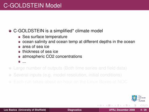
C-GOLDSTEIN is a simplified* climate modelSea surface temperatureocean salinity and ocean temp at different depths in the oceanarea of sea icethickness of sea iceatmospheric CO2 concentrations...
Large number of outputs (Both time series and field data)Several inputs (e.g. model resolution, initial conditions)Each run takes about an hour on the Linux Boxes at NOC
Leo Bastos (University of Sheffield) Diagnostics UFRJ, December 2008 4 / 29
C-GOLDSTEIN Model
C-GOLDSTEIN is a simplified* climate modelSea surface temperatureocean salinity and ocean temp at different depths in the oceanarea of sea icethickness of sea iceatmospheric CO2 concentrations...
Large number of outputs (Both time series and field data)Several inputs (e.g. model resolution, initial conditions)Each run takes about an hour on the Linux Boxes at NOC
Leo Bastos (University of Sheffield) Diagnostics UFRJ, December 2008 4 / 29
Leo Bastos (University of Sheffield) Diagnostics UFRJ, December 2008 5 / 29
Computer models can be very expensive
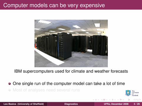
IBM supercomputers used for climate and weather forecasts
One single run of the computer model can take a lot of timeMost of analyses need several runs
Leo Bastos (University of Sheffield) Diagnostics UFRJ, December 2008 5 / 29
Computer models can be very expensive
IBM supercomputers used for climate and weather forecasts
One single run of the computer model can take a lot of timeMost of analyses need several runs
Leo Bastos (University of Sheffield) Diagnostics UFRJ, December 2008 5 / 29
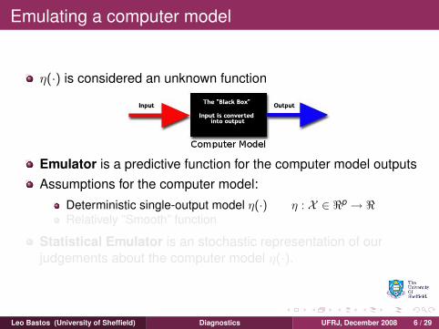
Emulating a computer model
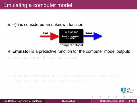
η(·) is considered an unknown function
Emulator is a predictive function for the computer model outputsAssumptions for the computer model:
Deterministic single-output model η(·) η : X ∈ <p → <Relatively ”Smooth” function
Statistical Emulator is an stochastic representation of ourjudgements about the computer model η(·).
Leo Bastos (University of Sheffield) Diagnostics UFRJ, December 2008 6 / 29
Emulating a computer model
η(·) is considered an unknown function
Emulator is a predictive function for the computer model outputsAssumptions for the computer model:
Deterministic single-output model η(·) η : X ∈ <p → <Relatively ”Smooth” function
Statistical Emulator is an stochastic representation of ourjudgements about the computer model η(·).
Leo Bastos (University of Sheffield) Diagnostics UFRJ, December 2008 6 / 29
Gaussian Process Emulator
Gaussian process emulator:
η(·)|β, σ2, ψ ∼ GP (m0(·),V0(·, ·)) ,
where
m0(x) = h(x)Tβ
V0(x,x′) = σ2C(x,x′;ψ)
Prior distribution for (β, σ2, ψ)
Conditioning on some training data
yk = η(xk), k = 1, . . . ,n
Leo Bastos (University of Sheffield) Diagnostics UFRJ, December 2008 7 / 29
Leo Bastos (University of Sheffield) Diagnostics UFRJ, December 2008 8 / 29
Toy Example
η(·) is a two-dimensional known functionGP emulator:
η(·)|β, σ2, ψ ∼ GP(
h(·)Tβ, σ2C(x,x′;ψ)),
h(x) = (1,x)T
C(x,x′) = exp
[−∑
k
(xk − x′kψk
)2]
p(β, σ2, ψ) ∝ σ−2
Leo Bastos (University of Sheffield) Diagnostics UFRJ, December 2008 9 / 29
Toy Example
η(·) is a two-dimensional known functionGP emulator:
η(·)|β, σ2, ψ ∼ GP(
h(·)Tβ, σ2C(x,x′;ψ)),
h(x) = (1,x)T
C(x,x′) = exp
[−∑
k
(xk − x′kψk
)2]
p(β, σ2, ψ) ∝ σ−2
Leo Bastos (University of Sheffield) Diagnostics UFRJ, December 2008 9 / 29
Toy Example
η(·) is a two-dimensional known functionGP emulator:
η(·)|β, σ2, ψ ∼ GP(
h(·)Tβ, σ2C(x,x′;ψ)),
h(x) = (1,x)T
C(x,x′) = exp
[−∑
k
(xk − x′kψk
)2]
p(β, σ2, ψ) ∝ σ−2
Leo Bastos (University of Sheffield) Diagnostics UFRJ, December 2008 9 / 29
Toy Example
η(·) is a two-dimensional known functionGP emulator:
η(·)|β, σ2, ψ ∼ GP(
h(·)Tβ, σ2C(x,x′;ψ)),
h(x) = (1,x)T
C(x,x′) = exp
[−∑
k
(xk − x′kψk
)2]
p(β, σ2, ψ) ∝ σ−2
Leo Bastos (University of Sheffield) Diagnostics UFRJ, December 2008 9 / 29
Toy Example
η(·) is a two-dimensional known functionGP emulator:
η(·)|β, σ2, ψ ∼ GP(
h(·)Tβ, σ2C(x,x′;ψ)),
h(x) = (1,x)T
C(x,x′) = exp
[−∑
k
(xk − x′kψk
)2]
p(β, σ2, ψ) ∝ σ−2
Leo Bastos (University of Sheffield) Diagnostics UFRJ, December 2008 9 / 29
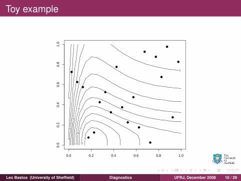
Toy example
2
3
4
5
5 6
7
8
9
1
0 1
1 1
2
13
0.0 0.2 0.4 0.6 0.8 1.0
0.0
0.2
0.4
0.6
0.8
1.0
Leo Bastos (University of Sheffield) Diagnostics UFRJ, December 2008 10 / 29
Toy example
2
3
4
5
5 6
7
8
9
1
0 1
1 1
2
13
0.0 0.2 0.4 0.6 0.8 1.0
0.0
0.2
0.4
0.6
0.8
1.0
●
●
●
●
●
●
●
●
●
●
●
●
●
●
●
●
●
●
●
●
Leo Bastos (University of Sheffield) Diagnostics UFRJ, December 2008 10 / 29
Toy example
2
3
4
5
5 6
7
8
9
1
0 1
1 1
2
13
0.0 0.2 0.4 0.6 0.8 1.0
0.0
0.2
0.4
0.6
0.8
1.0
2
4
4
6
8
10
12
14
●
●
●
●
●
●
●
●
●
●
●
●
●
●
●
●
●
●
●
●
Leo Bastos (University of Sheffield) Diagnostics UFRJ, December 2008 10 / 29
Toy example
0.0 0.2 0.4 0.6 0.8 1.0
0.0
0.2
0.4
0.6
0.8
1.0
2
3
4
5
5 6
7
8
9
1
0 1
1 1
2
13
2
4
4
6
8
10
12
14
●
●
●
●
●
●
●
●
●
●
●
●
●
●
●
●
●
●
●
●
Leo Bastos (University of Sheffield) Diagnostics UFRJ, December 2008 10 / 29
Toy example
0.0 0.2 0.4 0.6 0.8 1.0
0.0
0.2
0.4
0.6
0.8
1.0
2
3
4
5
5 6
7
8
9
1
0 1
1 1
2
13
2
3
4
5
5 6
7
8
9
10
11
12
13
●
●
●
●
●
●
●
●
●
●
●
●
●
●
●
●
●
●
●
●
●
●
●
●
●
●
●
●
●
●
●
●
●
●
●
●
●
●
●
●
●
●
●
●
●
Leo Bastos (University of Sheffield) Diagnostics UFRJ, December 2008 10 / 29
Toy example
0.0 0.2 0.4 0.6 0.8 1.0
0.0
0.2
0.4
0.6
0.8
1.0
2
3
4
5
5 6
7
8
9
1
0 1
1 1
2
13
2
3
4
5
5 6
7
8
9
10
11
12
13
●
●
●
●
●
●
●
●
●
●
●
●
●
●
●
●
●
●
●
●
●
●
●
●
●
●
●
●
●
●
●
●
●
●
●
●
●
●
●
●
●
●
●
●
●
●
●
●
●
●
Leo Bastos (University of Sheffield) Diagnostics UFRJ, December 2008 10 / 29
MUCM Topics
Design for Computer modelsEmulation (Multiple output emulation, Dynamic emulation)UA/SA - Uncertainty and Sensitivity AnalysesCalibration (Bayes Linear and Full Bayesian approaches)Diagnostics and Validation
Leo Bastos (University of Sheffield) Diagnostics UFRJ, December 2008 11 / 29
MUCM Topics
Design for Computer modelsEmulation (Multiple output emulation, Dynamic emulation)UA/SA - Uncertainty and Sensitivity AnalysesCalibration (Bayes Linear and Full Bayesian approaches)Diagnostics and Validation
Leo Bastos (University of Sheffield) Diagnostics UFRJ, December 2008 11 / 29
MUCM Topics
Design for Computer modelsEmulation (Multiple output emulation, Dynamic emulation)UA/SA - Uncertainty and Sensitivity AnalysesCalibration (Bayes Linear and Full Bayesian approaches)Diagnostics and Validation
Leo Bastos (University of Sheffield) Diagnostics UFRJ, December 2008 11 / 29
MUCM Topics
Design for Computer modelsEmulation (Multiple output emulation, Dynamic emulation)UA/SA - Uncertainty and Sensitivity AnalysesCalibration (Bayes Linear and Full Bayesian approaches)Diagnostics and Validation
Leo Bastos (University of Sheffield) Diagnostics UFRJ, December 2008 11 / 29
MUCM Topics
Design for Computer modelsEmulation (Multiple output emulation, Dynamic emulation)UA/SA - Uncertainty and Sensitivity AnalysesCalibration (Bayes Linear and Full Bayesian approaches)Diagnostics and Validation
Leo Bastos (University of Sheffield) Diagnostics UFRJ, December 2008 11 / 29
Diagnostics and Validation
Every emulator should be validatedNon-valid emulators can induce wrong conclusionsThere is little research into validating emulatorsValidation generally means: “the emulator predictions are closeenough to the simulator outputs”.We want to take account all the uncertainty associated with theemulator.“Do the choices that I have made, based on my knowledge of thissimulator, appear to be consistent with the observations?”Choices for the Gaussian process emulator:
NormalityStationarityCorrelation parameters
Leo Bastos (University of Sheffield) Diagnostics UFRJ, December 2008 12 / 29
Validating a GP Emulator
Our diagnostics should be based on a set of new runs of thesimulator
Why? Because predictions at observed input points are perfect.Validation data (y∗,X∗) : y∗k = η(xk
∗), k = 1, . . . ,m
Simulator and the predictive emulator outputs are compared
Numerical diagnosticsGraphical diagnostics
Leo Bastos (University of Sheffield) Diagnostics UFRJ, December 2008 13 / 29
Numerical diagnostics
Individual predictive errors
DIi (y∗) =
(y∗i −m1(x∗i ))√V1(x∗i ,x
∗i )
However, the DI(y∗)s are correlated:
DI(η(X∗)) ∼ Student-tm(n − q,0,C1(X∗))
Mahalanobis distance
DMD(y∗) = (y∗ −m1(X∗))T V1(X∗)−1 (y∗ −m1(X∗))
(n − q)
m(n − q − 2)DMD(η(X∗)) ∼ Fm,n−q
Leo Bastos (University of Sheffield) Diagnostics UFRJ, December 2008 14 / 29
Numerical diagnostics
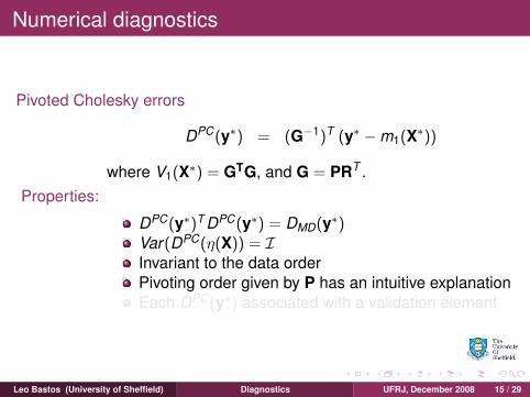
Pivoted Cholesky errors
DPC(y∗) = (G−1)T (y∗ −m1(X∗))
where V1(X∗) = GTG, and G = PRT .Properties:
DPC(y∗)T DPC(y∗) = DMD(y∗)Var(DPC(η(X)) = IInvariant to the data orderPivoting order given by P has an intuitive explanationEach DPC(y∗) associated with a validation element
Leo Bastos (University of Sheffield) Diagnostics UFRJ, December 2008 15 / 29
Numerical diagnostics
Pivoted Cholesky errors
DPC(y∗) = (G−1)T (y∗ −m1(X∗))
where V1(X∗) = GTG, and G = PRT .Properties:
DPC(y∗)T DPC(y∗) = DMD(y∗)Var(DPC(η(X)) = IInvariant to the data orderPivoting order given by P has an intuitive explanationEach DPC(y∗) associated with a validation element
Leo Bastos (University of Sheffield) Diagnostics UFRJ, December 2008 15 / 29
Graphical diagnostics
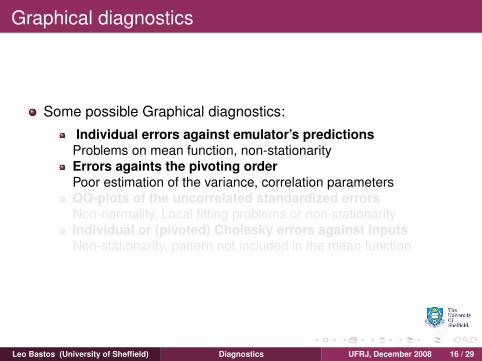
Some possible Graphical diagnostics:
Individual errors against emulator’s predictionsProblems on mean function, non-stationarityErrors againts the pivoting orderPoor estimation of the variance, correlation parametersQQ-plots of the uncorrelated standardized errorsNon-normality, Local fitting problems or non-stationarityIndividual or (pivoted) Cholesky errors against inputsNon-stationarity, pattern not included in the mean function
Leo Bastos (University of Sheffield) Diagnostics UFRJ, December 2008 16 / 29
Graphical diagnostics
Some possible Graphical diagnostics:
Individual errors against emulator’s predictionsProblems on mean function, non-stationarityErrors againts the pivoting orderPoor estimation of the variance, correlation parametersQQ-plots of the uncorrelated standardized errorsNon-normality, Local fitting problems or non-stationarityIndividual or (pivoted) Cholesky errors against inputsNon-stationarity, pattern not included in the mean function
Leo Bastos (University of Sheffield) Diagnostics UFRJ, December 2008 16 / 29
Example: Nuclear Waste Repository
Source: http://web.ead.anl.gov/resrad/
RESRAD is a computer model designed to estimate radiationdoses and risks from RESidual RADioactive materials.Output: 10,000 year time series of the release of contamination indrinking water (in millirems)
Leo Bastos (University of Sheffield) Diagnostics UFRJ, December 2008 17 / 29
Example: Nuclear Waste Repository
−5 0 5 10
−10
−5
05
1015
Simulator
Em
ulat
or
Output - Log of maximal doseof radiation in drinking water27 inputsTraining data: n = 190∗(900)
Validation data: m = 69∗(300)
Leo Bastos (University of Sheffield) Diagnostics UFRJ, December 2008 18 / 29
Graphical Diagnostics: Individual errors
●
●
●
●
●
●
●
●
●
●
●●
●
●
●●
●●
●
●●●
●
●
●
●
●
●
●
●
●
●
●
●
●●
●
●
●●
●
●
●
●
●
●●
●
●
●
●
●
●
●
●
●
●
●
●
●
●
●
●
●
●
●
●●
●
●
0 10 20 30 40 50 60 70
−2
−1
01
2
Data order
Di((y
* ))
●
●
●
●
●
●
●
●
●
●
●●
●
●
●●
●●
●
●●●
●
●
●
●
●
●
●
●
●
●
●
●
●●
●
●
● ●
●
●
●
●
●
●●
●
●
●
●
●
●
●
●
●
●
●
●
●
●
●
●
●
●
●
●●
●
●
−5 0 5 10
−2
−1
01
2E((ηη((xi
*))|y))D
i((y* ))
Leo Bastos (University of Sheffield) Diagnostics UFRJ, December 2008 19 / 29
Graphical Diagnostics: Individual errors
●
●
●
●
●
●
●
●
●
●
●●
●
●
●●
●●
●
● ●●
●
●
●
●
●
●
●
●
●
●
●
●
●●
●
●
●●
●
●
●
●
●
● ●
●
●
●
●
●
●
●
●
●
●
●
●
●
●
●
●
●
●
●
●●
●
●
−1.0 −0.5 0.0 0.5 1.0
−2
−1
01
2
DCU238.S
Di((y
* ))
●
●
●
●
●
●
●
●
●
●
●●
●
●
●●
●●
●
● ●●
●
●
●
●
●
●
●
●
●
●
●
●
●●
●
●
● ●
●
●
●
●
●
● ●
●
●
●
●
●
●
●
●
●
●
●
●
●
●
●
●
●
●
●
●●
●
●
−1.0 −0.5 0.0 0.5
−2
−1
01
2DUU238.S
Di((y
* ))
●
●
●
●
●
●
●
●
●
●
●●
●
●
●●
●●
●
● ●●
●
●
●
●
●
●
●
●
●
●
●
●
●●
●
●
●●
●
●
●
●
●
● ●
●
●
●
●
●
●
●
●
●
●
●
●
●
●
●
●
●
●
●
●●
●
●
−1.0 −0.5 0.0 0.5
−2
−1
01
2
DSU238.S
Di((y
* ))
●
●
●
●
●
●
●
●
●
●
●●
●
●
●●
●●
●
● ●●
●
●
●
●
●
●
●
●
●
●
●
●
●●
●
●
●●
●
●
●
●
●
● ●
●
●
●
●
●
●
●
●
●
●
●
●
●
●
●
●
●
●
●
●●
●
●
−1.0 −0.5 0.0 0.5
−2
−1
01
2
DU234.S
Di((y
* ))
●
●
●
●
●
●
●
●
●
●
●●
●
●
●●
●●
●
●●●
●
●
●
●
●
●
●
●
●
●
●
●
●●
●
●
● ●
●
●
●
●
●
● ●
●
●
●
●
●
●
●
●
●
●
●
●
●
●
●
●
●
●
●
●●
●
●
−1.0 −0.5 0.0 0.5
−2
−1
01
2
DUU234.S
Di((y
* ))
Leo Bastos (University of Sheffield) Diagnostics UFRJ, December 2008 20 / 29
Graphical Diagnostics: Correlated errors
●●
●●
●●●●●●●●
●
●●●●
●●●●●●
●●●●●●●
●●●●●●
●●●●●
●●●●●
●●●●●●
●●●●
●●●●●●●
●●● ● ● ●
●
−2 −1 0 1 2
−2
−1
01
2
Theoretical Quantiles
Sam
ple
Qua
ntile
s
●
●
●●
●
●
●
●
●
●
●
●●
●
●
●
●
●
●
●●
●
●
●
●
●
●●
●
●
●
●
●
●
●
●●
●
●●
●●
●
●
●
●●
●
●
●
●
●
●
●
●
●
●
●
●
●
●
●
●
●
●
●
●
●
●●
0 10 20 30 40 50 60 70
−2
−1
01
2
Pivoting orderD
iPC((y
* ))
DMD(y∗) = 58.96 and the 95% CI is (47.13; 104.70)
Leo Bastos (University of Sheffield) Diagnostics UFRJ, December 2008 21 / 29
Example: Nilson-Kuusk model
Nilson-Kuusk model is a plant canopy reflectance model.For interpretation of remote sensoring dataFor determination of agronomical and phytometric parameters
The Nilson-Kuusk model is a single output model with 5 inputsThe training data contains 150 pointsThe validation data contains 100 points
Leo Bastos (University of Sheffield) Diagnostics UFRJ, December 2008 22 / 29
Graphical Diagnostics - Individual Errors
0.0 0.1 0.2 0.3 0.4 0.5 0.6
0.0
0.1
0.2
0.3
0.4
0.5
0.6
Simulator
Em
ulat
or
●
●
●●
●●
●
●
●
●
●
●●
●
● ●
●
●●●
●●●
●
●
●●
●
●
●
●
●
●
●
●
●
●●
●
●
●
●●
●
●
●
●
●●●●●
●●
●
●
●
●
●●
●
●
●
●●●●
●
●
●●
●
●
●●●
●
●
●
●
●
●
●
●
●
●
●●
●
●
●
●
●
●
●
●
●
●
●
●
●
●
●
●
●
●
●
●
●
●
●
●
●
●
●
●
●
●
●●●
●
●
●
●
●
●
●●
●
●
●●
●●
●
●
●
●
●
●
●
●
●
●
●
●
●●●
●
●
●
●
●
●●
●
●
●
●
●
●
●
●
●●
●
●
● ●
●
●●
●
●
●
●
●
●
●
●
● ●
●
●
●
●
●●
●
●
●
●●
●●
●
●●
0.0 0.1 0.2 0.3 0.4 0.5 0.6−
50
510
E((ηη((xi*))|y))
DI ((y
* ))
Leo Bastos (University of Sheffield) Diagnostics UFRJ, December 2008 23 / 29
Graphical Diagnostics - Uncorrelated Errors
●
●●●
●
●●●
●
●●
●
●●●
●
●
●
●
●●
●
●
●
●●●●
●
●
●
●
●
●
●●●
●
●●
●
●
●●●
●
●
●
●
●
●●
●
●
●
●
●
●●
●
●
●
●
●
●
●
●
●
●
●●
●
●
●●
●
●
●
●
●
●
●
●
●
●
●
●
●
●
●
●
●
●
●
●
●
●
●
●
●
0 20 40 60 80 100
−5
05
1015
Pivoting order
DP
C((y
* ))
6
12
70
1740 10
2445
100
98
712
80
339
1
●
● ●● ● ●●
●●●●●●●●●●●
●●●●●●●●●●●●●●●●●●●
●●●●●●●●●●●●●●●
●●●●●●●●●●●
●●●●●●●●●●●●●●●
●●●●●●●●●●●
●●●●
●● ●
● ●
●
●
−2 −1 0 1 2
−5
05
1015
Theoretical QuantilesD
PC((y
* ))
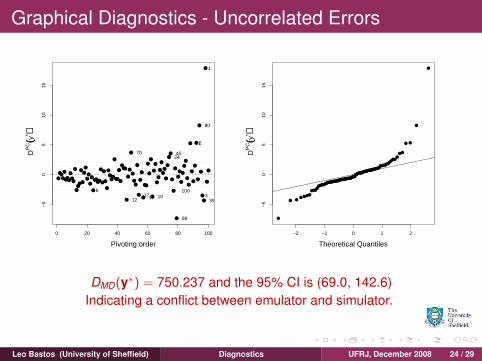
DMD(y∗) = 750.237 and the 95% CI is (69.0, 142.6)Indicating a conflict between emulator and simulator.
Leo Bastos (University of Sheffield) Diagnostics UFRJ, December 2008 24 / 29
Graphical Diagnostics - Input 5
●
●
●
●
●
●
●
●
●
●
●
●
●
●
●
●
●
●
● ● ●
●
●
●
●
●
●
●●
●
●
●●
●●
●
●
●
●
●
●
●
●
●
●
●
●
●●
●
●
●
●
●
●
●●
●
●
●
●
●
●
●
●
● ●
●
●
●●
●
●●
●
●
●
●
●
●
●
●
● ●
●
●
●
●
●●
●
●
●
●●
●●
●
●●
550 600 650 700 750 800 850
−5
05
10
Input 5
DI ((y
* ))
●
●
●
●● ●
●
●
●
●
●
●
●
●
●
●
●
●
●
●
●
●
● ●
●
●
●
●
●
●
●
●
●●
●
●
●●
●
●
●
●
●
●
●
●
●
●
●
●
●
●
●
●
● ●
●
● ●● ● ●●
●
●
●
●
●
●
●
●
● ●
●●
●
●
●
●
●
●●
●
●
●
●
●
●
●
●
●
● ●
●
●
●
●
●
●●
●
●
●
●
●
●
●
●
●
●
●
●
●
●
●
●●●
●● ●
●
●
●
●
●
●
●
●
●
●
●
●
●
●
●●
●●
●
●
●
●●
●
●
● ●●
●
●
●
●
●
●
●
●
●
●
●
●
●
●
●
●
●
●
●● ●●
●
●
●
●
●
●
●
●
●●
●
●
●
●
●
●
●
●
●
●
●
●
●
●
●
●● ● ●
● ●
●●
●●
●
●
●●
●
●
●
●●
●●
●
●
●●
●
●
● ●●
●
●
●
●
●
●
●
●
●
●●●
●
●
●
●
●
●
●
●
●
●
●
●
550 600 650 700 750 800 8500.
00.
10.
20.
30.
40.
50.
60.
7
Input 5
Mod
el O
utpu
t
Leo Bastos (University of Sheffield) Diagnostics UFRJ, December 2008 25 / 29
Actions for the Kuusk emulator
The mean function h(·) = (1,x, x25 , x
35 , x
45 )
Log transformation on outputs“new” dataset for validation
Leo Bastos (University of Sheffield) Diagnostics UFRJ, December 2008 26 / 29
Actions for the Kuusk emulator
The mean function h(·) = (1,x, x25 , x
35 , x
45 )
Log transformation on outputs“new” dataset for validation
Leo Bastos (University of Sheffield) Diagnostics UFRJ, December 2008 26 / 29
Actions for the Kuusk emulator
The mean function h(·) = (1,x, x25 , x
35 , x
45 )
Log transformation on outputs“new” dataset for validation
Leo Bastos (University of Sheffield) Diagnostics UFRJ, December 2008 26 / 29
Individual errors
−3.5 −3.0 −2.5 −2.0 −1.5 −1.0 −0.5
−4
−3
−2
−1
Simulator
Em
ulat
or
●●
●
●
●
●
●
●
●
●
●
●
●
●
●
●
●
●
●
●●
●
●
●● ●
●
●
●
●
●
●
●
●
●
●●
●
●
●
●
●
●
●
●
●
●
●
●
●
●
●
●
●
●
●
●
●●
●
●
●
●
●
●
●
●
●
●
●
●●
●
●
●
●
●
●
●
●
●
●
●
●
●
●
●
●
● ●●
●
●
●
●
●●
●
●
●
−3.5 −3.0 −2.5 −2.0 −1.5 −1.0 −0.5−
3−
2−
10
12
E((ηη((xi*))|y))
DI ((y
* ))
Leo Bastos (University of Sheffield) Diagnostics UFRJ, December 2008 27 / 29
Uncorrelated Errors
●●
●
●●●
●
●
●
●●
●
●
●
●
●
●
●●
●
●
●●
●
●
●
●
●
●
●
●
●
●
●
●●
●
●
●
●
●
●
●
●
●
●
●
●
●●
0 10 20 30 40 50
−3
−2
−1
01
2
Pivoting order
DP
C((y
* ))
1931 ●
●
●● ●
●
●●
●●●
●●●●
●●●●
●●●●●●
●●
●●●
●●●●
●●●●●●
●
●●
● ●●
●
● ●
●
−2 −1 0 1 2
−3
−2
−1
01
2
Theoretical QuantilesD
PC((y
* ))
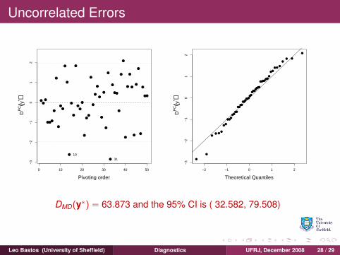
DMD(y∗) = 63.873 and the 95% CI is ( 32.582, 79.508)
Leo Bastos (University of Sheffield) Diagnostics UFRJ, December 2008 28 / 29
Conclusions
Emulation is important when the computer model is expensive.Validating the emulator is necessary before using it for analysesusing tyhe emulator as a surrogate of the computer model.Our diagnostics are useful tools inside the validation process.
Thank you!
Leo Bastos (University of Sheffield) Diagnostics UFRJ, December 2008 29 / 29


![bk - UFPR]](https://static.documents.pub/doc/80x56/61758fb6cf7668196277553b/bk-ufpr.jpg)

