+ All Categories
Home > Documents > University of Southampton Research Repository ePrints Soton · 2020. 1. 29. · the first...

University of Southampton Research Repository ePrints Soton · 2020. 1. 29. · the first...

Date post: 27-Mar-2021
Category:
Upload: others
View: 0 times
Download: 0 times
Share this document with a friend
298
University of Southampton Research Repository ePrints Soton Copyright © and Moral Rights for this thesis are retained by the author and/or other copyright owners. A copy can be downloaded for personal non-commercial research or study, without prior permission or charge. This thesis cannot be reproduced or quoted extensively from without first obtaining permission in writing from the copyright holder/s. The content must not be changed in any way or sold commercially in any format or medium without the formal permission of the copyright holders. When referring to this work, full bibliographic details including the author, title, awarding institution and date of the thesis must be given e.g. AUTHOR (year of submission) "Full thesis title", University of Southampton, name of the University School or Department, PhD Thesis, pagination http://eprints.soton.ac.uk
Transcript

University of Southampton Research Repository

ePrints Soton

Copyright © and Moral Rights for this thesis are retained by the author and/or other copyright owners. A copy can be downloaded for personal non-commercial research or study, without prior permission or charge. This thesis cannot be reproduced or quoted extensively from without first obtaining permission in writing from the copyright holder/s. The content must not be changed in any way or sold commercially in any format or medium without the formal permission of the copyright holders.

When referring to this work, full bibliographic details including the author, title, awarding institution and date of the thesis must be given e.g.

AUTHOR (year of submission) "Full thesis title", University of Southampton, name of the University School or Department, PhD Thesis, pagination

http://eprints.soton.ac.uk

University of SouthamptonFaculty of Engineering, Science and Mathematics

School of Electronics and Computer Science

Near-Capacity Fixed-Rate and Rateless Channel

Code Constructions

by

Nicholas Bonello

A thesis submitted in partial fulfilment of the

requirements of the award of Doctor of Philosophy

at the University of Southampton

June 2009

SUPERVISOR: Professor Lajos Hanzo

MSc, PhD, FREng, DSc, FIEEE, FIET

CO-SUPERVISOR: Professor Sheng Chen

BEng, PhD, DSc, CEng, FIEEE, FIET

University of Southampton

Southampton SO17 1BJ

United Kingdom

c© Nicholas Bonello 2009

ABSTRACT

Near-Capacity Fixed-Rate and Rateless Channel Code Constructions

by

Nicholas Bonello

Fixed-rate and rateless channel code constructions are designed for satisfying conflicting

design tradeoffs, leading to codes that benefit from practical implementations, whilst

offering a good bit error ratio (BER) and block error ratio (BLER) performance. More

explicitly, two novel low-density parity-check code (LDPC) constructions are proposed;

the first construction constitutes a family of quasi-cyclic protograph LDPC codes, which

has a Vandermonde-like parity-check matrix (PCM). The second construction constitutes a

specific class of protograph LDPC codes, which are termed as multilevel structured (MLS)

LDPC codes. These codes possess a PCM construction that allows the coexistence of both

pseudo-randomness as well as a structure requiring a reduced memory. More importantly,

it is also demonstrated that these benefits accrue without any compromise in the attainable

BER/BLER performance. We also present the novel concept of separating multiple users by

means of user-specific channel codes, which is referred to as channel code division multiple

access (CCDMA), and provide an example based on MLS LDPC codes. In particular, we

circumvent the difficulty of having potentially high memory requirements, while ensuring

that each user’s bits in the CCDMA system are equally protected.

With regards to rateless channel coding, we propose a novel family of codes, which

we refer to as reconfigurable rateless codes, that are capable of not only varying their

code-rate but also to adaptively modify their encoding/decoding strategy according to the

near-instantaneous channel conditions. We demonstrate that the proposed reconfigurable

rateless codes are capable of shaping their own degree distribution according to the near-

instantaneous requirements imposed by the channel, but without any explicit channel

knowledge at the transmitter. Additionally, a generalised transmit preprocessing aided

closed-loop downlink multiple-input multiple-output (MIMO) system is presented, in

which both the channel coding components as well as the linear transmit precoder exploit

the knowledge of the channel state information (CSI). More explicitly, we embed a rateless

code in a MIMO transmit preprocessing scheme, in order to attain near-capacity perfor-

mance across a wide range of channel signal-to-ratios (SNRs), rather than only at a specific

SNR. The performance of our scheme is further enhanced with the aid of a technique,

referred to as pilot symbol assisted rateless (PSAR) coding, whereby a predetermined

fraction of pilot bits is appropriately interspersed with the original information bits at the

channel coding stage, instead of multiplexing pilots at the modulation stage, as in classic

pilot symbol assisted modulation (PSAM). We subsequently demonstrate that the PSAR

code-aided transmit preprocessing scheme succeeds in gleaning more information from the

inserted pilots than the classic PSAM technique, because the pilot bits are not only useful

for sounding the channel at the receiver but also beneficial for significantly reducing the

computational complexity of the rateless channel decoder.

Declaration of Authorship

I, Nicholas Bonello, declare that the thesis entitled Near-Capacity Fixed-Rate and

Rateless Channel Code Constructions and the work presented in it are my own and has

been generated by me as the result of my own original research. I confirm that:

• This work was done wholly or mainly while in candidature for a research degree at

this University;

• Where any part of this thesis has previously been submitted for a degree or any other

qualification at this University or any other institution, this has been clearly stated;

• Where I have consulted the published work of others, this is always clearly attributed;

• Where I have quoted from the work of others, the source is always given. With the

exception of such quotations, this thesis is entirely my own work;

• I have acknowledged all main sources of help;

• Where the thesis is based on work done by myself jointly with others, I have made

clear exactly what was done by others and what I have contributed myself;

• Parts of this work have been published.

Signed: ................................................ Date: ................................................

Acknowledgements

I would like to express my heartfelt gratitude to Professor Lajos Hanzo for his out-

standing supervision throughout my research as well as for his invaluable friendship. His

constant guidance, inspiration and unfailing encouragement have greatly benefited me

not only in work but also in life. Sincere thanks are also extended to the staff of the

Communications Group, namely Professor Sheng Chen, Dr. Lie Liang Yang, Dr. Soon

Xin Ng, Dr. Robert G. Maunder and Dr. Yosef Akhtman, for their support and insightful

discussions throughout my research. Special thanks are also due to Ms. Denise Harvey for

her help in administrative matters and to all other colleagues, especially to Mr. Rong Zhang

and Ms. Du Yang. Finally, I would also like to express my appreciation to my family and to

Justyna for their love and support.

Contents

Abstract ii

Declaration of Authorship iii

Acknowledgements iv

1 Introduction 1

1.1 Preliminaries . . . . . . . . . . . . . . . . . . . . . . . . . . . . . . . . . . . . . . 2

1.2 Background of Low-Density Parity-Check Codes . . . . . . . . . . . . . . . . . 7

1.2.1 Historical Perspective and Important Milestones . . . . . . . . . . . . . 10

1.2.2 Iterative Decoding Techniques for Low-Density Parity-Check Codes . 17

1.2.3 Convergence of the Iterative Decoding . . . . . . . . . . . . . . . . . . 18

1.2.4 Encoding of Low-Density Parity-Check Codes . . . . . . . . . . . . . . 20

1.3 Attributes of LDPC Codes and Their Design Tradeoffs . . . . . . . . . . . . . . 22

1.3.1 BER/BLER Performance Metrics . . . . . . . . . . . . . . . . . . . . . . 24

1.3.2 Construction Attributes . . . . . . . . . . . . . . . . . . . . . . . . . . . 28

1.3.3 Hardware Implementation of Low-Density Parity-Check Codes . . . . 29

1.3.3.1 Encoder Characteristics . . . . . . . . . . . . . . . . . . . . . . 29

1.3.3.2 Decoder Characteristics . . . . . . . . . . . . . . . . . . . . . . 30

1.4 Background of Rateless Codes . . . . . . . . . . . . . . . . . . . . . . . . . . . . 31

1.4.1 Historical Perspective and Important Milestones . . . . . . . . . . . . . 32

1.5 Novel Contributions . . . . . . . . . . . . . . . . . . . . . . . . . . . . . . . . . 34

v

1.6 Outline of the Thesis . . . . . . . . . . . . . . . . . . . . . . . . . . . . . . . . . 37

1.6.1 Chapter 2 . . . . . . . . . . . . . . . . . . . . . . . . . . . . . . . . . . . 37

1.6.2 Chapter 3 . . . . . . . . . . . . . . . . . . . . . . . . . . . . . . . . . . . 37

1.6.3 Chapter 4 . . . . . . . . . . . . . . . . . . . . . . . . . . . . . . . . . . . 38

1.6.4 Chapter 5 . . . . . . . . . . . . . . . . . . . . . . . . . . . . . . . . . . . 38

1.6.5 Chapter 6 . . . . . . . . . . . . . . . . . . . . . . . . . . . . . . . . . . . 39

2 Quasi-Cyclic Protograph LDPC Codes 40

2.1 Introduction . . . . . . . . . . . . . . . . . . . . . . . . . . . . . . . . . . . . . . 40

2.1.1 Novelty and Rationale . . . . . . . . . . . . . . . . . . . . . . . . . . . . 41

2.1.2 Chapter Structure . . . . . . . . . . . . . . . . . . . . . . . . . . . . . . . 41

2.2 Code Constructions . . . . . . . . . . . . . . . . . . . . . . . . . . . . . . . . . . 42

2.2.1 MacKay’s Ensembles . . . . . . . . . . . . . . . . . . . . . . . . . . . . . 43

2.2.2 The Extended Bit-Filling Algorithm . . . . . . . . . . . . . . . . . . . . 44

2.2.3 The Progressive Edge Growth Algorithm . . . . . . . . . . . . . . . . . 45

2.3 Protograph LDPC Code Construction . . . . . . . . . . . . . . . . . . . . . . . 46

2.3.1 The Structure of Protograph LDPC Codes . . . . . . . . . . . . . . . . . 51

2.4 Vandermonde-Matrix-Based LDPC Code Construction . . . . . . . . . . . . . 52

2.5 Modifications to the Progressive Edge Growth Algorithm . . . . . . . . . . . . 53

2.5.1 Construction Example . . . . . . . . . . . . . . . . . . . . . . . . . . . . 54

2.6 Results and Discussion . . . . . . . . . . . . . . . . . . . . . . . . . . . . . . . . 58

2.6.1 Effect of Different Codeword Lengths . . . . . . . . . . . . . . . . . . . 58

2.6.2 Effect of Different Coding Rates . . . . . . . . . . . . . . . . . . . . . . 59

2.6.3 Encoder and Decoder Complexity . . . . . . . . . . . . . . . . . . . . . 62

2.7 Summary and Conclusions . . . . . . . . . . . . . . . . . . . . . . . . . . . . . 67

3 MLS LDPC Codes and Their Role in the Instantiation of CCDMA 68

3.1 Introduction . . . . . . . . . . . . . . . . . . . . . . . . . . . . . . . . . . . . . . 68

3.1.1 Novelty and Rationale . . . . . . . . . . . . . . . . . . . . . . . . . . . . 69

3.1.2 Chapter Structure . . . . . . . . . . . . . . . . . . . . . . . . . . . . . . . 70

3.2 General Construction Methodology . . . . . . . . . . . . . . . . . . . . . . . . 70

3.3 Complexity of the Code Description of MLS LDPC Codes . . . . . . . . . . . . 72

vi

3.4 Internal Structure of MLS LDPC Codes . . . . . . . . . . . . . . . . . . . . . . 73

3.5 External Structure of Multilevel Structured Codes . . . . . . . . . . . . . . . . 75

3.5.1 Class I MLS Codes Based on a Homogeneous Coherent Configuration 75

3.5.2 Class II MLS Codes Based on Latin Squares . . . . . . . . . . . . . . . . 76

3.6 Construction Example . . . . . . . . . . . . . . . . . . . . . . . . . . . . . . . . 76

3.7 Additional Constraints . . . . . . . . . . . . . . . . . . . . . . . . . . . . . . . . 78

3.8 Efficient Search for Graphs Having a Large Girth . . . . . . . . . . . . . . . . . 79

3.9 Results and Discussion . . . . . . . . . . . . . . . . . . . . . . . . . . . . . . . . 80

3.9.1 The Girth Distribution . . . . . . . . . . . . . . . . . . . . . . . . . . . . 80

3.9.2 MLS LDPC Codes Satisfying Only the Necessary Constraints . . . . . 86

3.9.2.1 MacKay Benchmarker Codes . . . . . . . . . . . . . . . . . . . 86

3.9.2.2 Rate 0.4 MLS LDPC Codes . . . . . . . . . . . . . . . . . . . . 87

3.9.2.3 Rate 0.5 MLS LDPC Codes . . . . . . . . . . . . . . . . . . . . 88

3.9.2.4 Rate 0.625 MLS LDPC Codes . . . . . . . . . . . . . . . . . . . 92

3.9.2.5 Rate 0.8 MLS LDPC Codes . . . . . . . . . . . . . . . . . . . . 94

3.9.2.6 Summary of BER Performance Results Versus the Block Length 96

3.9.3 MLS LDPC Codes Satisfying All Constraints . . . . . . . . . . . . . . . 100

3.10 Comparison with Other Multilevel LDPC Codes . . . . . . . . . . . . . . . . . 104

3.10.1 Gallager’s LDPC Codes . . . . . . . . . . . . . . . . . . . . . . . . . . . 105

3.10.2 Generalised LDPC codes . . . . . . . . . . . . . . . . . . . . . . . . . . . 106

3.11 Channel Code Division Multiple Access . . . . . . . . . . . . . . . . . . . . . . 110

3.11.1 Concept Definition . . . . . . . . . . . . . . . . . . . . . . . . . . . . . . 111

3.11.2 Limitations and Benefits of Channel Code Division Multiple Access . 111

3.12 General Model of the CCDMA System . . . . . . . . . . . . . . . . . . . . . . . 113

3.13 User-Specific Channel Codes Employing MLS LDPC Codes . . . . . . . . . . 114

3.13.1 User Separation by Distinct Latin Squares . . . . . . . . . . . . . . . . . 114

3.13.2 Isotopic Latin Squares and Isomorphic Edge-Coloured Graphs . . . . 115

3.14 Simulation Results . . . . . . . . . . . . . . . . . . . . . . . . . . . . . . . . . . 115

3.15 Summary and Conclusions . . . . . . . . . . . . . . . . . . . . . . . . . . . . . 119

4 Reconfigurable Rateless Codes 120

4.1 Introduction . . . . . . . . . . . . . . . . . . . . . . . . . . . . . . . . . . . . . . 120

vii

4.1.1 Related Work . . . . . . . . . . . . . . . . . . . . . . . . . . . . . . . . . 120

4.1.2 Novelty and Rationale . . . . . . . . . . . . . . . . . . . . . . . . . . . . 122

4.1.3 Chapter Structure . . . . . . . . . . . . . . . . . . . . . . . . . . . . . . . 122

4.2 Conventional Rateless Codes . . . . . . . . . . . . . . . . . . . . . . . . . . . . 123

4.2.1 Overview of Luby Transform Codes . . . . . . . . . . . . . . . . . . . . 123

4.2.2 Paradigms of Luby Transform Codes . . . . . . . . . . . . . . . . . . . 124

4.2.2.1 Luby Transform Codes as an Instance of Convolutional Codes 124

4.2.2.2 Luby Transform Codes as an Instance of Low-Density Gen-

erator Matrix Codes . . . . . . . . . . . . . . . . . . . . . . . . 126

4.2.3 Paradigms for Other Rateless Codes Families . . . . . . . . . . . . . . . 128

4.3 Soft Decoding of Luby Transform Codes . . . . . . . . . . . . . . . . . . . . . . 129

4.4 The Check Node Distribution . . . . . . . . . . . . . . . . . . . . . . . . . . . . 130

4.5 EXIT Chart Analysis of Luby Transform Codes . . . . . . . . . . . . . . . . . . 134

4.5.1 EXIT Curve for the Inner Check Node Decoder . . . . . . . . . . . . . . 135

4.5.2 EXIT Curve for the Outer Variable Node Decoder . . . . . . . . . . . . 137

4.5.3 EXIT Charts for Code Mixtures . . . . . . . . . . . . . . . . . . . . . . . 138

4.6 Reconfigurable Rateless Codes . . . . . . . . . . . . . . . . . . . . . . . . . . . 139

4.7 System Overview . . . . . . . . . . . . . . . . . . . . . . . . . . . . . . . . . . . 141

4.7.1 Channel Model . . . . . . . . . . . . . . . . . . . . . . . . . . . . . . . . 141

4.7.2 System Model . . . . . . . . . . . . . . . . . . . . . . . . . . . . . . . . . 142

4.8 System Description . . . . . . . . . . . . . . . . . . . . . . . . . . . . . . . . . . 145

4.8.1 Analysis Under Simplified Assumptions . . . . . . . . . . . . . . . . . 145

4.8.2 The Adaptive Incremental Degree Distribution . . . . . . . . . . . . . . 148

4.9 Simulation Results . . . . . . . . . . . . . . . . . . . . . . . . . . . . . . . . . . 152

4.10 Summary and Concluding Remarks . . . . . . . . . . . . . . . . . . . . . . . . 154

5 Generalised MIMO Transmit Preprocessing using PSAR Codes 157

5.1 Introduction . . . . . . . . . . . . . . . . . . . . . . . . . . . . . . . . . . . . . . 157

5.1.1 Novelty and Rationale . . . . . . . . . . . . . . . . . . . . . . . . . . . . 160

5.1.2 Chapter Structure . . . . . . . . . . . . . . . . . . . . . . . . . . . . . . . 161

5.2 Channel Model . . . . . . . . . . . . . . . . . . . . . . . . . . . . . . . . . . . . 161

5.3 System Model . . . . . . . . . . . . . . . . . . . . . . . . . . . . . . . . . . . . . 162

viii

5.3.1 Outer Closed-Loop: Encoder for PSAR Codes . . . . . . . . . . . . . . 162

5.3.2 Pilot-Bit Interleaving and Space-Time Block Coding . . . . . . . . . . . 166

5.3.3 Inner Closed-Loop System: MIMO Transmit Eigen-Beamforming . . . 167

5.3.4 Receiver . . . . . . . . . . . . . . . . . . . . . . . . . . . . . . . . . . . . 168

5.3.5 Adaptive Feedback Link . . . . . . . . . . . . . . . . . . . . . . . . . . . 169

5.3.5.1 Low Doppler Frequency . . . . . . . . . . . . . . . . . . . . . 170

5.3.5.2 Intermediate Doppler Frequency . . . . . . . . . . . . . . . . 170

5.3.5.3 High Doppler Frequency . . . . . . . . . . . . . . . . . . . . . 171

5.4 Pilot Symbol Assisted Rateless Codes . . . . . . . . . . . . . . . . . . . . . . . 171

5.4.1 Lower Bounds on the Realisable Rate and the Achievable Throughput 171

5.4.2 Graph-Based Analysis of Pilot Symbol Assisted Rateless Codes . . . . 172

5.5 EXIT Charts of Pilot Symbol Assisted Rateless Codes . . . . . . . . . . . . . . 174

5.5.1 PSAR Codes as Instances of Partially-Regular Non-Systematic Codes . 175

5.5.2 PSAR Codes as Instances of Irregular Partially-Systematic Codes . . . 178

5.6 The Equivalence of the Two PSAR Code Implementations . . . . . . . . . . . . 183

5.7 Code Doping in Pilot Symbol Assisted Rateless Codes . . . . . . . . . . . . . . 185

5.8 EXIT-Chart-Based Optimisation for PSAR Codes . . . . . . . . . . . . . . . . . 188

5.9 Simulation Results . . . . . . . . . . . . . . . . . . . . . . . . . . . . . . . . . . 191

5.9.1 Uncorrelated Rayleigh Channel . . . . . . . . . . . . . . . . . . . . . . . 192

5.9.2 Correlated Rayleigh Channel . . . . . . . . . . . . . . . . . . . . . . . . 195

5.10 Summary and Concluding Remarks . . . . . . . . . . . . . . . . . . . . . . . . 198

6 Summary and Conclusions 201

6.1 Chapter 1 . . . . . . . . . . . . . . . . . . . . . . . . . . . . . . . . . . . . . . . . 203

6.2 Chapter 2 . . . . . . . . . . . . . . . . . . . . . . . . . . . . . . . . . . . . . . . . 203

6.3 Chapter 3 . . . . . . . . . . . . . . . . . . . . . . . . . . . . . . . . . . . . . . . . 205

6.4 Chapter 4 . . . . . . . . . . . . . . . . . . . . . . . . . . . . . . . . . . . . . . . . 210

6.5 Chapter 5 . . . . . . . . . . . . . . . . . . . . . . . . . . . . . . . . . . . . . . . . 212

6.6 Future Work . . . . . . . . . . . . . . . . . . . . . . . . . . . . . . . . . . . . . . 214

A Long-Term Channel Prediction 217

B General Notation 219

ix

C List of Symbols 221

C.1 Conventional Linear Block Codes . . . . . . . . . . . . . . . . . . . . . . . . . . 221

C.2 Low-Density Parity-Check Codes . . . . . . . . . . . . . . . . . . . . . . . . . . 222

C.3 Code Attributes . . . . . . . . . . . . . . . . . . . . . . . . . . . . . . . . . . . . 223

C.4 Protograph LDPC Codes . . . . . . . . . . . . . . . . . . . . . . . . . . . . . . . 223

C.5 Multilevel Structured LDPC Codes . . . . . . . . . . . . . . . . . . . . . . . . . 223

C.6 Channel Code Division Multiple Access . . . . . . . . . . . . . . . . . . . . . . 224

C.7 Luby Transform Codes . . . . . . . . . . . . . . . . . . . . . . . . . . . . . . . . 224

C.8 Reconfigurable Rateless Codes . . . . . . . . . . . . . . . . . . . . . . . . . . . 226

C.9 Channel Models . . . . . . . . . . . . . . . . . . . . . . . . . . . . . . . . . . . . 227

C.9.1 Discrete-Time Quasi-Static Fading SISO Channel . . . . . . . . . . . . . 227

C.9.2 MIMO Channel . . . . . . . . . . . . . . . . . . . . . . . . . . . . . . . . 228

C.10 Generalised MIMO Transmit Preprocessing - Inner Closed-Loop . . . . . . . . 228

C.11 Generalised MIMO Transmit Preprocessing - Outer Closed-Loop . . . . . . . 228

D List of Abbreviations 230

Bibliography 235

Subject Index 269

Author Index 274

x

CHAPTER 1

Introduction

The birth of information and coding theory is marked by Shannon’s seminal paper,

A Mathematical Theory of Communication [1], published in 1948. At that time, his

theories disproved the widely supported belief that an increase in the information

transmission rate increases the probability of error. Shannon demonstrated that arbitrarily

reliable communication of information over an unreliable channel is possible, provided that

the transmission rate is less than the channel capacity.

This can be achieved by using forward error correction (FEC). The basic idea is that of

incorporating redundant bits, or check bits, and thus making the bits within each codeword

correlated. This creates a finite set of legitimate vectors defined over the input alphabet,

which is referred to as a code. If the check bits are introduced in a manner so as to make each

codeword sufficiently distinct from each other, the receiver will be capable of determining

the most likely transmitted codeword. The channel capacity determines the exact amount

of redundancy that has to be incorporated by the encoder in order to be able to correct the

errors imposed by the channel.

However, Shannon’s theory only proves the existence of capacity approaching codes,

but refrains from suggesting specific coding schemes, as well as from specifying how

the messages can be decoded. Diverse extensions, deeper interpretations and practical

realisations of Shannon’s work emerged throughout the last six decades, including the

discovery of low-density parity-check (LDPC) codes [2] in the early 60’s (and their re-

discovery in the mid-90’s [3]) and that of turbo codes [4].

The aim of this introductory chapter is to outline the rudimentary principles, to review

the available literature regarding LDPC and rateless codes as well as to underline the

rationale behind this thesis. We commence by describing the basic principles of conventional

linear block codes in Section 1.1. In Section 1.2, we extend these fundamental principles to

1

1.1. Preliminaries 2

LDPC codes and outline the most important milestones in their history. In particular, we

focus our attention on the encoding and iterative decoding techniques. We also describe the

tools we have at our disposal for analysing the decoding of the LDPC codes. Section 1.3

outlines the attributes of the codes and summarises the tradeoffs imposed on their design.

Subsequently, Section 1.4 lays down the fundamentals and provides a historical perspective

on rateless codes. Finally, the novel contributions and the organisation of this thesis are

described in Sections 1.5 and 1.6, respectively.

1.1 Preliminaries

In this section, we will introduce the basic concepts of block codes. For the sake of simplicity,

we will focus our attention on a specific subclass of linear block codes. Furthermore, we only

consider binary linear block codes, namely codes that are associated with symbols defined

over the binary Galois field GF(2). In this regard, the word ‘bit’ and ‘symbol’ will be used

interchangeably throughout our discourse. Figure 1.1 shows a simplified block diagram of

a channel coded communication system using linear block codes.

The theory of linear block codes has been covered in great detail in excellent textbooks,

amongst others that by Berkekamp [5], Hill [6], Lin and Costello [7], Lint [8], MacWilliams

and Sloane [9], McEliece [10], Peterson and Welson [11]. For the sake of completeness, in this

subsection we will provide a brief overview of the basic definitions and theorems related to

generic linear block codes. The material of this subsection is based on an amalgam of these

references [5–11].

A code can be termed as a block code, if the original information bit-sequence can

be segmented into fixed-length message blocks, hereby denoted by u, each having K

information digits. This implies that there are 2K possible distinct message blocks. The

encoder is capable of transforming each input message block u into a distinct binary N-tuple

z, N > K, according to a predefined set of rules. This binary N-tuple is the encoded bit-

sequence, which is typically referred to as the codeword (or code vector) whilst N is called the

block length (or word length). Again, there are 2K distinct legitimate codewords corresponding

to the 2K message blocks. This set of the 2K codewords is termed as a block code. The unique

and distinctive nature of the codewords implies that there is a one-to-one mapping between

an original information bit-sequence u and the corresponding codeword z.

These one-to-one correspondences between u and z form the set of rules of the encoder.

Clearly, if both K and N are small, then the 2K distinct message blocks and the corresponding

codewords can be stored in a look-up table (LUT). However, for large K and N, such an

encoder that lists all the legitimate codewords will be prohibitively complex. The complexity

of the encoder (as well as the decoder) can be significantly reduced if the code is linear. In

this regard, we have the following definition.

Definition 1.1.1 [6–8]. A block code having a block length of N and 2K codewords is

classified as a linear (N, K) block code C if and only if its 2K legitimate codewords form

1.1. Preliminaries 3

Channel Encoder

z = uG

BlockK-bit Message

CodewordN -bit

u = [u1u2 . . . uK ] z = [z1z2 . . . zN ]

Noise

CodewordBlockDemodulatedDecoded Message

r

Channel

Modulator

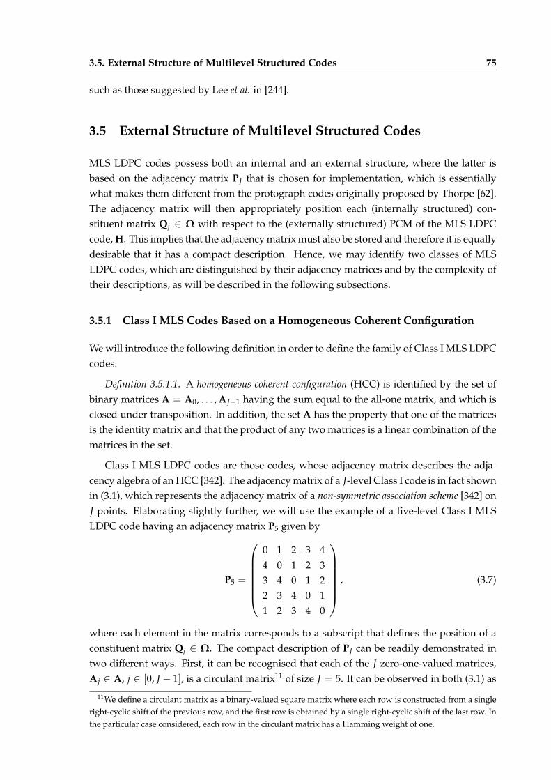
DemodulatorChannel Decoderu

Figure 1.1: A simplified block diagram of a channel coded system using linear block codes

such as LDPC codes.

a K-dimensional subspace of the vector space of all the N-tuples defined over the field

GF(2). The implies that the modulo-2 sum of any two or more codewords is another valid

codeword.

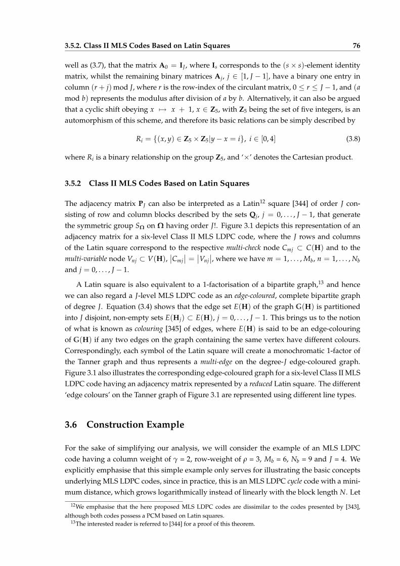
A (N, K) linear code can be specified by simply defining the basis1 of K codewords.

Definition 1.1.2 [6–8]. A (K × N)-element matrix whose rows form a basis of a linear

(N, K) code C is called the generator matrix G of the code.

Since the code C is linear, it is possible to find K linearly independent codewords,

g0, g1, . . . , gK−1, in C so that every codeword z ∈ C is constituted by the linear combination

of these K codewords. Let the input message block u be represented by u0, u1, . . . , uK−1,

where ui is either zero or one, for 0 ≤ i < K − 1. Then, the codeword z ∈ C can be

expressed as

z = u0g0 + u1g1 + · · ·+ uK−1gK−1. (1.1)

The codeword generation process can be more compactly represented in matrix form as

z = u ·G

= [u0 u1 . . . uK−1] ·

g0

g1...

gK−1

, (1.2)

which is equivalent to

z = [u0 u1 . . . uK−1] ·

g0,0 g0,1 . . . g0,N−1

g1,0 g1,1 . . . g1,N−1

...... . . .

...

gK−1,0 gK−1,1 . . . gK−1,N−1

, (1.3)

where gi,j, for 0 ≤ i ≤ K − 1 and 0 ≤ j ≤ N − 1, is either zero or one. The rows of the

generator matrix G are said to span (i.e. generate) the (N, K) linear code C.

1A basis of a vector space V is a linearly independent subset of V that can generate the same vector space V.

1.1. Preliminaries 4

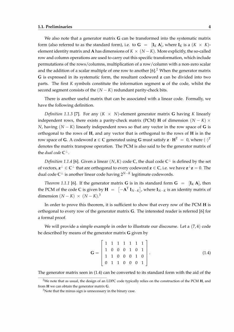
We also note that a generator matrix G can be transformed into the systematic matrix

form (also referred to as the standard form), i.e. to G = [IK A], where IK is a (K × K)-

element identity matrix and A has dimensions of K × (N−K). More explicitly, the so-called

row and column operations are used to carry out this specific transformation, which include

permutations of the rows/columns, multiplication of a row/column with a non-zero scalar

and the addition of a scalar multiple of one row to another [6].2 When the generator matrix

G is expressed in its systematic form, the resultant codeword z can be divided into two

parts. The first K symbols constitute the information segment u of the code, whilst the

second segment consists of the (N − K) redundant parity-check bits.

There is another useful matrix that can be associated with a linear code. Formally, we

have the following definition.

Definition 1.1.3 [7]. For any (K × N)-element generator matrix G having K linearly

independent rows, there exists a parity-check matrix (PCM) H of dimension (N − K) ×N, having (N − K) linearly independent rows so that any vector in the row space of G is

orthogonal to the rows of H, and any vector that is orthogonal to the rows of H is in the

row space of G. A codeword z ∈ C generated using G must satisfy z ·HT = 0, where (·)T

denotes the matrix transpose operation. The PCM is also said to be the generator matrix of

the dual code C⊥.

Definition 1.1.4 [6]. Given a linear (N, K) code C, the dual code C⊥ is defined by the set

of vectors, z⊥ ∈ C⊥ that are orthogonal to every codeword z ∈ C, i.e. we have z⊥z = 0. The

dual code C⊥ is another linear code having 2N−K legitimate codewords.

Theorem 1.1.1 [6]. If the generator matrix G is in its standard form G = [IK A], then

the PCM of the code C is given by H =[−AT IN−K

], where IN−K is an identity matrix of

dimension (N − K) × (N − K).3

In order to prove this theorem, it is sufficient to show that every row of the PCM H is

orthogonal to every row of the generator matrix G. The interested reader is referred [6] for

a formal proof.

We will provide a simple example in order to illustrate our discourse. Let a (7, 4) code

be described by means of the generator matrix G given by

G =

1 1 1 1 1 1 1

1 0 0 0 1 0 1

1 1 0 0 0 1 0

0 1 1 0 0 0 1

. (1.4)

The generator matrix seen in (1.4) can be converted to its standard form with the aid of the

2We note that as usual, the design of an LDPC code typically relies on the construction of the PCM H, and

from H we can obtain the generator matrix G.3Note that the minus sign is unnecessary in the binary case.

1.1. Preliminaries 5

Table 1.1: The codewords for the code C(7, 4) and its dual code C⊥(7, 3), given the generator

matrix and PCM represented in (1.5) and (1.6), respectively

z ∈ C z⊥ ∈ C⊥

0 0 0 0 0 0 0 0 0 0 0 0 0 0

0 0 0 1 0 1 1 1 1 1 1 0 0 1

0 0 1 0 1 1 0 0 1 1 1 0 1 0

0 0 1 1 1 0 1 1 0 1 0 0 1 1

0 1 0 0 1 1 1 1 1 1 0 1 0 0

0 1 0 1 1 0 0 0 0 1 1 1 0 1

0 1 1 0 0 0 1 1 0 0 1 1 1 0

0 1 1 1 0 1 0 0 1 0 0 1 1 1

1 0 0 0 1 0 1

1 0 0 1 1 1 0

1 0 1 0 0 1 1

1 0 1 1 0 0 0

1 1 0 0 0 1 0

1 1 0 1 0 0 1

1 1 1 0 1 0 0

1 1 1 1 1 1 1

previously described row and column operations, which results in

G =

1 0 0 0 1 0 1

0 1 0 0 1 1 1

0 0 1 0 1 1 0

0 0 0 1 0 1 1

. (1.5)

The PCM H is then given by

H =

1 1 1 0 1 0 0

0 1 1 1 0 1 0

1 1 0 1 0 0 1

. (1.6)

The resultant codewords corresponding to the (7, 4) linear block code and its dual code

C⊥(7, 3) are subsequently shown in Table 1.1, which were generated with the aid of (1.2).

Observe in Table 1.1 that the first four bits of a codeword are the systematic information

bits, followed by three parity-check (redundant) bits, each of which checks the parity of the

specific information bits as determined by the generator matrix represented in (1.5).

Some other important definitions follow below.

Definition 1.1.5 [6–8]. Consider a linear code C represented by its PCM H. Let the code-

word transmitted over an error-infested channel be represented by w = [w0w1 . . . wN−1]

and let the received codeword be represented by r = [r0r1 . . . rN−1]. The so-called syndrome

1.1. Preliminaries 6

S(r) of r is given by a [1 × (N − K)]-element row vector determined by

S(r) = r ·HT, (1.7)

where S(r) is equal to the zero vector if the received codeword r is a legitimate codeword

and hence we have r ∈ C.4 The syndrome can be used for error detection or for the so-

called decoding early stopping criterion. The latter is the criteria used to determine when the

decoder can be halted (due to r being correct or else has been corrected by the decoder)

before the maximum allowable number of iterations is reached.

Definition 1.1.6 [6–8]. The weight (also referred to as the Hamming weight) of a codeword

is equal to the number of non-zero components of the codeword. Given a codeword z1 ∈ C,

its weight is denoted by w(z1). For example, the weight of the codeword z = [1101001] is

w(z) = 4.

Definition 1.1.7 [6–8]. The distance (also referred to as the Hamming distance) between

two codewords is equal to the number of positions in which the codewords differ. Given

two codewords z1 ∈ C and z2 ∈ C, the Hamming distance between the two is denoted

by d (z1, z2). For instance, the distance between z1 = [1101001] and z2 = [0100101] is

d (z1, z2) = 3. Furthermore we have [6, 7]

d (z1, z2) = w (z1 + z2) . (1.8)

Definition 1.1.8 [6–8]. The minimum Hamming distance (or simply the minimum distance),

hereby denoted by dmin is defined by

dmin := min d (z1, z2) , z1, z2 ∈ C, z1 6= z2 . (1.9)

The minimum distance of a linear block code C is determined by the weight of the

codeword z ∈ C having the minimum weight since the all-zero codeword is always part

of a linear code. For example, the dmin of the code C represented in Table 1.1 is equal to

three.

The following three theorems relate the minimum distance of a linear block code to its

PCM.

Theorem 1.1.2 [7]. For each codeword in an (N, K) linear block code having a weight of h,

there exists h columns in the associated PCM H so that the vectorial sum of these h columns

is equal to the zero vector. A formal proof of this theorem can be found in [7].

Theorem 1.1.3 [7]. An (N, K) linear block code C having a PCM H and a minimum

distance of at least dmin will have dmin or fewer columns of H, which result in the zero

vector, when they are summed up.

Theorem 1.1.4 [7]. The minimum distance of a linear code C is equal to the smallest

number of columns of H that sum up to the zero vector.

4Note that this automatically imply that r is error-free and thus we say that the an undetected error has

occurred. Undetected error will be discussed in more detail in Section 1.3.1.

1.2. Background of Low-Density Parity-Check Codes 7

For instance, in the PCM represented in (1.6), there are no zero columns nor any

repeated columns. Therefore, since no two or fewer columns sum to the zero vector, we

can reasonably say that its minimum distance is equal to three. However, the second, third

and last column do sum up to the zero vector and therefore we can reasonable say that the

(7, 4) linear block code having the PCM represented in (1.6) has dmin = 3.

There are a number of important linear block code families. The first class of linear

block codes are constituted by Hamming codes, which were proposed by Hamming in [12]

as early as just two years after Shannon’s landmark paper [1]. Hamming codes have a

minimum distance of three and thus can correct a single-bit error. Other important families

of linear block codes are the Reed-Muller codes [13, 14] and Golay codes [15]. In this thesis,

we will only focus our attention on the class of LDPC and LDPC-like linear block codes.

1.2 Background of Low-Density Parity-Check Codes

We consider a binary LDPC code defined by the null space of a low-density PCM matrix H

constructed over GF(2). Then, assuming a full-rank and hence invertible PCM composed of

M = N − K rows and N columns, the rate of this code becomes R = 1 - M/N. This can also

be represented by means of a so-called bipartite Tanner graph [16], exemplified in Figure 1.2,

consisting of M = 4 check nodes and N = 7 variable nodes. A one-to-one relationship exists

between the set of all PCMs and the set of all bipartite Tanner graphs. For example, the PCM

associated with the Tanner graph illustrated in Figure 1.2 is given by

H =

1 0 1 0 0 1 1

1 1 0 0 0 0 1

0 1 1 1 1 0 0

0 0 0 1 1 1 0

. (1.10)

To relate the PCM of (1.10) to the Tanner graph of Figure 1.2, please observe that check-node

c1 is checking the parity of v1, v3, v6 and v7, as seen in the first row of (1.10). This implies

that if the transmitted bits represented by v1, v3, v6 and v7 are received correctly, then the

value of v1 ⊕ v3 ⊕ v6 ⊕ v7 ⊕ c1 = 0.

For the sake of completeness, we will introduce some basic definitions related to graph

theory. We will subsequently denote the Tanner graph associated with the PCM H by

G(H) = U, E, where U represents the set of nodes (also called vertices) and E is the set

of edges. For the case of a bipartite graph, we have U = V ∪ C, where V defines the set of

variable nodes (sometimes also referred to as symbol nodes) whilst C corresponds to the set

of M check nodes. The so-called degree of the check and the variable nodes will be denoted

by ρ and γ, which correspond to the row and column weight5 of the PCM, respectively, and

indicate the number of edges emerging from them. Alternatively, the bipartite Tanner graph

can be expanded to a tree structure having k levels (sometimes also referred to as the number

of tiers), as shown in Figure 1.3. This will split the sets V and C into k subsets, i.e. we have

5This is equal to the number of ones of the respective row and column of the PCM.

1.2. Background of Low-Density Parity-Check Codes 8

c4c3c2c1

v1 v2 v3 v4 v5 v6 v7

V

C

Figure 1.2: Example of a Tanner graph having a girth of four. A cycle of six (represented by

the bold edges) and a cycle of four (dashed bold) are shown.

V = V1 ∪V2 ∪ . . . Vk and C = C1 ∪ C2 ∪ . . . Ck. Therefore, by following this notation, we

can write the set of variable and check nodes as V =⋃k

q=1 Vq and C =⋃k

q=1 Cq. Additionally,

we also have Vq1∩Vq2 = ∅ and Cq1

∩ Cq2 = ∅, ∀ 0 ≤ q1 < q2 ≤ k.

The bipartite Tanner graph representing an LDPC code is said to be undirected since its

edges do not possess any sense of direction. Following this, a chain refers to the series of

successive edges that form a continuous curve passing from one vertex to another located

on an undirected graph. Then, a so-called cycle refers to that particular chain of nodes, where

the initial and final vertex are the same, provided that no edge is used more than once. The

number of edges in a cycle is called the length of the cycle and the shortest cycle of the graph

corresponds to what is referred to as the girth. For example, the graph depicted in Figure 1.2

has a girth of four and the corresponding cycle of four is shown by the dashed bold edges.

A cycle of six is also shown marked by the continuous bold edges. The length of the shortest

cycle predetermines the achievable bit error ratio (BER) performance of the code, because

short cycles prevent the decoder from gleaning independent parity-check information. It

is an often-quoted result in graph theory that the value of the girth in a bipartite graph is

always even.

An LDPC code is also said to be regular, if it is associated with a PCM having a

fixed row and column weight, hereby denoted by ρ and γ. A regular LDPC code will

then possess a Tanner graph, in which each node has the same degree or valency. On

the other hand, the row and column weights of a PCM associated with an irregular

LDPC code are not constant. In fact, these weights are typically specified by means of

polynomial distributions [17]. Carefully designed irregular LDPC codes may exhibit a

superior performance when compared to the corresponding regular LDPC codes. However,

this is achieved at the expense of a potentially increased implementational complexity. In

Chapter 2 as well as in Chapter 3, we have focused our efforts on the design of low-

complexity codes and therefore regular codes were of more interest than their irregular

counterparts, since having a regular structure may reduce the memory requirements and

achieve a simpler implementation. Irregular LDPC-like codes will then be proposed in

Chapters 4 and 5 of this thesis, where we consider rateless code constructions. It is important

to note that due to the underlying nature of a rateless code in which a codeword bit is

1.2. Background of Low-Density Parity-Check Codes 9

Check Nodes

VariableNodes

Level 0

V

CLevel 1

Level k

Figure 1.3: A Tanner graph expanded as a tree having k levels [18].

generated by the modulo-2 sum of a random number of original information bits, rateless

codes are typically irregular.

LDPC codes are typically decoded using the sum-product algorithm (SPA) [19], where

messages or ‘beliefs’ [20] are exchanged between the nodes residing at both sides of the

graph. The sparsity of the PCM guarantees low decoding complexity as well as relatively

simple implementations and also makes it possible for the corresponding Tanner graph to

attain a relatively high girth and hence benefit from independent parity-check information.

By the word ‘sparse’, we mean that the density; i.e. the expected fraction of binary ones in

the code’s PCM, is less than 0.5 [3]. It was also shown by Kschischang et al. [21] that LDPC

codes’ decoding using the SPA is sub-optimal for Tanner graphs that possess cycles and that

the independence of these messages exchanged between the nodes located on the opposite

sides of the graph is in fact characterised by the girth g. Specifically, Gallager demonstrated

in [2] that the number of independent iterations, i.e. the iterations that provide valuable

extrinsic information and hence an iteration gain, hereby denoted by T, is bounded by T <

g/4 ≤ T + 1. Clearly, for the girth to be high, the block length N also has to be sufficiently

high. The loose lower bound on the required block length N for achieving a specific girth of

g = 4x + 2, where x is an integer, is given by [2]

N ≥ 1 +x+1

∑k=2

γ(γ− 1)k−2(ρ− 1)k−1. (1.11)

1.2.1. Historical Perspective and Important Milestones 10

By contrast, we have [2]

N ≥x

∑k=1

ρ [(γ− 1)(ρ− 1)](k−1) (1.12)

for g = 4x. For example, an LDPC code having a code-rate of R = 0.625, associated with a

PCM having a column weight of γ = 3 and row weight ρ = 8 must have a block length of

at least N = 1688 bits in order to have a girth of g = 12. Needless to say that an LDPC code

having a girth of g = 12 and a block length of N = 1688 bits may not be realisable with

the aid of a regular code. Generally, the more regular or structured the LDPC construction,

the lower the value of the resultant girth. We also note that another reason for aiming for

constructions having a large girth is that the minimum distance also increases with the girth

of the graph, as shown by the bounds derived by Tanner in [16].

However, it is important to emphasise that whilst a code having a high girth is always

preferred, ironically, completely cycle-free codes constitute bad codes. This was shown by

Etzion et al. [22], who proved that for cycle-free codes, we have dmin ≤ 2 if the code-rate is

R ≥ 0.5, whilst

dmin <

⌊N

K + 1

⌋+

⌊N + 1

K + 1

⌋<

2

R, (1.13)

if the code-rate R < 0.5, where ⌊·⌋ denotes the floor function. Consequently, having a

low minimum distance of dmin ≤ 2 will definitely result in having a high error floor.

Furthermore, we note that in this thesis we only consider codes where we have γ ≥ 3 and

hence the minimum distance increases linearly rather than logarithmically6 with the block

length [2].

1.2.1 Historical Perspective and Important Milestones

In this subsection, we will review the available literature related to LDPC codes. For the

sake of convenience, we have summarised the most important milestones in the history of

LDPC codes in Tables 1.2 and 1.3. We emphasise that considering the large body of work

available, these tables are in no way complete.

LDPC codes were conceived by Gallager in his doctoral dissertation in 1962 [2, 24].

However, having limited computing resources prevented him from proving the near-

capacity operation of these codes and from finding rigorous performance bounds of the

decoding algorithm. In addition to this, the introduction of Reed-Solomon (RS) codes a few

years earlier [89], and the widely accepted belief that concatenated RS and convolutional

codes [90] were perfectly suited for practical error-control coding resulted in Gallager’s

work becoming neglected by researchers for approximately 30 years. Exceptions to this

which are worth mentioning are the work of Zyablov, Pinsker and Margulis from the

Russian school [25–27] and by Tanner [16]. Margulis proposed a structured regular

construction for a half-rate Gallager code based on the Cayley graph, which is nowadays

6This result may not be valid for some structured constructions, such as those proposed in [23].

1.2.1. Historical Perspective and Important Milestones 11

Table 1.2: Important milestones in the history of LDPC codes (1948-2001)

Date Author/s and Contribution

1948 Shannon [1]: Shannon limit quantified

1962 Gallager [2, 24]: LDPC codes invented

1971 Zyablov [25]: Complexity of the construction of linear cascade codes

1976 Zyablov and Pinsker [26]: Complexity of error correction by LDPC codes

1981 Tanner [16]: Bipartite graph description of LDPC codes, the Tanner graph

1982 Margulis [27]: Algebraic construction of LDPC Codes, the Margulis code

1994 Sipser and Spielman [28–30]: Expander codes

1995

Wiberg, Loeliger and Kotter [31, 32]: Codes and iterative decoding on graphs

MacKay and Neal [33]: MacKay-Neal (MN) codes

Alon, Edmonds and Luby [34]: LDPC codes for correcting erasures

1996MacKay and Neal [35]: Near-Shannon-limit performance reported

Forney [36]: The forward/backward algorithm

1997 Luby, Mitzenmacher, Shokrollahi, Spielman and Stemann [37, 38]: Cascaded graphs

1998

Luby, Mitzenmacher and Shokrollahi [39]: The And-Or tree evaluation

Luby, Mitzenmacher, Shokrollahi and Spielman [40, 41]: Irregular LDPC codes

Davey and MacKay [42–44]: Non-binary LDPC codes

Divsalar, Jin and McEliece [45]: Repeat-accumulate (RA) codes

1999 Lentmaier and Zigangirov [46]: Generalised LDPC codes

2000MacKay and Davey [47]: Small Gallager codes

Jin, Khandekar and McEliece [48]: Irregular RA codes

2001

Richardson and Urbanke [49]: Encoding complexity of LDPC codes

Richardson and Urbanke [17]: Density evolution was proposed

Chung, Forney, Richardson and Urbanke [50]: Discretised density evolution

Chung, Richardson and Urbanke [51]: SPA analysis using a Gaussian approximation

Vontobel and Tanner [52]: LDPC codes based on finite generalised quadrangles

Kou, Lin and Fossorier [53]: LDPC codes based on finite geometry

Kschischang, Frey and Loeliger [19]: Factor graphs and the SPA

Forney [54]: Normal graphs

Postol [55]: First quantum LDPC code based on finite geometry LDPC codes of [53]

1.2.1. Historical Perspective and Important Milestones 12

Table 1.3: Important milestones in the history of LDPC codes (2002-2009)

Date Author/s and Contribution

2002

Vasic, Kurtas and A. V. Kuznetsov [56]: LDPC codes based on Kirkman systems

Chen and Fossorier [57]: Near-optimum universal belief propagation

Hu, Eleftheriou and Arnold [58]: Progressive edge-growth Tanner graphs

Ammar, Honary, Kou and Lin [59]: BIBD-based LDPC codes

Haley, Grant and Buetefuer [60]: Iterative encoding of LDPC codes

2003

ten Brink and Kramer [61]: EXIT charts for RA codes

Thorpe [62]: Protograph LDPC codes

Yang and Helleseth [63]: Minimum distance of array codes as LDPC codes

Xu and Lin [64, 65]: Superposition codes

Lu and Moura [66]: Turbo-structured LDPC codes

MacKay, Mitchison and Mcfadden [67]: LDPC codes for quantum error correction

2004

ten Brink, Kramer and Ashikhmin [68]: EXIT charts for LDPC codes

Hu, Fossorier and Eleftheriou [69]: Computation of the minimum distance

Ardakani and Kschischang [70]: 1D analysis and design of irregular LDPC codes

Roumy, Guemghar, Caire and Verdu [71]: Design methods for IRA codes

Fossorier [23]: QC LDPC codes from circulant permutation matrices

2005

Wang, Zhang, Fossorier, and Yedidia [72]: Iterative decoding with reduced latency

Byers and Takawira [73]: EXIT charts for non-binary LDPC codes

Li, Chen, Zeng, Lin and Fong [74–76]: Efficient encoding of QC LDPC codes

Xu, Chen, Zeng, Lan and Lin [65]: Construction of LDPC codes by superposition

Rathi and Urabanke [77]: Density evolution for non-binary LDPC codes over the BEC

Bao and Li [78, 79]: Distributed LDPC codes or network-on-graphs

Camara, Ollivier and Tillich [80]: Two methods for creating quantum LDPC codes

2006 Franceschini, Ferrari and Raheli [81]: Novel design criterion for LDPC codes

2007Hagiwara and Imai [82]: Quantum quasi-cyclic LDPC codes

Tan and Li [83]: First non-CSS quantum LDPC codes

2008

Xia and Fu [84]: Minimum pseudo-weight and Minimum pseudocodewords

Djordjevic [85]: BIBD-based quantum LDPC codes

Ivkovic, Chilappagari and Vasic [86]: Tanner graph covers

2009

Djordjevic [87]: Photonic quantum LDPC encoders and decoders

Laender, Hehn, Milenkovic and Huber [88]: Trapping redundancy of LDPC codes

1.2.1. Historical Perspective and Important Milestones 13

known as the ‘Margulis’ code [27]. The algebraic construction rules for LDPC codes given

by Margulis were still found to be valid and applicable by Rosenthal and Vontobel [91] 20

years later, who proposed a similar code known as the ‘Ramanujan-Margulis’ code. Later,

MacKay and Postol [92] discovered the existence of near-codewords in the Margulis codes

and the presence of low-weight codewords in Ramanujan-Margulis codes.

Tanner [16] was first to propose the aforementioned graphical representation of LDPC

codes using bipartite graphs having two types of vertices representing code symbols

(typically referred to as bit, variable or symbol nodes or simply as left-vertices) and checks

(referred to as check nodes or right-vertices). Explicitly, it was shown that the performance

of the decoding algorithm proposed by Gallager depends on the shortest so-called cycle

in the graph, which is called the girth. Tanner also introduced the SPA and demonstrated

their convergence on cycle free-graphs. It was Wiberg [31, 32, 93], who first referred to these

graphs as ‘Tanner graphs’ and extended them to also include trellis codes. Forney in [36]

called these graphs as Tanner - Wiberg - Loeliger (TWL) graphs.

The excellent performance of turbo codes reported during the mid-1990s [4, 94, 95]

demonstrated the benefits of using low-complexity constituent codes and iterative decod-

ing, but since they were patented, this fact rekindled the community’s interest in LDPC

codes [96]. Sipser and Spielman [28, 29] analysed LDPC codes in terms of various code-

construction expansions and introduced a sub-class of LDPC codes based on the so-called

expander graphs, which were appropriately referred to as ‘expander codes’, and decoded

them with the aid of what is known as Gallager’s ‘Algorithm A’, devised by Gallager [2,24].

An encoder for these expander graphs was designed in [30].

The advantages offered by linear block codes having low-density PCMs were rediscov-

ered by MacKay and Neal, who proposed the MacKay-Neal (MN) codes [33] and showed

that pseudo-randomly7 constructed LDPC codes can perform within about 1.2 dB of the

theoretical upper bound of the Shannon limit [3, 35, 97]. Mao and Banihashemi in [98, 99]

employed a heuristic technique MacKay-Neal (MN) codesin order to construct pseudo-

random short-block-length LDPC codes according to the ‘girth distribution’ performance

criterion. Their method is based upon the intuition that the presence of short cycles

(i.e. having a graph with a low girth) severely violates the independence assumption

between the messages exchanged between the left and right vertices of the graph, potentially

propagating errors at a faster rate than they can be corrected.

Another important contribution was made by Kschischang et al. [19] by the introduction

of factor graphs, which was also related to the work of Tanner [16], and can be considered

as an alternative approach to the generalised distributive law (GDL)-based solution of [100]

and to the marginalise product-of-functions (MPF) problem outlined in [101]. The natural

association of factor graphs with the SPA was also discussed. The forward/backward

7In this thesis, we prefer to use the terminology ‘pseudo-random’ instead of ‘random’ since the specific

technique employed for pseudo-random number generation is computer-dependent and relies on finite-

memory mathematical algorithms. On the other hand, a true random generator has to use a completely

unpredictable source to generate the numbers.

1.2.1. Historical Perspective and Important Milestones 14

algorithm [36], the Viterbi algorithm and the Kalman filter were also considered as instances

of the SPA. Forney [54] later extended the concept of factor graphs to normal graphs.

Alon and Luby [102] made the first attempt to design an LDPC code capable of correcting

erasures. A more practical algorithm based on cascading random bipartite graphs was then

devised in [103]. It is important to note that up to this point in time the understanding

of LDPC codes was mostly limited to regular codes. The understanding of both regular

and irregular graphs was further deepened in [40, 41, 104] and it was demonstrated that

the performance of the latter may be superior to that exhibited by the former. In [39],

Luby et al. devised a new probabilistic tool, which significantly simplified the analysis

of the probabilistic decoding algorithm proposed by Gallager [2, 24]. Richardson and

Urbanke further improved the results of [104] by using a technique referred to as density

evolution [17] for analysing the behaviour of irregular LDPC codes. Discrete density

evolution was used by Chung et al. in [50] in order to simulate a half-rate code having a

block length of 107 bits exhibiting a performance within 0.04 dB of the Shannon limit at a

BER of 10−6.

Non-binary LDPC codes were proposed and investigated by Davey and Mackay [42],

demonstrating that these codes constructed over higher-order Galois fields may achieve

a superior performance in comparison to binary codes for transmission over binary

symmetric channels (BSCs) and binary Gaussian channels. The achievable performance

improvement may be attributed to two main factors; namely the reduced probability of

forming short cycles when compared to their binary counterparts, and to the increased

number of non-binary check and variable nodes, which ultimately improves the achievable

decoding performance. However, non-binary LDPC codes suffer from the disadvantage

of having an increased number of possible values, which renders the classification of

symbols more complex and hence naturally increases the decoding complexity imposed.

Non-binary codes have been applied for transmission over non-dispersive Rayleigh fad-

ing channels [105], over frequency selective channels [106] and multiple-input multiple-

output (MIMO) channels [107–110]. The results in [42] were also substantiated by Hu et

al. [111], who proposed a construction for irregular non-binary LDPC codes defined over

GF(q) constructed using the so-called progressive edge growth (PEG) algorithm and

demonstrated that the performance of these codes improves upon increasing the Galois field

size 2q.

Lentmaier et al. [46] and Boutros et al. [112] proposed a more generalised version of

the classic LDPC codes of Gallager [2, 24], which were referred to as generalised low-

density (GLD) codes (or generalised LDPC (GLDPC) codes), described by generalised

Tanner graphs [16], where instead of having each check node corresponding to a single-

parity-check (SPC) equation, the constraint nodes are associated with more powerful codes

such as Hamming codes,8 Bose Chaudhuri Hocquenghem (BCH) codes [113, 114] and RS

8Hamming codes are considered to be an efficient class of short codes having a minimum distance equal

to three. The resultant GLDPC codes constituted from Hamming component codes, are characterised by a

relatively high minimum distance. This conjecture was verified in [112].

1.2.1. Historical Perspective and Important Milestones 15

codes [115]. GLDPC codes have been investigated, for instance in [116–121]. Irregular

GLDPC codes have also been proposed by Liva et al. [122].9 Recently, Wang et al. [124]

proposed the doubly-GLDPC (D-GLDPC), which represent a wider class of codes than those

GLDPC codes proposed in [46, 112], where linear block codes can be used as component

codes for both the check and variable nodes. The investigation of D-GLDPC codes for

transmission over the binary erasure channel (BEC) was carried out by Paolini et al. [125].

Further developments on GLDPC and D-GLDPC codes were provided recently in [126,127].

In the last decade or so, we have witnessed the emergence of what is now known

as quantum information theory and quantum error correction [128–131]. It was Feyman

who originally proposed the idea of processing information by means of quantum systems.

A fundamental problem that arises is that of protecting the fragile quantum states from

unwanted evolutions, whilst guaranteeing the robust implementation of the quantum

processing devices. This phenomenon, referred to as decoherence, can be reduced by

what is now known as quantum error correction.10 Following the landmark papers of

Shor [133] in 1995 and Steane [134], it was Calderbank and Shor [135] who provided the

proof of existence of ‘good’11 quantum error correction codes, even though they did not

provide any explicit guidelines for their construction. These codes are often referred to as

Calderbank-Shor-Steane (CSS) codes.12 These contributions further motivated researchers

to construct interesting quantum codes based on classic binary codes, such as those

proposed in [136–138]. Other quantum codes were based on the family of algebraic-

geometric codes (see [139–142] amongst others).

In 2001, Postol proposed the first quantum CSS code constructed from classic finite-

geometry (FG)-based LDPC codes [53]. This contribution was followed by MacKay et al. [67],

who proposed quantum LDPC codes that are constructed of cyclic matrices. Camara et

al. [80] presented two methods for constructing quantum LDPC codes and adopted the

message passing algorithm for employment in generic quantum LDPC codes. Recently,

Hagiwara and Imai [82] realised a CSS code with the aid of quantum quasi-cyclic (QC)

LDPC codes. The first non-CSS quantum LDPC code was then proposed by Tan and

Li in [83]. Recently, Djordjevic also proposed balanced incomplete block design (BIBD)-

based quantum LDPC codes [85] as well as quantum LDPC encoders and decoders for

employment in an all-optical implementation [87].

A research area that has recently received substantial research attention is that of ‘cooper-

ative communications’, which was originally referred to as ‘cooperation diversity’ [143–146].

The design of cooperative systems was motivated by the widely accepted fact that diversity

is the most effective strategy of mitigating the effects of time-varying multipath fading in

9Liva et al. in [122, 123] refer to these codes as doped LDPC codes due to the presence of more powerful

(doped) nodes created by replacing any node by a linear block code.10The interested reader is referred to [132] for a thorough discussion on quantum error correction.11The attributes of codes, described by the adjectives of ‘very good’, ‘good’, ‘bad’ and ‘practical’, will be

treated in more detail in Section 1.3.12It is worth noting that CSS codes [134, 135] are suitable for both quantum error correction and for privacy

improvements in quantum cryptography.

1.2.1. Historical Perspective and Important Milestones 16

a wireless communication system. In practical terms, this directly implies that multiple

antennas must be employed at the transmitter and the receiver, thus creating a MIMO

system. One of the main benefits of MIMO systems is the linear increase in capacity with the

number of transmitting antennas [147–150], provided that the number of receiver antennas

matches this number. A further benefit of MIMOs is that they are capable of reducing the

interference among different transmissions, they increase the diversity gain, the array and

the spatial multiplexing gain. However, while employing multiple antennas at cellular base

stations is practically realisable, it might be less feasible for the mobile terminals due to their

limited size, battery power consumption and hardware complexity constraints.

This dilemma prompted researchers to move a further step away from having co-

located MIMO elements to having distributed MIMO elements [151, 152]. This prompted

a similar idea in the channel coding arena, which is now known as distributed coding.

The most commonly used concatenated coding schemes are constituted by a number of

constituent encoders/decoders. In this light, we may view a traditional concatenated

code as having co-located components, since its constituent encoders/decoders are literally

located within the same transmitter/receiver. On the other hand, a distributed code

involves having constituent components allocated to a number of geographically dispersed

transmitters/receivers. For example, Zhao and Valenti [153] investigated a distributed

turbo coded system, which effectively emulates a parallel concatenated convolutional

code (PCCC) by encoding the data twice, first at the source and then at the relay (after

interleaving). The data is then iteratively decoded at the destination by means of a classic

turbo decoder.

In 2005, Bao and Li [78, 79, 154, 155] proposed a solution that may be viewed as the

first distributed LDPC code. Their strategy was in fact based on systematic low-density

generator matrix (LDGM) based codes and on LDPC codes associated with lower triangular

PCMs. These two families of LDPC codes possess a PCM that is comprised of the horizontal

concatenation of a sparse matrix and a lower triangular (or in the case of systematic

LDGM codes, an identity) matrix. In [78, 79], Bao and Li related these two matrices to

two transmission phases of a cooperative communication system, whereby the first phase

consists of what is known as the broadcast phase, whilst the second phase corresponds

to the so-called relaying phase. In doing so, the authors allocated the function of the

check-combiner to the relay, rather than being also performed by the original transmitter.

However, Bao and Li do not portray their system as being a distributed LDPC coded system,

rather they make the interesting proposal of representing the cooperative network by a

Tanner graph, and in so doing, a code-on-graph [54] such as an LDPC code may be viewed

in the above-mentioned context as ‘network-on-graph’ [78, 79, 154, 155]. Subsequently,

the information theoretic analysis of network-on-graphs was carried out in [156, 157].

Interestingly enough, the principles underlying networks-on-graphs can be traced back to

the roots of network coding [158]. These network-on-graphs were also sometimes referred

to as adaptive network coded cooperation (ANCC) or progressive network coding. The

employment for LDPC codes for transmission over relay-aided channels was also suggested

by Razaghi and Yu [159], Chakrabarti et al. [160] as well as by Hu and Duman [161], amongst

1.2.2. Iterative Decoding Techniques for Low-Density Parity-Check Codes 17

many others.

1.2.2 Iterative Decoding Techniques for Low-Density Parity-Check Codes

The underlying principle of the different decoding techniques used for LDPC codes is

that of having messages exchanged between the left and right nodes of the Tanner graph

representing the code. The first decoding algorithm was introduced by Gallager in [2, 24]

and is commonly referred to as the bit-flipping (BF) algorithm. This hard-decoding

technique was later improved by Kuo et al. [53], who proposed a similar algorithm,

referred to as the weighted bit-flipping (WBF) algorithm, which further exploits the bit-

reliability information whilst still retaining the appealing conceptual and implementational

simplicity of the BF algorithm. The BER performance and decoding complexity of the

WBF algorithm were later improved by Nouh and Banihasehemi, using the so-called

bootstrapped WBF (BWBF) algorithm [162]. The basic principle of the BWBF algorithm is to

identify the symbols, which are less reliable than some predefined threshold (i.e. spotting

the ‘unreliable symbols’) and then estimate their values as well as their corresponding

reliabilities by exchanging information with both the more reliable symbols [162, 163] and

with the check nodes. Inaba and Ohtsuki [163] investigated the performance of LDPC

decoding using the BWBF technique for transmission over fast fading channels.

The WBF algorithm of [53] was also improved by Zhang and Fossorier [164] using a

technique which is different from the BWBF solution of [162], by considering both the parity

information supplied by the check nodes and that gleaned from the variable nodes. Their

algorithm, which is referred to as the modified WBF (MWBF), was invoked for the decoding

of LDPC codes based on FGs. Liu and Pados [165] modified the check node output in the

decoding algorithm of [164]. Guo and Hanzo [166] improved the algorithm of [165] by

using a reliability-based ratio and without relying on any off-line preprocessing. The BER

performance exhibited by the bootstrap version of the MWBF was characterised by Inaba

and Ohtsuki in [167], where it was shown than the bootstrap MWBF (BMWBF) is capable of

outperforming the WBF, the MWBF and the BWBF algorithms, despite its lower decoding

complexity.

As previously mentioned at the beginning of this chapter, soft decoding of LDPC codes

is typically performed using the SPA, which achieves a better performance than hard

decoding using the BF algorithm, at the expense of an increased complexity. The SPA comes

under a number of different names, largely due to its independent discovery by different

researchers. Its use has not been limited for the decoding of LDPC codes, it has also found

employment in solving inference problems in artificial intelligence, in computer vision and

in statistical physics.

The first soft decoding method proposed for LDPC codes was also introduced by

Gallager in [24] and was referred to as the probabilistic decoding method (please refer to Sec-

tion 5.3 of [24]). In principle, this method is identical to Pearl’s belief propagation (BP) [20],

which was proposed in 1988 in the context of belief networks for solving inference problems.

1.2.3. Convergence of the Iterative Decoding 18

Although it gained popularity within the artificial intelligence community, it remained

unknown to information theorists until it was employed by MacKay and Neal [33] as well

as by McEliece et al. [168]. The latter work [168] created the link between turbo decoding

and Pearl’s BP algorithm. Kschischang et al. [19] demonstrated that the SPA constitutes an

instance of Pearl’s BP operating on a factor graph.

Other researchers focused their attention on reducing the complexity of the SPA. One

of these reduced complexity algorithm is the min-sum algorithm (MSA) introduced by

Wiberg in [93], which is very much related to the Viterbi algorithm and to Tanner’s

‘Algorithm B’ [16]. A few years later, Fossorier et al. [169] proposed the universally

most-powerful (UMP) - BP technique, which reduces the complexity of the check-to-

source bit message passing step by using a combination of hard- and soft-decisions. The

normalised BP technique was later introduced by Chen and Fossorier [57], which improves

the accuracy of soft values of the UMP-BP by multiplying the log-likelihood ratios (LLRs)

during the check-to-source bit message exchange with a normalisation factor. A genetic

algorithm (GA)-based decoder designed for LDPC codes was detailed by Scandurra et al.

in [170]. In contrast to the SPA decoder, the proposed GA-based decoder does not require

the knowledge of the signal-to-noise ratio (SNR) value.13 Its BER performance and its

computational complexity can be readily modified by optimising the GA’s fitness function

and the other GA’s parameters.

Improving the performance of the conventional BP algorithm was also the focus of the

contribution of Yedidia et al. [172] who introduced the generalised BP (GBP) algorithm. The

achievable performance improvement can be attributed to the fact that the GBP focuses its

efforts on the messages exchanged by a group of nodes rather than single nodes. Wang et

al. [72] later introduced the ‘plain shuffled’ and the ‘replica shuffled’ BP algorithm, as

reduced-latency variants of the conventional BP and investigated their performance using

both density evolution and extrinsic information transfer (EXIT) charts. Further efforts

were invested by Fossorier [173], who suggested the combination of ordered statistical

decoding (OSD) and the SPA for the decoding of LDPC codes. The output of the decoder is

reprocessed using OSD in an attempt to bridge the gap between the performance exhibited

by the SPA and the optimum maximum likelihood (ML) decoding, which has a potentially

excessive complexity.

1.2.3 Convergence of the Iterative Decoding

The structure of the LDPC decoder is essentially constituted by a serial concatenation

of two decoders; a variable node and a check node decoder. The performance of the

LDPC code’s decoder can thus be characterised by monitoring the exchange of extrinsic

information between the two component decoders. Pictorially, this can be represented by

EXIT charts, which were introduced by ten Brink in [174] and which became a popular tool

13The independence of the performance exhibited by an LDPC code on the assumed and actual noise level

was investigated by MacKay and Hesketh in [171] both for the binary symmetric and Gaussian channels.

1.2.3. Convergence of the Iterative Decoding 19

for determining the convergence behaviour14 of any iterative decoding scheme.

A code that operates close to capacity has EXIT curves, which have a similar shape,

as it was demonstrated for a variety of channels such as the BEC [175], the single-input

single-output (SISO) as well as the MIMO Gaussian channels [61,68], for dispersive channels

imposing inter-symbol interference (ISI) [176] and for partial response [177] channels. As

a consequence, it was also shown in [175] that the area between the two EXIT curves

is proportional to the throughput difference with respect to the capacity. EXIT charts

created for systems amalgamating coded modulation (CM) schemes and LDPC codes have

been investigated in [81, 178]. The latter work by Franceschini et al. [81] presents a novel

bound and design criterion, which directly links the EXIT chart analysis to the achievable

BER performance, where the decoding convergence behaviour has been characterised as a

function of the LDPC code’s degree distributions. This design criterion of [81] also provides

a bound for the degree distribution coefficients, which must be satisfied in order to attain

convergence within a specified number of iterations.

Typically, the variable-to-check and check-to-variable node information, as well as the

channel’s output messages are assumed to be Gaussian distributed [61, 68, 174, 179–181].

However, in practice this is not an accurate assumption for the check-to-variable node

messages. The reason is essentially due to the fact that the check-node is performing a

tanh operation and so, the magnitude of the LLR at the output of the check node is typically

smaller than that of the incoming messages at the check node decoder (CND). Thus, one

can argue that the CND is producing the minimum soft value. This effectively makes

the probability density function (PDF) of the check-to-variable node messages skewed

towards the origin, thus rendering their distribution non-Gaussian, especially at low SNR

values [70, 182]. However, according to Chung et al. [51], this approximation produces

accurate results for codes having a code-rate between R = 0.5 and R = 0.9, provided that

the variable nodes have degrees less than or equal to 10. Ardakani and Kschischang [70,182]

prefer to use the true histogram-based probability density function for the messages arriving

from the check nodes and hence produce a more accurate EXIT chart analysis. The same

authors in [183] consider a general code design for achieving a specific desired convergence

behaviour and to provide the necessary as well as sufficient conditions satisfied by the EXIT

chart of the highest rate LDPC code.

Zheng et al. [184] discovered that there is only a 0.01 dB difference between the

results predicted by using EXIT chart analysis in comparison to those determined by

density evolution. However, EXIT chart analysis may be deemed to be more convenient,

especially when considering that no Fourier and inverse Fourier transform computations

are necessary. In the same paper [184], the EXIT chart analysis provided for LDPC codes was

also extended to flat uncorrelated Rayleigh flat fading channels. Jian and Ashikhmin [185]

utilised EXIT charts in order to determine the convergence SNR threshold15 for LDPC

14The convergence behaviour of a code can also be analysed by means of the aforementioned density

evolution [17].15The convergence SNR threshold will be discussed in more detail in Section 1.3.1.

1.2.4. Encoding of Low-Density Parity-Check Codes 20

coded systems transmitting over flat Rayleigh fading channels and exploiting channel

side information. Density evolution and EXIT chart analysis were also extended to the

case of non-binary LDPC codes by Rathi and Urbanke [77] as well as by Byers et al. [73],

respectively.16

1.2.4 Encoding of Low-Density Parity-Check Codes

An LDPC code is typically characterised by its sparse PCM H, while the encoding operation

requires the calculation of the generator matrix G, by invoking a process17 which is similar

to that of matrix inversion, whose complexity is typically a quadratic function of the size of

the matrix and hence that of the block length. In this sense, this property may be viewed as

a disadvantage of LDPC codes, when compared to turbo codes, considering that the latter

have a low encoding complexity.

Several authors have proposed complexity reduction measures in order to address this

issue. For example, Luby et al. [37, 38] investigated the performance of cascaded graphs

instead of bipartite graphs for transmission over the BEC. Careful selection of the number

of cascaded graph stages as well as of the size of each stage may result in codes, which are

encodable (and decodable) at a complexity, which is a linear function of the block length.

Likewise, Spielman [28, 29] promoted the employment of another concatenated scheme

employing expander codes. However, in both cases, the performance exhibited by the

resultant codes based on cascaded graphs appeared to be inferior to that of standard LDPC

codes18 since clearly, the block length of each stage of the cascaded code is lower than that of

the overall length of the standard LDPC code. MacKay et al. in [186] suggested that the PCM

must be constrained to be in an approximate lower triangular (ALT) form, which depicted in

Figure 1.4. Richardson and Urbanke [49] proved that in this case, the encoding complexity

increases nearly linear with the block length, being quadratic only in a small term g2, where

g is referred to as the gap [187], which is a measure of the ‘distance’ [187] between the PCM

and the lower triangular matrix as shown in Figure 1.4. For example, a regular LDPC code

associated with a PCM having a column weight of γ = 3 and a row weight of ρ = 6 has a

gap of g = 0.017. There are many LDPC code families with the gap of g = 0. For a more

detailed discussion on the topic, we would like to refer the interested reader to Section 4

of [187].

Haley et al. [60] described a method, which performs LDPC encoding using an iterative

matrix inversion technique. It was shown in [60] that if the matrix satisfies certain

conditions, then the proposed iterative encoding algorithm will converge after a finite

number of iterations and more importantly, the resultant codes exhibits no performance

loss when compared to the corresponding classic LDPC codes. This was only verified for

regular LPDC codes. In [111], Hu et al. constructed PCMs having a lower triangular form

16Rathi and Urbanke [77] only considered transmission over the BEC.17This process is performed off-line. The on-line encoding complexity is that of multiplying u by G.18By ‘standard’ code, we are referring to those codes that can only be encoded by using the conventional

encoded method [2, 24].

1.2.4. Encoding of Low-Density Parity-Check Codes 21

1

11

11

11

1

0

N−

K

N

g

H =

Figure 1.4: A pictorial representation of a PCM in the approximate lower triangular (ALT)

form. The parameter g denotes the so-called gap [187], which is a measure of the

‘distance’ [187] between the PCM and the lower triangular matrix.

using the PEG algorithm, which will be described in more detail in Section 2.2.3. Burshtein et

al. in [188] proposed the ALT-LDPC code ensemble, which has an inherent tradeoff between

the gap size (and hence the encoding complexity) as well as the achievable performance for

any given block length.

Another class of codes, which attracted the attention of many researchers due to having

linearly increasing block-length-dependent encoding complexity is that of the repeat-

accumulate (RA) codes, first proposed Divsalar et al. in [45], which encompass the attractive

characteristics of both LDPC codes and serial turbo codes. In the RA encoder, the source

message is repeated a given dv-number of times and then passed through an interleaver.

The parameter dv would then correspond to what is known as the variable node degree. The

interleaved bits are then grouped into groups of dc bits, where dc denotes the so-called check

node degree, and the modulo-2 sum of each group is then calculated. The resultant bits,

corresponding to the modulo-2 sum of each group of the interleaved and repeated source

bits, are then passed through a rate-1 encoder, which is also referred to as an accumulator

(or a rate-one recursive systematic convolutional (RSC) code). Jin et al. [48] also extended the

concept of RA codes to the family of irregular repeat-accumulate (IRA) codes, where the bits

of the information block are repeated in an irregular manner and where the interleaved bits

are grouped into sets of different sizes. In [71], Roumy et al. demonstrated that these codes

exhibit a near-capacity performance and have a linearly block-length-dependent encoding

complexity. Abbasfar et al. [189] have also proposed the further enhanced accumulate-

repeat-accumulate (ARA). Divsalar et al. [190] extended these concepts to accumulate-

repeat-accumulate-accumulate (ARAA) codes, which are basically punctured ARA codes

concatenated with another accumulator. Both ARA and ARAA codes enjoy the benefits

of having low-complexity encoding due to the sparse-matrix-multiplication-based encoder

and fast decoding due to their appropriately structured graph construction.

The class of algebraically constructed codes [191] may also be encoded at a complexity,

1.3. Attributes of LDPC Codes and Their Design Tradeoffs 22

which increases linearly as a function of the block length, which is a benefit of the cyclic

or QC nature of their PCM. Each row of the PCM of a cyclic code, such as the BIBD-based

LDPC codes [59, 192, 193], is constituted by a cyclic shift of the previous row and the first

row is the cyclic shift of the last row. A QC code, such as those proposed in [23,194–198] has

a PCM, which can be divided into circulant sub-matrices.19 For a QC code, the generator

matrix is also QC and hence only the first row of each circulant matrix will be stored, while

successive rows can be generated by a shift register generator. The encoding of QC codes

was detailed by Li et al. in [74–76].

Another class of algebraically constructed, cyclic or QC codes is constituted by the family

of FG-based LDPC codes, which were rediscovered by Kuo et al. [53]. The PCM of FG-LDPC

codes does have some redundant checks (similar to MacKay’s LDPC constructions [3]) and

the row as well as the column weights tend to be higher than those of other LDPC codes.

This implies that although FG-LDPC codes benefit from the same linearly block-length-

dependent encoding complexity of cyclic or QC codes, they achieve their relatively high

performance at the price of a higher decoding complexity owing to their increased logic

depth. Other construction methods for LDPC codes will be described in more detail in

Section 2.2.

1.3 Attributes of LDPC Codes and Their Design Tradeoffs

It is widely recognised that designing codes that perform close to Shannon’s ultimate

capacity bound is no longer a myth. However, the performance attributes of codes, in this

case those of LDPC codes, must be viewed from a wider perspective that also takes into

account other factors, such as the practicality of the code as well as the ease/difficulty of the

implementation.

The attributes of LDPC codes were considered by various authors [91, 97, 199]. MacKay

and Neal in [97] use two parameters, namely the probability of decoding error PE and the

code-rate R in order to distinguish between three code families. The first family is that of

the so-called ‘very good codes’, that are capable of achieving an arbitrarily small PE, at any

rate R up to the Shannon’s channel capacity C. On the other hand, ‘good codes’ are those,

which are capable of achieving an arbitrarily small PE at any code-rate satisfying Rmax > 0,

where Rmax is slightly smaller than the channel capacity. Finally, the family of ‘bad codes’ is

only capable of attaining a low PE value, when the rate approaches zero.

Error-correction codes can also be classified in terms of their minimum distance dmin.

Clearly, a large dmin will definitely minimise the probability that the decoding algorithm

converges to an incorrect codeword. A code is said to have a ‘very good distance’ if the

ratio dmin/N, N being the block length, approaches the Gilbert-Varshamov (GV) minimum

19A circulant matrix is a square matrix, where each row is constructed from a single right-cyclic shift of the

previous row, and the first row is obtained by a single right-cyclic shift of the last row [11].

1.3. Attributes of LDPC Codes and Their Design Tradeoffs 23

distance bound given by [200, 201]:

H2

(dmin

N

)= 1− R, (1.14)

where H2(·) represents the binary entropy function of the code defined over GF(2). Codes

are said to have a ‘good distance’, if the ratio dmin/N approaches a positive constant value

as N tends to infinity, i.e. the GV minimum distance bound is satisfied, when increasing

the block length N. If the ratio of dmin/N of the code tends towards zero or is always equal

to a constant irrespective of the block length, the codes are said to have ‘bad distance’ and

‘very bad distance’, respectively. An example of a code which has a ‘very bad distance’ is an

LDGM code, which constitute the duals of LDPC codes.

However, MacKay [97, 202] argues that apart from the above-mentioned desirable

properties, a ‘practical’ code must also possess low-complexity encoding and decoding

processes. According to MacKay [97], LDPC codes can be considered as ‘good’ codes owing

to two main reasons:

1. Their PCM is sparse, thus their decoding algorithm has a low complexity.

2. Their performance is capable of approaching the Shannon limit. This has been shown

in [33, 35, 50, 97], among many other valuable references.

Rosental and Vontobel in [91] consider a range of further desirable characteristics that

‘good’ as well as ‘practical’20 LDPC codes must possess:

1. The girth of the bipartite graph representing the code must be as high as possible. We

have seen in Section 1.2 that the girth of the underlying bipartite graph predetermines

the number of useful iterations of the decoder [24] during which sufficiently indepen-

dent extrinsic information may be gleaned.

2. The bipartite graph should be a ‘good expander’ [28, 29] which is satisfied by having

|δ(SV)| = ǫ |SV | , (1.15)

where SV denotes the subset of variable nodes, SV ⊂ V, of size |SV | = |V| /2, where

|·| denotes the cardinality of a set and |δ(SV)| represents the set of check nodes that are

connected to the subset of variable nodes defined by SV . The parameter ǫ represents

the so-called expansion factor. A good expander graph must have a large separation

between the first and second-largest eigenvalue [28, 29].21

3. It is also desirable to have a low encoding complexity.

20It is worth noting that there are a number of codes that can considered to be ‘very good’, whilst at the same

time being ‘impractical’. A classic example are the codes employed by Shannon in [1], which are ‘very good’

random codes but having no ‘practical’ encoding or decoding algorithms. Another example worth considering

is the algebraic construction of Shannon codes proposed by Delsarte and Piret [203], which have an NP-complete

decoding. The abbreviation ‘NP’ stands for non-deterministic polynomial time.21The eigenvalue of a graph can be obtained by calculating the eigenvalues of the corresponding PCM.

1.3.1. BER/BLER Performance Metrics 24

Pro

babi

lty o

f Err

or

SNR threshold

‘Waterfall’ Region

Error−floor Region

SNR (dB)

Figure 1.5: The probability of error of a channel code may be described by means of the

so-called SNR threshold, the ‘waterfloor’ region and the error floor region.

Against this backdrop, we summarise the various design tradeoffs of LDPC codes in

Figure 1.6. For the sake of simplifying our analysis further, we divide these tradeoffs

into four categories, namely, the BER and block error ratio (BLER) performance metrics as

well as the code construction and hardware implementation attributes, all of which will be

described in more detail in the forthcoming sections. The aim of Chapters 2 and 3 is in fact

that of proposing novel fixed-rate codes that carefully balance these design tradeoffs against

each other.

1.3.1 BER/BLER Performance Metrics

The overall BER/BLER versus SNR performance of an LDPC code is generally described by

two different regions and a threshold as illustrated in Figure 1.5.

The first region is commonly referred to as the ‘waterfall’ or the ‘turbo-cliff’ region,

which corresponds to the low-to-medium SNR region of the BER/BLER versus SNR plot.

By contrast, the error floor is located at the bottom of the ‘waterfall’-shaped curve, where

it can be observed that the BER/BLER no longer exhibits the rapid improvement as in

the ‘waterfall’ region. More often than not, the error floor is not explicitly visible in

the corresponding BER/BLER plot, since it is below the BERs readily generated by the

simulation performed. There is also the parlance of ‘turbo-cliff’ SNR or the convergence

SNR threshold, above which the BER/BLER performance improves rapidly upon increasing

the SNR. The word ‘cliff’ is again another figure of speech used to signify that the SNR

threshold occurs at that point where the ‘waterfall’-shaped BER/BLER curve exhibits a rapid

drop.

The SNR threshold phenomenon was first observed by Gallager [2, 24], when using

1.3.1. BER/BLER Performance Metrics 25

regular graph constructions and by Luby et al. [41] for randomly constructed irregular

graphs. Richardson and Urbanke [49] generalised these observations and argued that

LDPC codes will exhibit a decoding threshold phenomenon, regardless of the channels

encountered and the iterative decoders considered.22 An arbitrarily small BER/BLER can

be achieved with the aid of a high-girth LDPC code provided that the noise level is lower

than this SNR threshold, as the block length tends to infinity. This SNR threshold can be

determined using either the density evolution technique [17, 50] or by minimising the area

of the open EXIT tunnel between the CND and variable node decoder (VND) EXIT chart

curves.

It is also worth emphasising that both the EXIT chart as well as the density evolution

technique assume having an infinite block length, a high-girth and an infinite number of

decoder iterations. A number of authors have also considered finite-length codes, such as

Lee and Blahut [204–206] as well as Tuchler [207] for turbo codes, and the authors of [208–

211] for LDPC codes, where the emphasis was mostly placed on communications over the

BEC.

The achievable BER/BLER performance in the ‘waterfall’ region is influenced by the

value of the girth of the underlying bipartite graph. As we have briefly described in

Section 1.2, short cycles prevent the decoder from gleaning independent parity-check

information. Therefore, the higher the girth, the faster the iteration-aided BER/BLER

improvement. This is in fact the reason why we find quite a number of LDPC construc-

tions [23,53,66,99,212–218], which attempt to maximise the girth of the bipartite graph. One

of the most attractive examples is the aforementioned PEG algorithm proposed by Hu et

al. [18, 58, 111] since they have excellent error correction capabilities, especially for codes

having short block lengths.

On the other hand, the performance in the error floor region depends on three main

factors, namely (a) on dmin as well as the presence of particular graphical structures in the

underlying graph, which are referred to as (b) stopping sets and (c) trapping sets.23 We will

continue our discourse by discussing each of these factors in more detail.

Coding theory has always placed strong emphasis on trying to design codes that

have a large dmin, which is clearly justified when one recalls the fact that a code that is

decoded by means of a bounded distance decoder can only correct up to ⌊(dmin − 1) /2⌋errors. Tanner [16] derived the lower bounds on the achievable dmin of an LDPC code and

demonstrated that this increases with both the PCM column weight as well as with the girth

of the underlying graph. According to these bounds, a regular LDPC code having a girth of

10 and with a column weight of γ = 3 will attain a dmin ≥ 10, whilst that code having the

22The observation was generalised to include a wide range of binary-input channels, including the binary

erasure as well as the binary symmetric channels and the Laplace as well as the additive white Gaussian

noise (AWGN) channels, when employing various message passing decoding algorithms [49].23Besides the attributes mentioned in this treatise, contemporary research is also focusing on the effects of

the so-called pseudocodewords [84, 219], instantons [220, 221] and absorbing sets [222]. The exact nature of the

relationship between these range of parameters and the achievable performance of LDPC-coded transmission

over AWGN and fading channels remains still to be found.

1.3

.1.

BE

R/B

LE

RP

erfo

rman

ceM

etrics

26

Design Tradeoffs

Encoder Characteristics

Low Logic Depth

Simple MAGDecoder Characteristics

Performance Metrics

Computational Decoding ComplexitySimple Hardware Implementation

Code Description

Simple MAG

Linear Encoding Complexity

Error Floor Region

Expansion Factor

Girth

‘Waterfall’ Region

SNR Threshold

Construction Attributes

Pseudo-Random PCM

Minimum Distance

Structured PCM

Extrinsic Message Degree

Gap Factor

Simple On-Chip Interconnections

Parallel vs SerialArchitecture

Figure 1.6: Conflicting design factors related to the construction of LDPC codes.

1.3.1. BER/BLER Performance Metrics 27

same girth but with a column weight of γ = 4 will attain a dmin ≥ 17. Moreover, a regular

LDPC code having the same column weight of γ = 4 but with a higher girth of 12 will

achieve a dmin ≥ 26. However, the relationship between these parameters is quite intricate,

since whilst increasing the girth or the column weight of the associated PCM improves

the minimum distance, an increase in the column weight will degrade the girth. Hence,

if we consider two LDPC codes having the same rate but different column weights, the code

having the highest column weight will exhibit a lower error floor owing to its higher dmin,

but a worse BER/BLER performance in the ‘waterfall’ region due to its lower girth.

A code having a small dmin is characterised by the presence of low-weight codewords.

These will cause the so-called undetected errors, which occur when the decoding process

will find a valid codeword that satisfies all the parity-check nodes, but it is not the originally

transmitted codeword. However, given the fact that dmin of most LDPC codes increases

linearly with N, undetected errors are relatively uncommon,24 unless the block-length N is

short (less than a few hundred bits) or the code-rate R is high. Nonetheless, it is was shown

in [224] that it is computationally complex to directly design codes having a high dmin.

An indirect way of increasing dmin is to increase the girth of the bipartite graph. However

rather than using the conventional girth conditioning techniques, which only focus on

increasing the shortest cycle length, Tian et al. [224] revealed that it is also important to

consider the specific connectivity of the cycles with the other parts of the bipartite graph,

rather than only the length of the cycles. This is because not all cycles are equally harmful

- those which are well-connected to the rest of the graph are acceptable, whilst poorly

connected long cycles may be more detrimental. This technique, which is commonly

referred to as cycle conditioning - as opposed to girth conditioning - requires the identification

of the so-called stopping sets,25 which are a particular group of variable nodes that is

connected to a group of neighbouring parity-check nodes more than once. By means of

avoiding small stopping sets, the technique of Tian et al. [224] succeeded in significantly

reducing the error floor of irregular LDPC codes, whilst only suffering from a slight BER

degradation in the ‘waterfall’ region.

The so-called trapping sets also have a direct influence on the error floor of LDPC codes.

A trapping set (a, b) refers to that particular set of a variable nodes in the associated bipartite

graph which induces a sub-graph that contains b odd-degree and an arbitrary number of

even-degree parity-check nodes. When the values of a and b are relatively small, the variable

nodes in the trapping set are not well-connected to the rest of the graph and therefore the

corresponding bits are weakly protected. In some research literature [92, 225], trapping sets

are described as near-codewords, because when the parameters a and b are relatively small,

24This is in contrast with turbo codes, which typically do not possess a large dmin and therefore their error

floor is largely contributed by the low-weight codewords [223].25The study of stopping sets gained importance when Di et al. [208] managed to derive exact analytical BER

performance curves for the LDPC-coded transmission over the BEC in terms of the distribution of the stopping

set sizes. It is an often quoted result that the size of the smallest stopping set in the graph, which is called

the stopping number or the stopping distance, lower bounds the minimum distance of the code and essentially

corresponds to the smallest number of erasures which cannot be recovered under iterative decoding.

1.3.2. Construction Attributes 28

an incorrectly decoded codeword may only be slightly different from that transmitted. We

emphasise that the errors resulting from the presence of small trapping sets as well as small

stopping sets are detected by the decoder; i.e. the decoder will be aware that the no legitimate

codeword was found owing to having some unsatisfied (non-zero-valued) parity-check

nodes after the affordable maximum number of decoding iterations. The problems that

arise from the presence of trapping sets/near-codewords can be mitigated by either altering

the PCM [226] (without changing the actual code) or by modifying the decoder [227, 228].

1.3.2 Construction Attributes

One of the first dilemmas faced when designing LDPC codes is that of choosing between a

regular or an irregular construction. Carefully designed irregular LDPC codes can attain a

lower ‘turbo-cliff’ SNR than regular codes of the same rate; i.e. their exhibited BER/BLER

starts to rapidly decrease at a lower SNR value and hence their BER/BLER performance is

superior in the ‘waterfall’ region. The reason for this phenomenon lies in the conflicting

(ideal) requirements of the variable and parity-check nodes, whereby the variable nodes

benefit from having large degrees, which strongly protects them. By contrast, a parity-

check node should have a low degree to prevent error propagation, when it is corrupted.

In this regard, irregular codes are well-capable to compromise between these seemingly

competing variable and parity-check node requirements. We note however that the superior

BER/BLER performance of irregular LDPC codes is achieved at the expense of a potentially

increased implementational complexity.

Previously, we have emphasised that irregular LDPC codes must be ‘carefully designed’

for two main reasons. Firstly, the design of irregular codes necessitates the use of

sophisticated techniques such as the aforementioned density-evolution or else EXIT charts,

both of which can predict the value of the ‘turbo-cliff’ SNR. Both density-evolution and

EXIT charts can also provide the actual (non-uniform) distributions for the row and column

weights of the associated irregular PCM. Secondly, the BER/BLER performance exhibited

by irregular LDPC codes is inferior to that exhibited by regular LDPC codes in the error

floor region, unless specific techniques are employed at the PCM design stage. These

‘specific techniques’ are referred to in parlance as conditioning, and were briefly described in

Section 1.3.1. In fact, the achievable BER performance of relatively unconditioned irregular

LDPC codes will show an error floor at slightly below 10−6, which is higher than that

exhibited by their regular counterparts.

For the case of irregular LDPC codes, especially for those having a high proportion

of degree-2 and 3 check-nodes, the corresponding code construction becomes more chal-

lenging, since having large girths does not automatically result in good distance properties.

Chen et al. [229] provides an insightful example of flipping all the variable nodes in a cycle

constituted of only degree-2 variable nodes. In this case, all the check nodes were still

satisfied and therefore led to an undetected error. Therefore, the dmin value of this code

would be equal to the number of degree-2 variable nodes in that cycle. This observation led

1.3.3. Hardware Implementation of Low-Density Parity-Check Codes 29

some authors [230, 231] to suggest that irregular codes should preferably have no degree-2

variable nodes.

Another important design aspect that has to be considered at an early stage of the LDPC

construction is the issue of having a random (or more precisely pseudo-random) versus a

more structured construction. It is widely accepted that in general, the former construction

achieves a better performance in the ‘waterfall’ region than structured LDPC codes having

comparable parameters. However, we have already seen in Section 1.2.4 that structured

constructions, such as for example, cyclic or QC codes, have lower-complexity encoding

than most pseudo-random codes. The fact that the BER/BLER performance exhibited by

carefully designed structured LDPC codes can be comparable to that of pseudo-random

constructions has been shown in a number of publications, for example in [195, 232, 233].

1.3.3 Hardware Implementation of Low-Density Parity-Check Codes

The hardware implementation of any channel code is typically orders of magnitude faster

than their software-based counterparts, which results in a higher achievable bit rate.

Hence it is desirable that the LDPC construction can be conveniently implemented in

hardware. Several LDPC hardware implementations have been proposed, for example

in [234–242], with many of them exploiting the speed and flexibility of field programmable

gate arrays (FPGAs) and of digital signal processors.

Whilst it can never be denied that pseudo-random codes such as the classic regular

MacKay LDPC codes [3] and conditioned irregular codes [50, 224] exhibit an excellent

BER/BLER performance, the random selection of the connections between their parity-

check and variable nodes makes it particularly hard to create a convenient description

for the code. Hence their implementation often results in either inflexible hardwired

interconnections or large inefficient lookup tables. On the other hand, structured codes [213]

benefit from simplified descriptions as well as from facilitating efficient read and write

operations from/to memory. This underlines the argument that the design of an LDPC

code construction has to maintain a good BER/BLER performance as well as to benefit from

hardware-friendly implementations. The next subsections describe in more detail a range

of desirable encoder and decoder characteristics.

1.3.3.1 Encoder Characteristics

The primary factor which substantially affects the ease (or difficulty) of building an LDPC

encoder is the complexity of the code’s description, i.e. the amount of memory required

to store the LDPC code’s description, which is directly proportional to the number of non-

zero bits in the PCM or the number of edges in the corresponding Tanner Graph. For the

case of codes having a pseudo-random PCM, this simply means that the locations of all the

non-zero bits of the PCM must be enumerated. This is an important aspect to take into

consideration, especially for those encoders that will be positioned in a remote location with

1.3.3. Hardware Implementation of Low-Density Parity-Check Codes 30

limited resources, for example in deep space [243].

In Section 1.2.4, we have discussed the issue of the encoding complexity of LDPC

codes, in particular, we referred to the work of Richardson and Urbanke [49], which

demonstrated that in general, LDPC codes have a nearly-linear block-length-dependent

encoding complexity. Therefore it becomes evident that a desirable characteristic is to have

a small gap factor. Preferably, the code construction will consist of circulant permutation

matrices, which makes it possible to carry out the encoding operation using shift registers.

1.3.3.2 Decoder Characteristics

The main challenge which has to be tackled, when implementing the SPA in hardware is

that of effectively managing the exchange of extrinsic messages between the check and

variable nodes. Howland and Blanskby [240] suggest two possible hardware architectures,

namely a hardware-sharing and a parallel decoder architecture. After contrasting the two

architectures, the authors opt for advocating the parallel decoder architecture, mainly for

the reasons of its lower power dissipation and the reduced amount of control logic required,

as well as owing to the inherent suitability of the architecture for the SPA.

Andrews et al. [243] argue that the so-called protograph LDPC codes structured on a base

protograph having a low number26 of edges Eb are well-suited to semi-parallel hardware

architectures. In fact, Lee et al. [244] proposed a hardware architecture, which is capable of

simultaneously processing Eb edges per cycle, and therefore requiring 2J cycles per iteration,

where J is the number of base protographs in the resultant protograph LDPC code. This

implementation has the added advantage that the size of the protograph can be tailored to

match the available hardware.

We also take into account the decoding complexity, which is proportional to the number

of message updates per decoded bit required in order to arrive at a valid codeword.27

Clearly, a construction having a high girth will certainly have a reduced decoding com-

plexity.

A further point to consider is that of the column and row weights of the LDPC code’s

construction. Clearly, a code having high-degree nodes is expected to have a higher

decoding complexity than a corresponding code with lower degrees due to the higher logic

depth28 required for the computations and the memory address scheduling. Both cyclic and

QC codes facilitate simple memory address generation (MAG), which may be carried out

with the aid of counters or combinatorial circuits, rather than using lookup tables.

26Andrews et al. [243] suggest that the number of edges in the base protograph, hereby denoted by Eb, should

be less than 300 edges.27We consider to be valid codewords those ones which are either (a) correct or are (b) erroneous but remain

undetected.28The logic depth is directly related to the depth of the graph tree (please refer to Figure 1.3) spreading from

a variable node.

1.4. Background of Rateless Codes 31

1.4 Background of Rateless Codes

In the research literature, fixed-rate and rateless codes are generally treated separately and

hence, the reader inevitably gets the impression that these channel codes are somewhat

different and unrelated. By contrast, in this thesis we endeavour to portray the similarities

of fixed-rate and rateless codes.

In order to make our arguments conceptually appealing, we can commence by saying

that the analogy between rateless and fixed-rate channel codes may be viewed in the same

way as the correspondence between the continuous and the discrete representation of the

same signal or mathematical function. From a different perspective, one may interpret the

relationship between rateless and fixed-rate channel codes by considering the construction

of a video-clip from video frames. A fixed-rate code Cx having a rate Rx, which corresponds

to a discrete signal or to video frame in our simplified analogies, can be carefully designed in

order to attain a performance that is close to the capacity target C(ψx) at a specific channel

SNR value of ψx dB, for which it was originally contrived for. However, having a fixed-

rate will impose two limitations. Firstly, if the channel SNR encountered is actually higher

than ψx dB, the fixed-rate channel code Cx essentially becomes an inefficient channel code,

albeit it exhibits a good performance at ψx dB, since the code incorporates more redundancy

than the actual channel conditions require. Secondly, if on the other hand, the channel SNR

encountered becomes lower than the SNR value of ψx dB, then the link is said to be in outage

for the simple reason that the channel code Cx is failing to supply sufficient redundancy to

cope with the channel conditions encountered. The channel code Cx can be modified in

order to become more suitable or more efficient for employment in channels of higher or

lower quality by using code puncturing [245] or code extension techniques [246]. Code

puncturing involves removing some of the codeword bits and thus creating a code having a

rate that is higher than the original rate Rx whilst code extension is used to add more parity

bits and thus reducing the code-rate.

On the other hand, rateless codes solve this problem from a slightly different perspective.

By delving into their fundamental principles and thus portraying their philosophical

differences, rateless codes do not fix their code-rate before transmission. This is essentially

the interpretation of the terminology ‘rateless’. More explicitly, their code-rate can only be

determined by taking into account the total redundancy that had to be transmitted in order

to allow the receiver to correctly recover the transmitted data. Rateless codes were also

intended to be employed in situations, where channel state information (CSI) is unavailable

at the transmitter.29 However, we particularly emphasise that this does not automatically

imply that rateless codes do not require a feedback channel; on the contrary, there is still

the necessity of having a reliable low-rate feedback channel for the receiver to acknowledge

the correct recovery of the data by sending its acknowledgement flag and thus to allow

for the next codeword’s transmission to start. Another significant characteristic of rateless

29Nevertheless, this did not prevent us for investigating the performance of rateless codes by exploiting CSI

at the transmitter in Chapter 5. These codes may still be viewed as being rateless, since the channel code does

not possess a predetermined code-rate before the transmitter receives and estimates the CSI.

1.4.1. Historical Perspective and Important Milestones 32

codes, which makes them eminently suitable for employment on time-varying channels is

their inherent flexibility and practicality when it comes to the calculation of the transmitted

codeword.

1.4.1 Historical Perspective and Important Milestones

Similarly to our approach in the context of LDPC codes, we will outline the historical

perspective of rateless codes. We remark that rateless codes were first proposed for

transmission over the erasure channel, and therefore most of the available literature is

related to this specific channel model. However, we emphasise that in this thesis we are

more interested in the employment of rateless codes for transmission over fading and noisy

channels. For convenience, we have summarised the most important contributions related

to rateless codes in Table 1.4.

The foundation of erasure codes can be traced back to the proposal of the BEC in 1955

by Elias [247]. The encoded symbols transmitted over this channel can either be correctly

received or completely erased with a probability of (1− Pe) and Pe, respectively. It was also

demonstrated that a diminishingly low probability of error can be attained if random linear

codes with rates close to (1 − Pe) are decoded using an ML decoder. The encoding and

decoding complexity is at most a quadratic function of the block length.

However, research focusing on codes designed for the BEC remained dormant until the

Internet became used on a large-scale basis during the mid-1990s. The only codes which can

be regarded as being erasure-filling codes are the popular RS codes proposed in 1960 [115]

and their relatives, such as the BCH codes [113, 114] as well as redundant residue number

system (RRNS) codes [274–276]. Nonetheless, their employment for transmission over the

BEC modelling the Internet channel has been hampered by the fact that a-priori estimation

of the channel’s erasure probability has to be known and hence the code-rate has to be fixed

before the actual transmission commences.

The quest for more efficient erasure-filling codes was initiated by Alon et al. [34, 102]

and was first realised in the form of erasure-filling block codes designed on irregular

bipartite graphs, which were termed as Tornado codes [103]. Their performance is however

dependent on the validity of the assumption that the erasures are independent, which is

not always true, especially when taking into account the binary erasures of the Internet

channel imposed by statistical multiplexing-induced Internet protocol (IP) packet loss

events. Moreover, their rate is still fixed like that of RS codes and hence, they cannot be used

to serve multiple users communicating over channels having different qualities. Another

effective erasure code was proposed by Rizzo in [248] derived from a class of generator

matrix based codes, where the generator matrix was constructed to inherit the structure of

the Vandermonde matrix [277].

Luby transform (LT) codes [251], proposed by Luby in 2002, can be considered as

the first practical rateless code family, which are reminiscent of the ideal digital fountain

code concept advocated by Byers et al. in [249, 250]. Metaphorically speaking, a fountain

1.4.1. Historical Perspective and Important Milestones 33

Table 1.4: Important milestones in the history of rateless codes (1955 - 2009)

Date Author/s and Contribution

1955 Elias [247]: The BEC model was proposed

1960 Reed and Solomon [115]: RS codes were introduced

1996 Alon and Luby [34, 102]: Erasure-resilient codes were designed

1997Rizzo [248]: New erasure codes were contrived

Luby, Mitzenmacher, Shokrollahi, Spielman, Stemann [103]: Tornado codes

1998 Byers, Luby, Mitzenmacher, Rege [249, 250]: Digital fountain codes

2001 Luby, Mitzenmacher, Shokrollahi, Spielman [38]: Novel erasure-filling codes

2002Luby [251]: Luby Transform codes were proposed

Maymounkov [252, 253]: Online codes

2004Shokrollahi [254, 255]: Raptor codes

Palanki and Yedidia [256, 257]: LT and Raptor codes over the BSC and AWGN channel

2005

Eckford and Yu [258, 259]: Matrioshka codes were invented

Castura and Mao [260]: Rateless codes were introduced for the wireless relay channel

Jenkac, Mayer, Stockhammer and Xu [261]: Soft decoding of LT codes was suggested

2006

Shamai, Telatar and Verdu [262, 263]: Fountain capacity was introduced

Jenkac, Hagenauer, Mayer [264]: Turbo fountain codes was contrived

Brown, Pasupathy and Plataniotis [265]: Adaptive demodulation using rateless codes

Molisch, Mehta, Yedidia, Zhang [266, 267]: Fountain codes designed for relay networks

Puducheri, Kliewer, Fuja [268, 269]: Distributed LT codes were characterised

2007Eriksson and Goertz [270]: Rateless codes based on linear congruential recursions

Rahnavard, Vellambi and Fekri [271]: Rateless codes for unequal error protection

2008 Berger, Zhou, Wen, Willett and Pattipati [272]: Joint erasure- and error-correction

2009 Frescia, Vanderdorpe and Poor [273]: Distributed source coding using Raptor codes

code can be compared to an abundant water supply capable of sourcing a potentially

unlimited number of encoded packets (water-drops) [278]. The receiver is capable of

recovering K out of the N transmitted packets on a BEC, if N is sufficiently larger than

K. In this sense, fountain codes such as LT codes, are described as being rateless, since a

potentially unlimited number of encoded packets can be produced from the uncoded source

packets. LT codes also have the advantage that the number of encoded packets generated

can be modified ‘on-the-fly’, depending on the near-instantaneous channel-quality-related

demands. LT codes also benefit from having a low encoding and decoding cost, avoiding

an excessive complexity upon increasing the source’s codeword length. Due to these

characteristics, LT codes are considered to be universal in the sense that they are near-

1.5. Novel Contributions 34

optimal and thus applicable for every type of erasure channels. Maymounkov [252, 253]

proposed a family of rateless/fountain codes, which he termed as ‘online’ codes. Similarly

to LT codes, online codes are also ‘locally encodable’ [252, 253], implying that each encoded

packet can be generated at a low encoding complexity and independently of the others.

However, in contrast to LT codes, online codes have an encoding complexity which is a

linear function of the block length.

Recently, the lower-complexity family of Raptor codes [254, 255] was proposed, consist-

ing of a weak LT code preceded by an outer code such as an irregular LDPC code having a

low decoding complexity. Another type of rateless codes includes the LDPC-like Matrioshka

codes which were proposed by Eckford and Yu in [258,259] as a solution to the Slepian-Wolf

problem [279]. The striking similarities of rateless codes to hybrid automatic repeat request

schemes (HARQ) [7] were also exploited in [280, 281]. Caire et al. [282] investigated the

applicability of rateless coding for variable-length data compression.

It is important to emphasise the point that both LT and Raptor codes were originally

intended to be used for transmission over the BEC such as the Internet channel, where

the transmitted packets are erased by routers along the path. Nevertheless, this has not

prohibited the investigation of their performance for transmission over channels such as

the BSC, the AWGN and fading channels [256, 257, 283, 284]. In particular, Palanki and

Yedidia [256, 257] demonstrate that the BER and BLER performance curves of LT codes for

transmission over noisy channels exhibit high error floors. Their results implicitly suggest

that modifications of these codes are necessary in order to optimise them for other channels.

For this reason, the employment of LT codes for transmission over noisy channels has

always been combined with other FEC schemes, such as iteratively detected bit-interleaved

coded modulation (BICM) [285], GLDPC [286], convolutional and turbo codes [261,264,287].

Similarly to the case of LDPC codes, rateless codes have also been advocated in

cooperative networks. Castura and Mao [260] proposed a half-relaying protocol using

Raptor codes that naturally allows for their extension to multiple antennas and relays. A

different approach was also suggested by Molisch et al. in [266, 267]. Puducheri et al.

proposed what are known at the time of writing as distributed LT codes, when considering

a scenario, where the data is independently encoded from multiple sources and then

combined at a common relay. The authors proposed the degree selection distribution to

be employed at the source to ensure that the resultant packet stream at the common relay

has a degree distribution that approximates that of a conventional LT code.

1.5 Novel Contributions

This thesis is based on the following publications and submitted manuscripts of [288–304].

In the context of fixed-rate channel coding, the thesis makes the following contributions:

• In Chapter 2, we propose a novel PCM construction for protograph LDPC codes,

which is based on Vandermonde-like block matrices. Our construction is QC and

1.5. Novel Contributions 35

therefore has the benefit of significantly reducing the non-volatile memory-storage

requirements. Additionally, the encoding procedure can be implemented with the

aid of shift-registers, thus rendering the encoding complexity linear in the block

length. We further reduce the associated decoding complexity by invoking a so-called

projected graph construction, which is also referred to as a ‘protograph’ [62]. As a

benefit of imposing a structural regularity on the PCM, these codes can be decoded

using a semi-parallel architecture, as suggested by Lee et al. in [244], thus facilitating

high-speed decoding. Our analysis shows that the proposed codes satisfy the highest

number of desirable factors, from the range of conflicting design tradeoffs depicted

in Figure 1.6, when compared to the other benchmarker codes. We subsequently

demonstrate that the benefits of using the proposed QC protograph codes accrue

without any compromise in the attainable BER/BLER performance.

• We propose another novel LDPC code construction, which we refer to by the term

multilevel structured (MLS) LDPC codes, having a combinatorial nature, which

attempts to strike a balance between two conflicting factors in the design of LDPC

codes, i.e. that of having a pseudo-random versus structured PCM. In actual fact,

MLS LDPC codes are capable of favouring either of these factors. However, we are

particularly interested in how far the pseudo-random structure of the PCM can be

restricted in favour of becoming more structured, without adversely affecting either

the BER or the BLER performance. Similarly to the construction proposed in Chapter 2,

MLS LDPC codes also benefit from even further reduced storage requirements,

hardware-friendly implementations as well as from low-complexity encoding and

decoding.

• From another point of view, MLS LDPC codes may be viewed as a simple but effective

technique of constructing protograph LDPC codes without resorting to the often-

used modified-PEG algorithm [58]. The resultant protograph MLS LDPC code is

more structured than a corresponding protograph LDPC code constructed using the

modified-PEG algorithm, such as those proposed by Thorpe in [62].

• Furthermore, we propose a technique that simplifies the identification of isomorphic

graphs and thus results in a much more efficient search for LDPC codes having a large

girth.

• We also introduce the general concept of separating multiple users by means of

user-specific channel codes, hereby referred to as channel code division multiple

access (CCDMA).

• We circumvent the potentially high memory requirements of the LDPC code-based

CCDMA system by exploiting the compact PCM description of the proposed MLS

LDPC codes.

• We further propose a technique for ensuring that the bits for each user in the CCDMA

system are equally protected.

1.5. Novel Contributions 36

In addition, this thesis makes the following contributions to the realm of rateless codes:

• We provide a deeper insight into the relationship between fixed-rate and rateless

channel codes and thus relate conventional rateless codes such as LT codes to other

well understood, fixed-rate channel codes such as convolutional and LDGM-based

codes.

• We characterise the performance of LT codes for transmission over AWGN channels

by using EXIT chart analysis. Our analysis provided a deeper insight on how to design

rateless codes for noise-contaminated channels.

• We propose a novel family of rateless codes, hereby referred to as reconfigurable

rateless codes that are capable of not only varying their block length (and thus

their code-rate) but also to adaptively modify their encoding (and decoding) strat-

egy according to the near-instantaneous channel conditions. Subsequently, we

demonstrate that the proposed rateless codes are capable of shaping their own

degree distribution according to the near-instantaneous requirements imposed by the

channel, but without any explicit channel knowledge at the transmitter.

• We used the so-called EXIT chart matching technique, for the first time, to design

rateless codes. In fact, the distribution of the proposed reconfigurable rateless codes,

which we have termed as the adaptive incremental distribution, have been designed

by EXIT chart matching. However, we argue that since this technique is now being

employed in the context of rateless codes, it must therefore be performed ‘on-the-fly’.

• We further propose a generalised transmit preprocessing aided closed-loop downlink

MIMO system, in which both the channel coding components as well as the linear

transmit precoder exploit the knowledge of the CSI. In order to achieve this aim, we

have embedded, for the first time, a rateless code in a transmit preprocessing scheme,

in order to attain near-capacity performance across a wide range of channel SNRs,

rather than only at a specific SNR.

• In contrast to conventional rateless codes, which use a fixed degree distribution

and thus can only adapt to the time-varying channel conditions by modifying the

codeword length (i.e. the code-rate), the proposed rateless codes are capable of

calculating the required degree distributions before the ensuing transmission based

on the CSI at the transmsitter. We demonstrate that this scheme is capable of attaining

a performance that is less than 1 dB away from the discrete-input continuous-output

memoryless channel (DCMC)’s capacity over a wide range of channel SNRs.

• We propose a novel technique, hereby referred to as pilot symbol assisted rate-

less (PSAR) coding, whereby a predetermined fraction of pilot bits is appropriately

interspersed with the original information bits at the channel coding stage, instead

of multiplexing pilots at the modulation stage, as in classic pilot symbol assisted

modulation (PSAM).

1.6. Outline of the Thesis 37

• We derive the corresponding EXIT functions for the proposed PSAR codes.

• We also detail the code doping technique employed by PSAR codes; in particular, we

also show the similarities as well as the differences between PSAR code doping and

the previously proposed inner code doping and the perfect outer code doping of [305].

• We will subsequently demonstrate that the PSAR code-aided transmit preprocessing

scheme succeeds in gleaning more information from the inserted pilots than the classic

PSAM technique, because the pilot bits are not only useful for sounding the channel at

the receiver but also beneficial for significantly reducing the computational complexity

of the rateless channel decoder. Our results show that the proposed system is capable

of reducing the computational complexity at the decoder by more than 30%, when

compared to a corresponding benchmarker scheme having the same pilot overhead

but using the classic PSAM technique.

1.6 Outline of the Thesis

This thesis is constituted by two parts investigating fixed-rate and rateless codes. In

Chapters 2 and 3, we are interested in realising ‘good’ as well as ‘practical’ fixed-rate codes,

which are based on the family of protograph LDPC codes. Then in Chapters 4 and 5, we

extend this work further and thus strive to develop ‘practical’ rateless codes that maintain

‘good’ performance across a wide range of channel conditions. The structure of the thesis is

outlined chapter-by-chapter in the forthcoming subsections.

1.6.1 Chapter 2

We commence this chapter by outlining various LDPC code construction techniques. More

specifically, in Section 2.2 we detail MacKay’s pseudo-random constructions [306] and the

family of codes generated by means of the extended bit-filling (EBF) [218] techniques as

well as by the PEG [111] algorithms. Our discourse continues in Sections 2.3 and 2.4 with

the protograph and Vandermonde matrix-based constructions. Beneficial modifications of

the original PEG algorithm [111] are then developed in Section 2.5 and the concepts are

also supported by a detailed worked example. These discussions are followed by our

quantitative results in Section 2.6 as well as by the chapter summary and conclusions in

Section 2.7.

1.6.2 Chapter 3

This chapter is introduced by a detailed description of the general construction and the

necessary constraints of the proposed MLS codes. Our discourse continues in Section 3.3

with the characterisation of the complexity of the code’s description. We also describe the

internal and external structure of the MLS LDPC codes. In particular, in Section 3.5 we

1.6.3. Chapter 4 38

characterise two classes of MLS codes, referred to as Class I and Class II, and their respective

construction methodologies are elucidated by means of a simple example. We proceed in

Section 3.7 by what we refer to as the additional constraints of MLS codes, which were

introduced in order to aid the efficient hardware implementation of the proposed codes even

further. In Section 3.8, we present an efficient search method designed for graphs having

a large girth, which is based on exploiting the isomorphism of edge-coloured bipartite

graphs. The corresponding simulation results recorded for the proposed MLS LDPC codes

are provided in Section 3.9. The concept of CCDMA is then introduced, followed by a

technique proposed in Section 3.13 for generating user-specific channel codes by exploiting

the construction of MLS LDPC codes. Our simulation results for the CCDMA scheme based

on MLS LDPC codes are then offered in Section 3.14 together with the chapter conclusions.

1.6.3 Chapter 4

In Section 4.2, we commence by outlining the underlying principles of conventional rateless

codes, such as the family of LT codes. As it was previously mentioned in Section 1.4, we also

strive for bridging the two families of fixed-rate and rateless codes by introducing analogies

with the family of classic convolutional as well as with the LDGM-based codes. These

principles are then followed in Section 4.3 by a short description of the belief propagation

algorithm applied for the soft decoding of LT codes. We also discuss the effects of the LT

code’s check node distribution on the decoding process. The performance of LT codes

for transmission over noisy channels is then characterised in Section 4.5 by means of

using EXIT charts. The proposed reconfigurable rateless codes are then introduced in

Section 4.6 and their adaptive incremental degree distribution is analysed in Section 4.8.

Our simulation results are then presented in Section 4.9 followed by the chapter summary

and our concluding remarks.

1.6.4 Chapter 5

We commence this chapter by providing a description of the channel model considered

in Section 5.2 and the proposed system model in Section 5.3. For the sake of simplifying

our discussions, the latter model is decomposed into two feedback-assisted components

referred to as the inner and outer closed-loops. In Section 5.4, we describe the proposed

PSAR codes and derive a lower bound on their achievable throughput. We derive their

EXIT chart functions in Section 5.5. Subsequently, a detailed graph-based analysis of PSAR

codes is offered. Specifically, we analyse the PSAR codes from two separate, yet equivalent

viewpoints, namely from a partially-regular, non-systematic and from an irregular, partially-

systematic perspective. We then proceed to outline the doping technique [305] of the

proposed PSAR codes in Section 5.7. In Section 5.8, we detail the specific algorithm that

was employed for the ‘on-the-fly’ calculation of the PSAR code’s degree distributions based

on the available CSI at the transmitter. Our simulation results are presented in Section 5.9,

followed by a brief summary of the chapter and our final conclusions.

1.6.5. Chapter 6 39

1.6.5 Chapter 6

This chapter summarises the main findings of our research and offers some final concluding

remarks.

CHAPTER 2

Quasi-Cyclic Protograph LDPC Codes

2.1 Introduction

Following more than three decades of neglect, low-density parity-check (LDPC)

codes [2, 3] are in the centre of attention of the coding research community. This

rekindled interest has been motivated by the outstanding performance demonstrated

by turbo codes [4] which employ a similar soft-input soft-output (SISO) iterative decoding

algorithm [168].

In the context of LDPC codes, the relationship between the information bits and the

redundant parity-check bits is described by either a sparse parity-check matrix (PCM) or by

a corresponding Tanner graph [16], as we have described in Section 1.2. This Tanner graph

is simply a bipartite graph having nodes that can be divided in two disjoint sets having a

set of edges connecting these two sets of nodes. The bipartite graph and the corresponding

PCM representation are both pivotal parameters, which directly affect both the bit error

ratio (BER) as well as the block error ratio (BLER) performance of the underlying LDPC

code. Therefore, it is understandable why much of the research have been invested in the

design of the LDPC code’s construction, which hinges on the understanding of the graph-

theoretic properties of the LDPC code’s Tanner graph.

As it was discussed in the introductory chapter, the LDPC code design is characterised

by a range of conflicting factors, such as their BER/BLER performance, their mathematical

construction and their hardware complexity. Of prime concern is the BER/BLER perfor-

mance exhibited by the code in both the ‘waterfall’ and ‘error-floor’ region. The mathe-

matical construction of the code is related to the specific design of the PCM, which gen-

erally speaking, can be constructed in either an unstructured [2, 3, 50] or a structured man-

ner [213]. It has been shown that the former method exhibits excellent error-correction capa-

40

2.1.1. Novelty and Rationale 41

bilities [3,50] and thus is capable of operating close to the Shannon limit, especially for long

block lengths. However, such codes typically exhibit complex hardware implementations

due to their high-complexity description, and generally their encoding complexity increases

quadratically (or slower [307]) with the block length.

It is widely recognised that these design factors impose conflicting requirements and this

is probably the reason why the majority of the open literature related to LDPC code design

focuses on only one of the above-mentioned factors (which is typically the BER/BLER per-

formance). In this chapter as well as in Chapter 3, we attempt to pursue a more holistic

approach in our LDPC code design, and thus search for LDPC codes which strike an at-

tractive tradeoff between the diverse range of conflicting design factors. We are particularly

interested in determining how the LDPC encoder and decoder may be simplified without

adversely affecting the achievable BER/BLER performance.

2.1.1 Novelty and Rationale

Against this backdrop, we have proposed for the first time a PCM construction, which is

based on Vandermonde-like block matrices in the context of the so-called protograph LDPC

arrangements. Our construction has the benefit of having a quasi-cyclic (QC) form and

thus significantly reduces the non-volatile memory-storage requirements. Additionally, the

encoding procedure can be implemented with the aid of shift-registers, thus rendering the

encoding complexity a linear rather than a more rapidly increasing function of the block

length [74]. We further reduce the associated decoding complexity by invoking a so-called

projected graph construction, which was referred to as a ‘protograph’ in [62]. As a benefit of

imposing this structural regularity, these codes can be decoded by means of a semi-parallel

architecture, as suggested by Lee et al. in [244], thus facilitating high-speed decoding.

Our semi-analytical approach, to be presented in Section 2.6.3, shows that the proposed

codes satisfy the highest number of desirable factors from the range of conflicting design fac-

tors illustrated in Figure 1.6, when compared to the other benchmarker codes. Furthermore,

our simulation results, to be outlined in Section 2.6, will demonstrate that the proposed QC

protograph codes may in fact exhibit a slight BER/BLER performance gain when compared

to the family of pseudo-random codes such as the MacKay’s codes [306] as well as the ex-

tended bit-filling (EBF) codes, and only impose negligible performance losses in comparison

to the so-called progressive edge growth (PEG) LDPC codes [111]. In this regard, we will

demonstrate in Section 2.6.3 that the benefits of using the proposed QC protograph codes

will accrue without any compromise in the attainable BER/BLER performance.

2.1.2 Chapter Structure

This chapter proceeds by a description of various LDPC code construction techniques pre-

sented in Section 2.2. Specifically, we detail MacKay’s pseudo-random constructions [306]

and the family of codes generated by means of the EBF [218] techniques as well as by the

2.2. Code Constructions 42

PEG [111] algorithms. Our discourse continues with the protograph and Vandermonde ma-

trix (VM)-based constructions in Sections 2.3 and 2.4, respectively. Beneficial modifications

on the original PEG algorithm [111] are then developed in Section 2.5 and the concepts are

also supported by a detailed worked example. These discussions are followed by our quan-

titative results, which are presented in Section 2.6. Finally, the chapter is summarised and

our conclusions are offered in Section 2.7.

2.2 Code Constructions

As it was previously mentioned in Section 1.3.2, the PCM associated with an LDPC code can

be constructed in either an unstructured [2,3] or in a structured manner [213]. Table 2.1 lists

some noteworthy examples of both structured as well as of unstructured LDPC code classi-

fications. We note that the construction of LDPC codes has been a highly active research area

in the last decade or so, and therefore Table 2.1 represents only a small fraction of the body

of attractive designs available in the open literature. We also note that this classification into

two classes of structured and unstructured constructions is in itself very broad, since there

can be various levels as to how much a code is structured or unstructured.

A specific class of unstructured constructions is constituted by the pseudo-random con-

structions, which are typically distinguished by what is called an ensemble [2]. This defines

the group of pseudo-random constructions that are governed by the same constraints. Typ-

ical constraints can be the block length N, the row and column weights of the PCM and

their associated distributions, the global girth of the resultant Tanner graph and the rank

of their PCM. Let us continue by making the observation that the probability of generat-

ing a pseudo-randomly constructed LDPC code having a full rank PCM increases as the

block length is increased and when having an odd column-weight [3]. It is also understand-

able that the sparse nature of the PCM automatically imposes a low likelihood of having

several linearly dependent random rows in the PCM. Each code within an ensemble will

span a different null space, however, all the codes within the same ensemble exhibit an

asymptotically similar performance. Richardson and Urbanke [49] showed that any con-

stituent code can be used to approximate the average performance of the entire ensemble.

There is also another class of unstructured LDPC codes, where the codes are constructed

by means of a search algorithm, typically attempting to increase the girth of the underlying

Tanner graph. These techniques were for example proposed by Mao and Banihashemi [308],

Campello et al. [218, 309], Hu et al. [18, 111] as well as by Asamov and Aydin [217]. The un-

structured LDPC codes that do not impose any implementation-related constraints on their

corresponding PCM/graph typically exhibit a performance that is close to the best achiev-

able error correction performance [3, 50]. Hence, these unstructured constructions are often

considered to be the baseline benchmarkers in BER/BLER performance assessments.

Naturally, the excellent error-correction capabilities of unstructured LDPC codes are

however achieved at the expense of a relatively high encoding and decoding complex-

ity. Therefore, structured (sometimes referred to as deterministic) constructions may be

2.2.1. MacKay’s Ensembles 43

Table 2.1: Classification of the LDPC codes’ constructions together with some of their exem-

plars

Construction Construction Example

Structured

Designs based on finite geometries [53, 310]

Balanced incomplete block designs [56, 193, 214, 311–317]

Geometry-based designs [212, 215]

Turbo-structured designs [66]

Protograph codes [62]

Unstructured

Gallager’s construction†

MacKay’s ensembles [3]

Lin and Costello’s technique for random construction [7]

Bit-filling (BF) and extended bit-filling [218, 309]

The design of Mao and Banihashemi [308]

Progressive edge growth [18, 111]

Successive edge growth [217]

† This will be described in more detail in Section 3.10.1.

regarded as attractive design alternatives, especially when considering their increased flexi-

bility and adaptability, their lower cost and simpler implementation as well as their reduced

encoding/decoding latency. Various structured constructions have been investigated in the

literature, such as for example those using geometric approaches [53] or combinatorial de-

signs [318]. The latter family includes different balanced incomplete block designs (BIBDs)

classes [317] such as the Steiner and Kirkman triple systems [214, 313], Bose designs [193],

mutually orthogonal Latin rectangles [314] and the so-called anti-Pasch techniques [315].

We will be comparing the BER/BLER performance as well as the availability (or absence)

of the desirable attributes of the proposed regular, QC protograph codes based on the VM

to those attained by pseudo-random code constructions such as in MacKay’s codes [306]

and to the codes generated using the EBF technique of [218] as well as to the PEG [18, 111]

algorithm, all of which will be described in more detail in the next subsections.

2.2.1 MacKay’s Ensembles

MacKay distinguishes between six ‘ensembles of very sparse matrices’, which are charac-

terised below [3]:

1. The PCM H is pseudo-randomly generated by flipping γ (not necessarily distinct) bits

in each column.

2.2.2. The Extended Bit-Filling Algorithm 44

2. The PCM H is pseudo-randomly generated with columns having a weight of γ.

3. The PCM H is generated in a similar manner to that specified by Ensemble 2, but also

aiming to maintain a uniform weight per row as near as possible.

4. The PCM H is pseudo-randomly generated in a similar manner to that specified by

Ensemble 3, but without any cycles of four (i.e. we have g ≥ 6).

5. The PCM H is pseudo-randomly generated in a similar manner to that specified by

Ensemble 4, but the girth of the graph is constrained to be large.

6. The PCM H is pseudo-randomly generated in a similar manner to that specified by

Ensemble 5, where H is composed of two very sparse matrices, one of which is an

invertible matrix.

It is plausible that the higher the number of ensemble constraints, the more complex the

code generation process becomes. In our simulations, we have used codes from Ensemble 4

and 5.

2.2.2 The Extended Bit-Filling Algorithm

The EBF algorithm was introduced in 2001 by Campello and Modha [218], which evolved

from the proposal of the bit-filling (BF) algorithm [309]. The algorithm performs a heuristic

search for the PCM H having the largest girth g, given the constraints M, N, γ and ρmax,

where ρmax is the maximum check node degree, or equivalently, the maximum row weight

of the PCM.

The BF and EBF algorithms are quite similar in principle, the latter is in fact considered

to be an extension of the former. The BF algorithm searches for the specific PCM giving the

highest possible rate (largest N) under the constraints of a given M, γ, ρmax and g. Both the

BF and EBF algorithms were proposed assuming the constraint of γ(x) rather than having

a fixed γ, i.e. the PCM of the constructed code does not necessarily have a uniform weight

distribution. In our case, γ was uniformly distributed across the variable nodes, thus pro-

ducing regular (or semi-regular) constructions. The computational complexity of both BF

algorithms is proportional to the order of O(ρmax M3) [218]. A simplified version of both

algorithms can be implemented at a computational cost of O(ρmax M2), by considering only

the first-order heuristic [309].

The EBF algorithm will initially aim for achieving the maximum girth gmax of the graph,

and also specifies the minimum girth of the graph, hereby denoted by gmin. If the algorithm

arrives at a stage where it cannot further increase the block length of the code without vio-

lating this maximum girth constraint, then it will reduce the maximum girth constraint by

two. The search for the PCM will halt, if either the number of concatenated bits reaches the

block length N or if the local girth falls below gmin. In the latter case, the EBF algorithm will

fail to find a solution to the optimisation problem.

2.2.3. The Progressive Edge Growth Algorithm 45

Assume for example having a subgraph Gx−1(H), 1 ≤ x < N, having a girth

gmin < g′ ≤ gmax and a PCM representation of size M × Nx−1. The EBF algorithm

has to determine, which particular check nodes connect to which variable node vx ∈ V

without violating the girth constraint. Let us assume that the set of check nodes that has

already been connected to vx is represented by the set C1 ⊂ C. Therefore, the process of

adding an additional check node c′ ∈ C to C1 has to ensure that we keep the local (or global,

if Gx−1(H) = G(H)) girth of the graph equal to g > gmin.

Following the same procedure outlined in [218], we consider the pth check node,

1 ≤ p ≤ M, and let the set of all the check nodes sharing a variable node with the

pth check node, cp, be denoted by Np. We then define

Cω =⋃

cp∈Cω−1

Np for ω ≥ 2, (2.1)

where every check node in Cω is connected by two edges1 to a check node in Cω−1. Con-

sequently, no cycle of four will be created if c′ /∈ C2 will be added to C2. In general, we

have

C =⋃

1≤ω≤(g′/2)−1

Cω. (2.2)

If we have A = cp : 1 ≥ p ≤ M, deg(cp) < ρmax, where deg(·) denotes the degree of

a node, then the set of check nodes that can be added to Cω, 1 ≤ ω ≤ (g′/2)− 1, without

violating the girth constraint, is given by F = A\C. If F = ∅, then g′ is decreased by 2, and

if the new girth g′ is less than gmin, the algorithm will fail.

2.2.3 The Progressive Edge Growth Algorithm

The PEG algorithm, which was developed by Hu et al. [111], progressively determines

the connections between the check and variable nodes on an edge-by-edge basis. At the

time of writing, PEG-constructed LDPC codes are deemed to have the best performance

for transmission of codes having a short block length over the additive white Gaussian

noise (AWGN) channel.

Referring to Figure 1.3, we define the set Nkvr

, which consists of the set of check nodes

connected to the variable node vr, 1 ≥ r ≤ N, up to level k in the graph tree. We also define

the complementary set by Nkvr

= V\Nkvr

, i.e. Nkvr∪ Nk

vr= V [111], where V denotes the set of

all variable nodes in the Tanner graph. Furthermore, we define the set of edges connecting

variable node vr as the set Evr ⊂ E having a cardinality of γ. The set E contains all the edges

of the underlying bipartite graph. The PEG algorithm is summarised in Algorithm 1.

If multiple check nodes exist, which are members of the set Nkvr

and have the lowest

possible degree, then the algorithm will randomly opt for choosing one of the eligible nodes.

Hu et al. [18] also derived the upper bound of the girth and the lower bound of the minimum

1This is a ‘path of length 2’ [218] with a variable node in between.

2.3. Protograph LDPC Code Construction 46

input : M, N, γ

output: Evr for r = 1,. . . ,N

for rth variable node← 1 to N do1

for connection t← 1 to γ do2

if t = 1 then3

Choose the check node c having the lowest number of edges under the4

current graph setting. Then, the first edge E1vr∈ Evr is that edge

connecting c with vr.

else5

Expand a tree from variable node vr up to depth k under the current graph6

setting such that Nkvr6= ∅ but N

k+1vr

= ∅, then choose that check node

c ∈ Nkvr

having the lowest degree.

end7

end8

end9

Algorithm 1: The PEG algorithm [111].

distance of the Tanner graph constructed by the PEG algorithm. For a PEG-constructed

regular Tanner graph associated with a PCM having a row weight ρ and column weight γ,

the girth g is upper bounded by [18]

g ≤

4 ⌊t⌋+ 2 if ⌊t⌋ 6= 0

4 if ⌊t⌋ = 0,(2.3)

where ⌊·⌋ denotes the floor function. The parameter t is formulated as [18]

t =log[(M− 1)

(1− γ

ρ(γ−1)

)+ 1]

log (ρ− 1) (γ− 1). (2.4)

The minimum distance dmin of a PEG-based regular Tanner graph satisfies [111]

dmin ≥ 1 +γ[(γ− 1)⌊(g−2)/4⌋ − 1

]

γ− 2if g > 4. (2.5)

When the girth is a multiple of four, the lower bound on the minimum distance can be

tightened even further and becomes [111]

dmin ≥ 1 +γ[(γ− 1)⌊(g−2)/4⌋ − 1

]

γ− 2+ (γ− 1)⌊(g−2)/4⌋. (2.6)

2.3 Protograph LDPC Code Construction

Protograph LDPC codes were first proposed by Thorpe [62] in 2003, whilst working at the

National Aeronautics and Space Administration (NASA) Jet Propulsion Laboratory (JPL).

2.3. Protograph LDPC Code Construction 47

c11 c12 c13 c14

v11 v12 v13 v14 v15

c11 c12 c13 c14

v11 v12 v13 v14 v15

c33 c34c11 c12 c13 c14 c21 c22 c23 c24 c31 c32

c11 c12 c13 c14 c11 c12 c13 c14

v11 v12 v13 v14 v15 v11 v12v16 v16 v13 v14 v15 v16

v11 v12 v13 v14 v15 v16 v21 v22 v23 v24 v25 v26 v31 v32 v33 v34 v35 v36

(a)

(b)

(c)

v16

Figure 2.1: (a) The base protograph G(Hb) for this example.(b) The base protograph is repli-

cated by a factor J, in this case J = 3. (c) The construction of the derived graph is obtained

by permuting the edges between the check and variable nodes of the J copies of the base

protograph.

Protograph codes were originally designed to be employed in future Mars missions and thus

they must be capable of supporting low-complexity implementations, whilst still exhibit an

excellent BER/BLER performance [243, 319]. Protograph codes may also be considered as a

subclass of the so-called multi-edge type LDPC codes, which were previously proposed by

Richardson in [320, 321].

The construction of a protograph code, can be described in three main steps [62] as illus-

trated in Figure 2.1.

1. Determine the base protograph, which is typically a graph having a relatively low

number of nodes;

2. Replicate this base protograph J times by seeding it into a J-times larger graph;

3. Permute the edges of the nodes in the J replicas of the base protograph in order to

obtain the resultant composite graph.

We also note that the resultant graph of a protograph code was also referred to as a derived

graph [62], since it has been originally derived from a base protograph. In fact, Thorpe

simply defines a protograph code as ‘an LDPC code whose Tanner graph is a derived

graph’ [62].

Consider the base protograph, G(Hb) shown in Figure 2.1(a), which is described by

the set of check nodes Cb(Hb) =

cji : j = 1; i = 1, . . . , Mb

, the set of variable nodes

Vb(Hb) =

vji : j = 1; i = 1, . . . , Nb

and the set of edges Eb(Hb), where |Eb(Hb)| is equal to

Mbρ = Nbγ. We denote the number of check and variable nodes on the base protograph by

2.3. Protograph LDPC Code Construction 48

Mb and Vb, respectively. The value of j = 1 refers to the base protograph. It is also assumed

that there are no parallel connections, no doped nodes and that the information bits repre-

sented by all variable nodes are transmitted.2 The base protograph will therefore have the

corresponding base PCM of size (Mb × Vb). After replicating G(Hb) J times, we obtain the

resultant graph of the protograph code, G(H), defined by the sets C(H), V(H) and E(H),

where each set has a cardinality, which is J-times larger than the corresponding sets in the

base protograph.3 By replicating a base protograph J number of times, the edges of the

base protograph are then replicated in form of a bundle of J appropriately permuted edges,

which now interconnect J variable nodes with J check nodes. The derived graph of the pro-

tograph code is then constructed by means of an operation referred to as ‘unplugging’ [319]

the edges from the nodes in the J replicas of the base protogaraph, as shown in Figure 2.1(b),

permuting them, and then reconnecting them to the nodes of the derived graph, as finally

shown in Figure 2.1(c).

However, it is important to note that the permutations of the nodes’ edges in the graph

derived obey certain constraints, which preserve the same neighbourhood as in the base

protograph. For example, one can observe in Figure 2.1(a) that the first variable node v11

is interconnected with the first and second check node in the base protograph G(Hb). Sub-

sequently, every first variable node vi1 in each replica of the G(Hb), can be interconnected

with either ci1 or ci2, where i = 1, . . . , J. These particular constraints will be discussed in

more detail in the forthcoming Section 2.5.

The factors that contribute to the attainable BER/BLER performance of a protograph

LDPC code are twofold:

1. The characteristics of the specific base protograph chosen, and

2. The technique employed for interconnecting the edges in the J replicas of the derived

graph.

The base protograph effectively serves as a template or as in Thorpe’s words, as ‘a

blueprint’ [62] for the derived graph. As a result, the protograph LDPC code inherits charac-

teristics from the underlying base protograph codes. In fact, much of the research literature

related to protograph LDPC codes is focused on finding specific base protographs that can

be used in order to construct codes having a good BER and BLER performance. Thorpe

in [62] used simulated annealing in order to search for good base protographs and then ap-

plied density evolution techniques in order to predict the BER performance of the LDPC

codes based on the derived graph. In this light, this protographic technique can be used as

a method to create LDPC codes of arbitrary size by starting from smaller codes having a

graph (i.e. protograph) that can be more easily investigated.

However, having a suitable base protograph is insufficient to construct a protograph

LDPC code that is capable of exhibiting a good BER/BLER performance, unless it is sup-

2Examples of protographs with these types of nodes and connections are given in [62, 190, 243].3For the sake of simplicity, we will sometimes omit the PCM H or Hb from the notation of the set of check

nodes, variable nodes and edges.

2.3. Protograph LDPC Code Construction 49

ported by an efficient technique that interconnects the bundles of edges across the J replicas

of the base protograph. The permutations of the edges are typically performed by a modi-

fied version of the PEG algorithm invoked for maximising the girth (as well as the minimum

distance), whilst preserving the same neighbourhood as in the base protograph. Further de-

tails on this modified PEG algorithm will be provided in Section 2.5.

In this thesis, we are not developing new base protographs. The interested reader is re-

ferred to the optimised base protographs developed in [62, 322–324], all of which achieve

a high performance. On the other hand, in this chapter as well as in Chapter 3, we are in-

terested in further exploiting the inherent structure of protograph LDPC codes. In general,

we argue that protograph LDPC codes exhibit three levels of structure in their construc-

tion. The first level of structure4 is the aforementioned fact that all protograph LDPC codes

possess a macroscopic structure described by the base protograph; i.e. regardless of the

base protograph chosen, the resultant code construction can always be traced back to the

base protograph. This gives a substantial simplification of the decoder’s hardware, since

it facilitates the employment of semi-parallel decoder architectures such as those presented

in [244, 325].

In the implementation of a decoder, there is always a tradeoff between choosing a par-

allel or a serial implementation [325]. An implementation that uses parallel processing will

typically attain a higher decoding speed at the expense of an increase in the required sili-

con area. On the other hand, serial processing results in a smaller chip area. However, this

is achieved at the expense of a slower decoder. Protograph LDPC codes have the benefit

that they can be used in both serial as well as parallel processing structures. This will be

described in more detail with the aid of an example in Figure 2.2.

Figure 2.2(a) illustrates the base protograph, G(Hb), that will be used for this simple ex-

ample, consisting of three variable nodes, two check nodes and five edges. The first decoder

implementation is shown in Figure 2.2(b), which uses a replication factor J of six and thus

consists of six decoding units, working in parallel. The messages gleaned from the check

and variable nodes are exchanged with those of the corresponding nodes located within

other replicas of the derived graph, which requires serial processing. A second (equivalent)

implementation is then shown in Figure 2.2(c), which uses a base protograph having twice

the size of that in Figure 2.2(a) and a replication factor of J = 3.

In order to quantify the difference between the two decoder implementations, we will

also calculate the relative silicon area required by both implementations represented in Fig-

ure 2.2(b) and (c). Similarly to [325], we will calculate these values for a field-programmable

gate array (FPGA) implementation such as the Xilinx XC2V2000, having a total of two mil-

lion gates. The FPGA area will then be taken up by both the logic required for the variable

and check node units (CNUs) as well as by the memory required to store the binary ones

of the PCM H or the edges of the corresponding Tanner graph. Pollara in [325] estimates

that each single CNU and variable node unit (VNU) in the base protograph occupies about

4The second and third level of structure will be described in Section 2.3.1.

2.3. Protograph LDPC Code Construction 50

(a)ParallelProcessing

SerialProcessing

Check Nodes:

Variable Nodes:

Parallel Processing

ProcessingSerial

(c)(b)

Figure 2.2: (a) The base protograph G(Hb) for this example. (b) In this case the replication

factor is equal to J = 6. The first protograph decoder implementation consists of J = 6

simultaneously active decoding units, working in parallel. The beliefs or messages gleaned

from the check and variable nodes of the six replicas of the base protograph are then trans-

mitted in serial. This specific type of decoding implementation may be deemed suitable for

the mobile terminal, thus allowing the employment of smaller field-programmable gate ar-

rays (FPGAs). (c) This decoder implementation is equivalent to the one shown in (b), but it

may be more suitable for employment at the base station, where there is no strict limitations

on the silicon area to be used by both the logic required for the check and variable nodes as

well as by the actual memory used to save the location of the binary ones of the PCM. In

this case, the base protograph is twice the size of that represented in (a) and the replication

factor is equal to J = 3 [325].

0.94% and 0.73% of the total area of this XC2V2000 FPGA, respectively.5 On the other hand,

0.0048% of the device will be used to store a single edge of the Tanner graph of the code.

In this regard, the relative silicon area dedicated to the logic of the check and variable

node unit of the decoder implementation of Figure 2.2(b) will be (0.94%× 2) + (0.73%×3) = 4.070%. The relative area to be allocated for the memory to store the code’s description

will be equal to 0.0048% × 5 edges/protograph× 6 replicas, which will be equal to 0.144%.

Therefore the total silicon area occupied by the first decoder implementation shown in Fig-

ure 2.2(b) will be equal to 4.214%. By the same token, 8.140% of the total FPGA area will be

required for the logic of the CNUs and VNUs of the decoder implementation of Figure 2.2(c)

and another 0.0048% × 10 edges/protograph× 3 replicas for storing the code’s description

in memory, thus yielding a total silicon area of 8.284%. Hence we note that the first decoder

5Remember that the check node operation is more complex operation than the VNU operation. The former

is essentially a ‘box-plus’ operation [326, 327] whilst the latter is a simple addition. Zhong and Zhang in [328]

estimate that a VNU requires about 250 · q NAND gates, whilst a CNU requires 320 · q NAND gates, where q is

the number of bits that are used for quantising the decoding messages.

2.3.1. The Structure of Protograph LDPC Codes 51

implementation represented in Figure 2.2(b) is more suitable for the space-constrained mo-

bile terminals, since it allows the use of smaller FPGAs. On the other hand, the second LDPC

decoder implementation is more suitable for employment at the base station, where space

is not severely limited and thus may result in a faster decoder.

2.3.1 The Structure of Protograph LDPC Codes

In Section 2.3, we have argued that protograph LDPC codes possess three levels of struc-

ture, where the first level corresponds to the fact that all protograph LDPC codes can be

traced back to a small graph referred to as the base protograph. In fact, it was only for this

specific reason that we have listed the class of protograph LDPC codes under the structured

code family in Table 2.1. However, we note that if the protograph LDPC codes are actually

created from an unstructured base protograph and use the construction methodology pro-

posed by Thorpe [62] (please refer to Section 2.3), the resultant PCM of the corresponding

LDPC code does not have a deterministic nature. For example, it can be readily observed

from the simple example provided in Section 2.3 that despite the underlying internal struc-

ture provided by the base protograph, the LDPC encoder as well as the decoder still require

a considerable amount memory to store the permutations used in the bundles of J edges,

which are pictorially represented by a grey box in Figures 2.2(b) and (c). In this thesis, we

are proposing two additional features, which enhance the structure of the protograph LDPC

codes even further, beyond that of the original construction of Thorpe [62]. We refer to these

two additional features as the second and third level of structure in protograph LDPC codes,

which are summarised below:

1. Protograph LDPC codes constructed on a structured base protograph, and

2. Protograph LDPC codes that employ a particular technique for permuting the edges

of the nodes in the J replicas of the base protograph in order to obtain a resultant

structured PCM independent of whether a structured or unstructured base protograph

is used.

This chapter will investigate the first proposal. In fact, the protograph codes we are

proposing here are constructed from a base protogragh derived from the VM [277], which

is composed from circulant matrices, thus making the overall protograph construction de-

terministic. The permutations of the edges merging into and emanating from the nodes in

the J replicas of the base protograph are determined according to a modified version of PEG

algorithm having two additional constraints, instead of one as in [62]. More specifically, the

permutations are performed in a way so as to maximise the girth, whilst still maintaining

the same neighbourhood of the base protograph and at the same time exhibiting a QC con-

struction constrained by the VM-based protograph. The second of the above two proposals

will be investigated in Chapter 3, where we will propose novel protograph LDPC codes

termed as multilevel structured (MLS) LDPC codes, where the resultant PCM construction

is deterministic, and thus it is memory-efficient, regardless of the specific base protograph

2.4. Vandermonde-Matrix-Based LDPC Code Construction 52

chosen. These constructions will result in a more-hardware friendly implementation, ex-

hibiting further benefits at both the LDPC encoder as well as the decoder.

In the next section, we will progress by describing the VM-based protograph that were

chosen for the proposed LDPC construction.

2.4 Vandermonde-Matrix-Based LDPC Code Construction

The employment of Vandermonde block matrices was first proposed for classic Reed-

Solomon (RS) codes and was also adopted for array codes in a conference paper by Fan [198].

Yang et al. [63] as well as Mittelholzer [329] investigated the minimum distance bounds of

array codes, whilst the rank of various LDPC code constructions based on VMs was analyt-

ically determined by Gabidulin et al. in [330]. In [331], the authors constructed variable rate

codes using VM-based LDPC codes having rates compliant with the DVB-S2 standard.

Since we want to impose a QC structure on our protograph code, we opt for constructing

the QC base protograph from the VM [198] construction. Let Iq represent a (q× q)-element

identity matrix where q is either larger than the row as well as the column weight and it is a

relative prime with respect to all the numbers less than ρ, or else obeys q > (ρ− 1)(γ− 1).

We also construct the permutation matrix Pq, having elements of pmn, 0 ≤ m < q and

0 ≤ n < q, which are defined by [316]

pmn =

1 if m = (n− 1) mod q

0 otherwise,(2.7)

where a mod b represents the modulus after division of a by b. For the sake of simplifying

our analysis, we consider the example of q = 5, where the permutation matrices Pq, P2q, P3

q

and P4q are given by:

0 1 0 0 0

0 0 1 0 0

0 0 0 1 0

0 0 0 0 1

1 0 0 0 0

,

0 0 1 0 0

0 0 0 1 0

0 0 0 0 1

1 0 0 0 0

0 1 0 0 0

,

0 0 0 1 0

0 0 0 0 1

1 0 0 0 0

0 1 0 0 0

0 0 1 0 0

,

0 0 0 0 1

1 0 0 0 0

0 1 0 0 0

0 0 1 0 0

0 0 0 1 0

and

Pxq =

Iq if x mod q = 0,

Px mod q otherwise.(2.8)

Therefore, the permutation matrix Pxq is essentially constructed from an appropriate cyclic

shift of the identity matrix Iq. Then, the VM-based sparse PCM constructed for the base

2.5. Modifications to the Progressive Edge Growth Algorithm 53

1 0 0 0 0 1 0 0 0 0 1 0 0 0 0 1 0 0 0 0

0 1 0 0 0 0 1 0 0 0 0 1 0 0 0 0 1 0 0 0

0 0 1 0 0 0 0 1 0 0 0 0 1 0 0 0 0 1 0 0

0 0 0 1 0 0 0 0 1 0 0 0 0 1 0 0 0 0 1 0

0 0 0 0 1 0 0 0 0 1 0 0 0 0 1 0 0 0 0 1

1 0 0 0 0 0 1 0 0 0 0 0 1 0 0 0 0 0 1 0

0 1 0 0 0 0 0 1 0 0 0 0 0 1 0 0 0 0 0 1

0 0 1 0 0 0 0 0 1 0 0 0 0 0 1 1 0 0 0 0

0 0 0 1 0 0 0 0 0 1 1 0 0 0 0 0 1 0 0 0

0 0 0 0 1 1 0 0 0 0 0 1 0 0 0 0 0 1 0 0

1 0 0 0 0 0 0 1 0 0 0 0 0 0 1 0 1 0 0 0

0 1 0 0 0 0 0 0 1 0 1 0 0 0 0 0 0 1 0 0

0 0 1 0 0 0 0 0 0 1 0 1 0 0 0 0 0 0 1 0

0 0 0 1 0 1 0 0 0 0 0 0 1 0 0 0 0 0 0 1

0 0 0 0 1 0 1 0 0 0 0 0 0 1 0 1 0 0 0 0

Figure 2.3: The Vandermonde-matrix-based PCM construction for a quarter-rate LDPC code

having M = 15, N = 20, γ = 3, ρ = 4 and q = 5.

protograph is formulated by [316]

Hb =

Iq Iq Iq · · · Iq

Iq Pq P2q · · · P

ρ−1q

Iq P2q P4

q · · · P2(ρ−1)q

......

......

...

Iq P(γ−1)q P

2(γ−1)q · · · P

(γ−1)(ρ−1)q

. (2.9)

The PCM Hb of size (γq x ρq) will describe the null space for a base protograph LDPC

code defined by the block length Nb = ρq and rate R ≥ 1− γ/ρ. The aforementioned re-

strictions imposed on the parameters q, ρ and γ ensure that no permutation matrix Pxq ,

0 ≤ x ≤ (γ− 1) (ρ− 1), is repeated in the same row or column of the permutation ma-

trices. Therefore, the PCM Hb has a girth of g, which is higher than four.

Figure 2.3 illustrates a simple example of a VM-based PCM construction for a quarter-

rate LDPC code having M = 15, N = 20, γ = 3, ρ = 4 and q = 5.

2.5 Modifications to the Progressive Edge Growth Algorithm

The permutation pattern of the nodes’ edges in the derived graph was determined using a

modified version of the PEG algorithm. Whilst we still maintain the elegant characteristics

of the PEG as regards to maximising the girth of the graph and the minimum distance of the

code [111], we impose two additional constraints. The first constraint ensures that the de-

2.5.1. Construction Example 54

rived graph has the same structure as the base protograph whilst the second ascertains that

the derived graph is also QC. The procedure that was used is summarised in Algorithm 2.

It can be observed from Figure 2.1(c) that the permutations of the node’s edges follow

a particular pattern, which is governed by the PCM of the base protograph. For example,

the edges emerging from the variable nodes vj1, j = 1, . . . , 3, are only connected to the check

nodes cji associated with i = 1, 2 and j = 1, . . . , 3. This effectively imposes the structure

of the base protograph on the graph derived. For each variable node vji, j = 1, . . . , J and

i = 1, . . . , Nb, we define the set of ‘allowed’ checks Cji and the set of ‘forbidden’ checks by the

complementary set Cji = C\Cji, i.e. the set of elements in C but not in Cji. It is only necessary

to calculate Nb different sets, since the sets repeat every Nb variable nodes. Then, for each

vji, the algorithm selects the check node in the specific Cji set having the lowest number of

edges emerging from it under the current graph construction. On the other hand, we set the

number of edges of every check node in Cji equal to ρ, which corresponds to the maximum

number of connections a check node is allowed to have. In this manner, it is guaranteed that

no connection between a variable node and a check node in the corresponding set Cji will

be established.

However, when imposing only this constraint on the original PEG algorithm, the resul-

tant graph will become acyclic (AC). This is due to the fact that the PEG [111] will randomly

select the check nodes,6 if multiple choices are available. Therefore, we further restrict the

algorithm to choose a specific check node cji ∈ Cji, which is the nearest to the previously

selected one, namely to cj(i−1), for the same connection.7 Since the base protograph was

chosen to be QC, the algorithm is always capable of choosing that check node, which still

retains the structural characteristics of the base, and hence, the resultant protograph code

will also be QC. This modification will lead to similar results to those attained by the QC-

PEG proposed by Li et al. in [332], where in our case the ‘QC-constraint’ [332] is imposed by

the base protograph PCM. When compared to the PEG algorithm, as originally proposed by

Hu et al. [111], the modified algorithm is capable of reducing the size of the set of allowed

checks from being governed by the binomial coefficient (Nγ), N = JMb, to (Jγ

γ ).

2.5.1 Construction Example

In this subsection, we will outline a step-by-step example of the proposed algorithm in or-

der to construct a QC protograph which is based on the VM. For the sake of simplifying

our analysis, we will consider an example for an LDPC code having γ = 2 and ρ = 3. We

emphasise the point that this example serves only for the purposes of clarifying the con-

cepts involved; such an LDPC code family (or better an LDPC cycle code family [333]) with

such weight parameters exhibits a worse performance that LDPC codes with γ ≥ 3, for the

reason outlined in Section 1.1.

Starting with the VM construction having a parameter of q = 3, the resultant base proto-

6For the modified PEG, these check nodes will be members of the set Cji.7The total number of connections for each variable node is equal to γ.

2.5.1. Construction Example 55

input : Mb, Nb, J, q, γ

output: Cji for j = 1,. . . ,J and i = 1, . . . , Mb, G(H)

Lines 2 - 21 determine the forbidden set of check nodes based on the VM1

PCM of the base protograph (Constraint 1).

for kth variable node← 1 to Nb J do2

k← (kth variable node) mod Nb, n← 0, Ctmp3 = ∅3

if k ≤ q then4

Cji =

cji : j = 1, ..., J; i = k, k + q, k + 2q, . . . , Mb

5

else6

x ← (integer value of) [(k− 1)/q], r← 17

Ctmp1 =

cji : j = 1, ..., J; i = n + 1

8

for y← x to x(γ− 1), (step : y← 2× previous value of y) do9

Ctmp2 =

cji : j = 1, ..., J; i = (rq + 1) + (n− y) mod q

10

Ctmp3 = Ctmp2 ∪ (previous Ctmp3)11

r← r + 112

end13

Cji = Ctmp1 ∪ Ctmp3, Cji = C \Cji14

if x > previous value of x then15

n← 016

else17

n← n + 118

end19

foreach cji ∈ Cji do Store the number of connections under the current graph20

construction and then set their number of connections to ρ

end21

if j > 1 then22

Set the number of connections of the check nodes connected with variable23

nodes vji, with 1 ≥ j ≤ (current j) - 1 and i = k to ρ

end24

Starting the modified PEG algorithm.25

for connection← 1 to γ do26

if connection = 1 then27

Similar to PEG [111] with the chosen cji ∈ Cji28

else29

Similar to PEG [111] but the chosen cji ∈ Cji must have the lowest degree30

(under the current graph construction) and be the nearest to the selected

cj(i−1) for the same connection (Constraint 2).

end31

end32

foreach cji ∈ C do Restore the original number of connections.33

end34

Algorithm 2: The modified version of the PEG algorithm.

2.5.1. Construction Example 56

graph PCM, Hb, is given by

Hb =

1 0 0 1 0 0 1 0 0

0 1 0 0 1 0 0 1 0

0 0 1 0 0 1 0 0 1

1 0 0 0 1 0 0 0 1

0 1 0 0 0 1 1 0 0

0 0 1 1 0 0 0 1 0

, (2.10)

where we have Mb = 6 and Nb = 9. For this example, we will consider a simple duplication

of the VM base protograph, i.e. we have J = 2. The PCM for this protograph LDPC code

under the current graph construction can be represented by

Hb =

1 0 0 1 0 0 1 0 0 ∗ 0 0 ∗ 0 0 ∗ 0 0

0 1 0 0 1 0 0 1 0 0 ∗ 0 0 ∗ 0 0 ∗ 0

0 0 1 0 0 1 0 0 1 0 0 ∗ 0 0 ∗ 0 0 ∗1 0 0 0 1 0 0 0 1 ∗ 0 0 0 ∗ 0 0 0 ∗0 1 0 0 0 1 1 0 0 0 ∗ 0 0 0 ∗ ∗ 0 0

0 0 1 1 0 0 0 1 0 0 0 ∗ ∗ 0 0 0 ∗ 0

∗ 0 0 ∗ 0 0 ∗ 0 0 1 0 0 1 0 0 1 0 0

0 ∗ 0 0 ∗ 0 0 ∗ 0 0 1 0 0 1 0 0 1 0

0 0 ∗ 0 0 ∗ 0 0 ∗ 0 0 1 0 0 1 0 0 1

∗ 0 0 0 ∗ 0 0 0 ∗ 1 0 0 0 1 0 0 0 1

0 ∗ 0 0 0 ∗ ∗ 0 0 0 1 0 0 0 1 1 0 0

0 0 ∗ ∗ 0 0 0 ∗ 0 0 0 1 1 0 0 0 1 0

, (2.11)

where the non-zero entries (i.e. the ones and the asterisks) represent the edges defined by

the set of allowed check nodes, Cji, Cji ⊂ C. Therefore, each variable node vji, j = 1,. . . , J, i =

1,. . . , Nb, will be connected to γ check nodes selected from the set Cji.

Referring to Algorithm 2, the forbidden check node set Cji is calculated in lines 2 to 20.

For example, if we consider the first variable node, we arrive at C11 = c11, c14, c21, c24 and

C11 = c12, c13, c15, c16, c22, c23, c25, c26. Note that the allowed and forbidden sets for the tenth

variable node, which are denoted by C21 and C21, will be identical to the corresponding sets

for the first variable node (please refer to line 3 of Algorithm 2). We will also denote the

number of connections under the current graph construction for each check node by the set

ρtempji , where j = 1,. . . ,J and i = 1, . . . , JMb.

The resultant modified PEG algorithm can be described as follows:

Step 1: Determine the check nodes connected with the first variable node, v11, (i.e. the non-zero

entries of column one for the PCM of the protograph code.)

We have to calculate the number of edges connected to each check node. The number

of connections leading to the check nodes cji ∈ C11, will be temporarily increased to ρ,

as shown in line 20 of Algorithm 2. Hence, for the first variable node we have, ρtemp11 =

0, 3, 3, 0, 3, 3, 0, 3, 3, 0, 3, 3. The first edge incident to v11 will be connected to the first check

node having the lowest number of edges under this current graph setting, i.e. to c11.

2.5.1. Construction Example 57

In order to calculate the next edge connected to v11, we have to update the contents

of ρtemp11 to 1, 3, 3, 0, 3, 3, 0, 3, 3, 0, 3, 3. The algorithm will again select the first check node

having the lowest number of connections, i.e. c14.8 The number of edges incident on the

check nodes cji ∈ C will be restored back to the original value for the graph setting of the

previous variable node, as shown in line 33 of Algorithm 2.

Step 2: Similarly to the previous step, the modified PEG algorithm will determine the check nodes

connected to the second variable node, v12.

For this step, ρtemp12 will be initialised to ρ

temp12 = 4, 0, 3, 4, 0, 3, 3, 0, 3, 3, 0, 3, where the

entry ‘3’ indicates that the particular check node belongs to the forbidden set and therefore

has received a ‘penalty’ of ρ, while the entries ‘4’ in ρtemp12 are due to the ‘penalty’ and the

additional edge, which has been determined in the previous step. Consequently, the first

edge emerging from v12 will be connected to c12, since it is the first check node having the

lowest degree under the current graph setting. The decision concerning the connection of

the second edge emerging from v12 will be taken after recalculating ρtemp12 , which in this case

would be equal to ρtemp12 = 4, 1, 3, 4, 0, 3, 3, 0, 3, 3, 0, 3. By conforming to constraint 2, the

second edge incident on v12 will be connected to c15, since this is the check associated with

the lowest number of connections and nearest to the check chosen for the second connection

in the previous step (i.e. c14). We make the observation that in the case of the conventional

PEG algorithm [111] or else, in the construction of the AC protograph, the algorithm will

randomly choose between the check nodes c15, c22 and c25. It must be noted that if both the ρ

and the replication factor J are relatively small, there is a probability that the modified PEG

algorithm satisfying only the first constraint, will also produce a QC protograph LDPC code.

Step 3: The modified PEG algorithm will determine, which are the check nodes that will be connected

with the third variable node, v13.

We will again calculate ρtemp13 , which in this case is equal to 4, 4, 0, 4, 4, 0, 3, 3, 0, 3, 3, 0.

The first edge from v13 will be connected to c13, since this is the first check node having

the lowest degree under the current graph setting. The set ρtemp13 will be updated to ρ

temp13 =

4, 4, 1, 4, 4, 0, 3, 3, 0, 3, 3, 0, and the second connection for this step will be connected with

c16, since this is the check with the lowest number of connections (under the current graph

setting) and it is also nearest to the check node selected for the second connection in the

previous step (i.e. c15). Notice that in this step, four circulant matrices have been created in

the resultant protograph PCM, corresponding to the circulant permutation matrix P0q (which

is the identity matrix Iq), and the circulant Oq zero matrix.

The algorithm will proceed in a similar manner to that described in the first three steps

8For the first step, there is no ‘nearest’ check node cj(i−1) and so, in practice we can choose from any check

node cji ∈ C11, with the corresponding minimum number of connections in ρtemp11 .

2.6. Results and Discussion 58

explained above. Effectively, the PCM of the QC protograph will be given by

1 0 0 0 0 0 1 0 0 0 0 0 1 0 0 0 0 0

0 1 0 0 0 0 0 1 0 0 0 0 0 1 0 0 0 0

0 0 1 0 0 0 0 0 1 0 0 0 0 0 1 0 0 0

1 0 0 0 0 0 0 0 1 0 0 0 0 1 0 0 0 0

0 1 0 0 0 0 1 0 0 0 0 0 0 0 1 0 0 0

0 0 1 0 0 0 0 1 0 0 0 0 1 0 0 0 0 0

0 0 0 1 0 0 0 0 0 1 0 0 0 0 0 1 0 0

0 0 0 0 1 0 0 0 0 0 1 0 0 0 0 0 1 0

0 0 0 0 0 1 0 0 0 0 0 1 0 0 0 0 0 1

0 0 0 0 1 0 0 0 0 1 0 0 0 0 0 0 0 1

0 0 0 0 0 1 0 0 0 0 1 0 0 0 0 1 0 0

0 0 0 1 0 0 0 0 0 0 0 1 0 0 0 0 1 0

, (2.12)

which is of the form

H =

P0q Oq P0

q Oq P0q Oq

P0q Oq P2

q Oq P1q Oq

Oq P0q Oq P0

q Oq P0q

Oq P1q Oq P0

q Oq P2q

, (2.13)

where P0q, P1

q, P2q are (q× q)-element circulant permutation matrices (refer to Section 2.4) and

Oq is a (q× q)-element zero matrix, which can also be regarded as a circulant matrix [195,

334].

2.6 Results and Discussion

In this section, our simulation results will be discussed in order to characterise the achiev-

able performance of the protograph LDPC codes’ construction, based on the VM introduced

in Section 2.4, when communicating over both AWGN and uncorrelated Rayleigh (UR)

channels. We will consider codes having a column weight of γ = 3, a block length N ranging

from 200 to 3060 bits and code-rates R spanning from 0.4 to 0.8. We compare both the achiev-

able BER and the BLER performance for transmission over both AWGN and UR channels

for five different code constructions, namely those of the MacKay [306], the EBF [218], the

PEG [111] and the AC as well as the proposed QC protograph codes. The AC protograph

code was constructed by considering only the first constraint in the aforementioned modi-

fied PEG algorithm. We will appropriately distinguish between the codes using the notation

(N, K).

2.6.1 Effect of Different Codeword Lengths

The BER and BLER performance results for binary phase-shift keying (BPSK) modulated

transmission over the AWGN channel recorded for the half-rate LDPC codes having a block

length of N = 504 bits and N = 1008 bits are illustrated in Figures 2.4 and 2.5, respectively.

2.6.2. Effect of Different Coding Rates 59

1 1.5 2 2.5 3 3.510

−7

10−6

10−5

10−4

10−3

10−2

10−1

100

Eb/N

0 (dB)

BE

R/B

LER

R = 0.5, N = 504 (100 Iterations)

MacKayPEGEBFV−Proto ACV−proto QCBERBLER

Figure 2.4: A BER and BLER performance comparison of R = 0.5 LDPC codes with

N = 504 bits and I = 100 iterations, when communicating over the AWGN channel using

BPSK modulation. Error bars shown on the BLER curves are associated with a 95% confi-

dence level.

The protograph codes having a block length of N = 504 bits were constructed from 12

replicas of VM-based protographs using q = 7. In a similar manner, 14 replicas of VM-

based protographs having a permutation matrix of size (12 × 12) elements were used for

the protograph LDPC codes having a block length of N = 1008 bits. It can be observed

that the proposed QC protograph code still exhibits a performance gain of about 0.2 dB

over the pseudo-randomly generated MacKay LDPC code at a BER of 10−6. There is only

0.06 dB loss in the performance of the QC protograph LDPC code when compared to the

significantly more complex, unstructured PEG LDPC code, which is deemed to have the

best performance for the transmission of short blocks over the AWGN channel. Therefore,

our results demonstrate that the proposed QC LDPC codes having a protograph structure

and low-complexity hardware-friendly implementations, exhibit a BER/BLER performance

which is comparable to, or even slightly better than that of their more complex, unstructured

counterparts. Similar BER and BLER performance trends were observed for the UR channel,

as demonstrated in Figures 2.6 and 2.7.

2.6.2 Effect of Different Coding Rates

We also compare the achievable BER and BLER performance exhibited by the proposed

protograph LDPC codes to those of other benchmarker codes, when communicating over

AWGN and UR channels at different coding rates. The simulation parameters used for the

protograph LDPC codes are shown summarised in Table 2.2. In all the forthcoming figures,

we label the performance result curves for our proposed codes by ‘V-Proto’.

Figures 2.8 to 2.11 illustrate the performance of the LDPC codes considered at coding

2.6.2. Effect of Different Coding Rates 60

1 1.2 1.4 1.6 1.8 2 2.2 2.4 2.6 2.8 310

−7

10−6

10−5

10−4

10−3

10−2

10−1

100

Eb/N

0 (dB)

BE

R/B

LER

R = 0.5, N = 1008 (100 Iterations)

MacKayPEGEBFV−proto ACV−proto QCBERBLER

Figure 2.5: A BER and BLER performance comparison of R = 0.5 LDPC codes with

N = 1008 bits, I = 100 bits when communicating over the AWGN channel using BPSK mod-

ulation. Error bars shown on the BLER curves are associated with a 95% confidence level.

2 2.5 3 3.5 4 4.5 5 5.5 6 6.510

−7

10−6

10−5

10−4

10−3

10−2

10−1

100

Eb/N

0 (dB)

BE

R/B

LER

R = 0.5, N = 504 (100 Iterations)

MacKayPEGEBFV−Proto ACV−proto QCBERBLER

Figure 2.6: A BER and BLER performance comparison of R = 0.5 LDPC codes with

N = 504 bits, I = 100 iterations when communicating over the UR channel using BPSK

modulation. Error bars shown on the BLER curves are associated with a 95% confidence

level.

rates of R = 0.625 and 0.8. The distance from the Shannon limit measured in Eb/N0 at a

BER = 10−4 is shown in Table 2.3. It can be observed that as expected, when the coding

rate increases, the distance from the Shannon limit decreases when communicating over the

AWGN channel. However, this statement is not valid for the UR channel.

For the sake of completeness, Figure 2.12 summarises the coding gain attained at a BER

of 10−4 for the LDPC codes considered, when having both shorter and longer block lengths

and different code-rates. In this case, the maximum number of decoder iterations was set to

2.6.2. Effect of Different Coding Rates 61

2 2.5 3 3.5 4 4.5 5 5.510

−6

10−5

10−4

10−3

10−2

10−1

100

Eb/N

0 (dB)

BE

R/B

LER

R = 0.5, N = 1008 (100 Iterations)

MacKayPEGEBFV−proto ACV−proto QCBERBLER

Figure 2.7: A BER and BLER performance comparison of R = 0.5 LDPC codes with

N = 1008 bits, I = 100 iterations when communicating over the UR channel using BPSK

modulation. Error bars shown on the BLER curves are associated with a 95% confidence

level.

1 1.2 1.4 1.6 1.8 2 2.2 2.4 2.6 2.8 3

10−4

10−3

10−2

10−1

100

BE

R/B

LER

Eb/N

0 (dB)

MacKay

PEG

EBF

V − proto AC

V − proto QC

BER

BLER

R M N= 0.625, = 378, = 1008

Figure 2.8: A BER and BLER performance comparison of R = 0.625 LDPC codes with

N = 1008 bits for transmission over the AWGN channel. The maximum number of SPA

decoder iterations is I = 50. Additional parameters are summarised in Table 2.2.

I = 50 iterations. Our simulation results demonstrate that the performance of the proposed

QC protograph codes is comparable to that exhibited by the other benchmarker codes, al-

though a slight degradation can be observed for the protograph codes for a high code-rate

and very short block lengths, since it becomes impossible to determine a suitable q and J,

for constructing a code with a global girth higher than four.

2.6.3. Encoder and Decoder Complexity 62

Table 2.2: Summary of the parameters for the AC and QC VM-based protograph LDPC

codes

Parameters N q J

ρ = 3,

γ = 5,

R = 0.4

200 10 4

500 10 10

1020 12 17

3030 101 6

ρ = 3,

γ = 6,

R = 0.5

204 17 2

504 7 12

1008 12 14

3024 12 42

ρ = 3,

γ = 8,

R = 0.625

208 13 2

504 9 7

1008 9 14

3024 9 42

ρ = 3,

γ = 15,

R = 0.8

210 7 2

510 17 2

1020 17 4

3060 17 12

Table 2.3: The distance from the Shannon limit at a BER of 10−4, expressed in terms of

Eb/N0 in dB for BPSK modulated transmission over the AWGN and UR channels. The code-

rates considered are R = 0.625 and 0.8. The block length for both codes is approximately

N = 1000 bits. Additional parameters are summarised in Table 2.2.

AWGN UR

Code R = 0.625 R = 0.8 R = 0.625 N = 0.8

MacKay 1.89 0.48 2.65 2.83

PEG 1.85 0.38 2.71 2.64

EBF 1.92 0.46 2.75 2.88

AC Protograph 1.87 0.44 2.72 2.80

QC Protograph 1.86 0.46 2.74 2.81

2.6.3 Encoder and Decoder Complexity

In this subsection, we provide a more comprehensive comparison of the different code con-

structions that were considered by taking into account the associated encoder and decoder

2.6.3. Encoder and Decoder Complexity 63

1 1.5 2 2.5 3 3.5 4 4.5 5 5.5 610

−5

10−4

10−3

10−2

10−1

100

BE

R/B

LER

Eb/N

0 (dB)

MacKayPEGEBFV − proto ACV − proto QC

BER

BLER

R = 0.625, M = 378, N = 1008

Figure 2.9: A BER and BLER performance comparison of R = 0.625 LDPC codes with

N = 1008 bits for transmission over the UR channel. The maximum number of SPA decoder

iterations is I = 50. Additional parameters are summarised in Table 2.2.

1 1.5 2 2.5 3 3.5 410

−5

10−4

10−3

10−2

10−1

100

R = 0.8, M = 201, N = 1005

BE

R/B

LER

Eb/N

0 (dB)

MacKayPEGEBFV − Proto ACV − Proto QC

BER

BLER

Figure 2.10: A BER and BLER performance comparison of R = 0.8 LDPC codes with

N = 1008 bits, when transmitting over the AWGN channel using BPSK modulation. The

maximum number of SPA decoder iterations is I = 50. Additional parameters are sum-

marised in Table 2.2.

complexity. We employ a similar benchmarking technique to that employed in [243], where

the metrics used for comparison are based on an amalgam of the desirable encoder and

decoder characteristics. The former include a low-complexity description, as a benefit of

using structured row-column connections and simple memory address generation (MAG),

a linear dependence of the encoding complexity on the codeword length and a hardware

implementation based on simple components.

As regards to attractive decoder characteristics, we are concerned with the reduction of

2.6.3. Encoder and Decoder Complexity 64

1 2 3 4 5 6 7 8 9 1010

−5

10−4

10−3

10−2

10−1

100

R = 0.8, M = 102, N = 510

BE

R/B

LER

Eb/N

0 (dB)

MacKayPEGEBFV − proto ACV − proto QC

BER

BLER

Figure 2.11: A BER and BLER performance comparison of R = 0.8 LDPC codes with

N = 1005-1020 bits, when transmitting over the UR channel. Maximum number of SPA

decoder iterations is equal to 50. Additional parameters are summarised in Table 2.2.

the MAG and on-chip wire interconnections, with achieving a reduced logic depth and with

the ability to use parallel decoding architectures for systolic-array type implementations.

We also evaluate the decoder’s computational complexity expressed in terms of the number

of message-passing updates per decoded bit, which is given by ∆ = i|E|/K [243], where i

represents the average number of iterations required for finding a legitimate codeword at a

particular Eb/N0 value.

A summary of these measures recorded for each code considered is shown in Table 2.4.

It can be observed in Table 2.4 that the encoder structure is quite complex for the majority of

the five codes considered. Only the PEG and the QC protograph LDPC codes have a linearly

increasing complexity as a function of the codeword length. The QC protograph’s encoder

can also be implemented using a simple linear shift-register circuit of length K and therefore

the encoder only requires r(N − K) binary operations, where r is one less than the row

weight of the generator matrix. By contrast, the remaining codes must be encoded by means

of sparse matrix multiplications, which require (N − K)(2K− 1) binary operations [335].

As far as the decoder’s complexity is concerned, all the five code constructions score

at least one point due to their low logic depth which accrues from using small values of

ρ and γ. However, the lowest decoding complexity can only be attained using QC pro-

tograph codes. The AC protograph code does benefit from facilitating parallel hardware

implementations due to its underlying protograph structure, but it suffers from having a

high-complexity description due to the pseudo-random PEG permutations. Therefore, its

implementation still relies on inflexible hard-wired connections or on lookup tables that re-

quire a large amount of memory. By contrast, memory shifts corresponding to the cyclic

PCM structure can be used to address the messages exchanged between the nodes of the

QC protograph. Several decoders for QC codes have been proposed, in particular that of

Chen and Parhi [336], which is capable of doubling the decoding throughput (assuming a

2.6.3. Encoder and Decoder Complexity 65

0.4 0.5 0.6 0.7 0.8

4

6

AWGN

CG

(d

B)

Rate

Ma

cKa

yP

EG

EB

FV

− p

roto

AC

V −

pro

to Q

C

0.4 0.5 0.6 0.7 0.820

25

30

Uncorrelated Rayleigh

CG

(d

B)

Rate

0.4 0.5 0.6 0.7 0.8

4

6

CG

(d

B)

Rate0.4 0.5 0.6 0.7 0.8

20

25

30

CG

(d

B)

Rate

0.4 0.5 0.6 0.7 0.8

4

6

CG

(d

B)

Rate0.4 0.5 0.6 0.7 0.8

20

25

30

CG

(d

B)

Rate

0.4 0.5 0.6 0.7 0.8

4

6

CG

(d

B)

Rate0.4 0.5 0.6 0.7 0.8

20

25

30

CG

(d

B)

Rate

0.4 0.5 0.6 0.7 0.8

4

6

CG

(d

B)

Rate0.4 0.5 0.6 0.7 0.8

20

25

30

CG

(d

B)

Rate

N = 205 − 210 N = 504 − 510 N = 1005 − 1020 N = 3024 − 3060

Figure 2.12: The coding gain (CG) achieved at a BER of 10−4 by the MacKay, the PEG,

the EBF and the AC and QC VM-protograph LDPC codes, when communicating over the

AWGN and UR channels using BPSK modulation, parameterised by different block lengths

and various coding rates. In this case, the maximum number of decoder iterations was set

to I = 50 iterations. Additional parameters are summarised in Table 2.2.

dual port memory), when compared to the decoding of randomly constructed codes, by

overlapping the variable and check node updates.

2.6

.3.

En

cod

er

an

dD

eco

der

Co

mp

lexity

66

Table 2.4: Summary of the characteristics of the codes considered

Complexity/Performance Criteria MacKay PEG EBF AC Protograph QC Protograph

Desirable Encoder

Characteristics

Simple description and MAG

Complexity linear with N †

Simple hardware implementation

Desirable Decoder

Characteristics

Reduced logic depth

Simple semi-parallel architecture

Simple MAG and on-chip interconnections

∆ (message

updates/decoded bit)∗AWGN at Eb/N0 = 3 dB with I = 50 40 39 41 40 39

UR at Eb/N0 = 4.5 dB with I = 50 58 56 59 57 57

† The PEG codes that were simulated cannot be decoded in linear-time, however, linear-time encoding for PEG codes is possible using ‘zigzag’ [111] connections. On the other hand, the MacKay and

EBF codes can only be encoded using the near-linear encoding scheme as proposed by Richardson and Urbanke [307].∗ The computational decoding complexity ∆ (message updates/decoded bit) is measured for the (1008, 504) codes.

2.7. Summary and Conclusions 67

2.7 Summary and Conclusions

In this chapter, the reader was introduced to various LDPC code constructions, and in par-

ticular, we have detailed MacKay’s pseudo-random constructions as well as the codes gen-

erated by means of the EBF [218] and the PEG [111] algorithms, since these three construc-

tions were used as the benchmarker codes for the proposed protograph LDPC codes. We

have then proposed a structured protograph LDPC code construction, which amalgamates

the deterministic construction of QC VMs with that of the protograph construction. It was

shown that this family of LDPC codes benefits from having a low-complexity encoding due

to the fact that they are QC and thus can be encoded by simple linear shift registers as well as

from low-complexity decoder implementations due to their semi-parallel architectures. We

have investigated their BER and BLER performance for transmission over both AWGN and

UR channels, for various code-rates and block lengths. Explicitly, our experimental results

demonstrated that the performance of these protograph codes is similar to that exhibited by

the higher-complexity benchmarker codes. Therefore, it can be concluded that the advan-

tages offered by the family of QC protograph LDPC codes accrue without any compromise

in either their attainable BER or the BLER performance.

CHAPTER 3

Multilevel Structured Low-Density Parity-Check Codes and Their Role in

the Instantiation of Channel Code Division Multiple Access

3.1 Introduction

Low-density parity-check (LDPC) codes [2, 3] have attracted substantial interest in

the coding research community. It is widely recognised that their soft-input soft-

output (SISO) iterative decoding strategy, is capable of exhibiting a performance

close to the Shannon limit [17, 49, 50], when sufficiently high codeword lengths are con-

sidered. Moreover, the sparseness of their parity-check matrix (PCM) ensures that this per-

formance is achieved at an acceptable decoder complexity.

The pseudo-random allocation of the logical one values in the PCM was considered to

be an important feature in LDPC design, since it was demonstrated in [3, 17, 49, 50, 104] that

these codes exhibit excellent error correction capabilities. Other algorithmic constructions

tend to focus on a particular attribute of the associated graph such as the girth [111, 218] or

the employment of cycle-conditioning [224, 337, 338]. However, the resultant PCM remains

unstructured and therefore does not possess any compact description that would facilitate

its efficient implementation. For this reason, various structured constructions have been in-

vestigated, such as those using geometric approaches [53] or combinatorial designs [318].

The latter family includes different balanced incomplete block design (BIBD) [317] classes

such as the Steiner and Kirkman triple systems [214, 313], Bose designs [193] and the so-

called anti-Pasch [315] techniques. Most of these structured constructions are cyclic or quasi-

cyclic (QC) [23, 195], and therefore their encoding can be implemented with the aid of lin-

ear shift-registers, thus rendering the encoding complexity a linear function of the block

length [76]. Naturally, a structured code imposes additional constraints on the PCM and

therefore, some bit error ratio (BER) and block error ratio (BLER) performance degradation

68

3.1.1. Novelty and Rationale 69

may be expected [339].

The iterative decoder of an LDPC code may be regarded as a serial concatenation of two

constituent decoders separated by an edge interleaver, which defines the edge interconnec-

tions between the nodes involved in the parity-check equations, as governed by the code’s

PCM or by the corresponding bipartite Tanner graph [16]. This effectively means that each

non-zero position in the PCM or equivalently, each edge of the Tanner graph represents an

entry in either a large look-up table (LUT) or in a large-area hard-wired mesh of intercon-

nections on a chip. The complexity of the code’s description tends to increase linearly with

the block length and again, it is essentially determined by the specific design of the PCM.

3.1.1 Novelty and Rationale

In this chapter, we propose novel LDPC codes, termed multilevel1 structured LDPC codes,

which attempt to strike a balance between two conflicting factors in the design of LDPC

codes, i.e. that of having a pseudo-random versus a structured PCM. In actual fact, MLS

LDPC codes are capable of favouring either of these factors, however, we are particularly

interested in how far the pseudo-random structure of the PCM can be restricted in favour of

becoming more structured, without adversely affecting either the BER or the BLER perfor-

mance. We will also introduce a general concept, which we refer to as channel code division

multiple access (CCDMA) system and provide a design example based on MLS LDPC codes.

The novelty and rationale of this chapter may be summarised as follows:

1. We propose a class of LDPC codes, having a combinatorial nature, which bene-

fits from reduced storage requirements, hardware-friendly implementations as well

as from low-complexity encoding and decoding processes. Our simulation results

provided for both the additive white Gaussian noise (AWGN) and the uncorrelated

Rayleigh (UR) channels demonstrate that these advantages accrue without compro-

mising the attainable BER and BLER performance, when compared to their previously

proposed more complex counterparts as well as to other structured codes of the same

length.

2. Essentially, MLS LDPC codes constitute an effective yet simple technique of construct-

ing protograph LDPC codes without resorting to the often used modified-progressive

edge growth (PEG) algorithm. The resultant protograph MLS LDPC code becomes

more structured than a corresponding protograph LDPC code constructed using the

modified-PEG algorithm.

3. We propose a technique that simplifies the identification of isomorphic graphs,2 and

1Although they almost have the same nomenclature, multilevel structured (MLS) LDPC codes bear no re-

semblance to the previously proposed multilevel coding [340] and its relatives. The word ‘multilevel’ is here

used to emphasise the point that MLS LDPC codes are characterised by a PCM constructed of a number of

levels.2If two graphs are isomorphic, then they have identical graph-theoretical properties such as the degree,

diameter and girth.

3.1.2. Chapter Structure 70

thus facilitates a more efficient search for codes having a large girth.

4. We introduce the general concept of separating multiple users by means of user-

specific channel codes, hereby referred to as CCDMA.

5. We circumvent the problem of imposing high memory requirements in the LDPC

code-based CCDMA system by exploiting the compact PCM description of the pro-

posed MLS LDPC codes.

6. We propose a technique that ensures that each user’s bits are equally protected.

3.1.2 Chapter Structure

The structure of this chapter is as follows. Section 3.2 introduces the general construction

as well as the necessary constraints of MLS LDPC codes. Our discourse continues in Sec-

tions 3.3 and 3.4 with the characterisation of the code’s description complexity and its inter-

nal structure. The external structure of the proposed MLS LDPC codes is then detailed in

Section 3.5. We characterise two classes of MLS LDPC codes, which are here referred to as

Class I and Class II codes. A simple construction example is then provided in Section 3.6.

Section 3.7 describes the additional constraints, which were introduced in order to aid the

efficient hardware implementation of MLS LDPC codes even further. Then, in Section 3.8,

we present an efficient search method designed for graphs having a large girth, which is

based on exploiting the isomorphism of edge-coloured bipartite graphs in Section 3.8. The

corresponding simulation results for the proposed MLS LDPC codes are then detailed in

Section 3.9.

The concept of CCDMA is introduced in Section 3.11 and its general model is then de-

scribed in Section 3.12. Section 3.13 details the technique proposed for generating user-

specific channel codes by exploiting the construction of MLS LDPC codes. Our simulation

results are then presented in Section 3.14. Finally, our conclusions are offered in Section 3.15.

3.2 General Construction Methodology

Naturally, every structured code is governed by a set of constraints and the larger the num-

ber of constraints satisfied, the more structured the code’s construction becomes. For the

case of MLS LDPC codes, we distinguish between two types of constraints, the necessary

constraints which must be satisfied by every MLS LDPC code, and the additional constraints.

In addition to the necessary constraints, we impose a number of additional ones in order to

generate code constructions, which facilitate more efficient hardware implementations. For

the sake of simplifying our discourse, we introduce the following three definitions:

Definition 3.2.1. The base matrix, represented by Hb, which is a sparse matrix defined over

GF(2) having (Mb × Nb) elements and containing exactly ρ and γ non-zero entries in each

of its rows and columns, respectively.

3.2. General Construction Methodology 71

Definition 3.2.2. The constituent matrices, represented by Ω = Q0, Q1, . . . , QJ−1, where

each non-zero constituent matrix Qj, j = 0, . . . , J − 1, is a distinct3 sparse matrix over GF(2)

having the same dimensions as the base matrix. The parameter J denotes what we refer to

as the level of the MLS LDPC code.

Definition 3.2.3. The adjacency matrix, which is a (J× J)-element array matrix represented

by PJ , whose row blocks represent a sharply transitive set of J permutations within Ω. This

implies that given any pair of constituent matrices Qx, Qy ∈ Ω, there exists a unique bijec-

tive4 mapping function f : Ω 7→ Ω in the set described by the row (and column) block of PJ

that maps Qx ∈ Ω to the image Qy = f (Qx) ∈ Ω.

These definitions enable us to describe the necessary constraints:

• Constraint 1: Each of the sparse constituent matrices Qj ∈ Ω must avoid having pairs

of non-zero entries that are symmetrically repeated in two or more rows (or columns).5

It may be readily shown that this ensures that the girth of each constituent matrix is at

least six.

• Constraint 2: All the non-zero entries of all the sparse constituent matrices Qj ∈ Ω

must occur in the same position of the base matrix. Furthermore, a non-zero entry in

a particular location Qj ∈ Ω, implies that the entries in the corresponding locations of

Qi ∈ Ω are zero, where i ∈ [0, J − 1] and i 6= j.

It may be readily demonstrated that the first and second constraints are closely related; in

fact, any base matrix having a girth of g > 4 will produce a set of constituent matrices Qj, j =

0, . . . , J − 1, satisfying the first constraint. Naturally, a girth higher than four requires that

the base matrix has a sufficiently large dimension. If both the first and the second constraints

are satisfied, then the girth of the graph G(H) associated with the PCM of the MLS LDPC

code is definitely larger than g = 4, since the adjacency matrix will avoid positioning any

constituent matrix in the same row or column block. The PCM H of a J-level MLS LDPC

code will then have (JMb × JNb) elements. For example, given a particular adjacency

matrix PJ ,6 the PCM H of a J-level MLS LDPC code may have the following form:

H =

Q0 Q1 Q2 . . . QJ−1

QJ−1 Q0 Q1 . . . QJ−2

QJ−2 QJ−1 Q0 . . . QJ−3

.... . .

. . .. . .

...

Q1 Q2 . . . QJ−1 Q0

, (3.1)

3Note the emphasis on the words ‘non-zero’, since it is possible to have zero constituent matrices in Ω, which

cannot be distinct.4The function f : X 7→ Y is said to be a bijective function (or simply a bijection), if every y ∈ Y is an f (x)

value for exactly one x ∈ X.5Xu et al. [341] refer to this particular constraint as the row-column constraint.6We will provide further details on the adjacency matrix associated with the proposed MLS LDPC codes in

Section 3.5.

3.3. Complexity of the Code Description of MLS LDPC Codes 72

which is also sparse and its null space represents an LDPC code having a rate of R ≥ 1−Mb/Nb.

Previously, we have mentioned that the PCM construction of MLS LDPC codes simul-

taneously exhibits both pseudo-random as well as deterministic structural characteristics.

The pseudo-random PCM structure of MLS LDPC codes is attributed to the fact that no

constraints are imposed on the actual base matrix selected, and therefore any previously

proposed pseudo-random PCM construction can be utilised as a base matrix. The base ma-

trix chosen may obey a structured construction. However, we emphasise that all our results

were obtained using base matrices having pseudo-random constructions. Our decision was

based on the fact that the resultant construction of H will be definitely be structured due to

the necessary constraints imposed. This can be verified with the aid of the example in (3.1).

The position of the non-zero entries in each of the constituent matrices Qj in Ω can also be

chosen at random, while obeying the previously described first and second constraints.

In our work, we have assumed both randomly and uniformly distributed positions for

the non-zero entries in the constituent matrices Qj of the set Ω = Q0, Q1, . . . , QJ−1. For the

case of uniformly distributed positions, we have introduced additional constraints, which en-

hance the code’s structure and thus improve the associated implementational aspects even

further. The additional constraints will be discussed in Section 3.7.

3.3 Complexity of the Code Description of MLS LDPC Codes

It is quite easy to recognise the reduced complexity of the codes description that accrues

from having a PCM obeying (3.1). Increasing the number of levels J will automatically

imply that the size of both the base matrix as well as of the constituent matrices Qj ∈ Ω

will be decreased, and consequently, the grade of randomness in the resultant MLS LDPC

code’s construction will become less pronounced. Following this argument, we formulate

the following conjecture:

Conjecture 3.3.1. The complexity of an MLS LDPC code’s description is reduced by a

factor, which is proportional to the number of levels J, when compared to other pseudo-

random codes.

Using the terminology introduced in Section 1.2, we denote the two vertex-sets belong-

ing to the regular bipartite Tanner graph, G(H), representing an MLS LDPC code by the

variable node set and the check node set, represented by

V(G) =

vnj : n = 1, . . . , Nb; j = 0, . . . , J − 1

(3.2)

and

C(G) =

cmj : m = 1, . . . , Mb; j = 0, . . . , J − 1

, (3.3)

respectively.7 Furthermore, we assume that E(Hj) denotes the non-empty set of edge inter-

connections that uniquely and unambiguously describe the connections between the check

7We will interchangeably use the notation of V(G), C(G), E(G) and V(H), C(H), E(H).

3.4. Internal Structure of MLS LDPC Codes 73

nodes cmj, m = 1, . . . , Mb, and variable nodes vnj, n = 1, . . . , Nb. In effect, the edges rep-

resented by this set correspond to the non-zero entries of the constituent matrix Qj ∈ Ω,

j = 0, . . . , J − 1. In this light, the complete bipartite graph represented by the PCM H of an

MLS LDPC code can be interpreted as a specific partition of an edge set E(H) constituted by

the following union:

E(H) = E(H0) ∪ E(H1) ∪ E(H2) . . . E(HJ−1), (3.4)

where E(Hj), j = 0, . . . , J − 1, are all disjoint (as required by the second constraint), non-

empty sets of edges.

Consequently, the number of LUT entries required to store the PCM description of a

J-level MLS LDPC code is equal to |E(H)|, which by the second constraint is identical to

|E(Hb)| = Nbγ. On the other hand, an LUT that is storing a pseudo-random PCM de-

scription must enumerate Nγ edges, where N = Nb J. Therefore, it is only necessary to

enumerate the edges present in each constituent matrix Qj ∈ Ω in order to describe an

entire MLS LDPC code.

3.4 Internal Structure of MLS LDPC Codes

Furthermore, as a direct result of the second necessary constraint introduced in Section 3.2,

these Nbγ edges will be represented by the non-zero entries in the same positions of the base

matrix, Hb. Therefore, we also introduce the following conjecture:

Conjecture 3.4.2. MLS LDPC codes constitute a subclass of protograph codes, which were

defined in [62].

We have seen in Section 2.3 that the construction of a protograph code involves three

main steps; we first determine a base protograph, which typically consists of a graph having

a relatively low number of nodes, and then replicate this graph J times. Finally, we permute

the edges of the nodes in the J replicas of the base protograph in order to obtain the resultant

graph. The code represented by this (final) graph is typically referred to as a protograph

code [62].

Let a base protograph, denoted by G(Hb), be described by the set of check nodes and

variable nodes, represented by

C(Hb) =

cmj : m = 1, . . . , Mb; j = 0

(3.5)

and

V(Hb) =

vnj : n = 1, . . . , Nb; j = 0

, (3.6)

respectively. Furthermore, we also take into account the set of edges E(Hb), where Hb, Mb

and Nb represent the base PCM, the number of check and variable nodes in the base pro-

tograph, respectively. We also note that the index j = 0 is being assigned to the base proto-

graph. After replicating G(Hb) J times, we obtain the Tanner graph G(H) of the protograph

3.4. Internal Structure of MLS LDPC Codes 74

code, defined by the sets C(H), V(H) and E(H), where each set has a cardinality, which

is J times higher than that of the corresponding set in the base protograph. The matrix H

denotes the PCM of the graph derived, which has (JMb × JNb) elements.

An LDPC code is considered to be a protograph code if and only if the connection of the

edges in each of the J replicas obey the constraints governed by the base protograph, i.e.

the interconnections between the nodes on both sides of the derived graph follow the same

specific permutation pattern of the base protograph [62]. We note that this is also valid for

the case of an MLS LDPC code having J levels, since their adjacency matrix ensures that the

permutations of the edges incident to every Nb variable nodes, at each level of the graph

G(H), are determined using the same J constituent matrices (please refer to the column

blocks in the example shown in (3.1)), where the latter have non-zero entries occurring in the

same position of the base matrix (by the second constraint). Developing this analogy slightly

further, the base matrix of an MLS LDPC code will then correspond to a PCM representation

of a base protograph.

It is important to note that whilst all MLS LDPC codes constitute protograph codes, the

reverse is not necessarily true. The reason for this lies in the specific technique used for

the construction of protograph codes. Typically, protograph LDPC codes are constructed

using a variant of the PEG algorithm [111], which exploits the attractive characteristics of

the PEG algorithm as regards to maximising the girth of the corresponding graph as well as

the minimum distance, whilst satisfying the constraints governed by the base protograph.

By the term ‘constraints’, we imply that the connection of the edges in each of the J replicas

must follow the specific permutation pattern of the base protograph.

Consider the example of a variable node, vn0, n = 1, . . . , Nb, located on the base proto-

graph in a position adjacent to the check nodes cx0, cy0 and cz0, where the three indices x,

y and z are within the integer interval [1, Mb]. Then, a PEG-based algorithm will pseudo-

randomly8 connect every variable node vnj, n = 1, . . . , Nb, to either one of the check nodes

cxj, cyj and czj, where j = 0, . . . , J − 1. This ‘randomness’ introduced by the PEG algo-

rithm will render the resultant PCM for the protograph code H unstructured, hence slightly

complicating its implementation.9 Thus, it was argued in [243] that although protograph

codes do have some internal structure, they still suffer from a high-complexity description

due to the ‘random’ PEG permutations and thus they still require a considerable amount of

memory to store the addresses to which each input bit is mapped. On the other hand, the

‘randomness’ of an MLS LDPC code is restricted to a single level,10 whilst the remaining

J − 1 levels are essentially permutations of the above-mentioned single pseudo-randomly

generated level. This can be readily verified with the aid of the example shown in (3.1). In

this light, we may also interpret MLS LDPC codes as specific protograph codes having more

compact descriptions. Despite the above-mentioned construction-constraints, MLS LDPC

codes still benefit from inheriting implementationally attractive semi-parallel architectures,

8This is subject to the optimisation criterion of maximising the local girth of the variable node.9One possible solution for this was proposed in Chapter 2.

10A level of an MLS LDPC code can be compared to a replica of the base protograph in a protograph code.

3.5. External Structure of Multilevel Structured Codes 75

such as those suggested by Lee et al. in [244].

3.5 External Structure of Multilevel Structured Codes

MLS LDPC codes possess both an internal and an external structure, where the latter is

based on the adjacency matrix PJ that is chosen for implementation, which is essentially

what makes them different from the protograph codes originally proposed by Thorpe [62].

The adjacency matrix will then appropriately position each (internally structured) con-

stituent matrix Qj ∈ Ω with respect to the (externally structured) PCM of the MLS LDPC

code, H. This implies that the adjacency matrix must also be stored and therefore it is equally

desirable that it has a compact description. Hence, we may identify two classes of MLS

LDPC codes, which are distinguished by their adjacency matrices and by the complexity of

their descriptions, as will be described in the following subsections.

3.5.1 Class I MLS Codes Based on a Homogeneous Coherent Configuration

We will introduce the following definition in order to define the family of Class I MLS LDPC

codes.

Definition 3.5.1.1. A homogeneous coherent configuration (HCC) is identified by the set of

binary matrices A = A0, . . . , AJ−1 having the sum equal to the all-one matrix, and which is

closed under transposition. In addition, the set A has the property that one of the matrices

is the identity matrix and that the product of any two matrices is a linear combination of the

matrices in the set.

Class I MLS LDPC codes are those codes, whose adjacency matrix describes the adja-

cency algebra of an HCC [342]. The adjacency matrix of a J-level Class I code is in fact shown

in (3.1), which represents the adjacency matrix of a non-symmetric association scheme [342] on

J points. Elaborating slightly further, we will use the example of a five-level Class I MLS

LDPC code having an adjacency matrix P5 given by

P5 =

0 1 2 3 4

4 0 1 2 3

3 4 0 1 2

2 3 4 0 1

1 2 3 4 0

, (3.7)

where each element in the matrix corresponds to a subscript that defines the position of a

constituent matrix Qj ∈ Ω. The compact description of PJ can be readily demonstrated in

two different ways. First, it can be recognised that each of the J zero-one-valued matrices,

Aj ∈ A, j ∈ [0, J − 1], is a circulant matrix11 of size J = 5. It can be observed in both (3.1) as

11We define a circulant matrix as a binary-valued square matrix where each row is constructed from a single

right-cyclic shift of the previous row, and the first row is obtained by a single right-cyclic shift of the last row. In

the particular case considered, each row in the circulant matrix has a Hamming weight of one.

3.5.2. Class II MLS Codes Based on Latin Squares 76

well as (3.7), that the matrix A0 = IJ , where Is corresponds to the (s× s)-element identity

matrix, whilst the remaining binary matrices Aj, j ∈ [1, J − 1], have a binary one entry in

column (r + j) mod J, where r is the row-index of the circulant matrix, 0 ≤ r ≤ J − 1, and (a

mod b) represents the modulus after division of a by b. Alternatively, it can also be argued

that a cyclic shift obeying x 7→ x + 1, x ∈ Z5, with Z5 being the set of five integers, is an

automorphism of this scheme, and therefore its basic relations can be simply described by

Ri = (x, y) ∈ Z5 × Z5|y− x = i, i ∈ [0, 4] (3.8)

where Ri is a binary relationship on the group Z5, and ‘×’ denotes the Cartesian product.

3.5.2 Class II MLS Codes Based on Latin Squares

The adjacency matrix PJ can also be interpreted as a Latin12 square [344] of order J con-

sisting of row and column blocks described by the sets Qj, j = 0, . . . , J − 1, that generate

the symmetric group SΩ on Ω having order J!. Figure 3.1 depicts this representation of an

adjacency matrix for a six-level Class II MLS LDPC code, where the J rows and columns

of the Latin square correspond to the respective multi-check node Cmj ⊂ C(H) and to the

multi-variable node Vnj ⊂ V(H),∣∣Cmj

∣∣ =∣∣Vnj

∣∣, where we have m = 1, . . . , Mb, n = 1, . . . , Nb

and j = 0, . . . , J − 1.

A Latin square is also equivalent to a 1-factorisation of a bipartite graph,13 and hence

we can also regard a J-level MLS LDPC code as an edge-coloured, complete bipartite graph

of degree J. Equation (3.4) shows that the edge set E(H) of the graph G(H) is partitioned

into J disjoint, non-empty sets E(Hj) ⊂ E(H), j = 0, . . . , J − 1. This brings us to the notion

of what is known as colouring [345] of edges, where E(H) is said to be an edge-colouring

of G(H) if any two edges on the graph containing the same vertex have different colours.

Correspondingly, each symbol of the Latin square will create a monochromatic 1-factor of

the Tanner graph and thus represents a multi-edge on the degree-J edge-coloured graph.

Figure 3.1 also illustrates the corresponding edge-coloured graph for a six-level Class II MLS

LDPC code having an adjacency matrix represented by a reduced Latin square. The different

‘edge colours’ on the Tanner graph of Figure 3.1 are represented using different line types.

3.6 Construction Example

For the sake of simplifying our analysis, we will consider the example of an MLS LDPC

code having a column weight of γ = 2, row-weight of ρ = 3, Mb = 6, Nb = 9 and J = 4. We

explicitly emphasise that this simple example only serves for illustrating the basic concepts

underlying MLS LDPC codes, since in practice, this is an MLS LDPC cycle code with a mini-

mum distance, which grows logarithmically instead of linearly with the block length N. Let

12We emphasise that the here proposed MLS LDPC codes are dissimilar to the codes presented by [343],

although both codes possess a PCM based on Latin squares.13The interested reader is referred to [344] for a proof of this theorem.

3.6. Construction Example 77

1

1 0

2

23

3

4

1

1

1

1

0

0

0

4

3

3

2

2

23

35

5

5

5

5

5

4Vn0 Vn1 Vn2 Vn3 Vn4 Vn5Vn2

Cm0 Cm1 Cm2 Cm3 Cm4 Cm50

5

0

2 4

4

4Cm0

Cm1

Cm2

Cm3

Cm4

Cm5

Vn0 Vn2 Vn4 Vn5Vn3Vn1

Figure 3.1: A Latin square representation of the adjacency matrix of a six-level Class II

MLS LDPC code. The J rows and columns of the Latin square correspond to the respec-

tive multi-check node Cmj and multi-variable node Vnj, where m = 1, . . . , Mb, n = 1, . . . , Nb

and j = 0, . . . , J − 1. Each of the J symbols (or patterned box) in the Latin square repre-

sent the disjoint, non-empty (multi-edge) set E(Hj), j = 0, . . . , J − 1 (please refer to (3.4)).

The corresponding edge-coloured, complete bipartite graph is shown on the right, having a

degree of J, where the different ‘edge colours’ (corresponding to different multi-edges) are

represented by using a different line type.

us assume that the pre-determined base matrix on which the final MLS LDPC code is going

to be structured is the following:

Hb =

1 0 0 1 0 0 1 0 0

0 1 0 0 1 0 0 1 0

0 0 1 0 0 1 0 0 1

1 0 0 0 1 0 0 0 1

0 1 0 0 0 1 1 0 0

0 0 1 1 0 0 0 1 0

,

whilst the four permutation matrices, members of the set Ω = Q0, Q1, Q2, Q3, are

0 0 0 0 0 0 0 0 0

0 1 0 0 0 0 0 0 0

0 0 0 0 0 0 0 0 0

0 0 0 0 1 0 0 0 0

0 1 0 0 0 0 0 0 0

0 0 0 1 0 0 0 1 0

,

0 0 0 0 0 0 0 0 0

0 0 0 0 0 0 0 0 0

0 0 1 0 0 1 0 0 0

0 0 0 0 0 0 0 0 0

0 0 0 0 0 1 1 0 0

0 0 0 0 0 0 0 0 0

, (3.9)

and

0 0 0 0 0 0 0 0 0

0 0 0 0 1 0 0 0 0

0 0 0 0 0 0 0 0 0

1 0 0 0 0 0 0 0 1

0 0 0 0 0 0 0 0 0

0 0 1 0 0 0 0 0 0

,

1 0 0 1 0 0 1 0 0

0 0 0 0 0 0 0 1 0

0 0 0 0 0 0 0 0 1

0 0 0 0 0 0 0 0 0

0 0 0 0 0 0 0 0 0

0 0 0 0 0 0 0 0 0

.

3.7. Additional Constraints 78

It can be verified that all these four sparse constituent matrices satisfy the necessary con-

straints, which were detailed in Section 3.2. Following this, there are two main options,

either structuring the PCM H of the resultant MLS LDPC code based on (3.1), in order to

create a Class I MLS LDPC code or else structure the code based on any other Latin square

other than that represented in (3.1), in order to construct a Class II MLS LDPC code.

3.7 Additional Constraints

We also impose the additional constraints over the necessary constraints mentioned in Sec-

tion 3.2, in order to aid the efficient hardware implementation of MLS LDPC codes even

further. These constraints are described as follows:

• Constraint 3: Starting from any base matrix having (Mb × Nb) elements, uniformly

distribute the non-zero entries across the constituent matrices so that each row and

column of any Qj ∈ Ω contains a single non-zero entry. This constraint can only be

applied in the scenario when the number of levels J is at least equal to the row weight

ρ of the PCM.

• Constraint 4: Replace each non-zero entry in each constituent matrix by a circulant

matrix of size q from the set Iq, I(1)q , I

(2)q , . . . , I

(q−1)q , where I

(w)q represents a right-cyclic

shift by w positions for each row of the identity matrix Iq.

The third constraint will facilitate the parallel processing of messages exchanged over

the interconnections between the check and variable nodes. Since each non-zero entry in

each row or column of the base matrix is positioned in a different constituent matrix, each

memory block will only access (read or write) each location once per clock cycle. Further-

more, it becomes possible to simultaneously process the ρ edges incident on each check node

by the J memory blocks.

By the fourth constraint, the resultant PCM having (qJMb× qJNb) elements will be com-

posed of only circulant matrices of weight zero or one, and thus the code effectively be-

comes QC. The amount of memory required to store the code’s description is then reduced

by a factor of 1/qJ, when compared to other pseudo-random constructions, since mem-

ory shifts corresponding to the QC PCM structure can be used to address the messages

exchanged between the nodes. The encoding process can be implemented using simple lin-

ear shift-register circuits of length K [75], thus requiring only r(N − K) binary operations,

where r is one less than the row weight of the code’s generator matrix. The resultant QC

MLS LDPC code can also exploit the previously proposed efficient decoder specifically de-

signed for QC codes, such as for example that suggested by Chen and Parhi [336], which

is capable of doubling the achievable decoding speed with the aid of overlapping the vari-

able and check node updates (assuming a dual port memory), when compared to the de-

coding of pseudo-randomly constructed codes. By contrast, pseudo-random codes can be

encoded by using either (a not necessarily sparse) generator matrix multiplication which

3.8. Efficient Search for Graphs Having a Large Girth 79

require (N − K)(2K− 1) operations [335], or else by performing row and column permuta-

tions on the PCM in order to convert it into an approximate lower triangular form and thus

reducing the complexity to being nearly linear in the block length [187].

3.8 Efficient Search for Graphs Having a Large Girth

We have selected MLS LDPC codes based on the optimisation criterion of maximising the

average girth, using an approach similar to that of Mao and Banihashemi in [308]. However,

the differentiating feature of our search is that it is now possible to avoid the inspection of

isomorphic (edge-coloured) graphs based on their corresponding Latin square representa-

tion, and hence our search is much more efficient. Formally, we have the following defini-

tions:

Definition 3.8.1. Two Latin squares S and S′ are said to be isotopic if there exists a triple

(α, β, χ) (referred to as an isotopy), where α, β and χ correspond to a respective row, a column

and a symbol permutation, which carries the Latin square S to S′. Effectively, this implies

that if we consider any particular row and column position of the Latin square specified

by the check and variable node (cmj, vnj), containing entry e, where m = 1, . . . , Mb, n =

1, . . . , Nb and j = 0, . . . , J − 1, then the entry at position (α(cmj), β(vnj)) of the Latin square

S′ will be equal to χ(e). Subsequently, an isotopy class comprises the set of all the Latin

squares isotopic to a given Latin square. In particular, we note that every Latin square is

isotopic to a reduced (normalised) Latin square.

Definition 3.8.2. Two Latin squares S and S′′ are said to be conjugates (or parastrophes) if

S′′ is obtained from S by simply permuting the ‘roles’ of the rows, columns and symbols of

S. Therefore, there will be six conjugate Latin squares that can be obtained from S. If we use

the orthogonal array representation of a Latin square having order J, thus representing the

square by J2 triples in the form of (rows,column,symbol), we can obtain a conjugate of the

same Latin square by changing the roles in each triple.

With the aid of the following claim, we can effectively avoid searching through the iso-

morphic edge-coloured graphs.

Claim 3.8.1 [346]. Two Latin squares S1 and S2 will give rise to isomorphic edge-coloured

complete bipartite graphs if and only if S1 is isotopic to either S2 or to (S2)T, where the

superscript T denotes the transpose operation.

The transpose of Latin square S is actually one of its conjugates, which is obtained by

exchanging the roles of the columns with that of the rows. Therefore, it is only required

to search each isotopy class representative and four of its conjugates. A list of the isotopy

classes for Latin squares of small orders is given by McKay in [347]. We also note that

Class I MLS LDPC codes are effectively a subclass of Class II MLS LDPC codes. It is easy

to demonstrate that by permuting the rows, columns or symbols and/or by permuting the

roles of the rows, columns and symbols of the Latin square, one can obtain the adjacency

matrix of a Class II MLS LDPC code from that of a Class I code.

3.9. Results and Discussion 80

3.9 Results and Discussion

The generated results are detailed in our forthcoming discourse, which is organised in three

subsections; first we outline an experiment conducted in order to determine the character-

istics of the resultant girth distribution of the MLS LDPC code ensemble, then we proceed

to describe the BER/BLER results obtained for MLS LDPC codes satisfying the necessary

constraints of Section 3.2, whilst the third subsection details the BER/BLER results obtained

for MLS LDPC codes satisfying both the necessary constraints as well as the additional con-

straints of Section 3.7. All the test scenarios were obtained using binary phase shift key-

ing (BPSK) modulation, when transmitting over the AWGN as well as UR channels and

using a maximum of I = 100 decoding iterations of the sum-product algorithm (SPA).

3.9.1 The Girth Distribution

In the previous sections, we have alluded to the fact that MLS LDPC codes possess both

pseudo-random as well as structural characteristics. During our discourse, we have shown

in Section 3.2 that the construction of an MLS LDPC code is first moulded onto a base ma-

trix, Hb. It was also demonstrated in Section 3.4 that this particular matrix corresponds to the

PCM of the base protograph. This is the first structural attribute of the proposed MLS LDPC

codes, which was in fact referred to as the internal structure of the MLS LDPC code. Fol-

lowing this, the non-zero entries were pseudo-randomly or uniformly distributed (subject

to the aforementioned constraints) across J constituent matrices. This is the actual step that

contributes to the ‘pseudo-random nature’ of MLS LDPC codes. After this stage, the con-

stituent matrices will be positioned according to a pre-determined adjacency matrix, where

the latter will take the form a Latin square. This is the second structural feature character-

ising MLS LDPC codes, which was referred to as their external structure in Section 3.5. We

can therefore view MLS LDPC codes as a subset of the family pseudo-random LDPC codes,

which are, however, more constrained (and thus more structured) than say a corresponding

MacKay code. This set representation is portrayed in Figure 3.2.

In this light, we are naturally interested in determining whether the girth distribution of

the proposed MLS LDPC codes show any visible manifestations of these pseudo-random as

well as structural characteristics. This forthcoming analysis necessitates the following two

definitions (adopted from [308]):

Definition 3.9.1.1. The girth distribution, Γ(l), of the corresponding Tanner graph [16]

G(H), refers to the actual fraction of variable nodes, v ∈ V(H), having a local girth14 of

l = 4, 6, . . . , gmax, where gmax is the maximum girth of the corresponding graph.

Definition 3.9.1.2. The girth average, g, is then defined by

g =gmax

∑l=2

Γ(l) l. (3.10)

14The local girth of a node is defined as being the smallest cycle in which the node is involved. The global

girth, or simply the girth, will then become equal to the smallest local girth value.

3.9.1. The Girth Distribution 81

MacKay Construction

MLS Class I

MLS Class II

Pseudo-Random Construction

Figure 3.2: The set representation of pseudo-random, MacKay, Class I and Class II MLS

LDPC code constructions. Class II codes can be considered as a superclass of Class I codes

since the latter are actually included in the former code ensemble. This argument was de-

veloped in Section 3.8.

We have constructed ensembles of half-rate Class I MLS LDPC codes with J = 2, . . . , 6

levels and having block lengths of N = 504 and 1008 bits. For each ensemble, we then

computed the histogram of the girth average (i.e the girth average distribution) as well as

the mean girth distribution averaged over the ensemble. We have also calculated the ex-

pected value and the standard deviation of the girth average distribution, hereby denoted

as E(g) and σ, respectively. In order to make our discussion as concrete as possible, let us

consider a ‘toy example’ of having an ensemble consisting of four codes, each comprised of

10 nodes, which possibly have a local girth of one of the following values: l = 4, 6, 8, 10.

Let us assume that the resultant girth distributions for each code in this specific ensem-

ble are Γ1(l) = 0.1, 0.2, 0.3, 0.4, Γ2(l) = 0.4, 0.1, 0.5, 0.0, Γ3(l) = 0.0, 0.4, 0.1, 0.5 and

Γ4(l) = 0.2, 0.3, 0.2, 0.3 and thus the respective girth averages for each code are g1 = 8.0,

g2 = 6.2, g3 = 8.2 and g4 = 7.2. Subsequently, the mean girth distribution averaged over this

ensemble will be given by Γ(l) = 0.175, 0.250, 0.275, 0.300.

Figure 3.3 portrays the girth average distribution as well as the mean of the local girths

for the nodes in the half-rate Class I MLS LDPC code ensembles with J = 2, . . . , 5 levels. The

ensembles considered had M = 504, K = 504 and N = 1008 except for the J = 5 ensemble,

which produces codes having M = 510, K = 510 and N = 1020. The PCM of all the codes

in the ensemble had a column weight of γ = 3 and a row weight of ρ = 6. The codes of

each ensemble were structured on the same HCC and the same base matrix, whose girth

characteristics are summarised in Table 3.1. In order to further simplify our experiment, we

have relaxed the first construction constraint. As it was previously mentioned in Section 3.2,

this will not affect the codes that are structured on base matrices that have a girth g of six or

more. It can however be observed from Table 3.1 that the base matrices for the codes having

J = 2 and J = 4 do possess a small fraction of nodes having a girth of four, as a result of

which some MLS LDPC codes in the ensemble of J = 2 and J = 4 will also have a global

girth of four. However, we note that this event was so rare that it can be considered to be

3.9.1. The Girth Distribution 82

7.8 8 8.20

0.05

0.1

0.15

0.2

0.25

Girth Average

Rel

ativ

e fr

eque

ncy

4 6 8 10 120

0.2

0.4

0.6

0.8

1

Girth

Rel

ativ

e fr

eque

ncy

(Mea

n)

(a) J = 2

7.8 7.9 8 8.10

0.05

0.1

0.15

0.2

0.25

Girth Average

Rel

ativ

e fr

eque

ncy

4 6 8 10 120

0.2

0.4

0.6

0.8

1

Girth

Rel

ativ

e fr

eque

ncy

(Mea

n)

(b) J = 3

7.8 7.9 8 8.10

0.05

0.1

0.15

0.2

0.25

Girth Average

Rel

ativ

e fr

eque

ncy

4 6 8 10 120

0.2

0.4

0.6

0.8

1

Girth

Rel

ativ

e fr

eque

ncy

(Mea

n)

(c) J = 4

7.8 7.9 8 8.10

0.05

0.1

0.15

0.2

0.25

Girth Average

Rel

ativ

e fr

eque

ncy

4 6 8 10 120

0.2

0.4

0.6

0.8

1

Girth

Rel

ativ

e fr

eque

ncy

(Mea

n)

(d) J = 5

Figure 3.3: The girth average distribution (left panel), and the mean girth distribution av-

eraged over the ensemble (right panel) for the half-rate Class I MLS LDPC code ensembles

associated with J = 2, . . . , 5. All the ensembles considered had the parameters M = 504,

K = 504 and N = 1008 except for the J = 5 ensemble, which produces codes having M = 510,

K = 510 and N = 1020. The codes were structured on base matrices, whose characteristics

are displayed in Table 3.1. The maximum girth average, the expected value as well as the

standard deviation of the girth average distribution are then summarised in Table 3.2.

negligible, as seen from Figure 3.3.

In Section 3.3, we pointed out the fact that it is the parameter J that essentially controls

the pseudo-random versus structured nature of MLS LDPC codes. It was also demonstrated

that the resultant code becomes more structured as the number of levels J is increased. It

can also be observed from Figure 3.3, that a two-level MLS LDPC code still has characteris-

tics reminiscent of pseudo-random codes and in fact, its resultant girth average distribution

is essentially Gaussian. Interested readers can compare the distribution illustrated in Fig-

ure 3.3(a) with that obtained for MacKay’s LDPC codes, which is shown for example in

Figure 1 of [308]. However, we also note that as the MLS LDPC code becomes more struc-

tured (by increasing the number of levels), the effects of this on the girth distribution become

more apparent. Based on our observations from Figure 3.3, we argue that the structure of

MLS LDPC codes contributes to two specific phenomena:

1. The girth average distribution develops into a mixture of distributions [348, 349]; i.e. a

3.9.1. The Girth Distribution 83

Table 3.1: The girth average g together with the percentage of nodes having local girths of

4, 6, 8 and 10 for the base matrices that were used to generate the half-rate Class I MLS

LDPC codes having M = 504, K = 504 and N = 1008 (or M = 510, K = 510 and N = 1020 for

the case when J = 5). Please refer to Table 3.2 for a summary of the girth characteristics for

the LDPC codes generated with this block length. The column weight for all the generated

LDPC codes was γ = 3.

Nodes(%) with (local) girth

J Nb Mb g 4 6 8 10

2 504 252 7.98 0.00 0.99 98.81 0.20

3 336 168 7.90 0.60 4.46 94.94 0.00

4 252 126 7.85 0.79 5.95 93.25 0.00

5 204 102 7.81 0.00 9.31 90.69 0.00

6 168 84 7.40 0.00 29.76 70.24 0.00

weighted sum of two or more component distributions. It can be readily verified from

Figure 3.3 that the girth average distribution observed for the code ensemble having

three levels is essentially an asymmetric, positively skewed, bimodal normal mixture,

whilst the distribution observed for higher levels is essentially an asymmetric, skewed,

claw probability density function, which is again the mixture of a number of normal

distributions. Our conclusions were obtained after comparing our results to those

presented by Marron and Wand in [350]. Estimation of the parameter of each of the

component distribution in the mixture model requires the employment of techniques

such as expectation-maximisation [351], the details of which go beyond the scope of

this thesis.

2. The girth average distribution starts to exhibit visible effects of discretisation, as the

number of levels is increased. This effect can be explained by the fact that as the pa-

rameter J is increased, it is no longer possible to generate codes having girth averages

across the whole range. This does not present any difficulty; after all, we are only

interested in that code, which has the maximum girth average.

We have measured the maximum girth average gmax, the mean/mode as well as the stan-

dard deviation σ of the girth distributions for the half-rate Class I MLS LDPC code ensem-

bles having J = 2, . . . , 6. Four of these codes are also illustrated in Figure 3.3. Table 3.2 sum-

marises these distribution parameters for the specific case, when the block length was set to

1008 bits, and to 1020 bits for the code ensemble having five levels. We purposely opted for

measuring the mode rather than the mean, for the specific girth average distribution derived

for the MLS LDPC code ensembles recorded for J ≥ 3. This is justified by the fact that these

girth average distributions recorded for J ≥ 3 are actually bimodal/multimodal, and thus

we cannot draw any significant conclusions with the aid of the mean value parameter. It can

3.9.1. The Girth Distribution 84

Table 3.2: The maximum girth average gmax, the mean/mode and the standard deviation σ

as well as the percentage of nodes having local girths of 8 and 10 for that specific MLS LDPC

code which has the maximum girth average in the code ensemble generated. All the MLS

LDPC codes are half-rate Class I schemes using M = 504, K = 504 and N = 1008 bits, except

for the case when we have J = 5, which produces a code with M = 510, K = 510 and N = 1020†

bits. The column weight for all the generated LDPC codes was γ = 3.

Nodes(%) with (local) girth

J Nb Mb gmax Mean/Mode∗ σ 8 10

2 504 252 8.18 8.07 0.02 91.27 8.73

3 336 168 8.07 7.96 0.04 96.73 3.27

4 252 126 8.05 7.96 0.04 97.62 2.28

5 204 102 8.04 7.85 0.03 98.21 1.79

6 168 84 8.02 7.85 0.06 98.81 1.19

† As expected, the block length must be divisible by the number of levels J. It is also desirable to have Mb and Nb divisible by

γ and ρ, respectively.∗ The values displayed in this specific column correspond to the mode (rather than the mean) of the bimodal and multimodal

girth average distributions, which is the case for J ≥ 3. For J = 2, the girth average distribution is unimodal (please refer to

Figure 3.3), and thus the mean is equal to the mode.

be observed from Table 3.2 that both gmax as well as the mean/mode of the girth average

distribution, are decreased as the number of levels is increased. This trend suggests that a

BER/BLER performance degradation may be imposed as a result of the enhanced structure

in the MLS LDPC code. In Chapter 1, we have listed and explained a number of contradic-

tory tradeoffs, specifically for LDPC code design. This is actually the compromise we have

to make as regards to the proposed MLS LDPC codes; i.e. BER/BLER performance versus

reduction in the complexity of the code’s description. This issue will be developed further

in the next subsection.

Another point to note is related to the standard deviation of the girth distribution. It can

also be observed from Table 3.2, that this parameter increases with the number of levels. This

effectively shows that as the code becomes more structured, the search required in order to

locate the code having the highest girth average becomes more complex.

We have also repeated this experiment for half-rate Class I MLS LDPC code ensembles

having a block length of N = 504 bits, and N = 510 bits for the specific case when J = 5. All

the LDPC codes generated in this experiment were again associated with PCMs having a

column weight of γ = 3. The measured values of gmax, the mean/mode and σ for the girth

average distributions obtained for this specific test scenario are summarised in Table 3.3. The

codes in these ensembles were constructed on base matrices having the girth characteristics

shown in Table 3.4. The girth average distributions obtained in this case also consisted of

a mixture of distributions and effects of discretisation were again visible upon increasing

3.9.1. The Girth Distribution 85

Table 3.3: The maximum girth average gmax, the mean/mode and the standard deviation σ

as well as the percentage of nodes having local girths of 6, 8 and 10 for the specific MLS

LDPC code having the maximum girth average in the code ensemble generated. All codes

are half-rate, Class I MLS schemes associated with M = 252, K = 252 and N = 504 bits, except

for the case when J = 5, which produces a code having M = 255, K = 255 and N = 510 bits.

The column weight for all the generated LDPC codes was γ = 3.

Nodes(%) with (local) girth

J Nb Mb gmax Mean/Mode σ 6 8 10

2 252 126 8.01 7.92 0.05 0.00 99.60 0.40

3 168 84 8.00 7.76 0.07 100.00 0.00 0.00

4 126 63 7.86 7.34 0.12 6.94 93.06 0.00

5 102 51 7.69 6.96 0.14 15.69 84.31 0.00

6 84 42 7.45 6.67 0.15 27.38 72.62 0.00

Table 3.4: The girth average g together with the percentage of nodes having local girths of

4, 6, and 8 for the base matrices that were used to generate the half-rate LDPC codes having

M = 252, K = 252 and N = 504 (except for the case when J = 5, which creates an LDPC code

having M = 255, K = 255 and N = 510). Please refer to Table 3.3 for a summary of the girth

characteristics for the LDPC codes generated with this block length. The column weight for

all the generated LDPC codes was γ = 3.

Nodes(%) with (local) girth

J Nb Mb g 4 6 8

2 252 126 7.85 0.79 5.95 93.25

3 168 84 7.40 0.00 29.76 70.25

4 126 63 6.38 0.00 80.95 19.05

5 102 51 6.02 1.96 95.10 2.94

6 84 42 6.00 0.00 100.00 0.00

the number of levels. We also note that the actual values of the maximum girth average as

well as of the mean/mode are actually lower than in the previously described test scenario,

when we had N =1008/1020 bits. This observation agrees with that made by Mao and

Banihashemi in [308].

We point out that the standard deviation values for the girth average distribution that

resulted in the N = 504/510-bit test case are actually higher than those obtained in the pre-

vious N = 1008/1020-bit test case. This implies that as the block length of the MLS LDPC

code is increased, it becomes easier to locate codes having a girth average that is close to the

3.9.2. MLS LDPC Codes Satisfying Only the Necessary Constraints 86

one with gmax.

We also note that we did repeat these experiments for Class II MLS LDPC codes, but

no significant differences were observed in the shape of the girth average distributions that

resulted for Class I and Class II codes. However, we did notice an increase in the maximum

girth average as well as in the mode. For example, a Class II, J = 6, MLS LDPC code having a

block length of N = 504 bits may result in gmax = 7.865, which implies an approximately 20%

increase in the number of nodes with local girth of 8, when compared to the corresponding

Class I MLS LDPC code characterised in Table 3.3.

3.9.2 MLS LDPC Codes Satisfying Only the Necessary Constraints

In this subsection, we will provide BER/BLER performance results exhibited by Class I MLS

LDPC codes satisfying the necessary constraints detailed in Section 3.2. We consider LDPC

codes associated with a PCM having a column weight of γ = 3, a block length of N

ranging from 376 to 4008 bits and code-rates R spanning from 0.4 to 0.8. We benchmark

the BER/BLER performance exhibited by the proposed MLS LDPC codes against MacKay’s

pseudo-random codes [306]. The girth characteristics of the latter codes are summarised in

Section 3.9.2.1. The BER/BLER performance exhibited by Class I and Class II MLS LDPC

codes satisfying both the necessary as well as the additional constraints will then be detailed

in Section 3.9.3.

3.9.2.1 MacKay Benchmarker Codes

All the MacKay LDPC codes [306] that were constructed in order to benchmark the per-

formance of the proposed MLS LDPC codes had a girth of six and a girth average ranging

from 6.00 to 8.91. These girth characteristics for the benchmarker codes are summarised in

Table 3.5. All the codes were constructed according to what is commonly referred to as the

‘construction 2A’ [306]. We also point out that the PCMs generated for the corresponding

MacKay codes do possess some (usually a pair of) redundant rows. As a result, their actual

rate is slightly higher than their apparent rate, where the latter is equal to 1− (M/N). This

implies that there are some redundant check bits, which can actually improve the perfor-

mance of the SPA-based decoder. In fact, there exist families of codes for which the inclusion

of these redundant checks is actually vital for the sake of achieving a good performance. A

noteworthy example is the Type-I finite geometry (FG)-based LDPC codes of [53]. As a mat-

ter of fact, a degradation in the attainable BER performance was observed when the authors

in [53] have attempted to remove these redundant checks (please refer to the last paragraph

of Section V in [53]). On the other hand, there are no redundant checks for the Class I as well

as the Class II MLS LDPC codes and thus their PCM has a full rank.

3.9.2. MLS LDPC Codes Satisfying Only the Necessary Constraints 87

Table 3.5: The MacKay’s benchmarker codes [306] that were simulated, having an apparent

rate of 0.4, 0.5, 0.625 and 0.8. The table summarises the global girth g, the girth average g

and the percentage of nodes having a local girth of 4, 6, 8, 10 and 12. The column weight of

the PCM associated with these MacKay LDPC codes is γ = 3.

Nodes(%) having (local) girth

N M K R† ρ g g 6 8 10

375 225 152 0.41 5 6 7.28 36.00 64.00 0.00

505 303 204 0.41 5 6 7.34 33.06 66.93 0.00

1010 606 406 0.40 5 6 7.75 16.54 79.70 3.76

4000 2400 1602 0.40 5 6 8.91 3.78 47.03 49.03

372 186 188 0.51 6 6 6.69 65.32 34.68 0.00

504 252 252 0.50 6 6 6.73 39.48 60.52 0.00

1008 504 504 0.50 6 6 7.21 39.48 60.52 0.00

2016 1008 1010 0.50 6 6 7.65 19.10 79.07 1.96

4002 2001 2003 0.50 6 6 8.14 8.02 77.19 14.79

376 141 237 0.63 8 6 6.09 95.49 4.52 0.00

504 189 317 0.63 8 6 6.22 88.89 11.11 0.00

1008 378 632 0.63 8 6 6.69 65.67 34.33 0.00

4000 1500 2502 0.63 8 6 7.55 22.78 77.23 0.00

375 75 302 0.81 15 6 6.00 100.00 0.00 0.00

510 102 410 0.80 15 6 6.00 100.00 0.00 0.00

1005 201 806 0.80 15 6 6.00 100.00 0.00 0.00

4005 801 3206 0.80 15 6 6.23 88.41 11.59 0.00

† This corresponds to the actual rate of the code and not the apparent rate. Please refer to Section 3.9.2.1.

3.9.2.2 Rate 0.4 MLS LDPC Codes

Figure 3.4 provides a BER/BLER performance comparison between our Class I MLS LDPC

codes and MacKay’s now classic LDPC codes [306] having a code-rate of R = 0.4, for BPSK

transmissions over the AWGN channel. The MacKay’s LDPC code has a block length of

N = 504 bits (please refer to Table 3.5 for its girth characteristics), whilst the Class I MLS

LDPC using J = 3 and J = 5 codes have a block length of N = 510 and 500 bits, respectively.

All the PCMs associated with both the benchmarker code and the MLS LDPC codes have a

column weight of γ = 3 and row weight of ρ = 5. The MLS LDPC code using J = 3 and

J = 5 was constructed on a base protograph having (102 × 170)-element and (60 × 100)-

element PCMs, respectively. It can be observed from Figure 3.4 that both MLS LDPC codes

exhibit a BER performance improvement; at a BER of 10−6, the MLS LDPC codes attain a

gain of 0.16 dB (for the J = 3 code) and 0.10 dB (for the J = 5 code) over the corresponding

MacKay benchmarker code. The girth averages of MLS LDPC codes are also slightly higher;

3.9.2. MLS LDPC Codes Satisfying Only the Necessary Constraints 88

1 1.5 2 2.5 3 3.510

−6

10−5

10−4

10−3

10−2

10−1

100

Eb/N

0 (dB)

BE

R/B

LER

R = 0.4, N = 500 − 510

MacKayMLS J = 3MLS J = 5BERBLER

Figure 3.4: BER/BLER performance comparison for transmission over the AWGN channel

using BPSK modulation and employing R = 0.4, Class I MLS LDPC and MacKay’s [306]

LDPC codes. The MacKay LDPC code has a block length of N = 504 bits (please refer

to Table 3.5 for its girth characteristics) whilst the J = 3 and J = 5 Class I MLS LDPC codes

have a block length of N = 510 and 500 bits, respectively. A maximum of I = 100 decoder

iterations were used. All the codes shown are associated with PCM having a column weight

of γ = 3 and row weight of ρ = 5.

in fact the MLS LDPC codes have a global girth of g = 8 instead of g = 6 like the MacKay

LDPC code.

We have also investigated other rate 0.4 codes having a block length of 375, 1000/1010

and 4000/4005 bits for transmission over both the AWGN as well as the UR channel. The

coding gain (in dB) achieved by these codes, measured at a BER of 10−4 and 10−5 are shown

in Table 3.6. It can be observed that in all instances, the MLS LDPC codes provides a small

but noticeable performance improvement over the MacKay codes, albeit the former codes

are more structured and hence more convenient to implement than the latter. For the sake

of completeness, we have also summarised the girth characteristics of both the base ma-

trices that were used as well as the actual Class I MLS LDPC codes in Tables 3.7 and 3.8,

respectively.

3.9.2.3 Rate 0.5 MLS LDPC Codes

Figure 3.5 illustrates the achievable BER and BLER performance for transmission over

the AWGN channel using BPSK modulation and half-rate codes having a block length of

N = 504 bits, except for the Class I MLS LDPC code having J = 5 levels and a block length

of N = 510 bits. We note that these slight difference in the block length are unavoidable,

since we wish to ensure that the block length is divisible by the number of levels J. Fur-

thermore, it is desirable that the dimensions of the corresponding base matrix are divisible

3.9

.2.

ML

SL

DP

CC

od

es

Satisfy

ing

On

lyth

eN

ece

ssary

Co

nstra

ints

89

Table 3.6: The coding gain (in dB) achieved using R = 0.4 LDPC codes for transmission over the AWGN and the UR channel, measured at a BER

of 10−4 and 10−5. The maximum number of SPA decoding iterations was set to 100.

BER = 10−4

Block length N (AWGN) Block length N (UR)

Code 375 500/510 1000/1010 4000/4005 375 500/510 1000/1010 4000/4005

MacKay 5.42 5.67 6.19 6.83 29.01 29.35 29.98 30.69

MLS J = 3 5.45 5.71 6.20 6.84 29.04 29.38 30.00 30.70

MLS J = 5 5.44 5.69 6.20 6.84 29.01 29.37 30.00 30.69

BER = 10−5

Block length N (AWGN) Block length N (UR)

Code 375 500/510 1000/1010 4000/4005 375 500/510 1000/1010 4000/4005

MacKay 6.10 6.41 7.11 7.90 38.44 38.80 39.66 40.56

MLS J = 3 6.20 6.54 7.13 7.90 38.48 38.90 39.68 40.58

MLS J = 5 6.20 6.47 7.13 7.90 38.46 38.89 39.68 40.57

3.9.2. MLS LDPC Codes Satisfying Only the Necessary Constraints 90

Table 3.7: The girth average g together with the percentage of nodes having local girths of 6,

8, 10 and 12 for the base matrices that were used to generate the R = 0.4 Class I MLS LDPC

codes of length N = 375, 500/510, 1000/1010 and 4000/4005 bits. Please refer to Table 3.8 for

a summary of the girth characteristics of the Class I MLS LDPC codes generated using these

base matrices. The column and row weights for all the base matrices generated are γ = 3

and ρ = 5, respectively. All base PCMs are full-rank matrices.

Nodes(%) with (local) girth

J N M Nb Mb g 6 8 10 12

3 375 225 125 75 7.74 12.80 87.20 0.00 0.00

5 375 225 75 45 6.56 72.00 28.00 0.00 0.00

3 510 306 170 102 7.93 3.53 96.47 0.00 0.00

5 500 300 100 60 7.60 20.00 80.00 0.00 0.00

3 1005 603 335 201 8.11 0.00 93.22 6.79 0.00

5 1000 600 200 120 7.91 4.50 95.50 0.00 0.00

3 4005 2403 1335 801 9.99 0.00 0.60 99.33 0.08

5 4000 2400 800 480 9.92 0.00 0.08 3.25 96.38

Table 3.8: The girth average g together with the percentage of nodes having local girths of 8,

10 and 12 for the R = 0.4 Class I MLS LDPC codes having block length of N = 375, 500/510,

1000/1010 and 4000/4005 bits. The column and row weights for all the base matrices gen-

erated were γ = 3 and ρ = 5, respectively. All PCMs are full-rank matrices.

Nodes(%) with (local) girth

J N M g 8 10 12

3 375 225 8.03 98.40 1.60 0.00

5 375 225 8.03 98.60 1.33 0.00

3 510 306 8.14 92.94 7.06 0.00

5 500 300 8.08 96.00 4.00 0.00

3 1005 603 9.13 43.28 56.72 0.00

5 1000 600 8.58 71.00 29.00 0.00

3 4005 2403 10.21 0.30 89.04 10.66

5 4000 2400 10.08 0.00 96.20 3.80

by the column and row weight of the corresponding PCM. All the MLS LDPC codes are

Class I codes satisfying the necessary constraints of Section 3.2 and structured on base ma-

trices whose girth characteristics are summarised in Table 3.4. All codes are associated with

PCMs having a column weight of γ = 3 and a row weight of ρ = 6. The maximum number

of affordable decoder iterations was limited to 100. At least 100 block errors were collected

3.9.2. MLS LDPC Codes Satisfying Only the Necessary Constraints 91

1 1.5 2 2.5 3 3.510

−6

10−5

10−4

10−3

10−2

10−1

Eb/N

0 (dB)

BE

R

R = 0.5, N = 504

MacKayMLS J = 2MLS J = 3MLS J = 4MLS J = 5MLS J = 6

1 1.5 2 2.5 3 3.5

10−4

10−3

10−2

10−1

100

Eb/N

0 (dB)

BL

ER

R = 0.5, N = 504

MacKayMLS J = 2MLS J = 3MLS J = 4MLS J = 5MLS J = 6

Figure 3.5: The BER (top) and BLER (bottom) performance for transmission over the AWGN

channel for Class I MLS LDPC codes with R = 0.5, N = 504/510 bits, and a maximum of 100

decoder iterations. All codes are associated with PCMs having a column weight of γ = 3 and

a row weight of ρ = 6. The Class I MLS codes satisfy the necessary constraints of Section 3.2

and are structured on base matrices whose girth characteristics are summarised in Table 3.4.

At least 100 block errors were collected at each point simulated.

at each point simulated.

It can be observed from Figure 3.5, that despite offering a remarkable 83% reduction

in the code’s descriptional complexity, the J = 6, Class I MLS code still exhibits a slight

but noticable gain of 0.05 dB at a BER of 10−5 over the higher complexity, pseudo-random

MacKay code. On the other hand, the J = 2, Class I MLS LDPC code exhibits more than

0.1 dB gain at a BER of 10−5 over the corresponding MacKay benchmarker, with a 50%

reduction in the code descriptional complexity.

3.9.2. MLS LDPC Codes Satisfying Only the Necessary Constraints 92

Table 3.9: The coding gain (dB) achieved using the R = 0.5 MacKay and Class I MLS LDPC

codes having a block length of N = 504 bits (and N = 510 for the MLS LDPC code having

J = 5 levels) when transmitting over the AWGN as well as the UR channel using BPSK

modulation, measured at a BER of 10−4 and 10−5. The maximum number of SPA decoding

iterations was set to 100. All MLS LDPC codes satisfy the necessary constraints described in

Section 3.2.

BER = 10−4 BER = 10−5

Code AWGN UR AWGN UR

MacKay 5.609 28.717 6.344 38.079

MLS J = 2 5.654 28.760 6.450 38.204

MLS J = 3 5.640 28.752 6.440 38.195

MLS J = 4 5.637 28.743 6.427 38.184

MLS J = 5 5.634 28.734 6.412 38.162

MLS J = 6 5.621 28.730 6.393 38.144

Figure 3.5 also highlights the inevitable tradeoff in the exhibited BER/BLER performance

with respect to the increasing level of the code, which directly corresponds to the (decreas-

ing) memory requirements. This effect was in fact predicted in Section 3.9.1 by looking at

the corresponding girth average distributions of the MLS LDPC code ensemble. Likewise,

Figure 3.5 shows that the coding gain over the uncoded BPSK modulation achieved at a

BER of 10−5 by a half-rate Class I MLS LDPC codes having a block length of N = 504 when

communicating over the AWGN channel and constructed using J = 2, 3, 4, 5, 6 levels was

equal to 6.45 dB, 6.44 dB, 6.43 dB, 6.41 dB, 6.39 dB, respectively. The corresponding MacKay

benchmarker code exhibited a coding gain of 6.34 dB.

For the sake of convenience, we have also summarised the corresponding coding gains

for uncoded BPSK modulation attained by the proposed Class I MLS LDPC codes as well

as by the benchmarker codes at a BER of 10−4 and 10−5, when transmitting over the AWGN

and the UR channel. Table 3.9 summarises these values for half-rate LDPC codes having

a block length of N = 504 bits (and N = 510 bits for the MLS LDPC code having J = 5

levels), whilst Table 3.10 portrays the coding gains of half-rate codes having a block length

of N = 1008 bits (and N = 1020 bits for the MLS LDPC code having J = 5 levels).

3.9.2.4 Rate 0.625 MLS LDPC Codes

Figure 3.6 portrays the BER as well as the BLER performance exhibited by the R = 0.625

Class I MLS LDPC codes and the corresponding classic MacKay benchmarker codes when

transmitting over the UR channel using BPSK modulation. MacKay’s and the J = 2 and J = 3

Class I MLS LDPC codes have a block length of N = 1008 bits, whilst the J = 5 Class I MLS

LDPC code has a block length of N = 1000 bits. All the codes characterised are associated

with a PCM having a column weight of γ = 3 and a row weight of ρ = 8. A maximum of

3.9.2. MLS LDPC Codes Satisfying Only the Necessary Constraints 93

Table 3.10: The coding gain (dB) achieved using the R = 0.5 MacKay and Class I MLS LDPC

codes having a block length of N = 1008 bits (and N = 1020 bits for the MLS LDPC code

having J = 5 levels) over the AWGN and the UR channel, measured at a BER = 10−4 and

10−5. The MLS LDPC codes are structured on base matrices whose girth characteristics, are

shown summarised in Table 3.1. The maximum number of SPA decoding iterations was set

to 100.

BER = 10−4 BER = 10−5

Code AWGN UR AWGN UR

MacKay 6.078 29.346 6.982 38.968

MLS J = 2 6.121 29.378 7.040 39.041

MLS J = 3 6.102 29.375 7.037 39.034

MLS J = 4 6.096 29.368 7.008 39.028

MLS J = 5 6.095 29.367 6.999 39.024

MLS J = 6 6.074 29.366 7.987 39.010

I = 100 decoder iterations were used and it was ensured that at least 100 block errors were

collected for each point on the curve shown. It can be observed from Figure 3.6 that at a BER

of 10−6, the J = 2, 3, 5 Class I MLS LDPC codes, respectively exhibit a 0.22 dB, 0.17 dB and

0.10 dB gain and a 50%, 67% and 80% reduction in the code’s descriptional complexity over

the corresponding classic MacKay benchmarker codes.

This experiment was also repeated for other R = 0.625 LDPC codes having block lengths

of N = 376 - 408, 496 - 520 and 3744/4000 bits, when transmitting over both the AWGN as

well as the UR channel. The MLS LDPC codes are constructed on base matrices having the

girth characteristics portrayed in Table 3.11, whilst the girth characteristics of the resulting

PCMs for the corresponding Class I MLS LDPC codes are then summarised in Table 3.12. It

can be observed from Table 3.11, that some of the base matrices on which the corresponding

R = 0.625 MLS LDPC codes were structured, did in fact contain a small percentage of nodes

having a girth of g = 4. However, it can also be verified from Table 3.12, that all resultant

MLS LDPC codes have a girth of at least six. Any possible nodes having a local girth of four

were avoided by satisfying the first necessary constraint, which was outlined in Section 3.2.

Table 3.13 also summarises the coding gain values over the uncoded BPSK modulation

that was attained by means of employing the proposed Class I MLS LDPC codes as well

as the benchmarker codes with the aforementioned range of block lengths. These values

were measured at a BER of 10−4 and 10−5, when transmitting over the AWGN and the UR

channel. It can be observed from Table 3.13 that for the specific number of levels shown, the

proposed MLS LDPC codes can still attain a small but noticeable gain over the correspond-

ing pseudo-random benchmarker code.

3.9.2. MLS LDPC Codes Satisfying Only the Necessary Constraints 94

4 4.5 5 5.5 6 6.5 710

−7

10−6

10−5

10−4

10−3

10−2

10−1

100

Eb/N

0 (dB)

BE

R/B

LER

R = 0.625, N = 1000/1008

MacKayMLS J = 2MLS J = 3MLS J = 5BERBLER

Figure 3.6: BER/BLER performance comparison for transmission over the UR channel using

BPSK modulation and employing R = 0.625, Class I MLS and MacKay’s [306] LDPC codes.

MacKay’s and the J = 2 and J = 3 Class I MLS LDPC codes have a block length of N = 1008

bits, whilst the J = 5 Class I MLS LDPC code has a block length of N = 1000 bits. The

MLS LDPC codes are constructed on base matrices having the girth characteristics outlined

in Table 3.11. The girth characteristics of the resultant Class I MLS LDPC codes and the

MacKay benchmarker code are summarised in Table 3.12 and 3.5, respectively. All the codes

shown are associated with a PCM having a column weight of γ = 3 and a row weight of

ρ = 8. A maximum of I = 100 decoder iterations were used.

3.9.2.5 Rate 0.8 MLS LDPC Codes

Figure 3.7 illustrates the BER as well as the BLER performance exhibited by the R = 0.8 classic

MacKay benchmarker LDPC code and the J = 3 Class I MLS LDPC code, when transmitting

over the UR channel using N = 1005-bit LDPC codes and employing BPSK modulation. Both

codes are associated with a PCM having a column weight of γ = 3 and a row weight of

ρ = 8. A maximum of I = 100 decoder iterations were used and it was ensured that at

least 100 block errors were collected for each point on the curve shown. It can be observed

from Figure 3.7 that the J = 3 Class I MLS LDPC code stills exhibits a marginal gain over the

corresponding benchmarker code, despite the fact that the MLS code offers a 67% reduction

in the code’s descriptional complexity.

Other R = 0.8 LDPC codes having both longer and shorter block lengths were also in-

vestigated, when transmitting over the UR as well as the AWGN channel. The MLS LDPC

codes were constructed on base matrices having the girth characteristics portrayed in Ta-

ble 3.14, whilst the girth characteristics of the resultant PCMs for the corresponding Class I

MLS LDPC codes were those summarised in Table 3.15. It can be observed from Table 3.14

that three out of the four base matrices that were employed in order to support the internal

structure of the resultant R = 0.8 MLS LDPC codes did indeed contain a certain percentage

3.9.2. MLS LDPC Codes Satisfying Only the Necessary Constraints 95

Table 3.11: The girth average g together with the percentage of nodes having local girths of

4, 6, and 8 for the base matrices that were used to generate the R = 0.625 Class I MLS LDPC

codes having block length of N = 376 - 408, 496 - 520, 1000/1008 and 3744/4000 bits. Please

refer to Table 3.12 for a summary of the girth characteristics for the Class I MLS LDPC codes

generated using these base matrices. The column and row weights for all the base matrices

generated are γ = 3 and ρ = 8, respectively. All base PCMs are full-rank matrices.

Nodes(%) with (local) girth

J N M Nb Mb g 4 6 8

2 384 144 192 72 6.00 0.00 100.00 0.00

3 408 153 136 51 5.97 1.47 98.53 0.00

5 400 150 80 30 5.90 5.00 95.00 0.00

2 496 186 248 93 6.20 0.00 89.92 10.08

3 504 189 168 63 5.97 1.19 98.81 0.00

5 520 195 104 39 5.96 99.01 98.08 0.00

2 1008 378 504 189 7.93 0.40 2.58 97.02

3 1008 378 336 126 7.51 0.00 24.40 75.59

5 1000 375 200 75 6.05 0.00 97.50 2.50

2 4000 1500 2000 750 8.14 0.00 93.15 6.85

3 3784 1404 1248 468 7.97 0.16 1.20 98.64

5 4000 1550 800 300 7.95 0.25 1.88 97.87

of nodes having a girth of g = 4. For example, the (25 × 125)-element base matrix used

to structure the J = 3 Class I MLS LDPC code having a block length of N = 375 bits had

76% of its nodes with a girth of g = 4. Although this value is quite large, it is expected.

As the code-rate is increasing, the row weight is also increasing whilst the number of rows

in the base matrix is decreasing. This phenomenon makes it quite difficult to obtain a base

matrix having a girth of g > 4, especially at short block lengths. Nevertheless, it can also be

observed from Table 3.15 that this large number of nodes having such a low girth effectively

prohibits us from satisfying the first necessary constraint of Section 3.2, and so, the resultant

MLS LDPC code having a block length of N = 375 bits had 20.80% of its nodes associated

with a girth of four. On the other hand, it was still possible to satisfy the first necessary

constraint and thus to avoid having nodes with a local girth of four in the MLS LDPC codes

having a block length of N = 510 bits and 1005 bits, despite the fact that their corresponding

base matrices did possess a small percentage of girth-four nodes, as shown in Table 3.14.

Table 3.16 summarises the values for the coding gain attained by Class I MLS LDPC

codes, having J = 3 and R = 0.8, and their corresponding benchmarker codes having block

lengths of N =375/376, 510, 1005 and 4005 bits. We employ BPSK modulated transmission

over both the AWGN and the UR channel and measure the coding gain values at a BER of

10−4 as well as of 10−5. It can be observed from Table 3.16 that the J = 3 Class I MLS LDPC

3.9.2. MLS LDPC Codes Satisfying Only the Necessary Constraints 96

Table 3.12: The girth average g together with the percentage of nodes having local girths

of 6, 8 and 10 for the R = 0.625 Class I MLS LDPC codes associated with a block length

of N = 376 - 408, 496 - 520, 1000/1008 and 3744/4000 bits. All codes are associated with

full-rank PCMs having a column weight of γ = 3 and a row weight of ρ = 8.

Nodes(%) with (local) girth

J N M g 6 8 10

2 384 144 6.45 77.60 22.39 0.00

3 408 153 6.21 89.71 10.29 0.00

5 400 150 6.15 92.50 7.50 0.00

2 496 186 7.01 49.40 50.60 0.00

3 504 189 6.51 74.40 25.60 0.00

5 520 195 6.29 85.60 14.42 0.00

2 1008 378 8.00 0.00 100.00 0.00

3 1008 378 7.98 0.89 99.11 0.00

5 1000 375 7.38 31.00 69.00 0.00

2 4000 1500 8.57 0.00 64.60 35.40

3 3744 1404 8.12 0.00 94.07 5.93

5 4000 1500 8.04 0.00 98.00 2.00

codes still exhibit a small but measurable gain over the corresponding classic MacKay codes,

except for the shortest MLS LDPC code having a block length of N = 375 bits. We recall that

this particular MLS LDPC code does not satisfy the first necessary constraint and thus a

global girth of six could not be achieved. For the same reason, it becomes also difficult to

realise MLS LDPC codes having a higher number of levels and without suffering from any

BER/BLER performance loss with respect to the corresponding benchmarker code.

3.9.2.6 Summary of BER Performance Results Versus the Block Length

In the previous subsections, it was demonstrated that the BER/BLER performance of MLS

LDPC codes is very much dependent on the number of levels employed; i.e. the BER/BLER

performance improves upon decreasing the number of levels J, which is at the expense of a

higher code description complexity. In this subsection, we summarise the BER performance

results provided in the previous Sections 3.9.2.2 to 3.9.2.5. We particularly emphasise that

the MLS LDPC performance results reported in this subsection represent the worst-case

scenario in terms of the associated BER/BLER performance of the MLS LDPC code, because

a code having a lower number of levels J, will exhibit a better performance than the codes

characterised here. However, this is actually the best-case scenario in terms of the achievable

complexity reduction in the code’s description. The simulation results shown correspond to

codes having γ = 3, a block length of N ranging from 376 to 4008 bits and code-rates R

3.9

.2.

ML

SL

DP

CC

od

es

Satisfy

ing

On

lyth

eN

ece

ssary

Co

nstra

ints

97

Table 3.13: The coding gain over uncoded BPSK modulation, achieved using R = 0.625 Class I MLS LDPC and classic MacKay LDPC codes, when

transmitting over the AWGN as well as the UR channel, measured at a BER of 10−4 and 10−5. These LDPC codes are associated with PCMs

having a column weight of γ = 3 and a row weight of ρ = 8. The maximum number of SPA decoding iterations was set to 100.

BER = 10−4

Block length N (AWGN) Block length N (UR)

Code 376-408 496-520 1000/1008 3744/4000 376-408 496-520 1000/1008 3744/4000

MacKay 5.10 5.30 5.72 6.23 27.19 29.51 28.16 28.93

MLS J = 2 5.15 5.40 5.80 6.32 29.21 29.63 28.28 28.95

MLS J = 3 5.12 5.31 5.73 6.27 29.20 29.52 28.18 28.94

MLS J = 5 - - 5.72 6.26 - - 28.17 28.94

BER = 10−5

Block length N (AWGN) Block length N (UR)

Code 376-408 496-520 1000/1008 3744/4000 376-408 496-520 1000/1008 3744/4000

MacKay 5.81 6.07 6.59 7.31 36.45 36.84 37.71 38.78

MLS J = 2 5.89 6.11 6.67 7.40 36.50 36.91 37.78 38.80

MLS J = 3 5.83 6.09 6.62 7.35 36.47 36.89 37.76 38.79

MLS J = 5 - - 6.61 7.33 - - 37.74 38.78

3.9.2. MLS LDPC Codes Satisfying Only the Necessary Constraints 98

6 6.5 7 7.5 8 8.5 9 9.510

−6

10−5

10−4

10−3

10−2

10−1

100

Eb/N

0 (dB)

BE

R/B

LER

R = 0.8, N = 1005

MacKayMLS J = 3BERBLER

Figure 3.7: BER/BLER performance comparison for transmission over the UR channel us-

ing BPSK modulation and employing R = 0.8, J = 3 Class I MLS and MacKay’s [306] LDPC

codes. The codes have a block length of N = 1005 bits. The J = 3 Class I MLS LDPC code

is constructed on a base matrix having the girth characteristics displayed in Table 3.14. The

girth characteristics of the resultant Class I MLS LDPC code and of MacKay’s classic bench-

marker code are summarised in Tables 3.15 and 3.6, respectively. All the codes shown are

associated with a PCM having a column weight of γ = 3 and a row weight of ρ = 8. A

maximum of I = 100 decoder iterations were used.

Table 3.14: The girth average g together with the percentage of nodes associated with local

girths of 4, 6, and 8 for the base matrices that were used to generate the R = 0.8 Class I MLS

LDPC codes having block length of N = 375, 510, 1005 and 4005 bits. Refer to Table 3.15 for a

summary of the girth characteristics for the Class I MLS LDPC codes generated using these

base matrices. The column and row weights for all the base matrices generated are γ = 3

and ρ = 15, respectively. All base PCMs are full-rank matrices.

Nodes(%) with (local) girth

J N M Nb Mb g 4 6 8

3 375 75 125 25 4.48 76.00 24.00 0.00

3 510 102 170 34 5.80 0.10 0.90 0.00

3 1005 201 335 67 5.99 0.59 99.40 0.00

3 4005 801 1335 267 6.22 0.00 88.84 11.16

spanning from 0.4 to 0.8.

Figure 3.8 depicts the coding gain achieved by the proposed MLS LDPC codes and by

MacKay’s pseudo-random code [306] at a BER of 10−5. The number of levels that was ac-

tually used is summarised in Table 3.17 for each code-rate and block length range. It can

3.9.2. MLS LDPC Codes Satisfying Only the Necessary Constraints 99

Table 3.15: The girth average g together with the percentage of nodes associated with local

girths 4, 6 and 8 for the R = 0.8 Class I MLS LDPC codes having a block length of N = 375,

510, 1005 and 4005 bits. These MLS LDPC codes are structured on base matrices having

girth characteristics that are summarised in Table 3.14. All codes are associated with full-

rank PCMs having a column weight of γ = 3 and a row weight of ρ = 15.

Nodes(%) with (local) girth

J N M g 4 6 8

3 375 75 5.58 20.80 79.20 0.00

3 510 102 6.00 0.00 100.00 0.00

3 1005 201 6.01 0.00 99.70 0.30

3 4005 801 7.08 0.00 45.82 54.18

Table 3.16: The coding gain over uncoded BPSK modulation, achieved using Class I MLS

and MacKay LDPC codes, having a coding-rate of R = 0.8, when transmitting over the

AWGN as well as the UR channel, measured at a BER of 10−4 and 10−5. These LDPC codes

are associated with PCMs having a column weight of γ = 3 and a row weight of ρ = 15. The

maximum number of SPA decoding iterations was set to 100.

BER = 10−4

Block length N (AWGN) Block length N (UR)

Code 375/376† 510 1005 4005 375/376† 510 1005 4005

MacKay 4.25 4.44 4.78 5.28 24.14 24.24 25.20 26.41

MLS J = 3 4.22∗ 4.49 4.80 5.30 24.11∗ 25.24 25.24 26.50

BER = 10−5

Block length N (AWGN) Block length N (UR)

Code 375/376† 510 1005 4005 375/376† 510 1005 4005

MacKay 4.95 5.22 5.65 6.31 33.21 33.77 34.62 35.89

MLS J = 3 4.90∗ 5.31 5.70 6.40 33.14∗ 33.82 34.67 35.90

† The MacKay LDPC code has a block length of N = 376 bits, whilst the J = 3 Class I MLS LDPC code has a block length of

N = 375 bits.

* Note that this specific MLS LDPC code does not satisfy the first necessary constraint of Section 3.2 and thus has a girth of

g = 4.

be observed from Figure 3.8 that despite the complexity reduction in the code’s descrip-

tion, the performance of the proposed MLS LDPC codes is still comparable to that of the

corresponding pseudo-random benchmarker codes.

It can also be observed from Table 3.17, that it was always possible to design MLS LDPC

codes that achieve the maximum parallelisation factor (equal to N/ρ), for the case of low to

3.9.3. MLS LDPC Codes Satisfying All Constraints 100

0.4 0.5 0.6 0.7 0.84.5

5

5.5

6

6.5

7

7.5

8

Rate

Cod

ing

Gai

n (d

B)

AWGN channel

MacKay MLS N = 376 − 408 N = 496 − 510 N = 1000−1008 N = 3744−4008

0.4 0.5 0.6 0.7 0.833

34

35

36

37

38

39

40

41

Rate

Cod

ing

Gai

n (d

B)

Uncorrelated Rayleigh Channel

Figure 3.8: Coding gain achieved at a BER of 10−5 by MacKay’s [306] and Class I MLS LDPC

codes when communicating over the AWGN and UR channels using BPSK modulation.

Table 3.17: The number of levels J for the MLS LDPC codes whose performance is illustrated

in Figure 3.8

Block length N

Rate 376 - 408 496 - 510 1000 - 1008 3744 - 4008

0.4 5 5 5 5

0.5 5 6 6 6

0.625 3 3 5 5

0.8 3 3 3 3

medium code-rates. However, it becomes quite difficult to increase the number of levels up

to the PCM row weight for the case of high rate codes without suffering any BER or BLER

performance loss compared to the pseudo-random benchmarker codes.

3.9.3 MLS LDPC Codes Satisfying All Constraints

This subsection details our BER/BLER performance results for MLS LDPC codes that also

satisfy the additional constraints of Section 3.7. We note that no BER/BLER performance

degradation was observed for the MLS LDPC codes satisfying one or both additional con-

straints, when compared to the corresponding MLS LDPC codes satisfying only the neces-

sary constraints. On the contrary, the average girth of the associated Tanner graphs was

slightly improved after imposing the first additional constraint (please refer to third con-

straint in Section 3.7). In fact, it can easily be demonstrated that it is more beneficial (in

terms of improving the girth of the associated Tanner graph) to uniformly distribute the

non-zero entries of the base matrix Hb across the J constituent matrices, instead of using

3.9.3. MLS LDPC Codes Satisfying All Constraints 101

any other random distribution of the logical one values.

We will appropriately distinguish between MacKay’s pseudo-random codes [306], and

the proposed MLS LDPC codes satisfying the first three constraints as well as the QC MLS

LDPC codes satisfying all the previously mentioned constraints using the notation (N, K),

(N, K, J) and (N, K, J, q), respectively.

Figure 3.9 illustrates the comparison of the achievable BER performance for transmission

over the AWGN channel employing half-rate, six-level Class I MLS LDPC codes as well as

the corresponding MacKay codes having block lengths of 1008, 2016, 3888 and 8064 bits.

The achievable BLER performance is then portrayed in Figure 3.10, where the error bars

shown on the curves are associated with a 95% confidence level. It was ensured that at least

100 block errors were collected at each point on the simulation curve. The MLS(1008,504,6)

code was constructed using an (84 × 168)-element base matrix as well as six constituent

matrices. Both the QC MLS(2016,1008,6,7) as well as the QC MLS(8064,4032,6,28) LDPC

codes were constructed using the same (24 × 48)-element base matrix, but the former was

expanded using circulant matrices of size 7, whilst the latter used circulant matrices of size

28. The QC MLS(3888,1944,6,18) LDPC code was then constructed using a base matrix hav-

ing dimensions of (18 × 36) elements, decomposed over six constituent matrices and then

expanded by circulant matrices of size 18. The adjacency matrix for these four MLS LDPC

codes is based on a 6-point HCC, while the row and column weight of their PCM is equal to

3 and 6, respectively. It can be observed that despite their constrained PCM, the MLS LDPC

codes exhibit no BER and BLER performance loss, when compared to their pseudo-random

counterparts, although the MLS LDPC codes exhibit substantial implementational benefits.

Similar BER and BLER performance trends are exhibited over the UR channel, as illustrated

in Figures 3.11 and 3.12.

Table 3.18 summarises the distance between the Shannon limit of the codes’ exhibited

BER performance for both the AWGN as well as the UR channels, measured at a BER of

10−6. We also compared the complexities of the codes’ description for the MLS LDPC codes

and the corresponding MacKay benchmarker codes, by quantifying the effective number of

edges ǫ that must be stored, or equivalently, the number of LUT entries that are needed in

order to store the code’s description. It is evident from Table 3.18 that the proposed MLS

LDPC codes benefit from considerable gains in terms of the required storage memory. For

example, the QC MLS(8064,4032,6,28) is uniquely and unambiguously described by as few

as 144 edges, whilst the corresponding MacKay(8064,4030) code requires the enumeration

of a significantly higher number of 24,192 edges.

Our BER performance comparison between the half-rate Class I and Class II MLS LDPC

codes and the MacKay benchmarker codes is provided in Figure 3.13, for BPSK transmission

over the AWGN channel. It can be observed that the Class II MLS(1008,504,6) LDPC code ex-

hibits a BER versus Eb/N0 performance that is approximately 0.15 dB better than that of the

aforementioned Class I MLS LDPC code and 0.21 dB better than that of the corresponding

MacKay-style benchmarker code. Furthermore, a modest but measurable gain of approxi-

mately 0.07 dB and 0.10 dB was attained by the Class II QC MLS(2016,1008,6,7) LDPC code

3.9.3. MLS LDPC Codes Satisfying All Constraints 102

0 0.5 1 1.5 2 2.5 310

−6

10−5

10−4

10−3

10−2

10−1

100

Eb/N

0 (dB)

BE

R

MLS(1008,504,6)MacKay(1008,504)MLS(2016,1008,6,7)MacKay(2016,1010)MLS(3888,1944,6,18)MacKay(3888,1946)MLS(8064,4032,6,28)MacKay(8064,4034)

Figure 3.9: BER performance comparison of half-rate Class I MLS and MacKay’s [306] LDPC

codes with N = 1008-8064 bits and a maximum of I = 100 decoder iterations when transmit-

ting over the AWGN channel using BPSK modulation. All the codes shown are associated

with a PCM having a column weight of γ = 3 and a row weight of ρ = 6.

0 0.5 1 1.5 2 2.5 3 3.510

−6

10−5

10−4

10−3

10−2

10−1

100

Eb/N

0 (dB)

BLE

R

MLS(1008,504,6)MacKay(1008,504)MLS(2016,1008,6,7)MacKay(2016,1010)MLS(3888,1944,6,18)MacKay(3888,1946)MLS(8064,4032,6,28)MacKay(8064,4034)

Figure 3.10: BLER performance comparison of half-rate Class I MLS and MacKay’s [306]

LDPC codes with N = 1008-8064 bits and a maximum of I = 100 decoder iterations when

transmitting over the AWGN channel using BPSK modulation. All the codes are associated

with a PCM having a column weight of γ = 3 and a row weight of ρ = 6. The error bars

shown are associated with a 95% confidence level.

over the respective Class I QC MLS LDPC code and the corresponding MacKay’s LDPC

code. Class II MLS LDPC codes attain a superior BER/BLER performance in comparison to

Class I MLS LDPC codes, since the former have to satisfy a lower number of constraints and

thus attain a higher average girth.

3.9.3. MLS LDPC Codes Satisfying All Constraints 103

3 3.5 4 4.5 5 5.5 610

−6

10−5

10−4

10−3

10−2

10−1

100

Eb/N

0 (dB)

BE

R

MLS(1008,504,6)MacKay(1008,506)MLS(2016,1008,6,7)MacKay(2016,1010)MLS(3888,1944,6,18)MacKay(3888,1946)MLS(8064,4032,6,28)MacKay(8064,4034)

Figure 3.11: BER performance comparison of R = 0.5, Class I MLS and MacKay’s [306] LDPC

codes with N = 1008-8064 bits and a maximum of I = 100 decoder iterations when transmit-

ting over the UR channel using BPSK modulation. All the codes shown are associated with

a PCM having a column weight of γ = 3 and a row weight of ρ = 6.

3 3.5 4 4.5 5 5.5 610

−6

10−5

10−4

10−3

10−2

10−1

100

Eb/N

0 (dB)

BLE

R

MLS(1008,504,6)MacKay(1008,504)MLS(2016,1008,6,7)MacKay(2016,1010)MLS(3888,1944,6,18)MacKay(3888,1946)MLS(8064,4032,6,28)MacKay(8064,4034)

Figure 3.12: BLER performance comparison of R = 0.5, Class I MLS and MacKay’s [306]

LDPC codes with N = 1008-8064 bits and a maximum of I = 100 decoder iterations when

transmitting over the UR channel using BPSK modulation. All the codes shown are associ-

ated with a PCM having a column weight of γ = 3 and a row weight of ρ = 6. The error

bars shown are associated with a 95% confidence level.

Figure 3.13 also depicts the BER performance for transmission over the AWGN channel

for the Class II QC MLS(8064,4032,8,4) LDPC code associated with a PCM having a column

weight of γ = 4 and a row weight of ρ = 8. The internal structure for this code was

3.10. Comparison with Other Multilevel LDPC Codes 104

Table 3.18: Performance comparison between the Class I MLS and classic MacKay

codes [306]

Code ǫ† Shannon Gap* (AWGN) Shannon Gap* (UR)

MLS(1008,504,6) 504 2.70 3.59

MacKay(1008,504) 3024 2.77 3.70

MLS(2016,1008,6,7) 144 2.10 2.76

MacKay(2016,1006) 6048 2.12 2.77

MLS(3888,1944,6,18) 108 1.76 2.33

MacKay(3888,1942) 11664 1.76 2.34

MLS(8064,4032,6,28) 144 1.50 2.05

MacKay(8064,4030) 24192 1.50 2.05

† The effective number of edges that must be stored, or equivalently, the number of entries in the memory LUT storing the

code description.

* The distance (measured in dB) between the Shannon limit and the exhibited code’s performance at a BER of 10−6. The

Shannon limit for the AWGN and the UR channel was assumed to be 0.188 dB and 1.834 dB, respectively.

provided by means of a (126 × 252)-element base matrix, which was subsequently decom-

posed over eight constituent matrices and then expanded by circulant matrices of size 4.

The Class II QC MLS(8064,4032,8,4) LDPC code achieves a BER of 10−6 at a signal-to-noise

ratio (SNR) of approximately 1.64 dB, and thus is only 1.45 dB away from the Shannon limit.

This code achieves a similar performance to a corresponding QC half-rate LDPC code based

on the Euclidean sub-geometry EG*(3,23) (please refer to Table I in [195]) and having a block

length of N = 8176 bits. Moreover, all our MLS LDPC codes benefit from a readily parallelis-

able protograph decoder structure [244], which is not the case for the EG*(3,23) code of [195].

Furthermore, these geometry-based LDPC codes, such as those presented in [53, 195], tend

to have higher row and column weights than other LDPC codes (see for example, Tables

I to III in [53]). Thus their attractive BER/BLER performance is somewhat achieved at the

expense of a higher decoding complexity imposed by their higher logic depth. In fact, this

was probably the motivation behind the low complexity decoder proposed by Liu and Pa-

dos in [165], which was specifically designed for FG-LDPC codes. On the other hand, we

were still able to attain excellent BER/BLER performance with codes having only γ = 3.

3.10 Comparison with Other Multilevel LDPC Codes

In the section, we will highlight the similarities as well as the differences between the pro-

posed MLS LDPC codes and the other families of LDPC codes whose PCM can be termed

as being ‘multilevel’.

3.10.1. Gallager’s LDPC Codes 105

1 1.5 2 2.5 310

−6

10−5

10−4

10−3

10−2

10−1

100

Eb/N

0 (dB)

BE

R

MLS(1008,504,6) Class IMLS(1008,504,6) Class IIMacKay(1008,504)MLS(2016,1008,6,7) Class IMLS(2016,1008,6,7) Class IIMacKay(2016,1010)MLS(8064,4032,8,4) Class II

Figure 3.13: BER performance comparison of R = 0.5, Class I and Class II MLS and

MacKay’s [306] classic LDPC codes with N = 1008 and 2016 bits, when transmitting over

the AWGN channel using BPSK modulation. The maximum number of allowable decoder

iterations, I, was set to 100. All the codes have a PCM associated with column weight of

γ = 3 and row weight of ρ = 6, except for the Class II QC MLS(8064,4032,8,4) LDPC code,

which is associated with a PCM having a column weight of γ = 4 and a row weight of

ρ = 8.

3.10.1 Gallager’s LDPC Codes

Interestingly enough, the first LDPC construction proposed in Gallager’s thesis [24] also

possesses a PCM that can be divided into a number of levels. This PCM construction is

illustrated in Figure 3.14. It can be readily observed from this figure that the rows of this

PCM may be viewed as being located on three levels. The rows in the first level consist of

binary ones in the columns spanning from [ρ · (i− 1) + 1] to ρ i, where i denotes the row

index. The second and third levels of the PCM of Figure 3.14 are then constructed by means

of a pseudo-random permutation of the columns located in the first level. For example, it can

be noted that the second and fifth columns in the second PCM level are essentially swapped

from the first level. Therefore, Gallager’s construction essentially divides the PCM into γ

number of levels.

From a slightly different standpoint, we can consider the PCM H represented in Fig-

ure 3.14 as a concatenation of γ number of parity-check sub-matrices (PCSMs), H1, . . . , Hγ,

each having a fraction of 1/γ of the rows of H. More explicitly, the first PCSM H1 seen in

Figure 3.14 is a block diagonal matrix having the matrix elements H0 = [1 1 1 1], which is

essentially the PCM of a single parity-check code SPC(n, n− 1). The remaining (γ − 1) PC-

SMs are formulated as Hj = πj

(H1), j = 2, . . . , γ, where πj denotes a pseudo-random

interleaver.

3.10.2. Generalised LDPC codes 106

1 1 1 1 0 0 0 0 0 0 0 0 0 0 0 0 0 0 0 0

0 0 0 0 1 1 1 1 0 0 0 0 0 0 0 0 0 0 0 0

0 0 0 0 0 0 0 0 1 1 1 1 0 0 0 0 0 0 0 0

0 0 0 0 0 0 0 0 0 0 0 0 1 1 1 1 0 0 0 0

0 0 0 0 0 0 0 0 0 0 0 0 0 0 0 0 1 1 1 1

1 0 0 0 1 0 0 0 1 0 0 0 1 0 0 0 0 0 0 0

0 1 0 0 0 1 0 0 0 1 0 0 0 0 0 0 1 0 0 0

0 0 1 0 0 0 1 0 0 0 0 0 0 1 0 0 0 1 0 0

0 0 0 1 0 0 0 0 0 0 1 0 0 0 1 0 0 0 1 0

0 0 0 0 0 0 0 1 0 0 0 1 0 0 0 1 0 0 0 1

1 0 0 0 0 1 0 0 0 0 0 1 0 0 0 0 0 1 0 0

0 1 0 0 0 0 1 0 0 0 1 0 0 0 0 1 0 0 0 0

0 0 1 0 0 0 0 1 0 0 0 0 1 0 0 0 0 0 1 0

0 0 0 1 0 0 0 0 1 0 0 0 0 1 0 0 1 0 0 0

0 0 0 0 1 0 0 0 0 1 0 0 0 0 1 0 0 0 0 1

Figure 3.14: A PCM constructed using Gallager’s technique [24] representing a regular

LDPC code construction having M = 15, N = 20, γ = 3, ρ = 4 and R = 0.25. This PCM is

divided into three levels.

In this context, we note that although Gallager’s construction technique [24] results in a

multilevel PCM, it is still unstructured and hence does not inherit any benefits in terms of

memory storage reduction.

3.10.2 Generalised LDPC codes

Lentmaier et al. [46] and Boutros et al. [112] proposed a more generalised version of the

classic LDPC codes’ construction originally proposed by Gallager [2, 24], referred to as a

generalised LDPC (GLDPC) code, which is characterised by a so-called generalised Tanner

graph [16]. Instead of using a simple SPC code for each check node, more powerful codes

may be employed. Examples of these include Hamming codes [12], Reed Solomon (RS)

codes [89], binary and non-binary Bose, Ray-Chaudhuri, Hocquenghem (BCH) codes [113,

114, 352], or even classic binary as well as non-binary LDPC codes [2, 24, 42]. GLDPC

codes may also be viewed as an extension of the classic turbo coding concept, where low-

complexity constituent codes are combined in the interest of creating a powerful, high-

distance code, which exchanges information between the component codes.

The PCM construction of a GLDPC code having a block length of N bits is shown in Fig-

ure 3.15. It can be observed that the [(N − K) × N]-element PCM is divided into J levels,

where each level corresponds to what is commonly referred to as a super-code [353, 354].

Instead of the (1 × n)-element PCM of the constituent SPC(n, n − 1) code shown in

Figure 3.14, the GLDPC code employs a constituent code C0(n, k) with a PCM H0 of

3.10.2. Generalised LDPC codes 107

[(n− k) × n]-elements. Consequently, the first PCSM H1, corresponding to the first super-

code C1, and located on the first level of the GLDPC code’s PCM portrayed in Figure 3.15,

is constructed by means of the concatenation of N/n number of constituent codes C0(n, k)

according to [354]

C1 =⊕N/n

l=1C0, (3.11)

where N is the block length of the (N, K) GLDPC code, n is the codeword length of the

corresponding constituent code C0(n, k) whilst the symbol⊕

denotes the concatenation

operation. The PCM of the (N, K) GLDPC code is then constructed by a process which is

analogous to Gallager’s construction. More explicitly, we vertically concatenate J number of

PCSMs represented by H1, . . . , HJ , which are essentially the PCMs of the respective super-

codes C0, . . . , C1. The PCSMs H2, . . . , HJ are then derived by applying pseudo-random per-

mutations on the columns of the first PCSM H1.

As a result, the codewords of the super-codes Cj, j ∈ 2, . . . , J, are constituted by the

pseudo-random permutations of the codewords of the first super-code C1. Hence, we have

Cj = πj(C1), (3.12)

where πj, j ∈ 2, . . . , J, denotes a pseudo-random bit-interleaver. Then, the codeword C of the

resultant (N, K) GLDPC code may be regarded as being the intersection of the codewords

of the J number of super-codes [354] which is expressed as

C =⋂J

j=1Cj. (3.13)

This set-based representation of the GLPDC codeword is also illustrated in Figure 3.16. The

codeword C of the (N, K) GLDPC code may be checked by all the corresponding J PCSMs

of the super-codes, ensuring that the legitimate codewords satisfy

C · (Hj)T = 0, ∀ j ∈ 1, . . . , J. (3.14)

In this light, we can argue that whilst a GLDPC code is also a multilevel code by virtue of

its level-divisible PCM, the resultant construction still remains unstructured, since a pseudo-

random interleaver is used in order to create the super-codes Cj, j ∈ 2, . . . , J. However, both

GLDPC codes and the proposed MLS LDPC codes share some common traits. For example,

the J levels of the MLS LDPC code may be viewed to be the result of J separate PCSMs, and

the PCM of the resultant MLS LDPC code is also derived by the vertical concatenation of

these J PCSMs. However, the process by which the super-codes Cj, j ∈ 1, . . . , J, are created,

is in fact dissimilar to that used for generating a GLDPC code, and thus we emphasise that

both (3.11) and (3.12) are not valid for the proposed MLS LDPC codes. The construction

of the proposed MLS LDPC codes, previously described in Section 3.2, is pictorially rep-

resented in Figure 3.17, in order to simplify our comparison with the GLDPC construction

illustrated in Figure 3.15. It can be observed from Figure 3.17 that the first PCSM is not cre-

ated by concatenating the PCM of the selected constituent code H0, but instead, the binary

ones of a pre-selected base PCM Hb are pseudo-randomly distributed across J constituent

3.10.2. Generalised LDPC codes 108

H0

HJ

H0

0

0

H0

H2

H1

n−k

N−K

n

N

...

πJ

π2

Figure 3.15: A pictorial representation of the PCM construction of the (N, K) GLPDC code.

matrices represented by the set Ω = Q0, Q1, . . . , QJ−1 subject to the first and/or third con-

straint, described in Sections 3.2 and 3.7, respectively. Consequently, the first PCSM H1 used

for the proposed MLS LDPC code, is constructed by means of a horizontal concatenation of

the J constituent matrices; i.e.

H1 = [Q0||Q1|| . . . ||QJ−1] , (3.15)

instead of the operation represented in (3.11) for the GLDPC code. We note that the symbol

‘||’ in (3.15) represents the matrix horizontal concatenation. We also remark that the matrix

3.10.2. Generalised LDPC codes 109

C

C1

C

Ci · (Hi)T = 0

C2 · (H2)T = 0CJ · (HJ)T = 0

C · (H1)T = 0

...

...

C · (H2)T = 0

C · (Hi)T = 0

C · (HJ)T = 0

C1 · (H1)T = 0

C2CJ

Ci

Figure 3.16: The codeword of a GLDPC/MLS LDPC code may be viewed as the intersection

of the super-codes C1, . . . , C J .

1

11

1

1

11

1

1

11

1

All the logical ones in the constituent matricesmust occur in the same position as in thebase matrix Hb

N−K

...

...

N

H1

H2

HJ

Hb =

Non-zero entries of

Hb distributed across the J

constituent matrices subject to

satisfying the predefined constraints

For Class I: Hi is a cyclic shift of Hi−1

For Class II: The constituent matrices are permutatedaccording to the selected Latin square

H =

Figure 3.17: A pictorial representation of an MLS LDPC code.

Hb was shown to represent the base protograph and serves as the internal structure for the

proposed MLS LDPC codes (please refer to Section 3.4).

The remaining set of PCSMs, H2, . . . , HJ , is then structured according to a pre-selected

Latin square, in a manner reminiscent of Section 3.5. For Class I MLS LDPC codes, the

PCSM Hi is simply constructed by a cyclic shift of the previous PCSM Hi−1. For a Class II

3.11. Channel Code Division Multiple Access 110

MLS code, Hi is constructed by permuting the constituent matrices of the first PCSM H1

according to the selected Latin square, as described in Section 3.5.2. As a result, MLS LDPC

codes do not need to resort to pseudo-random bit-interleavers, like the GLDPC code as

shown in (3.12). Nonetheless, the J PCSMs, H1, . . . , HJ , derived for the resultant MLS LDPC

code, are also the PCMs of J respective super-codes, Cj, j ∈ 1, . . . , J, which also satisfy

the set intersection represented in (3.13) and consequently, the codeword check represented

in (3.14).

Apart from their better memory efficiency, another advantage of the proposed MLS

LDPC codes over the corresponding GLDPC codes is the ease by which we can construct

MLS LDPC codes having a girth of at least six. We have demonstrated in Section 3.2, that by

simply selecting a base matrix having a girth of six, we may ensure that the resultant MLS

LDPC code will also have a girth of at least six. In cases when the base matrix has a girth of

four, satisfying the first constraint will then ensure that the MLS LDPC code constructed has

a girth of six or more. On the other hand, the interleavers πj, j ∈ 2, . . . , J, have to be carefully

selected in order to avoid cycles of four in the resultant GLDPC code. For example, Pothier

in [354] considers interleavers constructed from the projective geometry15 PG(2, q) and from

Cayley graphs [355].

3.11 Channel Code Division Multiple Access

In this second part of this chapter, we will introduce the concept of a channel code division

multiple access (CCDMA) system and detail a specific design example based on the previ-

ously described MLS LDPC codes. In Section 3.2, we have shown that a J-level MLS LDPC

code inherently possesses both pseudo-random as well as structured LDPC characteristics,

and can be described by a base matrix, a J number of constituent matrices and an adjacency

matrix, where the latter can be represented by means of a Latin square. By using the same J

constituent matrices for each user of the hereby proposed MLS LDPC code-aided CCDMA

system, we succeeded in making the memory requirements practically independent of the

total number of users supported by the system, since each user is separated by means of a

different (J × J)-component Latin square instead of a different PCM. We ascertain further-

more that each user benefits from the same level of protection by exploiting isotopic Latin

squares, and thus propose a technique of constructing channel codes that are user-specific

whilst at the same time guaranteeing a similar attainable BER/BLER performance for each

user. Finally, we will also demonstrate that despite their beneficial compact structure, the

proposed MLS LDPC codes do not suffer from any BER/BLER performance degradation,

when compared to an otherwise identical CCDMA benchmarker scheme using significantly

more complex LDPC codes having pseudo-random PCMs.

15The use of such interleavers for the underlying structure of LDPC codes wast first proposed by Tanner

in [16].

3.11.1. Concept Definition 111

3.11.1 Concept Definition

The concept of a generalised code division multiple access (CDMA) may be defined as a

multiple access scheme, which separates the users in the code domain, whilst allowing them

to share the same time and frequency resources. Its discrete-time, linear, scalar and real-

valued model supporting Q users can be simply described by

y =Q

∑q=1

Cq(bq) + n, (3.16)

where bq represents the qth user’s signal encoded by his/her user-specific code Cq, and

n ∼ N (0, σ2n) denotes the AWGN component having a variance of σ2

n . A traditional way of

generating the user-specific codes is by employing distinct spreading codes, as in the well-

known direct sequence (DS)-CDMA [356] scheme. Another possibility is to distinguish be-

tween users using user-specific channel codes, which is reminiscent of the concept of trellis

coded multiple access (TCMA) [357] and interleave division multiple access (IDMA) [358].

In the former, the separation of the users is achieved by the unique combination of user-

specific generator polynomials (GP) combined with bit-to-symbol mapping schemes and

interleavers, whilst the latter employs user-specific DS-CDMA chip-interleavers, which may

be regarded as rate-one channel codes. In this light, we will jointly refer to these schemes

using the generic terminology of CCDMA. On a practical note, CCDMA may be employed

for differentiating several users or symbol streams transmitted within the same time- or

frequency-slot, or users sharing the same DS-CDMA sequence. In this sense, it has a similar

philosophy to spatial division multiplexing (SDM), where the users/streams are differenti-

ated by their unique impulse responses.

3.11.2 Limitations and Benefits of Channel Code Division Multiple Access

In TCMA, typically a relatively short code constraint length is favoured in order to attain

a reasonable low decoding complexity. Naturally, this reduces the number of GPs and the

number of users supported. It also makes it more difficult for the users to possess random-

like, low-correlation codewords. For this reason, it is widely recognised that in a TCMA

system, a user-specific interleaver πq ∈ Π, q = 1, . . . , Q, is required at the output of the

TCM scheme in order to achieve a good BER performance [357], since the cardinality of

the interleaved unique codeword space |Π(C)| becomes significantly larger than that of the

codeword space |C| using no interleaver. Therefore the interleaved codewords become more

random-like and potentially impose a reduced interference owing to their lower correlation.

Consequently, a TCMA system can be considered to be a special case of IDMA [358] em-

ploying TCM codes as the outer channel code and dispensing with the DS-spreading stage

of IDMA, hence potentially resulting in a narrowband multiple access system. A particular

feature of TCMA is that each user’s transmitted symbol tends to contain more than 2 bits

per symbol in the mapping scheme. Such a scheme typically requires a maximum likeli-

hood (ML) type detector, such as that proposed in [357]. This results in a complex receiver,

3.11.2. Limitations and Benefits of Channel Code Division Multiple Access 112

when the number of bits/symbol and/or the number of users increases. Another poten-

tial problem associated with TCMA is the high peak-to-average ratio of the higher-order

modulation based transmitted signal.

On the other hand, IDMA typically employs binary transmitted symbols for each user

and thus results in a low-complexity receiver even for the ML detector, hence, avoiding

the crest-factor problems of higher-order modulation. However, these benefits accrue at

the cost of sacrificing the individual users’ throughput and hence this technique is more

applicable for low-rate uplink (UL) communications. It was also shown in [358] that the

amalgamation of channel codes with IDMA systems and further enhanced by sophisticated

power allocation is capable of approaching the channel’s capacity [359]. Thus it becomes

evident that the family of pseudo-random LDPC codes, such as those proposed in [2, 3],

constitutes particularly attractive component codes for CCDMA schemes, since they exhibit

a near-capacity performance as well as being capable of differentiating the users, with the

aid of their inherent interleavers.

Despite the aforementioned advantages, LDPC code-aided CCDMA may suffer from

two potential drawbacks:

1. Memory inefficiency: Each user transmitting over the Q-user multiple access chan-

nel (MAC) is encoded as well as decoded by a channel code having a distinct PCM.

This implies that a different PCM must be stored in a LUT for each user having a

length, which is determined by the LDPC block length. As an example, if we assume

that each of the Q PCMs has a column weight of γ and a block length of N, then the

LUT has to store the position of QNγ non-zero PCM entries, each representing an

edge of the corresponding Tanner graph [16]. Therefore, the memory requirements

are (linearly) dependent on both the LDPC code’s block length and on the PCM pa-

rameters - such as the column (or row) weight - as well as on the number of users sup-

ported by the system. Unfortunately, this relatively high memory requirement makes

an LDPC-based CCDMA system unattractive for employment in memory-constrained

shirt-pocket-sized transceivers.

2. Unequal protection: When using LDPC codes having pseudo-random PCMs, it becomes

quite difficult to construct a sufficiently high number of user-specific codes having

identical graph-theoretical properties such as the girth, in order to offer the same level

of protection.16 For example, the complexity of choosing pseudo-random LDPC codes

having the same girth will become dependent on the variance of the girth average

distribution [308], to maintain the same protection for each user.

16It is widely recognised that the performance of an LDPC code is quite dependent on the girth of the corre-

sponding LDPC bipartite graph (please refer to [111, 308]).

3.12. General Model of the CCDMA System 113

bqChannel Detector

bq(Decoder)q

C

Cq

..

.

πq

..

.

..

..

..

Figure 3.18: A general simplified model for a channel coded IDMA-like CCDMA system.

3.12 General Model of the CCDMA System

Figure 3.18 depicts the general model of the CCDMA system, where the qth user’s signal

bq is encoded by his/her user-specific channel code Cq, q = 1, . . . , Q, having a rate of R,

resulting in the codeword xq = Cq(bq). In a conventional IDMA system, the channel code

may be the same for all users if a user-specific interleaver is employed, hence user q will

transmit the bit-stream of xq = πq[C(bq)] over the MAC. The canonical discrete-time real-

valued model of the MAC seen in Figure 3.18 is then given by

y =Q

∑q=1

hqxq + n, (3.17)

where xq ∈ ±1, y and n ∼ N (0, σ2n) denotes the transmitted signal, the received signal and

the AWGN component, respectively. The parameter hq denotes the identical independently

distributed (i.i.d.) UL channel impulse response (CIR) of user q, whilst σ2n represents the

noise variance.

An iterative receiver, consisting of a SISO detector and a bank of Q individual SISO MLS

LDPC decoders, is used for the sake of seeking a tradeoff between the higher performance

and complexity of the optimal joint detection and decoding as well as the performance

loss of the lower-complexity separate detection and single-user LDPC decoding. Using the

low-complexity parallel interference cancellation (PIC) scheme introduced in [358], we can

rewrite (3.17) as

y = hqxq + ξ, (3.18)

where ξ = ∑Qj 6=q hjxj + n represents the interference plus noise. In the case of binary mod-

ulation, the real (Re) part of h∗q y constitutes sufficient statistics for estimating xq, resulting

in:

Re(h∗q y) = |hq|2xq + Re(h∗q ξ), (3.19)

where (·)∗ denotes the complex conjugate computation. We denote the soft estimate of a

variable a by a. Then, Re(h∗q ξ) and its variance V[Re(h∗q ξ)] are formulated by:

Re(h∗q ξ) = hReq yRe + hIm

q yIm − |hq|2xq, (3.20)

3.13. User-Specific Channel Codes Employing MLS LDPC Codes 114

V[Re(h∗q ξ)] = (hReq )2V(yRe) + (hIm

q )2V(yIm) (3.21)

−|hq|4V(xq) + 2hReq hIm

q φ,

where φ = ∑Qq=1 hRe

q hImq V(xq) and Im(·) represents the imaginary part of a complex number.

The soft estimate y and its variance can be expressed by:

yRe =Q

∑q=1

hReq xq (3.22)

V(yRe) =Q

∑q=1

(hReq )2V(xq) + σ2

n . (3.23)

We remark that (3.22) and (3.23) would be equally valid for the imaginary counterpart. The

soft bit xq can be represented as xq = tanh[Ledec(xq)/2], while its variance is given by V(xq) =

1− x2q. Assuming that ξ is Gaussian distributed, the extrinsic information Le

det(xq) is given

by:

Ledet(xq) = 2|hq|2

Re(h∗q y)− Re(h∗q ξ)

V[Re(h∗q ξ)]. (3.24)

Then, this extrinsic information gleaned from the detector is used as the a priori infor-

mation input to the channel decoder, which computes a more reliable extrinsic information

Ledec(xq) for the next iteration. LDPC decoding was performed using the SPA [19].

3.13 User-Specific Channel Codes Employing MLS LDPC Codes

Two seemingly contradictory problems must be outlined. Firstly, since the Q users are being

separated in the MLS LDPC code domain, a user-specific channel code is required. How-

ever, as it was previously outlined in Section 3.11.2, the different channel codes necessitate

a distinct code description. This makes the memory requirements at the transceiver de-

pendent on the number of users present in the system, which is undesirable in memory-

constrained hand-held transceivers. Secondly, each of the Q user must be guaranteed the

same BER/BLER performance at any SNR. If we assume equal average UL transmitted pow-

ers for each user, so that each user experiences the same inter-user interference at the base

station’s receiver, then the BER/BLER performance of each user is only dependent on the

channel code employed. Therefore, the channel code must be distinct, whilst at the same

time guarantee a similar attainable BER/BLER performance for each user.

These two problems are tackled separately in the forthcoming subsections.

3.13.1 User Separation by Distinct Latin Squares

We reduce the memory requirements by using the same base matrix and J constituent ma-

trices for all the Q users in the system. This implies that the receiver will only have J distinct

3.13.2. Isotopic Latin Squares and Isomorphic Edge-Coloured Graphs 115

memory blocks, each corresponding to a constituent matrix having a dimension, which is a

factor of 1/J lower than that of a single PCM. However, a distinct adjacency matrix is then

allocated for each user, and hence the required user separation is achieved by assigning a

different Latin square to each of the Q users. The number of distinct Latin squares of order

J is given by XJ = J!× (J − 1)!× L(J, J) [360], where L(J, J) is the number of normalised

(J × J)-element Latin squares.

For the sake of simplifying our analysis, let us consider the simple example of a six-level

MLS LDPC code. The total number of Latin squares of order six is equal to X6 = 6!× 5!×9408 [360]. This means that using a six-level MLS LDPC code, we can describe a total of

X6 unique PCMs, corresponding to X6 unique Tanner graphs, and thus representing a total

of X6 unique binary codes, whilst still sharing the same base matrix and requiring a total of

only six constituent matrices for differentiating the Q users. Therefore, a CCDMA system

employing six-level MLS LDPC codes can potentially distinguish between a total ofX6 users

by only storing six (Mb × Nb)-element constituent matrices and Q adjacency matrices,

where we have Mb = M/J and Nb = N/J. The dimension of an adjacency matrix is only

(J × J), where J is much smaller than both M and N, therefore its storage requirements can

be considered to be negligible when compared to the (M × N)-element PCM. Therefore,

our proposed system renders the memory requirements practically independent of the total

number of users supported by the system. On the other hand, any other LDPC code-aided

CCDMA system has to store Q PCMs, each having a dimension of (M × N), thus requiring

in total the enumeration of QNγ number of edges.

3.13.2 Isotopic Latin Squares and Isomorphic Edge-Coloured Graphs

This subsection outlines the technique that was employed in order to ensure that all the Q

users benefit from the same level of protection. This again brings us to the notion of isotopic

Latin squares and isomorphic edge-coloured graphs. We recall from Section 3.8, that two

Latin squares S and S′ are said to be isotopic, if one can obtain the Latin square S′ from S

by means of either a row, a column or a symbol permutation, or any combination of all the

three.

Since the decoding of LDPC codes is very much dependent on their graph-theoretic

properties, we can ensure the same QoS for each user, if all the user-specific channel codes

Cq, q = 1, . . . , Q, have the corresponding edge-coloured Tanner graphs that exhibit identical

graph-theoretic properties, and thus are isomorphic. This can be achieved by allocating ad-

jacency matrices to the Q users that are represented by both distinct as well as isotopic Latin

squares.

3.14 Simulation Results

The results presented in this section were obtained using BPSK modulation, when transmit-

ting over the AWGN as well as UR MACs and using LDPC code-aided CCDMA systems in

3.14. Simulation Results 116

Table 3.19: Summary of the simulation parameters

Modulation type BPSK

Multiple access channel type AWGN and UR

LDPC construction MLS and MacKay [306]

Number of levels for the MLS LDPC code 6

LDPC parameters γ = 3, ρ = 6

Block length (N) 1008

Code-rate (R) 0.5

Number of users/symbol streams (Q) 3

Number of iterations for the IC detector 5 (2 users), 10 (3 users)

LDPC decoder SPA

Number of iterations for the LDPC code decoder maximum of 100 iterations

conjunction with both six-level MLS LDPC codes as well as pseudo-random MacKay [306]

codes. We have considered half-rate LDPC codes having γ = 3 and a block length of

N = 1008 bits. The number of users supported by the system was Q = 2 and Q = 3,17 and

therefore the bandwidth efficiency defined as RQ was 1.5 bps/Hz. The number of iterations

between the PIC detector and the LDPC decoder was set to I = 5 for Q = 2 users and

I = 10 for Q = 3 users. The LDPC decoding was performed using the SPA having a max-

imum of 100 iterations. For the sake of convenience, we have summarised these simulation

parameters in Table 3.19.

In Figures 3.19 and 3.20, we compare the achievable BER as well as the BLER perfor-

mance using the N = 1008 MacKay and MLS LDPC codes as component codes, and a

user-specific pseudo-random interleaver after the channel encoder. It can be observed that

the BER/BLER performance of both systems is comparable. We point out that in this case

there is no need for a distinct code description Cq for each user, q ∈ [1, Q], since the LDPC

encoded bit stream of each user is interleaved by a user-specific interleaver before being

transmitted over the multiple access channel. Our motivation of showing the results in Fig-

ures 3.19 and 3.20 is to explicitly demonstrate that both systems have a similar performance.

We then proceed to remove the user-specific interleaver, when user separation is then en-

tirely achieved by the distinct (and isotopic) Latin squares. The BER and BLER performance

exhibited in this scenario is shown in Figures 3.21 and 3.22, where we compared the per-

formance of the MLS LDPC coded CCDMA system both with and without the interleaver.

Once again, we can observe that the proposed system does not suffer from any BER/BLER

performance loss.

However, the proposed system has considerable gains in terms of the interleaver storage

and delay requirements, since there is no need to store user-specific interleavers or user-

specific PCMs. For the case of the benchmarker system using the pseudo-random MacKay

17A higher number of users may have been supported by also exploiting user-separation in other domains

such as the time- or frequency-domain and thus employing multi-domain user-separation.

3.14. Simulation Results 117

0 1 2 3 4 5 6 7

10−4

10−3

10−2

10−1

100

Eb/N

0 (dB)

BE

R

MacKayMLS

AWGN

UR

10−5

Figure 3.19: A BER performance comparison of a channel coded CCDMA using half-rate

MacKay [306] and six-level MLS LDPC codes having a block length of N when transmitting

over the AWGN and UR channels. For such a result, both systems also have a user-specific

interleaver, for 1, 2 and 3 users. Additional simulation parameters are summarized in Ta-

ble 3.19.

0 1 2 3 4 5 6 7 8

10−4

10−3

10−2

10−1

100

Eb/N

0 (dB)

BLE

R

MacKayMLS

10−5

AWGN

UR

Figure 3.20: A BLER performance comparison of a channel coded CCDMA using half-rate

MacKay [306] and six-level MLS LDPC codes having a block length of N when transmitting

over the AWGN and UR channels. For such a result, both systems also have a user-specific

interleaver, for 1, 2 and 3 users. At least 100 block errors were collected at each point on the

simulation curve shown. Additional simulation parameters are summarised in Table 3.19.

codes, the memory LUT must store the location of 9,072 edges in order to fully describe

the three distinct PCMs. On the other hand, the CCDMA system using the proposed MLS

LDPC codes as component codes is more memory-efficient, since in this case the LUT has to

enumerate only 612 edges in order to store the six distinct (84 × 168)-element constituent

3.14. Simulation Results 118

0 1 2 3 4 5 6 7

10−4

10−3

10−2

10−1

100

Eb/N

0 (dB)

BE

R

MLS (with interleaver)MLS (without interleaver)

AWGN

UR

10−5

Figure 3.21: A comparison of the BER performance for 2 and 3 users of the CCDMA system

using MLS LDPC codes with and without the user-specific interleaver. Additional simula-

tion parameters are summarised in Table 3.19.

0 1 2 3 4 5 6 7 8 9 10 11

10−4

10−3

10−2

10−1

100

Eb/N

0 (dB)

BLE

R

MLS (with interleaver)MLS (without interleaver)

AWGN

UR

10−5

Figure 3.22: A comparison of the BLER performance for 2 and 3 users of the CCDMA system

using MLS LDPC codes with as well as without the user-specific interleaver. At least 100

block errors were collected at each point on the simulation curve. Additional simulation

parameters are summarised in Table 3.19.

matrices and the three (6 × 6)-component Latin squares (adjacency matrices). Furthermore,

we note that the difference in the memory requirements of the two systems will become

more pronounced upon increasing the number of users Q or the block length N. The pro-

posed system will be applicable in situations, where low-delay requirements are an absolute

necessity, for example in interactive, lip-synchronised speech and video communications.

3.15. Summary and Conclusions 119

3.15 Summary and Conclusions

In this chapter, we have proposed the construction of protograph MLS LDPC codes, which

benefit from having a low-complexity description due to the structured row-column connec-

tions, whilst having low-complexity encoding and decoding implementations due to their

semi-parallel architectures. We investigated their BER and BLER performance for transmis-

sion over both AWGN and UR channels, for various code-rates and block lengths. Explicitly,

our experimental results demonstrated that whilst there is no BER/BLER performance loss

for the MLS LDPC codes when compared to the corresponding MacKay codes, considerable

implementational benefits accrue in terms of the storage memory required for storing the

code’s description.

The concept of CCDMA was also proposed, arguing that an LDPC code-aided CCDMA

system is generally inapplicable in memory-constrained scenarios, since a distinct PCM

code description is required for each user, which has to be stored in memory, in order to

be able to differentiate each user. Hence, we proposed a specific instantiation of a CCDMA

system using MLS LDPC codes, where we exploited the compactness of the MLS LDPC

code description in order to significantly reduce the memory requirements. By employing

the same J constituent matrices for each user, we succeeded in rendering the memory re-

quirements practically independent of the total number of users present in the system, since

each user is only distinguished by means of a different (J × J)-component Latin square

instead of a different PCM. Furthermore, we have outlined a technique based on isotopic

Latin squares that makes it possible to easily construct channel codes that are distinct, whilst

guaranteeing a similar attainable BER/BLER performance for each user. We have demon-

strated that these advantages accrue without any compromise in the attainable BER/BLER

performance, when compared to the corresponding pseudo-random LDPC based CCDMA

benchmarker, which imposes significantly higher memory requirements. Our scheme is at-

tractive in interactive, low-delay speech and video applications and is equally applicable for

other classes of random-like codes such as repeat-accumulate (RA) codes.

CHAPTER 4

Reconfigurable Rateless Codes

4.1 Introduction

More than a decade after the discovery of turbo codes [4,94,95] and the rediscovery

of low-density parity-check (LDPC) codes [2, 3], the problem of operating arbi-

trarily close to capacity using practical encoding and decoding algorithms is fea-

sible, when assuming perfect channel knowledge. These research advances were achieved

with the advent of high-performance iterative decoders [361], and design techniques such

as density evolution [17, 49] or extrinsic information transfer charts (EXIT) [174].

Lately, the community’s interest has been shifted towards the quest for codes that are

capable of maintaining this excellent performance over channels characterised with widely

varying qualities within a diverse range of signal-to-noise ratios (SNRs) and where the chan-

nel state information (CSI) is unknown to the transmitter. By employing a conventional

fixed-rate channel code over such channels, we will naturally be facing the dilemma of opt-

ing for high rates to increase the throughput or to reduce the rate in order to achieve a higher

error resilience. A channel exhibiting time-variant conditions will therefore necessitate an

adaptive channel coding scheme, which is exemplified by rateless (or fountain) codes, allow-

ing us to freely vary the block length (and thus the code-rate) in order to match a wide range

of fluctuating channel conditions.

4.1.1 Related Work

As we have seen in Chapter 1, rateless codes were originally designed to fill erasures in-

flicted by the binary erasure channel (BEC) [247], with the Luby transform (LT) code [251]

being their first practical realisation. Metaphorically speaking, rateless codes can be com-

120

4.1.1. Related Work 121

pared to an abundant water supply (fountain) capable of providing an unlimited number

of drops, i.e redundant packets. Palanki and Yedidia [256, 257] were the first to document

the achieved performance of LT codes for transmission over the binary symmetric and the

binary-input additive white Gaussian noise (BIAWGN) channels. More particularly, it was

demonstrated that the bit error ratio (BER) and block error ratio (BLER) performance of LT

codes over these channels exhibit high error floors [256,257]. For this reason, LT codes used

for transmission over noisy channels have always been concatenated with other forward

error correction (FEC) schemes, such as iteratively detected bit-interleaved coded modula-

tion (BICM) [285], generalised LDPC [286], convolutional and turbo codes [261, 264, 287]. In

the literature, the concatenation of LT codes with turbo codes was referred to as the ‘turbo

fountain’ code [264].

Recently, we have also witnessed the emergence of Raptor codes [254,255], which do not

share the error floor problem of their predecessors. In fact, the results published in [256,

257, 283, 284, 362–366] attest near-capacity performance and ‘universal-like’ attributes on a

variety of noisy channels. Note that our emphasis is on the phrase ‘universal-like’; since it

has been shown in [283] that Raptor codes are not exactly universal on symmetric channels,

since their degree distribution is in fact dependent on the channel statistics. The benefits

provided by Raptor codes were then exploited in a number of practical scenarios, such as for

wireless relay channels [260, 367, 368] as well as for multimedia transmission [271, 369–373].

Other types of rateless codes proposed in the literature are the systematic LT codes [374–

377], the online codes [252, 253], the codes based on linear congruential recursions [270] as

well as the LDPC-like Matrioshka codes [258, 259]. The latter codes were proposed as a

solution to the Slepian-Wolf problem [279]. Caire et al. [282] delved into the applicability of

rateless coding for variable-length data compression.

From another point of view, we can consider the family of rateless codes for the provi-

sion of incremental redundancy (IR) [378–381]; for example in the context of adaptive-rate

schemes or as an instance of the so-called type-II hybrid automatic repeat-request (HARQ) [7,

382, 383] schemes. In such schemes, the transmitter continues to send additional incremen-

tal redundancies of a codeword until a positive acknowledgement (ACK) is received or all

redundancy available for the current codeword was sent. If the latter case happens, i.e. the

decoding is still unsuccessful after all the parity-bits have been sent, the codeword is either

discarded or rescheduled for retransmission. The FEC codes that are employed in conjunc-

tion with IR are typically referred to as rate-compatible (RC) codes [384]. The techniques

applied in order to design RC codes either use puncturing [384–386] of the parity bits from

a low rate mother code in order to obtain higher rate codes or employ code extension [246]

for concatenating additional parity-bits to a high-rate code in order create a low-rate code.

Both methods have their own limitations and typically a combination of both techniques is

generally preferred [246, 387]. The striking similarities of rateless coding with HARQ were

first exploited by Soljanin et al. in [280,281], who compared the performance of Raptor codes

as well as punctured LDPC codes for transmission over the BIAWGN channel. Their results

demonstrated that the family of Raptor codes represents a more suitable alternative than

punctured LDPC codes for covering an extensive range of channel SNRs (and thus rates).

4.1.2. Novelty and Rationale 122

4.1.2 Novelty and Rationale

In the previous two chapters, we have attempted to realise ‘practical’ as well as ‘good’ fixed-

rate codes,1 which were based around the family of protograph LDPC codes. In this chapter

as well as in Chapter 5, we are interested in developing novel ‘practical’ rateless codes that

are capable of achieving a ‘good’ performance across a wide range of channel conditions.

We remark that for rateless codes, practicality is an integral attribute in their nature; rateless

codes do in fact possess encoding and decoding techniques of relatively low, manageable

complexities.

The novelty and rationale of this chapter can be summarised below:

• We create the link between LT codes and well understood, previously designed codes

such as convolutional codes and low-density generator matrix (LDGM) codes.

• We also characterise the performance of LT codes for transmission over additive white

Gaussian noise (AWGN) channels by using EXIT chart analysis.

• We propose a novel family of rateless codes, hereby referred to as reconfigurable rate-

less codes that are capable of not only varying their block length (and thus the rate) but

also of adaptively modifying their encoding/decoding strategy according to the chan-

nel conditions. We will subsequently demonstrate that the proposed rateless codes are

capable of shaping their own degree distribution according to the near-instantaneous

requirements imposed by the channel, but without any explicit channel knowledge at

the transmitter.

In particular, we will characterise a reconfigurable rateless code designed for the trans-

mission of 9500 information bits2 that achieves a performance, which is approximately 1 dB

away from the discrete-input continuous-output memoryless channel (DCMC)’s capacity

over a diverse range of channel SNRs.

4.1.3 Chapter Structure

The remainder of this chapter is structured as follows. We start by describing conventional

rateless codes such as the family of LT codes in Section 4.2. The underlying principles of

LT codes are further detailed in Section 4.2.2, by introducing analogies with other fixed-rate

codes. These principles are followed by a short description of the belief propagation (BP)

algorithm applied for the soft decoding of LT codes in Section 4.3. A brief discussion on the

effects of the LT code’s check node distribution on the decoding process is then provided in

Section 4.4. Subsequently, Section 4.5 characterises the performance of LT codes for trans-

mission over noisy channels by means of using EXIT charts. Reconfigurable rateless codes

1Please refer to Section 1.3 for a deeper understanding of what we mean by ‘practical’ and ‘good’ codes.2This particular design example was chosen in the interest of direct comparison to the benchmarker results

of [280, 281].

4.2. Conventional Rateless Codes 123

are then introduced in Section 4.6, whilst Section 4.7 introduces the system and the channel

model that were taken into consideration. The chapter then proceeds by the analysis of the

proposed reconfigurable rateless codes and their adaptive incremental degree distribution

as detailed in Section 4.8. Our simulation results are then presented in Section 4.9, while our

concluding remarks are offered in Section 4.10.

4.2 Conventional Rateless Codes

This section bridges fixed-rate and rateless codes by searching for links and paradigms

shared by the two families. We will further characterise the performance of LT codes for

transmission over noisy channels by means of EXIT charts.

4.2.1 Overview of Luby Transform Codes

The encoding and decoding process of an LT code is conceptually appealing. Assume a mes-

sage consisting of K input (source) symbols v = [v1 v2 . . . vK], where each symbol contains

an arbitrary number of bits.3 The LT-encoded symbol cj, j = 1, . . . , N, is simply the modulo-

2 sum of dc distinct input symbols, chosen uniformly at random. The actual degree of each

symbol to be encoded is then chosen from a pre-defined distribution δLT(x) [251]. Given the

nature of this encoding scheme, there is no limit on the possible number of encoded symbols

that can be produced and for this reason, LT codes are referred to as being rateless codes.

Similarly to other families of the so-called fixed-rate codes defined on graphs, the con-

nection between the input and output symbols can also be diagrammatically represented

by means of a bipartite graph, commonly referred to as a Tanner graph [16] or a factor

graph [19], as shown in Figure 4.1. In this context, an input source symbol can be treated

as a variable node, whilst an LT-encoded symbol can be regarded as a check node. In our

discourse, we will interchangeably use the terminology input/output symbols, source/LT-

encoded symbols and variable/check nodes.

The decoding process as detailed by Luby in [251] commences by locating a self-

contained symbol, i.e. a so-called degree-one input symbol which is not combined with

any other. The decoder will then add (modulo-2) the value of this symbol to all the LT-

encoded symbols relying on it and then removes the corresponding modulo-2 connections.

The decoding procedure will continue in an iterative manner, each time commencing from

a degree-one symbol. If no degree-one symbol is present at any point during the decoding

process, the decoding operation will abruptly halt. However, a carefully designed degree

distribution, such as the robust soliton distribution [251], guarantees that this does not occur

more often than a pre-defined probability of decoding failure. This LT decoding process is

illustrated in Figure 2 of [38].

3The terminology used in [251] refers to the original data message as a ‘file’. Due to the natural applicability

of LT codes to the Internet channel, the authors in [285, 286] prefer to refer to the encoded symbols as the ‘LT-

encoded packets’.

4.2.2. Paradigms of Luby Transform Codes 124

. . .

. . .c1 c2 c3 c4 c5 cN

v1 v2 vK

L1ch L2

ch L3ch L4

ch L5ch L6

ch

Output/Encoded Symbols

Input/Source Symbols(Variable Nodes)

(Check Nodes)

i = 1, 2, . . . , K

j = 1, 2, . . . , N

v3

Ai = AK

Bj = BN

Lcj→vi

Lvi→cj

Figure 4.1: A Tanner graph based description of LT code showing the source symbols (vari-

able nodes) and the LT-encoded symbols (check nodes). The symbols are of an arbitrarily

size.

Clearly, using this decoding technique for LT codes designed for transmission over noisy

channels constitutes an additional challenge, since a single corrupted symbol will produce

uncontrolled error propagation. This have led the authors in [261] to formalise the concept

of a ‘wireless erasure’. A cyclic redundancy check (CRC) sequence is appended to a block of

LT-encoded symbols and are consequently declared to be erased if the CRC fails. In such a

manner, the noisy channel can be effectively treated as a block erasure channel. A superior

decoding strategy for LT codes over channels such as the binary symmetric channel (BSC)

and the AWGN channel is to allow the exchange of soft information between the source and

LT-encoded symbols [257,261,282]. This method will be re-visited in Section 4.3. It becomes

explicit that in this situation, the symbol size is constrained to a single bit. Therefore, the

achievable performance improvement is attained at an added complexity, since the encoding

and decoding operations have to be performed on a bit-by-bit basis, rather than on a packet-

by-packet basis.

4.2.2 Paradigms of Luby Transform Codes

Our understanding of rateless codes can be enhanced by considering them as instances of

other well understood, traditional codes. In this section, we show the similarities as well as

the differences between LT codes, convolutional codes and LDGM codes.

4.2.2.1 Luby Transform Codes as an Instance of Convolutional Codes

We commence by specifying that the analogy between an LT code and a convolutional code

is not exact, however we feel that this comparison does provide an additional valuable in-

sight into the realms of rateless codes. Furthermore, we note that in contrast to convolutional

codes, LT codes can be considered as block codes.

Taking these comments into consideration, the LT encoder can be regarded as a

constraint-length K convolutional encoder. This specific topology, illustrated in Figure 4.2,

4.2.2. Paradigms of Luby Transform Codes 125

sK−1s1 ...

...

DegreeSelection

sK

(N)Output

Input

(K)s3 s4s2

dc

+

Figure 4.2: LT codes regarded as an example of convolutional codes.

consists of K register stages connected by modulo-2 connections described by the N gener-

ator polynomials of g1, g2, . . . , gN . The number of connections within each generator poly-

nomial depends on the degree dc, chosen at random from a pre-defined distribution δLT(x).

Further details on this distribution will be given in the forthcoming sections.

As it can be observed from Figure 4.2, the difference between the LT encoder considered

and a classic convolutional encoder is that the register stages in the LT encoder cannot be

described as being linear shift-registers, since the input bits are not being shifted. Further-

more, the objective of the imposing redundancy by the LT encoder is different from that

introduced by a classic convolutional code. In the latter, the redundancy imposed by a con-

volutional encoder permits the convolution decoder to detect and correct errors, since the

legitimate encoded sequence is distinct and thus it is restricted to a number of legitimate bit

patterns due to the constraints imposed by the modulo-2 connections. On the other hand,

the ‘constraints’ imposed by the connections in the LT encoder makes each bit dependent

on the dc neighbouring bits thus producing an LT-encoded bit, which is capable of supply-

ing information about a number of source bits, namely on those that contributed to it. This

statement is valid for all LT-encoded bits, except for degree-one bits, which only supply

information about themselves and they hence may be regarded as systematic bits. In this

sense, LT codes are also reminiscent of multiple description coding (MDC) [388–390], where

the encoded symbols represent multiple descriptions of the original source symbols. From

another point of view, the LT code can also be viewed as a source of time-diversity, where a

lost symbol may be recovered at a later instant upon receiving a delayed, modulo-2-encoded

function of the obliterated symbol.

4.2.2. Paradigms of Luby Transform Codes 126

4.2.2.2 Luby Transform Codes as an Instance of Low-Density Generator Matrix Codes

LT codes can more exactly be regarded as irregular, non-systematic LDGM-based codes [391–

393], which constitute the duals4 of LDPC codes. Following the concept of a random linear

fountain code introduced in [278], the previously highlighted encoding process can be more

conveniently described by means of a time-variant generator matrix G having K rows and

N columns. The parameter N represents the total number of encoded symbols, where we

have N > K. Let the element in the ith row and jth column of G be denoted by Gi,j, where

we have i = 1, . . . , K and j = 1, . . . , N. The encoded symbol cj is then given by

cj =K

∑i=1

vi Gi,j, (4.1)

where vi denotes the ith symbol of the information sequence v. For instance, if we consider

a ‘toy-example’ of having a generator matrix given by

G =

1 1 1 0 1 1 0 1

1 0 1 1 0 1 0 0

0 0 1 0 0 1 1 1

0 0 1 1 0 1 0 0

, (4.2)

and where the original data consists of four two-bit symbols given by the vector v =

[00 10 11 01], then the LT-encoded symbols c = [c1 . . . cN ] would be then equal to [10 00 00 11

00 00 11 11] according to (4.1).

The only difference between traditional (i.e fixed-rate) LDGM codes and LT codes is that:

• The generator matrix of the LT codes is calculated online during the encoding pro-

cess, whereas that of the traditional LDGM codes is time-invariant and thus can be

hardwired;

• The dimensions of the generator matrix of LT codes, in particular the number of

columns (i.e. N) of G, is not fixed and thus can change for every information sequence

to be transmitted. For instance, the value of N will actually depend on the erasure

probability if the channel considered is the erasure channel or on the value of the SNR

for transmission over noisy channels.

Despite these differences, the generator matrix of LT codes can still be considered to be

sparse, i.e. the expected fraction of logical one elements in the generator matrix is less than

0.5 [3]. This implies that the complexity of the encoding is lower than that of LDPC codes5

and comparable to that of turbo codes.

Figure 4.3 depicts the encoder and decoder schematic of LT codes. The LT-encoded sym-

bols can be treated as a sequence of parity-check equations determined by G. The degree of

the ith variable nodes is given by d(i)v , i = 1, . . . , K, whilst the degree of the jth check nodes

4We defined dual codes in Definition 1.1.3.5LDPC codes have a sparse parity-check matrix but not necessarily a sparse generator matrix.

4.2.2. Paradigms of Luby Transform Codes 127

Channel

d(1)v

d(K)v

d(1)c

d(N)c

d(1)c

d(N)c

d(1)v

d(K)v

Π Π−1

Input/

Sou

rce

Sym

bol

s(K

)

Outp

ut/

LT

-Enco

ded

Sym

bol

s(N

)

Input/

Sou

rce

Sym

bol

s(K

)

Figure 4.3: The encoder and decoder of LT codes. The LT-encoded symbols are constituted

by a sequence of parity-checks determined by a LDGM.

is represented by d(j)c , j = 1, . . . , N. We will also denote the set containing the list of check

node degree values by d. For the sake of simplifying our argument, if we consider the hy-

pothetical example of an LT code having check nodes with degrees of 2, 3, 5 and 60, then

we have d = [2 3 5 60]. The check node degrees will correspond to the number of logical

one elements across the columns of the generator matrix G, which can be characterised by

means of the polynomial distribution given by

δ(x) = ∑∀dc∈d

δdcxdc−1,

= δ1 + δ2x + . . . + δdcxdc−1 + . . . + δDc xDc−1, (4.3)

which represent the check node distribution, and

Dc = max(dc), ∀ dc ∈ d, (4.4)

where max(·) represents the maximum operator. The parameter δdcin (4.3), which is positive

for all dc ∈ d, denotes the specific fraction of check nodes which have a degree dc and

satisfies

∑∀dc∈d

δdc= 1. (4.5)

The distribution δ(x) in (4.3), is typically referred to as the degree distribution and essen-

tially specifies the δdc-fraction of the symbols that is protected by a given dc number of

modulo-2 connections. The fraction of systematic bits (degree-one check nodes) is then equal

to δ1. For LT codes, δ(x) = δLT(x) is usually either the robust soliton distribution [251] or the

so-called truncated Poisson (TP) 1 distribution [255]. These distributions will be described in

more detail in Section 4.4. We also remark that the indices (dc − 1) in (4.3) represent the fact

that the BP algorithm excludes one of the intrinsic information components from the pro-

cess of message passing rules between the nodes, namely that component coming from that

node to which the resultant log-likelihood ratio (LLR) extrinsic value will be later passed.

This will become more explicit in Section 4.3.

It is interesting to note that Luby [251] does not specify the so-called variable node dis-

tribution, which corresponds to the distribution of logical elements across the rows of the LT

4.2.3. Paradigms for Other Rateless Codes Families 128

code’s generator matrix G. However, it can be reasonably argued that since the dc informa-

tion bits are selected uniformly at random, the actual degree dv attributed to each informa-

tion bit can be modelled as a random variable Υ, Υ ∼ π(λ), where π(λ) denotes the Poisson

distribution associated with the parameter λ. Therefore, the variable node distribution of

the LT codes6 can be approximated by

υLT(x) ≈ π(λ) = ∑∀dv∈d

υdvxdv−1, (4.6)

where d is the set containing all the possible variable node degrees, whilst υdvis a positive

quantity representing the fraction of variable nodes of degree dv and is formulated by

υdv=

e−λλdv

dv!, (4.7)

and satisfies

∑∀dv∈d

υdv= 1. (4.8)

The Poisson parameter λ is then defined by

λ := dc,avgN

K(4.9)

where K and N are assumed to be asymptotically large and where the average check node

degree dc,avg is given by

dc,avg = ∑∀dc∈d

δdc· dc. (4.10)

In any coded system, the transmitter and the receiver has perfect knowledge of the cod-

ing scheme employed. This implies that for fixed-rate coded systems such as the case of

an LDPC- or LDGM-coded system, the transmitter and the receiver must know the connec-

tions between the encoded symbols and the original source symbols, which are described

by the parity-check or generator matrix. However, for the case of a rateless code, this consti-

tutes an additional challenge, since this information is time-variant. For the case of packet

transmissions over the Internet, this can be resolved by adding a header to each packet

describing its relation to the other packets [251] or else employ transmitters and receivers

having synchronised clocks used for the random seed of their pseudo-random number gen-

erators. Provided that this condition is satisfied, the degrees as well as the specific modulo-2

connections selected by both the transmitter and the receiver will be identical [202, 278].

4.2.3 Paradigms for Other Rateless Codes Families

It is important to note that it is not only the rateless code family constituted by LT codes that

is closely related to its fixed-rate counterpart. For example, we can similarly regard Raptor

6Our analysis is also valid for the Raptor code [255], considering the fact that it is precoded by an LT code.

4.3. Soft Decoding of Luby Transform Codes 129

codes [254, 255] as a serial concatenation of a (typically) high-rate LDPC code as the outer

code combined with a rateless LDGM (i.e. LT) code as the inner code. Both the LT as well

as the Raptor codes are decoded using the classic BP [394] algorithm, in a similar fashion

to the decoding of LDPC codes. However, in contrast to fixed-rate codes, code-design op-

timisation techniques such as the often used girth-conditioning [111] or cycle-connectivity

analysis [224] - which where described in Section 1.3.1 - are inapplicable since the parity-

check connections between the information and parity-bits must be determined ‘on-the-fly’.

Nonetheless, this is advantageous in terms of memory requirements, since there is no need

to store the code’s description (e.g. parity-check matrix (PCM) or the generator matrix).

4.3 Soft Decoding of Luby Transform Codes

The decoding method described in Section 4.2.1 is identical to what is described as ‘erasure

decoding’ in [38] and effectively results in the BP [394] algorithm invoked for the BEC. This

decoding method can also be considered as the hard decoding technique of LT codes (analo-

gous to the bit-flipping (BF) algorithm [2] of LDPC codes), because it involves the exchange

of hard-decision information between the nodes. We will demonstrate in this section that

soft decoding of LT codes [261,282] may be performed by graphically representing the code

in terms of a Bayesian network and then using the same BP algorithm.

We will use upper-case letters to denote random variables and lower-case letters to de-

note their realisations. Let us assume that the LT-encoded bit-stream xj = ±1, j = 1, . . . , N,

is transmitted using binary phase shift keying modulation (BPSK) over a Gaussian channel

having zero mean and a variance of σ2n = N0/2, where N0 denotes the two-dimensional

noise variance. The soft output of the channel is represented by the conditional LLRs L(j)ch ,

which are defined using

L(j)ch := ln

(P(yj|xj = +1)

P(yj|xj = −1)

)=

2

σ2n

yj, ∀j = 1, . . . , N, (4.11)

where the P(yj|xj) is the channel’s conditional probability density function (PDF) for the

output random variable Y given X, which is formulated using

P(yj|X = xj) =1

σn

√2π

e

(− Eb

2σ2n(yj−xj)

2

)

, ∀j = 1, . . . , N, (4.12)

where Eb is the transmitted energy per bit. The mean and variance of Lch are given by

µch = 2/σ2n and σ2

ch = 4/σ2n. The parameters Lvi→cj

and Lcj→viportrayed in Figure 4.1 rep-

resent the messages passed from the variable-to-check and check-to-variable nodes, respec-

tively. The update rules for the variable-to-check node message passing are given by

Lvi→cj= ∑

j′∈Ai ,j′ 6=i

Lcj′→vi, (4.13)

and for the check-to-variable node message passing by

Lcj→vi= 2 tanh−1

tanh

L(j)ch

2 ∏i′∈Bj,i′ 6=j

tanhLvi′→cj

2

, (4.14)

4.4. The Check Node Distribution 130

for all values of j = 1, . . . , N and i = 1, . . . , K. The parameters Ai and Bj denote the set

of check nodes and variable nodes connected to the variable node i and check node j, re-

spectively. The decoded value for the source symbols, v = [v1v2 . . . vK], is given by the

variable-update rule calculated by

vi = ∑j∈Ai

Lcj→vi. (4.15)

During the introduction of LT codes in Section 4.2.1, we have used the terminology of

input and output symbols, both of which can have an arbitrarily (though identical) size.

However, we emphasise that when employing soft decoding for LT codes as described in

this section, then the size of both the input as well as the output symbols will be constrained

to a single bit, for the simple reason that the soft value represented by an LLR can only

correspond to a single bit.

4.4 The Check Node Distribution

The available research literature investigating the performance of rateless codes for trans-

mission over fading and noisy channels [256, 257, 261, 264, 283–287], assume that the check

node distribution is either the robust soliton distribution [251] or the TP 1 distribution. The

latter was proposed by Shokrollahi [255] for the inner code component of the Raptor code.

MacKay in [278] explains the principle underlying the robust soliton distribution in

a strikingly appealing way by conducting a simple probabilistic experiment of randomly

throwing N balls into K bins. In such a situation, the probability of having a particular

bin empty after randomly throwing a single ball is equal to (1− 1/K). Subsequently, the

probability of having a particular bin empty after randomly throwing N balls into K bins is

constituted by the series of N independent events and thus is equal to (1− 1/K)N , which

can be approximated by e−N/K. This implies that the expected number of empty bins, hereby

denoted by ς, is equal to ς = Ke−N/K. After a few mathematical manipulations, it follows

that if all the K bins must have a ball, then we have to choose an N value which satisfies

N > K ln

(K

ς

). (4.16)

This probabilistic experiment can be further extended by the following analogy [278]; let

the original K source symbols be analogous to the previously described K bins, whilst the

connections (or edges) created during the encoding process between the source and the LT-

encoded symbols as being the balls. Clearly, every source symbol must be connected to the

LT-encoded symbol by at least a single edge in order to be recovered. By applying the result

of (4.16) to this analogy, it can be argued that if the operation of the LT encoder is regarded as

being a probabilistic experiment, where the encoder randomly throws edges on the source

symbols, then at least K ln(K) edges are required in order to ensure that each source symbol

is connected by at least a single edge. Therefore, if all the original K symbols have to be

4.4. The Check Node Distribution 131

recovered, then the average check node degree must be at least ln(K). In this light, the ideal

check node distribution must be be designed according to the following goals [251]:

• The average check node degree must be as low as possible in order to guarantee low

complexity encoding and decoding processes. The average time required to recover

the original source symbols, expressed in terms of the number of symbol intervals,

will be equal to K multiplied by this average check node degree.

• There must be at least one degree-one check node available at each decoding iteration

step.

These two goals were satisfied by what Luby termed as the ideal soliton distribution, which

attaches a weight of 1/K to the degree dc = 1 and a weight of 1/ [dc(dc − 1)] to the check

node degrees dc = 2, . . . , K. The expected check degree of this distribution is approximately

ln(K).

However, it turns out that this distribution is quite fragile in the sense that any variation

in the expected propagation environment may impose an abrupt decoding failure [251].

This problem was mitigated by superimposing the so-called improved distribution on the pre-

viously described ideal soliton distribution and thus creating what is known as the robust

soliton distribution. In summary, the robust soliton distribution has the following two dis-

tinguishing traits [251, 278]:

1. The expected number of degree-one checks,7 hereby denoted by S is increased to

S = c√

K lnK

Pf, (4.17)

rather than one as in the ideal soliton distribution. It can be observed in (4.17) that this

expected number of degree-one checks now depends on two parameters, Pf and c,

where Pf is a bound on the probability that the decoding fails to be completed and c is

in practice a free parameter, where a value smaller than one generally gives acceptable

results [278].

2. A probability spike occurs at the check degree value of dc = K/S in order to ensure

that every source symbol is likely to be represented in the encoded sequence at least

once.

Figure 4.4 illustrates the robust soliton distribution calculated for K = 10, 000 input sym-

bols, for a constant of c = 0.2 in (4.17) and for Pf = 0.05.

We have previously mentioned that another frequently used check node distribution is

the so-called TP 1 distribution. As in (4.3), this distribution can be represented by means of

7Interestingly, the issue of introducing a fraction of degree-one check nodes becomes also crucial for other

non-systematic codes, when transmitting over noisy channels. The technique is typically referred to as ‘code

doping’ [305] and will be treated in more detail in Chapter 5.

4.4. The Check Node Distribution 132

0 10 20 30 40 500

0.05

0.1

0.15

0.2

0.25

0.3

0.35

0.4

Check Degree dc

Pro

babi

lity

Robust Soliton Distribution

Probability spike at dc = K/S

Figure 4.4: The robust soliton distribution [251] for K =10,000 input symbols, for a constant

of c = 0.2 in (4.17) and for a probability of the decoding failure of Pf = 0.05.

0 10 20 30 40 50 60 700

0.05

0.1

0.15

0.2

0.25

0.3

0.35

0.4

0.45

0.5

Check Degree dc

Pro

babi

lity

Truncated Poisson 1 Distribution

Figure 4.5: The truncated Poisson (TP) 1 distribution [255] represented in (4.18).

the polynomial given by

δLT(x) = 0.007969 + 0.493570x + 0.166220x2 + 0.072646x3 + 0.082558x4 +

0.056058x7 + 0.037229x8 + 0.055590x18 + 0.025023x64 + 0.003135x65, (4.18)

which is pictorially represented in Figure 4.5.

Palanki in [257] demonstrated that the BER performance exhibited by the TP 1 distribu-

tion is superior to the robust soliton distribution of [251]. We will also confirm this result in

Section 4.5, when we derive the EXIT charts of LT codes. Additionally, the TP 1 distribution

also offers a lower encoding and decoding complexity, growing as a function on the order of

4.4. The Check Node Distribution 133

O(K) and the average check node degree remains constant as the number of input symbols

is increased. On the other hand, we have seen that the robust soliton distribution has an

encoding and decoding complexity proportional toO(K ln(K)) and the average check node

degree is a function of K.

We emphasise that both the robust soliton as well as the TP 1 distributions have been op-

timised to be used for transmission over the BEC, and in particular, we have also seen that

the robust soliton distribution has been specifically designed for the erasure decoder that

was described in Section 4.2.1. In this regard, we argue that a distribution designed for the

erasure channel might not necessarily provide a good performance for transmission over

other types of channels, such as those corrupted by noise. Furthermore, it is important to

note that some beneficial attributes of a distribution designed for the erasure channel might

prove to be detrimental in terms of the achievable BER performance, when employing a dis-

tribution designed for other types of channels. The reason behind this is very simple and lies

within the actual nature of the channel; it is important to remember that all the symbols/bits

received (i.e. not erased) over an erasure channel are in fact correct, and therefore cannot

in any way corrupt the remaining symbols/bits in the received codeword. Hence, when

aiming for improving the achievable BER performance using soft decoding for transmis-

sion over fading and noise-contaminated channels, the appropriately designed distribution

should take into consideration the following points:

1. We have previously seen that a distribution designed for the erasure channel has to

ensure that every input symbol is represented in the encoded stream in a way to en-

sure that it can eventually be recovered again during the decoding process. This in-

volves having a number of variable nodes associated with a relatively high check node

degrees. For example, the robust soliton distribution achieves this by including the

probability spike seen at dc = K/S in Figure 4.4. However, when considering noise-

contaminated fading channels, this will increase the probability of having corrupted

check nodes passing flawed messages to a large number of variable nodes.

2. It is also evident from (4.14), that a degree-one encoded symbol is self-contained; i.e. it

has no ability to improve the reliability of its own information and thus is unaffected

by the decoding process. This implies that if a degree-one check node becomes cor-

rupted during transmission, it cannot be corrected at the decoder. Hence on one hand,

their number must be limited. On the other hand, reducing the number of degree-one

checks, may prohibit the triggering of the decoding process, since we need at least one

degree-one symbol to commence the decoding process.

3. Having a high average variable node degree is desirable, so that the variable nodes are

updated with messages gleaned from a large number of checks, hence increasing the

probability of converging to the correct transmitted symbol/bit values. However, this

decreases the code-rate as well as increases the density of the underlying generator

matrix, thus rendering the decoding process more complex.

It is therefore clear that each design criteria is associated with a range of conflicting

4.5. EXIT Chart Analysis of Luby Transform Codes 134

CND VNDIE,CND IA,V ND

IE,V ND

IA,CND

Lch

+

Π−1

Π

-

-

+

Figure 4.6: Decoder structure of an LT code.

tradeoffs. In this chapter, we will be using the EXIT chart for the first time in the context

of rateless codes in order to design beneficial degree distributions.

4.5 EXIT Chart Analysis of Luby Transform Codes

The decoder structure of an LT code is illustrated in Figure 4.6 and essentially comprises of

a serial concatenation of two soft-input soft-output (SISO) decoders, exchanging extrinsic

LLR values after passing through edge interleavers. The inner check node decoder (CND)

receives both channel output values as well as the a-priori LLRs from the variable node

decoder (VND) (as formulated in (4.13)) and then converts them to a-posteriori LLRs. The

outer VND receives the de-interleaved extrinsic information from the CND, which is given

by (4.14). Observe that this scheme is identical to the concatenated decoder structure of an

LDPC code (refer to [68]) but with interchanged positions for the CND and VND. A VND

is equivalent to a repetition code’s decoder for a dv-fold repetition code, whilst a CND is

equivalent to a single-parity-check code’s decoder. The rate of a single-parity-check code of

degree dc is(

dc − 1dc

).

EXIT charts [174, 395] allow us to investigate the convergence properties iterative de-

coding schemes without performing the actual bit-by-bit decoding. This is achieved by

analysing the exchange of mutual information between the constituent decoders in con-

secutive iterations. Similarly to [61, 68], we will let J(σch) denote the mutual information

between X and the Lch(Y), where the latter is formulated using (4.11), thus yielding

J(σch) = I (X; Lch(Y)) = H(X)− H(X|Lch(Y)),

= 1−∫ +∞

−∞

e−(β−σ2ch/2)

2/2σ2

ch

√2πσ2

ch

log2

[1 + e−β

]dβ, (4.19)

where H(X) and H(X|Lch(Y)) represent the marginal and conditional entropies, respec-

tively. Subsequently, we have

σch = J−1 (I(X; Lch(Y))) . (4.20)

For the evaluation of the J(·) and J−1(·) functions, we have used the approximations given

in the appendix of [68]. The results shown in the forthcoming sections are valid for LT

4.5.1. EXIT Curve for the Inner Check Node Decoder 135

0 0.2 0.4 0.6 0.8 10

0.1

0.2

0.3

0.4

0.5

0.6

0.7

0.8

0.9

1

IA,CND

I E,C

ND

CND EXIT Curve (Truncated Poisson 1, R = 0.5)

Eb/N

0 = 7.5, 6.5, 5.5, 4.5, 3.5, 2.5, 1.5, 0.5 dB

Figure 4.7: The CND EXIT curve of an LT code having an effective rate of R = 0.5 and using

the TP 1 distribution, for transmission of K = 4000 source bits over an AWGN channel at

Eb/N0 = 0.5, 2.5, 4.5, 6.5, 8.5 and 10.5 dB.

codes having an effective8 rate of R = 0.5 and using either the TP 1 or the robust soliton

distribution. For the latter, we fix the constant c to c = 0.01 and the probability of decoding

failure in (4.17) to Pf = 0.5 [251].9

4.5.1 EXIT Curve for the Inner Check Node Decoder

Given an LT code having a check node distribution represented by means of a polynomial

distribution as in (4.3), the specific fraction of edges incident on the check nodes of degree

dc ∈ d, hereby denoted by the parameter ∆dc, is given by

∆dc= δdc

· dc

dc,avg, (4.21)

where dc,avg is the average check node degree given by (4.10).

A check node having a degree of dc ∈ d computes its extrinsic information, based on

(dc − 1) interleaved VND messages and one message arriving from the AWGN channel. We

follow the same procedure as in [61, 68] and express the CND EXIT curve function, IE,CND,

8In this chapter, we will be having certain parameters (such as the code-rate or the block length) described as

being either effective or near-instantaneous. For example, the effective rate of a rateless codes would signify that

rate realised at the point when the receiver is in a position to declare that the codeword has been successfully

received.9This value of the allowable probability of the decoder failure Pf might appear to be slightly high, how-

ever we note that the actual failure probability is generally much smaller than that assumed by Luby [251].

Furthermore, we remark that this parameter only makes sense when Luby’s erasure decoder (please refer to

Section 4.2.1.) is employed. In this case, soft decoding is being assumed, as described in Section 4.3.

4.5.1. EXIT Curve for the Inner Check Node Decoder 136

0 0.2 0.4 0.6 0.8 10

0.1

0.2

0.3

0.4

0.5

0.6

0.7

0.8

0.9

1

IA,CND

I E,C

ND

CND EXIT Curve (Robust Soliton)

K = 100 − 4000 source bits

Figure 4.8: The CND EXIT curve of an LT code having an effective rate of R = 0.5 and using

the robust soliton distribution (with c = 0.01 and Pf = 0.5 [251]), for transmission over an

AWGN channel at Eb/N0 = 0.5 dB with K = 100− 4000 source bits.

in terms of the extrinsic information IE,RP of a length dc repetition code, yielding

IE,CND

(IA,CND, dc,

Eb

N0

)≈ 1− IE,RP

(1− IA,CND, dc,

Eb

N0

),

= ∑∀dc∈d

∆dc

[1− J

(√(dc − 1)[J−1(1− IA,CND)]2 + [J−1(1− J(σch))]2

)]. (4.22)

Figure 4.7 illustrates the CND EXIT curve for a half-rate LT code using the TP 1 distribu-

tion for various values of the ratio of the energy-per-bit to the noise power spectral density,

hereby denoted by Eb/N0. It is evident that the CND EXIT curve is incapable of reaching the

point of perfect convergence at (IA,CND, IE,CND) = (1, 1), unless the Eb/N0 value is increased

to 10.5 dB. This explains the high error floors exhibited in [257], regardless of the number

of iterations used. Another aspect that requires further consideration is the low starting

value of the EXIT curve, namely IE,CND(IA,CND = 0) = 7.243 × 10⁻⁴ and 1.377 × 10⁻³ at

Eb/N0 = 0.5 and 10.5 dB, respectively. The higher the starting value, the higher the prob-

ability that the decoding process is triggered towards convergence [305]. The low starting

point of the CND curve is due to the low percentage of degree-one check nodes, which was

approximately 0.8% for the TP 1 distribution.

The EXIT curve of the CND recorded for an LT code using the robust soliton distribution

is depicted in Figure 4.8. In this case, the EXIT curve shape varies with the number of source

bits K. This is expected because the robust soliton distribution, as seen in Section 4.4, is also

dependent on K. One also has to note that the curves tend to exhibit lower IE values upon

increasing values of K.

Figure 4.9 compares the CND EXIT curves for LT codes using the TP 1 and the robust soli-

4.5.2. EXIT Curve for the Outer Variable Node Decoder 137

0 0.2 0.4 0.6 0.8 10

0.1

0.2

0.3

0.4

0.5

0.6

0.7

0.8

0.9

1

IA,CND

I E,C

ND

CND EXIT Curves

TP 1Robust Soliton

Figure 4.9: A comparison of the CND EXIT curves of an LT code having an effective rate R =

0.5 for transmission of K = 4000 source bits over an AWGN channel at Eb/N0 = 0.5 dB,

employing the TP 1 or the robust soliton distribution.

ton distribution, assuming K = 4000 source bits. Clearly, the performance exhibited by the

TP 1 is superior, since it attains a slightly higher IE,CND value at both the point IA,CND = 0

and the point IA,CND = 1.

4.5.2 EXIT Curve for the Outer Variable Node Decoder

We can calculate the average variable node degree by

dv,avg = ∑∀dv∈d

υdv· dv =

dc,avg

R, (4.23)

since we have K dv,avg = N dc,avg and the LT code’s effective rate is given by R = K/N. We

note that the parameters υdvand dc,avg were previously formulated in (4.7) and (4.10), re-

spectively. We also define the fraction of the Tanner graph edges incident upon the variable

nodes by [61, 68]

∆dv= R

dv

dc,avgυdv

, ∀dv ∈ d. (4.24)

The EXIT curve for the VND is then formulated as [61]

IE,VND(IA,VND, dv, R) = ∑∀dv∈d

∆dvJ(√

dv − 1 J−1(IA,VND))

, (4.25)

which is equivalent to the VND EXIT curve of an irregular, non-systematic repeat-accumu-

late (RA) code [61].

4.5.3. EXIT Charts for Code Mixtures 138

0 0.2 0.4 0.6 0.8 10

0.1

0.2

0.3

0.4

0.5

0.6

0.7

0.8

0.9

1

IE,VND

I A,V

ND

VND EXIT Curves (R = 0.5, Eb/N

0 = 0.5 dB)

Truncated Poisson 1 Dist., K = 1000 − 4000

Robust Soliton Dist., K = 1000 − 4000

Figure 4.10: A comparison of the VND EXIT curves of an LT code having an effective

rate of R = 0.5, using the TP 1 and the robust soliton distribution, for transmission of

K = 4000 source bits over an AWGN channel at Eb/N0 = 0.5 dB. The EXIT curves attain

lower values in the EXIT chart as the value of K increases.

The VND EXIT curves of a half-rate LT code using the TP 1 and robust soliton distribu-

tions are shown in Figure 4.10, where the number of source bits varied from K = 1000 to

4000 bits. The VND EXIT curves start at the origin, therefore we require CND EXIT curves,

which do not start from zero, for the sake of maintaining an open EXIT tunnel. We note

that the VND EXIT curves are also dependent on the number of source bits K and the block

length N, due to the fact that its constituent variable node distribution, modelled by the

Poisson distribution as formulated in (4.6), is also dependent on K and N, as demonstrated

by (4.9).

4.5.3 EXIT Charts for Code Mixtures

Figure 4.11 portrays the EXIT curves of a half-rate LT code for transmission over the AWGN

channel at Eb/N0 = 0.5 dB, employing both the TP 1 as well as the robust soliton distribu-

tions. Although there is no open convergence tunnel for either of these distributions, it can

be observed that the performance of the TP 1 distribution is superior, because the inner and

outer decoders’ curves intersect at a higher point in the EXIT chart. When the Eb/N0 value

increases to 5 dB (please refer to Figure 4.12), the tunnel between the decoder’s input-output

transfer curves becomes open but fails to reach the point of perfect convergence at (1,1). In

terms of the attainable BER performance, this translates to the fact that residual errors may

still persist, regardless of the number of iterations used. Nonetheless, the performance of

the TP 1 is still superior and the exhibited error floor will be lower.

4.6. Reconfigurable Rateless Codes 139

0 0.2 0.4 0.6 0.8 10

0.1

0.2

0.3

0.4

0.5

0.6

0.7

0.8

0.9

1

IA,CND

, IE,VND

I E,C

ND

, IA

,VN

D

EXIT Curve for LT Code ( R = 0.5, Eb/N

0 = 0.5 dB, K = 1000)

Crossover point

Robust Soliton

CND

VND

TP 1

Figure 4.11: The EXIT chart for an LT code having an effective rate of R = 0.5 when trans-

mitting K = 1000 source bits over the AWGN channel at Eb/N0 = 0.5 dB.

In summary, LT codes fail to achieve a good performance for transmission over noisy

channels owing to their the inability to reach the point (1, 1) in the EXIT chart, where decod-

ing convergence to an infinitesimally low BER may be expected. These deficiencies are also

shared by fixed-rate, non-systematic LDGM codes, which are known to exhibit high error

floors [3], as analysed in [393]. The BER performance of LDGM codes is usually improved

by using serially concatenated structures created by combining them, for example, with an-

other LDGM code [393], with BICM [391] or with continuous phase modulation (CPM) [392]

schemes, where the latter has the benefit of an infinite impulse response and hence efficiently

spreads the extrinsic information.

4.6 Reconfigurable Rateless Codes

Throughout this chapter, we will appropriately distinguish between the near-instantaneous

and the effective parameters using the (·) notation for the former. Without delving into the

intricate code-design-related details, we define what we refer to as a generic rateless encoder as

an arbitrary encoder that has the capability of generating ‘on-the-fly’ a potentially infinite-

length bit-stream from any K information bits, which is denoted by the binary bit-vector

a = [a1a2 . . . aK]. Let Cι be a(

Nι, K)

rateless code defined over GF(2), which is capable

of generating a codeword cι=[c1c2 . . . cNι

], cι ∈ Cι, where Nι represents the instantaneous

block length at a particular transmission instant10 ι and thus the instantaneous code-rate is

10All parameters having the subscript ι < N, are essentially the near-instantaneous parameters, whilst param-

eters having ι = N are the effective parameters. For example, Nι|ι=N = N.

4.6. Reconfigurable Rateless Codes 140

0 0.2 0.4 0.6 0.8 10

0.1

0.2

0.3

0.4

0.5

0.6

0.7

0.8

0.9

1

IA,CND

, IE,VND

I E,C

ND

, IA

,VN

D

EXIT chart for LT code ( R = 0.5, Eb/N

0 = 5 dB, K = 1000)

CNDVND

TP 1

Robust Soliton

Figure 4.12: The EXIT chart for an LT code having an effective rate of R = 0.5, when trans-

mitting K = 1000 source bits over the AWGN channel at Eb/N0 = 5 dB. The performance of

TP 1 is superior, exhibiting a reduced error floor as indicated by its higher IE,CND value at

IA,CND = 1.

defined by Rι := K/Nι. Moreover, the code Cι will actually be a prefix to all succeeding

codes Cι+κ having code-rates Rι+κ < Rι, for all κ > 0.

A generic rateless decoder is then defined as an arbitrary decoder, which is capable of re-

constructing the original information bit sequence a, with an arbitrarily low bit error prob-

ability from any received codeword cι after ι transmission instants. The successful decod-

ing decision is then communicated back to the transmitter in the form of a single-bit ACK

using an idealised error-free, zero-delay feedback channel. Subsequently, the transmitter

will cease transmission of the current information sequence a and proceeds to the next se-

quence. In this context, we can also see a similarity between rateless and variable-length

coding (VLC) schemes, where in the first scenario the effective block length depends on

the channel statistics, whilst in the second case, the length of the VLC message symbols is

dependent on the actual statistics of the source messages.

To the best of our knowledge, the state-of-the-art rateless codes employ a fixed degree

distribution [251]; i.e. the degree distribution used for coining the degree dc for each trans-

mitted bit is time-invariant and thus channel-independent. Consequently, these rateless

codes can only alter the number of bits transmitted (i.e. the code-rate) in order to cater

for the variations of the channel conditions encountered. However, it was shown in [396]

that a degree distribution designed for rateless coded transmissions over time-varying noisy

channels will depend on the underlying channel characteristics, and therefore a fixed degree

distribution can never attain a near-capacity performance at all code rates.

4.7. System Overview 141

To illustrate our point, let us consider a specific degree distribution δι(x) designed for a

high-rate code, which therefore would naturally contain a high percentage of high-degree

parity-check nodes. Such a degree distribution may exhibit a good performance in the high-

SNR region, however, in times of low channel quality, the realised low-rate code using the

same degree distribution δι(x) will definitely exhibit a poor performance due to the presence

of a large number of short cycles as well as owing to the propagation of corrupted parity-

check decisions to a large number of information bits. Nevertheless, this plausible argument

still suggests that having at least partial CSI at the transmitter is still mandatory, in order to

find and use the optimal degree distribution. In this context, we are using the adjective

‘optimal’ in terms of near-capacity performance.

Motivated by this, we propose novel rateless codes, hereby referred to as reconfigurable

rateless codes that are capable of mitigating the effects of a time-varying channel by

• Realising codes having a potentially infinite number of rates using a similar technique

to that used by conventional rateless codes, and additionally

• Adaptively modifying their encoding as well as their decoding strategies according

to their channel conditions. Subsequently, it will be demonstrated that the proposed

reconfigurable rateless codes are capable of shaping their own degree distribution ac-

cording to the near-instantaneous code-rate requirements imposed by the channel.

We emphasise that these techniques listed above are actuated by the reconfigurable rate-

less codes without any explicit channel knowledge at the transmitter.

4.7 System Overview

This section is divided into two parts; Section 4.7.1 introduces the channel model whilst

Section 4.7.2 details the system model considered.

4.7.1 Channel Model

The canonical discrete-time complex baseband-equivalent channel model used is given by

yq = hxq + nq, for q = 1, . . . , N, (4.26)

where xq, yq and nq ∼ CN (0, 2σ2n) denotes the transmitted signal (i.e. the modulated code-

word bit cq), the received signal and the complex AWGN, respectively, at any transmission

instant q. We consider a quasi-static fading (QSF) channel having a time-invariant channel

gain h generated according to a complex circularly symmetric Gaussian distribution hav-

ing a per-dimension noise variance of σ2n . This represents a non-frequency selective channel

having a coherence time τ that is higher than the system’s maximum affordable codeword

length determining the maximum system delay.

4.7.2. System Model 142

The instantaneous received SNR ψ associated with a particular channel realisation h is

defined by

ψ :=Es|h|22σ2

n

, (4.27)

where Es and |h|2 represent the constant energy-per-symbol and the fading power coeffi-

cient, respectively. The average received SNR is then defined by

ψavg :=EsE(|h|2)

2σ2n

=EsE(|h|2)

N0, (4.28)

where E(·) denotes the expectation operator. Furthermore we note that all the attributes

considered throughout this chapter are computed with respect to N0 and not to σ2n . The

achievable rate supported by the arbitrarily channel gain h is defined as

C(h) := log2

(1 + ψ

)(4.29)

bits per channel use.

The most commonly used performance metric for transmission over QSF channels is

the outage probability defined as the likelihood of using an insufficiently low code-rate R,

which is above the channel’s capacity. This is formulated as

Prout(R) = Pr(

R > C(h))

, (4.30)

where R has the same definition as specified in Section 4.1. Therefore, given a fixed-rate

code of rate Rx, there exist a fading coefficient h such that Prout(Rx) is non-zero. This also

explains the reason why the design of fixed-rate error correction codes contrived for the

QSF channels is significantly different than that constructed for the AWGN channel (see for

example [397]). Fixed-rate channel coding is capable of averaging out the effects of additive

noise, but cannot counteract that of deep fades corresponding to low values of C(h).

On the other hand, the outage probability Prout(R) of a rateless scheme may tend to zero

independent of the channel conditions, since the (effective) code-rate R is actually deter-

mined by the decoder (and not the encoder), when the decoding is terminated after correctly

decoding a. Therefore, rateless coded transmissions over the QSF channel can be modelled

as real AWGN channels having effective SNR equal of ψavg. The actual distribution of h

will affect the distribution of the realised rates R, shaping its distribution around its mean

value (see for example Figure 2 in [284]). We also note that this equivalent model of the QSF

channel has also been assumed by Hu et al. in [398] in the context of investigating rateless

codes.

4.7.2 System Model

The system model considered is illustrated in Figure 4.13. The rateless encoder performs the

four steps succinctly described below:

4.7.2. System Model 143

1. (Degree Selection) Randomly choose a degree dc from a degree distribution11 δι(x) sup-

plied by the degree distribution selector;

2. (Input bit/s Selection) Randomly choose dc input bits from the information bit sequence

a = [a1a2 . . . aK] having the least number of connections at the current transmission

instant;

3. (Intermediate bit calculation) Calculate the value of the intermediate (check) bit bq, q =

1, ..., N, by combining the dc input bits selected at the previous step using modulo-2

addition;

4. (Codeword bit calculation) Determine the value of the codeword bit cq by

cq = bq q = 1,

= bq ⊕ cq−1 q = 2, . . . , N, (4.31)

where ⊕ represents the modulo-2 addition operation. The degree distribution selector lo-

cated at the transmitter will be simply denoted by DDST. We also note that the complexity

of this rateless encoding process described above is linear in the block length.

Continuing the analogy we have drawn between rateless and fixed-rate codes in Sec-

tion 4.1.1, the degree distribution δι(x) would then correspond to what is commonly referred

to as the check node distribution. We will assume that all the different (check) degree val-

ues of the degree distribution at this transmission instant are contained in the set dι, where

dc ∈ dι. Accordingly, the probability generating function δι(x) can be represented by means

of a polynomial distribution as in (4.3), with positive coefficients δdcdenoting the particular

fraction of intermediate bits (or check nodes) of degree dc ∈ dι and where Dc = max(dι).

The variable or information node distribution can then be represented by

υι(x) := xdιv−1, (4.32)

which is regular due to the second step in the encoding procedure described above. Simi-

larly to [202, 278], we also assume that the transmitter and the receiver have synchronised

clocks used for the seed of their pseudo-random number generators, and therefore the de-

gree dc ∈ dι as well as the specific modulo-2 connections selected by both the transmitter

and the receiver are identical.

In order to provide further insights, below we highlight the differences between the rate-

less encoding technique presented above and the LT encoding method proposed by Luby

(please also refer to Section 4.2.1):

1. The aim of the DDST is to select (or compute online) an ‘appropriate’ degree distribu-

tion for the reconfigurable rateless codes. The DDST is not required in the conventional

11Notice how we are now using the notation of δι(x) instead of the previous δ(x) in order to signify that the

degree distribution of the proposed reconfigurable rateless codes is not fixed. By the same token, we will also be

using the notation of dι instead of d in order to signify that the actual set of degrees might possibly be changing

from one transmission instant to the next.

4.7.2. System Model 144

DemodulationModulationEncoder Rateless

Rateless

Decoder

Feedback Channel

Channel

(ACK)

Degree Distribution

Selector

c cx ya a

(DDST)

δι(x),υι(x)

ψι

ψι

Figure 4.13: The system model considered. The parameter ψι denotes to what we refer

to as the channel quality estimate at transmission instant ι. Perfect channel knowledge is

assumed at the receiver and so, ψι represents the true estimate of the channel quality. On

the other hand, the transmitter does not possess any CSI and therefore ψι can only be an

optimistic guess of ψι. However, the transmitter can still incrementally improve its estimate

by observing the feedback channel output (refer to Section 4.8.2).

rateless codes, such as the LT and Raptor codes, since the degree distribution is prede-

termined and fixed.

2. As we have seen in Section 4.2.2.2, the variable node distribution in LT codes can

be approximated by the Poisson distribution as formulated in (4.6). Consequently,

there will be some rows in the LT code generator matrix which have a low weight

with a non-negligible probability, regardless of the length of the code N. We remark

that if there exists a row in the LT code generator matrix having a (low) weight of r,

then the minimum distance of such a code is at most r and thus resulting in codes

that exhibit high error floors due to their poor distance properties.12 Furthermore,

the variable node distribution υLT(x) represented in (4.6) is effectively a function of

the block length,13 of the number of information bits as well as of the check node

degree distribution of the LT code, δLT(x). In our system, having such dependencies

would have presented a problem; hence this issue will be further elaborated on in

Section 4.8.2. On the other hand, the variable node distribution υι(x) of the proposed

rateless codes represented by (4.32) does not exhibit any of these dependencies.

3. The potential error floor of LDGM codes may be mitigated by their serial concatena-

tion with another code, which is typically another LDGM code [399, 400]. Motivated

by this, we have added a fourth step of the rateless encoding procedure outlined at

the beginning of this section, which essentially represents a unity-rate precoder (or

accumulator (ACC)).

12This was confirmed in [256, 257], however this result is expected considering that their fixed-rate counter-

parts (i.e. LDGM codes) are known to be asymptotically bad (see for example [3, 393]).13As it was mentioned in Section 4.1, the block length of a rateless code is increasing at every transmission

instant, until the receiver acknowledges the fact that a = a. The dependency of υLT(x) on the block length

suggests that there exist a different υLT(x) at every transmission instant.

4.8. System Description 145

In this light, the proposed codes can be considered as precoded LT codes,14 or instances

of ‘rateless RA’ codes. Establishing this relationship between fixed-rate and rateless codes

will significantly simplify our forthcoming analysis, since we can conveniently model the

proposed reconfigurable rateless codes as non-systematic RA codes.

4.8 System Description

The next subsections detail the technique that enables the proposed reconfigurable rateless

codes to adapt their encoding and decoding strategy (and thus modify their configuration)

in order to better match the prevalent channel conditions. This enhanced adaptivity of re-

configurable rateless codes is attributed to what we refer to as the DDS. Up to this point in

time, the DDST of Figure 4.13 was treated as a black box capable of calculating the degree

distribution δι(x) online by observing the feedback channel’s output. In Section 4.8.1, we

will simplify our analysis by temporarily assuming that the DDST of Figure 4.13 is equipped

with perfect channel knowledge and thus is capable of determining the optimal degree dis-

tribution that facilitates a near-capacity performance. This assumption is then discarded

in Section 4.8.2, where we only assume having perfect CSI at the receiver. The DDST of

Figure 4.13 will then only be able to monitor the ACKs received from the feedback channel.

4.8.1 Analysis Under Simplified Assumptions

In this subsection, we will stipulate the following simplifying assumptions: (a) perfect chan-

nel knowledge is available at both the receiver as well as at the transmitter; (b) the rateless

decoder is not bounded in terms of its complexity; and (c) the decoder is capable of detect-

ing15 whether the decoded a is a correct estimate of a.

Using the fixed-rate versus rateless code analogy introduced in the previous sections, the

rateless decoder of Figure 4.13 is constituted of two decoders separated by a uniform ran-

dom interleaver, where the inner decoder is the amalgam of a memory-one trellis decoder

used for the ACC and of a CND, whilst the outer decoder is a VND. We will assume that

the interleavers have sufficiently high girth to ensure that the non-negligible correlations

between the extrinsic LLRs do not have a severe impact on the decoder.

The convergence behaviour of this iterative rateless decoding process can then be anal-

ysed in terms of the evolution of the input and output mutual information exchange be-

tween the inner and outer decoders in consecutive iterations, which is diagrammatically

represented using the semi-analytical tool of EXIT charts [61, 174]. There are three require-

ments to be satisfied in order to design a near-capacity system; (a) both the inner as well as

the outer decoder’s EXIT curves should reach the point (1, 1) in the EXIT chart; (b) the inner

14In our case, the intermediate bit bq, where q = 1, . . . , N, will be identical to the LT-encoded bit, if we set

δι(x) = δLT(x) and υι(x) = υLT(x).15This can be easily achieved by either appending a short cyclic redundancy check (CRC) to the original bit

sequence a, which imposes a negligible rate-penalty as K → ∞.

4.8.1. Analysis Under Simplified Assumptions 146

decoder’s curve IACC&CND should always be above the outer decoder’s curve IVND and (c)

the IACC&CND curve has to match the shape of the IVND curve as accurately as possible, thus

resulting in an infinitesimally small EXIT-chart-tunnel area. There exists a direct relationship

between the two EXIT curves corresponding to the check and variable node distribution, as

represented by (4.3) and (4.32) respectively.

Given the distributions δι(x) and υι(x) of (4.3) and (4.32), the two EXIT curves corre-

spond to two EXIT functions formulated by [61]

IE,VND(IA,VND, dιv) = J

(√(dι

v − 1) · J−1(IA,VND)

), (4.33)

where IE,VND(IA,VND, dιv) represents the extrinsic information output of the VND as a func-

tion of the its a-priori information input IA,VND and its variable node degree dιv. The func-

tion J(·) denotes the mutual information, which was approximated in the appendix of [68].

Similarly, the combined ACC and CND EXIT function IE,ACC&CND(·) is then approximated

by [61]

IE,ACC&CND(IA,CND, dι, ψavg) ≈ ∑∀dc∈dι

∆ιdc

[1−

J

(√(dc − 1) · [J−1(1− IA,CND]

2 + [J−1(1− IE,ACC(IA,ACC))]2)

], (4.34)

where IA,CND represents the a-priori information input of the CND and the extrinsic infor-

mation ACC output is denoted by IE,ACC(IA,ACC), where IA,ACC denotes the a-priori ACC

information input. We further assume that the specific ∆ιdc

-fraction of edges emanating from

the intermediate bits (or check nodes) of degree dc ∈ dι and the average check node degree

dc,avg, are formulated by (4.21) and (4.10), respectively. Furthermore, we note that designing

the two EXIT curves determines the two distributions and vice versa.

Consider the scenario of having BPSK modulation transmissions over the BIAWGN

channel characterised by SNRs ranging from -10 to 15 dB. If the DDST of Figure 4.13 pos-

sesses perfect channel knowledge, then it is capable of computing online the decoder’s EXIT

curves that satisfy the above three requirements, and from which we can determine the dis-

tributions δι(x) and υι(x). This technique is typically referred to as EXIT chart matching,

however it is now applied in the context of rateless codes and therefore must also be per-

formed ‘on-the-fly’. It is also implicitly assumed that there is another subsidiary DDS lo-

cated at the receiver, namely DDSR, that can replicate the EXIT chart calculation and thus

communicate the distributions δι(x) and υι(x) to the rateless decoder.

The result of this experiment is portrayed in Figure 4.14, which shows particular δdc-

fractions of check nodes of degree dc that characterise the degree distribution δι(x) across

the range of SNR values considered. It can be observed from Figure 4.14 that the character-

istics of the degree distribution δι(x) across this range of SNRs are so distinctively dissimilar,

which also highlights the inadequacy of a rateless codes having a fixed degree distribution

in the face of time-variant SNRs. For example, the check degrees dc > 2 are the dominant de-

grees at high channel SNR values, whilst they are almost extinct when the channel quality is

4.8.1. Analysis Under Simplified Assumptions 147

−10−50510150

0.1

0.2

0.3

0.4

0.5

0.6

0.7

0.8

0.9

1

Received SNR(dB)

δ d c

dc = 2

dc = 1

dc = 5

dc = 3

dc = 100

dc = 6 d

c = 21

δ0(x)

δ1(x)

Figure 4.14: The fraction of check nodes of degree dc ∈ dι, δdc, with ι ≥ 0, calculated by the

DDST of Figure 4.13 under the assumptions detailed in Section 4.8.1. The degree distribution

δ0(x) given in (4.35) is covering the SNR values ranging from 15 to approximately 5 dB.

Note that we have purposely reversed the abscissa axis in order to underline the optimistic

philosophy adopted by the DDST (please also refer to Section 4.8.2.) We also remark that

there were additional degrees besides the dc = 1, 2, 3, 5, 6, 21, 100 in the figure, however

these occurred with a low probability.

poor. Furthermore, we note that at low channel SNR values, the system reduces to a simple

repetition code, with the exception of a very small percentage of nodes having dc = 100. We

emphasise that a non-systematic rateless coding scheme was preferred over its systematic

counterpart in order to completely eliminate the dependency of the variable node distribu-

tion on the channel condition. This can also be verified from (4.33). By doing so, the channel

dependency has been confined to only one of the two distributions; i.e. to δι(x) correspond-

ing to the IACC&CND EXIT curve. However, the outer decoder’s EXIT curve IVND will now

emerge from the point (0, 0) in the EXIT chart and hence a certain percentage of degree-one

check nodes δd1is always required in order to force the IACC&CND curve to emerge from a

higher initial value than the IVND curve and thus guarantee that the iterative decoder begins

to converge.16 This percentage of doped check nodes δd1is also dependent on the channel

quality, but the optimal IACC&CND curve is channel-quality dependent anyway.

Figure 4.14 also motivates the following two comments:

1. At low channel SNR values, the strategy of the code must be that of providing diver-

sity; in this case, this diversity is achieved in the time domain by means of a repetition

code (i.e. dc = 1). From a different angle, we can here recall our previous argument

that in such cases, it is beneficial not to use high-degree check nodes, since these will

unavoidably propagate flawed messages to a large number of variable nodes.

16This technique is sometimes referred to as code doping and was first proposed by Brink in [61, 305]. Code

doping will be discussed in more detail in Section 5.7.

4.8.2. The Adaptive Incremental Degree Distribution 148

2. At higher channel SNR values, the code is requested to provide a coding gain, which

in this case is achieved by means of higher-degree check nodes. In some sense, it can

be argued that as the channel SNR improves, the code can ‘take the risk’ of using check

nodes having high degrees.

However, it becomes again evident that the two seemingly contradictory strategies are

very much dependent of the channel quality and thus the task of implementing a trans-

mitter that adapts to the requirements without channel knowledge might at first appear to

be daunting. Nevertheless, we will see that this can indeed be achieved by exploiting the

inherently flexible nature of rateless codes.

4.8.2 The Adaptive Incremental Degree Distribution

In this subsection, we will no longer assume perfect CSI at the transmitter, but only a single-

bit ACK transmitted by the receiver on the feedback channel in a similar fashion to that

used in incremental redundancy aided [379–381] schemes. We were particularly interested

in finding the answer as to whether it is possible to design a variable incremental degree

distribution, that attempts to imitate the attributes of the optimal channel-state dependent

one. From another point of view, this question can be restated as to whether it is possible

for the DDST to estimate the inner decoder’s EXIT curve IACC&CND, so that near-capacity

performance is guaranteed, regardless of the channel conditions encountered. Once the

IACC&CND EXIT curve is computed, the degree distribution δι(x) can be readily calculated

and passed on to the rateless encoder. Hence there is a need for encoders and transmitters

having the capability of ‘thinking like decoders’ before encoding.

Against this backdrop, we introduce what we refer to as the adaptive incremental distri-

bution. The DDST of Figure 4.13 is initialised by making a conjecture of the channel quality.

For example, the initial estimate ψ0 provided for the DDST of Figure 4.13 can be set to the

highest SNR considered, i.e. to 15 dB, in an attempt to maximise the achievable throughput.

Alternatively, it can be observed from Figure 4.14 that the rateless decoder should still be

able to successfully decode a = a using the same distribution δ0(x), if the receiver expe-

riences an SNR of approximately 5 dB. Therefore, the estimate ψ0 can be set to this value.

Then, the rateless encoder employs the degree distribution δ0(x) designed for a code having

a rate of 0.9681, which is given by17

δ0(x) = 0.0007 + 0.6781x + 0.1156x2 + 0.1358x4 + 0.0386x5 + 0.0235x20 + 0.0077x99 (4.35)

and υ0(x) = x3. The corresponding EXIT curves are illustrated in Figure 4.15.

As it was already alluded to in Section 4.8, the DDST is continuously observing the feed-

back channel output and must try its utmost to glean as much information as possible from

it. While it is plausible that the simple ACK feedback is less beneficial than having complete

17We note that in the event when the rateless decoder succeeds in correctly decoding a, then the effective rate

is R = 0.9681.

4.8.2. The Adaptive Incremental Degree Distribution 149

0 0.2 0.4 0.6 0.8 10

0.1

0.2

0.3

0.4

0.5

0.6

0.7

0.8

0.9

1

IAACC&CND

,IE,VND

I EA

CC

&C

ND

,I A,V

ND

ACC & CNDVND

Figure 4.15: The EXIT curves achieved using the degree distribution δ0(x) represented

in (4.35) and the variable node distribution υ0(x) = x3, code-rate equal 0.9681, when the

received SNR was 15 dB.

channel knowledge, the ACK as well as the absence of the ACK can still prove to be useful

for the DDST to improve the estimate of ψ0. Recall from Section 4.8.1, that if DDST possesses

a precise estimate of the channel quality, then the problem is basically solved since the DDST

is capable of calculating the specific degree distribution that achieves a performance arbi-

trarily close to capacity.

To elaborate further, it can be argued that the absence of a received ACK may indicate

two options for the DDST; either that the estimate of ψ0 is correct but the rateless decoder

is unsuccessful in correctly decoding a due to using an insufficient number of iterations or

that ψ0 is representing an overly optimistic estimate of the channel conditions. We note that

the first possibility must not to be completely neglected, especially when considering that

the EXIT curves corresponding to the two distributions are closely matched in an attempt

to maximise the achievable throughput and therefore a considerable number of iterations

is necessary. If this occurs, then transmitting some additional redundant bits may make

up for the limited number of affordable iterations. Thus it is as if we are paying a rate-

penalty in exchange for a lower computational complexity. On the other hand, if the DDST

of Figure 4.13 has an incorrect estimate of the channel condition and thus no ACK has been

received, two further possibilities might have occurred. Namely, the rateless decoder may

have either started the decoding but was unsuccessful or else it did not even attempt to de-

code the received codeword, because R < C(h), where C(h) is given in (4.29). The pictorial

representation of all these possible scenarios is illustrated in Figure 4.16.

Since the SNR range considered is quite wide, we assume that the most likely cause

of failure is feeding the DDST with an inaccurate ψ0 and so, a modification of the encod-

ing strategy (thus a modification of the degree distribution δ0(x) and υ0(x)) is required.

Therefore, if an ACK is still not received after transmitting according to the degree distri-

4.8.2. The Adaptive Incremental Degree Distribution 150

B.1: The maximum number ofiterations is exceeded

A.2: Decoding is unsuccessfullEffect: ACK not

Estimate ψi is incorrect

received by DDST

A.1: Decoding did not start

(a 6= a→ Prout 6= 0)

Cause A: (Most likely) (R > C(h))

Cause B: Estimateψi is correct

Figure 4.16: The decision tree for the encoding strategy used by the DDST of Figure 4.13.

bution δ0(x), then the DDST of Figure 4.13 can reasonably assume that its next estimate is

ψ1 ≤ 5 dB.18 The immediate problem that has to be tackled by the DDST is that of calculating

an improved degree distribution δ1(x) for the improved estimate ψ1, given that the previ-

ous distribution was δ0(x). This can be viewed as an optimisation problem, i.e. given that

having an unsuccessful distribution δι(x) was attributed to the inaccurate channel quality

estimate ψι, the next degree distribution δι+1(x) can be determined by

max ∑∀dc∈dι+1

dc

∆ι+1dc

, (4.36)

subject to the equality constraint

∑∀dc∈dι+1

∆ι+1dc

= 1 (4.37)

and to the inequality constraints given by

IE,ACC&CND(I , dc ∈ dι+1, ψι+1) > IA,VND(I , dι+1v ) (4.38)

as well as to

∆ι+1dc|∀dc∈(dι+1 \ dι) > 0, (4.39)

where dι+1 is the set containing all the parity-check degree values of the next degree distri-

bution δι+1(x), dι ⊆ dι+1, and ψι+1 < ψι is the new channel quality estimate. In (4.38), Iis a discrete set of gradually increasing values in the interval [0, 1] over which the functions

IA,VND(·) = I−1E,VND(·) and IE,ACC&CND(·) (please refer to (4.33) and (4.34)) are calculated.

The specific value of dι+1v is selected by considering the smallest variable node degree value

that satisfies both dι+1v > dι

v as well as (4.38). We further note that the maximisation of the

objective function in (4.36) is equivalent to maximising the code-rate.

An important step to consider is that the newly calculated degree distribution δι+1(x)

must take into account the previous δι(x), since the bits connected to the degrees dc ∈ dι

coined from δι(x) have already been transmitted and thus will still affect the rateless decod-

ing.19 Due to this, we introduce an additional inequality constraint, in addition to that given

18This can be verified from Figure 4.14, which demonstrates that δ0(x) is the optimal distribution up to an

SNR value of about 5 dB.19This is the inherent effect of rateless codes.

4.8.2. The Adaptive Incremental Degree Distribution 151

by (4.38) and (4.39). Let eιdc

represent the total number of edges emanating from check nodes

of degree dc ∈ dι for the code realised by the distribution δι(x); i.e eιdc

is simply a multiple

of dc. It is evident that if we require that the newly calculated distribution δι+1(x) is con-

strained in such a way that it also takes into account the previously calculated one, namely

δι(x), we require that

eι+1dc

> eιdc

, ∀dc ∈ (dι ∩ dι+1). (4.40)

However, we also have

eιdc

= ∆ιdc

K dv,avg, ∀ι, (4.41)

where Kdv,avg denotes the total number of interleaver edges. Since our code is left-regular,

eιdc

= ∆ιdc

K dιv, ∀ι. (4.42)

Substituting (4.42) in (4.40), gives the required additional constraint expressed by

∆ι+1dc|∀dc∈(dι∩dι+1) >

dιv

dι+1v

· ∆ιdc

. (4.43)

The adaptive incremental distribution denoted by δadap(x, ψ) employed by the proposed

reconfigurable rateless codes can be formulated as

δadap(x, ψ) := δ0(x)1

ψ ≥ ψ0

+ δ1(x)1

ψ0 > ψ ≥ ψ1

+ . . . + δz(x)1

ψz−1 > ψ ≥ ψz

, (4.44)

where the DDST channel quality estimate is ψ ∈

ψ0, ψ1, . . . , ψz

and where 1 · denotes

the indicator function returning a value of one, if the argument is true, and zero otherwise.

As a further example, the next incremental distribution δ1(x) (and υ1(x)) determined by

relying on the distribution δ0(x) represented in (4.35), is calculated by solving the linear

programming problem outlined in (4.36)-(4.43), which leads to

δ1(x) = 0.0010 + 0.6400x + 0.1375x2 + 0.1281x4 + 0.0364x5 + 0.0188x7 + 0.0023x8

+ 0.0221x20 + 0.0138x99 (4.45)

and υ1(x) = x4.

In conclusion, the adaptive incremental distribution δadap(x, ψ) would then correspond

to the particular degree distribution that yields the Prout tending to zero. From (4.44), we

also note that in contrast to the conventional rateless codes, the reconfigurable rateless codes

adapt their communication strategy by shaping their degree distribution in order to better

match the rate requirements imposed by the channel quality encountered. Furthermore, it

can be readily demonstrated that the more promptly the DDST estimates the channel quality,

the more accurately the adaptive incremental degree distribution δadap(x, ψ) matches the

optimal distribution derived using the idealised assumptions presented in Section 4.8.1.

4.9. Simulation Results 152

−10 −5 0 5 10 150

0.1

0.2

0.3

0.4

0.5

0.6

0.7

0.8

0.9

1

Received SNR (dB)

Thr

ough

put (

bits

/cha

nnel

use

)

DCMC CapacityReconfigurable RatelessRaptor

Figure 4.17: Average throughput (bits/channel use) versus SNR (dB) for the proposed re-

configurable rateless codes as well as for the Raptor codes, assuming BPSK modulated trans-

mission over the QSF channel.

4.9 Simulation Results

The results presented in this section were obtained using BSPK modulation, when transmit-

ting over QSF channels. The rateless decoder was limited to a maximum of 200 iterations.

We compared our results to those presented by Soljanin et al. in [280, 281], who compared

Raptor codes with punctured regular and irregular LDPC codes. The Raptor code [255] was

constructed by serially concatenating a regular LDPC outer code described by a PCM hav-

ing a column weight of 3 and a row weight of 30 and thus realising a rate-0.9 code [280,281].

This LDPC code was then concatenated with a non-systematic LT code having a fixed degree

distribution given by δLT(x) = 0.05x + 0.5x2 + 0.05x3 + 0.25x4 + 0.05x6 + 0.10x8 [280, 281].

On the other hand, the proposed reconfigurable rateless codes employ an adaptive incre-

mental degree distribution δadap(x, ψ) represented in (4.44), which were initialised with the

distributions δ0(x) and υ0(x). The number of information bits K to be recovered was set to

9500 bits and the incremental redundancy segment used for both schemes was set to 100 bits.

Figure 4.17 illustrates the exhibited average throughput performance versus the SNR

for the proposed reconfigurable rateless codes. It can be observed that the proposed codes

achieve a performance within approximately 1 dB of the DCMC capacity across a diverse

range of SNRs. Furthermore, it can be verified that the performance exhibited by the re-

configurable rateless codes is superior to that of the Raptor code for all SNRs higher than

-4 dB. For example at -3 dB and 0 dB, the proposed codes require on average 560 and 730

less redundant bits than the corresponding Raptor benchmarker code. On the other hand,

Raptor codes excel at low SNR, and are suitable candidates to be used for signalling when

the channel quality may become very poor [281].

The excellent performance exhibited by the proposed reconfigurable rateless codes at

medium-to-high SNRs can be explained by their optimistic philosophy in calculating the

4.9. Simulation Results 153

−10 −5 0 5 100

0.1

0.2

0.3

0.4

0.5

0.6

0.7

0.8

0.9

1

Received SNR (dB)

Thr

ough

put (

bits

/cha

nnel

use

)

DCMC Capacity30 iterations50 iterations100 iterations200 iterations

Figure 4.18: Average throughput (bits/channel use) versus SNR (dB) for the proposed re-

configurable rateless codes with respect to the maximum allowable number of iterations,

assuming BPSK modulated transmission over the QSF channel.

channel quality estimate. The higher the average received SNR, the faster it is for the DDST

to estimate the channel quality and the more accurate the adaptive incremental degree dis-

tribution becomes. The effect is actually reversed, when the received SNR is very low, since

the adaptive incremental degree distribution δadap(x, ψ) = δz(x) employed in this case is still

taking into effect the previous distributions δy(x), for all 0 ≥ y < z, that were used to trans-

mit a fraction of N bits, when the DDST had an optimistic channel quality estimate ψy. The

effect of previous distributions δy(x), for all 0 ≥ y < z on the adaptive incremental degree

distribution δadap(x, ψ) = δz(x) is that of introducing slight curve matching inaccuracies,

thus resulting in a wider open tunnel between the two decoder’s EXIT curves. However,

this effect is beneficial in terms of the maximum number of iterations required. In fact, it

can be verified from Figure 4.18 that reducing the maximum number of affordable iterations

from 200 to 30 resulted in a negligible throughput loss in the low-SNR region.

Soljanin et al. in [281] demonstrated that in the high-SNR region, the performance ex-

hibited by punctured LDPC codes is superior to that of Raptor codes. Therefore, it was of

interest to verify, whether the performance of punctured LDPC codes is also superior to that

exhibited by the proposed reconfigurable rateless codes. We have considered the same sce-

nario as in [281], i.e. used a high-rate regular LDPC code such as the rate-0.9 outer LDPC

code employed for the Raptor code as well a rate-0.8 LDPC code associated with a PCM

having a column-weight of γ = 3 and row-weight of ρ = 15. We also considered a half-rate

irregular LDPC code having a variable node distribution given by

υ(x) = 0.2199x + 0.2333x2 + 0.0206x3 + 0.0854x4 + 0.0654x6 + 0.0477x7

+0.0191x8 + 0.0806x18 + 0.2280x19 (4.46)

and a check node distribution represented by δ(x) = 0.6485x7 + 0.3475x8 + 0.0040x9, where

both distributions were optimised using density evolution [17]. The number of information

4.10. Summary and Concluding Remarks 154

−10 −5 0 5 100

0.1

0.2

0.3

0.4

0.5

0.6

0.7

0.8

0.9

1

Received SNR (dB)

Thr

ough

put (

bits

/cha

nnel

use

)

DCMC CapacityReconfigurable RatelessRegular LDPC (R = 0.8)Regular LDPC (R = 0.9)Irregular LDPC (R = 0.5)

Figure 4.19: Average throughput (bits/channel use) performance versus SNR (dB), for BPSK

transmission over the BIAWGN channel using the proposed reconfigurable rateless codes as

well as for the incremental-redundancy-based HARQ schemes employing punctured regu-

lar LDPC codes having R = 0.8 and 0.9 and an optimised [17] punctured half-rate irregular

LDPC code.

bits used for the punctured LDPC codes was also set to 9,500 bits.

Our performance comparisons in terms of the average throughput versus SNR over

the BIAWGN channel between the proposed reconfigurable rateless codes as well as

the incremental-redundancy-based HARQ schemes using punctured regular and irregu-

lar LDPC codes are illustrated in Figure 4.19. It is demonstrated in Figure 4.19, that the

performance of the proposed reconfigurable rateless codes is also superior to that of punc-

tured regular and irregular LDPC codes.

4.10 Summary and Concluding Remarks

Whilst in Chapter 2 and 3, we have attempted to realise ‘practical’ as well as ‘good’ fixed-rate

codes based around the family of protograph LDPC codes, in this chapter, we were inter-

ested in developing novel ‘practical’ rateless codes that are capable of achieving a ‘good’

performance across a wide range of channel conditions. We have in fact shown that practi-

cality is indeed an integral attribute of their nature and thus possess encoding and decoding

techniques of relatively low complexities.

We have progressed in bridging the family of fixed-rate and rateless codes by search-

ing for links and paradigms between the two families. The performance of LT codes de-

signed for transmission over error-infested channels was then characterised, for the first

time, by means of EXIT charts. In doing so, we have confirmed results available in the lit-

erature [256, 257] as well as giving additional insight on the underlying traits of LT codes.

We have argued that the main factor contributing to the typically modest performance of

4.10. Summary and Concluding Remarks 155

LT codes is the unsophisticated encoding method that is employed, where the LT-encoded

bits are generated by the modulo-2 addition of a group of input bits, chosen uniformly at

random. The underlying concept behind it is to make each LT-encoded bit dependent on a

number of source bits, so that if an encoded bit is erased, then the lost information can be

recovered from the remaining bits. While this proves to be effective in combating erasures,

it has a modest performance over fading and noisy channels, where the transmitted bit can

be partially corrupted, and not erased. The reason for this can be explained in a conceptu-

ally appealing manner by understanding that corrupted bits will now supply erroneous or

flawed information to a (possible large) number of dependent bits in an attempt to correct

them. Owing to this ‘flawed feedback’ philosophy, the LT-coded performance actually be-

comes worse than the uncoded one. LT codes simply lack the necessary error protection for

the bits and thus cannot correct errors, only compensate for erasures.

In this chapter, we have also proposed novel reconfigurable rateless codes that are capa-

ble of overcoming these above-mentioned deficiencies of LT codes. They are also capable of

varying the block length as well as adaptively modifying their encoding strategy according

to the channel conditions. We have argued that the family of state-of-the-art rateless codes

employs a fixed degree distribution; i.e. the degree distribution used for coining the degree

dc for each transmitted bit is time-invariant and thus independent of the channel. Conse-

quently, such rateless codes can only alter the number of bits transmitted in order to cater

for the variations of the channel conditions. However, it was also demonstrated that the op-

timal degree distribution, i.e. the distribution that has the ability to realise a near-capacity

code, is actually channel-quality dependent. We have then analysed how the characteristics

attributed to optimal channel-quality controlled degree distributions depended on the chan-

nel conditions. Against this backdrop, we have proceeded to design what we referred to as

the adaptive incremental degree distribution, which allowed the transmitter to imitate the

attributes of the optimal channel-state dependent degree distributions across a diverse range

of channel SNRs. The main difficulty is related to the fact that the transmitter has to operate

blindly, i.e. calculate a distribution that reproduces the characteristics of the channel-quality

dependent one without the knowledge of the channel. The only information available to the

transmitter is a single-bit ACK feedback.

The transmitter starts by making an optimistic guess of the channel quality, denoted

by ψ0, in an attempt to maximise the achievable throughput. Following this, N0 bits are

transmitted using a degree distribution δ0(x) optimised for the hypothesised estimate ψ0.

If an ACK is still not received after the first transmission, the transmitter can improve the

previous channel quality estimate ψ0, by making a improved conjecture ψ1, where ψ1 < ψ0.

Based on the new estimate ψ1 and by exploiting the knowledge that the previous N0 bits

were transmitted using an (inappropriate) distribution δ0(x), the transmitter can calculate

a new distribution δ1 that is optimised for achieving a near-capacity performance. From

another perspective, the transmitter has to calculate a new distribution δ1(x) that will still

maintain an infinitesimally-small but open EXIT tunnel between the inner and outer decoder

curves, given that the previous distribution was δ0(x). Our method is therefore reminiscent

of what is referred to as EXIT chart matching, however it is now applied in the context of

4.10. Summary and Concluding Remarks 156

rateless codes and therefore must also be performed ‘on-the-fly’.

In this sense, the proposed rateless codes are capable of shaping their own degree dis-

tribution according to requirements imposed by the channel and without the availability of

the CSI at the transmitter. A reconfigurable rateless code was characterised for transmission

of 9500 information bits over QSF channels and achieves a performance that is approxi-

mately 1 dB away from the DCMC capacity over a diverse range of channel SNRs.

CHAPTER 5

Generalised MIMO Transmit Preprocessing using Pilot Symbol Assisted

Rateless Codes

5.1 Introduction

One of the most significant technological breakthroughs of contemporary wire-

less communications is constituted by multiple-input multiple-output (MIMO)

transceivers, which provide an elegant solution for further extending the channel’s

capacity limits [147–150] and for enhancing the link reliabilities [401,402]. More pronounced

efficiency gains can be expected if both the transmitter and the receiver are capable of ex-

ploiting channel state information (CSI). In such systems, the CSI at the receiver (CSIR) is

typically obtained by estimating the unknown channel parameters based on a known train-

ing sequence (i.e pilot bits), and then this information may also be fed back to the transmitter

using a feedback channel.

The study of systems exploiting the channel information at the transmitter was initiated

by Shannon [403] and Jelinek [404], and later continued by Gelfand and Pinsker [405]. Shan-

non [403] and Jelinek [404] studied what is referred to as causal CSI at the transmitter (CSIT),

where the transmitter possesses knowledge of the channel from time instant 1 to i. On

the other hand, the work of [405] considers the specific scenario of having non-causal CSIT,

where the transmitter exploits the knowledge of the CSI from the start to the end of a specific

transmission frame. Salehi [406] modelled the problem of storing information in a defective

medium as a finite-state channel having noisy CSI at both the transmitter as well as the re-

ceiver and showed how the results relate to those obtained by Shannon in [403]. The capacity

of fading channels characterised by perfect CSIT and CSIR was first investigated by Gold-

smith and Varaiya [407]. These results were further developed by Viswanathan [408] for

both perfect CSIR as well as for delay-dependent CSIT, and by Caire and Shamai [409], who

157

5.1. Introduction 158

DecoderPrecoderChannel

+Encoder

CSIT

a a

H

N0

Figure 5.1: The transmit preprocessing scheme proposed by Vu and Paulraj in [420]. We

note that the meaning of word ‘precoder’ in this context is different to that used for channel

coding.

considered scenarios in which both the CSIT and CSIR are non-ideal. Das and Narayan [410]

extended the results of [409] to time-varying multiple-access channels. Recently, the capacity

of feedback channels having periodic updates was investigated by Sadrabardi et al. in [411].

However, the focus in the above-mentioned literature [403–409] was on single-input

single-output systems. The theoretical MIMO capacity that may be achieved without

any CSIT but with CSIR was first presented by Foschini as well as Gans in [147] and by

Telatar [148], whilst Marzetta and Hochwald [412] concentrated their efforts on deriving the

MIMO capacity bounds for Rayleigh flat-fading scenarios, again, without the aid of CSI.

The performance limits of MIMO systems in block-fading Rayleigh channels in the presence

of perfect CSIT and CSIR were then considered by Biglieri et al. in [413]. Further results

for multiple-element transmitters and receivers possessing CSI were provided by Narula

et al. [414, 415], Madhow and Visotsky [416], Skoglund and Jongren [417], Jafar and Gold-

smith [418], Jorswieck and Boche [419] as well as Vu and Paulraj [420].

In such systems, the CSIT is typically exploited by a technique that is commonly re-

ferred to as transmit preprocessing1 or transmit precoding [420], an example of which is

illustrated in Figure 5.1. This configuration consists of two separate components; a pre-

determined (i.e. fixed-rate), CSIT-independent channel coding scheme amalgamated with

a linear CSIT-dependent MIMO transmit precoder. In this chapter, we are advocating a

solution, where both the channel coding as well as the linear MIMO transmit precoder com-

ponents exploit the knowledge of CSIT. We argue that since the scheme of [420], which

is illustrated in Figure 5.1, already received CSIT with the aid of a readily available feed-

back channel from the receiver, then providing CSIT information (such as for example the

prevalent near-instantaneous signal-to-noise ratio (SNR)) not only for the MIMO precoder

but also for the channel encoder does not impose substantial complications. In doing so,

we are adopting a wider perspective by amalgamating the two CSI-assisted components,

namely, the channel encoder and the MIMO linear precoder, into a more generalised trans-

mit preprocessing block. In this light, we can also regard a transmit preprocessing-aided

system as an adaptive transmission technique, whereby the transmitter modifies certain pa-

rameters such as the rate, power, modulation scheme etc., based on the knowledge of CSI

1These transmit preprocessing schemes are more applicable for the downlink due to the inevitable increase

in the complexity of the transmitter.

5.1. Introduction 159

received from a reliable feedback channel, in an attempt to maximise the spectral efficiency

of a time-varying channel. Adaptive transmission was originally proposed by Hayes [421],

and practical implementations were presented in [407, 422, 423], amongst others.

The first modification that has to be carried out for the system of Figure 5.1 [420], is that

the channel code to be employed can now no longer have predetermined constraints, such

as that of having a fixed-rate and a rigid construction, but has to additionally rely on online

processing techniques for exploiting the available CSIT, in a similar manner to that of the

linear MIMO transmit precoder. A channel code that does not have a fixed-rate is commonly

referred to as being a rateless code [38, 255]. We have seen in Chapter 4 that a rateless code

can be interpreted as an inherently flexible channel code that subsumes a potentially infinite

number of fixed-rate codes. The technique by which a rateless code generates a codeword

is strikingly simple; each encoded bit is effectively the modulo-2 sum of a randomly chosen

dc number of bits, where dc is chosen from an appropriately designed degree distribution.

The second modification that we impose is actually related to this degree distribution.

In the available literature, rateless codes are frequently employed in situations, where the

channel statistics are unknown to the transmitter and hence the degree distribution of rate-

less codes is fixed; i.e. the degree distribution employed for coining the specific random

degree for each transmitted bit is time-invariant and thus channel-independent. Such rate-

less codes can only control the total number of bits transmitted, i.e. the code-rate, in order to

cater for the variations of the channel conditions encountered. In Chapter 4, we have stud-

ied the degree distribution of a rateless code, analysed the optimum distribution2 across a

diverse range of channel SNRs and demonstrated that there are substantial differences be-

tween these distributions. Consequently, it was argued that a degree distribution designed

for rateless coded transmissions over time-varying noisy channels will depend on the un-

derlying channel characteristics, and therefore rateless codes employing a fixed degree dis-

tribution can never be optimal at all code rates.3 In the specific scenario we are considering

here, the rateless encoder is armed with side information and therefore it is capable of cal-

culating in a near-realtime online manner, the specific degree distribution that results in a

performance that is arbitrarily close to capacity.

Another contribution of this chapter is related to the channel estimation to be used

at the receiver for determining the CSIR. There are mainly two approaches that are fre-

quently employed to estimate the channel; namely that of either estimating the channel

blindly [424,425] or using reference/pilot symbols. Typically blind channel estimation tech-

niques impose a high complexity and suffer from a performance degradation as well as

from a slow rate of convergence. On the other hand, the insertion of known pilot symbols

2Throughout this chapter, the mathematical optimisation criterion of our interest is that of maximising the

achievable throughput.3This specific point was also demonstrated by Etesami et al. in [283].

5.1.1. Novelty and Rationale 160

into the transmitted data stream using pilot symbol assisted modulation4 (PSAM) poten-

tially achieves a better bit error ratio (BER) performance, at the expense of an unavoidable

reduction of the effective throughput due to the associated pilot overhead.

For all intents and purposes of this chapter, the downlink (DL) receiver of the mobile

station (MS) estimates the channel’s amplitude and phase using known pilots and then con-

veys this CSI estimate back to the DL transmitter of the base station (BS). However, instead

of inserting pilots at the modulation stage as in classic PSAM, we propose a novel rateless

code, termed as the pilot symbol assisted rateless (PSAR) code, that appropriately inter-

sperses a predetermined fraction of pilot bits along with the codeword bits. The motivation

behind using PSAR codes is that of gleaning more information from the pilot overhead ‘in-

vestment’, than just simply the capability of channel estimation such as in the PSAM tech-

nique. In fact, we will demonstrate that the pilot bits significantly enhance the performance

of the rateless decoder in addition to channel estimation. From another point-of-view, we

can regard PSAR codes and their fixed-rate counterparts, which we refer to as pilot symbol

assisted (PSA) codes, as a family of codes, which are specifically designed for systems that

require pilot-aided channel estimation.

5.1.1 Novelty and Rationale

Against this background, the novelty and rationale of this chapter can be summarised as

follows:

1. We propose a generalised transmit preprocessing aided closed-loop downlink MIMO

system, in which both the channel coding components as well as the linear transmit

precoder exploit the knowledge of the CSI. In order to achieve this aim we have em-

bedded, for the first time, a rateless code in our transmit preprocessing scheme, in

order to attain near-capacity performance across a wide range of channel SNRs.

2. In contrast to conventional rateless codes, which use a fixed degree distribution and

thus can only adapt to the time-varying channel conditions by modifying the code-

word length (i.e. the code-rate), the proposed rateless codes are capable of calculating

the required degree distributions before the ensuing transmission based on the avail-

able CSIT. More explicitly, we amalgamate the rateless encoder and the linear MIMO

precoder, into a generalised transmit preprocessing scheme. We will demonstrate that

this scheme is capable of attaining a performance that is less than 1 dB away from the

discrete-input continuous-output memoryless channel (DCMC)’s capacity over a wide

range of channel SNRs.

4Pilot symbol assisted modulation (PSAM) was originally proposed by Lodge and Moher [426, 427] as an

alternative technique to the use of transparent tones-in-band (TTIB) [428–431]. Closed form expressions for

the bit error ratio (BER) using binary phase-shift keying (BPSK) and quadrature phase-shift keying (QPSK)

modulation schemes as well as tight upper bounds on the symbol error ratio (SER) for 16-quadrature amplitude

modulation (QAM) were then provided by Cavers in [432]. A thorough comparative study of the PSAM modem

employing various interpolation methods was then given by Torrence and Hanzo in [433].

5.1.2. Chapter Structure 161

3. We propose a novel technique, hereby referred to as PSAR coding, where a predeter-

mined fraction of pilot bits is appropriately interspersed with the original information

bits at the channel coding stage, instead of multiplexing pilots at the modulation stage,

as in classic PSAM. We derive the corresponding extrinsic information transfer (EXIT)

functions for the proposed PSAR code and detail their code doping approach. We will

subsequently demonstrate that the PSAR code-aided transmit preprocessing scheme

succeeds in gleaning more information from the inserted pilots than the classic PSAM

technique, because the pilot bits are not only useful for sounding the channel at the

receiver but also beneficial for significantly reducing the computational complexity of

the rateless channel decoder. Our results show that at a 10% pilot-overhead, our sys-

tem is capable of reducing the computational complexity at the decoder by more than

30% when compared to a corresponding benchmarker scheme having the same pilot

overhead but using the classic PSAM technique.

5.1.2 Chapter Structure

The remaining parts of this chapter are organised as follows. Section 5.2 and 5.3 contain

the description of the channel model and the system model, respectively. Then, Section 5.4

describes the proposed PSAR codes and a lower bound on the achievable throughput is

derived. A detailed graph-based analysis of PSAR codes is offered in Section 5.4.2. The

EXIT chart functions of PSAR codes were then derived in Section 5.5. Two PSAR code

implementations were proposed; a partially-regular, non-systematic model and an irregu-

lar, partially-systematic representation. The equivalence between the two implementations

is subsequently demonstrated in Section 5.6. The doping [305] technique of the proposed

PSAR codes is then discussed in Section 5.7. In Section 5.8, we detail the specific algorithm

that was employed for the ‘on-the-fly’ calculation of the PSAR code’s degree distributions

based on the available CSIT. Our simulation results are then presented in Section 5.9. Finally,

Section 5.10 provides a brief summary of the chapter, followed by our final conclusions.

5.2 Channel Model

We consider a single-user MIMO system employing two transmit and two receive antennas.

The canonical complex baseband-equivalent MIMO channel model used is given by

y = Hx + n, (5.1)

where x, y are vectors corresponding to the transmitted and received signals of the respec-

tive antennas. The time-variant MIMO channel matrix H contains elements corresponding

to the channel gains of a Rayleigh-fading process generated according to a complex circu-

larly symmetric Gaussian distribution and an autocorrelation function raa(τ) formulated by

raa(τ) = J0(2π fmτ), (5.2)

5.3. System Model 162

where τ represents the correlation lag, J0(·) represents the zeroth-order Bessel function of

the first kind and fm is the maximum Doppler frequency. The vector n ∼ CN (0, N0) in (5.1)

represents the complex additive white Gaussian noise (AWGN) having a two-dimensional

noise variance of N0 = 2σ2n , where σ2

n denotes the per-dimension noise variance. Further-

more, we note that all the attributes considered throughout this chapter are computed with

respect to N0 and not to σ2n .

The near-instantaneous SNR encountered at the receiver antenna i, ψi associated with a

particular channel realisation hi = [hi,1hi,2 . . . hi,nT], where nT denotes the number of trans-

mit antennas, is then given by ψi := Es|hi|2/2σ2n , where Es and |H|2 represent the constant

energy-per-symbol at a specific antenna and the fading power coefficients, respectively. The

average SNR at the receiver antenna i is then defined by

ψi,avg :=EsE(|hi|2)

N0, (5.3)

where E(·) denotes the expectation operator. Since the statistical distribution of the channel

realisations between any two pair of transmit and receive antennas is identical, this implies

that the average SNR at each antenna is also identical. Consequently, we will simply use the

MIMO system’s SNR, denoted here by ψavg.

5.3 System Model

Figure 5.2 illustrates a top-level schematic of the proposed system model. For the sake of

simplifying our analysis, we will refer to the two CSI-assisted components in the system as

the inner and outer closed-loops. The outer closed-loop system consists of a reconfigurable

rateless code similar to that proposed in the previous Chapter 4. However, in this chapter,

we (a) enhance the achievable performance by appropriately embedding pilots symbols5

into the generated codeword as well as (b) exploit the availability of CSIT. On the other

hand, the inner closed-loop system is constituted by a single-user MIMO transmit eigen-

beamforming scheme. These two components of Figure 5.2 are separated by a pilot position

interleaver Πp and by an Alamouti space-time block code (STBC) [434]. Furthermore, we

assume an error- and delay-free feedback channel having infinite accuracy. The inner and

outer loops will be separately treated in more detail in the forthcoming subsections.

5.3.1 Outer Closed-Loop: Encoder for PSAR Codes

For every information bit sequence to be encoded at a specific transmission instant ι, the CSI

received via the feedback channel is exploited by what we refer to as the degree distribution

selector6 (DDS) of Figure 5.2 in order to calculate the required coding rate Rι as well as

the corresponding irregular degree (or check node) distribution δι(x). The latter can be

5In this chapter we will interchangeably be using the terminology of bits and symbols.6We will be referring to the degree distribution selector located at the transmitter by DDST.

5.3

.1.

Ou

ter

Clo

sed

-Lo

op

:E

nco

der

for

PS

AR

Co

des

163

Channel

Feedback Channel

Predictor

RatelessDecoder

Channel

MAP

pilots

pilots

pilots

h1

h3

h4

h2

DetectorcΠ−1

paΠp(c)

Inner closed-loop

Outer closed-loop

H

TransmitEigen-

Beamforming

Rateless

Encodera Πp

c

DegreeDistribution

Selector(DDST)

Modulator STBC

Estimator

Figure 5.2: The generic system model having two components that are exploiting the CSI feedback in the inner and outer closed-loops.

5.3.1. Outer Closed-Loop: Encoder for PSAR Codes 164

conveniently represented by means a polynomial distribution defined by

δι(x) := ∑∀dc∈dι

δdcxdc−1,

= δ1 + δ2x + . . . + δdcxdc−1 + . . . + δDc xDc−1, (5.4)

where the positive coefficients δdc, dc ∈ dι denote the particular fraction of intermediate bits

(or check nodes) of degree dc. The parameter Dc = max(dι) denotes the maximal check

(left) degree and dι contains the range of (check) degree values of the degree distribution.

In contrast to the reconfigurable rateless codes proposed in Chapter 4, there are now two

different categories of degree-one bits and as a result, the fraction δ1 of (5.4), can be rewritten

as

δ1 = δp1 + δ

¬p1 , (5.5)

where δp1 and δ

¬p1 denote the fraction of degree-one nodes corresponding to the pilot bits and

to the information bits, respectively. The rateless encoder of Figure 5.2 maps a K-bit (input)

information sequence represented by a = [a1a2 . . . aK] into a (K′R−1

ι )-bit output sequence

c by performing the steps succinctly described below:

1. (Modified input bit sequence) Attach a predetermined7 pilot-bit sequence, hereby de-

noted by p =[

p1 p2 . . . pKp

], to the beginning of the K-bit input stream a, so that the

modified K′-bit input sequence becomes equal to a′ = [p a];8

2. (Degree selection) Randomly choose a degree dc from a degree distribution δι(x) − δp1

calculated by the DDST based upon the received CSI;

3. (Input bit/s selection) Randomly choose the previously selected dc number of bits from

a′ having the least number of connections (selections) up to the current transmission

instant;

4. (Intermediate bit calculation) Calculate the value of the intermediate bit bi ∈ b by com-

bining the dc input bits selected during the previous step using modulo-2 addition.

Repeat the last three steps for all the K′

bits of a′;

5. (Modified intermediate bit sequence) Attach again the same pilot bit sequence p, as in

the initial step, to the beginning of the intermediate bit sequence b generated in the

previous step in order to create b′ = [p b];

6. (Codeword bit calculation) Determine the value of the encoded bit ci ∈ c by:

ci = b′i i = 1,

= b′i ⊕ ci−1 i = 2, . . . , K

′R−1

ι , (5.6)

7In our case, we have employed a sequence having a logical one in the first bit position, while all the remain-

ing bits were zeros.8The parameter K

′is equal to K + Kp.

5.3.1. Outer Closed-Loop: Encoder for PSAR Codes 165

where b′i ∈ b

′and ⊕ represents the modulo-2 addition operation. The pilot bits in c

correspond to the first Kp bits in c, whose value is equal to one due to the accumula-

tor (ACC) process of (5.6).

We deliberately opted for describing the encoding process of PSAR codes in a simi-

lar manner to that used in [38], in order to make it easier to point out the similarities as

well as the differences for the encoding technique used by proposed codes and that of the

Luby transform (LT) codes of [38]. We also wish to point out the fact that most rateless

codes do have a fixed-rate counterpart; for example, we have seen in Chapter 4 that LT

codes [38] can be regarded as an instance of non-systematic, (rateless) low-density genera-

tor matrix (LDGM)-based codes [393] with time-variant, pseudo-random generator matri-

ces, whilst Raptor codes are constituted by a serial amalgam of a (fixed-rate) low-density

parity-check (LDPC) code with a rateless LDGM code. On the other hand, the proposed

PSAR codes may be viewed as instances of rateless repeat-accumulate (RA) codes [48], that

are however interspersing pilot bits with the encoded bits.

The third step of the rateless encoding procedure described above, ensures that the vari-

able (or information) node distribution, υι, is regular, as defined by

υι(x) := xdιv−1, (5.7)

where dιv denotes the variable node degree, i.e. the number of times each input bit a

′i ∈ a

′, i =

1, . . . , K′, has been selected. The distribution υι is calculated by the DDST block of Figure 5.2

by using a similar technique to that used to determine δι(x). A more detailed explanation of

the procedure used by the degree distribution selector as well as the derivation of the values

of K′

and Kp will be offered in Sections 5.4 and 5.8.

As it was mentioned previously in Section 5.1, a rateless code is typically defined as a

code that does not have a predetermined rate, since its rate is only fixed at the specific instant

when the receiver succeeds in error-freely decoding the transmitted codeword, and thus can

subsequently send a positive acknowledgement (ACK) back to the transmitter in order to

signal the commencement of the next codeword’s transmission. This definition is indeed

a valid one, but needs to be interpreted in its original context of employing rateless codes

in a scenario where no CSI is available at the transmitter. On the other hand, we are here

considering a slightly different scenario; the transmitter does possess CSI, which is in fact

exploited by both the rateless encoder as well as by the MIMO transmit precoder. In such a

situation, a rateless encoder would be able fix the rate (as well as the degree distributions)

after observing the CSIT. Thus, it may be argued that this rateless encoder is not ‘rateless’ at

all, since it appears to be as if operating as a fixed-rate encoder. Nonetheless, one can still

argue that the proposed code does not possess a predetermined rate (and predetermined

degree distribution in this case) until the DDST receives the CSIT and then calculates that

degree distribution that provides the maximum possible achievable rate under the present

CSIT conditions. Thus a dilemma arises concerning the definition of a rateless code. From

another point-of-view, the proposed codes may also be interpreted as a member of the fam-

ily of rate-compatible codes [384], but then again, the technique employed in this case for

5.3.2. Pilot-Bit Interleaving and Space-Time Block Coding 166

a1 aKa2

a1 aKa2Modified Input Sequence: a

(K′

-bits)

Input Sequence: a (K-bits)

Codeword Sequence: c (K′

R−1ι -bits)

η − 1 data bits

p1 p2

Modified Intermediate Sequence: b′

(K′

R−1ι -bits)

p1 p2

Intermediate Sequence: b (K′

R−1ι −Kp-bits) bKp+1 bKp+2

pKp

pKp

bKp+1 bKp+2

bK′R−1

ι

bK′R−1

ι

Pilot position Interleaving: Πp(c)

c1 c2 cK cK′R−1

ιcKp+1 cKp+2

dιv

dc

Figure 5.3: The PSAR encoder.

generating different rate codes is neither puncturing [385] nor extending [246]; which are

the classic methods utilised by rate-compatible codes. The proposed PSAR codes still retain

the appealing simple method of generating the codeword bits, similarly to other rateless

codes such as LT codes [38] or Raptor codes [255]. Thus, we have opted to retain the classic

rateless code terminology in this chapter.

5.3.2 Pilot-Bit Interleaving and Space-Time Block Coding

For clarity, we have also provided a pictorial representation of the aforementioned rateless

encoder in Figure 5.3. As shown in the figure, the codeword c is then interleaved by the pilot

position interleaver Πp, which will position a pair of pilots every (η − 1) data bits, where

η denotes the pilot spacing. This process is similar to that described in [432, 435], which

represents the effective sampling of the channel’s complex-valued envelope at a rate that is

higher than the Nyquist rate and thus allows the receiver to extract the channel attenuation

as well as phase rotation estimates for each bit. The data bits are separated by means of a

pair of pilot bits (instead of a single pilot), since the channels between the two transmit and

two receive antennas have to be estimated. The interleaved codeword πp(c) is modulated

and re-encoded using the rate-one STBC specified by the transmission matrix G2 [434]. In

this regard, let s = [s1 s2]T, where s1 and s2 represent two consecutive bits of the modulated

sequence πp(c) of Figure 5.3. Correspondingly, the space-time codeword C is represented

by

C =

[s1 s2

−s∗2 s∗1

], (5.8)

where (·)∗ denotes the complex-conjugate operator.

5.3.3. Inner Closed-Loop System: MIMO Transmit Eigen-Beamforming 167

ChannelPredictor

Feedback Channel

STBC MAP

h1

h3

h4

h2

Detector

d1

d2

VHVHC

Hpilots

pilots

Transmit Eigen-Beamforming

Πp(c)Πp(c)

EstimatorChannel

pilots

Figure 5.4: The inner closed-loop system, in which the Alamouti space-time codeword is

first spatially decorrelated and then decoupled into spatially orthogonal modes matching

the eigen-directions of the MIMO channel.

5.3.3 Inner Closed-Loop System: MIMO Transmit Eigen-Beamforming

The inner closed-loop system, depicted in Figure 5.4, consists of a single-user MIMO sys-

tem employing two transmit and two receive antennas. Let the channel impulse responses

(CIRs) be stored in the (2× 2)-element channel matrix H,

H =

[h1 h2

h3 h4

], (5.9)

where each element of the matrix corresponds to an independent and identically-distributed

(i.i.d) complex-valued Gaussian random variable having zero mean and unity variance. The

transmit eigen-beamforming scheme illustrated in Figure 5.4 can be decomposed in three

main components [420], consisting of the input-shaping matrix VC representing the eigen-

vectors of the covariance matrix of the encoded codeword C, the beamforming matrix VH

and the power allocation vector d = [d1 d2]. More formally, we have

cov(C) = E(CCH) = VCΛCVHC , (5.10)

where cov(·) denotes the covariance matrix and (·)H represents the Hermitian operator. The

matrix ΛC = diag[λC1λC2

], where diag[·] represents a diagonal matrix having elements

in the leading diagonal. The parameter λCiwith i = [1, 2], denotes the eigenvalues of

C. The task of the input-shaping matrix VC is to spatially de-correlate the input signal so

as to disperse the input energy in the most effective way across the Alamouti space-time

codeword.

On the other hand, the beamforming matrix VH is the right-hand side (RHS) singular

matrix of the MIMO channel matrix H; hence we have

H = UHΛ

12HVH

H, (5.11)

where UH represents the unitary, left-hand side (LHS) singular matrix of H, Λ

12H =

diag[√

λH1

√λH2

] and λHiwith i = [1, 2] corresponds to the eigenvalues of HHH. The

5.3.4. Receiver 168

beamforming matrix VH decouples the input signal into spatially orthogonal modes in or-

der to match the eigen-directions of the MIMO channel.

At each transmission instant, a column of the space-time codeword C seen in (5.8), will

be linearly transformed by the transmit eigen-beamforming matrix P before transmission,

where P is formulated by

P = VHC ΛPVH, (5.12)

having ΛP = diag[d]. The total transmission power at every instant is normalised to unity

and controlled by the power allocation vector d. Based on the ergodic capacity-optimisation

criterion, the power is allocated according to the classic waterfilling algorithm. The power

allocated for each layer, Pi, is first calculated based on [420] as

Pi =

(µ− N0

λHi

)1

(µ− N0

λHi

)> 0

, for i = [1, 2], (5.13)

where 1 · denotes the indicator function returning a value of one, if the argument is true,

and zero otherwise, and µ denotes what is referred to as the water surface level [436]. Fur-

thermore, Pi must satisfy the total power constraint of

2

∑i=1

Pi = 1. (5.14)

After calculating the value of Pi, the value of the corresponding power gain di ∈ d, seen in

Figure 5.4, is given by

di =

√Pi

λCi

, (5.15)

where λCiis the corresponding eigenvalue element residing on the leading diagonal.9 Fur-

thermore, we note that as illustrated in Figures 5.2 and 5.4, the space-time codeword corre-

sponding to a pair of pilot bits will bypass the transmit eigen-beamforming stage.

5.3.4 Receiver

We denote the pilot bits received at the first and second antenna on the first and second

time-slot by y1,1, y1,2, y2,1 and y2,1, respectively. The four pilots bits, periodically occurring

every (η − 1) data bits, are then passed to the channel estimator (please refer to Figures 5.2

and 5.4), which estimates the corresponding MIMO channel matrix H having elements of

h1, h2, h3 and h4 formulated by

h1 =−√

2

2(y1,1 + y1,2) ,

h2 =−√

2

2(y2,1 + y2,2) ,

h3 =

√2

2(y1,1 − y1,2) ,

h4 =

√2

2(y2,1 − y2,2) , (5.16)

9The eigenvalues located on the leading diagonals of ΛC, ΛH and ΛP are stored in decreasing order.

5.3.5. Adaptive Feedback Link 169

Feedback Channel

Interpolator Predictor

Buffer Quantizer

MAP

pilots

Detector

S2

S1

S0

Transmit Eigen-Beamfoming

H

HC

Iz Iz

Πp(c)

Quantizer−1

ChannelEstimatorCodebook

Codebook

Figure 5.5: The adaptive feedback link. We explain the functioning of this link in the sce-

narios of having a low, an intermediate and a high Doppler frequency by means of the three

switches S0, S1 and S2, which position is described in Section 5.3.5 and summarised in Ta-

ble 5.1.

where the scaling factor√

2 results from the normalisation of the transmit power to unity,

as alluded to in Section 5.3.3. The channel estimates are then up-sampled and interpolated

by means of a low-pass interpolator [437]. Armed with this MIMO channel estimate, the

received signal is then detected using a soft-input soft-output (SISO) maximum a-posteriori

probability (MAP) detector.

The detected signal is then de-interleaved using the pilot position interleaver Πp de-

scribed in Section 5.3.2, and then passed to the rateless decoder, which estimates the original

information bit sequence, i.e. a. It is also implicitly assumed that there is another subsidiary

DDS located at the receiver, namely DDSR (not shown in the figures), that calculates the dis-

tributions δι(x) and υι(x) based on the estimated CSI and then passes these distributions to

the rateless decoder. Similarly to [251,278], we also assume that both the transmitter as well

as the receiver have synchronised clocks used for the seed of their pseudo-random number

generators and therefore the degrees dc ∈ dι, dιv, as well as the specific modulo-2 connections

selected by both the transmitter and the receiver are identical.

5.3.5 Adaptive Feedback Link

Figure 5.5 depicts the block diagram of what we refer to as the adaptive feedback link. The

MIMO channel estimate H is quantised according to a predetermined finite set of Z quanti-

sation levels. Alternatively, we can see this process as a simple comparison of the estimated

H with a codebook (look-up table), of size Z, storing the corresponding quantisation levels.

The selected quantisation level (or the selected codebook index) Iz, where z = 1, . . . , Z, is

then transmitted by the MS back to the BS over the feedback channel. The BS performs the

inverse-quantisation by reconstructing H using the index value Iz received on the feedback

channel.

5.3.5. Adaptive Feedback Link 170

Table 5.1: Summary of the operation of the switches in the adaptive feedback connection

Switches

Doppler Frequency S0 S1 S2

Low ON ON OFF

Intermediate ON OFF ON

High OFF OFF OFF

The feedback connection is said to be adaptive because it can adjust its operation accord-

ing to the prevalent channel conditions in order to provide more reliable CSI. For simplicity,

we highlight this adaptivity of the feedback connection using three switches S0, S1 and S2

in Figure 5.5. The positions of the switches for the specific scenarios of having a low, an

intermediate or a high Doppler frequency are shown in Table 5.1.

5.3.5.1 Low Doppler Frequency

The MS feeds the quantised10 RHS singular matrix VH as well as ΛH back to the BS, both

of which are obtained by calculating the singular value decomposition (SVD) of the esti-

mated MIMO channel matrix H. At the BS, the inverse-quantised ΛH is invoked in order

to calculate the corresponding power allocation vector d using (5.13),(5.14) and (5.15). This

CSI received via the feedback channel is considered to be valid for the whole transmission

frame, and as a result the channel predictor becomes redundant. Therefore, switch S2 is kept

in the off position, while S0 and S1 are both switched on.

At low SNRs, the waterfilling algorithm allocates all the power to the specific eigen-beam

possessing the highest gain, thus simplifying the transmission scheme to a single-element

transmitter. The amount of feedback information can also be reduced from the previously

considered unitary matrix VH to the singular vector corresponding to the highest power,

where the Grassmannian line packing [439] can be used as the quantiser.

5.3.5.2 Intermediate Doppler Frequency

In this scenario, it is no longer assumed that the CSI is constant over the entire frame du-

ration. Long-term channel prediction and channel interpolation are thus employed at the

transmitter by closing switches S0 and S2, whilst leaving S1 of Figure 5.5 open. Based on the

previous observations of the channel at time instant t0, t0 − η, . . . , t0 − kη, where t0 denotes

the current time instant, the long-term channel predictor (LTCP) predicts the future channel

impulse response (CIR) taps several instances into the future [440]. As further CSI informa-

tion is received, the LTCP replaces the previously predicted values with the actual received

CSI values. Further details about the LTCP algorithm are given in Appendix A.

10The Grassmannian unitary space packing algorithm [438] constitutes a suitable quantiser candidate. Vector

quantisation (VQ) can be used for quantising ΛH

.

5.4. Pilot Symbol Assisted Rateless Codes 171

5.3.5.3 High Doppler Frequency

When the channel is changing too rapidly to be captured, switch S0 is switched off and the

transmit preprocessing matrix P is set to an identity matrix. This effectively converts the

closed-loop system to an open-loop system. The system will then rely solely on Alamouti’s

STBC, i.e. reliable transmission is achieved by means of exploiting the associated transmit

diversity.

In all the cases described above, the CSI required by the DDST block of Figure 5.2 cor-

responds to the near-instantaneous/average SNR. In this case, using a simple scalar quan-

tiser [423] will suffice.

5.4 Pilot Symbol Assisted Rateless Codes

In this section, we will delve into more intricate details of the proposed PSAR codes. For the

sake of clarity, we opt for starting our analysis by briefly describing PSAM [426,432], which

is a simple technique in which known pilot symbols are periodically inserted into the data

(or channel coded) symbols to be transmitted. Therefore, the inevitable energy and through-

put loss due to the inserted pilots symbols is justified, because we benefit by estimating the

channel. On the other hand, the pilot symbols in PSAR codes are embedded in the actual

codeword in such a way that they can be used not only for deriving the channel’s amplitude

and phase, but also for supporting the convergence of the iterative rateless decoder as well

as for enhancing the code’s performance.

In the forthcoming subsections, we derive lower bounds for the code’s realisable rate

and the achievable throughput. The graph-based analysis of PSAR codes is then provided

in Section 5.4.2.

5.4.1 Lower Bounds on the Realisable Rate and the Achievable Throughput

In Section 5.3.1, the number of bits in the modified input bit sequence a′

was denoted by

K′= K + Kp, (5.17)

where K is equal to the number of information bits stored in a and Kp = δp1 K

′R−1

ι represents

the number of pilot bits. Therefore, we have a recursive process represented by

K′= K + δ

p1 K

′R−1

ι , (5.18)

where the value δp1 is typically determined according to the highest expected normalised

Doppler frequency and Rι is calculated by the DDS using the technique outlined in Sec-

tion 5.8. More formally, we can represent (5.18) by means of a geometric series having a

scale factor of K and a common ratio of δp1 /Rι, yielding

K′=

∑i = 0

K

p1

)i

. (5.19)

5.4.2. Graph-Based Analysis of Pilot Symbol Assisted Rateless Codes 172

It may be readily shown that this series converges to

K′=

KRι

Rι − δp1

, (5.20)

if and only if we have δp1 /Rι < 1, i.e. Rι > δ

p1 . This implies that whilst other rateless

codes such as LT codes [38] are capable of generating codes having an arbitrarily rate, PSAR

codes can only generate codes having rates that are higher than the fraction of pilots in the

code. At first glance this might appear to be a limitation, however we note that δp1 is selected

according to the worst expected fading rate,11 and hence for slow-fading channels PSAR

codes can practically realise codes having any rate. Moreover, it is more power-efficient for

the transmitter to opt for no transmission when the channel’s SNR is very low instead of

transmitting at a very low code-rate. We also point out that this is not the first proposed

rateless code with a bounded realisable rate. For instance, Raptor codes [254, 255] cannot

realise rates higher than Router, where Router is the rate of the outer code component of the

Raptor code.12

The number of pilot symbols required according to the pre-determined pilot overhead

δp1 is obtained by substituting (5.20) in (5.17), thus giving

Kp =Kδ

p1

Rι − δp1

. (5.21)

The achievable throughput, Teffective, measured in bits per second per Hz, which also takes

into consideration the power allocated to the pilot symbols, is then given by Teffective = Rι−δ

p1 .

5.4.2 Graph-Based Analysis of Pilot Symbol Assisted Rateless Codes

A Tanner graph [16] representation of a PSAR code is provided in Figure 5.6, which shows

an unbalanced tripartite graph G consisting of the finite set of vertices V and the finite set

of edges E. The vertices set V can be further divided into three disjoint sets representing the

variable nodes, the check nodes and the parity nodes. Following the notation introduced

in Section 5.3.1, the variable (information) nodes would then correspond to a′, the check

(intermediate) nodes are represented by the b′

whilst the parity nodes relate to the PSAR-

encoded codeword bits c.

As it can be observed from the Tanner graph [16] of Figure 5.6, PSAR codes can be

regarded as an instance of the rateless counterpart of left-regular, right-irregular, non-

systematic RA codes [48, 61]. However, in contrast to the (fixed-rated) RA codes [48, 61]

and to the reconfigurable rateless codes proposed in Chapter 4, PSAR codes also possess

what we refer to as pilot nodes and pilot edges. Formally, we have the pilot variable nodes,

pi ∈ a′, i = 1, . . . , Kp, having degree dι

v. Then, the pilot check nodes, pi ∈ b′, i = 1, . . . , Kp,

11By worst expecting fading rate, we meant the worst-case normalised Doppler frequency in realistic

vehicular-speed and transmission-rate scenarios.12The outer component of a Raptor code is typically an LDPC code having a rate Router of about 0.9.

5.4.2. Graph-Based Analysis of Pilot Symbol Assisted Rateless Codes 173

a1 aKa2

K = K′ −Kp

p1 p2 pKp

pilot parity node

pilot check node

pilot edge

pilot variable node

after the pilot position deinterleaver

Check nodes (b′

)

Variable nodes (a′

)

dιv

dc

b′

K′R−1

ιb′

Kp+2b′

Kp+1p1 p2 pKp

c1 cKpc2 cKp+1 cKp+2 Parity nodes (c)cK

′R−1

ι

Figure 5.6: A tripartite graph representation of a specific pilot symbol assisted rateless code

for the transmission instance ι. The degrees dιv and dc ∈ dι correspond to the discrete val-

ues assumed by the variable node distribution υι(x) and the check node distribution δι(x),

respectively. The actual design of these two distributions will be the subject of Section 5.8.

are the degree-one check nodes connected by a single edge to the pilot variable nodes. The

output of the ACC is represented by the pilot parity nodes, ci ∈ c, i = 1, . . . , Kp, which are

calculated according to (5.6).

The pilot parity nodes are further interleaved by means of the pilot position interleaver,

Πp, which positions pairs of pilot parity nodes every other (η − 1) parity nodes apart. The

channel’s complex-valued envelope is estimated by means of these pilot parity nodes. Fi-

nally, we also have the pilot edges, seen in Figure 5.6, consisting of the edges emerging from

the pilot variable nodes and those joining the pilot check nodes to the pilot parity nodes.

There are a total of Kpdιv pilot edges between the variable and check nodes, and a further

2Kp pilot edges between the pilot check and the pilot parity nodes. It is also important to

note from Figure 5.6, that in order to ensure the initialisation of the iterative decoding con-

vergence, the pilot edges sprouting from the Kp pilot variable nodes are not only associated

with the pilot check nodes, but are also involved in other parity-check equations containing

higher-degree check nodes. The messages passed over the pilot edges are perfectly known,

since they originate from nodes having predetermined values.

This subsection detailed the proposed PSAR codes from a graph-theoretic point-of-view

and in the context of the rateless encoding process introduced in Section 5.3.1. In the next

section, we will provide a semi-analytical study of PSAR codes using EXIT charts and fur-

ther elaborate on the task of the degree distribution selectors; i.e. given a certain instanta-

neous SNR, what are the optimal distributions δι(x) and υι(x) to be employed for the rateless

encoding as well as the rateless decoding?

5.5. EXIT Charts of Pilot Symbol Assisted Rateless Codes 174

5.5 EXIT Charts of Pilot Symbol Assisted Rateless Codes

The rateless decoder for the left-regular, right-irregular, non-systematic code represented

in the tripartite graph of Figure 5.6 is constituted by a serial concatenation of two decoders

separated by a uniform random interleaver. The inner decoder is the amalgam of a memory-

one trellis decoder used for the ACC and of a check node decoder (CND), whilst the outer

decoder is a variable node decoder (VND). We will assume that the interleavers facilitate

having a sufficiently high girth to ensure that the non-negligible correlations between the

extrinsic log-likelihood ratios (LLRs) do not severely degrade the decoder’s performance.

The convergence behaviour of this decoding process can then be analysed in a similar

manner to that used for other iterative decoding processes by observing the evolution of

the input and output mutual information exchange between the inner and outer decoders

in consecutive iterations, which is diagrammatically represented using the semi-analytical

tool of EXIT charts [174]. Assuming this EXIT-chart-based framework, there are three basic

requirements to be satisfied in order to design a near-capacity system; (a) both the inner

as well as the outer decoder’s EXIT curves should reach the point (1, 1) in the EXIT chart;

(b) the inner decoder’s curve consisting of the combination of the detector, ACC and CND,

hereby represented by ID&A&C, should always be above the outer decoder’s curve IVND and

(c) the ID&A&C curve has to match the shape of the IVND curve as accurately as possible,

thus resulting in an infinitesimally small EXIT-chart-tunnel area and hence maximising of

the achievable throughput. There exists a direct one-to-one mapping between the two EXIT

curves ID&A&C and IVND as well as the corresponding check and variable node distributions,

δι(x) and υι(x), represented by (5.4) and (5.7), respectively. Given the pair of distributions

δι(x) and υι(x), we can then proceed to determine the corresponding EXIT curves represent-

ing the two EXIT functions of both the inner and outer decoders.

In the forthcoming subsections, we will provide the EXIT-chart-based analysis of PSAR

codes. In Section 5.5.1, PSAR codes are regarded as being partially-regular non-systematic

codes in a similar manner to that discussed in the previous sections. By contrast, Sec-

tion 5.5.1 provides an alternative interpretation, where the same problem is addressed by

considering PSAR codes as being irregular, partially-systematic codes where the systematic

information segment of the code is assumed to be transmitted over a perfectly noiseless

equivalent channel. By ‘noiseless equivalent channel’, we refer to a channel that possesses

neither multiplicative nor additive noise components. This abstract concept was proposed

for the tangible physical interpretation of the a-priori information gleaned from an indepen-

dent decoder component corresponding to the pilot parity nodes. The value of these nodes is

known to both the transmitter and the receiver and therefore they may be viewed to possess

perfect a-priori and extrinsic information. We also remark that the systematic component in

this irregular, partially-systematic PSAR code interpretation does not correspond to any of

the data bits in a, but to the pilot bits in the modified data bit sequence a′.

5.5.1. PSAR Codes as Instances of Partially-Regular Non-Systematic Codes 175

5.5.1 PSAR Codes as Instances of Partially-Regular Non-Systematic Codes

For this specific case, the combined EXIT function IE,D&A&C(·) of the detector, ACC and

CND can be approximated as in [61] by

IE,D&A&C(IA, IE, dι, ψavg) ≈ ∑∀dc∈dι

∆ιdc

[1−

J

(√(dc − 1) · [J−1(1− IA)]

2 + [J−1(1− IE)]2)

], (5.22)

where the function J(·) denotes the mutual information and IA := IA,CND represents the a-

priori information input of the CND. The extrinsic information ACC output is then defined

by

IE := IE,ACC

[IA,ACC(IA,CND, dι), IE,D(ψavg)

], (5.23)

where IA,ACC(·) denotes the a-priori ACC information input and IE,D(·) represents the ex-

trinsic information detector output.13 The parameter ∆ιdc

in (5.22) corresponds to the specific

fraction of edges emanating from the intermediate bits (or check nodes) of degree dc ∈ dι

and is given by

∆ιdc

= δdc· dc

dc,avg, (5.24)

where the average check node degree dc,avg is defined by

dc,avg := ∑∀dc∈d´

δdc· dc. (5.25)

Then, by substituting (5.5) into (5.24), the fraction of edges attributed to the degree-one pilot

nodes as well as to the non-pilot degree-one check nodes is given by

∆ι1 =

δp1 + δ

¬p1

dc,avg. (5.26)

For the particular case of the proposed PSAR codes (and thus in contrast to [61]), the

inner decoder’s EXIT function IE,D&A&C(·) can be analysed in terms of three separate com-

ponents as follows

IE,D&A&C(IA, IE, dι, ψavg) ≈ I1E,D&A&C(IA, IE, ψavg, dc > 1)

+I2E,D&A&C(IA, IE, ψavg, dc = 1, δ1 = δ

¬p1 )

+I3E,D&A&C(dc = 1, δ1 = δ

p1 ). (5.27)

The first component of (5.27) represented by the function I1E,D&A&C(·) is determined by us-

ing (5.22) and by substituting dc ∈ dι for all the check nodes that are higher than one.

13We note that neither IA,ACC(IA,CND, dι) nor IE,D(ψavg) can be explicitly represented in closed form, thus

these functions are evaluated with the aid of Monte Carlo simulations. The functions J(·) and J(·)−1 are ap-

proximated according to the appendix of [68].

5.5.1. PSAR Codes as Instances of Partially-Regular Non-Systematic Codes 176

It may be readily shown that the second and third constituent functions of (5.27) are then

approximated by

I2E,D&A&C(IA, IE, ψavg, dc = 1, δ1 = δ

¬p1 ) ≈ δ

¬p1

dc,avg

[1− J

(√[J−1(1− IE)]

2)]

=δ¬p1

dc,avgIE, (5.28)

whilst I3E,D&A&C(·) is determined by the multivariable limit formulated by

I3E,D&A&C(dc = 1, δ1 = δ

p1 ) ≈ lim

(IA,ψavg) → (1,∞)

δp1

dc,avg

[1− J

([J−1(1− IE)

])]

p1

dc,avg, (5.29)

where IE is defined in (5.23). In (5.29), we are seeking the limit as (IA, ψavg) → (1, ∞) since

the fraction δp1 corresponds to pilot check nodes (please refer to Figure 5.6), which receive

perfect messages from both the pilot parity nodes as well as from the pilot variable nodes.

Subsequently, we can substitute (5.27), (5.28) and (5.29) into (5.22), yielding

IE,D&A&C(IA, IE, dc > 1, ψavg) ≈1

dc,avg

p1 + δ

¬p1 IE

)

+ ∑dc>1

∆ιdc

[1− J

(√(dc − 1) · [J−1(1− IA)]

2 + [J−1(1− IE)]2)]

. (5.30)

Given a variable node distribution υι(x), the outer decoder’s EXIT function representing

the extrinsic information output of the VND can be formulated in a similar manner to that

of a non-systematic RA code [61], namely as

IE,VND(IA,VND, dιv) = J

(√(dι

v − 1) · J−1(IA,VND)

), (5.31)

where IE,VND(IA,VND, dιv) represents the extrinsic information output of the VND as a func-

tion of the its a-priori information input IA,VND and its variable node degree dιv.

Against this background, we elucidate the following two points:

1. In the above analysis, the proposed PSAR codes were regarded as being partially-

regular, non-systematic codes where the pilot parity nodes are deemed to be trans-

mitted over a perfectly noiseless equivalent channel, as portrayed in Figure 5.7. We

note that the noiseless equivalent channel assumption was stipulated for the rateless

decoder, because it is implicitly assumed that after estimating the channel, the value

of the pilot parity nodes are perfectly known by the decoder. This results in perfect

(i.e. unity) IA,ACC(·), IE,ACC(·), IA,CND(·) and IE,CND(·) values for the accumulated pi-

lot parity nodes as well as perfect IA,CND(·) and IE,CND(·) values for the parity check

nodes. The effect of these perfect information components were taken into account

in (5.29).

5.5

.1.

PS

AR

Co

des

as

Insta

nce

so

fP

artia

lly-R

eg

ula

rN

on

-Sy

stem

atic

Co

des

177

+

+

+

+

+ +

..

..

..

..

..

..

..

Noisy Channel

Noiseless Channel

..

++

..

..

..

...

.

..

.

Π−1

..

..

..

+

..

.

+

+

Kp

pilot

vari

able

nodes

K(n

on-p

ilot)

vari

able

nodes

deinterleavingEdge

..

+.

..

+ +

..

+ +

+ +

Kp

pilots

dιv

dιv

Edge Checkinterleaving nodes

..

+

..

.

++

++

++

..

+

+

+

..

Π

Figure 5.7: The partially-regular, non-systematic representation of PSAR codes.

5.5.2. PSAR Codes as Instances of Irregular Partially-Systematic Codes 178

2. The initialisation of convergence for this rateless iterative decoding process is guaran-

teed by 1dc,avg

p1 + δ

¬p1 IE

)in (5.30). We note that the appropriate choice of this term

is necessary for the triggering of convergence, since the outer decoder’s EXIT curve

starts from the point (0, 0) in the EXIT chart. For the case of medium to high SNRs, the

optimisation technique we have employed (please refer to Section 5.8) yields δ¬p1 = 0,

and thus the initialisation of convergence is dependent on the pilot nodes. On the other

hand, at very low SNRs, a high fraction of degree-one check nodes is required in order

to maximise the achievable throughput, which fraction is higher than any practical

pilot overhead. Thus at low SNRs, the triggering of convergence must also rely on a

channel-quality dependent factor δ¬p1 IE. This specific aspect will be treated in more

detail in Section 5.8.

3. The analysis presented in this subsection may be termed as perfect inner code doping,

which is conceptually different from the systematic inner code doping, as proposed by

ten Brink in [305]. In Section 5.7, we will elaborate on the further aspects related to the

contribution of the pilots in PSAR codes as regards to the doping of the code.

5.5.2 PSAR Codes as Instances of Irregular Partially-Systematic Codes

In the previous subsection, we have analysed PSAR codes as being partially-regular, non-

systematic codes, as depicted in Figure 5.7. However, as we have previously mentioned,

we can also analyse PSAR codes as being partially-systematic, irregular codes. This specific

representation of PSAR codes is illustrated in Figure 5.8. We have specifically opted for

retaining the same figure format as in Figure 1 of [61] for both Figures 5.7 and 5.8, so that the

reader can explicitly observe the similarities as well as the differences between our PSAR

code’s construction and that of (rateless) RA codes. From this perspective, the irregular

variable node distribution υι can be defined by

υι(x) := δpdι

v−1xdιv−2 + δ

¬pdι

vxdι

v−1, (5.32)

where δpdι

v−1 = Kp/K′

= δp1 R−1

ι and δ¬pdι

v= K/K

′= 1 − δ

p1 R−1

ι denote the specific

fraction of nodes corresponding to the pilot and non-pilot (i.e. information) variable nodes,

respectively.14 In this specific case, the variable node distribution represented in (5.32) can

be said to be bi-regular, since it comprises of only two variable node degrees; i.e. dιv and

dιv − 1. For example, if we consider the partially-regular non-systematic implementation

of a PSAR code having a (regular) degree of dιv = 4, then the corresponding irregular

partially-systematic representation of the PSAR code will exhibit a δ¬pdι

v-fraction of variable

nodes having a degree of dιv = 4 and a δ

pdι

v−1-fraction of pilot variable nodes having a

degree of dιv = 3. The remaining edge emanating from the pilot variable nodes of Figure 5.7

will now be considered to be connected to a systematic (i.e. degree-one) pilot check node;

representing a systematic pilot bit.

14We are using the notation (·) for distinguishing between the regular and irregular representations of the

proposed PSAR codes.

5.5

.2.

PS

AR

Co

des

as

Insta

nce

so

fIrre

gu

lar

Partia

lly-S

yste

matic

Co

des

179

+

+

+

+

..

++ +

+

++

+

..

..

.. +

+

+

+

..

..

..

..

..

..

..

..

..

..

..

..

..

.

Π−1

..

..

..

+

+

+

+

+ ..

+

+

+

+

+

+

+

+

+

+

..

.

Π

..

.

+

+

Kp

pilot

vari

able

nodes

K(n

on-p

ilot)

vari

able

nodes

Edge Checkinterleaving

K′

R−

1

ι−

Kp

pari

tynodes

nodes

Syst

ematic

bits

Kp

pilot

pari

tynodes

Noiseless Channel

Noisy Channel

deinterleavingEdge

dιv

dιv−1

..

.

Figure 5.8: The irregular, systematic representation of PSAR codes.

5.5.2. PSAR Codes as Instances of Irregular Partially-Systematic Codes 180

The number of interleaver edges separating the VND and CND is equal to

K′dv,avg = (K

′R−1

ι − Kp)dc,avg, (5.33)

where dv,avg < dv,avg is the average variable node degree of this irregular PSAR code repre-

sentation given by

dv,avg = δpdι

v−1(dιv − 1) + δ

¬pdι

vdι

v (5.34)

and dc,avg is the average check node degree. The value of dc,avg is higher than the previously

considered dc,avg value used for the non-systematic representation of Figure 5.7 (please refer

to Section 5.5.1), since what were previously considered as degree-one pilot check nodes

are now systematic bits. Following this, let the fraction of edges emanating from the Kp

pilot variable nodes and the K (non-pilot) variable nodes be denoted by ∆pdι

v−1 and ∆¬pdι

v,

respectively, which can be formulated as

∆pdι

v−1 =δ

pdι

v−1(dιv − 1)

dv,avg

p1

(1− δp1 )dc,avg

(dιv − 1) (5.35)

and

∆¬pdι

v=

δ¬pdι

vdι

v

dv,avg

, (5.36)

since the code rate of the PSAR code is equal to

Rι =dc,avg

dv,avg

= (1− δp1 )

dc,avg

dv,avg

. (5.37)

Given υι(x), the EXIT function of the outer code can be separated into two components

as follows

IE,VND(IA,VND, dιv) = I1

E,VND(IA,VND, dιv) + I2

E,VND(IA,VND, dιv, σch), (5.38)

where σch = 2/σn denotes the standard deviation of the demodulator’s output LLR. The

function I1E,VND(IA,VND, dι

v) represents the non-systematic component of the outer code’s

EXIT function given by

I1E,VND(IA,VND, dι

v) = ∆¬pdι

vJ

(√(dι

v − 1) · J−1(IA,VND)

). (5.39)

On the other hand, the function I2E,VND(IA,VND, dι

v, σch) denotes the systematic component

of the PSAR codes (please refer to Figure 5.8) formulated by

I2E,VND(IA,VND, dι

v, σch) = limσch→∞

∆pdι

v−1 J

(√(dι

v − 2) · J−1(IA,VND) + σ2ch

). (5.40)

5.5.2. PSAR Codes as Instances of Irregular Partially-Systematic Codes 181

In (5.40), we are taking the limit as σch → ∞ (or σn → 0) in order to model the noiseless

equivalent channel-based transmission of the pilot variable nodes (please refer to Figure 5.8).

The effects of the ACC on the pilot variable nodes have been ignored in (5.40), since this

part of the ACC output is definitely always correct as a direct consequence of the noiseless

equivalent channel assumption. It can be readily observed from (5.40) that σ2ch becomes

the dominant term when taking the limit in (5.40), thus having perfect (i.e. unity) extrinsic

information I2E,VND(·) is guaranteed. Alternatively, we can explain this by analysing the

operation of the VND in terms of the input (a-priori) and extrinsic LLR values. Let Ei,j and

Lj,i represent the LLR messages passed from the check-to-variable nodes and the variable-

to-check nodes. The subscripts i and j correspond to the respective indices of the check and

variable nodes. Then, the VND LLR output of the variable node j provided for the check

node i is [326, 327]

Lj,i = ∑i 6= j

Ei,j. (5.41)

Clearly, if there exits at least one perfect incoming LLR message, Ei,j, having an infinitesi-

mally large magnitude, then its value clearly becomes dominant over the remaining incom-

ing messages and hence, the extrinsic information output of the VND decoder becomes also

perfect, i.e. unity. For the specific case of the Kp pilot variable nodes, the perfect incoming

LLR messages arrive from the Kp pilot parity nodes, where the latter are now being consid-

ered as being systematic nodes.

Following this, we can substitute (5.39) and (5.40) into (5.38) in order to obtain the EXIT

function of the outer decoder

IE,VND(IA,VND, dιv) = ∆

pdι

v−1 + ∆¬pdι

vJ

(√(dι

v − 1) · J−1(IA,VND)

), (5.42)

where ∆pdι

v−1 and ∆¬pdι

vare represented in (5.35) and (5.36), respectively.

We shall now proceed to calculate the EXIT function IE,D&A&C(·) of the combined de-

tector, ACC and CND for this irregular, partially-systematic representation of the proposed

PSAR codes. In doing so, we will address the issue of whether the Kp(dιv − 1) pilot edges

emerging from the Kp pilot variable nodes and incident on the check nodes (please refer to

Figure 5.8) are in some way affecting the achievable performance of the CND. This question

can be answered by examining the LLR output message values of the CND, which can be

formulated as [326, 327]

Ei,j = ∑j 6= i

⊞ Lj,i,

= ln

1−∏j 6= i1−e

Lj,i

1+eLj,i

1 + ∏j 6= i1−e

Lj,i

1+eLj,i

,

= 2 tanh−1

(

∏j 6= i

tanh

(Lj,i

2

)), (5.43)

5.5.2. PSAR Codes as Instances of Irregular Partially-Systematic Codes 182

which can also be approximated15 by [327]

Ei,j ≈(

∏j 6= i

sgn(

Lj,i

))· min

j 6= i

∣∣Lj,i

∣∣ , (5.44)

where ⊞ denotes the ‘box-plus’ operator [327], sgn(·) represents the signum function, whilst

|·| symbolises the absolute value. Clearly, (5.44) shows that the reliability of the LLR output

message values of the CND is determined by that specific input LLR message, which has the

lowest reliability. Therefore, the perfect (i.e high reliability) LLR messages exchanged over

the pilot edges between the VND and CND do not have any impact on the operation of the

latter. Consequently, the combined detector, ACC and CND EXIT function IE,D&A&C(·) can

be approximated in a similar manner to that of the RA codes [61] by:

IE,D&A&C(IA,CND, dc ∈ dι, ψavg) ≈ ∑∀dc∈dι

∆ιdc

[1−

J

(√(dc − 1) · [J−1(1− IA)]

2 + [J−1(1− IE)]2)

], (5.45)

where the fraction of edges emanating from a δdc-fraction of check nodes having degree dc

is

∆ιdc

= δdc· dc

dc,avg

. (5.46)

We further note that the fraction of degree-one pilot check nodes δ1p in the check node distri-

bution δι(x) of this specific irregular, partially-systematic representation considered in this

subsection is equal to zero, since the pilot check nodes have now been regarded as being

systematic nodes.

Before concluding this section, some remarks are in order.

1. The triggering of convergence for this iterative decoding process is guaranteed by the

factor ∆pdι

v−1 in (5.42), since the combined detector, ACC and CND EXIT curve for the

specific PSAR code representation detailed in this subsection commences from the

point (0, 0) in the EXIT chart. As a result, this code doping approach corresponds

to what we refer to as outer PSAR code doping. We particularly emphasise that this

doping is dissimilar to what ten Brink refers to as perfect outer code doping in [305],

as will be explained in more detail in Section 5.7.

2. In Sections 5.5.1 and 5.5.2, we have provided two different EXIT-chart-based perspec-

tives on the proposed PSAR codes. In Section 5.6, we will subsequently demonstrate

that although the derived EXIT functions for both the inner as well as the outer com-

ponents of the PSAR codes for the non-systematic representation are distinct from

those derived for the partially-systematic model, the two implementations are actu-

ally equivalent and hence naturally result in a similar exhibited performance.

15We note that this approximation of (5.44) is the essence of what is referred to as the uniformly most power-

ful (UMP) belief propagation (BP)-based decoding algorithm, which was proposed by Fossorier et al. in [169].

5.6. The Equivalence of the Two PSAR Code Implementations 183

Table 5.2: A summary of the EXIT functions for inner and outer components of the proposed

PSAR codes, for both the partially-regular, non-systematic model as well as the irregular,

partially-systematic implementation

Partially-regular, non-systematic implementation

InnerIE,D&A&C(IA, IE, dι, ψavg) ≈ 1

dc,avg

p1 + δ

¬p1 IE

)

+ ∑∀dc∈dι \ d1∆ι

dc

[1− J

(√(dc − 1) ·

[J−1(1− IA)

]2+[

J−1(1− IE)]2)]

Outer IE,VND(IA,VND, dιv) = J

(√(dι

v − 1) · J−1(IA,VND))

Irregular, partially-systematic implementation

Inner IE,D&A&C(IA,CND, dι, ψavg) ≈ ∑∀dc∈dι ∆ιdc

[1− J

(√(dc − 1) ·

[J−1(1− IA)

]2+[

J−1(1− IE)]2)

]

Outer IE,VND(IA,VND, dιv) = ∆

pdι

v−1 + ∆¬pdι

vJ(√

(dιv − 1) · J−1(IA,VND)

)

5.6 The Equivalence of the Two PSAR Code Implementations

In this section, we show the equivalence of the two implementations described in Sec-

tions 5.5.1 and 5.5.2 by using a specific PSAR code example. For clarity, in Table 5.2

we have summarised the inner16 and outer EXIT functions of both the partially-regular,

non-systematic model of Section 5.5.1 as well as of the corresponding irregular, partially-

systematic PSAR code representation of Section 5.5.2.

We will consider an example of a partially-regular, non-systematic PSAR code of rate

Rι = 0.8571 having 10% pilots and a check node distribution of

δι(x) = 0.1000 + 0.3250x + 0.5086x2 + 0.0025x8 + 0.0296x12 + 0.0215x14 + 0.0128x99, (5.47)

and a regular variable node distribution of υι(x) = x4. We remark that all the degree-one

check nodes of this specific PSAR code having the distribution of (5.47), correspond to pi-

lot check nodes. Subsequently, the distributions calculated for the corresponding irregular,

partially-systematic PSAR code are given by

δι(x) = 0.3611x + 0.5651x2 + 0.0028x8 + 0.0329x12 + 0.0239x14 + 0.0142x99, (5.48)

and the bi-regular variable node distribution of υι(x) = 0.1167x3 + 0.8833x4. We re-

mark that the following analysis was carried out assuming transmission over a correlated

Rayleigh channel having a normalised Doppler frequency of f m = 0.01 with an SNR of

0 dB. The distributions represented in (5.47) and (5.48) were calculated using the algorithm

that will be detailed in Section 5.8.

Figure 5.9 illustrates the EXIT curves for both the partially-regular, non-systematic PSAR

code model as well as the comparable PSAR code with the irregular, partially-systematic

16Throughout this chapter, we will be referring to the EXIT function of the combined detector, ACC and CND

as being the inner component or simply the inner code of the PSAR code. The outer component then corresponds

to the variable node decoder.

5.6. The Equivalence of the Two PSAR Code Implementations 184

0 0.2 0.4 0.6 0.8 10

0.1

0.2

0.3

0.4

0.5

0.6

0.7

0.8

0.9

1

IA,Inner

, IE,Outer

I E,In

ner, I

A,O

uter

SNR = 0 dB

Inner (D&A&C)Outer (VND)Irregular, partially−systematicPartially−regular, non−systematic

Figure 5.9: The EXIT chart for the PSAR code described in Section 5.6 having a rate

Rι = 0.86, showing both the irregular, partially-systematic and the partially-regular, non-

systematic representations. The channel is assumed to be correlated Rayleigh with a nor-

malised Doppler frequency of f m = 0.01 and an SNR of 0 dB. We also point out that

IE,Inner corresponds to IE,D&A&C or to IE,D&A&C, IE,Outer refers to IE,VND or to IE,VND, whilst

IA,Inner := IA,D&A&C and IA,Outer := IA,VND.

PSAR code implementation. Clearly, the EXIT curves are different for both models; in par-

ticular, it can be observed that the EXIT curve of the outer (repetition) code of the irregular

model is slightly above that of the corresponding outer code of the partially-regular coun-

terpart. This is because the former model has a fraction of δp1 R−1

ι nodes that are associated

with a lower repetition factor of (dιv − 1). By contrast, the coding rate of the inner (parity-

check) code of the irregular model is lower than that of the corresponding inner code of the

partially-regular, non-systematic PSAR code model. We remark that the coding rates of the

constituents codes can be inferred by using the area property of EXIT chart [175, 441].

Despite these differences, the performance exhibited by both models is identical. This

can be verified from Figure 5.10, which portrays an enlarged section of the EXIT chart of

Figure 5.9 as well as the Monte-Carlo simulation based decoding trajectories for both PSAR

code models up to the fourth iteration. In this light, we emphasise the following two points:

1. The iterative decoding process is always initiated by the doped component code.

As a result, the decoding process is triggered by the inner component code in the

partially-regular, non-systematic PSAR code implementation, yielding a value of

IE,D&A&C = IA,VND = δp1 /dc,avg. We point out that in this example, the code

doping is solely due to the fraction δp1 of pilot nodes, i.e. we have δ

¬p1 = 0. On

the other hand, the convergence towards the point (1, 1) in the EXIT chart is initiated

by the VND in the irregular, partially-systematic PSAR code implementation, where

we have IE,VND = IA,D&A&C = ∆pdι

v−1. Therefore, it can be argued that the two

5.7. Code Doping in Pilot Symbol Assisted Rateless Codes 185

0 0.05 0.1 0.15 0.20

0.01

0.02

0.03

0.04

0.05

0.06

0.07

0.08

0.09

0.1

IA,Inner

, IE,Outer

I E,In

ner, I

A,O

uter

SNR = 0 dB

Inner (D&A&C)Outer (VND)Irregular, partially−systematicPartially−regular, non−systematic

Equi−BER contour (1st iteration)

Equi−BER contour (2nd iteration)

AB

A

B

C

C

Figure 5.10: A closeup of the EXIT chart of Figure 5.9 for the PSAR code described in Sec-

tion 5.6, clearly showing the equivalence between the irregular, partially-systematic and

partially-regular, non-systematic representations. For clarity, we have used different scales

for the x-axis and y-axis of this EXIT chart. The channel is assumed to be correlated Rayleigh

with a normalised Doppler frequency of f m = 0.01 and an SNR of 0 dB. We also point out

that IE,Inner corresponds to IE,D&A&C or to IE,D&A&C, IE,Outer refers to IE,VND or to IE,VND,

whilst IA,Inner := IA,D&A&C and IA,Outer := IA,VND.

PSAR code implementations detailed in Sections 5.5.1 and 5.5.2 necessitate different

decoding strategies, for the simple reason that the code doping is applied to different

components.

2. However, despite the previously-mentioned dissimilarities, the two implementations

will still exhibit the same BER performance. This is demonstrated by Figure 5.10,

which shows that IE,VND and IE,D&A&C are always associated with the same equi-BER

contour [205].

5.7 Code Doping in Pilot Symbol Assisted Rateless Codes

In the previous subsection, we have demonstrated that the main difference between the non-

systematic and the partially-systematic implementations detailed in Sections 5.5.1 and 5.5.2

lies in distinctive feature of whether it is the inner or else the outer component of the code

that is doped. The type of code doping employed in the proposed PSAR codes has to satisfy

two requirements. First of all, it must be ensured that the receiver has perfect knowledge

of a δp1 -fraction of bits in the transmitted codeword. By ‘perfect knowledge’, we indirectly

imply that for the intents and purposes of the decoder, the δp1 -fraction of pilot bits must be

uncoded and known to both the transmitter and receiver. This particular requirement is

5.7. Code Doping in Pilot Symbol Assisted Rateless Codes 186

only necessary for PSAR codes but not for other codes,17 since this δp1 -fraction of pilot bits

is vital not only for code doping but also for channel estimation, and it is only for this latter

reason that we require perfect knowledge for the δp1 fraction of bits. Secondly, it must be

ascertained that the pilot bits are also involved in other parity-check equations in order to

ensure that the extrinsic information gained from the doped component decoder is readily

passed onto the other decoder/s in the decoding loop.

In the graph analysis provided in Section 5.4.2, we have referred to the δp1 -fraction of pi-

lots bits as being pilots check nodes, which in turn produce the pilot parity nodes. The pilot

parity (and check) nodes enable the first iteration of the rateless decoding to progress from

the point (0,0) to the point A (or A) of the EXIT chart depicted in Figure 5.10. We have then

introduced the notion of a pilot variable node and that of a pilot edge in order to justify the

above-mentioned second requirement for code doping; i.e. the initialisation of the disper-

sion of extrinsic messages from the doped component decoder to the undoped component

decoder/s within the decoding loop. The presence of pilot edges connecting the pilot vari-

able nodes to some (non-pilot) check nodes ensures that the EXIT trajectory advances from

point A to B to C etc. (or from A to B to C etc. for the irregular, partially-systematic imple-

mentation) in the EXIT chart of Figure 5.10. After some iterations, successive update of the

extrinsic information across all the check and parity nodes will take place.

At the time of writing, there are only few examples in the literature that delve into this

issue of code doping; in fact, we are only aware of the work of ten Brink [305, 442], which

distinguishes between the following two code doping classifications:

1. In systematic inner doping, depicted in Figure 5.11(a), a fraction of the systematic bits

emerging from the output of the outer encoder18 bypass the inner encoder. As a result,

these bits will serve as an imperfect source of readily available information for the

inner decoder, thus enabling the inner decoder’s EXIT curve to emerge from an IE

point that is slightly higher than zero at IA = 0.

2. In perfect outer doping, some of the bits provided by the outer encoder are replaced by

pilot bits. The pilot bits will also be involved in a number of parity-check equations of

the inner encoder. This scenario is illustrated in Figure 5.11(b).

In previous sections, we have also highlighted the fact that code doping in PSAR codes

possesses both similar as well as dissimilar characteristics in comparison to systematic in-

ner doping and perfect outer doping regimes of [305, 442]. This can be verified from Fig-

ure 5.11(c), which provides a schematic of the encoder for the PSAR codes. In contrast to

the systematic inner doping, the bits bypassing the inner encoder’s PSAR code doping stage

correspond to pilot bits rather than data bits and in this sense, PSAR code doping may be

17For other (i.e. non-PSAR) codes, it is necessary that the (inner) decoder is capable of providing some non-

zero extrinsic information without any a-priori information. Therefore, the knowledge of this fraction of bits does

not have to be perfect; imperfect knowledge (corresponding to imperfect a-priori information) would suffice.18In [305,442], the outer encoder is a repetition encoder and so, some repetitions of the bypassed bits will still

be available for the inner encoder.

5.7. Code Doping in Pilot Symbol Assisted Rateless Codes 187

Outer Innersourcebits

binary

systematic bitstransmittedcodeword

EncoderEncoder Π

(a)

Inner

RA = K/(N1 − p)RB = K/N1

Πbits

sourcebinaryK

bitstransmittedcodeword

Outer

Encoder A

Outer

Encoder B

N1

p pilots inserted

Encoder

(b)

EncoderOuter Inner

δp1-fraction of pilot bits

bits

binarysource

Π Encoder

pilotscodewordtransmitted

(c)

Figure 5.11: (a) Inner systematic doping [305, 442], in which some systematic bits bypass

the inner encoder. (b) Outer perfect doping [305, 442], in which some bits from the outer

encoder are replaced by pilots. These pilots are then encoded with other data bits by means

of the inner encoder. (c) PSAR code doping [305, 442], in which some of the pilot bits (after

the outer encoder) bypass the inner encoder whilst other pilot bits are encoded with other

data bits by means of the inner encoder.

termed as perfect inner doping. This also differentiates it from outer perfect doping, where

no pilots are left uncoded by the inner encoder. Nevertheless, the fact that PSAR code dop-

ing amalgamates concepts from both systematic inner doping as well as from perfect outer

doping was explicit in Sections 5.5.1 and 5.5.2, where it was demonstrated that by chang-

ing slightly our perspective from a non-systematic to a partially-systematic code resulted in

shifting the doped component code from the inner decoder stage to the outer decoder stage.

5.8. EXIT-Chart-Based Optimisation for PSAR Codes 188

5.8 EXIT-Chart-Based Optimisation for PSAR Codes

This section details the technique employed by the degree distribution selectors in order to

determine the specific check and variable node distribution, δι(x) and υι(x), that maximises

the code-rate.19 For the sake of the optimisation, we prefer the partially-regular version

of Section 5.5.1 instead of the irregular PSAR code of Section 5.5.2. Our choice is justified

by the fact that the preferred implementation has a regular variable node distribution, thus

allowing us to fix20 υι(x) (i.e. the variable node degree dιv) and design a matching check

node degree distribution δι(x). This optimisation problem is tackled by the following linear

programming approach,21 with the primal problem formulated by

max ∑∀dc∈dι

dc

∆ιdc

(5.49)

subject to the equality constraint

∑∀dc∈dι

∆ιdc

= 1 (5.50)

and to the inequality constraints given by

IE,D&A&C(I , dι, ψavg) > IA,VND(I , dιv) + ς, (5.51)

and

∆ιdc|∀dc∈dι > 0, (5.52)

where (5.50) and (5.52) ensures that the resultant ∆ιdc

values are valid and non-negative.

The parameter I represents the discrete set of gradually increasing values in the interval

[0, 1] over which the functions IE,D&A&C(·) and IA,VND(·) = I−1E,VND(·) (please refer to (5.30)

and (5.31)) are calculated, whilst ς assumes values across I , which determines the area of

the tunnel between the two EXIT curves. This area has a direct relationship to the number of

iterations required in order to reach the point (1, 1) in the EXIT chart. Optimising objective

function of (5.49) subject to the above-mentioned constraints, will determine the feasible set

of candidate solutions having values of ∆ιdc

(and consequently δdc) corresponding to the spe-

cific check node degrees dc ∈ dι that substantiate that distribution δι(x), which maximises

the design rate, for a predefined dιv value. Nevertheless, we remark that the constraints

represented in (5.50), (5.51) and (5.52) are not on their own sufficient to guarantee that the

resultant PSAR code will provide a δp1 -fraction of pilot bits. For this particular reason, a

stricter constraint than that of (5.52) must be introduced for the specific ∆ι1-fraction of edges

terminating in degree-one check nodes, which must also obey

∆ι1 ≥

δp1

dc,avg. (5.53)

19The DDSR utilises the readily available CSI whilst the DDST uses the CSI received via the feedback channel.

Since the feedback channel is assumed to be perfect, the CSI available to the receiver would be equivalent to

that received by the transmitter.20The fixed value of the variable node degree is chosen to be the lowest dι

v value resulting in a feasible primal

or equivalently, a bounded dual.21The maximisation of the objective function in (5.49) is equivalent to that of maximising the code-rate.

5.8. EXIT-Chart-Based Optimisation for PSAR Codes 189

The difficulty in satisfying the latter constraint arises from the dependence of ∆ι1 in (5.53)

on the average check node degree dc,avg, where the latter is again dependent on the value of

dc ∈ dι as well as on the value of δdc, both of which constitute part of the set of solutions for

the optimisation problem considered. This problem is circumvented by utilising a search

algorithm, similar to a binary search algorithm, which progressively finds better estimates

of the required ∆ι1 value that results in the required δ

p1 -fraction of pilot bits. We note that a

conventional binary search algorithm [443] cannot be directly applied in this scenario due

to the continuous nature of ∆ι1, which prevents its representation in a sorted array.

The first step of the PSAR code design technique was that of solving the optimisation

problem of (5.49) satisfying the constraints of (5.50), (5.51) and (5.52), and temporarily set-

ting δp1 to zero. This initial step is carried out in order to estimate the number of degree-one

check nodes that are available. The fraction of degree-one nodes, δ1, is then calculated ac-

cording to (5.24) and using the ∆ι1 value resulting from the first run of the linear program.

For the sake of further explaining the procedure used, we will denote the fraction of

edges and nodes calculated after the ith evaluation of the objective function of (5.49) by ∆ι1,i

and δ1,i, respectively. Following this, if the resultant initial value δ1,1 is smaller than the target

value δp1 , the linear program is run again by introducing a fourth inequality constraint22

given by ∆ι1 > 2∆ι

1,1. In doing so, the value ∆1,1 is set to be the (temporarily) lowest value

of the search interval ∆ι1. After the second iteration, which provides the solution for both

∆ι1,2 and for the corresponding fraction δ1,2, a comparison is made again between δ1,2 and

the target fraction of pilots. If the value of δ1,2 is found to be larger than δp1 , the value of

∆ι1,2 is set to be the (temporarily) highest value of the search interval. The search may then

continue by solving the objective function of (5.49) for the third time, with the additional

fourth constraint of

∆ι1 >

∆ι1,2 − ∆ι

1,1

2. (5.54)

On the other hand, if the calculated value δ1,2 is again smaller than the target value, then the

value ∆ι1,2 becomes the new lowest value of our search interval and the additional fourth

constraint is twice this lowest value; i.e. ∆ι1 > 2∆ι

1,2. Following this, every further run of

the linear program will enable use to narrow our search interval by a factor of two, until the

target value is found.

The procedure used is shown summarised in Algorithm 3. It can be observed that the

modified binary search algorithm is not applied in the case, when we have δ1,1 > δp1 . For a

reasonable number of required pilots, this specific scenario will only occur when the chan-

nel SNR is very low. We initially also attempted to search for the target value in this specific

scenario; i.e. by setting δ1,i to correspond to the upper value of our search interval. How-

ever, the resultant code rate was found to be lower to that obtained without carrying out

the search. This phenomenon can be explained by the fact that searching for a target value

which is lower than the initial δ1,1-fraction will unavoidably shift the combined inner de-

22The constraints represented by (5.50), (5.51) and (5.52) are kept valid throughout every run of the linear

program.

5.8. EXIT-Chart-Based Optimisation for PSAR Codes 190

input : dv, I , ς, δp1 , ψavg

output: ∆ιdc

, dι

Initialisations: target value← δp1 , (iteration) i← 01

while δ1,i < target value do2

i← i + 13

if i = 1 then4

Solve the optimisation problem of (5.49) satisfying the constraints5

of (5.50), (5.51) and (5.52), and temporarily setting δp1 to zero.

δ1,i ← δ1, ∆ι1,1 ← ∆ι

1. Set fourth constraint for iteration i = 2: ∆ι1 > 2∆ι

1,1.6

else7

Solve the optimisation problem of (5.49) subject to the constraints8

of (5.50), (5.51), (5.52) and the additional fourth constraint set in iteration i− 1.

δ1,i ← δ1, ∆ι1,i ← ∆ι

1.9

if δ1,i < target value then10

Fourth constraint for iteration i + 1: ∆ι1 > 2∆ι

1,i.11

else if δ1,i > target value then12

Fourth constraint for iteration i + 1: ∆ι1 > 0.5(∆ι

1,i − ∆ι1,i−1).13

else14

Target value has been reached. Return output parameters.15

end16

end17

end18

Algorithm 3: The EXIT-chart-based optimisation of PSAR codes.

coder’s EXIT curve downwards. Consequently, the linear program will then opt for a higher

dιv value in order to bring the outer decoder EXIT curve down to a point that satisfies the

constraint of (5.51). In doing so, the resulting code rate will inevitably be lower, since Rι is

inversely proportional to the variable node degree. Furthermore, from the point-of-view of

the decoder, it is clearly understandable that the lower the channel SNR value, the higher

must be the δ1-fraction in the degree distribution in order to limit the propagation of flawed

messages from the check nodes to a large number of variable nodes. Hence, we have pur-

posely carried out our analysis by assuming that the δ1-fraction of degree-one check nodes

contains both pilots as well as non-pilot nodes (please refer to (5.5)).

An important point to note is that the above-mentioned optimisation technique (without

the requirement of the search) is typically referred to as EXIT chart matching [181], which is

widely used for designing fixed-rate codes. However, in contrast to the existing literature,

we are employing this useful technique in the context of rateless codes, which are exploiting

the knowledge of the channel statistics in a transmit preprocessing scheme. In this context,

we argue that the employment of conventional rateless codes having fixed degree distribu-

tions for transmission over time-variant noisy channels is suboptimal, since they can only

attain a near-capacity performance at a fixed code-rate corresponding to their (fixed) de-

5.9. Simulation Results 191

gree distributions. This limitation would only be acceptable if the CSI is unavailable at the

transmitter.

Another benefit of the proposed system is that of fully exploiting the (inherent) flexibil-

ity of rateless codes, where the degree distributions are also calculated ‘on-the-fly’ by the

degree distribution selectors. We also take a further step away from the commonly shared

conception that EXIT charts are only suitable to design decoders. We further argue that suc-

cessful decoding can only be guaranteed if and only if a suitable encoding strategy using

a carefully designed pair of distributions, δι(x) and υι(x), is employed at the transmitter.

In this way, the proposed generalised transmit preprocessing system serves as a successful

example of joint transmitter and receiver design having a pre-encoding stage, whereby the

degree distributions are calculated by the DDST, followed by a pre-transmission stage, where

the codeword is linearly transformed by the transmit eigen-beamforming matrix in order to

mitigate the detrimental effects of the channel.

5.9 Simulation Results

The results presented in the forthcoming subsections were obtained using BSPK modula-

tion, when transmitting over uncorrelated as well as correlated Rayleigh channels. The pro-

posed rateless codes were decoded using the classic belief propagation (BP) [394] algorithm,

in a similar fashion to the decoding of LDPC codes. The rateless decoder was limited to a

maximum of Imax = 50, 100 and 200 iterations. Three different mobile terminal’s velocities

were considered; a pedestrian speed of 3 mph, and vehicular speeds of 60 mph as well as

100 mph. The data signalling rate and the carrier frequency were those from the Universal

Mobile Telecommunication System (UMTS) standard [444,445], and were set to 15 kbps and

2 GHz, respectively. Our results quantify the dependence of the achievable throughput with

respect to:

• the number of message bits, K, or equivalently, the effect of the transmission frame

length (i.e. delay);

• the maximum number of decoder iterations, or equivalently, the maximum affordable

complexity;

• the effect of the availability (or equally, the non-availability) of the CSI, i.e. the dif-

ference between the achievable average throughput performance between the closed-

loop and open-loop systems;

• the mobile terminal’s velocity, or equivalently, the normalised Doppler frequency f m

• and the pilot overhead, i.e. the fraction of pilot bits δp1 inserted.

The simulation parameters are summarised in Table 5.3.

5.9.1. Uncorrelated Rayleigh Channel 192

Table 5.3: System Parameters

Modulation BPSK

Channel Uncorrelated and correlated Rayleigh

Mobile terminal velocity 3 mph, 60 mph and 100 mph

Carrier frequency 2 GHz

Date signalling rate 15 kbps

Pilot overhead (δp1 ) 0% (uncorrelated Rayleigh), 5% and 10%

Number of information bits (K) 2500, 5000 and 10,000

Decoding algorithm Belief propagation [20]

Decoder iterations limit (Imax) 50, 100 and 200

5.9.1 Uncorrelated Rayleigh Channel

In this subsection, we present results for transmission over uncorrelated Rayleigh (UR)

channel and compare the attainable performance of the proposed generalised transmit pre-

processing scheme to the theoretical DCMC capacity. However, the uncorrelated nature

of the channel considered requires us to temporarily assume perfect channel estimation,

although we do not consider any pilot overhead at this stage. The rateless encoding and de-

coding strategies were detailed in the previous sections, but here δp1 was set to zero, i.e. the

rateless code did not use any pilot symbols. This simplifying assumption will be abolished

in the next subsection, where we consider more practical channel realisations.

Figure 5.12 illustrates the average throughput performance (in bits/channel use) achieved

by the proposed system in comparison to the theoretical closed-loop DCMC capacity. The

maximum number of affordable decoder iterations, Imax, was fixed to 200 iterations, whilst

the number of information bits per transmission frame, K, was varied from 2500 bits to a

maximum of 10,000 bits. It can be verified from Figure 5.12, that the achievable throughput

performance of the transmit preprocessing scheme having K = 10,000 bits is less than 1 dB

away from the DCMC capacity across the entire range of channel SNRs that were consid-

ered. By lowering down the number of information bits to K = 2500 bits, thus effectively

reducing the transmission delay, the achievable average throughput performance is approx-

imately 2 dB away from the DCMC capacity.

The gap between the throughput performance exhibited by our system and the theo-

retical closed-loop DCMC capacity is then shown in Figure 5.13. The maximum number

of affordable decoder iterations, Imax, was still fixed to 200. It can be observed that for

K = 10,000 bits, the maximum gap between the achievable throughput performance and the

DCMC capacity curves is barely 0.06 bits/channel use. The gap slightly increased to about

0.10 bits/channel use for the case when K was fixed to 2500 bits. This effectively shows

that for shorter delays, the designed distributions must allow for a larger EXIT tunnel open-

ing (i.e. larger values for ς in (5.51)), between the corresponding pair of inner and outer

decoder’s EXIT curves.

5.9.1. Uncorrelated Rayleigh Channel 193

−15 −10 −5 0 5 100

0.1

0.2

0.3

0.4

0.5

0.6

0.7

0.8

0.9

1

Thr

ough

put (

bits

/cha

nnel

use

)

SNR (dB)

Closed−loop: Uncorrelated Rayleigh Channel (Imax

= 200)

DCMC capacityK = 10000K = 5000K = 2500

Figure 5.12: A comparison of the achievable average throughput performance (measured

in bits/channel use) versus the SNR (measured in dB) for transmission over a UR channel

using BPSK modulation. The number of information bits for the rateless code, K, was set to

2500, 5000 and 10,000 bits. The maximum number of decoder iterations, Imax, was set to 200

iterations.

−15 −10 −5 0 5 100

0.02

0.04

0.06

0.08

0.1

0.12

Closed−loop: Uncorrelated Rayleigh Channel (Imax

= 200)

Thr

ough

put g

ap (

bits

/cha

nnel

use

) fr

om D

CM

C c

apac

ity

SNR (dB)

K = 10000K = 5000K = 2500

Figure 5.13: The gap between the achievable average throughput performance (measured in

bits/channel use) and the theoretical closed-loop DCMC capacity versus the SNR (measured

in dB), assuming transmission over a UR channel using BPSK modulation. The number of

information bits for the rateless code, K, was set to 2500, 5000 and 10,000 bits. The maximum

number of decoder iterations, Imax was set to 200 iterations.

Figure 5.14 provides an insight into the attainable gains resulting from exploiting the

CSI received via the feedback channel. For this specific scenario, K and Imax were set to

10,000 bits and 200 iterations, respectively. It can be readily verified that the proposed

closed-loop scheme exhibits a performance that is approximately 2.5 dB superior to that of a

corresponding benchmarker system operating without providing CSI for the transmit eigen-

5.9.1. Uncorrelated Rayleigh Channel 194

−15 −10 −5 0 5 100

0.1

0.2

0.3

0.4

0.5

0.6

0.7

0.8

0.9

1

Uncorrelated Rayleigh Channel (Imax

= 200)

SNR (dB)

Thr

ough

put (

bits

/cha

nnel

use

)

Closed−loop: DCMC capacityClosed−loop: K = 10000 simulationOpen−loop: DCMC capacityOpen−loop: K = 10000 simulation

Figure 5.14: A comparison of the achievable average throughput performance (measured in

bits/channel use) between the closed-loop and open-loop scenario, assuming transmission

over a UR channel using BPSK modulation. The number of information bits for the rateless

code, K, was set to 10,000 bits and the maximum number of decoder iterations, Imax was set

to 200 iterations.

beamforming (outer closed-loop) component of Figure 5.2. If CSI information is unavailable

for both the inner- as well as the outer-closed-loop system, the achievable throughput per-

formance becomes significantly worse than the curve marked as ‘open-loop’ in Figure 5.14.

The reason for this is the simple fact that the rateless channel coding essentially becomes

a fixed-rate channel code, which maintains the same rate, regardless of the channel quality

encountered and thus can only attain a near-capacity performance at the particular channel

SNR corresponding to the chosen rate. Other more suitable design alternatives for such a

scenario may include the employment of conventional rateless codes such as Raptor codes,

or that of reconfigurable rateless codes, such as those presented in Chapter 4, the incre-

mental redundancy aided schemes of [378–381] or even the classic Type-II hybrid automatic

repeat-request (HARQ) schemes [7, 382, 383]. Nevertheless, we have to emphasise that all

these schemes still necessitate a feedback channel, which allows the receiver to acknowledge

the correct/incorrect reception of the currently transmitted codeword.

The effect of Imax on the achievable throughput performance versus the channel SNR is

illustrated in Figure 5.15. The number of original information bits used for this simulation

was fixed to 10,000 bits. It can be observed that reducing the value of Imax from 200 to 100

and 50 iterations, increased the distance from the theoretical closed-loop DCMC capacity

curve in the low-SNR region to approximately 1.5 dB and 2 dB, respectively. Furthermore,

by limiting the maximum number of decoder iterations to 100 and 50 resulted in a slight

deterioration of the achievable throughput in the high-SNR region; from approximately

1 bits/channel use to about 0.95 bits/channel use and 0.90 bits/channel use, respectively.

Our last result recorded for this UR channel scenario is depicted in Figure 5.16, which

portrays the gap between the achievable throughput performance and the theoretical closed-

5.9.2. Correlated Rayleigh Channel 195

−15 −10 −5 0 5 100

0.1

0.2

0.3

0.4

0.5

0.6

0.7

0.8

0.9

1Closed−loop: Uncorrelated Rayleigh Channel (K = 10000)

Thr

ough

put (

bits

/cha

nnel

use

)

SNR (dB)

DCMC capacityImax

= 200

Imax

= 100

Imax

= 50

Figure 5.15: A comparison of the achievable average throughput performance (measured

in bits/channel use) versus the SNR (measured in dB) for transmission over a UR channel

using BPSK modulation, parametrised by the maximum number of decoder iterations, Imax,

which was set to 50, 100 and 200 iterations. The number of information bits for the rateless

code, K, was set to 10,000 bits.

loop DCMC capacity, parametrised by the maximum number of affordable iterations and

assuming a 10,000-bit input information sequence. It can be verified from Figure 5.16 that

at Imax = 100 and 50 iterations, the maximum throughput gap increases by approximately

0.02 bits/channel use and 0.05 bits/channel use from the previous 0.06 bits/channel use

attained using a maximum of 200 decoder iterations.

5.9.2 Correlated Rayleigh Channel

This subsection provides the results obtained by the proposed PSAR code-aided generalised

MIMO transmit preprocessing scheme when transmitting over correlated Rayleigh fading

channels. Again, we provide results for three different mobile terminal velocities; a pedes-

trian speed of 3 mph, and vehicular speeds of 60 mph and 100 mph. A low-pass interpolator

was used at the receiver to obtain the CSIR, as detailed in Section 5.3.4. We emphasise that

the results provided in this section cannot be directly compared to the previously presented

results in Figure 5.12 for the UR channel scenario, owing to the simple reason that the re-

sults of Section 5.9.1 did not take into account any pilot overhead, simply perfect channel

estimation was assumed. On the other hand, the throughput results shown in this section

also take into account the degradation due to the pilot overhead δp1 , which was set to 5% (for

the 3 mph and 60 mph scenario) and to 10% (for the 100 mph scenario).

Figure 5.17 illustrates the exhibited average throughput performance parametrised with

the mobile terminal velocity, for the range of channel SNR values considered. For this sim-

ulation, we have set the number of information bits for the rateless code, to K = 10,000 bits

and the maximum number of decoder iterations, Imax was fixed to 200 iterations. It can be

5.9.2. Correlated Rayleigh Channel 196

−15 −10 −5 0 5 100

0.02

0.04

0.06

0.08

0.1

0.12Closed−loop: Uncorrelated Rayleigh Channel (K = 10000)

Thr

ough

put g

ap (

bits

/cha

nnel

use

) fr

om D

CM

C c

apac

ity

SNR (dB)

Imax

= 200

Imax

= 100

Imax

= 50

Figure 5.16: The gap between the achievable average throughput performance (measured

in bits/channel use) and the theoretical closed-loop DCMC capacity versus the SNR (mea-

sured in dB) for transmission over a UR channel using BPSK modulation. The maximum

number of decoder iterations, Imax, was varied from 200 to 50 iterations whilst the number

of information bits for the rateless code, K, was set to 10,000 bits.

observed that by increasing the velocity from 3 mph to 100 mph, the throughput perfor-

mance suffers a loss of approximately 0.10 bits/channel use in the high SNR region. The

difference in the throughput performance between the 3 mph and 100 mph scenario in the

low-to-medium channel SNR region was about 0.50 dB.

The effect of the maximum allowable number of decoder iterations on the achievable

average throughput performance is then portrayed in Figure 5.18. For this specific scenario,

we set K = 10,000 bits, the mobile terminal’s velocity was fixed to 60 mph, whilst we had

δp1 = 0.05. Reducing Imax from 200 to 50 iterations resulted in an average throughput perfor-

mance loss of approximately 0.05 bits/channel use in the high SNR region and a 1 dB away

from the theoretical capacity curve in the low-SNR region.

Figures 5.19 and 5.20 illustrate our comparison of the achievable throughput perfor-

mance as well as the rateless decoder’s computational complexity for both the proposed

PSAR code-aided, generalised MIMO transmit preprocessing scheme and for a bench-

marker. The benchmarker is the same transmit preprocessing scheme, but instead of having

a PSAR code, we use a rateless code dispensing with pilots (i.e. we set δp1 = 0 at the encoding

stage, which was previously described in Section 5.3.1) but then insert the required number

of pilots at the modulation stage. In this sense, we are comparing pilot symbol assisted (rate-

less) coding with that of PSAM in an attempt to verify which of the two techniques offers a

better performance (in terms of achievable throughput as well as complexity) for the same

amount of pilot overhead.

In order to make a fair comparison, the parameters K and Imax were fixed to 10,000 bits

and 200 iterations, for both systems. The mobile terminal’s velocity was set to 100 mph. The

5.9.2. Correlated Rayleigh Channel 197

−10 −5 0 5 100

0.1

0.2

0.3

0.4

0.5

0.6

0.7

0.8

0.9

1

Correlated Rayleigh Channel (K = 10000, Imax

= 200)

Thr

ough

put (

bits

/cha

nnel

use

)

SNR (dB)

3 mph60 mph100 mph

Figure 5.17: A comparison of the achievable average throughput performance (measured

in bits/channel use) versus the SNR (in dB) for transmission over a correlated Rayleigh

channel using BPSK modulation. The number of information bits for the rateless code, K,

was set to 10,000 bits and the maximum number of decoder iterations, Imax was fixed to

200 iterations. The mobile terminal’s velocity was set to 3 mph, 60 mph and 100 mph. The

fraction of pilot bits, δp1 , was set to 0.05 (for the 3 mph and 60 mph scenario) and to 0.10 (for

the 100 mph scenario). Additional simulation parameters are summarised in Table 5.3.

fraction of pilot bits δp1 was set to 0.10 for the PSAR code, whilst 10% pilots were inserted

at the modulation stage for the benchmarker system. The rateless decoder’s computational

complexity for both systems was evaluated in terms of the number of message-passing up-

dates per decoded bit, given by Iavg|E|/K, where Iavg represents the average number of

iterations required for finding a legitimate codeword at a particular channel SNR value and

|E| represents the number of edges in the corresponding Tanner graph.

It can be observed from Figure 5.19 that there is no difference in the throughput perfor-

mance of the two systems. On the other hand, the proposed PSAR code-aided system offers

a considerable reduction in the rateless decoder’s computational complexity, as shown in

Figure 5.20. It was found that the complexity reduction in this specific scenario is (on aver-

age) more than 30%. Similarly, we have observed a complexity reduction of 25%, when the

mobile velocity was reduced from 100 mph to 60 mph.23

The complexity reduction can also be explained in terms of the corresponding EXIT

chart. We recall from Section 5.5, that the δp1 -fraction of pilot bits caused an upwards

shift of δp1 /dc,avg for the combined inner decoder’s EXIT curve in the partially-regular, non-

systematic PSAR code implementation or else, the outer decoder’s EXIT curve in the irreg-

ular, partially-systematic PSAR code model was shifted by ∆pdv−1 to the right of the EXIT

chart. Regardless of which PSAR code implementation is used, the effect of the δp1 -fraction

of pilot bits is that of widening the tunnel between the two decoder’s EXIT curves, and thus

23The δp1 -fraction of pilot bits was subsequently reduced from 0.10 to 0.05 (i.e. 5% pilot overhead).

5.10. Summary and Concluding Remarks 198

−10 −5 0 5 100

0.1

0.2

0.3

0.4

0.5

0.6

0.7

0.8

0.9

1Correlated Rayleigh Channel (K = 10000, 60 mph)

Thr

ough

put (

bits

/cha

nnel

use

)

SNR (dB)

Imax

= 200

Imax

= 100

Imax

= 50

Figure 5.18: A comparison of the achievable average throughput performance (measured

in bits/channel use) versus the SNR (in dB) for transmission over an correlated Rayleigh

channel using BPSK modulation. The number of information bits for the rateless code, K,

was set to 10,000 bits and the maximum number of decoder iterations, Imax was varied from

200 to 50 iterations. The mobile terminal’s velocity was set to 60 mph and the fraction of

pilot bits, δp1 , was set to 0.05. Additional simulation parameters are summarised in Table 5.3.

reducing the decoder’s computational complexity.

Our interest revolves here around the fact of whether the pilots should be inserted at the

modulation stage (like in PSAM) or at the channel coding stage. Our results demonstrate

that the proposed pilot symbol assisted coding technique manages to glean more benefits

from the inserted pilots, because the pilot bits are not only useful for estimating the channel

but also for significantly reducing the complexity of the channel decoder. On the other

hand, the pilot overhead of the classic PSAM technique only allows the system to estimate

the channel.

5.10 Summary and Concluding Remarks

In this chapter, we have proposed a generalised framework for a MIMO transmit prepro-

cessing aided closed-loop downlink system, in which both the channel coding components

as well as the linear transmit precoder exploit the knowledge of the CSI. In order to achieve

such an aim, we have embedded, for the first time, a rateless code in our transmit pre-

processing scheme, in order to attain near-capacity performance across a diverse range of

channel SNRs. Furthermore, the proposed rateless codes that we have employed are capable

of calculating (online) (i.e. preprocessing) the required degree distributions before transmis-

sion based on the available CSIT. Hence the two CSI-assisted components at the transmit-

ter; namely the rateless encoder and the linear MIMO precoder, may be interpreted as a

generalised transmit preprocessing scheme, when compared to their previously proposed

5.10. Summary and Concluding Remarks 199

−10 −5 0 5 100

0.1

0.2

0.3

0.4

0.5

0.6

0.7

0.8

0.9

1

Correlated Rayleigh Channel (K = 10000, Imax

= 200, v = 100 mph )

Thr

ough

put (

bits

/cha

nnel

use

)

SNR (dB)

PSAR codeBenchmarker

Figure 5.19: A comparison of the achievable average throughput performance (measured

in bits/channel use) by the PSAR code and the benchmarker scenario, versus the SNR (in

dB), assuming transmission over a correlated Rayleigh channel using BPSK modulation.

The benchmarker scenario consists of a rateless code, which is not aided with pilot symbols

(i.e. set δp1 = 0), and then followed by PSAM with a 10% pilot overhead. The number of

information bits for both scenarios, K, was set to 10,000 bits and Imax = 200 iterations. The

mobile terminal’s velocity was set to 100 mph and the fraction of pilot bits for the PSAR

code, δp1 , was set to 0.10. Additional simulation parameters are summarised in Table 5.3.

counterparts in the literature [420]. Using this scheme, we were able to attain a performance

which is less than 1 dB away from the DCMC capacity over a diverse range of channel SNRs,

rather than at a single SNR value.

We have also proposed a novel coding technique, hereby referred to as PSAR coding,

where a predetermined fraction of pilot bits is appropriately interspersed, in a meticulous

manner, along with the codeword bits at the channel coding stage, instead of inserting the

pilots at the modulation stage, such as in classic PSAM. We have derived the EXIT functions

for the proposed PSAR codes and also detailed their code doping approach. We demon-

strated that the PSAR code-aided MIMO transmit preprocessing scheme gleans more bene-

fits from the inserted pilots than the classic PSAM technique, because the pilot bits are not

only useful for sounding the channel at the receiver but also beneficial for significantly re-

ducing the computational complexity of the rateless channel decoder. Our results suggest

that more than a 30% reduction in the decoder’s computational complexity can be attained

when comparing the proposed system to an otherwise identical scheme employing the clas-

sic PSAM technique.

5.10. Summary and Concluding Remarks 200

−10 −5 0 5 100

50

100

150

200

250

300

350

400

450

500

550

Correlated Rayleigh Channel (K = 10000, Imax

= 200, v = 100 mph )

Com

puta

tiona

l Com

plex

ity (

mes

sage

upd

ates

/bit)

SNR (dB)

PSAR codeBenchmarker

Figure 5.20: A comparison of the rateless decoder’s computational complexity (measured in

message updates/bit) by the PSAR code and the benchmarker scenario, versus the SNR (in

dB), assuming transmission over an correlated Rayleigh channel using BPSK modulation.

The benchmarker scenario consists of a rateless code, which is not aided with pilot symbols

(i.e. set δp1 = 0), and then followed by PSAM with a 10% pilot overhead. The number of

information bits for both scenarios, K, was set to 10,000 bits and the maximum number

of decoder iterations, Imax was fixed to 200 iterations. The mobile terminal’s velocity was

set to 100 mph and the fraction of pilot bits for the PSAR code, δp1 , was set to 0.10. It can

be verified that the proposed PSAR codes reduce the complexity by more than 30%, when

compared with the corresponding benchmarker scenario. Additional simulation parameters

are summarised in Table 5.3.

CHAPTER 6

Summary and Conclusions

In this thesis, we have proposed novel constructions for fixed-rate and rateless channel

codes in an attempt to satisfy a large number of the conflicting tradeoffs illustrated in

Figure 1.6, thus creating a family of channel codes that benefit from practical implemen-

tations, yet still offer a good bit error ratio (BER) and block error ratio (BLER) performance.

More specifically, this thesis reported the following achievements:

• In Chapter 2, we proposed a novel PCM construction for quasi-cyclic (QC) protograph

low-density parity-check (LDPC) codes, based on Vandermonde-like block matrices,

which can be encoded with low-complexity techniques and has reduced non-volatile

memory-storage requirements. We subsequently demonstrated that the benefits of

using the proposed QC protograph codes accrue without any compromise in the at-

tainable BER/BLER performance.

• In Chapter 3, we proposed another novel protograph LDPC code construction, which

we referred to by the term of multilevel structured (MLS) LDPC codes, having a com-

binatorial nature, which also benefit from even further reduced storage requirements,

hardware-friendly implementations as well as from low-complexity encoding and de-

coding. MLS codes may be viewed as a simple but effective technique of construct-

ing protograph LDPC codes without resorting to the often-used modified progressive

edge growth (PEG) algorithm [58]. The resulting class of protograph LDPC codes are

more structured than the corresponding protograph LDPC codes constructed using

the modified-PEG algorithm, such as those proposed by Thorpe in [62]. Additionally,

we also proposed a technique that simplifies the unique and unambiguous identifica-

tion of isomorphic graphs and thus enabled us to efficiently conduct a search for codes

having a large girth.

201

202

• In Chapter 3, we also introduced the generic concept of separating multiple users by

means of user-specific channel codes, which was referred to as channel code division

multiple access (CCDMA). In particular, we managed to circumvent the difficulty of

having potentially high memory requirements and ensured that each user’s bits in the

CCDMA system are equally protected.

• In Chapter 4, we proposed a novel family of rateless codes, which was referred to

as the class of reconfigurable rateless codes, that are capable of not only varying

their block length (and thus their code-rate) like their relatives in the state-of-the-

art, but also to adaptively modify their encoding/decoding strategy according to the

near-instantaneous channel conditions. We demonstrated that the proposed rateless

codes are capable of shaping their own degree distribution according to the near-

instantaneous requirements imposed by the channel, but without any explicit chan-

nel knowledge at the transmitter. Their degree distribution, which was termed as the

adaptive degree distribution, was designed by the ‘on-the-fly’ application of the ex-

trinsic information transfer (EXIT) chart matching technique.

• In Chapter 5, we proposed a generalised transmit preprocessing aided closed-loop

downlink multiple-input multiple-output (MIMO) system, in which both the chan-

nel coding components and the linear transmit precoder exploit the knowledge of the

channel state information (CSI). More explicitly, we embedded for the first time, a

rateless code in a transmit preprocessing scheme, in order to attain near-capacity per-

formance across a wide range of channel signal-to-ratios (SNRs), rather than only at a

specific SNR. More quantitatively, we demonstrated that this scheme is capable of at-

taining a performance that is less than 1 dB away from the discrete-input continuous-

output memoryless channel (DCMC) capacity over a wide range of channel SNRs.

• In Chapter 5, we also proposed a novel technique, which was referred to as pilot sym-

bol assisted rateless (PSAR) coding, whereby a predetermined fraction of pilot bits

is appropriately interspersed with the original information bits at the channel coding

stage, instead of multiplexing pilots at the modulation stage, as in classic pilot sym-

bol assisted modulation (PSAM) [432]. We derived the corresponding EXIT functions

for the proposed PSAR codes as well as detailed their code doping technique. We

subsequently demonstrated that the PSAR code-aided transmit preprocessing scheme

succeeds in gleaning more information from the inserted pilots than the classic PSAM

technique [432], because the pilot bits are not only useful for sounding the channel at

the receiver but also beneficial for significantly reducing the computational complexity

of the rateless channel decoder.

This chapter summarises the content of each chapter of the thesis as well as offers our

final conclusions.

6.1. Chapter 1 203

6.1 Chapter 1

In this chapter, we laid the foundations of the thesis, commencing from the basic principles

of linear block codes. In Section 1.2, we then extended these fundamental principles to

LDPC codes and outlined the most important milestones in the history of LDPC codes. In

particular, we focused our attention on the available literature related to their encoding and

iterative decoding strategies. We also described our design tools such as the EXIT chart

and density evolution, both of which can be conveniently used to analyse the achievable

decoding performance of LDPC codes without resorting to time-consuming Monte Carlo

simulations. In Section 1.3, we delineated the attributes of codes in the spirit of [91, 97, 199].

In this light, we argued that the performance attributes of codes, in this case those of LDPC

codes, must be viewed from a wider perspective that also takes into consideration other

factors, such as the ease/difficulty of implementation. The conflicting tradeoffs involved

in the design of LDPC codes were classified under four categories, namely the BER/BLER

performance metrics, their construction attributes and the practicality of their encoder and

decoder implementations.

In Section 1.4, we have progressed further to discuss the family of rateless codes. In par-

ticular, we argued that the analogy between rateless and fixed-rate codes is equivalent to

the correspondence between a continuous signal and its equivalent discrete-time represen-

tation. Subsequently, we also reviewed the historical perspective of rateless codes. Finally,

the novel contributions and the organisation of this thesis were summarised in Sections 1.5

and 1.6, respectively.

6.2 Chapter 2

This chapter was commenced by a brief review of various structured and unstructured

LDPC code constructions in Section 2.2. In particular, we described in more detail MacKay’s

pseudo-random constructions [3] as well as the LDPC codes generated by means of the ex-

tended bit-filling (EBF) [218] and the PEG [111] algorithms.

The specific construction of protograph LDPC codes was then described in Section 2.3.

We reasoned that the BER/BLER performance exhibited by protograph LDPC codes is de-

pendent on both the actual base protograph selected as well as on the specific technique

employed for the interconnection of the edges between the replicas of the base protograph

across the derived graph. Explicitly, we emphasised the point that the motivation behind

this thesis is that of further exploiting the inherent structure of protograph LDPC codes. The

discussion was also augmented by a simple example, demonstrating that protograph LDPC

codes are capable of achieving the much desired compromise between having a serial or

parallel decoder implementation. A parallel decoder implementation will typically result in

higher decoding speeds, however, this naturally comes at the expense of an increased silicon

area. On the other hand, serial decoders are more applicable in mobile, space-constrained

terminals, since their implementation results in a reduced chip area. However, the achiev-

6.2. Chapter 2 204

able decoding speed is slower than that achieved by parallel implementations. Protograph

LDPC codes are attractive, since they can strike an attractive tradeoff between the serial and

parallel decoder structure, and as a matter of fact, their hardware decoder implementation

is typically referred to as a semi-parallel implementation [244, 325]. We also demonstrated

how this tradeoff between the serial and parallel decoder implementation can be achieved

by a careful selection of the protograph size and the number of the protograph replicas.

In Section 2.3.1, we defined what we refer to as the three levels of structure in protograph

LDPC codes. For the sake of convenience, these three levels are listed in the points below:

• All protograph LDPC codes possess a macroscopic structure described by their under-

lying base protograph. It is essentially this particular property of protograph LDPC

codes that facilitates a substantial simplification of the decoder’s hardware, leading

to semi-parallel decoder architectures [244, 325]. This implies that regardless of how

unstructured (or structured) the base protograph is, the resultant protograph LDPC

code’s construction is always structured, since it can always be traced back to the base

protograph.

• Protograph LDPC codes may have a further enhanced structure, if the underlying base

protograph also has a structured construction. This was the specific family of proto-

graph LDPC codes that was investigated in this chapter. The motivation behind this

technique is that of additionally attaining encoder-related benefits (in addition to the

aforementioned decoder-related advantages), such as a reduced encoder complexity

that becomes a linear function of the block length, rather than as a quadratic function.

• Protograph LDPC codes may also have an even further enhanced structure in com-

parison to those which only possess what we have referred to as the first and second

level of structure, which is achieved by employing a suitable technique for intercon-

necting the edges of the nodes in the replicas of the base protograph in order to obtain

a structured PCM regardless of the specific base protograph chosen. This technique

was utilised for the proposed MLS LDPC codes, as detailed in Chapter 3.

Rather than being viewed as the three distinct levels of protograph LDPC code structure, the

above-mentioned points may also be interpreted as three ensembles of protograph LDPC

codes distinguished by their increased grade of PCM structure.

The novel protograph LDPC codes proposed in this chapter were in fact QC and used a

base protograph based on the Vandermonde matrix (VM), where the latter was described in

Section 2.4. This implies that these codes can be encoded by means of linear shift registers

and thus there is no need to resort to costly matrix inversion, like other LDPC codes would.

Our discourse proceeded in Section 2.5 by outlining the modifications of the original PEG

algorithm of [111] in order to interconnect the edges across the replicas of the base proto-

graph in the derived graph, whilst still retaining the QC structure of the VM-based base

protograph. These concepts were also supported with the aid of a detailed worked example

in Section 2.5.1. These discussions were then followed in Section 2.6 by our BLER and BER

6.3. Chapter 3 205

performance results for transmission over both the additive white Gaussian noise (AWGN)

and the uncorrelated Rayleigh (UR) channels, for various rates and block lengths. Our ex-

perimental results demonstrated that the performance of these protograph codes was simi-

lar to that exhibited by the corresponding benchmarker codes constructed using MacKay’s

technique and to those of the EBF [218] and PEG [218] algorithms.

However, as we have argued in Chapter 1, the comparison of the codes should not be re-

stricted to analysing their achievable BER/BLER performance. Consequently, we employed

an additional benchmarking technique, similar to that used in [243], where the metrics used

for comparison are based on an amalgam of the diverse desirable encoder and decoder char-

acteristics. The former included a low-complexity description, as a benefit of using struc-

tured row-column connections and simple memory address generation (MAG), a linear de-

pendence of the encoding complexity on the codeword length and a hardware implemen-

tation based on simple components. As regards to the attractive decoder characteristics, we

were concerned with the reduction of the MAG and with the number of on-chip intercon-

nections, with achieving a reduced logic depth as well as with the ability to use semi-parallel

decoding architectures for systolic-array type implementations. The result of this compari-

son was summarised in Table 2.4, in which we have demonstrated that it was the proposed

family of QC LDPC codes that managed to attain the highest number of desirable character-

istics. Therefore, it was concluded that our protograph codes benefited from low-complexity

encoder and decoder implementations, which was achieved without compromising either

the attainable BER or the BLER performance.

6.3 Chapter 3

This chapter focused on two seemingly conflicting design factors shown in Figure 1.6,

namely on having a pseudo-random or a structured PCM construction. It is widely recog-

nised that pseudo-random PCM constructions are usually favoured for the sake of achieving

the best possible BER/BLER performance, whilst structured constructions offer benefits in

terms of simple mathematical attributes as well as in terms of having low-complexity en-

coders and decoders. Against the current state-of-the-art, we succeeded in constructing a

novel family of protograph LDPC codes, which were termed as MLS LDPC codes. As the

terminology implies, they represent a family of LDPC codes that also allow the coexistence

of both pseudo-randomness as well as structure in their PCM design.

In Section 3.2, we showed that the construction of MLS codes relies on:

• The definition of three types of matrices, namely the base, the adjacency matrices and

the set of J constituent matrices;

• The necessary constraints - whereby the first constraint ensures that the resultant MLS

LDPC code has a girth of at least six, whilst the second constraint ensures that the

resultant code indeed becomes a protograph LDPC code.

6.3. Chapter 3 206

The design of MLS LDPC codes is governed by diverse constraints and the higher the

number of constraints, the more structured the resultant code’s construction becomes. As

detailed in Section 3.3, MLS LDPC codes benefit from a considerable reduction in the com-

plexity of the code’s descriptional. Furthermore, we showed in Sections 3.4 and 3.5 that the

structural characteristics of MLS LDPC codes are manifested in two ways:

• The internal structure can be traced back to a base protograph. In fact, we showed

in Section 3.4 that the base matrix and the number of levels J of an MLS LDPC code

corresponds to the PCM of the base protograph and to the number of replicas in the

resultant LDPC code, respectively. Moreover, we also showed how the second neces-

sary constraint ensures that the interconnection of the edges across the J replicas of the

base protograph retain the same neighbourhood of the nodes in the selected base. It

is also this internal structure that makes it possible for the MLS LCPC codes to benefit

from the same decoder implementation-related advantages as those possessed by the

VM-based QC protograph LDPC codes of Chapter 2.

• The external structure provided by the adjacency matrices that are based on Latin

squares. It is this property that makes the proposed MLS LDPC codes a class of

memory-efficient codes.

The term ‘multilevel’ in our terminology indicates that MLS LDPC codes are described

by a PCM having J levels corresponding to the J constituent matrices, which will in turn

relate to the J symbols of a Jth-order Latin square. The factor that essentially makes the PCM

of MLS LDPC codes pseudo-random in nature is one of the initial steps in their construction,

which involves the appropriate seeding of the logical one values across the J constituent

matrices, which were originally located in the PCM of a base protograph.

We proposed two classes of MLS LDPC codes, which we refer to as Class I and Class II,

where the former are constructed using a Latin square, which constitutes a homogeneous

coherent configuration, whilst the latter are constructed on a Latin square having pseudo-

randomly positioned symbols. A simple construction example was provided in Section 3.6

in order to simplify the basic concepts of each class.

In Section 3.7, we described the additional constraints, which were introduced in or-

der to aid the efficient hardware implementation of MLS LDPC codes even further. The

first additional constraint of Section 3.7 will facilitate the parallel processing of messages

exchanged over the interconnections between the check and variable nodes. Moreover, the

second additional constraint of Section 3.7 will impose a QC structure on the resultant PCM

of the MLS codes.

An efficient search method designed for graphs having a large girth, which is based on

exploiting the isomorphism of edge-coloured bipartite graphs, was presented in Section 3.8.

The corresponding simulation results provided for the proposed MLS LDPC codes were

then detailed in Section 3.9. We demonstrated that the previously mentioned beneficial

attributes of MLS LDPC codes accrue without any compromise in their attainable BER and

6.3. Chapter 3 207

1 1.5 2 2.510

−6

10−5

10−4

10−3

10−2

10−1

100

Eb/N

0 (dB)

BE

R

N = 2016/3888 bits, R = 0.5, γ = 3, ρ = 6

MacKayQC MLS Class I ProtographQC MLS Class II ProtographVM−based QC Protograph

N = 3888

N = 2016

Figure 6.1: BER performance comparison for BPSK transmission over the AWGN channel,

when employing MacKay LDPC codes [306] as well as both the QC VM-based and the MLS

protograph LDPC codes, where the latter two constructions were proposed in Chapters 2

and 3. All the LDPC codes shown have a code-rate of R = 0.5, a block length of N = 2016

and 3888 bits and are associated with a PCM having a column weight of γ = 3 and ρ = 6.

BLER, when compared to their previously proposed more complex counterparts of the same

code-length.

Figure 6.1 compares the achievable BER performance for binary phase-shift keying (BPSK)

transmission over the AWGN channel, when employing MacKay LDPC codes [306] and the

Class I and II QC MLS LDPC codes as well as the VM-based QC protograph LDPC codes

proposed in Chapter 2. All the codes shown in the figure have code-rate of R = 0.5, a block

length of N = 2016 or 3888 bits and a PCM having a column weight of γ = 3 and ρ = 6.

The N = 2016 and N = 3888 MLS LDPC codes were all associated with a PCM constituted

from J = 6 levels and expanded by means of (7× 7)-element and (18× 18)-element circu-

lant matrices. All the VM-QC protograph LDPC codes characterised in Figure 6.1 were

constructed by means of 6 replicas of the base protographs and circulant matrices with

(56× 56)-elements for the N = 2016 code and (108× 108)-elements for the N = 3888 code.

It can be observed from Figure 6.1 that despite their advantages, our codes do not suffer

from any performance loss when compared to the higher-complexity MacKay benchmarker

codes [306]. The best performance is exhibited by the Class II QC MLS LDPC codes and the

VM-based QC protograph LDPC codes, which also offer a slight but noticeable gain over

the MacKay LDPC codes. Furthermore, we note that the proposed codes can be unambigu-

ously described by a lower number of edges; for instance, the MLS LDPC code having a

block length of N = 3888 bits offers approximately 83% reduction in the complexity of the

code’s description, when compared to the corresponding MacKay LDPC code.

6.3. Chapter 3 208

Πq

RepetitionCheck-

CombinerΠq

C

ΠqΠRepetitionCheck-

Combiner

Channel

...

...

Cq

(c)

(b)

(a)

...

...

...

...

Channel

Channel

Figure 6.2: The underlying concept of a CCDMA system, which has been proposed in Chap-

ter 3; (a) shows a channel-coded IDMA system’s transmitter in which users are separated

by a user-specific interleaver and assuming a spreading factor of one; (b) is equivalent to the

previous system (a), where C is linear block code and thus having an encoder that can be

decomposed into a repetition code, an interleaver and a check combiner; (c) The proposed

CCDMA system in which each user is separated by means of a user-specific channel-code.

We also proposed the general concept of CCDMA, which was introduced in Section 3.11,

where each user communicating over the multiple access channel (MAC) is separated by

means of a unique channel code. For the sake of simplifying our arguments, we have

depicted the underlying concepts of a CCDMA system in Figure 6.2. More specifically,

Figure 6.2(a) shows a channel-coded interleave division multiple access (IDMA) system’s

transmitter, in which users are separated by a user-specific interleaver, assuming a spread-

ing factor of one. If the channel-code is a linear block code, then the encoding technique

is essentially the multiplication of the information bit vector with a generator matrix as de-

tailed in Section 1.1, which is equivalent to a repetition code, an interleaver and a check com-

biner. This representation is then depicted in Figure 6.2(b). We remarked that in this system

there are two types of interleavers, where the first one is the channel-code interleaver which

separates the two constituent codes in the linear block codes, whilst the second interleaver

is the user-unique interleaver employed to separate the users for the transmission over the

MAC. In this context, we asked the question of whether user-separation can be achieved

by the inherent interleaver of the channel-code alone. This would inevitably require that

each user is protected by a unique channel-code, as shown in Figure 6.2(c). Despite the clear

benefits of this CCDMA implementation, we also demonstrated in Section 3.11.2 that an

6.3. Chapter 3 209

LDPC code-aided CCDMA system may suffer from two potential drawbacks, namely that

of memory inefficiency as well as unequal level of protection for different users. The first

drawback results from the fact that a different PCM must be stored in a look-up table (LUT)

for each user having a specific length, which is determined by the LDPC code length. There-

fore, the memory requirements will become a linearly dependent function of both the LDPC

code’s block length as well as of the PCM parameters, such as the column (or row) weight as

well as of the number of users supported by the system. Furthermore, it might also become

cumbersome to construct a number of pseudo-random LDPC codes having exactly identical

girth, in order to offer the same level of protection for each user.

Subsequently in Section 3.13, we demonstrated that these difficulties may in fact be cir-

cumvented by using MLS LDPC codes. The technique that was proposed for generating

user-specific channel codes by exploiting the construction of MLS LDPC codes was then de-

tailed in Section 3.13.1. We also outlined in Section 3.13.2 the specific method that was em-

ployed in order to ensure that all the users in the CCDMA system benefit from the same level

of protection. Our simulation results were then presented in Section 3.14, where it was ob-

served from Figures 3.21 and 3.22 that our CCDMA system represented in Figure 6.2(c) suf-

fers from no BER/BLER performance loss, when compared to an LDPC code-aided CCDMA

system using user-specific pseudo-random LDPC codes.

However, the proposed system does indeed exhibit considerable gains in terms of the

associated interleaver storage and delay requirements, since there is no need to store user-

specific interleavers or user-specific PCMs. This can also be confirmed from Figures 6.3

and 6.4, which illustrate our comparison between the memory storage requirements mea-

sured by the number of edges to be stored versus the number of users (or parallel bit

streams) and the block length N, respectively. Specifically, we compare three different sys-

tems in Figures 6.3 and 6.4. The system marked as ‘System A’ corresponds to an LDPC

code-aided CCDMA system using user-specific pseudo-random LDPC codes. Furthermore,

‘System B’ corresponds to LDPC code-aided IDMA, where all the users are protected by

means of the same channel code but are separated by means of a user-specific interleaver

as shown in Figure 6.2(b), which is contrasted to the proposed CCDMA system employ-

ing MLS LDPC codes. We also assume that the LDPC codes in the considered system have a

code-rate R = 0.5 and are associated with a PCM having a column weight of γ = 3 and a row

weight of ρ = 6. The block length in Figure 6.3 was set to N = 1000 bits, whilst the number

of users/parallel bit streams in Figure 6.4 was set to three. For instance, Figure 6.3 demon-

strates that in contrast to the corresponding benchmarker systems represented as ‘System

A’ and ‘System B’, the memory required by the proposed CCDMA system is practically in-

dependent of the number of users in the system. Moreover, it can also be observed from

Figure 6.4 that the memory requirements necessitated by our CCDMA systems increase at

a slower rate upon increasing the block length. This is however not the case for the bench-

marker systems. These attributes make the CCDMA system attractive for employment in

memory-constrained shirt-pocket-sized transceivers.

6.4. Chapter 4 210

1 2 30

1000

2000

3000

4000

5000

6000

7000

8000

9000

10000

Number of users/parallel bit−streams

Num

ber

of e

dges

req

uire

d to

be

stor

ed

N = 1000 bits, R = 0.5, γ = 3

System ASystem BProposed CCDMA System

Figure 6.3: Comparison between the memory requirements (measured by the number of

edges to be stored) versus the number of users/parallel bit streams. The comparison is

made between (a) ‘System A’ which corresponds to an LDPC code-aided CCDMA system

using user-specific pseudo-random LDPC codes, (b) ‘System B’ which corresponds to an

LDPC code-aided IDMA, where all the users are protected by means of the same channel

code, but are separated by means of a user-specific interleaver, as shown in Figure 6.2(b).

Finally, we also have (c) the proposed CCDMA system employing MLS LDPC codes. In

this scenario, we have LDPC codes of rate R = 0.5, a block length of N = 1000 bits and a

corresponding PCM having a column weight of γ = 3 and a row weight of ρ = 6.

6.4 Chapter 4

The chapter was commenced by the description of conventional rateless codes, such as the

Luby transform (LT) codes in Section 4.2. Section 4.2.2 detailed the underlying principles

of LT codes and introduced analogies with other well-understood fixed-rate codes. This

was followed by a short description of the belief propagation algorithm applied for the soft

decoding of LT codes in Section 4.3. The effect of the LT code’s check node distribution

on the decoding process was then discussed in Section 4.4. More specifically, we argued

that a distribution such as the robust soliton or the truncated Poisson 1 distributions - both

of which were designed for the erasure channel - might not necessarily provide a good

performance for transmission over other types of channels, such as those corrupted by noise.

In fact, we showed in Section 4.4 that some beneficial attributes of a distribution designed

for the erasure channel might actually prove to be detrimental in terms of the achievable

BER performance, when employing this distribution for transmission over other types of

channels. The reason behind this is plausible and lies within the actual nature of the channel

- all the symbols/bits received (i.e. not erased) over an erasure channel are in fact correct and

therefore cannot in any way corrupt the remaining symbols/bits in the received codeword.

Section 4.5 characterised the performance of LT codes for transmission over noisy chan-

6.4. Chapter 4 211

1000 1500 2000 2500 3000 3500 4000 4500 50000

0.5

1

1.5

2

2.5

3

3.5

4

4.5x 10

4

Block length N (bits)

Num

ber

of e

dges

to b

e st

ored

3 parallel bit streams, R = 0.5, γ = 3

System ASystem BProposed CCDMA System

Figure 6.4: Comparison between the memory requirements (measured by the number of

edges to be stored) versus the block length N. The comparison is made between (a) ‘Sys-

tem A’ which corresponds to an LDPC code-aided CCDMA system using user-specific

pseudo-random LDPC codes (b) ‘System B’ which corresponds to an LDPC code-aided

IDMA, where all the users are protected by the same channel code, but are separated by

a user-specific interleaver, as shown in Figure 6.2(b). Finally, we also have (c) the proposed

CCDMA system employing MLS LDPC codes. In this scenario, we have LDPC codes of rate

R = 0.5, and a corresponding PCM having a column weight of γ = 3 and a row weight of

ρ = 6. The number of users (or parallel bit streams) in the system was set to three.

nels by using EXIT charts. It was demonstrated that LT codes fail to achieve a good perfor-

mance for transmission over noisy channels owing to their the inability to reach the point

(1, 1) in the EXIT chart, where decoding convergence to an infinitesimally low BER may be

expected. From another point of view, this may be viewed as the manifestation of the un-

sophisticated encoding method that is employed, where the LT-encoded bits are generated

by the modulo-2 addition of a group of input bits, chosen uniformly at random. The under-

lying concept behind this simple encoding procedure is to merely make each LT-encoded

bits dependent on a number of source bits, so that if an encoded bit is erased, then the lost

information can be recovered from the remaining bits. While this proves to be effective in

combating erasures, it has a modest performance for transmission over fading and noisy

channels, where the transmitted bit can become corrupted, and not necessarily erased. For

transmission over these types of channels, corrupted bits will supply erroneous or flawed

information to a (possibly large) number of dependent bits in an attempt to correct them.

Owing to this ‘flawed feedback’ philosophy, the LT-coded performance may potentially be-

come worse than the uncoded one. In this respect, we concluded that LT codes simply lack

the necessary error protection for the transmitted bits.

In Section 4.6, we also proposed a novel family of rateless codes, termed as reconfig-

urable rateless codes, which - in contrast to the current state-of-the-art - are capable of not

6.5. Chapter 5 212

only varying their block length but also to adaptively modify their encoding (and decod-

ing) strategy by incrementally adjusting their degree distribution according to the prevalent

channel conditions without the availability of explicit CSI at the transmitter. Reconfigurable

rateless codes were introduced in Section 4.6, whilst Section 4.7 introduced the system and

the channel model that were taken into consideration. Then, the chapter proceeded by the

analysis of the proposed reconfigurable rateless codes in Section 4.8. We argued that the

family of state-of-the-art rateless codes employs a fixed degree distribution for coining the

degree dc for each transmitted bit and hence, this distribution is time-invariant and thus in-

dependent of the channel. Consequently, such rateless codes can only alter the number of

bits transmitted in order to cater for the variations of the channel conditions. However, we

demonstrated in Section 4.8.1 that the optimal degree distribution, i.e. the distribution that

has the ability to realise a near-capacity code is actually channel-quality dependent.

In Section 4.8.2, we described the technique employed by the proposed reconfigurable

rateless codes, which allows them to shape their own degree distribution according to the

near-instantaneous code-rate requirements imposed by the channel, but without the explicit

knowledge of the complex-valued channel impulse response (CIR). The only information

available to the transmitter is a single-bit acknowledgement (ACK) feedback. The distribu-

tion used by the proposed rateless codes was referred to as the adaptive incremental degree

distribution, which imitates the attributes of the optimal channel-state dependent degree

distributions across a diverse range of channel SNRs. The adaptive incremental distribution

was designed with the aid of a novel technique, reminiscent of EXIT chart matching, which

was employed for the first time in the context of rateless channel codes. More explicitly, we

showed that their distribution effectively changes the communication strategy of the pro-

posed reconfigurable rateless codes. It follows that at low channel SNR values, the rateless

code provides a diversity gain, achieved in the time domain by transforming the reconfig-

urable rateless code into a repetition code. On the other hand, the code provides coding gain

at higher channel SNR values with the aid of the higher-degree check nodes generated.

Our simulation results were then presented in Section 4.9, where we characterised a

reconfigurable rateless code designed for the transmission of K = 9500 information bits

that achieves a performance, which is approximately 1 dB away from the DCMC capacity

over a diverse range of channel SNRs. Specifically, Figure 4.17 demonstrated that our codes

achieve a superior performance to that of the Raptor code [255] for all SNRs higher than

-4 dB. Furthermore, we showed in Figure 4.19 that the performance of the proposed rateless

reconfigurable codes is also superior to that of punctured regular and irregular LDPC codes.

The chapter summary and our concluding remarks were then provided in Section 4.10.

6.5 Chapter 5

In this chapter, we proposed a generalised MIMO transmit preprocessing system, where

both the channel coding and the linear MIMO transmit precoding components exploited the

knowledge of the channel. This was achieved by exploiting the inherently flexible nature of

6.5. Chapter 5 213

reconfigurable rateless codes, which are capable of modifying their code-rate as well as their

degree distribution based on the CSI, in an attempt to adapt to the time-varying nature of

the channel.

This chapter was commenced by the description of the channel model and system model,

presented in Sections 5.2 and 5.3, respectively. As it can be observed from Figure 5.2, we

referred to the two CSI-assisted components in the system as the inner and outer closed-

loops. The outer closed-loop system, presented in Section 5.3.1, consists of a reconfigurable

rateless code similarly to that proposed in Chapter 4. On the other hand, the inner closed-

loop system discussed in Section 5.3.3 is constituted by a single-user MIMO transmit eigen-

beamforming scheme.

However, the reconfigurable rateless codes employed in this chapter possessed a further

beneficial characteristic in comparison to the ones in Chapter 4. In fact, in this chapter we

also proposed a novel technique, which was referred to PSAR coding, whereby a predeter-

mined fraction of binary pilot symbols is appropriately interspersed with the channel-coded

bits at the channel coding stage, instead of multiplexing the pilots with the data symbols at

the modulation stage, as in classic PSAM [432]. The motivation behind using PSAR codes is

that of gleaning more information from the pilot overhead ‘investment’, than just simply ex-

ploiting their capability of channel estimation as in the classic PSAM technique [432]. From

another point-of-view, we can regard PSAR codes as well as their fixed-rate counterparts,

as a family of codes, which are specifically designed for systems that require pilot-aided

channel estimation.

Following these arguments, Section 5.4 described the proposed PSAR codes and pro-

vided a lower bound on the achievable throughput. A detailed graph-based analysis of

PSAR codes was then offered in Section 5.4.2. We also derived the corresponding EXIT

chart functions of the proposed PSAR codes in Section 5.5. Two PSAR code configura-

tions were considered; a partially-regular, non-systematic model and an irregular, partially-

systematic representation. The equivalence between the two implementations was subse-

quently demonstrated in Section 5.6. We outlined the code doping [305] technique employed

by the proposed PSAR codes in Section 5.7 and compared this PSAR code doping approach

to the previously proposed inner and outer perfect code doping [305]. Following this, we de-

tailed the specific algorithm that was employed for the ‘on-the-fly’ calculation of the PSAR

code’s degree distributions based on the available CSIT.

Our simulation results were then presented in Section 5.9. In particular, we demon-

strated in Figure 5.12, that the achievable throughput of the proposed generalised transmit

preprocessing scheme using 10, 000 information bits for transmission over a UR channel was

less than 1 dB away from the DCMC capacity across the entire range of channel SNRs con-

sidered. By reducing down the number of information bits to K = 2500, thus effectively re-

ducing the transmission delay, the achievable average throughput was approximately 2 dB

away from the DCMC capacity. For the specific scenario of transmissions over a correlated

Rayleigh channel, Figure 5.17 attested that by increasing the vehicular velocity from 3 mph

to 100 mph, the throughput performance suffered a loss of approximately 0.1 bits/channel

6.6. Future Work 214

use in the high-SNR region. Additionally, the difference in the throughput performance

between the 3 mph and 100 mph scenario in the low-to-medium channel SNR region was

about 0.5 dB. For this scenario, we set the number of information bits for the rateless code

to K = 10, 000 bits per packet and the maximum number of decoder iterations was fixed to

Imax = 200. The pilot overhead was set to 5% for the 3 mph and 60 mph scenario and to 10%

for the 100 mph scenario.

We also compared the achievable throughput as well as the rateless decoder’s compu-

tational complexity for both the proposed PSAR code-aided, generalised MIMO transmit

preprocessing scheme and for the benchmarker, which employed a rateless code dispensing

with pilots instead of having a PSAR code, but then inserted the required number of pi-

lots at the modulation stage. In this sense, we effectively compared the techniques of PSAR

coding to that of PSAM in an attempt to verify which of the two techniques offers a better

performance in terms of the achievable throughput as well as the complexity imposed for

the same amount of pilot overhead.

It was verified in Figure 5.19 that there is no difference in the throughput performance

between the two systems. On the other hand, we subsequently demonstrated that the PSAR

code-aided transmit preprocessing scheme succeeds in gleaning more benefits from the in-

serted pilots, because the pilot bits are not only useful for estimating the channel at the

receiver, but they are also beneficial in terms of significantly reducing the computational

complexity of the rateless channel decoder. As a matter of fact, it was observed in Fig-

ure 5.20 that the proposed PSAR code-aided system offers a considerable reduction in the

rateless decoder’s computational complexity. It was found that the complexity reduction

in this specific scenario is (on average) more than 30% for the proposed generalised PSAR-

code-aided MIMO transmit preprocessing scheme transmitting 10, 000 information bits and

employing a maximum of Imax = 200 decoder iterations and having a mobile velocity of

100 mph and 10% pilot overhead. Similarly, we observed a complexity reduction of 25%,

when the mobile velocity was reduced from 100 mph to 60 mph. The pilot overhead in

this case was subsequently reduced from 10% to 5%. Finally, Section 5.10 provided a brief

summary of the chapter and offered our final conclusions.

6.6 Future Work

The work presented in this thesis can be further expanded by tackling the following issues:

• Is code doping required for triggering the decoding-convergence of non-systematic codes? -

All the state-of-the-art iteratively decoded (ID) non-systematic codes require a certain

fraction of degree-one systematic/pilot bits in order to trigger the convergence of their

ID process. However, our discussions presented in Section 5.7 indicates that there

might potentially be other methods that are capable of dispensing with code doping,

by slightly modifying the decoding process during the initial iterations.

• PSA coding and log-likelihood ratio (LLR) monitoring - Pilot symbol assisted (PSA) coding,

6.6. Future Work 215

which was proposed in Chapter 5, is essentially a generic technique, which is appli-

cable to most systems employing joint ID channel coding and channel estimation. In

fact, we recently discovered that a somewhat similar technique was employed in the

context of regular LDPC codes [446]. Our work generalises the technique to addi-

tionally include non-systematic codes. We also remark that the benefits gleaned from

the aforementioned PSA coding technique may potentially be further increased, if the

LLR-values of specific bits are appropriately monitored during the iterative decoding

process. If this method is successful, the proposed PSA coding technique may also

reduce the associated pilot overhead, when compared to the corresponding state-of-

the-art benchmarkers [432].

• Short-block-length code design - The performance of any error correction code tends to

degrade upon decreasing the block length, as a direct consequence of reducing its

minimum distance. We do believe that the design of error correction codes that are

appropriately optimised for short-block-lengths is still in its infancy. In fact, we are

still oblivious of the delay-limited performance bounds. In this situation, Shannon’s

capacity bounds [1] are inapplicable owing to their underlying infinite-block-length

assumption. Our work presented in Chapter 3 may potentially lead to short error

correction codes that exhibit a superior performance in comparison to the state-of-the-

art.

• High-performance regular LDPC codes - The MLS LDPC codes proposed in Chap-

ter 3 possess a PCM that can be decomposed into a number of structural levels,

and thus they are amenable for decoding with the aid of turbo-like (TL) LDPC de-

coders. Recently, we have become aware of results presented by Mansour and

Shanbhag [447], which demonstrate that TL LDPC decoders offer an additional cod-

ing gain, when compared to the conventional sum-product decoding algorithm. It

would indeed be an inspiring result, if we could demonstrate that simple regular and

implementation-friendly MLS LDPC code constructions, when decoded by the appro-

priate decoders [447], can narrow the margin between the BER/BLER performance of

low-complexity regular and highly-optimised irregular (but significantly more com-

plex) codes.

• Low-density generator matrix (LDGM) codes - In Chapter 4, we have analysed the EXIT

functions of such codes (and their rateless LT code relatives) and demonstrated that

their high error floor is a consequence of their deficient inner constituent code. Our

analysis also indicates potential modifications that are different from those already

proposed in the open literature, which can be applied in order to significantly improve

the attainable BER/BLER performance.

• Generalised distributed coding - The emergence of cooperative communications has pro-

moted the development of the distributed coding principle, in which the constituent

components are allocated to a number of geographically dispersed transmitters, re-

ceivers and relays. It would be a plausible idea to further generalise this principle to

6.6. Future Work 216

include rateless coding.

In the long run, we would also be interested in the following open problems:

• Performance tradeoffs - At this point in time, the research community is well aware of

the parameters governing the behaviour of a communications system as well as their

interplay and associated tradeoffs. However, we are still unaware of an exact for-

mulation, which specifies the intricate dependencies between these parameters. The

derivation of such an objective function will allow us to optimise future systems to

serve for the ever-changing needs of our society.

• Unification of linear error correction codes - In the last five decades or so, we have wit-

nessed a myriad of “different” error correction codes being proposed in the literature.

The question that naturally springs to mind is: how different are these codes? One can

easily observe that all linear codes can be decomposed into a number of similar build-

ing blocks. It thus becomes plausible to formulate a single solution, which can readily

be reconfigured in order to satisfy any of the potential requirements (BER/BLER per-

formance, computational complexity, implementational complexity etc.) imposed by

the end-user.

APPENDIX A

Long-Term Channel Prediction

It is well recognised fact that the time-variant nature of a narrowband fading channel is

characterised by its maximum Doppler frequency fm, which also determines the correlations

of the channel impulse response (CIR) taps as modelled by the auto-regressive (AR) process

of

hn =p

∑k=1

akhn−k + wn, (A.1)

where hn is the complex-valued non-dispersive CIR tap at time instant t = nTs, and p is the

number of previously reconstructed taps fed into the CIR predictor. This correlation prop-

erty enables us to predict the future CIRs, given the knowledge of the past reconstructed

CIRs and the AR process coefficients ak. The design of ak is based on the autocorrelation

function of the sampled CIR taps, which is known to be given by the zeroth-order Bessel

function of the first kind

r(τ) = J0(2π fmTsτ), τ = 1, 2, . . . , (A.2)

where Ts is the sampling interval. Provided that fm, p and Ts are known, the AR predictor

coefficient is calculated as follows:

1. Calculate

r(τ) = J0(2π fmTsτ), τ = 0, 1, . . . , p; (A.3)

2. Construct the autocorrelation matrix of the channel:

RRR =

r(0) r(1) . . . r(p− 1)

r(1) r(0) . . . r(p− 2)...

.... . .

...

r(p− 1) r(p− 2) . . . r(0)

; (A.4)

217

218

3. Construct the autocorrelation vector of the channel, which is given by

rrr =

r(1)

r(2)...

r(p)

; (A.5)

4. Calculate the AR predictor coefficient vector

aaak = [a(1), a(2), . . . , a(p)]T = R−1R−1R−1rrr. (A.6)

APPENDIX B

General Notation

• All vectors are denoted by bold lower-case letters.

• All matrices are denoted by bold upper-case letters. A (K × K)-element identity

matrix is denoted by IK. We also note that the bold upper-case letters of R, C and Z are

reserved for sets - see our fourth bullet point.

• Non-bold/regular upper-case letters are used to denote random variables, whilst reg-

ular lower-case letters are used to denote their realizations.

• Sets are also denoted by regular upper-case letters, whilst their elements are repre-

sented by means of regular lower-case letters. Three exceptions for this are the sets of

all real numbers, the set of all complex numbers and the set of all integers, which are

denoted by the bold upper-case letters of R, C and Z, respectively.

• Blackboard bold typeface is reserved to denote the code space C and the graph G.

• For the reconfigurable rateless codes proposed in Chapter 4, we distinguish between

the near-instantaneous and the effective parameters by using the (·) notation for the for-

mer.

• For the PSAR codes proposed in Chapter 5, we distinguish between their regular and

irregular representations by the notation (·) for the latter.

• For pilot symbol assisted codes, we distinguish between the parameters related to the

pilot and non-pilot (i.e information) bits by adding the subscript or superscript p or

¬p, respectively, with the corresponding parameter.

• CN (mean, variance) denotes the complex-valued normal distribution.

219

220

• The superscript (·)∗ is used to indicate the complex conjugation. Therefore, a∗ repre-

sents the complex conjugate of the variable a.

• The superscript (·)−1 is used to indicate the inverse of a matrix. Therefore, A−1 repre-

sents the inverse of matrix A.

• The superscript (·)T is used to indicate the matrix transpose operation. Therefore, AT

represents the transpose of the matrix A.

• The superscript (·)H is used to indicate the complex conjugate transpose operation.

Therefore, AH represents the complex conjugate transpose of the matrix A.

• The notation x represents the estimate of x.

• The notation |·| denotes either the cardinality of a set or the absolute value, the actual

meaning depends on the context.

• The notation E(·) represents the expectation operator.

• The notation ⊕ represents the modulo-2 operator.

• The notation⊕

denotes the concatenation operation.

• The notation max(·) represents the maximum operator.

• The symbol || represents the horizontal matrix concatenation.

• The symbol O(·) denotes the order of magnitude.

• The symbol × denotes either the Cartesian product of two sets, or else used to repre-

sent a (rows-by-columns)-element matrix (i.e. a matrix of order (rows × columns)).

APPENDIX C

List of Symbols

C.1 Conventional Linear Block Codes

u: Information bit-sequence

K: Length of the information bit-sequence, K = |u|

z: Generated codeword

N: Block/codeword length, N = |z|

w: Transmitted codeword

r: Received codeword

S(r): Syndrome

C: Code

C⊥: Dual code

G: Generator matrix

H: Parity-check matrix

w(z1): Weight of codeword z1

d (z1, z2): Hamming distance between codewords z1 and z2

dmin: Minimum Hamming distance

H2(): Binary entropy function

221

C.2. Low-Density Parity-Check Codes 222

C.2 Low-Density Parity-Check Codes

G: Generator matrix

H: Parity-check matrix

γ: Column weight of H

ρ: Row weight of H

ρmax: Maximum check node degree, or maximum row weight of H

υ(x): The variable node distribution for an irregular LDPC code

δ(x): The check node distribution for an irregular LDPC code

g: The gap [49], i.e. the ‘distance’ between the PCM H and the lower

triangular matrix

G(H): Tanner graph associated with H

V(G): Set of variable nodes in G(H)

SV : Subset of variable nodes, SV ⊂ V

C(G): Set of check nodes in G(H)

U(G): Sets of nodes (or vertices) in G(H), U = V ∪ C

E(G): Set of edges in G(H)

g: Global girth of G(H)

gmin: Minimum local girth

T: Number of independent iterations

v: A variable node, v ∈ V(G)

c: A check node, c ∈ C(G)

K: Number of original information bits

N: Block length of the LDPC code, N = |V(G)|

M: Number of parity bits for the LDPC code, M = N − K = |C(G)|

R: Code-rate

I: Maximum number of affordable iterations

C.3. Code Attributes 223

C.3 Code Attributes

PE: Probability of decoding error

C: Channel capacity

Rmax: The code-rate at which a ‘good code’ achieves an arbitrarily small PE,

where 0 < Rmax < C.

C.4 Protograph LDPC Codes

J: Number of replicas of the base protograph

Mb: Number of parity-check nodes in the base protograph

Nb: Number of variable nodes in the base protograph

Hb: Parity-check matrix of the base protograph

G(Hb): Tanner graph of the base protograph

Vb(Hb): Set of variable nodes in the base protograph

Cb(Hb): Set of check nodes in the base protograph

Eb(Hb): Set of edges in the base protograph

C.5 Multilevel Structured LDPC Codes

Hb: Base matrix

Mb: Number of rows in Hb

Nb: Number of columns in Hb

J: Number of levels

Qj: Constituent matrices, j = 0, . . . , J − 1

Ω: Set containing all constituent matrices

PJ : Adjacency matrix

C.6. Channel Code Division Multiple Access 224

C.6 Channel Code Division Multiple Access

Q: Number of users in the CCDMA system

bq: qth user’s data signal

Cq: User-specific code

xq: Transmitted signal

piq: A user-specific interleaver

y: Received signal

n: AWGN component

hq: Identical independently distributed uplink channel impulse response

ξ: Interference plus noise, ξ = ∑Qj 6=q hjxj + n

Ledet(xq): Extrinsic information bit at the detector for user q

XJ : Number of possible distinct Latin squares of order J

L(J, J): Number of normalised (J × J)-element Latin squares

C.7 Luby Transform Codes

K: Number of input symbols/bits or number of variable nodes

N: Number of LT encoded symbols/bits or number of check nodes

v: Vector containing the input source symbols/bits, v = [v1 v2 . . . vK]

ci: LT encoded symbol/bit, where ci, i = 1, . . . , N

δ(x): Degree selection distribution (for the check nodes)

υLT(x): Variable node distribution for an LT code

d: Vector containing the list of check node degree values

dc: The check node degree dc ∈ d

dc,avg: Average check node degree

dv,avg: Average variable node degree

δdc: The specific fraction of check nodes which have a degree dc, δdc

> 0

δ1: The specific fraction of systematic bits (degree-one check nodes)

C.7. Luby Transform Codes 225

∆dc: The specific fraction of Tanner graph edges incident on the check

nodes of degree dc ∈ d

∆dv: The specific fraction of the Tanner graph edges incident upon the vari-

able nodes

d: Vector containing the list of variable node degree values

dv: The variable node degree dv ∈ d

υdv: The specific fraction of variable nodes of degree dv, υdv

> 0

d(i)c : The degree of a particular check node i, where i = 1, . . . , N

d(j)v : The degree of a particular variable node j, where j = 1, . . . , K

gx: A generator polynomial

Gk,n: The element in the kth row and nth column of the time-variant LT

code’s generator matrix G

L(i)ch : The conditional log-likelihood ratios representing the soft output of

the channel

Lvj→ci: Messages passed from the variable-to-check nodes

Lci→vj: Messages passed from the check-to-variable nodes

Aj: The set of check nodes connected to variable node j

Bi: The set of variable nodes connected to check node i

S: The fraction of degree-one check nodes

Pf : Bound on the decoding failure probability

X: Random variable representing the channel input

Y: Random variable representing the channel output

I (·; ·): Mutual information between two random variables

J(σch): Mutual information between X and the Lch(Y)

H(X): Marginal entropy for X

H(X|Lch(Y)): Conditional entropy for X given Lch(Y))

IE: Extrinsic mutual information

IA: A-priori mutual information

IE,CND (·): Extrinsic mutual information EXIT curve function for the check node

decoder

C.8. Reconfigurable Rateless Codes 226

IE,VND (·): Extrinsic mutual information EXIT curve function for the variable

node decoder

IE,RP (·): Extrinsic mutual information EXIT curve function for a repetition code

of length dc

IA,CND: A-priori mutual information for the check node decoder

IA,VND: A-priori mutual information for the variable node decoder

C.8 Reconfigurable Rateless Codes

ι: Transmission instant

K: Number of information bits

a: Binary bit-vector containing the information bits

c´: Binary bit-vector representing the instantaneous codeword

Nι: Instantaneous block length at a particular transmission instant iota

Cι: Instantaneous(

Nι, K)

rateless code defined over GF(2), capable of

generating a codeword c´

Rι: Instantaneous code-rate

N: Effective block length

R: Effective code-rate

δι(x): Instantaneous degree distribution for the check nodes

υι(x): Instantaneous degree distribution for the variable nodes

dι: All the check node degree values of the degree distribution at this

transmission instant ι

dc: A particular check node degree, where dc ∈ dι

Dc: Maximum check node degree

dιv: A particular variable node degree a transmission instant ι

∆ιdc

: Specific fraction of Tanner graph edges incident on the check nodes of

degree dc ∈ dι at transmission instant ι

IE,ACC&CND(·): Extrinsic mutual information EXIT curve function for the combined

accumulator and check node decoder

IE,ACC(IA,ACC): Extrinsic mutual information EXIT curve function for the accumulator

C.9. Channel Models 227

IA,ACC: A-priori accumulator information input

ψ0: Initial estimate of the channel signal-to-noise ratio

δadap(x, ψ): Adaptive incremental distribution

C.9 Channel Models

σ2n : Per-dimension noise variance

N0: Two-dimensional noise variance, N0 = 2σ2n

raa(τ): Autocorrelation function

τ: Correlation lag

J0(·): Zero-order Bessel function of the first kind

fm: Maximum Doppler frequency

f m: Normalised Doppler frequency

Es: Constant energy-per-symbol

C.9.1 Discrete-Time Quasi-Static Fading SISO Channel

yι: Received signal at transmission instant ι

xι: Transmitted signal at transmission instant ι

nι: AWGN signal at transmission instant ι

h: Time-invariant channel gain

τ: Coherence time

ψ: Instantaneous received SNR ψ associated with a particular channel

realisation h

ψavg: Average received SNR

C(h): Achievable rate supported by the arbitrary channel gain h

Prout(R): Outage probability defined as the likelihood of using an insufficiently

low code-rate R

C.9.2. MIMO Channel 228

C.9.2 MIMO Channel

x: Transmitted signal

y: Received signal

n: Complex AWGN signal

H: Time-variant MIMO channel matrix

ψi: The near-instantaneous SNR encountered at the receiver antenna i

hi: Complex channel realisations vector at receiver antenna i

nT: Number of transmit antennas

ψi,avg: Average SNR at the receiver antenna i

ψavg: MIMO system’s SNR

C.10 Generalised MIMO Transmit Preprocessing - Inner Closed-

Loop

C: Alamouti space-time codeword

H: Channel matrix

VC: Input shaping matrix

VH: Beamforming matrix

d: Power allocation vector

UH: Unitary, LHS singular matrix of H

P: Transmit eigen-beamforming matrix

Pi: Power allocated for layer i

µ: Water surface level [436]

C.11 Generalised MIMO Transmit Preprocessing - Outer Closed-

Loop

K: Number of information bits

K′: Total number of variable nodes including the pilot variable nodes

Kp: Total number of pilot bits (or pilot variable/check/parity nodes)

C.11. Generalised MIMO Transmit Preprocessing - Outer Closed-Loop 229

Rι: Coding rate chosen at transmission instant ι

η: Pilot symbol spacing

δp1 : Fraction of pilot check/parity nodes

δ¬p1 : Fraction of degree-one check nodes connected to information bits

δdc: Fraction of check nodes having degree dc

δι(x): Check node distribution

υι(x): Variable node distribution

p: Pilot symbol vector

a: Input (information) bit vector

b: Intermediate bit vector

a′: Modified input (information) bit vector

b′: Modified intermediate bit vector

c: Codeword bit vector

dι: Vector containing the check node degrees; i.e. dc ∈ dι

IE,D&ACC&CND(·): Extrinsic mutual information of the combined EXIT curve function of

the detector, accumulator and check node decoder

APPENDIX D

List of Abbreviations

ACC accumulator

ACE approximate cycle extrinsic message degree

ACK acknowledgement

ALT approximate lower triangular

ANCC adaptive network coded cooperation

ARA accumulate-repeat-accumulate

ARAA accumulate-repeat-accumulate-accumulate

BCH Bose Chaudhuri Hocquenghem

BER bit error ratio

BF bit-flipping

BIAWGN binary-input additive white Gaussian noise

BIBD balanced incomplete block design

BICM bit-interleaved coded modulation

BLER block error ratio

BMWBF bootstrap modified weighted bit-flipping

BP belief propagation

230

231

BPSK binary phase-shift keying

BS base station

BSC binary symmetric channel

BWBF bootstrapped weighted bit-flipping

CCDMA channel code division multiple access

CSS Calderbank-Shor-Steane

CM coded modulation

CND check node decoder

CNU check node units

CPM continuous phase modulation

CRC cyclic redundancy check

CSI channel state information

CSIR channel state information at the receiver

CSIT channel state information at the transmitter

D-GLDPC doubly-generalised low-density parity-check

DCMC discrete-input continuous-output memoryless channel

DDS degree distribution selector

DL downlink

EBF extended bit-filling

EMD extrinsic message degree

EXIT extrinsic information transfer

FEC forward error correction

FG finite geometry

FPGA field programmable gate array

GA genetic algorithm

232

GBP generalised belief propagation

GDL generalised distributive law

GLDPC generalised low-density parity-check

GV Gilbert-Varshamov

HARQ hybrid automatic repeat request schemes

HCC homogeneous coherent configuration

IP Internet protocol

IR incremental redundancy

IRA irregular repeat-accumulate

ISI inter-symbol interference

LDGM low-density generator matrix

LDPC low-density parity-check

LHS left-hand side

LLR log-likelihood ratio

LUT look-up table

LT Luby transform

LTCP long-term channel predictor

MAG memory address generation

MAP maximum a-posteriori probability

MDS multiple description coding

MIMO multiple-input multiple-output

ML maximum likelihood

MLS multilevel structured

MN MacKay-Neal

MOLR mutually orthogonal Latin rectangles

233

MPA message passing algorithm

MPF marginalise product-of-functions

MS mobile station

MSA min-sum algorithm

MWBF modified weighted bit-flipping

OSD ordered statistical decoding

PCCC parallel concatenated convolutional code

PCM parity-check matrix

PDF probability density function

PEG progressive edge growth

PSA pilot symbol assisted

PSAM pilot symbol assisted modulation

PSAR pilot symbol assisted rateless

QAM quadrature amplitude modulation

QC quasi-cyclic

QPSK quadrature phase-shift keying

QSF quasi-static fading

RA repeat-accumulate

RC rate-compatible

RHS right-hand side

RRNS redundant residue number system

RS Reed-Solomon

RSC recursive systematic convolutional

SEG successive edge growth

SER symbol error ratio

234

SISO single-input single-output

SNR signal-to-noise ratio

SPA sum-product algorithm

SPC single-parity check

STBC space-time block code

SVD singular value decomposition

TP truncated Poisson

TTIB transparent tones-in-band

TWL Tanner - Wiberg - Loeliger

UMP universally most-powerful

UR uncorrelated Rayleigh

VLC variable-length coding

VND variable node decoder

VNU variable node unit

VM Vandermonde matrix

VQ vector quantisation

WBF weighted bit-flipping

Bibliography

[1] C. E. Shannon, “A mathematical theory of communication,” Bell System Technical Jour-

nal, vol. 27, pp. 379–423, 1948.

[2] R. G. Gallager, “Low-density parity-check codes,” IRE Transactions Information Theory,

vol. 45, pp. 21–28, Jan. 1962.

[3] D. J. C. MacKay, “Good error-correcting codes based on very sparse matrices,” IEEE

Transactions on Information Theory, vol. 45, pp. 399–431, Mar. 1999.

[4] C. Berrou, A. Glavieux, and P. Thitimajshima, “Near Shannon limit error-correcting

coding and decoding: Turbo-codes,” in Proceedings of the IEEE International Conference

on Communications, Geneva Technical Program, vol. 2, (Geneva, Switzerland), pp. 1064–

1070, May 23–26, 1993.

[5] E. R. Berlekamp, Algebraic Coding Theory. Aegean Park Press, 1984.

[6] R. Hill, A First Course in Coding Theory. Oxford University Press Inc., New York, US,

1999.

[7] S. Lin and D. J. Costello Jr., Error Control Coding. Prentice Hall, Englewood Cliffs, New

Jersey, Apr. 2004.

[8] J. H. van Lint, Introduction to Coding Theory. Springer-Verlag, Berlin, Germany,

Third ed., 1999.

[9] F. J. MacWilliams and N. J. A. Sloane, The Theory of Error-Correcting Codes. Elsevier

Science, 1977.

[10] R. J. McEliece, The Theory of Information and Coding. Cambridge University Press, 2002.

[11] W. Peterson and E. J. W. Jr., Error Correcting Codes. Cambridge, MA.: MIT Press, 2002.

[12] R. Hamming, “Error detection and error correcting codes,” Bell System Technical Jour-

nal, vol. 29, pp. 147–160, 1950.

235

BIBLIOGRAPHY 236

[13] D. E. Muller, “Applications of boolean algebra to switching circuits design and to error

detection,” Transactions of the IRE, vol. 3, pp. 6–12, Sept. 1954.

[14] I. S. Reed, “A class of multiple-error-correcting codes and the decoding scheme,”

Transactions of the IRE, vol. 4, pp. 38–49, Sept. 1954.

[15] M. J. E. Golay, “Complementary series,” IRE Transactions on Information Theory, vol. IT-

7, pp. 82–87, 1961.

[16] R. Tanner, “A recursive approach to low complexity codes,” IEEE Transactions on In-

formation Theory, vol. 27, pp. 533–547, Sept. 1981.

[17] T. J. Richardson and R. L. Urbanke, “Design of capacity-approaching irregular low-

density parity-check codes,” IEEE Transactions on Information Theory, vol. 47, pp. 619–

637, Feb. 2001.

[18] X.-Y. Hu, E. Eleftheriou, and D.-M. Arnold, “Progressive edge-growth Tanner graphs,”

in Proceedings of the IEEE Global Telecommunications Conference, vol. 2, (San Antonio,

TX), pp. 995–1001, Nov. 25–29, 2001.

[19] F. R. Kschischang, B. J. Frey, and H.-A. Loeliger, “Factor graphs and the sum-product

algorithm,” IEEE Transactions on Information Theory, vol. 47, pp. 498–519, Feb. 2001.

[20] J. Pearl, Probabilistic Reasoning in Intelligent Systems: Networks of Plausible Inference. San

Mateo, CA: Morgan Kaufman, 1988.

[21] F. R. Kschischang and B. J. Frey, “Iterative decoding of compound codes by probability

propagation in graphical models,” IEEE Journal of Selected Areas in Communications,

vol. 16, pp. 219–230, Feb. 1998.

[22] T. Etzion, A. Trachtenberg, and A. Vardy, “Which codes have cycle-free Tanner

graphs?,” IEEE Transactions on Information Theory, vol. 45, pp. 2173–2181, Sept. 1999.

[23] M. P. C. Fossorier, “Quasi-cyclic low-density parity-check codes from circulant permu-

tation matrices,” IEEE Transactions on Information Theory, vol. 50, pp. 1788–1793, Aug.

2004.

[24] R. G. Gallager, Low-density parity-check codes. Cambridge, MA: MIT Press, 1963.

[25] V. V. Zyablov, “An estimation of the complexity of constructing binary linear cascade

codes,” Problems of Information Transmission, vol. 7, pp. 3–10, 1971.

[26] V. V. Zyablov and M. S. Pinsker, “Estimation of error-correction complexity of Gallager

low-density codes,” Problems of Information Transmission, vol. 11, pp. 18–28, 1976.

[27] G. A. Margulis, “Explicit construction of graphs without short cycles and low-density

codes,” Combinatorica, vol. 2, pp. 71–78, 1982.

[28] M. Sipser and D. A. Spielman, “Expander codes,” in Proceedings of the 35th Annual IEEE

Conference on the Foundations of the Computer Science, pp. 566–576, Nov. 1994.

BIBLIOGRAPHY 237

[29] M. Sipser and D. A. Spielman, “Expander codes,” IEEE Transactions on Information

Theory, vol. 42, pp. 1660–1686, Nov. 1996.

[30] D. A. Spielman, “Linear-time encodable and decodable error-correcting codes,” IEEE

Transactions on Information Theory, vol. 42, pp. 1723–1731, Nov. 1996.

[31] N. Wiberg, H.-A. Loeliger, and R. Kotter, “Codes and iterative decoding on general

graphs,” in European Transactions on Telecommunications, pp. 513–525, Sept. 1995.

[32] N. Wiberg, H.-A. Loeliger, and R. Kotter, “Codes and iterative decoding on general

graphs,” in Proceedings of the IEEE International Symposium on Information Theory, p. 468,

1995.

[33] D. J. C. MacKay and R. M. Neal, “Good codes based on very sparse matrices,” in

Proceedings of the 5th IMA Conference in Cryptography and Coding, Dec. 1995.

[34] N. Alon, J. Edmonds, and M. G. Luby, “Linear time erasure codes with nearly optimal

recovery (extended abstract),” in IEEE Symposium on Foundations of Computer Science,

pp. 512–519, 1995.

[35] D. J. C. MacKay and R. M. Neal, “Near Shannon limit performance of low density

parity check codes,” Electronic Letters, vol. 32, pp. 1645–1646, Mar. 1996.

[36] G. D. Forney Jr., “The forward-backward algorithm,” in Proceedings of the 34th Allerton

Conference of Communications, Control and Computing, (Monticello,IL), pp. 432–446, Oct.

1996.

[37] M. G. Luby, M. Mitzenmacher, M. A. Shokrollahi, D. Spielman, and V. Stemann, “Prac-

tical loss resilient codes,” in Proceedings of the 29th annual ACM Symposium on Theory of

Computing, (Seattle, Washington), pp. 150–159, 1997.

[38] M. G. Luby, M. Mitzenmacher, M. A. Shokrollahi, and D. A. Spielman, “Efficient era-

sure correcting codes,” IEEE Transactions on Information Theory, vol. 47, pp. 569–584,

Feb. 2001.

[39] M. G. Luby, M. Mitzenmacher, and M. A. Shokrollahi, “Analysis of random processes

via the And-Or tree evaluation,” in Proceedings of the 9th Annual ACM-SIAM Symposium

on Discrete Algorithms, (Dallas, Texas), pp. 364–373, 1998.

[40] M. G. Luby, M. Mitzenmacher, M. A. Shokrollahi, and D. Spielman, “Analysis of low-

density codes and improved designs using irregular graphs,” in Proceedings of the 30th

Annual Symposium on Theory and Computing, (San Francisco, CA), pp. 249–258, May

1998.

[41] M. G. Luby, M. Mitzenmacher, M. A. Shokrollahi, and D. Spielman, “Analysis of low-

density codes and improved low-density parity-check codes using irregular graphs

and belief propagation,” in Proceedings of the IEEE International Symposium on Informa-

tion Theory, (Boston, USA), p. 111, Aug. 1998.

BIBLIOGRAPHY 238

[42] M. C. Davey and D. J. C. MacKay, “Low density parity check codes over GF(q),” IEEE

Communications Letters, vol. 2, pp. 165–167, June 1998.

[43] M. C. Davey and D. J. C. MacKay, “Low density parity check codes over GF(q),” in

Proceedings of the IEEE Information Theory Workshop, (Killarney, Ireland), pp. 70–71, June

22–26, 1998.

[44] M. C. Davey, “Error-correction using low density parity check codes,” PhD thesis, Uni-

versity of Cambridge, UK, 1999.

[45] D. Divsalar, H. Jin, and R. J. McEliece, “Coding theorems for “Turbo-Like” codes,”

in Proceedings of the 36th Annual Allerton Conference on Communinications, Control and

Computing, pp. 201–210, Sept. 1998.

[46] M. Lentmaier and K. S. Zigangirov, “On generalized low-density parity-check codes

based on hamming component codes,” IEEE Communications Letters, vol. 3, pp. 248–

250, Aug. 1999.

[47] M. C. Davey and D. J. C. MacKay, “Two small Gallager codes,” B. Marcus and J. Rosen-

thal (eds.), Codes, Systems and Graphical Models, IMA, Springer-Verlag, vol. 123, pp. 131–

134, 2000.

[48] H. Jin, A. Khandekar, and R. J. McEliece, “Irregular repeat-accumulate codes,” in Pro-

ceedings 2nd International Symposium on Turbo Codes and Related Topics, (Brest, France),

pp. 1–8, Sept. 2000.

[49] T. J. Richardson and R. L. Urbanke, “The capacity of low-density parity-check codes

under message-passing decoding,” IEEE Transactions on Information Theory, vol. 47,

pp. 599–618, 2001.

[50] S. Y. Chung, G. D. Forney Jr., T. J. Richardson, and R. L. Urbanke, “On the design of

low-density parity-check codes within 0.0045 dB of the Shannon limit,” IEEE Commu-

nications Letters, vol. 5, pp. 58–60, Feb. 2001.

[51] S.-Y. Chung, T. J. Richardson, and R. L. Urbanke, “Analysis of sum-product decoding

of low-density parity-check codes using a Gaussian approximation,” IEEE Transactions

on Information Theory, vol. 47, pp. 657–670, Feb. 2001.

[52] P. O. Vontobel and R. M. Tanner, “Construction of codes based on finite generalized

quadrangles for iterative decoding,” in Proceedings of the IEEE International Symposium

on Information Theory, (Washington, DC), p. 223, June 24–29, 2001.

[53] Y. Kou, S. Lin, and M. P. C. Fossorier, “Low-density parity-check codes based on finite

geometries: a rediscovery and new results,” IEEE Transactions on Information Theory,

vol. 47, pp. 2711–2736, Nov. 2001.

[54] G. D. Forney Jr., “Codes on graphs: normal realizations,” IEEE Transactions Information

Theory, vol. 47, pp. 520–548, Feb. 2001.

BIBLIOGRAPHY 239

[55] M. S. Postol, “A proposed quantum low density parity check code.” Technical Report.

Available online from http://arxiv.org/abs/quant-ph/0108131v1, Aug. 2003.

[56] B. Vasic, E. M. Kurtas, and A. V. Kuznetsov, “Kirkman systems and their applica-

tion in perpendicular magnetic recording,” in IEEE Transactions on Magnetics, vol. 38,

pp. 1705–1710, July 2002.

[57] J. Chen and M. P. C. Fossorier, “Near optimum Universal Belief Propagation based

decoding of low-density parity-check codes,” IEEE Transactions on Communications,

vol. 50, pp. 406–414, Mar. 2002.

[58] X.-Y. Hu, E. Eleftheriou, and D.-M. Arnold, “Irregular progressive edge-growth (PEG)

Tanner graphs,” in Proceedings of the IEEE International Symposium on Information The-

ory, (Lausanne, Switzerland), p. 480, June 30–July 5, 2002.

[59] B. Ammar, B. Honary, Y. Kou, and S. Lin, “Construction of low density parity check

codes: a combinatoric design approach,” in Proceedings of the IEEE International Sym-

posium on Information Theory, (Lausanne, Switzerland), p. 311, June 30–July 5, 2002.

[60] D. Haley, A. Grant, and J. Buetefuer, “Iterative encoding of low-density parity-check

codes,” in Proceedings of the IEEE Global Telecommunications Conference, vol. 2, (Taipei,

Taiwan), pp. 1289–1293, Nov. 17–21, 2002.

[61] S. ten Brink and G. Kramer, “Design of repeat-accumulate codes for iterative detection

and decoding,” IEEE Transactions on Signal Processing, vol. 51, pp. 2764–2772, Nov.

2003.

[62] J. Thorpe, “Low-density parity-check LDPC codes constructed from protographs,”

IPN Progress Report 42-154, Jet Propulsion Laboratory, Aug. 2003. Available online at

http://www.ldpc-codes.com/papers/154C.pdf.

[63] K. Yang and T. Helleseth, “On the minimum distance of array codes as LDPC codes,”

IEEE Transactions on Information Theory, vol. 49, pp. 3268–3271, Dec. 2003.

[64] J. Xu and S. Lin, “A combinatoric superposition method for constructing low-density

parity-check codes,” in Proceedings of the IEEE International Symposium on Information

Theory, (Yokohama, Japan), p. 30, June 29–July 4, 2003.

[65] J. Xu, L. Chen, L. Zeng, L. Lan, and S. Lin, “Construction of low-density parity-check

codes by superposition,” IEEE Transactions on Communications, vol. 53, pp. 243–251,

Feb. 2005.

[66] J. Lu and J. M. F. Moura, “Turbo design for LDPC codes with large girth,” in Proceed-

ings of the IEEE Signal Processing and Wireless Communications Workshop, (Rome, Italy),

July 15–18, 2003.

[67] D. J. C. Mackay, G. Mitchison, and P. L. Mcfadden, “Sparse-graph codes for quantum

error-correction,” IEEE Transactions on Information Theory, vol. 50, pp. 2315–2330, 2003.

BIBLIOGRAPHY 240

[68] S. ten Brink, G. Kramer, and A. Ashikhmin, “Design of low-density parity-check codes

for modulation and detection,” IEEE Transactions on Communications, vol. 52, pp. 670–

678, Apr. 2004.

[69] X.-Y. Hu, M. P. C. Fossorier, and E. Eleftheriou, “On the computation of the minimum

distance of low-density parity-check codes,” in Proceedings of the IEEE International

Conference on Communications, vol. 2, (Paris, France), pp. 767–771, June 20–24, 2004.

[70] M. Ardakani and F. R. Kschischang, “A more accurate one-dimensional analysis

and design of irregular LDPC codes,” IEEE Transactions on Communications, vol. 52,

pp. 2106–2114, Dec. 2004.

[71] A. Roumy, S. Guemghar, G. Caire, and S. Verdu, “Design methods for irregular repeat-

accumulate codes,” IEEE Transactions on Information Theory, vol. 50, Aug. 2004.

[72] Y. Wang, J. Zhang, M. P. C. Fossorier, and J. S. Yedidia, “Reduced latency iterative de-

coding of LDPC codes,” in Proceedings of the IEEE Global Telecommunications Conference,

vol. 3, 2005.

[73] G. J. Byers and F. Takawira, “EXIT charts for non-binary LDPC codes,” in Proceedings of

IEEE International Conference on Communications, vol. 1, pp. 652–657, May 16–20, 2005.

[74] Z. Li, L. Chen, L. Zeng, S. Lin, and W. Fong, “Efficient encoding of quasi-cyclic low-

density parity-check codes,” in Proceedings of the IEEE Global Telecommunications Con-

ference, vol. 3, Nov. 28–Dec. 2, 2005.

[75] Z. Li, L. Chen, L. Zeng, S. Lin, and W. Fong, “Efficient encoding of quasi-cyclic low-

density parity-check codes,” IEEE Transactions on Communications, vol. 53, pp. 71–81,

Nov. 2005.

[76] Z. Li, L. Chen, L. Zeng, S. Lin, and W. H. Fong, “Efficient encoding of quasi-cyclic low-

density parity-check codes,” IEEE Transactions on Communications, vol. 54, pp. 71–81,

Jan. 2006.

[77] V. Rathi and R. L. Urbanke, “Density evolution, thresholds and the stability condition

for non-binary LDPC codes,” IEE Proceedings Communications, vol. 152, pp. 1069–1074,

Dec. 9, 2005.

[78] X. Bao and J. Li, “Matching code-on-graph with network-on-graph: Adaptive net-

work coding for wireless relay networks,” in Proceedings of the Allerton Conference on

Communications, Control and Computing, (Monticello, Illinois), Sept. 28–30, 2005.

[79] X. Bao and J. Li, “Adaptive network coded cooperation (ANCC) for wireless relay net-

works: matching code-on-graph with network-on-graph,” IEEE Transactions on Wire-

less Communications, vol. 7, pp. 574–583, Feb. 2008.

[80] T. Camara, H. Ollivier, and J.-P. Tillich, “Constructions and performance of

classes of quantum LDPC codes.” Available online from http://arxiv.org/abs/quant-

ph/0502086.

BIBLIOGRAPHY 241

[81] M. Franceschini, G. Ferrari, and R. Raheli, “LDPC-coded modulation: Performance

bounds and a novel design criterion,” in Proceedings of the Turbo Coding Symposium,

(Munich, Germany), Apr. 3–7, 2006.

[82] M. Hagiwara and H. Imai, “Quantum quasi-cyclic LDPC codes,” in Proceedings of the

IEEE International Symposium on Information Theory, (Nice, France), pp. 806–810, June

24–29, 2007.

[83] P. Tan and J. Li, “On construction of two classes of efficient quantum error-correction

codes,” in Proceedings of the IEEE International Symposium on Information Theory, (Nice,

France), pp. 2106–2110, June 24–29, 2007.

[84] S.-T. Xia and F.-W. Fu, “Minimum pseudoweight and minimum pseudocodewords of

LDPC codes,” IEEE Transactions on Information Theory, vol. 54, pp. 480–485, Jan. 2008.

[85] I. B. Djordjevic, “Quantum LDPC codes from balanced incomplete block designs,”

IEEE Communications Letters, vol. 12, pp. 389–391, May 2008.

[86] M. Ivkovic, S. K. Chilappagari, and B. Vasic, “Eliminating trapping sets in low-density

parity-check codes by using tanner graph covers,” IEEE Transactions on Information

Theory, vol. 54, pp. 3763–3768, Aug. 2008.

[87] I. B. Djordjevic, “Photonic quantum dual-containing LDPC encoders and decoders,”

Accepted for future publication in the IEEE Photonics Technology Letters.

[88] S. Laendner, T. Hehn, O. Milenkovic, and J. B. Huber, “The trapping redundancy of

linear block codes,” IEEE Transactions on Information Theory, vol. 55, pp. 53–63, Jan.

2009.

[89] I. S. Reed and G. Solomon, “Polynomial codes over certain finite fields,” Journal of the

Society of Industrial and Applied Mathematics, vol. 8, pp. 300–304, June 1960.

[90] G. D. Forney Jr., Concatenated codes. Cambridge, MA: MIT Press, 1966.

[91] J. Rosenthal and P. O. Vontobel, “Construction of LDPC codes using Ramanujan

graphs and ideas from Margulis,” in Proceedings of the 38th Annual Allerton Conference

on Communication, Control and Computing, (Monticello, Illinois), pp. 248–257, Oct. 4–6

2000.

[92] D. J. C. MacKay and M. Postol, “Weaknesses of Margulis and Ramanujan-Margulis

low-density parity-check codes,” Electronic Notes in Theoretical Computer Science,

vol. 74, no. 8, pp. 1–8, 2003.

[93] N. Wiberg, “Codes and decoding on general graphs,” PhD thesis, Linkoping University,

Department of Electrical Engineering, Sweden, 1996.

[94] C. Berrou and A. Glavieux, “Near optimum error correcting coding and decoding:

Turbo codes,” IEEE Transactions on Communications, vol. 44, pp. 1261–1271, Oct. 1996.

BIBLIOGRAPHY 242

[95] S. L. Goff, A. Glavieux, and C. Berrou, “Turbo-codes and high spectral efficiency mod-

ulation,” in Proceedings of the IEEE International Conference on Communications, (New

Orleans, LA), pp. 645–649, Oct. 1994.

[96] T. J. Richardson and R. L. Urbanke, “The renaissance of Gallager’s low-density parity-

check codes,” IEEE Communications Magazine, vol. 41, pp. 121–131, 2003.

[97] D. J. C. MacKay and R. M. Neal, “Near Shannon limit performance of low density

parity check codes,” Electronic Letters (Reprint), vol. 33, pp. 457–458, Mar. 1997.

[98] Y. Mao and A. H. Banihashemi, “A heuristic search for good low-density parity-check

codes at shortblock lengths,” in Proceedings of IEEE International Conference on Commu-

nications, vol. 1, (Helsinki, Finland), pp. 41–44, June 11–14, 2001.

[99] Y. Mao and A. H. Banihashemi, “Design of good LDPC codes using girth distribution,”

in Proceedings of IEEE International Symposium on Information Theory, (Sorrento, Italy),

June 25–30, 2000.

[100] S. M. Aji and R. J. McEliece, “The generalised distributed law,” IEEE Transactions on

Information Theory, vol. 46, pp. 325–343, Mar. 2000.

[101] S. M. Aji and R. J. McEliece, “A general algorithm for distributing information

on a graph,” in Proceedings of IEEE International Symposium on Information Theory,

(Ulm,Germany), p. 6, July 1997.

[102] N. Alon and M. G. Luby, “A linear time erasure-resilient code with nearly optimal

recovery,” IEEE Transactions on Information Theory, vol. 42, 1996.

[103] M. G. Luby, M. Mitzenmacher, M. A. Shokrollahi, D. A. Spielman, and V. Stemann,

“Error-resilient codes,” in Proceedings of 29th Symposium on Theory of Computing,

pp. 150–159, 1997.

[104] M. G. Luby, M. Mitzenmacher, M. A. Shokrollahi, and D. A. Spielman, “Improved low-

density parity-check codes using irregular graphs,” IEEE Transactions on Information

Theory, vol. 47, pp. 585–598, Feb. 2001.

[105] R. Peng and R.-R. Chen, “Application of nonbinary LDPC codes for communication

over fading channels using higher order modulations,” in Proceedings of the IEEE Global

Telecommunications Conference, (San Francisco, CA, USA), pp. 1–5, Nov. 2006.

[106] J. J. Boutros, A. Ghaith, and Y. Yuan-Wu, “Non-binary adaptive LDPC codes for fre-

quency selective channels: code construction and iterative decoding,” in Proceedings

of the IEEE Information Theory Workshop, (Chengdu, China), pp. 184–188, Oct. 2006.

[107] J. J. Boutros, A. Ghaith, and Y. Yuan-Wu, “Nonbinary and concatenated LDPC codes

for multiple-antenna transmission,” in Proceedings of the 7th Africon Conference in Africa,

(Gaborne, Botswana), pp. 83–88, Sept. 15–17, 2004.

BIBLIOGRAPHY 243

[108] F. Guo and L. Hanzo, “Low complexity non-binary LDPC and modulation schemes

communicating over MIMO channels,” Proceedings of the IEEE 60th Vehicular Technology

Conference, vol. 2, pp. 1294–1298, Sept. 26–29, 2004.

[109] R. H. Peng and R.-R. Chen, “Design of Nonbinary LDPC Codes over GF(q) for

Multiple-Antenna Transmission,” in Proceedings of the IEEE Military Communications

Conference, (Washington, DC), pp. 1–7, Oct. 2006.

[110] O. Alamri, F. Guo, M. Jiang, and L. Hanzo, “Turbo detection of symbol-based non-

binary LDPC-coded space-time signals using sphere packing modulation,” Proceed-

ings of the IEEE 62nd Vehicular Technology Conference, vol. 1, pp. 540–544, Sept. 28–25,

2005.

[111] X.-Y. Hu, E. Eleftheriou, and D. M. Arnold, “Regular and irregular progressive edge-

growth Tanner graphs,” IEEE Transactions on Information Theory, vol. 51, pp. 386–398,

Jan. 2005.

[112] J. J. Boutros, O. Pothier, and G. Zemor, “Generalized low density (Tanner) codes,”

in Proceedings of the IEEE International Conference on Communications, (Vancou-

ver,Canada), pp. 441–445, June 1999.

[113] A. Hocquenghem, “Codes correcteurs derreurs,” Chiffres, vol. 2, pp. 147–156, Sept.

1959.

[114] R. C. Bose and D. K. Ray-Chaudhuri, “On a class of error correcting binary group

codes,” Information and Control, vol. 3, pp. 68–79, Mar. 1960.

[115] I. S. Reed and G. Solomon, “Polynomial codes over certain finite fields,” Journal Society

of Industrial and Applied Mathematics, vol. 8, pp. 300–304, June 1960.

[116] J. Chen and R. M. Tanner, “A hybrid coding scheme for the gilbert-elliot channel,” in

Proceedings of the Allerton Conference on Communications, Control and Computing, (Mon-

ticello, USA), Sept. 2004.

[117] N. Miladinovic and M. P. C. Fossorier, “Generalized LDPC codes with Reed-Solomon

and BCH codes as component codes for binary channels,” in Proceedings of IEEE Global

Telecommunications Conference, (St. Louis, USA), pp. 1239–1244, Dec. 2005.

[118] S. Abu-Surra, G. Liva, and W. E. Ryan, “Low-floor tanner codes via hamming-node

or rscc-node doping,” in Proceedings of the 16th Symposium on Applied Algebra, Algebraic

Algorithms and Error Correcting Codes, (Las Vegas, NV, USA), Oct. 2006.

[119] E. Paolini, M. P. C. Fossorier, and M. Chiani, “Analysis of generalized LDPC codes

with random component codes for the binary erasure channel,” in Proceedings of the

16th Symposium on Applied Algebra, Algebraic Algorithms and Error Correcting Codes,

(Seoul, Korea), Dec. 2006.

[120] G. Liva, W. E. Ryan, and M. Chiani, “Quasi-cyclic generalized LDPC codes with low

error floors,” submitted to IEEE Transactions on Communications.

BIBLIOGRAPHY 244

[121] A. Moinian, B. Honary, and E. M. Gabidulin, “Generalized quasi-cyclic LDPC codes

for wireless data transmission,” in Proceedings of the IET International Conference on

Wireless Mobile and Multimedia, (Hangzhou, China), Nov. 6–9 2006.

[122] G. Liva and W. E. Ryan, “Short low-error-floor Tanner codes with Hamming nodes,”

in Proceedings of the IEEE Military Communications Conference, pp. 208–213, Oct. 17–20,

2005.

[123] G. Liva, S. Song, L. Lan, Y. Zhang, S. Lin, and W. E. Ryan, “Design of LDPC codes: A

survey and new results,” Journal of Communication Software and Systems, vol. 2, pp. 191

– 211, 09 2006.

[124] Y. Wang and M. P. C. Fossorier, “Doubly-generalized low-density parity-check codes,”

in Proceedings of the IEEE International Symposium on Information Theory, (Seattle, USA),

July 2006.

[125] E. Paolini, M. P. C. Fossorier, and M. Chiani, “Analysis of doubly-generalized LDPC

codes with random component codes for the binary erasure channel,” in Proceedings

of the Allerton Conference on Communications, Control and Computing, (Monticello, USA),

Sept. 2006.

[126] N. Miladinovic and M. P. C. Fossorier, “Generalized LDPC codes and generalized

stopping sets,” IEEE Transactions on Communications, vol. 56, pp. 201–212, Feb. 2008.

[127] E. Paolini, M. P. C. Fossorier, and M. Chiani, “Doubly-generalized LDPC codes: Sta-

bility bound over the BEC,” IEEE Transactions on Information Theory, vol. 55, pp. 1027–

1046, Mar. 2009.

[128] H.-K. Lo, T. Spiller, and S. Popescu, Introduction to Quantum Computation and Informa-

tion. World Scientific, 1998.

[129] G. P. Berman, The Physics of Quantum Information. Springer, 2000.

[130] G. P. Berman, Introduction to Quantum Computers. World Scientific, 1998.

[131] M. Nielson and I. Chuang, Quantum Computation and Quantum Information. Cam-

bridge: Cambridge University Press, 2000.

[132] A. R. Calderbank, E. M. Rains, P. W. Shor, and N. J. A. Sloane, “Quantum error correc-

tion via codes over GF(4),” IEEE Transactions on Information Theory, vol. 44, pp. 1369–

1387, July 1998.

[133] P. W. Shor, “Scheme for reducing decoherence in quantum computer memory,” Physi-

cal Review A, vol. 52, pp. 2493–2496, Oct. 1995.

[134] A. Steane, “Multiple particle interference and quantum error correction,” Proceedings

of the Royal Society of London - A, vol. 452, p. 2551, 1996.

BIBLIOGRAPHY 245

[135] A. R. Calderbank and P. W. Shor, “Good quantum error-correcting codes exist,” Phys.

Rev. A, vol. 54, pp. 1098–1105, 1996.

[136] G. Cohen, S. Encheva, and S. Litsyn, “On binary construction of quantum codes,”

IEEE Transactions on Information Theory, vol. 45, pp. 2495–2498, Nov. 1999.

[137] M. Grassl, W. Geiselmann, and T. Beth, “Quantum Reed Solomon codes,” in Pro-

ceedings of the 16th International Symposium on Applied Algebra, Algebraic Algorithms

and Error-Correcting (M. P. C. Fossorier, H. Imai, S. Lin, and A. Poli, eds.), vol. 1719,

pp. 231–244, New York: Springer-Verlag, May 24–25, 1999.

[138] A. M. Steane, “Enlargement of Calderbank-Shor-Steane quantum codes,” IEEE Trans-

actions on Information Theory, vol. 45, pp. 2492–2495, Nov. 1999.

[139] A. Ashikhmin, S. Litsyn, and M. A. Tsfasman, “Asymptotically good quantum codes,”

Physical Review A, vol. 63, p. 032311, Feb 2001.

[140] H. Chen, S. Ling, and C. Xing, “Asymptotically good quantum codes exceeding the

Ashikhmin-Litsyn-Tsfasman bound,” IEEE Transactions on Information Theory, vol. 47,

pp. 2055–2058, July 2001.

[141] H. Chen, “Some good quantum error-correcting codes from algebraic-geometric

codes,” IEEE Transactions on Information Theory, vol. 47, pp. 2059–2061, July 2001.

[142] R. Matsumoto, “Improvement of Ashikhmin-Litsyn-Tsfasman bound for quantum

codes,” IEEE Transactions on Information Theory, vol. 48, pp. 2122–2124, July 2002.

[143] A. Serdonaris, E. Erkip, and B. Aazhang, “Increasing uplink capacity via user coopera-

tion diversity,” in Proceedings of the IEEE International Symposium on Information Theory,

(Boston, USA), Aug. 1998.

[144] A. Serdonaris, E. Erkip, and B. Aazhang, “User cooperation diversity part i: System

description,” IEEE Transactions on Communications, vol. 51, pp. 1927–1938, Nov. 2003.

[145] A. Serdonaris, E. Erkip, and B. Aazhang, “User cooperation diversity part ii: System

description,” IEEE Transactions on Communications, vol. 51, pp. 1939–1948, Nov. 2003.

[146] J. N. Laneman, Cooperative diversity in wireless networks: Algorithms and Architectures.

PhD thesis, MIT, Cambridge, MA, Aug. 2002.

[147] G. J. Foschini and M. J. Gans, “On limits of wireless communications in a fading en-

vironment when using multiple antennas,” Wireless Personal Communications, no. 6,

pp. 315–335, 1998.

[148] I. E. Telatar, “Capacity of multi-antenna Gaussian channels,” European Transactions on

Communications, vol. 10, pp. 585–596, Nov. 1999.

[149] D. Gesbert, M. Shafi, D.-S. Shiu, P. J. Smith, and A. Naguib, “From theory to practice:

an overview of MIMO space-time coded wireless systems,” IEEE Journal on Selected

Areas in Communications, vol. 21, pp. 281–302, Apr. 2003.

BIBLIOGRAPHY 246

[150] P. Stoica, Y. Jiang, and J. Li, “On MIMO channel capacity: an intuitive discussion,”

IEEE Signal Processing Magazine, vol. 22, pp. 83–84, May 2005.

[151] H. Dai, “Distributed versus co-located MIMO systems with correlated fading and

shadowing,” in Proceedings of the IEEE International Conference on Acoustics, Speech and

Signal Processing (ICASSP), vol. 4, (Toulouse), May 14–19, 2006.

[152] J. Mietzner, Spatial Diversity in MIMO communication systems with distributed or co-

located antennas. PhD thesis, Christian-Albrechts, University of Kiel, Kiel, Germany,

Dec. 2006.

[153] B. Zhao and M. C. Valenti, “Distributed turbo coded diversity for the relay channel,”

IEE Electronics Letters, vol. 39, pp. 786–787, May 2003.

[154] X. Bao and J. Li, “Progressive network coding for message-forwarding in ad-hoc wire-

less networks,” in Proceedings of the 3rd Annual IEEE Communications Society on Sensor

and Ad Hoc Communications and Networks, vol. 1, pp. 207–215, Sept. 28–28, 2006.

[155] X. Bao and J. Li, “A unified channel-network coding treatment for user cooperation

in wireless ad-hoc networks,” in Proceedings of the IEEE International Symposium on

Information Theory, (Seattle, Washington, USA), pp. 202–206, July 9–14, 2006.

[156] X. Bao and J. Li, “On the outage properties of adaptive network coded cooperation

(ANCC) in large wireless networks,” in Proceedings of the IEEE International Conference

on Acoustics, Speech and Signal Processing, vol. 4, May 14–19, 2006.

[157] X. Bao and J. Li, “An information theoretic analysis for adaptive-network-coded-

cooperation (ANCC) in wireless relay networks,” in Proceedings of the IEEE Interna-

tional Symposium on Information Theory, (Seattle, Washington, USA), pp. 2719–2723,

July 9–14, 2006.

[158] R. Ahlswede, C. Ning, S.-Y. R. Li, and R. W. Yeung, “Network information flow,” IEEE

Transactions on Information Theory, vol. 46, pp. 1204–1216, July 2000.

[159] P. Razaghi and W. Yu, “Bilayer LDPC codes for the relay channel,” in Proceedings of the

IEEE International Conference on Communications, vol. 4, pp. 1574–1579, June 2006.

[160] A. Chakrabarti, A. de Baynast, A. Sabharwal, and B. Aazhang, “Low density parity

check codes for the relay channel,” IEEE Journal on Selected Areas in Communications,

vol. 25, pp. 280–291, Feb. 2007.

[161] J. Hu and T. M. Duman, “Low density parity check codes over wireless relay chan-

nels,” IEEE Transactions on Wireless Communications, vol. 6, pp. 3384–3394, Sept. 2007.

[162] A. Nouh and A. H. Banihashemi, “Bootstrap decoding of low-density pariry-check

codes,” IEEE Communications Letters, vol. 6, pp. 391–393, Sept. 1971.

BIBLIOGRAPHY 247

[163] Y. Inaba and T. Ohtsuki, “Performance of low density parity check (LDPC) codes with

bootstrap decoding algorithm on a fast fading channel,” Proceedings of the IEEE 59th

Vehicular Technology Conference, vol. 1, pp. 333–337, May 17–19, 2004.

[164] J. Zhang and M. P. C. Fossorier, “A modified weighted bit-flipping decoding of low-

density parity-check codes,” IEEE Communications Letters, vol. 8, pp. 165–167, Mar.

2003.

[165] Z. Liu and D. A. Pados, “A decoding algorithm for finite geometry LDPC codes,” IEEE

Transactions on Communications, vol. 53, pp. 415–421, Mar. 2005.

[166] F. Guo and L. Hanzo, “Reliability ratio based weighted bit-flipping decoding for

LDPC codes,” in Proceedings of the IEEE Vehicular Technology Conference, (Stock-

holm,Sweden), pp. 415–421, May 2005.

[167] Y. Inaba and T. Ohtsuki, “Bootstrapped modified weighted bit flipping decoding

of low density parity check codes,” IEICE Transactions Fundamentals, vol. 1E89-A,

pp. 1145–1149, May 17–19, 2006.

[168] R. J. McEliece, D. J. C. MacKay, and J.-F. Cheng, “Turbo decoding as an instance of

Pearl’s belief propagation algorithm,” IEEE Journal on Selected Areas in Commununica-

tions, vol. 16, pp. 140–152, Feb. 1998.

[169] M. P. C. Fossorier, M. Mihaljevic, and H. Imai, “Reduced complexity iterative decod-

ing of low density parity-check codes based on belief propagation,” IEEE Transactions

on Information Theory, vol. 47, pp. 673–680, May 1999.

[170] A. G. Scandurra, A. L. D. Pra, L. Arnone, L. Passoni, and J. C. Moreira, “A genetic-

algorithm based decoder for low density parity check codes,” Latin American Applied

Research, vol. 36, pp. 169–172, Sept. 2006.

[171] D. J. C. MacKay and C. P. Hesketh, “Performance of low density parity check codes as

a function of actual and assumed noise levels,” Electronic Notes in Theoretical Computer

Science, vol. 74, pp. 1–8, 2003.

[172] J. S. Yedidia, W. T. Freeman, and Y. Weiss, “Generalized belief propagation,” in Ad-

vances in Neural Information Processing Systems (NIPS), pp. 689–695, MIT Press, 2001.

[173] A. Roumy, S. Guemghar, G. Caire, and S. Verdu, “Iterative reliability based decoding

of low-density parity check codes,” IEEE Journal of Selected Areas of Communications,

vol. 19, pp. 908–917, May 2001.

[174] S. ten Brink, “Convergence of iterative decoding,” IEE Electronics Letters, vol. 35,

pp. 806–808, May 13, 1999.

[175] A. Ashikhmin, G. Kramer, and S. ten Brink, “Extrinsic information transfer functions:

A model and two properties,” IEEE Transactions Information Theory, vol. 50, pp. 2657–

2673, Nov. 2004.

BIBLIOGRAPHY 248

[176] M. Franceschini, G. Ferrari, , and R. Raheli, “EXIT chart-based design of LDPC codes

for inter-symbol interference channels,” in Proceedings of the IST Mobile & Wireless Com-

munications Summit, (Dresden, Germany), June 19–23, 2005.

[177] H. Song, J. Liu, and V. Kumar, “Convergence analysis of iterative soft decoding in par-

tial response channels,” IEEE Transactions on Magnetics, vol. 39, pp. 2552–2554, Sept.

2003.

[178] N. Huaning and J. Ritcey, “Threshold of LDPC coded BICM for Rayleigh fading: Den-

sity evolution and EXIT chart,” in Proceedings IEEE Wireless Communications and Net-

working Conference (WCNC)), vol. 4, (Atlanta GA, USA), pp. 2422–2427, Mar. 21–25

2004.

[179] A. Ashikhmin, G. Kramer, and S. ten Brink, “Extrinsic information transfer func-

tions: model and erasure channel properties,” IEEE Transactions on Information Theory,

vol. 50, pp. 2657–2673, Nov. 2004.

[180] F. Lehman and G. M. Maggio, “An approximate analytical method of the message

passing decoder of LDPC codes,” in IEEE International Symposium on Information The-

ory, (Lausanne,Switzerland), p. 31, July 2002.

[181] S. R. Kollu and H. Jafarkhani, “On the EXIT chart analysis of low-density parity-check

codes,” in Proceedings IEEE Global Telecommunications Conference, vol. 3, pp. 1131–1136,

Nov. 28–Dec. 2, 2005.

[182] M. Ardakani and F. R. Kschischang, “Designing irregular LPDC codes using EXIT

charts based on message error rate,” in Proceedings of IEEE International Symposium on

Information Theory, (Lausanne, Switzerland), p. 454, June 30–July 5, 2002.

[183] M. Ardakani, T. H. Chan, and F. R. Kschischang, “EXIT-chart properties of the highest-

rate LDPC code with desired convergence behavior,” IEEE Communications Letters,

vol. 9, pp. 52–54, Jan. 2005.

[184] H. Zheng, X. Jin, and H. Hu, “More accurate performance analysis for BP decoding

of LDPC codes using EXIT trajectories,” in Proceedings of IEEE International Symposium

on Communications and Information Technology, vol. 2, (Beijing , China), pp. 1392–1395,

Oct. 12–14, 2005.

[185] Y. Jian and A. Ashikhmin, “LDPC codes for flat Rayleigh fading channels with channel

side information,” submitted to the IEEE Transactions on Communications.

[186] D. J. C. MacKay, S. T. Wilson, and M. C. Davey, “Comparison of constructions of ir-

regular gallager codes,” in Proceedings of the 36th Allerton Conference on Communication,

Control and Computing, (Monticello, IL, USA), Sept. 23–25 1998.

[187] T. J. Richardson and R. L. Urbanke, “Efficient encoding of low-density parity check

codes,” IEEE Transactions on Communications, vol. 47, pp. 808–821, Feb. 2001.

BIBLIOGRAPHY 249

[188] D. Burshtein, S. Freundlich, and S. Litsyn, “Approximately lower triangular ensem-

bles of LPDC codes with linear encoding complexity,” in Proceedings of the IEEE In-

ternational Symposium on Information Theory, (Seattle, Washington, USA), pp. 821–825,

July 9–14, 2006.

[189] A. Abbasfar, D. Divsalar, and K. Yao, “Accumulate repeat accumulate coded modula-

tion,” in Proceedings of the Military Communications Conference, vol. 1, pp. 169–174, Oct.

31–Nov. 3, 2004.

[190] D. Divsalar, S. Dolinar, and J. Thorpe, “Accumulate-repeat-accumulate-accumulate-

codes,” Proceedings of the IEEE 60th Vehicular Technology Conference, vol. 3, pp. 2292–

2296, Sept. 26–29, 2004.

[191] R. E. Blahut, Algebraic Codes for Data Transmission. Cambridge University Press, jul

2002.

[192] N. Hamada, “On the p-rank of the incidence matrix of a balance or partial balanced in-

complete block designs and its application to error correcting codes,” Hiroshima Math-

ematical Journal, vol. 3, pp. 153–226, 1973.

[193] B. Ammar, B. Honary, Y. Kou, J. Xu, and S. Lin, “Construction of low-density parity-

check codes based on balanced incomplete block designs,” IEEE Transactions on Infor-

mation Theory, vol. 50, pp. 1257–1269, June 2004.

[194] S. Lin, L. Chen, J. Xu, and I. Djurdjevic, “Near Shannon limit quasi-cyclic low-density

parity-check codes,” in Proceedings of the IEEE Global Telecommunications Conference,

vol. 4, pp. 2030–2035, Dec. 1–5, 2003.

[195] L. Chen, J. Xu, I. Djurdjevic, and S. Lin, “Near-Shannon-limit quasi-cyclic low-density

parity-check codes,” IEEE Transactions on Communications, vol. 52, pp. 1038–1042, July

2004.

[196] H. Tang, J. Xu, Y. Kou, S. Lin, and K. Abdel-Ghaffar, “On algebraic construction of

Gallager low density parity check codes,” in Proceedings of the IEEE International Sym-

posium on Information Theory, (Lausanne, Switzerland), p. 482, June 30–July 5, 2002.

[197] H. Tang, J. Xu, Y. Kou, S. Lin, and K. Abdel-Ghaffar, “On algebraic construction of Gal-

lager and circulant low-density parity-check codes,” IEEE Transactions on Information

Theory, vol. 50, pp. 1269–1279, June 2004.

[198] J. L. Fan, “Array codes as low-density parity-check codes,” in Proceedings 2nd Interna-

tional Symposium on Turbo Codes, vol. 3, (Brest, France), pp. 543–546, 2000.

[199] J. T. Coffey and R. M. Goodman, “Any code of which we cannot think is good,” IEEE

Transactions on Information Theory, vol. 1, pp. 1453–1461, 1990.

[200] E. N. Gilbert, “A comparison of signalling alphabets,” Bell System Technical Journal,

vol. 31, pp. 504–522, 1952.

BIBLIOGRAPHY 250

[201] R. R. Varshamov, “Estimate of the number of signals in error correcting codes,” Dokl.

Akad. Nauk. SSSR, vol. 117, pp. 739–741, 1957.

[202] D. J. C. MacKay, Information Theory, Inference and Learning Algorithms. Cambridge, UK:

Cambridge University Press, 2003.

[203] P. Delsarte and P. Piret, “Algebraic construction of Shannon codes for regular chan-

nels,” IEEE Transactions on Information Theory, vol. 28, pp. 539–599, 1982.

[204] J. W. Lee and R. E. Blahut, “A note on the analysis of finite length turbo decoding,”

in Proceedings of the IEEE International Symposium on Information Theory, (Lausanne,

Switzerland), p. 83, June 30–July 5, 2002.

[205] J. W. Lee and R. E. Blahut, “Lower bound on BER of finite-length turbo codes based

on EXIT characteristics,” IEEE Communications Letters, vol. 8, pp. 238–240, Apr. 2004.

[206] J. W. Lee and R. E. Blahut, “Convergence analysis and BER performance of finite-

length turbo codes,” IEEE Transactions on Communications, vol. 55, pp. 1033–1043, May

2007.

[207] M. Tuchler, “Design of serially concatenated systems depending on the block length,”

IEEE Transactions on Communications, vol. 52, pp. 209–218, Feb. 2004.

[208] C. Di, D. Proietti, I. E. Telatar, T. J. Richardson, and R. L. Urbanke, “Finite-length analy-

sis of low-density parity-check codes on the binary erasure channel,” IEEE Transactions

on Information Theory, vol. 48, pp. 1570–1579, June 2002.

[209] A. Amraoui, R. L. Urbanke, and A. Montanari, “Finite-length scaling of irregular

LDPC code ensembles,” in Proceedings of the IEEE Information Theory Workshop, Aug.

29–Sept. 1, 2005.

[210] T. J. Richardson, M. A. Shokrollahi, and R. L. Urbanke, “Finite-length analysis of var-

ious low-density parity-check ensembles for the binary erasure channel,” in Proceed-

ings of the IEEE International Symposium on Information Theory, (Lausanne, Switzerland),

p. 1, June 30–July 5, 2002.

[211] A. Amraoui, R. L. Urbanke, A. Montanari, and T. J. Richardson, “Further results on

finite-length scaling for iteratively decoded LDPC ensembles,” in Proceedings of the

IEEE International Symposium on Information Theory, (Chicago, IL USA), p. 103, June

27–July 2, 2004.

[212] H. Zhang and J. M. F. Moura, “Large-girth LDPC codes based on graphical models,”

in Proceedings of the IEEE Signal Processing and Wireless Communications, (Rome, Italy),

July 15–18, 2003.

[213] J. M. F. Moura, J. Lu, and H. Zhang, “Structured low-density parity-check codes,”

IEEE Signal Processing Magazine, vol. 21, pp. 42–55, Jan. 2004.

BIBLIOGRAPHY 251

[214] S. J. Johnson and S. R. Weller, “Regular low-density parity-check codes from combi-

natorial designs,” in Proceedings of the IEEE International Telecommunications Workshop,

(Cairns, Qld.), pp. 90–92, Sept. 2–7, 2001.

[215] H. Zhang and J. M. F. Moura, “Structured regular LDPC with large girth,” in Proceed-

ings of the IEEE Global Telecommunications Conference, vol. 2, (San Francisco, CA), Dec.

2003.

[216] F. Zhang, Y. Xu, X. Mao, and W. Zhou, “High girth LDPC codes construction based

on combinatorial design,” Proceedings of the IEEE 61st Vehicular Technology Conference,

vol. 1, pp. 591–594, May 30–June 1, 2005.

[217] T. Asamov and N. Aydin, “LDPC codes of arbitrary girth,” IEEE Transactions on Infor-

mation Theory, vol. 1, pp. 498–519, Nov. 2002.

[218] J. Campello and D. S. Modha, “Extended bit-filling and LDPC code design,” in Pro-

ceedings of the IEEE Global Telecommunications Conference, vol. 2, (San Antonio, TX),

pp. 985–989, Nov. 25–29, 2001.

[219] R. Koetter and P. O. Vontobel, “Graph covers and iterative decoding of finite-length

codes,” in Proceedings of the 3rd International Symposium of Turbo Codes and Related Topics,

(Brest, France), pp. 75–82, Sept. 2003.

[220] V. Chernyak, M. Chertkov, M. G. Stepanov, and B. Vasic, “Error correction on a tree:

an instanton approach,” Physics Review Letter, vol. 93, Nov. 2004. id. 198702.

[221] M. Stepanov and M. Chertkov, “Instanton analysis of low- density parity-check codes

in the error-floor regime,” in Proceedings of IEEE International Symposium on Information

Theory, (Nice, France), pp. 552–556, June 24–27 2006.

[222] L. Dolecek, Z. Zhang, V. Anantharam, M. Wainwright, and B. Nikolic, “Analysis of

absorbing sets for array-based LDPC codes,” in Proceedings of the IEEE International

Conference on Communications, (Glasgow, Scotland), pp. 6261–6268, June 24–28 2007.

[223] G. D. Forney Jr. and D. J. Costello Jr., “Channel coding: The road to channel capacity,”

Proceedings of the IEEE, vol. 95, pp. 1150–1177, June 2007.

[224] T. Tian, C. R. Jones, J. D. Villasenor, and R. D. Wesel, “Selective avoidance of cycles

in irregular LDPC code construction,” IEEE Transactions on Communications, vol. 52,

pp. 1242–1247, Aug. 2004.

[225] T. J. Richardson, “Error floors of LDPC codes,” in Proceedings of the 41st Annual Aller-

ton Conference on Communications, Control and Computing, (Urbana-Champaign, US),

pp. 1426–1435, Oct. 2003.

[226] C. C. Wang, “On the exhaustion and elimination of trapping sets: Algorithms & the

suppressing effect,” in Proceedings of the IEEE International Symposium on Information

Theory, (Nice, France), pp. 2271–2275, June 24–29, 2007.

BIBLIOGRAPHY 252

[227] A. I. V. Casado, M. Griot, and R. D. Wesel, “Improving LDPC decoders via informed

dynamic scheduling,” in Proceedings of the IEEE Information Theory Workshop, (Lake

Tahoe, California), pp. 208–213, Sept. 2–6, 2007.

[228] Y. Han and W. E. Ryan, “LDPC decoder strategies for achieving low error floors,” in

Information Theory and Applications Workshop, (San Diego, California), pp. 277–286, Jan.

27–Feb. 2 2008.

[229] J. Chen, R. M. Tanner, J. Zhang, and M. P. C. Fossorier, “Construction of Irregu-

lar LDPC Codes by Quasi-cyclic Extension,” IEEE Transactions on Information Theory,

vol. 53, pp. 1479–1483, Apr. 2007.

[230] T. J. Richardson, M. A. Shokrollahi, and R. L. Urbanke, “Design of capacity-

approaching irregular low-density parity-check codes,” IEEE Transactions on Informa-

tion Theory, vol. 47, pp. 619–637, Feb. 2001.

[231] M. Yang and W. E. Ryan, “Lowering the error-rate floors of moderate-length high-rate

irregular LDPC codes,” in Proceedings of the IEEE International Symposium on Informa-

tion Theory, (Yokohama, Japan), p. 237, June 29–July 4, 2003.

[232] S. Lin, J. Xu, I. Djurdjevic, and H. Tang, “Hybrid construction of LDPC codes,” in

Proceedings of the 40th Annual Conference on Communications, Control and Computing,

(Monticello, IL), pp. 1149–1158, Oct. 2002.

[233] J. Xu and S. Lin, “A combinatoric superposition method for constructing low-density

parity-check codes,” in Proceedings of the IEEE International Symposium of Information

Theory, vol. 30, (Yokohama,Japan), June 2003.

[234] B. Levine, R. R. Taylor, and H. Schmit, “Implementation of near Shannon limit error-

correcting codes using reconfigurable hardware,” in Proceedings of the IEEE Field-

Programmable Custom Computing Machines, (Napa Valley, CA), pp. 217–226, Apr. 17–19,

2000.

[235] T. Zhang, Z. Wang, and K. K. Parhi, “On finite precision implementation of low den-

sity parity check codes decoder,” in Proceedings of the IEEE Circuits and Systems ISCAS,

vol. 4, (Sydney, NSW), pp. 202–205, May 6–9, 2001.

[236] T. Zhang and K. K. Parhi, “VLSI implementation-oriented (3, k)-regular low-density

parity-check codes,” in Proceedings of IEEE Workshop on Signal Processing Systems,

(Antwerp, Belgium), pp. 25–36, Sept. 26–28, 2001.

[237] T. Zhang and K. K. Parhi, “A 54 Mbps (3,6)-regular FPGA LDPC decoder,” Proceedings

of the IEEE Workshop on Signal Processing Systems, pp. 127–132, Oct. 16–18, 2002.

[238] H. Zhong and T. Zhang, “Design of VLSI implementation-oriented LDPC codes,” Pro-

ceedings of the IEEE 58th Vehicular Technology Conference, vol. 1, pp. 670–673, Oct. 6–9,

2003.

BIBLIOGRAPHY 253

[239] T. Bhatt, K. R. Narayanan, and N. Kehtarnavaz, “Fixed-point dsp implementation of

low-density parity check codes,” in Proceedings of the IEEE Digital Signal Processing

Workshop, 2000.

[240] C. J. Howland and A. J. Blanksby, “Parallel decoding architectures for low density

parity check codes,” in Proceedings of the IEEE International Symposium on Circuits and

Systems, vol. 4, pp. 742–745, 2001.

[241] C. J. Howland and A. J. Blanksby, “A 220mW 1 Gbps 1024-Bit rate-1/2 low-density

parity-check code decoder,” in Proceedings of the IEEE Custom Integrated Circuit Confer-

ence, pp. 293–296, 2001.

[242] J. B. Dore, “Optimisation conjointe de codes ldpc et de leurs architectures de decodage

et mise en oeuvre sur FPGA,” PhD thesis, INSA de Rennes, 2007.

[243] K. Andrews, S. Dolinar, D. Divsalar, and J.Thorpe, “Design of low-density

parity-check codes LDPC codes for deep-space applications,” IPN Progress

Report 42-159, Jet Propulsion Laboratory, Nov. 2004. Available online at

http : //ipnpr.jpl.nasa.gov/progressreport/42− 159/159K.pdf.

[244] J. K.-S. Lee, B. Lee, J. Thorpe, K. Andrews, S. Dolinar, and J. Hamkins, “A scalable

architecture of a structured LDPC decoder,” in Proceedings of the IEEE International

Symposium on Information Theory, p. 292, June 27–July 2, 2004.

[245] J. Hagenauer, “Rate-compatible punctured convolutional codes (RCPC codes) and

their applications,” IEEE Transactions on Communications, vol. 36, pp. 389–400, Apr.

1988.

[246] J. Li and K. R. Narayanan, “Rate-compatible low density parity check codes for

capacity-approaching ARQ schemes in packet data communications,” in Proceedings of

the International Conference on Communications Internet and Information Technology, (U.S.

Virgin Islands), Nov. 2002.

[247] P. Elias, “Coding for two noisy channels,” Proceedings of 3rd London Symposium Infor-

mation Theory, Buttersworth’s Scientific Publications, pp. 61–76, Sept. 1955.

[248] L. Rizzo, “Effective erasure codes for reliable computer communication protocols,”

ACM SIGCOMM Computer Communication Review, vol. 27, no. 2, pp. 24–36, 1997.

[249] J. Byers, M. G. Luby, M. Mitzenmacher, and A. Rege, “A digital fountain approach

to reliable distribution of bulk data,” in Proceedings of ACM SIGCOMM, (Vancouver,

Canada), Sept. 1998.

[250] J. Byers, M. G. Luby, and M. Mitzenmacher, “A digital fountain approach to asyn-

chronous reliable multicast,” IEEE Journal on Selected Areas in Communications, vol. 20,

Oct. 2002.

[251] M. G. Luby, “LT codes,” in Proceedings of 43rd Annual IEEE Symposium on Foundations

of Computer Science, pp. 271–280, Nov. 16–19, 2002.

BIBLIOGRAPHY 254

[252] P. Maymounkov, “Online codes,” Technical Report TR2002-833,

New York University, New York, Nov. 2002. Available online:

http://pdos.csail.mit.edu/ petar/papers/maymounkov-online.pdf.

[253] P. Maymounkov and D. Mazieres, “Rateless codes and big downloads,” in Proceedings

of the 2nd International Workshop on Peer-to-Peer Systems, (Berkeley, California, USA),

Feb. 20–21, 2003.

[254] M. A. Shokrollahi, “Raptor codes,” in Proceedings of IEEE International Symposium on

Information Theory, p. 36, 2004.

[255] M. A. Shokrollahi, “Raptor codes,” IEEE Transactions on Information Theory, vol. 52,

pp. 2551–2567, June 2006.

[256] R. Palanki and J. S. Yedidia, “Rateless codes on noisy channels,” in Proceedings of the

IEEE International Symposium on Information Theory, (Chicago, IL, USA), p. 37, June

27–July 2, 2004.

[257] R. Palanki, “Iterative decoding for wireless networks,” PhD Thesis, Caltech, May 2005.

[258] A. W. Eckford and W. Yu, “Density evolution for the simultaneous decoding of LDPC-

based Slepian-Wolf source codes,” in Proceedings of the IEEE International Symposium

on Information Theory, (Adelaide, SA), pp. 1401–1405, Sept. 4–9, 2005.

[259] A. W. Eckford and W. Yu, “Rateless Slepian-Wolf codes,” in Proceedings of 39th Asilomar

Conference on Signals, Systems and Computers, pp. 1757–1761, Oct. 28–Nov. 1, 2005.

[260] J. Castura and Y. Mao, “Rateless coding for wireless relay channels,” in Proceedings of

the IEEE International Symposium on Information Theory, (Adelaide, SA), pp. 810–814,

Sept. 4–9, 2005.

[261] H. Jenkac, T. Mayer, T. Stockhammer, and W. Xu, “Soft decoding of LT-codes for wire-

less broadcast,” Proceedings of IST Mobile and Wireless Summit, June 19–23, 2005.

[262] S. Shamai, I. E. Telatar, and S. Verdu, “Fountain capacity,” in Proceedings of IEEE In-

ternational Symposium on Information Theory, (Seattle, WA), pp. 1881–1884, July 9–14,

2006.

[263] S. Shamai, I. E. Telatar, and S. Verdu, “Fountain capacity,” IEEE Transactions on Infor-

mation Theory, vol. 53, pp. 4372–4376, Nov. 2007.

[264] H. Jenkac, J. Hagenauer, and T. Mayer, “The turbo-fountain,” European Transactions on

Telecommunications (ETT), Special Issue on ”Next Generation Wireless and Mobile Commu-

nications”, vol. 17, pp. 337–349, May 2006.

[265] J. D. Brown, S. Pasupathy, and K. N. Plataniotis, “Adaptive demodulation using rate-

less erasure codes,” IEEE Transactions on Communications, vol. 54, pp. 1574–1585, Sept.

2006.

BIBLIOGRAPHY 255

[266] A. F. Molisch, N. B. Mehta, J. S. Yedidia, and J. Zhang, “Cooperative relay networks

using fountain codes,” in Proceedings of the IEEE Global Telecommunications Conference,

pp. 1–6, Nov. 2006.

[267] A. F. Molisch, N. B. Mehta, J. S. Yedidia, and J. Zhang, “Performance of fountain codes

in collaborative relay networks,” IEEE Transactions on Wireless Communications, vol. 6,

pp. 4108–4119, Nov. 2007.

[268] S. Puducheri, J. Kliewer, and T. E. Fuja, “Distributed LT codes,” in Proceedings of

the IEEE International Symposium on Information Theory, (Seattle, Washington, USA),

pp. 987–991, July 9–14, 2006.

[269] S. Puducheri, J. Kliewer, and T. E. Fuja, “The design and performance of distributed

LT codes,” IEEE Transactions on Information Theory, vol. 53, pp. 3740–3754, Oct. 2007.

[270] T. Eriksson and N. Goertz, “Rateless codes based on linear congruential recursions,”

Electronics Letters, vol. 43, pp. 402–404, Mar. 29, 2007.

[271] N. Rahnavard, B. N. Vellambi, and F. Fekri, “Rateless codes with unequal error pro-

tection property,” IEEE Transactions on Information Theory, vol. 53, pp. 1521–1532, Apr.

2007.

[272] C. Berger, S. Zhou, Y. Wen, P. Willett, and K. Pattipati, “Optimizing joint erasure-

and error-correction coding for wireless packet transmissions,” IEEE Transactions on

Wireless Communications, vol. 7, pp. 4586–4595, Nov. 2008.

[273] M. Fresia, H. V. Poor, and L. Vandendorpe, “Distributed source coding using Raptor

codes for hidden Markov sources,” Accepted for future publication in the IEEE Transac-

tions on Signal Processing.

[274] F. Taylor, “A single modulus complex ALU for signal processing,” IEEE Transactions

on Acoustics, Speech and Signal Processing, vol. 33, pp. 1302–1315, Oct. 1985.

[275] H. Krishna, K.-Y. Lin, and J.-D. Sun, “A coding theory approach to error control in

redundant residue number systems - part I: Theory and single error correction,” IEEE

Transactions on Circuits and Systems II: Analog and Digital Signal Processing, vol. 39,

pp. 8–17, Jan. 1992.

[276] J.-D. Sun and H. Krishna, “A coding theory approach to error control in redundant

residue number systems - part II: Multiple error detection and correction,” IEEE Trans-

actions on Circuits and Systems II: Analog and Digital Signal Processing, vol. 39, pp. 18–34,

Jan. 1992.

[277] M. Marcus and H. Minc, A Survey of Matrix Theory and Matrix Inequalities. Dover Pub-

lications, Apr. 1992.

[278] D. J. C. MacKay, “Fountain codes,” IEE Proceedings Communications, vol. 152, pp. 1062–

1068, Dec. 9, 2005.

BIBLIOGRAPHY 256

[279] D. Slepian and J. Wolf, “Noiseless coding of correlated information sources,” IEEE

Transactions on Information Theory, vol. 19, pp. 471–480, July 1973.

[280] E. Soljanin, N. Varnica, and P. Whiting, “Punctured vs rateless codes for hybrid ARQ,”

in Proceedings of IEEE Information Theory Workshop, (Punta del Este, Uruguay), pp. 155–

159, 2006.

[281] E. Soljanin, N. Varnica, and P. Whiting, “Incremental redundancy hybrid ARQ with

LDPC codes and raptor codes,” submitted to the IEEE Transactions on Information Theory,

Sept. 2005.

[282] G. Caire, S. Shamai, M. A. Shokrollahi, and S. Verdu, “Universal variable-length data

compression of binary sources using fountain codes,” in Proceedings of the IEEE Infor-

mation Theory Workshop, (San Antonio, USA), pp. 123–128, Oct.24–29, 2004.

[283] O. Etesami, M. Molkaraie, and M. A. Shokrollahi, “Raptor codes on symmetric

channels,” in Proceedings of the IEEE International Symposium on Information Theory,

(Chicago, IL, USA), p. 38, June 27–July 2, 2004.

[284] J. Castura and Y. Mao, “Rateless coding over fading channels,” IEEE Communications

Letters, vol. 10, pp. 46–48, Jan. 2006.

[285] R. Y. S. Tee, T. D. Nguyen, L. L. Yang, and L. Hanzo, “Serially concatenated Luby

transform coding and bit-interleaved coded modulation using iterative decoding for

the wireless Internet,” in Proceedings of the IEEE 63rd Vehicular Technology Conference,

vol. 1, pp. 22–26, 2006.

[286] T. D. Nguyen, F. C. Kuo, L. L. Yang, and L. Hanzo, “Amalgamated generalized low-

density parity-check and Luby transform codes for the wireless Internet,” in Proceed-

ings of the IEEE Vehicular Technology Conference, (Dublin, Ireland), pp. 2440–2444, Apr.

22–25, 2007.

[287] N. Dutsch, H. Jenkac, T. Mayer, and J. Hagenauer, “Joint source-channel-fountain cod-

ing for asynchronous broadcast,” Proceedings of the IST Mobile and Wireless Summit,

June 19–23, 2005.

[288] N. Bonello, S. Chen, and L. Hanzo, “Construction of regular quasi-cyclic protograph

LDPC codes based on Vandermonde matrices,” IEEE Transactions on Vehicular Technol-

ogy, vol. 57, pp. 2583–2588, July 2008.

[289] N. Bonello, R. Zhang, S. Chen, and L. Hanzo, “Channel code division multiple access

and its multilevel structured LDPC based instantiation,” IEEE Transactions on Vehicular

Technology, vol. 58, pp. 2549–2553, June 2009.

[290] N. Bonello, S. Chen, and L. Hanzo, “Multilevel structured low-density parity-check

codes.” revised for the IEEE Transactions on Wireless Communications, available on-

line from http : //eprints.ecs.soton.ac.uk/17389/1/MultilevelStructuredLDPC.pdf.

BIBLIOGRAPHY 257

[291] N. Bonello, R. Zhang, S. Chen, and L. Hanzo, “Reconfigurable rateless codes.” ac-

cepted in the IEEE Transactions on Wireless Communications, available online from

http : //eprints.ecs.soton.ac.uk/17390/1/Rateless RAcodes.pdf.

[292] N. Bonello, D. Yang, S. Chen, and L. Hanzo, “Generalized MIMO trans-

mit preprocessing using pilot symbol assisted rateless codes.” submitted to

the IEEE Transactions on Wireless Communications, available online from

http : //eprints.ecs.soton.ac.uk/17391/1/TransmitPre Journ.pdf.

[293] N. Bonello, S. Chen, and L. Hanzo, “Pilot symbol assisted cod-

ing.” accepted in the IET Electronics Letters, available online from

http : //eprints.ecs.soton.ac.uk/17392/1/PSAC− el.pdf.

[294] N. Bonello, S. Chen, and L. Hanzo, “LDPC codes and their rateless relatives.” sub-

mitted to the IEEE Communications Surveys and Tutorials, available online from

http : //eprints.ecs.soton.ac.uk/17394/1/Survey LDPC.pdf.

[295] N. Bonello, S. Chen, and L. Hanzo, “On the design of low-density parity-check

codes.” submitted to the IEEE Communications Magazine, available online from

http : //eprints.ecs.soton.ac.uk/17393/1/LDPC Design Magazine.pdf.

[296] N. Bonello, S. Chen, and L. Hanzo, “Low-complexity protograph ldpc code con-

structions.” submitted to the IEEE Communications Magazine, available online from

http : //eprints.ecs.soton.ac.uk/17395/1/Magazine Protograph.pdf.

[297] J. Akhtman, R. Maunder, N. Bonello, and L. Hanzo, “Coding-rate versus free dis-

tance trade-off in binary block codes,” submitted to the IEEE Transactions on Vehicu-

lar Technology.

[298] N. Bonello, S. Chen, and L. Hanzo, “Construction of regular quasi-cyclic protograph

LDPC codes based on vandermonde matrices,” in Proceedings of the 68th IEEE Vehicular

Technology Conference, (Calgary, Canada), pp. 1–5, Sept. 21–24, 2008.

[299] N. Bonello, S. Chen, and L. Hanzo, “Multilevel structured low-density parity-check

codes,” in Proceedings of the IEEE International Conference on Communications, (Beijing),

pp. 485–489, May 19–23, 2008.

[300] N. Bonello, R. Zhang, S. Chen, and L. Hanzo, “Channel code division multiple access

and its multilevel structured LDPC based instantiation,” in Proceedings of the IEEE 68th

Vehicular Technology Conference, (Calgary, Canada), pp. 1–5, Sept. 21–24, 2008.

[301] N. Bonello, R. Zhang, S. Chen, and L. Hanzo, “Reconfigurable rateless codes,” in Pro-

ceedings of the IEEE 69th Vehicular Technology Conference, (Barcelona, Spain), Apr. 26–29,

2009.

[302] N. Bonello, D. Yang, S. Chen, and L. Hanzo, “Generalized MIMO transmit preprocess-

ing using pilot symbol assisted rateless codes.” to be submitted, available online from

http : //eprints.ecs.soton.ac.uk/17397/1/TransmitPre conf.pdf.

BIBLIOGRAPHY 258

[303] N. Bonello, S. Chen, and L. Hanzo, “On the design of pilot symbol assisted codes.”

accepted for the IEEE Vehicular Technology Conference, 2009, available online from

http : //eprints.ecs.soton.ac.uk/17396/1/PSAC− conf.pdf.

[304] J. Akhtman, R. Maunder, N. Bonello, and L. Hanzo, “Closed-form approximation of

the coding-rate versus free distance trade-off,” submitted to the IEEE Vehicular Tech-

nology Conference, 2009.

[305] S. ten Brink, “Code doping for triggering iterative decoding convergence,” in Proceed-

ings of IEEE International Symposium on Information Theory, (Washington, DC), p. 235,

June 24–29, 2001.

[306] D. J. C. MacKay, “Online database of low-density parity-check codes.” Available on-

line from wol.ra.phy.cam.ac.uk/mackay/codes/data.html.

[307] T. J. Richardson and R. L. Urbanke, “The capacity of low-density parity-check codes

under message-passing decoding,” IEEE Transactions on Information Theory, vol. 47,

pp. 599–618, Feb. 2001.

[308] Y. Mao and A. H. Banihashemi, “A heuristic search for good LDPC codes at short

block lengths,” in Proceedings of the IEEE International Conference on Communications,

vol. 1, (Helsinki, Finland), pp. 41–44, Nov. 2001.

[309] J. Campello, D. S. Modha, and S. Rajagopalan, “Designing LDPC codes using bit-

filling,” in Proceedings of the IEEE International Conference on Communications, (Helsinki,

Finland), 2001.

[310] Y. Kou, S. Lin, and M. P. C. Fossorier, “Low density parity-check codes: Construc-

tion based on finite geometries,” in Proceedings of the IEEE Global Telecommunications

Conference, vol. 2, (San Franciso, CA), pp. 825–829, July 2000.

[311] D. J. C. MacKay and M. Davey, “Evaluation of Gallager codes for short block length

and high rate applications.” Available from wol.ra.phy.cam.ac.uk/mackay/.

[312] S. J. Johnson and S. R. Weller, “Construction of low-density parity-check codes from

Kirkman triple systems,” in Proceedings of the IEEE Global Telecommunications Confer-

ence, vol. 2, (San Antonio, TX), pp. 970–974, Nov. 25–29, 2001.

[313] B. Vasic, “Structured iteratively decodable codes based on Steiner systems and their

application in magnetic recording,” in Proceedings of the IEEE Global Telecommunications

Conference, vol. 5, (San Antonio, TX), pp. 2954–2960, Nov. 25–29, 2001.

[314] B. Vasic, E. M. Kurtas, and A. V. Kuznetsov, “LDPC codes based on mutually orthogo-

nal Latin rectangles and their application in perpendicular magnetic recording,” IEEE

Transactions on Magnetics, vol. 38, pp. 2346–2348, Sept. 2002.

[315] B. Vasic, “High-rate low-density parity-check codes based on anti-Pasch affine ge-

ometries,” in Proceedings of the IEEE International Conference on Communications, vol. 3,

pp. 1332–1336, Apr. 28–May 2, 2002.

BIBLIOGRAPHY 259

[316] B. Ammar, “Error protection and security for data transmission,” PhD thesis, University

of Lancaster, 2004.

[317] I. F. Blake and R. Mullin, The Mathematical theory of Coding. New York, USA: Academic,

1975.

[318] C. J. Colbourn and H. Dinitz, The CRC Handbook of Combinatorial Designs. Boca Raton,

Fl: CRC, 1996.

[319] K. S. Andrews, D. Divsalar, S. Dolinar, J. Hamkins, C. R. Jones, and F. Pollara, “The

development of turbo and LDPC codes for deep-space applications,” Proceedings of the

IEEE, vol. 95, pp. 2142–2156, Nov. 2007.

[320] T. J. Richardson, “Multi-edge type LDPC codes,” in Proceedings of the IEEE International

Symposium on Information Theory, 2002.

[321] T. J. Richardson and V. Novichkov, “Methods and apparatus for decoding LDPC

codes,” United States patent 6,633,856, Oct. 2003.

[322] S. Dolinar, “A rate-compatible family of protograph-based LDPC codes built by ex-

purgation and lengthening,” in Proceedings of the IEEE International Symposium on In-

formation Theory, (Adelaide, SA), pp. 1627–1631, Sept. 4–9, 2005.

[323] D. Divsalar, S. Dolinar, and C. Jones, “Construction of Protograph LDPC Codes with

Linear Minimum Distance,” in Proceedings of the IEEE International Symposium on Infor-

mation Theory, (Seattle, Washington, USA), pp. 664–668, July 9–14, 2006.

[324] M. B. S. Tavares, K. S. Zigangirov, and G. P. Fettweis, “Tail-biting LDPC convolutional

codes based on protographs,” in Proceedings of the IEEE 66th Vehicular Technology Con-

ference, (Baltimore, MD, USA), pp. 1047–1051, Sept. 30–Oct. 3, 2007.

[325] F. Pollara, “LDPC code selection for CCSDS.” CCSDS Meeting presentation. Available

online from http://www.ccsds.org/, Oct. 23, 2003.

[326] G. Battail and H. M. S. El-Sherbini, “Coding for radio channels,” Ann. Telekommun.,

vol. 37, pp. 75–96, Feb. 1982.

[327] J. Hagenauer, E. Offer, and L. Papke, “Iterative decoding of binary block and con-

volutional codes,” IEEE Transactions on Information Theory, vol. 42, pp. 429–445, Mar.

1996.

[328] H. Zhong and T. Zhang, “Block-LDPC: a practical LDPC coding system design ap-

proach,” IEEE Transactions on Circuits and Systems I: Regular Papers, vol. 52, pp. 766–

775, Apr. 2005.

[329] T. Mittelholzer, “Efficient encoding and minimum distance bounds of Reed-Solomon-

type array codes,” in Proceedings of the IEEE International Symposium on Information

Theory, (Lausanne, Switzerland), p. 282, June 30–July 5, 2002.

BIBLIOGRAPHY 260

[330] E. M. Gabidulin and M. Bossert, “On the rank of LDPC matrices constructed by Van-

dermonde matrices and RS codes,” in Proceedings of the IEEE International Symposium

on Information Theory, (Seattle, Washington USA), pp. 861–865, July 9–14, 2006.

[331] N. Pandya and B. Honary, “Variable-rate LDPC codes based on structured matrices for

DVB-S2 applications,” in Proceedings of the 8th Internation Symposium on Communication

Theory and Applications, (Ambleside, UK), pp. 368–373, 2005.

[332] Z. Li and B. V. K. V. Kumar, “A class of good quasi-cyclic low-density parity check

codes based on progressive edge growth graph,” in Proceedings of the 38th Asilomar

Conference on Signals, Systems and Computers, vol. 2, pp. 1990–1994, Nov. 7–10, 2004.

[333] R. Peng and R.-R. Chen, “Application of nonbinary LDPC cycle codes to MIMO chan-

nels,” IEEE Transactions on Wireless Communications, vol. 7, pp. 2020–2026, June 2008.

[334] L. Chen, I. Djurdjevic, and J. Xu, “Construction of quasi-cyclic LDPC codes based on

the minimum weight codewords of Reed-Solomon codes,” in Proceedings of the IEEE

International Symposium on Information Theory, (Chicago, IL USA), p. 239, June 27–July

2, 2004.

[335] S. J. Johnson and S. R. Weller, “A family of irregular LDPC codes with low encoding

complexity,” IEEE Communication Letters, vol. 7, pp. 79–81, Feb. 2003.

[336] Y. Chen and K. K. Parhi, “Overlapped message passing for quasi-cyclic low-density

parity check codes,” IEEE Transactions on Circuits and Systems I: Regular Papers, vol. 51,

pp. 1106–1113, June 2004.

[337] T. Tian, C. Jones, J. D. Villasenor, and R. D. Wesel, “Construction of irregular LDPC

codes with low error floors,” in Proceeding of the IEEE International Conference on Com-

munications, vol. 5, pp. 3125–3129, May 11–15, 2003.

[338] H. Xiao and A. H. Banihashemi, “Improved progressive-edge-growth PEG construc-

tion of irregular LDPC codes,” IEEE Communications Letters, vol. 8, pp. 715–717, Dec.

2004.

[339] R. M. Tanner, D. Sridhara, A. Sridharan, T. E. Fuja, and D. J. Costello Jr., “LDPC block

and convolutional codes based on circulant matrices,” IEEE Transactions on Information

Theory, vol. 50, pp. 2966–2984, Dec. 2004.

[340] H. Imai and S. Hirawaki, “A new multilevel coding method using error correcting

codes,” IEEE Transactions on Information Theory, vol. 23, pp. 371–377, 1977.

[341] J. Xu, L. Chen, L. Zeng, L. Lan, and S. Lin, “Construction of low-density parity-check

codes by superposition,” IEEE Transactions on Communications, vol. 53, pp. 243–251,

Feb. 2005.

[342] R. A. Bailey, Association Schemes, Designed Experiments, Algebra and Combinatorics. Cam-

bridge: Cambridge University Press, 2004.

BIBLIOGRAPHY 261

[343] S. Laendner and O. Milenkovic, “LDPC codes based on latin squares: Cycle structure,

stopping set, and trapping set analysis,” IEEE Transactions on Communications, vol. 55,

pp. 303–312, Feb. 2007.

[344] C. F. Laywine and G. L. Mullen, Discrete Mathematics using Latin Squares. New York,

USA: Wiley-Interscience, 1998.

[345] N. L. Biggs, Discrete Mathematics (2nd Edition). UK: Oxford University Press, Dec. 2002.

[346] R. A. Bailey and P. J. Cameron, “Latin squares: Equivalents and equivalence.” Avail-

able online from http://designtheory.org/.

[347] B. D. McKay, “Latin squares.” Available online from

http://cs.anu.edu.au/ bdm/data/latin.html.

[348] G. McLachlan and D. Peel, Finite Mixture Models. ‘New York, US: John Wiley & Sons,

Inc., 2000.

[349] J. M. G. Dias, Finite Mixture Models - Review, Applications, and Computer-intensive Meth-

ods. New York, US: John Wiley, 2000.

[350] J. S. Marron and M. P. Wand, “Exact mean integrated squared error,” Annals of Statis-

tics, vol. 20, pp. 712–736, June 1992.

[351] A. P. Dempster, N. M. Laird, and D. B. Rubin, “Maximum likelihood from incomplete

data via the EM algorithm,” Journal of the Royal Statistical Society B, vol. 39, no. 1, pp. 1–

38, 1977.

[352] R. C. Bose and D. K. Ray-Chaudhuri, “Further results on error correcting binary group

codes,” Information and Control, vol. 3, pp. 279–290, Sept. 1960.

[353] O. Pothier, L. Brunel, and J. J. Boutros, “A low complexity FEC scheme based on the

intersection of interleaved block codes,” in Proceedings of the IEEE Vehicular Technology

Conference, (Houston, Texas, USA), pp. 274–278, May 16–20, 1999.

[354] O. Pothier, Compound codes based on graphs and their iterative decoding. PhD thesis, Ecole

Nationale Superieure des Telecommunications, Paris, France, 2000.

[355] H. Schellwat, “Highly expanding graphs obtained from Dihedral groups,” DIMACS

Series in Discrete Mathematics and Theoretical Computer Science, vol. 10, pp. 117–123,

1993.

[356] L. Hanzo, L.-L. Yang, E.-L. Kuan, and K. Yen, Single- and Multi-Carrier DS-CDMA:

Multi-User Detection, Space-Time Spreading, Synchronisation, Networking and Standards.

Wiley-IEEE Press, 2003.

[357] F. Brannstrom, T. M. Aulin, and L. K. Rasmussen, “Iterative detectors for trellis-code

multiple-access,” IEEE Transactions on Communications, vol. 50, pp. 1478–1485, Sept.

2002.

BIBLIOGRAPHY 262

[358] L. Ping, L. Liu, K. Wu, and W. K. Leung, “Interleave-division multiple-access,” IEEE

Transactions on Wireless Communications, vol. 5, pp. 938–947, Apr. 2006.

[359] L. Ping, W. K. Leung, and K. Y. Wu, “Low-rate turbo-Hadamard codes,” IEEE Trans-

actions on Information Theory, vol. 49, pp. 3213–3224, Dec. 2003.

[360] B. D. McKay and E. Rogoyski, “Latin squares of order 10,” The Electronic Journal of

Combinatorics, vol. 2, 1995.

[361] L. Hanzo, T. H. Liew, and B. L. Yeap, Turbo Coding, Turbo Equalisation and Space-time

Coding for Transmission Over Fading Channels. Chichester UK: John Wiley and IEEE

Press, 2002.

[362] J. Castura, Y. Mao, and S. Draper, “On Rateless Coding over Fading Channels with

Delay Constraints,” in Proceedings of the IEEE International Symposium on Information

Theory, (Seattle, Washington, USA), pp. 1124–1128, July 9–14, 2006.

[363] Z. Yang and A. Host-Madsen, “Rateless coded cooperation for multiple-access chan-

nels in the low power regime,” in Proceedings of the IEEE International Symposium on

Information Theory, (Seattle, Washington, USA), pp. 967–971, July 9–14, 2006.

[364] K. Hu, J. Castura, and Y. Mao, “Performance-complexity tradeoffs of Raptor codes

over Gaussian channels,” IEEE Communications Letters, vol. 11, pp. 343–345, Apr. 2007.

[365] C. Lee and W. Gao, “Rateless-coded hybrid ARQ,” in Proceedings of the 6th International

Conference on Information, Communications and Signal Processing, (Singapore), pp. 1–5,

Dec. 10–13, 2007.

[366] J. Castura and Y. Mao, “A rateless coding and modulation scheme for unknown Gaus-

sian channels,” in Proceedings of the 10th Canadian Workshop on Information Theory, (Ed-

monton, Alta.), pp. 148–151, June 6–8, 2007.

[367] J. Castura and Y. Mao, “Rateless Coding for Wireless Relay Channels,” IEEE Transac-

tions on Wireless Communications, vol. 6, pp. 1638–1642, May 2007.

[368] J. Castura and Y. Mao, “Rateless coding and relay networks,” IEEE Signal Processing

Magazine, vol. 24, pp. 27–35, Sept. 2007.

[369] P. Cataldi, M. P. Shatarski, M. Grangetto, and E. Magli, “Implementation and perfor-

mance evaluation of LT and Raptor codes for multimedia applications,” in Proceedings

of the International Conference on Intelligent Information Hiding and Multimedia Signal Pro-

cessing, (Pasadena, CA, USA), pp. 263–266, Dec. 2006.

[370] M. G. Luby, T. Gasiba, T. Stockhammer, and M. Watson, “Reliable multimedia down-

load delivery in cellular broadcast networks,” IEEE Transactions on Broadcasting,

vol. 53, pp. 235–246, Mar. 2007.

BIBLIOGRAPHY 263

[371] Q. Xu, V. Stankovic, and Z. Xiong, “Distributed joint source-channel coding of video

using raptor codes,” IEEE Journal on Selected Areas in Communications, vol. 25, pp. 851–

861, May 2007.

[372] N. Rahnavard, B. N. Vellambi, and F. Fekri, “A fractional transmission scheme for

efficient broadcasting via rateless coding in multi-hop wireless networks,” in Proceed-

ings of the IEEE Military Communications Conference, (Orlando, FL, USA), pp. 1–7, Oct.

29–31, 2007.

[373] T. Schierl, S. Johansen, C. Hellge, T. Stockhammer, and T. Wiegand, “Distributed rate-

distortion optimization for rateless coded scalable video in mobile ad hoc networks,”

in Proceedings of the IEEE International Conference on Image Processing, vol. 6, (San Anto-

nio, TX, USA), pp. 497–500, Sept. 16–Oct. 2007, 2007.

[374] T. D. Nguyen, L. L. Yang, and L. Hanzo, “Systematic Luby transform codes and their

soft decoding,” in Proceedings of the IEEE Workshop on Signal Processing Systems, (Shang-

hai, China), pp. 67–72, Oct. 17–19, 2007.

[375] S. Argyropoulos, A. S. Tan, N. Thomos, E. Arikan, and M. G. Strintzis, “Robust trans-

mission of multi-view video streams using flexible macro block ordering and system-

atic LT codes,” in Proceedings of the 3DTV Conference, (Kos, Greece), pp. 1–4, May 7–9,

2007.

[376] A. W. Eckford, J. P. K. Chu, and R. S. Adve, “Low-complexity Cooperative Coding for

Sensor Networks using Rateless and LDGM Codes,” Proceedings of the IEEE Interna-

tional Conference on Communications, vol. 4, pp. 1537–1542, June 2006.

[377] X. Yuan and L. Ping, “On systematic LT codes,” IEEE Communications Letters, vol. 12,

pp. 681–683, Sept. 2008.

[378] J. J. Metzner, “An improved broadcast retransmission protocol,” IEEE Transactions on

Communications, vol. 32, pp. 679–683, June 1984.

[379] S. Sesia, G. Caire, and G. Vivier, “Incremental redundancy hybrid ARQ schemes based

on low-density parity-check codes,” IEEE Transactions on Communications, vol. 52,

pp. 1311–1321, Aug. 2004.

[380] M. Good and F. R. Kschischang, “Incremental redundancy via check splitting,” in Pro-

ceedings of the 23rd Biennial Symposium on Communications, (Kingston, Canada), pp. 55–

58, May 29–June 1, 2006.

[381] R. Liu, P. Spasojevic, and E. Soljanin, “Incremental redundancy cooperative coding

for wireless networks: Cooperative diversity, coding, and transmission energy gains,”

IEEE Transactions on Information Theory, vol. 54, pp. 1207–1224, Mar. 2008.

[382] D. J. Costello Jr., J. Hagenauer, H. Imai, and S. B. Wicker, “Applications of error-control

coding,” IEEE Transactions on Information Theory, vol. 44, pp. 2531–2560, Oct. 1998.

BIBLIOGRAPHY 264

[383] J. Hamorsky and L. Hanzo, “Performance of the turbo hybrid automatic repeat request

system type II,” in Proceedings of the IEEE Information Technical Workshop, (Metsovo,

Greece), p. 51, June 27–July 1, 1999.

[384] H. Y. Park, J. W. Kang, K. S. Kim, and K. C. Whang, “Efficient puncturing method for

rate-compatible low-density parity-check codes,” IEEE Transactions on Wireless Com-

munications, vol. 6, pp. 3914–3919, Nov. 2007.

[385] J. Ha, J. Kim, D. Klinc, and S. W. McLaughlin, “Rate-compatible punctured low-

density parity-check codes with short block lengths,” IEEE Transactions on Information

Theory, vol. 52, pp. 728–738, Feb. 2006.

[386] H. Pishro-Nik and F. Fekri, “Results on punctured low-density parity-check codes

and improved iterative decoding techniques,” IEEE Transactions on Information Theory,

vol. 53, pp. 599–614, Feb. 2007.

[387] G. Yue, X. Wang, and M. Madihian, “Design of rate-compatible irregular repeat-

accumulate codes,” IEEE Transactions on Communications, vol. 55, pp. 1153–1163, June

2007.

[388] V. K. Goyal, “Multiple description coding: compression meets the network,” IEEE

Signal Processing Magazine, vol. 18, pp. 74–93, Sept. 2001.

[389] R. Venkataramani, G. Kramer, and V. K. Goyal, “Multiple description coding with

many channels,” IEEE Transactions on Information Theory, vol. 49, pp. 2106–2114, Sept.

2003.

[390] M. Kang and M.-S. Alouini, “Transmission of multiple description codes over wire-

less channels using channel balancing,” IEEE Transactions on Wireless Communications,

vol. 4, pp. 2070–2075, Sept. 2005.

[391] M. Gonzalez-Lopez, L. Castedo, and J. Garcia-Frias, “Low density generator matrix

codes for bit-interleaved coded modulation,” in Proceedings of 59th IEEE Vehicular Tech-

nology Conference, vol. 1, pp. 338–342, May 17–19, 2004.

[392] X. Ming and T. Aulin, “Design of low density generator matrix codes for continuous

phase modulation,” in Proceedings of IEEE Global Telecommunications Conference, vol. 3,

Nov. 28–Dec. 2, 2005.

[393] J. Garcia-Frias and W. Zhong, “Approaching Shannon performance by iterative de-

coding of linear codes with low-density generator matrix,” IEEE Communication Let-

ters, vol. 7, pp. 266–268, June 2003.

[394] J. Pearl, Probabilistic Reasoning in Intelligent Systems: Networks of Plausible Interference.

San Mateo, CA: Morgan Kaufman, 1988.

[395] S. ten Brink, “Convergence behavior of iteratively decoded parallel concatenated

codes,” IEEE Transactions on Communications, vol. 49, pp. 1727–1737, Oct. 2001.

BIBLIOGRAPHY 265

[396] O. Etesami and M. A. Shokrollahi, “Raptor codes on binary memoryless symmetric

channels,” IEEE Transactions on Information Theory, vol. 52, pp. 2033–2051, May 2006.

[397] M. Lamarca, H. Lou, and J. Garcia-Frias, “Guidelines for channel code design in quasi-

static fading channels,” in Proceedings of the 41st Annual Conference on Information Sci-

ences and Systems, pp. 95–100, Mar. 14–16, 2007.

[398] K. Hu, J. Castura, and Y. Mao, “Reduced-complexity decoding of Raptor codes over

fading channels,” in Proceedings of the IEEE Global Telecommunications Conference 2006,

(San Francisco, California, USA), pp. 1–5, Nov. 2006.

[399] M. Gonzalez-Lopez, F. J. Vazquez-Araujo, L. Castedo, and J. Garcia-Frias, “Serially-

concatenated low-density generator matrix (SCLDGM) codes for transmission over

AWGN and Rayleigh fading channels,” IEEE Transactions on Wireless Communications,

vol. 6, pp. 2753–2758, Aug. 2007.

[400] F. J. Vazquez-Araujo, M. Gonzalez-Lopez, L. Castedo, and J. Garcia-Frias, “Serially-

concatenated LDGM codes for MIMO channels,” IEEE Transactions on Wireless Com-

munications, vol. 6, pp. 2860–2871, Aug. 2007.

[401] G. J. Foschini, “Layered space-time architecture for wireless communication in a fad-

ing environment when using multi-element antennas,” Bell System Technical Journal,

pp. 41–59, Sept. 1996.

[402] G. G. Raleigh and J. M. Cioffi, “Spatio-temporal coding for wireless communications,”

in Proceedings of the IEEE Global Communications Conference, pp. 95–100, Mar. 14–16,

2007.

[403] C. E. Shannon, “Channels with side information at the transmitter,” IBM Journal of

Research and Development, vol. 2, pp. 289–293, Oct. 1958.

[404] F. Jelinek, “Indecomposable channels with side information at the transmitter,” Infor-

mation and Control, vol. 8, no. 1, pp. 36–55, 1965.

[405] S. Gelfand and M. Pinsker, “Coding for channels with random parameters,” Problems

of Control Theory, vol. 9, no. 1, pp. 19–31, 1980.

[406] M. Salehi, “Capacity and coding for memories with real-time noisy defect information

at encoder and decoder,” IEE Proceedings I - Communications, Speech and Vision, vol. 139,

pp. 113–117, Apr. 1992.

[407] A. J. Goldsmith and P. P. Varaiya, “Capacity of fading channels with channel side

information,” IEEE Transactions on Information Theory, vol. 43, pp. 1986–1992, Nov.

1997.

[408] H. Viswanathan, “Capacity of Markov channels with receiver CSI and delayed feed-

back,” IEEE Transactions on Information Theory, vol. 45, pp. 761–771, Mar. 1999.

BIBLIOGRAPHY 266

[409] G. Caire and S. Shamai, “On the capacity of some channels with channel state infor-

mation,” IEEE Transactions on Information Theory, vol. 45, pp. 2007–2019, Sept. 1999.

[410] A. Das and P. Narayan, “Capacities of time-varying multiple-access channels with

side information,” IEEE Transactions on Information Theory, vol. 48, pp. 4–25, Jan. 2002.

[411] M. A. Sadrabadi, M. A. Maddah-Ali, and A. K. Khandani, “On the capacity of time-

varying channels with periodic feedback,” IEEE Transactions on Information Theory,

vol. 53, pp. 2910–2915, Aug. 2007.

[412] T. L. Marzetta and B. M. Hochwald, “Capacity of a mobile multiple-antenna commu-

nication link in Rayleigh flat fading,” IEEE Transactions on Information Theory, vol. 45,

pp. 139–157, Jan. 1999.

[413] E. Biglieri, G. Caire, and G. Taricco, “Limiting performance of block-fading channels

with multiple antennas,” IEEE Transactions on Information Theory, vol. 47, pp. 1273–

1289, May 2001.

[414] A. Narula, M. J. Lopez, M. D. Trott, and G. W. Wornell, “Efficient use of side infor-

mation in multiple-antenna data transmission over fading channels,” IEEE Journal on

Selected Areas in Communications, vol. 16, pp. 1423–1436, Oct. 1998.

[415] A. Narula, M. Trott, and G. W. Wornell, “Performance limits of coded diversity meth-

ods for transmitter antenna arrays,” IEEE Transactions on Information Theory, vol. 45,

pp. 2418–2433, Nov. 1999.

[416] E. Visotsky and U. Madhow, “Space-time transmit precoding with imperfect feed-

back,” IEEE Transactions on Information Theory, vol. 47, pp. 2632–2639, Sept. 2001.

[417] M. Skoglund and G. Jongren, “On the capacity of a multiple-antenna communication

link with channel side information,” IEEE Journal on Selected Areas in Communications,

vol. 21, pp. 395–405, Apr. 2003.

[418] S. A. Jafar and A. J. Goldsmith, “Transmitter optimization and optimality of beam-

forming for multiple antenna systems,” IEEE Transactions on Wireless Communications,

vol. 3, pp. 1165–1175, July 2004.

[419] E. A. Jorswieck and H. Boche, “Channel capacity and capacity-range of beamforming

in MIMO wireless systems under correlated fading with covariance feedback,” IEEE

Transactions on Wireless Communications, vol. 3, pp. 1543–1553, Sept. 2004.

[420] M. Vu and A. Paulraj, “MIMO wireless linear precoding,” IEEE Signal Processing Mag-

azine, vol. 24, pp. 86–105, Sept. 2007.

[421] J. Hayes, “Adaptive feedback communications,” IEEE Transactions on Communication

Technology, vol. 16, pp. 29–34, Feb. 1968.

[422] A. J. Goldsmith and S.-G. Chua, “Adaptive coded modulation for fading channels,”

IEEE Transactions on Communications, vol. 46, pp. 595–602, May 1998.

BIBLIOGRAPHY 267

[423] L. Hanzo, C. H. Wong, and M. S. Yee, Adaptive Wireless Transceivers: Turbo-Coded, Turbo-

Equalized and Space-Time Coded TDMA, CDMA, and OFDM Systems. Chichester, UK,:

John Wiley and IEEE Press, 2002.

[424] H. Liu and G. Xu, “Smart antennas in wireless systems: uplink multi-user blind chan-

nel and sequence detection,” IEEE Transactions on Communications, vol. 45, pp. 187–

199, Feb. 1997.

[425] M. Jiang, J. Akhtman, and L. Hanzo, “Iterative joint channel estimation and multi-user

detection for multiple-antenna aided OFDM systems,” IEEE Transactions on Wireless

Communications, vol. 6, pp. 2904–2914, Aug. 2007.

[426] J. H. Lodge and M. L. Moher, “Time diversity for mobile satellite channels using trellis

coded modulations,” in Proceedings of the IEEE Global Telecommunications Conference,

(Tokyo, Japan), pp. 95–100, Mar. 14–16, 1987.

[427] M. L. Moher and J. H. Lodge, “Tcmp-a modulation and coding strategy for Rician

fading channels,” IEEE Journal on Selected Areas on Communications, pp. 1347–1355,

Dec. 1989.

[428] J. P. McGeehan and A. J. Bateman, “Phase locked transparent tone-in-band (TTIB): A

new spectrum configuration particularly suited to the transmission of data over SSB

mobile radio networks,” IEEE Transactions on Communications, pp. 81–87, Jan. 1984.

[429] A. J. Bateman, G. Lightfoot, A. Lymer, and J. P. McGeehan, “Speech and data commu-

nications over 942 MHz TAB and TTIB single sideband mobile radio systems incor-

porating feed-forward signal regeneration,” IEEE Transactions on Vehicular Technology,

vol. 34, pp. 13–21, Feb. 1985.

[430] F. Davarian, “Mobile digital communications via tone calibration,” IEEE Transactions

on Vehicular Technology, vol. 36, pp. 55–62, May 1987.

[431] P. M. Martin, A. J. Bateman, J. P. McGeehan, and J. D. Marvill, “The implementation

of a 16-QAM mobile data system using TTIB-based fading correction techniques,” in

Proceedings of the IEEE 38th Vehicular Technology Conference, (Philadelphia, PA), pp. 71–

76, June 15–17, 1988.

[432] J. K. Cavers, “An analysis of pilot symbol assisted modulation for Rayleigh faded

channels,” IEEE Transactions on Vehicular Technology, vol. 40, pp. 686–693, Nov. 1991.

[433] J. M. Torrance and L. Hanzo, “Comparative study of pilot symbol assisted modem

schemes,” in Proceedings of the Sixth International Conference on Radio Receivers and As-

sociated Systems, (Bath, UK), pp. 36–41, Sept. 26–27, 1995.

[434] S. M. Alamouti, “A simple transmit diversity technique for wireless communications,”

IEEE Journal on Selected Areas in Communications, vol. 16, pp. 1451–1458, Oct. 1998.

BIBLIOGRAPHY 268

[435] L. Hanzo, S. X. Ng, T. Keller, and W. Webb, Quadrature Amplitude Modulation: From

basics to adaptive trellis-coded, turbo-equalized and space-time coded OFDM, CDMA and

MC-CDMA Systems. New York, USA: IEEE Press-John Wiley, second ed., 2004.

[436] T. Cover and J. Thomas, Elements of Information Theory. New York: Wiley-Interscience,

Aug. 1991.

[437] Programs for Digital Signal Processing. IEEE Press, New York, 1979.

[438] D. J. Love and R. W. Heath Jr., “Limited feedback unitary precoding for spatial multi-

plexing systems,” IEEE Transactions on Information Theory, vol. 51, pp. 2967–2976, Aug.

2005.

[439] D. J. Love, R. W. Heath Jr., and T. Strohmer, “Grassmannian beamforming for multiple-

input multiple-output wireless systems,” IEEE Transactions on Information Theory,

vol. 49, pp. 2737–2747, Oct. 2003.

[440] D. Yang, L. Wei, L.-L. Yang, and L. Hanzo, “Channel prediction and predictive vec-

tor quantization aided channel impulse response feedback for SDMA downlink pre-

processing,” in Proceedings of the IEEE 68th Vehicular Technology Conference, (Calgary,

Canada), 2008.

[441] R. G. Muander, “Irregular variable length coding,” PhD thesis, University of Southamp-

ton, 2007.

[442] S. ten Brink, “Designing iterative decoding schemes with the extrinsic information

transfer chart,” AEU Int. J. Electron. Commun., vol. 54, pp. 389–398, Dec. 2000.

[443] D. E. Knuth, The Art of Computer Programming - Volume 3: Sorting and searching. Read-

ing, Massachusetts, USA: Addison-Wesley, 1998.

[444] “The 3rd generation partnership project (3gpp) website,” http://www.3gpp.org/.

[445] A. F. Molish, Wireless Communications. Wiley-IEEE Press, Sept. 2005.

[446] M.-K. Oh, H. M. Kwon, D.-J. Park, and Y. H. Lee, “Iterative channel estimation

and LDPC decoding with encoded pilots,” IEEE Transactions on Vehicular Technology,

vol. 57, pp. 273–285, Jan. 2008.

[447] M. M. Mansour and N. R. Shanbhag, “Memory-efficient turbo decoder architec-

tures for LDPC codes,” Proceedings of the IEEE Workshop on Signal Processing Systems,

pp. 159–164, Oct. 16–18, 2002.

Subject Index

Absorbing sets, 25

Accumulate-repeat-accumulate codes, 21

Adaptive network coded cooperation, 16

Adaptive transmission, 159

Algebraically constructed codes, 21

Anti-Pasch techniques, 68

Approximate lower triangular (ALT), 20

Code ensembles, 21

Artifical intelligence, 17

Balanced incomplete block designs, 12, 22,

68

Kirkman triple systems, 68

Quantum, 15

Quantum codes, 12

Steiner systems, 68

Belief propagtion (BP), 18

Generalised, 18

Belief’s Propagation (BP), 17

BICM, 121

Bipartite Tanner graph, 7, 40

Cycle, 8

Edges, 7

Example, 7

Girth, 8

Irregular, 8

Nodes, 7

Check, 7

Variable, 7

Regular, 8

Relationship to PCM, 7

Tree Structure, 7

Levels, 7

Tiers, 7

Undirected, 8

Bipartite Tanner graphs

Regular, 14

Bit-flipping (BF), 17

Block length, 2

Bootstrap MWBF, 17

Bootstrapped WBF, 17

Bose Chaudhuri Hocquenghem codes, 15,

32

Calderbank-Shor-Steane (CSS) codes, 15

Cascaded graphs, 20

CCDMA, 110

Concept definition, 111

General model, 113

Limitations and benefits, 111

User seperation, 114

Channel capacity, 1

Check node decoder (CND), 19

Co-located code, 16

Code constructions, 42

Code vector, 2

Coded modulation, 19

Codeword, 2

Computer vision, 17

Construction attributes, 28

Convergence SNR threshold, see SNR thresh-

old

269

SUBJECT INDEX 270

Convolutional codes, 10

Cooperative comunications, 15

Cooperative cummunications, 16

Cooperative diversity, 15

Cooperative networks, 34

Cycle, see Bipartite Tanner graph

Cycle conditioning, 27, 68

Cycle-free codes, 10

Cyclic redundancy check, 124

Decoherence, 15

Degree of nodes, 7

Density evolution, 11, 12, 14, 18, 19, 25

Non-binary, 20

Dispersive channels, 19

Distance between codewords, 6

Example, 6

Distributed code, 16

Dual code, 4

Example, 5

Edge-coloured bipartite graph, 79

Error floor, 24

Error-floor region, 40

EXIT charts, 12, 18, 19, 120, 122, 123, 132,

134

Area, 19

Curve, 136, 137

Non-binary, 20

Expander codes, 13, 20

Extended bit-filling (EBF), 41

Factor graphs, see Bipartite Tanner graphs

Finite geometry (FG)-based codes, 17, 22,

86, 104

Decoder, 104

Quantum, 15

Forward error correction (FEC), 1

Fountain codes, see Rateless codes

Fourier transform, 19

Gallager’s LDPC codes

Construction example, 105

Generalised distributive law (GDL), 13

Generalised LDPC codes, see Generalised

low-density (GLD) codes

Generalised low-density (GLD) codes, 14,

15

Comparision with MLS codes, 107

Construction example, 106

Doubly, 15

Super-code, 107

Generalised Tanner graphs, 14

Generalised transmit preprocessing

Adaptive feedback link, 169

Eigen-beamforming matrix, 168

Inner closed-loop, 167

Outer closed-loop, 162

Receiver, 168

System model, 162

Generator matrix, 3

Standard form, 4

Systematic matrix form, 4

Genetic algorithm, 18

Girth, see Bipartite Tanner graph

Girth conditioning, 27, 68

Golay codes, 7

Hamming codes, 7

Hamming distance, see Distance between

codewords

Hamming weight, see Weight of a code-

word

Homogeneous coherent configuration, 75

Hybrid automatic repeat-request, 121

Inference, 17

Instantons, 25

Inter-symbol interference (ISI), 19

Isomorphic graphs, 79

Iterative decoding, 19

Iterative matrix inversion, 20

Latin square, 76, 78, 110

Conjugate, 79

Isotopic, 79

Normalised, 79

Parastrophe, 79

SUBJECT INDEX 271

Reduced, 76

Transpose, 79

LDGM codes, 126

LDPC decoder structure, 18

LDPC encoding, 20

Complexity, 20

Complexity reduction measures, 20

Linear block codes, 2

Types, 7

Linear congruential recursions, 121

Log-likelihood ratio (LLR), 18, 19, 127,

130, 174, 180

Extrinsic, 134, 181

Low-weight codewords, 27

LT codes, 123

Decoding, 123

Encoding, 123

EXIT chart analysis, 134

Code mixtures, 138

Inner decoder, 135

Outer decoder, 137

Graph representation, 123

Ideal soliton distribution, 131

Paradigms, 124

Robust soliton distribution, 127

Distinguishing traits, 131

Soft decoding, 129

Truncated Poisson (TP) 1, 127, 132

Variable node distribution, 127

MacKay-Neal (MN) codes, 13

MAP detector, 169

Marginalise product-of-functions, 13

Margulis code, 13

Matrioshka codes, 121

Message blocks, 2

Min-sum algorithm (MSA), 18

Minimim distance, 25

Minimum distance, 6

Relation to PCM, 6

Example, 7

Minimum Hamming distance, see Mini-

mum distance

MLS LDPC codes, 69

Additional constraints, 70, 78

Adjacency matrix, 71

Base matrix, 70

Class I, 75

Class II, 76

Complexity of code’s description, 72

Constituent matrices, 71

Construction methodology, 70

Contruction

Example, 76

Efficient search, 79

External structure, 75

Internal Structure, 73

Latin square description, 76

Necessary constraints, 70, 71

PCM level, 71

Protograph description, 73

Modified WBF (MWBF), 17

Multi-check node, 76

Multi-edge type codes, 47

Multi-variable node, 76

Multiple-input multiple-output, 14, 16, 19

Benefits, 16

Capacity, 158

Transmit eigen-beamforming, 167

Network coding, 16

Network-on-graphs, 16

Non-binary codes, 14

Online codes, 121

Ordered statistical decoding (OSD), 18

Parity-check matrix (PCM), 4

Calculation, 4

Example, 4

Column weight, 7

Full-rank matrix, 7

Relationship to the code-rate, 7

Row weight, 7

Partial response channels, 19

Progressive edge growth, 21, 25, 41

Modified, 35, 53

SUBJECT INDEX 272

Example, 56

Progressive network coding, 16

Protograph codes, 46

Base protograph, 47

Constraints, 48

Construction, 47

Example, 47

VM-based example, 54

Derived graph, 47

Implementation, 49

Example, 49

Permutations, 51, 54

Structure, 51

First level, 51

Second level, 51

Third level, 51

Unplugging, 48

PSAM, 160

PSAR codes, 171

Bounds on the realisable rate, 171

Code doping approach, 185

Encoder, 162

EXIT charts, 174

Graph-based analysis, 172

Pseudo-random, 13

Pseudo-random constructions, 42

Pseudo-random number generator, 128

Pseudocodewords, 25

Quantum error correction, 15

Quantum information theory, 15

Ramanujan-Margulis code, 13

Raptor codes, 33, 34

Rate-compatible codes, 121

Extension, 121

Puncturing, 121

Rateless code

Generic decoder, 140

Rateless codes, 31, 120

Effective parameters, 139

Near-instantaneous parameters, 139

Reconfigurable Rateless Codes

Basic principles, 139

Reconfigurable rateless codes

Adaptive incremental degree distri-

bution, 148

Analysis, 145

Motivation, 141

System overview, 141

Redundant residue number system codes,

32

Reed-Muller codes, 7

Reed-Solomon codes, 10, 33

Relay-aided channels, 16

Repeat-accumulate (RA) codes, 21

Irregular, 21

Row and column operations, 4

Shannon’s theorem, 1

Channel capacity, 1

SNR threshold, 24, 25

Space-time block code, 162, 166

Sructured codes

Cyclic, 68

Quasi-cyclic, 68

Statistical physics, 17

Stopping sets, 25, 27

Structured codes, 40, 42, 43

Constraints, 70

Sum-product algorithm (SPA), 9, 11, 13,

14, 17, 18

Symbol nodes, see Bipartite Tanner graph

Syndrome, 5

Tanner - Wiberg - Loeliger (TWL) graphs,

see Bipartite Tanner graphs

Tanner graph, see Bipartite Tanner graph

Tornado codes, 32, 33

Transmit precoding, 158

Transmit preprocessing, 158

Trapping sets, 25, 27

Turbo codes, 13

Turbo fountain codes, 121

Turbo-cliff region, 24

Turbo-cliff SNR, 24

SUBJECT INDEX 273

Undetected errors, 27

Universally most-powerful (UMP)-BP, 18

Unstructured codes, 40, 42, 43

EBF codes, 44

MacKay’s ensembles, 43

PEG codes, 45

Valency, see Degree of nodes

Vandermonde matrix (VM), 52

Example, 53

Variable length data compression, 121

Variable node decoder (VND), 25

Variable-length coding, 140

Vertices, see Bipartite Tanner graph

Waterfall region, 24, 40

Relationship to girth, 25

Weight of a codeword, 6

Weighted bit-flipping (WBF), 17

Word length, 2

Author Index

A

Aazhang, B. [160] . . . . . . . . . . . . . . . . . . . . . . 16

Aazhang, B. [143] . . . . . . . . . . . . . . . . . . . . . . 15

Aazhang, B. [144] . . . . . . . . . . . . . . . . . . . . . . 15

Aazhang, B. [145] . . . . . . . . . . . . . . . . . . . . . . 15

Abbasfar, A. [189] . . . . . . . . . . . . . . . . . . . . . 21

Abdel-Ghaffar, K. [196] . . . . . . . . . . . . . . . . 21

Abdel-Ghaffar, K. [197] . . . . . . . . . . . . . . . . 21

Abu-Surra, S. [118] . . . . . . . . . . . . . . . . . . . . 14

Adve, R.S. [376] . . . . . . . . . . . . . . . . . . . . . . 118

Ahlswede, R. [158] . . . . . . . . . . . . . . . . . . . . 16

Aji, S.M. [101] . . . . . . . . . . . . . . . . . . . . . . . . . 13

Aji, S.M. [100] . . . . . . . . . . . . . . . . . . . . . . . . . 13

Akhtman, J. [425] . . . . . . . . . . . . . . . . . . . . . 156

Akhtman, J. [304] . . . . . . . . . . . . . . . . . . . . . . 34

Akhtman, J. [297] . . . . . . . . . . . . . . . . . . . . . . 34

Alamouti, S.M. [434] . . . . . . . . . . . . . 159, 163

Alamri, O. [110] . . . . . . . . . . . . . . . . . . . . . . . 14

Alon, N. [34] . . . . . . . . . . . . . . . . . . . . 11, 32, 33

Alon, N. [102] . . . . . . . . . . . . . . . . . . 13, 32, 33

Alouini, M.-S. [390] . . . . . . . . . . . . . . . . . . . 122

Ammar, B. [59] . . . . . . . . . . . . . . . . . . . . . 12, 21

Ammar, B. [193] . . . . . . . . . . . . . . . . 21, 42, 66

Ammar, B. [316] . . . . . . . . . . . . . . . . . . . . 42, 51

Amraoui, A. [211] . . . . . . . . . . . . . . . . . . . . . 26

Amraoui, A. [209] . . . . . . . . . . . . . . . . . . . . . 26

Anantharam, V. [222] . . . . . . . . . . . . . . . . . . 26

Andrews, K.S. [319] . . . . . . . . . . . . . . . . 46, 47

Andrews, K. [243] 29, 30, 46, 47, 61, 62, 72,

202

Andrews, K. [244] . . 30, 34, 40, 48, 72, 102,

201

Ardakani, M. [182] . . . . . . . . . . . . . . . . . . . . 19

Ardakani, M. [70] . . . . . . . . . . . . . . . . . . 12, 19

Ardakani, M. [183] . . . . . . . . . . . . . . . . . . . . 19

Argyropoulos, S. [375] . . . . . . . . . . . . . . . . 118

Arikan, E. [375] . . . . . . . . . . . . . . . . . . . . . . . 118

Arnold, D.-M. [18] . . . . . 9, 26, 41, 42, 44, 45

Arnold, D.-M. [58] . . . . . . . . . 12, 26, 35, 198

Arnold, D.M. [111] . . . . . . . . . . 14, 20, 26, 37,

40–42, 44, 45, 52–54, 56, 57, 64–66,

72, 110, 126, 200, 201

Arnone, L. [170] . . . . . . . . . . . . . . . . . . . . . . . 18

Asamov, T. [217] . . . . . . . . . . . . . . . . 26, 41, 42

Ashikhmin, A. [139] . . . . . . . . . . . . . . . . . . . 15

Ashikhmin, A. [175] . . . . . . . . . . . . . . .19, 181

Ashikhmin, A. [179] . . . . . . . . . . . . . . . . . . . 19

Ashikhmin, A. [185] . . . . . . . . . . . . . . . . . . . 19

Ashikhmin, A. [68] . . . 12, 19, 131, 132, 134,

143, 172

Aulin, T.M. [357] . . . . . . . . . . . . . . . . . 108, 109

Aulin, T.M. [392] . . . . . . . . . . . . . . . . . 123, 136

Aydin, N. [217] . . . . . . . . . . . . . . . . . 26, 41, 42

B

Bailey, R.A. [342] . . . . . . . . . . . . . . . . . . . . . . 73

Bailey, R.A. [346] . . . . . . . . . . . . . . . . . . . . . . 77

Banihashemi, A.H. [98] . . . . . . . . . . . . . . . . 13

Banihashemi, A.H. [99] . . . . . . . . . . . . . 13, 26

Banihashemi, A.H. [308] . 41, 42, 77, 78, 80,

82, 110

274

AUTHOR INDEX 275

Banihashemi, A.H. [162] . . . . . . . . . . . . . . . 17

Banihashemi, A.H. [338] . . . . . . . . . . . . . . . 66

Bao, X. [78] . . . . . . . . . . . . . . . . . . . . . . . . . 12, 16

Bao, X. [156] . . . . . . . . . . . . . . . . . . . . . . . . . . . 16

Bao, X. [79] . . . . . . . . . . . . . . . . . . . . . . . . . 12, 16

Bao, X. [157] . . . . . . . . . . . . . . . . . . . . . . . . . . . 16

Bao, X. [154] . . . . . . . . . . . . . . . . . . . . . . . . . . . 16

Bao, X. [155] . . . . . . . . . . . . . . . . . . . . . . . . . . . 16

Bateman, A.J. [429] . . . . . . . . . . . . . . . . . . . 157

Bateman, A.J. [431] . . . . . . . . . . . . . . . . . . . 157

Bateman, A.J. [428] . . . . . . . . . . . . . . . . . . . 157

Battail, G. [326] . . . . . . . . . . . . . . . . . . . 49, 178

Berger, C. [272] . . . . . . . . . . . . . . . . . . . . . . . . 32

Berlekamp, E.R. [5] . . . . . . . . . . . . . . . . . . . . . 2

Berman, G.P. [129] . . . . . . . . . . . . . . . . . . . . . 15

Berman, G.P. [130] . . . . . . . . . . . . . . . . . . . . . 15

Berrou, C. [4] . . . . . . . . . . . . . . . . 1, 13, 39, 117

Berrou, C. [94] . . . . . . . . . . . . . . . . . . . . 13, 117

Berrou, C. [95] . . . . . . . . . . . . . . . . . . . . 13, 117

Beth, T. [137] . . . . . . . . . . . . . . . . . . . . . . . . . . 15

Bhatt, T. [239] . . . . . . . . . . . . . . . . . . . . . . . . . . 29

Biggs, N.L. [345] . . . . . . . . . . . . . . . . . . . . . . . 74

Biglieri, E. [413] . . . . . . . . . . . . . . . . . . . . . . 155

Blahut, R.E. [191] . . . . . . . . . . . . . . . . . . . . . . 21

Blahut, R.E. [204] . . . . . . . . . . . . . . . . . . . . . . 26

Blahut, R.E. [206] . . . . . . . . . . . . . . . . . . . . . . 26

Blahut, R.E. [205] . . . . . . . . . . . . . . . . . .26, 182

Blake, I.F. [317] . . . . . . . . . . . . . . . . . . . . . 42, 66

Blanksby, A.J. [240] . . . . . . . . . . . . . . . . . 29, 30

Blanksby, A.J. [241] . . . . . . . . . . . . . . . . . . . . 29

Boche, H. [419] . . . . . . . . . . . . . . . . . . . . . . . 155

Bonello, N. [288] . . . . . . . . . . . . . . . . . . . . . . . 34

Bonello, N. [295] . . . . . . . . . . . . . . . . . . . . . . . 34

Bonello, N. [294] . . . . . . . . . . . . . . . . . . . . . . . 34

Bonello, N. [299] . . . . . . . . . . . . . . . . . . . . . . . 34

Bonello, N. [290] . . . . . . . . . . . . . . . . . . . . . . . 34

Bonello, N. [296] . . . . . . . . . . . . . . . . . . . . . . . 34

Bonello, N. [303] . . . . . . . . . . . . . . . . . . . . . . . 34

Bonello, N. [293] . . . . . . . . . . . . . . . . . . . . . . . 34

Bonello, N. [301] . . . . . . . . . . . . . . . . . . . . . . . 34

Bonello, N. [291] . . . . . . . . . . . . . . . . . . . . . . . 34

Bonello, N. [302] . . . . . . . . . . . . . . . . . . . . . . . 34

Bonello, N. [292] . . . . . . . . . . . . . . . . . . . . . . . 34

Bonello, N. [298] . . . . . . . . . . . . . . . . . . . . . . . 34

Bonello, N. [300] . . . . . . . . . . . . . . . . . . . . . . . 34

Bonello, N. [289] . . . . . . . . . . . . . . . . . . . . . . . 34

Bonello, N. [304] . . . . . . . . . . . . . . . . . . . . . . . 34

Bonello, N. [297] . . . . . . . . . . . . . . . . . . . . . . . 34

Bose, R.C. [114] . . . . . . . . . . . . . . . . 14, 33, 104

Bose, R.C. [352] . . . . . . . . . . . . . . . . . . . . . . . 104

Bossert, M. [330] . . . . . . . . . . . . . . . . . . . . . . . 51

Boutros, J.J. [112] . . . . . . . . . . . . . . . . . . 14, 103

Boutros, J.J. [106] . . . . . . . . . . . . . . . . . . . . . . 14

Boutros, J.J. [107] . . . . . . . . . . . . . . . . . . . . . . 14

Boutros, J.J. [353] . . . . . . . . . . . . . . . . . . . . . 104

Brannstrom, F. [357] . . . . . . . . . . . . . .108, 109

Brown, J.D. [265] . . . . . . . . . . . . . . . . . . . . . . 32

Brunel, L. [353] . . . . . . . . . . . . . . . . . . . . . . . 104

Buetefuer, J. [60] . . . . . . . . . . . . . . . . . . . .12, 20

Burshtein, D. [188] . . . . . . . . . . . . . . . . . . . . . 20

Byers, G.J. [73] . . . . . . . . . . . . . . . . . . . . . 12, 19

Byers, J. [250] . . . . . . . . . . . . . . . . . . . . . . 32, 33

Byers, J. [249] . . . . . . . . . . . . . . . . . . . . . . 32, 33

C

Caire, G. [413] . . . . . . . . . . . . . . . . . . . . . . . . 155

Caire, G. [409] . . . . . . . . . . . . . . . . . . . 154, 155

Caire, G. [282] . . . . . . . . . . . 33, 118, 121, 126

Caire, G. [173] . . . . . . . . . . . . . . . . . . . . . . . . . 18

Caire, G. [71] . . . . . . . . . . . . . . . . . . . . . . . 12, 21

Caire, G. [379] . . . . . . . . . . . . . . . 118, 145, 191

Calderbank, A.R. [132] . . . . . . . . . . . . . . . . .15

Calderbank, A.R. [135] . . . . . . . . . . . . . . . . .15

Camara, T. [80] . . . . . . . . . . . . . . . . . . . . . 12, 15

Cameron, P.J. [346] . . . . . . . . . . . . . . . . . . . . 77

Campello, J. [218] .26, 37, 40–44, 57, 64, 66,

200, 202

Campello, J. [309] . . . . . . . . . . . . . . . . . . 41–43

Casado, A.I.V. [227] . . . . . . . . . . . . . . . . . . . . 27

Castedo, L. [391] . . . . . . . . . . . . . . . . . 123, 136

Castedo, L. [399] . . . . . . . . . . . . . . . . . . . . . 141

Castedo, L. [400] . . . . . . . . . . . . . . . . . . . . . 141

Castineira Moreira, J. [170] . . . . . . . . . . . . . 18

Castura, J. [260] . . . . . . . . . . . . . . . . 32, 34, 118

Castura, J. [284] . . . . . . . . . . . . . . 34, 118, 127

AUTHOR INDEX 276

Castura, J. [366] . . . . . . . . . . . . . . . . . . . . . . 118

Castura, J. [368] . . . . . . . . . . . . . . . . . . . . . . 118

Castura, J. [367] . . . . . . . . . . . . . . . . . . . . . . 118

Castura, J. [362] . . . . . . . . . . . . . . . . . . . . . . 118

Castura, J. [398] . . . . . . . . . . . . . . . . . . . . . . 139

Castura, J. [364] . . . . . . . . . . . . . . . . . . . . . . 118

Cataldi, P. [369] . . . . . . . . . . . . . . . . . . . . . . . 118

Cavers, J.K. [432] . . 157, 163, 168, 199, 210,

212

Chakrabarti, A. [160] . . . . . . . . . . . . . . . . . . 16

Chan, T.H. [183] . . . . . . . . . . . . . . . . . . . . . . . 19

Chen, H. [140] . . . . . . . . . . . . . . . . . . . . . . . . . 15

Chen, H. [141] . . . . . . . . . . . . . . . . . . . . . . . . . 15

Chen, J. [57] . . . . . . . . . . . . . . . . . . . . . . . . 12, 18

Chen, J. [229] . . . . . . . . . . . . . . . . . . . . . . . . . . 28

Chen, J. [116] . . . . . . . . . . . . . . . . . . . . . . . . . . 14

Chen, L. [195] . . . . . . . . . . . 21, 28, 57, 66, 102

Chen, L. [334] . . . . . . . . . . . . . . . . . . . . . . . . . 57

Chen, L. [74] . . . . . . . . . . . . . . . . . . . . 12, 22, 40

Chen, L. [76] . . . . . . . . . . . . . . . . . . . . 12, 22, 66

Chen, L. [75] . . . . . . . . . . . . . . . . . . . . 12, 22, 76

Chen, L. [194] . . . . . . . . . . . . . . . . . . . . . . . . . 21

Chen, L. [65] . . . . . . . . . . . . . . . . . . . . . . . . . . .12

Chen, L. [341] . . . . . . . . . . . . . . . . . . . . . . . . . 69

Chen, R.-R. [105] . . . . . . . . . . . . . . . . . . . . . . 14

Chen, R.-R. [333] . . . . . . . . . . . . . . . . . . . . . . 54

Chen, R.-R. [109] . . . . . . . . . . . . . . . . . . . . . . 14

Chen, S. [288] . . . . . . . . . . . . . . . . . . . . . . . . . . 34

Chen, S. [295] . . . . . . . . . . . . . . . . . . . . . . . . . . 34

Chen, S. [294] . . . . . . . . . . . . . . . . . . . . . . . . . . 34

Chen, S. [299] . . . . . . . . . . . . . . . . . . . . . . . . . . 34

Chen, S. [290] . . . . . . . . . . . . . . . . . . . . . . . . . . 34

Chen, S. [296] . . . . . . . . . . . . . . . . . . . . . . . . . . 34

Chen, S. [303] . . . . . . . . . . . . . . . . . . . . . . . . . . 34

Chen, S. [293] . . . . . . . . . . . . . . . . . . . . . . . . . . 34

Chen, S. [301] . . . . . . . . . . . . . . . . . . . . . . . . . . 34

Chen, S. [291] . . . . . . . . . . . . . . . . . . . . . . . . . . 34

Chen, S. [302] . . . . . . . . . . . . . . . . . . . . . . . . . . 34

Chen, S. [292] . . . . . . . . . . . . . . . . . . . . . . . . . . 34

Chen, S. [298] . . . . . . . . . . . . . . . . . . . . . . . . . . 34

Chen, S. [300] . . . . . . . . . . . . . . . . . . . . . . . . . . 34

Chen, S. [289] . . . . . . . . . . . . . . . . . . . . . . . . . . 34

Chen, Y. [336] . . . . . . . . . . . . . . . . . . . . . . 64, 76

Cheng, J.-F. [168] . . . . . . . . . . . . . . . . . . . 18, 39

Chernyak, V. [220] . . . . . . . . . . . . . . . . . . . . . 26

Chertkov, M. [220] . . . . . . . . . . . . . . . . . . . . . 26

Chertkov, M. [221] . . . . . . . . . . . . . . . . . . . . . 26

Chiani, M. [120] . . . . . . . . . . . . . . . . . . . . . . . 14

Chiani, M. [119] . . . . . . . . . . . . . . . . . . . . . . . 14

Chiani, M. [127] . . . . . . . . . . . . . . . . . . . . . . . 15

Chiani, M. [125] . . . . . . . . . . . . . . . . . . . . . . . 15

Chilappagari, S.K. [86] . . . . . . . . . . . . . . . . . 12

Chu, J.P.K. [376] . . . . . . . . . . . . . . . . . . . . . . 118

Chua, S.-G. [422] . . . . . . . . . . . . . . . . . . . . . 156

Chuang, I. [131] . . . . . . . . . . . . . . . . . . . . . . . 15

Chung, S.-Y. [50] . . 11, 14, 23, 24, 29, 39–41,

66

Chung, S.-Y. [51] . . . . . . . . . . . . . . . . . . . 11, 19

Cioffi, J.M. [402] . . . . . . . . . . . . . . . . . . . . . . 154

Coffey, J.T. [199] . . . . . . . . . . . . . . . . . . . 22, 200

Cohen, G. [136] . . . . . . . . . . . . . . . . . . . . . . . . 15

Colbourn, C.J. [318] . . . . . . . . . . . . . . . . 42, 66

Costello, D.J. Jr [382] . . . . . . . . . . . . . 118, 191

Costello, D.J. Jr [7] . . . . 2–6, 33, 42, 118, 191

Costello, D.J. Jr [339] . . . . . . . . . . . . . . . . . . . 67

Cover, T. [436] . . . . . . . . . . . . . . . . . . . . . . . . 165

D

Du, N. [287] . . . . . . . . . . . . . . . . . . 34, 118, 127

Dai, H. [151] . . . . . . . . . . . . . . . . . . . . . . . . . . . 16

Dai Pra, A.L. [170] . . . . . . . . . . . . . . . . . . . . . 18

Das, A. [410] . . . . . . . . . . . . . . . . . . . . . . . . . 155

Davarian, F. [430] . . . . . . . . . . . . . . . . . . . . . 157

Davey, M.C. [42] . . . . . . . . . . . . . . . 11, 14, 104

Davey, M.C. [43] . . . . . . . . . . . . . . . . . . . . . . . 11

Davey, M.C. [44] . . . . . . . . . . . . . . . . . . . . . . . 11

Davey, M.C. [186] . . . . . . . . . . . . . . . . . . . . . .20

Davey, M.C. [47] . . . . . . . . . . . . . . . . . . . . . . . 11

Davey, M. [311] . . . . . . . . . . . . . . . . . . . . . . . . 42

de Baynast, A. [160] . . . . . . . . . . . . . . . . . . . 16

Delsarte, P. [203] . . . . . . . . . . . . . . . . . . . . . . . 23

Dempster, A.P. [351] . . . . . . . . . . . . . . . . . . . 81

Di, C. [208] . . . . . . . . . . . . . . . . . . . . . . . . . 26, 27

Dias, J.M.G. [349] . . . . . . . . . . . . . . . . . . . . . . 80

Dinitz, H.J. [318] . . . . . . . . . . . . . . . . . . . 42, 66

AUTHOR INDEX 277

Divsalar, D. [189] . . . . . . . . . . . . . . . . . . . . . . 21

Divsalar, D. [243] . 29, 30, 46, 47, 61, 62, 72,

202

Divsalar, D. [319] . . . . . . . . . . . . . . . . . . . 46, 47

Divsalar, D. [45] . . . . . . . . . . . . . . . . . . . . 11, 21

Divsalar, D. [190] . . . . . . . . . . . . . . . . . . . 21, 47

Divsalar, D. [323] . . . . . . . . . . . . . . . . . . . . . . 48

Djordjevic, I.B. [85] . . . . . . . . . . . . . . . . . 12, 15

Djordjevic, I.B. [87] . . . . . . . . . . . . . . . . . 12, 15

Djurdjevic, I. [195] . . . . . . 21, 28, 57, 66, 102

Djurdjevic, I. [334] . . . . . . . . . . . . . . . . . . . . . 57

Djurdjevic, I. [194] . . . . . . . . . . . . . . . . . . . . . 21

Djurdjevic, I. [232] . . . . . . . . . . . . . . . . . . . . . 28

Dolecek, L. [222] . . . . . . . . . . . . . . . . . . . . . . . 26

Dolinar, S. [243] . . 29, 30, 46, 47, 61, 62, 72,

202

Dolinar, S. [319] . . . . . . . . . . . . . . . . . . . . 46, 47

Dolinar, S. [190] . . . . . . . . . . . . . . . . . . . . 21, 47

Dolinar, S. [323] . . . . . . . . . . . . . . . . . . . . . . . 48

Dolinar, S. [322] . . . . . . . . . . . . . . . . . . . . . . . 48

Dolinar, S. [244] . 30, 34, 40, 48, 72, 102, 201

Draper, S. [362] . . . . . . . . . . . . . . . . . . . . . . . 118

Duman, T.M. [161] . . . . . . . . . . . . . . . . . . . . . 16

E

Eckford, A.W. [258] . . . . . . . . . . . . 32, 33, 118

Eckford, A.W. [259] . . . . . . . . . . . . 32, 33, 118

Eckford, A.W. [376] . . . . . . . . . . . . . . . . . . . 118

Edmonds, J. [34] . . . . . . . . . . . . . . . . 11, 32, 33

El-Sherbini, H.M.S. [326] . . . . . . . . . . 49, 178

Eleftheriou, E. [18] . . . . . 9, 26, 41, 42, 44, 45

Eleftheriou, E. [58] . . . . . . . . . 12, 26, 35, 198

Eleftheriou, E. [69] . . . . . . . . . . . . . . . . . . . . . 12

Eleftheriou, E. [111] . . . . . . . . . 14, 20, 26, 37,

40–42, 44, 45, 52–54, 56, 57, 64–66,

72, 110, 126, 200, 201

Elias, P. [247] . . . . . . . . . . . . . . . . . . . . . . 32, 117

Encheva, S. [136] . . . . . . . . . . . . . . . . . . . . . . 15

Eriksson, T. [270] . . . . . . . . . . . . . . . . . . 32, 118

Erkip, E. [143] . . . . . . . . . . . . . . . . . . . . . . . . . 15

Erkip, E. [144] . . . . . . . . . . . . . . . . . . . . . . . . . 15

Erkip, E. [145] . . . . . . . . . . . . . . . . . . . . . . . . . 15

Etesami, O. [283] . . . . . . . . . 34, 118, 127, 156

Etesami, O. [396] . . . . . . . . . . . . . . . . . . . . . 137

Etzion, T. [22] . . . . . . . . . . . . . . . . . . . . . . . . . . 10

F

Fan, J.L. [198] . . . . . . . . . . . . . . . . . . . . . . 21, 51

Fekri, F. [386] . . . . . . . . . . . . . . . . . . . . . . . . . 118

Fekri, F. [372] . . . . . . . . . . . . . . . . . . . . . . . . . 118

Fekri, F. [271] . . . . . . . . . . . . . . . . . . . . . 32, 118

Ferrari, G. [176] . . . . . . . . . . . . . . . . . . . . . . . . 19

Ferrari, G. [81] . . . . . . . . . . . . . . . . . . . . . 12, 19

Fettweis, G.P. [324] . . . . . . . . . . . . . . . . . . . . 48

Fong, W.H. [76] . . . . . . . . . . . . . . . . . 12, 22, 66

Fong, W. [74] . . . . . . . . . . . . . . . . . . . 12, 22, 40

Fong, W. [75] . . . . . . . . . . . . . . . . . . . 12, 22, 76

Forney, G.D. Jr [50] . . . . . . 11, 14, 23, 24, 29,

39–41, 66

Forney, G.D. Jr [90] . . . . . . . . . . . . . . . . . . . . 10

Forney, G.D. Jr [36] . . . . . . . . . . . . . . . . . 11, 13

Forney, G.D. Jr [54] . . . . . . . . . . . . . 11, 13, 16

Forney, G.D. Jr [223] . . . . . . . . . . . . . . . . . . . 27

Foschini, G.J. [147] . . . . . . . . . . . .15, 154, 155

Foschini, G.J. [401] . . . . . . . . . . . . . . . . . . . .154

Fossorier, M.P.C. [57] . . . . . . . . . . . . . . . 12, 18

Fossorier, M.P.C. [229] . . . . . . . . . . . . . . . . . 28

Fossorier, M.P.C. [169] . . . . . . . . . . . . . 18, 179

Fossorier, M.P.C. [23] . . . . . 10, 12, 21, 26, 66

Fossorier, M.P.C. [69] . . . . . . . . . . . . . . . . . . 12

Fossorier, M.P.C. [310] . . . . . . . . . . . . . . . . . 42

Fossorier, M.P.C. [53] . 11, 15, 17, 22, 26, 42,

66, 84, 102

Fossorier, M.P.C. [117] . . . . . . . . . . . . . . . . . 14

Fossorier, M.P.C. [126] . . . . . . . . . . . . . . . . . 15

Fossorier, M.P.C. [119] . . . . . . . . . . . . . . . . . 14

Fossorier, M.P.C. [127] . . . . . . . . . . . . . . . . . 15

Fossorier, M.P.C. [125] . . . . . . . . . . . . . . . . . 15

Fossorier, M.P.C. [72] . . . . . . . . . . . . . . . 12, 18

Fossorier, M.P.C. [124] . . . . . . . . . . . . . . . . . 14

Fossorier, M.P.C. [164] . . . . . . . . . . . . . . . . . 17

Franceschini, M. [176] . . . . . . . . . . . . . . . . . 19

Franceschini, M. [81] . . . . . . . . . . . . . . . 12, 19

Freeman, W.T. [172] . . . . . . . . . . . . . . . . . . . .18

Fresia, M. [273] . . . . . . . . . . . . . . . . . . . . . . . . 32

Freundlich, S. [188] . . . . . . . . . . . . . . . . . . . . 20

AUTHOR INDEX 278

Frey, B.J. [21] . . . . . . . . . . . . . . . . . . . . . . . . . . . .9

Frey, B.J. [19] . . . . . . . . 8, 11, 13, 18, 111, 120

Fu, F.-W. [84] . . . . . . . . . . . . . . . . . . . . . . . 12, 26

Fuja, T.E. [268] . . . . . . . . . . . . . . . . . . . . . . . . . 32

Fuja, T.E. [269] . . . . . . . . . . . . . . . . . . . . . . . . . 32

Fuja, T.E. [339] . . . . . . . . . . . . . . . . . . . . . . . . . 67

G

Gabidulin, E.M. [330] . . . . . . . . . . . . . . . . . . 51

Gabidulin, E.M. [121] . . . . . . . . . . . . . . . . . . 14

Gallager, R.G. [24] 10, 11, 13, 14, 17, 20, 23,

24, 102–104

Gallager, R.G. [2] 1, 9–11, 13, 14, 17, 20, 24,

39, 41, 66, 103, 104, 109, 117, 126

Gans, M.J. [147] . . . . . . . . . . . . . . 15, 154, 155

Gao, W. [365] . . . . . . . . . . . . . . . . . . . . . . . . . 118

Garcia-Frias, J. [393] . . . . 123, 136, 141, 162

Garcia-Frias, J. [391] . . . . . . . . . . . . . .123, 136

Garcia-Frias, J. [399] . . . . . . . . . . . . . . . . . . 141

Garcia-Frias, J. [397] . . . . . . . . . . . . . . . . . . 139

Garcia-Frias, J. [400] . . . . . . . . . . . . . . . . . . 141

Gasiba, T. [370] . . . . . . . . . . . . . . . . . . . . . . . 118

Geiselmann, W. [137] . . . . . . . . . . . . . . . . . . 15

Gelfand, S. [405] . . . . . . . . . . . . . . . . . 154, 155

Gesbert, D. [149] . . . . . . . . . . . . . . . . . . 15, 154

Ghaith, A. [106] . . . . . . . . . . . . . . . . . . . . . . . 14

Ghaith, A. [107] . . . . . . . . . . . . . . . . . . . . . . . 14

Gilbert, E.N. [200] . . . . . . . . . . . . . . . . . . . . . 22

Glavieux, A. [4] . . . . . . . . . . . . . 1, 13, 39, 117

Glavieux, A. [94] . . . . . . . . . . . . . . . . . . 13, 117

Glavieux, A. [95] . . . . . . . . . . . . . . . . . . 13, 117

Goertz, N. [270] . . . . . . . . . . . . . . . . . . . 32, 118

Goff, S.L. [95] . . . . . . . . . . . . . . . . . . . . . 13, 117

Goldsmith, A.J. [407] . . . . . . . . . . . . . 154–156

Goldsmith, A.J. [422] . . . . . . . . . . . . . . . . . 156

Goldsmith, A.J. [418] . . . . . . . . . . . . . . . . . 155

Gonzalez-Lopez, M. [391] . . . . . . . . 123, 136

Gonzalez-Lopez, M. [399] . . . . . . . . . . . . 141

Gonzalez-Lopez, M. [400] . . . . . . . . . . . . 141

Good, M. [380] . . . . . . . . . . . . . . 118, 145, 191

Goodman, R.M. [199] . . . . . . . . . . . . . 22, 200

Goyal, V.K. [388] . . . . . . . . . . . . . . . . . . . . . 122

Goyal, V.K. [389] . . . . . . . . . . . . . . . . . . . . . 122

Grangetto, M. [369] . . . . . . . . . . . . . . . . . . . 118

Grant, A. [60] . . . . . . . . . . . . . . . . . . . . . . 12, 20

Grassl, M. [137] . . . . . . . . . . . . . . . . . . . . . . . . 15

Griot, M. [227] . . . . . . . . . . . . . . . . . . . . . . . . . 27

Guemghar, S. [173] . . . . . . . . . . . . . . . . . . . . 18

Guemghar, S. [71] . . . . . . . . . . . . . . . . . . 12, 21

Guo, F. [110] . . . . . . . . . . . . . . . . . . . . . . . . . . . 14

Guo, F. [108] . . . . . . . . . . . . . . . . . . . . . . . . . . . 14

Guo, F. [166] . . . . . . . . . . . . . . . . . . . . . . . . . . . 17

H

Hamorsky, J. [383] . . . . . . . . . . . . . . . 118, 191

Ha, J. [385] . . . . . . . . . . . . . . . . . . . . . . . 118, 162

Hagenauer, J. [245] . . . . . . . . . . . . . . . . . . . . 31

Hagenauer, J. [327] . . . . . . . . . . . 49, 178, 179

Hagenauer, J. [264] . . . . . . . . 32, 34, 118, 127

Hagiwara, M. [82] . . . . . . . . . . . . . . . . . . 12, 15

Haley, D. [60] . . . . . . . . . . . . . . . . . . . . . . 12, 20

Hamada, N. [192] . . . . . . . . . . . . . . . . . . . . . . 21

Hamkins, J. [319] . . . . . . . . . . . . . . . . . . . 46, 47

Hamkins, J. [244]30, 34, 40, 48, 72, 102, 201

Hamming, R. [12] . . . . . . . . . . . . . . . . . . 7, 103

Han, Y. [228] . . . . . . . . . . . . . . . . . . . . . . . . . . .27

Hanzo, L. [110] . . . . . . . . . . . . . . . . . . . . . . . . 14

Hanzo, L. [288] . . . . . . . . . . . . . . . . . . . . . . . . 34

Hanzo, L. [295] . . . . . . . . . . . . . . . . . . . . . . . . 34

Hanzo, L. [294] . . . . . . . . . . . . . . . . . . . . . . . . 34

Hanzo, L. [299] . . . . . . . . . . . . . . . . . . . . . . . . 34

Hanzo, L. [290] . . . . . . . . . . . . . . . . . . . . . . . . 34

Hanzo, L. [296] . . . . . . . . . . . . . . . . . . . . . . . . 34

Hanzo, L. [303] . . . . . . . . . . . . . . . . . . . . . . . . 34

Hanzo, L. [293] . . . . . . . . . . . . . . . . . . . . . . . . 34

Hanzo, L. [301] . . . . . . . . . . . . . . . . . . . . . . . . 34

Hanzo, L. [291] . . . . . . . . . . . . . . . . . . . . . . . . 34

Hanzo, L. [302] . . . . . . . . . . . . . . . . . . . . . . . . 34

Hanzo, L. [292] . . . . . . . . . . . . . . . . . . . . . . . . 34

Hanzo, L. [298] . . . . . . . . . . . . . . . . . . . . . . . . 34

Hanzo, L. [300] . . . . . . . . . . . . . . . . . . . . . . . . 34

Hanzo, L. [289] . . . . . . . . . . . . . . . . . . . . . . . . 34

Hanzo, L. [440] . . . . . . . . . . . . . . . . . . . . . . . 167

Hanzo, L. [108] . . . . . . . . . . . . . . . . . . . . . . . . 14

Hanzo, L. [166] . . . . . . . . . . . . . . . . . . . . . . . . 17

Hanzo, L. [383] . . . . . . . . . . . . . . . . . . 118, 191

AUTHOR INDEX 279

Hanzo, L. [423] . . . . . . . . . . . . . . . . . . 156, 168

Hanzo, L. [435] . . . . . . . . . . . . . . . . . . . . . . . 163

Hanzo, L. [361] . . . . . . . . . . . . . . . . . . . . . . . 117

Hanzo, L. [356] . . . . . . . . . . . . . . . . . . . . . . . 108

Hanzo, L. [425] . . . . . . . . . . . . . . . . . . . . . . . 156

Hanzo, L. [304] . . . . . . . . . . . . . . . . . . . . . . . . 34

Hanzo, L. [297] . . . . . . . . . . . . . . . . . . . . . . . . 34

Hanzo, L. [374] . . . . . . . . . . . . . . . . . . . . . . . 118

Hanzo, L. [286] . . . . . . . . . . 34, 118, 120, 127

Hanzo, L. [285] . . . . . . . . . . 34, 118, 120, 127

Hanzo, L. [433] . . . . . . . . . . . . . . . . . . . . . . . 157

Hayes, J. [421] . . . . . . . . . . . . . . . . . . . . . . . . 156

Heath, R.W. Jr [439] . . . . . . . . . . . . . . . . . . 167

Heath, R.W. Jr [438] . . . . . . . . . . . . . . . . . . 167

Hehn, T. [88] . . . . . . . . . . . . . . . . . . . . . . . . . . 12

Helleseth, T. [63] . . . . . . . . . . . . . . . . . . . 12, 51

Hellge, C. [373] . . . . . . . . . . . . . . . . . . . . . . . 118

Hesketh, C.P. [171] . . . . . . . . . . . . . . . . . . . . .18

Hill, R. [6] . . . . . . . . . . . . . . . . . . . . . . . . . . . . 2–6

Hirawaki, S. [340] . . . . . . . . . . . . . . . . . . . . . 67

Hochwald, B.M. [412] . . . . . . . . . . . . . . . . 155

Hocquenghem, A. [113] . . . . . . . .14, 33, 104

Honary, B. [59] . . . . . . . . . . . . . . . . . . . . . 12, 21

Honary, B. [193] . . . . . . . . . . . . . . . . 21, 42, 66

Honary, B. [121] . . . . . . . . . . . . . . . . . . . . . . . 14

Honary, B. [331] . . . . . . . . . . . . . . . . . . . . . . . 51

Host-Madsen, A. [363] . . . . . . . . . . . . . . . . 118

Howland, C.J. [240] . . . . . . . . . . . . . . . . 29, 30

Howland, C.J. [241] . . . . . . . . . . . . . . . . . . . . 29

Hu, H. [184] . . . . . . . . . . . . . . . . . . . . . . . . . . . 19

Hu, J. [161] . . . . . . . . . . . . . . . . . . . . . . . . . . . . 16

Hu, K. [398] . . . . . . . . . . . . . . . . . . . . . . . . . . 139

Hu, K. [364] . . . . . . . . . . . . . . . . . . . . . . . . . . 118

Hu, X.-Y. [18] . . . . . . . . . . 9, 26, 41, 42, 44, 45

Hu, X.-Y. [58] . . . . . . . . . . . . . . .12, 26, 35, 198

Hu, X.-Y. [69] . . . . . . . . . . . . . . . . . . . . . . . . . . 12

Hu, X.-Y. [111] . . . . . . . . . . . . . . 14, 20, 26, 37,

40–42, 44, 45, 52–54, 56, 57, 64–66,

72, 110, 126, 200, 201

Huaning, N. [178] . . . . . . . . . . . . . . . . . . . . . 19

Huber, J.B. [88] . . . . . . . . . . . . . . . . . . . . . . . . 12

I

Imai, H. [169] . . . . . . . . . . . . . . . . . . . . . 18, 179

Imai, H. [82] . . . . . . . . . . . . . . . . . . . . . . . 12, 15

Imai, H. [340] . . . . . . . . . . . . . . . . . . . . . . . . . . 67

Inaba, Y. [163] . . . . . . . . . . . . . . . . . . . . . . . . . 17

Inaba, Y. [167] . . . . . . . . . . . . . . . . . . . . . . . . . 17

Ivkovic, M. [86] . . . . . . . . . . . . . . . . . . . . . . . . 12

J

J.Thorpe, [243] . . . 29, 30, 46, 47, 61, 62, 72,

202

Jongren, G. [417] . . . . . . . . . . . . . . . . . . . . . 155

Jafar, S.A. [418] . . . . . . . . . . . . . . . . . . . . . . . 155

Jafarkhani, H. [181] . . . . . . . . . . . . . . . 19, 187

Jelinek, F. [404] . . . . . . . . . . . . . . . . . . . 154, 155

Jenkac, H. [261] . . 32, 34, 118, 121, 126, 127

Jenkac, H. [264] . . . . . . . . . . . 32, 34, 118, 127

Jian, Y. [185] . . . . . . . . . . . . . . . . . . . . . . . . . . . 19

Jiang, M. [110] . . . . . . . . . . . . . . . . . . . . . . . . . 14

Jiang, M. [425] . . . . . . . . . . . . . . . . . . . . . . . . 156

Jiang, Y. [150] . . . . . . . . . . . . . . . . . . . . . 15, 154

Jin, H. [45] . . . . . . . . . . . . . . . . . . . . . . . . . 11, 21

Jin, H. [48] . . . . . . . . . . . . . . . . 11, 21, 162, 169

Jin, X. [184] . . . . . . . . . . . . . . . . . . . . . . . . . . . . 19

Johansen, S. [373] . . . . . . . . . . . . . . . . . . . . . 118

Johnson, S.J. [214] . . . . . . . . . . . . . . . 26, 42, 66

Johnson, S.J. [335] . . . . . . . . . . . . . . . . . . 64, 76

Johnson, S.J. [312] . . . . . . . . . . . . . . . . . . . . . 42

Jones, C.R. [319] . . . . . . . . . . . . . . . . . . . . 46, 47

Jones, C.R. [224] . . . . . . . . . . . . 27, 29, 66, 126

Jones, C. [323] . . . . . . . . . . . . . . . . . . . . . . . . . 48

Jones, C. [337] . . . . . . . . . . . . . . . . . . . . . . . . . 66

Jorswieck, E.A. [419] . . . . . . . . . . . . . . . . . .155

K

Kang, J.W. [384] . . . . . . . . . . . . . . . . . . 118, 162

Kang, M. [390]. . . . . . . . . . . . . . . . . . . . . . . .122

Kehtarnavaz, N. [239] . . . . . . . . . . . . . . . . . 29

Keller, T. [435] . . . . . . . . . . . . . . . . . . . . . . . . 163

Khandani, A.K. [411] . . . . . . . . . . . . . . . . . 155

Khandekar, A. [48] . . . . . . . . 11, 21, 162, 169

Kim, J. [385] . . . . . . . . . . . . . . . . . . . . . 118, 162

Kim, K.S. [384] . . . . . . . . . . . . . . . . . . . 118, 162

AUTHOR INDEX 280

Kliewer, J. [268] . . . . . . . . . . . . . . . . . . . . . . . . 32

Kliewer, J. [269] . . . . . . . . . . . . . . . . . . . . . . . . 32

Klinc, D. [385] . . . . . . . . . . . . . . . . . . . 118, 162

Knuth, D.E. [443] . . . . . . . . . . . . . . . . . . . . . 186

Koetter, R. [219] . . . . . . . . . . . . . . . . . . . . . . . 26

Kollu, S.R. [181] . . . . . . . . . . . . . . . . . . . 19, 187

Kou, Y. [59] . . . . . . . . . . . . . . . . . . . . . . . . 12, 21

Kou, Y. [193] . . . . . . . . . . . . . . . . . . . . 21, 42, 66

Kou, Y. [310] . . . . . . . . . . . . . . . . . . . . . . . . . . . 42

Kou, Y. [53]11, 15, 17, 22, 26, 42, 66, 84, 102

Kou, Y. [196] . . . . . . . . . . . . . . . . . . . . . . . . . . . 21

Kou, Y. [197] . . . . . . . . . . . . . . . . . . . . . . . . . . . 21

Kramer, G. [175] . . . . . . . . . . . . . . . . . . 19, 181

Kramer, G. [179] . . . . . . . . . . . . . . . . . . . . . . . 19

Kramer, G. [61] . . . . . . 12, 19, 131, 132, 134,

142–144, 169, 172, 173, 175, 179

Kramer, G. [68] . . 12, 19, 131, 132, 134, 143,

172

Kramer, G. [389] . . . . . . . . . . . . . . . . . . . . . . 122

Krishna, H. [275] . . . . . . . . . . . . . . . . . . . . . . 33

Krishna, H. [276] . . . . . . . . . . . . . . . . . . . . . . 33

Kschischang, F.R. [182] . . . . . . . . . . . . . . . . 19

Kschischang, F.R. [70] . . . . . . . . . . . . . . 12, 19

Kschischang, F.R. [183] . . . . . . . . . . . . . . . . 19

Kschischang, F.R. [380] . . . . . . 118, 145, 191

Kschischang, F.R. [21] . . . . . . . . . . . . . . . . . . . 9

Kschischang, F.R. [19]8, 11, 13, 18, 111, 120

Kuan, E-L. [356] . . . . . . . . . . . . . . . . . . . . . . 108

Kumar, B.V.K.V. [332] . . . . . . . . . . . . . . . . . . 54

Kumar, V. [177] . . . . . . . . . . . . . . . . . . . . . . . . 19

Kuo, F.C. [286] . . . . . . . . . . . 34, 118, 120, 127

Kurtas, E.M. [56] . . . . . . . . . . . . . . . . . . . 12, 42

Kurtas, E.M. [314] . . . . . . . . . . . . . . . . . . . . . 42

Kuznetsov, A.V. [56] . . . . . . . . . . . . . . . . 12, 42

Kuznetsov, A.V. [314] . . . . . . . . . . . . . . . . . . 42

Kwon, H.M. [446] . . . . . . . . . . . . . . . . . . . . 212

L

Lo, H.-A. [31] . . . . . . . . . . . . . . . . . . . . . . 11, 13

Lo, H.-A. [32] . . . . . . . . . . . . . . . . . . . . . . 11, 13

Laendner, S. [343]. . . . . . . . . . . . . . . . . . . . . .74

Laendner, S. [88] . . . . . . . . . . . . . . . . . . . . . . . 12

Laird, N.M. [351] . . . . . . . . . . . . . . . . . . . . . . 81

Lamarca, M. [397] . . . . . . . . . . . . . . . . . . . . 139

Lan, L. [123] . . . . . . . . . . . . . . . . . . . . . . . . . . . 14

Lan, L. [65] . . . . . . . . . . . . . . . . . . . . . . . . . . . . 12

Lan, L. [341] . . . . . . . . . . . . . . . . . . . . . . . . . . . 69

Laneman, J.N. [146] . . . . . . . . . . . . . . . . . . . .15

Laywine, C.F. [344] . . . . . . . . . . . . . . . . . . . . 74

Lee, B. [244] . . . . 30, 34, 40, 48, 72, 102, 201

Lee, C. [365] . . . . . . . . . . . . . . . . . . . . . . . . . . 118

Lee, J.K.-S. [244] 30, 34, 40, 48, 72, 102, 201

Lee, J.W. [204] . . . . . . . . . . . . . . . . . . . . . . . . . 26

Lee, J.W. [206] . . . . . . . . . . . . . . . . . . . . . . . . . 26

Lee, J.W. [205] . . . . . . . . . . . . . . . . . . . . . 26, 182

Lee, Y.H. [446] . . . . . . . . . . . . . . . . . . . . . . . . 212

Lehman, F. [180] . . . . . . . . . . . . . . . . . . . . . . . 19

Lentmaier, M. [46] . . . . . . . . . . . . . 11, 14, 103

Leung, W.K. [359] . . . . . . . . . . . . . . . . . . . . 109

Leung , W.K. [358] . . . . . . . . . . . . . . . 108–110

Levine, B. [234] . . . . . . . . . . . . . . . . . . . . . . . . 29

Li, J. [78] . . . . . . . . . . . . . . . . . . . . . . . . . . . 12, 16

Li, J. [156] . . . . . . . . . . . . . . . . . . . . . . . . . . . . . 16

Li, J. [79] . . . . . . . . . . . . . . . . . . . . . . . . . . . 12, 16

Li, J. [157] . . . . . . . . . . . . . . . . . . . . . . . . . . . . . 16

Li, J. [154] . . . . . . . . . . . . . . . . . . . . . . . . . . . . . 16

Li, J. [155] . . . . . . . . . . . . . . . . . . . . . . . . . . . . . 16

Li, J. [246] . . . . . . . . . . . . . . . . . . . . 31, 118, 162

Li, J. [150] . . . . . . . . . . . . . . . . . . . . . . . . . 15, 154

Li, J. [83] . . . . . . . . . . . . . . . . . . . . . . . . . . . 12, 15

Li, S.-Y.R. [158] . . . . . . . . . . . . . . . . . . . . . . . . 16

Li, Z. [332] . . . . . . . . . . . . . . . . . . . . . . . . . . . . . 54

Li, Z. [74] . . . . . . . . . . . . . . . . . . . . . . . 12, 22, 40

Li, Z. [76] . . . . . . . . . . . . . . . . . . . . . . . 12, 22, 66

Li, Z. [75] . . . . . . . . . . . . . . . . . . . . . . . 12, 22, 76

Liew, T.H. [361] . . . . . . . . . . . . . . . . . . . . . . .117

Lightfoot, G. [429] . . . . . . . . . . . . . . . . . . . . 157

Lin, K.-Y. [275] . . . . . . . . . . . . . . . . . . . . . . . . .33

Lin, S. [59] . . . . . . . . . . . . . . . . . . . . . . . . . 12, 21

Lin, S. [193] . . . . . . . . . . . . . . . . . . . . . 21, 42, 66

Lin, S. [195] . . . . . . . . . . . . . 21, 28, 57, 66, 102

Lin, S. [310] . . . . . . . . . . . . . . . . . . . . . . . . . . . . 42

Lin, S. [53] 11, 15, 17, 22, 26, 42, 66, 84, 102

Lin, S. [74] . . . . . . . . . . . . . . . . . . . . . . 12, 22, 40

Lin, S. [76] . . . . . . . . . . . . . . . . . . . . . . 12, 22, 66

AUTHOR INDEX 281

Lin, S. [75] . . . . . . . . . . . . . . . . . . . . . . 12, 22, 76

Lin, S. [194] . . . . . . . . . . . . . . . . . . . . . . . . . . . . 21

Lin, S. [7] . . . . . . . . . . . . . 2–6, 33, 42, 118, 191

Lin, S. [232] . . . . . . . . . . . . . . . . . . . . . . . . . . . . 28

Lin, S. [123] . . . . . . . . . . . . . . . . . . . . . . . . . . . . 14

Lin, S. [196] . . . . . . . . . . . . . . . . . . . . . . . . . . . . 21

Lin, S. [197] . . . . . . . . . . . . . . . . . . . . . . . . . . . . 21

Lin, S. [64] . . . . . . . . . . . . . . . . . . . . . . . . . . . . . 12

Lin, S. [65] . . . . . . . . . . . . . . . . . . . . . . . . . . . . . 12

Lin, S. [233] . . . . . . . . . . . . . . . . . . . . . . . . . . . . 28

Lin, S. [341] . . . . . . . . . . . . . . . . . . . . . . . . . . . . 69

Ling, S. [140] . . . . . . . . . . . . . . . . . . . . . . . . . . 15

Litsyn, S. [139] . . . . . . . . . . . . . . . . . . . . . . . . . 15

Litsyn, S. [188] . . . . . . . . . . . . . . . . . . . . . . . . . 20

Litsyn, S. [136] . . . . . . . . . . . . . . . . . . . . . . . . . 15

Liu, H. [424] . . . . . . . . . . . . . . . . . . . . . . . . . . 156

Liu, J. [177] . . . . . . . . . . . . . . . . . . . . . . . . . . . . 19

Liu, L. [358] . . . . . . . . . . . . . . . . . . . . . . 108–110

Liu, R. [381] . . . . . . . . . . . . . . . . . 118, 145, 191

Liu, Z. [165] . . . . . . . . . . . . . . . . . . . . . . . 17, 102

Liva, G. [122] . . . . . . . . . . . . . . . . . . . . . . . . . . 14

Liva, G. [123] . . . . . . . . . . . . . . . . . . . . . . . . . . 14

Liva, G. [120] . . . . . . . . . . . . . . . . . . . . . . . . . . 14

Liva, G. [118] . . . . . . . . . . . . . . . . . . . . . . . . . . 14

Lo, H.-K. [128] . . . . . . . . . . . . . . . . . . . . . . . . . 15

Lodge, J.H. [426] . . . . . . . . . . . . . . . . . 157, 168

Lodge, J.H. [427] . . . . . . . . . . . . . . . . . . . . . 157

Loeliger, H.-A. [19] . . 8, 11, 13, 18, 111, 120

Lopez, M.J. [414] . . . . . . . . . . . . . . . . . . . . . 155

Lou, H. [397] . . . . . . . . . . . . . . . . . . . . . . . . . 139

Love, D.J. [439] . . . . . . . . . . . . . . . . . . . . . . . 167

Love, D.J. [438] . . . . . . . . . . . . . . . . . . . . . . . 167

Lu, J. [66] . . . . . . . . . . . . . . . . . . . . . . . 12, 26, 42

Lu, J. [213] . . . . . . . . . . . . . . . . . . 26, 29, 39, 41

Luby, M.G. [34] . . . . . . . . . . . . . . . . . 11, 32, 33

Luby, M.G. [102] . . . . . . . . . . . . . . . . 13, 32, 33

Luby, M.G. [250] . . . . . . . . . . . . . . . . . . . 32, 33

Luby, M.G. [249] . . . . . . . . . . . . . . . . . . . 32, 33

Luby, M.G. [39] . . . . . . . . . . . . . . . . . . . . 11, 14

Luby, M.G. [40] . . . . . . . . . . . . . . . . . . . . 11, 14

Luby, M.G. [41] . . . . . . . . . . . . . . . . . 11, 14, 24

Luby, M.G. [104] . . . . . . . . . . . . . . . . . . . 14, 66

Luby, M.G. [37] . . . . . . . . . . . . . . . . . . . . 11, 20

Luby, M.G. [38] . . . 11, 20, 32, 120, 126, 156,

162, 169

Luby, M.G. [251] .32, 33, 117, 120, 124, 125,

127–129, 132, 133, 137, 166

Luby, M.G. [370] . . . . . . . . . . . . . . . . . . . . . .118

Luby, M.G. [103] . . . . . . . . . . . . . . . . 13, 32, 33

Lymer, A. [429] . . . . . . . . . . . . . . . . . . . . . . . 157

M

MacKay, D.J.C. [42] . . . . . . . . . . . . 11, 14, 104

MacKay, D.J.C. [43] . . . . . . . . . . . . . . . . . . . . 11

MacKay, D.J.C. [186] . . . . . . . . . . . . . . . . . . . 20

MacKay, D.J.C. [3] . . . . . . . . . . . . . . . . 1, 9, 13,

22, 23, 29, 39–42, 66, 109, 117, 123,

136, 141, 200

MacKay, D.J.C. [202] . . . . . . 22, 23, 125, 140

MacKay, D.J.C. [278] 33, 123, 125, 127, 128,

140, 166

MacKay, D.J.C. [311] . . . . . . . . . . . . . . . . . . . 42

MacKay, D.J.C. [47] . . . . . . . . . . . . . . . . . . . . 11

MacKay, D.J.C. [171] . . . . . . . . . . . . . . . . . . . 18

MacKay, D.J.C. [33] . . . . . . . . . . 11, 13, 17, 23

MacKay, D.J.C. [35] . . . . . . . . . . . . . 11, 13, 23

MacKay, D.J.C. [97] . . . . . . . . . 13, 22, 23, 200

MacKay, D.J.C. [92] . . . . . . . . . . . . . . . . .10, 27

MacKay, D.J.C. [306] . 37, 40, 42, 57, 84–86,

91, 95, 97–101, 113, 114, 204

MacKay, D.J.C. [168] . . . . . . . . . . . . . . . 18, 39

Mackay, D.J.C. [67] . . . . . . . . . . . . . . . . . 12, 15

MacWilliams, F.J. [9] . . . . . . . . . . . . . . . . . . . . 2

Maddah-Ali, M.A. [411] . . . . . . . . . . . . . . 155

Madhow, U. [416] . . . . . . . . . . . . . . . . . . . . 155

Madihian, M. [387] . . . . . . . . . . . . . . . . . . . 118

Maggio, G.M. [180] . . . . . . . . . . . . . . . . . . . . 19

Magli, E. [369] . . . . . . . . . . . . . . . . . . . . . . . . 118

Mansour, M.M. [447] . . . . . . . . . . . . . . . . . 212

Mao, X. [216] . . . . . . . . . . . . . . . . . . . . . . . . . . 26

Mao, Y. [260] . . . . . . . . . . . . . . . . . . 32, 34, 118

Mao, Y. [284] . . . . . . . . . . . . . . . . . 34, 118, 127

Mao, Y. [366] . . . . . . . . . . . . . . . . . . . . . . . . . 118

Mao, Y. [368] . . . . . . . . . . . . . . . . . . . . . . . . . 118

Mao, Y. [367] . . . . . . . . . . . . . . . . . . . . . . . . . 118

AUTHOR INDEX 282

Mao, Y. [362] . . . . . . . . . . . . . . . . . . . . . . . . . 118

Mao, Y. [398] . . . . . . . . . . . . . . . . . . . . . . . . . 139

Mao, Y. [364] . . . . . . . . . . . . . . . . . . . . . . . . . 118

Mao, Y. [98] . . . . . . . . . . . . . . . . . . . . . . . . . . . .13

Mao, Y. [99] . . . . . . . . . . . . . . . . . . . . . . . . 13, 26

Mao, Y. [308] . . . . . 41, 42, 77, 78, 80, 82, 110

Marcus, M. [277] . . . . . . . . . . . . . . . . . . . 33, 50

Margulis, G.A. [27] . . . . . . . . . . . . . . . . . 10, 11

Marron, J.S. [350] . . . . . . . . . . . . . . . . . . . . . . 81

Martin, P.M. [431] . . . . . . . . . . . . . . . . . . . . 157

Marvill, J.D. [431] . . . . . . . . . . . . . . . . . . . . 157

Marzetta, T.L. [412] . . . . . . . . . . . . . . . . . . . 155

Matsumoto, R. [142] . . . . . . . . . . . . . . . . . . . 15

Maunder, R. [304] . . . . . . . . . . . . . . . . . . . . . 34

Maunder, R. [297] . . . . . . . . . . . . . . . . . . . . . 34

Mayer, T. [261] . . . 32, 34, 118, 121, 126, 127

Mayer, T. [264] . . . . . . . . . . . . 32, 34, 118, 127

Maymounkov, P. [252] . . . . . . . . . 32, 33, 118

Maymounkov, P. [253] . . . . . . . . . 32, 33, 118

Mazieres, D. [253] . . . . . . . . . . . . . 32, 33, 118

McEliece, R.J. [101] . . . . . . . . . . . . . . . . . . . . 13

McEliece, R.J. [100] . . . . . . . . . . . . . . . . . . . . 13

McEliece, R.J. [45] . . . . . . . . . . . . . . . . . . 11, 21

McEliece, R.J. [48] . . . . . . . . . 11, 21, 162, 169

McEliece, R.J. [168] . . . . . . . . . . . . . . . . . 18, 39

McEliece, R.J. [10] . . . . . . . . . . . . . . . . . . . . . . .2

Mcfadden, P.L. [67] . . . . . . . . . . . . . . . . . 12, 15

McGeehan, J.P. [429] . . . . . . . . . . . . . . . . . . 157

McGeehan, J.P. [431] . . . . . . . . . . . . . . . . . . 157

McGeehan, J.P. [428] . . . . . . . . . . . . . . . . . . 157

McKay, B.D. [347] . . . . . . . . . . . . . . . . . . . . . 77

McKay, B.D. [360] . . . . . . . . . . . . . . . . . . . . 112

McLachlan, G. [348] . . . . . . . . . . . . . . . . . . . 80

McLaughlin, S.W. [385] . . . . . . . . . . 118, 162

Mehta, N.B. [266] . . . . . . . . . . . . . . . . . . 32, 34

Mehta, N.B. [267] . . . . . . . . . . . . . . . . . . 32, 34

Metzner, J.J. [378] . . . . . . . . . . . . . . . . 118, 191

Mietzner, J. [152] . . . . . . . . . . . . . . . . . . . . . . 16

Mihaljevic, M. [169] . . . . . . . . . . . . . . . 18, 179

Miladinovic, N. [117] . . . . . . . . . . . . . . . . . . 14

Miladinovic, N. [126] . . . . . . . . . . . . . . . . . . 15

Milenkovic, O. [343] . . . . . . . . . . . . . . . . . . . 74

Milenkovic, O. [88] . . . . . . . . . . . . . . . . . . . . 12

Minc, H. [277] . . . . . . . . . . . . . . . . . . . . . . 33, 50

Ming, X. [392] . . . . . . . . . . . . . . . . . . . .123, 136

Mitchison, G. [67] . . . . . . . . . . . . . . . . . . 12, 15

Mittelholzer, T. [329] . . . . . . . . . . . . . . . . . . . 51

Mitzenmacher, M. [250] . . . . . . . . . . . . 32, 33

Mitzenmacher, M. [249] . . . . . . . . . . . . 32, 33

Mitzenmacher, M. [39] . . . . . . . . . . . . . 11, 14

Mitzenmacher, M. [40] . . . . . . . . . . . . . 11, 14

Mitzenmacher, M. [41] . . . . . . . . . . 11, 14, 24

Mitzenmacher, M. [104] . . . . . . . . . . . . 14, 66

Mitzenmacher, M. [37] . . . . . . . . . . . . . 11, 20

Mitzenmacher, M. [38] 11, 20, 32, 120, 126,

156, 162, 169

Mitzenmacher, M. [103] . . . . . . . . . 13, 32, 33

Modha, D.S. [218] 26, 37, 40–44, 57, 64, 66,

200, 202

Modha, D.S. [309] . . . . . . . . . . . . . . . . . . 41–43

Moher, M.L. [426] . . . . . . . . . . . . . . . . 157, 168

Moher, M.L. [427] . . . . . . . . . . . . . . . . . . . . 157

Moinian, A. [121] . . . . . . . . . . . . . . . . . . . . . . 14

Molisch, A.F. [266] . . . . . . . . . . . . . . . . . 32, 34

Molisch, A.F. [267] . . . . . . . . . . . . . . . . . 32, 34

Molish, A.F. [445] . . . . . . . . . . . . . . . . . . . . . 188

Molkaraie, M. [283] . . . . . . 34, 118, 127, 156

Montanari, A. [211] . . . . . . . . . . . . . . . . . . . . 26

Montanari, A. [209] . . . . . . . . . . . . . . . . . . . . 26

Moura, J.M.F. [66] . . . . . . . . . . . . . . . 12, 26, 42

Moura, J.M.F. [213] . . . . . . . . . . 26, 29, 39, 41

Moura, J.M.F. [215] . . . . . . . . . . . . . . . . . 26, 42

Moura, J.M.F. [212] . . . . . . . . . . . . . . . . . 26, 42

Muander, R.G. [441] . . . . . . . . . . . . . . . . . . 181

Mullen, G.L. [344] . . . . . . . . . . . . . . . . . . . . . 74

Mullin, R. [317] . . . . . . . . . . . . . . . . . . . . 42, 66

N

Naguib, A. [149] . . . . . . . . . . . . . . . . . . 15, 154

Narayan, P. [410] . . . . . . . . . . . . . . . . . . . . . 155

Narayanan, K.R. [239] . . . . . . . . . . . . . . . . . 29

Narayanan, K.R. [246] . . . . . . . . 31, 118, 162

Narula, A. [414] . . . . . . . . . . . . . . . . . . . . . . 155

Narula, A. [415] . . . . . . . . . . . . . . . . . . . . . . 155

Neal, R.M. [33] . . . . . . . . . . . . . . 11, 13, 17, 23

AUTHOR INDEX 283

Neal, R.M. [35] . . . . . . . . . . . . . . . . . 11, 13, 23

Neal, R.M. [97] . . . . . . . . . . . . . 13, 22, 23, 200

Ng, S.X. [435] . . . . . . . . . . . . . . . . . . . . . . . . . 163

Nguyen, T.D. [374] . . . . . . . . . . . . . . . . . . . 118

Nguyen, T.D. [286] . . . . . . . 34, 118, 120, 127

Nguyen, T.D. [285] . . . . . . . 34, 118, 120, 127

Nielson, M. [131] . . . . . . . . . . . . . . . . . . . . . . 15

Nikolic, B. [222] . . . . . . . . . . . . . . . . . . . . . . . 26

Ning, C. [158] . . . . . . . . . . . . . . . . . . . . . . . . . 16

Nouh, A. [162] . . . . . . . . . . . . . . . . . . . . . . . . .17

Novichkov, V. [321] . . . . . . . . . . . . . . . . . . . . 46

O

Offer, E. [327] . . . . . . . . . . . . . . . . . 49, 178, 179

Oh, M.-K. [446] . . . . . . . . . . . . . . . . . . . . . . . 212

Ohtsuki, T. [163] . . . . . . . . . . . . . . . . . . . . . . . 17

Ohtsuki, T. [167] . . . . . . . . . . . . . . . . . . . . . . . 17

Ollivier, H. [80] . . . . . . . . . . . . . . . . . . . . 12, 15

P

Pados, D.A. [165] . . . . . . . . . . . . . . . . . 17, 102

Palanki, R. [256]. .32, 34, 118, 127, 141, 151

Palanki, R. [257] . 32, 34, 118, 121, 127, 129,

133, 141, 151

Pandya, N. [331] . . . . . . . . . . . . . . . . . . . . . . . 51

Paolini, E. [119] . . . . . . . . . . . . . . . . . . . . . . . . 14

Paolini, E. [127] . . . . . . . . . . . . . . . . . . . . . . . . 15

Paolini, E. [125] . . . . . . . . . . . . . . . . . . . . . . . . 15

Papke, L. [327] . . . . . . . . . . . . . . . 49, 178, 179

Parhi, K.K. [336] . . . . . . . . . . . . . . . . . . . .64, 76

Parhi, K.K. [237] . . . . . . . . . . . . . . . . . . . . . . . 29

Parhi, K.K. [235] . . . . . . . . . . . . . . . . . . . . . . . 29

Parhi, K.K. [236] . . . . . . . . . . . . . . . . . . . . . . . 29

Park, D.-J. [446] . . . . . . . . . . . . . . . . . . . . . . .212

Park, H.Y. [384] . . . . . . . . . . . . . . . . . . 118, 162

Passoni, L. [170] . . . . . . . . . . . . . . . . . . . . . . . 18

Pasupathy, S. [265] . . . . . . . . . . . . . . . . . . . . .32

Pattipati, K. [272] . . . . . . . . . . . . . . . . . . . . . . 32

Paulraj, A. [420] . . . . 155, 156, 164, 165, 196

Pearl, J. [20] . . . . . . . . . . . . . . . . . . . . .8, 17, 189

Pearl, J. [394] . . . . . . . . . . . . . . . . . . . . .126, 188

Peel, D. [348] . . . . . . . . . . . . . . . . . . . . . . . . . . 80

Peng, R.-H. [109] . . . . . . . . . . . . . . . . . . . . . . 14

Peng, R. [105] . . . . . . . . . . . . . . . . . . . . . . . . . . 14

Peng, R. [333] . . . . . . . . . . . . . . . . . . . . . . . . . . 54

Peterson, W.W. [11] . . . . . . . . . . . . . . . . . . 2, 22

Ping, L. [358] . . . . . . . . . . . . . . . . . . . . 108–110

Ping, L. [359] . . . . . . . . . . . . . . . . . . . . . . . . . 109

Ping, L. [377] . . . . . . . . . . . . . . . . . . . . . . . . . 118

Pinsker, M.S. [26] . . . . . . . . . . . . . . . . . . . 10, 11

Pinsker, M. [405] . . . . . . . . . . . . . . . . . 154, 155

Piret, P. [203] . . . . . . . . . . . . . . . . . . . . . . . . . . 23

Pishro-Nik, H. [386] . . . . . . . . . . . . . . . . . . 118

Plataniotis, K.N. [265] . . . . . . . . . . . . . . . . . 32

Pollara, F. [319] . . . . . . . . . . . . . . . . . . . . . 46, 47

Pollara, F. [325] . . . . . . . . . . . . . . . . 48, 49, 201

Poor, H.V. [273] . . . . . . . . . . . . . . . . . . . . . . . . 32

Popescu, S. [128] . . . . . . . . . . . . . . . . . . . . . . .15

Postol, M.S. [92] . . . . . . . . . . . . . . . . . . . . 10, 27

Postol, M.S. [55] . . . . . . . . . . . . . . . . . . . . . . . 11

Pothier, O. [112] . . . . . . . . . . . . . . . . . . . 14, 103

Pothier, O. [353] . . . . . . . . . . . . . . . . . . . . . . 104

Pothier, O. [354] . . . . . . . . . . . . . . . . . .104, 107

Proietti, D. [208] . . . . . . . . . . . . . . . . . . . . 26, 27

Puducheri, S. [268] . . . . . . . . . . . . . . . . . . . . 32

Puducheri, S. [269] . . . . . . . . . . . . . . . . . . . . 32

R

Raheli, and R. [176] . . . . . . . . . . . . . . . . . . . . 19

Raheli, R. [81] . . . . . . . . . . . . . . . . . . . . . . 12, 19

Rahnavard, N. [372] . . . . . . . . . . . . . . . . . . 118

Rahnavard, N. [271] . . . . . . . . . . . . . . . 32, 118

Rains, E.M. [132] . . . . . . . . . . . . . . . . . . . . . . 15

Rajagopalan, S. [309] . . . . . . . . . . . . . . . 41–43

Raleigh, G.G. [402] . . . . . . . . . . . . . . . . . . . 154

Rasmussen, L.K. [357] . . . . . . . . . . . .108, 109

Rathi, V. [77] . . . . . . . . . . . . . . . . . . . . 12, 19, 20

Ray-Chaudhuri, D.K. [114] . . . . 14, 33, 104

Ray-Chaudhuri, D.K. [352] . . . . . . . . . . . 104

Razaghi, P. [159] . . . . . . . . . . . . . . . . . . . . . . . 16

Reed, I.S. [89] . . . . . . . . . . . . . . . . . . . . . 10, 103

Reed, I.S. [115] . . . . . . . . . . . . . . . . . . . . . 14, 32

Reed Taylor, R. [234] . . . . . . . . . . . . . . . . . . . 29

Rege, A. [249] . . . . . . . . . . . . . . . . . . . . . . 32, 33

Richardson, T.J. [211] . . . . . . . . . . . . . . . . . . 26

Richardson, T.J. [51] . . . . . . . . . . . . . . . . 11, 19

AUTHOR INDEX 284

Richardson, T.J. [208] . . . . . . . . . . . . . . . 26, 27

Richardson, T.J. [307] . . . . . . . . . . . . . . . 40, 65

Richardson, T.J. [320] . . . . . . . . . . . . . . . . . . 46

Richardson, T.J. [187] . . . . . . . . . . . 20, 21, 77

Richardson, T.J. [225] . . . . . . . . . . . . . . . . . . 27

Richardson, T.J. [96] . . . . . . . . . . . . . . . . . . . 13

Richardson, T.J. [230] . . . . . . . . . . . . . . . . . . 28

Richardson, T.J. [321] . . . . . . . . . . . . . . . . . . 46

Richardson, T.J. [49] . . 11, 20, 24, 29, 41, 66,

117

Richardson, T.J. [17] . . . 8, 11, 14, 18, 24, 66,

117, 150, 151

Richardson, T.J. [210] . . . . . . . . . . . . . . . . . . 26

Ritcey, J. [178] . . . . . . . . . . . . . . . . . . . . . . . . . 19

Rizzo, L. [248] . . . . . . . . . . . . . . . . . . . . . . 32, 33

Rogoyski, E. [360] . . . . . . . . . . . . . . . . . . . . 112

Rosenthal, J. [91] . . . . . . . . . . . 10, 22, 23, 200

Roumy, A. [173] . . . . . . . . . . . . . . . . . . . . . . . 18

Roumy, A. [71] . . . . . . . . . . . . . . . . . . . . . 12, 21

Rubin, D.B. [351] . . . . . . . . . . . . . . . . . . . . . . 81

Ryan, W.E. [228] . . . . . . . . . . . . . . . . . . . . . . . 27

Ryan, W.E. [122] . . . . . . . . . . . . . . . . . . . . . . . 14

Ryan, W.E. [123] . . . . . . . . . . . . . . . . . . . . . . . 14

Ryan, W.E. [120] . . . . . . . . . . . . . . . . . . . . . . . 14

Ryan, W.E. [118] . . . . . . . . . . . . . . . . . . . . . . . 14

Ryan, W.E. [231] . . . . . . . . . . . . . . . . . . . . . . . 28

S

Sabharwal, A. [160] . . . . . . . . . . . . . . . . . . . . 16

Sadrabadi, M.A. [411] . . . . . . . . . . . . . . . . 155

Salehi, M. [406] . . . . . . . . . . . . . . . . . . 154, 155

Scandurra, A.G. [170] . . . . . . . . . . . . . . . . . . 18

Schellwat, H. [355] . . . . . . . . . . . . . . . . . . . 107

Schierl, T. [373] . . . . . . . . . . . . . . . . . . . . . . . 118

Schmit, H. [234] . . . . . . . . . . . . . . . . . . . . . . . 29

Serdonaris, A. [143] . . . . . . . . . . . . . . . . . . . . 15

Serdonaris, A. [144] . . . . . . . . . . . . . . . . . . . . 15

Serdonaris, A. [145] . . . . . . . . . . . . . . . . . . . . 15

Sesia, S. [379] . . . . . . . . . . . . . . . . 118, 145, 191

Shafi, M. [149] . . . . . . . . . . . . . . . . . . . . 15, 154

Shamai, S. [409] . . . . . . . . . . . . . . . . . . 154, 155

Shamai, S. [282] . . . . . . . . . . 33, 118, 121, 126

Shamai, S. [262] . . . . . . . . . . . . . . . . . . . . . . . .32

Shamai, S. [263] . . . . . . . . . . . . . . . . . . . . . . . .32

Shanbhag, N.R. [447] . . . . . . . . . . . . . . . . . 212

Shannon, C.E. [1] . . . . . . . . . .1, 7, 11, 23, 212

Shannon, C.E. [403] . . . . . . . . . . . . . . 154, 155

Shatarski, M.P. [369] . . . . . . . . . . . . . . . . . . 118

Shiu, D.-S. [149] . . . . . . . . . . . . . . . . . . . 15, 154

Shokrollahi, M.A. [282] . . 33, 118, 121, 126

Shokrollahi, M.A. [283] . . 34, 118, 127, 156

Shokrollahi, M.A. [396] . . . . . . . . . . . . . . . 137

Shokrollahi, M.A. [39] . . . . . . . . . . . . . . 11, 14

Shokrollahi, M.A. [40] . . . . . . . . . . . . . . 11, 14

Shokrollahi, M.A. [41] . . . . . . . . . . 11, 14, 24

Shokrollahi, M.A. [104] . . . . . . . . . . . . . 14, 66

Shokrollahi, M.A. [37] . . . . . . . . . . . . . . 11, 20

Shokrollahi, M.A. [38] . 11, 20, 32, 120, 126,

156, 162, 169

Shokrollahi, M.A. [103] . . . . . . . . . 13, 32, 33

Shokrollahi, M.A. [230] . . . . . . . . . . . . . . . . 28

Shokrollahi, M.A. [210] . . . . . . . . . . . . . . . . 26

Shokrollahi, M.A. [255] . . 32, 33, 118, 124–

127, 129, 149, 156, 162, 169, 209

Shokrollahi, M.A. [254] . . . 32, 33, 118, 126,

169

Shor, P.W. [132] . . . . . . . . . . . . . . . . . . . . . . . . 15

Shor, P.W. [135] . . . . . . . . . . . . . . . . . . . . . . . . 15

Sipser, M. [28] . . . . . . . . . . . .11, 13, 20, 23, 24

Sipser, M. [29] . . . . . . . . . . . .11, 13, 20, 23, 24

Skoglund, M. [417] . . . . . . . . . . . . . . . . . . . 155

Slepian, D. [279] . . . . . . . . . . . . . . . . . . 33, 118

Sloane, N.J.A. [132] . . . . . . . . . . . . . . . . . . . . 15

Sloane, N.J.A. [9] . . . . . . . . . . . . . . . . . . . . . . . 2

Smith, P.J. [149] . . . . . . . . . . . . . . . . . . . 15, 154

Soljanin, E. [381] . . . . . . . . . . . . 118, 145, 191

Soljanin, E. [280] . . . . . . . . . 33, 118, 119, 149

Soljanin, E. [281] . . . . .33, 118, 119, 149, 150

Solomon, G. [89] . . . . . . . . . . . . . . . . . . 10, 103

Solomon, G. [115] . . . . . . . . . . . . . . . . . . 14, 32

Song, H. [177] . . . . . . . . . . . . . . . . . . . . . . . . . 19

Song, S. [123] . . . . . . . . . . . . . . . . . . . . . . . . . . 14

Spasojevic, P. [381] . . . . . . . . . . 118, 145, 191

Spielman, D.A. [104] . . . . . . . . . . . . . . . 14, 66

AUTHOR INDEX 285

Spielman, D.A. [38] . . . 11, 20, 32, 120, 126,

156, 162, 169

Spielman, D.A. [103] . . . . . . . . . . . . 13, 32, 33

Spielman, D.A. [28] . . . . . . 11, 13, 20, 23, 24

Spielman, D.A. [29] . . . . . . 11, 13, 20, 23, 24

Spielman, D.A. [30] . . . . . . . . . . . . . . . . 11, 13

Spielman, D. [40] . . . . . . . . . . . . . . . . . . . 11, 14

Spielman, D. [41] . . . . . . . . . . . . . . . 11, 14, 24

Spielman, D. [37] . . . . . . . . . . . . . . . . . . . 11, 20

Spiller, T. [128] . . . . . . . . . . . . . . . . . . . . . . . . . 15

Sridhara, D. [339] . . . . . . . . . . . . . . . . . . . . . . 67

Sridharan, A. [339] . . . . . . . . . . . . . . . . . . . . 67

Stankovic, V. [371] . . . . . . . . . . . . . . . . . . . . 118

Steane, A.M. [138] . . . . . . . . . . . . . . . . . . . . . 15

Steane, A. [134] . . . . . . . . . . . . . . . . . . . . . . . . 15

Stemann, V. [37] . . . . . . . . . . . . . . . . . . . . 11, 20

Stemann, V. [103] . . . . . . . . . . . . . . . 13, 32, 33

Stepanov, M.G. [220] . . . . . . . . . . . . . . . . . . . 26

Stepanov, M. [221] . . . . . . . . . . . . . . . . . . . . . 26

Stockhammer, T. [261]32, 34, 118, 121, 126,

127

Stockhammer, T. [370] . . . . . . . . . . . . . . . . 118

Stockhammer, T. [373] . . . . . . . . . . . . . . . . 118

Stoica, P. [150] . . . . . . . . . . . . . . . . . . . . .15, 154

Strintzis, M.G. [375] . . . . . . . . . . . . . . . . . . 118

Sun, J.-D. [275] . . . . . . . . . . . . . . . . . . . . . . . . 33

Sun, J.-D. [276] . . . . . . . . . . . . . . . . . . . . . . . . 33

T

Tu, M. [207] . . . . . . . . . . . . . . . . . . . . . . . . . . . 26

Takawira, F. [73] . . . . . . . . . . . . . . . . . . . .12, 19

Tan, A.S. [375] . . . . . . . . . . . . . . . . . . . . . . . . 118

Tan, P. [83] . . . . . . . . . . . . . . . . . . . . . . . . . 12, 15

Tang, H. [232] . . . . . . . . . . . . . . . . . . . . . . . . . 28

Tang, H. [196] . . . . . . . . . . . . . . . . . . . . . . . . . 21

Tang, H. [197] . . . . . . . . . . . . . . . . . . . . . . . . . 21

Tanner, R.M. [229] . . . . . . . . . . . . . . . . . . . . . 28

Tanner, R.M. [116] . . . . . . . . . . . . . . . . . . . . . 14

Tanner, R.M. [339] . . . . . . . . . . . . . . . . . . . . . 67

Tanner, R.M. [52] . . . . . . . . . . . . . . . . . . . . . . 11

Tanner, R. [16] . . 7, 10, 11, 13, 14, 18, 26, 39,

67, 78, 103, 107, 109, 120, 169

Taricco, G. [413] . . . . . . . . . . . . . . . . . . . . . . 155

Tavares, M.B.S. [324] . . . . . . . . . . . . . . . . . . . 48

Taylor, F. [274] . . . . . . . . . . . . . . . . . . . . . . . . . 33

Tee, R.Y.S. [285] . . . . . . . . . . 34, 118, 120, 127

Telatar, E. [262] . . . . . . . . . . . . . . . . . . . . . . . . 32

Telatar, E. [148] . . . . . . . . . . . . . . . 15, 154, 155

Telatar, I.E. [208] . . . . . . . . . . . . . . . . . . . 26, 27

Telatar, I.E. [263] . . . . . . . . . . . . . . . . . . . . . . . 32

ten Brink, S. [175] . . . . . . . . . . . . . . . . . 19, 181

ten Brink, S. [179] . . . . . . . . . . . . . . . . . . . . . . 19

ten Brink, S. [174] 18, 19, 117, 131, 142, 171

ten Brink, S. [442] . . . . . . . . . . . . . . . . 183, 184

ten Brink, S. [395] . . . . . . . . . . . . . . . . . . . . . 131

ten Brink, S. [61] . . . . . 12, 19, 131, 132, 134,

142–144, 169, 172, 173, 175, 179

ten Brink, S. [68] . 12, 19, 131, 132, 134, 143,

172

ten Brink, S. [305]36, 38, 128, 133, 144, 158,

175, 179, 183, 184, 210

Thitimajshima, P. [4] . . . . . . . . . 1, 13, 39, 117

Thomas, J. [436] . . . . . . . . . . . . . . . . . . . . . . 165

Thomos, N. [375] . . . . . . . . . . . . . . . . . . . . . 118

Thorpe, J. [190] . . . . . . . . . . . . . . . . . . . . . 21, 47

Thorpe, J. [244] . 30, 34, 40, 48, 72, 102, 201

Thorpe, J. [62] . 12, 34, 35, 40, 42, 45–48, 50,

71–73, 198

Tian, T. [337] . . . . . . . . . . . . . . . . . . . . . . . . . . .66

Tian, T. [224] . . . . . . . . . . . . . . . 27, 29, 66, 126

Tillich, J.-P. [80] . . . . . . . . . . . . . . . . . . . . 12, 15

Torrance, J.M. [433] . . . . . . . . . . . . . . . . . . . 157

Trachtenberg, A. [22] . . . . . . . . . . . . . . . . . . 10

Trott, M.D. [414] . . . . . . . . . . . . . . . . . . . . . . 155

Trott, M. [415] . . . . . . . . . . . . . . . . . . . . . . . . 155

Tsfasman, M.A. [139] . . . . . . . . . . . . . . . . . . 15

U

Urbanke, R.L. [211] . . . . . . . . . . . . . . . . . . . . 26

Urbanke, R.L. [209] . . . . . . . . . . . . . . . . . . . . 26

Urbanke, R.L. [51] . . . . . . . . . . . . . . . . . . 11, 19

Urbanke, R.L. [208] . . . . . . . . . . . . . . . . .26, 27

Urbanke, R.L. [77] . . . . . . . . . . . . . . 12, 19, 20

Urbanke, R.L. [307] . . . . . . . . . . . . . . . . .40, 65

Urbanke, R.L. [187] . . . . . . . . . . . . . 20, 21, 77

Urbanke, R.L. [96] . . . . . . . . . . . . . . . . . . . . . 13

AUTHOR INDEX 286

Urbanke, R.L. [230] . . . . . . . . . . . . . . . . . . . . 28

Urbanke, R.L. [49]11, 20, 24, 29, 41, 66, 117

Urbanke, R.L. [17] 8, 11, 14, 18, 24, 66, 117,

150, 151

Urbanke, R.L. [210] . . . . . . . . . . . . . . . . . . . . 26

V

Valenti, M.C. [153] . . . . . . . . . . . . . . . . . . . . . 16

van Lint, J.H. [8] . . . . . . . . . . . . . . . . . 2, 3, 5, 6

Vandendorpe, L. [273] . . . . . . . . . . . . . . . . . 32

Varaiya, P.P. [407] . . . . . . . . . . . . . . . . 154–156

Vardy, A. [22] . . . . . . . . . . . . . . . . . . . . . . . . . . 10

Varnica, N. [280] . . . . . . . . . 33, 118, 119, 149

Varnica, N. [281]. . . . .33, 118, 119, 149, 150

Varshamov, R.R. [201] . . . . . . . . . . . . . . . . . 22

Vasic, B. [220] . . . . . . . . . . . . . . . . . . . . . . . . . .26

Vasic, B. [86] . . . . . . . . . . . . . . . . . . . . . . . . . . . 12

Vasic, B. [56] . . . . . . . . . . . . . . . . . . . . . . . 12, 42

Vasic, B. [313] . . . . . . . . . . . . . . . . . . . . . . 42, 66

Vasic, B. [314] . . . . . . . . . . . . . . . . . . . . . . . . . .42

Vazquez-Araujo, F.J. [399] . . . . . . . . . . . . 141

Vazquez-Araujo, F.J. [400] . . . . . . . . . . . . 141

Vellambi, B.N. [372] . . . . . . . . . . . . . . . . . . 118

Vellambi, B.N. [271] . . . . . . . . . . . . . . . 32, 118

Venkataramani, R. [389] . . . . . . . . . . . . . . 122

Verdu, S. [282] . . . . . . . . . . . 33, 118, 121, 126

Verdu, S. [173] . . . . . . . . . . . . . . . . . . . . . . . . . 18

Verdu, S. [71] . . . . . . . . . . . . . . . . . . . . . . . 12, 21

Verdu, S. [262] . . . . . . . . . . . . . . . . . . . . . . . . . 32

Verdu, S. [263] . . . . . . . . . . . . . . . . . . . . . . . . . 32

Villasenor, J.D. [337] . . . . . . . . . . . . . . . . . . . 66

Villasenor, J.D. [224] . . . . . . . . 27, 29, 66, 126

Visotsky, E. [416] . . . . . . . . . . . . . . . . . . . . . 155

Viswanathan, H. [408] . . . . . . . . . . . 154, 155

Vivier, G. [379] . . . . . . . . . . . . . . 118, 145, 191

Vontobel, P.O. [219] . . . . . . . . . . . . . . . . . . . . 26

Vontobel, P.O. [91] . . . . . . . . . .10, 22, 23, 200

Vontobel, P.O. [52] . . . . . . . . . . . . . . . . . . . . . 11

Vu, M. [420] . . . . . . . . 155, 156, 164, 165, 196

W

Wainwright, M. [222] . . . . . . . . . . . . . . . . . . 26

Wand, M.P. [350] . . . . . . . . . . . . . . . . . . . . . . 81

Wang, C.-C. [226] . . . . . . . . . . . . . . . . . . . . . . 27

Wang, X. [387] . . . . . . . . . . . . . . . . . . . . . . . . 118

Wang, Y. [72] . . . . . . . . . . . . . . . . . . . . . . . 12, 18

Wang, Y. [124] . . . . . . . . . . . . . . . . . . . . . . . . . 14

Wang, Z. [235] . . . . . . . . . . . . . . . . . . . . . . . . . 29

Watson, M. [370] . . . . . . . . . . . . . . . . . . . . . 118

Webb, W. [435] . . . . . . . . . . . . . . . . . . . . . . . 163

Wei, L. [440] . . . . . . . . . . . . . . . . . . . . . . . . . . 167

Weiss, Y. [172] . . . . . . . . . . . . . . . . . . . . . . . . . 18

Weldon, E.J. Jr [11] . . . . . . . . . . . . . . . . . . 2, 22

Weller, S.R. [214] . . . . . . . . . . . . . . . . 26, 42, 66

Weller, S.R. [335] . . . . . . . . . . . . . . . . . . . 64, 76

Weller, S.R. [312] . . . . . . . . . . . . . . . . . . . . . . . 42

Wen, Y. [272] . . . . . . . . . . . . . . . . . . . . . . . . . . 32

Wesel, R.D. [227] . . . . . . . . . . . . . . . . . . . . . . 27

Wesel, R.D. [337] . . . . . . . . . . . . . . . . . . . . . . 66

Wesel, R.D. [224] . . . . . . . . . . . 27, 29, 66, 126

Whang, K.C. [384] . . . . . . . . . . . . . . . 118, 162

Whiting, P. [280] . . . . . . . . . 33, 118, 119, 149

Whiting, P. [281] . . . . . 33, 118, 119, 149, 150

Wiberg, N. [93] . . . . . . . . . . . . . . . . . . . . . 13, 18

Wiberg, N. [31] . . . . . . . . . . . . . . . . . . . . . 11, 13

Wiberg, N. [32] . . . . . . . . . . . . . . . . . . . . . 11, 13

Wiegand, T. [373] . . . . . . . . . . . . . . . . . . . . . 118

Willett, P. [272] . . . . . . . . . . . . . . . . . . . . . . . . 32

Wilson, S.T. [186] . . . . . . . . . . . . . . . . . . . . . . 20

Wolf, J. [279] . . . . . . . . . . . . . . . . . . . . . . 33, 118

Wong, C.H. [423] . . . . . . . . . . . . . . . . .156, 168

Wornell, G.W. [414] . . . . . . . . . . . . . . . . . . . 155

Wornell, G.W. [415] . . . . . . . . . . . . . . . . . . . 155

Wu, K.Y. [359] . . . . . . . . . . . . . . . . . . . . . . . . 109

Wu, K. [358] . . . . . . . . . . . . . . . . . . . . . 108–110

X

Xia, S.-T. [84] . . . . . . . . . . . . . . . . . . . . . . . 12, 26

Xiao, H. [338] . . . . . . . . . . . . . . . . . . . . . . . . . . 66

Xing, C. [140] . . . . . . . . . . . . . . . . . . . . . . . . . . 15

Xiong, Z. [371]. . . . . . . . . . . . . . . . . . . . . . . .118

Xu, G. [424] . . . . . . . . . . . . . . . . . . . . . . . . . . 156

Xu, J. [193] . . . . . . . . . . . . . . . . . . . . . . 21, 42, 66

Xu, J. [195] . . . . . . . . . . . . . . 21, 28, 57, 66, 102

Xu, J. [334] . . . . . . . . . . . . . . . . . . . . . . . . . . . . .57

Xu, J. [194] . . . . . . . . . . . . . . . . . . . . . . . . . . . . .21

AUTHOR INDEX 287

Xu, J. [232] . . . . . . . . . . . . . . . . . . . . . . . . . . . . .28

Xu, J. [196] . . . . . . . . . . . . . . . . . . . . . . . . . . . . .21

Xu, J. [197] . . . . . . . . . . . . . . . . . . . . . . . . . . . . .21

Xu, J. [64] . . . . . . . . . . . . . . . . . . . . . . . . . . . . . . 12

Xu, J. [65] . . . . . . . . . . . . . . . . . . . . . . . . . . . . . . 12

Xu, J. [233] . . . . . . . . . . . . . . . . . . . . . . . . . . . . .28

Xu, J. [341] . . . . . . . . . . . . . . . . . . . . . . . . . . . . .69

Xu, Q. [371] . . . . . . . . . . . . . . . . . . . . . . . . . . 118

Xu, W. [261] . . . . . . 32, 34, 118, 121, 126, 127

Xu, Y. [216] . . . . . . . . . . . . . . . . . . . . . . . . . . . . 26

Y

Yang, D. [302] . . . . . . . . . . . . . . . . . . . . . . . . . 34

Yang, D. [292] . . . . . . . . . . . . . . . . . . . . . . . . . 34

Yang, D. [440] . . . . . . . . . . . . . . . . . . . . . . . . 167

Yang, K. [63] . . . . . . . . . . . . . . . . . . . . . . . 12, 51

Yang, L-L. [356] . . . . . . . . . . . . . . . . . . . . . . 108

Yang, L.-L. [440] . . . . . . . . . . . . . . . . . . . . . . 167

Yang, L.L. [374] . . . . . . . . . . . . . . . . . . . . . . . 118

Yang, L.L. [286] . . . . . . . . . . 34, 118, 120, 127

Yang, L.L. [285] . . . . . . . . . . 34, 118, 120, 127

Yang, M. [231] . . . . . . . . . . . . . . . . . . . . . . . . . 28

Yang, Z. [363] . . . . . . . . . . . . . . . . . . . . . . . . 118

Yao, K. [189] . . . . . . . . . . . . . . . . . . . . . . . . . . . 21

Yeap, B.L. [361] . . . . . . . . . . . . . . . . . . . . . . . 117

Yedidia, J.S. [266] . . . . . . . . . . . . . . . . . . . 32, 34

Yedidia, J.S. [267] . . . . . . . . . . . . . . . . . . . 32, 34

Yedidia, J.S. [256] 32, 34, 118, 127, 141, 151

Yedidia, J.S. [72] . . . . . . . . . . . . . . . . . . . . 12, 18

Yedidia, J.S. [172] . . . . . . . . . . . . . . . . . . . . . . 18

Yee, M.S. [423] . . . . . . . . . . . . . . . . . . . 156, 168

Yen, K. [356] . . . . . . . . . . . . . . . . . . . . . . . . . . 108

Yeung, R.W. [158] . . . . . . . . . . . . . . . . . . . . . . 16

Yu, W. [258] . . . . . . . . . . . . . . . . . . . 32, 33, 118

Yu, W. [259] . . . . . . . . . . . . . . . . . . . 32, 33, 118

Yu, W. [159] . . . . . . . . . . . . . . . . . . . . . . . . . . . 16

Yuan, X. [377] . . . . . . . . . . . . . . . . . . . . . . . . 118

Yuan-Wu, Y. [106] . . . . . . . . . . . . . . . . . . . . . 14

Yuan-Wu, Y. [107] . . . . . . . . . . . . . . . . . . . . . 14

Yue, G. [387] . . . . . . . . . . . . . . . . . . . . . . . . . .118

Z

Zemor, G. [112] . . . . . . . . . . . . . . . . . . . 14, 103

Zeng, L. [74] . . . . . . . . . . . . . . . . . . . . 12, 22, 40

Zeng, L. [76] . . . . . . . . . . . . . . . . . . . . 12, 22, 66

Zeng, L. [75] . . . . . . . . . . . . . . . . . . . . 12, 22, 76

Zeng, L. [65] . . . . . . . . . . . . . . . . . . . . . . . . . . . 12

Zeng, L. [341] . . . . . . . . . . . . . . . . . . . . . . . . . . 69

Zhang, F. [216] . . . . . . . . . . . . . . . . . . . . . . . . .26

Zhang, H. [213] . . . . . . . . . . . . . 26, 29, 39, 41

Zhang, H. [215] . . . . . . . . . . . . . . . . . . . . 26, 42

Zhang, H. [212] . . . . . . . . . . . . . . . . . . . . 26, 42

Zhang, J. [229] . . . . . . . . . . . . . . . . . . . . . . . . . 28

Zhang, J. [266] . . . . . . . . . . . . . . . . . . . . . 32, 34

Zhang, J. [267] . . . . . . . . . . . . . . . . . . . . . 32, 34

Zhang, J. [72] . . . . . . . . . . . . . . . . . . . . . . .12, 18

Zhang, J. [164] . . . . . . . . . . . . . . . . . . . . . . . . . 17

Zhang, R. [301] . . . . . . . . . . . . . . . . . . . . . . . . 34

Zhang, R. [291] . . . . . . . . . . . . . . . . . . . . . . . . 34

Zhang, R. [300] . . . . . . . . . . . . . . . . . . . . . . . . 34

Zhang, R. [289] . . . . . . . . . . . . . . . . . . . . . . . . 34

Zhang, T. [237] . . . . . . . . . . . . . . . . . . . . . . . . 29

Zhang, T. [235] . . . . . . . . . . . . . . . . . . . . . . . . 29

Zhang, T. [236] . . . . . . . . . . . . . . . . . . . . . . . . 29

Zhang, T. [238] . . . . . . . . . . . . . . . . . . . . . . . . 29

Zhang, T. [328] . . . . . . . . . . . . . . . . . . . . . . . . 49

Zhang, Y. [123] . . . . . . . . . . . . . . . . . . . . . . . . 14

Zhang, Z. [222] . . . . . . . . . . . . . . . . . . . . . . . . 26

Zhao, B. [153] . . . . . . . . . . . . . . . . . . . . . . . . . .16

Zheng, H. [184] . . . . . . . . . . . . . . . . . . . . . . . . 19

Zhong, H. [238] . . . . . . . . . . . . . . . . . . . . . . . . 29

Zhong, H. [328] . . . . . . . . . . . . . . . . . . . . . . . . 49

Zhong, W. [393] . . . . . . . . . 123, 136, 141, 162

Zhou, S. [272] . . . . . . . . . . . . . . . . . . . . . . . . . .32

Zhou, W. [216] . . . . . . . . . . . . . . . . . . . . . . . . . 26

Zigangirov, K.Sh. [46] . . . . . . . . . . 11, 14, 103

Zigangirov, K.Sh. [324] . . . . . . . . . . . . . . . . 48

Zyablov, V.V. [25] . . . . . . . . . . . . . . . . . . .10, 11

Zyablov, V.V. [26] . . . . . . . . . . . . . . . . . . .10, 11


Recommended