UNIVERSITY OF SOUTHERN CALIFORNIA

Department of Civil Engineering

SELECTED NOTES ON

ROTATIONS IN STRUCTURAL RESPONSE

by

M.D. Trifunac

Report CE 07-04

September 2007

Los Angeles, California

www.usc.edu/dept/civil_eng/Earthquake_eng/

i

ABSTRACT

Early engineering studies of earthquake strong motion assumed linear materials and small

deformations. Also, it was observed that under favorable conditions (long waves) the

accompanying rotational motions are usually small, and so their effects could be

neglected. When in 1932 Biot opted for the vibrational method of solution, in his

formulation of the response spectrum concept, his choice of the discrete mathematical

models of buildings further led to the conditions that did not appear to require

consideration of the rotations. The engineering profession was not prepared in the 1930s

and 1940s for Biot’s new theory and first had to learn the basic dynamics of structures

before it could question the wisdom and the consequences of the vibrational versus the

wave-propagation approaches to the solution. Also, there were too many other concerns,

often caused by the modeling simplifications, that pushed the studies of the rotational

motion down to the low levels of priority. Even today, 40 years after the arrival of digital

computers and the emergence of powerful numerical computational capabilities, which

uncovered unexpectedly large families of chaotic solutions accompanying large

deformations, and nonlinear response, most researchers continue to ignore the role of

rotations. Had Biot chosen the wave propagation approach for the solution of the

earthquake engineering problems in 1932, the “progress” might have been faster. The

wave representation can be differentiated with respect to a space coordinate, giving the

rotations at a point directly. In contrast, the lumped-mass models in the vibrational

approach do not make this possible, and the closest one can come to considering rotations

is in terms of average, per-floor rotation, or drift.

In this work, we review some elementary examples of ground motion and the resulting

structural response that illustrate the role of the rotations. We show examples of how

large such rotations can be in the response of actual structures, and we suggest how the

profession might proceed to study and to interpret their consequences. Whether our aim is

to understand why micro-tremors in metropolitan areas abound with high-frequency

Rayleigh waves, why buildings rock and even overturn during strong earthquake shaking,

or why columns fail, we must consider the rotational components of ground and

structural motions. Only then will we be able to understand and control the response to

strong earthquake excitation.

ii

TABLE OF CONTENTS

ABSTRACT………………………………………………………………………..i

TABLE OF CONTENTS…………………………………………………………..ii

INTRODUCTION………………………………………………………………….1

SOURCES OF ROTATIONAL GROUND MOTION…………………………….3

Earthquake Source………………………………………………………………..4

Wave Propagation………………………………………………………………..10

Asymmetry of Support…………………………………………………………...11

Full-Scale Experiments…………………………………………………………..11

ROTATIONS IN STRUCTURAL RESPONSE…………………………………..12

Elementary Representation of Linear Response……………………………….14

Advanced Representation of Response……………………………………….…16

Dynamic Instability …………………………………………………………....16

Soil-Structure Interaction………………………………………………………18

Differential Motions…………………………………………………………. 20

Observations of Structural Response……………………………………………21

Hollywood Storage Building……………………………………………….22

Torsion…………………………………………………………………………29

Van Nuys Hotel…………………………………………………………….33

Rocking………………………………………………………………………..39

Component Response……………………………………………………………..45

Two-Dimensional Displacements and Migration of Centers of Torsion………45

Two-Dimensional Displacements along Transverse Building Cross-Section…48

Nonlinear Response………………………………………………………………49

Nonlinear Waves……………………………………………………………...50

SUMMARY AND CONCLUSIONS……………………………………………...62

REFERENCES…………………………………………………………………….64

iii

iv

1

INTRODUCTION

Selection of the mathematical model for the dynamic analysis of structures influences and often

dictates the method of solution. The physical nature of the model also influences the spatial and

temporal details of the information that can be extracted from the computed response. Solution

of the equations that describe the dynamic response of structures can be formulated in terms of

waves (D’Alembert (1717–1783) first described this method of solution in a memoir of the

Berlin Academy in 1750) or using a vibrational approach in terms of the characteristic functions

(mode shapes) (Bernoulli (1700–1782), first wrote about this method in a memoir of the Berlin

Academy in 1755). Mathematically, these two approaches led to the same solution, provided that

the problem was linear and that all waves and all mode shapes were considered. The principles

and the mathematical methods associated with the latter approach have been researched and

described extensively by Rayleigh (1945) (the first edition of the Theory of Sound was published

in England in 1877), and it might be argued that his work and the finite dimensions of

engineering structures both contributed to the popularity of, and preference for, the vibrational

approach in the engineering solutions of the dynamic response of structures.

The contemporary form of the vibrational approach for solving linear dynamic response of multi-

degree-of-freedom systems in earthquake engineering can be traced back to Biot’s Ph.D. thesis

(Biot 1932), which dealt with the general theory of transient response. In Chapter II of his thesis,

Biot introduced the formulation of what would later become known as the response spectrum

method (RSM), which he fully developed in Biot (1933, 1934). Very little has changed since

1932, and earthquake engineers still follow the method and the representation Biot introduced 75

years ago.

The material reviewed in the following will also consider elastic waves in homogeneous

isotropic and elastic media using the first-order linear theory of elasticity. If nonlinear

phenomena occur along the wave path, and if they are investigated, the engineering analysis is

usually restricted to the response of soft soil deposits near the ground surface and to waves in the

buildings, in terms of most elementary representations of nonlinear behavior of the material (e.g.,

Gičev and Trifunac 2007a,b). The more advanced representations of the material involve the

microphysics of fracture and include the irreversible deformations from dislocations,

disclinations, and micro-cracks (Teisseyre and Majewski 2002). However, in the following

review of the rotational strong ground motion in the response of man-made structures, only the

former, macroscopic representation will be considered.

Rotational components of strong motion accompany the displacements induced by seismic

waves. In linear elastic media, “point rotations” can be expressed by space derivatives of the

displacements (e.g., Trifunac 1982). Other contributions to rotational motion can result from the

internal structure of the medium, non-symmetric processes of fracture, and friction (Teisseyre et

al. 2003). Once generated, these additional rotational motions are believed to attenuate quickly,

and so, to be studied experimentally, they have to be recorded in the near field (Teisseyre 2002;

Teisseyre and Boratynski 2002).

“Average rotations” (rotation of a line connecting two moving points and separated by a distance

that can be comparable to and longer than the representative wavelengths) can be computed from

the differences in the recordings of two translational records from an array of stations on the

ground (Huang 2003; Castellani and Boffi 1986, 1989; Oliveira and Bolt 1989; Nathan and

MacKenzie 1975; Droste and Teisseyre 1976) and in structures (Moslem and Trifunac 1986;

Trifunac and Todorovska 2001a; Trifunac and Ivanović 2003). Such estimates approximate the

average rotations over the distance separating the two translational records and may approximate

the rotations at a point only for the wavelengths that are much longer than this separation

distance. This is a limitation for the studies of point rotations of strong motion in the ground and

in the flexible foundations of structures (Trifunac et al. 1999a; Trifunac and Todorovska

2001a,b), but is suitable, and in some cases it is desirable for describing relative rotations in

engineering analyses of buildings in terms of inter-story drifts (Trifunac and Ivanović 2003).

In the absence of recorded rotational components of strong ground motion (Trifunac and

Todorovska 2001c), it is necessary for engineering studies of response to have at least

preliminary and physically realistic simulations of such motions. The method of Lee and

Trifunac meets some of these requirements in that it generates torsional and rocking

accelerograms using an exact analytical method, if it is accepted that (1) the motion occurs in a

2

linear-elastic, layered half–space, and (2) synthetic ground motion can be constructed by

superposition of body P and SV and surface Rayleigh waves for rocking (Lee and Trifunac 1987)

and by body SH and surface Love waves for torsion (Lee and Trifunac 1985). This method has

been extended to predict the associated strains (Lee 1990) and curvatures near the ground surface

(Trifunac 1990) during passage of seismic waves.

In the following, I will (1) summarize the sources and amplitudes of rotational motions that are

relevant for engineering analyses of the response of structures, (2) illustrate how rotations can be

used to extend the information and refine the resolution of the data on full-scale response of

structures, and (3) suggest how rotations can be used in structural health monitoring and system

identification through the monitoring of large rotations that occur in the areas of strain

localization during nonlinear response.

Finally, it should be noted that this presentation is neither meant to be comprehensive nor

complete, and many studies and topics related to the rotational components of strong motion in

structures and in the soil will not be reviewed. Laboratory experiments on the rotations of beam-

column connections, and the associated computer simulations, for example, will not be discussed

here because this subject involves a voluminous body of literature and should be studied in

detail, which is beyond our present scope. Here, selected full-scale experiments and strong-

motion recordings in damaged buildings, which were studied by the members of the Earthquake

Engineering Strong Motion Group (www.usc.edu/dept/civil_eng/Earthquake_eng/) at the

University of Southern California, will be used as primary sources of data to illustrate the

subject.

SOURCES OF ROTATIONAL MOTION

The generation of seismic waves can be assumed to begin with kinematic representation of

faulting (e.g., Haskell 1969; Bouchon and Aki 1982; Graizer 1989), which then evolves with

radiated elastic waves, all in terms of the first-order linear theory of elasticity. In the following,

as we analyze the rotational motions in the response of man-made structures, only this

macroscopic representation will be considered.

3

Earthquake Source

Strong ground motion near faults can be complicated due to the irregular distribution of fault slip

caused by non-uniform and asymmetric distribution of geologic rigidities surrounding the fault,

non-uniform distribution of stress on the fault, and complex nonlinear processes that accompany

faulting. Thus, in general, it is not

possible to predict the detailed nature

of the near-fault ground motion. In the

following, we adopt a qualitative

approach and illustrate these motions

by smooth pulses, which have correct

average amplitudes and duration, and

which have been calibrated against the

observed fault slip and the recorded

strong motions in terms of their peak

amplitudes in time and their spectral

tent (Trifunac 1993; Trifunac and

Todorovska 1994).

con

Figure 1 shows schematically a fault

and two characteristic simple motions,

and , which we adopt here to

describe monotonic growth of the

displacement toward the permanent

static offset, and a pulse, which near

faults may be perpendicular to the fault

and could represent a failure of a

nearby asperity or passage of

dislocation under or past the

observation point. By appropriate transformations these displacements can be generalized to

Nd Fd

0 10 20Time - s

0

10

20

0 2 4 60

2

4

Dis

plac

emen

t - m

Fault

dN(t) dF(t)

dF(t)

dN(t)

2dN(t)

Dis

plac

emen

t - m

Fig.1. Fault-parallel, , and fault-normal(pulse), ents adopted torepresent near-source motions in this study.

( )Nd t, displacem ( )Fd t

4

describe any component of ground motion, for arbitrary orientation of faults, but for simplicity,

in the following we will discuss the above example for a vertical strike-slip fault only. For

arbitrary fault orientation, static fault offset will lead to permanent tilting of ground surface, and

this will result in the corresponding tilting of structures. Analysis of the consequences of this

tilting on the response of structures is beyond the scope of this work.

For a pulse, we chose the functional form (Fig. 1, center)

( ) FtF Fd t A te α−= , (1)

where the values of and FA Fα , for different earthquake magnitudes, are shown in Table 1

(Trifunac 1993). Because the strong-motion data are abundant only up to about M = 6.5, the

-2 -1 0 1 2 3 4Log ( Average Dislocation - cm )

2

3

4

5Mag

nitu

de

8

7

6

2 dN,max

xx

x

xxxx

xx

xx

+

+++

+

+

++

+

+

F

F

FF

FFF

FFF

F

FFF

F

2 dN,max for G4RM and p = 0.1, and 0.9

Fletcher et al. (1984)

Trifunac (1972a)P-wave dataS-wave data

Trifunac (1972b)P-wave dataS-wave data

+

,max2 Nu d=Fig. 2 Comparison of the average dislocation amplitudes on the fault, , evaluatedin several spectral analyses of the recorded strong ground motion (dif ols), witferent symb hthe amplitudes of (Table 2) being adopted for scaling in this work (dashed line). ,maxNd ( )Nd t

5

values of the scaling coefficients for M = 7 and 8 in Tables 1 and 2 are placed in parentheses to

emphasize that they are based on extrapolation. For the near-field permanent displacement, we

consider (Fig. 1, bottom)

( ) (1 )2

N

tN

NAd t e τ

−

= − , (2)

where the values of and NA Nτ , for different earthquake magnitudes are shown in Table 2.

The amplitudes of and have been studied in many regression analyses of recorded peak

displacements at various distances from the fault and in terms of the observed surface

expressions of fault slip. The latter are traditionally presented as average dislocation amplitudes,

Fd Nd

u , and are related to , as Nd 2 Nu d= (see Fig. 1, top).

Figure 2 summarizes the trends of average dislocation amplitudes, 2 Nu d= , versus magnitude

M. Average dislocation is the value of dislocation amplitudes averaged over the fault surface and

is the quantity used in spectral interpretations of near-fault and near-field motions and of the

body wave amplitudes in the far field. Various symbols show the results extracted from the

studies of selected earthquakes, while the two shaded zones outline the 80-percent confidence

interval (bounded by p = 0.1 and 0.9, where p is the probability of not exceeding) for the

amplitudes of 2 Nu d= based on four regression models (G4RM) that describe attenuation of

strong-motion amplitudes (Trifunac 1993). The dashed line in Fig. 2 shows the amplitudes of

, as given in Table 2. It can be seen that the agreement is satisfactory. ,max2 Nd

An important physical property of the and functions is their initial velocity. It can be

shown that

Fd Nd

~ /Fd sσβ μ , where σ is the effective stress (~ stress drop) on the fault surface

(Trifunac 1998), β is the velocity of shear waves in the fault zone, and sμ is the rigidity of

rocks surrounding the fault. For , it can be shown that Nd 00.5Nd C / sσβ μ= at t = 0, where

typical values of are 0.6, 0.65, 1.00, 1.52, and 1.52 for M = 4, 5, 6, 7, and 8, respectively

(Trifunac 1998). The largest peak velocities of strong ground motion observed so far are in the

range of 200 cm/s (170 cm/s, 5 to 20 km above the fault of the 1994 Northridge, California

0C

6

earthquake ( LM = 6.4, WM = 6.7) (Trifunac et al. 1998) and 229 cm/s at station TCU068, near

the end of surface expression of the Che-lungpu fault, during the 1999 Chi-Chi, Taiwan

earthquake ( LM = 7.3, WM = 7.6) (Chen et al. 2001).

Table 1. Characteristics of Pulse Displacement (Trifunac 1993)

M (magnitude) Fα (1/s) ,max ( )Fd cm ,max ( / sFd cmFA (cm/s)

Because there are no strong-motion measurements of peak ground velocity at the fault surface,

the peak velocities and can be evaluated only indirectly in terms of Fd Nd σ . The accuracy of

the stress estimates depends upon the assumptions and methods used in the interpretation of

recorded strong-motion records and is typically about one order of magnitude. Therefore, by

solving the above equations for σ one can use (dotted lines in Fig. 3) and 0~ 2 /( )s Nd Cσ μ β

~ s Fd /σ μ β (continuous lines in Fig. 3) to check their consistency with other published

estimates of σ . Fig 3 shows this comparison for typical values of sμ and β .

Fig. 3 also describes the order of magnitude of the peak rotational ground motions at the fault

(assuming the phase velocity c ~ 1 km/s) and the order of magnitude of the expected drift in the

buildings (assuming that a typical value of the phase velocity c in the building is 0.1 km/s—e.g.,

Todorovska and Trifunac 2007). It can be seen that for the buildings located at or very close to

) 14.04 56.48 1.48 56.48 5 7.90 151.61 7.06 151.61 6 4.44 546.97 45.32 546.97 7 (2.50) (860.34) (126.6) (860.34) 8 (1.40) (1560.29) (410.0) (1560.29)

Table 2. Characteristics of Fault-parallel Displacement (Trifunac 1993)

NA ,max ( )Nd cm,max ( / s)Nd cm (cm) M (magnitude) (s)Nτ

4 0.55 4.9 2.45 4.45 5 1.2 29.2 14.6 12.17 6 1.8 245.5 122.75 68.19 7 (3.0) (1288.0) (644.0) (214.7) 8 (5.0) (4169.0) (2084.5) (416.9)

7

surface faults, large initial velocities / sσβ μ , associated with either or , will begin to

damage the buildings for earthquake magnitudes larger than about 5. As the distance between the

fault and the recording site increases, attenuation and dispersion will diminish and smooth out

the sharp jump in initial strong-motion velocity

Fd Nd

/ sσβ μ . Figure 3 includes three such examples

of peak ground velocity, recorded during the Parkfield 1966, the Northridge 1994, and the Chi-

Chi 1999 earthquakes.

0 1 2 4

2

4

6

8

log10 (Stress Drop - bars), log 10( ~ Peak Velocity - cm/s)

Mag

nitu

de

P-wave data

P-wave data

β=3 km/s, μ0=10 11 2

β μ0=10 dyne/cm 2

3

Trifunac (1972a)

S-wave data

Trifunac (1972b)

S-wave data

Fletcher at al. (1984)

=1 km/s, 11

dyne/cm

Chi-Chi EarthquakeChen et al.(2001)

+

+

+

+

++ +

F

F F

F

F

F F

F

F

xx

x

xxx

++

F

F

xxxxx

Northridge EarthquakeTrifunac et al.(1998)

+x

F

10-410-5 10-3 10-110-2

g = 1 km/s

10-3 10-2 10-1b ~ 0.1 km/s

~ Ground Rotation - rad, if c

~ Drift in Buildings - rad, if c

Parkfield Eartquake Housner & Trifunac (1967)

Fig. 3 Comparison of stress drop determined from near-field recordings of strong motion(different symbols), with the stress drop associated with (solid lines, Table 1) and (dotted lines, Table 2) as used in this work. Also shown are the order-of-magnitude estimatesof peak rotational ground motions at the fault (assuming the phase velocity c ~ 1 km/s), an

Fd Nd

dthe order of magnitude of the expected drift in the buildings excited by the and displacements (assuming that a typical value of the phase velocity c in the building is 0.1km/s).

Fd Nd

8

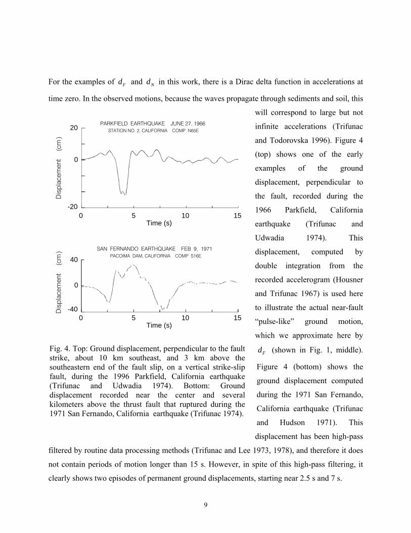
For the examples of and in this work, there is a Dirac delta function in accelerations at

time zero. In the observed motions, because the waves propagate through sediments and soil, this

will correspond to large but not

infinite accelerations (Trifunac

and Todorovska 1996). Figure 4

(top) shows one of the early

examples of the ground

displacement, perpendicular to

the fault, recorded during the

1966 Parkfield, California

earthquake (Trifunac and

Udwadia 1974). This

displacement, computed by

double integration from the

recorded accelerogram (Housner

and Trifunac 1967) is used here

to illustrate the actual near-fault

“pulse-like” ground motion,

which we approximate here by

(shown in Fig. 1, middle).

Figure 4 (bottom) shows the

ground displacement computed

during the 1971 San Fernando,

California earthquake (Trifunac

and Hudson 1971). This

displacement has been high-pass

filtered by routine data processing methods (Trifunac and Lee 1973, 1978), and therefore it does

not contain periods of motion longer than 15 s. However, in spite of this high-pass filtering, it

clearly shows two episodes of permanent ground displacements, starting near 2.5 s and 7 s.

Fd Nd

Fd

STATION NO. 2, CALIFORNIA COMP N65EPARKFIELD EARTHQUAKE JUNE 27, 1966

Time (s)10

Dis

plac

emen

t (c

m)

PACOIMA DAM, CALIFORNIA COMP S16ESAN FERNANDO EARTHQUAKE FEB 9, 1971

5

40

150-40

0

Time (s)105 150

20

-20

0

Dis

plac

emen

t (c

m)

Fig. 4. Top: Ground displacement, perpendicular to the faultstrike, about 10 km southeast, and 3 km above thesoutheastern end of the fault slip, on a vertical strike-slipfault, during the 1996 Parkfield, California earthquake(Trifunac and Udwadia 1974). Bottom: Grounddisplacement recorded near the center and severalkilometers above the thrust fault that ruptured during the1971 San Fernando, California earthquake (Trifunac 1974).

9

Wave Propagation

Translational and rotational components of strong motion that are radiated from an earthquake

source change along the propagation path through interference, focusing, scattering, and

diffraction. For example, reflection of plane P and SV waves from half space can lead to large

displacement amplitudes for incident angles between 30° and 43°, but the associated rotations

(rocking for P and SV waves, and torsion for SH waves) change monotonically and do not lead

to large amplifications (Trifunac 1982; Lin et al. 2001). Scattering and diffraction of plane waves

from topographic features can lead to focusing and to amplification for both displacements and

rotations (Sanchez-Sesma et al. 2002).

Beyond the results of linear theory, in the near field the nonlinear response of soil and ultimately

soil failure and liquefaction can also lead to large transient and permanent rotations. Four types

of ground failure can follow liquefaction: lateral spreading, ground oscillations, flow failure, and

loss of bearing strength. Lateral spreads involve displacements of surface blocks of sediment

facilitated by liquefaction in a subsurface layer. This type of failure may occur on slopes up to 3°

and is particularly destructive to pipelines, bridge piers, and other long and shallow structures

situated in flood plain areas adjacent to rivers. Ground oscillations occur when the slopes are too

small to result in lateral spreads following liquefaction at depth. The overlying surface blocks

break one from another and then oscillate on liquefied substrate. Flow failures are a more

catastrophic form of material transport and usually occur on slopes greater than 3°. The flow

consists of liquefied soil and blocks of intact material riding on and with liquefied substrate on

land or under the sea (e.g., at Seward and Valdez during the 1964 Alaska earthquake; Trifunac

and Todorovska 2003). Loss of bearing strength can occur when the soil liquefies under

structures. The buildings can settle, tip, or float upward if the structure is buoyant. The

accompanying motions can lead to large transient and permanent rotations, which so far have

been neither evaluated through simulation nor recorded by strong-motion instruments.

10

Asymmetry of Support

Most man-made structures are built above the ground and can be tens of meters to several

hundred of meters high. Supported asymmetrically at their base, with their center of gravity near

mid-height, they undergo rocking motions when excited by earthquakes, strong winds, and man-

made transient and steady excitations. Through the rocking compliance, the soil-structure

interaction then acts as a mechanism for conversion of the wave energy in the building into

rotational motions of the foundation, which then radiate this wave energy into the soil (Trifunac

2007). During earthquake and ambient noise (microseisms and micro-tremor) excitations, the

incident waves are scattered and diffracted by the foundation-soil interface, and together with the

waves generated by the soil-structure interaction radiate rotational motions back into the soil.

During wind and man-made excitation, a part of the wave energy in the building is converted

into rotational excitation of the soil. The early work on the waves created by soil structure-

interaction dates back to the 1930s (Sezawa and Kanai 1935, 1936) and the 1940s (see Biot

2006).

Full-Scale Experiments

Full-scale experiments of soil-structure interaction have provided some data to quantify the

nature of the motions at the interface between the soil and the building foundations (Luco et al.

1986; Todorovska 2002; Trifunac and Todorovska 2001a). The emphasis in the full-scale tests

thus far has been on the response of structures and on how this response is affected by soil-

structure interaction. Some experiments, however, did investigate the nature of the near-field

deformation of soil surrounding the building foundation (Luco et al. 1975; 1988; Foutch et al.

1975; Wong et al. 1977a). It has been found that for stiff foundation-structure systems the soil-

foundation interaction can be approximated by a rigid foundation model having only six degrees

of freedom. For flexible foundations (Trifunac et al. 1999a) and multiple foundations, the soil

deformation is far more complex, and the translational and rotational waves in the near field,

radiated by the motion of the foundations, require complex, three-dimensional (3-D) analyses. In

densely populated metropolitan areas where the separation distances between adjacent buildings

11

are small or negligible, and where long bridges have multiple supports resting on soil, detailed 2-

D and 3-D analyses are required (Werner et al. 1979; Wong and Trifunac 1975). Analytical

studies of 2-D soil-structure interaction (of long buildings on rigid foundations) have shown how

the interference of the incident waves and of the scattered waves from the foundation can lead to

nearly standing-wave motions on the ground surface, which, at the nodes, result in strong

torsional ground motions (Trifunac 1972c; Trifunac et al. 2001a; Todorovska et al. 1988).

Analytical studies of the response of 3-D models show amplification of the torsional response of

building-foundation-soil systems and the radiation of torsional scattered waves for near-

horizontal incidence of SH waves (Lee 1979). Studies of the wave passage effects around rigid,

embedded foundations have explained amplification of the rocking foundation motions and the

more energetic radiation of rotational waves when half-wavelengths of the incident waves are

comparable to the foundation width (Todorovska and Trifunac 1990a; 1991; 1992a,b; 1993).

Observational and analytical studies of buildings in an urban setting have examined the site-city

interaction (Boutin and Roussillon 2004; Gueguen et al. 2000; 2002; Kham et al. 2006; Tsogka

and Wirgin 2003) and have interpreted the prolonged duration of strong ground motion in urban

settings (Wirgin and Bard 1996) in terms of the waves delayed by prolonged paths up and down

the buildings (Gičev 2005).

Experiments using forced vibration of full-scale structures have been used to investigate the

wave motion in the far field radiated by the soil-structure interaction (Luco et al. 1975; Favela

2004). The radiated waves in the far field have been used as monochromatic sources of waves to

investigate the relative significance of irregular topography and of irregular geometry of

sedimentary layers on amplification of surface displacements (Wong et al. 1977b).

ROTATIONS IN STRUCTURAL RESPONSE

As already noted, in earthquake engineering most dynamic response analyses are based on the

vibrational representation of the solution, within the framework of linear analysis, and the use of

the response spectrum method, in which each mode shape and its natural frequency can be

represented by one equivalent single-degree-of-freedom (SDOF) system. Then, for linear

systems the response is given by a superposition of the responses of those equivalent SDOF

12

systems. Therefore, the analysis of the linear response of an n-degree-of-freedom system can be

reduced to a study of individual SDOF systems (Fig. 5a) one at a time.

Fig. 5. (a) Equivalent SDOF system (with damping Ce, rotational stiffness Ke, equivalent massmb, and equivalent height He, on a rigid foundation with mass mf) supported by flexible soil.(b) Multi-degree-of-freedom system (e.g., moment-resistant frame) supported by independentspread footings on elastic soil. (c) Continuous-model representation of a tall building with astiff central core (Todorovska et al. 1988). (d) Continuous-model representation of a buildingwith a soft first story, on flexible soil (Todorovska et al. 1988). (e) Discrete MDOF system ofan n-story building with rigid floors (mi= floor mass; Ki = floor stiffness; A, B, and C = strong-motion instruments). (e) A section through a six-story, reinforced-concrete structure supportedby a foundation on piles (Kojic et al. 1984).

centralcore

shearwall

A

C

B

1

2

3

n-1

n

m1

m2

mn-1

mn

K1

K2

Kn-1

Kn

(a) (b)

(c) (d)

(e) (f)

mb

Ke

mf

Ce

He

13

The n-degree-of-freedom systems (e.g., Figs. 5b,e,f) can be modeled by lumped masses

interconnected with springs and dashpots or by finite elements, but the accuracy of final

representation ultimately depends upon the number of mode shapes included in the analysis and

upon realistic representation of the boundary conditions. Because the computation of point

rotations will require differentiation of mode shapes with respect to appropriate space

coordinates, it can be seen that the description of transient point rotations will require a large

number of mode shapes to be included in the analyses. Since this is not practical, the typical

outcome will represent a low-pass-filtered approximation of point rotations.

Elementary Representation of Linear Response

In the basic model in earthquake engineering employed to

describe the response of (1) a simple structure or (2) the

equivalent oscillator (representing one of the

characteristic functions in an n-degree-of-freedom system)

to only horizontal earthquake ground acceleration, xΔ , is

an SDOF system experiencing rocking rψ relative to the

normal with regard to the ground surface, assuming that

the ground does not deform in the vicinity of the

foundation—that is, neglecting the soil-structure

interaction (Fig. 6a). The rocking rψ is restrained by a

spring with stiffness and by a dashpot with rocking

damping constant , providing a fraction of the critical damping

rK

rC rς . The natural frequency of

this system is , and for small rocking angles it is governed by the linear

ordinary differential equation

( 1/ 22/r r bK h mω

m

)=

22 /r r r r r r x hψ ω ς ψ ω ψ+ + = − Δ . (3)

Δx

h

O

B x

zy

bψr

KrCr

Fig. 6a. An SDOF representationof a building (inverted pendulum)with equivalent mass anbm dmass-less column height h ,experiencing rocking rψ due tohorizontal motion of its base xΔ .

14

For any initial conditions, and for arbitrary excitation, this system always leads to a deterministic

and predictable response. Equation (3) was used originally to develop the concept of the relative-

response spectrum, which continues to this day to be the main vehicle in the formulation of most

earthquake engineering analyses of response (Trifunac 2003). If the gravity force is considered,

rω in Eqn. (3) has to be reduced (Biot 2006). The system described by Eqn. (3) is meta-stable for

rψ smaller than its critical value. At the critical value of rψ , the overturning moment of the

gravity force is just balanced by the elastic moment in the restraining spring, and for values

greater than the critical value the system becomes unstable.

We note that in this model (Fig. 6a)

the angle rψ does not describe the

rocking angle of the structure; instead,

it is a mathematical degree of freedom.

Because the model of the structure in

this representation is fixed at the base,

actual rocking in the structure will be

represented by the deformation of the

structure only and will depend upon

the nature of the model and the

number of the mode shapes in the

analysis. It will include neither rocking

nor torsional excitations by strong-

motion waves nor the rocking induced

by the soil-structure interaction. Thus,

the contributions of all components of

ground motion, and of soil-structure

interaction, to the estimated response

are excluded from contributing to the

total picture by the restrictive model

selection process.

φy

Δx Δ

z

h

ψr

m Ib b

O

B

x

zy

θSV P

a

Fig. 6b. An SDOF representation of a building(inverted pendulum), with equivalent mass ,moment of inertia (aboutO )

bm

bI , and a mass-lesscolumn of height h , experiencing relative rocking

rψ due to horizontal, vertical, and rocking motionsof its foundation ( xΔ zΔ y, , and φ , respectively),which result from soil-structure interaction underexcitation by incident-wave motion.

15

Advanced Representation of Response

In a more advanced vibrational representation of the response, additional components of the

earthquake excitation (including rocking and torsional excitation by ground waves), dynamic

instability, soil-structure interaction, spatial and temporal variations of the excitation, differential

motions at different support points, and nonlinear behavior of the stiffness can be considered,

but in earthquake engineering the structure usually continues to be modeled by mass-less

columns, springs, and dashpots, and with a rigid mass (Jalali and Trifunac 2007a,b; Jalali et

al. 2007). In the following, we illustrate some of the above cases.

rK

bm

Dynamic Instability

An example of a simple model that includes instability is shown in Fig. 6b. It experiences

horizontal, vertical, and rocking components of ground motion, which can result, for example

from incident P and SV body waves and from Rayleigh surface waves. The structure is

represented by an equivalent SDOF system with a concentrated mass at height h above the

foundation. It has a radius of gyration and a moment of inertia

bm

br2

b b bI m r= about point O. The

degree-of-freedom in the model is the relative rocking angle rψ . This rotation is restrained by a

spring with rocking stiffness and by a dashpot with rocking damping (as in Fig. 6a, but

not shown in Fig. 6b). The gravitational force is considered. Taking moments about B

results in the equation of motion

rK rC

bm g

( ) ( ){22 / cy r r r r r r x y ra osφ ψ ω ς ψ ω ψ φ ψ+ + + = − Δ + ( ) ( )}2 / sin /r g z y raω ε φ ψ+ + Δ + ε , (4)

where , ( )( )21 / /bh r hε = + a ( )2 2/r r bK m h rω 2⎡ ⎤= +⎣ ⎦ , rω is the fixed-base natural frequency of

rocking, rζ is a fraction of critical damping in ( )2 22 /r bC m h rr rω ς ⎡ ⎤= +⎣ ⎦ , and 22 /g r aε ω=

y

.

Equation (4) is a differential equation coupling the rocking of the foundation, φ , and the

structure, rψ , with the horizontal and vertical motions of the foundation. It is a nonlinear

16

equation the solution of which requires numerical analysis. In this example, we will discuss only

the case in which y rφ ψ+

{is small. Then,

( ) }22 1r r / /r r r g z raψ ω ς ψ ε ε ε ψ− − Δ = ( ){ }2/ /y x r g z ya a /φ ω ε φ ε− + −Δ + + Δ . (5) ω+ +

For steady-state excitation with frequency ω (illustrated in this example only for incident P and

SV waves), ,x yφΔ , and , and therefore the forcing function of Eqn. (5), will be periodic.

Equation (5) is then a special form of Hill's equation, and analysis of the stability of this equation

can be found in the work of Lee

(1979). For general earthquake

excitation,

zΔ

,x yφΔ , and zΔ will be

determined by the recorded

components of motion and in

predictive analyses by simulated

ground motions (Lee and

Trifunac 1985, 1987; Wong and

Trifunac 1979).

In Eqn. (5), yφ describes rocking

of the foundation to which the

structure is attached. In analyses

that do not consider soil-structure

interaction, yφ will be given by

the rocking component of strong

ground motion (e.g., Lee and

Trifunac 1987; Jalali and

Trifunac 2007a). In studies that

consider soil-structure interaction, yφ will be one of the variables to be determined by the

analysis (Lee 1979).

φz

φy

φx

d

Δx

Δy

θ

SH

SV P

a

Fbx

Fbz

FbyMbz

Mby

Mbx

m0B

Δz

Fig. 7. Six components of motion (three translations andthree rotations) of point B { } , , , , ,x y z x y zφ φ φΔ Δ Δ

{

, and sixcomponents of force (three forces and three moments)

}extF = { }, , , , ,bx by bz bx by bzF F F M M M , that the structureexerts on the foundation at B .

17

Soil-Structure Interaction.

The problem of linear soil-structure interaction includes the phenomena that result from (1) the

presence of an inclusion (foundation, Fig. 7) in the soil (Lee and Trifunac 1982), and (2) the

vibration of the structure supported by the foundation, which exerts dynamic forces on the

foundation (Lee 1979). Examples and a discussion of nonlinear aspects of soil-structure

interaction can be found in Gičev (2005) and in a review of observations of response to

earthquake shaking of full-scale structures in Todorovska (2002) and Trifunac et al. (2001b,c).

The dynamic response of a rigid, embedded foundation to seismic waves can be separated into

two parts. The first part corresponds to the determination of the restraining forces due to the

motion of the inclusion, usually assumed to be a rigid body. The second part deals with the

evaluation of the driving forces due to scattering of the incident waves by the inclusion, which is

presumed to be immobile. This can be illustrated by considering a foundation embedded in an

elastic medium and supporting an elastic superstructure (Fig. 6b). The steady-state

harmonic motion of the foundation having frequency ω can be described by a vector

{ } , , , , ,T

x y z x y zφ φ φΔ Δ Δ (Fig. 7), where xΔ and yΔ are horizontal translations, is vertical

translation,

zΔ

xφ and yφ are rotations about horizontal axes, and zφ is torsion about the vertical axis.

Using superposition, displacement of the foundation is the sum of two displacements, as follows:

{ } { } { }0*U U U= + , (6)

where { }*U is the foundation input motion corresponding to the displacement of the foundation

under the action of the incident waves in the absence of external forces and { }0U is the relative

displacement corresponding to the displacement of the foundation under the action of the

external forces in the absence of incident-wave excitation. The interaction force { }sF generates

the relative displacement { }0U , which are related to { } ( ) { }0s sF K Uω= ⎡ ⎤⎣ ⎦ , where ( )sK ω⎡ ⎤⎣ ⎦ is

the 6 x 6 complex stiffness matrix of the embedded foundation. This force depends upon the

material properties of the soil medium, the characteristics and shape of the foundation, and the

18

frequency of the harmonic motion, and it describes the force-displacement relationship between

the rigid foundation and the soil medium.

The driving force of the incident waves is equal to { } { }* [ ]s sF K U= * , where the input motion

{ }*U is measured relative to an inertial frame. The "driving force" is the force that the ground

exerts on the foundation when the rigid foundation is kept fixed under the action of the

incident waves, and it depends upon the properties of the foundation and the soil and on the

nature of excitation.

The displacement { }U is related to the interaction and driving forces via { } { } { }*[ ]s s sK U F F= + .

For a rigid foundation having a mass matrix [ ]0M and subjected to a periodic external

force{ }extF , the dynamic equilibrium equation is

[ ]{ } { } { }0 s extM U F F= − + , (7)

where { }extF = { }, , , , ,bx by bz bx by bzF F F M M M is the force the structure exerts on the foundation

(Fig. 7). Then Eqn. (7) becomes

[ ]{ } [ ]{ } { } { }0 *s extsM U K U F F+ = + . (8)

The solution of { }U requires the determination of the mass matrix, the impedance matrix, the

driving forces and the external forces (Lee 1979).

After the mass matrix [ ]0M , the stiffness matrix [ ]sK , and the force { }*sF have all been

evaluated, they can be used to determine the foundation displacement { }U . For in-plane response,

excited by P and SV waves, for example, the relative response rψ is given by Eqn. (5).

19

Differential Motions

Common use of the response

spectrum method (Trifunac 2003)

and many dynamic analyses in

earthquake engineering implicitly

assume that all points of building

foundations move synchronously and

with the same amplitudes. This, in

effect, implies that the wave

propagation in the soil is neglected.

Unless the structure is long (e.g., a

bridge with long spans, a dam, a

tunnel) or “stiff” relative to the

underlying soil, these simplifications

are justified and can lead to a

selection of approximate design

forces if the effects of soil-foundation

interaction in the presence of

differential ground motions can be

neglected (Bycroft 1980). Simple

analyses of 2-D models of long

buildings suggest that when a/λ <

10-4, where a is wave amplitude and λ is the corresponding wavelength, the wave-propagation

effects on the response of simple structures can be neglected (Todorovska and Trifunac 1990b).

λ

a

H

L

c

x

c

SH or Love Wave

L

Ha

λ

Rayleigh Wave

Fig. 8. Schematic representation of the deformation ofcolumns accompanying differential wave excitation oflong structures for out-of-plane response (top) and in-plane response (bottom) when SH or Lave waves (top)or Rayleigh waves (bottom) propagate along thelongitudinal axis of a structure.

Figure 8 illustrates the “short” waves propagating along the longitudinal axis of a long building

or a multiple-span bridge. For simplicity, the incident-wave motion has been separated into out-

of-plane motion (Fig. 8, top), consisting of SH and Love waves, and in-plane motion (Fig. 8,

bottom), consisting of P, SV, and Rayleigh waves. The in-plane motion can further be separated

20

into horizontal (longitudinal), vertical, and rocking components, while out-of-plane motion

consists of horizontal motion in the transverse direction and torsion along the vertical axis.

Trifunac and Todorovska (1997) analyzed the effects of the horizontal in-plane components of

differential motion for buildings with models that are analogous to the sketch in Fig. 8 (bottom),

and they showed how the response spectrum method can be modified to include the first-order

effects of differential motions. Trifunac and Gičev (2006) showed how to modify the spectra of

translational motions into a spectrum that approximates the total (translational and torsional)

responses and how this approximation is valid for strong-motion waves an order of magnitude

longer than the structure ( Lλ >> ).

As can be seen from the above examples, the differential motions lead to complex excitation and

deformation of the structural members (columns, shear walls, beams, braces), cause increases in

the dimensions of the governing differential equations, lead to 3-D dynamic instability problems,

and can lead to nonlinear boundary conditions. These are all conditions that create an

environment in which, even with the most detailed numerical simulations, it is difficult to predict

all complexities of the possible responses.

Observations of Structural Response

In the following, we review selected cases dealing with rotational motion, from our studies of

buildings in southern California. We describe in more detail the examples from two buildings—

the Hollywood Storage Building in Hollywood and the Van Nuys Holiday Inn in Van Nuys—

both in the greater Los Angeles metropolitan area. These buildings are neither typical nor

representative of the general building population in the area. The reasons they are considered

here is that both were instrumented for extended periods, so that multiple earthquake recordings

of their responses are available, and that studies of their responses have been published and are

available for distribution (http://www.usc.edu/dept/civil_eng/ Earthquake_eng/).

21

Hollywood Storage Building (HSB, Fig. 9a,b). This is the first structure to have been equipped

with permanent strong-motion accelerographs in California, in 1933 (Trifunac et al 2001a). It is

also the first building in California for which strong motion was recorded (October 1933), and

the first building for which it could be shown that both theoretical analysis and observation of

soil-structure interaction are consistent. This building served as a testing ground for intuitive

(Housner 1957) and theoretical and quantitative (Duke et al. 1970) studies of soil-structure

interaction. The data recorded in and near this building were also used in several other related

0 100SCALE IN FEET TYPICAL FLOOR PLAN

217'6"

N

ACCELEROGRAPH(GROUND)

51'0"

112'0"

ACCELEROGRAPH (BASEMENT)

ACCELEROGRAPH (ROOF)

B B

A

A

*

* 80 ' after April, 1975 (NUREG/CR - 0985, Vol. 5)139 ' as reported by CDMG (in OSMS 92-10)

SECTION A-A

9'0"

149'6"

Accelerographs

ROOF14

910111213

B1

234567

8

1456k

1828k1774k1723k1658k1567k

2064k2041k2042k2021k1988k1931k1871k

1872k

Storyweights

SECTION B-B

Fig. 9(a). Hollywood Storage Building in the early 1950s, with strong-motion accelerograph stations in the basement, on the roof, and at the "free-field" site 112 ft west of the southwest corner of the building (Trifunac et al. 2001a).

22

types of studies—for example, the scattering of waves by a "rigid" foundation, the associated

"filtering" of high-frequency motions, and the associated torsional excitation of foundations

(Cloud 1978, Shioya and Yamahara 1980). Since 1933 there have been numerous triggers of

strong-motion acceleraographs in HSB, but thus far only a few have been processed and are

available for analysis (Trifunac et al. 2001a). HSB was also studied using ambient and forced

vibration tests (Carder 1936; 1964).

Analyses of the effects of soil-structure interaction involve comparison of the motions recorded

in a structure with those recorded at a free-field site (typically several hundred feet away from

the structure—e.g., Fig. 9a). It is usually assumed that the free-field record approximates the

motions in the absence of the structure (Trifunac, 1972c). The transfer functions between the

foundation motion and the corresponding motions at the free-field site are then used for analysis.

The first successful interpretation of observed data using analysis of this type was presented by

Duke et al. (1970). They interpreted the EW recorded motions (along the longitudinal building

11

7

4

2

3

8

5

12

6

9

1110

87

54

3

2

1

SECTION A-A

9'0"

149'6"

51' 217'6"

9,1

12,10

SECTION B-B

Fig. 9(b). Location and orientations of 12 accelerometers maintained in the Hollywood StorageBuilding by the California Division of Mines and Geology since 1976 (Trifunac et al. 2001a).

23

direction, see Fig. 9a) of the Hollywood Storage Building in terms of an analytic solution of soil-

structure interaction, with a rigid, semi-cylindrical foundation, and for vertically incident SH

waves. Duke et al. (1970) did not

interpret soil-structure interaction for

NS (transverse) response because at

that time the needed theoretical solution

did not exist—it was formulated 20

years later by Todorovska and Trifunac

(1990a). As for the solutions of Luco

(1969) and Trifunac (1972c) for SH-

wave excitation, Todorovska and

Trifunac (1990a) showed that the

horizontal motions of a rigid

foundation, Δ, excited by P, SV, and

Rayleigh waves, have minima at fixed-

base natural frequencies of the building

(Figs. 10). However, for all other

frequencies the amplitudes of the

transfer functions are "complicated"

0 321ωa/βb

|Δ|

|ϕa|

|ub |rel

|V|

|vb |rel

1.5

0

1

0.5

0

0.5

1

0

1

2

0

1

10

0

1

10

ε=4, H/a=8W/H=0.25, ν=1/3

Incident P-waves

a)

b)

c)

d)

e)

Pγ

γ=30 o

Fig. 10a. Transfer-function amplitudesfor (a) horizontal foundation motion Δ,(b) foundation rocking ϕa, (c) relativehorizontal motion of the building u ,(d) vertical foundation motion V, an

relb

d(e) relative vertical motion of thebuilding , versus dimensionlessfrequency ωa/βb for incident P waves

relbv

— after Todorovska and Trifunac(1990a). For description of full anddashed lines see Fig. 10c.

24

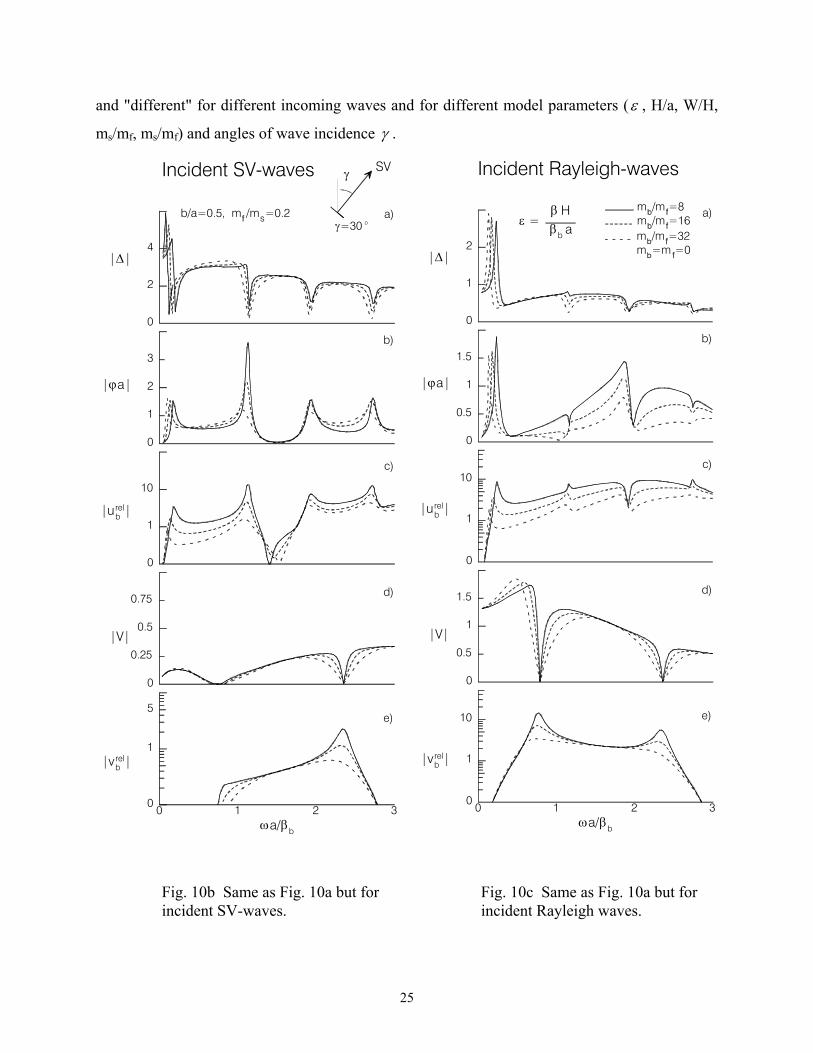
and "different" for different incoming waves and for different model parameters (ε , H/a, W/H,

ms/mf, ms/mf) and angles of wave incidence γ .

0 321ωa/βb

|Δ|

|ϕa|

|ub |rel

|V|

|vb |rel

1.5

0

1

0.5

1.5

0

1

0.5

0

1

2

0

1

10

0

1

10

Incident Rayleigh-waves

mb=m f=0mb/mf=32mb/mf=16mb/mf=8 a)

b)

c)

d)

e)

ε = βb a β H

0 321ωa/βb

|Δ|

|ϕa|

|ub |rel

|V|

|vb |rel

3

0

2

1

0.75

0

0.5

0.25

5

0

1

0

2

4

0

1

10

Incident SV-waves

a)

b)

c)

d)

e)

SVγ

b/a=0.5, mf /ms=0.2

γ=30 o

Fig. 10b Same as Fig. 10a but for incident SV-waves.

Fig. 10c Same as Fig. 10a but for incident Rayleigh waves.

25

In Figs. 10, W and H are building width and height; a is the radius of a semi-circular rigid

foundation; sm is the mass of the soil, per unit length, replaced by the foundation; fm is the

mass of the foundation per unit length; and is the mass of the building per unit length. In

addition, , V, and

bm

Δ ϕ are the horizontal, vertical, and rocking motions of the foundation,

respectively; and are the relative horizontal and vertical deformations of the structure

with respect to the moving rigid foundation; and

relbu rel

bv

/ bH aε β β= .

In contrast to horizontal motion Δ, Todorovska and Trifunac (1990a) show that the transfer

functions for vertical motion V, are "simpler" and more "similar" for all incident waves and all

incident angles (Fig. 10). They also show the transfer functions of rocking motions (equivalent to

yφ in Fig. 6, and shown normalized by ), whose nature is very dependent upon the type of

incident waves. It can be seen that, as the half-wavelength of Rayleigh waves becomes

comparable to the diameter of the foundation, Rayleigh waves cause large rocking motions of the

foundation and large relative response of the building.

a

In the analysis by Duke et al. (1970), and for the results illustrated in Figs. 10, it has been

assumed that the building foundation can be represented by a semi-cylindrical, rigid mass.

Clearly, this is a rough approximation for the foundation system of the Hollywood Storage

Building, which is on Raymond concrete piles 12 ft to 30 ft long (Fig. 9a,b). Thus, if this

foundation is to be modeled by a rigid equivalent foundation, it would be good to consider some

more representative embedment ratios because this affects the nature of the waves scattered from

the foundation (Wong and Trifunac 1974). It is more likely, however, that this foundation does

not behave like a rigid body, especially for intermediate- and high-frequency waves (Trifunac et

al. 1999a). How soil-structure interaction with a flexible 3-D foundation should be represented

has not been studied in sufficient detail thus far to allow any definite interpretation, and so we

leave this interesting topic for a future analysis.

An example of early earthquake engineering analysis of the rocking period of a rigid building on

flexible soil can be found in papers by Biot (1942, 2006). Merritt and Housner (1954) also

26

investigated the rocking motions, from which Housner (1957) concluded that “significant effects

could be expected only with exceptionally soft ground.” It is interesting to note that the Housner

10

-10

0

Dis

plac

emen

t(c

m)

Tors

iona

l ang

le(r

ad x

10

-3)

3.0

-3.0

0.0

10

-10

0

0 252015105 4403530 5

Dis

plac

emen

t(c

m)

Time (s)

(12-1)

(10-1)

(12-10)/3060(9-1)/3060

(12-10-9+1)

(12-1)

LANDERS EARTHQUAKE JUN 28, 1992 -1157 GMTLOS ANGELES -- HOLLYWOOD STORAGE BLDG.

(12-1) means y12(t) y 1(t)

Fig. 11a. Response of the HSB during the 1992 Landers earthquake. Top: Comparison of relative (with respect to basement-center) displacements recorded at the west end of the roof (“12-1,” solid line) and at the roof center (“10-1,” light dashed line). Center: Comparison of average torsion of the western half of the building (“(12-10)/3060,” solid line) and at ground level (“9-1)/3060,” light dashed line). Bottom: Comparison of relative (with respect to basement-center) displacements at the west end of the roof due to torsion alone (“12-10-9+1,” solid line) and due to torsion and translation (“12-1,” dashed line).

27

(1957) and Duke et al. (1970) papers appear to have left an impression on subsequent

researchers, who stated, for example, that the “evidence of soil-structure interaction can be

8

-8

0

Dis

plac

emen

t(c

m)

Tors

iona

l ang

le(r

ad x

10

-3)

2

-2

0

0 605040302010

8

-8

0

Dis

plac

emen

t(c

m)

Time (s)

(12-1)

(10-1)

(12-10)/3060

(9-1)/3060

(12-10-9+1)

(12-1)

NORTHRIDGE EARTHQUAKE JANUARY 17, 1994 04:31 PSTLOS ANGELES -- HOLLYWOOD STORAGE BLDG.

(12-1) means y12(t) y1(t)

Fig. 11b. Same as Fig. 11a, but for 1994 Northridge earthquake.

quantitatively detected in the frequency domain by the ratio hg

Hg uu+Δ ” (Hradilek et al.

1973). Rocking and torsional contribution to interaction were rarely addressed in the papers that

aimed to interpret earthquake accelerograms recorded in buildings.

28

Duke et al. (1970) conclude that “soil-structure interaction produced marked change in the

horizontal base displacements, in the east-west direction,” with little or no rocking in this

direction. For the north-south direction, soil-structure interaction did not drastically affect the

horizontal base displacements but instead produced rocking of the foundation, as can be

observed by its effect on the roof motion.

Torsion

Torsional response in non-symmetrical structures is caused by geometrical separation of the

centers of mass and rigidity. For symmetric structures, torsional response occurs because of a

non-symmetrical foundation system or is excited by wave-passage effects (Luco 1976; Trifunac

et al. 1999a), or both. Long and narrow symmetrical buildings, for example, can experience

significant torsional response and whipping (Trodorovska and Trifunac 1989; 1990b) when

excited by earthquake waves propagating along the longitudinal axis of the soil-structure system.

Full-scale measurements of torsional response and torsional components of soil-structure

interaction cannot be performed directly because no rotational strong-motion accelerographs had

been installed in the buildings in California during past strong earthquakes. It is only possible to

estimate average rotations when multiple recorders in the structures are arranged so that relative

motions can be computed from the differences in translational motions. In the following we

illustrate this for the Hollywood Storage Building.

Fig. 9b shows locations and orientations of strong motion accelerometers in the Hollywood

Storage Building. For this configuration of instruments (since 1976) strong-motion data, in

processed form, is available only from four earthquakes: Whittier-Narrows, 1987; Landers, 1992;

Big Bear, 1992; and Northridge, 1994. By suitable combination of displacements yi computed by

double integration from the recorded accelerograms it is possible to estimate average torsion in

the west side of the building. Thus,

φb(t) = (y9(t) – y1(t))/3060 (9)

29

(3060 cm is the separation distance between recorders 1 and 9) gives the average torsion at the

foundation level, and

φr(t) = (y12(t) – y10(t))/3060 (10)

gives average torsion of the western half of the building at the roof. Relative NS vibrations at the

center of the building are described by y10(t) – y1(t), while y12(t) – y1(t) gives the NS motion at

the roof, at the western end of the building, relative to the central station at the ground level.

Then, y12(t) – y10(t) – y9(t) + y1(t) gives the contribution to the motion of the western end of the

building, at roof level, associated with torsion of the building, relative to its base. Figs. 11a and b

illustrate these functions versus time for the motions recorded during the Landers and Northridge

earthquakes. It can be seen that y12(t) – y10(t) – y9(t) + y1(t) ~ y12(t) – y1(t) and that y12(t) – y1 (t) ~

21 (y10(t) – y1(t)). It can also be seen that (most of the time) the relative motions at recording site

12 (western end of the building, on the roof) are about one half the motions at recording site 10

(roof, center) and that the two motions are in phase. An exception to this (see Fig. 11b) occurred

during the Northridge earthquake, 8 to 12 s after trigger time. Thus, most of the time the building

is twisting about a point (rotating about a vertical axis) that is west of its geometric center. We

reported on a similar behavior for a seven-story reinforced concrete building that is also

supported by a pile foundation (Trifunac et al. 1999a). Such behavior may be caused in part by

non-symmetry of the foundation (the HSB has the basement only beneath its western half, see

Figs. 9a,b). Such torsional eccentricity thus causes whipping of the eastern end of the building,

particularly for EW arrivals of SH and Love waves (in this example during the Landers, 1992

earthquake). Unfortunately, there are no strong-motion instruments along the eastern end of the

Hollywood Storage Building to verify this interpretation.

When soil-structure interaction is considered in the dynamic analyses of soil-structure systems, it

is convenient to assume that the foundation is rigid (Fig. 12). This assumption simplifies the

analysis and reduces the number of additional degrees of freedom required to model soil-

structure interaction, and thereby the number of simultaneous equations that must be solved.

Whether such an assumption can be made must be carefully investigated, and the outcome does

30

not depend only on the relative rigidity of the foundation and of the soil but is also influenced by

the overall rigidity and type of the structure, its lateral load-resisting system, and its orientation.

uNH(φy+ψr)

H - h j

h j2

1,9

7

10,12R

13

11

9

7

5

3

1

14

12

10

8

6

4

2

8

5 4

3

11

h j (φy+ψ

r) ub, j

rel

Δ

ab

m f

mb

V

W

φy

θφ

ugH

ugV

Fig. 12. Two-dimensional model of a soil-foundation-structure system excited into motion by ground translations H

gu , Vgu and ground rocking angle θ . The relative local soil deformation

caused by soil-structure interaction is described by translations Δ and V and by relative rocking angle ϕ, such that , and H

x g +uΔ = Δ Vz gu VΔ = − − yφ θ ϕ= + (see Fig. 6b). The masses per unit

length (in a direction perpendicular to the cross-section shown in this figure) of the building and of the foundation, respectively, are mb and mf. Numbers 1 through 12 show the locations of 12 accelerometers in the HSB (see Fig. 9b).

31

This can be illustrated by comparison of the NS versus EW vibrations of the Millikan Library in

Pasadena a nine-story reinforced concrete structure that was studied by Luco et al. (1986). Even

N E

(a) (b)

(c)N

E

UP(d) UP N

E

N-S EXCITATION E-W EXCITATION

elevatorcore

shear wall

shear wall

shear wall

elevatorcore

Fig. 13. Deformation of the Millikan Library, a nine-story concrete building, excited at the roof by a shaker with two counter-rotating masses (a) along the west shear wall during NS excitation, (b) along a section through the elevator core during EW excitation, (c) deformation of the basement slab during NS excitation, and (d) deformation of the basement slab during EW excitation (Foutch et al. 1975).

32

though the foundation system of this building is relatively flexible, for NS vibrations two

symmetric shear walls at each end (east and west) of the building act to stiffen the foundation

slab (Figs. 13a and c), and this allows one to proceed with "rigid" foundation representation, as

in Fig. 12. For EW vibrations, the building carries

lateral loads by an elevator core, which deforms the

foundation slab in the middle, while the shear walls

act as membranes providing axial constraints but

provide little bending stiffness (Figs. 13b and d). For

EW vibrations, the foundation slab cannot be

approximated by a "rigid" foundation model. These 3-

D deformation shapes, which showed how this

structure deforms while vibrating in NS and EW

directions, were measured during forced vibration

tests (Foutch et al. 1975) and were essential for this

interpretation. Figure 14 shows schematically the

relative contribution of horizontal deformation of soil

(4 percent), roof displacement resulting from rigid

body rocking (25 percent), and relative deformation of

the Millikan Library Building (71 percent) during

steady-state forced vibrations in the NS direction (as

in Figure 13a).

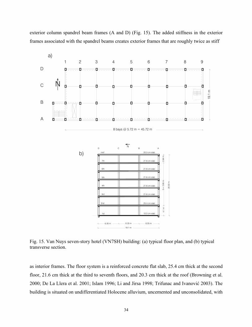
Van Nuys Hotel (VN7SH)-Holiday Inn (Figs. 15 and

16) is located in Van Nuys, California. It was

damaged by the 1994 Northridge, California earthquake (Ivanović et al. 1999, Trifunac and Hao

2001, Trifunac et al. 1999a,b). The reinforced concrete building, designed in 1965 and

constructed in 1966 (Blume and Assoc. 1973, Mulhern and Maley 1973), is 18.9 × 45.7 m in

plan, has seven stories, and is 20 m high. The typical framing consists of four rows of columns

spaced on 6.1-m centers in the transverse direction and 5.7-m centers in the longitudinal

direction (nine columns). Spandrel beams surround the perimeter of the structure. Lateral forces

in the longitudinal (EW) direction are resisted by interior column-slab frames (B and C) and

Fig.14. Contributions of foundationtranslation and rocking to the roofmotion of the Millikan Library for N-Sshaking (Foutch et al. 1975).

0.06

0.04

α

1.00

α

N

0.710.25

33

exterior column spandrel beam frames (A and D) (Fig. 15). The added stiffness in the exterior

frames associated with the spandrel beams creates exterior frames that are roughly twice as stiff

1 2 3 4 5 6 7 8 9

8 bays @ 5.72 m = 45.72 m

a)

D

C

B

A

N

19.

1 m

b)

4.

1 m

5 x

2.6

5 m

6.35 m

D C B A

20.3 cm slab

21.6 cm slab

25.4 cm slab

roof

7th

6th

5th

4th

3rd

1st

2nd

10.2 cm slab

19.1 m

20.

03 m

N

21.6 cm slab

21.6 cm slab

21.6 cm slab

21.6 cm slab

2.6

4 m

6.35 m 6.35 m

Fig. 15. Van Nuys seven-story hotel (VN7SH) building: (a) typical floor plan, and (b) typical transverse section.

as interior frames. The floor system is a reinforced concrete flat slab, 25.4 cm thick at the second

floor, 21.6 cm thick at the third to seventh floors, and 20.3 cm thick at the roof (Browning et al.

2000; De La Llera et al. 2001; Islam 1996; Li and Jirsa 1998; Trifunac and Ivanović 2003). The

building is situated on undifferentiated Holocene alluvium, uncemented and unconsolidated, with

34

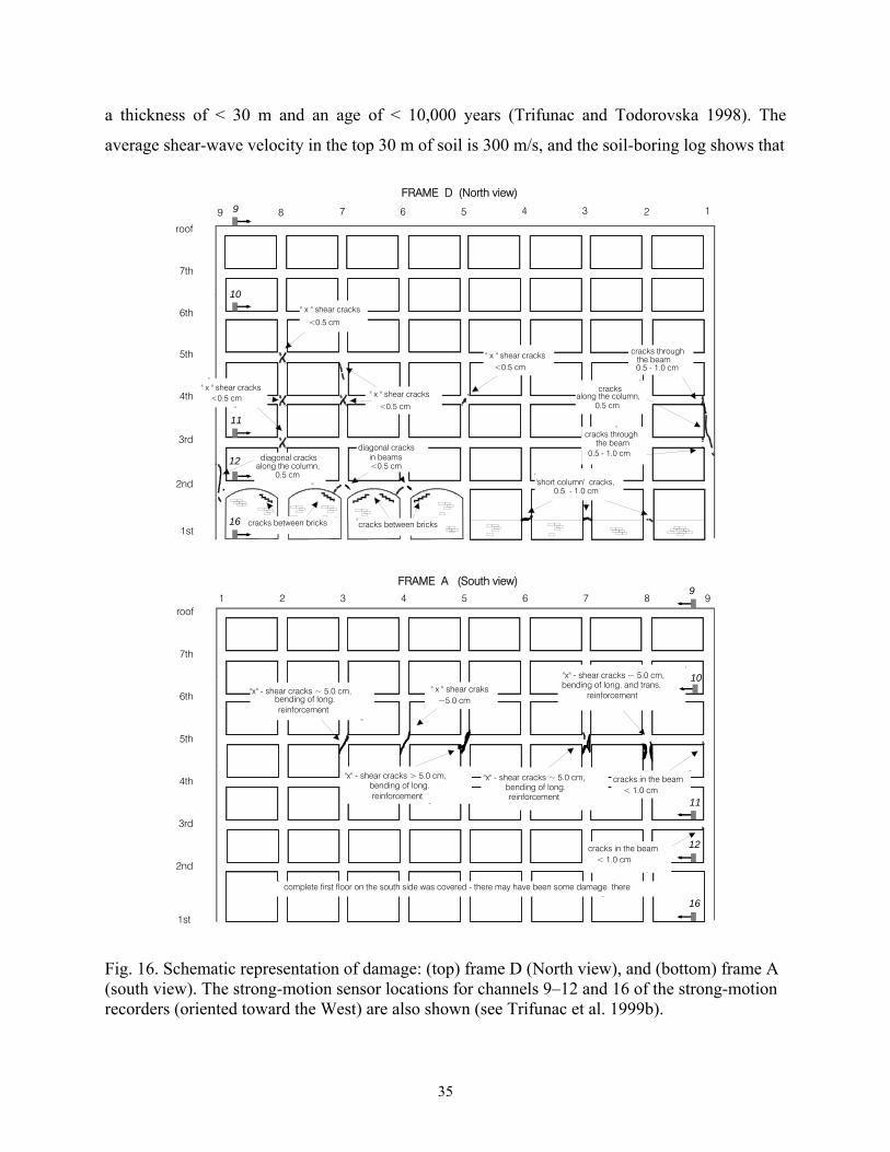
a thickness of < 30 m and an age of < 10,000 years (Trifunac and Todorovska 1998). The

average shear-wave velocity in the top 30 m of soil is 300 m/s, and the soil-boring log shows that

9 8 7 6 5 4 3 2 1

roof

7th

6th

5th

4th

3rd

2nd

1st

" x " shear cracks

<0.5 cm

" x " shear cracks<0.5 cm

cracks through the beam0.5 - 1.0 cm

the beam0.5 - 1.0 cm

cracks through

diagonal cracks

cracks along the column,

0.5 cm

'short column' cracks,0.5 - 1.0 cm

cracks between bricks cracks between bricks

diagonal cracksalong the column,

0.5 cm

in beams<0.5 cm

" x " shear cracks<0.5 cm

" x " shear cracks<0.5 cm

FRAME D (North view)9

10

11

12

16

roof

7th

6th

5th

4th

3rd

2nd

1st

FRAME A (South view)1 2 3 4 5 6 8 97

" x " shear craks~5.0 cm

"x" - shear cracks ~ 5.0 cm,bending of long. reinforcement

"x" - shear cracks > 5.0 cm,bending of long. reinforcement

"x" - shear cracks ~ 5.0 cm,bending of long. reinforcement

"x" - shear cracks ~ 5.0 cm,bending of long. and trans.

reinforcement

cracks in the beam< 1.0 cm

cracks in the beam< 1.0 cm

complete first floor on the south side was covered - there may have been some damage there

9

10

11

12

16

Fig. 16. Schematic representation of damage: (top) frame D (North view), and (bottom) frame A (south view). The strong-motion sensor locations for channels 9–12 and 16 of the strong-motion recorders (oriented toward the West) are also shown (see Trifunac et al. 1999b).

35

the underlying soil consists primarily of fine sandy silts and silty fine sands. The foundation

system consists of 96.5-cm-deep pile caps supported by groups of two to four poured-in-place,

61-cm-diameter, reinforced-concrete friction piles, which are centered under the main building

98

7

7

6

5

4

3

2

Roof

Fig. 17a. Post-earthquake view of damaged columns in frame D (see Figs. 15 and 16).

columns. All of the pile caps are connected by a grid of beams, and each pile is approximately

12.2 m long and has a design capacity of over 444.82 × 103 N vertical load and up to a 88.96 ×

103 N lateral load. The structure is constructed of normal-weight reinforced concrete (Blume and

Assoc. 1973).

36

The ML = 6.4 Northridge earthquake of January 17, 1994 severely damaged the building. The

structural damage was extensive in the exterior north (D) (Fig. 16 top) and south (A) (Fig. 16

bottom and Figs. 17a,b, and c) frames, which were designed to take most of the lateral load in the

longitudinal (EW) direction. Severe shear cracks occurred at the middle columns of frame A,

Roof765432

2

3

4

57

65432

89

Frame A (South view)9 8 7

7

6

5

4

3

2

Frame D (North view)

Fig. 17b. North (left) and South (right) views of wooden braces in frames D and A, as seen at the time of Experiment II (April 19, 1994).

near the contact with the spandrel beam of the 5th floor (Figs. 16 and 17), and those cracks

significantly decreased the axial, moment, and shear capacity of the columns. The shear cracks

that appeared in the north (D) frame (Fig. 16) caused minor to moderate changes in the capacities

of these structural elements. No major damage to the interior longitudinal (B and C) frames was

observed, and there was no visible damage to the slabs or around the foundation, but the

nonstructural damage was significant. Photographs and detailed descriptions of the damage from

the earthquake can be found in Trifunac et al. (1999b) and Trifunac and Hao (2001), and analysis

of the relationship between the observed damage and the changes in equivalent vertical shear-

wave velocity in the building can be found in Todorovska and Trifunac (2006, 2007). A

discussion of the extent to which this damage has contributed to the changes in the apparent

period of the soil-structure system can be found in Trifunac et al. (2001b,c).

37

The earthquake response of VN7SH was recorded by a 13-channel CR-1 central recording

system and by one tri-component SMA-1 accelerograph with an independent recording system

but with a common trigger time with the CR-1 recorder (Trifunac et al. 1999b).

1 2 3 4 5 6 7 8 9

FRAME A FRAME D 1 2 3 4 5 6 7 8 9

1 2 3 4 5 6 7 8 9 1 2 3 4 5 6 7 8 9

roof

6th

7th

5th

4th

3rd

2nd

1st

roof

6th

7th

5th

4th

3rd

2nd

1st

roof

6th

7th

5th

4th

3rd

2nd

1st

roof

6th

7th

5th

4th

3rd

2nd

1st

FRAME C FRAME B

roof

6th

7th

5th

4th

3rd

1st

Location of Wooden Braces and Damage at the Time of Experiment II

Fig. 17c. Schematic representation of the structure and location of damage and of wooden braces as seen at the time of Experiment II (April 19, 1994). Different open circles show schematically the degrees of damage in columns.

Ambient vibration tests in VN7SH have shown that the foundation supported by piles deforms

during passage of micro-tremor waves. It was then inferred that the same happens during passage

of much larger strong-motion waves. A detailed ambient vibration survey of this symmetric

structure, on symmetric pile foundations, showed that the center of torsion for this structure is

outside the building plan, close to its southeastern corner (Ivanović et al. 1999). Subsequent re-

examination of the strong-motion records in this building has shown that this eccentricity may

have been present in all post-1971 excitations and that it is associated with some asymmetry in

the soil-pile system dating from its construction in 1966, or that it was caused by some partial

damage during the 1971 San Fernando earthquake (Trifunac et al. 1999a).

38

Differential motions of building foundations (Trifunac 1997) may reduce the translational

response at the upper floors but lead to large additional shear forces and bending moments in the

columns of the first floor, which are caused by differential displacements and rocking of the

ground. The response spectrum method can be modified to include the consequences of such

differential motion (Trifunac and Todorovska 1997), but it is necessary to study this further

using full-scale measurements during future strong earthquakes and to verify the theory against

the observations.

The assumption that foundations can be represented by rigid “slabs” (Fig. 12) seems to be

implicit in most full-scale instrumentation programs for the buildings where strong motion has

been recorded so far, but this assumption must be verified by comparison with the recorded

motions. Technically, it should be easy to supplement the existing instrumentation to provide

data on differential motion of building foundations, and ideally this should be done first in all

instrumented buildings where strong motion has already been recorded during many past

earthquakes, so that additional value can be added to the existing data, interpretation, and

analyses.

Rocking

Figures 18a and b compare the overall "rocking angles" ((displacement at roof–displacement at

ground level)/building height) versus instantaneous apparent frequency computed for most half-

period segments of the response of the Hollywood Storage Building during seven earthquakes. It

can be seen that the apparent system frequency depends upon the amplitude of excitation and

that for small amplitudes it approaches the frequencies measured by Carder (1936, 1964) during

full-scale ambient- and forced-vibration tests. These trends can be explained in terms of the

conceptual nonlinear soil-structure model shown in Fig. 19.

Nonlinear effects in the response of soil-structure systems depend upon the level of the excitation

and also on the initial state of the system (e.g., the state of the soil, such as degree of

consolidation, water content, etc., Todorovska and Al Rjoub 2006a,b). The building damage

39

changes the building permanently, but the soil can “heal” itself and recover the original stiffness

by settlement with time and dynamic compaction from shaking during smaller events.

10-3

10-4

10-5

Roc

king

ang

le (r

ad)

10-6

0.8 1.41.21.0 2.01.81.6 2.42.2

Apparent Frequency, f (Hz)

E-W Comp.

Carder (1936, 1964)

Northridge1994

Southern California1933

Kern County1952

BorregoMountain

1968

WhittierNarrows

1987

Big Bear1992

Landers1992

Fig. 18a. Dependence of apparent system frequency on amplitude of response ("rocking angle") for EW translational responses of the HSB. Small-amplitude, ambient-vibration, and forced-vibration estimates of system frequencies by Carder (1936, 1964) are shown by solid vertical lines.

Time-frequency analysis of multiple earthquake records by two independent methods (short-time

Fourier transform and zero-crossing analyses) showed that the system frequency changes from

40

earthquake to earthquake and during larger earthquakes (Todorovska and Trifunac 2007).

Figures 20a and 20b show the instantaneous system frequency fp on the abscissa and the peaks of

0.2 1.00.80.60.4

Apparent Frequency, f (Hz)

10-3

10-4

10-5

Roc

king

ang

le (r

ad)

N-S Comp.(West Wall)

Carder (1936, 1964)

Northridge1994

SouthernCalifornia

1933

Kern County1952

BorregoMountain

1968

WhittierNarrows

1987

Landers1992

Big Bear1992

Fig. 18b. Same as Fig. 18a, but for NS response.

the “rocking” accelerations x(t) and y(t) (band-pass filtered by Ormsby filters between 0.1 ~

0.2 Hz to 0.8 ~ 1.0 Hz) in the VN7SH. These figures show progressive reduction of fp with

increasing amplitude of response, but the reduction is not permanent. It can be seen that, during

both ambient-vibration tests, fp of the transverse (NS) response is near 1.4 Hz and close to the

θ θ

41

value for the smallest earthquake motions (Montebello, 1989 earthquake, Fig. 20a,b). This

suggests that the soil-foundation-structure stiffness can be “regenerated” by the weak shaking

during aftershocks. For the longitudinal (EW) response, ambient-vibration surveys indicate only

partial recovery, from 0.4 ~ 0.6 Hz during Northridge to fp = 1.0 ~ 1.1 Hz (note that during the

aftershock on March 20, 1994, fp ~ 1.3 ~ 1.4 Hz, see Fig. 20a). The shift in fp from 1.0 Hz

(Ambient-Vibration Experiment I, February 4–5, 1994, Ivanović et al. 1999) to 1.1 Hz (Ambient-

Vibration Experiment II, April 19–20, 1994, Ivanović et al. 1999) can be interpreted as having

resulted in part from an increase in the “building stiffness” associated with temporary wooden

Leq

M=K θ

deq

H

a)

b)

θmax

θ

K

K ~ 1(H+d eq)2

K=L eq3

b

a

Equivalent level of fixityat depth d eq

Fig. 19 (a) Nonlinear changes in rocking stiffness caused by passive soil pressure on sidewalls of the building and variable equivalent depth of fixity deg. (b) Schematic representation of “permanent” soil deformation after large rocking response.

braces along frames A and D (see Ivanović et al. 1999, and Figs. 17b and c). Consistent with this

interpretation is the fact that, for Experiment II, the peaks of the transfer-functions were smaller

by 30% than for Experiment I, which suggests a stiffer overall system at the time of Experiment

II. Figures 20a and 20b also suggest that the soil-pile-foundation system during strong shaking

42

behaves as a nonlinear system with gap elements, which open during strong motion and are

closed by aftershock excitations (Fig. 19).

10-1

10-3

10-4

10-2

0.4 0.6 0.8 1.0 1.2 1.4 1.6

f p- Hz

1.8

N

x

y

zθy

θz

9

θx

1612

EW-Rocking

θx

.. First ambient noise test 4 - 5 Feb. 1994

Second ambient noise test 19 - 20 April 1994

Whitter-Narrows Aftersh. 1987

Landers, 1992

Whittier-Narrows,1987

Big Bear, 1992

0.002 (2 πf P)2

Montebello, 1989

Pasadena, 1988

Malibu, 1989

Northridge Aftersh. (20 March,1994)

Sierra Madre, 1991

San Fernando, 1971

Northridge Aftershock (6 Dec,1994)

0.0033 (2π f P

)2

Northridge, 1994

Fig. 20a. Peak amplitudes of x (EW rocking acceleration) versus fp (apparent frequency of the soil-foundation-structure system) during twelve earthquakes recorded in the VN7SH building. The wide vertical lines show the apparent EW frequencies of the system response, as determined from Experiments I and II. The hatched zone near the top-left describes the range of typical code values for allowed drift in concrete structures.

θ

43

Figs. 16 and 17a show the structural damage as observed at the time of the first ambient-

vibration experiment in the VN7SH (Experiment I, performed February 4–5, 1994). A detailed

First and second ambient noise tests4 - 5 Feb. and 19 - 20 April 1994

10-1

10-3

10-4

10-2

0.4 0.6 0.8 1.0 1.2 1.4 1.6

f p- Hz

1.8

NS-Rockingθy

..

N

2

1

13x

y

z

θy

θz

3

Northridge, 1994

Landers, 1992

Whittier-Narrows, 1987

Big Bear1992

Whitter-Narrows Aftershock, 1987

Montebello, 1989

Pasadena, 1988

Malibu, 1989

Northridge Aftershock (20 March,1994)

Sierra Madre, 1991

Northridge Aftershock (6 Dec,1994)

0.002 (2π f P

)2

0.003

3 (2

π f P)2

Fig. 20b. Peak amplitudes of y (NS rocking acceleration) versus fp (apparent frequency of the soil-foundation-structure system) during twelve earthquakes recorded in the VN7SH building. The wide vertical line shows the apparent NS frequency of the system response, as determined from Experiments I and II. The hatched zone near the top-left describes the range of typical code values for allowed drift in concrete structures.

θ

pictorial documentation of the damage observed at the time of Experiment I can be found in the

report by Trifunac et al. (1999a). The second ambient-vibration experiment (Experiment II) was

44

carried out on Tuesday and Wednesday, April 19 and 20, 1994, three months after the January

17, Northridge, California earthquake, and one month after a strong aftershock with epicenter at

1 km from the building (March 20, 1994, M = 5.2). The building was restrained between the two

experiments. Wooden braces were installed to increase the structural capacity near the areas of

structural damage, and braces were also placed in the first three or four stories at selected spans

in the exterior longitudinal frames (A and D) (Figs. 17b,c). Only the first floor of the interior

longitudinal frames was restrained. We do not know when exactly the addition of the braces was

completed or whether this preceded the aftershock on March 20. However, we did observe that

the width of the cracks, especially the shear cracks in the south (A) frame, had become larger

(relative to our first inspection on February 4). No new structural damage was noticed in the

building or around its foundation, and no braces were added to the transverse frames. Figs. 17c

and d show the locations of structural damage and the braces as observed on April 19, 1994. In

Fig. 17c, the size of the “hinges” is proportional to the level of damage.

Component Response

Two-Dimensional Displacements Along the Floor Slabs and Migration of Centers of Torsion

The first torsional mode (f = 1.6 Hz) in VN7SH could be seen in both the transverse and the

longitudinal vibrations, and therefore both longitudinal and transverse components of the modal

displacement could be determined. Fig. 21 shows the modal displacements in the plane of each

floor. Parts (a) and (b) show, respectively, the results from Experiments I (February 4–5, 1994,

before the wooden braces were added to strengthen the damaged building) and II (April 19–20,

1994, after the wooden braces were added, see Ivanović et al. 1999). The measurements were

taken along longitudinal frame C. The most severely damaged columns were 7 and 8 of

longitudinal frame A (south of frame C, see Figs. 17a,b, and c) and columns 3, 4, and 5 on the

fifth floor, which were cracked. The wooden braces were added to the damaged building after

ambient-vibration Experiment I and before Experiment II (Fig. 17b,c).

45

It can be seen that the reinforced-concrete floor slabs, 8.5 inches thick and stiff in their own

plane, translate and rotate about vertical axes. While the transverse component of motion is

1 2 3 4

5 6 7 8 9

1 2 3 4 5

6 7 8 9

1 2 3 4

5 6 7 8 9

1 2 3 4 5

6 7 8 9

1 2 3 4 5

6 7 8 9

1 2 3 4 5

6 7 8 9

1 2 3 4

5 6 7 8 9

roof

7th floor

6th floor

5th floor

4th floor

3rd floor

2nd floor

roof

7th floor

6th floor

5th floor

4th floor

3rd floor

2nd floor

Na) f=1.6 HzExperiment I b) Experiment II

Fig. 21. Vector displacement amplitudes in the planes of the floor slabs (at 2nd through 7th floors and roof) at the frequency of the first torsional mode (f = 1.6 Hz). (a) Experiment I, (b) Experiment II. The oval gray zones show approximate locations of the centers of rotation. Notice in part (a) the jump in the position of the centers of rotation between the 5th and 6th floors.

dominant, the response in the longitudinal direction is also significant, especially for the top

floors. It can be noticed that during Experiment I (Fig. 21a) the transverse component of motion

changes phase but the longitudinal component does not. Also, the amplitudes of the longitudinal

displacements are not proportional to the transverse displacements, as would be expected for a

“clean” rotation (maximum displacements at the end columns for both directions of motion, and

46

almost zero displacements at the centers of rotation). The longitudinal response of the middle

columns (C4, C5, and C6) is clearly seen at each floor, which indicates coupling of the torsional

D C B Aroof

7th

6th

5th

4th

3rd

1st

2nd

FRAME 2

D C B Aroof

7th

6th

5th

4th

3rd

1st

2nd

FRAME 2

D C B Aroof

7th

6th

5th

4th

3rd

1st

2nd

FRAME 5

D C B Aroof

7th

6th

5th

4th

3rd

1st

2nd

FRAME 5

D C B Aroof

7th

6th

5th

4th

3rd

1st

2nd

FRAME 8

D C B Aroof

7th

6th

5th

4th

3rd

1st

2nd

FRAME 8

f=1.4 Hza)

f=1.6 Hzb)

Fig. 22. Experiment II: in-plane displacements of transverse frames 2, 5, and 8; (a) at the frequency of the first transverse mode (f = 1.4 Hz), and (b) at the frequency of the first torsional mode f = 1.6 Hz.

response for this mode with the longitudinal response. The phase of the longitudinal response of

the upper floors (roof, 7th, and 6th) is opposite from the one at the lower floors (3rd and 4th).

47

The shaded oval zones in Fig. 21a illustrate the loci of the centers of rotation for the floor slabs,

determined by drawing a normal to the displacement vectors. Because of measurement errors and

some deformation of the floor slabs, the “center of rotation” for a floor slab is not a point but a

zone. The “centers of rotation” are located south of frame C at the upper floors (above the 5th),

and north of frame C at the lower floors (5th and below). At the lower floors, the centers are

located close to the middle (column 5), and then they “jump” to the east part of the frame at the

6th floor. Between the 6th floor and the roof, they move again toward the center of the frame. The

jump from south to north is between the 5th and 6th floors, exactly where the most severe damage

occurred (Figs. 16 and 17).

The results of Experiment II (Fig. 21b) show that, in contrast to Experiment I, the “centers of

rotation” are all south of frame C and are all near the center of the frame (near column line 5).

This may be explained by the added braces (see Ivanović et al. 1999), which may have

eliminated torsional eccentricities caused by the damaged columns at the 5th floor and mainly

along (south) frame A (Figs. 15, 16, and 17).

The above example illustrates the association of the discontinuous behavior of the torsional

centers of rotation with the locations of the damaged columns, and it suggests that mapping

discontinuities in the rotational response of full-scale structures can become a useful tool for

locating damage in structural members.

Two-Dimensional Displacements Along Transverse Building Cross-Sections

As the building vibrates, most of the deformations occur in the columns. Consequently, the floor

slabs also move in the vertical direction. Therefore, the transverse and longitudinal modes can

also be “seen” in the vertical response, especially at the upper floors.

Figure 22 shows 2-D, in-plane motions of transverse frames 2, 5, and 8 at the frequency of the

first transverse mode (part (a), f = 1.4 Hz) and at the frequency of the first torsional mode (part

48

(b), f = 1.6 Hz). The vertical displacements, shown in Fig. 22, are exaggerated by a factor of two

to emphasize the deformation of the columns. A noticeable vertical displacement is seen only at

column A5 of the 5th floor, and only at the frequency of the first transverse mode (see Fig. 22

part (a)). This column experienced large shear cracks (Fig. 17) during the Northridge earthquake,

and the rotation of the floor slab and large vertical displacement in Fig. 22 indicate decreased

axial capacity of this column. No large vertical displacement or floor rotations are noticeable

near column A5 at the 7th floor, presumably because of participation of the neighboring frames

and slabs. The vertical displacements of transverse frames 2 and 8 were small, as would be

expected, because the columns in these frames suffered less (frame 8) or no (frame 2) damage

(Figs. 15, 16, and 17). No unusual vertical displacements of the transverse frames 2, 5, and 8 or

rotations of the corresponding segments of the floor slabs could be seen at the first torsional

frequency (f = 1.6 Hz, Fig. 14, part (b)) (Ivanović et al. 1999).

The above examples from the HSB and the VN7SH show significant departures from what

would normally be assumed and inferred in analyses, which thus far have generally ignored

rotational degrees of freedom and have interpreted translational components of recorded motions

only. It is clear that the additional information, which is provided by the rotational motions, plays

an important role in the description of overall structural models, in the analysis of structural

components, and in the experimental determination of the location of the damaged members.

Nonlinear Response

Nonlinear response studies, which use lumped-mass models of buildings, cannot provide

information about point rotations. The rotations that can be observed in the results for these

models can only describe inter-story drifts, which are predetermined by the modeling

assumptions. Such models provide useful results about a structure’s overall response, including

instability and failure, and they can be used to evaluate the relative significance of the rotational

components of strong motion, especially near faults, where a sudden onset of motion with a large

velocity jump is associated with sudden, large rotations (Fig. 1,3; Jalali and Trifunac 2007a,b;

Jalali et al. 2007), but they should not be considered for analysis of point rotations and for

studies of deformation of individual structural members.

49

Nonlinear Waves

Strong ground motion can be viewed as resulting from a sequence of pulses emitted from failing

asperities on the fault surface (Trifunac 1972a,b; 1974; 1998). Through multiple arrivals with

different source to station paths and

scattering, the strong motion observed

at a site assumes the appearance of

irregular oscillations in time but

usually preserves one or several larger

and long-velocity “pulses.” These

pulses are “spread out” in time due to

multiple arrival paths and dispersion,

but they appear systematically in

recordings at adjacent stations, up to

epicentral distances approaching 100

km (Todorovska and Trifunac

1997a,b).

As a first approximation, the motion at

the base of the building can be

represented by a velocity pulse with amplitude vb and duration t0. For small t0, this pulse

approximates a delta function and can be used as a building block to represent more general

velocity pulses in input motion. For an elastic building on rigid soil (i.e., no soil-structure

interaction), a velocity pulse with amplitude vb = = vG,max ( is the velocity-pulse amplitude

inside the building, and is the peak ground velocity in the free field outside the building)

will create a wave propagating up the building with phase velocity c =

linV bv

,maxGv

bβ (see Fig. 23). For

times shorter than H/c and for elastic strain (∂u/∂x = vb /c)—i.e., strain ( , )x tε smaller than the

elastic limit yε (Fig. 24)—the wave propagating up into the building will be defined by a

straight line, as follows:

u(x,t)

x

H βb

vlin

u(0,t) = vlint

βbt

roof

base

Fig. 23. A wave caused by sudden movement at thebase of the shear building, for a constant-velocitypulse with amplitude Vlin = , and for time t < t0

(= pulse duration). bv

50

, for 0( , )

0 , for

bb

vv t x x ctu x t c

x ct

⎧ − ≤⎪= ⎨⎪ >⎩

≤ . (11)

During reflection from the stress-free top of the building, the incident wave from below and the

reflected wave from above will

interfere with each other, leading

to double amplitude at the roof.

The propagation of the energy of

the pulse will continue downward

as a linear wave as long as the

incident strain amplitude is smaller

than / 2yε (Fig. 24).

Figure 25 illustrates the “peak drift

amplitudes” (vb/c) in a shear-beam

model of a building, assuming c =

100 m/s and assuming short transient pulses and linear response. For 12 earthquakes (Trifunac et

al. 2001d), the maximum drift at the base of the structure is plotted versus vb (solid points). For

the Landers, San Fernando, and Northridge earthquakes, the maximum drift at the roof is also

shown (2vb/c). It can be seen that the maximum drift at the base occurs during the Northridge

earthquake and is approximately 0.5%, while at the roof it is equal to about 1%.

Sress

StrainO

YU

εu

εy

For a building supported by flexible soil, the soil-structure interaction will lead to horizontal and

rocking deformations of the soil, and in general this will modify and usually reduce the

amplitude vb of the strong-motion pulse entering the structure (Gičev 2005). Partitioning of the

incident wave energy into horizontal and rocking motions of the building-foundation-soil system

and scattering of the incident wave from the foundation will thus change the energy available to

cause relative deformation of the structure.

σ0

σy

σu

μ0

μe

μ1

μ1=γμ0

Fig. 24. Bilinear stress-strain representation of a shear-beam model experiencing nonlinear response.

51

The presence of the foundation within the soil creates an impedance jump for incident-wave

motion, and this causes scattering of the incident waves (Trifunac 1972c; Iguchi and Luco 1982;

Lee et al. 1982; Moslem and Trifunac 1987; Todorovska and Trifunac 1990a,b; 1992b; 1993;

Trifunac et al. 2001c). Gičev (2005) illustrates the extent and nature of the reduction of the

incident free-field amplitude of vG,max through scattering and refraction for a 2-D soil-foundation-

building model.

-1

-5

-4

-3

-2

0 21

Northridge

San Fernando

Northridge AftershockNorthridgeAftershock

Big Bear

Landers

Whittier AftershockSierra Madre

MontebelloPasadena

Malibu

0.5% drift

0.1% drift

topbottom

2vlin

bottom

top

drift

vlin

DRIFT = vlin / βbβ

b = 100 m/s

1.5% drift

βb

log10 vlin (cm/s)

log

10 v

lin /

β b

Fig. 25. Drift amplitudes in a shear-beam building with linear shear-wave velocity

100 / .b m sβ =

To illustrate the nonlinear wave motion in a building, we consider horizontal deformations, u , in

a 1-D model of a building supported by 1-D half space and excited by a vertically propagating

52

shear wave described by a half-sine-pulse. For simplicity, the incident displacement in the soil is

chosen to be a sinusoidal pulse with characteristics as shown in Fig. 26. The constitutive law of

the building material is assumed to be bilinear, with the first slope, 0μ , representing the linear

(initial) shear modulus and the second slope, 01 γμμ = , representing the material during yielding

(Fig. 24). The yielding strain in the building is ybε .

The equation of motion is

( ) /t xv σ ρ= , (12)

and the relation between the derivative of the strain and the velocity is

t xvε = , (13)

where ν , ρ , σ , and ε are particle velocity, density, shear stress, and shear strain, respectively,

and the subscripts t and x represent derivatives with respect to time and space.

The domain for this example consists of two materials (see Fig. 26): (1) soil with physical

properties sρ and μs, and (2) a building with physical properties bρ and μb, where iρ is the

density and μi is the initial shear modulus in the soil (i = s) or in the building (i = b). The velocity

and rotation (strain) of a particle are tuv

∂∂

= and xu

∂∂

=ε , respectively, and u is the out-of-plane

displacement of a particle perpendicular to the velocity along the propagation ray.

It is assumed that the incoming wave is known and that its displacement as a function of t is

prescribed at the soil point 1 ( sxx Δ−= 2 ). For analysis, in this example it is assumed that the soil

is always in the linear elastic state. To model the radiation of the wave from the building, we

provide an artificial boundary at the bottom of the model. The transparent boundary adopted for

this study is described in Fujino and Hakuno (1978), and it is a perfect transparent boundary for

one-dimensional waves when 1=ΔΔxtβ .

53

For the numerical analysis, the densities of the soil and of the beam are assumed to be the same:

ρρρ == sb = 2000 kg/m3. The velocity of the shear waves in the soil is taken as sms /250=β ,

and the velocity in the building is set as smb / 100=β . The height of the building is mH B 10= .

β s

ρs,

Hb

Hs =2Δxs

x(m

)

Δxb

N

ΔxbN'

u 0 (m)

t(s)

u0

max

= A

td

1

2

3

4

u(m)

a)

b)

β b

ρb,

Fig. 26. Shear-beam building and incoming strong-motion displacement pulse: (a) model of the beam, and (b) the pulse in the soil.

To study nonlinear response and the development of transient and permanent strains in the

building, we introduce two dimensionless parameters (Gičev 2005): (a) dimensionless amplitude

54

ybbHAε

α⋅

= , (14)

where is the amplitude of the pulse (see Fig. 26), is the height of the building, and A bH ybε is

the yielding strain in the building, and (b) dimensionless frequency

db

b

db

b

b

b

tH

tHH

ββλη =

⋅==

22

2

, (15)

where bλ is the wavelength of the wave in the building, bβ is the shear wave velocity in the

building, and is the duration of the half-sine pulse. dt

For the linear motions at the contact (point 3 in Fig. 26), one part of the incoming wave is

transmitted into the other medium and one is reflected back into the same medium. The

corresponding coefficients are obtained from the boundary conditions of continuity of the

displacements and stresses at the contact. For a transmitted wave from medium B to medium A,

and for a reflected wave from medium B back into medium B, these coefficients are

2 / 1 a atrB A

b b

k ρ βρ β→

⎛ ⎞= +⎜ ⎟

⎝ ⎠ (16)

and

1 / 1a a a arefB B

b b b b

k ρ β ρ βρ β ρ→

⎛ ⎞ ⎛= − +⎜ ⎟ ⎜

⎝ ⎠ ⎝ β⎞⎟⎠

. (17)

For the opposite direction of propagation, the numerators and the denominators in these fractions

exchange places. For the shear-wave velocities in our example ( 250 /s m sβ = and 100 /b m sβ =

/ 7

),

the coefficient of transmission of the wave from the soil to the building is = 10 and the tk

55

coefficient of reflection of the incident wave from the building, back to the building, is

. 3 / 7rk = −

250s

Gičev and Trifunac (2006), have derived the conditions for the first occurrence of permanent

strain in the building, which relate the amplitude and frequency of the pulse, the physical

properties of the building, and the soil stiffness. For material properties in this example

( /m s and 100 /b m sβ = ), these conditions are β =

12b s

t skβ βαη

π πβ+

> = = 0.2228 (18)

12 4

b s

t skβ βαη

π πβ+

> = = 0.1114 (19)

1 0.2228(2 ) 2 (2 ) 2

b s

t r s rk k k kr

β βαηπ πβ

+> = =

+ + + = 0.09174 . (20)

The condition (18) requires the biggest product αη , and if it is satisfied it describes the

occurrence of the first permanent strain, which is always located at the bottom of the building.

We refer to this part of the building as Zone 2, or 2Z (when 0.5η > ). If the condition (18) is not

satisfied, the condition (19) becomes relevant and, if it is satisfied, the first permanent strain

occurs at some point (T) in the building, between the base and top. We refer to this part of the

building as Zone 3, or 3Z (when 0.5η > ). Finally, if both conditions (18) and (19) are not

satisfied, and if 5.0≤η , the condition (20) describes the amplitude-frequency condition for the

occurrence of the first permanent strain. This can occur anywhere in the building, and we refer to

this as Zone 1, or 1Z (when 0.5η < ).

In the following, the results are illustrated based on the studies of Gičev and Trifunac (2006;

2007a,b) who investigated the range of the dimensionless frequencies ( 506.0 ≤≤ η ), five

dimensionless amplitudes ( 0.01, 0.05, 0.10, 0.20,α = and 0.30), and four ratios of moduli

( 0.3 and 0.2, 0.1, 0.0,0

1 ==μμ

γ ). Their results are best illustrated in terms of dimensionless ratios

56

of the governing variables. One of those variables, , is the maximum velocity entering the

beam (building), assuming that the building is linear (Fig. 23). This velocity is a linear function

of

linv

η :

tbybtd

lin kktAv βπαηεπ

=⋅= . (21)

Instead of studying the absolute maxima of the rotations (strains), we can consider the

normalized maxima, defined by the ratio

lin

b

linnorm v ε

ε

β

εε maxmaxmax == . (22)

This quantity will show the degree of nonlinearity in the building response and the effects of the

interference on the amplification of the linear entry strain. This strain is always larger than one.

The normalized strain at the end of the analysis (permanent strain) can be described by the ratio

lin

end

b

lin

endendnorm v ε

ε

β

εε == . (23)

This will show the ratio of the permanent strain (after all of the wave energy exits the building)

and of the linear entry strain. It can be larger or smaller than one, and for linear waves (when

neither condition 19 nor condition 20 are satisfied) it is zero.

In Figs. 27a,b,c, the normalized strains versus dimensionless amplitude α are shown for the four

values of 0.3 and 0.2, 0.1, ,0.0=γ in the three zones Z1, Z2, and Z3, respectively, using a semi-

logarithmic scale. From condition (20), the first nonlinear strain in Zone 1 occurs for

1835.05.0

09174.009174.0

max1 ==>

ηα . (24)

As can be noticed, in Zone 1 (Fig. 27a), while the strain is linear ( 1αα ≤ ), there is no

dependence on γ , and all of the curves coincide. The normalized maximum strain, (see maxnormε

57

Eqn. 22), is constant, and its value is about 17/7, corresponding to the summation of the three

strain-wave amplitudes at the beginning of the second wave passage (see Gičev and Trifunac

2006). Because the response is linear, in this interval shows only the effect of the

interference on the amplification of the linear entry strain.

maxε norm

0 0.1 0.3

0.1

1

10

100

α

Nor

mal

ized

Stra

in

Zone 1

εmax / εyb

βb / v lin

εmax βb / v lin

γ = 0.0

0.2

εend

0.1

0.2

0.3

η < 0.5 for all x

0.0 0.10.20.3

Fig. 27a. Dependence of the normalized strains on the dimensionless amplitude, α , in Zone 1 for γ = 0.0, 0.1, 0.2, and 0.3.

58

The normalized strain in this interval is zero, showing that the strains are reversible. The

normalized strain

endnormε

mam x /ynor ybε ε ε= approaches zero as α approaches zero. With increasing α ,

beyond 1α , the response at the bottom of the building becomes nonlinear at the beginning of the

second wave passage, the curves for different γ separate, and the normalized strains increase

with decreasing γ , being the largest for elasto-plastic material, .0=γ

0 0.1 0.2 0.3

0.1

1

10

100

α

Nor

mal

ized

Stra

in

Zone 2

εmax / εyb

εend βb / v lin

εmax βb / v lin

γ = 0.0

0.1

0.30.2

γ = 0.0

0.2 0.3

0.10.0

0.1

0.20.3

η > 0.5 x ~ 0

Fig. 27b. Dependence of the normalized strains on the dimensionless amplitude, α , in Zone 2 for γ = 0.0, 0.1, 0.2, and 0.3.

59

For the amplitude range considered, the normalized strain (rotation) reaches its maximum

value of 29.74 at

maxnormε

0.3α = , for elasto-plastic material. In this case, the effect of the nonlinearity of

the building response overwhelms the effect of constructive interference of the three strains at

the bottom. The remaining normalized permanent strain at the end, after the wave exits the beam

completely, , is 28.17 for the elasto-plastic material, while the normalized strain, endnormε

ybmax /ynormε ε= ε , is 16.18, indicating that the beam will probably fail at 3.0=α .

0 0.1 0.2 0.30.1

10

α

Nor

mal

ized

Stra

in

Zone 3

εmax / εyb

εend βb / v lin

εmax βb / v lin

γ = 0.0

1 0.3

0.2

0.1

γ = 0.1 γ = 0.2

γ = 0.3

η > 0.5, x ε (>0, H)

Fig. 27c. Dependence of the normalized strains on the dimensionless amplitude,α , in Zone 3 for γ = 0.0, 0.1, 0.2, and 0.3.

60

In Fig. 27b, the normalized strains versus α in Zone 2 are shown, again using the semi-

logarithmic scale. It can be seen that for small amplitudes, 05.0≤α , all of the curves converge

to zero. As α increases, all normalized strains increase. For α larger than 0.1, the dependence

of all of the normalized strains on α for elasto-plastic material, 0=γ , resembles, in this scale, a

logarithmic function, which means that the normalized strains (rotations) for elasto-plastic

material behave like linear functions of α . For materials with 0≠γ , the normalized strains

are independent of endnormε α , while the normalized strains and are approximately

linear, with the slope

maxnormε y

normε

α

maxnormε

∂∂

being smaller than the slope α

ε∂

∂ ynorm .

In Fig. 27c, the normalized strains (rotations) versus α in Zone 3 are shown using a semi-

logarithmic scale. For any γ , the normalized strains and maxnormε max /y

norm ybε ε ε= approach 2 and 0,

respectively, as α approaches 0. The normalized strain depends only on endnormε γ and is

independent of α . The lowest amplitude, when it occurs, can be found from condition (19) at the

highest considered η as 02228.05

1114.0min =>α . For minαα ≤ , . 0end

norm =ε

In this example, we described the consequences of earthquake energy flow into a structure, with

the objectives of providing some understanding of the resulting response and making this useful

for the design of structures experiencing transient excitation. We examined some elementary

aspects of transient waves propagating in a structure, and we illustrated the relationships between

the amplitude of peak velocity of the wave entering the structure, lin bv v= , and transient and

permanent point rotations associated with the resulting response. Our analysis is qualitative in

that it only describes the response of a simple shear beam with constant material properties. In

real buildings, variations of material properties with height introduce additional complications

(although they are qualitatively similar) (Gičev and Trifunac 2007b). Nevertheless, the above

example shows that consideration of the response in terms of propagating nonlinear waves can

provide invaluable details on where inter-story drifts and large point rotations may occur and

how large those might be. In terms of the more detailed models of actual structures (or layers of

61

soft soil near the ground surface), the approach we have presented can offer major improvements

and can represent an excellent starting point for use in earthquake-resistant design. These results

provide direct data for initiating displacement-based design, but the power of incident waves—

that is, the time rate of the incoming seismic wave energy—must also be considered if damage to

structures is to be controlled and eliminated.

SUMMARY AND CONCLUSIONS

While every effort was made in this overview to illustrate the physical nature of added insights

and the benefits and significance of considering rotations in structural response, it must be

emphasized that, at present, we have essentially no full-scale measurements, either of point

rotations in strong ground motion or of rotations in structural response. Consequently, the

observational inferences we can make at present are based only on the “average” rotations

(measured from the differences in the translational motion at two points, separated by a

distance ), and therefore they can describe at best that part of the rotational spectrum that is

associated with the very long wavelengths

d

λ (such that dλ >> ). Furthermore, as we noted at

the beginning, we employed only the classical wave representation, which applies only to

homogeneous, elastic, and continuous idealization of the medium. Obviously, this is a

simplification for earth materials and an oversimplification for structures, which are made up of

discrete beams and columns. Under these conditions, it is reasonable to expect that most of what

was presented here can be assumed to be representative only for the long wavelengths of the

complete spectrum of the rotational motions. However, in spite of these limitations it should be

clear that we must continue to study the rotational components of motion if we wish to consider

all physical aspects of the engineering description of the response of structures to transient

dynamic loads.

The examples in this work are neither general nor complete, and we illustrated only a small

number of cases that describe the role of the rotational components of motion. Based on these

examples, the roles of (1) sudden and very strong rotational motion in the near field, associated

with the first arrival of earthquake waves, and (2) large rotations that are associated with strain

62

localization in the zones of nonlinear response of the building materials, may be the most

important aspects to study and to include in future engineering analyses. The first is important

because it represents a powerful excitation that has not been previously described, theoretically

or via measurements, and that consequently is not currently considered in the design of structures

that are expected to survive strong near-field earthquake shaking. The second aspect is important

because it has great potential for structural health monitoring because it can improve the spatial

resolution in a monitoring process aimed at identifying the locations of damage.

63

REFERENCES

Biot, M.A. (1932). Vibrations of building during earthquake, Chapter II in Ph.D. Thesis

No. 259 entitled Transient Oscillations in Elastic Systems. Aeronautics Department,

Calif. Inst. of Tech., Pasadena, CA.

Biot, M.A. (1933). Theory of elastic systems vibrating under transient impulse with an

application to earthquake – proof buildings Proc. National Academy of Sciences, 19(2),

262-268.

Biot, M.A. (1934). Theory of vibration of buildings during earthquake. Zeitschrift für

Angewandte matematik and Mechanik, 14(4), 213-223.

Biot, M.A. (1942). analytical and experimental methods in engineering seismology.

ASCE Transactions, 108, 365–408.

Biot, M.A. (2006). Influence of foundation on motion of blocks. Soil Dynamics &

Earthquake Engrg, 26(6–7), 486–490.

Blume, J.A., and Assoc. (1973). Holiday Inn, Chapter 29 in San Fernando, California

Earthquake of February 9, 1971, Vol. I, Part A. U.S. Dept. of Commerce, National

Oceanic and Atmospheric Administration, Washington, D.C.

Bouchon, M., and Aki, K. (1982). Strain and rotation associated with strong ground

motion in the vicinity of earthquake faults. Bull. Seism. Soc. Am., 72(5), 1717–1738.

Boutin, C., and Roussillon, P. (2004). Assessment of the urbanization effect on seismic

response. Bull. Seism. Soc. Amer., 94(1), 251–268.

Browning, J.A., Li, R.Y., Lynn, A., and Moehle, J.P. (2000). Performance assessment for

a reinforced concrete frame building, Earthquake Spectra, 16(3), 541–555.

Bycroft, G.N. (1980). Soil-foundation interaction and differential ground motions.

Earthquake Engng. Struct. Dyn., 8, 397–404.

Carder, D.S. (1936). Vibration observation, Chapter 5 in Earthquake Investigation in

California 1934–1935, Special Publication No. 201, U.S. Dept. of Commerce, Coast and

Geodetic Survey, 49–106.

Carder, D.S. (Ed.). (1964). Earthquake Investigations in the Western United States 1931–

1964, Publication 41-2. U.S. Dept. of Commerce, Coast and Geodetic Survey.

Castellani, A., and Boffi, G. (1986). Rotational components of the surface ground motion

during an earthquake. Earthquake Eng. Struct. Dyn., 14, 751–767.

Castellani, A., and Boffi, G. (1989). On the rotational components of seismic motion.

Earthquake Eng. Struct. Dyn., 18, 785–797.

Chen, K-C., Huang, B-S., Wang, J-H., Huang, W-G., Chang, T-M., Hwang, R-D., Chiu,

H-C., and Tsai, C-C. (2001). An observation of rupture pulses of the 20 September 1999

Chi-Chi, Taiwan, earthquake from near-field seismograms. Bull. Seism. Soc. Amer.,

91(5), 1247–1254.

Cloud, W.K. (1978). Modification of seismic waves by a building. Proc. Sixth European

Conf. on Earthquake Eng, Dubrovnik, Yugoslavia, 289–295.

De la Llera, J.C., Chopra, A.K., and Almazan, J.L. (2001). Three-dimensional inelastic

response of an RC building during the Northridge earthquake. J. of Structural Eng.,

ASCE, 127(5), 482–489.

65

Droste, Z., and Teisseyre, R. (1976). Rotational and displacement components of ground

motion as deduced from data of the azimuth system of seismographs. Publs. Inst.

Geophys. Pol. Acad. Sci., 97, 157–167.

Duke, C.M., Luco, J.E., Carriveau, A.R., Hradilek, P.J., Lastrico, R., and Ostrom, D.

(1970). Strong earthquake motion and site conditions: Hollywood. Bull. Seism. Soc.

Amer., 60(4), 1271–1289.

Favela, J. (2004). Energy Radiation from a Multi-Story Building, Ph.D. Thesis, Calif.

Inst. of Tech., Pasadena, CA.

Foutch, D.A., Luco, J.E., Trifunac, M.D., and Udwadia, F.E. (1975). Full-scale three-

dimensional tests of structural deformations during forced excitation of a nine-story

reinforced concrete building. Proc. U.S. National Conference on Earthquake

Engineering, Ann Arbor, MI, 206–215.

Fujino, Y., and Hakuno, M. (1978). Characteristics of elasto-plastic ground motion

during an earthquake. Bull. Earthquake Res. Institute, Tokyo Univ., 53, 359–378.

Gičev, V. (2005). Investigation of Soil-Flexible Foundation-Structure Interaction for

Incident Plane SH Waves, Ph.D. Dissertation, Dept. of Civil Engineering, Univ. Southern

California, Los Angeles, CA.

Gičev, V., and Trifunac, M.D. (2006). Permanent deformations and strains in a shear

building excited by a strong motion pulse. Soil Dynamics and Earthquake Engineering,

26(12), 1149–1160.

Gičev, V., and Trifunac, M.D. (2007a). Permanent deformations and strains in a shear

building excited by a strong motion pulse. Soil Dynamics and Earthquake Engineering,

27(8), 774–792.

66

Gičev, V., and Trifunac, M.D. (2007b). Energy and power of nonlinear waves in a seven

story reinforced concrete building. Indian Society of Earthquake Technology Journal,

44(1), (in press).

Graizer, V.M. (1989). Ob izmerenii naklona zemnoi poverhnosti vblizi epicentra vzriva.

Dokladi Akademii Nauk S.S.S.R., Geofizika, 305(2), 314–318.

Gueguen, P., Bard, P-Y., and Oliveira, C.S. (2000), Experimental and numerical analysis

of soil motions caused by free vibrations of a building model. Bull. Seism. Soc. Amer.,

90(6), 1464–1479.

Gueguen, P., Bard, P-Y., and Chavez-Garcia, F. (2002). Site-city interaction in Mexico

city-like environments: An analytical study. Bull. Seism. Soc. Amer., 92(2), 794–811.

Haskell, N.A. (1969). Elastic displacements in the near field of a propagating fault. Bull.

Seism. Soc. Am., 59, 865–908.

Housner, G.W. (1957). Interaction of building and ground during an earthquake. Bull.

Seism. Soc. Amer., 47, 179–186.

Housner, G.W., and Trifunac, M.D. (1967). Analysis of accelerograms—Parkfield

earthquake. Bull. Seism. Soc. Amer., 57(6), 1193–1220.

Hradilek, P.J., Carriveau, A.R., Saragoni, G.R., and Duke, C.M. (1973). Evidence of soil-

structure interaction in earthquakes. Proc. Fifth World Conf. on Earthquake Eng., Rome,

Italy, 2, 2076–2079.

Huang, B.S. (2003). Ground rotational motions of the 1999 Chi-Chi, Taiwan earthquake

as inferred from dense array observations. Geophysical Res. Letters, 30(6), Art. No.

1307, 40-1, 40-4.

67

Iguchi, M., and Luco, J.E. (1982). Vibration of flexible plate on viscoelastic medium, J.

of Engng Mech., ASCE, 108(6), 1103–1120.

Islam, M.S. (1996). Analysis of the Response of an Instrumented 7-Story Nonductile

Concrete Frame Building Damaged During the Northridge Earthquake, Professional

Paper 96-9, Los Angeles Tall Buildings Structural Design Council, Los Angeles, CA.

Ivanović, S., Trifunac, M.D., Novikova, E.I., Gladkov, A.A., and Todorovska, M.I.

(1999). Instrumental 7-Story Reinforced Concrete Building in Van Nuys, California:

Ambient Vibration Survey Following the Damage From the 1994 Northridge Earthquake.

Dept. of Civil Eng., Rep. No. CE 99-03, Univ. of Southern California, Los Angeles, CA.

Jalali, R., and Trifunac, M.D. (2007a). Strength-reduction factors for structures subjected

to differential near-source ground motion. Indian Society of Earthquake Technology

Journal, 44(1), (in press).

Jalali, R., and Trifunac, M.D. (2007b). A note on strength reduction factors for design of

structures near earthquake faults, Soil Dynamics and Earthquake Engineering, (in press).

Jalali, R., Trifunac, M.D., Ghodrati Amiri, G., and Zahedi, M. (2007). Wave-passage

effects on strength-reduction factors for design of structures near earthquake faults. Soil

Dynamics and Earthquake Engineering, 27(8), 703–711.

Kham, M., Semblat, J-F., Bard, P-Y., and Dangla, P. (2006). Seismic site-city interaction:

main governing phenomena through simplified numerical models. Bull. Seism. Soc.

Amer., 96(5), 1934–1951.

Kojić, S., Trifunac, M.D., and Anderson, J.C. (1984). A Post-Earthquake Response

Analysis of the Imperial County Services Building. Dept. of Civil Eng. Report CE 84-02,

Univ. of Southern California, Los Angeles, CA.

68

Lee, V.W. (1979). Investigation of Three-Dimensional Soil-Structure Interaction, Report

CE 79-11, Dept. of Civil Eng., Univ. Southern California, Los Angeles, CA.

Lee, V.W. (1990). Surface strains associated with strong earthquake shaking. J.S.C.E.,

422n, (1-14), 187–194.

Lee, V.W., and Trifunac, M.D. (1982). Body wave excitation of embedded hemisphere,

ASCE, EMD, 108(3), 546–563.

Lee, V.W., and Trifunac, M.D. (1985). Torsional accelerograms, Soil Dynam. & Earthq.

Eng., 4(3), 132–139.

Lee, V.W. and Trifunac, M.D. (1987). Rocking strong earthquake accelerations, Soil

Dynam. & Earthq. Eng., 6(2), 75–89.

Lee, V.W., Trifunac, M.D., and Feng, C.C. (1982). Effects of foundation size on Fourier

spectrum amplitudes of earthquake accelerations recorded in buildings, Soil Dynam. and

Earthquake Eng., 1(2), 52–58.

Li, R.Y., and Jirsa, J.D. (1998). Nonlinear analysis of an instrumented structure damaged

in the 1994 Northridge earthquake, Earthquake Spectra, 14(2), 265–283.

Lin, C.H., Lee, V.W., and Trifunac, M.D. (2001). Effects of Boundary Drainage on the

Reflection of Elastic Waves in a Poroelastic Half Space Saturated With Non-Viscous

Fluid. Dept. of Civil Eng. Report No. CE 01-04, Univ. of Southern California, Los

Angeles, CA.

Luco, J.E. (1969). Dynamic interaction of a shear wall with the soil. J. Eng. Mechanics

Division, ASCE, 95, 333–346.

69

Luco, J.E. (1976). Torsional response of structures to obliquely incident seismic SH

waves, Earthquake Enging. Struct. Dyn., 4, 207–219.

Luco, J.E., Trifunac, M.D., and Udwadia, F.E. (1975). An experimental study of ground

deformations caused by soil-structure interaction, Proc. U.S. National Conf. on Earthq.

Eng., Ann Arbor, MI, 136–145.

Luco, J.E., Wong, H.L., and Trifunac, M.D. (1986). Soil-Structure Interaction Effects on

Forced Vibration Tests, Department of Civil Engineering, Report CE 86-05, University

of Southern Calif., Los Angeles, CA.

Luco, J.E., Trifunac, M.D., and Wong, H.L (1988). Isolation of soil-structure interaction

effects by full-scale forced vibration tests, Earthquake Engineering and Structural

Dynamics, 16(1), 1–21.

Merritt, G.H., and Housner, G.W. (1954). Effects of Foundation compliance on

earthquake stresses in multistory buildings, Bull. Seism. Soc. Amer., 44(4), 551-569.

Moslem, K., and Trifunac, M.D. (1986). Effects of Soil-Structure Interaction on the

Response of Buildings During Strong Earthquake Ground Motion, Dept. of Civil Eng.

Report No. CE 86-04, Univ. of Southern California, Los Angeles, CA.

Mulhern, M.R., and Maley, R.P. (1973). Building Period Measurements Before, During,

and After the San Fernando, California, Earthquake of February 9, 1971, U.S. Depart.

Of Commerce, National Oceanic and Atmospheric Administration, Washington D.C.,

Vol. I, Part B, 725–733.

Nathan, N.D., and MacKenzie, J.R. (1975). Rotational components of earthquake motion,

Canadian Journal of Civil Engineering, 2, 430–436.

70

Oliveira, C.S., and Bolt, B.A. (1989). Rotational components of surface strong ground

motion, Earthquake Eng. Struct. Dyn., 18, 517–526.

Rayleigh, J.W.S. (1945). The Theory of Sound, Vol. I and II, New York: Dover

Publications (First American Edition. First edition was printed in England in 1877).

Sanchez-Sesma, F.J., Palencia, V.J., and Luzon, F. (2002). Estimation of local site effects

during earthquakes: An overview, Indian Society of Earthquake Technology Journal,

39(3), 167–194.

Sezawa, K., and Kanai, K. (1935). Decay in the seismic vibration of a simple or tall

structure by dissipation of their energy into the ground, Bull. Earth. Res. Inst., XIII(3),

681–697.

Sezawa, K., and Kanai, K. (1936). Improved theory of energy dissipation in seismic

vibrations on a structure, Bull. Earth. Res. Inst., XIV(2), 164–168.

Shioya, K., and Yamahara, H. (1980). Study on filtering effect of foundation slab based

on observational records, Proc. Seventh World Conf. on Earthquake Eng., Istanbul,

Turkey, 5, 181–188.

Teisseyre, R. (2002). Continuum with defect and self rotation fields, Acta Geophys. Pol.,

50, 51–68.

Teisseyre, R., and Boratynski, W. (2002). Continuum with self-rotational nuclei:

Evolution of defect fields and equations of motion, Acta Geophys. Pol., 50, 223–230.

Teisseyre, R., and Majewski, E. (2002). Physics of earthquakes, International Handbook

of Earthquake and Engineering Seismology, Part A, 229–235.

71

Teisseyre, R., Suchcicki, J., Teisseyre, K., Wiszniowski, J., and Palangio, P. (2003).

Seismic rotation waves: Basic elements of theory and recording, Annals of Geophysics,

46(4), 671–685.

Todorovska, M.I. (2002). Full-scale experimental studies of soil-structure interaction,

Indian Society of Earthquake Technology Journal, 39(3), 139–166.

Todorovska, M.I., and Al Rjoub, Y. (2006a). Plain strain soil-structure interaction model

for a building supported by a circular foundation embedded in a poroelastic half-space,

Soil Dynamics and Earthquake Eng., 26(6–7), 694–707.

Todorovska, M.I., and Al Rjoub, Y. (2006b). Effects of rainfall on soil-structure system

frequency: Examples based on poroelasticity and a comparison with full-scale

measurements, Soil Dynamics and Earthquake Eng., 26(6–7), 708–717.

Todorovska, M.I., and Trifunac, M.D. (1989). Anitiplane earthquake waves in long

structures. J. of Eng. Mech., ASCE, 115(2), 2687–2708.

Todorovska, M.I., and Trifunac, M.D. (1990a). Analytical Model for Building

Foundation Soil Interaction: Incident P, SV, and Rayleigh Waves, Report CE 90-01,

Dept. of Civil Eng., Univ. of Southern California, Los Angeles, CA.

Todorovska, M.I., and Trifunac, M.D. (1990b). A note on the propagation of earthquake

waves in buildings with soft first floor, J. Engrg. Mech., ASCE, 116(4), 892–900.

Todorovska, M.I., and Trifunac, M.D. (1991). Radiation Damping During Two-

Dimensional In-Plane Building-Soil Interaction, Report CE 91-01, Dept. of Civil Eng.,

Univ. Southern California, Los Angeles, CA.

72

Todorovska, M.I., and Trifunac, M.D. (1992a). The system damping, the system

frequency and the system response peak amplitudes during in-plane building-soil

interaction, Earthquake Engrg. and Struct. Dynam., 21(2), 127–144.

Todorovska, M.I., and Trifunac (1992b). Effect of input base rocking on the relative

response of long buildings on embedded foundations, Europ. Earthq. Engng., VI(1), 36–

46.

Todorovska, M.I., and Trifunac, M.D. (1993). The Effects of Wave Passage on the

Response of Base-Isolated Buildings on Rigid Embedded Foundations, Report CE 93-10,

Dept. of Civil Eng., Univ. of Southern California, Los Angeles, CA.

Todorovska, M.I., and Trifunac, M.D. (1997a). Distribution of pseudo spectral velocity

during Northridge, California earthquake of 17 January 1994, Soil Dynamics and

Earthquake Eng., 16(3), 173–192.

Todorovska, M.I., and Trifunac, M.D. (1997b). Amplitudes, polarity and time of peaks of

strong ground motion during the 1994 Northridge, California earthquake, Soil Dynamics

and Earthquake Eng., 16(4), 235–258.

Todorovska, M.I., and Trifunac, M.D. (2006). Impulse Response Analysis of the Van

Nuys 7-Story Hotel During 11 Earthquakes (1971–1994): One-Dimensional Wave

Propagation and Inferences on Global and Local Reduction of Stiffness Due to

Earthquake Damage, Report CE 06-01, Dept. of Civil Eng., University of Southern

California, Los Angeles, CA.

Todorovska, M.I., and Trifunac, M.D. (2007). Impulse response analysis of the Van

Nuys 7-story hotel during 11 earthquakes and earthquake damage detection, Structural

Control and Health Monitoring (in press).

73

Todorovska, M.I., Trifunac, M.D. and Lee, V.W. (1988). Investigation of Earthquake

Response of Long Buildings, Report No. CE 88-02, Dept. of Civil Engrg., Univ. of

Southern California, Los Angeles, CA.

Trifunac, M.D. (1972a). Stress estimates for San Fernando, California earthquake of

February 9, 1971: Main event and thirteen aftershocks, Bull. Seism. Soc. Amer., 62(3),

721–750.

Trifunac, M.D. (1972b). Tectonic stress and source mechanism of the Imperial Valley,

California earthquake of 1940, Bull. Seism. Soc. Amer., 62(5), 1283–1302.

Trifunac, M.D. (1972c). Interaction of a shear wall with the soil for incident plane sh

waves, Bull. Seism. Soc. Amer., 62(1), 63–83.

Trifunac, M.D. (1974). A three-dimensional dislocation model for the San Fernando,

California earthquake of February 9, 1971, Bull. Seism. Soc. Am., 64, 149–172.

Trifunac, M.D. (1982). A note on rotational components of earthquake motions for

incident body waves, Soil Dynamics and Earthquake Eng., 1(1), 11–19.

Trifunac, M.D. (1990). Curvograms of strong ground motion, ASCE, J. Eng. Mech. Div.,

116(6), 1426–1432.

Trifunac, M.D. (1993). Broad Band Extension of Fourier Amplitude Spectra of Strong

Motion Acceleration, Report CE 93-01, Dept. of Civil Eng., Univ. of Southern

California, Los Angeles, CA.

Trifunac, M.D. (1997). Differential earthquake motion of building foundations, J.

Structural Eng., ASCE, 4, 414–422.

74

Trifunac, M.D. (1998). Stresses and intermediate frequencies of strong motion

acceleration, Geofizika, 14, 1–27.

Trifunac, M.D. (2003). 70th anniversary of Biot spectrum, Indian Society of Earthquake

Technology Journal, 40(1), 19–50.

Trifunac, M.D. (2007). Buildings as sources of rotational waves, (submitted for

publication).

Trifunac, M.D., and Gičev, V. (2006). Response spectra for differential motion of

columns, paper II: Out-of-plane response, Soil Dynamics and Earthquake Engineering,

26(12), 1149–1160.

Trifunac, M.D., and Hao, T.Y. (2001).* 7-Story Reinforced Concrete Building in Van

Nuys, California: Photographs of the Damage from the 1994 Northridge Earthquake,

Report No. CE 01-05, Dept. of Civil Eng., Univ. of Southern California, Los Angeles,

CA.

Trifunac, M.D., and Hudson, D.E. (1971). Analysis of the Pacoima Dam Accelerogram,

San Fernando, California Earthquake of 1971, Bull. Seism. Soc. Amer., 61(5), 1393-

1411.

Trifunac, M.D., and Ivanović, S.S. (2003). Analysis of Drifts in a Seven-Story Reinforced

Concrete Structure, Report No. CE 03-01, Dept. of Civil Eng., Univ. of Southern

California, Los Angeles, CA.

Trifunac, M.D., and Lee, V.W. (1973). Routine Computer Processing of Strong-Motion

Accelerograms, Earthquake Engineering Research Laboratory, EERL 73-03, California

Institute of Technology, Pasadena, CA.

75

Trifunac, M.D., and Lee, V.W. (1978). Uniformly Processed Strong Earthquake Ground

Accelerations in the Western United States of America for the Period from 1933 to 1971:

Corrected Acceleration, Velocity and Displacement Curves, Report CE 78-01, Dept. of

Civil Eng., University of Southern Calif., Los Angeles, CA.

Trifunac, M.D., and Todorovska, M.I. (1994). Broad Band Extension of Pseudo Relative

Velocity Spectra of Strong Motion, Report CE 94-02, Dept. of Civil Eng., Univ. Southern

California, Los Angeles, CA.

Trifunac, M.D., and Todorovska, M.I. (1996). Nonlinear Soil Response - 1994

Northridge California, Earthquake, J. of Geotechnical Eng., ASCE, 122(9), 725-735.

Trifunac, M.D., and Todorovska, M.I. (1997). Response spectra and differential motion

of columns, Earthquake Eng. and Structural Dyn., 26(2), 251–268.

Trifunac, M.D., and Todorovska, M.I. (1998). Damage distribution during the 1994

Northridge, California, earthquake in relation to generalized categories of surface

geology, Soil Dynamics and Earthquake Eng., 17(4), 238–252.

Trifunac, M.D., and Todorovska, M.I. (2001a). Recording and interpreting earthquake

response of full-scale structures, Proc. NATO Advanced Research Workshop on Strong-

Motion Instrumentation for Civil Eng. Structures, June 2–5, 1999, Istanbul, Turkey,

Dordrecht: Kluwer Academic Publ., 131–155.

Trifunac, M.D., and Todorovska, M.I. (2001b). Evolution of accelerographs, data

processing, strong motion arrays and amplitude and spatial resolution in recording strong

earthquake motion, Soil Dynamics and Earthquake Eng., 21(6), 537–555.

Trifunac, M.D., and Todorovska, M.I. (2001c). A note on useable dynamic range in

accelerographs recording translation, Soil Dynamics and Earthquake Eng., 21(4), 275–

286.

76

Trifunac, M.D., and Todorovska (2003). Tsunami source parameters of submarine

earthquakes and slides, First International Symposium on Submarine Mass Movements

and Their Consequences, EGS-AGU-EUG Joint Meeting, Nice, France, April 7–11,

edited by J. Locat and J. Mienert, Kluwer Academic Publishers, 121–128.

Trifunac, M.D., and Udwadia, F.E. (1974). Parkfield, California, earthquake of June 27,

1966: A three-dimensional moving dislocation, Bull. Seism. Soc. Amer., 64(3), 511–533.

Trifunac, M.D., Todorovska, M.I., and Lee, V.W. (1998). The Rinaldi strong motion

accelerogram of the Northridge, California, earthquake of 17 January, 1994, Earthquake

Spectra 1998, 14(1), 225–239.

Trifunac, M.D., Ivanovic, S.S., Todorovska, M.I., Novikova, E.I., and Gladkov, A.P.

(1999a). Experimental evidence for flexibility of a building foundation supported by

concrete friction piles, Soil Dynamics and Earthquake Eng., 18(3), 169–187.

Trifunac, M.D., Ivanovic, S.S., and Todorovska, M.I. (1999b).* Seven Story Reinforced

Concrete Building in Van Nuys, California: Strong Motion Data Recorded Between 7

February 1971 and 9 December 1994, and Description of Damage Following

Northridge, 17 January 1994 Earthquake, Rep. No. 99-02, Dept. of Civil Eng., Univ. of

Southern California, Los Angeles, CA.

Trifunac, M.D., Hao, T.Y., and Todorovska, M.I. (2001a). Response of a 14 Story

Reinforced Concrete Structure to Excitation by Nine Earthquakes: 61 Years of

Observation in the Hollywood Storage Building, Report CE 01-02, Dept. of Civil Eng.,

Univ. of Southern California, Los Angeles, CA.

Trifunac, M.D., Ivanović, S.S., and Todorovska, M.I. (2001b). Apparent periods of a

building, Part I: Fourier analysis, J. of Structural Engrg., ASCE, 127(5), 517–526.

77

Trifunac, M.D., Ivanović, S.S., and Todorovska (2001c). Apparent periods of a building,

part II: Time-frequency analysis, J. of Structural Engrg., ASCE, 127(5), 527–537.

Trifunac, M.D., Hao, T.Y., & Todorovska, M.I. (2001d). On Energy Flow in Earthquake

Response, Report CE 01-03, Dept. of Civil Eng., Univ. of Southern California, Los

Angeles, CA.

Tsogka, C., and Wirgin, A. (2003). Simulation of seismic response in an idealized city,

Soil Dynamics and Earthquake Engineering, 23(5), 391–402.

Werner, S.D., Lee, L.C., Wong, H.L., and Trifunac, M.D. (1979). Structural response to

traveling seismic waves, J. of Structural Division, ASCE, 105(ST12), 2547–2564.

Wirgin, A., and Bard, P-Y. (1996). Effects of buildings on the duration and amplitude of

ground motion in Mexico City, Bull. Seism. Soc. Amer., 86(3), 914–920.

Wong, H.L., and Trifunac, M.D. (1974). Interaction of a shear wall with the soil for

incident plane SH waves: Elliptical rigid foundation, Bull Seism. Soc. Amer., 64, 1825–

1842.

Wong, H.L., and Trifunac, M.D. (1975). Two-dimensional, antiplane, building-soil-

building interaction for two or more buildings and for incident plane SH-waves, Bull.

Seism. Soc. Amer., 65, 1863–1885.

Wong, H.L., and Trifunac, M.D. (1979). Generation of artificial strong motion

accelerograms, Int. J. Earthquake Engineering Struct. Dynamics, 7, 509–527.

Wong, H.L., Luco, J.E., and Trifunac, M.D. (1977a). Contact stresses and ground motion

generated by soil-structure interaction, Earthquake Engineering and Structural

Dynamics, 5(1), 67–79.

78

Wong, H.L., Trifunac, M.D., and Westermo, B. (1977b). Effects of surface and

subsurface irregularities on the amplitudes of monochromatic waves, Bull. Seism. Soc.

Amer., 67(2), 353–368.

*Can be downloaded from: http://www.usc.edu/dept/civil_eng/Earthquake_eng/

79