University of Trento Parallel FDTD Electromagnetic Simulation of Dispersive Plasmonic

PhD Dissertation

International Doctoral School in Information andCommunication Technologies

DISI - University of Trento

Parallel FDTD Electromagnetic

Simulation of Dispersive Plasmonic

Nanostructures and Opal Photonic

Crystals in the Optical Frequency Range

Antonino Cala Lesina

Advisor: Dott. Alessandro Vaccari

FBK - Fondazione Bruno Kessler

REET - Renewable Energies and Environmental Technologies

XXV Cycle - April 2013

Abstract

In the last decade, nanotechnology has enormously and rapidly developed.

The technological progress has allowed the practical realization of devices

that in the past have been studied only from a theoretical point of view.

In particular we focus here on nanotechnologies for the optical frequency

range, such as plasmonic devices and photonic crystals, which are used

in many areas of engineering. Plasmonic noble metal nanoparticles are

used in order to improve the photovoltaic solar cell efficiency for their for-

ward scattering and electromagnetic field enhancement properties. Pho-

tonic crystals are used for example in low threshold lasers, biosensors and

compact optical waveguide. The numerical simulation of complex problems

in the field of plasmonics and photonics is cumbersome. The dispersive

behavior has to be modeled in an accurate way in order to have a detailed

description of the fields. Besides the code parallelization is needed in order

to simulate large and realistic problems. Finite Difference Time Domain

(FDTD) is the numerical method used for solving the Maxwell’s equations

and simulating the electromagnetic interaction between the optical radiation

and the nanostructures. A modified algorithm for the Drude dispersion is

proposed and validated in the case of noble metal nanoparticles. The modi-

fied approach is extended to other dispersion models from a theoretical point

of view. A parallel FDTD code with a mesh refinement (subgridding) for

the more detailed regions has been developed in order to speed up the sim-

ulation time. The parallel approach is also needed for the large amount of

required memory due to the dimension of the analysis domain. Plasmonic

nanostructures of different shapes and dimensions on the front surface of

a silicon layer have been simulated. The forward field scattering has been

evaluated in order to optimize the concentration of the light inside the ac-

tive region of the solar cell. Some design parameters have been deduced

from this study. Opal photonic crystals with different filling factors have

been simulated in order to tune the optical transmittance band-gap and find

a theoretical explanation to the experimental evidences.

4

Acknowledgements

Ringrazio Alessandro, il mio advisor, e suo il merito di questo traguardo.

Ne ho ammirato la dedizione, attinto la passione. Sono stato seguito con

responsabilita. Mi sono nutrito di umanita prima che di nozioni.

E’ stato un cammino lungo e faticoso.

Ho incontrato persone sincere, respirato aria di casa.

Ho colto il mio riflesso in molti sguardi.

Mi sono arricchito incrociando vari mondi.

Negli occhi di Maurizio, Luca, Lucia, Alessio e Andrea

ho visto risplendere la gioia della conoscenza.

Il sapere senza amore non puo dirsi tale.

Li ringrazio perche sono persone di inestimabile bellezza.

Ringrazio l’unita REET di FBK per avermi accolto

e fatto crescere supportando ogni mio slancio.

Ringrazio la commissione di dottorato, mi ha dato emozioni e gratificazione.

Ringrazio la mia famiglia, presenza costante nella mia vita.

Ringrazio i nuovi e i vecchi amici, rendono i miei giorni felici.

Ringrazio chi mi ha regalato serenita e affetto. E anche chi, passandomi

accanto, ha inflitto dolore alla mia esistenza. Cio che non uccide fortifica.

Ringrazio me stesso poiche nulla mi spaventa.

E’ gia ora di andare, e tempo di partenza...

Glossary

ABC: Absorbing Boundary Conditions

API: Application Programming Interface

CPU: Central Processing Unit

DFT: Discrete Fourier Transform

FCC: Face-Centered Cubic

f.f. : filling factor

FDTD: Finite-Difference Time-Domain

HPC: High Performance Computing

IFT: Inverse Fourier Transform

ILT: Inverse Laplace Transform

LSP: Localized Surface Plasmon

LSPR Localized Surface Plasmon Resonance

MPI: Message Passing Interface

PDE: Partial Differential Equation

PC: Photonic Crystal

RBC: Radiation Boudary Conditions

RC: Recursive Convolution

SEM: Scanning Electron Microscope

SPMD: Single-Program Multiple-Data

SPP: Surface Plasmon Polariton

SMP: Symmetrical MultiProcessor

TFSF: Total Field/Scattered Field

1D: one-dimensional

2D: two-dimensional

3D: three-dimensional

8

Contents

1 Introduction 1

1.1 The FDTD method for electromagnetics . . . . . . . . . . 1

1.2 The simulation of dispersive media . . . . . . . . . . . . . 3

1.3 The parallelization for large simulations . . . . . . . . . . . 4

1.4 Simulation of plasmonic nanostructures . . . . . . . . . . . 7

1.5 Simulation of opal photonic crystals . . . . . . . . . . . . . 10

1.6 Summary of publications . . . . . . . . . . . . . . . . . . . 12

2 The simulation of dispersive media 15

2.1 Theoretical Approach . . . . . . . . . . . . . . . . . . . . . 15

2.2 The Drude model . . . . . . . . . . . . . . . . . . . . . . . 17

2.2.1 Simulations . . . . . . . . . . . . . . . . . . . . . . 20

2.3 The N-order Drude model . . . . . . . . . . . . . . . . . . 29

2.4 The Lorentz model . . . . . . . . . . . . . . . . . . . . . . 34

2.5 The N-order Lorentz model . . . . . . . . . . . . . . . . . 36

2.6 The Drude with N critical points model . . . . . . . . . . . 40

3 The parallelization for large simulations 43

3.1 MPI parallelization strategy for the Subgridding algorithm 43

3.1.1 Dynamic memory allocation and user defined MPI

types . . . . . . . . . . . . . . . . . . . . . . . . . . 50

3.2 Parallel Subgridding Algorithm Performance Analysis . . . 53

i

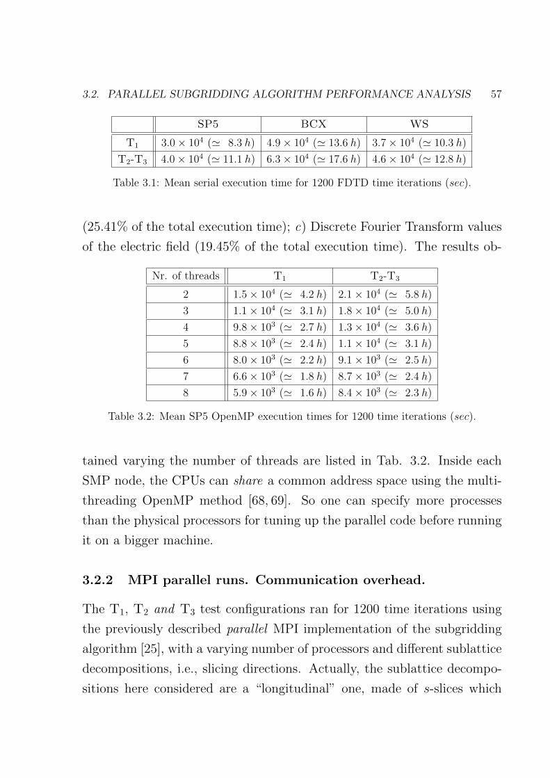
3.2.1 Profiling the serial version. OpenMP loop-level par-

allelism. . . . . . . . . . . . . . . . . . . . . . . . . 56

3.2.2 MPI parallel runs. Communication overhead. . . . 57

3.2.3 Scalability analysis. . . . . . . . . . . . . . . . . . . 60

3.2.4 Load balancing. Nonblocking communication. . . . 70

3.3 A large FDTD numerical experiment . . . . . . . . . . . . 74

4 Simulation of plasmonic nanostructures 79

4.1 Scattering by spherical nanoparticles . . . . . . . . . . . . 79

4.1.1 Theory of extinction . . . . . . . . . . . . . . . . . 79

4.1.2 Results and discussion . . . . . . . . . . . . . . . . 84

4.2 Scattering by non-spherical nanoparticles . . . . . . . . . . 92

5 Simulation of opal photonic crystals 97

5.1 Modeling and Results . . . . . . . . . . . . . . . . . . . . . 97

6 Conclusions 107

Bibliography 109

ii

List of Tables

2.1 Noble Metals Drude Parameters . . . . . . . . . . . . . . . 23

2.2 Error Evaluation at the resonance frequencies . . . . . . . 23

2.3 LQξ over the total frequency range. . . . . . . . . . . . . . 23

3.1 Mean serial execution time for 1200 FDTD time iterations

(sec). . . . . . . . . . . . . . . . . . . . . . . . . . . . . . . 57

3.2 Mean SP5 OpenMP execution times for 1200 time iterations

(sec). . . . . . . . . . . . . . . . . . . . . . . . . . . . . . . 57

3.3 Size parameter values for the paper test models. . . . . . . 65

3.4 Floating point, latency and bandwidth time . . . . . . . . 65

3.5 MPI parallel execution times for 1200 FDTD iterations (sec) 75

3.6 Power balance (Watt) for the large FDTD numerical exper-

iment . . . . . . . . . . . . . . . . . . . . . . . . . . . . . . 75

4.1 Averaged scattering and absorption, and fsub in air for metal

spheres as a function of the particle metal and size. . . . . 88

4.2 Averaged scattering and absorption, and fsub in SiO2 for

metal spheres as a function of the particle metal and size. . 88

4.3 Averaged scattering and absorption, and fsub in Si3N4 for

metal spheres as a function of the particle metal and size. . 89

iii

4.4 Extinction parameters, and integrated fsub for aluminium

cylinders and ellipsoid of different heights and with r =

100nm, compared with an aluminium sphere with r = 100nm.

All particles are placed in air. . . . . . . . . . . . . . . . . 95

iv

List of Figures

1.1 Yee FDTD cell. . . . . . . . . . . . . . . . . . . . . . . . . 2

1.2 Light trapping by scattering from metal nanoparticles at the

surface of the solar cell. . . . . . . . . . . . . . . . . . . . . 8

1.3 Light trapping by the excitation of localized surface plas-

mons in metal nanoparticles embedded in the semiconductor. 8

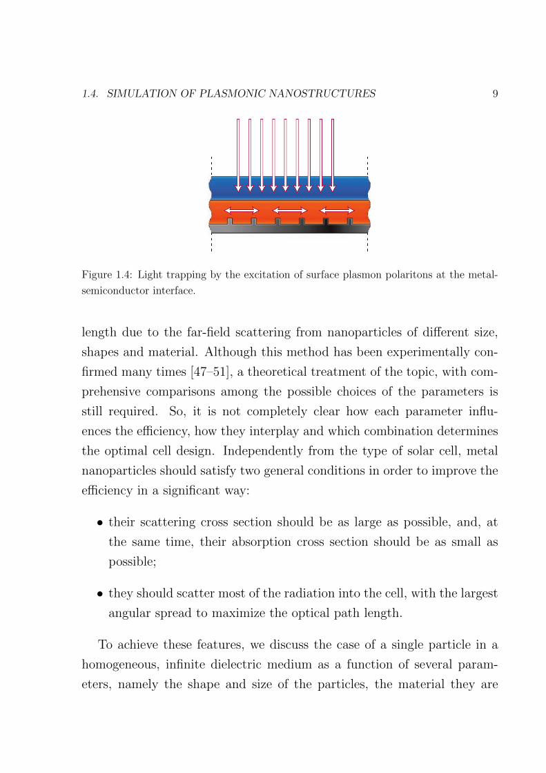
1.4 Light trapping by the excitation of surface plasmon polari-

tons at the metal-semiconductor interface. . . . . . . . . . 9

2.1 Analytical Qext for Au and Ag nanospheres (r = 96nm)

modeled by Drude dispersion. . . . . . . . . . . . . . . . . 22

2.2 Error parameters Lξ,η and Lξ comparison for Au (DFT at

λ = 480nm). . . . . . . . . . . . . . . . . . . . . . . . . . . 25

2.3 Total field Ex, Ey, Ez for Au nanosphere (DFT at λ =

480nm) along the x axis (y = 170, z = 120). . . . . . . . . 26


480nm) along the y axis (x = 150, z = 150). . . . . . . . . 26


480nm) along the z axis (x = 150, y = 170). . . . . . . . . 27

2.6 LQξ comparison for gold in the total frequency range, and

in the region of Qext minimum and maximum. . . . . . . . 28

2.7 Qext for a gold nanosphere (r = 96nm) modeled by Drude

dispersion. . . . . . . . . . . . . . . . . . . . . . . . . . . . 28

v

3.1 2D view example of a D′ with L = 5. The ` = 3 z-slice is

empty. . . . . . . . . . . . . . . . . . . . . . . . . . . . . . 44

3.2 Scheme of the process rank ρ assignment for z-slices and

s-slices. . . . . . . . . . . . . . . . . . . . . . . . . . . . . 45

3.3 Data sharing at the cutting plane between two s-slices (2D

view). . . . . . . . . . . . . . . . . . . . . . . . . . . . . . 46

3.4 Fields layout at a coarse/fine grid interface in the yz-plane

with a mesh refinement factor R = 5. . . . . . . . . . . . . 48

3.5 Parallel FDTD functional scheme for the subgridding algo-

rithm. . . . . . . . . . . . . . . . . . . . . . . . . . . . . . 51

3.6 Schematic of the T2 −T3 FDTD test configurations. . . . 55

3.7 Schematic of the human male model LS (left) and TS (right)

slicings. . . . . . . . . . . . . . . . . . . . . . . . . . . . . 58

3.8 LS-TS comparison for the T1 test model on SP5. . . . . . 60

3.9 T2-T3 test models comparison for LS on SP5. . . . . . . . 61

3.10 T1 test model timing on SP5. . . . . . . . . . . . . . . . . 67

3.11 T1 test model efficiency on SP5. . . . . . . . . . . . . . . . 68

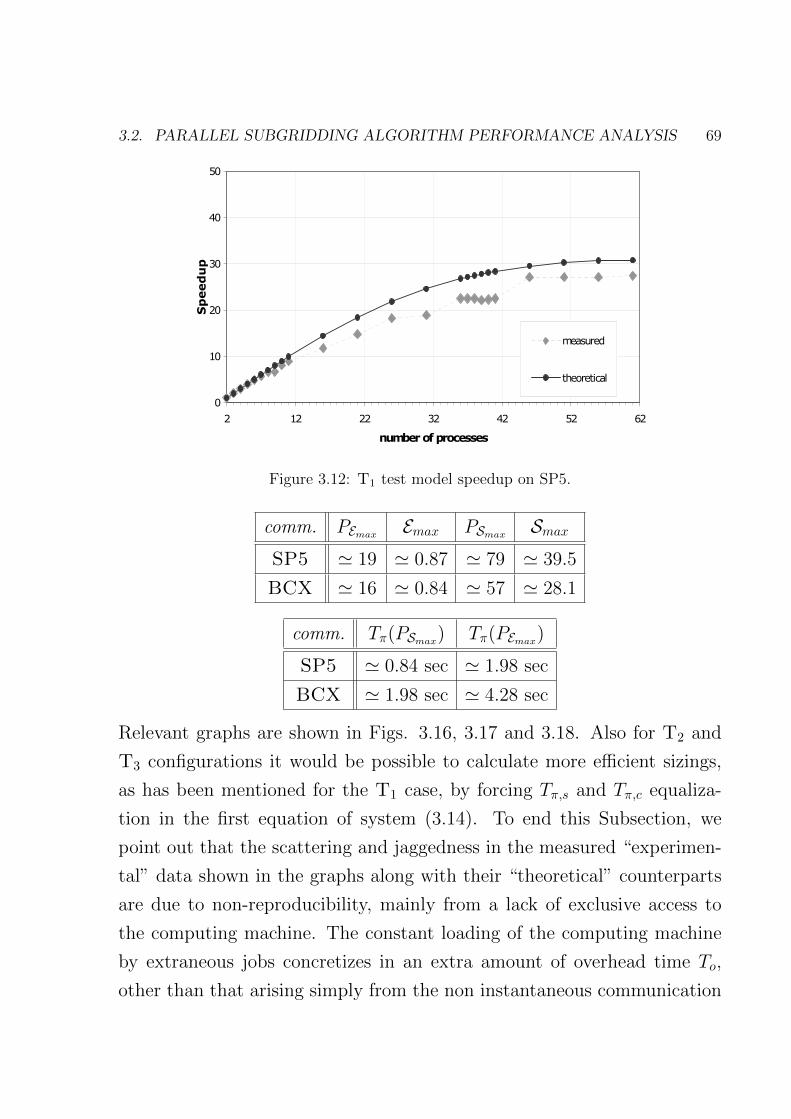
3.12 T1 test model speedup on SP5. . . . . . . . . . . . . . . . 69







3.19 Top view of a plane from the outer coarse lattice with in-

formation about geometry and displacements of the various

embedded refined sublattices for the antenna and the hu-

mans. Log. scale. . . . . . . . . . . . . . . . . . . . . . . . 77

vi

3.20 Three planes from the coarse grid. Perspective back view.

Log. scale. . . . . . . . . . . . . . . . . . . . . . . . . . . . 78

4.1 Solar spectrum together with a graph that indicates the solar

energy absorbed by a crystalline Si film. . . . . . . . . . . 81

4.2 Different types of plasmonic nanoparticle effects on photo-

voltaic. . . . . . . . . . . . . . . . . . . . . . . . . . . . . . 82

4.3 Scattering efficiency Qsca as a function of the wavelength

for different choices of the parameters. Top row: air, middle

row: SiO2, bottom row: Si3N4. Left column: r = 50nm, cen-

tral column: r = 100nm, right column: r = 150nm. Blue

line: silver, red dotted: gold, yellow dashed: aluminium,

green dashed-dotted: copper. . . . . . . . . . . . . . . . . . 85

4.4 Absorption efficiency Qabs as a function of the wavelength

for different choices of the parameters. Top row: air, middle

row: SiO2, bottom row: Si3N4. Left column: r = 50nm, cen-

tral column: r = 100nm, right column: r = 150nm. Blue

line: silver, red dotted: gold, yellow dashed: aluminium,

green dashed-dotted: copper. . . . . . . . . . . . . . . . . . 86

4.5 Albedo α as a function of the wavelength for different choices

of the parameters. Top row: silver, second row: gold, third

row: aluminium, bottom line: copper. Left column: air,

central column: SiO2, right column: Si3N4. Blue line: 50nm,

red dotted: 100nm, yellow dashed: 150nm. . . . . . . . . . 87

vii

4.6 Fraction of forward scattered light as a function of the wave-

length for different choices of the parameters. Top row:

air, middle row: SiO2, bottom row: Si3N4. Left column:

r = 50nm, central column: r = 100nm, right column:

r = 150nm. Blue line: silver, red dotted: gold, yellow

dashed: aluminium, green dashed-dotted: copper. . . . . . 91

4.7 FDTD/TFSF simulation of the electric field intensity sur-

rounding an aluminium ellipsoid, a hemisphere and a cylin-

der with h = 100nm. For each case, the polarized radiation

comes from the top side. Colors represent a logarithmic

scale of the intensity, normalized to a reference value of 1

V/m. The wavelength is 500nm. . . . . . . . . . . . . . . . 94

4.8 Scattering efficiency (left), absorbing efficiency (middle) and

albedo (right) as a function of the wavelength for aluminium

spheroids and cylinders. In the first row, blue line: spheroid

with h = 300nm; red dotted: spheroid with h = 100nm;

yellow dashed: semisphere with r = 100nm; green dashed-

dotted: sphere with r = 100nm. In the second row, blue

line: cylinder with h = 300nm; red dotted: cylinder with

h = 200nm; yellow dashed: cylinder with h = 100nm; green

dashed-dotted: sphere with r = 100nm. All particles are

placed in air. . . . . . . . . . . . . . . . . . . . . . . . . . 95

viii

4.9 Fraction of light scattered into the substrate as a function

of the wavelength for different choices of the parameters.

On the left: spheroids, semisphere and sphere. Blue line:

spheroid with h = 300nm, red dotted: h = 100nm, yellow

dashed: sphere with r = 100nm. On the right: cylinders

and sphere. Blue line: cylinder with h = 300nm, red dotted:

h = 200nm, yellow dashed: h = 100nm, green dashed-

dotted: sphere with r = 100nm. All particles are placed in

air. . . . . . . . . . . . . . . . . . . . . . . . . . . . . . . . 96

5.1 SEM example image of an artificial opal PC. . . . . . . . . 98

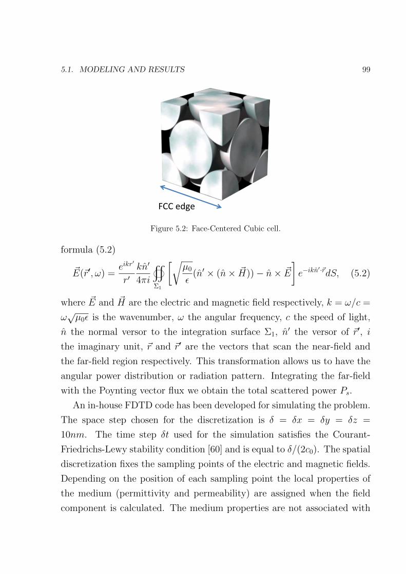
5.2 Face-Centered Cubic cell. . . . . . . . . . . . . . . . . . . . 99

5.3 Total-Field/Scattered-Field plane source method. . . . . . 100

5.4 Near-to-far transformation. . . . . . . . . . . . . . . . . . . 101

5.5 Domain decomposition and data exchange between adjacent

blocks. . . . . . . . . . . . . . . . . . . . . . . . . . . . . . 102

5.6 Transmittance varying the filling factor. . . . . . . . . . . 103

5.7 Experimental transmittance of the reference opal PC. . . . 103

5.8 Transmittance of the opal PC with f.f. = 0.774. . . . . . . 104

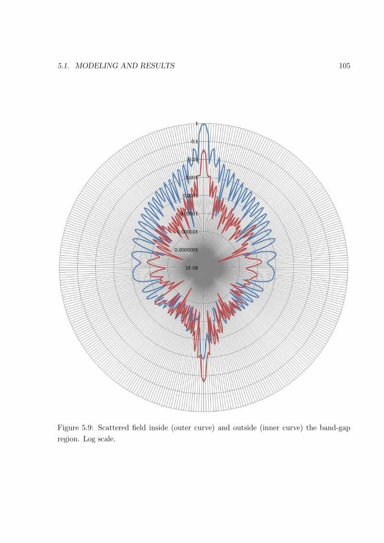
5.9 Scattered field inside (outer curve) and outside (inner curve)

the band-gap region. Log scale. . . . . . . . . . . . . . . . 105

5.10 Ez component normalized to the incident field. . . . . . . . 106

ix

Chapter 1

Introduction

1.1 The FDTD method for electromagnetics

Simulation allows us to realize a virtual laboratory, it stays in fact in the

middle between the theoretical and the experimental approach. Simula-

tion is the only way to investigate a large quantity of physical problems.

For example when we want to do a measure related to an object where it

is impossible to go inside. In electromagnetics the numerical simulation

is needed for solving almost all the problems of the real life, for design-

ing new devices, measure the electromagnetic field inside the objects over

which an electromagnetic radiation impings, evaluate the scattered field,

calculate the radiation pattern of a radiating structure, simulate the elec-

tromagnetic propagation in a complex environment, etc. The analytical so-

lution indeed is not available for complex problems. The Finite-Difference

Time-Domain (FDTD) method is the numerical technique we deal with.

The early Yee formulation [1] of the FDTD method [2] and its successive

enrichments, such as the pulsed FDTD method, the absorbing (ABC) or

radiation (RBC) boundary conditions for appropriate mesh truncation, are

a powerful tool in computational electromagnetics [3]. FDTD is a fully ex-

plicit numerical solution method of the hyperbolic first order Maxwell’s

curl PDEs system. The computational domain is discretized by cubic Yee

1

2 CHAPTER 1. INTRODUCTION

cells [1] (Fig. 1.1) and all the spatial values of the electromagnetic field

components are updated step by step. The electric field is calculated bas-

Figure 1.1: Yee FDTD cell.

ing on the values of the fields at the previous instants in time, then the

magnetic field is calculated basing on the previous values of the fields, etc.

The temporal evolution of the fields is then obtained. A frequency domain

analysis is not precluded, because a Discrete Fourier Transform (DFT)

can be performed in-line. With a single run of the code it is possible to ob-

tain the frequency behavior of the system. In this thesis we deal with the

electromagnetic simulation of complex problems in the field of plasmon-

ics and photonics. These problems require a certain amount of memory,

a detailed description at the nano-scale, the study of dispersive media,

etc. The absorbing boundary conditions are those described in [4, 5]. A

parallel approach is used for the code development in order to reduce the

simulation time using High Performance Computing (HPC) systems. The

1.2. THE SIMULATION OF DISPERSIVE MEDIA 3

dispersion in the optical frequency range of noble metals is also treated in

order to simulate in the more accurate way as possible the plasmonic reso-

nances. Plasmonics in particular is applied to the photovoltaics in order to

increase the photon concentration within the solar cell. The problems of

the FDTD simulation are also treated in the case of opal photonic crystals

for simulation and design purposes.

1.2 The simulation of dispersive media

In the field of nanotechnology the noble metal nanoparticles have an im-

portant role. In the optical range noble metals act as plasma and surface

waves appear along the metal-dielectric interface. These waves originate

collective oscillations of the electrons and are called Localized Surface Plas-

mons (LSP). The main phenomena are the field confinement, the field en-

hancement, the scattering cross section increase. They are maximized at

the resonance condition, known as Localized Surface Plasmon Resonance

(LSPR), which has also the property of the tunability. The plasmonic

behavior appearing in the light spectrum region can be used in optoelec-

tronics devices and photonic applications. These phenomena are important

also for the photovoltaic efficiency improvement. The dispersive behavior

of the noble metal has to be modeled in an accurate way in order to have

a detailed description of the plasmonic resonances. We focus at the be-

ginning on the Drude model for describing the noble metals dispersion.

Although some other approaches for the simulation of Drude dispersive

media already exist [6–17], we consider the Recursive Convolution (RC)

algorithm [18], that we call standard, as reference. We propose then a

modified algorithm for improving the accuracy at the plasmonic resonance

frequencies. Our approach time-discretizes directly the convolution inte-

gral expressing the temporal non-locality between the D and E fields. In


order to minimize the truncation error, we propose here to find a closed

form solution of the Ampere-Maxwell equation, and only after to proceed

with the time discretization. We calculate explicitly the kernel of such a

closed form solution in the case of Drude media deducing the modified RC

algorithm, and show how it can be updated recursively with the same mem-

ory requirements than the standard RC scheme. The evaluation of some

error parameters and the comparison of the electromagnetic fields highlight

the better accuracy of the proposed modified RC algorithm with respect

to the standard one at the plasmonic resonances. The test has been done

for Au and Ag noble metals [19] nanospheres, comparing the numerical

solution with the analytical one [20] in the optical frequency range. The

modified RC algorithm appears suitable for the simulation of plasmonic

resonant nanostructures and optical antennas. The modified approach was

then extended from a theoretical point of view to the case of the Drude

model with the two critical points correction [21–23] and to the case of the

Lorentz model [24]. We used the Convolutional Perfectly Matched Layer

(CPML) boundary conditions described in [4, 5]

1.3 The parallelization for large simulations

At the nano-scale the simulation parameters as the space-step used for

the domain discretization determines a memory requirement very high for

being supported by a single calculator. Due to the large sizes of the mod-

els, a serial encoding of the FDTD method may result in long calcula-

tion time. The increase of the computational efficiency is then necessary.

The need to solve complex and large problems has been dealt with a sub-

gridding approach besides a code parallelization. The simulation time is

then reduced and more realistic scenarios can be studied. We start on the

ground of a subgridding algorithm for the three-dimensional (3D) FDTD

1.3. THE PARALLELIZATION FOR LARGE SIMULATIONS 5

explicit numerical solution method of the Maxwell’s Equations, proposed

in a preceding paper [25]. This algorithm is efficient, non-recursive, and

incorporates a spatial filtering technique of the numerical signals and was

described using a serial programming approach. A parallel code version

of the same algorithm is here proposed, for very large size FDTD calcu-

lations. The algorithm enables the embedding of finer meshes into coarse

ones with a reduction of the space step by factors of 3, 5, 7 or greater,

maintaining also a good accuracy and the long term stability. The ba-

sic assumption of the subgridding (or mesh refinement) algorithm is that

increased mesh densities are introduced only in sub-regions where an ac-

curate discretized description of the geometrical surface details are really

needed [26–29] or subregions where the wavelength is shortened by the

presence of high permittivity media. It is assumed that such subregions

are embedded in homogeneous, isotropic, air-like regions where the ac-

curacy criterion is easily verified with a larger space step. The subgrid-

ding is thus confined to volumes of minimum possible extent. For a given

coarse/fine ratio (which we assume the best from the viewpoint of the ge-

ometrical/electrical constraints), the shortest simulation time is achieved

with an accurate load balancing obtained by an appropriate domain de-

composition (slicing). The execution time depends also on the cluster

network bandpass, due to the data exchange between processes executing

contiguous domain portions. Besides the subgridding for accuracy purposes

another step is to increase the computational efficiency running the code

on HPC systems, i.e. parallel or massive parallel machines with large RAM

and storage resources. The parallelization is made by means of an Message

Passing Interface (MPI) Application Programming Interface (API) imple-

mentation. To keep the parallel part of the code at the speed level of the

bulk FDTD calculations, suitable user defined MPI data types were intro-

duced, along with an adequate domain decomposition of the coarse and


refined meshes and their interfaces organization. MPI realizes the Single-

Program Multiple-Data (SPMD) programming approach: many instances

of a single program, the processes, are executed autonomously on distinct

physical processors of a cluster. This is a collection of interconnected SMP

(Symmetrical MultiProcessor) nodes, each of them with a certain number

of Central Processing Unit (CPU). Previous works on FDTD code par-

allelization by means of the MPI Library are reported in [30–33]. These

papers describe 2D or 3D Cartesian topologies of processes for the FDTD

grid decomposition, along with user defined MPI data structures for the

data exchange at the subdomain boundaries. They also report some per-

formance analysis. We start giving some details on how the MPI parallel

version of our subgridding algorithm [25] is implemented, in particular it

is described how to dynamically allocate the data structures in memory

in order to have a fast access and an efficient management of the data

transition at the coarse/coarse, refined/refined and coarse/refined domain

interfaces. According to the intrinsic modularity of this algorithm, all the

code is object-oriented C++ [34], which makes easier its understanding, de-

velopment and maintenance. Our domain decomposition is through slices,

i.e. 1D. We analyze quantitatively the performances of our parallel code

applying it to some FDTD test configurations involving the electromag-

netic field human exposure in a complex propagation environment. The

code can be adapted to the study of plasmonic nanostructures and opal

photonic crystals as shown in the next sections. We have assumed cubic

uniform grid cell shapes everywhere. The absorbing boundary conditions

are those described in [35].

1.4. SIMULATION OF PLASMONIC NANOSTRUCTURES 7

1.4 Simulation of plasmonic nanostructures

In the last years there has been a growing interest in the application of

plasmonic light-trapping techniques to photovoltaic cells [36–42]. The main

inefficiency causes due to the photon absorption are that:

• not all the incident photons go deep into the lattice, some photons are

reflected at the surface. The use of plasmonic nanoparticles can be an

alternative method to the simple anti-reflective coating.

• the photon energy is not completely used for the electron-hole pairs

creation and a fraction is lost in thermal phenomena.

• not all the electron-hole pairs contribute to the electric current because

of the recombination.

The presence of metal nanostructures on the front and rear surfaces or

in the bulk of a cell is a promising tool to enhance the efficiency through

surface plasmon resonances, especially in thin film (e.g. a-Si:H) solar cells.

Plasmon resonances from metal nanoparticles is a wide and popular sector

of investigations, with many applications [43–45] also in other fields. In

solar cell devices light can be converted to electricity using the plasmon

resonances of the noble metal nanostructures in three ways [46]:

• nanoparticles can be used as subwavelenght scattering elements that

couple and trap within the solar device the propagating plane waves

through a far-field effect that extends the optical path length of the

radiation into the cell (Fig. 1.2).

• nanoparticles can be used as subwavelenght antennas in which the

plasmonic near-field is coupled to the semiconductor increasing its

effective cross-section (Fig. 1.3). The result is a local absorption

increase due to the local field enhancement.


• a corrugated metallic film on the back surface of a thin photovoltaic

absorber layer can couple sunlight into surface plasmon polaritons

(SPP) modes supported at the metal-semiconductor interface as well

as guided modes in the semiconductor slab (Fig. 1.4).

Figure 1.2: Light trapping by scattering from metal nanoparticles at the surface of the

solar cell.

Figure 1.3: Light trapping by the excitation of localized surface plasmons in metal

nanoparticles embedded in the semiconductor.

Among the different physical mechanisms leading to better performing

photovoltaic cells, we discuss here the enhancement in the optical path

1.4. SIMULATION OF PLASMONIC NANOSTRUCTURES 9

Figure 1.4: Light trapping by the excitation of surface plasmon polaritons at the metal-

semiconductor interface.

length due to the far-field scattering from nanoparticles of different size,

shapes and material. Although this method has been experimentally con-

firmed many times [47–51], a theoretical treatment of the topic, with com-

prehensive comparisons among the possible choices of the parameters is

still required. So, it is not completely clear how each parameter influ-

ences the efficiency, how they interplay and which combination determines

the optimal cell design. Independently from the type of solar cell, metal

nanoparticles should satisfy two general conditions in order to improve the

efficiency in a significant way:

• their scattering cross section should be as large as possible, and, at

the same time, their absorption cross section should be as small as

possible;

• they should scatter most of the radiation into the cell, with the largest

angular spread to maximize the optical path length.

To achieve these features, we discuss the case of a single particle in a

homogeneous, infinite dielectric medium as a function of several param-

eters, namely the shape and size of the particles, the material they are


composed of, and the optical characteristics of the surrounding environ-

ment. Since the number of parameters is very large, it is important to

treat the scattering analytically whenever possible, before starting time-

expensive numerical simulations or cell fabrication. The scattering problem

is exactly solvable only for few particle shapes, as ellipsoid (spheres [52],

in particular) and infinitely long cylinders. We discuss here the equations

governing the extinction mechanism by a metallic sphere in order to inves-

tigate the scattering and the absorption properties, and study the effects

of changing the material, the dimensions and the media which embed the

spheres. The analytical discussion can go so far and cannot extend to

other shapes. Numerical simulations fill this gap; in particular the FDTD

method is used to simulate the evolution of the electromagnetic field during

the extinction process. The method will be applied to study the response

of hemispheres, cylinders and spheroids of various size. An analysis of the

angular distribution of the scattered radiation is also included.

1.5 Simulation of opal photonic crystals

Another complex problem dealt with a simulation approach is the analysis

and the characterization of opal photonic crystals [53–55] (PC) is described.

These crystals are modeled by an ordered face-centered cubic (FCC) lattice

structure of spherical particles with a given filling factor (f.f.). The filling

factor is the ratio between the filled space by the nanospheres and the total

space. It can be evaluated over a single FCC cell. These particles are made

of a non-absorptive and non-dispersive material with a constant dielectric

permittivity. The physical phenomenon to investigate is the multiple scat-

tering by the spheres of an impinging monochromatic light beam, which

is obtained in laboratory through a monochromator. The modeling of the

exciting signal is based on a plane wave electromagnetic pulse and the in-

1.5. SIMULATION OF OPAL PHOTONIC CRYSTALS 11

teraction with the opal PC is simulated through the numerical solution of

the Maxwell’s Equations using the FDTD method [3]. The resulting field is

calculated in a discretized fashion on a three dimensional grid of sampling

points. Frequency Domain results are obtained by means of a DFT of the

system response to the transient excitation due to the impinging pulse.

The simulation target is the opal PC reflectance and transmittance calcu-

lation in the 300÷700 nm wavelength range. The scattering by the spheres

originates a non-omnidirectional pattern for the transmitted and the re-

flected light. Through an analytical approach (Kirchhoff’s formula [56])

the angular distribution of the scattered field in the far-zone is evaluated

and the total scattered power calculated. The structure, due to the nano-

scale and to the fine space-discretization needed for accuracy reasons, is

cumbersome and challenging from a simulation point of view and a parallel

approach is required for that. By using the MPI API the simulation can

run on HPC systems. A cubic slicing approach is used for the decomposi-

tion of the analysis domain into blocks. MPI allows the field components

exchange between processes running adjacent blocks. The computational

result for the transmittance as function of the wavelength in the 300÷ 700

nm range reveals the presence of a band-gap in the curve. The compari-

son with the experimental measures carried out in our laboratory shows a

satisfactory agreement. Although some modeling approximation has to be

done the proposed numerical technique seems appear as a promising tool

for the theoretical characterization of opal PCs.


1.6 Summary of publications

This thesis is based on the following publications.

• A. Vaccari, A. Cala Lesina, L. Cristoforetti, and R. Pontalti: Parallel

implementation of a 3D subgridding FDTD algorithm for large sim-

ulations, Progress In Electromagnetics Research, Vol. 120, 263-292,

2011.

http://www.jpier.org/PIER/pier.php?paper=11063004

• A. Paris, A. Vaccari, A. Cala Lesina, E. Serra, and L. Calliari: Plas-

monic scattering by metal nanoparticles for solar cells, Plasmonics,

Vol. 7, no. 3, pp. 525-534, 2012.

http://link.springer.com/article/10.1007%2Fs11468-012-9338-4?

LI=true

• A. Cala Lesina, A. Vaccari, and A. Bozzoli: A modified RC-FDTD

algorithm for plasmonics in Drude dispersive media nanostructures,

6th European Conference on Antennas and Propagation (EuCAP),

Prague, Czech Republic, 2012.

http://ieeexplore.ieee.org/xpls/abs_all.jsp?arnumber=6206111

• A. Cala Lesina, A. Vaccari, and A. Bozzoli, A novel RC-FDTD algo-

rithm for the Drude dispersion analysis, Progress In Electromagnetics

Research M, Vol. 24, 251-264, 2012.

http://www.jpier.org/PIERM/pier.php?paper=12041904

• A. Cala Lesina, A. Vaccari, and A. Bozzoli, A modified RC-FDTD

algorithm for plasmonics in Drude dispersive media, Proceedings of

http://www.jpier.org/PIER/pier.php?paper=11063004

http://link.springer.com/article/10.1007%2Fs11468-012-9338-4?LI=true

http://link.springer.com/article/10.1007%2Fs11468-012-9338-4?LI=true

http://ieeexplore.ieee.org/xpls/abs_all.jsp?arnumber=6206111

http://www.jpier.org/PIERM/pier.php?paper=12041904

1.6. SUMMARY OF PUBLICATIONS 13

the XIX RiNEm (Riunione Nazionale di Elettromagnetismo), Roma,

Italy, 2012.

• A. Vaccari, A. Cala Lesina, L. Cristoforetti, A. Chiappini, and M. Fer-

rari, A computational approach to the optical characterization of pho-

tonic crystals and photonic glasses, Proceedings of the XIX RiNEm

(Riunione Nazionale di Elettromagnetismo), Roma, Italy, 2012.

• A. Chiappini, A. Armellini, A. Cala Lesina, A. Vaccari, L. Cristo-

foretti, F. Prudenzano, G. C. Righini, and M. Ferrari, Colloidal plas-

monic photonic crystals, 1st International workshop on Metallic Nano-

objects, Sant-Etienne, France, 2012.

• A. Vaccari, A. Cala Lesina, L. Cristoforetti, A. Chiappini, F. Pruden-

zano, A. Bozzoli, M. Ferrari, A parallel computational FDTD approach

to the analysis of the light scattering from an opal photonic crystal,

Proceedings of SPIE 8781, Integrated Optics: Physics and Simula-

tions, p. 87810, Prague, Czech Republic, 2013.

• A. Vaccari, A. Cala Lesina, L. Cristoforetti, A. Chiappini, F. Pruden-

zano, A. Bozzoli, and M. Ferrari, A parallel FDTD computation of the

photonic crystal transmittance, 15th National Conference on Photonic

Technologies (Fotonica 2013), Milano, Italy, 2013.


Chapter 2

The simulation of dispersive media

2.1 Theoretical Approach

The temporal non-locality relation between the D and E fields in dispersive

media is expressed by means of the convolution integral

D(t) = ε0ε∞E(t) + ε0

∫ t

0

E(t− τ)χ(τ)dτ (2.1)

which exhibits a Dirac-delta contribution representing the instantaneous

response at the infinite frequency through the (relative) permittivity ε∞

term. In (2.1) χ(τ) is the Inverse Fourier Transform (IFT) of the electric

susceptibility χ(ω). This measures the media polarization and enters the

complex permittivity ε(ω) in

D(ω) = ε0 [ε∞ + χ(ω)]E(ω) = ε(ω)E(ω), (2.2)

i.e. the proportionality coefficient between D and E in the angular fre-

quency domain ω after a Fourier transform with respect to the time vari-

able. In (2.2) the same letters are used to denote the fields both in the

time and frequency domain and the space dependence is understood. The

Ampere-Maxwell equation which is time stepped in the FDTD method,

along with the Faraday-Maxwell curl equation for the E and B fields, is

∇×H =∂D

∂t+ σE, (2.3)

15

16 CHAPTER 2. THE SIMULATION OF DISPERSIVE MEDIA

where σ is the static conductivity contribution. Before discretizing (2.3)

for time stepping however, we analytically solve it with respect to the time

variable by the Laplace transform method, to get a closed form solution

for the electric field E at a given time instant t. If we denote by s the dual

of the time variable t, omit an understood space dependence as before, and

now use a tilde for a Laplace transformed quantity, we have from (2.1)

D(s) = ε0 [ε∞ + χ(s)]E(s) (2.4)

and from (2.3)

∇×H(s) = sD(s)−D(0) + σE(s), (2.5)

where we assumed that the curl operator ∇×, acting on the space vari-

ables, commutes with the Laplace transform operator. By solving for D(s)

the first of the two previous equations, inserting the result in the second

one, where an initial time zero-field condition has been assumed, and then

solving for E(s) we have

E(s) = G(s) ·∇×H(s), (2.6)

where G(s) stands for

G(s) =1

sε0 [ε∞ + χ(s)] + σ. (2.7)

Note that χ(s = −iω) = χ(ω) where i =√−1 is the imaginary unit. By

returning to the time domain through an Inverse Laplace Transform (ILT),

we get the aforementioned closed form exact solution for the electric field

E(t) =

∫ t

0

G(t− τ) ·∇×H(τ)dτ, (2.8)

where the convolutional kernel G(τ) depends on the medium dispersion

characteristic. Note that if in (2.1) χ(τ) were identically zero, we would

2.2. THE DRUDE MODEL 17

recover the usual non-dispersive behavior with the absolute dielectric con-

stant ε = ε0ε∞. This would imply an identically zero χ in (2.7) too. For

the corresponding original G we would then get

G(τ) =1

εe−

σε τ , (2.9)

where a Heaviside step function factor of argument is understood. Using

this result in (2.8) and, as is usual in FDTD, sampling at discrete times nδt,

where δt is the time step, with ∇×H and H temporally sampled halfway

at (n + 1/2)δt, one gets an updating equation for E with exponential

coefficients

En+1 = e−σδtε En +

(1− e−σδtε )

σ∇×Hn+ 1

2 , (2.10)

where superscripts denote time levels. By Taylor expanding to first order

the coefficients in (2.10) with respect to the small quantity σδt/ε, they

equal their FDTD discrete counterparts expanded to the same order. With

this in mind we think that our approach based on (2.8) is less prone to time

truncation errors, mainly for highly absorptive media with rapidly time

decaying fields, than the standard method based on an early discretization

of the convolution integral (2.1).

2.2 The Drude model

We now calculate explicitly the convolutional kernel G(s) shown in (2.7) in

the case of Drude dispersion. This is formulated by the single term electric

susceptibility

χ(s) =ω2D

s(s+ γ), (2.11)

where ωD and γ are the plasma frequency and the damping coefficient.

This gives

G(s) =s+ γ

ε0ε∞(s− s+)(s− s−), (2.12)


where

s± = −P ± iQ (2.13)

and

P =1

2

(γ +

σ

ε0ε∞

), Q =

√ε0ω2

D + σγ

ε0ε∞− P 2 . (2.14)

After returning to the time-domain we get

G(τ) =1

ε0ε∞

[es+τ(s+ + γ)

s+ − s−+es−τ(s− + γ)

s− − s+

](2.15)

which, putting

S =1

2(γ − σ

ε0ε∞), (2.16)

has the following form

G(τ) = ImKe−Wτ+iΦ

, (2.17)

where

K =1

ε0ε∞

√1 +

(S

Q

)2

, (2.18)

W = P − iQ, (2.19)

Φ = arctanQ

S, (2.20)

with K and Φ real quantities. Re and Im denote the real and imaginary

parts of a complex quantity. By defining the complex vector

Ψ(t) =

∫ t

0

Ke−W (t−τ)+iΦ ·∇×H(τ)dτ (2.21)

one sees that, according with (2.8) and (2.17), the electric field E results

to be

E(t) = Im Ψ(t) =

∫ t

0

ImKe−W (t−τ)+iΦ

·∇×H(τ)dτ. (2.22)


Sampling (2.21) at the discrete times nδt (n = 1, 2, ...) we have

Ψn+1 =

∫ (n+1)δt

0

Ke−W ((n+1)δt−τ)+iΦ ·∇×H(τ)dτ. (2.23)

Separating the integration interval we obtain

Ψn+1 = e−Wδt

∫ nδt

0

Ke−W (nδt−τ)+iΦ ·∇×H(τ)dτ+

+∇×Hn+ 12 ·∫ (n+1)δt

nδt

Ke−W ((n+1)δt−τ)+iΦdτ

(2.24)

and then

Ψn+1 = e−Wδt ·Ψn + A ·∇×Hn+ 12 , (2.25)

where the complex coefficient A is given by

A =

∫ (n+1)δt

nδt

Ke−W ((n+1)δt−τ)+iΦdτ = KeiΦ(1− e−Wδt)

W. (2.26)

Thus storing, as in the RC traditional scheme [18], one extra complex vari-

able for each sampling point and each electric field component, updating

it according to (2.25), and using its imaginary part as a new electric field

value, allows us to include dispersive media in a simpler and more accurate

recursive procedure. By expanding the exponential factor according to the

Euler formula

e−Wδt = e−Pδt [cos(Qδt) + i sin(Qδt)] (2.27)

and taking the imaginary part of both sides of (2.25) we have the modified

form of the electric field updating equation

En+1 = e−Pδt sin(Qδt) ·Re Ψn+

+e−Pδt cos(Qδt) ·En + Im A ·∇×Hn+ 12 .

(2.28)

For completeness we report the updating equation of the standard method

[18]:

En+1 = C1 ·Φn + C2 ·En + C3 ·∇×Hn+ 12 , (2.29)


where

Φn = C4 ·En−1 + e−γδt ·Φn−1 (2.30)

and

C1 =1

ε0 + χ0, (2.31)

C2 = (ε∞ + ∆χ0)C1, (2.32)

C3 =δt

ε0C1, (2.33)

C4 = e−γδt∆χ0, (2.34)

χ0 =

∫ δt

0

χ(τ)dτ, (2.35)

∆χ0 = −ω2D

γ[1− e−γδt]2. (2.36)

2.2.1 Simulations

To test the modified RC algorithm previously proposed, we apply it to a

96nm radius nanosphere, made of gold or silver, in a plane wave light beam.

The static conductivity is assumed null. We have tested our modified al-

gorithm in particular for Au at λ = 480nm and for Ag at λ = 336nm

and λ = 380nm, i.e. the resonance wavelengths evidenced in Fig. 2.1

through the extinction coefficient Qext defined in [56]. This coefficient is

an efficiency parameter defined as the particle cross section Cext (effec-

tive surface) reported in (4.1) normalized to the geometrical projection of

the particle on a plane perpendicular to the incoming field (real surface).

The extinction, scattering and absorption coefficients for a small spherical

particle [20] are:

Qext =2

r2k2

∞∑n=1

(2n+ 1)Re(an + bn), (2.37)


Qsca =2

r2k2

∞∑n=1

(2n+ 1)(|an|2 + |bn|2), (2.38)

Qabs = Qext −Qsca, (2.39)

where k = (2πN)/λ, N is the refractive index of the medium surrounding

the sphere, λ is the wavelength of the incident radiation, an and bn are

combinations of Riccati-Bessel functions [20]. These functions are explicitly

dependent on the radius r of the sphere and on the complex permittivity

of the medium. We used a 200× 200× 200 cubic Yee cell discretization to

accommodate the nanosphere. The cell edge (space step δ = δx = δy = δz)

amounts to 2nm for a good representation of the geometrical details. The

time step was set to δ/(2c0), with c0 the vacuum light velocity, to satisfy

the Courant stability condition [3] in three dimensions. We also used a

Total Field/Scattered Field (TFSF) source [3], placed 8 cells inward from

the outer boundary of the FDTD lattice, to create a plane wave linearly

polarized (along the z-axis), impinging along the positive y-direction on

the nanostructure. The FDTD lattice was completed with an extra layer,

15 cells thick, supporting the CPML boundary conditions [4] to simulate

an open to infinity surrounding media. We used the CPML parameters

reported in [5]. We used a compact pulse exciting signal, i.e. of finite

duration and with zero value outside a given time interval [25] [57]. The

signal duration T = 1/fmax is suitably chosen to get spectral distribution

results in the range 200÷ 1000nm, where fmax is the maximum frequency,

as obtained by the DFT which is updated at every FDTD time iteration,

until the excitation is extinguished inside the whole numerical lattice. The

excitation signal is a raised cosine

s(t) = (1− cos(2πt

T))3, (2.40)

where T is the duration of the pulse. It can be considered extinguished in

3÷4 the time the radiation needs for propagating along the lattice diagonal.


200 300 400 500 600 700 800

wavelength[nm]

0

1

2

3

4

5

6

7

8

Qext

GoldSilver

Figure 2.1: Analytical Qext for Au and Ag nanospheres (r = 96nm) modeled by Drude

dispersion.


The Drude parameters for Au and Ag were taken from the literature [19]

and are reported in Tab. 2.1.

ε∞ ωD [rad/s] γ [s−1]

Au 9.84 1.3819 · 1016 1.09387 · 1014

Ag 3.70 1.3521 · 1016 3.19050 · 1013

Table 2.1: Noble Metals Drude Parameters

Au(480nm) Ag(336nm) Ag(380nm)

Lm,x (Ls,x) 0.0386 (0.0548) 0.1275 (0.1533) 0.0374 (0.0421)

Lm,y (Ls,y) 0.0592 (0.0872) 0.2085 (0.2485) 0.0585 (0.0687)

Lm,z (Ls,z) 0.0440 (0.0633) 0.1718 (0.2024) 0.0430 (0.0478)

Lm (Ls) 0.0693 (0.1011) 0.2670 (0.3282) 0.0594 (0.0684)

LQm (LQs) 0.2216 (0.3376) 0.3265 (0.3646) 0.4579 (0.5052)

Table 2.2: Error Evaluation at the resonance frequencies

Au Ag

LQm (LQs) 0.0515 (0.0747) 0.0926 (0.1019)

Table 2.3: LQξ over the total frequency range.

The electric fields, by means of the DFT, are computed for each sam-

pling point of the lattice at the frequency of interest and are normalized

with respect to the incident electric field component at the same frequency.

The numerical results for the electric field and the extinction coefficient

have been compared with those from the standard RC method [18] through

the analytical solutions obtained by implementing the methods described


in [56]. The numerical counterpart of Qext is calculated by adding the ab-

sorption coefficient Qabs to the scattering coefficient Qsca, indeed only these

two are evaluable through a numerical approach. The first is the Poynt-

ing vector flux through a closed surface containing the sphere in the total

field domain, the second is calculated by means of the same flux through a

closed surface located in the scattered field region. In order to evaluate the

deviation of the numerical results from the exact solution we considered

the average error for each electric field component

Lξ,η =1

N 3

N∑i,j,k=1

∣∣Eξη(i, j, k)− Ea

η (i, j, k)∣∣ , (2.41)

the average error for the electric field module

Lξ =1

N 3

N∑i,j,k=1

∣∣|Eξ(i, j, k)| − |Ea(i, j, k)|∣∣ (2.42)

and the average error for Cext

LQξ =1

Nλ

Nλ∑i=1

∣∣∣Qξexti −Q

aexti

∣∣∣ , (2.43)

where η = x, y, z indicates the cartesian component, ξ = s,m, the

letters s,m, a denote standard, modified and analytical solution, and Nλ is

the number of wavelengths at which Qext has been evaluated. The values

in Tab. 2.2 were obtained with 12000 time iterations simulations. For

the gold resonance the error parameters (2.41) and (2.42) are reported as a

function of the number of FDTD iterations (Fig. 2.2). We can observe that

the convergence is reached after the same number of FDTD time iterations

than in the standard case and in all the cases the level of accuracy is better.

The better numerical accuracy is also evidenced with a comparison of the

total electric field extracted from the lattice along one direction in x, y

and z (Fig. 2.3, 2.4 and 2.5). In each figure the three components of the


0 5000 10000 15000 20000 25000 30000FDTD time iterations

0.00

0.05

0.10

0.15

0.20

0.25

Err

or

para

mete

rs L

Lm,x

Ls,x

Lm,y

Ls,y

Lm,z

Ls,z

Lm

Ls

Figure 2.2: Error parameters Lξ,η and Lξ comparison for Au (DFT at λ = 480nm).


0 50 100 150 200

x

0.0

0.2

0.4

0.6

0.8

1.0

1.2

Ex

AnalyticFDTD modifiedFDTD standard

0 50 100 150 200

x

0.0

0.2

0.4

0.6

0.8

1.0

1.2

Ey

50 100 150

x

0.0

0.2

0.4

0.6

0.8

1.0

1.2

Ez

Figure 2.3: Total field Ex, Ey, Ez for Au nanosphere (DFT at λ = 480nm) along the x

axis (y = 170, z = 120).

0 50 100 150 200

y

0.0

0.2

0.4

0.6

0.8

1.0

Ex


0 50 100 150 200

y

0.0

0.2

0.4

0.6

0.8

1.0

Ey

50 100 150

y

0.0

0.2

0.4

0.6

0.8

1.0

Ez

Figure 2.4: Total field Ex, Ey, Ez for Au nanosphere (DFT at λ = 480nm) along the y

axis (x = 150, z = 150).


0 50 100 150 200

z

0.0

0.1

0.2

0.3

0.4

0.5

0.6

Ex


0 50 100 150 200

z

0.0

0.1

0.2

0.3

0.4

0.5

0.6

Ey

50 100 150

z

0.0

0.1

0.2

0.3

0.4

0.5

0.6

Ez

Figure 2.5: Total field Ex, Ey, Ez for Au nanosphere (DFT at λ = 480nm) along the z

axis (x = 150, y = 170).

electric field (Ex on the left, Ey in the middle and Ez on the right) are

represented. The sharp peaks are due to the field inside the sphere, that is

very low (metallic sphere), and to some symmetry planes where the field

is zero. For gold and silver the extinction coefficient has been calculated

and the error parameter (2.43) at the resonance frequencies (Tab. 2.2)

and over the total frequency range are reported (Tab. 2.3). For gold the

error parameter (2.43) is evaluated for the total frequency range and in

the peak regions (λ = 400nm and λ = 480nm) varying the number of time

iterations (Fig. 2.6), while the Qext comparison is shown in Fig. 2.7.


5000 10000 15000 20000 25000FDTD time iterations

0.00

0.02

0.04

0.06

0.08

0.10

0.12

0.14

Err

or

para

mete

r LQ

LQm tot

LQs tot


0.00

0.02

0.04

0.06

0.08

0.10

0.12

0.14 LQm 400nm

LQs 400nm


0.15

0.20

0.25

0.30

0.35

0.40

LQm 480nm

LQs 480nm

Figure 2.6: LQξ comparison for gold in the total frequency range, and in the region of

Qext minimum and maximum.

200 300 400 500 600 700 800

wavelength[nm]

0

1

2

3

4

5

6

7

Qext

AnalyticalModified FDTDStandard FDTD

Figure 2.7: Qext for a gold nanosphere (r = 96nm) modeled by Drude dispersion.

2.3. THE N-ORDER DRUDE MODEL 29

2.3 The N-order Drude model

Let assume a dispersive medium described by a Drude multiple poles

model. Let assume also a time dependence e−iωt. If N is the order of

the poles the complex susceptibility is

χ(ω) =N∑p=1

−ω2p

ω(iγp + ω), (2.44)

where ωp is the pth plasma frequency, γp is the pth damping coefficient and

i the imaginary unit. In the Laplace domain (s = −iω) we have

χ(s) =N∑p=1

ω2p

s(s+ γp). (2.45)

Substituting (2.45) into (2.7) we obtain

G(s) =

∏Np=1(s+ γp)∑N+1

k=0 CksN+1−k

, (2.46)

where Ck = fk(ε0, ε∞, σ, γp, ωp) for p = 1, ...N and k = 0, ...N + 1 are

real coefficients, fk is a kth function depending on the polynomial devel-

opment. Let’s distinguish two cases: even and odd N -order.

If N is odd the grade of the denominator of (2.46) is even. Developing

it whit N+12 couples of complex conjugate poles we have

G(s) =

∏Np=1(s+ γp)

C0

∏N+12

k=1 (s+ sk)(s+ s∗k), (2.47)

where sk = Ak + iBk is the kth pole. Acting the ILT of (2.47) we obtain

G(t) =

N+12∑

k=1

e−Akt [Mk cos(Bkt) +Nk sin(Bkt)] , (2.48)


where Mk and Nk

k = 1, ...N+1

2

are real coefficients that depend on γp

p = 1, ..N, C0, Ak and Bk

k = 1, ...N+1

2

. Setting

Mk

Nk= tan Θk =

sin Θk

cos Θk(2.49)

we obtain

G(t) =

N+12∑

k=1

Nke−Akt

cos Θksin(Bkt+ Θk). (2.50)

If we put

F (t) =

N+12∑

k=1

Fk(t), (2.51)

where

Fk(t) =Nke

−Akt

cos Θkei(Bkt+Θk) (2.52)

and

Ψ(t) =

∫ t

0

F (t− τ) ·∇×H(τ)dτ, (2.53)

we have

E(t) = =Ψ(t) . (2.54)

Developing Ψ(t) we obtain

Ψ(t) =

∫ t

0

N+12∑

k=1

Fk(t− τ) ·∇×H(τ)dτ =

N+12∑

k=1

Φk(t) (2.55)

with

Φk(t) =

∫ t

0

Fk(t− τ) ·∇×H(τ)dτ. (2.56)


Sampling at the discrete times nδt n = 1, 2, ... we have

Ψn+1 =

N+12∑

k=1

Φn+1k =

N+12∑

k=1

∫ (n+1)δt

0

Fk [(n+ 1)δt− τ ] ·∇×H(τ)dτ =

=

N+12∑

k=1

∫ nδt

0

e−AkδteiBkδtFk(nδt− τ) ·∇×H(τ)dτ+

+

N+12∑

k=1

∫ (n+1)δt

nδt

Fk [(n+ 1)δt− τ ] ·∇×H(τ)dτ =

=

N+12∑

k=1

e−AkδteiBkδtΦnk + A ·∇×Hn+ 1

2 ,

(2.57)

where

A =

N+12∑

k=1

∫ (n+1)δt

nδt

Fk [(n+ 1)δt− τ ] dτ =

N+12∑

k=1

eiΘkNk

cos Θk

e(−Ak+iBk)δt − 1

−Ak + iBk.

(2.58)

The expression for the electric field then becomes

En+1 = =Ψn+1

=

N+12∑

k=1

e−Akδt [sin(Bkδt)<Φnk+ cos(Bkδt)=Φn

k] +

+=A ·∇×Hn+ 12

(2.59)

and the number of required extra memorizations for the auxiliary vari-

ables needed for the code execution is N − 1.

If N is even the grade of the denominator of (2.46) is odd. Developing

it whit N/2 couples of complex conjugate poles and one real pole we have

G(s) =

∏Np=1(s+ γp)

C0 · (s+ Γ)∏N

2

k=1(s+ sk)(s+ s∗k), (2.60)


where sk = Ak + iBk is the kth pole. Acting the ILT of (2.60) we obtain

G(t) = M0e−Γt +

N2∑

k=1


where Mk

k = 0, ...N2

and Nk

k = 1, ...N2

are real coefficients and they

depend on γp p = 1, ...N, C0, Ak and Bk

k = 1, ...N2

. Setting

Nk

Mk= tan Θk =

sin Θk

cos Θk(2.62)

we obtain

G(t) = M0e−Γt +

N2∑

k=1

Mke−Akt

cos Θkcos(Bkt−Θk). (2.63)

If we put

F (t) =

N2∑

k=0

Fk(t), (2.64)

where

F0(t) = M0e−Γt (2.65)

Fk(t) =Mke

−Akt

cos Θkei(Bkt−Θk) (k = 1, 2...

N

2) (2.66)

and

Ψ(t) =

∫ t

0

F (t− τ) ·∇×H(τ)dτ, (2.67)

we have

E(t) = <Ψ(t) . (2.68)


Ψ(t) =

∫ t

0

N2∑

k=0

Fk(t− τ) ·∇×H(τ)dτ =

N2∑

k=0

Φk(t), (2.69)

where

Φk(t) =

∫ t

0

Fk(t− τ) ·∇×H(τ)dτ. (2.70)



Ψn+1 =

N2∑

k=0

Φn+1k =

N2∑

k=0

∫ (n+1)δt

0

Fk [(n+ 1)δt− τ ] ·∇×H(τ)dτ =

=

∫ nδt

0

e−ΓδtF0(nδt− τ) ·∇×H(τ)dτ+

+

N2∑

k=1

∫ nδt

0


+

N2∑

k=0

∫ (n+1)δt

nδt

Fk [(n+ 1)δt− τ ] ·∇×H(τ)dτ =

= e−ΓδtΦn0 +

N2∑

k=1


2 ,

(2.71)

where

A =

N2∑

k=1

∫ (n+1)δt

nδt

Fk [(n+ 1)δt− τ ] dτ =

N2∑

k=1

e−iΘkMk

cos Θk


−Ak + iBk.

(2.72)


En+1 = <Ψn+1

= e−ΓδtΦn

0+

+

N2∑

k=1

e−Akδt [cos(Bkδt)<Φnk − sin(Bkδt)=Φn

k] + <A ·∇×Hn+ 12

(2.73)

and the number of required extra memorizations is N with respect to the

non-dispersive case.


2.4 The Lorentz model

Let assume a dispersive medium described by a Lorentz function (single

pair of complex conjugate poles) and a time dependence e−iωt. If ω0 is the

resonant frequency of the medium and δ0 is the damping coefficient the

complex susceptibility is

χ(ω) = (εs − ε∞)ω2

0

ω20 − 2iωδ0 − ω2

, (2.74)

where εs is the static permettivity. In the Laplace domain (s = −iω) it

becomes

χ(s) = (εs − ε∞)ω2

0

ω20 + 2sδ0 + s2

. (2.75)

This expression can be simplified in the form

χ(s) =Ω0

(s+ α0 + iβ0)(s+ α0 − iβ0), (2.76)

where α0 = δ0, β0 =√ω2

0 − δ20 and Ω0 = (εs − ε∞)ω2

0. Putting (2.75) into

(2.7), considering σ = 0 and developing some calculation it results

G(s) =(s+ α0 + iβ0)(s+ α0 − iβ0)

Cs[(s+ A0 + iB0)(s+ A0 − iB0)], (2.77)

where C = ε0ε∞, A0 = α0 and B0 =√β2

0 + Ω0/ε∞.

Acting the ILT of (2.77) we obtain

G(t) = K + e−A0t [M0 cos(B0t) +N0 sin(B0t)] , (2.78)

where

K =1

ε0εs, (2.79)

M0 =εs − ε∞ε0ε∞εs

, (2.80)

and

N0 =δ0(εs − ε∞)

B0ε0ε∞εs(2.81)

2.4. THE LORENTZ MODEL 35

are real quantities.

Setting

Θ0 = arctan(N0

M0) (2.82)

we have

G(t) = K +M0e

−A0t

cos Θ0cos(B0t−Θ0). (2.83)

If we put

F (t) = K + F0(t), (2.84)

where

F0(t) =M0e

−A0t

cos Θ0ei(B0t−Θ0) (2.85)

and

Ψ(t) =

∫ t

0

F (t− τ) ·∇×H(τ)dτ, (2.86)

Φ(t) =

∫ t

0

F0(t− τ) ·∇×H(τ)dτ, (2.87)

it results

E(t) = <Ψ(t) . (2.88)


Ψn+1 =

∫ (n+1)δt

0

[K + F0 ((n+ 1)δt− τ)] ·∇×H(τ)dτ =

=

∫ (n+1)δt

0

K ·∇×H(τ)dτ+

+

∫ nδt

0

e−A0δteiB0δtF0(nδt− τ) ·∇×H(τ)dτ+

+

∫ (n+1)δt

nδt

F0 ((n+ 1)δt− τ) ·∇×H(τ)dτ =

= e−A0δteiB0δtΦn + ((n+ 1)Kδt+ Z) ·∇×Hn+ 12 ,

(2.89)

where

Z =

∫ (n+1)δt

nδt

F0 ((n+ 1)δt− τ) dτ =M0(e

(−A0+iB0)δt − 1)

(−A0 + iB0) cos Θ0e−iΘ0. (2.90)


Taking the real part of (2.89), the expression for the electric field becomes

En+1 = e−A0δt [cos(B0δt)<Φn − sin(B0δt)=Φn] +

+<(n+ 1)Kδt+ Z ·∇×Hn+ 12

(2.91)

and the number of extra variables for each electric field component is 2 as

in the traditional algorithm [24]. The magnetic field indeed does not need

auxiliary variables and the updating equations are the same than in the

standard FDTD algorithm.

2.5 The N-order Lorentz model

Let assume a dispersive medium described with a Lorentz multiple second-

order poles. If N is the number of natural frequencies ωp p = 1, 2, ...Nthe complex susceptibility is

χ(ω) = (εs − ε∞)N∑p=1

Gpω2p

ω2p − 2iωδp − ω2

, (2.92)

where εs is the static permittivity, ωp is the pth resonant frequency and δp

is the pth dumping coefficient, with the condition

N∑i=1

Gp = 1. (2.93)

In the Laplace domain (s = −iω) we have

χ(s) = (εs − ε∞)N∑p=1

Gpω2p

ω2p + 2sδp + s2

, (2.94)

that can be simplified in the form

χ(s) =N∑p=1

Ωp

(s+ ξp)(s+ ξ∗p), (2.95)

2.5. THE N-ORDER LORENTZ MODEL 37

where ξp = αp + iβp is a complex number (the pth pole), ξ∗p its conjugate

and Ωp = (εs − ε∞)Gpω2p. Putting (2.94) into (2.7) and developing some

calculation we obtain

G(s) =

∏Np=1(s+ ξp)(s+ ξ∗p)∑2N+1k=0 Cks2N+1−k

, (2.96)

where Ck = fk(ε0, ε∞, εs,Ωp, ξp, ξ∗p) for p = 1, ...N and k = 0, ...2N + 1

are real coefficients because the dependence from ξp and ξ∗p is of the type

ξp+ ξ∗p and ξp · ξ∗p, which are real quantities. fk is a kth function depending

on the polynomial calculation.

Developing the denominator of (2.96) with N conjugate poles and a real

pole we have

G(s) =

∏Np=1(s+ ξp)(s+ ξ∗p)

C0 · (s+ Γ) ·∏N

k=1(s+ sk)(s+ s∗k)=

=

∏Np=1(s+ αp + iβp)(s+ αp − iβp)

C0 · (s+ Γ) ·∏N

k=1(s+ Ak + iBk)(s+ Ak − iBk),

(2.97)

where sk = Ak + iBk k = 1, ...N are complex quantities. Acting the ILT

of (2.97) it results

G(t) = M0e−Γt +

N∑k=1


where Mk k = 0, ...N, Nk k = 1, ...N are real coefficients and are func-

tions of αp, βp, Ak, Bk, Γ and C0 i, k = 1, ...N. Setting

Nk

Mk= tan Θk =

sin Θk

cos Θk(2.99)

we obtain

G(t) = M0e−Γt +

N∑k=1

Mke−Akt

cos Θkcos(Bkt−Θk). (2.100)


If we put

F (t) =N∑k=0

Fk(t), (2.101)

where

F0(t) = M0e−Γt, (2.102)

Fk(t) =Mke

−Akt

cos Θkei(Bkt−Θk) (k = 1, 2...N) (2.103)

and

Ψ(t) =

∫ t

0

F (t− τ) ·∇×H(τ)dτ, (2.104)

we have

E(t) = <Ψ(t) . (2.105)


Ψ(t) =

∫ t

0

N∑k=0

Fk(t− τ) ·∇×H(τ)dτ =N∑k=0

Φk(t), (2.106)

where

Φk(t) =

∫ t

0

Fk(t− τ) ·∇×H(τ)dτ. (2.107)

2.5. THE N-ORDER LORENTZ MODEL 39


Ψn+1 =N∑k=0

Φn+1k =

N∑k=0

∫ (n+1)δt

0

Fk [(n+ 1)δt− τ ] ·∇×H(τ)dτ =

=

∫ nδt

0

e−ΓδtF0(nδt− τ) ·∇×H(τ)dτ+

+N∑k=1

∫ nδt

0


+N∑k=0

∫ (n+1)δt

nδt

Fk [(n+ 1)δt− τ ] ·∇×H(τ)dτ =

= e−ΓδtΦn0 +

N∑k=1


2 ,

(2.108)

where

A =N∑k=1

∫ (n+1)δt

nδt

Fk [(n+ 1)δt− τ ] dτ =N∑k=1

e−iΘkMk

cos Θk


−Ak + iBk.

(2.109)


En+1 = <Ψn+1

= e−ΓδtΦn

0+

+N∑k=1

e−Akδt [cos(Bkδt)<Φnk − sin(Bkδt)=Φn

k] + <A ·∇×Hn+ 12

(2.110)

and the number of required extra memorizations is 2N .


2.6 The Drude with N critical points model

Starting from the description of noble metals by the Drude model together

with 2 critical points [21–23,58], we develop the FDTD theory in the gen-

eral case of N critical points. Let assume a complex susceptibility

χ(ω) =−ω2

D

ω(ω + iγ)+

N∑p=1

ApΩp

(eiφp

Ωp − ω − iΓp+

e−iφp

Ωp + ω + iΓp

), (2.111)

where ωD and γ are the Drude parameters and the time dependence is of

the type e−iωt. Ap, Ωp, φp and Γp for p = 1, ...N are the parameters of

the critical points model. In the Laplace domain (s = −iω) we have

χ(s) =ω2D

s(s+ γ)+2

N∑p=1

ApΩp

(Ωp cosφp − Γp sinφp − sinφp · s

s2 + 2Γp · s+ Γ2p + Ω2

p

), (2.112)

that can be expressed in the form

χ(s) =ω2D

sΓ(s)+

N∑p=1

Rp(s)

Qp(s). (2.113)

Putting (2.112) into (2.7) and developing some calculation we obtain

G(s) =Γ(s)

∏Np=1Qp(s)

P (s), (2.114)

with

P (s) = (ε0ε∞s+σ)Γ(s)N∏p=1

Qp(s)+ε0

ω2D

N∏p=1

Qp(s) + Γ(s)N∑q=1

Rq(s)N∏

p=1,p 6=q

Qp(s)

,(2.115)

that can be simplified in

G(s) =

∑2N+1n=0 ans

2N+1−k∑2(N+1)k=0 cks2(N+1)−k

, (2.116)

2.6. THE DRUDE WITH N CRITICAL POINTS MODEL 41

where an and ck are real coefficients.

Putting the denominator of (2.116) in the monic form and developing

it with N + 1 conjugate poles through a complex expansion we have

G(s) =N+1∑k=1

(rk

s− sk+

r∗ks− s∗k

), (2.117)

where sk = Ak + iBk is the kth pole and rk = Uk + iVk is the residual of

(2.116) in sk

rk = (s− sk) ·G(s)|s=sk.

Acting the ILT of (2.117) we obtain

G(t) =N+1∑k=1

MkeAkt cos(Bkt+ Θk), (2.118)

where Mk = 2√U 2k + V 2

k and Θk = arctan(Vk/Uk). If we set

F (t) =N+1∑k=1

Fk(t), (2.119)

where

Fk(t) = MkeAktei(Bkt+Θk) k = 1, ...N + 1 (2.120)

and

Ψ(t) =

∫ t

0

F (t− τ) ·∇×H(τ)dτ, (2.121)

we have

E(t) = <Ψ(t) . (2.122)

Developing Ψ(t) it results

Ψ(t) =N+1∑k=1

Φk(t), (2.123)

where

Φk(t) =

∫ t

0

Fk(t− τ) ·∇×H(τ)dτ. (2.124)


Sampling (2.123) at the discrete times nδt n = 1, 2, ... it results

Ψn+1 =N+1∑k=1

Φn+1k =

N+1∑k=1

∫ (n+1)δt

0

Fk [(n+ 1)δt− τ ] ·∇×H(τ)dτ =

=N+1∑k=1

∫ nδt

0

eAkδteiBkδtFk(nδt− τ) ·∇×H(τ)dτ+

+N+1∑k=1

∫ (n+1)δt

nδt

Fk [(n+ 1)δt− τ ] ·∇×H(τ)dτ =

=N+1∑k=1

(eAkδteiBkδtΦn

k + Zk ·∇×Hn+ 12

),

(2.125)

where

Zk =

∫ (n+1)δt

nδt

Fk [(n+ 1)δt− τ ] dτ = eiΘkMke(Ak+iBk)δt − 1

Ak + iBk. (2.126)


En+1 = <Ψn+1

=

N+1∑k=1

(eAkδt cos(Bkδt)<Φn

k − eAkδt sin(Bkδt)=Φnk)

+

+<Zk ·∇×Hn+ 12

(2.127)

and the number of required extra memorizations is 2N + 2.

Chapter 3

The parallelization for large

simulations

3.1 MPI parallelization strategy for the Subgridding

algorithm

We start with a parallelepiped domain D, the coarser one, sampled with a

uniform space step δ and a corresponding time step δt = δ/(2c0) satisfying

the Courant stability criterion [59–61], c0 being the vacuum light velocity.

The resulting space lattice D consists of Nx × Ny × Nz cubic Yee cells of

edge size δ. D has to be augmented with extra cells of the same size to

get a bigger D′ parallelepiped lattice, in such a way that the set D′ \ D is

an external shell used to accomodate the absorbing boundary conditions.

We use a fixed number of b = 20 extra cells for each face of D, so that the

total memory cost for D′ amounts to (Nx + 2b)× (Ny + 2b)× (Nz + 2b) Yee

cells.

The D′ domain is partitioned (see Fig. 3.1) into L ≥ 1 subdomains,

by “slicing” it along the z-axis through cutting planes parallel to the xy

coordinate plane. Each one of the resulting L slices, referred to as a “z-

slice”, will have a thickness of given Z` > 0 cells in the z direction (1 ≤

43

44 CHAPTER 3. THE PARALLELIZATION FOR LARGE SIMULATIONS

x

z

D

D'

Z1

Z3

Z5

b

b b

b

middle z-slice

bottom z-slice

top z-slice

Huygens’ box

O

absorbing boundary

embedded subdomain

s-slice

s-s

lice

Figure 3.1: 2D view example of a D′ with L = 5. The ` = 3 z-slice is empty.

` ≤ L), such that:

Z1 + Z2 + . . .+ ZL = Nz + 2b.

Into each z-slice with index ` (1 ≤ ` ≤ L) a given number M` ≥ 0 of sublat-

tices can be embedded. Any two of them do not intersect and all are strictly

contained inside the z-slice intersection with D. The various sublattices are

characterized by a mesh refinement factor R`m (1 ≤ ` ≤ L; 1 ≤ m ≤ M`).

Their space and time steps are δ/R`m and δt/R`m respectively so that the

Courant limit remains unchanged. R`m are assumed to be odd integers:

3, 5, 7, . . . without loss of generality. Every sublattice can be partitioned

through cutting planes into S`m ≥ 1 slices (called “s-slice”) along one,

arbitrarily chosen, of the three coordinate directions (see Fig. 3.1). If

3.1. MPI PARALLELIZATION STRATEGY FOR THE SUBGRIDDING ALGORITHM45

the positive integers T`mq are the refined-cell thicknesses of the s-slices

(1 ≤ q ≤ S`m), they have to be chosen so that R`m is, for each q, a divisor

of T`mq and consequently

C`m =

S`m∑q=1

T`mqR`m

gives the coarse-cell span, along the slicing direction, of the mth sublattice

in the `th z-slice. Each slice, being it of the z-type or of the s-type, will

be assigned to a single MPI process. The total number P of processes

required is therefore given by (see Fig. 3.2):

P = L+L∑`=1

M∑m=1

S`m.

Each process executes the usual FDTD “bulk” algorithm on its own lat-

ρ0

… … … … …

L

.... ....

P-1

………

S1,1

S1,M1

SL,ML

SL,1

M1

ML

z-slices s-slices

Figure 3.2: Scheme of the process rank ρ assignment for z-slices and s-slices.

tice variables, inside a private local memory space. The overall space-grid

continuity is achieved by message passing data at the various interfaces

between the slices (cutting planes) and at the coarse/fine mesh interfaces.

The task of data sharing is accomplished by means of MPI point-to-point

communication routines. The FDTD bulk algorithm cannot advance to

the next time step, until the data sharing in the whole space grid has been

completed. In the MPI environment, the rank ρ of each of the P pro-

cesses (0 ≤ ρ ≤ P − 1) is assigned as follows: processes with ρ = 0 to


ρ = L− 1 contain the L z-slices; the process running the q′ s-slice, of the

m′ sublattice, in the `′ z-slice (1 ≤ q′ ≤ S`′m′), has rank:

ρ = L+`′−1∑`=1

M∑m=1

S`m +m′−1∑m=1

S`′m + q′.

Processes could be grouped into 1 +∑L

`=1M` disjoint subsets. There is

up down

ρ ρ +1

tangential E tangential H

π+ π−

message passing data

Figure 3.3: Data sharing at the cutting plane between two s-slices (2D view).

“intra-communication” between their members, but no “inter-communication”

between any two of the subsets. One of such subsets is formed from the

first L processes running the various z-slices; the others are formed from


the various S`m processes running all the s-slices of the mth generic sub-

lattice in the `th generic z-slice. Inside each of the subsets, a process ρ

communicates with its two neighbors ρ − 1 and ρ + 1 only. It must share

the tangential electric (E) and magnetic (H) fields components of the Yee

cells lying on its two boundary cutting planes: the upstream one, π−, and

the downstream one, π+. More precisely, it sends H from π− to ρ− 1 and

E from π+ to ρ + 1; it receives E in π− from ρ − 1 and H in π+ from

ρ+ 1 (see Fig. 3.3). To avoid deadlocks, this task is best accomplished by

calling the Sendrecv MPI routine. If ρ implements a first or last s-slice,

then MPI::PROC_NULL is passed to the routine, instead of ρ − 1 or ρ + 1

respectively. The subgridding algorithm [25] is now described through the

following cyclic sequence of steps (E and H denote the fields in the coarse

grid, e and h denote the fields in the refined grid):

(1) Storing of the current time step tangential coarse E field components.

(2) Updating of the coarse bulk E field values (using also the H values in

step (10) below). Add excitations if any.

(3) Updating of the coarse E field Discrete Fourier Transforms.

(4) Updating of the coarse bulk H field values (normal components to the

coarse/refined interfaces included). Add excitations if any.

(5) Updating of the interior refined e field values.

(6) Calculation of the refined tangential e field components by bilinear

space interpolation (needed to fill in missing refined locations) and

linear time inter/extra-polation (needed to get values at refined times).

The valued stored in step (1) and those obtained in step (2) are used.

(7) Updating of the refined e field Discrete Fourier Transforms.

(8) Updating the refined h field values.


Figure 3.4: Fields layout at a coarse/fine grid interface in the yz-plane with a mesh

refinement factor R = 5.


(9) Repeat steps from (5) to (8) R times (R being the refinement factor).

(10) Application of the spatial filtering technique to a subset (correspond-

ing to the coarse grid sampling) of the refined tangential h field com-

ponents and storing of the values.

(11) Repetition of steps from (1) to (10): an FDTD iteration.

Extra communication is then required at the coarse/fine grid interfaces

(see Fig. 3.4). To this end, each z-slice manages the data sharing for all

the s-slice interfaces of every sublattice it contains. In turn, a process ρ

running a s-slice has to know the rank of the z-slice in which it is contained.

Tangential E values on the interfaces have to be passed from the coarse

side to the refined one and a space-time interpolation must be performed.

In our parallelized implementation, the interpolation task is left to the

process receiving the data, after the program has returned from the MPI

Recv call. Moreover, the refined side has to pass part of its tangential H

interface values, back to the coarse one. Such values have to undergo a

“spatial” filtering procedure, according to formula (5) of [25], before they

can be used in the FDTD bulk algorithm of the coarse side. Such task

is left again to the refined side and then the program calls the MPI Send

function. The functional scheme for the parallel version of the subgridding

algorithm [25] is shown in Fig. 3.5 (labels 1, 2, 1′, 2′, A, B, A′, B′ in the

figure will be referenced later on in Subsections 3.2.3 and 3.2.4).

Before the FDTD algorithm is entered, initial data for antenna struc-

tures or target complex permittivities are loaded from binary files. There

is a data file for every sublattice. The loaded data are partitioned and

dispatched to the appropriate s-slice processes by means of pointers. Ad-

ditional initial data files are loaded, one for each z-slice: they contain

parameters for the numbers of cells, numbers of sublattices, numbers of

slices, placement of the sublattices, filtering order, and so on. At the end,


the resulting data are collected from the various slices and packed, in such

a way that there is a file of results for the D domain and each of its refined

subdomains. As far as accuracy is concerned, we use the λmin/10÷λmin/20

criterion [3], where λmin is the shortest wavelength of interest in the re-

sponse spectrum. This should assure an accuracy amounting to at least

5%. In early subgridding tests with experimental to analytical compari-

son, we found [25] an accuracy of about 3% or better for canonical objects

20 space step apart from the outer boundary of the FDTD grid, where

Higdon-Mur absorbing boundary conditions [62] were imposed. We also

did not found any relevant effect of the coarse/refined transition bound-

aries, if an adequate spatial filtering order is used, provided that the stencil

of the filtering procedure involves homogeneous Yee cells only. For prob-

lems of electromagnetic field interaction with complex structures then, the

subgridding should be applied only to those space regions where the local

value of the relative permittivity reduces the local wavelength and thus the

local space step value needed for a satisfactory accuracy.

3.1.1 Dynamic memory allocation and user defined MPI types

This subsection gives basic information about memory management spe-

cific of our MPI parallel implementation of our subgridding algorithm [25].

In the C++ encoding we use pointers and dynamic memory allocation to

implement the data structures for the electric and magnetic field compo-

nents lattice variables. In fact, no previous knowledge of the actual size of

the model is available before compilation. Let then F be a generic field com-

ponent and suppose we want for it a 3D lattice of (M+1)× (N+1)× (P+1)

points along the x, y and z axes respectively. As has been seen in Section

3.1, data corresponding to the faces of parallelepipeds embedded in the F

lattice have to be exchanged between pairs of processes at the coarse/fine

grids interfaces. From the viewpoint of either the sender or receiver, the


z-slice FDTD time iteration

coarse grid – δ, τs-slice FDTD time iteration

refined grid – R = 3, 5, 7, …

receives H at the various

coarse/fine interfaces

sends-receives H to/from

neighboring z-slices

bulk FDTD E update

E plane wave excitation

(if any)

E = 0 ground planes

enforcement (if any)

sends E at the various

coarse/fine interfaces

sends-receives E to/from

neighboring z-slices

bulk FDTD H update

DFT update

sends H at his

coarse/fine interface

H spatial filtering at his


receives E at his


holds E at his coarse/fine

interface for space-time

interpolation

sends-receives H to/from

neighboring s-slices

bulk FDTD E update

E space-time interpolation

at his coarse/fine interface

E antenna excitation (if any)

E = 0 ground planes

enforcement (if any)

sends-receives E to/from

neighboring s-slices

bulk FDTD H update

DFT update

rep

ea

ted

R t

imes

wit

h t

ime

-ste

p ττ ττ

/R

to n

eig

hb

orin

g z

-slic

es

to n

eig

hb

orin

g s

-slic

es o

f a

giv

en

sub

-dom

ain

in

sid

e a

giv

en

z-s

lice

from other

s-slices

to other

s-slices

H plane wave excitation

(if any)

A A’

B B’

1

2 1’

2’

Figure 3.5: Parallel FDTD functional scheme for the subgridding algorithm.


best way to do this is by defining new MPI types [63,64], derived from the

original MPI::FLOAT one. Such definitions require additional parameters,

used by MPI to recognize regular patterns of subsets of F and to group and

collect them out of F in a Send routine, or to fill in F appropriately with

an incoming data flush in a Recv routine. In defining those new types,

it is important to keep in mind the original ordering of the F array, that

is to say the contiguity pattern of its memory locations (by appropriately

changing the above lines of code, one could equally well allocate memory

for F to include different orderings).

• For a face parallel to the xy-plane, consisting of m × n lattice points

and lower left vertex at I, J, K (0 < I, J; I+m < M; J+n < N; 0 < K < P), one

can create the derived type by invoking the method Create_vector with

parameters values: count = n blocks, each of blocklength = m and with

a stride = M of old types between the blocks. The whole face can then be

sent or received in a single call, starting at the address &F[K][J][I].

• For a face parallel to the xz-plane, consisting of m × p lattice points

and lower left vertex at I, J, K (0 < I, K; I+m < M; K+p < P; 0 < j < N),

one can invoke again the Create_vector method, with parameters values:

count = p blocks, each of blocklength = m and with a stride = M× N of

old types between the blocks. The whole face can then be sent or received

in a single call, starting at the address &F[K][J][I].

• Data in a face parallel to the yz-plane, having n × p lattice points

and lower left vertex at I, J, K (0 < J, K; J+n < N; K+p < P; 0 < i < M),

could be sent in p chunks, each starting at the address &F[K+k][J][I],

0 ≤ k ≤ p. Each chunk would correspond to an MPI derived type with

count = n, blocklength = 1 and stride = M. The drawback of such

a choice is that it requires p calls to the Send and Recv routines, with

the bad side effect of amplifying the latency time by the same factor p.

A better way is to create a derived MPI type by invoking the method

3.2. PARALLEL SUBGRIDDING ALGORITHM PERFORMANCE ANALYSIS 53

Create_indexed [63, 64]. Create_vector does not work here, because

the parameters must be constant integers. With Create_indexed one can

specify an array of blocklengths and, instead of a constant stride, an

array of corresponding displacements, in units of the old type from the

starting location.

3.2 Parallel Subgridding Algorithm Performance Anal-

ysis

To analyze the parallel subgridding algorithm implementation performances,

we defined three 3D FDTD test configurations, here conventionally referred

to as T1, T2 and T3.

• T1 has an outer D′ domain with a single z-slice (L = 1). D ⊂ D′ has

Nx = 200, Ny = 100, Nz = 100 coarse Yee cells with a space step of 1.4 cm.

It embeds a single subdomain (M1 = 1) made of 875× 252× 147 Yee cells

with a space step of 0.2 cm., corresponding to a refinement factor R1,1 =

7. The latter models a standing human male body through the complex

permittivity (dielectric constant in Farad/m and electric conductivity in

Siemens/m) values, at a frequency of 2 GHz, of its anatomical structures.

The human has its feet on a ground yz plane and is exposed to a x linearly

polarized electromagnetic plane pulse of that frequency, impinging on it

along the decreasing z direction. Such a model, without subgridding, was

developed and used in [65]. The refined space step value has been chosen to

get a good accuracy at the anatomical space scale for the given wavelength.

If one uses this space step value for the entire model, there would be

an increase by a factor of about 18 in the memory and simulation time

requests.

• T2 has the same outer D′ domain than T1. It embeds two subdomains

(M1 = 2). One modeling a commercial Radio Base Station antenna, made


of 700 × 154 × 112 Yee cells with a space step of 0.2 cm. The antenna

operates at a frequency of 1862.5 MHz and is made of a double array (for

a double polarization of ±45) of radiating elements, each array consisting

of 8 dipole pairs. Moreover, there is a metallic shield in the back. The

other subdomain models the above mentioned standing human male body

on a grounded yz plane, made of 875 × 252 × 147 Yee cells with a space

step of 0.2 cm. Both sublattices have the same refinement factor: R1,1 =

R1,2 = 7. T2 increases the complexity of T1 by adding an e.m. source-

containing sublattice. Now the human body is not in a plane wave regime,

but exposed to the antenna electromagnetic near-field (see Fig. 3.6).

• T3 is the same as T2, but realized with two z-slices (L = 2): one for

each of the sublattices (M1 = M2 = 1). From a serial programming point

of view, there is no difference between T2 and T3. However, in parallel

programming, T3 adds complexity to T2, because one more process is

required in the D′ modelization. T3 has been introduced here to test the z-

slice communication, which also affects the absorbing boundary conditions

[35] implementation.

The parallel runs of T1, T2 and T3 are made with variable s-slice num-

bers (S`m) for the embedded sublattices. Also, various possible slicing

directions (along the x or y or z axes) are taken into account. The code

was compiled and executed on three types of systems, here conventionally

referred to as WS, SP5 and BCX.

• WS is a dual processor Linux workstation, with two 3 GHz XeonTM

EM64T Hyper-Threading TechnologyTM CPUs, having a cache size of 1024

KB each and sharing a 6 GB memory space. Each CPU is treated by the

operating system as two virtual processors. Installed are the GNU C++

ver. 3.4.6 compiler and the MPICH2 ver. 0.4 implementation [66] of the

Message Passing API.

• SP5 is an IBM SP Cluster 1600, made of 64 SMP nodes intercon-


x

y

z

D ⊂ D'

body subdomain

antennasubdomain

ground plane

Figure 3.6: Schematic of the T2 −T3 FDTD test configurations.


nected through a Federation High Performance Switch with a bandwidth

of 2 GB/s. Each node contains 8 IBM Power5 1.9 GHz processors, for a

total of 512 CPUs: 60 of the nodes have 16 GB of shared memory, the

remaining 4 have 64 GB. Installed are the IBM AIX ver. 5.3 operating

system and the IBM xlC C++ serial compiler. SP5 has the IBM Paral-

lel Operating Environment (POE) and the LoadLeveler job management

system to submit and schedule batch jobs. The SP5 peak performance

amounts to 3.89 Tflop/s.

• BCX is an IBM BCX Cluster, made of 1280 SMP nodes, each con-

taining 2 AMD OpteronTM 2.6 GHz Dual Core processors (i.e., 4 cores

per node) and with 8 GB of shared memory, for a total of 5120 cores. The

nodes are interconnected through an InfiniBand network with a bandwidth

of 5 Gb/s. Installed is the Intel C++ serial compiler iCC. The OpenMPI

(not to be confused with OpenMP) implementation of the Message Pass-

ing API can be used [67]. The queuing system is LSF. The BCX peak

performance amounts to 26.6 Tflop/s.

3.2.1 Profiling the serial version. OpenMP loop-level paral-

lelism.

The T1 and T2 -T3 test configurations ran for 1200 time iterations using

the serial code version of the subgridding algorithm [25] on a single proces-

sor (remember that T2 and T3 coincide in this case). T1 required about 1.8

GB of memory, while T2 -T3 took about 2.4 GB of memory. The running

times reported in Tab. 3.1 refer to the program calculation kernels only. In

fact, times for initial data loading and final results output are negligible.

A lot of time is spent (the top of list) in the space loop structures which

update, in the refined grid, the: a) time domain values of the electric fields

by the finite difference equations (44.66% of the total execution time); b)

time domain values of the magnetic fields by the finite difference equations


SP5 BCX WS

T1 3.0× 104 (' 8.3 h) 4.9× 104 (' 13.6 h) 3.7× 104 (' 10.3 h)

T2-T3 4.0× 104 (' 11.1 h) 6.3× 104 (' 17.6 h) 4.6× 104 (' 12.8 h)

Table 3.1: Mean serial execution time for 1200 FDTD time iterations (sec).

(25.41% of the total execution time); c) Discrete Fourier Transform values

of the electric field (19.45% of the total execution time). The results ob-

Nr. of threads T1 T2-T3

2 1.5× 104 (' 4.2 h) 2.1× 104 (' 5.8 h)

3 1.1× 104 (' 3.1 h) 1.8× 104 (' 5.0 h)

4 9.8× 103 (' 2.7 h) 1.3× 104 (' 3.6 h)

5 8.8× 103 (' 2.4 h) 1.1× 104 (' 3.1 h)

6 8.0× 103 (' 2.2 h) 9.1× 103 (' 2.5 h)

7 6.6× 103 (' 1.8 h) 8.7× 103 (' 2.4 h)

8 5.9× 103 (' 1.6 h) 8.4× 103 (' 2.3 h)

Table 3.2: Mean SP5 OpenMP execution times for 1200 time iterations (sec).

tained varying the number of threads are listed in Tab. 3.2. Inside each

SMP node, the CPUs can share a common address space using the multi-

threading OpenMP method [68, 69]. So one can specify more processes

than the physical processors for tuning up the parallel code before running

it on a bigger machine.

3.2.2 MPI parallel runs. Communication overhead.

The T1, T2 and T3 test configurations ran for 1200 time iterations using

the previously described parallel MPI implementation of the subgridding

algorithm [25], with a varying number of processors and different sublattice

decompositions, i.e., slicing directions. Actually, the sublattice decompo-

sitions here considered are a “longitudinal” one, made of s-slices which


cut the subdomains through planes perpendicular to the body or antenna

height (yz planes in Fig. 3.6, corresponding to a x slicing direction) and

a “transversal” one, made of s-slices which cut the subdomains through

planes parallel to the body or antenna height (xy planes in Fig. 3.6, cor-

responding to a z slicing direction). The former, hereafter referred to as

the Longitudinal Slicing (LS, see left of Fig. 3.7), involves an interface ex-

change area between neighboring s-slices of 252×147 (human) or 154×112

(antenna) Yee cells. The latter, hereafter referred to as the Transversal

Slicing (TS, see right of Fig. 3.7), involves an interface exchange area be-

tween neighboring s-slices of 875 × 252 (human) or 700 × 154 (antenna)

Yee cells. As to the coarse cell s-slice thicknesses T`mq = T`mq/R`m, their

s-slice

x subdomain

s-slice

interface

Figure 3.7: Schematic of the human male model LS (left) and TS (right) slicings.

values are all chosen to be about the same, within ±1 or ±2. This way, we


are trying to avoid large unbalances in the processor loading. For example,

in the TS slicing of the human body sublattice with S`m = 5 s-slices, we

alternate 3 s-slices of thickness 5 with 2 s-slices of thickness 3. This gives

a total of C`m = 21 coarse cells which amount, for a refinement factor of

R`m = 7, to the given 147 refined cells along the z-axis. In the human

body LS slicing with S`m = 35 s-slices, we shuffle 20 s-slices of thickness 4

with 15 s-slices of thickness 3, for a total of C`m = 125 coarse cells which

amount, for a refinement factor of R`m = 7, to the given 875 refined cells

along the x-axis. There is, however, a lower limit for the s-slice thickness.

A thickness T`mq < 2 (1 ≤ q ≤ S`m, for fixed ` and m) would make in-

applicable the spatial filtering procedure [25] at the coarse/fine interface.

As can be seen from Fig. 3.8 the T1 configuration has been tested for a

wide range of s-slice numbers and for both LS and TS decompositions. A

number of s-slices equal to 0 means serial execution: the values are taken

from Tab. 3.1. Parallel MPI executions start with a number of s-slices at

least equal to 1, which means a single embedding coarse FDTD lattice —

the z-slice — and an embedded uncut refined FDTD sublattice, i.e., two

processes which communicate between them at the coarse/fine interface.

One sees LS is faster than TS. This is due to the bigger amount of data

passed between processes in TS slicing. From Fig. 3.8 it is also apparent

the saturation effect due to the communication overhead with increasingly

P . In Fig. 3.9 the T2 and T3 models are compared for LS only. They are

more complex than T1, including the extra antenna subdomain. For T2,

P is given by the number read on the horizontal axis plus one and for T3,

P is given by the horizontal axis value plus two. This explains the faster

behavior of the T3 model compared with that of T2. Both Fig.s 3.8 and

3.9 evidence fluctuations due to the non-exclusive access to the computing

machine.


0

0.5

1

1.5

2

2.5

3

3.5

0 1 2 3 4 5 6 7 8 9 10 15 20 25 30 35 36 37 38 39 40 45 50 55 60

s-slices number

Execution time (X 10^4 sec)

SP5 - T1 - LS slicing

SP5 - T1 - TS slicing

Figure 3.8: LS-TS comparison for the T1 test model on SP5.

3.2.3 Scalability analysis.

This Subsection deals with the analysis of the expected performances of the

proposed MPI parallel implementation of the subgridding algorithm [25]

and their comparison with the numerical experiments in the previously two

Subsections. Let Ω be the input size [63] of the FDTD model, which in

our case is given by the pair:

Ω = (Ωc ,Ωs) = (Ωc ,

N∑i=1

Ωs,i)

where Ωc refers to the outer embedding coarse grid size and Ωs,i to the ith

sublattice refined grid size with N ≥ 1 (N =∑L

`=1M`) the total sublattice

number inside it. Then:

Ωc = N ′x ×N ′y ×N ′z

where primed quantities include the extra 20 + 20 cells needed for the

absorbing boundary conditions [35], and:

Ωs,i = nx,i × ny,i × nz,i


0

0.2

0.4

0.6

0.8

1

1.2

1.4

1.6

3 4 7 9 10 15 20 25 30 40 50 60 65 70 75 80 85 90 95 100 105 110

s-slices number

Execution time (X 10^4 sec) SP5 - T2 - LS slicing

SP5 - T3 - LS slicing

Figure 3.9: T2-T3 test models comparison for LS on SP5.

where nρ,i are refined sizes (ρ = x, y, z and i = 1, . . . ,N ). Let Tσ(Ω) and

Tπ(Ω, P ) be the serial and parallel running times respectively (the latter

referring to the slowest of P ≥ 2 processes on separate physical processors)

of the subgridding algorithm [25]. Important parameters of interest to

measure performances ( [63,64,70,71]) are the speedup S:

S(Ω, P ) ≡ Tσ(Ω)

Tπ(Ω, P )(3.1)

and efficiency of process utilization E :

E(Ω, P ) ≡ S(Ω, P )

P=

Tσ(Ω)

P × Tπ(Ω, P ). (3.2)

Taking into account message-passing communication overhead but, as al-

ready pointed out, discarding any input/output or initialization code time

contributions, we have [63]:

Tσ(Ω) = T calcσ (Ω) (3.3)

and

Tπ(Ω, P ) = T calcπ (Ω, P ) + T commπ (Ω, P ) . (3.4)


Moving data among processes is a task which is a priori more expensive

than local calculation times. In fact, the cost of a single Send/Recv pair

with α floats of data transmitted may be written as [63,64]:

τla + α× τbw (3.5)

where τla is the latency time (a start-up time needed to initiate a message)

of the MPI communication system, while τbw depends inversely on the com-

munication bandwidth and its units in (3.5) are sec/|float|.Commonly

one has: τla τbw & τfp, where τfp is the typical cost of an arithmetic

floating point operation. It is also useful to introduce a P processes total

overhead To with respect to ideal parallelism:

To(Ω, P ) ≡ Tπ(Ω, P )− Tσ(Ω)

P. (3.6)

Through To, (3.2) can be rewritten as:

E(Ω, P ) =

[1 + P

To(Ω, P )

Tσ(Ω)

]−1

. (3.7)

According to [63] we will then say that a parallel program is scalable if it, as

Ω and P vary, admits a suitable To(Ω, P ) adjustment that keeps efficiency

E constant and as close to 1 as possible. The complexity of the bulk

FDTD algorithm plus the electric field DFT updating code is O(N 3), where

N is a typical grid linear size. Since 39 or 42 (single precision) floating

point operations (sums and multiplications) are required per FDTD time

iteration per vacuum and dielectric/metallic cell respectively. We have for

an average estimate of Tσ in (3.3) (accounting for about the 94% of the

total computation time):

Tσ(Ω) ≡ T calcσ (Ω) '

[42

N∑i=1

Ri Ωs,i + 39 Ωc

]τfp , (3.8)

where Ri is the refinement factor of the ith sublattice (for each coarse

FDTD time iteration, there are Ri FDTD time iterations inside the ith


sublattice). Turning now to Tπ in (3.4) and differentiating between coarse

grid calculations (c extra subscript) and refined grids (i.e. sublattices) cal-

culations (s extra subscript), for a parallel code running with P processes

(P ≥ N + L) we can write:

T calcπ,c (Ω, P ) ' 39 Ωc τfpL

(3.9)

and

T calcπ,s (Ω, P ) ' 1

P − L

[42

N∑i=1

Ri Ωs,i

]τfp (3.10)

respectively. By introducing the average number Γ of s-slices per sublat-

tice:

Γ ' P − LN

,

(L will depend on P through N and Γ), we deduce the following three

contributions for the communication time overhead per FDTD iteration.

The first one:

T commπ,c (Ω, P ) = 2× 4 (L− 1)(τla +N ′xN

′y τbw

)(3.11)

is for the coarse grid computations (labels 1 and 2 in the left column of

Fig. 3.5). The second one:

T commπ,s (Ω, P ) = 2× 4 (Γ− 1)N∑i=1

Ri (τla + nα,i nβ,i τbw) (3.12)

for the refined grid computations (labels 1′ and 2′ in the right column of

Fig. 3.5). The third contribution is:

T commπ,both (Ω, P ) = 6

[N Γ τla +

N∑i=1

(nx,i ny,i + nx,i nz,i + ny,i nz,i

R2i

)τbw

](3.13)


and affects both the coarse and refined grid computations (labels AA′ and

BB′ in Fig. 3.5). As previously pointed out, these data are passed effi-

ciently by means of suitable data templates. We thus have:

Tπ,c(Ω, P ) = T calcπ,c (Ω, P ) + T commπ,c (Ω, P ) + T commπ,both (Ω, P )

and

Tπ,s(Ω, P ) = T calcπ,s (Ω, P ) + T commπ,s (Ω, P ) + T commπ,both (Ω, P ) .

We now formulate the general criterion which would give our parallel sub-

gridding algorithm optimal scalability:

Tπ,c(Ω, P )(1)= Tπ,s(Ω, P )

(2)=Tσ(Ω)

P Et(3.14)

where Et is a target value (necessarily Et < 1), for the attainable efficiency

E(Ω, P ) (3.2) or (3.7). The first equation of system (3.14) will make all

of the P processes (of both kind, those running z-slice calculations and

those running s-slice calculations) to take, on average, an equal running

time. The second equation in (3.14), on the other hand, should reduce the

overhead To(Ω, P ) — as defined in (3.6) — according to the chosen value

Et for E(Ω, P ). Tab. 3.3 summarizes the values for the size parameters just

introduced. From them one can easily deduce that (3.8) evaluates to:

Tσ(Ω) ' 9.71× 1009 × τfp (3.15)

for the T1 test model. For the T2 -T3 test model it evaluates to:

Tσ(Ω) ' 1.33× 1010 × τfp . (3.16)

Comparing with the results of Tab. 3.1, which hold for 1200 FDTD time

iterations, empirical estimates for τfp are obtained. We also got values for

τla and τbw by looking at elapsed times when running ad hoc MPI pieces

of code. The values found are:


Size Param. T1 T2 T3

N ′x 20 + 200 + 20 20 + 200 + 20 20 + 200 + 20

N ′y 20 + 100 + 20 20 + 100 + 20 20 + 100 + 20

L 1 1 2

N ′z 20 + 100 + 20 20 + 100 + 20 (20 + 50) + (50 + 20)

N 1 2 2

nx,1 875 875 875

ny,1 252 252 252

nz,1 147 147 147

R1 7 7 7

nx,2 – 700 700

ny,2 – 154 154

nz,2 – 112 112

R2 – 7 7

Table 3.3: Size parameter values for the paper test models.

τfp τla τbw

SP5 ' 2.5 nsec ' 40 µsec ' 2 nsec/float

BCX ' 4.2 nsec ' 200 µsec ' 4 nsec/float

WS ' 3.0 nsec – –

Table 3.4: Floating point, latency and bandwidth time

We then proceed to extrapolate, accordingly to the above analysis, the

expected performances of the algorithm proposed by applying it to the

three general test configurations T1, T2 and T3 previously mentioned. We

point out here that, with the values in Tab. 3.3 and Tab. 3.4, we are not

able to satisfy the first constraint in the general criterion (3.14) and always

get:

Tπ,s(Ω, P ) > Tπ,c(Ω, P ) ,

meaning the coarse embedding grid code runs faster than that for the

refined grids, with a limiting parallel execution time, per FDTD iteration,


given by the middle member Tπ,s of (3.14). For the T1, T2 cases it has the

general form:

Tπ(Ω, P ) ≡ Tπ,s(Ω, P ) =a

P − 1+ b (P − 1) + c , (3.17)

while for the T3 case it has the general form:

Tπ(Ω, P ) ≡ Tπ,s(Ω, P ) =a

P − 2+ b (P − 2) + c . (3.18)

where a, b, c are coefficients depending on the model size, on τfb, τla and τbw.

Asymptotically both these two times grow linearly with P , thus indicat-

ing that the communication overhead ends up overwhelming the speedup

achievable by reducing further and further the s-slice bulk sizes.

T1 test model: here we have N = 1 and L = 1 (thus implying Γ =

P − 1), with P ≥ 2. The coefficients in (3.17) amount to:

a = 9.53× 109 × τfp sec.

b = (56× τla + 2074464× τbw) sec.

c = (−56× τla + 10242× τbw) sec.

By means of (3.15) and (3.17), expressions for the efficiency E(Ω, P ) and

the speedup S(Ω, P ) = P E(Ω, P ) can be calculated as functions of P ,

starting from their definitions (3.1), (3.2). Graphs of Tπ(Ω, P ), efficiency

and speedup are shown in Figs. 3.10, 3.11 and 3.12 under the “theoretical”

label. From those expressions, values for PSmax, Emax, PEmax and Smax are

obtained by deriving with respect to P . Omitting cumbersome calcula-

tions, we get for the SP5 and BCX machines the following results:

PEmax Emax PSmax SmaxSP5 ' 13 ' 0.91 ' 61 ' 30.8

BCX ' 11 ' 0.89 ' 45 ' 23.0

to which corresponds the following times per FDTD iteration:


Tπ(PSmax) Tπ(PEmax)

SP5 ' 0.79 sec ' 2.0 sec

BCX ' 1.8 sec ' 4.2 sec

It would be possible to get a better efficiency, say E = 0.95, by increasing ad

hoc the size Ωc of the coarse embedding grid and/or reducing the size Ωs,1

of the embedded refined sublattice, to force the Tπ,s and Tπ,c equalization

in the first equation of system (3.14).

0

5

10

15

20

25

30

2 12 22 32 42 52 62

number of processes

Execution time per FDTD iteration (sec)

measured

theoretical

Figure 3.10: T1 test model timing on SP5.


(P − 1)/2), with P ≥ 3. The set of coefficients in (3.17) is now:

a = 1.31× 1010 × τfp sec.

b = (62× τla + 1520176× τbw) sec.

c = (−112× τla − 2968154× τbw) sec.

Going on as in the T1 case, we get:


0

0.1

0.2

0.3

0.4

0.5

0.6

0.7

0.8

0.9

1

2 12 22 32 42 52 62

number of processes

Efficiency

measured

theoretical

Figure 3.11: T1 test model efficiency on SP5.

PEmax Emax PSmax SmaxSP5 ' 16 ' 0.92 ' 78 ' 39.5

BCX ' 13 ' 0.90 ' 56 ' 28.1

Tπ(PSmax) Tπ(PEmax)

SP5 ' 0.84 sec ' 2.3 sec

BCX ' 2.0 sec ' 4.9 sec

Relevant graphs are shown in Figs. 3.13, 3.14 and 3.15.


(P − 2)/2), with P ≥ 4. The set of coefficients in (3.18) is now:

a = 1.31× 1010 × τfp sec.

b = (62× τla + 1520176× τbw) sec.

c = (−112× τla − 2968154× τbw) sec.

Going on as in the T1 case, we get:


0

10

20

30

40

50

2 12 22 32 42 52 62

number of processes

Speedup

measured

theoretical

Figure 3.12: T1 test model speedup on SP5.

comm. PEmax Emax PSmax SmaxSP5 ' 19 ' 0.87 ' 79 ' 39.5

BCX ' 16 ' 0.84 ' 57 ' 28.1

comm. Tπ(PSmax) Tπ(PEmax)

SP5 ' 0.84 sec ' 1.98 sec

BCX ' 1.98 sec ' 4.28 sec

Relevant graphs are shown in Figs. 3.16, 3.17 and 3.18. Also for T2 and

T3 configurations it would be possible to calculate more efficient sizings,

as has been mentioned for the T1 case, by forcing Tπ,s and Tπ,c equaliza-

tion in the first equation of system (3.14). To end this Subsection, we

point out that the scattering and jaggedness in the measured “experimen-

tal” data shown in the graphs along with their “theoretical” counterparts

are due to non-reproducibility, mainly from a lack of exclusive access to

the computing machine. The constant loading of the computing machine

by extraneous jobs concretizes in an extra amount of overhead time To,

other than that arising simply from the non instantaneous communication


0

2

4

6

8

10

12

4 14 24 34 44 54 64 74 84 94 104

number of processes


measured

theoretical


between processes. Although unpredictable (and apart the possibly un-

corrected estimates for τla, τbw and τfp), such effect let one to appreciate

the fairly good efficiency and scalability of the proposed parallelization al-

gorithm, once the most suitable amount of slicing has been chosen for a

given geometry and model complexity. There is no limitation on the num-

ber of slices decomposing a given domain, but it is shown that, for a given

initial size, there is an optimum of slices beyond which communication

overwhelms computation.

3.2.4 Load balancing. Nonblocking communication.

With a better load balancing — a fine tuning of the amount of work made

by each process — one may hope to lower further the overhead time To

(3.6), by reducing the idle time contribution due to a lack of synchronism

between processes execution. A good way to achieve such a reduction is,

if the program structure allows it, by overlapping computation and com-

munication. This is accomplished by using the nonblocking MPI::Isend


0

0.1

0.2

0.3

0.4

0.5

0.6

0.7

0.8

0.9

1

4 14 24 34 44 54 64 74 84 94 104

number of processes

Efficiency

measured

theoretical


and MPI::Irecv routines [63, 64] and [70, 71], were the I prefix stands

for “Immediate” return, in place of the more common blocking ones, i.e.,

MPI::Send and MPI::Recv. As already pointed out, however, the FDTD

algorithm iteration cycle is poorly prone to such an overlapping, because

the field values are passed among the processes in a domain decomposi-

tion context, and are immediately used in the difference equations. As a

consequence, a little gain is got from the use of the nonblocking communi-

cation functions. The better strategy remains an optimal choice of the size

parameter values, so that the processes happen to be evenly loaded. The

only point in the task list of Fig. 3.5 which could suit a “small” commu-

nication/computation overlapping is that labeled B′ in the right column.

After the Recv call, an R sequence of subcycles (R being the refinement

factor) iterating on the refined sublattice grid is started. The first of such

iterations could indeed start immediately without waiting the Recv com-

pletion, at least until the space-time interpolation routine is called. Hence

the Recv completion can be slightly forward shifted. The better way to

load balancing the code is by the fulfillment, as much as possible, of the


0

5

10

15

20

25

30

35

40

45

4 14 24 34 44 54 64 74 84 94 104

number of processes

Speedup

measured

theoretical


0

2

4

6

8

10

12

5 15 25 35 45 55 65 75 85 95 105 115

number of processes


measured

theoretical


criterion (3.14), particularly with respect to the size of the coarse grid rela-

tively to the embedded refined ones, because a great amount of inefficiency

is seen by processes running coarse grid computations spending a lot of

time in communication. Keeping in mind that the subgridding is fixed, i.e.


0

0.1

0.2

0.3

0.4

0.5

0.6

0.7

0.8

0.9

1

5 15 25 35 45 55 65 75 85 95 105 115

number of processes

Efficiency

measured

theoretical


0

5

10

15

20

25

30

35

40

45

50

5 15 25 35 45 55 65 75 85 95 105 115

number of processes

Speedup

measured

theoretical



not dynamically varying during the code runs, a rough criterion for load

balancing, given the refinement factor R, is that the flop number in the

refined grid is R4 greater than the flop number in the coarse one.

3.3 A large FDTD numerical experiment

In this Section we apply the above described parallel version of the sub-

gridding algorithm [25] to a moderately large FDTD model, made of five

standing men on a perfectly conducting ground plane and exposed to the

e.m. near-field of an antenna (Fig.3.19). The constitutive elements of the

model are the same as those previously used in the test configurations T1,

T2 or T3, but now arranged to give an estimated serial execution time of

' 216 sec per FDTD iteration on BCX, and of ' 129 sec per FDTD time

iteration on SP5. The modeled space volume has sizes of: 2.80 m (Height,

along x-axis) × 1.40 m (Width, along y-axis) × 2.80 m (Depth, along z-

axis) and thus, assuming that 1200 FDTD iterations suffice to stimulate

every part of the computational domain by the excitation antenna signal

— for good frequency domain results via Semi-Discrete Fourier transforms

—, about 72 hours (3 days) on BCX and about 43 hours (1.8 days) on

SP5 should be required for completing the calculations with conventional

sequential programming. The parallel execution of the model uses 2 z-

slices (like the T3 test), each taking 100 coarse cells along the z-axis. Each

z-slice contains 3 sublattices, each refined by a factor of 7 with respect

to the coarse cubic cells which have an edge of 1.4 cm. Five sublattices

contain, at a refined level, the relative dielectric constant and conductivity

(Siemens/m) data values for the standing man (875×252×147 cubic cells),

conformed to the anatomical structures as described in [65]. The remaining

one contains data for the antenna metallic structures (700× 154× 112 cu-

bic cells). On the final field values, we also perform some energetic checks,

3.3. A LARGE FDTD NUMERICAL EXPERIMENT 75

both to assess the reliability of the numerical calculations for dosimetric

analysis and as an inspection of the goodness of the numerical solution,

being lacking for such a complex model the analytic reference solution.

For pure MPI code the running time results are shown in Tab. 3.5, from

which we can see how the parallelization technique here proposed allows

for a strong shortening of the execution FDTD times and with a fairly

good scalability.

# proc.s: 105 + 2 # proc.s: 140 + 2 # proc.s: 350 + 2

BCX 4, 137 (' 1.15 h) 3, 862 (' 1.07 h) 1, 934 (' 0.54 h)

SP5 2, 470 (' 0.69 h) N/A N/A

Table 3.5: MPI parallel execution times for 1200 FDTD iterations (sec)

Emitted Poynting (antenna-refined) 79.96 79.96

Escaped Poynting/Kirchhoff (outer-coarse) 43.57 43.56

Absorbed Poyn./Dissip. (sublatt.1-refined) 6.03 6.02





Subtotal Absorbed (1 to 5) 33.96 33.77

Subtotal Absorbed + Escaped 77.53 77.33

Deviation from Emitted 2.43 (3%) 2.63 (3.2%)

Table 3.6: Power balance (Watt) for the large FDTD numerical experiment

In Tab. 3.6 it is summarized the mentioned power balance check at

the antenna working frequency of 1862.5 MHz (human relative dielectric

constants and conductivities are given for this frequency value too). The

first row gives the total e.m. power emitted by the antenna, in equilibrium

with the loads represented by the five humans in front to it. That value


is the real part of the complex Poynting vector flux on a parallelepiped

surface completely surrounding the antenna inside the refined sublattice

(five refined cells apart from its outer surface). The second row gives

the e.m. power leaving the computational domain. Of the two value in

the row, the first is the real part of the complex Poynting vector flux on a

parallelepiped surface completely surrounding the antenna and the humans

inside the coarse lattice (five coarse cells apart from its outer surface). The

second value is obtained by means of a near-to-far field transformation —

a Kirchhoff integral formula [72] implementation — and an integration

over the 4π steradian angle at an extrapolated infinite distance from the

center of the model. Rows from the third to the seventh have values of

the e.m. power absorbed by the human loads. The absorbed power can

be calculated in either of two ways. The first value is obtained as the

real part of the complex Poynting vector inflow on a parallelepiped surface

completely surrounding the human inside the refined sublattice (five refined

cells apart from its outer surface). The alternative is to calculate the power

dissipation in the subregions where the electric conductivity σ 6= 0, as

σ‖ ~E‖2/2 and summing (integrating) up. The eighth row gives the total

amount of e.m. absorbed power. The ninth row gives the sum of the

e.m. powers absorbed and leaving the volume space under consideration,

a value which has to equal the e.m. power emitted from the antenna.

As can be seen, a fairly good result is obtained (within the 3% of the

emitted power reference), despite the single precision floating point format,

the absorbing boundary conditions effect, the coarse/refined mesh sizes

coupling (with filtering) effect, the 1200 FDTD iterations (which become

1200× 7 = 8400 inside the refined sublattices) cumulative truncation error

effect. Fig. 3.20 is a perspective view of three simultaneous mutually

perpendicular planes from the coarse domain. The test has given good

accuracy and performance results and the algorithm could be proposed

3.3. A LARGE FDTD NUMERICAL EXPERIMENT 77

for solving accurately the problems described in [73] and [74] with bigger

sizes. There is no limitation on the number of slices decomposing a given

domain, but it is shown that, for a given initial size, there is an optimum

of slices beyond which communication overwhelms computation.

Electric Field Magnitude (Volt/meter)

1 500

z-slice #1z-slice #2

1

2

3

4

5

antenna

50.4 cm

29.9 cm

44.8 cm

28 cm

12.6 cm

12.6 cm

12.6 cm

12.6 cm

29.4 cm

30.8 cm

22.4 cm

54.6 cm

28 cm

29.4 cm

z axis

280 cm 140 cm

70 cm

140 cm

y axis

0

0

Figure 3.19: Top view of a plane from the outer coarse lattice with information about

geometry and displacements of the various embedded refined sublattices for the antenna

and the humans. Log. scale.


Figure 3.20: Three planes from the coarse grid. Perspective back view. Log. scale.

Chapter 4

Simulation of plasmonic

nanostructures

4.1 Scattering by spherical nanoparticles

4.1.1 Theory of extinction

Scattering and absorption of light by a sphere is a well-known problem

whose solution is given by the Lorentz-Mie theory [20]. Within this the-

ory, the extinction, scattering and absorption cross sections for a spherical

particle are

Cext =2π

k2

∞∑n=1

(2n+ 1)Re(an + bn), (4.1)

Csca =2π

k2

∞∑n=1

(2n+ 1)(|an|2 + |bn|2), (4.2)

Cabs = Cext − Csca, (4.3)

where k = (2πN)/λ, N is the refractive index of the medium around

the particle and λ is the wavelength of the incident radiation. an and bn

79

80 CHAPTER 4. SIMULATION OF PLASMONIC NANOSTRUCTURES

are defined as

an =mψn(mkr)ψ

′n(kr)− ψn(kr)ψ′n(mkr)

mψn(mkr)χ′n(kr)− χn(kr)ψ′n(mkr), (4.4)

bn =ψn(mkr)ψ

′n(kr)−mψn(kr)ψ′n(mkr)

ψn(mkr)χ′n(kr)−mχn(kr)ψ′n(mkr), (4.5)

where ψ and χ are Riccati-Bessel functions of the first and third kind,

respectively. r is the radius of the particle, and m = Np/N , where Np

is the complex refractive index of the particle [20]. When dealing with

the behavior of nanoparticles illuminated by light in the visible range, the

small particle approximation is often taken for granted, leading to stop at

the lowest order term of the previous equations, which amounts to treat

the particle as a simple dipole. As shown in [20], the cross sections (4.1),

(4.2) and (4.3) can also be written as a power series in the adimensional

parameter x = 2πr/λ; for wavelengths in the visible region and spheres

with r ≥ 100nm, x ∼ 1. The dipole approximation, which is then valid

only for very small particles (x 1), is not appropriate and would neglect

an important part of the scattering mechanism. Hence, in our analysis we

will truncate the series at n = 10, a choice that guarantees satisfactory

convergence of the results.

An efficiency parameter is usually defined as the ratio of the particle

cross section over a surface which is the geometrical projection of the par-

ticle on a plane perpendicular to the incoming light. For a sphere it is

Qi =Ciπr2

(4.6)

where i = ext, sca, abs.Note that the efficiency parameter Qsca defines a minimum distance

between neighbor particles if they are arranged in an array. In fact, a

sphere scatters the radiation contained in a circle of area Csca = πr2Qsca;

if we require the effective area of neighboring particles not to overlap,

4.1. SCATTERING BY SPHERICAL NANOPARTICLES 81

the distance d between them should satisfy the condition d > 2r√Qsca.

Examining our data presented below, where in most cases Q ∼ 3 − 4,

we found a good agreement with the results reported in [75], where it is

claimed that a 30% surface coverage is enough to scatter almost all of the

incident radiation. Moreover, our results are not in conflict with those

presented in [76], given the difference in the choice of the parameters.

Although the efficiency parameters contain all the dynamics of the ex-

tinction process, they are unrelated to the spectrum of the incoming light.

In order to consider a realistic situation functional to the solar cell design,

we introduce an averaged efficiency defined as

Qi =

∫I(λ)Qi(λ) dλ∫I(λ) dλ

, (4.7)

where I(λ) is the standard AM1.5G spectrum intensity [77] (Fig. 4.1)

and the integration is extended from 300 to 1100nm. The figure reveals

Figure 4.1: Solar spectrum together with a graph that indicates the solar energy absorbed

by a crystalline Si film.


the high absorbance of a thin silicon layer in most of the optical frequency

range. The silicon solar cell works in the infrared and red regions (600 ÷1100nm). Here a thin silicon layer cannot absorb most of the radiation.

Tipically thicker silicon layer are required for increasing the absorption also

in this frequency range. This is not convenient from a business viewpoint.

The presence of plasmonic nanostructures on the top of a thin silicon layer

improves its performance for different reasons [78]:

• can prolonge the optical path of the photons due to the far-field scat-

tering (Fig. 4.2a).

• can locally cause an increased absorption due to the near-field scat-

tering and the resulting local field enhancement (Fig. 4.2b).

• can originate a direct injection of photo-excited carriers into the semi-

conductor (Fig. 4.2c).

Figure 4.2: Different types of plasmonic nanoparticle effects on photovoltaic.

The new parameter Qi weights the scattering efficiency of a sphere at

each wavelength with the intensity of the incident radiation. Qi is then

a useful tool to compare different configurations and represents a sort of

global response of the particle to a given illumination spectrum (since we

worked on a set of discrete data, we used the trapezoidal formula for the


evaluation of the integral). As a reference, for an opaque particle, whose

cross section corresponds simply to its geometrical size, we have Qext =

1 all over the entire spectrum and consequently Qext = 1. It is worth

stressing that, though Qi combines the effect of all the parameters and of

the solar spectrum features, thereby allowing a quick comparison among

several configurations, the design of specific solar cells should nonetheless

consider non-averaged features like the position of the resonance peaks or

their absolute magnitude.

Since scattering should be maximized and, at the same time, absorp-

tion should be minimized, a useful quantity to describe this feature is the

albedo, defined as the fraction of the extinct light which is re-emitted as

radiation. Written in percentage form the albedo is

α =CscaCext

× 100 . (4.8)

If the nanoparticles are placed on the front surface of a solar cell, we

want the scattered radiation to be highly peaked in the forward direction.

In principle, this feature could depend on the particle size, the surrounding

medium and the wavelength of the incident radiation. The fraction of light

scattered in the forward direction is

fsub =

∫ 2π

0

∫ π/20

~Ss · ~err2 sin θ dθ dφ∫ 2π

0

∫ π0~Ss · ~err2 sin θ dθ dφ

, (4.9)

where ~Ss is the Poynting vector of the scattered field. The coordinates

(r, θ, φ) form a spherical system of reference, centred on the particle and

with the propagation vector of the incoming radiation aligned along the

θ = 0 direction. fsub varies between 0 and 1 by definition and it should

be maximized for solar cell applications. For fsub < 0.5 light is mostly

scattered backward. As done with the extinction efficiency, we calculate


an averaged parameter

fsub =

∫I(λ)fsub(λ) dλ∫

I(λ) dλ, (4.10)

which represents the total amount of radiation scattered in the forward

direction.

4.1.2 Results and discussion

The quantities introduced above are calculated for different combinations

of the parameters:

• the metals chosen are silver, gold, aluminium and copper;

• the radius of the spheres is 50, 100 and 150nm;

• nanospheres are embedded in air, silica (SiO2) and silicon nitride

(Si3N4).

The choice of different media could reflect the presence of a dielectric pas-

sivating layer in the solar cell. The complex dielectric functions of the

metals are taken from Palik [79], while we assume a constant value for the

refractive index of each medium, N = 1.05 for air, N = 1.54 for silica

and N = 2.02 for silicon nitride. Although the true refractive index of

the three environments is not constant over the optical range, this approx-

imation should give an error of only a few percent. We also neglect any

absorption in the media surrounding the nanoparticles. Results for the

extinction efficiency are shown in Figures 4.3, 4.4 and 4.5, and in Tables

4.1, 4.2 and 4.3.

From the combination of tables and plots we draw several conclusions:

• the optimal size for scattering is around 150nm in air, but tends to

decrease toward 100nm in SiO2 and Si3N4. In general more than one


Figure 4.3: Scattering efficiency Qsca as a function of the wavelength for different choices

of the parameters. Top row: air, middle row: SiO2, bottom row: Si3N4. Left column:

r = 50nm, central column: r = 100nm, right column: r = 150nm. Blue line: silver, red

dotted: gold, yellow dashed: aluminium, green dashed-dotted: copper.


Figure 4.4: Absorption efficiency Qabs as a function of the wavelength for different choices

of the parameters. Top row: air, middle row: SiO2, bottom row: Si3N4. Left column:

r = 50nm, central column: r = 100nm, right column: r = 150nm. Blue line: silver, red

dotted: gold, yellow dashed: aluminium, green dashed-dotted: copper.


Figure 4.5: Albedo α as a function of the wavelength for different choices of the parame-

ters. Top row: silver, second row: gold, third row: aluminium, bottom line: copper. Left

column: air, central column: SiO2, right column: Si3N4. Blue line: 50nm, red dotted:

100nm, yellow dashed: 150nm.


Metal r (nm) Qsca Qabs fsub

50 0.98 0.26 0.46

Ag 100 2.80 0.19 0.50

150 3.21 0.16 0.61

50 0.49 0.67 0.48

Au 100 2.44 0.56 0.52

150 2.84 0.50 0.63

50 0.60 0.15 0.40

Al 100 2.27 0.24 0.45

150 2.56 0.22 0.59

50 0.41 0.69 0.47

Cu 100 2.10 0.73 0.52

150 2.71 0.67 0.63

Table 4.1: Averaged scattering and absorption, and fsub in air for metal spheres as a

function of the particle metal and size.


50 2.19 0.22 0.47

Ag 100 3.20 0.16 0.63

150 3.03 0.14 0.75

50 1.74 0.66 0.49

Au 100 2.85 0.49 0.66

150 2.72 0.42 0.77

50 1.70 0.22 0.41

Al 100 2.55 0.22 0.61

150 2.47 0.20 0.74

50 1.40 0.80 0.49

Cu 100 2.72 0.66 0.65

150 2.69 0.58 0.77

Table 4.2: Averaged scattering and absorption, and fsub in SiO2 for metal spheres as a




50 2.82 0.19 0.50

Ag 100 3.09 0.15 0.70

150 2.95 0.13 0.78

50 2.45 0.56 0.52

Au 100 2.76 0.45 0.72

150 2.67 0.39 0.80

50 2.28 0.24 0.45

Al 100 2.48 0.20 0.69

150 2.42 0.19 0.77

50 2.12 0.73 0.52

Cu 100 2.74 0.60 0.72

150 2.63 0.54 0.80

Table 4.3: Averaged scattering and absorption, and fsub in Si3N4 for metal spheres as a


peak, due to the multipole excitation, is observable for large spheres.

This leads to scattering of a larger part of the spectrum;

• embedding particles in a high-refractive environment slightly increases,

especially at long wavelengths, the averaged scattering efficiency, but

it tends to reduce the maximum intensity and to widen the profile

in the scattering efficiency as a function of λ, as shown in Figure

4.3. This effect is due to the polarization of the medium, which tends

to weaken the restoring force inside the polarized particles, to excite

different oscillation modes and to shift the resonance peaks;

• increasing the particle size or the refractive index of the external

medium reduces absorption, possibly by decreasing the damping of

plasmon excitations. Copper and aluminium are partial exceptions to

this rule. As a consequence, the albedo is maximum for Si3N4 and

for r = 150nm. Absorption profiles are less affected than scattering

profiles by the change in the parameters, as shown in figure 4.4;


• silver is by far the best scattering materials, both in absolute and

integrated magnitude, followed by aluminium, gold and copper; the

spread among different materials is reduced increasing the refractive

index, as the polarization of the surrounding environment becomes

more and more important;

• silver and aluminium in particular, are very poor absorbers and in

general have a very high albedo. On the contrary, gold and copper

absorb more light, especially at the peak of the solar spectrum between

400 and 500nm, as shown in Figures 4.4 and 4.5.

Regarding the angular distribution of the scattered light, Figure 4.6

shows how fsub varies with different combinations of sphere size, material

and surrounding medium. Values for fsub are reported in the last column

of Tables 4.1, 4.2 and 4.3. As a general feature, short-wavelength radiation

is scattered in the forward direction more than long-wavelength radiation.

Spheres with larger size tend to scatter more in the forward direction, a

well-known fact; less appreciated is that the same behavior is observed

if the dielectric constant of the surrounding medium is increased. The

presence of a surrounding dielectric, in fact, helps to excite higher-multipole

scattering, for which the re-emitted radiation is peaked in the forward

direction more than that of a dipole. The angular distribution is more or

less unaffected by the material of which the spheres are composed, although

aluminium is less efficient than other metals. This angular spread could

enhance the optical path in a solar cell. We assume the enhancement to

behave like 1/ < cos θ >, where < cos θ > is the average cosine of the

scattered distribution and only the forward half-plane is considered in the

averaging process. In the most favorable cases, this quantity is ≈ 2, i.e.

the path length is doubled. It turns out that fsub and 1/ < cos θ > cannot

be maximized at the same time, so that a trade-off should be looked for


Figure 4.6: Fraction of forward scattered light as a function of the wavelength for different

choices of the parameters. Top row: air, middle row: SiO2, bottom row: Si3N4. Left

column: r = 50nm, central column: r = 100nm, right column: r = 150nm. Blue line:

silver, red dotted: gold, yellow dashed: aluminium, green dashed-dotted: copper.


in practical applications, e.g. solar cell design. From a naive combination

of the two parameters, i.e. taking fsub times 1/ < cos θ >, fsub appears to

be the dominant factor. As a consequence, configurations for which fsub is

maximized should be preferred.

4.2 Scattering by non-spherical nanoparticles

In order to investigate the effect of changing the nanoparticle shape, we

resorted to numerical simulation. We developed an in-house FDTD code

for the solution of Maxwell’s equations [1,3]. We used a 120×Ny×120 cu-

bic Yee [1] cell lattice, with an increasing number of cells along the y axis:

Ny=120, 168, 216. We need a varying Ny because we want to accommo-

date metal nanostructures of different dimensions along the incident beam

propagation direction, which we assume to lie along the y axis. The space

step amounts to 2nm for a fairly good representation of the geometrical

details. The time step is δt = δ/(2c0), with c0 the vacuum light speed and

δ the space step, to satisfy the stability condition [3, 60] in three spatial

dimensions. We use the TFSF source [3], placed 8 cells inward from each

face of the outer boundary of the FDTD lattice, to create a plane wave

linearly polarized electromagnetic pulse impinging on the nanostructures

(polarization is along the z axis). The FDTD lattice is completed with

an extra layer, 15 cells thick, simulating an infinite surrounding medium.

This layer acts as an absorbing boundary condition [3]. It is implemented

using the CPML boundary conditions [4]. We use a compact pulse ex-

citing signal, i.e. of finite duration and with zero values outside a given

time interval [25, 57]. The signal duration is suitably chosen to get spec-

tral distribution results in the range 300÷ 1100nm, as obtained by DFT,

which is updated at every FDTD time iteration, until the excitation is ex-

tinguished inside the whole numerical lattice. To correctly track the metal

4.2. SCATTERING BY NON-SPHERICAL NANOPARTICLES 93

behavior in the frequency domain with a single run, however, we also need

to include frequency dispersion in the time domain algorithm. This is ac-

complished by generalizing the recursive convolution approach described

in [18] to the “two critical points” correction of a Drude dielectric func-

tion as given in [58]. To calculate fsub in (4.9), the angular distribution of

the Poynting vector is obtained by implementing the Kirchhoff’s integral

formula [72], which transforms the near-fields, calculated with the FDTD

algorithm around the nanoparticles, into plane scattered waves far away

from them, one for each sampled direction. Angular values were sampled

at one degree steps. Before applying the method to variable shapes, we

verified that for spherical nanoparticles FDTD results reproduce those ob-

tained by the analytical approach. Choosing Al as the nanoparticle metal,

we have evaluated the scattering and absorption efficiency Qi for spheroids,

hemispheres and cylinders. For each geometry, the projected surface on the

plane normal to the incident radiation is a circle of radius 100nm, so that

results are comparable to those obtained above for spheres of the same ra-

dius. For spheroids, the height is 100 and 3000nm (corresponding to oblate

and prolate spheroids respectively, while h = 200nm would correspond to

the sphere discussed above). Cylinders are 100, 200 and 300nm high, while

the hemisphere has, clearly, r = h = 100nm. Figure 4.7 shows the distri-

bution of the field intensity inside and outside the nanoparticles. Figure

4.8 compares Qsca, Qabs and the albedo α for the different shapes to the

results obtained for a sphere of radius r = 100nm. As done with spheres,

we can extract the integrated efficiency Qi and compare it to the previous

results, as shown in Tab. 4.4. Spheroidal shapes, including spheres and

hemispheres, show a similar behavior, with very similar extinction cross

sections and albedo. The most remarkable effect of abandoning a spher-

ical shape is a shift of the scattering peaks. Another interesting feature

is the reduction of the absorption when the height is reduced. Cylinders


Figure 4.7: FDTD/TFSF simulation of the electric field intensity surrounding an alu-

minium ellipsoid, a hemisphere and a cylinder with h = 100nm. For each case, the

polarized radiation comes from the top side. Colors represent a logarithmic scale of the

intensity, normalized to a reference value of 1 V/m. The wavelength is 500nm.

show a different behavior: independently from their height the scattering

and absorption efficiency are increased with respect to the sphere, both in

absolute and integrated value. On the contrary, the albedo resembles very

close that of a sphere; cylinders seem then to be a better choice as scatterer.

Finally, the angular distributions of scattered light is shown in Figure 4.9.

We see that cylinders and spheroids are less performing than spheres at

short wavelengths, but, in most cases, they perform better at long wave-

lengths. As shown in Tab. 4.4, if the averaged values are considered, the

sphere is outperformed by all the other shapes excluded the spheroids with

h = 300nm. In conclusion we recognize that varying the metal has a very

poor impact on the angular distribution of scattered light. For spheres, the

particle radius should be confined to the range 100 ÷ 150nm, where scat-

tering dominates over absorption and the radiation is re-emitted mostly

into the cell. A high dielectric constant medium has a positive impact in

many respects. In particular, it drives a bigger fraction of the scattered ra-

diation in the half-space which would be occupied by the cell. It also tends

to decrease the restoring force and the damping of the plasmon excitations

inside the nanoparticle, leading to lower absolute magnitude for scatter-

4.2. SCATTERING BY NON-SPHERICAL NANOPARTICLES 95

Figure 4.8: Scattering efficiency (left), absorbing efficiency (middle) and albedo (right) as

a function of the wavelength for aluminium spheroids and cylinders. In the first row, blue

line: spheroid with h = 300nm; red dotted: spheroid with h = 100nm; yellow dashed:

semisphere with r = 100nm; green dashed-dotted: sphere with r = 100nm. In the second

row, blue line: cylinder with h = 300nm; red dotted: cylinder with h = 200nm; yellow

dashed: cylinder with h = 100nm; green dashed-dotted: sphere with r = 100nm. All

particles are placed in air.

h (nm) Qsca Qabs fsub

100 2.98 0.30 0.49

Cylinders 200 3.29 0.41 0.50

300 3.57 0.53 0.49

Ellipsoids 100 2.00 0.20 0.49

300 1.75 0.35 0.42

Semisphere 100 1.81 0.22 0.50

Sphere 200 2.27 0.24 0.45

Table 4.4: Extinction parameters, and integrated fsub for aluminium cylinders and ellip-

soid of different heights and with r = 100nm, compared with an aluminium sphere with

r = 100nm. All particles are placed in air.


Figure 4.9: Fraction of light scattered into the substrate as a function of the wavelength

for different choices of the parameters. On the left: spheroids, semisphere and sphere.

Blue line: spheroid with h = 300nm, red dotted: h = 100nm, yellow dashed: sphere with

r = 100nm. On the right: cylinders and sphere. Blue line: cylinder with h = 300nm,

red dotted: h = 200nm, yellow dashed: h = 100nm, green dashed-dotted: sphere with

r = 100nm. All particles are placed in air.

ing and absorption, but it allows the excitation of higher multipoles and

the efficient scattering of larger parts of the spectrum. Regarding shapes,

we show that cylinders have the greatest scattering efficiency, especially if

the height of the cylinder is increased, but they also exhibit high absorp-

tion. There is not a big difference among sphere and spheroids in general,

although for spheroids it is better to reduce the height in order to keep

absorption low. We also show that albedo is almost independent from the

chosen shape. The present analysis is independent from the choice of a

specific cell design, and it neglects the presence of the air/cell interface.

Including it might change some of the conclusions, without invalidating

their general value. We leave this part of the investigation to a future

work, where we aim at the complete simulation of a realistic cell.

Chapter 5

Simulation of opal photonic crystals

5.1 Modeling and Results

Artificial opals can be prepared by self-assembling of silica or polystyrene

spheres, for example, in a colloidal solution. In Fig. 5.1 a SEM (Scanning

Electron Microscope) image [80] of an artificial opal PC is shown as ex-

ample. The analytical solution of the scattered field by a single sphere is

well known [20], but the scattering behavior by a multiple spheres system

can be obtained only through numerical approach. The opal PC mod-

eled here is made of non-dispersive polystyrene nanospheres with radius

R = 122nm, relative permittivity εr = 2.4, conductivity σ = 0. They are

ordered in a structure of 25× 25× 5 FCC cells, where 5 is the number of

lattice planes in the propagation direction. The structure of a single FCC

cell is illustrated in Fig. 5.2. The edge of the FCC cell measures 340nm.

The filling factor used for simulating a light overlapping or crushing be-

tween the nanospheres is 0.774. The theoretical filling factor of the FCC

cell is instead 0.74.

The impinging electromagnetic plane pulse in the optical range is real-

ized by the TFSF plane source method (Fig. 5.3). The wave propagates

along the y-direction and is polarized along the x-direction. The Huygens

box separates the scattered from the total field region and allows us to

97

98 CHAPTER 5. SIMULATION OF OPAL PHOTONIC CRYSTALS

Figure 5.1: SEM example image of an artificial opal PC.

introduce the exciting plane wave signal s(t) already mentioned in (2.40).

The transmittance T of the opal PC is calculated by the equation (5.1)

T = 1− Ps + PaPi

, (5.1)

where Pi is the power associated to the incident field, Ps is the scattered

power and Pa the absorbed power from the opal PC. The absorbed power

is assumed to be zero because we are dealing with a non-absorptive di-

electric. The scattered power is calculated by means of an integration of

the scattered field in the far-field region. Starting from the values of the

scattered field over a closed surface Σ1, that is localized in the near-field

region, it is possible to obtain the far-field for each propagation direction

(Fig. 5.4). The near-to-far transformation is realized using the Kirchhoff’s

5.1. MODELING AND RESULTS 99

FCC edge

Figure 5.2: Face-Centered Cubic cell.

formula (5.2)

~E(~r′, ω) =eikr

′

r′kn′

4πi

Σ1

[√µ0

ε(n′ × (n× ~H))− n× ~E

]e−ikn

′·~rdS, (5.2)

where ~E and ~H are the electric and magnetic field respectively, k = ω/c =

ω√µ0ε is the wavenumber, ω the angular frequency, c the speed of light,

n the normal versor to the integration surface Σ1, n′ the versor of ~r′, i

the imaginary unit, ~r and ~r′ are the vectors that scan the near-field and

the far-field region respectively. This transformation allows us to have the

angular power distribution or radiation pattern. Integrating the far-field

with the Poynting vector flux we obtain the total scattered power Ps.

An in-house FDTD code has been developed for simulating the problem.

The space step chosen for the discretization is δ = δx = δy = δz =

10nm. The time step δt used for the simulation satisfies the Courant-

Friedrichs-Lewy stability condition [60] and is equal to δ/(2c0). The spatial

discretization fixes the sampling points of the electric and magnetic fields.

Depending on the position of each sampling point the local properties of

the medium (permittivity and permeability) are assigned when the field

component is calculated. The medium properties are not associated with


s(𝑡) s 𝑡 −∆𝑦

𝑐

𝑦

CPML boundary conditions

Huygens box

Figure 5.3: Total-Field/Scattered-Field plane source method.

the whole Yee cell, but with each component of the electromagnetic field.

This per-component based assignation of the material parameters allowed

us to obtain an accurate value of the filling factor. The total simulation

domain, comprehensive also of the boundary conditions, is made of 999×999 × 300 Yee cells. We used the CPML boundary conditions [4, 5]. An

HPC cluster is necessary for simulating such kind of problem and a parallel

approach has been used in order to reduce the computational time. The

total domain has been divided into 27 blocks, each one composed by 333×333 × 100 Yee cells. Each block runs as an MPI process on a different

core of the cluster. The cores exchange information during the simulation

through the InfiniBand network. At the end all the data are collected and

the solution of the total domain is given. The solution for the message

passing data between adjacent blocks has been proposed in chapter 3 in

the case of a 1D-slicing. In this case a 3D-slicing has been made. The


Far-zone

Near-zone

Figure 5.4: Near-to-far transformation.

exchange of the tangential electric and magnetic field components follows

the scheme shown in Fig. 3.3. It is done at each face of the block with

the neighbors as illustrated in Fig. 5.5. We observed a strong dependence

of the band-gap position from the filling factor (Fig. 5.6). In Fig. 5.7

the experimental transmittance [53] of the opal photonic crystal we have

simulated is shown.

The transmittance curves reported in Figs. 5.8 for different x-axis rep-

resentations have been deduced by simulation with the aforementioned

filling factor in the whole optical frequency range. They evidences an

agreement with a 5% of error compared to the experimental curve in Fig.

5.7. The tolerance error is due to the FDTD staircasing and to the diffi-

culty of knowing the exact experimental filling factor. The band-gap region

is large because of the small number of lattice planes used for modeling

the opal PC. The radiation pattern of the scattered field is obtained bas-

ing on the far-field calculated through the near-to-far transformation. The

comparison between the scattered field in the band-gap region (outer blue

curve at λ = 530nm) and outside the band-gap region (inner red curve


Yee FDTD cell

x

y

z

Each block runs as an MPI process

Figure 5.5: Domain decomposition and data exchange between adjacent blocks.

at λ = 400nm) is shown in Fig. 5.9. It highlights the different scattering

behavior in the band-gap region, where the scattering is maximum, with

respect to the external region. In Figs. 5.10 a side and a back view of the

Ez electric field component on a cut plane of the analysis domain is shown.

The maps result from the DFT at the wavelength λ = 550nm, which stays

in the transmittance band-gap region.


300 350 400 450 500 550 600 650 700wavelength [nm]

0.5

0.6

0.7

0.8

0.9

1.0

T

f.f.=0.67f.f.=0.76f.f.=0.87

Figure 5.6: Transmittance varying the filling factor.

350 400 450 500 550 600 650 700 750 800

wavelength [nm]

0.0

0.2

0.4

0.6

0.8

1.0

T

Figure 5.7: Experimental transmittance of the reference opal PC.


300 350 400 450 500 550 600 650 700wavelength [nm]

0.5

0.6

0.7

0.8

0.9

1.0

T

0.6 0.8 1.0 1.2 1.4 1.6

2D/

0.5

0.6

0.7

0.8

0.9

1.0

T

Figure 5.8: Transmittance of the opal PC with f.f. = 0.774.


Figure 5.9: Scattered field inside (outer curve) and outside (inner curve) the band-gap

region. Log scale.


10−3 2.1

𝐸𝑧 𝐻𝑥

0

3.1

𝐸𝑧

𝐻𝑥

Figure 5.10: Ez component normalized to the incident field.

Chapter 6

Conclusions

Numerical simulation is the only way to analyze and make prediction about

complex electromagnetic problems.

In the first chapter a modified Recursive Convolution algorithm for the

FDTD analysis of Drude dispersive media is proposed. The algorithm has

been tested by comparing the electric field and the extinction coefficient de-

viation from the analytical solution for gold and silver nanospheres. It evi-

dences an accuracy improvement with respect to the standard RC method.

The better precision is observable in particular at the plasmonic resonance

frequencies and makes the modified algorithm suitable for plasmonic sim-

ulations. The modified approach was also extended to other dispersion

models from a theoretical point of view revealing an increased ease of im-

plementation. This approach is more general especially for the N-order

models.

The second chapter is dedicated to the parallelization of a subgridding

FDTD algorithm, previously proposed in a serial version. Complex prob-

lems can need a detailed discretization in some subregions. The subridding

allows us to use a different space-step in these subdomains, while the par-

allel approach speeds up the computational time. The parallel code has

been tested with moderately large FDTD models. Although affected by

107

108 CHAPTER 6. CONCLUSIONS

a lack of exclusive access to the cluster, it gives fairly good speedup and

scalability. These parameters are also analyzed from a theoretical point of

view.

Using analytical and numerical methods, in the third chapter, the light

scattering and absorption from small metal particles embedded in an infi-

nite and homogeneous medium have been investigated. Beside calculating

the wavelength dependence of the relevant cross sections in the proxim-

ity of the plasmon resonance frequency, we have introduced the averaged

quantities Qi and fsub which provide a quick means to evaluate the opti-

cal response of the nanoparticles under a given illumination. The aim is

to provide a guide for choosing the particle size and composition as well

as the characteristics of the surrounding dielectric in order to design the

plasmonic layers for solar cell applications. As a general conclusion, silver

and aluminium are the best choice for metals, the former for showing high

scattering efficiency, the latter having poor absorption and high albedo.

In the fourth chapter a parallel FDTD code has been developed for

simulating the transmittance of opal photonic crystals. The numerical

results are in good agreement with the experimental ones. We are confi-

dent in future to apply this simulation tool to the random close packing

sphere configuration for the analysis of photonic glasses. Besides optimized

photonic crystals could be designed. The transmittance tuning could be

obtained varying the permittivity, introducing defects as nanoparticles of

different materials or plasmonic noble metal nanospheres, changing the

filling factor, etc.

Bibliography

[1] K. S. Yee, “Numerical solution of initial boundary value problems

involving Maxwell’s Equations in isotropic media,” IEEE Transactions

on Antennas and Propagation, vol. 14, no. 3, pp. 302–307, 1966.

[2] A. Taflove, “Application of the finite-difference time-domain method

to sinusoidal steady-state electromagnetic penetration problems,”

IEEE Trans. Electromagnetic Compatibility, vol. 22, pp. 191–202,

1980.

[3] A. Taflove and S. C. Hagness, Computational Electrodynamics: The

Finite-Difference Time-Domain Method, 3rd ed. Norwood: MA:

Artech House, 2005.

[4] J. A. Roden and S. D. Gedney, “Convolution PML (CPML): An ef-

ficient FDTD implementation of the CFS-PML for arbitrary media,”

Microwave and Optical Technology Letters, vol. 27, no. 5, pp. 334–339,

2000.

[5] I. Laakso, S. Ilvonen, and T. Uusitupa, “Performance of convolutional

PML absorbing boundary conditions in finite-difference time-domain

sar calculations,” Phys. Med. Biol., vol. 52, pp. 7183–7192, 2007.

[6] D. M. Sullivan, “Frequency-dependent FDTD methods using Z trans-

forms,” IEEE Trans. Antennas Propagat., vol. 40, pp. 1223–1230,

1992.

109

110 BIBLIOGRAPHY

[7] O. P. Gandhi, B.-H. Gao, and J.-Y. Chen, “A frequency-dependent

Finite-Difference Time-Domain formulation for general dispersive me-

dia,” IEEE Trans. Microwave Theory Tech., vol. 41, pp. 658–665,

1993.

[8] J. L. Young, “Propagation in linear dispersive media: Finite-

difference time-domain methodologies,” IEEE Trans. Antennas Prop-

agat., vol. 43, pp. 422–426, 1995.

[9] J. A. Pereda, L. A. Vielva, A. Vegas, and A. Prieto, “State-space ap-

proach to the FDTD formulation for dispersive media,” IEEE Trans.

Magn., vol. 31, pp. 1602–1605, 1995.

[10] D. F. Kelly and R. J. Luebbers, “Piecewise linear recursive convolution

for dispersive media using FDTD,” IEEE Trans. Antennas Propagat.,

vol. 44, pp. 792–797, 1996.

[11] M. Okoniewski, M. Mrozowski, and M. A. Stuchly, “Simple treatment

of multi-term dispersion in FDTD,” IEEE Microwave Guided Wave

Lett., vol. 7, pp. 121–123, 1997.

[12] Q. Chen, M. Katsuari, and P. H. Aoyagi, “An FDTD formulation

for dispersive media using a current density,” IEEE Trans. Antennas

Propagat., vol. 46, pp. 1739–1746, 1998.

[13] J. A. Pereda, A. Vegas, and A. Prieto, “FDTD modeling of wave

propagation in dispersive media by using the Mobius transformation

technique,” IEEE Trans on Microwave Theory and Techniques, vol. 50,

pp. 1689–1695, 2002.

[14] M. Okoniewski and E. Okoniewska, “Drude dispersion in ADE FDTD

revisited,” Electronics Letters, vol. 42, no. 9, pp. 503–504, 2006.

BIBLIOGRAPHY 111

[15] S. Kong, J. J. Simpson, and V. Backman, “ADE-FDTD scattered-field

formulation for dispersive materials,” IEEE Microwave and Wireless

Components Letters, vol. 18, no. 1, pp. 4–6, 2008.

[16] J. S. et al, “Simple trapezoidal recursive convolution technique for

the frequency-dependent FDTD analysis of a Drude-Lorentz model,”

IEEE Photonics Technology Letters, vol. 21, no. 2, pp. 100–102, 2009.

[17] M. A. Alsunaidi and A. A. Al-Jabr, “A general ADE-FDTD algorithm

for the simulation of dispersive structures,” IEEE Photonics Technol-

ogy Letters, vol. 21, no. 12, pp. 817–819, 2009.

[18] R. J. Luebbers, F. Hunsberger, and K. S. Kunz, “A frequency-

dependent finite-difference time-domain formulation for transient

propagation in plasma,” IEEE Transactions on Antennas and Propa-

gation, vol. 39, no. 1, pp. 29–34, 1991.

[19] K. Kolwas, A. Derkachova, and M. Shopa, “Size characteristics of sur-

face plasmons and their manifestation in scattering properties of metal

particles,” Journal of Quantitative Spectroscopy & Radiative Transfer,

vol. 110, pp. 1490–1501, 2009.

[20] C. F. Bohren and D. R. Huffman, Absorption and scattering of light

by small particles. New York: Wiley, 1998.

[21] A. Vial, A. S. Grimault, D. Macias, D. Barchiesi, and M. L. de la

Chapelle, “Improved analytical fit of gold dispersion: Application to

the modeling of extinction spectra with a finite-difference time-domain

method,” Phys. Rev. B, vol. 71, no. 8, pp. 085416–085422, 2005.

[22] A. Vial, “Implementation of the critical points model in the recursive

convolution method for modelling dispersive media with the finite-

112 BIBLIOGRAPHY

difference time domain method,” J. Opt. A-Pure Appl. Opt., vol. 9,

pp. 745–748, 2007.

[23] A. Vial and T. Laroche, “Description of dispersion properties of metals

by means of the critical points model and application to the study of

resonant structures using the FDTD method,” J. Phys. D-Appl. Phys.,

vol. 40, no. 22, pp. 7152–7158, 2007.

[24] R. J. Luebbers and F. Hunsberger, “FDTD for Nth-order dispersive

media,” IEEE Transactions on Antennas and Propagation, vol. 40,

no. 11, pp. 1297–1301, 1992.

[25] A. Vaccari, R. Pontalti, C. Malacarne, and L. Cristoforetti, “A robust

and efficient subgridding algorithm for finite-difference time-domain

simulations of Maxwell’s equations,” J. Comput. Phys., vol. 194, no. 1,

pp. 117–139, 2004.

[26] M. Okoniewski, E. Okoniewska, and M. A. Stuchly, “Three-

dimensional subgridding algorithm for FDTD,” IEEE Trans. Antenna

Propagat., vol. 45, pp. 422–429, 1997.

[27] W. Yu and R. Mittra, “A new subgridding method for finite differ-

ence time domain (FDTD) algorithm,” Microwave Opt. Technol. Lett.,

vol. 21, no. 5, pp. 330–333, 1999.

[28] B. Wang, Y. Wang, W. Yu, and R. Mittra, “A hybrid 2-D ADI-FDTD

subgridding scheme for modeling on-chip interconnets,” IEEE Trans-

actions on Advanced Packaging, vol. 24, no. 4, pp. 528–533, 2001.

[29] M. Marrone, R. Mittra, and W. Yu, “A novel approach to deriving a

stable hybridized FDTD algorithm using the cell method,” (Columbus

(OH)), June 2003.

BIBLIOGRAPHY 113

[30] C. Guiffaut and K. Mahdjoubi, “A parallel FDTD algorithm using

the MPI library,” IEEE Antennas and Propagat. Mag., vol. 43, no. 2,

pp. 94–103, 2001.

[31] W. Yu, Y. Liu, T. Su, N. Huang, and R. Mittra, “A robust parallel

conformal finite-difference time-domain processing package using the

MPI library,” IEEE Antennas and Propagat. Mag., vol. 47, no. 3,

pp. 39–59, 2005.

[32] X. Chen, M. Cracraft, Y. Zhang, J. Zhang, J. Drewniak, B. Ar-

chambeault, and S. Connor, “An efficient implementation of parallel

FDTD,” EMC 2007, (Honolulu (HI)), July 2007.

[33] W. Yu, X. Yang, Y. Lin, L. Ma, T. Su, N. Huang, R. Mittra,

R. Maaskant, Y. Lu, Q. Che, R. Lu, and Z. Su, “A new direction in

computational electromagnetics: Solving large problems using the par-

allel FDTD on the blugene/l supercomputer providing teraflop-level

performance,” IEEE Antennas and Propagat. Mag., vol. 50, no. 2,

pp. 26–44, 2008.

[34] N. M. Josuttis, The C++ Standard Library. A Tutorial and Reference.

Addison-Wesley, 1999.

[35] S. D. Gedney, “An anisotropic perfectly matched layer-absorbing

medium for the truncation of FDTD lattices,” IEEE Trans. Antenna

Propagat., vol. 44, no. 12, pp. 1630–1639, 1996.

[36] V. E. Ferry, A. Polman, and H. A. Atwater, “Modeling light trapping

in nanostructured solar cells,” ACS Nano, vol. 5, no. 12, pp. 10055–

10064, 2011.

[37] U. W. Paetzold, E. Moulin, B. E. Pieters, U. Rau, and R. Carius, “Op-

tical simulations of microcrystalline silicon solar cells applying plas-

114 BIBLIOGRAPHY

monic reflection grating back contacts,” J. Photon. Energy., vol. 2,

no. 1, p. 027002, 2012.

[38] A. Polman and H. A. Atwater, “Photonic design principles for

ultrahigh-efficiency photovoltaics,” Nature Materials, vol. 11, pp. 174–

177, 2012.

[39] P. Spinelli, V. E. Ferry, J. van de Groep, M. van Lare, M. A. Ver-

schuuren, R. E. I. Schropp, H. A. Atwater, and A. Polman, “Plas-

monic light trapping in thin-film si solar cells,” J. Opt., vol. 14, no. 2,

p. 024002, 2012.

[40] K. R. Catchpole and A. Polman, “Plasmonic solar cells,” Optics Ex-

press, vol. 16, no. 26, pp. 21793–21800, 2008.

[41] A. Polman, “Plasmonics applied,” Science Magazine, vol. 322,

no. 5903, pp. 868–869, 2008.

[42] S. Mokkapati, F. J. Beck, R. de Waele, A. Polman, and K. R. Catch-

pole, “Resonant nano-antennas for light trapping in plasmonic solar

cells,” J. Phys. D: Appl. Phys., vol. 44, no. 18, p. 185101, 2011.

[43] K. L. Kelly, E. Coronado, L. L. Zhao, and G. Schatz, “The optical

properties of metal nanoparticles: The influence of size, shape, and

dielectric environment,” Journal of Physical Chemistry B, vol. 107,

no. 3, pp. 668–677, 2003.

[44] M. Pelton, J. Aizpurua, and G. Bryant, “Metal-nanoparticle plasmon-

ics,” Laser and Photonic Review, vol. 2, no. 3, pp. 136–159, 2008.

[45] M. Knight, Y. Wu, J. B. Lassiter, P. Nordlander, and N. J. Halas,

“Substrates matter: Influence of an adjacent dielectric on an individ-

ual plasmonic nanoparticle,” Nanoletters, vol. 9, no. 5, pp. 2188–2192,

2009.

BIBLIOGRAPHY 115

[46] H. A. Atwater and A. Polman, “Plasmonics for improved photovoltaic

devices,” Nature Materials, vol. 9, pp. 205–213, 2010.

[47] D. M. Schaadt, B. Feng, and E. T. Yu, “Enhanced semiconductor opti-

cal absorption via surface plasmon excitation in metal nanoparticles,”

Applied Physics Letters, vol. 86, p. 063106, 2005.

[48] S. Pillai, K. R. Catchpole, T. Trupke, and M. A. Green, “Surface plas-

mon enhanced silicon solar cells,” Journal of Applied Physics, vol. 101,

p. 093105, 2007.

[49] T. L. Temple, G. D. K. Mahanama, H. S. Reehal, and D. M. Bagnall,

“Influence of localized surface plasmon excitation in silver nanoparti-

cles on the performance of silicon solar cells,” Solar Energy Materials

and Solar Cells, vol. 93, pp. 1978–1985, 2009.

[50] S. Pillai and M. A. Green, “Plasmonics for photovoltaic applications,”

Solar Energy Materials and Solar Cells, vol. 94, pp. 1481–1486, 2010.

[51] S. Pillai, F. J. Beck, K. R. Catchpole, Z. Ouyang, and M. A. Green,

“The effect of dielectric spacer thickness on surface plasmon enhanced

solar cells front and rear side deposition,” Journal of Applied Physics,

vol. 109, p. 073105, 2011.

[52] I. Diukman and M. Orenstein, “How front side plasmonic nanostruc-

tures enhance solar cell efficiency,” Solar Energy Materials and Solar

Cells, vol. 95, pp. 2628–2631, 2011.

[53] A. Chiappini, C. Armellini, A. Chiasera, M. Ferrari, L. Fortes, M. C.

Gonalves, R. Guider, Y. Jestin, R. Retoux, G. N. Conti, S. Pelli, R. M.

Almeida, and G. C. Righini, “An alternative method to obtain direct

opal photonic crystal structures,” Journal of Non-Crystalline Solids,

vol. 355, pp. 1167–1170, 2009.

116 BIBLIOGRAPHY

[54] A. Chiappini, S. Guddala, C. Armellini, S. Berneschi, I. Cacciari,

C. Duverger-Arfuso, M. Ferrari, and G. C. Righini, “Fabrication and

characterization of colloidal crystals infiltrated with metallic nanopar-

ticles,” Proceedings of SPIE, vol. 7725, p. 77250, 2010.

[55] A. Chiappini, A. Chiasera, S. Berneschi, C. Armellini, A. Carpentiero,

M. Mazzola, E. Moser, S. Varas, G. C. Righini, and M. Ferrari, “Sol-

gel-derived photonic structures: fabrication, assessment, and applica-

tion,” Journal of Sol Gel Science and Technology, vol. 60, pp. 408–425,

2011.

[56] J. A. Stratton, Electromagnetic Theory. New York and London:

McGraw-Hill, 1941.

[57] R. Pontalti, L. Cristoforetti, and L. Cescatti, “The frequency depen-

dent FD-TD method for multi-frequency results in microwave hyper-

thermia treatment simulation,” Phys. Med. Biol., vol. 38, pp. 1283–

1298, 1993.

[58] A. Vial and T. Laroche, “Comparison of gold and silver dispersion laws

suitable for FDTD simulations,” Applied Physics B, vol. 93, pp. 139–

143, 2008.

[59] R. Courant, K. O. Friedrichs, and H. Lewy, “Uber di partiellen

differenzenglei-chungen der mathematischen physik,” Math. Ann.,

vol. 100, pp. 32–74, 1928. German original paper.

[60] R. Courant, K. O. Friedrichs, and H. Lewy, “On the partial differ-

ence equations of mathematical physics,” IBM Jour. of Res. and Dev.,

vol. 11, pp. 215–234, 1967. English translation of the original paper.

[61] A. Taflove and M. E. Brodwin, “Numerical solution of steady-

state electromagnetic scattering problems using the time-dependent

BIBLIOGRAPHY 117

Maxwell’s equations,” IEEE Trans. Microwave Theory Tech., vol. 23,

pp. 623–630, 1975.

[62] G. Mur, “Absorbing boundary conditions for the finite difference

approximation of the time domain electromagnetic field equations,”

IEEE Trans. Electromagn. Comp., vol. 23, pp. 377–382, 1981.

[63] P. S. Pacheco, Parallel Programming with MPI. San Francisco: Mor-

gan Kaufmann Publishers, 1997.

[64] W. Gropp, E. Lusk, and A. Skjellum, Using MPI. Portable Paral-

lel Programming with the Message-Passing Interface. Second Edition.

Cambridge, Mass.: The MIT Press, 1999.

[65] M. Mazzurana, L. Sandrini, A. Vaccari, C. Malacarne, L. Cristoforetti,

and R. Pontalti, “A semi-automatic method for developing an anthro-

pomorphic numerical model of dielectric anatomy by MRI,” Physics

in Medicine and Biology, vol. 48, no. 19, pp. 3157–3170, 2004.

[66] http://www.mcs.anl.gov/mpi. The MPICH implementation of the

MPI libraries.

[67] http://www.open-mpi.org. The OpenMPI implementation of the

MPI libraries official web site.

[68] http://www.openmp.org. The OpenMP official web site.

[69] R. Chandra, L. Dagun, D. Kohr, D. Maydan, J. McDonald, and

R. Menon, Parallel Programming in OpenMP. San Francisco: Morgan

Kaufmann Publishers, 2001.

[70] M. J. Quinn, Parallel Programming in C with MPI and OpenMP.

McGraw-Hill, 2003.

http://www.mcs.anl.gov/mpi

http://www.open-mpi.org

http://www.openmp.org

118 BIBLIOGRAPHY

[71] G. E. Karniadakis and R. M. K. II, Parallel Scientific Computing in

C++ and MPI. Cambridge University Press, 2005.

[72] J. D. Jackson, Classical Electrodynamics. Third Edition. Wiley, 1998.

[73] A. Hirata, H. Sugiyama, and O. Fujiwara, “Estimation of core temper-

ature elevation in humans and animals for whole-body averaged SAR,”

Progress In Electromagnetics Research, vol. PIER 99, pp. 53–70, 2009.

[74] M. T. Islam, M. R. I. Faruque, and N. Misran, “Design analysis of

ferrite sheet attachment for SAR reduction in human head,” Progress

In Electromagnetics Research, vol. PIER 98, pp. 191–205, 2009.

[75] J. R. Cole and N. J. Halas, “Optimized plasmonic nanoparticle dis-

tributions for solar spectrum harvesting,” Applied Physics Letters,

vol. 89, p. 153120, 2006.

[76] Y. A. Akimov, K. Ostrikov, and E. P. Li, “Surface plasmon enhance-

ment of optical absorption in thin-film silicon solar cells,” Plasmonics,

vol. 4, pp. 107–113, 2009.

[77] http://rredc.nrel.gov/solar/spectra/am1.5. Reference Solar

Spectral Irradiance: Air Mass 1.5.

[78] P. Bharadwaj, B. Deutsch, and L. Novotny, “Optical antennas,” Ad-

vances in Optics and Photonics, vol. 1, no. 3, 2009.

[79] E. D. Palik, Handbook of Optical Constants of Solids. Boston: Aca-

demic Press, 1985.

[80] K. Wostyn, Y. Zhao, G. de Schaetzen, L. Hellemans, N. Matsuda,

K. Clays, and A. Persoons, “Insertion of a two-dimensional cavity into

a self-assembled colloidal crystal,” Langmuir, vol. 19, no. 10, pp. 4465–

4468, 2003.

http://rredc.nrel.gov/solar/spectra/am1.5

Date post:	11-Feb-2022
Category:	Documents
Upload:	others
View:	4 times
Download:	0 times

University of Trento Parallel FDTD Electromagnetic Simulation of Dispersive Plasmonic

Documents