Corporate investments and financing constraints: unraveling investment-cash flow sensitivities * Bert D’Espallier 1 , Sigrid Vandemaele 2 ABSTRACT In the literature on financing constraints, recent studies estimate firm-varying investment-cash flow sensitivities (ICFS) to avoid methodological problems related to comparing sample-level estimates across groups. We go along with these advances and suggest two additional methodological improvements. First, we estimate firm- varying ICFS by modeling heterogeneous slopes in the investment equation, thereby taking into account the dynamics of the underlying investment model. Secondly, we study the drivers of ICFS in an ex-post regression thereby accounting for non-linear effects and ‘ceteris-paribus’-conditions. The results show that the ICFS is negatively related to size, dividend payout, profitability, and positively related to leverage suggesting a tight link between the ICFS and the firm’s constraints-status. Additionally, the ICFS is negatively related to the level and volatility of cash flow, suggesting that a significant ICFS occurs mainly in low cash flow-states and is lowered by the practice of cash-buffering when cash flows are volatile. Finally, we find evidence of a non-linear tangibility effect in line with the non-monotonic credit multiplier suggested in previous research. Keywords: financing constraints, investment-cash flow sensitivities, firm-specific sensitivities, slope heterogeneity JEL-classification codes: G30, G31 1 Bert D’Espallier is from the Lessius Hogeschool, Antwerp. All correspondence related to this paper can be addressed to Korte Nieuwstraat 33, 2000 Antwerp, Belgium; e-mail: [email protected]; phone: +32 496 07 81 79; fax: +32 3 201 18 99. 2 Sigrid Vandemaele is from the KIZOK-Institute, Hasselt University, Belgium. * The authors thank Sean Cleary for numerous helpful comment and his support in data-collection. We also acknowledge helpful support from Tom Berglund, Félix López-Iturriaga, José Marti Pellon as well as participants of the 2007 EFA Annual Meeting.
Transcript
Corporate investments and financing constraints: unraveling investment-cash flow
sensitivities *
Bert D’Espallier1, Sigrid Vandemaele2
ABSTRACT
In the literature on financing constraints, recent studies estimate firm-varying investment-cash flow sensitivities
(ICFS) to avoid methodological problems related to comparing sample-level estimates across groups. We go
along with these advances and suggest two additional methodological improvements. First, we estimate firm-
varying ICFS by modeling heterogeneous slopes in the investment equation, thereby taking into account the
dynamics of the underlying investment model. Secondly, we study the drivers of ICFS in an ex-post regression
thereby accounting for non-linear effects and ‘ceteris-paribus’-conditions. The results show that the ICFS is
negatively related to size, dividend payout, profitability, and positively related to leverage suggesting a tight link
between the ICFS and the firm’s constraints-status. Additionally, the ICFS is negatively related to the level and
volatility of cash flow, suggesting that a significant ICFS occurs mainly in low cash flow-states and is lowered
by the practice of cash-buffering when cash flows are volatile. Finally, we find evidence of a non-linear
tangibility effect in line with the non-monotonic credit multiplier suggested in previous research.
1 Bert D’Espallier is from the Lessius Hogeschool, Antwerp. All correspondence related to this paper can be addressed to Korte Nieuwstraat 33, 2000 Antwerp, Belgium; e-mail: [email protected]; phone: +32 496 07 81 79; fax: +32 3 201 18 99. 2 Sigrid Vandemaele is from the KIZOK-Institute, Hasselt University, Belgium.
* The authors thank Sean Cleary for numerous helpful comment and his support in data-collection. We also acknowledge helpful support from Tom Berglund, Félix López-Iturriaga, José Marti Pellon as well as participants of the 2007 EFA Annual Meeting.
1. INTRODUCTION
In the empirical literature on financing constraints, a number of recent studies such as
Hovakimian and Hovakimian (2009), Hovakimian (forthcoming) and D’Espallier et al. (2008)
estimate firm-specific investment-cash flow sensitivities rather than sample-level investment-
cash flow sensitivities in discrete sub-samples. The main reasons for using firm-level
sensitivities are a. to avoid relying on a priori classification schemes that might not reflect a
different susceptibility to capital market imperfections b. to avoid relying on sample-level
estimates that might be severely biased because of endogeneity problems in the underlying
investment equation and c. to be more in line with the firm-level theory on financing
constraints.
In this paper, we go along with these advances in the literature and propose two important
improvements to recent studies adopting this new approach. First, we argue that the firm-level
sensitivity computed in Hovakimian and Hovakimian (2009; HH09 from hereinafter) looks at
levels of cash flow and investment instead of marginal effects, thereby ignoring the original
theoretical definition of investment-cash flow sensitivity. Therefore, we suggest to estimate
firm-level sensitivities by allowing for heterogeneous slopes in the underlying investment
equation, thereby taking into account the original definition of investment-cash flow
sensitivity and respecting the dynamics of the underlying investment model.
Secondly, we suggest that the determinants of the investment-cash flow sensitivity should be
analyzed through an ex-post regression analysis, rather than by investigating differences in
averages for different ad-hoc sensitivity-classes. Such a regression analysis allows studying
the continuous impact of a certain observable, holding constant (or controlling for) a number
of necessary controls such as the level of investment (see discussion in Pawlina and
Renneboog, 2005) and the level of cash flow (see discussion in HH09). Additionally, the
regression analysis allows us to study non-linear effects in line with recent research in the
field (see for instance Almeida and Campello, 2007 who suggest a non-monotonic effect of
tangibility).
The results based upon a large longitudinal dataset of 1,233 US-based listed firms over a 5
year time period from 2000-2004 support a number of recent findings reported in the
literature while contradicting a few others. First, we find a positive relation between the
investment-cash flow sensitivity and a number of observable proxies of financing constraints,
which is in line with recent research by Islam and Mozumdar (2007), Ağca and Mozumdar
(2008), Carpenter and Guariglia (2008), among others. Secondly, we find empirical support
for a non-linear relation between tangibility and the ICFS, which reflects the non-monotonic
credit multiplier effect described in Almeida and Campello (2007). Thirdly, we find a
negative relation between cash flow volatility and the ICFS confirming the findings by Cleary
(2006) that firms facing high cash flow volatility will be inclined to buffer cash, thereby
reducing the sensitivity of investment to cash flow. Finally, we find a significant negative
relation between cash flow and ICFS suggesting that the ICFS is largely driven by under-
investment in low cash flow-states rather than by over-investment in high cash flow-states.
This last result is at odds with Pawlina and Renneboog (2005) who find that ICFS is mainly
driven by over-investment resulting from wasting free cash flow.
The remainder of this paper is organized as follows. In the next section we describe the
relevant literature on financing constraints, with specific attention to the recent attempts to
estimate firm-level investment-cash flow sensitivities. The third section discusses our
methodological approach and highlights its improvements over the existing studies that
compute a firm-varying ICFS. Section 4 presents the main empirical finding and section 5
presents a number of additional analyses. Finally, in section 6 we present the main
conclusions and limitations of this study.
2. LITERATURE
2.1 FINANCING CONSTRAINTS AND INVESTMENT-CASH FLOW SENSITIVITIES
In their seminal paper, Fazzari, Hubbard and Petersen (1988; FHP88 from hereinafter) project
that the investment response due to a change in cash flow or the investment-cash flow
sensitivity (ICFS) might be an interesting proxy to assess the degree of financing constraints a
firm faces. This metric is intuitively appealing because a firm that has only limited access to
external funds depends mainly on its internal funds and therefore grows or invests at the pace
of its retained earnings (Carpenter and Petersen, 2002). FHP88 provide empirical evidence for
this assertion by showing that the ICFS is higher for firms that pay out fewer dividends (and
therefore are more likely to be financially constrained).
A large body of literature follows the argument of FHP88 and compares sample-level ICFS
estimates for sub-samples of firms that have a different likelihood of financing constraints.
For instance, Hoshi et al. (1991) and Deloof (1998) find that the ICFS is higher for firms with
a looser banking relation. Kashyap et al. (1994) and Calomiris et al. (1995) find that the ICFS
is higher for younger firms, confirming the assertion that the ICFS is higher for firms more
likely to face financing constraints. Similarly, Bond et al. (2003) and Islam and Mozumdar
(2007) find that the ICFS is higher in market-based Anglo-Saxon economies in comparison to
bank-based European economies.
However, a number of recent empirical studies present counter-evidence and suggest that the
ICFS is actually lower for firms more likely to face financing constraints. For instance,
Kaplan and Zingales (1997, KZ97 from hereinafter) investigate the subset of most financially
constrained firms of FHP88, i.e. the firms with the lowest dividend payout ratio, and find that
the ICFS is lower for the most financially constrained firms. Cleary (1999) extends this
research to a larger scale and finds a lower ICFS for firms more subject to capital market
imperfections according to a constructed Z-score index based upon discriminant-analysis that
predicts whether or not a firm has cut its dividends. Finally, Kadapakkam et al. (1998) find
the ICFS is lower for smaller firms using a large international dataset covering 6 OECD
countries.
This contradicting empirical evidence has inspired many researchers to revisit the theoretical
evidence and identify several theoretical and methodological problems that affect the ICFS-
approach such as potential endogeneity in the investment equation (Bond et al., 2003), a
spurious cash flow effect originating from inadequacy to control for investment opportunities
(Erickson and Whited, 2000; Bond and Cummins, 2001; Cummins et al. 2006) and problems
related to the ex-ante sample classification approach (Gilchrist and Himmelberg, 1995;
Almeida and Campello, 2007). Despite many efforts to resolve these methodological issues,
there seems to be growing disagreement on the usefulness of the ICFS-metric even in the
most recent literature on financing constraints. For instance, while Carpenter and Guariglia
(2008), Guariglia (2008), Islam and Mozumdar (2007) and Ağca and Mozumdar (2008)
present recent evidence in favor of the ICFS-approach, Lyandres (2007) and Cummins et al.
A recent stream of literature initiated by D’Espallier et al. (2008) and followed by
Hovakimian (forthcoming) and HH09 estimates the ICFS on the firm-level rather than on the
sample-level in order to avoid some of the methodological issues raised in the literature.
These studies emphasize that there are a number of important benefits in analyzing firm-
specific sensitivities compared to studying sample-level estimates across groups.
First, it is widely acknowledged that cash flow might be an endogenous variable in the
investment equation and therefore the sample-level ICFS estimate (which is the coefficient of
cash flow) might be severely biased. This potential endogeneity stems from the possibility of
an omitted variables bias in the underlying investment equation or reversed causality between
cash flow and investments (for a detailed discussion on potential estimation-bias, see for
instance Bond et al., 2003). Note that not only the cash flow variable is potentially affected by
this bias, but also cash flow interaction terms that are often added to investigate the direct
impact of some observables on the estimated ICFS (see for instance Rauh, 2006 or Ascioglu
et al., 2008; among others).
Endogeneity-proof estimation techniques such as GMM can be used to account for
endogeneity of cash flow when estimating the parameters of the investment equation.
However, these estimation techniques are critically dependent upon the ability to find good
instruments that are both relevant i.e. highly correlated with the endogenous variables and
exogenous i.e. low or uncorrelated with the error term. It remains an open issue whether
GMM estimation techniques do away fully with the endogeneity problem and return
consistent or unbiased sample-level estimates. Consequently, the first main benefit of using
firm-level sensitivities is to avoid working with sample-level estimates that are potentially
biased because of endogeneity in the underlying investment equation.
Secondly, a main benefit of using firm-level sensitivities is to avoid the practice of ex-ante
sample classification where observations are being classified beforehand using a classification
variable that reflects a different ‘susceptibility’ to capital market imperfections. As many
authors point out, the results are critically dependent upon the classification scheme under
consideration, and most classification schemes are in fact theoretically ambiguous with
respect to financing constraints (KZ97, Almeida and Campello, 2007). As Gilchrist and
Himmelberg (1995) point out: “neither of the classification variables directly measure credit
quality and are likely to produce a noisy signal of the severity of financing constraints”.
A number of studies make the classification less rigid by using switching regression models
(see for instance Almeida and Campello, 2007) or constructing indices that incorporate
multiple variables (see for instance Cleary, 1999 or more recently Whited and Wu, 2006).
Although these methods are considerable improvements over studies using a single
classification scheme, it remains unclear whether resulting sub-samples are in fact to a
different degree affected by financing constraints.
Finally, using firm-level sensitivities seems to be more in line with the firm-level theory on
financing constraints. Essentially, financing constraints happen at the firm-level and not at the
sample-level. As such, a methodological framework that empirically tests for financing
constraints should account for firm-level heterogeneity instead of statistically neutralizing all
firm-specific heterogeneity into a single sample-level estimate (see for instance, Cleary and
D’Espallier, 2007 for a detailed discussion).
The previous discussion shows that there are a number of important methodological benefits
in using firm-level sensitivities as opposed to the traditional empirical framework in which
sample-level estimates are compared across groups. These benefits relate to (a) avoiding
working with sample-level estimates that are potentially biased (b) avoiding classifying
observations beforehand and (c) allowing for firm-specific heterogeneity instead of
neutralizing all this information in an aggregate sample-level ICFS-coefficient.
2.3 HH09 REVISITED
HH09 estimate firm-level sensitivities by calculating the difference between the cash flow
weighted time-series average investment of a firm and its simple arithmetic time-series
average investment. Next, they compare averages of a selection of financial variables across
different sensitivity-groups. We believe that there are two important limitations to this
approach which we want to address in this paper.
First, the mathematical proxy for ICFS advanced in HH09 seems to be ad odds with the
original definition of investment-cash flow sensitivity which has little to do with the
correlation between the level of investment and the level of cash flow. HH09 compute the
firm-level investment cash flow sensitivity as follows:
∑ ,,
∑ ,∑ , (1)
where Ii,t represents investment, CFi,t is cash flow and n is the number of observations for firm
i and t represents the time-period. This can also be written as:
(2)
Equation (2) shows that the HH09-proxy for a firm-specific ICFS is merely the firm’s
correlation between the level of cash flow and the level of investment corrected with a factor
that represents the coefficient of variation of cash flow times the standard deviation of
investment.
We believe that this is a rather crude definition of the firm’s ICFS that looks only at the
correlation between the firm’s investments and cash flow, without any control for investment
opportunities. In fact, this definition seems to ignore totally any underlying model
specification and seems to be at odds with the original definition of ICFS which is the
investment response due to a change in cash flow, holding constant investment opportunities.
Put differently, whereas the original theoretical proxy developed in FHP88 suggests studying
the marginal impact of cash flow on investments controlling for the firm’s future investment
opportunities, HH09 looks only at the levels of cash flow and investment. We believe that this
is an important limitation of the HH09-proxy.
We argue that the firm-specific ICFS can be estimated by introducing slope heterogeneity into
the underlying investment equation. A firm-varying sensitivity estimated from the underlying
investment model is much more in line with the original definition of the ICFS i.e. looks at
the marginal investment effect and controls for the firm’s future investment opportunities. In
the next section we show how a panel data equation with varying slopes can be estimated
using the Generalized Maximum Entropy (GME)-estimator, which is a semi-parametric
estimation technique. Such an approach takes into account the dynamics of the underlying
investment mode and therefore should return much better estimates for the firm’s ICFS than
the mathematical proxy calculated in HH09.
A second important limitation of the HH09-approach is the ex-post analysis on the basis of the
estimated sensitivities. In HH09 the drivers of the ICFS are determined by analyzing
differences in average values for a number of variables in arbitrarily determined ex-post
ICFS-classes. Obviously, results are critically dependent upon the ICFS cut-off points used to
classify the observations into the different ICFS-classes. In fact, it is unclear why certain cut-
offs were used in this study. Moreover, no sensitivity-analysis was carried out to study the
robustness of the results to the use of different cut-off points. Additionally, the approach does
not isolate the impact of a single observable holding constant everything else.
We believe that firm-specific sensitivities provide an excellent opportunity to determine the
drivers of the ICFS by means of a regression analysis. This analysis is able to investigate the
continuous and marginal impact of one observable, controlling for other observables that are
likely to have an important impact on ICFS. For instance, Pawlina and Renneboog (2005)
argue that a significant ICFS might reflect both under-investment due to limited borrowing
capacity as well as over-investment resulting from managers wasting free cash flow. In our
specification, we add the level of investment as an additional explanatory variable so as to
control for the differential investment effect. As a result, the marginal impact of certain
variables is investigated holding constant the level of investment.
Similarly, there is recent evidence that the severity of financing constraints varies over the
cash flow-cycle (see for instance Ağca and Mozumdar, 2008 or HH09). Therefore, we add
cash flow as an additional control in the ex-post regression equation in order to study the
marginal impact of a number of observables, controlling for the level of cash flow that
captures the impact of the firm’s cash flow-cycle.
Next to the benefit of studying marginal impacts of the explanatory variables under ceteris-
paribus-assumptions, the ex-post regression offers the opportunity to study non-linear effects
by adding higher order coefficients of certain observables in the regression equation. Recent
research suggests that some observables show a non-linear relation to the estimated sensitivity
(see for instance the non-monotonic credit multiplier effect described in Almeida and
Campello, 2007).
In conclusion, we believe that the firm-specific sensitivities provide an excellent opportunity
to study their relation to certain observables in detail using a regression analysis. Thereby we
want to look at marginal effects ‘ceteris paribus’ and account for potential non-linear effects.
We believe that the methodology presented below is a considerable improvement over the
existing approach that compares averages across discrete and arbitrarily defined sensitivity-
classes.
3. METHODOLOGY
In this section we describe a two-step estimation procedure for estimating the firm-varying
sensitivities by modeling heterogeneous slopes in the investment equation (step 1) and
unraveling the determinants of the ICFS through an ex-post regression analysis (step 2).
3.1. FIRM-VARYING SENSITIVITIES USING GME
The model under consideration is the static Q model of investment augmented with cash flow
and time- and firm-fixed effects. This specification is frequently used in the literature and has
been investigated in KZ97, Cleary (1999), Alayannis and Mozumdar (2004), Cleary (2006),
Islam and Mozumdar (2007), among others. This specification relates corporate investments
to Tobin’s Q, cash flow and firm- and time-dummies and can be written as follows:
, ,, , (3)
where ⁄ , is investments scaled by beginning-of year capital stock; ⁄ , is cash flow
scaled by capital stock; , is Tobin’s Q added to capture the firm’s investment opportunities;
δi are firm-fixed effects added to capture all unobserved firm-specific changes in investment
rate; ηt are time-fixed effects added to capture all unobserved time-specific changes in
investment; β1 is the ICFS defined as the investment response due to a change in cash flow
holding constant the level of investment opportunities.
In order to calculate a firm-varying sensitivity we make the cash flow coefficient varying over
firms by introducing slope heterogeneity in the specification as follows:
,,
,, , (4)
Equation (4) shows that the cash flow coefficient will be estimated for each individual firm in
the sample. Firm-varying slopes in a panel data context cannot be estimated using traditional
methods such as Fixed Effects (FE) or the Random Coefficients Model (RCM). The
parameters of equation (4) will therefore be estimated using the Generalized Maximum
Entropy- estimator (GME) developed in Golan et al. (1996). This is a semi-parametrical
estimation method particularly suited to tackle models with heterogeneous slopes in a panel
data setting. The GME-approach is attractive because it has a number of advantages over
classical methods such as OLS or GMM. First, GME requires minimal distributional
assumptions whereas classical methods rely on asymptotic distributions for the error term to
make statistical inferences. Secondly, GME is well-suited to tackle problems where the
number of parameters to be estimated is large, whereas the traditional dummy-variable panel
data estimation typical for a fixed or random effects model quickly runs into a degrees-of-
freedom problem. Finally, Golan et al. (1996) have shown that the GME estimator tends to
outperform traditional estimators under various general conditions and that the GME-
estimates are less sensitive to potential outliers or influential observation. Details about this
estimation method can be found in a short appendix to this paper.
3.2 DETERMINANTS OF THE INVESTMENT-CASH FLOW SENSITIVITY
In a second step we determine the drivers of the ICFS by regressing the estimated firm-
varying sensitivities on a number of explanatory variables. The model incorporates
a set of traditional financial ratios that have a long-standing tradition in the literature on
financing constraints and assess the firm’s financial status in terms of the firm’s debt, liquidity
and profitability position (see Cleary, 2006, p.1567). We also control for the level of
investment, the level of cash flow and the volatility of cash flows and account for a potential
non-linear tangibility-effect.
The baseline model can be written as follows:
inancial ratios
(5)
where div is the dividend payout rate, lnTA is the natural logarithm of total assets, cash/K is
the ratio of cash over capital stock, debt is the debt ratio, coverage is earnings over interests,
(CF/K) is the cash flow rate, (I/K) is the investment rate, CFvol is volatility of cash flow,
TANG is tangibility rate. All right-hand side variables are averages over the observed-sample
period and for robustness we also use the values in the most recent year of the sample-period.
For the definition of the variables see Table 1.
Hypotheses with respect to the firm’s financial status
A large literature projects a negative relation between the firm’s dividend payout ratio and the
existence of financing constraints (see for instance FHP88 and many subsequent studies).
Therefore, if the ICFS is a meaningful indicator of the firm’s financing constraints we expect
a negative relation between and the ICFS so that 0.
Similarly, many studies project that smaller firms face tougher credit conditions and therefore
are more likely to be financially constrained (see for instance Carpenter and Petersen, 2002 or
Bond et al., 2003). Therefore we expect a negative relation between and ICFS so that
0.
Whited and Wu (2006) project a negative relation between the firm’s cash ratio and the
existence of financing constraints. This finding follows the belief that constrained firms fully
exhaust their internal funds and therefore have a lower overall liquidity position. Therefore
we expect a negative relation between and ICFS so that 0.
A number of studies such as KZ97 and Moyen (2004) investigate the relation between the
firm’s debt ratio and the existence of financing constraints on the basis of the wide-spread
belief that external finance providers take into account the firm’s existing debt position in
their decision whether or not to extend credit. We expect that a high debt position negatively
affects the firm’s ability to obtain additional borrowings. Therefore, we expect a positive
relation between the firm’s and the ICFS so that 0.
Finally, KZ97 investigate the relation between the firm’s interest coverage and the existence
of financing constraints. Following these studies we expect that the firm’s profitability
position alleviates the firm’s financing constraints, leading to a negative relation between
and the ICFS so that 0.
Necessary controls
As argued before, we add a number of controls in the ex-post regression to account for
variables that have been shown to have a direct impact on the ICFS. As a first control we
consider the level of cash flow. A number of authors (e.g. Ağca and Mozumdar, 2008 and
HH09) argue that the severity of financing constraints varies over the cash flow-cycle.
Specifically, financing constraints might play a more important role in low cash flow-states
compared to high cash flow-states. Therefore, we control for the level of cash flow in the ex-
post regression equation. By doing so we study the marginal effects of different constraints-
proxies, controlling for the firm’s cash flow-cycle.
Secondly, we add the level of investment in the ex-post regression equation. It seems logical
that firms that hardly invest have a lower ICFS, ceteris paribus. Additionally, Pawlina and
Renneboog (2005) argue that a significant ICFS might occur because of under-investment due
to the existence of financing constraints as well as over-investments resulting from managers
wasting free cash flow. By adding the level of investment we control for the differences in
investment-rate described in Pawlina and Renneboog (2005).
Finally, in a recent study, Cleary (2006) argues that firms with more volatile cash flows will
hold more cash in order to buffer against future cash flow-fluctuations. As a result, they will
display a lower ICFS. Following this argument we add cash flow volatility as an additional
regressor into the regression equation and expect a negative relation between and the
ICFS.
The non-linear tangibility-effect
Almeida and Campello (2007) describe a non-linear relation between asset tangibility and the
ICFS. Specifically, they show that at low levels of tangibility, the sensitivity should be
increasing in tangibility, whereas at high levels of tangibility, the sensitivity is independent of
tangibility. The economic rationale behind this reasoning is the differential impact of the
credit multiplier effect at high versus low levels of tangibility. This multiplier effect, which
indicates that more tangible assets support more borrowing and therefore more investments,
should only play at modest levels of tangibility whereas at higher levels, an extra unit of
tangibility should not have a large effect. Following this reasoning a non-linear tangibility
effect that can easily be studied by adding in the regression equation. The partial
derivative of ICFS with respect to tangibility can be written as:
⁄
When the coefficient ⁄ is negative, the ICFS is increasing in asset tangibility at a
decreasing rate. At high levels of tangibility, the marginal impact of tangibility on the ICFS
decreases towards 0. Following Almeida and Campello (2007), we therefore expect to be
negative.
4. RESULTS
4.1 DATA AND SAMPLE DESCRIPTIVES
Annual financial data for US-based manufacturing firms were extracted from COMPUSTAT
over a five year time-period from 2000-2004. Firms belonging to regulated and financial
industries according to their two-digit SIC codes were excluded from the sample (43XX,
48XX, 49XX, 6XXX, 9XXX). An additional requirement for firms to enter our sample is that
they do not report negative values for market-to-book, total assets or capital stock during the
entire sample-period. Negative cash flow observations were also excluded from the sample so
as to focus on firms facing financing constraints rather than on firms who are in a situation of
financial distress (see for instance Alayannis and Mozumdar, 2004). In order to remove
influential outliers, the upper and lower 1% of observations was deleted for all variables in the
dataset. This leaves us with a large panel of 6,165 observations (1,233 firms over 5 years). In
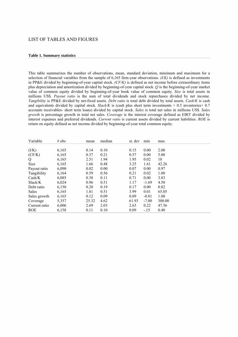
Table 1 we present a number of summary statistics for the sample under study.
< Insert Table 1 around here >
4.2 THE TRADITIONAL FRAMEWORK
In this section we follow the traditional framework and compare sample-level ICFS estimates
across ex-ante classified groups according to five different classification schemes frequently
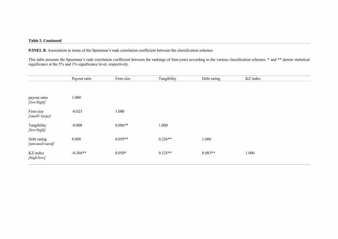
used in the literature (payout ratio, size, tangibility, debt rating and KZ-index). Table 2
analyzes the association between the different schemes in terms of ‘overlapping’ observations
(Panel A) and the Spearman’s rank correlation coefficient (Panel B). From this table, it can be
seen that the association between the different schemes is surprisingly low. For instance,
column (1) of Panel A indicates that 3,391 observations were classified in the low-payout
group, which represent ‘constrained’ observations following the traditional view. Only 29%
of these observations were also classified as being ‘constrained’ observations according to the
classification scheme size. This means that less than one third of the observations actually
obtain the same constraints-status when using two different schemes. In fact an equal share of
30% of the 3,391 observations receives the classification ‘unconstrained’ according to the
criterion size. The table shows that overlaps are rather low, indicating that different
observations are being captured in the constrained and unconstrained group, depending upon
the classification scheme that is being used. Panel B confirms this general finding by
reporting relatively low and sometimes negative associations between classification schemes
in terms of the Spearman’s rank correlation coefficient.
< Insert Table 2 around here >
Table 3 presents the sample-level ICFS estimates in the different sub-groups computed by
regressing equation (3) in the different sub-groups. In addition to the OLS-estimator, we
report the GMM-estimator developed in Arellano and Bond (1991) that accounts for
endogeneity of cash flow. As can be seen from the table, the ICFS-estimates are highly
significant for all sub-groups, but differ largely across classification schemes. In general, the
dividend payout scheme seems to reflect the finding of FHP88 in the sense that the ICFS is
higher for firms more likely to face financing constraints (i.e. the ones that pay out less
dividends). On the other hand, the other schemes seem to reflect the finding by KZ97 in the
sense that the ICFS is lower for firms more likely to suffer from financing constraints.
< Insert Table 3 around here>
These results indicate that, even in a single sample, different conclusions can be reached
depending on the classification scheme under consideration. As argued before, this is not very
surprising given the low association between the different schemes and the use of sample-
level estimates that are potentially biased because of endogeneity-issues. These findings
seriously question the traditional approach of comparing sample-level ICFS estimates across
groups and give further support to the novel approach of using firm-specific sensitivities as in
HH09, Hovakimian (forthcoming) and D’Espallier et al. (2008).
4.3 THE TWO-STEP ESTIMATION PROCEDURE
Table 4 reports the estimation results from estimating the varying coefficients model of
equation (4) using the GME-estimator. The mean firm-specific ICFS is 0.41 which is close to
what is usually found in previous studies. As can be seen, this mean value originates from a
wide dispersion of firm-specific sensitivities with a minimum value of 0 and a maximum of
1.41. A value greater than 1 means that a 1% increase in cash flow leads to an investment
response greater than 1%. Although such a disproportionately large effect is perfectly possible
from a theoretical viewpoint, only 0.6% of the firms show an investment response higher than
the cash flow shock. Additionally, the table shows that the vast majority of firms (91.8%)
have an ICFS between 0 and 0.5. This is very much in line with previous literature where
similar values for the ICFS have been found.
< Insert Table 4 around here>
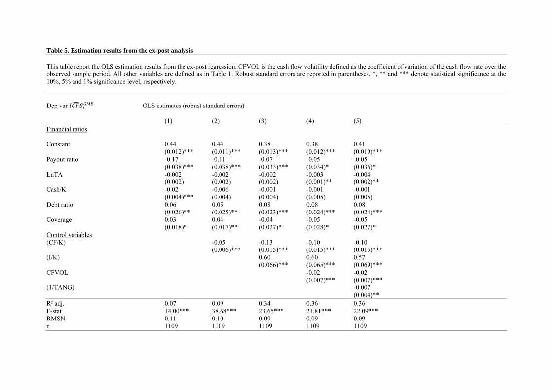
Table 5 presents the regression results from the ex-post regression analysis described in
equation (5). Column (1) shows the results when the only regressors are the financial ratios
proxying for the firm’s constraints-status. In columns (2) to (5) the different controls are
added one by one. As can be seen, the adjusted R² increases substantially from 7% to 36%
when the different controls are added, indicating a substantial gain in explanatory power of
the model. Moreover, all control variables are highly significant (1% significance level)
indicating that controlling for the level of investment, the level of cash flow, cash flow
volatility and the non-linear tangibility effect seriously improves the model fit.
< Insert Table 5 around here >
The coefficients on the financial ratios all have the expected signs. The coefficient on the
dividend payout ratio is negative indicating that firms paying out lower dividends have a
higher ICFS, which is in line with our expectations. However, when all controls are added, the
coefficient is only marginally significant at the 10% significance level.
The coefficient on lnTA is, in line with expectations, negative in all model specifications. This
means that the ICFS is higher for smaller firms and vice versa, the effect becoming
statistically significant at the 5% significance level when the different controls are added.
Interest coverage is also always significantly negative (10% level) in all model specifications,
indicating that a higher ICFS is associated with lower profitability. The effect, however, is not
particularly strong. The debt ratio is always positive and highly significant (1% significance
level), indicating that a higher ICFS is associated with a higher leverage. Finally, the
coefficient on cash/K is always negative, which is in line with expectations. However, the
coefficient looses its significance when the level of cash flow enters the regression equation
as can be seen in column (3). Likely, this result is caused by the high correlation between cash
flow and the level of cash.
Turning towards the control variables added in the different columns, it can be seen that the
coefficient on investment is always positive and highly significant at the 1% significance
level. This finding suggests that a high ICFS is associated with higher levels of investment,
ceteris paribus which is likely to reflect the obvious fact that the ICFS is low when the firm is
not investing or investing at a very low pace.
The coefficient on cash flow is significantly negative in all model specifications, indicating
that high ICFS is associated with low cash flows. This finding confirms recent research by
HH09 and Ağca and Mozumdar (2008) who show that the ICFS depends upon the cash flow-
cycle. However, our findings seem to contradict the findings by Pawlina and Renneboog
(2005) who argue that ICFS is mainly driven by managers wasting free-cash flows reflecting
an agency conflict between the managers and the shareholders of the firm. We find that ICFS
is mainly observed when cash flows are low, suggesting that ICFS is given in by the existence
of financing constraints when cash flows are low, and not by excessive cash flow spending in
high cash flow-states.
The coefficient on the volatility of cash flow is always negative and highly significant (1%
level). This finding is in line with the recent research by Cleary (2006) who finds that firms
with volatile cash flows buffer cash in order to anticipate future fluctuations in cash flow.
This buffering practice by firms facing high uncertainty about future cash flows, lowers the
sensitivity of investment to cash flow.
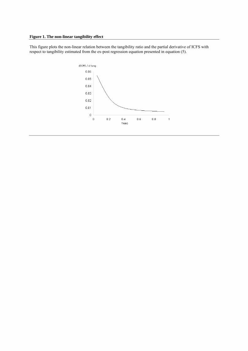
Finally the coefficient on (1/TANG) is significantly negative supporting the non-linear
tangibility effect described in Almeida and Campello (2007). In line with the non-linear
effect, we find that at low levels of tangibility, ICFS is increasing with tangibility, whereas for
high levels of tangibility, the ICFS becomes independent of asset tangibility. In Figure 1, we
plot the partial derivative of ICFS with respect to tangibility against the level of tangibility
derived from the estimated coefficient on (1/TANG) in the ex-post regression. From this
figure, the non-linear relation between asset tangibility and the ICFS is clear.
< Insert Figure 1 around here>
Overall, the results from the ex-post regression indicate that a higher ICFS is associated with
smaller firms, less profitable firms, lower dividends and higher debt ratios indicating a
positive relation between the firm’s ICFS and the existence of financing constraints. These
findings seem to support recent studies that highlight the link between the ICFS and financing
constraints such as Islam and Mozumdar (2007), Ağca and Mozumdar (2008), Carpenter and
Guariglia (2008), among others.
Additionally, a high ICFS is associated with lower levels of cash flow, higher levels of
investment, and lower cash flow volatility. These findings are in line with recent research by
HH09 and Cleary (2006). Finally, there is substantial empirical evidence of a non-linear
relation between ICFS and the level of asset tangibility. All observed effects are marginal or
isolated effects, holding constant everything else or ‘ceteris paribus’.
5. ADDITIONAL ANALYSES
5.1. COMPARISON WITH THE HH09-RESULTS
For comparison with the HH09-results we present the firm-specific sensitivities according to
the mathematical proxy suggested in HH09 in Table 6. From this table, it appears that the
mean and median ICFS are very close to zero with negative ICFS-values for a substantial part
of the sample (40.3%). The values seem to be centered around zero with a minimum of -0.81
and 0.84. These values seem to be in contrast with ICFS-values usually found in previous
studies, where the values usually vary between 0.20 and 0.50.
Additionally, the large number of negative values seems to be difficult to reconcile with
economic rationale. A negative ICFS can only occur when the firm has persistently invested
over the observed sample-period despite negative cash flows, or when a firm has persistently
de-vested over the observed sample-period despite positive cash flows. While such behavior
is perfectly possible from a theoretical viewpoint in a certain given year, it is highly unlikely
that such firm-behavior occurs over longer sample-periods. Therefore, it is hard to maintain
that around 40% of the firms have consistently invested despite negative cash flows or vice
versa, over the observed sample period of 20-years studied in HH09.
< Insert Table 6 around here >
In Table 7 we report the regression results from regressing the HH09-proxy on the variables
suggested in section 3. In the columns (2) to (5) the different controls are added one by one. It
can be seen that neither the financial variables nor the different controls show any statistically
significant relation with the HH09-proxy. Moreover, the F-statistics denote that the regression
models are jointly insignificant (the only exception being the full-model in column (5) where
the F-stat denotes joint significance at the 10% significance level). This means that none of
the observables suggested to have an impact on the ICFS according to a number of previous
studies show any significance.
This finding together with the previous finding that the HH09-proxy returns values for the
firm-specific ICFS that are not in line with economic theory, nor with previous research,
seriously questions whether the mathematical HH09-proxy provides a good firm-varying
equivalent for the investment-cash flow sensitivity.
< Insert Table 7 around here >
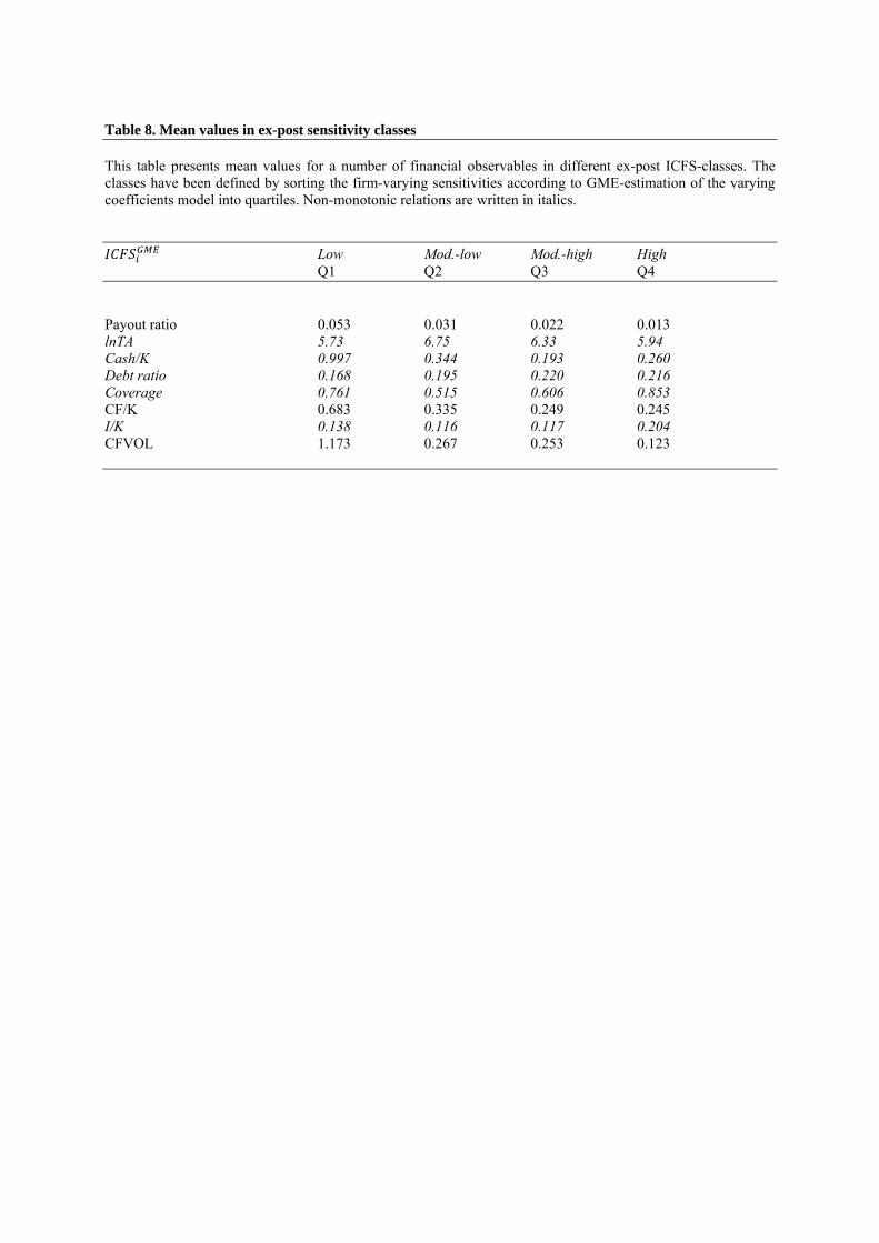
5.2. MEAN VALUES IN DISCRETE ICFS-CLASSES
For comparison with previous studies, we report mean values for the different observables in
discrete ICFS-classes going from ‘low sensitivity’ (first quartile) to ‘high sensitivity’ (4th
quartile) in Table 8. This is essentially the same analysis as presented in previous studies
focusing on firm-varying sensitivities such as D’Espallier et al. (2008) and HH09. In general,
the same relations emerge for the different financial ratios and control variables that were
tested in the ex-post analysis. In that respect, this analysis provides a further robustness check
for the analysis presented in the previous section. Again the ICFS seems to be negatively
related with the dividend payout ratio, firm size, cash, cash flow, interest coverage and cash
flow volatility and positively related with debt ratio and the investment rate.
However, for most of the variables (such as lnTA, cash/K, debt ratio, coverage and I/K) the
average value first increases and then decreases with the sensitivity-classes or vice versa.
Such evidence has been identified in previous literature as evidence of a non-monotonic
relation between the ICFS and a certain observable. However, it should be noted that this
analysis does not satisfy ‘ceteris paribus’-assumptions i.e. it does not control for other firm-
observables. Secondly, this analysis looks only at mean-values i.e. provides an aggregation of
the observable in the various sensitivity-classes. Therefore, we believe that the ex-post
regression analysis provides considerable improvements over the conventional analysis of
investigating differences in mean-values between different ICFS-classes.
< Insert Table 8 around here >
6. CONCLUSIONS, DISCUSSION AND LIMITATIONS
A new stream of literature estimates firm-specific investment-cash flow sensitivities rather
than sample-level sensitivities when studying empirically the concept of financing constraints.
These studies emphasize three main benefits of using firm-varying sensitivities. First, sample-
level estimates might be seriously biased because of endogeneity of cash flow in the
underlying investment equation. Secondly, using firm-varying sensitivities offers the
possibility to study the drivers of the ICFS without having to rely on ex-ante classification
into discrete sub-groups. Finally, estimating firm-varying sensitivities accounts for firm-
heterogeneity instead of statistically neutralizing all firm-level variation into a single sample-
level estimate.
The aim of this paper is to go along with these new advances and to propose a number of
important improvements to the existing studies that deploy this new approach. First, we argue
that the mathematical proxy developed in HH09 looks only at the levels of cash flow and
investment, thereby ignoring the original definition of investment-cash flow sensitivity. We
suggest estimating the firm-specific ICFS by allowing for slope-heterogeneity in the
underlying investment equation. This approach yields a firm-level sensitivity that takes into
account the underlying model dynamics and is in line with the original definition i.e. the
investment response due to a change in cash flow holding constant the level of investment
opportunities.
Secondly, we argue that the use of firm-specific sensitivities provides a unique opportunity to
study the drivers of the ICFS using regression analysis. The regression analysis allows us to
study marginal effects while controlling for other observables that have been shown to have
an impact on the ICFS. Additionally, we can study non-linear effects by incorporating higher
order coefficients into the regression equation. We believe that this analysis provides
important benefits over the traditional approach in which averages are compared across ex-
post defined sensitivity-classes.
This new estimation framework is put to the test using a large longitudinal sample of 1,233
US-based listed firms in a Q –investment model augmented with cash flow, time and firm-
fixed effects. The main results can be summarized as follows: First, when analyzing a number
of financial ratios that proxy for the firm’s constraint-status, we find that the ICFS is
negatively related with the firm’s dividend payout, size, profitability and liquidity and
positively related with the firm’s debt ratio, ceteris paribus, indicating a tight link between the
ICFS and the existence of financing constraints. These results are in line with recent findings
by Islam and Mozumdar (2007), Carpenter and Guariglia (2008), Guariglia (2008), Ağca and
Mozumdar (2008), among others.
Secondly, the ICFS is significantly negatively related to cash flow, ceteris paribus, suggesting
that a positive ICFS emerges mainly when cash flows are low. This finding reflects the view
of recent studies such as HH09 and Pawlina and Renneboog (2005) that the cash flow-cycle is
an important determinant of the firm’s ICFS. However, our findings are contrary to the
findings of Pawlina and Renneboog (2005) who find that ICFS is mainly caused by over-
investment due to managers wasting free cash flow in high-cash flow years. Rather, our
results indicate that a high ICFS is mainly observed when cash flows are low, suggesting that
mainly under-investment in the presence of low cash flows is driving the ICFS.
Thirdly, we find that the ICFS is negatively related to the firm’s cash flow volatility, ceteris
paribus. This finding confirms the results by Cleary (2006) who finds that firms with more
volatile cash flows have the tendency to buffer cash in order to cope with future uncertain
cash flow fluctuations. This cash buffering practice has a negative impact on the ICFS.
Finally, we find empirical support for the non-linear tangibility effect described in Almeida
and Campello (2007). Specifically, at low levels of tangibility the ICFS increases with the
level of tangibility because of the credit multiplier effect. At high levels of tangibility the
marginal impact of tangibility on the ICFS decreases towards zero.
We believe that this study entails a number of implications that might be important for the
empirical literature on financing constraints. First, we show that estimating firm-level
sensitivities offers a number of important benefits over the traditional framework of
comparing sample-level estimates across groups. As such, we highly support this new
approach that might be an important element in the debate on the usefulness of estimating
investment-cash flow sensitivities to capture financing constraints. Secondly, we show that
investment models with firm-varying slopes can be estimated using modern econometrical
techniques. As such, we can compute firm-level sensitivities that take into account the
underlying model dynamics and stay close to the original definition, instead of computing
mathematical proxies that look mainly at levels of investments and cash flows. Finally, we
show that firm-specific sensitivities provide a unique opportunity to investigate the drivers of
the sensitivity, thereby opening up the black-box of investment-cash flow sensitivities. Using
an ex-post regression offers the possibility to look at marginal effects and to study non-linear
effects.
Of course, this study also comes with a number of important caveats that should be kept in
mind and that offer a number of interesting routes for future research. First, the augmented Q
model of investment, although widely studied, is not the only investment paradigm that could
be used, and, like any theoretical model, comes with a number of limitations. For instance,
Gomes (2001) and Cummins et al. (2006) question whether Tobin’s Q is an adequate proxy to
capture investment opportunities, and whether the ICFS is not merely an artifact of cash flow
capturing investment opportunities rather than signaling financing frictions. Our analysis
shows that the ICFS, originating from this Q model, is related to the firm’s constraints-status
and therefore is not just merely an artifact of cash flow capturing investment opportunities.
However, it would be interesting to see whether the results hold for other investment
paradigms that have been suggested in the literature such as the neoclassical investment
model (see for instance Guariglia, 2008) or the sales accelerator model (see for instance
Kadapakkam et al., 1998).
Secondly, although the ex-post regression includes a wide variety of financial ratios as well as
control variables that have a longstanding tradition in the literature, there might be other
observables associated with the ICFS. In fact, the R² adjusted in the ex-post regression
indicates that around 36% of cross-sectional is consistently explained by our observables.
Therefore, a substantial part of residual cross-sectional variation remains unexplained by the
observables used in the current study. Future research could aim at further unpacking the
black-box of investment-cash flow sensitivities by analyzing the impact of other firm-
characteristics such as managerial decision making (see for instance Bloom and Van Reenen,
2007) or reluctance to borrow (see for instance Howorth, 2001) on the ICFS.
Finally, in this study, the GME-estimator has been used to estimate the parameters of the
varying-coefficients model. It should be noted, though, that this is not the only estimator
suited to tackle slope heterogeneity in the context of panel data. For instance, full Bayesian
econometrics (see for instance Lancaster, 2004) or mixed models for longitudinal data (see for
instance Verbeke and Molenberghs, 1999) could also be used to estimate the model
parameters. In that respect, it would be interesting to see whether the results would hold for
these alternative estimation techniques.
APPENDIX ON ENTROPY ECONOMETRICS
The GME-estimator is a Quasi-Bayesian estimation technique based upon the principles of
Information Theory. The estimator is developed and thoroughly discussed in the book by
Golan et al. (1996). Applications of the GME-estimator to various fields in economics can be
found in Judge and Golan (1992); Léon et al. (1999); Fraser (2000), Peeters (2004), among
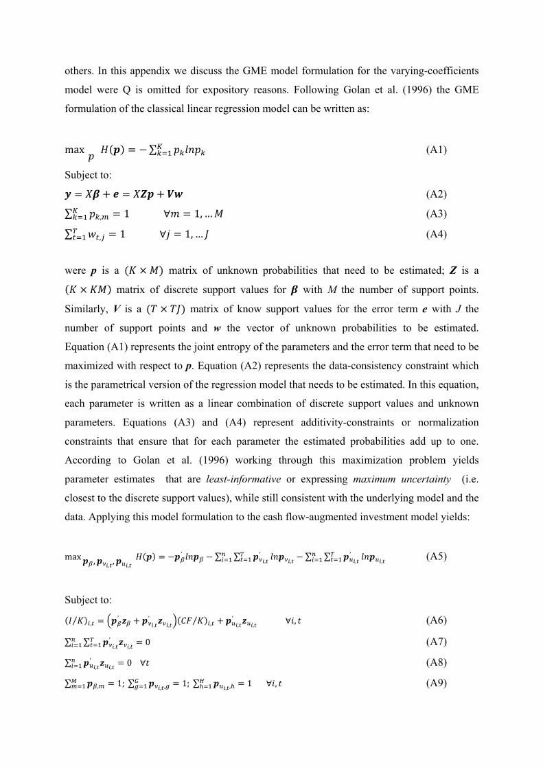
others. In this appendix we discuss the GME model formulation for the varying-coefficients
model were Q is omitted for expository reasons. Following Golan et al. (1996) the GME
formulation of the classical linear regression model can be written as:
max ∑ (A1)
Subject to:
(A2)
∑ , 1 1, … (A3)
∑ , 1 1, … (A4)
were p is a matrix of unknown probabilities that need to be estimated; Z is a
matrix of discrete support values for with M the number of support points.
Similarly, V is a matrix of know support values for the error term e with J the
number of support points and w the vector of unknown probabilities to be estimated.
Equation (A1) represents the joint entropy of the parameters and the error term that need to be
maximized with respect to p. Equation (A2) represents the data-consistency constraint which
is the parametrical version of the regression model that needs to be estimated. In this equation,
each parameter is written as a linear combination of discrete support values and unknown
parameters. Equations (A3) and (A4) represent additivity-constraints or normalization
constraints that ensure that for each parameter the estimated probabilities add up to one.
According to Golan et al. (1996) working through this maximization problem yields
parameter estimates that are least-informative or expressing maximum uncertainty (i.e.
closest to the discrete support values), while still consistent with the underlying model and the
data. Applying this model formulation to the cash flow-augmented investment model yields:
max , , , , ′ ∑ ∑
,′
,∑ ∑
,′
, (A5)
Subject to:
⁄ ,′
,′
,⁄ , ,
′, , (A6)
∑ ∑,
′, 0 (A7)
∑,
′, 0 (A8)
∑ , 1; ∑ , , 1; ∑, , 1 , (A9)
In this constrained maximization problem (A5) is again the joint entropy of the parameters
and the error term that needs to be maximized in order to obtain ‘least-informative’ parameter
estimates closest to the support values. (A6) represents the data-consistency constraint which
is the parametrical version of cash flow –augmented investment model where the unknown
parameters are written as linear combinations of the unknown probabilities and discrete
support values. Equation (A7) is a mean preservation constraint that ensures a consistent
mean cash flow coefficient so that ‘shrinkage’ is avoided (Golan et al., 1996, pg. 163).
Equation (A8) imposes a mean zero error in each year so that covariates and errors are
determined exogenously. Equation (A9) represents the additivity-constraints that ensure that
for each parameter to be estimated, the estimated probabilities add up to one.
The posterior parameter estimates can be recovered by recombining the optimal probabilities
and the discrete support values in a linear way as follows:
′ (A10)
, ,′
, (A11)
, ,′
, (A12)
In line with the Bayesian research paradigm, the GME estimator combines both prior
information and data in order to form a posterior parameter estimate. Following prior
information sets were used:
0,1 ′ (A13)
, 10,10 ′ (A14)
, 3 / , , 3 / , (A15)
Equation (A13) expresses that the supports for the mean cash flow coefficient were chosen to
be distributed symmetrically around 0.50. Equation (A14) expresses a wide support value for
the shrinkage-parameter νi,t and (A15) expresses that the priors for the error term are bounded
by three times the empirical standard deviation of the dependent variable, consistent with the
‘three-sigma’ rule suggested in Pukelsheim (1994).
For the Bayesian researcher, combining prior information with data is a natural way to
enhance parameter estimates. However, for researchers not adhering to the Bayesian
paradigm, an objection often raised is the sensitivity of the results to using different
information sets. While it is true that the prior information plays a role in the estimation
process, its effect should not be overstated. First, when samples are sufficiently large, the
information contained in the data often overshadows the information content provided by the
non-sample information (Lancaster, 2004). Secondly, with the prior information sets wide
enough and containing the true value of the parameter, the researcher imposes a minimal
restriction and maximizes the influence of the data on posterior estimates (Koop, 2003).
Therefore, we do not expect the support values to have a large impact on the GME-estimates.
However, in order to investigate the sensitivity of the estimates to the use of alternative prior
information sets, we have conducted a sensitivity-analysis using the dual cross-entropy
formulation in Golan et al. (1996). This procedure calculates the parameter estimates for 100
different prior values drawn randomly out of a distribution of choice. Specifically, 100 spike
priors for β were drawn from a uniform distribution U(-1,1), a uniform distribution (-10,10)
and a normal distribution N(0.5,0.3). This exercise reveals that the results are extremely
insensitive to the use of different prior sets, which was to be expected given the large number
of data points and the wide intervals that were used. Results from this exercise are available
upon request.
REFERENCES
Ağca, S. and Mozumdar, A., ’The impact of capital market imperfections on investment-cash
flow sensitivity’, Journal of Banking and Finance, Vol. 32, 2008, pp. 207-216.
Allayannis, G. and Mozumdar, A., ‘The impact of negative cash flow and influential
observations on investment-cash flow sensitivity estimates’, Journal of Banking and
Finance, Vol. 28, 2004, pp. 901-930.
Almeida, H. and Campello, M., ‘Financial constraints, asset tangibility, and corporate
investment’, Review of Financial Studies, Vol. 20, 2007, pp. 1429-1460.
Arellano, M. and Bond, S.R., ‘Some tests of specification for panel data: Monte Carlo
Evidence and an Application to Employment Equations’, The Review of Economic
Studies, Vol. 58, 1991, pp. 277-297.
Ascioglu, A., Hedge, S.P. and McDermott, J.B., ‘Information asymmetry and investment-cash
flow sensitivity’, Journal of Banking and Finance, Vol. 32, 2008, pp. 1036-1048.
Bloom, N., Bond, S. and Van Reenen, J., ‘Uncertainty and investment dynamics’, Review of
Economic Studies, Vol. 74, 2006, pp. 391-415.
Bond, S. and Cummins, J., ‘Noisy share prices and the Q model of investment’, Institute for
Fiscal Studies, Discussion paper no 22, 2001.
Bond, S., Elston, J.A., Mairesse, J. and Mulkay, B., ‘Financial factors and investment in
Belgium, France, Germany, and the United Kingdom: A comparison using company
panel data’, The Review of Economics and Statistics, Vol. 85, 2003, pp. 153-165.
Calomiris, C., Himmelberg, C. and Wachtel, P., ’Internal finance and firm-level investment:
Evidence from the undistributed profits tax of 1936-1937’, Journal of Business, Vol.
68, 1995, pp. 443-482.
Carpenter, R.E. and Guariglia, A., ‘Cash flow, investment and investment opportunities: new
tests using UK panel data’, Journal of Banking and Finance, Vol. 32, 2008, pp. 1894-
1906.
Carpenter, R.E. and Petersen, B.C., ‘Is the growth of small firms constrained by internal
finance?’, The Review of Economics and Statistics, Vol. 84, 2002, pp. 298-309.
Cleary, S., ‘The relationship between firm investment and financial status’, Journal of
Finance, Vol. 54, 1999, pp. 673-691.
Cleary, S., ‘International corporate investment and the relationships between financial
constraints measures’, Journal of Banking and Finance, Vol. 30, 2006, pp. 1559-1580.
Cleary, S. and D’Espallier, B., ‘Financial constraints and investment: an alternative empirical
framework’, Anales de Estudios Económicos y Empresariales, Vol. 17, 2007, pp. 1-
41.
Cummins, J., Hasset, K. and Oliner, S., ‘Investment behaviour, observable expectations and
internal funds’, American Economic Review, Vol. 96, 2006, pp. 796-810.
Deloof, M., ‘Internal capital markets, bank borrowing, and financial constraints: evidence
from Belgian firms’, Journal of Business Finance and Accounting, Vol. 25, 1998, pp.
945-968.
D’Espallier, B., Vandemaele, S. and Peeters, L., ‘Investment-cash flow sensitivities or cash-
cash flow sensitivities? An evaluative framework for measures of financial
constraints’, Journal of Business Finance and Accounting, Vol. 35, 2008, pp. 943-
968.
Erickson, T. and Whited, T., ‘Measurement error and the relationship between investments
and Q’, Journal of Political Economy, Vol. 108, 2000, pp. 1027-1057.
Fazzari, S.M., Hubbard, R.G. and Petersen, B.C., ‘Financing constraints and corporate
investment’, Brookings Papers on Economic Activity, Vol. 1, 1988, pp. 141-195.
Fraser, I., 2000, ‘An application of maximum entropy estimation: the demand for meat in the
United Kingdom’, Applied Economics, Vol. 32, 2000, pp. 45-59.
Gilchrist, S. and C.P. Himmelberg, C.P., ‘Evidence on the role of cash flow for investment’,
Journal of Monetary Economics, Vol. 36, 1995, pp. 541-572.
Golan, A., Judge, G.G. and Miller D., ‘Maximum Entropy Econometrics: Robust Estimation
with Limited Data’, John Wiley & Sons Ltd, Indianapolis, 1996.
Gomes, J., ‘Financing investment’, American Economic Review, Vol. 91, 2001, pp. 1263-
1285.
Guariglia, A., ‘Internal financial constraints, external financial constraints and investment
choice: Evidence from a panel of UK firms’, Journal of Banking and Finance, Vol.
32, 2008, pp. 1795-1809.
Hoshi, T., Kashyap, A. and Scharfstein, D., ‘Corporate structure, liquidity and investment:
Evidence from Japanese industrial groups’, Quarterly Journal of Business and
Finance, Vol. 106, 1991, pp. 33-60.
Hovakimian, G., ‘Determinants of investment cash flow sensitivity’, Financial Management,
forthcoming.
Hovakimian, A. and Hovakimian, G., ‘Cash flow sensitivity of investment’, European
Financial Management, Vol. 15, 2009, pp. 47-65.
Islam, S.S. and Mozumdar, A., ‘Financial market development and the importance of
internal cash: Evidence from international data’, Journal of Banking and Finance,
Vol. 31, 2007, pp. 641-658.
Howorth, C., ‘Small firm’s demand for finance: A research note’, International Small
Business Journal, Vol. 19, 2001, pp. 78-86.
Judge, G. and Golan, A., ‘Recovering information in the case of ill-posed inverse problems
with noise’, MIMEO Research paper, University of California, Berkely, 1992.
Kadapakkam, P.R., Kumar, P.C. and Riddick, L.A., ‘The impact of cash flows and firm size
on investment: The international evidence’, Journal of Banking and Finance, Vol. 22,
1998, pp. 293-320.
Kaplan, S.N. and Zingales, L., ‘Do investment-cash flow sensitivities provide useful measures
of financing constraints?’, Quarterly Journal of Economics, Vol. 112, 1997, pp. 169-
215.
Kashyap, A., Lamont, O. and Stein, J., ‘Credit conditions and the cyclical behavior of
inventories’, Quarterly Journal of Economics, Vol. 109, 1994, pp. 565-592.
Koop, G., ‘Bayesian econometrics’, Wiley-Interscience, New Jersey, 2003.
Lancaster, T., ‘An introduction to modern Bayesian econometrics’, Blackwell publishing ltd,
New Jersey, 2004.
Léon, Y., Peeters, L., Quinqu, M. and Surry, Y., ‘The use of Maximum Entropy to estimate
input-output coefficients from regional farm accounting data’, Journal of Agricultural
Economics, Vol. 50, 1999, pp. 425-439.
Lyandres, E., ‘Costly external financing, investment timing and investment-cash flow
sensitivity’, Journal of Corporate Finance, Vol. 13, 2007, pp. 959-980.
Moyen, N., ‘Investment- cash flow sensitivities: constrained versus unconstrained
firms’, Journal of finance, Vol. 59, 2004, pp. 2061-2092.
Pawlina, G. and Renneboog, L., ‘Is investment cash flow sensitivity caused by the
agency costs or asymmetric information? Evidence from the UK’, European Financial
Management, Vol. 11, 2005, pp. 483-513.
Peeters, L., ‘Estimating a random-coefficients sample-selection model using generalized
maximum entropy’, Economics Letters, Vol. 84, 2004, pp. 87-92.
Pukelsheim, F., ‘The three sigma rule’, The American Statistician, Vol. 48, 1994, pp. 88-91.
Rauh, J.D., ‘Investment and financing constraints: evidence from the funding of corporate
pension plans’, The Journal of Finance, Vol. 61, 2006, pp. 33-71.
Verbeke, G. and Molenberghs, G., ‘Linear mixed models for longitudinal data’, Springer-
Verlag, New York, 1999.
Whited, T. and Wu, G., ‘Financial constraints risk’, The Review of Financial Studies, Vol. 19,
2006, pp. 531-558.
LIST OF TABLES AND FIGURES
Table 1. Summary statistics
This table summarizes the number of observations, mean, standard deviation, minimum and maximum for a selection of financial variables from the sample of 6,165 firm-year observations. (I/K) is defined as investments in PP&E divided by beginning-of-year capital stock. (CF/K) is defined as net income before extraordinary items plus depreciation and amortization divided by beginning-of-year capital stock. Q is the beginning-of-year market value of common equity divided by beginning-of-year book value of common equity. Size is total assets in millions US$. Payout ratio is the sum of total dividends and stock repurchases divided by net income. Tangibility is PP&E divided by net-fixed assets. Debt ratio is total debt divided by total assets. Cash/K is cash and equivalents divided by capital stock. Slack/K is (cash plus short term investments + 0.5 inventories+ 0.7 accounts receivables- short term loans) divided by capital stock. Sales is total net sales in millions US$. Sales growth is percentage growth in total net sales. Coverage is the interest coverage defined as EBIT divided by interest expenses and preferred dividends. Current ratio is current assets divided by current liabilities. ROE is return on equity defined as net income divided by beginning-of-year total common equity.
Table 2. Association between ‘popular’ ex-ante classification schemes PANEL A. Association in terms of percentage ‘overlapping’ observations This table presents the number of observations within each sub-group on the diagonal elements as well as the percentage overlaps between the sub-groups on the off-diagonal element. Groups were formed as follows: first, observations were ranked annually according to their payout ratio, size, tangibility, and KZ-index. Then observations in the upper 30% tail were designated high payout, large, high tangibility, high KZ. Observations in the lower 30% tail were designated low payout, small, low tangibility and low KZ. For the debt-rating scheme, the observation is classified in the unrated subgroup if the firm had no debt rating in that particular year, and rated if the firm did have a debt-rating in that particular year. Payout ratio Firm size Tangibility Debt rating KZ index low high small large low high unrated rated high low payout ratio low 3,391 high 2,754 Firm size small 29.13% 31.05% 1,845 large 30.61% 29.48% 1,860 Tangibility low 29.69% 29.95% 35.50% 28.98% 1,835 high 30.49% 29.74% 25.42% 29.35% 1,860 Debt rating unrated 67.97% 67.25% 72.25% 66.77% 81.14% 56.45% 4,164 rated 32.03% 32.75% 27.75% 33.23% 18.86% 43.55% 2,001 KZ-index high 21.35% 40.56% 33.71% 28.39% 34.82% 27.47% 31.63% 26.39% 1,783 low 36.53% 19.61% 28.62% 29.46% 24.90% 32.47% 27.23% 32.43% 1,845
Table 2. Continued PANEL B. Association in terms of the Spearman’s rank correlation coefficient between the classification schemes This table presents the Spearman’s rank correlation coefficient between the rankings of firm-years according to the various classification schemes. * and ** denote statistical significance at the 5% and 1% significance level, respectively. Payout ratio Firm size Tangibility Debt rating KZ index payout ratio 1.000 [low/high] Firm size -0.025 1.000 [small/ large] Tangibility -0.008 0.086** 1.000 [low/high] Debt rating 0.008 0.059** 0.226** 1.000 [unrated /rated] KZ-index -0.304** 0.050* 0.125** 0.083** 1.000 [high/low]
Table 3. OLS and GMM estimation results for the ICFS in different sub-samples This table reports OLS and GMM estimates from regression equation (3) for the different sub-samples. Robust standard errors are provided in parentheses and *,** and *** denote statistical significance at the 10%, 5% and 1% significance level. The χ² statistic for the GMM estimation denotes the joint significance of the model. Dep. var. (I/K) OLS GMM CF/K Q R²adj CF/K Q χ²-stat All firms 0.18** 0.008*** 0.19 0.16*** 0.006** 39.82*** (0.006) (0.002) (0.009) (0.002) Payout ratio Low 0.20*** 0.010*** 0.26 0.22*** 0.003 46.43*** (0.008) (0.002) (0.012) (0.003)
Table 4. GME estimation results of the varying coefficients model This table presents a number of statistics for the GME estimates of the firm-varying ICFS estimated from equation (4). P(x) represents the xth percentile. The pseudo-R² is defined as the squared correlation between actual and predicted (fitted) values of the dependent variable. firm-specific ICFS mean 0.41 st.dev. 0.11 minimum 0.00 maximum 1.41 P(0.05) 0.28 P(0.10) 0.32 P(0.30) 0.39 median 0.41 P(0.60) 0.42 P(0.70) 0.43 P(0.90) 0.48 P(0.95) 0.56 Proportion in [0, 0.50[ 91.8% Proportion in [0.50, 1] 7.60% Proportion > 1 0.60% Mean lower 30% tail 0.32 Mean middle 40% area 0.41 Mean upper 30% tail 0.48 Other model parameters: β (fixed) 0.417 β0 (constant) 0.008 β2 (Tobin’s Q) 0.001 Pseudo-R²: no fixed effects 0.63 time-fixed effects incl. 0.65 firm-fixed effects incl. (full model) 0.71
Table 5. Estimation results from the ex-post analysis This table report the OLS estimation results from the ex-post regression. CFVOL is the cash flow volatility defined as the coefficient of variation of the cash flow rate over the observed sample period. All other variables are defined as in Table 1. Robust standard errors are reported in parentheses. *, ** and *** denote statistical significance at the 10%, 5% and 1% significance level, respectively. Dep var OLS estimates (robust standard errors) (1) (2) (3) (4) (5) Financial ratios Constant 0.44 0.44 0.38 0.38 0.41 (0.012)*** (0.011)*** (0.013)*** (0.012)*** (0.019)*** Payout ratio -0.17 -0.11 -0.07 -0.05 -0.05 (0.038)*** (0.038)*** (0.033)*** (0.034)* (0.036)* LnTA -0.002 -0.002 -0.002 -0.003 -0.004 (0.002) (0.002) (0.002) (0.001)** (0.002)** Cash/K -0.02 -0.006 -0.001 -0.001 -0.001 (0.004)*** (0.004) (0.004) (0.005) (0.005) Debt ratio 0.06 0.05 0.08 0.08 0.08 (0.026)** (0.025)** (0.023)*** (0.024)*** (0.024)*** Coverage 0.03 0.04 -0.04 -0.05 -0.05 (0.018)* (0.017)** (0.027)* (0.028)* (0.027)* Control variables (CF/K) -0.05 -0.13 -0.10 -0.10 (0.006)*** (0.015)*** (0.015)*** (0.015)*** (I/K) 0.60 0.60 0.57 (0.066)*** (0.065)*** (0.069)*** CFVOL -0.02 -0.02 (0.007)*** (0.007)*** (1/TANG) -0.007 (0.004)** R² adj. 0.07 0.09 0.34 0.36 0.36 F-stat 14.00*** 38.68*** 23.65*** 21.81*** 22.09*** RMSN 0.11 0.10 0.09 0.09 0.09 n 1109 1109 1109 1109 1109
Table 6. Firm-specific ICFS according to HH09 This table presents a number of statistics for the firm-varying ICFS computed according to the definition suggested in HH09. The ICFS is defined as the difference between the cash flow weighted time-series average investment and its simple arithmetic time-series average investment. P(x) represents the xth percentile. firm-specific ICFS mean 0.006 st.dev. 0.057 minimum -0.81 maximum 0.84 P(0.05) -0.027 P(0.10) -0.012 P(0.30) -0.001 median 0.0008 P(0.60) 0.002 P(0.70) 0.005 P(0.90) 0.023 P(0.95) 0.046 Proportion < 0 40.3% Proportion in [0, 0.50[ 58.8% Proportion in [0.50, 1] 0.90% Mean lower 30% tail -0.02 Mean middle 40% area 0.001 Mean upper 30% tail 0.035
Table 7. Regressing the HH09-proxy on the firm-observables This table report the OLS estimation results from regressing the firm-varying ICFS computed as in HH09 on the observable measures suggested to have an impact on the ICFS in section 3.2. Robust standard errors are reported in parentheses. *, ** and *** denote statistical significance at the 10%, 5% and 1% significance level, respectively. Dep var OLS estimates (robust standard errors) (1) (2) (3) (4) (5) Financial ratios Constant -0.003 -0.002 -0.014 -0.015 -0.017 (0.005) (0.006) (0.011) (0.012) (0.025) Payout ratio -0.03 -0.04 -0.06 -0.02 -0.02 (0.011)** (0.04) (0.023) (0.023) (0.023) LnTA 0.0008 0.0009 0.0008 0.0006 -0.0007 (0.0008) (0.0009) (0.007) (0.0009) (0.0011) Cash/K 0.013 0.007 0.008 0.01 0.01 (0.0051 (0.007) (0.007) (0.008) (0.008) Debt ratio -0.003 -0.003 0.002 0.004 0.005 (0.011) (0.011) (0.011) (0.011) (0.013) Coverage 0.02 0.019 0.004 0.001 0.002 (0.021) (0.021) (0.027) (0.025) (0.024) Control variables (CF/K) 0.004 -0.013 -0.003 -0.003 (0.018) (0.013) (0.013) (0.013) (I/K) 0.11 0.11 0.11 (0.071) (0.071) (0.085) CFVOL -0.007 -0.007 (0.012) (0.008) (1/TANG) 0.0007 (0.005) R² adj. 0.02 0.02 0.05 0.06 0.06 F-stat 1.33 1.11 1.34 2.42 3.01* RMSN 0.05 0.05 0.05 0.05 0.05 n 1104 1104 1104 1104 1104
Table 8. Mean values in ex-post sensitivity classes This table presents mean values for a number of financial observables in different ex-post ICFS-classes. The classes have been defined by sorting the firm-varying sensitivities according to GME-estimation of the varying coefficients model into quartiles. Non-monotonic relations are written in italics.
Figure 1. The non-linear tangibility effect This figure plots the non-linear relation between the tangibility ratio and the partial derivative of ICFS with respect to tangibility estimated from the ex-post regression equation presented in equation (5).


![Student’s t Sensitivities: GreeksfortheGossetFormulaearXiv:1003.1344v2 [q-fin.PR] 16 Jul 2010 Student’st-DistributionBasedOption Sensitivities: GreeksfortheGossetFormulae Daniel](https://static.documents.pub/doc/80x56/5fa1f5e65b7bfb78540e321a/studentas-t-sensitivities-greeksforthegossetformulae-arxiv10031344v2-q-finpr.jpg)


