NASA Contractor Report 4698 R95-95707 : Unsteady Aerodynamic Models for Turbomachinery Aeroelastic and Aeroacoustic Applications Joseph M. Verdon, Mark Barnett, and Timothy C. Ayer CONTRACT NAS3--25425 NOVEMBER 1995 :iL i" National Aeronautics and ' Space Administration : 1,7: _J https://ntrs.nasa.gov/search.jsp?R=19960020548 2018-06-16T04:13:05+00:00Z
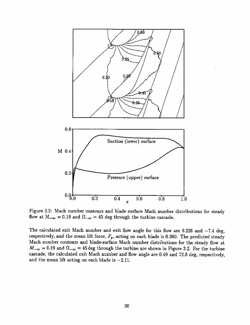
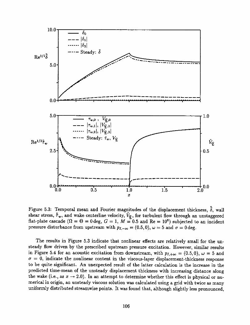
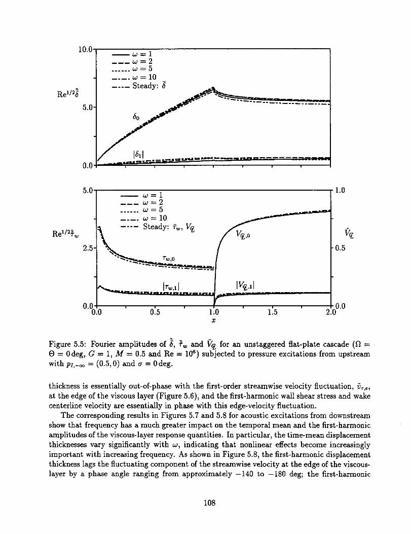
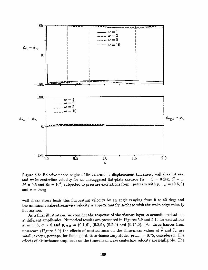
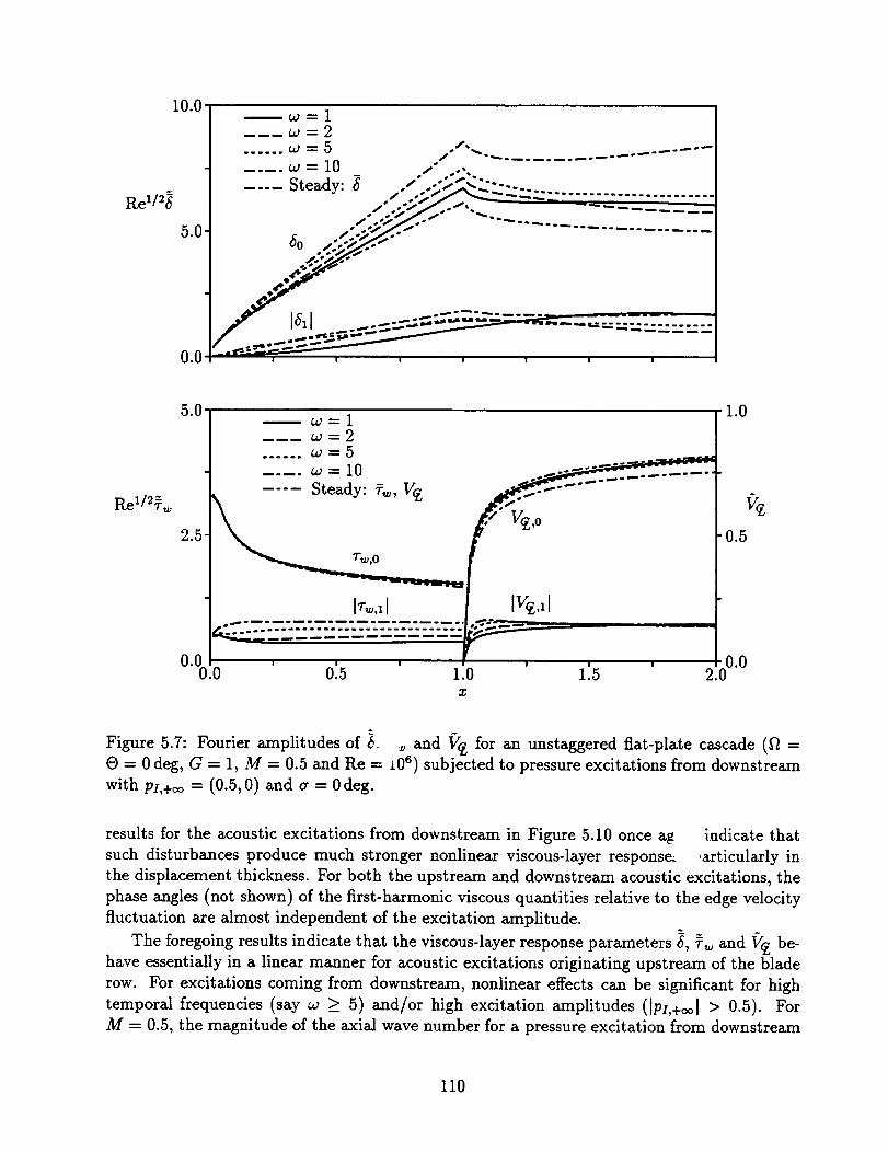
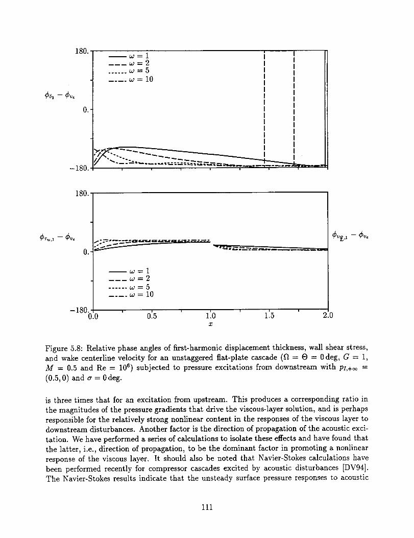
stress, and wake centerline velocity for an unstaggered flat-plate cascade (f_ = 0 = 0 deg,
G = 1, M = 0.5 and Re = l0 s) subjected to pressure excitations from downstream with
pI,+oo = (0.5, 0) and cr = 0 deg.
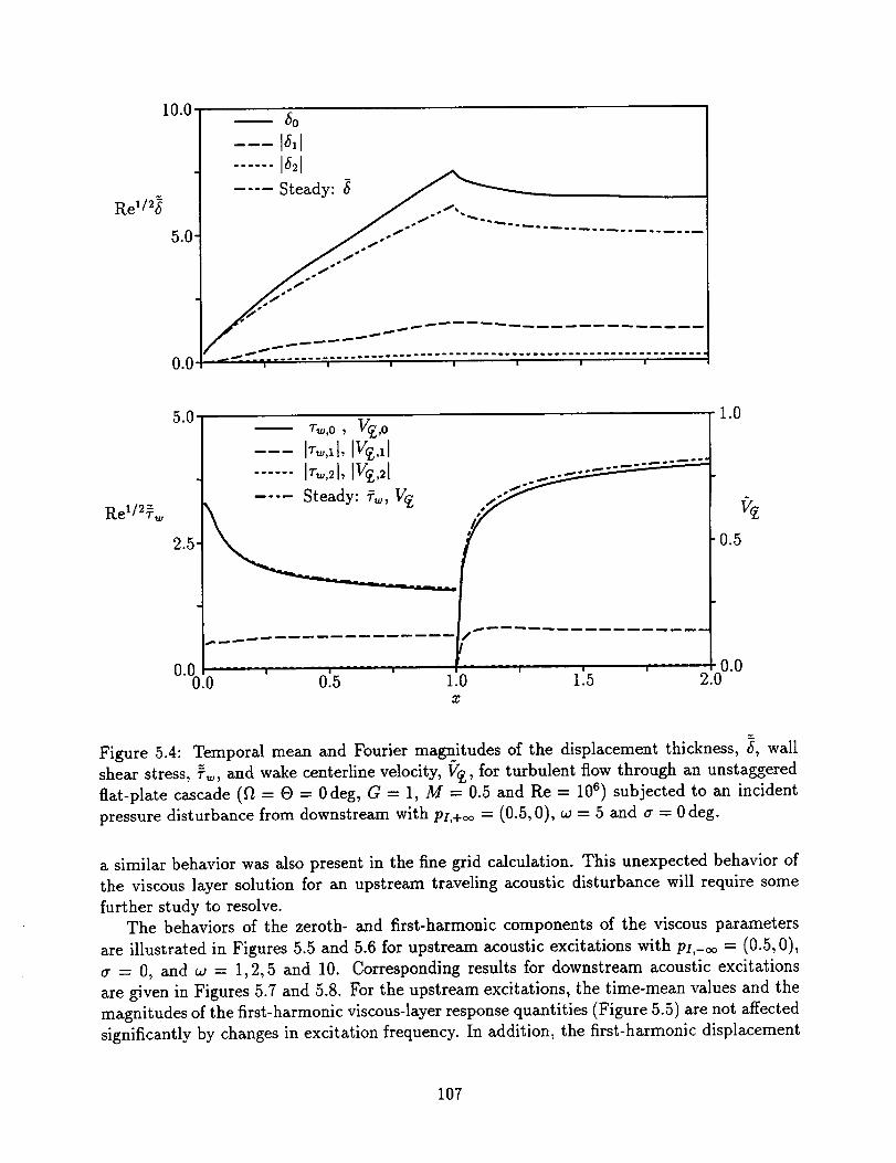
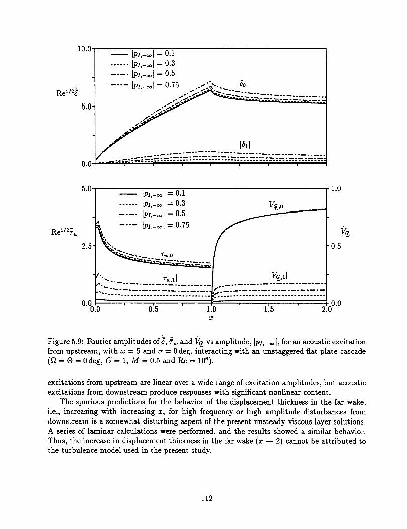
Figure 5.9. Fourier amplitudes of _, _r,_ and 17_ vs amplitude, Ip,,-.ol, for an acoustic
excitation from upstream, with w = 5 and a = 0 deg, interacting with an unstaggered flat-
plate cascade (_ = O = 0 deg, G = 1, M = 0.5 and Re = 106).
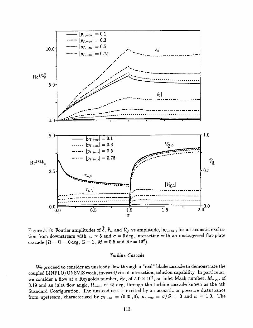
Figure 5.10. Fourier amplitudes of _, r_ and Vg vs amplitude, [px,+ool, for an acoustic
excitation from downstream with, w = 5 and a = 0 deg, interacting with an unstaggered
flat-plate cascade (fl = O = 0 deg, G = 1, M = 0.5 and Re = 106).
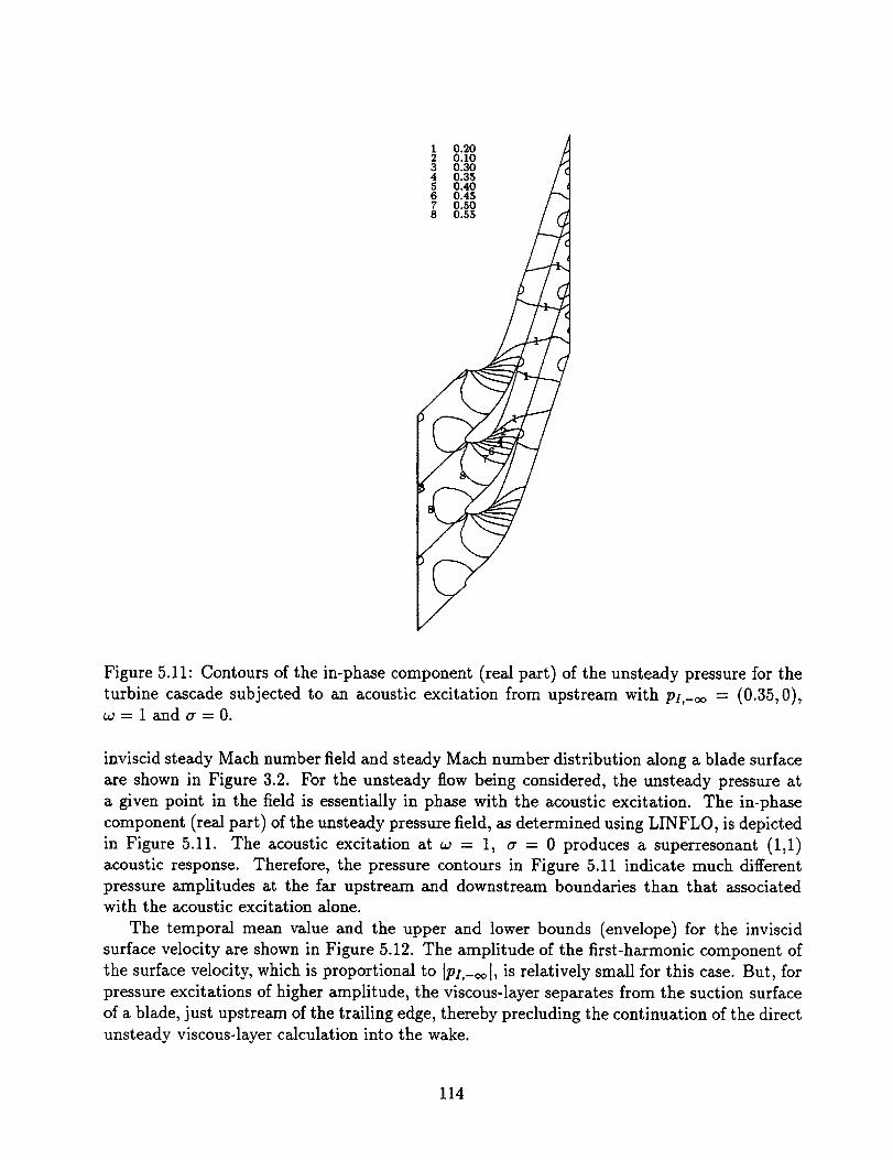
Figure 5.11. Contours of the in-phase component (real part) of the unsteady pressure for
the turbine cascade subjected to an acoustic excitation from upstream with px,-_ = (0.35, 0),
_=landa=0.
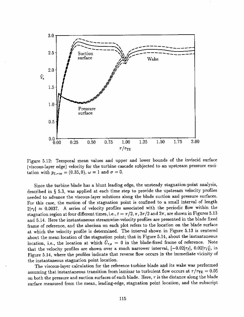
Figure 5.12. Temporal mean values and upper and lower bounds of the inviscid surface
(viscous-layer edge) velocity for the turbine cascade subjected to an upstream pressure exci-
tation with pr,-oo = (0.35, 0), w = 1 and a = 0.
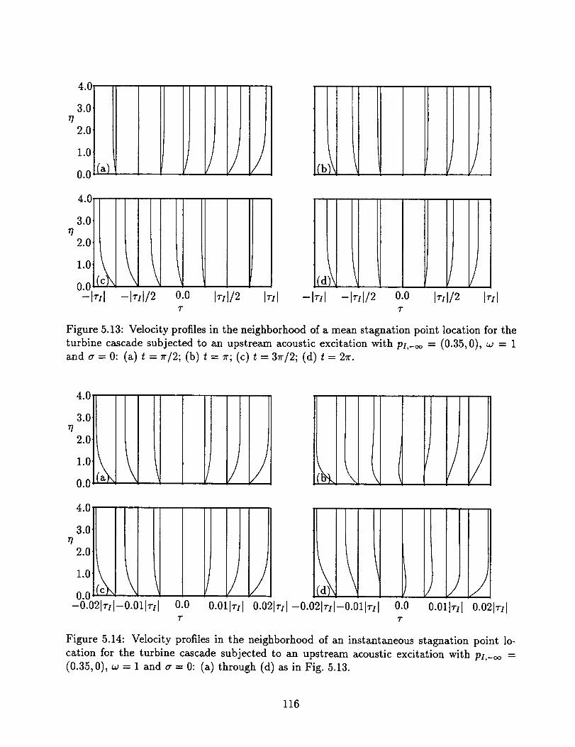
Figure 5.13. Velocity profiles in the neighborhood of a mean stagnation point location for
the turbine cascade subjected to an upstream acoustic excitation with pl,-oo = (0.35, 0), w = 1
and a = 0: (a) t = 7r/2; (b) t = 7r; (c) t = 3r/2; (d) t = 2zr.
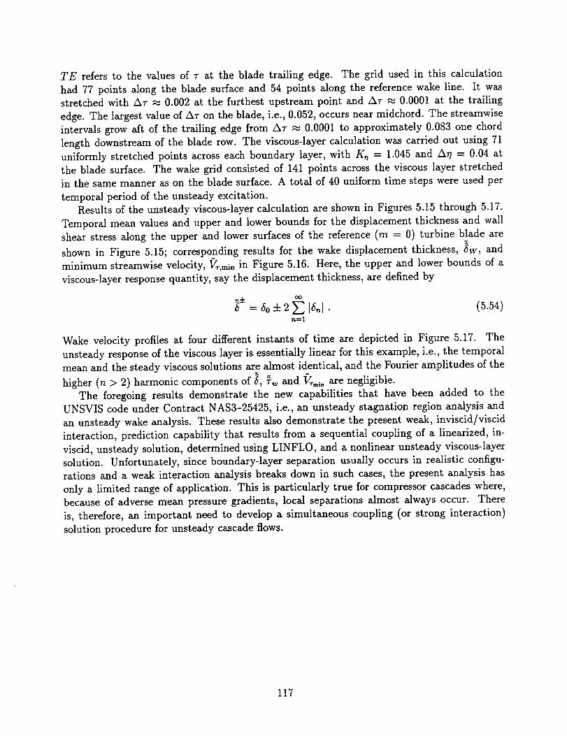
Figure 5.14. Velocity profiles in the neighborhood of an instantaneous stagnation point
location for the turbine cascade subjected to an upstream acoustic excitation with p_,-oo =
(0.35,0), w = 1 and a = 0: (a) through (d) as in Fig. 5.13.
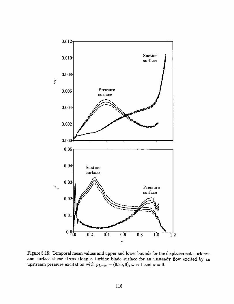
Figure 5.15. Temporal mean values and upper and lower bounds for the displacement
thickness and surface shear stress along a turbine blade surface for an unsteady flow excited
by an upstream pressure excitation with pz,-¢¢ = (0.35, 0), w = 1 and a = 0.
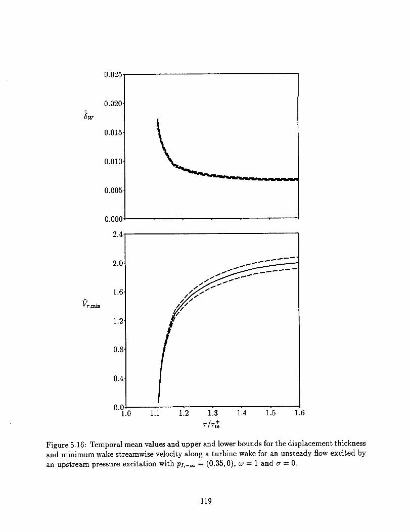
Figure 5.16. Temporal mean values and upper and lower bounds for the displacementthickness and minimum wake streamwise velocity along a turbine wake for an unsteady flow
excited by an upstream pressure excitation with pl,-oo = (0.35, 0), w = 1 and a = 0.
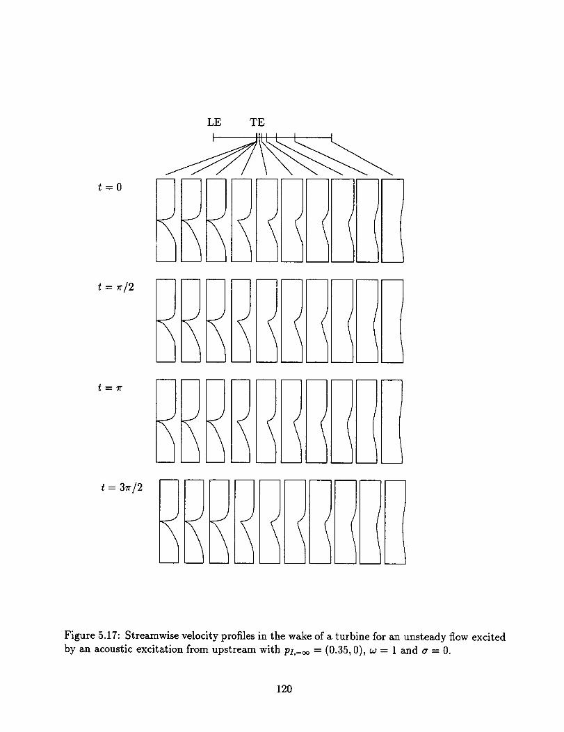
Figure 5.17. Streamwise velocity profiles in the wake of a turbine for an unsteady flow
excited by an acoustic excitation from upstream with pI,-oo = (0.35, 0), w = 1 and a = 0.
vii
Unsteady Aerodynamic Models for TurbomachineryAeroelastic and Aeroacoustic Applications
Summary
Theoretical analyses and computer codes have been developed for predicting compressible
unsteady inviscid and viscous flows through blade rows of axial-flow turbomachines. Such
analyses are needed to determine the impact of unsteady flow phenomena on the structural
durability and noise generation characteristics of the blading. The emphasis here has been
placed on developing analyses based on asymptotic representations of unsteady flow phenom-
ena. Thus, high Reynolds number flows driven by small amplitude unsteady excitations in
which viscous effects are concentrated within thin layers have been considered. The resulting
analyses should apply in many practical situations and lead to a better understanding of the
relevant flow physics. In addition, they will be efficient computationally, and therefore, appro-
priate for use in aeroelastic and aeroacoustic design studies. Finally, the asymptotic analyses
will be useful for calibrating and validating the time-accurate, nonlinear, Euler/Navier-Stokes
analyses that are currently being developed for predicting unsteady flows through turboma-
chinery blade rows.
Under the present research program, the effort has been focused on formulating invis-
cid/viscid interaction and linearized inviscid unsteady flow models, and on providing inviscid
and viscid prediction capabilities for subsonic steady and unsteady cascade flows. In this
report we describe the lineaxized, inviscid, unsteady aerodynamic, analysis, LINFLO, the
steady, strong, inviscid/viscid interaction analysis, SFLOW-IVI, and the unsteady viscous
layer analysis, UNSVIS, that have been developed under this program. The LINFLO analysis
can be applied to efficiently predict the unsteady aerodynamic response of a two-dimensional
blade row to prescribed structural, (i.e., blade) motions and external aerodynamic (acous-
tic, vortical and entropic) disturbances. The SFLOW-IVI analysis can be applied to predict
steady cascade flows, at high Reynolds numbers, in which regions of strong inviscid/viscid
interaction, including viscous layer separation, occur. The UNSVIS analysis can be applied
to predict nonlinear unsteady flows in thin boundary layers and wakes. The capabilities of
the three analyses axe demonstrated via applications to unsteady flows through compressor
and turbine cascades. The numerical results pertain to unsteady flows excited by prescribed
vortical disturbances at inlet, acoustic disturbances at inlet and exit and blade bending and
torsional vibrations. Recommendations axe also given for the future research needed for ex-
tending and improving the foregoing asymptotic analyses, and to meet the goal of providing
an efficient inviscid/viscid interaction capability for subsonic and transonic unsteady cascade
flOWS.
1. Introduction
The unsteady aerodynamic analyses intended for use in predicting the aeroelastic and
aeroacoustic responses of turbomachinery blading must be applicable over wide ranges of
blade-row geometries, mean operating conditions, and modes and frequencies of unsteady
excitation. In particular, these analyses must be capable of predicting unsteady pressure
responses of blade rows to a variety of unsteady excitations. The latter include structural
(blade) motions, variations in total temperature and total pressure (entropy and vorticity
waves) at inlet and variations in static pressure (acoustic waves) at inlet and exit. Finally,
because of the large number of controlling parameters involved, there is a stringent requirement
for computational efficiency, if an analysis is to be used successfully in the blade design process.
To sat,: rv this latter requirement a m_ :lber of restrictive assumptions must be introduced into
the de_,::opment of appropriate unsteady aerodynamic models. The analyses described in this
report have been developed to provide reliable and efficient theoretical prediction capabilities
for inviscid and viscid, steady and small-disturbance unsteady, flows, at high Reynolds number,
through two-dimensional cascades.
1.1 Background
The theoretical analyses that have been developed to predict the aeroelastic and aeroa-
coustic behavior of turbomachinery blading, i.e., the onset of blade flutter, the amplitudes
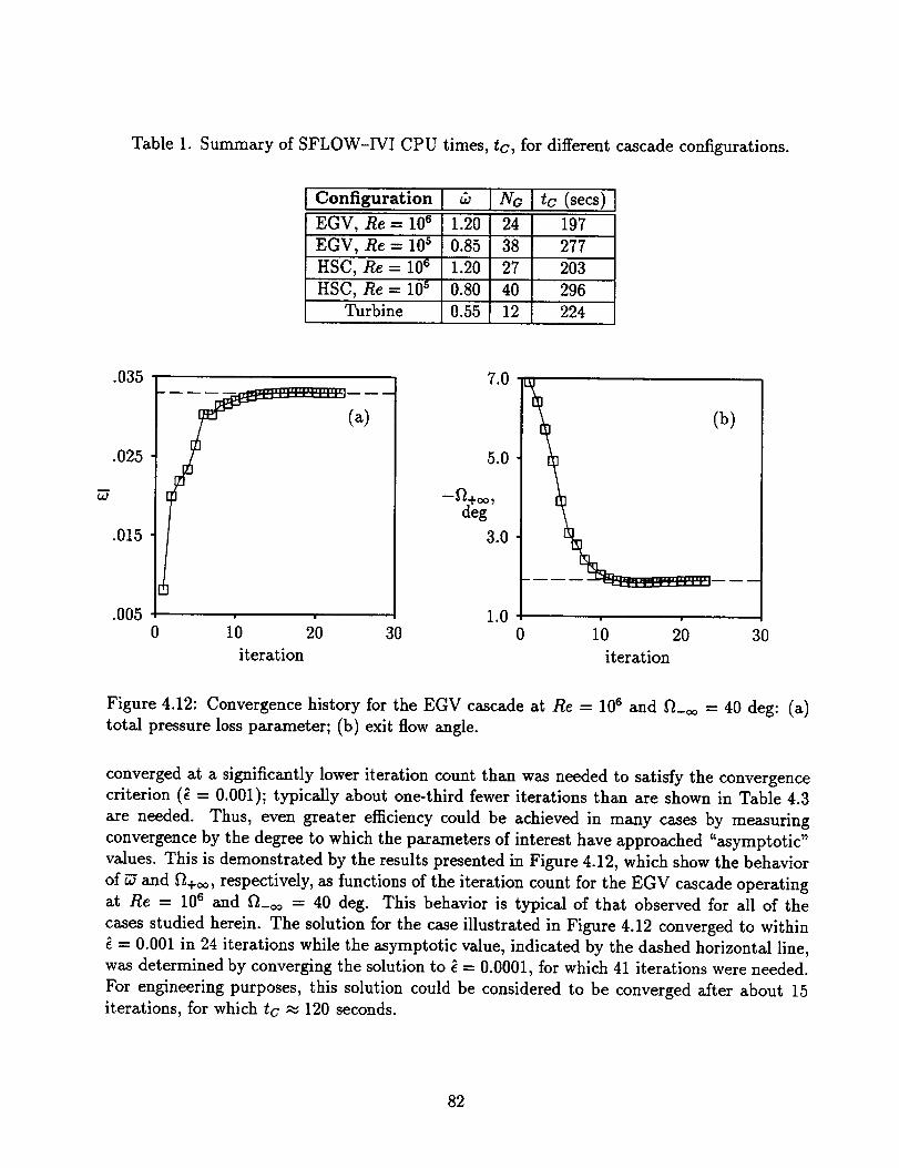
of forced blade vibration and the sound pressure levels that exist upstream and downstream
of the blade row have, for the most part, b_n based on the following geometric and aerody-
namic assumptions. The blades of an isolat: J, two-dimensional cascade are usually considered
with the aerodynamic effects associated with neighboring structures being represented via pre-
scribed nonuniform flow conditions at inlet and exit. The unsteady excitations are assumed to
be periodic in time and in the blade-to-blade direction. The flow Reynolds number is taken to
be sufficiently high so that viscous effects have a negligible impact on the unsteady pressure
field. Finally, the unsteady excitations are assumed to be sufficiently small so that a linearized
treatment of the unsteady inviscid flow is justified.
Until fairly recently, the inviscid unsteady aerodynamic analyses that have been available
for turbomachinery aeroelastic and aeroacoustic design applications have been based on clas-
sical linearized theory (see [Whi87] for a review). Here the steady and harmonic unsteady
departures of the flow variables from their uniform free-stream values are regarded as small
and of the same order of magnitude, leading to uncoupled, linear, constant coefficient, bound-
ary value problems for the steady and the complex amplitudes of the unsteady disturbances.
Thus, unsteady solutions based on the classical linearization apply essentially to cascades
of unloaded flat-plate blades. Very efficient semi-analytic solution procedures have been de-
veloped for two-dimensional attached subsonic and supersonic flows and applied with some
success in turbomachinery aeroelastic and aeroacoustic design calculations. It should also be
mentioned that extensive efforts (as reviewed by Namba [Nam87]) have been made to develop
three-dimensional unsteady aerodynamic analyses, based on the classical linearization.
Because of the limitations in physical modeling associated with the classical linearization,
more general two-dimensional inviscid linearizations have been developed. These include the
2
effectsof important design featuressuch as real blade geometry,mean blade loading, andoperation at transonic Mach numbers. Here, unsteady disturbancesare regardedas small-amplitude harmonic fluctuations relative to a fully nonuniform, isentropic and irrotational,mean or steadybackgroundflow. The steadyflow is determined as a solution of a nonlinearinviscid equation set, and the unsteady flow is governedby linear equations with variablecoefficientsthat dependon the underlying steady flow. This type of analytical model is de-scribed in [Ver92,Ver93] and is often referred to as a linearized potential model; however,the potential-flow restriction appliesonly to the steadybackgroundflow. It has receivedcon-siderableattention in recent years,and solution algorithms for the nonlinearsteady and thelinearized unsteadyproblem have reachedthe stagewhere they are being applied in turbo-machinery aeroelasticand aeroacousticdesignstudies (e.g., see [Smi90, SS90,MM94]). Inparticular, one such analysis, the linearized inviscid flow analysis, LINFLO, has been ex-tendedunder the present contract for cascadegust responsepredictions. In previouswork,this analysishasbeendevelopedand applied to predict unsteadysubsonicand transonic flowsexcited by blade vibrations or acousticdisturbances[VC84,Ver89a,UV91, KV93b] and, un-der the presentcontract, to predict unsteadysubsonicflowsexcited by entropic and vorticalgusts [VH90, HV91, VBHA91].
The unsteadyflowsof practical interestusuallyoccurat high, but finite Reynoldsnumber,so that viscous-layerdisplacementscan have an impact on the unsteadypressureresponse.Provided that large-scaleflow separationsfrom the blade surfacesdo not occur, the overallflow field canbe divided conceptuallyinto "inner" viscousor dissipativeregions,consistingofthin boundary layersandwakes,and an "outer" inviscid region. Solutions to the complete flow
problem can then be determined by an iterative procedure involving successive solutions to the
inviscid and viscid equations. If the inviscid/viscid interaction is "weak", then at each step of
the iteration process, the inviscid and viscid solutions can be determined sequentially with the
pressure being determined by the inviscid flow. However, in most flows, strong inviscid/viscid
interactions occur due, for example, to boundary-layer separations, shock/boundary-layer
interactions and trailing-edge/near-wake interactions. For such flows the pressure must be
determined by solving the inviscid and viscous layer equations simultaneously at each iteration
level.
The construction of a high Reynolds number viscous cascade solver involves first, the de-
velopment of component flow solvers, and second, the implementation of these component
solvers into an overall computational procedure to provide an analysis for the complete flow
field. Solution methods for steady, subsonic and transonic, inviscid flows through cascades and
for steady boundary-layer and wake flows have been developed to a relatively mature state.
Methods for coupling such solutions have also been developed and applied to predict steady
cascade flows, with strong inviscid/viscid interactions (e.g., see [HSS79, JH83, CH80, BV89,
BHE91, BVA93a, BVA93b]), with the work in [BVA93a, BVA93b] being performed as part
of the present effort. Similar approaches ave needed for unsteady flows. Under the present
Contract, nonlinear steady and linearized unsteady inviscid analyses have been coupled to the
unsteady viscous-layer analysis of [PVK91], but only to predict unsteady cascade flows with
weak inviscid/viscid interactions [VBHA91, BV93]. To date, there has been very little effort to
couple unsteady inviscid and viscous-layer analyses to provide a strong inviscid/viscid interac-
tion analysis for unsteady cascade flows. As steps toward this goal, the steady inviscid/viscid
interaction analysis for cascades, SFLOW-IVI, that can provide the foundation for an un-
steady procedureto be developedlater, and the unsteady viscous-layer analysis (UNSVIS)
have been developed under the present research program.
1.2 Scope of the Present Effort
The objectives of the research program conducted under Contract NAS3-25425 are to
provide efficient theoretical analyses for predicting compressible unsteady flows through two-
dimensional blade rows. Such analyses are needed to understand the impact of unsteady
aerodynamic phenomena on the aeroelastic and aeroacoustic performances of turbomachinery
blading. For this purpose, we have developed a detailed inviscid/viscid interaction formu-
lation for unsteady cascade flows, which is described in § 2 of this report. We have also
developed or extended several analyses that will form the components of an unsteady, invis-
cid/viscid interaction, solution procedure. The latter include the linearized inviscid unsteady
aerodynamic analysis, LINFLO, the steady inviscid/viscid interaction analysis, SFLOW-IVI,
and the unsteady viscous layer analysis, UNSVIS. The steady full potential analysis, SFLOW
[HV93, HV94], which is also considered to be a component of the overall prediction scheme,
has been developed at NASA Lewis under a separate, but related, research program. The
present work has been directed primarily towards subsonic aeroelastic applications, however,
for the most part, this work will apply, more generally, for predicting the aeroelastic and
aeroacoustic responses of turbomachinery blading operating at subsonic and tr: _sonic Mach
numbers.
In the first phase of this program [VH90, HV91] the linearized inviscid analy,_ LINFLO)
was extended to predict the responses of a cascade to entropic and vortical excitations. A
velocity decomposition introduced by Goldstein [Go178, Go179], and later modified by Atassi
and Grzedzinski [AG89], is employed to split the linearized unsteady velocity into rotational
and irrotational components. This decomposition leads to a very convenient descrip on of
the linearized unsteady perturbation -- one in which dosed form solutions can be determined
for the entropy and vorticity or rotational velocity fluctuations in terms of the drift and
stream functions of the underlying steady flow. Numerical field methods are required only
to determine the unsteady potential and from this, the unsteady pressure. The potential is
governed by an inhomogeneous wave equation in which the source term depends upon the
rotational velocity field. The potential fluctuations are determined numerically on an H-type
mesh in which the streamlines of the steady background flow are used as mesh lines. Numerical
solutions are reported in [VH90, HV91, VBHA91] for several configurations including flat-
plate cascades, a compressor exit guide vane, a high-speed compressor cascade, and a turbine
cascade. The I..INt;'LO analysis is described in § 3 of this report, with particular emphasis on
its capabilities h': predicting unsteady flows excited by vortical gusts.
An efficient steady analysis for predicting strong inviscid/viscid interaction phenomena;
such as, viscous-layer separation, shock/boundary-layer interaction and trailing-edge/near-
wake interaction, in turbomachinery blade passages is needed as part of a comprehensive
analytical blade design prediction system. Such an analysis, called SFLOW-IVI, has been
reported in [BVA93a, BVA93b] and is described in § 4. Here, the flow in the outer or in-
viscid region is governed by the full-potential equation and that in the inner viscous region,
by Prandtl's viscous-layer equations. The non-hierarchical nature of strong interactions is
taken into account in the semi-inverse iteration procedure used to couple the two solutions.
The steady, full-potential analysis, SFLOW, [HV93, HV94] is employed in this procedure
to determine inviscid solutions. SFLOW was constructed, for use with the LINFLO analy-
sis, to provide comprehensive and compatible, steady and unsteady, inviscid, flow prediction
capabilities for cascades.
In the IVI procedure, which is referred to as SFLOW-IVI, viscous effects are incorpo-
rated by adjusting the blade and wake surface boundary conditions in SFLOW to account
for the effects of viscous displacement. Inviscid solutions are determined using an implicit,
least-squares, finite-difference approximation, viscous-layer solutions using an inverse, finite-
difference, space-marching method which is applied along the blade surfaces and wake stream-
lines. The inviscid and viscid solutions are coupled using a semi-inverse, global iteration proce-
dure, which permits the prediction of boundary-layer separation and other strong-interaction
phenomena, and allows nonlinear changes to the inviscid flow, due to viscous effects, to be
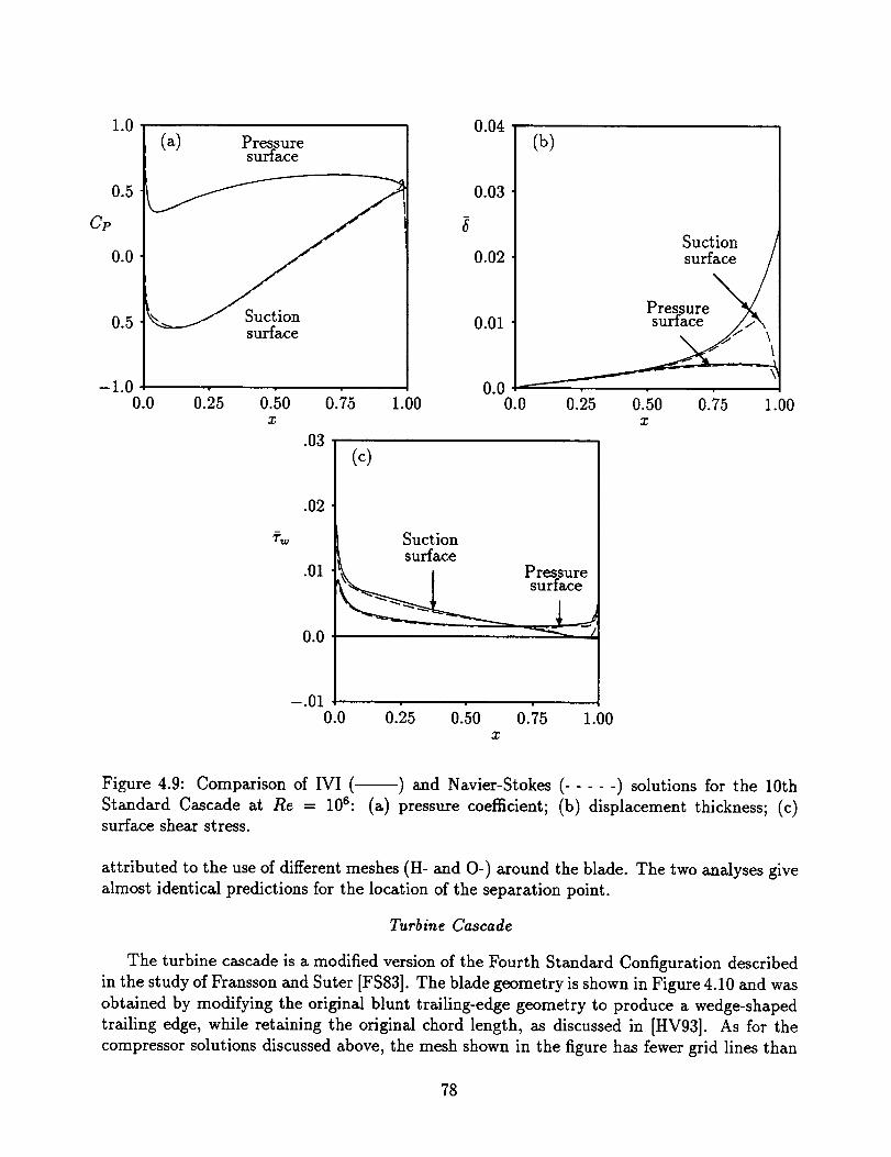
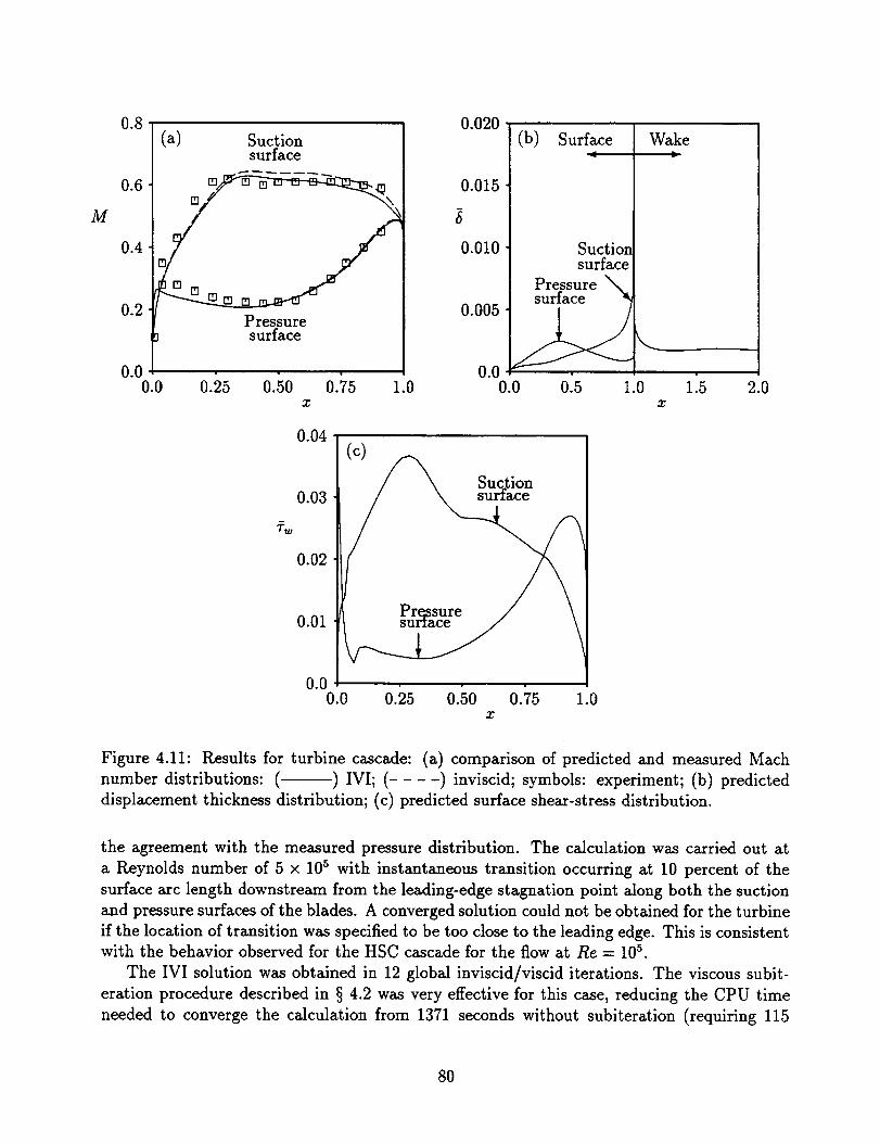
evaluated. Results are presented for three cascades, with a range of inlet flow conditions
considered for one of them, including conditions leading to large-scale flow separation. Com-
parisons with Navier-Stokes solutions and experimental data are also given.
Finally the UNSV/S analysis of IPVK91] was extended so that unsteady viscous effects
in the vicinity of leading-edge stagnation points and in blade wakes could be predicted
[VBHA91, BV93]. The nonlinear unsteady flow in a viscous layer is described by Prandtl's
equations. As in the SFLOW-IVI analysis, algebraic models are used to account for the effects
of transition and turbulence. The viscous-layer equations are solved in terms of Levy-Lees
type variables using a finite-difference technique in which solutions are advanced in time and
in the streamwise direction. Numerical solutions are determined by marching implicitly, first
in time and then in the streamwise direction, over several periods of unsteady excitation,
from an initial steady soIution, and from an approximate time-dependent, upstream flow so-
lution. This analysis, rather than one in which the results of separate nonlinear steady and
linearized unsteady viscous-layer analyses are superposed, allows an assessment to be made
of the relative importance of nonlinear unsteady effects in viscous regions.
Under the present effort, a similarity analysis was developed to predict unsteady viscous
compressible flow in the vicinity of a moving leading-edge stagnation point and incorporated
into the UNSVIS code. The stagnation region analysis provides the "initial" upstream flow
information needed to advance or march a viscous-layer calculation downstream along the
blade surfaces and into the wake. In addition, the wake analysis, used previously in UNSVIS,
was extended so that the changes or jumps in the inviscid velocity that occur across vortex-
sheet unsteady wakes could be properly accommodated. The linearized inviscid analysis,
LINFLO, and the nonlinear viscous-layer analysis, UNSVIS, were also coupled to provide a
weak viscid/inviscid interaction solution capability for unsteady cascade flows. The UNSVIS
analysis is described in § 5, where it is also applied to study the viscous-layer responses of
an unstaggered flat-plate cascade to pressure or acoustic excitations originating upstream and
downstream of the blade row. Finally, the coupled LINFLO/UNSVIS analysis is applied to a
turbine cascade subjected to a pressure excitation from upstream to demonstrate the current
weak inviscid/viscid interaction solution capability on a realistic cascade configuration.
The component analyses, described in this report, are important in their own right. They
can be applied to improve our understanding of the complex steady and unsteady flow pro-
cesses that occur in turbomachine cascades, and to provide useful aeroelastic and aeroacoustic
design information. Hopefully, along with the general inviscid/viscid interaction and inviscid
5
small-disturbance formulations, presented in § 2, they will contribute to the future develop-
ment of a comprehensive inviscid/viscid interaction analysis for unsteady cascade flows. Such
an analysis will provide useful aeroelastic and aeroacoutic response information for a wide
range of blade-row geometries and operating conditions. It will also be of help in calibrat-
ing the time-accurate, nonlinear, Euler and Navier-Stokes analyses that are currently being
developed for predicting turbomachinery unsteady flow fields.
2. Physical Problem and Mathematical Models
2.1 Unsteady Flow through a Two-Dimensional Cascade
We consider time-dependent flow, at high Reynolds number (Re) and with negligible body
forces, of a perfect gas with constant specific heats and constant Prandtl number (Pr) through
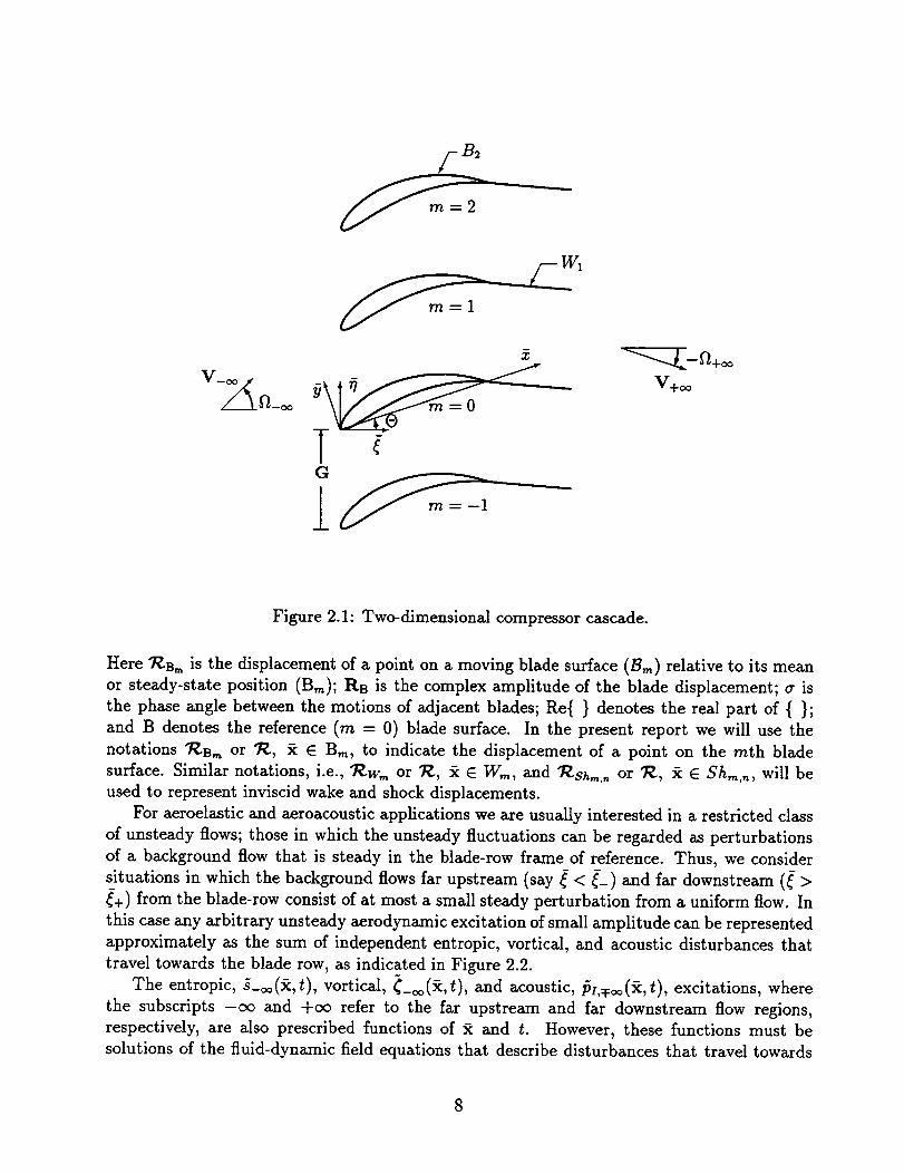
a two-dimensional cascade, such as the one shown in Figure 2.1. The unsteady fluctuations
in the flow arise from one or more of the following sources: blade motions, upstream total
temperature and total pressure disturbances, and upstream and/or downstream static pres-
sure disturbances that carry energy toward the blade row. These excitations are assumed to
be of small amplitude, periodic in time, and periodic in the blade-to-blade or cascade "cir-
cumferential" direction. Also, blade shape and orientation relative to the inlet freestream
direction, the inlet to exit mean static pressure ratio and the amplitudes, modes, frequencies
and wave numbers of the unsteady excitations are such that viscous effects are confined within
thin layers, that lie along the blade surfaces and extend downstream from the blade trailing
edges. We should note that the aerodynamic models to be developed below, apply to subsonic
flows and to transonic flows containing normal shocks; however, the applications presented
throughout this report are restricted to subsonic flows.
In the following discussion all physical variables are dimensionless. Vector quantities are in
boldface type, and a tilde over a dependent variable indicates time dependence. Lengths have
been scaled with respect to blade chord (L*), time with respect to the ratio of blade chord
to upstream freestream flow speed (1/_Ioo), density with respect to the upstream freestream
density (P:-_o), velocity with respect to the upstream freestream flow speed, and stress with
respect to the product of the upstream free.stream density and the square of the upstream
freestream speed (_'_o_V_*oo2). Here the superscript * denotes a dimensional quantity and the
subscript -oo refers to the prescribed freestream conditions far upstream. The scalings for
the remaining variables can be determined from the equations that follow, which have the
same forms as their dimensional counterparts.
We will analyze the unsteady flow in a blade-row fixed coordinate frame in terms of the
Cartesian (x, y) or (_, r/) coordinates and the time t. Here, for example, _ and r/ measure
distances in the cascade axial and circumferential directions, respectively. To describe flows
in which the fluid domain varies with time it is useful to consider two sets of independent
variables, say (x, t) and (_, t). The position vector x(_, t) = _ + 7_(_, t) describes the instan-
taneous location of a moving point, say _, _ refers to the reference or steady-state position
of _, and 7_(_, t) is the displacement of :P from its reference position. The displacement
field, 7_., is usually prescribed so that the solution domain moves with solid boundaries and
is stationary far from the blade row. If we set 7_ -- 0, then the position vector x, like _¢,
describes a stationary point in the blade-row fixed reference frame.
The mean or steady-state positions of the blade chord lines coincide with the line segments
= _tan O +raG, 0 < _ < cos O, m = 0, +l, 4-2, ..., where m is a blade number index, O is
the cascade stagger angle, and G is the cascade gap vector which is directed along the _-axis
with magnitude equal to the blade spacing. The blade motions are prescribed as functions of
and t, i.e.,
7_-Sm(_+ mG, t)= Re{RB(_)exp[i(wt + ma)]}, for _ e B (or x E B). (2.1)
w1
T
Figure 2.1: Two-dimensional compressor cascade.
Here _B. is the displacement of a point on a moving blade surface (B,_) relative to its mean
or steady-state position (B,_); RB is the complex amplitude of the blade displacement; a is
the phase angle between the motions of adjacent blades; Re{ } denotes the real part of { };
and B denotes the reference (m = 0) blade surface. In the present report we will use the
notations 7_B,_ or $Z, _ E Bin, to indicate the displacement of a point on the ruth blade
surface. Similar notations, i.e., "R.w. or 7E, _ E W,,,, and "P--Sh,,. or _, i E Shin,n, will be
used to represent inviscid wake and shock displacements.
For aeroelastic and aeroacoustic applications we are usually interested in a restricted class
of unsteady flows; those in which the unsteady fluctuations can be regarded as perturbations
of a background flow that is steady in the blade-row frame of reference. Thus, we consider
situations in which the background flows far upstream (say _ < __) and far downstream (_ >
_+) from the blade-row consist of at most a small steady perturbation from a uniform flow. In
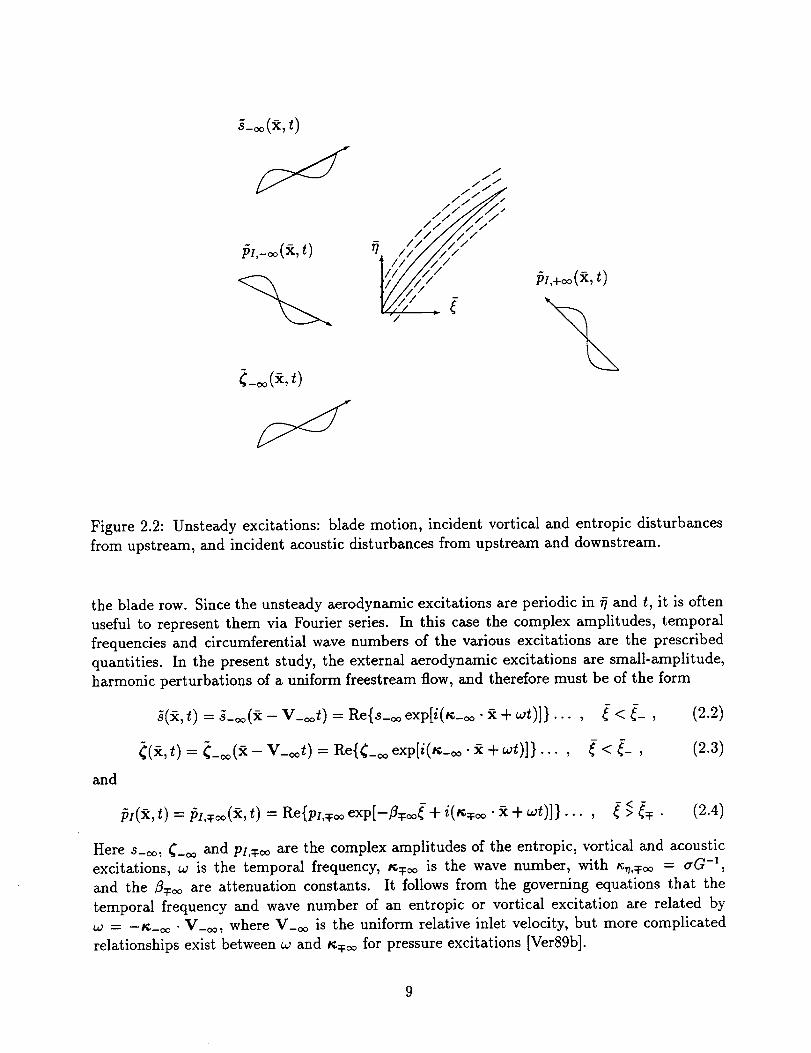
this case any arbitrary unsteady aerodynamic excitation of small amplitude can be represented
approximately as the sum of independent entropic, vortical, and acoustic disturbances that
travel towards the blade row, as indicated in Figure 2.2.
The entropic, ._-oo(_,t), vortical, __¢0(_,t), and acoustic, _5A_:,o(_,t), excitations, where
the subscripts -oo and +c¢ refer to the far upstream and far downstream flow regions,
respectively, are also prescribed functions of _ and t. However, these functions must be
solutions of the fluid-dynamic field equations that describe disturbances that travel towards
where T = /_/ : Wx ® V is the viscous dissipation and the symbol : indicates the scalar
product of two tensors.
Boundary Conditions
For application to turbomachinery unsteady flows the foregoing field equations must be
supplemented by conditions at the vibrating blade surfaces and conditions at the inflow and
outflow boundaries. Since transient unsteady aerodynamic behaviors are usually not consid-
ered, a precise knowledge of the initial state of the fluid is not required. The no-slip condition,
i.e.,
=7_ for x e B,_ (or_ES,_), (2.16)
11
where "R.B,, is prescribed, applies at blade surfaces. In addition, either the heat flux Q- n or
the temperature _F must be prescribed at such surfaces, i.e.,
Q.n = or T = _F_(x,t), x e B,,, (or _ e B,_) (2.17)
We also require conditions on the flow far upstream and far downstream from the blade
row, i.e., at the inflow and outflow boundaries of the computational domain. Typically the
circumferentially- and temporally-averaged values of the total pressure, total temperature
and the inlet flow angle are specified at the inflow boundary. At the outflow boundary, the
"circumferentially" and temporally averaged pressure is specified. In addition, total pressure
and total temperature fluctuations at inlet and pressure fluctuations at inlet and exit, that
carry energy towards the blade row, must be specified. Total pressure and total temperature
fluctuations at exit and unsteady pressure disturbances at inlet and exit, that carry energy
away from the blade row, are determined as part of the unsteady solution.
2.3 Inviscid/Viscid Interaction Model
The Reynolds-averaged Navier-Stokes equations must be considered if viscous effects axe
expected to be important throughout the fluid domain. However, for most flows of practical
interest the Reynolds number (Re) is usually sufficiently high so that such effects are concen-
trated in relatively thin layers across which the flow properties vary rapidly. Provided that
large scale flow separations do not occur, these layers generally lie adjacent to the blade sur-
faces (boundary layers) and extend downstream from the blade trailing edges (wakes). Thus,
if we assume that the Reynolds number is high and the flow remains essentially "attached" to
the blade surfaces, we can apply an inviscid/viscid interaction (IVI) analysis to determine the
unsteady flow field. The terminology "inviscid/viscid interaction" refers to all flow situations
in which viscous layers have a significant influence on the pressure field. Weak interactions
are defined as those in which viscous effects on the pressure are small, or more specifically, on
the order of the viscous-layer displacement thickness, _ ,,, O(Re-1/2). If viscous effects on the
pressure disturbance are larger than this, i.e., > O(_), the interaction is classified as strong
[Mel80].
In an IVI analysis separate sets of approximate equations, i.e., reduced forms of the Navier-
Stokes equations, are constructed, using the method of matched asymptotic expansions, to
describe the flows in "outer" inviscid and "inner" viscous-layer regions. This approach offers
the potential for providing efficient predictions of the effects of viscous layer displacement and
curvature on the unsteady aerodynamic behaviors of blade rows. The governing equations can
be derived with respect to moving, shear-layer surfaces S,_, each of which is contained entirely
within a viscous layer. These surfaces are usually taken to coincide with the suction and
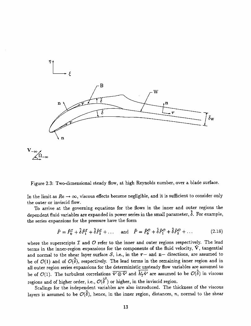
pressure surfaces of the blades and lie entirely within the viscous wake, e.g., see Figure 2.3.
The curvatures of the reference shear layer surfaces are assumed to be O(1) or less, and here
we will assume that their motions, which depend on the blade motions, are also of O(1) or
less. Ultimately, we will assume that the motions of the blades and their wakes, and hence,
those of the reference shear-layer surfaces are of small amplitude. The inviscid and viscous
layer equations must be solved simultaneously, subject to appropriate matching conditions
along the blades and wakes, to determb - the flows in the inviscid and viscous-layer regions.
12
BW
n n
?w
V OO
Figure 2.3: Two-dimensional steady flow, at high Reynolds number, over a blade surface.
In the limit as Re _ oo, viscous effects become negligible, and it is sufficient to consider only
the outer or inviscid flow.
To arrive at the governing equations for the flows in the inner and outer regions the
dependent fluid variables are expanded in power series in the small parameter, _. For example,
the series expansions for the pressure have the form
p = po_+_p,_+ _P_+... and P = P0° +_po+_po+... (2.1s)
where the superscripts Z and O refer to the inner and outer regions respectively. The lead
terms in the inner-region expansions for the components of the fluid velocity, V, tangential
and normal to the shear layer surface S, i.e., in the -r- and n- directions, are assumed to
be of O(1) and of O(_), respectively. The lead terms in the remaining inner region and in
all outer region series expansions for the deterministic unsteady flow variables are assumed to
be of O(1). The turbulent correlations "_'® _' and h_' are assumed to be O(_) in viscous_-2
regions and of higher order, i.e., O(_ ) or higher, in the inviscid region.
Scalings for the independent variables are also introduced. The thickness of the viscous
layers is assumed to be O(_), hence, in the inner region, distances, n, normal to the shear
13
layer surfacesare of O(_) and partial derivatives in the normal direction are of order 6 1, i.e.,
n. Vx _ _n _ 0(6 ). (2.19)
Partial derivatives along the surface, r. Vx, and local time derivatives, O/Otlx , are assumed
to be of 0(1) in both the inner and outer regions. In the outer region, normal derivatives,
n. Vx, are also assumed to be of O(1).
Approximate field equations that describe the flows in the inner and outer regions are
determined by simply substituting the series expansions for the dependent variables and the
scalings for the independent variables into the Reynolds-averaged Navier-Stokes equations and
equating terms of like power in 6. When expressed in terms of the original variables, /5, V,
etc., the zeroth-order inviscid flow is governed by the Euler equations, i.e., equations (2.5),
(2.6) and (2.7) or (2.15) with right-hand-sides set equal to zero; the zeroth-order viscous flows,
by Prandtl's viscous-layer equations, which will be given below. The inviscid flow in the outer
region is determined as a solution of the Euler equations subject to flow tangency conditions
at the blade surfaces and jump conditions at shocks and at blade wakes. The blade and
wake conditions contain terms that account for the effects of viscous-layer displacement and
curvature, which become negligible as Re _ oo. The viscous flows in the inner regions are
determined as solutions to Prandtl's equations subject to edge conditions that depend on the
behaviors of the inviscid flow variables along the blade and wake surfaces. The specific forms
of the inviscid and viscid blade and wake conditions follow from an asymptotic matching of
the outer inviscid and the inner viscous-layer solutions, e.g., see [Mel80].
Inviscid Region
The field equations that govern continuous, inviscid, fluid motion are determined from the
Reynolds averaged Navier-Stokes equations, (2.5), (2.6) and, in this case, (2.15), and are given
by
--O_ +Vx-(9_)=0 (2.20)X
-D9#-_-- + _'x/5 = 0 (2.21)
D#D--T = 0 (2.22)
For turbomachinery applications, we require solutions of these equations subject to boundary
conditions at moving blade surfaces, jump conditions at moving wake and shock surfaces, and
appropriate conditions far from the blade row.
The inviscid solution for the normal component of the fluid velocity at a moving blade
surface must match the viscous solution for this velocity at the outer edge of the viscous
layer. This is equivalent to the condition that the inviscid flow must be tangential to the
blade and wake displacement surfaces. After carrying out the asymptotic matching process
and neglecting terms of second and higher order in _, we find that the normal component of
the inviscid fluid velocity must satisfy the condition
(9 - "_)-n = _-[l[O(_6)/Otlx + O(_¢V,,_6)/Or I + ('_. Wx)6, x E Bm (2.23)
14
at the ruth (m = 0,d=l,=k2,...) moving blade surface. In equation (2.23), _, and V_,, are
the inviscid values of the fluid density and streamwise velocity at the moving blade surface,
Bin, or the viscous density and streamwise velocity at the edge (e) of the viscous layer, r is
the distance measured along this surface downstream from the leading-edge, and n is a unit
vector normal to Bm and pointing into the fluid.
Two types of terms arise from the wake matching conditions, one due to the displacement
thickness effect and the other, to the wake curvature effect. The first leads to the requirement
that the inviscid solution for the normal component of the fluid velocity must be discontinuous
across a wake with jump given by
[9].n = <_'['[O(_,_)/Ot x + O(_?,-,,$)/O'r]) + ('#,..•Vx)($), x • "W,,,. (2.24)
Here I ] and ( ) denote the difference (upper minus lower) and the sum (upper plus lower),
respectively, across a wake, and n is an "upward" pointing, unit vector, normal to the moving
reference wake surface, kY. Note that (_) = _w is the displacement thickness of the complete
wake. The wake curvature effect gives rise to a pressure difference across the wake. The
requirement that the outer inviscid flow match this pressure difference leads to the condition
(2.25)
where (3) = 0w is the momentum thickness of the complete wake and Pc = r. On/Orlw is
the curvature of the reference wake surface, which is taken as positive when the curvature
is concave upwards. Since there is some ambiguity in establishing the shape and location of
a viscous wake the right-hand-side of (2.25) is usually ignored in inviscid/viscid interaction
calculations. Consequently, the pressure jump across the wake is usually set equal to zero.
In deriving the surface conditions (2.23)-(2.25), we have assumed that the viscous layer is
thin, i.e., _ << 1, and therefore, that the effects of terms of second and higher order in the
viscous displacement thickness are negligible. In the inviscid limit Re --* oo, the thicknesses
of the viscous layers, and hence, the right-hand-sides of (2.23)-(2.25) become zero.
Jump conditions must also be imposed at inviscid shock discontinuities. Such conditions
are obtained from the integral conservation laws by considering a control volume that contains
a segment of a shock surface, and taking limits, first, as the lateral extent of this volume, nor-
mal to the surface segment, approaches zero, and, then, as the area of the segment approaches
zero. The resulting jump conditions for conserving mass momentum and energy at a shock
are given by
_M_ = 0, M_IV] + _Pln = 0, and MA_I+ _PV]-n = 0, x • Sh_,, (2.26)
respectively. Here [[ ] denotes the jump in a flow quantity as experienced by an observer in
moving across the shock Sh,_,,_ in the n direction,
Mj = _(9- 7_).n, x 6 $h_,. (2.27)
is the fluid mass flux through the shock, ET = HT --/5/_ is the total specific internal energy
of the fluid and the subscripts m, n refer to the nth shock associated with the ruth blade.
15
In the inviscid limit, the conditions (2.26) also apply acrossthe vortex-sheet "viscous"layers. In this case,since_[V_] # 0, and the inviscid jump conditions (2.26) indicate that, for
vortex sheets, M I = 0, [ P] - 0, and [ V]'n = 0. At shocks, Sh,,,n, the mass flux is generally
nonzero (i.e., Mj # 0). Hence, it follows from (2.26) that the component of fluid velocity
tangent to a shock surface, V .7", must be continuous across the shock. The remaining jump
conditions, along with the thermodynamic equations of state, are then required to determine
the shock velocity, "R-sh,.,n, and the changes in the normal component of the fluid velocity and
the thermodynamic properties of the fluid as it passes through the shock.
The far-field conditions used in the inviscid approximation are the same as those indicated
in § 2.2 for Navier-Stokes simulations. In particular, averaged values of the inlet total pressure,
total temperature and flow angle and the exit static pressure are specified along with the
entropic and vortical fluctuations at inlet and the static pressure disturbances at inlet and
exit that carry energy towards the blade row. In addition, disturbances generated within the
solution domain must be allowed to pass through the inflow and outflow boundaries withoutreflection.
Viscous Layers
The flows in the viscous layers are governed by Prandtl's equations and are subject to
no-slip and prescribed heat-flux or wall temperature conditions, cf. (2.16) and (2.17), at the
moving blade surfaces. In addition, the streamwise velocity and the thermodynamic properties
of the fluid at the edges of the viscous layers are determined by the values of the corresponding
inviscid quantities at the blade surfaces and along the reference wake (shear-layer) surfaces.
We describe the flow in these layers in terms of curvilinear coordinates z and n which measure
distance along and normal to, respectively, a moving, reference, shear-layer surface S. The
unit vectors T(e, t) and n(e, t), where e measures distance along the mean position of the
shear layer surface, are tangent and normal to S.
The field equations that govern the lead terms, _-'.0, V_z .n, Poz, etc., in the inner-region
series expansions, are :etermined in a m_nner similar to that used for the inviscid region. In
particular, the series expansions for the inner-region dependent variables and the scalings for
the independent variables are substituted into the Reynolds-averaged Navier-Stokes equations,
(2.5), (2.6) and (2.7), and only terms of O(1) are retained. Then, in terms of the original
variables, the zeroth-order equations for the two-dimensional flows in the thin boundary layers
that lie along the upper and lower surfaces of each blade and in the thin wake that extends
downstream from the blade trailing edge have the form
into the full time-dependent surface conditions, subtracting out the corresponding zeroth-
order conditions and neglecting terms of higher than first order in e. These procedures lead to
19
nonlinearand linear variable-coefficientequations,respectively,for the zeroth- and first-orderflows. The variable coefficientsthat appearin the linearizedunsteadyequationsdependuponthe steadybackgroundflow.
Note also,that asa consequenceof the assumptionsregardingcascadegeometry,the inletandexit mean-flowconditions,and the temporal andcircumferential behaviorsof the unsteadyexcitations, the steadybackgroundflow will beperiodicfrom blade-to-bladeand the first-orderunsteadyflow will exhibit a phase-lagged,blade-to-bladeperiodicity. Thus, for example,wecanwrite
where_(x,t)= $(_)+ ae{,_(_)exp(i,o0}+...and$and6~ O([Ri$)arethesteadyandthecomplex amplitude of the first-harmonic components of the viscous displacement thickness,
respectively, and R(_), _ E B,,, is the complex amplitude of the unsteady blade displacement.
As a convenience, we have omitted the subscript e on the densities and velocities appearing
in the surface conditions (2.56) and those given below. But, it is to be understood that the
values of these inviscid fluid properties at a blade or wake surface are equal to their viscous
values at the edges of the corresponding viscous layers.
The linearized conditions on the jumps in the normal velocity and the pressure across
wakes follow from (2.24) and (2.25), and the corresponding zeroth-order conditions, and havethe form
Iv]. fi - [ [V_]0R/0_ + (R. V_)[V] ]. fi = _v]. _ + _o[V,]lO_
- 0(Rn-[V_])/0"_- R.n-I(V. V) lnfi]] - kRn-[Vn]]
= [(p_-I + _'-0'R./0_) V]. fi + (iw_-t(p$ + _6))(2.57)
where k = q" - Ofi/O_ and x are the steady and the complex amplitude of the first-order
unsteady wake curvatures.
22
As do the steady, the first-order unsteady blade and wake conditions also simplify con-siderably in the inviscid limit Re .--* _. In particular, the right-hand-sides of (2.56)-(2.58)
become zero. Also, for Re ---* _ the left-hand-sides of the first-order wake conditions can be
simplified by making use of the inviscid forms of steady wake-jump conditions and the field
equations (2.43) and (2.44). After performing the necessary algebra, we find that
lv]._:O(_lV_l)/O_+R.-lY.O(lnj)/O_l, _, e Win, (2.59)
and
[p]=-kP_-[I_V_], Y¢ E W_. (2.60)
Equations (2.57) and (2.58) provide two independent relations for determining the jump in the
linearized unsteady normal velocity and pressure across each wake. However, since the wake
normal displacement, R- fi, _ E W,_, is unknown a priori, these relations are not sufficient
to determine [p]] and [[v] • n, unless the steady tangential velocity, V. _', and density, _, are
continuous across wakes.
The linearized equations that ensure that mass, momentum and energy are conserved
across shock discontinuities are
[rnl] = [mlc ] = [_v + pV - iw_R], fi - O(Rn-[_]Ve)/O_ = 0, _ on Sh,_,,, (2.61)
and
Mslv + [O(_Y.)lO_ + _]÷l + msolV.]_ + _l_
-_[j(Yg - W)]_- _v.lzOy.lo_]_ = 0, x on Shin,.(2.62)
Mf_eT + P/P] + m]c[ET] + _Pv] . fi - O(Rn-V_[[P])/O_- P_-V_[_OET/O_] = 0, x on Shin,,,(2.63)
where _ = V_ x V and er = e+V-v. Equations (2.61), (2.62) and (2.63), with the first-order
respectively, are the relations needed for determining the jumps in the first-order fluid prop-
erties across moving shocks and the normal component of the shock displacement R- n, x E
Sh,.,,,,. These conditions along with the zeroth-order conditions (2.49) must be enforced to
ensure that mass, momentum and energy are conserved to within first-order across moving
shocks. Again, however, there is one more unknown associated with the unsteady shock-
jump conditions, than there are independent equations. Therefore, these conditions are not
sufficient for determining the relevant unsteady shock information.
The first-order density and specific total internal energy can be eliminated from the first-
order shock jump conditions by applying the thermodynamic relations (2.53) and
e = ,6-'[7-' p + (7 -- 1) -1PSI = (7/5)-1P + 7-'('7 -- 1) -1A2s (2.65)
23
to (2.61)-(2.64). By so doing, we would retain the convention, adopted in the derivation of
the field ec _tions, of regarding pressure, entropy and velocity as the dependent variables of
the lineariz, 5 unsteady flow problem. However, since the jump conditions, derived above, are
not sufficient for fitting wakes and shocks into an unsteady solution, based on the linearized
Euler equations, additional information will be required.
The foregoing equations provide linearized surface conditions, in which viscous displace-
ment and wake curvature effects are taken into account. Such conditions are needed to account
for viscous effects in a linearized inviscid analysis of the unsteady perturbation of a nonlin-
ear steady background flow. The flow tangency condition (2.56) applies at the mean blade
pos;_ions, and also on the upper and lower sides of the mean wakes; the jump conditions
on normal velocity and pressure (2.57) and (2.58) also apply at mean wake positions; and
the mass, momentum and energy conservation conditions (2.61), (2.62) and (2.63), respec-
tively, apply at the mean shock positions. Unfortunately, these surface conditions are quite
complicated and, to date, they have not been fully incorporated into a linearized unsteady
aerodynamic analysis. Indeed, as presently posed, the wake and shock conditions are not
sufficient to determine the jumps in the flow variables across a wake or shock surface and the
surface normal displacement. Inviscid forms of the flow tangency condition (2.56) have been
used successfully in linearized Euler calculations in which wake and shock effects are captured
[HC93a, KK93, MV94], but there have not been any attempts to include the viscous terms
on the right-hand-side of (2.56) in such calculations.
In addition to the foregoing surface conditions, phase-lagged periodicity [cf. (2.42)] and
far-field conditions must be imposed on the linearized unsteady flow. The latter must allow
for the prescription of incoming entropy, vorticity and pressure disturbances at the inflow
boundary and incoming pressure disturbances at the outflow boundary of the computational
domain. In addition, unsteady disturbances coming from within the solution domain must
pass through the computational inflow and outflow boundaries without distortion or reflection.
It should be noted that to be precise, we have presented the foregoing steady and linearized
unsteady equations in terms of the independent variable _, the mean-surface coordinates
and fi, and the mean-surface, unit vectors ÷ and ft. However, since the displacement field
7_ = 0 and, as a result, the surface coordinates and unit vectors in the resulting steady
and linearized unsteady equations always apply to the mean surface locations, we could have
omitted the overbars in presenting the governing equations. To simplify the nomenclature, we
will adopt the latter strategy in describing the LINFLO and SFLOW-IVI analyses in § 3 and
§ 4, respectively.
2.5 Discussion
We have presented an inviscid/viscid interaction model for two-dimensional unsteady flows,
occurring at high Reynolds numbers, in which the unsteadiness is driven by excitations of small
amplitude. Although we have not yet developed solution procedures for the complete model,
we have developed and evaluated solution procedures for several of the components needed
for a complete inviscid/viscid interaction analysis of unsteady cascade flows. In particular, we
have developed efficient flow solvers for linearized inviscid unsteady flows, for steady flows with
strong inviscid/viscid interactions, and for unsteady flows with weak inviscid/viscid interac-
tions. In constructing these analyses we have restricted our consideration to flows in which
24
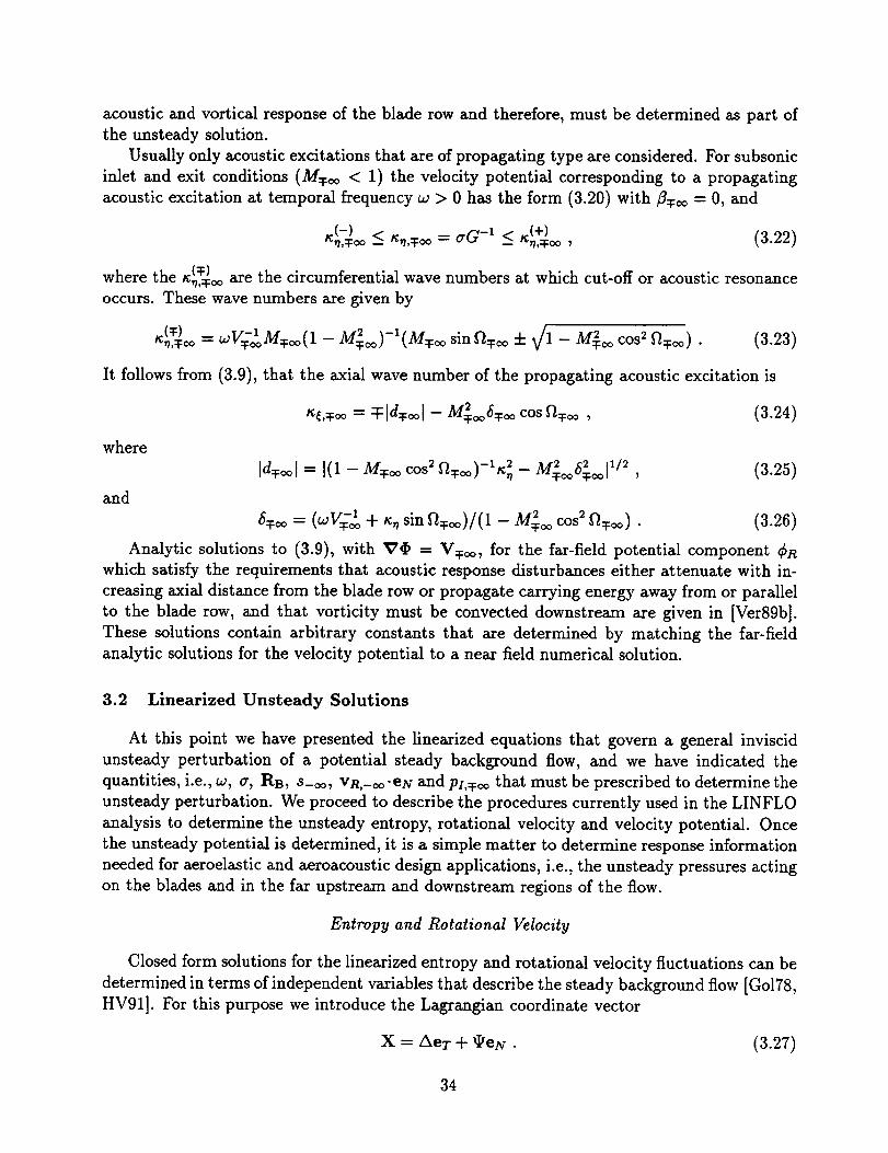
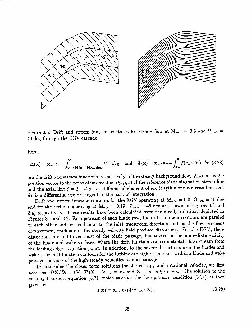
any shocksthat might occur are of weakto moderatestrength and in which the free-streamflow conditions far upstreamof blade rowsareuniform. In suchcases,the steadybackgroundflows in the inviscid regions can be regardedas isentropic and irrotational. For potentialmeanflows, the inviscid wake-andshock-jumpconditions becomewell-posed,in that, therearea sufficientnumber of conditionsto determinethe flow propertiesat wakesand shocks.Inaddition, the potential meanflow assumptionleadsto two-dimensional,steadyand unsteady,aerodynamicanalysesthat arevery efficient computationally.
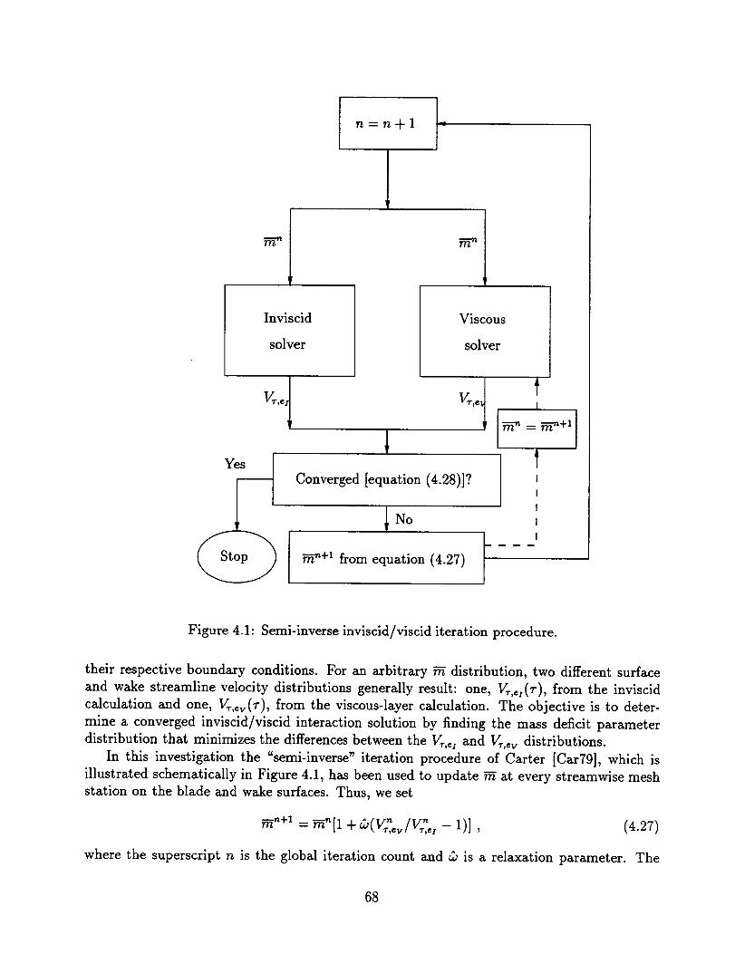
In the following sectionsof this report wewill describethe componentunsteadyaerody-namic analysesmentionedabove. In particular, in § 3 wewill describethe linearized inviscidanalysisLINFLO, which appliesto flows in whichthe unsteadinesscanbe regardedasa smallperturbation of an isentropicand irrotational meanor steadybackgroundflow. The SFLOW-IVI analysisfor steady flowswith strong inviscid/viscid interactionswill be describedin § 4.Finally, the unsteady viscouslayer analysisUNSVIS, which canbe usedin conjunction withLINFLO to predict unsteady flows with weak inviscid/viscid interactions, will be presentedin§5.
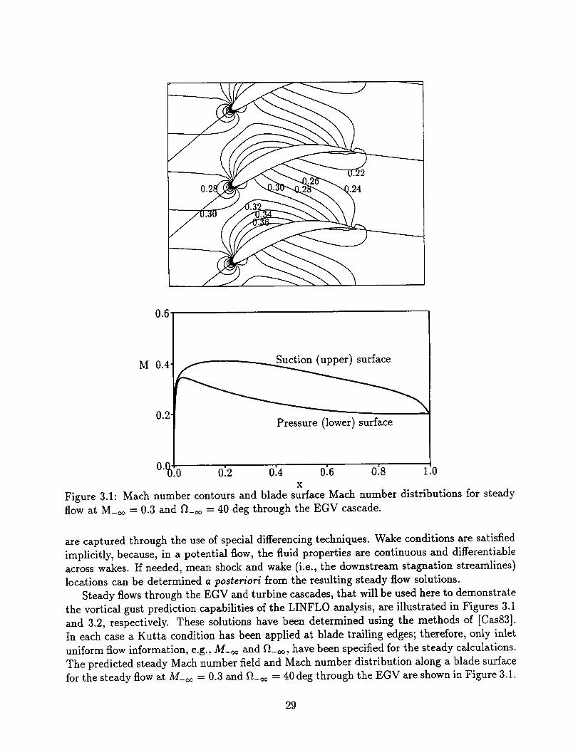
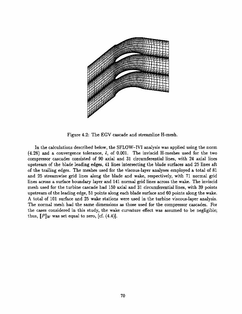
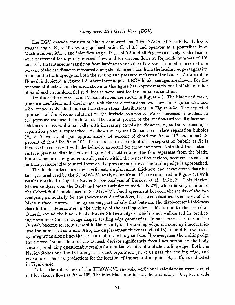
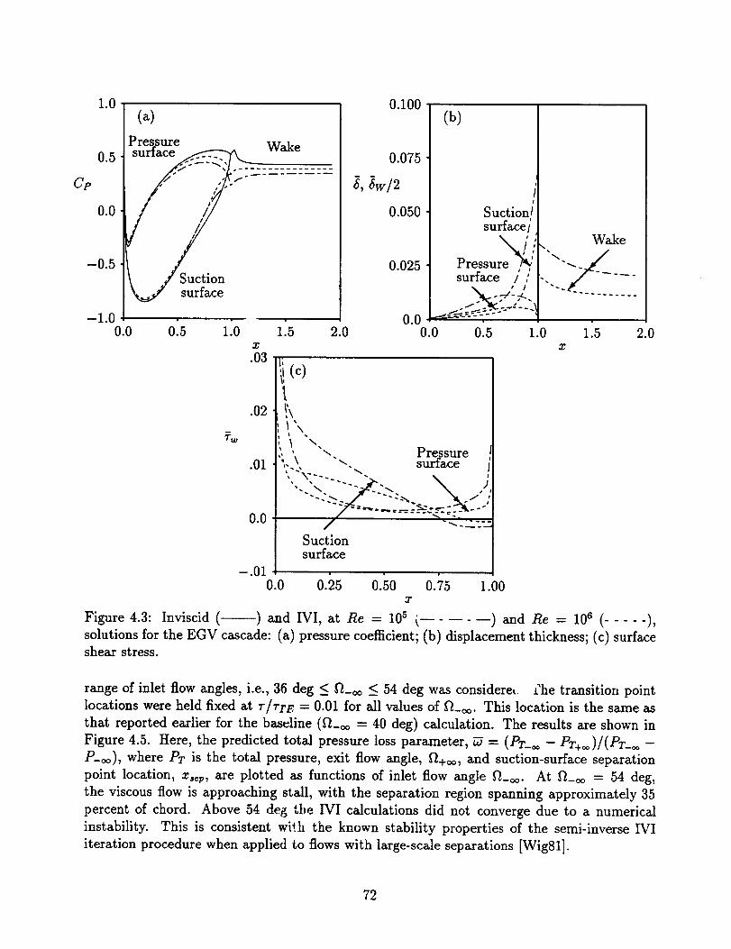
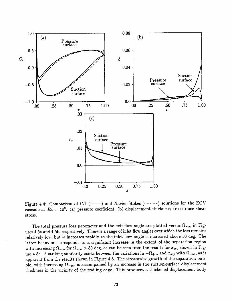
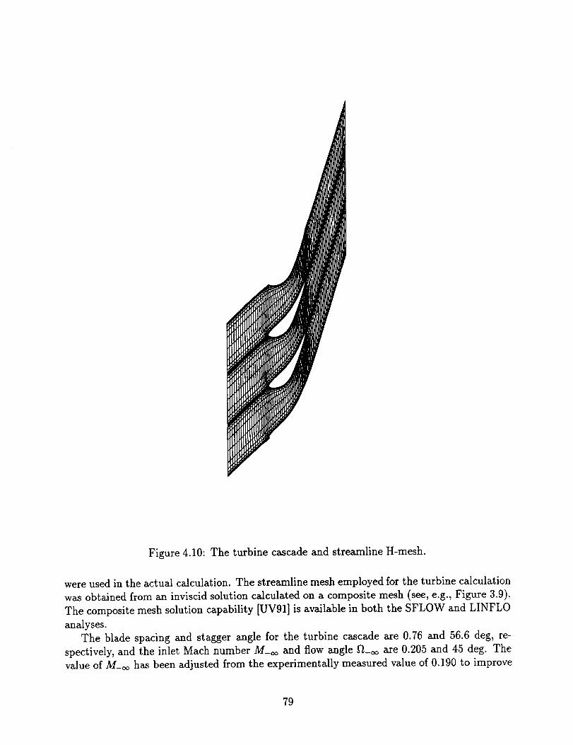
To demonstratethese analyses,we will apply them to three of the cascadesstudied inpreviousinvestigations [VH90,VBHA91, BVA93a]-- a compressorexit guidevane (EGV), ahigh speedcompressor(HSC) cascade,known asthe Tenth Standard CascadeConfiguration[FS83,FV93], and a turbine cascade,known asthe Fourth Standard CascadeConfiguration[FS83].The bladesof the EGV and HSCcascadesareconstructedby superposingthe thicknessdistribution of a modified NACA four-digit seriesairfoil on a circular-arc camber line. Thethicknessdistribution is given by
F(_) = w-l(t¢-¢¢ x A__oo).ezGcosft_oo . "2r[_(x)- _(x_)]" (3.34)2r(1 - iaow) sm Gcos gt_oo
is a complex function that depends upon, among other things, the behavior of the mean flow
in the vicinity of a leading-edge stagnation point. This choice of ¢. ensures that v. • n =
(vn + We.) • n = 0 at blade and wake mean positions.
After combining (3.30), (3.33) and (3.34), we find that the complex amplitude of the
source-term velocity, v. = vR + _7¢., is given by
v. = FV(i___.X) + _-
(3.35)
It follows from (3.34) and (3.35) that v. behaves like s_¢¢_7(I) exp(i0c__-X)/2 in the immediate
vicinity of the mean blade and wake surfaces, i.e., as n _ 0. Thus, v.. n = 0, but, if s__ :_ 0,
the tangential component of the source-term velocity will be indeterminate at such surfaces.
It would be useful in future work to construct a convected potential, ¢., that also removes
this indeterminacy, thereby allowing more accurate numerical resolutions of unsteady flows
excited by entropic disturbances.
The velocities vR and v, depend upon A and • and the first partial derivative of these
functions. Therefore, the complex amplitudes of the unsteady vorticity, _ = V x vn =
X7 x v., and the source term, fi -iV. (_v.), in (3.9) depend also upon the second partial
derivatives of A and q. Thus, an accurate solution for the nonlinear steady background flow
is a critical prerequisite for determining the unsteady effects associated with entropic and
vortical excitations.
The complex amplitudes of the entropy, rotational velocity, vorticity, and source term
velocity are readily determined once the values of the drift and stream functions and their
spatial derivatives are specified over the single extended blade-passage solution domain. For
this purpose it is convenient to use an H-grid in which one set of mesh lines are the streamlines
of the steady background flow, for resolving unsteady flows excited by entropic and vortical
gusts. An H- grid which covers the solution domain, i.e., one which is bounded by the upstream
and downstream axial lines _ = _:F and two neighboring mean-flow stagnation streamlines,
is appropriate. The locations of the latter are determined a posteriori from the solution for
the nonlinear steady background flow. Once the boundaries of the H-grid are established,
the locations of the interior grid points can be determined using an elliptic grid generation
technique, as described in [VH90, HV91].
Because a streamline mesh is used, the drift function can be evaluated at each point in the
computational domain by a straightforward numerical integration of (3.28). The procedure
37
0" ""
m
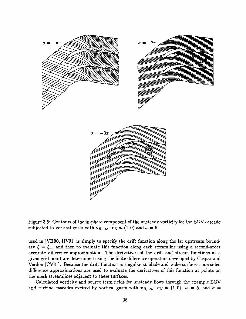
Figure 3.5: Contours of the in-phase component of the unsteady vorticity for the E(4V cascade
subjected to vortical gusts with vn,-oo • eN -- (1, 0) and o., --- 5.
used in [VH90, HV91] is simply to specify tbe drift function along the far upstream bound-
ary _ = __, and then to evaluate this function along each streamline using a second-order
accurate difference approximation. The derivatives of the drift and stream functions at a
given grid point are determined using the finite difference operators developed by Caspar and
Verdon [CV81]. Because the drift function is singular at blade and wake surfaces, one-sided
difference approximations are used to evaluate the derivatives of this function at points on
the mesh streamlines adjacent to these surfaces.
Calculated vorticity and source term fields for unsteady flows through the example EGV
and turbine cascades excited by vortical gusts with vR,-_o • eN = (1,0), ca = 5, and a =
38
m D
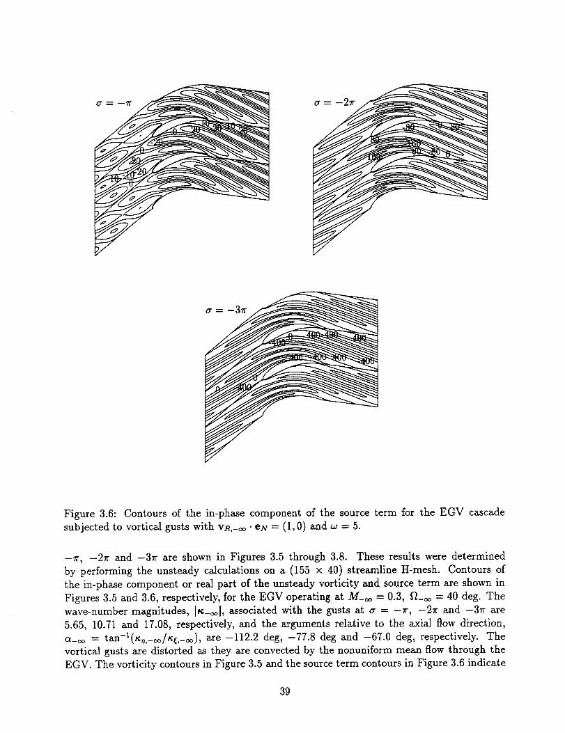
Figure 3.6: Contours of the in-phase component of the source term for the EGV cascade
subjected to vortical gusts with vn,-oo • eN = (1, 0) and w = 5.
-Tr, -2_r and -3zr are shown in Figures 3.5 through 3.8. These results were determined
by performing the unsteady calculations on a (155 × 40) streamline H-mesh. Contours of
the in-phase component or real part of the unsteady vorticity and source term are shown in
Figures 3.5 and 3.6, respectively, for the EGV operating at M__o = 0.3, _-oo = 40 deg. The
wave-number magnitudes, [t¢-oo[, associated with the gusts at a = -_', -27r and -3zr are
5.65, 10.71 and 17.08, respectively, and the arguments relative to the axial flow direction,
a-oo = tan-l(_,,-oo/t_¢,-oo), are -112.2 deg, -77.8 deg and -67.0 deg, respectively. The
vortical gusts are distorted as they axe convected by the nonuniform mean flow through the
EGV. The vorticity contours in Figure 3.5 and the source term contours in Figure 3.6 indicate
39
a _ wTI"
0" "-- m37f"
/
/
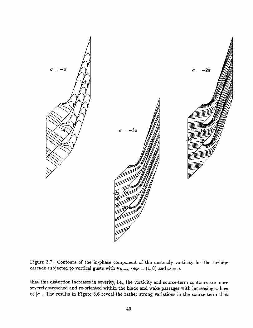
Figure 3.7: Contours of the in-phase component of the unsteady vorticity for the turbine
cascade subjected to vortical gusts with vn,-oo • eg = (1, 0) and w = 5.
that this distortion increases in severity, i.e., the vorticity and source-term contours are more
severely stretched and re-oriented within the blade and wake passages with increasing values
of Icrl. The results in Figure 3.6 reveal the rather strong variations in the source term that
40
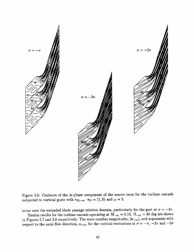
O" _ B27/"
Figure 3.8: Contours of the in-phase component of the source term for the turbine cascade
subjected to vortical gusts with Vn,-oo • en = (1, 0) and a; = 5.
occur over the extended blade passage solution domain, particularly for the gust at a = -3_'.
Similar results for the turbine cascade operating at M-oo = 0.19, fl-oo = 45 deg are shown
in Figures 3.7 and 3.8 respectively. The wave number magnitudes, [t¢_oo [, and arguments with
respect to the axial-flow direction, a-oo, for the vortical excitations at a = -Tr, -27r and -3_r
41
are5.07,8.35and 13.50and -125.4 deg, -81.8 deg and -66.7 deg, respectively. As indicated
in Figures 3.7 and 3.8, the vortical gusts are highly distorted as they are convected past the
thick, highly cambered turbine blades. The unsteady vorticity and source term contours for
the gusts at a = -2rr and a = -31r are quite different from those for the gust at a = -_'.
For a = -Tr the rectilinear vorticity contours far upstream of the blade row evolve into bowed
shapes as the gust is carried through the blade row by the mean flow. The vorticity contours,
within the passage and far downstream of the blade row, for the gusts at a = -2_r and
a = -37r are close to being straight lines. These lie at substantially different orientations than
the contours upstream of the blade row. The source term contours in Figure 3.8 are severely
distorted for the turbine blade row from mid-blade passage to the downstream boundary of
the solution domain, particularly for the vortical gusts at a = -2rr and a = -37r. Also, the
source terms associated with the gusts at a = -2_r and a = -37r have very large gradients
within the blade passage and downstream of the blade row. These features make it difficult
to determine an accurate numerical resolution of the unsteady potential, for these turbine
unsteady flows.
Velocity Potential
The unsteady potential (¢) is determined as a solution of the field equation (3.9) subject
to conditions at the mean blade, wake and shock surfaces, and conditions in the far field. Flow
tangency [cf. (3.11)] applies at the blade surfaces, the fluid pressure and normal velocity must
be continuous [cf. (3.12)] across blade wakes, and mass and tangential momentum must be
conserved [cf. (3.13)] across shocks. The velocity potential in the far field is given by (3.19);
the potential due to an acoustic excitation at frequency w and circumferential wave number
_,_,_=oo= o'/G, by (3.20).
A numerical resolution of the linear, variable-coefficient, boundary-value problem for ¢
is required over a single, extended, blade-passage region of finite axial extent. The field
equation must be solved in continuous regions of the flow subject to the surface and far
field conditions on the unsteady potential. In particular, the near-field numerical solution for
the potential must be matched to far-field analytical solutions at finite distances (_ = _:)
upstream and downstream from the blade row. Numerical methods for determining ¢ for
isentropic and irrotational (i.e., s -= _ = 0) unsteady, subsonic, transonic, and supersonic
flows have been reported in [CV81, VC82, VC84, UV91, MVF94]. Such solutions apply to
unsteady flows excited by prescribed blade motions and/or acoustic excitations at inlet and
exit. Numerical solution procedures for unsteady flows excited by entropic and/or vortical
gusts [VH90, HV91, VBHA91] have been developed and implemented only for subsonic flows.
The development of such procedures for transonic and supersonic flows remains, therefore, asa subject for future research.
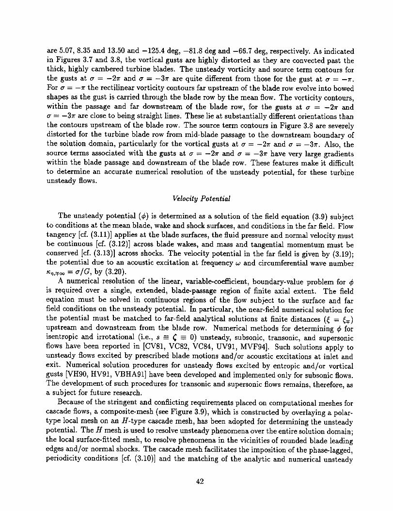
Because of the stringent and conflicting requirements placed on computational meshes for
cascade flows, a composite-mesh (see Figure 3.9), which is constructed by overlaying a polar-
type local mesh on an H-type cascade mesh, has been adopted for determining the unsteady
potential. The H mesh is used to resolve unsteady phenomena over the entire solution domain;
the local surface-fitted mesh, to resolve phenomena in the vicinities of rounded blade leading
edges and/or normal shocks. The cascade mesh facilitates the imposition of the phase-lagged,
periodicity conditions [cf. (3.10)] and the matching of the analytic and numerical unsteady
42
Figure 3.9: Extended blade-passagesolution domain and compositemeshusedin LINFLOunsteady transonic calculations.
solutions at the far upstream (_ = __) and far downstream (_ = (+) boundaries of the
numerical solution domain. Use of this mesh alone is often sufficient for resolving unsteady
subsonic flows, and this has been the strategy applied for calculating the unsteady subsonic
solutions for cascade/vortical gust interactions presented in this report. The local mesh allows
an accurate modeling of the unsteady flow in the vicinities of blade leading edges and normal
shocks. It is constructed so that two "radial" lines coincide with the predicted mean shock
locus to provide upstream and downstream shock mesh lines for the accurate imposition of
unsteady shock-jump conditions.
Since the cascade and local body-fitted meshes differ topologically, a zonal solution pro-
cedure for overlapping meshes has been adopted in [UV91] for determining the unsteady
potential. In the region of intersection between the two meshes, i.e., the region covered by the
local mesh, certain cascade mesh points are eliminated depending upon their location within
the local mesh domain. The discrete equations are written separately for the cascade and
local meshes and coupled implicitly through special interface conditions, resulting in a single
composite system of finite-difference equations that describe the unsteady flow over the entire
43
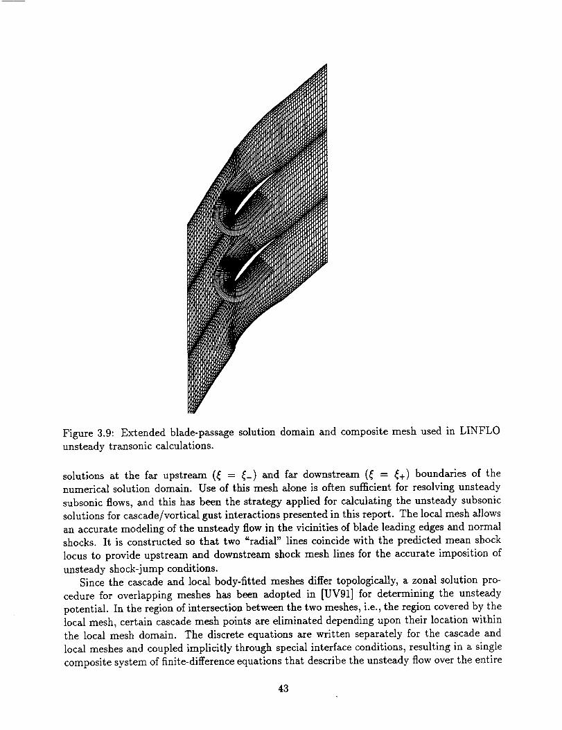
Figure 3.10: Contours of the in-phase componentof the unsteady potential for the EGVcascadesubjected to vortical gustswith vn,-oo• eN = (1, 0) and w = 5.
solution domain.
The finite-difference model used to approximate the unsteady equations on the cascade
and local meshes has been described in detail in [CV81]. Algebraic approximations to the
various linear operators, which make up the unsteady boundary-value problem, are obtained
using an implicit, least-squares, interpolation procedure that is applicable on arbitrary grids.
This procedure employs a nine point "centered" difference star at subsonic field points, and
a twelve point difference star at supersonic points. At a blade boundary point a nine point
one-sided difference star is used on the cascade mesh, whereas nine- or six-point one-sided
stars are used on the local mesh. Normal shocks are fitted in the local-mesh calculation
by approximating the shock-jump condition (3.13) using one-sided difference expressions to
44
°i
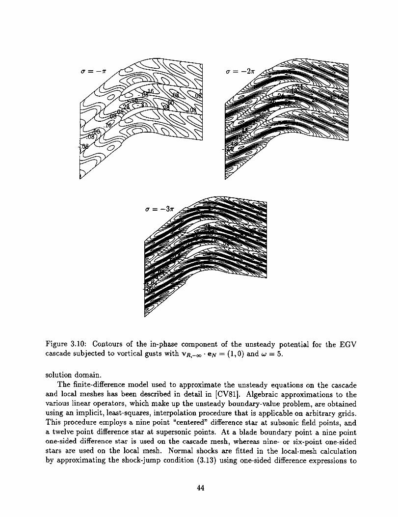
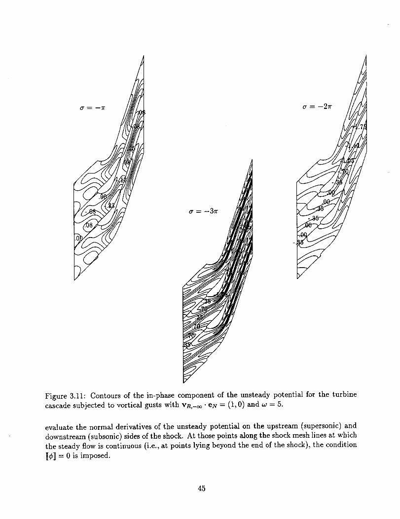
Figure 3.11: Contours of the in-phase component of the unsteady potential for the turbine
cascade subjected to vortical gusts with vn,-o_ "eN = (1, 0) and w = 5.
evaluate the normal derivatives of the unsteady potential on the upstream (supersonic) and
downstream (subsonic) sides of the shock. At those points along the shock mesh lines at which
the steady flow is continuous (i.e., at points lying beyond the end of the shock), the condition
_¢]] = 0 is imposed.
45
The systemsof linear algebraicequationsthat approximate the unsteady boundary-value
problem on the cascade and local meshes are block-tridiagonal for subsonic flow and, because
shocks are fitted, block-pentadiagonal for transonic flow. A subsonic solution on the H-mesh
alone is determined using a direct block inversion scheme. Composite (cascade/local) mesh
solutions are determined using a different scheme. Because of the cascade/local mesh coupling
conditions, the composite system of discrete equations contains a sparse coefficient matrix of
large bandwidth. Consequently, special storage and inversion techniques must be applied to
achieve an efficient solution. Once the composite system of unsteady equations is cast into an
appropriate format, it can be solved using Gaussian elimination [UV91].
The calculated unsteady potential (¢) fields associated with the interactions of vortical
gusts with the example EGV and turbine configurations are depicted in Figures 3.10 and 3.11,
respectively. In particular, contours of the in-phase components of the unsteady potential,
Re{C}, are given for vortical gusts at vR,-_ "eN = (1, 0), w = 5, and a = -% -2_r and
-37r. Vorticity and source-term fields for the unsteady flows through the EGV are shown in
Figures 3.5 and 3.6, respectively; those for the flows through the turbine, in Figures 3.7 and
3.8. The potential solutions depicted in Figures 3.10 and 3.11 were determined on 155 × 40
streamline meshes and show variations over a blade passage that are associated primarily with
the source term on the right-hand-side of (3.9). Once the unsteady potential is determined,
the complete, linearized, inviscid, unsteady flow problem is solved.
3.3 The Inviscid Response
At this point we have provided a linearized unsteady aerodynamic formulation that de-
scribes the general first-order fluid-dynamic perturbation of an isentropic and irrotational
mean or steady background flow. We have also outlined the solution procedures used in the
LINFLO analysis to determine the unsteady entropy, rotational velocity and velocity poten-
tial. Solutions to the linearized unsteady problem are required to determine the aerodynamic
response information needed for aeroacoustic and aeroelastic applications, e.g., the unsteady
pressure fields far upstream and far downstream of the blade row, and the unsteady pres-
sures acting at the moving blade surfaces. We refer the reader to [Ver89a, Ver92] for detailed
derivations of other local and global unsteady aerodynamic response parameters that are used
in aeroelastic investigations.
Approximate solutions for the full, nonlinear, time-dependent flow properties are con-
structed by superposing the results for the steady and the linearized unsteady flow properties,
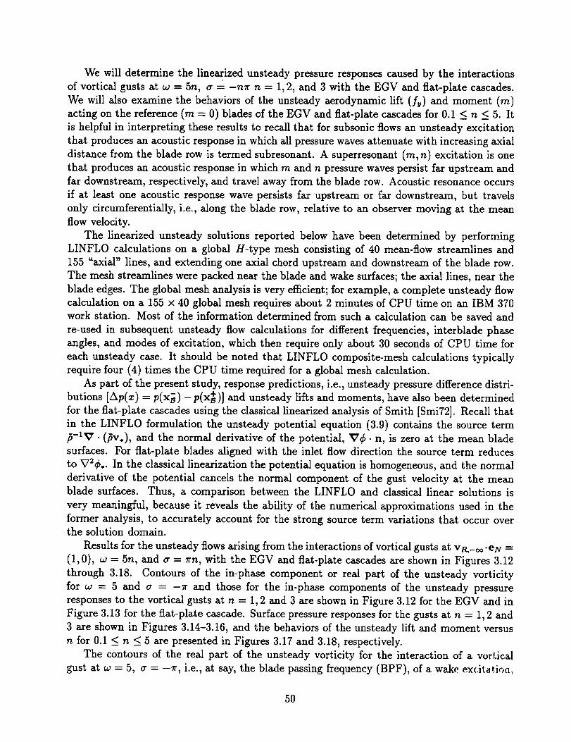
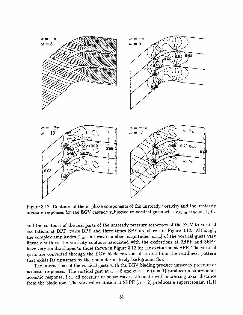
The acoustic response behaviors of the EGV and the flat plate cascades to the excitation
at to = 15, cr = -37r differ in the far-downstream region. The reason for this is that different
mean flow conditions prevail far downstream of the two blade rows, which, for the excitation
at 3BPF, lead to very different far-downstream acoustic environments. Recall that the EGV
operates at an exit Mach number and flow angle of 0.226 and -7.4 deg; the flat plate cascade,
at M+oo = M = 0.3 and ft+oo = ll = 40 deg. A vortical excitation at to = 15 and a = -37r,
is superresonant (1,0) for the EGV cascade; therefore, a propagating acoustic wave persists
far upstream, but all acoustic response waves attenuate with increasing distance downstream.
This same excitation produces a superresonant (1,1) acoustic response for the flat-plate blade
row, with a relatively strong propagating acoustic response wave in the far downstream field.
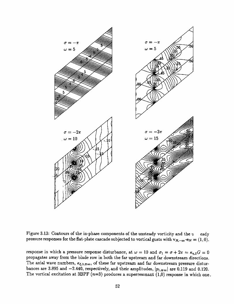
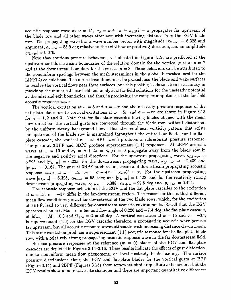
Surface pressure responses at the reference (m = 0) blades of the EGV and flat-plate
cascades are depicted in Figures 3.14-3.16. These results indicate the effects of gust distortion,
due to nonuniform mean flow phenomena, on local unsteady blade loading. The surface
pressure distributions along the EGV and flat-plate blades for the vortical gusts at BPF
(Figure 3.14) and 2BPF (Figures 3.15) show somewhat similar qualitative behaviors, but theEGV results show a more wave-like character and there are important quantitative differences
53
2.0
1.0 °
0.0 °
°
--2.1
EGV
_,_ / Pressure surface
Flat Plate
"x .. j-__. Pressure (lower) surface
2.0
1.0 •
0.0 °
Im{_}0
-2.0-
f Suction surface
_Pressure surface
-3.0 0.0 012 014 016 ols 1.0X
I|I
ix f Suction (upper) surface
f _ Pressure (lower) sur_ceIIItIIII
0.0 012 014 016 018 1.0X
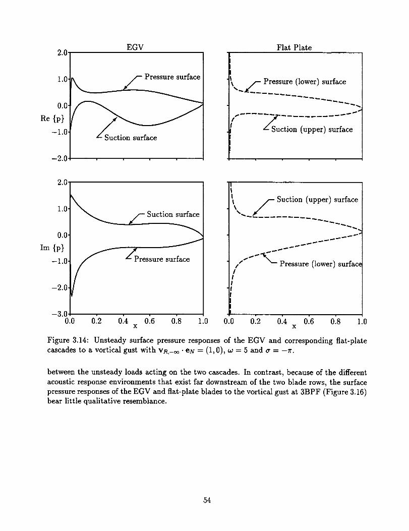
Figure 3.14: Unsteady surface pressure responses of the EGV and corresponding flat-plate
cascades to a vortical gust with vn,-oo • en = (1,0), co = 5 and a = -Tr.
between the unsteady loads acting on the two cascades. In contrast,because of the different
acousticresponse environments that existfar downstream of the two blade rows, the surface
pressure responses of the EGV and flat-plateblades to the vorticalgust at 3BPF (Figure 3.16)
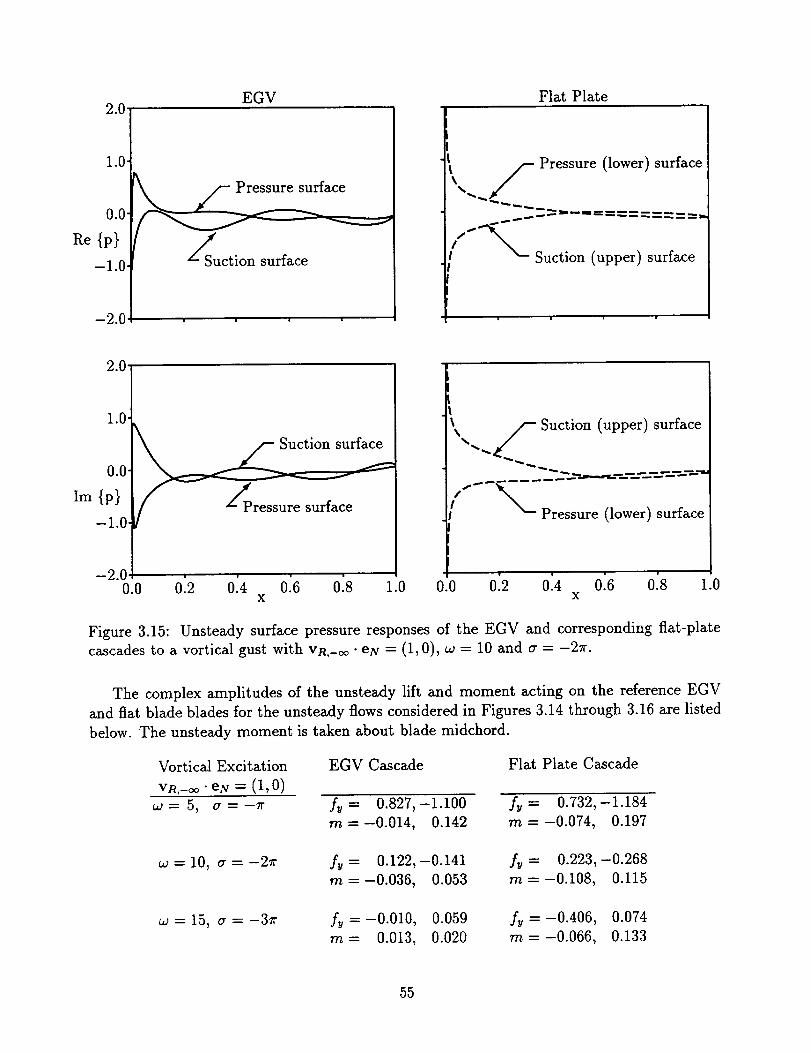
Figure 3.15: Unsteady surface pressure responses of the EGV and corresponding flat-plate
cascades to a vortical gust with vR,-oo • eN = (1, 0), w ---- 10 and a = -2_r.
The complex amplitudes of the unsteady lift and moment acting on the reference EGV
and flat blade blades for the unsteady flows considered in Figures 3.14 through 3.16 are listed
below. The unsteady moment is taken about blade midchord.
Vortical Excitation
VR,-oo " ey ---- (1,0)
EGV Cascade Flat Plate Cascade
w = 5, a = -Tr fy = 0.827,-1.100 f_ = 0.732,-1.184
rn = -0.014, 0.142 m = -0.074, 0.197
w=10, a=-2r f_ = 0.122,-0.141 fy - 0.223,-0.268
m -- -0.036, 0.053 m - -0.108, 0.115
w=15, a=-3r fy=-0.010, 0.059 f_ =-0.406, 0.074
m = 0.013, 0.020 m = -0.066, 0.133
55
2.0
1.0]
0.0"
Re {PI
--1.0"
--2.1
EGV
_Pressure surface
Flat Plate
II
4
I1
III
I /- Suction (upper) surface1 J..-
_-Pressure (lower) surface
2.0
1.0_ /Pressure surface
Im {:iO_ ;uction suffa_
-1"01
III
-2.00.0 0:2 0:4 0:6 0:8 1.0 0.0 0:2 0:4 0:6 0:8
X X
I
t\ _- Suction (upper)surface
_.f____ _,._'---.....,.... ",
Pressure (lower) surface!
.0
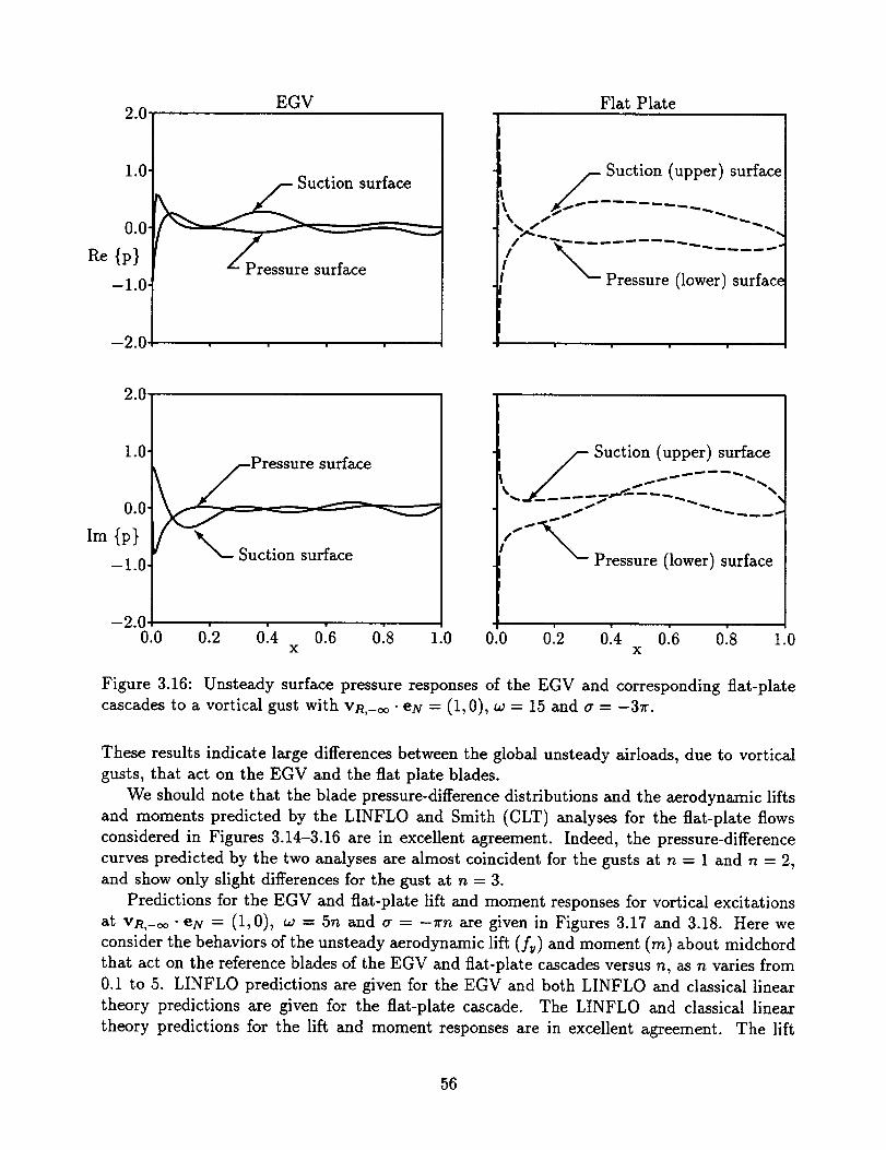
Figure 3.16: Unsteady surface pressure responses of the EGV and corresponding flat-plate
cascades to a vortical gust with vR,-oo • eN = (1, 0), w = 15 and a = -3rr.
These results indicate large differences between the global unsteady airloads, due to vortical
gusts, that act on the EGV and the flat plate blades.
We should note that the blade pressure-difference distributions and the aerodynamic lifts
and moments predicted by the LINFLO and Smith (CLT) analyses for the flat-plate flows
considered in Figures 3.14-3.16 are in excellent agreement. Indeed, the pressure-difference
curves predicted by the two analyses are almost coincident for the gusts at n = 1 and n = 2,
and show only slight differences for the gust at n = 3.
Predictions for the EGV and flat-plate lift and moment responses for vortical excitations
at vR,-¢o • eN = (1, 0), w = 5n and a = -_rn are given in Figures 3.17 and 3.18. Here we
consider the behaviors of the unsteady aerodynamic lift (f_) and moment (m) about midchord
that act on the reference blades of the EGV and flat-plate cascades versus n, as n varies from
0.1 to 5. LINFLO predictions are given for the EGV and both LINFLO and classical linear
theory predictions are given for the flat-plate cascade. The LINFLO and classical linear
theory predictions for the lift and moment responses are in excellent agreement. The lift
56
2.0
1.0"
0.0
-1.0
-2.0-
1.0
EGV
Flat Plate (LINFLO)
Flat Plate (CLT)
v
l I I l
Im{fy}
0.0"
-I.0-
-2.0-
-3.0-
0.0 1]0 2]0 3]0 4]0 i.0
n
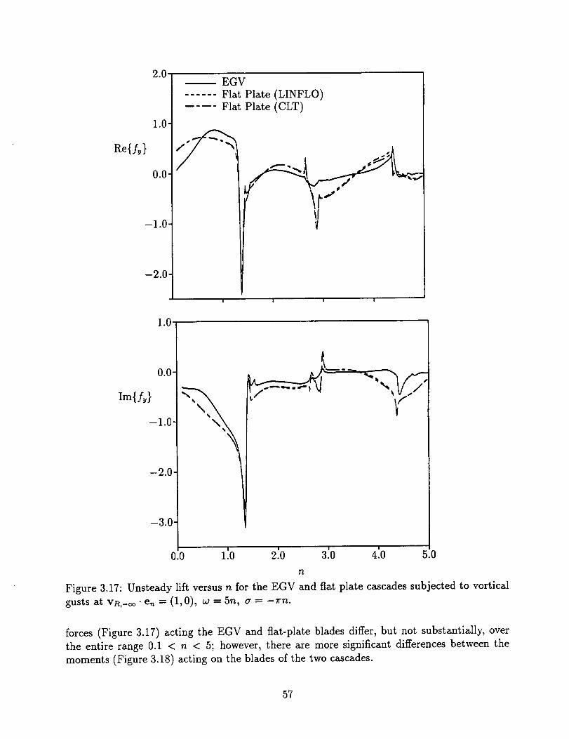
Figure 3.17: Unsteady lift versus n for the EGV and flat plate cascades subjected to vortical
gusts at vn,-oo .e= = (1, 0), w = 5n, a = -_rn.
forces (Figure 3.17) acting the EGV and flat-plate blades differ, but not substantially, over
the entire range 0.1 < n < 5; however, there are more significant differences between the
moments (Figure 3.18) acting on the blades of the two cascades.
57
0.4
0.2"
P_{m}
0.0-
-0.2-
-0.4
EGV
Flat Plate (LINFLO)
Flat Plate (CLT)I
!
0.6
0.4"
Im{m}
0.2"
0o0"
I!
-0.20.0 1:0 2:o 3:0 4:0 5.o
n
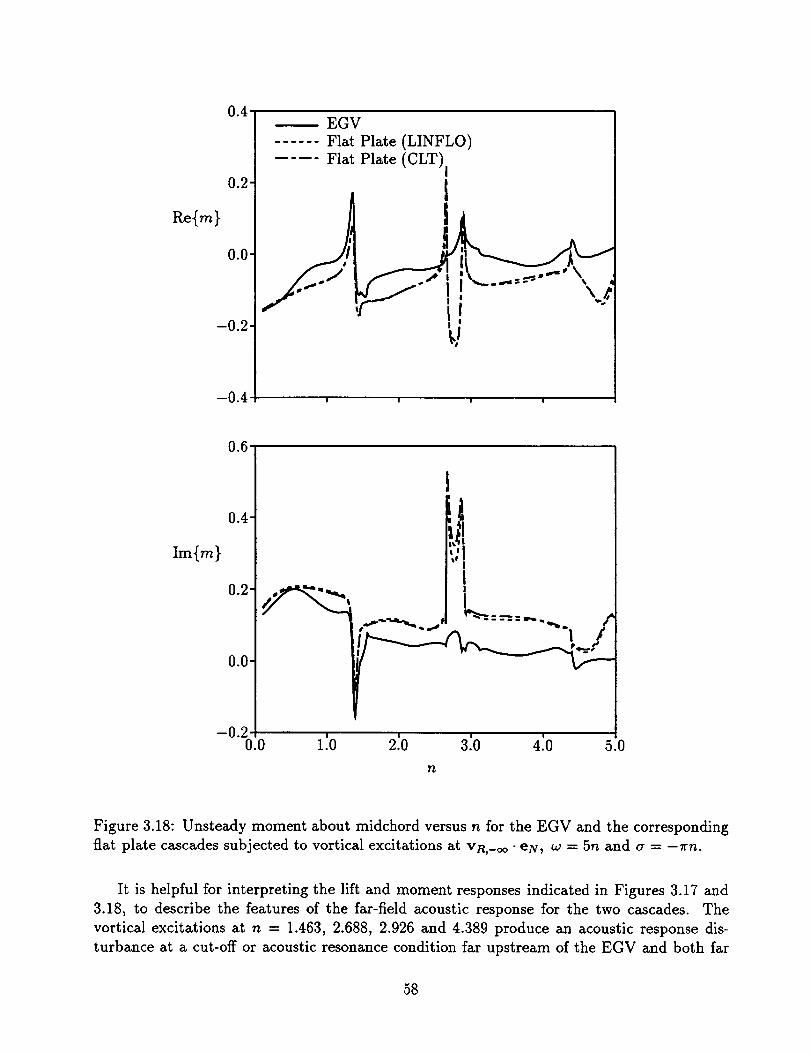
Figure 3.18: Unsteady moment about midchord versus n for the EGV and the corresponding
flat plate cascades subjected to vortical excitations at vn,-oo • ey, ca = 5n and a = -Trn.
It is helpful for interpreting the lift and moment responses indicated in Figures 3.17 and
3.18, to describe the features of the far-field acoustic response for the two cascades. The
vortical excitations at n = 1.463, 2.688, 2.926 and 4.389 produce an acoustic response dis-
turbance at a cut-off or acoustic resonance condition far upstream of the EGV and both far
58
upstream and far downstreamof the flat plate cascade. The excitation at n = 2.688 pro-
duces a resonant acoustic response disturbance that travel along the blade row in the positive
q-direction; those at n =1.463, 2.926 and 4.389 produce resonant disturbances that travel
down the blade row, i.e., in the negative r/-direction. Vortical excitations at n =1.558, 2.865,
3.115 and 4.673 produce a cut-off or resonant acoustic reponse disturbance far downstream
of the EGV. The resonant response disturbance at n =2.865 travels upward along the blade
row; those at n =1.558, 3.115 and 4.673 travel downward. As is readily determined from the
curves in Figures 3.17 and 3.18, the unsteady aerodynamic lift and moment undergo abrupt
and often large changes in the vicinity of an acoustic resonance condition. Such a condition
also represents a boundary for different types of unsteady response behaviors.
For example, the responses of the flat-plate cascade to the vortical excitations in the range
0.1 < n < 5.0 are subresonant for n < 1.463 and 2.688 < n < 2.926; superresonant (1,1)
for 1.463 < n < 2.688 and 2.926 < n < 4.389; and superresonant (2,2) for n > 4.389.
Because the inlet and exit free-stream conditions for the EGV differ, this blade row has a
wider variety of far-field acoustic response behaviors than its flat plate counterpart. For
example, the acoustic responses of the EGV are superresonant (0,1) for vortical excitations
at 2.688 < n < 2.865; subresonant for 2.865 < n < 2.926; superresonant (1,0) for 2.926 < n <
3.115 and superresonant (1,1) for 3.115 < n < 4.389. The different types of far-field acoustic
response behavior seem to have a strong impact on the unsteady blade loads. In particular, the
flat plate cascade has large amplitude moment responses to vortical excitations in the range
2.688 < n < 2.926 which produce subresonant acoustic responses. The moment responses of
the EGV to vortical excitations in this range are much smaller in magnitude. The acoustic
responses of the EGV are superresonant (0,1) for 2.688 < n < 2.865 and subresonant for
2.865 < n < 2.926.
Discussion
This completes our description of the LINFLO analysis and of the capabilities of this analy-
sis, developed under Contract NAS3-25425, to describe cascade/vortical gust interactions. In
subsequent sections of this report we will describe a steady inviscid/viscid interaction analysis
and an unsteady viscous layer analysis that are being developed for use in conjunction with
LINFLO to provide efficient prediction capabilities for unsteady viscous flows. We will also
present LINFLO results for unsteady flows caused by prescribed blade motions and acoustic
excitations.
The LINFLO analysis represents a powerful analytical capability for efficiently predict-
ing the unsteady aerodynamic information needed in blade row aeroelastic and aeroacous-
tic response studies, in which many controlling parameters are involved. In recent stud-
ies [DV94, AV94] LINFLO has been applied to assist in calibrating modern, time-accurate,
Euler/Navier-Stokes analyses. Very good agreement between LINFLO predictions and non-
linear Euler and Navier-Stokes predictions has been determined for unsteady subsonic flows
excited by small-amplitude, vortical or acoustic disturbances [DV94] and for unsteady subsonic
and transonic flows excited by prescribed blade vibrations [AV94]. Based upon the limited
ranges of parametric studies that were conducted using the nonlinear analyses, it was also
found that unsteady pressure responses are linear over surprisingly wide ranges of excitation
amplitudes. Such results provide evidence on the usefulness of a linearized inviscid, unsteady,
aerodynamic analysis for aeroelastic and aeroacoustic design studies.
59
4. The Steady Inviscid/Viscid Interaction Analysis: SFLOW-IVI
Efficient analyses for predicting the effects of strong inviscid/viscid interaction (IVI) phe-
nomena, due, for example, to viscous-layer separations, shock/boundary-layer interactions and
trailing-edge/near-wake interactions, on the aerodynamic, aeroelastic, and aeroacoustic per-
formances of turbomachinery blading are needed as part of a comprehensive analytical design
prediction system. The focus here will be on the development of an accurate and efficient IVI
analysis for steady cascade flows, that can provide the foundation for an unsteady procedure
to be developed later. The steady analysi_ is described below and is being developed as part of
an overall research program, which has the goal of providing reliable and efficient theoretical
prediction methods for steady and unsteady viscous flows, at high Reynolds numbers, throughsubsonic and transonic cascades.
The present steady analysis uses an inviscid/viscid interaction (IVI) approach, in which
the flow in the outer inviscid region is assumed to be potential, and the flows in the inner or
viscous-layer regions are governed by Prandtl's viscous-layer equations. The inviscid equations
are solved using a Newton iteration procedure and an implicit, least-squares, finite-difference
approximation, similar to that used in LINFLO. The viscous-layer equations are solved using
a modified Levy-Lees transformation and an inverse, finite-difference, space-marching method,
which is applied along the blade surfaces and the wake streamlines. Complete details on the
inviscid and viscous solution procedures can be found in [HV93, HV94] and [BVA93a], respec-
tively. The inviscid and viscid solutions are coupled via a semi-inverse global iteration pro-
cedure that permits the prediction of boundary-layer separation and other strong-interaction
phenomena. Numerical results will be presented below for the three example cascades de-
scribed in § 2.5 with a range of inlet flow conditions considered for one of them, including
conditions leading to large-scale flow separations. Comparisons with Navier-Stokes solutions
and experimental data will also be given.
4.1 General Concepts
For the flows oi :'tactical interest in either internal or external aerodynamics, the Reynolds
number is usually sufficiently high so that the flow past an airfoil or blade can be divided into
two regions: an "inner" dissipative region consisting of boundary layers and wakes, and an
"outer" inviscid region. The principal interaction between the flows in the viscid and inviscid
regions arises from the displacement thickness effect which leads to thickened semi-infinite
equivalent bodies _ : corresponding changes in surface pressures.
If the interacti s "weak," then the complete flow problem can be solved sequentially.
In this case the pr. _re distributions along the blades and wakes are first determined by a
pure inviscid soluti_a. These distributions are then imposed when solving the viscous-layer
equations to determine viscous displacement thickness, _(T), distributions along the blades
and wakes. The latter are then used to obtain a new inviscid solution, that accounts for
viscous displacement effects. The resulting changes in the blade pressure distributions and
in the downstream freestream flow properties (e.g., Mach number and flow angle) can then
be calculated. It is sometimes possible to continue this sequential solution procedure until a
converged solution for the entire flow is achieved.
60
Flows over airfoils or blades, however, involve both a weak overall interaction arising from
standard displacement thickness and wake curvature effects, and local strong-displacement
interactions caused, for example, by viscous-layer separations, shock/boundary-layer interac-
tions, and trailing-edge/near-wake interactions. Viscous displacements in a strong-interaction
region can cause substantial changes in the local inviscid pressure and, in some cases, in the
overall pressure field. The concept of an inner viscous region and an outer inviscid region
still applies, but the classical hierarchical structure of the flow breaks down. In particular, for
flows with strong interactions the inviscid/viscid hierarchy changes from "direct", in which
the pressure is determined by the inviscid flow, to "interactive" in which the pressure is de-
termined by the mutual interaction between the flows in the inviscid and the viscous-layer
regions. This change must be accommodated within an inviscid/viscid interaction solution
procedure.
The construction of an IVI analysis involves, first, the development of component, i.e.,
inviscid and viscous-layer analyses, and, second, the implementation of these components into
a strong-interaction iteration procedure to produce a solution for the complete flow field.
Solution methods for steady subsonic and transonic inviscid flows through cascades (e.g.,
see [Cas83, HV94]) and for steady boundary-layer and wake flows (e.g., [VV85] and [BV87])
have been developed to a relatively mature state. Methods for coupling such solutions have
also been developed and assessed through a number of model problem studies (e.g., see [Vel80,
VV85, BV87]). Inviscid/viscid interaction procedures for predicting steady flows in cascades
have also been developed [HSS79, JH83, CH80, BV89, BHE91] and applied over a wide range
of inlet flow conditions, including conditions leading to stall [BHE91].
In the present approach we consider high Reynolds number (Re = _*_._V'_ L*/p* ) steady
flow, with negligible body forces, of a perfect gas with constant specific heats and Prandtl
number through a two-dimensional cascade (cf. Figures 2.1 and 2.3). In particular, we willrestrict our consideration to adiabatic flows at unit Prandtl number, however, it is a relatively
simple matter to extend the analysis to heat conducting flows at arbitrary Prandtl numbers.
The flow in the outer inviscid region is assumed to be isentropic and irrotational and hence,
governed by the full-potential equation; those in the inner viscous-layer regions, by Prandtl's
viscous-layer equations. The non-hierarchical nature of strong interactions is taken into ac-
count by the procedure used to couple the inviscid and viscid solutions. In addition, an inverse
viscous-layer calculation, in which the displacement thickness is specified instead of the pres-
sure, is employed to permit viscous solutions to be continued through local strong-interaction
regions, including regions of separated flow. In regions of the flow where the inviscid/viscid
interactions are weak, the pressure, as determined from the inviscid solution, can be imposed,
instead of the displacement thickness, to obtain a direct viscous-layer solution.
In the present approach, the steady, cascade, full-potential analysis (SFLOW) developed
by Hoyniak and Verdon [HV93, HV94] is employed to determine the flow in the inviscid
region. SFLOW has been constructed for use with the linearized inviscid unsteady flow anal-
ysis, LINFLO, to provide compatible and comprehensive steady and unsteady inviscid flow
prediction capabilities for cascades. In the IVI calculation procedure (which is referred to as
SFLOW-IVI), viscous effects are incorporated by modifying the blade and wake boundary
conditions used in SFLOW to account for the effects of viscous displacement. The nonlinear
inviscid analysis, coupled with the IVI iteration procedure, allows nonlinear changes to the
inviscid base flow due to viscous effects to be evaluated. The ability to treat such nonlinear
61
perturbations isespeciallyimportant in transonic flowsin which shockpositionsand strengthsare significantly altered by viscousdisplacements. Althoug : the analysisdescribedbelow ispresentlyrestricted to subsonicflows, it canbeextendedto treat transonic flowsin the future.
4.2 Inviscid/Viscid Interaction Analysis
Inviscid Region
The flow in the inviscid region is determined as a solution of the field equations (3.1)
and (3.2) subject to flow tangency conditions at the blade surfaces, jump conditions on the
normal velocity and pressure across the blade wakes, and prescribed uniform flow conditions
far upstream of the blade row. Blade-to-blade periodicity conditions [cf. (2.42)] are applied
upstream and downstream of the blade row to limit the computational domain to a single,
extended, blade-passage. Kutta conditions at the blade trailing edges and a global massconservation condition that relates the flows at the inlet and exit boundaries and accounts for
the blockage effects of the viscous layers are enforced in lieu of specifying the uniform flow far
downstream of the blade row. For the flows considered here, the inlet and exit velocities aresubsonic.
The field equation (3.1) can be written in the form
A2V_¢ - We. V(V¢)2/2 = 0 (4.1)
where the speed of sound propagation A is given in terms of the potential q_ in (3.2). The
SFLOW inviscid analysis is based on this non-conservative form of the full potential equation.
The specific forms of the blade and wake conditions for the potential steady flow in the
inviscid region can be determined by setting V = Vq_ in (2.47) and (2.48). Thus, at each
blade surface
V¢. n = #-_ld(#_V_,,$)/dr, for x E Sm , (4.2)
where _ and V_,_ = O¢/Orl_ are the inviscid density and velocity at this surface, or the
viscous density and streamwise velocity component at the edge of the viscous layer, and _ is
the boundary-layer displacement thickness (see Figure 2.3). The quantities r and n denote
the arc distance along the blade (positive in the downstream direction and zero at the leading-
edge stagnation point) and the local unit normal vector directed outward from the surface,
respectively. At the blade wakes the inviscid solution for the normal component of the fluid
velocity and the pressure must be discontinuous with jumps given by
[V¢_.n = (_-_ld(_eV_,e$)/dr) and [[P] = _(/5¢V_(_+ 0)) , for x e Win, (4.3)
where n is the upward pointing unit normal vector to the reference wake streamline (i.e., W
in Figure 2.3), ($) = Sw and (0) = 0w are the displacement and momentum thicknesses of
the complete wake, and _ is the curvature of the wake which is taken as positive when the
reference wake streamline is concave upwards.
As mentioned in § 2.3, a complication arises in that the location of the reference wake
streamline is unknown a priori; however, to within lowest order, the wake conditions can be
referenced to any arbitrary curve emanating from the trailing edge and lying within the actual
viscous wake [Vel80]. Usually, wake curvature effects are regarded as negligible. In this case
62
the inviscid pressure,density and tangential velocity are continuousacrossblade wakes,andthe wakeconditions (4.3) reduceto
[Vff_]-n = _d(_,V,.,,_w)/dT and [[P] = 0, x E W,_. (4.4)
For steady flows, the reference wake streamline is taken to be the aft stagnation streamline as
determined by a pure inviscid solution. This is adequate except in extreme cases where the
location of the stagnation streamline is significantly altered by viscous effects. In this case, it
is possible to periodically update the location of the wake streamline during the calculation,
although this has not been done in the present study.
The foregoing boundary-value problem is solved using a Newton iteration procedure. Thus,
we set
¢,+1 = ¢, + ¢,, n = 0,1,2,... (4.5)
where _P, is the estimate to the final solution at the nth iteration level and Cn is a correction
to this estimate. The quantity ¢= is determined at each step of the iteration process by solving
linear equations that are derived by substituting (4.5) into (4.1)-(4.3) and neglecting terms
that are of second and higher order in ¢,. For example, the linear field equation for the
where A,_, the nth estimate to the speed of sound propagation, is determined from (3.2) with
¢ replaced by _n and f)/Dt = re,. _7. The right-hand side of (4.6) is known and the linear
operator on the left-hand side is readily derived from the linear unsteady operator appearing
on the left-hand side of (3.9). The various equations used to determine ¢, are approximated
using the same implicit, least-squares, finite-difference approximations as those used in the
LINFLO analysis. The resulting linear system of algebraic equations that approximate the
linear boundary value problem for Cn is solved by direct matrix inversion, as in LINFLO, using
lower-upper decomposition and Gaussian elimination. The Newton iterations are continued
until I15.11< where ]] ]l denotes a prescribed norm and _ << 1 is a user specified tolerance
level. This nonlinear steady analysis, called SFLOW, is described in detail in [HV93, HV94].
The present inviscid solutions were obtained on a "streamline" type H-mesh, rather than
on the "sheared" H-mesh described in [VC84] and [HV93]. The SFLOW analysis was modified
by Hoyniak to use the streamline H-mesh developed by Hall and Verdon [HV91]. Thus, prior
to initiating an IVI calculation, a pure inviscid solution is first obtained on a sheared H-mesh.
The resulting solution is then used to generate a streamline H-mesh, in which one set of mesh
lines corresponds to the streamlines of the inviscid flow, and the second set consists of lines
that are "nearly" orthogonal to the first set. The principal advantage of the streamline H-
mesh over the sheared mesh is an improved resolution of the flow in the vicinities of blade
leading edges.
An alternative to this procedure is available in SFLOW and was used for one of the cases
described in this report, i.e., the turbine cascade. In the turbine case, a useful streamline
H-mesh could not be determined from the solution on a sheared H-mesh, because the latter
provided an inadequate resolution of the flows at blade leading-edges. To remedy this, the
initial inviscid solution was obtained on a composite mesh constructed by overlaying a local,
63
surface-fitted, C-meshon a global shearedH-mesh. A detailed description of this procedure,as applied to linearizedunsteadyflows, canbe found in [UV91].
Viscous Layers
The flows in the inner or viscous regions are assumed to be governed by Prandtl's viscous-
layer equations [cf. (2.28)-(2.32)]. For steady flows (a/Otlx - 0 and P = P, _ = p, etc.) the
continuity and streamwise momentum equations have the form
We assume that the flow in the viscous layer is adiabatic and occurs at unit Prandtl number.
In this case the energy equation, cf. (2.30), reduces to the requirement that the total enthalpy
of the fluid, Hr ._ T + V_/2, must be constant across the viscous layer.
In equation (4.8) the subscript e refers to fluid properties at the edge of the viscous layer,
and the effective viscosity, Pea, is defined to be
/2,fr =/2 + _, (4.9)
where/2 is the molecular viscosity, which is assumed to be a function of temperature alone,
o¢ 7T, is the turbulent eddy viscosity, and q_, is the streamwise intermittency factor. In the
present study, the molecular viscosity,/2, is determined by Sutherland's equation (2.10); the
eddy viscosity in blade boundary layers, using the Cebeci-Smith model [CS74], as modified
in [BV87] to account for flow separation; and the eddy viscosity in wakes, using the model
of Chang, et al. [CBCW86]. The specific turbulence model, used in the present study, is
described in detail in § 5.1. For the present IVI calculations, instantaneous transition, i.e.,
7Tr changes abruptly from 0 to 1, is assumed to occur at specified locations along the bladesurfaces.
The foregoing field equations govern the flow in the viscous layers along the upper and
lower surfaces of the blades and in the blade wakes. They are solved subject to conditions at
the edges of the viscous layers, on the blade surfaces, and along the reference wake streamlines,
i.e.,
V.-*V.# forn-.oo, r>_O, (4.10)
V_=V.=O forn=O, O_<r_<r_ (4.11)
and
V, = 0 for n = 0, r > r e (4.12)TE '
respectively, where r_E are the trailing-edge values of the upper- (+) and lower-surface (-) arc-
length coordinates measured from the leading-edge stagnation point. The condition expressed
by (4.10) is also applied along a wake streamline for n --* -oo. Equations (4.11) and (4.12)
imply that the curve n = 0 corresponds to the blade surfaces and reference wake streamlines,
respectively.
64
The displacement($) and momentum (_) thicknessesof the viscouslayersare neededtodetermine the effectsof viscousdisplacementand wake curvature on the outer inviscid flow.For steady flows, thesequantitiesare determinedby [seealso (2.37)and (2.38)]
( an (4.1316(T) = fO 1 p_V_,e/
and
p-_,_ 1 _,_ dn, (4.14)
where the zero lower bound on the integrals is replaced with -oc when determining the
displacement and momentum thicknesses of a wake.
Levy-Lees Transformation
To facilitate the numerical resolution of the viscous-layer equations we introduce a modified
version [BV87] of the Levy-Lees transformation [Blo70]. Thus, we define new independent
and _ = (Re/2_)I/2V_,_ pdn, (4.15)
variables
and new dependent variables
F = V,/V_,_ and f = (Re/2_)'/:gY . (4.16)
Here _ and y are scaled streamwise and normal spatial coordinates, F is the ratio of the local
to the edge value of the streamwise velocity, and f is a scaled stream function for the flow in
the viscous layer. The quantity gCfr,_(r) in (4.15) is the effective viscosity at the edge of the
viscous layer. It is used in the definition of _ to maintain a nearly constant value of _7at the
edge of a turbulent viscous layer [VWV82]. The variable g2 in (4.16) is the stream function of
the flow; therefore, O_/(:3n = pV_ and (:3g//0r = -pVn. The Levy-Lees transformation permits
the leading-edge, stagnation-point, laminar, similarity solution to be easily recovered and leads
to a reduced truncation error in the numerical approximation to the viscous-layer equations
relative to that associated with an analysis based on the use of primitive flow variables.
After applying the transformation relations (4.15) and (4.16), we find that the continuity
(4.7) and momentum (4.8) equations can be written as
F- Of (4.17)O_
and
0 {gOF__2_F + f+2_-_ N +fl(0-F 2)=0. (4.18)V,] ¢Here g = PPea/(P_P¢_,_), 0 = PJP, and _ is a pressure gradient parameter, defined by
Z- 2_ dV,,, (4.19)V_,, d_
65
Sincethe total enthalpy HT _ T + V_/2 and the pressure are constant across the viscous
layer, it follows from the Bernoulli relations (3.2) and the equation of state for a thermally
perfect gas, cf. (2.11), that
=TIT, = = 1 + -L_M_(1 - F2), (4.20)
where T/Te and fi/#e are the ratios of the local to the edge values of the fluid temperature
(or enthalpy) and density.
The following boundary conditions are applied. The stream function is constant along
the blades and the reference wake streamlines (i.e., at r/ = 0). Therefore, without loss in
generality, we can set
f=O at r/=0. (4.21)
The no-slip condition applies at a blade surface, i.e.,
F = 0 at rI = 0 for _ < _TE , (4.22)
where _TE is the trailing-edge value of _. At the edges of the blade-surface boundary layers
F0?_ ) = 1 for ( < _TE, (4.23)
since V_ ---, V_,r as r/--, yr. This condition forces the flow variables to approach their appro-
priate edge (inviscid) values as _ --_ yr.
The edge conditions for a wake are more complicated because of the jumps in the inviscid
flow variables, associated with wake curvature [cf. (4.3)]. We indicate the upper- and lower-
edge values of _ and the edge velocity, V_,_, by the superscripts + and -. If we use upper
surface flow variables to define the Levy-Lees transformation for the wake calculation, e.g., if
we set F "- V_/V_+e, then
F(rl +) = 1 and F(rl-_)= yjJy +o for ¢ > (4.24)
If the curvature effect is negligible, i.e., if _P] _ 0 for x E W, the wake-edge conditions become
F(rl_) = 1.
Solution Procedure
The viscous-layer equations are parabolic in the (-direction and therefore require initial
conditions. These are provided by determining a similarity solution which holds in the vicinity
of a leading-edge stagnation point, i.e., near _ = 0. Such a solution is obtained by solving
the Levy Lees equations with/7 = 1. Solutions for the flows along a blade surface and its
wake are then obtained using space-marching in the downstream direction. As discussed in
§ 4.1, a complete IVI calculation requires the ability to solve the viscous-layer equations in
both the "direct" mode, in which the pressure gradient parameter /3 is specified and the
displacement thickness 5 is determined, and in the "inverse" mode, in which 5 is specified
and/3 is determined. In the present study the equations are solved in the direct mode over
a forward part of the blade, that includes the leading edge stagnation point, and in the
inverse mode downstream of an axial station, whose location is either specified in advance or
66
determinedduring the calculation to ensurethat the inversemode is initiated upstream of astrong interaction region. A wakeis calculatedentirely in the inversemode. For a calculationin the inversemode, the quantities fl and V_.,_ are unknown. Thus, a supplemental equation
relating these two variables is needed. This is obtained by discretizing (4.19), which defines
in terms of V_,e.
In the direct viscous-layer calculation, the value of fl is determined by the inviscid analysis
and the displacement thickness is obtained from the viscous analysis. In the inverse procedure,
the displacement thickness is specified, and the edge values of the flow variables, V_.,e, Me, etc.,
are obtained as part of the viscous-layer solution. This is accomplished via the introduction
of a "mass deficit parameter", _ = _V_.e_. An expression relating the value of f at the edge
of the viscous layer to _ is derived by integrating equation (4.17) across the boundary layer
and employing the definitions of _, r/and 0, cf. equations (4.13), (4.15) and (4.20). We find
that
fn TM _dr I - (Re/2_)1/2"_ . (4.25)f(r]_)
Equation (4.25) is used at blade surfaces to impose the specified value of _ through the
corresponding value of f at the outer edge of the viscous layer, i.e., at 77= r/e. The integral
term in (4.25) is determined from the previous global IVI iteration, and is therefore specified
or lagged in the current iteration.
An expression for the difference between the stream function values at the upper and lower
edges of a wake is obtained by integrating (4.17) across the entire wake (i.e., from 71[ to 77+),
where the value of _ is specified by the user and IE is the number of streamwise mesh stations.
Equation (4.28) is applied on both blade surfaces and along the wake. The viscous-layer
solution is obtained at the locations corresponding to the intersections of the inviscid mesh
lines with the blades and the reference wake streamlines. This avoids the need for interpolation
between different inviscid and viscid streamwise mesh.
During the global iterations, the independent variable _ is updated using equation (4.15),
where the current values of the variable appearing in the integrand are applied. Because a
major objective of this study has been to develop an efficient analysis, various techniques for
accelerating convergence were examined. We found that one of the most effective approaches
for reducing the CPU time needed to obtain a converged IVI solution is to use the largest
value of the relaxation parameter, &, for which the iterative procedure remains stable. It was
also observed that the inviscid velocity distribution, V_,_I, changes relatively little between the
initial purely inviscid solution and the final IVI solution. This is in contrast to the significantly
larger changes observed in the viscous velocity distribution, V,.,_v. This observation prompted
the introduction of a sub-iteration loop in which the viscous equations are solved repeatedly
during each global iteration. Thus, equation (4.27) is applied Nv times during a single global
iteration, with V_,,I being frozen at its most recent value and V_.,,v being re-calculated during
each sub-iteration by solving the viscous-layer equations using the latest _ distribution. The
value of Nv is a user-specified input, and the standard iteration procedure is recovered if
Nv = 1. This strategy is only effective in reducing the total CPU time if the number of
global iterations needed to obtain a converged IVI solution, No, can be reduced enough
to more than balance the increased computational effort needed for the additional viscous
calculations performed at each global iteration level. Of the three cascades examined in § 4.3,
the sub-iteration procedure was of benefit only for the turbine. The dashed lines in Figure 4.1
correspond to the viscous subiteration technique described above.
4.3 Numerical Examples: Steady Flows with Strong Inviscid/Viscid Interactions
The foregoing inviscid/viscid interaction analysis has been applied to the cascade configu-
rations described in § 2.5; in particular, the compressor exit guide vane (EGV), the high-speed
compressor (HSC) cascade known as the Tenth Standard Cascade, and the turbine cascade,
which is a modified version of the Fourth Standard Configuration. Surface pressure coefficient,
Cp = (P- P_¢¢)/2, or Mach number, M, displacement thickness, 6, and surface shear stress,
_ = Re-l#OV,./Onl,_=o, distributions will be presented, as functions of chordwise distance
x, for the three cascades. IVI solutions for the compressor cascades will be evaluated via
comparisons with Navier-Stokes solutions; the solution for the turbine against experimental
measurements. In addition, predicted values of the total pressure loss, the exit flow angle,
and separation point location will be presented for the EGV operating over a wide range of
inlet flow conditions. These predictions were obtained using the mixing analysis of Stewart
[Ste55]. Finally, the performance of the SFLOW-IVI analysis, i.e., its efficiency and conver-
gence properties, will be discussed.
69
Figure 4.2: The EGV cascade and streamline H-mesh.
In the calculations described below, the SFLOW-IVI analysis was applied using the norm
(4.28) and a convergence tolerance, _, of 0.001. The inviscid H-meshes used for the two
compressor cascades consisted of 90 axial and 31 circumferential lines, with 24 axial lines
upstream of the blade leading edges, 41 lines intersecting the blade surfaces and 25 lines aft
of the trailing edges. The meshes used for the viscous-layer analyses employed a total of 81
and 25 streamwise grid lines along the blade and wake, respectively, with 71 normal grid
lines across a surface boundary layer and 141 normal grid lines across the wake. The inviscid
mesh used for the turbine cascade had 150 axial and 31 circumferential lines, with 39 points
upstream of the leading edge, 51 points along each blade surface and 60 points along the wake.
A total of 101 surface and 25 wake stations were used in the turbine viscous-layer analysis.
The normal mesh had the same dimensions as those used for the compressor cascades. For
the cases considered in this study, the wake curvature effect was assumed to be negligible;
thus, [P]w was set equal to zero, [cf. (4.4)].
7O
Compressor Exit Guide Vane (EGV)
The EGV cascade consists of highly cambered, modified NACA 0012 airfoils. It has a
stagger angle, O, of 15 deg, a gap-chord ratio, G, of 0.6 and operates at a prescribed inlet
Mach number, M-oo, and inlet flow angle, _/-oo, of 0.3 and 40 deg, respectively. Calculations
were performed for a purely inviscid flow, and for viscous flows at Reynolds numbers of l0 s
and 106 . Instantaneous transition from laminar to turbulent flow was assumed to occur at one
percent of the arc distance measured along the blade surfaces from the leading-edge stagnation
point to the trailing edge on both the suction and pressure surfaces of the blades. A streamline
H-mesh is depicted in Figure 4.2, where three adjacent EGV blade passages are shown. For the
purpose of illustration, the mesh shown in this figure has approximately one-half the number
of axial and circumferential grid lines as were used for the actual calculations.
Results of the inviscid and IVI calculations are shown in Figure 4.3. The blade and wake,
pressure coefficient and displacement thickness distributions are shown in Figures 4.3a and
4.3b, respectively; the blade-surface shear-stress distributions, in Figure 4.3c. The expected
approach of the viscous solutions to the inviscid solution as Re is increased is evident in
the pressure coefficient predictions. The rate of growth of the suction-surface displacement
thickness increases dramatically with increasing chordwise distance, x, as the viscous-layer
separation point is approached. As shown in Figure 4.3c, suction-surface separation bubbles
(_ < 0) exist and span approximately 14 percent of chord for Re = 106 and about 24
percent of chord for Re = l0 s. The decrease in the extent of the separation bubble as Re is
increased is consistent with the behavior expected for turbulent flows. Note that the suction-
surface pressure distributions in Figure 4.4a flatten after the flow separates from the blade,
but adverse pressure gradients still persist within the separation regions, because the suction
surface pressures rise to meet those on the pressure surface as the trailing edge is approached.
The blade-surface pressure coefficient, displacement thickness and shear-stress distribu-
tions, as predicted by the SFLOW-IVI analysis for Re = 10 s, are compared in Figure 4.4 with
results obtained using the Navier-Stokes analysis of Dorney, et al. [DDE92]. This Navier-
Stokes analysis uses the Baldwin-Lomax turbulence model [BL78], which is very similar to
the Cebeci-Smith model used in SFLO_h -IVI. Good agreement between the results of the two
analyses, particularly for the shear-stress distributions, has been obtained over most of the
blade surface. However, the agreement, particularly that between the displacement thickness
distributions, deteriorates in the vicinity of the trailing edge. This is due to the use of an
O-mesh around the blades in the Navier-Stokes analysis, which is not well-suited for predict-
ing flows over thin or wedge-shaped trailing edge geometries. In such cases the lines of the
O-mesh become severely skewed in the vicinity of the trailing edge, introducing inaccuracies
into the numerical solution. Also, the displacement thickness [cf. (4.13)] should be evaluated
by integrating along lines that are normal to the body surface.
the skewed "radial" lines of the O-mesh deviate significantly
surface, producing questionable results for 5 in the vicinity of
However, near the trailing edge
from lines normal to the body
a blade trailing edge. Both the
Navier-Stokes and the IVI analyses predict separation ('Yw < 0) near the trailing edge, and
give almost identical predictions for the location of the separation point (_to = 0); as indicated
in Figure 4.4c.To test the robustness of the SFLOW-IVI analysis, additional calculations were carried
out for viscous flows at Re = 106. The inlet Mach number was held at M-oo = 0.3, but a wide
71
Ce
1.0
0.5
0.0
-0.5
(a)Pressure ,,,,
_a_e
.-:_:=_:: ........
] Suction
;urface
0.I00
0.075
_, _w/2
0.050
0.025
(b)
0.5 1.0 1.5 2.0X
.03
.O2
.01
0.0
I
Suction/surf e/
/,t #
t
Pressu
surface / :
0.0 0.5 1.0
(c)
_"'"'\ Pressure
_',:,.\, "\.. surface
' "-:-'--:S-----._'X....',,Suctionsur{ace
Wake
1.5 2.0X
0.25 0.50 0.75 1.002"
Figure 4.3: Inviscid (_) and IVI, at Re = 105 ( ..... ) and Re = 106 ( ..... ),
solutions for the EGV cascade: (a) pressure coefficient; (b) displacement thickness; (c) surfaceshear stress.
range of inlet flow angles, i.e., 36 deg < fLoo _< 54 deg was considere, £he transition point
locations were held fixed at r/rrF, = 0.01 for all values of f_-oo. This location is the same as
that reported earlier for the baseline (f/-oo = 40 deg) calculation. The results are shown in
Figure 4.5. Here, the predicted total pressure loss parameter, _ = (PT-oo -- PT+_)/(PT__ --
P-oo), where PT is the total pressure, exit flow angle, f_+oo, and suction-surface separation
point location, z,,p, are plotted as functions of inlet flow angle f_-oo. At fLoo = 54 deg,
the viscous flow is approaching stall, with the separation region spanning approximately 35
percent of chord. Above 54 deg the IVI calculations did not converge due to a numerical
instability. This is consistent wi!h the known stability properties of the semi-inverse IVI
iteration procedure when applied to flows with large-scale separations [Wig81].
72
1.0 0.08(a)
Pressuresurface
0.06
0.04
0.02
(b)
Pressuresurface
Suctionsurface
.02
G
.01
0.0
(c)
-.01
Suction
surface, Pressure
1.0 0.25 0.50 0.75 1.00X
Figure 4.4: Comparison of IVI (--) and Navier-Stokes ( ..... ) solutions for the EGV
cascade at Re = 106: (a) pressure coefficient; (b) displacement thickness; (c) surface shear
stress.
The total pressure loss parameter and the exit flow angle axe plotted versus f_-o_ in Fig-
ures 4.5a and 4.5b, respectively. There is a range of inlet flow angles over which the loss remains
relatively low, but _ increases rapidly as the inlet flow angle is increased above 50 deg. The
latter behavior corresponds to a significant increase in the extent of the separation region
with increasing f_-oo for _-oo > 50 deg, as can be seen from the results for x_p shown in Fig-
ure 4.5c. A striking similarity exists between the variations in -f_+¢¢ and x,ep with fl-oo, as is
apparent from the results shown in Figure 4.5. The streamwise growth of the separation bub-
ble, with increasing f_-oo, is accompanied by an increase in the suction-surface displacement
thickness in the vicinity of the trailing edge. This produces a thickened displacement body
73
0.045 4.0
0.040
0.035
0.030
(a)
2.0
-_+_,
dego. 0
-2.0
0.025 --4.035 40 45 50 55 35
__=, deg
(b)40 45 50 55
_-_
1.0
_$ep
0.9
0.8
_7
(c)
35 40 45 50 55
__¢¢, deg
Figure 4.5: SFLOW-IVI predictions for the EGV cascade operating over a range of inlet flow
angles: (a) loss parameter; (b) exit flow angle; (c) separation point location.
(i.e., the profile made up of the viscous displacement thickness superimposed on the actual
blade), thereby reducing the effective camber of the blade, and hence, the blade loading. As
a direct consequence, there is a reduction in the turning of the flow, i.e., an increase in _+_.
The predicted streamline patterns indicating the size of the trailing-edge separation bubble
for __¢¢ = 36, 45 and 54 deg are shown in Figure 4.6. For 36 < F__¢¢ < 45 deg, the separation
bubble grows slowly, whereas a much more rapid growth occurs between 45 and 54 deg [see
Figure 4.5c]. The "decambering" effect produced by the growth of the separation bubble is
also indicated by the results in Figure 4.6. The kinks that appear in the streamlines near
74
y
Y
0.4
0.3
0.2
0.1
0.3
0.2
0.1
0.3
0.2
(b)
(c)
0.10.5 0:7 0:9 1:1 1.3
X
Figure 4.6: Trailing-edge streamline patterns for the EGV cascade: (a) f_-oo = 36 deg; (b)
f_-oo = 45 deg; (c) g/-oo = 54 deg.
the trailing edge require some explanation. Since the blade trailing edge is wedge shaped,
the surface coordinate line formed by the blade surface and reference wake streamline has a
geometric singularity of "kink" at the trailing edge. This singularity influences the solution
throughout the trailing-edge region as shown by the streamline plots in Figure 4.6. Because
this singular behavior is highly localized, its effect on the solution for the overall flow field
appears to be negligible.
High-Speed Compressor Cascade (HSC)
The HSC cascade or Tenth Standard Configuration, consists of modified NACA 5506
airfoils. It has a blade spacing of unity and a stagger angle of 45 deg. We consider a high-
subsonic inlet operating condition, i.e., M-co = 0.7 and fl-oo = 55 deg, and viscous flows at
Reynolds numbers of l0 s and 106 . Instantaneous transition is assumed to occur at ten and at
75
Figure 4.7: StreamlineH-meshfor the HSC cascade.
one percentof the surfacearc length for the flowsat Re = l0 s and 106, respectively, on both
the suction and pressure surfaces of each blade. The IVI analysis for the flow at Re = l0 s was
found to be sensitive to the specified transition location. In particular, the iterative solutions
would not converge, if transition was specified to occur at one percent of arc length, whereas
if transition was assumed to occur further downstream, the iterations converged. The cascade
along with a streamline H-mesh, which has, for the sake of clarity, a lower grid point density
than that used for the actual calculations, are shown in Figure 4.7. The results of the inviscid
and viscous calculations are presented in Figures 4.8 and 4.9.
The predicted pressure and displacement thickness distributions along the blade surfaces
and the wake are shown in Figures 4.8a and 4.8b, respectively, for pure inviscid flow and for
the viscous flows at Re = 105 and Re = 106. The behavior of both of these quantities is similar
to that observed for the EGV. The surface shear-stress distributions, shown in Figure 4.8c,
76
1.0
0.5
Cp
0.0
-0.5
(a) Pressuresurface Wake
k..¢ e surface
0.5 1.0 1.5X
0.03
0.02
0.01
0.0
-0.01
0.08
0.06
6, 6w/2
0.04
0.02
0.02.0 0.0
(b)
Suctionsurface
Pressur_e /
surface /'_
0.5
(c)
i\ Pre_ssure, '_\,-. surtace
', ,:_:-.. "_. I
........... _._.. =&-,:- -..
Suctionsurface
0 0.25 0.50 0.75 1.0X
Wake
1.0 1.5 2.0X
Figure 4.8: Inviscid (_) and IVI, at Re = 105 (..... ) and Re = 10 s ( ..... ),
solutions for the 10th Standard Cascade: (a) pressure coefficient; (b) displacement thickness;
(c) surface shear stress.
indicate that the streamwise extents of the suction-surface separation bubbles are smaller than
those predicted for the EGV cascade, decreasing from approximately 20 percent to about 8
percent of chord as the Reynolds number is increased from 105 to 106 . The kinks in the shear-
stress distributions for the Re = l0 s case are associated with the instantaneous transition
that occurs at T/TTE --" 0.1 on both the suction and pressure surfaces of each blade.
The surface pressure coefficient, displacement thickness and shear-stress distributions de-
termined for the flow at Re = 106 using SFLOW-IVI are compared with those obtained using
the Navier-Stokes analysis of [DDE92] in Figure 4.9. The agreement is excellent except in the
immediate vicinity of the trailing edge. Again, the differences between the two solutions are
77
1.0
0.5
Cp
0.0
0.5
(a) Pressuresurface
surface
0.04
0.03
0.02
0.01
(b)
-1.0 0.00.0 0.25 0.50 0.75 1.00 0.0 0.25
x
.03
.02
.01
0.0
(c)
Suction
Pressure "_surface //_
0.50 0.75 1.00X
Suction
surface
Pressure
surface
-.010.0 0.25 0.50 0.75 1.00
X
Figure 4.9: Comparison of IVI (--) and Navier-Stokes ( ..... ) solutions for the 10th
Standard Cascade at Re = 108: (a) pressure coefficient; (b) displacement thickness; (c)surface shear stress.
attributed to the use of different meshes (H- and O-) around the blade. The two analyses give
almost identical predictions for the location of the separation point.
Turbine Cascade
The turbine cascade is a modified version of the Fourth Standard Configuration described
in the study of Fransson and Suter [FS83]. The blade geometry is shown in Figure 4.10 and was
obtained by modifying the original blunt trailing-edge geometry to produce a wedge-shaped
trailing edge, while retaining the original chord length, as discussed in [HV93]. As for the
compressor solutions discussed above, the mesh shown in the figure has fewer grid lines than
78
Figure 4.10: The turbine cascadeand streamlineH-mesh.
wereusedin the actual calculation. The streamlinemeshemployedfor the turbine calculationwasobtainedfrom an inviscid solution calculatedon a compositemesh (see,e.g.,Figure 3.9).The compositemeshsolution capability [UV91] is availablein both the SFLOW and LINFLOanalyses.
The blade spacingand staggerangle for the turbine cascadeare 0.76 and 56.6 deg, re-spectively,and the inlet Mach number M__ and flow angle g/-_o are 0.205 and 45 deg. The
value of M-o_ has been adjusted from the experimentally measured value of 0.190 to improve
79
M
0.8
0.6
0.4
0.2
(a) Suctionsurface
k_ D _
Pressuresurface
0.020
0.015
0.010
0.005
0.0 0.0
(b) Surface,.0......--
Wake
Suctionsurface
Pressure _ 0
!
0.0 0.25 0.50 0.75 1.0 0.0 0.5 1.0 1.5 2.0X X
1 / \ Suction !0.03
%
0.02
0.01
0.00.0 0.25 0.50 0.75 1.0
X
Figure 4.11: Results for turbine cascade: (a) comparison of predicted and measured Much
the agreement with the measured pressure distribution. The calculation was carried out at
a Reynolds number of 5 x l0 s with instantaneous transition occurring at 10 percent of the
surface arc length downstream from the leading-edge stagnation point along both the suction
and pressure surfaces of the blades. A converged solution could not be obtained for the turbine
if the location of transition was specified to be too close to the leading edge. This is consistentwith the behavior observed for the HSC cascade for the flow at Re = l0 s.
The IVI solution was obtained in 12 global inviscid/viscid iterations. The viscous subit-
eration procedure described in § 4.2 was very effective for this case, reducing the CPU time
needed to converge the calculation from 1371 seconds without subiteration (requiring 115
80
global iterations) to 224 seconds (in 12 global iterations), using four viscous subiterations
(i.e., Nv = 4) during each global IVI iteration.
The computed and measured blade surface Math number distributions are shown in Fig-
ure 4.11a. Viscous effects produce a nearly uniform decrease in the suction surface Mach
number distribution aft of x ,_ 0.4, whereas the pressure surface Mach number distribu-
tion is almost unaffected. The agreement between the IVI solution and the experimental
data is reasonable; the disagreement in the trailing-edge region can be attributed to the geo-
metric modification mentioned above. It is difficult to draw definitive conclusions regarding
the comparison between the predictions and the data because the solution for this case is
particularly sensitive to the inviscid mesh used. The predicted displacement thickess and sur-face skin-friction coefficient distributions are shown in Figures 4.11b and 4.11c, respectively.
No separation was predicted for the flow conditions considered, however, the suction-surface
viscous-layer is close to separation at the trailing edge.
Timin# Study and Convergence Behavior
Because the development of an efficient analysis has been a major objective of this analyti-
cal investigation, a timing study was conducted for the three cascade configurations examined
herein. This study provides both a measure of the computational effort currently required to
obtain solutions using SFLOW-IVI, and benchmarks against which future efforts to improve
efficiency can be compared. The results axe summarized in Table 1. In addition to the CPU
time to, the relaxation factor _b, and the number of global iterations Na required to converge
solutions using a tolerance level _ of 0.001 are given in Table 1. The execution times were
determined using a nearly optimal value of dJ, as determined by a trial and error procedure.
The calculations were carried out on an HP-Apollo 720 workstation where SFLOW-IVI
has been compiled using an optimizing preprocessor. No attempt has been made to "tune"
the code to take advantage of special features of the optimizer. The times given in Table 1
are CPU times for the portion of the calculation associated with the IVI iteration loop. Any
overhead associated with the initialization of the data structure, the generation of the mesh
and the calculation of the initial inviscid solution is not included. However, this overhead
amounts to a small percentage of the overall CPU time required by the SFLOW-IVI analysis.
Note that each of the solutions was obtained in less than five minutes. Recent calculations on
an IBM RS/6000 3CT workstation indicate a factor of four (4) reduction in the computing
times reported in Table 1.
It is difficult to make direct comparisons with Navier-Stokes CPU times since these can
vary considerably, even by orders of magnitude, depending on numerous factors, including
whether the code is a research or a design code, the number of grid points, the grid stretching,
the convergence tolerance, and so on. An estimate based on a Navier-Stokes analysis that is
currently used in design indicates that the present IVI analysis requires one to two orders of
magnitude less CPU time to produce similar results.
The convergence behavior of two parameters of interest to compressor blade designers was
examined to determine if a different measure of convergence than that given by equation (4.28)
would be more appropriate for engineering applications. For the two compressor cascades,
the total pressure loss parameter _ and exit flow angle f_+_o were monitored during the
IVI iteration procedure. We have found that the values of _ and f_+oo could be considered
81
Table 1. Summary of SFLOW-IVI CPU times, tv, for different cascade configurations.
Configuration I if; I (sewEGV, Re- 106 1.20 24 197
EGV, Re= 10s 0.85 38 277
HSC, Re = 10s 1.20 27 203
HSC, Re = l0 s 0.80 40 296
Turbine 0.55 12 224
.035
.025
.015
.005
(a)
0 10 20 30
iteration
7.0
5.0
--12÷¢o,deg
3.0
1.0 w
0 10 20 30
iteration
Figure 4.12: Convergence history for the EGV cascade at Re = l0 s and f_-oo = 40 deg: (a)
total pressure loss parameter; (b) exit flow angle.
converged at a significantly lower iteration count than was needed to satisfy the convergencecriterion (_ = 0.001); typically about one-third fewer iterations than are shown in Table 4.3
are needed. Thus, even greater efficiency could be achieved in many cases by measuring
convergence by the degree to which the parameters of interest have approached "asymptotic"
values. This is demonstrated by the results presented in Figure 4.12, which show the behavior
of _ and _/+oo, respectively, as functions of the iteration count for the EGV cascade operating
at Re = 106 and ft-¢o = 40 deg. This behavior is typical of that observed for all of the
cases studied herein. The solution for the case illustrated in Figure 4.12 converged to within
= 0.001 in 24 iterations while the asymptotic value, indicated by the dashed horizontal line,
was determined by converging the solution to _ = 0.0001, for which 41 iterations were needed.
For engineering purposes, this solution could be considered to be converged after about 15
iterations, for which tc _, 120 seconds.
82
Discussion
Existing nonlinear inviscid and inverse viscous-layer analyses have been extended and cou-
pled to provide a strong inviscid/viscid interaction analysis (SFLOW-IVI) for two-dimensional,
steady, subsonic cascade flows. This IVI solution procedure can be used to predict the ef-
fects of local strong interactions, including trailing-edge/near-wake interactions and small-
to moderate-scale viscous-layer separations, on cascade performance. The present analysis is
restricted to subsonic flows, but it can be extended to treat transonic flows in the future.
The SFLOW-IVI analysis has proven to be both efficient and robust. Converged solutions
for each of the baseline configurations examined were obtained in less than five CPU minutes
on an HP-Apollo 720 Workstation. Even lower CPU times could be obtained by basing conver-
gence on the global quantities of interest to an engine designer. Robustness was demonstrated
via application to a wide range of inlet conditions, including cases with large-scale separation,
spanning up to 35 percent of blade chord.
A number of issues still need to be addressed in order to improve the accuracy of the
SFLOW-IVI analysis and to expand its range of applicability. Among them are the inclu-
sion of quasi-three-dimensional (i.e., streamtube contraction and radius change) effects, the
incorporation of better models for transition and turbulence, and the addition of a procedure
for updating the location of the wake streamline during the global iteration process. In addi-
tion, the overall utility of this SFLOW-IVI analysis for design-system applications needs to
be explored through further testing and validation. Finally, as this effort continues, a steady
transonic capability should be developed and the focus should turn increasingly towards the
development of a strong inviscid/viscid interaction capability for subsonic and transonic un-
steady flows.
4.4 Numerical Examples: Effects of Strong Steady Inviscid/Viscid Interaction
on Unsteady Response
We have applied the SFLOW-IVI and LINFLO analyses in an effort to estimate the effects
of steady viscous displacement on the unsteady aerodynamic response of a cascade undergoing
prescribed blade motions. The calculation procedure is as follows. A strong inviscid/viscid
interaction solution is first determined by applying the SFLOW-IVI analysis using an H-type
mesh for the flow in the outer or inviscid region. The blade and wake displacement-thickness
distributions resulting from this calculation are then used in the surface conditions (4.2) and
(4.4), and the SFLOW analysis is applied on a composite-mesh to determine an accuratesolution for the inviscid component of the high Reynolds number flow. This composite-mesh
SFLOW solution is then used to provide the steady background flow information needed to
determine a linearized inviscid unsteady solution, also on a composite mesh, using LINFLO.
In this approach, the SFLOW inviscid solution accounts for the effects of steady viscous-
displacement via the imposition of the appropriate blade and wake boundary conditions. The
linearized inviscid flow is determined as a solution of the field equation (3.9), with v. -- 0, and
the blade and wake surface conditions (3.11) and (3.12). Thus, steady viscous displacement
effects are incorporated into the linearized inviscid analysis through the steady potential ¢,
which is the potential for the outer inviscid flow of a strong inviscid/viscid interaction calcu-
lation. Unsteady viscous-displacement effects are not taken into account by this procedure.
83
M
1.0
0.8
0.6
0.4
0.2
0.00.0 0.2 0.4 0.6 0.8 1.0
X
Figure 4.13: Surface Mach-number distributions for inviscid (--) and viscous, at Re = l0 s
( ..... ) and Re = 106 (- - -), flows through the 10th Standard Cascade operating at
M_= = 0.70, fL= = 55 deg.
The foregoing approach has been applied to predict steady and unsteady flows through
the 10th Standard or HSC cascade operating at an inlet Mach number of 0.7 and inlet flow
angle of 55 deg. The blade-surface, Mach number distributions, as determined using SFLOW
on a composite mesh, for pure inviscid flow and for viscous flows are Re = 106 and Re = 10 s
are shown in Figure 4.13. The C'v, 6 and V_ distributions for the_ -_ flows, as determined by
an H-mesh IVI solution, are shown in Figure 4.8. The predict, exit Mach number, exit
flow angle, and lift force for three steady flows are 0.447, 40.2 deg, and 0.348 for Re --* oo;
0.470, 41.5 deg, and 0.321 for Re = 106; and 0.488, 42.2 deg, and 0.303 for Re = 10 s. The
viscous flows at Re = 106 and Re = 10 s separate from the suction surface at z,_p = 0.927 and
z_p = 0.808, respectively. The traihng-edge streamlines for the flow at Re = 10 s are depicted
in Figure 4.14.
Unsteady response predictions, i.e., predictions for the global and local works per cycle
[Ver89a, Ver93], are shown in Figures 4.15-4.17 for blades undergoing single-degree-of-freedom
torsional, with a = (1, 0), and bending, with h_ = (1, 0), vibrations. The torsional vibrations
occur about the blade midchords. The global work per cycle, We, is the work done by the
airstrearn on a given blade over one cycle of its motion. Therefore, a prescribed blade motion
is stable, neutrally stable, or unstable according to whether the (global) work per cycle is
less than, equal to, or greater than zero, respectively. The local work per cycle or pressure-
displacement function, we, describes the distribution of the work per cycle over a blade
surface. For subsonic flows in which the blades are undergoing small-amplitude rigid-body
motions these quantities are determined from the relations
Wc = wc( s)d , (4.29)
84
0.8
y
0.7
0.6 ._
0.5 0.6 0.7 0.8 0.9X
Figure 4.14: Trailing-edge streamlines for 10th Standard Cascade operating at M-co = 0.70,
where "_ = 07elOt]_. If the blade motions are of small-amplitude, i.e., on the order of the
displacement thickness, _, then to within the order of the viscous-layer approximation, the
right-hand sides of (5.2)-(5.4) can be regarded as negligible.
91
The symbols _, 0_, 0,_, /5, /_n, _ and _ in (5.2)-(5.4) refer to ensemble (or Reynolds)
' _ and h_ are the values associated withaveraged values of the fluid dynamic variables; v_, v n
random turbulent fluctuations; and the overbar indicates a turbulent correlation, which must
be determined empirically. As a consequence of the high Re and surface curvature assump-
tions, the pressure in the thin viscous layers is a function only of r and t, and _rn _ T+ 0_/2.
Also, the pressure and the flow properties at the edge of each viscous layer are equal to the in-
viscid values of these variables at the reference shear layer surface. If the interactions between
the flows in the viscous layer and the external inviscid stream are weak, then the pressure
within a viscous layer and the flow properties at its edge are determined by an inviscid solution
for these flow variables. The latter is determined subject to surface conditions that account
for the effects of viscous displacement.
In addition to the foregoing field equations, the equation of state for a perfect gas, i.e.,
(2.11), empirical laws relating the molecular viscosity and the thermal conductivity to the
temperature, e.g., (2.10), and equations relating the turbulent correlations v,.vn' ' = uru,_'' andI I l I
hTV,_ = haul, to the ensemble-averaged flow quantities, are also required. The turbulentI Icorrelations v,_v n' and hTV,_ are related to gradients of the mean-flow variables, using Prandtl's
mixing-length hypothesis, cf., (2.32).
Initial and Boundary Conditions
The foregoing system of field equations, (5.2)-(5.4) is parabolic in time and in the stream-
wise or r-direction. Therefore, the streamwise component of the relative velocity, 0,, and the
relative total enthalpy, HR, must be known for all time at some upstream streamwise loca-
tion, and these variables, along with the normal velocity, 0n, must be known throughout the
solution domain at some initial time. Also, conditions on the fluid properties at the edge(s)
of the viscous layer, i.e.,
Or--_O.,_(r,t) and [IR--_f-IR,_(T,t) for n--+4-c_, (5.6)
where the limits +_ and -_ refer to the edges of the upper (+) and lower (-) surface
boundary layers and the upper and lower edges of a wake, a no-slip condition and either a
prescribed temperature or heat flux condition at a solid blade surface, i.e.,
_ .pr)_ O for . = 0,0=0 and or 0.
and a condition on the fluid velocity normal to a reference wake streamline, i.e.,
lJ.n=0 for n=0, r>rTE, (5.8)
must be enforced. Here the subscripts w and e denote the values of the fluid properties at a
solid wall and at the edge of the viscous layer, respectively, and the subscript TE refers to the
airfoil trailing-edge point. The relative fluid velocity, 0_,,, and relative total enthalpy,/tnx, at
the edges of the viscous layers are determined by the inviscid solution along the blade surfacesand the reference wake surfaces.
92
Turbulenceand Transition Models
The models used here and in [PVK91] to simulate the effects of turbulence and tran-
sition on the flow in the viscous layer are the algebraic eddy-viscosity model proposed by
Cebeci and Smith [CS74], the transition length correlation model proposed by Dhawan and
Narashima [DN58], and the wake turbulence model proposed by Chang et al [CBCW86].
Also, since flows in turbomachines are known to be characterized by high freestream turbu-
lence levels, a simple modification, developed by Yuhas [Yuh81], has been incorporated into
the turbulence model to account for the effects of freestream turbulence on the viscous layer.
These models are easy to implement, and are known to be reasonably accurate for steady
flows with mild pressure gradients; however, they have only been developed for steady flows.
We have modified them here for application to unsteady flows simply by replacing steady flow
variables by their time-dependent counterparts. Thus, the ability of the models given below
to accurately represent turbulence and transition in unsteady flows is not known; therefore,
any resulting unsteady flow predictions must be interpreted with some caution.
The Cebeci-Smith algebraic model divides a solid-surface boundary layer into inner and
outer regions, where _ = _i and _ = _o, respectively. The inner model is applied from the wall
out to the point at which _i = _o; the outer model, from this point to the edge of the boundary
layer. For unsteady flows over moving blades, we set the eddy viscosity in the inner region
according to
0_ (5.9)= _r'_(0"41n)2[1 - exp(-n/fi'r)]2ae On '
where
26DI' [--,- o&1
3
,o t-5/- + "'° or ) tf _-_--.7 'and _Tr is a longitudinal intermittency factor which models transitional flow.
The eddy viscosity in the outer region is given by
The parameter_ hasbeendefinedto accountfor low momentumthicknessReynoldsnumber.The Clauserconstant, X0, is usually set equal to 0.0168, but following Yuhas [Yuh81] we set
CO [27r/__,(x) = _jo _(x,t)exp(-inwt)dt, n = 0,=t=1,:t=2, ... , (5.52)
to examine the behavior of their Fourier components. In this way we can gain insight into
the relative importance of nonlinear effects on the flow in a viscous layer and, therefore, into
104
whetheror not a linearizedviscousanalysiscouldbeappliedto provideefficientandmeaningfulunsteadyviscous-layersolutions. Note that the lower limit on the integral in (5.51)must bechangedto -oo, if the wakedisplacementthicknessis to bedetermined.
A seriesof resultsweredeterminedfor acousticexcitationstravelling towardsthe bladerowfrom upstreamor downstream. In eachcasethe steadyMach number is 0.5 and the Reynoldsnumber, Re, is 106.The excitations occur at the frequencies,w, listed above, and at complex
amplitudes, pI,+oo, of (0.1,0), (0.3,0), (0.5,0) and (0.75,0). The pressure, P = (7M2) -1, in the
steady background flow is 2.857. The viscous-layer numerical calculations were initiated at
(x, t) = (0.01,0). Laminar similarity solutions were used for 0 < x < 0.1 and imposed as theinitial conditions in x and t for the numerical calculations. The viscous flows were assumed
to undergo an instantaneous transition from laminar to turbulent flow at x = 0.02.
The boundary layer calculations were carried out using 51 uniformly stretched (with K, =
1.10) points across each boundary layer, with AT/---- 0.0175 at the blade surface. In the wake
the grid consisted of 101 points across the viscous layer stretched in the same manner as for the
surface boundary layers. A total of 25 uniform time steps were used per temporal period of the
unsteady excitation. Two different axial or streamwise mesh distributions were used -- one
for the excitations coming from upstream; the other, for excitations coming from downstream.
In each case the streamwise distribution was selected so that there were at least 20 axial mesh
lines per wave length, 2r/_e,:_oo, for the highest frequency considered, i.e., w = 10.
For disturbances originating upstream, a variably spaced streamwise mesh was used with
points clustered near the blade leading and trailing edges. The minimum streamwise spacing
on the blade was Ax _ 0.0177 at the blade edges, and the maximum was Ax _ 0.0611
near midchord. The stretching used in the wake was identical to that used for the forward
portion of the blade, with Ax _ 0.0177 in the first wake interval and monotonically increasingto Ax _ 0.11 at the downstream boundary of the computational domain (x = 2.0). The
resulting grid had 29 points on the blade surface and 20 points along the wake. For the
disturbances originating downstream a nearly uniform grid was employed, with Ax _ 0.025
on the blade and 0.025 < Ax < 0.030 along the wake, where the grid was mildly stretched
in the flow direction to distribute the points throughout the interval x E (1,2]. The resulting
grid had 40 points along the blade and 36 points along the wake.
First, we consider the solution for a pressure disturbance from upstream with pl,-oo --
(0.5, 0), w = 5 and a = 0 deg. The temporal means, 60, _'_,0 and V_,0, and the magnitudes, ]_n[,
]r_,n[ and [V_,_[, of the first two harmonics (n = 1,2) of the displacement thickness, _, surface
she_r stress, _r_, and wake centerline velocity, V_, as determined by the unsteady viscous-layer
solution, are presented in Figure 5.3 along with the corresponding steady ([px,-oo[ - 0) results,
which were also determined using the UNSVIS code. The steady displacement thickness and
surface shear stress are given by
$(x) - [1 - ZV_/(p,V.,o)ldn (5.53)
and _ = (Re)-_(fiOV_./On)_, where fi and V_ are the density and streamwise velocity, respec-
tively, in the steady background flow. The differences between the steady and the temporal
mean values of the unsteady viscous quantities, and the amplitudes of the higher (n >_ 2) har-
monic unsteady quantities provide a measure of the relative importance of nonlinear effects
on the unsteady flow in the viscous layer.
105
10.0
5.0
0.0
.... Steady:
! ! ! ! | i |
Rel/2_r,,
x
' 1:5 '
1.0
0.5
0.02.0
Figure 5.3: Temporal mean and Fourier magnitudes of the displacement thickness, _, wall
shear stress, _r_, and wake centerline velocity, I)£, for turbulent flow through an unstaggered
flat-plate cascade (gt = O = 0deg, G = 1, M = 0.5 and Re = 106) subjected to an incident
pressure disturbance from upstream with pl,-oo = (0.5, 0), w = 5 and a = 0 deg.
The results in Figure 5.3 indicate that nonlinear effects are relatively small for the un-
steady flow driven by the prescribed upstream pressure excitation. However, similar results
in Figure 5.4 for an acoustic excitation from downstream, with pI,+oo = (0.5, 0), w = 5 and
a = 0, indicate the nonlinear content in the viscous-layer displacement-thickness response
to be quite significant. An unexpected result of the latter calculation is the increase in the
predicted time-mean of the unsteady displacement thickness with increasing distance along
the wake (i.e., as x _ 2.0). In an attempt to determine whether this effect is physical or nu-
merical in origin, an unsteady viscous solution was calculated using a grid with twice as many
uniformly distributed streamwise points. It was found that, although slightly less pronounced,
Figure 5.12: Temporal mean values and upper and lower bounds of the inviscid surface
(viscous-layer edge) velocity for the turbine cascade subjected to an upstream pressure exci-
tation with pI,-o_ = (0.35, 0), w = 1 and a = 0.
Since the turbine blade has a blunt leading edge, the unsteady stagnation-point analysis,
described in § 5.3, was applied at each time step to provide the upstream velocity profiles
needed to advance the viscous-layer solutions along the blade suction and pressure surfaces.
For this case, the motion of the stagnation point is confined to a small interval of length
2tTII _ 0.0037. A series of velocity profiles associated with the periodic flow within the
stagnation region at four different times, i.e., t = _'/2, _r, 3r/2 and 27r, are shown in Figures 5.13
and 5.14. Here the instantaneous streamwise-velocity profiles are presented in the blade fixed
frame of reference, and the abscissa on each plot refers to the location on the blade surface
at which the velocity profile is determined. The interval shown in Figure 5.13 is centered
about the mean location of the stagnation point; that in Figure 5.14, about the instantaneous
location, i.e., the location at which U_,e = 0 in the blade-fixed frame of reference. Note
that the velocity profiles are shown over a much narrower interval, [-0.02[rlI, 0.021_'iI], in
Figure 5.14, where the profiles indicate that reverse flow occurs in the immediate vicinity of
the instantaneous stagnation point location.
The viscous-layer calculation for the reference turbine blade and its wake was performed
assuming that instantaneous transition from laminar to turbulent flow occurs at r/_'TE = 0.05
on both the pressure and suction surfaces of each blade. Here, r is the distance along the blade
surface measured from the mean, leading-edge, stagnation point location, and the subscript
115
4.0
3.0
2.0
1.0
0.0 la)
I
I
#
/t Ib)\
I
1
I
I AI I
I I
Ii
i
J
)4.0
3.0 I2.0 I
1.0
0.0 Ich
i
i
k
\-I-,1/2
!
I
1 Id)\ _ t
o.o I-,112 IT,I -I-,I -b-,l12 o.o I-,1/2T T
/Figure 5.13: Velocity profiles in the neighborhood of a mean stagnation point location for the
turbine cascade subjected to an upstream acoustic excitation with pI,-_ = (0.35, 0), w = 1
and a = 0: (a) t = _r/2; (b) t = or; (c) t = 3r/2; (d) t = 27r.
4.0
3.0
2.0
1.0
0.0
Ji /
II
I
I / / /"'
q
4.0 I
3.0 [
2.0I i
1.0 :
o.o:c_-o.o21,,I-o.o11,_1 0.0
!I
//o.o o.o11,,I o.o21-sl
Figure 5.14: Velocity profiles in the neighborhood of an instantaneous stagnation point lo-
cation for the turbine cascade subjected to an upstream acoustic excitation with pl,-¢¢ =
(0.35,0), w = 1 and a = 0: (a) through (d) as in Fig. 5.13.
116
TE refers to the values of r at the blade trailing edge. The grid used in this calculation
had 77 points along the blade surface and 54 points along the reference wake line. It was
stretched with AT _-, 0.002 at the furthest upstream point and /kT _ 0.0001 at the trailing
edge. The largest value of Ar on the blade, i.e., 0.052, occurs near midchord. The streamwise
intervals grow aft of the trailing edge from Ar _ 0.0001 to approximately 0.083 one chord
length downstream of the blade row. The viscous-layer calculation was carried out using 71
uniformly stretched points across each boundary layer, with Kn = 1.045 and A_ = 0.04 at
the blade surface. The wake grid consisted of 141 points across the viscous layer stretched
in the same manner as on the blade surface. A total of 40 uniform time steps were used per
temporal period of the unsteady excitation.Results of the unsteady viscous-layer calculation are shown in Figures 5.15 through 5.17.
Temporal mean values and upper and lower bounds for the displacement thickness and wall
shear stress along the upper and lower surfaces of the reference (m = 0) turbine blade are
shown in Figure 5.15; corresponding results for the wake displacement thickness, _w, and
minimum streamwise velocity, V_,_in in Figure 5.16. Here, the upper and lower bounds of a
viscous-layer response quantity, say the displacement thickness, are defined by
___± oo
= + 2 16.1. (5.54)n---_l
Wake velocity profiles at four different instants of time are depicted in Figure 5.17. The
unsteady response of the viscous layer is essentially linear for this example, i.e., the temporal
mean and the steady viscous solutions are almost identical, and the Fourier amplitudes of the
higher (n > 2) harmonic components of _, _,_ and l)_m,n are negligible.
The foregoing results demonstrate the new capabilities that have been added to the
UNSVIS code under Contract NAS3-25425, i.e., an unsteady stagnation region analysis and
an unsteady wake analysis. These results also demonstrate the present weak, inviscid/viscid
interaction, prediction capability that results from a sequential coupling of a linearized, in-
viscid, unsteady solution, determined using LINFLO, and a nonlinear unsteady viscous-layer
solution. Unfortunately, since boundary-layer separation usually occurs in realistic configu-
rations and a weak interaction analysis breaks down in such cases, the present analysis has
only a limited range of application. This is particularly true for compressor cascades where,
because of adverse mean pressure gradients, local separations almost always occur. There
is, therefore, an important need to develop a simultaneous coupling (or strong interaction)
solution procedure for unsteady cascade flows.
117
0.012.
Suctionsurface
Pressure
surface
0.04'
_ 0.03'
0.02.
O.01.
0._0
Suction
surface
.2" \N..
0:2 024 026 0:8 120
T
1.2
Figure 5.15: Temporal mean values and upper and lower bounds for the displacement thickness
and surface shear stress along a turbine blade surface for an unsteady flow excited by an
upstream pressure excitation with pI,-_ = (0.35, 0), w - 1 and a = 0.
118
0.025"
_W
0.020"
0.015-
0.010'
0.005'
0.000
T_r,mi,n
2.4'
2.0'
1.6
1.2
0.8
0.4"
0.01.0 1:1 1:2 1:3 1:4 1:5 1.6
Figure 5.16: Temporal mean values and upper and lower bounds for the displacement thickness
and minimum wake streamwise velocity along a turbine wake for an unsteady flow excited by
an upstream pressure excitation with pz,-oo = (0.35, 0), w = 1 and a = 0.
119
t=0
t = _r/2
t = 3_r/2
i
I
\
J
I i
• I_',J v" (' J
__1 _
Ii
' II
°
I
(
t
I
III
I
(
Figure 5.17: Strea.mwise velocity profiles in the wake of a turbine for an unsteady flow excited
by an acoustic excitation from upstream with pI,-oo = (0.35, 0), w = 1 and a = 0.
120
6. Concluding Remarks
Under the present effort, we have contributed to the development of efficient, and rea-
sonably comprehensive, unsteady fluid dynamic analyses that can be used in turbomachinery
aeroelastic and aeroacoustic design studies. In particular, we have invoked the assumptions
of high-Reynolds-number, "attached" flow and small-amplitude unsteady excitation to de-
velop asymptotic unsteady aerodynamic models that apply to realistic cascade configurations
and mean operating conditions. Based on the high Reynolds number assumption, an invis-
cid/viscid interaction model has been formulated for unsteady flows through two-dimensional
cascades. In addition, based on the small-disturbance assumption, a linearized analysis has
been formulated for the unsteady flow in the inviscid region, but at this point, the unsteady
flows in viscous layers, i.e., boundary layers and wakes, are still regarded as nonlinear. To
further expedite the unsteady flow predictions, we have assumed that the nonlinear steady
background flow in the inviscid region is isentropic and irrotational -- an assumption that
leads to considerable simplifications in the equations that describe the behavior of inviscid
unsteady perturbations. The foregoing assumptions can lead to very efficient predictions of
the unsteady pressure responses of realistic cascades to prescribed structural (blade) motions
and external unsteady aerodynamic (entropic, vortical, and acoustic) disturbances.
To provide a strong inviscid/viscid interaction analysis for unsteady cascade flows, several
component analyses must be constructed, along with methods for coupling these components
into an overall solution procedure. Here, the component analyses include a full potential
analysis to predict the isentropic and irrotational steady background flow, a linearized inviscid
analysis to predict the behaviors of unsteady entropic, vortical and acoustic perturbations,
and a nonlinear unsteady viscous layer analyses, which, in the future, might be replaced by
nonlinear steady and linearized unsteady analyses, to predict the flows in boundary layers
and wakes. In the present report, we have described and demonstrated the linearized inviscid
analysis LINFLO, the steady, strong, inviscid/viscid interaction analysis SFLOW-IVI and
the nonlinear unsteady viscous-layer analysis UNSVIS. The steady full-potential analysis,
SFLOW, developed at NASA Lewis under a related research program [HV93, HV94], serves
as the inviscid component of the steady inviscid/viscid interaction analysis, and is also used
to provide the steady background flow information needed for a LINFLO linearized inviscid
analysis. The SFLOW-IVI analysis entails the iterative coupling of SFLOW to a steady,
inverse, viscous-layer analysis.
The LINFLO analysis describes unsteady perturbations of a potential steady background
flow. It applies to unsteady flows excited by prescribed blade vibrations and external entropic,
vortical and acoustic disturbances. Applications of LINFLO to blade flutter and blade-row
aeroacoustic response predictions are described in [VerS9a, UV91, Ver93] and [KV93b, KV94],
respectively. Under the present contract, LINFLO was extended to predict the unsteady flows
excited by entropic and vortical gusts. Because the steady background flow is assumed to be
potential, closed form solutions can be determined for the entropy and vorticity or rotational
velocity fluctuations. Consequently, numerical field methods are only required to determine
the unsteady potential, and hence, the unsteady pressure. The former is governed by an
inhomogeneous wave equation in which the source term depends upon the rotational velocity
field. Since only a single partial differential equation must be solved numerically, the LINFLO
121
analysisprovidesvery efficient unsteady aerodynamic response predictions. Moreover, such
predictions have been shown to be in good agreement with those based upon time-accurate,
nonlinear, Euler and Navier-Stokes solutions for subsonic unsteady flows excited by vortical
and acoustic excitations [DV94] and for subsonic and transonic unsteady flows excited by
blade vibrations [AV94].
In future work, the LINFLO vortical gust response prediction capability should be ex-
tended to transonic flows. Also, the convected potential developed in [AG89] and used herein,
cf. (3.33), should be modified to remove the indeterminacy in the unsteady velocity, associ-
ated with entropic gusts, at blade and wake surfaces. This would lead to improved resolutions
of unsteady flows excited by entropic disturbances. Finally, since we have experienced some
difficulties in providing accurate unsteady pressure responses for thick, highly-cambered, tur-
bine blades, particularly the pressure responses to high frequency vortical gusts, work should
be directed towards improving LINFLO for application to vortical gust/turbine blade-rowinteractions.
The SFLOW-IVI analysis describes high Reynolds number, steady flows, containing re-
gions of strong inviscid interaction, including local separations, through turbomachine cas-
cades. Here, the flow in the outer or inviscid region is governed by the full potential equation;
that in the inner or viscous layer regions, by Prandtl's viscous layer equations. Inviscid and
viscid solutions are iteratively matched using a semi-inverse global iteration procedure until a
converged result for the complete flow field is determined. The SFLOW analysis [HV93, HV94],
with modified surface conditions to account for the effects of viscous displacement, is used
to determine the inviscid component of the flow, and an inverse viscous layer analysis, to
determine the flows in viscous-layer regions.
As part of the present effort, the SFLOW-IVI analysis has been applied to predict steady
viscous flows through compressor and turbine cascades, including flows with extensive trailing-
edge separations. Results, for selected cases, particularly those for surface shear stress, have
been shown to be in good agreement with corr,_ponding Navier-Stokes predictions. The
inviscid components of SFLOW-IVI solutions l:,::ve also been used to provide the steady
background flow information for a linearized inv:scid analysis, in an effort to determine the
effects of steady viscous displacement on blade .' '.tter margins. For the limited applications
considered here, steady viscous displacement effects tend to be stabilizing for torsional blade
motions, but destabilizing for bending vibrations.
As it stands, the SFLOW-IVI analysis is efficient and robust, but it is restricted to sub-
sonic, adiabatic flows at unit Prandtl number. In future work the viscous-component of the
SFLOW-IVI analysis could be easily extended so that heat conducting flows at arbitrary
Prandtl numbers can be considered. More importantly, the SFLOW-IVI analysis should be
extended for application to transonic flows. A steady, transonic, inviscid/viscid interaction
analysis would be of value for steady-state design applications, and could be used in conjunc-
tion with LINFLO to determine the impact of steady viscous displacements on unsteady shock
loads. Recent Navier-Stokes studies [AV94] have indicated that, for cascades operating near
design, the effects of viscous-displacement on unsteady aerodynamic response are significant
only in the vicinity of a shock, where such effects tend to weaken the shock and shift its mean
position. In this case, a steady analysis that accounted for such effects could be coupled to
LINFLO to provide useful unsteady aerodynamic response information for transonic flow._
This type of approach has been applied successfully in external aerodynamics [Edw93]. Its
122
usefor internal flows could lead to very efficientunsteady aerodynamicresponsepredictionsfor viscoustransonicunsteady flows.
The nonlinearunsteady viscous-layeranalysisand code,UNSVIS, hasbeendevelopedtopredict the unsteadyflows in bladeboundary layersand wakes.This analysiscan be appliedto predict the viscous-layerresponsesthat arisefrom imposedinviscid conditions at the bladeand wakesurfaces.At presentonly a direct viscous-layercalculation and a weakor sequentialcoupling of inviscid and viscous-layersolutionshas beenconsidered. The developmentof astrong inviscid/viscid interaction analysisinvolving a simultaneouscouplingof the inviscidandviscoussolutionsshouldbe consideredin future work. Under the presenteffort, the existingunsteadyviscouslayer analysishasbeenextended,by incorporating a similarity analysisforthe flow in the vicinity of a moving stagnationpoint and by accountingfor the jumps in theinviscid flow variablesacrossvortex-sheetunsteady wakes,and applied to predict unsteadycascadeflows excited by prescribedacousticexcitations.
The coupled linearized inviscid LINFLO and nonlinear viscous-layerUNSVIS analyseshave beendemonstratedvia applications to an unstaggeredflat-plate cascadesubjected toacousticexcitationsfrom upstreamand downstream,and to aturbine cascadeinteracting withan upstream acousticexcitation. The flat-plate example is, perhaps, the simplest unsteadycascadeproblem that can be analyzed,both becauseof its geometricsimplicity and becausethe unsteady pressureis nonsingular at the flat-plate leading edges. The numerical resultsindicate that the viscouslayerrespondslinearly, for the most part, to acousticexcitationsfromupstream, but significant nonlinear responsecomponentsoccur for downstreamexcitationsat high temporal frequency and/or high amplitude, which travel against the mainstream
flow velocity. A similar conclusion, based on Navier-Stokes solutions for acoustic excitations
interacting with a low-speed compressor cascade has also been reported in [DV94]. The
numerical results for the turbine demonstrate the present weak inviscid/viscid interaction
solution capability for a realistic cascade configuration.
Because of boundary-layer separation, the range of application of a weak unsteady in-
viscid/viscid interaction analysis is severely limited. For example, the mean pressure rise
produced by a compressor blade row typically causes boundary-layer separations near blade
leading edges, thereby precluding a continuation of a direct viscous-layer calculation along
the blades and into their wakes. Thus, the development of a strong inviscid/viscid interaction
analysis for unsteady flows will be needed so that the effects of steady and unsteady viscous
displacements on the unsteady aerodynamic responses of blade rows can be predicted. The
responses of viscous layers to prescribed blade vibrations and entropic and vortical excita-
tions are other issues that require further study. In particular, as an important next step,
the UNSVIS analysis should be applied to unsteady cascade flows excited by prescribed blade
motions. The viscous layer responses in such flows should be studied to understand the rela-
tive importance of nonlinearities and the potential impact of unsteady viscous displacement
on unsteady pressure response.
123
References
[AG89]
[AV941
[BHE91]
[BL78]
[Blo70]
[BV87]
[BV89]
[BV931
[BVA93a]
[BVA93b]
[Car79]
[Cas83]
H. M. Atassi and J. Grzedzinski. Unsteady Disturbances of Streaming Motions
around Bodies. Journal of Fluid Mechanics, 209:385--403, December 1989.
T. C. Ayer and J. M. Verdon. Numerical Unsteady Aerodynamic Simulator for
Vibrating Blade Rows, 1994. Final Report prepared for the GUide Consortium
under Air Force Contract F33615-92-C-2212, to be published as an Air Force
Contractor Report, 1995.
M. Barnett, D. E. Hobbs, and D. E. Edwards. Inviscid-Viscous Interaction Anal-
ysis of Compressor Cascade Performance. Transactions of the ASME: Journal
of Turbomachinery, 113(4):538-553, October 1991.
B. S. Baldwin and H. Lomax. Thin-Layer Approximation and Algebraic Model
for Separated Turbulent Flow. AIAA Paper 78-257, 16th Aerospace Sciences
Meeting, Huntsville, Alabama, January 16-18 1978.
F. G. Blottner. Finite Difference Method of Solution of the Boundary-Layer
Equations. AIAA Journal, 18:193-205, February 1970.
M. Barnett and J. M. Verdon. Viscid/Inviscid Interaction Analysis of Subsonic
Turbulent Trailing-Edge Flows. AIAA Journal, 25(9):1184-1193, September
1987.
M. Barnett and J. M. Verdon. Theoretical Prediction of High Reynolds Number
Viscid/Inviscid Interaction Phenomena in Cascades. In Proceedings of the Fourth
Symposium on Numerical and Physical Aspects of Aerodynamic Flows, Long
Beach, California, January 1989.
M. Barnett and J. M. Verdon. Analysis of Blade Unsteady Boundary Layers and
Wakes. Unsteady Aerodynamics, Aeroacoustic, and Aeroelasticity of Turboma-
chines and Propellers, pages 377-395, 1993. Springer-Verlag, New York, edited
by H. M. Atassi.
M. Barnett, J. M. Verdon, and T. C. Ayer. An Analysis for High Reynolds
Number Inviscid/Viscid Interaction in Cascades. CR 4519, NASA, May 1993.
M. Barnett, J. M. Verdon, and T. C. Ayer. Analysis for High Reynolds Number
Inviscid/Viscid Interaction in Cascades. AIAA Journal, 31(11):1969-1976, 1993.
J. E. Carter. A New Boundary Layer Inviscid Iteration Technique for Separated
Flow. P per 78-1459, AIAA Fourth Computational Fluid Dynamics Meeting,
Williamsburg, Virginia, July 23-24 1979.
J. R. Caspar. Unconditionally Stable Calculation of Transonic Potential Flow
through Cascades using an Adaptive Mesh for Shock Capture. Transactions of
the ASME: Journal of Engineering for Power, 105(3):504-513, July 1983.
124
[CBCW86]
[CH80]
[CS74]
[cv81]
[DBJ+89]
[DDE92]
[DN58]
[DV94]
[Edw93]
[FS83]
[FV93]
[Gil90]
K. C. Chang, M. N. Bui, T. Cebeci, and J. H. Whitelaw. The Calculation of
Turbulent Wakes. AIAA Journal, 24:200-201, February 1986.
W. J. Calvert and M. V. Hebert. An Inviscid-Viscous Interaction Method to Pre-
dict the Blade-to-Blade Performance of Axial Compressors. Aeronautical Quar-
terly, XXXh173-196, 1980. Part 3.
T. Cebeci and A. M. O. Smith. Analysis of Turbulent Boundary Layers, pages
211-239. Academic Press, New York, 1974.
J. R. Caspar and J. M. Verdon. Numerical Treatment of Unsteady Subsonic Flow
Past an Oscillating Cascade. AIAA Journal, 19(12):1531-1539, December 1981.
R. P. Dring, M. F. Blair, H. D. Joslyn, G. D. Power, and J. M. Verdon. The
Effects of Inlet Turbulence and Rotor/Stator Interactions in the Aerodynamics
and Heat Transfer of a Large-Scale Rotating Model. Vol. I -- Final Report CR
4079, NASA, June 30 1989.
D. J. Dorney, R. L. Davis, and D. E. Edwards. Investigation of Hot Streak
Migration and Film Cooling Effects on Heat Transfer in Rotor/Stator Interacting
Flows. Report 91-29, UTRC, East Hartford, CT, April 1992. Prepared under
Contract N00014-88-C-0677 (Report 1).
S. Dhawan and R. Narashima. Some Properties of Boundary-Layer Flow During
the Transition from Laminar to Turbulent Motion. Journal of Fluid Mechanics,
3, 1958.
D. J. Dorney and J. M. Verdon. Numerical Simulations of Unsteady Cascade
Flows. Trans. of the ASME: Journal of Turbomachinery, 116(4):665-675, October
1994.
J. W. Edwards. Transonic Shock Oscillations Calculated with a New Interactive
Boundary Layer Coupling Method. Paper 93-0777, AIAA 31st Aerospace Sciences
Meeting and Exhibit, Reno, Nevada, January 11-14 1993.
T. H. Fransson and P. Suter. Two-Dimensional and Quasi Three-Dimen-
sional Experimental Standard Configurations for Aeroelastic Investigations in
I Form ApprovedREPORT DOCUMENTATION PAGE OMBNo.0704-0188Public reportingburdenfor this collectionof Mformation is eslimated to average 1 hourper response, includingthe timefor raviewlnginstructions, searching existing data sources,gathering and maintainingthe data needed, and completingand reviewing the collection of inforrrmtion. Send comments regarding_is burdenestimate or any other aspect of hiscollection of information,includng suggestionsfor teOucingthis burden,to WashingtonHeadquartersServices, Directoratefor InformationOperations and Reports, 1215 JeffersonDavis Highway, Suite 1204, Arlington,VA 22202-4302, and to the Office of Managementand Budget,Paperwork ReductionProject (0704-0188), Washington, DC 20503,
1. AGENCY USE ONLY (Leave blank) 2. REPORT DATE 3. REPORT TYPE AND DATES COVERED
November 1995 Final Contractor Report4. TITLE AND SUBTITLE 5. FUNDING NUMBERS
Unsteady Aerodynamic Models for Turbomachinery Aeroelastic and
Aeroacoustic Applications
6. AUTHOR(S)
Joseph M. Verdon, Mark Barnett, and Timothy C. Ayer
7. PERFORMINGORGANIZATIONNAME(S)AND ADDRESS(ES)
United Technologies Research Center411 Silver Lane, MS 129-20