RESEARCH PAPER

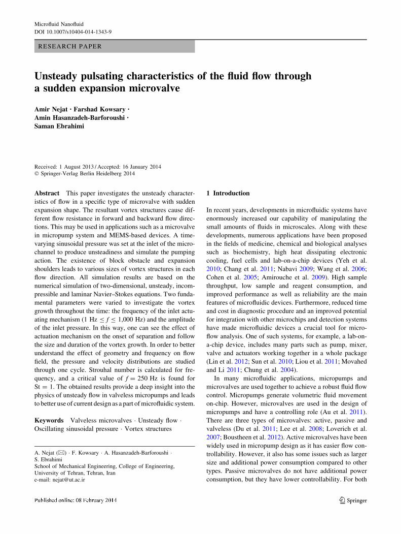
Unsteady pulsating characteristics of the fluid flow througha sudden expansion microvalve

Amir Nejat • Farshad Kowsary •

Amin Hasanzadeh-Barforoushi •

Saman Ebrahimi

Received: 1 August 2013 / Accepted: 16 January 2014

� Springer-Verlag Berlin Heidelberg 2014

Abstract This paper investigates the unsteady character-

istics of flow in a specific type of microvalve with sudden

expansion shape. The resultant vortex structures cause dif-

ferent flow resistance in forward and backward flow direc-

tions. This may be used in applications such as a microvalve

in micropump system and MEMS-based devices. A time-

varying sinusoidal pressure was set at the inlet of the micro-

channel to produce unsteadiness and simulate the pumping

action. The existence of block obstacle and expansion

shoulders leads to various sizes of vortex structures in each

flow direction. All simulation results are based on the

numerical simulation of two-dimensional, unsteady, incom-

pressible and laminar Navier–Stokes equations. Two funda-

mental parameters were varied to investigate the vortex

growth throughout the time: the frequency of the inlet actu-

ating mechanism (1 Hz B f B 1,000 Hz) and the amplitude

of the inlet pressure. In this way, one can see the effect of

actuation mechanism on the onset of separation and follow

the size and duration of the vortex growth. In order to better

understand the effect of geometry and frequency on flow

field, the pressure and velocity distributions are studied

through one cycle. Strouhal number is calculated for fre-

quency, and a critical value of f = 250 Hz is found for

St = 1. The obtained results provide a deep insight into the

physics of unsteady flow in valveless micropumps and leads

to better use of current design as a part of microfluidic system.

Keywords Valveless microvalves � Unsteady flow �Oscillating sinusoidal pressure � Vortex structures

1 Introduction

In recent years, developments in microfluidic systems have

enormously increased our capability of manipulating the

small amounts of fluids in microscales. Along with these

developments, numerous applications have been proposed

in the fields of medicine, chemical and biological analyses

such as biochemistry, high heat dissipating electronic

cooling, fuel cells and lab-on-a-chip devices (Yeh et al.

2010; Chang et al. 2011; Nabavi 2009; Wang et al. 2006;

Cohen et al. 2005; Amirouche et al. 2009). High sample

throughput, low sample and reagent consumption, and

improved performance as well as reliability are the main

features of microfluidic devices. Furthermore, reduced time

and cost in diagnostic procedure and an improved potential

for integration with other microchips and detection systems

have made microfluidic devices a crucial tool for micro-

flow analysis. One of such systems, for example, a lab-on-

a-chip device, includes many parts such as pump, mixer,

valve and actuators working together in a whole package

(Lin et al. 2012; Sun et al. 2010; Liou et al. 2011; Movahed

and Li 2011; Chung et al. 2004).

In many microfluidic applications, micropumps and

microvalves are used together to achieve a robust fluid flow

control. Micropumps generate volumetric fluid movement

on-chip. However, microvalves are used in the design of

micropumps and have a controlling role (Au et al. 2011).

There are three types of microvalves: active, passive and

valveless (Du et al. 2011; Lee et al. 2008; Loverich et al.

2007; Boustheen et al. 2012). Active microvalves have been

widely used in micropump design as it has easier flow con-

trollability. However, it also has some issues such as larger

size and additional power consumption compared to other

types. Passive microvalves do not have additional power

consumption, but they have lower controllability. For both

A. Nejat (&) � F. Kowsary � A. Hasanzadeh-Barforoushi �S. Ebrahimi

School of Mechanical Engineering, College of Engineering,

University of Tehran, Tehran, Iran

e-mail: nejat@ut.ac.ir

123

Microfluid Nanofluid

DOI 10.1007/s10404-014-1343-9

active and passive microvalves, the fatigue of the valve and

the switching control may have some adverse effects on the

pump performance and its reliability. In order to overcome

these problems, valveless micropumps using a valveless

rectifier are introduced (Stemme and Stemme 1993; Van De

Pol 1989).

Two common types of valveless rectifiers are introduced

in the literature: Tesla valve (Truong and Nguyen 2003;

Thompson et al. 2011) and nozzle/diffuser valve (Nabavi and

Mongeau 2009; Yang et al. 2008). The main concept of these

valves is based on the direction-dependent flow resistance. In

Tesla valves, for example, due to different entrance angles of

serpentine side channel, most of the forward flow passes

through the straight channel, but backward flow encounters

more resistance than forward flow. A diffuser structure was

proposed by Forster and Bardell (1995) that had a rectifica-

tion performance equivalent to Tesla valve, and its geometry

was simpler so that it had superiority in design and manu-

facturing. Yang et al. (2006) also reported the performance

of nozzle/diffuser micropumps with parallel and series

combinations. These microfluidic rectifiers have simple

structure as they have no moving parts; however, the lower

rectification performance index limits their applications.

In many cases such as piezoelectric micropumps, the

velocity field is pulsatile and the unsteadiness of the flow

affects the performance of the micropump. Therefore,

investigation of how that oscillation affects the flow field

within the channel seems to be necessary. Several numerical

and experimental studies on unsteady flow through micro-

pumps with different types of microvalves have been

reported (Wang et al. 2007; Sun and Huang 2006; Sheen et al.

2008). Sun and Huang (2006) numerically investigated the

problem of unsteady flow in a microdiffuser using com-

mercial software FLUENT. In their investigation, they

considered two primary parameters, diffuser half-angle and

excitation frequency. They found that the net flow rate was

independent of excitation frequency for f \ 25 Hz but

decreased with increasing frequency for f [ 25 Hz.

Wang et al. (2007) studied the performance of no-mov-

ing-part valves (NMPV) of a diffuser type both numerically

and experimentally under steady and unsteady flow condi-

tions. The diffuser angle was 20� because it leads to better

production of net volume rate. An optimal Strouhal number

(St = xDh/umax) with maximum net volume flow rate was

found at St = 0.013 for unsteady flow conditions. Their

findings showed that the relation between the driving pres-

sure amplitude and the net volume flow is of great impor-

tance in NMPV micropump system.

Recently, formation of recirculation zones in a sudden

expansion channel with rectangular block structure under

steady flow conditions was investigated both numerically

and experimentally by Tsai et al. (2012a, b). They showed

that the Reynolds number and the aspect ratio have a sig-

nificant impact on the sequence of vortex growth down-

stream of the expansion channel. They also draw the

Reynolds number/aspect ratio (Re-c) flow pattern map to

classify how the flow structures vary with Reynolds num-

ber. In another paper, Tsai et al. (2012a, b) introduced a

microfluidic rectifier based on sudden expansion channel

and with an embedded block structure. That structure

induced two vortices at the end of the microchannel under

reverse flow conditions. These vortices reduced the effec-

tive hydraulic diameter of the channel and, therefore,

increased the flow resistance.

In this paper, the flow of a Newtonian fluid within a

valveless micropump is investigated by means of numeri-

cal simulation in order to have a better understanding of the

effects of expansion and contraction on the transient

behavior of the flow. The embedded obstacle (some dis-

tances away from the expansion) helps the growth of the

vortices. As the frequency varies between 1 and 1,000 Hz,

the results can cover many typical micropumping require-

ments, for example, in electronics cooling and in microfuel

cells. The effects of frequency on the onset of flow sepa-

ration and circulation size and duration are investigated in

detail. Strouhal number variations are detected to introduce

different unsteady regimes as a function of frequency

changes of the inlet pressure.

2 Mathematical formulation

Figure 1 represents a schematic illustration of the problem

under investigation. According to Fig. 1, the simulation

domain consists of an inlet, the walls, the block obstacle and

the outlet. The length of inlet, outlet, contraction region and

expansion region are 300, 900, 1,500 and 3,000 lm,

respectively. The obstacle has a height of 300 lm and a

width of 150 lm. A time-varying sinusoidal pressure is

applied at the inlet boundary. The flow is assumed laminar as

the Reynolds number does not exceed 300. Note that Rey-

nolds number is defined as umaxDh

m , where umax is the maximum

streamwise velocity, Dh is the hydraulic diameter of the inlet,

and m is the kinematic viscosity of water.

2.1 Governing equations

In order to analyze the flow within the channel, the gov-

erning equations are simplified using the following

assumptions: (1) The working fluid is an incompressible,

Newtonian fluid which in our case is water with density of

998 kg/m3 and dynamic viscosity of 0.001 kg/ms; (2)

Microfluid Nanofluid

123

constant fluid properties; (3) the gravitational and buoy-

ancy effects are sufficiently small and are ignored; (4) the

flow is unsteady and laminar; and (5) the flow field is two

dimensional. Our 2D analysis seems to provide a reason-

ably realistic simulation due to infinite aspect ratio and

Re� 1 (Tsai et al. 2007). As the simulation is performed

for an unsteady flow, the full 2D Navier–Stokes equations

must be solved. The governing equations are the following:

ou

oxþ ov

oy¼ 0 ð1Þ

qðou

otþ u

ou

oxþ v

ou

oyÞ ¼ � oP

oxþ lðo

2u

ox2þ o2u

oy2Þ ð2Þ

qðov

otþ u

ov

oxþ v

ov

oyÞ ¼ � oP

oyþ lðo

2v

ox2þ o2v

oy2Þ ð3Þ

where q is the fluid density; u and v are velocity

components in x- and y-directions, respectively; P is the

pressure; l is the fluid dynamic viscosity; and t denotes

time. In order to solve the above equations, the flow is

initially assumed stationary so that u(x, y, 0) = 0 and

v(x, y, 0) = 0. Also, no slip boundary condition is applied

at the walls. This is true because the Knudsen number is

very small (i.e., Kn \ 0.01). The Kn number is defined as:

Kn ¼ kL

ð4Þ

where k is the mean free path of molecules and L is the

characteristic length of the channel. For water k is

approximately 2.5 A or 2.5 9 10-10 m and L = 300 lm,

calculating for Kn,

Kn ¼ kL¼ 8:3� 10�7 � 0:01

Therefore, no slip assumption at the wall is satisfied.

There are different types of micropumps according to the

method in which the fluid is flowed. In this paper, we

studied a type of positive displacement micropump design

working under sinusoidal boundary condition for the inlet

and a constant (i.e., atmospheric) pressure at the outlet. In

fact, the fluid flows to a reservoir. Thus, the boundary

conditions are expressed as follows:

Inlet:

Pinlet ¼ P0 � sinð2pftÞ ð5Þ

Outlet:

Poutlet ¼ Patm ¼ 0 ð6Þ

Walls:

u ¼ v ¼ 0 ð7Þ

2.2 Numerical method and computational grid

The COMSOL (multiphysics) software, which is based on

finite-element scheme, was used to discrete and solve the

governing continuity and momentum equations. The sim-

ulations were performed for the frequency range of

1–1,000 Hz and the pressure amplitude varying from

200–500 Pa. Laminar flow and 2D model are used to

perform the simulations. Since the flow is unsteady, the

second-order time marching technique is employed. The

upper band of the time range was chosen in such a way to

resolve variation in flow structures in several consecutive

periods. A time step of 0.02 of a period was taken

accordingly to make sure that all the major velocity scales

are resolved, i.e., the obtained results are not dependent on

the adopted time step. A time-dependent solver is used to

solve the transient equations of motion. There are several

time-stepping methods that can be used. In this paper, we

use the backward differentiation method, which is an

implicit method with linear multisteps and sometimes

called backward differentiation formulas (BDFs). On that

method, an approximation to a derivative of a variable at

time tn is given in terms of its function values information

from already computed times, and thus, the accuracy of

the approximations is enhanced. The time step for different

Fig. 1 Schematic illustration of the microchannel with rectangular obstacle

Microfluid Nanofluid

123

inlet frequencies can be chosen accordingly. As an

example, for f = 100 Hz, we used t = 0.0002 s as time

step, which is two hundredth of the oscillation period. In

order to show the time-step independency of the results,

we performed the simulation for two different time steps.

In fact, we reduced the time step to reach the time-step

independency. We found that making time step equal to

0.02 T or smaller does not cause a tangible difference in

the obtained results for all frequency ranges. Our decision

on time step was based on both being accurate enough to

capture the required vortices on the one hand and time-

step independency on the other hand. Figure 2 represents

the results of time steps 0.02 and 0.01 of the employed

period.

An unstructured grid with triangular mesh elements was

used (Fig. 3). The use of unstructured grid is common in

finite-element analysis and facilitates the mesh generation

(and possible refinement) near the corners and sharp edges.

The number of cells was 19842 with average mesh size of

about 156 lm2, and the maximum and minimum element

sizes were 400 and 1.82 lm2, respectively, with maximum

growth rate of 1.3.

A grid study was performed to examine the sensitivity of

solution to the number of elements. We carried two grid

systems with mesh elements for the case when f = 100 Hz

and P0 = 200 Pa. At the first step, the maximum element

size was decreased from 20 to 15 lm. This caused the total

number of elements to change from 19,842 to 34,912. The

velocity at the point that is 3,000 lm downstream of the

inlet is plotted through time in Fig. 4. It is clear from the

figure that using smaller mesh size does not cause a tan-

gible difference in results.

Model verification is performed to verify the accuracy and

the validity of the numerical method to simulate the unsteady

fluid flow through the microchannel. In the study by Nabavi

(2009), the velocity profiles were obtained for 2D micro-

channel of width 2a and length L with a sinusoidal pressure

gradient of oPox¼ p�eixt and with P = 1,000 Pa, a = 60 lm,

L = 1,000 lm and f = 10 kHz. We adopted these values to

find the evolution of the velocity profiles shown in Fig. 5.

Comparing the computed results with those reported by

Nabavi (2009) demonstrates that our simulation method is

reasonably accurate.

3 Results and discussion

The role of actuation mechanism in the production of

vortex generation and recirculation zones is very important.

A pulsatile pressure boundary condition is set at the inlet of

the channel, meaning if one assumes a single period, in half

of that period the pressure is positive and the flow is

injected into the channel. In the other half of the period, the

Fig. 2 Variation of u_velocity with time for two time steps of a 0.0001 s and b 0.0002 s in case f = 100 Hz

Fig. 3 Schematic drawing of the mesh in the expansion zone

Microfluid Nanofluid

123

pressure becomes negative, meaning that we have suction

at the inlet and the flow is pulled back to the inlet region.

Therefore, we can have both forward and backward flows

with this actuation mechanism through one cycle.

First, we should note that at the first few cycles the

variation in flow rate is non-regulated because of quick

changes in pressure and initial transient behavior of the

flow field. This could be important when accurate manip-

ulation of fluid is needed and when the fluid is sensitive to

pressure changes. We should also note that the number of

non-regulated periods depends highly on the inlet

frequency.

Figure 6a–n represents the evolution of vortices when

the fluid flow gets regulated. This happens after approxi-

mately two to three cycles pass from the initial time

(t = 0), but it varies for different values of the inlet fre-

quency. We tracked the circulations from t = 0.0224 s,

which is three cycles after the initial time. It is seen that the

evolution of vortices repeats every t = 0.01 s as we have

expected from the relation: T = 1/f = 0.01 s. We bring the

results in the time interval t = 0.0244–0.0324, which is

one complete cycle in Fig. 6a–n.

The separation in the flow field takes place for two

reasons: (1) the pulsatile pressure and (2) the shape of the

geometry. As we can see in Fig. 6a–n, at the first few

time steps, the flow field has not been developed yet and

the streamlines are smooth. This situation continues for a

very short time, and the first signs of circulation are seen

at t = 0.22 T (Fig. 6b) at the shoulders of the expansion

region. For the next time steps, the circulation also occurs

at the back of the obstacle. The vortices continue to grow

from this time until the third and forth vortices appear. It

is interesting to know that the forth vortex structure,

which happens when the pressure is negative about

P = -168 Pa (maximum pressure is 200 Pa), is extended

along the side walls of the channel and then at the ter-

minal part of the channel. The vortex growth continues as

far as t = 0.52 T (Fig. 6f) when they collide with each

other, and the flow field reaches its maximum suction.

After the collision of vortices, the sizes of the vortex

regions decrease along with the pressure getting smaller

in magnitude.

It is also important to note that the sizes of the vortices

become smaller and their positions shift into the inlet

region. From t = 0.88 T (Fig. 6j), a strange behavior

happens. Two circulation regions are produced, one at the

shoulders and the other in front of the obstacle. The regions

Fig. 4 The velocity magnitude at the point which is 3,000 lm downstream of the inlet for maximum element size of a 20 lm and b 15 lm

Fig. 5 Velocity profiles obtained for p = 1,000 Pa and f = 10 kHz;

current method (solid lines) and the results of Nabavi et al. (symbols)

Microfluid Nanofluid

123

also grow in such a way that an oblong vortex structure is

produced at the inlet region of the channel behind the step

expansion. However, the vortex structures will be damped

as fast as its production and the flow gain smooth

streamlines at t = T (Fig. 6n). This time is the beginning of

the next cycle.

(a) (b)

(c) (d)

(e) (f)

(g) (h)

(i) (j)

(k) (l)

(m) (n)

Fig. 6 Evolution of

recirculation zones for the third

cycle at specified times for

P0 = 200 Pa and f = 100 Hz

Microfluid Nanofluid

123

Figure 7 shows that the instantaneous velocity and the

pressure variations do not have the same phase. This hap-

pens because of the waves produced by pressure oscillation

and the flow inertial effects. In order to detect the unsteady

behavior of the flow, we must let the fluid to flow for some

cycles so that the effect of pressure disturbances will be

damped and the flow gains a regulated sinusoidal periodic

behavior.

3.1 Frequency effects

Flow structure in pulsating micropumps highly depends on the

frequency of the actuation mechanism. It is also important to

note that different applications of micropump demand specific

interval of frequency. As an example in the work done by

Nabavi and Mongeau (2009), the high-frequency pulsating

flow through a diffuser/nozzle element was investigated that

had an application in valveless acoustic micropumps.

In the present study, we investigate the effect of fre-

quency variations on the onset of separation, the pressure

and the velocity contours inside the microchannel. The

range of frequencies is varied from f = 1–1,000 Hz to

investigate the efficiency of this geometry for very low,

medium and high frequencies.

3.1.1 Stream function contours

As noticed in the previous section, when f = 100 Hz, i.e.,

medium frequency, separation occurs when pressure

changes sign. However, when the frequency becomes very

low (f = 1 Hz) or very high (f = 1,000 Hz), a different

situation takes place. In Fig. 8, the streamlines are shown

for six phases of the inlet pressure.

As it is seen in the figure, at high frequencies, which in

our case is f = 1,000 Hz, one key change occurs comparing

to the medium frequency f = 100 Hz. The onset of sepa-

ration will be some time after the midtime of the cycle when

the inlet pressure changes sign and shifts into the times of

maximum and minimum inlet pressure. This means that

increasing the frequency causes a delay in onset of sepa-

ration so that we subsequently expect a delay in vortex

generation. At low frequencies, i.e., f = 1 Hz, however, a

reverse condition is set and flow circulation proceeds and

takes place before the inlet pressure changes sign. The

separation begins at t = 0.02 s for inlet conditions of

f = 1 Hz and P0 = 200 Pa. This is the two hundredth of the

period time. For inlet conditions of f = 100 Hz and

P0 = 200 Pa and f = 1,000 Hz and P0 = 200 Pa, the onset

of circulation increases to approximately 24 and 52 % of

the total period time.

Another point to mention is the size and the duration of

the recirculation regions. As we can see in Fig. 8, recir-

culation regions are much larger for f = 1 Hz compared to

f = 1,000 Hz. As a result, increasing the frequency

increases the effective hydraulic diameter of the channel.

Also according to Fig. 8, one can conclude that recircula-

tion region remains in more portion of a single period at

lower frequencies.

Figures 9 and 10 show the velocity and pressure varia-

tion throughout time for f = 1 Hz and f = 1,000 Hz,

respectively, at the inlet midpoint. Comparing these plots

with Fig. 7, we achieve two important results: First, the

phase difference between the velocity and pressure

increases as the frequency increases. As we can see in

f = 1 Hz, the velocity and pressure are approximately at

the same phase. Second, it is clear that by increasing the

Fig. 7 Velocity and pressure phase difference for P0 = 200 Pa and f = 100 Hz

Microfluid Nanofluid

123

frequency, the number of periods toward achieving a reg-

ulated change in velocity increases.

3.1.2 Pressure and velocity distribution within the channel

Pressure and its manipulation is one of the key factors that

must be considered in microvalve analysis. The pressure

contours at the selected times are represented in Fig. 11.

We show here the results only for f = 100 Hz.

Figure 11a shows the pressure distribution at the

beginning of a period. We can see that at the inlet region

the pressure is very high and it decreases along the channel.

At t = T/4, the pressure magnitude at the inlet begins to

reduce, and then it increases in further regions due to the

sinusoidal behavior of the actuation mechanism. The pre-

sence of the rectangular obstacle causes a region of rela-

tively high pressure at its front edge and decreases the

pressure near the corner vertices.

Fig. 8 Time-dependent

streamlines when P0 = 200 Pa

for a f = 1,000 Hz and

b f = 1 Hz at specified times

Microfluid Nanofluid

123

At t = T/2, the inlet pressure changes sign. This time the

pressure at the right side is much larger than at the left side,

and reverse flow will be set in the domain. The fourth

figure shows that the negative pressure amplitude decreases

at the end of the cycle. Ultimately after passing a period (at

t = T), the pressure becomes equal to what it was at the

beginning of the cycle. We also notice the inlet and outlet

pressure difference through one period. We can see that

this value changes considerably in one cycle, showing that

the flow resistance increases in the reverse flow cycle. This

indicates that the geometry shows an efficient rectification

capability.

The velocity contours are shown in Fig. 12. As shown in

this figure, the fluid flow begins at the first few moments

and decreases in magnitude till t = 0.25 T. This time the

pressure reaches its minimum value, and as there exists a

harmony between velocity and pressure at f = 100 Hz, the

velocity reaches its minimum too (Fig. 12b). Then, the

pressure suction begins which causes three large circula-

tion zones. The vortices together shape a diffuser-like path

that highly increases the flow rate through the channel. In

Fig. 12c, we can see that the velocity magnitude increases

suddenly between two vortex structures that have been

formed one at the shoulders and one behind the obstacle.

Approximately near t = 0.52 T, a reverse flow is set, and it

destroys the vortices. Now, the channel acts like a nozzle,

and the shoulders prevent the fluid flow. This prevention

will then be improved by the generation of three vortices so

that the velocity magnitude decreases as a result of

decrease in effective hydraulic diameter of the channel

(Figs. 6k, 12e). Finally, the velocity magnitude diminishes

in all regions and next period commence.

Fig. 9 Velocity and pressure are nearly in phase for P0 = 200 Pa and f = 1 Hz

Fig. 10 Phase difference between velocity and pressure for P0 = 200 Pa and f = 1,000 Hz

Microfluid Nanofluid

123

Figure 13 represents the inlet velocity profile for dif-

ferent phases. It is worthwhile to compare this plot with

the one when we set a sinusoidal velocity at the inlet. It is

obvious that in our problem the velocity profile changes

constantly with time. As a result, a variable momentum

will be carried by the fluid into the channel.

In order to study the frequency effect on velocity profile

and the net flow rate, we reported the inlet velocity profiles

for f = 1Hz and f = 1,000 Hz for the same channel and the

same pressure amplitude. As shown in Fig. 14, increasing

the frequency leads to lower velocity and thus lower flow

rates. However, at high frequencies (i.e., f = 1,000 Hz),

separation occurs after the midtime of a period, for

example, for f = 1,000 Hz, separation occurs after t = 7T/

12 as shown in Fig. 14b. Therefore, forward flow is dom-

inant at high frequencies. For lower frequencies, i.e.,

f = 1 Hz, the flow rates are considerably higher for both

forward and backward flow directions. Table 1 illustrates

the net volumetric flow rate for P0 = 200 Pa at different

frequency values. As shown in this table, when frequency

decreases, net flow rate increases. The value of net flow

rate for f = 1 Hz is 2.8 times bigger than its value for

f = 100 Hz and 5.7 times bigger than its value for

f = 1,000 Hz.

3.2 Effect of pressure amplitude

Another important parameter that has noticeable impact on

micropump system performance is the pressure amplitude. In

order to consider this effect, we have solved the problem for

two pressure amplitude of P0 = 500 Pa and P0 = 200 Pa and

have reported the results at the same interval to perform the

comparison. Figure 15 shows that when the pressure ampli-

tude is increased, separation occurs earlier. This time is

t = 0.22 T and t = 0.14 T for P0 = 200 Pa and P0 =

500 Pa, respectively. Also, if we track the vortex evolution in

those two cases at the same times, we can see that for the

greater value of amplitude, the size of the vortices is larger. It

is also noticed that the life of the circulation is increased with

the increase in pressure amplitude.

Fig. 11 Pressure distribution within the channel for P0 = 200 Pa, f = 100 Hz and t = 0, 0.25, 0.5 and 0.75 T, respectively

Microfluid Nanofluid

123

Figure 16 and Table 2 illustrate the variation in flow

rate and the net volumetric flow rate for two pressure

amplitudes. According to Fig. 16, the flow rate magnitude

is considerably higher for 500 Pa in comparison with

200 Pa. For example, the maximum value of flow rate for

500 Pa is three times its value for 200 Pa. However, in

order to perform a better comparison between the perfor-

mance of the valve and pressure amplitude magnitude, we

Fig. 12 Velocity distribution within the channel for the case P0 = 200 Pa, f = 100 Hz and t = 0.0224, 0.26, 0.48, 0.76, 0.90 and 0.96 T,

respectively

Microfluid Nanofluid

123

calculated the net volumetric flow rate and show them in

Table 2. As we can see, this value is approximately two

times bigger for 500 Pa comparing to 200 Pa.

3.3 Measuring the unsteadiness of the flow, Strouhal

number

In a study of any unsteady flow, measuring the unsteadi-

ness of the flow is a necessity as it is important to know that

what forces are dominant through one cycle period. It is

also important to know the interaction between the inertia

Fig. 13 Inlet velocity profile for P0 = 200 Pa, f = 100 Hz at

t = T/6, T/4, T/3, 5T/12, T/2, 7T/12, 2T/3, 3T/4, 5T/6 and 11T/12,

respectively

Fig. 14 Volumetric flow rate and inlet velocity profile for P0 = 200 Pa and a f = 1 Hz and b f = 1,000 Hz at t = T/6, T/4, T/3, 5T/12, T/2, 7T/

12, 2T/3, 3T/4, 5T/6 and 11T/12, respectively

Table 1 Net volumetric flow rate for different frequencies in case

P0 = 200 Pa

Frequency (Hz) 1 100 1,000

Net volumetric flow

rate (m3/s)

1.45 9 10-5 5.18 9 10-6 2.56 9 10-6

Microfluid Nanofluid

123

forces and the oscillation of the flow. Strouhal number is

defined as follows:

St ¼ fL

umax

ð8Þ

where L is the characteristic length, which in our case is the

height of the inlet channel; f is inlet pressure frequency;

and umax is the maximum velocity in the streamwise

direction. We should note that we can define a unique value

of St at each frequency value. Table 3 shows this value for

different frequency and pressure amplitudes.

As we can see in Table 3, for P0 = 200 Pa and

f = 1 Hz, St = 0.0042. As frequency increases to

f = 100 Hz, St is increased to 0.1775. We can conclude

Fig. 15 Streamlines for a P0 = 200 Pa and b P0 = 500 Pa for t = 0.22, 0.32, 0.42, 0.52, 0.88 and 0.98 T, respectively (f = 100 Hz)

Microfluid Nanofluid

123

that unsteadiness of the flow is negligible on that frequency

interval. Further increasing the frequency to f = 250 Hz

enhances the Strouhal value to approximately St = 1.

Thus, we can see that increase in frequency causes a rapid

increase in St value between 100 and 250 Hz. In fact,

f = 250 Hz is a critical value of frequency. This means

that below f = 250 Hz unsteady effects are small and

frequency effect on net flow rate is negligible.

This increase in St value becomes much sensible from

100 to 1,000 Hz. At f = 1,000 Hz, the Strouhal value is

12.6. This result was somehow expectable because as the

frequency increases to 1,000 Hz, unsteady effects become

dominant over inertial forces and thus the maximum

velocity and the net flow rate within our domain highly

decrease. One more point to consider is that as pressure

amplitude increases in each frequency, the maximum

velocity is augmented reducing St number.

Figure 17 represents the variation of maximum Rey-

nolds number with Strouhal number. As we can see in this

figure, as the dimensionless frequency (Strouhal number) is

increased, the maximum Reynolds number is reduced.

Another point is that as frequency reaches 1,000 Hz, there

will be no sensible change in Reynolds number value. This

means that at high frequencies, the inertial forces will no

longer have considerable effect on the flow.

4 Conclusion

In this paper, unsteady pulsatile flow of a Newtonian fluid

through a microchannel was investigated numerically. The

vortex evolution within the channel was obtained for

pressure amplitude of P0 = 200 Pa and frequency of

f = 100 Hz to investigate the unsteady behavior of flow

within the microchannel geometry. The velocity and

pressure changes through time were captured at the inlet

midpoint, which showed that as frequency increases, the

phase difference between velocity and pressure increases.

The streamlines were shown for frequency magnitude of 1

and 1,000 Hz. The results showed that the onset of sepa-

ration grows with increase in frequency. Also decreasing

the frequency leads to increase in recirculation zone size

and causes it to last for a longer portion of a single cycle.

Furthermore, as frequency increases, the phase shift

between velocity and pressure increases and more time is

needed for the velocity to reach a regulated behavior. It is

shown that pressure has a significant effect on flow recti-

fication. The higher pressure amplitudes limit the onset of

separation. We found that the critical value of frequency,

where St = 1, is f = 250 Hz. Increasing the frequency

Fig. 16 Variation in volumetric flow rate with time for pressure

amplitude of 200 and 500 Pa at f = 100 Hz

Table 2 Comparison of net

volumetric flow ratePressure

amplitude

(Pa)

Net volumetric

flow rate (m3/s)

200 5.18 9 10-6

500 1.31 9 10-5

Table 3 Strouhal number values for different frequency and pressure conditions

f = 1 Hz f = 100 Hz f = 1,000 Hz

P0 = 200 Pa P0 = 500 Pa P0 = 200 Pa P0 = 500 Pa P0 = 200 Pa P0 = 500 Pa

St 0.00042 0.00025 0.1775 0.0707 12.60 4.87

Fig. 17 Maximum Reynolds number versus Strouhal number

Microfluid Nanofluid

123

beyond this value makes the unsteady effects dominant,

and as a result, maximum velocity and net volumetric flow

rate considerably decrease.

References

Amirouche F, Zhou Y, Johnson T (2009) Current micropump

technologies and their biomedical applications. Microsyst Tech-

nol 15:647–666

Au AK, Lai H, Utela BR, Folch A (2011) Microvalves and

micropumps for biomems. Micromachines 2:179–220

Boustheen A, Homburg FGA, Dietzel A (2012) A modular microv-

alve suitable for lab on a foil: manufacturing and assembly

concepts. Microelectron Eng 98:638–641

Chang CL, Leong JC, Hong TF, Wang YN, Fu LM (2011)

Experimental and numerical analysis of high-resolution injection

technique for capillary electrophoresis microchip. Int J Mol Sci

12:3594–3605

Chung YC, Hsu YL, Jen CP, Lu MC, Lin YC (2004) Design of

passive mixers utilizing microfluidic self-circulation in the

mixing chamber. Lab Chip 4(1):70–77

Cohen JL, Westly DA, Pechenik A, Abruna HD (2005) Fabrication

and preliminary testing of a planar membraneless microchannel

fuel cell. J Power Sour 139:96–105

Du X, Zhang P, Liu Y, Wu Y (2011) A passive through hole

microvalve for capillary flow control in microfluidic systems.

Sens Actuators A Phys 165:288–293

Forster FK, Bardell RL (1995) Design, fabrication and testing of

fixed-valve micropumps. ASME 234:277–286

Lee DE, Soper S, Wang WJ (2008) Design and fabrication of an

electrochemically actuated microvalve. Microsyst Technol

14:1751–1756

Lin CH, Wang YN, Fu LM (2012) Integrated microfluidic chip for

rapid DNA digestion and time-resolved capillary electrophoresis

analysis. Biomicrofluidics 6:012818

Liou D, Hsieh Y, Kuo L, Yang C, Chen P (2011) Modular component

design for portable microfluidic design. Microfluid Nanofluid

10:465–474

Loverich J, Kanno I, Kotera H (2007) Single-step replicable

microfluidic check valve for rectifying and sensing low Reynolds

number flow. Microfluid Nanofluid 3:427–435

Movahed S, Li D (2011) Microfluidics cell electroporation. Micro-

fluid Nanofluid 10:703–734

Nabavi M (2009) Steady and unsteady flow analysis in microdiffusers

and micropumps: a critical review. Microfluid Nanofluid

7:599–619

Nabavi M, Mongeau L (2009) Numerical analysis of high frequency

pulsating flows through a diffuser-nozzle element in valveless

acoustic micropumps. Microfluid Nanofluid 7:669–681

Sheen H, Hsu C, Wu T, Chang C, Chu H, Yang C, Lei U (2008)

Unsteady flow behaviors in an obstacle-type valveless micro-

pump by micro-PIV. Microfluid Nanofluid 4:331–342

Stemme E, Stemme G (1993) A valveless diffuser/nozzle-based fluid

pump. Sens Actuators A Phys 39:159–167

Sun C, Huang K (2006) Numerical characterization of the flow

rectification of dynamic microdiffusers. J Micromech Microeng

16:1331–1339

Sun H, Nie Z, Fung YS (2010) Determination of free bilirubin and its

binding capacity by HSA using a microfluidic chip-capillary

electrophoresis device with a multi-segment circular-ferrofluid-

driven micromixing injection. Electrophoresis 31:3061–3069

Thompson SM, Ma HB, Wilson C (2011) Investigation of a flat-plate

oscillating heat pipe with Tesla-type check valves. Exp Therm

Fluid Sci 35:1265–1273

Truong TQ, Nguyen NT (2003) Simulation and optimization of tesla

valves. Nanotech 1:178–181

Tsai CH, Chen HT, Wang YN, Lin CH, Fu LM (2007) Capabilities

and limitations of 2-dimensional and 3-dimensional numerical

methods in modeling the fluid flow in sudden expansion

microchannels. Microfluid Nanofluid 3:13–18

Tsai CH, Lin CH, Fu LM, Chen HC (2012a) High performance

microfluidic rectifier based on the sudden expansion channel

with embedded block structure. Biomicrofluidics 6:024108

Tsai CH, Yeh CH, Lin CH, Yang RJ, Fu LM (2012b) Formation of

recirculation zones in a sudden expansion microchannel with a

rectangular block structure over a wide Reynolds number range.

Microfluid Nanofluid 12:213–220

Van De Pol FCM (1989) A pump based on micro-engineering

techniques. University of Twente, Enschede

Wang K, Yue S, Wang L, Jin A, Gu C, Wang P, Feng Y, Wang Y,

Niu H (2006) Manipulating DNA molecules in nanofluidic

channels. Microfluid Nanofluid 2:85–88

Wang C, Leu T, Sun J (2007) Unsteady analysis of microvalves with

no moving parts. J Mech 23:9–14

Yang KS, Chen IY, Wang CC (2006) Performance of nozzle/diffuser

micro-pumps subject to parallel and series combinations. Chem

Eng Technol 29:703–710

Yang KS, Chen IY, Chien KH, Wang CC (2008) A numerical study

of the nozzle/diffuser micropump. Proc Inst Mech Eng C J Mech

E 222(3):525–533

Yeh CH, Lin PW, Lin YC (2010) Chitosan microfiber fabrication

using a microfluidic chip and its application to cell cultures.

Microfluid Nanofluid 8:115–121

Microfluid Nanofluid

123