Unsteady RANS computations of flow around a circular cylinder for a wide range of Reynolds numbers R.M. Stringer a,n , J. Zang a , A.J. Hillis b a Department of Architecture and Civil Engineering, University of Bath, Bath BA2 7AY, UK b Department of Mechanical Engineering, University of Bath, Bath BA2 7AY, UK article info Article history: Received 5 April 2013 Accepted 19 April 2014 Available online 11 June 2014 Keywords: CFD Cylinder OpenFOAM Tidal URANS VIV abstract A methodology for computation of flow around circular cylinders is developed and tested using prominent commercial and open-source solvers; ANSYS s CFX-13.0 and OpenFOAM s 1.7.1 respectively. A range of diameters and flow conditions are accounted for by generating solutions for flows at Reynolds numbers ranging from 40 to 10 6 . To maintain practical solve times a 2D Unsteady Reynolds-Averaged Navier–Stokes (URANS) approach is taken. Furthermore, to maximise accuracy a tightly controlled meshing methodology, suitable adaptive timestepping, and appropriate turbulence modelling, are assembled. The resulting data is presented for lift and drag forces, Strouhal frequency, time accuracy and boundary layer correlation. Despite closely matching case definitions, significant differences are found in the results between solvers; OpenFOAM displays high correlation with experimental data at low to sub-critical values, whereas ANSYS proves to be more effective in the high sub-critical and critical regions. This variance demonstrates the sensitivity of the case to solver specific mathematical constraints and that for practical engineering a parameter study is essential. By removing many common variances associated with grid and transient components of URANS computations the developed methodology can be used as a benchmark case for further codes solving cylindrical structures. & 2014 Elsevier Ltd. All rights reserved. 1. Introduction Understanding the flow around a circular cylinder has histori- cally been a fundamental challenge for researchers, largely due to the complexity and transient nature of the wake. However, in the last decade, desktop computational resources have increased sufficiently such that high resolution solutions for practical engi- neering have become feasible. One such application, the motiva- tion for the study, is the use of cylindrical geometries as structural members and pipelines in offshore applications. This usage is particularly relevant due to the exploitation of new renewable energy technologies both wind and marine, many of which include cylindrical features in some form. Analysis of circular cylinders for the offshore market has been primarily to assess structural loading caused by vortex shedding. This phenomenon has influenced new offshore technologies aimed at reducing the impact of vortex induced vibration (VIV) on structural elements such as riser fairings and platform leg surfacing. In the context of marine renewables, it is also possible that vortices shed from cylindrical components may reduce device efficiency and therefore require an increased level of resolution in design and development solutions. To address this, this research aims to develop and assess a rigorous numerical methodology for modelling such cases. The flow around cylinders has been extensively investigated through experimentation by notable contributors such as Tritton (1959), Roshko (1955) and Achenbach (1968), amongst many others. One of the key outcomes of this work was to categorise flow by regimes of vortex shedding with Reynolds number (Re), given in Eq. (1). A prominent early paper by Lienhard (1966) proposes an outline of flow characteristics from laminar flow, up to supercritical values ERe 3.5 10 6 . However, the complexity of the turbulent wake has undergone many new discoveries, with a distinct contribution from advancing numerical modelling. A review by Williamson (1996) considers the wake in detail; highlights include a detailed account of the transition of wakes from 2D to 3D in the range 180 oRe o190, control of the shedding by modification of the cylinder end conditions, and the Direct Numerical Simulation (DNS) of 3D instabilities in landmark detail. The regimes of flow around a cylinder as Reynolds number increases have been refined by numerous researchers, most notably Zdravkovich (1990) with 15 distinct ranges. A summary of the key stages in flow development are presented in Table 1. The study here considers incremental values of Re from 40 up to a maximum of 10 6 . To give a perspective on the range, the peak Contents lists available at ScienceDirect journal homepage: www.elsevier.com/locate/oceaneng Ocean Engineering http://dx.doi.org/10.1016/j.oceaneng.2014.04.017 0029-8018/& 2014 Elsevier Ltd. All rights reserved. n Corresponding author. E-mail address: [email protected](R.M. Stringer). Ocean Engineering 87 (2014) 1–9
Transcript
Unsteady RANS computations of flow around a circular cylinder for awide range of Reynolds numbers
R.M. Stringer a,n, J. Zang a, A.J. Hillis b
a Department of Architecture and Civil Engineering, University of Bath, Bath BA2 7AY, UKb Department of Mechanical Engineering, University of Bath, Bath BA2 7AY, UK
a r t i c l e i n f o
Article history:Received 5 April 2013Accepted 19 April 2014Available online 11 June 2014
Keywords:CFDCylinderOpenFOAMTidalURANSVIV
a b s t r a c t
A methodology for computation of flow around circular cylinders is developed and tested usingprominent commercial and open-source solvers; ANSYSs CFX-13.0 and OpenFOAMs 1.7.1 respectively.A range of diameters and flow conditions are accounted for by generating solutions for flows at Reynoldsnumbers ranging from 40 to 106. To maintain practical solve times a 2D Unsteady Reynolds-AveragedNavier–Stokes (URANS) approach is taken. Furthermore, to maximise accuracy a tightly controlledmeshing methodology, suitable adaptive timestepping, and appropriate turbulence modelling, areassembled. The resulting data is presented for lift and drag forces, Strouhal frequency, time accuracyand boundary layer correlation. Despite closely matching case definitions, significant differences arefound in the results between solvers; OpenFOAM displays high correlation with experimental data atlow to sub-critical values, whereas ANSYS proves to be more effective in the high sub-critical and criticalregions. This variance demonstrates the sensitivity of the case to solver specific mathematical constraintsand that for practical engineering a parameter study is essential. By removing many common variancesassociated with grid and transient components of URANS computations the developed methodology canbe used as a benchmark case for further codes solving cylindrical structures.
& 2014 Elsevier Ltd. All rights reserved.
1. Introduction
Understanding the flow around a circular cylinder has histori-cally been a fundamental challenge for researchers, largely due tothe complexity and transient nature of the wake. However, in thelast decade, desktop computational resources have increasedsufficiently such that high resolution solutions for practical engi-neering have become feasible. One such application, the motiva-tion for the study, is the use of cylindrical geometries as structuralmembers and pipelines in offshore applications. This usage isparticularly relevant due to the exploitation of new renewableenergy technologies both wind and marine, many of which includecylindrical features in some form. Analysis of circular cylinders forthe offshore market has been primarily to assess structural loadingcaused by vortex shedding. This phenomenon has influenced newoffshore technologies aimed at reducing the impact of vortexinduced vibration (VIV) on structural elements such as riserfairings and platform leg surfacing. In the context of marinerenewables, it is also possible that vortices shed from cylindricalcomponents may reduce device efficiency and therefore require an
increased level of resolution in design and development solutions.To address this, this research aims to develop and assess a rigorousnumerical methodology for modelling such cases.
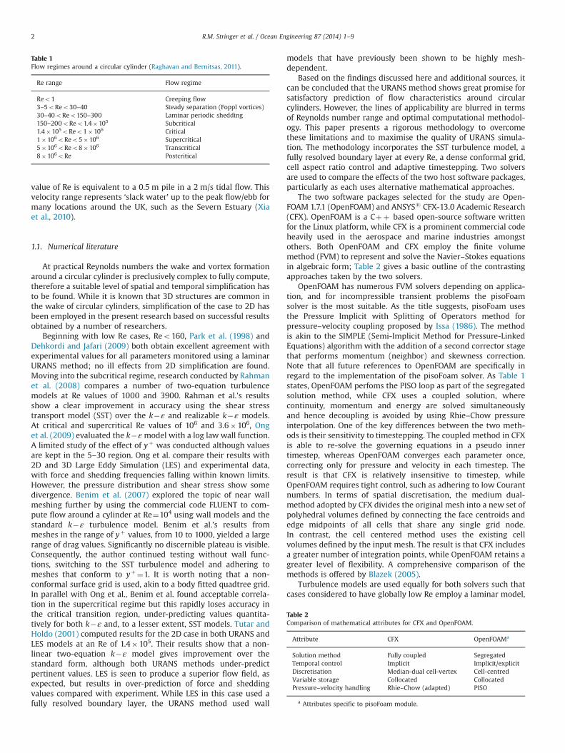
The flow around cylinders has been extensively investigatedthrough experimentation by notable contributors such as Tritton(1959), Roshko (1955) and Achenbach (1968), amongst manyothers. One of the key outcomes of this work was to categoriseflow by regimes of vortex shedding with Reynolds number (Re),given in Eq. (1). A prominent early paper by Lienhard (1966)proposes an outline of flow characteristics from laminar flow, upto supercritical values ERe 3.5�106. However, the complexity ofthe turbulent wake has undergone many new discoveries, with adistinct contribution from advancing numerical modelling.A review by Williamson (1996) considers the wake in detail;highlights include a detailed account of the transition of wakesfrom 2D to 3D in the range 180oReo190, control of the sheddingby modification of the cylinder end conditions, and the DirectNumerical Simulation (DNS) of 3D instabilities in landmark detail.The regimes of flow around a cylinder as Reynolds numberincreases have been refined by numerous researchers, mostnotably Zdravkovich (1990) with 15 distinct ranges. A summaryof the key stages in flow development are presented in Table 1.
The study here considers incremental values of Re from 40 upto a maximum of 106. To give a perspective on the range, the peak
value of Re is equivalent to a 0.5 m pile in a 2 m/s tidal flow. Thisvelocity range represents ‘slack water’ up to the peak flow/ebb formany locations around the UK, such as the Severn Estuary (Xiaet al., 2010).
1.1. Numerical literature
At practical Reynolds numbers the wake and vortex formationaround a circular cylinder is preclusively complex to fully compute,therefore a suitable level of spatial and temporal simplification hasto be found. While it is known that 3D structures are common inthe wake of circular cylinders, simplification of the case to 2D hasbeen employed in the present research based on successful resultsobtained by a number of researchers.
Beginning with low Re cases, Reo160, Park et al. (1998) andDehkordi and Jafari (2009) both obtain excellent agreement withexperimental values for all parameters monitored using a laminarURANS method; no ill effects from 2D simplification are found.Moving into the subcritical regime, research conducted by Rahmanet al. (2008) compares a number of two-equation turbulencemodels at Re values of 1000 and 3900. Rahman et al.'s resultsshow a clear improvement in accuracy using the shear stresstransport model (SST) over the k�ε and realizable k�ε models.At critical and supercritical Re values of 106 and 3.6�106, Onget al. (2009) evaluated the k�εmodel with a log law wall function.A limited study of the effect of yþ was conducted although valuesare kept in the 5–30 region. Ong et al. compare their results with2D and 3D Large Eddy Simulation (LES) and experimental data,with force and shedding frequencies falling within known limits.However, the pressure distribution and shear stress show somedivergence. Benim et al. (2007) explored the topic of near wallmeshing further by using the commercial code FLUENT to com-pute flow around a cylinder at Re¼104 using wall models and thestandard k�ε turbulence model. Benim et al.'s results frommeshes in the range of yþ values, from 10 to 1000, yielded a largerange of drag values. Significantly no discernible plateau is visible.Consequently, the author continued testing without wall func-tions, switching to the SST turbulence model and adhering tomeshes that conform to yþ¼1. It is worth noting that a non-conformal surface grid is used, akin to a body fitted quadtree grid.In parallel with Ong et al., Benim et al. found acceptable correla-tion in the supercritical regime but this rapidly loses accuracy inthe critical transition region, under-predicting values quantita-tively for both k�ε and, to a lesser extent, SST models. Tutar andHoldo (2001) computed results for the 2D case in both URANS andLES models at an Re of 1.4�105. Their results show that a non-linear two-equation k�ε model gives improvement over thestandard form, although both URANS methods under-predictpertinent values. LES is seen to produce a superior flow field, asexpected, but results in over-prediction of force and sheddingvalues compared with experiment. While LES in this case used afully resolved boundary layer, the URANS method used wall
models that have previously been shown to be highly mesh-dependent.
Based on the findings discussed here and additional sources, itcan be concluded that the URANS method shows great promise forsatisfactory prediction of flow characteristics around circularcylinders. However, the lines of applicability are blurred in termsof Reynolds number range and optimal computational methodol-ogy. This paper presents a rigorous methodology to overcomethese limitations and to maximise the quality of URANS simula-tion. The methodology incorporates the SST turbulence model, afully resolved boundary layer at every Re, a dense conformal grid,cell aspect ratio control and adaptive timestepping. Two solversare used to compare the effects of the two host software packages,particularly as each uses alternative mathematical approaches.
The two software packages selected for the study are Open-FOAM 1.7.1 (OpenFOAM) and ANSYSs CFX-13.0 Academic Research(CFX). OpenFOAM is a Cþþ based open-source software writtenfor the Linux platform, while CFX is a prominent commercial codeheavily used in the aerospace and marine industries amongstothers. Both OpenFOAM and CFX employ the finite volumemethod (FVM) to represent and solve the Navier–Stokes equationsin algebraic form; Table 2 gives a basic outline of the contrastingapproaches taken by the two solvers.
OpenFOAM has numerous FVM solvers depending on applica-tion, and for incompressible transient problems the pisoFoamsolver is the most suitable. As the title suggests, pisoFoam usesthe Pressure Implicit with Splitting of Operators method forpressure–velocity coupling proposed by Issa (1986). The methodis akin to the SIMPLE (Semi-Implicit Method for Pressure-LinkedEquations) algorithm with the addition of a second corrector stagethat performs momentum (neighbor) and skewness correction.Note that all future references to OpenFOAM are specifically inregard to the implementation of the pisoFoam solver. As Table 1states, OpenFOAM perfoms the PISO loop as part of the segregatedsolution method, while CFX uses a coupled solution, wherecontinuity, momentum and energy are solved simultaneouslyand hence decoupling is avoided by using Rhie–Chow pressureinterpolation. One of the key differences between the two meth-ods is their sensitivity to timestepping. The coupled method in CFXis able to re-solve the governing equations in a pseudo innertimestep, whereas OpenFOAM converges each parameter once,correcting only for pressure and velocity in each timestep. Theresult is that CFX is relatively insensitive to timestep, whileOpenFOAM requires tight control, such as adhering to low Courantnumbers. In terms of spatial discretisation, the medium dual-method adopted by CFX divides the original mesh into a new set ofpolyhedral volumes defined by connecting the face centroids andedge midpoints of all cells that share any single grid node.In contrast, the cell centered method uses the existing cellvolumes defined by the input mesh. The result is that CFX includesa greater number of integration points, while OpenFOAM retains agreater level of flexibility. A comprehensive comparison of themethods is offered by Blazek (2005).
Turbulence models are used equally for both solvers such thatcases considered to have globally low Re employ a laminar model,
Table 1Flow regimes around a circular cylinder (Raghavan and Bernitsas, 2011).
R.M. Stringer et al. / Ocean Engineering 87 (2014) 1–92
whereas turbulent flows, Re4150, implement the Shear StressTransport turbulence model (SST), as developed by Menter (1994).The model uses a k�ω model to estimate turbulence in the nearwall region and k�ε outside the boundary layer; a blendingfunction connects the two models. The SST model has been chosenfor the study due to its availability in both solvers and a history ofpreferable results in high shear conditions, demonstrated byBardina et al. (1997), over alternative mainstream models.
In terms of iterative method and general interpolation of thevariables, both solvers have been kept to settings suggested bytheir accompanying literature. In OpenFOAM this comprises Gaus-sian methods for gradient divergence and Laplacian schemes, withsecond order accuracy throughout. Both preconditioned conjugategradient and bi-conjugate gradient solvers are used for solution ofthe physical and turbulence parameters as found in examplepisoFoam models. CFX uses a proprietary method which isdescribed at length by Gretton (2009). While a comprehensiveaccount of the setup is provided in the next section, any omissionsregarding underlying constants should be assumed to be solverdefault values.
2. Numerical method
In this section a detailed account of the setup is given,including boundary and solver constraints, meshing strategy andturbulence modelling. The dimensions of the domain for all casesare given in Fig. 1. The proportions are analogous to those ofprevious publications, including Ong et al., and Rahman et al.where blockage is rendered negligible; also note that the 3rddimension (z) was set to 0.1D.
2.1. Boundary conditions
The boundary conditions for all cases were defined in Open-FOAM and CFX with similarity as a stringent objective. Theproperties are as follows.
2.1.1. InletA uniform flow is specified at the inlet, whose Reynolds
number is given by Eq. (1), for flow velocity U, where ρ is density,D is diameter and μ is dynamic viscosity.
Re¼ ρUDμ
ð1Þ
2.1.2. OutletThe outlet is sufficiently downstream such that any vortices are
not yet present in the flow stream. In this case a pressure orvelocity outlet is applicable with both showing identical results.For a pressure boundary in CFX the relative pressure is set to zero;
Prel ¼ 0. In OpenFOAM the equivalent setting used is a ‘free stream’
pressure outlet.
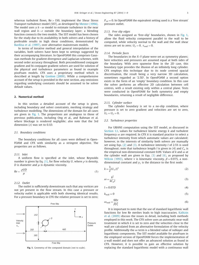
2.1.3. Free slip edgesThe sides assigned as ‘free-slip’ boundaries, shown in Fig. 1,
allow the fluid velocity component parallel to the wall to becomputed, while velocity normal to the wall and the wall shearstress are set to zero; Uy ¼ 0; τwall ¼ 0.
2.1.4. Periodic facesThe boundaries in the X–Y plane were set as symmetry planes;
here velocities and pressures are assumed equal at both sides ofthe boundary. With zero spanwise flow in the 2D case, thisboundary type provides the illusion of an infinitely long cylinder.CFX employs this technique due to its node centred spacialdiscretisation, the result being a very narrow 3D calculation,sometimes regarded as ‘2.5D’. In OpenFOAM a second optionexists in the form of an ‘empty’ boundary condition. In this casethe solver performs an effective 2D calculation between cellcentres, with a result existing only within a central plane. Testswere conducted in OpenFOAM for both symmetry and emptyboundaries, returning a result of negligible difference.
2.1.5. Cylinder surfaceThe cylinder boundary is set to a no-slip condition, where
pressure is set to zero gradient and velocities are set to zero,Ux ¼Uy ¼ 0.
2.2. Turbulence properties
For URANS computation using the SST model, as discussed inSection 1.1, values for turbulence kinetic energy k and turbulentfrequency ω are required. In CFX it is standard practice to select aturbulence intensity from which automatic values are calculated;however, in the interests of similarity both solvers are manuallyset using Eqs. (2) and (3). A turbulence intensity I of 2.5% is usedthroughout; note that turbulence length l is given in (4) and Cμ isthe empirical non-dimensional constant 0.09. Values of k and ω atthe cylinder wall are given in Eqs. (5) and (6), as proposed byWilcox (1993), where v is kinematic viscosity, β¼ 0:075, a non-dimensional constant and y1 is the distance to the first node:
k¼ 32ðU1IÞ2 ð2Þ
ω¼ k32
kCμlð3Þ
l¼ 0:07D ð4Þ
kwall ¼ 0 ð5Þ
ωwall ¼60vβy21
ð6Þ
It is important to note that the use of standard logarithmic wallfunctions for low Re meshes leads to high inaccuracies. Kalitzinet al. (2005) discuss the issues in detail, including both methodsemployed in this work. The CFX solver uses an automatic near-walltreatment in which k is set to zero and the velocities close to thewall are calculated from an alternative formulation of the velocityprofile. Additionally the ω term is a blended value of sublayer andlogarithmic components. The SST model available for pisoFoam inthe employed version of OpenFOAM forces the implementation ofa wall model and does not offer an advanced solution as found inCFX. However, it is possible to gain an effective solution byreplacing the standard logarithmic model with a continuous wall
Velocity Inlet
Free Slip
Free Slip
Pressure Outlet
Fig. 1. Geometry of the computed domain (not to scale).
formulation; in this case Spalding's solution to the ‘law of the wall’is used (Spalding, 1961).
2.3. Meshing
To assure a high level of grid independence a low-Re approachto meshing is taken. The term ‘low-Re’ is not to be confused withglobal Reynolds number, but indicates the low turbulent Reynoldsnumber that exists in the viscous sublayer. The yþ value repre-sents a non-dimensional distance of the first node from a no-slipwall. It links the node distance to shear stress τω, by non-dimensionalising the value with the fluid properties density andviscosity—refer to Eq. (7). In order to utilise low-Re boundaryproperties it is generally accepted that the mesh must achieve firstlayer cell thicknesses equivalent to yþ o1 for most solvers, seeANSYSs (2010) and Benim et al. (2007). However, a study of hullforms in comparably high Re marine flows by Jagadeesh andMurali (2009) concludes that a mesh of yþ o2 with 5 cells in theboundary layer was sufficient for accurate solution of a number oftwo-equation turbulence models.
yþ ¼ffiffiffiffiffiffiffiffiffiffiffiτω=ρ
py1
νð7Þ
To achieve a mesh within the constraints identified, a commonlyemployed empirical calculation based on flat plate theory isinitially used, as follows:
y1 ¼Dyþ �ffiffiffiffiffiffi74
pRe�13=14
L ð8ÞInitial tests were conducted using the predicted values and post-processed to acquire boundary layer thicknesses using velocity at0:99U1. The result was a clear over-prediction for thickness y1,particularly at walls adjacent to the maximum flow velocities.Therefore a second round of meshing was completed whichensured that a minimum 5 cells were located in the boundarylayer; for the majority of the cylinder surface this number washigher. To assess and correct the inflated hexahedral mesh layers,equations were derived to link total height (of boundary layer) h,number of layers c, expansion ratio r and first cell height y1.Eqs. (9)–(11) represent the derivation of the total thickness, andEqs. (12) and (13) are rearrangements for post-processing thenumber of layers and establishing a replacement first cell thick-ness respectively. Note that the final meshes conformed to amaximum value of 0:5oyþ o1:5 on post-processing.
h¼ y1þy1rþy1r2þy1r
3þ…þy1rc�1 ð9Þ
h¼ ∑c�1
0y1r
c ð10Þ
h¼ y1rc�1r�1
� �ð11Þ
c¼ln hðr�1Þþy1
y1
� �ln r
ð12Þ
y1 ¼ hr�1rc�1
� �ð13Þ
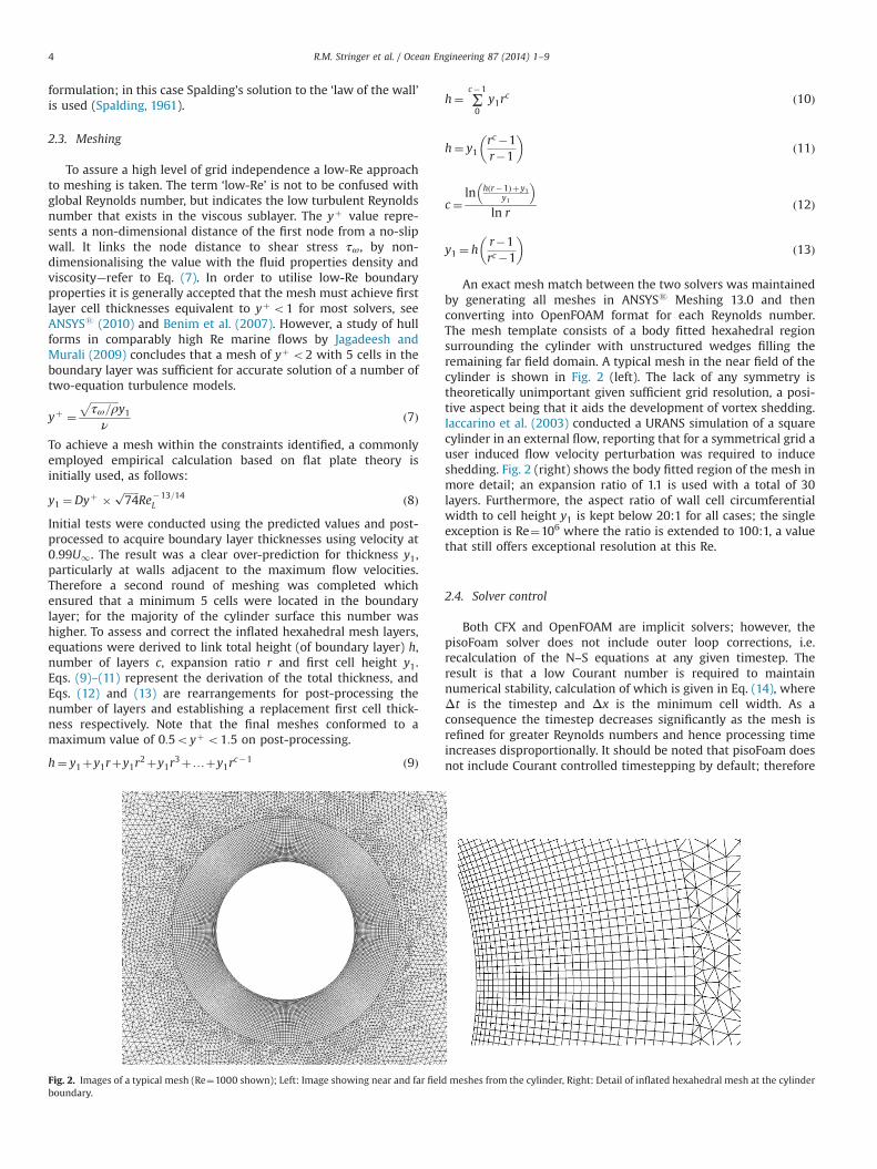
An exact mesh match between the two solvers was maintainedby generating all meshes in ANSYSs Meshing 13.0 and thenconverting into OpenFOAM format for each Reynolds number.The mesh template consists of a body fitted hexahedral regionsurrounding the cylinder with unstructured wedges filling theremaining far field domain. A typical mesh in the near field of thecylinder is shown in Fig. 2 (left). The lack of any symmetry istheoretically unimportant given sufficient grid resolution, a posi-tive aspect being that it aids the development of vortex shedding.Iaccarino et al. (2003) conducted a URANS simulation of a squarecylinder in an external flow, reporting that for a symmetrical grid auser induced flow velocity perturbation was required to induceshedding. Fig. 2 (right) shows the body fitted region of the mesh inmore detail; an expansion ratio of 1.1 is used with a total of 30layers. Furthermore, the aspect ratio of wall cell circumferentialwidth to cell height y1 is kept below 20:1 for all cases; the singleexception is Re¼106 where the ratio is extended to 100:1, a valuethat still offers exceptional resolution at this Re.
2.4. Solver control
Both CFX and OpenFOAM are implicit solvers; however, thepisoFoam solver does not include outer loop corrections, i.e.recalculation of the N–S equations at any given timestep. Theresult is that a low Courant number is required to maintainnumerical stability, calculation of which is given in Eq. (14), whereΔt is the timestep and Δx is the minimum cell width. As aconsequence the timestep decreases significantly as the mesh isrefined for greater Reynolds numbers and hence processing timeincreases disproportionally. It should be noted that pisoFoam doesnot include Courant controlled timestepping by default; therefore
Fig. 2. Images of a typical mesh (Re¼1000 shown); Left: Image showing near and far field meshes from the cylinder, Right: Detail of inflated hexahedral mesh at the cylinderboundary.
R.M. Stringer et al. / Ocean Engineering 87 (2014) 1–94
modifications to the source code are required.
Cr¼ UΔtΔx
ð14Þ
The second important aspect of solver control is the conver-gence criteria. Both CFX and OpenFOAM include residual calcula-tions for the solution variables, mass, momentum and turbulenceparameters in the case of CFX and pressure, velocity and turbu-lence in the case of OpenFOAM. The recommended value for bothCFX and the pisoFoam solver in accompanying guidance notes is10�6 for tight convergence; this value is selected for all cases, aswell as solving all parameters to double precision.
The specified total time is calculated from a non-dimensionaltime value tn as given in Eq. (15). All simulations are solved to 150non-dimensional time units.
tn ¼ tUD
ð15Þ
2.5. Post-processing
Data from CFX and OpenFOAM were post-processed usingANSYS CFD-Post 13.0 and ParaView 3.12.0-RC2 respectively.Instantaneous values of drag coefficient CD and root mean squareof lift coefficient CLrms are calculated using Eqs. (16) and (17),where FD and FL are the corresponding unit forces. The Strouhalnumber ðStÞ represents a normalised value of shedding frequency;see Eq. (18), where f is the shedding frequency in Hz. Thecoefficient of pressure p1 is calculated by Eq. (19), where p isthe static pressure, and where all values with the subscript infinitydenote free-stream values taken 0.1 m from the inlet on the x-axisand at the centreline of the cylinder on the y-axis:
To represent the full range of conditions expected in the case ofa cylinder in tidal flow, computations have been performed atRe¼40, 100, 103, 104, 105 and 106. The following results serve toevaluate a number of objectives, namely, the performance ofURANS simulation using the Menter SST turbulence model com-bined with low-Re meshing, and the comparability of the com-mercial code ANSYSs CFX 13.0 with the open-source codeOpenFOAM (using the pisoFoam solver), given nominally identicalcases. A number of key parameters have been identified forpresentation and discussion.
3.1. Calibration testing Re¼40
Testing initially at a low Reynolds number using a laminarmodel was conducted to provide validation of the boundary setupstrategy outlined throughout Section 2 (excluding turbulence), andto evaluate the success of the modified pisoFoam solver to includeCourant timestepping control. The Courant number is initiallydefined as 0.8.
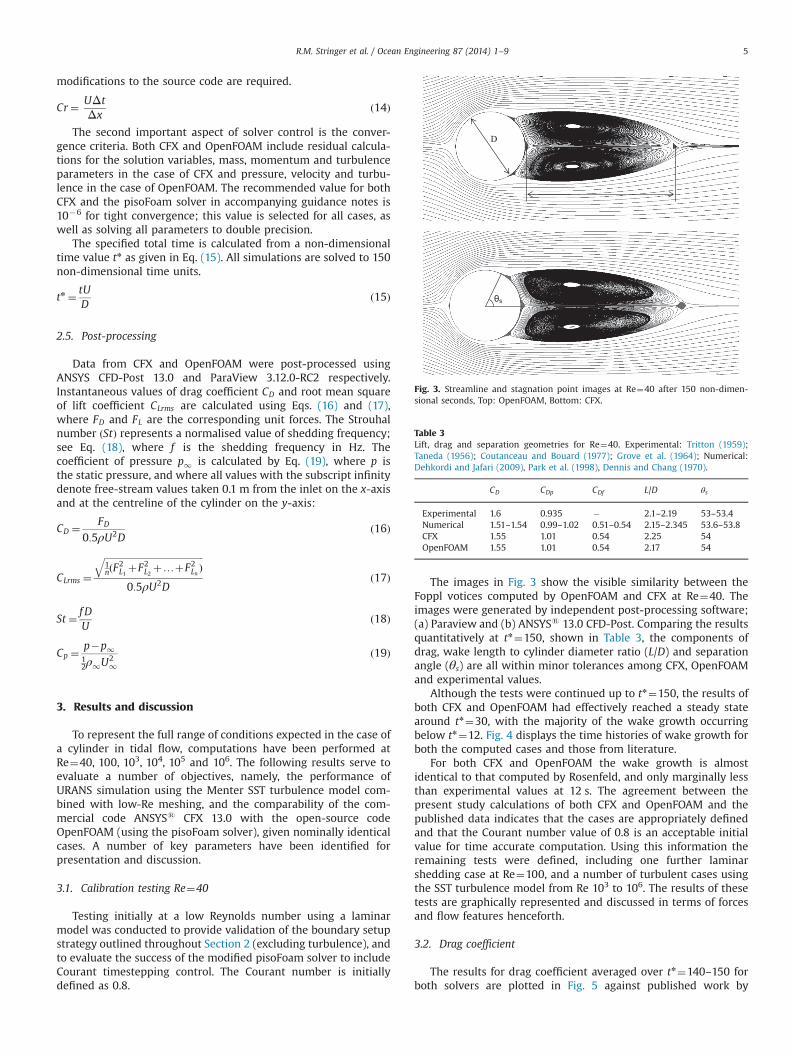
The images in Fig. 3 show the visible similarity between theFoppl votices computed by OpenFOAM and CFX at Re¼40. Theimages were generated by independent post-processing software;(a) Paraview and (b) ANSYSs 13.0 CFD-Post. Comparing the resultsquantitatively at tn¼150, shown in Table 3, the components ofdrag, wake length to cylinder diameter ratio (L/D) and separationangle (θs) are all within minor tolerances among CFX, OpenFOAMand experimental values.
Although the tests were continued up to tn¼150, the results ofboth CFX and OpenFOAM had effectively reached a steady statearound tn¼30, with the majority of the wake growth occurringbelow tn¼12. Fig. 4 displays the time histories of wake growth forboth the computed cases and those from literature.
For both CFX and OpenFOAM the wake growth is almostidentical to that computed by Rosenfeld, and only marginally lessthan experimental values at 12 s. The agreement between thepresent study calculations of both CFX and OpenFOAM and thepublished data indicates that the cases are appropriately definedand that the Courant number value of 0.8 is an acceptable initialvalue for time accurate computation. Using this information theremaining tests were defined, including one further laminarshedding case at Re¼100, and a number of turbulent cases usingthe SST turbulence model from Re 103 to 106. The results of thesetests are graphically represented and discussed in terms of forcesand flow features henceforth.
3.2. Drag coefficient
The results for drag coefficient averaged over tn¼140–150 forboth solvers are plotted in Fig. 5 against published work by
D
θs
Fig. 3. Streamline and stagnation point images at Re¼40 after 150 non-dimen-sional seconds, Top: OpenFOAM, Bottom: CFX.
Table 3Lift, drag and separation geometries for Re¼40. Experimental: Tritton (1959);Taneda (1956); Coutanceau and Bouard (1977); Grove et al. (1964); Numerical:Dehkordi and Jafari (2009), Park et al. (1998), Dennis and Chang (1970).
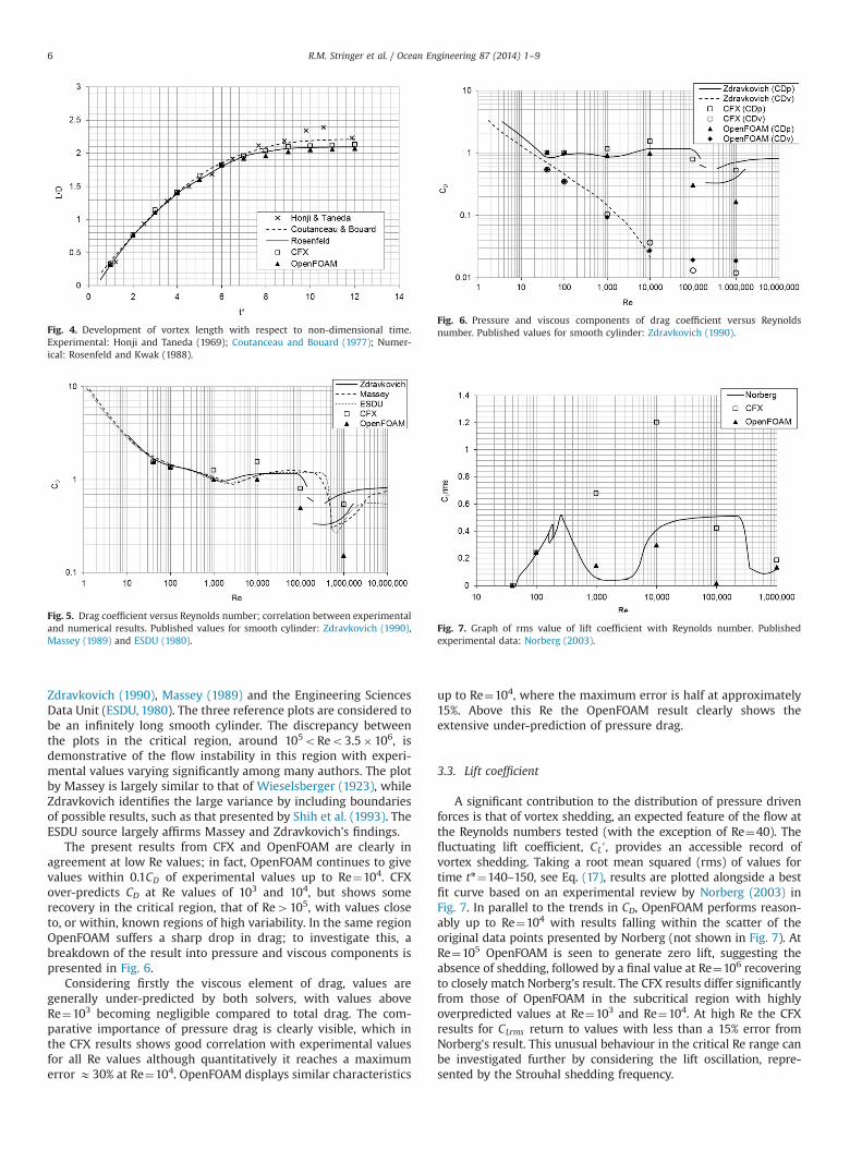
Zdravkovich (1990), Massey (1989) and the Engineering SciencesData Unit (ESDU, 1980). The three reference plots are considered tobe an infinitely long smooth cylinder. The discrepancy betweenthe plots in the critical region, around 105oReo3.5�106, isdemonstrative of the flow instability in this region with experi-mental values varying significantly among many authors. The plotby Massey is largely similar to that of Wieselsberger (1923), whileZdravkovich identifies the large variance by including boundariesof possible results, such as that presented by Shih et al. (1993). TheESDU source largely affirms Massey and Zdravkovich's findings.
The present results from CFX and OpenFOAM are clearly inagreement at low Re values; in fact, OpenFOAM continues to givevalues within 0.1CD of experimental values up to Re¼104. CFXover-predicts CD at Re values of 103 and 104, but shows somerecovery in the critical region, that of Re4105, with values closeto, or within, known regions of high variability. In the same regionOpenFOAM suffers a sharp drop in drag; to investigate this, abreakdown of the result into pressure and viscous components ispresented in Fig. 6.
Considering firstly the viscous element of drag, values aregenerally under-predicted by both solvers, with values aboveRe¼103 becoming negligible compared to total drag. The com-parative importance of pressure drag is clearly visible, which inthe CFX results shows good correlation with experimental valuesfor all Re values although quantitatively it reaches a maximumerror E30% at Re¼104. OpenFOAM displays similar characteristics
up to Re¼104, where the maximum error is half at approximately15%. Above this Re the OpenFOAM result clearly shows theextensive under-prediction of pressure drag.
3.3. Lift coefficient
A significant contribution to the distribution of pressure drivenforces is that of vortex shedding, an expected feature of the flow atthe Reynolds numbers tested (with the exception of Re¼40). Thefluctuating lift coefficient, CL
0, provides an accessible record ofvortex shedding. Taking a root mean squared (rms) of values fortime tn¼140–150, see Eq. (17), results are plotted alongside a bestfit curve based on an experimental review by Norberg (2003) inFig. 7. In parallel to the trends in CD, OpenFOAM performs reason-ably up to Re¼104 with results falling within the scatter of theoriginal data points presented by Norberg (not shown in Fig. 7). AtRe¼105 OpenFOAM is seen to generate zero lift, suggesting theabsence of shedding, followed by a final value at Re¼106 recoveringto closely match Norberg's result. The CFX results differ significantlyfrom those of OpenFOAM in the subcritical region with highlyoverpredicted values at Re¼103 and Re¼104. At high Re the CFXresults for CLrms return to values with less than a 15% error fromNorberg's result. This unusual behaviour in the critical Re range canbe investigated further by considering the lift oscillation, repre-sented by the Strouhal shedding frequency.
Fig. 4. Development of vortex length with respect to non-dimensional time.Experimental: Honji and Taneda (1969); Coutanceau and Bouard (1977); Numer-ical: Rosenfeld and Kwak (1988).
Fig. 5. Drag coefficient versus Reynolds number; correlation between experimentaland numerical results. Published values for smooth cylinder: Zdravkovich (1990),Massey (1989) and ESDU (1980).
Fig. 6. Pressure and viscous components of drag coefficient versus Reynoldsnumber. Published values for smooth cylinder: Zdravkovich (1990).
Fig. 7. Graph of rms value of lift coefficient with Reynolds number. Publishedexperimental data: Norberg (2003).
R.M. Stringer et al. / Ocean Engineering 87 (2014) 1–96
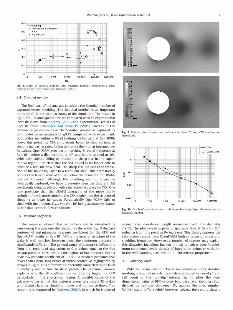
3.4. Strouhal number
The final part of the analysis considers the Strouhal number ofcaptured vortex shedding. The Strouhal number is an importantindicator of the transient accuracy of the simulation. The results inFig. 8 for CFX and OpenFOAM are compared with an experimental‘best fit’ curve from Norberg (2003) and experimental results athigh Re from Achenbach and Heinecke (1981). Success in thelaminar range continues as the Strouhal number is captured byboth codes to an accuracy of ±0.1% compared with experiment.Both codes are within 79% of findings by Norberg at Re¼1000;above this point the CFX simulations begin to shed vortices atsteadily increasing rates, failing to predict the drop at intermediateRe values. OpenFOAM provides a matching Strouhal frequency atRe¼104, before a distinct drop at 105 and failure to shed at 106.With both solvers failing to predict the sharp rise in the super-critical region, it is clear that the SST model is no longer able toproduce a realistic flow field. The sharp rise indicates the transi-tion of the boundary layer to a turbulent state; this dramaticallyreduces the length scale of eddies below the resolution of URANSmethod. However, although the shedding can no longer berealistically captured, we have previously seen the drag and liftcoefficients being predicted with satisfactory accuracy by CFX. Onemay postulate that the URANS averaging of the more highlyturbulent flow is more suited to the CFX model than the structuredshedding at lower Re values. Paradoxically OpenFOAM fails toshed, with the previous CLrms value at 106 being accurate by chancerather than realistic flow conditions.
3.5. Pressure coefficient
The variance between the two solvers can be visualised byconsidering the pressure distribution in the wake. Fig. 9 displayscontours of instantaneous pressure coefficient for the CFX andOpenFOAM results at Re¼104. While the general structure of thewake is well matched between plots, the minimum pressure issignificantly different. The general range of pressure coefficient isfrom 1, at regions of stagnation, to 0 at values equal to the freestream pressure, to values o1 for regions of low pressure. With apeak low pressure coefficient of �2.4, CFX predicts pressures 65%lower than OpenFOAM values at vortex centres, as highlighted byarrows in Fig. 9. This difference is inherently connected to the levelof vorticity and in turn to shear profile. The pressure varianceexplains why the lift coefficient is significantly higher for CFXparticularly in the sub-critical region. A possible cause of theextreme values is that this region is prone to strongly 3D wakeswith distinct laminar shedding modes and transverse flows. Thisreasoning is supported by Norberg (2003), in which Re is plotted
against axial correlation length normalised with the diameterΛ=d� �
. The plot reveals a peak in spanwise flow at ReE5�103,reducing from this point as Re increases. This theory opposes thesatisfactory results from OpenFOAM both in terms of forces andshedding frequency. However, a number of reasons may explainthis disparity, including, but not limited to, solver specific mini-mum turbulence levels, density of integration points or variationin the wall handling (see Section 2– Turbulence properties).
3.6. Boundary layer
With boundary layer thickness not known a priori, iterativemeshing is required in order to satisfy established values of yþ andcell count at the non-slip surface. Fig. 10 plots the non-dimensional value of 99% velocity boundary layer thickness (δU)divided by cylinder diameter (D), against Reynolds number.While results differ slightly between solvers, the results show a
Fig. 8. Graph of Strouhal number with Reynolds number. Experimental data:Norberg (2003); Achenbach and Heinecke (1981).
Fig. 9. Contour plots of pressure coefficient for Re¼104; top: CFX and bottom:OpenFOAM.
consistent rate of decay in velocity boundary layer thickness withincreasing Re; this relationship was confirmed by solving twoother cylinder regimes. Using a trend line approximation a powerlaw can be established to describe the link between Re and δU=D,see Eq. (20). The approximation tracks the OpenFOAM result moreclosely due to the higher solution accuracy produced at sub-critical values, and is proposed as guidance for numerical model-ling of smooth circular cylinders.
δU=Dffi1:5Re�0:625 ð20Þ
4. Conclusions
The aim of the research presented was to perform a robustassessment of the URANS method over a wide range of Reynoldsnumbers within the limits of a 2D simplification. Success is judgedby comparison of forces and transient flow field parameters withexperimental values in literature. Two finite volume solvers havebeen employed and compared; ANSYSs CFX-13.0 and Open-FOAMs 1.7.1. To extract the best possible outcome for the circularcylinder case, a high resolution methodology was established withregard to geometric, numerical and dicrestisation practices whichwere applied to all cases. Specifically this includes:
� application of URANS calculation using SST turbulence model;� domain size/cylinder ratio chosen to avoid blockage effects;� surface meshing to specified yþ and cell count in
boundary layer;� cell aspect ratio conformity and far field size limitation;� utilising fully adaptive Courant controlled timestepping;� maintaining maximum commonality between solvers;
Although previous studies have found successful application ofthe URANS method for some of the Reynolds numbers consideredhere, a clear methodology for all flow cases has not previouslybeen proposed and evaluated. For low Reynolds numbers,Reo103, the method developed in the present research is highlyaccurate with both solvers achieving correlation with experiment.At subcritical Reynolds numbers, Reo105, the findings are lessconclusive. Use of two solvers has exposed fundamental differ-ences despite closely matched definitions for this Re region. Whilethe differences and possible causes have been discussed in theresults section of this paper, further work is required to establishexact root causes. However, despite the unavoidable subtle differ-ences between the two setups, OpenFOAM delivers significantlycloser values for coefficients of lift, drag and shedding frequencywhen compared to experiment.
At the onset of drag crisis, considered as the critical region for105oReo107, CFX agrees with findings from published work,such as Ong et al. (2009), achieving high correlation with experi-mental values for force coefficients, but fails to capture a realisticwake. The pisoFoam solver does not follow this trend, failing toshed at critical Re values. Further work has already includedreducing the timestep to a Courant of 0.1 in order to reduce anyinstability which may result from the absence of under-relaxation.However this provided no change to the result, pointing to a possibleissue with the accumulation of numerical truncation errors or thelike. The implementation of an Algebraic Multi-Grid (AMG), orsolution using pimpleFoam, a solver capable of outer loop time-stepping, may improve high Re convergence in OpenFOAM.
Fundamentally the simplification of the case to 2D and use of aReynolds-averaged method means that applicability falls predo-minantly in the subcritical flow region, with OpenFOAM providingvalues suitable for engineering activities. Above this value LES isadvised for fully capturing the forces and wake as demonstrated
by alternative publications. Having formed differing conclusionsfor each solver tested, it is clear that individual benchmarking ofsoftware is an essential step for any simulation, a requirementheightened in this case with increasing boundary layer and waketurbulence.
The overall research provides both an insight into the limits ofURANS for modelling of circular cylinders and a benchmark forfurther studies where comparable methods and software are used.As part of this the plot of non-dimensional velocity boundary layerthickness versus Re, and associated relationship given in Eq. (20),is given to assist further numerical studies in RANS and LES whereresolution of the boundary layer down to sublayer accuracy isdesired.
Acknowledgements
This study is part of a Ph.D. funded by the EPSRC, who are dulythanked for their support.
References
Achenbach, E., 1968. Distribution of local pressure and skin friction around acircular cylinder in cross-flow up to re¼5�106. J. Fluid Mech. 34 (625-&).
Achenbach, E., Heinecke, E., 1981. On vortex shedding from smooth and roughcylinders in the range of reynolds-numbers 6�103 to 5�106. J. Fluid Mech.109, 239–251.
ANSYSs, 2010. Academic Research, Release 13.0, Help system, CFX ReferenceGuide, 6.3.4.1.5.2: Integration to the wall (low-reynolds number formulaton).
Benim, A.C., Cagan, M., Nahavandi, A., Pasqualotto, E., 2007. RANS predictions ofturbulent flow past a circular cylinder over the critical regime. In: Proceedings ofthe 5th Iasme/Wseas International Conference on Fluid Mechanics and Aerody-namics (Fma ‘07), pp. 235–240.
Coutanceau, M., Bouard, R., 1977. Experimental-determination of main features ofviscous-flow in wake of a circular-cylinder in uniform translation. 2. Unsteady-flow. J. Fluid Mech. 79, 257.
Dehkordi, B.G., Jafari, H.H., 2009. Numerical simulation of flow through tubebundles in in-line square and general staggered arrangements. Int. J. Num.Methods Heat Fluid Flow 19, 1038–1062.
Dennis, S.C.R., Chang, G.Z., 1970. Numerical solutions for steady flow past a circularcylinder at reynolds numbers up to 100. J. Fluid Mech. 42, 471.
ESDU, 1980. Mean Forces, Pressures and Flow Field Velocities for Circular Cylind-rical Structures: Single Cylinder with Two-Dimensional Flow.
Gretton, G.I., 2009. The Hydrodynamic Analysis of a Vertical Axis Tidal CurrentTurbine (Ph.D. thesis). The University of Edinburgh.
Grove, A.S., Shair, F.H., Petersen, E.E., Acrivos, A., 1964. An experimental investigationof the steady separated flow past a circular cylinder. J. Fluid Mech. 19 (60-&).
Iaccarino, G., Ooi, A., Durbin, P.A., Behnia, M., 2003. Reynolds averaged simulation ofunsteady separated flow. Int. J. Heat Fluid Flow 24, 147–156.
Issa, R.I., 1986. Solution of the implicitly discretized fluid-flow equations byoperator-splitting. J. Comput. Phys. 62, 40–65.
Jagadeesh, P., Murali, K., 2009. Application of low-Re turbulence models for flowsimulations past underwater vehicle hull forms. J. Nav. Archit. Mar. Eng., 2.
Kalitzin, G., Medic, G., Iaccarino, G., Durbin, P., 2005. Near-wall behavior of RANSturbulence models and implications for wall functions. J. Comput. Phys. 204,265–291.
Lienhard, J.H., 1966. Synopsis of Lift, Drag, and Vortex Frequency Data for RigidCircular Cylinders. Research Division Bulletin, Washington State UniversityCollege of Engineering , 32.
Massey, B.S., 1989. Mechanics of Fluids. Van Nostrand Reinhold.Menter, F.R., 1994. 2-equation eddy-viscosity turbulence models for engineering
applications. AIAA J. 32, 1598–1605.Norberg, C., 2003. Fluctuating lift on a circular cylinder: review and new measure-
ments. J. Fluids Struct. 17, 57–96.Ong, M.C., Utnes, T., Holmedal, L.E., Myrhaug, D., Pettersen, B., 2009. Numerical
simulation of flow around a smooth circular cylinder at very high reynoldsnumbers. Mar. Struct. 22, 142–153.
Park, J., Kwon, K., Choi, H., 1998. Numerical solutions of flow past a circular cylinderat reynolds numbers up to 160. J. Mech. Sci. Technol. 12, 1200–1205.
Raghavan, K., Bernitsas, M.M., 2011. Experimental investigation of reynolds numbereffect on vortex induced vibration of rigid circular cylinder on elastic supports.Ocean Eng. 38, 719–731.
Rahman, M.M., Karim, M.M., Alim, M.A., 2008. Numerical investigation of unsteadyflow past a circular cylinder using 2-d finite volume method. J. Nav. Archit. Mar.Eng., 4.
R.M. Stringer et al. / Ocean Engineering 87 (2014) 1–98
Roshko, A., 1955. On the wake and drag of bluff bodies. J. Aeronaut. Sci. 22, 124–132.Shih, W.C.L., Wang, C., Coles, D., Roshko, A., 1993. Experiments on flow past rough
circular-cylinders at large reynolds-numbers. J. Wind Eng. Ind. Aerodyn. 49,351–368.
Spalding, D.B., 1961. A single formula for the law of the wall. Trans ASME Series A:J. Appl. Mech. 28, 444–458.
Taneda, S., 1956. Experimental investigation of the wakes behind cylinders andplates at low reynolds numbers. J. Phys. Soc. Jpn. 11, 302–307.
Tritton, D.J., 1959. Experiments on the flow past a circular cylinder at low reynoldsnumbers. J. Fluid Mech. 6, 547.
Tutar, M., Holdo, A.E., 2001. Computational modelling of flow around a circularcylinder in sub-critical flow regime with various turbulence models. Int. J. Num.Methods Fluids 35, 763–784.
Wieselsberger, C., 1923. Ergebnisse der aerodynamischen versuchsanstalt zugottingen, unter mitwirkung von… C. Wieselsberger und… A. Betz herausge-geben von… L. Prandtl,… I.[-ii.] lieferung.
Wilcox, D.C., 1993. A two-equation turbulence model for wall-bounded and free-shear flows. In: Proceedings of the AIAA 24th Fluid Dynamics Conference, AIAA,Orlando, FL.
Williamson, C.H.K., 1996. Vortex dynamics in the cylinder wake. Annu. Rev. FluidMech. 28, 477–539.
Xia, J.Q., Falconer, R.A., Lin, B.L., 2010. Impact of different operating modes for asevern barrage on the tidal power and flood inundation in the severn estuary,UK. Appl. Energy 87, 2374–2391.
Zdravkovich, M.M., 1990. Conceptual overview of laminar and turbulent flows pastsmooth and rough circular-cylinders. J. Wind Eng. Ind. Aerodyn. 33, 53–62.


![this page%PDF-1.5 %âãÏÓ 9815 0 obj > endobj 9830 0 obj >/Filter/FlateDecode/ID[3437D649C0F73942B7D74B44C42A12BC>]/Index[9815 31]/Info 9814 0 R/Length 80/Prev 900120/Root 9816 0](https://static.documents.pub/doc/80x56/5aaeb7847f8b9a6b308c6b37/translate-this-pagepdf-15-9815-0-obj-endobj-9830-0-obj-filterflatedecodeid3437d649c0f73942b7d74b44c42a12bcindex9815.jpg)


