Unsteady Simulation of a Transport Aircraft Propeller … 7 - 1 UNCLASSIFIED/UNLIMITED...

RTO-MP-AVT-123 7 - 1

UNCLASSIFIED/UNLIMITED


Unsteady Simulation of a Transport Aircraft Propeller Using MEGAFLOW

Arne Stuermer and Mark Rakowitz DLR, Institute of Aerodynamics and Flow Technology

Lilienthalplatz 7, D-38108 Braunschweig GERMANY

[email protected]

ABSTRACT

A series of unsteady CFD simulations have been conducted for an isolated propeller configuration at low-speed flight conditions using both a structured and an unstructured CFD method. The propeller geometry investigated is representative of a modern eight-bladed design for high-speed turboprop transport aircraft. Two typical low-speed conditions, one at zero and one at ten degrees angle of attack, were investigated and results of the two CFD methods compared with experimental data obtained from a wind tunnel test campaign. The computations were performed with the DLR FLOWer and TAU-codes respectively and employed Chimera grids, which enable the modelling of multiple rigid bodies in relative motion. The results of Euler and Navier-Stokes computations show good agreement with the available wake data measured in the wind tunnel. Additionally, a detailed analysis of the forces acting on the blades and the propeller is performed, which show a strong influence of the propeller angle of attack.

NOMENCLATURE

CT = FX / ρn² D4 Thrust force coefficient, [-] R Propeller radius, [m] CY = FY / ρn² D4 Lateral force coefficient, [-] r Radial position, [m] CZ = FZ / ρn² D4 Lift force coefficient, [-] u Axial velocity component, [m/s] D Propeller diameter, [m] V∞ Freestream velocity, [m/s] F Force, [N] x Axial position, [m] J= V∞ / nD Advance ratio, [-] α Angle of attack, [˚] Ma Mach number [-] ρ Density, [kg/m³] n Propeller rotational speed [1/s] ψ Azimuthal angle, [˚]

1.0 INTRODUCTION

For many transport aircraft configurations and missions, propeller propulsion offers significant benefits over the use of jet or turbofan engines. For regional commercial transports, the higher propulsive efficiency of propellers means turboprop-powered aircraft have better economic performance than their jet-powered counterparts. Furthermore, for many military transport aircraft applications, the turboprop offers an optimal combination of take-off and landing performance, low fuel-burn and tactical mission performance such as ground manoeuvring, steep descent and air-drop capability. The aerodynamic interactions of the propeller slipstream with the aircraft are complex and require careful analysis to ensure

Stuermer, A.; Rakowitz, M. (2005) Unsteady Simulation of a Transport Aircraft Propeller Using MEGAFLOW. In Flow Induced Unsteady Loads and the Impact on Military Applications (pp. 7-1 – 7-14). Meeting Proceedings RTO-MP-AVT-123, Paper 7. Neuilly-sur-Seine, France: RTO. Available from: http://www.rto.nato.int/abstracts.aps.

http://www.rto.nato.int/abstracts.aps

Report Documentation Page Form ApprovedOMB No. 0704-0188

Public reporting burden for the collection of information is estimated to average 1 hour per response, including the time for reviewing instructions, searching existing data sources, gathering andmaintaining the data needed, and completing and reviewing the collection of information. Send comments regarding this burden estimate or any other aspect of this collection of information,including suggestions for reducing this burden, to Washington Headquarters Services, Directorate for Information Operations and Reports, 1215 Jefferson Davis Highway, Suite 1204, ArlingtonVA 22202-4302. Respondents should be aware that notwithstanding any other provision of law, no person shall be subject to a penalty for failing to comply with a collection of information if itdoes not display a currently valid OMB control number.

1. REPORT DATE 25 APR 2005

2. REPORT TYPE N/A

3. DATES COVERED -

4. TITLE AND SUBTITLE Unsteady Simulation of a Transport Aircraft Propeller Using MEGAFLOW

5a. CONTRACT NUMBER

5b. GRANT NUMBER

5c. PROGRAM ELEMENT NUMBER

6. AUTHOR(S) 5d. PROJECT NUMBER

5e. TASK NUMBER

5f. WORK UNIT NUMBER

7. PERFORMING ORGANIZATION NAME(S) AND ADDRESS(ES) DLR, Institute of Aerodynamics and Flow Technology Lilienthalplatz 7,D-38108 Braunschweig GERMANY

8. PERFORMING ORGANIZATIONREPORT NUMBER

9. SPONSORING/MONITORING AGENCY NAME(S) AND ADDRESS(ES) 10. SPONSOR/MONITOR’S ACRONYM(S)

11. SPONSOR/MONITOR’S REPORT NUMBER(S)

12. DISTRIBUTION/AVAILABILITY STATEMENT Approved for public release, distribution unlimited

13. SUPPLEMENTARY NOTES See also ADM201978, Flow-Induced Unsteady Loads and the Impact on Military Applications (Chargesinstables induites par ecoulement et impact sur les applications militaires)., The original documentcontains color images.

14. ABSTRACT

15. SUBJECT TERMS

16. SECURITY CLASSIFICATION OF: 17. LIMITATION OF ABSTRACT

UU

18. NUMBEROF PAGES

14

19a. NAME OFRESPONSIBLE PERSON

a. REPORT unclassified

b. ABSTRACT unclassified

c. THIS PAGE unclassified

Standard Form 298 (Rev. 8-98) Prescribed by ANSI Std Z39-18


7 - 2 RTO-MP-AVT-123



maximum propulsive efficiency can be achieved with a minimal adverse impact on the wing aerodynamics for example. Furthermore, a detailed knowledge of the loads acting on the propeller at various flight conditions is necessary for the structural design of the engine-aircraft integration. Computational Fluid Dynamics (CFD) simulations of propeller flows, as described here, can greatly help an aircraft designer understand and evaluate the complex aerodynamics of propeller flows [1]. At DLR, CFD has recently been used to investigate in detail the complex aerodynamics of propeller flows and to analyze the mutual interaction of the propeller slipstream and the wing [2,3]. In this study, an isolated propeller-configuration, for which wind tunnel measurements are available for comparison purposes, is chosen as the basis for an analysis using both an unstructured and a structured CFD method. The test campaign, conducted in a low-speed tunnel with a test section measuring 2.1m x 2.1 m x 4.3m, focused on obtaining data on the propeller slipstream development through measurements using a five hole probe. For the computations, the CAD geometry used for the CFD modelling featured some simplifications of the geometry tested in the wind tunnel. Most notably, the tunnel mounting assembly was omitted in order to reduce the complexity and the number of grid nodes. The flow parameters of the CFD simulation correspond to conditions used in the experiment and are typical low-speed conditions, with a Mach number of Ma = 0.173 and an advance ratio of J = 0.8. As one aim of the wind tunnel test campaign was to simulate full-scale advance ratios, the rotational speed of the 1/17th-scale model propeller was on the order of 14.000rpm. Two sets of computations were performed: one with the propeller rotational axis aligned with the flow and one at 10° angle of attack.

2.0 COMPUTATIONAL APPROACH

2.1 The Numerical Methods

The computations were performed with the structured DLR FLOWer-code and the unstructured DLR TAU-code [4,5,6]. These codes were developed in the MEGAFLOW project, and are state of the art finite volume CFD methods using multi-block structured and unstructured grids respectively. FLOWer and TAU feature upwind and central schemes for spatial discretization, Runge-Kutta time stepping schemes as well as convergence acceleration techniques in the form of multigrid, residual smoothing and local time stepping. Both codes enable the unsteady simulation of propeller flows, which requires the CFD method to enable the computation of time-accurate flows and allow for the modelling of multiple rigid bodies in relative motion. The latter is facilitated through the Chimera grid approach, which is available in both the FLOWer- and the TAU-code. The Chimera method is based on the use of several independently generated grids which have regions of overlap. To establish communication between the grids, grid nodes lying on the Chimera block boundaries are updated with interpolated flow data from a surrounding donor cell of an overlaying grid. In both solvers, the interpolation uses an Alternating Digital Tree (ADT) search method. Due to the use of tri-linear interpolation, the transfer of flow data is not flux conservative, but for external flows this usually does not reduce the accuracy of the flow solution. The implementation of the Chimera method differs slightly between the two solvers, which has a direct impact on the necessary preparation of the CAD-geometry and the generation of the computational grids.

2.2 Grid Generation

2.2.1 Structured Grid Generation

The Chimera functionality of the DLR FLOWer-code enables a simplification of the complex task of grid generation through the decomposition of the geometry into simpler geometric sub-parts. The only requirement to be met by the component meshes is to have an adequate grid overlap. All component grids are placed inside a simple Cartesian background mesh, which covers the entire computational domain. Grid points which lie within a solid body of a neighbouring grid are marked and excluded from the flow calculation. The multi-block structured and overlapping grid blocks were generated using the DLR grid generator MegaCads [7] and an in-house program for generating the Cartesian background mesh.





The mesh generation is done in several stages: at first the blocks associated to the rotating spinner and the propeller blades are created. These blocks are generated in a 45°-slice for each of the eight propeller blades and spinner segments. The first of the two boundary layer blocks of the propeller blade has an O-topology and includes 32 cells normal to the wall, 48 cells in spanwise direction and 208 cells in circumferential direction. The second block closes the OO-topology in spanwise direction and covers the planar tip with 32*16*208 cells. The number of grid cells and the extension of the block boundaries are a compromise between good grid resolution and the need for an appropriate overlap region with the other blocks as required for the Chimera interpolation. In the second stage, the boundary layer blocks of the nacelle and the propeller wake blocks are generated. A cylindrical wake block is used to ensure a good resolution of the blade wakes and the tip vortices. It begins just in front of the propeller block and features a quasi-equidistant point distribution in all Cartesian directions. The outer boundary in circumferential direction is positioned outwards of the propeller diameter to allow for computations at angle of attack. The wake block contains 4.042.353 grid points and thus a good third of the number of grid points of the whole grid. This underlines the particular effort put into ensuring that the propeller slipstream can be properly resolved and sustained to behind the propeller. Thirdly, the Chimera cutout grids are generated for the propeller blades, the nacelle and the wake block. Finally, the Cartesian background grid is generated with an in-house program. A cut through the grids around the propeller geometry is presented in figure 1. The whole grid generation process is replayed many times (in interaction with FLOWer Chimera preprocessing and steady flow solutions) to modify the blocks to achieve both a good grid overlap and to adapt the first grid spacing at the wall to achieve a y+-value of one. The final structured grid consists of 201 blocks with a total of 11.448.654 nodes.

Figure 1: Structured (left) and Unstructured (right) Chimera Grids.

2.2.2 Unstructured Grid Generation

The current implementation of the Chimera technique in the DLR TAU-code does not have an automatic blanking or hole-cutting procedure. Thus the two-block Chimera grids used for these computations require taking special care during the creation of the CAD geometry to reduce or eliminate the occurrence of grid nodes lying within the solid bodies of the overlaying grid block. Therefore the nacelle part of the geometry has a cylindrical hole at the position of the propeller, which needs to be set up in the CAD-geometry. In addition, an adequate overlap of the two separately generated grids needs to be assured through the appropriate positioning of the geometric boundaries which make up the Chimera boundaries.





The unstructured grid generation employed the CentaurSoft CentaurTM grid generation software [8], which enables fast and largely automatic mesh generation, while allowing a good control of mesh quality and density by the user. The first grid block was created for the stationary nacelle part of the isolated propeller geometry. Exploiting the symmetry of the nacelle, the mesh was generated for half of the domain and subsequently joined with its mirror image. To ensure an adequate resolution of the propeller wake and the blade tip vortices, very small grid elements were generated in a cylindrical area downstream of the propeller disc through the specification of appropriate sources in the Centaur mesh generator. For the second block, a grid was generated for the rotating parts of the geometry, i.e. the propeller. Again, use was made of symmetry and a 45°-slice was meshed and subsequently copied and rotated to complete the cylindrical propeller grid block. This exploitation of the geometric symmetry during the mesh generation process is of particular importance for this grid block, since this approach guarantees an identical spatial discretization for all eight blade passages, greatly enhancing the ability of the CFD solver to resolve the expected periodic unsteady fluctuations of the flow. As the geometry used for these computations has the spinner bluntly abutting against the nacelle block, a chamfering of the propeller grid towards the surface of the spinner was introduced. This was done to ensure the propeller grid extends far enough into the nacelle grid block to allow for an adequate overlap region while avoiding possible Chimera interpolation problems near the surfaces of the geometry. The final two-block Chimera grid, shown on the right in figure 2, has a total of 2.013.763 nodes.

2.3 Unsteady Computations

The unsteady computations are performed using the dual time method [9] for both the structured and the unstructured approach. In all the unsteady computations, one propeller revolution is resolved with 360 physical time steps. Each physical time step is converged using 50 inner iterations in the case of the TAU computations and 30 for the FLOWer runs. Both methods employ a central scheme for spatial discretization [10], with the second and fourth order scalar dissipation coefficients scaled with k2 = 0.5 and k4 = 1/64 respectively in TAU, and k2=0.5 and k4=1/128 in FLOWer, where additionally a matrix dissipation scheme [11,12] is used. While presently only Euler results are available from the unstructured computations, the FLOWer results are Navier-Stokes solutions, which were performed using the Wilcox k-ω turbulence model [13] using the Kok-modification [14] in vortex cores to reduce numerical dissipation. The convergence of the unsteady computations was monitored using the lift-, drag- and side-force-coefficients based on the forces acting on the eight propeller blades and the spinner. To achieve periodicity in the fluctuations of the propeller force coefficients, the simulation of a minimum of four full propeller revolutions is necessary.





3.0 COMPUTATIONAL RESULTS

3.1 Validation: Propeller Slipstream Development

Figure 2: Slipstream axial velocity profiles at x/R=0.2 on the left and right of the nacelle; Left: FLOWer Navier-Stokes, Right: TAU Euler.

The validation of the simulations is performed through a comparison of the computed propeller slipstream development with experimental data obtained in a wind tunnel test of the isolated propeller configuration. In the wind tunnel test campaign, the propeller slipstream development was measured using a five hole probe, which was traversed along several radial rays extending out from the nacelle in four planes behind the propeller. In the following discussions, all velocities are normalized with the respective freestream velocity. Furthermore, the analysis of the unsteady wake development requires the definition of a reference blade or azimuthal position through an azimuthal angle Ψ. When the reference blade pitch axis points upwards, the angle Ψ is defined as being 0° and it increases in the direction of propeller rotation, which is clockwise when looking upstream from behind the propeller.

Figure 2 shows a comparison of the computational and experimental wake axial velocities in the slipstream for the propeller at 10° angle of attack, with the FLOWer Navier-Stokes results presented on the left and the inviscid TAU results on the right. The comparison is performed at an axial position of x/R=0.2, which is the closest the five hole probe was traversed towards the propeller, and along rays extending out to the left (Ψ=270°) and right (Ψ=90°) of the nacelle. While the experimental measurements with the five-hole probe, shown as the diamonds in the figure, represent time-averaged data, the numerical results allow an analysis of the unsteady fluctuations in the propeller wake. As the propeller has eight blades, the wake at a fixed position will be periodic for every 45° of propeller rotation. From each of the simulations, the figures show two selected time-accurate snapshots at blade reference positions of Ψ=5° and Ψ=25° as red and blue curves respectively, as well as a time-averaged axial velocity profile in black to allow a better comparison with the experimental data. The time-averaged TAU results show a good agreement of the general profile shape with the wind tunnel data with a slight overprediction of the peak axial velocity magnitude. This overprediction is less pronounced in the FLOWer Navier-Stokes results, which also show a slightly better agreement with the experimental data close to the nacelle. The latter is due to the fact that the TAU Euler results do not include the viscous effects of the boundary layer on the nacelle. The primary cause of the discrepancy in peak velocity magnitude between the two numerical results is again thought to be the neglect of physical viscosity in the Euler simulations. As the blades are modelled as slip walls in this computation, no boundary layers are present, which mean the





wake region behind the blades have a more uniform velocity distribution of higher magnitude. The strong unsteadiness in the propeller slipstream can be seen in the two selected time accurate velocity profiles, which show the periodic occurrence of a velocity peak at the border of the propeller slipstream, which is linked to the passage of a blade tip vortex. This effect is not visible in the experimental data, partly because the five-hole probe measurements represent only the time-averaged slipstream data, but also due to the inaccuracy of such measurements in regions of strong flow gradients. It should also be noted that the experimental data is uncorrected for the wind tunnel influence and the measurements were performed at a slightly higher freestream velocity, which also explains the slight differences in the velocity distributions.

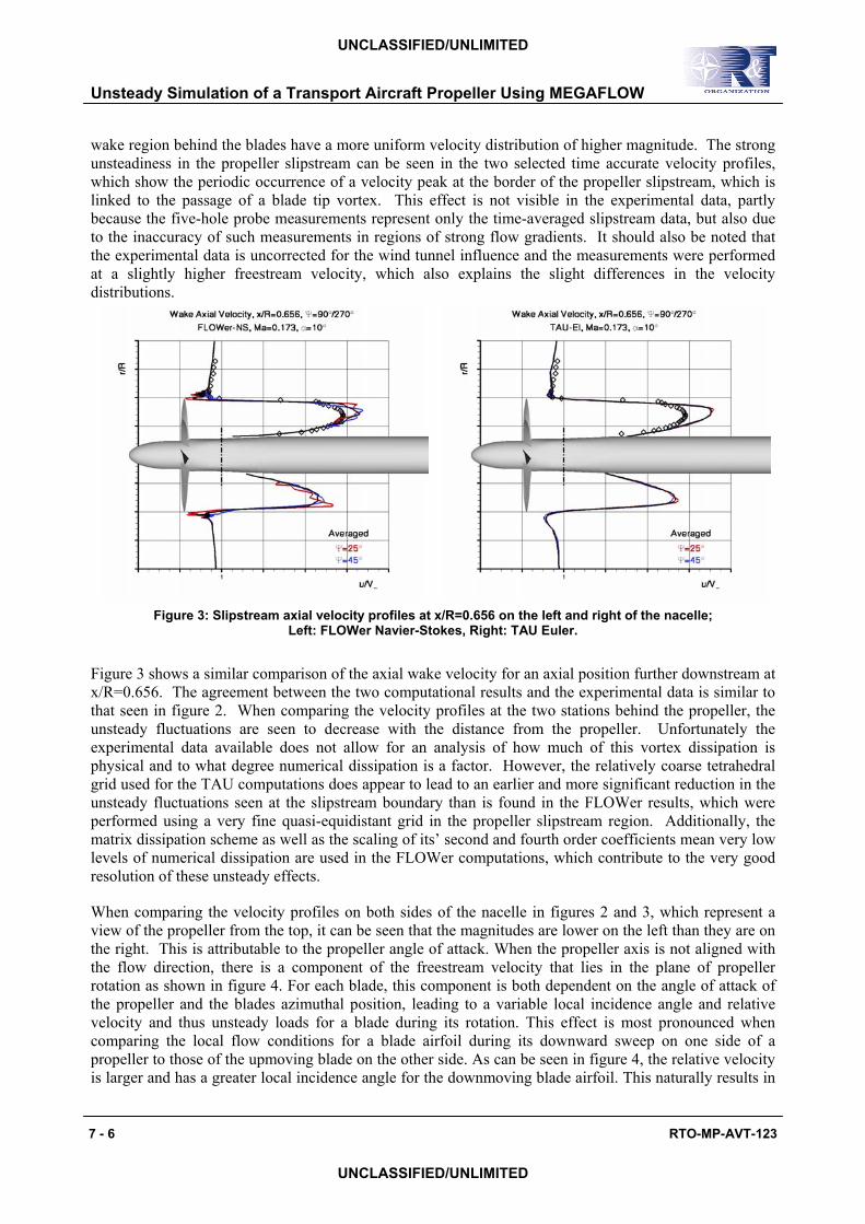
Figure 3: Slipstream axial velocity profiles at x/R=0.656 on the left and right of the nacelle; Left: FLOWer Navier-Stokes, Right: TAU Euler.

Figure 3 shows a similar comparison of the axial wake velocity for an axial position further downstream at x/R=0.656. The agreement between the two computational results and the experimental data is similar to that seen in figure 2. When comparing the velocity profiles at the two stations behind the propeller, the unsteady fluctuations are seen to decrease with the distance from the propeller. Unfortunately the experimental data available does not allow for an analysis of how much of this vortex dissipation is physical and to what degree numerical dissipation is a factor. However, the relatively coarse tetrahedral grid used for the TAU computations does appear to lead to an earlier and more significant reduction in the unsteady fluctuations seen at the slipstream boundary than is found in the FLOWer results, which were performed using a very fine quasi-equidistant grid in the propeller slipstream region. Additionally, the matrix dissipation scheme as well as the scaling of its’ second and fourth order coefficients mean very low levels of numerical dissipation are used in the FLOWer computations, which contribute to the very good resolution of these unsteady effects.

When comparing the velocity profiles on both sides of the nacelle in figures 2 and 3, which represent a view of the propeller from the top, it can be seen that the magnitudes are lower on the left than they are on the right. This is attributable to the propeller angle of attack. When the propeller axis is not aligned with the flow direction, there is a component of the freestream velocity that lies in the plane of propeller rotation as shown in figure 4. For each blade, this component is both dependent on the angle of attack of the propeller and the blades azimuthal position, leading to a variable local incidence angle and relative velocity and thus unsteady loads for a blade during its rotation. This effect is most pronounced when comparing the local flow conditions for a blade airfoil during its downward sweep on one side of a propeller to those of the upmoving blade on the other side. As can be seen in figure 4, the relative velocity is larger and has a greater local incidence angle for the downmoving blade airfoil. This naturally results in





larger lift and drag being produced on the blades during the downward sweep than on the upmoving blades with corresponding effects on the propeller slipstream. Figure 4 also depicts the variation of the local velocity and incidence angle for a blade section of the propeller at r/R = 0.75 during one revolution with the propeller at 10° angle of attack. Only the freestream velocity and the velocity component due to the rotation of the propeller are considered for this discussion. This is of course a simplification, as any 3D-effects, the mutual interaction between the blade wakes, as well as the induced velocities which are produced by each blades downwash are neglected. The figure shows that for this blade section a sinusoidal variation by more than +/-5% in velocity and by a little more than +/-1° in incidence occurs due to the propellers 10° angle of attack. As velocity and angle variations are in phase, the aerodynamic impact can be expected to be quite strong.

Figure 4: Asymmetry of local relative flow conditions for a blade of a propeller at angle of attack.

3.2 Analysis of Forces The asymmetric flow a blade experiences during its rotation has a very pronounced impact on the forces acting on the individual propeller blades as well as on the propeller as a whole. The unsteady CFD results allow for a very detailed analysis of the force development which is presented in the following section. Knowledge of the resulting forces is of great importance for the structural design of the engine-airframe integration. Unfortunately the measurement of forces and moments was not conducted during the wind tunnel test, so no comparisons can be made here.





3.2.1 Blade Force Development

Figure 5: Comparison of blade force development during the rotation; Left: Propeller at α =0°, Right: Propeller at α=10°.

Figure 5 shows a comparison of the development of the aerodynamic forces acting on a blade during a rotation. The evaluation of the forces is performed in a stationary coordinate system fixed to the nacelle of the isolated propeller configuration as shown in the figure. The left figure compares the inviscid TAU results with the viscous FLOWer results for the propeller at axial flow conditions, while the right figure shows the corresponding comparison for the propeller at 10° angle of attack. The solid lines represent the FLOWer results and the dashed lines show the TAU results. All force coefficients are normalized with the computed blade thrust force coefficient for the propeller at axial flow taken from the FLOWer results.

The thrust coefficient development is shown as the black lines in the figures, which is seen to be a constant value for the propeller at axial flow conditions. Not surprisingly, the inviscid results show a slightly larger thrust coefficient than the Navier-Stokes results, naturally due to the absence of viscous drag on the blades. At angle of attack, the thrust coefficient shows a sinusoidal evolution during its rotation. This is attributable to the unsteady variation of the local relative flow the blade experiences during its rotation. The maximum thrust coefficient is produced by the blade on its downward sweep at an azimuthal position of Ψ=120° and the minimum during the upward sweep at Ψ=300°. Again, the larger values from the inviscid TAU results are explainable through the neglect of viscous effects.

The blue curves show the lift force coefficient development. As the force evolution is performed in a stationary coordinate system, a sinusoidal evolution is found even at axial flow conditions, with the minima occurring at a blade position of Ψ=100° during the downward sweep and the maxima at Ψ=280° on the upward sweep. The Euler results show a slightly larger amplitude in the fluctuations than the Navier-Stokes results. At first glance the blade azimuth positions for the maximum and minimum lift force coefficients are surprising. One would expect the greatest lift force to occur at Ψ=90°, as this position should result in the most significant portion of the total blade force being aligned with the z-axis. The reason for this phase shift to larger azimuth angles can be found in the blade geometry, which features an upward sweep of the tip. This results in the blade force vector still having a component aligned with the y-axis at a blade azimuth position of Ψ=90° or Ψ=270°, respectively. For the propeller at angle of attack, the lift force coefficient development is significantly different as a result of the variation of the relative flow for a blade during the rotation. The minimum lift force coefficient is shifted to a slightly later





azimuthal position of Ψ=105° and is larger in magnitude. This is caused by the increase in local relative incidence angle and velocity on the blades downward sweep for the propeller at angle of attack. The maximum lift force coefficient is lower and produced slightly earlier than at axial flow, at a position of Ψ=275°, as during the blades upward sweep the relative incidence angle and flow velocity decrease.

The development of the blade lateral force coefficient is shown as the red curves. At axial flow, these curves are effectively identical to the lift curve with a phase shift of Ψ=-90°. At angle of attack the minimum lateral force coefficient magnitude remains largely unaffected but its occurrence is shifted to a later azimuthal position of Ψ=30°. This shift is a result of the increasing flow velocity and incidence angles on the downward sweep of the blade. The maximum of the lateral force coefficient occurs slightly earlier at Ψ=175° than at axial flow and is of greater magnitude due to the increased local relative flow velocities and incidence angles on the downward rotation, which are however already decreasing as the blade rotates towards the Ψ=180° position.

3.2.2 Propeller Force Development

The total propeller forces are the sum of the computed forces acting on the eight blades as well as the spinner. Each of the propeller force components is a constant value during the rotation, i.e. it is no longer a function of any blade azimuthal positions. This is because each blade has an identical force evolution during the propellers rotation, as shown in figure 5, but with a phase shift in 45°-increments for each consecutive blade.

Figure 6: Comparison of the propeller force coefficients; Left: Propeller thrust coefficients, Right: Propeller in-plane force coefficients at α=10°.

On the left in figure 6, the propeller thrust coefficients as computed by the two different numerical methods are shown for the two angles of attack. For comparison purposes all the coefficients are normalized with the propeller thrust coefficient of the axial flow case taken from the viscous FLOWer results. Both the inviscid TAU as well as the viscous FLOWer computations show a propeller thrust force increase of around 3% at 10° angle of attack over the axial flow case, with a slightly larger increase seen in the FLOWer Navier Stokes computations. The spinners contribution to this difference is important, as for the viscous computation it produces a drag component, which is reduced noticeably at the higher angle of attack. In the inviscid simulation, the spinner contributes to the propeller thrust and shows a smaller change with the angle of attack than seen in the FLOWer results. The propeller thrust of the TAU computations is 17% larger than that computed using FLOWer, which is due to the neglect of viscous effects in the present unstructured computations [2,3]. Again, the fact that the spinner produces positive


7 - 10 RTO-MP-AVT-123



thrust in the Euler results versus its drag production when viscous effects are taken into account in the FLOWer computations is an important part of the differences between the two results.

At 10° angle of attack, significant in-plane forces act on the propeller. On the right in figure 6, the coefficients of the lateral and lift forces are plotted as a percentage of the respective propeller thrust. At this incidence angle, the propeller produces a lift force of 10.4% and 11.7% of the respective thrust for the inviscid and the viscous computations respectively. This total lift is due to the fact that a positive lift force is produced on a downmoving blade, which benefits from the increased relative velocities and incidence angles due to the propeller angle of attack, while the diametrically opposed upmoving blade generates lower forces in the opposite direction due to the lower relative velocities and incidence angles. The latter cannot fully compensate for the forces generated on the opposing side of the propeller, resulting in a net lift force being produced. Similarly, the propeller produces a net lateral force for non-axial flow conditions, which grows from a value of zero at α=0° to around 3.3% of the respective propeller thrust at 10° angle of attack. This in-plane force component is smaller than the lift force as there is a change in sign for the blade lateral force on both the up- and downmoving sweep of the blade as can be seen in figure 5.

4.0 CONCLUSION

Unsteady computations of an isolated propeller configuration at low speed flight conditions at several angles of attack have been performed both with the structured DLR FLOWer-code and the unstructured DLR TAU-code. The propeller geometry is a modern eight bladed design intended for use on high speed turboprop transport aircraft. A comparison of the computed propeller slipstream development with available wind tunnel data was performed. Both the Euler and the Navier-Stokes results show reasonably good agreement with the experimental results, with a larger discrepancy in velocity magnitude visible for the inviscid results. This underlines the importance of viscous effects on the development of the propeller slipstream. Strong unsteady fluctuations were seen in the propwash during the propellers rotation with the primary effect being the periodic passage of the blade tip vortices. The importance of numerical dissipation and the density and quality of the grid for the proper resolution of the propeller slipstream, in particular the blade wakes and the tip vortices, can be seen in the reduced fluctuation amplitudes and earlier decay of the unsteady phenomena found in the inviscid results. These computations were performed on a relatively coarse tetrahedral grid, whereas the great effort undertaken to generate a quasi-equidistant structured grid to resolve the propeller slipstream in the FLOWer computations was able to capture and sustain these flow features far behind the propeller disc.

The unsteady computations allow a detailed analysis of the aerodynamic forces acting on the blades of the propeller. These forces exhibit unsteady fluctuations when the propeller is at an angle of attack. Furthermore, when the propeller rotational axis is not aligned with the flow direction, significant lift and lateral forces, so-called in-plane forces, are produced by the propeller, which reach around 11% and 3.3% of the propeller thrust respectively when the propeller is at 10° angle of attack. Propeller thrust is about 3% greater for this case than it is for the propeller at axial flow. The inviscid computations show a propeller thrust force which is 17% larger than the numerical results of the Navier-Stokes computations, which is a result of the neglect of viscous effects in the Euler simulation.

Based on the experience gained in this as well as other applications of DLRs CFD methods to the simulation of propeller flows, the importance of good grid quality, low numerical dissipation and the selection of an appropriate turbulence model have been shown to be important factors in achieving proper resolution of the unsteady development of the propeller slipstream. A detailed analysis of these parameters for Navier-Stokes simulations using the unstructured DLR TAU-code is in progress and further investigations of more complex geometries to investigate the aerodynamic interactions of the propeller slipstream and the aircraft are planned using both methods.


RTO-MP-AVT-123 7 - 11



REFERENCES

[1] Bousquet, J.-M. and Garderin, P., “Improvements on Computations of High Speed Propeller Unsteady Aerodynamics”, Aerospace Sciences and Technology, Vol. 7, 2003.

[2] Stuermer, A., “Unsteady Euler and Navier-Stokes Simulations of Propeller Flows with the Unstructured DLR TAU-Code”, 14. DGLR Fachsymposium der AG STAB 2004, Bremen.

[3] Stuermer, A.: "Unsteady Euler and Navier-Stokes Simulations of Propeller Flows with the Unstructured DLR TAU-Code", 14. DGLR-Fachsymposium der AG STAB 2004; Bremen, Germany; 16.-18.11.2004; DGLR; 2004.

[4] Kroll, N., Rossow, C.-C., Becker, K., and Thiele, F., “MEGAFLOW – A Numerical Flow Simulation System,” International Council of the Aeronautical Sciences, Paper 2.7.4, 1998.

[5] Kroll, N., Radespiel, R., and Rossow, C.-C., “Accurate and Efficient Flow Solvers for 3D Applications on Structured Meshes,” R-807, AGARD, 1995, pp.4.1-4.59.

[6] Gerhold, T., Friedrich, O., Evans, J., and Galle, M., “Calculation of Complex Three-Dimensional Configurations Employing the DLR TAU-Code,” AIAA Paper 97-0167, 1997.

[7] Brodersen, O., Hepperle, M., Ronzheimer, A., Rossow, C.-C., and Schöning, B., „The Parametric Grid Generation System MegaCads,“ 5th International Conference on Numerical Grid Generation in Computational Fluid Dynamics and Related Fields, edited by B.K. Soni, J.F. Thompson, J. Häuser, and P. Eisenmann , NSF Engineering Research Center for Computational Field Simulation, College of Engineering, Mississippi State Univ., MS, pp. 353-362, 1996.

[8] CentaurSoft, http://www.centaursoft.com, 2005.

[9] Jameson, A., “Time Dependant Calculations using Multigrid, with Applications to Unsteady Flows past Airfoils and Wings”, 10th Computational Fluid Dynamics Conference, Honolulu, HI, USA, 1991.

[10] Jameson, A, Schmidt W., Turkel, E., “Numerical Solutions of the Euler Equations by Finite-Volume Methods Using Runge-Kutta Time-Stepping Schemes”, AIAA-Paper 81-1259, 1981.

[11] Turkel, E., “Improving the Accuracy of Central Difference Schemes”, 11th International Conference on Numerical Methods in Fluid Dynamics, Lecture Notes in Physics, Vol. 323, pp. 586-591, 1988.

[12] Kroll, N., Radespiel, R., Rossow, C.-C., “Accurate and Efficient Flow Solvers for 3D Applications on Structured Meshes”, AGARD Report R-807, pp.4-1 – 4-59, 1995.

[13] Wilcox, D.C., “Turbulence Modelling for CFD”, DCW Industries Inc., La Canada, CA, pp. 84-87, 1993.

[14] Dol, H.S., Kok, J.C., Oskam, B., “Turbulence Modelling for Leading-Edge Vortical Flows”, AIAA-Paper 2002-0843, 2002.

http://www.centaursoft.com/


7 - 12 RTO-MP-AVT-123



SYMPOSIA DISCUSSION

REFERENCE AND/OR TITLE OF THE PAPER: 7 DISCUSSOR’S NAME: H. Dol AUTHOR’S NAME: A. Stürmer QUESTION: Do you have any plans to improve the actuator disk method using your results? AUTHOR’S REPLY: Not at the moment. Maybe in the near future. The actuator method has its limitations (zero slip angle), and improvements are thus needed, especially since it is used widely for engineering applications. DISCUSSOR’S NAME: A. Veldman AUTHOR’S NAME: A. Stürmer QUESTION: The Euler and Navier-Stokes method use the same basic time step, the Euler grid is common and it uses more numerical dissipation. Yet the amount of inner iterations in the Euler method is larger than in the Navier-Stokes method (50 versus 30). Can you explain this? AUTHOR’S REPLY: At the time the computations were performed the TAU-code’s agglomeration multi-grid was not able to handle multi-block chimera grids properly. Thus the TAU computation could not employ multi-grid acceleration. In order to obtain an equal level of convergence per physical time step as the FLOWer computations (which used a 3W-multigrid cycle) more inner iterations were used in the TAU simulations. DISCUSSOR’S NAME: C. Petiau AUTHOR’S NAME: A. Stürmer QUESTION: Is somebody able to compute the blade dynamic response from your CFD result calculations? AUTHOR’S REPLY: Due to the rigid construction and small span of the blades, aeroelasticity is not believed to be a major concern for this model propeller. In principle several approaches to coupling these CFD computations with a structural simulation are available at DLR and could be used for an analysis of propeller blade structural response. DISCUSSOR’S NAME: B. Oskam AUTHOR’S NAME: A. Stürmer QUESTION: Can you inform us on the computational time of the time-accurate method if it is applied to the slipstream-tail plane interaction on a Lockheed C-130 or an Airbus A900M military air lifter?


RTO-MP-AVT-123 7 - 13



AUTHOR’S REPLY: Slipstream-tail plane interaction simulations require large mesh sizes with resolution of the propeller slipstream to the rear of the aircraft and the computation of a sufficient number of propeller rotations to propagate the slipstream far enough aft to interact with the tail. Extrapolating especial mesh sizes and computation lines from current experience to this case should result in an expected 72h computation time per propeller revolution. The required number of revolutions needed is a function of Mach number. Overall, expected simulation time would be around 2 weeks, depending on the number of CPUs used.


7 - 14 RTO-MP-AVT-123



Date post:	28-Apr-2018
Category:	Documents
Upload:	ngodien
View:	225 times
Download:	1 times

Unsteady Simulation of a Transport Aircraft Propeller … 7 - 1 UNCLASSIFIED/UNLIMITED...

Documents