24
Unstructured uncertainties and small gain theorem Robust Control Course Department of Automatic Control, LTH Autumn 2011

Unstructured uncertainties
and small gain theorem
Robust Control Course
Department of Automatic Control, LTH
Autumn 2011
Introduction
Computable solutions of standard H2 and H∞ problems provide ready touse tools for the synthesis of MIMO controllers.
The resulting controllers, however, are not necessarily robust.“Guaranteed Margins for LQG Regulators - they are none,” J. C. Doyle, 1978
Recall that the purpose of robust control is that the closed loopperformance should remain acceptable in spite of perturbations in theplant. Namely,
P∆ ≈ P0 ⇒ (P∆, C) ≈ (P0, C),
where P0 and P∆ are the nominal and the perturbed plants.
Introduction
Four kinds of specifications
Nominal stability
The closed loop is stable for the nominal plant P0
(Youla/Kucera parameterization)
Nominal performance
The closed loop specifications hold for the nominal plant P0
(Standard H2 and H∞ problems)
Robust stability
The closed loop is stable for all plants in the given set P∆
Robust performance
The closed loop specifications hold for all plants in P∆

Introduction
This lecture is dedicated to
- robust stability (mainly)
- robust performance (a brief touch only)
subject to unstructured uncertainties.
Our main tools will be
- small gain theorem (later in this lecture)
- H∞ optimization (previous lecture)

One way to describe uncertainty
Additive uncertainty
P∆ = P0 +∆, ∆ ∈ k · BRH∞,
where BRH∞ is a ball in RH∞, i.e.,
BRH∞ := {G ∈ RH∞ : ||G||∞ ≤ 1}
Graphical interpretation of additive uncertainty (SISO case):
One way to describe uncertainty (contd.)
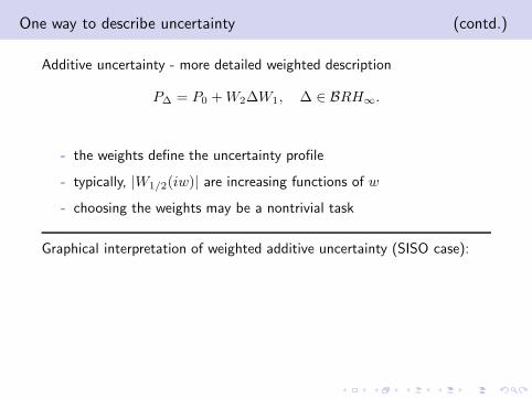
Additive uncertainty - more detailed weighted description
P∆ = P0 +W2∆W1, ∆ ∈ BRH∞.
- the weights define the uncertainty profile
- typically, |W1/2(iw)| are increasing functions of w
- choosing the weights may be a nontrivial task
Graphical interpretation of weighted additive uncertainty (SISO case):

Example 1
Consider a plant with parametric uncertainty
P (s) =1 + α
s+ 1, α ∈ [−0.2, 0.2].
It can be cast as a nominal plant with additive uncertainty
P∆ =1
s+ 1︸ ︷︷ ︸
P0
+0.2
s+ 1︸ ︷︷ ︸
W
∆, ∆ ∈ BRH∞.
Note that this representation is conservative.
Graphical interpretation:

Example 2 (course book, page 133)
Consider a plant with parametric uncertainty
P (s) =10((2 + 0.2α)s2 + (2 + 0.3α+ 0.4β)s+ (1 + 0.2β))
(s2 + 0.5s+ 1)(s2 + 2s+ 3)(s2 + 3s+ 6),
for α, β ∈ [−1, 1]. It can be cast as
P∆ = P0 +W∆, ∆ ∈ BRH∞,
where P0 = P |α,β=0 and W = P |α,β=1 − P |α,β=0.
−2 −1.5 −1 −0.5 0 0.5 1 1.5 2 2.5−3.5
−3
−2.5
−2
−1.5
−1
−0.5
0
0.5

The small gain theorem
Theorem
Suppose M ∈ RH∞. Then the closed loop system (M,∆) is internallystable for all
∆ ∈ BRH∞ := {∆ ∈ RH∞ | ‖∆‖∞ ≤ 1}
if and only if ‖M‖∞ < 1.
Interpretation in terms of Nyquist criterion (SISO case):
The small gain theorem (proof)
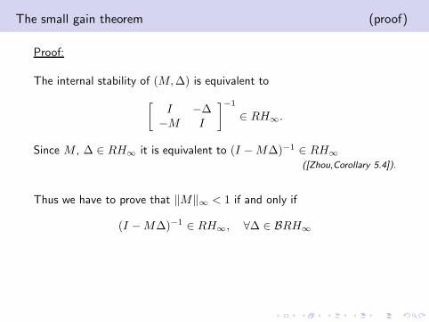
Proof:
The internal stability of (M,∆) is equivalent to
[I −∆
−M I
]−1
∈ RH∞.
Since M , ∆ ∈ RH∞ it is equivalent to (I −M∆)−1 ∈ RH∞
([Zhou,Corollary 5.4]).
Thus we have to prove that ‖M‖∞ < 1 if and only if
(I −M∆)−1 ∈ RH∞, ∀∆ ∈ BRH∞
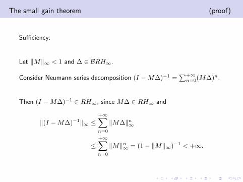
The small gain theorem (proof)
Sufficiency:
Let ‖M‖∞ < 1 and ∆ ∈ BRH∞.
Consider Neumann series decomposition (I −M∆)−1 =∑+∞
n=0(M∆)n.
Then (I −M∆)−1 ∈ RH∞, since M∆ ∈ RH∞ and
‖(I −M∆)−1‖∞ ≤
+∞∑
n=0
‖M∆‖n∞
≤
+∞∑
n=0
‖M‖n∞ = (1− ‖M‖∞)−1 < +∞.

The small gain theorem (proof)
Necessity:
Fix ω ∈ [0,+∞].
A constant ∆ = λM(jω)∗
‖M(jω)‖ satisfies ‖∆‖∞ ≤ 1, ∀λ ∈ [0, 1].
As a result, we have that
∀λ ∈ [0, 1] : (I −M∆)−1 ∈ RH∞ ⇒ det
(‖M‖
λI −MM∗
)
6= 0.
It gives ‖M‖2 < ‖M‖ and, hence, ‖M‖ < 1.
The frequency is arbitrary, so we have ‖M‖∞ < 1.�

The small gain theorem - restatement
Obviously, the theorem can be reformulated as follows
Corollary
Suppose M ∈ RH∞. Then the closed loop system (M,∆) is internallystable for all
∆ ∈1
γ· BRH∞ := {∆ ∈ RH∞ | ‖∆‖∞ ≤
1
γ}
if and only if ‖M‖∞ < γ.
Once the H∞ norm of M decreases,
the radius of the admissible uncertainty increases.

Back to the control problem
Consider stabilization of a plant with additive uncertainty.
It can be represented in the following form.
This is a unified form for the stabilization problem with unstructureduncertainty.
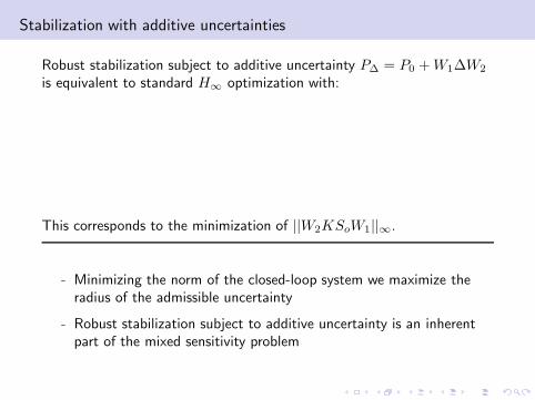
Stabilization with additive uncertainties
Robust stabilization subject to additive uncertainty P∆ = P0 +W1∆W2
is equivalent to standard H∞ optimization with:
This corresponds to the minimization of ||W2KSoW1||∞.
- Minimizing the norm of the closed-loop system we maximize theradius of the admissible uncertainty
- Robust stabilization subject to additive uncertainty is an inherentpart of the mixed sensitivity problem
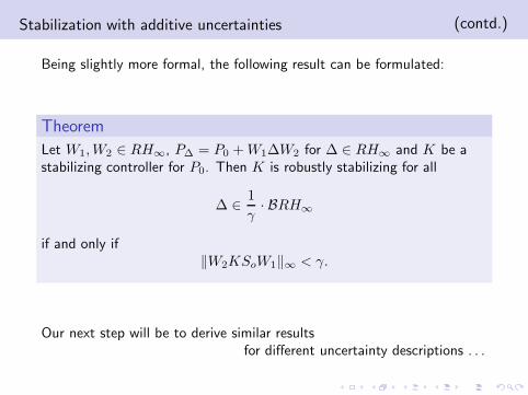
Stabilization with additive uncertainties (contd.)
Being slightly more formal, the following result can be formulated:
Theorem
Let W1,W2 ∈ RH∞, P∆ = P0 +W1∆W2 for ∆ ∈ RH∞ and K be astabilizing controller for P0. Then K is robustly stabilizing for all
∆ ∈1
γ· BRH∞
if and only if‖W2KSoW1‖∞ < γ.
Our next step will be to derive similar resultsfor different uncertainty descriptions . . .

Basic Uncertainty Models
Additive uncertainty:
P∆ = P0 +W1∆W2, ∆ ∈ BRH∞
Input multiplicative uncertainty:
P∆ = P0(I +W1∆W2), ∆ ∈ BRH∞
Output multiplicative uncertainty:
P∆ = (I +W1∆W2)P0, ∆ ∈ BRH∞
Inverse input multiplicative uncertainty:
P∆ = P0(I +W1∆W2)−1, ∆ ∈ BRH∞
Inverse output multiplicative uncertainty:
P∆ = (I +W1∆W2)−1P0, ∆ ∈ BRH∞
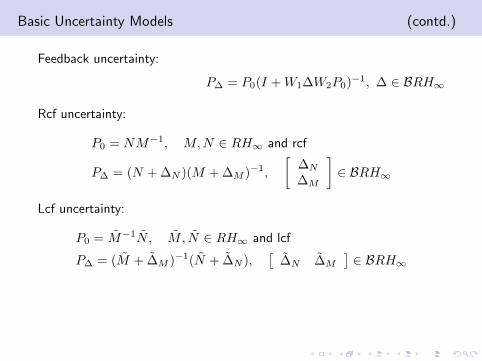
Basic Uncertainty Models (contd.)
Feedback uncertainty:
P∆ = P0(I +W1∆W2P0)−1, ∆ ∈ BRH∞
Rcf uncertainty:
P0 = NM−1, M,N ∈ RH∞ and rcf
P∆ = (N +∆N )(M +∆M )−1,
[∆N
∆M
]
∈ BRH∞
Lcf uncertainty:
P0 = M−1N , M , N ∈ RH∞ and lcf
P∆ = (M + ∆M )−1(N + ∆N ),[
∆N ∆M
]∈ BRH∞
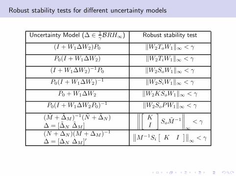
Robust stability tests for different uncertainty models
Uncertainty Model (∆ ∈ 1γBRH∞) Robust stability test
(I +W1∆W2)P0 ‖W2ToW1‖∞ < γ
P0(I +W1∆W2) ‖W2TiW1‖∞ < γ
(I +W1∆W2)−1P0 ‖W2SoW1‖∞ < γ
P0(I +W1∆W2)−1 ‖W2SiW1‖∞ < γ
P0 +W1∆W2 ‖W2KSoW1‖∞ < γ
P0(I +W1∆W2P0)−1 ‖W2SoPW1‖∞ < γ
(M + ∆M )−1(N + ∆N )
∆ = [∆N ∆M ]
∥∥∥∥
[K
I
]
SoM−1
∥∥∥∥∞
< γ
(N +∆N )(M +∆M )−1
∆ = [∆N ∆M ]′∥∥M−1Si
[K I
]∥∥∞
< γ
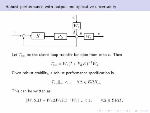
Robust performance with output multiplicative uncertainty
ff P∆-- We
Wd
- -?
?
K--6
r
−
e
w
yd
Let Tew be the closed loop transfer function from w to e. Then
Tew = We(I + P∆K)−1Wd.
Given robust stability, a robust performance specification is
‖Tew‖∞ < 1, ∀∆ ∈ BRH∞
This can be written as
‖WeSo(I +W1∆W2To)−1Wd‖∞ < 1, ∀∆ ∈ BRH∞

SISO case
Consider for simplicity a case when K and P0 are scalar. Then we canjoin We and Wd as well as W1 and W2 to get RP condition
‖WTT ‖∞ < 1,
∥∥∥∥
WSS
1 + ∆WTT
∥∥∥∥∞
< 1
for all ∆ ∈ BRH∞.
Theorem: A necessary and sufficient condition for RP is
∥∥|WSS|+ |WTT |
∥∥∞
< 1.
Proof: The condition∥∥|WSS|+ |WTT |
∥∥∞
< 1 is equivalent to
‖WTT ‖∞ < 1,
∥∥∥∥
WSS
1− |WTT |
∥∥∥∥∞
< 1.
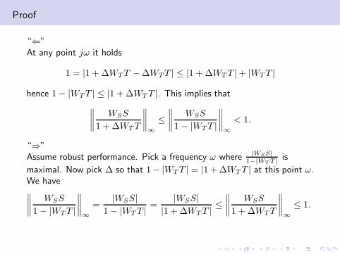
Proof
“⇐”At any point jω it holds
1 = |1 + ∆WTT −∆WTT | ≤ |1 + ∆WTT |+ |WTT |
hence 1− |WTT | ≤ |1 + ∆WTT |. This implies that
∥∥∥∥
WSS
1 + ∆WTT
∥∥∥∥∞
≤
∥∥∥∥
WSS
1− |WTT |
∥∥∥∥∞
< 1.
“⇒”Assume robust performance. Pick a frequency ω where |WSS|
1−|WTT | is
maximal. Now pick ∆ so that 1− |WTT | = |1 +∆WTT | at this point ω.We have∥∥∥∥
WSS
1− |WTT |
∥∥∥∥∞
=|WSS|
1− |WTT |=
|WSS|
|1 + ∆WTT |≤
∥∥∥∥
WSS
1 + ∆WTT
∥∥∥∥∞
≤ 1.
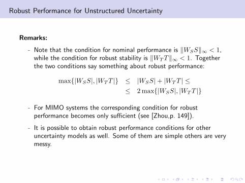
Robust Performance for Unstructured Uncertainty
Remarks:
- Note that the condition for nominal performance is ‖WSS‖∞ < 1,while the condition for robust stability is ‖WTT ‖∞ < 1. Togetherthe two conditions say something about robust performance:
max{|WSS|, |WTT |} ≤ |WSS|+ |WTT | ≤
≤ 2max{|WSS|, |WTT |}
- For MIMO systems the corresponding condition for robustperformance becomes only sufficient (see [Zhou,p. 149]).
- It is possible to obtain robust performance conditions for otheruncertainty models as well. Some of them are simple others are verymessy.

What did we study today?
- Standard ways to describe uncertainty
- Small gain theorem
- The use of small gain theorem:the idea to form LFT by pulling out the uncertainty
- Robust performance criteria (for a special case)


