Unstructured large eddy and conjugate heattransfer simulations of wall-bounded flows
B. Niceno & K. HanjalicDepartment of Multi-scale Physics, Delft University of Technology,Delft, The Netherlands
Abstract
We present a finite-volume numerical algorithm for large eddy simulations (LES)and conjugate heat transfer of wall-bounded turbulent flowsusing unstructuredcomputational grids. The focus is on predicting temperature and heat-flux varia-tion on walls and protrusions made of multiple materials with different properties,in flows of industrial relevance such as cooling of electronics or of internal pas-sages of gas turbine blades. The approach adopted follows the rationale used in theReynolds-average Navier-Stokes approach (RANS), but withnecessary modifica-tions pertinent to LES strategy. The method uses the colocated cell arrangementwith variables defined at cell centres and varying linearly in between. The algo-rithm was tested in simulation of several generic test casesof laminar and turbulentflows. The performance of the algorithm is illustrated by LESof flow and conju-gate heat transfer over a surface-mounted cube in a matrix using a boundary-fittedhexahedral grid and a hybrid unstructured grid.
1 Introduction
Predicting the time fluctuations of wall temperature and heat−flux distribution anda priori detecting of hot spots in electronics, gas turbine blades and combustionchambers, in IC engines and other thermal equipment, is still a major challenge.Common experimental techniques for measuring surface temperature, such as liq-uid crystals, infrared thermography, usually have too slowa response to captureturbulent fluctuations. Because many applications involverelatively low to mod-erate Reynolds number, these problems seem very suitable for large-eddy simula-tions (LES) provided that simultaneous solution of unsteady conduction in solids
of different composition and materials can be performed andthe numerical reso-lution can be ensured in the fluid near-wall regions.
LES has long been regarded as the most promising computational techniquefor solving complex turbulent flow problems in technological and environmentalapplications. Recognizing the limitations of the Reynolds-averaged Navier−Stokes(RANS) approach, industry has turned its attention to LES asan emerging indus-trial tool expected to replace the RANS methods. However, the early expectationshave not yet been fulfilled: LES is still under development and is considered moreas a research target on its own, and less as a tool for predicting complex turbulentflows. Its applications are still limited to low and moderateReynolds numbers inrelatively simple flow configurations.
One of the major deficiencies of LES is the treatment of the near-wall regions,particularly at realistic Reynolds numbers in fully three-dimensional flows (with-out any homogeneous direction). The LES performs poorly in the near-wall re-gions simply because there are no large eddies there. In order to predict accuratelythe wall friction, heat and mass transfer, one needs to resolve the small-scale mo-tion and streaks structure in the buffer zone, which requires a very fine numer-ical mesh not only in the wall-normal direction, but also in the streamwise andspanwise directions. It is generally believed that near-wall phenomena are cap-tured well with LES only if the near-wall grid is sufficientlyfine for subgrid-scalestresses to become the same order of magnitude as (or less than) the molecularstresses. In this case the subgrid-scale model (SGS) becomes almost irrelevantand its role is only to drain the turbulence kinetic energy, so that the computationsreduce essentially to pseudo-direct numerical simulation(DNS). Such grid refine-ment with structured and even with block-structured grids leads to an increase inthe number of cells even in the regions far away from walls where it is not needed.The problem becomes especially serious at high Reynolds numbers when the vis-cous sublayer and the buffer zone become very thin, imposingexorbitant demandson computing resources.
Alternative routes, such as modifying the SGS model for the near-wall region,or bridging the viscous and buffer regions by wall functions, both aimed at us-ing coarser meshes, have led to partial success and only in near-equilibrium wall-bounded flows. In short, the conventional LES is also still unreliable for predict-ing near-wall phenomena such as friction, heat and mass transfer in more complexflows and at high Reynolds numbers.
The use of unstructured grids can extend the applicability of the LES. In ad-dition to the possibility of using arbitrarily shaped polyhedral elementary controlcells (e.g tetrahedra, hexahedra, polyhedra, or mixed) that enable one to easilydiscretise complex flow domains, the unstructured grids make it possible to applyadaptive meshing and thus provide more flexibility to control the grid refinementin a desired area in a more rational way than the structured grids. This enablessufficient resolution to be achieved in regions where it is needed, with compara-bly less total number of grid cells then with structured and even block-structuredgrids. Such local grid refinement is particularly useful in flows with complex walltopology, e.g. protrusions and corners, or in flows with highlocal gradients of flow
properties, e.g. the area around the burner mouth in combustion studies.The objective of the work presented here was to develop and validate an algo-
rithm for simultaneous LES of incompressible fluid flow and conjugate heat trans-fer for unstructured grids. Although LES is a well established technique, there arenot many applications of LES on unstructured grids. Despitedecades of experi-ence both in modelling and numerical methods for LES gained with structured,highly vectorised codes, the application of unstructured grids in LES still poses anumber of challenges.
The literature on LES with unstructured grids is relativelyscarce, especiallydealing with heat transfer. Jansen [9] applied the finite element unstructured LESsolver to flow around an airfoil. Rollet-Mietet al. [24] used the commercial finiteelement code N3S to solve the flow around a single cube mountedon the channelwall. In [23] the same methodology was used to compute the flowaround a tubebundle. Laurence [11] shows some other examples of LES with N3S unstructuredcode and argues that computational demands will deter industry from using LES inthe near future apart from some specific problems such as aeroacoustics and fluid-structure interaction. Frohlich et al. [4] compared the unstructured finite elementLES computations with the block-structured finite-volume simulations. O’Rourkeand Sahota [19] reported on a variable explicit/implicit advection scheme for un-structured meshes. This method was subsequently used by Haworth and Jansen [7]to perform LES in a simplified reciprocating engine flow. Howard and Lesieur [8]reported non-structured LES over a reference vehicle body in infinite surrounding.
We describe here the approach adopted in the development of the unstructuredLES solver for finite-volume computations. Since such an approach for LES isstill relatively novel, there are many open issues, such as the definition of the filter,influence of numerical error, efficiency on high-performance computing platforms.Addressing all issues mentioned goes beyond the scope of this chapter and will notbe considered here. Instead, we outline briefly the discretisation schemes adoptedhere, discuss other options for LES, and present some results of validation of nu-merical scheme and achieved accuracy in several cases of generic laminar andturbulent flows each with at least three different grids. Thepotential of the al-gorithm is illustrated in a test case of industrial relevance: heat transfer over asurface-mounted, internally heated cube covered by low-conducting epoxy layer.More details can be found in [15].
2 Governing equations and their discretisation
For incompressible fluid flow, the continuity, momentum and energy equations canbe written in the conservative integral form, which is convenient for a general finitevolume computational approach:
These equations are valid for an arbitrary part of fluid volumeV bounded by sur-faceS, with surface normaln pointing outwards. Here,u is the velocity vector,ρis the density,T is the stress tensor,f is the body force,h is enthalpy,qh is the heat-flux vector andsh is heat source or sink. The stress tensor for an incompressibleNewtonian fluid is expressed as:
T = 2µS = µ(∇u + (∇u)T ), (4)
whereS is the rate of deformation.In the following we give a brief summary of the discretisation adopted and
discuss possible alternatives. The aim was to follow the rationale used in finite-volume RANS for a general unstructured grid, but to test the implications for LESand to make modifications pertinent to LES strategy.
2.1 Discretisation in space
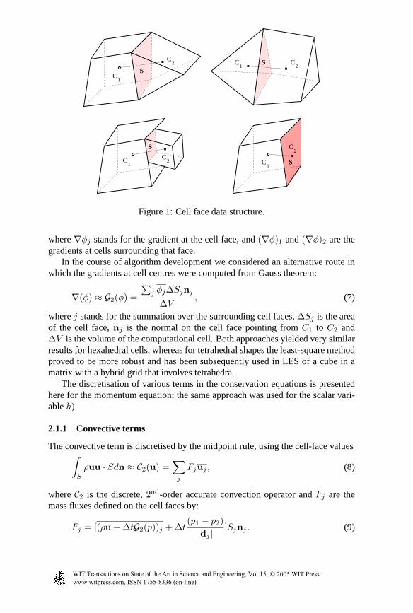
Spatial discretisation of the governing equations is basedon the finite volumemethod on unstructured grids [2], consisting of prismatic,pyramidal, or generaltetrahedral and hexahedral cells, or of their combinations. In principle, cells canhave any polyhedral shape, but not all of them are possible togenerate with avail-able mesh generators. All dependent variables, velocity components and pressure,are discretised in the cell centres, i.e. they are colocated. Although the staggeredarrangements of grid nodes are generally regarded as numerically more robustthan the colocated ones, their implementation on unstructured grids is very com-plex [25, 26]. Furthermore, higher memory demands for indexing of staggeredunstructured grids, can limit the number of computational cells that can be appliedin practical computations.
The data structure is based on the cell faces, i.e. for each cell face the twoadjacent cell indices are stored. Some possible cell faces are shown in Figure 1. Itis this, cell-face data structure that gives the possibility to have any cell shape andto have arbitrary number of neighbours. For each cell faces, it is only importantto know the adjacent cellsC1 andC2 and its surface to be able to calculate thediscrete convective and diffusive fluxes, as described below. Even locally refinedgrids by cell splitting, are described with the same data structure.
All dependent variables are assumed to vary linearly between the cell centres,so that their values at the cell faces are calculated by a linear interpolation:
φj = wjφ1 + (1 − wj)φ2, (5)
whereφ stands for any dependent variable or physical property, andwj is theweight factor. The gradients of dependent variables are calculated at cell centresusing the least square method described in [1, 2], and are assumed to be constantover each cell. Their values at the cell faces are calculatedas arithmetic meansbetween the gradients prevailing over the neighbouring cells:
where∇φj stands for the gradient at the cell face, and(∇φ)1 and(∇φ)2 are thegradients at cells surrounding that face.
In the course of algorithm development we considered an alternative route inwhich the gradients at cell centres were computed from Gausstheorem:
∇(φ) ≈ G2(φ) =
∑j φj∆Sjnj
∆V, (7)
wherej stands for the summation over the surrounding cell faces,∆Sj is the areaof the cell face,nj is the normal on the cell face pointing fromC1 to C2 and∆V is the volume of the computational cell. Both approaches yielded very similarresults for hexahedral cells, whereas for tetrahedral shapes the least-square methodproved to be more robust and has been subsequently used in LESof a cube in amatrix with a hybrid grid that involves tetrahedra.
The discretisation of various terms in the conservation equations is presentedhere for the momentum equation; the same approach was used for the scalar vari-ableh)
2.1.1 Convective terms
The convective term is discretised by the midpoint rule, using the cell-face values∫
S
ρuu · Sdn ≈ C2(u) =∑
j
Fjuj , (8)
whereC2 is the discrete,2nd-order accurate convection operator andFj are themass fluxes defined on the cell faces by:
The cell-centred pressure derivates (G2(p)) are extracted from cell-centred veloc-ities (u), and staggered terms(p1 − p2)/|dj | are added. Equation (9) representsthe implementation of the Rhie and Chow [22] technique on arbitrary grids.
In addition to the second-order convective termC2, the first order term is alsointroduced to increase the numerical stability of the scheme, as explained below:
∫
S
ρuu · Sdn ≈ C1(u) =∑
j
(max(0, Fj)u1 − min(0, Fj)u2). (10)
The flux through the cell faceFj is defined as positive when moving from the cellC1 to cellC2, and negative otherwise.
After introducing the second- and first-order convective operators, we write theconvective terms as follows:
C(u) = CL(u) + CR(u), (11)
whereCL(u) = C1(u) is the implicit andCR(u) = γ(C2(u) − C1(u)) is theexplicit part of the convective flux. (Note that, in principle, terms implicit andexplicit introduced here do not have any connection with thetime discretisation,which is discussed in the section below.)
The implicit part (L) is added to system matrix to increase the stability of thelinear system, whereas the explicit part (R) is added to the right-hand side. Hereγ is the upwind blending factor ranging from0 − 1. It has been argued that inLES the second-order-accurate full central differencing need to be used (γ = 1) topreserve high-frequency fluctuations [21]. However, the central differencing causesinstabilities when the local Peclet numberPe exceeds certain value irrespective ofthe local CFL number. The cure for this simply to refine the mesh. In practicalcalculations this is not always possible and depending on the mesh size and onthe Reynolds number of the flow, it is convenient to use a smallpercentage ofupwind. Although the upwind acts as a false diffusion, i.e. as an addition to thesub-grid scale model, the effect on mean flow properties and second moments isnegligible, provided that the contribution of upwind is kept sufficiently small. In allthe computations reported here the amount of upwind differencing never exceeded2.5%. More recently we have introduced the QUICK convectionscheme, but theresults for the cases considered changed only marginally.
2.1.2 Diffusion terms
Diffusive fluxes are discretised by replacing the integralswith the sums,∫
S
T · Sjdn ≈∑
j
TjSjnj , (12)
whereTj is the value of the stress tensor defined on the cell face. In expres-sion (12), all three velocity components are included, which, if discretized in thestraightforward way, results in a system matrix for all velocity components. Highmemory demands for storing such large matrices can limit thenumber of cell faces
Figure 2: a) Numerical stencil for discretisation of explicit viscous stressesDE onunstructured grid b) Necessary communication pattern after parallelisation.
a) b)
Figure 3: a) Numerical stencil for discretisation of implicit viscous stressesDI onunstructured grid, b) Necessary communication pattern after parallelisation.
allocated for a certain problem. This is very undesirable for LES, since the mainidea of LES is to solve as wide a range of scales as possible, i.e. to use grids asfine as possible. Therefore, we use the segregated approach of [2] by which theviscous stress tensor is decomposed into two parts:
T = TL + TR, (13)
whereTL = µ∇u includes only the diagonal part of the stress tensor, andTR =µ∇uT is the remaining of the viscous stress tensor. We can now treat TL implic-itly, andTR explicitly.
Such a discretisation of the stress tensor by a finite volume method on an un-structured grid includes the unknown velocity components at the first and secondneighbours of each control volume (see Figure 2a).
Although it is possible to define such a discretisation, its parallelisation bya domain decomposition technique results in a very cumbersome communication
pattern (Figure 2b) and overhead in memory allocated to buffer regions. In order toovercome this problem, we decided to narrow the numerical stencil even further.For this purpose, we decompose the gradient at the cell face by the followingexpression:
(∇u)⋆j = (∇u)j +
u2 − u1
|dj |nj +
(∇u)j · dj
|dj |nj . (14)
The first and second terms on the right-hand side of eqn (14) are the approxima-tions of the gradient of velocity. The first term is second-order accurate, obtainedfrom least-square approximation or Gauss theorem, whereasthe second term isfirst-order accurate. The latter is calculated from the velocities surrounding thecell faceψjψ. To recover second order accuracy of the discretisation, we introducedthe third term on the right-hand side. This additional term represents the differencebetween the second- and the first-order approximation of thederivative at the cellface. It contains the values from a wider numerical stencil (Figure 2a), but it istreated explicitly using the values either from the previous iteration, or from theold time step, leaving the number of entries in the system matrix low. The finalform of the viscous term is:
DL(u) =∑
j
µ[u2 − u1
|dj |nj ]Sjnj (15)
DR(u) =∑
j
µ[(∇u)j + (∇u)jT
+(∇u)j · dj
|dj |nj ]Sjnj . (16)
The final form of the discretised system of equations is written as follows:
C(1) = 0, (17)
which is the discretised continuity equation, and:
I(u) + C(u) = D(u) + G2(p) (18)
is the discretised Navier−Stokes equation. It is recalled that the convective anddiffusive terms were decomposed into implicit and explicitparts, i.e. C(u) =CL(u)+CR(u) andD(u) = DL(u)+DR(u), respectively, and, depending on thetime-stepping scheme, each part can be treated differentlyin time.
2.2 Integration in time
For numerical integration of unsteady terms we apply the midpoint rule, assumingthat the value of the dependent variable in the cell centre isrepresentative of theentire cell. Assuming a linear variation between the current and previous time step,the discretised terms have the following form:
whereI = ρ∆V∆t u is the discrete inertial operator,n is the new time step,n− 1 is
the old time step and∆t is the discrete time step.Traditionally, explicit or semi-implicit time-marching schemes are used in LES
because one needs to keep the time step very small for physical reasons, i.e. to re-solve small-scale turbulence eddies up to the cut-off limit. However, fully implicitschemes, used commonly in RANS computations, are more robust, allow largertimes steps, are easier to control and require less memory. Anticipating situationsin which the turbulence physics will tolerate larger time steps than permitted byexplicit schemes, we considered three popular schemes of which two are semi-implicit (fractional step and Crank−Nicholson scheme) and one is fully implicit.The aim was to check if the semi-implicit methods that are often used in LES,offer significant advantage over fully implicit time integration. Comparison ofperformance of the three schemes is presented in direct numerical simulation ofturbulent flow in a plane channel ([17]).
The linear variation between the current and the previous time step is used inconjunction with the fractional step method and the Crank−Nicholson time discreti-sation. A fully implicit time-advancing scheme in conjunction with a linear varia-tion between the current and previous time step, eqn (19), has been known tobe too diffusive for LES. This suppresses turbulence fluctuations and often leadsto laminarization, especially in flows with a smooth turbulence spectrum in the ab-sence of a dominated eddy structure or other sources of large-scale instability, e.g.in a channel flow. For this reason a three-level scheme with quadratic variationbetween the current time step, the old time step and the one before the old, mustbe assumed, yielding the following time integration expression:
d
dt
∫
V
ρudV ≈3
2I(un) − 2I(un−1) +
1
2I(un−2) (20)
For the fractional step method the Navier−Stokes equations (eqn 18) can berewritten as:
I(un) − I(un−1) +3
2C(un−1) −
1
2C(un−2) =
1
2DL(un)
+1
2DL(un−1) +
3
2DR(un−1) −
1
2DR(un−2),+G2(p
n), (21)
where the convective fluxes are treated for simplicity with Adams−Bashforth method,and diffusive terms are treated with Crank−Nicholson method for ensuring betterstability. Since one of the main strengths of the fractional-step method is thatit does not need inner iterations in a time step, we discretised the explicit diffu-sion terms with Adams−Bashforth as well. This is one of the most widely usedtime-stepping schemes in LES of turbulence and is very robust on regular grids.However, as soon as the grid becomes distorted, the explicitdiffusive terms (DR)increase. Because they are treated explicitly in time, theylimit the numerical timestep. This method is, therefore, suitable only for orthogonal and slightly deformedgrids, if used with the spatial discretisation explained above.
The stability problem of the fractional step method can be overcome by usingthesemi-implicit Crank-Nicholson method:
I(un) − I(un−1) +1
2C(un) +
1
2C(un−1) =
1
2DL(un)
+1
2DL(un−1) +
1
2DR(un) +
1
2DR(un−1)
+1
2G2(p
n) +1
2G2(p
n−1) (22)
where all the terms are discretised with the Crank−Nicholson scheme. It featuressecond-order accuracy in time, but due to semi-implicit treatment of the convectiveand explicit diffusive terms, it requires iterations in each time step.
Finally, we also tested thefully implicit treatment of all terms, which is rarelyused in LES of turbulence because of its dissipative nature:
I(un) + I(un−1) + I(un−2) + C(un)
= DL(un) + DR(un) + G2(pn). (23)
Here the inertial term is discretised using the quadratic approximation over thethree time steps, thus making this scheme second-order accurate in time. It mustbe noted that the fully implicit method is the most economic in terms of computermemory needed, since it only stores convective and diffusive fluxes of the currenttime step.
2.2.1 Pressure-velocity coupling
For coupling the velocity and pressure field we apply an iterative procedure similarto the SIMPLE algorithm. First, the equations for a tentative velocity field aresolved (shown here for the Crank−Nicholson scheme):
I(u⋆) − I(un−1) +1
2C(u⋆) +
1
2C(un−1) =
1
2DL(u⋆)
+1
2DL(un−1) +
1
2DR(u⋆) +
1
2DR(un−1) + G2(p
⋆), (24)
wheren−1 is the old time step,⋆ denotes the tentative velocity field that in generaldoes not satisfy the continuity equation. The solution of the tentative velocity fieldis then used to solve the Poisson equation for the pressure correctionψ:
DL(ψ) =∑
j
F ⋆j , (25)
with the Neumann boundary condition on all boundary faces where the normal ve-locity components are specified,∂ψ/∂n = 0: The solution of the pseudo-pressureis then obtained by the projection of the velocities into a divergence-free field:
Because we have introduced the volume fluxes as new dependentvariables, theyare also projected into the divergence-free field by:
F ⋆j = F ⋆
j +∆t
∆V
(ψ1 − ψ2)
|dj |. (27)
It is noted that the mass fluxes are updated in a staggered fashion, i.e. on the cellfaces that are placed between the two pressure cells. The pressure is updated fromthe following relation
p⋆ = p⋆ + ψ/∆t. (28)
After the projection of the velocity and mass fluxes, the masserror in the wholedomain is calculated from:
ǫn+1 =∑
j
Fj . (29)
The maximum mass errorǫn+1m after the projection of the velocity field can be
reduced to arbitrary small value. Its magnitude depends only on the accuracyof the solution of the pseudo-pressure equation (25). In theLES computationspresented here, the pseudo-pressure equation was solved until reaching the levelfour orders below the estimated numerical method on the given grid.
When using the Crank−Nicholson or the fully implicit scheme, we continue theiterative procedure described above until the discretisedequations forDE ,DI , andC stop changing. Then we setun+1 = un and proceed to a new time step. In LES,were the time step is relatively small, this takes3 − 4 iterations. If the fractionalstep method is used, no iterations in a time step are needed. It is noted that withthe SIMPLE method it is usually necessary to do under-relaxation [3]. In all thecomputations reported here, due to the small time step used,no under-relaxationwas needed.
2.3 Linear system solvers
Two different systems of equations arise after the discretisation of governing equa-tions, one for the velocities:
[A] {u} = {b}, (30)
and another one for the pressure corrections:
[M] {ψ} = {d}. (31)
The system matrix for eqn (24) is formed by summing the contributions fromall implicit discrete operators (I, CL andDL):
wherei implies summation over the cells,NC is the number of cells,j impliessummation over cell faces andNS is the number of cell faces in the grid. Theunknown vector is:
{u} =NC∑
i=1
u⋆, (33)
and the right-hand side{b} is formed by summing all explicit discrete operators(I, CL, DL andG2(p))
{b} =
NC∑
i=1
I(u)n−1 +1
2
NS∑
j=1
CR(u)n−1 +1
2
NS∑
j=1
DR(u)n−1
+1
2
NC∑
i=1
G2(p)n +
1
2
NC∑
i=1
G2(p)n−1. (34)
Inertial terms increase the condition of the system matrix for velocities, and usuallya few iterations,3−6, are sufficient to solve the system to the prescribed tolerance.Since the first-order implicit convection introduces asymmetry in the system ofequations, it has to be solved by a linear solver capable of solving asymmetricsystems of equations. In the present work we have used bi-conjugate gradient(BiCG) with diagonal pre-conditioning.
The linear systems for the pressure correction is formed by:
[M] =
NS∑
j=1
DL. (35)
The unknown vector is
{ψ} =
NC∑
i=1
ψi, (36)
and the right-hand side:
{d} =
NS∑
j=1
Fj . (37)
This system of equations is very poorly conditioned and requires typically15−25iterations. Because the matrix[M] is symmetric, we used the diagonally precon-ditioned conjugate gradient (CG) solver.
3 Multiple materials
The common type of wall boundary conditions for enthalpy equation are pre-scribed temperature of prescribed heat flux. However, in many real problems,
neither of these conditions is applicable because the surface temperature is deter-mined by the flow and turbulence field around the wall. Such is the case withthe matrix of surface-mounted cubes with copper core covered by an epoxy layer,which was chosen to test the implementation of the enthalpy equation and for con-jugate heat transfer combined with LES. Because of the low conductivity of theepoxy layer, the temperature at the surface of the cube is farfrom being constant,as shown by experiment (see below). The measured mean temperature profilecould have been prescribed asknown. The interpolations used in such a prescrip-tion would inevitably lead to inaccuracies, but more importantly, the temperaturefluctuations at the wallare not zero and they can not be provided by any experi-ment with desirable certainty. The algorithm described here was thus extended tomake it possible to deal with domains made up from different materials and solvethe fluid flow in the fluid part and conjugate heat transfer in both the fluid and solidparts of the domain of arbitrary shapes. The modifications required in the numeri-cal method are described in this section. It has to be noted that all the explanationsgiven in this section refer to two materials for simplicity,but the generalisationsfor n materials is straightforward.
In principle, two different strategies could have been adopted:
• Define fluid and solid parts as two distinct problem domains and store dis-cretised systems of equations in two mutually independent matrices. Then,solve all the governing equations (momentum + enthalpy) in the fluid partand only the enthalpy equation in the solid part. The two problem domainsshould then exchange the information on inter-connection boundaries.
• Discretise both fluid and solid parts of the domain as a singleentity andstore the discretised system of equations into one matrix only. Additionalflags are introduced for each cell in the domain, indicating if the cell is inthe fluid or solid phase. The treatment of the interface between materials hasto be accounted for in the system matrix itself.
We adopted the second approach, since it was felt that it willrequire less effortin development, particularly for the parallel version of the code. The implementa-tion of multiple materials was done when the code was alreadydeveloped for onematerial only, so in what follows, the additions/changes tothe numerical methodrelevant for treatment of multiple materials are described. The most importantchanges took place in the discretisation and solving the pressure correction equa-tion, momentum equations and, finally, the enthalpy equation.
3.1 Modifications of the pressure-correction equation
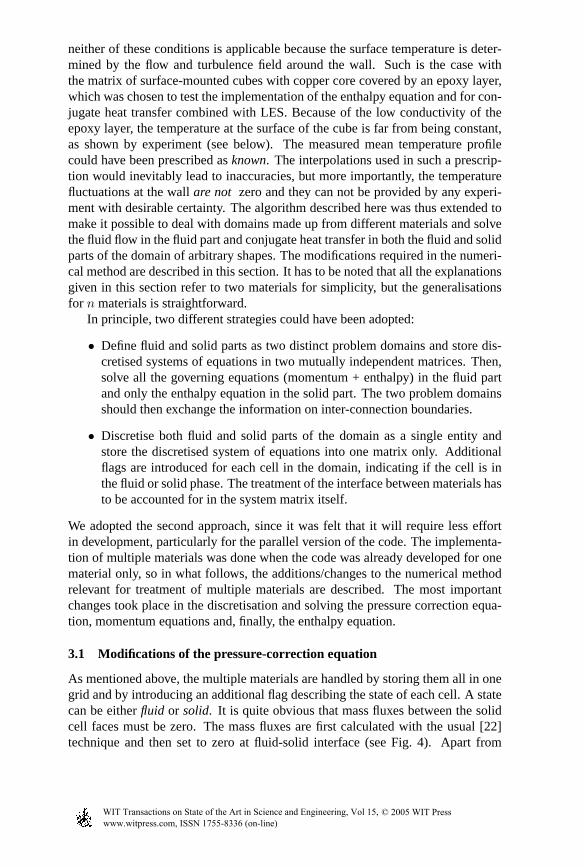
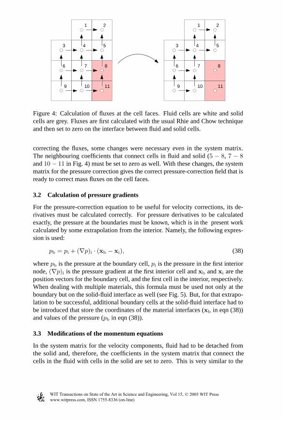
As mentioned above, the multiple materials are handled by storing them all in onegrid and by introducing an additional flag describing the state of each cell. A statecan be eitherfluid or solid. It is quite obvious that mass fluxes between the solidcell faces must be zero. The mass fluxes are first calculated with the usual [22]technique and then set to zero at fluid-solid interface (see Fig. 4). Apart from
Figure 4: Calculation of fluxes at the cell faces. Fluid cellsare white and solidcells are grey. Fluxes are first calculated with the usual Rhie and Chow techniqueand then set to zero on the interface between fluid and solid cells.
correcting the fluxes, some changes were necessary even in the system matrix.The neighbouring coefficients that connect cells in fluid andsolid (5 − 8, 7 − 8and10 − 11 in Fig. 4) must be set to zero as well. With these changes, the systemmatrix for the pressure correction gives the correct pressure-correction field that isready to correct mass fluxes on the cell faces.
3.2 Calculation of pressure gradients
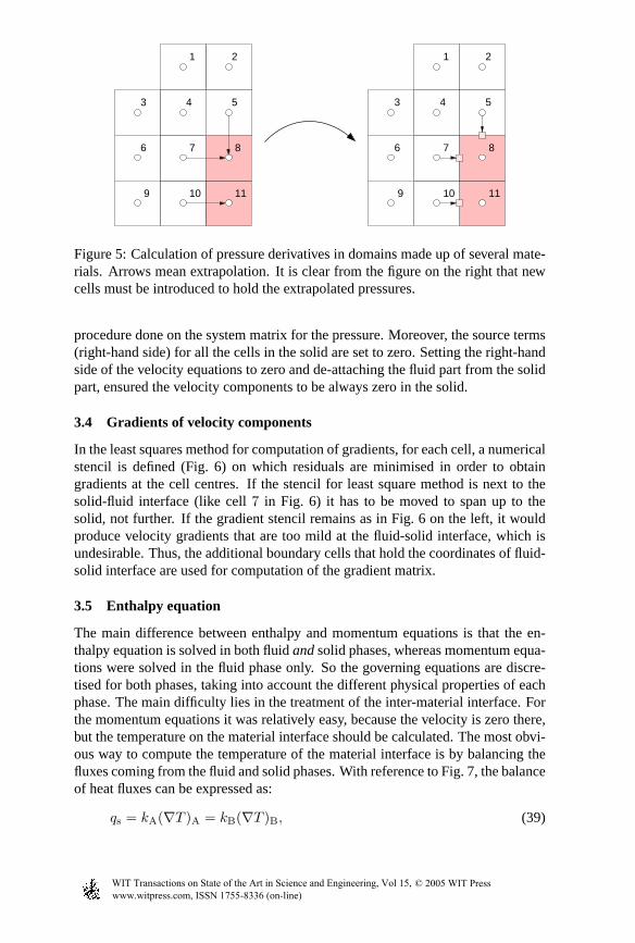
For the pressure-correction equation to be useful for velocity corrections, its de-rivatives must be calculated correctly. For pressure derivatives to be calculatedexactly, the pressure at the boundaries must be known, which is in the present workcalculated by some extrapolation from the interior. Namely, the following expres-sion is used:
pb = pi + (∇p)i · (xb − xi), (38)
wherepb is the pressure at the boundary cell,pi is the pressure in the first interiornode,(∇p)i is the pressure gradient at the first interior cell andxb andxi are theposition vectors for the boundary cell, and the first cell in the interior, respectively.When dealing with multiple materials, this formula must be used not only at theboundary but on the solid-fluid interface as well (see Fig. 5). But, for that extrapo-lation to be successful, additional boundary cells at the solid-fluid interface had tobe introduced that store the coordinates of the material interfaces (xb in eqn (38))and values of the pressure (pb in eqn (38)).
3.3 Modifications of the momentum equations
In the system matrix for the velocity components, fluid had tobe detached fromthe solid and, therefore, the coefficients in the system matrix that connect thecells in the fluid with cells in the solid are set to zero. This is very similar to the
Figure 5: Calculation of pressure derivatives in domains made up of several mate-rials. Arrows mean extrapolation. It is clear from the figureon the right that newcells must be introduced to hold the extrapolated pressures.
procedure done on the system matrix for the pressure. Moreover, the source terms(right-hand side) for all the cells in the solid are set to zero. Setting the right-handside of the velocity equations to zero and de-attaching the fluid part from the solidpart, ensured the velocity components to be always zero in the solid.
3.4 Gradients of velocity components
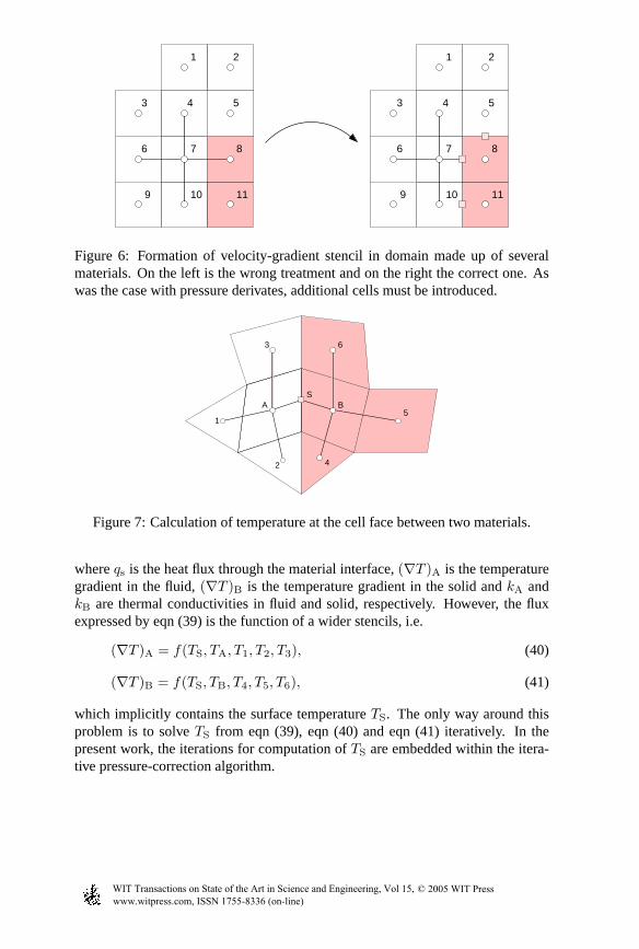
In the least squares method for computation of gradients, for each cell, a numericalstencil is defined (Fig. 6) on which residuals are minimised in order to obtaingradients at the cell centres. If the stencil for least square method is next to thesolid-fluid interface (like cell7 in Fig. 6) it has to be moved to span up to thesolid, not further. If the gradient stencil remains as in Fig. 6 on the left, it wouldproduce velocity gradients that are too mild at the fluid-solid interface, which isundesirable. Thus, the additional boundary cells that holdthe coordinates of fluid-solid interface are used for computation of the gradient matrix.
3.5 Enthalpy equation
The main difference between enthalpy and momentum equations is that the en-thalpy equation is solved in both fluidandsolid phases, whereas momentum equa-tions were solved in the fluid phase only. So the governing equations are discre-tised for both phases, taking into account the different physical properties of eachphase. The main difficulty lies in the treatment of the inter-material interface. Forthe momentum equations it was relatively easy, because the velocity is zero there,but the temperature on the material interface should be calculated. The most obvi-ous way to compute the temperature of the material interfaceis by balancing thefluxes coming from the fluid and solid phases. With reference to Fig. 7, the balanceof heat fluxes can be expressed as:
Figure 6: Formation of velocity-gradient stencil in domainmade up of severalmaterials. On the left is the wrong treatment and on the rightthe correct one. Aswas the case with pressure derivates, additional cells mustbe introduced.
A BS
1
2
3
4
5
6
Figure 7: Calculation of temperature at the cell face between two materials.
whereqs is the heat flux through the material interface,(∇T )A is the temperaturegradient in the fluid,(∇T )B is the temperature gradient in the solid andkA andkB are thermal conductivities in fluid and solid, respectively. However, the fluxexpressed by eqn (39) is the function of a wider stencils, i.e.
(∇T )A = f(TS, TA, T1, T2, T3), (40)
(∇T )B = f(TS, TB, T4, T5, T6), (41)
which implicitly contains the surface temperatureTS. The only way around thisproblem is to solveTS from eqn (39), eqn (40) and eqn (41) iteratively. In thepresent work, the iterations for computation ofTS are embedded within the itera-tive pressure-correction algorithm.
4.1 Effects of grid configuration: flow in a lid-driven cavity
The computer code used for the present research was developed “from scratch”and before we applied it to LES, we tested the code in several generic laminarflows. The first test case, used to investigate the effects of various grid shapesand their density, is flow in a lid-driven cavity, often used to validate numericalmethods and computer programs [6].
Three different grids were used: orthogonal hexahedral, arbitrary tetrahedraland hybrid mesh. For each grid we have used three levels of refinement: 400, 1600and 6400 cells. The medium-density grids are shown in Figure8. It is importantto note that the grids were generated without a bias to the flowpattern, i.e. withoutstretching towards the walls or refining in the regions of steep gradients.
a) b) c)
Figure 8: Grid types used for the test in lid-driven cavity flow at Re = 1000.a) hexahedral, b) tetrahedral c) hybrid. Figure shows medium density grids with1600 cells. Coarser (400) and finer (6400) grids were also used for each type.
All meshes considered perform similarly at equal density levels. It is seen thatall three grid types, hexahedral, tetrahedral and hybrid, yield very good agreementwith the benchmark solutions for the finest grid with 6400 cells. A further test ofgrid configuration is provided in the next example.
4.2 Discretisation error and accuracy test: Taylor vortices
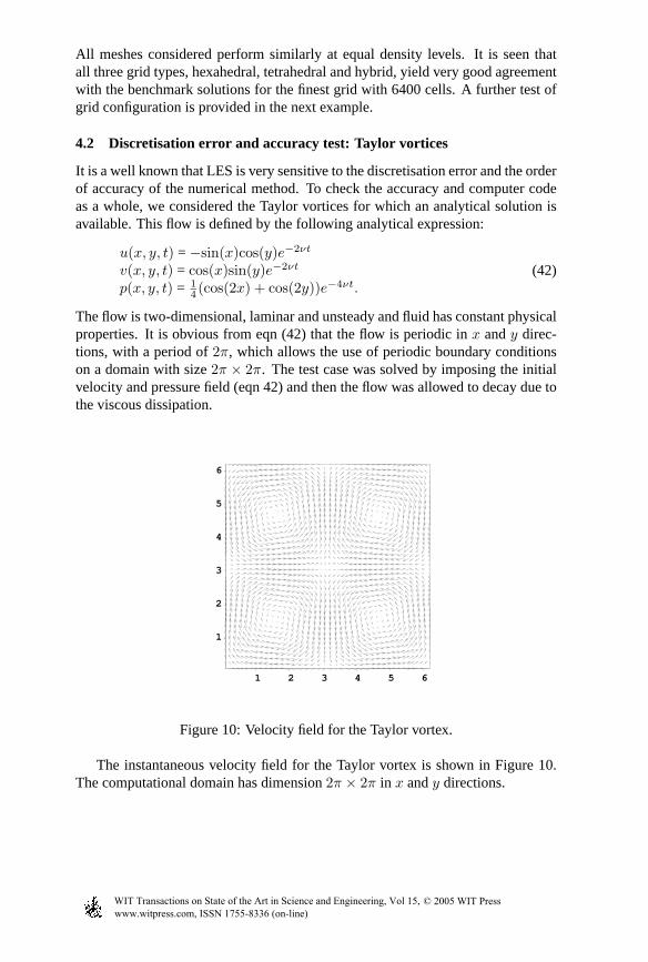
It is a well known that LES is very sensitive to the discretisation error and the orderof accuracy of the numerical method. To check the accuracy and computer codeas a whole, we considered the Taylor vortices for which an analytical solution isavailable. This flow is defined by the following analytical expression:
u(x, y, t) = −sin(x)cos(y)e−2νt
v(x, y, t) = cos(x)sin(y)e−2νt
p(x, y, t) = 14(cos(2x) + cos(2y))e−4νt.
(42)
The flow is two-dimensional, laminar and unsteady and fluid has constant physicalproperties. It is obvious from eqn (42) that the flow is periodic in x andy direc-tions, with a period of2π, which allows the use of periodic boundary conditionson a domain with size2π × 2π. The test case was solved by imposing the initialvelocity and pressure field (eqn 42) and then the flow was allowed to decay due tothe viscous dissipation.
1
2
3
4
5
6
1 2 3 4 5 6
Figure 10: Velocity field for the Taylor vortex.
The instantaneous velocity field for the Taylor vortex is shown in Figure 10.The computational domain has dimension2π × 2π in x andy directions.
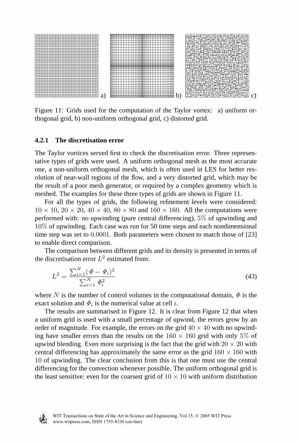
Figure 11: Grids used for the computation of the Taylor vortex: a) uniform or-thogonal grid, b) non-uniform orthogonal grid, c) distorted grid.
4.2.1 The discretisation error
The Taylor vortices served first to check the discretisationerror. Three represen-tative types of grids were used. A uniform orthogonal mesh asthe most accurateone, a non-uniform orthogonal mesh, which is often used in LES for better res-olution of near-wall regions of the flow, and a very distortedgrid, which may bethe result of a poor mesh generator, or required by a complex geometry which ismeshed. The examples for these three types of grids are shownin Figure 11.
For all the types of grids, the following refinement levels were considered:10 × 10, 20 × 20, 40 × 40, 80 × 80 and160 × 160. All the computations wereperformed with: no upwinding (pure central differencing),5% of upwinding and10% of upwinding. Each case was run for 50 time steps and each nondimensionaltime step was set to0.0001. Both parameters were chosen to match those of [23]to enable direct comparison.
The comparison between different grids and its density is presented in terms ofthe discretisation errorL2 estimated from:
L2 =
∑Ni=1(Φ − Φi)
2
∑Ni=1 Φ
2i
(43)
whereN is the number of control volumes in the computational domain, Φ is theexact solution andΦi is the numerical value at celli.
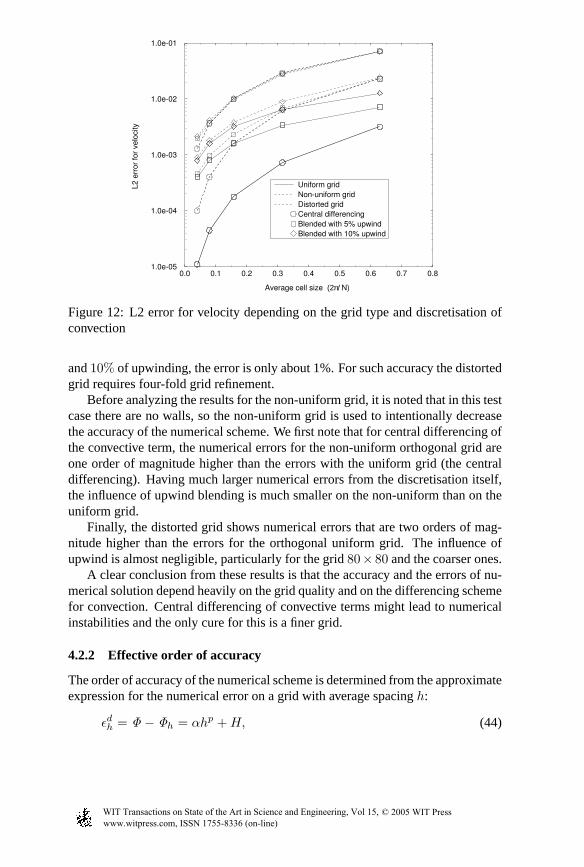
The results are summarised in Figure 12. It is clear from Figure 12 that whena uniform grid is used with a small percentage of upwind, the errors grow by anorder of magnitude. For example, the errors on the grid40 × 40 with no upwind-ing have smaller errors than the results on the160 × 160 grid with only 5% ofupwind blending. Even more surprising is the fact that the grid with 20 × 20 withcentral differencing has approximately the same error as the grid160 × 160 with10 of upwinding. The clear conclusion from this is that one mustuse the centraldifferencing for the convection whenever possible. The uniform orthogonal grid isthe least sensitive: even for the coarsest grid of10 × 10 with uniform distribution
Figure 12: L2 error for velocity depending on the grid type and discretisation ofconvection
and10% of upwinding, the error is only about 1%. For such accuracy the distortedgrid requires four-fold grid refinement.
Before analyzing the results for the non-uniform grid, it isnoted that in this testcase there are no walls, so the non-uniform grid is used to intentionally decreasethe accuracy of the numerical scheme. We first note that for central differencing ofthe convective term, the numerical errors for the non-uniform orthogonal grid areone order of magnitude higher than the errors with the uniform grid (the centraldifferencing). Having much larger numerical errors from the discretisation itself,the influence of upwind blending is much smaller on the non-uniform than on theuniform grid.
Finally, the distorted grid shows numerical errors that aretwo orders of mag-nitude higher than the errors for the orthogonal uniform grid. The influence ofupwind is almost negligible, particularly for the grid80× 80 and the coarser ones.
A clear conclusion from these results is that the accuracy and the errors of nu-merical solution depend heavily on the grid quality and on the differencing schemefor convection. Central differencing of convective terms might lead to numericalinstabilities and the only cure for this is a finer grid.
4.2.2 Effective order of accuracy
The order of accuracy of the numerical scheme is determined from the approximateexpression for the numerical error on a grid with average spacingh:
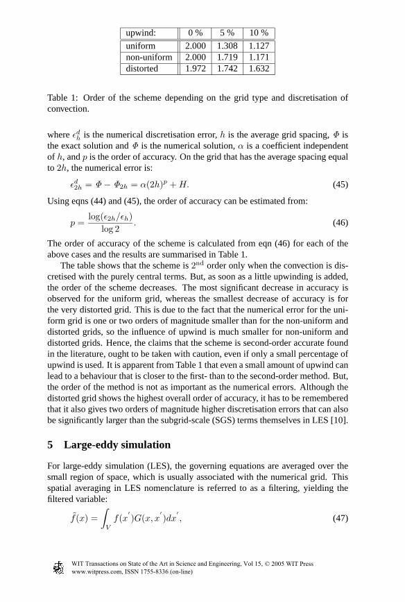
Table 1: Order of the scheme depending on the grid type and discretisation ofconvection.
whereǫdh is the numerical discretisation error,h is the average grid spacing,Φ isthe exact solution andΦ is the numerical solution,α is a coefficient independentof h, andp is the order of accuracy. On the grid that has the average spacing equalto 2h, the numerical error is:
ǫd2h = Φ − Φ2h = α(2h)p +H. (45)
Using eqns (44) and (45), the order of accuracy can be estimated from:
p =log(ǫ2h/ǫh)
log 2. (46)
The order of accuracy of the scheme is calculated from eqn (46) for each of theabove cases and the results are summarised in Table 1.
The table shows that the scheme is2nd order only when the convection is dis-cretised with the purely central terms. But, as soon as a little upwinding is added,the order of the scheme decreases. The most significant decrease in accuracy isobserved for the uniform grid, whereas the smallest decrease of accuracy is forthe very distorted grid. This is due to the fact that the numerical error for the uni-form grid is one or two orders of magnitude smaller than for the non-uniform anddistorted grids, so the influence of upwind is much smaller for non-uniform anddistorted grids. Hence, the claims that the scheme is second-order accurate foundin the literature, ought to be taken with caution, even if only a small percentage ofupwind is used. It is apparent from Table 1 that even a small amount of upwind canlead to a behaviour that is closer to the first- than to the second-order method. But,the order of the method is not as important as the numerical errors. Although thedistorted grid shows the highest overall order of accuracy,it has to be rememberedthat it also gives two orders of magnitude higher discretisation errors that can alsobe significantly larger than the subgrid-scale (SGS) terms themselves in LES [10].
5 Large-eddy simulation
For large-eddy simulation (LES), the governing equations are averaged over thesmall region of space, which is usually associated with the numerical grid. Thisspatial averaging in LES nomenclature is referred to as a filtering, yielding thefiltered variable:
wheref(x) is the general function to be filtered,V is the entire domain andG(x, x
′
) is the localised filter function. We used implicit box filtering, which isnaturally associated with the control-volume method. The localised filter functionG is defined as:
Gi(x, x′
) =
{1 if x
′
∈ Vi
0 if x′
/∈ Vi,(48)
whereVi is the control volume under consideration. It is noted that the box fil-ter defined by eqn (48) is analogous to the mid-point integration rule applied inthe derivation of discretised equations by the control-volume method described inSection 2. In other words, the very discretisation of the governing equations by thecontrol-volume method, is practically the filtering of the governing equations.
After filtering, Navier-Stokes equation can be written as:
d
dt
∫
V
udV +
∫
S
ρuu · Sdn =
∫
S
T · Sdn +
∫
S
pSdn +
∫
S
fdV, (49)
and the filtered continuity equation:∫
S
ρu · Sdn = 0. (50)
Because generallyuu 6= u u, this inequality has to be taken into account as anadditional stress
Tsg = ρ(uu − uu), (51)
whereTsg is the sub-grid stress tensor, which must be provided from a subgrid-scale (SGS) model to close the filtered eqn (49).
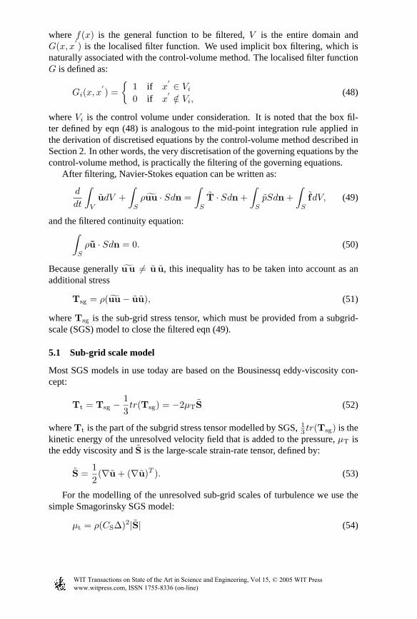
5.1 Sub-grid scale model
Most SGS models in use today are based on the Bousinessq eddy-viscosity con-cept:
Tt = Tsg −1
3tr(Tsg) = −2µTS (52)
whereTt is the part of the subgrid stress tensor modelled by SGS,13tr(Tsg) is the
kinetic energy of the unresolved velocity field that is addedto the pressure,µT isthe eddy viscosity andS is the large-scale strain-rate tensor, defined by:
S =1
2(∇u + (∇u)T ). (53)
For the modelling of the unresolved sub-grid scales of turbulence we use thesimple Smagorinsky SGS model:
whereCS is the Smagorinsky constant,|S| = (2S S)1/2 and ∆ is the size ofthe largest sub-grid scale eddy, which is comparable with the filter width. Moregeneral models, such as the dynamic model of [5], which does not require spec-ification ofCS could easily be implemented in the code. However, such modelsare computationally more demanding. It has frequently beenshown (e.g. [12])that a more elaborate and more general model shows little or no improvements incomputing mean flow properties and turbulence statistics, since with a sufficientlyfine mesh the contribution of the SGS stresses is very small. Since the focus of thepresent work is the application of LES on unstructured mesh and related numericalaspects, we have retained the basic Smagorinsky model in allsimulations.
5.2 Discretisation of LES equations
The final form of equations solved in LES is:
d
dt
∫
V
ρudV +
∫
S
ρuu·dS =
∫
S
T·dS+
∫
S
Tt·dS+
∫
S
P dS+
∫
S
fdV, (55)
whereP is the pressure combined with the sub-grid kinetic energy:
P = p+ tr(Tsg). (56)
Since the filtering by a box filter is analogous to discretisation by a control-volume method, thediscretisedequations for LES have the same form as for thelaminar flows (eqns 15 and 16), but with molecular viscosity replaced by the ef-fective viscosity:
DL(u) =∑
j
(µ+ µt)[uj2 − uj1
|dj |nj ]Sjnj (57)
DR(u) =∑
j
(µ+ µt)[(∇u)j + (∇u)jT
+(∇u)j · dj
|dj |nj ]Sjnj , (58)
whereµt is turbulent viscosity.
6 Illustration: LES of flow and conjugate heat transfer over aheated cube in a matrix
As an illustration of industrial relevance we show some results of LES of heattransfer on an internally heated, surface-mounted cubic protrusion. The configura-tion considered is relevant to cooling of electronics components on circuit boards,or cooling of gas-turbine blades through internal passagesequipped with ribs orpins. More details can be found in [16]. The configuration simulated reflects theexperimental set-up in which one cube in an equidistantly spaced matrix of wall-mounted cubes was heated. The dimension of the cubes wash3 (h = 15 mm)and the height of the channel wasD = 3.4h. The distances between the cubes
were3h, giving centre-to-centre distances ofSx = Sy = 4h. The computationaldomain consisted of a sub-channel unit of dimension (4h × 4h × 3.4h), encom-passing the cube that was placed in the domain centre. Periodic conditions wereapplied for the velocity at all free boundaries of the computational domain, butnot for the temperature. Instead, the temperature of the incoming fluid was fixedto Tref = 20 oC. At the domain outlet the normal derivative of temperaturewasassumed to be zero. The cubes were mounted on a base plate at constant temper-ature equal to the temperature of the incoming fluid. On the join of the heatedcube and the floor the Neumann boundary condition was appliedwith zero heatflux. The heated cube consisted of a constant-temperature core covered with a thinepoxy mantle of thickness0.1h with low thermal conductivity of 0.24 W/m K.The inner side of the epoxy layer was set to a constant temperature of the cubecoreTc = 75 oC during the whole simulation. The temperature distribution in theepoxy layer is determined by the inside temperatureTc and the surface temperatureTs. The latter was obtained by simultaneous solution of unsteady heat conductionthrough the epoxy layer and heat convection in the fluid. Thiscoupling of the tem-perature fields and computation of the instantaneous cube surface temperatureTs
is one of the major outcomes of the present simulation. The computations wereperformed at a Reynolds number ofReD = UoD/ν = 13, 000, corresponding to aReynolds number based on the cube height ofReh = 3854, and withPr = 0.712(air). To obtain this value, the bulk velocity was set toUo = 3.86 m/s yielding themass flux per sub-channelm = 13.70 × 10⁻³ kg/s. All relevant dimensions andphysical properties are taken from the experiments of [13]).
6.1 Computational grid and numerical procedure
Two different grids were used for the computation of this test case. The first gridcontained hexahedral cells only, whereas the second grid was hybrid with tetrahe-dra in the interior of the domain and triangular prisms in thenear-wall region. Onthe hexahedral grid both the heat transfer and fluid flow were computed, whereasthe hybrid grid was used for the solution of the fluid flow only.
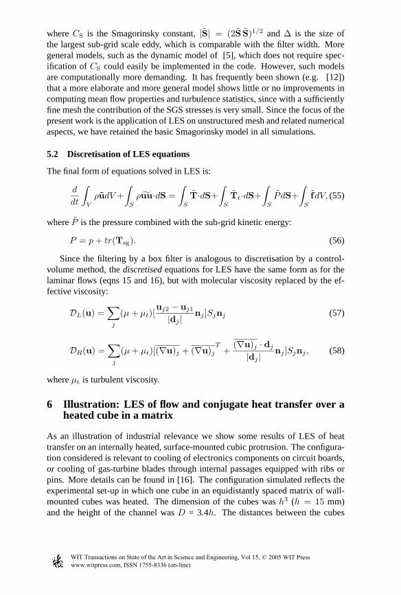
Hexahedral grid. This grid contained 427,680 cells (373,248 cells in the outerregion and 54,264 cells for the epoxy layer), Figure 13. In order to resolve the near-wall region the mesh was clustered hyperbolically towards the walls and edgesin such a way that the first calculation point was at0.006h. For the consideredReynolds number this corresponds toy+ ≈ 1 for the channel flow without a cube.The wall-nearesty+ around the cube was roughly of the same order of magnitude.
In order to avoid cells of high aspect ratio near the wall, with consequent degra-dation of the resolution and numerical accuracy, the grid spacing in streamwise andspanwise directions was ensured to be< 0.032h (which is found to be sufficientfor LES, [20]). This corresponds to the dimensionless streamwise and spanwisespacing ofx+, z+ < 6 for a channel flow, though somewhat larger values weredetected on the cube. The cube-surface mantle (epoxy layer), indicated in Fig. 13was covered by 38 cells in each direction, with 6 cells acrossthe epoxy layer thick-
ness. These cells were also clustered towards the edges and outer boundary of thecube, in order to have approximately the same cell sizes at the fluid solid interface.
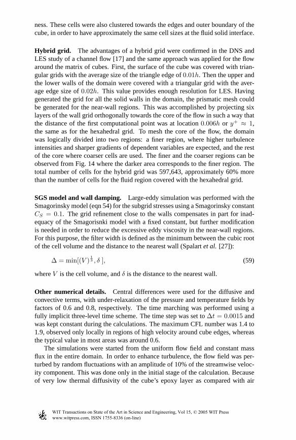
Hybrid grid. The advantages of a hybrid grid were confirmed in the DNS andLES study of a channel flow [17] and the same approach was applied for the flowaround the matrix of cubes. First, the surface of the cube wascovered with trian-gular grids with the average size of the triangle edge of0.01h. Then the upper andthe lower walls of the domain were covered with a triangular grid with the aver-age edge size of0.02h. This value provides enough resolution for LES. Havinggenerated the grid for all the solid walls in the domain, the prismatic mesh couldbe generated for the near-wall regions. This was accomplished by projecting sixlayers of the wall grid orthogonally towards the core of the flow in such a way thatthe distance of the first computational point was at location0.006h or y+ ≈ 1,the same as for the hexahedral grid. To mesh the core of the flow, the domainwas logically divided into two regions: a finer region, wherehigher turbulenceintensities and sharper gradients of dependent variables are expected, and the restof the core where coarser cells are used. The finer and the coarser regions can beobserved from Fig. 14 where the darker area corresponds to the finer region. Thetotal number of cells for the hybrid grid was 597,643, approximately 60% morethan the number of cells for the fluid region covered with the hexahedral grid.
SGS model and wall damping. Large-eddy simulation was performed with theSmagorinsky model (eqn 54) for the subgrid stresses using a Smagorinsky constantCS = 0.1. The grid refinement close to the walls compensates in part for inad-equacy of the Smagorisnki model with a fixed constant, but further modificationis needed in order to reduce the excessive eddy viscosity in the near-wall regions.For this purpose, the filter width is defined as the minimum between the cubic rootof the cell volume and the distance to the nearest wall (Spalart et al. [27]):
∆ = min[(V )1
3 , δ ], (59)
whereV is the cell volume, andδ is the distance to the nearest wall.
Other numerical details. Central differences were used for the diffusive andconvective terms, with under-relaxation of the pressure and temperature fields byfactors of 0.6 and 0.8, respectively. The time marching was performed using afully implicit three-level time scheme. The time step was set to ∆t = 0.0015 andwas kept constant during the calculations. The maximum CFL number was 1.4 to1.9, observed only locally in regions of high velocity around cube edges, whereasthe typical value in most areas was around 0.6.
The simulations were started from the uniform flow field and constant massflux in the entire domain. In order to enhance turbulence, theflow field was per-turbed by random fluctuations with an amplitude of 10% of the streamwise veloc-ity component. This was done only in the initial stage of the calculation. Becauseof very low thermal diffusivity of the cube’s epoxy layer as compared with air
Figure 13: Hexahedral grid used for computation of matrix ofcubes with heattransfer.
(αair/αepoxy ≈ 180), the evolution of the temperature field in the solid takes verylong time before reaching a statistically stationary statein the epoxy layer. There-fore,αepoxy was increased by an order of magnitude at the start of the simulation,and was gradually decreased during the computations. Gathering the results forthe evaluation of the statistics was started only after the proper value forαepoxy
was introduced.The SIMPLE algorithm was used for coupling velocities and pressure. In order
to keep the mass flux constant through the domain, the pressure drop was recal-culated after each time step, as a difference between the imposed mass fluxmo
and the calculated onem. The calculated mass flux changed from one time stepto another, resulting in a varying Reynolds number. However, these variation werequite small,≈ 0.02%. The gathering of the statistics started at time step 15,000and continued until time step 50,000. Meinders and Hanjalic [14] calculated thedominant characteristic wake frequency from the maximum energy in the power-density spectrum, which was obtained from 20,000 − 40,000 vortex-shedding cy-cles. For this case (Reh = 3854), the dominant frequency was found to bef = 27Hz, yielding the Strouhal numberSt = 0.109 (based on the cube heighth and in-coming bulk velocityU0). From this value, we can conclude that the time averageswere computed over about 35 shedding cycles.
Figure 14: Unstructured hybrid grid used for computation ofmatrix of cubes.Above: vertical cross-sections; below: surface grid.
6.2 Velocity field
Figures 15 and 16 shows the typical streamline patterns in the vertical symmetryplane and in the horizontal plane very close to the bottom channel wall. For illus-tration, in both figures we show one selected time realization and the time meanpattern. Note that the time-averaged patterns are periodicand compare well inboth planes with the experimental results of [14]. The mean streamlines displaythe well-known vortex structure in front of and behind the cube, similar to a sin-gle cube, but, of course, modified here due to the presence of neighbouring cubes.This vortex structure has a very strong effect on the wall-temperature distribution,as discussed below. The stagnation point in the symmetry plane appears at aboutz = 0.8h, whereas the recirculation behind the cube occupies almostthe completehalf-space between the two cubes with the dividing streamline dropping sharplytowards the bottom wall towards the reattachment. However,the instantaneouspattern does not look so orderly and is characterised by a number of vortical nestsaround the cube, even including the top face. It is interesting that such multiplevortical nests appear in many instantaneous realisations,but are not present in thetime-averaged picture. Nevertheless, the presence of these small vortices aroundthe tube, which are very difficult to detect (to resolve in time and space) experimen-
tally are the main cause of the strong variation in the cube-surface temperature, asdiscussed below. Detailed discussion of the instantaneousand time-averaged ve-locity field can be found in [16].
Figure 17 shows a selection of the profiles of the normalised streamwise ve-locity U/Uo and the normalised Reynolds stressesu′2/U2
o andv′2/U2o at three
locations in the vertical symmetry plane. The results obtained on hexahedral grids(full lines) and the results obtained on the hybrid grid (dashed lines) are plottedtogether with the experimental results of Meinders and Hanjalic [13, 14] (sym-bols). The latter were obtained using laser Doppler anemometry (LDA) with theexperimental uncertainty of5% for the mean velocities and8% for the Reynoldsstresses. The mean velocity profiles of the present simulations are generally ingood agreement with experimental data.
6.3 Surface temperature and heat transfer
Although fluid flow was computed using two types of grids, for convenience wehave performed the computation of the heat transfer only with the hexahedral grid.
6.3.1 Temperature profiles in characteristic mid-planes
We focus now on the prediction and analysis of the cube-surface temperature andheat-transfer distribution as the most interesting achievement with this algorithm.Experiments [14] provided liquid crystal and infrared pictures of the surface tem-perature, but the detailed profiles have been reported only along the cube circum-ference in the characteristic mid-planes. In Fig. 18 the temperature profiles of boththe simulation results and the experimental data are plotted. The results are in goodagreement with the experiments (with experimental uncertainty of 0.4 oC), exceptat the locations A and D in Fig. 18b. The simulation predicts ahigher surface tem-perature near the channel floor. These overpredictions are due to the fact that theunavoidable heat loss of the epoxy layer through the base wall was not modelled.The overpredictions are of the order∼ 10%, in agreement with experimental find-ings, [13]. The temperature profiles show a relatively uniform temperature overthe central portion of each cube face, with steep gradients and minima at all cubeedges, where the temperature drops by 8-15oC (about 15-25% of the temperaturein the central regions). This sharp decrease is a direct consequence of high localheat-transfer rates, caused by intensive heat removal by high-speed fluid and flowseparation. In view of the small size of the cube (h = 15 mm), such a strongtemperature variation is a good indication of the complex vortex structure and ofthe possible danger of highly nonuniform cooling. A slight asymmetry of the LESdata is possibly the consequence of an insufficient number ofrealization used forcomputing the averaged fields.
6.3.2 Structure imprint and temperature distribution on th e cube surface
A further support of the role of vortical structure on the surface temperature dis-tribution is given by the striking similarity of the time-averaged structure imprints
Figure 18: Distribution of the surface temperature along, respectively, the pathABCDA in the horizontal plane (a) and the path ABCD in the vertical plane (b).
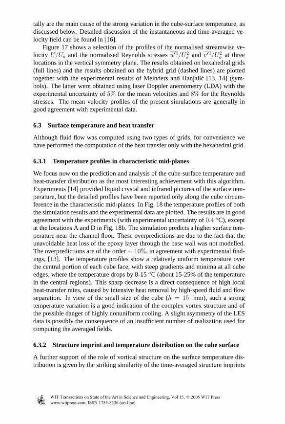
and the temperature field on the cube surface. Figure 19 showsthe near-surfacestreamlines (“streaks”) of the time-averaged flow and the isotherm maps on the fivefree faces of the cube, respectively. The five faces are folded out and mapped intoa plane. The flow is from left to right. The topology of the surface-temperatureplot shows a marked correlation with the streamlines imprint. These should becompared with the temperature distribution along two path lines in the horizontaland vertical plane, respectively, given in Figure 18. In thefollowing we give ashort discussion on the flow structure – temperature field correlation.
Front face. From the streamlines plot, Figure 19(a), one can observe the stagna-tion line atz/h ≈ 0.8, caused by the flow impingement. This flow impingementcaused a large convective heat transfer, which can be seen from Figure 18 wherethe temperature profile at the front is significantly lower. Approaching the leadingedges of the front side the profiles show a large decrease in the temperature. Thisregion is characterised by high flow velocity: the fluid sweeps along the cube edgesand removes the heat. Higher temperatures are found at the foot of the front faceclose to the channel wall. Since this region is dominated by the horseshoe vortex,the induced flow recirculation prolongs the residence time of the fluid in the vor-tex. This allows the local fluid temperature to increase, andthe vortex is, therefore,acting as a kind of insulation layer. This prevents beneficial local convective heattransfer.
Top face. The temperature distribution on the top face shows a large spatialstreamwise gradient: due to the large velocity at the leading edge, the tempera-
Figure 19: Time averaged streamlines on the five faces of the cube (a) and surfacetemperature map (b) of the cube in the matrix of cube arrangement. The flow isfrom left to right.
ture is highly decreased. Though the imprint of the streamlines in Fig. 19 showsa small recirculation bubble on the top face, no significant temperature increase isseen at this location. This could be explained by the highly fluctuating character(vortex shedding) of this recirculation zone. Its characteristic frequency is muchhigher, but with a smaller amplitude than detected in the horseshoe vortex in frontof the cube, or in the vortex-shedding area behind the cube. As a consequence,the trapped fluid has a very short residence time, resulting in an insignificant localfluid warming.
Rear face. The streamline plot of the rear face shows the stagnation point at ap-proximatelyz/h ≈ 0.25 from the base wall, indicating the impingement of theback flow in the wake. This recirculation is explained by the inward rotation ofthe wake vortex and the import of low-temperature fluid into the wake from thebottom. In the upwash flow at the rear face the fluid is heated, which results in adecrease of the local convective heat transfer. The local minimum in the temper-ature profile at the upper edge of the leeward face is explained by the presence ofthe shear layer, which convects cold air with it.
Side faces. The imprints of the streamlines on both side faces are practicallysymmetrical. In contrast, the temperature maps in Fig. 19(b) seem to be asymmet-ric. However, the temperature differences, according to the caption in Fig. 19b, arerather small and could be explained by the fact that the flow (and conjugate tem-
perature field) statistics were gathered over approximately only 35 periodic cycles.At the leading edges the flow separates and reattaches downstream on the side faceatx/h ≈ 0.5. As discussed in the previous section, these flow separations result inside vortices, which are oriented nearly parallel to the leading side edges. Analo-gous to the horseshoe vortex, heat is entrapped in the side vortices, decreasing theconvective heat transfer.
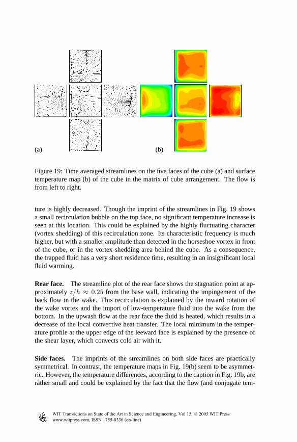
6.3.3 Instantaneous plumes and cube-surface temperature
As an illustration of the spatial and time non-uniformity ofthe instantaneous tem-perature field on and around the cube, we show some instantaneous snapshots ofthe temperature field, selected randomly. The pattern changes continuously, witha stochastic periodicity and the illustration have only a qualitative character. Fig-ure 20 shows one realization of the instantaneous surface temperature viewed fromfront and back of the cube surface (note that the same side face appears in both pic-tures). Although not regular, the pattern reflects the averaged surface temperaturefield shown in Fig. 19 and the flow structure: warm zones are visible in the lowerpart of the front face, just after the cube edge at the side face, and in the upperportion of the back face − all corresponding to local recirculation regions. Localhot spots are also discernible on the back face. The instantaneous fluid tempera-ture, corresponding to the same realization as in Fig. 20, isillustrated in Figure 21.The figures show the thermal plume around the front and rear cube faces, repre-sented by the surface of constant temperature− here 24.5
o C, and coloured by fluidvelocity magnitude. Low fluid velocity (darker areas) are visible behind the cubecorresponding to regions of low heat transfer, in contrast to high velocity (lighterareas), which correspond to intensive heat removal from the cube.
Z
Y X
Z
Y
X
a) b)
Figure 20: Instantaneous temperature on the cube surface (random realizations):(a) view from front, (b) view from back.
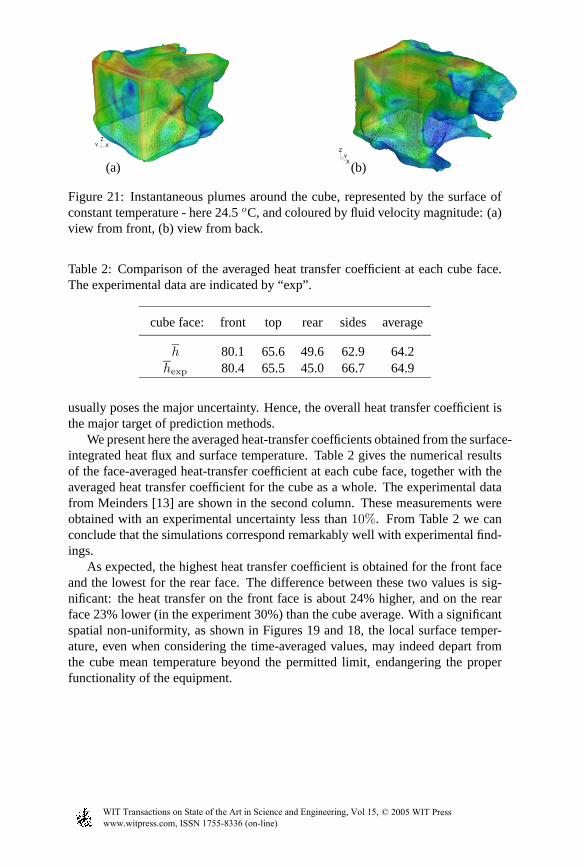
6.3.4 Averaged heat transfer on cube faces
Designers of electronics equipment are usually mainly interested in the total heatdissipation and heat removal from individual components. Although radiation andconduction through the base plate (made deliberately of finned, high-conductingslabs to act as a heat sink) play an important role, the convective heat removal
Figure 21: Instantaneous plumes around the cube, represented by the surface ofconstant temperature - here 24.5oC, and coloured by fluid velocity magnitude: (a)view from front, (b) view from back.
Table 2: Comparison of the averaged heat transfer coefficient at each cube face.The experimental data are indicated by “exp”.
usually poses the major uncertainty. Hence, the overall heat transfer coefficient isthe major target of prediction methods.
We present here the averaged heat-transfer coefficients obtained from the surface-integrated heat flux and surface temperature. Table 2 gives the numerical resultsof the face-averaged heat-transfer coefficient at each cubeface, together with theaveraged heat transfer coefficient for the cube as a whole. The experimental datafrom Meinders [13] are shown in the second column. These measurements wereobtained with an experimental uncertainty less than10%. From Table 2 we canconclude that the simulations correspond remarkably well with experimental find-ings.
As expected, the highest heat transfer coefficient is obtained for the front faceand the lowest for the rear face. The difference between these two values is sig-nificant: the heat transfer on the front face is about 24% higher, and on the rearface 23% lower (in the experiment 30%) than the cube average.With a significantspatial non-uniformity, as shown in Figures 19 and 18, the local surface temper-ature, even when considering the time-averaged values, mayindeed depart fromthe cube mean temperature beyond the permitted limit, endangering the properfunctionality of the equipment.
An unstructured, cell-centered, colocated finite-volume algorithm for large-eddysimulations (LES) and simultaneous coupled solution of heat conduction in mul-tiple-material bounding the flow has been presented. The algorithm has beenaimed at providing a convenient and robust numerical tool tosolve heat trans-fer and capture the local space and time variation of surfacetemperature in tur-bulent flows in complex passages such as encountered in cooling electronics orgas-turbine blades. The approach is based on a RANS rationale, but meets specificLES requirements such as full second-order-accurate discretisation for convection,diffusion and time changes.
Different grid topologies have been tested and their influence on numericalaccuracy, errors and performance of the code have been addressed. Because com-plex geometries and wall topologies usually impose high grid skewness, keepingthe full second-order accuracy may cause numerical instabilities, especially withfull central-differencing schemes. Detailed tests in several generic flows showedthat blending even a small amount of upwind-bias information helps remarkablyin stabilizing the solver, but progressively reduces the order of accuracy.
Computations for the matrix of cubes, used for illustration, shows that the codecan indeed provide all information on instantaneous and averaged temperature andvelocity field and related heat transfer, as demonstrated bythe good agreementwith experimental data. The computations with two different grids: hexahedraland a hybrid yielded very similar results. The hexahedral grid showed slightlybetter agreement because of the smaller numerical errors associated with it.
The computations of the matrix of cubes have also shown that the unstruc-tured grids, whether hexahedral or hybrid offered a cost-effective meshing of theproblem domain and the present authors achieved 50% savingsin the number ofcomputational cells used compared to other authors studying the same problemusing a structured grid.
Well-resolved LES of flow around complex protrusions makes it possible toidentify the vortical structures and associate it with the temperature on the surfaceof bounding walls and their role in the creation of local hot spots that can leadto the malfunction or damage of, e.g., electronic of other equipment that requireefficient cooling.
7.1 A note on non-periodic inflow conditions
The prescription of the inflow conditions, if non-periodic,poses a particular chal-lenge in LES of turbulence. The information at the inflow cross-section mustcontain all flow and turbulence details. Several approachesare possible, but formany real situations where the inflow turbulence is not known, there is no uniqueand universal solution.Random-generated velocity or vorticity fluctuations, su-perimposed on an assumed realistic mean field, is among the most popular andrelatively simple approaches, but has several shortcomings: random fluctuationsdo not have the character of a real turbulence, the velocity field is not conserva-
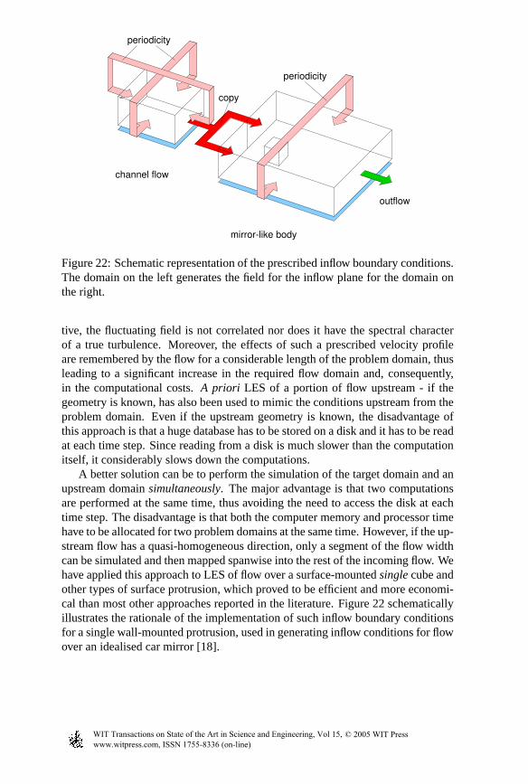
Figure 22: Schematic representation of the prescribed inflow boundary conditions.The domain on the left generates the field for the inflow plane for the domain onthe right.
tive, the fluctuating field is not correlated nor does it have the spectral characterof a true turbulence. Moreover, the effects of such a prescribed velocity profileare remembered by the flow for a considerable length of the problem domain, thusleading to a significant increase in the required flow domain and, consequently,in the computational costs.A priori LES of a portion of flow upstream - if thegeometry is known, has also been used to mimic the conditionsupstream from theproblem domain. Even if the upstream geometry is known, the disadvantage ofthis approach is that a huge database has to be stored on a diskand it has to be readat each time step. Since reading from a disk is much slower than the computationitself, it considerably slows down the computations.
A better solution can be to perform the simulation of the target domain and anupstream domainsimultaneously. The major advantage is that two computationsare performed at the same time, thus avoiding the need to access the disk at eachtime step. The disadvantage is that both the computer memoryand processor timehave to be allocated for two problem domains at the same time.However, if the up-stream flow has a quasi-homogeneous direction, only a segment of the flow widthcan be simulated and then mapped spanwise into the rest of theincoming flow. Wehave applied this approach to LES of flow over a surface-mountedsinglecube andother types of surface protrusion, which proved to be efficient and more economi-cal than most other approaches reported in the literature. Figure 22 schematicallyillustrates the rationale of the implementation of such inflow boundary conditionsfor a single wall-mounted protrusion, used in generating inflow conditions for flowover an idealised car mirror [18].
[1] Barth, T. J. Apsects of unstructured grids and finite volume solvers for theEuler and Navier-Stokes equations. Invon Karman Institute for Fluid Dy-namics Lecture Series 1994-05, 1994.
[2] Demirdzic, I., Muzaferija, S. & Peric, M. Advances in computation ofheat transfer, fluid flow and solid body deformation using finite volume ap-proaches. In Minkowicz, W. J. & Sparrow, E. M., (eds.),Advances in Numer-ical Heat Transfer 1, pp. 59–96. Taylor & Francis, 1997.
[3] Ferziger, J. H. Large-eddy and direct simulation of turbulent flows. InLecturenotes for the short course on calculations of turbulent flows. University ofHamburg, 1995.
[4] Frohlich, J., Rodi, W., Kessler, P., Parpais, S., Bertoglio, J. P. & Laurence, D.Large-eddy simulation around circular cylinders on structured and unstruc-tured grids. In Hirschel, E. H., (ed.),Notes on Numerical Fluid Mechanics66, pp. 319–338. Vieweg, Braunschweig, 1998.
[5] Germano, M. Turbulence: the filtering approach.J. Fluid Mech., 238, 325–336, 1992.
[6] Ghia, U., Ghia, K. N. & Shin, C. T. High-Re solutions for incompressibleflow using the Navier-Stokes equations and a multigrid method. J. Comput.Phys., 48, 387–411, 1982.
[7] Haworth, D. C. & Jansen, K. E. Large-eddy simulation on unstructured de-forming meshes: towards reciprocating IC engines.Computers and Fluids,29, 493–524, 2000.
[8] Howard, R. & Lesieur, M. Structured and non-structured large eddy sim-ulation of the ahmed reference model. In Friedrich, R. & Rodi, W., (eds.),Advances in LES of Complex Flows, Proc. EuroMech Coll. 412, pp. 185–198.Kluwer Academic Publishers., 2002.
[9] Jansen, K. E. Large-eddy simualtion using unstructuredgrids. In Liu, C. &Liu, Z., (eds.),Advances in LES/DNS, Proc. of the First AFOSR Int. Conf. onDNS/LES. Greyden Press, Columbus, 1997.
[10] Kravchenko, A. G. & Moin, P. On the effect of numerical errors in large-eddysimulations of turbulent flows.J. Comput. Phys., 131, 310–322, 1997.
[11] Laurence, D. Large-eddy simulation of industrial flows. In Launder, B. E.& Sandham, N. D., (eds.),Closure Strategies for Turbulent and TransitionalFlows, pp. 392–406. Cambridge University Press, Cambridge, 2002.
[12] Mathey, F., Frohlich, J. & Rodi, W. LES of turbulent flow over a wall-mounted matrix of cubes. In Voke, P., Sandham, N. D. & Kleiser, L., (eds.),Direct and Large-Eddy Simulation III, pp. 51–62. Kluwer Academic Publish-ers, 1999.
[13] Meinders, E. R.Experimental study of heat transfer in turbulent flows overwall-mounted cubes. PhD Thesis, Delft University of Technology, 1998.
[14] Meinders, E. R. & Hanjalic, K. Vortex structure and heat transfer in turbulentflow over a wall-mounted matrix of cubes.Int. J. Heat and Fluid Flow, 20,255–267, 1999.
[15] Niceno, B.An unstructured parallel finite volume algorithm forlarge-eddyand conjugate heat transfer simulations. PhD thesis, Delft University ofTechnology, 2001.
[16] Niceno, B., Dronkers, A. & Hanjalic, K. Turbulent heat transfer from a multi-layered wall-mounted cube matrix: a large eddy simulation.Int. J. Heat FluidFlow, 23, 173–185, 2002.
[17] Niceno, B. & Hanjalic, K. Large eddy simulation of fluid flow and heattransfer around a matrix of cubes using unstructured grids.In Friedrich, R.& Rodi, W., (eds.),Advances in LES of Complex Flows, pp. 199–216. KluwerAcad. Publishers, 2002.
[18] Niceno, B., Hanjalic, K. & Basara, B. Unstructured large-eddy simulationfor vehicle-components aerodynamics: flow over an idealised car mirror.Progress in Computational Fluid Dynamics, , (to appear).
[19] O’Rourke, P. J. & Sahota, M. S. A variable explicit/implicit numericalmethod for calculating advection on unstructured meshes.J. Comp. Physics,142, 312–345, 1998.
[20] Piomelli, U. Large-eddy simulations: Where we stand. InLiu, C. & Liu,Z., (eds.),Advances in LES/DNS, Proc. of the First AFOSR Int. Conf. onDNS/LES. Greyden Press, Columbus, 1997.
[21] R., M. & Moin, P. Suitability of upwind-biased finite-difference schemes forlarge-eddy simulation of turbulent flows.AIAA J., 35, 1415–1417, 1997.
[22] Rhie, C. M. & Chow, W. L. A numerical study of the turbulent flow past anisolated airfoil with trailing edge separation.AIAA J., 21, 1525–1532, 1983.
[23] Rollet-Miet, P. Simulation des grandes echelles sur maillage non-structurepour geometries complexes. PhD Thesis, Ecole Centrale de Lyon, 1998.
[24] Rollet-Miet, P., D., L. & Nitrosso, B. Large-eddy simulation with unstruc-tured grids and finite elements. In Durst, F., Launder, B.,Schmidt, F. W. &Whitelaw, J. H., (eds.),10th Symposium on Turbulent Shear Flows. Pennsyl-vania State University, 1995.
[25] Rosenfeld, M. Uncoupled temporally second-order accurate implicit solverof incompressible Navier-Stokes equations.AIAA Journal, 34, 1892–1834,1996.
[26] Rosenfeld, M., Kwak, D. & Vinokur, M. A fractional step solution methodfor the unsteady incompressible Navier-Stokes equations in generalized co-ordinate systems.J. Comput. Phys., 94, 102–137, 1991.
[27] Spalart, P. R., Jou, W. H., M., S. & Allmaras, S. R. Comments on the fea-sibility of LES for wings, and on a hybrid RANS/LES approach. In Liu, C. &Liu, Z., (eds.), Advances in LES/DNS, Proc. of the First AFOSR Int. Conf. onDNS/LES. Greyden Press, Columbus, 1997.


![Conjugate heat transfer in OpenFOAM - Chalmershani/kurser/OS_CFD_2016/TuroValikangas/Repo… · problem. [2] 1.2 ... For the conjugate heat transfer problems in OpenFOAM, a conjugate](https://static.documents.pub/doc/80x56/5a7a0bbc7f8b9adf228cbdf0/conjugate-heat-transfer-in-openfoam-hanikurseroscfd2016turovalikangasrepoproblem.jpg)


