Unsupervised illuminant estimation from naturalscenes: an RGB digital camera suffices
Juan L. Nieves,* Clara Plata, Eva M. Valero, and Javier RomeroDepartamento de Óptica, Facultad de Ciencias, Universidad de Granada, Campus Fuentenueva, 18071 Granada, Spain
The color of objects depends upon the spectral reflec-tance properties of their surfaces and the spectralpower distribution (SPD) of the light that illuminatesthem [1]. Therefore the color of a natural scene cap-tured by any conventional or digital camera can varyconsiderably when the ambient light changes. Mostcommercial digital cameras incorporate a simplewhite balance mechanism to solve this problem,but more sophisticated spectral imaging deviceseither directly measure the light impinging on thescene or derive some canonical image that is inde-pendent of the illuminant conditions. In the formersituation a white reference surface has to be locatedwithin the scene and its spectral radiance measuredwith a telespectroradiometer [2]. In the latter casedifferent strategies, usually referred to as color con-stancy algorithms, are used to obtain color-constantimage descriptors [3].
Spectral imaging has been used extensively duringthe past decade to obtain spectral functions in eachimage pixel [2,4–11]. Unlike conventional imagingdevices, they capture illuminant-independent imagesand allow accurate spectral and colorimetric repro-duction of color images under any lighting conditions.The experimental setups canbe verydifferent in prac-tice. Multispectral imaging uses several images(usually no more than a few tens) with discrete andfairly narrow bands. Hyperspectral techniques dealwith imaging narrow spectral bands (up to 100) overa contiguous spectral range. Ultraspectral devices(with more than 100 bands) are typically designedfor interferometer-type imaging sensors.While no for-mal procedure exists, in practice the spectral imagingsystems used to acquire scene reflectances have tomeasure, immediately after acquisition, the illumina-tion impingingupon the scene.Thismeans that aneu-tral reference surface embedded in the scene shouldbe recorded with a telespectroradiometer [6,7], whichcan be critical, particularly for hyperspectral devicesconsisting of a digital monochromatic camera with aliquid crystal tunable filter dealingwith imaging overa contiguous spectral range and over a fixed exposure
time for each band. If atmospheric conditions changeduring the band capture, the device can fail to associ-ate the appropriate radiance with the band. Thus,spectral calibration may limit the use of spectralimaging devices to derive simplified illuminant-independent images. Different authors have reliedon the underlying smoothness of signal spectra, withilluminants and spectral reflectances represented bylow-dimensional models based either on principal-component analysis or independent-component ana-lysis to develop a multispectral imaging system [12–17], butwhena scene is digitally imagedunder light ofunknown SPD the image pixels give incomplete infor-mation about the spectral reflectances of the objectsin the scene. Thus the use of spectral imaging devicesto recover the spectral reflectanceor spectral radianceat a single pixel requires previous measurements ofthe illumination impinging on a scene.Over recent years different color-constancy algo-
rithms have also been proposed for a priori illumi-nant estimation. In computational vision anddigital photography, color constancy seeks a color-constant description of images under varying illumi-nant conditions instead of estimating the spectrum ofthe light, as spectral imaging does. The methods canusually be categorized into statistical-based modelsand physics-based models [18–22]. The statistical-based algorithms, which embrace the statisticalknowledge of the possible image colors (possible sur-face reflectances and SPDs of illuminants), are ro-bust but also very sensitive to the learning testdata. Color-by-correlation and gamut-mapping algo-rithms, which have been widely analyzed and tested[21–23], provide excellent results, but large data-bases of real images are needed to obtain good algo-rithm performance.The physics-based algorithms rely fundamentally
on how light interacts with the object surface. Be-cause of the complexity of this interaction it is neces-sary to introduce some approximations and to relaxthe constraints embedded within the physical phe-nomenon of light interaction. The dichromatic reflec-tance model assumes that the color signal can bedecomposed into two additive terms, one originatingin the interface reflectance and the other associatedwith the diffuse reflectance [24]. This algorithm hasproved to be of particular interest in multichannelcameras in which a set of a reduced number of broad-band color filters are coupled to a monochrome CCDcamera [4]. A combination of statistical- and physics-based models has also been put forward as an alter-native to deciding which method to apply accordingto the image content [20].The target of our work here has been to estimate
the SPD of the illumination of a natural scene. Byusing an RGB digital camera and by capturing thesame image with and without a cutoff color filterin front of the camera lens the effective number ofcamera sensors can be increased [16]. Computationalresults are shown for different natural scenes anddaylight illuminant conditions. The main difference
from earlier multispectral imaging techniques for il-luminant or radiance recoveries [16,17] is that we didnot use any white reference surface in the scene. Inprevious studies [9,17] we found that it was possibleto use a white reference surface and a linear pseudo-inverse algorithm to recover the SPD of illuminantswith good spectral and colorimetric performance. Adirect mapping between RGBs and illuminant spec-tra led to excellent spectral recoveries for daylight,which was characterized by relatively smooth spec-tral profiles (with the exception of some particularabsorption bands beyond the visible spectrum) andwas very similar for most of the hours during a clearday [9,25]. Nevertheless, spectral performance maydecrease if more than three sensors are used in mul-tispectral-illuminant estimation [17]. Mosny andFunt [26] also developed a multispectral experimentwith different color-constancy algorithms and haveshown that increasing the number of camera sensorsfrom three to six or nine does not significantly im-prove the accuracy of illuminant estimation. For dif-ferent indoor scenes under a relatively small set ofartificial illuminants, their results suggest that illu-minant recovery benefits from the use of a six-channel camera but that little improvement is tobe gained by adding successive color filters.
In the following sections we analyze the use of alinear pseudo-inverse method for multispectral re-covery of the SPD of the illuminants of naturalscenes. This is particularly important for spectralimaging devices because our algorithm needs neithera white reference located in the scene nor telespec-troradiometer measurement of the SPD of the lightcoming from this white surface. The results arediscussed in terms of spectral and colorimetricperformance in the analysis and synthesis of naturalcolor images. A comparative analysis with othercolor-constancy algorithms that use only threecolor channels (max-RGB, gray-world, color-by-correlation, and dichromatic) is also presented.
2. Methods
A. Computations for Spectral Image Acquisition
When a CCD digital color camera is pointed at a sur-face with spectral reflectance function rx, the re-sponse of the kth sensor for pixel x can be modeledlinearly by
ρxk ¼X700λ¼400
ExðλÞrxðλÞQkðλÞΔλ; ð1Þ
where QkðλÞ is the spectral sensitivity of the kth sen-sor and ExðλÞ is the SPD of the illuminant impingingon the surface; both functions are sampled at 5nmintervals in the visible range of 400–700nm. Butany real spectral device is affected by image noise,which can degrade both its spectral and colorimetricperformance [10]. There are different noise sources,which include fixed pattern noise, dark current noise,shot noise, amplifier noise, and quantization noise.
Assuming a linear response for the CCD camera sen-sor outputs, the noisy sensor responses ρ0 can be re-presented as a function of the noise-free sensorresponses ρ as
ρ0 ¼ ρþ η ¼ CE; ð2Þ
where ρ is a k ×N matrix whose columns contain thesensor responses for each of theN image pixels, η is ak ×N matrix vector of uncorrelated components thataffects each sensor separately, C is a k × n matrixwhose rows contain the wavelength-by-wavelengthmultiplication (n means the number of wavelengthsamples) of the surface reflectance and the sensorsensitivities, and E is a n ×N matrix whose rows con-tain the SPD of the illuminant. In what follows wesimulated thermal and shot noise with standard de-viations of 3% (that correspond to a signal-to-noiseratio of around 30dB) which is an average noisevalue for nonrefrigerated color cameras. Althoughwe simulated the additive noise from the calculatedset of noise-free sensor responses ρ, it is straightfor-ward from Eq. (2) that noise is also affecting the coef-ficients of the matrix.An estimate of a set of test spectra may then be
obtained from the corresponding set of camera re-sponses ρ0 by solving the underestimation problem,e.g., increasing the number, k, of the camera sensorsby using successive cutoff filters in front of the cam-era lens as each cutoff filter generates three new sen-sitivity curves. These new sensitivities may be moreor less correlated with the old ones depending on theshape of the spectral transmittance of the cutoff fil-ters used. We first simulated digital counts by usingthe spectral sensitivities of a Retiga 1300 digitalCCD color camera (QImaging Corporation, Canada)with 12 bit intensity resolution per channel. Cameraresponses ρ in Eqs. (1) and (2) are based on a set ofcamera sensitivities but are only used to generate aset of noise-free fictitious data. The RGB camera out-puts are modified to use a three- to six-band spectralcamera when no color filter (k ¼ 3) or one successivecolor filter (k ¼ 6) is used (Fig. 1). Following from pre-
vious results, [17] the color glass filter GG475 fromOWIS GmbH was selected. Although the spectraltransmittance of this color filter does not seem togenerate an appropriate set of three new indepen-dent spectral sensitivities because it modifies theblue sensor response much more than the othertwo, it corresponded to that producing the best re-sults. Some results will be cited later in case of usinganother cutoff filter less correlated with our cameraRGB sensors.
B. Linear Pseudo-Inverse Illuminant Estimation
A priori the linear pseudo-inverse algorithm needs toapply a learning-based procedure by assigning sen-sor outputs to one reference surface in the scene.We begin by segmenting the images and selectingthe bright areas (not necessarily the whitest) in thenatural scenes. To form the sensor outputs for thetraining set of illuminants we use a seeded-region growing procedure. It starts with assignedluminance seeds and grows segmented areas by mer-ging a pixel into its nearest neighboring seed area.For automatic seed selection, we first calculate theluminance component of each image as the sum ofthe red, green, and blue components. Next we imple-ment a MATLAB routine that thresholds thisluminance component and produces binary imagescontaining labels for the segmented areas [27]. Simi-lar areas are merged, and finally a single image withdifferent seeded regions is derived for each scene andeach training illuminant. Since image complexitycan vary from one image to another, we further useddifferent threshold values. Thus, if a high luminancethreshold level is used, a smaller number of seededareas is derived, while more segmented areas will beobtained for small threshold values. The segmenta-tion procedure and its implementation is simple,computationally effective, and very fast in terms ofcomputation times.
For spectral-illuminant recovery, it was shown thata direct relationship between the camera responsesand the SPD of the illuminants can be established[17]. The method is based on a direct transformation
Fig. 1. (a) Spectral sensitivities of the RGB digital camera (QImaging Retiga 1300); (b) spectral transmittance of the GG475 colored-glassfilter from OWIS GmbH.
between the estimated illuminant spectra E (an n × 1vector) and sensor responses ρ0 (a k × 1 vector) ex-pressed by
E ¼ Fρ0: ð3Þ
In this expression, the matrix F is derived following alinear pseudo-inverse method by
F ¼ Eo½ðρ0To ρ0
oÞ−1ρ0To � ¼ Eoρ0þ
o ; ð4Þ
where Eo (an n × tmatrix, with t being the number oftraining illuminants) and ρ0
o (a k × t matrix) are theSPDs and their corresponding sensor outputs for thetraining set of illuminants, and ρ0þ
o is the pseudo-inverse matrix of ρ0
o. Therefore, using this methodwith experimental RGB values, there is no need touse any mathematical base or to know the spectralsensitivity of the camera sensors.Thus, suppose we are given m seeded regions for
the same image under a fixed training illuminant.We can average the sensor outputs for the set of pix-els belonging to the same seed and form a k ×mmatrix of sensor responses ρ0
o for this training illu-mination. Repeating this procedure for each trainingilluminant, a set of t sensor response matricesfρ0
o;1;ρ0o;2;…;ρ0
o;tg is obtained and concatenated ina rowwise manner; this procedure is iteratively re-peated with each of the natural scenes to derivethe overall sensor output matrix ρ0
o. After the seg-mentation and the learning-phase procedure eachρ0
o is assigned to one individual illuminant spec-trum, which is replicated m times. In this workthe sensor output matrix comprised k × 28; 834 digi-tal counts, as we had 28,834 pixels corresponding tothe segmentation for the training scenes describedbelow, thus yielding a matrix training set of illumi-nants Eo of 61 × 28; 834 spectra each defined over400–700nm sampled at 5nm intervals. Finally ma-trices ρ0
o and Eo are used in Eq. (4) to estimate therecovery matrix F.
C. Hyperspectral Data, Illuminants, and Computations
A set of spectral data from nine natural scenes, sevenof rural environments and two of urban environ-ments, was used for image reproduction under differ-ent illuminant conditions. The images, which containrocks, trees, leaves, grass, and earth, were acquiredin daylight between mid-morning and mid-afternoonand were illuminated by direct sunlight from a clearsky. Additional details of the scenes, the hyperspec-tral imaging system, and calibration procedure canbe found in [7]. For the present work different frag-ments of these scenes were used for the training andtesting sets.The training set of images was made up of nine dif-
ferent fragments, one for each scene, of 400 × 400 pix-els and reproduced under 100 phases of daylightmeasured previously in our laboratory [13]. The testset comprised 12 fragments of 400 × 400 pixels (noneof their pixels in common with the training set, but
extracted from the same scenes), and the radiance foreach pixel was calculated by using as illumination 25different daylights not included in the training set.
D. Comparative Color-Constancy Methods
For comparison with the spectral-illuminant estima-tion method introduced in the subsection above, weimplemented different standard color-constancy al-gorithms. Unlike spectral imaging, color-constancymodels do not recover the spectrum of the illumina-tion thrown onto a scene but seek a color imagerendered under a reference light, and thus the pro-jection of the color of the light onto the cameraRGB sensors is generally enough. Because we areusing bright segmented areas, we first implementa dichromatic method, which assumes that the cam-era sensor RGB outputs lie in a two-dimensionalplane, one corresponding to the reflectance proper-ties of the surfaces and the other describing theSPD of the interface [28].
Another successful color-constancy algorithm iscolor-by-correlation (CbC), which estimates the sceneilluminant by determining a priori a set of plausibleilluminant colors [22]. These two methods lead tovery good color-constancy results but are computa-tionally complex, requiring a large image data basefor the training phase. Thus we have also used twoadditional color-constancy algorithms that estimatethe color of the illuminant by using a simpler and fas-ter, though somewhat less accurate, procedure thanthe previous ones. The gray-world algorithm as-sumes that the average reflectance in an image isachromatic and uses the fact that the mean camerasensor response for each channel gives informationabout the color of the light source [29]. Finally, weuse the max-RGB algorithm, which estimates the il-luminant color prevailing in a scene by determiningthe maximum sensor outputs in each channel of thecolor image [30]. This algorithm, which is very com-mon in digital image processing, assumes the pre-sence of a white point in the image and assumesthat this point is that which most reflects the lightover a scene.
3. Results
In evaluating the results we have analyzed the per-formance of the algorithm in a variety of differentquality measures.We used four very commonmetricsto quantify both the spectral and colorimetric qualityof the recovered illuminant: the goodness-of-fit coef-ficient (GFC), the CIELab color difference ΔE�
ab, theroot-mean-square error (RMSE), and the angular er-ror (AE) [31,32]. The GFC is based on Schwartz’s in-equality and is defined as the cosine of the anglebetween the original signal f ðλÞ and the recoveredsignal f rðλÞ; thus
This measurement of spectral similarity has the ad-vantage of not being affected by scale factors. Color-imetrically accurate illuminant estimations requireGFC > 0:995; GFC > 0:999 indicates quite goodspectral fit, and GFC > 0:9999 an almost exact fit[13]. The CIELab color difference ΔE�
ab was usedto evaluate colorimetric quality and was calculatedwith reference to the color signal of a white patchin the scene for illuminant estimation. The thirdmeasure was the AE, defined as
AE ¼ cos−1ðρl · ρeÞ; ð6Þ
where ρ1 and ρe are the color components of the lightsource and the algorithm’s estimate of the color of thelight source, respectively. Finally, the RMSE wasalso used.
A. Spectral and Colorimetric Performance
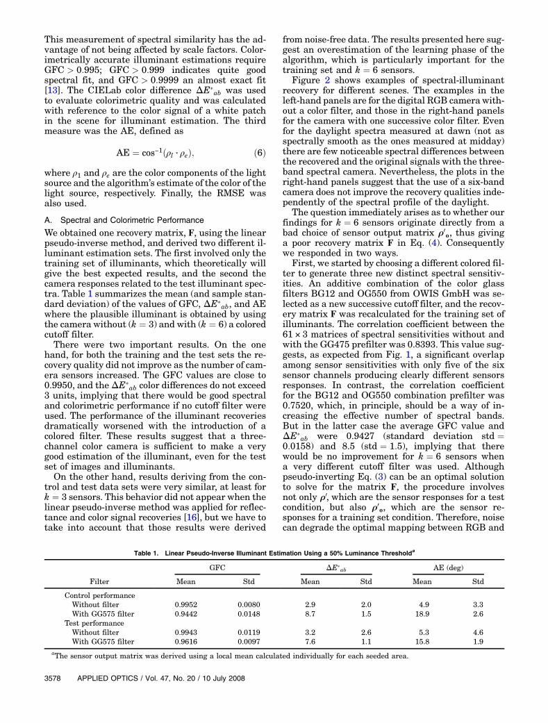
We obtained one recovery matrix, F, using the linearpseudo-inverse method, and derived two different il-luminant estimation sets. The first involved only thetraining set of illuminants, which theoretically willgive the best expected results, and the second thecamera responses related to the test illuminant spec-tra. Table 1 summarizes the mean (and sample stan-dard deviation) of the values of GFC, ΔE�
ab, and AEwhere the plausible illuminant is obtained by usingthe camera without (k ¼ 3) and with (k ¼ 6) a coloredcutoff filter.There were two important results. On the one
hand, for both the training and the test sets the re-covery quality did not improve as the number of cam-era sensors increased. The GFC values are close to0.9950, and theΔE�
ab color differences do not exceed3 units, implying that there would be good spectraland colorimetric performance if no cutoff filter wereused. The performance of the illuminant recoveriesdramatically worsened with the introduction of acolored filter. These results suggest that a three-channel color camera is sufficient to make a verygood estimation of the illuminant, even for the testset of images and illuminants.On the other hand, results deriving from the con-
trol and test data sets were very similar, at least fork ¼ 3 sensors. This behavior did not appear when thelinear pseudo-inverse method was applied for reflec-tance and color signal recoveries [16], but we have totake into account that those results were derived
from noise-free data. The results presented here sug-gest an overestimation of the learning phase of thealgorithm, which is particularly important for thetraining set and k ¼ 6 sensors.
Figure 2 shows examples of spectral-illuminantrecovery for different scenes. The examples in theleft-hand panels are for the digital RGB camera with-out a color filter, and those in the right-hand panelsfor the camera with one successive color filter. Evenfor the daylight spectra measured at dawn (not asspectrally smooth as the ones measured at midday)there are few noticeable spectral differences betweenthe recovered and the original signals with the three-band spectral camera. Nevertheless, the plots in theright-hand panels suggest that the use of a six-bandcamera does not improve the recovery qualities inde-pendently of the spectral profile of the daylight.
The question immediately arises as to whether ourfindings for k ¼ 6 sensors originate directly from abad choice of sensor output matrix ρ0
o, thus givinga poor recovery matrix F in Eq. (4). Consequentlywe responded in two ways.
First, we started by choosing a different colored fil-ter to generate three new distinct spectral sensitiv-ities. An additive combination of the color glassfilters BG12 and OG550 from OWIS GmbH was se-lected as a new successive cutoff filter, and the recov-ery matrix F was recalculated for the training set ofilluminants. The correlation coefficient between the61 × 3 matrices of spectral sensitivities without andwith the GG475 prefilter was 0.8393. This value sug-gests, as expected from Fig. 1, a significant overlapamong sensor sensitivities with only five of the sixsensor channels producing clearly different sensorsresponses. In contrast, the correlation coefficientfor the BG12 and OG550 combination prefilter was0.7520, which, in principle, should be a way of in-creasing the effective number of spectral bands.But in the latter case the average GFC value andΔE�
ab were 0.9427 (standard deviation std ¼0:0158) and 8.5 (std ¼ 1:5), implying that therewould be no improvement for k ¼ 6 sensors whena very different cutoff filter was used. Althoughpseudo-inverting Eq. (3) can be an optimal solutionto solve for the matrix F, the procedure involvesnot only ρ0, which are the sensor responses for a testcondition, but also ρ0
o, which are the sensor re-sponses for a training set condition. Therefore, noisecan degrade the optimal mapping between RGB and
Table 1. Linear Pseudo-Inverse Illuminant Estimation Using a 50% Luminance Thresholda
spectra after solving for Eq. (3). We should keep inmind that we are increasing the number of camerasensors by adding broadband filters in front of ourdigital RGB camera lens and not by adding narrow-band filters as hyperspectral devices do.Second, we recalculated the matrix ρ0
o, using dif-ferent luminance threshold values in determiningthe seeded regions for each scene. Figure 3 showsan example of the influence of the segmentation pro-cedure on the quality of illuminant recoveries. Theupper row illustrates how the number of seeded re-gions (different colors in the plots) changes as thethreshold value increases. The lower part of the fig-ure shows the cumulative distribution plots for thespectral performance of this scene under the 100training illuminants, and the whole figure showsthe proportion of spectral recoveries that takes onvalues of less than or equal to some GFC values,without (left-hand plot) and with (right-hand plot)the prefilter. What is clear is that the performanceof the linear pseudo-inverse algorithm is very goodfor the three-channel camera, giving very similar re-sults for all threshold values, but the results worsenfor the six-channel camera, which yields a wide dis-persion in the spectral performance according to the
threshold value used. Figure 4 summarizes the re-sults for the control set of illuminants.
The effects of threshold values and number of fil-ters have been tested by a repeated-measures analy-sis of variance of three factors: the number of sensors(two levels, k ¼ 3 or k ¼ 6), the metric (four levels,GFC, RMSE, ΔE�
ab, and AE) and the threshold (fivelevels, u ¼ 10; 30; 50; 70; 90). We obtain very goodspectral and colorimetric accuracy for the three-channel camera without prefilter. Our results showthat both the spectral and colorimetric performancefor k ¼ 3 sensors do not depend on the number of theselected seeded regions (p ≫ 0:05). The average GFCand ΔE�
ab color difference for all of the thresholdvalues are 0.995 and 2.9, respectively. In contast,the results for k ¼ 6 sensors not only worsen butare also different for the various threshold valuesused. We found an average GFC and ΔE�
ab of0.9420 and 8.8, respectively, indicating a poor qualityof illuminant recovery with the six-channel camera.There are also significant differences for all themetrics (p ≪ 0:05) according to the threshold value.Post hoc comparisons suggest significant differencesbetween GFC, ΔE�
ab, and AE for a threshold of70% (p ≪ 0:05) and close to significant for the RMSE(p ¼ 0:04).
Fig. 2. Examples of the spectral-illuminant recovery (left-hand panels) with k ¼ 3 sensors and (right-hand panels) with k ¼ 6 sensors fordifferent illuminants and scenes (—, original spectrum; •, recovered spectrum).
B. Chromatic Differences in Natural Color ImageReproduction
The above results suggest that a three-channel cam-era is sufficient for good spectral and colorimetric il-luminant estimation. But can we reproduce naturalimage colors with the same accuracy? To test thispoint we used Eqs. (1) and (2) to derive the originaland recovered sensor responses when each hyper-spectral image was reproduced under the originaland estimated illuminant. The error in color imagereproduction is calculated as
RGBerrorx ¼�13
X3i¼1
ðρxi − ρxiÞ2�1=2
; ð7Þ
where ρx and ρx are the digital counts for R, G, and Bof the original and recovered image, respectively, at
pixel x. The RGBs were all normalized to valueswithin the range 0–255.
Figure 5 illustrates the visual significance of theRGB color errors for different scenes when theyare reproduced under the estimated illuminant spec-trumwith and without a prefilter. We show examplesof the 95% percentile results for two very differentnatural images: one corresponding to a rural land-scape, which contains a reduced color range centeredaround green hues, and an urban landscape, whichcontains a variety of different surfaces rangingthrough a more complex gamut of colors. The errorhistogram for the rural scene supports our previousfindings and shows that we achieved good color re-production using k ¼ 3 sensors, with RGB errors be-low five digital counts. The use of more sensors withthis image also leads to good color preproduction,with a great percentage of RGB errors around five
Fig. 3. (Color online) Example of the seeded regions obtained by using different luminance threshold values. Results for the cumulativedistributions of GFCs with and without a prefilter are also shown for this scene.
Fig. 4. Mean spectral (left) and colorimetric (right) performance for the linear pseudo-inverse algorithm using different luminancethreshold values.
digital counts. Nevertheless, the differences betweenthe use of a three- or six-channel camera are moreevident for the urban scene. The color differenceΔE�
ab obtained for the estimated illuminant whenthe algorithm was applied for the two scenes wasvery similar in both cases (7.1 units for the ruralscene and 7.6 for the urban one), but the RGB errorhistogram suggests more errors when the scene en-compasses a complex gamut of colors.
C. Color-Constancy Comparative Results
In this section we compare the performance of thelinear pseudo-inverse algorithm to other color-constancy algorithms. For comparison’s sake we usedthree estimates of the recovery matrix, F, in the lin-ear pseudo-inverse algorithm for a three-channel col-or camera without successive cutoff filters. The firstestimate (LPI) was obtained by segmenting the testimages using a 50% luminance threshold value. Thesecond version involved only those image pixels with-
in 90% of the maximum luminance level. We calledthis version the white-patch linear pseudo-inverse(WLPI) because of its similarity to the max-RGBcolor-constancy algorithms. The third version, ormax-linear pseudo-inverse (MLPI), on the otherhand, used a luminance threshold value of 10%and tended to compute the average of the RGBs inall the seeded regions.
Table 2 summarizes the performance of the differ-ent illuminant estimation algorithms. Because color-constancy approaches recover the color of the light,the results only show the AE measurements. It isclear that the linear pseudo-inverse method per-forms very well in comparison with the other color-constancy algorithms. Our results show that thecolor-by-correlation and all three versions of the lin-ear pseudo-inverse method outperform the max-RGB, gray-world, and dichromatic approaches asfar as mean RGB error and AE metrics are con-cerned. The color-by-correlation paradigm is slightly
Fig. 5. (Color online) Visualized images of original scene fragments and the histogram of RGB errors. The upper histograms are for thecamera without a prefilter, and the lower ones for the six-band camera.
better in terms of AE and also gives very good resultsfor the RMSE (of only 0.0019). The max-linearpseudo-inverse gives the worst results, suggestinga limitation of the method if you overload the linearpseudo-inverse algorithm. Nevertheless, with regardto color differences, the corresponding averageΔE�
abis around 3 units, indicating a good colorimetric colorreproduction.
4. Discussion
We have investigated the question of how to apply alinear pseudo-inverse method for unsupervised illu-minant recovery from natural scenes. The methodwe have introduced is a spectral-imaging learning-based algorithm that directly relates camera sensoroutputs and illuminant spectra. The RGB sensoroutputs can be modified by the use of a successivecutoff color filter, and thus the algorithm needs noinformation about the spectral sensitivities of thecamera sensors or eigenvectors to estimate the SPDsof illuminants.Our results suggest that daylight spectra can be re-
covered with acceptable spectral and colorimetric ac-curacy with a three-band camera (e.g., a digital RGBcamera without a prefilter). Although linear pseudo-inverse approaches have been applied successfully forcolor signals and natural reflectance recoveries [16],the results suggest serious limitations of the algo-rithm for multispectral-illuminant recovery whenmore than three sensors are used. One reason forthe poor results for the six-band color camera couldbe the inappropriate choice of the particular color cut-off filter, but we have obtained similar low spectraland colorimetric performance when other uncorre-lated sets of RGB sensors were used. In a previouscomputational work [16] we found that a noise-freeRGBcamera coupledwith color filters provided signif-icantly better recovery of radiance and spectral reflec-tances in natural scenes than an RGB camera alone.However, later results suggest that digital camerasaffected by high noise levels do not improve the per-formance of the algorithm for recovering illuminants[17]. This also agrees with the results anticipated byMosny andFunt [26],who foundminor improvementsby extending the number of channels from RGB cam-eras to six and nine. Thus the influence of noise in therecovering process could bemore relevant than the se-lection of filters, at least for spectral applicationsusing digital RGB cameras with a prefilter.With our results, we seek not only to establish the
limits of spectral direct mapping for illuminant esti-mation, but also to provide a newmultispectral color-constancy approach. By combining the device withthe appropriate computations, spectral informationabout objects and illuminants can be obtained simul-
taneously without any spectroradiometric measure-ment. But will the method work well for a widervariety of indoor scenes that include fluorescent illu-minants? Nothing precludes the application of ourmethod to indoor scenes, although it can fail to de-scribe some kind of fluorescent illuminants appropri-ately. These limitations were already demonstratedin previous work [17], and some examples with in-door scenes and artificial illuminants suggest similarperformance here. Figure 6 illustrates the recoveryresults for an indoor scene and two artificial illumi-nants without a prefilter. In this example the train-ing set of illuminants was composed of 82 SPDs offluorescent-type illuminants, and the test set com-prised a set of 20 commercial fluorescent and incan-descent lights that were not included in the trainingset (see [17] for more details about these SPDs); twofragments of the toys hyperspectral scene [7] wereused with the training set of illuminants, and onefragment with the test illuminants (with none oftheir pixels in commonwith the training set). Resultssuggest good colorimetric performance, but we find adependency on the spectral profile of the artificial il-luminant. As expected, an RGB digital camera with-out prefilter does not provide recoveries of artificiallighting as well as with daylight, and it can fail todescribe some kind of fluorescent illuminants appro-priately [17]. Nevertheless this simple example de-monstrates that the linear pseudo-inverse methodfor unsupervised illuminant recovery could also workfor indoor scenes with an adequate training.
The advantage of the linear pseudo-inverse illumi-nant estimation algorithm is that it recovers not onlythe color of the light but also the illuminant spec-trum. Comparing this method with other color-constancy algorithms, the spectral and colorimetricperformances surpass other approaches. Our resultsare close in performance to those deriving from thecolor-by-correlation method, but avoid a huge data-base for training and show that multispectral ima-ging fundamentals can also be used for illuminantestimation in color-constancy applications.
This work was supported by the Spanish Ministryof Education and Science and the European Fund forRegional Development (FEDER) through grant num-ber FIS2007-60736. The authors thank A.L. Tate forrevising their text.
References1. B. A. Wandell, “The synthesis and analysis of color images,”
IEEE Trans. Pattern Anal. Mach. Intell. 9, 2–13 (1987).2. J. Y. Hardeberg, “Acquisition and reproduction of color images:
colorimetric andmultispectral approaches,”Ph.D. dissertation(Ecole Nationale Superieure des Telecommunications, 1999).
3. M. Ebner, Color Constancy (Wiley, 2007).
Table 2. Summary of Performance (AE, degrees) for Linear Pseudo-Inverse Illuminant Estimation and Different Color-Constancy Algorithms
4. S. Tominaga, “Multichannel vision system for estimating sur-face and illumination functions,” J. Opt. Soc. Am. A 13, 2163–2173 (1996).
5. F. H. Imai and R. Berns, “Spectral estimation using trichro-matic digital cameras,” in Proceedings of the InternationalSymposium onMultispectral Imaging and Color Reproductionfor Digital Archives (Society of Multispectral Imaging ofJapan, 1999), pp. 42–49.
6. C.-C. Chiao, D. Osorio, M. Vorobyev, and T. W. Cronin, “Char-acterization of natural illuminants in forests and the use ofdigital video data to reconstruct illuminant spectra,” J. Opt.Soc. Am. A 17, 1713–11721 (2000).
7. S. M. C. Nascimento, F. P. Ferreira, and D. H. Foster, “Statis-tics of spatial cone excitation ratios in natural scenes,” J. Opt.Soc. Am. A 19, 1484–1490 (2002).
8. V. Cheung, S. Westland, C. Li, J. Hardeberg, and D. Connah,“Characterization of trichromatic color cameras by using anew multispectral imaging technique,” J. Opt. Soc. Am. A22, 1231–1240 (2005).
9. J. L. Nieves, E. M. Valero, S. M. C. Nascimento, J. Hernández-Andrés, and J. Romero, “Multispectral synthesis of daylight
using a commercial digital CCD camera,” Appl. Opt. 44,5696–5703 (2005).
10. N. Shimano, “Evaluation of a multispectral image acquisitionsystem aimed at reconstruction of spectral reflectances,” Opt.Eng. 44, 107005 (2005).
11. H.-L. Shen, J. H. Xin, and S.-J. Shao, “Improved reflectancereconstruction for multispectral imaging by combining differ-ent techniques,” Opt. Express 15, 5531–5536 (2007).
12. S. Tominaga and B. A. Wandell, “Standard surface-reflectancemodel and illuminant estimation,” J. Opt. Soc. Am. A 6, 576–584 (1989).
13. J. Hernández-Andrés, J. Romero, J. L. Nieves, and R. L. Lee,Jr., “Color and spectral analysis of daylight in southern Eur-ope,” J. Opt. Soc. Am. A 18, 1325–1335 (2001).
14. S. Tominaga, “Natural image database and its use for scene il-luminant estimation,”J.Electron. Imaging11, 434–444 (2002).
15. S. Tominaga and B. A. Wandell, “Natural scene-illuminant es-timation using the sensor correlation,” in Proc. IEEE 90, 42–56 (2002).
16. E. M. Valero, J. L. Nieves, S. M. C. Nascimento, K. Amano, andD. H. Foster, “Recovering spectral data from natural scenes
Fig. 6. (Color online) Visualized image of an indoor scene fragment and the histogram of RGB errors. Results are examples of the spectral-illuminant recovery with k ¼ 3 sensors and two artificial illuminants (—, original spectrum; •, recovered spectrum).
with an RGB digital camera,” Color Res. Appl. 32, 352–360(2007).
17. J. L. Nieves, E. M. Valero, J. Hernández-Andrés, andJ. Romero, “Recovering fluorescent spectra of lights with anRGB digital camera and color filters using different matrixfactorizations,” Appl. Opt. 46, 4144–4154 (2007).
18. M. D’Zmura and G. Iverson, “Color constancy. I. Basictheory of two-stage linear recovery of spectral descriptionsfor lights and surfaces,” J. Opt. Soc. Am. A 10, 2148–2165(1993).
19. D. H. Brainard andW. T. Freeman, “Bayesian color constancy,”J. Opt. Soc. Am. A 14, 1393–1411 (1997).
20. G. Shaefer and S. Hordley, “A combined physical and statis-tical approach to color constancy,” in 2005 IEEE Computer So-ciety Conference on Computer Vision and Pattern Recognition(CVPR’05) (IEEE Computer Society, 2005), Vol. 1, pp.148–153.
21. S. D. Hordley and G. D. Finlayson, “Reevaluation of color con-stancy algorithm performance,” J. Opt. Soc. Am. A 23, 1008–1020 (2006).
22. G. D. Finlayson, S. D. Hordley, and P. M. Hubel, “Color by cor-relation: a simple, unifying framework for color constancy,”IEEE Trans. Pattern Anal. Machine Intell. 23, 1209–1221(2001).
23. D. A. Forsyth, “A novel algorithm for colour constancy,” Int. J.Comput. Vision 5, 5–36 (1990).
24. S. A. Shafer, “Using color to separate reflection components,”Color Res. Appl. 10, 210–218 (1985).
25. M. A. López-Álvarez, J. Hernández-Andrés, E. M. Valero, andJ. Romero, “Selecting algorithms, sensors and linear bases foroptimum spectral recovery of skylight,” J. Opt. Soc. Am. A 24,942–956 (2007).
26. M. Mosny and B. Funt, “Multispectral color constancy: realimage tests” Proc. SPIE 6492, 64920S (2007).
27. N. Otsu, “A threshold selection method from grey-level histo-grams,” IEEE Trans. Syst. Man. Cybern. 9, 62–66 (1979).
28. G. Schaefer, “Robust dichromatic colour constancy,” in ImageAnalysis and Recognition. Part II, A. Campilho andM. Kamel,eds. (Springer 2004), pp. 257–264.
29. G. Buchsbaum, “A spatial processor model for object color per-ception,” J. Franklin Inst. 310, 1–26 (1980).
30. V. C. Cardei and B. Funt, “Committee-based color constancy,”in Proceedings of the IS&T/SID Seventh Color Imaging Con-ference (Society for Imaging Science and Technology, 1999),pp. 311–313.
31. F. H. Imai, M. R. Rosen, and R. S. Berns, “Comparative studyof metrics for spectral match quality,” in Proceedings of theFirst European Conference on Colour in Graphics, Imagingand Vision (Society for Imaging Science and Technology(2002), pp. 492–496.
32. M. J. Vrhel, R. Gershon, and L. S. Iwan, “Measurement andanalysis of object reflectance spectra,” Color Res. Appl. 19,4–9 (1994).


![Jing Brochure [RGB]](https://static.documents.pub/doc/80x56/54571f3bb1af9f29328b46ff/jing-brochure-rgb-55844f40c125a.jpg)