Unsupervised LearningWeinan Zhang

Shanghai Jiao Tong Universityhttp://wnzhang.net

2018 CS420, Machine Learning, Lecture 9

http://wnzhang.net/teaching/cs420/index.html

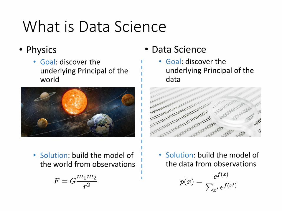
What is Data Science• Physics

• Goal: discover the underlying Principal of the world

• Solution: build the model of the world from observations

• Data Science• Goal: discover the

underlying Principal of the data

• Solution: build the model of the data from observations

F = Gm1m2

r2F = G

m1m2

r2 p(x) =ef(x)Px0 e

f(x0)p(x) =ef(x)Px0 e

f(x0)

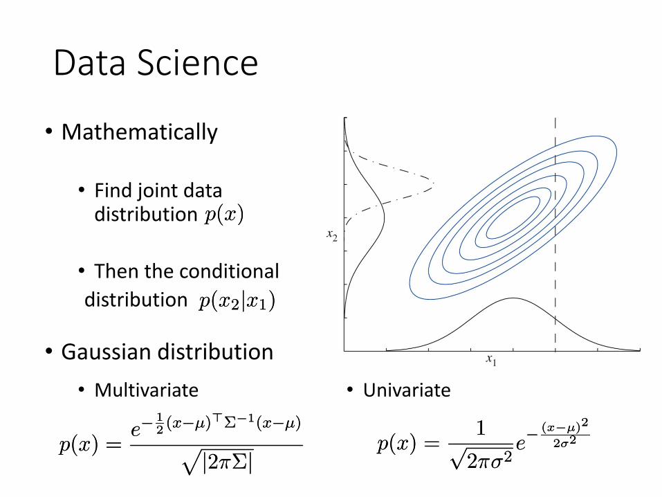
Data Science

• Mathematically

• Find joint data distribution

• Then the conditional distribution

p(x)p(x)

p(x2jx1)p(x2jx1)

p(x) =1p

2¼¾2e¡

(x¡¹)2

2¾2p(x) =1p

2¼¾2e¡

(x¡¹)2

2¾2p(x) =e¡

12(x¡¹)>§¡1(x¡¹)pj2¼§jp(x) =

e¡12(x¡¹)>§¡1(x¡¹)pj2¼§j

• Gaussian distribution• Multivariate • Univariate

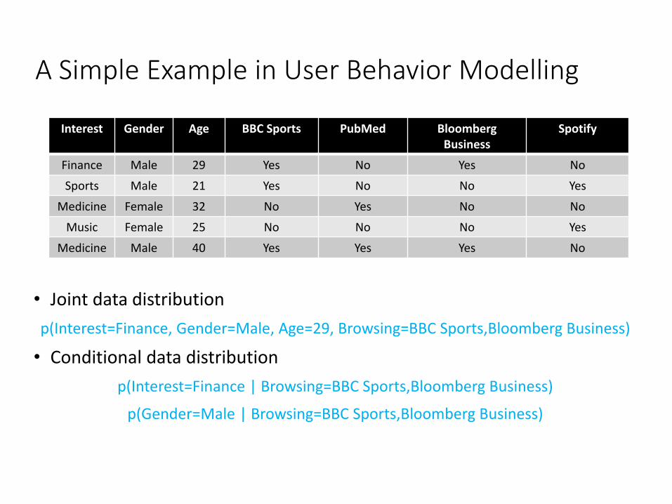
A Simple Example in User Behavior Modelling

Interest Gender Age BBC Sports PubMed Bloomberg Business

Spotify

Finance Male 29 Yes No Yes NoSports Male 21 Yes No No Yes

Medicine Female 32 No Yes No NoMusic Female 25 No No No Yes

Medicine Male 40 Yes Yes Yes No

• Joint data distribution p(Interest=Finance, Gender=Male, Age=29, Browsing=BBC Sports,Bloomberg Business)

• Conditional data distributionp(Interest=Finance | Browsing=BBC Sports,Bloomberg Business)

p(Gender=Male | Browsing=BBC Sports,Bloomberg Business)

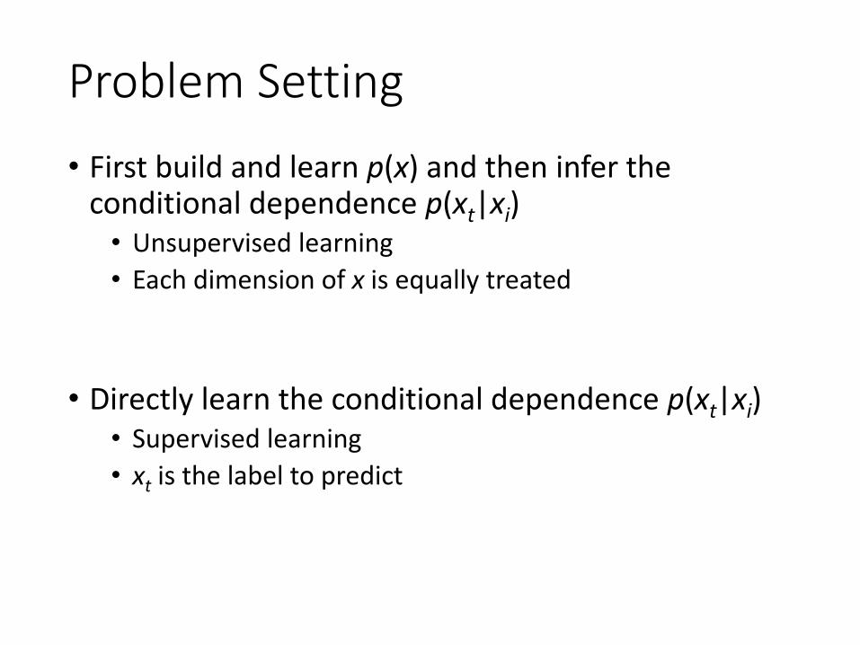
Problem Setting• First build and learn p(x) and then infer the

conditional dependence p(xt|xi)• Unsupervised learning• Each dimension of x is equally treated

• Directly learn the conditional dependence p(xt|xi)• Supervised learning• xt is the label to predict

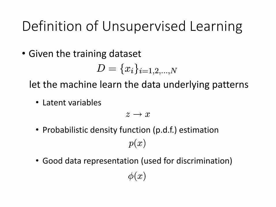
Definition of Unsupervised Learning

• Given the training dataset

let the machine learn the data underlying patternsD = fxigi=1;2;:::;ND = fxigi=1;2;:::;N

p(x)p(x)

• Probabilistic density function (p.d.f.) estimation

• Latent variablesz ! xz ! x

• Good data representation (used for discrimination)Á(x)Á(x)

Uses of Unsupervised Learning• Data structure discovery, data science

• Data compression

• Outlier detection

• Input to supervised/reinforcement algorithms (causes may be more simply related to outputs or rewards)

• A theory of biological learning and perception

Slide credit: Maneesh Sahani

Content• Fundamentals of Unsupervised Learning

• K-means clustering• Principal component analysis

• Probabilistic Unsupervised Learning• Mixture Gaussians• EM Methods

• Deep Unsupervised Learning• Auto-encoders• Generative adversarial nets

Content• Fundamentals of Unsupervised Learning

• K-means clustering• Principal component analysis

• Probabilistic Unsupervised Learning• Mixture Gaussians• EM Methods

• Deep Unsupervised Learning• Auto-encoders• Generative adversarial nets

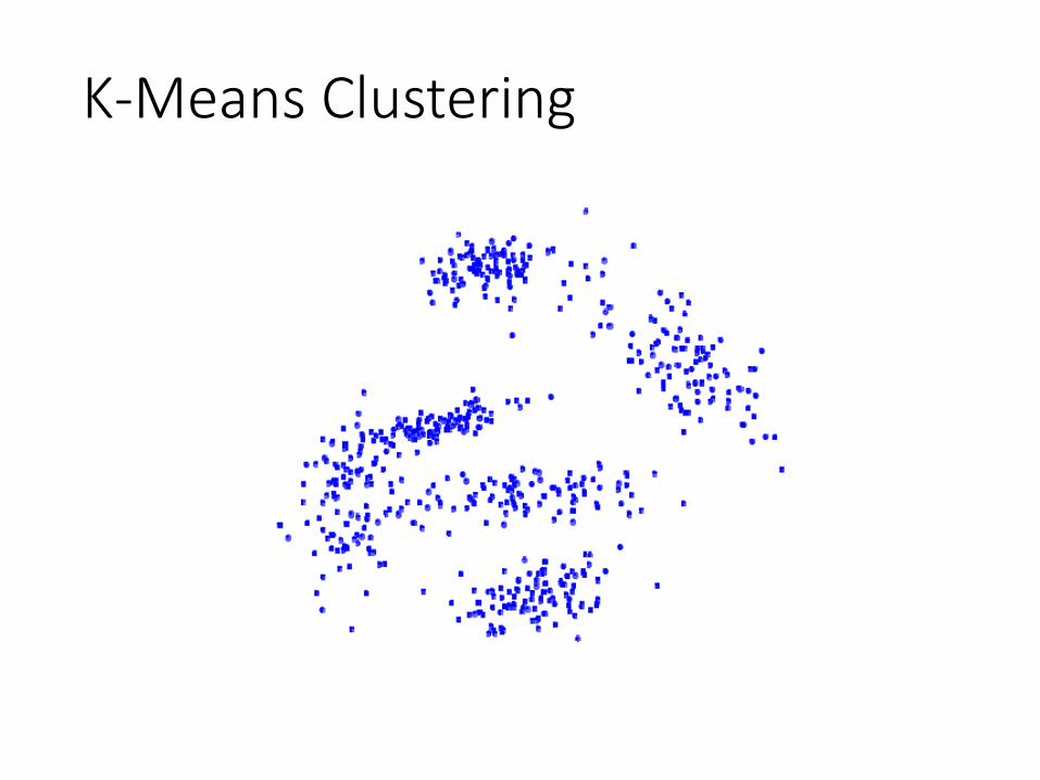
K-Means Clustering

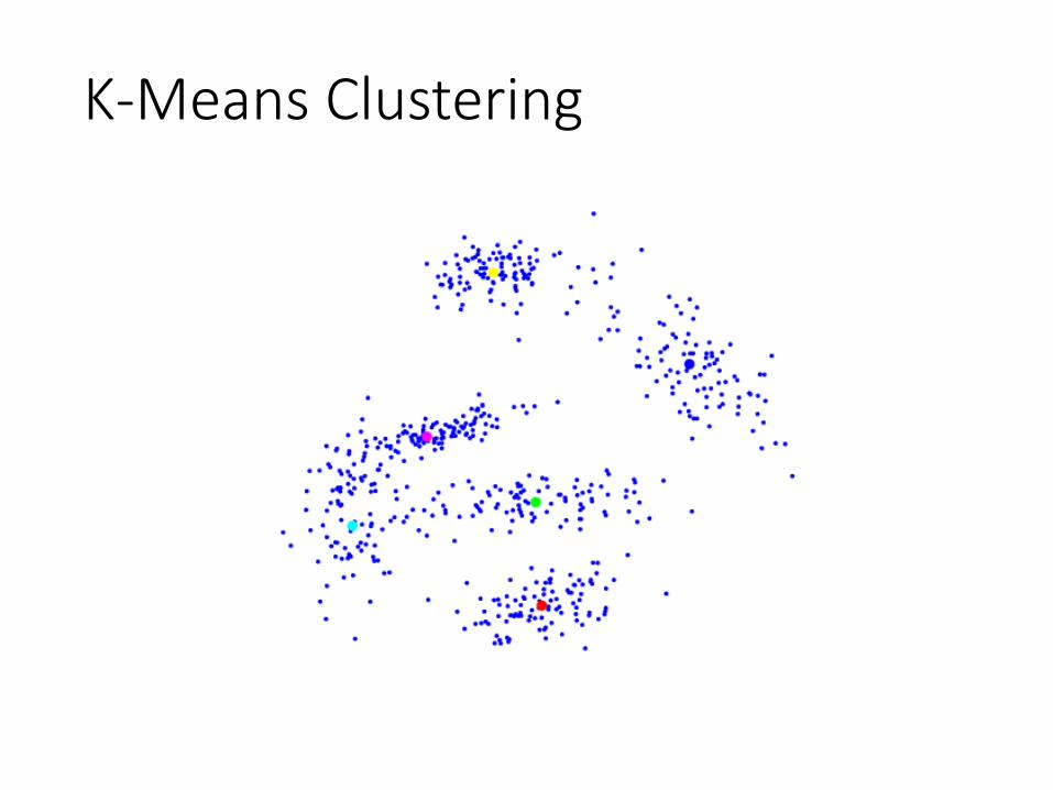
K-Means Clustering

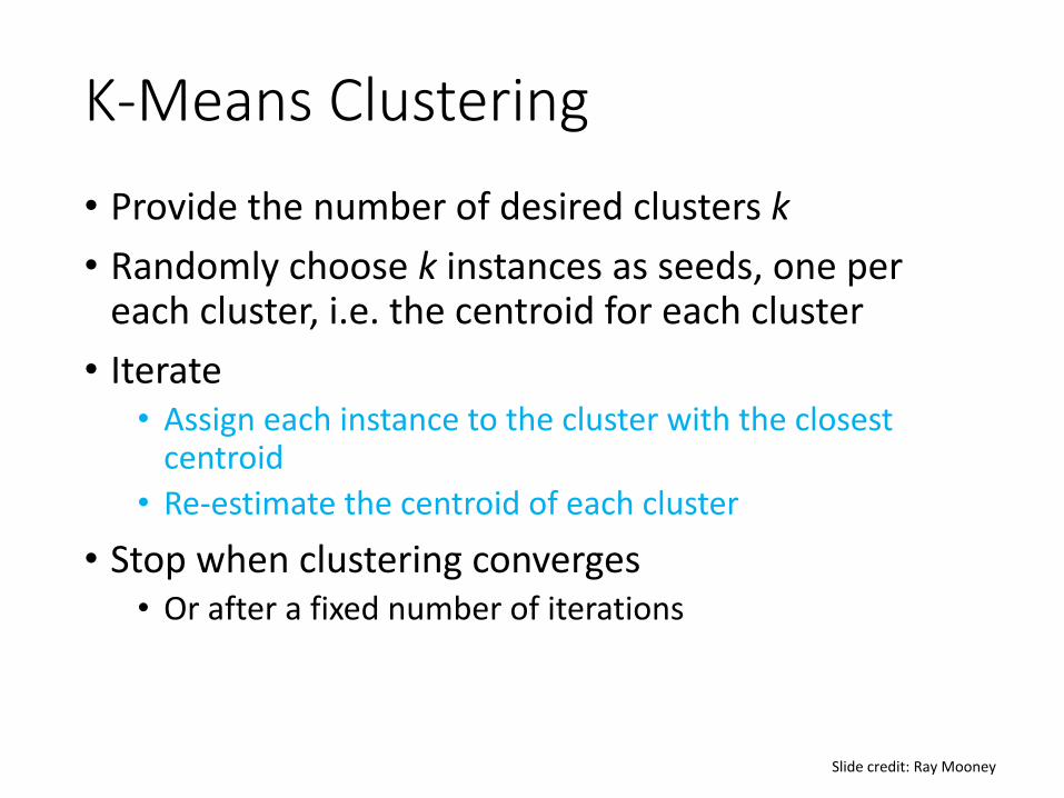
K-Means Clustering• Provide the number of desired clusters k• Randomly choose k instances as seeds, one per

each cluster, i.e. the centroid for each cluster• Iterate

• Assign each instance to the cluster with the closest centroid

• Re-estimate the centroid of each cluster• Stop when clustering converges

• Or after a fixed number of iterations

Slide credit: Ray Mooney

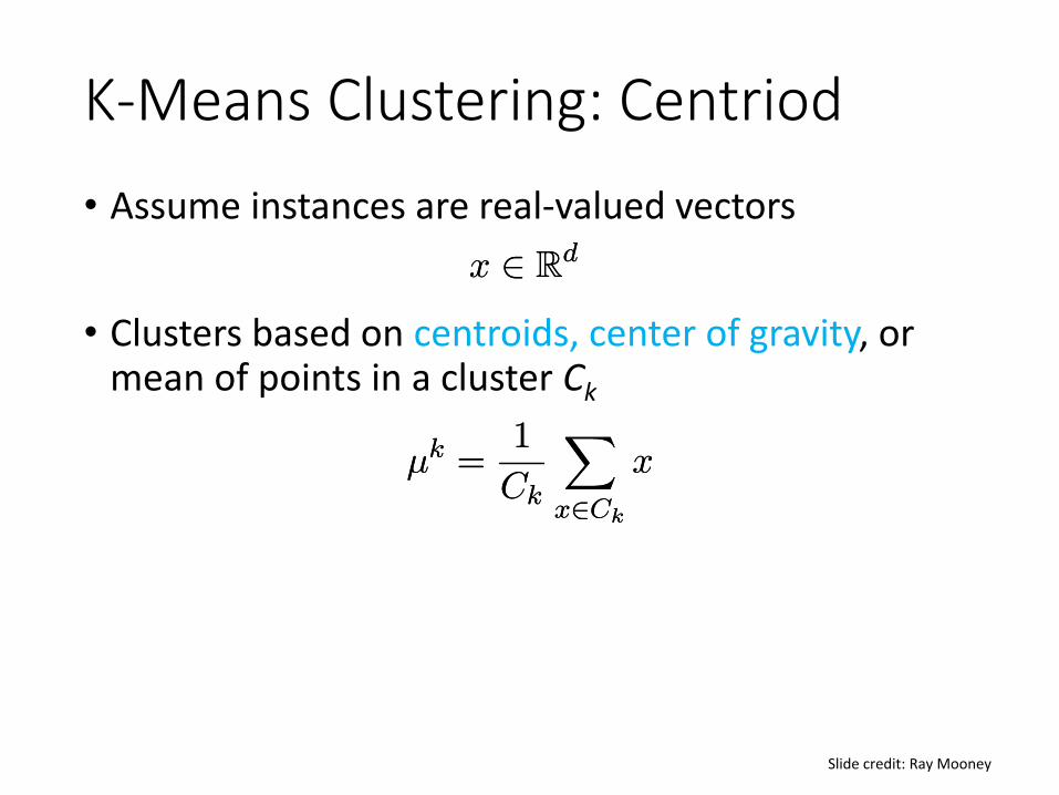
K-Means Clustering: Centriod• Assume instances are real-valued vectors

Slide credit: Ray Mooney

x 2 Rdx 2 Rd

• Clusters based on centroids, center of gravity, or mean of points in a cluster Ck

¹k =1

Ck

Xx2Ck

x¹k =1

Ck

Xx2Ck

x

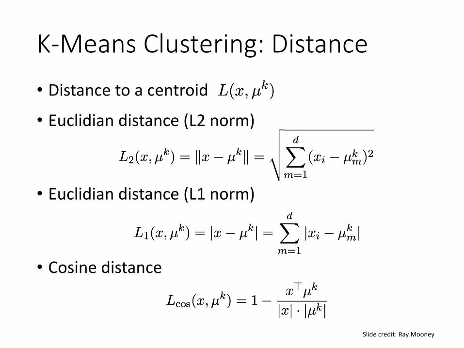
K-Means Clustering: Distance• Distance to a centroid

Slide credit: Ray Mooney

L(x; ¹k)L(x; ¹k)

• Euclidian distance (L2 norm)

L2(x; ¹k) = kx¡ ¹kk =

vuut dXm=1

(xi ¡ ¹km)2L2(x; ¹k) = kx¡ ¹kk =

vuut dXm=1

(xi ¡ ¹km)2

• Euclidian distance (L1 norm)

L1(x; ¹k) = jx¡ ¹kj =dX

m=1

jxi ¡ ¹kmjL1(x; ¹k) = jx¡ ¹kj =

dXm=1

jxi ¡ ¹kmj

• Cosine distance

Lcos(x; ¹k) = 1¡ x>¹k

jxj ¢ j¹kjLcos(x; ¹k) = 1¡ x>¹k

jxj ¢ j¹kj

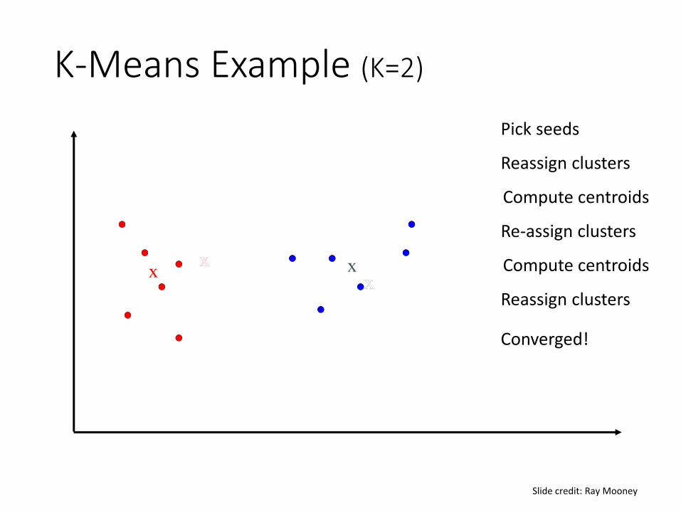
K-Means Example (K=2)

Pick seeds

Reassign clusters

Compute centroids

xx

Re-assign clusters

xx xx Compute centroids

Reassign clusters

Converged!

Slide credit: Ray Mooney

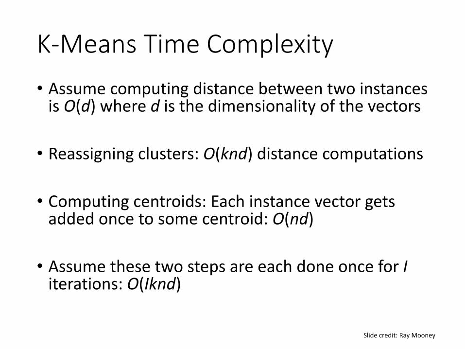
K-Means Time Complexity• Assume computing distance between two instances

is O(d) where d is the dimensionality of the vectors

• Reassigning clusters: O(knd) distance computations

• Computing centroids: Each instance vector gets added once to some centroid: O(nd)

• Assume these two steps are each done once for Iiterations: O(Iknd)

Slide credit: Ray Mooney

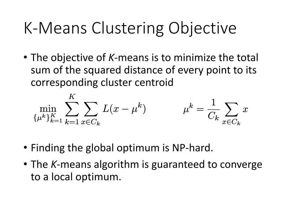
K-Means Clustering Objective• The objective of K-means is to minimize the total

sum of the squared distance of every point to its corresponding cluster centroid

minf¹kgK

k=1

KXk=1

Xx2Ck

L(x¡ ¹k)minf¹kgK

k=1

KXk=1

Xx2Ck

L(x¡ ¹k) ¹k =1

Ck

Xx2Ck

x¹k =1

Ck

Xx2Ck

x

• Finding the global optimum is NP-hard.• The K-means algorithm is guaranteed to converge

to a local optimum.

Seed Choice• Results can vary based on random seed selection.

• Some seeds can result in poor convergence rate, or convergence to sub-optimal clusterings.

• Select good seeds using a heuristic or the results of another method.

Clustering Applications• Text mining

• Cluster documents for related search• Cluster words for query suggestion

• Recommender systems and advertising• Cluster users for item/ad recommendation• Cluster items for related item suggestion

• Image search• Cluster images for similar image search and duplication

detection• Speech recognition or separation

• Cluster phonetical features

Principal Component Analysis (PCA)

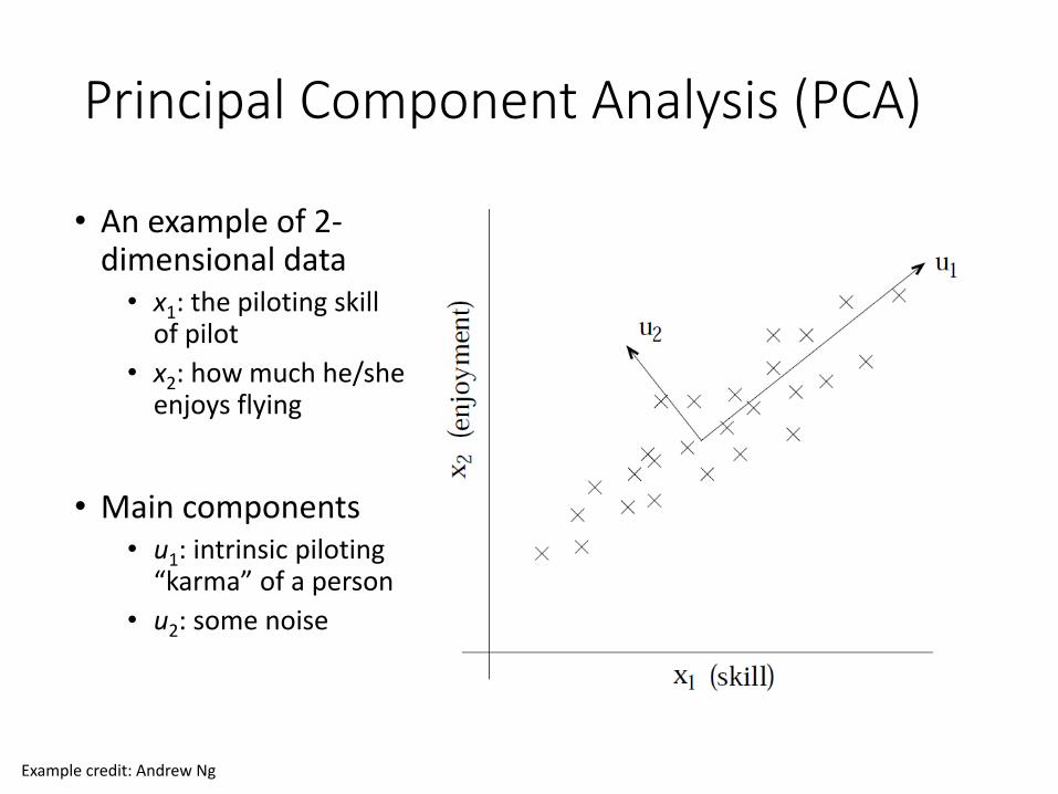
• An example of 2-dimensional data

• x1: the piloting skill of pilot

• x2: how much he/she enjoys flying

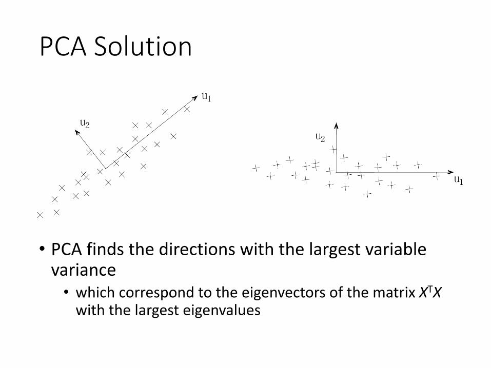
• Main components• u1: intrinsic piloting

“karma” of a person• u2: some noise

Example credit: Andrew Ng

Principal Component Analysis (PCA)

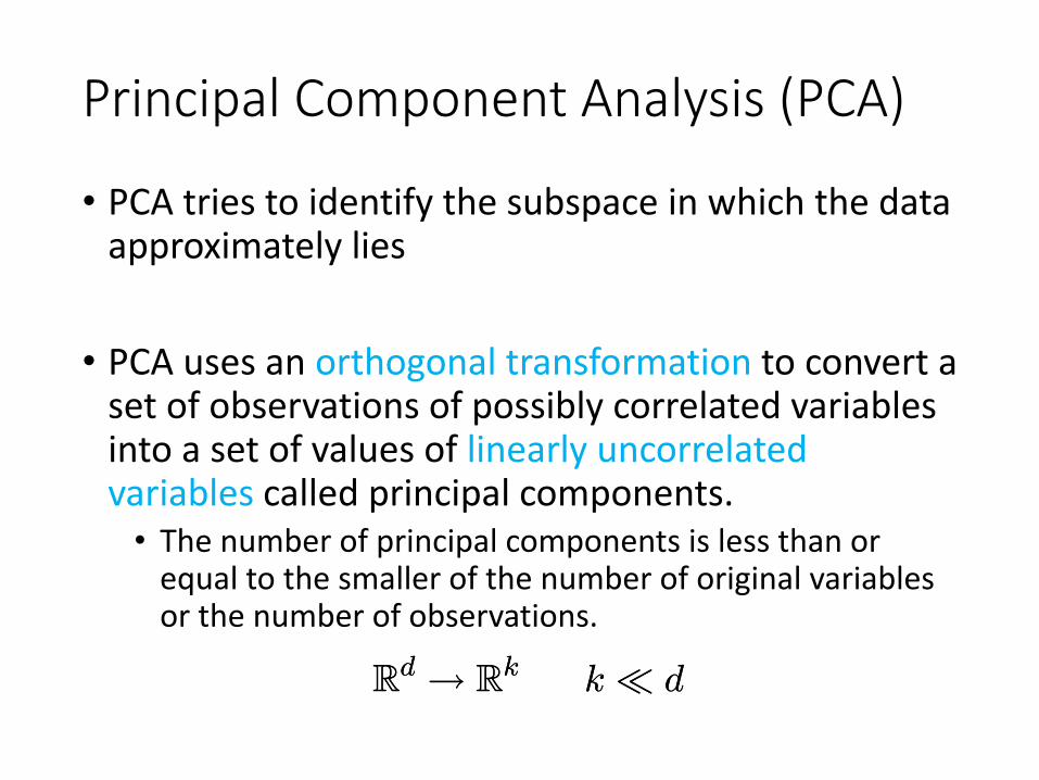
• PCA tries to identify the subspace in which the data approximately lies

• PCA uses an orthogonal transformation to convert a set of observations of possibly correlated variables into a set of values of linearly uncorrelated variables called principal components.

• The number of principal components is less than or equal to the smaller of the number of original variables or the number of observations.

Rd ! Rk k ¿ dRd ! Rk k ¿ d

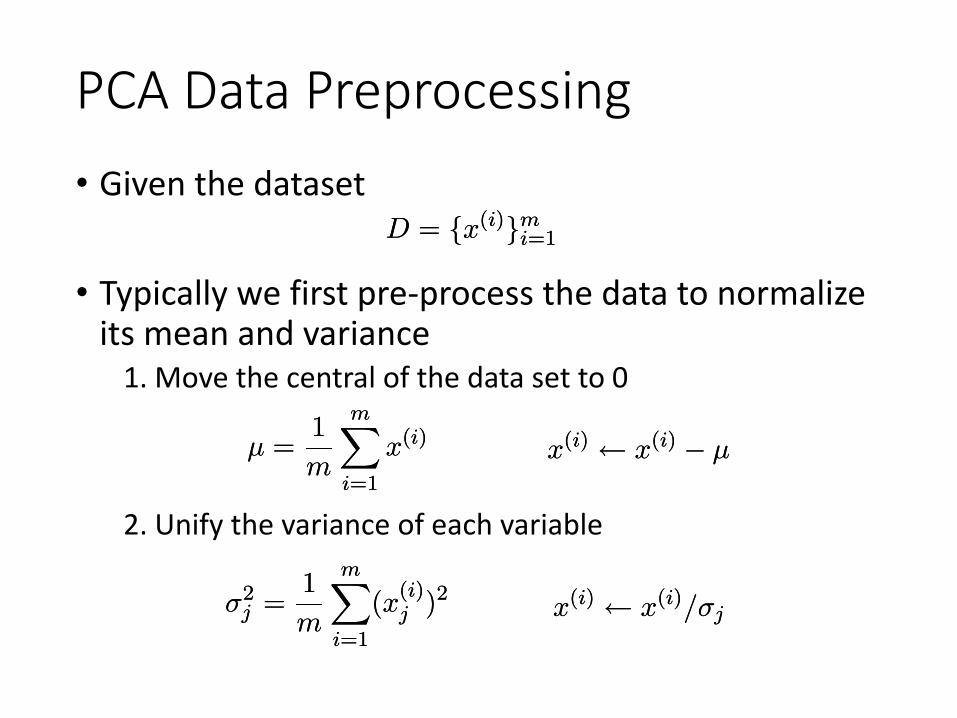
PCA Data Preprocessing

• Typically we first pre-process the data to normalize its mean and variance

1. Move the central of the data set to 0

¹ =1

m

mXi=1

x(i)¹ =1

m

mXi=1

x(i)

• Given the datasetD = fx(i)gm

i=1D = fx(i)gmi=1

x(i) Ã x(i) ¡ ¹x(i) Ã x(i) ¡ ¹

2. Unify the variance of each variable

¾2j =

1

m

mXi=1

(x(i)j )2¾2

j =1

m

mXi=1

(x(i)j )2 x(i) Ã x(i)=¾jx(i) Ã x(i)=¾j

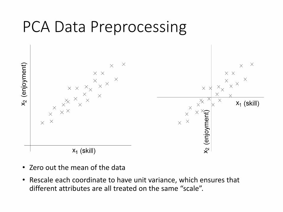
PCA Data Preprocessing

• Zero out the mean of the data• Rescale each coordinate to have unit variance, which ensures that

different attributes are all treated on the same “scale”.

PCA Solution

• PCA finds the directions with the largest variable variance

• which correspond to the eigenvectors of the matrix XTXwith the largest eigenvalues

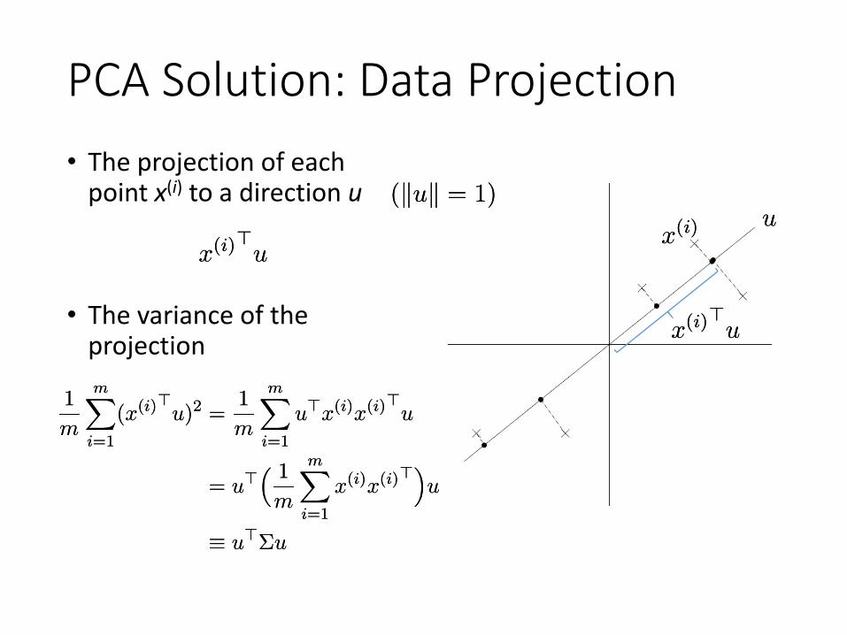
PCA Solution: Data Projection• The projection of each

point x(i) to a direction uuu

x(i)x(i)

x(i)>ux(i)>u

x(i)>ux(i)>u

• The variance of the projection

1

m

mXi=1

(x(i)>u)2 =1

m

mXi=1

u>x(i)x(i)>u

= u>³ 1

m

mXi=1

x(i)x(i)>´u

´ u>§u

1

m

mXi=1

(x(i)>u)2 =1

m

mXi=1

u>x(i)x(i)>u

= u>³ 1

m

mXi=1

x(i)x(i)>´u

´ u>§u

(kuk = 1)(kuk = 1)

uux(i)x(i)

x(i)>ux(i)>u

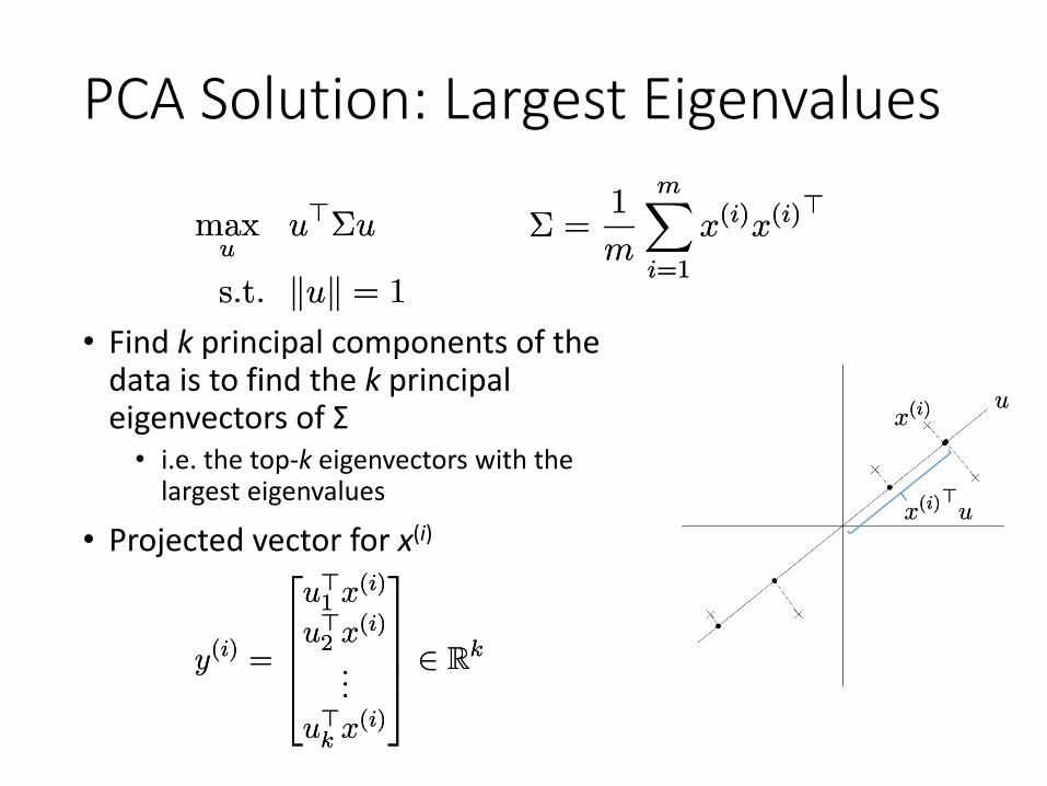
PCA Solution: Largest Eigenvalues

• Find k principal components of the data is to find the k principal eigenvectors of Σ

• i.e. the top-k eigenvectors with the largest eigenvalues

• Projected vector for x(i)

maxu

u>§u

s.t. kuk = 1

maxu

u>§u

s.t. kuk = 1

§ =1

m

mXi=1

x(i)x(i)>§ =1

m

mXi=1

x(i)x(i)>

y(i) =

26664u>1 x(i)

u>2 x(i)

...

u>k x(i)

37775 2 Rky(i) =

26664u>1 x(i)

u>2 x(i)

...

u>k x(i)

37775 2 Rk

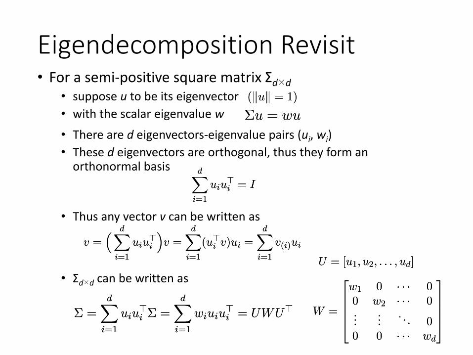
Eigendecomposition Revisit• For a semi-positive square matrix Σd×d

• suppose u to be its eigenvector • with the scalar eigenvalue w §u = wu§u = wu

(kuk = 1)(kuk = 1)

• Thus any vector v can be written as

• There are d eigenvectors-eigenvalue pairs (ui, wi)• These d eigenvectors are orthogonal, thus they form an

orthonormal basis dXi=1

uiu>i = I

dXi=1

uiu>i = I

v =³ dX

i=1

uiu>i

´v =

dXi=1

(u>i v)ui =dX

i=1

v(i)uiv =³ dX

i=1

uiu>i

´v =

dXi=1

(u>i v)ui =dX

i=1

v(i)ui

• Σd×d can be written as

§ =dX

i=1

uiu>i § =

dXi=1

wiuiu>i = UWU>§ =

dXi=1

uiu>i § =

dXi=1

wiuiu>i = UWU>

U = [u1; u2; : : : ; ud]U = [u1; u2; : : : ; ud]

W =

26664w1 0 ¢ ¢ ¢ 00 w2 ¢ ¢ ¢ 0...

.... . . 0

0 0 ¢ ¢ ¢ wd

37775W =

26664w1 0 ¢ ¢ ¢ 00 w2 ¢ ¢ ¢ 0...

.... . . 0

0 0 ¢ ¢ ¢ wd

37775

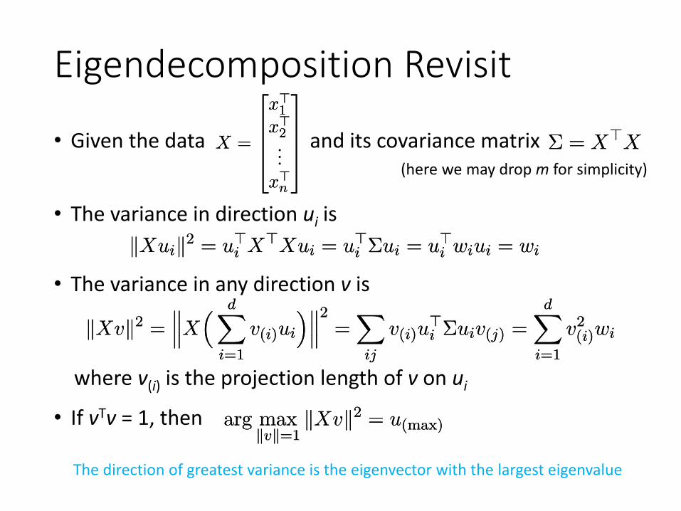
Eigendecomposition Revisit

and its covariance matrix § = X>X§ = X>XX =

26664x>1x>2...

x>n

37775X =

26664x>1x>2...

x>n

37775

• The variance in any direction v is

• Given the data

kXvk2 =°°°X

³ dXi=1

v(i)ui

´°°°2=

Xij

v(i)u>i §uiv(j) =

dXi=1

v2(i)wikXvk2 =

°°°X³ dX

i=1

v(i)ui

´°°°2=

Xij

v(i)u>i §uiv(j) =

dXi=1

v2(i)wi

• The variance in direction ui is kXuik2 = u>i X>Xui = u>i §ui = u>i wiui = wikXuik2 = u>i X>Xui = u>i §ui = u>i wiui = wi

where v(i) is the projection length of v on ui

• If vTv = 1, then arg maxkvk=1

kXvk2 = u(max)arg maxkvk=1

kXvk2 = u(max)

The direction of greatest variance is the eigenvector with the largest eigenvalue

(here we may drop m for simplicity)

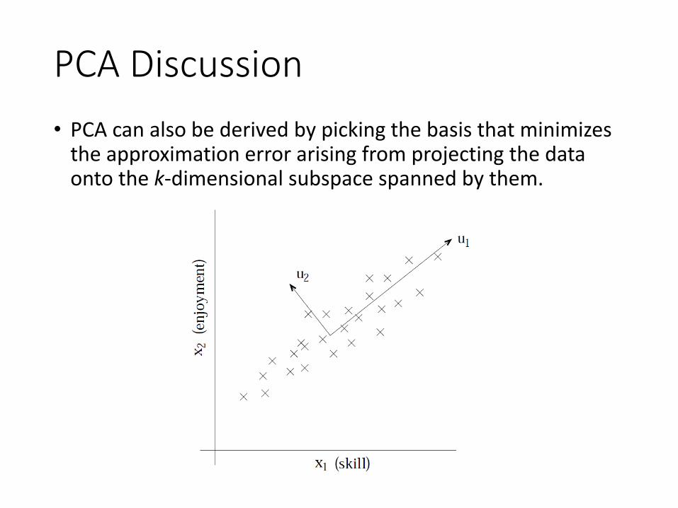
PCA Discussion• PCA can also be derived by picking the basis that minimizes

the approximation error arising from projecting the data onto the k-dimensional subspace spanned by them.

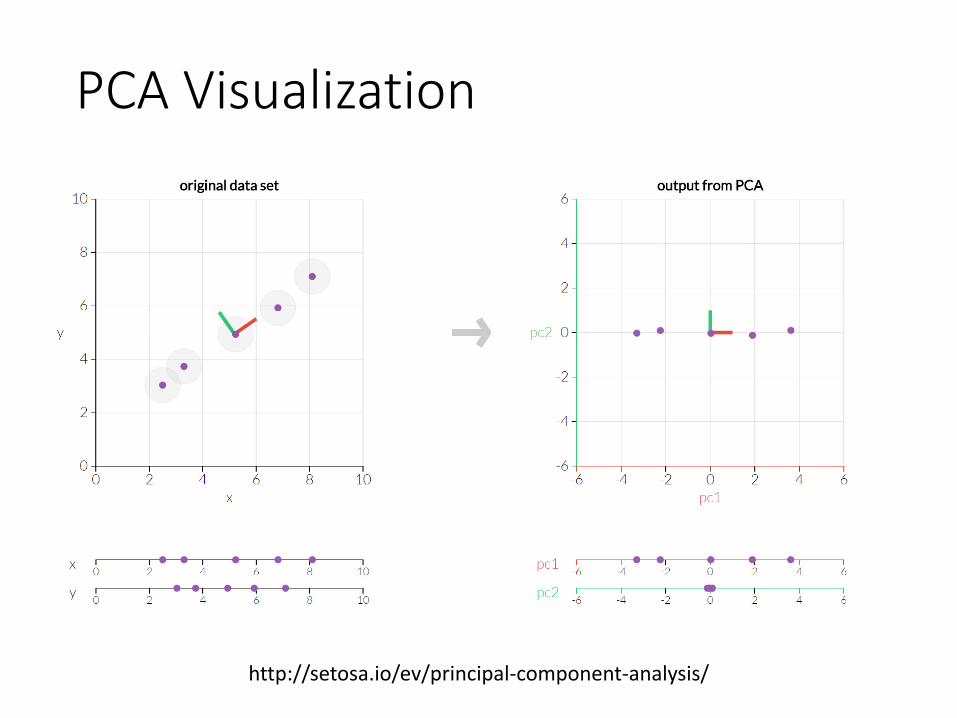
PCA Visualization

http://setosa.io/ev/principal-component-analysis/

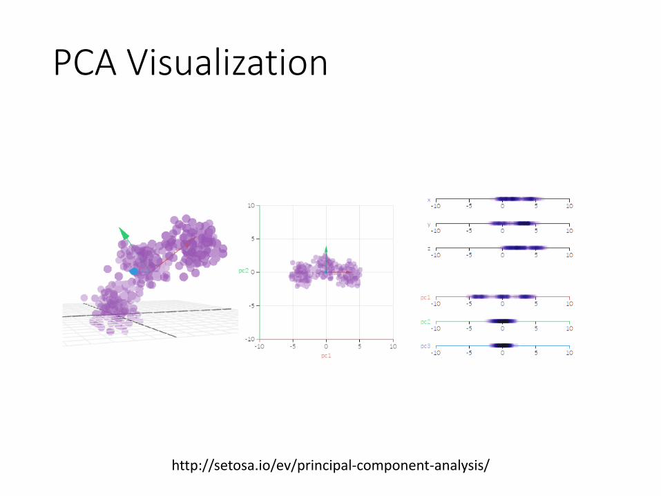
PCA Visualization

http://setosa.io/ev/principal-component-analysis/

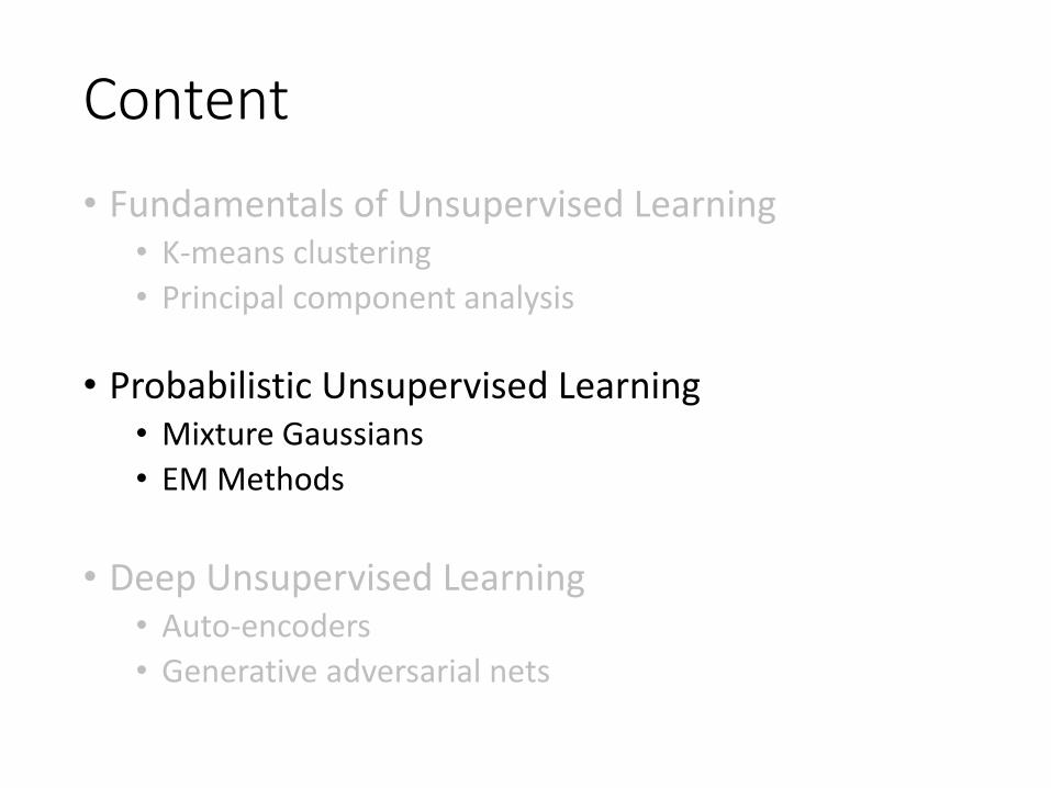
Content• Fundamentals of Unsupervised Learning

• K-means clustering• Principal component analysis

• Probabilistic Unsupervised Learning• Mixture Gaussians• EM Methods

• Deep Unsupervised Learning• Auto-encoders• Generative adversarial nets

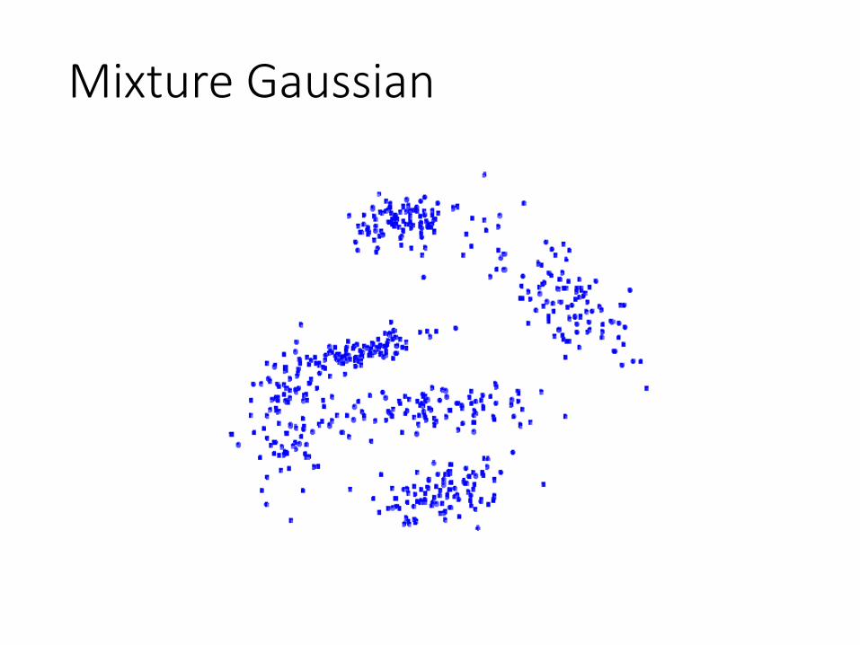
Mixture Gaussian

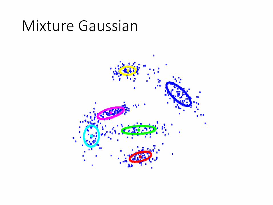
Mixture Gaussian

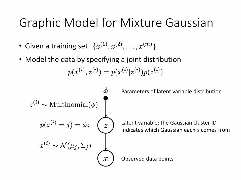
Graphic Model for Mixture Gaussian

• Given a training set

ÁÁ

zz

xx

fx(1); x(2); : : : ; x(m)gfx(1); x(2); : : : ; x(m)g• Model the data by specifying a joint distribution

p(x(i); z(i)) = p(x(i)jz(i))p(z(i))p(x(i); z(i)) = p(x(i)jz(i))p(z(i))

z(i) » Multinomial(Á)z(i) » Multinomial(Á)

x(i) » N (¹j ; §j)x(i) » N (¹j ; §j)

p(z(i) = j) = Ájp(z(i) = j) = ÁjLatent variable: the Gaussian cluster IDIndicates which Gaussian each x comes from

Observed data points

Parameters of latent variable distribution

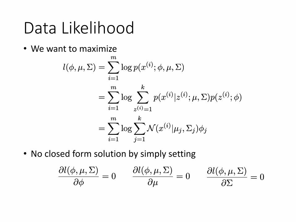
Data Likelihood

• No closed form solution by simply setting

l(Á; ¹; §) =

mXi=1

log p(x(i); Á; ¹;§)

=mX

i=1

logkX

z(i)=1

p(x(i)jz(i);¹;§)p(z(i);Á)

=

mXi=1

log

kXj=1

N (x(i)j¹j ; §j)Áj

l(Á; ¹; §) =

mXi=1

log p(x(i); Á; ¹;§)

=mX

i=1

logkX

z(i)=1

p(x(i)jz(i);¹;§)p(z(i);Á)

=

mXi=1

log

kXj=1

N (x(i)j¹j ; §j)Áj

@l(Á; ¹;§)

@Á= 0

@l(Á; ¹;§)

@Á= 0

@l(Á; ¹;§)

@¹= 0

@l(Á; ¹;§)

@¹= 0

@l(Á; ¹; §)

@§= 0

@l(Á; ¹; §)

@§= 0

• We want to maximize

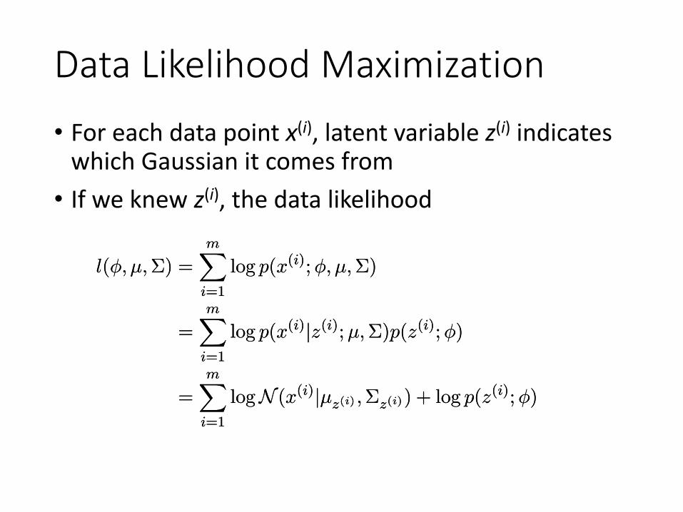
Data Likelihood Maximization• For each data point x(i), latent variable z(i) indicates

which Gaussian it comes from• If we knew z(i), the data likelihood

l(Á; ¹;§) =

mXi=1

log p(x(i); Á; ¹;§)

=mX

i=1

log p(x(i)jz(i); ¹;§)p(z(i);Á)

=mX

i=1

logN (x(i)j¹z(i) ;§z(i)) + log p(z(i);Á)

l(Á; ¹;§) =

mXi=1

log p(x(i); Á; ¹;§)

=mX

i=1

log p(x(i)jz(i); ¹;§)p(z(i);Á)

=mX

i=1

logN (x(i)j¹z(i) ;§z(i)) + log p(z(i);Á)

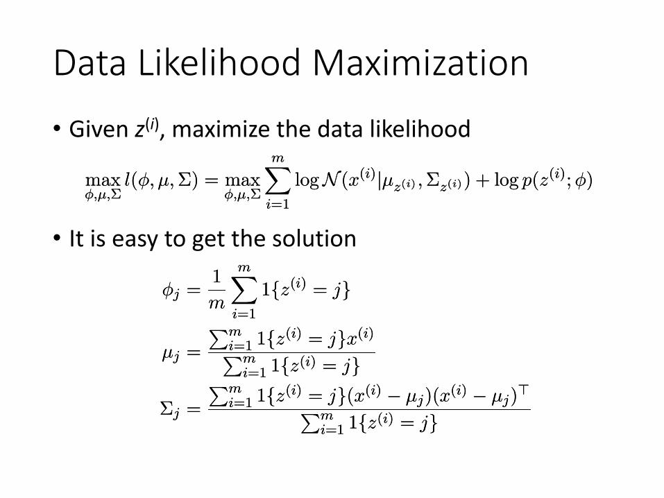
Data Likelihood Maximization• Given z(i), maximize the data likelihood

maxÁ;¹;§

l(Á; ¹; §) = maxÁ;¹;§

mXi=1

logN (x(i)j¹z(i) ;§z(i)) + log p(z(i);Á)maxÁ;¹;§

l(Á; ¹; §) = maxÁ;¹;§

mXi=1

logN (x(i)j¹z(i) ;§z(i)) + log p(z(i);Á)

• It is easy to get the solution

Áj =1

m

mXi=1

1fz(i) = jg

¹j =

Pmi=1 1fz(i) = jgx(i)Pm

i=1 1fz(i) = jg

§j =

Pmi=1 1fz(i) = jg(x(i) ¡ ¹j)(x

(i) ¡ ¹j)>Pm

i=1 1fz(i) = jg

Áj =1

m

mXi=1

1fz(i) = jg

¹j =

Pmi=1 1fz(i) = jgx(i)Pm

i=1 1fz(i) = jg

§j =

Pmi=1 1fz(i) = jg(x(i) ¡ ¹j)(x

(i) ¡ ¹j)>Pm

i=1 1fz(i) = jg

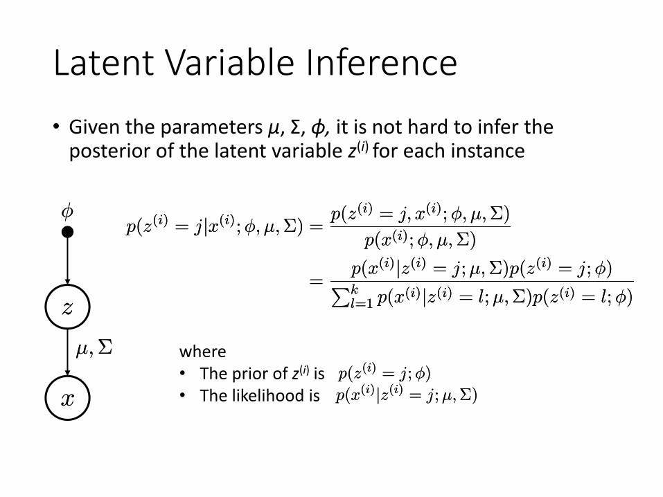
Latent Variable Inference• Given the parameters μ, Σ, ϕ, it is not hard to infer the

posterior of the latent variable z(i) for each instance

p(z(i) = jjx(i);Á; ¹;§) =p(z(i) = j; x(i);Á; ¹;§)

p(x(i);Á; ¹; §)

=p(x(i)jz(i) = j;¹; §)p(z(i) = j;Á)Pkl=1 p(x(i)jz(i) = l;¹;§)p(z(i) = l;Á)

p(z(i) = jjx(i);Á; ¹;§) =p(z(i) = j; x(i);Á; ¹;§)

p(x(i);Á; ¹; §)

=p(x(i)jz(i) = j;¹; §)p(z(i) = j;Á)Pkl=1 p(x(i)jz(i) = l;¹;§)p(z(i) = l;Á)

ÁÁ

zz

xx

¹;§¹;§ where• The prior of z(i) is• The likelihood is

p(z(i) = j; Á)p(z(i) = j; Á)

p(x(i)jz(i) = j; ¹;§)p(x(i)jz(i) = j; ¹;§)

Expectation Maximization Methods• E-step: infer the posterior distribution of the latent

variables given the model parameters• M-step: tune parameters to maximize the data

likelihood given the latent variable distribution

• EM methods• Iteratively execute E-step and M-step until convergence

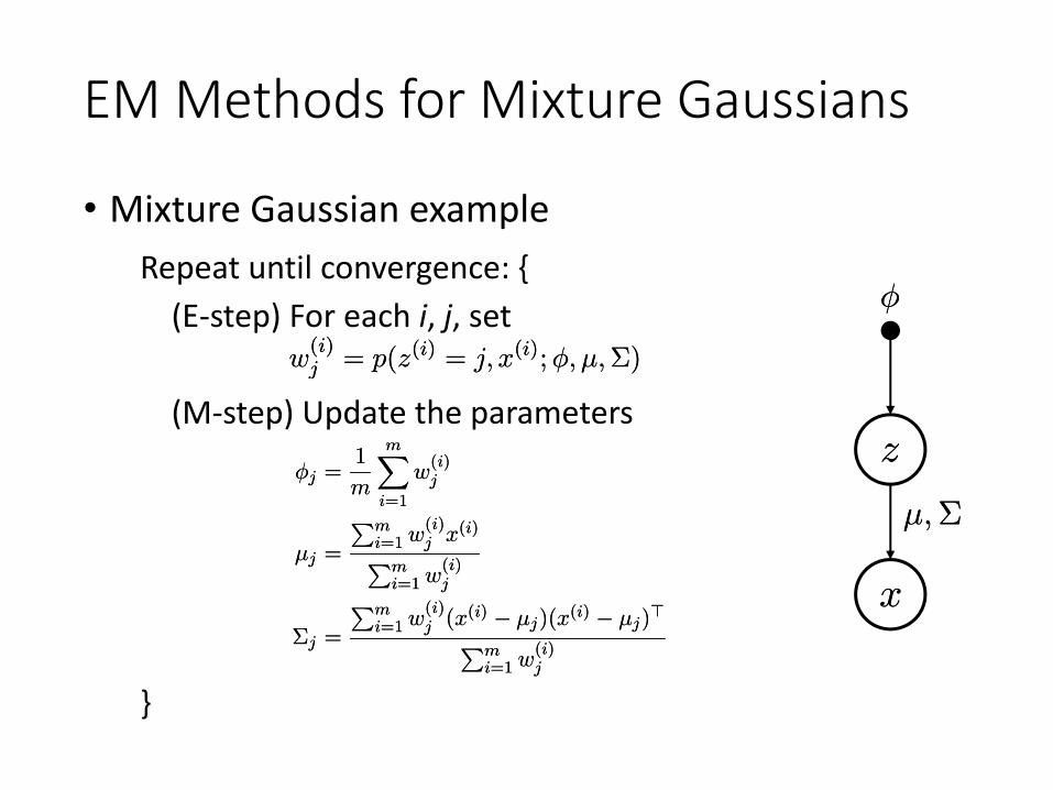
EM Methods for Mixture Gaussians

ÁÁ

zz

xx

¹;§¹;§

Repeat until convergence: {(E-step) For each i, j, set

(M-step) Update the parameters

}

• Mixture Gaussian example

w(i)j = p(z(i) = j; x(i);Á; ¹; §)w(i)j = p(z(i) = j; x(i);Á; ¹; §)

Áj =1

m

mXi=1

w(i)j

¹j =

Pmi=1 w

(i)j x(i)Pm

i=1 w(i)j

§j =

Pmi=1 w

(i)j (x(i) ¡ ¹j)(x

(i) ¡ ¹j)>Pm

i=1 w(i)j

Áj =1

m

mXi=1

w(i)j

¹j =

Pmi=1 w

(i)j x(i)Pm

i=1 w(i)j

§j =

Pmi=1 w

(i)j (x(i) ¡ ¹j)(x

(i) ¡ ¹j)>Pm

i=1 w(i)j

General EM Methods• Claims: 1. After each E-M step, the data likelihood will not

decrease.2. The EM algorithm finds a (local) maximum of a

latent variable model likelihood

• Now let’s discuss the general EM methods and verify its effectiveness of improving data likelihood and its convergence

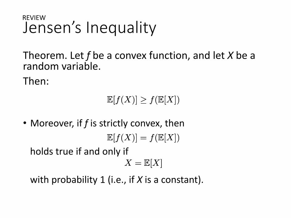
Jensen’s InequalityTheorem. Let f be a convex function, and let X be a random variable.Then:

E[f(X)] ¸ f(E[X])E[f(X)] ¸ f(E[X])

• Moreover, if f is strictly convex, then

holds true if and only if

with probability 1 (i.e., if X is a constant).

E[f(X)] = f(E[X])E[f(X)] = f(E[X])

X = E[X]X = E[X]

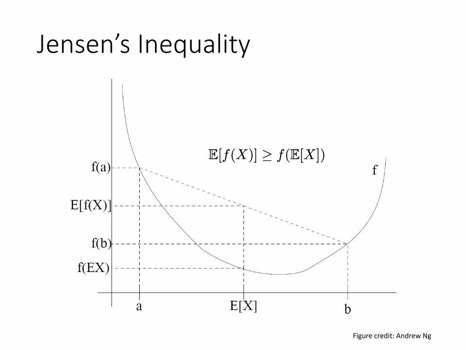
Jensen’s Inequality

E[f(X)] ¸ f(E[X])E[f(X)] ¸ f(E[X])

Figure credit: Andrew Ng

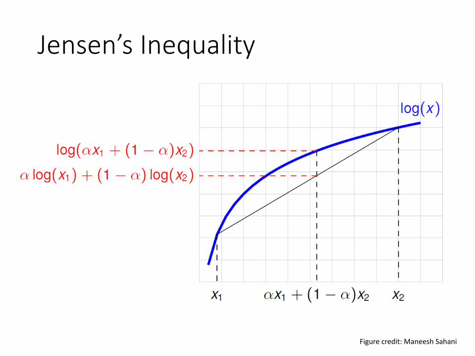
Jensen’s Inequality

Figure credit: Maneesh Sahani

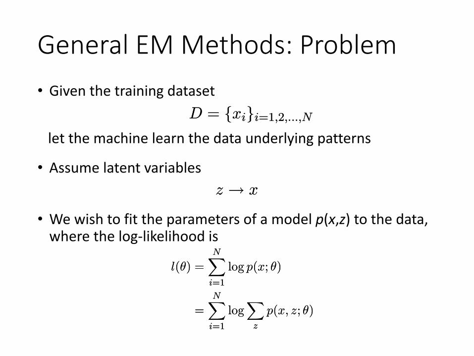
General EM Methods: Problem• Given the training dataset

let the machine learn the data underlying patternsD = fxigi=1;2;:::;ND = fxigi=1;2;:::;N

• Assume latent variablesz ! xz ! x

• We wish to fit the parameters of a model p(x,z) to the data, where the log-likelihood is

l(μ) =NX

i=1

log p(x; μ)

=NX

i=1

logX

z

p(x; z; μ)

l(μ) =NX

i=1

log p(x; μ)

=NX

i=1

logX

z

p(x; z; μ)

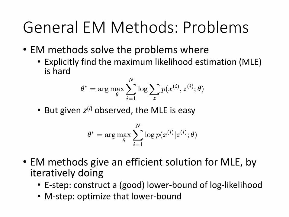
General EM Methods: Problems• EM methods solve the problems where

• Explicitly find the maximum likelihood estimation (MLE) is hard

μ¤ = arg maxμ

NXi=1

logX

z

p(x(i); z(i); μ)μ¤ = arg maxμ

NXi=1

logX

z

p(x(i); z(i); μ)

• But given z(i) observed, the MLE is easy

μ¤ = arg maxμ

NXi=1

log p(x(i)jz(i); μ)μ¤ = arg maxμ

NXi=1

log p(x(i)jz(i); μ)

• EM methods give an efficient solution for MLE, by iteratively doing

• E-step: construct a (good) lower-bound of log-likelihood• M-step: optimize that lower-bound

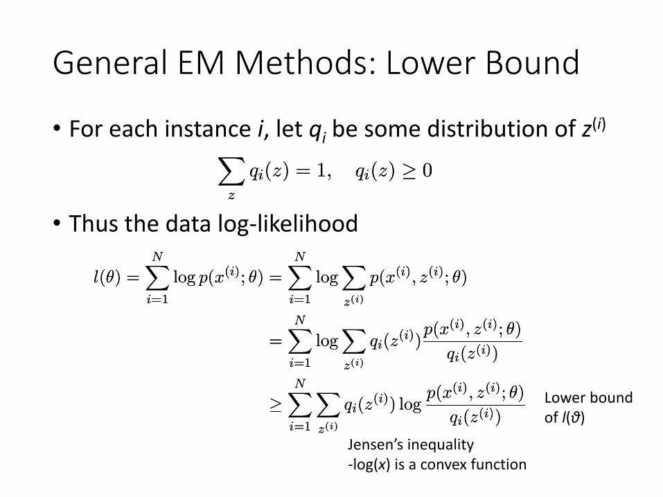
General EM Methods: Lower Bound

• For each instance i, let qi be some distribution of z(i)Xz

qi(z) = 1; qi(z) ¸ 0X

z

qi(z) = 1; qi(z) ¸ 0

• Thus the data log-likelihood

l(μ) =NX

i=1

log p(x(i); μ) =NX

i=1

logXz(i)

p(x(i); z(i); μ)

=NX

i=1

logXz(i)

qi(z(i))

p(x(i); z(i); μ)

qi(z(i))

¸NX

i=1

Xz(i)

qi(z(i)) log

p(x(i); z(i); μ)

qi(z(i))

l(μ) =NX

i=1

log p(x(i); μ) =NX

i=1

logXz(i)

p(x(i); z(i); μ)

=NX

i=1

logXz(i)

qi(z(i))

p(x(i); z(i); μ)

qi(z(i))

¸NX

i=1

Xz(i)

qi(z(i)) log

p(x(i); z(i); μ)

qi(z(i))

Jensen’s inequality-log(x) is a convex function

Lower boundof l(θ)

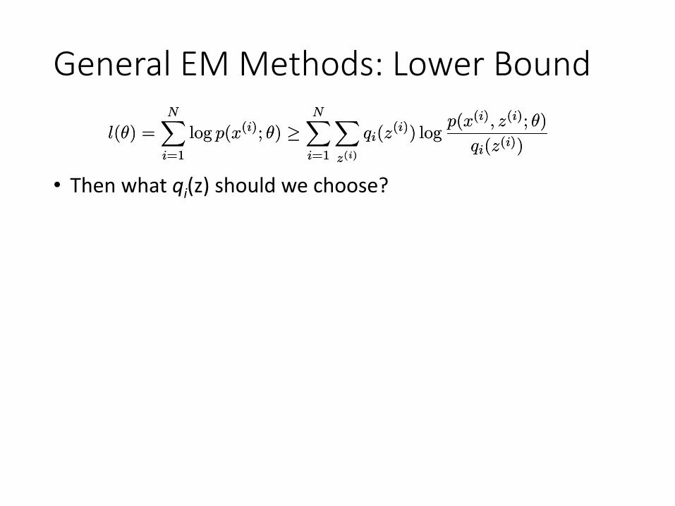
General EM Methods: Lower Bound

• Then what qi(z) should we choose?

l(μ) =NX

i=1

log p(x(i); μ) ¸NX

i=1

Xz(i)

qi(z(i)) log

p(x(i); z(i); μ)

qi(z(i))l(μ) =

NXi=1

log p(x(i); μ) ¸NX

i=1

Xz(i)

qi(z(i)) log

p(x(i); z(i); μ)

qi(z(i))

Jensen’s InequalityTheorem. Let f be a convex function, and let X be a random variable.Then:

E[f(X)] ¸ f(E[X])E[f(X)] ¸ f(E[X])

• Moreover, if f is strictly convex, then

holds true if and only if

with probability 1 (i.e., if X is a constant).

E[f(X)] = f(E[X])E[f(X)] = f(E[X])

X = E[X]X = E[X]

REVIEW

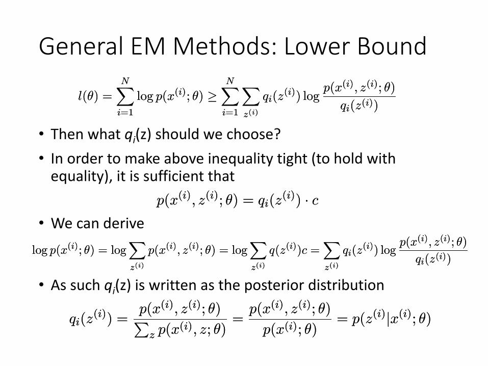
General EM Methods: Lower Bound

• Then what qi(z) should we choose?• In order to make above inequality tight (to hold with

equality), it is sufficient that

l(μ) =NX

i=1

log p(x(i); μ) ¸NX

i=1

Xz(i)

qi(z(i)) log

p(x(i); z(i); μ)

qi(z(i))l(μ) =

NXi=1

log p(x(i); μ) ¸NX

i=1

Xz(i)

qi(z(i)) log

p(x(i); z(i); μ)

qi(z(i))

p(x(i); z(i); μ) = qi(z(i)) ¢ cp(x(i); z(i); μ) = qi(z(i)) ¢ c

log p(x(i); μ) = logXz(i)

p(x(i); z(i); μ) = logXz(i)

q(z(i))c =Xz(i)

qi(z(i)) log

p(x(i); z(i); μ)

qi(z(i))log p(x(i); μ) = log

Xz(i)

p(x(i); z(i); μ) = logXz(i)

q(z(i))c =Xz(i)

qi(z(i)) log

p(x(i); z(i); μ)

qi(z(i))

• We can derive

• As such qi(z) is written as the posterior distribution

qi(z(i)) =

p(x(i); z(i); μ)Pz p(x(i); z; μ)

=p(x(i); z(i); μ)

p(x(i); μ)= p(z(i)jx(i); μ)qi(z

(i)) =p(x(i); z(i); μ)P

z p(x(i); z; μ)=

p(x(i); z(i); μ)

p(x(i); μ)= p(z(i)jx(i); μ)

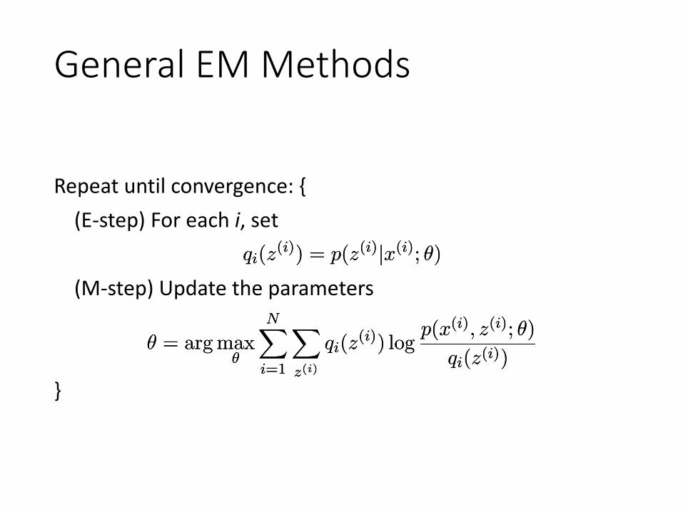
General EM Methods

Repeat until convergence: {(E-step) For each i, set

(M-step) Update the parameters

}

qi(z(i)) = p(z(i)jx(i); μ)qi(z(i)) = p(z(i)jx(i); μ)

μ = arg maxμ

NXi=1

Xz(i)

qi(z(i)) log

p(x(i); z(i); μ)

qi(z(i))μ = arg max

μ

NXi=1

Xz(i)

qi(z(i)) log

p(x(i); z(i); μ)

qi(z(i))

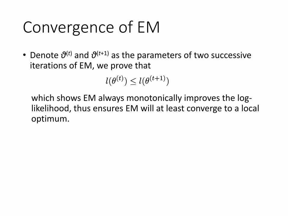
Convergence of EM• Denote θ(t) and θ(t+1) as the parameters of two successive

iterations of EM, we prove thatl(μ(t)) · l(μ(t+1))l(μ(t)) · l(μ(t+1))

which shows EM always monotonically improves the log-likelihood, thus ensures EM will at least converge to a local optimum.

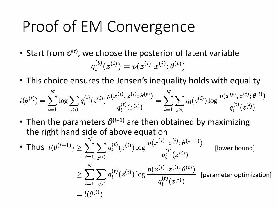
Proof of EM Convergence• Start from θ(t), we choose the posterior of latent variable

q(t)i (z(i)) = p(z(i)jx(i); μ(t))q(t)i (z(i)) = p(z(i)jx(i); μ(t))

• This choice ensures the Jensen’s inequality holds with equality

l(μ(t)) =NX

i=1

logXz(i)

q(t)i (z(i))

p(x(i); z(i); μ(t))

q(t)i (z(i))

=NX

i=1

Xz(i)

qi(z(i)) log

p(x(i); z(i); μ(t))

q(t)i (z(i))

l(μ(t)) =NX

i=1

logXz(i)

q(t)i (z(i))

p(x(i); z(i); μ(t))

q(t)i (z(i))

=NX

i=1

Xz(i)

qi(z(i)) log

p(x(i); z(i); μ(t))

q(t)i (z(i))

• Then the parameters θ(t+1) are then obtained by maximizing the right hand side of above equation

• Thus l(μ(t+1)) ¸NX

i=1

Xz(i)

q(t)i (z(i)) log

p(x(i); z(i); μ(t+1))

q(t)i (z(i))

¸NX

i=1

Xz(i)

q(t)i (z(i)) log

p(x(i); z(i); μ(t))

q(t)i (z(i))

= l(μ(t))

l(μ(t+1)) ¸NX

i=1

Xz(i)

q(t)i (z(i)) log

p(x(i); z(i); μ(t+1))

q(t)i (z(i))

¸NX

i=1

Xz(i)

q(t)i (z(i)) log

p(x(i); z(i); μ(t))

q(t)i (z(i))

= l(μ(t))

[lower bound]

[parameter optimization]

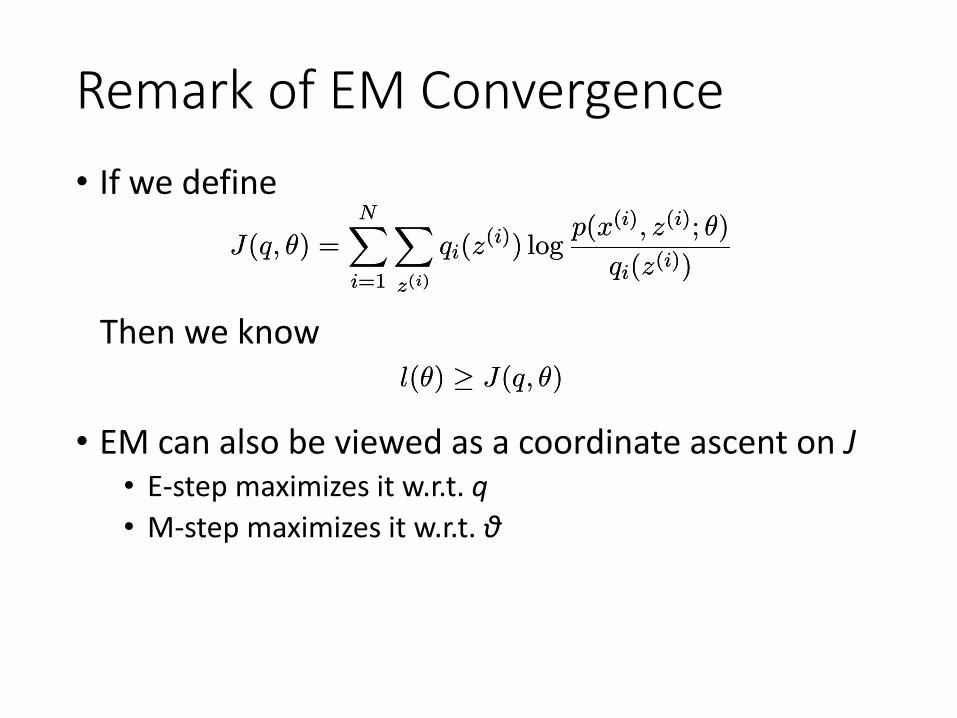
Remark of EM Convergence• If we define

J(q; μ) =NX

i=1

Xz(i)

qi(z(i)) log

p(x(i); z(i); μ)

qi(z(i))J(q; μ) =

NXi=1

Xz(i)

qi(z(i)) log

p(x(i); z(i); μ)

qi(z(i))

Then we knowl(μ) ¸ J(q; μ)l(μ) ¸ J(q; μ)

• EM can also be viewed as a coordinate ascent on J• E-step maximizes it w.r.t. q• M-step maximizes it w.r.t. θ

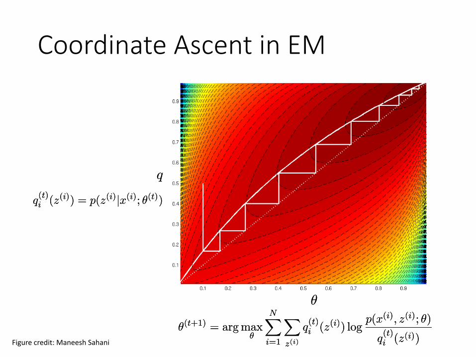
Coordinate Ascent in EM

μμ

qq

Figure credit: Maneesh Sahani

q(t)i (z(i)) = p(z(i)jx(i); μ(t))q(t)i (z(i)) = p(z(i)jx(i); μ(t))

μ(t+1) = arg maxμ

NXi=1

Xz(i)

q(t)i (z(i)) log

p(x(i); z(i); μ)

q(t)i (z(i))

μ(t+1) = arg maxμ

NXi=1

Xz(i)

q(t)i (z(i)) log

p(x(i); z(i); μ)

q(t)i (z(i))

Content• Fundamentals of Unsupervised Learning

• K-means clustering• Principal component analysis

• Probabilistic Unsupervised Learning• Mixture Gaussians• EM Methods

• Deep Unsupervised Learning• Auto-encoders• Generative adversarial nets

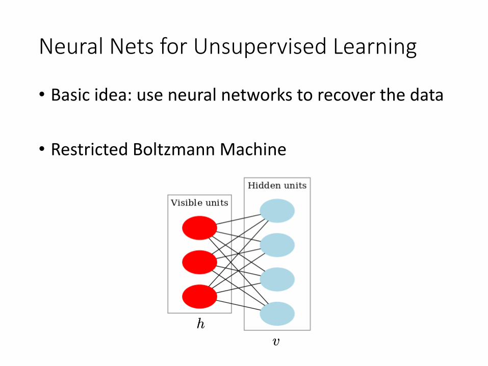
Neural Nets for Unsupervised Learning

• Basic idea: use neural networks to recover the data

• Restricted Boltzmann Machine

hhvv

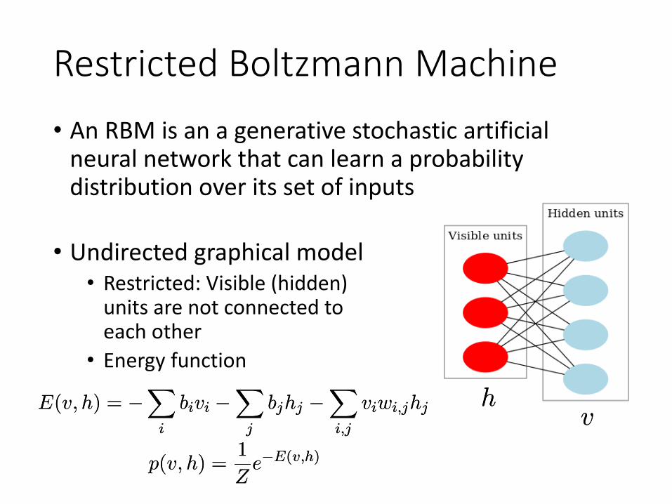
Restricted Boltzmann Machine• An RBM is an a generative stochastic artificial

neural network that can learn a probability distribution over its set of inputs

hhvv

• Undirected graphical model• Restricted: Visible (hidden)

units are not connected to each other

• Energy function

E(v; h) = ¡X

i

bivi ¡X

j

bjhj ¡Xi;j

viwi;jhjE(v; h) = ¡X

i

bivi ¡X

j

bjhj ¡Xi;j

viwi;jhj

p(v; h) =1

Ze¡E(v;h)p(v; h) =

1

Ze¡E(v;h)

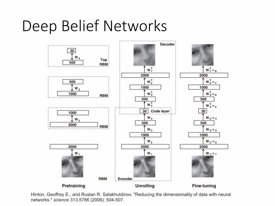
Deep Belief Networks

Hinton, Geoffrey E., and Ruslan R. Salakhutdinov. "Reducing the dimensionality of data with neural networks." science 313.5786 (2006): 504-507.

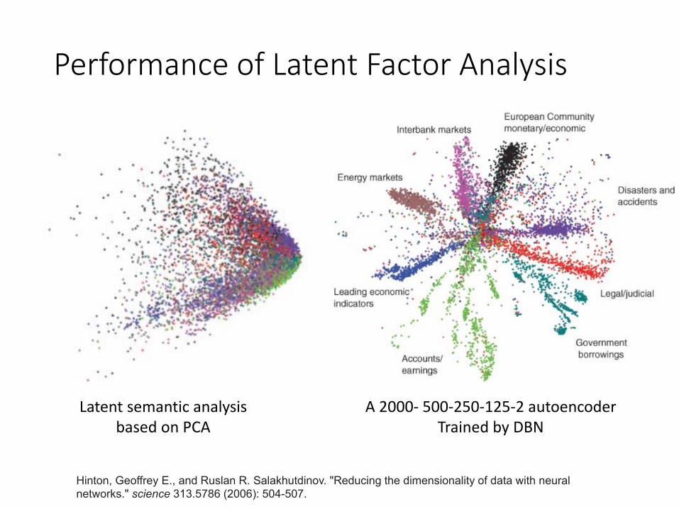
Performance of Latent Factor Analysis

Latent semantic analysisbased on PCA

A 2000- 500-250-125-2 autoencoderTrained by DBN

Hinton, Geoffrey E., and Ruslan R. Salakhutdinov. "Reducing the dimensionality of data with neural networks." science 313.5786 (2006): 504-507.

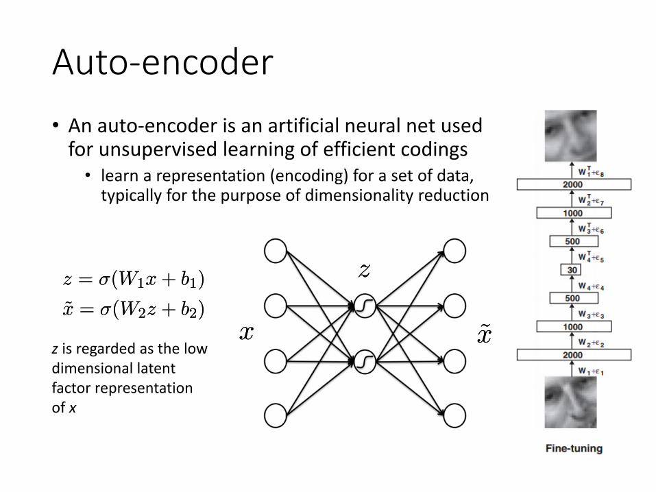
Auto-encoder• An auto-encoder is an artificial neural net used

for unsupervised learning of efficient codings• learn a representation (encoding) for a set of data,

typically for the purpose of dimensionality reduction

xx ~x~x

zzz = ¾(W1x + b1)

~x = ¾(W2z + b2)

z = ¾(W1x + b1)

~x = ¾(W2z + b2)

z is regarded as the low dimensional latent factor representation of x

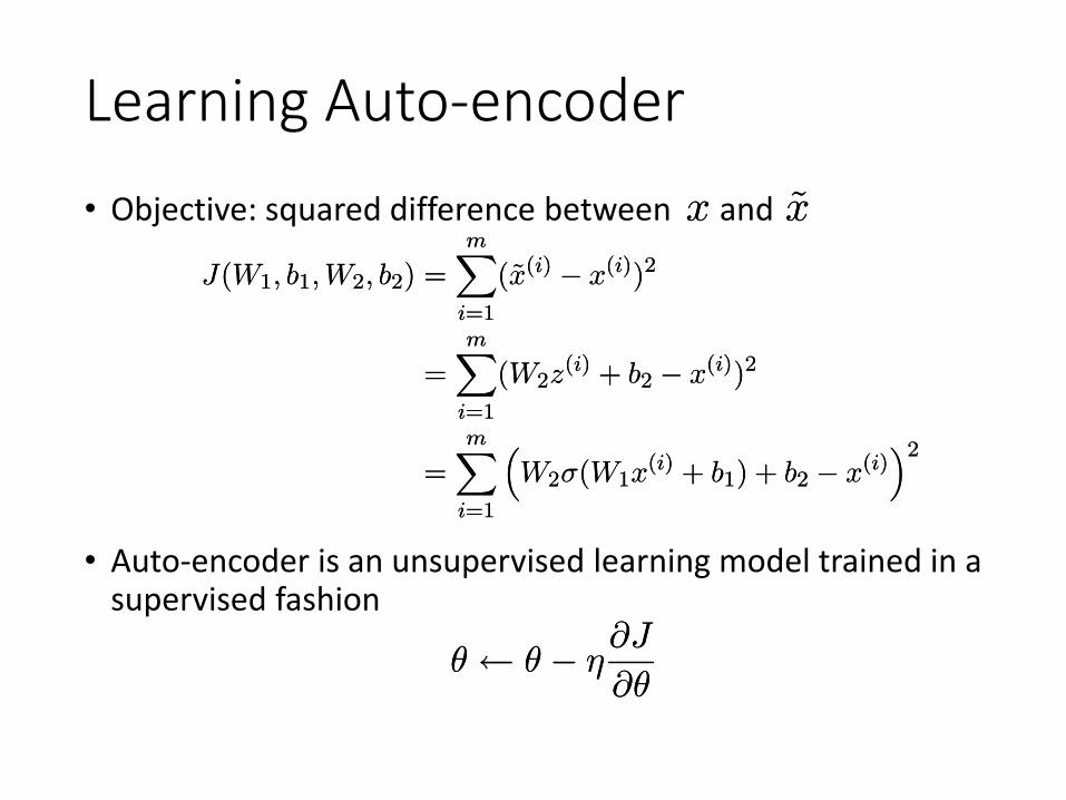
Learning Auto-encoder

• Objective: squared difference between and xx ~x~x

J(W1; b1;W2; b2) =

mXi=1

(~x(i) ¡ x(i))2

=mX

i=1

(W2z(i) + b2 ¡ x(i))2

=mX

i=1

³W2¾(W1x

(i) + b1) + b2 ¡ x(i)´2

J(W1; b1;W2; b2) =

mXi=1

(~x(i) ¡ x(i))2

=mX

i=1

(W2z(i) + b2 ¡ x(i))2

=mX

i=1

³W2¾(W1x

(i) + b1) + b2 ¡ x(i)´2

μ Ã μ ¡ ´@J

@μμ Ã μ ¡ ´

@J

@μ

• Auto-encoder is an unsupervised learning model trained in a supervised fashion

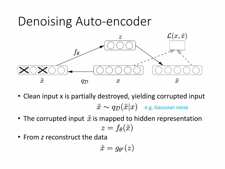
Denoising Auto-encoder

• Clean input x is partially destroyed, yielding corrupted input ~x » qD(~xjx)~x » qD(~xjx)

• The corrupted input is mapped to hidden representation ~x~xz = fμ(~x)z = fμ(~x)

xxqDqD~x~x

fμfμ

zz

x̂̂x

L(x; x̂)L(x; x̂)

• From z reconstruct the datax̂ = gμ0(z)x̂ = gμ0(z)

e.g. Gaussian noise

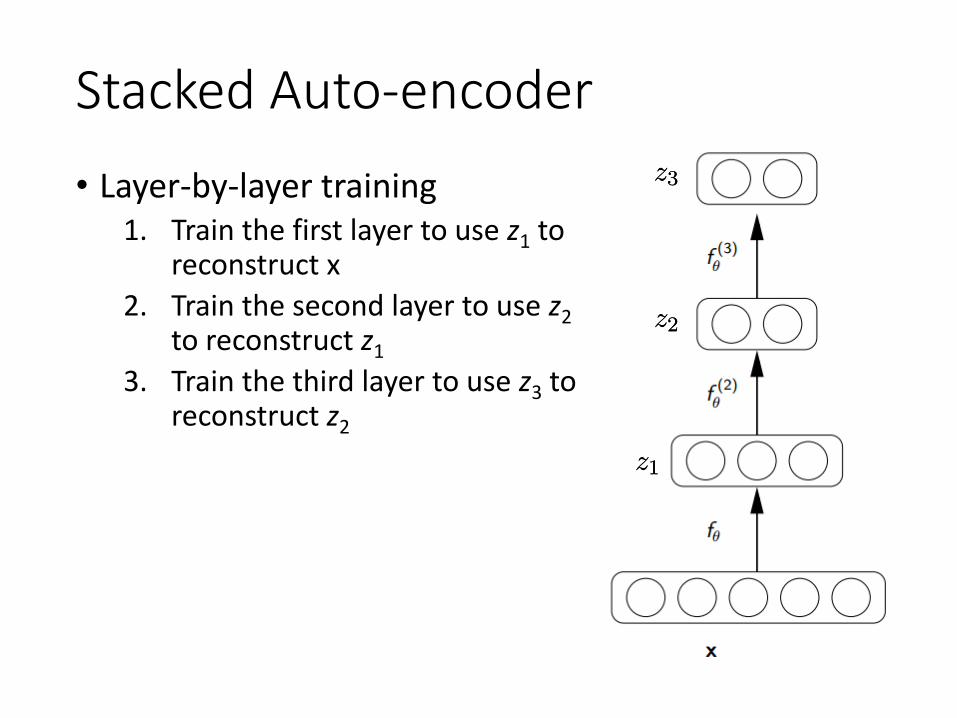
Stacked Auto-encoder• Layer-by-layer training

1. Train the first layer to use z1 to reconstruct x

2. Train the second layer to use z2to reconstruct z1

3. Train the third layer to use z3 to reconstruct z2

z1z1

z2z2

z3z3

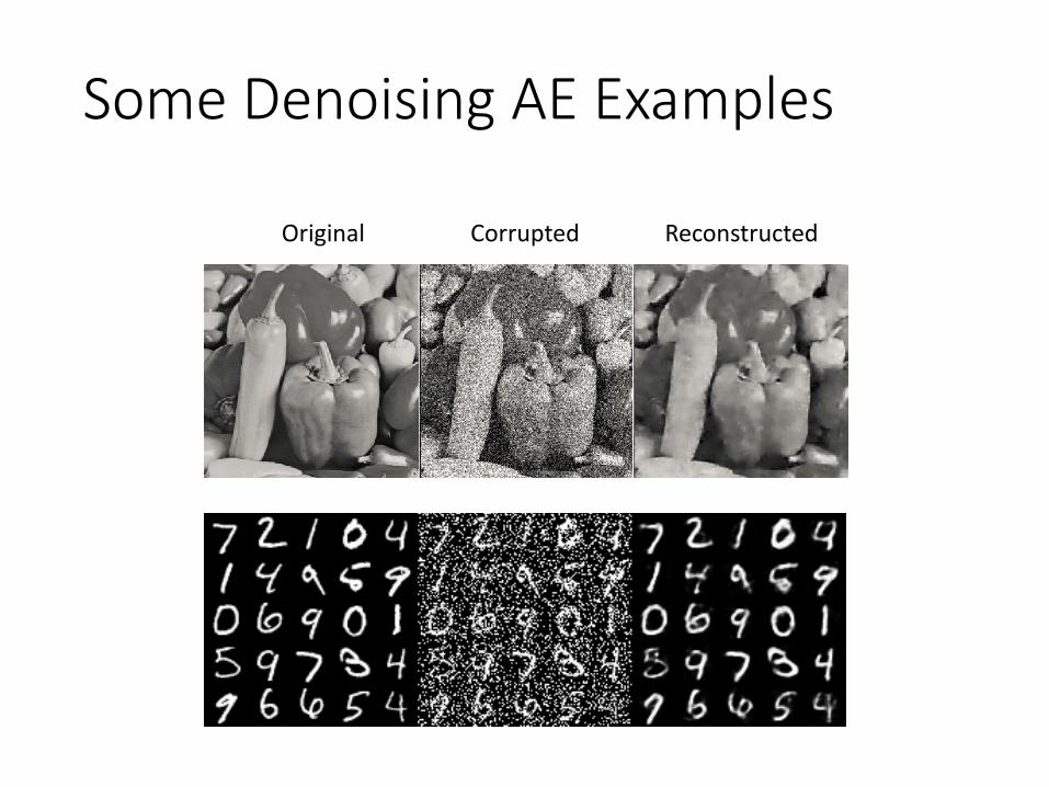
Some Denoising AE Examples

Original Corrupted Reconstructed

Generative Adversarial Networks (GANs)[Goodfellow, I., et al. 2014. Generative adversarial nets. In NIPS 2014.]

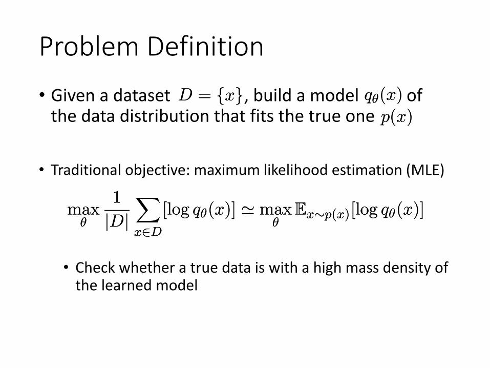
Problem Definition• Given a dataset , build a model of

the data distribution that fits the true oneD = fxgD = fxg qμ(x)qμ(x)

• Traditional objective: maximum likelihood estimation (MLE)

maxμ

1

jDjXx2D

[log qμ(x)] ' maxμ

Ex»p(x)[log qμ(x)]maxμ

1

jDjXx2D

[log qμ(x)] ' maxμ

Ex»p(x)[log qμ(x)]

p(x)p(x)

• Check whether a true data is with a high mass density of the learned model

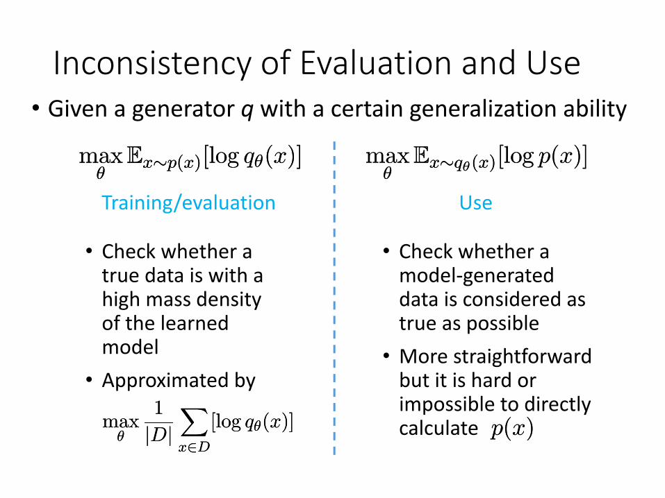
Inconsistency of Evaluation and Use

• Check whether a true data is with a high mass density of the learned model

• Approximated by

maxμ

Ex»p(x)[log qμ(x)]maxμ

Ex»p(x)[log qμ(x)] maxμ

Ex»qμ(x)[log p(x)]maxμ

Ex»qμ(x)[log p(x)]

Training/evaluation Use

• Check whether a model-generated data is considered as true as possible

• More straightforward but it is hard or impossible to directly calculate p(x)p(x)max

μ

1

jDjXx2D

[log qμ(x)]maxμ

1

jDjXx2D

[log qμ(x)]

• Given a generator q with a certain generalization ability

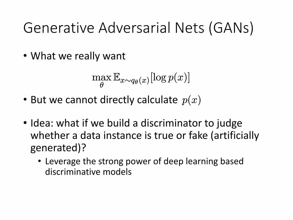
Generative Adversarial Nets (GANs)

• What we really want

maxμ

Ex»qμ(x)[log p(x)]maxμ

Ex»qμ(x)[log p(x)]

• But we cannot directly calculate p(x)p(x)

• Idea: what if we build a discriminator to judge whether a data instance is true or fake (artificially generated)?

• Leverage the strong power of deep learning based discriminative models

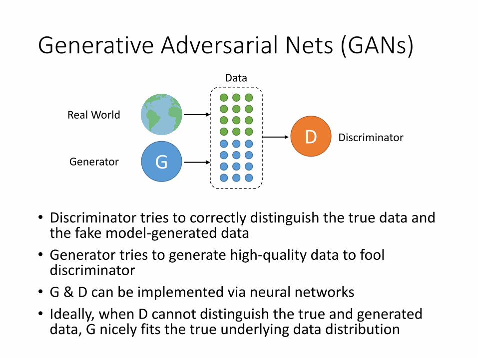
Generative Adversarial Nets (GANs)

• Discriminator tries to correctly distinguish the true data and the fake model-generated data

• Generator tries to generate high-quality data to fool discriminator

• G & D can be implemented via neural networks• Ideally, when D cannot distinguish the true and generated

data, G nicely fits the true underlying data distribution

GD

Real World

Generator

Discriminator

Data

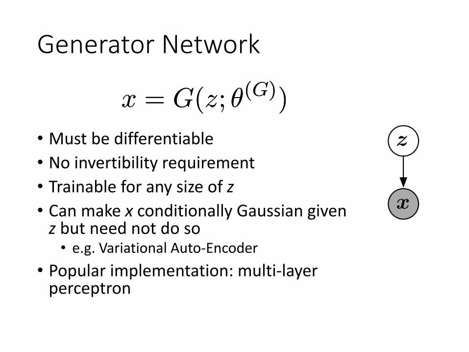
Generator Network

• Must be differentiable• No invertibility requirement• Trainable for any size of z• Can make x conditionally Gaussian given

z but need not do so• e.g. Variational Auto-Encoder

• Popular implementation: multi-layer perceptron

x = G(z; μ(G))x = G(z; μ(G))

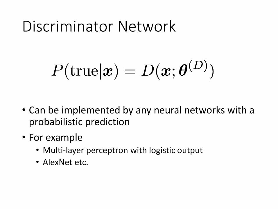
Discriminator Network

• Can be implemented by any neural networks with a probabilistic prediction

• For example• Multi-layer perceptron with logistic output• AlexNet etc.

P (truejx) = D(x;μ(D))P (truejx) = D(x;μ(D))

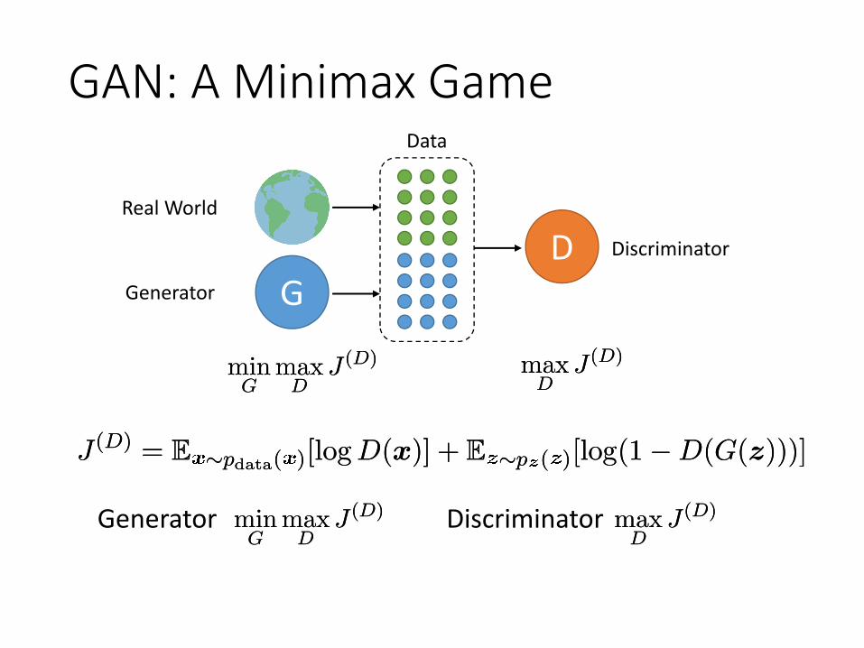
GAN: A Minimax Game

GD

Real World

Generator

Discriminator

Data

J (D) = E »pdata( )[log D(x)] + E »p ( )[log(1¡D(G(z)))]J (D) = E »pdata( )[log D(x)] + E »p ( )[log(1¡D(G(z)))]

minG

maxD

J (D)minG

maxD

J (D) maxD

J (D)maxD

J (D)

minG

maxD

J (D)minG

maxD

J (D) maxD

J (D)maxD

J (D)Generator Discriminator

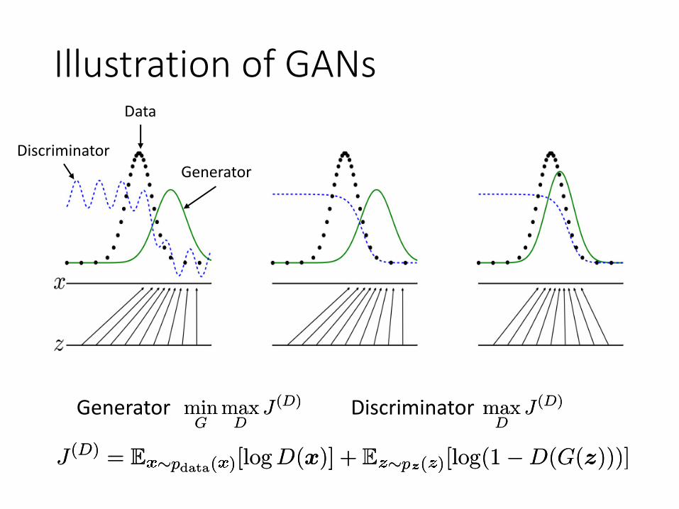
Illustration of GANs

Discriminator

Data

Generator

J (D) = E »pdata( )[log D(x)] + E »p ( )[log(1¡D(G(z)))]J (D) = E »pdata( )[log D(x)] + E »p ( )[log(1¡D(G(z)))]

minG

maxD

J (D)minG

maxD

J (D) maxD

J (D)maxD

J (D)Generator Discriminator

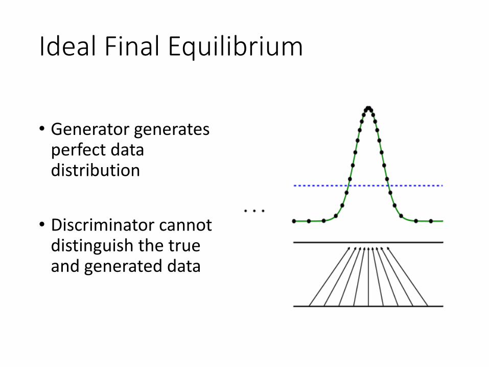
Ideal Final Equilibrium

• Generator generates perfect data distribution

• Discriminator cannot distinguish the true and generated data

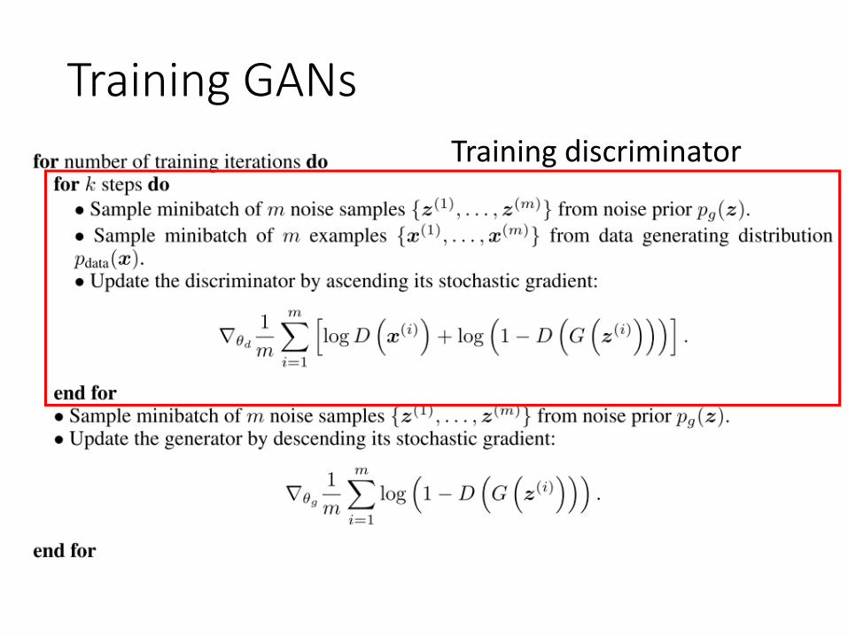
Training GANsTraining discriminator

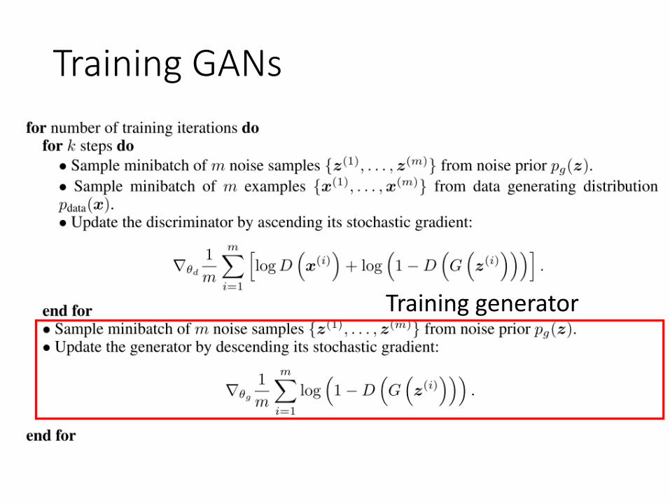
Training GANs

Training generator

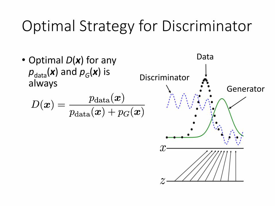
Optimal Strategy for Discriminator

• Optimal D(x) for any pdata(x) and pG(x) is always

D(x) =pdata(x)

pdata(x) + pG(x)D(x) =

pdata(x)

pdata(x) + pG(x)

Discriminator

Data

Generator

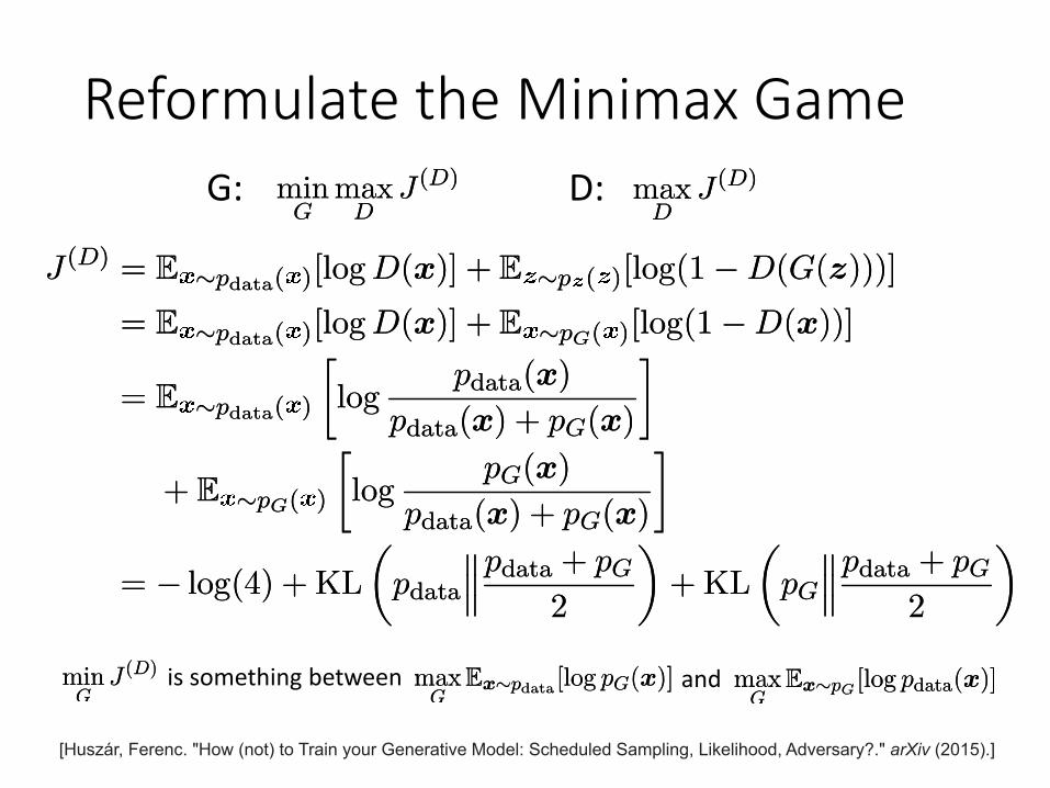
Reformulate the Minimax Game

J (D) = E »pdata( )[log D(x)] + E »p ( )[log(1¡D(G(z)))]

= E »pdata( )[log D(x)] + E »pG( )[log(1¡D(x))]

= E »pdata( )

·log

pdata(x)

pdata(x) + pG(x)

¸+ E »pG( )

·log

pG(x)

pdata(x) + pG(x)

¸= ¡ log(4) + KL

μpdata

°°°pdata + pG

2

¶+ KL

μpG

°°°pdata + pG

2

¶

J (D) = E »pdata( )[log D(x)] + E »p ( )[log(1¡D(G(z)))]

= E »pdata( )[log D(x)] + E »pG( )[log(1¡D(x))]

= E »pdata( )

·log

pdata(x)

pdata(x) + pG(x)

¸+ E »pG( )

·log

pG(x)

pdata(x) + pG(x)

¸= ¡ log(4) + KL

μpdata

°°°pdata + pG

2

¶+ KL

μpG

°°°pdata + pG

2

¶

minG

maxD

J (D)minG

maxD

J (D) maxD

J (D)maxD

J (D)G: D:

is something between and

[Huszár, Ferenc. "How (not) to Train your Generative Model: Scheduled Sampling, Likelihood, Adversary?." arXiv (2015).]

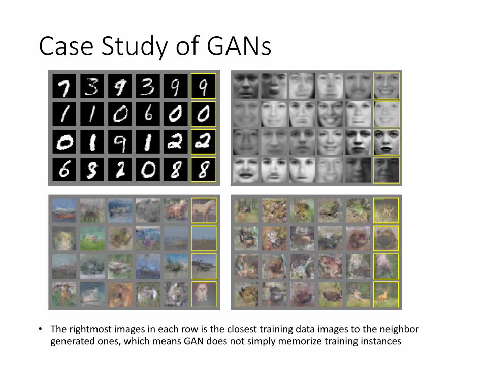
Case Study of GANs

• The rightmost images in each row is the closest training data images to the neighbor generated ones, which means GAN does not simply memorize training instances

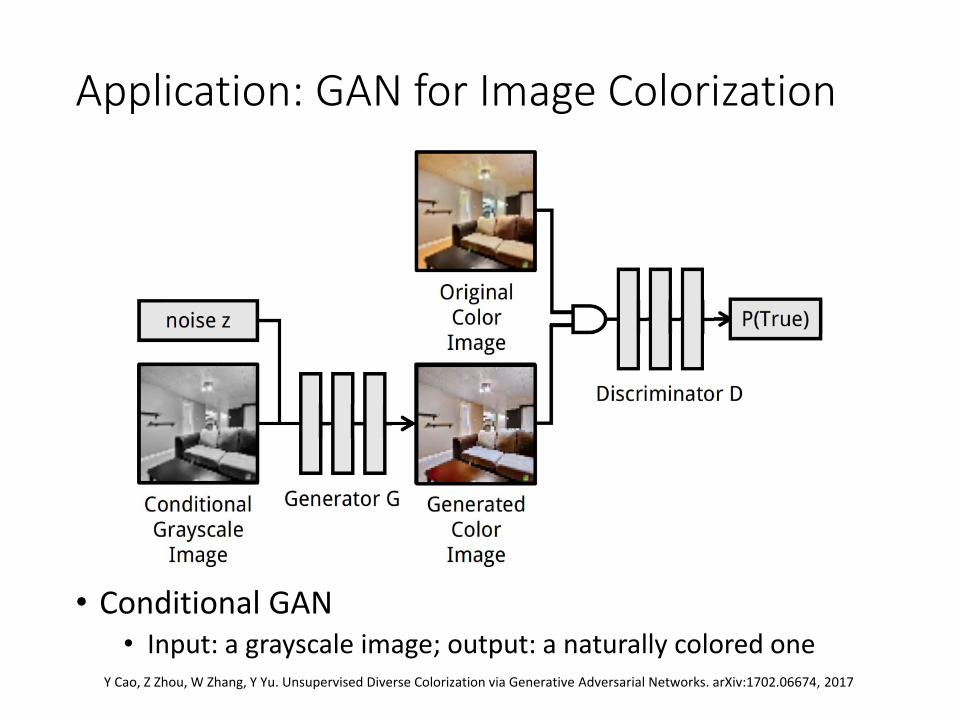
Application: GAN for Image Colorization

• Conditional GAN• Input: a grayscale image; output: a naturally colored one

Y Cao, Z Zhou, W Zhang, Y Yu. Unsupervised Diverse Colorization via Generative Adversarial Networks. arXiv:1702.06674, 2017

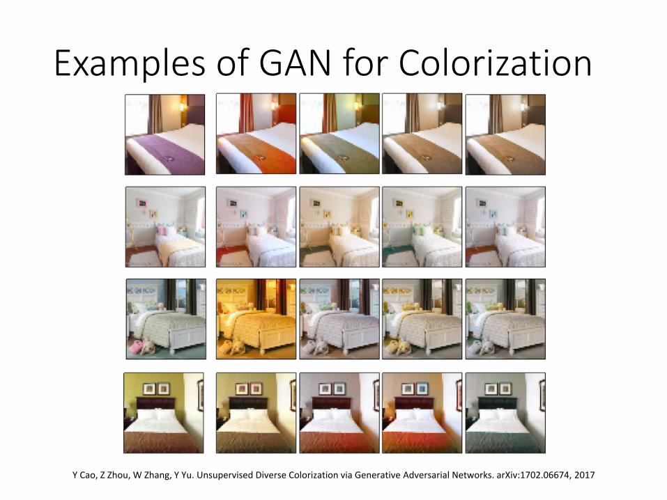
Examples of GAN for Colorization

Y Cao, Z Zhou, W Zhang, Y Yu. Unsupervised Diverse Colorization via Generative Adversarial Networks. arXiv:1702.06674, 2017