Up or Down? Adaptive Rounding for Post-Training Quantization Markus Nagel *1 Rana Ali Amjad *1 Mart van Baalen 1 Christos Louizos 1 Tijmen Blankevoort 1 Abstract When quantizing neural networks, assigning each floating-point weight to its nearest fixed-point value is the predominant approach. We find that, perhaps surprisingly, this is not the best we can do. In this paper, we propose AdaRound, a bet- ter weight-rounding mechanism for post-training quantization that adapts to the data and the task loss. AdaRound is fast, does not require fine- tuning of the network, and only uses a small amount of unlabelled data. We start by theo- retically analyzing the rounding problem for a pre-trained neural network. By approximating the task loss with a Taylor series expansion, the round- ing task is posed as a quadratic unconstrained bi- nary optimization problem. We simplify this to a layer-wise local loss and propose to optimize this loss with a soft relaxation. AdaRound not only outperforms rounding-to-nearest by a significant margin but also establishes a new state-of-the-art for post-training quantization on several networks and tasks. Without fine-tuning, we can quantize the weights of Resnet18 and Resnet50 to 4 bits while staying within an accuracy loss of 1%. 1. Introduction Deep neural networks are being used in many real-world applications as the standard technique for solving tasks in computer vision, machine translation, voice recognition, ranking, and many other domains. Owing to this success and widespread applicability, making these neural networks efficient has become an important research topic. Improved efficiency translates into reduced cloud-infrastructure costs and makes it possible to run these networks on heteroge- neous devices such as smartphones, internet-of-things appli- * Equal contribution 1 Qualcomm AI Research, an initia- tive of Qualcomm Technologies, Inc.. Correspondence to: Markus Nagel <[email protected]>, Rana Ali Am- jad <[email protected]>, Tijmen Blankevoort <tij- [email protected]>. Proceedings of the 37 th International Conference on Machine Learning, Vienna, Austria, PMLR 119, 2020. Copyright 2020 by the author(s). cations, and even dedicated low-power hardware. One effective way to optimize neural networks for infer- ence is neural network quantization (Krishnamoorthi, 2018; Guo, 2018). In quantization, neural network weights and activations are kept in a low-bit representation for both memory transfer and calculations in order to reduce power consumption and inference time. The process of quantizing a network generally introduces noise, which results in a loss of performance. Various prior works adapt the quantization procedure to minimize the loss in performance while going as low as possible in the number of bits used. As Nagel et al. (2019) explained, the practicality of neu- ral network quantization methods is important to take into consideration. Although many methods exist that do quantization-aware training (Jacob et al., 2018; Louizos et al., 2019) and get excellent results, these methods require a user to spend significant time on re-training models and hyperparameter tuning. On the other hand, much attention has recently been dedi- cated to post-training quantization methods (Nagel et al., 2019; Cai et al., 2020; Choukroun et al., 2019; Banner et al., 2019), which can be more easily applied in practice. These types of methods allow for network quantization to happen on-the-fly when deploying models, without the user of the model spending time and energy on quantization. Our work focuses on this type of network quantization. Rounding-to-nearest is the predominant approach for all neural network weight quantization work that came out thus far. This means that the weight vector w is rounded to the nearest representable quantization grid value in a fixed-point grid by b w = s · clip w s , n, p , (1) where s denotes the quantization scale parameter and, n and p denote the negative and positive integer thresholds for clipping. We could round any weight down by replacing b·e with b·c, or up using d·e. But, rounding-to-nearest seems the most sensible, as it minimizes the difference per-weight in the weight matrix. Perhaps surprisingly, we show that for post-training quantization, rounding-to-nearest is not optimal. Our contributions in this work are threefold: arXiv:2004.10568v2 [cs.LG] 30 Jun 2020
Transcript
Up or Down? Adaptive Rounding for Post-Training Quantization
Markus Nagel * 1 Rana Ali Amjad * 1 Mart van Baalen 1 Christos Louizos 1 Tijmen Blankevoort 1
AbstractWhen quantizing neural networks, assigning eachfloating-point weight to its nearest fixed-pointvalue is the predominant approach. We find that,perhaps surprisingly, this is not the best we cando. In this paper, we propose AdaRound, a bet-ter weight-rounding mechanism for post-trainingquantization that adapts to the data and the taskloss. AdaRound is fast, does not require fine-tuning of the network, and only uses a smallamount of unlabelled data. We start by theo-retically analyzing the rounding problem for apre-trained neural network. By approximating thetask loss with a Taylor series expansion, the round-ing task is posed as a quadratic unconstrained bi-nary optimization problem. We simplify this to alayer-wise local loss and propose to optimize thisloss with a soft relaxation. AdaRound not onlyoutperforms rounding-to-nearest by a significantmargin but also establishes a new state-of-the-artfor post-training quantization on several networksand tasks. Without fine-tuning, we can quantizethe weights of Resnet18 and Resnet50 to 4 bitswhile staying within an accuracy loss of 1%.
1. IntroductionDeep neural networks are being used in many real-worldapplications as the standard technique for solving tasks incomputer vision, machine translation, voice recognition,ranking, and many other domains. Owing to this successand widespread applicability, making these neural networksefficient has become an important research topic. Improvedefficiency translates into reduced cloud-infrastructure costsand makes it possible to run these networks on heteroge-neous devices such as smartphones, internet-of-things appli-
*Equal contribution 1Qualcomm AI Research, an initia-tive of Qualcomm Technologies, Inc.. Correspondence to:Markus Nagel <[email protected]>, Rana Ali Am-jad <[email protected]>, Tijmen Blankevoort <[email protected]>.
Proceedings of the 37 th International Conference on MachineLearning, Vienna, Austria, PMLR 119, 2020. Copyright 2020 bythe author(s).
cations, and even dedicated low-power hardware.
One effective way to optimize neural networks for infer-ence is neural network quantization (Krishnamoorthi, 2018;Guo, 2018). In quantization, neural network weights andactivations are kept in a low-bit representation for bothmemory transfer and calculations in order to reduce powerconsumption and inference time. The process of quantizinga network generally introduces noise, which results in a lossof performance. Various prior works adapt the quantizationprocedure to minimize the loss in performance while goingas low as possible in the number of bits used.
As Nagel et al. (2019) explained, the practicality of neu-ral network quantization methods is important to takeinto consideration. Although many methods exist that doquantization-aware training (Jacob et al., 2018; Louizoset al., 2019) and get excellent results, these methods requirea user to spend significant time on re-training models andhyperparameter tuning.
On the other hand, much attention has recently been dedi-cated to post-training quantization methods (Nagel et al.,2019; Cai et al., 2020; Choukroun et al., 2019; Banner et al.,2019), which can be more easily applied in practice. Thesetypes of methods allow for network quantization to happenon-the-fly when deploying models, without the user of themodel spending time and energy on quantization. Our workfocuses on this type of network quantization.
Rounding-to-nearest is the predominant approach for allneural network weight quantization work that came out thusfar. This means that the weight vector w is rounded to thenearest representable quantization grid value in a fixed-pointgrid by
w = s · clip(⌊
w
s
⌉, n, p
), (1)
where s denotes the quantization scale parameter and, n andp denote the negative and positive integer thresholds forclipping. We could round any weight down by replacing b·ewith b·c, or up using d·e. But, rounding-to-nearest seemsthe most sensible, as it minimizes the difference per-weightin the weight matrix. Perhaps surprisingly, we show thatfor post-training quantization, rounding-to-nearest is notoptimal.
Our contributions in this work are threefold:
arX
iv:2
004.
1056
8v2
[cs
.LG
] 3
0 Ju
n 20
20
Adaptive Rounding for Post-Training Quantization
• We establish a theoretical framework to analyze theeffect of rounding in a way that considers the charac-teristics of both the input data as well as the task loss.Using this framework, we formulate rounding as a per-layer Quadratic Unconstrained Binary Optimization(QUBO) problem.
• We propose AdaRound, a novel method that finds agood solution to this per-layer formulation via a con-tinuous relaxation. AdaRound requires only a smallamount of unlabelled data, is computationally efficient,and applicable to any neural network architecture withconvolutional or fully-connected layers.
• In a comprehensive study, we show that AdaRound de-fines a new state-of-the-art for post-training quantiza-tion on several networks and tasks, including Resnet18,Resnet50, MobilenetV2, InceptionV3 and DeeplabV3.
Notation We use x and y to denote the input and the targetvariable, respectively. E [·] denotes the expectation operator.All the expectations in this work are w.r.t. x and y. W(`)
i,j
denotes weight matrix (or tensor as clear from the context),with the bracketed superscript and the subscript denotingthe layer and the element indices, respectively. We also usew(`) to denote flattened version of W(`). All vectors areconsidered to be column vectors and represented by smallbold letters, e.g., z, while matrices (or tensors) are denotedby capital bold letters, e.g., Z. Functions are denoted byf(·), except the task loss, which is denoted by L. Constantsare denoted by small upright letters, e.g., s.
2. MotivationTo gain an intuitive understanding for why rounding-to-nearest may not be optimal, let’s look at what happens whenwe perturb the weights of a pretrained model. Consider aneural network parametrized by the (flattened) weights w.Let ∆w denote a small perturbation and L(x,y,w) denotethe task loss that we want to minimize. Then
E [L (x,y,w + ∆w)− L (x,y,w)] (2)(a)≈E
[∆wT · ∇wL (x,y,w)
+1
2∆wT · ∇2
wL (x,y,w) ·∆w]
(3)
= ∆wT · g(w) +1
2∆wT ·H(w) ·∆w, (4)
where (a) uses the second order Taylor series expansion.g(w) and H(w) denote the expected gradient and Hessianof the task loss L w.r.t. w, i.e.,
g(w) = E [∇wL (x,y,w)] (5)
H(w) = E[∇2
wL(x,y,w)]. (6)
All the gradient and Hessian terms in this paper are of taskloss L with respect to the specified variables. Ignoringthe higher order terms in the Taylor series expansion is agood approximation as long as ∆w is not too large. As-suming the network is trained to convergence, we can alsoignore the gradient term as it will be close to 0. There-fore, H(w) defines the interactions between different per-turbed weights in terms of their joint impact on the task lossL (x,y,w + ∆w). The following toy example illustrateshow rounding-to-nearest may not be optimal.
Example 1. Assume ∆wT = [∆w1 ∆w2] and
H(w) =
[1 0.5
0.5 1
], (7)
then the increase in task loss due to the perturbation is(approximately) proportional to
∆wT ·H(w) ·∆w = ∆w21 + ∆w2
2 + ∆w1∆w2. (8)
For the terms corresponding to the diagonal entries ∆w21
and ∆w22, only the magnitude of the perturbations matters.
Hence rounding-to-nearest is optimal when we only con-sider these diagonal terms in this example. However, forthe terms corresponding to the ∆w1∆w2, the sign of theperturbation matters, where opposite signs of the two pertur-bations improve the loss. To minimize the overall impact ofquantization on the task loss, we need to trade-off betweenthe contribution of the diagonal terms and the off-diagonalterms. Rounding-to-nearest ignores the off-diagonal contri-butions, making it often sub-optimal.
The previous analysis is valid for the quantization of anyparametric system. We show that this effect also holds forneural networks. To illustrate this, we generate 100 stochas-tic rounding (Gupta et al., 2015) choices for the first layerof Resnet18 and evaluate the performance of the networkwith only the first layer quantized. The results are presentedin Table 1. Among 100 runs, we find that 48 stochasti-cally sampled rounding choices lead to a better performancethan rounding-to-nearest. This implies that many round-ing solutions exist that are better than rounding-to-nearest.Furthermore, the best among these 100 stochastic samplesprovides more than 10% improvement in the accuracy of thenetwork. We also see that accidentally rounding all valuesup, or all down, has an catastrophic effect. This implies thatwe can gain a lot by carefully rounding weights when doingpost-training quantization. The rest of this paper is aimedat devising a well-founded and computationally efficientrounding mechanism.
3. MethodIn this section, we propose AdaRound, a new rounding pro-cedure for post-training quantization that is theoretically
Adaptive Rounding for Post-Training Quantization
Rounding scheme Acc(%)
Nearest 52.29Ceil 0.10Floor 0.10
Stochastic 52.06±5.52Stochastic (best) 63.06
Table 1. Comparison of ImageNet validation accuracy among dif-ferent rounding schemes for 4-bit quantization of the first layerof Resnet18. We report the mean and the standard deviation of100 stochastic (Gupta et al., 2015) rounding choices (Stochastic)as well as the best validation performance among these samples(Stochastic (best)).
well-founded and shows significant performance improve-ment in practice. We start by analyzing the loss due toquantization theoretically. We then formulate an efficientper-layer algorithm to optimize it.
3.1. Task loss based rounding
When quantizing a pretrained NN, our aim is to minimizethe performance loss incurred due to quantization. Assum-ing per-layer weight quantization1, the quantized weightw
(`)i is
w(`)i ∈
{w
(`),floori ,w
(`),ceili
}, (9)
where
w(`),floori = s(`) · clip
(⌊w
(`)i
s(`)
⌋, n, p
)(10)
and w(`),ceili is similarly defined by replacing b·c with d·e
and ∆w(`)i = w(`) − w
(`)i denotes the perturbation due to
quantization. In this work we assume s(`) to be fixed priorto optimizing the rounding procedure. Finally, whenever weoptimize a cost function over the ∆w
(`)i , the w
(`)i can only
take two values specified in (9).
Finding the optimal rounding procedure can be formulatedas the following binary optimization problem
arg min∆w
E [L (x,y,w + ∆w)− L (x,y,w)] (11)
Evaluating the cost in (11) requires a forward pass of theinput data samples for each new ∆w during optimization.To avoid the computational overhead of repeated forwardpasses throught the data, we utilize the second order Taylorseries approximation. Additionally, we ignore the interac-tions among weights belonging to different layers. This, in
1Note that our work is equally applicable for per-channelweight quantization.
Figure 1. Correlation between the cost in (13) vs ImageNet valida-tion accuracy (%) of 100 stochastic rounding vectors w for 4-bitquantization of only the first layer of Resnet18.
turn, implies that we assume a block diagonal H(w), whereeach non-zero block corresponds to one layer. We thus endup with the following per-layer optimization problem
arg min∆w(`)
E[g(w(`))
T∆w(`) +
1
2∆w(`)TH(w(`))∆w(`)
].
(12)
As illustrated in Example 1, we require the second orderterm to exploit the joint interactions among the weight per-turbations. (12) is a QUBO problem since ∆w
(`)i are binary
variables (Kochenberger et al., 2014). For a converged pre-trained model, the contribution of the gradient term foroptimization in (13) can be safely ignored. This results in
arg min∆w(`)
E[∆w(`)TH(w(`))∆w(`)
]. (13)
To verify that (13) serves as a good proxy for optimizingtask loss due to quantization, we plot the cost in (13) vs val-idation accuracy for 100 stochastic rounding vectors whenquantizing only the first layer of Resnet18. Fig. 1 shows aclear correlation between the two quantities. This justifiesour approximation for optimization, even for 4 bit quantiza-tion. Optimizing (13) show significant performance gains,however its application is limited by two problems:
1. H(w(`)) suffers from both computational as well mem-ory complexity issues even for moderately sized layers.
2. (13) is an NP-hard optimization problem. The com-plexity of solving it scales rapidly with the dimen-sion of ∆w(`), again prohibiting the application of (13)to even moderately sized layers (Kochenberger et al.,2014).
In section 3.2 and section 3.3 we tackle the first and thesecond problem, respectively.
Adaptive Rounding for Post-Training Quantization
3.2. From Taylor expansion to local loss
To understand the cause of the complexity associated withH(w(`)), let us look at its’ elements. For two weights in thesame fully connected layer we have
∂2L∂W
(`)i,j ∂W
(`)m,o
=∂
∂W(`)m,o
[∂L∂z
(`)i
· x(`−1)j
](14)
=∂2L
∂z(`)i ∂z
(`)m
· x(`−1)j x(`−1)
o , (15)
where z(`) = W(`)x(`−1) are the preactivations for layer` and x(`−1) denotes the input to layer `. Writing this inmatrix formulation (for flattened w(`)), we have (Botevet al., 2017)
H(w(`)) = E[x(`−1)x(`−1)T ⊗∇2
z(`)L], (16)
where ⊗ denotes Kronecker product of two matrices and∇2
z(`)L is the Hessian of the task loss w.r.t. z(`). It is clearfrom (16) that the complexity issues are mainly caused by∇2
z(`)L that requires backpropagation of second derivativesthrough the subsequent layers of the network. To tackle this,we make the assumption that the Hessian of the task lossw.r.t. the preactivations, i.e., ∇2
z(`)L is a diagonal matrix,denoted by diag
(∇2
z(`)Li,i). This leads to
H(w(`)) = E[x(`−1)x(`−1)T ⊗ diag(∇2
z(`)Li,i)]. (17)
Note that the approximation of H(w(`)) expressed in (17) isnot diagonal. Plugging (17) into our equation for findingthe rounding vector that optimizes the loss (13), we obtain
arg min∆W
(`)k,:
E[∇2
z(`)Lk,k ·∆W(`)k,:x
(`−1)x(`−1)T ∆W(`)k,:
T]
(18)(a)= arg min
∆W(`)k,:
∆W(`)k,: E
[x(`−1)x(`−1)T
]∆W
(`)k,:
T(19)
= arg min∆W
(`)k,:
E[(
∆W(`)k,:x
(`−1))2], (20)
where the optimization problem in (13) now decomposesinto independent sub-problems in (18). Each sub-problemdeals with a single row ∆W
(`)k,: and (a) is the outcome of
making a further assumption that ∇2z(`)Li,i = ci is a con-
stant independent of the input data samples. It is worthwhileto note that optimizing (20) requires no knowledge of thesubsequent layers and the task loss. In (20), we are simplyminimizing the Mean Squared Error (MSE) introduced inthe preactivations z(`) due to quantization. This is the samelayer-wise objective that was optimized in several neuralnetwork compression papers, e.g., Zhang et al. (2016); He
et al. (2017), and various neural network quantization pa-pers (albeit for tasks other than weight rounding), e.g., Wanget al. (2018); Stock et al. (2020); Choukroun et al. (2019).However, unlike these works, we arrive at this objective in aprincipled way and conclude that optimizing the MSE, asspecified in (20), is the best we can do when assuming noknowledge of the rest of the network past the layer that weare optimizing. In the supplementary material we performan analogous analysis for convolutional layers.
The optimization problem in (20) can be tackled by eitherprecomputing E
[x(`−1)x(`−1)T
], as done in (19), and then
performing the optimization over ∆W(`)k,: , or by performing
a single layer forward pass for each potential ∆W(`)k,: during
the optimization procedure.
In section 5, we empirically verify that the constant diagonalapproximation of ∇2
z(`)L does not negatively influence theperformance.
3.3. AdaRound
Solving (20) does not suffer from complexity issues associ-ated with H(w(`)). However, it is still an NP-hard discreteoptimization problem. Finding good (sub-optimal) solu-tion with reasonable computational complexity can be achallenge for larger number of optimization variables. Totackle this we relax (20) to the following continuous opti-mization problem based on soft quantization variables (thesuperscripts are the same as (20))
arg minV
∥∥∥Wx− Wx∥∥∥2
F+ λfreg (V) , (21)
where ‖·‖2F denotes the Frobenius norm and W are thesoft-quantized weights that we optimize over
W = s · clip(⌊
W
s
⌋+ h (V) , n, p
). (22)
In the case of a convolutional layer the Wx matrix multipli-cation is replaced by a convolution. Vi,j is the continuousvariable that we optimize over and h (Vi,j) can be any dif-ferentiable function that takes values between 0 and 1, i.e.,h (Vi,j) ∈ [0, 1]. The additional term freg (V) is a dif-ferentiable regularizer that is introduced to encourage theoptimization variables h (Vi,j) to converge towards either0 or 1, i.e., at convergence h (Vi,j) ∈ {0, 1}.
We employ a rectified sigmoid as h (Vi,j), proposed in(Louizos et al., 2018). The rectified sigmoid is defined as
h (Vi,j) = clip(σ (Vi,j) (ζ − γ) + γ, 0, 1), (23)
where σ(·) is the sigmoid function and, ζ and γ are stretchparameters, fixed to 1.1 and −0.1, respectively. The rec-tified sigmoid has non-vanishing gradients as h (Vi,j) ap-proaches 0 or 1, which helps the learning process when we
Adaptive Rounding for Post-Training Quantization
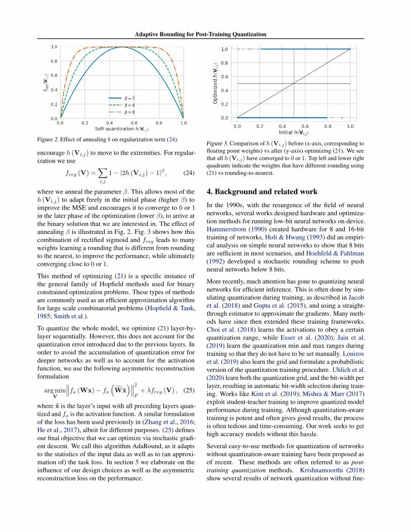
Figure 2. Effect of annealing b on regularization term (24).
encourage h (Vi,j) to move to the extremities. For regular-ization we use
freg (V) =∑i,j
1− |2h (Vi,j)− 1|β , (24)
where we anneal the parameter β. This allows most of theh (Vi,j) to adapt freely in the initial phase (higher β) toimprove the MSE and encourages it to converge to 0 or 1in the later phase of the optimization (lower β), to arrive atthe binary solution that we are interested in. The effect ofannealing β is illustrated in Fig. 2. Fig. 3 shows how thiscombination of rectified sigmoid and freg leads to manyweights learning a rounding that is different from roundingto the nearest, to improve the performance, while ultimatelyconverging close to 0 or 1.
This method of optimizing (21) is a specific instance ofthe general family of Hopfield methods used for binaryconstrained optimization problems. These types of methodsare commonly used as an efficient approximation algorithmfor large scale combinatorial problems (Hopfield & Tank,1985; Smith et al.).
To quantize the whole model, we optimize (21) layer-by-layer sequentially. However, this does not account for thequantization error introduced due to the previous layers. Inorder to avoid the accumulation of quantization error fordeeper networks as well as to account for the activationfunction, we use the following asymmetric reconstructionformulation
arg minV
∥∥∥fa (Wx)− fa(Wx
)∥∥∥2
F+ λfreg (V) , (25)
where x is the layer’s input with all preceding layers quan-tized and fa is the activation function. A similar formulationof the loss has been used previously in (Zhang et al., 2016;He et al., 2017), albeit for different purposes. (25) definesour final objective that we can optimize via stochastic gradi-ent descent. We call this algorithm AdaRound, as it adaptsto the statistics of the input data as well as to (an approxi-mation of) the task loss. In section 5 we elaborate on theinfluence of our design choices as well as the asymmetricreconstruction loss on the performance.
Figure 3. Comparison of h (Vi,j) before (x-axis, corresponding tofloating point weights) vs after (y-axis) optimizing (21). We seethat all h (Vi,j) have converged to 0 or 1. Top left and lower rightquadrants indicate the weights that have different rounding using(21) vs rounding-to-nearest.
4. Background and related workIn the 1990s, with the resurgence of the field of neuralnetworks, several works designed hardware and optimiza-tion methods for running low-bit neural networks on-device.Hammerstrom (1990) created hardware for 8 and 16-bittraining of networks, Holi & Hwang (1993) did an empiri-cal analysis on simple neural networks to show that 8 bitsare sufficient in most scenarios, and Hoehfeld & Fahlman(1992) developed a stochastic rounding scheme to pushneural networks below 8 bits.
More recently, much attention has gone to quantizing neuralnetworks for efficient inference. This is often done by sim-ulating quantization during training, as described in Jacobet al. (2018) and Gupta et al. (2015), and using a straight-through estimator to approximate the gradients. Many meth-ods have since then extended these training frameworks.Choi et al. (2018) learns the activations to obey a certainquantization range, while Esser et al. (2020); Jain et al.(2019) learn the quantization min and max ranges duringtraining so that they do not have to be set manually. Louizoset al. (2019) also learn the grid and formulate a probabilisticversion of the quantization training procedure. Uhlich et al.(2020) learn both the quantization grid, and the bit-width perlayer, resulting in automatic bit-width selection during train-ing. Works like Kim et al. (2019); Mishra & Marr (2017)exploit student-teacher training to improve quantized modelperformance during training. Although quantization-awaretraining is potent and often gives good results, the processis often tedious and time-consuming. Our work seeks to gethigh accuracy models without this hassle.
Several easy-to-use methods for quantization of networkswithout quantization-aware training have been proposed asof recent. These methods are often referred to as post-training quantization methods. Krishnamoorthi (2018)show several results of network quantization without fine-
Adaptive Rounding for Post-Training Quantization
tuning. Works like Banner et al. (2019); Choukroun et al.(2019) optimize the quantization ranges for clipping to finda better loss trade-off per-layer. Zhao et al. (2019) improvequantization performance by splitting channels into morechannels, increasing computation but achieving lower bit-widths in the process. Lin et al. (2016); Dong et al. (2019)set different bit-widths for different layers, through the in-formation of the per-layer SQNR or the Hessian. Nagel et al.(2019); Cai et al. (2020) even do away with the requirementof needing any data to optimize a model for quantization,making their procedures virtually parameter and data-free.These methods are all solving the same quantization prob-lem as in this paper, and some like Zhao et al. (2019) andDong et al. (2019) could even be used in conjunction withAdaRound. We compare to the methods that improve weightquantization for 4/8 and 4/32 bit-widths without end-to-endfine-tuning, Banner et al. (2019); Choukroun et al. (2019);Nagel et al. (2019), but leave out comparisons to the mixed-precision methods Cai et al. (2020); Dong et al. (2019) sincethey improve networks on a different axis.
5. ExperimentsTo evaluate the performance of AdaRound, we conductexperiments on various computer vision tasks and models.In section 5.1 we study the impact of the approximations anddesign choices made in section 3. In section 5.2 we compareAdaRound to other post-training quantization methods.
Experimental setup For all experiments we absorb batchnormalization in the weights of the adjacent layers. Weuse symmetric 4-bit weight quantization with a per-layerscale parameter s(`) which is determined prior to the appli-cation of AdaRound. We set s so that it minimizes the MSE||W−W||2F , where W are the quantized weights obtainedthrough rounding-to-nearest. In some ablation studies, wereport results when quantizing only the first layer. Thiswill be explicitly mentioned as “First layer”. In all othercases, we have the weights of the whole network quantizedusing 4 bits. Unless otherwise stated, all activations are inFP32. Most experiments are conducted using Resnet18 (Heet al., 2016) from torchvision. The baseline performanceof this model with full precision weights and activationsis 69.68%. In our experiments, we report the mean andstandard deviation of the (top1) accuracy on the ImageNetvalidation set, calculated using 5 runs with different initialseeds. To optimize AdaRound we use 1024 unlabeled im-ages from the ImageNet (Russakovsky et al., 2015) trainingset, Adam (Kingma & Ba, 2015) optimizer with defaulthyper-parameters for 10k iterations and a batch-size of 32,unless otherwise stated. We use Pytorch (Paszke et al., 2019)for all our experiments. It is worthwhile to note that theapplication of AdaRound to Resnet18 takes only 10 minuteson a single Nvidia GTX 1080 Ti.
Rounding First layer All layers
Nearest 52.29 23.99H(w) task loss (cf. (13)) 68.62±0.17 N/ALocal MSE loss (cf. (20)) 69.39±0.04 65.83±0.14Cont. relaxation (cf (21)) 69.58±0.03 66.56±0.12
Table 2. Impact of various approximations and assumptions madein section 3 on the ImageNet validation accuracy (%) for Resnet18.N/A implies that the corresponding experiment was computation-ally infeasible.
5.1. Ablation study
From task loss to local loss We make various approxi-mations and assumptions in section 3.1 and section 3.2 tosimplify our optimization problem. In Table 2, we look attheir impact systematically. First, we note that optimizingbased on the Hessian of the task loss (cf. (13)) providesa significant performance boost compared to rounding-to-nearest. This verifies that the Taylor expansion based round-ing serves as a much better alternative for the task loss whencompared to rounding-to-nearest. Similarly, we show that,although moving from the optimization of Taylor expansionof the task loss to the local MSE loss (cf. (20)) requiresstrong assumptions, it does not degrade the performance.Unlike the Taylor series expansion, the local MSE lossmakes it feasible to optimize all layers in the network. Weuse the cross-entropy method (Rubinstein, 1999) to solvethe QUBO problems in (13) and (20), where we initializethe sampling distribution for the binary random variableswi as in (Gupta et al., 2015)2. Finally, the continuous relax-ation for the local MSE optimization problem (cf. (21)) notonly reduces the optimization time from several hours to afew minutes but also slightly improves our performance.
Design choices for AdaRound As discussed earlier, ourapproach to solve (21) closely resembles a Hopfield method.These methods optimize h (Vi,j) = σ
(Vi,j
T
)with a ver-
sion of gradient descent with respect to Vi,j , and annealingthe temperature T (Hopfield & Tank, 1985; Smith et al.).This annealing acts as an implicit regularization that al-lows h (Vi,j) to optimize for the MSE loss initially uncon-strained, while encouraging h (Vi,j) to converge towards0 or 1 in the later phase of optimization. In Table 3 weshow that even after an extensive hyper-parameter searchfor the annealing schedule of T , using the sigmoid functionwith our explicit regularization term (24) outperforms theclassical method. Using explicit regularization also makesthe optimization more stable, leading to lower variance asshown in Table 3. Furthermore, we see that the use of therectified sigmoid also provides a consistent small improve-
2In the supplementary material we compare the performanceof different QUBO solvers on our problem.
Table 4. The influence on the ImageNet validation accuracy (%)for Resnet18, by incorporating asymmetric reconstruction MSEloss and activation function in the rounding optimization objective.
ment in accuracy for different models.
Table 4 shows the gain of using the asymmetric reconstruc-tion MSE (cf. section 3.3). We see that this provides anoticeable accuracy improvement when compared to (21).Similarly, accounting for the activation function in the opti-mization problem provides a small gain.
Optimization using STE Another option we consideredis to optimize W directly by using the straight-through es-timator (STE) (Bengio et al., 2013). This is inspired byquantization-aware training (Jacob et al., 2018), which opti-mizes a full network with this procedure. We use the STEto minimize the MSE loss in (21). This method technicallyallows more flexible movement of the quantized weightsW, as they are no longer restricted to just rounding up ordown. In Table 5 we compare the STE optimization withAdaRound. We can see that AdaRound clearly outperformsSTE-based optimization. We believe this is due to the biasedgradients of the STE, which hinder the optimization in thisrestricted setting.
Influence of quantization grid We studied how thechoice of weight quantization grid affects the performancegain that AdaRound brings vs rounding-to-nearest. Welooked at three different options for determining the scaleparameter s; using minimum and maximum values ofthe weight tensor W, minimizing the MSE
∥∥W −W∥∥2
Fintroduced in the weights, and minimizing the MSE∥∥Wx−Wx
∥∥2
Fintroduced in the preactivations. W
denotes the quantized weight tensor obtained throughrounding-to-nearest for a given s. Note, we do not opti-mize step size and AdaRound jointly as it is non-trivial tocombine the two tasks: any change in the step size wouldresult in a different QUBO problem. The results in Table6 clearly show that AdaRound significantly improves over
Optimization Acc (%)
Nearest 23.99STE 66.63±0.06AdaRound 68.60±0.09
Table 5. Comparison between optimizing (25) using STE (withoutexplicit regularization freg) vs AdaRound. We report ImageNetvalidation accuracy (%) for Resnet18.
Grid Nearest AdaRound
Min-Max 0.23 61.96±0.04∥∥W −W∥∥2
F23.99 68.60±0.09∥∥Wx−Wx
∥∥2
F42.89 68.62±0.08
Table 6. Comparison between various quantization grids in combi-nation with rounding-to-nearest and AdaRound. We report Ima-geNet validation accuracy (%) for Resnet18.
rounding-to-nearest, independent of the choice of the quan-tization grid. Both MSE based approaches are superior tothe Min-Max method for determining the grid. Since thereis no clear winner between the two MSE formulations forAdaRound, we continue the use of
∥∥W −W∥∥2
Fformula-
tion for all other experiments.
Optimization robustness to data We also investigatehow little data is necessary to allow AdaRound to achievegood performance and investigate if this could be donewith data from different datasets. The results can be seenin Fig. 4. We see that the performance of AdaRound isrobust to the number of images required for optimization.Even with as little as 256 images, the method optimizesthe model to within 2% of the original FP32 accuracy. Wealso see that when using unlabelled images that are froma similar domain but do not belong to the original trainingdata, AdaRound achieves competitive performance. Here,we observe a less than 0.2% degradation on average. It isworthwhile to note that both Pascal VOC and MS COCOonly contain a small subset of the classes from Imagenet,implying that the optimization data for AdaRound does notneed to be fully representative of the original training set.
5.2. Literature comparison
Comparison to bias correction Several recent papershave addressed a specific symptom of the problem we de-scribe with rounding-to-nearest (Banner et al., 2019; Finkel-stein et al., 2019; Nagel et al., 2019). These works observethat quantizing weights often changes the expected valueof the output of the layer, i.e., E [Wx] 6= E[Wx]. In orderto counteract this, these papers adjust the bias terms forthe preactivations by adding E [Wx]− E[Wx]. This “biascorrection” can be viewed as another approach to minimize
Table 7. Comparison among different post-training quantization strategies in the literature. We report results for various models in termsof ImageNet validation accuracy (%). *Uses per-channel quantization. †Using CLE (Nagel et al., 2019) as preprocessing.
Figure 4. The effect on ImageNet validation accuracy when usingdifferent number of images belonging to different datasets forAdaRound optimization.
the same MSE loss as AdaRound (20), but by adjusting thebias terms as
E [Wx]− E[Wx] = arg minb
E[∥∥∥Wx−
(Wx + b
)∥∥∥2
F
].
(26)
Our method solves this same problem, but in a better way.In Table 8 we compare empirical bias correction from Nagelet al. (2019) to AdaRound, under the exact same experi-mental setup, on ResNet18. While bias correction improvesperformance over vanilla quantization without bias correc-tion, we see that for 4 bits it only achieves 38.87% accuracy,where AdaRound recovers accuracy to 68.60%.
ImageNet In Table 7, we compare AdaRound to severalrecent post-training quantization methods. We use the sameexperimental setup as described earlier, with the exceptionof optimizing AdaRound with 2048 images for 20k iter-ations. For both Resnet18 and Resnet50, AdaRound iswithin 1% of the FP32 accuracy for 4-bit weight quantiza-tion and outperforms all competing methods, even thoughsome rely on the more favorable per-channel quantization
Table 8. Comparison between AdaRound and empirical bias cor-rection, which also counteracts a symptom of the quantization errorintroduced by rounding to nearest. We report ImageNet validationaccuracy (%) for Resnet18.
and do not quantize the first and the last layer. Similarly,on the more challenging networks, InceptionV3 and Mo-bilenetV2, AdaRound stays within 2% of the original accu-racy and outperforms any competing method.
To be able to compare to methods that also do activationquantization, we report results of AdaRound with all ac-tivation tensors quantized to 8 bits. For this scenario, wequantized the activations to 8 bits and set the scaling factorfor the activation quantizers based on the minimum andmaximum activations observed. We notice that activationquantization, in most cases, does not significantly harm thevalidation accuracy. AdaRound again outperforms the com-peting methods such as DFQ (Nagel et al., 2019) and biascorrection (Banner et al., 2019).
Semantic segmentation To demonstrate the wider appli-cability of AdaRound, we apply it to DeeplabV3+ (Chenet al., 2018) evaluated on Pascal VOC (Everingham et al.,2015). Since the input images here are significantly big-ger, we only use 512 images to optimize AdaRound. Allother aspects of the experimental setup stay the same. Tothe best of our knowledge, there are no other post-trainingquantization methods doing 4-bit quantization for semanticsegmentation. DFQ works well for 8 bits, however perfor-mance drastically drops when going down to 4-bit weightquantization. AdaRound still performs well for 4 bits andhas only a 2% performance decrease for 4-bit weights and
Adaptive Rounding for Post-Training Quantization
Optimization #bits W/A mIOU
Full precision 32/32 72.94DFQ (Nagel et al., 2019) 8/8 72.33Nearest 4/8 6.09DFQ (our impl.) 4/8 14.45
Table 9. Comparison among different post-training quantizationstrategies, in terms of Mean Intersection Over Union (mIOU) forDeeplabV3+ (MobileNetV2 backend) on Pascal VOC.
8-bit activations quantization.
6. ConclusionIn this paper we proposed AdaRound, a new roundingmethod for post-training quantization of neural networkweights. AdaRound improves significantly over rounding-to-nearest, which has poor performance for lower bit widths.We framed and analyzed the rounding problem theoreti-cally and by making appropriate approximations we arriveat a practical method. AdaRound is computationally fast,uses only a small number of unlabeled data examples, doesnot need end-to-end fine-tuning, and can be applied to anyneural network that has convolutional or fully-connectedlayers without any restriction. AdaRound establishes a newstate-of-the-art for post-training weight quantization withsignificant gains. It can push networks like Resnet18 andResnet50 to 4-bit weights while keeping the accuracy dropwithin 1%.
ReferencesBanner, R., Nahshan, Y., and Soudry, D. Post training
4-bit quantization of convolutional networks for rapid-deployment. Neural Information Processing Systems(NeuRIPS), 2019.
Bengio, Y., Leonard, N., and Courville, A. Estimating orpropagating gradients through stochastic neurons for con-ditional computation. arXiv preprint arXiv:1308.3432,2013.
Botev, A., Ritter, H., and Barber, D. Practical gauss-newtonoptimisation for deep learning. International Conferenceon Machine Learning (ICML), 2017.
Cai, Y., Yao, Z., Dong, Z., Gholami, A., Mahoney, M. W.,and Keutzer, K. Zeroq: A novel zero shot quantizationframework. arXiv preprint arXiv:2001.00281, 2020.
Chen, L.-C., Zhu, Y., Papandreou, G., Schroff, F., and Adam,H. Encoder-decoder with atrous separable convolution for
semantic image segmentation. The European Conferenceon Computer Vision (ECCV), 2018.
Choi, J., Wang, Z., Venkataramani, S., Chuang, P. I., Srini-vasan, V., and Gopalakrishnan, K. PACT: parameterizedclipping activation for quantized neural networks. arXivpreprint arxiv:805.06085, 2018.
Choukroun, Y., Kravchik, E., and Kisilev, P. Low-bit quan-tization of neural networks for efficient inference. Inter-national Conference on Computer Vision (ICCV), 2019.
Dong, Z., Yao, Z., Gholami, A., Mahoney, M. W., andKeutzer, K. HAWQ: hessian aware quantization of neuralnetworks with mixed-precision. International Conferenceon Computer Vision (ICCV), 2019.
Esser, S. K., McKinstry, J. L., Bablani, D., Appuswamy,R., and Modha, D. S. Learned step size quantization.International Conference on Learning Representations(ICLR), 2020.
Everingham, M., Eslami, S., Van Gool, L., Williams, C.,Winn, J., and Zisserman, A. The pascal visual objectclasses challenge: A retrospective. International Journalof Computer Vision, 111(1):98–136, 1 2015.
Finkelstein, A., Almog, U., and Grobman, M. Fighting quan-tization bias with bias. arXiv preprint arxiv:1906.03193,2019.
Guo, Y. A survey on methods and theories of quantized neu-ral networks. arXiv preprint: arxiv:1808.04752, 2018.
Gupta, S., Agrawal, A., Gopalakrishnan, K., and Narayanan,P. Deep learning with limited numerical precision. Inter-national Conference on Machine Learning, ICML, 2015.
Hammerstrom, D. A vlsi architecture for high-performance,low-cost, on-chip learning. International Joint Confer-ence on Neural Networks (IJCNN), 1990.
He, K., Zhang, X., Ren, S., and Sun, J. Deep residuallearning for image recognition. Conference on ComputerVision and Pattern Recognition, CVPR, 2016.
He, Y., Zhang, X., and Sun, J. Channel pruning for accelerat-ing very deep neural networks. International Conferenceon Computer Vision (ICCV), 2017.
Hoehfeld, M. and Fahlman, S. E. Learning with limited nu-merical precision using the cascade-correlation algorithm.IEEE Transactions on Neural Networks, 3(4):602–611,1992.
Holi, J. L. and Hwang, J. N. Finite precision error analysis ofneural network hardware implementations. IEEE Trans.Comput., 42(3):281290, 1993.
Adaptive Rounding for Post-Training Quantization
Hopfield, J. J. and Tank, D. W. “neural” computation of de-cisions in optimization problems. Biological Cybernetics,52(3):141–152, 1985.
Jacob, B., Kligys, S., Chen, B., Zhu, M., Tang, M., Howard,A., Adam, H., and Kalenichenko, D. Quantizationand training of neural networks for efficient integer-arithmetic-only inference. Conference on Computer Vi-sion and Pattern Recognition (CVPR), 2018.
Jain, S. R., Gural, A., Wu, M., and Dick, C. Trained uni-form quantization for accurate and efficient neural net-work inference on fixed-point hardware. arxiv preprintarxiv:1903.08066, 2019.
Kim, J., Bhalgat, Y., Lee, J., Patel, C., and Kwak, N. QKD:quantization-aware knowledge distillation. arxiv preprintarxiv:1911.12491, 2019.
Kingma, D. P. and Ba, J. Adam: A method for stochas-tic optimization. International Conference for LearningRepresentations (ICLR), 2015.
Kochenberger, G., Hao, J.-K., Glover, F., Lewis, M., Lu,Z., Wang, H., and Wang, Y. The unconstrained binaryquadratic programming problem: a survey. Journal ofCombinatorial Optimization, 28(1):58–81, Jul 2014.
Krishnamoorthi, R. Quantizing deep convolutional networksfor efficient inference: A whitepaper. arXiv preprintarXiv:1806.08342, 2018.
Lin, D. D., Talathi, S. S., and Annapureddy, V. S. Fixedpoint quantization of deep convolutional networks. InInternational Conference on Machine Learning, 2016.
Louizos, C., Welling, M., and Kingma, D. P. Learning sparseneural networks through l0 regularization. InternationalConference on Learning Representations (ICLR), 2018.
Louizos, C., Reisser, M., Blankevoort, T., Gavves, E., andWelling, M. Relaxed quantization for discretized neu-ral networks. In International Conference on LearningRepresentations (ICLR), 2019.
Mishra, A. K. and Marr, D. Apprentice: Using knowledgedistillation techniques to improve low-precision networkaccuracy. arXiv preprint arxiv:1711.05852, 2017.
Nagel, M., van Baalen, M., Blankevoort, T., and Welling, M.Data-free quantization through weight equalization andbias correction. International Conference on ComputerVision (ICCV), 2019.
Paszke, A., Gross, S., Massa, F., Lerer, A., Bradbury, J.,Chanan, G., Killeen, T., Lin, Z., Gimelshein, N., Antiga,L., Desmaison, A., Kopf, A., Yang, E., DeVito, Z., Rai-son, M., Tejani, A., Chilamkurthy, S., Steiner, B., Fang,
L., Bai, J., and Chintala, S. Pytorch: An imperativestyle, high-performance deep learning library. In NeuralInformation Processing Systems (NeuRIPS). 2019.
Rubinstein, R. The cross-entropy method for combinatorialand continuous optimization. Methodology And Comput-ing In Applied Probability, 1(2):127–190, Sep 1999.
Russakovsky, O., Deng, J., Su, H., Krause, J., Satheesh, S.,Ma, S., Huang, Z., Karpathy, A., Khosla, A., Bernstein,M., Berg, A. C., and Fei-Fei, L. ImageNet Large ScaleVisual Recognition Challenge. International Journal ofComputer Vision (IJCV), 115(3):211–252, 2015.
Smith, K. A., Palaniswami, M., and Krishnamoorthy, M.Neural techniques for combinatorial optimization withapplications. IEEE Trans. Neural Networks, 9(6):1301–1318.
Stock, P., Joulin, A., Gribonval, R., Graham, B., and Jgou,H. And the bit goes down: Revisiting the quantization ofneural networks. In International Conference on Learn-ing Representations, 2020.
Uhlich, S., Mauch, L., Yoshiyama, K., Cardinaux, F., Garcıa,J. A., Tiedemann, S., Kemp, T., and Nakamura, A. Mixedprecision dnns: All you need is a good parametrization.International Conference on Learning Representations(ICLR), 2020.
Wang, P., Hu, Q., Zhang, Y., Zhang, C., Liu, Y., and Cheng,J. Two-step quantization for low-bit neural networks.Conference on Computer Vision and Pattern Recognition(CVPR), pp. 4376–4384, 2018.
Zhang, X., Zou, J., He, K., and Sun, J. Accelerating verydeep convolutional networks for classification and detec-tion. IEEE Trans. Pattern Anal. Mach. Intell., 38(10):1943–1955, 2016.
Zhao, R., Hu, Y., Dotzel, J., Sa, C. D., and Zhang, Z. Im-proving neural network quantization without retrainingusing outlier channel splitting. International Conferenceon Machine Learning, ICML, 2019.
Up or Down? Adaptive Rounding for Post-Training Quantization
A. Comparison among QUBO solversWe compared optimizing task loss Hessian using the cross-entropy method vs QUBO solver from the publicly availablepackage qbsolv3. We chose this qbsolv QUBO solver for comparison due to its ease of use for our needs as well its freeavailability for any researcher to reproduce our work. Table 10 presents the comparison between the two solvers. Wesee that cross-entropy method significantly outperforms the qbsolv QUBO solver. Furthermore the qbsolv QUBO solverhas worse performance than rounding-to-nearest. We believe this is mainly due to the reason that the API does not allowus to provide a smart initialization (as we do for cross-entropy method). The performance of random rounding choicesis significantly worse, on average, when compared to the rounding choices in the neighbourhood of rounding-to-nearest.Hence this initialization can provide a significant advantage in finding a better local minimum in this large problem space.We did not conduct an extensive search for better QUBO solvers as our own implementation of the cross-entropy methodprovided very good results with very little tweaking and allowed us to exploit GPU and memory resources more efficiently.Furthermore the choice of QUBO solver does not impact our final method AdaRound while clearly showing the gains thatwe can exploit via optimized rounding.
Table 10. Comparison between the cross-entropy method vs qbsolv QUBO solver. Only the first layer of Resnet18 is quantized to 4-bitsand the results are reported in terms of ImageNet validation accuracy.
B. From Taylor expansion to local loss (conv. layer)For a convolutional layer, defined as z(`) = W(`) ∗ x(`−1), we have
∂L∂W
(`)
h1,w1,ci1,co1
=∑i,j
∂z(`)i,j,co1
∂W(`)
h1,w1,ci1,co1
· ∂L∂z
(`)i,j,co1
(27)
=∑i,j
∂L∂z
(`)i,j,co1
· x(`−1)
i+h1,j+w1,ci1, (28)
where h1 andw1 denote the spatial dimensions, ci1 denotes input channel dimension and co1 denotes output channel dimension.Additionally, we have assumed appropriate zero padding of x(`−1). Differentiating (28) once again (possibly w.r.t. a differentweight in the same layer), we get
∂2L∂W
(`)
h1,w1,ci1,co1∂W
(`)
h2,w2,ci2,co2
=∑i,j
∑k,m
x(`−1)
i+h1,j+w1,ci1x
(`−1)
k+h2,m+w2,ci2· ∂2L∂z
(`)i,j,co1
∂z(`)k,m,co2
. (29)
In order to transform the Hessian QUBO optimization problem to a local loss based per-layer optimization problem, weassume that ∇2
z(`)L is a diagonal matrix that is independent of the data samples (x,y), i.e.,
Under the assumptions in (30) there are no interactions between weights in the same layer that affect two different outputfilters (co1 6= co2). We then reformulate the Hessian QUBO optimization
E[∆w(`),TH(w(`))∆w(`)
](32)
(a)= E
∑co
cco∑
h1,w1,ci1
∑h2,w2,ci2
∑i,j
∆W(`)
h1,w1,ci1,co∆W
(`)
h2,w2,ci2,cox
(`−1)
i+h1,j+w1,ci1x
(`−1)
i+h2,j+w2,ci2
(33)
= E
∑co
cco∑i,j
∑h,w,ci
∆W(`)h,w,ci,cox
(`−1)i+h,j+w,ci
2 (34)
= E
[∑co
cco∥∥∥∆W
(`):,:,:,co ∗ x(`−1)
∥∥∥2
F
], (35)
where (a) follows from the assumption in (30). Hence the Hessian optimization problem, under the assumptions in (30), isthe same as MSE optimization for the output feature map. Furthermore, it breaks down to an optimization problem for eachindividual output channel separately (each element in the summation in (35) is independent of the other elements in thesummation for optimization purposes as they involve disjoint sets of variables).


![Robust Face Hallucination Using Quantization-Adaptive ... · CCTV to identify perpetrators and potential eye witnesses [1]. Several learning-based face super-resolution methods ...](https://static.documents.pub/doc/80x56/5c7ba6d709d3f26c268c5f0e/robust-face-hallucination-using-quantization-adaptive-cctv-to-identify-perpetrators.jpg)


