UPC PMSM Control (FOC & DTC) for WECS &...

UPC

PMSM Control (FOC & DTC) for

WECS & Drives

Dr. Antoni Arias. Universitat Politècnica de Catalunya. Catalonia. (Spain)

1/94

UPC

• Introduction & motivation

• Permanent Magnet

Synchronous Machine

(PMSM)

– Dynamic equations

– Modeling

• Vector Control Strategies

– Field Oriented Control (FOC)

• Current & Speed Loops

• PI & IP controllers: root locus,

specifications, tuning and DSP

C code

Guidelines

–Direct Torque Control (DTC) • VSI review

• Flux & Torque Loops

• Hysteresis Comparators

• Space Vector Modulation

(SVM)

• Case study: Wind Turbine

• Experimental approach:

– Platforms

– Implementing issues

2/94

UPC

Introduction & Motivation

• An electric drive is an industrial system which performs the

conversion of electrical energy to mechanical energy (in

monitoring) or vice versa (in generator braking)

– Production plants, transportation, home appliances, pumps, air

compressors, computer disk drives, robots, etc…

Electric

Power

Source

Power

Electronic

Converter

ELECTRIC

MOTORLoad

Voltage

Sensors

Current

Sensors

Speed / Position

Sensors

or

Observers

Power Electronic Converter Control

Torque Control

Speed / Position Control DRIVE CONTROL

Power Source Performance Commands

Motion CommandsUser Interface

Regenerative

braking

3/94

UPC


Field Orientated Control (FOC) & Direct Torque Control (DTC) deserve special attention since both are high performance vector controllers.

• Electric drives involves many applications ranging from

below 1kW up to several dozens of MW.

High performance means:

(i) wide speed range,

(ii) fast and precise response

in speed or position.

4/94

UPC

• Electric machines drives absorb a large amount of the

electrical energy produced.

– 50% of the electrical energy is used in electric drives today (1).

– In the industrial countries, EM take around 65% of the entire electrical

energy available (2). (1) I. Boldea, S. A. Nasar. “Electric Drives”. CRC Press. Second Edition. 2006

(2) Kazmierkowski, M. P; Tunia, H. “Automatic Control of Converter-Fed Drives".

Elsevier. Studies in Electrical and Electronic Engineering 46. 1994.

• Electric Drives market by 2017: US$ 62.3 billion by 2017 (3). (3) Global Industry Analysts, Inc.

• Sensorless and High Performance Controls are still hot

research topics (4). (4) IEEE Xplore & Elsevier


5/94

UPC

AC60%

AC70%

AC75%

AC80%

DC40%

DC20%

DC25%

DC30%

1990 1995 2000 2005

• AC versus DC: (i) brushless (ii) higher torque density (iii)

lower initial and maintenance costs, (iv) power electronics

for AC and DC have comparable prices.

AC versus DC electric drives market evolution (1)

(1) I. Boldea, S. A. Nasar. “Electric Drives”. CRC Press. Second Edition. 2006


6/94

UPC

• DC

• AC

– Induction

– Switched Reluctance. Stepper. Hybrid.

– Permanent Magnet

• PMDC – Brushless

• PMSM: SMPMSM, IPMSM

• Linear

• Nano

• etc...

PMSMs are gaining market

becoming a key point for the

sustainable development

of the present century.


SRMs possess potential market.

Second machine most used in China ! http://green.autoblog.com/2011/06/28/need-rare-earth-

metals-switched-reluctance-motors-dont/

cla

ssific

ation

7/94

http://green.autoblog.com/2011/06/28/need-rare-earth-metals-switched-reluctance-motors-dont/















UPC

Permanent Magnet Machines

• Magnetic material to establish the rotor flux. – Neodymium-iron-boron (Nd2Fe14B) magnet is the strongest type of

rare-earth permanent magnet, which was developed in 1982 by GM.

• Advantages: – No rotor currents => no rotor losses => higher efficiency => energy

saving capability. Attractive for Wind applications.

– Smaller rotor diameters, higher power density and lower rotor inertia.

– Higher torque per ampere constant.

– Less weight and volume for the same power. Attractive for aerospace applications such as aircraft actuators.

– Other applications: machine tools, position servomotors (replacing the DC motors).

• Inconvenience: – Synchronous machines => need of rotor position. Sensorless control.

– Price.

– Permanent magnet is becoming a scarce raw material.

8/94

UPC


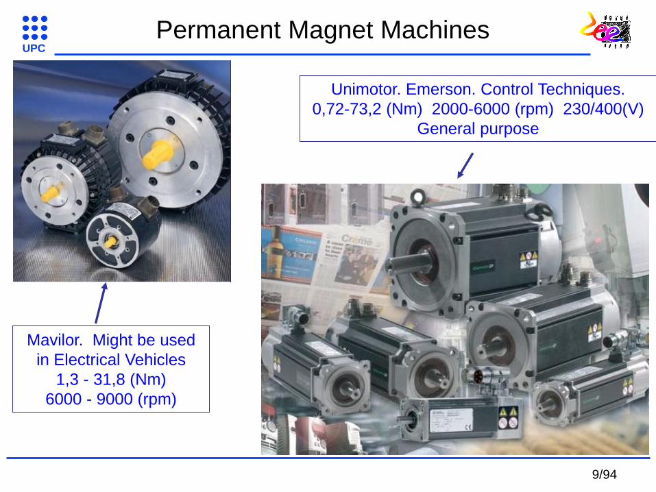
Mavilor. Might be used

in Electrical Vehicles

1,3 - 31,8 (Nm)

6000 - 9000 (rpm)

Unimotor. Emerson. Control Techniques.

0,72-73,2 (Nm) 2000-6000 (rpm) 230/400(V)

General purpose

9/94

UPC


PMSG 11kW

Multi-pole. External rotor

Wind turbine laboratory rig

(in collaboration with

Robotiker - Tecnalia)

4Q Motor Drive System

4kW DC – PMSM 1 kW

General purpose laboratory rig

10/94

UPC

• Considering the shape of the back EMF

• PMDC – brushless DC (BLDC) - trapezoidal

• PMAC – sinusoidal

Surface Mount Permanent Magnet

Synchronous Machine (SMPMSM)


Interior Mount Permanent Magnet

Synchronous Machine (IMPMSM)

11/94

UPC

PMSM Dynamic Equations

• Combines the individual phase quantities into a single vector in the complex plane

• Same transformation is applied to all other magnitudes such as voltages, fluxes, etc…

invariant power

invariantpower non

)()()(

32

32

3

4

3

2

c

etietiticij

c

j

ba

• Space vector transformation

12/94

UPC


• Basic equation for phase windings voltages

• Total flux linkage

flux produced by the rotor magnet

Leakage inductance

Magnetising inductance

Self inductance

Mutual inductance

c

b

a

c

b

a

s

c

b

a

dt

d

i

i

i

R

v

v

v

)cos(

)cos(

)cos(

34

32

r

r

r

m

c

b

a

ccbca

bcbba

acaba

c

b

a

ψ

i

i

i

LMM

MLM

MML

ψ

ψ

ψ

mψ

lL

mL

mlcba LLLLL

2m

cabcab

LMMM baab MM; = cbbc MM; = acca MM; =

a

b

c

i

ib

ic

b

c

a

a

va +-

vc

+

-

-

+

vb

m

r

13/94

UPC


• Voltage vector equation in the stationary - frame

)cos(

)cos(

2

3

2

r

r

mmlsdt

dψ

i

i

dt

dLL

i

iR

v

v

i

v +-

m

r

i

v

+

-

a

b

c

i

ib

ic

b

c

a

a

va +-

vc

+

-

-

+

vb

m

rClarke

transformation

invariant power

invariantpower non

º30cosº30cos

º60cosº60cos

32

32

c

xxcx

xxxcx

cb

cba

14/94

UPC

i

v +-

m

r

i

v

+

-

a

b

c

i

ib

ic

b

c

a

a

va +-

vc

+

-

-

+

vb

m

r

invariant power

invariantpower non;

2

3

2

30

2

1

2

11

32

32

c

x

x

x

cx

x

c

b

a

invariant power

invariantpower non1;

2

3

2

12

3

2

1

01

32

cx

xc

x

x

x

c

b

a

Clarke-1 Transformation

Clarke Transformation

• Non power invariant versus power invariant. See the comparison.


15/94

UPC


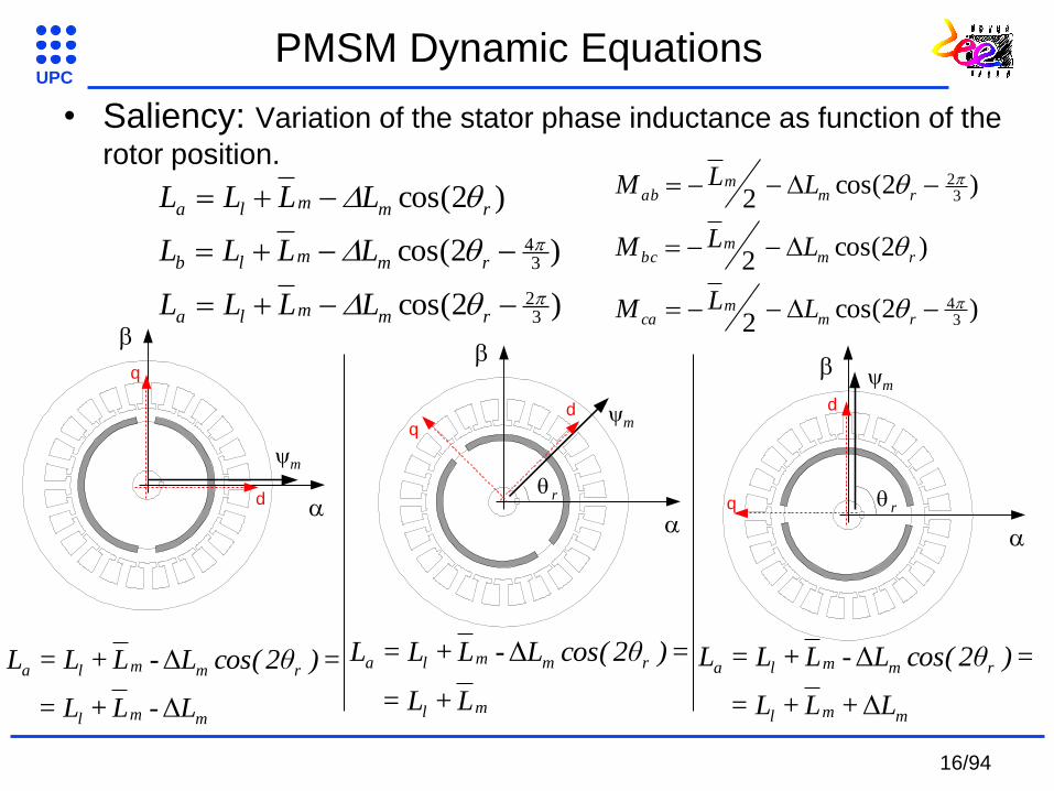
• Saliency: Variation of the stator phase inductance as function of the

rotor position.

)2cos(

)2cos(

)2cos(

32

34

rmmla

rmmlb

rmmla

LLLL

LLLL

LLLL

)2cos(2

)2cos(2

)2cos(2

34

32

rmm

ca

rmm

bc

rmm

ab

LLM

LLM

LLM

m

d

q

mml

rmmla

LLL

)θ2cos(LLLL

Δ-+=

=Δ-+=

m

r

dq

ml

rmmla

LL

)θ2cos(LLLL

+=

=Δ-+=

m

r

d

q

mml

rmmla

LLL

)θ2cos(LLLL

Δ++=

=Δ-+=

16/94

UPC


• voltage vector equation in the stationary - frame

considering saliency

• Where

• If there is no saliency and it is obtained the previous

equation.

)cos(

)cos(

)2cos()2sin(

)2sin()2cos(

2

r

r

m

rssrs

rsrss

s

dt

dψ

i

i

LLL

LLL

dt

d

i

iR

v

v

msmls LLLLL 2

3;

2

3

0mL

17/94

UPC


• Voltage vector equation in the synchronous reference d/q

frame fixed to the rotor

• Angle chosen equal to the PM position

• Direct axis ( Ld = LS-ΔLS ) and quadrature ( Lq = LS+ΔLS ) axis

inductances

m

r

d

id

+

-v

d

vq

+

-

iq

q

Park

transformation

i

v +-

m

r

i

v

+

-

1

0rm

q

d

qrd

rqd

q

d

s

q

dψ

i

i

dtdLL

LdtdL

i

iR

v

v

18/94

UPC

i

v +-

m

r

i

v

+

-

x

x

x

x

q

d

cossin

sincos

m

r

d

id

+

-v

d

vq

+

-

iq

q

q

d

x

x

x

x

cossin

sincos


Park Transformation

Park-1 Transformation

19/94

UPC

0 0.05 0.1 0.15 0.2 0.25 0.3 0.35-0.25

-0.2

-0.15

-0.1

-0.05

0

0.05

0.1

0.15

0.2

0.25

Time [ s ]

[ A

]

ialpha

ibeta

ib

ic

iq

id

• Non power invariant

• Different constant values. (c=2/3) for Clark & (c=1) for Clarke-1.

• Same amplitudes for (a,b,c) & (α,β) & (d,q).


20/94

UPC

0 0.05 0.1 0.15 0.2 0.25 0.3 0.35-0.4

-0.3

-0.2

-0.1

0

0.1

0.2

0.3

Time [ s ]

[ A

]

ialpha

ibeta

ib

ic

iq

id

ia

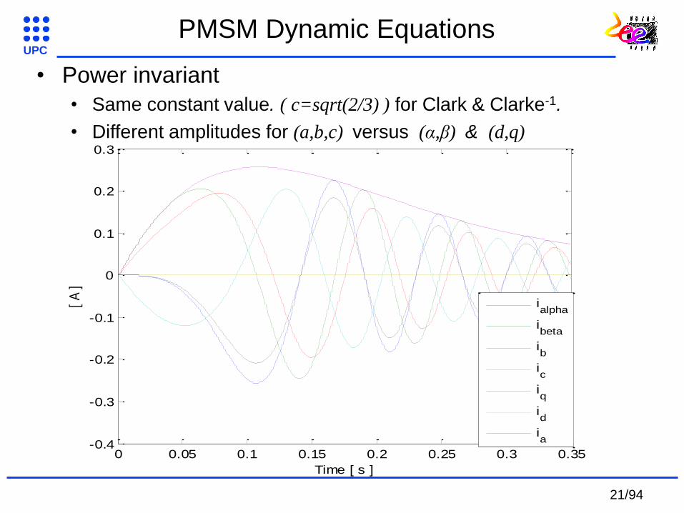
• Power invariant

• Same constant value. ( c=sqrt(2/3) ) for Clark & Clarke-1.

• Different amplitudes for (a,b,c) versus (α,β) & (d,q)


21/94

UPC

c

b

a

q

d

x

x

x

cx

x

2

3

2

30

2

1

2

11

cossin

sincos

invariant power

invariantpower non;

32sin

32sinsin

32cos

32coscos

32

32

cwhere

x

x

x

cx

x

c

b

a

q

d

• Direct (Clarke & Park) transformation


22/94

UPC

q

d

c

b

a

x

xc

x

x

x

cossin

sincos

23

2

1

23

2

1

01

invariant power

invariantpower non1;

32sin

32cos

32sin

32cos

sincos

32

cwhere

x

xc

x

x

x

q

d

c

b

a

• Direct (Clarke & Park) Inverse transformation


23/94

UPC


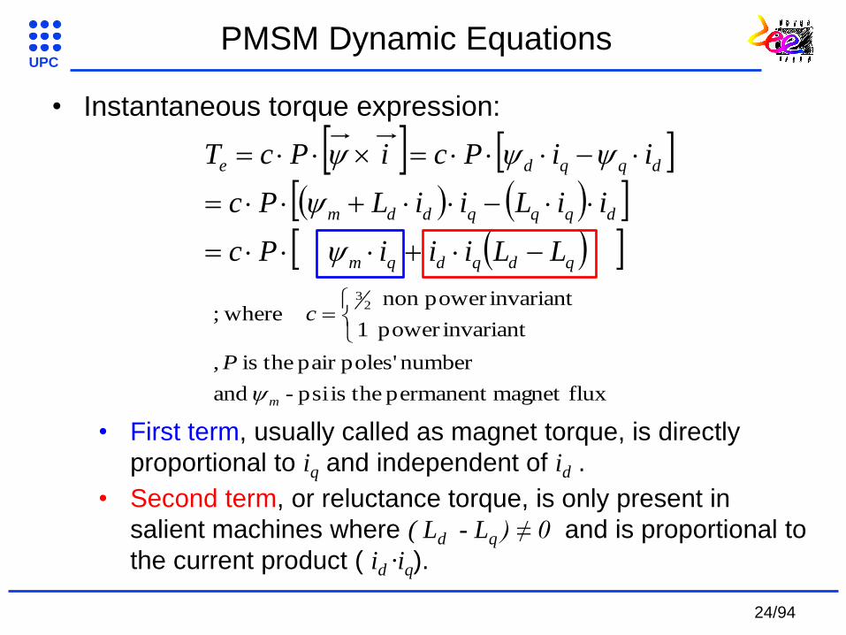
• Instantaneous torque expression:

qdqdqm

dqqqddm

dqqde

LLiiiPc

iiLiiLPc

iiPciPcT

fluxmagnet permanent theis psi - and

number poles'pair theis ,

invariant power 1

invariantpower non where;

23

m

P

c

• First term, usually called as magnet torque, is directly

proportional to iq and independent of id .

• Second term, or reluctance torque, is only present in

salient machines where ( Ld - Lq ) ≠ 0 and is proportional to

the current product ( id ·iq).

24/94

UPC

function transfer;

equation ldiferentia ;

DJs

TTw

TTwDdt

dwJ

Lem

Lemm

• Motion equation

• Drive Inertia ( J )

• Damping constant due to Friction ( D or F )

• Load Torque ( TL )


25/94

UPC

Exercise: Sketch a complete PMSM scheme model

• Use the d/q model equations

• Find out all the required equations involved

• Determine where the Clarke (a,b,c) to (α,β) & Park (α,β) to (d,q)

transformations should be applied to get a more realistic model

PMSM Modeling

26/94

UPC

PMSM Modeling

27/94

UPC

PMSM Modeling

•The adopted parameters for the model are as follows:

Lq=0.009165; Ld=0.006774; R=1.85; psi=0.1461; P=3.

(specific motor data is on the next page)

•For the motion equation of the whole drive it can be used:

J=0.77e-3; F=1e-3.

28/94

UPC

unimotor fm

Emerson Control Techniques

Model: 115E2A300BACAA115190

Number of poles: 6

Rated speed: 3000 (rpm)

Rated torque: 3.0 (Nm)

Rated power 0.94 (kW)

KT: 0.93 (Nm/Arms)

KE: 57.0 (Vrms/krpm)

Inertia: 4.4 (kgcm²)

R (ph-ph): 3.7 (Ohms)

L (ph-ph): 15.94 (mH)

Continuous stall: 3.5 (Nm)

Peak: 10.5 (Nm)

PMSM Modeling

• Ld and Lq values?

• ΔLs can be obtained measuring the

inductance for different rotor positions.

• The first order system, composed by

an L and R, can be identified by

supplying a step voltage in the d and q

components.

How to obtain the parameters

from a commercial catalogue?

ssdssq

dqdq

s

LLLLLL

LLLs

LLL

;

2;

2

29/94

UPC

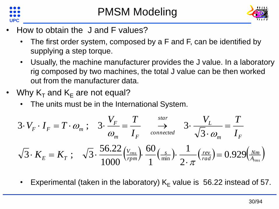
• How to obtain the J and F values?

• The first order system, composed by a F and F, can be identified by

supplying a step torque.

• Usually, the machine manufacturer provides the J value. In a laboratory

rig composed by two machines, the total J value can be then worked

out from the manufacturer data.

• Why KT and KE are not equal?

• The units must be in the International System.

• Experimental (taken in the laboratory) KE value is 56.22 instead of 57.

rms

rms

ANm

radrevs

rpm

V

TE

Fm

Lstar

connectedFm

FmFF

KK

I

TV

I

TVTIV

929.02

1

1

60

1000

22.563;3

333;3

min

PMSM Modeling

30/94

UPC

•How to obtain the value?

From the torque expression, and the KT (Nm/Arms)

parameter, it can be deduced the following expression:

Finally, the numerical value will be:

And the factor is used to convert the rms to the maximum value.

qme iPcT

Pc

KPcK

i

T TmmT

q

e

WbPc

KTm 1461.0

32

3

93.02

1

m

21

PMSM Modeling

31/94

UPC

Types of Controllers

32/94

UPC

Field Oriented Control (FOC) for PMSM

• Instantaneous torque for the PM synchronous machine

m

r

dq

Iq>0

m

r

dq

Iq<0

Te > 0 Te < 0

)( 2

3qdqdqme LLiiiψPT

• If id = 0, for not demagnetizing the PMSM, the reluctance torque is 0.

• Therefore, the electromagnetic torque will be regulated with iq .

• Duality with the DC Machine control.

qm iψP 2

3

id = 0

33/94

UPC

m

Te

m

r

dq

iq<0

m

r

dq

iq>0

m

m

m

r

dq

iq<0

m

m

r

dq

iq>0

m

FOC in PMSM

Four quadrant Motor (Q1 & Q3) Generator (Q2 & Q4) 34/94

UPC

FOC Scheme

SVM

4 step

Matrix

Converter

Grid

LC filter

UsAUsB

UsC

V

V

PMSM

32d q

iq* +

PI

PI

+id*

-

-d q

PWM m* +

PI-

m

d/dt

Pe

ia

ib

ic

UA UB UC

Kt -1

Speed

Current

Typical dynamic values (for a PMSM 0.5 / 10 kW)

discretization time /

switching frequency

Closed loop time response /

band width

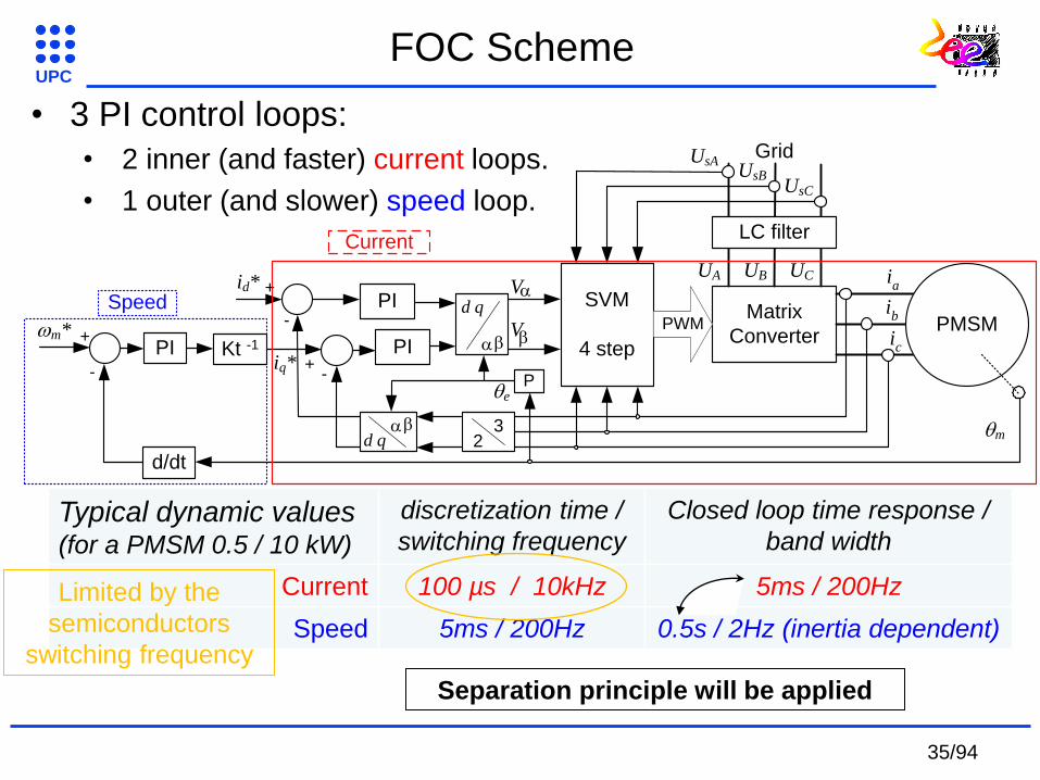
Current 100 µs / 10kHz 5ms / 200Hz

Speed 5ms / 200Hz 0.5s / 2Hz (inertia dependent)

• 3 PI control loops:

• 2 inner (and faster) current loops.

• 1 outer (and slower) speed loop.

Limited by the

semiconductors

switching frequency

Separation principle will be applied

35/94

UPC

Current Controller

• The current loop, for controlling design purposes, can be modeled as

a first order system.

s

s

s

RL

sRL

R

v

i

;1

1

1

0em

q

d

qed

eqd

q

d

s

q

dψ

i

i

sLL

LsL

i

iR

v

v

vd

+

Lq·we·iq

id

1

1

sRL

R

sd

svd id

1

1

sRL

R

sd

s

vq

-

iq

1

1

sRL

R

sq

s

( Ld·id +PM )·we

vq iq

1

1

sRL

R

sq

s

• The coupling terms are eliminated, since they are considered as a

perturbation.

36/94

UPC

• The current loop can be modeled as a first order system, whose

transfer function in Laplace domain is:

)(99.01)(;5

)(98.01)(;4

)(95.01)(;3

)(632.01)(;

)()1(1)(

tvRtit

tvRtit

tvRtit

tvRtit

tveRti

s

s

s

s

t

s

4

1)(

1

)(

)(

sRL

R

sV

sI

s

s

• Its open loop step time

response is:

Current Controller

37/94

UPC

0 0.005 0.01 0.015 0.02 0.025 0.030

0.1

0.2

0.3

0.4

0.5

0.6

0.7

System: g

Time (seconds): 0.0172

Amplitude: 0.531

System: g

Time (seconds): 0.0298

Amplitude: 0.54

Step Response

Time (seconds)

Am

plit

ud

e

• Considering the motor

parameters given before:

• Time constant:

• Time response at 98%

• Final value:

)(23.174 ms

185.110·97.7

85.11

)(

)(3

ssV

sI

)(31.485.1

10·97.7 3

ms

54.085.1

1

Current Controller

38/94

UPC

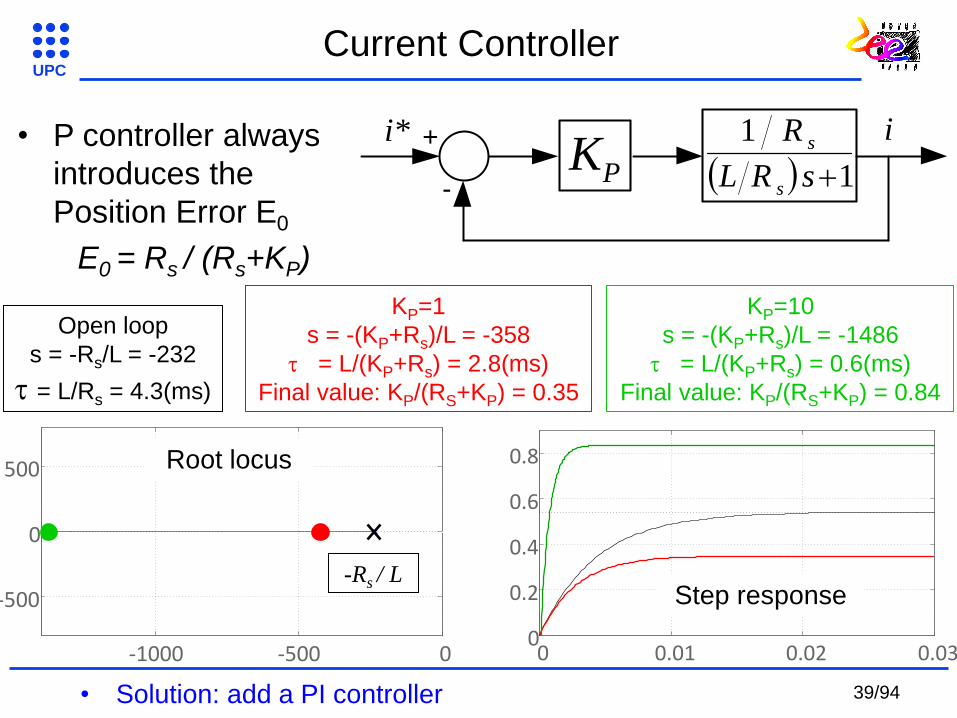
0 0.01 0.02 0.030

0.2

0.4

0.6

0.8

-1000 -500 0

-500

0

500

Open loop

s = -Rs/L = -232

= L/Rs = 4.3(ms)

KP=1

s = -(KP+Rs)/L = -358

= L/(KP+Rs) = 2.8(ms)

Final value: KP/(RS+KP) = 0.35

KP=10

s = -(KP+Rs)/L = -1486

= L/(KP+Rs) = 0.6(ms)

Final value: KP/(RS+KP) = 0.84

Root locus

Step response

+

-

i* i

1

1

sRL

R

s

s

PK• P controller always

introduces the

Position Error E0

E0 = Rs / (Rs+KP)

-Rs / L

• Solution: add a PI controller

Current Controller

39/94

UPC

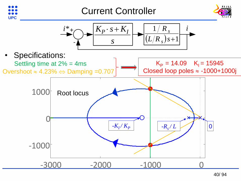
-3000 -2000 -1000 0

-1000

0

1000

KP = 14.09 KI = 15945

Closed loop poles -1000+1000j

• Specifications: Settling time at 2% = 4ms

Overshoot 4.23% Damping =0.707

Root locus

-Rs / L 0 -KI / KP

+

-

i* i

1

1

sRL

R

s

s

s

KsK IP

Current Controller

40/ 94

UPC

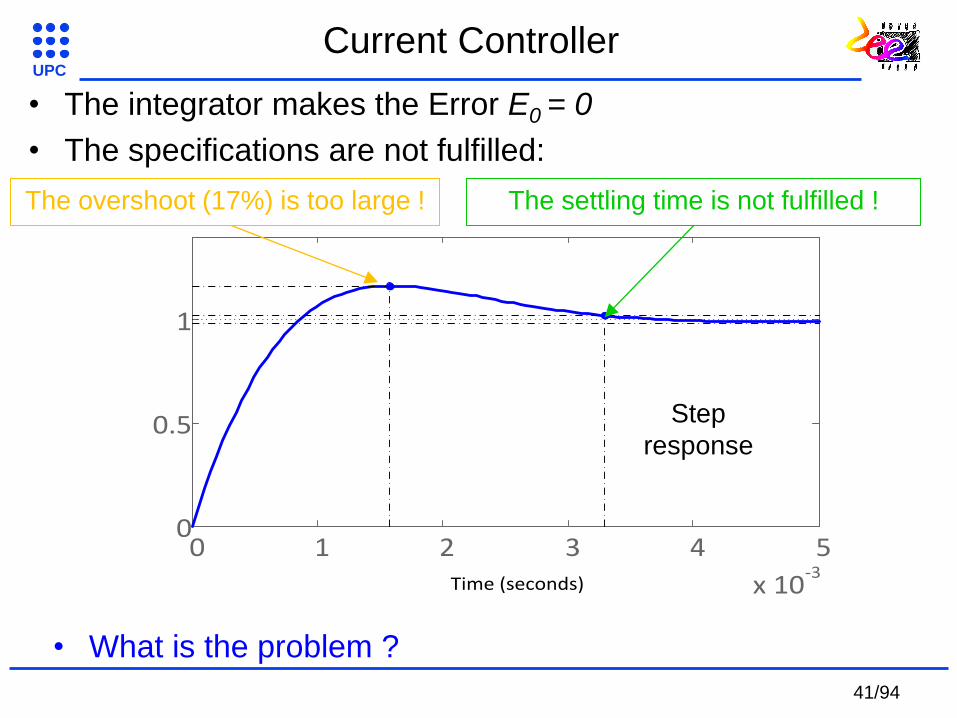
Time (seconds)

0 1 2 3 4 5

x 10-3

0

0.5

1

Step

response

The overshoot (17%) is too large !

The settling time is not fulfilled !

• The integrator makes the Error E0 = 0

• The specifications are not fulfilled:

• What is the problem ?

Current Controller

41/94

UPC

L

K

L

K

L

Rss

sK

K

L

K

i

i

IPs

I

PI

2

1

*

22

2

2 nn

n

ss

• What is the closed loop transfer function?

• Is it a pure 2nd

order term? NO! There is an

unwanted zero !

A pre filter is used

to cancel the zero +

-

i

1

1

sRL

R

s

s

s

KsK IP i*PFi*

1

1

sKK IP

L

K

L

K

L

Rss

sK

K

L

K

sK

Ki

i

IPs

I

PI

I

P

2

1

1

1

*

L

K

L

K

L

Rss

L

K

i

i

IPs

I

2*

Current Controller

42/94

UPC

0 1 2 3 4 5 6 7

x 10-3

0

0.5

1

Time (s)

L

K

L

K

L

Rss

L

K

L

K

L

K

L

Rss

L

K

sK

K

L

K

L

K

L

Rss

sK

K

L

K

i

i

IPs

I

IPs

I

I

P

IPs

I

PI

222

1

*

+

-

i* i

1

1

sRL

R

s

s

s

KsK IP i*PFi*

1

1

sKK IP+ -

i

1

1

sRL

R

s

s

s

KsK IP

zero

PI

PF+PI

Current Controller

43/94

UPC

+

-

i* i

1

1

sRL

R

s

s

s

K I +

-

PK

+

-

i* i

s

K I

1

1

sKR

L

KR

Ps

Ps

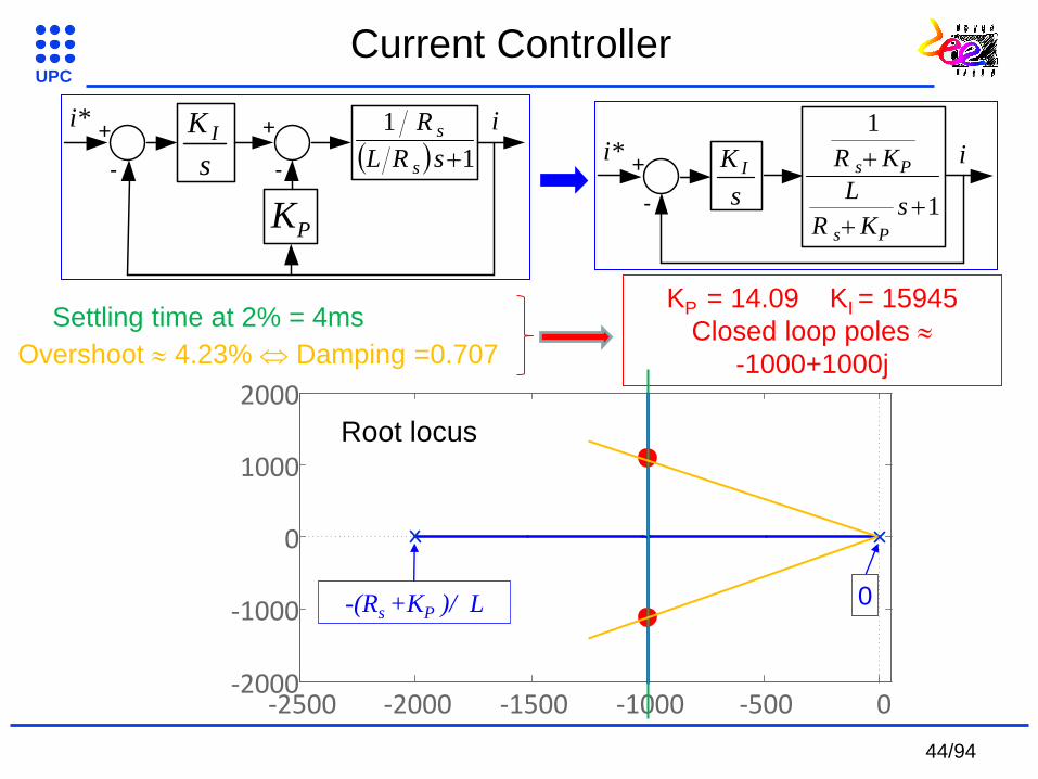
-2500 -2000 -1500 -1000 -500 0-2000

-1000

0

1000

2000

Root locus

-(Rs +KP )/ L 0

KP = 14.09 KI = 15945

Closed loop poles

-1000+1000j

Settling time at 2% = 4ms

Overshoot 4.23% Damping =0.707

Current Controller

44/94

UPC

Current Controller

Fixing the settling time at 2% (Ts2%) and the damping factor (ζ)

the KP and KI can be calculated

n

Ts

4

%2

22

2

2 nn

n

ss

L

K

L

K

L

Rss

L

K

i

i

IPs

I

2*

L

KR Psn

2

snP RLK 2

sP RTs

LK

%2

8

L

K In 2

2nI LK

2%2

2

16

Ts

LK I

2nd order TF

Current loop TF with PI or IP

Identifying coefficients

4.22 instead of 4 when ζ = 0.707

45/94

UPC

+

-

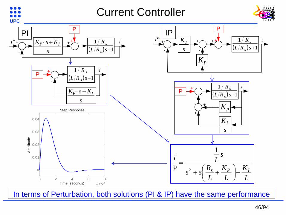
i* i

1

1

sRL

R

s

s

s

K I +

-

PK

+

P

+

P

++

-

i* i

1

1

sRL

R

s

s

s

KsK IP +

-

i

1

1

sRL

R

s

s

s

KsK IP

+P

i

1

1

sRL

R

s

s

s

K I

+

+PK

+P

-

L

K

L

K

L

Rss

sLi

IPs

2

1

P

0 2 4 6 8

x 10-3

0

0.01

0.02

0.03

0.04

Step Response

Time (seconds)

Am

plit

ud

e

PI IP

In terms of Perturbation, both solutions (PI & IP) have the same performance

Current Controller

46/94

UPC

PI+ -

id*PF + vd*id*

+

Lq·we·iq

PMSMControl

id

1

1

sRL

R

sd

s

1

1

sKK IP

• Decoupling terms have to be added:

iq*+

-

IP+ vq*

-

iq

1

1

sRL

R

sq

s

( Ld·id +PM )·we

PMSMControl

• Current loop with PI + PF (d axis) and IP (q axis)

-

Lq·we·iq

Ld·we·id +PM·we

+

Current Controller

47/94

UPC

• Implementing PI in a DSP

– From S to Z domain

– Ts=100us

Step Response

Time (sec)

Am

plitu

de

0 1 2 3 4 5 6 7 8

x 10-3

0

0.2

0.4

0.6

0.8

1

1.2

1.4

1-z

)Ts-1(-zK)z(PI

s

sK)s(PI

P

I

P

IK

K

P

KK

P=→

+=

1-z

,920-z5,5)z(PI

s

800s5,5)s(PI =→

+=

-1 -0.8 -0.6 -0.4 -0.2 0 0.2 0.4 0.6 0.8 1-1

-0.8

-0.6

-0.4

-0.2

0

0.2

0.4

0.6

0.8

1

Root Locus Editor (C)

Real Axis

Imag A

xis

0.84 0.86 0.88 0.9 0.92 0.94 0.96 0.98 1-0.2

-0.15

-0.1

-0.05

0

0.05

0.1

0.15

0.2

Root Locus Editor (C)

Real Axis

Ima

g A

xis

Current Controller

48/ 94

UPC

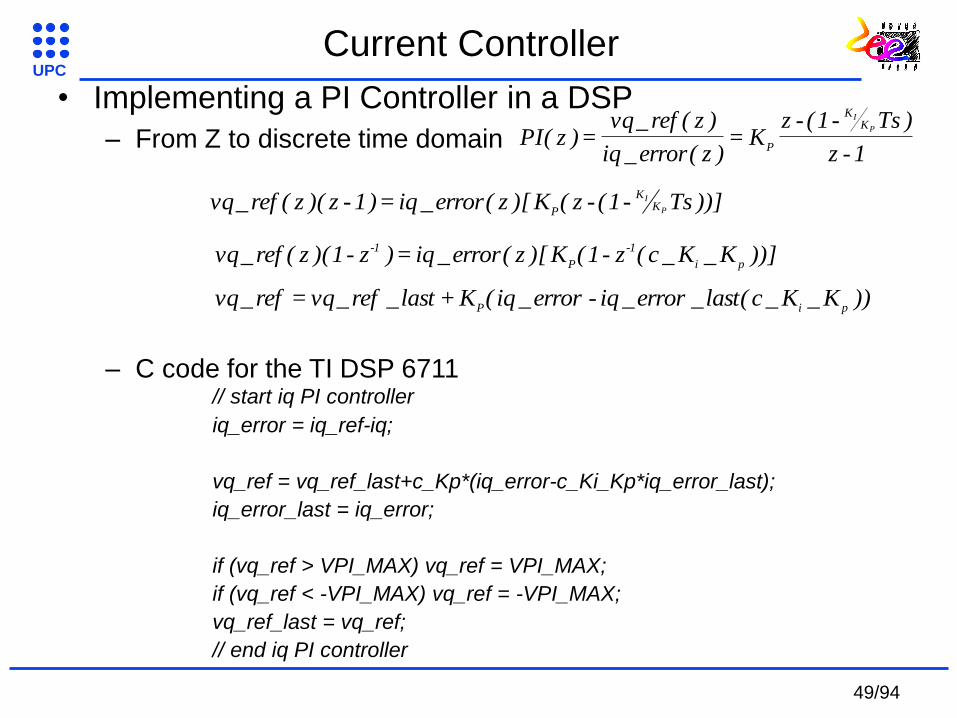
// start iq PI controller

iq_error = iq_ref-iq;

vq_ref = vq_ref_last+c_Kp*(iq_error-c_Ki_Kp*iq_error_last);

iq_error_last = iq_error;

if (vq_ref > VPI_MAX) vq_ref = VPI_MAX;

if (vq_ref < -VPI_MAX) vq_ref = -VPI_MAX;

vq_ref_last = vq_ref;

// end iq PI controller

• Implementing a PI Controller in a DSP

– From Z to discrete time domain

– C code for the TI DSP 6711

1-z

)Ts-1(-zK

)z(error_iq

)z(ref_vq)z(PI

P

IK

K

P==

))]Ts-1(-z(K)[z(error_iq)1-z)(z(ref_vqP

IK

K

P=

))]K_K_c(z-1(K)[z(error_iq)z-1)(z(ref_vqpi

-1

P

-1 =

))K_K_c(last_error_iq-error_iq(Klast_ref_vqref_vqpiP

+=

Current Controller

49/94

UPC

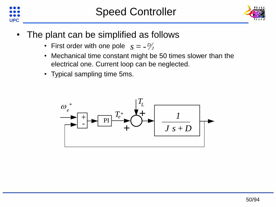
• The plant can be simplified as follows • First order with one pole

• Mechanical time constant might be 50 times slower than the

electrical one. Current loop can be neglected.

• Typical sampling time 5ms.

JD-s =

+- PI

Te*

DsJ

1

+

e*

+

+

TL

Speed Controller

50/94

UPC

Kp

In Out

++

s

1

e_ref

e_int

+e_sat

-e_sat

Saturation

Kt

Adapt TàI

e_oute_pro eo

Ki

0

10<>

e_dif

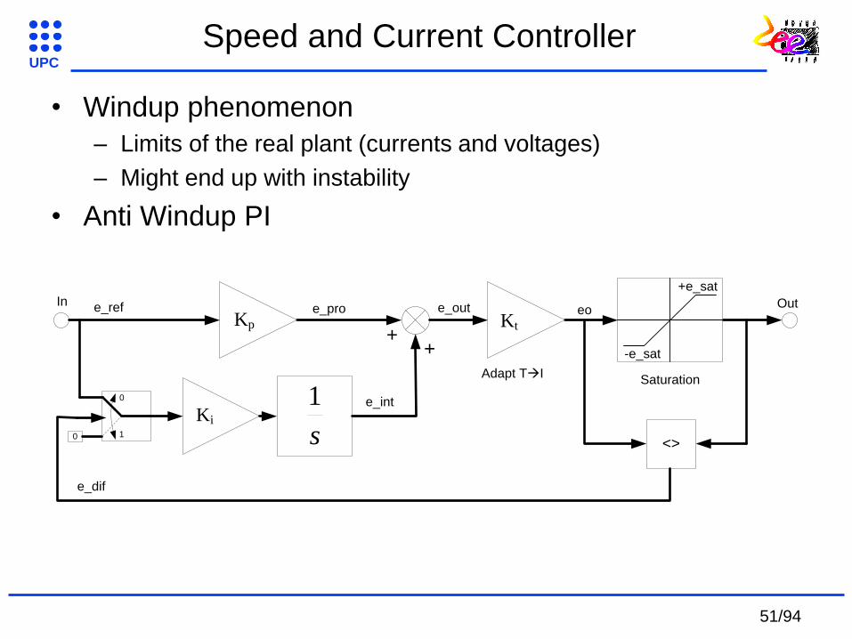
• Windup phenomenon

– Limits of the real plant (currents and voltages)

– Might end up with instability

• Anti Windup PI

Speed and Current Controller

51/94

UPC

Exercise

• Sketch a complete FOC scheme for a PMSM. It has to

include:

Speed and currents control loops

(PI + pre filter) or IP

Saturations (software protections)

Anti Windup

Feed forward (decoupling) terms

• Draw the magnitudes (speed reference, speed response, iq

reference and iq response) waveforms for the cases: (i)

electrical car & (ii) lift. Indicate, in the drawn waveforms,

the motoring or generating operating modes.

• Propose a programming code (any generic language) to

implement a PI.

52/94

UPC

• SISO tool. Matlab

• Matlab/Simulink PMSM FOC. Waveforms.

• FOC in a DSP

53/94

UPC

• Direct Torque Control (DTC) was firstly introduced by Takahashi in 1986

[Ref 1]. It was an important new method becoming very popular.

• Depenbrock in 1988 [Ref 2] introduced a similar idea under the name

Direct Self Control.

• However, just ABB company has got a popular commercial drive based

on DTC, the ASC600.

– Great number of applications such as: pumps, conveyors, lifts…from 2.2kW

until 630kW.

– Thanks to its 40MHz Toshiba processor plus ASIC, ASC600/800 closes the

entire control loop every 25us.

Takahashi, I and Nogushi, T. “A New Quick-Response and High-Efficiency Control Strategy of

an Induction Motor”, IEEE Trans. Industry Appl., Vol. 1A-22, pages 820-827, October 1986.

Depenbrock, M. "Direct Self Control of Inverter-Fed Induction Machines". IEEE Trans. on Power

Electronics. vol: PE-3, no:4 October 1988. pp: 420-429.

Direct Torque Control

54/94

UPC

Classical DTC schematic

Features

– Direct torque and stator flux control

– Indirect control of stator currents and

voltages

– Sinusoidal stator fluxes and currents

Table

Torque

ref

Flux ref +

-

+

-VSI

stator flux

torque

estimators

flux sector wm

DT

inductionmotor

Advantages

– Fastest torque response.

– Absence of co-ordinate transform.

– Absence of voltage modulator block

– Absence of PI controllers for flux and torque.

– Robustness against parameters variation.

55/94

UPC

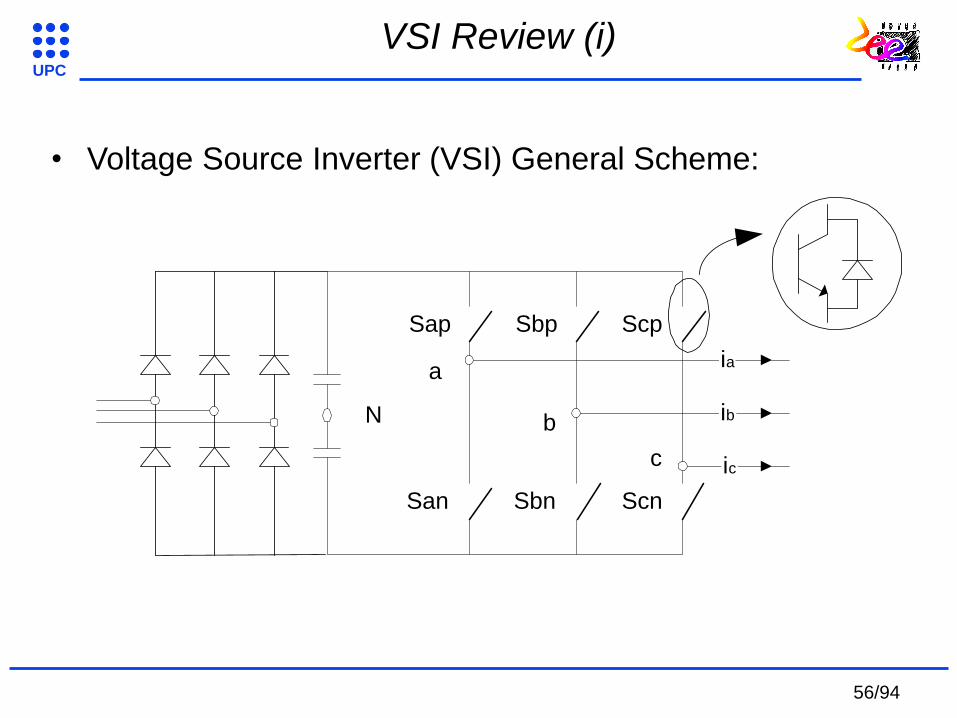
• Voltage Source Inverter (VSI) General Scheme:

N

San

Sap

Sbn

Sbp Scp

Scn

ia

ic

ib

a

b

c

VSI Review (i)

56/94

UPC

+Va+Vc

+Vb -Vb E1

a b c

E2

a b c

+Vb

-Vc

3

4

3

2

)()()(3

2

j

c

j

ba etvetvtvv

• Vector representation using the space vector transformation:

VSI Review (ii)

Questions:

(i) How many vectors?

(ii) Deduce the other

vectors.

57/94

UPC

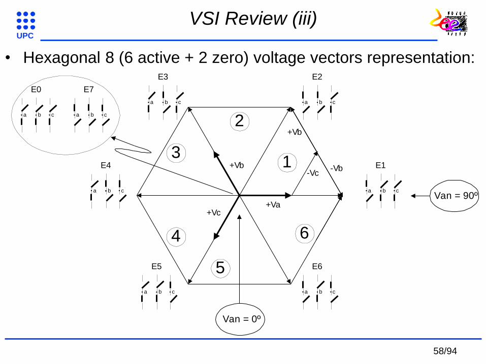
• Hexagonal 8 (6 active + 2 zero) voltage vectors representation:

VSI Review (iii)

+Va+Vc

+Vb -Vb E1

a b c

E2

a b c

+Vb

-Vc

E3

a b c

E4

a b c

E6

a b c

E5

a b c

1

5

4

3

2

6

E7

a b c

E0

a b c

Van = 0º

Van = 90º

58/94

UPC

Tangential component - torque Normal component - modulus flux

v1(100)

v4(011)

v3(010) v2(110)

v5(001) v6(101)

v3(FD,TI)

v2 (FI,TI)

1

65

4

32

v6(FI,TD)v5(FD,TD)

tg

n

DTC Principles

rss

'

r2mrs

me sin

LLL

LP

2

3t

S1

TI V2

T= V0FI

TD V6

TI V3

T= V7FD

TD V5

tu ss

59/94

UPC

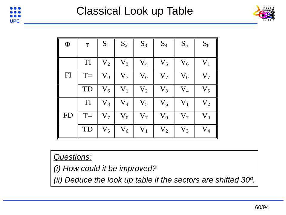
Classical Look up Table

S1 S2 S3 S4 S5 S6

TI V2 V3 V4 V5 V6 V1

T= V0 V7 V0 V7 V0 V7FI

TD V6 V1 V2 V3 V4 V5

TI V3 V4 V5 V6 V1 V2

T= V7 V0 V7 V0 V7 V0FD

TD V5 V6 V1 V2 V3 V4

Questions:

(i) How could it be improved?

(ii) Deduce the look up table if the sectors are shifted 30º.

60/94

UPC

Te* - hst

Te*

t1 t2 t3

S / H

1/TzTe* + hst

Te*

Tz Tz Tz

• The discrete or digital implementation of the hysteresis is possible only for huge

sampling frequency.

• Variable switching frequency.

Te*

Tz classic DTC

2_states

modulation

3_states

modulation

Tz

V1 V7V2

V7V2

V2V1

V2

V0 V2 V2V7V1 V1

THESIS

SVM

V0

V0

Classical DTC disadvantages

• Inherent torque and flux ripples. Non of the VSI states is able to generate the exact

voltage value required for make zero both the torque error and the stator flux error.

61/94

UPC

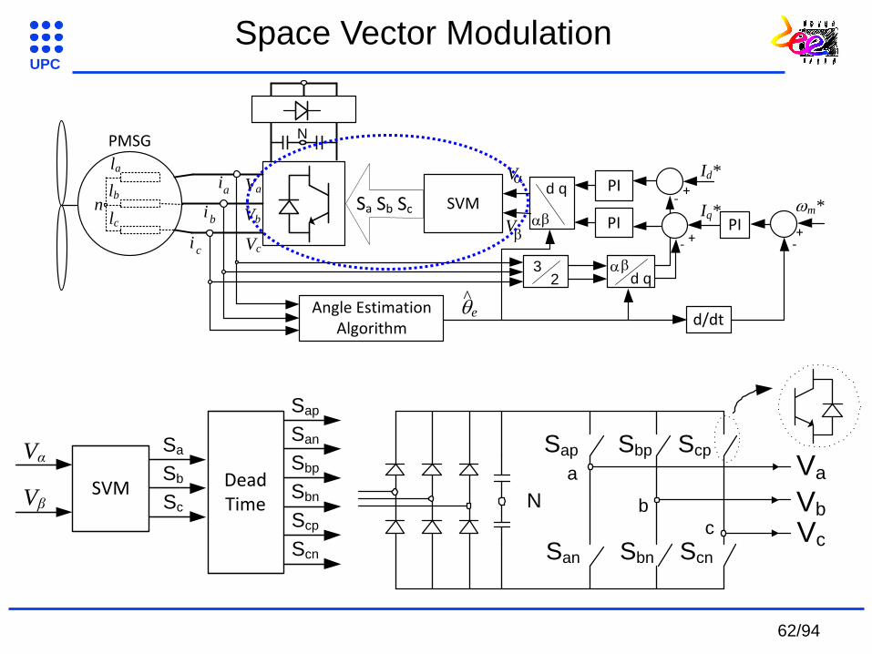
SVM

Vα

Vβ

Sa

Sb

Sc

Dead Time

Sap

San

Sbp

Sbn

Scp

Scn

N

Sap Sbp Scp

a

b

c

Va

Vb

VcSan Sbn Scn

SVM

V

V

PMSG

32 d q

Iq*

+

PI

PI

+

Id*

-

-d q

Angle EstimationAlgorithm

Sa Sb Sc m*

+PI-

e^

d/dt

ia

ib

ic

la

lb

lc

n

Va

Vb

Vc

N

Space Vector Modulation

62/94

UPC

SVM

Vα

Vβ

Sa

Sb

Sc

a b c

V2

a b ca b c

a b c

a b ca b c

5

4

3

6

β

α

V1

V3

V4

V5 V6

Vα

Vβ

Vref

jVVVref


63/94

UPC

Vref

d1·V1

d2·V2

2211 VdVdVref

PWMPWM T

Td

T

Td 2

21

1 ;

07

2107

322

321

º60sin

sin

º60sin

º60sin

TT

TTTTT

V

VTT

V

VTT

PWM

dc

ref

PWM

dc

ref

PWM

θ

sinº60sin

º60sinº60sin

22

11

ref

ref

VdV

VdV

a b c

V2

a b c

V1


64/94

UPC


Sa

Sb

Sc

Dead Time

Sap

San

Sbp

Sbn

Scp

Scn

• Ton < Toff The DC bus can be short circuited.

0

1Sa

off

onSap

off

on

San

N

Sap

a

San

0

1Sa

off

onSap

off

on

San

• Turn on transitions

have to be delayed.

dead time• Dead time appears.

65/94

UPC


LA

+

-

eA(t)

n

ia

icib

N

San

Sap

Sbn

Sbp Scp

Scn

ia

ic

ib

a

b

c

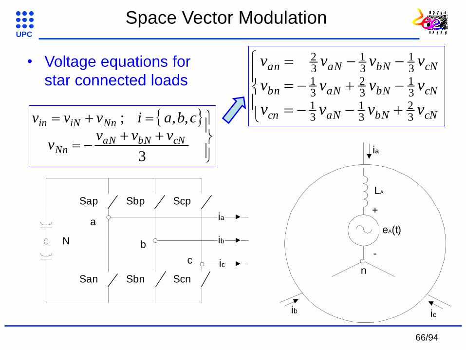
3

,,;

cNbNaNNn

NniNin

vvvv

cbaivvv

cNbNaNcn

cNbNaNbn

cNbNaNan

vvvv

vvvv

vvvv

32

31

31

31

32

31

31

31

32• Voltage equations for

star connected loads

66/94

UPC

cNbNaNcn

cNbNaNbn

cNbNaNan

vvvv

vvvv

vvvv

32

31

31

31

32

31

31

31

32

• Voltage waveforms for star connected load and using

double sided pattern:

V0

T0 /2

V1

T1 /2

V2

T2 /2

V7

T7

V1

T1 /2

V2

T2 /2

V0

T0 /2

• All sequence and V0 and V7 are placed in order to

minimize the commutations.


67/94

UPC

Vdc/2

VaN

VcN

VbN

VNn

Vcn

Vbn

Van

-Vdc/2

-Vdc/2

-Vdc/6

Vdc/6

Vdc/2

-Vdc/3

-Vdc/3

Vdc/3

Vdc/3

2/3Vdc

-2/3Vdc

Vdc/2

Vdc/2

-Vdc/2

-Vdc/2

TPWM

V2

a b c

V2

a b c

V1

a b c

V1

a b c

V0

a b c

V7

a b c

V0

a b c

68/94

UPC

Lu

eU(t)

ia

icib

+

-

iu

iv

iwN

San

Sap

Sbn

Sbp Scp

Scn

ia

ic

ib

a

b

c

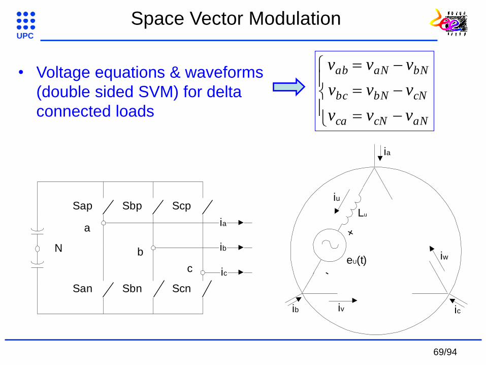
aNcNca

cNbNbc

bNaNab

vvv

vvv

vvv• Voltage equations & waveforms

(double sided SVM) for delta

connected loads


69/94

UPC

Vdc/2

VaN

VcN

VbN

-Vdc/2

Vdc/2

Vdc/2

-Vdc/2

-Vdc/2

TPWM

Vca

Vbc

Vab

-Vdc

Vdc

Vdc

V2

a b c

V2

a b c

V1

a b c

V1

a b c

V0

a b c

V7

a b c

V0

a b c

70/94

UPC

Fixed-speed WT Variable-speed WT

Case study: Wind Turbine Classification

Advantages:

• More energy production.

• Less mechanical stress.

• Reduce power fluctuation.

• Capacity of noise reduction.

• Greater grid currents control.

Drawbacks:

• Need of power electronic

converters.

• More expensive.

Advantages:

• Robust.

• Low Maintenance.

• Low Price

Drawbacks:

•Uncontrollable reactive power

consumption

•More mechanical strees.

•Gear box

In collaboration with Dr. Josep Pou 71/94

UPC

Case study: Wind Turbine fixed speed

Induction generator operating at fixed speed

Advantages:

- Robust design.

- No need for maintenance.

- Well enclosed.

- Produced in large series.

- Low price.

- Can withstand overloads.

Disadvantages:

- Uncontrollable reactive power consumption.

- Fixed speed means more mechanical stress.


UPC

- Capacitors banks compensate for reactive power from the induction

generator.

- Maxim use of the electrical grid is done operating at unity power

factor.

C C C

Voltage

Current

Capacitor Banks



UPC

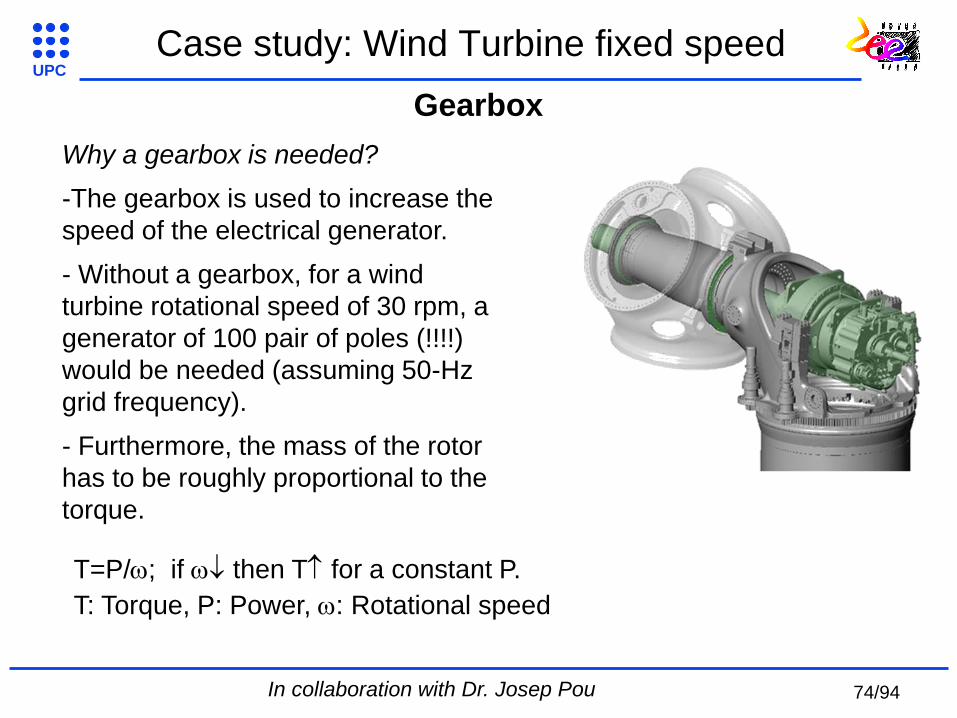
Why a gearbox is needed?

-The gearbox is used to increase the

speed of the electrical generator.

- Without a gearbox, for a wind

turbine rotational speed of 30 rpm, a

generator of 100 pair of poles (!!!!)

would be needed (assuming 50-Hz

grid frequency).

- Furthermore, the mass of the rotor

has to be roughly proportional to the

torque.

T=P/; if then T for a constant P.

T: Torque, P: Power, : Rotational speed

Gearbox



UPC

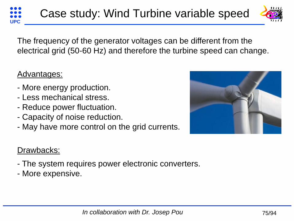
The frequency of the generator voltages can be different from the

electrical grid (50-60 Hz) and therefore the turbine speed can change.

Advantages:

- More energy production.

- Less mechanical stress.

- Reduce power fluctuation.

- Capacity of noise reduction.

- May have more control on the grid currents.

Drawbacks:

- The system requires power electronic converters.

- More expensive.

Case study: Wind Turbine variable speed


UPC

- The slip of the rotor can change within a wide range (and therefore the

wind-turbine speed as well).

- It is the most common topology produced by large manufacturers

nowadays.

ALSTOM-ECOTECNIA

Doubly-Fed Induction Generator (DFIG)



UPC

-Multipole synchronous generators may not need a gearbox (these

generators have a large diameter).

- The rotational speed can change within a wide range.

- This is expected to be the most common wind turbine configuration in

the future.

?

ENERCON E-126 (7 MW)

Multipole Synchronous Generators (MPSG)



UPC

Bi-directional

switch

SAc

T2

D2

T1

D1

LOAD

UsB

UsA

UsC

Ua

U U

UC

UB

UA

b c

N

i sC

icibia

i sB

i sA

SAa SAb SAc

SBa SBb SBc

SCa SCb SCcInput RL filter

n

iA

iB

iC

Matrix Converter (from AC to AC)


78/94

UPC

Back-to-back-connected (three-level) converter

(NP)

C vC2

vC1

C

r Vd

c s

t

a

b

c

Wind-Turbine NPC Converter Grid-Connected NPC Converter

vr

vs

vt

3*Lg iwt ig

Multipole Synchronous Wind Turbine

Electrical Grid



UPC

Case study: Wind Turbine Control

Wind

Models


UPC

Permanent Magnet

Synchronous Generator Electrical Grid

AC

DC

AC

DC

DTC (Direct Torque Control)

FOC (Field Oriented Control)

DPC (Direct Power Control)

VOC (Voltage Oriented Control)

Dual Solution

• 2 Power Converters & 4 control loops.

– PMSM. Inner current control & outer speed control

– Electrical Grid. Inner current control & outer voltage control


81/94

UPC

qv

dv

di

*dcV

Voltage Controller

Current Controller

Current Controller

*qI

qi

dcv

*dI

gL

gL

'dv

'qv

MAF(Tg )

Transf.

rst-dq

ir is it

Angle

Pos. Sequ.

d

Transf.

dq-rst

Grid Voltages

vr vs vt Converter Voltages

vrc vsc vtc Grid

Voltages

vr vs vt

Dip

Detector

Modification

of *dI and *

qI

Yes


SVM

LC filter

UsAUsBUsC

V

V

PMSG

32 d q

Iq*

+

PI

PI

+

Id*

-

-d q

Angle Estimation

Algorithm

PWM Pattern m*

+PI-

d/dte^

d/dt

test p

uls

es

ia

ib

ic

UAUBUC

la

lb

lc

n

Va

Vb

Vc

N

Grid

FOC

VOC


UPC

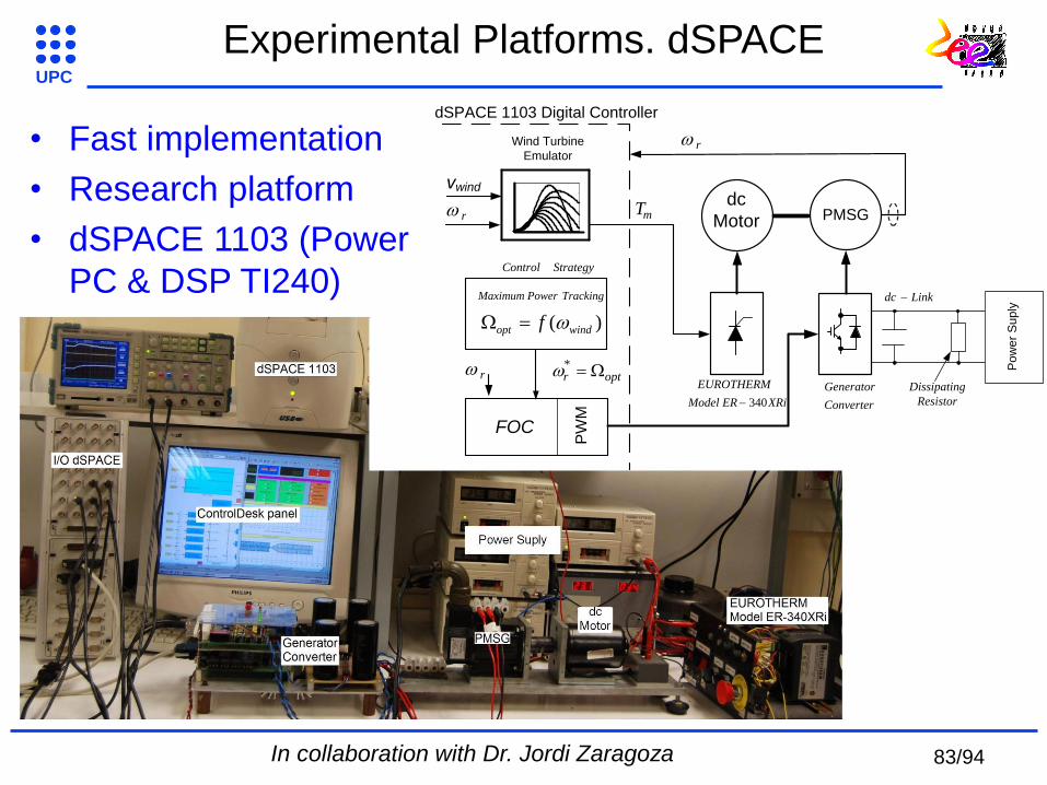
Experimental Platforms. dSPACE

• Fast implementation

• Research platform

• dSPACE 1103 (Power

PC & DSP TI240)

mT

rWind Turbine

Emulator

vwind

optr *

TrackingPowerMaximum

)( windopt f

StrategyControl

PMSG

FOC

dc

Motor

XRiERModel

EUROTHERM

340 Converter

Generatorr

PW

M

Linkdc

Po

we

r S

up

ly

dSPACE 1103 Digital Controller

Dissipating

Resistor

r

In collaboration with Dr. Jordi Zaragoza 83/94

UPC

• Easy to monitor and debug with the Control Desk

In collaboration with Dr. Jordi Zaragoza

Experimental Platforms. dSPACE

84/94

UPC

SVM

V

V

PMSG

32 d q

Iq*

+

PI

PI

+

Id*

-

-d q

Angle EstimationAlgorithm

Sa Sb Sc m*

+PI-

e^

d/dt

ia

ib

ic

la

lb

lc

n

Va

Vb

Vc

N

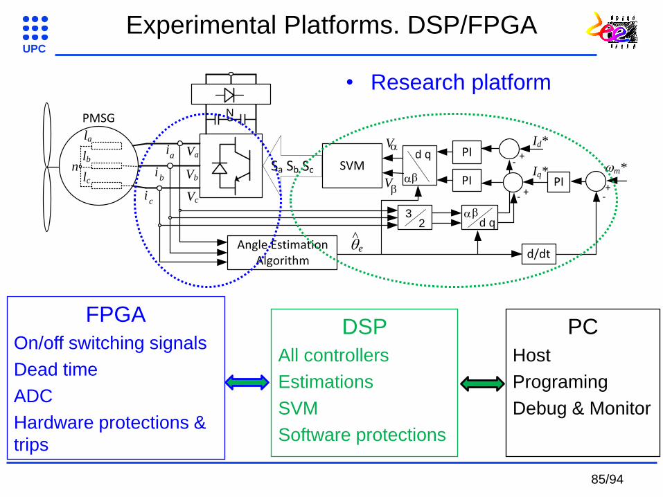
FPGA

On/off switching signals

Dead time

ADC

Hardware protections &

trips

DSP

All controllers

Estimations

SVM

Software protections

PC

Host

Programing

Debug & Monitor

Experimental Platforms. DSP/FPGA

• Research platform

85/94

UPC

In collaboration with Dr. Lee Empringham & Dr. Liliana de Lillo. University of Nottingham. UK. 86/94

UPC

Experimental Platforms. DSPIC

With the permission of MICROCHIP

http://www.microchip.com/pagehandler/en

-us/technology/motorcontrol/home.html

• Industrial platform

87/94

http://www.microchip.com/pagehandler/en-us/technology/motorcontrol/home.html



UPC

Experimental implementing issues

• Synchronisation: in order to minimise the commutation noise, the

currents’ sampling instant must be either at the middle or at the end of

the PWM period (i.e. during the applications of zero states V0 or V7).

Vcn

Vbn

Van

V2

a b c

V2

a b c

V1

a b c

V1

a b c

V0

a b c

V7

a b c

V0

a b c

2/3Vdc1/3Vdc

1/3Vdc

-1/3Vdc

-1/3Vdc-2/3Vdc

• Current and speed controllers must be also synchronised with the PWM.

88/94

UPC

Speed loop task

• Priorities: computing resources can be optimised if current loop task

has the highest priority. After the speed loop task and finally any software

for monitoring or debugging.

TintTint Tint

Tint Tint TintTint Tint

Current loop task

Same priority

Different priorities


89/94

UPC

• Incremental encoder: Number of pulses per interruption?

• It is assumed a sampling time of 100 (µs) and 5 (ms) for the current and

speed, respectively.

srev

pulsesN

rev

min

1060

1

min 6

N 3000 (rev/min) 30 (rev/min)

16384 (pulses/rev) 819,2 (pulses)

40960 (pulses)

8,192 (pulses)

409,6 (pulses)

4096 (pulses/rev) 204,8 (pulses)

10240 (pulses)

2,048 (pulses)

102,4 (pulses)

ms

pulsesN

510

2·60

1 2

s

pulsesN

10010

60

1 4

• Two speeds must be calculated for the speed (higher

accuracy) and current (lower accuracy) loops separately.


90/94

UPC

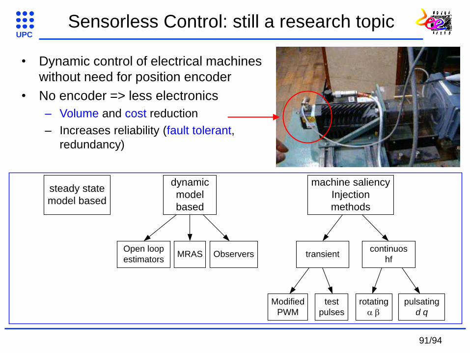
• Dynamic control of electrical machines

without need for position encoder

• No encoder => less electronics

– Volume and cost reduction

– Increases reliability (fault tolerant,

redundancy)

Sensorless Control: still a research topic

steady state

model based

dynamic

model

based

machine saliency

Injection

methods

Open loop

estimatorsMRAS Observers transient

continuos

hf

Modified

PWM

test

pulses

rotating

pulsating

d q

91/94

UPC

• Permanent Magnet Synchronous Machines

– Advantages:

• No rotor currents => no rotor losses.

• Higher efficiency => energy saving capability.

• Smaller rotor diameters, higher power density and lower rotor

inertia.

• Attractive for Wind applications, Aerospace applications such

as aircraft actuators, Machine tools, position servomotors

(replacing the DC motors).

– Inconveniences:

• Synchronous machines => need for rotor position.

• Price.

• Permanent magnet is becoming a scarce raw material.

Summary

92/94

UPC Summary

• PMSM dynamic equations and modelling

• FOC for PMSM has been introduced

– Principles & Scheme.

– PI & IP Controllers: root locus, specifications, design and

implementation.

• Classical DTC

– VSI Review.

– Principles, features & scheme.

– Hysteresis controllers.

• Space Vector Modulation

– Voltage equations & voltage waveforms.

– Dead time.

93/94

UPC

• Case study: Wind Turbine

– Constant versus variable speed.

– Dual solution for the Grid Connected Power Converter.

• Experimental approach

– Hardware platforms.

– (Some typical) implementing issues.

• Research: Sensorless Control of PMSM

Summary

94/94

Date post:	06-Mar-2018
Category:	Documents
Upload:	dodiep
View:	243 times
Download:	5 times

UPC PMSM Control (FOC & DTC) for WECS &...

Documents