Electronic Journal of Differential Equations, Vol. 2016 (2016), No. 318, pp. 1–22. ISSN: 1072-6691. URL: http://ejde.math.txstate.edu or http://ejde.math.unt.edu UPPER BOUNDS FOR THE NUMBER OF LIMIT CYCLES OF POLYNOMIAL DIFFERENTIAL SYSTEMS SELMA ELLAGGOUNE, SABRINA BADI Abstract. For ε small we consider the number of limit cycles of the polyno- mial differential system ˙ x = y - f 1 (x, y)y, ˙ y = -x - g 2 (x, y) - f 2 (x, y)y, where f 1 (x, y)= εf 11 (x, y)+ ε 2 f 12 (x, y), g 2 (x, y)= εg 21 (x, y)+ ε 2 g 22 (x, y) and f 2 (x, y)= εf 21 (x, y)+ ε 2 f 22 (x, y) where f 1i ,f 2i ,g 2i have degree l, n, m respectively for each i =1, 2. We provide an accurate upper bound of the maximum number of limit cycles that this class of systems can have bifurcating from the periodic orbits of the linear center ˙ x = y, ˙ y = -x using the averaging theory of first and second order. We give an example for which this bound is reached. 1. Introduction One of the main problems in the theory of ordinary differential equations is the study of their limit cycles, their existence, their number and their stability. A limit cycle of a differential equation is a periodic orbit in the set of all isolated periodic orbits of the differential equation. The second part of the 16th Hilbert’s problem (see [4]) is related to the least upper bound on the number of limit cycles of polynomial vector fields having a fixed degree. These years many papers have studied the limit cycles of planar polynomial differential systems. In this paper we will try to give a partial answer to this problem for the class of polynomial differential systems given by ˙ x = y - f 1 (x, y)y, ˙ y = -x - g 2 (x, y) - f 2 (x, y)y, (1.1) where f 1 (x, y)= εf 11 (x, y)+ ε 2 f 12 (x, y), g 2 (x, y)= εg 21 (x, y)+ ε 2 g 22 (x, y) and f 2 (x, y)= εf 21 (x, y)+ ε 2 f 22 (x, y) wheref 1i ,f 2i and g 2i have degree l, n and m respectively for each i =1, 2 and ε is a small parameter. Note that when f 1 (x, y)= 0,g 2 (x, y) = 0 and f 2 (x, y)= f (x) these systems coincide with the generalized polynomial Li´ enard differential systems ˙ x = y, ˙ y = -x - f (x)y, (1.2) where f (x) is a polynomial in the variable x of degree n. In 1977 Lins, de Melo and Pugh [7] studied the classical polynomial Li´ enard differential system (1.2) and stated the following conjecture: 2010 Mathematics Subject Classification. 34C25, 34C29, 37G15. Key words and phrases. Limit cycle; Li´ enard differential equation; averaging method. c 2016 Texas State University. Submitted October 1, 2016. Published December 14, 2016. 1
Transcript
Electronic Journal of Differential Equations, Vol. 2016 (2016), No. 318, pp. 1–22.
ISSN: 1072-6691. URL: http://ejde.math.txstate.edu or http://ejde.math.unt.edu
UPPER BOUNDS FOR THE NUMBER OF LIMIT CYCLES OFPOLYNOMIAL DIFFERENTIAL SYSTEMS
SELMA ELLAGGOUNE, SABRINA BADI
Abstract. For ε small we consider the number of limit cycles of the polyno-
and f2(x, y) = εf21(x, y) + ε2f22(x, y) where f1i, f2i, g2i have degree l, n, mrespectively for each i = 1, 2. We provide an accurate upper bound of the
maximum number of limit cycles that this class of systems can have bifurcating
from the periodic orbits of the linear center x = y, y = −x using the averagingtheory of first and second order. We give an example for which this bound is
reached.
1. Introduction
One of the main problems in the theory of ordinary differential equations is thestudy of their limit cycles, their existence, their number and their stability. Alimit cycle of a differential equation is a periodic orbit in the set of all isolatedperiodic orbits of the differential equation. The second part of the 16th Hilbert’sproblem (see [4]) is related to the least upper bound on the number of limit cyclesof polynomial vector fields having a fixed degree. These years many papers havestudied the limit cycles of planar polynomial differential systems. In this paperwe will try to give a partial answer to this problem for the class of polynomialdifferential systems given by
x = y − f1(x, y)y, y = −x− g2(x, y)− f2(x, y)y, (1.1)
where f1(x, y) = εf11(x, y) + ε2f12(x, y), g2(x, y) = εg21(x, y) + ε2g22(x, y) andf2(x, y) = εf21(x, y) + ε2f22(x, y) wheref1i, f2i and g2i have degree l, n and mrespectively for each i = 1, 2 and ε is a small parameter. Note that when f1(x, y) =0, g2(x, y) = 0 and f2(x, y) = f(x) these systems coincide with the generalizedpolynomial Lienard differential systems
x = y, y = −x− f(x)y, (1.2)
where f(x) is a polynomial in the variable x of degree n.In 1977 Lins, de Melo and Pugh [7] studied the classical polynomial Lienard
differential system (1.2) and stated the following conjecture:
Submitted October 1, 2016. Published December 14, 2016.
1
2 S. ELLAGGOUNE, S. BADI EJDE-2016/318
If f(x) has degree n ≥ 1, then (1.2) has at most [n2 ] limit cycles.Then they proved this conjecture for n = 1, 2. The conjecture for n = 3 has beenproved recently by Chengzi and Llibre [8]. For more information see [11].
Many of the results on the limit cycles of polynomial differential systems havebeen obtained by considering limit cycles which bifurcate from a single degeneratesingular point, that are so called small amplitude limit cycles, see for instance[13]. We denote by H(m,n) the maximum number of small amplitude limit cyclesfor systems of the form (1.2). The values of H(m,n) give a lower bound for themaximum number H(m,n) (i.e. The Hilbert number) of limit cycles that thedifferential equation (1.2) with m and n fixed can have. For more informationabout the Hilbert’s 16th problem and related topics see [5].
In [10] the authors ise the averaging theory of first and second order to studythe system
x = y − ε(g11(x) + f11(x)y)− ε2(g12(x) + f12(x)y),
y = −x− ε(g21(x) + f21(x)y)− ε2(g22(x) + f22(x)y),(1.3)
where g1i, f1i, g2i, f2i have degree l, k,m, n respectively for each i = 1, 2, and ε is asmall parameter. They provided an accurate upper bound of the maximum numberof limit cycles that the above system can have bifurcating from the periodic orbitsof the linear center x = y, y = −x.
In this article, first we consider the more general systemx = y − ε(f11(x, y)y),
y = −x− ε(g21(x, y) + f21(x, y)y),(1.4)
where f11, g21 and f21 have degree l,m and n respectively, and ε is a small param-eter. We obtain the following result.
Theorem 1.1. For |ε| sufficiently small, the maximum number of limit cycles ofthe generalized polynomial differential system (1.4) bifurcating from the periodicorbits of the linear center x = y, y = −x using the averaging theory of first order is[n2 ].
The proof of the above theorem is given in section 3.Secondly we consider the system
where f11 andf12 have degree l; g21 and g22 have degree m; and f21, f22 have degreen. Furthermore, ε is a small parameter. We obtain the theorem bellow.
Theorem 1.2. For |ε| sufficiently small, the maximum number of limit cycles ofthe generalized polynomial differential system (1.5) bifurcating from the periodicorbits of the linear center x = y, y = −x using the averaging theory of second orderis
λ = max{λ1, λ2 + 1, λ3 + 2},where
λ1 = max{
[O(m) + E(l)− 1
2], [E(m) +O(l)− 1
2], [O(n) +O(l)− 2
2],
m− 1, [E(n)
2], [E(m) +O(n)− 1
2]},
EJDE-2016/318 UPPER BOUNDS FOR THE NUMBER OF LIMIT CYCLES 3
λ2 = max{O(n)− 1, [
E(m) +O(n)− 32
], [O(m) + E(n)− 3
2],
[O(n) +O(l)− 2
2], l − 1, E(m)− 2, [
E(m) +O(n)− 32
],
[O(m) + E(l)− 3
2], [E(n) +O(m)− 3
2]},
λ3 = [E(n) + E(l)− 4
2],
where O(i) is the largest odd integer less than or equal to i, E(i) is the largest eveninteger less than or equal to i and [·] denotes the integer part function.
The proof of the above theorem is given in section 4. The results that we shalluse from the averaging theory of first and second order for computing limit cyclesare presented in section 2.
2. Averaging theory of first and second order
The averaging theory of first and second orders was introduced to study periodicorbits, which is summarized as follows. Consider a differential system
where F1, F2 : R×D → Rn, R : R×D× (−εf , εf )→ Rn are continuous functions,which are T-periodic in the first variable, and D is an open subset of Rn. Assumethat:
(i) F1(t, ·) ∈ C1(D) for all t ∈ R, F1, F2, R,DxF1 are locally Lipschitz withrespect to x, and R is differentiable with respect to ε. We define
F10(z) =1T
∫ T
0
F1(s, z)ds,
F20(z) =1T
∫ T
0
[DzF1(s, z)y1(s, z) + F2(s, z)]ds,
where
y1(s, z) =∫ θ
0
F1(t, z)dt.
(ii) For V ⊂ D an open and bounded set and for each ε ∈ (−εf , εf ) \ {0},there exists an aε ∈ V such that F10(aε) + εF20(aε) = 0 and dB(F10 +εF20, V, aε) 6= 0. Then, for |ε| > 0 sufficiently small there exists a T-periodic solution ϕ(·, ε) of the system (2.1) such that ϕ(0, ε) = aε.
The expression dB(F10 + εF20, V, aε) 6= 0 means that the Brouwer degree of thefunction F10+εF20 : V → Rn at the fixed point aε is not zero. A sufficient conditionfor the inequality to be true is that the Jacobian of the function F10 + εF20 at aεis not zero.
If F10 is not identically zero, then the zeros of F10 + εF20 are mainly those ofF10 for ε sufficiently small. In this case the previous result provides the averagingtheory of first order.
If F10 is identically zero and F20 is not identically zero, then the zeros of F10+εF20
are mainly the zeros of F20 for ε sufficiently small. In this case the previous resultprovides the averaging theory of second order.
For more information about the averaging theory see ([16],[17]).
4 S. ELLAGGOUNE, S. BADI EJDE-2016/318
3. Proof of Theorem 1.1
We need the first order averaging theory, for this we write system (1.4) in polarcoordinates (r, θ) where x = r cos(θ), y = r sin(θ), r > 0. In this way system (1.4)is written in the standard form for applying the averaging theory. If we write
f11(x, y) =l∑
i+j=0
aij,1xiyj , f21(x, y) =
n∑i+j=0
aij,2xiyj ,
g21(x, y) =m∑
i+j=0
bij,2xiyi,
(3.1)
then system (1.4) becomes
r = −ε( n∑i+j=0
aij,2ri+j+1 cosi(θ) sinj+2(θ) +
m∑i+j=0
bij,2ri+j cosi(θ) sinj+1(θ)
+l∑
i+j=0
aij,1ri+j+1 cosi+1(θ) sinj+1(θ)
),
θ = −1− 1r
[ε( n∑i+j=0
aij,2ri+j+1 cosi+1(θ) sinj+1(θ)
+m∑
i+j=0
bij,2ri+j cosi+1(θ) sinj(θ)
−l∑
i+j=0
aij,1ri+j+1 cosi(θ) sinj+2(θ)
)].
(3.2)
Now taking θ as the new independent variable, this system becomesdr
dθ= εF1(r, θ) +O(ε2),
where
F1(r, θ) =n∑
i+j=0
aij,2ri+j+1 cosi(θ) sinj+2(θ) +
m∑i+j=0
bij,2ri+j cosi(θ) sinj+1(θ)
+l∑
i+j=0
aij,1ri+j+1 cosi+1(θ) sinj+1(θ).
Using the notation introduced in section 2 we must calculate
F10(r) =1
2π
∫ 2π
0
F1(r, θ)dθ.
Since ∫ 2π
0
cosi(θ) sinj+2(θ)dθ =
{0 if i odd or j odd,παij if i even, j even,
where αij is a constant, we obtain
F10(r) =12r
n∑i+j=0
aij,2αijri+j , (3.3)
EJDE-2016/318 UPPER BOUNDS FOR THE NUMBER OF LIMIT CYCLES 5
where i and j are both even.Then the polynomial F10(r) has at most [n2 ] positive roots, and we can choose
the coefficients αij with i even, j even in such a way that F10(r) has exactly [n2 ]simple positive roots, hence Theorem 1.1 is proved.
4. Proof of Theorem 1.2
For the proof we shall use the second order averaging theory as it was stated insection 2. We write f11, f21 and g21 as in (3.1) and
f12(x, y) =l∑
i+j=0
Cij,1xiyj , f22(x, y) =
n∑i+j=0
cij,2xiyj ,
g22(x, y) =m∑
i+j=0
dij,2xiyi.
Then system (1.5) in polar coordinates becomes
r = −ε(A+ εB),
θ = −1− ε
r(A1 + εB1),
(4.1)
where
A =n∑
i+j=0
aij,2ri+j+1 cosi(θ)sinj+2(θ) +
m∑i+j=0
bij,2ri+j cosi(θ) sinj+1(θ)
+l∑
i+j=0
aij,1ri+j+1 cosi+1(θ) sinj+1(θ),
B =n∑
i+j=0
cij,2ri+j+1 cosi(θ) sinj+2(θ) +
m∑i+j=0
dij,2ri+j cosi(θ) sinj+1(θ)
+l∑
i+j=0
Cij,1ri+j+1 cosi+1(θ) sinj+1(θ),
A1 =n∑
i+j=0
aij,2ri+j+1 cosi+1(θ) sinj+1(θ) +
m∑i+j=0
bij,2ri+j cosi+1(θ) sinj(θ)
−l∑
i+j=0
aij,1ri+j+1 cosi(θ) sinj+2(θ),
B1 =n∑
i+j=0
cij,2ri+j+1 cosi+1(θ) sinj+1(θ) +
m∑i+j=0
dij,2ri+j cosi+1(θ) sinj(θ)
−l∑
i+j=0
Cij,1ri+j+1 cosi(θ) sinj+2(θ).
Taking θ as the new independent variable, this system becomes
dr
dθ= εF1(r, θ) + ε2F2(r, θ) +O(ε3),
6 S. ELLAGGOUNE, S. BADI EJDE-2016/318
where
F1(r, θ) = A, F2(r, θ) = B − 1rAA1.
To compute F20(r), we need that F10(r) be identically zero, which is equivalent toaij,2 = 0 for i even, j even.
Now we determine the corresponding function
F20(r) =1
2π
∫ 2π
0
[ ddrF1(r, θ)y1(r, θ) + F2(r, θ)
]dθ.
First, we have
d
drF1(r, θ) =
n∑i+j=0
i odd or j odd
(i+ j + 1)aij,2ri+j cosi(θ) sinj+2(θ)
+m∑
i+j=0
(i+ j)bij,2ri+j−1 cosi(θ) sinj+1(θ)
+l∑
i+j=0
(i+ j + 1)aij,1ri+j cosi+1(θ) sinj+1(θ),
and we write
y1(r, θ) =∫ θ
0
F1(r, t)dt = y11 + y2
1 + y31 ,
so we obtain
y11(r, t) =
∫ θ
0
n∑i+j=0
aij,2ri+j+1cosi(t) sinj+2(t)dt
= a10,2r2(α110 sin(θ) + α210 sin(3θ)
)+ . . .
+ ac1e1,2rc1+e1+1
(α1c1e1 sin(θ) + α2c1e1 sin(3θ) + . . .
+ α (c1+e1+2)+12 c1e1
sin((c1 + e1 + 2)θ))
+ a01,2r2(α101 + α201 cos(θ) + α301 cos(3θ)
)+ . . .
+ ap1q1,2rp1+q1+1
(α1p1q1 + α2p1q1 cos(θ) + α3p1q1 cos(3θ) + . . .
+ α (p1+q1+2)+32 p1q1
cos((p1 + q1 + 2)θ))
+ a11,2r3(α111 + α211 cos(2θ) + α311 cos(4θ)
)+ . . .
+ ac1q1,2rc1+q1+1
(α1c1q1 + α2c1q1 cos(2θ) + α3c1q1 cos(4θ) + . . .
+ α (c1+q1+2)+22 c1q1
cos((c1 + q1 + 2)θ)),
where c1 is the greatest odd number and e1 is the greatest even number so thatc1 + e1 is less than or equal to n. p1 is the greatest even number and q1 is thegreatest odd number so that p1 + q1 is less than or equal to n. αijk are realconstants exhibited during the computation of
∫ θ0
cosi(t) sinj+2(t)dt for all i and j.
EJDE-2016/318 UPPER BOUNDS FOR THE NUMBER OF LIMIT CYCLES 7
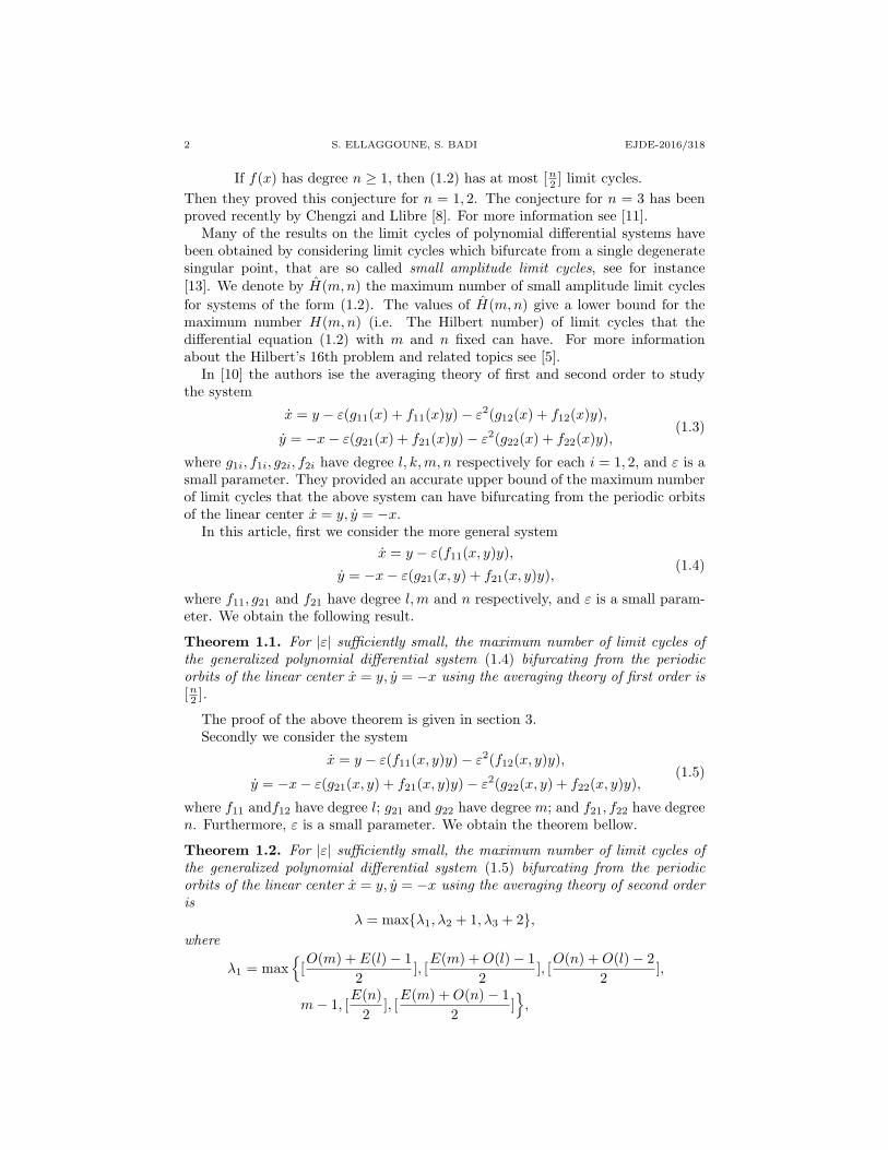
where p2 is the greatest even number and e2 is the greatest even number so thatp2 + e2 is less than or equal to m. c2 is the greatest odd number and q2 is thegreatest odd number so that c2 + q2 is less than or equal to m. αijk are realconstants exhibited during the computation of
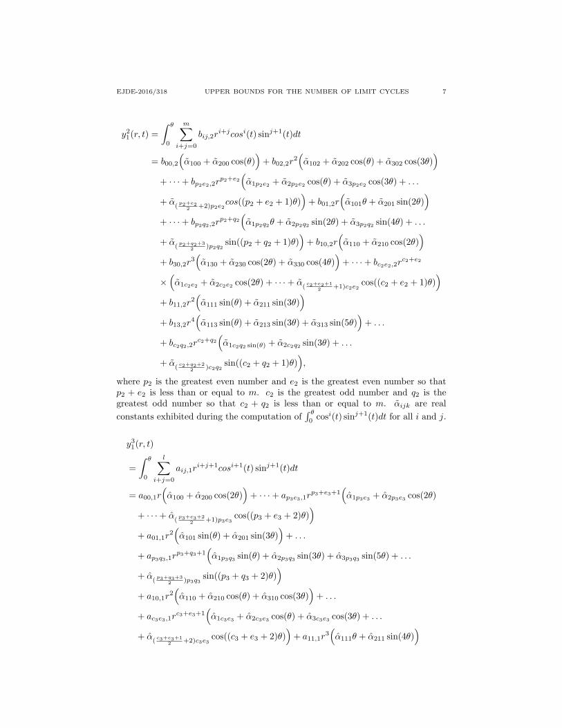
where p3 is the greatest even number and e3 is the greatest even number so thatp3 +e3 is less than or equal to l, c3 is the greatest odd number and q3 is the greatestodd number so that c3+q3 is less than or equal to l, αijk are real constants exhibitedduring the computation of
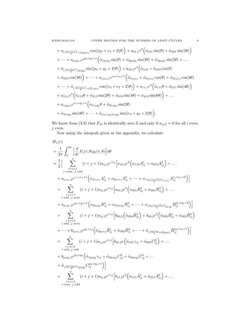
We know from (3.3) that F10 is identically zero if and only if aij,2 = 0 for all i even,j even.
Now using the integrals given at the appendix, we calculate
H1(r)
=1
2π
∫ 2π
0
[ ddrF1(r, θ)y1(r, θ)
]dθ
=12
[ n∑i+j=1
i even, J odd
(i+ j + 1)aij,2ri+j[a10,2r
2(α110A
1ij + α210A
3ij
)+ . . .
+ ac1e1,2rc1+e1+1
(α1c1e1A
1ij + α2c1e1A
3ij + · · ·+ α (c1+e1+2)+1
2 c1e1Ac1+e1+2ij
)]+
n∑i+j=1
i odd, j even
(i+ j + 1)aij,2ri+j[a01,2r
2(α201B
1ij + α301B
3ij
)+ . . .
+ ap1q1,2rp1+q1+1
(α2p1q1B
1ij + α3cp1q1B
3ij + · · ·+ α (p1+q1+2)+3
2 p1q1Bp1+q1+2ij
)]+
n∑i+j=1
i odd, j even
(i+ j + 1)aij,2ri+j[b00,2
(α200B
1ij
)+ b02,2r
2(α202B
1ij + α302B
3ij
)
+ · · ·+ bp2e2,2rp2+e2
(α2p2e2B
1ij + α302B
3ij + · · ·+ α
(p2+e2
2 +2)p2e2Bp2+e2+1ij
)]+
n∑i+j=2
i odd, j odd
(i+ j + 1)aij,2ri+j[b01,2r
(α101γij + α201C
2ij
)+ . . .
+ bp2q2,2rp2+q2
(α1p2q2γij + α2p2q2C
2ij + α3p2q2C
4ij + . . .
+ α(
p2+q2+32 )p2q2
Cp2+q2+1ij
)]+
n∑i+j=1
i even, j odd
(i+ j + 1)aij,2ri+j[b11,2r
2(α111A
1ij + α211A
3ij
)+ . . .
10 S. ELLAGGOUNE, S. BADI EJDE-2016/318
+ bc2q2,2rc2+q2
(α1c2q2A
1ij + α2c2q2A
3ij + · · ·+ α
(c2+q2+2
2 )c2q2Ac2+q2+1ij
)]+
n∑i+j=1
i even, j odd
(i+ j + 1)aij,2ri+j[a01,1r
2(α101A
1ij + α201A
3ij
)
+ · · ·+ ap3q3,1rp3+q3+1
(α1p3q3A
1ij + α2p3q3A
3ij + · · ·+ α
(p3+q3+3
2 )p3q3Ap3+q3+2ij
)]n∑
i+j=1i odd, j even
(i+ j + 1)aij,2ri+j[a10,1r
2(α210B
1ij + α310B
3ij
)+ . . .
+ ac3e3,1rc3+e3+1
(α2c3e3B
1ij + α3c3e3B
3ij + · · ·+ α
(c3+e3+1
2 +2)c3e3Bc3+e3+2ij
)]+
n∑i+j=2
i odd, j odd
(i+ j + 1)aij,2ri+j[a11,1r
3(α111γij + α211C
4ij
)+ . . .
+ ac3q3,1rc3+q3+1
(α1c3q3γij + α2c3q3C
2ij + · · ·+ α(c3+q3)c3q3C
c3+q3+2ij
)]+
m∑i+j=2
i even, j even
(i+ j)bij,2ri+j−1[a10,2r
2(α110D
1ij + α210D
3ij
)+ . . .
+ ac1e1,2rc1+e1+1
(α1c1e1D
1ij + α2c1e1D
3ij + · · ·+ α (c1+e1+2)+1
2 c1e1Dc1+e1+2ij
)]+
m∑i+j=2
i odd, j odd
(i+ j)bij,2ri+j−1[a01,2r
2(α201E
1ij + α301E
3ij
)+ . . .
+ ap1q1,2rp1+q1+1
(α2p1q1E
1ij + α3p1q1E
3ij + . . .
+ α (p1+q1+2)+32 p1q1
Ep1+q1+2ij
)]+
m∑i+j=1
i even, j odd
(i+ j)bij,2ri+j−1[a11,2r
3(α111βij + α211F
2ij + α311F
4ij
)+ . . .
+ ac1q1,2rc1+q1+1
(α1c1q1βij + α2c1q1F
2ij + α3c1q1F
4ij + . . .
+ α (c1+q1+2)+22 c1q1
F c1+q1+2ij
)]+
m∑i+j=2
i odd, j odd
(i+ j)bij,2ri+j−1[b00,2
(α200E
1ij
)+ b02,2r
2(α202E
1ij + α302E
3ij
)
+ · · ·+ bp2e2,2rp2+e2
(α2p2e2E
1ij + α3p2e2E
3ij + · · ·+ α
(p2+e2
2 +2)p2e2Ep2+e2+1ij
)]+
m∑i+j=1
i odd, j even
(i+ j)bij,2ri+j−1[b01,2r
(α101σij + α201G
2ij
)+ . . .
+ bp2q2,2rp2+q2
(α1p2q21σij + α2p2q2G
2ij + . . .
EJDE-2016/318 UPPER BOUNDS FOR THE NUMBER OF LIMIT CYCLES 11
+ α(
p2+q2+32 )p2q2
Gp2+q2+1ij
)]+
m∑i+j=1
i even, j odd
(i+ j)bij,2ri+j−1[b10,2r
(α110βij + α210F
2ij
)+ . . .
+ bc2e2,2rc2+e2
(α1c2e2βij + α210F
2ij + · · ·+ α
(c2+e2+1
2 +1)c2e2F c2+e2+1ij
)]+
m∑i+j=2
i even, j even
(i+ j)bij,2ri+j−1[b11,2r
2(α111D
1ij + α211D
3ij
)+ . . .
+ bc2q2,2rc2+q2
(α1c2q2D
1ij + α2c2q2D
3ij + · · ·+ α
(c2+q2+2
2 )c2q2Dc2+q2+1ij
)]+
m∑i+j=1
i even, j odd
(i+ j)bij,2ri+j−1[a00,1r
(α100βij + α200F
2ij
)+ . . .
+ ap3e3,1rp3+e3+1
(α1p3e3βij + α2p3e3 F
2ij + · · ·+ α
(p3+e3+2
2 +1)p3e3F p3+e3+2ij
)]+
m∑i+j=2
i even, j even
(i+ j)bij,2ri+j−1[a01,1r
2(α101D
1ij + α201D
3ij
)+ . . .
+ ap3q3,1rp3+q3+1
(α1p3q3D
1ij + α2p3q3D
3ij + · · ·+ α
(p3+q3+3
2 )p3q3Dp3+q3+2ij
)]+
m∑i+j=2
i odd, j odd
(i+ j)bij,2ri+j−1[a10,1r
2(α210E
1ij + α310E
3ij
)+ . . .
+ ac3e3,1rc3+e3+1
(α2c3e3E
1ij + α3c3e3E
3ij + · · ·+ α
(c3+e3+1
2 +2)c3e3Ec3+e3+2ij
)]+
m∑i+j=1
i odd, j even
(i+ j)bij,2ri+j−1[a11,1r
3(α111σij + α211G
4ij
)+ . . .
+ ac3q3,1rc3+q3+1
(α1c3q3σij + α2c3q3G
2ij + α3c3q3G
4ij + . . .
+ α(c3+q3)c3q3Gc3+q3+2ij
)]+
l∑i+j=1
i odd, j even
(i+ j + 1)aij,1ri+j[a10,2r
2(α110H
1ij + α210H
3ij
)+ . . .
+ ac1e1,2rc1+e1+1
(α1c1e1H
1ij + α2c1e1H
3ij + · · ·+ α (c1+e1+2)+1
2 c1e1Hc1+e1+2ij
)]+
l∑i+j=1
i even, j odd
(i+ j + 1)aij,1ri+j[a01,2r
2(α201I
1ij + α301I
3ij
)+ . . .
+ ap1q1,2rp1+q1+1
(α2p1q1I
1ij + α3p1q1I
3ij + · · ·+ α (p1+q1+2)+3
2 p1q1Ip1+q1+2ij
)]
12 S. ELLAGGOUNE, S. BADI EJDE-2016/318
+l∑
i+j=2i odd, j odd
(i+ j + 1)aij,1ri+j[a11,2r
3(α111δij + α211K
2ij + α311K
4ij
)+ . . .
+ ac1q1,2rc1+q1+1
(α1c1q1δij + α21c1q1K
2ij + · · ·+ α (c1+q1+2)+2
2 c1q1Kc1+q1+2ij
)]+
l∑i+j=1
i even, j odd
(i+ j + 1)aij,1ri+j[b00,2
(α200I
1ij
)+ b02,2r
2(α202I
1ij + α302I
3ij
)
+ · · ·+ bp2e2,2rp2+e2
(α2p2e2 I
1ij + · · ·+ α
(p2+e2
2 +2)p2e2Ip2+e2+1ij
)]+
l∑i+j=0
i even, j even
(i+ j + 1)aij,1ri+j[b01,2r
(α101µij + α201L
2ij
)+ . . .
+ bp2q2,2rp2+q2
(α1p2q2µij + α2p2q2L
2ij + · · ·+ α
(p2+q2+3
2 )p2q2Lp2+q2+1ij
)]+
l∑i+j=2
i odd, j odd
(i+ j + 1)aij,1ri+j[b10,2r
(α110δij + α210K
2ij
)+ . . .
+ bc2e2,2rc2+e2
(α1c2e2δij + α2c2e2K
2ij + · · ·+ α
(c2+e2+1
2 +1)c2e2Kc2+e2+1ij
)]+
l∑i+j=1
i odd, j even
(i+ j + 1)aij,1ri+j[b11,2r
2(α111H
1ij + α211H
3ij
)+ . . .
+ bc2q2,2rc2+q2
(α1c2q2H
1ij + · · ·+ α
(c2+q2+2
2 )c2q2Hc2+q2+1ij
)]+
l∑i+j=2
i odd, j odd
(i+ j + 1)aij,1ri+j[a00,1r
(α100δij + α200K
2ij
)+ . . .
+ ap3e3,1rp3+e3+1
(α1p3e3δij + α2p3e3K
2ij + · · ·+ α
(p3+e3+2
2 +1)p3e3Kp3+e3+2ij
)]+
l∑i+j=1
i odd, j even
(i+ j + 1)aij,1ri+j[a01,1r
2(α101H
1ij + α201H
3ij
)+ . . .
+ ap3q3,1rp3+q3+1
(α1p3q3H
1ij + α2p3q3H
3ij + · · ·+ α
(p3+q3+3
2 )p3q3Hp3+q3+2ij
)]+
l∑i+j=1
i even, j odd
(i+ j + 1)aij,1ri+j[a10,1r
2(α210I
1ij + α310I
3ij
)+ . . .
+ ac3e3,1rc3+e3+1
(α2c3e3 I
1ij + · · ·+ α
(c3+e3+1
2 +1)c3e3Ic3+e3+2ij
)]+
l∑i+j=0
i even, j even
(i+ j + 1)aij,1ri+j[a11,1r
3(α111µij + α211L
4ij
)+ . . .
+ ac3q3,1rc3+q3+1
(α1c3q3µij + α2c3q3L
2ij + · · ·+ α(c3+q3)c3q3L
c3+q3+2ij
)]].
EJDE-2016/318 UPPER BOUNDS FOR THE NUMBER OF LIMIT CYCLES 13
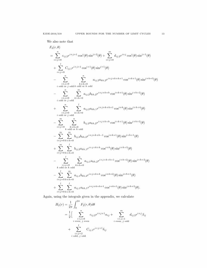
We also note that
F2(r, θ)
=n∑
i+j=0
cij,2ri+j+1 cosi(θ) sinj+2(θ) +
m∑i+j=0
dij,2ri+j cosi(θ) sinj+1(θ)
+l∑
i+j=0
Cij,1ri+j+1 cosi+1(θ) sinj+1(θ)
−n∑
i+j=0i odd or j odd
n∑k+h=0
k odd or h odd
aij,2akh,2ri+j+k+h+1 cosi+k+1(θ) sinj+h+3(θ)
−n∑
i+j=0i odd or j odd
m∑k+h=0
aij,2bkh,2ri+j+k+h cosi+k+1(θ) sinj+h+2(θ)
+n∑
i+j=0i odd or j odd
l∑k+h=0
aij,2akh,1ri+j+k+h+1 cosi+k(θ) sinj+h+4(θ)
−m∑
i+j=0
n∑k+h=0
k odd or h odd
bij,2akh,2ri+j+k+h cosi+k+1(θ) sinj+h+2(θ)
−m∑
i+j=0
m∑k+h=0
bij,2bkh,2ri+j+k+h−1 cosi+k+1(θ) sinj+h+1(θ)
+m∑
i+j=0
l∑k+h=0
bij,2akh,1ri+j+k+h cosi+k(θ) sinj+h+3(θ)
−l∑
i+j=0k odd or h odd
n∑k+h=0
aij,1akh,2ri+j+k+h+1 cosi+k+2(θ) sinj+h+2(θ)
−l∑
i+j=0
m∑k+h=0
aij,1bkh,2ri+j+k+h cosi+k+2(θ) sinj+h+1(θ)
+l∑
i+j=0
l∑k+h=0
aij,1akh,1ri+j+k+h+1 cosi+k+1(θ) sinj+h+3(θ).
Again, using the integrals given in the appendix, we calculate
H2(r) =1
2π
∫ 2π
0
F2(r, θ)dθ
=12
[ n∑i+j=0
i even, j even
cij,2ri+j+1αij +
m∑i+j=1
i even, j odd
dij,2ri+jβij
+l∑
i+j=2i odd, j odd
Cij,1ri+j+1δij
14 S. ELLAGGOUNE, S. BADI EJDE-2016/318
−n∑
i+j=1i odd, j even
n∑k+h=1
k even, h odd
aij,2akh,2ri+j+k+h+1Mijkh
−n∑
i+j=1i even, j odd
n∑k+h=1
k odd, h even
aij,2akh,2ri+j+k+h+1Mijkh
−n∑
i+j=1i odd, j even
m∑k+h=0
k even, h even
aij,2bkh,2ri+j+k+hNijkh
−n∑
i+j=2i odd, j odd
m∑k+h=1k even, h odd
aij,2bkh,2ri+j+k+hNijkh
−n∑
i+j=1i even, j odd
m∑k+h=2
k odd, h odd
aij,2bkh,2ri+j+k+hNijkh
+n∑
i+j=1i odd, j even
l∑k+h=1
k odd, h even
aij,2akh,1ri+j+k+h+1Pijkh
+n∑
i+j=1i even, j odd
l∑k+h=1
k even, h odd
aij,2akh,1ri+j+k+h+1Pijkh
+n∑
i+j=2i odd, j odd
l∑k+h=2
k odd, h odd
aij,2akh,1ri+j+k+h+1Pijkh
−m∑
i+j=2i odd, j odd
n∑k+h=1
k even, h odd
bij,2akh,2ri+j+k+hNijkh
−m∑
i+j=0i even, j even
n∑k+h=1
k odd, h even
bij,2akh,2ri+j+k+hNijkh
−m∑
i+j=1i even, j odd
n∑k+h=2
k odd, h odd
bij,2akh,2ri+j+k+hNijkh
−m∑
i+j=0i even, j even
m∑k+h=2
k odd, h odd
bij,2bkh,2ri+j+k+h−1Qijkh
−m∑
i+j=2i odd, j odd
m∑k+h=0
k even, h even
bij,2bkh,2ri+j+k+h−1Qijkh
−m∑
i+j=1i odd, j even
m∑k+h=1
k even, h odd
bij,2bkh,2ri+j+k+h−1Qijkh
EJDE-2016/318 UPPER BOUNDS FOR THE NUMBER OF LIMIT CYCLES 15
−m∑
i+j=1i even, j odd
m∑k+h=1
k odd, h even
bij,2bkh,2ri+j+k+h−1Qijkh
+m∑
i+j=0i even, j even
l∑k+h=1
k even, h odd
bij,2akh,1ri+j+k+hRijkh
+m∑
i+j=1i even, j odd
l∑k+h=0
k even, h even
bij,2akh,1ri+j+k+hRijkh
+m∑
i+j=1i odd, j even
l∑k+h=2
k odd, h odd
bij,2akh,1ri+j+k+hRijkh
+m∑
i+j=2i odd, j odd
l∑k+h=1
k odd, h even
bij,2akh,1ri+j+k+hRijkh
−l∑
i+j=1//i even, j odd
n∑k+h=1
k even, h odd
aij,1akh,2ri+j+k+h+1Tijkh
−l∑
i+j=1i odd, j even
n∑k+h=1
k odd, h even
aij,1akh,2ri+j+k+h+1Tijkh
−l∑
i+j=2i odd, j odd
n∑k+h=2
k odd, h odd
aij,1akh,2ri+j+k+h+1Tijkh
−l∑
i+j=0i even, j even
m∑k+h=1
k even, h odd
aij,1bkh,2ri+j+k+hUijkh
−l∑
i+j=1i even, j odd
m∑k+h=0
k even, h even
aij,1bkh,2ri+j+k+hUijkh
−l∑
i+j=1i odd, j even
m∑k+h=2
k odd, h odd
aij,1bkh,2ri+j+k+hUijkh
−l∑
i+j=2i odd, j odd
m∑k+h=1
k odd, h even
aij,1bkh,2ri+j+k+hUijkh
+l∑
i+j=0i even, j even
l∑k+h=2
k odd, h odd
aij,1akh,1ri+j+k+h+1Vijkh
16 S. ELLAGGOUNE, S. BADI EJDE-2016/318
+l∑
i+j=1i even, j odd
l∑k+h=1
k odd, h even
aij,1akh,1ri+j+k+h+1Vijkh
+l∑
i+j=1i odd, j even
l∑k+h=1
k even, h odd
aij,1akh,1ri+j+k+h+1Vijkh
].
Finally, we obtain H1(r) +H2(r) is a polynomial in the variable r2 of the form
H1(r) +H2(r) = r[P1(r2) + r2P2(r2) + r4P3(r2)
],
where P1(r2) is a polynomial in the variable r2 of degree
λ1 = max{
[O(m) + E(l)− 1
2], [E(m) +O(l)− 1
2], [O(n) +O(l)− 2
2],
m− 1, [E(n)
2], [E(m) +O(n)− 1
2]},
P2(r2) is a polynomial in the variable r2 of degree
λ2 = max{O(n)− 1, [
E(m) +O(n)− 32
], [O(m) + E(n)− 3
2], [O(n) +O(l)− 2
2],
l − 1, E(m)− 2, [E(m) +O(n)− 3
2], [O(m) + E(l)− 3
2], [E(n) +O(m)− 3
2]},
P3(r2) is a polynomial in the variable r2 of degree
λ3 = [E(n) + E(l)− 4
2],
where O(i) is the largest odd integer less than or equal to i, E(i) is the largest eveninteger less than or equal to i and [·] denotes the integer part function. Then
F20 =1
2πr[P1(r2) + r2P2(r2) + r4P3(r2)
].
To find the real positive roots of F20 we must find the zeros of a polynomial in r2 ofdegree λ = max{λ1, λ2 + 1, λ3 + 2}. This yields that F20 has at most λ real positiveroots. Hence, the Theorem 1.2 is proved.
Moreover, we can choose the coefficients aij,1, aij,2, bij,2, Cij,1, cij,2, dij,2 in sucha way that F20 has exactly λ real positive roots. In fact, we consider the example
x = y − ε(1 + xy − 2x2 − x)y − ε2(−2xy − y2)y,
y = −x− ε(4xy + (−x2 − y)y)− ε2(x2 − y + (−xy + y2 − x)y),(4.2)
Conclusion. This article concerns the second part of the 16th Hilbert problem inwhich we study the bifurcation of limit cycles from the periodic orbits of a linearcenter when we perturb it inside a general class of all polynomial differential sys-tems. We provide an accurate upper bound of the maximum number of limit cyclesthat this class of systems can have and we give an example which illustrates thatthis bound can be reached. We would like to stress that although this work ulti-mately focuses a general class of polynomial differential systems, the “Averagingmethod” summarized in section 2 can be adapted to the study of other polyno-mial systems. However, the difficulty lies in the complicated form of the averagedfunction of second order obtained when the first order one is identically zero. Thebifurcation of limit cycles from isochronous center will be the subject of a futurework.
Acknowledgements. We want to thank the reviewers all their comments andsuggestions which help us to improve the presentation of this article.
References
[1] Abramowitz, M. Stegun, I.; Handbook of mathematical function with formulas, graphs, and
mathematical tables. National Bureau of Standards Applied Mathematics Series, no. 55.
Washington, DC:US Government, Printing Office. 1964[2] A. Buica, J. Llibre; Averaging methods for finding periodic orbits via Brouwer degree, Bull
Sci Math 2004; 128: 7-22.
[3] L. Chengzy, J. Llibre; Uniqucness of limit cycles for Lienard differential equations of degreefour, J. Differ Equ 2012; 252: 3142-62.
[4] D. Hilbert; Mathematische Problems, Lecture in: Second Internat. Congr. Math. Paris, 1900,Nachr. Ges. Wiss. Gttingen Math. Phys. Ki 5 (1900), 253-297; English transl. Bull. Amer.
Soc. 8 (1902), 437-479.
[5] Y. Ilyashenko; Centennial history of Hilbert’s 16th problem, Bull. Amer. Math. Soc. 39(2002), 301-354.
[6] A. Lienard; Etude des oscillations entrenues, Revue Gnlectr 1928; 23: 946-54.[7] A. Lins, W. De Melo, CC. Pugh; On Lienard’s equation, Lecture notes in mathematics, Vol.
597. Berlin: Springer; 1977. p.335-357.[8] C. Li, J. Llibre; Uniqueness of limit cycles for Lienard differential equations of degree four,
Diff Equ 2012; 252: 3142-62.
[9] J. Llibre, A. C. Mereu A, M. A. Teixeira; Limit cycles of the generalized polynomial Lienard
differential equations, Math Proc Camb phil Soc 2010; 148: 363-83.[10] J. Llibre, C. Valls; On the number of limit cycles of a class of polynomial differential systems,
Proc A: R Soc., 2012; 468: 2347-60.[11] J. Llibre, C. Valls; Limit cycles for a generalization of polynomial Lienard differential sys-
tems, Chaos, Soltions and Fractals 46 (2013), 65-74.
[12] N. G. Lloyd; Limit cycles of polynomial systems-some recent developments. London mathe-matical society lecture note series, Vol. 127. Cambridge University Press; 1988; p: 192-234.
[13] N. G. Lloyd, S. Lynch; Small-amplitude limit cycles of certain Lienard systems, Proc R Soc
Lond Ser A 1988; 418: 199-208.[14] S. Lynch; limit cycles of generalized Lienard equation, Appl Math Lett 1995; 8:15-7.
[15] GS. Rychkov; The maximum number of limit cycle of the system x = y−a1x3−a2x5, y = −x
is two, Differ Uravn 1975; 11: 380-91.[16] J. A. Sanders, F. Verhulst; Averaging methods in nonlinear dynamical systems, Applied
Mathematical Sci, 59, Springer-Verlag, New york, 1985.
[17] F. Verhulst; Nonlinear differential equations and dynamical systems, Universitex, Springer-Verlag, Berlin, 1996.
22 S. ELLAGGOUNE, S. BADI EJDE-2016/318
Selma Ellaggoune
Laboratory of Applied Mathematics and Modeling, University 8 Mai 1945, Guelma,