UNIVERSITY OF THESSALY SCHOOL OF ENGINEERING Department of Computer and Communications Engineering UPPER BOUNDS ON THE VALUES OF THE POSITIVE ROOTS OF POLYNOMIALS by Panagiotis S. Vigklas A dissertation submitted in partial fulfillment of the requirements for the degree of Doctor of Philosophy University of Thessaly Volos, Greece 2010
Transcript
UNIVERSITY OF THESSALY
SCHOOL OF ENGINEERING
Department of Computer and Communications Engineering
UPPER BOUNDS ON THE VALUES OF THE POSITIVE ROOTS OF POLYNOMIALS
by
Panagiotis S. Vigklas
A dissertation submitted in partial fulfillment of the requirements for the degree of
Doctor of Philosophy
University of Thessaly Volos, Greece
2010
Supervisor Dr Alkiviadis Akritas, Associate Professor, University of Thessaly
Co-supervisors Dr Elias Houstis, Professor, University of Thessaly Dr Michalis Hatzopoulos, Professor, University of Athens
Doctoral Committee Dr Elias Houstis, Professor, University of Thessaly Dr Michalis Hatzopoulos, Professor, University of Athens Dr Panagiotis Sakkalis, Professor, Agricultural University of Athens Dr Evangelos Fountas, Professor, University of Piraeus Dr Alkiviadis Akritas, Associate Professor, University of Thessaly Dr Maria Gousidou-Koutita, Associate Professor, Aristotle Univ. of Thessaloniki Dr Panagiota Tsompanopoulou, Assistant Professor, University of Thessaly
To my parents
ii
ACKNOWLEDGEMENTS
Heartfelt thanks go to my scientific adviser, Prof. Alkiviadis Akritas for making
me familiar with computer algebra systems and root isolation methods, for his patient
support and his indefatigable interest in my thesis and for his friendship.
I am deeply indebted to Adam Strzebonski and Prof. Doru Stefanescu for their
significant contributions towards the completion of this research.
I am grateful to Prof. Elias Houstis and Prof. Michael Hatzopoulos for serving
on my thesis committee.
Last but not least I want to thank my parents who encourage me to complete this
βιομηχανικά προβλήματα, κλπ. Η υιοθέτηση της μεθόδου απομόνωσης
πραγματικών ριζών με συνεχή κλάσματα από μεγάλα εμπορικά και ανοικτού
κώδικα μαθηματικά πακέτα λογισμικού αποδεικνύει τη δύναμή της και τις
δυνατότητές της. Δύναμη και δυνατότητες που οφείλονται εν μέρει και στα
αποτελέσματα αυτής της διατριβής.
CHAPTER I
Introduction
1.1 Historical Note
One of the oldest and maybe for centuries the only area of study in Algebra had
been polynomial equations. The problem was to find formulas that could give the
roots of polynomials in terms of their coefficients.
It has been found, from historical searches, that the ancient Babylonians, who
created their civilization in 2000 B.C. in Mesopotamia, knew how to find the roots
of 1st and 2nd degree polynomials. Also they could approximate the square roots of
numbers. They formulated the problems and their solutions mostly verbally.
The next big step was done by the ancient Greeks. A group of mathematicians
called Pythagoreans (5th century B.C.), proved that the square roots that appeared
in the study of 2nd degree equations resulted in irrational numbers.
The ancient Greeks were using geometrical designs for solving polynomial equa-
tions of the 1st, 2nd and 3rd degree. That is geometrical designs made with a ruler
and a pair of compasses. Traces of algebraic representation for solving 2nd degree
equations did not exist until 100 B.C. The mathematician Diofante in 250 B.C. in-
troduced a form of algebraic symbolism. The arithmetic of Diofante is for algebra of
the same importance as the elements of Euclid for geometry. The Arabians improved
algebraic calculus but did not manage to solve 3rd degree equations.
1
In the Middle Age, European mathematicians improved the things they learned
from the Arabs, the most famous of them being Al-Khwarismi and introduced new
symbols. During the Renaissance, the development of algebra was remarkable, like
all other branches of mathematics.
Approximately at the end of the 15th century the University of Bologna in Italy,
was one of the most famous in Europe. This fame was related with the attempt of
the Bolognese mathematicians to solve 3rd and 4th degree equations.
It seems that Professor Scipio del Ferro, who died in 1526 managed to solve the
equation of the 3rd degree, without ever publishing his work. Niccolo Fontana known
as Tartaglia found again the solution of the 3rd degree equation. This particular
project of Fontana was published in 1545 from a polymath doctor in Milan, Hieronimo
Cardano in his work Ars Magna (The Great Art). Ars Magna also includes a method
for solving polynomial equations of degree four, by reducing them to equations of
degree three.
Of course, after that discovery, the effort was concentrated in finding formulas
which would give the roots of equations of degree 5 or greater than 5.
In the 18th century Josheph Louis Lagrange, influenced drastically the theory
of equations and approximately three years later C.F. Gauss (1777-1855) based on
Lagrange’s conclusions proved The Fundamental Theorem of Algebra.
The proof of the fact that there is not a formula to compute the roots of equations
of degree 5 was given by Paolo Ruffini (1804), who preceded Horner by about 15 years.
The Norwegian mathematician, N.H. Abel (1802-1829), in 1824, generalized Ruffini‘s
work by showing the impossibility of solving the general quintic equation by means of
radicals, thus finally put to rest a difficult problem that had puzzled mathematicians
for many years. Of course there was still the problem of finding the conditions that
such an equation must satisfy in order to be solved. Abel was working on this problem
until his death in 1829.
2
Eventually this problem was solved by the young French mathematician Evariste
Galois (1811-1832). His theory virtually contains the solution of this problem. Galois
wrote his conclusions in an illegible manuscript 31 pages long, the night before he
died at the age of 20. This manuscript became well known when Joseph Liouville
presented it in the French Academy in 1843.
Since then (and for some time before in fact), researchers have concentrated on
numerical (iterative) methods such as the famous Newton’s method of the 17th cen-
tury, Bernoulli’s method of the 18th, and Graeffe’s method of the early 19th. During
the same period, Fourier conceived the idea to split the problem, of the higher degree
equation solving, in two subproblems; that is, fist to isolate the real roots, and then
to approximate them to any desired degree of accuracy. The major problem was iso-
lation, which attracted immediately the attention of the mathematicians. To isolate
the roots two theorems were initially proposed: Budan’s (1807) and Fourier’s (1820)
theorems on which Vincent’s (1836) and Sturm’s (1829) theorems were based later
on. Vincent’s (1836) theorem, was, in turn, the foundation of the Akritas’ continued
fractions method of 1978, a method that is considered the most efficient today1.
1For Descartes’, Budan’s, Fourier’s, Vincent’s and Sturm’s theorems, see the Appendix. Fordetails on Vincent’s theorem, see Chapter IV.
3
CHAPTER II
Bounds
2.1 Definitions
2.1.1 Univariate Polynomials
A polynomial is a mathematical expression of the form
p(x) = α0xn + α1x
n−1 + ...+ αn−1x+ αn, (α0 > 0) (2.1)
If the highest power of x is xn, the polynomial is said to be of degree n. It was proved
by Gauss in the early 19th century that every polynomial of positive degree has at
least one zero (i.e. a value z which makes p(z) equal to zero), and that a polynomial
of degree n has n zeros (not necessarily distinct). Often we use x for a real variable,
and z for a complex one. A zero of a polynomial is synonymous to the “root” of the
equation p(x) = 0. A zero may be real or complex, and if the “coefficients” αi are
all real, then complex zeros occur in conjugate pairs α + iβ, α− iβ. The purpose of
the first part of this study is to describe methods which have been developed to find
bounds for the real positive roots of polynomials with real coefficients.
4
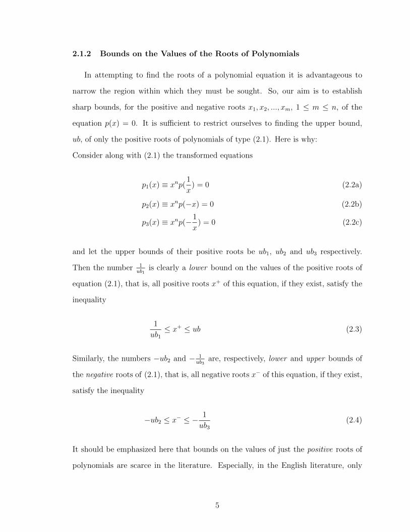
2.1.2 Bounds on the Values of the Roots of Polynomials
In attempting to find the roots of a polynomial equation it is advantageous to
narrow the region within which they must be sought. So, our aim is to establish
sharp bounds, for the positive and negative roots x1, x2, ..., xm, 1 ≤ m ≤ n, of the
equation p(x) = 0. It is sufficient to restrict ourselves to finding the upper bound,
ub, of only the positive roots of polynomials of type (2.1). Here is why:
Consider along with (2.1) the transformed equations
p1(x) ≡ xnp(1
x) = 0 (2.2a)
p2(x) ≡ xnp(−x) = 0 (2.2b)
p3(x) ≡ xnp(−1
x) = 0 (2.2c)
and let the upper bounds of their positive roots be ub1, ub2 and ub3 respectively.
Then the number 1ub1
is clearly a lower bound on the values of the positive roots of
equation (2.1), that is, all positive roots x+ of this equation, if they exist, satisfy the
inequality
1
ub1
≤ x+ ≤ ub (2.3)
Similarly, the numbers −ub2 and − 1ub3
are, respectively, lower and upper bounds of
the negative roots of (2.1), that is, all negative roots x− of this equation, if they exist,
satisfy the inequality
−ub2 ≤ x− ≤ − 1
ub3
(2.4)
It should be emphasized here that bounds on the values of just the positive roots of
polynomials are scarce in the literature. Especially, in the English literature, only
5
bounds on the absolute values (positive and negative) of the roots existed until 1978.
As Akritas points out, he was able to find Cauchy’s bound (described below) on the
values of the positive roots in Obrechkoff’s book, (Obreschkoff , 1963). Bounds on
the values of the positive roots of polynomials are important, because it is only those
bounds that can be used in the root isolation process described in Chapter IV.
2.2 Classical Methods for Computing Bounds
In this section we first present the two classical theorems by Cauchy and Lagrange-
MacLaurin. Until recently, the first was the only method used for computing the
bounds, on the values of the positive roots of polynomials. In addition, we in-
clude, Kioustelidis’ bound, (Kioustelidis , 1986), which is closely related to the one by
Cauchy.
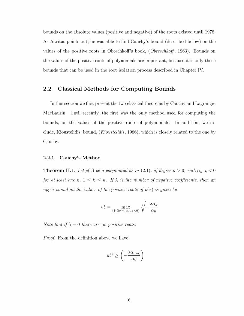
2.2.1 Cauchy’s Method
Theorem II.1. Let p(x) be a polynomial as in (2.1), of degree n > 0, with αn−k < 0
for at least one k, 1 ≤ k ≤ n. If λ is the number of negative coefficients, then an
upper bound on the values of the positive roots of p(x) is given by
ub = max{1≤k≤n:αn−k<0}
k
√−λαkα0
Note that if λ = 0 there are no positive roots.
Proof. From the definition above we have
ubk ≥(−λαn−k
α0
)
6
for every k such that αn−k < 0. For these k, the inequality above could be written
ubn ≥(−λαn−k
α0
)ubn−k
Summing for all k’s we have
λubn ≥ λ∑
1≤k≤n:αn−k<0
(−αn−k
α0
)ubn−k
or
ubn ≥∑
1≤k≤n:αn−k<0
(−αn−k
α0
)ubn−k
i.e., dividing p(x) = 0 by α0, making unitary the leading coefficient, and replacing x
with ub, x← ub, the first term, i.e. ubn, would be greater than, or equal to, the sum
of the absolute values of the terms with negative coefficient. Hence, for all x > ub,
p(x) > 0.
Even though the proof is sound, and easy to follow, it gives us no insight on what is
going on. Hence, we cannot improve on it. The same holds for the following theorem.
2.2.2 The Lagrange–MacLaurin Method
Theorem II.2. Suppose αn−k, k ≥ 1, is the first of the negative coefficients1 of a
polynomial p(x), as in (2.1). Then an upper bound on the values of the positive roots
of p(x) is given by
ub = 1 + k
√B
α0
,
where B is the largest absolute value of the negative coefficients of the polynomial
p(x).
1If there is no negative coefficient then p(x) has no positive roots.
7
Proof. Set x > 1. If in p(x) each of the nonnegative coefficients α1, α2, . . . ,
αk−1 is replaced by zero, and each of the remaining coefficients αk, αk+1, . . . , αn is
replaced by the negative number −B, we obtain
p(x) ≥ α0xn −B(xn−k + xn−k−1 + . . .+ 1) = α0x
n −Bxn−k+1 − 1
x− 1
Hence for x > 1 we have
p(x) > α0xn − B
x− 1xn−k+1 =
xn−k+1
x− 1(α0x
k−1(x− 1)−B)
>xn−k+1
x− 1(α0(x− 1)k −B)
Consequently for
x ≥ 1 + k
√B
α0
= ub
we have p(x) > 0 and all the positive roots x+ of p(x) satisfy the inequality
x+ < ub.
2.2.3 Kioustelidis’ Method
Theorem II.3. Let p(x) be a polynomial as in (2.1), of degree n > 0, with αn−k < 0
for at least one k, 1 ≤ k ≤ n. Then an upper bound on the values of the positive roots
of p(x) is given by
ub = 2 max{1≤k≤n:αn−k<0}
k
√−αn−k
α0
.
Proof. From the definition above we have
ubk ≥ 1
2k
(−αn−k
α0
)
8
for every k such that αn−k < 0. For these k, the inequality above could be written
ubn ≥ 1
2k
(−αn−k
α0
)ubn−k
Summing for all k’s we have
ubn ≥∑
1≤k≤n:αn−k<0
1
2k
(−αn−k
α0
)ubn−k
or
ubn ≥ (1− 1
2n)
∑1≤k≤n:αn−k<0
(−αn−k
α0
)ubn−k
and because (1− 2−n) < 1 we get
ubn ≥∑
1≤k≤n:αn−k<0
(−αn−k
α0
)ubn−k
i.e., dividing p(x) = 0 by α0, making unitary the leading coefficient, and replacing x
with ub, x← ub, the first term, i.e. ubn, would be greater than, or equal to, the sum
of the absolute values of the terms with negative coefficient. Hence, for all x > ub,
p(x) > 0.
In the next chapter, we will present a theorem by Stefanescu, (Stefanescu, 2005),
that gives some insight into the nature of how these bounds are computed. Extending
Stefanescu’s theorem, (Akritas and Vigklas , 2006), (Akritas, Strzebonski, and Vigklas ,
2006), we obtain a general theorem, which includes the above three methods as special
cases, and from which new, sharper, bounds can be derived.
9
CHAPTER III
A General Theorem for Computing Bounds on the
Positive Roots of Univariate Polynomials
3.1 Preliminaries
In the following discussion we shall consider polynomials with integer or ratio-
nal coefficients of any (arbitrary) bit–length. The methods that will be presented
here are methods of infinite precision (based on exact arithmetic) and must not be
confused with numerical or other approximate methods where someone has to take
under consideration various types of errors that infiltrate the computation process
and progressively degrade the final results.
3.2 Stefanescu’s Theorem and its Extension
Despite the fact that in the literature one can find many formulas1 that estimate
an upper bound on the largest absolute value of the real or complex roots, (Yap,
2000), (Mignotte, 1992), the most recent addition for a method to compute bound on
the positive roots of polynomials, that is of importance to us, has been by Stefanescu.
Namely, in (Stefanescu, 2005), the following theorem is proved:
1A bibliographical search till 2005 gives over 50 articles or books which give such bounds.
10
Theorem III.1 (Stefanescu’s, 2005). Let p(x) ∈ R[x] be such that the number of
variations of signs of its coefficients is even. If
p(x) = c1xd1 − b1x
m1 + c2xd2 − b2x
m2 + . . .+ ckxdk − bkxmk + g(x), (3.1)
with g(x) ∈ R+[x], ci > 0, bi > 0, di > mi > di+1 for all i, the number
B3(p) = max
{(b1
c1
)1/(d1−m1)
, . . . ,
(bkck
)1/(dk−mk)}
(3.2)
is an upper bound for the positive roots of the polynomial p for any choice of c1, . . . , ck.
We point out that Stefanescu’s theorem introduces the concept of matching or pairing
a positive coefficient with a negative coefficient of a lower order term. That is, to
obtain an upper bound, we match each negative coefficient–in fact we match a nega-
tive term, with a positive one, but for short we mention coefficient–with a preceding
positive one, and take the maximum. Clearly, Stefanescu’s theorem has limited use
since it works only for polynomials with an even number of sign variations2.
The following theorem generalizes Theorem III.1, in the sense that it applies to
polynomials with any number of sign variations. To accomplish this, we introduce
the new concept of breaking-up a positive coefficient into several parts to be paired
with negative coefficients (of lower order terms)3.
2In (Tsigaridas and Emiris, 2006), Tsigaridas and Emiris mention slightly different the sametheorem “Moreover, when the number of negative coefficients is even then a bound due to Stefanescucan be used which is much better”. Unfortunately, still with this version of the theorem its weaknessremains.
3After the publication of this work, (Akritas, Strzebonski, and Vigklas, 2006), Stefanescu alsoextended Theorem III.1 in (Stefanescu, 2007).
11
Theorem III.2. Let
p(x) = αnxn + αn−1x
n−1 + . . .+ α0, (αn > 0) (3.3)
be a polynomial with real coefficients and let d(p), t(p) denote the degree and the
number of its terms, respectively. Moreover, assume that p(x) can be written as
Algorithm 7: 1st part of “first–λ Quadratic” implementation of Theorem III.2.
33
sumPosCoeff = 0;34
i = n+ 1;35
// Last of the first-λ coefficients
while sumPosCoeff < λ do36
if usedV ector(i) 6= 0 then37
sumPosCoeff+ = usedV ector(i);38
flPos = i;39
end40
i−−;41
end42
/* If the last of the first-λ coefficients is a broken one (usedV ector(flPos) > 1), there might
be a chance that the sum of the positive coefficients (including broken ones) is more than
λ. For Example: Let the signs of p be + + + - + + - - - + + + - the 5th positive
coefficient will be broken into 2 pieces (usedV ector(8) = 2). However, the sum of the
first-λ (5 non broken) positive coefficients is 6 (incl. broken). As a result we are going
to use the last of the positive first-λ coefficients timesToUse(8)− (sum− λ) = 1 time only.
*/
timesToUse(flpos)− = (sumPosCoeff − λ);43
denomV ector ←− usedV ector;44
m = n;45
ub = 0;46
while λ > 0 do47
if cl(m) < 0 then48
tempub =∞;49
for k = n+ 1 to max(m+ 1, f lPos) do50
if usedV ector(k) > 0 then51
tempB = (−cl(m)cl(k)
denomV ector(k)
)1
k−m ;52
if tempub > tempB then53
tempub = tempB;54
tempN = k;55
end56
end57
end58
usedV ector(tempN)−−;59
λ−−;60
if ub < tempub then ub = tempub;61
end62
m−−;63
end64
ubFLQ = ub;65
return ubFLQ;66
Algorithm 8: 2nd part of “first–λ Quadratic” implementation of Theorem III.234
3.5.2 Testing Quadratic Complexity Bounds
In this section, we present some results using the same classes of polynomials8, as
in (Akritas and Strzebonski , 2005) in order to compare “first–λ Quadratic” and
“local-max Quadratic” implementation of Theorem III.2.
In Table 3.2, “first–λ Quadratic” and “local-max Quadratic” names were
shortened to ubFLQ and ‘ubLMQ respectively. Also, in parenthesis the respective
computation time is given for each algorithm, whereas MPR stands for the maximum
positive root, computed numerically.
8For exact mathematical formulas of the benchmark polynomials, please see the Appendix.
35
Tab
le3.
2:Q
uad
rati
cco
mp
lexit
yb
oun
ds
ofp
osit
ive
root
sfo
rva
riou
sty
pes
of
poly
nom
ials
.D
egre
esP
oly
nom
ial
Bou
nd
s10
100
200
300
400
500
600
700
800
900
Lagu
erre
ub L
MQ
200
2×
104
8×
104
18×
104
32×
104
50×
104
72×
104
98×
104
128×
104
162×
104
(0.)
(0.5
63)
(3.5
62)
(11.1
87)
(25.5
94)
(49.7
82)
(87.3
44)
(142.4
53)
(220.7
66)
(329.7
19)
ub F
LQ
100
104
4×
104
9×
104
16×
104
25×
104
36×
104
49×
104
64×
104
81×
104
(0.)
(0.0
15)
(0.0
31)
(0.0
78)
(0.1
09)
(0.1
72)
(0.2
5)
(0.3
28)
(0.4
06)
(0.5
)M
PR
29.9
2374.9
8767.8
21162.8
1558.8
11955.4
42352.5
2749.8
73147.4
83545.2
9
Ch
ecysh
evI
ub L
MQ
2.2
3607
7.0
7107
10
12.2
474
14.1
421
15.8
114
17.3
205
18.7
083
20
21.2
132
(0.)
(0.0
78)
(0.5
15)
(1.5
47)
(3.4
53)
(6.4
53)
(10.6
88)
(15.8
91)
(23.4
06)
(33.7
5)
ub F
LQ
1.5
8114
57.0
7107
8.6
6025
10
11.1
803
12.2
474
13.2
88
14.1
421
15
(0.)
(0.)
(0.0
15)
(0.0
47)
(0.6
2)
(0.1
1)
(0.1
41)
(0.1
72)
(0.2
34)
(0.2
81)
MP
R0.9
87688
0.9
99877
0.9
99969
0.9
99989
0.9
99992
0.9
99995
0.9
99997
0.9
99997
0.9
99998
0.9
99998
Ch
ecysh
evII
ub L
MQ
2.1
2132
7.0
3562
9.9
7497
12.2
27
14.1
244
15.7
956
17.3
061
18.6
949
19.9
875
21.2
014
(0.0
15)
(0.0
79)
(0.5
31)
(1.5
63)
(3.4
53)
(6.4
68)
(10.7
19)
(16.6
87)
(24.6
56)
(34.7
34)
ub F
LQ
1.5
4.9
7494
7.0
5337
8.6
4581
9.9
8749
11.1
692
12.2
372
13.2
193
14.1
333
14.9
917
(0.)
(0.0
16)
(0.0
15)
(0.0
47)
(0.0
78)
(0.1
09)
(0.1
41)
(0.1
87)
(0.2
19)
(0.2
65)
MP
R0.9
59493
0.9
99516
0.9
99878
0.9
99945
0.9
99969
0.9
9998
0.9
99986
0.9
9999
0.9
99992
0.9
99994
Wilkin
son
ub L
MQ
110
10100
40200
90300
160400
250500
360600
490700
640800
810900
(0.)
(6.3
91)
(52.2
34)
(179.7
5)
(438.5
16)
(878.)
(1549.8
9)
(2508.5
2)
(3833.5
2)
(5569.4
2)
ub F
LQ
55
5050
20100
45150
80200
125250
180300
245350
320400
405450
(0.)
(0.0
16)
(0.0
47)
(0.0
78)
(0.0
14)
(0.2
03)
(0.2
82)
(0.3
59)
(0.5
16)
(0.6
56)
MP
R10
100
200
300
400
500
600
700
800
900
Mig
nott
e
ub L
MQ
1.7
7828
1.0
4811
1.0
2353
1.0
1557
1.0
1164
1.0
0929
1.0
0773
1.0
0662
1.0
0579
1.0
0514
(0.)
(0.)
(0.0
15)
(0.)
(0.)
(0.0
16)
(0.)
(0.)
(0.)
(0.0
15)
ub F
LQ
1.6
3069
1.0
4073
1.0
1995
1.0
1321
1.0
0988
1.0
0789
1.0
0656
1.0
0562
1.0
0491
1.0
0437
(0.)
(0.0
16)
(0.)
(0.0
16)
(0.1
5)
(0.0
16)
(0.0
16)
(0.0
15)
(0.0
16)
(0.0
15)
MP
R1.5
763
1.0
362
1.0
177
1.0
117
1.0
088
1.0
070
1.0
058
1.0
050
1.0
044
1.0
039
sRan
dom
ub L
MQ
2.0
1011
14.3
673
1.3
9904
3.5
4546
3.6
5744
7.7
5602
2.5
257
1.5
3975
1.7
0317
1.6
5478
(0.)
(0.2
19)
(1.0
16)
(2.1
1)
(3.8
28)
(6.)
(8.6
25)
(11.7
35)
(14.7
65)
(18.7
34)
ub F
LQ
2.4
5417
25.1
062
1.0
4472
3.5
4546
2.5
862
7.7
5602
2.0
3158
1.6
409
1.4
8873
1.1
7328
(0.)
(0.0
31)
(0.1
57)
(0.2
81)
(0.5
47)
(0.8
43)
(1.1
57)
(1.6
56)
(1.5
)(2
.375)
MP
R1.6
173
8.1
5106
0.9
82276
1.1
221
1.7
1921
1.0
12339
0.9
83633
0.9
83628
1.0
10844
0.9
83628
usR
an
dom
ub L
MQ
1.5
7532
1916790
1.4
0849
1.7
8915
105264
1272940
1803160
12.6
533
1197500
790432
(0.)
(0.2
5)
(1.0
32)
(2.1
25)
(3.7
97)
(5.8
91)
(8.5
)(1
1.5
31)
(14.8
75)
(18.7
65)
ub F
LQ
3.1
6629
1916790
1.0
6293
15.6
504
105264
1272940
901580
6.3
2665
598750
790432
(0.0
16)
(0.0
47)
(0.1
56)
(0.2
66)
(0.5
31)
(0.8
28)
(1.1
56)
(1.6
41)
(2.0
46)
(2.3
28)
MP
R0.9
25381
1.0
18871
0.9
82509
0.9
841
1.0
26689
1.0
11621
1.3
31235
1.7
55769
1.0
13423
1.2
28396
pR
an
dom
ub L
MQ
5984.5
58818.6
314435.4
(10.2
97)
(75.4
53)
(1053.5
5)
ub F
LQ
4231.7
25555.3
99093.7
5(0
.562)
(1.4
53)
(21.1
56)
MP
R998
998
1019
36
From the data presented in the Table 3.2, it becomes obvious that the sharpness
of the estimates of both ubFLQ and ubLMQ is about the same, but ubFLQ in most cases
runs faster (or quite faster) than ubLMQ. So, when it comes to quadratic complexity
bounds the ubFLQ algorithm is undoubtedly the best choice regarding sharpness to
speed of computation, ratio. However, examining both Table 3.2 and Table 3.1,
one must be very careful in his choice of quadratic versus linear complexity bounds
because then he has to trade-off between a slightly better bound estimation and a
greater algorithmic complexity and execution time. This last remark seems to have
been exploited by the commercial computational software program, Mathematica,
(Wolfram Research, 2008), as we can see in the following section.
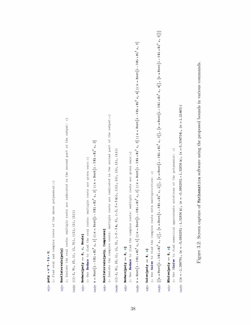
3.5.3 Mathematica Session Demonstration of New Bounds
The Mathematica’s real root isolation source code, by default, uses the better
bound from each category, i.e. “first–λ”, ubFL, from the linear complexity bounds
and “local-max Quadratic”, ubLMQ from the quadratic complexity ones, (Strzebonski ,
2010). However, its source code also contains implementations of Cauchy’s, (§ 2.2.1),
and Hong’s bound, (Hong , 1998), which we call “Kioustelidis’ Quadratic” in our
work as well as the “local-max”, ubLM and “first–λ Quadratic”, ubFLQ, bounds.
There is an undocumented system variable which allows to change the bound used to
any combination of those bounds. The new bounds have been added in Mathematica
version 7.
These bounds are always implicity used for calculating intervals isolating polyno-
mial real roots. Intervals are given by command RootIntervals. Real root isolation
is used by any Mathematica function that requires real algebraic number computa-
tion.
See the following examples:
37
Fig
ure
3.2:
Scr
een
cap
ture
ofMathematica
soft
war
eu
sin
gth
ep
rop
osed
bou
nd
sin
vari
ou
sco
mm
and
s.
38
CHAPTER IV
Application of the New Bounds to Real Root
Isolation Methods
4.1 Introduction
In this chapter we apply the newly proposed linear and quadratic complexity (up-
per) bounds on the values of the positive roots of polynomials on a method for the
isolation of real roots of polynomials. Although there are many root isolations meth-
ods (based on continued fractions, bisection, exclusion, etc) that could greatly benefit
from our new sharper bounds we decided to study their impact on the performance of
the Vincent-Akritas-Strzebonski (VAS) method for the isolation of real roots of poly-
nomials. The VAS real root isolation method is based on continued fractions and till
today is considered the fastest among its rivals, having already being incorporated in
major mathematical software packages.
Computing (lower) bounds on the values of the positive roots of polynomials is a
crucial operation in the VAS method. Therefore, we begin by reviewing some basic
facts about this method, which is based on Vincent’s theorem1, (Vincent , 1836):
1For a complete overview of Vincent’s theorem of 1836 and its implications to root isolation, see(Akritas, 2010).
39
Theorem IV.1 (Vincent, 1836). If in a polynomial, p(x), of degree n, with rational
coefficients and without multiple roots we perform sequentially replacements of the
form
x← α1 +1
x, x← α2 +
1
x, x← α3 +
1
x, . . .
where α1 ≥ 0 is an arbitrary non negative integer and α2, α3, . . . are arbitrary positive
integers, αi > 0, i > 1, then the resulting polynomial either has no sign variations or
it has one sign variation. In the last case the equation has exactly one positive root,
which is represented by the continued fraction
α1 +1
α2 + 1α3+ 1
...
whereas in the first case there are no positive roots.
The thing to note is that the quantities αi (the partial quotients of the continued
fraction) are computed by repeated application of a method for estimating lower
bounds2 on the values of the positive roots of a polynomial.
Therefore, the efficiency of the VAS continued fractions method heavily depends
on how good these estimates are.
4.2 Algorithmic Background of the VAS Method
In the sequel we present the VAS algorithm –as found in (Akritas and Strzebonski ,
2005)– and correct a misprint in Step 5 that had appeared in that presentation;
moreover, we explain where the new bound on the positive roots is used.
2A lower bound, `b, on the values of the positive roots of a polynomial f(x), of degree n, isfound by first computing an upper bound, ub, on the values of the positive roots of xnf( 1
x ) and thensetting `b = 1
ub , see (§ 2.1.2).
40
4.2.1 Description of the VAS-Continued Fractions Algorithm
Using the notation of the paper Akritas and Strzebonski (2005), let f ∈ Z[x]\{0}.
By sgc(f) we denote the number of sign changes in the sequence of nonzero coefficients
of f . For nonnegative integers a, b, c, and d, such that ad− bc 6= 0, we put
intrv(a, b, c, d) := Φa,b,c,d((0,∞))
where
Φa,b,c,d : (0,∞) 3 x −→ ax+ b
cx+ d∈ (min(
a
c,b
d),max(
a
c,b
d))
and by interval data we denote a list
{a, b, c, d, p, s}
where p is a polynomial such that the roots of f in intrv(a, b, c, d) are images of
positive roots of p through Φa,b,c,d, and s = sgc(p).
The value of parameter α0 used in step 4 below needs to be chosen empirically.
In our implementation α0 = 16.
Algortihm Continued Fractions (VAS).
Input: A squarefree polynomial f ∈ Z[x] \ {0}
Output: The list rootlist of the isolation intervals of the positive roots of f .
1. Set rootlist to an empty list. Compute s ← sgc(f). If s = 0 return an empty
list. If s = 1 return {(0,∞)}. Put interval data {1, 0, 0, 1, f, s} on intervalstack.
2. If intervalstack is empty, return rootlist, else take interval data {a, b, c, d, p, s}
off intervalstack.
3. Compute a lower bound α ∈ Z on the positive roots of p.
41
4. If α > α0 set p(x)← p(αx), a← αa, c← αc, and α← 1.
5. If α ≥ 1, set p(x) ← p(x + α), b ← αa + b, and d ← αc + d. If p(0) = 0, add
[b/d, b/d] to rootlist, and set p(x)← p(x)/x. Compute s← sgc(p). If s = 0 go
to step 2. If s = 1 add intrv(a, b, c, d) to rootlist and go to step 2.
6. Compute p1(x) ← p(x + 1), and set a1 ← a, b1 ← a + b, c1 ← c, d1 ← c + d,
and r ← 0. If p1(0) = 0, add [b1/d1, b1/d1] to rootlist, and set p1(x)← p1(x)/x,
and r ← 1. Compute s1 ← sgc(p1), and set s2 ← s− s1− r, a2 ← b, b2 ← a+ b,
c2 ← d, and d2 ← c+ d.
7. If s2 > 1, compute p2(x) ← (x + 1)mp( 1x+1
), where m is the degree of p. If
p2(0) = 0, set p2(x)← p2(x)/x. Compute s2 ← sgc(p2).
8. If s1 < s2, swap {a1, b1, c1, d1, p1, s1} with {a2, b2, c2, d2, p2, s2}.
9. If s1 = 0 goto step 2. If s1 = 1 add intrv(a1, b1, c1, d1) to rootlist, else put
interval data {a1, b1, c1, d1, p1, s1} on intervalstack.
10. If s2 = 0 goto step 2. If s2 = 1 add intrv(a2, b2, c2, d2) to rootlist, else put
interval data {a2, b2, c2, d2, p2, s2}on intervalstack. Go to step 2.
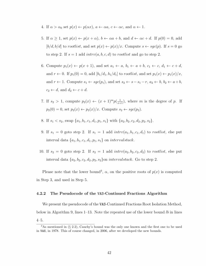
Please note that the lower bound3, α, on the positive roots of p(x) is computed
in Step 3, and used in Step 5.
4.2.2 The Pseudocode of the VAS-Continued Fractions Algorithm
We present the pseudocode of the VAS-Continued Fractions Root Isolation Method,
below in Algorithm 9, lines 1–13. Note the repeated use of the lower bound lb in lines
4–5.
3As mentioned in (§ 2.2), Cauchy’s bound was the only one known and the first one to be usedin VAS, in 1978. This of course changed, in 2006, after we developed the new bounds.
42
Input: The square-free polynomial p(x) ∈ Z[x], p(0) 6= 0, and the Mobius transformation
M(x) = ax+bcx+d
= x, a, b, c, d ∈ Z
Output: A list of isolating intervals of the positive roots of p(x)
var ←− the number of sign changes of p(x);1
if var = 0 then RETURN ∅;2
if var = 1 then RETURN {]a, b[} // a = min(M(0),M(∞)), b = max(M(0),M(∞));3
`b←− a lower bound on the positive roots of p(x);4
if `b > 1 then {p←− p(x+ `b),M ←−M(x+ `b)};5
p01 ←− (x+ 1)deg(p)p( 1x+1
),M01 ←−M( 1x+1
) // Look for real roots in ]0, 1[ ;6
m←−M(1) // Is 1 a root? ;7
p1∞ ←− p(x+ 1),M1∞ ←−M(x+ 1) // Look for real roots in ]1,+∞[ ;8
if p(1) 6= 0 then9
RETURN VAS(p01,M01)⋃
VAS(p1∞,M1∞)10
else11
RETURN VAS(p01,M01)⋃{[m,m]}
⋃VAS(p1∞,M1∞)12
end13
Algorithm 9: VAS-Continued Fractions Algorithm.
4.2.3 Example of the Real Root Isolation Method
Executing Algorithm 9 for the polynomial 8x4 − 18x3 + 9x − 2 which has one
negative, −√
2/2 and three positive real roots, 1/4,√
2/2 and 2, we have:
43
Figure 4.1: Tree-diagram of the VAS-CF Real Root Isolation Algorithm 9, for thepolynomial 8x4 − 18x3 + 9x− 2.
44
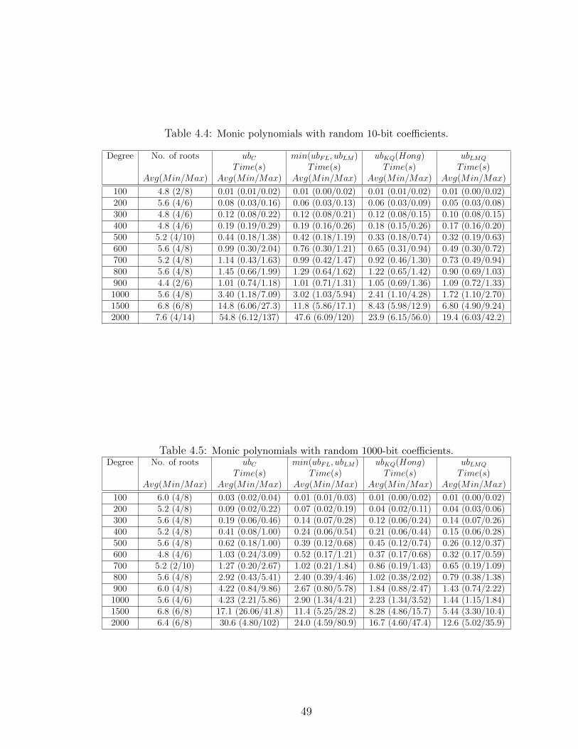
4.3 Benchmarking VAS with New Bounds
In this section we compare four implementations of the VAS real root isolation
method using two linear and two quadratic complexity bounds on the values of the
positive roots of polynomials.
The two linear complexity bounds are: Cauchy’s, ubC and min(ubFL, ubLM), the
minimum of “first–λ” and “local-max” bounds, (Akritas, Strzebonski, and Vigklas ,
2006), whereas the two quadratic complexity ones are: ubKQ, the Quadratic complex-
ity variant of K ioustelidis’ bound, studied by Hong, (Hong , 1998), and ubLMQ, the
Quadratic complexity version of the “local-max” bound, (Akritas, Strzebonski, and
Vigklas , 2008a).
Our choice of the various bounds in the implementations of VAS is justified as
follows:
1. From the linear complexity bounds we included:
(a) Cauchy’s bound, ubC , to be used as a point of reference, since it has been
in use for the past 30 years, and
(b) min(ubFL, ubLM) bound, (Akritas, Strzebonski, and Vigklas , 2006), which
is the best among the linear complexity bounds, in order to see when
it’s implementation will outperform that of the two quadratic complexity
bounds.
2. From the quadratic complexity bounds we included:
(a) Kioustelidis’ bound, ubKQ and
(b) ubLMQ bound in order to compare their performance; as explained in the
previous chapter ubLMQ computes sharper estimates than ubKQ.
45
They all use the same implementation of Shaw and Traub’s algorithm for Taylor
shifts (von zur Gathen and Gerhard , 1997). We followed the standard practice and
used as benchmark the Laguerre, Chebyshev (first and second kind), Wilkinson and
Mignotte polynomials4, as well as several types of randomly generated polynomials of
degrees {100, 200, 300, 400, 500, 600, 700, 800, 900, 1000, 1500, 2000}. For the random
polynomials the size of the coefficients ranges from −220 to 220.
4For exact mathematical formulas of the benchmark polynomials, please see the Appendix.
46
Table 4.1: Special polynomials of some indicative degrees.
Then, for every Table, the average value of Speed− up was computed giving a rough
overall estimation on time gain that VAS algorithm received after the incorporation
of the new bounds.
Taking these test results into consideration, one could safely conclude that us-
ing the new proposed bounds (linear or quadratic) in VAS real root isolation algo-
rithm would see a average overall improvement in computation time of about 20%
for min(ubFL, ubLM) and about 40% for ubLMQ bound.
Also, notice that ubLMQ is fastest for all classes of polynomials tested, except for
the case of very many very large roots, Table 4.8. In the case of very many very
large roots VAS using ubLMQ is a very close second to VAS using our linear complexity
bound min(ubFL, ubLM)6.
We end this chapter by presenting the following graph, Figure 4.3. This graph
depicts the overall time of VAS-CF in comparison with the time spent for computing
bounds. Especially, the left scale shows the total time in seconds (bars) needed by
VAS-CF to isolate the roots of a certain class of polynomials (Laguerre) using both
ubLM , the “local-max” bound, and ubLMQ, its quadratic version. The right scale
is associated with the two curves which show the total time spent by VAS-CF in
computing just these bounds.
5The change in memory use was negligible in every case, and hence, it is not included. Also,timing results are subject to measurement error, which especially affect small timings.
6For additional discussion on these conclusions, see (Akritas, Strzebonski, and Vigklas, 2007),(Akritas, Strzebonski, and Vigklas, 2008b) and (Akritas, 2009).
52
Figure 4.3: Computation times for the Laguerre polynomials of degree (100...1000). TheVAS-CF(LM), VAS-CF(LMQ), (LM), and (LMQ) are described above in the text.Note that the bars are scaled to the left Y axis whereas the lines to the rightone.
53
CHAPTER V
Conclusions
5.1 Final Note
This thesis was motivated by an old, but still important for many modern scientific
fields, problem in polynomial algebra, namely, the determination of upper bounds on
the values of the positive roots of polynomials. The widespread development and use
of computer algebra systems, (CAS ), along with an increasing interest in root isolation
methods, provided a fruitful context for reexamination of this classical problem.
We have presented and analyzed a variety of algorithms both of linear and quadratic
computational complexity that take advantage of a theorem that we extended, in or-
der to establish a unified general framework in which the classical ones fitted perfectly
and new ones came out naturally. These algorithms are simple in implementation, and
in most cases outperform in speed and accuracy the established preexisting methods.
The incorporation of these new bounds in the Vincent-Akritas-Strzebonski, (VAS),
continued fractions polynomial real root isolation algorithm offered a significant speed-
up to an already fast method extending significant the range of its applicability and
its robustness.
The immediate adoption of our new algorithms by major mathematical software
systems, such as Mathematica and Sage, bear witness to their usefulness and their
effectiveness. However, this thesis is by no means exhaustive and questions such as:
54
• Is there an optimal way to break up the coefficients in the“first–λ” method?
• Is it possible to extend these bounds to multivariate polynomials with similar
success?
• Can these bounds be suitably modified to constitute a complex analogue for
polynomials with complex coefficients?
and many others, seek to be answered by our long term on-going research.
55
APPENDICES
56
APPENDIX A
Theorems on the Number of Real Roots of a
Polynomial
A.1 Number of Real Roots of a Polynomial in an Interval
After the bounds of the positive and negative real roots of the polynomial equation
p(x) = 0 have been calculated according to the methods presented in Chapter 3.2
the next question that arises concerns the number of real roots of a polynomial in a
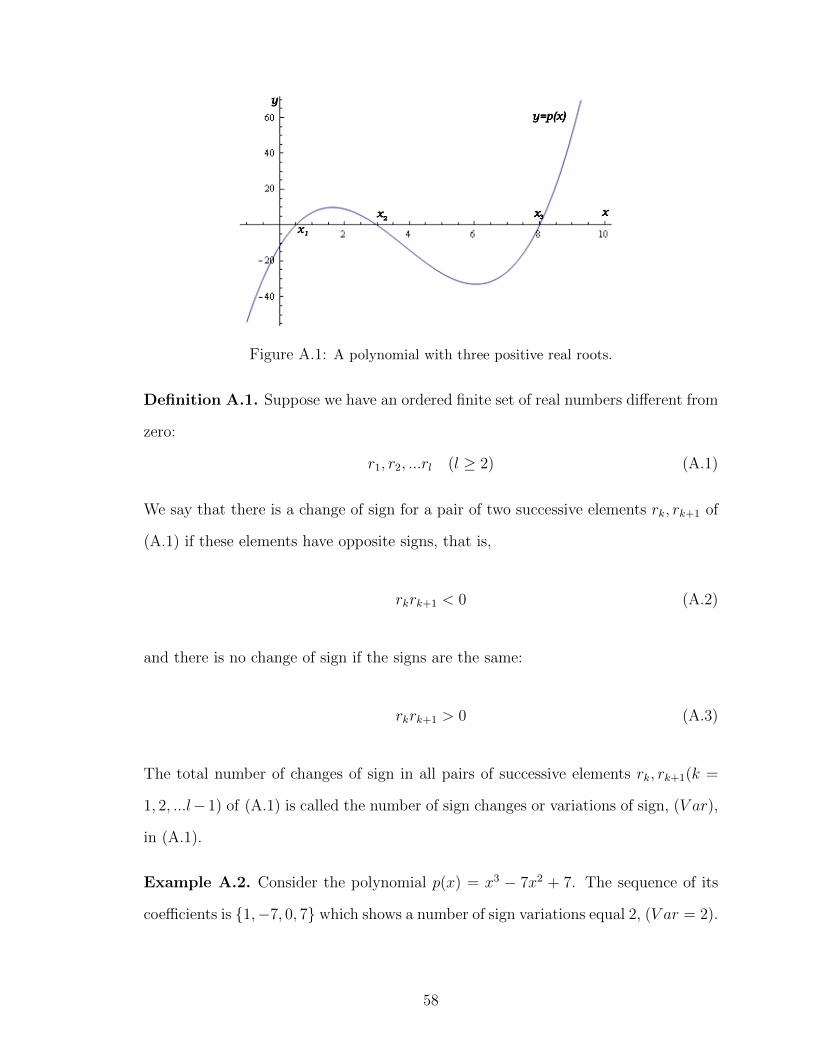
given interval (a, b). A picture of the number of real roots of equation p(x) = 0 in
an interval (a, b) is shown in Figure A.1, for the function y = p(x), where the roots
x1, x2, x3 are found as the points of intersection of the graph with the x-axis. We note
that (a) If p(a)p(b) < 0, then on the interval (a, b) there is an odd number of roots of
p(x), counting multiplicities, (b) If p(a)p(b) > 0, then on the interval (a, b) there are
either no roots of p(x) or there is an even number of such roots. The question of the
number of real roots of an algebraic equation in a given interval is solved completely
by the Sturm method, (Kurosh, 1988). Before going into that let us introduce the
notion of the number of sign changes in a set of numbers.
57
Figure A.1: A polynomial with three positive real roots.
Definition A.1. Suppose we have an ordered finite set of real numbers different from
zero:
r1, r2, ...rl (l ≥ 2) (A.1)
We say that there is a change of sign for a pair of two successive elements rk, rk+1 of
(A.1) if these elements have opposite signs, that is,
rkrk+1 < 0 (A.2)
and there is no change of sign if the signs are the same:
rkrk+1 > 0 (A.3)
The total number of changes of sign in all pairs of successive elements rk, rk+1(k =
1, 2, ...l−1) of (A.1) is called the number of sign changes or variations of sign, (V ar),
in (A.1).
Example A.2. Consider the polynomial p(x) = x3 − 7x2 + 7. The sequence of its
coefficients is {1,−7, 0, 7} which shows a number of sign variations equal 2, (V ar = 2).
58
A.1.1 Sturm’s Theorem (1827)
For a given polynomial p(x), we can form the Sturm sequence
p(x), p1(x), p2(x), ..., pm(x) (A.4)
where p1(x) = p′(x), p2(x) is the remainder, with reversed sign, left after the division
of the polynomial p(x) by p1(x), p3(x) is the remainder, with reversed sign, after
the division of the polynomial p1(x) by p2(x), and so on. The polynomials pk(x)(k =
2, ...,m) may be computed by a modified Euclidean algorithm. If the polynomial p(x)
does not have any multiple roots, then the last element pm(x) in the Sturm sequence
is a nonzero real number.
If we represent by V ar(r) the number of sign changes in a Sturm sequence for
x = r, provided that the zero elements of the sequence have been ignored, we have
the Sturm’s theorem:
Theorem A.3 (Sturm (1827)). If a polynomial p(x) does not have multiple roots
and p(a) 6= 0, p(b) 6= 0, then the number of its real roots N(a, b) in the interval
a < x < b is exactly equal to the number of lost sign changes in the Sturm sequence
of the polynomial p(x) when going from x = a to x = b, that is,
N(a, b) = V ar(a)− V ar(b) (A.5)
Corollary A.4. If p(0) 6= 0, then the number N+ of positive and the number N− of
negative roots of the polynomial p(x) are respectively:
N+ = V ar(0)− V ar(+∞) (A.6a)
N− = V ar(−∞)− V ar(0) (A.6b)
59
Corollary A.5. For all the roots of a polynomial p(x) of degree n to be real, in the
absence of multiple roots, it is necessary and sufficient that the following condition
holds:
V ar(−∞)− V ar(+∞) = n (A.7)
Example A.6. Let us determine the number of positive and negative roots of the
equation p(x) = x7 − 7x+ 1. The Sturm sequence is
p(x) = x7 − 7x+ 1 (A.8a)
p1(x) = x6 − 1 (A.8b)
p2(x) = 6x− 1 (A.8c)
p3(x) = 46655 (A.8d)
so
V ar(−∞) = 3, V ar(0) = 2, V ar(+∞) = 0 (A.9)
We find that equation p(x) = x7 − 7x+ 1 has
N+ = 2− 0 = 2 positive roots (A.10a)
N− = 3− 2 = 1 negative roots (A.10b)
and its rest four roots are complex roots. We can easily deduce here a way to isolate
the roots of algebraic equations by using Sturm sequence in order to partition the
interval (a, b) containing all the real roots of the equation into a finite number of
subintervals (α, β) such that V ar(α)− V ar(β) = 1.
60
A.1.2 Fourier’s Theorem (1819)
Sturm arrived at his method (1827) by extending an earlier theorem by Fourier
(1819). Let us return to the method described above (A.1) for the counting of the
number variations of sign in a sequence of numbers:
Definition A.7. Suppose we have a finite ordered sequence of real numbers:
r1, r2, ..., rl (A.11)
where r1 6= 0 and rl 6= 0. We define: (a) lower number of variations of sign V arlo
of the sequence (A.11) for the number of sign changes in an appropriate subsequence
that does not contain zero elements and (b) upper number of variations of sign V arup
of a sequence of numbers (A.11) for the number of sign changes in a transformed
sequence of (A.11) where the zero elements
rk = rk+1 = ... = rk+m−1 = 0 (A.12)
(rk−1 6= 0, rk+m 6= 0) are replaced by the elements rk+i(i = 0, 1, 2, ...,m− 1) such that
sgn(rk+i) = (−1)m−isgn(rk+m) (A.13)
It is clear that if (A.11) has no zero elements, then the number V ar of sign changes
in the sequence coincides with its lower V arlo and upper V arup number of variation
of sign: V ar = V arlo = V arup whereas generally V arup ≥ V arlo.
Example A.8. Let us determine the lower and upper number of changes of sign in
the sequence 1, 0, 0,−1, 1. Omitting the zeros, we have V arlo = 2. To calculate V arup
using (A.13), we form the sequence 1,−σ, σ,−1, 1 where σ > 0, and V arup = 4.
Theorem A.9 (Fourier, 1820). If the numbers a and b (a < b) are not roots of a
polynomial p(x) of degree n, then the number N(a, b) of real roots of the equation
61
p(x) = 0 lying between a and b is equal to the minimal number ∆V ar of the sign
changes lost in the sequence of successive derivatives
p(x), p′(x), ..., pn−1(x), pn(x) (A.14)
when going from x = a to x = b, or less that ∆V ar by an even number: N(a, b) =
∆V ar − 2k where ∆V ar = V arlo(a)− V arup(b) and V arlo(a) is the lower number of
variations of sign in the sequence (A.14) for x = a, V arup(b) is the upper number of
variations of sign in that sequence for x = b [k = 0, 1, ..., E(∆V ar2
)]
Fourier’s theorem is the only one found in the literature under the names: Budan,
Budan-Fourier, Fourier or Fourier-Budan. We expalin why in the sequel. In the
above theorem it is assumed that each root of the equation p(x) = 0 is counted
according to its multiplicity. If the derivatives pk(x) (k = 1, 2, ..., n) do not vanish
at x = a and x = b, then counting the signs is simplified and ∆V ar becomes ∆V ar =
V ar(a)− V ar(b).
Corollary A.10. . If ∆V ar = 0, then there are no real roots of the equation p(x) = 0
between a and b.
Corollary A.11. . If ∆V ar = 1, then there is exactly one real root of the equation
p(x) = 0 between a and b.
A.1.3 Descartes’ Theorem (1637)
Somewhat easier in applications, but still unable to determine precisely the num-
ber of roots, is Descartes’ rule of signs (given in his work Geometrie in 1637 and
proved by Gauss in 1828), (Bartolozzi and Franci , 1993).
Theorem A.12 (Descartes’ rule of signs, 1637). The number of positive roots of an
algebraic equation p(x) = 0 such that a root of multiplicity m being counted as m
roots, is equal to the nummber of variations in sign in the sequence of coefficients
62
an, an−1, an−2, ..., a0 (A.15)
(where the coefficients equal to zero are not counted) or less than that by an even
integer.
Clearly, Descartes’ rule of sign is an application of the Fourier theorem to the
interval (0,+∞). Since
p(x) = anxn + ...+ a0 (A.16a)
p′(x) = nanxn−1 + ...+ a1 (A.16b)
p(2)(x) = n(n− 1)anxn−2 + ...+ 2a2 (A.16c)
... (A.16d)
... (A.16e)
... (A.16f)
p(n)(x) = n!an (A.16g)
sequence (A.15) is, to within positive factors, a collection of derivatives p(k)(0) (k =
0, 1, 2..., n) written in ascending order, i.e. a0, a1, 2a2, ..., n!an, therefore, the number
of variations in sign in the sequence (A.15) is equal to V arlo(0), zero coefficients not
counted. On the other hand, the derivatives p(k)(+∞) (k = 0, 1, 2..., n) have no sign
variations and follows that V arup(+∞) = 0. Then, we have
∆V ar = V arlo(0)− V arup(+∞) = V arlo(0) (A.17)
and on the basis of the Fourier theorem, the number of positive roots of p(x) = 0 is
either equal to ∆V ar or is less than that by an even integer.
Corollary A.13. If the coefficients of p(x) = 0 are different from zero, then the
63
number of negative roots of p(x) = 0, counting multiplicities, is equal to the number
of non-variations of sign in the sequence (A.15) of its coefficients or is less than that
by an even integer. The proof of this follows directly from the application of Descartes’
rule to the polynomial p(−x).
A.1.4 Budan’s Theorem (1807)
Budan’s theorem of 1807 is equivalent to, but not the same, as, Fourier’s theo-
rem. Due to this equivalence, it was not considered essential and therefore, it was
only Fourier’s theorem that gained popularity among researchers. Budan’s theorem
appears in the literature only in Vincent’s paper, (Vincent , 1836) and in Akritas’
work, (Akritas , 1982). Budan’s theorem despite its similarity to Fourier’s, leads in a
different direction. It states:
Theorem A.14 (Budan, 1807). If in an algebraic equation p(x) = 0, we make two
distinct substitutions x = α+x′ and x = β+x′′, where α and β are real numbers and
α < β, getting the equations A(x′) =∑aix
i = 0 and B(x′′) =∑bix
i = 0. Then
• V ar(ai) ≥ V ar(bi)
• The number of real roots of p(x) = 0 between α and β is: N(α, β) = V ar(ai)−
V ar(bi)− 2k, where as above k is an integer and k ≥ 0.
To see that this theorem is equivalent to Fourier’s theorem we must replace, in
Fourier’s sequence, x by any real number c. Then, the n + 1 resulting numbers are
proportional to the corresponding coefficients of the transformed polynomial equation
p(x + c) =∑
0≤i≤n[p(i)(c)/i!]xi obtained by Taylor’s expansion theorem. Budan’s
theorem is the base of Vincent’s theorem that plays an important role to the real
root isolation algorithms.
64
APPENDIX B
Mathematical Formulas of Testing Polynomials
B.1 Mathematical Formulas of the Benchmark Polynomials
Below we present the exact mathematical formulas of the polynomials that were
used for the tests, during the computational evaluation of the various bounds. We
followed the standard practice and used as benchmark the Laguerre polynomials
recursively defined as:
L0(x) = 1 (B.1a)
L1(x) = 1− x (B.1b)
Ln+1(x) =1
n+ 1((2n+ 1− x)Ln(x)− nLn−1(x)) (B.1c)
ChebyshevI of the first kind recursively defined as:
T0(x) = 1 (B.2a)
T1(x) = x (B.2b)
Tn+1(x) = 2xTn(x)− Tn−1(x) (B.2c)
65
ChebyshevII of the second kind recursively defined as:
U0(x) = 1 (B.3a)
U1(x) = 2x (B.3b)
Un+1(x) = 2xUn(x)− Un−1(x) (B.3c)
Wilkinson recursively defined as:
W (x) =n∏i=1
(x− i) (B.4a)
Mignotte recursively defined as:
Mn(x) = xn − 2(5x− 1)2 (B.5a)
as well as several types of randomly generated polynomials of degrees {100, 200, 300,
400, 500, 600, 700, 800, 900, 1000, 1500, 2000}. For the random polynomials the size of
the coefficients ranges from −220 to 220. “uRandom” indicates a random polynomial
whose leading coefficient is one, whereas ‘“sRandom” indicates a random polynomial
obtained with the randomly chosen seed 1001; also “pRandom” denotes products of
Akritas, A. G. (1982), Reflections on a pair of theorems by budan and fourier, Math-ematics Magazine, 55 (5), 292–298.
Akritas, A. G. (2009), Linear and quadratic complexity bounds on the values of thepositive roots of polynomials, Journal of Universal Computer Science, 15 (3), 523–537.
Akritas, A. G. (2010), Vincent’s theorem of 1836: overview and future research,Journal of Mathematical Sciences, 168 (3), 309–325.
Akritas, A. G., and A. Strzebonski (2005), A comparative study of two real rootisolation methods, Nonlinear Analysis, Modelling and Control, 10 (4), 297–304.
Akritas, A. G., and P. Vigklas (2006), Comparison of various methods for comput-ing bounds for positive roots of polynomials, Abstracts of the 12th InternationalConference on Applications of Computer Algebra, ACA, p. 32.
Akritas, A. G., and P. Vigklas (2007), A comparison of various methods for computingbounds for positive roots of polynomials, Journal of Universal Computer Science,13 (4), 455–467.
Akritas, A. G., A. Strzebonski, and P. Vigklas (2006), Implementations of a newtheorem for computing bounds for positive roots of polynomials, Computing, 78,355–367.
Akritas, A. G., A. Strzebonski, and P. Vigklas (2007), Advances on the continuedfractions method using better estimations of positive root bounds, Proceedings ofthe 10th International Workshop on Computer Algebra in Scientific Computing,CASC, pp. 24–30.
Akritas, A. G., A. Strzebonski, and P. Vigklas (2008a), Quadratic complexity boundson the values of positive roots of polynomials, Abstracts of the International Con-ference on Polynomial Computer Algebra, PCA 2008, p. 6.
Akritas, A. G., A. Strzebonski, and P. Vigklas (2008b), Improving the performanceof the continued fractions method using new bounds of positive roots, NonlinearAnalysis Modelling and Control, 13 (3), 265–279.
68
Bartolozzi, M., and R. Franci (1993), La regola dei segni dall enunciato di r. descartes(1637) alla dimostrazione di c.f. gauss (1828)., Archive for History of Exact Sci-ences, 45 (4), 335–374.
Stefanescu, D. (2005), New bounds for positive roots of polynomials, Journal of Uni-versal Computer Science, 11 (12), 2132–2141.
Stefanescu, D. (2007), Bounds for real roots and applications to orthogonal polynomi-als, in Proceedings of Computer Algebra in Scientific Computing, 10th InternationalWorkshop, Lecture Notes in Computer Science, CASC 2007, vol. 4770, edited byM. W. E. Ganzha G. V. and V. V. E., pp. 377–391, Springer, Bonn, Germany.
Hoeven, J., G. Lecerf, B. Mourrain, and O. Ruatta (2008), Mathemagix computeralgebra system,: Version 0.2,URL http://www.mathemagix.org/.
Hong, H. (1998), Bounds for absolute positiveness of multivariate polynomials, Jour-nal of symbolic Computation, 25 (5), 571–585.
Kioustelidis, B. (1986), Bounds for positive roots of polynomials, Journal of Compu-tational and Applied Mathematics, 16 (2), 241–244.
Kurosh, A. (1988), Higher Algebra, Mir Publishers, Moscow.
Mignotte, M. (1992), Mathematics for Computer Algebra, Springer-Verlag, New York.
Obreschkoff, N. (1963), Verteilung und Berechnung der Nullstellen reeller Polynome,VEB Deutscher Verlag der Wissenschaften, Berlin.
SAGE (2004–2010), Sage, open-source mathematics software, version 4.6,URL http://www.sagemath.org/.
Strzebonski, A. (2010), Wolfram research, inc. personal communication. 23 november.
Tsigaridas, P. E., and Z. I. Emiris (2006), Univariate polynomial real root isola-tion: continued fractions revisited, in Proceedings of the 14th conference on AnnualEuropean Symposium - Volume 14, (ESA, LNCS 4168), edited by Y. Azar andT. Erlebach, pp. 817–828, Springer-Verlag, London, UK.
Vincent, A. J. H. (1836), Sur la resolution des equations numeriques, Journal deMathematiques Pures et Appliquees, 1, 341–372.
von zur Gathen, J., and J. Gerhard (1997), Fast algorithms for taylor shifts andcertain difference equations, in Proceedings of the 1997 international symposiumon Symbolic and algebraic computation, ISSAC ’97, pp. 40–47, ACM, New York,NY, USA.
Wolfram Research, I. (2008), Mathematica edition: Version 7.0,URL http://www.wolfram.com/.
69
Yap, C. K. (2000), Fundamental Problems of Algorithmic Algebra, Oxford UniversityPress, Oxford.