Fundedby:

Upping the Ante: The Equilibrium Effects of Unconditional Grants to Private Schools

Tahir Andrabi, Jishnu Das, Asim I Khwaja, Selcuk Ozyurt, and Niharika Singh

RISE-WP-18/023

WORKING PAPER July 2018

Thefindings,interpretations,andconclusionsexpressedinRISEWorkingPapersareentirelythoseoftheauthor(s).CopyrightforRISEWorkingPapersremainswiththeauthor(s).www.riseprogramme.org

Upping the Ante: The Equilibrium Effects ofUnconditional Grants to Private Schools

By Tahir Andrabi, Jishnu Das, Asim I Khwaja, Selcuk Ozyurt, andNiharika Singh ∗

We test for financial constraints as a market failure in educa-tion in a low-income country by experimentally allocating uncon-ditional cash grants to either one (L) or to all (H) private schoolsin a village. Enrollment increases in both treatments, accompa-nied by infrastructure investments. However, test scores and feesonly increase in H along with higher teacher wages. This differen-tial impact follows from a canonical oligopoly model with capacityconstraints and endogenous quality: greater financial saturationcrowds-in quality investments. Higher social surplus in H, butgreater private returns in L underscores the importance of lever-aging market structure in designing educational subsidies.

JEL Codes: I25; I28; L22; L26; O16

Keywords: Private schools, Financial innovation, EducationalAchievement, Education Markets, Return to Capital, SMEs

∗ Pomona College; Development Research Group, World Bank; Harvard University; Sa-banci University; and Harvard University. Email: tandrabi@pomona.edu; jdas1@worldbank.org;akhwaja@hks.harvard.edu; ozyurt@sabanciuniv.edu; and niharikasingh@g.harvard.edu. We thankNarmeen Adeel, Christina Brown, Asad Liaqat, Benjamin Safran, Nivedhitha Subramanian, and Fa-had Suleri for excellent research assistance. We also thank seminar participants at Georgetown, UCBerkeley, NYU, Columbia, University of Zurich, BREAD, NBER Education Program Meeting, Harvard-MIT Development Workshop, and the World Bank. This study is registered in the AEA RCT Registrywith the unique identifying number AEARCTR-0003019. This paper was funded through grants fromthe Aman Foundation, Templeton Foundation, National Science Foundation, Strategic Impact Evalua-tion Fund (SIEF) and Research on Improving Systems of Education (RISE) with support from UK Aidand Australian Aid. We would also like to thank Tameer Microfinance Bank (TMFB) for assistancein disbursement of cash grants to schools. All errors are our own. The findings, interpretations, andconclusions expressed in this paper are entirely those of the authors. They do not necessarily representthe view of the World Bank, its Executive Directors, or the countries they represent.

1

Government intervention in education is often predicated on market failures.1

However, addressing such failures does not require government provision. Thisrecognition has allowed alternate schooling models that separate the financingand provision of education by the state to emerge. These range from vouchersin developing countries (Hsieh and Urquiola, 2006; Muralidharan et al., 2015;Barrera-Osorio et al., 2017) to charter schools in the United States (Hoxby andRockoff, 2004; Hoxby et al., 2009; Angrist et al., 2013; Abdulkadiroglu et al.,2016) and, more recently, to public–private partnership arrangements with pri-vate school chains (Romero et al., 2017). One key consideration is that the impactof these interventions is mediated by the underlying market structure. Yet, es-tablishing the causal impact of such policies on schools and understanding howthe impact is mediated by program design and the prevailing market structure ischallenging.

The rise of private schooling in low- and middle-income countries offers anopportunity to map policies to school responses by designing market-level inter-ventions that uncover and address underlying market failures. In previous work,we have leveraged “closed” education markets in rural Pakistan to identify laborand informational market failures and evaluated interventions that amelioratethem and improve education outcomes (Andrabi et al., 2013, 2017).2 In addi-tion to these failures, data from our longitudinal study of rural schooling marketsand interviews with school owners suggest that private schools also lack access tofinancing, with few external funding sources outside their own families.

Here, we present results from an experiment that alleviated financial constraintsfor private schools in rural Pakistan. We study how this intervention affectseducational outcomes and how variations in intervention design interact withmarket structure. Specifically, our experiment allocates an unconditional cashgrant of Rs.50,000 ($500 and 15 percent of the median annual revenue for sampleschools) to each treated (private) school from a sample of 855 private schools in266 villages in the province of Punjab, Pakistan. We assign villages to a controlgroup and one of two treatment arms: In the first treatment, referred to as the‘low-saturation’ or L arm, we offer the grant to a single, randomly assigned,private school within the village (from an average of 3.3 private schools). Inthe second treatment, the ‘high-saturation’ or H arm, all private schools in theexperimentally assigned village are offered the Rs.50,000 grant.

The motivation for this experimental design is twofold. First, it helps examinewhether limited financial access hinders private school quality and expansion.Even if private schools lack access to finance, it is not immediately clear that the

1Examples include credit market failures for households (Carneiro and Heckman, 2002), the lackof long-term contracting between parents and children (Jensen, 2012), and the social externalities fromeducation (Acemoglu and Angrist, 2000).

2Private sector primary enrollment shares are 40 percent in countries like India and Pakistan and28 percent in all LMIC combined with significant penetration in rural areas (Baum et al., 2013; Andrabiet al., 2015). Because villages are “closed”— children attend schools in the village and schools in thevillage are mostly attended by children in the village— it is both easier to define markets and to isolatethe impact of interventions on a schooling market as a whole.

2

results from the small and medium enterprises (SME) literature will extend toeducation (Banerjee and Duflo, 2012; de Mel et al., 2012).3 Second, our designallows us to assess whether the nature of financing— in our case, the extent ofmarket saturation with unconditional grants— affects equilibrium outcomes. Thissaturation design is motivated by our previous research documenting the role ofmarket competition in determining supply-side responses (Andrabi et al., 2017)as well as concerns that the return on funds may be smaller if all firms in themarket receive financing (Rotemberg, 2014). Intervening experimentally in thismanner thus presents a unique opportunity to better understand school reactionsto changes in access to finance and link them to models of firm behavior andfinancial access in the literature on industrial organization.

We start with two main results. First, the provision of the grant leads togreater expenditures in both treatment arms with no evidence that treated schoolsin either arms used the grant to substitute away from more expensive formsof capital, such as informal loans to the school owner’s household. FollowingBanerjee and Duflo (2012), this suggests the presence of credit constraints in oursetting. It also confirms that the money was used to make additional investmentsin the school even though the cash grants were unconditional.

Second, school responses differ across the two treatment arms. In the L arm,treated (Lt) schools enroll an additional 22 children, but there are no averageincreases in test scores or fees. We do not detect any impact on untreated (Lu)private schools in this arm. In the H arm, enrollment increases are smaller at9 children per school. Unlike the L arm however, test scores improve by 0.22standard-deviations for children in these schools, accompanied by an increase intuition fees by Rs.19 (8 percent of baseline fees). Revenue increases among Hschools therefore reflect both an increase in enrollment and in fees. Even so,revenue increases in the H arm still fall short relative to that in Lt schools:Although we cannot reject equal revenue increases in Lt and H schools, the pointestimates for the former are consistently larger.

Our theoretical framework highlights why Lt schools expand capacity while Hschools improve test scores (with smaller capacity expansion). We first extendthe canonical model of Bertrand duopoly competition with capacity constraintsdue to Kreps and Scheinkman (1983) to allow for vertically differentiated firms.Then, using the same rationing rule, whereby students are allocated to the schoolsthat produce the highest value for them, we prove that expanding financial accessto both firms in the same market is more likely to lead to quality improvements.Here, ‘more likely’ implies that the parameter space under which quality improve-ments occur as an equilibrium response is larger in H relative to L arm.

3Despite better access to finance, parents may be unable to discern and pay for quality improvements;school owners themselves may not know what innovations increase quality; alternate uses of such fundsmay give higher returns; or bargaining within the family may limit how these funds can be used to improveschooling outcomes (de Mel et al., 2012). Alternatively, financial constraints may be exacerbated in theeducational sector with fewer resources that can be used as collateral, social considerations that hindercollection and enforcement, and outcomes that are multi-dimensional and difficult to value for lenders.

3

The key intuition is as follows: When schools face capacity constraints, theymake positive profits even when they provide the same quality. This is the fa-miliar result that Bertrand competition with capacity constraints recovers theCournot equilibrium (Kreps and Scheinkman, 1983). If only one school receivesan additional grant, it behaves like a monopolist on the residual demand fromthe capacity constrained school: The (untreated) credit-constrained school cannotreact by increasing investments since these reactions require credit. The treatedschool now faces a trade-off between increasing revenue by bringing in additionalchildren or increasing quality. While the former brings in additional revenuethrough children who were not in the school previously, the latter increases rev-enues from children already enrolled in the school. To the extent that the schoolcan increase market share without poaching from other private schools, it willchoose to expand capacity as it can increase enrollment without triggering a pricewar that leads to a loss in profits. In this model, Lt schools should increase en-rollment, but not beyond the point where they would substantially ‘poach’ fromother private schools and must rely instead on primarily attracting children frompublic schools or those not currently attending school. We indeed find increasesin enrollment in Lt schools without a discernible decline in the enrollment of Lu

schools.On the other hand, if both schools receive the grant money, neither school can

behave like the residual monopolist and this makes it more likely that they investin quality. The logic is as follows. If both schools attempt to increase capacityequally, this makes a price war more likely, leading to a low-payoff equilibrium.There are only two ways around this adverse competitive effect: schools must ei-ther increase the overall size of the market or must retain some degree of marketpower in equilibrium. Investing in quality allows for both as the overall revenuein the market increases, and schools can relax market competition through (ver-tical) product differentiation. Investments in quality thus protect positive profits,although these are not as high as in the L case.4

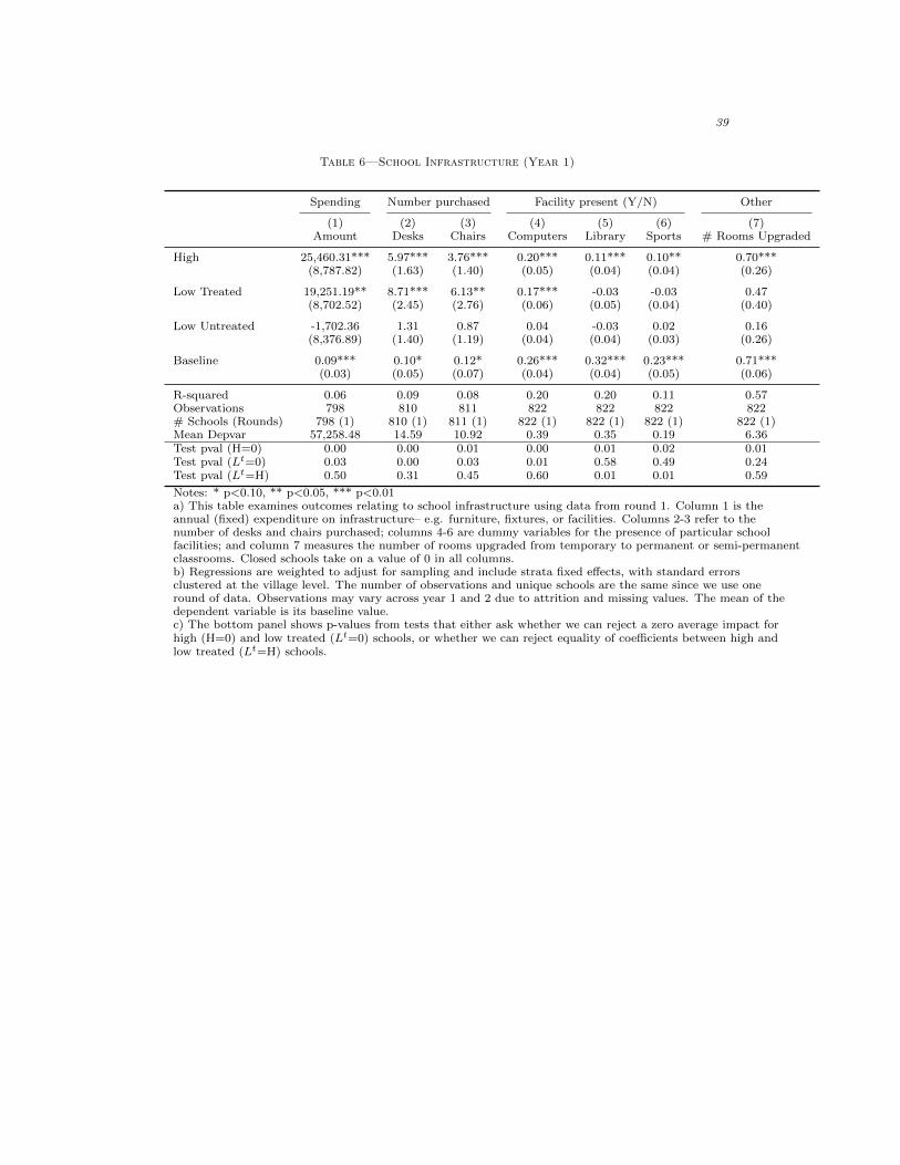
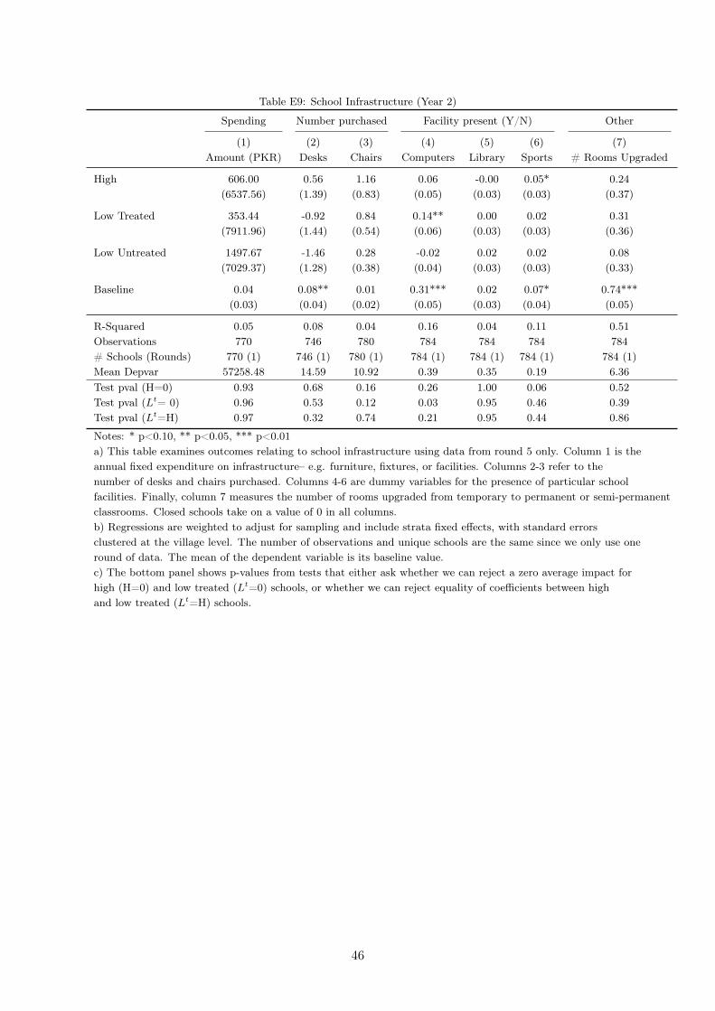
The model assumes that schools know how to increase quality but are respond-ing to market constraints in choosing not to do so. This is consistent with ourprevious work showing that low cost private schools are able to improve test scoreswithout external training or inputs (Andrabi et al., 2017). How they choose todo so is of independent interest for estimates of education production functions.We therefore further empirically investigate changes in school inputs to shed lighton the channels through which schools are able to attract more students or raisetest scores. We find that Lt schools invest in desks, chairs and computers. Mean-while, while H schools invest in these items as well, they also spend money onupgrading classrooms, on libraries, and on sporting facilities. More significantly,the wage bill in H schools increased, reflecting increased pay for both existing

4In equilibrium, all schools in a village may invest in quality if the cost of quality investment issufficiently small and the schools’ existing capacities are sufficiently close to their Cournot optimalcapacities.

4

and new teachers. Bau and Das (2016) show that a 1 standard deviation increasein teacher value-added increases student test scores by 0.15sd in a similar sam-ple from Punjab, and, in the private sector, this higher value-added is associatedwith 41% higher wages. A hypothesis consistent with the test score increases in Hschools is that schools used higher salaries to retain and recruit higher value-addedteachers.

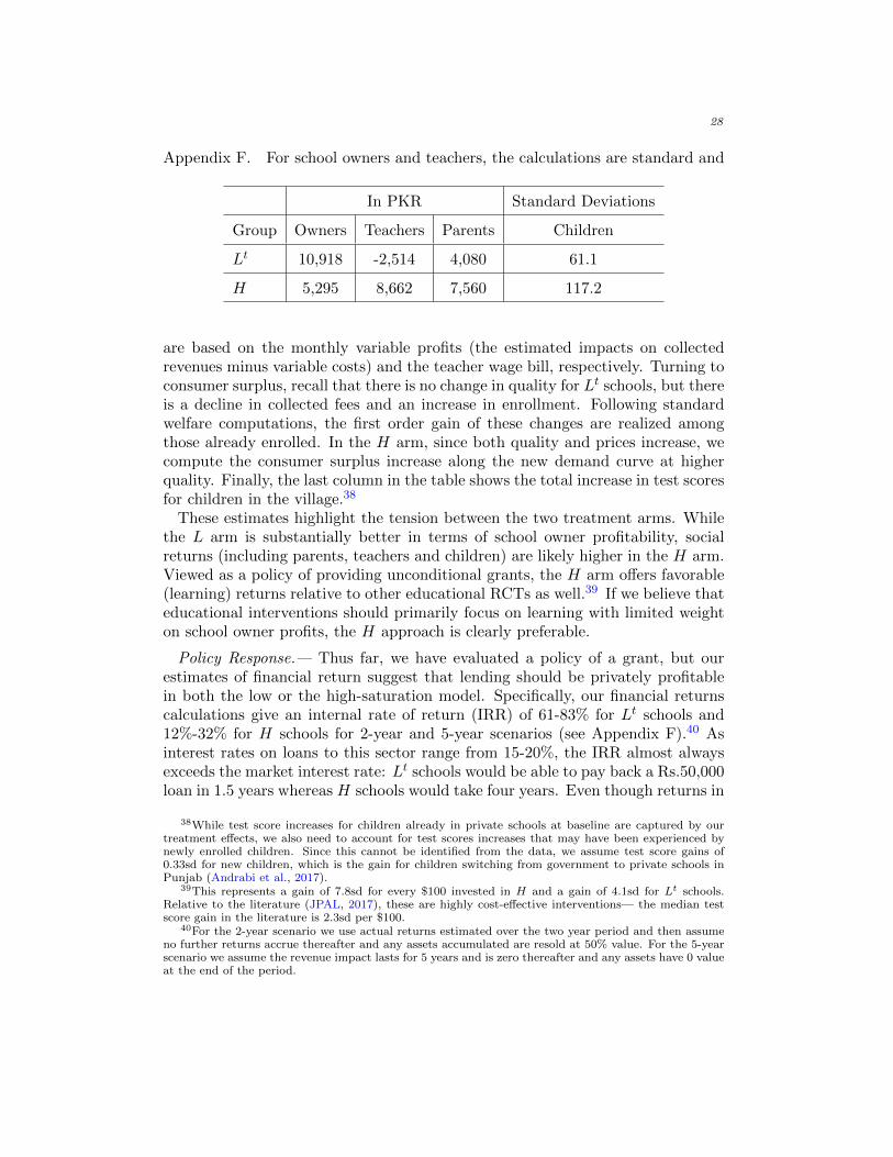
Given the different responses under the two treatment arms, it is natural to askwhich one is more socially desirable. Accurate welfare estimates require strongassumptions, but we can provide suggestive estimates. While school owners seea large increase in their profits under the L arm, this is comparable to the esti-mated gain in welfare that parents obtain under the H arm, driven by test scoreimprovements. If, in addition, we factor in that society at large may value testscores gains over and above parental valuations, then the H treatment is moresocially desirable. Higher weights to teacher salaries compared to owner profitsstrengthen this conclusion further.

This analysis highlights a tension between market-based and socially preferredoutcomes. Left to the market, a private financier would prefer to finance a singleschool in each village; theH arm however is preferable for society. A related policyquestion is then whether the government would want to subsidize the privatesector to lend in a manner that multiple schools receive loans in the same village.To the extent that a lender is primarily concerned with greater likelihood ofdefault and using the fact that school closures were 9 percentage points lower inthe L arm, a plausible form of this subsidy is a loan-loss guarantee for privateinvestors. We estimate that the expected cost of such a guarantee is a third of thegain in consumer surplus suggesting that such a policy may indeed be desirable.Interestingly, this also implies that the usual “priority sector” lending policiesneed to be augmented with a “geographical targeting” subsidy that rewards themarket for increasing financial saturation in a given area–the density of coveragematters.

Our paper contributes to the literatures on education and on SMEs, with a focuson financial constraints to growth and innovation. In education, efforts to improvetest scores include direct interventions in the production function; improvementsin allocative efficiency through vouchers or school matching algorithms; and struc-turing partnerships to select privately operated schools using public funding.5 Asa complement to this literature, we have focused on the impact of policies thatalter the overall operating environments for schools, leaving school inputs and en-rollment choices to be determined in equilibrium. Such policies, especially when

5McEwan (2015), Evans and Popova (2015), and JPAL (2017), provide reviews of the ‘productionfunction’ approach (the causal impact of changing specific school, teacher, curriculum, parent or studentinputs in the education production function) to improving test scores. Recent studies with considerablepromise tailor teaching to the level of the child rather than curricular standards— see Banerjee et al.(2017) and Muralidharan et al. (2016). Examples of approaches designed to increase allocative efficiencyinclude a literature on vouchers (see Epple et al. (2015) for a critical review) and school matchingalgorithms (Abdulkadiroglu et al., 2009; Ajayi, 2014; Kapor et al., 2017).

5

they address market failures, are increasingly relevant for education with the riseof market-based providers, where flexibility allows schools to respond to changesin the local policy regime.6 In two previous papers, we have shown that thesefeatures permit greater understanding of the role of teacher availability (Andrabiet al., 2013) as well as information about school performance for private schoolgrowth and test scores (Andrabi et al., 2017).

Closest to our approach of evaluating financing models for schools are two recentpapers from Liberia and Pakistan. In Liberia, Romero et al. (2017) show that aPPP arrangement brought in 7 school operators, each of whom managed severalschools with evidence of test-score increases, albeit at costs that were higher thanbusiness-as-usual approaches. In Pakistan, Barrera-Osorio et al. (2017) studya program where new schools were established by local private operators usingpublic funding on a per-student basis. Again, test scores increased. Further,decentralized input optimization came close to what a social welfare maximizinggovernment could achieve by tailoring school inputs to local demand. However,these interventions are not designed to exploit competitive forces within markets.

Viewed through this lens, our contributions are twofold. First, we extend ourmarket-level interventions approach to the provision of grants to private schoolsand track the effects of this new policy on test scores and enrollment. Second, weconfirm that the specific design of subsidy schemes matter (Epple et al., 2015) inthe context of a randomized controlled trial, and show that these design effectsare consistent with (an extension of) the theory of oligopolistic competition withcredit constraints. In doing so, we are able to directly isolate the link betweenpolicy and school level responses.7

Our paper also contributes to an ongoing discussion in the SME literature onhow best to use financial instruments to engender growth. Previous work from theSME literature consistently finds high returns to capital for SMEs in low-incomecountries (Banerjee and Duflo, 2012; de Mel et al., 2008, 2012; Udry and Anagol,2006). A more recent literature raises the concern that these returns may be“crowded out” when credit becomes more widely available if these returns are dueto diversion of profits from one firm to another (Rotemberg, 2014). We are able toextend this literature to a service like education and simultaneously demonstratea key trade-off between low and high-saturation approaches. While low-saturationinfusions may lead SMEs to invest more in capacity and increase market shareat the expense of other providers, high-saturation infusions can induce firms tooffer better value to the consumer and effectively grow the size of the market by

6Private schools in these markets face little (price/input) regulation, rarely receive public subsidiesand, optimize based on local economic factors. Public school inputs are governed through an adminis-trative chain that starts at the province and includes the districts. While we can certainly see changesin locally controlled inputs (such as teacher effort), it is harder for government schools to respond tolocal policy shocks with a centralized policy change. In Andrabi et al. (2018), we examine the impact ofsimilar grants to public schools, which addresses government rather than market failures.

7Isolating the causal link between policies and educational improvements that is due to school re-sponses (as opposed to compositional changes) has proven difficult. Large-scale policies usually changehow children sort across schools, making it difficult to find an appropriate control group for the policy.

6

“crowding in” innovations and increasing quality. That the predictions of ourexperiment are consistent with a canonical model of firm behavior establishesfurther parallels between the private school market and small enterprises. Likethese enterprises, private schools cannot sustain negative profits, obtain revenuefrom fee paying students, and operate in a competitive environment with multiplepublic and private providers. We have shown previously that, with these features,the behavior of private schools can be approximated by standard economic modelsin the firm literature (Andrabi et al., 2017). If the returns to alleviating financialconstraints for private schools are as large as those documented in the literatureon SMEs, the considerable learnings from the SME literature becomes applicableto this sector as well (Beck, 2007; de Mel et al., 2008; Banerjee and Duflo, 2012).

The remainder of the paper is structured as follows: Section 1 outlines thecontext; Section 2 presents the theoretical framework; Section 3 describes theexperiment, the data, and the empirical methodology; Section 4 presents anddiscusses the results; and Section 5 concludes.

I. Setting and Context

The private education market in Pakistan has grown rapidly in the last threedecades. In Punjab, the largest province in the country and the site of our study,the number of private schools increased from 32,000 in 1990 to 60,000 in 2016with the fastest growth taking place in rural areas of the province. In 2010-11,38% of all enrollments among children between the ages of 6 and 10 was in privateschools (Nguyen and Raju, 2014). These schools operate in environments withsubstantial school choice and competition; in our study district, 64% of villageshave at least one private school, and within these villages there is a median of5 (public and private) schools (NEC, 2005). Our previous work has shown thatthese schools are not just for the wealthy; 18 percent of the poorest third sendtheir children to private schools in villages where they existed (Andrabi et al.,2009). One reason for this success is better learning. While absolute levels oflearning are below curricular standards across all types of schools, test scores ofchildren enrolled in private schools are 1 standard deviation higher than for thosein public schools, which is a difference of 1.5 to 2.5 years of learning (dependingon the subject) by Grade 3 (Andrabi et al., 2009). These differences remain largeand significant after accounting for selection into schooling using the test scoretrajectories of children who switch schools (Andrabi et al., 2011).

A second reason for this success is that private schools have managed to keeptheir fees low; in our sample, the median private school reports a fee of Rs.201 or$2 per month, which is less than half the daily minimum wage in the province. Wehave argued previously that the ‘business model’ of these private schools relieson the local availability of secondary school educated women with low salariesand frequent churn (Andrabi et al., 2008). In villages that have a secondaryschool for girls, there is a steady supply of such potential teachers, but alsofrequent bargaining between teachers and school owners around wage setting—in the teacher market, a 1sd increase in teacher value-added is associated with a

7

41% increase in wages (Bau and Das, 2016). A typical teacher in our sample isfemale, young and unmarried, and is likely to pause employment after marriageand her subsequent move to the marital home. An important feature of thismarket is that the occupational choice for teachers is not between public andprivate schools: Becoming a teacher in the public sector requires a college degree,and an onerous and highly competitive selection process as earnings are 5-10times as much as private school teachers and applicants far outweigh the intake.Accordingly, transitions from public to private school teaching and vice versa areextremely rare.

Despite their successes in producing higher test-scores at low costs, once avillage has a private school, future quality improvements appear to be limited.We have collected data through the Learning and Educational Achievement inPakistan Schools (LEAPS) panel for 112 villages in rural Punjab, each of whichreported a private school in 2003. Over five rounds of surveys spanning 2003 to2011, tests scores remain constant in “control” villages that were not exposed toany interventions from our team. Furthermore, there is no evidence of an increasein the enrollment share of private schools or greater allocative efficiency wherebymore children attend higher quality schools. This could represent a (very) stableequilibrium, but could also be consistent with the presence of systematic con-straints that impede the growth potential of this sector.

This study focuses on one such constraint: access to finance. This focus onfinance is driven, in part, by what school owners themselves tell us. In oursurvey of 800 school owners, two-thirds report that they want to borrow, butonly 2% percent report any borrowing for school related loans.8 School ownerswish to make a range of investments to improve school performance as well astheir revenues and profits. The most desired investments are in infrastructure,especially additional classrooms and furniture, which owners report as the primarymeans of increasing revenues. While also desirable, school owners find raisingrevenues through better test scores and therefore higher fees a somewhat riskierproposition. Investments like teacher training that may directly impact learningare thought to be risky as they may not succeed (the training may not be effectiveor a trained teacher may leave) and even if they do, they may be harder todemonstrate and monetize.

The Pakistani educational landscape therefore presents an active and compet-itive educational marketplace, but one where schools may face significant con-straints, including financial, that may limit their growth and innovation. Thissetting suggests that alleviating financial constraints may have positive impactson educational outcomes; whether these impacts arise due to infrastructure orpedagogical improvements depends on underlying features of the market and thecompetitive pressure schools face.

8This is despite the fact that school owners are highly educated and integrated with the financialsystem: 65 percent have a college degree; 83 percent have at least high school education; and 73 percenthave access to a bank account.

8

II. Theoretical Framework

Our theoretical exercise consists of two parts that shed light on the marketlevel impacts of an increase in financial resources. First, we introduce creditconstrained firms and quality into the canonical Kreps and Scheinkman (1983)framework (henceforth KS).9 Schools in our model are willing to increase theircapacities or qualities (to charge higher fees) but are credit constrained beyondtheir initial capital. Second, we introduce comparative static exercises throughthe provision of unconditional grants and study the equilibrium with varyingdegrees of financial saturation. Our approach of extending a canonical modeldisciplines the theory exercise and provides us with a robust conceptual frameworkto conduct empirical analysis and interpret findings.

A. Setup

Two identical private schools, indexed by i = 1, 2, choose whether to investin capacity, xi ≥ 0, or quality, qt, where t ∈ {H,L} is high or low quality.High quality is conceptualized as investments that allow schools to offer betterquality/test scores and charge higher prices, such as specialty infrastructure (e.g.library or sports facility) or higher-quality teachers. Low quality investments,such as basic infrastructure (desks or chairs) or basic renovations, allow schoolsto retain or increase enrollment but do not change existing students’ willingnessto pay.

SCHOOLS: Each school i maximizes Πi = (pi− c)xei +Ki− rxi−wt subject torxi + wt ≤ Ki and xei ≤ xi, where xei is the enrollment, pi is the price of school iper seat, c is the constant marginal cost for a seat, r is the fixed cost for a seat, wtis the fixed cost for quality type, and Ki is the amount of fixed capital availableto the school. Schools face the same marginal and fixed costs for investments.The fixed cost for low quality is normalized to 0, and so w is the fixed cost ofdelivering high quality.10

STUDENTS: There are T students each of whom demands only one seat. Eachstudent j has a taste parameter for quality θj and maximizes utility U(θj , qt, pi) =θjqt− pi by choosing a school with quality qt and fee pi. The value of the outsideoption is zero for all students, and students choose to go to school as long as U ≥ 0.We initially assume students are homogeneous with θ = 1. Later, we show ourresults hold when the model is extended to allow for consumer heterogeneity.

TIMING: The investment game has three stages. In the first stage, schoolssimultaneously choose their capacity and quality. After observing these choices,schools simultaneously choose their prices in the second stage. Demand is realizedin the final stage. Standard allocation rules are assumed.11

9KS (1983) develop a model of firm behavior under binding capacity commitments. In their model,the Cournot equilibrium is recovered as the solution to a Bertrand game with capacity constraints.

10Alternative parameterizations for the profit function including allowing for school heterogeneity,will naturally lead to different sets of equilibrium outcomes. However, our main results, which areconcerned with the comparisons between the H and L treatments, will remain unaffected as long asparameterizations do not vary by treatment arm. We discuss this point further at the end of this section.

11We assume: (i) The school offering the higher surplus to students serves the entire market up to

9

B. Equilibrium Analysis

We first examine the subgame perfect Nash equilibrium (NE) of this investmentgame at baseline and then assess how the equilibrium changes in the L arm whereonly one school receives a grant K > 0, and in the H arm where both schoolsreceive the same grant K. The receipt of grants is common knowledge among allschools in a given market.

An Example

Prior to the full analysis, consider the following example to build intuition forthe pricing decisions of schools. Suppose that the fixed cost of quality is w = 8;the cost of expanding capacity by one unit is r = 1; and, there are 30 (identical)consumers who value qL at $3 and qH at $5. The marginal cost of each enrolledstudent is c = 0.

Capacity constrained schools and student homogeneity suggests the existenceof an uncovered market in the baseline equilibrium. That is, there are studentswilling to attend a (private) school at the prevailing price but cannot do so becauseschools do not have the capacity to accommodate these students.12 Without lossof generality (WLOG), we assume that in the baseline, schools produce low qualityand cannot seat more than 10 students each. Therefore, the size of the uncoveredmarket is N = 10. Both schools charge $3 and earn a profit of $3 per child for atotal profit of $30. Given capacity constraints, decreasing the price only lowersschool profits.

In the L arm, a single school receives $9, which it can spend on expandingcapacity by 9 units or increasing quality and expanding capacity by 1 unit. Com-paring profits establishes that capacity expansions are favored with a profit of$57.13

In the H arm, each of the two schools receives $9. First, consider the subgamewhere both schools invest in capacity so that the overall market capacity expandsto 38, which is more than the 30 children in the village. In this subgame, there isno pure strategy NE. In the mixed strategy equilibrium, schools will randomizebetween $3 and $33

19 (≈ $1.74) with a continuous and atomless probability distri-bution and obtain an (expected) profit of $33.14 However, the subgame whereboth schools invest in capacity is not consistent with equilibrium in the full game,

its capacity and the residual demand is met by the other school; (ii) If schools set the same price andquality, market demand is split in proportion to their capacities as long as their capacities are not met;(iii) If schools choose different qualities but offer the same surplus, then the school offering the higherquality serves the entire market up to its capacity and the residual demand is met by the other school.

12These rationed students may instead enroll in public schools in the village, an outside option in thismodel, or not attend any school at all.

13If the school expands capacity, it enrolls 9 more children for a total profit of 19×3=$57. In contrast,if it invests in quality it receives (10 + 1) × 5=$55.

14To see why, note that $3 is not an equilibrium price since a school can deviate by charging $3−ε andenrolling 19 children while the other school obtains the residual demand of 30 − 19 = 11. Alternatively,$0 is not an equilibrium price either— deviating to $0 + ε with an enrollment of 11 yields a positiveprofit as the other school cannot enroll more than 19 children. To derive the mixed strategy equilibrium,schools must be indifferent between any two prices in the support of the mixing distribution. Supposeone school charges $3. Given that the mixing distribution is atomless, the price of the other school mustbe lower. Therefore, the school that charges $3 is price undercut for sure and it will obtain the residual

10

where schools can also choose quality. Specifically, if one school deviates and in-vests $8 in quality and $1 in an additional chair instead, then schools could servethe entire market of 30 children without a price war and the deviating schoolwould charge $5 for a total profit of $55, which is higher than $33.

The possibility of a price war thus compels schools to not spend the entiregrant on capacity expansion when the size of uncovered market is ‘small.’ Nowconsider the case where each school buys 5 additional chairs, serves 15 students,and keeps the remaining $4. In this case, equilibrium dictates that each schoolshould charge a price of $3 and achieve profit of $49. However, investing in5 additional chairs is also not consistent with equilibrium because one of theschools would profitably deviate and invest in quality and one additional chairfor a profit of $55. Therefore, when the size of the uncovered market is sufficientlysmall, at least one of the schools will switch to quality investments instead of apartial expansion in capacity. In fact, the only equilibrium in this case is such thatone school expands quality with a profit of $55 and the other expands capacitywith a profit of $57. If the uncovered market size had been less than 10, thenboth schools investing in quality would be consistent with equilibrium becausethe school that deviates cannot fully utilize the grant to avoid price competitionwith a rival offering higher quality.

Full Analysis

Consider first the baseline scenario. As before, WLOG, we consider the casewhere schools produce low quality initially. It is straightforward to show thatin the unique baseline equilibrium, schools enroll the same number of students,M2 (where M < T refers to the covered market and N = T −M is the size of

the uncovered market) and charge the same price p = qL, extract full consumersurplus and earn positive profits. Schools do not lower prices since they cannotmeet the additional demand.

Now consider the impact of the grants. When schools receive additional financ-ing, they can increase capacity at the risk of price competition or increase qualityat a (possibly) higher cost. Our previous example illustrates the tension betweenthese two strategies. Two key parameters influence the investment strategies ofschools, the cost of quality, w, and the size of the uncovered market, N . Whenboth w and N are very low, schools prefer to invest in quality in both treatmentarms. For sufficiently high values of w, schools in both treatments prefer to investin capacity as long as N is quite large. As N decreases, schools will invest in ca-pacity as long as increasing revenues through new students is more rewarding thanincreasing revenues among existing students through higher quality and prices,but spend less of their grants to escape from price competition. At a thresholdlevel of N , at least one of the schools switches to quality investment instead of

demand of 11 children and a profit of $33. Now consider a lower bound, y, of the mixing distribution.Suppose one school charges y. Then it must be the case that it price undercuts the other school andobtains a demand of 19. But the school must be indifferent between charging $3 and charging y, whichimplies that $33 = 19 × y, or y ≈ 1.74.

11

a partial expansion in capacity. This threshold for N decreases as w increases,suggesting a negative relationship between the two. We formally prove theseclaims for both treatment arms and characterize the wN−space where qualityinvestment by at least one school is consistent with equilibrium.

Because the schools are credit constrained, they cannot afford high quality ifits cost is greater than the grant size. Therefore, we are concerned with the partof the wN−space where quality investment is feasible, i.e. w ≤ K. We alsoparametrize the size of the grant, K, to be neither ‘too small’ nor ‘too large.’In particular, we assume that K is large enough such that investing in qualityis not always the optimal action but small enough so that rate of return of eachinvestment is positive.15

2Kr

Kr

Kw∗

L

N

w

Figure 1a: Low-saturation Treatment

EL

2Kr

Kr

Kw∗

H

N

w

EH

Figure 1b: High-saturation Treatment

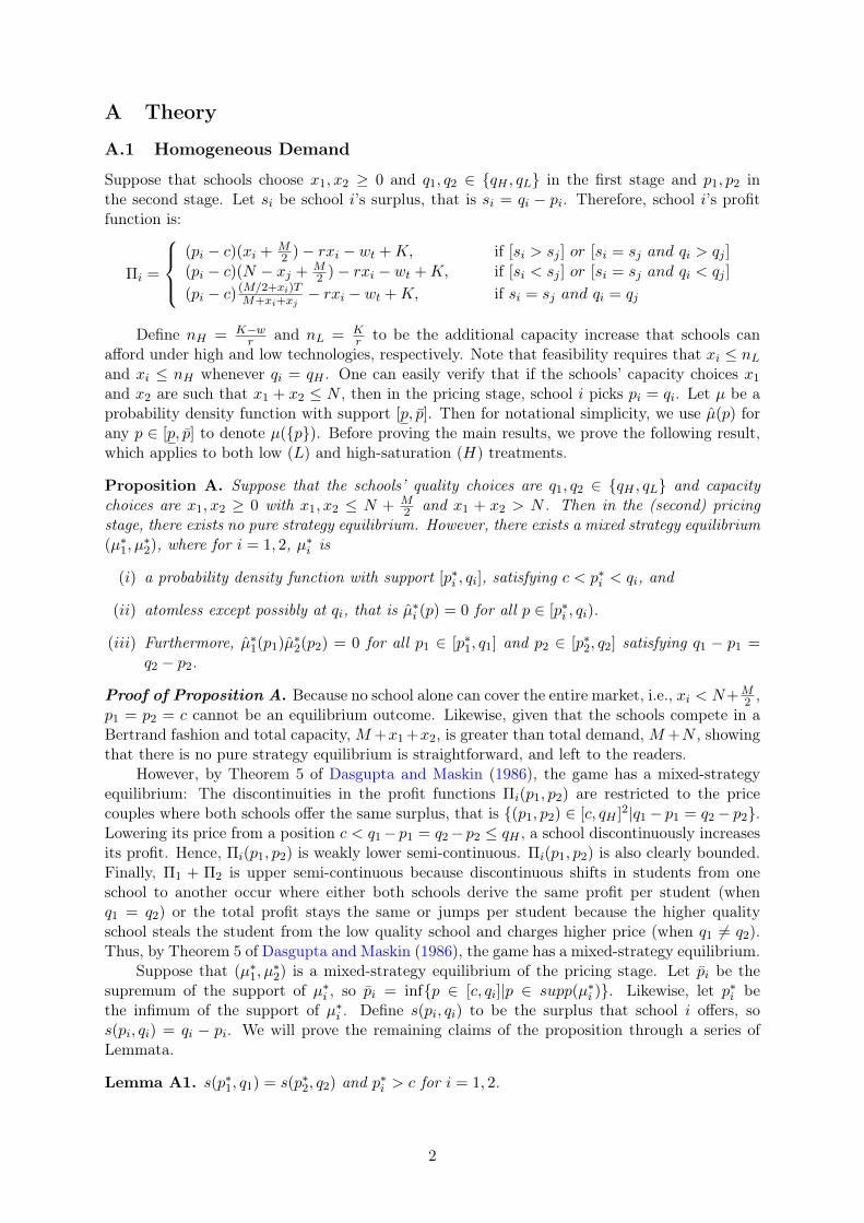
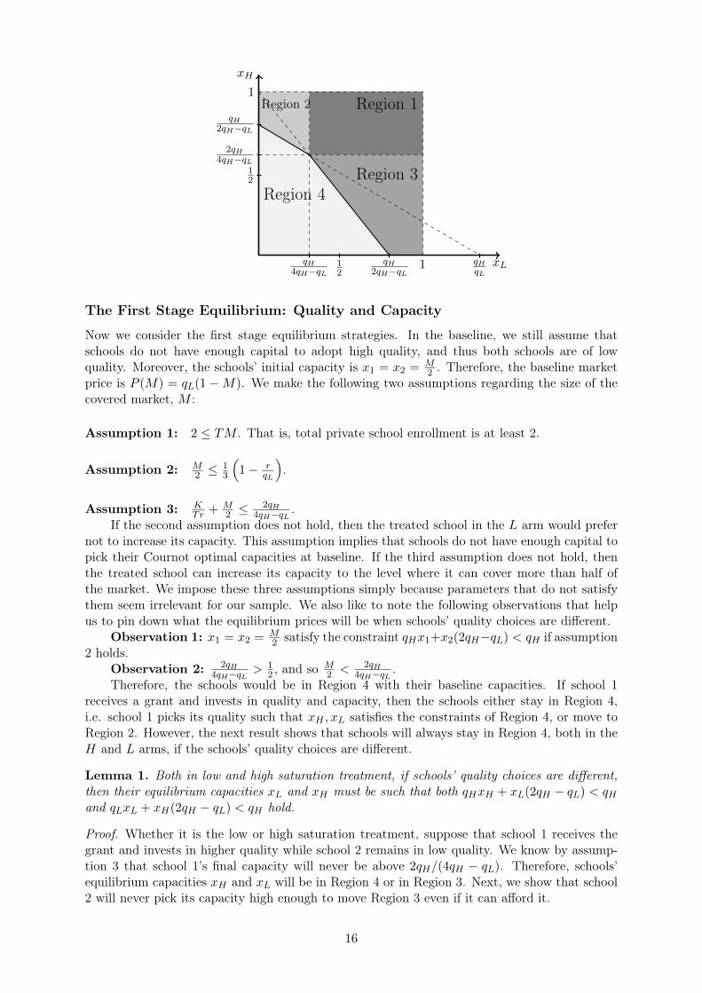
Theorem 1. The shaded regions EL and EH in Figure 1 represent the set ofparameters in wN−space where there exists an equilibrium of the investment gamein the low and high-saturation treatment, respectively, such that (at least one)treated school invests in quality.

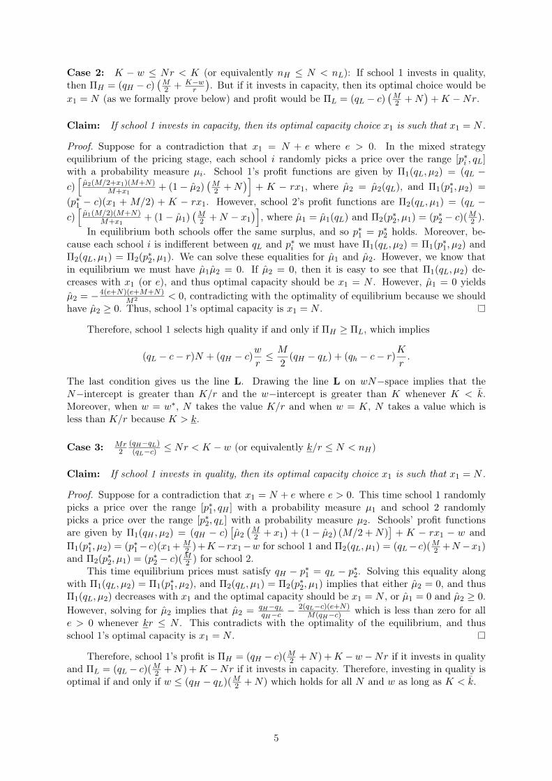
All the proofs are presented in Appendix A1. Suppose that the size of theuncovered market is sufficiently large such that the Lt school cannot cover it evenif it spends the entire grant on capacity, i.e. K/r ≤ N . If this school increasescapacity, then the gain in profits is equal to the return on each new studenttimes the number of new students, (qL − c)Kr . If it increases quality instead,then the gain in profits is equal to the sum of (i) increase in return on existingstudents from the higher price times the number of existing students and (ii) thereturn from higher quality to each new student times the number of new students,(qH − qL)M2 + (qH − c)K−w

r . Therefore, investing in capacity is more profitable if

15We suppose that k < K < k where k = Mr2

(qH−qLql−c

)and k = M

2(qH − qL). If the inequality

k < K does not hold, then the revenue from capacity investment, Kr

(qL − c), is lower than revenue from

quality (only) investment, M2

(qH − qL), and thus, quality investment is always optimal. The rate of

return from capacity investment is positive because we assume qL − c − r > 0. Finally, K < k impliesthat rate of return from quality (only) investment is always positive. This assumption is not essentialfor our results, and in Appendix A1, we show how equilibrium sets would change if we relax it.

12

the former term is greater than the latter, yielding the condition w > w∗ where

w∗ = r(qH−qLqH−c

)(M2 +K

r

). However, if the size of the uncovered market is smaller,

in particularN < Kr , then spending the entire grant on additional capacity implies

that the treated school must steal some students from the rival school, resultingin a price war and lower payoffs. In order to avoid lower payoffs, the treatedschool will partially invest in capacity. The line L indicates the parameters wand N that equate the treated school’s profit from quality investment to its profitfrom partial capacity investment.16

On the other hand, schools will never engage in a price war in the H arm aslong as the uncovered market size is large enough, so that schools cannot cover iteven if both spend the entire grant on capacity, i.e. 2K

r ≤ N . Therefore, for thesevalues of N , equilibrium predictions will be no different than the L arm. However,when N is less than 2K

r , spending the entire grant on additional capacity impliesthat the school must steal some students from the rival school, resulting againin a price war. The constraint indicating the indifference between profit fromquality investment and from partial capacity investment, the line H in Figure 1b,is much farther out because now both schools can invest in capacity, and henceprice competition is likely even for higher values of the uncovered market size,N .17 The next result is self evident from the last two figures and thus providedwith no formal proof.

Corollary 1 (Homogeneous Consumers). If the treated school in the low-saturation treatment invests in quality, then there must exist an equilibrium inthe high-saturation treatment that at least one school invests in quality. However,the converse is not always true.

C. Generalization of the Model and Discussion

Consumer Heterogeneity

Now, we extend our analysis by incorporating consumer heterogeneity in will-ingness to pay. We assume that students’ taste parameter for quality θj is uni-formly distributed over [0, 1], resulting in a downward sloping demand curve.Specifically, if the schools’ quality and price are q and p, respectively, then de-mand is D(p) = T (1− p

q ). Unlike the case with homogeneous consumers, there arenever students who would like to enroll in a school at the existing price but arerationed out— prices always rise to ensure that the marginal student is kept at herreservation utility. Nevertheless, our previous intuition will carry forward. Thedriving force for our results in the homogeneous case was the tension between theuncovered market and the schools’ actual capacities; in the heterogeneous case,the role of the uncovered market is played by the schools’ Cournot best responsecapacities, akin to KS (1983).

In the formal exposition in Appendix A2, we maintain the entire KS framework,

16More formally, L represents the line (qH − c)(

M2

+ K−wr

)= (qL − c)

(M2

+N)

+K −Nr.17More formally, H represents the line (qH − c)(M

2+ K−w

r) = (qL − c)(M

2+N − K

r) −Nr.

13

including their rationing rule, and prove two results. We first show that if schoolscan choose quality, there always exists a pure strategy NE.18 We then prove that,as in the case of homogeneous consumers, if both schools invest in capacity in theH arm, this makes capacity expansion beyond the Cournot best response levelsmore likely, thereby increasing the likelihood of price competition. It is thus morelikely that (at least one) treated school in the H arm will invest in quality. Usingthis intuition, we prove a version of Theorem 1 under a mild set of parameterrestrictions discussed in Appendix A2.

Theorem 2 (Heterogeneous Consumers). If the treated school in the low-saturation treatment invests in quality, then there must exist an equilibrium in thehigh-saturation treatment where at least one school invests in quality. However,the converse is not always true.

Potential Extensions

There are a number of other plausible modifications that could be made to themodel. For instance, we could introduce risk-averse owners who are insurance(rather than credit) constrained, or introduce a degree of altruism in the profitfunction to allow for school owners who intrinsically care about the number ofchildren in school. We can also allow quality to be a continuous variable andalso move beyond our static setting to introduce dynamic considerations such asover-investment to deter entry. These modifications potentially change the setof parameters supporting equilibria where (at least one) treated school invests inquality. However, our theorems will remain unchanged as long as these changesaffect the schools’ profit functions symmetrically in each treatment arm. In thiscase, the risk of price competition will still be higher in the H arm, and thusquality investment will still be more likely in H than the L arm.

On the other hand, adjustments to the model that generate asymmetric pa-rameterization of the profit function in each treatment arm may alter our mainresults. For example, if school owners have the ability to collectively affect themarket size or input prices (e.g. higher competition among schools may raiseteachers’ salaries), then the return or cost of an investment would be different ineach treatment arm, which may meaningfully change our results. Given that thetotal resources available in a village vary across treatment arms, we assess thispossibility further in Section IV.A and show that it is not empirically salient inour case.

To summarize, our model provides insights on how schools in the two treatmentarms respond to a relaxation of credit constraints, either by increasing revenue

18The intuition follows from the nature of the profit function. The mixed strategy equilibrium in theKS game is due to discontinuities in the profit function. When both firms produce the same quality, ifone price undercuts the other, then it takes all consumers up to its capacity and sees a discontinuousjump in profits. When firms are differentiated in quality, profits always change smoothly as the marginalconsumer’s valuation distribution is atomless. If all consumers are homogeneous as before however, evenwith differentiated quality, the smoothness in consumer demand vanishes and we again find no purestrategy equilibria in the game.

14

from existing consumers or expanding market share and risking price competi-tion. Our main result is that we are more likely to observe higher enrollment intreated schools in the L arm and higher quality (and increased fees) in the H arm.Moreover, private profits will be higher for Lt schools. Although, conceptually, atest of the theory can be based on variation in the size of the uncovered marketand the cost of quality investments, these are not observed in the data. Therefore,we focus attention in our empirical results on the difference in impact betweenlow and high-saturation villages.

III. Experiment, Data and Empirical Methods

A. Experiment

Our intervention tests the impact of increasing financial access for schools foroutcomes guided by theory (revenue, expenditures, enrollment, fees and qualitycaptured as test scores) and assesses whether this impact varies by the degree offinancial saturation in the market. Our intervention has three features: (i) it iscarried out only with private schools where all decisions are made at the level ofthe school;19 (ii) we vary financial saturation in the market by comparing villageswhere only one (private) school receives a grant (L arm) versus villages whereall (private) schools receive grants (H arm); and (iii) we never vary the grantamount at the school level, which remains fixed at Rs.50,000.

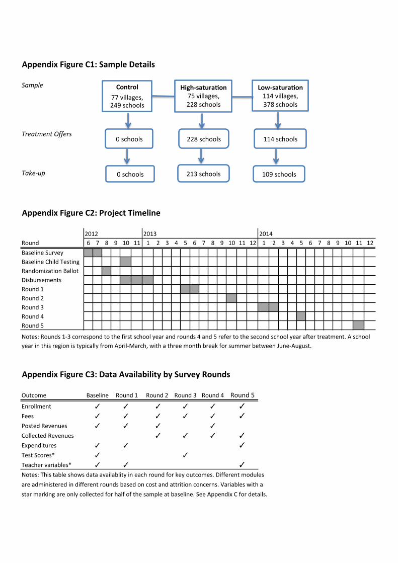
Randomization Sample and Design.— Our sampling frame is defined as allvillages in the district of Faisalabad in Punjab province with at least 2 privateor NGO schools; 42 percent (334 out of 786) of villages in the district fall inthis category. Based on power calculations using longitudinal LEAPS data, wesampled 266 villages out of the 334 eligible villages with a total of 880 schools, ofwhich 855 (97%) agreed to participate in the study.

Table 1 presents summary statistics from our sample at the village (Panel A)and the private school level (Panel B). The median village has 2 public schools, 3private schools and 416 children enrolled in private schools. The median privateschool has 140 enrolled children, charges Rs. 201 in monthly fees, and reportsa monthly revenue of Rs. 26,485. Monthly variable costs are Rs. 16,200 andannual fixed costs are Rs. 33,000, for an annual profit of Rs. 90,420. The rangeof outcome variables is quite large. Relative to a mean of 164 students, the5th percentile of enrollment is 45 compared to 353 at the 95th percentile of thedistribution. Similarly, fees range from Rs. 81 (5th percentile) to Rs. 503 (95thpercentile) and monthly revenues from Rs. 4,943 to Rs. 117,655. The kurtosis,a measure of the density at the tails, is 17 for annual fixed expenses and 51for revenues relative to a kurtosis of 3 for a standard normal distribution. Ourdecision to include all schools in the market provides external validity, but hasimplications for precision and mean imbalance, both of which we discuss.

19This excludes public schools, which cannot charge fees and lack control over hiring and pedagogicdecisions. In Andrabi et al. (2018), we study the impact of a parallel experiment with public schoolsbetween 2004 and 2011. It also excludes 5 (out of close to 900) private schools that were part of a largerschool chain with schooling decisions taken at the central office rather than within each school.

15

We use a two-stage stratified randomization design where we first assign eachvillage to one of three experimental groups and then schools within these villagesto treatment. Stratification is based on village size and village average revenues,as both these variables are highly auto-correlated in our panel dataset (Bruhnand McKenzie, 2009). Based on power calculations, 3

7 of the villages are assigned

to the L arm, and 27 to the H arm and the control group; a total of 342 schools

across 189 villages receive grant offers (see Appendix Figure C1). In the secondstage, for the L arm, we randomly select one school in the village to receive thegrant offer; in the H arm, all schools receive offers; and, in the control group, noschools receive offers.

The randomization was conducted through a public computerized ballot in La-hore on September 5, 2012, with third-party observers (funders, private schoolowners and local NGOs) in attendance. The public nature of the ballot andthe presence of third-party observers ensured that there were no concerns aboutfairness; consequently, we did not receive any complaints from untreated schoolsregarding the assignment process. Once the ballot was completed, schools re-ceived a text message informing them of their own ballot outcome. Given villagestructures, information on which schools received the grant in the L arm was notlikely to have remained private, so we assume that the receipt of the grant waspublic information.

Intervention.— We offer unconditional cash grants of Rs.50,000 (approximately$500 in 2012) to every treated school in both L and H arms. The size of the grantrepresents 5 months of operating profits for the median school and reflects bothour overall budget constraint and our estimate of an amount that would allow formeaningful fixed and variable cost investments. For instance, the median wagefor a private school teacher in our sample is Rs. 24,000 per year; the grant thusallows the school to hire 2 additional teachers a year. Similarly, the costs of desksand chairs in the local markets range from Rs. 500 to Rs. 2,000, allowing theschool to purchase 25-100 additional desks and chairs.

We deliberately do not impose any conditions on the use of the grant apart fromsubmission of a (non-binding) business plan (see below). School owners retaincomplete flexibility over how and when they spend the grant and the amountthey spend on schooling investments with no requirements of returning unusedfunds. As we show below, most schools choose not to spend the full amount in thefirst year and the total spending varies by the treatment arm. Our decision not toimpose any conditions follows our desire to provide policy-relevant estimates forthe simplest possible design; the returns we observe therefore provide a ‘baseline’for what can be achieved through a relatively ‘hands-off’ approach to privateschool financing.

Grant Disbursement.— All schools selected to receive grant offers are visitedthree times. In the first visit, schools choose to accept or reject the grant offer: 95

16

percent (325 out of 342) of schools accept.20 School owners are informed that theymust (a) complete an investment plan to gain access to the funds and may spendthese funds on items that would benefit the school and (b) be willing to open aone-time use bank account for cash deposits. Schools are given two weeks to fillout the plan and must specify a disbursement schedule with a minimum of twoinstallments. In the second visit, investment plans are collected and installmentsare released according to desired disbursement schedules.21 A third and finaldisbursement visit is conducted once at least half of the grant amount has beenreleased. While schools are informed that failure to spend on items may result ina stoppage of payments, in practice, as long as schools provide an explanation oftheir spending or present a plausible account of why plans changed, the remainderof the grant is released. As a result, all 322 schools receive the full amount of thegrant.

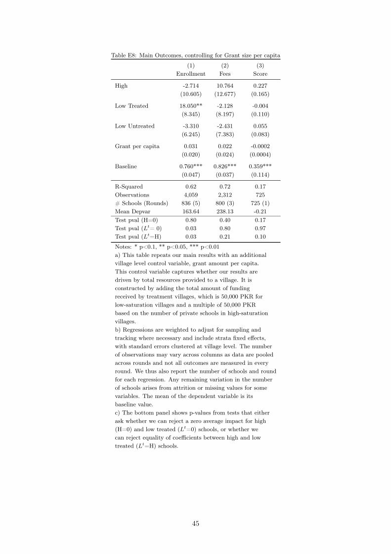
Design Confounders.— If the investment plan or the temporary bank accountaffected decision making, our estimates will reflect an intervention that bundlescash with these additional features. We discuss the plausibility of these channelsin Section IV.A below and use additional variation and tests in our experimentto show that any contribution of these mechanisms to our estimated treatmenteffects are likely small. In Section IV.A, we also discuss that the treatment unit ina saturation experiment is a design variable; in our case, this unit could have beeneither the village (total grants are equalized at the village level) or the school. Wechose the latter to compare schools in different treatment arms that receive thesame grant. Consequently, in the H arm, with a median of 3 private schools, thetotal grant to the village is 3 times as large as to the L arm. Observed differencesbetween these arms could therefore reflect the equilibrium effects of the totalinflow of resources into villages, rather than the degree of financial saturation.Again, using variation in village size, we show in section IV.A that this is unlikelyto be a concern since our results remain qualitatively the same when we comparevillages with similar per-capita grant inflow.

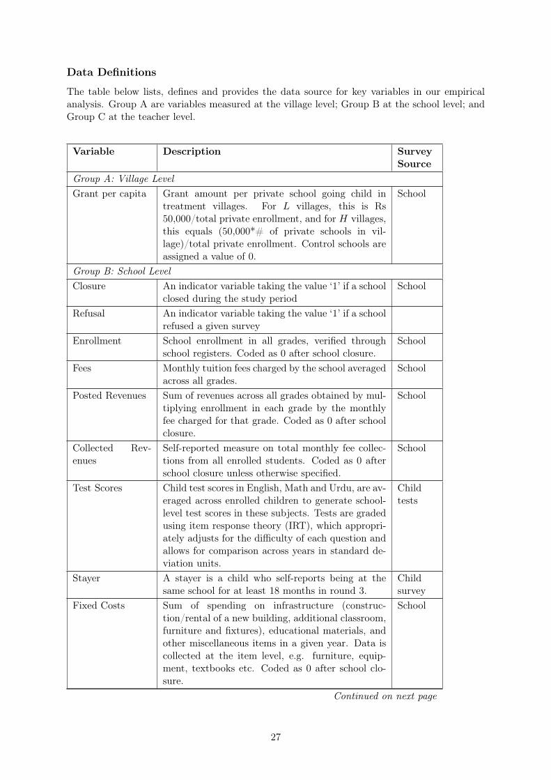
B. Data Sources

Between July 2012 and November 2014, we conducted a baseline survey and fiverounds of follow-up surveys. In each follow-up round, we survey all consentingschools in the original sample and any newly opened schools.22

Our data come from three different survey exercises, detailed in Appendix C.

20Reasons for refusal include anticipated school closure; unwillingness to accept external funds; or afailure to reach owners despite multiple attempts.

21At this stage, 3 schools refused to complete the plans and hence do not receive any funds. Our finaltake-up is therefore 94% (322 out of 342 schools), with no systematic difference between the L and Harms.

22There are 31 new school openings two years after baseline: 3 public and 28 private schools. 13new private schools open in H villages, 10 in the L villages, and 5 in control villages. Given these smallnumbers, we omit these schools from our analysis. Even though the overall number of school openings islow, we find that H villages report a higher fraction of new schools relative to control, though this effectis small at an increase of 2%. Our main results remain qualitatively similar if we include these schoolsin our analyses with varying assumptions on their baseline value.

17

We conduct an extended school survey twice, once at baseline and again 8 monthsafter treatment assignment in May 2013 (Round 1 in Appendix Figure C2), col-lecting information on school characteristics, practices and management, as wellas household information on school owners. In addition, there are 4 shorter follow-up rounds every 3-4 months that focus primarily on enrollment, fees and revenues.Finally, children are tested at baseline and once more, 14 months after treatment(Round 3). During the baseline, we did not have sufficient funds to test everyschool and therefore administered tests to a randomly selected half of the sampleschools. We also never test children in public schools. At baseline, this decisionwas driven by budgetary constraints and in later rounds we decided not to testchildren in public schools because our follow-up surveys showed enrollment in-creases of at most 30 children in treatment villages. Even if we were to assumethat these children came exclusively from public schools, this suggests that publicschools enrollment across all grades declined at most 2-3% on average. This effectseemed too small to generate substantial impacts on public school quality.23

C. Regression Specification

We estimate intent-to-treat (ITT) effects using the following school-level spec-ification:24

Yijt = αs + δt + β1Hijt + β2Ltijt + β3L

uijt + γYij0 + εijt

Yijt is an outcome of interest for a school i in village j at time t, which is mea-sured in at least one of five follow-up rounds after treatment. Hijt, L

tijt, and Luijt

are dummy variables for schools assigned to high-saturation villages, and treatedand untreated schools in low-saturation villages respectively. We use strata fixedeffects, αs, since randomization was stratified by village size and revenues, and δtare follow-up round dummies, which are included as necessary. Yij0 is the baselinevalue of the dependent variable, and is used whenever available to increase preci-sion and control for any potential baseline mean imbalance between the treatedand control groups (see discussion in section III.D). All regressions cluster stan-dard errors at the village level and are weighted to account for the differentialprobability of treatment selection in the L arm as unweighted regressions wouldassign disproportionate weight to treated (untreated) schools in smaller (larger)L villages relative to schools in the control or H arms (see Appendix B). Ourcoefficients of interest are β1, β2, and β3, all of which identify the average ITTeffect for their respective group.

23Another option would have been to test those students at baseline whom we expected to be marginalmovers due to the treatment and see their gains from the switch. Detecting marginal movers ex-antehowever is a difficult especially given that churn is not uncommon in this setting.

24We focus on ITT effects and do not present other treatment effect estimates since take-up is nearuniversal at 94 percent.

18

D. Validity

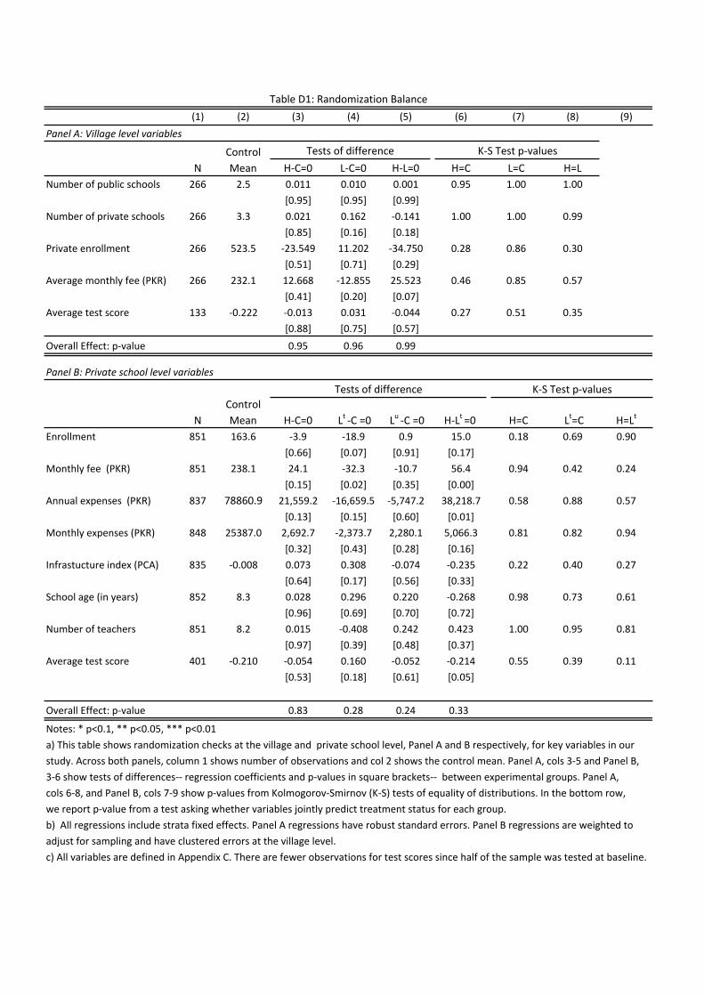
Balance.— Appendix Table D1 presents tests for baseline differences in meansand distributions as well as joint tests of significance across experimental groupsat the village (Panel A) and at the school level (Panel B). At the village level,covariates are balanced across the three experimental groups (H, L and Control),and village level variables do not jointly predict village treatment status for theH or L arm.

Balance tests at the school level involve four experimental groups: Lt and Lu

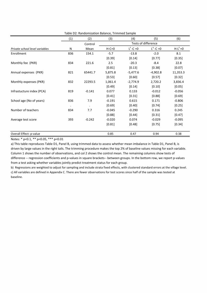
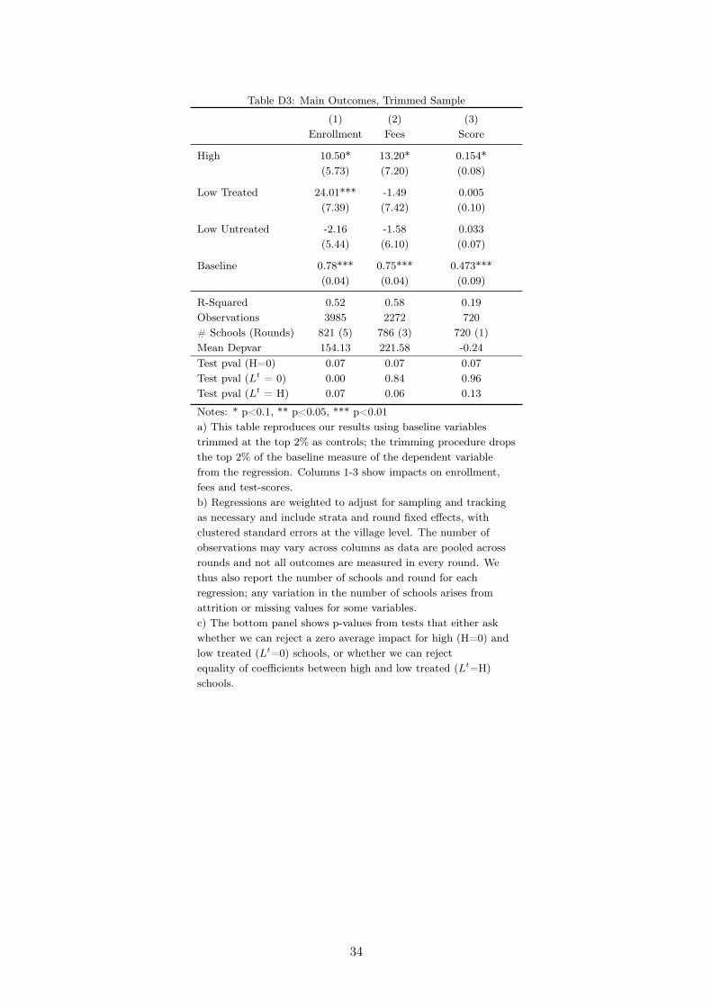
schools; schools in the H arm; and untreated schools in control. Panel B showscomparisons between control and each of the three treatment groups (cols 3-5)and between the H and Lt schools (col 6), our other main comparison of interest.5 out of 32 univariate comparisons (Panel B, cols 3-6) show mean imbalance atp-values lower than 0.10— a fraction slightly higher than what we may expectby random chance. If this imbalance leads to differential trends beyond what canbe accounted for through the inclusion of baseline variables in the specification,our results for the Lt schools may be biased (Athey and Imbens, 2017). Despitethis mean imbalance however, our distributional tests are always balanced (PanelB, colss 7-9), and, furthermore, covariates do not jointly predict any treatmentstatus. Nevertheless, we conduct a number of robustness checks in Appendix Dand show that the mean imbalance we observe is largely a function of heavy(right)-tailed distributions arising from the inclusion of all schools in our sample andtrimming our data eliminates the imbalance without qualitatively changing ourtreatment effects (see Appendix Tables D2 and D3).

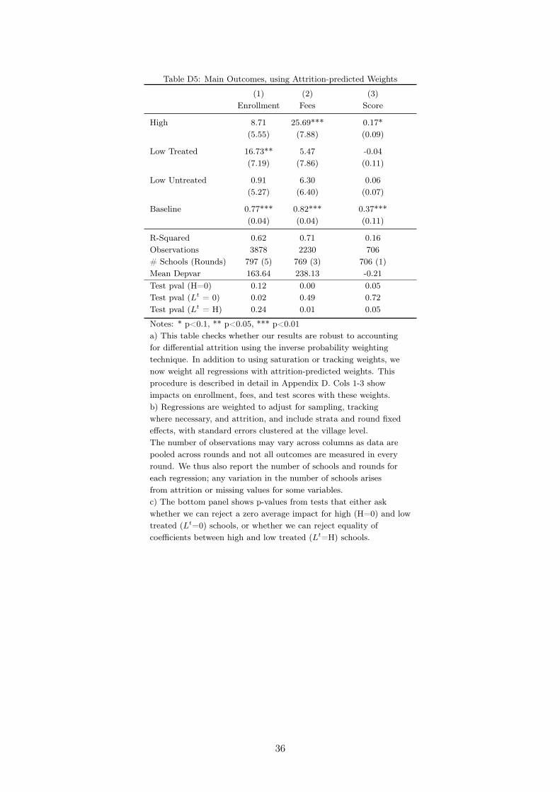
Attrition.— Schools may exit from the study either due to closure, a treat-ment effect of interest that we examine in Section IV.A, or due to survey refusals.Survey completion rates in any given round are uniformly high (95% for rounds1-4 and 90% for round 5), with only 14 schools refusing all follow-up surveys(7 control, 5 H, and 2 Lu). Nevertheless, since round 5 was conducted 2 yearsafter baseline, we implemented a randomized procedure for refusals, where weintensively tracked half of the schools who refused the survey in round 5 for aninterview. We apply weights to the data from this round to account for thisintensive tracking (see Appendix B for details). In regressions, we find that Lt

schools are less likely to attrit relative to control in every round (Appendix Ta-ble D4, Panel A). For other experimental groups, attrition is more idiosyncratic.Despite this differential attrition, baseline characteristics of those who refuse sur-veying at least once do not vary by treatment status in more than 2 (of 21) cases,which could occur by random chance (Appendix Table D4, Panel B).25 We checkrobustness to attrition using inverse probability weights in Appendix Table D5,discussed in greater detail in section IV.A, and find that our results are unaffected

25Comparing characteristics for the at-least-once-refused set is a more conservative approach thanlooking at the always-refused set since the former includes idiosyncratic refusals. There are 14 schoolsin the always-refused set however making inference difficult; nevertheless, when we do consider this set,one significant difference emerges with lower enrollment in Lu relative to control schools.

19

by this correction.

IV. Results

In this section, we present results on the primary outcomes of interest, inves-tigate potential channels of impact, and discuss the implications and potentialwelfare impact of our findings.

A. Main Results

Expenditures and Revenues

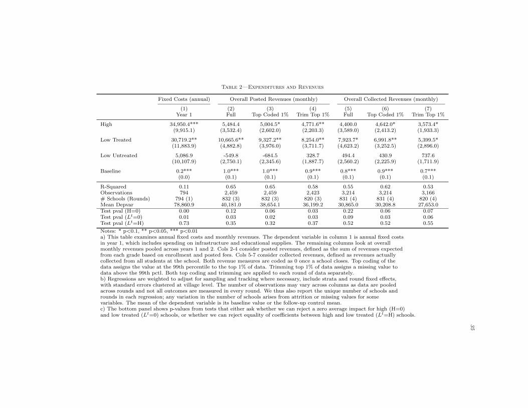
We first present evidence that the grant increased school expenditures; this isof independent interest as school and household finances are fungible and schoolowners had considerable leeway in how the grant could be spent. Table 2, column1, shows that school fixed expenditures increased for Lt and H schools relative tocontrol in the first year after treatment; the magnitudes as a fraction of the grantamount in the first year were 61% for Lt and 70% for the H schools. Fixed costsprimarily includes infrastructure-related investments, such as upgrading rooms ornew furniture and fixtures; spending on these items is consistent with self-reportedinvestment priorities in our baseline data.

The fact that schools increase their overall expenditures despite the grant being(effectively) unconditional suggests that school investments offer better returnsrelative to other investment options. While consistent with the presence of creditconstraints, investing in the school could also reflect the lower (zero) cost of fi-nancing through a grant. In this context, Banerjee and Duflo (2012) suggest atest to directly establish the presence of credit constraints. Suppose that firmsborrow from multiple sources. When cheaper credit (i.e. a grant) becomes avail-able, if firms are not credit constrained, they should always use the cheaper creditto pay off more expensive loans. In fact, they should draw down the expensiveloans to zero if credit is freely available. In Appendix Table E1, we examinedata on borrowing for school and household accounts of school owner households.While there is limited borrowing for investing in the school, over 20% of schoolowner households do borrow (presumably for personal reasons). Yet, we find nostatistically significant declines in borrowing at the school or household level asa result of our intervention.

We now consider whether these expenditure changes affected school revenues.Since schools may not always be able to fully collect fees from students, we use tworevenue measures: (i) posted revenues based on posted fees and enrollment (cols2-4), calculated as the sum of revenues expected from each grade as given by thegrade-specific monthly tuition fee multiplied by the grade-level enrollment; and(ii) collected revenues as reported by the school (cols 5-7).26 To obtain the lattermeasure, we inspected the school account books and computed revenues actuallycollected in the month prior to the survey.27 While this measure captures revenue

26Posted revenues are available for rounds 1,2, and 4, and collected revenues are available from rounds2-5. We use baseline posted revenues as the control variable in all revenue regressions.

27Over 90% of schools have registers for fee payment collection, and for the remainder, we record

20

shortfalls due to partial fee payment, discounts and reduced fees under exceptionalcircumstances, it may not adjust appropriately for delayed fee collection.

First, there are substantial posted revenue increases in all treated schools. Col-umn 2 shows that schools in the H arm gain Rs.5,484 (p=0.12) each monthwhile Lt schools gain Rs.10,665 (p=0.03) a month. Annual revenue increases(twelve times the reported monthly coefficient estimates) compare favorably tothe Rs.50,000 grant amount for the returns on investment. In contrast, we neverfind any significant change in revenues among Lu schools, with small coefficientsacross all specifications. Second, the impact on collected revenues is similar for Hschools (Rs.4,400 with p=0.22), but is smaller (Rs.7,924, p=0.09) for Lt schools(col 5). One explanation for this difference could be that marginal new childrenpay lower (than posted) fees in Lt schools. We examine this in more detail later(Table 3) when we decompose our revenue impacts into enrollment and schoolfees. Third, the results are large but often imprecise due to the high variance inthe revenue distribution (the distribution is highly skewed with a skewness of 5.6and kurtosis of 51.2); precision increases however when we either top-code thedata, assigning the 99th percentile value to the top 1% of data, or drop the top1 percent of data (cols 3 & 6 and cols 4 & 7, respectively), and our results aresignificant at conventional levels. We (still) cannot reject equality of coefficientsacross the treatment arms of the intervention.28

Enrollment and Fees

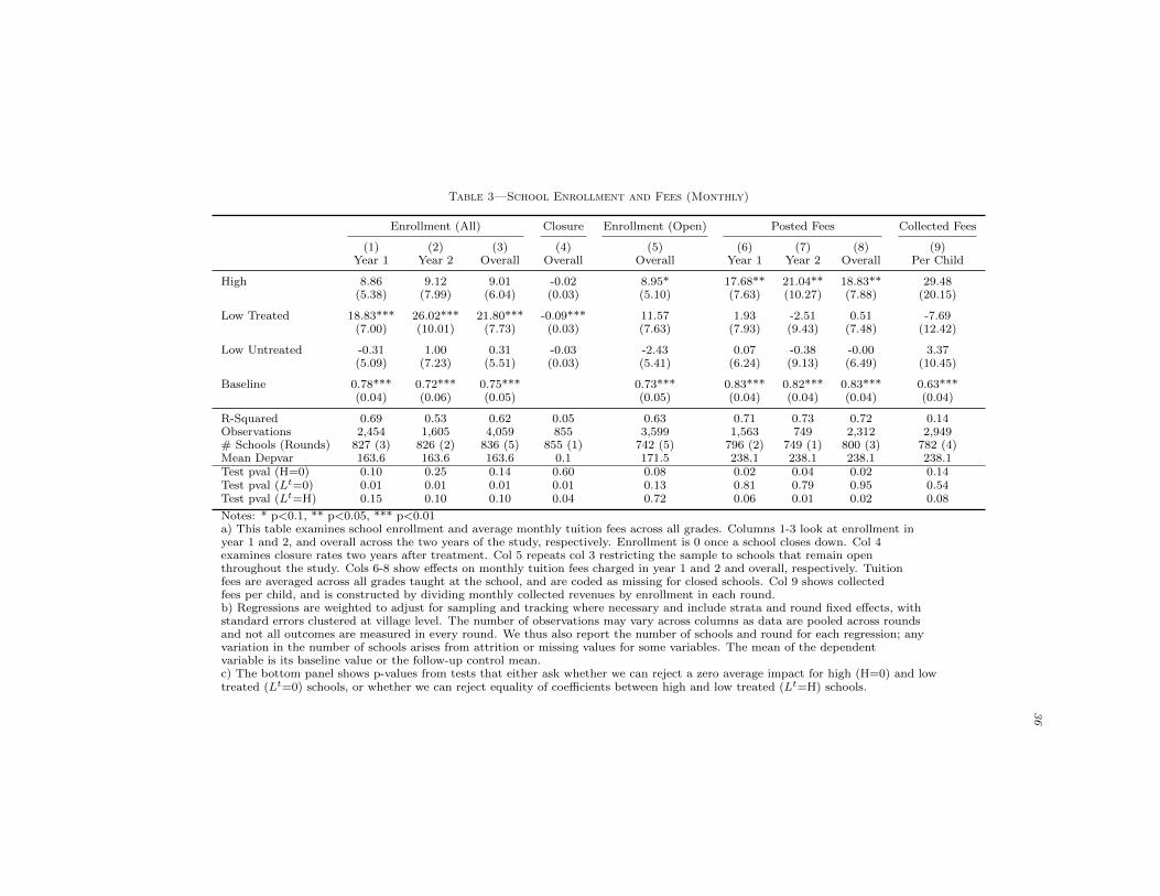
Table 3 considers the impact of the grant on the two main components of(posted) school revenue— school enrollment and fees— to shed light on the sourcesof revenue changes and whether they differ across treatment arms.

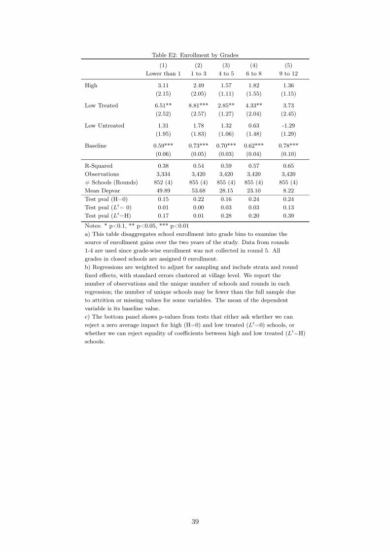
Our first result is that school enrollment increased in Lt and H schools, whereenrollment is measured across all grades in a given school and coded as zero if aschool closed. Columns 1-3 examine enrollment impacts, annually in columns 1-2and pooling across the two treatment years in column 3. In the first year, theLt schools enroll 19 additional children, representing a 12 percent increase overbaseline enrollment. This compares to an average increase of 9 children for Hschools (p=0.10). These gains are sustained and even higher in the second year(col 2); the pooled estimate thus gives an overall increase of 22 children for Lt

schools (col 3). Appendix Table E2 shows that these gains are not grade-specificwith significant positive effects of 11-18 percent over baseline enrollment acrossthe grade distribution. We never observe an average impact on Lu schools, whichis consistent with our theory prediction: Schools should not increase capacitybeyond the point where they decrease the enrollment of their competitors, as thiscan trigger severe price competition leading to lower profits for all schools.

Part of the higher enrollment among Lt schools is due to a reduction in the

self-reported fee collections.28In this analysis, we assign a zero value to a school once it closes down. If instead, we restrict our

analysis to schools that remain open throughout the study with the caveat that these estimates partiallyreflect selection, we still observe revenue impacts though they are smaller in magnitude, especially for Lt

schools. We discuss this further in Section IV.A when we break down the sources of revenue impacts.

21

number of school closures. Over the period of our experiment, 13.7 percent of theschools in the control group closed. As column 4 shows, Lt schools were 9 percent-age points less likely to close over the study period. We find no average impact onschool closure for H or Lu schools relative to control. Although fewer school clo-sures naturally imply higher enrollments for the average school (given that closedschools are assigned zero enrollment), we emphasize that there were enrollmentgains among the schools that remained open throughout the study: Column 5restricts the analysis sample to open schools only, and still shows higher enroll-ment for H and Lt schools, though magnitudes for the latter are naturally smallerfor the latter relative to Column 3 (11.6 children, p=0.13). Conditioning on aschool remaining open without accounting for the selection into closure impliesthat enrollment gains are likely biased downwards, as schools that closed tend tohave fewer children at baseline. This suggests that Lt schools not only staved offclosure, but also benefited through investments that increased enrollment amongopen schools.

Understanding where this enrollment increase came from would have requiredus to track over 100,000 children in these villages over time. Even with thistracking, it would not have been possible to separately identify the children whomoved due to the experiment from regular churn. However, to the extent thatthere is typically more entry at lower grades and greater drop-out in higher grades,the fact that we see similar increase in both these grade levels suggests that bothnew student entry (in lower grades) and greater retention (in higher grades) arelikely to have played a role.29

Unlike enrollment, which increased in both treatment arms, fees increased onlyamong H schools as seen in Table 3, columns 6-8. Average monthly tuition feesacross all grades in H schools is Rs.19 higher than control schools, an increase of8 percent relative to the baseline fee (col 8). These magnitudes are similar acrossthe two years of the intervention. Appendix Table E4 also shows that all gradesexperienced fee increases, with effect sizes ranging from 8-12% of baseline fee. Ashigher grades have higher baseline fees, there is a hint of greater absolute increasesfor grades 6 and above, but small sample sizes preclude further investigation ofthis difference. In sharp contrast, we are unable to detect any impact on schoolfees for either Lt or Lu schools. Consequently, we reject equality of coefficientsbetween H and Lt at a p-value of 0.02 (col 8).

These results use posted (advertised) fees, but actual fees paid by parents maybe different as collection rates may be below 100%. As we found previously, theimpacts on posted and collected revenues were similar for H schools, but not forLt schools, suggesting that collected fees may have been lower in these schools. We

29While noisier and limited to the tested grades, we can track enrollment using data on the testedchildren. Doing so in Appendix Table E3, we find that Lt schools have a higher fraction of children whoreport being newly enrolled in round 3, measured as attending their contemporaneous school for fewerthan 18 months from the date of treatment assignment (col 2). The data do not however allow us todistinguish whether these children switched from other (public) schools in the village or were not-enrolledat baseline but re-enrolled as a consequence of the treatment.

22

confirm this in column 9 by computing collected fees as collected revenues dividedby school enrollment. These estimates are less precise than for posted fees, butsuggest that fees increased by Rs.29 in H schools (p=0.14) and decreased by Rs.8(p=0.54) among Lt schools.30

Treated schools therefore respond to the same amount of cash grant in differentways depending on the degree of financial saturation in their village. Consistentwith the predictions of our model, the main increase in revenue for Lt schoolscomes from marginal children who may otherwise have not been in school, whereasover half of the revenue increase among schools in H schools is from higher feescharged to inframarginal children (which, as we examine below, likely reflectsincreases in school quality).

Test Scores

We now examine whether increases in school revenues are accompanied bychanges in school quality, as measured by test scores. To assess this, we usesubject tests administered in Math, English and the vernacular, Urdu, to chil-dren in all schools 16 months after the start of the intervention (near the end ofthe first school year after treatment).31 We graded the tests using item responsetheory, which allows us to equate tests across years and place them on a commonscale (Das and Zajonc, 2010). Appendix C provides further details on testing,sample and procedures.

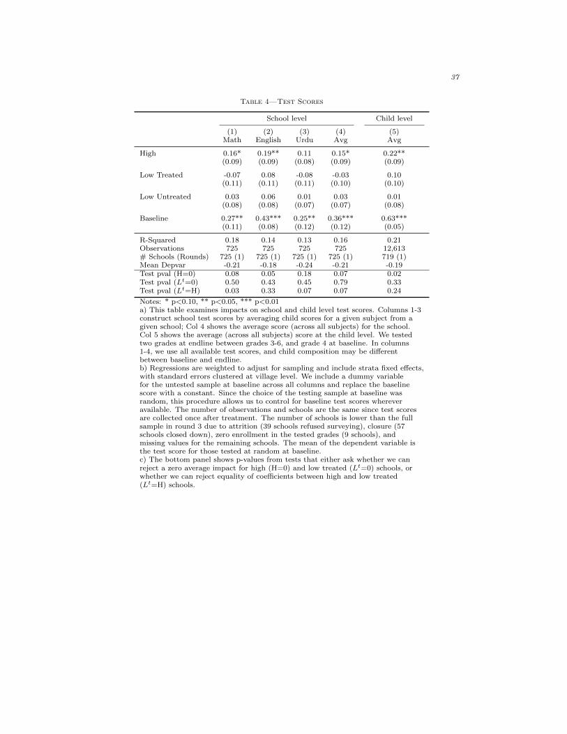
Columns 1 to 4 in Table 4 present school level test score impacts (unweightedby the number of children in the school) and column 5 presents the impact at thechild level. While the latter is relevant for welfare computations, the school levelscores ensure comparability with our other (school level) outcome variables. Toimprove precision, we include the baseline test score where available.32

Test score increases for H schools are comparably high in all subjects with co-efficients ranging from 0.19sd in English (p=0.04) to 0.11sd in Urdu (p=0.12).Averaged across subjects, children in H schools gain an additional 0.16sd, rep-resenting a 42% additional gain relative to the (0.38sd) gain children in controlschools experience over the same 16-month period. In contrast, and consistentwith the school fee results, there are no detectable impacts on test scores forschools in the L relative to control. Given this pattern, we also reject a test of

30This decline is consistent with our theory given heterogeneous consumer preferences over schoolquality. With a downward sloping demand curve, schools would have to decrease their fees to bring inmore children as they increase capacity.

31As discussed previously, budgetary considerations precluded testing the full sample at baseline, sowe instead randomly chose half our villages for testing. In the follow-up round however, an average of 23children from at least two grades were tested in each school, with the majority of tested children enrolledin grades 3-5; in a small number of cases, children from other grades were tested if enrollment in thesegrades was zero. In tested grades, all children were administered tests and surveys regardless of classsize; the maximum enrollment in any single class was 78 children.

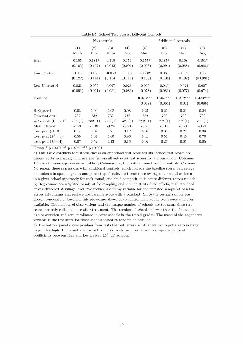
32Since we randomly tested half our sample at baseline, we replace missing values with a constantand an additional dummy variable indicating the missing value. In Appendix Table E5, we show thatalternate specifications that either exclude baseline controls (cols 1-4) or include additional controls(cols 5-8) do not affect our results, with similar point estimates but a reduction in precision in somespecifications.

23

equality of coefficients between H and Lt schools at p-value 0.07 (col 4). Finally,column 5 shows that child level test score impacts are higher at 0.22sd, suggestingthat gains are higher in larger schools.

Given that enrollment increases across all grades and H schools see an addi-tional enrollment of 9 children or 5% of baseline enrollment, compositional effectswould have to be unduly large to drive these effects. To formally assess thisclaim, we first restrict the sample to those children who were in the same schoolthroughout our study, which includes 90% of all children in the follow-up round.Average school level and child level test score increases for this restricted sampleare 0.14sd (p=0.09) and 0.24sd (p=0.01) for the H arm, respectively (AppendixTable E6, col 4).33

One may also believe that test score increases reflect a change in the compositionof peers. Although we cannot rule out such peer effects, we note that Lt schoolsgain more children but show no learning gains. Moreover, a school in the Harm attracts an average of at most 1 new child into a tested grade average of13 children. The peer effects from this single child would have to be very largeto induce the changes we see and is unlikely given the typical magnitude of sucheffects in the literature (Sacerdote, 2011).

Finally, we tested at most two grades per school. Therefore, we cannot directlyexamine whether children across all grades in the school have higher test scoresdue to our treatment. Instead, we make two points: (i) average fees are higheracross all grades in H schools and insofar as fee increases are sustained throughtest score increases, this suggests that test score increases likely occurred across allgrades; and (ii) if we examine test scores gains in the two tested grades separately,we still observe positive (if imprecise) test score improvements in H schools foreach grade.

Robustness and Further Results

Our preferred explanation for the reduced form results— especially the dif-ferential results between the treatment arms— relies on the strategic returns toinvesting in quality when financial saturation in markets is high. We now ex-amine factors in our design and analysis that could potentially confound thisinterpretation.

Investment Plan.— Our intervention required every treated school to submitan investment plan before any disbursement could take place. It is not obvioushow this requirement, by itself, could lead to the differential treatment effects weobserve, particularly as the experimental literature on business plans seldom findssignificant effects (McKenzie, 2017). Moreover, our process was designed to beminimally invasive and effectively non-binding as schools could propose any planand change it at any time as long as they informed us.34 Nevertheless, consider thetwo following channels of impact. The plan could either have forced school owners

33If stayers were positively selected in terms of their baseline test scores, this result would be biasedupwards; in fact, stayers have lower test scores at baseline in the H relative to control.

34Schools could propose investments with private value as long as they could argue it benefited the

24

to consider new investments or, perhaps, the act of submission itself notionallycommitted school owners to a course of action. We can show neither of thesechannels is salient by drawing on three separate sources of (proposed and actual)school investments: (a) pre-treatment proposed investment questions from thebaseline survey; (b) investment plan data; and (c) investments as reported inthe follow-up surveys. First, the correlation in proposed investments between (a)and (b) is high, suggesting that simply asking schools about investment plans isunlikely to explain our treatment effects since (a) is asked of both treatment andcontrol schools and (a) provides similar information to (b). Second, it also doesnot seem that (b) was particularly binding as the correlation between investmentsin (b) and (c) is low. Schools do not seem to have treated the business plan as acommitment device; instead, owners appeared to have finalized school investmentsafter disbursement. Thus, it is unlikely that the submission of investment plansinduced the kinds of large effects we document here, and even less likely that itinduced differential effects between the treatment arms.

Bank Account.— In order to receive the grant funds, school owners had to opena one-time use bank account with our banking partner. This begs the question:Could this account opening have driven the effects we observe? In our sample,73% of school owner households already had bank accounts at baseline and thisfraction is balanced across treatment arms. Further, in Appendix Table E7, weuse an interaction between treatment and baseline bank account availability tocheck whether our pattern of treatment effects is driven by previously unbankedhouseholds. We detect no statistically significant differential impact by baselinebank account status.

Village level Resources.— Given our design preference for school level compar-isons, the grant amount was the same for all schools regardless of treatment arm.Therefore, grant per capita in a L village is necessarily always lower than in aH village, holding constant village size. To investigate whether this differencein overall resource availability at the village level can explain our results, we usebaseline variation in village size to additionally control for the per-capita grantsize in each village. If per-capita grant size is an omitted variable that is corre-lated with treatment saturation and driving our results, we should find that theadditional inclusion of this variable drives the difference in our treatment coeffi-cients to zero. We therefore replicate our base specifications including per-capitagrant size as an additional control in Appendix Table E8, columns 1-3. We findthat the qualitative pattern of our core results on enrollment, fees and test scoresis unchanged. Lt schools see higher enrollment on average, while H schools ex-perience higher fees and test scores on average. While we lose precision in the Harm, we cannot reject that these coefficients are identical to our base specification.This suggests that alternative explanations based on equilibrium effects from an

school or spend the money on previously planned investments, thereby effectively using the grant forpersonal uses. They could also propose changes to their plans at any time during the disbursement.

25

increase in overall resources at the village level are unlikely.

Attrition:— As discussed previously, attrition in our data never exceeds 5% inthe first year and 10% in the second year of the study, and baseline characteristicsof attriters are similar across treatment groups (Appendix Table D4, Panel B).Although attrition is higher in the second year of treatment, recall that whereveravailable our first and second year estimates are similar (Table 3). This suggeststhat any bias from increased attrition in the second year is likely small. Further-more, our results are robust to using inverse probability weights to account forhigher attrition (see Appendix Table D5).

B. Channels

In this section, we consider potential channels of impact by examining changesin school investments as a result of the grants. We first look at overall fixed andvariable costs and then focus on the main components of each— infrastructureand teacher costs.

Overall Fixed and Variable Costs

Table 5 presents the average impacts of the intervention on (annualized) fixedand variable costs. Fixed costs represent annual investments, usually before thestart of the school year, for school infrastructure (furniture, fixtures, classroomupgrades) or educational materials (textbooks, school supplies); variable costs arerecurring monthly expenses on teacher salaries, the largest component of theseexpenses, and non-teaching staff salaries, utilities, and rent. Columns 1-4 includeclosed schools in the regressions assigning them zero costs once closed; cols 5-6sum costs over the years; and cols 7-8 restrict the sample to schools that wereopen throughout the study period.

To facilitate comparisons, column 1 repeats the regression presented in Table 2,Column 1. Whereas in the first year, H schools spend Rs.34,950 and Lt schoolsspend Rs.30,719 more than control schools on fixed costs, by the second year,there is no detectable difference in fixed costs between the treated and controlschools (col 3). On the other hand, annualized variable costs are higher among Hschools and increase over time, though these estimates are imprecisely measuredat p-values of 0.20 (col 2 and 4). Cumulatively over two years, fixed costs arehigher in all treated schools (col 5 and 7), but variable costs are higher only in Hschools (col 6 and 8). Therefore, if we consider open schools only, we cannot rejectequality of coefficients between the treated groups for fixed costs (col 7), but canreject equality in variable costs at a p-value of 0.02 (col 8). Since teacher salariescomprise 75 percent of variable costs, H schools were likely spending more onteachers after the intervention leading us to further investigate this in Table 7.

Infrastructure

For treated schools, infrastructure constitutes the largest fraction of fixed costs,and although we cannot reject that the magnitudes are the same, H schools spendRs. 6,209 more on average than Lt schools (Table 6, column 1). Table 6 also pro-vides evidence that spending on infrastructure components differs by treatment

26

saturation. While we cannot reject equality of coefficients for H and Lt compar-isons, relative to Lt schools, H schools purchase fewer desks and chairs (cols 2and 3); are more likely to report increased access to computers, library and sportsfacilities (cols 4-6); and report a higher number of upgraded classrooms (col 7).35

There are no further effects in year 2 (Appendix Table E9), which is consistentwith most schools choosing to front-load their investments at the beginning ofthe school year immediately after they received the grant. If we are willing toassume that libraries, computers and better classrooms contribute to learning,these patterns are quite consistent with a focus on capacity expansion (desksand chairs) among Lt schools and a greater emphasis on quality improvementsamong H schools.36 This differential emphasis becomes clearer once we focus onteachers.

Teachers

Table 7 shows that variable costs increase by Rs.3,145 per month among Hschools, but not in Lt schools, which if anything show a negative coefficient (col-umn 1). This 12% increase in costs is in large part due to the significantly higherwage bill for teachers in H relative to Lt schools (p = 0.05, column 2). Thereis no significant average increase in the number of teachers employed at a school(col 3); however, there is an increase in the number of new teachers in H schoolssuggesting the presence of teacher churn (col 4). There are significant differencesin remuneration with greater monthly pay for teachers in H schools relative tocontrol. This pay differential emerges both for newly hired teachers (column 6)and (to a slightly lesser degree) for existing teachers (column 7). The increase inteacher wages is consistent with school owners increasing salaries to attract or re-tain better teachers as previous evidence shows that in Pakistani private schools,a 1sd increase in teacher value added is associated with 41% higher wages (Bauand Das, 2016).

C. Discussion

Our results present a consistent narrative in terms of the use of grant funds, thesubsequent impacts, and the channels through which these impacts are realized.Lt schools invest primarily in increasing capacity with no average changes in testscores, and, as a result, bring in more children while collecting slightly lower feesper child. On the other hand, H schools raise test scores and fees, with a smallerincrease in capacity. These different strategies are reflected in schools’ choice offixed and variable investments, with H schools more focused on teacher hiring,remuneration and retention. These results are also consistent with the predictionsof our model. As long as increasing capacity does not impinge on the enrollmentof existing private schools (and it appears not to have done so), Lt schools act as

35A standard desk accommodates 2 students implying that 12 additional students can be seated inH schools, and 18 students in Lt school; these numbers are similar in magnitude to the enrollment gainsdocumented earlier.

36While additional facilities could justify increasing prices, the per-student availability of desks andchairs in Lt schools was arguably the same, although there is an increase in the availability of computers.

27

monopolists on the residual demand from other schools. This option is no longeravailable when all schools receive the funds, as capacity enhancements among allschools will trigger a price war. The only option then is to expand the size of themarket through quality investments and this is indeed what we observe in thedata.

Welfare Comparisons.— The differential responses between the low and high-saturation arms naturally raise the question of whether the public sector has a roleto play in this financing model for private schools, which depends on the computedbenefits of the intervention for different groups. Since estimating demand curvesrequires household choice data (which we do not have), we use the experimentalestimates together with a linear parametrization of the demand curve to computethe gains that accrue to schools owners, parents, teachers and children. Consid-ering child test scores beyond the parental consumer surplus calculation allows usto incorporate the idea that there may be social externalities from learning gainsbeyond the direct benefits to parents. The key intuition driving our comparison isthat when quality remains the same, gains in consumer surplus are concentratedamong inframarginal consumers, as the welfare gains from new, ‘marginal’, en-rollees is small given they are indifferent between attending the school or notprior to the intervention. However, on the producer side, gains in firm profitsdepend entirely on new enrollment among marginal consumers. Consequently,when schools expand enrollment without increasing quality, increases in profitscan be substantial even as the change in consumer surplus is small. When schoolsimprove quality and quantity, consumers accrue the benefits of higher quality andan implicit decline in price at the higher quality required to bring in new students.

We start by considering the exact policy analogue to our experiment, wherea government decides to give unconditional grants to private schools but faces abudget constraint. With a total grant budget of PKR 150K, it can either provide(i) PKR 50K to one school each in three villages (L treatment), or (ii) PKR50K to each of the three schools in one village (H treatment). The table belowshows welfare computations for Lt and H schools, giving monetary returns forthe first three beneficiary groups and test score increases for children; we omitconsideration of Lu schools in these calculations given the lack of any detectableimpacts. The monetary returns are monthly, while the test score increases arefrom a snapshot in time 16 months after treatment. We should emphasize thatthese calculations, especially for consumer surplus are necessarily speculative andoften require strong assumptions.37 Details of the computations are provided in

37For consumer surplus computations, we assume that (a) the demand curve can be approximatedas linear and (b) regardless of quality, demand at zero price in the village is fixed at an upper-bound,which follows in our case from the assumption of ‘closed’ markets. For test score increases, we examinethe overall standard deviation increase from the grant. As Dhaliwal et al. (2013) discuss, this assumesthat gains across students are perfectly substitutable and returns are linear. Finally, we use pointestimates from our experiment regardless of statistical significance. We could alternatively only considerstatistically significant estimates and assume 0 values for statistically insignificant coefficients. Whiledoing so does not qualitatively alter our results, we prefer the approach taken.

28

Appendix F. For school owners and teachers, the calculations are standard and

In PKR Standard Deviations

Group Owners Teachers Parents Children

Lt 10,918 -2,514 4,080 61.1

H 5,295 8,662 7,560 117.2

are based on the monthly variable profits (the estimated impacts on collectedrevenues minus variable costs) and the teacher wage bill, respectively. Turning toconsumer surplus, recall that there is no change in quality for Lt schools, but thereis a decline in collected fees and an increase in enrollment. Following standardwelfare computations, the first order gain of these changes are realized amongthose already enrolled. In the H arm, since both quality and prices increase, wecompute the consumer surplus increase along the new demand curve at higherquality. Finally, the last column in the table shows the total increase in test scoresfor children in the village.38

These estimates highlight the tension between the two treatment arms. Whilethe L arm is substantially better in terms of school owner profitability, socialreturns (including parents, teachers and children) are likely higher in the H arm.Viewed as a policy of providing unconditional grants, the H arm offers favorable(learning) returns relative to other educational RCTs as well.39 If we believe thateducational interventions should primarily focus on learning with limited weighton school owner profits, the H approach is clearly preferable.

Policy Response.— Thus far, we have evaluated a policy of a grant, but ourestimates of financial return suggest that lending should be privately profitablein both the low or the high-saturation model. Specifically, our financial returnscalculations give an internal rate of return (IRR) of 61-83% for Lt schools and12%-32% for H schools for 2-year and 5-year scenarios (see Appendix F).40 Asinterest rates on loans to this sector range from 15-20%, the IRR almost alwaysexceeds the market interest rate: Lt schools would be able to pay back a Rs.50,000loan in 1.5 years whereas H schools would take four years. Even though returns in

38While test score increases for children already in private schools at baseline are captured by ourtreatment effects, we also need to account for test scores increases that may have been experienced bynewly enrolled children. Since this cannot be identified from the data, we assume test score gains of0.33sd for new children, which is the gain for children switching from government to private schools inPunjab (Andrabi et al., 2017).

39This represents a gain of 7.8sd for every $100 invested in H and a gain of 4.1sd for Lt schools.Relative to the literature (JPAL, 2017), these are highly cost-effective interventions— the median testscore gain in the literature is 2.3sd per $100.

40For the 2-year scenario we use actual returns estimated over the two year period and then assumeno further returns accrue thereafter and any assets accumulated are resold at 50% value. For the 5-yearscenario we assume the revenue impact lasts for 5 years and is zero thereafter and any assets have 0 valueat the end of the period.

29

both treatment arms pass a market interest rate threshold, from the perspectiveof an investor, investing using a low-saturation approach is more desirable.

The above calculus suggests that left to the market, a monopolist lender willfavor the L approach as long as the (village level) fixed costs of financing are nottoo large. If a government or a social planner prefers the H approach instead, wecan ask what level of subsidy would make the private lender indifferent betweenthe two approaches. Our results point towards a loan-loss guarantee for banks,which would encourage greater market saturation by mitigating the higher defaultrisk from the H approach (as the rate of school closures is 1% for Lt schoolscompared to 8% for the H schools).

We show in Appendix F that a loan loss guarantee of Rs.17,363 over a twoyear period for a total loan value of Rs.150K would make banks indifferent be-tween the two approaches.41 To evaluate this policy, we compare the subsidyto the additional consumer surplus generated from the H approach, which isRs.41,760 a year, computed as the difference in consumer surplus between thetwo arms ([Rs.7,560-Rs.4,080]*12). Thus, such a policy passes the test requiredfor a Pigouvian subsidy— households should themselves to be willing to offer sucha loan-loss guarantee, with gains for both firms and households. Interestingly, thispolicy also differs somewhat from standard “priority sector” lending policies inthat the subsidy is not based on a sectoral preference per se but rather on the“density/saturation” of the financial offering by a lender.

V. Conclusion

Alleviating financial constraints of (private) schools by providing unconditionalgrants leads to significants gains in enrollment and/or learning. In addition, vary-ing the design of the financial infusion through the degree of market saturationaffects the margins of improvement. Consistent with theory, when all schools in agiven market receive grants, they have a greater incentive to invest in quality toavoid a price war by competing over the same set of students. Further, and con-sistent with the emphasis on capacity versus quality, in low-saturation villages,schools invest in basic infrastructure or on capacity-focused investments, whileschools in high-saturation villages invest in both capacity and quality-focused in-vestments. Most starkly, these schools invest more in teachers by paying highersalaries. Alleviating credit constraints for a wider set of market participants thus“crowds-in” higher quality service provision.

Our estimates suggest that the financial returns to investing in the low-cost(private) educational sector are large and above normal market lending rates,especially in the low-saturation case. This raises questions about why financial

41This calculation makes the conservative assumption that schools that shutdown will not pay backany of their loan. In practice, from ongoing work, we note that default in the case of school closure isnever 100%. Moreover, the first instance of default, missing a cycle of payment, in this sector typicallyoccurs about 7 months after loan disbursement, and even then owners often end up partially repayingthe remaining loan amount. Furthermore, even if school owners decide to close the school, they will oftencontinue to pay back the loan. The risks to the lender are therefore quite minimal.

30

players haven’t entered this sector. We maintain this is yet another market failureas lenders perceive this market to be risky. These concerns may be legitimate—after all, even if schools make money, they may choose not to repay their loans.However, in an ongoing collaboration with a micro-finance provider where weextend loans to private schools, our preliminary results show that lending to thissector is working well with relatively high take-up and very low default rates.

Yet, even when one is able to catalyze the private sector to start lending inthis space, there remains the question of financial saturation. Barring cost ofdelivery considerations, for a monopolist financial intermediary seeking to max-imize returns the decision is quite straight-forward–— invest in single schoolsusing the low-saturation approach. Indeed, this approach to venture funding iswhat we typically see for larger players in the education sector worldwide, whetherthrough investments in franchises or in single schools. Surprisingly, our approach,which selected a school at random led to higher IRR than the typical approachof picking a franchise or single school. Existing financial models can also enablethe emergence of monopolies. Already in our data, we find that schools in low-saturation villages increase revenues only through increases in market share andalthough we do not explicitly model this (we do not have an empirical counter-part as our grant size is small relative to market revenue), it is straightforward toconstruct situations where a low-saturation approach wipes out the competition.In contrast, in the high-saturation villages, while school level financial return islower, we observe large test score gains across all children enrolled in the villageand, as we suggest above, potentially higher social gains. Thus, a governmentseeking to enhance child learning may favor the latter approach because it helpscrowd-in more investments in quality that benefit students. This is not a newtrade-off— governments can always alleviate market constraints in a way thatallow select providers to flourish and grow rapidly or in a manner that enhancesrather than curtails competition. Ultimately, this is a judgment call that eachgovernment will need to make and will critically depend on the nature of marketcompetition, market demand, and the production function facing providers. Ourwork emphasizes that the educational marketplace is remarkably similar to othersectors in this regard, with arguably greater social and long-term consequences.

31

REFERENCES

Abdulkadiroglu, A., Angrist, J. D., Hull, P. D., and Pathak, P. A. (2016). Charterswithout lotteries: Testing takeovers in new orleans and boston. AmericanEconomic Review, 106(7):1878–1920.

Abdulkadiroglu, A., Pathak, P. A., and Roth, A. E. (2009). Strategy-proofnessversus efficiency in matching with indifferences: Redesigning the nyc high schoolmatch. American Economic Review, 99(5):1954–78.

Acemoglu, D. and Angrist, J. (2000). How large are human-capital externalities?evidence from compulsory schooling laws. NBER macroeconomics annual, 15:9–59.

Ajayi, K. F. (2014). Does school quality improve student performance? newevidence from ghana. Unpublished working paper.

Andrabi, T., Das, J., and Khwaja, A. I. (2008). A Dime a Day: The Possibilitiesand Limits of Private Schooling in Pakistan. Comparative Education Review,52(3):329–355.

Andrabi, T., Das, J., and Khwaja, A. I. (2013). Students today, teachers tomor-row: Identifying constraints on the provision of education. Journal of PublicEconomics, 100:1–14.

Andrabi, T., Das, J., and Khwaja, A. I. (2015). Delivering education a pragmaticframework for improving education in low-income countries. (May).

Andrabi, T., Das, J., and Khwaja, A. I. (2017). Report cards: The impactof providing school and child test scores on educational markets. AmericanEconomic Review, 107(6):1535–63.

Andrabi, T., Das, J., Khwaja, A. I., and Karachiwalla, N. (2018). The equilibriumeffects of grants to public schools. Working Paper.

Andrabi, T., Das, J., Khwaja, A. I., Vishwanath, T., and Zajonc, T. (2009).Learning and Educational Achievements in Punjab Schools (LEAPS): Insightsto inform the education policy debate.

Andrabi, T., Das, J., Khwaja, A. I., and Zajonc, T. (2011). Do value-addedestimates add value? accounting for learning dynamics. American EconomicJournal: Applied Economics, 3(3):29–54.

Angrist, J. D., Pathak, P. A., and Walters, C. R. (2013). Explaining charter schooleffectiveness. American Economic Journal: Applied Economics, 5(4):1–27.

Athey, S. and Imbens, G. W. (2017). The econometrics of randomized experi-ments. Handbook of Economic Field Experiments, 1:73–140.

Banerjee, A., Banerji, R., Berry, J., Duflo, E., Kannan, H., Mukerji, S., Shotland,M., and Walton, M. (2017). From proof of concept to scalable policies: Chal-lenges and solutions, with an application. Journal of Economic Perspectives,31(4):73–102.

Banerjee, A. and Duflo, E. (2012). Do Firms Want to Borrow More: TestingCredit Constraints Using a Targeted Lending Program. Review of EconomicStudies, page Forthcoming.

Barrera-Osorio, F., Blakeslee, D. S., Hoover, M., Linden, L., Raju, D., and Ryan,

32

S. P. (2017). Delivering education to the underserved through a public-privatepartnership program in Pakistan. Policy Research working paper; No. WPS8177; Impact Evaluation series.

Bau, N. and Das, J. (2016). The Misallocation of Pay and Productivity in thePublic Sector: Evidence from the Labor Market for Teachers. Working Paper.

Baum, D., Lewis, L., and Patrinos, H. (2013). Engaging the private sector: Whatpolicies matter? a framework paper. SABER Working Paper Series.

Beck, T. (2007). Financing Constraints of SMEs in Developing Countries : Evi-dence , Determinants and Solutions. Financing Innovation-Oriented Businessesto Promote Entrepreneurship, (April):1–35.

Bruhn, M. and McKenzie, D. (2009). In pursuit of balance: Randomizationin practice in development field experiments. American Economic Journal:Applied Economics, 1(4):200–232.

Carneiro, P. and Heckman, J. J. (2002). The evidence on credit constraints inpost-secondary schooling*. The Economic Journal, 112(482):705–734.

Das, J. and Zajonc, T. (2010). India shining and bharat drowning: Comparingtwo indian states to the worldwide distribution in mathematics achievement.Journal of Development Economics, 92(2):175–187.

de Mel, S., McKenzie, D., and Woodruff, C. (2008). Returns to capital in mi-croenterprises: Evidence from a field experiment. The Quarterly Journal ofEconomics, 123(4):1329–1372.

de Mel, S., McKenzie, D., and Woodruff, C. (2012). One-time transfers of cashor capital have long-lasting effects on microenterprises in sri lanka. Science,335(6071):962–966.

Dhaliwal, I., Duflo, E., Glennerster, R., and Tulloch, C. (2013). Comparativecost-effectiveness analysis to inform policy in developing countries: a generalframework with applications for education. Education Policy in DevelopingCountries, pages 285–338.

Epple, D., Romano, R. E., and Urquiola, M. (2015). School vouchers: A surveyof the economics literature. Technical report, National Bureau of EconomicResearch.

Evans, D. and Popova, A. (2015). What really works to improve learning indeveloping countries? an analysis of divergent findings in systematic reviews.

Hoxby, C. M., Murarka, S., and Kang, J. (2009). How new york city’s charterschools affect achievement. Cambridge, MA: New York City Charter SchoolsEvaluation Project, pages 1–85.

Hoxby, C. M. and Rockoff, J. E. (2004). The impact of charter schools on studentachievement. Department of Economics, Harvard University Cambridge, MA.

Hsieh, C.-T. and Urquiola, M. (2006). The effects of generalized school choice onachievement and stratification: Evidence from chile’s voucher program. Journalof public Economics, 90(8):1477–1503.

Jensen, R. (2012). Do labor market opportunities affect young women’s work andfamily decisions? experimental evidence from india. The Quarterly Journal of

33

Economics, 127(2):753–792.JPAL (2017). Increasing test score performance. Retrieved from:

https://www.povertyactionlab.org/policy-lessons/education/increasing-test-score-performance.

Kapor, A., Neilson, C. A., Zimmerman, S. D., et al. (2017). Heterogeneous beliefsand school choice mechanisms. Technical report.

Kreps, D. M. and Scheinkman, J. a. (1983). Quantity Precommitment andBertrand Competition Yield Cournot Outcomes. The Bell Journal of Eco-nomics, 14(2):326–337.

McEwan, P. J. (2015). Improving learning in primary schools of developing coun-tries: A meta-analysis of randomized experiments. Review of Educational Re-search, 85(3):353–394.

McKenzie, D. (2017). Identifying and spurring high-growth entrepreneurship:Experimental evidence from a business plan competition. American EconomicReview, 107(8):2278–2307.

Muralidharan, K., Singh, A., and Ganimian, A. J. (2016). Disrupting education?experimental evidence on technology-aided instruction in india. Technical re-port, National Bureau of Economic Research.

Muralidharan, K., Sundararaman, V., and Sundararaman, K. M. V. (2015). TheAggregate Effect of School Choice: Evidence from a two-stage experiment inIndia. The Quarterly Journal of Economics, 130(3):1011–1066.

NEC (2005). National education census. Technical report, Pakistan Bureau ofStatistics.

Nguyen, Q. and Raju, D. (2014). Private school participation in pakistan.Romero, M., Sandefur, J., and Sandholtz, W. A. (2017). Can Outsourcing Im-

prove Liberia’s Schools? Working Paper 462.Rotemberg, M. (2014). Equilibrium effects of firm subsidies.Sacerdote, B. (2011). Peer effects in education: How might they work, how big

are they and how much do we know thus far? volume 3, chapter 04, pages249–277. Elsevier, 1 edition.

Udry, C. and Anagol, S. (2006). The return to capital in ghana. AmericanEconomic Review, 96(2):388–393.

(1) (2) (3) (4) (5) (6) (7) (8)

Variable Mean 5th6pctl 25th6pctl Median 75th6pctl 95th6pctl

Standard6

Deviation N

Number6of6public6schools 2.45 1.0 2.0 2.0 3.0 5.0 1.03 266

Number6of6private6schools 3.33 2.0 2.0 3.0 4.0 7.0 1.65 266

Private6enrollment 523.52 149.0 281.0 415.5 637.0 1,231.0 378.12 266

Enrollment 163.6 45.0 88.0 140.0 205.0 353.0 116.0 851

Monthly6fee6(PKR) 238.4 81.3 150.0 201.3 275.0 502.5 166.1 851

Monthly6revenue6(PKR) 40,181.1 4,943.0 13,600.0 26,485.0 44,400.0 117,655.0 54,883.9 850

Monthly6variable6costs6(PKR) 25,387.0 3,900.0 9,400.0 16,200.0 27,200.0 79,000.0 30,961.1 848

Annual6fixed6expenses6(PKR) 78,860.9 0.0 9,700.0 33,000.0 84,000.0 326,000.0 136,928.2 837

School6age6(No6of6years) 8.3 0.0 3.0 7.0 12.0 19.0 6.7 852

Number6of6teachers 8.2 3.0 5.0 7.0 10.0 17.0 4.8 851

Monthly6teacher6salary6(PKR) 2,562.8 1,000.0 1,500.0 2,000.0 2,928.5 5,250.0 3,139.5 768

Number6of6enrolled6children6in6

tested6grade

13.1 1.0 5.0 10.0 18.0 34.5 11.7 420

Number6of6tested6children 11.7 1.0 4.0 9.0 16.0 31.5 10.6 420

Average6test6score O0.21 O1.24 O0.59 O0.22 0.15 0.84 0.64 401

Notes:

a)6This6table6displays6summary6statistics6for6the62666villages6(Panel6A)6and6the68556private6schools6(Panel6B)6in6our6sample.

b)6These6baseline6data6come6from6two6sources:6school6surveys6administered6to6the6full6sample6(8556schools),6and6child6tests

administered6to6half6of6the6sample6(4206schools).6Any6missing6data6are6due6to6school6refusals,6child6absences6or6zero6enrollment

in6the6tested6grades6at666schools.

Table61:6Baseline6Summary6Statistics6

Panel&A:&Village&level&Variables

Panel&B:&&Private&School&level&Variables&

35

Table 2—Expenditures and Revenues

Fixed Costs (annual) Overall Posted Revenues (monthly) Overall Collected Revenues (monthly)

(1) (2) (3) (4) (5) (6) (7)Year 1 Full Top Coded 1% Trim Top 1% Full Top Coded 1% Trim Top 1%

High 34,950.4*** 5,484.4 5,004.5* 4,771.6** 4,400.0 4,642.0* 3,573.4*(9,915.1) (3,532.4) (2,602.0) (2,203.3) (3,589.0) (2,413.2) (1,933.3)

Low Treated 30,719.2** 10,665.6** 9,327.2** 8,254.0** 7,923.7* 6,991.8** 5,399.5*(11,883.9) (4,882.8) (3,976.0) (3,711.7) (4,623.2) (3,252.5) (2,896.0)

Low Untreated 5,086.9 -549.8 -684.5 328.7 494.4 430.9 737.6(10,107.9) (2,750.1) (2,345.6) (1,887.7) (2,560.2) (2,225.9) (1,711.9)

Baseline 0.2*** 1.0*** 1.0*** 0.9*** 0.8*** 0.9*** 0.7***(0.0) (0.1) (0.1) (0.1) (0.1) (0.1) (0.1)

R-Squared 0.11 0.65 0.65 0.58 0.55 0.62 0.53Observations 794 2,459 2,459 2,423 3,214 3,214 3,166# Schools (Rounds) 794 (1) 832 (3) 832 (3) 820 (3) 831 (4) 831 (4) 820 (4)Mean Depvar 78,860.9 40,181.0 38,654.1 36,199.2 30,865.0 30,208.8 27,653.0Test pval (H=0) 0.00 0.12 0.06 0.03 0.22 0.06 0.07Test pval (Lt=0) 0.01 0.03 0.02 0.03 0.09 0.03 0.06Test pval (Lt=H) 0.73 0.35 0.32 0.37 0.52 0.52 0.55

Notes: * p<0.1, ** p<0.05, *** p<0.01a) This table examines annual fixed costs and monthly revenues. The dependent variable in column 1 is annual fixed costsin year 1, which includes spending on infrastructure and educational supplies. The remaining columns look at overallmonthly revenues pooled across years 1 and 2. Cols 2-4 consider posted revenues, defined as the sum of revenues expectedfrom each grade based on enrollment and posted fees. Cols 5-7 consider collected revenues, defined as revenues actuallycollected from all students at the school. Both revenue measures are coded as 0 once a school closes. Top coding of thedata assigns the value at the 99th percentile to the top 1% of data. Trimming top 1% of data assigns a missing value todata above the 99th pctl. Both top coding and trimming are applied to each round of data separately.b) Regressions are weighted to adjust for sampling and tracking where necessary, include strata and round fixed effects,with standard errors clustered at village level. The number of observations may vary across columns as data are pooledacross rounds and not all outcomes are measured in every round. We thus also report the unique number of schools androunds in each regression; any variation in the number of schools arises from attrition or missing values for somevariables. The mean of the dependent variable is its baseline value or the follow-up control mean.c) The bottom panel shows p-values from tests that either ask whether we can reject a zero average impact for high (H=0)and low treated (Lt=0) schools, or whether we can reject equality of coefficients between high and low treated (Lt=H) schools.

36

Table 3—School Enrollment and Fees (Monthly)

Enrollment (All) Closure Enrollment (Open) Posted Fees Collected Fees

(1) (2) (3) (4) (5) (6) (7) (8) (9)Year 1 Year 2 Overall Overall Overall Year 1 Year 2 Overall Per Child

High 8.86 9.12 9.01 -0.02 8.95* 17.68** 21.04** 18.83** 29.48(5.38) (7.99) (6.04) (0.03) (5.10) (7.63) (10.27) (7.88) (20.15)

Low Treated 18.83*** 26.02*** 21.80*** -0.09*** 11.57 1.93 -2.51 0.51 -7.69(7.00) (10.01) (7.73) (0.03) (7.63) (7.93) (9.43) (7.48) (12.42)

Low Untreated -0.31 1.00 0.31 -0.03 -2.43 0.07 -0.38 -0.00 3.37(5.09) (7.23) (5.51) (0.03) (5.41) (6.24) (9.13) (6.49) (10.45)

Baseline 0.78*** 0.72*** 0.75*** 0.73*** 0.83*** 0.82*** 0.83*** 0.63***(0.04) (0.06) (0.05) (0.05) (0.04) (0.04) (0.04) (0.04)

R-Squared 0.69 0.53 0.62 0.05 0.63 0.71 0.73 0.72 0.14Observations 2,454 1,605 4,059 855 3,599 1,563 749 2,312 2,949# Schools (Rounds) 827 (3) 826 (2) 836 (5) 855 (1) 742 (5) 796 (2) 749 (1) 800 (3) 782 (4)Mean Depvar 163.6 163.6 163.6 0.1 171.5 238.1 238.1 238.1 238.1Test pval (H=0) 0.10 0.25 0.14 0.60 0.08 0.02 0.04 0.02 0.14Test pval (Lt=0) 0.01 0.01 0.01 0.01 0.13 0.81 0.79 0.95 0.54Test pval (Lt=H) 0.15 0.10 0.10 0.04 0.72 0.06 0.01 0.02 0.08

Notes: * p<0.1, ** p<0.05, *** p<0.01a) This table examines school enrollment and average monthly tuition fees across all grades. Columns 1-3 look at enrollment inyear 1 and 2, and overall across the two years of the study, respectively. Enrollment is 0 once a school closes down. Col 4examines closure rates two years after treatment. Col 5 repeats col 3 restricting the sample to schools that remain openthroughout the study. Cols 6-8 show effects on monthly tuition fees charged in year 1 and 2 and overall, respectively. Tuitionfees are averaged across all grades taught at the school, and are coded as missing for closed schools. Col 9 shows collectedfees per child, and is constructed by dividing monthly collected revenues by enrollment in each round.b) Regressions are weighted to adjust for sampling and tracking where necessary and include strata and round fixed effects, withstandard errors clustered at village level. The number of observations may vary across columns as data are pooled across roundsand not all outcomes are measured in every round. We thus also report the number of schools and round for each regression; anyvariation in the number of schools arises from attrition or missing values for some variables. The mean of the dependentvariable is its baseline value or the follow-up control mean.c) The bottom panel shows p-values from tests that either ask whether we can reject a zero average impact for high (H=0) and lowtreated (Lt=0) schools, or whether we can reject equality of coefficients between high and low treated (Lt=H) schools.

37

Table 4—Test Scores

School level Child level

(1) (2) (3) (4) (5)Math English Urdu Avg Avg

High 0.16* 0.19** 0.11 0.15* 0.22**(0.09) (0.09) (0.08) (0.09) (0.09)

Low Treated -0.07 0.08 -0.08 -0.03 0.10(0.11) (0.11) (0.11) (0.10) (0.10)

Low Untreated 0.03 0.06 0.01 0.03 0.01(0.08) (0.08) (0.07) (0.07) (0.08)

Baseline 0.27** 0.43*** 0.25** 0.36*** 0.63***(0.11) (0.08) (0.12) (0.12) (0.05)

R-Squared 0.18 0.14 0.13 0.16 0.21Observations 725 725 725 725 12,613# Schools (Rounds) 725 (1) 725 (1) 725 (1) 725 (1) 719 (1)Mean Depvar -0.21 -0.18 -0.24 -0.21 -0.19Test pval (H=0) 0.08 0.05 0.18 0.07 0.02Test pval (Lt=0) 0.50 0.43 0.45 0.79 0.33Test pval (Lt=H) 0.03 0.33 0.07 0.07 0.24

Notes: * p<0.10, ** p<0.05, *** p<0.01a) This table examines impacts on school and child level test scores. Columns 1-3construct school test scores by averaging child scores for a given subject from agiven school; Col 4 shows the average score (across all subjects) for the school.Col 5 shows the average (across all subjects) score at the child level. We testedtwo grades at endline between grades 3-6, and grade 4 at baseline. In columns1-4, we use all available test scores, and child composition may be differentbetween baseline and endline.b) Regressions are weighted to adjust for sampling and include strata fixed effects,with standard errors clustered at village level. We include a dummy variablefor the untested sample at baseline across all columns and replace the baselinescore with a constant. Since the choice of the testing sample at baseline wasrandom, this procedure allows us to control for baseline test scores whereveravailable. The number of observations and schools are the same since test scoresare collected once after treatment. The number of schools is lower than the fullsample in round 3 due to attrition (39 schools refused surveying), closure (57schools closed down), zero enrollment in the tested grades (9 schools), andmissing values for the remaining schools. The mean of the dependent variable isthe test score for those tested at random at baseline.c) The bottom panel shows p-values from tests that either ask whether we canreject a zero average impact for high (H=0) and low treated (Lt=0) schools, orwhether we can reject equality of coefficients between high and low treated(Lt=H) schools.

38

Table 5—Fixed and Variable Costs (Annual)

Year 1 Year 2 Cumulative Cumulative (Open Only)

(1) (2) (3) (4) (5) (6) (7) (8)Fixed Variable Fixed Variable Fixed Variable Fixed Variable

High 34,950.4*** 26,108.5 2,560.1 34,961.9 39,202.0*** 72,241.5* 42,570.5*** 103,181.5**(9,915.1) (20,508.3) (6,868.1) (27,985.1) (10,792.0) (38,049.5) (11,866.0) (40,227.5)

Low Treated 30,719.2** -8,133.1 6,207.0 13,943.1 42,630.4*** 26,609.9 38,353.5** 1,154.6(11,883.9) (25,486.1) (9,063.6) (20,355.2) (14,199.2) (38,284.8) (15,018.8) (39,812.1)

Low Untreated 5,086.9 1,402.7 4,992.3 2,656.0 10,509.8 34,854.1 9,595.2 33,530.2(10,107.9) (17,596.0) (7,904.8) (19,907.5) (11,732.7) (33,815.7) (12,814.7) (34,829.3)

Baseline 0.2*** 0.9*** 0.0* 0.9*** 0.2*** 1.1*** 0.2*** 1.1***(0.0) (0.1) (0.0) (0.1) (0.0) (0.1) (0.0) (0.1)

R-Squared 0.11 0.71 0.05 0.60 0.10 0.56 0.09 0.57Observations 794 817 768 777 837 842 745 747# Schools (Rounds) 794 (1) 817 (1) 768 (1) 777 (1) 837 (1) 842 (1) 745 (1) 747 (1)Mean Depvar 78,860.9 304,644.2 78,860.9 304,644.2 78,860.9 304,644.2 82,453.9 319,550.0Test pval (H=0) 0.00 0.20 0.71 0.21 0.00 0.06 0.00 0.01Test pval (Lt=0) 0.01 0.75 0.49 0.49 0.00 0.49 0.01 0.98Test pval (Lt=H) 0.73 0.23 0.67 0.42 0.81 0.28 0.78 0.02

Notes: * p<0.1, ** p<0.05, *** p<0.01a) This table looks at the treatment impact on annualized fixed and variable costs. Annualized fixed costs include spending oninfrastructure or educational materials and supplies; annualized variable costs include recurring expenses— teaching andnon-teaching staff salaries, utilities and rent. Columns 1-2 show these costs for year 1, and cols 3-4 for year 2. Closed schoolsare coded as having 0 costs in cols 1-4. Cols 5-6 show cumulative fixed and variable costs across the two years of the study, i.e.instead of pooling, these columns sum data across rounds. Cols 7-8 repeat cols 5-6 restricting to those schools that remain openthroughout the experiment.b) Regressions are weighted to adjust for sampling and tracking where necessary and include strata fixed effects, withstandard errors clustered at village level. The number of observations and unique schools are the same since we either show oneround of data (cols 1-4) or show cumulative costs across rounds (cols 5-8). Observations vary across year 1 and 2 due toattrition and missing values for some schools. The mean of the dependent variable is its baseline value.c) The bottom panel shows p-values from tests that either ask whether we can reject a zero average impact for high (H=0) andlow treated (Lt=0) schools, or whether we can reject equality of coefficients between high and low treated (Lt=H) schools.

39

Table 6—School Infrastructure (Year 1)

Spending Number purchased Facility present (Y/N) Other

(1) (2) (3) (4) (5) (6) (7)Amount Desks Chairs Computers Library Sports # Rooms Upgraded

High 25,460.31*** 5.97*** 3.76*** 0.20*** 0.11*** 0.10** 0.70***(8,787.82) (1.63) (1.40) (0.05) (0.04) (0.04) (0.26)

Low Treated 19,251.19** 8.71*** 6.13** 0.17*** -0.03 -0.03 0.47(8,702.52) (2.45) (2.76) (0.06) (0.05) (0.04) (0.40)

Low Untreated -1,702.36 1.31 0.87 0.04 -0.03 0.02 0.16(8,376.89) (1.40) (1.19) (0.04) (0.04) (0.03) (0.26)

Baseline 0.09*** 0.10* 0.12* 0.26*** 0.32*** 0.23*** 0.71***(0.03) (0.05) (0.07) (0.04) (0.04) (0.05) (0.06)

R-squared 0.06 0.09 0.08 0.20 0.20 0.11 0.57Observations 798 810 811 822 822 822 822# Schools (Rounds) 798 (1) 810 (1) 811 (1) 822 (1) 822 (1) 822 (1) 822 (1)Mean Depvar 57,258.48 14.59 10.92 0.39 0.35 0.19 6.36Test pval (H=0) 0.00 0.00 0.01 0.00 0.01 0.02 0.01Test pval (Lt=0) 0.03 0.00 0.03 0.01 0.58 0.49 0.24Test pval (Lt=H) 0.50 0.31 0.45 0.60 0.01 0.01 0.59

Notes: * p<0.10, ** p<0.05, *** p<0.01a) This table examines outcomes relating to school infrastructure using data from round 1. Column 1 is theannual (fixed) expenditure on infrastructure– e.g. furniture, fixtures, or facilities. Columns 2-3 refer to thenumber of desks and chairs purchased; columns 4-6 are dummy variables for the presence of particular schoolfacilities; and column 7 measures the number of rooms upgraded from temporary to permanent or semi-permanentclassrooms. Closed schools take on a value of 0 in all columns.b) Regressions are weighted to adjust for sampling and include strata fixed effects, with standard errorsclustered at the village level. The number of observations and unique schools are the same since we use oneround of data. Observations may vary across year 1 and 2 due to attrition and missing values. The mean of thedependent variable is its baseline value.c) The bottom panel shows p-values from tests that either ask whether we can reject a zero average impact forhigh (H=0) and low treated (Lt=0) schools, or whether we can reject equality of coefficients between high andlow treated (Lt=H) schools.

40

Table 7—Teacher Salaries and Composition

School Costs (monthly) Teacher Roster Teacher Salaries (monthly)

(1) (2) (3) (4) (5) (6) (7)Total Wage Bill Total Num New All New Existing

High 3,147.48* 2,741.83* 0.42 0.46** 519.52** 580.05** 492.01*(1,894.67) (1,510.50) (0.32) (0.18) (257.94) (265.80) (284.29)

Low Treated -1,127.41 -838.26 0.32 0.27 -175.63 -89.45 -223.10(1,716.66) (1,520.25) (0.33) (0.24) (273.11) (406.49) (246.45)

Low Untreated -302.25 65.14 0.25 0.25 194.48 89.47 253.39(1,374.56) (1,106.67) (0.29) (0.18) (202.53) (236.07) (201.69)

Baseline 0.88*** 0.85*** 0.77***(0.07) (0.08) (0.05)

R-Squared 0.69 0.63 0.50 0.19 0.20 0.23 0.20Observations 1,470 1,470 1,590 1,645 11,725 3,903 7,818# Schools (Rounds) 797 (2) 797 (2) 816 (2) 840 (2) 802 (2) 723 (2) 793 (2)Mean Depvar 25,387.0 19,491.2 6.7 2.0 2,676.6 2,665.5 2,681.9Test pval (H=0) 0.10 0.07 0.19 0.01 0.05 0.03 0.08Test pval (Lt=0) 0.51 0.58 0.33 0.25 0.52 0.83 0.37Test pval (Lt=H) 0.05 0.05 0.78 0.45 0.04 0.13 0.04

Notes: * p<0.10, ** p<0.05, *** p<0.01a) This table looks at impacts on teacher salaries and composition from the intervention. The dependentvariable in column 1 is monthly variable costs, which includes utilities, rent, teaching andnon-teaching staff salaries, over two years of the experiment. Column 2 shows the impact on the teachingsalary component of variable costs. Data used in the first two columns are from school survey data. Theremaining columns use teacher level data from the teacher roster. Columns 3-4 collapse data at the schoollevel to understand changes in teacher composition; cols 5-7 decompose teacher salaries by employmentstatus at the school before and after treatment. Whether a teacher is new or existing is determined bytheir start date at the school relative to baseline. Closed schools are coded as missing in all columns,except cols 3-4 where they are coded as 0.b) Regressions are weighted to adjust for sampling and tracking where necessary and include strataand round fixed effects, with have standard errors clustered at village level. The number of observationsmay vary across columns as data are pooled across rounds and not all outcomes are measured in everyround. We thus also report the unique number of schools and rounds in each regression; any variation inthe number of unique schools arises from attrition or missing values for some variables. The mean of thedependent variable is the baseline value or the follow-up control mean.c) The bottom panel shows p-values from tests that either ask whether we can reject a zero average impactfor high (H=0) and low treated (Lt=0) schools, or whether we can reject equality of coefficientsbetween high and low treated (Lt=H) schools.

ONLINE APPENDIX

Upping the Ante: The Equilibrium Effects of UnconditionalGrants to Private Schools

T. Andrabi, J. Das, A.I. Khwaja, S. Ozyurt, and N. Singh

Contents

A Theory 2A.1 Homogeneous Demand . . . . . . . . . . . . . . . . . . . . . . . . . . . . . . . . . 2A.2 Generalization of the Model . . . . . . . . . . . . . . . . . . . . . . . . . . . . . . 10

B Weighting of average treatment effects with unequal selection probabilities 23B.1 Saturation Weights . . . . . . . . . . . . . . . . . . . . . . . . . . . . . . . . . . . 23B.2 Tracking Weights . . . . . . . . . . . . . . . . . . . . . . . . . . . . . . . . . . . . 24

C Sampling, Surveys and Data 25

D Balance and Attrition 30D.1 Balance . . . . . . . . . . . . . . . . . . . . . . . . . . . . . . . . . . . . . . . . . 30D.2 Attrition . . . . . . . . . . . . . . . . . . . . . . . . . . . . . . . . . . . . . . . . . 30

E Additional Results 37

F Private and Social Returns Calculations 48F.1 Welfare Calculations . . . . . . . . . . . . . . . . . . . . . . . . . . . . . . . . . . 48F.2 IRR and Loan-loss guarantee . . . . . . . . . . . . . . . . . . . . . . . . . . . . . 51

1

A Theory

A.1 Homogeneous Demand

Suppose that schools choose x1, x2 ≥ 0 and q1, q2 ∈ {qH , qL} in the first stage and p1, p2 inthe second stage. Let si be school i’s surplus, that is si = qi − pi. Therefore, school i’s profitfunction is:

Πi =

(pi − c)(xi + M

2 )− rxi − wt +K, if [si > sj ] or [si = sj and qi > qj ]

(pi − c)(N − xj + M2 )− rxi − wt +K, if [si < sj ] or [si = sj and qi < qj ]

(pi − c) (M/2+xi)TM+xi+xj

− rxi − wt +K, if si = sj and qi = qj

Define nH = K−wr and nL = K

r to be the additional capacity increase that schools canafford under high and low technologies, respectively. Note that feasibility requires that xi ≤ nLand xi ≤ nH whenever qi = qH . One can easily verify that if the schools’ capacity choices x1and x2 are such that x1 + x2 ≤ N , then in the pricing stage, school i picks pi = qi. Let µ be aprobability density function with support [p, p]. Then for notational simplicity, we use µ(p) forany p ∈ [p, p] to denote µ({p}). Before proving the main results, we prove the following result,which applies to both low (L) and high-saturation (H) treatments.

Proposition A. Suppose that the schools’ quality choices are q1, q2 ∈ {qH , qL} and capacitychoices are x1, x2 ≥ 0 with x1, x2 ≤ N + M

2 and x1 + x2 > N . Then in the (second) pricingstage, there exists no pure strategy equilibrium. However, there exists a mixed strategy equilibrium(µ∗1, µ

∗2), where for i = 1, 2, µ∗i is

(i) a probability density function with support [p∗i , qi], satisfying c < p∗i < qi, and

(ii) atomless except possibly at qi, that is µ∗i (p) = 0 for all p ∈ [p∗i , qi).

(iii) Furthermore, µ∗1(p1)µ∗2(p2) = 0 for all p1 ∈ [p∗1, q1] and p2 ∈ [p∗2, q2] satisfying q1 − p1 =

q2 − p2.

Proof of Proposition A. Because no school alone can cover the entire market, i.e., xi < N+M2 ,

p1 = p2 = c cannot be an equilibrium outcome. Likewise, given that the schools compete in aBertrand fashion and total capacity, M+x1 +x2, is greater than total demand, M+N , showingthat there is no pure strategy equilibrium is straightforward, and left to the readers.

However, by Theorem 5 of Dasgupta and Maskin (1986), the game has a mixed-strategyequilibrium: The discontinuities in the profit functions Πi(p1, p2) are restricted to the pricecouples where both schools offer the same surplus, that is {(p1, p2) ∈ [c, qH ]2|q1− p1 = q2− p2}.Lowering its price from a position c < q1− p1 = q2− p2 ≤ qH , a school discontinuously increasesits profit. Hence, Πi(p1, p2) is weakly lower semi-continuous. Πi(p1, p2) is also clearly bounded.Finally, Π1 + Π2 is upper semi-continuous because discontinuous shifts in students from oneschool to another occur where either both schools derive the same profit per student (whenq1 = q2) or the total profit stays the same or jumps per student because the higher qualityschool steals the student from the low quality school and charges higher price (when q1 6= q2).Thus, by Theorem 5 of Dasgupta and Maskin (1986), the game has a mixed-strategy equilibrium.

Suppose that (µ∗1, µ∗2) is a mixed-strategy equilibrium of the pricing stage. Let pi be the

supremum of the support of µ∗i , so pi = inf{p ∈ [c, qi]|p ∈ supp(µ∗i )}. Likewise, let p∗i bethe infimum of the support of µ∗i . Define s(pi, qi) to be the surplus that school i offers, sos(pi, qi) = qi − pi. We will prove the remaining claims of the proposition through a series ofLemmata.

Lemma A1. s(p∗1, q1) = s(p∗2, q2) and p∗i > c for i = 1, 2.

2

Proof. Note that the claim turns into the condition p∗1 = p∗2 > c when q1 = q2. To shows(p∗1, q1) = s(p∗2, q2), suppose for a contradiction that s(p∗1, q1) 6= s(p∗2, q2). Assume, withoutloss of generality, that s(p∗1, q1) > s(p∗2, q2). For any p1 ≥ p∗1 in the support of µ∗1 satisfyings(p∗1, q1) ≥ s(p1, q1) > s(p∗2, q2), player 1 can increase its expected profit by deviating to a pricep′1 = p1 + ε satisfying s(p′1, q1) > s(p∗2, q2). This is true because by slightly increasing its pricefrom p1 to p′1 school 1 keeps its expected enrollment the same. This opportunity of a profitabledeviation contradicts with the optimality of equilibrium. The case for s(p∗1, q1) < s(p∗2, q2) issymmetric. Thus, we must have s(p∗1, q1) = s(p∗2, q2).

Showing that p∗i > c for i = 1, 2 is straightforward: Suppose for a contradiction that pi = cfor some i, so school i is making zero profit per student it enrolls. However, because no schoolcan cover the entire market, i.e., xj < M

2 + N , school i can get positive residual demand andpositive profit by picking a price strictly above c, contradicting the optimality of equilibrium.

Definition 1. Let [ai, bi) be a non-empty subset of [c, qi] for i = 1, 2. Then [a1, b1) and [a2, b2)are called surplus-equivalent if s(a1, q1) = s(a2, q2) and s(b1, q1) = s(b2, q2).

Lemma A2. Let [ai, bi) be a non-empty subset of [c, qi] for i = 1, 2. If [a1, b1) and [a2, b2) aresurplus equivalent, then µ∗1([a1, b1)) = 0 if and only if µ∗2([a2, b2)) = 0.

Proof. Take any two such intervals and suppose, without loss of generality, µ∗1([a1, b1)) = 0.That is, [a1, b1) is not in the support of µ∗1. Therefore, for any p ∈ [a2, b2), player 2’s expectedenrollment does not change by moving to a higher price within this set [a2, b2). However, player2 receives a higher profit simply because it is charging a higher price per student. Hence,optimality of equilibrium implies that player 2 should never name a price in the interval [a2, b2),implying that µ∗2([a2, b2)) = 0.

Lemma A3. If pi ∈ (c, qi] for i = 1, 2 with s(p1, q1) = s(p2, q2), then µ∗1(p1)µ∗1(p2) = 0.

Proof. Suppose for a contradiction that there exists some p1 and p2 as in the premises of thisclaim such that µ∗1(p1)µ∗1(p2) > 0. Because µ∗1(p1) > 0, player 2 can enjoy the discrete chance ofprice-undercutting his opponent. That is, there exists sufficiently small ε > 0 such that player2 gets strictly higher profit by naming price p2 − ε rather than price p2. This contradicts theoptimality of the equilibrium.

Lemma A4. Equilibrium strategies must be atomless except possibly at pi. More formally,suppose that s(pi, qi) ≥ s(pj , qj) where i, j ∈ {1, 2} and j 6= i, then for any k ∈ {1, 2} andp ∈ [c, qH ], satisfying p 6= pj, it must be the case that µ∗k(p) = 0.

Proof. Suppose without loss of generality that k = 1 and suppose for a contradiction thatµ∗1(p) > 0 for some p ∈ [c, qH ] \ {pj}. Therefore, there must exist sufficiently small ε > 0 andδ > 0 such that for all p2 ∈ I ≡ [q2 − s(p, q1), q2 − s(p, q1) + ε) player 2 prefers to name a pricep2−δ instead of p2 and enjoy the discrete chance of price-undercutting his opponent. Therefore,the optimality of the equilibrium strategies suggests that µ∗2(I) = 0. Because the intervals[p, p+ ε) and I are surplus-equivalent, Lemma A2 implies that we must have µ∗1([p, p+ ε)) = 0,contradicting µ∗1(p) > 0.

Lemma A5. s(p1, q1) = s(p2, q2) = 0, and thus pi = qi for i = 1, 2.

Proof. To show s(p1, q1) = s(p2, q2) suppose for a contradiction that s(p1, q1) 6= s(p2, q2).Suppose, without loss of generality, that s(p2, q2) > s(p1, q1). Therefore, by Lemma A4 wehave µ∗2([p2, p2)) = 0 where p2 ≡ q2 − s(p1, q1), and by Lemma A2 µ∗1([p1, p1)) = 0 wherep1 ≡ q1 − s(p2, q2)). In fact, there must exist some small ε > 0 such that µ∗1([p1 − ε, p1)) = 0.The last claim is true because player 1 prefers to deviate from any p ∈ [p1−ε, p1] to price p1 sincethe change in profit, Π1(p, p2)−Π1(p1, p2) is equal to (p− c)µ∗([p, p1])x1− (p1− c)(T − x2) < 0as ε converges zero. Because the sets [p2 − ε, p2) and [p1 − ε, p1) are surplus-equivalent and

3

µ∗1([p1 − ε, p1)) = 0, Lemma A2 implies that µ∗2([p2 − ε, p2)) = 0, contradicting that p2 is thesupremum of the support of µ∗2. Thus, s(p1, q1) = s(p2, q2) must hold.

To show that s(pi, qi) = 0 for i = 1, 2, assume for a contradiction that s(p1, q1) = s(p2, q2) >0. By Lemma A3 we know that µ∗1(p1)µ∗1(p2) = 0. Suppose, without loss of generality, thatµ∗1(p1) = 0. Therefore, player 2 can profitable deviate from price p2 to price q2: the deviationdoes not change player 2’s expected enrollment, but it increases expected profit simply becauseplayer 2 is charging a higher price per student it enrolls. This contradicts with the optimalityof the equilibrium, and so we must have s(pi, qi) = 0 for i = 1, 2.

Lemma A6. For each i ∈ {1, 2}, pi > p∗i , and there exists no p, p′ with p∗i < p < p′ < qi suchthat µ∗i ([p, p

′]) = 0.

Proof. If pi = p∗i for some i, that is player i is playing a pure strategy, then player j can profitablydeviate from qj by price undercutting its opponent, contradicting the optimality of equilibrium.

Next, suppose for a contradiction that there exists p, p′ with p∗i < p < p′ < qi such thatµ∗i ([p, p

′]) = 0. By Lemma A2, there exists pj , p′j that are surplus equivalent to p, p′, respectively,

and µ∗j ([pj , p′j ]) = 0. Then the optimality of equilibrium and Lemma A4 implies that there

exists some ε > 0 such that µ∗i ([p− ε, p′]) = 0. This is true because instead of picking a price in[p− ε, p], school i would keep expected enrollment the same and increase its profit by picking ahigher price p′. Repeating the same arguments will eventually yield the conclusion that we haveµ∗i ([p

∗i , p′]) = 0, contradicting the assumption that p∗i is the infimum of the support of µ∗i .

For the rest of the proofs, we use Πt to denote the profit of a school that picks qualityt ∈ {H,L}. Let ΠDev

H denote the deviation profit of a school that deviates from high to lowquality (once the other school’s actions are fixed). Similarly, ΠDev

L denotes the deviation profitof a school that deviates from low to high quality.

Proof of Theorem 1 (Low-Saturation Treatment). Suppose that (only) school 1 receivesthe grant. Because the schools are symmetric, this does not affect our analysis. There arefour exhaustive cases we must consider for the low-saturation treatment and all these cases aresummarized in the following figure:

Case 1

2Kr

Kr

Kw∗

Nr +

w=K

Case 2L

k/r

Case 3

w=

(qH−q L

)(M/2

+N

)

Case 4

as K ↗ k

Case 3 & 4

N

w

Case 1: K ≤ Nr (or equivalently nL ≤ N): There would be no price competition among theschools whether school 1 invests in capacity or quality. Therefore, ΠH = (qH − c)

(M2 + K−w

r

)and ΠL = (qL − c)

(M2 + K

r

). Thus, there is an equilibrium where school 1 invests in quality if

and only if ΠH ≥ ΠL, implying w ≤ w∗.

4

Case 2: K − w ≤ Nr < K (or equivalently nH ≤ N < nL): If school 1 invests in quality,then ΠH = (qH − c)

(M2 + K−w

r

). But if it invests in capacity, then its optimal choice would be

x1 = N (as we formally prove below) and profit would be ΠL = (qL − c)(M2 +N

)+K −Nr.

Claim: If school 1 invests in capacity, then its optimal capacity choice x1 is such that x1 = N .

Proof. Suppose for a contradiction that x1 = N + e where e > 0. In the mixed strategyequilibrium of the pricing stage, each school i randomly picks a price over the range [p∗i , qL]with a probability measure µi. School 1’s profit functions are given by Π1(qL, µ2) = (qL −c)[µ2(M/2+x1)(M+N)

M+x1+ (1− µ2)

(M2 +N

)]+ K − rx1, where µ2 = µ2(qL), and Π1(p

∗1, µ2) =

(p∗1 − c)(x1 + M/2) + K − rx1. However, school 2’s profit functions are Π2(qL, µ1) = (qL −c)[µ1(M/2)(M+N)

M+x1+ (1− µ1)

(M2 +N − x1

)], where µ1 = µ1(qL) and Π2(p

∗2, µ1) = (p∗2 − c)(M2 ).

In equilibrium both schools offer the same surplus, and so p∗1 = p∗2 holds. Moreover, be-cause each school i is indifferent between qL and p∗i we must have Π1(qL, µ2) = Π1(p

∗1, µ2) and

Π2(qL, µ1) = Π2(p∗2, µ1). We can solve these equalities for µ1 and µ2. However, we know that

in equilibrium we must have µ1µ2 = 0. If µ2 = 0, then it is easy to see that Π1(qL, µ2) de-creases with x1 (or e), and thus optimal capacity should be x1 = N . However, µ1 = 0 yieldsµ2 = −4(e+N)(e+M+N)

M2 < 0, contradicting with the optimality of equilibrium because we shouldhave µ2 ≥ 0. Thus, school 1’s optimal capacity is x1 = N .

Therefore, school 1 selects high quality if and only if ΠH ≥ ΠL, which implies

(qL − c− r)N + (qH − c)w

r≤ M

2(qH − qL) + (qh − c− r)

K

r.

The last condition gives us the line L. Drawing the line L on wN−space implies that theN−intercept is greater than K/r and the w−intercept is greater than K whenever K < k.Moreover, when w = w∗, N takes the value K/r and when w = K, N takes a value which isless than K/r because K > k.

Case 3: Mr2

(qH−qL)(qL−c) ≤ Nr < K − w (or equivalently k/r ≤ N < nH)

Claim: If school 1 invests in quality, then its optimal capacity choice x1 is such that x1 = N .

Proof. Suppose for a contradiction that x1 = N + e where e > 0. This time school 1 randomlypicks a price over the range [p∗1, qH ] with a probability measure µ1 and school 2 randomlypicks a price over the range [p∗2, qL] with a probability measure µ2. Schools’ profit functionsare given by Π1(qH , µ2) = (qH − c)

[µ2(M2 + x1

)+ (1− µ2) (M/2 +N)

]+ K − rx1 − w and

Π1(p∗1, µ2) = (p∗1− c)(x1 + M

2 )+K−rx1−w for school 1 and Π2(qL, µ1) = (qL− c)(M2 +N −x1)and Π2(p

∗2, µ1) = (p∗2 − c)(M2 ) for school 2.

This time equilibrium prices must satisfy qH − p∗1 = qL − p∗2. Solving this equality alongwith Π1(qL, µ2) = Π1(p

∗1, µ2), and Π2(qL, µ1) = Π2(p

∗2, µ1) implies that either µ2 = 0, and thus

Π1(qL, µ2) decreases with x1 and the optimal capacity should be x1 = N , or µ1 = 0 and µ2 ≥ 0.However, solving for µ2 implies that µ2 = qH−qL

qH−c −2(qL−c)(e+N)M(qH−c) which is less than zero for all

e > 0 whenever kr ≤ N . This contradicts with the optimality of the equilibrium, and thusschool 1’s optimal capacity is x1 = N .

Therefore, school 1’s profit is ΠH = (qH − c)(M2 +N) +K −w−Nr if it invests in qualityand ΠL = (qL − c)(M2 +N) +K −Nr if it invests in capacity. Therefore, investing in quality isoptimal if and only if w ≤ (qH − qL)(M2 +N) which holds for all N and w as long as K < k.

5

Case 4: Nr < Mr2

(qH−qL)(qL−c) (or equivalently Nr < k): In this case, school 1 prefers to select

x1 > N and start a price war. This is true because the profit maximizing capacity (derivedfrom the profit function ΠH calculated in the previous case) is greater than N , and so pricecompetition ensues. Therefore, school 1’s profit function is strictly greater than (qH − c)(M2 +N) + K − w − Nr if it invests in quality. However, if school 1 invests in capacity, then as weproved in the second case school 1 prefers to choose its capacity as N , and thus its profit wouldbe ΠL = (qL − c)(M2 +N) +K −Nr. Therefore, school 1 prefers to invest in quality as long asthe first term is greater than or equal to ΠL, implying that w ≤ (qH − qL)(M2 +N) which is lessthan K because K < k.

Proof of Theorem 1 (High-Saturation Treatment). There are four exhaustive cases wemust consider for the high-saturation treatment and all these cases are summarized in the fol-lowing figure:

Case 1

Case 2

Case 3Case 4

2Kr

Kr

Kw∗

H(case 2)

N

w

as K ↗ k

w3(Case 3)

as K ↗ k

w4(Case 4)

K(qH + qL − 2c)

(qL − c − r)︸ ︷︷ ︸>1

+M(qH−qL)

2(qL−c−r)

Kr

(qH + qL − 2c)

(qL − c − r)︸ ︷︷ ︸>2

+M(qH−qL)

2(qL−c−r)

Nr + w = 2KNr +

2w=

2K

Case 1: Suppose that 2K ≤ Nr (or equivalently, 2nL ≤ N): Because the uncovered marketis large, price competition never occurs in this case. Therefore, ΠH = (qH − c)(M2 + K−w

r ) andΠL = (qL − c)(M2 + K

r ). Moreover, ΠDevH = (qL − c)(M2 + K

r ) and ΠDevL = (qH − c)(M2 + K−w

r ).To have an equilibrium where one school invests in high quality and the other invests in low

quality, we must have ΠH ≥ ΠDevH = ΠL and ΠL ≥ ΠDev

L = ΠH implying that w = w∗, which isless than K because k < K. To have an equilibrium where both schools pick the high quality,we must have ΠH ≥ ΠDev

H , implying w ≤ w∗. Hence, there exists an equilibrium where at leastone school invests in quality if and only if w ≤ w∗.

Case 2: Suppose that 2K − w ≤ Nr < 2K (or equivalently, nL + nH ≤ N < 2nL): Becausewe still gave nH +nH ≤ N , there exists an equilibrium where (H,H) is an equilibrium outcomefor all values of w ≤ w∗. Now, consider an equilibrium where only one school, say school 1,invests in high quality, and so (H,L) is the outcome. In this case nL + nH ≤ N and no pricecompetition occurs, so ΠH = (qH − c)(M2 + K−w

r ) and ΠL = (qL − c)(M2 + Kr ). Moreover,

ΠDevL = (qH − c)(M2 + K−w

r ) because the other school has picked nH and 2nH < N . However,if school 1 deviates to low quality and picks quantity higher than nL, price competition ensues.First we prove that it is not optimal for school 1 to pick a large capacity if it deviates to L.

6

Claim: Consider an equilibrium strategy where both schools invest in capacity only and x2 =nL. Then school 1’s optimal capacity choice x1 is such that x1 = N − nL.

Proof. Suppose for a contradiction that x1 = N − nL + e where e > 0. In the mixed strategyequilibrium each school i randomly picks a price over the range [p∗i , qL] with a probability measureµi and we have

Π1(qL, µ2) = (qL − c)[µ2(M/2 + x1)(M +N)

M + x1 + x2+ (1− µ2)

(M

2+N − x2

)]+K − rx1 (1)

andΠ1(p∗1, µ2) = (p∗1 − c)(x1 +M/2) +K − rx1 (2)

where µ2 = µ2({qL}). Moreover,

Π2(qL, µ1) = (qL − c)[µ1(M/2 + x2)(M +N)

M + x1 + x2+ (1− µ1)

(M

2+N − x1

)]+K − rx2 (3)

andΠ2(p∗2, µ1) = (p∗2 − c)(M/2 + x2) +K − rx2 (4)

where µ1 = µ1({qL}). In equilibrium we have p∗1 = p∗2, Π1(qL, µ2) = Π1(p∗1, µ2), and Π2(qL, µ1) =

Π2(p∗2, µ1). Moreover, if µ2 = 0, then Π1(qL, µ2) decreases with x1, and thus the optimal capacity

should be x1 = N − x2. Therefore, we must have µ1 = 0. Solving for µ2 ≥ 0, and then solving∂Π1(qL, µ2)/∂e = 0 implies

e =K

r− N

2− Mr + 2K

4(qL − c).

Because N ≥ (2K −w)/r, e is less than or equal to −K−wr − Mr+2K

4(qL−c) , which is negative becauseK < w, contradicting with the initial assumption that e > 0.

Therefore, if school 1 deviates to low quality, then its payoff is ΠDevH = (qL − c)(M2 + N −

Kr )−Nr. Thus, there is an equilibrium with one school investing in quality and other investing incapacity if and only if ΠL ≥ ΠDev

L and ΠH ≥ ΠDevH , which implies the following two inequalities:

w ≥ w∗ andw ≤ Mr(qH − qL)

2(qH − c)+

(qH + qL − 2c)K

qH − c− Nr(qL − c− r)

qH − c.

The last condition gives us the line H. Drawing the line H on wN−space implies that theN -intercept is greater than 2K/r because qH+qL−2c

qL−c−r > 2 and the w-intercept is bigger than K

because qH+qL−2cqH−c > 1. However, when w = K, H gives the value of M(qH−qL)

2(qL−c−r) + K(qL−c)r(qL−c−r) for

N which is strictly greater than K/r. However, it is less than or greater than 2K/r dependingon whether Mr(qH−qL)

2(qL−c−2r) is greater or less than K/r. That is, for sufficiently small values of K, Hlies above 2K/r. However, it is easy to verify that H always lies above K/r.

Case 3: Suppose that 2K − 2w ≤ Nr < 2K − w (or equivalently, 2nH ≤ N < nL + nH):Note that for all values of w ≤ w∗ there exists an equilibrium where (H,H) is an equilibriumoutcome. This is true because ΠH is the same as the one we calculated in Case 1 in the proofof Theorem 1 (Low-saturation Treatment) but ΠDev

H is much less.If (H,L) is an equilibrium outcome, then the optimal capacity for school 2 is x2 = N − x1.

The reason for this is that if it ever starts a price war (i.e., a mixing equilibrium), then school 2will only get the residual demand when it picks the price of qL, implying that its payoff will bea decreasing function of x2 as long as x2 > N − x1. On the other hand, because schools’ profitsincrease with their capacity, as long as there is no price competition, the school 1’s optimalcapacity choice will be x1 = nH = K−w

r . Thus, in an equilibrium where (H,L) is the outcome,

7

the profit functions are ΠH = (qH − c)(M2 + K−w

r

)and ΠL = (qL − c)

(M2 +N − K−w

r

)+

K − r(N − K−w

r

). If school 2 deviates to high quality, then its deviation payoff is ΠDev

L =

(qH − c)(M2 +N − K−w

r

)because 2nH ≤ N . Now we prove that it is not optimal for school 1

to deviate to L and pick a large capacity that will ensue price competition.

Claim: Consider an equilibrium strategy where both schools invest in capacity only and x2 =N − nH . Then school 1’s optimal capacity choice x1 is such that x1 = nH .

Proof. Suppose for a contradiction that x1 = nH + e where e > 0. In the mixed strategyequilibrium schools’ profit functions are given by Equations 1-4 of Case 2. Once again, solvingp∗1 = p∗2, Π1(qL, µ2) = Π1(p

∗1, µ2), and Π2(qL, µ1) = Π2(p

∗2, µ1) imply that if µ2 = 0, then

Π1(qL, µ2) decreases with x1, and so the optimal capacity should be x1 = N − x2. Therefore,we must have µ1 = 0. Solving for µ2 ≥ 0, and then solving ∂Π1(qL, µ2)/∂e = 0 implies

e =N(qL − c− r)

2(qL − c)+w(2qL − 2c− r)

2r(qL − c)︸ ︷︷ ︸e1

−K(2qL − 2c− r)r(ql − c)

− Mr

4(qL − c).

which is strictly less than zero because e1 ≤(w2r + N

2

) (2qL−2c−r)(qL−c) and it is less than K

r(2qL−2c−r)

(qL−c)because we are in the region where w + Nr < 2K. However, e < 0 contradicts with our initialassumption.

Therefore, x1 = nH is the optimal choice for school 1 if it deviates to low quality, and thuswe have ΠDev

H = (qL−c)(M2 + K−w

r

)+w. To have an equilibrium outcome (H,L) we must have

Πq ≥ ΠDevq for each q ∈ {H,L}. Equivalently,

(qL − c− r)N +w

r(qH + qL − 2c− r) ≥ (qH − qL)

(M

2+K

r

)− 2K

and(qH − qL)

(M

2+K

r

)≥ w

r(qH − qL + r).

It is easy to verify that the first inequality holds for all w ≥ w∗ and N ≥ 0. The second inequal-ity implies w ≤ (qH−qL)r

(qH−qL+r)(M2 + K

r

)≡ w3 which is strictly higher than K whenever K ≤ k.

Case 4: Suppose that Nr < 2K − 2w (or equivalently, N < 2nH): We will prove, for allparameters in this range, that there exists an equilibrium where both schools invest in qualityand x1 = x2 = N/2. For this purpose, we first show that school 1’s best response is to pickx1 = N/2 in equilibrium where both schools invest in quality and x2 = N/2. Suppose fora contradiction that school 1 picks x1 = N/2 + e where e > 0. Then in the mixed strategyequilibrium of the pricing stage, each school i randomly picks a price over the range [p∗i , qH ]with a probability measure µi and the profit functions are given by

Π1(qH , µ2) = (qH − c)

[µ2(

M2 + x1)(M +N)

M + x1 + x2+ (1− µ2)

(M

2+N − x2

)]+K − rx1 − w

where µ2 = µ2({qH}) and Π1(p∗1, µ2) = (p∗1− c)(x1 +M/2)−+K− rx1−w. On the other hand,

Π2(qH , µ1) = (qH − c)

[µ1(

M2 + x2)(M +N)

M + x1 + x2+ (1− µ1)

(M

2+N − x1

)]+K − rx2 − w

8

where µ1 = µ1({qH}) and Π2(p∗2, µ1) = (p∗2 − c)(x2 +M/2) +K − rx2 − w.

Once again, solving p∗1 = p∗2, Π1(qH , µ2) = Π1(p∗1, µ2), and Π2(qH , µ1) = Π2(p

∗2, µ1) imply

that if µ2 = 0, then Π1(qL, µ2) decreases with x1, and so the optimal capacity should bex1 = N − x2. Therefore, we must have µ1 = 0. Solving for µ2 ≥ 0 yields µ2 = −4e(e+M+N)

(M+N)2

which is clearly negative for all values of e > 0, yielding the desired contradiction. Therefore,school 1’s optimal capacity choice is x1 = N − x2 = N/2.

In equilibrium with (H,H) and xi = N/2 for i = 1, 2, profit function is ΠH = (qH −c)(M+N

2

)+K −w− Nr

2 . However, if a school deviates to low quality, then its optimal capacitychoice would still be N/2 because entering into price war is advantageous for the opponent,making profit of the deviating school a decreasing function of its own capacity (beyond N/2).Therefore, ΠDev

H = (qL − c)(M+N

2

)+ K − Nr

2 . Thus, no deviation implies that w ≤ (qH −qL)(M+N

2

)≡ w4 which holds for all w ≤ k and N ≥ 0. That is, for all the parameters of

interest, (H,H) is an equilibrium outcome.

9

A.2 Generalization of the Model

Suppose that each of T students has a taste parameter for quality θj that is uniformly distributedover [0, 1] and rest of the model is exactly the same as before. Therefore, if the schools havequality q and price p, then demand is D(p) = T (1 − p

q ). We adopt the rationing rule ofKreps and Scheinkman (1983), henceforth KS. In what follows, we first characterize the secondstage equilibrium prices (given the schools’ quality and capacity choices), and thus calculatethe schools’ equilibrium payoffs as a function of their quality and capacity. We do not need tocharacterize equilibrium prices when the schools’ qualities are the same because they are givenby KS. For that reason, we will only provide the equilibrium prices when schools’ qualities aredifferent. After the second stage equilibrium characterization, we prove, for a reasonable setof parameters, that if the treated school in the L arm invests in quality then at least one ofthe schools in the H arm must invest in quality. We prove this result formally for the casew = K, which significantly reduces the number of cases we need to consider. Therefore, evenwhen the cost of quality investment is very high, quality investment in the H arm is optimal ifit is optimal in the L arm. There is no reason to suspect that our result would be altered if thecost of quality investment is less than the grant amount, and thus we omit the formal proof forw < K. To build intuition, consider the following modification of the example in the main textto 10 consumers, A to J , who value low quality in descending order:

Consumers A B C D E F G H I JValue for low quality 10 9 8 7 6 5 4 3 2 1

where A values low quality at $10 and J at $1. Following KS, the rationing rule allocatesconsumers to schools in order of maximal surplus.1 Fix the capacity of the first school at 2 andlet the capacity of the second school increase from 1 to 6. As School 2’s capacity increases from1 to 5, equilibrium prices in the second stage drop from $8 to $4 as summarized in the nexttable:2

Capacity of School 2 1 2 3 4 5 6NE prices 8 7 6 5 4 mixed

The reason for the existence of pure strategy equilibrium prices is provided by Proposition 1 ofKS that the schools’ unique equilibrium price is the market clearing price whenever both schools’capacity is less than or equal to their Cournot best response capacities.3 But, once school 2’scapacity increases to 6, there is no pure strategy NE.4 The threat of mixed strategy equilibriumprices forces schools to not expand their capacities beyond their Cournot optimal capacities.5

Equilibrium Prices when Qualities are the Same

Following this basic intuition, when both schools’ qualities are the same in the first stage, weare in the KS world, where the schools’ optimal capacity choices will be equal to their Cournot

1Suppose that both schools have a capacity of 2 and school 1 charges $7 and School 2 charges $9. Then, therationing rule implies that consumers A and B will choose School 1 since they obtain a higher surplus by doingso and consumer C is rationed out of the market.

2For example, the equilibrium price is $8 when School 2 capacity is 1 because if school 1 charges more than$8, given the rationing rule, A derives maximal surplus from choosing school 2 and School 1’s enrollment declinesto 1. A lower price also decreases profits since additional demand cannot be met through existing capacity.

3Given that school 1’s capacity is 2, school 2’s Cournot best response capacity is both 4 and 5 (if only integervalues are allowed).

4Now p = $3 is no longer a NE, since school 2 can increase profits by charging $4 and serving 5 studentsrather than charging $3 and enrolling 6 students. But, $4 is not a NE either, since $4 − ε will allow 6 studentsto enroll for a profit just below $4× 6 = 24.

5In our example, suppose now that schools can also offer high quality, which doubles consumer valuation (Avalues low quality at $10 but high quality at $20). Now, when School 1 has a capacity of 2 and school 2 has acapacity of 6, in an equilibrium where school 2 chooses high quality, school 1 charges $3 and caters to consumersG and H and school 2 charges $9 and caters to consumers A through F .

10

quantity choices in the absence of credit constraint. However, if schools are credit constrained,then they will choose their capacities according to their capital up to their Cournot capacity.

In the Cournot version of our model, when schools’ quantities are x1 and x2, the marketprice is P (x1 + x2) = q(1 − x1 + x2). Therefore, the best response function for school with nocapacity cost is

B(y) = arg max0≤x≤1−y

{xTP (x+ y)}

which implies that

B(y) =1− y

2.

According to Proposition 1 of KS, if xi ≤ B(xj) for i, j = 1, 2 and i 6= j, then a subgameequilibrium is for each school to name price P (x1 + x2) with probability one. The equilib-rium revenues are xiP (x1 + x2) for school i. However, if xi ≥ xj and xi > B(xj), thenthe price equilibrium is randomized (price war) and school i’s expected revenue is R(xj) =B(xj)P (B(xj) + xj), i.e., school i cannot fully utilize its capacity, and school j’s profit is some-where between [

xjxiR(xj), R(xj)].

Equilibrium Prices when Qualities are Different

Suppose that one school has quality qH and the other school has quality qL. Let xH and xLdenote these schools’ capacity choices and pH and pL be their prices, where pL

qL≤ pH

qH. The next

figure summarizes students’ preferences as a function of their taste parameter θ ∈ [0, 1].

0 1pLqL

pHqH

pH−pLqH−qL

students willing to go to (any) schoolstudents willing to go to High

prefer High to Lowprefer Low to High

Figure 1: Student’s preferences over the space of taste parameter

Therefore, demand for the high quality school is DH = 1− pH−pLqH−qL and enrollment is eH =

min(xH , 1− pH−pL

qH−qL

). Demand for the low quality school is

DL =

{pH−pLqH−qL −

pLqL, if xH ≥ 1− pH−pL

qH−qL1− pL

qL− xH , otherwise,

and enrollment of the low quality school is eL = min(xL,max

(pH−pLqH−qL −

pLqL, 1− pL

qL− xH

)).

Best response prices: Next, we find the best response functions for the schools given theirfirst stage choices, qH , qL, xH and xL. The high quality school’s profit is pHeH which takes itsmaximum value at pH = qH−qL+pL

2 . Therefore, the best response price for the high qualityschool is PH(pL) = qH−qL+pL

2 whenever the school’s capacity does not fall short of the demandat these prices, i.e. pL ≤ (qH − qL)(2xH − 1). Otherwise, i.e. pL > (qH − qL)(2xH − 1), we havePH(pL) = pL + (1− xH)(qH − qL). To sum,

PH(pL) =

{ qH−qL+pL2 , if pL ≤ (qH − qL)(2xH − 1)

pL + (1− xH)(qH − qL), otherwise.

Now, given xH , xL and pH , we find the best response price for the low quality school, pL.We know that if xH ≥ 1− pH−pL

qH−qL , then the enrollment is eL = min(xL,

pH−pLqH−qL −

pLqL

). However,

11

if xH < 1 − pH−pLqH−qL , then the enrollment is eL = min

(xL, 1− pL

qL− xH

). Therefore, the profit

functions are as follows:

1) xH ≥ 1− pH−pLqH−qL

(i) If xL < pH−pLqH−qL −

pLqL, then eL = xL, and so ΠL = pLxL.

(ii) If xL ≥ pH−pLqH−qL −

pLqL, then eL = pH−pL

qH−qL −pLqL, and so ΠL = pL

(pH−pLqH−qL −

pLqL

).

2) xH < 1− pH−pLqH−qL

(i) If xL < 1− pLqL− xH , then eL = xL, and so ΠL = pLxL.

(ii) If xL ≥ 1− pLqL− xH , then eL = 1− pL

qL− xH , and so ΠL = pL

(1− pL

qL− xH

).

Profit maximizing pL’s yield the following best response function:

PL(pH) =

pHqL2qH

, if xH ≥ 1− pH−pLqH−qL and pH ≤ 2xL(qH − qL)

pHqL−xLqL(qH−qL)qH

, if xH ≥ 1− pH−pLqH−qL and pH > 2xL(qH − qL)

(1−xH)qL2 , if xH < 1− pH−pL

qH−qL and xH + 2xL ≥ 1

qL(1− xL − xH), if xH < 1− pH−pLqH−qL and xH + 2xL < 1

Finding Optimal Prices: Solving the best response functions simultaneously implies workingout the following eight cases:

Case 1: Consider the parameters satisfying

pL ≤ (qH − qL)(2xH − 1) (5)

so that the best response function for the high quality school is PH(pL) = qH−qL+pL2 . We need

to consider the following four sub-cases:

Case 1.1: Consider the parameters satisfying

xH ≥ 1− pH − pLqH − qL

(6)

pH ≤ 2xL(qH − qL) (7)

so that the best response function for the low quality school is PL(pH) = pHqL2qH

. Solving the bestresponse functions simultaneously yields

pL =qL(qH − qL)

4qH − qL

pH =2qH(qH − qL)

4qH − qL

Therefore, the inequalities (5) and (6) yield xH ≥ 2qH4qH−qL and equation (7) yields xL ≥ qH

4qH−qL .

Case 1.2: Consider the parameters satisfying

xH ≥ 1− pH − pLqH − qL

(8)

pH > 2xL(qH − qL) (9)

12

so that the best response function for the low quality school is PL(pH) = pHqL−xLqL(qH−qL)qH

.Solving them simultaneously yields

pL =qL(qH − qL)(1− 2xL)

2qH − qL

pH =(qH − qL)(qH − qLxL)

2qH − qL

Therefore, the inequalities (5) and (8) yield qH ≤ qLxL + (2qH − qL)xH and equation (9) yieldsxL <

qH4qH−qL .

Case 1.3: Consider the parameters satisfying

xH < 1− pH − pLqH − qL

(10)

1 ≤ xH + 2xL (11)

so that the best response function for the low quality school is PL(pH) = (1−xH)qL2 . Solving

them simultaneously yields

pL =(1− xH)qL

2

pH =qH − qL

2+qL(1− xH)

4

The inequality (10) yields xH < 2qH−qL4qH−3qL and the inequality (5) yields xH ≥ 2qH−qL

4qH−3qL , which can-not be satisfied simultaneously. Therefore, there cannot exist an equilibrium for the parametervalues satisfying inequalities (5), (10) and (11).

Case 1.4: Consider the parameters satisfying

xH < 1− pH − pLqH − qL

(12)

1 > xH + 2xL (13)

so that the best response function for the low quality school is PL(pH) = qL(1 − xH − xL).Solving them simultaneously yields

pL = qL(1− xH − xL)

pH =qH − qL(xL + xH)

2

The inequality (12) yields xH < qH−qLxL2qH−qL and the inequality (5) yields xH ≥ qH−qLxL

2qH−qL , which can-not be satisfied simultaneously. Therefore, there cannot exist an equilibrium for the parametervalues satisfying inequalities (12), (13) and (5).

Case 2: Now, consider the parameters satisfying

pL > (qH − qL)(2xH − 1) (14)

so that the best response function for the high quality school is PH(pL) = pL+(1−xH)(qH−qL).We need to consider the following four sub-cases:

13

Case 2.1: Consider the parameters satisfying

xH ≥ 1− pH − pLqH − qL

(15)

pH ≤ 2xL(qH − qL) (16)

so that the best response function for the low quality school is PL(pH) = pHqL2qH

. Solving the bestresponse functions simultaneously yields

pL =qL(qH − qL)(1− xH)

2qH − qL

pH =2qH(qH − qL)(1− xH)

2qH − qL

Therefore, the inequalities (14), (15), and (16) yield xH < 2qH4qH−qL , xH ≥ xH , and qHxH+(2qH−

qL)xL ≥ qH respectively.

Case 2.2: Consider the parameters satisfying

xH ≥ 1− pH − pLqH − qL

(17)

pH > 2xL(qH − qL) (18)

so that the best response function for the low quality school is PL(pH) = pHqL−xLqL(qH−qL)qH

.Solving them simultaneously yields

pL = qL(1− xH − xL)

pH = (1− xH)qH − xLqL

Therefore, the inequalities (14), (17), and (18) yield qH > xLqL + xH(2qH − qL), xH ≥ xH , andqHxH + (2qH − qL)xL < qH respectively.

Case 2.3: Consider the parameters satisfying

xH < 1− pH − pLqH − qL

(19)

1 ≤ xH + 2xL (20)

so that the best response function for the low quality school is PL(pH) = (1−xH)qL2 . Solving

them simultaneously yields

pL =(1− xH)qL

2

pH = (1− xH)(qH −qL2

)

The inequality (19) yields xH < xH implying that there cannot exist an equilibrium for theparameter values satisfying inequalities (14), (19), and (20).

14

Case 2.4: Consider the parameters satisfying

xH < 1− pH − pLqH − qL

(21)

1 > xH + 2xL (22)

so that the best response function for the low quality school is PL(pH) = qL(1 − xH − xL).Solving them simultaneously yields

pL = qL(1− xH − xL)

pH = (1− xH)qH − qLxL

The inequality (21) yields xH < xH implying that there cannot exist an equilibrium for theparameter values satisfying inequalities (14), (21), and (22).

Summary of the Equilibrium: The equilibrium prices can be summarized in the followingpicture where

Region 1: Parameters satisfy xH ≥ 2qH4qH−qL and xL ≥ qH

4qH−qL . Equilibrium prices are

pL = qL(qH−qL)4qH−qL and pH = 2qH(qH−qL)

4qH−qL . Therefore, enrollment and revenue (per student)

of the high quality school are eH = 2qH4qH−qL and ΠH =

4q2H(qH−qL)(4qH−qL)2 . Note that this is not

the profit function of the high quality school, and so the cost of choosing capacity xH andhigh quality are excluded.

Region 2: Parameters satisfy xL < qH4qH−qL and qLxL + (2qH − qL)xH ≥ qH . Equilibrium

prices are pL = qL(qH−qL)(1−2xL)2qH−qL and pH = (qH−qL)(qH−qLxL)

2qH−qL . Therefore, enrollment andrevenue (per student) of the high quality school are eH = qH−qLxL

2qH−qL and ΠH = (qH −qL) (qH−qLxL)

2

(2qH−qL)2 .

Region 3: Parameters satisfy xH < 2qH4qH−qL and qHxH +(2qH − qL)xL ≥ qH . Equilibrium

prices are pL = qL(qH−qL)(1−xH)2qH−qL and pH = 2qH(qH−qL)(1−xH)

2qH−qL . Therefore, enrollment and

revenue of the high quality school are eH = xH and ΠH = 2qH(qH−qL)(1−xH)xH2qH−qL . Moreover,

the profit of the low quality school is ΠL = pL

(pH−pLqH−qL −

pLqL

)= qHqL(qH−qL)(1−xH)2

(2qH−qL)2 .

Region 4: Parameters satisfy qHxH +(2qH−qL)xL < qH and qLxL+(2qH−qL)xH < qH .Equilibrium prices are pL = qL(1 − xH − xL) and pH = (1 − xH)qH − xLqL. Enrollmentand revenue of the high quality school are eH = xH and ΠH = xH [(1 − xH)qH − xLqL].Enrollment and revenue of the low quality school are eL = xL and ΠL = pLxL = qL(1 −xH − xL)xL.

15

Region 1

Region 3

Region 2

Region 4

1

qH2qH−qL

2qH4qH−qL

12

qH4qH−qL

12

qH2qH−qL

qHqL

1

xH

xL

The First Stage Equilibrium: Quality and Capacity

Now we consider the first stage equilibrium strategies. In the baseline, we still assume thatschools do not have enough capital to adopt high quality, and thus both schools are of lowquality. Moreover, the schools’ initial capacity is x1 = x2 = M

2 . Therefore, the baseline marketprice is P (M) = qL(1 −M). We make the following two assumptions regarding the size of thecovered market, M :

Assumption 1: 2 ≤ TM . That is, total private school enrollment is at least 2.

Assumption 2: M2 ≤

13

(1− r

qL

).

Assumption 3: KTr + M

2 ≤2qH

4qH−qL .If the second assumption does not hold, then the treated school in the L arm would prefer

not to increase its capacity. This assumption implies that schools do not have enough capital topick their Cournot optimal capacities at baseline. If the third assumption does not hold, thenthe treated school can increase its capacity to the level where it can cover more than half ofthe market. We impose these three assumptions simply because parameters that do not satisfythem seem irrelevant for our sample. We also like to note the following observations that helpus to pin down what the equilibrium prices will be when schools’ quality choices are different.

Observation 1: x1 = x2 = M2 satisfy the constraint qHx1+x2(2qH−qL) < qH if assumption

2 holds.Observation 2: 2qH

4qH−qL > 12 , and so M

2 < 2qH4qH−qL .

Therefore, the schools would be in Region 4 with their baseline capacities. If school 1receives a grant and invests in quality and capacity, then the schools either stay in Region 4,i.e. school 1 picks its quality such that xH , xL satisfies the constraints of Region 4, or move toRegion 2. However, the next result shows that schools will always stay in Region 4, both in theH and L arms, if the schools’ quality choices are different.

Lemma 1. Both in low and high saturation treatment, if schools’ quality choices are different,then their equilibrium capacities xL and xH must be such that both qHxH + xL(2qH − qL) < qHand qLxL + xH(2qH − qL) < qH hold.

Proof. Whether it is the low or high saturation treatment, suppose that school 1 receives thegrant and invests in higher quality while school 2 remains in low quality. We know by assump-tion 3 that school 1’s final capacity will never be above 2qH/(4qH − qL). Therefore, schools’equilibrium capacities xH and xL will be in Region 4 or in Region 3. Next, we show that school2 will never pick its capacity high enough to move Region 3 even if it can afford it.

16

School 2’s profit, if it picks x such that x+ M2 and xH remains in Region 4, is

ΠL = TqL(x+M

2)(1− xH −

M

2− x) +K − Trx.

The first order conditions imply that the optimal (additional) capacity is 1−xH−r/qL2 − M

2 orless if the grant is not large enough to cover this additional capacity. On the other hand, thecapacity school 2 needs to move to Region 3, xL, must satisfy xL ≥ qH(1−xH)

2qH−qL , which is strictlyhigher x + M

2 . Therefore, given school 1’s choice, school 2’s optimal capacity will be such thatschools remain in Region 4.

On the other hand, if school 2 could pick the capacity required to move into Region 3, theprofit maximizing capacity would be qH(1−xH)

2qH−qL because school 2’s profit does not depend on itscapacity beyond this level. Therefore, the profit under this capacity level would be

Π3 =TqH(1− xH)

2qH − qL

(qL(qH − qL)(1− xH)

2qH − qL− r)− TrM

2.

However, if school 2 picks x and remains in Region 4, then its profit would be

Π4 =TqL

2

(1− xH −

r

qL

)2

− TrM2.

The difference yields

Π3 −Π4 = −T (2qHr + q2L(1− xH)− qLr)2

4qL(2qH − qL)2< 0

implying that school 2 prefers to choose a lower capacity and remain in Region 4 even if it canchoose a higher capacity.

Theorem 2. If the treated school in the low saturation treatment invests in quality, then theremust exist an equilibrium in the high saturation treatment where at least one school invests inquality. However, the converse is not always true.

Proof. We prove our claim for w = K.Low saturation treatment: If school 1 invests in quality its profit is

ΠHLow =

TM

2

[(1− M

2

)qH −

M

2qL

]However, if school 1 invests in capacity, then its optimal capacity choice is xl = 1

2

(1− 3M

2 −rqL

)and profit is

ΠLLow =

K + T

[(2−M)2

16 qL − (2−3M)4 r + r2

4qL

], if xl ≤ min

(KTr , B(M2 )

)TqL

(KTr + M

2

) (1−M − K

Tr

), if K

Tr < xl ≤ B(M2 )

TqL(B(M2 ) + M

2

) (1−M −B(M2 )

)+K − TrB(M2 ), if B(M2 ) < min

(xl, KTr

)High saturation treatment with (H,L) Equilibrium: We are trying to create an equilibrium

where at least one school invests in high quality. In an equilibrium where only one school investsin quality, the low quality school’s optimal capacity choice is xl = 1

2

(1− 3M

2 −rqL

)and profit

17

is

ΠL(H,L) =

K + T

[(2−M)2

16 qL − (2−3M)4 r + r2

4qL

], if xl ≤ min

(KTr , B(M2 )

)TqL

(KTr + M

2

) (1− K

Tr −M), if K

Tr < xl ≤ B(M2 )

TqL(B(M2 ) + M

2

) (1−B(M2 )−M

)+K − TrB(M2 ), if B(M2 ) < min

(xl, KTr

)On the other hand, the high quality school’s equilibrium profit is

ΠH(H,L) =

TM

2

[(1− M

2

)qH − xLqL

]where

xL =

M2 + xl, if xl ≤ min

(KTr , B(M2 )

)M2 + K

Tr , if KTr < xl ≤ B(M2 )

M2 +B(M2 ), if B(M2 ) < min

(xl, KTr

)Deviation payoffs from (H,L): If the low type deviates to high quality, then we are back in

KS world, and thus its (highest) deviation payoff will be

ΠL(H,L) =

TM

2(1−M)qH .

However, if the high quality school deviates to low quality, then we are again in KS world.Thus, given that the other school’s capacity is xL, deviating school’s optimal capacity is x =12

(1−M − xL − r

qL

)and optimal profit is

ΠH(H,L) =

K + T

[(1−xL)2

4 qL − (1−xL−M)2 r + r2

4qL

], if x ≤ min

(KTr , B(xL)

)TqL

(KTr + M

2

) (1− M

2 − xL −KTr

), if K

Tr < x ≤ B(xL)

TqL(B(xL) + M

2

) (1− M

2 − xL −B(xL))

+K − TrB(xL), if B(xL) < min(x, KTr

)High saturation treatment with (H,H) Equilibrium: Because w = K, schools cannot in-

crease their capacities. Moreover, we are in KS world, and so the equilibrium payoff is

Π(H,H) =TM

2(1−M)qH .

Deviation payoffs from (H,H): If a school deviates then the payoff is identical with the equi-librium of (H,L). Therefore, the deviating school’s optimal capacity is xl = 1

2

(1− 3M

2 −rqL

)and profit is

Π(H,H) =

K + T

[(2−M)2

16 qL − (2−3M)4 r + r2

4qL

], if xl ≤ min

(KTr , B(M2 )

)TqL

(KTr + M

2

) (1− K

Tr −M), if K

Tr < xl ≤ B(M2 )

TqL(B(M2 ) + M

2

) (1−B(M2 )−M

)+K − TrB(M2 ), if B(M2 ) < min

(xl, KTr

)Note the following:

Claim 1. If xl < min(KTr , B(M2 )

), then x < min

(KTr , B(xL)

).

Proof. Assume that xl satisfies the above inequality. Then xL = M2 + xl, B(xL) = B(M2 )− xl

2 ,and x = xl

2 , which is less than KTr . Moreover, x < B(xL) because xl < B(M2 ), and thus the

desired result.

Claim 2. If KTr < xl ≤ B(M2 ), then either x < min

(KTr , B(xL)

)or K

Tr < x ≤ B(xL).

18

Proof. In this case xL = M2 + K

Tr , B(xL) = B(M2 )− K2Tr , and x = xl − K

2Tr . Therefore, we havex ≤ B(xL) because xl < B(M2 ). However, x may be greater or less than K

Tr , hence the desiredresult.

Claim 3. If B(M2 ) < min(KTr , x

l), then B(xL) < min

(KTr , x

).

Proof. In this case xL = M2 + B(M2 ), B(xL) = 1

2B(M2 ), and x = xl − 12B(M2 ), Therefore, we

have x > B(xL) and B(xL) < B(M2 ) < KTr , and thus the desired result.

Lemma 1. Suppose that xl ≤ min(KTr , B(M2 )

)and x ≤ min

(KTr , B(xL)

). If the treated school in

the low saturation treatment invests in quality, then there is an equilibrium in the high saturationtreatment such that at least one school invests in quality.

Proof. For the given parameter values we know that the optimal capacity of the low qualityschool in low saturation treatment is xl, and thus xL = M

2 + xl and x = xl

2 . Assume that thetreated school in the low saturation treatment invests in quality. Then we must have

ΠHLow ≥ ΠL

Low

or equivalently, TM2

[(1− M

2

)qH − M

2 qL]≥ K + T

[(2−M)2

16 qL − (2−3M)4 r + r2

4qL

]. We need to

show that either (H,L) or (H,H) is an equilibrium outcome. Equivalently, we need to provethat either the inequalities in (1) or (2) below hold:

(1) Both the low and high quality schools do not deviate from (H,L), i.e.,

ΠL(H,L) ≥ ΠL

(H,L) and ΠH(H,L) ≥ ΠH

(H,L).

Equivalently, K + T[(2−M)2

16 qL − (2−3M)4 r + r2

4qL

]≥ TM

2 (1−M)qH andTM2

[(1− M

2

)qH − xLqL

]≥ K + T

[(1−xL)2

4 qL − (1−xL−M)2 r + r2

4qL

]hold.

(2) Alternatively, the schools do not deviate from (H,H), that is

Π(H,H) ≥ Π(H,H)

or equivalently, TM2 (1−M)qH ≥ K + T[(2−M)2

16 qL − (2−3M)4 r + r2

4qL

].

Note that if ΠL(H,L) < ΠL

(H,L), then the inequality in (2) holds, and so we have an equilibriumwhere both schools pick high quality. Inversely, if the inequality in (2) does not hold, thenΠL

(H,L) ≥ ΠL(H,L), i.e., the low quality school does not deviate from (H,L). If we show that the

high quality school also doesn’t deviate from (H,L), then we complete our proof. Because ΠHLow ≥

ΠLLow, showing ΠH

(H,L)−ΠHLow ≥ ΠH

(H,L)−ΠLLow would prove that the second inequality in (1) holds

as well. Therefore, we will prove that ΠHLow−ΠH

(H,L)+ΠH(H,L)−ΠL

Low = TMqL2 xl+ΠH

(H,L)−ΠLLow ≤ 0.

TMqL2

xl + ΠH(H,L) −ΠL

Low =TqL

4xl[r

qL− 2 + 3M + xl

]=TqL

4xl[r

2qL− 3

2+

3M

2

]since xl =

1

2

(1− 3M

2− r

qL

)≤ TqL

4xl[− r

2qL− 1

2

]since

3M

2≤ 1− r

qLby Assumption 2

< 0.

Thus, either (H,L) or (H,H) is an equilibrium outcome.

19

Lemma 2. Suppose that KTr < xl ≤ B(M2 ) and x ≤ min

(KTr , B(xL)

). If the treated school in

low saturation treatment invests in quality, then there is an equilibrium in the high saturationtreatment such that at least one school invests in quality.

Proof. For the given parameter values we know that the optimal capacity of the low qualityschool is xl is greater than K

TR , and thus xL = M2 + K

Tr . Moreover, because x < min(KTr , B(xL)

)holds, we have xl < 3K

2Tr . Assume that the treated school in the low saturation treatment investsin quality. Then we must have

ΠHLow ≥ ΠL

Low

or equivalently, TM2

[(1− M

2

)qH − M

2 qL]≥ TqL

(KTr + M

2

) (1−M − K

Tr

). Then we need to

show that either (H,L) or (H,H) is an equilibrium. Equivalently, we need to show that eitherthe inequalities in (1) or (2) below hold:

(1) Both the low and high quality schools do not deviate from (H,L), i.e.,

ΠL(H,L) ≥ ΠL

(H,L) and ΠH(H,L) ≥ ΠH

(H,L).

Equivalently, TqL(KTr + M

2

) (1−M − K

Tr

)≥ TM

2 (1−M)qH andTM2

[(1− M

2

)qH − xLqL

]≥ K + T

[(1−xL)2

4 qL − (1−xL−M)2 r + r2

4qL

]hold.

(2) Alternatively, the schools do not deviate from (H,H), that is

Π(H,H) ≥ Π(H,H)

or equivalently, TM2 (1−M)qH ≥ TqL(KTr + M

2

) (1−M − K

Tr

).

Note that if ΠL(H,L) < ΠL

(H,L), then the inequality in (2) holds, and so we have an equilibriumwhere both schools pick high quality. Inversely, if the inequality in (2) does not hold, thenΠL

(H,L) ≥ ΠL(H,L), i.e., the low quality school does not deviate from (H,L). If we show that the

high quality school also doesn’t deviate from (H,L), then we complete our proof. Because ΠHLow ≥

ΠLLow, showing ΠH

(H,L)−ΠHLow ≥ ΠH

(H,L)−ΠLLow would prove that the second inequality in (1) holds

as well. Therefore, we will prove that ΠHLow−ΠH

(H,L) +ΠH(H,L)−ΠL

Low = KMqL2r +ΠH

(H,L)−ΠLLow ≤ 0.

KMqL2r

+ ΠH(H,L) −ΠL

Low =T

16qL(2r − (2− 3M)qL)2︸ ︷︷ ︸

= TqL(xl)2

+3K

4r(2r − (2− 3M)qL)︸ ︷︷ ︸

− 3KqLxl

r

+5K2qL4r2T

=KqLr

(Tr

K(xl)2 − 3xl +

5K

4Tr

)≤ KqL

r

(Tr

K(xl)2 − 3xl +

5

4xl)

sinceK

Tr< xl

=KqLr

(Tr

K(xl)2 − 7

4xl)

≤ KqLr

(3

2xl(xl)2 − 7

4xl)

since xl <3K

2Tr

< 0.

Thus, either (H,L) or (H,H) is an equilibrium outcome.

Lemma 3. Suppose that KTr < xl ≤ B(M2 ) and K

Tr < x ≤ B(xL). If the treated school in thelow saturation treatment invests in quality, then there is an equilibrium in the high saturationtreatment such that at least one school invests in quality.

20

Proof. Assume that the treated school in the low saturation treatment invests in quality. Thenwe must have

ΠHLow ≥ ΠL

Low

or equivalently, TM2

[(1− M

2

)qH − M

2 qL]≥ TqL

(KTr + M

2

) (1−M − K

Tr

). Then we need to

show that either (H,L) or (H,H) is an equilibrium. Equivalently, we need to show that eitherthe inequalities in (1) or (2) below hold:

(1) Both the low and high quality schools do not deviate from (H,L), i.e.,

ΠL(H,L) ≥ ΠL

(H,L) and ΠH(H,L) ≥ ΠH

(H,L).

Equivalently, TqL(KTr + M

2

) (1−M − K

Tr

)≥ TM

2 (1−M)qH and TM2

[(1− M

2

)qH − xLqL

]≥

TqL(KTr + M

2

) (1−M − xL − K

Tr

)hold.

(2) Alternatively, the schools do not deviate from (H,H), that is

Π(H,H) ≥ Π(H,H)

or equivalently, TM2 (1−M)qH ≥ TqL(KTr + M

2

) (1−M − K

Tr

).

Same as before if we show that the high quality school doesn’t deviate from (H,L), i.e.,ΠH

Low −ΠH(H,L) + ΠH

(H,L) −ΠLLow = KMqL

2r + ΠH(H,L) −ΠL

Low ≤ 0, then we complete our proof.

KMqL2r

+ ΠH(H,L) −ΠL

Low =KMqL

2r+ TqL

(K

Tr+M

2

)(− KTr

)=KqLr

(M

2− K

Tr− M

2

)< 0.

Thus, either (H,L) or (H,H) is an equilibrium outcome.

Lemma 4. Suppose that B(M2 ) < min{KTr , x

l}and B(xL) < min

{KTr , x

}. If the treated school

in the low saturation treatment invests in quality, then there is an equilibrium in the high satu-ration treatment such that at least one school invests in quality.

Proof. For the given parameter values B(M2 ) = 12 −

M4 , xL = M

2 +B(M2 ), and B(xL) = 12B(M2 ).

Assume that the treated school in the low saturation treatment invests in quality. Then we musthave ΠH

Low ≥ ΠLLow or equivalently, TM2

[(1− M

2

)qH − M

2 qL]≥ TqL

(B(M2 ) + M

2

) (1−M −B(M2 )

)+

K−TrB(M2 ). Then we need to show that either (H,L) or (H,H) is an equilibrium. Equivalently,we need to show that either the inequalities in (1) or (2) below hold:

(1) Both the low and high quality schools do not deviate from (H,L), i.e., ΠL(H,L) ≥ ΠL

(H,L)

and ΠH(H,L) ≥ ΠH

(H,L). Equivalently, TqL(B(M2 ) + M

2

) (1−M −B(M2 )

)+K − TrB(M2 ) ≥

TM2 (1−M)qH andTM2

[(1− M

2

)qH − xLqL

]≥ TqL

(B(xL) + M

2

)(1−M − xLB(xL)) +K − TrB(xL) hold.

(2) Alternatively, the schools do not deviate from (H,H), that is Π(H,H) ≥ Π(H,H) or equiva-lently, TM2 (1−M)qH ≥ TqL

(B(M2 ) + M

2

) (1−M −B(M2 )

)+K − TrB(M2 ).

Same as before if we show that the high quality school doesn’t deviate from (H,L), i.e.,

21

ΠHLow −ΠH

(H,L) + ΠH(H,L) −ΠL

Low = TMqL2 B(M2 ) + ΠH

(H,L) −ΠLLow ≤ 0, then we complete our proof.

TMqL2

B(M

2) + ΠH

(H,L) −ΠLLow =

TMqLB(M2

)

2+TrB(M

2)

2+TqLB(M

2)

2

[M

2+B(M

2)

2− 1

]

=TB(M

2)

2

[r + qL

(11M

8− 3

4

)]< 0 since

M

2<

1

3

(1− r

qL

)by Assumption 2.

Thus, either (H,L) or (H,H) is an equilibrium outcome.

Finally, the converse of the claim is not necessarily true because ΠHLow−ΠH

(H,L)+ΠH(H,L)−ΠL

Low

is strictly negative. That is, there are many parameters in which at least one school invests inquality in the high saturation treatment, but the treated school invests only in capacity in thelow saturation treatment.

22

B Weighting of average treatment effects with unequal selectionprobabilities

B.1 Saturation Weights

Our experimental design is a two-stage randomization. First, villages are assigned to one of threegroups: Pure Control; High-saturation, H; and Low-saturation, L; based on power calculations,37 of the villages are assigned to the L arm, and 2

7 each to the H arm and the control group.Second, in the L arm, one school in each village is further randomly selected to receive a grantoffer; meanwhile, all schools in H and no school in control villages receive grant offers. Thisdesign is slightly different from randomization saturation designs that have been recently usedto measure spillover effects (see Crépon et al., 2013; Baird et al., 2016) since the proportionof schools that receive grant offers is not randomly assigned within L villages. Instead, sincewe are interested in examining what happens when a single school is made the grant offer, theproportion of schools within L villages assigned to treatment depends on village size at the timeof treatment; this changes the probability of selection into treatment for all schools in thesevillages. For instance, if a L village has 2 schools, then probability of treatment is 0.5 for a givenschool, whereas if the village has 5 schools, the selection probability reduces to 0.20.

While this consideration does not affect the estimates for the H arm, the impact for schoolsin the L arm need to adjust for this differential selection probability. This can be done fairlysimply by constructing appropriate weights for schools in the L villages. Not doing so wouldoverweight treated schools in small villages and untreated schools in large villages. Followingthe terminology in Baird et al. (2016), we refer to the weights given below as saturation weights,sg where g represents the treatment group:

• shigh = scontrol = 1

• slowtreated = B, where B is the number of private schools in the village

• slowuntreated = BB−1

To see why weighting is necessary, consider this example. Assume we are interested in thefollowing unweighted simple difference regression: Yij = α+ βTij + εij , where i indexes a schoolin village j; Tij is a treatment indicator that takes value 1 for a treated school in L villagesand 0 for all control schools. That is, we are only interested in the difference in outcomesbetween low-treated and control schools. Without weighting, our treatment effect is the usualβ = [E(TT ′)]−1E(TY ).

If instead we were to account for the differential probability of selection of the low-treatedschools, we would weight these observations by B and control observations by 1. This weightingtransforms the simple difference regression as follows: Yij = α + β0Tij + εij , and our β0 =[E(T T ′)]−1E(T Y ), where T and Y are obtained by multiplying through by

√Bj where Bj is

the weight assigned to the low-treated observation based on village size. Note that the bias fromnot weighting is therefore more severe as village size increases. However, since our empiricalvillage size distribution is quite tight (varying only between 1 and 9 private schools), in practice,weighting does not make much of a difference to our results.

While we must account for weights to address the endogenous sampling at the school levelin the low-saturation treatment, we do not need weights to account for the unequal probabilityof village level assignment in the first stage since this assignment is independent of villagecharacteristics. Nevertheless, if we were to do so, our results are nearly identical. The weightsin this case would be as follows:

• shigh = scontrol = 72

• slowtreated = 73B

• slowuntreated = 73

BB−1

23

B.2 Tracking Weights

In addition to the saturation weights, tracking weights are required to account for the random-ized intensive tracking procedure used in round 5. These weights are only used for regressionscontaining data from round 5; regressions using data from rounds 1-4 only require saturationweights. We implemented this randomized tracking procedure in order to address attrition con-cerns, which we expected to be more severe two years after treatment. We describe below thedetails of the procedure and specify the tracking weights for round 5 data.

In round 5, 60 schools do not complete surveys despite being operational. We randomlyselect half of these schools to be intensively tracked, i.e. our enumerators make multiple visits tothese schools to track down the respondent, and, if necessary, survey the respondents over thephone or at non-school premises. These efforts increase our round 5 survey completion rate from88 to 94 percent. To account for the additional attention received by this tracked subsample, weassign a weight of 2 if the school was selected to be part of the intensively tracked subsample,and 0 if it was not.

24

C Sampling, Surveys and Data

Sampling Frame

Villages: Our sampling frame includes any village with at least two non-public schools, i.e.private or NGO, in rural areas of Faisalabad district in the Punjab province. The data comefrom the National Education Census (NEC) 2005 and are verified and updated during field visitsin 2012. There are 334 eligible villages in Faisalabad, comprising 42 percent of all villages inthe district; 266 villages are chosen from this eligible set to be part of the study based on powercalculations.

Schools: Our intervention focuses on the impact of untied funding to non-public schools. Theunderlying assumption here is that a school owner or manager has discretion over spending intheir own school. If instead the school is part of a network of schools and is centrally managed,as is the case for certain NGO schools in the area, then it is often unclear how money is allocatedacross schools in the network. Therefore, we decided to exclude schools in our sample where wecould not obtain guarantees from officials that the money would be spent only on the randomlyselected schools. In practice, this was a minor concern since it only excluded 5 schools (less than1 percent of non-public schools) across all 266 villages from participation in the study. The finalset of eligible schools for participation in the study was 880.

Study Sample

All eligible schools that consented to participate across the 266 villages are included in the finalrandomization sample for the study. This includes 822 private and 33 NGO schools, for a totalof 855 schools; there were 25 eligible schools (about 3 percent) that refused to participate ineither the ballot or the surveys. The reasons for refusals were: impending school closure, lackof trust, survey burden, etc. Note that while the ballot randomization included all 855 schools,the final analysis sample has 852 schools (unbeknownst to us 1 school had closed down by thetime of the ballot and the other 2 were actually refusals that were mis-recorded by field staff).Appendix Figure C1 summarizes the number of villages and schools in each experimental group.

Power Calculations

We use longitudinal LEAPS data for power calculations and were able to compare power un-der various randomization designs. Given high auto-correlation in school revenues, we chose astratified randomization design, which lowers the likelihood of imbalance across treatment armsand increases precision since experimental groups are more comparable within strata than acrossstrata (Bruhn and McKenzie, 2009). The sample size was chosen so that the experiment had 90percent power to detect a 20 percent increase in revenue for H schools, and 78 percent powerfor the same percentage increase in revenue for Lt schools (both at 5% significance level).

Survey Instruments

We use data from a range of surveys over the project period. We outline the content and therespondents of the different surveys below. For the exact timing of the surveys, please refer toAppendix Figure C2.

Village Listing: This survey collects identifying data such as school names and contact num-bers for all public and private schools in our sampling frame.

25

School Survey Long: This survey is administered twice, once at baseline in summer 2012and again after treatment in the first follow-up round in May 2013. It contains two modules:the first module collects detailed information on school characteristics, operations and priorities;and the second module collects household and financial information from school owners. Thepreferred respondent for the first module is the operational head of the school, i.e. the individualmanaging day-to-day operations; if this individual was absent the day of the survey, either theschool owner, the principal or the head teacher could complete the survey. For the secondmodule, the preferred respondent was either the legal owner or the financial decision-maker ofthe school. In practice, the positions of operational head or school owner are often filled by thesame individual.

School Survey Short: This survey is administered quarterly between October 2013 andDecember 2014, for a total of four rounds of data. Unlike the long school survey, this surveyfocuses on our key outcome variables: enrollment, fees, revenues and costs. The preferredrespondent is the operational head of the school, followed by the school owner or the headteacher. Please consult Appendix Figure C3 to see the availability of outcomes across rounds.

Child Tests and Questionnaire: We test and collect data from children in our sampleschools twice, once at baseline and once after treatment in follow-up round 3. Tests in Urdu,English and Mathematics are administered in both rounds; these tests were previously used andvalidated for the LEAPS project (Andrabi et al., 2002). Baseline child tests are only administeredto a randomly selected half of the sample (426 schools) in November 2012. Testing is completedin 408 schools for over 5000 children, primarily in grade 4.6 If a school had zero enrollment ingrade 4 however, then the preference ordering of grades to test was grade 3, 5, and then 6.7 Afollow-up round of testing was conducted for the full sample in January 2014. We tested twogrades between 3 and 6 at each school to ensure that zero enrollment in any one grade stillprovided us with some test scores from every school. From a roster of 20,201 enrolled childrenin this round, we tested 18,376 children (the rest were absent). For children tested at baseline,we test them again in whichever grade they are in as long as they were enrolled at the sameschool. We also test any new children that join the baseline test cohort. In the follow-up round,children also complete a short survey, which collects family and household information (assets,parental education, etc.), information on study habits, and self-reports on school enrollment.

Teacher Rosters: This survey collects teacher roster information from all teachers at a school.Data include variables such as teacher qualifications, salary, residence, tenure at school and inthe profession. It was administered thrice during the project period, bundled with other surveys.The first collection was combined with baseline child testing in November 2012, and hence datawas collected from only half of the sample. Two follow-up rounds with the full sample took placein May 2013 (round 1) and November 2014 (round 5).

Investment Plans: These data are collected once from the treatment schools as part of thedisbursement activities during September-December 2012. The plans required school ownersto write down their planned investments and the expected increase in revenues from theseinvestments— whether through increases in enrollment or fees. School owners also submitted adesired disbursement schedule for the funds based on the timing of their investments.

6The remaining schools had either closed down (2), refused surveying (10) or had zero enrollment in thetested grades at the time of surveying (6). The number of enrolled children is 5611, of which 5018 children aretested; the remaining 11% are absent.

797 percent of schools (394/408) had positive enrollment in grade 4.

26

Data Definitions

The table below lists, defines and provides the data source for key variables in our empiricalanalysis. Group A are variables measured at the village level; Group B at the school level; andGroup C at the teacher level.

Variable Description SurveySource

Group A: Village LevelGrant per capita Grant amount per private school going child in

treatment villages. For L villages, this is Rs50,000/total private enrollment, and for H villages,this equals (50,000*# of private schools in vil-lage)/total private enrollment. Control schools areassigned a value of 0.

School

Group B: School LevelClosure An indicator variable taking the value ‘1’ if a school

closed during the study periodSchool

Refusal An indicator variable taking the value ‘1’ if a schoolrefused a given survey

Enrollment School enrollment in all grades, verified throughschool registers. Coded as 0 after school closure.

School

Fees Monthly tuition fees charged by the school averagedacross all grades.

School

Posted Revenues Sum of revenues across all grades obtained by mul-tiplying enrollment in each grade by the monthlyfee charged for that grade. Coded as 0 after schoolclosure.

School

Collected Rev-enues

Self-reported measure on total monthly fee collec-tions from all enrolled students. Coded as 0 afterschool closure unless otherwise specified.

School

Test Scores Child test scores in English, Math and Urdu, are av-eraged across enrolled children to generate school-level test scores in these subjects. Tests are gradedusing item response theory (IRT), which appropri-ately adjusts for the difficulty of each question andallows for comparison across years in standard de-viation units.

Childtests

Stayer A stayer is a child who self-reports being at thesame school for at least 18 months in round 3.

Childsurvey

Fixed Costs Sum of spending on infrastructure (construc-tion/rental of a new building, additional classroom,furniture and fixtures), educational materials, andother miscellaneous items in a given year. Data iscollected at the item level, e.g. furniture, equip-ment, textbooks etc. Coded as 0 after school clo-sure.

School

Continued on next page

27

Continued from previous pageVariable Description Survey

SourceVariable Costs Sum of spending on teacher salaries, non-teaching

staff salaries, rent and utilities for a given month.Coded as 0 after school closure.

School

Sources of schoolfunding (Y/N)

Indicator variables for whether school items werepurchased through (i) self-financing- school fees orowner’s own household income, or (ii) credit- loansfrom a bank or MFI

School

Household bor-rowing (Y/N)

Indicator variables for borrowing behavior of theschool owner’s household: whether household everborrowed from any sources, formal sources (e.g.bank, MFI) and informal (e.g. family, friend, pawn-shop, moneylender) sources.

Schoolowner

Household bor-rowing: Loanvalue

Value of total borrowing in PKR by the ownerhousehold from any source for any purpose.

Schoolowner

Group C: Teacher LevelTeacher salaries Monthly salary collected for each teacher present

during survey.Teacherroster

Teacher start date YYYY-MM at which the teacher started her tenureat the school. This allows us to tag a teacher asa newly arrived or an existing teacher relative totreatment date.

Teacherroster

28

Appendix(Figure(C1:(Sample(Details

Sample

Treatment+Offers

Take0up

Appendix(Figure(C2:(Project(Timeline

Round 6 7 8 9 10 11 1 2 3 4 5 6 7 8 9 10 11 12 1 2 3 4 5 6 7 8 9 10 11 12Baseline6SurveyBaseline6Child6Testing6Randomization6BallotDisbursementsRound61Round62Round636Round64Round656

Appendix(Figure(C3:(Data(Availability(by(Survey(Rounds

Outcome

Enrollment ✓ ✓ ✓ ✓ ✓ ✓

Fees ✓ ✓ ✓ ✓ ✓ ✓

Posted6Revenues ✓ ✓ ✓ ✓

Collected6Revenues ✓ ✓ ✓ ✓

Expenditures6 ✓ ✓ ✓

Test6Scores* ✓ ✓

Teacher6variables* ✓ ✓ ✓

Notes:6This6table6shows6data6availablity6in6each6round6for6key6outcomes.6Different6modulesare6administered6in6different6rounds6based6on6cost6and6attrition6concerns.6Variables6with6astar6marking6are6only6collected6for6half6of6the6sample6at6baseline.6See6Appendix6C6for6details.

2012 2013 2014

Notes:6Rounds61T36correspond6to6the6first6school6year6and6rounds646and656refer6to6the6second6school6year6after6treatment.6A6school6year6in6this6region6is6typically6from6AprilTMarch,6with6a6three6month6break6for6summer6between6JuneTAugust.6

Baseline Round61 Round62 Round63 Round64 Round65

Control(776villages,6662496schools6

06schools6 2286schools6 1146schools6

2136schools6 1096schools6

LowDsaturaEon(

1146villages,6666663786schools6

HighDsaturaEon(

756villages,6666662286schools6

06schools6

D Balance and Attrition

In this section, we discuss and address issues of experimental balance and attrition in detail.

D.1 Balance

As noted in the main text of the paper, our randomization is always balanced in distributionaltests across the village and school level. While there is no mean imbalance at the village levelin univariate comparisons, we do detect mean imbalance in a few comparisons between the Lt

schools and schools in H and control. This imbalance is primarily driven by the skewness (heavyright tail) of some of our covariates. To see this, recall that our randomization is stratified byvillage size and average revenue and takes place in two stages, first at the village level and thenat the school level. While stratification helps in reducing the ex-ante probability of imbalanceat the village level, it does not automatically guarantee the same for school level regressions.Instead, the source of imbalance for the Lt group is related to distributional skewness and thesample sizes we realize as a result of our design. Because only 1 school in a low-saturationvillage is offered a grant, there are 114 Lt schools in comparison with 228 H and 249 controlschools. The smaller sample size for the Lt group increases the likelihood that the distributionaloverlap for a given covariate between the Lt group and the H or control group may have unevenmass, especially in the tails of the distribution. It is therefore reassuring that though we mayhave mean imbalance in comparisons with the Lt group, the Kolmogorov-Smirnov (K-S) testsin Appendix Table D1 show that we cannot reject that the covariate distributions are the samefor comparisons between Lt and other groups. Nevertheless, we conduct two types of additionalanalyses, presented below, to address any concerns arising from the detected imbalance.

First, we conduct simulations to see whether we still observe mean covariate imbalance whenwe randomly select data from 1 school in the control or H arm to compare with our Lt sample.The thought experiment here is as follows: Assume we only had money to survey 1 school in eachexperimental group, but the treatment condition remained the same (i.e. all schools are treatedin H; 1 school in L; and no schools in control). Our school level balance regressions would nowonly use data from the surveyed schools. Since these sample sizes are more comparable, thelikelihood of imbalance is now lower. Indeed, when we run 1000 simulations of this procedure,we find no imbalance on average using this approach between either Lt and control, or Lt andH schools. This approach can also be applied to estimate our treatment effects, and we findthat our key results are quite similar in magnitudes though we lose some precision due to thesmaller sample sizes. This exercise lends support to the idea that the mean imbalance at theschool level does not reflect a randomization failure but rather issues of covariate overlap ingroup distributions.

Second, we assess the robustness of our results by trimming the right tails, top 2%, of theimbalanced variables and re-running the balance and main outcome regressions. The previousanalysis provides justification for undertaking these approaches as a way to understand ourtreatment effects. Appendix Table D2 shows our balance regressions with trimmed baselinevariables. There is no average imbalance for enrollment or fees in comparisons between Lt versuscontrol; we observe some imbalance at the 10% level for H vs Lt schools for fees. However,observing 3 out of 32 imbalanced tests at the 10% level may occur by random chance. Ouroutcome regressions using trimmed baseline data in Appendix Tables D3 are also nearly identicalto the tables in the main text. Together, these tests reveal that the limited imbalance we detectdoes not pose any noteworthy concerns for our results.

D.2 Attrition

Even though we have high survey completion rates throughout the study, we do observe somedifferential response rates between the Lt and control schools (see Appendix Table D4). It is not

30

surprising that treated schools, especially in the L arm, may be more willing to participate insurveys given the sizable nature of the cash grant they received. Here, we check robustness of ourresults to this (small) differential attrition using predicted attrition weights. The procedure is asfollows: We calculate the probability of refusal (in any follow-up round) given treatment variablesand a set of covariates using a probit model, and use the predicted values to construct weights.8

The weight is the inverse probability of response (1− prob(attrition))−1, and is simply multipliedto the existing saturation weight. This procedure gives greater weight to those observations thatare more likely to refuse in a subsequent round.

Appendix Table D5 shows our key regressions using attrition weights. Given the low levelsof attrition, our results, unsurprisingly, are similar in magnitudes and significance to tables inthe main text.

8The probit model reveals that only our treatment variable has any predictive power for attrition.

31

(1) (2) (3) (4) (5) (6) (7) (8) (9)

H-C=0 L-C=0 H-L=0 H=C H=LNumber8of8public8schools 266 2.5 0.011 0.010 0.001 0.95 1.00

[0.95] [0.95] [0.99]

Number8of8private8schools 266 3.3 0.021 0.162 -0.141 1.00 0.99

[0.85] [0.16] [0.18]

Private8enrollment 266 523.5 -23.549 11.202 -34.750 0.28 0.30

[0.51] [0.71] [0.29]

Average8monthly8fee8(PKR) 266 232.1 12.668 -12.855 25.523 0.46 0.57

[0.41] [0.20] [0.07]

Average8test8score 133 -0.222 -0.013 0.031 -0.044 0.27 0.35

[0.88] [0.75] [0.57]

Overall8Effect:8p-value 0.95 0.96 0.99

H-C=0 8Lt8-C8=0 8Lu8-C8=0 H=C 8Lt=C H=Lt

Enrollment 851 163.6 -3.9 -18.9 0.9 15.0 0.18 0.69 0.90

[0.66] [0.07] [0.91] [0.17]

Monthly8fee88(PKR) 851 238.1 24.1 -32.3 -10.7 56.4 0.94 0.42 0.24

[0.15] [0.02] [0.35] [0.00]

Annual8expenses88(PKR) 837 78860.9 21,559.2 -16,659.5 -5,747.2 38,218.7 0.58 0.88 0.57

[0.13] [0.15] [0.60] [0.01]

Monthly8expenses8(PKR) 848 25387.0 2,692.7 -2,373.7 2,280.1 5,066.3 0.81 0.82 0.94

[0.32] [0.43] [0.28] [0.16]

Infrastucture8index8(PCA) 835 -0.008 0.073 0.308 -0.074 -0.235 0.22 0.40 0.27

[0.64] [0.17] [0.56] [0.33]

School8age8(in8years) 852 8.3 0.028 0.296 0.220 -0.268 0.98 0.73 0.61

[0.96] [0.69] [0.70] [0.72]

Number8of8teachers 851 8.2 0.015 -0.408 0.242 0.423 1.00 0.95 0.81

[0.97] [0.39] [0.48] [0.37]

Average8test8score 401 -0.210 -0.054 0.160 -0.052 -0.214 0.55 0.39 0.11

[0.53] [0.18] [0.61] [0.05]

Overall8Effect:8p-value 0.83 0.28 0.24

Notes:8*8p<0.1,8**8p<0.05,8***8p<0.01

a)8This8table8shows8randomization8checks8at8the8village8and88private8school8level,8Panel8A8and8B8respectively,8for8key8variables8in8our

study.8Across8both8panels,8column818shows8number8of8observations8and8col828shows8the8control8mean.8Panel8A,8cols83-58and8Panel8B,

3-68show8tests8of8differences--8regression8coefficients8and8p-values8in8square8brackets--88between8experimental8groups.8Panel8A,

cols86-8,8and8Panel8B,8cols87-98show8p-values8from8Kolmogorov-Smirnov8(K-S)8tests8of8equality8of8distributions.8In8the8bottom8row,

we8report8p-value8from8a8test8asking8whether8variables8jointly8predict8treatment8status8for8each8group.

b)88All8regressions8include8strata8fixed8effects.8Panel8A8regressions8have8robust8standard8errors.8Panel8B8regressions8are8weighted8to

adjust8for8sampling8and8have8clustered8errors8at8the8village8level.

c)8All8variables8are8defined8in8Appendix8C.8There8are8fewer8observations8for8test8scores8since8half8of8the8sample8was8tested8at8baseline.

8H-Lt8=0

0.33

0.51

Panel&B:&Private&school&level&variables

NControl8Mean

Tests8of8difference K-S8Test8p-values

1.00

1.00

0.86

0.85

Table8D1:8Randomization8Balance

Panel&A:&Village&level&variables

NControl8Mean

Tests8of8difference K-S8Test8p-values

L=C

(1) (2) (3) (4) (5) (6)

Private(school(level(variables H*C=0 .Lt.*C.=0 .Lu.*C.=0 .H*Lt.=0Enrollment 836 154.1 *5.7 *13.8 *2.0 8.1

[0.39] [0.14] [0.77] [0.35]Monthly.fee..(PKR) 834 221.6 2.5 *20.3 *8.4 22.8

[0.81] [0.13] [0.38] [0.07]Annual.expenses..(PKR) 821 65441.7 5,875.8 *5,477.6 *4,902.8 11,353.3

[0.53] [0.60] [0.57] [0.32]Monthly.expenses.(PKR) 832 22293.5 1,061.4 *2,774.9 2,720.2 3,836.4

[0.49] [0.14] [0.10] [0.05]Infrastucture.index.(PCA) 819 *0.141 0.077 0.133 *0.012 *0.056

[0.41] [0.31] [0.88] [0.69]School.age.(No.of.years) 836 7.9 *0.191 0.615 0.171 *0.806

. . [0.69] [0.40] [0.74] [0.25]Number.of.teachers 834 7.7 *0.045 *0.290 0.316 0.245

[0.88] [0.44] [0.31] [0.47]Average.test.score 393 *0.242 *0.020 0.074 *0.029 *0.095

[0.81] [0.48] [0.75] [0.34]

Overall.Effect:.p*value 0.85 0.47 0.94 0.38

Notes:.*.p<0.1,.**.p<0.05,.***.p<0.01a).This.table.reproduces.Table.D1,.Panel.B,.using.trimmed.data.to.assess.whether.mean.imbalance.in.Table.D1,.Panel.B,.is.driven.by.large.values.in.the.right.tails..The.trimming.procedure.makes.the.top.2%.of.baseline.values.missing.for.each.variable.Column.1.shows.the.number.of.observations,.and.col.2.shows.the.control.mean..The.remaining.columns.show.tests.of.difference.**.regression.coefficients.and.p*values.in.square.brackets**.between.groups..In.the.bottom.row,.we.report.p*valuesfrom.a.test.asking.whether.variables.jointly.predict.treatment.status.for.each.group.b)..Regressions.are.weighted.to.adjust.for.sampling.and.include.strata.fixed.effects,.with.clustered.standard.errors.at.the.village.level.

c).All.variables.are.defined.in.Appendix.C..There.are.fewer.observations.for.test.scores.since.half.of.the.sample.was.tested.at

baseline.

Table.D2:.Randomization.Balance,.Trimmed.Sample

NControl.Mean

Tests.of.difference

Table D3: Main Outcomes, Trimmed Sample

(1) (2) (3)Enrollment Fees Score

High 10.50* 13.20* 0.154*(5.73) (7.20) (0.08)

Low Treated 24.01*** -1.49 0.005(7.39) (7.42) (0.10)

Low Untreated -2.16 -1.58 0.033(5.44) (6.10) (0.07)

Baseline 0.78*** 0.75*** 0.473***(0.04) (0.04) (0.09)

R-Squared 0.52 0.58 0.19Observations 3985 2272 720# Schools (Rounds) 821 (5) 786 (3) 720 (1)Mean Depvar 154.13 221.58 -0.24Test pval (H=0) 0.07 0.07 0.07Test pval (Lt = 0) 0.00 0.84 0.96Test pval (Lt = H) 0.07 0.06 0.13

Notes: * p<0.1, ** p<0.05, *** p<0.01a) This table reproduces our results using baseline variablestrimmed at the top 2% as controls; the trimming procedure dropsthe top 2% of the baseline measure of the dependent variablefrom the regression. Columns 1-3 show impacts on enrollment,fees and test-scores.b) Regressions are weighted to adjust for sampling and trackingas necessary and include strata and round fixed effects, withclustered standard errors at the village level. The number ofobservations may vary across columns as data are pooled acrossrounds and not all outcomes are measured in every round. Wethus also report the number of schools and round for eachregression; any variation in the number of schools arises fromattrition or missing values for some variables.c) The bottom panel shows p-values from tests that either askwhether we can reject a zero average impact for high (H=0) andlow treated (Lt=0) schools, or whether we can rejectequality of coefficients between high and low treated (Lt=H)schools.

34

(1) (2) (3) (4) (5)Control High Low4Treated Low4Untreated N

Round41 0.059 @0.032 @0.044** @0.035* 824(0.02) (0.02) (0.02)

Round42 0.052 @0.028 @0.045** @0.031 806(0.02) (0.02) (0.02)

Round43 0.087 @0.063*** @0.079*** @0.038 798(0.02) (0.02) (0.02)

Round44 0.054 @0.030 @0.054*** @0.029 781(0.02) (0.02) (0.02)

Round45 0.126 @0.084*** @0.106*** @0.030 758(0.02) (0.02) (0.03)

Always4refused 0.033 @0.007 @0.033** @0.025* 758(0.02) (0.01) (0.01)

Enrollment 191.4 8.4 6.4 @33.0* 79(44.68) (28.77) (18.74)

Monthly4fee4(PKR) 257.5 @28.5 @47.5 37.2 79(60.78) (42.46) (50.90)

Annual4fixed4expenses4(PKR) 103745.0 55017.7 20106.0 @49684.0 77(90071.94) (26347.19) (39480.86)

Monthly4variable4costs4(PKR) 31768.8 7830.1 44448.2 @4501.2 79(19060.95) (31225.62) (9184.26)

Infrastructure4index 0.062 0.536 1.140 @0.192 78(0.39) (0.74) (0.36)

School4age4(No4of4years) 8.8 6.3* @3.47 0.59 79(3.64) (2.79) (2.62)

Number4of4teachers 9.7 1.01 @0.61 @0.81 79(2.59) (0.94) (0.79)

Notes:4*4p<0.1,4**4p<0.05,4***4p<0.01a)4This4table4examines4differential4attrition,4defined4as4refusal4to4participate4in4follow@up4surveying,4across4experimental4groups,4and4assesses4whether4attriters4have4systematically4different4baseline4characteristics4across4groups.4Panel4A4tests4for4differential4attritionin4each4follow@up4round4(1@5)4and4across4all4rounds.4Only4144schools4refuse4surveying4in4every4follow@up4round.4Panel4B4restricts4toattriters4to4look4for4any4differences4in4baseline4characteristics4by4treatment.4Since4doing4this4exercise4on4144schools4would4not4beinformative,4we4conservatively4define4an4attriter4to4be4any4school4that4refuses4surveying4at4least4once4after4treatment4(794schools).b)4All4regressions4include4strata4fixed4effects4and4are4weighted4to4adjust4for4sampling,4with4clustered4standard4errors4at4the4villagelevel.4The4number4of4observations4in4Panel4A4is4declining4over4time4because4closed4schools4are4coded4as4missing4in4these4regressions.

Table4D4:4Differential4Attrition

Panel&A:&Differential&Survey&Attrition&

Panel&B:&Differential&Baseline&Characteristics&for&Attriters&(At&least&once&refused)&by&Treatment&Status&

Table D5: Main Outcomes, using Attrition-predicted Weights

(1) (2) (3)Enrollment Fees Score

High 8.71 25.69*** 0.17*(5.55) (7.88) (0.09)

Low Treated 16.73** 5.47 -0.04(7.19) (7.86) (0.11)

Low Untreated 0.91 6.30 0.06(5.27) (6.40) (0.07)

Baseline 0.77*** 0.82*** 0.37***(0.04) (0.04) (0.11)

R-Squared 0.62 0.71 0.16Observations 3878 2230 706# Schools (Rounds) 797 (5) 769 (3) 706 (1)Mean Depvar 163.64 238.13 -0.21Test pval (H=0) 0.12 0.00 0.05Test pval (Lt = 0) 0.02 0.49 0.72Test pval (Lt = H) 0.24 0.01 0.05

Notes: * p<0.1, ** p<0.05, *** p<0.01a) This table checks whether our results are robust to accountingfor differential attrition using the inverse probability weightingtechnique. In addition to using saturation or tracking weights, wenow weight all regressions with attrition-predicted weights. Thisprocedure is described in detail in Appendix D. Cols 1-3 showimpacts on enrollment, fees, and test scores with these weights.b) Regressions are weighted to adjust for sampling, trackingwhere necessary, and attrition, and include strata and round fixedeffects, with standard errors clustered at the village level.The number of observations may vary across columns as data arepooled across rounds and not all outcomes are measured in everyround. We thus also report the number of schools and rounds foreach regression; any variation in the number of schools arisesfrom attrition or missing values for some variables.c) The bottom panel shows p-values from tests that either askwhether we can reject a zero average impact for high (H=0) and lowtreated (Lt=0) schools, or whether we can reject equality ofcoefficients between high and low treated (Lt=H) schools.

36

E Additional Results

This section includes additional tables referenced in the main text.

37

Table E1: Credit Behavior (Year 1)

School funding sources (Y/N) HH borrowing (Y/N) HH loan value

(1) (2) (3) (4) (5) (6)Self-financed Credit Any Formal Informal Any

High -0.007 0.002 -0.010 0.020 -0.033 1,063.0(0.01) (0.01) (0.05) (0.02) (0.05) (15,092.8)

Low Treated -0.0004 -0.006 -0.039 0.010 -0.053 17,384.2(0.01) (0.01) (0.05) (0.02) (0.05) (29,982.8)

Low Untreated -0.002 -0.011 -0.005 0.035* -0.055 13,611.9(0.01) (0.01) (0.04) (0.02) (0.04) (21,581.8)

Baseline 0.078 -0.017 0.080** 0.208*** 0.003 0.064*(0.09) (0.01) (0.04) (0.05) (0.04) (0.03)

R-Squared 0.03 0.02 0.04 0.14 0.02 0.03Observations 795 795 784 784 784 784# Schools (Rounds) 795 (1) 795 (1) 784 (1) 784 (1) 784 (1) 784 (1)Mean Depvar 0.99 0.02 0.23 0.02 0.21 44,782.7Test pval (H=0) 0.48 0.88 0.83 0.23 0.47 0.94Test pval (Lt= 0) 0.97 0.68 0.45 0.64 0.27 0.56Test pval (Lt=H) 0.53 0.56 0.60 0.65 0.69 0.60

Notes: * p<0.10, ** p<0.05, *** p<0.001a) This table looks at credit behavior of school owners in year 1 to understand whether the treatmentsimply acted as a substitute for other types of credit. Data for columns 1-2 are from the school surveyand from the school owner survey for cols 3-6. The dependent variables in col 1-2 are indicators forwhether a school reports financing school expenditures through fees or owner income or through a formalor informal financial institution, respectively. Col 3 reports whether the household of the school ownerhas ever borrowed any money for any reason. Cols 4-5 disaggregate this household borrowing into formaland informal sources. Col 6 examines total borrowing by the owner’s household for any reason. If theowner household did not borrow, the loan value is coded as 0. Schools that closed or refused surveyingare coded as missing for credit behavior.b) Regressions are weighted to adjust for sampling and include strata and round fixed effects, withstandard errors clustered at the village level. The number of observations and unique schools are thesame since we use one round of data. Observations may vary across columns due to attrition and missingvalues. The mean of the dependent variable is the follow-up control mean.c) The bottom panel shows p-values from tests that either ask whether we can reject a zero average impactfor high (H=0) and low treated (Lt=0) schools, or whether we can reject equality of coefficientsbetween high and low treated (Lt=H) schools.

38

Table E2: Enrollment by Grades

(1) (2) (3) (4) (5)Lower than 1 1 to 3 4 to 5 6 to 8 9 to 12

High 3.11 2.49 1.57 1.82 1.36(2.15) (2.05) (1.11) (1.55) (1.15)

Low Treated 6.51** 8.81*** 2.85** 4.33** 3.73(2.52) (2.57) (1.27) (2.04) (2.45)

Low Untreated 1.31 1.78 1.32 0.63 -1.29(1.95) (1.83) (1.06) (1.48) (1.29)

Baseline 0.59*** 0.73*** 0.70*** 0.62*** 0.78***(0.06) (0.05) (0.03) (0.04) (0.10)

R-Squared 0.38 0.54 0.59 0.57 0.65Observations 3,334 3,420 3,420 3,420 3,420# Schools (Rounds) 852 (4) 855 (4) 855 (4) 855 (4) 855 (4)Mean Depvar 49.89 53.68 28.15 23.10 8.22Test pval (H=0) 0.15 0.22 0.16 0.24 0.24Test pval (Lt= 0) 0.01 0.00 0.03 0.03 0.13Test pval (Lt=H) 0.17 0.01 0.28 0.20 0.39

Notes: * p<0.1, ** p<0.05, *** p<0.01a) This table disaggregates school enrollment into grade bins to examine thesource of enrollment gains over the two years of the study. Data from rounds1-4 are used since grade-wise enrollment was not collected in round 5. Allgrades in closed schools are assigned 0 enrollment.b) Regressions are weighted to adjust for sampling and include strata and roundfixed effects, with standard errors clustered at village level. We report thenumber of observations and the unique number of schools and rounds in eachregression; the number of unique schools may be fewer than the full sample dueto attrition or missing values for some variables. The mean of the dependentvariable is its baseline value.c) The bottom panel shows p-values from tests that either ask whether we canreject a zero average impact for high (H=0) and low treated (Lt=0) schools, orwhether we can reject equality of coefficients between high and low treated (Lt=H)schools.

39

Table E3: Enrollment Decomposition Using Year 1 Child Data

(1) (2)Enrollment % New

High 0.348 0.025*(0.702) (0.015)

Low Treated 0.776 0.056**(0.740) (0.024)

Low Untreated -0.382 0.024(0.706) (0.017)

Baseline 0.641***(0.048)

R-Squared 0.61 0.04Observations 765 711# Schools (Rounds) 765 (1) 711 (1)Mean Depvar 14.69 0.07Test pval (H=0) 0.62 0.10Test pval (Lt= 0) 0.30 0.02Test pval (Lt=H) 0.56 0.21

Notes: * p<0.1, ** p<0.05, *** p<0.01a) This table examines changes in child enrollment status.The dependent variables are from tested children in round 3.Col 1 is the number of children enrolled in grade 4, andcol 2 is the fraction of those children who newly enroll inthe school after treatment. Enrollment status is determinedbased on child self-reports; any child who reports joiningthe school fewer than 18 months before are considered new.b) Regressions are weighted to adjust for sampling andinclude strata and round fixed effects, with standard errorsclustered at village level. The number of observations andschools is the same in this table since we survey childrenjust once. Observations may be lower than the full sampledue to missing values for some variables. The mean of thedependent variable is its baseline value or the follow-upcontrol mean.c) The bottom panel shows p-values from tests that eitherask whether we can reject a zero average impact for high(H=0) and low treated (Lt=0) schools, or whether we canreject equality of coefficients between high and low treated(Lt=H) schools.

40

Table E4: Monthly Tuition Fees by Grades

(1) (2) (3) (4) (5)Lower than 1 1 to 3 4 to 5 6 to 8 9 to 12

High 14.43 21.22* 19.38 36.87** 142.64**(10.49) (12.12) (12.54) (17.75) (66.98)

Low Treated -4.85 -3.22 -8.05 -18.75 88.64(5.39) (6.39) (8.04) (12.58) (78.69)

Low Untreated 2.33 4.23 -1.06 -2.44 -68.85(4.59) (6.21) (6.54) (11.24) (54.93)

Baseline 0.83*** 0.75*** 0.79*** 0.67*** 0.47***(0.05) (0.05) (0.04) (0.06) (0.13)

R-Squared 0.64 0.60 0.59 0.57 0.48Observations 2,277 2,278 2,240 1,485 360# Schools (Rounds) 789 (3) 789 (3) 773 (3) 542 (3) 144 (3)Mean Depvar 169.89 207.82 237.43 319.88 425.94Test pval (H=0) 0.17 0.08 0.12 0.04 0.04Test pval (Lt= 0) 0.37 0.61 0.32 0.14 0.26Test pval (Lt=H) 0.08 0.05 0.04 0.00 0.53

Notes: * p<0.1, ** p<0.05, *** p<0.01a) This table averages monthly tuition fees by grade bins to assess whetherfee changes occur in specific grades. Fees for closed schools or schoolsthat do not offer certain grade levels are coded as missing.b) Regressions are weighted to adjust for sampling and include strata andround fixed effects, with standard errors clustered at village level. Wereport the number of observations and the unique number of schools androunds in each regression. Higher grades have fewer school observationsbecause fewer schools offer those grade levels and hence post tuitionfees. These observations are subsequently coded as missing. In contrast,in Table E2, enrollment in higher grades is coded as 0 if a school doesnot offer those grades. The pattern of results in Table E2 stay the sameif we restrict its sample to the sample in this table. The mean of thedependent variable in all regressions is its baseline value.c) The bottom panel shows p-values from tests that either ask whether wecan reject a zero average impact for high (H=0) and low treated (Lt=0)schools, or whether we can reject equality of coefficients between high andlow treated (Lt=H) schools.

41

Table E5: School Test Scores, Different Controls

No controls Additional controls

(1) (2) (3) (4) (5) (6) (7) (8)Math Eng Urdu Avg Math Eng Urdu Avg

High 0.155 0.181* 0.115 0.150 0.157* 0.185* 0.108 0.151*(0.105) (0.102) (0.092) (0.096) (0.093) (0.094) (0.088) (0.088)

Low Treated -0.066 0.108 -0.059 -0.006 -0.0832 0.069 -0.087 -0.038(0.122) (0.114) (0.114) (0.111) (0.106) (0.104) (0.102) (0.0981)

Low Untreated 0.021 0.055 0.007 0.028 0.005 0.046 -0.024 0.007(0.091) (0.091) (0.081) (0.083) (0.078) (0.082) (0.077) (0.074)

Baseline 0.373*** 0.457*** 0.312*** 0.433***(0.077) (0.064) (0.01) (0.086)

R-Squared 0.08 0.06 0.08 0.08 0.27 0.20 0.21 0.24Observations 732 732 732 732 722 722 722 722# Schools (Rounds) 732 (1) 732 (1) 732 (1) 732 (1) 722 (1) 722 (1) 722 (1) 722 (1)Mean Depvar -0.21 -0.18 -0.24 -0.21 -0.21 -0.18 -0.24 -0.21Test pval (H=0) 0.14 0.08 0.21 0.12 0.09 0.05 0.22 0.08Test pval (Lt= 0) 0.59 0.34 0.60 0.96 0.43 0.51 0.40 0.70Test pval (Lt=H) 0.07 0.52 0.13 0.16 0.02 0.27 0.05 0.05

Notes: * p<0.10, ** p<0.05, *** p<0.001a) This table conducts robustness checks on our school test score results. School test scores aregenerated by averaging child average (across all subjects) test scores for a given school. Columns1-4 are the same regressions as Table 4, Columns 1-4, but without any baseline controls. Columns5-8 repeat these regressions with additional controls, which include the baseline score, percentageof students in specific grades and percentage female. Test scores are averaged across all childrenin a given school separately for each round, and child composition is hence different across rounds.b) Regressions are weighted to adjust for sampling and include strata fixed effects, with standarderrors clustered at village level. We include a dummy variable for the untested sample at baselineacross all columns and replace the baseline score with a constant. Since the testing sample waschosen randomly at baseline, this procedure allows us to control for baseline test scores whereveravailable. The number of observations and the unique number of schools are the same since testscores are only collected once after treatment. The number of schools is lower than the full sampledue to attrition and zero enrollment in some schools in the tested grades. The mean of the dependentvariable is the test score for those schools tested at random at baseline.c) The bottom panel shows p-values from tests that either ask whether we can reject a zero averageimpact for high (H=0) and low treated (Lt=0) schools, or whether we can reject equality ofcoefficients between high and low treated (Lt=H) schools.

42

Table E6: Test Scores, Stayers Only

School level Child level

(1) (2) (3) (4) (5)Math Eng Urdu Avg Avg

High 0.150 0.191* 0.120 0.132* 0.235**(0.093) (0.098) (0.085) (0.077) (0.094)

Low Treated -0.114 0.054 -0.090 -0.034 0.095(0.115) (0.111) (0.111) (0.089) (0.108)

Low Untreated 0.031 0.055 0.015 0.016 0.002(0.077) (0.084) (0.071) (0.063) (0.083)

Baseline Score 0.279** 0.429*** 0.365*** 0.337*** 0.637***(0.135) (0.118) (0.109) (0.098) (0.049)

R-Squared 0.17 0.13 0.15 0.17 0.21Observations 720 720 720 720 11,676# Schools (Rounds) 720 (1) 720 (1) 720 (1) 720 (1) 711 (1)Mean Depvar -0.21 -0.21 -0.21 -0.21 -0.18Test pval (H=0) 0.11 0.05 0.16 0.09 0.01Test pval (Lt= 0) 0.32 0.62 0.42 0.71 0.38Test pval (Lt=H) 0.02 0.21 0.06 0.06 0.19

Notes: * p<0.10, ** p<0.05, *** p<0.001a) This table examines whether our school test score results are driven by compositionalchanges. As before, school test scores are generated by averaging child average (acrossall subjects) test scores for a given school. We repeat all of the regressions in Table4, but only include all children who report being at the same school for at least 1.5years.b) Regressions are weighted to adjust for sampling and include strata fixed effects,with standard errors clustered at village level. We include a dummy variable for theuntested sample at baseline across all columns and replace the baseline score with aconstant. Since the testing sample was chosen randomly at baseline, this procedure allowsus to control for baseline test scores wherever available. The number of observations andthe unique number of schools are the same since test scores are only collected once aftertreatment. The number of schools is lower than the full sample due to attrition and zeroenrollment in some schools in the tested grades. The mean of the dependent variable isthe test score for those tested at random at baseline.c) The bottom panel shows p-values from tests that either ask whether we can reject azero average impact for high (H=0) and low treated (Lt=0) schools, or whether we canreject equality of coefficients between high and low treated (Lt=H) schools.

43

Table E7: Main Outcomes, Interacted with Baseline Availability of Bank Account

(1) (2) (3)Enrollment Fees Score

High 6.93 18.28* 0.118(7.36) (10.09) (0.10)

Low Treated 21.85** -1.76 0.021(10.35) (10.14) (0.13)

Low Untreated -0.49 0.75 0.005(6.86) (8.14) (0.08)

High*NoBankAct 7.55 2.09 0.110(10.72) (15.12) (0.16)

Low Treated*NoBankAct 0.05 6.98 -0.133(14.41) (14.93) (0.22)

Low Untreated*NoBankAct 2.93 -2.91 0.091(11.63) (13.60) (0.15)

HH does not have bank act -1.13 -0.77 -0.102(7.42) (10.01) (0.11)

Baseline 0.75*** 0.83*** 0.35***(0.05) (0.04) (0.11)

R-Squared 0.62 0.72 0.17Observations 4,059 2,312 725# Schools (Rounds) 836 (5) 800 (3) 725 (1)Mean Depvar 163.64 238.13 -0.21

Notes: * p<0.1, ** p<0.05, *** p<0.01a) This table examines whether our results are driven bybaseline access to bank accounts in school owner households.Cols 1-3 reproduce our key results adding an interactionwith a dummy variable for whether the owner’s householddoes not have a bank account with treatment indicators.The primary coefficients of interest are the threeinteraction terms with the treatment groups, which tell uswhether treated schools where the owner did not have accessto a bank account at baseline benefited more from treatment.b) Regressions are weighted to adjust for sampling andtracking and include strata and round fixed effects, withstandard standard errors clustered at village level. Thenumber of observations may vary across columns as data arepooled across rounds and not all outcomes are measured inevery round. We thus also report the number of schools androunds for each regression, and any remaining variation inthe number of schools arises from attrition or missingvalues for variables. The mean of the dependent variable isits baseline value or the follow-up control mean.

44

Table E8: Main Outcomes, controlling for Grant size per capita

(1) (2) (3)Enrollment Fees Score

High -2.714 10.764 0.227(10.605) (12.677) (0.165)

Low Treated 18.050** -2.128 -0.004(8.345) (8.197) (0.110)

Low Untreated -3.310 -2.431 0.055(6.245) (7.383) (0.083)

Grant per capita 0.031 0.022 -0.0002(0.020) (0.024) (0.0004)

Baseline 0.760*** 0.826*** 0.359***(0.047) (0.037) (0.114)

R-Squared 0.62 0.72 0.17Observations 4,059 2,312 725# Schools (Rounds) 836 (5) 800 (3) 725 (1)Mean Depvar 163.64 238.13 -0.21Test pval (H=0) 0.80 0.40 0.17Test pval (Lt= 0) 0.03 0.80 0.97Test pval (Lt=H) 0.03 0.21 0.10

Notes: * p<0.1, ** p<0.05, *** p<0.01a) This table repeats our main results with an additionalvillage level control variable, grant amount per capita.This control variable captures whether our results aredriven by total resources provided to a village. It isconstructed by adding the total amount of fundingreceived by treatment villages, which is 50,000 PKR forlow-saturation villages and a multiple of 50,000 PKRbased on the number of private schools in high-saturationvillages.b) Regressions are weighted to adjust for sampling andtracking where necessary and include strata fixed effects,with standard errors clustered at village level. The numberof observations may vary across columns as data are pooledacross rounds and not all outcomes are measured in everyround. We thus also report the number of schools and roundfor each regression. Any remaining variation in the numberof schools arises from attrition or missing values for somevariables. The mean of the dependent variable is itsbaseline value.c) The bottom panel shows p-values from tests that eitherask whether we can reject a zero average impact for high(H=0) and low treated (Lt=0) schools, or whether wecan reject equality of coefficients between high and lowtreated (Lt=H) schools.

45

Table E9: School Infrastructure (Year 2)

Spending Number purchased Facility present (Y/N) Other

(1) (2) (3) (4) (5) (6) (7)Amount (PKR) Desks Chairs Computers Library Sports # Rooms Upgraded

High 606.00 0.56 1.16 0.06 -0.00 0.05* 0.24(6537.56) (1.39) (0.83) (0.05) (0.03) (0.03) (0.37)

Low Treated 353.44 -0.92 0.84 0.14** 0.00 0.02 0.31(7911.96) (1.44) (0.54) (0.06) (0.03) (0.03) (0.36)

Low Untreated 1497.67 -1.46 0.28 -0.02 0.02 0.02 0.08(7029.37) (1.28) (0.38) (0.04) (0.03) (0.03) (0.33)

Baseline 0.04 0.08** 0.01 0.31*** 0.02 0.07* 0.74***(0.03) (0.04) (0.02) (0.05) (0.03) (0.04) (0.05)

R-Squared 0.05 0.08 0.04 0.16 0.04 0.11 0.51Observations 770 746 780 784 784 784 784# Schools (Rounds) 770 (1) 746 (1) 780 (1) 784 (1) 784 (1) 784 (1) 784 (1)Mean Depvar 57258.48 14.59 10.92 0.39 0.35 0.19 6.36Test pval (H=0) 0.93 0.68 0.16 0.26 1.00 0.06 0.52Test pval (Lt= 0) 0.96 0.53 0.12 0.03 0.95 0.46 0.39Test pval (Lt=H) 0.97 0.32 0.74 0.21 0.95 0.44 0.86

Notes: * p<0.10, ** p<0.05, *** p<0.01a) This table examines outcomes relating to school infrastructure using data from round 5 only. Column 1 is theannual fixed expenditure on infrastructure– e.g. furniture, fixtures, or facilities. Columns 2-3 refer to thenumber of desks and chairs purchased. Columns 4-6 are dummy variables for the presence of particular schoolfacilities. Finally, column 7 measures the number of rooms upgraded from temporary to permanent or semi-permanentclassrooms. Closed schools take on a value of 0 in all columns.b) Regressions are weighted to adjust for sampling and include strata fixed effects, with standard errorsclustered at the village level. The number of observations and unique schools are the same since we only use oneround of data. The mean of the dependent variable is its baseline value.c) The bottom panel shows p-values from tests that either ask whether we can reject a zero average impact forhigh (H=0) and low treated (Lt=0) schools, or whether we can reject equality of coefficients between highand low treated (Lt=H) schools.

46

Table E10: Revenues, excluding Closed schools

Overall Posted (monthly) Overall Collected (monthly)

(1) (2) (3) (4) (5) (6)Full Top Coded 1% Trim Top 1% Full Top Coded 1% Trim Top 1%

High 5,471.4 4,872.2* 4,543.6** 4,748.8 4,775.2** 3,593.5*(3,432.9) (2,498.8) (2,094.2) (3,482.7) (2,425.1) (1,871.3)

Low Treated 8,589.9* 7,287.7* 6,271.1* 5,600.5 4,747.5 3,191.9(4,988.8) (4,032.3) (3,742.7) (4,804.2) (3,349.9) (2,964.8)

Low Untreated -1,239.5 -1,434.3 -405.0 -119.6 -298.1 6.9(2,843.0) (2,378.4) (1,847.0) (2,753.9) (2,364.5) (1,765.4)

Baseline Posted Revenues 1.0*** 1.0*** 0.9*** 0.8*** 0.9*** 0.7***(0.1) (0.1) (0.1) (0.1) (0.1) (0.1)

R-Squared 0.66 0.67 0.61 0.57 0.64 0.56Observations 2,312 2,312 2,276 2,948 2,948 2,900# Schools (Rounds) 800 (3) 800 (3) 788 (3) 781 (4) 781 (4) 770 (4)Mean Depvar 40,181.0 38,654.1 36,199.2 30,865.0 30,208.8 27,653.0Test pval (H=0) 0.11 0.05 0.03 0.17 0.05 0.06Test pval (Lt= 0) 0.09 0.07 0.10 0.24 0.16 0.28Test pval (Lt=H) 0.57 0.57 0.65 0.87 0.99 0.89

Notes: * p<0.1, ** p<0.05, *** p<0.01a) This table repeats Table 2, Columns 2-7, to look at monthly posted and collected revenues dropping schoolsonce they close down. Columns 1-3 consider posted revenues, defined as the sum of revenues expected from eachgrade based on enrollment and posted fees. Cols 4-6 consider collected revenues, defined as self-reportedrevenues actually collected from all students at the school. Top coding of the data assigns the value at the99th percentile to the top 1% of data. Trimming top 1% of data assigns a missing value to data above the 99thpctl. Both top coding and trimming are applied to each round of data separately.b) Regressions are weighted to adjust for sampling and tracking where necessary and include strata and roundfixed effects, with standard errors clustered at village level.The number of observations may vary acrosscolumns as data are pooled across rounds and not all outcomes are measured in every round. We thus also reportthe unique number of schools and rounds in each regression. Any remaining variation in the number of schoolsarises from missing values for some variables. The mean of the dependent variable is its baseline value or thefollow-up control mean.c) The bottom panel shows p-values from tests that either ask whether we can reject a zero average impact forhigh (H=0) and low treated (Lt=0) schools, or whether we can reject equality of coefficients between highand low treated (Lt=H) schools.

47

F Private and Social Returns Calculations

In this section, we describe our calculations from Section 4 in the main text as well as show IRRcalculations. Note that this exercise is necessarily suggestive since a complete welfare calculusis beyond the scope of this paper. We document changes for four beneficiary groups from ourintervention: school owners, teachers, parents and children.

Note that for these calculations, we take all point estimates seriously even if they are notstatistically significant or precise. We use these estimates to compare gains from a total grantof PKR 150K under two different financial saturations— the L arm where we give PKR 50K toone school in three villages, and the H arm where each school in one village receives PKR 50K.

We now proceed by looking at each beneficiary group separately.

F.1 Welfare Calculations

Summary of calculations: We reproduce the table from the main text below for reference.

In Rupees Standard Deviations

Group Owners Teachers Parents Children

Lt 10,918 -2,514 4,080 61.1

H 5,295 8,662 7,560 117.2

School Owners: We consider net collected revenues, subtracting variable costs from actualcollected revenues, as the monthly gains for school owners. Closed schools are considered missingin these calculations (different from Table 2) because we are interested in the gains for schoolowners rather than the average impact on schools. That is, we implicitly assume that ownerswho close down their school make (on the margin) a similar amount to what they did beforeclosing the school. Imputing a zero revenue value would be a less plausible and more extremeassumption.

Using Table Table E10, col 5, monthly collected revenues for Lt are Rs.4,748 and Rs.4,775for H schools. Variable costs are computed using estimates from Table 5, col 6– the cumulativeeffect is divided by 24 (12 months per year over 2 years of the intervention) for a monthly increaseof Rs.1,109 for Lt and Rs.3,010 for H schools. Thus, we have a monthly profit of Rs.3,639 forLt and Rs.1,765 for H schools. Multiplying by 3 gives us the owner estimates in table above.

Teachers: We use changes in the teacher wage bill to understand how the intervention affectedthe teacher market. Recall from Table 7 that we do not observe significant overall changes innumber of teachers employed by schools, but do observe teacher churn in the H arm. Underthe assumption that this churn arises simply from switches in employment status for teachers,we can use these estimates of wage gains to compute changes in teacher welfare. We see thatthe average monthly wage bill in H increases by Rs.2,742 relative to control and decreases byRs.838 for the Lt schools (Table 7, Column 2). We simply multiply these coefficients by 3, andfind that teachers in H increase their overall income by Rs.8,226, while teachers in Lt over threevillages decrease their overall income by Rs.2,514.

Parents: Calculating consumer surplus requires some strong assumptions on the demand func-tion. These assumptions include: (i) the demand curve can be approximated as linear; and (ii)there is an upper bound to demand at zero price because of the reasonable assumption of ‘closed’markets in our context.

48

Since quality does not change in the L arm, our treatment effects arise from a movementalong the demand curve, as in Appendix Figure F1, Panel A. We derive this linear demand curveusing two points from our experiment— the baseline price-enrollment (PQ) combination of (238,164), denoted by (P0, Q0) in the figure, and the Lt PQ-combination, denoted by (PL, QL). Sincecollected fees drop by Rs 8 (Table 3, Col 9) and enrollment increases by 12 children (Table 3,col 5), the Lt PQ-combination is PL=230Rs and QL=176. Hence, our linear demand curve isQ = 521− 1.5P .

From Appendix Figure F1, Panel A, we can calculate the baseline consumer surplus, thetriangle CS0, and the additional surplus gain in Lt from movement down the demand curve,represented by the dotted quadrilateral region. This additional surplus is calculated as thedifference in areas of the two triangles generated by the baseline and Lt PQ-combinations andequals Rs.1,360. For a total 150K in grants across three villages, the increase in CS is thereforeRs.4,080. The increase in consumer surplus in Lt is largely driven by the fee reduction facedby the inframarginal children; the newly enrolled, ‘marginal,’ children were just at the cusp ofindifference before the intervention and so their gains are quite small.

For the H arm, we see test score gains accompanied by fee increases. This implies amovement of the demand curve. Given our earlier assumption of an upper bound on demandarising from closed markets, an increase in quality pivots our baseline demand curve outward,as in Appendix Figure F1, Panel B. We use our H estimates to obtain this new demand curve.Since collected fees increase by Rs 29 and enrollment by 9 children, our pivoted linear demandcurve is Q = 521 − 1.3P . The consumer surplus from this new demand curve is Rs.11,485;relative to the baseline consumer surplus, this represents an increased surplus of Rs.2,520 perschool. The total consumer surplus increase from grant investment of RS.150K is thus Rs 7,560.

Children: We measure benefit to children in terms of test score gains. Conceptually, thereare two types of children we need to consider: (i) children that remain at their baseline schools,and (ii) children that newly enroll at the school.

As seen in Appendix Table E6, the H arm dramatically improves test scores for alreadyenrolled children. In particular, considering a total baseline enrollment of 492 children from 3schools, our H child test score gains of 0.22 sd (Table 4, Col 5) suggest a total increase of 108.2sd. In comparison, the total gain in Lt is substantially lower at 49.2sd, even if we take the(statistically insignificant) 0.1sd coefficient at face value.

For newly enrolled children, we rely on our previous work, Andrabi et al. (2017), showingtest score gains of 0.33sd for children who switch from public to private schools.9 In H villages,this leads to a total test score gain of 8.9 standard deviations as each of the three schools gains 9children (0.33sd*9*3). For the Lt sample, each school gains 12 children (Table 3, Col 5), whichmeans a total increase of 36 children across 3 villages, and a total test score increase of 11.9sd(0.33*36).

Summing the gains for already and newly enrolled children, we obtain a total sd gain of117.2 for H and 61.1 for L approaches.

These calculations assume that test score gains accrue to children across all grades, whichmay be reasonable given that fee increases are observed across grades (Appendix Table E4).Using the same method, if we instead restrict to the tested children in grades 3-5, we obtain atotal increase of 31sd in H compared with a 18.2sd increase in Lt.

9Our current study was not designed to estimate the effects for newly enrolled children since it would havebeen enormously expensive to test all enrolled children in each public and private school in the village, andidentifying marginal movers for testing at baseline is a difficult, if not impossible, task.

49

Appendix(Figure(F1:(Consumer(Surplus(

Panel&A:!Consumer!surplus!at!baseline,!CS0,!and!in!Lt!from!movement

along!demand!curve

Panel&B:!Consumer!surplus!in!H!after!a!pivot!of!the!demand!curve!

Q

P

Q0

P0

QL

PL

CS0

CSL

Q

P

Q0

P0

QH

PH

CSH

CS0

F.2 IRR and Loan-loss guarantee

The welfare calculations show the tension between private and social returns posed by the twofinancing treatments. We will now compute the internal rate of return (IRR) directly, and seewhether lenders would be willing to lend to schools in this sector.

We conduct two types of IRR calculations and then assess whether schools would be ableto pay back a Rs.50,000 loan at 15% interest rate based on the IRR. We begin by calculating:(i) Returns over a 2 year period with resale of assets at 50% value at the end of the term; and(ii) Returns over a 5 year period with no resale of assets. We still use the same estimates ofcollected revenues and costs as for the welfare calculations, but now also consider fixed costs forassets purchased in year 1 (Table 5, Col 1). With these assumptions, we find returns between61-83% for Lt and between 12-32% for H schools.

These rates of return are above or just around market interest rates in Pakistan, whichrange from 15-20%, suggesting that this may be a profitable lending sector. If we were to offerour grant as a RS 50,000 loan at 15% interest rate, it would take a Lt school 1.5 years to payoff the loan and a H school 4 years to pay off their loan.

The higher rates of return coupled with the lower chance of default (Table 3, Col 4) maylead the lender to prefer L over the H approach, unless the fixed costs of visiting three villages(versus one) is much higher. A social planner who cares about child test scores may howeverprefer the H approach. To incentivize the H approach, the social planner could subsidize thelender based on the expected losses from defaults in a manner that makes the lender indifferentbetween the L and H approaches.

We calculate this subsidy amount as follows. We first note that closure rates are differentialacross the Lt and H groups by 7pp (Table 3, col 4). The closure rate in Lt group is 1% and 8%for the H group. If we assume that closed schools would default on their loans completely, thenwe can estimate the expected loss that would make a lender indifferent. The expected loss for agiven school in Lt group is Rs.613, while it is Rs.6400 for a H school. For every Rs.150K givenout in loans, the social planner would need to subsidize the lender by Rs.17,363 over a two yearperiod of the loan to make them indifferent between the two approaches. This subsidy comparesfavorably to the annual consumer surplus gain estimated to be Rs.41,760 higher ([Rs.7,560-Rs.4,080]*12) in the H arm as compared to the L arm.

51

References

Andrabi, T., Das, J., and Khwaja, A. I. (2002). Test Feasibility Survey PAKISTAN : EducationSector.

Andrabi, T., Das, J., and Khwaja, A. I. (2017). Report cards: The impact of providing schooland child test scores on educational markets. American Economic Review, 107(6):1535–63.

Baird, S., Bohren, J. A., Mcintosh, C., and Ozler, B. (2016). Designing Experiments to MeasureSpillover Effects. Policy Research Working Paper No. 6824.

Bruhn, M. and McKenzie, D. (2009). In pursuit of balance: Randomization in practice indevelopment field experiments. American Economic Journal: Applied Economics, 1(4):200–232.

Crépon, B., Duflo, E., Gurgand, M., Rathelot, R., and Zamora, P. (2013). Do labor market poli-cies have displacement effects? Evidence from a clustered randomized experiment. QuarterlyJournal of Economics, 128(2):531–580.

Dasgupta, P. and Maskin, E. (1986). DasguptaMaskin1986.pdf. The Review of Economic Studies,53(1):1–26.

Kreps, D. M. and Scheinkman, J. a. (1983). Quantity Precommitment and Bertrand CompetitionYield Cournot Outcomes. The Bell Journal of Economics, 14(2):326–337.

52