Upward or Downward: Occupational Mobility and Return Migration

1

Upward or Downward:

Occupational Mobility and Return Migration

Nelly El-Mallakha,b

and Jackline Wahbac1

July 2015

Abstract

We study the extent to which temporary overseas migration enables returnees to climb the occupational

ladder. Using data from Egypt, we estimate the occupational mobility of different labor market entrants’

cohorts, returnees relative to non-migrants, controlling for the non-randomness nature of migration. We

rely on instrumental variable approach and also employ a Difference-in-Differences, as well as

Difference-in-Differences matching techniques to control for the endogeneity and selection into migration.

We find evidence that return migration increases the probability of upward occupational mobility.

Conditioning on the destination country, the impact of migration experience in non-oil countries is about

two times greater than the estimated coefficient for oil countries. The findings underscore the role played

by temporary overseas work experience in enhancing human capital accumulation of skilled migrants.

Keywords: return migration, occupational mobility, Egypt.

JEL codes: F22, J62.

1 ‘‘a’’ : Université Paris 1 Panthéon-Sorbonne, Centre d’Economie de la Sorbonne ; ‘‘b’’ : Faculty of Economics and Political

Science, Cairo University ; ‘‘c’’ : University of Southampton.

* Financial support from the Economic Research Forum (ERF) is gratefully acknowledged.

2

1. Introduction

There is a growing recognition that a substantial proportion of international migration is

temporary in nature and is characterized by frequent return migration. Migration experience

provides an opportunity for migrants to acquire physical capital, to accumulate savings and assets

and most importantly to acquire new skills and knowledge.2 Upon return to their home country,

migrants represent an inflow of both human capital and financial capital. The return of emigrants

can be a potential source of economic growth (see, for example Djajic (2014) and Dos Santos and

Postel-Vinay (2003)). A few studies have examined the impact of international migration on the

human capital accumulation of returnees focusing on estimating the wage premium of return

migrants compared to non-migrants. Overall the evidence suggest a positive wage premium

associated with overseas migration for returnees in developing countries, see for example

Lacuesta (2010), De Vreyer et al. (2010), Reinhold and Thom (2013), and Wahba (2015).

Another measure of the acquisition of human capital of migrants is their skill upgrading or

occupational mobility. However, there are hardly any studies that have examined the

occupational mobility of returnees to developing countries- exceptions are Carletto and Kilic

(2011) and Masso et al. (2014) who have studied Albania and Estonia and found mixed results.

Whether migrants acquire human capital whilst overseas is an important question for the

economic development of the home country since the public debates tend to underscore the

negative impact of emigration resulting in a brain drain for home developing countries. This

paper contributes to this literature by providing evidence on the impact of temporary migration

experience on human capital accumulation of returnees by examining occupational mobility, a

less studied issue, of return migrants vis-à-vis working-age individuals who have never migrated,

controlling for the potential endogeneity and selection of migration. Unlike the studies on wage

premiums where wages of returnees are only observed at the time of survey, we are able to

construct individual occupational mobility based on the first job and the current occupation.

Furthermore, we adopt a novel approach in order to identify the impact of overseas migration by

constructing cohort groups who entered the labor market in the same decade to control for the

initial labor market conditions and examine current occupational mobility relative to their first

job.

The relevance of this research question is twofold. On the one hand, the answer to this question is

not straightforward. Temporary migrants might acquire additional human capital due to their

work experience abroad and hence, the human capital accumulated abroad might help those

temporary migrants to find occupations higher in the skill and remuneration ladder upon return.

Conversely, it might be the case that temporary migration experience is motivated by the shortage

of unskilled labor in destination countries and subsequently, the positive effects of temporary

migration on human capital and occupational mobility might be contested. On the other hand, the

2 See Wahba (2014) for a survey on return migration.

3

brain drain literature often views international migration as a curse to developing countries due to

the permanent exodus of human capital. Hence, it’s interesting to examine whether return

migration can provide a leeway to promote the economic development of sending countries and

compensate for the loss of human capital due to outward migration, through the returnees’ higher

human capital.

In this context, understanding the development effects of return migration is crucial. We use data

from Egypt, a country with substantial temporary migration. The literature on return migration in

Egypt focuses primarily on the impact of temporary migration experience on self-employment,

entrepreneurial activities, wage premiums of temporary migrants or fertility choices. For

example, Wahba and Zenou (2012) the impact of temporary migration on entrepreneurial

activities of returnees in Egypt. Bertoli and Marchetta (2015) have examined how the prevailing

social norms in the countries of destination of Egyptian migrants affect their fertility choices

upon return. More recently, Wahba (2015) has examined the returns to returning by estimating

the wage premium incurred by Egyptian returnees. We extend this literature by investigating the

extent to which return migrants move up the occupational ladder relative to non-migrants.

The existing literature on the impact of return on upward mobility is very sparse. Carletto and

Kilic (2011) estimate the impact of international migration experience on the occupational

mobility of returnees compared to stayers in Albania. Relying on an instrumental variable

approach to control for the non-random nature of international migration and return, they find

that past migration experience increases the probability of upward occupational mobility. They

also explore the heterogeneity of the effect by host country and find that their results are mainly

driven by past migration experience in Italy and countries further afield, whereas, they don’t find

any significant impact for migration experience in Greece. Using the online job search portal of

Estonia, Masso, Eamets and Motsmees (2014) also investigate the effect of temporary migration

experience on the upward occupational mobility. However, they find that temporary migration

experience does not exhibit any significant effect on upward occupational movement and in the

case of females, they find a negative effect. However, it is not clear from their analysis to what

extent their results are driven by the selectivity of their online job search data.

In this paper, we estimate occupational mobility of returnees relative to non-migrants taking into

account the selection into emigration, using the Egypt Labor Market Panel Survey (ELMPS), a

nationally representative household survey with very rich information on labor market

characteristics and dynamics, including retrospective data on international migration and

individual experiences before, during and after migration. We rely on cohorts’ study by focusing

on various cohorts, individuals who had their first job in the same decade and examine

occupational mobility between the first job and their job in 2010, before the Egyptian Revolution

of the 25th

of January 2011, to ensure that our results can be generalized and are not affected by

momentous events in the aftermath of the Egyptian Uprising. Estimating the impact of temporary

migration on occupational mobility poses the challenge of addressing the non-random selection

of who migrates and who returns. To control for the non-randomness nature of migration, we rely

4

on an instrumental variable approach, following Wahba and Zenou (2012). Hence, to obtain an

exogenous source of variation in the probability of migration, we use the historical inflation-

adjusted oil prices. We also employ a Difference-in-Differences technique that differences out all

unobserved time-invariant differences between the treatment and control groups, as well as

Difference-in-Differences matching technique that controls for the observable characteristics as

well as the unobserved time-invariant heterogeneity of returnees relative to stayers.

Unconditional on the country of destination of Egyptian migrants, we find that return migration

increases the probability of upward occupational mobility. Interestingly, conditioning on the

destination country during the last migration episode, we find that the impact of return migration

on upward occupational mobility is greater for migration experience in non-oil countries

compared to oil countries. Controlling for the potential non-randomness of migration and

selection bias using historic oil prices as an instrument for return migration, results in coefficient

estimates that are greater than the standard Probit model. Our results are robust to different

specifications using Difference-in-differences and Difference-in-differences matching techniques

and also using different cohorts of entry in the labor market. Our results seem to be driven by

returnees who had their first job abroad, who seem to be more likely to climb the occupational

ladder upon return in Egypt. This subgroup of return migrants also seem to be more educated on

average and are better off both in terms of their first occupation as well as their occupation upon

return in Egypt.

The rest of this paper is organized as follows. Section 2 provides a description of the data.

Section 3 describes the empirical strategy. Section 4 presents the results, mechanisms and

robustness checks. Section 5 briefly concludes.

2. Data

The empirical analysis relies on data from the Egypt Labor Market Panel Survey 2012 (ELMPS

12). The ELMPS is a nationally representative panel survey carried out by the Economic

Research Forum (ERF) in cooperation with Egypt’s Central Agency for Public Mobilization and

Statistics (CAPMAS) since 1998. The ELMPS is a wide-ranging panel survey that covers topics

such as employment, unemployment, job dynamics and earnings as in a typical labor force survey

but also provides very rich information on education, residential mobility, migration and

entrepreneurial activities (Assaad and Krafft, 2013).

The ELMPS has been administered to nationally representative samples in 1998, 2006 and 2012.

We focus particularly on the third round, the ELMPS 2012. The total sample size is 12,060

households and 49,186 individuals. It tracks households and individuals that were previously

interviewed in 2006, both those also interviewed in 1998 as well as individuals added in 2006. In

2012, the refresher sample of 2,000 households was selected from an additional 200 PSUs

randomly selected from a new master sample prepared by CAPMAS. By design, the 2012

5

refresher sample over-sampled areas with high migration rates. (Assaad and Krafft, 2013). We

exploit rich information derived from a supplementary module on return migration, surveying

individuals aged between 15 and 59 years old who have worked abroad for more than six months.

This module features return migrants’ characteristics, incidences of migration, reason for

migration, and financial situation before migration, year and country of first migration episode,

year of final return, savings abroad, remittances, as well as other relevant information. We also

rely on retrospective data from the job mobility module. This section traces job trajectories for all

individuals aged 15 years old and above. Explicitly, it tracks the occupation, economic activity,

sector of employment, job stability, incidence of work contract and social security for the first,

second, third, fourth jobs and the job in 2011, if any changes in job status occurred after the 25th

of January 2011 uprising. This module allows us to identify returnees, since there is available

information regarding each job location.

In our analysis, we focus mainly on the 1980s cohort, individuals who had their first job in the

1980s aged at least 15 years old at first job and less than 64 years old, but also use different

cohorts to check for the robustness of the results.3 Throughout the analysis, we consider the year

2010 for the current occupation instead of 2012, before the Egyptian Revolution of the 25th

of

January 2011, to ensure that our results can be generalized and are not affected by momentous

events in the aftermath of the Egyptian Uprising. We only focus on males as we only have 3.6%

of female returnees among those in the 1980s cohort, as Egyptian migration is mostly male-

dominated. Our 1980s cohort is comprised of 956 stayers and 304 returnees.

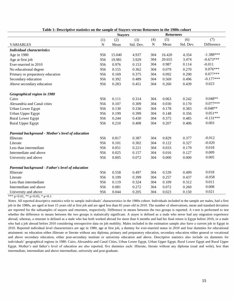
Descriptive statistics on the sample of stayers versus returnees in the 1980s cohort are reported in

Table 1. Returnees are slightly older than stayers both in 1980 and at first job. Regarding their

educational attainment, returnees are on average more educated compared to stayers. Explicitly,

83% of return migrants have either secondary education or above secondary education compared

to 68% of stayers, and hence, the least educated category among the stayers, no educational

degree, primary or preparatory education, is two times greater compared to the returnees and the

difference is statistically significant. Returnees in the 1980s cohort are also found to be less likely

to live in Greater Cairo, Alexandria and the Canal cities, whereas, they are found to be more

likely to live in Urban and Rural Lower Egypt in 1980. With respect to their parental background,

there isn’t any significant difference between the two groups in terms of their mother and father’s

highest level of educational attainment.

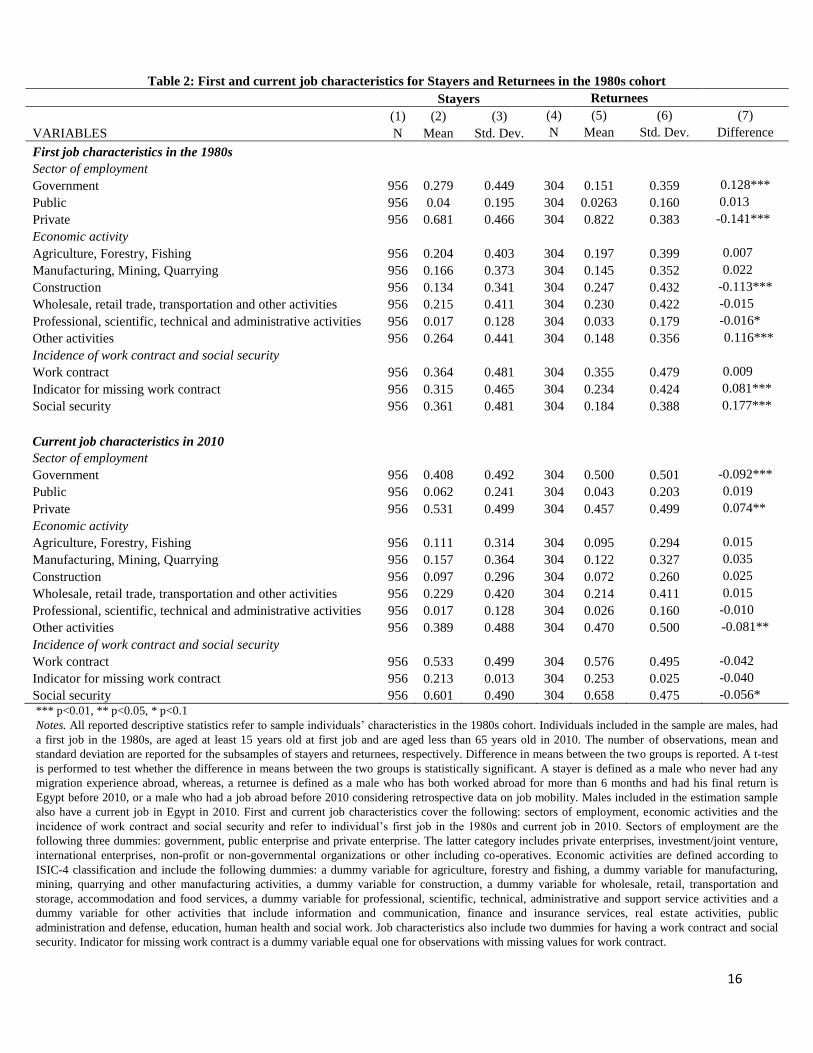
In Table 2, we also explore the first and current job characteristics for stayers and returnees in the

1980s cohort. For their first job, returnees were more likely to be employed in the private sector

compared to stayers and also less likely to be employed in the governmental sector. Returnees

were also more likely to work in economic activities, such as wholesale and retail trade,

transportation and storage, accommodation and food services, as well as, professional, scientific,

technical and administrative activities, for their first job compared to stayers. The incidence of

3 The years considered for the 1980s cohort are from the 1980 to 1989, included.

6

social security for the first job is 18% lower among returnees compared to stayers. Interestingly,

we find contrasted figures when we consider the current job characteristics for the two groups. In

2010, returnees were on average more likely to be employed in the governmental sector

compared to stayers and less likely to be employed in the private sector. In addition, the

incidence of social security for the current job in 2010 is 6% higher among returnees compared to

stayers.

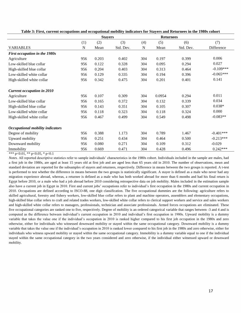
Table 3 sheds some light on individuals’ first and current occupations and occupational

indicators, for the sample of stayers and returnees respectively. For their first occupation,

returnees were significantly more likely to have either high-skilled blue collar or low-skilled

white collar occupations compared to stayers. In 2010, return migrants are significantly less

likely to be employed in high-skilled blue collar occupations and more likely to be employed in

high-skilled white collar occupations compared to stayers. When we consider the occupational

mobility indicators, we find that the difference in means between the two groups is statistically

significant. Returnees are found to be significantly more mobile compared to stayers and more

likely to witness upward mobility, when we compare their first job in the 1980s and their current

occupation in 2010.

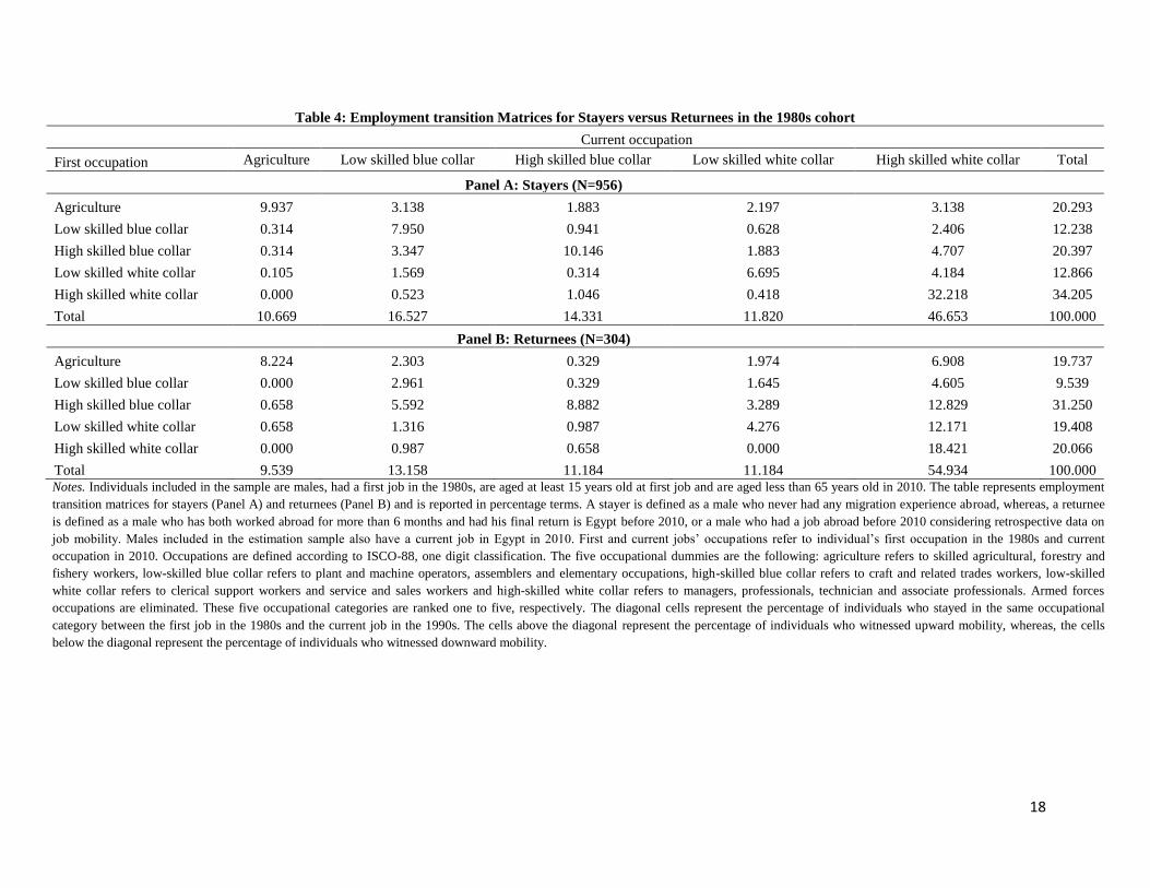
In Table 4, we also construct employment transition matrices for stayers (Panel A) versus

returnees (Panel B) in the 1980s cohort, to better understand the dynamics of occupational

mobility. The diagonal cells represent the percentage of individuals who stayed in the same

occupational category between the first job in the 1980s and the current job in 2010. The cells

above the diagonal represent the percentage of individuals who witnessed upward mobility,

whereas, the cells below the diagonal represent the percentage of individuals who witnessed

downward mobility. Among the sample of returnees in the 1980s cohort, we find that 46%4 of

return migrants witnessed upward occupational mobility when we compare their first job in the

1980s and their current job in 2010. This figure drops to 25% when we consider the sample of

stayers. Interestingly, we also find that 61% of the returnees who witnessed upward mobility had

either high-skilled blue collar or low-skilled white collar occupations in 1980s and they moved

up the occupational ladder to hold either white collar occupations in general for the former

category or high-skilled white collar occupations for the latter. Whereas, 57% of the stayers who

witnessed upward occupational mobility, had in the 1980s less qualified occupations to start,

namely agricultural or low-skilled blue collar occupations.

4 To compute the share of individuals witnessing upward mobility, we consider for each occupation category, the sum of the cells

above the diagonal. For example, if the occupational category for the first job is agriculture, the share of individuals witnessing

upward occupational mobility would be the sum of the shares of individuals employed in low-skilled blue collar, high-skilled blue

collar, low-skilled white collar or high skilled white collar occupations in 2010.

7

3. Empirics

3.1 Regression Specification

We estimate the effect of return migration on occupational mobility for the 1980s cohort,

focusing on males aged at least 15 years old at first job and 64 years old in 2010. For each

individual, we compare his first occupation in the 1980s to his current occupation in 2010.5

Occupational categories are split into six distinct categories according to the ISCO-88 one digit

classification, and are the following: not working, agriculture, low-skilled blue collar, high-

skilled blue collar, low skilled white collar and high skilled white collar occupations.6 These six

occupational categories are ranked one to six, respectively. We estimate the following

specification, using Probit and Ordered Probit Models:

(1)

For the Probit Model, is a dummy variable for upward mobility that takes the value one if the

individual’s occupation in 2010 is ranked higher compared to his first job occupation in the 1980s

and zero otherwise, either for individuals who witnessed downward mobility or stayed within the

same occupational category. For the Ordered Probit Model, is an ordered categorical variable,

the degree of occupational mobility, it is computed as the difference between individual’s current

occupation in 2010 and individual’s first occupation in 1980s.7 Returnee is a dummy variable

equal one for males who had both worked abroad for more than 6 months and had his final return

to Egypt before 2010, or a male who had a job abroad before 2010 considering retrospective data

on job mobility and equal zero for stayers who never had any migration experience abroad. is

a vector of individual and household characteristics. Individual-level characteristics are the

following: age in 1980 and its squared term, three dummies for individual’s educational

attainment: primary and preparatory education, secondary education either general or vocational

and above secondary education, either post-secondary institute or university education and above;

the reference category is no educational degree either illiterate or literate without any diploma

and five dummies for individual’s geographical regions in 1980: Cairo, Alexandria and Canal

Cities, Urban Lower Egypt, Urban Upper Egypt and Rural Lower Egypt; the reference category

5 Since we rely on the ELMPS 2012, we use current job occupation in 2012 as individual’s occupation in 2010 if the individual

didn’t witness any job status changes with the 25th of January 2011 Egyptian Revolution. Whereas, for those individuals who

witnessed job status changes in 2011, we consider their employment status in 2010 and subsequently, we determine their job

occupation in 2010. 6 The six occupational dummies are the following: not working refers to returnees’ first occupation in Egypt for those who had

their first job abroad, agriculture refers to skilled agricultural, forestry and fishery workers, low-skilled blue collar refers to plant

and machine operators, assemblers and elementary occupations, high-skilled blue collar refers to craft and related trades workers,

low-skilled white collar refers to clerical support workers and service and sales workers and high-skilled white collar refers to

managers, professionals, technician and associate professionals. Armed forces occupations are eliminated. These six occupational

categories are ranked one to six, respectively. 7 This variable ranges from -3 to 5. It is equal zero, if the individual stayed in the same occupational category between the first job

in the 1980s and the current job in 2010, and it takes positive (negative) values if the individual witnessed upward (downward)

mobility. The greater the value of the indicator in absolute term, the greater is the mobility. In the estimation sample, we don’t

have any individual who had a first job occupation as a high-skilled white collar and a current job in 2010 as agricultural

occupation, hence, the variable’s range is -3 to 5.

8

is Rural Upper Egypt. Household level characteristics include mother’s and father’s level of

education, four dummies each: literate without any diploma (read and write), less than

intermediate, intermediate and above intermediate, university and post-graduate; the reference

category is illiterate. is a vector of first job characteristics in the 1980s8 and includes:

sectors of employment, economic activities and the incidence of work contract and social security

in the 1980s. Sectors of employment are the following two dummies: government and public

enterprises. The reference category is private enterprises and it includes private enterprises as

well as investment/joint venture, international enterprises, non-profit or non-governmental

organizations or other including co-operatives. Economic activities are defined according to

ISIC-4 classification and include the following five dummies: a dummy variable for agriculture,

forestry and fishing, a dummy variable for manufacturing, mining, quarrying and other

manufacturing activities, a dummy variable for construction, a dummy variable for wholesale,

retail, transportation and storage, accommodation and food services and a dummy variable for

professional, scientific, technical, administrative and support service activities. The reference

category is a dummy variable for other activities that include information and communication,

finance and insurance services, real estate activities, public administration and defense,

education, human health and social work. First job characteristics also include two dummies for

having a work contract and social security.

3.2 IV approach and selection-corrected estimations

We face two methodological challenges when estimating the impact of occupational mobility of

returnees versus stayers. Unobserved individual characteristics might simultaneously affect the

probability of migration and the return decision to Egypt, on the one hand and occupational

choices, on the other hand. Aware of the potential endogeneity problem inherent in this type of

analysis, we rely on an instrumental variable approach, following the same identification strategy

proposed by Wahba and Zenou (2012). Hence, to obtain an exogenous source of variation in the

probability of migration, we use the historical inflation-adjusted oil prices when the individual

was 26 years old.9 The rationale behind using historic oil prices as a predictor of the migration

probability, as argued by Wahba and Zenou (2012), is that other Arab countries constitute the

most important destination for Egyptian countries, where oil prices played a crucial role in

driving the demand for foreign labor both directly in the Gulf countries or indirectly, in other

non-oil Arab countries.10

8 In unreported regressions, we have only conditioned on individual and household characteristics, eliminating the vector of first

job characteristics Zi. We are likely to overestimate the effect of return migration on upward occupational mobility if we don’t

condition on the vector of first job characteristics. 9 In our estimation sample, the average age for males at the time of migration for the last episode is 26 years old. We also

performed some robustness checks by matching the historic oil prices data with the year when the individual was 25 years old or

27 years old and coefficient estimates remain robust. 10 98% of Egyptian migrants, in our estimation sample, migrated to other Arab countries during the last migration episode.

9

The second methodological issue is the non-random selection into temporary migration. We

hence provide additional selection-corrected estimations. Since, unobserved differences between

treatment and control groups, returnees and stayers, respectively, might be plaguing our standard

Probit and Ordered Probit results; we also estimate the following Difference-in-Differences

specification:

(2)

is the individual’s occupation at time t, split into six distinct occupational categories according

to the one digit ISCO-88 classification, not working, agriculture, low-skilled blue collar, high-

skilled blue collar, low-skilled white collar and high-skilled white collar. is a dummy

variable equal one for the sample returnees and zero, for the sample of stayers, it captures

differences between the treatment and control groups, before the treatment. As we mentioned

earlier, the treatment group is the sample of return migrants, all males who had both worked

abroad for more than 6 months and had his final return is Egypt before 2010, or males who had a

job abroad before 2010 considering retrospective data on job mobility. The control group is the

sample of stayers, all males who never had any migration experience abroad. is a dummy

variable equal one for the second time period and equal zero for the 1980s. The time dummy

captures aggregate factors that would cause changes in the individual’s occupational choice even

in the absence of the treatment. The coefficient of interest is , it multiplies the interaction term

between the treatment variable and the time period dummy. The difference-in-differences

estimator is the difference in average occupational ranking among the returnees between the

follow-up and baseline periods, minus the difference in occupational ranking among the stayers

for the same periods. It differences out all unobserved time-invariant differences between the

treatment and control groups.

We also employ a Difference-in-Differences matching technique that controls for the observable

characteristics as well as the unobserved time-invariant heterogeneity. First, we estimate the

propensity score or the individual’s probability of receiving the treatment, given the same set of

covariates presented earlier, using a Logit model. It enables us to pair return migrants with

stayers who have similar values of the propensity score. Hence, the two groups are similar, after

the fact, in terms of observable characteristics, apart from the treatment. Second, we combine the

Propensity score matching technique with a standard Difference-in-Differences specification,

based on the matched sample of returnees and stayers.

10

4. Results

4.1 Estimating the effect of return migration on upward occupational mobility

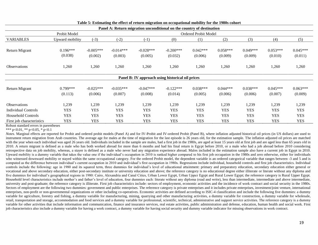
In Table 5, we estimate Equation 1 using Probit and Ordered Probit models (Panel A) and IV-

Probit and IV-ordered Probit models (Panel B), while conditioning on individual, household

controls, as well as, the first job characteristics. We find a positive and statistically significant

effect of return migration on upward occupational mobility for males who first entered the labor

market in the 1980s, in both panels. In Panel A, being a return migrant increases the probability

of upward occupational mobility by about 20 percentage points. Controlling for the potential non-

randomness of migration and selection bias using historic oil prices as an instrument for return

migration in Panel B, results in coefficient estimates about four times greater than the standard

Probit Model. Results from the ordered Probit and the IV-ordered Probit models also support this

finding. Standard Probit Model results present a lower bound of the selection-corrected estimates.

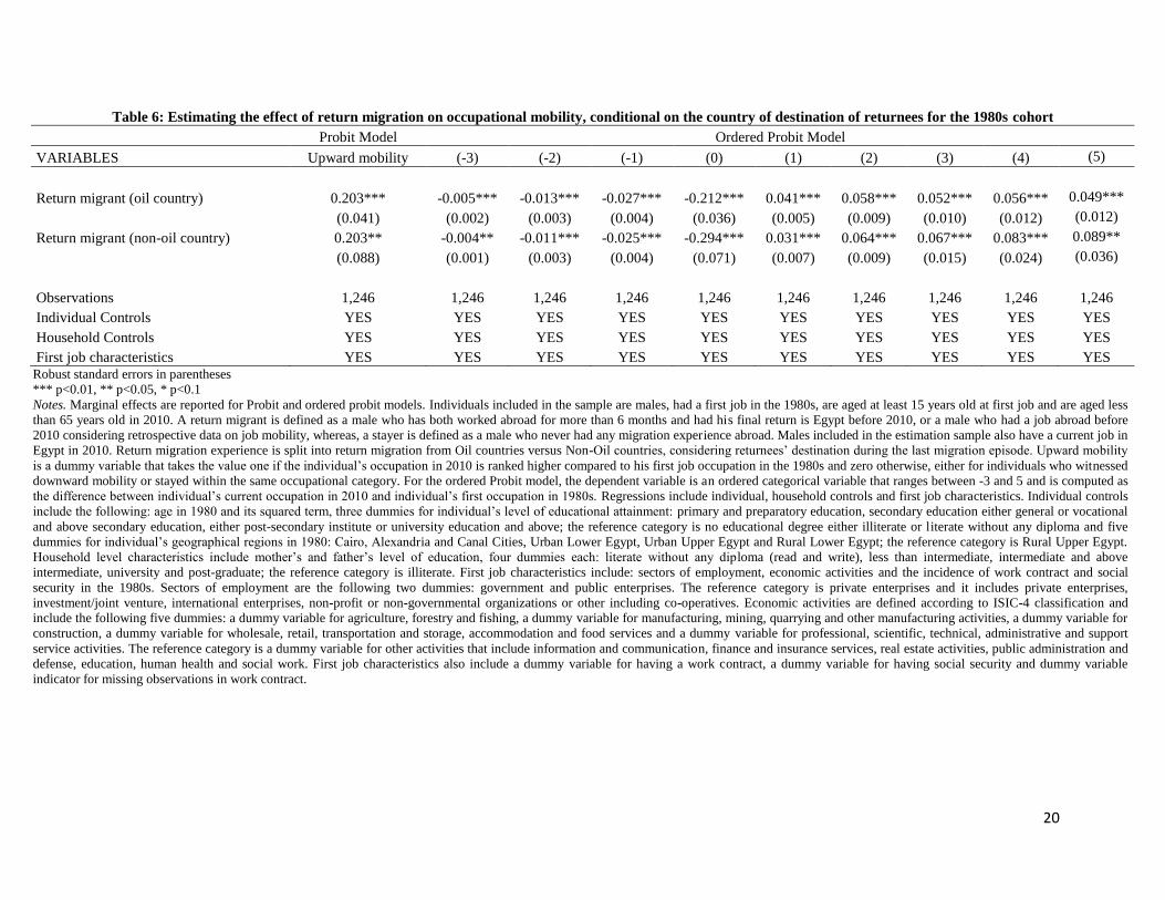
In Table 6, we also estimate the effect of return migration on occupational mobility, by

disentangling the effect conditional on the country of destination of Egyptian returnees during the

last migration episode, namely oil and non-oil countries. As we mentioned earlier, Egyptian

migration is mostly towards Arab oil producing countries, hence, the sample size of Egyptians

heading to non-oil countries is much smaller. Using a Probit model, return migration from oil

countries or non-oil countries increases the probability of upward occupational mobility by 20

percentage points. Relying on the Ordered Probit model, the coefficient estimate of return

migration from non-oil countries is greater than the coefficient estimate of return migration from

oil countries.

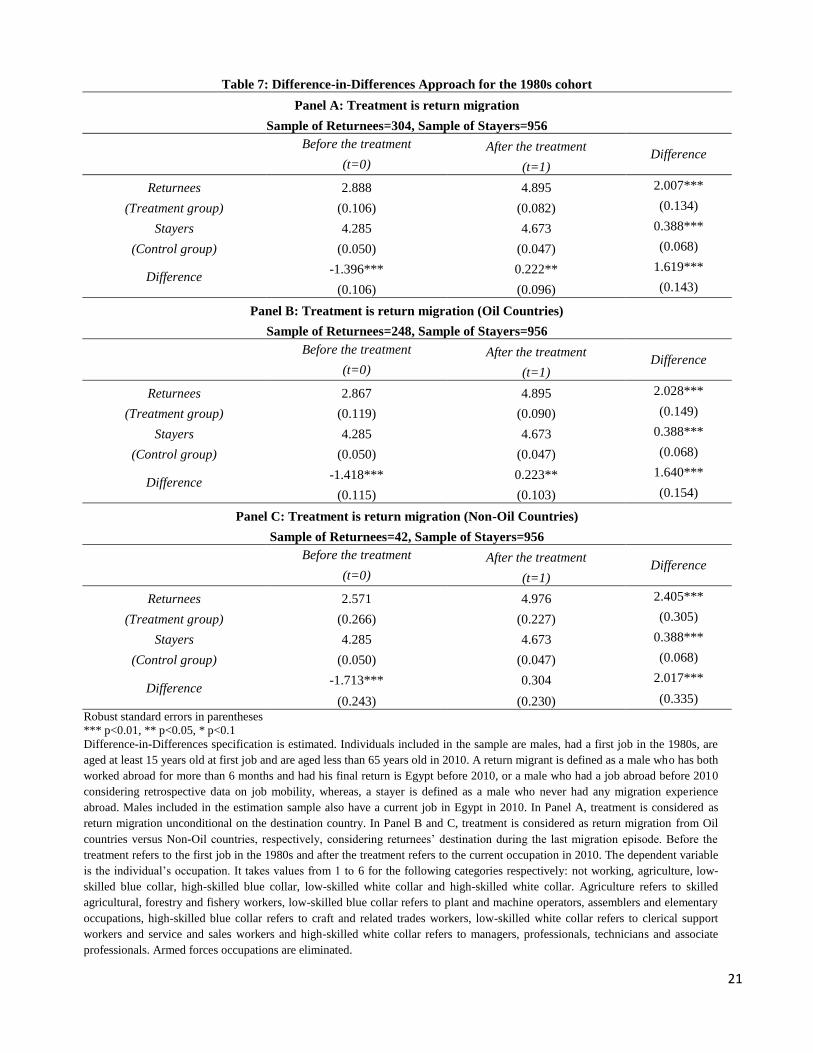
In Table 7, we provide additional selection-corrected estimates. We estimate a Difference-in-

differences specification, by considering return migration unconditional on the country of

destination of Egyptian migrants (Panel A), return migration from oil countries during the last

migration episode (Panel B) and return migration from non-oil countries during the last migration

episode (Panel C). Difference-in-differences estimators are positive and statistically significant.

Unconditional on the country of destination of Egyptian migrants, return migration increases the

probability of upward occupational mobility. Interestingly, conditioning on the destination

country during the last migration episode, the magnitude of the estimated coefficient for non-oil

countries is greater than the estimated difference-in-differences estimator for oil countries. On

average, returnees from the 1980s cohort are found to be more likely to climb the occupational

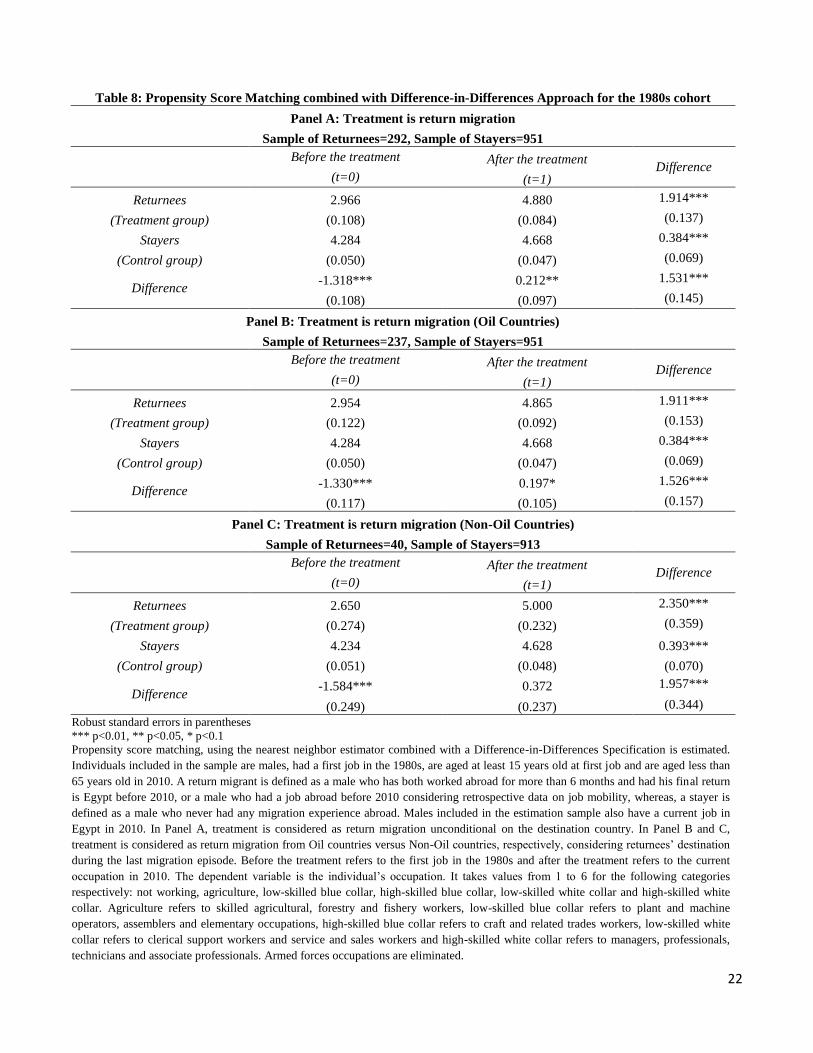
ladder in Egypt, by about two categories. Results are qualitatively very similar in Table 8, when

we use Difference-in-Differences matching estimator.

It is important, though, to note that since we are controlling for selection into temporary

migration but not for the double selection of emigration and return, and based on Wahba (2015),

if migrants are positively selected relative to non-migrants and return migrants are negatively

selected amongst migrants, our estimates would be an over-estimate of the impact of migration

11

on occupational upgrade. Indeed, the OLS estimates provide a lower bound whilst the IV-Probit

and Difference in differences estimators would provide an upper bound.

4.2 Mechanisms

Our results are driven by the subsample of Egyptian returnees who had their first job abroad in

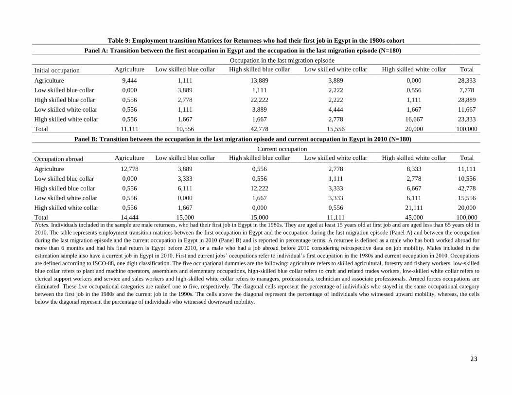
comparison with returnees who had their first job in Egypt. In Table 9 and Table 10, we construct

transitional matrices for the two groups of returnees. In Table 9, we investigate the employment

transition for returnees who had their first job Egypt by looking at the employment transition

between the first occupation in the 1980s in Egypt and the occupation in the last migration

episode and subsequently, the employment transition between the occupation in the last migration

episode and the occupation in Egypt upon return in 2010. We find that 28% of the returnees

witness an upward mobility between the first occupation in Egypt and the occupation during the

last migration episode, whereas about 16% downgrade while being abroad compared to their first

occupation in Egypt. Following the occupational mobility of the same subsample of returnees

between the occupation during the last migration episode and the current occupation in Egypt, we

find that 36% of the returnees witness an upward mobility upon return, whereas, about 12%

witness some sort of downgrading.

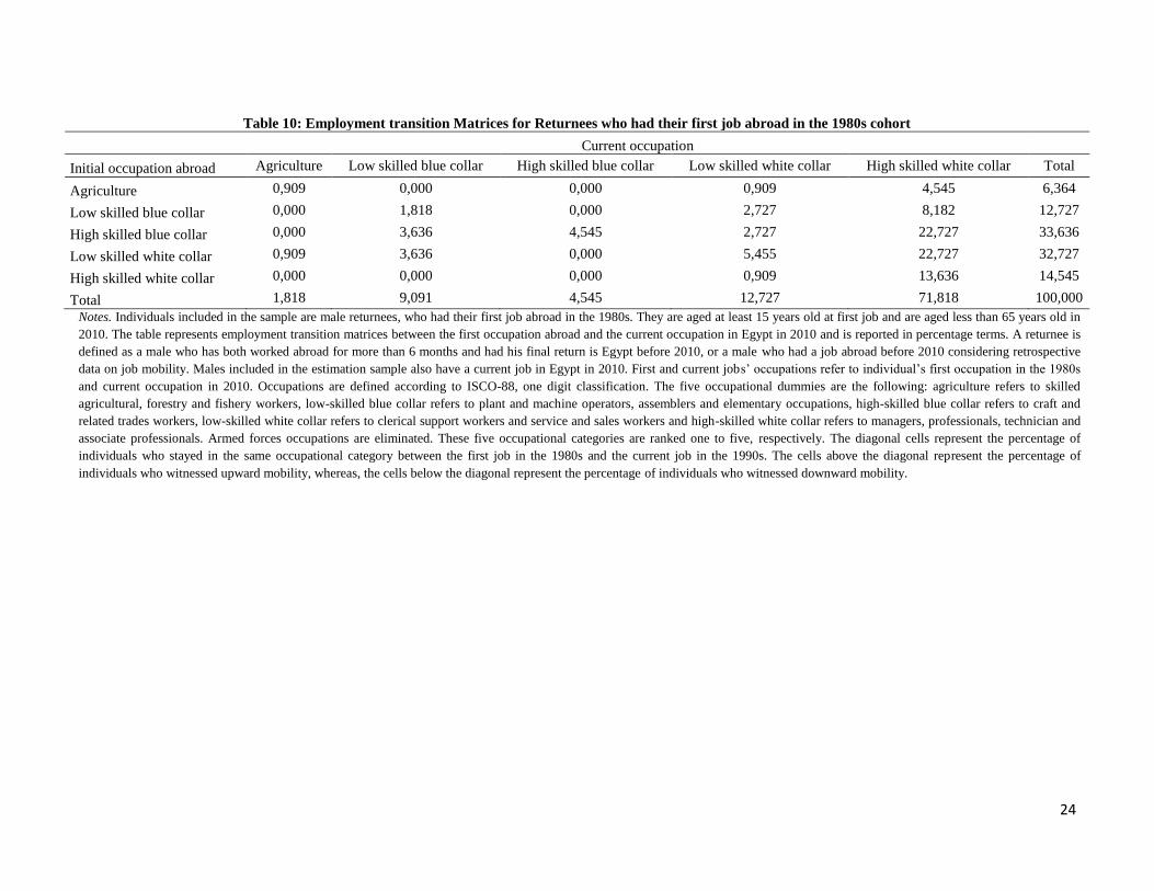
By contrast, considering the subsample of returnees who had their first job abroad, we investigate

in Table 10, the occupational mobility between the first occupation abroad and the current

occupation upon return. Interestingly, on the one hand, we find that 65% of those returnees

witness an upward mobility compared to their first occupation abroad. On the other hand, only

9% witness some sort of downgrading when we compare the first occupation abroad to the

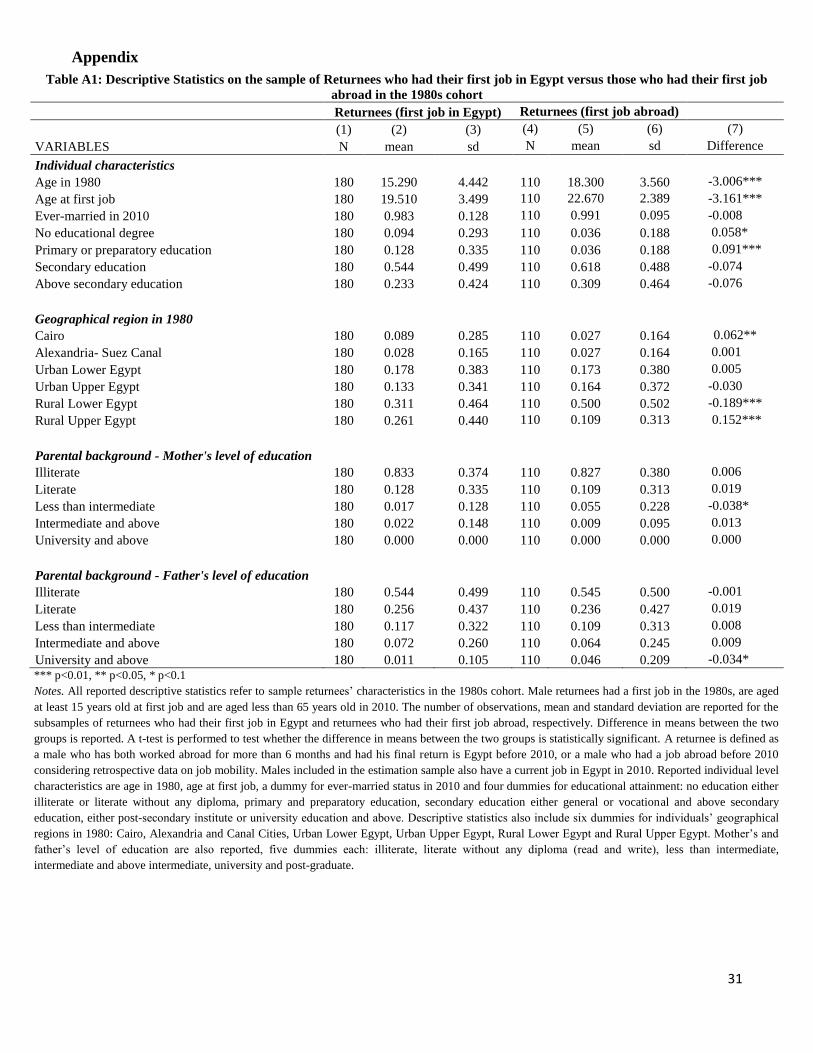
current occupation in Egypt in 2010. To further tackle differences between the two groups of

returnees, those who had their first job in Egypt and those who had their first job abroad, in the

1980s cohort, we present descriptive statistics in Table A1, Table A2 and Table A3 in the

Appendix. In Table A1, returnees who had their first job abroad are about 3 years older when

they had their first job and they are also less likely to belong to the lowest two educational

attainment categories: no educational degree or primary or preparatory degree. They are also

found to be less likely to come from Cairo or Rural Upper Egypt, however, they are found to be

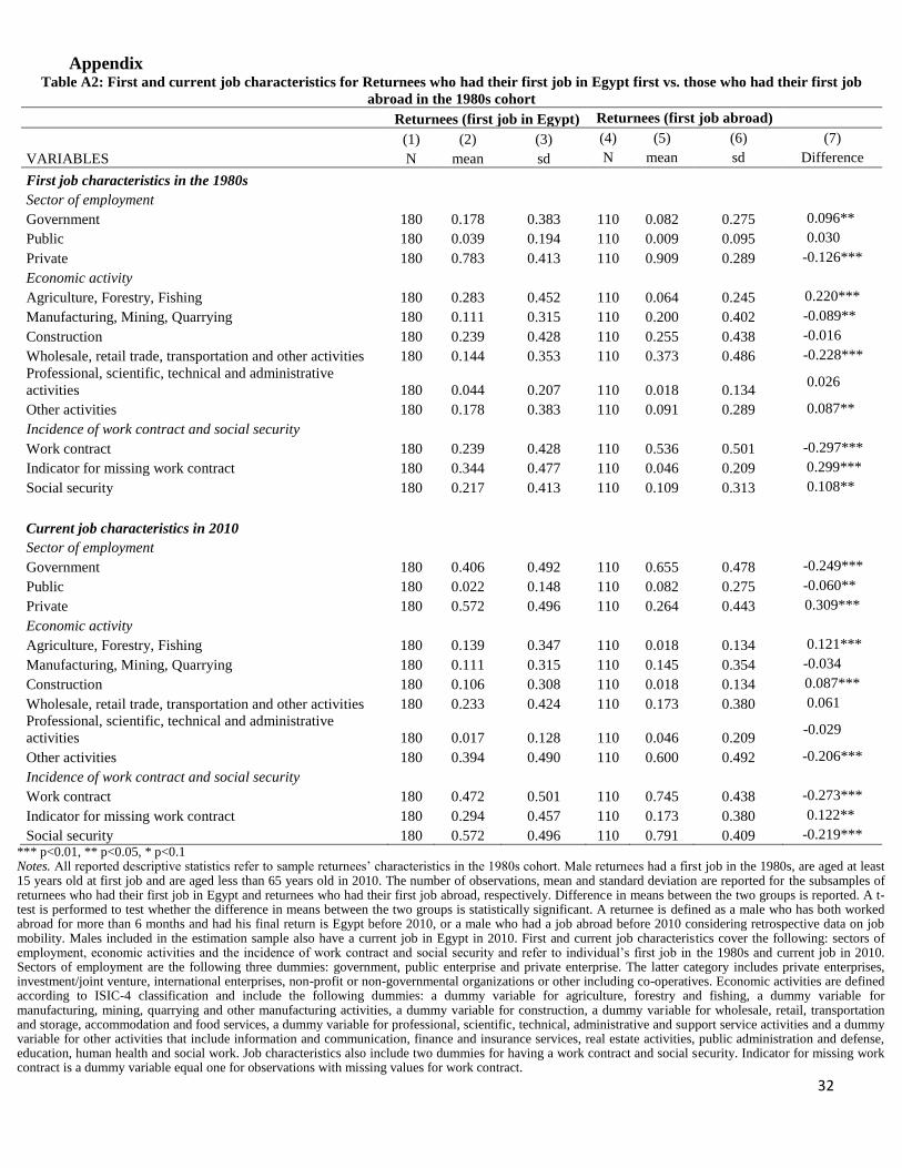
more likely to come from Rural Lower Egypt. Regarding their first job characteristics, in Table

A2, returnees in the 1980s cohort who had their first job abroad are found to be more likely to

work in the private sector compared to the public sector. They are much less likely to work in

agricultural activities compared to returnees who had their first job in Egypt, who are about 22

percentage points more likely to have an agricultural activity for their first job. Returnees who

had their first job abroad were found to be more likely to work in activities such as

manufacturing, mining and quarrying; and wholesale and retail trade compared to returnees who

had their first job in Egypt. Returnees who had their first job abroad were also better off in terms

12

of having a work contract; however, they were less likely to have social insurance compared to

returnees who had their first job in Egypt.

Upon return, we find that returnees who had their first job abroad are more likely to work in the

government/public sector compared to the subsample of returnees who had their first job abroad.

They are also found to be significantly different in terms of current job activity compared to the

sample of returnees who had their first job in Egypt. The former are much less likely to work in

agricultural activities and more likely to work in construction. Upon return, the incidence of work

contract and social security is significantly greater among the returnees who had their first job in

Egypt compared to returnees who had their first job abroad.

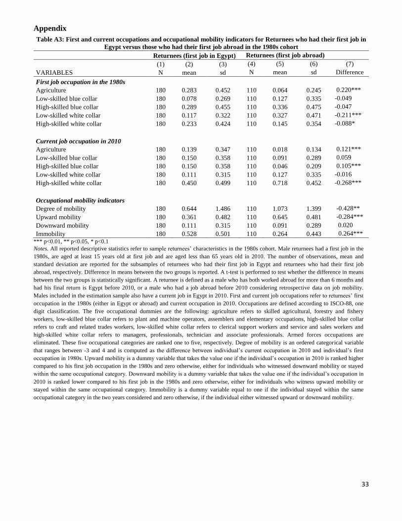
According to Table A3, returnees who had their first job abroad are better off in terms of their

first occupation abroad compared to the other returnees who had their first job in Egypt and for

their current occupation upon return. Regarding their first job, they are significantly less likely to

work in the agricultural sector but more likely to have a white-collar occupation, both low and

high skilled. Upon return, the same figures persist. In terms of mobility indicators, the degree of

mobility is much greater, the incidence of upward mobility is 28 percentage points greater and

the degree of immobility is also significantly less pronounced compared to the returnees who had

their first job in Egypt.

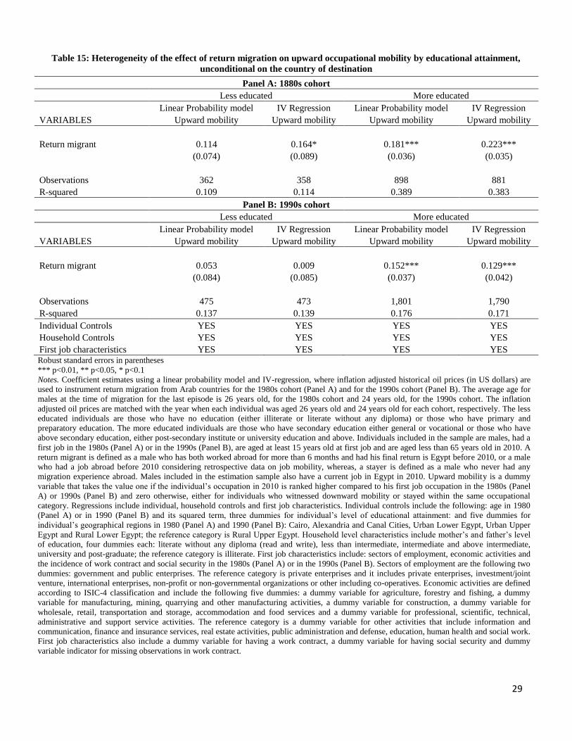
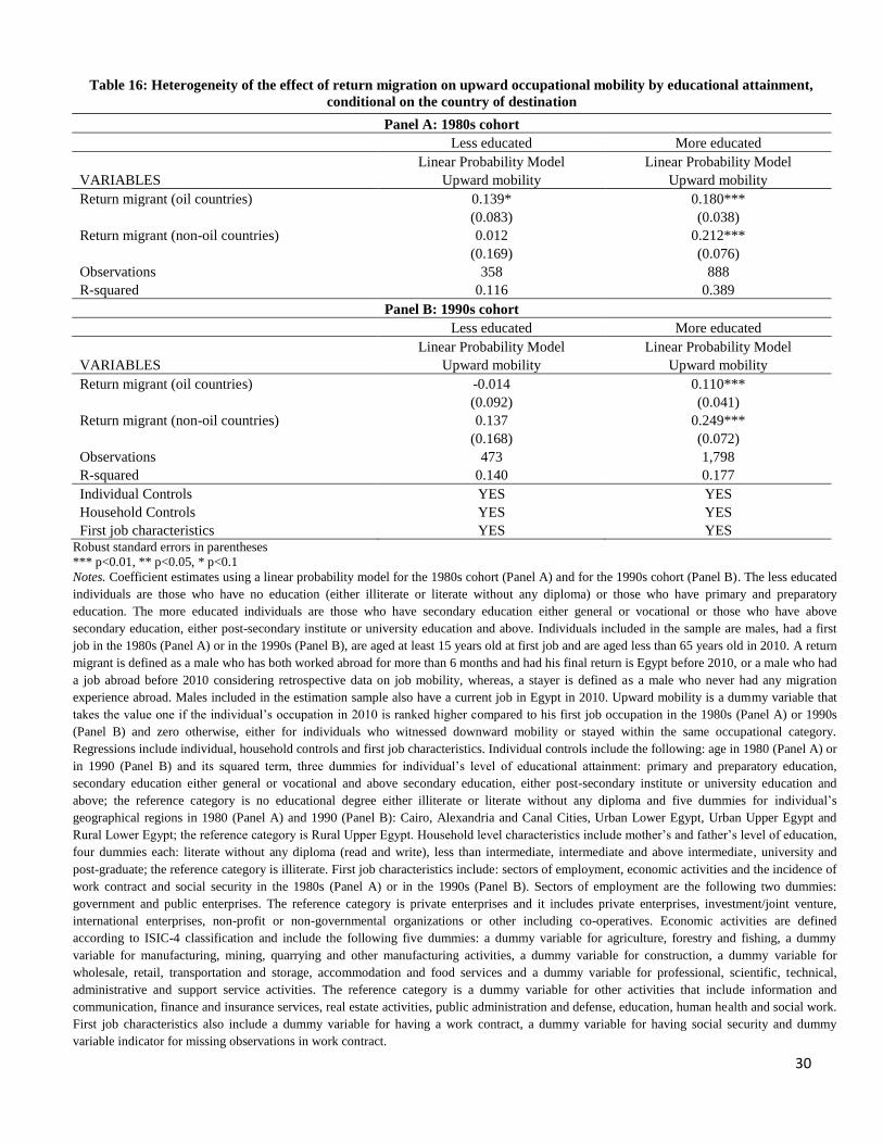
We have also exploited the heterogeneity of the effects by educational attainment, for the 1980s

cohort in Panel A and for the 1990s cohort in Panel B, unconditional on the country of

destination of Egyptian migrants using a standard linear probability model for upward

occupational mobility and IV regression to instrument for return migration from Arab countries

(Table 16) and conditional on the country of destination of Egyptian migrants during the last

migration episode using a linear probability model (Table 17). Our results suggest that only males

who belong to the upper end of the educational distribution are likely to witness upward

occupational mobility for both in the 1980s cohort and in the 1990s cohort. Those individuals

have either secondary or above secondary education whereas our results are not significant for

the subsample of individuals who have either no educational degree or primary and preparatory

education. This is in line with our results presented earlier, as returnees who have their first job

abroad are also found to be on average more educated compared to returnees who had their first

job in Egypt.

4.3 Robustness checks

We also check the robustness of our results using the 1990s cohort.11

In this section, we focus on

males who had their first job in the 1990s12

, were aged at least 15 years old at first job and had a

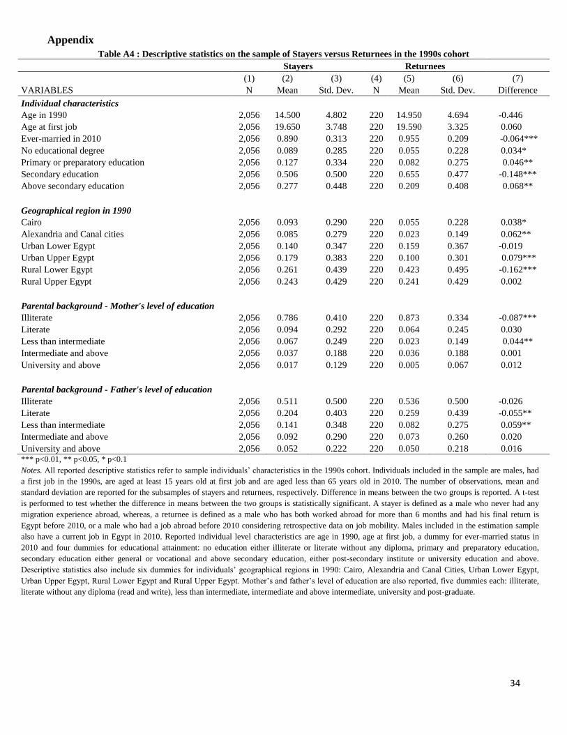
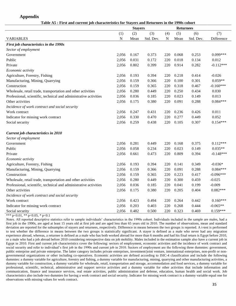
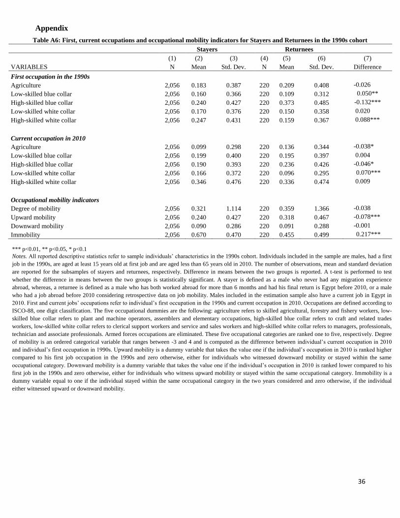
11 In Tables A4, A5 and A6 in the Appendix, we provide descriptive statistics for the 1990s cohort regarding individuals’

characteristics, first and current job characteristics, occupations and occupational mobility indicators. 12 The years considered for the 1990s cohort are from the 1990 to 1999, included.

13

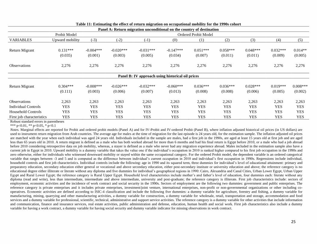
current job in Egypt in 2010. In Table 11, we also estimate the effect of return migration on

occupational mobility for the 1990s cohort. In Panel A, we employ a standard Probit and

Ordered-Probit Models, whereas, in Panel B, we present IV-Probit and IV-ordered Probit models,

using historical oil prices. In line with our previous findings, we find the return migration

increases the probability of upward occupational mobility by 13 percentage points using a

standard Probit Model. Relying on our IV specification, the magnitude of the estimated

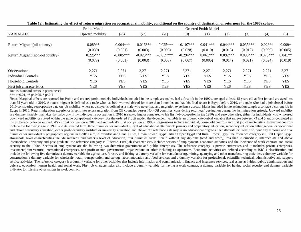
coefficient is more than two times greater. Disentangling the effect by country of destination, we

find that migration experience in non-oil countries have a greater impact on upward occupational

mobility. According to the standard Probit Model, returnees from non-oil countries are 22

percentage points more likely to witness upward mobility, compared to 9 percentage points for

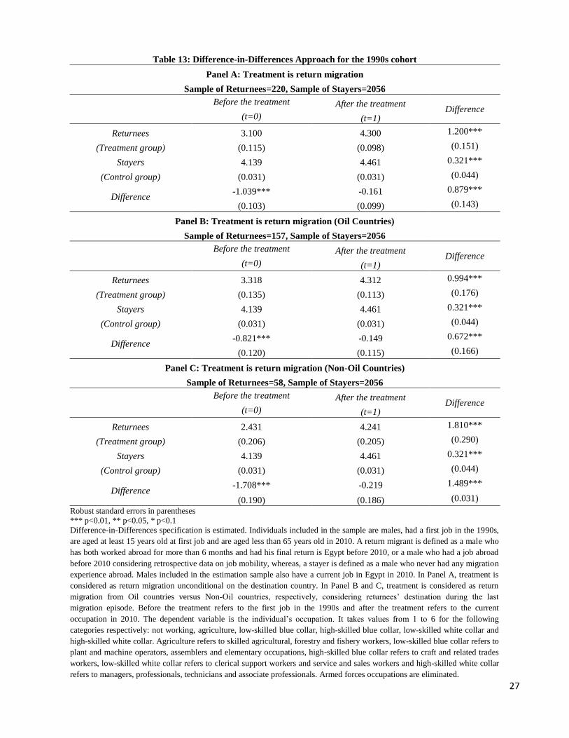
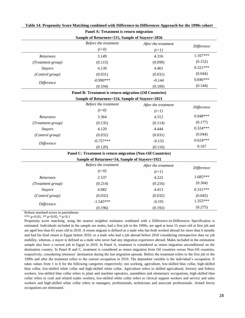
returnees from oil countries. Table 13 and Table 14 also provide additional robustness checks

relying on a Difference-in-Differences and a Difference-in-Differences matching techniques. Our

results are robust to the different specifications and we find suggestive evidence of a greater

impact of migration experience in non-oil countries on upward occupational mobility.

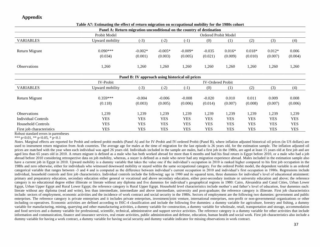
In Tables A7, A8, A9 and A10 in the Appendix, we perform additional robustness checks for the

1980s cohort where we consider the occupational mobility between the first job (whether the first

job is in Egypt or abroad) and the current job in Egypt. Our results are still robust and we find

suggestive evidence of upward mobility for return migrants. In Table A7, we find that return

migration increases the probability of upward occupational mobility by about 9 percentage

points. Controlling for the potential non-randomness of migration and selection bias using

historic oil prices as an instrument for return migration in Panel B, results in coefficient estimates

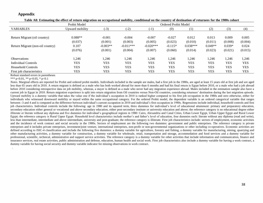
about four times greater than the standard Probit Model. In Table A8, we also estimate the effect

of return migration on occupational mobility conditional on the country of destination of

Egyptian returnees during the last migration episode. Using a Probit model, return migration from

oil countries increases the probability of upward occupational mobility by 9 percentage points.

The coefficient estimate of return migration from non-oil countries is slightly greater, however,

not significant. Relying on the Ordered Probit estimates, the positive effect of return migration on

upward occupational mobility is mostly driven by return migration from non-oil countries.

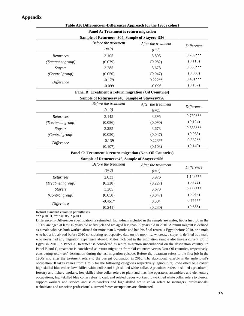
In Table A9, we estimate a Difference-in-differences specification. The Difference-in-differences

estimators are positive and statistically significant. The magnitude of the estimated coefficient is

very similar to our IV-estimates presented in Table A7. Unconditional on the country of

destination of Egyptian migrants, return migration increases the probability of upward

occupational mobility. Interestingly, conditioning on the destination country during the last

migration episode, the magnitude of the estimated coefficient for non-oil countries is about two

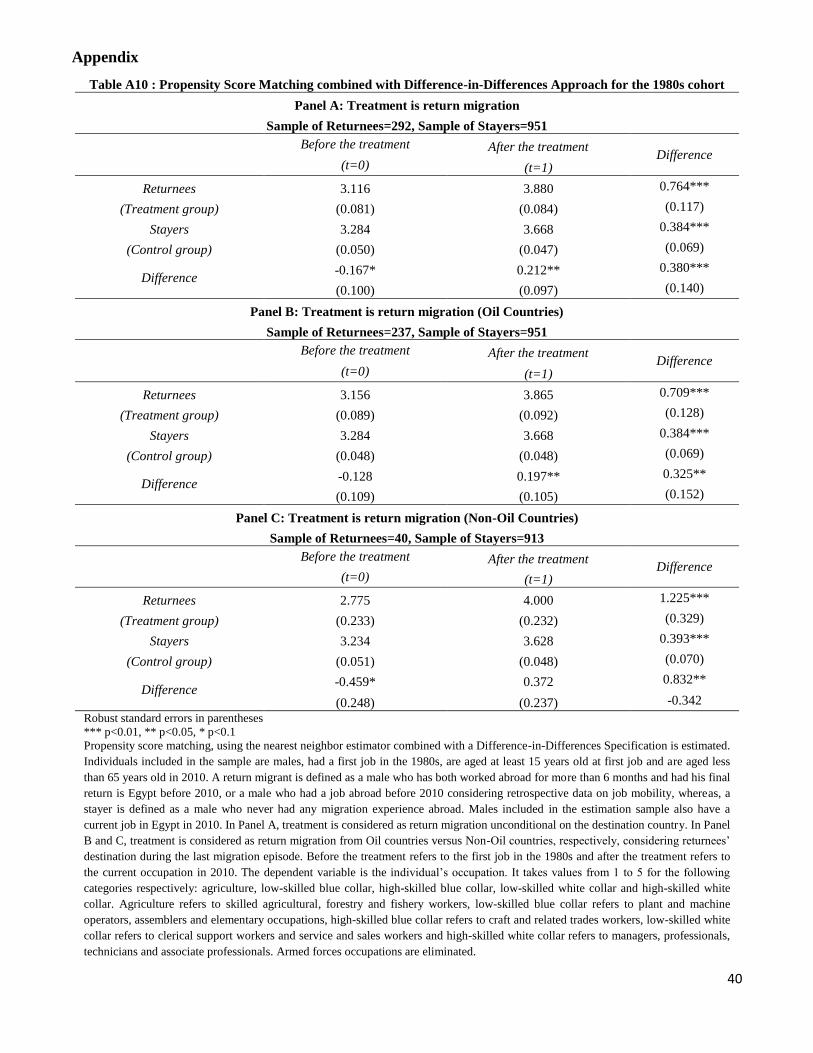
times greater than the estimated difference-in-differences estimator for oil countries. Results are

qualitatively very similar in Table A10, when we use Difference-in-Differences matching

estimator.

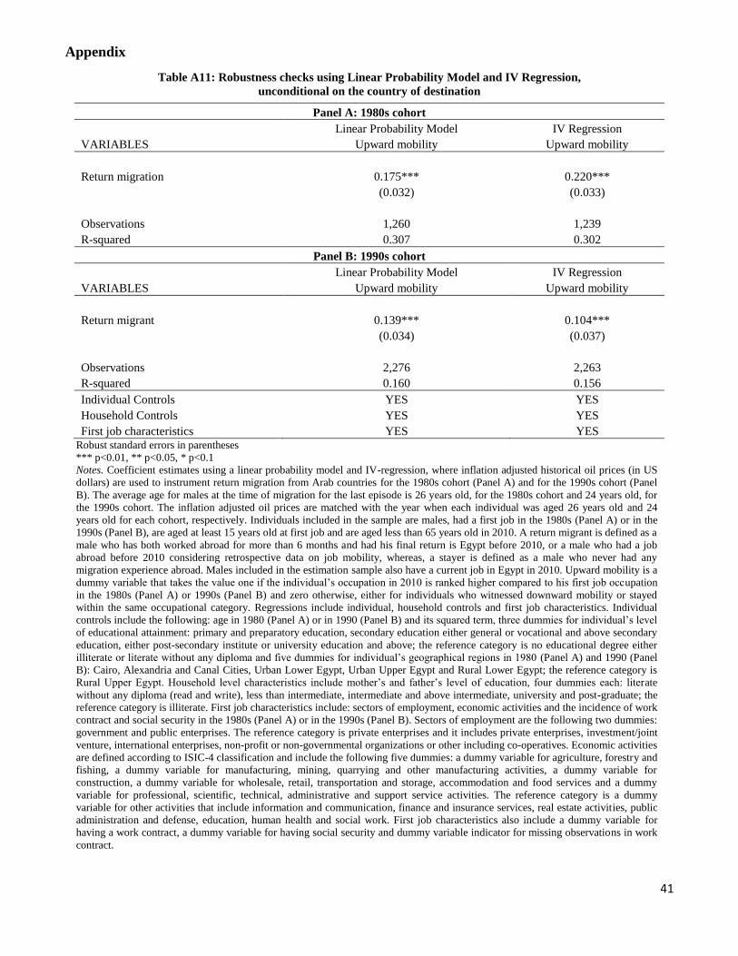
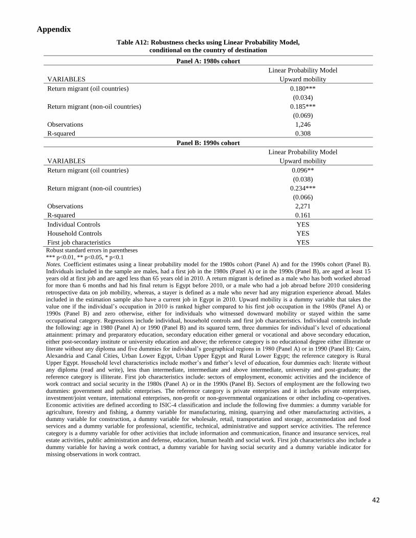
We also employ a standard linear probability model for upward occupational mobility instead of

a Probit model and a standard IV regression instead of IV-Probit model in Table A11 for the

14

1980s cohort (Panel A) and for the 1990s cohort (Panel B) unconditional on the country of

destination and a standard linear probability model to estimate the effect of return migration on

upward occupational mobility, conditional on the country of destination of Egyptian migrants

during the last migration episode in Table A12 for the 1980s cohort (Panel A) and for the 1990s

cohort (Panel B). Our results are robust and qualitatively very similar.

5. Conclusion

The impact of overseas migration experience on skill acquisition of migrants is very sparse.

Previous studies have focused on measuring the wage premium of returnees versus stayers. This

paper studies the extent to which temporary overseas migration enables returnees to climb the

occupational ladder. We use the Egypt Labor Market Panel Survey 2012 (ELMPS 12), a

nationally representative household survey with very rich information on labor market

characteristics and dynamics, including retrospective data on international migration and

individual experiences before, during and after migration. We estimate the occupational mobility

of returnees relative to non-migrants focusing on cohort groups who entered the labor market in

the same decade, to control for initial labor market conditions, and compare individual

occupational mobility based on the first jobs relative to in 2010. We rely on both instrumental

variable approach and a Difference-in-Differences, as well as Difference-in-Differences matching

techniques to control for the endogeneity and selection into migration.

The findings suggest that return migration increases the probability of upward occupational

mobility. Furthermore, the impact of migration experience in non-oil countries is about two times

greater than the estimated coefficient for oil countries. Overall, the results highlight the role

played by migration in human capital accumulation of migrants.

15

Table 1: Descriptive statistics on the sample of Stayers versus Returnees in the 1980s cohort

Stayers Returnees

(1) (2) (3) (4) (5) (6) (7)

VARIABLES N Mean Std. Dev. N Mean Std. Dev. Difference

Individual characteristics

Age in 1980 956 15.040 4.937 304 16.420 4.354 -1.388***

Age at first job 956 19.981 3.929 304 20.655 3.474 -0.673***

Ever-married in 2010 956 0.976 0.153 304 0.987 0.114 -0.011

No educational degree 956 0.155 0.362 304 0.079 0.270 0.076***

Primary or preparatory education 956 0.169 0.375 304 0.092 0.290 0.077***

Secondary education 956 0.392 0.489 304 0.569 0.496 -0.177***

Above secondary education 956 0.283 0.451 304 0.260 0.439 0.023

Geographical region in 1980

Cairo 956 0.111 0.314 304 0.063 0.242 0.048**

Alexandria and Canal cities 956 0.107 0.309 304 0.030 0.170 0.077***

Urban Lower Egypt 956 0.130 0.336 304 0.178 0.383 -0.048**

Urban Upper Egypt 956 0.199 0.399 304 0.148 0.356 0.051**

Rural Lower Egypt 956 0.244 0.430 304 0.375 0.485 -0.131***

Rural Upper Egypt 956 0.210 0.408 304 0.207 0.406 0.003

Parental background - Mother's level of education

Illiterate 956 0.817 0.387 304 0.829 0.377 -0.012

Literate 956 0.101 0.302 304 0.122 0.327 -0.020

Less than intermediate 956 0.051 0.221 304 0.033 0.179 0.018

Intermediate and above 956 0.025 0.157 304 0.016 0.127 0.009

University and above 956 0.005 0.072 304 0.000 0.000 0.005

Parental background - Father's level of education

Illiterate 956 0.558 0.497 304 0.539 0.499 0.018

Literate 956 0.199 0.399 304 0.257 0.437 -0.058




*** p<0.01, ** p<0.05, * p<0.1

Notes. All reported descriptive statistics refer to sample individuals’ characteristics in the 1980s cohort. Individuals included in the sample are males, had a first

job in the 1980s, are aged at least 15 years old at first job and are aged less than 65 years old in 2010. The number of observations, mean and standard deviation

are reported for the subsamples of stayers and returnees, respectively. Difference in means between the two groups is reported. A t-test is performed to test

whether the difference in means between the two groups is statistically significant. A stayer is defined as a male who never had any migration experience

abroad, whereas, a returnee is defined as a male who has both worked abroad for more than 6 months and had his final return is Egypt before 2010, or a male

who had a job abroad before 2010 considering retrospective data on job mobility. Males included in the estimation sample also have a current job in Egypt in

2010. Reported individual level characteristics are age in 1980, age at first job, a dummy for ever-married status in 2010 and four dummies for educational

attainment: no education either illiterate or literate without any diploma, primary and preparatory education, secondary education either general or vocational

and above secondary education, either post-secondary institute or university education and above. Descriptive statistics also include six dummies for

individuals’ geographical regions in 1980: Cairo, Alexandria and Canal Cities, Urban Lower Egypt, Urban Upper Egypt, Rural Lower Egypt and Rural Upper

Egypt. Mother’s and father’s level of education are also reported, five dummies each: illiterate, literate without any diploma (read and write), less than

intermediate, intermediate and above intermediate, university and post-graduate.

16

Table 2: First and current job characteristics for Stayers and Returnees in the 1980s cohort

Stayers Returnees

(1) (2) (3) (4) (5) (6) (7)


First job characteristics in the 1980s

Sector of employment

Government 956 0.279 0.449 304 0.151 0.359 0.128***

Public 956 0.04 0.195 304 0.0263 0.160 0.013

Private 956 0.681 0.466 304 0.822 0.383 -0.141***

Economic activity

Agriculture, Forestry, Fishing 956 0.204 0.403 304 0.197 0.399 0.007

Manufacturing, Mining, Quarrying 956 0.166 0.373 304 0.145 0.352 0.022

Construction 956 0.134 0.341 304 0.247 0.432 -0.113***

Wholesale, retail trade, transportation and other activities 956 0.215 0.411 304 0.230 0.422 -0.015

Professional, scientific, technical and administrative activities 956 0.017 0.128 304 0.033 0.179 -0.016*

Other activities 956 0.264 0.441 304 0.148 0.356 0.116***

Incidence of work contract and social security

Work contract 956 0.364 0.481 304 0.355 0.479 0.009

Indicator for missing work contract 956 0.315 0.465 304 0.234 0.424 0.081***

Social security 956 0.361 0.481 304 0.184 0.388 0.177***

Current job characteristics in 2010


Government 956 0.408 0.492 304 0.500 0.501 -0.092***

Public 956 0.062 0.241 304 0.043 0.203 0.019

Private 956 0.531 0.499 304 0.457 0.499 0.074**

Economic activity

Agriculture, Forestry, Fishing 956 0.111 0.314 304 0.095 0.294 0.015

Manufacturing, Mining, Quarrying 956 0.157 0.364 304 0.122 0.327 0.035

Construction 956 0.097 0.296 304 0.072 0.260 0.025

Wholesale, retail trade, transportation and other activities 956 0.229 0.420 304 0.214 0.411 0.015

Professional, scientific, technical and administrative activities 956 0.017 0.128 304 0.026 0.160 -0.010

Other activities 956 0.389 0.488 304 0.470 0.500 -0.081**


Work contract 956 0.533 0.499 304 0.576 0.495 -0.042

Indicator for missing work contract 956 0.213 0.013 304 0.253 0.025 -0.040

Social security 956 0.601 0.490 304 0.658 0.475 -0.056*

*** p<0.01, ** p<0.05, * p<0.1

Notes. All reported descriptive statistics refer to sample individuals’ characteristics in the 1980s cohort. Individuals included in the sample are males, had

a first job in the 1980s, are aged at least 15 years old at first job and are aged less than 65 years old in 2010. The number of observations, mean and

standard deviation are reported for the subsamples of stayers and returnees, respectively. Difference in means between the two groups is reported. A t-test

is performed to test whether the difference in means between the two groups is statistically significant. A stayer is defined as a male who never had any

migration experience abroad, whereas, a returnee is defined as a male who has both worked abroad for more than 6 months and had his final return is

Egypt before 2010, or a male who had a job abroad before 2010 considering retrospective data on job mobility. Males included in the estimation sample

also have a current job in Egypt in 2010. First and current job characteristics cover the following: sectors of employment, economic activities and the

incidence of work contract and social security and refer to individual’s first job in the 1980s and current job in 2010. Sectors of employment are the

following three dummies: government, public enterprise and private enterprise. The latter category includes private enterprises, investment/joint venture,

international enterprises, non-profit or non-governmental organizations or other including co-operatives. Economic activities are defined according to

ISIC-4 classification and include the following dummies: a dummy variable for agriculture, forestry and fishing, a dummy variable for manufacturing,

mining, quarrying and other manufacturing activities, a dummy variable for construction, a dummy variable for wholesale, retail, transportation and

storage, accommodation and food services, a dummy variable for professional, scientific, technical, administrative and support service activities and a

dummy variable for other activities that include information and communication, finance and insurance services, real estate activities, public

administration and defense, education, human health and social work. Job characteristics also include two dummies for having a work contract and social

security. Indicator for missing work contract is a dummy variable equal one for observations with missing values for work contract.

17

Table 3: First, current occupations and occupational mobility indicators for Stayers and Returnees in the 1980s cohort

Stayers Returnees

(1) (2) (3) (4) (5) (6) (7)


First occupation in the 1980s

Agriculture 956 0.203 0.402 304 0.197 0.399 0.006

Low-skilled blue collar 956 0.122 0.328 304 0.095 0.294 0.027

High-skilled blue collar 956 0.204 0.403 304 0.313 0.464 -0.109***

Low-skilled white collar 956 0.129 0.335 304 0.194 0.396 -0.065***

High-skilled white collar 956 0.342 0.475 304 0.201 0.401 0.141

Current occupation in 2010

Agriculture 956 0.107 0.309 304 0.0954 0.294 0.011


High-skilled blue collar 956 0.143 0.351 304 0.105 0.307 0.038*

Low-skilled white collar 956 0.118 0.323 304 0.118 0.324 0.000

High-skilled white collar 956 0.467 0.499 304 0.549 0.498 -0.083**

Occupational mobility indicators

Degree of mobility 956 0.388 1.173 304 0.789 1.467 -0.401***

Upward mobility 956 0.251 0.434 304 0.464 0.500 -0.213***

Downward mobility 956 0.080 0.271 304 0.109 0.312 -0.029

Immobility 956 0.669 0.471 304 0.428 0.496 0.242*** *** p<0.01, ** p<0.05, * p<0.1







also have a current job in Egypt in 2010. First and current jobs’ occupations refer to individual’s first occupation in the 1980s and current occupation in

2010. Occupations are defined according to ISCO-88, one digit classification. The five occupational dummies are the following: agriculture refers to

skilled agricultural, forestry and fishery workers, low-skilled blue collar refers to plant and machine operators, assemblers and elementary occupations,

high-skilled blue collar refers to craft and related trades workers, low-skilled white collar refers to clerical support workers and service and sales workers

and high-skilled white collar refers to managers, professionals, technician and associate professionals. Armed forces occupations are eliminated. These

five occupational categories are ranked one to five, respectively. Degree of mobility is an ordered categorical variable that ranges between -3 and 4 and is

computed as the difference between individual’s current occupation in 2010 and individual’s first occupation in 1980s. Upward mobility is a dummy

variable that takes the value one if the individual’s occupation in 2010 is ranked higher compared to his first job occupation in the 1980s and zero

otherwise, either for individuals who witnessed downward mobility or stayed within the same occupational category. Downward mobility is a dummy

variable that takes the value one if the individual’s occupation in 2010 is ranked lower compared to his first job in the 1980s and zero otherwise, either for

individuals who witness upward mobility or stayed within the same occupational category. Immobility is a dummy variable equal to one if the individual

stayed within the same occupational category in the two years considered and zero otherwise, if the individual either witnessed upward or downward

mobility.

18

Table 4: Employment transition Matrices for Stayers versus Returnees in the 1980s cohort

Current occupation

First occupation Agriculture Low skilled blue collar High skilled blue collar Low skilled white collar High skilled white collar Total

Panel A: Stayers (N=956)

Agriculture 9.937 3.138 1.883 2.197 3.138 20.293

Low skilled blue collar 0.314 7.950 0.941 0.628 2.406 12.238

High skilled blue collar 0.314 3.347 10.146 1.883 4.707 20.397

Low skilled white collar 0.105 1.569 0.314 6.695 4.184 12.866

High skilled white collar 0.000 0.523 1.046 0.418 32.218 34.205

Total 10.669 16.527 14.331 11.820 46.653 100.000

Panel B: Returnees (N=304)

Agriculture 8.224 2.303 0.329 1.974 6.908 19.737

Low skilled blue collar 0.000 2.961 0.329 1.645 4.605 9.539

High skilled blue collar 0.658 5.592 8.882 3.289 12.829 31.250

Low skilled white collar 0.658 1.316 0.987 4.276 12.171 19.408

High skilled white collar 0.000 0.987 0.658 0.000 18.421 20.066

Total 9.539 13.158 11.184 11.184 54.934 100.000 Notes. Individuals included in the sample are males, had a first job in the 1980s, are aged at least 15 years old at first job and are aged less than 65 years old in 2010. The table represents employment

transition matrices for stayers (Panel A) and returnees (Panel B) and is reported in percentage terms. A stayer is defined as a male who never had any migration experience abroad, whereas, a returnee

is defined as a male who has both worked abroad for more than 6 months and had his final return is Egypt before 2010, or a male who had a job abroad before 2010 considering retrospective data on

job mobility. Males included in the estimation sample also have a current job in Egypt in 2010. First and current jobs’ occupations refer to individual’s first occupation in the 1980s and current

occupation in 2010. Occupations are defined according to ISCO-88, one digit classification. The five occupational dummies are the following: agriculture refers to skilled agricultural, forestry and

fishery workers, low-skilled blue collar refers to plant and machine operators, assemblers and elementary occupations, high-skilled blue collar refers to craft and related trades workers, low-skilled

white collar refers to clerical support workers and service and sales workers and high-skilled white collar refers to managers, professionals, technician and associate professionals. Armed forces

occupations are eliminated. These five occupational categories are ranked one to five, respectively. The diagonal cells represent the percentage of individuals who stayed in the same occupational

category between the first job in the 1980s and the current job in the 1990s. The cells above the diagonal represent the percentage of individuals who witnessed upward mobility, whereas, the cells

below the diagonal represent the percentage of individuals who witnessed downward mobility.

19

Table 5: Estimating the effect of return migration on occupational mobility for the 1980s cohort

Panel A: Return migration unconditional on the country of destination

Probit Model Ordered Probit Model

VARIABLES Upward mobility (-3) (-2) (-1) (0) (1) (2) (3) (4) (5)

Return Migrant 0.196*** -0.005*** -0.014*** -0.028*** -0.200*** 0.042*** 0.058*** 0.049*** 0.053*** 0.045***

(0.038) (0.002) (0.003) (0.005) (0.032) (0.006) (0.009) (0.009) (0.010) (0.011)

Observations 1,260 1,260 1,260 1,260 1,260 1,260 1,260 1,260 1,260 1,260

Panel B: IV approach using historical oil prices

Return Migrant 0.799*** -0.025*** -0.035*** -0.047*** -0.122*** 0.038*** 0.044*** 0.038*** 0.045*** 0.063***

(0.113) (0.006) (0.007) (0.008) (0.014) (0.005) (0.006) (0.006) (0.007) (0.009)

Observations 1,239 1,239 1,239 1,239 1,239 1,239 1,239 1,239 1,239 1,239

Individual Controls YES YES YES YES YES YES YES YES YES YES

Household Controls YES YES YES YES YES YES YES YES YES YES

First job characteristics YES YES YES YES YES YES YES YES YES YES Robust standard errors in parentheses

*** p<0.01, ** p<0.05, * p<0.1

Notes. Marginal effects are reported for Probit and ordered probit models (Panel A) and for IV-Probit and IV-ordered Probit (Panel B), where inflation adjusted historical oil prices (in US dollars) are used to

instrument return migration from Arab countries. The average age for males at the time of migration for the last episode is 26 years old, for the estimation sample. The inflation adjusted oil prices are matched

with the year when each individual was aged 26 years old. Individuals included in the sample are males, had a first job in the 1980s, are aged at least 15 years old at first job and are aged less than 65 years old in

2010. A return migrant is defined as a male who has both worked abroad for more than 6 months and had his final return is Egypt before 2010, or a male who had a job abroad before 2010 considering

retrospective data on job mobility, whereas, a stayer is defined as a male who never had any migration experience abroad. Males included in the estimation sample also have a current job in Egypt in 2010.

Upward mobility is a dummy variable that takes the value one if the individual’s occupation in 2010 is ranked higher compared to his first job occupation in the 1980s and zero otherwise, either for individuals

who witnessed downward mobility or stayed within the same occupational category. For the ordered Probit model, the dependent variable is an ordered categorical variable that ranges between -3 and 5 and is

computed as the difference between individual’s current occupation in 2010 and individual’s first occupation in 1980s. Regressions include individual, household controls and first job characteristics. Individual

controls include the following: age in 1980 and its squared term, three dummies for individual’s level of educational attainment: primary and preparatory education, secondary education either general or

vocational and above secondary education, either post-secondary institute or university education and above; the reference category is no educational degree either illiterate or literate without any diploma and

five dummies for individual’s geographical regions in 1980: Cairo, Alexandria and Canal Cities, Urban Lower Egypt, Urban Upper Egypt and Rural Lower Egypt; the reference category is Rural Upper Egypt.

Household level characteristics include mother’s and father’s level of education, four dummies each: literate without any diploma (read and write), less than intermediate, intermediate and above intermediate,

university and post-graduate; the reference category is illiterate. First job characteristics include: sectors of employment, economic activities and the incidence of work contract and social security in the 1980s.

Sectors of employment are the following two dummies: government and public enterprises. The reference category is private enterprises and it includes private enterprises, investment/joint venture, international

enterprises, non-profit or non-governmental organizations or other including co-operatives. Economic activities are defined according to ISIC-4 classification and include the following five dummies: a dummy

variable for agriculture, forestry and fishing, a dummy variable for manufacturing, mining, quarrying and other manufacturing activities, a dummy variable for construction, a dummy variable for wholesale,

retail, transportation and storage, accommodation and food services and a dummy variable for professional, scientific, technical, administrative and support service activities. The reference category is a dummy

variable for other activities that include information and communication, finance and insurance services, real estate activities, public administration and defense, education, human health and social work. First

job characteristics also include a dummy variable for having a work contract, a dummy variable for having social security and dummy variable indicator for missing observations in work contract.

20

Table 6: Estimating the effect of return migration on occupational mobility, conditional on the country of destination of returnees for the 1980s cohort



Return migrant (oil country) 0.203*** -0.005*** -0.013*** -0.027*** -0.212*** 0.041*** 0.058*** 0.052*** 0.056*** 0.049***

(0.041) (0.002) (0.003) (0.004) (0.036) (0.005) (0.009) (0.010) (0.012) (0.012)

Return migrant (non-oil country) 0.203** -0.004** -0.011*** -0.025*** -0.294*** 0.031*** 0.064*** 0.067*** 0.083*** 0.089**

(0.088) (0.001) (0.003) (0.004) (0.071) (0.007) (0.009) (0.015) (0.024) (0.036)

Observations 1,246 1,246 1,246 1,246 1,246 1,246 1,246 1,246 1,246 1,246




*** p<0.01, ** p<0.05, * p<0.1

Notes. Marginal effects are reported for Probit and ordered probit models. Individuals included in the sample are males, had a first job in the 1980s, are aged at least 15 years old at first job and are aged less

than 65 years old in 2010. A return migrant is defined as a male who has both worked abroad for more than 6 months and had his final return is Egypt before 2010, or a male who had a job abroad before

2010 considering retrospective data on job mobility, whereas, a stayer is defined as a male who never had any migration experience abroad. Males included in the estimation sample also have a current job in

Egypt in 2010. Return migration experience is split into return migration from Oil countries versus Non-Oil countries, considering returnees’ destination during the last migration episode. Upward mobility

is a dummy variable that takes the value one if the individual’s occupation in 2010 is ranked higher compared to his first job occupation in the 1980s and zero otherwise, either for individuals who witnessed

downward mobility or stayed within the same occupational category. For the ordered Probit model, the dependent variable is an ordered categorical variable that ranges between -3 and 5 and is computed as

the difference between individual’s current occupation in 2010 and individual’s first occupation in 1980s. Regressions include individual, household controls and first job characteristics. Individual controls

include the following: age in 1980 and its squared term, three dummies for individual’s level of educational attainment: primary and preparatory education, secondary education either general or vocational

and above secondary education, either post-secondary institute or university education and above; the reference category is no educational degree either illiterate or literate without any diploma and five

dummies for individual’s geographical regions in 1980: Cairo, Alexandria and Canal Cities, Urban Lower Egypt, Urban Upper Egypt and Rural Lower Egypt; the reference category is Rural Upper Egypt.

Household level characteristics include mother’s and father’s level of education, four dummies each: literate without any diploma (read and write), less than intermediate, intermediate and above

intermediate, university and post-graduate; the reference category is illiterate. First job characteristics include: sectors of employment, economic activities and the incidence of work contract and social

security in the 1980s. Sectors of employment are the following two dummies: government and public enterprises. The reference category is private enterprises and it includes private enterprises,

investment/joint venture, international enterprises, non-profit or non-governmental organizations or other including co-operatives. Economic activities are defined according to ISIC-4 classification and

include the following five dummies: a dummy variable for agriculture, forestry and fishing, a dummy variable for manufacturing, mining, quarrying and other manufacturing activities, a dummy variable for

construction, a dummy variable for wholesale, retail, transportation and storage, accommodation and food services and a dummy variable for professional, scientific, technical, administrative and support

service activities. The reference category is a dummy variable for other activities that include information and communication, finance and insurance services, real estate activities, public administration and

defense, education, human health and social work. First job characteristics also include a dummy variable for having a work contract, a dummy variable for having social security and dummy variable

indicator for missing observations in work contract.

21

Table 7: Difference-in-Differences Approach for the 1980s cohort

Panel A: Treatment is return migration

Sample of Returnees=304, Sample of Stayers=956

Before the treatment After the treatment Difference

(t=0) (t=1)

Returnees 2.888 4.895 2.007***

(Treatment group) (0.106) (0.082) (0.134)

Stayers 4.285 4.673 0.388***

(Control group) (0.050) (0.047) (0.068)

Difference -1.396*** 0.222** 1.619***

(0.106) (0.096) (0.143)

Panel B: Treatment is return migration (Oil Countries)



(t=0) (t=1)

Returnees 2.867 4.895 2.028***

(Treatment group) (0.119) (0.090) (0.149)

Stayers 4.285 4.673 0.388***

(Control group) (0.050) (0.047) (0.068)

Difference -1.418*** 0.223** 1.640***

(0.115) (0.103) (0.154)

Panel C: Treatment is return migration (Non-Oil Countries)



(t=0) (t=1)

Returnees 2.571 4.976 2.405***

(Treatment group) (0.266) (0.227) (0.305)

Stayers 4.285 4.673 0.388***

(Control group) (0.050) (0.047) (0.068)

Difference -1.713*** 0.304 2.017***

(0.243) (0.230) (0.335)

Robust standard errors in parentheses

*** p<0.01, ** p<0.05, * p<0.1

Difference-in-Differences specification is estimated. Individuals included in the sample are males, had a first job in the 1980s, are

aged at least 15 years old at first job and are aged less than 65 years old in 2010. A return migrant is defined as a male who has both

worked abroad for more than 6 months and had his final return is Egypt before 2010, or a male who had a job abroad before 2010

considering retrospective data on job mobility, whereas, a stayer is defined as a male who never had any migration experience

abroad. Males included in the estimation sample also have a current job in Egypt in 2010. In Panel A, treatment is considered as

return migration unconditional on the destination country. In Panel B and C, treatment is considered as return migration from Oil

countries versus Non-Oil countries, respectively, considering returnees’ destination during the last migration episode. Before the

treatment refers to the first job in the 1980s and after the treatment refers to the current occupation in 2010. The dependent variable

is the individual’s occupation. It takes values from 1 to 6 for the following categories respectively: not working, agriculture, low-

skilled blue collar, high-skilled blue collar, low-skilled white collar and high-skilled white collar. Agriculture refers to skilled

agricultural, forestry and fishery workers, low-skilled blue collar refers to plant and machine operators, assemblers and elementary

occupations, high-skilled blue collar refers to craft and related trades workers, low-skilled white collar refers to clerical support

workers and service and sales workers and high-skilled white collar refers to managers, professionals, technicians and associate

professionals. Armed forces occupations are eliminated.

22

Table 8: Propensity Score Matching combined with Difference-in-Differences Approach for the 1980s cohort




(t=0) (t=1)

Returnees 2.966 4.880 1.914***

(Treatment group) (0.108) (0.084) (0.137)

Stayers 4.284 4.668 0.384***

(Control group) (0.050) (0.047) (0.069)

Difference -1.318*** 0.212** 1.531***

(0.108) (0.097) (0.145)




(t=0) (t=1)

Returnees 2.954 4.865 1.911***

(Treatment group) (0.122) (0.092) (0.153)

Stayers 4.284 4.668 0.384***

(Control group) (0.050) (0.047) (0.069)

Difference -1.330*** 0.197* 1.526***

(0.117) (0.105) (0.157)




(t=0) (t=1)

Returnees 2.650 5.000 2.350***

(Treatment group) (0.274) (0.232) (0.359)

Stayers 4.234 4.628 0.393***

(Control group) (0.051) (0.048) (0.070)

Difference -1.584*** 0.372 1.957***

(0.249) (0.237) (0.344)


*** p<0.01, ** p<0.05, * p<0.1

Propensity score matching, using the nearest neighbor estimator combined with a Difference-in-Differences Specification is estimated.

Individuals included in the sample are males, had a first job in the 1980s, are aged at least 15 years old at first job and are aged less than

65 years old in 2010. A return migrant is defined as a male who has both worked abroad for more than 6 months and had his final return

is Egypt before 2010, or a male who had a job abroad before 2010 considering retrospective data on job mobility, whereas, a stayer is

defined as a male who never had any migration experience abroad. Males included in the estimation sample also have a current job in

Egypt in 2010. In Panel A, treatment is considered as return migration unconditional on the destination country. In Panel B and C,

treatment is considered as return migration from Oil countries versus Non-Oil countries, respectively, considering returnees’ destination

during the last migration episode. Before the treatment refers to the first job in the 1980s and after the treatment refers to the current

occupation in 2010. The dependent variable is the individual’s occupation. It takes values from 1 to 6 for the following categories

respectively: not working, agriculture, low-skilled blue collar, high-skilled blue collar, low-skilled white collar and high-skilled white

collar. Agriculture refers to skilled agricultural, forestry and fishery workers, low-skilled blue collar refers to plant and machine

operators, assemblers and elementary occupations, high-skilled blue collar refers to craft and related trades workers, low-skilled white

collar refers to clerical support workers and service and sales workers and high-skilled white collar refers to managers, professionals,

technicians and associate professionals. Armed forces occupations are eliminated.

23

Table 9: Employment transition Matrices for Returnees who had their first job in Egypt in the 1980s cohort

Panel A: Transition between the first occupation in Egypt and the occupation in the last migration episode (N=180)

Occupation in the last migration episode

Initial occupation Agriculture Low skilled blue collar High skilled blue collar Low skilled white collar High skilled white collar Total

Agriculture 9,444 1,111 13,889 3,889 0,000 28,333

Low skilled blue collar 0,000 3,889 1,111 2,222 0,556 7,778

High skilled blue collar 0,556 2,778 22,222 2,222 1,111 28,889

Low skilled white collar 0,556 1,111 3,889 4,444 1,667 11,667

High skilled white collar 0,556 1,667 1,667 2,778 16,667 23,333

Total 11,111 10,556 42,778 15,556 20,000 100,000

Panel B: Transition between the occupation in the last migration episode and current occupation in Egypt in 2010 (N=180)

Current occupation

Occupation abroad Agriculture Low skilled blue collar High skilled blue collar Low skilled white collar High skilled white collar Total

Agriculture 12,778 3,889 0,556 2,778 8,333 11,111





Total 14,444 15,000 15,000 11,111 45,000 100,000 Notes. Individuals included in the sample are male returnees, who had their first job in Egypt in the 1980s. They are aged at least 15 years old at first job and are aged less than 65 years old in

2010. The table represents employment transition matrices between the first occupation in Egypt and the occupation during the last migration episode (Panel A) and between the occupation

during the last migration episode and the current occupation in Egypt in 2010 (Panel B) and is reported in percentage terms. A returnee is defined as a male who has both worked abroad for

more than 6 months and had his final return is Egypt before 2010, or a male who had a job abroad before 2010 considering retrospective data on job mobility. Males included in the

estimation sample also have a current job in Egypt in 2010. First and current jobs’ occupations refer to individual’s first occupation in the 1980s and current occupation in 2010. Occupations

are defined according to ISCO-88, one digit classification. The five occupational dummies are the following: agriculture refers to skilled agricultural, forestry and fishery workers, low-skilled

blue collar refers to plant and machine operators, assemblers and elementary occupations, high-skilled blue collar refers to craft and related trades workers, low-skilled white collar refers to

clerical support workers and service and sales workers and high-skilled white collar refers to managers, professionals, technician and associate professionals. Armed forces occupations are

eliminated. These five occupational categories are ranked one to five, respectively. The diagonal cells represent the percentage of individuals who stayed in the same occupational category

between the first job in the 1980s and the current job in the 1990s. The cells above the diagonal represent the percentage of individuals who witnessed upward mobility, whereas, the cells

below the diagonal represent the percentage of individuals who witnessed downward mobility.

24

Table 10: Employment transition Matrices for Returnees who had their first job abroad in the 1980s cohort

Current occupation

Initial occupation abroad Agriculture Low skilled blue collar High skilled blue collar Low skilled white collar High skilled white collar Total

Agriculture 0,909 0,000 0,000 0,909 4,545 6,364





Total 1,818 9,091 4,545 12,727 71,818 100,000

Notes. Individuals included in the sample are male returnees, who had their first job abroad in the 1980s. They are aged at least 15 years old at first job and are aged less than 65 years old in

2010. The table represents employment transition matrices between the first occupation abroad and the current occupation in Egypt in 2010 and is reported in percentage terms. A returnee is

defined as a male who has both worked abroad for more than 6 months and had his final return is Egypt before 2010, or a male who had a job abroad before 2010 considering retrospective

data on job mobility. Males included in the estimation sample also have a current job in Egypt in 2010. First and current jobs’ occupations refer to individual’s first occupation in the 1980s

and current occupation in 2010. Occupations are defined according to ISCO-88, one digit classification. The five occupational dummies are the following: agriculture refers to skilled

agricultural, forestry and fishery workers, low-skilled blue collar refers to plant and machine operators, assemblers and elementary occupations, high-skilled blue collar refers to craft and

related trades workers, low-skilled white collar refers to clerical support workers and service and sales workers and high-skilled white collar refers to managers, professionals, technician and

associate professionals. Armed forces occupations are eliminated. These five occupational categories are ranked one to five, respectively. The diagonal cells represent the percentage of

individuals who stayed in the same occupational category between the first job in the 1980s and the current job in the 1990s. The cells above the diagonal represent the percentage of

individuals who witnessed upward mobility, whereas, the cells below the diagonal represent the percentage of individuals who witnessed downward mobility.

25

Table 11: Estimating the effect of return migration on occupational mobility for the 1990s cohort




Return Migrant 0.131*** -0.004*** -0.020*** -0.031*** -0.147*** 0.051*** 0.058*** 0.048*** 0.032*** 0.014**

(0.035) (0.001) (0.003) (0.005) (0.034) (0.007) (0.011) (0.011) (0.009) (0.005)

Observations 2,276 2,276 2,276 2,276 2,276 2,276 2,276 2,276 2,276 2,276


Return Migrant 0.304*** -0.008*** -0.026*** -0.032*** -0.060*** 0.036*** 0.036*** 0.028*** 0.019*** 0.008***

(0.111) (0.003) (0.006) (0.007) (0.013) (0.008) (0.008) (0.006) (0.005) (0.002)

Observations 2,263 2,263 2,263 2,263 2,263 2,263 2,263 2,263 2,263 2,263




*** p<0.01, ** p<0.05, * p<0.1

Notes. Marginal effects are reported for Probit and ordered probit models (Panel A) and for IV-Probit and IV-ordered Probit (Panel B), where inflation adjusted historical oil prices (in US dollars) are

used to instrument return migration from Arab countries. The average age for males at the time of migration for the last episode is 24 years old, for the estimation sample. The inflation adjusted oil prices

are matched with the year when each individual was aged 24 years old. Individuals included in the sample are males, had a first job in the 1990s, are aged at least 15 years old at first job and are aged

less than 65 years old in 2010. A return migrant is defined as a male who has both worked abroad for more than 6 months and had his final return is Egypt before 2010, or a male who had a job abroad

before 2010 considering retrospective data on job mobility, whereas, a stayer is defined as a male who never had any migration experience abroad. Males included in the estimation sample also have a

current job in Egypt in 2010. Upward mobility is a dummy variable that takes the value one if the individual’s occupation in 2010 is ranked higher compared to his first job occupation in the 1990s and

zero otherwise, either for individuals who witnessed downward mobility or stayed within the same occupational category. For the ordered Probit model, the dependent variable is an ordered categorical

variable that ranges between -3 and 5 and is computed as the difference between individual’s current occupation in 2010 and individual’s first occupation in 1990s. Regressions include individual,

household controls and first job characteristics. Individual controls include the following: age in 1990 and its squared term, three dummies for individual’s level of educational attainment: primary and

preparatory education, secondary education either general or vocational and above secondary education, either post-secondary institute or university education and above; the reference category is no

educational degree either illiterate or literate without any diploma and five dummies for individual’s geographical regions in 1990: Cairo, Alexandria and Canal Cities, Urban Lower Egypt, Urban Upper

Egypt and Rural Lower Egypt; the reference category is Rural Upper Egypt. Household level characteristics include mother’s and father’s level of education, four dummies each: literate without any

diploma (read and write), less than intermediate, intermediate and above intermediate, university and post-graduate; the reference category is illiterate. First job characteristics include: sectors of

employment, economic activities and the incidence of work contract and social security in the 1990s. Sectors of employment are the following two dummies: government and public enterprises. The

reference category is private enterprises and it includes private enterprises, investment/joint venture, international enterprises, non-profit or non-governmental organizations or other including co-

operatives. Economic activities are defined according to ISIC-4 classification and include the following five dummies: a dummy variable for agriculture, forestry and fishing, a dummy variable for

manufacturing, mining, quarrying and other manufacturing activities, a dummy variable for construction, a dummy variable for wholesale, retail, transportation and storage, accommodation and food

services and a dummy variable for professional, scientific, technical, administrative and support service activities. The reference category is a dummy variable for other activities that include information

and communication, finance and insurance services, real estate activities, public administration and defense, education, human health and social work. First job characteristics also include a dummy

variable for having a work contract, a dummy variable for having social security and dummy variable indicator for missing observations in work contract.

26

Table 12 : Estimating the effect of return migration on occupational mobility, conditional on the country of destination of returnees for the 1990s cohort



Return Migrant (oil country) 0.089** -0.004*** -0.016*** -0.025*** -0.107*** 0.041*** 0.044*** 0.035*** 0.023** 0.009*

(0.039) (0.001) (0.003) (0.006) (0.038) (0.010) (0.013) (0.012) (0.009) (0.005)

Return Migrant (non-oil country) 0.225*** -0.005*** -0.023*** -0.039*** -0.294*** 0.061*** 0.092*** 0.093*** 0.075*** 0.041**

(0.073) (0.001) (0.003) (0.005) (0.067) (0.005) (0.014) (0.021) (0.024) (0.019)

Observations 2,271 2,271 2,271 2,271 2,271 2,271 2,271 2,271 2,271 2,271




*** p<0.01, ** p<0.05, * p<0.1

Notes. Marginal effects are reported for Probit and ordered probit models. Individuals included in the sample are males, had a first job in the 1990s, are aged at least 15 years old at first job and are aged less

than 65 years old in 2010. A return migrant is defined as a male who has both worked abroad for more than 6 months and had his final return is Egypt before 2010, or a male who had a job abroad before

2010 considering retrospective data on job mobility, whereas, a stayer is defined as a male who never had any migration experience abroad. Males included in the estimation sample also have a current job in

Egypt in 2010. Return migration experience is split into return migration from Oil countries versus Non-Oil countries, considering returnees’ destination during the last migration episode. Upward mobility

is a dummy variable that takes the value one if the individual’s occupation in 2010 is ranked higher compared to his first job occupation in the 1990s and zero otherwise, either for individuals who witnessed

downward mobility or stayed within the same occupational category. For the ordered Probit model, the dependent variable is an ordered categorical variable that ranges between -3 and 5 and is computed as

the difference between individual’s current occupation in 2010 and individual’s first occupation in 1990s. Regressions include individual, household controls and first job characteristics. Individual controls

include the following: age in 1990 and its squared term, three dummies for individual’s level of educational attainment: primary and preparatory education, secondary education either general or vocational

and above secondary education, either post-secondary institute or university education and above; the reference category is no educational degree either illiterate or literate without any diploma and five

dummies for individual’s geographical regions in 1990: Cairo, Alexandria and Canal Cities, Urban Lower Egypt, Urban Upper Egypt and Rural Lower Egypt; the reference category is Rural Upper Egypt.

Household level characteristics include mother’s and father’s level of education, four dummies each: literate without any diploma (read and write), less than intermediate, intermediate and above

intermediate, university and post-graduate; the reference category is illiterate. First job characteristics include: sectors of employment, economic activities and the incidence of work contract and social

security in the 1990s. Sectors of employment are the following two dummies: government and public enterprises. The reference category is private enterprises and it includes private enterprises,

investment/joint venture, international enterprises, non-profit or non-governmental organizations or other including co-operatives. Economic activities are defined according to ISIC-4 classification and

include the following five dummies: a dummy variable for agriculture, forestry and fishing, a dummy variable for manufacturing, mining, quarrying and other manufacturing activities, a dummy variable for

construction, a dummy variable for wholesale, retail, transportation and storage, accommodation and food services and a dummy variable for professional, scientific, technical, administrative and support

service activities. The reference category is a dummy variable for other activities that include information and communication, finance and insurance services, real estate activities, public administration and

defense, education, human health and social work. First job characteristics also include a dummy variable for having a work contract, a dummy variable for having social security and dummy variable

indicator for missing observations in work contract.

27

Table 13: Difference-in-Differences Approach for the 1990s cohort




(t=0) (t=1)

Returnees 3.100 4.300 1.200***

(Treatment group) (0.115) (0.098) (0.151)

Stayers 4.139 4.461 0.321***

(Control group) (0.031) (0.031) (0.044)

Difference -1.039*** -0.161 0.879***

(0.103) (0.099) (0.143)




(t=0) (t=1)

Returnees 3.318 4.312 0.994***

(Treatment group) (0.135) (0.113) (0.176)

Stayers 4.139 4.461 0.321***

(Control group) (0.031) (0.031) (0.044)

Difference -0.821*** -0.149 0.672***

(0.120) (0.115) (0.166)




(t=0) (t=1)

Returnees 2.431 4.241 1.810***

(Treatment group) (0.206) (0.205) (0.290)

Stayers 4.139 4.461 0.321***

(Control group) (0.031) (0.031) (0.044)

Difference -1.708*** -0.219 1.489***

(0.190) (0.186) (0.031)


*** p<0.01, ** p<0.05, * p<0.1

Difference-in-Differences specification is estimated. Individuals included in the sample are males, had a first job in the 1990s,

are aged at least 15 years old at first job and are aged less than 65 years old in 2010. A return migrant is defined as a male who

has both worked abroad for more than 6 months and had his final return is Egypt before 2010, or a male who had a job abroad

before 2010 considering retrospective data on job mobility, whereas, a stayer is defined as a male who never had any migration

experience abroad. Males included in the estimation sample also have a current job in Egypt in 2010. In Panel A, treatment is

considered as return migration unconditional on the destination country. In Panel B and C, treatment is considered as return

migration from Oil countries versus Non-Oil countries, respectively, considering returnees’ destination during the last

migration episode. Before the treatment refers to the first job in the 1990s and after the treatment refers to the current

occupation in 2010. The dependent variable is the individual’s occupation. It takes values from 1 to 6 for the following

categories respectively: not working, agriculture, low-skilled blue collar, high-skilled blue collar, low-skilled white collar and

high-skilled white collar. Agriculture refers to skilled agricultural, forestry and fishery workers, low-skilled blue collar refers to

plant and machine operators, assemblers and elementary occupations, high-skilled blue collar refers to craft and related trades

workers, low-skilled white collar refers to clerical support workers and service and sales workers and high-skilled white collar

refers to managers, professionals, technicians and associate professionals. Armed forces occupations are eliminated.

28

Table 14: Propensity Score Matching combined with Difference-in-Differences Approach for the 1990s cohort




(t=0) (t=1)

Returnees 3.149 4.316 1.167***

(Treatment group) (0.115) (0.099) (0.152)

Stayers 4.139 4.461 0.321***

(Control group) (0.031) (0.031) (0.044)

Difference -0.990*** -0.144 0.846***

(0.104) (0.100) (0.144)




(t=0) (t=1)

Returnees 3.364 4.312 0.948***

(Treatment group) (0.135) (0.114) (0.177)

Stayers 4.120 4.444 0.324***

(Control group) (0.032) (0.031) (0.044)

Difference -0.757*** -0.133 0.624***

(0.120) (0.116) 0.167




(t=0) (t=1)

Returnees 2.537 4.222 1.685***

(Treatment group) (0.214) (0.216) (0.304)

Stayers 4.082 4.413 0.331***

(Control group) (0.032) (0.032) (0.045)

Difference -1.545*** -0.191 1.355***

(0.196) (0.192) (0.275)


*** p<0.01, ** p<0.05, * p<0.1

Propensity score matching, using the nearest neighbor estimator combined with a Difference-in-Differences Specification is

estimated. Individuals included in the sample are males, had a first job in the 1990s, are aged at least 15 years old at first job and

are aged less than 65 years old in 2010. A return migrant is defined as a male who has both worked abroad for more than 6 months

and had his final return is Egypt before 2010, or a male who had a job abroad before 2010 considering retrospective data on job

mobility, whereas, a stayer is defined as a male who never had any migration experience abroad. Males included in the estimation

sample also have a current job in Egypt in 2010. In Panel A, treatment is considered as return migration unconditional on the

destination country. In Panel B and C, treatment is considered as return migration from Oil countries versus Non-Oil countries,

respectively, considering returnees’ destination during the last migration episode. Before the treatment refers to the first job in the

1990s and after the treatment refers to the current occupation in 2010. The dependent variable is the individual’s occupation. It

takes values from 1 to 6 for the following categories respectively: not working, agriculture, low-skilled blue collar, high-skilled

blue collar, low-skilled white collar and high-skilled white collar. Agriculture refers to skilled agricultural, forestry and fishery

workers, low-skilled blue collar refers to plant and machine operators, assemblers and elementary occupations, high-skilled blue

collar refers to craft and related trades workers, low-skilled white collar refers to clerical support workers and service and sales

workers and high-skilled white collar refers to managers, professionals, technicians and associate professionals. Armed forces

occupations are eliminated.

29

Table 15: Heterogeneity of the effect of return migration on upward occupational mobility by educational attainment,

unconditional on the country of destination

Panel A: 1880s cohort

Less educated More educated

Linear Probability model IV Regression Linear Probability model IV Regression

VARIABLES Upward mobility Upward mobility Upward mobility Upward mobility

Return migrant 0.114 0.164* 0.181*** 0.223***

(0.074) (0.089) (0.036) (0.035)

Observations 362 358 898 881

R-squared 0.109 0.114 0.389 0.383

Panel B: 1990s cohort


Linear Probability model IV Regression Linear Probability model IV Regression

VARIABLES Upward mobility Upward mobility Upward mobility Upward mobility

Return migrant 0.053 0.009 0.152*** 0.129***

(0.084) (0.085) (0.037) (0.042)

Observations 475 473 1,801 1,790

R-squared 0.137 0.139 0.176 0.171

Individual Controls YES YES YES YES

Household Controls YES YES YES YES

First job characteristics YES YES YES YES Robust standard errors in parentheses

*** p<0.01, ** p<0.05, * p<0.1

Notes. Coefficient estimates using a linear probability model and IV-regression, where inflation adjusted historical oil prices (in US dollars) are

used to instrument return migration from Arab countries for the 1980s cohort (Panel A) and for the 1990s cohort (Panel B). The average age for

males at the time of migration for the last episode is 26 years old, for the 1980s cohort and 24 years old, for the 1990s cohort. The inflation

adjusted oil prices are matched with the year when each individual was aged 26 years old and 24 years old for each cohort, respectively. The less

educated individuals are those who have no education (either illiterate or literate without any diploma) or those who have primary and

preparatory education. The more educated individuals are those who have secondary education either general or vocational or those who have

above secondary education, either post-secondary institute or university education and above. Individuals included in the sample are males, had a

first job in the 1980s (Panel A) or in the 1990s (Panel B), are aged at least 15 years old at first job and are aged less than 65 years old in 2010. A

return migrant is defined as a male who has both worked abroad for more than 6 months and had his final return is Egypt before 2010, or a male

who had a job abroad before 2010 considering retrospective data on job mobility, whereas, a stayer is defined as a male who never had any

migration experience abroad. Males included in the estimation sample also have a current job in Egypt in 2010. Upward mobility is a dummy

variable that takes the value one if the individual’s occupation in 2010 is ranked higher compared to his first job occupation in the 1980s (Panel

A) or 1990s (Panel B) and zero otherwise, either for individuals who witnessed downward mobility or stayed within the same occupational

category. Regressions include individual, household controls and first job characteristics. Individual controls include the following: age in 1980

(Panel A) or in 1990 (Panel B) and its squared term, three dummies for individual’s level of educational attainment: and five dummies for

individual’s geographical regions in 1980 (Panel A) and 1990 (Panel B): Cairo, Alexandria and Canal Cities, Urban Lower Egypt, Urban Upper

Egypt and Rural Lower Egypt; the reference category is Rural Upper Egypt. Household level characteristics include mother’s and father’s level

of education, four dummies each: literate without any diploma (read and write), less than intermediate, intermediate and above intermediate,

university and post-graduate; the reference category is illiterate. First job characteristics include: sectors of employment, economic activities and

the incidence of work contract and social security in the 1980s (Panel A) or in the 1990s (Panel B). Sectors of employment are the following two

dummies: government and public enterprises. The reference category is private enterprises and it includes private enterprises, investment/joint

venture, international enterprises, non-profit or non-governmental organizations or other including co-operatives. Economic activities are defined

according to ISIC-4 classification and include the following five dummies: a dummy variable for agriculture, forestry and fishing, a dummy

variable for manufacturing, mining, quarrying and other manufacturing activities, a dummy variable for construction, a dummy variable for

wholesale, retail, transportation and storage, accommodation and food services and a dummy variable for professional, scientific, technical,

administrative and support service activities. The reference category is a dummy variable for other activities that include information and

communication, finance and insurance services, real estate activities, public administration and defense, education, human health and social work.

First job characteristics also include a dummy variable for having a work contract, a dummy variable for having social security and dummy

variable indicator for missing observations in work contract.

30

Table 16: Heterogeneity of the effect of return migration on upward occupational mobility by educational attainment,

conditional on the country of destination



Linear Probability Model Linear Probability Model

VARIABLES Upward mobility Upward mobility

Return migrant (oil countries) 0.139* 0.180***

(0.083) (0.038)

Return migrant (non-oil countries) 0.012 0.212***

(0.169) (0.076)

Observations 358 888

R-squared 0.116 0.389



Linear Probability Model Linear Probability Model


Return migrant (oil countries) -0.014 0.110***

(0.092) (0.041)

Return migrant (non-oil countries) 0.137 0.249***

(0.168) (0.072)

Observations 473 1,798

R-squared 0.140 0.177

Individual Controls YES YES

Household Controls YES YES

First job characteristics YES YES Robust standard errors in parentheses

*** p<0.01, ** p<0.05, * p<0.1

Notes. Coefficient estimates using a linear probability model for the 1980s cohort (Panel A) and for the 1990s cohort (Panel B). The less educated

individuals are those who have no education (either illiterate or literate without any diploma) or those who have primary and preparatory

education. The more educated individuals are those who have secondary education either general or vocational or those who have above

secondary education, either post-secondary institute or university education and above. Individuals included in the sample are males, had a first

job in the 1980s (Panel A) or in the 1990s (Panel B), are aged at least 15 years old at first job and are aged less than 65 years old in 2010. A return

migrant is defined as a male who has both worked abroad for more than 6 months and had his final return is Egypt before 2010, or a male who had

a job abroad before 2010 considering retrospective data on job mobility, whereas, a stayer is defined as a male who never had any migration

experience abroad. Males included in the estimation sample also have a current job in Egypt in 2010. Upward mobility is a dummy variable that

takes the value one if the individual’s occupation in 2010 is ranked higher compared to his first job occupation in the 1980s (Panel A) or 1990s

(Panel B) and zero otherwise, either for individuals who witnessed downward mobility or stayed within the same occupational category.

Regressions include individual, household controls and first job characteristics. Individual controls include the following: age in 1980 (Panel A) or

in 1990 (Panel B) and its squared term, three dummies for individual’s level of educational attainment: primary and preparatory education,

secondary education either general or vocational and above secondary education, either post-secondary institute or university education and

above; the reference category is no educational degree either illiterate or literate without any diploma and five dummies for individual’s

geographical regions in 1980 (Panel A) and 1990 (Panel B): Cairo, Alexandria and Canal Cities, Urban Lower Egypt, Urban Upper Egypt and

Rural Lower Egypt; the reference category is Rural Upper Egypt. Household level characteristics include mother’s and father’s level of education,

four dummies each: literate without any diploma (read and write), less than intermediate, intermediate and above intermediate, university and

post-graduate; the reference category is illiterate. First job characteristics include: sectors of employment, economic activities and the incidence of

work contract and social security in the 1980s (Panel A) or in the 1990s (Panel B). Sectors of employment are the following two dummies:

government and public enterprises. The reference category is private enterprises and it includes private enterprises, investment/joint venture,

international enterprises, non-profit or non-governmental organizations or other including co-operatives. Economic activities are defined

according to ISIC-4 classification and include the following five dummies: a dummy variable for agriculture, forestry and fishing, a dummy

variable for manufacturing, mining, quarrying and other manufacturing activities, a dummy variable for construction, a dummy variable for

wholesale, retail, transportation and storage, accommodation and food services and a dummy variable for professional, scientific, technical,

administrative and support service activities. The reference category is a dummy variable for other activities that include information and

communication, finance and insurance services, real estate activities, public administration and defense, education, human health and social work.

First job characteristics also include a dummy variable for having a work contract, a dummy variable for having social security and dummy

variable indicator for missing observations in work contract.

Appendix

31

Table A1: Descriptive Statistics on the sample of Returnees who had their first job in Egypt versus those who had their first job

abroad in the 1980s cohort

Returnees (first job in Egypt) Returnees (first job abroad)

(1) (2) (3) (4) (5) (6) (7)

VARIABLES N mean sd N mean sd Difference


Age in 1980 180 15.290 4.442 110 18.300 3.560 -3.006***

Age at first job 180 19.510 3.499 110 22.670 2.389 -3.161***

Ever-married in 2010 180 0.983 0.128 110 0.991 0.095 -0.008

No educational degree 180 0.094 0.293 110 0.036 0.188 0.058*

Primary or preparatory education 180 0.128 0.335 110 0.036 0.188 0.091***

Secondary education 180 0.544 0.499 110 0.618 0.488 -0.074

Above secondary education 180 0.233 0.424 110 0.309 0.464 -0.076


Cairo 180 0.089 0.285 110 0.027 0.164 0.062**

Alexandria- Suez Canal 180 0.028 0.165 110 0.027 0.164 0.001

Urban Lower Egypt 180 0.178 0.383 110 0.173 0.380 0.005

Urban Upper Egypt 180 0.133 0.341 110 0.164 0.372 -0.030

Rural Lower Egypt 180 0.311 0.464 110 0.500 0.502 -0.189***

Rural Upper Egypt 180 0.261 0.440 110 0.109 0.313 0.152***


Illiterate 180 0.833 0.374 110 0.827 0.380 0.006

Literate 180 0.128 0.335 110 0.109 0.313 0.019

Less than intermediate 180 0.017 0.128 110 0.055 0.228 -0.038*




Illiterate 180 0.544 0.499 110 0.545 0.500 -0.001

Literate 180 0.256 0.437 110 0.236 0.427 0.019



University and above 180 0.011 0.105 110 0.046 0.209 -0.034*

*** p<0.01, ** p<0.05, * p<0.1

Notes. All reported descriptive statistics refer to sample returnees’ characteristics in the 1980s cohort. Male returnees had a first job in the 1980s, are aged

at least 15 years old at first job and are aged less than 65 years old in 2010. The number of observations, mean and standard deviation are reported for the

subsamples of returnees who had their first job in Egypt and returnees who had their first job abroad, respectively. Difference in means between the two

groups is reported. A t-test is performed to test whether the difference in means between the two groups is statistically significant. A returnee is defined as

a male who has both worked abroad for more than 6 months and had his final return is Egypt before 2010, or a male who had a job abroad before 2010

considering retrospective data on job mobility. Males included in the estimation sample also have a current job in Egypt in 2010. Reported individual level

characteristics are age in 1980, age at first job, a dummy for ever-married status in 2010 and four dummies for educational attainment: no education either

illiterate or literate without any diploma, primary and preparatory education, secondary education either general or vocational and above secondary

education, either post-secondary institute or university education and above. Descriptive statistics also include six dummies for individuals’ geographical

regions in 1980: Cairo, Alexandria and Canal Cities, Urban Lower Egypt, Urban Upper Egypt, Rural Lower Egypt and Rural Upper Egypt. Mother’s and

father’s level of education are also reported, five dummies each: illiterate, literate without any diploma (read and write), less than intermediate,

intermediate and above intermediate, university and post-graduate.

Appendix

32

Table A2: First and current job characteristics for Returnees who had their first job in Egypt first vs. those who had their first job

abroad in the 1980s cohort


(1) (2) (3) (4) (5) (6) (7)




Government 180 0.178 0.383 110 0.082 0.275 0.096**

Public 180 0.039 0.194 110 0.009 0.095 0.030

Private 180 0.783 0.413 110 0.909 0.289 -0.126***

Economic activity

Agriculture, Forestry, Fishing 180 0.283 0.452 110 0.064 0.245 0.220***

Manufacturing, Mining, Quarrying 180 0.111 0.315 110 0.200 0.402 -0.089**

Construction 180 0.239 0.428 110 0.255 0.438 -0.016

Wholesale, retail trade, transportation and other activities 180 0.144 0.353 110 0.373 0.486 -0.228***

Professional, scientific, technical and administrative

activities 180 0.044 0.207 110 0.018 0.134 0.026

Other activities 180 0.178 0.383 110 0.091 0.289 0.087**


Work contract 180 0.239 0.428 110 0.536 0.501 -0.297***

Indicator for missing work contract 180 0.344 0.477 110 0.046 0.209 0.299***

Social security 180 0.217 0.413 110 0.109 0.313 0.108**



Government 180 0.406 0.492 110 0.655 0.478 -0.249***

Public 180 0.022 0.148 110 0.082 0.275 -0.060**

Private 180 0.572 0.496 110 0.264 0.443 0.309***

Economic activity

Agriculture, Forestry, Fishing 180 0.139 0.347 110 0.018 0.134 0.121***

Manufacturing, Mining, Quarrying 180 0.111 0.315 110 0.145 0.354 -0.034

Construction 180 0.106 0.308 110 0.018 0.134 0.087***

Wholesale, retail trade, transportation and other activities 180 0.233 0.424 110 0.173 0.380 0.061

Professional, scientific, technical and administrative

activities 180 0.017 0.128 110 0.046 0.209 -0.029

Other activities 180 0.394 0.490 110 0.600 0.492 -0.206***


Work contract 180 0.472 0.501 110 0.745 0.438 -0.273***

Indicator for missing work contract 180 0.294 0.457 110 0.173 0.380 0.122**

Social security 180 0.572 0.496 110 0.791 0.409 -0.219***

*** p<0.01, ** p<0.05, * p<0.1 Notes. All reported descriptive statistics refer to sample returnees’ characteristics in the 1980s cohort. Male returnees had a first job in the 1980s, are aged at least 15 years old at first job and are aged less than 65 years old in 2010. The number of observations, mean and standard deviation are reported for the subsamples of returnees who had their first job in Egypt and returnees who had their first job abroad, respectively. Difference in means between the two groups is reported. A t-test is performed to test whether the difference in means between the two groups is statistically significant. A returnee is defined as a male who has both worked abroad for more than 6 months and had his final return is Egypt before 2010, or a male who had a job abroad before 2010 considering retrospective data on job mobility. Males included in the estimation sample also have a current job in Egypt in 2010. First and current job characteristics cover the following: sectors of employment, economic activities and the incidence of work contract and social security and refer to individual’s first job in the 1980s and current job in 2010. Sectors of employment are the following three dummies: government, public enterprise and private enterprise. The latter category includes private enterprises, investment/joint venture, international enterprises, non-profit or non-governmental organizations or other including co-operatives. Economic activities are defined according to ISIC-4 classification and include the following dummies: a dummy variable for agriculture, forestry and fishing, a dummy variable for manufacturing, mining, quarrying and other manufacturing activities, a dummy variable for construction, a dummy variable for wholesale, retail, transportation and storage, accommodation and food services, a dummy variable for professional, scientific, technical, administrative and support service activities and a dummy variable for other activities that include information and communication, finance and insurance services, real estate activities, public administration and defense, education, human health and social work. Job characteristics also include two dummies for having a work contract and social security. Indicator for missing work contract is a dummy variable equal one for observations with missing values for work contract.

Appendix

33

Table A3: First and current occupations and occupational mobility indicators for Returnees who had their first job in

Egypt versus those who had their first job abroad in the 1980s cohort


(1) (2) (3) (4) (5) (6) (7)


First job occupation in the 1980s

Agriculture 180 0.283 0.452 110 0.064 0.245 0.220***

Low-skilled blue collar 180 0.078 0.269 110 0.127 0.335 -0.049

High-skilled blue collar 180 0.289 0.455 110 0.336 0.475 -0.047

Low-skilled white collar 180 0.117 0.322 110 0.327 0.471 -0.211***

High-skilled white collar 180 0.233 0.424 110 0.145 0.354 -0.088*

Current job occupation in 2010

Agriculture 180 0.139 0.347 110 0.018 0.134 0.121***


High-skilled blue collar 180 0.150 0.358 110 0.046 0.209 0.105***

Low-skilled white collar 180 0.111 0.315 110 0.127 0.335 -0.016

High-skilled white collar 180 0.450 0.499 110 0.718 0.452 -0.268***


Degree of mobility 180 0.644 1.486 110 1.073 1.399 -0.428**

Upward mobility 180 0.361 0.482 110 0.645 0.481 -0.284***

Downward mobility 180 0.111 0.315 110 0.091 0.289 0.020

Immobility 180 0.528 0.501 110 0.264 0.443 0.264***

*** p<0.01, ** p<0.05, * p<0.1

Notes. All reported descriptive statistics refer to sample returnees’ characteristics in the 1980s cohort. Male returnees had a first job in the

1980s, are aged at least 15 years old at first job and are aged less than 65 years old in 2010. The number of observations, mean and

standard deviation are reported for the subsamples of returnees who had their first job in Egypt and returnees who had their first job

abroad, respectively. Difference in means between the two groups is reported. A t-test is performed to test whether the difference in means

between the two groups is statistically significant. A returnee is defined as a male who has both worked abroad for more than 6 months and

had his final return is Egypt before 2010, or a male who had a job abroad before 2010 considering retrospective data on job mobility.

Males included in the estimation sample also have a current job in Egypt in 2010. First and current job occupations refer to returnees’ first

occupation in the 1980s (either in Egypt or abroad) and current occupation in 2010. Occupations are defined according to ISCO-88, one

digit classification. The five occupational dummies are the following: agriculture refers to skilled agricultural, forestry and fishery

workers, low-skilled blue collar refers to plant and machine operators, assemblers and elementary occupations, high-skilled blue collar

refers to craft and related trades workers, low-skilled white collar refers to clerical support workers and service and sales workers and

high-skilled white collar refers to managers, professionals, technician and associate professionals. Armed forces occupations are

eliminated. These five occupational categories are ranked one to five, respectively. Degree of mobility is an ordered categorical variable

that ranges between -3 and 4 and is computed as the difference between individual’s current occupation in 2010 and individual’s first

occupation in 1980s. Upward mobility is a dummy variable that takes the value one if the individual’s occupation in 2010 is ranked higher

compared to his first job occupation in the 1980s and zero otherwise, either for individuals who witnessed downward mobility or stayed

within the same occupational category. Downward mobility is a dummy variable that takes the value one if the individual’s occupation in

2010 is ranked lower compared to his first job in the 1980s and zero otherwise, either for individuals who witness upward mobility or

stayed within the same occupational category. Immobility is a dummy variable equal to one if the individual stayed within the same

occupational category in the two years considered and zero otherwise, if the individual either witnessed upward or downward mobility.

Appendix

34

Table A4 : Descriptive statistics on the sample of Stayers versus Returnees in the 1990s cohort

Stayers Returnees

(1) (2) (3) (4) (5) (6) (7)



Age in 1990 2,056 14.500 4.802 220 14.950 4.694 -0.446

Age at first job 2,056 19.650 3.748 220 19.590 3.325 0.060

Ever-married in 2010 2,056 0.890 0.313 220 0.955 0.209 -0.064***

No educational degree 2,056 0.089 0.285 220 0.055 0.228 0.034*

Primary or preparatory education 2,056 0.127 0.334 220 0.082 0.275 0.046**

Secondary education 2,056 0.506 0.500 220 0.655 0.477 -0.148***

Above secondary education 2,056 0.277 0.448 220 0.209 0.408 0.068**


Cairo 2,056 0.093 0.290 220 0.055 0.228 0.038*

Alexandria and Canal cities 2,056 0.085 0.279 220 0.023 0.149 0.062**

Urban Lower Egypt 2,056 0.140 0.347 220 0.159 0.367 -0.019

Urban Upper Egypt 2,056 0.179 0.383 220 0.100 0.301 0.079***

Rural Lower Egypt 2,056 0.261 0.439 220 0.423 0.495 -0.162***

Rural Upper Egypt 2,056 0.243 0.429 220 0.241 0.429 0.002


Illiterate 2,056 0.786 0.410 220 0.873 0.334 -0.087***

Literate 2,056 0.094 0.292 220 0.064 0.245 0.030

Less than intermediate 2,056 0.067 0.249 220 0.023 0.149 0.044**

Intermediate and above 2,056 0.037 0.188 220 0.036 0.188 0.001

University and above 2,056 0.017 0.129 220 0.005 0.067 0.012


Illiterate 2,056 0.511 0.500 220 0.536 0.500 -0.026

Literate 2,056 0.204 0.403 220 0.259 0.439 -0.055**

Less than intermediate 2,056 0.141 0.348 220 0.082 0.275 0.059**

Intermediate and above 2,056 0.092 0.290 220 0.073 0.260 0.020

University and above 2,056 0.052 0.222 220 0.050 0.218 0.016 *** p<0.01, ** p<0.05, * p<0.1







also have a current job in Egypt in 2010. Reported individual level characteristics are age in 1990, age at first job, a dummy for ever-married status in

2010 and four dummies for educational attainment: no education either illiterate or literate without any diploma, primary and preparatory education,

secondary education either general or vocational and above secondary education, either post-secondary institute or university education and above.

Descriptive statistics also include six dummies for individuals’ geographical regions in 1990: Cairo, Alexandria and Canal Cities, Urban Lower Egypt,

Urban Upper Egypt, Rural Lower Egypt and Rural Upper Egypt. Mother’s and father’s level of education are also reported, five dummies each: illiterate,

literate without any diploma (read and write), less than intermediate, intermediate and above intermediate, university and post-graduate.

Appendix

35

Table A5 : First and current job characteristics for Stayers and Returnees in the 1990s cohort

Stayers Returnees

(1) (2) (3) (4) (5) (6) (7)




Government 2,056 0.167 0.373 220 0.068 0.253 0.099***

Public 2,056 0.031 0.172 220 0.018 0.134 0.012

Private 2,056 0.802 0.399 220 0.914 0.282 -0.112***

Economic activity

Agriculture, Forestry, Fishing 2,056 0.193 0.394 220 0.218 0.414 -0.026

Manufacturing, Mining, Quarrying 2,056 0.159 0.366 220 0.100 0.301 0.059**

Construction 2,056 0.159 0.365 220 0.318 0.467 -0.160***

Wholesale, retail trade, transportation and other activities 2,056 0.280 0.449 220 0.250 0.434 0.030

Professional, scientific, technical and administrative activities 2,056 0.036 0.185 220 0.023 0.149 0.013

Other activities 2,056 0.175 0.380 220 0.091 0.288 0.084***


Work contract 2,056 0.247 0.431 220 0.236 0.426 0.011

Indicator for missing work contract 2,056 0.330 0.470 220 0.277 0.449 0.052

Social security 2,056 0.259 0.438 220 0.105 0.307 0.154***



Government 2,056 0.281 0.449 220 0.168 0.375 0.112***

Public 2,056 0.058 0.234 220 0.023 0.149 0.035**

Private 2,056 0.661 0.473 220 0.809 0.394 -0.148***

Economic activity

Agriculture, Forestry, Fishing 2,056 0.193 0.394 220 0.141 0.349 -0.036*

Manufacturing, Mining, Quarrying 2,056 0.159 0.366 220 0.091 0.288 0.084***

Construction 2,056 0.159 0.365 220 0.223 0.417 -0.096***

Wholesale, retail trade, transportation and other activities 2,056 0.280 0.449 220 0.300 0.459 -0.025

Professional, scientific, technical and administrative activities 2,056 0.036 0.185 220 0.041 0.199 -0.009

Other activities 2,056 0.175 0.380 220 0.205 0.404 0.082***


Work contract 2,056 0.423 0.494 220 0.264 0.442 0.160***

Indicator for missing work contract 2,056 0.203 0.403 220 0.268 0.444 -0.065**

Social security 2,056 0.482 0.500 220 0.323 0.469 0.159*** *** p<0.01, ** p<0.05, * p<0.1

Notes. All reported descriptive statistics refer to sample individuals’ characteristics in the 1990s cohort. Individuals included in the sample are males, had a

first job in the 1990s, are aged at least 15 years old at first job and are aged less than 65 years old in 2010. The number of observations, mean and standard

deviation are reported for the subsamples of stayers and returnees, respectively. Difference in means between the two groups is reported. A t-test is performed

to test whether the difference in means between the two groups is statistically significant. A stayer is defined as a male who never had any migration

experience abroad, whereas, a returnee is defined as a male who has both worked abroad for more than 6 months and had his final return is Egypt before 2010,

or a male who had a job abroad before 2010 considering retrospective data on job mobility. Males included in the estimation sample also have a current job in

Egypt in 2010. First and current job characteristics cover the following: sectors of employment, economic activities and the incidence of work contract and

social security and refer to individual’s first job in the 1990s and current job in 2010. Sectors of employment are the following three dummies: government,

public enterprise and private enterprise. The latter category includes private enterprises, investment/joint venture, international enterprises, non-profit or non-

governmental organizations or other including co-operatives. Economic activities are defined according to ISIC-4 classification and include the following

dummies: a dummy variable for agriculture, forestry and fishing, a dummy variable for manufacturing, mining, quarrying and other manufacturing activities, a

dummy variable for construction, a dummy variable for wholesale, retail, transportation and storage, accommodation and food services, a dummy variable for

professional, scientific, technical, administrative and support service activities and a dummy variable for other activities that include information and

communication, finance and insurance services, real estate activities, public administration and defense, education, human health and social work. Job

characteristics also include two dummies for having a work contract and social security. Indicator for missing work contract is a dummy variable equal one for

observations with missing values for work contract.

Appendix

36

Table A6: First, current occupations and occupational mobility indicators for Stayers and Returnees in the 1990s cohort

Stayers Returnees

(1) (2) (3) (4) (5) (6) (7)


First occupation in the 1990s

Agriculture 2,056 0.183 0.387 220 0.209 0.408 -0.026

Low-skilled blue collar 2,056 0.160 0.366 220 0.109 0.312 0.050**

High-skilled blue collar 2,056 0.240 0.427 220 0.373 0.485 -0.132***

Low-skilled white collar 2,056 0.170 0.376 220 0.150 0.358 0.020

High-skilled white collar 2,056 0.247 0.431 220 0.159 0.367 0.088***

Current occupation in 2010

Agriculture 2,056 0.099 0.298 220 0.136 0.344 -0.038*

Low-skilled blue collar 2,056 0.199 0.400 220 0.195 0.397 0.004

High-skilled blue collar 2,056 0.190 0.393 220 0.236 0.426 -0.046*

Low-skilled white collar 2,056 0.166 0.372 220 0.096 0.295 0.070***

High-skilled white collar 2,056 0.346 0.476 220 0.336 0.474 0.009


Degree of mobility 2,056 0.321 1.114 220 0.359 1.366 -0.038

Upward mobility 2,056 0.240 0.427 220 0.318 0.467 -0.078***

Downward mobility 2,056 0.090 0.286 220 0.091 0.288 -0.001

Immobility 2,056 0.670 0.470 220 0.455 0.499 0.217***

*** p<0.01, ** p<0.05, * p<0.1

Notes. All reported descriptive statistics refer to sample individuals’ characteristics in the 1990s cohort. Individuals included in the sample are males, had a first

job in the 1990s, are aged at least 15 years old at first job and are aged less than 65 years old in 2010. The number of observations, mean and standard deviation

are reported for the subsamples of stayers and returnees, respectively. Difference in means between the two groups is reported. A t-test is performed to test

whether the difference in means between the two groups is statistically significant. A stayer is defined as a male who never had any migration experience

abroad, whereas, a returnee is defined as a male who has both worked abroad for more than 6 months and had his final return is Egypt before 2010, or a male

who had a job abroad before 2010 considering retrospective data on job mobility. Males included in the estimation sample also have a current job in Egypt in

2010. First and current jobs’ occupations refer to individual’s first occupation in the 1990s and current occupation in 2010. Occupations are defined according to

ISCO-88, one digit classification. The five occupational dummies are the following: agriculture refers to skilled agricultural, forestry and fishery workers, low-

skilled blue collar refers to plant and machine operators, assemblers and elementary occupations, high-skilled blue collar refers to craft and related trades

workers, low-skilled white collar refers to clerical support workers and service and sales workers and high-skilled white collar refers to managers, professionals,

technician and associate professionals. Armed forces occupations are eliminated. These five occupational categories are ranked one to five, respectively. Degree

of mobility is an ordered categorical variable that ranges between -3 and 4 and is computed as the difference between individual’s current occupation in 2010

and individual’s first occupation in 1990s. Upward mobility is a dummy variable that takes the value one if the individual’s occupation in 2010 is ranked higher

compared to his first job occupation in the 1990s and zero otherwise, either for individuals who witnessed downward mobility or stayed within the same

occupational category. Downward mobility is a dummy variable that takes the value one if the individual’s occupation in 2010 is ranked lower compared to his

first job in the 1990s and zero otherwise, either for individuals who witness upward mobility or stayed within the same occupational category. Immobility is a

dummy variable equal to one if the individual stayed within the same occupational category in the two years considered and zero otherwise, if the individual

either witnessed upward or downward mobility.

Appendix

37

Table A7: Estimating the effect of return migration on occupational mobility for the 1980s cohort



VARIABLES Upward mobility (-3) (-2) (-1) (0) (1) (2) (3) (4)

Return Migrant 0.090*** -0.002* -0.005* -0.009* -0.035 0.016* 0.018* 0.012* 0.006

(0.034) (0.001) (0.003) (0.005) (0.021) (0.009) (0.010) (0.007) (0.004)

Observations 1,260 1,260 1,260 1,260 1,260 1,260 1,260 1,260 1,260


IV-Probit IV-Ordered Probit


Return Migrant 0.359*** -0.004 -0.006 -0.008 -0.020 0.010 0.011 0.009 0.008

(0.118) (0.003) (0.005) (0.006) (0.014) (0.007) (0.008) (0.007) (0.006)

Observations 1,239 1,239 1,239 1,239 1,239 1,239 1,239 1,239 1,239

Individual Controls YES YES YES YES YES YES YES YES YES

Household Controls YES YES YES YES YES YES YES YES YES

First job characteristics YES YES YES YES YES YES YES YES YES Robust standard errors in parentheses *** p<0.01, ** p<0.05, * p<0.1 Notes. Marginal effects are reported for Probit and ordered probit models (Panel A) and for IV-Probit and IV-ordered Probit (Panel B), where inflation adjusted historical oil prices (in US dollars) are used to instrument return migration from Arab countries. The average age for males at the time of migration for the last episode is 26 years old, for the estimation sample. The inflation adjusted oil prices are matched with the year when each individual was aged 26 years old. Individuals included in the sample are males, had a first job in the 1980s, are aged at least 15 years old at first job and are aged less than 65 years old in 2010. A return migrant is defined as a male who has both worked abroad for more than 6 months and had his final return is Egypt before 2010, or a male who had a job abroad before 2010 considering retrospective data on job mobility, whereas, a stayer is defined as a male who never had any migration experience abroad. Males included in the estimation sample also have a current job in Egypt in 2010. Upward mobility is a dummy variable that takes the value one if the individual’s occupation in 2010 is ranked higher compared to his first job occupation in the 1980s and zero otherwise, either for individuals who witnessed downward mobility or stayed within the same occupational category. For the ordered Probit model, the dependent variable is an ordered categorical variable that ranges between -3 and 4 and is computed as the difference between individual’s current occupation in 2010 and individual’s first occupation in 1980s. Regressions include individual, household controls and first job characteristics. Individual controls include the following: age in 1980 and its squared term, three dummies for individual’s level of educational attainment: primary and preparatory education, secondary education either general or vocational and above secondary education, either post-secondary institute or university education and above; the reference category is no educational degree either illiterate or literate without any diploma and five dummies for individual’s geographical regions in 1980: Cairo, Alexandria and Canal Cities, Urban Lower Egypt, Urban Upper Egypt and Rural Lower Egypt; the reference category is Rural Upper Egypt. Household level characteristics include mother’s and father’s level of education, four dummies each: literate without any diploma (read and write), less than intermediate, intermediate and above intermediate, university and post-graduate; the reference category is illiterate. First job characteristics include: sectors of employment, economic activities and the incidence of work contract and social security in the 1980s. Sectors of employment are the following two dummies: government and public enterprises. The reference category is private enterprises and it includes private enterprises, investment/joint venture, international enterprises, non-profit or non-governmental organizations or other including co-operatives. Economic activities are defined according to ISIC-4 classification and include the following five dummies: a dummy variable for agriculture, forestry and fishing, a dummy variable for manufacturing, mining, quarrying and other manufacturing activities, a dummy variable for construction, a dummy variable for wholesale, retail, transportation and storage, accommodation and food services and a dummy variable for professional, scientific, technical, administrative and support service activities. The reference category is a dummy variable for other activities that include information and communication, finance and insurance services, real estate activities, public administration and defense, education, human health and social work. First job characteristics also include a dummy variable for having a work contract, a dummy variable for having social security and dummy variable indicator for missing observations in work contract.

Appendix

38

Table A8: Estimating the effect of return migration on occupational mobility, conditional on the country of destination of returnees for the 1980s cohort



Return Migrant (oil country) 0.088** -0.001 -0.004 -0.007 -0.027 0.012 0.013 0.009 0.005

(0.037) (0.001) (0.003) (0.005) (0.023) (0.010) (0.011) (0.008) (0.004)

Return Migrant (non-oil country) 0.107 -0.003** -0.011*** -0.020*** -0.115* 0.038*** 0.049** 0.039* 0.024

(0.076) (0.001) (0.004) (0.007) (0.060) (0.014) (0.023) (0.021) (0.015)

Observations 1,246 1,246 1,246 1,246 1,246 1,246 1,246 1,246 1,246

Individual Controls YES YES YES YES YES YES YES YES YES

Household Controls YES YES YES YES YES YES YES YES YES

First job characteristics YES YES YES YES YES YES YES YES YES Robust standard errors in parentheses

*** p<0.01, ** p<0.05, * p<0.1

Notes. Marginal effects are reported for Probit and ordered probit models. Individuals included in the sample are males, had a first job in the 1980s, are aged at least 15 years old at first job and are aged

less than 65 years old in 2010. A return migrant is defined as a male who has both worked abroad for more than 6 months and had his final return is Egypt before 2010, or a male who had a job abroad

before 2010 considering retrospective data on job mobility, whereas, a stayer is defined as a male who never had any migration experience abroad. Males included in the estimation sample also have a

current job in Egypt in 2010. Return migration experience is split into return migration from Oil countries versus Non-Oil countries, considering returnees’ destination during the last migration episode.

Upward mobility is a dummy variable that takes the value one if the individual’s occupation in 2010 is ranked higher compared to his first job occupation in the 1980s and zero otherwise, either for

individuals who witnessed downward mobility or stayed within the same occupational category. For the ordered Probit model, the dependent variable is an ordered categorical variable that ranges

between -3 and 4 and is computed as the difference between individual’s current occupation in 2010 and individual’s first occupation in 1980s. Regressions include individual, household controls and first

job characteristics. Individual controls include the following: age in 1980 and its squared term, three dummies for individual’s level of educational attainment: primary and preparatory education,

secondary education either general or vocational and above secondary education, either post-secondary institute or university education and above; the reference category is no educational degree either

illiterate or literate without any diploma and five dummies for individual’s geographical regions in 1980: Cairo, Alexandria and Canal Cities, Urban Lower Egypt, Urban Upper Egypt and Rural Lower

Egypt; the reference category is Rural Upper Egypt. Household level characteristics include mother’s and father’s level of education, four dummies each: literate without any diploma (read and write),

less than intermediate, intermediate and above intermediate, university and post-graduate; the reference category is illiterate. First job characteristics include: sectors of employment, economic activities

and the incidence of work contract and social security in the 1980s. Sectors of employment are the following two dummies: government and public enterprises. The reference category is private

enterprises and it includes private enterprises, investment/joint venture, international enterprises, non-profit or non-governmental organizations or other including co-operatives. Economic activities are

defined according to ISIC-4 classification and include the following five dummies: a dummy variable for agriculture, forestry and fishing, a dummy variable for manufacturing, mining, quarrying and

other manufacturing activities, a dummy variable for construction, a dummy variable for wholesale, retail, transportation and storage, accommodation and food services and a dummy variable for

professional, scientific, technical, administrative and support service activities. The reference category is a dummy variable for other activities that include information and communication, finance and

insurance services, real estate activities, public administration and defense, education, human health and social work. First job characteristics also include a dummy variable for having a work contract, a

dummy variable for having social security and dummy variable indicator for missing observations in work contract.

.

Appendix

39

Table A9: Difference-in-Differences Approach for the 1980s cohort




(t=0) (t=1)

Returnees 3.105 3.895 0.789***

(Treatment group) (0.079) (0.082) (0.113)

Stayers 3.285 3.673 0.388***

(Control group) (0.050) (0.047) (0.068)

Difference -0.179 0.222** 0.401***

-0.099 -0.096 (0.137)




(t=0) (t=1)

Returnees 3.145 3.895 0.750***

(Treatment group) (0.086) (0.090) (0.124)

Stayers 3.285 3.673 0.388***

(Control group) (0.050) (0.047) (0.068)

Difference -0.139 0.223** 0.362**

(0.107) (0.103) (0.149)




(t=0) (t=1)

Returnees 2.833 3.976 1.143***

(Treatment group) (0.228) (0.227) (0.322)

Stayers 3.285 3.673 0.388***

(Control group) (0.050) (0.047) (0.068)

Difference -0.451* 0.304 0.755**

(0.241) (0.230) (0.333)


*** p<0.01, ** p<0.05, * p<0.1

Difference-in-Differences specification is estimated. Individuals included in the sample are males, had a first job in the

1980s, are aged at least 15 years old at first job and are aged less than 65 years old in 2010. A return migrant is defined

as a male who has both worked abroad for more than 6 months and had his final return is Egypt before 2010, or a male

who had a job abroad before 2010 considering retrospective data on job mobility, whereas, a stayer is defined as a male

who never had any migration experience abroad. Males included in the estimation sample also have a current job in

Egypt in 2010. In Panel A, treatment is considered as return migration unconditional on the destination country. In

Panel B and C, treatment is considered as return migration from Oil countries versus Non-Oil countries, respectively,

considering returnees’ destination during the last migration episode. Before the treatment refers to the first job in the

1980s and after the treatment refers to the current occupation in 2010. The dependent variable is the individual’s

occupation. It takes values from 1 to 5 for the following categories respectively: agriculture, low-skilled blue collar,

high-skilled blue collar, low-skilled white collar and high-skilled white collar. Agriculture refers to skilled agricultural,

forestry and fishery workers, low-skilled blue collar refers to plant and machine operators, assemblers and elementary

occupations, high-skilled blue collar refers to craft and related trades workers, low-skilled white collar refers to clerical

support workers and service and sales workers and high-skilled white collar refers to managers, professionals,


Appendix

40

Table A10 : Propensity Score Matching combined with Difference-in-Differences Approach for the 1980s cohort




(t=0) (t=1)

Returnees 3.116 3.880 0.764***

(Treatment group) (0.081) (0.084) (0.117)

Stayers 3.284 3.668 0.384***

(Control group) (0.050) (0.047) (0.069)

Difference -0.167* 0.212** 0.380***

(0.100) (0.097) (0.140)




(t=0) (t=1)

Returnees 3.156 3.865 0.709***

(Treatment group) (0.089) (0.092) (0.128)

Stayers 3.284 3.668 0.384***

(Control group) (0.048) (0.048) (0.069)

Difference -0.128 0.197** 0.325**

(0.109) (0.105) (0.152)




(t=0) (t=1)

Returnees 2.775 4.000 1.225***

(Treatment group) (0.233) (0.232) (0.329)

Stayers 3.234 3.628 0.393***

(Control group) (0.051) (0.048) (0.070)

Difference -0.459* 0.372 0.832**

(0.248) (0.237) -0.342


*** p<0.01, ** p<0.05, * p<0.1

Propensity score matching, using the nearest neighbor estimator combined with a Difference-in-Differences Specification is estimated.

Individuals included in the sample are males, had a first job in the 1980s, are aged at least 15 years old at first job and are aged less

than 65 years old in 2010. A return migrant is defined as a male who has both worked abroad for more than 6 months and had his final

return is Egypt before 2010, or a male who had a job abroad before 2010 considering retrospective data on job mobility, whereas, a

stayer is defined as a male who never had any migration experience abroad. Males included in the estimation sample also have a

current job in Egypt in 2010. In Panel A, treatment is considered as return migration unconditional on the destination country. In Panel

B and C, treatment is considered as return migration from Oil countries versus Non-Oil countries, respectively, considering returnees’

destination during the last migration episode. Before the treatment refers to the first job in the 1980s and after the treatment refers to

the current occupation in 2010. The dependent variable is the individual’s occupation. It takes values from 1 to 5 for the following

categories respectively: agriculture, low-skilled blue collar, high-skilled blue collar, low-skilled white collar and high-skilled white

collar. Agriculture refers to skilled agricultural, forestry and fishery workers, low-skilled blue collar refers to plant and machine

operators, assemblers and elementary occupations, high-skilled blue collar refers to craft and related trades workers, low-skilled white

collar refers to clerical support workers and service and sales workers and high-skilled white collar refers to managers, professionals,


Appendix

41

Table A11: Robustness checks using Linear Probability Model and IV Regression,

unconditional on the country of destination


Linear Probability Model IV Regression


Return migration 0.175*** 0.220***

(0.032) (0.033)

Observations 1,260 1,239

R-squared 0.307 0.302


Linear Probability Model IV Regression


Return migrant 0.139*** 0.104***

(0.034) (0.037)

Observations 2,276 2,263

R-squared 0.160 0.156

Individual Controls YES YES

Household Controls YES YES

First job characteristics YES YES Robust standard errors in parentheses

*** p<0.01, ** p<0.05, * p<0.1

Notes. Coefficient estimates using a linear probability model and IV-regression, where inflation adjusted historical oil prices (in US

dollars) are used to instrument return migration from Arab countries for the 1980s cohort (Panel A) and for the 1990s cohort (Panel

B). The average age for males at the time of migration for the last episode is 26 years old, for the 1980s cohort and 24 years old, for

the 1990s cohort. The inflation adjusted oil prices are matched with the year when each individual was aged 26 years old and 24

years old for each cohort, respectively. Individuals included in the sample are males, had a first job in the 1980s (Panel A) or in the

1990s (Panel B), are aged at least 15 years old at first job and are aged less than 65 years old in 2010. A return migrant is defined as a

male who has both worked abroad for more than 6 months and had his final return is Egypt before 2010, or a male who had a job

abroad before 2010 considering retrospective data on job mobility, whereas, a stayer is defined as a male who never had any

migration experience abroad. Males included in the estimation sample also have a current job in Egypt in 2010. Upward mobility is a

dummy variable that takes the value one if the individual’s occupation in 2010 is ranked higher compared to his first job occupation

in the 1980s (Panel A) or 1990s (Panel B) and zero otherwise, either for individuals who witnessed downward mobility or stayed

within the same occupational category. Regressions include individual, household controls and first job characteristics. Individual

controls include the following: age in 1980 (Panel A) or in 1990 (Panel B) and its squared term, three dummies for individual’s level

of educational attainment: primary and preparatory education, secondary education either general or vocational and above secondary

education, either post-secondary institute or university education and above; the reference category is no educational degree either

illiterate or literate without any diploma and five dummies for individual’s geographical regions in 1980 (Panel A) and 1990 (Panel

B): Cairo, Alexandria and Canal Cities, Urban Lower Egypt, Urban Upper Egypt and Rural Lower Egypt; the reference category is

Rural Upper Egypt. Household level characteristics include mother’s and father’s level of education, four dummies each: literate

without any diploma (read and write), less than intermediate, intermediate and above intermediate, university and post-graduate; the

reference category is illiterate. First job characteristics include: sectors of employment, economic activities and the incidence of work

contract and social security in the 1980s (Panel A) or in the 1990s (Panel B). Sectors of employment are the following two dummies:

government and public enterprises. The reference category is private enterprises and it includes private enterprises, investment/joint

venture, international enterprises, non-profit or non-governmental organizations or other including co-operatives. Economic activities

are defined according to ISIC-4 classification and include the following five dummies: a dummy variable for agriculture, forestry and

fishing, a dummy variable for manufacturing, mining, quarrying and other manufacturing activities, a dummy variable for

construction, a dummy variable for wholesale, retail, transportation and storage, accommodation and food services and a dummy

variable for professional, scientific, technical, administrative and support service activities. The reference category is a dummy

variable for other activities that include information and communication, finance and insurance services, real estate activities, public

administration and defense, education, human health and social work. First job characteristics also include a dummy variable for

having a work contract, a dummy variable for having social security and dummy variable indicator for missing observations in work

contract.

Appendix

42

Table A12: Robustness checks using Linear Probability Model,

conditional on the country of destination


Linear Probability Model

VARIABLES Upward mobility

Return migrant (oil countries) 0.180***

(0.034)

Return migrant (non-oil countries) 0.185***

(0.069)

Observations 1,246

R-squared 0.308


Linear Probability Model

VARIABLES Upward mobility

Return migrant (oil countries) 0.096**

(0.038)

Return migrant (non-oil countries) 0.234***

(0.066)

Observations 2,271

R-squared 0.161

Individual Controls YES

Household Controls YES

First job characteristics YES Robust standard errors in parentheses

*** p<0.01, ** p<0.05, * p<0.1

Notes. Coefficient estimates using a linear probability model for the 1980s cohort (Panel A) and for the 1990s cohort (Panel B).

Individuals included in the sample are males, had a first job in the 1980s (Panel A) or in the 1990s (Panel B), are aged at least 15

years old at first job and are aged less than 65 years old in 2010. A return migrant is defined as a male who has both worked abroad

for more than 6 months and had his final return is Egypt before 2010, or a male who had a job abroad before 2010 considering

retrospective data on job mobility, whereas, a stayer is defined as a male who never had any migration experience abroad. Males

included in the estimation sample also have a current job in Egypt in 2010. Upward mobility is a dummy variable that takes the

value one if the individual’s occupation in 2010 is ranked higher compared to his first job occupation in the 1980s (Panel A) or

1990s (Panel B) and zero otherwise, either for individuals who witnessed downward mobility or stayed within the same

occupational category. Regressions include individual, household controls and first job characteristics. Individual controls include

the following: age in 1980 (Panel A) or 1990 (Panel B) and its squared term, three dummies for individual’s level of educational

attainment: primary and preparatory education, secondary education either general or vocational and above secondary education,

either post-secondary institute or university education and above; the reference category is no educational degree either illiterate or

literate without any diploma and five dummies for individual’s geographical regions in 1980 (Panel A) or in 1990 (Panel B): Cairo,

Alexandria and Canal Cities, Urban Lower Egypt, Urban Upper Egypt and Rural Lower Egypt; the reference category is Rural

Upper Egypt. Household level characteristics include mother’s and father’s level of education, four dummies each: literate without

any diploma (read and write), less than intermediate, intermediate and above intermediate, university and post-graduate; the

reference category is illiterate. First job characteristics include: sectors of employment, economic activities and the incidence of

work contract and social security in the 1980s (Panel A) or in the 1990s (Panel B). Sectors of employment are the following two

dummies: government and public enterprises. The reference category is private enterprises and it includes private enterprises,

investment/joint venture, international enterprises, non-profit or non-governmental organizations or other including co-operatives.

Economic activities are defined according to ISIC-4 classification and include the following five dummies: a dummy variable for

agriculture, forestry and fishing, a dummy variable for manufacturing, mining, quarrying and other manufacturing activities, a

dummy variable for construction, a dummy variable for wholesale, retail, transportation and storage, accommodation and food

services and a dummy variable for professional, scientific, technical, administrative and support service activities. The reference

category is a dummy variable for other activities that include information and communication, finance and insurance services, real

estate activities, public administration and defense, education, human health and social work. First job characteristics also include a

dummy variable for having a work contract, a dummy variable for having social security and a dummy variable indicator for

missing observations in work contract.

43

References

Assaad, R. and Krafft, C. (2013), “The Egypt Labor Market Panel Survey: Introducing the 2012 round”,

IZA Journal of Labor & Development 2013, 2:8.

Binzel, C., and R. Assaad (2011), “Egyptian men working abroad: Labour supply responses by the

women left behind”, Labour Economics, 18(1): 98-114.

Bertoli, S. and Marchetta, F. (2015), “Bringing it all back home – Return Migration and Fertility

Choices”, World Development, Vol. 65, pp. 27-40.

Carletto, C. and Kilic, T. (2011), “Moving up the ladder? The impact of migration experience on

occupational mobility in Albania”, Journal of Development Studies, 47(6): 846–869.

De Vreyer P, Gubert F, Robilliard AS (2010) Are there returns to migration experience? An empirical

analysis using data on return migrants and non-migrants in West Africa. Ann Econ Stat 97–98:307–328.

Dos Santos, D. and P-V Fabien (2003), ‘Migration as a Source of Growth: The Perspective of a

Developing Country’, Journal of Population Economics , 16(1), 161–75.

Djajic, S. (2014), ‘Temporary Emigration and Welfare: The Case of Low-Skilled Labor’, International

Economic Review.

Heitmueller, A. (2004), “Job Mobility in Britain: Are the Scots different?”, Scottish Journal of Political

Economy, 51(3): 329-358.

Lacuesta A (2010) A revision of the self-selection of migrants using returning migrant’s earnings. Ann

Econ Stat 97(98):235–259.

Masso, J., Eamets, R. and Motsmees, P. (2014), “Temporary migrants and occupational mobility:

Evidence from the case of Estonia”, International Journal of Manpower, 35(6): 753-775.

Reinhold S, Thom K (2013) Migration experience and earnings in the Mexican labor market. J Hum Res

48(3):768–820.

Wahba, J. (2015), “Selection, Selection, Selection: the impact of return migration, Journal of Population

Economics. July 2015 vol 28: 535-563.

Wahba, J., (2014) Return Migration and Economic Development, In International Handbook on

Migration and Economic Development, Robert E. B. Lucas, (ed.), Edward Elgar Publishing Ltd.

Wahba, J. and Zenou, Y. (2012), “Out of sight, out of mind: Migration, entrepreneurship and social

capital”, Regional Science and Urban Economics, 42(5): 890–903.

Date post:	11-Dec-2021
Category:	Documents
Upload:	others
View:	3 times
Download:	0 times

Upward or Downward: Occupational Mobility and Return Migration

Documents