Urban Growth and · PDF fileof urban growth and transportation, we rely on an instrumental...

Review of Economic Studies (2012) 01, 1–36 0034-6527/12/00000001$02.00

c© 2012 The Review of Economic Studies Limited

Urban Growth and Transportation

GILLES DURANTON

University of Toronto, 150 Saint George Street, Toronto, Ontario m5s 3g7, Canada.E-mail: [email protected]

MATTHEW A. TURNER

University of Toronto, 150 Saint George Street, Toronto, Ontario m5s 3g7, Canada.E-mail: [email protected]

First version received March 2008; final version accepted December 2011 (Eds.)

We estimate the effects of interstate highways on the growth of US cities between 1983and 2003. We find that a 10% increase in a city’s initial stock of highways causes about a1.5% increase in its employment over this 20 year period. To estimate a structural modelof urban growth and transportation, we rely on an instrumental variables estimation whichuses a 1947 plan of the interstate highway system, an 1898 map of railroads, and maps ofthe early explorations of the US as instruments for 1983 highways.

1. INTRODUCTION

We investigate the role of interstate highways in the growth of US cities. Our investigationis in three parts. In the first we develop a simple structural model describing the jointevolution of highways and employment in cities. In the second we develop an instrumentalvariables strategy which allows us to identify key parameters of our structural model.We are also able to provide out of sample evidence for the validity of our estimates andfor the central assumptions of our model. In the third, we use our estimates to assesscounterfactual transportation policies.

We find that a 10% increase in a city’s stock of (interstate) highways causes abouta 1.5% increase in its employment over 20 years and that an additional kilometre ofhighway allocated to a city at random is associated with a larger increase in employmentor population than is a road assigned to a city by the prevailing political process. Ourresults also suggest that too many new highways were built between 1983 and 2003.

These findings are important for three reasons. First, transportation generally, andinfrastructure in particular are large segments of the economy. The median US householddevotes about 18% of its income to road transportation while all levels of governmenttogether spend another 200 billion dollars annually. Overall, the value of capital stockassociated with road transportation in the US tops 5 trillion dollars (US BTS, 2007and 2010). Given the magnitude of transportation expenditures it is important that theimpact of these expenditures on economic growth be carefully evaluated and not assessedon the basis of the claims of advocacy groups. Our analysis provides a basis for assessingwhether these resources are well allocated.

Our results also provide useful guidance to policy makers charged with planningcities. Since changes in a city’s transportation infrastructure cause changes to the city’semployment, new transportation infrastructure causes complementary changes in thedemand for public utilities and schools. Our results provide a basis for estimating themagnitude of such changes.

1

2 REVIEW OF ECONOMIC STUDIES

Finally, this research is important to furthering our understanding of how citiesoperate and grow. Transportation costs are among the most fundamental quantities intheoretical models of cities. Our model and associated parameter estimates provide abasis for a more complete understanding of the role of transportation costs in shapingcities.

To conduct our investigation we first develop a simple dynamic model of therelationship between transportation infrastructure and urban growth. This model impliesa relationship between a city’s employment growth, its initial level of employment,and its supply of transportation infrastructure. It also implies that the transportationinfrastructure of a city depends on its past levels of employment, its initial level oftransportation infrastructure, and the suitability of its geography for building roads.

Our primary identification problem is the simultaneous determination of urbangrowth and transportation infrastructure. While one hopes that cities with high predictedemployment and population growth receive new transportation infrastructure, we fearthat such infrastructure is allocated to places with poor prospects. The resolution ofthis problem requires finding suitable instruments for transportation infrastructure.Our analysis suggests that such instruments should reflect either a city’s level oftransportation infrastructure at some time long ago, or the suitability of its geography forbuilding roads (keeping in mind that we also require the instruments to be uncorrelatedwith the residuals in our regressions).

To implement such an instrumental variables estimation, we gather data on USmetropolitan statistical areas (MSAs). These data describe interstate highways, decennialpopulation levels since 1920, and the physical geography of cities. We also consider threeinstruments for the road infrastructure. The first follows Baum-Snow (2007) and Michaels(2008) and is based on the 1947 plan of the interstate highway system. We derive oursecond instrument from a map of the US railroad network at the end of the 19th century.Our third instrument is based on maps of routes of major expeditions of exploration ofthe US from 1518 to 1850.

This research contributes to several strands of literature. First, it adds to the workon the determinants of urban growth. Despite the central role of internal transportationin theoretical models of cities, the empirical literature has mostly ignored urbantransportation. It has instead emphasized dynamic agglomeration effects (Glaeser et al.,1992; Henderson et al., 1995), the presence of human capital (Glaeser and Saiz,2004), and climate and other amenities (Rappaport, 2007; Carlino and Saiz, 2008).We believe that this neglect of transportation results from a lack of data about urbantransportation infrastructure, a lack of clear predictions regarding the effect of the level oftransportation infrastructure on subsequent city growth, and the difficulty of dealing withthe simultaneous determination of employment or population growth and transportationinfrastructure in cities — the three main innovations of this paper.

Taking the advice of Lucas (1988) seriously, it may be in cities that economic growthis best studied. Hence, this research is also related to the large cross-country growthliterature precipitated by Barro’s (1991) work. As made clear below, our estimationsresemble cross-country growth regressions. However, cross-country regressions areafflicted by fundamental data and country heterogeneity problems which are much lessimportant in the context of metropolitan areas within a country. Furthermore, growthregressions are plagued by endogeneity problems which are often extremely hard to dealwith in a cross-country setting (Durlauf et al., 2005). Looking at cities within countriesoffers more hope of finding solutions to these identification problems.

There is a substantial empirical literature that investigates various aspects of

DURANTON & TURNER URBAN GROWTH AND TRANSPORTATION 3

theoretical urban models. Much of it is concerned with variation in land use and landprices within cities, an issue not directly related to our work. Only a small a number ofpapers look at the relationship between transportation costs or infrastructure and thespatial distribution of population. In what is probably the most closely related paperto our own, Baum-Snow (2007) uses instrumental variables estimation to investigate theeffect of the interstate highway system on suburbanization. Put differently, Baum-Snow(2007) is concerned with the effects of transportation infrastructure on the distributionof population within cities while we look at the distribution of employment across cities,a complementary inquiry.

Finally, our work is also related to the large literature dealing with the effects ofinfrastructure investment. By showing that more transport-intensive industries tendto benefit more from state level road investment, Fernald (1999) provides the mostconvincing evidence about the productivity effects of road investment, although hisapproach does not completely resolve the simultaneity of road provision and productivitygrowth. Gramlich (1994) summarizes and critiques this line of research. More recent workhas moved away from the macroeconomic approach used in the 1980s and 1990s towardsan explicit modelling of sub-national units such as cities or states (Haughwout, 2002).It also shifted its focus away from hard to measure variables such as productivity anddeveloped models with predictions concerning the composition of economic activity andthe distribution of population (Chandra and Thompson, 2000; Michaels, 2008). Finally, ithas attempted to tackle the fundamental simultaneity problems that plagued earlier workby either relying on plausibly exogenous developments such as the gradual expansion ofthe US interstate system (Chandra and Thompson, 2000; Michaels, 2008).

2. THEORY AND ESTIMATION

We begin with a simple model of how employment and roads evolve in a system of citiesbefore turning to the main issues that arise when attempting to estimate it.

2.1. The model

By driving down travel costs, extra roads increase the attractiveness of a city, whichbrings new residents. In turn, the stock of roads depends on employment: higher levelsof use increase depreciation and affect funding. This basic intuition suggests that werequire two main equations to describe the evolution of a city’s stock of employment androads. The first must describe the growth of employment as a function of roads and othercharacteristics. The second must describe the evolution of the stock of roads in cities.

For a given city, A indexes the quality of amenities in the city, C is the consumptionof a numeraire composite good, X is the distance travelled, and L is the consumption ofland. To ease exposition, we think of housing capital as being part of the consumption ofnumeraire. The budget constraint for a representative agent in our city is w = C+pX+qL,where w is earnings, p is the cost of driving, and q is the price of land. The utility functionfor such a representative resident is,

U =AC1−α−βXαLβ

ααββ(1− α− β)1−α−β. (1)


Solving the resident’s problem yields demand functions; C = (1 − α − β)w, X = αw/p,and L = βw/q. Inserting these expressions into (1) gives the indirect utility function,

V =Aw

pαqβ. (2)

While intuitive, this specification is novel. It provides a parsimonious description of theallocation of four goods: amenities which are not paid for directly, land, transportation,and the composite numeraire.1 Unlike traditional ‘monocentric’ approaches, ourspecification does not impose a particular (and restrictive) geography for cities.Traditional approaches also focus almost exclusively on commuting, which representsless than 20% of all trips with privately-owned vehicles in the US (Small and Verhoef,2007). This said, Appendix A shows that the specification we derive below also arisesnaturally in the context of a monocentric model. A more extensive discussion of themonocentric city model in this context is available in Duranton and Puga (2012).

One of the main characteristics of roads is that they are congestible and in most casesun-priced (Small and Verhoef, 2007). Therefore, we should expect the cost of driving toincrease with total kilometres travelled and to decrease with the provision of roadway fora given level of travel. To describe this cost structure we suppose that the cost of travelper unit of distance is given by,

p = R−δ(NX)δ, (3)

where R is the roadway, N is city employment, and NX is aggregate vehicle travel inthe city. Equation (3) assumes constant returns to scale: doubling roads and travel leavescosts unchanged. This assumption of constant returns in the provision of vehicle travelreceives strong support from a large transportation literature (see Small and Verhoef,2007, for a discussion of the evidence). Note that (3) is an inverse supply equation.

To close the model, it remains to specify the land market. Following standardtheoretical models, we assume that the supply of land is limited not by its availability,but rather by the willingness of residents to live far from the centre of the city. That is,the ‘supply’ of land for urban use is limited not by the price of land, but rather by thewillingness of residents to drive. To capture this intuition in a simple way, we supposethat the supply of land to the city is given by

L = bXφ. (4)

where we can normalize b to unity without loss of generality by choice of units. Clearly, wecould also write the land supply as depending on the price of travel. Our dual formulationis essentially equivalent and, as we will see, is based on quantities that are more easilyobserved.

Production in the city is subject to agglomeration economies. In particular,individual earnings in a city of size 1 are w and increase with employment accordingto,

w = wNσ, (5)

1. We are aware that ‘travel distance’ is not always a final good but an intermediate consumptionproduced with the numeraire and time to allow residents to go to work, to shop for other consumptiongoods, and to enjoy their leisures. It would be easy but cumbersome (and restrictive) to introduce a timeconstraint and treat distance as an intermediate good in the production of leisure or in the consumptionof the numeraire good. We also limit our model to one mode of transportation: privately owned vehicles.It represents nonetheless a vast majority of trips, including more than 90% of the commutes (US BTS,2007).


for σ > 0. We postpone a detailed discussion of agglomeration economies, but note thattheir existence and magnitude are well established (Rosenthal and Strange, 2004; Meloet al., 2009; Puga, 2010).

Between 1980 and 2000, non-MSA population in the US grew by 14 percent whilethe percentage of foreign born Americans increased from 6 percent to more than 11percent. Thus, during our study period cities draw immigrants from a large and growingpool of people in rural areas of the US and have increasing access to people from abroad.To describe this situation, we suppose that all workers in the countryside receive utilityU and that cities draw their new workers from this rural pool. This is the standard‘open city’ assumption. In our application it implies that we may look at changes inone city while holding other cities fixed (rather than treating all cities as part of aninterconnected system). This allows us to treat the city as the unit of observation inour empirical work and in our welfare analysis. Section 4 provides further evidence tosupport this assumption.

Equalization of utility between residents and non-residents, together withequilibrium in land and travel markets, implies that the equilibrium employment of acity can be written as a function of R,

N∗(R) =

[U δ+1

(βw

b

)β(δ+1)

(αw)αδ−φβ

R−δ(α+φβ)

] −1αδ(σ+1)−φβ(σ−δ)−σ(δ+1)

. (6)

N∗(R) describes a deterministic steady-state. Consistent with the fact thatemployment levels adjust to changes in local conditions, and more specifically, that therate of adjustment depends on how far ‘out of steady-state’ is a city, we describe theadjustment of a city’s employment by,

Nt+1 = N∗λt N1−λt , (7)

for λ ∈ (0, 1). It is easy to check that N∗t is a steady state of this equation and thatthe rate of convergence increases as λ approaches unity. Together, equations (6) and (7)imply:

Nt+1 = EtRatN

1−λt , (8)

where

a ≡ λδ(α+ φβ)

αδ(σ + 1)− φβ(σ − δ)− σ(δ + 1). (9)

and Et is all terms that multiply R in equation (6).A comment is required. Frictionless labour markets are a common feature of simple

growth models. However, the migration of workers to cities is both costly and, sincethe housing stock needs to adjust, subject to crowding. As a result, we expect a stickylabour adjustment process. Equation (7) provides a reduced form description of thisprocess. An alternative approach would allow workers to choose their city as a resultof an intertemporal optimizing process subject to migration costs and congestion in themigration process. In fact, for the two region case, Baldwin (2001) shows that thesemicro-foundations can lead to a reduced form like (7). Two facts lead us to prefer ourreduced form model of migration. First, our understanding of local labour markets isstill too incomplete to provide much help in understanding the precise determinants ofmigration decisions (Moretti, 2011). Second, the extant literature on migration typicallyproceeds by estimating a reduced form equation like (7) and using these estimates toinfer migration costs. Given our focus, this would add little to what we do.


Taking logs for any city i and denoting r = ln(R) and n = ln(N), expression (8)implies

ni t+1 − nit = arit − λnit + ei + ε1it, (10)

where ei is a city effect depending on its amenities and its stock of land and ε1it is arandom disturbance term.

We note that this equation is a natural reduced-form urban growth regressiondescribing city employment growth as a function of initial employment, initial stockof roads, and other city characteristics that enter ei. The main parameter of interestis a. Aside from its structural interpretation in (9), a describes the rate at which cityemployment responds to road provision.

During our study period, the US federal government pays for about 90 percent of thecosts of the interstate highway system using earmarked funds from the federal gas tax(which are also used to fund public transportation) and from general revenue. Federalhighway funds are allocated to states based on planned projects and a complicatedformula that depends upon mileage, population, the legal drinking age and maximumspeed limit among others (US BTS, 2007).

Consistent with this institutional setting, we assume that the stock of roads Rt+1 attime t+ 1 depends on the stock of roads in the preceding period, Rt and on last period’semployment Nt. Finally, roads depend on fixed city characteristics and may be subjectto random shocks, either from natural events or from randomness in the appropriationsprocess, so that there is both a fixed city specific, mi and a random component, ε2it.Formally, we assume that,

Rit+1 = emi+ε2itR1−θt Nη

t , (11)

where we expect θ, η ∈ (0, 1). Taking logs, expression (11) becomes

ri t+1 − rit = −θrit + ηnit +mi + +ε2it. (12)

This specification has commonsense implications. All else equal, a citywith a larger employment today will have more transportation infrastructuretomorrow. A city with more transportation infrastructure today will have moretransportation infrastructure tomorrow. Transportation infrastructure depreciates.Finally, transportation infrastructure depends on some fixed city characteristics andmay be subject to random shocks, either from natural events or from randomness inthe appropriations process. In addition, this specification is flexible enough to allow thedata to tell us what drives the road allocation process.2

2.2. Estimation

Equations (10) and (12) provide a coherent theoretical description of the evolution ofemployment and roads in cities. We now turn our attention to estimating these equations.

We face a number of inference problems. First, data limitations preclude meaningfulestimates the fixed effects ei and mi. Instead, we approximate these fixed effects as a

2. It is tempting to specify a model of road provision that would allocate roads on the basisof an explicitly specified dynamic optimizing process to mimic the way capital is usually allocated ingrowth models. Such a model would, however, be difficult to reconcile with the funding mechanism justdescribed and with well-documented evidence of political interference in transportation projects (e.g.,Knight, 2004). Our simple specification allows us to focus attention on the identification of the causaleffect of employment and existing highways on the allocation of new highways. We can then use theresults of our estimation to assess the efficiency of this allocation process for new roads.


function of observable city characteristics, denoted xi, but postpone a detailed descriptionof these variables.

Second, we suspect that roads are not assigned to cities at random, and in particular,that rit is correlated with ε1it, in equation (10). In particular, we hope that new roads areassigned to cities realizing a positive employment shock, but fear that they are given tocities realizing a negative employment shock. In both cases, reverse causation would be atwork. In addition, and formally related to the first problem, some omitted variable maybe correlated with the initial level of roads and cause subsequent employment growth.We are also concerned that in equation (12), rit may be correlated with ε2it. This mightoccur if some unobserved city characteristic, e.g., geography or industrial composition,leads to more roads at the beginning of our study period and a greater allocation ofnew roads after. We also worry about classical measurement error in (12). In some ofthe cities we observe, roads may have just opened, while in others road openings may beimminent. In these cases, the ‘true’ stock of roads relevant to our study period will bemismeasured.

We exploit exogenous variation in three instrumental variables to resolve theseendogeneity problems. Denote our vector of instrumental variables zi. To exploit thesevariables, we describe our data with a system of three equations, the two structuralequations corresponding to equations (10) and (12), and a reduced form equationdescribing the initial level of roads. Formally, we have,

ni t+1 − nit = A1 + arit + λnit + c1xi + ε1it (13)

ri t+1 − rit = A2 + θrit + ηnit + c2xi + ε2it (14)

rit = A3 + c3nit + c4xi + c5zi + ε3it. (15)

This system is identified only if the instruments zi satisfy,

c5 6= 0 (16)

Cov(z, ε1) = 0 (17)

Cov(z, ε2) = 0. (18)

Condition (16) is a relevance condition. It requires that, conditional on control variables,the instruments predict the endogenous dependent variable. Conditions (17) and (18) areexogeneity conditions or exclusion restrictions. They require that the instruments affectthe dependent variables only through their affect on roads.

We include exactly the same explanatory variables in both of the structuralequations. This is a minor simplifying assumption with two useful consequences. First,there is no efficiency gain from estimating the system jointly (e.g., with 3SLS) rather thanseparately estimating the two pairs of equations, (13) and (15), and (14) and (15). Second,the relevance condition (16) is appropriate and we need not investigate more complicatedjoint-relevance conditions like those discussed in Arellano et al. (2012). This would not bethe case if the structural equations did not include the same list of explanatory variablesor if we had additional cross-equation restrictions.

3. DATA

Our unit of observation is a US (Consolidated) Metropolitan Statistical Area (MSA)within the continental US constructed from 1999 boundaries. MSAs are defined as acollection of counties. Our main variables are described in Appendix B while table 1


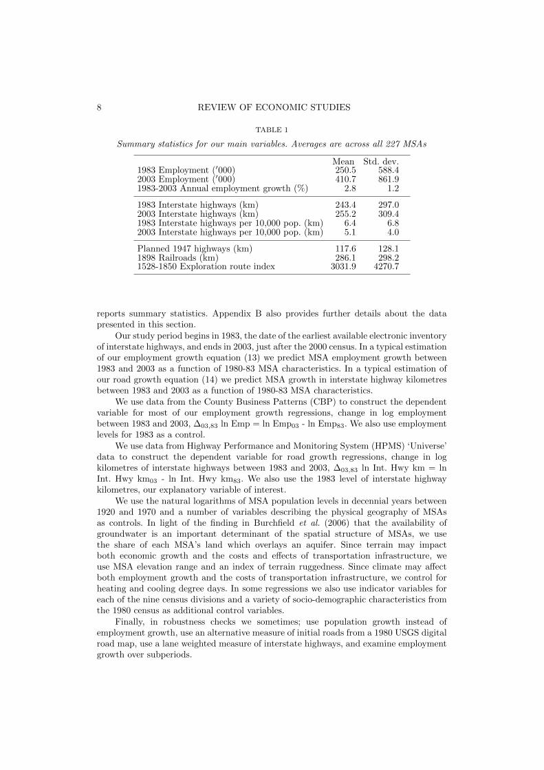
TABLE 1

Summary statistics for our main variables. Averages are across all 227 MSAs

Mean Std. dev.1983 Employment (′000) 250.5 588.42003 Employment (′000) 410.7 861.91983-2003 Annual employment growth (%) 2.8 1.2

1983 Interstate highways (km) 243.4 297.02003 Interstate highways (km) 255.2 309.41983 Interstate highways per 10,000 pop. (km) 6.4 6.82003 Interstate highways per 10,000 pop. (km) 5.1 4.0

Planned 1947 highways (km) 117.6 128.11898 Railroads (km) 286.1 298.21528-1850 Exploration route index 3031.9 4270.7

reports summary statistics. Appendix B also provides further details about the datapresented in this section.

Our study period begins in 1983, the date of the earliest available electronic inventoryof interstate highways, and ends in 2003, just after the 2000 census. In a typical estimationof our employment growth equation (13) we predict MSA employment growth between1983 and 2003 as a function of 1980-83 MSA characteristics. In a typical estimation ofour road growth equation (14) we predict MSA growth in interstate highway kilometresbetween 1983 and 2003 as a function of 1980-83 MSA characteristics.

We use data from the County Business Patterns (CBP) to construct the dependentvariable for most of our employment growth regressions, change in log employmentbetween 1983 and 2003, ∆03,83 ln Emp = ln Emp03 - ln Emp83. We also use employmentlevels for 1983 as a control.

We use data from Highway Performance and Monitoring System (HPMS) ‘Universe’data to construct the dependent variable for road growth regressions, change in logkilometres of interstate highways between 1983 and 2003, ∆03,83 ln Int. Hwy km = lnInt. Hwy km03 - ln Int. Hwy km83. We also use the 1983 level of interstate highwaykilometres, our explanatory variable of interest.

We use the natural logarithms of MSA population levels in decennial years between1920 and 1970 and a number of variables describing the physical geography of MSAsas controls. In light of the finding in Burchfield et al. (2006) that the availability ofgroundwater is an important determinant of the spatial structure of MSAs, we usethe share of each MSA’s land which overlays an aquifer. Since terrain may impactboth economic growth and the costs and effects of transportation infrastructure, weuse MSA elevation range and an index of terrain ruggedness. Since climate may affectboth employment growth and the costs of transportation infrastructure, we control forheating and cooling degree days. In some regressions we also use indicator variables foreach of the nine census divisions and a variety of socio-demographic characteristics fromthe 1980 census as additional control variables.

Finally, in robustness checks we sometimes; use population growth instead ofemployment growth, use an alternative measure of initial roads from a 1980 USGS digitalroad map, use a lane weighted measure of interstate highways, and examine employmentgrowth over subperiods.


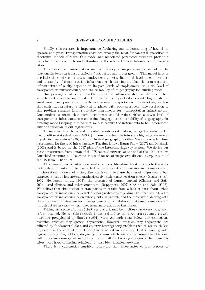
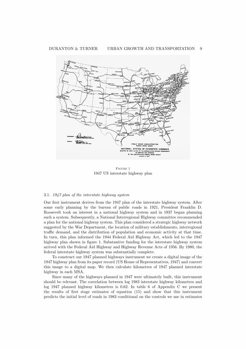
Figure 1

1947 US interstate highway plan

3.1. 1947 plan of the interstate highway system

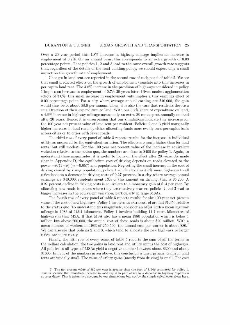
Our first instrument derives from the 1947 plan of the interstate highway system. Aftersome early planning by the bureau of public roads in 1921, President Franklin D.Roosevelt took an interest in a national highway system and in 1937 began planningsuch a system. Subsequently, a National Interregional Highway committee recommendeda plan for the national highway system. This plan considered a strategic highway networksuggested by the War Department, the location of military establishments, interregionaltraffic demand, and the distribution of population and economic activity at that time.In turn, this plan informed the 1944 Federal Aid Highway Act, which led to the 1947highway plan shown in figure 1. Substantive funding for the interstate highway systemarrived with the Federal Aid Highway and Highway Revenue Acts of 1956. By 1980, thefederal interstate highway system was substantially complete.

To construct our 1947 planned highways instrument we create a digital image of the1947 highway plan from its paper record (US House of Representatives, 1947) and convertthis image to a digital map. We then calculate kilometres of 1947 planned interstatehighway in each MSA.

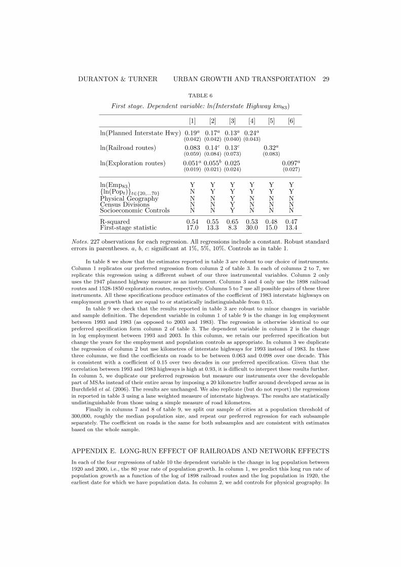
Since many of the highways planned in 1947 were ultimately built, this instrumentshould be relevant. The correlation between log 1983 interstate highway kilometres andlog 1947 planned highway kilometres is 0.62. In table 6 of Appendix C we presentthe results of first stage estimates of equation (15) and show that this instrumentpredicts the initial level of roads in 1983 conditional on the controls we use in estimates


of the structural equations (13) and (14). We repeat these results for the other twoinstruments described below. While exact critical values for weak instrument tests varywith specification and econometric technique, the relevant first-stage statistics for ourinstruments are large enough that our instruments are unlikely to be weak. Thus, ourinstruments satisfy the relevance condition (16).

Condition (17) requires that our instruments affect the growth of city employmentonly through their effect on the initial stock of roads. The 1947 plan was first drawnto ‘connect by routes as direct as practicable the principal metropolitan areas, cities andindustrial centres, to serve the national defense and to connect suitable border points withroutes of continental importance in the Dominion of Canada and the Republic of Mexico’(US Federal Works Agency, 1947, cited in Michaels, 2008). Importantly, the mandate forthe highway plan makes no mention of transportation within cities or future development.In particular, it does not require planners to anticipate employment growth.3 Historicalevidence confirms that the 1947 highway plan was, in fact, drawn to this mandate (seeMertz, undated, and Mertz and Ritter, undated, as well as other sources cited in Chandraand Thompson, 2000, Baum-Snow, 2007, and Michaels, 2008). Further evidence thatthe 1947 highway plan was drawn in accordance with its mandate is obtained directlyfrom the data. In a regression of log 1947 kilometres of planned highway on log 1950population, the coefficient on planned highways is almost exactly one. Adding controlsfor geography and past population growth from the 1920s, 1930s, and 1940s does notchange this result, and pre-1950 population coefficients do not approach conventionallevels of statistical significance. Thus, we conclude that the 1947 plan was drawn, asstipulated by its mandate, to connect major population centres and satisfy the needsof inter-city trade and national defense as of the mid-1940s. In sum, the 1947 highwayplan predicts roads in 1983 but should not predict employment growth between 1983 and2003.

Note that equation (17) requires orthogonality of the dependent variable and theinstruments conditional on control variables, not unconditional orthogonality. This isan important distinction. Cities that receive more roads in the 1947 plan tend to belarger than cities that receive less. Since we observe that large cities grow more slowlythan small cities, 1947 highway planned highway kilometres predicts employment growthdirectly as well operating indirectly through its ability to predict 1983 interstate highwaykilometres. Thus the exogeneity of this instrument hinges on having an appropriate set ofcontrols, historical population variables in particular. This is consistent with our findingbelow that results for the over-identification tests sometimes fail when we do not controlfor historical population levels.

Condition (18) requires that, conditional on controls, our instruments affectroad growth only through their affect on initial roads. Thus, to the extent thatmeasured highway kilometres does not reflect functional highway kilometres, i.e., classicalmeasurement error, we require only that the ‘error’ with which our 1947 highway planmeasures the true stock of highways is independent of the error with which the HPMSmeasures true roads. This seems plausible.

Alternatively, if initial roads and change in roads both depend on some omittedvariable, ‘suitability for roads’ then we should be concerned that the 1947 Highway planvariable, which itself describes an alternative road network, is also partly determined

3. The fact that the interstate highway system quickly diverged from the 1947 plan is consistentwith this mandated myopia: the 1947 plan was amended and extended from about 37,000 to 41,000 milesbefore it was funded in 1956, and additional miles were subsequently added. Some of these additionalhighways were surely built to accommodate population growth that was not foreseen by the 1947 plan.


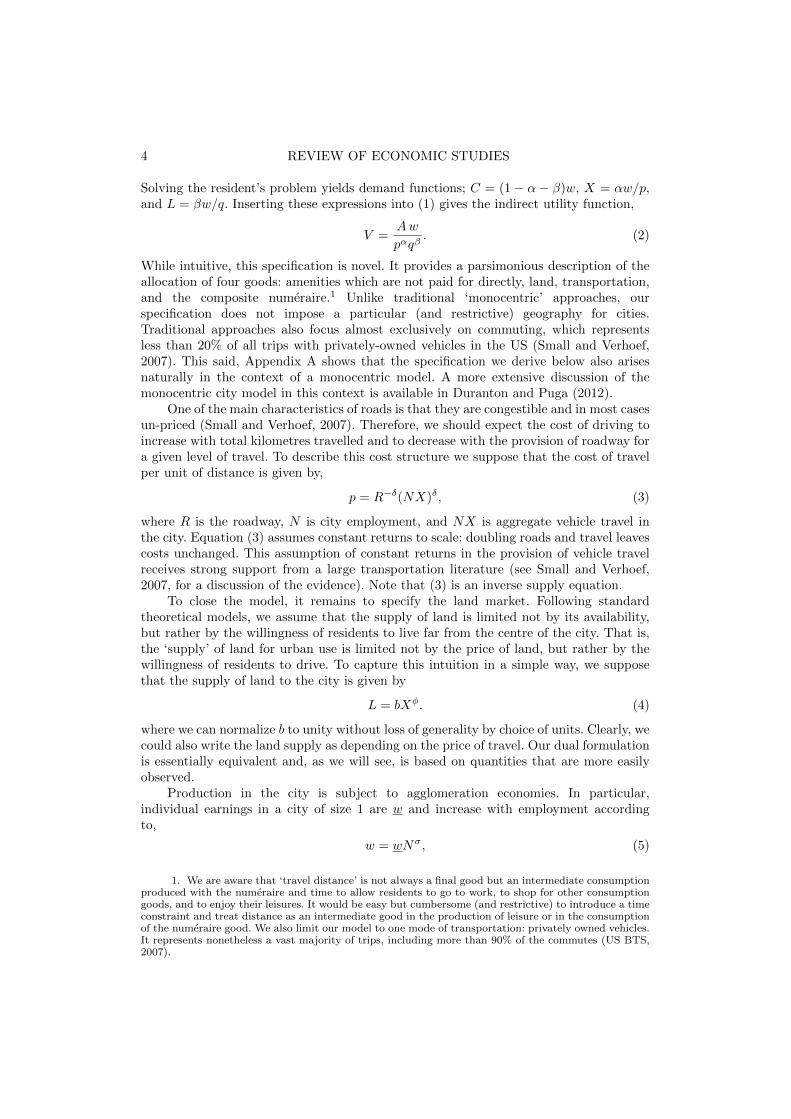
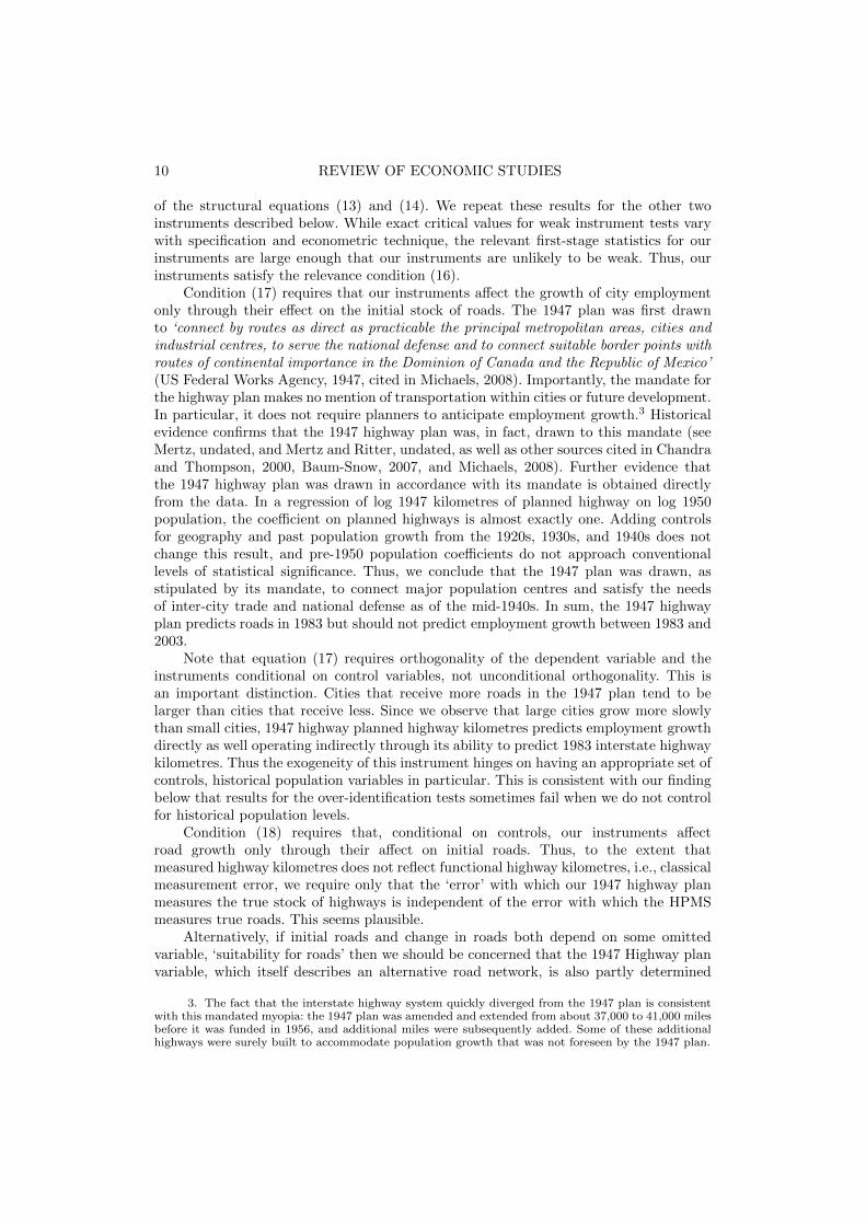
Figure 2

Gray’s map of 1898 railroads

by this unobserved trait. With this said, we expect that any omitted variable whichdetermines our initial road measure, changes in roads, and our instruments will likelyreflect either the physical geography or the industrial composition of a city. If such anomitted variable is important to our estimations we should find that observed measuresof physical geography and industrial composition are important. In our estimations, weinclude these types of variables as controls and find no evidence that they affect ourresults.

3.2. 1898 railroad routes

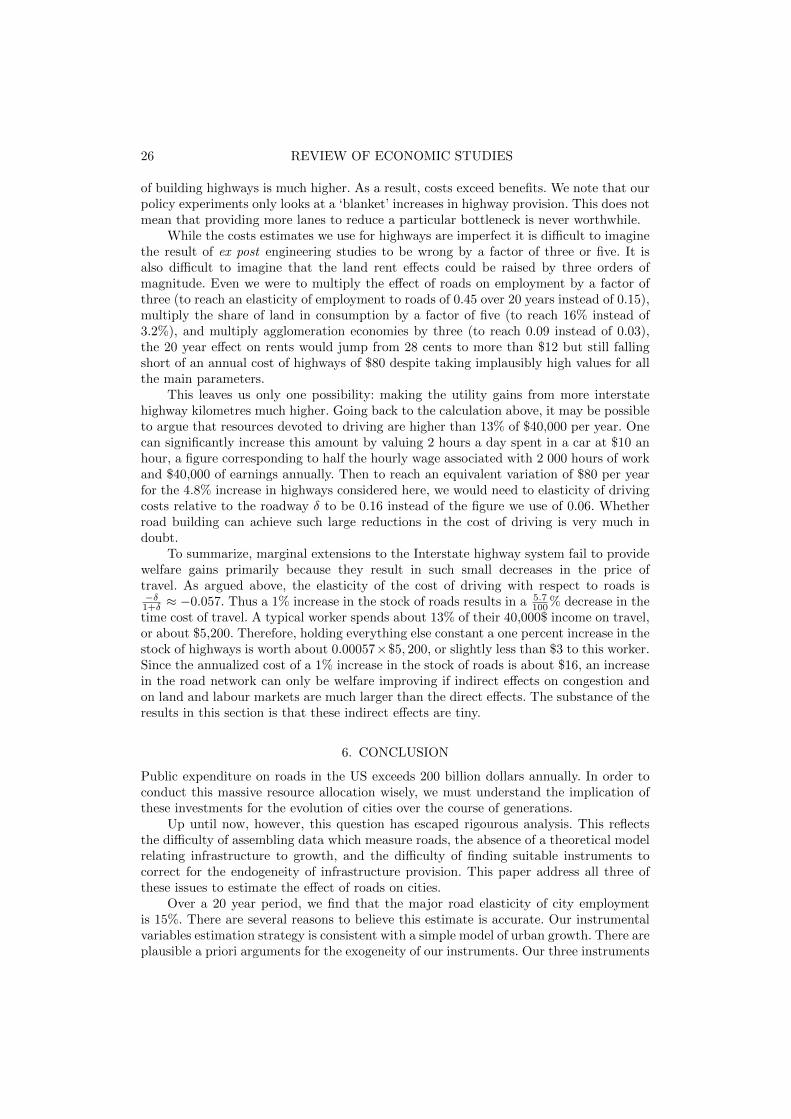
Our second instrument is based on the map of major railroad lines from about 1898(Gray, c. 1898) shown in figure 2. We convert this image to a digital map and calculatekilometres of 1898 railroad contained in each MSA.

Building both railroad tracks and automobile roads requires levelling and gradinga roadbed. Hence, an old railroad track is likely to become a modern road because oldrailroads may be converted to automobile roads without the expense of levelling andgrading. Second, railroad builders and road builders are interested in finding straightlevel routes from one place to another. Thus, the prevalence of old railroads in an MSAis an indicator of the difficulty of finding straight level routes through the local terrain.The ability of the 1898 railroad network to predict the modern highway network isdemonstrated by the 0.53 correlation between log 1983 interstate highways kilometresand log 1898 railroad kilometres, and in representative first stage results reported inAppendix C.

The a priori case for thinking that 1898 railroad kilometres satisfy exogeneitycondition (17) rests on the length of time since these railroads were built and thefundamental changes in the nature of the economy in the intervening years. The rail


network was built, for the most part, during and immediately after the civil war, andduring the industrial revolution. At the peak of railroad construction, around 1890, theUS population was 55 million, with 9 million employed in agriculture or nearly 16% of thepopulation (US Bureau of Statistics, 1899, p. 3 and 10). By 1980, the population of theUS was about 220 million with only about 3.5 million, or 1.6% employed in agriculture(US Bureau of Census, 1981, p. 7 and 406). Thus, while the country was building the1898 railroad network the economy was much smaller and more agricultural than it wasin 1980, and was in the midst of technological revolution and a civil war, both longcompleted by 1980.

Furthermore, the rail network was constructed by private companies who werelooking to make a profit from railroad operations in a not too distant future (Fogel,1964; Fishlow, 1965). It is difficult to imagine how a rail network built for profit duringthe civil war and the industrial revolution could affect economic growth in cities 100years later save through its effect on roads. As for the highway plan, the same importantqualifying comment applies: instrument validity requires that rail routes need only beuncorrelated with the dependent variable conditional on the control variables.

The argument that log 1898 rail kilometres satisfies the second exogeneity condition,i.e., affects road growth only through its affect on initial roads, is the same as for the1947 highway plan.

3.3. Routes of major expeditions of exploration 1528-1850

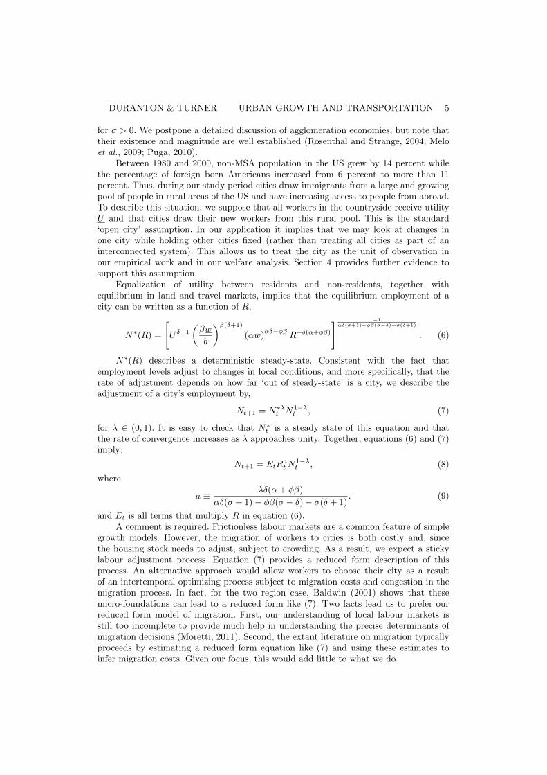
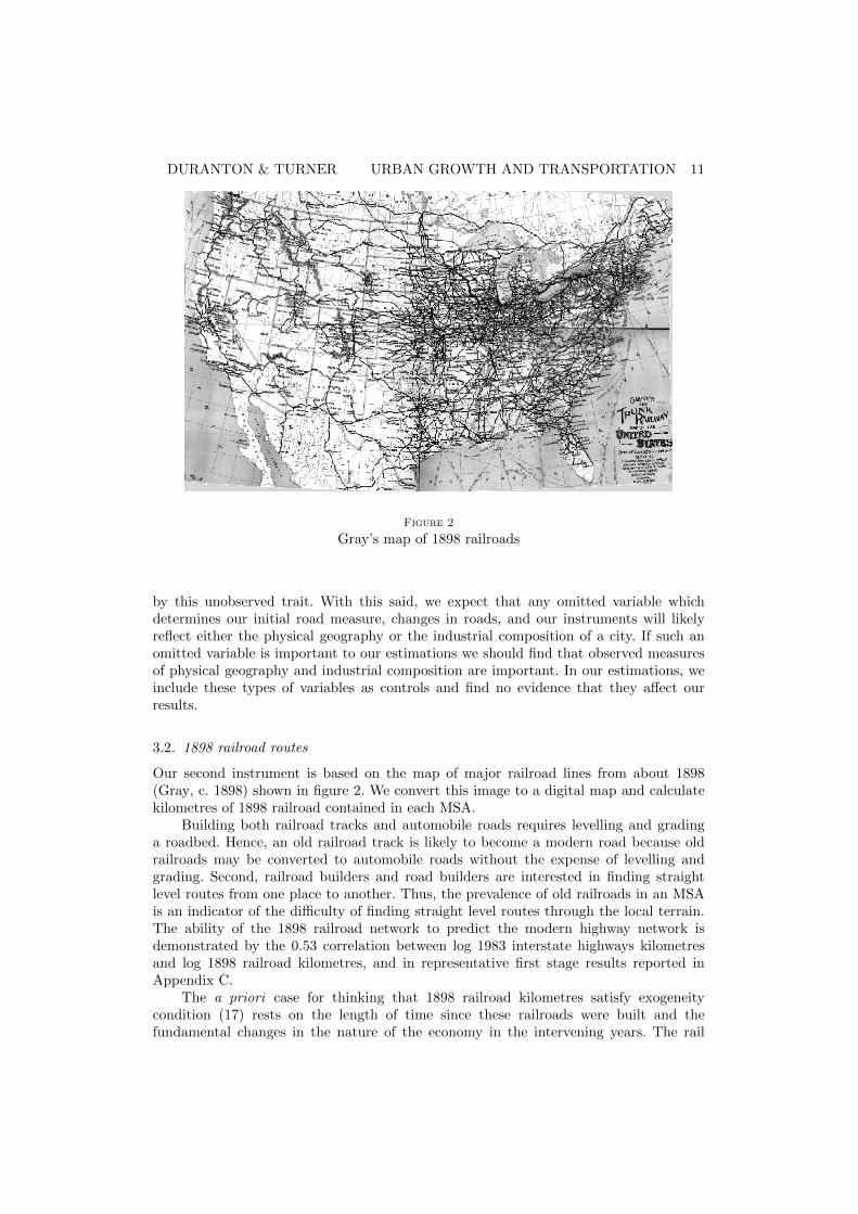
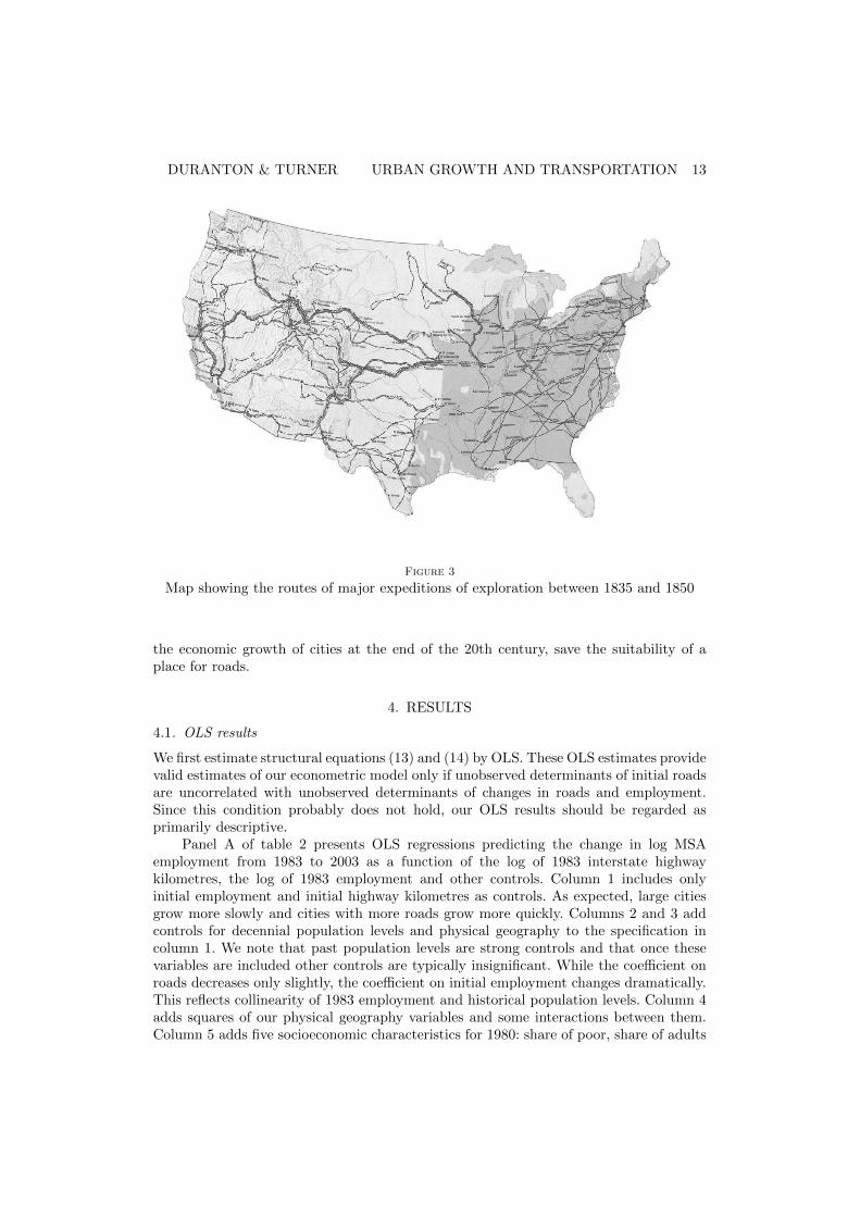
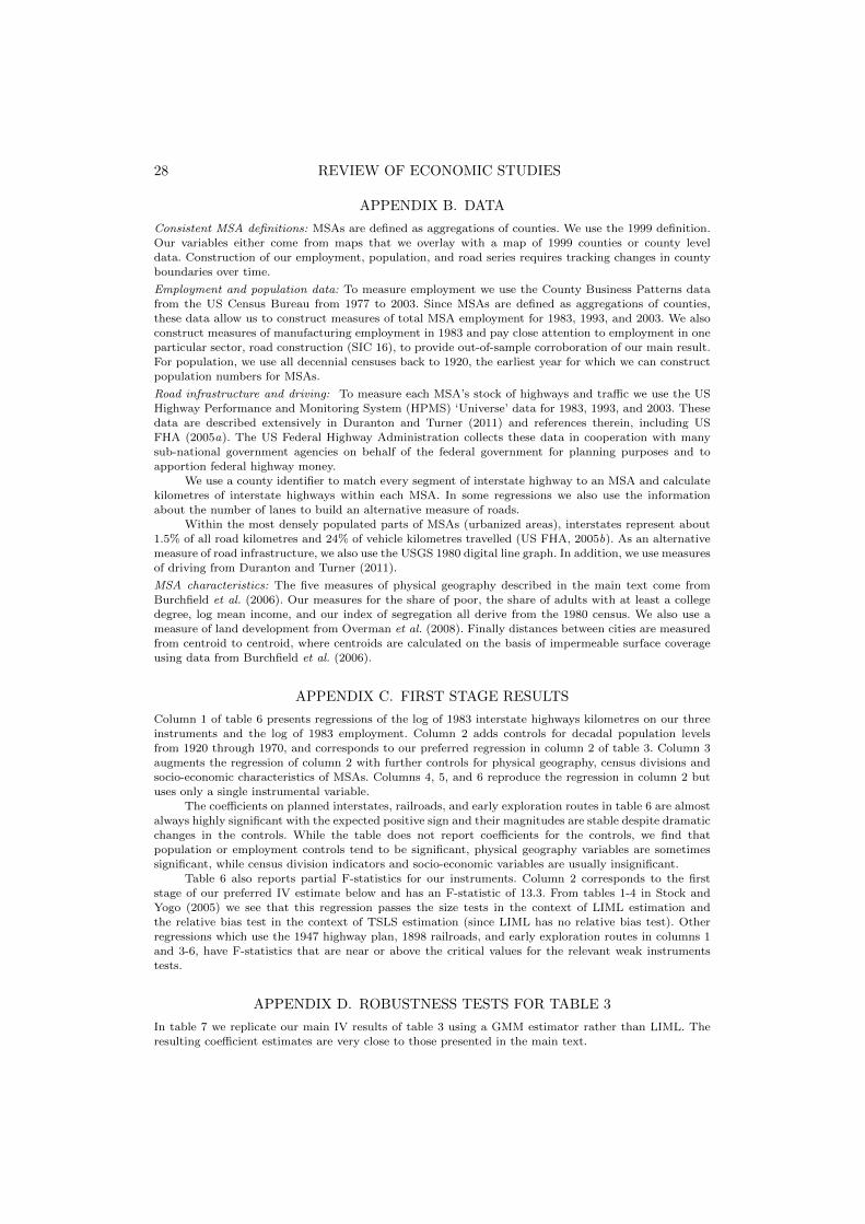
Our third instrument is based on exploration routes in early US history. The NationalAtlas of the United States of America (1970) describes the routes of major expeditionsof exploration that occurred during each of five time periods; 1528–1675, 1675–1800,1800–1820, 1820–1835, and 1835–1850. We digitize each map and count 1 km by 1 kmpixels crossed by an exploration route in each MSA. We then compute our index bysumming those counts across all maps. Following this procedure, routes used throughoutthe 1528-1850 period receive a higher weight than those used for a shorter period of time.We also count minor variants of any route because the existence of such variants reflectsthe intensity with which the route is used. The 1835-1850 map is displayed in figure 3.

Exploration routes result from a search for an easy way to get from one place toanother on foot, horseback, or wagon. Since a good route for a man, horse or wagonwill likely be a good route for a car, exploration routes will often be good routes forcontemporary interstate highways. The ability of the exploration routes variable topredict the modern highway network is demonstrated by the 0.43 correlation betweenthe log of the exploration routes index an 1983 interstate highways kilometres and inrepresentative first stage results reported in Appendix C.

Our maps of exploration routes describe major expeditions of exploration rangingover three centuries; from those of the early Spanish explorers Hernando de Soto andAlvar Nunez Cabeza de Vaca, who explored the American South and Southwest in themid-16th century, to the great French explorer, Robert de LaSalle, who explored theMississippi and the Great Lakes region in the late 17th century, to the famous Lewis andClark expedition of 1804 and to Fremont’s explorations of the West in the mid-1800’s. Themotivations for these expeditions were as varied as the explorers and times in which theylived, from the search for gold and the establishment of fur trading territories to findingemigration routes to Oregon or the expansion of the US territory towards the PacificOcean. Our argument for the exogeneity of these routes rests on the improbability ofthese explorers choosing routes that were systematically related to anything that affects


Figure 3

Map showing the routes of major expeditions of exploration between 1835 and 1850

the economic growth of cities at the end of the 20th century, save the suitability of aplace for roads.

4. RESULTS

4.1. OLS results

We first estimate structural equations (13) and (14) by OLS. These OLS estimates providevalid estimates of our econometric model only if unobserved determinants of initial roadsare uncorrelated with unobserved determinants of changes in roads and employment.Since this condition probably does not hold, our OLS results should be regarded asprimarily descriptive.

Panel A of table 2 presents OLS regressions predicting the change in log MSAemployment from 1983 to 2003 as a function of the log of 1983 interstate highwaykilometres, the log of 1983 employment and other controls. Column 1 includes onlyinitial employment and initial highway kilometres as controls. As expected, large citiesgrow more slowly and cities with more roads grow more quickly. Columns 2 and 3 addcontrols for decennial population levels and physical geography to the specification incolumn 1. We note that past population levels are strong controls and that once thesevariables are included other controls are typically insignificant. While the coefficient onroads decreases only slightly, the coefficient on initial employment changes dramatically.This reflects collinearity of 1983 employment and historical population levels. Column 4adds squares of our physical geography variables and some interactions between them.Column 5 adds five socioeconomic characteristics for 1980: share of poor, share of adults


TABLE 2

Growth of employment and roads as a function of initial roads, OLS estimates

[1] [2] [3] [4] [5] [6] [7] [8]

Panel A: Employment or population growth

ln(Int. Hwy km83) 0.073a 0.074a 0.061a 0.060a 0.042a 0.030b 0.056a(0.017) (0.013) (0.014) (0.014) (0.014) (0.015) (0.014)

ln(Emp83) -0.086a -0.24 -0.26 -0.26 -0.26 -0.25 -0.27 0.26a(0.020) (0.19) (0.19) (0.19) (0.22) (0.23) (0.19) (0.077)

ln(USGS maj. roads80) 0.17a(0.030)

R-squared 0.11 0.43 0.47 0.48 0.53 0.59 0.46 0.64

Panel B: Road growthln(Int. Hwy km83) -0.52a -0.53a -0.54a -0.55a -0.56a -0.54a

(0.10) (0.10) (0.11) (0.11) (0.10) (0.089)

ln(Emp83) 0.34a 0.31b 0.29b 0.28b 0.19c 0.12 0.25c(0.067) (0.12) (0.12) (0.12) (0.11) (0.098) (0.15)

ln(USGS maj. roads80) -0.22(0.14)

R-squared 0.54 0.55 0.56 0.57 0.59 0.63 0.06

ln(Popt)t∈20,...70 N Y Y Y Y Y Y YPhysical Geography N N Y Ext. Ext. Ext. N NSocioeconomic controls N N N N Y Y N NCensus Divisions N N N N N Y N N

Notes. 227 observations for each regression. All regressions include a constant. Robust standarderrors in parentheses. a, b, c: significant at 1%, 5%, 10%. Panel A: Dependent variable is∆03,83 ln Emp in columns 1-7 and ∆00,80 log Pop in column 8. Panel B: Dependent variable is∆03,83 log Interstate Highway kilometres.

with at least some college education, log mean income, a segregation index, and shareof manufacturing employment. Column 6 further adds census division indicators. Thisextensive set of controls reduces the coefficient on initial roads.

In column 7, we repeat column 3 but measure initial roads with log 1980 USGS majorroads kilometres. This leads to a somewhat larger estimated coefficient for roads than inthe corresponding coefficient in column 3. We suspect that this reflects the process bywhich roads are selected into the 1980 USGS map. In column 8, we also duplicate theregression of column 3 but use the change in log population from 1980 to 2000 as ourdependent variable. Using this alternative dependent variable leads to a slightly lowercoefficient on initial roads than we see in column 3.

Despite differences across specifications, the OLS elasticity of city employmentrelative to initial roads remains low, between 0.03 and 0.17. If we restrict attention toregressions predicting change in employment as a function of initial interstate highway,the range of estimates is just 0.03 to 0.07.

Panel B of table 2 is similar to panel A, except that the dependent variable ischange in log interstate highway kilometres from 1983 to 2003 rather than change in logemployment (or population). Where panel A presents estimates of equation (13), panelB presents estimates of equation (14).


In column 1 of table 2 panel B, we include only two regressors, the log of kilometresof 1983 interstate highways and the log of 1983 employment. As expected, growth inlog interstate highway kilometres increases with 1983 employment, but this increaseis far from proportional. There is also strong mean reversion in road provision. Thecoefficient on initial roads is −0.52. In columns 2 to 6, we gradually add more controls.The coefficient on 1983 interstate highways remains stable across these specificationsand is estimated quite accurately. The coefficient on log 1983 employment is positiveand statistically different from zero in almost all specifications except for column 6.Given the high correlation between 1983 employment and historical employment levels,it is not surprising that the coefficient on log 1983 employment is less stable acrossspecifications than is the coefficient on log 1983 interstate highway kilometres. In column7, we repeat the estimation of column 3, but use log 1980 USGS major road kilometresas our measure of initial roads. Reassuringly, the point estimate for this coefficient isalso negative, though unsurprisingly, it has less explanatory power than does log 1983interstate highway kilometres. Column 8 of panel A uses an alternative measure of citygrowth as a robustness check. Data limitations preclude a similar exercise for changes inroads, so that panel B has no regression corresponding to column 8 of panel A.

4.2. Main IV results

Table 3 presents our main results. Since it provides more reliable point estimates andtest statistics with weak instruments than TSLS, we use limited information maximumlikelihood (LIML) to separately estimate the two structural equations for change inemployment and change in roads, with the initial stock of roads treated as endogenous.In all regressions we use all three of our instruments, 1947 planned interstate highwaykilometres, 1898 kilometres of railroads, and our index of 1528-1850 exploration routes.The format of the table is similar to table 2. In panel A the dependent variable is ameasure of city growth, change in log employment from 1983 to 2003 for columns 1-7,and change in log population from 1980 to 2000 for column 8. In panel B the dependentvariable is the change in log interstate highway kilometres from 1983 to 2003. In allcolumns but 7, we use log 1983 interstate highway kilometres to measure initial roads.As a robustness check, column 7 uses log 1980 USGS major road kilometres to measureinitial roads. The control variables used in each column of table 3 match the correspondingcolumn of table 2.

In column 1 of panel A, we estimate the effect of log 1983 interstate highwaykilometres and log 1983 employment on the change on log employment from 1983 to2003. The coefficient on 1983 interstate highway kilometres is 0.13. In column 2 we addhistorical population levels as controls, and in column 3 we also control for physicalgeography. In both columns the coefficient on initial roads is 0.15 and is -0.26 and -0.27for initial employment levels. Columns 4-6 add more control variables to the specificationof column 3. The coefficient estimates for initial roads and employment are remarkablystable across the first six columns of panel A. Because of collinearity between 1983employment and historical population, the effect of initial employment on change inemployment is not statistically distinguishable from zero, except in column 1 where wedo not include historical population levels as controls. In column 7 we use log 1980USGS major road kilometres to measure initial roads. As for the OLS results, we finda somewhat larger coefficient. In column 8 we use the same specification as in column3, but use change in log population from 1980 to 2000 as our dependent variable. The


TABLE 3

Growth of employment and roads as a function of initial roads, LIML IV

[1] [2] [3] [4] [5] [6] [7] [8]


ln(Int. Hwy km83) 0.13b 0.15a 0.15a 0.16a 0.13b 0.096c 0.13a(0.056) (0.037) (0.043) (0.047) (0.054) (0.053) (0.030)

ln(Emp83) -0.11a -0.26 -0.27 -0.27 -0.27 -0.28 -0.30 0.24a(0.037) (0.19) (0.19) (0.19) (0.21) (0.21) (0.19) (0.075)


Overid p-value 0.04 0.96 0.93 0.59 0.65 0.59 0.18 0.47

Panel B: Road growth

ln(Int. Hwy km83) -0.27a -0.28a -0.26a -0.26a -0.28a -0.25b(0.086) (0.093) (0.099) (0.097) (0.10) (0.10)

ln(Emp83) 0.21a 0.25b 0.26b 0.26b 0.14 0.017 0.34b(0.050) (0.11) (0.11) (0.12) (0.091) (0.099) (0.17)

ln(USGS maj. roads80) -0.53b(0.23)

Overid p-value 0.42 0.41 0.54 0.57 0.72 0.96 0.47


First-stage statistic 17.0 13.3 11.8 13.9 11.3 9.7 11.9 13.3

Notes. 227 observations for each regression. All regressions include a constant. Robust standarderrors in parentheses. a, b, c: significant at 1%, 5%, 10%. Panel A: Dependent variable is∆03,83 ln Emp in columns 1-7 and ∆00,80 ln Pop in column 8. Panel B: Dependent variable is∆03,83 ln Interstate Highway kilometres. All regressions use 1947 planned highway kilometres,1898 kilometres of railroads, and index of 1528-1850 exploration routes as instruments.

resulting coefficient on initial roads is not statistically different from estimates in columns1-6.

Table 3 panel A also reports the p-values for an over-identification test (Hansen’s Jstatistic). For our preferred specification in column 3, the p-value of this statistic is 0.93,so that we easily fail to reject our over-identifying restriction. In fact, in all columns of thetable, except for column 1, we easily fail to reject our overidentifying restriction. Recallthat the over-id test is a test of joint-exogeneity. In particular, instruments can pass thistest if they are all endogenous and the bias that this endogeneity induces is of similarsign and magnitude. Given different rationales for the exogeneity of the planned highwaynetwork, the 1898 rail network, and early exploration routes, this sort of endogeneityseems unlikely.

In column 1, our test of over-identifying restrictions marginally fails. This suggeststhat, consistent with our intuition, highway planners in 1947 and railroad builders in the19th century did choose routes on the basis of factors like contemporaneous populationthat affect 1983 to 2003 employment growth independently of roads. It follows that our


instruments are probably not exogenous when we do not control for historical populationlevels.

To sum up, our preferred estimate in column 2 gives a value of 0.15 for the parametera in equation (10). This value implies that 10% more interstate highway kilometres in1983 leads to 1.5% more employment after 20 years.

Panel B presents results describing the effect of the initial level of interstate highwayon its subsequent provision. This panel duplicates panel A, but uses changes in loginterstate highway kilometres from 1983 to 2003 as the dependent variable rather thanchanges in log employment. In columns 1 to 6, the coefficient on log 1983 interstatehighway kilometres is extremely stable, between -0.25 and -0.28, is estimated preciselyand is statistically different from zero. The coefficient for log of initial employment isalso fairly stable across specifications, and is statistically different from zero except whenwe use the very extensive sets of controls in columns 5 and 6. In column 7 we measurethe initial stock of roads with log 1980 USGS major road kilometres. While the pointestimate for the coefficient for this variable is larger in magnitude than the coefficientfor log 1983 interstate highway variable kilometres, it is not different at standard levelsof confidence.

Given that the first stage for regressions in panel B is the same as for panel A, thefirst stage statistics are the same and hence pass weak instrument tests. We also alwayseasily fail to reject our over-identifying restrictions.

Our preferred estimate in column 3 gives a value of 0.27 for the parameter θ inequation (12). This value implies that 10% more interstate highway kilometres in 1983leads to 2.7% less growth in the provision of roads over the subsequent 20 years. Putdifferently, a standard deviation of 1983 interstate highways corresponds to a negativestandard deviation in road growth over the following 20 years.

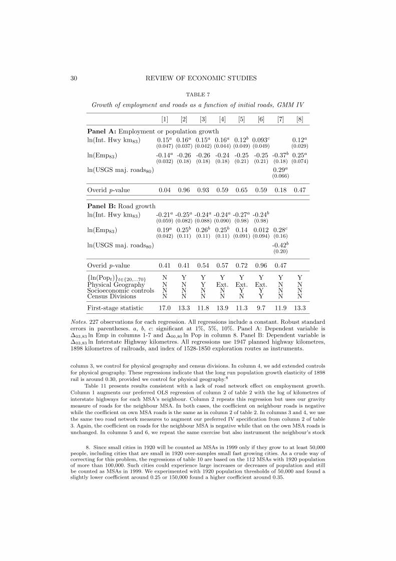
In Appendix D we verify the robustness of the results presented in table 3. Table7 repeats the estimations of table 3 using GMM estimation. The GMM estimations arepractically indistinguishable from the LIML estimations. Table 8 demonstrates that ourmain results do not vary when we use subsets of our three instruments. Table 9 showsthat our results do not vary if we measure changes in employment over sub-periods ofour study period, if we split our sample into large and small cities, or if we recalculateour instruments on the basis the developed area of MSA’s as described in Appendix B.

4.3. Discussion

Table 3 suggests that a 10% increase in an MSA’s stock of interstate highways in 1983causes the MSA’s employment to increase by about 1.5% over the course of the following20 years. Since the standard deviation of log 1983 interstate highways is 0.98, using ourpreferred estimate from table 3 panel A, a one standard deviation increase in the logof 1983 interstate highway kilometres causes a 15% increase in employment over thefollowing 20 years. This is slightly less than two thirds of the standard deviation of theMSA employment growth rate during our study period. Thus, the effects of roads onurban growth are large in absolute terms.

The effects of roads on urban growth are also large relative to the three widelyaccepted drivers of recent urban growth in the US: good weather, human capital, anddynamic externalities. According to the findings of Glaeser and Saiz (2004) for US MSAsbetween 1970 and 2000, one standard deviation in the proportion of university graduatesat the beginning of a decade is associated with a quarter of a standard deviation ofpopulation growth. In his analysis of the effects of climate for US counties since 1970,


Rappaport (2007) finds that one standard deviation increases in January and Julytemperature are associated with, respectively, an increase of 0.6 standard deviation ofpopulation growth and a decrease of 0.2 of the same quantity. A direct comparison withthe findings of Glaeser et al. (1992) on dynamic externalities is more difficult but astandard deviation of their measures of dynamic externalities is never associated withmore than a fifth of a standard deviation of employment growth for city-industries. Insum, that a standard deviation in roads per worker causes nearly two thirds of a standarddeviation in employment growth suggests that roads and infrastructure are importantdrivers of urban growth.

Our results also highlight two important aspects of the provision of new interstatehighways: strong mean reversion and a small effect of initial MSA employment. Thesetwo results are consistent with core features of the policy for funding transportationinfrastructure in the US. This policy tends to equalize spending per capita across differenttypes of areas. Because roads are more expensive to build in larger MSAs (Ng and Small,2008), large cities get fewer new roads per capita and the provision of interstate highwaysthen falls behind urban growth.

4.4. Explaining the differences between OLS and IV

Column 2 of table 3 gives our preferred estimate of the effect of initial roads onemployment growth. At 0.15, this LIML IV estimate is more than twice as large as thecorresponding OLS estimate of 0.06 from table 2. More generally, the LIML IV estimatesof the effects of initial roads on employment growth are dramatically larger than thesimilar OLS estimates.

Larger LIML IV than OLS coefficient estimates for endogenous initial roads may bedue to classical measurement error. If so, then the larger LIML IV than OLS coefficientestimate for the effect of log of 1980 USGS major road kilometres on employmentgrowth is probably also due to measurement error. However, for both road measures,OLS coefficient estimates increase by about a factor of two in LIML IV. This meansthat the effect of measurement error on coefficient estimates is about the same forboth variables. Given the different nature of the two measures of roads, this seemsimprobable. Furthermore, if classical measurement error were behind the LIML IV versusOLS difference, we should see a similar difference in regressions which predict growth ofroads. In fact, for these regressions, we see the opposite pattern.

Another explanation for larger LIML IV than OLS coefficient estimates is a negativecorrelation between properly measured log 1983 interstate highway kilometres and theerror term in equation (13). This could be due to either missing variables or reversecausation. One possible missing variable is ‘good consumption amenities’, which couldbe associated faster employment growth during 1983 to 2003 and with fewer interstatehighways in 1983. While past population and geography are powerful controls, thepossibility remains that the difference between our LIML IV and OLS estimates couldbe explained by such a missing variable.

Turning to reverse causation, it may be that conditional on controls, cities whichexperience negative shocks to employment, also on average experience positive shocks totheir stock of roads. While our data do not allow us to test this hypothesis directly, weare able to look at the relationship between changes in city employment and changes inemployment in road construction — a precursor of new roads.

To investigate the proposition that roads are given to cities experiencing negativegrowth shocks, we use detailed employment data from the CBP to calculate the share


TABLE 4

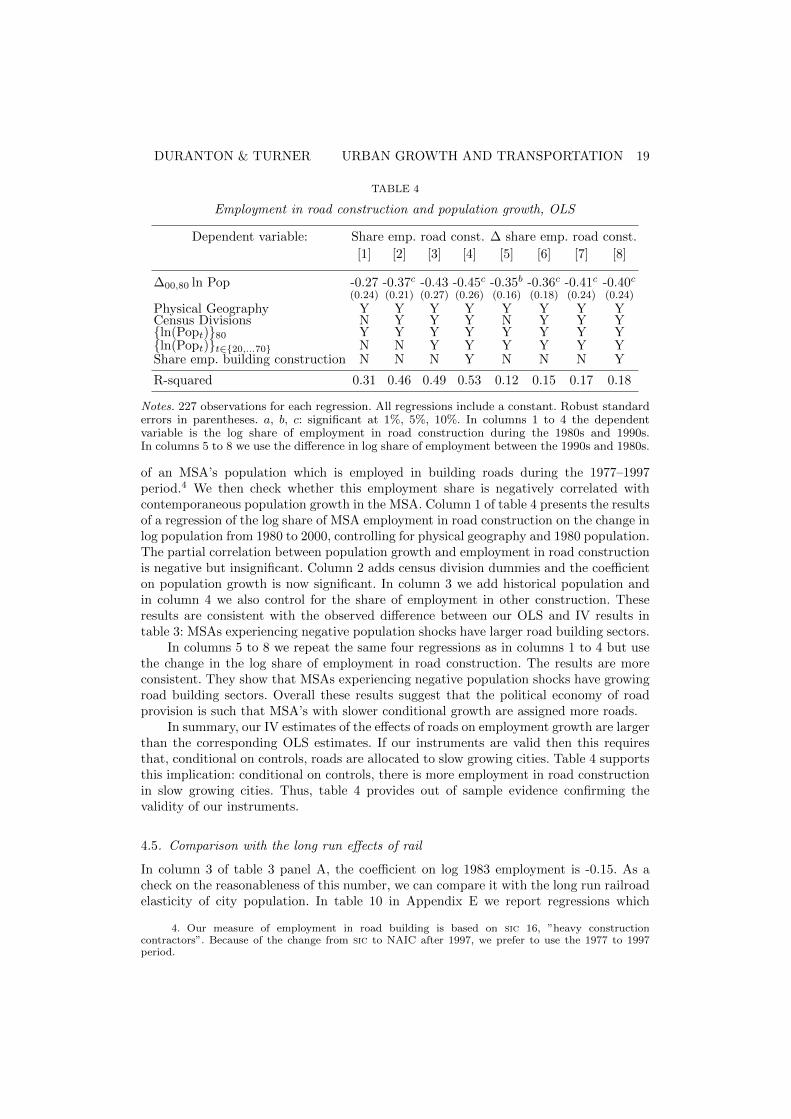
Employment in road construction and population growth, OLS

Dependent variable: Share emp. road const. ∆ share emp. road const.

[1] [2] [3] [4] [5] [6] [7] [8]

∆00,80 ln Pop -0.27 -0.37c -0.43 -0.45c -0.35b -0.36c -0.41c -0.40c(0.24) (0.21) (0.27) (0.26) (0.16) (0.18) (0.24) (0.24)

Physical Geography Y Y Y Y Y Y Y YCensus Divisions N Y Y Y N Y Y Yln(Popt)80 Y Y Y Y Y Y Y Yln(Popt)t∈20,...70 N N Y Y Y Y Y YShare emp. building construction N N N Y N N N Y

R-squared 0.31 0.46 0.49 0.53 0.12 0.15 0.17 0.18

Notes. 227 observations for each regression. All regressions include a constant. Robust standarderrors in parentheses. a, b, c: significant at 1%, 5%, 10%. In columns 1 to 4 the dependentvariable is the log share of employment in road construction during the 1980s and 1990s.In columns 5 to 8 we use the difference in log share of employment between the 1990s and 1980s.

of an MSA’s population which is employed in building roads during the 1977–1997period.4 We then check whether this employment share is negatively correlated withcontemporaneous population growth in the MSA. Column 1 of table 4 presents the resultsof a regression of the log share of MSA employment in road construction on the change inlog population from 1980 to 2000, controlling for physical geography and 1980 population.The partial correlation between population growth and employment in road constructionis negative but insignificant. Column 2 adds census division dummies and the coefficienton population growth is now significant. In column 3 we add historical population andin column 4 we also control for the share of employment in other construction. Theseresults are consistent with the observed difference between our OLS and IV results intable 3: MSAs experiencing negative population shocks have larger road building sectors.

In columns 5 to 8 we repeat the same four regressions as in columns 1 to 4 but usethe change in the log share of employment in road construction. The results are moreconsistent. They show that MSAs experiencing negative population shocks have growingroad building sectors. Overall these results suggest that the political economy of roadprovision is such that MSA’s with slower conditional growth are assigned more roads.

In summary, our IV estimates of the effects of roads on employment growth are largerthan the corresponding OLS estimates. If our instruments are valid then this requiresthat, conditional on controls, roads are allocated to slow growing cities. Table 4 supportsthis implication: conditional on controls, there is more employment in road constructionin slow growing cities. Thus, table 4 provides out of sample evidence confirming thevalidity of our instruments.

4.5. Comparison with the long run effects of rail

In column 3 of table 3 panel A, the coefficient on log 1983 employment is -0.15. As acheck on the reasonableness of this number, we can compare it with the long run railroadelasticity of city population. In table 10 in Appendix E we report regressions which

4. Our measure of employment in road building is based on sic 16, ”heavy constructioncontractors”. Because of the change from sic to NAIC after 1997, we prefer to use the 1977 to 1997period.


predict the change in MSA population between 1920 and 2000, i.e., the 80 year rate ofpopulation growth, as a function of the MSA’s stock of 1898 railroads. After we controlfor initial population and physical geography, we find that the long run population growthelasticity of 1898 rail is around 0.30. While a comparison of the long run effect of rail andthe long run effect of 1983 interstate highways is a bit strained, the relevant elasticitiesare close.

4.6. The roles of internal transportation versus market access

Our analysis so far implicitly assumes that changes to an MSA’s roads affect employmentby changing the cost of driving within this MSA. However, it is possible that changes tothe road network affect an MSA’s employment by improving its access to markets (i.e.,by reducing transportation costs of accessing markets outside the MSA).

The hypothesis that roads affect employment through market access has twoimplications. First, that an MSA’s employment increases with improvements to its ownroads. Second that an MSA’s employment increases with improvements in the roadnetwork of its trading partners, because such improvements also reduce the cost ofaccessing markets. By checking whether changes to roads in neighbouring MSAs affectemployment in the subject MSA, we can test whether roads affect an MSA’s employmentby reducing the costs of travelling within the MSA or by improving market access.

We calculate two measures of neighbouring MSAs’ stocks of roads. First, for eachMSA we identify the largest MSA which is between 150 and 500 kilometres away, i.e.,too far to commute but still within a day’s drive. For each such neighbouring MSA wecalculate two measures of roads. The first is simply the log kilometres of 1983 interstatehighways. The second is a ‘gravity’ based measure,

Neighbour gravity =Neighbour population×Neighbour Interstate Highway km

Distance to neighbour.

In table 11 in Appendix E we present regressions which test for the role of networkeffects by including these two measures of roads in a regression (like that of column 2 oftable 3) predicting change in employment as a function of initial roads. While we cannotprove a negative statement, these results are consistent with our premise that the changesin road infrastructure affect city employment growth by affecting driving within the city,not by affecting market access. This conclusion is consistent with Duranton et al. (2011)who find that a city’s road network does not affect the total value of inter-city trade,although it does affect the composition of this trade.

5. USING OUR MODEL

We now recover the structural parameters of our model and use them to conduct anumber of policy experiments.

5.1. Recovering the structural parameters

Our model has nine structural parameters: α (share of transportation in expenditure), β(share of land in expenditure), δ (elasticity of unit transportation costs to road provision),λ (employment adjustment), η (elasticity of current roads to past employment), θ (roadadjustment), σ (agglomeration economies), φ (land supply elasticity), and w (rural wage).Using our estimates and others from the literature, we now assign values to each of thesevariables.


From our estimation of equation (13), we obtain a (a function of α, β, δ, λ, and σ)and λ. For a, our preferred value is a = 0.15 as obtained from our favourite specificationin column 2 of table 3. For λ, the strong collinearity between log 1980 population andlog 1983 employment makes its estimation sensitive to the inclusion of the populationcontrols. We retain λ = 0.11 from column 1 of table 3, a specification that does notcontrol for population.

From our estimation of equation (14), we obtain η and θ. For η, our preferred value is

η = 0.25 from column 2 of table 4. For θ, the same estimation yields θ = 0.28. Despite thestrong collinearity between log 1980 population and log 1983 employment, the coefficienton initial employment is virtually the same as in column 1 of the same table, where wedo not control for historical population levels.

The parameter α is the share of transportation in expenditure. According to theUS BTS (2007), US households devoted slightly above 13% of their income on average(and 18% for the median) to transportation, 95% of which is associated with buying,maintaining, and operating a private vehicle. This suggests 0.13 as an estimate for α.

The parameter β is the share of land in expenditure, and our estimate for thisparameter is β = 0.032. We calculate our estimate for this parameter from estimatesof the share of housing in consumption and the share of land in housing production.The details of this calculation are given in Appendix F. In the same appendix, we alsoestimate φ to be 0.70.

The parameter δ is the elasticity of unit transportation costs to road provision.Duranton and Turner (2009) provide direct estimates of δ by estimating the MSA meancost of driving (as measured by inverse speed) as a function of interstate lane kilometres.

Their preferred estimate is δ = 0.06.5 Alternatively, using the first order condition forutility maximization with respect to driving distance and inserting it into expression (3)implies that equilibrium driving is

X = Rδ

1+δN−δ

1+δ (αw)1

1+δ . (19)

This exact expression is estimated in Duranton and Turner (2011). For roads andpopulation, they find coefficients that are equal but opposite in sign as predicted by(19). Depending on the particular measure of driving that they use, their results yield avalue of δ between 0.05 and 0.10. Although this procedure is less direct and less precise,it yields results consistent with our preferred value of 0.06.

To approximate w, the reservation wage in a city of size one, we use the 1980Statistical Abstract of the United States to find national average hourly wage and hoursworked in 1979. This gives us mean weekly earnings of 212$. Multiplying by weeks peryear, adjusting to 2007 dollars, and rounding up to the nearest thousand, we have $32,000per year.

A large literature estimates σ. Rosenthal and Strange (2004) survey earlier estimatesand conclude that the range for σ is between 0.04 and 0.08. More recent estimates thatdeal with a series of econometric problems find somewhat lower values. Davis et al. (2009)find a value of 0.02 for σ in the US. Glaeser and Resseger (2010) suggest a value of 0.04or less. These estimates are consistent with recent estimates obtained in other countries(e.g., Combes et al., 2010, for France). Our preferred value of 0.03 is central in the rangeof these estimates.

5. Page 23, table 6, column 4.


5.2. Policy experiment: road building

We now compare status quo and alternative highway policies. A transportation policyis a sequence describing the provision of roads in each period from 0 to T , (Rt)

Tt=0.

Our estimates of equation (14) describe the realized equilibrium transportation policy.Equation (13) describes the evolution of employment, (Nt)

Tt=0, associated with this policy.

To assess the optimality of observed policy, we compare it with alternative policies. Analternative policy is an alternative sequence of roads, (Rt)

Tt=0. It generates an alternative

sequence of employment, (Nt)Tt=0.

Our model consists of two classes of agents, city residents, whose preferences we havedescribed, and an implicit class of absentee landlords who own land in the city. For arepresentative resident, let Vt and Vt denote utility at t (as defined in equation 2) underthe status quo and alternative policies. For a resident, the change in welfare only involvesthe difference between these two quantities. We monetize this change using the standardnotion of equivalent variation, which we denote EVt. In Appendix G, we establish thatunder the assumptions of section 2, equivalent variation for our representative agent is

EVt = wNσ

( RtRt

) δ(α+βφ)δ+1 (

Nt

Nt

)αδ(σ+1)+(β−1)σ(δ+1)−βφ(σ−δ)δ+1

− 1

. (20)

Let πt and πt denote per capita land rents under the status quo and alternativetransportation policy, and ∆πt = πt − πt the per capita change in land rents. AppendixG shows that,

∆πt = βw[Nσt −Nσ

t

]. (21)

The change in welfare on a per capita basis caused by the change from the status quo tothe alternative policy for period t is the sum of EVt and ∆πt. Note that we use averagewelfare rather than total welfare. This relieves us of some accounting when employmentlevels change. It is equal to

∆Ωt = EVt + ∆πt . (22)

The total change in welfare is the corresponding discounted sum,

ΣTt=0ρt∆Ωt. (23)

Our simulations take 1983 as their initial date and 2083 as their terminal date, sothat T varies from 0 to 99. We take the annual social discount rate to be 5%. After100 years, the discount factor is about 1/130 so there is no reason to expect that longersimulations will arrive at qualitatively different conclusions. Our estimations describechanges over a 20 year period and thus our estimates of equations (13) and (14) predictthe path of roads and employment at 20 year intervals. We construct annual predictionsby linear interpolation of the 20 year values given by the model.

It remains to assess the costs of a change in transportation policy. According tothe Congressional Budget Office, the average kilometre of interstate completed after1970 came at a cost of nearly 21 million of 2007 dollars. Ng and Small (2008) arrive atgenerally higher estimates for interstate highways in metropolitan areas. In particular for2006, they find that the total costs of an extra lane kilometre of interstate are: m$3.64 forMSAs with a population less than 200,000; m$5.34 for MSAs with a population between200,000 and 1 million; and m$11.96 for MSAs with a population greater that 1 million.Multiplying by about 4.69 lanes for an average lane kilometre of 1983 MSA interstate in


our sample gives construction costs per interstate kilometre of: m$17.07 per kilometresfor MSAs with a population less than 200,000; m$25.04 per kilometres for MSAs with apopulation between 200,000 and 1 million; and m$56.09 per kilometres for MSAs with apopulation greater that 1 million. In what follows we maintain the Ng and Small (2008)classification of ‘small’, ‘intermediate’ and ‘large’ MSAs.

Around 136 billion dollars per year are spent on maintaining the federal road system(US BTS, 2007). The interstate highway system accounts for about one quarter of allpassenger miles on this system. If we suppose that about one quarter of all maintenancedollars are also directed to the 75000 kilometres of interstate highways, maintenanceof these roads is about 450,000 dollars per kilometres annually. This is probably anunderstatement since highways within MSAs are more intensively used and thus requiremore maintenance. Taking a cost of capital of 5% per year, we have total costs perinterstate kilometre per year of: m$1.30 for MSAs with a population less than 200,000;m$1.70 for MSAs with a population between 200,000 and 1 million; and m$3.25 for MSAswith a population greater that 1 million. Letting pR denote the cost of a kilometre ofinterstate in a given city, the annual per capita cost of changing from transportationpolicy (Rt)

Tt=0 to (Rt)

Tt=0 is pR(Rt −Rt)/Nt.

Putting together the calculation of changes in welfare and changes in cost, we havethat the alternative transportation plan, (Rt)

Tt=0, is socially preferred to the status quo,

(Rt)Tt=0, if and only if the following expression is positive,

ΣTt=0ρt(

∆Ωt − pR(Rt −Rt)/Nt)> 0 , (24)

where ∆Ωt is given by (22).We use equation (24) to compare the status quo transportation policy with three

alternatives. The status quo transportation policy is given by the observed level ofinterstate highways in 1983, and evolves over time according to equation (14) using ourpreferred estimates of θ and η. Under the status quo transportation policy, we use 1983employment and have it evolve according to equation (13) using our preferred estimatesof a and λ.

Our three counterfactuals all involve a one time increase in highway provision,after which highway provision and employment are determined by the same structuralparameters as determines highway provision and employment under the status quo. Thatis, our counterfactual policies describe ‘stimulus’ policies that build more highways in theshort run, but leave unchanged the institutions for allocating highways over the long run.

Under alternative policy 1 we adjust the status quo policy by increasing the initial1983 stock of highways by 4.8% in each of the 227 MSAs in our sample. From table 1 thisis the sample mean increase in roads over 1983-2003. In words, alternative policy 1 moveshighway construction forward twenty years and assigns new highway kilometres on thebasis of the initial stock of roads. Under alternative policy 2 we calculate the discountpresent value of policy 1 and allocate these funds across MSAs on the basis of their 1983share of aggregate MSA employment.6 Alternative policy 3 is qualitatively the same aspolicy 2, but only assigns new 1983 highways to MSAs which have fewer kilometres ofinterstate per employee than the median MSA. Thus, policy 1 assigns new roads onthe basis of the stock of existing roads, policy 2 assigns new roads on the basis of initialemployment, and policy 3 directs new roads to cities where roads are relatively scarce. We

6. This cost is Σ99t=0ρ

t(R0 −R0). This is the 100 year discounted present value of the new roads.It is not quite equal to the full cost of the policy because it does not account for induced changes to roadconstruction or depreciation after the initial period since we assume no change in the policy regime.


TABLE 5

Effects of three hypothetical highway construction policies

Status quo Policy 1 Policy 2 Policy 3

Total MSAs% annual growth in employment 1.78 1.79 1.80 1.80Σρt∆π - 5.26 9.76 10.51ΣρtEV - 432.22 803.92 866.45ΣρtpR(R−R) - 1366.71 1517.59 1558.94Net ∆ welfare - -929.23 -703.92 -681.98

Small MSAs% annual growth in employment 1.91 1.92 1.92 1.92Σρt∆π - 4.84 5.84 4.09ΣρtEV - 396.98 480.37 336.86ΣρtpR(R−R) - 1981.07 1486.35 619.57Net ∆ welfare - -1579.25 -1000.14 -278.61

Medium MSAs% annual growth in employment 1.85 1.86 1.87 1.87Σρt∆π - 5.04 6.70 6.41ΣρtEV - 413.79 550.36 526.67ΣρtpR(R−R) - 1385.57 1468.02 1195.51Net ∆ welfare - -966.74 -910.96 -662.43

Large MSAs% annual growth in employment 1.74 1.76 1.77 1.77Σρt∆π - 5.38 11.22 12.59ΣρtEV - 442.11 925.27 1037.84ΣρtpR(R−R) - 1303.78 1538.39 1776.31Net ∆ welfare - -856.29 -601.90 -725.88

Notes. Small MSAs have 1980 populations less than 200, 000. Intermediate MSAs have 1980populations above 200, 000 but less than 1, 000, 000. Large MSAs have 1980 populations above1, 000, 000. All quantities are 2007 dollars per MSA employee.

note that these policy experiments refer explicitly to expansions of the highway network.The nature of our data and analysis does not allow us to do more than speculate aboutthe effects of the depreciation or maintenance of the highway network.

Table 5 describes the effects of these policies. The top panel describes the averageeffects of different transportation policies over our whole sample of MSAs. The subsequentthree panels provide the corresponding statistics for small, medium and large MSAs,where this classification is based on the 1980 population and the size categories definedearlier. The four columns of the panel refer to the status quo policy and the threealternative transportation policies.

Within each panel of table 5, the top row gives the predicted average annualpercentage growth rate of an average MSA between 1983 and 2083. Under the statusquo transportation policy described in column 1, employment in an average city grewby about 1.8% per year over 100 years. We also note that large cities are predicted togrow more slowly than small cities by about one fifth of a percentage point per year.These predictions follow from the fact that small cities in our sample typically have morehighways per capita than large and are allocated more new highways than large cities.

Comparing across policies, we can see that an immediate 4.8% increase in highwaymileage has very small effect on the growth rate of cities. This is easy to understand.


Over a 20 year period this 4.8% increase in highway mileage implies an increase inemployment of 0.7%. On an annual basis, this corresponds to an extra growth of 0.03percentage points. That policies 1, 2 and 3 lead to the same overall growth rate suggeststhat, regardless of the details of the road building policy, we should expect only a smallimpact on the growth rate of employment.

Changes in land rent are reported in the second row of each panel of table 5. We seethat small predicted effects on the growth of employment translate into tiny increases inper capita land rent. The 4.8% increase in the provision of highways considered in policy1 implies an increase in employment of 0.7% 20 years later. Given modest agglomerationeffects of 3.0%, this small increase in employment only implies a tiny earnings effect of0.02 percentage point. For a city where average annual earning are $40,000, the gainwould thus be of about $8.6 per annum. Then, it is also the case that residents devote asmall fraction of their expenditure to land. With our 3.2% share of expenditure on land,a 4.8% increase in highway mileage means only an extra 28 cents spent annually on landafter 20 years. Hence, it is unsurprising that our simulations indicate tiny increases forthe 100 year net present value of land rent per resident. Policies 2 and 3 yield marginallyhigher increases in land rents by either allocating funds more evenly on a per capita basisacross cities or to cities with fewer roads.

The third row of every panel of table 5 reports results for the increase in individualutility as measured by the equivalent variation. The effects are much higher than for landrents, but still modest. For the 100 year net present value of the increase in equivalentvariation relative to the status quo, the numbers are close to $400 for policy 1. Again, tounderstand these magnitudes, it is useful to focus on the effect after 20 years. As madeclear in Appendix D, the equilibrium cost of driving depends on roads elevated to thepower −δ/(1+δ) (≈ −0.057) and population. Neglecting the small increase in the cost ofdriving caused by rising population, policy 1 which allocates 4.8% more highways to allcities leads to a decrease in driving costs of 0.27 percent. In a city where average annualearnings are $40,000, residents spent 13% of this amount on driving, that is $5,200. A0.27 percent decline in driving costs is equivalent to a monetary gain of $14 per year. Byallocating new roads to places where they are relatively scarcer, policies 2 and 3 lead tobigger increases in the equivalent variation, particularly in large MSAs.

The fourth row of every panel of table 5 reports results for the 100 year net presentvalue of the cost of new highways. Policy 1 involves an extra cost of around $1,350 relativeto the status quo. To understand this magnitude, consider an MSA with a mean highwaymileage in 1983 of 243.4 kilometres. Policy 1 involves building 11.7 extra kilometres ofhighways in that MSA. If that MSA also has a mean 1980 population which is below 1million but above 200,000, the annual cost of these roads is about $20 million. With amean number of workers in 1983 of 250,500, the annual cost per worker is about $80.7

We can also see that policies 2 and 3, which tend to allocate the new highways to largercities, are more costly.

Finally, the fifth row of every panel of table 5 reports the sum of all the terms inthe welfare calculation, the two gains in land rent and utility minus the cost of highways.All policies in all types of MSAs yield a negative number between about $300 and about$1600. In light of the numbers given above, this conclusion is unsurprising. Gains in landrents are trivially small. The value of utility gains (mostly from driving) is small. The cost

7. The net present value of $80 per year is greater than the cost of $1366 estimated for policy 1.This is because the immediate increase in roadway is in part offset by a decrease in highway expansionat later dates. This is taken into account by our simulations but not by the simple calculation given here.


of building highways is much higher. As a result, costs exceed benefits. We note that ourpolicy experiments only looks at a ‘blanket’ increases in highway provision. This does notmean that providing more lanes to reduce a particular bottleneck is never worthwhile.

While the costs estimates we use for highways are imperfect it is difficult to imaginethe result of ex post engineering studies to be wrong by a factor of three or five. It isalso difficult to imagine that the land rent effects could be raised by three orders ofmagnitude. Even we were to multiply the effect of roads on employment by a factor ofthree (to reach an elasticity of employment to roads of 0.45 over 20 years instead of 0.15),multiply the share of land in consumption by a factor of five (to reach 16% instead of3.2%), and multiply agglomeration economies by three (to reach 0.09 instead of 0.03),the 20 year effect on rents would jump from 28 cents to more than $12 but still fallingshort of an annual cost of highways of $80 despite taking implausibly high values for allthe main parameters.

This leaves us only one possibility: making the utility gains from more interstatehighway kilometres much higher. Going back to the calculation above, it may be possibleto argue that resources devoted to driving are higher than 13% of $40,000 per year. Onecan significantly increase this amount by valuing 2 hours a day spent in a car at $10 anhour, a figure corresponding to half the hourly wage associated with 2 000 hours of workand $40,000 of earnings annually. Then to reach an equivalent variation of $80 per yearfor the 4.8% increase in highways considered here, we would need to elasticity of drivingcosts relative to the roadway δ to be 0.16 instead of the figure we use of 0.06. Whetherroad building can achieve such large reductions in the cost of driving is very much indoubt.

To summarize, marginal extensions to the Interstate highway system fail to providewelfare gains primarily because they result in such small decreases in the price oftravel. As argued above, the elasticity of the cost of driving with respect to roads is−δ1+δ ≈ −0.057. Thus a 1% increase in the stock of roads results in a 5.7

100% decrease in thetime cost of travel. A typical worker spends about 13% of their 40,000$ income on travel,or about $5,200. Therefore, holding everything else constant a one percent increase in thestock of highways is worth about 0.00057×$5, 200, or slightly less than $3 to this worker.Since the annualized cost of a 1% increase in the stock of roads is about $16, an increasein the road network can only be welfare improving if indirect effects on congestion andon land and labour markets are much larger than the direct effects. The substance of theresults in this section is that these indirect effects are tiny.

6. CONCLUSION

Public expenditure on roads in the US exceeds 200 billion dollars annually. In order toconduct this massive resource allocation wisely, we must understand the implication ofthese investments for the evolution of cities over the course of generations.

Up until now, however, this question has escaped rigourous analysis. This reflectsthe difficulty of assembling data which measure roads, the absence of a theoretical modelrelating infrastructure to growth, and the difficulty of finding suitable instruments tocorrect for the endogeneity of infrastructure provision. This paper address all three ofthese issues to estimate the effect of roads on cities.

Over a 20 year period, we find that the major road elasticity of city employmentis 15%. There are several reasons to believe this estimate is accurate. Our instrumentalvariables estimation strategy is consistent with a simple model of urban growth. There areplausible a priori arguments for the exogeneity of our instruments. Our three instruments


each yield the same elasticity estimate. Our estimate is robust to changes of specificationand estimation strategy. Our estimate of the road elasticity of employment growth isconsistent with a crude estimate of the long run effect of rail infrastructure on populationgrowth. Finally, we provide out-of-sample verification for the difference between the OLSand IV results.

Our findings are important because they help to inform us about how cities evolveand grow, because they provide a sounder empirical basis for workhorse theoreticalmodels of cities, and because they provide guidance to policy makers who must planhighway construction and complementary public infrastructure.

Our results also shed light on the process by which roads are allocated to cities.In particular, they indicate that roads are allocated to cities, in part, in response tonegative population shocks. This suggests that road construction may be a substitutefor social assistance and that roads are built where land and labour are cheap ratherthan in the places where they are most needed. It is unlikely that this is an optimaluse of infrastructure dollars. Indeed, the structural model underlying our estimatingequations allows us to analyse the social benefits of alternative transportation policies.This analysis suggests continuing to expand the interstate highway system at the 1983-2003 rate probably involves building more highways than is socially optimal.

APPENDIX A. ALTERNATIVE FOUNDATIONS FOR EQUATION (10)

We here present an alternative derivation of our estimating equation (10) based on the conventionalmonocentric city model.

A city consists of a segment of the real line with its centre at zero. Each location in the city is

described by its displacement from the centre, x. All production in the city takes place at x = 0. Allagents in the city choose a location x and commute to the city centre where they earn wage w. The unit

cost of commuting is p. All agents consume one unit of land at rental price r(x), and spend their income,

net of rent and commuting, on a num/’eraire good c. Agents derive utility from consumption accordingto an increasing concave utility function u and have reservation utility u.

Thus, with free migration, we must have

u(w − px− r(x)) = u, (A.1)

or, inverting u

w − px− r(x) = k, (A.2)

for k = u−1(u). Thus we have that r(x) = w − px− k for any occupied location in the city.

Land outside of the city is employed in agriculture and generates reservation land rent r. Thus, atthe boundary of the city x we must have r = w − px − k. Since agents consume one unit of land, this

condition also determines equilibrium city population,

N =2

p(w − r − k) (A.3)

If, as in equation (3), we allow unit transportation cost to vary to be a function of a city’s stock ofroads and population, p(N,R) then the equation above implicitly defines an equilibrium population

level corresponding to the one used in the body of the paper, equation (6).

We can then use the same logic used in the body of the paper to derive the estimating equation

(10) from (6).

To ease exposition, we here deliberately abstract from a number of important details: agglomerationeffects, the production of housing, endogenous lot size, the details of the transportation cost function.

These features may be incorporated into the basic monocentric city model described here, at some costin complexity (see Duranton and Puga, 2012, for further details). The specification given in the text,and on which our analysis is based, reflects many of these details in a parsimonious way, although it is

less specific about how, exactly, all of these different processes interact.


APPENDIX B. DATA

Consistent MSA definitions: MSAs are defined as aggregations of counties. We use the 1999 definition.Our variables either come from maps that we overlay with a map of 1999 counties or county level

data. Construction of our employment, population, and road series requires tracking changes in county

boundaries over time.

Employment and population data: To measure employment we use the County Business Patterns data

from the US Census Bureau from 1977 to 2003. Since MSAs are defined as aggregations of counties,these data allow us to construct measures of total MSA employment for 1983, 1993, and 2003. We also

construct measures of manufacturing employment in 1983 and pay close attention to employment in oneparticular sector, road construction (SIC 16), to provide out-of-sample corroboration of our main result.

For population, we use all decennial censuses back to 1920, the earliest year for which we can construct

population numbers for MSAs.

Road infrastructure and driving: To measure each MSA’s stock of highways and traffic we use the US

Highway Performance and Monitoring System (HPMS) ‘Universe’ data for 1983, 1993, and 2003. Thesedata are described extensively in Duranton and Turner (2011) and references therein, including US

FHA (2005a). The US Federal Highway Administration collects these data in cooperation with many

sub-national government agencies on behalf of the federal government for planning purposes and toapportion federal highway money.

We use a county identifier to match every segment of interstate highway to an MSA and calculatekilometres of interstate highways within each MSA. In some regressions we also use the information

about the number of lanes to build an alternative measure of roads.

Within the most densely populated parts of MSAs (urbanized areas), interstates represent about1.5% of all road kilometres and 24% of vehicle kilometres travelled (US FHA, 2005b). As an alternative

measure of road infrastructure, we also use the USGS 1980 digital line graph. In addition, we use measures

of driving from Duranton and Turner (2011).

MSA characteristics: The five measures of physical geography described in the main text come from

Burchfield et al. (2006). Our measures for the share of poor, the share of adults with at least a collegedegree, log mean income, and our index of segregation all derive from the 1980 census. We also use a

measure of land development from Overman et al. (2008). Finally distances between cities are measuredfrom centroid to centroid, where centroids are calculated on the basis of impermeable surface coverage

using data from Burchfield et al. (2006).

APPENDIX C. FIRST STAGE RESULTS

Column 1 of table 6 presents regressions of the log of 1983 interstate highways kilometres on our three

instruments and the log of 1983 employment. Column 2 adds controls for decadal population levels

from 1920 through 1970, and corresponds to our preferred regression in column 2 of table 3. Column 3augments the regression of column 2 with further controls for physical geography, census divisions and

socio-economic characteristics of MSAs. Columns 4, 5, and 6 reproduce the regression in column 2 butuses only a single instrumental variable.

The coefficients on planned interstates, railroads, and early exploration routes in table 6 are almost

always highly significant with the expected positive sign and their magnitudes are stable despite dramaticchanges in the controls. While the table does not report coefficients for the controls, we find thatpopulation or employment controls tend to be significant, physical geography variables are sometimes

significant, while census division indicators and socio-economic variables are usually insignificant.Table 6 also reports partial F-statistics for our instruments. Column 2 corresponds to the first

stage of our preferred IV estimate below and has an F-statistic of 13.3. From tables 1-4 in Stock and

Yogo (2005) we see that this regression passes the size tests in the context of LIML estimation andthe relative bias test in the context of TSLS estimation (since LIML has no relative bias test). Otherregressions which use the 1947 highway plan, 1898 railroads, and early exploration routes in columns 1

and 3-6, have F-statistics that are near or above the critical values for the relevant weak instrumentstests.

APPENDIX D. ROBUSTNESS TESTS FOR TABLE 3

In table 7 we replicate our main IV results of table 3 using a GMM estimator rather than LIML. Theresulting coefficient estimates are very close to those presented in the main text.


TABLE 6

First stage. Dependent variable: ln(Interstate Highway km83)

[1] [2] [3] [4] [5] [6]

ln(Planned Interstate Hwy) 0.19a 0.17a 0.13a 0.24a(0.042) (0.042) (0.040) (0.043)

ln(Railroad routes) 0.083 0.14c 0.13c 0.32a(0.059) (0.084) (0.073) (0.083)

ln(Exploration routes) 0.051a 0.055b 0.025 0.097a(0.019) (0.021) (0.024) (0.027)

ln(Emp83) Y Y Y Y Y Yln(Popt)t∈20,...70 N Y Y Y Y YPhysical Geography N N Y N N NCensus Divisions N N Y N N NSocioeconomic Controls N N Y N N N

R-squared 0.54 0.55 0.65 0.53 0.48 0.47First-stage statistic 17.0 13.3 8.3 30.0 15.0 13.4

Notes. 227 observations for each regression. All regressions include a constant. Robust standarderrors in parentheses. a, b, c: significant at 1%, 5%, 10%. Controls as in table 1.

In table 8 we show that the estimates reported in table 3 are robust to our choice of instruments.

Column 1 replicates our preferred regression from column 2 of table 3. In each of columns 2 to 7, wereplicate this regression using a different subset of our three instrumental variables. Column 2 only

uses the 1947 planned highway measure as an instrument. Columns 3 and 4 only use the 1898 railroad

routes and 1528-1850 exploration routes, respectively. Columns 5 to 7 use all possible pairs of these threeinstruments. All these specifications produce estimates of the coefficient of 1983 interstate highways on

employment growth that are equal to or statistically indistinguishable from 0.15.

In table 9 we check that the results reported in table 3 are robust to minor changes in variableand sample definition. The dependent variable in column 1 of table 9 is the change in log employment

between 1993 and 1983 (as opposed to 2003 and 1983). The regression is otherwise identical to our

preferred specification form column 2 of table 3. The dependent variable in column 2 is the changein log employment between 1993 and 2003. In this column, we retain our preferred specification but

change the years for the employment and population controls as appropriate. In column 3 we duplicate

the regression of column 2 but use kilometres of interstate highways for 1993 instead of 1983. In thesethree columns, we find the coefficients on roads to be between 0.063 and 0.098 over one decade. This

is consistent with a coefficient of 0.15 over two decades in our preferred specification. Given that the

correlation between 1993 and 1983 highways is high at 0.93, it is difficult to interpret these results further.In column 5, we duplicate our preferred regression but measure our instruments over the developable

part of MSAs instead of their entire areas by imposing a 20 kilometre buffer around developed areas as in

Burchfield et al. (2006). The results are unchanged. We also replicate (but do not report) the regressionsin reported in table 3 using a lane weighted measure of interstate highways. The results are statisticallyundistinguishable from those using a simple measure of road kilometres.

Finally in columns 7 and 8 of table 9, we split our sample of cities at a population threshold of300,000, roughly the median population size, and repeat our preferred regression for each subsampleseparately. The coefficient on roads is the same for both subsamples and are consistent with estimates

based on the whole sample.

APPENDIX E. LONG-RUN EFFECT OF RAILROADS AND NETWORK EFFECTS

In each of the four regressions of table 10 the dependent variable is the change in log population between

1920 and 2000, i.e., the 80 year rate of population growth. In column 1, we predict this long run rate ofpopulation growth as a function of the log of 1898 railroad routes and the log population in 1920, theearliest date for which we have population data. In column 2, we add controls for physical geography. In


TABLE 7

Growth of employment and roads as a function of initial roads, GMM IV

[1] [2] [3] [4] [5] [6] [7] [8]


ln(Int. Hwy km83) 0.15a 0.16a 0.15a 0.16a 0.12b 0.093c 0.12a(0.047) (0.037) (0.042) (0.044) (0.049) (0.049) (0.029)

ln(Emp83) -0.14a -0.26 -0.26 -0.24 -0.25 -0.25 -0.37b 0.25a(0.032) (0.18) (0.18) (0.18) (0.21) (0.21) (0.18) (0.074)


Overid p-value 0.04 0.96 0.93 0.59 0.65 0.59 0.18 0.47

Panel B: Road growth

ln(Int. Hwy km83) -0.21a -0.25a -0.24a -0.24a -0.27a -0.24b(0.059) (0.082) (0.088) (0.090) (0.98) (0.98)

ln(Emp83) 0.19a 0.25b 0.26b 0.25b 0.14 0.012 0.28c(0.042) (0.11) (0.11) (0.11) (0.091) (0.094) (0.16)

ln(USGS maj. roads80) -0.42b(0.20)

Overid p-value 0.41 0.41 0.54 0.57 0.72 0.96 0.47


First-stage statistic 17.0 13.3 11.8 13.9 11.3 9.7 11.9 13.3

Notes. 227 observations for each regression. All regressions include a constant. Robust standarderrors in parentheses. a, b, c: significant at 1%, 5%, 10%. Panel A: Dependent variable is∆03,83 ln Emp in columns 1-7 and ∆00,80 ln Pop in column 8. Panel B: Dependent variable is∆03,83 ln Interstate Highway kilometres. All regressions use 1947 planned highway kilometres,1898 kilometres of railroads, and index of 1528-1850 exploration routes as instruments.

column 3, we control for physical geography and census divisions. In column 4, we add extended controls

for physical geography. These regressions indicate that the long run population growth elasticity of 1898rail is around 0.30, provided we control for physical geography.8

Table 11 presents results consistent with a lack of road network effect on employment growth.

Column 1 augments our preferred OLS regression of column 2 of table 2 with the log of kilometres ofinterstate highways for each MSA’s neighbour. Column 2 repeats this regression but uses our gravity

measure of roads for the neighbour MSA. In both cases, the coefficient on neighbour roads is negativewhile the coefficient on own MSA roads is the same as in column 2 of table 2. In columns 3 and 4, we usethe same two road network measures to augment our preferred IV specification from column 2 of table3. Again, the coefficient on roads for the neighbour MSA is negative while that on the own MSA roads is

unchanged. In columns 5 and 6, we repeat the same exercise but also instrument the neighbour’s stock

8. Since small cities in 1920 will be counted as MSAs in 1999 only if they grow to at least 50,000people, including cities that are small in 1920 over-samples small fast growing cities. As a crude way ofcorrecting for this problem, the regressions of table 10 are based on the 112 MSAs with 1920 populationof more than 100,000. Such cities could experience large increases or decreases of population and stillbe counted as MSAs in 1999. We experimented with 1920 population thresholds of 50,000 and found aslightly lower coefficient around 0.25 or 150,000 found a higher coefficient around 0.35.


TABLE 8

Growth of employment and roads as a function of initial roads, robustness toinstruments

[1] [2] [3] [4] [5] [6] [7]

Panel A: Employment growth. Dependent variable: ∆03,83 ln Employment

ln(Int. Hwy km83) 0.15a 0.15a 0.15b 0.17a 0.15a 0.16a 0.16a(0.037) (0.038) (0.062) (0.057) (0.039) (0.037) (0.047)

ln(Emp83) -0.26 -0.26 -0.25 -0.26 -0.26 -0.26 -0.26(0.19) (0.19) (0.19) (0.19) (0.19) (0.19) (0.19)

Over-id test p-value 0.96 . . . 0.92 0.77 0.79

Panel B: Road growth. Dependent variable: ∆03,83 ln Interstate Highway kmln(Int. Hwy km83) -0.28a -0.28a -0.21c -0.41a -0.26a -0.30a -0.28a

(0.093) (0.099) (0.11) (0.12) (0.089) (0.10) (0.096)

ln(Emp83) 0.25b 0.25b 0.24b 0.28b 0.25b 0.26b 0.25b(0.11) (0.11) (0.11) (0.11) (0.11) (0.11) (0.11)

Over-id test p-value 0.41 . . . 0.56 0.21 0.22

Instruments used:ln(Planned Interstate Hwy.) Y Y N N Y Y Nln(Railroad routes) Y N Y N Y N Yln(Exploration routes) Y N N Y N Y Y

First stage statistic 13.3 30.0 15.0 13.4 15.8 18.2 14.4

Notes. 227 observations for each regression. All regressions are LIML IV and include a constantand controls for log 1983 employment and log population for all decades between 1920 and1970. Robust standard errors in parentheses. a, b, c: significant at 1%, 5%, 10%.

TABLE 9

City growth and initial roads, further robustness tests

∆93,83 ∆03,93 ∆03,93 ∆03,83 ∆03,83 ∆03,83ln Emp ln Emp ln Emp ln Emp ln Emp ln Emp

(> 0.3m) (≤ 0.3m)[1] [2] [3] [4] [5] [6]

ln(Int. Hwy km83) 0.063a 0.078a 0.15a 0.12a 0.16a(0.020) (0.030) (0.039) (0.029) (0.059)

ln(Int. Hwy km93) 0.098a(0.037)

First-stage statistic 13.3 12.3 15.0 11.4 13.3 5.93Over-id test p-value 0.78 0.63 0.56 0.90 0.91 0.96Observations 227 227 227 227 107 120

Notes. All regression are LIML IV with robust standard errors in parentheses. a, b, c: significantat 1%, 5%, 10%. In all columns but 4 instruments are MSA values of early exploration routes,1898 railroads, and 1947 highways. In column 4 instrument values are calculated for thedevelopable area of each MSA. Columns 1 and 4-6 include a constant, controls for decennialpopulation growth from 1920 to 1970 and 1983 employment. Columns 2 and 3 include aconstant, controls for decennial population from 1920 to 1980 and 1993 employment, othersinclude controls for decennial population from 1920 to 1970 and 1983 employment.


TABLE 10

Long run effects of rail on population growth

∆00,20 ln Pop[1] [2] [3] [4]

ln(1898 railroad routes) 0.56a 0.34a 0.30a 0.32a(0.15) (0.088) (0.11) (0.12)

ln(Pop1920) -0.39a -0.18a -0.13c -0.17b(0.099) (0.062) (0.067) (0.073)

Physical Geography N Y Y Ext.Census Divisions N N Y Y

R-squared 0.14 0.65 0.72 0.76Observations 112 112 112 112

Notes. All OLS regressions including a constant. Robust standard errors in parentheses. a, b, c:significant at 1%, 5%, 10%.

TABLE 11

Employment growth rate 1983-2003 and network effects

Dependent variable: ∆03,83 ln Emp

[1] [2] [3] [4] [5] [6] [7] [8]

OLS OLS LIML LIML LIML LIML LIML LIML

ln(Int. Hwy km83) 0.066a 0.062a 0.14a 0.13a 0.13a 0.13a 0.096b 0.091b(0.013) (0.013) (0.036) (0.036) (0.035) (0.035) (0.047) (0.045)

ln(Neighbour Int. Hwy83) -0.056b -0.043b -0.053b -0.034(0.022) (0.020) (0.022) (0.032)

ln(Neighbour gravity83) -0.028a -0.021b -0.023b -0.018(0.0097) (0.0092) (0.0099) (0.015)

ln(Emp83) -0.26 -0.27 -0.27 -0.27 -0.28 -0.27 -0.29 -0.29(0.19) (0.19) (0.19) (0.19) (0.19) (0.19) (0.22) (0.22)

ln(Popt)t∈20,...70 Y Y Y Y Y Y Y YPhysical Geography N N N N N N Y YSocioeconomic controls N N N N N N Y YCensus Divisions N N N N N N Y Y

Instruments used:3 IV for own city hwy. Y Y Y Y Y Y3 IV for neighbour hwy. N N Y Y Y Y

First stage statistic 12.3 11.0 7.63 7.28 4.70 4.71Over-id test p-value 0.91 0.94 0.78 0.55 0.88 0.91

Notes. 227 observations for each regression. All regressions include a constant. Robust standarderrors in parentheses. a, b, c: significant at 1%, 5%, 10%. In columns 3-8 kilometres of MSA1983 interstate highways are instrumented by early exploration routes, 1898 railroads, and1947 highways. In columns 5-8 1983 measures of neighbour roads are instrumented by thecorresponding 3 instruments for the neighbour city.

of interstate highways. Our instrumental variables estimation mirror for neighbour MSA roads what we

do for subject MSA roads. The coefficients on neighbour roads are still negative while the coefficient onown MSA roads remains close to that of our preferred LIML IV regression. Finally in columns 7 and 8,we add extended controls for physical geography, census division, and socio-economic characteristics of

MSAs. The coefficients on roads for the neighbouring MSA are again not distinguishable from zero.


APPENDIX F. CALCULATION OF β AND φ

Assuming that housing capital and land enter the production function of housing in Cobb-Douglas

fashion and using our Cobb-Douglas utility function, β is the product of the share of land in housing

and the share of housing in household expenditure.

A recent and detailed study by Davis and Ortalo-Magne (2011) sets the share of housing inexpenditure to 0.24. Turning to the share of land in housing, note that the first-order condition for

profit maximization in housing development with respect to land implies that the user cost of land rL is

such that rLL = φH where φ is the share of land in housing production and H is the value of housing.The second first-order condition implies that the user cost of capital rK is such that rKK = (1 − φ)H.

These two first order conditions imply

φ

1 − φ=

rL L

rK K. (F.1)

Then, we know from Davis and Heathcote (2007) that the value of land accounts for about a third of the

value of housing. That is, L/K ≈ 0.5. Because housing capital depreciates, we think of the user cost ofcapital as being equal to the interest rate plus the rate of housing depreciation. Taking values of 5% for the

interest and 1.5% for housing capital depreciation as in Davis and Heathcote (2005) yields rK = 0.065.

Land, unlike capital does not generally depreciate. Instead, according to Davis and Heathcote (2007) itappreciates by about 3% per year. That suggests a user cost of land rL = 0.05 − 0.03 = 0.02. Inserting

these numbers into (F.1) yields φ = 0.13. We note that this value for the share of land in housingis consistent with an estimate of 0.106 from the US Census Bureau reported by Davis and Heathcote

(2007). Combining this estimate of 0.13 for the share of land in housing with 0.24 for the share of housing

in expenditure yields a value β = 0.032.

We are aware that taking a lower rate of depreciation of housing capital, a lower rates ofappreciation for land, or a higher share of housing in expenditure would all lead to a higher value

for β. In turn, the benefits from road investments turn out to be linear in β in a welfare analysis.

Next we calculate φ by regressing the developed area in each MSA on MSA total driving. We

measure total developed area in an MSA in 1992 using the same data on which the analysis of Overmanet al. (2008) is based. We measure total driving using three measures of total MSA driving used in

Duranton and Turner (2011) and described in their table 5: Mean Vehicle kilometre per person, Distance

to work, and Total HPMS VKT. The first two of these variables are based on the 1995 National HouseholdTransportation Survey and measure total driving by recording changes in vehicle odometer reading over

the course of a year or the distance driven to work on an typical day. The third measure of driving isbased on the same source as we use to describe roads in this paper and measures the total driving on

interstate highways within the MSA for 1993.

In the regression ln(area) = b+ φ ln(total driving) + ε we estimate φ to be about 0.70 for each of

our three measures of driving.

APPENDIX G. SUPPLEMENTAL WELFARE CALCULATIONS

We here derive equations (20) and (21). If x refers to a quantity under the status quo policy, then x

denotes the corresponding quantity under the alternative transportation policy.

Let e(p, q, V ) denote the expenditure function, the minimum expenditure to attain utility V givenprices p and q. From the definition of equivalent variation the monetary value of the utility changeV (p, q, w) − V (p, q, w) is EV = e(p, q, V ) − w where V is a shorthand for V (p, q, w).

Recalling (1), we solve

minC + pX + qL (G.1)

s.t. U(C,X,L) = U0 (G.2)

to obtain the Hicksian demand functions for land, consumption, and travel:

X(p, q, U0) =αU0qβ

Ap1−α, C(p, q, U0) =

(1 − α− β)U0qβ

Ap−α, L(p, q, U0) =

βU0qβ−1

Ap−α. (G.3)

Using these Hicksian demand functions it is straightforward to calculate that

e(p, q, U0) =pαqβ

AU0. (G.4)


In turn, this gives us EV = pαqβ

AV −w. Substituting the indirect utility function (2) into this allows us

to write the equivalent variation entirely in terms of the various prices,

EV =pαqβ

pαqβw − w. (G.5)

Using the demand equation for X in (G.3) together with the inverse supply for travel (3) andthe agglomeration equation (5) we can solve for the equilibrium value of p as a function of roads and

employment,

p =(αwNσ+1/R

) δδ+1 . (G.6)

Similarly, using the demand equation for L in (G.3), together with the inverse supply for land (4) and

the agglomeration equation (5) allows us to find the equilibrium value of q as a function of roads and

employment,

q =

(βw

b

)(αw)

−φδδ+1 R

−φδδ+1 N

σ+−φ(σ−δ)δ+1 . (G.7)

Substituting the expressions (G.7) and (G.6) and the corresponding expressions for q and p into (G.5)

we obtain equation (20) in the text.

To derive (21) note that the total land rent is simply price times quantity, q×L. Using the demandequation for land, we know that at the equilibrium each household’s expenditure on land is βw. Using

the agglomeration rule (5), we have that qL = βwNσ . Using this expression we calculate equation (21)

immediately.

Acknowledgements. Thanks to Victor Aguirregaberia, Dwayne Benjamin,Johannes Brocker, Jan Brueckner, Morris Davis, Xavier Duran, Laurent Gobillon,Andrew Haughwout, Vernon Henderson, Angelo Melino, Guy Michaels, ArthurO’Sullivan, Esteban Rossi-Hansberg, Enrique Sentana, two anonymous referees, andseminar and conference participants for comments. Financial support from the CanadianSocial Science and Humanities Research Council is gratefully acknowledged. We are alsograteful to Magda Biesiada, Adam Found, Zhongfang He, and Michael Lackner, for theirassistance in preparing the data used in this project.

REFERENCES

Arellano, Manuel, Lars Peter Hansen, and Enrique Sentana. 2012. Underidentification?Journal of Econometrics Forthcoming.

Baldwin, Richard E. 2001. Core-periphery model with forward-looking expectations.Regional Science and Urban Economics 31(1):21–49.

Barro, Robert J. 1991. Economic growth in a cross section of countries. Quarterly Journalof Economics 106(2):407–443.

Baum-Snow, Nathaniel. 2007. Did highways cause suburbanization? Quarterly Journalof Economics 122(2):775–805.

Burchfield, Marcy, Henry G. Overman, Diego Puga, and Matthew A. Turner. 2006.Causes of sprawl: A portrait from space. Quarterly Journal of Economics 121(2):587–633.

Carlino, Gerald A. and Albert Saiz. 2008. Beautiful city: Leisure amenities and urbangrowth. FRB of Philadelphia Working Paper No. 08-22.

Chandra, Amitabh and Eric Thompson. 2000. Does public infractsructure affect economicactivity? Evidence from the rural interstate highway system. Regional Science andUrban Economics 30(4):457–490.

Combes, Pierre-Philippe, Gilles Duranton, Laurent Gobillon, and Sebastien Roux. 2010.Estimating agglomeration economies with history, geology, and worker effects. In


Edward L. Glaeser (ed.) The Economics of Agglomeration. Cambridge (MA): NationalBureau of Economic Research, 15–65.

Davis, Morris A., Jonas D.M. Fisher, and Toni M. Whited. 2009. Macroeconomicimplications of agglomeration. Processed, University of Wisconsin.

Davis, Morris A. and Jonathan Heathcote. 2005. Housing and the business cycle.International Economic Review 46(3):751–784.

Davis, Morris A. and Jonathan Heathcote. 2007. The price and quantity of residentialland in the United States. Journal of Monetary Economics 54(8):2595–2620.

Davis, Morris A. and Francois Ortalo-Magne. 2011. Household expenditures, wages,rents. Review of Economic Dynamics 14(2):248–261.

Duranton, Gilles, Peter M. Morrow, and Matthew A. Turner. 2011. Roads and trade:Evidence from us cities. Processed, University of Toronto.

Duranton, Gilles and Diego Puga. 2012. The growth of cities. Manuscript in preparationfor the Handbook of Economic Growth volume 2 edited by Philippe Aghion and StevenN. Durlauf.

Duranton, Gilles and Matthew A. Turner. 2009. The fundamental law of road congestion:Evidence from us cities. NBER Working Paper 15376.

Duranton, Gilles and Matthew A. Turner. 2011. The fundamental law of road congestion:Evidence from US cities. American Economic Review 101(6):2616–52.

Durlauf, Steven N., Paul A. Johnson, and Jonathan W. Temple. 2005. Growtheconometrics. In Philippe Aghion and Steven N. Durlauf (eds.) Handbook of EconomicGrowth, volume 1A. Amsterdam: North-Holland, 555–677.

Fernald, John G. 1999. Roads to prosperity? Assessing the link between public capitaland productivity. American Economic Review 89(3):619–638.

Fishlow, Albert. 1965. American Railroads and the Transformation of the Ante-BellumEconomy. Cambridge (MA): Harvard University Press.

Fogel, Robert. 1964. Railroads and American Economic Growth: Essays in EconometricHistory. Baltimore (MD): Johns Hopkins University Press.

Glaeser, Edward L., Heidi Kallal, Jose A. Scheinkman, and Andrei Schleifer. 1992.Growth in cities. Journal of Political Economy 100(6):1126–1152.

Glaeser, Edward L. and Matthew R. Resseger. 2010. The complementarity between citiesand skills. Journal of Regional Science 50(1):221–244.

Glaeser, Edward L. and Albert Saiz. 2004. The rise of the skilled city. Brookings-WhartonPapers on Urban Affairs 5(0):47–94.

Gramlich, Edward M. 1994. Infrastructure investment: A review essay. Journal ofEconomic Literature 32(3):1176–1196.

Gray, Charles P. c. 1898. Gray’s New Trunk Railway Map of the United States, Dom. ofCanada and Portion of Mexico. Compiled from latest official sources, showing carefullyselected list of cities & towns in readable type for quick reference. New York, NY.Library of congress catalogue # G3701.P3 1898 G7 RR 67.

Haughwout, Andrew F. 2002. Public infrastructure investments, productivity and welfarein fixed geographical areas. Journal of Public Economics 83(3):405–428.

Henderson, J. Vernon, Ari Kuncoro, and Matt Turner. 1995. Industrial development incities. Journal of Political Economy 103(5):1067–1090.

Knight, Brian. 2004. Parochial interests and the centralized provision of local publicgoods: Evidence from congressional voting on transportation projects. Journal ofPublic Economics 88(3-4):845–866.

Lucas, Robert E. Jr. 1988. On the mechanics of economic development. Journal ofMonetary Economics 22(1):3–42.


Melo, Patricia C., Daniel J. Graham, and Robert B. Noland. 2009. A meta-analysis ofestimates of urban agglomeration economies. Regional Science and Urban Economics39(3):332–342.

Mertz, W. Lee. Undated. Origins of the Interstate. Processed, Federal HighwayAdministration (United States Department of Transportation).

Mertz, W. Lee and Joyce Ritter. Undated. Building the Interstate. Processed, FederalHighway Administration (United States Department of Transportation).

Michaels, Guy. 2008. The effect of trade on the demand for skill - Evidence from theInterstate Highway System. Review of Economics and Statistics 90(4):683–701.

Moretti, Enrico. 2011. Local labor markets. In Orley Ashenfelter and David Card (eds.)Handbook of Labor Economics, volume 4B. Amsterdam: North-Holland, 1237–1313.

Ng, Chen Feng and Kenneth A. Small. 2008. Tradeoffs among free-flow speed, capacity,cost, and environmental footprint in highway designs. Processed, University ofCalifornia at Irvine.

Overman, Henry G., Diego Puga, and Matthew A. Turner. 2008. Decomposing thegrowth in residential land in the united states. Regional Science and Urban Economics38:487–497.

Puga, Diego. 2010. The magnitude and causes of agglomeration economies. Journal ofRegional Science 50(1):203–219.

Rappaport, Jordan. 2007. Moving to nice weather. Regional Science and UrbanEconomics 37(3):375–398.

Rosenthal, Stuart S. and William C. Strange. 2004. Evidence on the nature and sources ofagglomeration economies. In J. Vernon Henderson and Jacques-Francois Thisse (eds.)Handbook of Regional and Urban Economics, volume 4. Amsterdam: North-Holland,2119–2171.

Small, Kenneth A. and Erik T. Verhoef. 2007. The Economics of Urban Transportation.New York (NY): Routledge.

Stock, James H. and Motohiro Yogo. 2005. Testing for weak instruments in linear IVregression. In Donald W.K. Andrews and James H. Stock (eds.) Identification andInference for Econometric Models: Essays in Honor of Thomas Rothenberg. Cambridge:Cambridge University Press, 80–108.

United States Bureau of Statistics. 1899. Statistical abstract of the United States: FirstNumber 1898. Washington, DC: US Government printing office.

United States Bureau of the Census. 1981. Statistical abstract of the United States 1980.Washington, DC: US Government printing office.

United States Bureau of Transportation Statistics. 2007. Transportation Statistics AnnualReport 2007. Washington, DC: US Government printing office.

United States Bureau of Transportation Statistics. 2010. Transportation Statistics AnnualReport 2010. Washington, DC: US Government printing office.

United States Department of Transportation, Federal Highway Administration. 2005a.HPMS Field Manual. Washington, DC.

United States Department of Transportation, Federal Highway Administration. 2005b.Highway Statistics 2005, Functional System Travel, Table VM-2. Washington, DC.

United States Federal Works Agency, Public Roads Administration. 1947. Press release.United States Geological Survey. 1970. The National Atlas of the United States of

America. Washington, DC.United States House of Representatives. 1947. A Report on the National Interregional

Highway Committee, Outlining and Recommending a National System of InterregionalHighways. Washington, DC: US Government printing office.

Date post:	12-Feb-2018
Category:	Documents
Upload:	trankhuong
View:	213 times
Download:	0 times

Urban Growth and · PDF fileof urban growth and transportation, we rely on an instrumental...

Documents