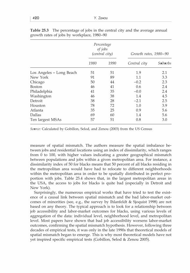
In the United States, it is generally observed that unemployment is unevenlydistributed both within and between metropolitan areas. In particular, in mostcities, the unemployment rate is nearly twice as high downtown as in the sub-urbs (see Table 25.1), mainly because of the concentration of blacks in these areas(see Table 25.1), who are mainly unskilled (see Table 25.2). Indeed, because ofmassive migration of blacks from the rural south to the urban north after the twoworld wars, and because of discrimination in the housing market, blacks had nochoice but to live in the central-city ghettoes. While there has been substantialsuburbanization of blacks in some cities, the legacy of that period remains inthe form of inner-city ghettoes. During the same period, there has been massivesuburbanization of jobs (see Table 25.3). To what extent does this history explainthe higher rates of unemployment among blacks than whites?
Since the seminal work of Kain (1968), many economists contend that thespatial fragmentation of cities can entail adverse social and economic outcomes.These adverse effects typically include the poor labor-market outcomes of ghettodwellers (such as high unemployment and low income) and a fair amount ofsocial ills (such as low educational attainment and high local criminality). Eventhough there is no general theory of ghetto formation, there has been a series oftheoretical and empirical contributions, each giving a particular insight into someof the mechanisms at stake.
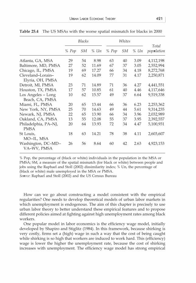
An interesting line of research revolves around the “spatial mismatch hypo-thesis,” which states that, because minorities are physically distant from job oppor-tunities, they are more likely to be unemployed and to obtain low net incomes.Table 25.4 documents these features by using the Raphael and Stoll (2002)
ACTC25 18/04/2006, 04:14PM418
A Companion to Urban EconomicsEdited by Richard J. Arnott, Daniel P. McMillen
a No high school diploma, no experience of training, no reading, writing, or math.The black (white) central city is defined as that area within the central area with contiguous Censustracts of blacks (whites) representing 50 percent or more of the population. The black (white)suburbs are defined as that area within the suburbs with contiguous Census tracts of blacks(whites) representing 30 (80) percent or more of the population. The remaining suburban Censustracts are defined as integrated suburban areas.Source: Stoll, Holzer, and Ihlanfeldt (2000)
ACTC25 18/04/2006, 04:14PM419
420 Y. ZENOU
Table 25.3 The percentage of jobs in the central city and the average annualgrowth rates of jobs by workplace, 1980–90
Source: Calculated by Gobillon, Selod, and Zenou (2003) from the US Census
measure of spatial mismatch. The authors measure the spatial imbalance be-tween jobs and residential locations using an index of dissimilarity, which rangesfrom 0 to 100, with higher values indicating a greater geographical mismatchbetween populations and jobs within a given metropolitan area. For instance, adissimilarity index of 50 for blacks means that 50 percent of all blacks residing inthe metropolitan area would have had to relocate to different neighborhoodswithin the metropolitan area in order to be spatially distributed in perfect pro-portion with jobs. Table 25.4 shows that, in the largest metropolitan areas inthe USA, the access to jobs for blacks is quite bad (especially in Detroit andNew York).
Surprisingly, the numerous empirical works that have tried to test the exist-ence of a causal link between spatial mismatch and the bad labor-market out-comes of minorities (see, e.g., the survey by Ihlanfeldt & Sjoquist 1998) are notbased on any theory. The typical approach is to look for a relationship betweenjob accessibility and labor-market outcomes for blacks, using various levels ofaggregation of the data: individual level, neighborhood level, and metropolitanlevel. Most papers have shown that bad job accessibility worsens labor-marketoutcomes, confirming the spatial mismatch hypothesis. However, following threedecades of empirical tests, it was only in the late 1990s that theoretical models ofspatial mismatch began to emerge. This is why most theoretical models have notyet inspired specific empirical tests (Gobillon, Selod & Zenou 2005).
ACTC25 18/04/2006, 04:14PM420
URBAN LABOR ECONOMIC THEORY 421
Table 25.4 The US MSAs with the worse spatial mismatch for blacks in 2000
% Pop, the percentage of (black or white) individuals in the population in the MSA orPMSA; SM, a measure of the spatial mismatch (for black or white) between people andjobs using the Raphael and Stoll (2002) dissimilarity index; % Un, the percentage of(black or white) male unemployed in the MSA or PMSA.Source: Raphael and Stoll (2002) and the US Census Bureau
How can we go about constructing a model consistent with the empiricalregularities? One needs to develop theoretical models of urban labor markets inwhich unemployment is endogenous. The aim of this chapter is precisely to useurban labor theory to better understand these empirical features and to proposedifferent policies aimed at fighting against high unemployment rates among blackworkers.
One popular model in labor economics is the efficiency wage model, initiallydeveloped by Shapiro and Stiglitz (1984). In this framework, because shirking isvery costly, firms set a (high) wage in such a way that the cost of being caughtwhile shirking is so high that workers are induced to work hard. This (efficiency)wage is lower the higher the unemployment rate, because the cost of shirkingincreases with unemployment. The efficiency wage model has strong empirical
ACTC25 18/04/2006, 04:14PM421
422 Y. ZENOU
support. The traditional attempts to test efficiency wage theory showed thatthere are large wage differences between sectors for identical workers due todifferences in supervision/monitoring rates (see, e.g., Kruger & Summers 1988;Neal 1993). So identical individuals working in different sectors can experiencedifferent unemployment rates because of inter-industry wage differences.
We first develop a simple urban efficiency wage model in which housing pricesand workers’ location (the land market), as well as wages and unemployment(the labor market) are determined in equilibrium. In this model, in whichworkers’ relocation is costless, firms set efficiency wages to prevent shirking andto compensate workers for commuting. The interaction between these two mar-kets is here explicit, since both wages and unemployment depend on commutingcosts, and housing prices as well as location are in turn based on workers’ wages.
We then adapt this model to the US spatial mismatch in order to provide twodifferent mechanisms. First, by assuming that workers’ effort negatively dependson distance to jobs, we show that, in equilibrium, firms draw a red line beyondwhich they will not hire workers. This is because, depending on their residentiallocation, workers do not contribute to the same level of production, even thoughthe wage cost is location independent. As a result, the per-worker profit decreaseswith distance to jobs and firms stop recruiting workers who reside too far away;that is, when the per-worker profit becomes negative. This model offers an explana-tion of the spatial mismatch of black workers by focusing on the point of view offirms. If housing discrimination against blacks forces them to live far away fromjobs, then, even though firms have no prejudices, they are reluctant to hire blackworkers because they have relatively lower productivity than whites.
Second, we introduce two employment centers and high relocation costs sothat workers do not change residence as soon as they change employment status.We show that housing discrimination, by skewing black workers toward the citycenter, increases the number of applications for central jobs and decreases it forsuburban jobs. As a result, blacks living in the central part of the city but workingin the suburbs experience lower unemployment rates and earn higher wagesthan blacks living and working in the central part of the city.
25.2 THE BASIC URBAN LABOR ECONOMIC MODEL
We here develop a simple model of an urban labor market based on Zenou andSmith (1995). This model was constructed with the European situation in mind,where the unemployment rate is higher in the suburbs (as, for example, in Parisor London), and is introduced primarily to set out the method of construction ofmodels in urban labor economic theory. This model will obviously have to beadapted to deal with the US spatial mismatch. This will be done in sections 25.3and 25.4 below.
There are N identical workers and M identical firms. Among the N workers, Lare employed and U unemployed, so that N = L + U. Each individual is identifiedwith one unit of labor and can decide either to work hard or to shirk (Shapiro& Stiglitz 1984). In the former case, the worker provides full effort, e > 0, and
ACTC25 18/04/2006, 04:14PM422
URBAN LABOR ECONOMIC THEORY 423
contributes to e units of production, while in the latter, no effort is exerted on thejob (e = 0) and the contribution to production is nil.
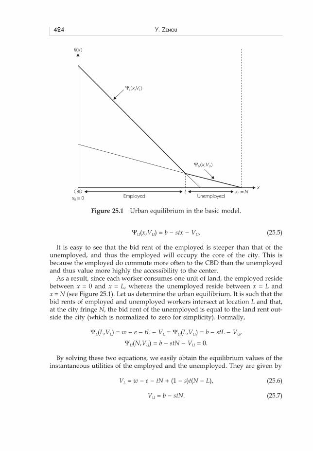
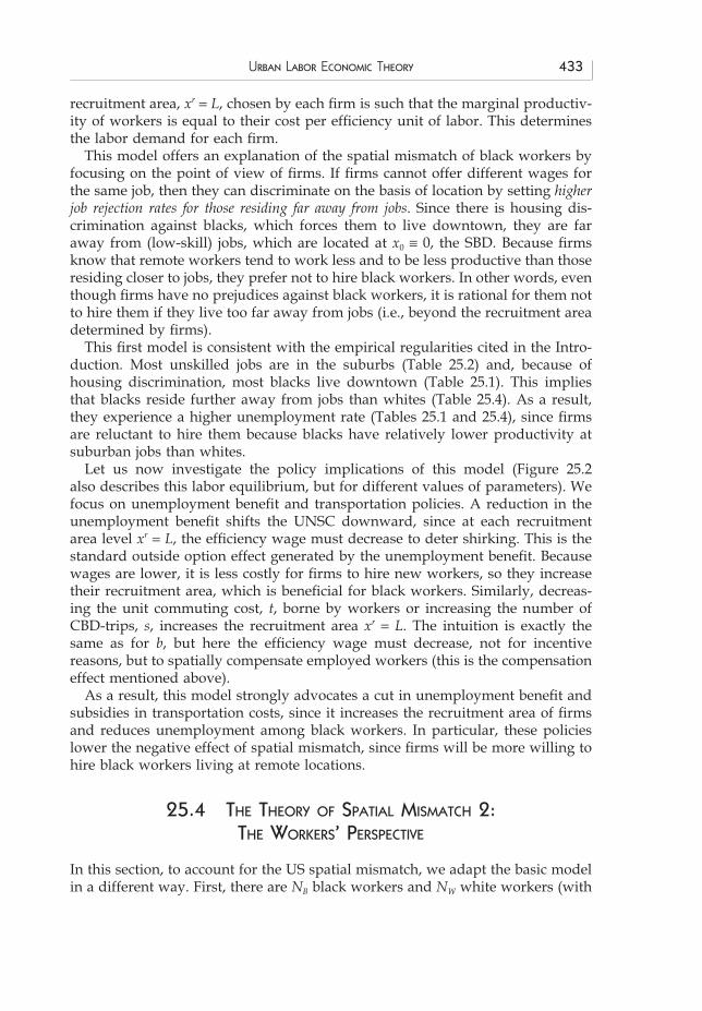
For the ease of exposition, we will first present the urban equilibrium and thenthe labor-market equilibrium. The city is a line whose origin, x0 ≡ 0, consists ofthe central business district (CBD hereafter) where all firms are located and whoseend point is the city-fringe, denoted by xf. Workers are uniformly distributedalong this line and decide where to locate between x = 0 and x = xf . The city isclosed so that there is no relation with the outside world, which implies that thepopulation is fixed. Absentee landlords own all land. There are no relocationcosts, either in terms of time or money.
Each employed worker goes to the CBD to work and incurs a fixed commutingcost t per unit of distance. When living at a distance x from the CBD, he or shealso pays a land rent R(x), consumes one unit of land and earns a wage w. Weadopt the following notations. The subscript L refers to the employed, whereasthe subscript U refers to the unemployed. Among the employed workers, thesuperscripts NS and S refer, respectively, to nonshirkers and shirkers. In thiscontext, the instantaneous (indirect) utilities of an employed nonshirker and shirkerresiding at a distance x from the CBD are, respectively, given by:
VLNS = w − e − tx − R(x), (25.1)
VLS = w − tx − R(x), (25.2)
Concerning the unemployed, they commute less often to the CBD, since theymainly go there to search for jobs. So, we assume that they incur a commutingcost st per unit of distance, with 0 < s < 1. For example, s = 1/2 implies that theunemployed make only half as many CBD-trips as the employed workers. Eachunemployed worker earns a fixed weekly unemployment benefit b > 0, pays aland rent R(x), and consumes one unit of land. In this context, the instantaneous(indirect) utility of an unemployed worker is equal to:
VU = b − stx − R(x). (25.3)
We have first to determine where workers reside and the price of land at eachlocation x in the city. In equilibrium (this will become clear below), none of theemployed workers will shirk, so that we only need to analyze the urban land-useequilibrium for nonshirkers and unemployed workers. Since there are no reloca-tion costs, the urban equilibrium is such that all the employed enjoy the samelevel of utility VL
NS ≡ VL, while all the unemployed obtain VU. Indeed, any utilitydifferential within the city would lead to the relocation of some workers up tothe point at which all differences in utility disappear. We are now able to derivethe bid rent, which is a standard concept in urban economics. It indicates themaximum land rent that a worker located at a distance x from the CBD is readyto pay in order to achieve a utility level. The bid rents of (nonshirking) employedand unemployed workers are given, respectively, by
ΨL(x,VL) = w − e − tx − VL, (25.4)
ACTC25 18/04/2006, 04:14PM423
424 Y. ZENOU
ΨU(x,VU) = b − stx − VU. (25.5)
It is easy to see that the bid rent of the employed is steeper than that of theunemployed, and thus the employed will occupy the core of the city. This isbecause the employed do commute more often to the CBD than the unemployedand thus value more highly the accessibility to the center.
As a result, since each worker consumes one unit of land, the employed residebetween x = 0 and x = L, whereas the unemployed reside between x = L andx = N (see Figure 25.1). Let us determine the urban equilibrium. It is such that thebid rents of employed and unemployed workers intersect at location L and that,at the city fringe N, the bid rent of the unemployed is equal to the land rent out-side the city (which is normalized to zero for simplicity). Formally,
ΨL(L,VL) = w − e − tL − VL = ΨU(L,VU) = b − stL − VU,
ΨU(N,VU) = b − stN − VU = 0.
By solving these two equations, we easily obtain the equilibrium values of theinstantaneous utilities of the employed and the unemployed. They are given by
VL = w − e − tN + (1 − s)t(N − L), (25.6)
VU = b − stN. (25.7)
x
R(x)
LCBDx0 ≡ 0 Employed Unemployed
xf = N
ΨL(x,VL)
ΨU(x,VU)
Figure 25.1 Urban equilibrium in the basic model.
ACTC25 18/04/2006, 04:14PM424
URBAN LABOR ECONOMIC THEORY 425
We have solved the urban equilibrium, since we know where workers locate inthe city (the employed reside close to jobs, while the unemployed live furtheraway because the former have higher commuting costs than the latter and thusbid them away) and what the price of land is at each location (it is equal to thebid rent of the employed for locations between 0 and L and to the bid rent of theunemployed for locations between L and N).
We would now like to determine the labor-market equilibrium; that is, thewages paid by firms and the level of unemployment in the city. Firms face aproblem, since they do not perfectly observe the behavior of workers (whetherthey work hard or shirk), which affects production and thus their profit. Weassume that, at each period, firms can monitor some workers but not all of them,because it is too costly. The rate of monitoring is denoted by θ and if a workeris caught shirking, he or she is automatically fired. The job acquisition rate isdenoted by a and δ is the job destruction rate. The lifetime expected utilities ofnonshirkers, shirkers, and unemployed workers, IL
NS, ILS, and IU, are given, respect-
ively, by
rILNS = VL
NS − δ (ILNS − IU), (25.8)
rILS = VL
S − (δ + θ)(ILS − IU), (25.9)
rIU = VU + a(IL − IU), (25.10)
where r is the discount rate, and where VLNS ≡ VL and VU are given by equa-
tions (25.6) and (25.7), respectively, and VLS = VL + e. The first equation that deter-
mines ILNS states that a nonshirker obtains today a utility level VL
NS but can lose hisor her job with probability δ (because, for example, the job is destroyed or becausethe worker decides to live in another city). In that case, he or she obtains a negativesurplus of IU − IL
NS. For shirkers, ILS, the probability of losing a job, is even higher
because either the job is destroyed (with probability δ ) or he or she is caughtshirking and fired (with probability θ). The last equation for the unemployed hasa similar interpretation.
We can see straightaway the trade-off faced by a worker when deciding whetheror not to shirk. There is a short-run gain of shirking because workers do not provideeffort e (the gain is thus VL
S − VLNS = e) but there is a long-run cost of shirking
because the rate at which workers lose their jobs is higher (δ + θ instead of δ ).Because shirking is very costly for firms (workers do not produce at all while
being paid), firms would like to set wages in such a way that no rational workershirks. These wages are called efficiency wages and are determined by the follow-ing incentive inequality: IL
NS > ILS. Since all firms compete with each other to deter-
mine this wage, there is no need to pay more than ILNS = IL
S. There are two waysto justify that IL
NS = ILS. Either one assumes that when workers are indifferent
between shirking and nonshirking, they always prefer to work than to shirk, orone can set an efficiency wage that is infinitesimally above the threshold IL
NS = ILS.
This obviously makes no difference in the analysis.By using equations (25.8) and (25.9), IL
NS = ILS can be written as
ACTC25 18/04/2006, 04:15PM425
426 Y. ZENOU
I I
eL U .− =
θ(25.11)
This highlights the nature of the (urban) efficiency wage we. The intertemporalsurplus of being employed, IL − IU, is strictly positive and does not depend onspatial variables. This is a pure incentive effect (to deter shirking) that increasesin effort and decreases in the monitoring rate θ (indeed, if firms better monitortheir workers, then wages and thus IL
NS = ILS are lower).
In equilibrium, it has to be that the flows in unemployment are equal to theflows out of unemployment; that is,
a(N − L) = δL. (25.12)
In words, the number of unemployed workers who find a job is equal to thenumber of employed workers who lose their job. By combining equations (25.11)and (25.12) and using equations (25.8)–(25.10), we are now able to calculate theefficiency wage:
w L b e
e N
N Lr s tLe( )
( ) .= + +
−+
⎛⎝⎜
⎞⎠⎟
+ −θ
δ1 (25.13)
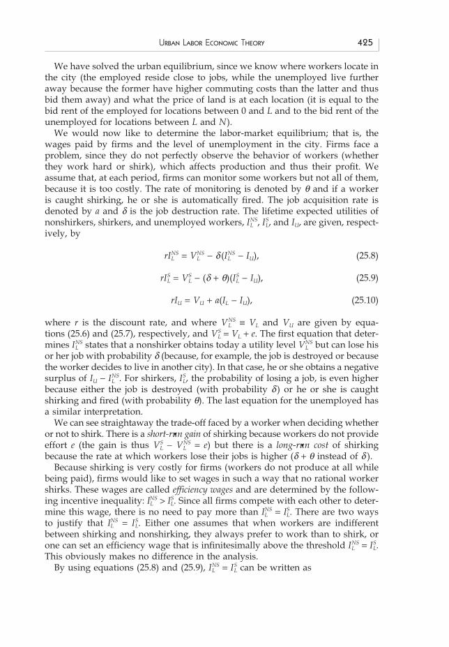
This equation is referred to as the Urban No-Shirking Condition (UNSC hereafter),since it is the wage that firms have to set at each employment level L in orderto prevent shirking; that is, IL
NS = ILS. Indeed, the lower the unemployment level
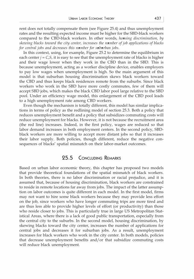
N – L in the city (or, equivalently, the higher the employment level L), the higheris the efficiency wage (see Figure 25.2). This is because unemployment acts as aworker discipline device, since the higher the unemployment, the more difficultit is to find a job and the higher are the long-run costs of shirking. As a result, indownturn economies with high unemployment rates, firms do not need to payhigh wages to workers, since they discipline themselves because the cost of shirk-ing is too high.
Interestingly, an increase in the unemployment benefit, b, would induce a risein the efficiency wage, we(L), because the outside option of not working is betterand workers are more likely to shirk. As a result, firms have to increase wages tomeet the condition IL
NS = ILS. A similar interpretation can be made for the positive
impact on wages of an increase in the job destruction rate δ or the discount rater, or of a decrease in the monitoring rate θ.
Let us now understand the role of the spatial variables in the efficiency wage(25.13); that is, the commuting cost t and the unemployed CBD-trips s. Firmshave to compensate their employed workers for spatial costs. Indeed, whensetting their (efficiency) wage, firms must compensate the spatial cost differentialbetween the employed and the unemployed. For the employed and the unem-ployed who both live at L (which is the border distance between the employedand the unemployed) and thus pay the same land rent, this differential is exactlyequal to (1 − s)tL. Now, since mobility is costless, all the employed and unem-ployed workers obtain, respectively, the same utility level whatever their location.
ACTC25 18/04/2006, 04:15PM426
URBAN LABOR ECONOMIC THEORY 427
NL
wLabor demand
UNSC
0Unemployment
Le
we(L)
(δ + r)eθb + e +
wpc
δθ
Figure 25.2 Labor equilibrium in the basic model.
! @
Therefore, the spatial cost differential between any employed and unemployedworker is equal to (1 − s)tL. In order to see this, we can calculate the spatial costsof each individual, which consist of transportation plus land rent. In equilibrium,using equations (25.6) and (25.7), they are given by
SCL = tN − (1 − s)t(N − L)
for the employed and
SCU = stN
for the unemployed. We can thus calculate the spatial cost differential betweenthe employed and the unemployed:
∆SC ≡ SCL − SCU = (1 − s)tL. (25.14)
It is easy to see that ∆SC is precisely the last term in equation (25.13) and itsrole is to compensate workers for spatial costs. This implies that the efficiencywage can be written as
w L b WI SCe
Work Inducement Spatial Compensation
( ) ,
= + + ∆ (25.15)567
ACTC25 18/04/2006, 04:15PM427
428 Y. ZENOU
where
WI e
e N
N Lr
= +
−+
⎛⎝⎜
⎞⎠⎟θ
δ
and ∆SC is given by equation (25.14), so that, compared to unemployment, work-ing gives a wage premium of WI + ∆SC. In other words, the efficiency wage hastwo roles: to prevent shirking (the incentive component) and to insure thatworkers stay in the city (the spatial compensation component).
Finally, by maximizing their profit F(eL) − weL, firms determine the labor demandLe in the city. The model is closed and the labor-market equilibrium is depicted inFigure 25.2. The intersection between the Urban No-Shirking Condition (UNSC)curve (equation (25.13) ) and the labor demand curve gives the equilibrium valuesof wage we(L) and employment Le. Observe that at L = N, there is full employ-ment and the corresponding wage, wpc, is the wage that would be paid by firmsin a perfectly competitive environment. Urban unemployment occurs here becausewages are too high (we(L) > wpc) and are downward rigid. Indeed, even withexcess supply, firms will not cut their (efficiency) wages because the UNSC curvewill not be met and all workers will shirk in equilibrium.
We would now like to adapt this model to deal with the US spatial mismatch,where the unemployment rate is higher in the central part of the city (Table 25.1),blacks live disproportionately downtown (Table 25.1), far away from jobs(Table 25.4), and there are more jobs in the suburbs than in the city center(Table 25.3).
There are several ways in which this model can be adapted to account forthe US spatial mismatch. The easiest way is to flip the city so that the CBDcorresponds to a suburban business district (SBD) that concentrates all jobs. So, ifall jobs are in the suburbs rather than the CBD, all we require for consistency is todefine x = 0 to be the workplace location, which is in the suburbs. But in fact, jobsare more centralized than residences. Indeed, Glaeser and Kahn (2001) have shownthat jobs have been suburbanizing faster than residences, so that, in the large USmetropolitan areas, the average job is now only 1 mile closer to the CBD than theaverage residence. So, even if we flip the city in the above model, there seems tobe some inconsistency, since the unemployment rate in US cities is higher at(central) locations that appear to have better access to jobs. However, since mostblacks are unskilled, we need to differentiate between skilled and unskilled jobs.Using both the 1994 Multi-City Study of Urban Inequality (MCSUI) and the 1990Census, Table 25.2 displays the spatial distribution of recently filled low-skill jobsand of people by race and education. This table shows that the distribution oflow-skill jobs is similar to that of all jobs, except that there is a greater share of low-skill jobs in general in white suburbs. This implies that low-skill jobs are much moredecentralized than high-skill jobs. If one compares jobs with people, then thesituation is worse: 79.6 percent of the metropolitan areas’ lowest-skilled jobs, butonly 23.6 percent of the least-educated black people (i.e., those with no highschool degree) are located in the suburbs. The access to low-skill jobs is thusquite bad for unskilled black workers. Since unskilled jobs are further on average
ACTC25 18/04/2006, 04:16PM428
URBAN LABOR ECONOMIC THEORY 429
from the CBD than unskilled black workers’ residences, and since unemploy-ment is a problem for the unskilled, then our basic model can be adapted todescribe the situation for the unskilled, but with x = 0 corresponding to a locationin the suburbs. But the phenomenon of spatial mismatch is made more compli-cated by the presence of two modes of transportation – mass transit and the car– along with the relatively low incidence of car ownership among blacks, as wellas the asymmetry between commuting inward and commuting outward. This, infact, reinforces the spatial mismatch problem for blacks, since they are not onlyfar away from (low-skill) jobs but, because of the lack of good public transporta-tion in large US metropolitan areas, they have difficulty accessing these jobs, asconfirmed by Table 25.4.
In this essay, we will not focus on the transport issue but, rather, assume aunique transport mode for all workers (whether they are black or white) in thecity. Instead, by adapting the basic model of this section to the US spatial mis-match, we propose two different theories that can explain why distance to jobscan have adverse consequences in the labor market for black workers. In boththeories, we generate a link between unemployment and a seemingly unrelatedphenomenon: racial discrimination in the housing market.
25.3 THE THEORY OF SPATIAL MISMATCH 1:
THE FIRMS’ PERSPECTIVE
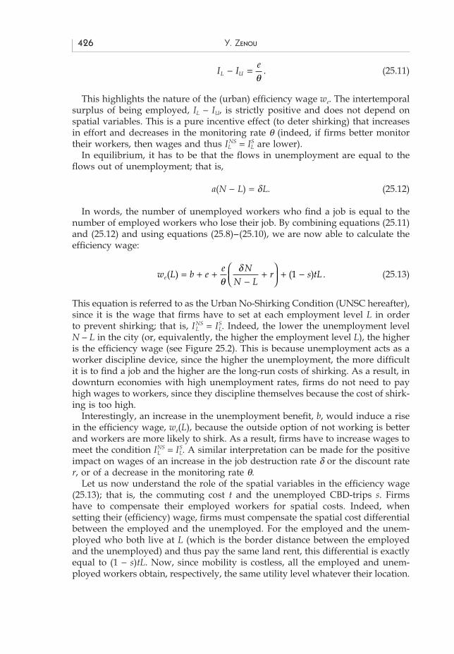
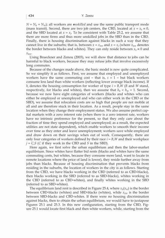
In this section, we adapt the basic model as follows. First, we only focus onlow-skill workers (black or white) and low-skill jobs. Also, all workers use thesame transport mode (mass transit). Second, x = x0 is now the SBD – that is, theworkplace is located in the suburbs, where all low-skill jobs are located – whilex = xf is now the city center (there are no jobs there, only people). To be consistentwith the basic model, we normalize the SBD to zero; that is, x0 = x. This meansthat we take the firms’ perspective when calculating the distance to jobs, so thatxf, the city center, is now the longest distance from the job center located at x0 = 0.See Figure 25.3 for an illustration of this city. Finally, there is housing discrimina-tion against blacks (housing discrimination against blacks is a well-documentedfact; see, e.g., Yinger 1986), which forces them to live downtown (i.e., close to thecity-center xf) and causes them to have poorer access to unskilled jobs than dowhites living in the suburbs.
We focus on the firms’ viewpoint to explain the spatial mismatch for blackworkers. We will show that, even though firms have no prejudices against blackworkers, it can be rational for them not to hire black workers if they live too faraway from jobs (they live downtown while jobs are in the suburbs), because theyare less productive than white workers who live closer to jobs.
Based on Zenou (2002), let us show how an extension of the model of sect-ion 25.2 can capture this idea. Apart from the modifications mentioned above,we use exactly the same model, but we change only one aspect. There are still onlytwo possible effort levels: either the worker shirks, exerting zero effort, e = 0, andcontributing zero to production, or he or she does not shirk, providing full effort
ACTC25 18/04/2006, 04:16PM429
430 Y. ZENOU
x
R(x)
SBDx0 ≡ 0
xf = NUnemployed Employed
L
ΨU(x,VU)
ΨL(x,VL)
Figure 25.3 Urban equilibrium in the redlining model.
e > 0. However, the latter now depends on x, the distance to jobs. That is, e(x) > 0is the contribution to production, with e(0) = e0 > 0. We assume that the greaterthe distance to work, the lower is the effort level (e′(x) < 0) and, for remotelocation, the marginal difference in effort is quite small (e″(x) ≥ 0).
This assumption, e′(x) < 0, aims at capturing the fact that workers who havelonger commuting trips are more tired and are thus less able to provide higherlevels of effort (or productivity) than those who reside closer to jobs. This impliesthat commuting costs include more than just money and time costs. They alsoinclude these negative effects of a longer commute such as nonwork-relatedfatigue. Moreover, this assumption can also capture the fact that workers whoreside further away from jobs have less flexible working hours. For example, insome jobs (e.g., working in a restaurant), there are long breaks during the day(typically between 2 p.m. and 6 p.m. in restaurants). The worker who lives nextdoor can go back home and relax, whereas the others, who live far away, cannotrest at home. This obviously also affects workers’ productivity.
One can question this assumption by arguing that one can take a nap on atrain. Indeed, driving 2 hours is tiring, but riding a train isn’t. This is true if thereis a very good public transport system, which implies, for example, that there isa direct train from home to the workplace. Remember that we are dealing with(low-educated) black workers who are forced to live far away from jobs (housingdiscrimination). It is well documented that most blacks do not have access tocars and use public transportation. Indeed, using data drawn from the 1995Nationwide Personal Transportation Survey, Raphael and Stoll (2001) show that,
ACTC25 18/04/2006, 04:16PM430
URBAN LABOR ECONOMIC THEORY 431
in the USA, 5.4 percent of white households have zero automobiles while24 percent of black households do not hold a single car. Even more striking, theyshow that 64 percent of black households have one or zero cars, whereas thisnumber was 36 percent for white households.
It is also well documented that, in large US Metropolitan Statistical Areas,there is a lack of good public transportation, especially from the central city tothe suburbs. For instance, The New York Times of May 26, 1998, told the story ofDorothy Johnson, a Detroit inner-city black female resident who had to commuteto an evening job as a cleaning lady in a suburban office. By using public trans-portation, it took her 2 hours, whereas if she could have afforded a car, thecommute would have taken only 25 minutes. This story illustrates the fact thatblacks have relatively low productivity at suburban jobs because they arrive lateat work due to the unreliability of the mass transit system, which frequentlycauses black workers to miss transfers.
The worker’s behavior can now be seen as a two-stage decision. First, eachworker must decide whether or not to shirk, depending on his or her residentiallocation. Since effort is costly, it is clear that the worker who lives the closestto jobs will be more inclined to shirk than those who reside further away. Thus,contrary to the previous model, the shirking behavior of workers is here locationallydependent. Second, once the worker has decided not to shirk (this is the behaviorthat will emerge in equilibrium), he or she must decide how much effort he orshe will provide. This decision is also locationally dependent, since we assumethat workers who have longer commutes are more tired and provide less effortthan those who live closer to their jobs.
As before, let us first determine the urban land-use equilibrium and then thelabor equilibrium. All the locational analysis is exactly the same as in section 25.2,the only difference being that now e negatively depends on x. This creates anew locational trade-off for the employed. They would like to be close to jobs(the SBD located at x0 ≡ 0) to save on commuting costs, but would also like to befar away from jobs to provide lower levels of effort (since effort is costly). How-ever, by assuming that t > −e′(L)/(1 − s), we can guarantee that the employedreside close to the SBD, whereas the unemployed live close to the city center (seeFigure 25.3). The intuition of this result is as follows. An increase in distance xhas offsetting effects on employed workers: they pay higher commuting costs,but lower effort is exerted on the job. The net effect is thus less than the purecommuting cost effect, and the question is whether this net effect is stronger thanthe shrunken commuting cost effect for unemployed workers, which is smallerthan that of the employed worker because s < 1. In this context, when the com-muting cost t is high enough, the employed workers reside close to jobs byoutbidding the unemployed.
Let us now solve for the labor equilibrium. Firms have to set an efficiencywage that prevents workers from shirking. Here, the main difference with theprevious section is that the lifetime expected utility of shirkers IS
L is now a functionof x, since VS
L(x) is now given by VLS(x) = VL + e(x). As in the previous section, the
efficiency wage has to be set in order to make workers indifferent between shirk-ing and not shirking. However, the utility of shirkers is not constant over locations,whereas it is constant for nonshirkers.
ACTC25 18/04/2006, 04:16PM431
432 Y. ZENOU
When workers are heterogeneous in terms of location, it is clear that workers’residence matters in the process of wage formation. Firms observe where workerslive, but cannot discriminate on the basis of residence or, equivalently, race (i.e.,cannot make the wage location dependent or race dependent). In other words,they cannot offer different wages to identical workers who live in different areasof the city (because of housing discrimination, whites tend to live close to jobs,while blacks reside further away from jobs). One reason why firms cannot offerdifferent wages to identical workers is antidiscrimination laws.
It is easy to see that the utility of shirkers increases as x, the distance to theSBD, decreases. The intuition is straightforward. Since the land rent compensatesfor both commuting costs and effort levels, then shirkers, who do not provideeffort, have a higher utility when residing closer to the SBD (since their commut-ing costs are lower). This implies, in particular, that the highest utility that ashirker can reach is at x0 ≡ 0, the SBD) and the lowest is at L. As a result, becausefirms cannot discriminate in terms of location or race, the efficiency wage mustbe set such that workers are indifferent between shirking at location x0 ≡ 0 andnot shirking, since if the worker at x0 ≡ 0 does not shirk, then all workers locatedfurther away will not shirk. In other words, the condition that determines theefficiency wage is now given by IL
NS = ILS(0) = IL. Proceeding exactly as before, we
obtain
w L b e L
e N
N Lr s tLe
r( ) ( )
( ) .= + +−
+⎛⎝⎜
⎞⎠⎟
+ −0 1θ
δ(25.16)
If we compare equations (25.13) and (25.16), the main difference is that, inequation (25.16), the effort function, e(⋅), now depends on x, the distance to jobs.Two locations are crucial: the SBD, where x0 ≡ 0 and effort is e0, and the borderbetween the employed and the unemployed, where x = L and effort is e(L).
Our setting thus implies that there is a fundamental asymmetry between work-ers and firms. All workers obtain the same efficiency wage whatever their loca-tion. However, they do not contribute to the same level of production becausetheir effort decreases with distance to jobs. In other words, even though the wagecost is location independent, the contribution to production is not. This impliesthat the per-worker profit decreases with distance to jobs, so that firms willdetermine a red line beyond which they will not hire workers; that is, when theper-worker profit becomes negative. The interesting implication of this model isthat it can explain why firms do not hire remote workers. Indeed, if firms cannotdiscriminate in terms of location (make wages location dependent), they doanticipate that remote workers provide lower effort level. So they stop recruitingworkers who reside too far away.
To be more precise, all (identical) firms set the same red line xr = L, abovewhich they do not hire workers. The total production (or effort) level provided in
each firm is given by B = �0
L
e(x)dx. As above, by taking the efficiency wage as
given, each firm maximizes its profit to choose the optimal size of the red line(recruitment area L). We obtain f ′(B) = w/e(L). This equation states that the optimal
ACTC25 18/04/2006, 04:17PM432
URBAN LABOR ECONOMIC THEORY 433
recruitment area, xr = L, chosen by each firm is such that the marginal productiv-ity of workers is equal to their cost per efficiency unit of labor. This determinesthe labor demand for each firm.
This model offers an explanation of the spatial mismatch of black workers byfocusing on the point of view of firms. If firms cannot offer different wages forthe same job, then they can discriminate on the basis of location by setting higherjob rejection rates for those residing far away from jobs. Since there is housing dis-crimination against blacks, which forces them to live downtown, they are faraway from (low-skill) jobs, which are located at x0 ≡ 0, the SBD. Because firmsknow that remote workers tend to work less and to be less productive than thoseresiding closer to jobs, they prefer not to hire black workers. In other words, eventhough firms have no prejudices against black workers, it is rational for them notto hire them if they live too far away from jobs (i.e., beyond the recruitment areadetermined by firms).
This first model is consistent with the empirical regularities cited in the Intro-duction. Most unskilled jobs are in the suburbs (Table 25.2) and, because ofhousing discrimination, most blacks live downtown (Table 25.1). This impliesthat blacks reside further away from jobs than whites (Table 25.4). As a result,they experience a higher unemployment rate (Tables 25.1 and 25.4), since firmsare reluctant to hire them because blacks have relatively lower productivity atsuburban jobs than whites.
Let us now investigate the policy implications of this model (Figure 25.2also describes this labor equilibrium, but for different values of parameters). Wefocus on unemployment benefit and transportation policies. A reduction in theunemployment benefit shifts the UNSC downward, since at each recruitmentarea level xr = L, the efficiency wage must decrease to deter shirking. This is thestandard outside option effect generated by the unemployment benefit. Becausewages are lower, it is less costly for firms to hire new workers, so they increasetheir recruitment area, which is beneficial for black workers. Similarly, decreas-ing the unit commuting cost, t, borne by workers or increasing the number ofCBD-trips, s, increases the recruitment area xr = L. The intuition is exactly thesame as for b, but here the efficiency wage must decrease, not for incentivereasons, but to spatially compensate employed workers (this is the compensationeffect mentioned above).
As a result, this model strongly advocates a cut in unemployment benefit andsubsidies in transportation costs, since it increases the recruitment area of firmsand reduces unemployment among black workers. In particular, these policieslower the negative effect of spatial mismatch, since firms will be more willing tohire black workers living at remote locations.
25.4 THE THEORY OF SPATIAL MISMATCH 2:
THE WORKERS’ PERSPECTIVE
In this section, to account for the US spatial mismatch, we adapt the basic modelin a different way. First, there are NB black workers and NW white workers (with
ACTC25 18/04/2006, 04:17PM433
434 Y. ZENOU
N = NB + NW); all workers are unskilled and use the same public transport mode(mass transit). Second, there are two job centers, the CBD, located at x = x0 ≡ 0,and the SBD located at x = xf. To be consistent with Table 25.2, we assume thatthere are more firms and thus more unskilled jobs in the SBD than in the CBD.Finally, there is housing discrimination against blacks in such a way that theycannot live in the suburbs; that is, between x = xBW and x = xf (where xBW denotesthe border between blacks and whites). They can only reside between x0 ≡ 0 andxBW.
Using Brueckner and Zenou (2003), we will show that distance to jobs can beharmful to black workers, because they may refuse jobs that involve excessivelylong commutes.
Because of the changes made above, the basic model is now quite complicated.So we simplify it as follows. First, we assume that employed and unemployedworkers have the same commuting cost – that is, s = 1 – but black workersconsume less land than white workers (reflecting lower average black income). Ifhi denotes the housing consumption for worker of type i = B,W (B and W stand,respectively, for blacks and whites), then we assume that hB < hW = 1. Second,because we now have eight categories of workers (blacks and whites who caneither be employed or unemployed and who can either work in the CBD or theSBD), we assume that relocation costs are so high that people are not mobile atall and are therefore stuck in their location. As a result, people stay in the samelocation when they change their employment status. We also assume perfect cap-ital markets with a zero interest rate (when there is a zero interest rate, workershave no intrinsic preference for the present, so that they only care about thefraction of time they spend employed and unemployed; as a result, the expectedutilities are not state dependent), which enable workers to smooth their incomeover time as they enter and leave unemployment; workers save while employedand draw down on their savings when out of work. Consequently, there areonly four categories of workers defined by their race i = B,W and their workplacej = C,S (C if they work in the CBD and S in the SBD).
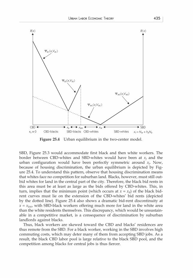
Here again, we first solve the urban equilibrium and then the labor-marketequilibrium. Since whites have flatter bid rents (blacks and whites have the samecommuting costs, but whites, because they consume more land, want to locate inremote locations where the price of land is lower), they reside further away fromjobs than blacks. Because of housing discrimination that prevents blacks fromresiding in the suburbs, the location of workers in the city is as follows. Startingfrom the CBD, we have blacks working in the CBD (referred to as CBD-blacks),then blacks working in the SBD (referred to as SBD-blacks), whites working inthe CBD (referred to as CBD-whites), and finally whites working in the SBD(referred to as SBD-whites).
The equilibrium land rent is described in Figure 25.4, where xB(xW) is the borderbetween CBD-blacks (whites) and SBD-blacks (whites), while xBW is the borderbetween SBD-blacks and CBD-whites. If there were no housing discriminationagainst blacks, then to obtain the urban equilibrium, we would have to juxtaposeFigures 25.1 and 25.3. In this new configuration, starting from the CBD, Fig-ure 25.1 would locate first black and then white workers, while, starting from the
ACTC25 18/04/2006, 04:17PM434
URBAN LABOR ECONOMIC THEORY 435
Figure 25.4 Urban equilibrium in the two-center model.
R(x)
x0 ≡ 0SBD
xf = NW + hBNBCBD-blacks
R(x)
CBDSBD-blacks CBD-whites SBD-whitesxB xBW xW
ΨBC(x,VBC)
ΨWC(x,VWC)
ΨWS(x,VWS)
ΨBS(x,VBS)
SBD, Figure 25.3 would accommodate first black and then white workers. Theborder between CBD-whites and SBD-whites would have been at xf and theurban configuration would have been perfectly symmetric around xf. Now,because of housing discrimination, the urban equilibrium is depicted by Fig-ure 25.4. To understand this pattern, observe that housing discrimination meansthat whites face no competition for suburban land. Blacks, however, must still out-bid whites for land in the central part of the city. Therefore, the black bid rents inthis area must be at least as large as the bids offered by CBD-whites. This, inturn, implies that the minimum point (which occurs at x = xB) of the black bid-rent curves must lie on the extension of the CBD-whites’ bid rents (depictedby the dotted line). Figure 25.4 also shows a dramatic bid-rent discontinuity atx = xBW, with SBD-black workers offering much more for land in the white areathan the white residents themselves. This discrepancy, which would be unsustain-able in a competitive market, is a consequence of discrimination by suburbanlandlords against blacks.
Thus, black workers are skewed toward the CBD and blacks’ residences arethus remote from the SBD. For a black worker, working in the SBD involves highcommuting costs, which may deter many of them from accepting SBD jobs. As aresult, the black CBD labor pool is large relative to the black SBD pool, and thecompetition among blacks for central jobs is thus fiercer.
ACTC25 18/04/2006, 04:18PM435
436 Y. ZENOU
We can calculate the efficiency wage for a worker of type ij (i = B,W, j = C,S). Itis given by
w L b e
e N
N Lijm
ij
ij
( )
,= + +−
⎛
⎝⎜⎞
⎠⎟θδ
(25.17)
which is the wage (25.13) when r → 0 and s = 1.As stated above, there are more “unskilled” firms in the SBD than in the
CBD. To determine their labor demand, each firm maximizes its profit and thelabor-market equilibrium in each center for each type of labor is depicted byFigure 25.2 (for different parameter values). Because of housing discriminationand because there are more unskilled jobs in the SBD, it is then easy to show that,compared to whites, the unemployment rate is higher and wages are lower forblack workers, which is consistent with the US spatial mismatch. The intuitionis straightforward. Because of housing discrimination, blacks are forced to live inthe central part of the city. Because there are more unskilled jobs in the SBD,most blacks have poor access to unskilled jobs and the ones who accept workingin the SBD support long and costly commuting costs. As a result, few blacks willaccept a job in the SBD and most of them will seek a CBD-job. This leads to ahigh unemployment rate for CBD-black workers (which encompasses most blacks)and, because in an efficiency wage framework, unemployment acts as a workerdiscipline device, CBD-firms can set low wages to black workers without fearingshirking behavior. So, even if all workers (black or white) are ex ante totallyidentical, mainly because of housing discrimination, white workers end up withhigher wages and lower unemployment rates.
This model is also consistent with the empirical regularities mentioned in theintroduction. The unemployment rate is higher downtown than in the suburbs(Table 25.1) because blacks, who are mainly unskilled (Table 25.2), are forced tolive around the city center (Tables 25.1 and 25.2), far away from the suburbswhere most unskilled jobs are located (Tables 25.2 and 25.4).
Let us now show another interesting result by focusing only on black workers.It has been observed that blacks working downtown tend to have higher unem-ployment rates and lower wages than blacks working in the suburbs (see, e.g.,Brueckner & Zenou 2003, table 3). In other words, let us show that blacks livingin the central part of the city but working in the SBD experience lower unem-ployment rates and earn higher wages than blacks living in the central part of thecity but working in the CBD. The argument is as follows. Since, in equilibrium, itmust be that all blacks wherever they work (in the CBD or the SBD) must reachthe same utility level, then there must be some compensation for those whocommute to the SBD. Indeed, because blacks are discriminated against in thehousing market, they are forced to live in the central part of the city. Becauseblacks are forced to live in the central part of the city, the ones who work in theSBD support long and costly commuting costs. So in order for blacks to obtainthe same utility level wherever they work, the SBD workers have to be com-pensated. Because, for blacks, competition in the land market is quite fierce, land
ACTC25 18/04/2006, 04:18PM436
URBAN LABOR ECONOMIC THEORY 437
rent does not totally compensate them (see Figure 25.4) and thus unemploymentrates and the resulting expected income must be higher for the SBD-black workerscompared to the CBD-black workers. In other words, housing discrimination, byskewing blacks toward the city center, increases the number of job applications of blacksfor central jobs and decreases this number for suburban jobs.
In this context, using, for example, Figure 25.2 to determine the equilibrium ineach center j = C,S, it is easy to see that the unemployment rate of blacks is higherand their wage lower when they work in the CBD than in the SBD. This isbecause unemployment, acting as a worker discipline device, enables employersto pay low wages when unemployment is high. So the main argument of thismodel is that suburban housing discrimination skews black workers towardthe CBD and thus keeps black residences remote from the suburbs. Since blackworkers who work in the SBD have more costly commutes, few of them willaccept SBD jobs, which makes the black CBD labor pool large relative to the SBDpool. Under an efficiency wage model, this enlargement of the CBD pool leadsto a high unemployment rate among CBD workers.
Even though the mechanism is totally different, this model has similar implica-tions in terms of policy as the redlining model of section 25.3. Both a policy thatreduces unemployment benefit and a policy that subsidizes commuting costs willreduce unemployment for blacks. However, it is not because the recruitment area(the red line) increases. Indeed, in the first policy, wages are reduced so thatlabor demand increases in both employment centers. In the second policy, SBD-black workers are more willing to accept more distant jobs so that it increasestheir labor supply. Both policies, though different, reduce the negative con-sequences of blacks’ spatial mismatch on their labor-market outcomes.
25.5 CONCLUDING REMARKS
Based on urban labor economic theory, this chapter has proposed two modelsthat provide theoretical foundations of the spatial mismatch of black workers.In both theories, there is no labor discrimination or racial prejudice, and it isassumed that, because of housing discrimination, black workers are constrainedto reside in remote locations far away from jobs. The impact of the latter assump-tion on labor outcomes is quite different in each model. In the first model, firmsmay not want to hire some black workers because they may provide less efforton the job, since workers who have longer commuting trips are more tired andare thus less able to provide higher levels of effort (or productivity) than thosewho reside closer to jobs. This is particularly true in large US Metropolitan Stat-istical Areas, where there is a lack of good public transportation, especially fromthe central city to the suburbs. In the second model, housing discrimination, byskewing blacks toward the city center, increases the number of applications forcentral jobs and decreases it for suburban jobs. As a result, unemploymentincreases for black workers who work in the city center. In both models, policiesthat decrease unemployment benefits and/or that subsidize commuting costswill reduce black unemployment.
ACTC25 18/04/2006, 04:18PM437
438 Y. ZENOU
So, how relevant are these models? Interestingly, Zax and Kain (1996) have insome sense illustrated the model of section 25.4 by studying a “natural experi-ment” (the case of a large firm in the service industry, which relocated fromthe center of Detroit to the suburb Dearborn in 1974). They show that, amongworkers whose commuting time was increased, black workers were overrepres-ented, and not all could follow the firm. This had two consequences: first, as inour model, segregation forced some blacks to quit their jobs. Second, the share ofblack workers applying for jobs to the firm decreased drastically (from 53 percentto 25 percent in 5 years before and after the relocation), and the share of blackworkers in hires also fell from 39 percent to 27 percent.
It would be interesting to test the redlining model of section 25.3. The popularpress often relates stories about firms that do not want to hire workers living in“bad” neighborhoods, which are in general not well connected to job centers.An empirical test to see how policy-relevant this model is would be more thanwelcome.
Acknowledgments
I would like to thank Richard Arnott as well as an anonymous referee for extremelyhelpful comments. I also thank the Marianne and Marcus Wallenberg Foundation forfinancial support.
Bibliography
Brueckner, J. K. and Zenou, Y. 2003: Space and unemployment: the labor-market effects ofspatial mismatch. Journal of Labor Economics, 21, 242–66.
Glaeser, E. L. and Kahn, M. 2001: Decentralized employment and the transformation ofthe American city. Brookings–Wharton Papers on Urban Affairs, 2, 1–64.
Gobillon, L., Selod, H., and Zenou, Y. 2003: Spatial mismatch: from the hypotheses to thetheory. CEPR Discussion Paper Series 3740.
——, ——, and —— 2005: The mechanisms of spatial mismatch. CEPR Discussion PaperSeries 5346.
Ihlanfeldt, K. R. and Sjoquist, D. L. 1998: The spatial mismatch hypothesis: a review ofrecent studies and their implications for welfare reform. Housing Policy Debate, 9,849–92.
Kain, J. F. 1968: Housing segregation, negro employment, and metropolitan decentraliza-tion. Quarterly Journal of Economics, 82, 32–59.
Kruger, A. and Summers, L. 1988: Efficiency wages and the inter-industry wage structure.Econometrica, 56, 259–93.
Neal, D. 1993: Supervision and wages across industries. Review of Economics and Statistics,75, 409–17.
Raphael, S. and Stoll, M. A. 2001: Can boosting minority car-ownership rates narrowinterracial employment gaps? Brookings–Wharton Papers on Urban Economic Affairs, 2,99–145.
—— and —— 2002: Modest progress: the narrowing spatial mismatch between blacks andjobs in the 1990s. The Brookings Institution, Washington, DC.
Shapiro, C. and Stiglitz, J. E. 1984: Equilibrium unemployment as a worker disciplinedevice. American Economic Review, 74, 433–44.
ACTC25 18/04/2006, 04:18PM438
URBAN LABOR ECONOMIC THEORY 439
Stoll, M., Holzer, H., and Ihlanfeldt, K. 2000: Within cities and suburbs: racial residentialconcentration and the spatial distribution of employment opportunities across sub-metropolitan areas. Journal of Policy Analysis and Management, 19, 207–31.
Yinger, J. 1986: Measuring racial discrimination with fair housing audits. American Eco-nomic Review, 76, 881–93.
Zax, J. and Kain, K. F. 1996: Moving to the suburbs: Do relocating companies leave theirblack employees behind? Journal of Labor Economics, 14, 472–93.
Zenou, Y. 2002: How do firms redline workers? Journal of Urban Economics, 52, 391–408.Zenou, Y. and Smith, T. E. 1995: Efficiency wages, involuntary unemployment and urban
spatial structure. Regional Science and Urban Economics, 25, 821–45.