Urban Water Security Research Alliance Technical Report … · 2.1 Image Analysis Using the ErDAS...

South East Queensland Catchment Modelling for Stormwater Harvesting Research: Instrumentation and Hydrological Model Calibration and Validation Rezaul Chowdhury1, Ted Gardner1,2, Richard Gardiner2, Mick Hartcher1, Santosh Aryal1, Stephanie Ashbolt1, Kevin Petrone1, Michael Tonks2, Ben Ferguson2, Shiroma Maheepala1 and Brian S. McIntosh3,4

March 2012

Urban Water Security Research Alliance Technical Report No. 83

Urban Water Security Research Alliance Technical Report ISSN 1836-5566 (Online)

Urban Water Security Research Alliance Technical Report ISSN 1836-5558 (Print)

The Urban Water Security Research Alliance (UWSRA) is a $50 million partnership over five years between the

Queensland Government, CSIRO’s Water for a Healthy Country Flagship, Griffith University and The

University of Queensland. The Alliance has been formed to address South-East Queensland's emerging urban

water issues with a focus on water security and recycling. The program will bring new research capacity to

South-East Queensland tailored to tackling existing and anticipated future issues to inform the implementation of

the Water Strategy.

For more information about the:

UWSRA - visit http://www.urbanwateralliance.org.au/

Queensland Government - visit http://www.qld.gov.au/

Water for a Healthy Country Flagship - visit www.csiro.au/org/HealthyCountry.html

The University of Queensland - visit http://www.uq.edu.au/

Griffith University - visit http://www.griffith.edu.au/

Enquiries should be addressed to:

The Urban Water Security Research Alliance Project Leader – Shiroma Maheepala

PO Box 15087 CSIRO Land and Water

CITY EAST QLD 4002 HIGHETT VIC 3190

Ph: 07-3247 3005 Ph: 03-9252 6072

Email: [email protected] Email: [email protected]

Authors: 1 – CSIRO Land and Water; 2 – Queensland Department of Environment and Resource Management;

3 – International WaterCentre; 4 – Smart Water Research Centre

Chowdhury, R., Gardner, T., Gardiner, R., Hartcher, M., Aryal, S., Ashbolt, S., Petrone, K., Tonks, M.,

Ferguson, B., Maheepala, S. and McIntosh, B.S. (2012). South East Queensland Catchment Modelling for

Stormwater Harvesting Research: Instrumentation and Hydrological Model Calibration and Validation. Urban

Water Security Research Alliance Technical Report No. 83.

Copyright

© 2012 CSIRO. To the extent permitted by law, all rights are reserved and no part of this publication covered by

copyright may be reproduced or copied in any form or by any means except with the written permission of

CSIRO.

Disclaimer

The partners in the UWSRA advise that the information contained in this publication comprises general

statements based on scientific research and does not warrant or represent the accuracy, currency and

completeness of any information or material in this publication. The reader is advised and needs to be aware that

such information may be incomplete or unable to be used in any specific situation. No action shall be made in

reliance on that information without seeking prior expert professional, scientific and technical advice. To the

extent permitted by law, UWSRA (including its Partner’s employees and consultants) excludes all liability to

any person for any consequences, including but not limited to all losses, damages, costs, expenses and any other

compensation, arising directly or indirectly from using this publication (in part or in whole) and any information

or material contained in it.

Cover Photograph:

Description: Gauged catchment

Photographer: Richard Gardiner, DERM

© CSIRO

http://www.urbanwateralliance.org.au/

http://www.qld.gov.au/

http://www.csiro.au/org/HealthyCountry.html

http://www.uq.edu.au/

http://www.griffith.edu.au/

blocked::mailto:[email protected]

South East Queensland Catchment Modelling for Stormwater Harvesting Research: Instrumentation and Hydrological Model Calibration and Validation Page i

ACKNOWLEDGEMENTS

This research was undertaken as part of the South East Queensland Urban Water Security Research

Alliance, a scientific collaboration between the Queensland Government, CSIRO, The University of

Queensland and Griffith University.

Particular thanks go to Professor Stewart Burn from CSIRO and Mr John Ridler from DERM for their

valuable support through out the project.

South East Queensland Catchment Modelling for Stormwater Harvesting Research: Instrumentation and Hydrological Model Calibration and Validation Page ii

FOREWORD

Water is fundamental to our quality of life, to economic growth and to the environment. With its

booming economy and growing population, Australia's South East Queensland (SEQ) region faces

increasing pressure on its water resources. These pressures are compounded by the impact of climate

variability and accelerating climate change.

The Urban Water Security Research Alliance, through targeted, multidisciplinary research initiatives,

has been formed to address the region’s emerging urban water issues.

As the largest regionally focused urban water research program in Australia, the Alliance is focused on

water security and recycling, but will align research where appropriate with other water research

programs such as those of other SEQ water agencies, CSIRO’s Water for a Healthy Country National

Research Flagship, Water Quality Research Australia, eWater CRC and the Water Services

Association of Australia (WSAA).

The Alliance is a partnership between the Queensland Government, CSIRO’s Water for a Healthy

Country National Research Flagship, The University of Queensland and Griffith University. It brings

new research capacity to SEQ, tailored to tackling existing and anticipated future risks, assumptions

and uncertainties facing water supply strategy. It is a $50 million partnership over five years.

Alliance research is examining fundamental issues necessary to deliver the region's water needs,

including:

ensuring the reliability and safety of recycled water systems.

advising on infrastructure and technology for the recycling of wastewater and stormwater.

building scientific knowledge into the management of health and safety risks in the water supply

system.

increasing community confidence in the future of water supply.

This report is part of a series summarising the output from the Urban Water Security Research

Alliance. All reports and additional information about the Alliance can be found at

http://www.urbanwateralliance.org.au/about.html.

Chris Davis

Chair, Urban Water Security Research Alliance

http://www.urbanwateralliance.org.au/about.html

South East Queensland Catchment Modelling for Stormwater Harvesting Research: Instrumentation and Hydrological Model Calibration and Validation Page iii

CONTENTS

Acknowledgements .................................................................................................... i

Foreword .................................................................................................................... ii

Executive Summary .................................................................................................. 1

1. Description of Gauged Catchments ................................................................ 2

2. Total Impervious Area Estimation ................................................................... 5

2.1 Image Analysis Using the ErDAS Imagine and ESRI ArcGIS Software .............................. 5

2.2 Manual Digitisation of Aerial Photos Using the ArcGIS Software ........................................ 6

2.3 Rainfall and Runoff Depth Relationship ............................................................................... 8

2.4 Comparison among Different TIA Estimation Methods ..................................................... 10

3. Time of Concentration .................................................................................... 12

4. Catchment Characteristics............................................................................. 13

5. Catchment Instrumentation ........................................................................... 17

5.1 Rain Gauge ........................................................................................................................ 17

5.2 Gauge Board ...................................................................................................................... 17

5.3 Pressure Transducer and Data Logger ............................................................................. 19

5.4 Creek Cross Section .......................................................................................................... 21

6. Rating Curve Development ............................................................................ 24

6.1 Flow Gauging ..................................................................................................................... 25

6.2 Rating Curves .................................................................................................................... 26

7. Observed Flow Characteristics ..................................................................... 33

8. Stormwater Management Model (SWMM) ..................................................... 35

8.1 Surface Runoff Component ............................................................................................... 35 8.1.1 Reservoir Routing ........................................................................................................... 35 8.1.2 Kinematic Wave Routing ................................................................................................ 37

8.2 Water Loss Component ..................................................................................................... 38 8.2.1 Infiltration ........................................................................................................................ 38

8.3 Groundwater Flow Component .......................................................................................... 39

9. Catchment Calibration and Validation .......................................................... 40

9.1 Methodology ...................................................................................................................... 41 9.1.1 Model Calibration ............................................................................................................ 41 9.1.2 Automatic Optimisation ................................................................................................... 41 9.1.3 Assessment of Model Performance and Model Robustness .......................................... 42 9.1.4 Validation ........................................................................................................................ 42 9.1.5 Input Data ....................................................................................................................... 42

9.2 Catchment Results ............................................................................................................. 42 9.2.1 Tingalpa Creek at Sheldon ............................................................................................. 43 9.2.2 Upper Yaun Creek at Coomera ...................................................................................... 43 9.2.3 Scrubby Creek at Karawatha Forest ............................................................................... 44 9.2.4 Blunder Creek (Daintree Crescent) at Forest Lake ......................................................... 44 9.2.5 Stable Swamp Creek at Sunnybank ............................................................................... 45 9.2.6 Oxley Creek at Heathwood ............................................................................................. 45 9.2.7 Pimpama River at Kingsholme ....................................................................................... 46 9.2.8 Blunder Creek at Carolina Parade .................................................................................. 46 9.2.9 Sheepstation Creek at Parkinson ................................................................................... 47 9.2.10 Blunder Creek at Durack ................................................................................................ 47

9.3 Overview of Calibration and Validation Results ................................................................. 48

South East Queensland Catchment Modelling for Stormwater Harvesting Research: Instrumentation and Hydrological Model Calibration and Validation Page iv

10. Summary and Next Steps ............................................................................... 49

References ............................................................................................................... 50

LIST OF FIGURES

Figure 1: Types and locations of gauged catchments in SEQ, these catchments are grouped into

three categories: Reference indicates un-impacted catchments, Urban indicates catchments

with significant degree of urban development, WSUD indicates catchments having features

such as wetlands. Mixed indicates catchments with a combination of reference, urban and

WSUD components. .......................................................................................................................... 2 Figure 2: Locations of hydrologically gauged catchments within 25 EHMP monitoring sites in SEQ................ 4 Figure 3: Two major constraints in image analysis processes, shading and multiple roof colours. .................. 6 Figure 4: Total impervious area estimation using image analysis of aerial orthophotos. Aerial

orthophoto and impervious signature colours are shown in the left hand side and identified

impervious areas are shown in the right hand side (“red colour” and “blue colour” are

impervious and pervious area respectively). ..................................................................................... 7 Figure 5: Manual digitisation of impervious area (roof, road, drive area and other paved surfaces such

as swimming pool and tool shed) using the ArcGIS software. ........................................................... 7 Figure 6: Rainfall – runoff depth scatter plot relationships for gauged catchments. For urban

catchments (indicated by U), two sets of scatter plots are shown, from 0 mm to 10 mm

rainfall depth and 10 mm to 100 mm rainfall depth, in order to identify relationship at small

events. The 1:1 line is also shown in each graphic. ........................................................................ 10 Figure 7: Estimated total impervious area (TIA) for two sets of catchments, (a) urban catchments (b)

WSUD catchments. Different methods are expressed as Manual (manual digitization of

aerial photo), RR (rainfall-runoff depth relationship) and GIS (automated image analysis

technique). BCC indicates Brisbane City Council data. Catchment areas in hectare (ha) are

shown for each catchment. For Blunder Creek (Durack), Stable Swamp Creek (Rocklea)

and Lower Yuan Creek (Coomera), rainfall–runoff linear relationships were absent. The

Lower Yuan Creek is located outside of BCC impervious area data (adapted from

Chowdhury et al., 2010). ................................................................................................................. 11 Figure 8: Equal area slope estimation using the (25 m x 25 m) digital elevation model (DEM) data for

the Stable Swamp Creek at Rocklea catchment. ............................................................................ 12 Figure 9: Delineation of 12 gauged catchments grouped into three categories: (a - d) are reference or

unimpacted catchments, (e - h) are urban catchments with WSUD features and (i - l) are

urban catchments. In all figures black solid line within the figure indicates catchment

boundary, blue line is stream or creek and black circle is gauging station. Left image –

elevation from the DEM; right image – aerial view from the orthophoto. ......................................... 16 Figure 10: Tipping Bucket rain gauge (TBRG) at the Scrubby Creek, Karawatha Forest. ................................ 17 Figure 11: Gauge board installation at the Pimpama River, Kingsholme. ......................................................... 18 Figure 12: Gauge board installation at the Stable Swamp Creek, Rocklea. ..................................................... 18 Figure 13: Pressure transducer and data logger installation at Upper Yuan Creek, Coomera (top view). ........ 19 Figure 14: Pressure transducer and data logger placement at Upper Yuan Creek, Coomera (side view)........ 19 Figure 15: (a) Raised data logger position in order to avoid flooding inundation at Scrubby Creek,

Karawatha Forest. (b) Data logger placement at Blunder Creek, Durack. ...................................... 20 Figure 16: Replacement of battery of data logger / pressure transducer at Stable Swamp Creek,

Sunnybank. The lid of the environmental enclosure is on the left of photo. ..................................... 20 Figure 17: Sedimentation and erosion problem at Blunder Creek, Forest Lake due to civil construction

subdivision works. The gauging station was relocated to suitable location. .................................... 21 Figure 18: Surveying the cross section of the gauging location at Scrubby Creek, Karawatha Forest

using a Dumpy level. ....................................................................................................................... 21 Figure 19: (a) Measured creek cross section for reference or unimpacted catchments. (b) Measured

creek cross section for WSUD/Mixed catchments. (c) Measured creek cross section for

urban catchments. ........................................................................................................................... 23

South East Queensland Catchment Modelling for Stormwater Harvesting Research: Instrumentation and Hydrological Model Calibration and Validation Page v

Figure 20: Surveying water surface slope at Stable Swamp Creek, Sunnybank using pegs installed

during a prior high flow event. ......................................................................................................... 24 Figure 21: Velocity-Area method of discharge calculation, where d is water stage height and b is

horizontal distance from a reference point. Dashed lines indicate midsection and hatched

area indicates discharge (qi) corresponds to the depth di. ............................................................... 25 Figure 22: Low and medium flow gauging using a current meter (left) and high flow gauging using an

Acoustic Doppler (right). .................................................................................................................. 25 Figure 23: Developed rating curves at the outlet of 12 gauged catchments (* Concrete channel,

theoretical rating curve is used). ...................................................................................................... 32 Figure 24: Observed flow-duration curves for all 12 catchments based on March/April 2009 to April/May

2010 flow data, grouped into three categories: reference, WSUD and urban catchments. ............. 33 Figure 25: System concept of the non-linear reservoir routing in SWMM, where every sub-catchment is

considered as a system of reservoir with a constant depression storage depth (Dp). System

input is precipitation (rainfall) and system outputs are evaporation, infiltration and surface

runoff. .............................................................................................................................................. 36 Figure 26: Horton’s exponential decay of infiltration capacity. Infiltration capacity reduced as a function

of cumulative infiltration, F (the shaded area under curve up to time, tp). ....................................... 38 Figure 27: SWMM groundwater flow simulations: (top) system concept of SWMM groundwater flow;

(botom) user-defined power function to generate groundwater flow. ............................................... 39 Figure 28: Schematic of the SWMM model calibration flow diagram (trial and error method). ......................... 40 Figure 29: Observed and modelled hourly flows in Tingalpa catchment. .......................................................... 43 Figure 30: Observed and modelled hourly flows in Upper Yaun Creek catchment. .......................................... 43 Figure 31: Observed and modelled hourly flows in Scrubby Creek catchment. ................................................ 44 Figure 32: Observed and modelled hourly flows in Blunder Creek catchment at Forest Lake. ......................... 44 Figure 33: Observed and modelled hourly flows in Stable Swamp Creek. ....................................................... 45 Figure 34: Observed and modelled hourly flows in Oxley Creek. ..................................................................... 45 Figure 35: Observed and modelled hourly flows in Pimpama River. ................................................................ 46 Figure 36: Observed and modelled hourly flows in Blunder Creek catchment Carolina Parade. ...................... 46 Figure 37: Observed and modelled hourly flows in Sheepstation Creek catchment. ........................................ 47 Figure 38: Observed and modelled hourly flows in Blunder Creek catchment Durrack. ................................... 47

LIST OF TABLES

Table 1: Description and location of 12 gauged catchments. .......................................................................... 3 Table 2: Characteristics of 12 gauged catchments. ....................................................................................... 13 Table 3: Observed flow characteristics of creeks. ......................................................................................... 34 Table 4: Calibration and validation results for 10 catchments in SEQ. NSE is the Nash Sutcliff

Efficiency value, a measure of the goodness of fit. ......................................................................... 48

South East Queensland Catchment Modelling for Stormwater Harvesting Research: Instrumentation and Hydrological Model Calibration and Validation Page 1

EXECUTIVE SUMMARY

Stormwater is one of the last major untapped sources of water in the urban landscape. South

East Queensland (SEQ) urban runoff varies between 240 and 750 GL/year, of which about

half is required to maintain environmental flow requirements in the lower reaches of the SEQ

river systems. The challenge for using stormwater includes its capture, storage, appropriate

treatment, and supply to end users at cost effective prices. Major potential end uses include

dual reticulation in greenfield urban developments (in lieu of rainwater tanks to achieve the

mandated mains water saving of 70 kL/household/year) and irrigation of high value public

open spaces such as playing fields.

There is a consensus view amongst freshwater ecologists that the increased frequency and

peak discharge of runoff has seriously degraded the ecosystem health of urban creeks. Hence,

stormwater harvesting is one method to reduce adverse ecosystem impacts and achieve the

runoff objectives (contaminants, frequency, amount, peak discharge) defined in the SEQ

Regional Plan (2009) Implementation Guideline #7. However, the science linking

hydrological response to creek ecosystem response is poorly understood. Until it can be

demonstrated that stormwater harvesting does not adversely affect environmental flows, state

regulators are disinclined to promote (or even approve) the practice in the Resource Operating

Plan/Resource Allocation Plan (ROP/RAP) environment of water regulation in SEQ.

An inevitable hydrological consequence of urbanisation is an increase in the fraction of impervious

areas (roads, roofs, paving etc.) and consequent increases in runoff, frequency of runoff events, and

peak discharges at various return intervals. The consequences of this changed hydrology are elevated

concentrations of nutrients and contaminants, degraded channel morphology, reduced biota richness,

and increased dominance of tolerant species (Walsh et al., 2005). Land uses in an urban catchment

which reduce the frequency of runoff events, (and hence runoff %) and the peak discharges are

considered to be beneficial to the restoration of stream ecosystem function. It follows that stormwater

harvesting practices that can reduce the frequency of small events and take the top off peak discharge

rates should be beneficial to the creek ecosystem. However, the other view is that abstraction of water

from streams and rivers is likely to cause environmental harm, and until the safe environmental flows

(based on the natural flow regime) are defined, extraction for beneficial uses should not be allowed.

This stance has been adopted by the water regulator (DERM) as required by the Queensland Water

Act (2000) and supported by numerous studies that many of our (inland) river systems are degraded

due to over-extraction of water (both in its timing and amount) for human purposes.

Therefore, catchment hydrology modelling is an essential part of this project. Calibrated hydrologic

models are widely used for stream flow simulation and to define hydrologic characteristics of streams.

A reliable flow simulation depends on availability of reliable stream flow data and a reliable rainfall

runoff model. Therefore, considerable effort has been invested in instrumentation of 12 catchments

located in SEQ across a land use gradient from nil to significant urbanisation, in order to obtain

continuous rainfall and creek flow data. A US EPA Stormwater Management Model (SWMM) has

been calibrated and validated for each catchment at an hourly resolution, using two years of

continuous hourly rainfall and runoff data. This technical report documents the work involved in doing

so from instrumentation to catchment calibration and validation.

This report consists of a detailed description of catchments, hydrologic instrumentation techniques,

rating curve development, estimation of catchment impervious fraction, description of the US EPA

Stormwater Management Model, calibration and SWMM parameter estimations, and sensitivity

analysis of SWMM parameters. The results of running the SWMM catchment models under baseline

(current) land use conditions, and a series of stormwater harvesting and urbanisation scenarios will be

reported separately.


1. DESCRIPTION OF GAUGED CATCHMENTS

Twelve gauged catchments located in SEQ (Figure 1) are used for hydrologic calibration. These

catchments are part of 25 Ecological Health Monitoring Program (EHMP) sites, located in 24 EHMP

catchments, monitored by the Healthy Waterways Partnership in SEQ. Figure 2 shows the location of

the 12 hydrologically gauged catchments in relation to the 25 EHMP monitoring sites. Table 1 shows

their land use and location. These gauged catchments are grouped into three categories based on their

land use characteristics:

Reference or unimpacted catchments (without urbanisation);

Urban catchments with Water Sensitive Urban Design (WSUD) features such as a wetland or

lake; and

Urban catchments.

Various characteristics of catchment such as area (A), slope (S), total impervious area (TIA) and time

of concentration (ToC) were estimated for each catchment. The 25 m resolution Digital Elevation

Model (DEM) data set available from the Department of Environment and Resource Management

(DERM) was used to estimate area and slope of these catchments. The TIA and ToC estimation

procedures are described below.

Figure 1: Types and locations of gauged catchments in SEQ, these catchments are grouped into three categories: Reference indicates un-impacted catchments, Urban indicates catchments with significant degree of urban development, WSUD indicates catchments having features such as wetlands. Mixed indicates catchments with a combination of reference, urban and WSUD components.


Table 1: Description and location of 12 gauged catchments.

Creek Name and Location in SEQ

Area (ha)

Catchment Key Features Latitude (degree)

Longitude (degree)

Tingalpa Creek (R1) Sheldon

2785 Reference1 catchment

Waterholes (depression) present; creek water are not usually turbid and well shaded

Very little impervious surfaces

Some rural residential properties are observed at upstream

Directly connected impervious area is absent except some road run-off

-27.57 153.18

Pimpama River (R2) Kingsholme


Waterholes (depression) present; creek water are not usually turbid and well shaded

Very little impervious surfaces

Directly connected impervious area is absent

-27.83 153.22

Scrubby Creek

(R3) Karawatha Forest


Virtually no impervious surfaces

Old metal mine is present at upstream but unlikely to flow in wet conditions


-27.64 153.07

Upper Yaun Creek (R4) Coomera


Directly connected impervious area is absent -27.86 153.31

Blunder Creek (W1) Carolina Parade

2176 Mixed2 catchment

Located at downstream of forest lake and large forested catchment area of military reserve

Healthy wide riparian zone is present

Residential land uses are present at upstream

Recently established development works

Limited directly connected impervious area

Recent earthworks (early 2008) have started at south east of sampling site

WSUD features are present such as swales, sediment ponds and wetland

-27.62 152.98

Oxley Creek

(W2) Heathwood

46 WSUD3 catchment

Drains into Oxley Creek

May be influences from road runoff and sewerage pump station overflow

Residential land uses are present at upstream


-27.63 152.99

Blunder Creek (W3) Daintree Crescent

360 WSUD3 catchment

Sampling site is located on Blunder Creek, downstream of military reserve area and a small but relatively new industrial development area is located at upstream

Residential land uses at upstream

Channel has been excavated during construction

Creek water are turbid after rain events but clear when settled

New residential development is undergoing

-27.62 152.97

Lower Yaun Creek (W4) Coomera

504 WSUD3 catchment

Good riparian zone area is observed

Limited directly connected impervious area

WSUD features are present such as rain gardens, swales, sediment ponds, retention basin and wetland

-27.86 153.31

Stable Swamp Creek (U1) Sunnybank

442 Urban4 catchment

Non turbid water flow

Mixed residential and industrial land uses are present at upstream

Directly connected stormwater pipes are present

Open concrete lined channel is constructed at upstream

-27.58 153.05

Stable Swamp Creek (U2) Rocklea


Non turbid stream often flowing

Open canopy

Mixed residential and industrial land uses are present upstream


-27.55 153.02

Blunder Creek (U3) Durack


Large waterhole is present

Non turbid water flow is observed

Residential land uses are present upstream


Open concrete lined channel is constructed upstream of the sampling site

-27.59 152.98

Sheepstation Creek (U4) Parkinson


Turbid water flow is observed

Residential land uses are present upstream

sedimentation pond upstream

Direct connection to stormwater pipes is present

Constructed pond/wetland system is present upstream

-27.63 153.04

1 unimpacted or forest catchment; 2 combinations of reference, WSUD and urban land use types; 3 catchment involves water sensitive urban design (WSUD) features (wetland / pond); 4 traditional urban catchments


Figure 2: Locations of hydrologically gauged catchments within 25 EHMP monitoring sites in SEQ.


2. TOTAL IMPERVIOUS AREA ESTIMATION

In hydrological science, the most important surrogate measure of urbanisation is the fraction of

impervious surfaces, which includes pavement, roof, paved parking, driveways and other sealed

surfaces. Catchment imperviousness increases surface runoff, sediment concentration, associated

pollutant discharge and heating of receiving water bodies, and reduces evapotranspiration and aquifer

recharge potential (Han and Burian, 2009). Numerous previous studies have delineated catchment

imperviousness as a predictor of stream ecosystem health (Beach, 2003; Walsh et al., 2005).

Impervious surfaces are either hydraulically connected to waterways via stormwater pipe inlets or

separated by pervious surfaces. Hydraulically connected indicates runoff follows an entirely sealed

pathway prior to entry to stormwater pipes or drains. The hydraulically connected portion of total

impervious area (TIA) is known as directly connected impervious area (DCIA). Some recent studies

have identified a strong empirical relationship between DCIA and ecosystem health indicators (Walsh

et al., 2005). Therefore estimation of catchment imperviousness is an essential task.

Several recent studies have attempted to estimate DCIA using a high resolution digital elevation model

(DEM), multi-spectral satellite image and digital stormwater drainage pipe network database (Han and

Burian, 2009; Kunapo et al., 2009). However, due to lack of availability of required data and

estimation difficulties, TIA is widely accepted as an indicator of urbanisation for hydrologic modelling

and hydro-ecological studies. Several studies have reported on estimation methods for catchment

imperviousness (Lee and Heaney, 2003). All of these methods are based on image analysis techniques.

In this study, TIA fractions were estimated using image analyses of orthophotos, and the results were

compared with two other methods: the rainfall-runoff relationship method; and manual digitisation of

orthophotos. Results from all 3 methods were compared with existing imperviousness data from

Brisbane City Council (BCC). However BCC data covers only eight of the 24 EHMP catchments. The

methods are described below.

2.1 Image Analysis Using the ErDAS IMAGINE and ESRI ArcGIS Software

This automated technique involves conversion of geo-referenced colour aerial photo (tiff format) to

native IMAGINE format (.IMG), then creation of mosaics for each catchment area. Development of

sample signature sets were then taken for each mosaic with a good representation of surfaces such as

different roof colours, road, grass, trees and other key surfaces. An initial supervised classification was

run for each mosaic using the respective signature set as training data, with further sampling of

signatures and a re-run of the classification to correct false positives. Classified IMAGINE (.IMG)

files were converted to ArcGIS GRID format. The GRIDs were re-classified into impervious and

pervious classes. Each GRID was clipped to the respective catchment boundary extent. Finally, a

comparison was made with digital cadastral data (DCDB) for SEQ to help eliminate large pervious

areas (i.e. forest), which contain false-positives in the classified outputs.

During the supervised classification process, performance quality was checked with some additional

signature class sampling where spectral confusion occurred, such as for different coloured road

surfaces and where roof colours were confused with non-impervious areas such as a green roof and

green grass. Total impervious area (TIA) was estimated for each catchment by viewing summary

statistics (number of impervious grid cells for reclassified catchment grid) and subtracting number of

false positive areas from the digital cadastre comparison.

The major constraints of automated image analysis technique were the shading effects and different

colours of roofs. However, while the shading effects cannot easily be corrected, the effects of coloured

surface confusion, e.g. green roof and forest, can be reduced with careful selection of signature colours

and several iterations of the supervised classification. The method requires advanced skill in GIS


software (ArcGIS and ErDAS IMAGINE). Figure 3 and Figure 4 shows problems in image analysis

and TIA estimation respectively.

Figure 3: Two major constraints in image analysis processes, shading and multiple roof colours.

2.2 Manual Digitisation of Aerial Photos Using the ArcGIS Software

The method involves digitisation of roof, pavement, paved driveway and other sealed areas, such as

swimming pool surrounds, for representative sample areas (8 to 10 sample areas were taken) within

the catchment boundary. Representative sample areas were selected based on an aerial view of

dwelling density. A weighted average technique was applied to estimate TIA fraction. Mathematically

the method can be expressed (Equation 1) as:

(1)

Where:

TIA is total impervious area in percentage; ai is estimated area for representative sample area i

(in m2); Ii is estimated impervious area for representative sample area i; and Ai is part of

catchment area (in m2) represented by sample area ai. The method is shown in Figure 5, one of

numerous samples selected from an orthophoto of a given catchment.

i

i

i

i

A

Aa

I

TIA

)(

100(%)


Figure 4: Total impervious area estimation using image analysis of aerial orthophotos. Aerial orthophoto and impervious signature colours are shown in the left hand side and identified impervious areas are shown in the right hand side (“red colour” and “blue colour” are impervious and pervious area respectively).

Figure 5: Manual digitisation of impervious area (roof, road, drive area and other paved surfaces such as swimming pool and tool shed) using the ArcGIS software.


2.3 Rainfall and Runoff Depth Relationship

The method involves scatter plot and linear regression of rainfall and runoff depth over the catchment.

The method was described in Boyd et al. (1993). Ideally for an urban catchment, after initial losses of

rainfall, there are three segments of linear relationship. Slopes of these segments represent: 1 directly

connected impervious area (DCIA) fraction; 2 total impervious area fraction (TIA); and 3 the whole

catchment contributing to runoff (1:1 slope). However, easily defined linear relationships are not

always observed due to the heterogeneous nature of catchment. None the less, this method is widely

used for catchment calibration processes. The major constraint of the rainfall-runoff relationship

method is the requirement for a rated gauging station at the catchment outlet. Figure 6 shows the

rainfall and runoff scatter plot for the 12 gauged catchments.

Tingalpa Creek (R1)

(2785 ha Reference Catchment)

0

25

50

75

100

125

150

0 25 50 75 100 125 150

Rainfall (mm)

Ru

no

ff (

mm

)

Pimpama River (R2)


0

50

100

150

200

0 50 100 150 200

Rainfall (mm)

Ru

no

ff (

mm

)

Scrubby Creek (R3)


0

20

40

60

80

100

120

0 20 40 60 80 100 120

Rainfall (mm)

Ru

no

ff (

mm

)

Upper Yuan Creek (R4)


0

25

50

75

100

125

150

0 25 50 75 100 125 150

Rainfall (mm)

Ru

no

ff (

mm

)


Blunder Creek (W1)

(2176 ha Mixed Catchment)

0

20

40

60

80

100

0 20 40 60 80 100

Rainfall (mm)

Ru

no

ff (

mm

)

Oxley Creek (W2)

(46 ha WSUD Catchment)

Slope = 48%

R2 = 0.83

0

20

40

60

80

100

120

0 20 40 60 80 100 120

Rainfall (mm)

Ru

no

ff (

mm

)

Blunder Creek (W3)

(360 ha WSUD Catchment)

Slope = 43%

R2 = 0.8

0

20

40

60

80

100

0 20 40 60 80 100

Rainfall (mm)

Ru

no

ff (

mm

)

Lower Yaun Creek (W4)

(504 ha Mixed Catchment)

0

25

50

75

100

125

150

0 25 50 75 100 125 150

Rainfall (mm)

Ru

no

ff (

mm

)

Stable Swamp Creek (U1)

(442 ha Urban Catchment)

Slope = 9%

R2 = 0.13

0

2

4

6

8

10

0 2 4 6 8 10

Rainfall (mm)

Ru

no

ff (

mm

)



Slope = 38%

R2 = 0.49

0

20

40

60

80

100

0 20 40 60 80 100

Rainfall (mm)

Ru

no

ff (

mm

)


Figure 6: Rainfall – runoff depth scatter plot relationships for gauged catchments. For urban catchments (indicated by U), two sets of scatter plots are shown, from 0 mm to 10 mm rainfall depth and 10 mm to 100 mm rainfall depth, in order to identify relationship at small events. The 1:1 line is also shown in each graphic.

2.4 Comparison among Different TIA Estimation Methods

Estimated impervious percentages for Urban and WSUD catchments are given in Figure 7. Results

were compared with the Brisbane City Council (BCC) GIS data on impervious area. For three

catchments (Oxley Creek at Heathwood, Blunder Creek at Forest Lake and Stable Swamp Creek at

Rocklea), standard deviations of TIA (%) lie between 5% and 8%. For the Oxley Creek catchment, the

rainfall-runoff method over-estimated impervious area in comparison to other methods. For Stable

Swamp Creek and Blunder Creek catchments, the image analysis technique under-estimated results.

For the five other catchments, standard deviations of TIA (%) varied from 0.8% to 3.7%, indicating

reasonably good estimation by all techniques.

The rainfall-runoff relationship method did not provide a linear relationship between rainfall and

runoff for most of catchments (Figure 6) due to heterogeneous catchment characteristics. Whilst the

manual digitisation technique (Figure 5) is time consuming, it provided a reasonably good estimation

of impervious area. This method requires basic skill on ArcGIS and needs a careful selection of

representative sample areas for manual digitisation.

Blunder Creek (U3)


Slope = 8%

R2

= 0.33

0

1

2

3

4

5

6

7

8

9

10

0 1 2 3 4 5 6 7 8 9 10

Rainfall (mm)

Runo

ff (

mm

)

Blunder Creek (U3)


Slope = 6%

R2 = 0.22

0

20

40

60

80

100

0 20 40 60 80 100

Rainfall (mm)

Ru

no

ff (

mm

)

Sheepstation Creek (U4)


Slope = 5%

R2 = 0.04

0

1

2

3

4

5

6

7

8

9

10

0 1 2 3 4 5 6 7 8 9 10

Rainfall (mm)

Ru

no

ff (

mm

)



Slope = 43%

R2 = 0.7

0

10

20

30

40

50

60

70

80

90

100

0 10 20 30 40 50 60 70 80 90 100

Rainfall (mm)

Ru

no

ff (

mm

)


(a)

(b)

Figure 7: Estimated total impervious area (TIA) for two sets of catchments, (a) urban catchments (b) WSUD catchments. Different methods are expressed as Manual (manual digitization of aerial photo), RR (rainfall-runoff depth relationship) and GIS (automated image analysis technique). BCC indicates Brisbane City Council data. Catchment areas in hectare (ha) are shown for each catchment. For Blunder Creek (Durack), Stable Swamp Creek (Rocklea) and Lower Yuan Creek (Coomera), rainfall–runoff linear relationships were absent. The Lower Yuan Creek is located outside of BCC impervious area data (adapted from Chowdhury et al., 2010).

Whilst the automated image analysis technique is robust, it underestimated impervious area for few

catchments, mainly due to shading effects and the presence of many different roof colours, each

having multiple shades due to different sun angles. A careful selection of signature colours and several

iterations of a supervised classification may improve the accuracy of results. The method is suitable

for any catchment but it requires advanced remote sensing and GIS skills. The rainfall-runoff method

was found suitable for urban catchments only. A linear relationship was not observed for some urban

catchments with WSUD features. The accuracy of the manual digitisation method depends on

selection of representative sample areas. This method gives a reasonably good estimation and it

requires only basic GIS skill. However, the method is time consuming. A future improvement by

coupling some manual digitising with the automated classification to refine the signature sampling is

recommended.

0 10 20 30 40 50

Stable Swamp

Creek, Sunnybank

(442 ha)

Stable Swamp

Creek, Rocklea

(2299 ha)

Blunder Creek,

Durack (563 ha)

Sheepstation

Creek, Parkinson

(190 ha)

Total Impervious Area (%)

BCC Manual RR GIS

0 10 20 30 40 50

Blunder Creek,

Carolina Parade

(2176 ha)

Oxley Creek,

Heathwood (46 ha)

Blunder Creek,

Forest Lake (360

ha)

Lower Yaun Creek,

Coomera (124 ha)

Total Impervious Area (%)

BCC Manual RR GIS


3. TIME OF CONCENTRATION

The time of concentration (Tc) is generally defined as the time required for a particle of water to travel

from the most hydrologically remote point in the catchment to the catchment outlet or point of

collection. Time of concentration influences the shape and peak of the runoff hydrograph.

Urbanisation (imperviousness) usually decreases time of concentration, thereby increasing the peak

discharge. Factors affecting Tc are:

Surface roughness: catchment imperviousness generally reduces flow retardance and therefore

increases flow velocity.

Flow patterns: in a non-urban or forest catchment, travel time results from overland flow and

thereby increases Tc , whereas in an urban area, flow follows a lined channel or stormwater pipe

thereby reducing Tc.

Slope: increased slope reduces Tc and vice versa.

The travel time of the overland flow path can be estimated using either the Bransby-Williams formula

for time of concentration, or by the overland kinematic wave equation (Australian Rainfall and

Runoff, 2003). In this study, the former one was used. The Bransby-Williams formula is well suited to

situations where no actual relationships for Tc have been calculated based on observed data, and it

does not require an iterative process to reach a solution making it attractive to designers new to these

theories, or in areas where little catchment response data exists. It should be noted, however, that

where a system is being designed to incorporate detention/retention for downstream flood control, Tc

should be replaced with critical Tc, i.e. the time of concentration for the critical point of the total

downstream catchment (the point at which unacceptable flooding is most likely to occur) (WSUD

Guidelines for Tasmania, 2005). The Bransby-William formula is given in Equation 2.

(2)

Where:

Tc is time of concentration in minutes, A is catchment area in km2, L is flow length in km and S

is equal area slope in %, as recommended by Australian Rainfall and Runoff (2003).

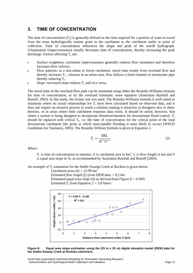
An example of Tc estimation for the Stable Swamp Creek at Rocklea is given below:

Catchment area (A) = 22.99 km2

Estimated flow length (L) from DEM data = 8.2 km

Estimated equal area slope (S) as derived from Figure 8 = 0.94%

Estimated Tc from Equation 2 = 5.8 hours

Figure 8: Equal area slope estimation using the (25 m x 25 m) digital elevation model (DEM) data for the Stable Swamp Creek at Rocklea catchment.

Y = 9.36 X - 11.86

R2 = 0.8

-20

0

20

40

60

80

0 1 2 3 4 5 6 7 8

Distance from catchment outlet, X (km)

He

igh

t a

bo

ve

ou

tle

t, Y

(m

)

2.01.0

58

SA

LTc


4. CATCHMENT CHARACTERISTICS

Estimated catchment characteristics for all 12 catchments are given in Table 2, whilst Figure 9 shows

their elevation and aerial views.

Table 2: Characteristics of 12 gauged catchments.

Creek Name Location in SEQ Area (ha)

Land Use TIA#

(%) Slope (%) ToC

^

(hour)

Tingalpa Creek (R1) Sheldon 2,785 Reference1 1 0.9 8.25

Pimpama River (R2) Kingsholme 415 Reference1 1 7.0 1.70

Scrubby Creek (R3) Karawatha Forest 144 Reference1 0 2.9 1.10

Upper Yaun Creek (R4) Coomera 362 Reference1 3 6.8 1.90

Blunder Creek (W1) Carolina Parade 2,176 Mixed2 14 0.4 8.85

Oxley Creek (W2) Heathwood 46 WSUD3 37 3.5 0.80

Blunder Creek (W3) Daintree Crescent 360 WSUD3 42 1.1 2.15

Lower Yaun Creek (W4) Coomera 504 WSUD3 10 1.0 3.00

Stable Swamp Creek (U1) Sunnybank 442 Urban4 38 1.5 2.50

Stable Swamp Creek (U2) Rocklea 2,299 Urban4 43 0.9 5.80

Blunder Creek (U3) Durack 563 Urban4 33 1.6 2.80

Sheepstation Creek (U4) Parkinson 190 Urban4 39 1.6 1.50

1 unimpacted or forest catchment

2 combinations of reference, WSUD and urban land use types

3 catchment involves water sensitive urban design (WSUD) features (wetland / pond)

4 traditional urban catchments,

# TIA = total impervious area,

^ ToC = time of concentration

(a) Tingalpa Creek at Sheldon (R1)

(b) Pimpama River at Kingsholme (R2)


(c) Scrubby Creek at Karawatha Forest (R3)

(d) Upper Yuan Creek at Coomera (R4)

(e) Blunder Creek at Carolina Parade (W1)

(f) Oxley Creek at Heathwood (W2)


(g) Blunder Creek at Daintree Crescent (W3)

(h) Lower Yuan Creek at Coomera (W4) (in the right hand side aerial photo, 1 indicates upper and 2 indicates lower Yuan Creek)

(i) Stable Swamp Creek at Sunnybank (U1) (white space indicates unavailability of orthophotos)


(j) Stable Swamp Creek at Rocklea (U2) (white space indicates unavailability of orthophotos)

(k) Blunder Creek at Durack (U3)

(l) Sheepstation Creek at Parkinson (U4)

Figure 9: Delineation of 12 gauged catchments grouped into three categories: (a - d) are reference or unimpacted catchments, (e - h) are urban catchments with WSUD features and (i - l) are urban catchments. In all figures black solid line within the figure indicates catchment boundary, blue line is stream or creek and black circle is gauging station. Left image – elevation from the DEM; right image – aerial view from the orthophoto.


5. CATCHMENT INSTRUMENTATION

All 12 catchments have been instrumented with a controlled section, eg. weirs (less affected by

erosion and sedimentation), tipping-bucket rain gauge (0.2 mm) and pressure transducer with data

logger for measuring continuous six-minute rainfall and water height data respectively. A gauge board

was installed at every site for quality control of pressure transducer water height data. Cross sections

of all creeks at the gauging section have been surveyed. Flow rate and depth of water at the creek

gauging section have been estimated using a Current Meter and an Acoustic Doppler Current Profiler

(mounted in a small boat) for different flow conditions (low, medium and high flow). Rating curves

(stage vs discharge relationship) have been developed and validated for all catchments using the

HydStra software. This allowed converting continuous water height data into flow rates. A Sonde was

also installed in the catchments (3 Sondes rotated around 12 catchments) for continuous measurement

of pH, dissolved oxygen, turbidity and electrical conductivity.

5.1 Rain Gauge

A tipping-bucket rain gauge (TBRG) (0.2 mm) has been installed at each catchment to collect six-

minute time step continuous rainfall data. Suitable areas were selected for their installation in order to

avoid any obstruction from trees and/or building structures. Data were collected regularly in a

fortnightly (or monthly) basis. Data quality and TBRG calibration were checked in a regular basis. An

installation of TBRG is shown in Figure 10.

Figure 10: Tipping Bucket rain gauge (TBRG) at the Scrubby Creek, Karawatha Forest.

5.2 Gauge Board

A gauge board was installed at each gauging station. They were made of steel and marked with black

colour in a white background. Gauge board elevations were coincided with the pressure transducer

water height elevation. Therefore, gauge board reading of water elevation provides an opportunity for

onsite calibration of pressure transducer water elevation data. Gauge boards were installed / attached

to some rigid structures (concrete bridge, steel pole etc.) in the stream and in a suitable location so that

they could be easily readable. Figures 11 and 12 show installation of gauge boards at two catchments.


Figure 11: Gauge board installation at the Pimpama River, Kingsholme.

Figure 12: Gauge board installation at the Stable Swamp Creek, Rocklea.


5.3 Pressure Transducer and Data Logger

A pressure transducer and data logger was installed at each site in order to collect water level data

(Figures 13 to 16). The pressure transducer continuously measured (6-minute) the water height above

it, and the data were stored in the Campbell data logger. Data were collected at regular interval

(monthly or fortnightly) and were post-processed using the HydStra software system located at the

Department of Environment and Resource Management (DERM).

Sedimentation in the creek due to civil construction works and high flood events posed difficulties in

data collection in some sites. For example, Scrubby Creek at Karawatha Forest was affected by a high

flood event and the data logger was inundated. Therefore, precautions were taken by raising the

position of data logger and battery as shown in Figure 15a. Sedimentation and erosion problems at the

Blunder Creek site in Forest Lake caused changes in creek cross section area and hence altered flow

gauging consistency (Figure 17). The gauged location was changed for this case.

Figure 13: Pressure transducer and data logger installation at Upper Yuan Creek, Coomera (top view).

Figure 14: Pressure transducer and data logger placement at Upper Yuan Creek, Coomera (side view).


(a)

(b)

Figure 15: (a) Raised data logger position in order to avoid flooding inundation at Scrubby Creek, Karawatha Forest. (b) Data logger placement at Blunder Creek, Durack.

Figure 16: Replacement of battery of data logger / pressure transducer at Stable Swamp Creek, Sunnybank. The lid of the environmental enclosure is on the left of photo.


Figure 17: Sedimentation and erosion problem at Blunder Creek, Forest Lake due to civil construction subdivision works. The gauging station was relocated to suitable location.

5.4 Creek Cross Section

Creek cross section is an essential parameter for rating curve development (water level or stage vs.

flow rate discharge relationship) and hydraulic modelling. Efforts have been made to estimate cross

sections for all 12 catchments. A Dumpy level surveying instrument was used for this purpose.

Figure 18 shows a photograph of cross section measurement, whilst Figure 19 (a-c) show the

estimated cross sections for all catchments.

Figure 18: Surveying the cross section of the gauging location at Scrubby Creek, Karawatha Forest using a Dumpy level.


(a)

(b)

Tingalpa Creek (R1)

0

0.5

1

1.5

2

2.5

3

3.5

4

1 3 5 7 9 11 13 15 17 19 21 23 25 27 29 31

Distance (m)

He

igh

t (m

)Pimpama River (R2)

0

0.5

1

1.5

2

2.5

3

0 2 4 6 8 10 12 14 16 18 20

Distance (m)

He

igh

t (m

)

Scrubby Creek (R3)

0

0.2

0.4

0.6

0.8

1

1.2

1.4

0 2 4 6 8 10 12 14 16 18 20 22 24 26 28 30 32 34

Distance (m)

He

igh

t (m

)

Upper Yuan Creek (R4)

0

0.5

1

1.5

2

2.5

0 1 2 3 4 5 6 7 8 9 10 11 12 13 14

Distance (m)

He

igh

t (m

)

Blunder Creek (W1)

0

0.5

1

1.5

2

2.5

3

0 2 4 6 8 10 12 14 16 18 20 22

Distance (m)

He

igh

t (m

)

Oxley Creek (W2)

0

0.1

0.2

0.3

0.4

0.5

0.6

0.7

0.8

0.9

1

0 2 4 6 8 10

Distance (m)

He

igh

t (m

)

Blunder Creek (W3)

0

0.5

1

1.5

2

2.5

3

0 2 4 6 8 10 12

Distance (m)

He

igh

t (m

)

Lower Yaun Creek (W4)

0

0.5

1

1.5

2

2.5

3

3.5

0 2 4 6 8 10 12 14 16 18

Distance (m)

He

igh

t (m

)


(c)

Figure 19: (a) Measured creek cross section for reference or unimpacted catchments. (b) Measured creek cross section for WSUD/Mixed catchments. (c) Measured creek cross section for urban catchments.


0

0.5

1

1.5

2

2.5

3

0 2 3 5 6.35 8 10 12

Distance (m)

He

igh

t (m

)


0

0.5

1

1.5

2

2.5

3

3.5

4

0 4 8 12 16 20 24 28 32 36 40

Distance (m)

He

igh

t (m

)

Blunder Creek (U3)

0

0.5

1

1.5

2

2.5

3

0 4 8 12 16 20 24 28 32 36

Distance (m)

He

igh

t (m

)


0

0.25

0.5

0.75

1

1.25

1.5

1.75

2

2.25

2.5

1 3 5 7 9 11 13 15 17 19 21 23 25 27 29

Distance (m)

Heig

ht

(m)


6. RATING CURVE DEVELOPMENT

Rating curves, which describe the relationship between creek discharge and water level (or stage),

were developed for all 12 catchments. Development of rating curves was essential in order to convert

the continuous water stage data from the pressure transducers into discharge data. The cross section

measured at the site enables the determination of the area of the flow at different water levels. This

area is then combined with factors such as the slope of the channel and a roughness coefficient of the

bed to calculate a theoretical flow. The surface slope of the channel can be measured by marking the

edge of the water upstream and downstream of the measured section during high flows. Figure 20

shows the surveying of the height markers which had been placed upstream and downstream of the

weir at Sunnybank during a prior high flow event.

Figure 20: Surveying water surface slope at Stable Swamp Creek, Sunnybank using pegs installed during a prior high flow event.

Using mean value of water surface slope, Manning’s equation was used to estimate flow velocity.

Manning’s equation is shown in Equations 2 and 3 below:

(2)

(3)

Where:

v is mean velocity (m/sec), R is hydraulic radius (m), S is slope (m/m), A is cross sectional area

(m2) and P is wetted perimeter (m) and n is Manning’s roughness coefficient.

The quality of stream flow data conversion from the pressure transducer water stage data depends on

the quality of the rating curves. The rating curve is one of major sources of uncertainty in hydrologic

simulation studies. Rating curves may not generate accurate runoff data because of time depended

changes in creek cross sections due to sedimentation and erosion, and also because of systematic error.

Therefore validation of rating curves from time to time is recommended. The general equation for a

rating curve is shown in Equation 4 (Mosley and McKerchar, 1993):

(4)

Where:

Q is discharge (m3/sec), h is water stage (m), a is stage (m) at which Q = 0 and C and N are

fitted constants.

2/13/21SR

nv

P

AR

NahCQ )(


6.1 Flow Gauging

Calibration and validation of theoretical rating curves require flow gauging at different flow

conditions. At low, medium and high flow conditions, flow velocities were measured using a current

meter (for low and medium flow) and an Acoustic Doppler (for high flow). The objective of flow

gauging is to measure creek discharge at known water stage heights. The velocity–area method of

discharge calculation (Mosley and McKerchar, 1993) was followed in this study. Flow velocities were

measured at known intervals perpendicular to flow direction. The method is shown in Figure 21.

Figure 21: Velocity-Area method of discharge calculation, where d is water stage height and b is horizontal distance from a reference point. Dashed lines indicate midsection and hatched area indicates discharge (qi) corresponds to the depth di.

Discharge (qi) corresponds to depth (di) is the product of hatched area and measured velocity (vi). This

is expressesed mathematically suing Equation 5:

(5)

The total discharge is the summation of incremental discharges for all segments. Figure 22 shows

photographs of typical velocity measurements undertaken in all 12 catchments.

Figure 22: Low and medium flow gauging using a current meter (left) and high flow gauging using an Acoustic Doppler (right).

iii

iiiiii

ii dbb

vdbbbb

vq )2

()22

( 1111


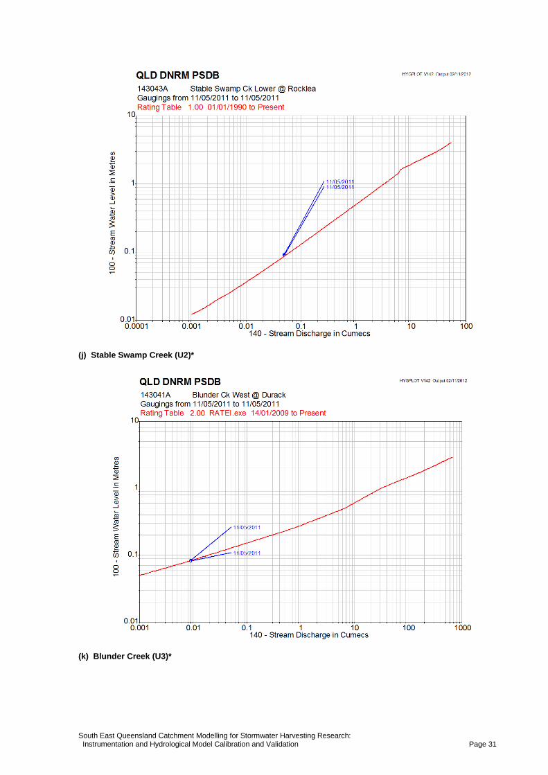
6.2 Rating Curves

Rating curves were developed using the HydStra software installed in the DERM hydrology database

system. Theoretical rating curves were calibrated, chiefly by altering Manning’s roughness coefficient

value to better reflect the measured flows obtained from field gaugings. Figures 23 (a-l) show

developed rating curves for all 12 catchments.

(a) Tingalpa Creek (R1)

0.001 0.01 0.1 1 10 100

QLD DNRM PSDB HYGPLOT V142 Output 02/11/2012

145028A Tingalpa Ck @ Campbell Rd, Sheldon

Gaugings from 23/01/2009 to 04/01/2010

Rating Table 1.00 01/01/1990 to Present

10

0 -

Str

ea

m W

ate

r L

eve

l in

Me

tre

s

140 - Stream Discharge in Cumecs

21/05/2009 21/05/2009 21/05/2009

04/01/2010 21/05/2009 06/04/2009

04/01/2010 04/01/2010

02/10/2009

23/01/2009

0.001

0.01

0.1

1

10


(b) Pimpama River (R2)

(c) Scrubby Creek (R3)


(d) Upper Yaun Creek (R4)

(e) Blunder Creek (W1)


(f) Oxley Creek (W2)

(g) Blunder Creek (W3)


(h) Lower Yaun Creek (W4)

(i) Stable Swamp Creek (U1)


(j) Stable Swamp Creek (U2)*

(k) Blunder Creek (U3)*


(l) Sheepstation Creek (U4)

Figure 23: Developed rating curves at the outlet of 12 gauged catchments (* Concrete channel, theoretical rating curve is used).


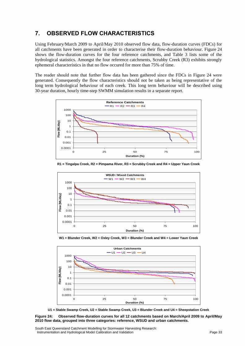
7. OBSERVED FLOW CHARACTERISTICS

Using February/March 2009 to April/May 2010 observed flow data, flow-duration curves (FDCs) for

all catchments have been generated in order to characterise their flow-duration behaviour. Figure 24

shows the flow-duration curves for the four reference catchments, and Table 3 lists some of the

hydrological statistics. Amongst the four reference catchments, Scrubby Creek (R3) exhibits strongly

ephemeral characteristics in that no flow occured for more than 75% of time.

The reader should note that further flow data has been gathered since the FDCs in Figure 24 were

generated. Consequently the flow characteristics should not be taken as being representative of the

long term hydrological behaviour of each creek. This long term behaviour will be described using

30-year duration, hourly time-step SWMM simulation results in a separate report.

R1 = Tingalpa Creek, R2 = Pimpama River, R3 = Scrubby Creek and R4 = Upper Yaun Creek

W1 = Blunder Creek, W2 = Oxley Creek, W3 = Blunder Creek and W4 = Lower Yaun Creek

U1 = Stable Swamp Creek, U2 = Stable Swamp Creek, U3 = Blunder Creek and U4 = Sheepstation Creek

Figure 24: Observed flow-duration curves for all 12 catchments based on March/April 2009 to April/May 2010 flow data, grouped into three categories: reference, WSUD and urban catchments.

Reference Catchments

0.0001

0.001

0.01

0.1

1

10

100

1000

0 25 50 75 100

Duration (%)

Flo

w (M

L/d

ay)

R1 R2 R3 R4

WSUD / Mixed Catchments

0.0001

0.001

0.01

0.1

1

10

100

1000

0 25 50 75 100

Duration (%)

Flo

w (

ML

/da

y)

W1 W2 W3 W4

Urban Catchments

0.0001

0.001

0.01

0.1

1

10

100

1000

0 25 50 75 100

Duration (%)

Flo

w (

ML

/da

y)

U1 U2 U3 U4


Table 3: Observed flow characteristics of creeks.

Flow Characteristics Reference Catchments

R1 R2 R3 R4

Mean daily runoff (ML/day/km2)* 0.58 1.34 0.64 1.30

Median daily runoff (ML/day/km2) 0.04 0.29 0.00 0.09

CV of daily flow 3.50 3.01 6.68 5.13

Skewness of daily flow 6.41 7.78 10.91 8.56

Rise rate (ML/day/day) 26.9 5.27 11.59 7.13

CV of rise rate 3.12 4.23 2.43 4.58

Fall rate (ML/day/day) 7.87 2.54 3.93 4.68

CV of fall rate 4.23 4.74 3.83 5.44

Base Flow Index (BFI) 0.14 0.33 0.03 0.10

* ML/day/km2 is equivalent to mm/day.

Tingalpa Creek (R1), Pimpama River (R2), Scrubby Creek (R3), Upper Yaun Creek (R4)

Flow Characteristics WSUD/Mixed Catchments

W1 W2 W3 W4

Mean daily runoff (ML/day/km2) 0.40 3.29 1.68 6.25


CV of daily flow 3.94 2.40 4.55 3.78



CV of rise rate 3.88 2.80 3.43 3.56


CV of fall rate 4.98 3.69 4.60 4.74


Blunder Creek (W1), Oxley Creek (W2), Blunder Creek (W3), Lower Yaun Creek (W4)

Flow Characteristics Urban Catchments

U1 U2 U3 U4

Mean daily runoff (ML/day/km2) 3.81 1.55 0.71 1.50


CV of daily flow 3.55 3.23 2.86 3.60



CV of rise rate 3.23 2.50 4.25 2.62


CV of fall rate 4.82 3.10 5.21 4.12


Stable Swamp Creek (U1), Stable Swamp Creek (U2), Blunder Creek (U3), Sheepstation Creek (U4)


8. STORMWATER MANAGEMENT MODEL (SWMM)

In this section, we provide an overview of the theory and methodology adopted for the development of

the Stormwater Management Model (SWMM) for each of the catchments in this study.

8.1 Surface Runoff Component

Two of the most widely used routing methods in hydrology are non-linear reservoir routing and

kinematic-wave routing. Hydrologic models are developed based on hypothesised relationships

between catchment storage and overflow, where the sub-catchments are considered as conceptual

reservoirs (Xiong and Melching, 2005). Hydraulic models are developed on the basis of

approximations of the real rainfall-runoff processes. The kinematic-wave routing in hydraulic models

is the solution of the simplest form of the full dynamic equations of motion for one dimensional flow

(Saint Venant’s equation) (Xiong and Melching, 2005). SWMM (Huber and Dickinson, 1988) and

Dynamic Watershed Simulation Model (Borah et al., 2002) are examples of hydrologic and hydraulic

models respectively (Xiong and Melching, 2005).

SWMM uses a non-linear reservoir routing method for surface runoff routing over pervious and

impervious surfaces. It accounts for infiltration using either the Horton or Green-Ampt equation,

evaporation, depression storage (abstractions). It estimates surface runoff using simple routing through

pipes or channels (Walters and Geurink, 2001).

8.1.1 Reservoir Routing

Reservoir routing is also known as a storage–discharge model, where storage in a catchment is

approximated by a reservoir, and is a function of inflow and outflow to and from the catchment. The

reservoir routing method concentrates on flood water storage and considers as negligible the effects of

resistance to flow (Raudkivi, 1979). The continuity equation is shown as Equation 6:

(6)

where:

I is inflow to catchment at time t, O is outflow from the catchment at time t and S is storage at

time t.

Two forms of reservoir routing are: linear reservoir routing, where outflow is a linear function of

stored water in the reservoir; and non-linear reservoir routing, where stored water in the reservoir is a

non-linear function of inflow and outflow. Mathematically, these are shown in Equations 7 and 8:

KOS (7)

),( OIfS (8)

Equation (7) represents linear reservoir routing, K is a proportionality constant, and Equation (8)

represents non-linear routing.

The mass balance equation for non-linear reservoir routing in SWMM (Figure 25) can be expressed

using Equation 9 as:

QAidt

dDA

dt

de

(9)

where:

is volume of water in a sub-catchment; A is sub-catchment area; D is water depth in the sub-

catchment; t is time; ie is rainfall excess which is equal to rainfall intensity minus infiltration

rate, and Q is surface runoff or overland flow.

dt

dSOI


Figure 25: System concept of the non-linear reservoir routing in SWMM, where every sub-catchment is considered as a system of reservoir with a constant depression storage depth (Dp). System input is precipitation (rainfall) and system outputs are evaporation, infiltration and surface runoff.

Flow from a sub-catchment with length (L) and characteristics width (W) can be simulated using the

Manning’s equation (Equation 10):

3/52/1 )(1

DpDSn

WQ (10)

where:

Q is surface flow (m3/s) per unit length (L), W is sub-catchment width (m), n is Manning’s

roughness coefficient, S is sub-catchment slope (m/m), Dp is depth of depression storage (m).

The SWMM model used a spatially lumped continuity equation coupled with Manning’s equation in

order to simulate continuous flow (Huber, 2003). The algorithm is given below:

From Equations 6 and 10:

dt

dDASDD

nWAi Pe 2/13/5)(

1 (11)

fiie (12)

where:

ie is rainfall excess intensity (m/hour), i is rainfall intensity (m/hour) at time t, f is infiltration

rate (m/hour) at time t, W is the conceptual or characteristic width of sub-catchment (m)

calculated as the ratio of catchment area to average maximum flow path length, and A is sub-

catchment area (m2).

Dividing Equation 11 by the sub-catchment area gives:

dt

dDSDD

nA

Wi Pe 2/13/5)(

1 (13)

dt

dDDDi Pe 3/5)( (14)

An

WS 2/1

(15)

where:

ψ is a constant which spatially lumps all parameters of Manning’s equation for the sub-

catchment.


Equation 14 is a nonlinear function with dependent variable D and ie is an arbitrary function of time, t.

Therefore numerical solution of Equation 14 using a simple finite difference scheme is (Huber, 2003):

3/52112 }2

)({

)(Pe D

DDi

t

DD

(16)

12 DDD (17)

2

)()1(}

2

)({)(

3/52

3/53/5213/5 DpDDpD

DDD

DpD P

(18)

where:

subscripts 1 and 2 indicate start and end of time step respectively, Δt is length of time step, ie is

average rainfall excess over the time step Δt. Equation 16 can be solved using the Newton-

Raphson iteration method (Huber, 2003; Chapra and Canale, 2002).

8.1.2 Kinematic Wave Routing

The kinematic wave routing method is widely used in hydraulic routing of overland and channel flow

(Xiong and Melching, 2005). The method differs from the reservoir routing method because stream

storage is not a function of stream stage or discharge only (Raudkivi, 1979). The method is based on

laws of conservation of mass (continuity equation) and momentum (equations of motion). The

continuity equation as given by Raudkivi (1979) in Equation 19:

(19)

where:

Ac is cross section area of stream perpendicular to the x direction and q is lateral inflow per unit

length of catchment.

The driving forces for open channel flow are gravity force, friction forces due to surface wind and

boundary drag and internal pressure gradient. In the kinematic wave theory, internal pressure gradient

force is neglected (Xiong and Melching, 2005). For steady uniform flow condition, Raudkivi (1979)

expressed the equation of momentum as (Equation 20):

(20)

where:

Sf is friction slope and S0 is bed slope of the channel. The Manning’s equation can be written as

Equation 21:

(21)

where:

R is hydraulic radius which is a ratio of flow cross sectional area to flow wetted perimeter.

Xiong and Melching (2005) showed that discharge (Q) can be expressed as function of cross-sectional

area (Ac) using Equations 22 to 25:

(22)

(23)

(24)

(25)

where:

α and m are constants determined from sub-catchment geometry, slope and roughness

coefficient; P is wetted perimeter; and a and b are constants. For overland flow, a = 1 and b =0.

m

cAQ

na

S3/2

2/1

0

3

)25( bm

b

caAP

2/1

0

3/21SRA

nQ c

0SS f

qdx

dQ

dt

dAc


8.2 Water Loss Component

Three types of water losses are considered in SWMM: evaporation, depression storage and

infiltration. SWMM does not compute evaporation losses, rather this is an input parameter from the

user as a daily time series or monthly average value. Evaporation losses are subtracted from rainfall

values before computation of surface flow (Huber, 2003). Depression storage (Dp, in Figure 25) is the

initial abstraction of rainwater and it may evaporate and infiltrate. It is a constant value which differs

for pervious and impervious surfaces. Impervious surfaces consists less depression storage than

pervious surfaces. It is also used to account for interception losses from vegetation (Huber, 2003).

SWMM computes infiltration losses and is described in the next section.

8.2.1 Infiltration

Either Horton’s equation or the Green-Ampt method is used in SWMM to simulate infiltration losses.

Both methods require three parameters: initial infiltration capacity, ultimate infiltration capacity and

decay constant. The Horton’s equation (Equation 26) for exponential decay of infiltration capacity

(illustrated in Figure 26) is:

(26)

where:

f is infiltration rate at time t when surface water is not limiting, fo is initial infiltration capacity, fc

is ultimate infiltration capacity and K is a decay rate (time-1

). Unit of infiltration rate is mm/hour

or m/hour.

Figure 26: Horton’s exponential decay of infiltration capacity. Infiltration capacity reduced as a function of cumulative infiltration, F (the shaded area under curve up to time, tp).

In SWMM, Horton’s infiltration capacity decays as a function of cumulative infiltration, F (Huber and

Dickenson, 1988) (Equation 27).

(27)

The Green–Ampt method of infiltration capacity estimation described in Huber (2003) is shown in

Equation 28:

(28)

where:

Ks is saturated hydraulic conductivity, ψf is average soil suction along the wetting front

(negative value), F is cumulative infiltration and Md is initial moisture deficit which is different

between upper soil water storage limit (or Field Capacity) and initial moisture content.

)1)(( 0K

t

cc effKtftfF

)1(F

MKsf

fd

Kt

cc effff )( 0


8.3 Groundwater Flow Component

The SWMM groundwater component simulates two zones: unsaturated upper zone and saturated

lower zone. Figure 27 represents the groundwater modelling component of SWMM. Flow from

unsaturated zone to saturated zone is performed by an empirical equation (Equation 29). Infiltration

and evapotranspiration are the only inflow (fl) and loss (fEU) from the unsaturated zone respectively

(Figure 27). Outflows from lower saturated zone consists of deep percolation (fL), saturated zone

evapotranspiration (fEL) and groundwater flow to stream (fG). The user-defined power function of

groundwater flow is a function of groundwater table stage (HGW) and water depth in stream (HSW)

(Huber and Dickenson, 1988; Walters and Geurink, 2001). The power function is given in

Equation 29:

(29)

where:

QGW is groundwater flow, A1 is groundwater influence coefficient, A2 is stream water influence

coefficient, HGW is average groundwater table elevation HB stream bottom elevation, HSW is

water elevation in stream, B1 is groundwater influence flow exponent and B2 is stream water

influence flow exponent.

Figure 27: SWMM groundwater flow simulations: (top) system concept of SWMM groundwater flow; (botom) user-defined power function to generate groundwater flow.

21 )()( 21

B

BSW

B

BGWGW HHAHHAQ


9. CATCHMENT CALIBRATION AND VALIDATION

The calibration of catchment models requires the determination of the set of model parameter values

which maximise the goodness of fit between model outputs and the real response of the catchment for

a given rainfall (input). This is accomplished by adjustments of control parameters in order to

minimise prediction errors between observed and model generated flow data (Choi and Ball, 2002).

Control parameters can be divided into two categories based on their estimation techniques.

Measured Parameters: Physically measured parameters such as stream cross section, catchment area,

impervious fraction, rainfall intensity etc. These parameters are assumed error free and are not

adjusted in the calibration process.

Adjusted Parameters: These parameters are not physically estimated, but rather are adjusted during

the model calibration process in order to minimise prediction errors between observed and model

computed flow data.

Two alternative techniques of parameter estimation are described in Choi and Ball (2002). The first

technique is the modification of parameter values until both observed and computed hydrographs are

well matched. The second technique is selection of parameter values on the basis of catchment hydro-

geological characteristics. For example, selection of soil hydrologic properties (hydraulic conductivity

and field capacity) from soil texture information. The first method is also called trial and error

method. Several previous studies have used optimisation search technique to determine control

parameters’ value (Kuczera, 1983; Liong and Ibrahim, 1994). The trial and error approach is only

applicable when monitoring data on rainfall and stream flow are available. This calibration process is

shown in Figure 28. The reader should note that the actual computational process details will vary

substantially depending upon the technique used, e.g., in some cases (as with the technique employed

in this study) the output to recorded data loop is automated within an optimisation process.

Figure 28: Schematic of the SWMM model calibration flow diagram (trial and error method).


9.1 Methodology

Observed streamflows from the SEQ catchments were used to calibrate and validate the SWMM. The

calibration was used to adjust model parameter values so that the modelled flows agree with observed

flow data to user specified criteria. These criteria can either be subjective (e.g., visual matching of

flow hydrographs) or objective (e.g., comparing Nash Sutcliff efficiency (NSE) (Nash and Sutcliffe,

1970)). Manual or automatic calibration methods or a combination of these can be used.

The ‘split sample testing’ approach is used in hydrologic modelling for calibration and validation to

prepare the model for scenario prediction. In this approach, a part of observed data is used for

calibration for parameter estimation and the other part is used for model validation to test the model’s

capability for satisfactory prediction.

9.1.1 Model Calibration

Ten catchments in SEQ with varying degree of urbanisation were calibrated against the hourly

streamflow data from 2009 to 2012. In the calibration, the model parameter was optimised using the

shuffled complex evolution automated optimiser (Duan et al., 1992) to maximise the objective

function given by the NSE for hourly flow data.

NSE is a common measure of goodness of fit in water resource modelling and is calculated using

Equation 30:

(30)

where:

Qo is the observed flow, oQ is the mean of the observed flow and Qm is the modelled flow.

The NSE is an estimate of the variance in model error between simulated and observed data. Values

can vary from – to 1, with 1 indicating a perfect fit, and a value of zero indicating that the model is

no better than assuming an average flow over the period. A negative NSE value implies a bad

prediction which is hard to interpret. Whilst undue influence of high flows can be an issue with NSE,

it is considered a reliable statistic for assessing the goodness of fit of hydrological models and is

recommended for a variety of model types (ASCE, 1993; McCuen et al., 2006).

The use of hourly rainfall streamflow data was adopted to capture the rapid rise and fall of flows in

urban catchments during a storm event. The time of concentration, a measure of travel time for water

particle from the farthest point in the catchment to its outlet, of all catchments is more than one hour

(see Table 1). Thus the SWMM modelling using a time step less than an hour was deemed

unnecessary.

9.1.2 Automatic Optimisation

The shuffled complex evolution (SCE) algorithm used to optimise of the model parameters is a

general purpose global optimisation program and is available as a MATLAB routine at

http://www.mathworks.com/matlabcentral/fileexchange/7671. We coupled the SCE routine with the

SWMM executable in MATLAB to develop a tool for the parameter optimisation.

2

2

1

oQo

Q

mQ

oQ

NSE

http://www.mathworks.com/matlabcentral/fileexchange/7671


Seven parameters of SWMM found to be most sensitive (Javaheri, 1998) were chosen for the

optimisation. Those parameters were:

1. Overland flow width

2. Manning’s n for pervious surface

3. Pervious depression store

4. Porosity

5. Field capacity

6. Hydraulic conductivity

7. Lower groundwater loss rate.

The first six parameters were changed in unison for all subcatchments but the lower groundwater loss

rate was varied for each aquifer within a catchment (see Equation 29 and Figure 26). The optimisation

to maximise the NSE using hourly observed and modelled flow was done by varying the above

parameter values within predetermined upper and lower bounds.

9.1.3 Assessment of Model Performance and Model Robustness

Model performance refers to the ability of the models to reproduce observed hydrological patterns and

can therefore only be tested retrospectively. Model performance was assessed using the NSE of both

hourly and daily streamflows. A set of objective criteria were used to determine model performance.

These included the model’s ability to reproduce the observed runoff series with:

(a) hourly NSE values greater than 0.5 in at least 90% of subcatchments; and

(b) daily NSE values greater than 0.6 in at least 90% of subcatchments.

The model was assessed for its ability to represent the observed conditions within the calibration data

period. Hourly and daily NSEs greater than 0.5 and 0.6 for the majority of catchments gives

confidence in the calibrated parameter values used in the determinations of runoff for these time steps.

9.1.4 Validation

The data not used in calibration were used for validation. The purpose was to assess the model’s

potential performance for simulating catchment response to future input rainfall. Ideally, validation

NSE should be as good as the calibration NSE. However, in reality, the validation NSEs are usually

lower due to the shorter time series of data employed.

9.1.5 Input Data

The hourly rainfall data were obtained from the network of tipping bucket (0.2 mm) rain gauges

installed for the project. The stream flow data were also obtained from the streamflow gauging

stations. Although data from 2009 were available, providing about two years of rainfall and

streamflow data for calibration/validation, data for the year 2009 and early 2010 suffered from

frequent gaps and quality problems. Furthermore, 2009 was drier compared to 2010 and 2011.

Therefore data mostly from 2010 and 2011 was used in calibration to expose the model to a range of

flow conditions to determine a more robust parameter set.

9.2 Catchment Results

Table 4 shows the start and end dates for calibration and validation, and the daily and hourly NSE

values for all 10 catchments. The hourly and daily calibration NSEs for nine of ten catchments are

more than 0.5 and 0.6 respectively. This fulfils the criteria set for the good model calibration as

described in Section 9.1.3.


9.2.1 Tingalpa Creek at Sheldon

One year of hourly data is used calibrate the Tingalpa catchment with hourly and daily calibration

NSEs of 0.49 and 0.64 respectively. The corresponding validation NSEs are 0.51 and 0.50. Except for

one large event, the hourly observed and modelled streamflow during the calibration periods match

reasonably well (Figure 29).

Figure 29: Observed and modelled hourly flows in Tingalpa catchment.

9.2.2 Upper Yaun Creek at Coomera

For the Upper Yaun Creek hourly observed and modelled streamflows events match quite well during

the calibration (Figure 30) resulting in hourly and daily NSEs of 0.78 and 0.81 respectively. The

hourly validation NSE is the lowest (0.33) of all the catchments, however the daily flow NSE f is quite

good (0.75). This could be due to the hourly time step for the observed not fully synchronised with the

rainfall data.

Figure 30: Observed and modelled hourly flows in Upper Yaun Creek catchment.

Tingalpa (2785 ha)

Apr-

10

May-1

0

Jun-1

0

Jul-10

Aug-1

0

Sep-1

0

Oct-

10

Nov-

10

Dec-1

0

Jan-1

1

Feb-1

1

Mar-

11

Apr-

11

May-1

1

Jun-1

1

Ra

infa

ll (m

m d

ay-1

)

0

10

20

30

40

50

Dis

cha

rge

(m

3 s

-1)

0

5

10

15

20

25

30

35

rain

Observed

Modelled

Tingalpa (2785 ha)

Apr

-10

May

-10

Jun-

10

Jul-1

0

Aug

-10

Sep

-10

Oct

-10

Nov

-10

Dec

-10

Jan-

11

Feb

-11

Mar

-11

Apr

-11

May

-11

Jun-

11

Ra

infa

ll (m

m d

ay-1

)

0

10

20

30

40

50

Dis

cha

rge

(m

3 s

-1)

0

5

10

15

20

25

30

35

rain

Observed

Modelled

Stable Swamp Cr Sunnybank (442 ha)

Oct

-10

Nov

-10

Dec

-10

Jan-

11

Feb

-11

Mar

-11

Apr

-11

May

-11

Jun-

11

Ra

infa

ll (m

m d

ay-1

)

0

10

20

30

40

50

Dis

cha

rge

(m

3 s

-1)

0

5

10

15

20

25

rain

Observed

Modelled

Upper Yaun Cr Reserve(362 ha)

Apr

-10

May

-10

Jun-

10

Jul-1

0

Aug

-10

Sep

-10

Oct

-10

Nov

-10

Dec

-10

Jan-

11

Feb

-11

Mar

-11

Apr

-11

May

-11

Jun-

11

Ra

infa

ll (m

m d

ay-1

)

0

10

20

30

40

50

Dis

cha

rge

(m

3 s

-1)

0

2

4

6

8

10

12

rain

Observed

Modelled


9.2.3 Scrubby Creek at Karawatha Forest

One year of hourly data is used calibrate the Scrubby Creek catchment at Karawatha Forest with

hourly NSE of 0.55. The hourly validation NSE is 0.59, giving reasonable confidence in the predictive

ability of the model for future scenarios. Figure 31 shows that the model has not been able to capture

the full extent of observed flow at the hourly time scale. However, as indicated by the daily calibration

and validation NSEs (0.75 and 0.85 respectively), the matching of these flows at daily time scale is

much better.

Figure 31: Observed and modelled hourly flows in Scrubby Creek catchment.

9.2.4 Blunder Creek (Daintree Crescent) at Forest Lake

The calibration for the Blunder Creek at Forest Lake runs from March 2010 to May 2011, with hourly

calibration NSE of 0.55. The hourly validation NSE is 0.74. The daily calibration and validation NSEs

are still better (Table 1) implying satisfactory modelling results at this time scale. Figure 32 shows the

observed and modelled flow for the Blunder Creek for the calibration period.

Figure 32: Observed and modelled hourly flows in Blunder Creek catchment at Forest Lake.

Scrubby Cr Karawatha (144 ha)

Apr

-10

May

-10

Jun-

10

Jul-1

0

Aug

-10

Sep

-10

Oct

-10

Nov

-10

Dec

-10

Jan-

11

Feb

-11

Mar

-11

Apr

-11

May

-11

Jun-

11

Rai

nfal

l (m

m d

ay-1

)

0

10

20

30

40

50

Dis

char

ge (m

3 s-1

)

0

1

2

3

4

5

6

7

rain

Observed

Modelled

Blunder Cr Daintree (360 ha)

Oct

-10

Nov

-10

Dec

-10

Jan-

11

Feb

-11

Mar

-11

Apr

-11

May

-11

Jun-

11

Rai

nfal

l (m

m d

ay-1

)

0

10

20

30

40

50

Dis

char

ge (m

3 s-1

)

0

5

10

15

20

25

rain

Observed

Modelled

Pimpama (415 ha)

Apr

-09

May

-09

Jun-

09

Jul-0

9

Aug

-09

Sep

-09

Oct

-09

Nov

-09

Dec

-09

Jan-

10

Feb

-10

Mar

-10

Apr

-10

May

-10

Jun-

10

Jul-1

0

Rai

nfal

l (m

m d

ay-1

)0

10

20

30

40

50

Dis

char

ge (m

3 s-1

)

0

5

10

15

20

rain

Observed

Modelled

Blunder Cr Daintree (360 ha)

Mar-

10

Apr-

10

May-1

0

Jun-1

0

Jul-10

Aug-1

0

Sep-1

0

Oct-

10

Nov-

10

Dec-1

0

Jan-1

1

Feb-1

1

Mar-

11

Apr-

11

May-1

1

Jun-1

1

Ra

infa

ll (m

m d

ay

-1)

0

10

20

30

40

50

Dis

cha

rge

(m

3 s

-1)

0

2

4

6

8

10

12

14

16

18

rain

Observed

Modelled


9.2.5 Stable Swamp Creek at Sunnybank

Seven months of hourly data is used in calibration for the Stable Swamp Creek (Figure 33) due to a

lack of longer rainfall and runoff data without missing periods and suspect quality. The hourly

calibration and validation NSEs are 0.60 and 0.81. Although these are good values, they have come

from relatively smaller data set compared to that for the other catchments.

Figure 33: Observed and modelled hourly flows in Stable Swamp Creek.

9.2.6 Oxley Creek at Heathwood

Oxley creek is the smallest of the study catchment resulting in smaller observed flow (Figure 34). It

was calibrated using a comparatively longer period of data with good hourly calibration and validation

NSEs (0.59 and 0.66 respectively). This gives confidence in the calibrated model’s ability for

prediction.

Figure 34: Observed and modelled hourly flows in Oxley Creek.

Stable Swamp Cr Sunnybank (442 ha)

Oct-

10

Nov-

10

Dec-1

0

Jan-1

1

Feb-1

1

Mar-

11

Apr-

11

May-1

1

Jun-1

1

Ra

infa

ll (m

m d

ay

-1)

0

10

20

30

40

50

Dis

cha

rge

(m

3 s

-1)

0

5

10

15

20

25

rain

Observed

Modelled

Oxley Cr Wadeville (46 ha)

Mar-

10

Apr-

10

May-1

0

Jun-1

0

Jul-10

Aug-1

0

Sep-1

0

Oct-

10

Nov-

10

Dec-1

0

Jan-1

1

Feb-1

1

Mar-

11

Apr-

11

May-1

1

Jun-1

1

Ra

infa

ll (m

m d

ay

-1)

0

10

20

30

40

50

Dis

cha

rge

(m

3 s

-1)

0.0

0.5

1.0

1.5

2.0

2.5

rain

Observed

Modelled


9.2.7 Pimpama River at Kingsholme

The hourly flow hydrographs for the Pimpama River shows (Figure 35) missing response for rainfall

during October 2009. The hourly calibration is quite good at 0.6, while the validation NSE is lower.

This is due to a lack of higher intensity rainfall during the validation period which failed to initiate

quick runoff response in the model. The daily calibration and validation NSEs are better suggesting

that the model is able to capture daily flows better than the hourly flows.

Figure 35: Observed and modelled hourly flows in Pimpama River.

9.2.8 Blunder Creek at Carolina Parade

The flow hydrographs for Blunder Creek catchment at Carolina Parade shows the model is simulating

the flow events well (Figure 36). The hourly calibration NSE is quite good (0.68), while the hourly

validation is also reasonable (0.52). The modelled runoffs at daily time scale are still better as

indicated by the higher daily NSEs (Table 4).

Figure 36: Observed and modelled hourly flows in Blunder Creek catchment Carolina Parade.

Pimpama (415 ha)

Apr-

09

May-0

9

Jun-0

9

Jul-09

Aug-0

9

Sep-0

9

Oct-

09

Nov-

09

Dec-0

9

Jan-1

0

Feb-1

0

Mar-

10

Apr-

10

May-1

0

Jun-1

0

Jul-10

Ra

infa

ll (m

m d

ay

-1)

0

10

20

30

40

50

Dis

cha

rge

(m

3 s

-1)

0

5

10

15

20

rain

Observed

Modelled

Blunder Cr Carolina (2176 ha)

Jul-10

Aug-1

0

Sep-1

0

Oct-

10

Nov-

10

Dec-1

0

Jan-1

1

Feb-1

1

Mar-

11

Apr-

11

May-1

1

Jun-1

1

Jul-11

Ra

infa

ll (m

m d

ay-1

)

0

10

20

30

40

50

Dis

cha

rge

(m

3 s

-1)

0

5

10

15

20

25

30

35

rain

Observed

Modelled


9.2.9 Sheepstation Creek at Parkinson

Figure 37 shows that the model was able to pick the flow event reasonably well for this catchment.

The hourly calibration NSE is good (0.63), with slightly low validation NSE of 0.47. The daily

calibration and validation NSEs show mixed results.

Figure 37: Observed and modelled hourly flows in Sheepstation Creek catchment.

9.2.10 Blunder Creek at Durack

Blunder Creek at Durack has reasonably good hourly and daily calibration NSEs (0.52 and 0.71

respectively). The model has picked up the timing of storm events well (Figure 38). The hourly

validation is less than the corresponding calibration NSE however the daily validation NSE is quite

good (Table 4).

Figure 38: Observed and modelled hourly flows in Blunder Creek catchment Durrack.

Sheepstation (190 ha)

Jul-10

Aug-1

0

Sep-1

0

Oct-

10

Nov-

10

Dec-1

0

Jan-1

1

Feb-1

1

Mar-

11

Apr-

11

May-1

1

Jun-1

1

Jul-11

Ra

infa

ll (m

m d

ay

-1)

0

10

20

30

40

50

Dis

cha

rge

(m

3 s

-1)

0

1

2

3

4

5

6

rain

Observed

Modelled

Blunder Cr Durack (563 ha)

Apr-

09

May-

09

Jun-0

9

Jul-09

Aug-0

9

Sep-0

9

Oct-

09

Nov-0

9

Dec-0

9

Jan-1

0

Feb-1

0

Mar-

10

Apr-

10

May-

10

Jun-1

0

Jul-10

Aug-1

0

Sep-1

0

Oct-

10

Nov-1

0

Dec-1

0

Ra

infa

ll (m

m d

ay

-1)

0

10

20

30

40

50

Dis

ch

arg

e (

m3 s

-1)

0

10

20

30

rain

Observed

Modelled


9.3 Overview of Calibration and Validation Results

Table 4 below provides an overview of the calibration and validation results for all the catchments,

describing the data periods used, the separate calibration and validation NSE scores.

Table 4: Calibration and validation results for 10 catchments in SEQ. NSE is the Nash Sutcliff Efficiency value, a measure of the goodness of fit.

Creek / River

Location Area (ha)

Calibrat’n Start

Calibrat’n End

Validation Start

Validation End

Hourly Calibrat’n NSE

Hourly Validation NSE

Daily Calibrat’n NSE

Daily Validat’n NSE

Tingalpa Ck

Sheldon 2,785 Apr-2010 May-2011 Mar-2009 Sep-2009 0.49 0.51 0.64 0.50

Stable Swamp Ck

Sunnybank 442 Oct-2010 May-2011 April-2009 Sep-2009 0.60 0.81 0.73 0.87

Upper Yaun Ck (Reserve Rd)

Upper Coomera

362 May-2010 April-2011 Aug-2009 Jan-2010 0.78 0.33 0.81 0.75

Scrubby Ck Karawatha Forest

144 Apr-2010 Apr2011 Jun-2009 Dec-2009 0.55 0.59 0.75 0.85

Blunder Ck (Daintree Ck)

Forest Lake 360 Mar-2010 May-2011 May-2009 Oct-2009 0.55 0.74 0.77 0.83

Pimpama R Kingsholme 415 Apr-2009 Jun-2010 July-2010 Dec-2011 0.60 0.44 0.72 0.75

Blunder Ck Carolina Pde 2,176 Jul-2010 Jun-2011 July-2011 Dec-2011 0.68 0.52 0.75 0.72

Oxley Ck (Wadeville St)

Heathwood 46 Mar-2010 Oct-2011 Mar-2011 Dec-2011 0.59 0.66 0.54 0.59

Sheepstation Ck

Parkinson 190 Jul-2010 Jun-2011 July-2011 Dec-2011 0.63 0.47 0.85 0.31

Blunder Ck Durack 563 Jun-2009 Dec-2010 Jan-2011 Dec-2011 0.52 0.42 0.71 0.78


10. SUMMARY AND NEXT STEPS

Having selected a set of 12 creek catchments in SEQ to represent a range of urbanisation extents from

no impervious area through to significant IA, and with (prototype) water sensitive urban design

features in the built environment in some of the catchments, a GIS based method for IA determination

from aerial photographs was developed. This method was used to characterise each catchment in terms

of percentage of total IA (TIA), which enabled the construction and parameterisation of a set of

SWMM catchment models. In parallel with this activity, the flow of each of the creeks was gauged

and rating curves developed. Flow data was gathered along with rainfall data for over two years for

each catchment to allow each SWMM model to be calibrated and then validated against a separate

length of flow data.

Despite the time series of available flow data being relatively short by hydrological standards, most

models were both calibrated and validated with an NSE of > 0.5. In a few cases, the calibration NSE

was > 0.5, whilst the validation was slightly under 0.5. The calibration technique used selected the

optimal set of parameter values to maximise NSE, so the goodness of fit cannot be improved further

without more flow data.

Having developed this set of sufficiently well calibrated and validated SWMM catchment models, the

task is now to use those models with extended (20- to 30-year) rainfall time series to generate 20- to

30-year flow time series. Having a set of long term (simulated) flow time series for each catchment

will enable the flow regime and metrics to be characterised with confidence, and the impact of

different stormwater management actions on each catchment to be evaluated. This work is reported on

separately.


REFERENCES

Chapra, S.C. and Canale, R.P. (2002). Numerical Methods for Engineers, with Software and Programming

Applications, 4th Edition, McGraw-Hill, New York.

Duan, Q., Sorooshian, S. and Gupta, V. (1992). Effective and Efficient Global Optimization for Conceptual

Rainfall-Runoff Models, Water Resources Research 28(4), pp. 1015-1031.

Huber, W.C. (2003). Hydrologic Modelling Processes of the EPA Stormwater Management Model

(SWMM), World Water Congress 2003, American Society of Civil Engineers (ASCE), 1-10.

Huber, W.C. and Dickinson, R.E. (1988). Stormwater Management Model, Version 4: User’s Manual,

Prepared for the U. S. Environmental Protection Agency (EPA) under Cooperative agreement CR-

811607.

Javaheri, H. (1998). Austomatic calibration of urban runoff models using global optimisation techniques,

Master of Engineering Thesis, Department of Civil Engineering and Applied Mechanics, McGill

University, Canada, http://digitool.library.mcgill.ca/R/?func=dbin-jump-full&object_id=21305&local_base=GEN01-MCG02

Nash, J. and Sutcliffe, J. (1970). River flow forecasting through conceptual models, 1: a discussion of

principles. Journal of Hydrology, 10, 282–290.

Raudkivi, A.J. (1979). Hydrology – An Advanced Introduction to Hydrological Processes and Modelling,

1st Edition, Pergamon Press Ltd., England.

Walters, M.O. and Geurink, E.R. (2001). Application of the Groundwater Component of SWMM to a Low-

Relief, High Water Table Area, World Water Congress 2001, American Society of Civil Engineers

(ASCE).

Xiong, Y. and Melching, C.S. (2005). Comparison of kinematic-Wave and Nonlinear Reservoir Routing of

Urban Watershed Runoff, journal of Hydrologic Engineering 10(1): 39-49.

http://hydromad.catchment.org/man/SCEoptim.html

http://digitool.library.mcgill.ca/R/?func=dbin-jump-full&object_id=21305&local_base=GEN01-MCG02

Urban Water Security Research Alliance

www.urbanwateralliance.org.au

Date post:	19-Jul-2018
Category:	Documents
Upload:	trinhbao
View:	217 times
Download:	2 times

Urban Water Security Research Alliance Technical Report … · 2.1 Image Analysis Using the ErDAS...

Documents