U.S. Army Corps of Engineers - California Division of …. Army Corps of Engineers Los Angeles...

U.S. Army Corps of Engineers Los Angeles District

The ArcGIS Coastal Sediment Analyst:

A Prototype Decision Support tool for Regional Sediment Management

Appendix A – Coastal and Economic Analyses

U.S. Army Corps of Engineers Los Angeles District

915 Wilshire Boulevard Los Angeles, California 90017

July 2004

Appendix A – Coastal and Economic Analyses i

CONTENTS

1. INTRODUCTION ...........................................................................................................1.1 1.1 Study Authority......................................................................................................1.1

1.2 Study Purpose and Scope ....................................................................................1.1

1.3 Prior Studies..........................................................................................................1.2

1.3.1 Prior Studies by the Corps ........................................................................1.2 1.3.2 Prior Studies by Others .............................................................................1.3

1.4 Existing Federal Projects ......................................................................................1.3

2. STUDY AREA................................................................................................................2.1 2.1 Locations and Descriptions ...................................................................................2.1

2.2 Coastal Processes and Trends .............................................................................2.1

2.2.1 Water Levels .............................................................................................2.1 2.2.2 Waves and Currents..................................................................................2.3 2.2.3 Littoral Processes......................................................................................2.4

3. DREDGING AND DISPOSAL OPERATIONS AT VENTURA HARBOR .......................3.1 3.1 Current Practice ....................................................................................................3.1

4. Alternative Disposal Sites ..............................................................................................4.1 4.1 Overview ...............................................................................................................4.1

4.2 Available Beach Profile Data.................................................................................4.1

4.3 Carpinteria State and City Beaches ......................................................................4.3

4.3.1 Recreation and Amenities .........................................................................4.3 4.3.2 Beach Use Survey.....................................................................................4.6

4.4 Oil Piers Beach .....................................................................................................4.9

4.4.1 Recreation and Amenities .......................................................................4.10 4.4.2 Beach Use Survey...................................................................................4.10

4.5 Oxnard Shores ....................................................................................................4.18

4.5.1 Recreation and Amenities .......................................................................4.19 4.5.2 Beach Use Survey...................................................................................4.22

4.6 Alternative Disposal Scenarios ...........................................................................4.27

Appendix A – Coastal and Economic Analyses ii

5. Cost Function for Dredged Material Disposal ................................................................5.1 5.1 Overview ...............................................................................................................5.1

5.2 Transportation and Disposal Methods ..................................................................5.1

5.2.1 Hydraulic Pipeline......................................................................................5.1 5.2.2 Truck .........................................................................................................5.1 5.2.3 Railroad .....................................................................................................5.2 5.2.4 Scow and Tow...........................................................................................5.2 5.2.5 Hopper Dredge and Pumpout ...................................................................5.2

5.3 Cost Functions ......................................................................................................5.3

6. Benefits for Beach Fill Alternatives ................................................................................6.1 6.1 Overview ...............................................................................................................6.1

6.2 Beach Fill Characteristics......................................................................................6.1

6.3 Projected Beach Erosion/Change in Planform......................................................6.6

6.4 Recreational Benefits ............................................................................................6.6

6.4.1 Carpinteria Beach....................................................................................6.11 6.4.2 Oil Piers Beach........................................................................................6.17 6.4.3 Oxnard Shores ........................................................................................6.20 6.4.4 Benefits of Beach Fill by Scenario...........................................................6.24

7. Differential Cost Versus Regional Benefits ....................................................................7.1 7.1 Overview ...............................................................................................................7.1

7.2 Regional Benefits ..................................................................................................7.1

7.3 Cost Benefit Analysis ..........................................................................................7.14

7.4 Sensitivity Analysis and limitations of the Study .................................................7.17

8. Summary........................................................................................................................8.1

9. References.....................................................................................................................9.1

ATTACHMENT A – Complete Survey Results of Carpinteria Beach (Summer 2001)

ATTACHMENT B – Cost Estimates

Appendix A – Coastal and Economic Analyses iii

TABLES

Table 2.1 Distances between Ventura Harbor and Alternative Beach Fill Sites............2.1

Table 2.2 Tidal Elevation at Ricon Island (Tide Epoch: 1983-2001) .............................2.3

Table 3.1 Historical Dredging Volumes and Costs (October 2002 Price Levels) ..........3.2

Table 5.1 Comparison of Transportation and Disposal Unit Costs by Volumes, Distances, and Transportation Methods .......................................................5.4

Table 6.1 Point Values for Off-Season Recreation at Carpinteria Beach....................6.12

Table 6.2 Total Recreational Value of Carpinteria Beach ...........................................6.13

Table 6.3 Increased Value of 450,000 cy of Beach Fill ...............................................6.14


Table 6.6 Point Values for Recreation at Oil Piers......................................................6.17

Table 6.7 Recreational Value of Oil Piers Beach ........................................................6.18



Table 6.10 Point Values for Recreation at Oxnard Shores ...........................................6.21

Table 6.11 Recreational Value of Oxnard Shores Beach .............................................6.21



Table 6.14 Increase in Recreation Value for the Four Beach Disposal Scenarios........6.25

Table 7.1a Daily Spending (Per Individual) at California Beaches by California Day Trippers .........................................................................................................7.2

Table 7.1b Daily Spending (Per Individual) at California Beaches by US Vacationers (Not California) ..........................................................................7.3

Table 7.1c Daily Spending (per Individual) at California Beaches for All Visitors ...........7.4

Table 7.2 Estimated Spending per Visitor at three Beaches.........................................7.5

Table 7.3 State Impact of 450,000 cy to Carpinteria’s Beaches ...................................7.6

Table 7.4 State Impact of 175,000 cy to Carpinteria’s Beaches ...................................7.8

Table 7.5 State Impact of 275,000 cy to Oil Piers Beach..............................................7.9

Table 7.6 State Impact of 450,000 cy to Oxnard Shores ............................................7.10

Appendix A – Coastal and Economic Analyses iv

Table 7.7 State Impact of 150,000 cy to Carpinteria’s Beaches .................................7.11

Table 7.8 State Impact of 150,000 cy to Oil Piers Beach............................................7.12

Table 7.9 State Impact of 150,000 cy to Oxnard Shores ............................................7.13

Table 7.10 Costs and Benefits of Scenario 1................................................................7.14




Appendix A – Coastal and Economic Analyses v

FIGURES

Figure 2.1 Site Location Map .........................................................................................2.2

Figure 4.1 BEACON Beach Profile Stations...................................................................4.2

Figure 4.2 Photographs of Carpinteria Beach ................................................................4.4

Figure 4.3 Historical Beach Profiles at Carpinteria Beach..............................................4.5

Figure 4.4 Photograph of Oil Piers Beach....................................................................4.11

Figure 4.5 Historical Beach Profile at Oil Piers Beach .................................................4.12

Figure 4.6 Photographs of Oxnard Shores...................................................................4.20

Figure 4.7 Historical Beach Profiles at Oxnard Shores ................................................4.21

Figure 5.1 Comparison of Beach Nourishment Unit Costs.............................................5.5

Figure 6.1 Carpinteria Beach – Beach Fill Location .......................................................6.2

Figure 6.2 Oil Piers Beach – Beach Fill Location ...........................................................6.3

Figure 6.3 Oxnard Shores – Beach Fill Location............................................................6.4

Figure 6.4 Increase in Beach Width ...............................................................................6.5

Figure 6.5 Beach Fill Evolution at Carpinteria Beach.....................................................6.7

Figure 6.6 Beach Width Evolution at Carpinteria Beach ................................................6.8

Figure 6.7 Beach Width Evolution at Oil Piers Beach ....................................................6.9

Figure 6.8 Beach Width Evolution at Oxnard Shores...................................................6.10

Appendix A – Coastal and Economic Analyses 1.1

1. INTRODUCTION

The National Regional Sediment Management (RSM) Program was implemented to develop methodologies and protocols to address and abate site-specific shoreline erosion problem at regional scales. The U.S. Army Corps of Engineers, Los Angeles District has been given the task to implement the California component of the National RSM Program. This report presents the coastal and economic analyses for a study conducted in support of the California component of the National RSM Program to develop a pilot ArcGIS decision support tool for Regional Sediment Management.

1.1 STUDY AUTHORITY

This study is being conducted in accordance of the National Shoreline Erosion Control Development and Demonstration Program (Section 227) of the Water Resource and Development Act of 1996.

1.2 STUDY PURPOSE AND SCOPE

The purpose of this Coastal and Economic Analyses Appendix is to provide a preliminary evaluation on the differential cost and benefits in disposing dredged sediment from the Ventura Harbor to three beach locations other than McGrath Beach or South Beach – the normal disposal areas. The cost functions developed for the study were on a conceptual level to be used as input to the pilot ArcGIS tool presented in the Main Report that is being developed to provide a management tool to evaluate future dredging and disposal options along the California coast. The Ventura Harbor dredging and disposal operation were selected only as an example to demonstrate the concept of using ArcGIS as a decision tool for Regional Sediment Management. Hence, as noted in the Main Report, the placement scenarios presented in the report were for illustration only, and were not intended to be realistic projects that could be implemented as specified. In addition, the cost functions and benefit analyses were done at a crude level with broad assumptions to cover a wide range of possible transportation and disposal scenarios to test the pilot GIS-based model, hence, the examples shown should not be viewed as sufficient analyses for any site-specific scenarios.

The following tasks were performed to meet the purpose of this study.

• Create a cost function for dredge material disposal.


• Compute benefits associated with placing the dredged material from Ventura Harbor onto three alternative beach fill sites.

• Evaluate the differential cost versus regional benefits for the three selected alternative sites.

1.3 PRIOR STUDIES

1.3.1 Prior Studies by the Corps

The Study Area has been investigated extensively by the U.S. Army Corps of Engineers (USACE), which has performed its first erosion study of the Santa Barbara shoreline in 1938. Since then, USACE has performed many other shoreline erosion or shore protection studies in the Study Area. The following list some of the study reports prepared by the USACE.

• “Beach Erosion at Santa Barbara”, Prepared by U.S. Army Corps of Engineers, 1938.

• “Shore Protection Report on Proposed Harbor Improvements at Ventura and Hueneme”. Prepared by U.S. Army Corps of Engineers, 1940.

• “Beach Erosion Control Report on Cooperative Study of Pacific Coastline of the State of California, Carpinteria to Point Mugu”. Prepared by U.S. Army Corps of Engineers, 1951.

• “Beach Erosion Control Report on Cooperative Study of Coast of Southern California, Point Conception to Mexican Boundary, Appendix VII, Interim Report”. Prepared by U.S. Army Corps of Engineers, Los Angeles District, 1960.

• “Beach Erosion Control Report on Cooperative Study of Coast of Southern California, Point Conception to Mexican Boundary, Appendix VII, 2nd Interim Report”. Prepared by U.S. Army Corps of Engineers, Los Angeles District, 1962.

• “Inspection Tour of Shoreline Santa Barbara to Imperial Beach”. Prepared by U.S. Army Corps of Engineers, 1978.

• “Beach Erosion Initial Appraisal, Santa Barbara County, California”. Prepared by U.S. Army Corps of Engineers, 1986.

• “Santa Barbara County Beach Erosion and Storm Damage Reconnaissance Study”. Prepared by U.S. Army Corps of Engineers, 1990.

• “Santa Barbara and Ventura Counties Shoreline, California”. Prepared by U.S. Army Corps of Engineers, Los Angeles District, 1997.


In addition to the above shoreline protection and erosion studies, USACE has performed the following studies related to the development of the Ventura Harbor.

• “Survey Report for Navigation, Ventura Harbor”. Prepared by U.S. Army Corps of Engineers, 1968a.

• “Design Memorandum No. 1”. Prepared by U.S. Army Corps of Engineers, 1970.

• “Memorandum for Record, Ventura Model Study”. Prepared by U.S. Army Corps of Engineers, 1980.

• “Feasibility Study, Ventura Harbor”. Prepared by U.S. Army Corps of Engineers, 1989.

• “Basis for Design, Estimate of Cost, Ventura Harbor”. Prepared by U.S. Army Corps of Engineers, 1992.

1.3.2 Prior Studies by Others

The Study Area has also been extensively studied by others. A partial list of major studies in addition to those listed in the References is presented below.

• “Beach Erosion and Pier Study”. Prepared for City of Carpinteria, Prepared by Bailard/Jenkins Consultants, 1982.

• “Annual Project Summary for Winter Protection Berm Project”. Prepared by City of Carpinteria, 1986-1996.

• “Coastal Sand Management Plan; Santa Barbara/Ventura County Coastline”. Prepared for BEACON by Nobel Consultants, Inc., 1989.

• “South Central Coast Beach Enhancement Program Criteria and Concept Design”. Prepared for BEACON by Moffat & Nichol Engineers, 1991.

1.4 EXISTING FEDERAL PROJECTS

Existing federal project in the Study Area includes maintaining the navigation channel into the Ventura Harbor and the placement of the dredged material onto McGrath Beach, as well as the Ventura Pierpoint and the groinfield.


2. STUDY AREA

2.1 LOCATIONS AND DESCRIPTIONS

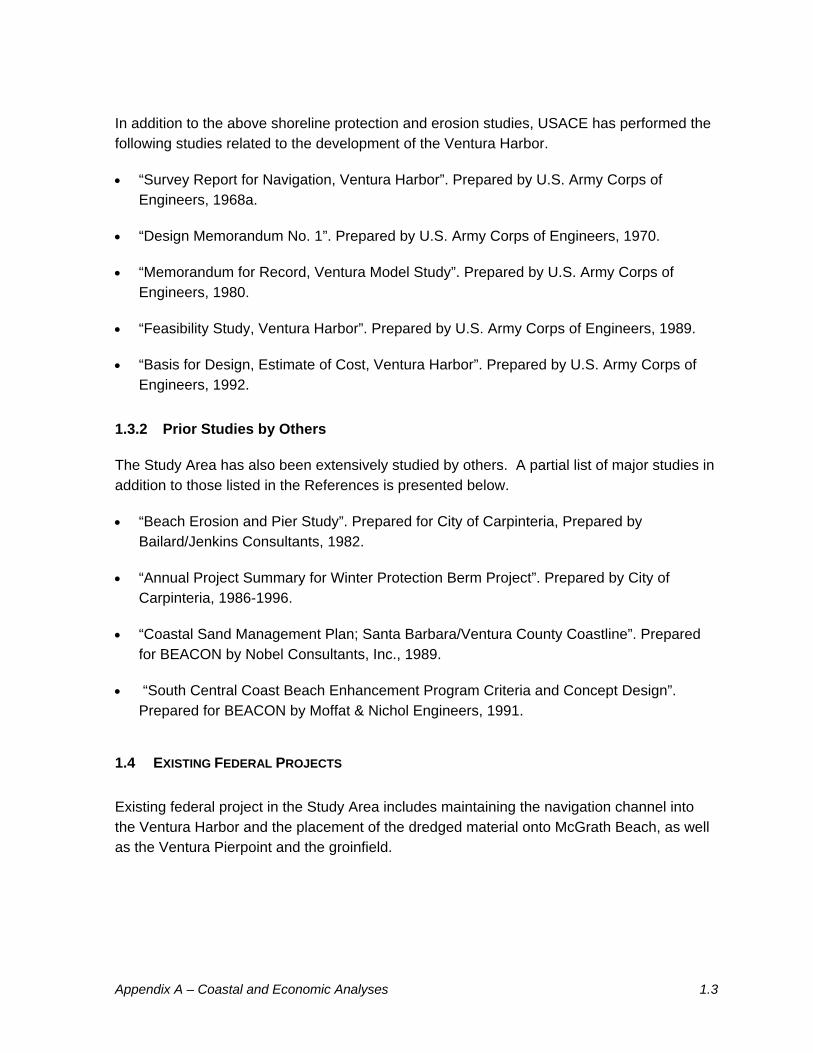
The study area is located along a stretch of 22 miles of coastline from Carpinteria Beach in Santa Barbara County to Oxnard Shores in the Ventura County. A site location map for the study area is shown in Figure 2.1. The map shows the location for Ventura Harbor where maintenance dredging is required, and McGrath Beach where dredged material is currently being disposed. In the figure, the three alternative disposal sites – Carpinteria Beach, Oil Piers Beach and Oxnard Shores, are also shown. Table 2.1 below summarizes the distances between Ventura Harbor and the three alternative beach fill sites.

Table 2.1 Distances between Ventura Harbor and Alternative Beach Fill Sites

BEACH FILL SITE APPROXIMATE DISTANCE FROM VENTURA HARBOR (MILES)

Carpinteria State Beach 17.5

Oil Piers 13.0

Oxnard Shores 4.5

2.2 COASTAL PROCESSES AND TRENDS

2.2.1 Water Levels

The ocean water levels in the study area are influenced primarily by the astronomical tides that result from the gravitational forces of the celestial bodies, primarily the earth, sun, and moon. The other factors that affect the ocean water levels include temperature variations, for example during El Nino Southern Oscillation (ENSO), barometric pressure changes, wind setup (i.e., storm surge), and wave setup. These factors are secondary in magnitude and episodic (e.g., hours, days, and seasons) in nature; hence the effects are relatively small and short-term. Therefore, the long-term representation of the ocean water levels is comprised primarily of the astronomical tide component.

Figure 2.1 - Site Location Map

0 5 (miles)

Ventura Harbor

Channel Islands Harbor

Oxnard Shores McGrath State Beach

Oil Piers Beach

Carpinteria Beach

(Source: 3-D TopoQuads)


Tides along the Southern California coastline are of the mixed semi-diurnal nature, with two high and two low tides of different magnitude in each lunar day. The National Oceanic and Atmospheric Administration (NOAA) monitors gauging stations around the United States to obtain ocean water level measurements. NOAA analyzes the data collected from these gauges to prepare long-term, ocean water level statistics. The NOAA station closest to the study area that has been updated with the latest tidal epoch (1983-2001) is located at Ricon Island. Tidal characteristics along the study area based on the latest tidal epoch (1983-2001) are presented in Table 2.2.

Storm surge along the Southern California coastline is small with typical amplitude of 1 foot or less. Strong ENSO events have an averaged return period of 14 years with 0.2 feet tidal departures lasting for about two to three years (USACE, 1997).

Table 2.2 Tidal Elevation at Ricon Island (Tide Epoch: 1983-2001)

DATUM ELEVATION (FT, MLLW)

Highest Observed Water Level (1/27/1983) 7.8

Mean Higher High Water (MHHW) 5.6

Mean High Water (MHW) 4.7

Mean Tide Level (MTL) 2.8

Mean Low Water (MLW) 1.0

Mean Lower Low Water (MLLW) 0.0

Lowest Observed Water Level (1/16/1965) -2.3

Source: National Ocean Service Tidal Bench Mark sheet for Ricon Island

2.2.2 Waves and Currents

The Santa Barbara and Ventura County coastline is partially sheltered from waves by the Santa Barbara Channel Islands – San Miguel, Santa Rosa, Santa Cruz, and Anacapa Islands. Therefore, the coastline is primarily exposed to waves from the west and southeast, as well as the southern swells passing through the Anacapa passage between Santa Cruz and Anacapa Islands.


The prevailing and storm wave climate at Santa Barbara and Ventura shorelines are composed of wind, swell, and local sea waves produced by six meteorological patterns: Northern Pacific extratropical cyclones, tropical cyclones, extratropical cyclones of the southern hemisphere, wind swells, west to northwest local seas, and pre-frontal local seas. Among these six meteorological patterns, the extratropical cyclones of the northern hemisphere impact the coastline the most, with the induced storms frequently causing significant damages to private and public facilities within the coastal area.

Deep water waves propagating towards coastline are altered by refraction, diffraction, and shoaling effects. The dominant breaker pattern between Point Conception and Point Mugu results in a unidirectional component of alongshore transport. As the shoreline orientation shifts to a more north/south direction near the Ventura River, the intensity of incident wave energy increase. This increase in wave energy results in a corresponding gradient of alongshore energy flux that increases from Isla Vista to a maximum between Ventura Harbor and Oxnard Shores. Moving south along the coast, the wave sheltering of Channel Islands reduces the wave energy at the south facing shoreline between Hueneme Beach and Point Mugu. The nearshore wave energy is also decreased in the vicinity of the two submarine canyons, Hueneme and Mugu Canyon (USACE, 1997).

Nearshore currents are driven by waves breaking on the shoreline at an oblique angle. The alongshore flow along the Santa Barbara and Ventura County shoreline is predominantly west to east because of the prevailing directionality of wave incidence mentioned above. Cross-shore currents exist throughout the study area, especially during high surf. These currents tend to concentrate at creek mouths and near structures, but can appear anywhere along the coastline in the forms of rip currents. The offshore currents consist of the large-scale coastal currents and the tidal and event-driven fluctuations. Among the major coastal currents, the Southern California Countercurrent has the highest velocity with maxima as high as 15 to 30 cm/sec (0.49 to 0.98 ft/sec) (USACE, 1997).

2.2.3 Littoral Processes

The study area is located within the Santa Barbara Littoral Cell, which extends from Point Conception to Point Mugu. The Santa Barbara Littoral Cell is the longest littoral cell in Southern California with a distance of 154 kilometers (96 miles) and is composed of a variety of coastal types and shoreline orientations. The principal feature of this littoral cell is the west to east net alongshore littoral transport direction. The offshore wave sheltering of Channel Islands, as discussed previously, results in an essentially unilateral movement of sand along the coastline from west to east. The shoreline orientation shifts in the southern portion of the Santa Barbara Littoral Cell to a more north/south directions along the Ventura and Oxnard portion. The wave exposure is shifted to the southern hemisphere swell, thus the littoral transport direction is an upcoast reversal in the southern portion of the Santa


Barbara Littoral Cell. However, since the dominant wave energy is from the west, the reversed transport volume is estimated to be only a small fraction of the total annual volume. The Hueneme and Mugu Submarine Canyons intercept most, if not all, of the littoral material (USACE, 1997).


3. DREDGING AND DISPOSAL OPERATIONS AT VENTURA HARBOR

3.1 CURRENT PRACTICE

Ventura Harbor is located next to the mouth of the Santa Clara River, about 28 miles southeast of Santa Barbara Harbor and seven miles northwest of Port Hueneme Harbor. It resides within the City of San Buenaventura (Ventura), County of Ventura. The harbor is an artificial commercial and recreational harbor developed by the Ventura Port District in 1963. Three breakwaters along with an entrance channel, turning basin, and three berthing basins were constructed. In 1969, when severe storm flooding of Santa Clara River damaged the harbor, USACE repaired the damages and reinforced the levy between the Santa Clara River delta and the harbor. An offshore breakwater was constructed in 1971 to form a sand trap to reduce shoaling at the entrance channel. Now, the Los Angeles District of USACE maintains the navigation features in the harbor and performs periodic dredging.

The Harbor and the local shoreline are situated such that waves originating from the west cause sediment to move predominantly in the downcoast direction. During most of the year, clean beach sand from upcoast beaches and the Ventura River migrates downcoast along the beaches into the sand traps and entrance channel. Littoral drift material has accumulated at a rate that required annual dredging of the entrance channel to maintain safe navigational depths of 20 to 30 feet below Mean Lower Low Water (MLLW). Dredged material has been deposited primarily at McGrath State Beach, south of the Santa Clara River. If the McGrath site is not available, dredged material will be deposited at South Beach. Historical maintenance dredging volumes and costs form 1969 to 2003 are summarized in Table 3.1 in the following page.

As shown in the table, over 21 million cubic yards (cy) of material have been dredged since 1969, or nearly 600,000 cy on an average annual basis. The harbor has been dredged 31 times over the 35-year period, or about 0.89 times per year. After adjusting for inflation, over $52 million has been spent on dredging the Harbor since 1969. The inflation-adjusted average dredging cost per cubic yard is approximately $3.29 (in Oct 2003 price level), with a range of $2.29 to $5.19.


Table 3.1 Historical Dredging Volumes and Costs (October 2002 Price Levels)

FY DREDGING VOLUME

CY TOTAL COST COST

INDEX* UPDATED

COST UPDATED COST/CY

1969 1,883,000 $1,242,780 4.779 $5,939,827 $3.15 1970 325,000 $318,500 4.508 $1,435,809 $4.42 1971 1,208,000 NA 4.114 1972 17,000 NA 3.863 1973 1,194,000 $1,334,292 3.651 $4,870,868 $4.08 1974 420,000 $607,269 3.234 $1,963,930 $4.68 1976 152,000 $280,000 2.560 $716,685 $4.72 1977 754,000 NA 2.375 1978 498,000 NA 2.223 1979 1,022,000 $1,387,491 1.986 $2,754,976 $2.70 1981 1,133,000 $1,987,141 1.506 $2,992,889 $2.64 1983 1,186,000 $2,230,367 1.421 $3,169,952 $2.67 1984 1,215,000 $1,977,006 1.381 $2,730,280 $2.25 1986 850,000 $1,588,000 1.419 $2,252,826 $2.65 1987 363,000 $902,245 1.462 $1,318,697 $3.63 1988 800,000 $1,375,863 1.428 $1,964,625 $2.46 1989 230,000 $544,486 1.376 $749,302 $3.26 1990 218,000 $527,163 1.322 $696,911 $3.20 1991 377,000 $800,422 1.307 $1,046,245 $2.78 1992 525,000 $993,523 1.287 $1,278,522 $2.44 1993 486,000 $891,864 1.252 $1,116,618 $2.30 1994 470,000 $1,965,100 1.241 $2,439,071 $5.19 1995 271,000 $1,122,417 1.207 $1,354,963 $5.00 1996 833,000 $1,726,350 1.162 $2,006,421 $2.41 1997 449,000 NA 1.133 1998 742,000 $1,989,014 1.147 $2,280,879 $3.07 1999 639,000 $2,228,892 1.127 $2,512,573 $3.93 2000 818,000 $2,248,290 1.049 $2,358,226 $2.88 2001 625,000 $1,945,000 1.039 $2,021,476 $3.23 2002 670,000 $1,888,972 1.036 $1,957,777 $2.92 2003 670,000 $1,888,972 1.000 $1,888,972 $2.82 Total 21,043,000 Cy $55,819,319 Years 35

Average 601,229 Cy $3.29

* Civil Works Construction Cost Index, Navigation Port & Harbor Component (USACE 2003) Source: USACE – Los Angeles District


4. ALTERNATIVE DISPOSAL SITES

4.1 OVERVIEW

In this section, the characteristic of the three selected alternative beach fill sites - Carpinteria Beach, Oil Piers and Oxnard Shores, are described. Historical beach profiles for the area were analyzed to provide background information on the beach conditions of the three sites. Recreation and amenities at each beach are described. In addition, results of beach surveys conducted at the beaches to collect beach user information are summarized.

4.2 AVAILABLE BEACH PROFILE DATA

The USACE, Los Angeles District had collected beach profiles along the Santa Barbara and Ventura County shorelines between 1938 and the 1970’s. Since 1987, the Beach Erosion Authority for Clean Oceans and Nourishment (BEACON) has established a series of 25 beach profile stations between Elwood and Mugu Beaches. A map showing these 25 beach profile stations is shown in Figure 4.1. As shown in the figure, those stations including the selected beach fill sites Carpinteria (Station #10) and Oxnard Shores (Station #20) for this study. Profile data was collected at October 1987, April 1988, December 1992, and October 1997. Another survey was established between Ventura Harbor and Channel Islands Harbor in September 1994. Survey covered three of the existing profile stations (including Oxnard Shores) in addition to seven new stations. For this study, the BEACON beach profiles were used to establish the average beach conditions for Carpinteria Beach and Oxnard Shores.

As a condition for the demolition of the Mobile Seacliff Oil Piers, the California Coastal Commission imposed a 5-year (1998-2002) beach monitoring program to observe shoreline changes adjacent to the Oil Piers. The monitoring program consists of monthly beach profile surveys for the first two years and quarterly surveys for the remaining three years. The most recently available survey data at the Oil Piers Beach were used to establish the baseline condition at the Oil Piers Beach.

(Reference: BEACON 1989)

Figure 4.1 - BEACON Beach Profile Stations


4.3 CARPINTERIA STATE AND CITY BEACHES

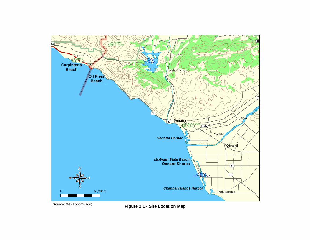
Carpinteria’s State and City Beaches are located in the City of Carpinteria, Santa Barbara County. The shoreline stretches over one mile of the Santa Barbara coast and is owned by both the City and State. This beach is narrow and back by public and private developments, state park facilities and the Santa Monica Creek estuary. Figure 4.2 shows photographs of the beach taken in August, 2003. The photograph on top shows the western end of the beach owned by the City, while the bottom photograph shows the eastern end of the beach owned by the State.

Since the construction of the Santa Barbara Harbor in 1929, the beach has erosion problem because the harbor breakwater effectively block the alongshore movement of sand. A sand bypassing program was implemented in 1933 to compensate for the interruption in natural sediment transport. The operations essentially restored the littoral system to the pre-harbor status-quo, providing enough sand to avoid sever shoreline recession but insufficient quantities to rebuild the eroded beaches.

Sediments samples collected near Ash Avenue by BEACON (2001) indicates that the medium grain size (D50) for the beach sand is 0.195 mm with a fines content (passing the #200 sieve) of 5%. Beach profiles collected by BEACON (2001) for Years 1987, 1988, 1992 and 1997 are shown in Figure 4.3. Based on beach profile data taken from1958 to 1987, USACE (1997) estimated that the shoreline along Carpinteria Beach had been eroding at about 13 feet/year. Adding survey data taken between 1987 and 1997, the average shoreline erosion at Carpinteria Beach was found to be about 12 ft/yr from 1958 to 1997.

4.3.1 Recreation and Amenities

Carpinteria City and State beaches provide a wide variety of amenities for beachgoers including day-trippers and visitors on extended stays. In addition to swimming, the State beach provides camping facilities, picnicking and some fishing, as well as opportunities for surfing. The City beach has volleyball courts and is adjacent to numerous condominiums which are rented weekly for visitors. The downtown area provides other amenities. Carpinteria is ranked among the top twenty beaches in the US by Florida International University’s Stephen Leatherman—it is the only beach in California to receive this award.

The beach is highly ranked by Dr Leatherman and its visitors because of the clean, soft sand (especially the City beach - the City cleans the sand regularly), the gentle surf, and good lifeguard services. In this regard, the beach at Carpinteria has fewer substitutes than most other beaches, particularly given its location.

(a) Western End (City Beach)

(b) Eastern End (State Beach)

Figure 4.2 - Photographs of Carpinteria Beach

Figure 4.3 - Historical Beach Profiles at Carpinteria Beach

-50

-40

-30

-20

-10

0

10

20

30

0 500 1000 1500 2000 2500 3000

Distance from Baseline (feet)

Elev

atio

n (ft

, MLL

W)

Oct-87 Apr-88 Dec-92 Oct-97


In contrast to many beach towns in southern California, Carpinteria provides adequate parking, even during crowded days. Parking near the City beach is free for two hours and parking at the State beach is available for a fee. Access is off of Highway 101 through the town. Although traffic is heavy in the summer, access is good.

4.3.2 Beach Use Survey

Dr. King has conducted two significant beach surveys at Carpinteria - one in the summer of 2001 for the City of Carpinteria (King, 2002a) and the other was prepared for the State of California as part of a larger project (King and Symes, 2003). In addition, Dr. King prepared a preliminary analysis of erosion at Carpinteria for the State in April 2001 (King, 2001) based on surveys conducted the previous summer. This section will present the most important results from the survey conducted in 2001 (and published in 2002), which focused on the recreational value of the beach and the level of amenities provided. Complete survey results are presented in Attachment A.

The survey was pre-tested in early July and then a full-scale survey was conducted in late July and August. Surveyors were carefully trained to zigzag along the beach and choose respondents in a random fashion (i.e., choosing every nth group). Both weekday and weekend, as well as morning and afternoon times were chosen to reflect actual visitation patterns as well.

A written questionnaire was composed, and the questions were vetted by Mr. Matt Roberts, the Director of Parks and Recreation, and other officials in Carpinteria. The questions were then pre-tested on the beach, problematic questions were re-written, and again the questionnaire was sent to Mr. Roberts for comments. Respondents were given a choice of filling out the written questionnaire themselves or having the questions read to them. The vast majority (roughly 90%) chose to fill out the survey themselves. All respondents were told that the survey was conducted under the auspices of the City of Carpinteria through a professor at San Francisco State University and that the purpose was to learn more about beach attendance. Surveyors were told not to say that the survey was designed to “help” the beach since this type of pre-survey discussion is known to bias results. A high percentage of people approached (over 85%) agreed to answer the questions. A high participation rate is reassuring since it also reduces the possibility of bias (if people who choose not to respond have different characteristics from people who do). Overall 283 households participated in the survey representing over 1,100 visitors. Briefly, the main points of the survey are as follows:

• Visitors to Carpinteria come from a wide variety of destinations, with 82.8% arriving from out of town.


• The composition of visitors was split evenly between people on day-trips (48.5%) and those staying overnight in the area (50.2%). [1.3% did not respond.]

• Of those visitors staying overnight, 26.9% were campers, 25.2% stayed at a hotel, 35.3% stayed in house/condo rentals and 12.6% stayed with friends.

• A significant majority of people replied that clean beaches, restrooms, and lifeguards were important to them.

A complete presentation of the results is provided in Attachment A. However, certain key results critical to the analysis are summarized below.

Question 1: How far away from this beach do you live (your primary residence)?

LOCATION FREQUENCY

In Carpinteria 17.2%

Outside Carpinteria, but within 20 miles 8.8%

Within 60 miles 24.7%

More than 60 miles but in California 41.0%

In the US, but not in California 7.0%

Outside the US 1.3%

The results from this question indicate that most visitors (74%) come from more than twenty miles to go to Carpinteria and almost half come from more than sixty miles. This result is significant since it indicates a willingness to drive a considerable distance to get to the beach. The result is especially significant given that many other potential substitute beaches exist near Carpinteria. It is consistent with respondents’ anecdotal responses that Carpinteria is a unique beach.

Question 7: Please check the most appropriate box.

RESPONSE FREQUENCY

Day Trip from home 48.5%

Trip or Vacation to the area 50.2%

Non response 1.3%


Question 12: We’d like to know how important visiting the beach is for your trip/vacation.

RESPONSE FREQUENCY

The beach is important to me--No beach, no trip 61.2%

If there were no beach I might not come or would stay less often 19.2%

I would still come but I like the fact that I can go to the beach 17.1%

I can take the beach or leave it; it would not affect my decision 2.5%

Questions 7 and 12 indicate that just over half of visitors were staying overnight and most of these (61% of overall respondents but a far higher percentage of overnight visitors) indicated that the beach was the primary reason for their trip. This result is significant since it indicates that Carpinteria Beach has significant recreational value.

Question 18: What was your reason for coming to this beach?

RESPONSE FREQUENCY

So I could swim 9.1%

So my children could play/swim 34.9%

To surf 2.5%

To hike 1.1%

To play on the beach 8.5%

To hang-out on the beach 40.0%

To walk my dog 0.5%

I like the beach 0.4%

Relaxation 1.8%

Non response 1.3%

Question 18 of the survey asked respondents about their activities on the beach. The responses indicated a wide variety of activities, with “hanging-out” (40%) and allowing children to swim (34%) the primary answers.


Question 19: What is the minimum width a beach needs to be before you would stop going?

WIDTH FREQUENCY

5 ft 3.1%

10 ft 7.9%

20 ft 15.2%

40 ft 0.4%

50 ft 26.7%

100 ft 19.4%

200 ft 13.7%

Doesn't Matter 1.8%

Write in* 1.3%

Non response 10.6%

Question 19 focuses on a critical component for this study, beach width. Roughly 60% of respondents indicate that 50 feet was a minimum width necessary for beach recreation at Carpinteria. Given the current rate of erosion (indeed many parts of the beach already have less than 50 feet of width even at low tide) this is a significant result and indicates that the substantial recreational value of Carpinteria Beach is threatened by erosion.

Question 20 examined whether, for Carpinteria’s visitors, whether other types of recreation were equivalent to beaches. About half of respondents indicated that swimming pools were not equivalent, with 42% indicating it was “somewhat equivalent,” lakes and reservoirs were considered a better substitute (though few are available near Carpinteria). Surprisingly, 45% said State or National parks were not equivalent and few thought movies were equivalent.

When asked about amenities, most visitors indicated that restrooms (85%) and lifeguards (74%) were “very important” and virtually everyone (99%) said that clean beaches were very important. Showers, food concessions, picnic courts, and drinking fountains were considered less important and volleyball courts (though they currently exist) were not considered important.

4.4 OIL PIERS BEACH

Oil Piers Beach is located in northern Ventura County along Highway 101. Its name is in reference to the recently (1998) demolished Mobil Seacliff Oil Piers. As shown in a


photograph taken in August 2003 (Figure 4.4), the beach is backed by a high rock revetment and a bluff. In the past, this site was a popular spot for surfers. However, since the piers were demolished, this spot is not surfed as heavily. Beach access is provided along an access road that runs parallel the Pacific Ocean and via pedestrian underpasses under Highway 101.

Based on the BEACON study (2001), the beach material has a median grain size (D50) of 0.18 mm and a fines content of 13%. A beach profile surveyed on October 2000 (Beacon, 2001) is provided in Figure 4.5. Based on the beach profiles collected between 1998 and 2002, Oil Piers Beach has been eroding at about 12 feet/year.


In contrast to Carpinteria, Oil Piers Beach provides few amenities. Parking is along a dirt shoulder of a basic access road from Highway 101. There are no bathrooms, no drinking fountains, no concessions, no garbage cans and no lifeguards. Visitors to the beach are primarily surfers with a few jet skiers as well. The quality of the sand is good and some respondents to our survey (see below) were concerned about adding lower quality sand to the beach.

At one time the beach was very popular, particularly for surfers. The old oil pier (for which the beach is named) provided a break which surfers found useful. Since the pier was removed the beach has become less popular. Access to the beach is fairly simple for frequent visitors who know the way, but poor for those who are not aware of the beach’s location.


A short survey was developed for this project to asses the recreation value, use and composition of visitors to the beach. Unfortunately the time frame for this survey was extremely narrow and visitors were sampled on Labor Day weekend. While this ensured a fairly large sample, we are somewhat concerned about the issue of “selection” bias, particularly in regard to the composition of visitors. The sample size was also quite small (38 people) though 85-90% of people on the beach responded, so we believe our sample is quite representative of the people on the beach those days.

Figure 4.4 - Photograph of Oil Piers Beach

Figure 4.5 - Historical Beach Profile at Oil Piers Beach

-50.0

-40.0

-30.0

-20.0

-10.0

0.0

10.0

20.0

30.0

0 500 1000 1500 2000 2500 3000


Elev

atio

n (ft

, MLL

W)

Oct-00



LOCATION FREQUENCY





Outside the US 0.00%

As one would expect, our survey indicates that “Oil Piers” beach is predominately a local beach, with 63% of respondents reporting that they lived within 20 miles. Our previous two site visits on Fridays in July and August also indicated that the beach is predominantly local. However, our survey on Labor Day indicated a surprisingly high number of visitors from farther away, 26% between 20-60 miles and 10% more than 60 miles. We believe that these numbers maybe somewhat overstate the degree to which visitors are willing to drive to visit Oil Piers. On the other hand, since most visitors indicated that they come to Oil Piers frequently (see question 3 below), our sample is probably not too skewed. Since a significant number of people are willing to drive more than 20 miles (and thus these people could find many other substitute beaches), Oil Piers does offer a significant degree of recreational potential.

Question 2: We’d like to know, how many people from your household are in your group today?

NUMBER OF PEOPLE 1 2 3 4 5 TO 7 8 TO 15

FREQUENCY 20.6% 16.2% 24.3% 24.3% 8.1% 5.4%

Question 2a: Of these people, how many are under 16?

NUMBER UNDER AGE 16 0 1 2 3 TO 4 5 TO 8

FREQUENCY 35.3% 26.5% 32.4% 0.0% 5.9%

Questions 2 and 2a indicate that Oil Piers also has the potential to be a family destination, though our observations during the week are that few children are present.


Question 3: How many days this year will you go to “Oil Piers” beach?

NUMBER OF DAYS 0 TO 5 6 TO 20 21 TO 40 41 TO 80 81 TO 120 121 TO

200 MORE

THAN 200

FREQUENCY 32.4% 21.6% 21.6% 8.1% 10.8% 2.7% 2.7%

A significant number of people (almost half) go more than 21 days a year, typical of a “local” beach

Question 4: How many days this year will you go to any beach, including this one?


200 MORE

THAN 200

FREQUENCY 13.2% 10.5% 28.9% 21.1% 10.5% 2.6% 13.2%

Question 5: On a typical day, how many hours do you spend at “Oil Piers” beach?

NUMBER OF HOURS

LESS THAN 1 HOUR 1-3 HOURS 3-5 HOURS 5-8 HOURS MORE THAN 8

HOURS

FREQUENCY 0.0% 13.5% 67.6% 18.9% 0.0%

Question 5a: What is the primary reason you and your group go to “Oil Piers” beach?

PRIMARY REASON TO SURF TO SWIM SO CHILDREN

CAN SWIM TO RELAX ON

THE BEACH

FREQUENCY 23.7% 44.7% 34.2% 76.3%

*Many people checked multiple boxes for this question.

The results of 5a are somewhat surprising and, we believe, not representative. Only 24% indicated that surfing was part of their reason for going to “Oil Piers.” This is clearly understated, but again indicates a potential for other recreational activities.

Question 6: Do you ever go to beaches other than this one?

ANSWER YES NO

FREQUENCY 86.8% 13.2%


Question 6a: What beach do you go to most often, other than this beach?

We received a wide variety of responses to this question. The most common answers were Carpinteria, Ventura and Solimar, but few respondents gave the same answers.

Question 6b: How many days a year do you go to the beach you listed in 6a?

Our results here indicated that most visitors went to other beaches frequently as well, with a mean of 36 days at other beaches.

Question 6c: Please compare the alternative beach you listed in 6a to “Oil Piers” beach. We would like you to compare your overall satisfaction including services available at the beach. Please DO NOT consider the time it takes to get to the beach in your rating.

The other beach is:

Worse than “Oil Piers” Same Better than “Oil Piers”

|….....…|…….....|….….….|…..….||……..…|…….….|….…….|….…….|

0% 25% 50% 75% 100% 125% 150% 175% 200%

ANSWER 0 TO 49% 50 TO 99% 100% (SAME)

101 TO 150%

151 TO 200%

FREQUENCY 12.9% 19.4% 25.8% 29.0% 12.9%

Question 6c is a qualitative question meant to evaluate whether the other beaches that respondents visit are good substitutes. In general, most respondents indicated that there were other alternatives as good or better (68%), though a substantial number (32%) indicated that they preferred Oil Piers. Given the lack of amenities, this result seems somewhat surprising, but it is likely that some of the people who go to Oil Piers prefer a beach with fewer amenities (perhaps because they tend to be less crowded).

Question 7: Please check the most appropriate box:

ANSWER FREQUENCY

I’m here on a day trip. 97.3%

I’m on a trip/vacation away from my permanent residence. 2.7%


This result is not surprising. Even on Labor Day weekend, the vast majority of respondents (97%) are on day trips.

Question 8: The State and Federal Governments are considering using public money to add more sand to “Oil Piers” beach. This sand would increase the width of the beach.

Question 8a: Suppose the width of “Oil Piers” beach was doubled. How much more often would you go?

ANSWER THE SAME AMOUNT 1 TO 25% 26 TO 50% 51 TO 75% 76 TO 100%

FREQUENCY 63.9% 2.8% 25.0% 5.6% 2.8%

The results here are significant, especially given that the survey was conducted on one of the most crowded weekends of the year. 64% of respondents stated that adding more sand would not increase their attendance. However, 25% indicated that they would come 26-50% more often if beach width was doubled, but only a small number (8%) indicated that they would come more than 50% more often if beach width was doubled. Overall, the results indicate that doubling beach width would increase attendance among current users by 15.7%. Keep in mind that the survey did not sample from the population of people who do not go to Oil Piers at all, but might go if the beach width was wider. These results will be discussed in more detail in section 6.3.

Question 8b: Suppose the width of “Oil Piers” beach was doubled. How much more recreational value would you receive from a wider beach.


FREQUENCY 47.2% 11.1% 19.4% 11.1% 11.1%

Our results here indicate that widening the beach will provide significantly more recreational value for those who already attend with just over half of respondents indicating that doubling beach size would significantly increase quality. The mean response was that doubling the beach width would increase recreational value by 25.4%.


Question 8c: Suppose that the width of “Oil Piers” beach was halved. How much less often would you go?


FREQUENCY 41.7% 30.6% 13.9% 11.1% 2.8%

A substantial number (58%) also indicated that erosion of the beach would affect recreational quality. The mean response was that halving beach size would reduce attendance by 18.4%.

Question 8d: Suppose that the width of “Oil Piers” beach was halved. How much less recreational value would you receive from a narrower beach.


FREQUENCY 47.2% 19.4% 16.7% 11.1% 5.6%

A substantial number (58%) also indicated that erosion of the beach would affect recreational quality. The mean response was that halving beach size would reduce the recreational value by 18.4% (the same reduction as above).

Question 9: How old are you?

AGE 16-19 20-24 25-34 35-44 45-54 55-64 65-74 75 OR OLDER

FREQUENCY 0.0% 25.7% 28.6% 31.4% 11.4% 2.9% 0.0% 0.0%

As one would expect, beach goers at Oil Piers are predominantly young and white and have attended college (see below).

Question 10: What is your ethnicity?

ETHNICITY WHITE HISPANIC ASIAN/PACIFIC ISLANDER BLACK OTHER

FREQUENCY 77.1% 14.3% 5.7% 0.0% 5.7%

*One person checked two boxes.


Question 11: What is your highest level of Education?

EDUCATIONAL ATTAINMENT

LESS THAN HIGH SCHOOL HIGH SCHOOL SOME

COLLEGE COLLEGE DEGREE

POST GRADUATE

FREQUENCY 0.0% 8.6% 37.1% 45.7% 8.6%

Question 12: Including yourself, how many people are in your current household (people you live and share financial resources with)?

NUMBER OF PEOPLE 1 2 3 4 5 TO 6 7 TO 9 10 OR

MORE

FREQUENCY 2.9% 31.4% 22.9% 31.4% 8.6% 2.9% 0.0%

Question 13: What would you estimate is the current yearly income of your entire household (before taxes)?

INCOME FREQUENCY

Less than $9,999 3.1%

$10,000-14,999 6.3%

$15,000-24,999 0.0%

$25,000-34,999 3.1%

$35,000-49,999 28.1%

$50,000-74,999 9.4%

$75,000-99,999 18.8%

$100,000-149,999 18.8%

$150,000 or more 12.5%

4.5 OXNARD SHORES

The Oxnard Shores beach fill site is along a stretch of 2.4 miles of shoreline in the City of Oxnard, Ventura County. The beach fill site being considered is between the W. Fifth Street at the north and the Oxnard State Beach at the south. As shown in the photographs taken in


August 2003 (Figure 4.6), beaches along Oxnard Shores are in general rather wide. Samples taken near the W. Fifth Street by BEACON (2001) indicates that the median grain size (D50) of the beach sand is 0.21mm with a fines content (passing the #200 sieve) of 6.3%. Beach profiles taken in Years 1987, 1988, 1992, 1994 and 1997 are shown in Figure 4.7. Historically, this stretch of shoreline has been eroding at about 4 feet/year (USACE, 1997).


Oxnard provides a large number of wide sandy beaches. The focus of this analysis is on the beaches on the northern end at Oxnard shores including Oxnard shores beach, parts of Mandalay County Park and Oxnard State beach. Oxnard Shores and Oxnard State Beach lie just north and south of a large resort/hotel structure. North of this structure is a very large park, with plenty of parking, at least two restroom buildings, a number of well kept grass field spaces, picnic tables, barbeque pits and sand volleyball courts. On weekends, this park is crowded with families picnicking. Parking is also available in adjacent residential areas, though this parking is less convenient

The beach area tends to be more crowded near the park than farther north. Given the relatively wide beach here, most people recreate near the water. Away from the park, there are no lifeguards, restrooms or other facilities available. There are no concessions along any of these beaches. Mandalay County Park beach is more sparsely populated by fishermen and families. Parking is limited.

A number of State and local officials we interviewed indicated that the weather also plays a significant role at Oxnard. The area has a significantly greater number of cold windy days and foggy days, compared to Carpinteria and Oil Piers beach, which limits the recreational value of the beach. A number of respondents (see survey below) commented on the quality of the water, which is somewhat darkish. The perception of mediocre water quality may be an issue in Oxnard.

We conducted two site visits of the area on Fridays in July and August. The beach was sparsely populated (with fewer than one person for every hundred yards of beach) and virtually no one was in the water. Our general impression was that the amount of sand currently available at Oxnard is more than adequate.

(a) Southern End near Oxnard Beach Park

(b) Northern End near West Fifth Street

Figure 4.6 - Photographs of Oxnard Shores

Figure 4.7 - Historical Beach Profiles at Oxnard Shores

-50

-40

-30

-20

-10

0

10

20

30

0 500 1000 1500 2000 2500 3000


Elev

atio

n (ft

, MLL

W)

Oct-87 Apr-88 Dec-92 Sep-94 Oct-97



A short survey was conducted for this project to asses the recreation value, use and composition of visitors to the beach. Unfortunately the time frame for this survey was extremely narrow and visitors were sampled on Labor Day weekend. While this ensured a fairly large sample, we are somewhat concerned about the issue of “selection” bias, particularly in regard to the composition of visitors. The sample size was also quite small (68 people) though 85-90% of people on the beach responded, so we believe our sample is quite representative of the people on the beach those days.


LOCATION FREQUENCY

In Oxnard 20.6%

Outside Oxnard, but within 20 miles 23.5%




Outside the US 0.0%

Although the results are skewed by Labor Day, they indicate that a substantial number of people are willing to travel to Oxnard, with just over half indicating that they came from more than 60 miles. Whether these visitors came primarily for the beaches is not known. A substantial number of these people were families with children (see question 2 below).

Question 2: We’d like to know how many people from your household are in your group today.

LOCATION 0 1 2 3 4 5 6 7 OR MORE

FREQUENCY 1.5% 16.4% 17.9% 17.9% 17.9% 14.9% 7.5% 6.0%



NUMBER UNDER AGE 16 0 1 2 3 4

FREQUENCY 29.2% 27.7% 15.4% 20.0% 7.7%

Question 3: How many days this year will you go to this beach in Oxnard?


200 MORE

THAN 200

FREQUENCY 50.7% 29.9% 4.5% 1.5% 1.5% 4.5% 7.5%

Question 3 indicates that most visitors come relatively infrequently compared to most other beaches we have surveyed in California.

Question 4: How many days this year will you go to any beach, including this one?

NUMBER OF DAYS

1 TO 5 6 TO 20 21 TO 40 41 TO 80 81 TO 120 121 TO 200

MORE THAN 200

FREQUENCY 24.6% 33.8% 18.5% 3.1% 3.1% 7.7% 9.2%

Question 5: On a typical day, how many hours do you spend at this beach?

NUMBER OF HOURS

LESS THAN 1 HOUR 1-3 HOURS 3-5 HOURS 5-8 HOURS MORE THAN 8

HOURS

FREQUENCY 2.9% 38.2% 44.1% 13.2% 1.5%

Question 5a: What is the primary reason you and your group go to this beach?

PRIMARY REASON

TO SURF TO SWIM SO CHILDREN CAN SWIM

TO RELAX ON THE BEACH

FREQUENCY 16.0% 11.7% 18.1% 54.3%

*Many people checked multiple answers to this question. So the values represent the percentage that each answer was selected compared to all answers selected.


Question 6: Do you ever go to beaches other than this one?

ANSWER YES NO

FREQUENCY 89.4% 10.6%

Question 6a: What beach do you go to most often, other than this beach?

Respondents mentioned Manhattan Beach, Ventura Beach, Huntington Beach and Zuma Beach most often, indicating most probably came from the south.

Question 6b: How many days a year do you go to the beach you listed in 6a?

Our results indicated most people go an average of 30 days a year to other beaches, which is slightly higher than is typical for this type of survey.

Question 6c: Please compare the alternative beach you listed in 6a to this beach. We would like you to compare your overall satisfaction including services available at the beach. Please DO NOT consider the time it takes to get to the beach in your rating.

The other beach is:

Worse than “Oil Piers” Same Better than “Oil Piers”

|….....…|…….....|….….….|…..….||……..…|…….….|….…….|….…….|

0% 25% 50% 75% 100% 125% 150% 175% 200%

ANSWER 0 TO 49% 50 TO 99% 100% (SAME)

101 TO 150%

151 TO 200%

FREQUENCY 5.3% 36.8% 19.3% 28.1% 10.5%

Slightly more people indicated that they preferred other beaches to Oxnard, indicating that other substitutes are clearly viable options.


Question 7: Please check the most appropriate box:

ANSWER FREQUENCY

I’m here on a day trip. 73.8%

I’m on a trip/vacation away from my permanent residence. 26.2%

Just over 25% indicated that they were staying overnight in the area, though this result is skewed by the fact that the survey was conducted on Labor Day weekend. We would expect a smaller percentage during the rest of the year, however there are a substantial number of condo owners in the area with permanent residences elsewhere.

Question 8: The State and Federal Governments are considering using public money to add more sand to Oxnard beach. This sand would increase the width of the beach.

Question 8a: Suppose the width of this beach was doubled. How much more often would you go?


FREQUENCY 83.1% 3.1% 6.2% 1.5% 6.2%

Our results here are not surprising given the adequate width of the beaches at Oxnard. 83% of respondents indicated that doubling of beach width would not increase their attendance. Overall, our data indicates that doubling the beach width would only increase attendance by 9%. Indeed, we think that this result, if anything, overstates the case.

Question 8b: Suppose the width of this beach was doubled. How much more recreational value would you receive from a wider beach.


FREQUENCY 70.8% 9.2% 12.3% 3.1% 4.6%

A slightly greater number of people indicated that increasing width would increase recreational value. Overall, our data indicate that doubling the beach width would increase recreational value by 11.7%.


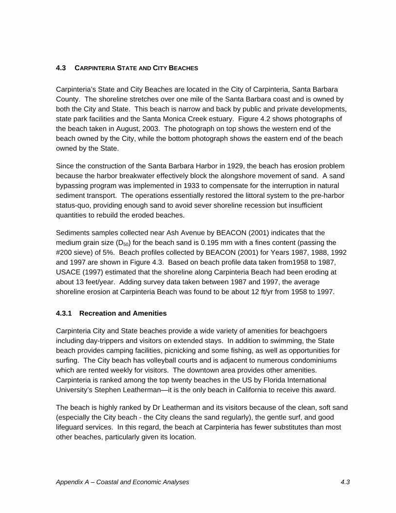
Question 8c: Suppose that the width of this beach was halved. How much less often would you go?


FREQUENCY 57.1% 15.9% 15.9% 4.8% 6.3%

Halving beach width would have a modest effect on attendance and recreational value. Overall, our data indicates that halving the beach width would decrease attendance by 16.5% and recreational value by 25.4%.

Question 8d: Suppose that the width of this beach was halved. How much less recreational value would you receive from a narrower beach.


FREQUENCY 38.1% 21.9% 20.3% 10.9% 9.4%


AGE 16-19 20-24 25-34 35-44 45-54 55-64 65-74 75 OR OLDER

FREQUENCY 10.8% 15.4% 15.4% 29.2% 20.0% 6.2% 3.1% 0.0%


ETHNICITY WHITE HISPANIC ASIAN/PACIFIC ISLANDER BLACK OTHER

FREQUENCY 73.8% 21.5% 4.6% 1.5% 3.1%

*Two people checked multiple boxes.


EDUCATIONAL ATTAINMENT

LESS THAN HIGH SCHOOL HIGH SCHOOL SOME

COLLEGE COLLEGE DEGREE

POST GRADUATE

FREQUENCY 0.0% 9.2% 40.0% 29.2% 23.1%


Question 12: Including yourself, how many people are in your current household (people you live and share financial resources with)?

NUMBER OF PEOPLE

1 2 3 4 5 TO 6 7 TO 9 10 OR MORE

FREQUENCY 7.8% 23.4% 21.9% 23.4% 20.3% 1.6% 1.6%


INCOME FREQUENCY

Less than $9,999 0.0%

$10,000-14,999 0.0%

$15,000-24,999 1.6%

$25,000-34,999 4.9%

$35,000-49,999 13.1%

$50,000-74,999 21.3%

$75,000-99,999 16.4%

$100,000-149,999 11.5%

$150,000 or more 31.1%

4.6 ALTERNATIVE DISPOSAL SCENARIOS

In Section 5, the additional cost to transport and dispose the dredged material from Ventura Harbor to the three alternative sites via different methods will be discussed. The associated benefits for the increased beach width will be discussed in Section 6. The cost functions and benefits are developed over a wide range of parameters such that sufficient data will be developed for the pilot GIS-based model, not limited to the four scenarios described below. However, for the study addressed in this report, four specific alternative disposal scenarios will be presented as examples for the testing of the ArcGIS tool. These four scenarios are developed based on the assumption that 150,000 cy out of the 600,000 cy dredged annually from the Ventura Harbor will be placed at McGrath Beach to maintain the existing condition


there. The remaining 450,000 cy will be disposed at the three alternative sites under the following four scenarios.

• Scenario 1 - All the remaining 450,000 cy goes to Carpinteria Beach.

• Scenario 2 - 275,0001 cy goes to Oil Piers, 175,000 cy goes to Carpinteria Beach.

• Scenario 3 - All the remaining 450,000 cy goes to Oxnard Shores.

• Scenario 4 - One-third of the remaining material goes to each alternative site, i.e. 150,000 cy to each site.

These four disposable scenarios were selected only as examples for testing the pilot ArcGIS model and were not intended as realistic implementable disposal alternatives for Ventura Harbor dredging project.

1 275,000 cy is the maximum volume Oil Piers Beach can take annually (BEACON 2001)


5. COST FUNCTION FOR DREDGED MATERIAL DISPOSAL

5.1 OVERVIEW

In this section, unit cost for different transportation and disposal methods are evaluated. The cost functions are developed to cover a wide range of transportation modes and distances to be used as input for the ArcGIS tool. These cost functions were developed based on simplified assumptions, and were not intended to be in a detail sufficient for any site-specific conditions. These crude estimates of unit cost were used to establish generic cost functions for the pilot ArcGIS model, which will use the Ventura Harbor dredging as an example to evaluate the transportation costs for disposing different quantities of dredged material from Ventura Harbor to the three alternative beach sites. Since the cost functions were developed to cover a wide range of dredged volumes, transportation mode, and transportation distances, some of the scenarios when viewed individually would be unrealistic. For example, the use of railroad to transport a small dredge volume over a short distance, or the use of truck to transport a large volume over a long distance may both be unrealistic.

5.2 TRANSPORTATION AND DISPOSAL METHODS

5.2.1 Hydraulic Pipeline

The use of hydraulic pipeline is the current practice in delivering the Ventura Harbor dredged sediment to McGrath Beach. Under this method, floating or submerged pipelines are connected to the pipeline dredger to deliver the dredged material to the receiver beach area. If the pumping distance is too long such that the hydraulic losses in the pipe is causing the deposition of sediment along the pipes, booster pumps can be use to achieve the goal of pumping the sediment over a longer distance. However, the efficiency of this method decreases as the distances become too long. In addition, this method would be most cost effective if there is no physical obstacle between the dredged locations and the nourishment area. In general, this method is best for short distance between the dredged area and the receiver beach.

5.2.2 Truck

Truck haul of dredged material can be economically competitive for short distance (say up to 50 miles). At greater distances, transport by truck is labor- and fuel-intensive and not economically justifiable. The simplicity of loading and unloading requirements and the relative abundance of available roadways make truck hauling technically feasible.


The capacity of dump trailers range from 16 to 20 cy, and 22 to 60 cy for rear/bottom dump truck. Dump and tank compartments are suitable for hauling dredged material. Dump and tank compartment can be mounted on a trailer chassis or a single gas or diesel powered tractor chassis and towed by a tractor. Trailer gates and hatches can be sealed with rubber gaskets, straw or other material to prevent leaking or spillage.

The cost advantage of truck transportation is that it requires no costly fixed plant. On the other hand, the unit cost will be high in long distance, and it needs a large number of round trips on the roads. The transport route from dredged to disposal site need to be investigated and planned. Some public and residential streets may have restrictions for heavy trucks. Environmental impacts such as traffic congestion, air pollution and noise for the neighborhood need to be considered as well.

5.2.3 Railroad

Rail haul using the unit train concept is technically feasible and economically competitive with other transport modes for hauling dredged material for a long distance (over 100 miles). A unit train is one reserved to carry one commodity (dredged material) from specific points on a tightly regulated schedule. Facilities are required for rapid loading and unloading to make the unit train concept work and to enable benefits from reduced rates on large volumes of bulk movement. Bottom dump cars or rotary car dumpers can be used for rapid loading and unloading. Economic feasibility demands the utilization of existing railroad tracks; however, the building of short intermediate spurs may be required to reach disposal areas.

Only Carpinteria Beach and Oil Piers beach fill sites have railroad nearby. Oxnard Shores still need trucks to transport material from railroad station to the disposal site.

5.2.4 Scow and Tow

Barges and scows, used in combination with mechanical dredges, have been one of the most used methods of transporting large quantities of dredged material over long distances. Barges are designed with bottom doors or with a split-hull and the contents can be emptied in a few seconds.

5.2.5 Hopper Dredge and Pumpout

Hopper dredges consist of a ship-type hull with an internal hopper to hold material dredged from the bottom. The material is brought to the surface through a suction pipe and draghead and discharged into hoppers built in the vessel. Hopper dredges are capable of transporting the material for long distances in the self-contained hopper. Like barge, hopper dredges normally discharge the material from the bottom of the vessel by opening the hopper doors.


However, some hopper dredges are equipped to pump out the material from the hopper much like a hydraulic pipeline dredge.

5.3 COST FUNCTIONS

As discussed above, pipeline dredging and direct pumping of the dredged material through pipeline is the current practice in the maintenance dredging at Ventura Harbor. Hence, the cost of disposal of the dredged material from Ventura Harbor to the nourishment site is imbedded in the dredging cost. Since the purpose of the current study is to determine the “additional” cost of transporting and disposing the Ventura Harbor, the cost functions developed for this study only consider the transportation and disposal cost, i.e. dredging cost is not considered.

Transportation unit costs were determined for the truck, railroad, and scow and tow methods. The hopper dredge and pump-out method was not considered for the cost evaluation since it is difficult to separate the dredging cost from the total cost (including transportation and disposal costs) for this method. The unit costs were estimated based on various dredge volumes and transport distances for application in the GIS cost-function model. Table 5.1 summarizes the transportation and disposal unit costs based on volume, distance, and transportation methods. The volumes were based on 20, 40, 60, 80, and 100% of the total available volume of 600,000 cy. The transportation distance was based on the distance from the borrow site ranging from 2 to 300 miles. These cost estimates are graphically represented in Figure 5.1. Rail has the highest starting unit cost between $37 to $38 and increases at a slower rate with increasing distance compared to the other methods. The truck method starts between $4 and $5, but has the fastest increase in unit cost over increasing distance. Beyond 175 miles, the truck unit cost exceeds the railroad unit cost. The scow and tow method has the lowest unit cost over the entire range of transport distances.

It has to be noted that the unit costs shown were developed based on broad assumptions that may not be applicable for some site-specific conditions. For example, the cost for using railroad was estimated based on the assumption that railroad tracks are available directly to the site, hence, cost for laying temporary tracks were not included. For the use of scow-and-tow, if it is desirable to pump the sand directly onto the beach instead of disposing as a submerged berm, additional pumping cost is not included in the cost function. In addition, cost associated with mitigating environmental impacts has not been considered.

More details and assumptions used for the cost estimates for the three mode of transportation are provided in Attachment B.


Table 5.1 Comparison of Transportation and Disposal Unit Costs by Volumes, Distances, and Transportation Methods

Total Volume (cy) of Available Material = 600,000

Dist. from Borrow Site

Dist. from Borrow Site

20% of Total Dredged Volume 120,000 cy 80% of Total Dredged Volume 480,000 cy

Miles Truck Railroad Scow & Tow Miles Truck Railroad Scow & Tow

2 $5.21 $37.77 $3.55 2 $4.58 $37.15 $1.685 $5.86 $37.77 $3.92 5 $5.23 $37.15 $2.0510 $6.97 $37.77 $4.54 10 $6.34 $37.15 $2.6715 $8.06 $37.77 $5.16 15 $7.43 $37.15 $3.2820 $9.14 $37.77 $5.77 20 $8.52 $37.15 $3.9025 $10.22 $37.77 $6.39 25 $9.59 $37.15 $4.5250 $15.69 $37.77 $9.47 50 $15.06 $37.15 $7.60100 $26.85 $39.92 $15.64 100 $26.22 $39.29 $13.76150 $37.14 $41.34 $21.80 150 $36.52 $40.72 $19.93300 $69.88 $42.77 $40.30 300 $69.26 $42.15 $38.42

40% of Total Dredged Volume 240,000 cy 100% of Total Dredged Volume 600,000 cy

Miles Truck Railroad Scow & Tow Miles Truck Railroad Scow & Tow

2 $4.79 $37.36 $2.30 2 $4.54 $37.11 $1.555 $5.44 $37.36 $2.67 5 $5.19 $37.11 $1.9210 $6.55 $37.36 $3.29 10 $6.30 $37.11 $2.5415 $7.64 $37.36 $3.91 15 $7.39 $37.11 $3.1620 $8.72 $37.36 $4.52 20 $8.47 $37.11 $3.7725 $9.80 $37.36 $5.14 25 $9.55 $37.11 $4.3950 $15.27 $37.36 $8.22 50 $15.02 $37.11 $7.47100 $26.43 $39.50 $14.39 100 $26.18 $39.25 $13.64150 $36.72 $40.93 $20.55 150 $36.47 $40.68 $19.80300 $69.47 $42.36 $39.05 300 $69.22 $42.11 $38.30

60% of Total Dredged Volume 360,000 cy

Miles Truck Railroad Scow & Tow

2 $4.65 $37.22 $1.895 $5.30 $37.22 $2.2610 $6.41 $37.22 $2.8715 $7.50 $37.22 $3.4920 $8.58 $37.22 $4.1125 $9.66 $37.22 $4.7250 $15.13 $37.22 $7.81100 $26.29 $39.36 $13.97150 $36.58 $40.79 $20.14300 $69.33 $42.22 $38.63

Note1. All costs do not include dredging cost.

Mode of Transportation Mode of Transportation

Figure 5.1 - Comparison of Transporation and Disposal Unit Costs

$0

$5

$10

$15

$20

$25

$30

$35

$40

$45

$50

0 25 50 75 100 125 150 175 200 225 250

Miles between Borrow Site and Disposal Site

Uni

t Cos

t ($/

cubi

c ya

rd o

f dre

dged

mat

eria

l)

Truck

20% of Total Dredged Volume40% of Total Dredged Volume60% of Total Dredged Volume80% of Total Dredged Volume100% of Total Dredged Volume

Scow & Tow

Rail

Oil

Pier

sC

arpi

nter

ia

Oxn

ard

Shor

es


6. BENEFITS FOR BEACH FILL ALTERNATIVES

6.1 OVERVIEW

The following sections summarize the analyses to determine the benefits of using the available Ventura Harbor dredge material for beach nourishment at Carpinteria Beach, Oil Piers, and Oxnard Shores. Simple analytical analyses were performed to estimate the increase in beach width for a given placement volume (Section 6.2), and the subsequent reduction in beach width over a 20-year period (Section 6.3). Given the increase in beach width, the additional recreational benefits were calculated from the increase in attendance and recreational value associated with a wider beach. The method used to determine the recreational benefit is fairly general and allows variation of the current beach width according to existing conditions, the current discount rate, and the additional amount of beach fill available (Section 6.4).

As noted in the Main Report, these simple analytical analyses were intended to provide example data for testing the pilot GIS-based model, they were not intended to be sufficient analyses for the placement scenarios presented in the report.

6.2 BEACH FILL CHARACTERISTICS

Figures 6.1 to 6.3 show the beach fill lengths and locations for the Carpinteria Beach, Oil Piers Beach and Oxnard Shores, respectively. Assuming the beachfill material has similar grain size characteristics as the native beach material, the increase in beach width, W, at each of the three beaches was estimated as:

)( cDBLVW+×

=

where V is the beachfill volume, L is the beachfill length, B is berm height, Dc is the depth of

closure.

Assuming a combined beach profile height (B+DC) of 30 ft, the increase in beach widths for placing 20, 40, 60 and 80% of the dredged material from Ventura Harbor on the three beach locations were calculated and shown in Figure 6.4. The placement of 20% (120,000 cy) of the Ventura Harbor dredged material on the three beaches will result in an increase of beach widths of about 20 to 35 feet. The placement of 80% (480,000 cy) of the dredged material can result in an increase in beach area of about 80 to 130 feet.

Figure 6.4 - Increase in Beach Width

-

20

40

60

80

100

120

140

0% 20% 40% 60% 80% 100%

% of Dredged Material for Beach Fill

Incr

ease

d B

each

Wid

th (f

t)Carpinteria Oil Piers Oxnard Shores


6.3 PROJECTED BEACH EROSION/CHANGE IN PLANFORM

New beach fills spread laterally along the shoreline in upcoast and downcoast directions as waves rework the artificial deposit to restore the beach to its natural equilibrium shape. A diffusion theory is generally used to describe the lateral spreading of newly placed beach fill (Dean, 2002). The spreading rate depends on the longshore diffusivity (G), which is a function the wave energy (wave height) and other physical characteristics of the shoreline. The longshore diffusivity established for the study area by USACE (1997) was used to estimate the change in beach planforms over time.

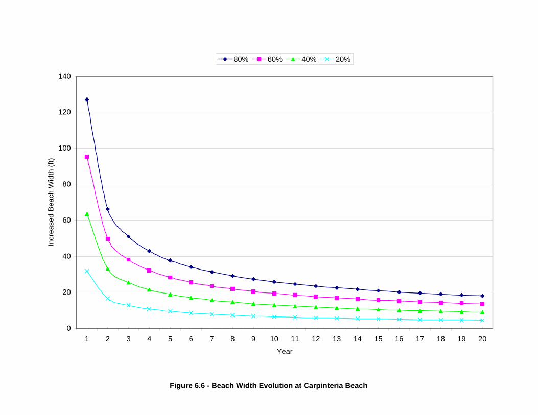
Figure 6.5 shows an example of the change in beach planform over time for Carpinteria Beach. The figures illustrate the lateral spreading and change in beach widths 1, 5, 10 and 20 years after the initial placement of 80% of the Ventura Harbor dredged material (600,000 cy) on the beach. The predicted increased beach widths based on the range of beach fill volumes for the Carpinteria Beach, Oil Piers Beach and Oxnard Shores are shown in Figures 6.6 to 6.8, respectively. The results show that the beach fills rapidly diffuses initially, followed by subsequently slower lateral spreading and reduction in beach widths.

6.4 RECREATIONAL BENEFITS

Economists have devised a number of standard ways to calculate the economic value of what is referred to as “non-market goods,” that is, goods that are free. In the case of beaches, it is clear that people place a value on the beach (despite paying parking fees) as demonstrated by their willingness to fly or drive substantial distances to get to a beach and often in heavy traffic. One widely accepted and used method of calculating the economic value of a day at the beach is the “travel cost method.” This method estimates the cost of traveling to and from the beach as a measure of the willingness of visitors to pay. The travel cost method is officially approved by USACE to measure ability to pay, and it is widely used in the economic profession to value recreational sites like beaches.

To calculate the willingness to pay for a day at the beaches, information provided by the survey coupled with attendance data is used to estimate consumer surplus for the beaches. The travel cost method generally involves the following:

• Estimate the demand curve for beach visits using the travel cost method

• Estimate consumer surplus by integrating the demand curve

Figure 6.5 - Beach Fill Evolution at Carpinteria Beach

0

20

40

60

80

100

120

140

0 1000 2000 3000 4000 5000 6000 7000 8000

Distance from Center of Fill (feet)

Berm

Wid

th (f

eet)

Initial Planform

1 Year Later

5 Years Later

10 Years Later20 Years Later

Figure 6.6 - Beach Width Evolution at Carpinteria Beach

0

20

40

60

80

100

120

140

1 2 3 4 5 6 7 8 9 10 11 12 13 14 15 16 17 18 19 20

Year

Incr

ease

d B

each

Wid

th (f

t)80% 60% 40% 20%

Figure 6.7 - Beach Width Evolution at Oil Piers Beach

0

20

40

60

80

100

120

140

1 2 3 4 5 6 7 8 9 10 11 12 13 14 15 16 17 18 19 20

Year

Incr

ease

d B

each

Wid

th (f

t)80% 60% 40% 20%

Figure 6.8 - Beach Width Evolution at Oxnard Shores

0

20

40

60

80

100

120

140

1 2 3 4 5 6 7 8 9 10 11 12 13 14 15 16 17 18 19 20

Year

Incr

ease

d B

each

Wid

th (f

t)80% 60% 40% 20%


The day-use value of each beach was determined for the high season (late May through mid September) and low season (October through early May). The value was calculated based on point values using the USACE method (USACE, 1990) and visitor surveys. The day-use value and the seasonal attendance was then used to compute the beach fill benefits.

For the beach fill benefits, the four specific scenarios described in Section 4.6 were analyzed. For each scenario, the increase in beach width over a 20-year period was determined for the recreational benefit.

6.4.1 Carpinteria Beach

Based on summer 2001 data, the value of one beach day at Carpinteria was estimated at $23.38 per person per day during the high season (King, 2002a). For the low season, a conservative estimate of $3 per day2 was used. This value is consistent with other economist’s estimates for Southern California beaches (e.g., see Hanemann and Rudd, 1998), but is substantially higher than the value used by the USACE, even taking into account the higher value attributable to camping. Our estimate reflects the fact that a substantial number of people are willing to travel quite far to spend a day at Carpinteria Beach, which provides a significantly different set of amenities compared to other beaches in California. The study conducted by King (2002a) did not fully take into account the availability of substitutes, though it should be noted from our general survey data that many visitors consider Carpinteria Beach unique and that the amenities provided there are superior to most other beaches in the area. Perhaps most important is the fact that it is considered to be a children’s beach.

Table 6.1 presents the US Army Corps methodology for assessing the unit day value of recreation. For each of the categories shown in the table, a point value has been assigned using the Corps methodology. For more information on this methodology, the reader is referred to USACE (1990). Overall, we have assessed Carpinteria’s beach at 92 points. This is a high valuation but appropriate for the only beach in California ranked in the top 50 in the US. Indeed, one might argue for a higher score. The score of 92 points translates into a day unit value of $4.60 in July 1, 1982 dollars and $8.71 in August 2003 dollars.

In an earlier study, Dr. King used the travel cost method to derive an estimate of $23.38 for a day at Carpinteria’s beaches (King 2002a). The estimate of $23 is in line with other studies of the value of a beach day at a major southern California beach. It should be noted that policy makers who use the model which will be developed from this study may choose different values for a day at the beach. The ArcGIS model will eventually allow the end user to input his or her own dollar values. For the purposes of this study, an average of the two

2 Low season visits are considered less valuable by economists since they involve local visitors, who have a low travel cost, and who typically use the beach for lower value uses, such as walking.


values discussed above ($8.71 and $23.38)--$16.05 person per day in high season (late May to mid September). For off season visitation (which is small) unit day value of $3 was used, which we believe is reasonable.

Table 6.1 Point Values for Off-Season Recreation at Carpinteria Beach

CRITERIA TOTAL POSSIBLE POINTS POINTS ASSIGNED

Recreation Experience 30 28

Availability (Substitutes) 18 16

Capacity 14 11

Accessibility 18 18

Environmental 20 19

Total 100 92

Source: USACE, 1990

Attendance

Unfortunately, Carpinteria does not keep seasonal attendance records. However, we have visited the beach for several years and spoken to lifeguards and to Matt Roberts, who is in charge of Parks and Recreation for the City. Mr. Roberts estimates the high season (Mid May to Mid September) attendance to be 1.6 million people for both the City and State beaches and a significantly smaller low season attendance estimated at 300,000. This estimate is consistent with the numerous site visits and with estimates of other southern California with similar levels of crowding over similar areas, such as San Clemente City Beach.

Recreational Value

Table 6.2 below provides the total recreational value of Carpinteria’s City and State beaches for both the high and low season. Overall, the total recreational value is $26.6 million per year.


Table 6.2 Total Recreational Value of Carpinteria Beach

SEASON DAY USE VALUE EST. ATTENDANCE RECREATIONAL VALUE

High Season $16.05 1,600,00 $25,672,000

Low Season $3.00 300,000 $900,000

Total 1,900,000 $26,572,000

Costs and Benefits of Erosion and Additional Beach Fill

Estimating the benefits of additional beach fill is difficult and most of the literature on the recreational value of beaches ignores the critical issue of beach nourishment. A series of survey questions were created for the State of California, which elicit responses to two key questions: (1) will increasing or decreasing a beaches width increase the respondents visitation to that beach, (2) will a wider (or narrower) beach increase (or decrease) the visitors recreational experience. Dr. King conducted a survey at several beaches in southern California in 2000 (King, 2001) which found, in general, that respondents preferred wider beaches and, everything else equal, they would attend wider beaches more often. Responses varied depending upon beach width. As one would expect, respondents indicated that widening particularly narrow beaches (e.g., those in Carlsbad) would significantly increase their attendance and perceived recreational value. On the other hand, increasing the width of beaches which are already quite wide (e.g., Huntington Beach) added little in terms of value or attendance. There was some evidence of self-selection (i.e., visitors who attended narrow beaches tended to be less bothered by lack of beach width than others), nevertheless the report concluded that at all but the widest beaches, there was a significant demand for beach nourishment and that the narrower the beach, the larger the benefit. Survey data from beaches similar to Carpinteria were analyzed. Applying this analysis to Carpinteria, we conclude that doubling beach width would increase attendance by 20% and recreational value (per visitor) by 18%. It should be noted that while these assumptions are consistent with the current survey results, estimating the precise changes in attendance and recreational value is difficult. More study in this area is needed, in particular, direct observations of changes in attendance after nourishment.

Benefits of Beach Fill

Scenario 1

Table 6.3 presents our estimate of the gain in recreational value from adding 450,000 cy of beach fill to Carpinteria’s beaches. If we discount the twenty years of gains at a 6% rate, we


estimate the total benefit to be $32.5 million. The increased beach width is calculated based on an initial beach width of 150 feet.

Table 6.3 Increased Value of 450,000 cy of Beach Fill

YEAR INCREASED

BEACH WIDTH (FT)

INCREASED BEACH WIDTH

(%)

TOTAL BEACH WIDTH

(FT)

GAIN IN RECREATIONAL

VALUE

PV OF GAIN (YEAR 1)

1 119 79% 269 $8,769,469 $8,769,469

2 62 41% 212 $4,572,922 $4,069,884

3 48 32% 198 $3,514,573 $2,950,903

4 40 27% 190 $2,958,185 $2,343,160

5 35 24% 185 $2,602,489 $1,944,731

6 32 21% 182 $2,350,235 $1,656,823

7 29 20% 179 $2,159,427 $1,436,142

8 27 18% 177 $2,008,604 $1,260,223

9 26 17% 176 $1,885,512 $1,116,032

10 24 16% 174 $1,782,581 $995,384

11 23 15% 173 $1,694,849 $892,825

12 22 15% 172 $1,618,910 $804,549

13 21 14% 171 $1,552,339 $727,797

14 20 14% 170 $1,493,357 $660,513

15 20 13% 170 $1,440,624 $601,122

16 19 13% 169 $1,393,108 $548,392

17 18 12% 168 $1,350,003 $501,343

18 18 12% 168 $1,310,667 $459,184

19 17 12% 167 $1,274,579 $421,265

20 17 11% 167 $1,241,317 $387,049

TOTAL $46,973,749 $32,546,789

Scenario 2

Table 6.4 presents our estimate of the gain in recreational value from adding 175,000 cy of beach fill to Carpinteria’s beaches. If we discount the twenty years of gains at a 6% rate, we estimate the total benefit to be $12.6 million.



YEAR INCREASED

BEACH WIDTH (FT)


(%)

TOTAL BEACH WIDTH

(FT)


VALUE

PV OF GAIN (YEAR 1)

1 46 31% 196 $3,389,879 $3,389,879

2 24 16% 174 $1,767,684 $1,573,233

3 18 12% 168 $1,358,574 $1,140,685

4 16 10% 166 $1,143,500 $905,759

5 14 9% 164 $1,006,004 $751,745

6 12 8% 162 $908,494 $640,452

7 11 8% 161 $834,737 $555,147

8 11 7% 161 $776,435 $487,145

9 10 7% 160 $728,854 $431,407

10 9 6% 159 $689,065 $384,770

11 9 6% 159 $655,152 $345,126

12 8 6% 158 $625,797 $311,002

13 8 5% 158 $600,064 $281,333

14 8 5% 158 $577,264 $255,324

15 8 5% 158 $556,880 $232,366

16 7 5% 157 $538,512 $211,983

17 7 5% 157 $521,850 $193,797

18 7 5% 157 $506,644 $177,500

19 7 4% 157 $492,695 $162,842

20 7 4% 157 $479,837 $149,615

TOTAL $18,157,920 $12,581,112


Scenario 4

Table 6.5 presents our estimate of the gain in recreational value from adding 150,000 cy of beach fill to Carpinteria’s beaches. If we discount the twenty years of gains at a 6% rate, we estimate the total benefit to be $10.9 million.


YEAR INCREASED

BEACH WIDTH (FT)


(%)

TOTAL BEACH WIDTH

(FT)


VALUE

PV OF GAIN (YEAR 0)

1 40 27% 190 $2,947,721 $2,947,721

2 21 14% 171 $1,537,117 $1,368,028

3 16 11% 166 $1,181,369 $991,900

4 13 9% 163 $994,348 $787,617

5 12 8% 162 $874,786 $653,691

6 11 7% 161 $789,995 $556,915

7 10 7% 160 $725,858 $482,737

8 9 6% 159 $675,161 $423,604

9 9 6% 159 $633,786 $375,137

10 8 5% 158 $599,187 $334,583

11 8 5% 158 $569,697 $300,109

12 7 5% 157 $544,171 $270,436

13 7 5% 157 $521,795 $244,638

14 7 5% 157 $501,969 $222,021

15 7 4% 157 $484,243 $202,058

16 6 4% 156 $468,272 $184,333

17 6 4% 156 $453,783 $168,519

18 6 4% 156 $440,560 $154,348

19 6 4% 156 $428,430 $141,602

20 6 4% 156 $417,249 $130,100

TOTAL $15,789,495 $10,940,097


6.4.2 Oil Piers Beach

Table 6.6 presents the US Army Corps methodology for assessing the unit day value of recreation. For each of the categories shown in the table, a point value has been assigned using the Corps methodology. For more information on this methodology, the reader is referred to USACE (1990). Given the relative lack of amenities, we have assessed Oil Piers beach at 43 points, the score would be even lower but Oil Piers is used heavily by surfers and hence has value for a specialized activity; it also has relatively easy access. The score of 43 points translates into a day unit value of $3.00 in July 1, 1982 dollars and $5.68 in August 2003 dollars.3 We have assumed that off season value is the same, since surfers surf year round.

Table 6.6 Point Values for Recreation at Oil Piers




Capacity 14 5

Accessibility 18 12

Environmental 20 5

Total 100 43

Source: USACE, 1990

The methodology used by the USACE is rather conservative and yields estimates that are significantly lower than other studies of similar beach in California. This is particularly true given that many use Oil Piers as for surfing, which is generally considered to be a higher value activity. Applying a benefits transfer analysis, from studies of other beaches in California, we believe a value of $8 a day is more reasonable. Since surfing is a year round activity, we apply this value to attendance year-round. It should be noted that policy makers who use the ArcGIS decision support tool presented in the main report may choose different values for a day at the beach.

3 Adjusting using the CPI index at www.bls.gov.


Attendance

No official attendance records are available. We interviewed Karl Treiberg, Environmental Planner for the County of Santa Barbara, who told us that attendance was much before the piers were removed (the piers created a break for surfers). He provided some information about attendance. We used data from three site visits, estimated use per day and turnover. From these calculations, we estimate that Oil Piers beach receives 23,000 visitors per year. It should be noted that we do not have a great degree of confidence in this estimate; indeed, we could be off by a factor of two.

Recreational Value

Given our estimates of day use value and attendance, we can calculate the recreational value of Oil Piers beach. Table 6.7 presents our estimate of the Recreational Value of Oil Piers Beach, which is $184,800 per year.

Table 6.7 Recreational Value of Oil Piers Beach

SEASON DAY USE VALUE ESTIMATED ATTENDANCE RECREATIONAL VALUE

YEAR ROUND $8.00 23,100 $184,800


Scenario 2

Table 6.8 presents our estimate of the gain in recreational value from adding 275,000 cy of beach fill to Oil Piers beach. If we discount the twenty years of gains at a 6% rate, we estimate the total benefit to be $396,000. The increased beach width is calculated based on an initial beach width of 50 feet.



YEAR INCREASED

BEACH WIDTH (FT)


(%)

TOTAL BEACH WIDTH

(FT)


VALUE

PV OF GAIN (YEAR 1)

1 65 130% 115 $99,940 $99,940

2 36 72% 86 $55,272 $49,192

3 28 56% 78 $43,325 $36,376

4 24 48% 74 $36,765 $29,121

5 21 42% 71 $32,487 $24,276

6 19 38% 69 $29,420 $20,740

7 18 35% 68 $27,083 $18,012

8 16 33% 66 $25,226 $15,827

9 15 31% 65 $23,705 $14,031

10 15 29% 65 $22,430 $12,525

11 14 28% 64 $21,340 $11,242

12 13 27% 63 $20,395 $10,136

13 13 25% 63 $19,566 $9,173

14 12 24% 62 $18,830 $8,328

15 12 24% 62 $18,171 $7,582

16 11 23% 61 $17,577 $6,919

17 11 22% 61 $17,037 $6,327

18 11 22% 61 $16,545 $5,796

19 10 21% 60 $16,092 $5,319

20 10 20% 60 $15,675 $4,888

TOTAL $576,881 $395,750

Scenario 4

Table 6.9 presents our estimate of the gain in recreational value from adding 150,000 cy of beach fill to Oil Piers beach. If we discount the twenty years of gains at a 6% rate, we estimate the total benefit to be $218,000.



YEAR INCREASED

BEACH WIDTH (FT)


(%)

TOTAL BEACH WIDTH

(FT)


VALUE

PV OF GAIN (YEAR 0)

1 35 70% 85 $53,814 $53,814

2 20 40% 70 $30,707 $27,329

3 16 31% 66 $24,069 $20,209

4 13 27% 63 $20,425 $16,178

5 12 23% 62 $18,049 $13,487

6 11 21% 61 $16,344 $11,522

7 10 20% 60 $15,046 $10,007

8 9 18% 59 $14,015 $8,793

9 9 17% 59 $13,170 $7,795

10 8 16% 58 $12,461 $6,958

11 8 15% 58 $11,856 $6,245

12 7 15% 57 $11,331 $5,631

13 7 14% 57 $10,870 $5,096

14 7 14% 57 $10,461 $4,627

15 7 13% 57 $10,095 $4,212

16 6 13% 56 $9,765 $3,844

17 6 12% 56 $9,465 $3,515

18 6 12% 56 $9,191 $3,220

19 6 12% 56 $8,940 $2,955

20 6 11% 56 $8,708 $2,715

TOTAL $318,781 $218,153

6.4.3 Oxnard Shores

Table 6.10 below presents the USACE methodology for assessing the unit day value of recreation at Oxnard Shores. For each of the categories shown in the table, a point value has been assigned using the Corps methodology. For more information on this methodology, the reader is referred to USACE (1990). The level of amenities varies significantly depending upon the location but we have taken an average level. Further, although these amenities are greater than Oil Piers, there are few opportunities for surfing


and access is poor at many locations relative to Oil Piers. Consequently, we have given Oxnard a score of 37 points. The score of 37 points translates into a day unit value of $3.00 in July 1, 1982 dollars and $5.68 in August 2003 dollars. We have assumed that off season value is the same.

Table 6.10 Point Values for Recreation at Oxnard Shores




Capacity 14 5

Accessibility 18 13

Environmental 20 7

TOTAL 100 37

Source: USACE, 1990

The methodology used by the USACE is rather conservative and yields estimates that are significantly lower than other studies of similar beach in California. Applying a benefits transfer analysis, from studies of other beaches in California, we believe a value of $9 a day is more reasonable. It should be noted that policy makers who use the ArcGIS decision support tool presented in the main report may choose different values for a day at the beach.

Attendance

No official attendance records are available. We estimated the yearly attendance at 80,500 based on our own observations and interviews with local beach-goers. While we believe that our estimate is reasonable, it should be noted that we could be off by a factor of two.

Recreational Value

Given our estimates of day use value and attendance, we can calculate the recreational value of Oxnard Shores/Mandalay Park beaches. Table 6.11 presents our estimate of the Recreational Value of Oxnard Shores/Mandalay Park beaches, which is $728,000 per year.

Table 6.11 Recreational Value of Oxnard Shores Beach

SEASON DAY USE VALUE ESTIMATED ATTENDANCE RECREATIONAL VALUE

YEAR ROUND $9.00 80,850 $727,650



Scenario 3

Table 6.12 presents our estimate of the gain in recreational value from adding 450,000 cy of beach fill to Oxnard Shores beach. If we discount the twenty years of gains at a 6% rate, we estimate the total benefit to be $234,000. It should be noted that this estimate is based on limited data. The increased beach width is calculated based on an initial beach width of 250 feet.


YEAR INCREASED

BEACH WIDTH (FT)


(%)

TOTAL BEACH WIDTH

(FT)


VALUE

PV OF GAIN (YEAR 0)

1 80 32% 330 $48,898 $48,898

2 53 21% 303 $32,218 $28,674

3 43 17% 293 $26,413 $22,177

4 37 15% 287 $22,879 $18,122

5 33 13% 283 $20,454 $15,284

6 31 12% 281 $18,661 $13,156

7 28 11% 278 $17,269 $11,485

8 26 11% 276 $16,146 $10,130

9 25 10% 275 $15,217 $9,007

10 24 9% 274 $14,432 $8,059

11 23 9% 273 $13,757 $7,247

12 22 9% 272 $13,168 $6,544

13 21 8% 271 $12,649 $5,930

14 20 8% 270 $12,186 $5,390

15 19 8% 269 $11,771 $4,912

16 19 7% 269 $11,396 $4,486

17 18 7% 268 $11,054 $4,105

18 18 7% 268 $10,741 $3,763

19 17 7% 267 $10,454 $3,455

20 17 7% 267 $10,188 $3,177

TOTAL $349,961 $234,000


Scenario 4

Table 6.13 presents our estimate of the gain in recreational value from adding 150,000 cy of beach fill to Oxnard Shores beach. If we discount the twenty years of gains at a 6% rate, we estimate the total benefit to be $78,900.


YEAR INCREASED

BEACH WIDTH (FT)


(%)

TOTAL BEACH WIDTH

(FT)


VALUE

PV OF GAIN (YEAR 1)

1 27 11% 277 $16,503 $16,503

2 18 7% 268 $10,874 $9,678

3 15 6% 265 $8,914 $7,485

4 13 5% 263 $7,722 $6,116

5 11 5% 261 $6,903 $5,158

6 10 4% 260 $6,298 $4,440

7 10 4% 260 $5,828 $3,876

8 9 4% 259 $5,449 $3,419

9 8 3% 258 $5,136 $3,040

10 8 3% 258 $4,871 $2,720

11 8 3% 258 $4,643 $2,446

12 7 3% 257 $4,444 $2,209

13 7 3% 257 $4,269 $2,001

14 7 3% 257 $4,113 $1,819

15 6 3% 256 $3,973 $1,658

16 6 3% 256 $3,846 $1,514

17 6 2% 256 $3,731 $1,385

18 6 2% 256 $3,625 $1,270

19 6 2% 256 $3,528 $1,166

20 6 2% 256 $3,439 $1,072

TOTAL $118,108 $78,975


6.4.4 Benefits of Beach Fill by Scenario

Scenario 1

Adding 450,000 cy of sand to Carpinteria’s beaches would provide an estimated gain of $32.2 million (discounted at 6% per year) in recreational value.

Scenario 2

Adding 175,000 cy of sand to Carpinteria’s beaches would provide an estimated gain of $12.6 million (discounted at 6% per year) in recreational value. Adding 275,000 cy of sand to Oil Piers’ beach would provide an estimated gain of $396,000 (discounted at 6% per year) in recreational value. Hence, the total increase in recreational value for this scenario is estimated to be about $13.0 million.

Scenario 3

Adding 450,000 cy of sand to Oxnard Shores beach would provide an estimated gain of $238,000 (discounted at 6% per year) in recreational value.

Scenario 4

Adding 150,000 cy of sand to Carpinteria’s beaches would provide an estimated gain of $10.9 million (discounted at 6% per year) in recreational value. Adding 150,000 cy of sand to Oil Piers’ beach would provide an estimated gain of $218,000 (discounted at 6% per year) in recreational value. Adding 150,000 cy of sand to Oxnard Shores beach would provide an estimated gain of $78,000 (discounted at 6% per year) in recreational value. Hence, the total increase in recreational value for this scenario is estimated to be about $11.2 million.

Summary

This study shows that additional benefits for adding sediment at Oxnard are quite small compared to Carpinteria or Oil Piers Beach. It is also clear that the gains from adding sand at Carpinteria are substantial. The gains to Oil Piers are much smaller compared to Carpinteria but a lot higher than Oxnard Shores. Table 6.14 below summarizes the increase in recreational value for the four beach disposal scenarios.


Table 6.14 Increase in Recreation Value for the Four Beach Disposal Scenarios

SCENARIO DESCRIPTION INCREASED RECREATION

VALUE (IN MILLION)

1 450,000 cy. to Carpinteria Beach $ 32.50

2 175,000 cy to Carpinteria Beach, 275,000 cy to Oil Piers Beach $ 13.00

3 450,000 cy. to Oxnard Shore $ 0.24

4 150,000 cy each to Carpinteria Beach, Oil Piers Beach and Oxnard Shore $ 11.20


7. DIFFERENTIAL COST VERSUS REGIONAL BENEFITS

7.1 OVERVIEW

The previous section examined the issue of the estimated recreational benefits to be derived from transporting opportunistic sediment. However, politicians and policy makers are generally also interested in regional impacts, in particular how widening these beaches will influence visitors spending and subsequent increases in taxation. This section examines these impacts, primarily at the State level.

7.2 REGIONAL BENEFITS

In the past 5 years, Dr. King has conducted a number of surveys and analyses of the economic impact and regional benefits of beach spending. Most recently, in the summer of 2002, he conducted a comprehensive survey of over 2,500 beach visitors at various beaches in Southern and central California. Tables 7.1a, 7.1b and 7.1c present data on spending patterns at several beaches for day trippers for US visitors from outside California (who are mostly overnight visitors) and from all visitors. We have comprehensive data for Carpinteria, which was part of our survey; however, we do not have data for Oxnard’s beaches or for Oil Piers. Please note in these tables that there are some significant differences in spending patterns depending upon the beach surveyed. Also note that overnight visitors spend substantial more (on lodging and food) than do day trippers.


Table 7.1a Daily Spending (Per Individual) at California Beaches by California Day Trippers

GAS & AUTOFOOD FROM STORES AND TAKE OUT

BEER, WINE, AND LIQUOR

SIT-DOWN RESTAURANTS

PARKING SUNDRIES LODGING TOTAL DAILY SPENDING

Carpinteria $3.05 $4.58 $1.17 $2.86 $0.29 $1.78 $0.00 $13.73

Del Mar/Encinitas/SB* $2.49 $4.12 $1.91 $4.03 $0.60 $1.61 $0.00 $14.75

Huntington Beach $4.13 $6.19 $2.42 $5.60 $1.38 $2.19 $0.00 $21.92

Mission Beach $2.93 $6.18 $4.73 $5.73 $0.41 $1.82 $0.00 $21.80

San Clemente $3.64 $4.89 $1.00 $4.54 $1.09 $1.22 $0.00 $16.38

Santa Barbara $3.43 $4.42 $1.44 $5.37 $0.80 $1.89 $0.00 $17.34

Venice Beach $5.22 $6.82 $3.13 $6.44 $1.68 $2.09 $0.00 $25.38


Table 7.1b Daily Spending (Per Individual) at California Beaches by US Vacationers (Not California)





Carpinteria $3.90 $10.42 $3.38 $6.94 $0.42 $2.81 $15.67 $43.54



Mission Beach $8.03 $10.33 $5.01 $14.28 $0.49 $2.53 $30.45 $71.11

San Clemente $5.27 $9.45 $2.62 $11.00 $0.95 $1.71 $18.43 $49.42

Santa Barbara $8.31 $8.64 $5.58 $20.53 $1.45 $2.64 $31.58 $78.73

Venice Beach $7.45 $11.90 $5.22 $16.32 $2.55 $2.42 $17.96 $63.81


Table 7.1c Daily Spending (per Individual) at California Beaches for All Visitors





Carpinteria $3.73 $7.78 $2.12 $5.53 $0.45 $1.88 $11.93 $33.41



Mission Beach $5.65 $8.92 $5.03 $11.33 $0.51 $2.25 $20.36 $54.05

San Clemente $4.15 $6.75 $1.84 $7.76 $1.01 $1.54 $13.42 $36.48

Santa Barbara $5.53 $6.19 $3.14 $10.94 $1.02 $2.09 $14.32 $43.22

Venice Beach $7.60 $9.16 $4.25 $11.19 $1.90 $2.22 $21.06 $57.38

*Average for overnight visitors only


For Oil Piers beach and Oxnard, we assume that spending patterns are similar to Carpinteria and Encinitas/Solana/Del Mar beaches, which are at the low end of the entire sample. However Oil Piers beach and Oxnard have significantly fewer overnight visitors than Carpinteria. We conservatively assume that all of Oil Piers visitors are day-trippers (97% of our Labor Day sample were day-trippers) visitors and that 80% of Oxnard Shores visitors are day trippers (25% of our Labor Day sample were overnight visitors). Table 7.2 below presents our estimate of spending per visitor at all three beaches using our data from Carpinteria and our assumptions about Oil Piers and Oxnard Shores.

Table 7.2 Estimated Spending per Visitor at three Beaches

BEACH DAY TRIPPER SPENDING

OVERNIGHT SPENDING

% DAY TRIPPER

SPENDING PER VISITOR

Carpinteria $13.73 $33.41

Oil Piers $13.73 $43.54 100% $13.73

Oxnard $13.73 $43.54 80% $19.69

We also have detailed information on spending broken down by type of spending and location of spending for several cities in Southern California as well as detailed information on taxes generated locally by this spending.

Given our estimates of attendance and daily spending per visitor (accounting for the different spending patterns of day trippers and overnight visitors), we have estimated the economic and tax revenue impact for the State of California. We do not have sufficient data to estimate the value for local communities, since there is a great deal of “leakage”—a significant amount of spending occurs outside of the town (e.g., gas, food and even lodging are often purchased outside). Estimating the tax impact is also complicated by the fact that property taxes make up a significant component of the local tax benefit. In addition, Oil Piers beach is located outside of a town and near the border of two counties (Ventura and Santa Barbara). Consequently, estimating local benefits is difficult and depends critically on how one defines “local.” As a rule of thumb, based on other more detailed studies we have conducted, we believe that approximately two-thirds of the State benefits would be captured by the cities of Oxnard and Carpinteria, but the benefits from attendance at Oil Piers would be much more disaggregated, though we believe that 80-90% would go to Santa Barbara and Ventura counties.

For our discussion of regional benefits, we believe it is more useful to group the benefits by Scenario, rather than by town.


Scenario 1

Table 7.3 presents the State impact for Scenario 1, where all of the available 450,000 cy goes to Carpinteria’s City and State beaches. Given our estimates of attendance and spending, we estimate that, over a twenty year period, the increased beach width created by the addition of sand would generate $ 54 million. Discounting at 6%, this estimate is just over $36.8 million. The discounted estimate of future state tax revenues is $2.9 million.

Table 7.3 State Impact of 450,000 cy to Carpinteria’s Beaches

YEAR INCREASE IN TOTAL SPENDING PV OF INCREASE STATE TAX IMPACT

(PV)

1 $10,072,001 $9,501,888 $760,151

2 $5,252,139 $4,674,385 $373,950

3 $4,036,593 $3,389,201 $271,136

4 $3,397,565 $2,691,190 $215,295

5 $2,989,037 $2,233,582 $178,686

6 $2,699,315 $1,902,911 $152,232

7 $2,480,167 $1,649,453 $131,956

8 $2,306,943 $1,447,404 $115,792

9 $2,165,568 $1,281,796 $102,543

10 $2,047,348 $1,143,228 $91,458

11 $1,946,585 $1,025,436 $82,034

12 $1,859,367 $924,048 $73,923

13 $1,782,908 $835,897 $66,871

14 $1,715,165 $758,619 $60,689

15 $1,654,599 $690,406 $55,232

16 $1,600,026 $629,844 $50,387

17 $1,550,519 $575,807 $46,064

18 $1,505,340 $527,386 $42,190

19 $1,463,893 $483,835 $38,706

20 $1,425,690 $444,537 $35,562

TOTAL $53,950,779 $36,810,863 $2,944,869


Scenario 2

Tables 7.4 and 7.5 presents the State impact for Scenario 2, where 175,000 cy goes to Carpinteria’s City and State beaches and 275,000 goes to Oil Piers Beach. Given our estimates of attendance and spending, we estimate that, over a twenty year period, the increased beach width created by the addition of sand would generate $20.8 million from Carpinteria’s beaches and $0.48 million from Oil Piers Beach. Discounting at 6%, this estimate is just over $14 million at Carpinteria and $322,000 at Oil Piers Beach. The discounted estimate of future state tax revenues is $1.1 million at Carpinteria and $26,000 at Oil Piers Beach.

The difference in these estimates for Carpinteria and Oil Piers is striking, particularly since Scenario 2 calls for more sand to be deposited at Oil Piers and is worth discussing. The main reason for the difference lies in attendance. Carpinteria receives just under 2 million visitors per year and even a modest increase in attendance and spending would generate substantial revenues for the State. In contrast, we estimate that Oil Piers receives 23,000 visitors a year, roughly one per cent of Carpinteria’s visitors. Further, these visitors spend less money per visit since virtually all are day trippers. Consequently, even though we estimate the percentage increase in visitors at Oil Piers will be much higher (since the 275,000 cy will add a substantial amount of beach), even a doubling of current visitation would have a relatively small economic impact. Further, given the shortage of parking at Oil Piers and the lack of facilities and amenities4, using government resources to add sand without adding other amenities would, represent a misallocation of resources. If the State, local or Federal government developed other aspects of Oil Piers beach in conjunction, our estimates might change.

4 In contrast, parking at Carpinteria is adequate on most days, which is unusual for a Southern California beach town.




(PV)

1 $3,893,378 $3,672,998 $293,839

2 $2,030,238 $1,806,905 $144,552

3 $1,560,363 $1,310,111 $104,808

4 $1,313,344 $1,040,291 $83,223

5 $1,155,426 $863,401 $69,072

6 $1,043,433 $735,579 $58,846

7 $958,720 $637,603 $51,008

8 $891,759 $559,500 $44,760

9 $837,110 $495,484 $39,638

10 $791,412 $441,920 $35,353

11 $752,461 $396,387 $31,710

12 $718,746 $357,195 $28,575

13 $689,191 $323,119 $25,849

14 $663,005 $293,247 $23,459

15 $639,593 $266,879 $21,350

16 $618,497 $243,469 $19,477

17 $599,360 $222,581 $17,806

18 $581,896 $203,863 $16,309

19 $565,874 $187,028 $14,962

20 $551,107 $171,837 $13,747

TOTAL $20,854,923 $14,229,409 $1,138,352


Table 7.5 State Impact of 275,000 cy to Oil Piers Beach

YEAR INCREASE IN TOTAL SPENDING PV OF INCREASE STATE TAX

IMPACT (PV)

1 $82,462 $77,795 $6,224

2 $45,606 $40,589 $3,247

3 $35,748 $30,015 $2,401

4 $30,335 $24,028 $1,922

5 $26,806 $20,031 $1,602

6 $24,275 $17,113 $1,369

7 $22,347 $14,862 $1,189

8 $20,815 $13,059 $1,045

9 $19,560 $11,577 $926

10 $18,507 $10,334 $827

11 $17,608 $9,276 $742

12 $16,829 $8,363 $669

13 $16,144 $7,569 $606

14 $15,537 $6,872 $550

15 $14,993 $6,256 $500

16 $14,503 $5,709 $457

17 $14,058 $5,221 $418

18 $13,651 $4,783 $383

19 $13,278 $4,389 $351

20 $12,934 $4,033 $323

TOTAL $475,995 $321,873 $25,749

Scenario 3

Table 7.6 presents the State impact for Scenario 3, where all of the available 450,000 cy goes to Oxnard Shores. Given our figures for attendance and spending, we estimate that, over a twenty year period, the increased beach width created by the addition of sand would generate $365,000. Discounting at 6%, this estimate is $240,000. The discounted estimate of future state tax revenues is $19,000.


Again, it should be noted that the revenues generated here are much lower (by more than a factor of ten) than those estimated for Carpinteria. There are a number of reasons for this result. First and foremost, Oxnard shores already has adequate sand and adding more will add relatively little to current attendance and recreational value. Further, current attendance is much lower (at 80,000 it is about 4% of Carpinteria’s) and the other recreational amenities, access and parking are all much poorer than Carpinteria’s. One other factor that should be mentioned is Oxnard’s poor weather. Even though the beach is only a 45 minute drive south of Carpinteria, the beach experiences a large number of cold windy days that makes Oxnard relatively undesirable.

Table 7.6 State Impact of 450,000 cy to Oxnard Shores


(PV)

1 $50,942 $48,058 $3,845

2 $33,565 $29,873 $2,390

3 $27,517 $23,104 $1,848

4 $23,835 $18,880 $1,510

5 $21,309 $15,923 $1,274

6 $19,441 $13,705 $1,096

7 $17,990 $11,965 $957

8 $16,821 $10,554 $844

9 $15,853 $9,384 $751

10 $15,035 $8,396 $672

11 $14,332 $7,550 $604

12 $13,718 $6,818 $545

13 $13,177 $6,178 $494

14 $12,696 $5,615 $449

15 $12,263 $5,117 $409

16 $11,872 $4,673 $374

17 $11,516 $4,277 $342

18 $11,190 $3,921 $314

19 $10,891 $3,600 $288

20 $10,614 $3,310 $265

TOTAL $364,578 $240,899 $19,272


Scenario 4

Tables 7.7, 7.8, and 7.9 present the State impact for Scenario 4, the available 450,000 cy is distributed evenly among all three proposed sites. We estimate that, over a twenty year period, the increased beach width created by the addition of sand would generate $18 million in Carpinteria, $263,000 at Oil Piers, and $123,000 at Oxnard Shores. Discounting at 6%, these estimate are (respectively) $12 million, $177,000, and $81,000. The discounted estimate of future state tax revenues are $989,000, $14,000, and $7,000.



(PV)

1 $3,385,547 $3,193,912 $255,513

2 $1,765,425 $1,571,222 $125,698

3 $1,356,838 $1,139,228 $91,138

4 $1,142,039 $904,602 $72,368

5 $1,004,718 $750,784 $60,063

6 $907,333 $639,634 $51,171

7 $833,670 $554,438 $44,355

8 $775,443 $486,523 $38,922

9 $727,922 $430,856 $34,468

10 $688,184 $384,279 $30,742

11 $654,314 $344,685 $27,575

12 $624,997 $310,605 $24,848

13 $599,297 $280,974 $22,478

14 $576,526 $254,998 $20,400

15 $556,168 $232,069 $18,566

16 $537,824 $211,712 $16,937

17 $521,183 $193,549 $15,484

18 $505,997 $177,273 $14,182

19 $492,065 $162,634 $13,011

20 $479,224 $149,424 $11,954

TOTAL $18,134,715 $12,373,399 $989,871


Table 7.8 State Impact of 150,000 cy to Oil Piers Beach


(PV)

1 $44,403 $41,889 $3,351

2 $25,337 $22,550 $1,804

3 $19,860 $16,675 $1,334

4 $16,853 $13,349 $1,068

5 $14,892 $11,128 $890

6 $13,486 $9,507 $761

7 $12,415 $8,257 $661

8 $11,564 $7,255 $580

9 $10,867 $6,432 $515

10 $10,282 $5,741 $459

11 $9,782 $5,153 $412

12 $9,349 $4,646 $372

13 $8,969 $4,205 $336

14 $8,631 $3,818 $305

15 $8,329 $3,476 $278

16 $8,057 $3,172 $254

17 $7,810 $2,900 $232

18 $7,584 $2,657 $213

19 $7,377 $2,438 $195

20 $7,185 $2,240 $179

Total $263,032 $177,489 $14,199


Table 7.9 State Impact of 150,000 cy to Oxnard Shores


(PV)

1 $17,193 $16,220 $1,298

2 $11,328 $10,082 $807

3 $9,287 $7,798 $624

4 $8,044 $6,372 $510

5 $7,192 $5,374 $430

6 $6,562 $4,626 $370

7 $6,072 $4,038 $323

8 $5,677 $3,562 $285

9 $5,351 $3,167 $253

10 $5,074 $2,833 $227

11 $4,837 $2,548 $204

12 $4,630 $2,301 $184

13 $4,447 $2,085 $167

14 $4,285 $1,895 $152

15 $4,139 $1,727 $138

16 $4,007 $1,577 $126

17 $3,887 $1,443 $115

18 $3,777 $1,323 $106

19 $3,676 $1,215 $97

20 $3,582 $1,117 $89

Total $123,045 $81,303 $6,504


7.3 COST BENEFIT ANALYSIS

Given the data and analysis presented earlier, we can compare the costs of transporting sand (from Section 5) to the benefits that we have estimated. The tables below present the benefits for each of the four scenarios discussed earlier in terms of recreational benefits, State economic impact benefits and State tax benefits along with the respective benefit/cost ratios. From an economist’s standpoint, the ratio of recreational benefits (which measures a consumer’s willingness to pay for the recreational benefit) to the costs of providing the benefit is the most important, and we have presented these estimates in bold figures to reflect this importance. If the benefit/cost ratio is greater than one, then the policy is worth pursuing (unless other policies using the same resource yield higher benefits, as is the case here). However, from a State policy maker’s point of view, the State impact and tax revenue generated may also be an important consideration, so we have provided these data as well.

Table 7.10 presents the costs and benefits of Scenario 1. The most striking result from the table is that the benefit/cost ratio is 18.3; the ratio of Economic Impact to cost, 20.7, is also high. Indeed, the estimated State tax revenues generated are 1.7 times the cost of the project. Keep in mind that Federal and some additional local taxes generated have not been estimated here and would add to the total estimated taxes generated.

Table 7.10 Costs and Benefits of Scenario 1

ITEM CARPINTERIA

Least Cost Option $1,777,500

Recreational Benefit (PV) $32,546,781

Ratio Recreational Benefit/Cost 18.3

State Economic Impact (PV) $36,810,864

Ratio Economic Impact/Cost 20.7

State Tax Revenues (PV) $2,944,869

Ratio State Tax Revenue/Cost 1.7

Table 7.11 presents the costs and benefits of Scenario 2. For this scenario, the benefit/cost ratio is 13.8 for Carpinteria, but only 0.4 for Oil Piers beach. The estimated ratios for State economic impact are similar – high for Carpinteria and below 1 for Oil Piers. Estimated State


tax revenues generated at Carpinteria significantly exceed benefits, whereas the State tax revenues at Oil Piers would be very small in proportion to the benefits (about 3%). The overall benefit/cost ratio for the project, at 6.9, is quite high, but this estimate masks the fact that almost all of the benefit (about 97%) comes from Carpinteria.


ITEM CARPINTERIA OIL PIERS TOTAL

Least Cost Option $910,000 $973,500 $1,883,500

Recreational Benefit (PV) $12581,111 $395,750 $12,976,862

Ratio Recreational Benefit/Cost 13.8 0.41 6.9

State Economic Impact (PV) $14,229,138 $321,874 $14,551,283

Ratio Economic Impact/Cost 15.6 0.33 21.8

State Tax Revenues (PV) $1,138,353 25,750 $1,164,103

Ratio State Tax Revenue/Cost 1.3 0.026 0.6

Table 7.12 presents the costs and benefits of Scenario 3. For this scenario, the benefit/cost ratio is 0.25, implying that the benefits are not worth the cost. The estimated ratios for State economic impact are similar and the State tax revenues generated would be a very small in proportion to the benefits (about 2%).


ITEM OXNARD SHORES

Least Cost Option $918,000

Recreational Benefit (PV) $234,000

Ratio Recreational Benefit/Cost 0.25

State Economic Impact (PV) $240,898

Ratio Economic Impact/Cost 0.26

State Tax Revenues (PV) $19,272

Ratio State Tax Revenue/Cost 0.02


Table 7.13 presents the costs and benefits of Scenario 4. For this scenario, the benefit/cost ratio is 13.4 for Carpinteria, but only 0.3 for Oil Piers beach and 0.1 for Oxnard Shores. The estimated ratios for State economic impact are similar – high for Carpinteria and below 1 for Oil Piers and Oxnard. Estimated State tax revenues generated at Carpinteria significantly exceed benefits, whereas the State tax revenues at Oil Piers and Oxnard are small. The overall benefit/cost ratio for the project, at 5.5, is quite high, but this estimate masks the fact that most of the benefit (over 97%) comes from Carpinteria.


ITEM CARPINTERIA OIL PIERS OXNARD SHORES TOTAL

Least Cost Option $819,000 $690,000 $532,500 $2,041,500

Recreational Benefit (PV) $10,940,097 $218,153 $78,975 $11,237,225

Ratio Recreational Benefit/Cost 13.4 0.3 0.1 5.5

State Economic Impact (PV) $12,373,400 $177,489 $81,303 $12,632,191

Ratio Economic Impact/Cost 15.1 0.3 0.2 6.2

State Tax Revenues (PV) $989,872 $14,199 $6,504 $1,010,575

Ratio State Tax Revenue/Cost 1.2 0.02 0.01 0.5

It is quite clear from our estimates placing all of the dredge material on Carpinteria’s beaches would maximize public welfare—the benefits exceed the cost by a considerable amount. In contrast, Oxnard shores has a sufficient quantity of sand, relatively poor amenities and weather, so that the additional benefits of adding dredge material are smaller than the cost of transportation. The benefits of moving dredge material are more substantial for Oil Piers beach, but still less than the costs and far less than the benefits of placing the same material at Carpinteria. In short, although political pressures and perhaps some abstract sense of fairness might encourage policy makers to distribute the material to all three beaches, this outcome would represent a waste of valuable material which would benefit the citizens of California more if placed at Carpinteria. One should also keep in mind that 82% of visitors to Carpinteria’s beaches live outside of Carpinteria, so it would be incorrect to argue that placing sand on Carpinteria’s beaches would not provide benefits to State residents who do not reside in Carpinteria.


7.4 SENSITIVITY ANALYSIS AND LIMITATIONS OF THE STUDY

The data and parameters used in this study vary significantly in their quality and reliability. For the purposes of this discussion, we will divide these data/parameters into three categories:

1. Data about which we are quite confident.

2. Data about which we are fairly confident.

3. Data about which we have less confidence.

In general, we would categorize data on recreational value and spending per visitor on the first category. While there is disagreement among economists (and between the USACE and most economists) about specific recreational value, the relative recreational values of these three beaches are quite clear. Further, there is a growing consensus among economists about the value of a beach day. We also have a great deal of data on spending per visitor throughout the state and the results are quite consistent in different studies. The main difference is generally between day-trippers and overnight visitors. Finally, we believe that our specific data on the composition of visitors to Carpinteria is quite accurate since we have conducted two full studies (only one is discussed here) with large samples.

On the other hand, our estimates of attendance at Carpinteria’s beaches would fall into Category 2 above, since it could be off by as much as 25% (and no official attendance estimate is taken). We would note that Carpinteria’s estimate is consistent with attendance figures at other city and State beaches which have similar sizes and crowds, such as San Clemente’s City beaches. We have less confidence in our estimates of attendance at Oil Piers beach and Oxnard Shores, but we nevertheless believe, after having analyzed attendance at dozens of beaches in Southern California, that we are most like within 50% either way.

The estimates of initial (baseline condition) beach width also matters for the benefit analysis. Beach width varies significantly depending upon the spot where the width is measured, the season, and the year. Nevertheless, the initial beach widths used for this study are based on direct observations in the summer of 2003 from several site visits and shall be fairly representative. On the other hand, estimates of the effect of increasing beach width on additional attendance and additional recreational value per visitor are quite basic, since little is known about these parameters. However, we do believe that the relative effects we have posited (i.e., that additions of dredge material will have relatively higher benefits to narrower beaches and to beaches with higher levels of amenities) are accurate and hence we are quite confident in the relative rankings between different disposal scenarios.


Fortunately, the differences in benefit/cost ratios in the analysis here are quite substantial. For example, distributing 150,000 cy of sand to each beach yields 50 times the benefit to Carpinteria than to Oil Piers Beach and 138 times the benefit to Carpinteria than to Oxnard Shores. Thus, for our analysis to be incorrect, we would have to be off by at least a factor of fifty, which is extremely unlikely, particularly since systematic errors (i.e., overestimating attendance at all sites by 10%) would not change our basic results.

Finally, it should be noted that the cost-benefit model we have developed is more general than the one presented here. We allow for a number of variables to be altered, in particular, the initial beach width (which changes over time), the discount rate, and the amount of dredge material available. These variables are all included in the GIS model so that the user can change the variables as needed. As our knowledge of a given variable changes, or as circumstances change, the new data can easily be used in the GIS model to provide cost-benefit analysis based on the new data.


8. SUMMARY

This Appendix presents a preliminary evaluation of the differential cost and benefits in disposing dredged sediment from Ventura Harbor to three beach locations (Carpinteria City and State Beaches, Oil Piers Beach and the Oxnard Shores) other than McGarth Beach – the normal disposal area. The cost functions developed for the study were on a conceptual level to be used as input to the pilot ArcGIS tool presented in the Main Report that is being developed to provide a management tool to evaluate future dredging and disposal options along the California coast. The Ventura Harbor dredging and disposal operation were selected only as an example to demonstrate the concept of using ArcGIS as a decision tool for Regional Sediment Management. Hence, as noted in the Main Report, the placement scenarios presented in the report were for illustration only, and were not intended to be realistic projects that could be implemented as specified.

Four disposal scenarios were presented as examples, they are:

• Scenario 1 - All the remaining 450,000 cy goes to Carpinteria Beach.

• Scenario 2 - 275,000 cy goes to Oil Piers, 175,000 cy goes to Carpinteria Beach.

• Scenario 3 - All the remaining 450,000 cy goes to Oxnard Shores.

• Scenario 4 - One-third of the remaining material goes to each alternative site, i.e. 150,000 cy to each site.

Based on the likely increase in recreational value created by adding opportunistic beach fill to the three beaches under study, it is quite clear that the most sensible policy would be to move all of the fill to Carpinteria since the benefits are significantly greater than the costs (the benefit cost ratio is 18 to 1). While the benefit cost ratio for Oil Piers Beach is less than one and hence adding beach fill would not be justified, the sand would be far more usefully employed at Carpinteria. Adding more sand to Oxnard Shores is not justified, even though the costs of doing so are lower, because the benefits are quite small.

While, as noted in the report, some of the estimates used are subject to a reasonably large margin of error, the relative magnitudes of the cost-benefit estimates should still be valid since the estimated benefit-cost ratios are substantially different for the three beaches. Even if the absolute values for the benefit analyses are off by an order of magnitude, the conclusion that the Carpinteria Beach has the most benefit will remain the same.

The results also indicate that the use of opportunistic sand can pay for itself in terms of extra tax revenues generated. At least in the case of Carpinteria, the taxes generated at the State


level are several times the costs of adding beach fill, indicating that the State of California may have an interest in financing these policies. The results indicate that for a relatively small cost (particularly when compared to the costs of traditional beach nourishment projects conducted by the Corps) one can achieve quite significant benefits.

Although the report only presents the cost-benefit analyses for four specific disposal scenarios, the study includes cost functions covering a wide range of beach nourishment conditions such as transportation methods, distance of travel, increase in beach width for different fill volumes, and change in beach widths over time. These data were incorporated into the pilot GIS-based model presented in the Main Report. With the GIS model, the user can input site specific data for other disposal scenarios, as well as to adjust other economic variables such as beach attendance, recreation values, and discount rates. The pilot GIS model can be used to analyze the cost-benefits for other disposal scenarios not covered by this study.


9. REFERENCES

BEACON. 2001. South Central Coast Beach Enhancement Program Criteria and Concept Design. Prepared by Moffatt & Nichol Engineers. Prepared for Beach Erosion Authority for Clean Oceans and Nourishment. March.

Bureau of Labor Statistics (U.S.). 2000. Consumer Price Index Data. Available at www.bls.gov.

California Coastal Commission. 1997. California Coastal Access Guide. Berkeley: University of California Press.

Chapman, D., Hanemann, M., and Ruud, P. 1998. The American Trader Oil Spill.

Dean. 2002. Beach Nourishment: Theory and Practice.

Department of Finance. 2000. California Statistical Abstract. Department of Finance, State of California, Sacramento California.

King, Philip G. 1999. The Fiscal Impact of Beaches in California. San Francisco State University: Public Research Institute.

King, Philip G. 2001. Overcrowding and the Demand for Public Beaches in California, Prepared for the Department of Boating and Waterways, April 2001.

King, Philip G. 2002a. Economic Analysis of Beach Spending and the Recreational Benefits of Beaches in the City of Carpinteria. Prepared for the City of Carpinteria.

King, Philip G. 2002b. Economic Analysis of Beach Spending and the Recreational Benefits of Beaches in the City of San Clemente. Prepared for the City of San Clemente.

King, Philip G. and Potepan, Michael. 1995. The Economic Value of California’s Beaches. San Francisco State University: Public Research Institute.

King, Philip G. and Symes, Douglas. 2003. The Potential Loss in Gross National Product and Gross State Product from a failure to Maintain California’s Beaches. Prepared for the State of California.

National Park Service. Benefits Estimation. Available at www.nps.gov/pwro/rtca/benefit.htm.


USACE. 1990. Report # ER 1105-2. U.S. Army Corps of Engineers, pp. 98-102. December 1990.

USACE. 1997. Santa Barbara and Ventura Counties Shoreline, California Final Reconnaissance Report. U.S. Army Corps of Engineers, Los Angeles District. April 1997.


ATTACHMENT A

Complete Survey Results of Carpinteria Beach

Summer 2001

Appendix A – Coastal and Economic Analyses A.1 Attachment A


Location IN CARPINTERIA

OUTSIDE CARPINTERIA,BUT WITHIN 20

MILES

WITHIN 60 MILES

MORE THAN 60 MILES

BUT IN CALIFORNIA

IN THE US, BUT NOT IN CALIFORNIA

OUTSIDE THE US

Frequency 17.2% 8.8% 24.7% 41.0% 7.0% 1.3%

Question 2: We’d like to know how many people are in your group today (friends and family member) who have approximately the same beach attendance as you and live with or near you.

NUMBER OF PEOPLE FREQUENCY

1 8.8%

2 14.1%

3 12.8%

4 21.1%

5 to 6 19.4%

7 to 9 15.0%

10 to 12 3.1%

13 or more 5.3%

Non response 0.4%




0 28.2%

1 13.2%

2 22.9%

3 12.8%

4 6.6%

5 to 6 8.8%

7 to 9 2.6%

10 to 12 1.3%

13 or more 0.4%

Non response 3.1%

Question 3: How many days this year will you go to this (Carpinteria City or State) Beach?

NUMBER OF DAYS

FREQUENCY

1 to 3 20.3%

4 to 7 25.6%

8 to 10 9.7%

11 to 14 11.5%

15 to 21 8.8%

21 to 28 6.6%

28 to 50 7.5%

50 to 100 4.4%

More than 100 5.3%

Non Response 0.4%


Question 4: How many additional days this year will you go to other beaches in California?

NUMBER OF DAYS FREQUENCY

0 19.8%

1 to 3 28.6%

4 to 7 18.9%

8 to 10 13.2%

11 to 14 7.0%

15 to 21 4.0%

21 to 28 3.1%

28 to 50 3.1%

50 to 100 1.3%

More than 100 0.9%

Question 5: How did you get to Carpinteria Beach today?

Mode of Transportation CAR FOOT RV STAYING AT BEACH

CONDO BICYCLE

Frequency 74.0% 20.0% 3.7% 0.9% 1.3%

Question 6: How long did it take you to get to this beach today?

Time LESS THAN 20 MINUTES

20 - 45 MINUTES

45 MINUTES - 1½ HOURS

1½ HOURS - 3 HOURS

3 - 5 HOURS

MORE THAN 8 HOURS

Frequency 42.9% 11.7% 14.2% 10.6% 0.7% 0.4%


Question 7: Please check the most appropriate box.

DAY TRIP FROM HOME

TRIP OR VACATION TO THE AREA

NON RESPONSE

Frequency 48.5% 50.2% 1.3%

Questions 8-15 were only answered by overnight guests.

Question 8: How many days do you plan to be away from home on your current trip?


2 days (overnight) 16.0%

3-4 days 26.1%

5-7 days 36.1%

8-10 days 9.2%

11-14 days 5.9%

14-21 days 1.7%

More than 21 days 4.2%

Non response 0.8%


Question 9: How many days will you spend at the beach on your current trip?


One day or less 6.7%

2 days (overnight) 16.8%

3-4 days 30.3%

5-7 days 30.3%

8-10 days 7.6%

11-14 days 3.4%

14-21 days 2.5%

More than 21 days 1.7%

Non response 0.8%

Question 10: How did you get to this area?

DROVE TOOK PLANE WALKED CAMPING HERE RV

Frequency 94.1% 3.4% 0.8% 0.8% 0.8%

Question 11: Consider how you arrived on this trip (drove, flew, etc.). What best describes your attitude toward the process of traveling?

I HATE TRAVELING I DON'T MIND TRAVELING, BUT MY TIME IS VALUABLE I LIKE TRAVELING

Frequency 2.5% 31.9% 65.5%


Question 12: We’d like to know how important visiting the beach is for your trip/vacation.

FREQUENCY

The beach is important to me--No beach, no trip 61.2%

If there were no beach I might not come or would stay less often 19.2%

I would still come but I like the fact that I can go to the beach 17.1%

I can take the beach or leave it; it would not affect my decision 2.5%

Question 13: Where are you staying?

CAMPING HOTEL HOUSE OR CONDO RENTAL WITH FRIENDS/FAMILY

Frequency 26.9% 25.2% 35.3% 12.6%

Question 14: If California’s beaches disappeared, would you go to beaches in another state/country?

YES MAYBE NO NON RESPONSE

Frequency 50.4% 31.9% 16.8% 0.8%


Question 15: On a typical day, how many hours do you spend at the beach?

Length of Time

LESS THAN 1 HOUR 2-3 HOURS 3-5 HOURS 5-8 HOURS

MORE THAN 8 HOURS

Frequency 5.9% 21.0% 42.0% 26.9% 4.2%

Question 16: How many miles away is your home (permanent residence)?

Box Plot for Miles from Carpinteria Beach

0

50

100

150

200

250

Miles away from Home

Mile

s

q1minmeanmedianmaxq3


Question 17: How long does it take to get from your (permanent) home to here?

Box Plot for Time Taken to get to Carpinteria Beach

0

20

40

60

80

100

120

140

Time taken to get to the Beach

Tim

e (in

min

utes

) q1minmeanmedianmaxq3

Question 18: What was your reason for coming to this beach?

FREQUENCY

So I could swim 9.1%

So my children could play/swim 34.9%

To surf 2.5%

To hike 1.1%

To play on the beach 8.5%

To hang-out on the beach 40.0%

To walk my dog 0.5%

I like the beach 0.4%

Relaxation 1.8%

Non response 1.3%


Question 19: What is the minimum width a beach needs to be before you would stop going?

WIDTH FREQUENCY

5 ft 3.1%

10 ft 7.9%

20 ft 15.2%

40 ft 0.4%

50 ft 26.7%

100 ft 19.4%

200 ft 13.7%

Doesn't Matter 1.8%

Write in* 1.3%

Non response 10.6%

* If only cliffs and no sand. Wider is better. As long as there is sand.

Question 20: consider alternate forms of recreation to the beach. How would you rate the following as alternatives to the beach?

Item 1: Swimming Pool

6.6%

41.9%

48.5%

3.1%

0.0%

10.0%

20.0%

30.0%

40.0%

50.0%

Perc

enta

ge

Equivalent SomewhatEquivalent

NotEquivalent

Nonresponse

Beach Equivalence to a Swimming Pool


Item 2: Lake or Reservoir

16.7%

52.0%

28.2%

3.1%

0.0%

10.0%

20.0%

30.0%

40.0%

50.0%

60.0%

Perc

enta

ge


NotEquivalent

Nonresponse

Beach Equivalence to a Lake or Reservoir

Item 3: State or National Park

15.0%

36.1%

45.8%

3.1%

0.0%

10.0%

20.0%

30.0%

40.0%

50.0%

Perc

enta

ge


NotEquivalent

Nonresponse

Beach Equivalence to a State or National Park

Item 4: Movies

1.8% 8.8%

85.0%

4.4%

0.0%

20.0%

40.0%

60.0%

80.0%

100.0%

Perc

enta

ge


NotEquivalent

Nonresponse

Beach Equivalence to the Movies


Question 21: How important are the following amenities/services to you?

Amenity 1: Restrooms

83.0%

13.0%3.1% 0.9%

0.0%

20.0%

40.0%

60.0%

80.0%

100.0%

Perc

enta

ge

VeryImportant

SomewhatImportant

NotImportant

Nonresponse

Restroom Importance at Carpinteria Beach

Amenity 2: Clean beaches

99.1%

0.9% 0.0%

0.0%

20.0%

40.0%

60.0%

80.0%

100.0%

Perc

enta

ge

Very Important SomewhatImportant

Not Important

Clean Beach Importance at Carpinteria Beach

Amenity 3: Showers

38.3% 42.3%

18.5%

0.9%

0.0%

10.0%

20.0%

30.0%

40.0%

50.0%

Perc

enta

ge

VeryImportant

SomewhatImportant

NotImportant

Nonresponse

Importance of Showers at Carpinteria Beach


Amenity 4: Food Concession

10.6%

42.3% 44.5%

2.6%

0.0%

10.0%

20.0%

30.0%

40.0%

50.0%

Perc

enta

ge

VeryImportant

SomewhatImportant

NotImportant

Nonresponse

Food Concession Importance at Carpinteria Beach

Amenity 5: Lifeguards

74.0%

20.3%

5.7%

0.0%

20.0%

40.0%

60.0%

80.0%

Perc

enta

ge

Very Important SomewhatImportant

Not Important

Lifeguard Importance at Carpinteria Beach

Amenity 6: Drinking Fountains

28.6%

44.9%

26.0%

0.4%

0.0%

10.0%

20.0%

30.0%

40.0%

50.0%

Perc

enta

ge

VeryImportant

SomewhatImportant

NotImportant

Nonresponse

Importance of Drinking Fountains at Carpinteria Beach


Amenity 7: Volleyball Courts

8.4%

28.6%

61.2%

1.8%

0.0%10.0%20.0%30.0%40.0%50.0%60.0%70.0%

Perc

enta

ge

VeryImportant

SomewhatImportant

NotImportant

Nonresponse

Importance of Volleyball Courts at Carpinteria Beach

Amenity 8: Picnic area

13.7%

40.1%44.5%

1.8%

0.0%

10.0%

20.0%

30.0%

40.0%

50.0%

Perc

enta

ge

VeryImportant

SomewhatImportant

NotImportant

Nonresponse

Picnic Area Importance at Carpinteria Beach


Question 22: Daily Spending.

DOLLAR AMOUNT

PERCENTAGE OF TOTAL SPENT

Average daily spending in Carpinteria Beach $101.38 79.5%

Average daily spending outside Carpinteria Beach $26.20 20.5%

Please refer to the following box plots.

Box Plot for Average Daily Spending in Carpinteria Beach

0102030405060708090

100

Gas

& A

uto

Beer

, Win

e&

Liqu

or

Res

taur

ants

and

Fast

Food

Sun

drie

s

Items

Aver

age

amou

nt s

pent

per

da

y (in

dol

lars

)

q1

min

mean

median

max

q3

Box Plot for Percentage of Daily Spending in Carpinteria Beach

020406080

100120

Gas

& A

uto

Beer

, Win

e&

Liqu

or

Res

taur

ants

and

Fast

Food

Sun

drie

s

Items

Perc

enta

ge

q1

min

mean

median

max

q3


Question 23: Spending on Equipment.

DOLLAR AMOUNT

PERCENTAGE OF TOTAL SPENT

Average yearly spending in Carpinteria Beach $32.63 32.3%

Average yearly spending outside Carpinteria Beach $68.53 67.7%

Please refer to the following box plots.

Box Plot for Average Yearly Spending on Equipment in Carpinteria Beach

0102030405060708090

100

Equipment for Water Equipment for Sand

Items

Aver

age

amou

nt s

pent

per

ye

ar (i

n do

llars

) q1

min

mean

median

max

q3

Box Plot for Percentage of Yearly Spending on Equipment in Carpinteria Beach

02468

101214161820

Equipment for Water Equipment for Sand

Items

Perc

enta

ge

q1

min

mean

median

max

q3


Question 24: When you go to this beach, how often do you visit downtown Carpinteria?

NEVER EVERY DAY EVERY OTHER DAY

TWICE A WEEK ONCE A WEEK NON

RESPONSE Frequency 19.6% 46.7% 16.3% 4.9% 5.4% 7.1%

Question 25: Would you be more likely to go to downtown Carpinteria if a free shuttle were available?

YES MAYBE NO NON RESPONSE

Frequency 22.8% 26.6% 44.6% 6.0%

Question 26: Are you aware of community activities and shopping in the City?

FREQUENCY

I know nothing about Carpinteria other than the beach 19.6%

I have a vague idea of what is available 36.4%

I believe I know what is available 38.6%

Non response 5.4%

Question 27: Have you received any information regarding events or activities in the City?

YES NO I'M NOT SURE NON RESPONSE

Frequency 25.5% 65.2% 3.8% 5.4%


Question 28: Which would you find helpful (check as many as appropriate):

FREQUENCY*

A map with local activities, restaurants and stores made available to visitors 70.1%

A kiosk with information for visitors 41.8%

Other** 5.4%

I'm not interested in knowing more 9.2%

Non response 7.1%

* Frequency totals more than 100% because of multiple responses.

** Other

• We enjoy the local magazine and Coastal News • Mailing List • Free web site • List of local activities • Info at camping area when you come in • Camp ground to let us know flyer or something. • Mailing list • Local newspaper • Info, as above, provided at motel • No! Will be too crowded!

Question 29: Have you been to the Carpinteria Salt Marsh Nature Park?

YES NO I'M NOT SURE NON RESPONSE

Frequency 25.5% 67.4% 1.6% 5.4%


Question 30: The City is considering placing a food concession just off the beach. Profits would go to the beach upkeep and lifeguard services. What best describes your reaction? (Check as many as appropriate).

FREQUENCY*

I like the idea but would probably not use it 12.8%

I would buy small snacks or beverages occasionally 53.7%

I would buy meals to take out occasionally 26.9%

I would buy meals and sit down if seats and tables were available 26.9%

I would go there all the time 7.0%

I don't like the idea 9.7%

Comments** 20.3%

Non response 5.3%

* Frequency totals more than 100% because of multiple responses.

** Comments

• We try to keep our expenses down, so if it was very reasonably priced we might use it. • Good idea as long as trash didn’t become an issue. • We have it in Hunt Beach – watch out for trash • If it’s good and prices are reasonable, I’ll use it. Don’t like being gouged. Need beach

venders like Cabo San Lucas. • It’s a fine idea as long as the concession stand is low key and not commercial.

Carpinteria already has enough fast food places and I wouldn’t want to take business away from them.

• Would compete with the spot- unfair. Too much litter. • Please do not clutter the beach with food concessions- more garbage. We can bring

our own. Locals benefit from visitor shopping uptown. • Sounds great. • We go to Santa Claus Lane beach sometimes because of Padaro Beach Grill. We

would come to Carpinteria for beach and food too. • Use especially if the money goes back to the city. • Like idea. • Excellent idea if it was noticeable that profits went to beach. • Keep this concession at Linden Beach. Most people would appreciate- small

concession- ice cream, drinks, burgers- But keep it small and off the beach. • I don’t like the idea if it increases the crowds. I do not like it. • If beach is kept clean. • Keep it natural! • Very good idea.


• Kiss keep it simple stupid- Owner of a food chane (chain). • Depends on the day. • I would use it all the time, especially if it helps keeping beaches clean and safe. • Great. • Depends if already use the money allotted for here on the concession stand. No more

taxes! • It takes away from the beauty of the beach. • Worry about trash. • But is not gonna affect the area or make it dirty. • If is not so (much) money and it does go to lifeguard. • Supply garbage cans and encourage use. • The Spot and other fast restaurants are plenty close to the beach. • Could be good for campers or day visitors. • Love the idea! • It would bring too much traffic. Carpinteria is a secluded beach lets keep it that way! • Seems good. • I think there are enough places to buy food within walking distance to the beach. I

would not want to see the city in competition with private business. • We love this beach because it’s free of commercial facilities, unlike most beaches. In

addition, food is available close by in town. • As long as it didn’t further create parking problems. • Think this is a very good idea. • Teen crowds would start hanging out. I think it is a bad idea. This is a family style

area. • Go for it! • Depends on type of food. • Not necessary for us. • Good idea. • We like the new bathroom that was put in at the north end of the beach. • Like the idea of lifeguard spending, but don’t know if will use it. • Too much trash and people. Don’t want any more developments! • A huge sign saying “Profits would go to the beach upkeep and lifeguard services”

would attract business. • But trash cans would be nice ☺


Age 16-19 20-24 25-34 35-44 45-54 55-64 65 OR OLDER

NON RESPONSE

Frequency 2.2% 2.9% 13.4% 36.3% 29.3% 9.7% 2.6% 3.5%



Ethnicity WHITE (CAUCASIAN) HISPANIC ASIAN BLACK (AFRICAN

AMERICAN) OTHER NON RESPONSE

Frequency 78.6% 13.8% 2.0% 0.8% 0.9% 4.0%


Level of Education

DID NOT FINISH HIGH SCHOOL

HIGH SCHOOL

SOME COLLEGE

COLLEGE DEGREE

POST GRADUATE DEGREE

NON RESPONSE

Frequency 0.1% 9.4% 29.7% 37.2% 19.6% 4.0%

Question 34: How many people are in your current household (people you live with and share financial resources)?


1 9.7%

2 17.2%

3 18.9%

4 27.8%

5 to 6 20.3%

7 to 9 1.8%

10 or more 0.4%

Non response 4.0%



INCOME (IN DOLLARS) FREQUENCY

Less than 9,999 1.3%

10,000-14,999 0.0%

15,000-24,999 0.9%

25,000-34,999 4.8%

35,000-49,999 15.0%

50,000-74,999 16.3%

75,000-99,999 17.6%

100,000-149,999 18.9%

150,000 or more 11.0%

Non response 14.1%


ATTACHMENT B

Cost Estimates

Assumptionsweight of 1 cy material 1.4 tonload per container 20 toncontainer per car 4 containersno. of cars per set 40 carstotal ton per set 3200 tonstotal vol 2286 cyloader cost/day $1,400 /daydozer cost/day $1,400 /daymob. & demob. cost 100,000$ /project

1-50 100 150 300hauling cost/ton $50 $53 $55 $57hauling cost/cy $36 $38 $39 $41haulage per day (cy) 2286 2286 2286 2286loader cost/day $1,400 $1,400 $1,400 $1,400dozer cost/day $1,400 $1,400 $1,400 $1,400

For 20% volumeMob. & Demob/cy $0.83 $0.83 $0.83 $0.83total unit cost/cy $37.77 $39.92 $41.34 $42.77





Notes1

2 Does not include dredging cost.3 Cost of traffic impact is not included.4 Cost does not include engineering and project management costs.5

6 Assume no problem of availability of rail tracks, transfer point, loading and unloading stations.7 Does not include cost of temporary track that may be necessary near disposal site.8 Assume material to be moved in containers.9

10 3 sets of cars are recommended for continuous operation, especially in the case of long trips.11

12 Cost information is based on conversation with John Lindsey of Waste by Rail, Inc.

Cost Estimate for Rail Transportation

Mileage between Borrow Site and Disposal Site

Containers are carried by rail cars. Each rail car carries 4 containers. A set of rail cars can have 20 to 40 cars.

Truck may be needed to haul containers from dredging/disposal sites to rail station. Nominal cost is included. For Oxnard Shores, about 5 miles of truck transport will be needed.

Include cost of mobilization and demobilization (for transportation and disposal only) at $200,000 per project.

Assume that trains are readily available on a daily basis irrespective of the number of destinations and/or length of trips envisaged.

Appendix A - Coastal and Economic AnalysesAttachment B B.1

AssumptionsWeight of 1 cy material tonTruck capacity tonTruck capacity cyTruck /dayLoader cost /dayDozer cost /daySpeed of truck mile/hrAssume load and unload time hourHaulage per day tonHaulage per day cyMob. & demob. cost /project

Mileage between Borrow Site and Disposal Site 2 5 10 15 20 25 30 35 50 75 100 150 300

Number of trips per truck per day 13.7 11.3 8.7 7.1 6 5.2 4.5 4.1 3.1 2.2 1.7 1.2 0.6Number of hours of operation per day 8.0 8.0 8.0 8.0 8.0 8.0 7.9 8.0 8.0 8.0 7.9 8.1 8.1haulage / day /truck (cy) 196 161 124 101 86 74 64 59 44 31 24 17 9loader cost / day $1,400 $1,400 $1,400 $1,400 $1,400 $1,400 $1,400 $1,400 $1,400 $1,400 $1,400 $1,400 $1,400dozer cost /day $1,400 $1,400 $1,400 $1,400 $1,400 $1,400 $1,400 $1,400 $1,400 $1,400 $1,400 $1,400 $1,400Number of trucks for 3,000 tons/day 11 13 17 21 25 29 33 37 48 68 88 125 242

transportation/disposal cost/cy $4.37 $5.02 $6.13 $7.22 $8.31 $9.38 $10.64 $11.55 $14.86 $20.40 $26.01 $36.31 $69.05

For 20% volumeMob. & Demob/cy $0.83 $0.83 $0.83 $0.83 $0.83 $0.83 $0.83 $0.83 $0.83 $0.83 $0.83 $0.83 $0.83total unit cost/cy $5.21 $5.86 $6.97 $8.06 $9.14 $10.22 $11.47 $12.38 $15.69 $21.23 $26.85 $37.14 $69.88





Notes1 Include cost of mobilization and demobilization (for transportation and disposal only)

at $100,000 per project.2 Assume eight hours of labor per day.3 Trips are not rounded down to a whole number per day, i.e. a trip can take more than a day,4 Assume dewatering to be done at stockpile at no extra cost.5 Cost does not include dredging.6 Cost of traffic impact is not included.7 Cost does not include engineering and project management costs8 Cost information is based on conversation with John Lindsey of Waste by Rail, Inc.

0.53,000 2,143

$100,000

$600$1,400$1,400

48

Cost Estimate for Truck Transportation

1.420

14.3


AssumptionsOn Station Time 1 hourDisposal Hours 0.5 hourNo. of Large Scows 2 eaNo. of Small Scows 0 eaNo. of Large Tows 1 eaNo. of Small Tows 2 eaAverage Vessel Speed 6 kts 1knot =1.15 mile/hour =1.85 km/hourOperation Hours Per Day 17 hours 1mile=1.6 kmLarge Scow Capacity 2500 cySmall Scow Capacity 1500 cyLarge Scow Daily Cost $2,000 /daySmall Scow Daily Cost $800 /dayLarge Tow Daily Cost $6,000 /daySmall Tow Daily Cost $3,000 /dayEquipment Cost Per Day $16,000 /dayMobilization / demobilization $300,000 /projectCost Index (2003/1999) 1.13 From ENR

20% 40% 60% 80% 100%miles hrs hrs ea cy/day $/cy $/cy $/cy $/cy $/cy $/cy $/cy $/cy

1 0.29 1.79 9.50 23745 $0.67 $0.15 $0.82 $3.43 $2.18 $1.76 $1.56 $1.432 0.58 2.08 8.17 20436 $0.78 $0.15 $0.93 $3.55 $2.30 $1.89 $1.68 $1.553 0.87 2.37 7.17 17936 $0.89 $0.15 $1.04 $3.68 $2.43 $2.01 $1.80 $1.684 1.16 2.66 6.39 15981 $1.00 $0.15 $1.15 $3.80 $2.55 $2.13 $1.93 $1.805 1.45 2.95 5.76 14410 $1.11 $0.15 $1.26 $3.92 $2.67 $2.26 $2.05 $1.92

10 2.90 4.40 3.86 9662 $1.66 $0.15 $1.81 $4.54 $3.29 $2.87 $2.67 $2.5415 4.35 5.85 2.91 7268 $2.20 $0.15 $2.35 $5.16 $3.91 $3.49 $3.28 $3.1620 5.80 7.30 2.33 5824 $2.75 $0.15 $2.90 $5.77 $4.52 $4.11 $3.90 $3.7725 7.25 8.75 1.94 4859 $3.29 $0.15 $3.44 $6.39 $5.14 $4.72 $4.52 $4.3950 14.49 15.99 1.06 2657 $6.02 $0.15 $6.17 $9.47 $8.22 $7.81 $7.60 $7.47100 28.99 30.49 0.56 1394 $11.48 $0.15 $11.63 $15.64 $14.39 $13.97 $13.76 $13.64150 43.48 44.98 0.38 945 $16.93 $0.15 $17.08 $21.80 $20.55 $20.14 $19.93 $19.80200 57.97 59.47 0.29 715 $22.39 $0.15 $22.54 $27.97 $26.72 $26.30 $26.09 $25.97250 72.46 73.96 0.23 575 $27.85 $0.15 $28.00 $34.13 $32.88 $32.47 $32.26 $32.13300 86.96 88.46 0.19 480 $33.30 $0.15 $33.45 $40.30 $39.05 $38.63 $38.42 $38.30

Notes1 Scow and Tow cost information is based on Army Corps Data for the Palos Verdes Shelf project.2 Include cost of mobilization and demobilization (for transportation and disposal only) at $300,000 per project.3 Cost does not include engineering and project management costs4 Two large scows are used.5 Cost does not include dredging cost.

Production Daily Cost

Onshore Handling

Cost Estimate for Scow and Tow

Including Mob. & Demob, 2003 AdjTotal Transport Unit Cost

Distance From borrow

Site

Round Trip Hrs. to Site

Total Cycle Time (Trip)

No. Loads Per Day

Production Rate Per Day


Date post:	15-Jun-2018
Category:	Documents
Upload:	dinhtuong
View:	218 times
Download:	0 times

U.S. Army Corps of Engineers - California Division of …. Army Corps of Engineers Los Angeles...

Documents