U.S. Stock Market Crashes and Their Aftermath ... · U.S. Stock Market Crashes and Their Aftermath:...

U.S. Stock Market Crashes and Their Aftermath:Implications for Monetary Policy

Frederic S. MishkinGraduate School of Business, Columbia University

and National Bureau of Economic Research

and

Eugene N. WhiteRutgers University

and National Bureau of Economic Research

January 2002

Asset Price Bubbles ConferenceFederal Reserve Bank of Chicago

and The World Bank

Chicago, IllinoisApril 23, 2002

1

I. INTRODUCTION

In recent years, there has been increased concern about asset price bubbles and whatmonetary policymakers should do about them. For example, the stock market collapse in Japan inthe early 1990s, which is seen as the bursting of a bubble, has been followed by a decade ofstagnation. Concerns about a stock market bubble in the United States were expressed by AlanGreenspan in his December 5, 1996 speech when he raised the possibility that the stock market wasdisplaying "irrational exuberance".

To understand what the implications of stock market bubbles might be for monetary policywe pursue a historical approach. Because it is far from obvious when the stock market isundergoing a bubble, we look at historical episodes in the United States over the last one hundredyears of major stock market crashes. Although we cannot be sure that all these crashes werebubbles, a bursting of a bubble surely results in a stock market crash and so analyzing the aftermathof stock market crashes can provide some clues as to the impact of a bursting bubble and whatpolicymakers should do about it.

The paper is organized as follows. First we describe the data and the procedures we used toidentify the stock market crashes in the United States over the last one hundred years. Then wepursue a narrative approach to discuss what happened in the aftermath of these crashes, and thenend by drawing out the implications for monetary policy.

II. THE DATA AND CHOOSING EPISODES OF STOCK MARKET CRASHES

Whether stock market crashes may be attributed to expectations of an economic decline or aloss of “irrational exuberance”, they are believed to have an independent effect on economic activity.The shock is transmitted via the effect that a large loss in wealth has on consumer spending andthrough effects on the cost of capital on investment, both of which are standard channels in themonetary transmission mechanism.1 Because stock price movements have an important impact oneconomic activity, they clearly enter monetary policy decisions.

However, the question arises as to whether the monetary authorities should react even morestrongly to stock market price fluctuations. For example, Cecchetti, Genburg, Lipsky andWadhwani (2000) argue that central banks should at times react to stock prices in order to stopbubbles from getting out of hand.2 Alternatively, the monetary authorities might want to try toprop up the stock market after a crash, by pursuing expansionary policy greater than that whichwould be indicated by simply looking at the standard transmission mechanisms of monetary policy. Such a strategy might be an appropriate one if stock market crashes produce additional stress on theeconomy by their effect on financial instability. As pointed out in Mishkin (1997), financialinstability occurs when shocks to the financial system interfere with information flows so that thefinancial system can no longer do its job of channeling funds to those with productive investmentopportunities. Without access to these funds, individuals and firms cut their spending, resulting in acontraction of economic activity, which can sometimes be quite severe. Abrupt declines in stockprices do not necessarily affect financial instability, unless the asset price fall makes balance-sheets 1 See Mishkin (1995) and the other papers in this symposium for discussion of how changes in stock prices affect

aggregate economic activity.2 For an opposing view, see Bernanke and Gertler (1999).

2

sufficiently weak that asymmetric information problems increase dramatically. If balance-sheets areinitially strong, then a stock market crash might not increase asymmetric information substantiallybecause the shock from the crash will still leave balance sheets in a healthy condition. On the otherhand, if balance-sheets start out in a weakened condition, then a stock market crash will leavebalance-sheets in a precarious state, which can lead to financial instability and a sharp decline ineconomic activity. This represents a different type of shock to the economy and may justifyadditional intervention by the central bank.

The mechanisms through which a stock market crash leads to financial instability and a sharpeconomic contraction have been outlined in Mishkin (1991). A stock market crash when balancesheets are initially weak increases adverse selection in credit markets because net worth of firmsfalls to very low levels (or may even be negative) and so no longer functions as good collateral forloans. As pointed out in Calomiris and Hubbard (1990) and Greenwald and Stiglitz (1988), thisworsens the adverse selection problem because the loss from loan defaults are now higher when thelender has been uncertain about whether a borrower is a poor credit risk. Uncertainty, which oftenaccompanies a stock market crash in the form of increased volatility of asset prices, will also make itmore difficult for lenders to screen out good from bad borrowers, thus also increasing the adverseselection problem. The result of the increase in adverse selection will be that lenders pull out of thecredit market, and the sharp contraction in lending will then result in a sharp contraction of economicactivity.

A stock market crash which leaves firms’ balance sheets in a weakened state also increasesthe moral hazard problem. As demonstrated by Bernanke and Gertler (1989), when a stock marketcrash leaves firms with low net worth, they then have little at stake and so are likely to take risks atthe lender’s expense. The resulting increase in moral hazard thus also produces a contraction inlending and economic activity. Stock market crashes might also reduce financial intermediation bypromoting a bank panic in which depositors, fearing for the safety of their deposits (if there is nodeposit insurance) withdraw them from the banking system, causing a contraction of bank loans.Given that banks perform a special role in the financial system (Battacharya and Thakor, 1993)because of their capacity to more closely monitor borrowers and reduce problems generated byinformation asymmetries, shocks that force them to curtail lending will also promote financialinstability and have a serious impact on economic activity.

The stress on the financial system from a stock market crash should become visible ininterest rate risk premiums. The mechanisms above suggest that an important manifestation offinancial instability would be a large rise in interest rates for borrowers for whom there is substantialdifficulty in obtaining reliable information about their characteristics: that is, for whom there is aserious asymmetric information problem. At the same time, there would be a much smaller effect oninterest rates to borrowers for whom almost no asymmetric information problems exist becauseinformation about their characteristics is easily obtainable. Low quality borrowers are more likely tobe those firms for which information about their characteristics is difficult to obtain, while highquality borrowers are more likely to be ones for which the asymmetric information problem is leastsevere. Therefore, a rise in the spread between interest rates on low quality versus high qualitybonds can provide information on when asymmetric information problems are more severe in creditmarkets. Furthermore, high quality firms, which are not only well known but also have high networth, are much less likely to have greatly increased agency costs (costs due to asymmetricinformation in the market which lead to adverse selection and moral hazard problems) when a stockmarket crash occurs because their balance sheets will remain strong. On the other hand, lower quality

3

firms, if their balance sheets are initially not strong, will be subject to much higher agency costswhen a stock market crash causes their balance sheets to become weak. Therefore a stock marketcrash which produces financial instability should lead to a rise in interest rate spreads for low versushigh quality bonds.

To examine whether stock market crashes are associated with financial instability, we look at allstock market crashes in the twentieth century, examining what happens to interest-rate spreads andreal economic activity. On the face of it, defining a stock market crash or collapse is simple. When you see it, you know it. However, attempting a more precise definition and measurementover the course of a century is more difficult. The choice of stock market index, the size of thecollapse and the time frame of the decline are key factors. To select the biggest stock marketdeclines in this paper we have examined the behavior of three well known stock indexes. Thefirst is the Dow Jones Industrials, which represents a select group of large, leading companies andis an equally weighted index. Initially, there were 20 stocks in the index, with the numberincreasing to 30 on October 1, 1928 (Pierce, 1991).3 The second index is the Standard and Poor's500 and its predecessor the Cowles Index. This value-weighted index offers broad coverage ofthe stock market.4 Lastly, representing smaller and lately high tech firms, the NASDAQcomposite index, for 1971-2001, was examined.5.

As October 1929 and October 1987 are universally agreed to be stock market crashes, theprocedure to identify stock market crashes used them as benchmarks. On October 28 and 29,1929, the Dow Jones declined 12.8 and 11.7 percent; and on October 19, 1987, the Dow Jonesfell 22.6 percent. As both fell slightly over 20 percent, a 20 percent drop in the market is used todefine a stock market crash. The fall in the market, the depth is, however, only one characteristicof a crash. Speed is another feature. Therefore, we look at declines over windows of one day,five days, one month, three months, and one year. For the effects that a crash can have on themarket, the duration of the crash is also important. To throw a fine net out to capture thefeatures of speed and depth, we sorted the percentage changes for each window and looked at thefifty largest declines.

The Dow Jones is only index available on a daily and weekly basis for the whole of thetwentieth century. Only 1929 and 1987 had one or two day declines of 20 percent or more, andtheir weekly declines were even greater. No 20 percent crashes were evident for a span of fivedays, although the five days ending July 22, 1933, the market fell 18.6 percent. The one monthwindow, finds crashes in the Dow for October and November 1929, October 1987, April 1932, andDecember 1931, while the S&P500 picks out only November 1929 and April 1932. Thus, at onemonth there is an additional crash---which dominates the procedure---the relentless fall of the market 3 The daily Dow Jones index was obtained from www.economagic.com . The end-of-month figures for the indexwere provided by NBER's Macro History database series 11009a and 11009b ( www.nber.org ) for 1900 to 1968 andwww.economagic.com for 1968 to 2001. 4 The end-of-month Cowles index for 1900 to 1945 was obtained from the NBER's Macro History database series

11025, and the end-of-month S&P 500 for 1946-2001 was found at the Freelunch website, www.economy.com .5 The end-of-month NASDAQ composite index was found at www.economagic.com for 1971-2001. Although most

observers consider only the nominal value of stocks when they describe a crash, over long periods of time, the realvalue of securities is a concern. To obtain the real value of the indexes, the consumer price index (1982-1984=100)was employed. The monthly CPI from 1910 to 2001 was obtained from the NBER's Macro History data base,series 04072 and 04028. Lacking a good measure for the first decade of the twentieth century the wholesale priceindex (series 04048b) was spliced to the CPI. Although it should be cautioned that this index is more volatile thanthe CPI.

4

from 1930 to 1932. At one month, the only decline near the 20 percent cutoff is April 2000 at 19.6percent.

At three months, the Dow additionally identifies, several more months in the 1930-1932slide, November and December 1987, October and November 1907, October, November andDecember 1937, and June 1962. Meanwhile, the S&P500 finds crashes in 1929, 1930-1933, 1937,1962, 1974, and 1987, with June 1940 narrowly missing at 19.2 percent. For the NASDAQ, thereare crashes in a three-month window in 1974, 1987, 1990, 2000, 2001

For the Dow Jones, declines in the 12 month window in excess of 20 percent, pick out 1900,1903, 1904, 1907, 1908, (December 1914), 1915, 1917, 1920, 1921, 1930-1933, 1937, 1938, 1970, 1974, 1988. Using the S&P500 and a 12 month window there are crashes, ending in monthsin 1903, 1907, 1908, 1917, 1918, 1920, 1930-1933, 1937, 1938, 1941, 1947, 1970, 1974, 1975.Looking at the NASDAQ for one year crashes, picks out the same years as using a three monthwindow, plus 1973, 1975, 1982, 1983, and 1984.

According to our procedure we find 15 major stock market crashes in the twentiethcentury, which are presented in Figures 1 to 13. These show monthly stock market indexescentering on the crash with windows of three years before and after the crash. The stock marketindex is set at 100 in the month prior to the month conventionally identified as the crash, eventhough the downturn may have begun well before this date. The Dow Jones index is used for1903 to 1940. In 1946, we shift to the S&P500 when it is first reported.

In the pre-Federal Reserve era, there were two crashes, 1903 and 1907. The crash of 1903began when market started to fall from its peak in February 1903 and hit bottom in November 1903,recovering by November 1904. Shown in Figure 1, the Dow Jones dropped 34.1 percent peak totrough. In Figure 2, the 1907 crash began when the market descended from its peak in December1906. Hitting bottom in November 1907, the Dow Jones fell 40.9 percent.

During World War I and its aftermath, there were three distinct crashes in the market. However, we exclude the 1914-1915 crash because although there is a drop, stock markets wereclosed from July 31 to to December, 12, 1914, leaving little data for analysis. The stock marketpeaked in November 1916 and hit bottom in December 1917, collapsing 34.9 percent in the crash of1917 depicted in Figure 3. Also shown in Figure 3 is the crash of 1920. The market recovered fromits previous low in July 1919 and then peaked in October 1919. A slide began that finally found itstrough in August 1921, for a total drop in the Dow Jones of 41.2 percent. Recovery in prices wasnot achieved until December 1924.

The crashes of 1929 and 1930-1933 are presented in Figure 4. The stock market boom ofthe 1920s peaked in September 1929, then rapidly fell 37 percent by the end of November 1929.We term this, the crash of 1929 because there were several months of recovery, although stockprices did not return to their September 1929 levels, before new shocks forced stock prices todrop again. The recovery partial ended in April 1930, and a long bumpy slide downwards began.Measured by either the Dow Jones or the Cowles, the market reached its nadir in May 1932when it slowly and unevenly began to rise. The drop from peak to tough was 81.8 percent. Wecall this the crash of 1930-1933, even though the Dow Jones did not reach the April 1930 levelagain until 1952, because it represents the Great Depression. Although the market had notrecovered, there was another crash in the late 1930s. The market had a local peak in August1937, before it plunged 39.3 percent to a low point in April 1938. This crash of 1937 is shownin Figure 5.

At the outset of World War II, a collapse of stock prices began, seen in Figure 6. Peaking

5

in April 1940, a 20.5 percent drop brought them to a low in June 1940. Figure 7 records thecrash of 1946, where after reaching a peak in May 1946, prices fell a total of 25.3 percentthrough to May 1947.

Not until the 1962 was there another crash. After rising through December 1961, theS&P500 dropped and the collapsed to a low in June 1962. Figure 8 shows this 22.5 percent fall.The market again peaked in November 1968, then moved downwards to a trough in June 1970,presenting a 30.6 percent decline, seen in Figure 9. Viewed in Figure 10, an even larger crashbegan from a high in January 1973, when prices fell 45.7 percent through to December 1974.

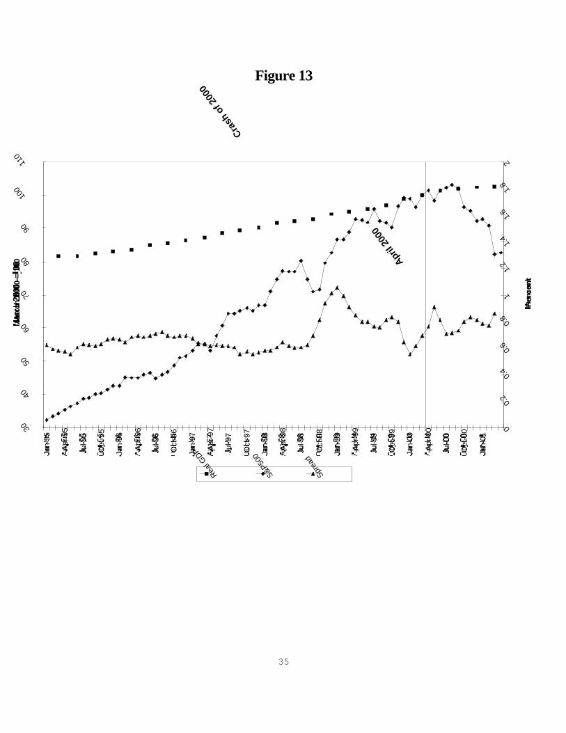
The second “great” crash of October 1987 is shown in Figure 11. Reaching a high inAugust 1987, the market plummeted 26.8 percent by December 1987. After this epic crash,there are several 3 month and one year movements in 1982 and 1984 of over 20 percent decline inthe NASDAQ, but these are not counted as a bona fide crash as they mirror more extremevolatility, with relatively quick corrections. Also, there is no folklore on "the Street" about thesemovements constituting a crash. Figure 12, displays the collapse of 1990. According to the DowJones and the S&P500, this episode should not qualify as the June to October 1990 declineamounted only to 14.7 percent. However, it is the NASDAQ which pushes the downturn in1990 into the category of a crash. From October 1989 to October 1990, there was a 28.0percent tumble in the market. Lastly, the most recent retreat of the market is shown in Figure 13. Reaching a peak in August 2000, the market had fallen 19.9 percent by April 2001, according tothe S&P500. The collapse is much more severe when measured by the NASDAQ, which fell51.9 percent from July 2000 to April 2001. The decline of the markets may well not be over. The total decline in the S&P500 to the end of August 2001 was 25.3 percent, and the totaldecline of the NASDAQ from its peak in March 2000 to the end of August was 60.5 percent.

To examine the effects of stock market crashes on credit markets, we needed a measure ofreal activity for the economy. For this purpose, we selected the quarterly series for real GDP wasproduced by Nathan Balke and Robert Gordon (1986), measured in 1972 dollars. No series coveredthe whole of the century that could have produced an interest rate premium. The interest ratespread for the 1920s onward is the difference between Moody’s Aaa corporate bond rate andMoody’s Baa corporate bond rate.6 However before 1919, an alternative measure is required. Thespread used here was constructed by Mishkin (1991) using Macaulay’s (1938) data by subtractingthe average yield on the best one-fourth of the bonds from the average yield on the worst one-fourthof the bonds. As discussed in Mishkin (1991), this spread series does have some disadvantagesover the Baa-Aaa spread. First by the beginning of the nineteenth century, even the lowest qualityrailroad bonds are of pretty high quality, thus making this spread substantially smaller than the Baa-Aaa spread. Thus it might not display a sufficient difference in the quality of bonds to pick up thechanges in the interest rates for low- and high-quality borrowers. Nevertheless, the correlation ofthe Mishkin (1991) spread variable and the Baa-Aaa spread is quite high – 0.88 -- for the periodwhen data for both are available, 1919-35. It is important to note that that the level of the twospreads is quite different and so the scale for the spreads in the first three figures is not comparableto those for the later figures.

Clearly, one single interest rate spread for each stock market crash episode does not capturethe full effect of increased risk in credit markets. Shocks that raise the Aaa-Baa spread will have

6These series were obtained from the FRED data base maintained by the Federal Reserve Bank of St.Louis. See

www.frstls.gov.

6

even larger impacts on higher risk securities. Unfortunately, long term series for these are notavailable, nor is data on bank loan rates and how credit might be rationed. However, where somedata is available the series will be supplemented by a description of additional data in the narrative.

III. STOCK MARKET CRASHES AND THEIR AFTERMATH

The effects of a stock market crash on credit, and its pricing and availability to more riskycustomers, is not easily modeled econometrically. Over the course of a century, there are few seriesare available over long spans of time. Even when they are their interpretation may changedramatically. Furthermore, some key factors, like the strength of the financial system, are difficultto measure. Thus, in this paper we follow a narrative approach to pull together the complex storiesof the consequences of stock market crashes on the credit markets.

Whether a stock market crash will have a distinct and severe effect on the terms that creditare offered to higher risk borrowers, thereby transmitting an independent shock to the economy,depends critically on two factors. First, the initial condition of the financial system is important. Ifthe financial system is weak, being highly leveraged or having experienced cumulative shocks, it ismore likely that a crash will induce lenders to raise rates to higher risk borrowers relative to low riskones and produce financial instability. Secondly, given that a shock transmitted from the stockmarket crash promotes financial instability, how the monetary authorities react is critical. They canignore the shock, in which case interest rate spreads will rise sharply, or they can inject liquidityinto the system and dampen its effects. Lastly, it should be added that the more rapid and violentthe crash, the more likely it will be a surprise. Intermediaries will have less time to makeadjustments other than altering the terms of credit.

1903

The first crash of the twentieth century occurred in 1903, an event often referred to as the“rich man’s panic” and identified as occurring in October 1903. However, as can be seen in Figure 1,the decline in the market began much earlier. The Dow Jones fell by 7.5 percent in July 1903, andby almost the same amount, 8.2 percent, in October. By the end of this month, the index was down16 percent over the year. By the Cowles index, the biggest monthly decline was in August 1903,12.9 percent, and the yearly decline to September 1903 was a cumulative 26.8 percent. Whether thestock market anticipated or followed the business cycle is unclear. The NBER dates the peak of thecycle in the last quarter of 1902, while the best real GDP data, shown in Figure 1, indicates that thedecline began a year later. This difference is the result of the fragile nature of economic data in theearly twentieth century. In any event the economic contraction was relatively mild, and the bankingsystem had experienced no prior stress.

The stock market collapse began when banks called in the loans of underwriting syndicates,which had sponsored new issues in the previous two years. The syndicates responded by sellingthe unsold underwritten securities plus older higher grade stocks and bonds. This liquidation in thelast quarter of 1903 helped to drive down the market. According to Friedman and Schwartz (1963)railroads found it difficult to borrow, and other companies and financial houses failed. The effect ofthe collapse on spreads was relatively mild. Using Mishkin’s (1991) spread in Figure 1, there is no

7

significant movement in the spread, even as interest rates rose. However, looking at the differencebetween high grade industrial bonds and high grade railroad bonds, where the former would havebeen considered riskier in this period, there is a rise in the spread of 25 basis points.7 Part of thismild effect of the stock market may be attributed to the actions of Secretary of the Treasury LeslieM. Shaw. In the absence of a central bank, he anticipated the November payment of interest onoutstanding bonds, bought bonds for the sinking fund at high premiums and increased governmentdeposits at national banks, adding significantly to funds available to the money market (Friedmanand Schwartz, 1963). Although the stock market crash of 1903 represented a large fall in stockprices, the initial soundness of the financial system and the monetary response of the Treasury ledto a result in which there was little evidence of financial instability.

1907

The crash of 1907 is the first stock market collapse of the twentieth century that had adiscernable effect on the credit markets. After a sustained boom in the stock market from 1904through 1906, the market began to collapse in early 1907, as seen in Figure 2. As measured by theDow Jones, the market sustained losses of 9.7 percent in March 1907, 8.2 percent in August 1907,and then 11.3 and 10.9 percent in October and November of that year.8 Real GDP had continuedto grow through the end of the second quarter of 1907, before falling 1 percent by the third quarterand then a shocking 5.5 percent in the last quarter. The NBER dates the peak of the business cycleas May 1907, with a long slide to the trough in June 1908.

The rapidly declining stock market, well in advance of the economy may have been animportant factor stressing the financial system, and spreads began moving upwards. The financialsystem appears to have been much more susceptible than in 1903, with banks becoming involved inmore risky ventures and a serious rivalry emerging between banks and their newest competitors,trust companies. One speculative venture, the manipulation of prices of prices of coppercompanies in the midst of a boom in the price of copper, failed. Eight bank associated with thisactivity were forced to seek assistance from the New York Clearing House on October 14, which inthe years before the establishment of the Federal Reserve provided some limited lender of last resortsupport. When the Knickerbocker Trust Company was discovered to have been involved in thisventure, the Clearing House, composed of commercial banks, refused to come to its assistance.Knickerbocker was then forced to suspend payment on October 22, creating a banking panic first inNew York and then throughout the country. A nationwide suspension of specie payments todepositors quelled the panic and payments were not resumed until January 1908 (Sprague, 1910 andFriedman and Schwartz, 1963, Mishkin, 1991, Wicker, 2000).

The clearinghouses in New York and other cities began to issue clearinghouse loancertificates, a partial substitute for high power money, in late October 1907. However theseinstitutions were not full-fledged lenders of last resort; their inability to halt the crisis eventually ledto the creation of the Federal Reserve. The delay in the action of the clearinghouse was notcompensated by the actions of Secretary of the Treasury George Cortelyou. As in 1903, theTresury tried to increase funds to the money market, depositing government funds in banks and 7 Both series are from Standard & Poor’s. The high grade railroad bonds and the high grade industrial bonds areavailable on the Macro History data set in the NBER’s web site (www.nber.org) as series, 13024 and 13026.8The Cowles index showed similar movements with declines of 15.2, 18.6 and 17.0 percent in March, October,

and November 1907.

8

exempting them from the legal reserves against these deposits while stimulating the importation ofgold. But these actions were limited and late (Wicker, 2000).

Friedman and Schwartz (1963) identify a 2 _ percent drop in the money stock from May toSeptember 1907 as putting downward pressure on the economy. They point to the drop in themoney stock following the panic as a key factor turning a mild recession into a severe one that lasteduntil June 1908. However, while the banking panic clearly contributed to the economic decline,interest rates in general and the spreads had been widening well before October 1907. The firstphase of the stock market decline and rise in the risk premium was not accompanied by a fallingmoney stock. It appears that the declining value of firms on the stock markets independentlyincreased the adverse selection and agency problems for borrowers, effectively lowering their networth. Numerous examples from the financial press indicate that these became severe problemsearly in the crisis. In March 1907, the price of Union Panic shares, which were widely used tocollateralize finance bills, fell by 50 points in less than two weeks. Then in June, New York City’snew bond offering of $29 million failed with only $2 million being purchased (Sprague, 1910). Ingeneral, as seen in Figure 2, most of the increase in the spread occurred in advance of the bankingpanic, although there was a sharp increase in October and November. Once the stock market beganto rebound, the risk premium started to decline, in advance of the economic recovery. Given the exposure of the banking system, and the late and limited response of the Treasury,the crash of 1907 thus might have been an important factor in the rise in risk premiums in the creditmarkets, thereby contributing to a severe recession.

1917

World War I and its aftermath produced huge fluctuations in the stock market. At the outsetof the war, the market began a rapid descent that was terminated when all markets were closed fromthe beginning of August to December 12, 1914 in fear of a banking and financial crisis. Figure 3shows the crash in the second half of 1917. In nominal and real terms, these were huge declines. Inthe twelve months ending November 1917, the Dow Jones fell 33.8 percent in nominal terms and44.4 percent in real terms.

The crash of the market in late 1917 is stunning. It is notable, especially as the economywas booming. Real GDP in Figure 3 is clearly on the rise and the peak of the NBER business cyclewas only reached in August 1918. The rising spread as the collapse of the market proceeded is thusnoteworthy. Other spreads also increased in this downturn including the Junk-AAA spread whichincreased over 1 percent (Basile, 1989). This market decline, although large in magnitude, has beenvirtually ignored by historians. However, it would appear that the fall in share prices may beattributed in part to generally rising interest rates and controls on new capital issues. Furthermore,there were strong efforts to divert financial resources to the purchase of government bonds to thefinance the war (Friedman and Schwartz, 1963).

1920

The post-World War I fall in the market, although spread over a long period, was quite large,as viewed in Figure 3. For the twelve months ending December 1920, the Dow Jones index fell 31.8and 31.5 percent respectively. The Cowles Index mirrors the Dow Jones for 1917, but for thisindex the 1920 collapse is not in the top 50 crashes in nominal or real terms.

9

In the quickly declining market of late 1920, the economy was entering a very steeprecession. The peak of the business cycle, according to the NBER dating, was reached in January1920, with the economy spiraling downwards until July 1921. This decline was largely driven bythe Federal Reserve’s efforts to halt inflation, raising discount rates sharply from January to June1920. Although gold inflows, offset some of its efforts, the Fed managed an 11 percent decline intotal high-powered money from September 1920 to the trough of the business cycle in July 1921.This contraction did not produce a banking panic, but it did induce a rise in bank failures from 63 in1919 to 506 in 1921. Declining asset values rather than liquidity problems were at the root of mostof these failures. The spread in Figure 3 rises very quickly as the market is dropping but thenstabilize, while the Junk-AAA (Basile, 1989) spread remained at the high level it had reachedfollowing the 1917 crash. The Baa-Aaa spread (which is available from 1919 on) also rises by 95basis points from a low of 1.57 in October 1919 to a high of 2.52 in August 1921. In the recoverywhen the economy and the stock market recovered, the spreads again fall to lower levels.

The weakened condition of the banking system, the tight monetary policy of the Fed, allprobably played a role in the substantial rise in the interest rate spread.

1929 and 1930-33

Although we will treat them separately, the two “great” crashes of 1929 and 1987 are animportant pairing. The pattern of the crashes---with spectacularly rapid declines in stock prices---were similar, as was the Federal Reserve’s successful lender-of-last resort intervention to preventeffects of a crash from spilling over to the rest of the financial system (Mishkin, 1991). Themonetary authorities response subsequently, however, offer an important contrast. After the crashof 1929, the Federal Reserve Board maintained its tight monetary policy, helping to push theeconomy into deeper recession. The stock market continued to collapse and distress to the financialsystem led to the highest ever risk premiums. Well aware of the aftermath of 1929, the Fed did notallow its concern for the market to distort its policy after October 1987. The economy continuedto grow and the market recovered.

The stock market crash of October 1929 was one of the sharpest and most abrupt collapses. On two days October 28-29, the Dow Jones fell a total of 24 percent, down 19.6 percent for themonth and down a further 22 percent in November. The Cowles index was down 10 percent inOctober and 25 percent in November 1929. Although Figure 4 shows that there was a briefrecovery in the market in early 1930, it continued to bounce downwards almost continuously for thenext two years, producing the greatest long-term market declines by any measure.

Given the magnitude of the shock, the behavior of the spread is puzzling, it rises as themarket moved upwards in late 1928 and 1929 and then falls when the market plunges. Only whenthere is a slow sustained drop in share prices from mid-1930 onwards do spreads begin to soar offthe chart. However, the behavior of the spreads in crux of the crisis can be largely explained by theactions of the Federal Reserve. Operating under a gold standard where gold flowed to France andthere was a perceived need to aid the weak British pound, the Fed began a tight monetary policy inearly 1928, with the discount rate rising from 3 _ to 5 percent (Friedman and Schwartz, 1963;Hamilton, 1987). This policy was reinforced by the Federal Reserve’s fears that excessive creditwas fueling the boom in the stock market.

In February 1929, the Fed stepped up its policy of “direct pressure,” instructing its memberbanks to limit “speculative loans,” that is loans to brokers. Finally, the Fed raised the discount rate

10

in August 1929. However, higher rates and direct pressure did not suppress the demand for creditto buy stock, which was supplied by other intermediaries. Nevertheless, the market did extract apremium for brokers’ loans, reflecting lenders’ concerns that the rise in the market was notsustainable. Rates on brokers’ loans had traditionally been similar to those on bankers’ acceptancesand commercial paper, relatively safe assets. But, in the boom, a premium arose for brokers’ loansof 2 to 3 percent and the margin demand climbed from 25 to 50 percent (White, 1990; Rappoportand White, 1993 and 1994). Some markets, like commercial paper which declined by half in volumeand new foreign bonds which almost disappeared, were squeezed by the flow of funds to brokers’loans. All risk premiums also moved upwards, including the Baa-Aaa depicted in Figure 4.

When the market collapsed in October 1929, banks and lenders of New York rushed toliquidate their call loans to brokers. In order to keep the call loan market from freezing up theFederal Reserve Bank of New York engaged in a classic lender-of-last-resort operation, very similarto one conducted in 1987. The New York Fed let it be known that member banks could borrowfreely from the New York Fed in order to take over the brokers loans called by others. (Friedmanand Schwartz, 1963). In addition, the New York Fed made open market purchases of $160 millionduring this period, even though this amount was far in excess of what was auhorized by the FederalReserve System’s Open Market Investment Committee. As a result, New York City banksstepped into the breach and increased their loans. The crisis was contained and there were no panicincreases in money market rates or threats to banks from defaults on brokers’ loans. The premiumon brokers’ loans collapsed, as the market believed that there was no further danger. This decline inperceived risk was mirrored in fall in other risk premiums, including the Baa-Aaa spread.

Unfortunately, the Federal Reserve Board did not approve of the New York Fed’sintervention. It censured the New York bank and in spite of the recession that had begun during thesummer and was in full swing by the end of the year, the Board maintained its tight monetarypolicy. The tentative recovery in 1930, seen in the GDP movements in Figure 4 was aborted bythis policy. The continued decline in the stock market from 1930 through early 1933 reflected theeconomy’s policy-aggravated slide into depression. The collapsing economy placed enormousstress on the banking system. The banking crises of 1930, 1931 and 1933 underminedintermediation (Friedman and Schwartz, 1963; and Bernanke, 1983, Mishkin, 1991), contributingfurther to the decline of the economy. In these circumstances, risk premiums soared, as seen inFigure 4, as lenders fled from risky borrowers.9

The stock market collapse beginning in 1929 shows in high relief the importance of the twofactors we have identified. In 1929, the banking system was relatively weak and the drop in themarket was large and sudden. However, the effects were quickly contained by the response of theNew York Fed. Yet, the further though less sudden decline in stocks and other asset values in the1930s appears to have contributed to the rising risk premiums as the Fed stuck to its tight moneypolicy.

1937

The stress imposed on financial markets is perhaps most evident in 1937. In Figure 5, the

9 Bank loans also began to carry large premiums relatively to bankers’ acceptances, treasury securities or any othersafe assets, rising from just over 0.5 percent in 1929 to 2 to 4 percent in the worst years of the depression. Bankingand Monetary Statistics .

11

stock market plunges as the economy moves into recession, while the interest rate spread increasesmuch more sharply than in any other crash in the twentieth century. The decline in the market wassteep but not greater than in other episodes. In three consecutive months, the market bounceddownward, losing a total of 22.4 percent by December 1937 as measured by the Dow Jones and22.8 percent by the Cowles index. By April 1938, both indexes had another 10 percent. The peakin the business cycle was reached in May 1937 and reached its bottom in June 1938, over its coursereal GDP declined 10 percent. The leap in the risk premium shown in the spread variable in Figure5, was in plain evidence elsewhere. The Junk-AAA premium increased from 4.1 percent to 10.4percent from April 1937 to April 1938.

In early 1937, the Federal Reserve believed that it was time to tighten monetary policy. There had been steady economic expansion for two years, wholesale prices were up 50 percent andstock prices had doubled. Focusing erroneously on the nominal level of interest rates, which seemedextremely low, the Fed concluded that policy was easy. This conclusion was buttressed by the factthat commercial banks held very large excess reserves. Instead of using open market purchases orincreases in the discount rate, the Fed decided that it should increase reserve requirements beginningin July 1936 (Friedman and Schwartz, 1963). In a series of actions in August 1936, and March andMay 1937, the Fed doubled reserve requirements, jacked up margin requirements for stockpurchases, and cut slightly the discount rate. Banks responded by cutting lending to restore theirexcess reserves, contributing to the sharp contraction.

The decline in the stock market reflects the seriousness of the economic downturn. However, the decline in asset values may have been a key part in the increase in the interest ratespread. The banking system had taken a pounding during the banking crises of 1930, 1931, and1933. In June 1929, there had been 24,504 commercial banks with $49 billion of deposits. Afterthe banking panics, and the March 1933 bank holiday, the number of banks had been winnowed to14,440 with $33 billion of deposits by December 1933. The rush for liquidity by the bankingpublic had been accompanied by an effort by the banks to increase their liquidity as well. Theyslashed their lending and vastly increased their holdings of cash and bonds. Savings banks, savingsand loan associations, and insurance companies had suffered similar collapses and had moved tovastly increase their liquidity (White, 2000).

In this dramatic rush to cut lending, banks and other intermediaries would have sought toavoid even more strenuously risky borrowers. Increased adverse selection and moral hazardproblems would have then propelled risk premiums to higher levels, as is evident in Figure 5. Thedramatic fall in asset values would have exacerbated this development. The lower value of firmswould have made it increasing difficult for any one perceived to be risky to borrow either from anintermediary or on a financial market.

The existing weakness of the banking system, tight monetary policy and the decline in thestock market and other asset values, were probably all factors in the rise in up risk spreads,contributing further to the severity of the 1937-1938 recession.

1940

In May and June 1940, with the defeat of France by the Germans and the Dunkirkevacuation, the Dow Jones and the Cowles index lost 20 percent of their value, as seen in Figure 6.While real GDP declined in first quarter of 1940, there was no recession and expansion continueduntil February 1945. Although small by comparison to jumps in the interest rate spread in 1937,

12

there was a small but obvious increase during the collapse of the market. However, the spread stilldid not rise above levels reached in 1938 and 1939, and immediately fell to the pre-crash levels andthen continued to decline. The economy and the financial system were in no immediate threat fromthe crash of the market. In September 1939 when war broke out in Europe, the Federal Reservepurchased $400 million of government securities to offset the big fall in the price of U.S. governmentbonds. This action was regarded by the Federal Reserve Board, and probably the markets as well,as a break from past practice. The professed aim was to protect member bank portfolios and toensure an “orderly” capital market for economic recovery (Friedman and Schwartz, 1963). Thisaction and the steady growth of the money stock from rising gold flows may have limited thereaction of the credit markets to the stock market crash.

By 1940, the weaker financial institutions had been eliminated and the balance sheets ofmost banks and firms had been substantially strengthened. These improved initial conditions andthe Fed’s monetary policy earlier meant that the credit markets responded very little to the stockmarket crash.

1946

After several months of slow decline, there was an abrupt drop in the stock market inSeptember 1946, of 12 percent measured by the Dow Jones and 14.7 percent by the S&P500. Thiscollapse is quite surprising as it came after the severe post-World War II recession. According to theNBER dating, the peak of the previous boom was in February 1945 and the bottom was hit inOctober 1945. The crash thus appears to be unrelated to the recovery of the economy. What isalso striking is that there is almost no effect of the crash on the interest rate spread in Figure 7. Thelack of response of the debt markets to the collapse in equity prices may be attributed to thecontinuance of the government’s wartime policy of supporting the price of government bonds. Theposted rate on Treasury bills was 3/8 of 1 percent and 2 _ percent on long term securities (Friedmanand Schwartz, 1963). Any upward pull on these rates by higher rates elsewhere in the market wasoffset by open market operations by the Fed.

The continued growth of the money stock and the bond price supports helped insulate thecredit markets from the stock market crash. In addition, by the end of World War II, the financialsystem had been purged of almost any risk, except that derived from holding government bonds. Thus, not surprisingly, the collapse in stock prices in 1946 was not followed by significant rises ininterest-rate spreads.

1962

The stock market crash in 1962 occurred at a time when the economy was expanding. RealGDP, as seen in Figure 8, was rising and the expansion begun in February 1961 would continueduntil December 1969. Beginning April 1962, the market had lost 20.6 percent of its value asmeasured by the Dow Jones by June and 20.9 percent by the S&P500. Yet, this shock did little todrive the interest rate spread upward. In fact, it appears to have been remarkably steady. Thebanking system was very stable, there had been no significant loan losses or bank failures in decades.The Federal Reserve was concerned about maintaining orderly markets for treasury securities andkept interest rate movements modest. Thus, even a shock from a stock market crash appears tohave had little effect on interest rate risk premiums in credit markets.

13

1969-1970

The sharp decline in the stock market in mid-1970 occurred at the time of a very mildrecession. Although the economy had peaked in December 1969, the slowdown has been referred toas a "hiatus" rather than a recession (Gordon, 1980). However, the expansion was also quitesluggish. The market peaked in advance in November 1968, then began to drift downwards,declining abruptly in May 1970, as seen in Figure 9. Eventually, the market would hit bottom inJune 1970, for a 30.6 percent drop. In this uncertain atmosphere when there was a decrease inthe valuation of firms from a fall in net worth, adverse selection problems began to appear incredit markets and the spread began to widen.

By May 1970, Penn Central Railroad was on the verge of bankruptcy. The railroad askedfor assistance first, from the Nixon administration and then the Federal Reserve. Both theserequests were rebuffed and on June 21, 1970, Penn Central was forced to declare bankruptcy. As amajor issuer of commercial paper, the Federal Reserve was concerned that this default would make itimpossible for other corporations to roll over their commercial paper, producing furtherbankruptcies and perhaps a panic. To prevent this from happening, the Fed encouraged moneycenter banks to continue lending, promising that the discount window would be available to them(Mishkin, 1991).

In spite of the Fed’s actions in response to a potential problem in the commercial papermarket, interest rate spreads widened. Not only did the commercial paper-Treasury bill rate rise(Mishin, 1991), but so did the Baa-Aaa spread in Figure 9. The general rise in risk premiumsindicates that problems of the commercial paper market had the potential for spreading to parts ofthe capital market. However, the increase in the spread variables from the Penn Central bankruptcywere not large by standards of other crises, and were likely to have been dampened by the promptaction of the Fed.

1973-1974

One of the largest and longest stock market collapses, viewed in Figure 9, began in the early1970s. Beginning with a monthly fall in the Dow Jones of 14 percent and the S&P 500 of 7 percentin November 1973, the twelve month decline ending in October 1974 were 30.4 percent and 36.8percent for the two indexes. Beginning at the same time as the economy began to turn down, themarket dropped as the economy moved into a recession that lasted until March 1975. The marketcrash was accompanied by a large increase in the interest rate spread in Figure 9. However, theincrease occurred mostly after the stock market decline had occurred. Unlike the earlier post-WorldWar II decades the financial markets and institutions were forced to cope with rising inflation andinflation uncertainty, following the OPEC oil price shock. The large decline in asset values alsowould have contributed to making low quality borrowers seem even worse risks. The existingcondition of the banking system was not as favorable to the absorption of any shock. With arecession and inflation, bank earnings fell as borrowers failed to make payments and loan losses rose. Banks found an increased difficulty in funding as market rates moved well above the Regulation Qceilings that set rates for bank deposits. Banks found themselves troubled by real estate loans andloans made to non-oil-producing countries. In the previous two decades bank failures had been veryrare and involved only small institutions. In October 1973, the first large bank failure since the

14

depression occurred in San Diego, followed by failure of the nation’s 20th largest bank, FranklinNational in October 1974. These failures highlighted the generally weakened state of the bankingsystem (Sinkey, 1979; Spero, 1980; White, 1992).

The stock market crash in this environment could only aggravate the problems of agencycosts, thereby reducing the willingness of lenders to provide low quality borrowers with credit anddriving up the interest rate risk premiums. However, the fact that majority of the increase in thespread occurred well after the market had turned upward suggests that the other factors were clearlyimportant in producing financial instability.

1987

The October 1987 crash had the largest one-day decline in stock market values in U.S.history. On October 19, the Dow Jones fell 22.6 percent and for the month, the index was down23.2 percent. As measured by the S&P 500, the market fell 12.1 percent in October and 12.5percent in November. Thus, the pattern of the rise and fall of the market for 1926-1929 in Figure 4and 1984-1987 in Figure 10 look remarkably similar.

Unlike the 1920s, the Fed in the 1980s was no longer preoccupied by speculation, but afterthe 1970s it was concerned about inflation and tightened policy to prevent any acceleration. At theoutset of the stock market boom, monetary aggregates had increased at a fairly rapid pace. But, inthe first six months of 1987, their growth slowed considerably. Concerned about rising foreigninterest rates, a poor trade balances, and a weak dollar, interest rates in the U.S. rose in anticipationof action by the Fed, which increased the discount rate from 5.5 to 6 percent on September 4(Mussa, 1994). These actions did not slow down the economy, and it continued to grow steadily asseen in the real GDP movement in Figure 10. The risk premium was steady, and the spread appearsto have declined even when the market moved into the last phase of the boom in mid-1987.

The sharp decline on October 19 put the financial system under great stress because in orderto keep the stock market and the related stock index futures market operating in an orderly fashion,brokers needed to extend huge amounts of credit on behalf of their customers for margin calls. Themagnitude of the problem is illustrated by two brokerage firms, Kidder, Peabody and Goldman,Sachs, who by themselves had advanced $1.5 billion in response to margin calls on their customersby noon of October 20. Clearly, brokerage firms as well as specialists were severely in need ofadditional funds to finance their activities. Despite the financial strength of these firms, there was somuch uncertainty that banks were reluctant to lend to the securities industry at a time when it wasmost needed. The Federal Reserve thus began to fear a breakdown in the clearing and settlementsystems and the collapse of securities firms. To prevent this from happening, Alan Greenspan, theChairman of the Board of Governors of the Federal Reserve, announced before the market openedon October 20 the Federal Reserve System’s “readiness to serve as a source of liquidity to supportthe economic and financial system.” The Open Market Desk then supplied $17 billion to thebanking system, or more than 25 percent of bank reserves and 7 percent of the monetary base. Inaddition, commercial banks were told that they were expected to continue supplying otherparticipants of the financial system with credit, including loans to broker-dealers to ensure that theycould carry their inventories of securities.10 Spreads widened at the outset of the crisis, but thenquickly decreased in response to the actions of the Fed. Although stock prices continued to oscillate

10

See Brimmer (1989) and Mishkin (1991) for a description of the Fed’s lender-of-last resort role in this episode.

15

violently for the remainder of 1987, financial markets gradually calmed down. The Fed carefullywithdrew most of the high-powered money that it had provided, ensuring that the Federal funds ratewas stable at 6.75 percent or about 1 percent below the level before the crash.

Thus, cushioned by the Federal Reserve’s action which were very reminiscent of the actionsthe New York Fed took in the October 1929 episode, the crash was not seen as a threat to thestability of the financial system or borrowers despite the large loss in equity values. Bank failuresand loan losses were rising rapidly in the late 1980s, and yet the crash was prevented from damagingthe susceptible financial system. There was almost no movement in the spread shown in Figure 10from mid-1987 to mid-1988.11 The Fed’s lender of last resort operation was again successful, butthis time there was no overreaction to the boom in the market and monetary policy was focused oneconomic activity, not the stock market.

1990

In August 1990, a major stock market decline began with the Dow Jones falling 10 percentand the S&P500 declining 8.1 percent. By October 1990, the market had fallen 15.9 percent and14.7 percent by these measures. The decline in the market closely followed the movement of theeconomy into a recession, the peak of the expansion having been reached in July 1990. Yet,although the 1990-91 recession was a relatively mild one and the stock market decline was moderate,the interest-rate spread did rise substantially. A likely source of this widening of the spread was thevery weak initial condition of depository institutions. The savings and loans already required abailout from the government on the order of $150 billion, while commercial bank failures had risen toover 200 per year by the late 1980s. and loan losses were steadily rising (White, 1992).

2000

Lastly, Figure 11 shows the current movement in the S&P 500 and its slump beginning inApril 2000. Growth may have slowed, but a recession is still in the wings, if it intends to make anappearance. The collapse in stock prices has not been evenly felt across the market. BetweenMarch 2000 and April 2001, the Dow Jones dropped approximately 2 percent, the S&P500 fell 17percent and the NASDAQ nearly 60 percent. The higher tech, higher risk stocks took a beating. Yet, this has not been translated into a higher risk premium for these borrowers. One explanationfor this surprise is the financial system is stronger than at any time since the 1960s. The weakbanks have been culled out by failure and merger, and new regulations and a strong economy havemade intermediaries stronger and less susceptible to a sudden decline in asset values. Thus, therehas been no reason for a squeeze on the less creditworthy customers, despite the decline in the stockmarket.

IV. IMPLICATIONS FOR MONETARY POLICY

The description of the fourteen episodes of twentieth century stock market crashes suggests 11

However, as shown in Mishkin (1991), there was a sharp but brief increase in the junk bond-Treasury spreadwhen the crash occurred. This suggests that there was the potential for the crash to lead to substantial financialinstability, but this did not occur because of the quick action by the Federal Reserve.

16

that we can place them into four categories.

1. Episodes in which the crashes did not appear to put stress on the financial systembecause interest-rate spreads did not widen appreciably. These include the crashes of1903, 1940, 1946, 1962 and 2000.

2. Episodes in which the crashes were extremely sharp and which did put stress on thefinancial system, but there was little widening of spreads subsequently because ofintervention by the Federal Reserve to keep the financial system functioning in the wakeof these crashes. These include the crashes of 1929 and 1987.

3. Episodes in which the crashes were associated with large increases in spreads suggestingsevere financial distress. These include the crashes of 1907, 1930-33, 1937, 1973-74.

4. Episodes in which the crashes were associated with increases in spreads that were not aslarge as in the third category, suggesting some financial distress. These include thecrashes of 1917, 1920, 1969-70 and 1990.

Obviously, deciding which crashes go into categories 3 and 4 is somewhat arbitrary. For example,the 1920 crash episode does have a substantially greater increase in the spread than 1917 using theMishkin measure, but the increase for the Baa-Aaa spread (which was available from 1919 on) issimilar to that in 1990 and is less than in the other category 3 episodes.

Looking at these four categories of crash episodes, what conclusions can we draw? First, isthe fact that many stock market crashes (category 1) are not accompanied by increases in spreadssuggests that stock market crashes by themselves do not necessarily produce financial instability. These episodes also are ones in which the balance sheets and the financial system are in good shapebefore the onset of the stock market crash. Furthermore, in these cases where financial instabilitydoes not appear, economic downturns tend to be fairly mild. Secondly, very sharp stock marketcrashes like those in 1929 and 1987 (category 2) do have the potential to disrupt financial markets.But actions by the central bank to prevent the crashes from seizing up markets--not to prop upstock prices---are able to prevent financial instability from spinning out of control. Thirdly,situations in which financial instability becomes severe, when spreads widen substantially (category3) are associated with the worst economic downturns.

Because stock market crashes are often not followed by signs of financial instability, wemust always be cautious about assigning causality from timing evidence. Certainly, one cannotmake the case that stock market crashes are the main cause of financial instability. Indeed, in manyepisodes, a case can be made that the source of financial instability might have been caused by otherfactors, such as the collapse of the banking system or the severity of the economic contraction. Only in the case of the extremely sharp market crashes as in 1929 and 1987 do we have more directevidence that some financial markets were unable to function as a result of the stock market crash.The theory of how stock market crashes can interfere with the efficient functioning of financialmarkets suggests that the impact of a stock market crash will be very different depending on theinitial conditions of balance sheets in the economy. Thus the lack of evidence for the view thatstock market crashes usually lead to financial instability should not be surprising.

What then are the monetary policy implications of the analysis of the stock market crashesexamined here?12 12

There are other implications for other types of policy besides monetary policy that are beyond the scope of thispaper. For example, concerns about preventing financial instability lead to the need to focus on financial regulation

17

The first is that financial instability is the key problem facing the policymaker and not stockmarket crashes, even if they reflect the bursting of an asset price bubble. If the balance sheets offinancial and nonfinancial institutions are initially strong, then a stock market crash (bursting of thebubble) is unlikely to lead to financial instability. In this case, the effect of a stock market crash onthe economy will operate through the usual wealth and cost of capital channels, only requiring themonetary policymakers to respond to the standard effects of the stock market decline on aggregatedemand. In this situation, optimal monetary policy which focuses solely on minimizing a standardloss function will not respond to the stock market decline over and above its affects on inflation andoutput. Indeed, a regime of flexible inflation targeting, which is what all so-called inflation targetersactually pursue (see Bernake, Laubach, Mishkin and Posen, 1999), is consistent with this type ofoptimal monetary policy (Svensson, 1999). Also Bernanke and Gertler (1999) have shown that aregime of flexible inflation targeting is likely to make financial instability less likely and to bestabilizing in the presence of asset price bubbles.

However, central banks will sometimes need to directly respond to a stock market crashwhen the crash puts stress on the financial system in order to prevent financial instability. We haveseen exactly this response of the Fed in the crashes of 1929 and 1987 when the Fed had directevidence that financial markets were unable to function in the immediate aftermath of the crashes. What is important about both these two episodes is nature of the stress on financial markets. Thesource of stress had more to do with the speed of the stock market decline than the overall decline ofthe market over time, which has often been far larger with little impact on the financial system. Furthermore, in both episodes, the focus of the Federal Reserve was not to try to prop up stockprices, but was rather to make sure that the financial markets, which were starting to seize up,would begin functioning normally again.

A focus on financial instability also implies that central banks will respond to disruptions inthe financial markets even if the stock market is not a major concern. For example, as described inMaisel (1973), Brimmer (1989) and Mishkin (1991), the Fed responded aggressively to prevent afinancial crisis after the Penn-Central bankruptcy in June 1970 without much concern fordevelopments in the stock market even though it had an appreciable decline from its peak in late1968. In the aftermath of the Penn-Central bankruptcy, the commercial paper market stoppedfunctioning and the Fed stepped in with a lender-of-last-resort operation. The New York Fed got intouch with money center banks, encouraged them to lend to their customers who were unable to rollover their commercial paper, and indicated that the discount window would be made available to thebanks so that they could make these loans. These banks then followed the Fed’s suggestion andreceived $575 million through the discount window for this purpose. In addition, the Fed, alongwith the FDIC and the Federal Home Loan Banks decided to suspend Regulation Q ceilings ondeposits of $100,000 or more in order to keep interest rates from rising, and the Fed suppliedliquidity to the banks through open market operations. Similarly, in the fall of 1998, the Fedsupplied liquidity to the system and lowered the federal funds rate sharply by 75 basis points evenwhen the market was at levels that were considered to be very high by Federal Reserve officials. The Fed’s intervention stemmed from its concerns about the stress put on the financial system bythe Russian crisis and the failure of Long Term Capital Management. Too much of a focus on thestock market rather than on the potential for financial instability might lead central banks to fail totake the appropriate actions to limit financial instability, as in 1970 and 1998, when the level of thestock market was not a major concern. and supervision, as is discussed in Mishkin (2000).

18

Too great a focus on the stock market also presents other dangers for central banks. Toomuch attention on asset prices, in this case common stocks, can lead to the wrong policy responses.The optimal response to a change in asset prices very much depends on the source of the shock tothese prices and the duration of the shock. An excellent example of this pitfall of too much focus onan asset price is the tightening of monetary policy in Chile and New Zealand in response to thedownward pressure on the exchange rate of their currencies in the aftermath of the East Asian andRussian crises in 1997 and 1998 (see Mishkin and Schmidt-Hebbel, 2001). Given that the shock tothe exchange rate was a negative terms of trade shock, it would have better been met by an easing ofpolicy rather than a tightening. Indeed, the Reserve Bank of Australia responded in the oppositedirection to the central banks of New Zealand and Chile, and eased monetary policy after thecollapse of the Thai baht in July 1997 because it was focused on inflation control and not theexchange rate. The excellent performance of the Australian economy relative to New Zealand andChile’s during this period illustrates the benefit of focusing on the main objective of the central bankrather than on the asset price.

A second problem with the central bank focusing too much on stock prices is that it raisesthe possibility that the central bank will be made to look foolish. The linkage between monetarypolicy and stock prices, although an important part of the transmission mechanism, is stillnevertheless, a weak one. Most fluctuations in stock prices occur for reasons unrelated tomonetary policy, either reflecting real fundamentals or animal spirits. The loose link betweenmonetary policy and stock prices therefore means that the ability of the central bank to controlstock prices is very limited. Thus, if the central bank indicates that it wants stock prices tochange in a particular direction, it is likely to find that stock prices may move in the oppositedirection, thus making the central bank look inept. Recall that when Alan Greenspan made hisspeech in 1996 suggesting that the stock market might be exhibiting "irrational exuberance", theDow Jones average was around 6500. This didn't stop the market from rising, with the Dowsubsequently climbing to above 11000.

An third problem with focusing on stock prices is that it may weaken support for acentral bank because it looks like it is trying to control too many elements of the economy. Partof the recent successes of central banks throughout the world has been that they have narrowedtheir focus and have more actively communicated what they can and cannot do. Specifically,central banks have argued that they are less capable of managing short-run business cyclefluctuation and should therefore focus more on price stability as their primary goal. A keyelement of the success of the Bundesbank's monetary targeting regime was that it did not focuson short-run output fluctuation in setting its monetary policy instruments.13 Thiscommunication strategy for the Bundesbank has been very successful, as pointed out inBernanke, Laubach, Mishkin and Posen (1999), has been adopted as a key element in inflationtargeting, a monetary regime that has been gaining in popularity in recent years. By narrowingtheir focus, central banks in recent years have been able to increase public support for theirindependence. Extending their focus to asset prices has the potential to weaken public supportfor central banks and may even cause the public to worry that the central bank is too powerful,having undue influence over all aspects of the economy.

A fourth problem with too much focus on the stock market is that it may create a form of

13See Bernanke, Laubach, Mishkin and Posen (1999).

19

moral hazard. The markets knowing that the central bank is likely to prop up the stock market if itcrashes, are then more likely to bid up stock prices. This might help facilitate excessive valuation ofstocks and help encourage a stock market bubble that might crash later, something that the centralbank would rather avoid.

This begs the question of whether monetary authorities should try to prick asset pricebubbles, because subsequent collapses of these asset prices might be highly damaging to theeconomy, as they were in Japan in the 1990s. Cecchetti, Genburg, Lipsky and Wadhwani(2000), for example, argue that central banks should at times react to asset prices in order to stopbubbles from getting too far out of hand. However, there as serious flaws in their argument. First is that it is very hard for monetary authorities to identify that a bubble has actuallydeveloped. To assume that they can is to assume that the monetary authorities have betterinformation and predictive ability than the private sector. If the central bank has noinformational advantage, then if it knows that a bubble has developed that will eventually crash,then the market knows this too and then the bubble would unravel and thus would be unlikely todevelop. Without an informational advantage, the central bank is as likely to mispredict thepresence of a bubble as the private market and thus will frequently be mistaken, thus frequentlypursuing the wrong monetary policy. Cecchetti, Genburg, Lipski and Wadhwani (1999) findfavorable results in their simulations when the central bank conducts policy to prick asset pricebubble because they assume that the central bank knows the bubble is in progress. Thisassumption is highly dubious because it is hard to believe that the central bank has this kind ofinformational advantage over private markets. Indeed, the view that government officials knowbetter than the markets has been proved wrong over and over again.

V. CONCLUSIONS

This paper has examined fifteen episodes of stock market crashes in the United States in thetwentieth century. The basic conclusion from studying these episodes is that the key problemfacing monetary policymakers is not stock market crashes and the possible bursting of a bubble, butrather whether serious financial instability is present. Indeed, the current situation depicted inFigure 12, which shows that the recent stock market crash has had little impact on interest-ratespreads, appears to be one that is not associated with financial instability. Thus, the currentenvironment does not appear to be one that requires an unusual response to the stock marketdecline. With a focus on financial stability rather than the stock market, the response of centralbanks to stock market fluctuations is more likely to be optimal and maintain support for theindependence of the central bank.

20

Bibliography

Balke, Nathan, and Robert J. Gordon, "Historical Data, Appendix B." in Robert J. Gordon, TheAmerican Business Cycle: Continuity and Change (University of Chicago: Chicago, 1986), 781-850.

Basile, Peter, "The Cyclical Variation of Junk Bond Risk Premiums in a Historical Perspective:1910-1955," (Rutgers University, Master’s Thesis, 1989).

Battacharya, Sudipto and Anjan Thakor, "Contemporary Banking Theory," Journal of FinancialIntermediation (October 1993), 2-50.

Bernanke, Ben S. (1983) “Non-Monetary Effects of the Financial Crisis in the Propogation of theGreat Depression,” American Economic Review 73 (June): 257-76.

Bernanke, Ben S., Laubach, Thomas, Mishkin, Frederic S. and Adam S. Posen (1999) InflationTargeting: Lessons from the International Experience (Princeton: Princeton University Press).

Bernanke, Ben .S and Gertler Mark (1989). "Agency Costs, Collateral, and Business Fluctuations", American Economic Review, Vol. 79, pp. 14-31.

Brimmer, Andrew F. (1989) “Distinguished Lecture on Economics in Government: Central Bankingand Systemic Risks in Capital Markets,” Journal of Economic Perspectives 3 (Spring): 3-16.

Board of Governors of the Federal Reserve System, Banking and Monetary Statistics, 1914-1941(1943).

Calomiris, C.W., Hubbard, R.G. (1990). "Firm Heterogeneity, Internal Finance, and `CreditRationing'", Economic Journal, 100, pp. 90-104.

Cecchetti, Stephen G., Hans Genburg, John Lipsky and Sushil Wadhwani, 2000. Asset Prices andCentral Bank Policy, Geneva Reports on the World Economy (International Center for Monetaryand Banking Studies and Centre for Economic Policy Research, London).

Economagic, www.economagic.com, stock indices.

Federal Reserve Bank of St. Louis, FRED. www.frstls.gov

Freelunch, www.economy,com, stock indices.

Friedman, Milton and Anna Jacobson Schwartz, A Monetary History of the United States, 1867-1960 (Princeton: Princeton University Press, 1963).

Greenwald, B., Stiglitz, J.E. (1988) "Information, Finance Constraints, and Business Fluctuations",in Kahn, M., and Tsiang, S.C. (eds) Oxford University Press, Oxford.

21

Macaulay, Frederick R. (1938) The Movements of Interest Rates,Bond Yields and Stock Prices in theUnited States Since 1856 (New York: National Bureau of Economic Research).

Maisel, Sherman (1973) Managing the Dollar (New York: Norton).

Mishkin, Frederic S., “Asymmetric Information and Financial Crises: A Historical Perspective,” inR. Glenn Hubbard, Financial Markets and Financial Crises (Chicago: Chicago University Press,1991): 69-108.

Mishkin, Frederic S., "Symposium on the Monetary Transmission Mechanism," Journal ofEconomic Perspectives, 9, #4 (Fall 1995): 3-10.

Mishkin, Frederic S., "The Causes and Propagation of Financial Instability: Lessons forPolicymakers," Maintaining Financial Stability in a Global Economy (Federal Reserve Bank ofKansas City, Kansas City, MO., 1997): 55-96.

Mishkin, Frederic S. (2001) "Financial Policies and the Prevention of Financial Crises inEmerging Market Countries," NBER Working Paper No. ????, forthcoming in Martin Feldstein,ed., Economic and Financial Crises in Emerging Market Countries (University of ChicagoPress: Chicago)

Mishkin, Frederic S. and Klaus Schmidt-Hebbel (2001) "One Decade of Inflation Targeting inthe World: What Do We Know and What Do We Need to Know?" NBER Working Paper No.????, forthcoming in Norman Loayza and Raimundo Soto, eds., A Decade of Inflation Targetingin the World (Central Bank of Chile: Santiago)

Mussa, Michel, “Monetary Policy,” in Martin Feldstein, American Economic Policy in the1980s (Chicago: Chicago University Press, 1994).

National Bureau of Economic Research, Macro History Database.

Pierce, Phyllis, The Dow Jones Averages, 1885-1990 (Homewood, IL: Business One Irwin,1991).

Rappoport, Peter and Eugene N. White, “Was There a Bubble in the 1929 Stock Market?”Journal of Economic History 53 (3) September 1993, 549-574.

Rappoport, Peter and Eugene N. White, “Was the Crash of 1929 Expected?” American EconomicReview 84 (1) March 1994, 271-281.

Romer, Christina, Quarterly Journal of Economics (1990)

Sprague, O. M. W., History of Crises Under the National Banking System (U.S. GovernmentPrinting Office: Washington, D.C., 1910).

22

Svensson, L. (1997), “Inflation Forecast Targeting: Implementing and Monitoring InflationTargets,” European Economic Review, 41: 1111-1146.

White, Eugene N., “The Stock Market Boom and Crash of 1929 Revisited,” Journal of EconomicPerspectives 4 (2), Spring 1990, 67-83.

White, Eugene N., The Comptroller and the Transformation of American Banking, 1960-1990(Office of the Comptroller of the Currency: Washington, D.C., 1992).

White, Eugene N., “Banking and Finance in the Twentieth Century,” in S. Engerman and R.Gallman, eds., The Cambridge Economic History of the United States Vol III. (Cambridge:Cambridge University Press, 2000), 743-802.

Wicker, Elmus, Banking Panics of the Gilded Age (Cambridge: Cambridge University Press,2000).

23

Figure 1

Cra

sh o

f 190

3

5070

9011

013

015

017

019

021

0

Jan-

00

Apr

-00

Jul-0

0

Oct

-00

Jan-

01

Apr

-01

Jul-0

1

Oct

-01

Jan-

02

Apr

-02

Jul-0

2

Oct

-02

Jan-

03

Apr

-03

Jul-0

3

Oct

-03

Jan-

04

Apr

-04

Jul-0

4

Oct

-04

Jan-

05

Apr

-05

Jul-0

5

Oct

-05

Jan-

06

Apr

-06

Jul-0

6

Oct

-06

Se

pte

mb

er

19

03

= 1

00

00.

20.

40.

60.

81

1.2

1.4

1.6

1.8

2

Pe

rce

nt

Real G

DP

Dow J

ones

Spre

ad

Oct

ober

190

3

24

Figure 2

Cra

sh o

f 19

07

5060

7080

9010

011

012

013

014

015

0

Jan-0

4

Mar-

04

Ma

y-0

4

Jul-04

Se

p-0

4

Nov-0

4

Jan-0

5

Mar-

05

Ma

y-0

5

Jul-05

Se

p-0

5

Nov-0

5

Jan-0

6

Mar-

06

Ma

y-0

6

Jul-06

Se

p-0

6

Nov-0

6

Jan-0

7

Mar-

07

Ma

y-0

7

Jul-07

Se

p-0

7

Nov-0

7

Jan-0

8

Mar-

08

Ma

y-0

8

Jul-08

Se

p-0

8

Nov-0

8

Jan-0

9

Mar-

09

Ma

y-0

9

Jul-09

Se

p-0

9

Nov-0

9

Jan-1

0

Mar-

10

Ma

y-1

0

Jul-10

Se

p-1

0

Nov-1

0

Se

pte

mb

er

19

07

= 1

00

00.

20.

40.

60.

81

1.2

1.4

1.6

1.8

2

Pe

rce

nt

Rea

l GD

P

Dow

Jon

es

Spr

ead

Oct

ober

190

7

25

Figure 3

Cra

shes

of 1

917

and

1920

5060

7080

9010

011

012

013

014

015

0

Jan-

15

Apr

-15

Jul-1

5

Oct

-15

Jan-

16

Apr

-16

Jul-1

6

Oct

-16

Jan-

17

Apr

-17

Jul-1

7

Oct

-17

Jan-

18

Apr

-18

Jul-1

8

Oct

-18

Jan-

19

Apr

-19

Jul-1

9

Oct

-19

Jan-

20

Apr

-20

Jul-2

0

Oct

-20

Jan-

21

Apr

-21

Jul-2

1

Oct

-21

Jan-

22

Apr

-22

Jul-2

2

Oct

-22

Octo

ber

1917 =

100

00.

20.

40.

60.

81

1.2

1.4

1.6

1.8

2

Pe

rce

nt

Real G

DP

Dow J

ones

Spre

ad

Nov

embe

r 19

17

Dec

embe

r 19

20

26

Figure 4

Cra

sh o

f 192

9

1020

3040

5060

7080

9010

011

0

Jan-

26

Apr

-26

Jul-2

6

Oct

-26

Jan-

27

Apr

-27

Jul-2

7

Oct

-27

Jan-

28

Apr

-28

Jul-2

8

Oct

-28

Jan-

29

Apr

-29

Jul-2

9

Oct

-29

Jan-

30

Apr

-30

Jul-3

0

Oct

-30

Jan-

31

Apr

-31

Jul-3

1

Oct

-31

Jan-

32

Apr

-32

Jul-3

2

Oct

-32

Se

pte

mb

er

19

29

= 1

00

0.5

11.

52

2.5

Pe

rce

nt

Real G

DP

Dow J

ones

Spre

ad

Oct

ober

192

9

27

Figure 5

Cra

shes

of 1

937

40.0

050

.00

60.0

070

.00

80.0

090

.00

100.

00

110.

00

120.

00

Jan-

34

Apr

-34

Jul-3

4

Oct

-34

Jan-

35

Apr

-35

Jul-3

5

Oct

-35

Jan-

36

Apr

-36

Jul-3

6

Oct

-36

Jan-

37

Apr

-37

Jul-3

7

Oct

-37

Jan-

38

Apr

-38

Jul-3

8

Oct

-38

Jan-

39

Apr

-39

Jul-3

9

Oct

-39

Jan-

40

Apr

-40

Jul-4

0

Oct

-40

Au

gu

st

1937 =

100

1.4

1.9

2.4

2.9

3.4

Pe

rce

nt

Real G

DP

Dow J

ones

Spre

ad

Sep

tem

ber 19

37

28

Figure 6

Cra

sh o

f 19

40

7080

9010

011

012

013

014

015

016

0

Jan-

38

Mar

-38

May

-38

Jul-3

8

Sep

-38

Nov

-38

Jan-

39

Mar

-39

May

-39

Jul-3

9

Sep

-39

Nov

-39

Jan-

40

Mar

-40

May

-40

Jul-4

0

Sep

-40

Nov

-40

Jan-

41

Mar

-41

May

-41

Jul-4

1

Sep

-41

Nov

-41

Jan-

42

Mar

-42

May

-42

Jul-4

2

Sep

-42

Nov

-42

May 1

940 =

100

1.4

1.6

1.8

22.

22.

42.

62.

83

3.2

3.4

Pe

rce

nt

Real G

DP

Dow J

ones

Spre

ad

June

194

0

29

Figure 7

Cra

sh o

f 194

6

5060

7080

9010

011

012

013

0

Jan-

43

Apr

-43

Jul-4

3

Oct

-43

Jan-

44

Apr

-44

Jul-4

4

Oct

-44

Jan-

45

Apr

-45

Jul-4

5

Oct

-45

Jan-

46

Apr

-46

Jul-4

6

Oct

-46

Jan-

47

Apr

-47

Jul-4

7

Oct

-47

Jan-

48

Apr

-48

Jul-4

8

Oct

-48

Jan-

49

Apr

-49

Jul-4

9

Oct

-49

Au

gu

st

1946 =

100

00.

20.

40.

60.

81

1.2

1.4

1.6

1.8

2

Pe

rce

nt

Real G

DP

S&P5

00

Spre

ad

Sep

tem

ber 19

46

30

Figure 8

Cra

sh o

f 196

2

7080

9010

011

012

013

014

0

Jan-

59

Apr

-59

Jul-5

9

Oct

-59

Jan-

60

Apr

-60

Jul-6

0

Oct

-60

Jan-

61

Apr

-61

Jul-6

1

Oct

-61

Jan-

62

Apr

-62

Jul-6

2

Oct

-62

Jan-

63

Apr

-63

Jul-6

3

Oct

-63

Jan-

64

Apr

-64

Jul-6

4

Oct

-64

Jan-

65

Apr

-65

Jul-6

5

Oct

-65

Ma

rch

19

62

= 1

00

00.

20.

40.

60.

81

1.2

1.4

1.6

1.8

2

Pe

rce

nt

S&P5

00

Real G

DP

Spre

ad

A

pril

1962

31

Figure 9

Cra

sh o

f 197

0

5060

7080

9010

011

012

013

014

015

0

Jan-

67

Apr

-67

Jul-6

7

Oct

-67

Jan-

68

Apr

-68

Jul-6

8

Oct

-68

Jan-

69

Apr

-69

Jul-6

9

Oct

-69

Jan-

70

Apr

-70

Jul-7

0

Oct

-70

Jan-

71

Apr

-71

Jul-7

1

Oct

-71

Jan-

72

Apr

-72

Jul-7

2

Oct

-72

Jan-

73

Apr

-73

Jul-7

3

Oct

-73

Ap

ril 1970 =

100

00.

20.

40.

60.

81

1.2

1.4

1.6

1.8

2

Pe

rce

nt

Real G

DP

S&P5

00

Spre

ad

May

197

0

32

Figure 10

Cra

sh o

f 197

3

5060

7080

9010

011

012

0

Jan-

70

Apr

-70

Jul-7

0

Oct

-70

Jan-

71

Apr

-71

Jul-7

1

Oct

-71

Jan-

72

Apr

-72

Jul-7

2

Oct

-72

Jan-

73

Apr

-73

Jul-7

3

Oct

-73

Jan-

74

Apr

-74

Jul-7

4

Oct

-74

Jan-

75

Apr

-75

Jul-7

5

Oct

-75

Jan-

76

Apr

-76

Jul-7

6

Oct

-76

Octo

berr

1973 =

100

0.5

0.7

0.9

1.1

1.3

1.5

1.7

1.9

2.1

2.3

2.5

Pe

rce

nt

S&P5

00

Real G

DP

Spre

ad

Nov

embe

r 19

73

33

Figure 11

Cra

sh o

f 198

7

4050

6070

8090

100

110

120

Jan-

84

Mar

-84

May

-84

Jul-8

4

Sep

-84

Nov

-84

Jan-

85

Mar

-85

May

-85

Jul-8

5

Sep

-85

Nov

-85

Jan-

86

Mar

-86

May

-86

Jul-8

6

Sep

-86

Nov

-86

Jan-

87

Mar

-87

May

-87

Jul-8

7

Sep

-87

Nov

-87

Jan-

88

Mar

-88

May

-88

Jul-8

8

Sep

-88

Nov

-88

Jan-

89

Mar

-89

May

-89

Jul-8

9

Sep

-89

Nov

-89

Se

pte

mb

er

19

87

= 1

00

00.

20.

40.

60.

81

1.2

1.4

1.6

1.8

2

Pe

rce

nt

Real G

DP

S&P5

00

Spre

adO

ctob

er 1

987

34

Figure 12

Cra

sh o

f 199

0

6070

8090

100

110

120

130

140

Jan-

88

Apr

-88

Jul-8

8

Oct

-88

Jan-

89

Apr

-89

Jul-8

9

Oct

-89

Jan-

90

Apr

-90

Jul-9

0

Oct

-90

Jan-

91

Apr

-91

Jul-9

1

Oct

-91

Jan-

92

Apr

-92

Jul-9

2

Oct

-92

Jan-

93

Apr

-93

Jul-9

3

Oct

-93

Ju

ly 1

99

0 =

10

0

00.

20.

40.

60.

81

1.2

1.4

1.6

1.8

2

Pe

rce

nt

Real G

DP

S&P5

00

Spre

ad

Aug

ust 1

990

35

Figure 13

Cra

sh o

f 200

0

3040

5060

7080

9010

011

0

Jan-

95

Apr

-95

Jul-9

5

Oct

-95

Jan-

96

Apr

-96

Jul-9

6

Oct

-96

Jan-

97

Apr

-97

Jul-9

7

Oct

-97

Jan-

98

Apr

-98

Jul-9

8

Oct

-98

Jan-

99

Apr

-99

Jul-9

9

Oct

-99

Jan-

00

Apr

-00

Jul-0

0

Oct

-00

Jan-

01

Ma

rch

20

00

= 1

00

00.

20.

40.

60.

81

1.2

1.4

1.6

1.8

2

Pe

rce

nt

Real G

DP

S&P5

00

Spre

ad

Apr

il 20

00

Date post:	26-May-2018
Category:	Documents
Upload:	tranhanh
View:	218 times
Download:	0 times

U.S. Stock Market Crashes and Their Aftermath ... · U.S. Stock Market Crashes and Their Aftermath:...

Documents