Use of Least Means Squares Filter in Control of Optical Beam Jitter R. Joseph Watkins ∗ U.S. Naval Academy, Annapolis, Maryland 21402 and Brij N. Agrawal † Naval Postgraduate School, Monterey, California 93943 DOI: 10.2514/1.26778 Meeting optical beam jitter requirements is becoming a challenging problem for several space programs. A laser beam jitter control test bed has been developed at the Naval Postgraduate School to develop improved jitter control techniques. Several control techniques, such as least means squares and linear–quadratic regulator were applied for jitter control. Enhancement in least means squares techniques to improve convergence rate was achieved by adding an adaptive bias filter to the reference signal. In the experiments, the platform is vibrated at 50 and 87 Hz. In addition, a fast steering mirror is used to inject a random component of 200 Hz band-limited white noise. The experimental results demonstrated that the addition of the adaptive bias filter to the least means squares algorithm significantly increased the converging rate of the controller. To achieve the reduction of both sinusoidal and random jitter, a combination of least means squares/adaptive bias filter and linear–quadratic regulator is most effective. The least means squares/adaptive bias filter control is most effective for a sinusoidal jitter and the linear–quadratic regulator control for a random jitter. Nomenclature A = cross-coupling factor A, B, C, D = state–space matrices D m = distance from source to mirror d = disturbance signal E = bias error E 0 = adaptive bias e = error signal F = amplitude of sinusoidal disturbance f = frequency, cycles per second G = gain H = transfer function J = cost function K = amplitude of reference signal P = optical bench gain Q, R = weighting matrices S = fast steering mirror transfer function s = Laplace variable ^ s = estimate of fast steering mirror transfer function, finite impulse response coefficients T = time constant T s = sample time u = control signal or input V = voltage v = disturbance source W = gain of adapting filter wn= vector of tap gains x = state vector xn= reference signal y = output vector = damping coefficient = angle of mirror = delay through a transfer function ! n = natural frequency, radians per second subscripts o = optical bench and mirrors p = optical detector s = fast steering mirror transfer function w = adapting filter transfer function x = x axis y = y axis I. Introduction M ANY future space missions, laser communication systems, and imaging systems will require optical beam jitter control in the nanoradian regime [1]. Jitter is the undesired fluctuations in the pointing of an optical beam due to environmental or structural interactions, and consists of both broadband and narrowband disturbances. The narrow band jitter is generally created in a spacecraft by rotating devices such as reaction wheels, control moment gyros, cryocoolers and the motion of flexible structures, such as solar arrays. The effect of the atmosphere on the laser beam adds a broadband disturbance, when transmissions to or from the ground are considered. The control of jitter is currently a challenging problem for programs such as the James Webb Space Telescope, the U.S. Department of Defense Airborne Laser project, and any type of imaging spacecraft [2]. Jitter has a great effect on the resolution of an image or the intensity of an optical beam. For example, a 100 mm diam laser beam with 10 rad of jitter will result in roughly a 400- fold decrease in the intensity of the beam at 100 km, due to the jitter alone. To achieve jitter control, several techniques have been proposed, including both classical and adaptive control systems. Several experimental setups have been used to test the viability of different control techniques. McEver and Clark used a linear–quadratic Gaussian (LQG) design to actively control jitter in an experiment designed around fast steering mirrors (FSM), accelerometers, and microphones [3]. The disturbance was acoustically induced by loudspeakers and control was attempted using feedforward from a Received 25 July 2006; accepted for publication 12 January 2007. This material is declared a work of the U.S. Government and is not subject to copyright protection in the United States. Copies of this paper may be made for personal or internal use, on condition that the copier pay the $10.00 per- copy fee to the Copyright Clearance Center, Inc., 222 Rosewood Drive, Danvers, MA 01923; include the code 0731-5090/07 $10.00 in correspondence with the CCC. ∗ Military Professor, Department of Mechanical Engineering; rwatkin@ usna.edu. † Distinguished Professor and Director, Spacecraft Research and Design Center; [email protected]. Associate Fellow AIAA. JOURNAL OF GUIDANCE,CONTROL, AND DYNAMICS Vol. 30, No. 4, July–August 2007 1116
Transcript
Use of Least Means Squares Filter in Controlof Optical Beam Jitter
R. Joseph Watkins∗
U.S. Naval Academy, Annapolis, Maryland 21402
and
Brij N. Agrawal†
Naval Postgraduate School, Monterey, California 93943
DOI: 10.2514/1.26778
Meeting optical beam jitter requirements is becoming a challenging problem for several space programs. A laser
beam jitter control test bed has been developed at the Naval Postgraduate School to develop improved jitter control
techniques. Several control techniques, such as least means squares and linear–quadratic regulator were applied for
jitter control. Enhancement in least means squares techniques to improve convergence rate was achieved by adding
anadaptive biasfilter to the reference signal. In the experiments, the platform is vibrated at 50 and87Hz. In addition,
a fast steering mirror is used to inject a random component of 200 Hz band-limited white noise. The experimental
results demonstrated that the addition of the adaptive bias filter to the least means squares algorithm significantly
increased the converging rate of the controller. To achieve the reduction of both sinusoidal and random jitter, a
combination of least means squares/adaptive bias filter and linear–quadratic regulator is most effective. The least
means squares/adaptive bias filter control is most effective for a sinusoidal jitter and the linear–quadratic regulator
control for a random jitter.
Nomenclature
A = cross-coupling factorA, B, C, D = state–space matricesDm = distance from source to mirrord = disturbance signalE = bias errorE0 = adaptive biase = error signalF = amplitude of sinusoidal disturbancef = frequency, cycles per secondG = gainH = transfer functionJ = cost functionK = amplitude of reference signalP = optical bench gainQ, R = weighting matricesS = fast steering mirror transfer functions = Laplace variables = estimate of fast steering mirror transfer function,
finite impulse response coefficientsT = time constantTs = sample timeu = control signal or inputV = voltagev = disturbance sourceW = gain of adapting filterw�n� = vector of tap gainsx = state vectorx�n� = reference signaly = output vector
� = damping coefficient� = angle of mirror� = delay through a transfer function!n = natural frequency, radians per second
subscripts
o = optical bench and mirrorsp = optical detectors = fast steering mirror transfer functionw = adapting filter transfer functionx = x axisy = y axis
I. Introduction
M ANY future space missions, laser communication systems,and imaging systemswill require optical beam jitter control in
the nanoradian regime [1]. Jitter is the undesired fluctuations in thepointing of an optical beam due to environmental or structuralinteractions, and consists of both broadband and narrowbanddisturbances. The narrow band jitter is generally created in aspacecraft by rotating devices such as reaction wheels, controlmoment gyros, cryocoolers and the motion of flexible structures,such as solar arrays. The effect of the atmosphere on the laser beamadds a broadband disturbance, when transmissions to or from theground are considered. The control of jitter is currently a challengingproblem for programs such as the JamesWebb Space Telescope, theU.S. Department of Defense Airborne Laser project, and any type ofimaging spacecraft [2]. Jitter has a great effect on the resolution of animage or the intensity of an optical beam. For example, a 100 mmdiam laser beam with 10 �rad of jitter will result in roughly a 400-fold decrease in the intensity of the beam at 100 km, due to the jitteralone.
To achieve jitter control, several techniques have been proposed,including both classical and adaptive control systems. Severalexperimental setups have been used to test the viability of differentcontrol techniques. McEver and Clark used a linear–quadraticGaussian (LQG) design to actively control jitter in an experimentdesigned around fast steering mirrors (FSM), accelerometers, andmicrophones [3]. The disturbance was acoustically induced byloudspeakers and control was attempted using feedforward from a
Received 25 July 2006; accepted for publication 12 January 2007. Thismaterial is declared a work of the U.S. Government and is not subject tocopyright protection in the United States. Copies of this paper may be madefor personal or internal use, on condition that the copier pay the $10.00 per-copy fee to the Copyright Clearance Center, Inc., 222 Rosewood Drive,Danvers, MA 01923; include the code 0731-5090/07 $10.00 incorrespondence with the CCC.
∗Military Professor, Department of Mechanical Engineering; [email protected].
†Distinguished Professor and Director, Spacecraft Research and DesignCenter; [email protected]. Associate Fellow AIAA.
microphone or the accelerometers to the FSM as well as feedback tothe FSM using a position sensing detector (PSD) at the target. Glaeseet al. [4] conducted similar experiments as McEver and Clark, usingacoustically induced jitter and LQG control. These experimentsshowed a decrease of about one-half of the input disturbanceamplitude for broadband disturbances, and almost completeelimination of narrowband disturbances. Adaptive methods such asthe least means squares (LMS), broadband feedforward active noisecontrol, model reference, or adaptive lattice filters have also beenused to control jitter. Skormin, Tascillo, and Busch developed acomputer simulation in 1995 of an airborne to satellite optical link inwhich the use of a self-tuning regulator (STR) as well as a filtered-Xleast means squares (FXLMS) controller was used to mitigate theeffects of jitter on the optical beam. The simulation shows thatadaptive feedforward vibration compensation can be used tominimize induced jitter [1]. In 1997, Skormin and Busch proposedthe use of model reference control for jitter reduction. Experimentswere conducted using a specially designed high bandwidth FSM anda commercially available low bandwidth FSM. In each case,significant reduction (on the order of 20 dB) in acoustically inducedjitter was achieved [5]. Also in 1997, Skormin, Tascillo, and Buschdemonstrated the use of a self-tuning regulator in an acousticallyinduced jitter rejection experiment using FSMs, accelerometers andPSDs. The data showed that the STR was superior to classicalfeedback control in frequency ranges above about 300 Hz [6].
Adaptive systems require a reference signal to reject thedisturbance. The development of this reference signal for the LMSalgorithm, and enhancements made to it particular to the lasertargeting situation is the subject of this paper. An experimental laserjitter control (LJC) test bed, equipped with fast steering mirrors tocorrect the beam, has been developed to test various controltechniques on vibrational induced jitter. Using this test bed, we willshow experimentally that the addition of an adaptive bias signal tothe reference signal results in a rapid correction of the bias error bythe adaptive controller. The bias effect has been shown previously byWidrow [7], but we have adapted the concept to the laser targetingsituation, and provided a means for this bias signal to adapt tochanging errors. This paper will first discuss the experimental setup.Following that, the development of the basic control methods used inthe experiment, as well as the enhancements made to the referencesignal will be explained. Experimental results and conclusions willthen be presented.
II. Experimental Setup
A. Laser Jitter Control Test Bed
The LJC test bed is located in the Spacecraft Research and DesignCenter, Optical Relay Mirror Lab, at the Naval Postgraduate SchoolinMonterey, California. The components are mounted on a Newportoptical bench, which is used to isolate the components from externalvibrations. The idea is to simulate a satellite or vehicle “bus” thathouses an optical relay system. The laser beam originates from asource and passes through a disturbance injection fast steeringmirror(DFSM). The DFSM corrupts the beam using random or periodicdisturbances simulating the disturbances that might occur as a resultof the transmitting station or the tip and tilt the beam may suffer as itpasses through the atmosphere. A vibration isolation platform is usedto mount the relay system, and to isolate the relay system from theoptical bench. The relay system platformmay be disturbed by a 5 lbfinertial actuator, simulating onboard running equipment such ascontrol moment gyros, reaction wheels, cryocoolers, and so on. Theinertial actuator may be located as required on the platform toproduce the desired effect. The incoming beam is split and reflectedoff the platform to a PSD to obtain a reference signal that indicates theonboard and injected disturbances. The PSDs are labeled OT1, forthe feedforward detector, and OT2 for the target detector (see Fig. 1).It is recognized that using the PSD labeledOT1 is not a normalmeansto measure the disturbances onboard the platform used to relay thebeam as one would not be able to mount a detector separate from thesatellite bus in a practical application. However, this reference PSDmay be seen as simulating an onboard inertial measurement unit
(IMU), which is normally available in satellites with an opticalpayload. The IMU provides an accurate inertial position of theplatform, which is the same as provided by a PSD mounted on astable reference plane with respect to the vibrating platform. Thissetup allows an identical measurement without the added cost of anIMU. A control fast steering mirror (FSM), designated the receiveFSM or RFSM, is used to correct the disturbed beam. The correctedbeam is then reflected off the platform by a second folding mirror tothe target PSD, OT2. A block diagram of the system as well as apicture of the actual setup are shown in Figs. 1 and 2.
B. Fast Steering Mirrors
The fast steering mirrors are the heart of the LJC. They are used torapidly and accurately direct the laser beam through the system. TheFSMs in the LJC use voice coils to position themirrors in response tocommanded inputs. The LJC uses two different FSMs, one by theNewport Corporation, and one by Baker Adaptive Optics. TheNewport FSM is used as the control mirror (RFSM) for allexperiments conducted during this research. The mirror comes withits own controller, the FSM-CD100, capable of both open loop andclosed loop operation. The controller also provides an output of themirror’s angular position about each of the axis. In theseexperiments, the controller is configured in the open loopmode, withcontrol inputs provided from the computer control system. TheNewport FSM has a control bandwidth of about 800–1000 Hz.
The second FSM used in the LJC is from Baker Adaptive Optics.The Light Force One model is a 1 in. diam DFSM in theseexperiments. The Baker mirror comes with a small driver forpositioning the mirror; however, there is no closed loop option andmirror position is not available. The control bandwidth for the Bakermirror is about 3 kHz.
C. Position Sensing Detectors
The laser beamoptical position sensors, known as position sensingmodules or PSMs, have a detection area of 10 � 10 mm. Eachduolateral, dual axis PSM requires an amplifier, theOT-301 to outputthe x and y position (in volts) of the centroid of the laser beam spot.The combination of amplifier and detector is called a position sensingdetector or PSD. The frequency response of the detectors for the gain
LaserSourceLaser
Source
2.5 mW
DFSM
Disturbance Injection
Target
Newport Table
OnTrac
Newport Vibration Isolation Platform
80/20 Beam split
36 in
OnTrac
RFSM
mirror
Folding Mirror 1
Ref. Sig.
X axis
Z axisVibration axis in Y direction
(OT1)
(OT2)
LaserSourceLaser
Source
2.5 mW
DFSM
Disturbance Injection
Target
Newport Table
OnTrac
Newport Vibration Isolation Platform
80/20 Beam split
CSA 5LB Shaker
36 in
OnTrac
RFSM 24 in
mirror
Folding Mirror 2
Ref. Sig.
X axis
Z axisVibration axis in Y direction
Control Mirror(OT1)
(OT2)
Vibration Isolation Platform
PSD
PSDAccelerometerKistler 3-axis
Fig. 1 Laser jitter control test bed schematic.
Vibration IsolatPlatform
DFSM
PSD
Laser
RFSM
InertialActuator ion
Fig. 2 Laser jitter control test bed.
WATKINS AND AGRAWAL 1117
settings normally used is 15 kHz. The minimum resolution of thePSD is 0:5 �m.
D. Newport Vibration Isolation Platform and Inertial Actuator
The RFSM, beam splitters, and folding mirrors are mounted on abench top pneumatic Newport vibration isolation platform. Thisplatform allows the control system actuators and optical path to bevibrated independent of the optical bench. The breadboard, which isself-leveling, rests on four pneumatic isolators. To vibrate theplatform at desired frequencies, an inertial actuator is mounted on thevibration isolation platform. This actuator is a CSA model SA-5,
capable of delivering a rated force of 5 lbf, in a frequency range of 20to 1000 Hz.
E. Computer Control System
The computer control system is based on MATLAB, version 6.1release 13 with SIMULINK, and the xPC Targetbox, all from theMathworks. The main computer for control implementation andexperiment supervision is a 2.4 GHzDell Dimension 8250. The xPCTargetbox is a Pentium III class computer running at 700MHz and isused to perform digital-to-analog and analog-to-digital conversion.A separate disturbance computer is used to control the inertialactuator and has a 1.4 GHz processor; dSPACE ver 3.3 withControlDesk ver 2.1.1 is used to interfacewith the inertial actuator. Asample rate of 2 kHz was used throughout the experiment, whichprecluded aliasing of any signals of interest.
III. Mathematical Model
A state–spacemodel of the RFSM/PSD systemwas used to modelthe dynamics of the control system. The state–space model is of theform
_x� Ax� Bu; y� Cx� Du (1)
A simple second order transfer function of the RFSM (used tocorrect the beam) about one axis is defined:
Hm�s� �!2n
s2 � 2�!ns� !2n
(2)
where !n and � are experimentally determined using the methods inOgata [8]. The transfer functionHm�s� relates the ordered position of
the mirror to the output position of the mirror as measured by theRFSM’s integral mirror position measurement system. A first-ordersystem was added to model the optical sensor system:
Hd�s� �1
Ts� 1(3)
The transfer function Hd�s� describes the time response betweenthe actual laser beam’s position on the surface of the detector and thereported position as measured by the voltage from the detector. Thevalue for T was determined from the data given for the opticalsensors by the manufacturer. The resulting state–space set ofequations is given as follows:
_Vpy_�x��x_Vpx_�y��y
266666664
377777775�
�1=T 2GpyDm=T 0 0 0 0
0 0 1 0 0 0
0 �!2x �2�x!x 0 Ax!
2x Ax2�x!x
0 0 0 �1=T 2GpxDm=T 0
0 0 0 0 0 1
0 Ay!2y Ay2�y!y 0 �!2
y �2�y!y
26666664
37777775
Vpy�x_�xVpx�y_�y
26666664
37777775�
0 0
0 0
Gmx!2x 0
0 0
0 0
0 Gmy!2y
26666664
37777775
VmxVmy
� �(4)
VpyVpx
� �� 1 0 0 0 0 0
0 0 0 �1 0 0
� �Vpy�x_�xVpx�y_�y
26666664
37777775�
0 0
0 0
0 0
0 0
0 0
0 0
26666664
37777775
VmxVmy
� �(5)
The values for G and A are determined experimentally and areprovided in Table 1, as well as the values used for the otherparameters.
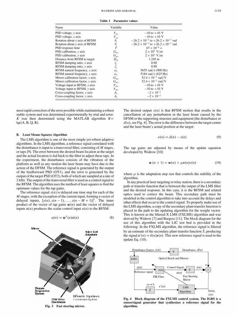
A top level view of the FSM provided by Newport ApplicationNote: Opto-Mechanics 2 is shown in Fig. 3.
IV. Control Methods
A. Linear–Quadratic Regulator
The linear–quadratic regulator (LQR) is first developed toinvestigate how classical control algorithms handle broadband andnarrowband disturbances for the control of laser jitter. The system tobe controlled, modeled in the preceding section, is used to determinethe optimal gains. The LQR requires full state feedback, which, if notavailable, must be estimated. In this experiment, a Kalman filter is
used to estimate the states _�x and _�y, all others being measured bysensors. The matrix of linear–quadratic optimal gains (K) iscalculated to minimize the following cost function:
J�Z 10
�xTQx� uTRu� dt (6)
The control law is
u ��Kx (7)
The optimum gains are determined using the state–spacemodel ofthe system, Eqs. (4) and (5). Matrices R and Q in Eq. (6) are used toweight the importance of each state and input. For this investigation,the matrices R and Q are identity matrices, with the exception of theelements along the diagonal of Q corresponding to the state Vp foreach axis having a value of 103. This value was chosen to provide the
1118 WATKINS AND AGRAWAL
most rapid correction of the error possible while maintaining a robuststable system and was determined experimentally by trial and error.K was then determined using the MATLAB algorithm K�lqr�A;B;Q;R�.
B. Least Means Squares Algorithm
The LMS algorithm is one of the most simple yet robust adaptivealgorithms. In the LMS algorithm, a reference signal correlated withthe disturbance is input to a transversal filter, consisting ofM stages,or taps [9]. The error between the desired beam location at the targetand the actual location is fed back to the filter to adjust these taps. Inthe experiment, the disturbance consists of the vibration of theplatform as well as any motion the laser beam may have due to theaction of the DFSM. The reference signal is generated by the outputof the feedforward PSD (OT1), and the error is generated by theoutput of the target PSD (OT2), both of which are sampled at a rate of2 kHz. The output of the transversal filter is used as a control signal tothe RFSM. The algorithm uses themethod of least squares to find theoptimum values for the tap gains.
The reference signal x�n� is delayed one time step for each of theM stages, with the exception of the current input, forming a vector ofdelayed inputs, �x�n�; x�n � 1�; . . . ; x�n �M� 1��T . The innerproduct of the vector of tap gains w�n� and the vector of delayedinputs x�n� produces the scalar control input u�n� to the RFSM:
u�n� �wT�n�x�n� (8)
The desired output s�n� is that RFSM motion that results in thecancellation of any perturbation in the laser beam caused by theDFSM or the supporting structure and equipment [the disturbance ord�n�, see Fig. 4]. The error is the difference between the target centerand the laser beam’s actual position at the target:
e�n� � d�n� � s�n� (9)
The tap gains are adjusted by means of the update equationdeveloped by Widrow [10]:
w �n� 1� �w�n� � �x�n�e�n� (10)
where � is the adaptation step size that controls the stability of thealgorithm.
In any practical laser targeting or relay station, there is a secondarypath or transfer function that is between the output of the LMS filterand the desired response. In this case, it is the RFSM and relatedoptics used to correct the beam. This secondary path must bemodeled in the control algorithm to take into account the delays andother effects that occur to the control signal. To properly make use ofthe LMS algorithm, a copy of the secondary plant transfer function isplaced in the path to the updating algorithm for the weight vector.This is known as the filtered-X LMS (FXLMS) algorithm and wasderived by Widrow [7] and Burgess [11]. The block diagram for theuse of this algorithm with the LJC test bed is provided in thefollowing: In the FXLMS algorithm, the reference signal is filtered
by an estimate of the secondary plant transfer function S, producingthe signal x0�n� � s�n�x�n�. This new reference signal is used in theupdate Eq. (10).
Table 1 Parameter values
Name Variable Value
PSD voltage, y axis Vpy �10 to�10 VPSD voltage, x axis Vpx �10 to�10 VRotation about x axis of RFSM �x �26:2 � 10�3 to�26:2 � 10�3 radRotation about y axis of RFSM �y �26:2 � 10�3 to�26:2 � 10�3 radPSD response time T 67 � 10�6 sPSD calibration, y axis Gpy 2 � 103 V=mPSD calibration, x axis Gpx 2 � 103 V=mDistance from RFSM to target Dm 1.245 mRFSM damping ratio, x axis �x 0.90RFSM damping ratio, y axis �y 0.90RFSM natural frequency, x axis !x 5655 rad=s (900 Hz)RFSM natural frequency, y axis !y 5184 rad=s (825 Hz)Mirror calibration factor, x axis Gmx 52:4 � 10�3 rad=VMirror calibration factor, y axis Gmy 52:4 � 10�3 rad=VVoltage input to RFSM, x axis Vmx �10 to�10 VVoltage input to RFSM, y axis Vmy �10 to�10 VCross-coupling factor, x axis Ax �2 � 10�2
Cross-coupling factor, y axis Ay �2 � 10�2
Fig. 3 Fast steering mirror.
P
LMS
Algorithm
+Sw(n)
Error,e(n)
Fast SteeringMirror
Control Signal,
Disturbance, d(n)
FIR Filter
Reference signal
Optical Bench and Mirrors
Sx’(n)
x(n)
Disturbance Source, v(n)
u(n)
IGRS
est of S
s(n)+
-
Fig. 4 Block diagram of the FXLMS control system. The IGRS is a
sensor/signal generator that synthesizes a reference signal for the
algorithm.
WATKINS AND AGRAWAL 1119
V. Correction of Bias Effects Using a Least MeansSquares Filter
A. Effect of Bias on the Least Means Squares Filter
In most laser targeting schemes, a compensator is used to correctthe bias error at the target. A second, parallel controller is then used toremove the “noise” in the beam. It has been noted byWidrow that anadaptable bias weight may be used to counteract the effect of “plantdrift” in an adaptive inverse modeling situation [12]. This singleadjustableweight adapts to remove any bias in the output of the plant.This effect may be analyzed as follows. Referring to Fig. 4 let thedisturbance be
v�n� � E� F sin�2�fnTs� (11)
Then the desired signal (the signal that must be cancelled) is
d�n� � PE� PF sin�2�fnTs � �o� (12)
Now, considering only the bias effect, let the generated referencesignal be
Thus the proper selection ofE0 will result in the cancellation of the dccomponent of the error. It is also noted that if E0 is zero, the LMSalgorithm will be unable to completely cancel the resulting error. E0
should be adaptable, because the bias error may change and becauseW is adapting during the process to some quasi–steady state value.
B. Adaptive Bias Filter
Using a one or two weight LMS filter, the bias in the referencesignal is adjusted to remove the dc component of the error signal. Anestimate ofE0 is used as the reference signal to the adaptive bias filter(ABF); see Fig. 5. The error signal in this case is the mean error,which stops the adaptation once the signal is centered on the target.
VI. Experimental Results
Five experiments were run on the LJC test bed to explore thecapabilities of the FXLMS/ABF controller. The first series of twoexperiments was run maintaining the vibration isolation platformstable. Two controllers are compared in their ability to remove a biaserror as well as two periodic disturbances introduced by the DFSM.In the second series of experiments, the platform is vibrated at thesame two frequencies used in the first series, and theDFSM is used toprovide a random error to the beam. Three controllers are compared
in their ability to remove the frequency and random components aswell as the bias error; the LQR, FXLMS/ABF, and an LQR�FXLMS=ABF combination.
A. Bias Effect
The FXLMS controller with the ABF modification was comparedwith a FXLMS controller with an unbiased reference signal, using aparallel LQR as a compensator. This experiment was run todetermine if the addition of bias to the reference signal was betterthan using a compensator. Random noise was not injected. The LQRcompensator was designed using standard MATLAB commands.The mathematical model from Sec. III above was used for the LQRstate–space system of equations. An integrator was added to themodel to complete the design. A 50 and 87 Hz signal was injected bythe DFSM and each controller was used to remove the error in thetarget signal. The power spectral density (PSD) and mean squareerror (MSE) for the y axis of the experiment are provided in Figs. 6and 7. The x axis is similar.
From these figures, we see that the addition of the ABF in the LMScontroller results in a similar decrease in the power spectral density asusing a straight compensator, and that the time constant (the time ittakes for the MSE to be reduced by a factor of 1=e) for the FXLMS/
Fig. 6 Power spectral density plot of the stable platform, two frequencybias experiment. TheFXLMScontroller for both caseswas provided a 50
and 87 Hz signal, normalized by the power of the reference signal.
0 1 2 3 4 5 6 7 8 9 1010
1
102
103
104
105
106
sec
MS
E, µ
2
MSE , stable p la tform 50, 87 Hz d isturbance
LMS/LQR Contro l
LMS/ABF Contro l
FXLMS/LQR
FXLMS/ABF
Fig. 7 Mean square error plot of the stable platform, two frequency
bias experiment.
1120 WATKINS AND AGRAWAL
ABF controller is less than that for the parallel FXLMS/LQRcontroller.
B. Vibrating Platform Results
In this experiment, the platform is vibrated by the inertial actuatorat the same two frequencies as in the previous experiment, 50 and87 Hz. In addition, the DFSM is used to inject a random componentof 200 Hz band-limited white noise, to simulate the effect ofatmospheric turbulence on the uplink laser beam for a simulated relaystation. Because the FXLMS controller uses an internally generatedreference signal (IGRS) consisting of the two disturbancefrequencies, the controller will not remove the random component.However, by combining the FXLMS controller with the LQR,control of the random component as well as the frequencies added bythe inertial actuator may be realized. Additionally, by adding theABF modification and removing the integrator from the LQR, afaster response to the bias error may also be achieved. A comparisonof three experiments using the different control methods is shown inFigs. 8 and 9.
It can be seen from these plots that the use of the LQR�FXLMS=ABF controller results in the best response. The randomcomponent is removed and the narrowband frequencies areattenuated. The time constant for the system is dramaticallyimproved over the FXLMS/ABF or LQR controller alone. Table 2presents the experimental data comparison.
In Table 2, themeasure of effectiveness for the jitter is the standarddeviation of the laser beam during the last 1 s of a 10 s data run(reported as the controlled beam, standard deviation). The input jitteris the standard deviation of the beam before controller cut on(controller cut on occurs at 1.6 s from the start of data collection). Thepercent reduction in jitter is the percent reduction in the standarddeviation of the beam as compared with the input jitter. The meanvalue of the beam position is the mean position, in nanometers (nm)over the last 1 s of the data run. It must be noted that the minimumsensitivity of the detector is 500 nm. The total MSE is the combinedMSE for both axis, averaged over the last 1 s of the run. As expected,the FXLMS/ABF controller alone does not perform as well as thecombination LQR� FXLMS=ABF in the presence of a randomdisturbance.
VII. Summary and Conclusions
A unique test bed for the study of the control of jitter in an opticalbeam has been designed and developed at the Naval PostgraduateSchool, Spacecraft Research andDesign Center. This test bed allowsresearchers to implement control techniques using fast steeringmirrors as actuators to control a disturbed optical beam, whetherfrom the vibration of the support platform or external disturbances tothe beam.During this series of experiments, the benefits of providinga properly biased reference signal to a FXLMS controller wasinvestigated. This reference signal was provided by a sensormounted on a stable platform with respect to the vibrating platformsupporting the relay system. This setup simulates what an onboardIMU would provide as a reference signal. A new, adaptive bias filterwas demonstrated. This new filter allows rapid zeroing of the opticalbeam on the target without the use of a compensator, such as a LQR.
It was also shown that for the case of a vibrating support structure forthe control system, with a random fluctuating optical beam, acombination of FXLMS/ABF and LQR control could remove therandom as well as narrowband components in the disturbed beam.The time constant for the combination controller yielded animprovement of 75% over the LQR control alone. Additionally, thecombination LQR� FXLMS=ABF controller reaches the finalvalue for the mean square error of the LQR controller a full 5 s fasterthan the LQR controller. This may be explained as follows. The
Fig. 9 y axis MSE plot of the two frequency vibrating platform
experiment.
Table 2 Summary of experimental results for the two frequency vibration, random noise case
Controller LQR FXLMS LQR� FXLMS=ABF
Control mirror axis x axis y axis x axis y axis x axis y axisInput jitter, standard deviation, � 47.7 68.2 47.2 63.9 44.9 65.5Controlled beam, standard deviation, � 12.4 18.2 43.3 46.4 12.5 15.3No. of stages/order —— —— 24 24 24 24Adaptation rate, m —— —— 0.05 0.05 0.05 0.05Percent reduction in jitter 73.9 73.3 8.3 27.3 72.2 76.7Mean value of beam position, nm 165 �763 342 �3063 2 57dB reduction in PSD of 50 Hz �14:1 �15:1 �5:0 �16:1 �23:7 �38:7dB reduction in PSD of 87 Hz �13:3 �11:2 �1:6 �7:5 �13:1 �10:4Total MSE at 10 s, �2 484.8 4054.9 389.2Time constant, s 0.73 0.26 0.18
WATKINS AND AGRAWAL 1121
FXLMS algorithm will converge faster than the LQR for sinusoidaldisturbances, whereas the LQR will be faster than the FXLMS forrandom disturbances. The combination of FXLMS and LQR willworkmore effectively and converge faster than either controlmethodalone in the presence of both sinusoidal and random disturbances.
In conclusion, the experimental results demonstrate that theaddition of the ABF filter to the FXLMS controller significantlyincreases the convergence rate of the controller. The FXLMS/ABFcontrol ismost effective for a sinusoidal jitter and theLQRcontrol fora random jitter. To achieve a rapid reduction of both sinusoidal andrandom jitter, a combination of FXLMS/ABF and LQR is moreeffective than either alone.
References
[1] Skormin, V. A., Tascillo, M. A., and Busch, T. E., “Adaptive JitterRejection Technique Applicable to Airborne Laser CommunicationSystems,” Optical Engineering, Vol. 34, May 1995, p. 1267.
[2] Hyde, T. T., Ha, K. Q., Johnston, J. D., Howard, J. M., and Mosier, G.E., “Integrated Modeling Activities for the James Webb SpaceTelescope: Optical Jitter Analysis,” Proceedings of the Society of
Photo-Optical InstrumentationEngineers, Vol. 5487, Society of Photo-Optical Instrumentation Engineers, International Society for OpticalEngineering, Bellingham, WA, 2004, pp. 588–599.
[3] McEver, M. A., and Clark, R. L., “Active Jitter Suppression of OpticalStructures,” Proceedings of the Society of Photo-Optical Instrumenta-tion Engineers, Vol. 4327, Society of Photo-Optical InstrumentationEngineers, International Society for Optical Engineering, Bellingham,
WA, 2001, pp. 596–598.[4] Glaese, R. M., Anderson, E. H., and Janzen, P. C., “Active Suppression
ofAcoustically Induced Jitter for theAirborneLaser,”Society of Photo-Optical Instrumentation Engineers Paper 4034-19,April 2000, pp. 157–162.
[5] Skormin, V. A., and Busch, T. E., “Experimental Implementation ofModel Reference Control for Fine Tracking Mirrors,” Proceedings ofthe Society of Photo-Optical Instrumentation Engineers Vol. 2990,Society of Photo-Optical Instrumentation Engineers, InternationalSociety for Optical Engineering, Bellingham,WA, Feb. 1997, pp. 183–189.
[6] Skormin, V. A., Tascillo, M. A., and Busch, T. E., “Demonstration of aJitter Rejection Technique for Free-Space Laser Communication,”IEEE Transactions on Aerospace and Electronic Systems, Vol. 33,No. 2, April 1997, pp. 571–574.
[7] Widrow, B., Adaptive Signal Processing, 1st ed., Prentice–Hall, UpperSaddle River, NJ, 1985, pp. 283–285.
[8] Ogata, K.,Modern Control Engineering, 4th ed., Prentice–Hall, UpperSaddle River, NJ, 2002, pp. 224–239.
[9] Haykin, S., Adaptive Filter Theory, 3rd ed., Prentice–Hall, UpperSaddle River, NJ, 1996, pp. 366–370.
[10] Widrow, B., Adaptive Signal Processing, 1st ed., Prentice–Hall, UpperSaddle River, NJ, 1985, pp. 99–101.
[11] Burgess, J. C., “Active Adaptive Sound Control in a Duct: A ComputerSimulation,” Journal of the Acoustical Society of America, Vol. 70,Sept. 1981, pp. 715–726.
[12] Widrow, B., Shur, D., and Shaffer, S., “On Adaptive Inverse Control,”Proceedings of the 15th Asilomar Conference, IEEE Signal ProcessingSociety, Pacific Grove, CA, 1981, pp. 185–189.