Use of NZ Garden Bird Survey Data in Environmental …...Use of NZ Garden Bird Survey Data in...

Use of NZ Garden Bird Survey Data in

Environmental Reporting

Preliminary Models to Account for Spatial Variation in Sampling Effort

Catriona J. MacLeod, Peter Green, Andrew M. Gormley (Landcare Research) Eric B. Spurr (New Zealand Garden Bird Survey)

Acknowledgements This work was partly funded by the MBIE-funded Building Trustworthy Biodiversity Indicators project. Access to the power analysis package was kindly provided by the MBIE-funded New Zealand Sustainability Dashboard project, which developed the software. We thank Dan Tompkins, Sarah Richardson and Peter Bellingham (Landcare Research) for reviewing this report. This report may be cited as: MacLeod CJ, Green P, Gormley AM, Spurr EB. 2015. Use of Garden Bird Survey data in environmental reporting. Preliminary models to account for spatial variation in sampling effort. Wellington: Ministry for the Environment. Published in [month, year] by the Ministry for the Environment Manatū Mō Te Taiao PO Box 10362, Wellington 6143, New Zealand

ISBN: [ISBN print version] (print) [ISBN online version] (electronic)

Publication number: [ME xxx]

Other publications in this series include: [Series titles]

© Crown copyright New Zealand 2015

This document is available on the Ministry for the Environment’s website: www.mfe.govt.nz

http://www.mfe.govt.nz/

Use of NZ Garden Bird Survey Data in Environmental Reporting iii

Contents

Executive Summary vi Opportunities for data improvement vi

Future challenges for data improvement vii

1 Introduction 1

New Zealand Garden Bird Survey 1

Annual trends in garden bird populations 2

Data access and analysis challenges 4

2 Making data spatial and confidential 5

Unedited data structure 5

Data editing steps 5

Data access and sharing 6

Future data management considerations 6

3 Data exploration 7

Spatial variation in sampling effort 7

Focal bird species 10

Preliminary analyses of abundance trends 11

Preliminary results 13

Recommendations for future analysis 21

4 Power analysis 22

Current data: Using linear mixed models 22

Future datasets: Using linear mixed models 23

Future datasets: Using weighted national averages 25

5 Conclusions 26

Opportunities for data improvement 26

Future challenges for data improvement 27

Appendix A 28

Meta-data: identifier and location 28

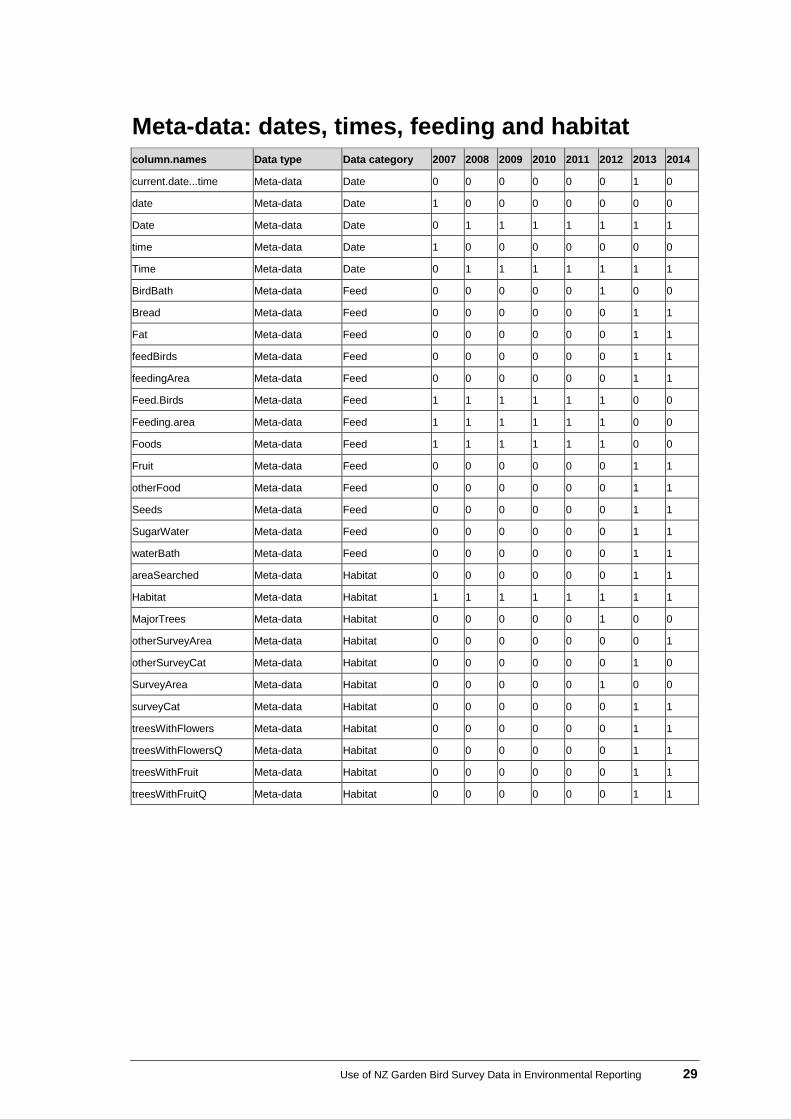
Meta-data: dates, times, feeding and habitat 29

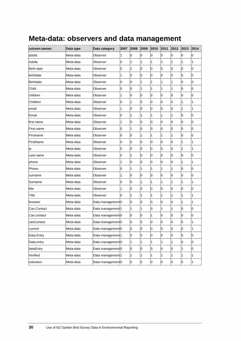
Meta-data: observers and data management 30

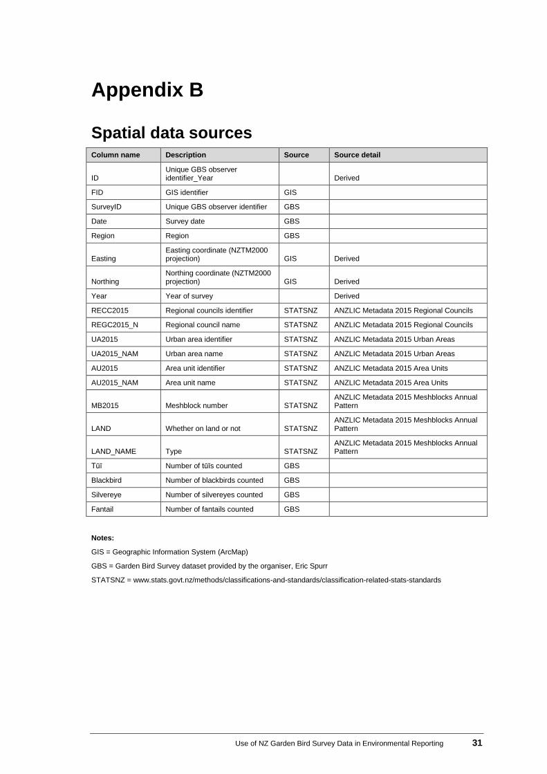
Appendix B 31

Spatial data sources 31

Appendix C 32

Calculating annual alert thresholds 32

iv Use of NZ Garden Bird Survey Data in Environmental Reporting

Appendix D 33

National and regional trends based on an easily computed Bayesian modelling approach 33

References 37

Tables

Table 1: Number of garden records per year in relation to data editing filters used. 6

Table 2: Models fitted to the NZGBS data for the four focal bird species (silvereye, blackbird, tūī and fantail) to account for spatial variation in sampling effort among years. The best-fit models (based on AIC values) are highlighted in bold. Time = time taken to run the model. Converge = whether the model converged to a stable solution or not. CI = confidence interval. CI width is the difference between the lower CI and upper CI (see figure 8). 12

Figures

Figure 1: National trends (2007–2014) for four garden bird species: blackbird (Turdus merula), fantail/pīwakawaka (Rhipidura fuliginosa), silvereye/tauhou (Zosterops lateralis) and tūī (Prosthemadera novaeseelandiae). Note that only the trend for blackbird was statistically significant, where fitted lines are linear regressions assuming normally-distributed errors with Year as a continuous predictor. (These graphs were extracted directly from the Landcare Research website). 3

Figure 2: The different spatial scales to potentially consider in the NZGBS data analysis. 4

Figure 3: Variation among years (n = 7) in the total number of gardens sampled within each region. (Note: these analyses only consider Urban Areas within each region; see table 1 for the total number of gardens surveyed in Urban Areas in each year). Boxes contain the 25th and 75th percentiles and the line within the box is the median. The whiskers extend to the most extreme data point (which is no more than 1.5 times the interquartile range from the box), and outlier points show the minimum and maximum values. 7

Figure 4: Variation among years (n = 7) in the number of gardens (+1) surveyed within each Urban Area (n = 141) by region. Boxes contain the 25th and 75th percentiles and the line within the box is the median. The whiskers extend to the most extreme data point (which is no more than 1.5 times the interquartile range from the box), and outlier points show the minimum and maximum values. 8

Figure 5: Variation in the number of survey gardens among years (n = 7) within each of the 59 Area Units in one Urban Area (Dunedin). 9

Use of NZ Garden Bird Survey Data in Environmental Reporting v

Figure 7: Boxplots of counts for each bird species (considering Urban areas only; see table 1 for the total number of gardens surveyed per year). Boxes contain the 25th and 75th percentiles and the line within the box is the median. The whiskers extend to the most extreme data point (which is no more than 1.5 times the interquartile range from the box), and outlier points show the minimum and maximum values. 10

Figure 8: Garden bird abundance trend estimates with 95% confidence intervals extracted from the four candidate models fitted (table 2). 13

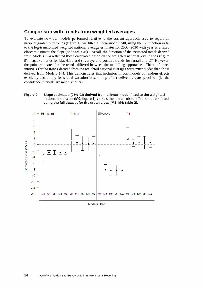
Figure 9: Slope estimates (95% CI) derived from a linear model fitted to the weighted national estimates (M0; figure 1) versus the linear mixed effects models fitted using the full dataset for the urban areas (M1–M4; table 2). 14

Figure 10: Garden bird abundance trend estimates with 95% confidence intervals extracted from the four fitted models (M1–M4) and one linear (M0) model (figure 9) in relation to ‘alert thresholds’. 15

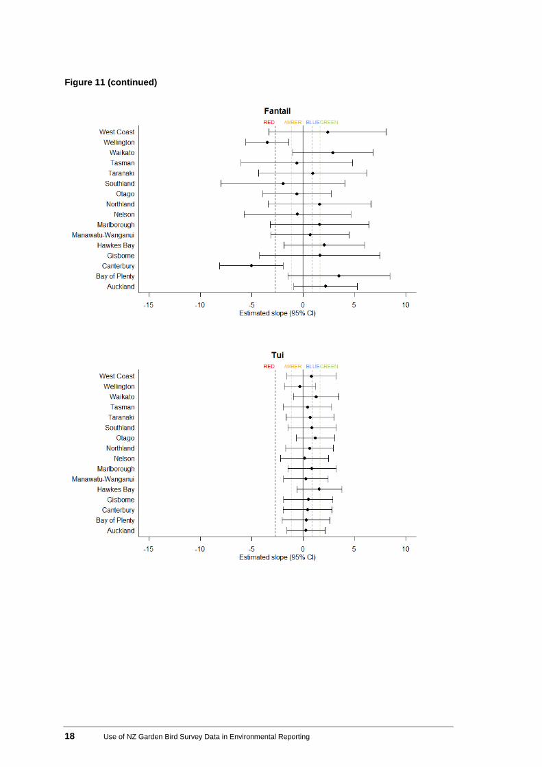
Figure 11: Regional abundance trend estimates (and 95% CI) extracted from model M4 (table 2). Dashed lines indicate alert thresholds: red = –2.73, amber = –1.14, blue = 0.893, green = 0.164. Solid vertical line shows a value of zero (ie, no trend). 17

Figure 11 (continued) 18

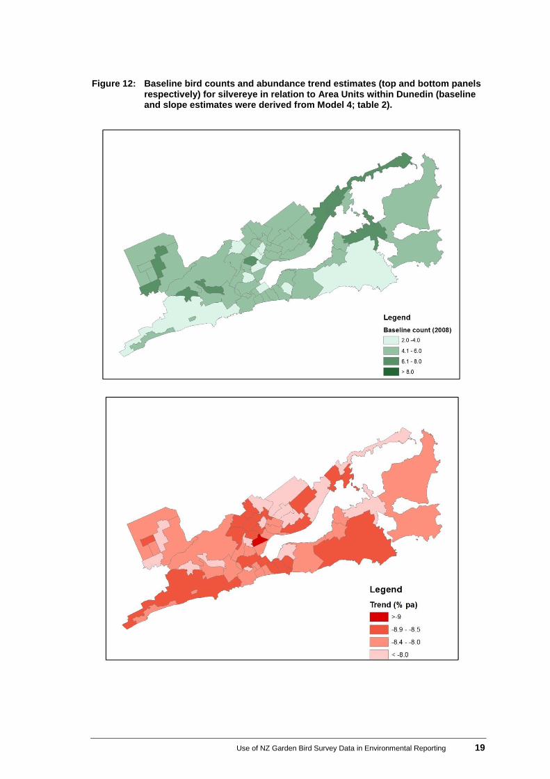
Figure 12: Baseline bird counts and abundance trend estimates (top and bottom panels respectively) for silvereye in relation to Area Units within Dunedin (baseline and slope estimates were derived from Model 4; table 2). 19

Figure 13: Baseline bird counts and abundance trend estimates (top and bottom panels respectively) for tūī in relation to Area Units within Dunedin (baseline and slope estimates were derived from Model 4; table 2). 20

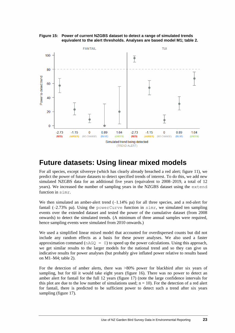
Figure 15: Power of current NZGBS dataset to detect a range of simulated trends equivalent to the alert thresholds. Analyses are based model M1; table 2. 23

Figure 16: Power to detect a simulated amber alert in relation to the number of sampling years (based on a simplified linear mixed effects model) for blackbird and tūī. (Confidence intervals were based on 100 simulations.) 24

Figure 17: Power to detect a simulated red alert and amber alert in relation to the number of sampling years (based on a simplified linear mixed effects model) for fantail. (Confidence intervals are based on 100 simulations.) 24

Figure 18: Power to detect amber (black points and lines) and red (grey points and lines) alert trends derived using the national weighted averages (figure 1). 25

vi Use of NZ Garden Bird Survey Data in Environmental Reporting

Executive Summary

As the country’s longest running annual survey of biodiversity in urban and rural landscapes at

the national scale, the New Zealand Garden Bird Survey (NZGBS) holds potential for informing

future reporting on the state of the Land Domain under the Environmental Reporting

Framework.

This report highlights some opportunities and challenges for making the NZGBS data more

accessible, reliable and flexible for reporting on status and trends in common garden birds. In

particular, it considers the benefits of merging the NZGBS data (2008–2014) with spatial layers

provided by Statistics New Zealand, using four common garden bird species as examples to

illustrate the approach: blackbird (Turdus merula), fantail/pīwakawaka (Rhipidura fuliginosa),

silvereye/tauhou (Zosterops lateralis) and tūī (Prosthemadera novaeseelandiae).

Opportunities for data improvement Potential benefits of refining the spatial resolution of the NZGBS dataset in the future include:

1. Facilitating data confidentiality and sharing: Merging the NZGBS data with the

Statistics NZ spatial layers (depicting boundaries for Region, Urban Area, Area Unit,

Meshblock) allows for sharing the NZGBS data at a finer spatial resolution, without

providing confidential information about the participants and survey locations.

2. Calculating biodiversity metrics using a flexible and harmonised approach: Recent

advances in statistical modelling techniques demonstrate the potential for cost-effectively

calculating consistent metrics at multiple spatial scales. The analyses explicitly account for

variation in sampling effort over space and time using the full data set (ie, fitting models at

the garden level rather than modelling based on derived regional or national averages).

Comparable metrics (baseline count and trend estimates) can then be derived

simultaneously (from the same model) for reporting at national, regional and local scales.

3. Enhancing the inferences drawn from existing data: Using the full data set and

explicitly accounting for spatial variation (rather than modelling based on derived regional

or national averages) facilitates greater precision of derived metrics. Based on the full data

set analyses, for example, the population trend estimates show blackbird and silvereye are

declining and have clearly breached amber and red alert thresholds respectively. This

indicates that, if these current trends are sustained, blackbird and silvereye will respectively

undergo moderate and rapid declines in 25 years. Trend estimates derived from a weighted

national average model would not only have failed to raise these alerts for blackbird and

silvereye, but would also have missed the declining trend for silvereye altogether.

4. Predicting the power of future datasets to detect specified trends: To evaluate the

power of future datasets to detect specified trends of interest, new NZGBS data and

sampling events were simulated for an additional five years (equivalent to 2008–2019, a

total of 12 years). By using the full data set analysis approach rather than weighted

averages one, the time taken to achieve >80% power for the detection of amber alerts for

blackbird, for example, was halved from 12 to 6 years. This comparison illustrates the

greater power of the analytical approaches suggested here to detect such trends.

5. Interpreting and communicating results: Critically evaluating the precision and power

of estimates derived from existing and future NZGBS datasets also helps inform the

reporting process, allowing the user to identify fit-for-purpose biodiversity metrics.

Specifically, we illustrate the potential use of a standardised set of alert thresholds to help

the audience identify population trends that might be of conservation concern. In addition,

Use of NZ Garden Bird Survey Data in Environmental Reporting vii

over 85% of participants (n = c. 3500) in a survey on the NZGBS indicated a preference for

maps, in particular, but also written summaries with images for reporting results. The

potential for better visual presentation of results using maps is demonstrated.

6. Informing future monitoring: Ways to improve the resolution of the data could be

explored by plotting and evaluating trends in participation in the NZGBS at different

spatial scales. This information could be used as a basis for campaigns to engage the public

and enhance the survey.

Future challenges for data improvement Potential future challenges associated with managing and using the NZGBS datasets include:

1. Establishing an enduring and cost-effective data management system: Currently, the

NZGBS data, which are stored in MS Excel spreadsheets in varying formats, are manually

edited by the survey organiser. Establishing a secure and enduring framework for

gathering, editing and storing the NZGBS data in a consistent format in the future should

be a top priority. This will require financial support at the set-up phase but also, at a

reduced rate, for ongoing maintenance.

2. Clarifying the metrics of interest: Options for editing the data and refining the analyses

presented in this report include considering whether:

species distribution metrics are more sensitive for monitoring change than abundance

for some species (eg, fantail)

other sources of sampling bias need to be accounted for (eg, whether early NZGBS

participants had more birds in their gardens or were more likely to feed birds)

Variation in the number and density of gardens within different spatial units/levels (eg,

region, urban area) is necessary

including habitat variables (eg, feeding activities, garden type or residence densities) as

predictor variables improves the model fit, increasing the power to detect change and

interpretation of results, as indicated by earlier analyses.

3. Calculating the metrics: Some technical challenges associated with model fitting and

extracting estimates need to be addressed before developing a standardised protocol

suitable for calculating and reporting biodiversity metrics at different spatial scales.

4. Improving future datasets: Future power analyses could evaluate different strategies for

improving NZGBS participation rates. The results of such analyses could in turn be used to

target public campaigns to enhance engagement.

Use of NZ Garden Bird Survey Data in Environmental Reporting 1

1 Introduction

As New Zealand’s longest running annual survey of biodiversity in urban and rural landscapes

at the national scale, the NZ Garden Bird Survey (NZGBS) holds potential for informing future

reporting on the state of the Land Domain under the Environmental Reporting Framework.

This report provides a preliminary assessment of the reliability of the NZGBS dataset for

reporting on trends in common garden birds. Specifically, it aims to enhance the spatial

resolution of information available in three ways:

1. making the NZGBS data spatial and confidential using existing Statistics NZ GIS data

2. modelling trends for a subset of garden bird species taking into account spatial variation

in sampling effort over time (using the revised NZGBS dataset)

3. interpreting and reporting of trends in garden bird species, informed by power analyses

where appropriate.

The analytical methods used, the results derived, and any limitations/caveats are documented,

with the relevant datasets and R-scripts provided separately.

Our analyses do not attempt to identify which habitat variables (eg, feeding activities, garden

type or residence densities) are the best predictors of garden bird abundance or distribution; this

was the focus of earlier related work (Spurr 2012a).

New Zealand Garden Bird Survey The NZ Garden Bird Survey (NZGBS) is a citizen science project established by Landcare

Research Associate, Eric Spurr (henceforth, survey organiser), primarily to monitor population

trends in common garden birds (Spurr, 2012a). Other objectives are to provide data to assist

local authorities with the planning and management of their biodiversity responsibilities, to

provide an opportunity for the general public to become involved in science in their own

gardens (‘citizen science’), and to educate and raise awareness of participants about

biodiversity, birds, conservation, and the environment, and at the same time to have fun.

Since 2007, over 2000 people have taken part in the survey each winter, to record birds in urban

and rural gardens. The NZGBS method was based on the Big Garden Birdwatch in the UK.

Volunteers spend one hour in midwinter each year recording for each bird species the largest

number of individuals detected at any one time in their gardens, as an index of abundance

(Spurr, 2012a).

Survey data have been entered directly online or returned as hardcopy to the survey organiser.

Hardcopy data were entered online by volunteers. The online platform used from 2007–2012

was designed by Landcare Research and located on the Landcare Research website, and the

platform used from 2013 onwards was designed by Stuff.co.nz and located on

http://birdsurvey.org.nz/ (accessible from Landcare Research, Stuff, and other websites).

The survey data are currently stored in Excel spreadsheets, held by the survey organiser, with a

separate file for each of the eight years. The data entered online contains many errors (including

misidentification of species, missing data, incorrect entry of hardcopy data etc). Data for 2007–

2014 have been edited extensively by the survey organiser, but still contain errors. The raw data

2 Use of NZ Garden Bird Survey Data in Environmental Reporting

remain confidential because of privacy issues (names, addresses, and contact details of survey

participants).

Annual summaries of results at national and major regional scales have been produced by the

survey organiser and posted on the Landcare Research website,1 presented at science

conferences, published in society magazines (Spurr, 2008a, 2014, 2015a, 2015b) and journals

(Spurr, 2007, 2008b), research newsletters (Spurr, 2012b), reported in regional newspapers, and

made available to interested parties. The NZGBS survey organiser is planning to conduct

intensive analyses of NZGBS results after 10 years, 15 years, and 20 years since the survey was

initiated.

Annual trends in garden bird populations Preliminary analyses of the NZGBS dataset have explored the effects of four factors

individually (region of the country in which the counts were made, urban compared with rural

areas, provision of supplementary food, and year), on counts within species (Spurr, 2012a).

Accounting for these spatial changes in sampling effort over time is important. If we consider

the large variation in the number of respondents from Canterbury, for example, mean national

counts for species that are uncommon in Canterbury may appear to change over time, but this

will be an artefact of the temporal changes in the number of respondents from that region.

For the period 2007–2010, for example, the number of survey returns that came from each

region of the country was not in proportion to the number of households in each region (Spurr,

2012a). Furthermore, the percentage of survey returns from each region varied from year to

year, partially reflecting whether or not regional newspapers published the survey form. These

patterns have persisted over time. To account for these problems in the analyses conducted, the

average counts of each species in each region were multiplied by the proportion of New Zealand

households (substituting for gardens) in each region, and these values were summed to provide

more representative national averages (Spurr, 2012a; see also the project website1). The

weighting is only approximate because some households (eg, apartments) do not have

individual gardens, and some regions have a higher proportion of households without gardens

than others. In future calculations of long-term bird population trends it will be necessary to

weight for other factors such as the proportion of urban compared with rural gardens, and the

proportion of gardens with and without provision of supplementary food in a region, especially

if these proportions change over time (Spurr, 2012a).

According to these analyses, counts have fluctuated from year to year for most species, but not

shown a consistent or significant trend over the last eight years (eg, figure 1). Silvereye/tauhou

(Zosterops lateralis) counts have probably fluctuated more than the counts of most other

species, and seem to be particularly influenced by weather (and potentially also diseases such as

avian pox). Counts for blackbird (Turdus merula) appear to have declined, but for

fantail/pīwakawaka (Rhipidura fuliginosa) and tūī (Prosthemadera novaeseelandiae) have not

changed significantly (figure 1).

1 gardenbirdsurvey.landcareresearch.co.nz (accessed 24 Jun 2015).

http://www.landcareresearch.co.nz/science/plants-animals-fungi/animals/birds/garden-bird-surveys/2014-results/desease


Figure 1: National trends (2007–2014) for four garden bird species: blackbird (Turdus merula), fantail/pīwakawaka (Rhipidura fuliginosa), silvereye/tauhou (Zosterops lateralis) and tūī (Prosthemadera novaeseelandiae). Note that only the trend for blackbird was statistically significant, where fitted lines are linear regressions assuming normally-distributed errors with Year as a continuous predictor. (These graphs were extracted directly from the Landcare Research website

1).


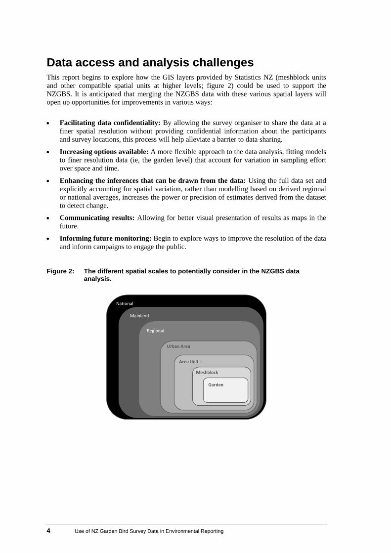
Data access and analysis challenges This report begins to explore how the GIS layers provided by Statistics NZ (meshblock units

and other compatible spatial units at higher levels; figure 2) could be used to support the

NZGBS. It is anticipated that merging the NZGBS data with these various spatial layers will

open up opportunities for improvements in various ways:

Facilitating data confidentiality: By allowing the survey organiser to share the data at a

finer spatial resolution without providing confidential information about the participants

and survey locations, this process will help alleviate a barrier to data sharing.

Increasing options available: A more flexible approach to the data analysis, fitting models

to finer resolution data (ie, the garden level) that account for variation in sampling effort

over space and time.

Enhancing the inferences that can be drawn from the data: Using the full data set and

explicitly accounting for spatial variation, rather than modelling based on derived regional

or national averages, increases the power or precision of estimates derived from the dataset

to detect change.

Communicating results: Allowing for better visual presentation of results as maps in the

future.

Informing future monitoring: Begin to explore ways to improve the resolution of the data

and inform campaigns to engage the public.

Figure 2: The different spatial scales to potentially consider in the NZGBS data

analysis.


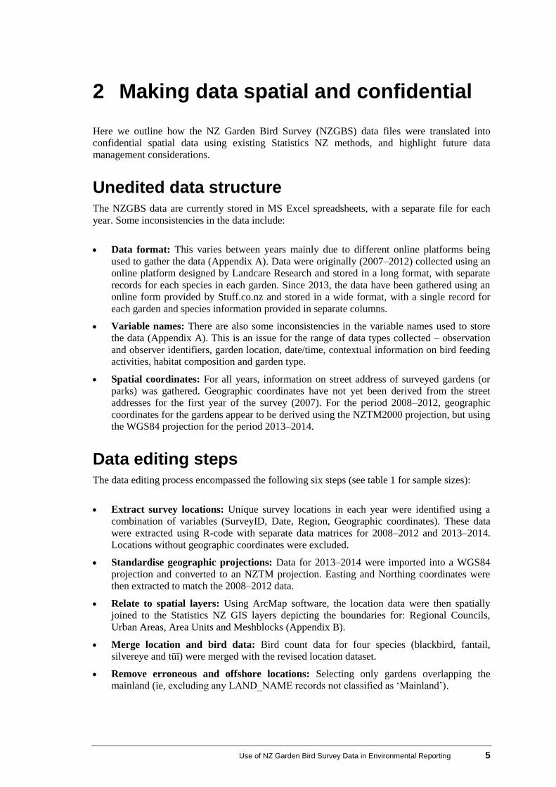
2 Making data spatial and confidential

Here we outline how the NZ Garden Bird Survey (NZGBS) data files were translated into

confidential spatial data using existing Statistics NZ methods, and highlight future data

management considerations.

Unedited data structure The NZGBS data are currently stored in MS Excel spreadsheets, with a separate file for each

year. Some inconsistencies in the data include:

Data format: This varies between years mainly due to different online platforms being

used to gather the data (Appendix A). Data were originally (2007–2012) collected using an

online platform designed by Landcare Research and stored in a long format, with separate

records for each species in each garden. Since 2013, the data have been gathered using an

online form provided by Stuff.co.nz and stored in a wide format, with a single record for

each garden and species information provided in separate columns.

Variable names: There are also some inconsistencies in the variable names used to store

the data (Appendix A). This is an issue for the range of data types collected – observation

and observer identifiers, garden location, date/time, contextual information on bird feeding

activities, habitat composition and garden type.

Spatial coordinates: For all years, information on street address of surveyed gardens (or

parks) was gathered. Geographic coordinates have not yet been derived from the street

addresses for the first year of the survey (2007). For the period 2008–2012, geographic

coordinates for the gardens appear to be derived using the NZTM2000 projection, but using

the WGS84 projection for the period 2013–2014.

Data editing steps The data editing process encompassed the following six steps (see table 1 for sample sizes):

Extract survey locations: Unique survey locations in each year were identified using a

combination of variables (SurveyID, Date, Region, Geographic coordinates). These data

were extracted using R-code with separate data matrices for 2008–2012 and 2013–2014.

Locations without geographic coordinates were excluded.

Standardise geographic projections: Data for 2013–2014 were imported into a WGS84

projection and converted to an NZTM projection. Easting and Northing coordinates were

then extracted to match the 2008–2012 data.

Relate to spatial layers: Using ArcMap software, the location data were then spatially

joined to the Statistics NZ GIS layers depicting the boundaries for: Regional Councils,

Urban Areas, Area Units and Meshblocks (Appendix B).

Merge location and bird data: Bird count data for four species (blackbird, fantail,

silvereye and tūī) were merged with the revised location dataset.

Remove erroneous and offshore locations: Selecting only gardens overlapping the

mainland (ie, excluding any LAND_NAME records not classified as ‘Mainland’).


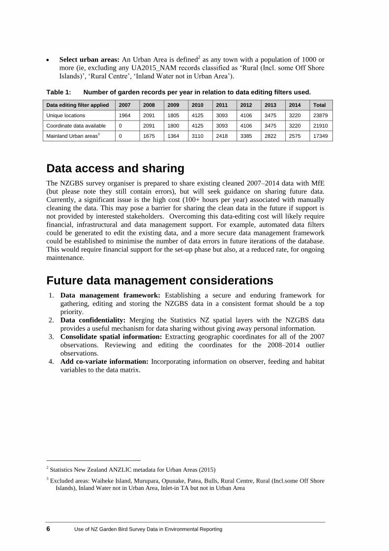
Select urban areas: An Urban Area is defined2 as any town with a population of 1000 or

more (ie, excluding any UA2015_NAM records classified as ‘Rural (Incl. some Off Shore

Islands)’, ‘Rural Centre’, ‘Inland Water not in Urban Area’).

Table 1: Number of garden records per year in relation to data editing filters used.

Data editing filter applied 2007 2008 2009 2010 2011 2012 2013 2014 Total

Unique locations 1964 2091 1805 4125 3093 4106 3475 3220 23879

Coordinate data available 0 2091 1800 4125 3093 4106 3475 3220 21910

Mainland Urban areas3 0 1675 1364 3110 2418 3385 2822 2575 17349

Data access and sharing The NZGBS survey organiser is prepared to share existing cleaned 2007–2014 data with MfE

(but please note they still contain errors), but will seek guidance on sharing future data.

Currently, a significant issue is the high cost (100+ hours per year) associated with manually

cleaning the data. This may pose a barrier for sharing the clean data in the future if support is

not provided by interested stakeholders. Overcoming this data-editing cost will likely require

financial, infrastructural and data management support. For example, automated data filters

could be generated to edit the existing data, and a more secure data management framework

could be established to minimise the number of data errors in future iterations of the database.

This would require financial support for the set-up phase but also, at a reduced rate, for ongoing

maintenance.

Future data management considerations 1. Data management framework: Establishing a secure and enduring framework for

gathering, editing and storing the NZGBS data in a consistent format should be a top

priority.

2. Data confidentiality: Merging the Statistics NZ spatial layers with the NZGBS data

provides a useful mechanism for data sharing without giving away personal information.

3. Consolidate spatial information: Extracting geographic coordinates for all of the 2007

observations. Reviewing and editing the coordinates for the 2008–2014 outlier

observations.

4. Add co-variate information: Incorporating information on observer, feeding and habitat

variables to the data matrix.

2 Statistics New Zealand ANZLIC metadata for Urban Areas (2015)

3 Excluded areas: Waiheke Island, Murupara, Opunake, Patea, Bulls, Rural Centre, Rural (Incl.some Off Shore

Islands), Inland Water not in Urban Area, Inlet-in TA but not in Urban Area


3 Data exploration

Here, we explore how to best account for spatial variation in sampling effort over time. We

focus on estimating national trends in the abundance of four garden bird species, while also

beginning to explore the feasibility of quantifying and assessing trends at finer spatial scales

(Regional or Area Units). The data analyses focussed on the NZGBS information available for

mainland urban areas and the period 2008–2014. (Data for 2007 were excluded due to the lack

of geographic coordinate information; table 1.)

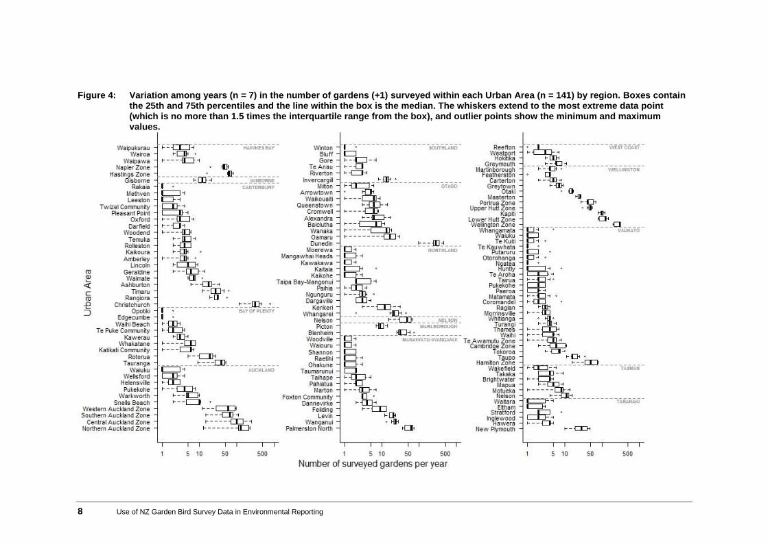
Spatial variation in sampling effort As previous work has highlighted (Spurr, 2012a), sampling effort varied among regions and

years within regions (figure 3). Regions with large cities (Auckland, Canterbury, Wellington

and Otago) tended to contribute more observations than other areas, which is evident when we

consider sampling effort within Urban Areas (figure 4). Within Area Units, sampling effort also

varied widely over time. In Dunedin (an Urban Area containing 59 Area Units), for example,

there was often large temporal variation in levels of participation, particularly in those Area

Units with 10 or more gardens surveyed, on average, per year (figure 5).

Figure 3: Variation among years (n = 7) in the total number of gardens sampled within

each region. (Note: these analyses only consider Urban Areas within each region; see table 1 for the total number of gardens surveyed in Urban Areas in each year). Boxes contain the 25th and 75th percentiles and the line within the box is the median. The whiskers extend to the most extreme data point (which is no more than 1.5 times the interquartile range from the box), and outlier points show the minimum and maximum values.


Figure 4: Variation among years (n = 7) in the number of gardens (+1) surveyed within each Urban Area (n = 141) by region. Boxes contain the 25th and 75th percentiles and the line within the box is the median. The whiskers extend to the most extreme data point (which is no more than 1.5 times the interquartile range from the box), and outlier points show the minimum and maximum values.


Figure 5: Variation in the number of survey gardens among years (n = 7) within each of the 59 Area Units in one Urban Area (Dunedin).


Focal bird species Our analysis focussed on quantifying population trends of four bird species: blackbird (Turdus

merula), fantail/pīwakawaka (Rhipidura fuliginosa), silvereye/tauhou (Zosterops lateralis) and

tūī (Prosthemadera novaeseelandiae).

Summary plots of the NZGBS bird counts highlighted some differences in data characteristics

among the four species (figure 7). Silvereye and blackbird consistently had relatively high

counts compared to the other two species. Annual fluctuations in the median counts (figure 7)

were evident for tūī and silvereye but less so for fantail and blackbird. The data are counts with

many values of zero (ie, gardens in which the species was not seen), in particular for fantail and,

to a lesser extent, tūī. The skewed nature of these data needs careful consideration when

analysing the data and fitting the models (requiring Poisson error distributions).

Figure 7: Boxplots of counts for each bird species (considering Urban areas only; see

table 1 for the total number of gardens surveyed per year). Boxes contain the 25th and 75th percentiles and the line within the box is the median. The whiskers extend to the most extreme data point (which is no more than 1.5 times the interquartile range from the box), and outlier points show the minimum and maximum values.


Preliminary analyses of abundance trends We explored the use of generalised mixed effects models to account for repeated measures

gathered from spatially nested units. A set of four models were fitted for each species

independently (table 2) using the glmer function in the lme4 package (lme4 1.1-8; Bates et

al, 2015a, 2015b) in R (R Core Team, 2015).

Model specifications

The sampling unit was the garden, with the bird count for the focal species (‘Count’) specified

as the response variable and the year of the survey (‘YearStd’) specified as the only fixed effect.

To account for the spatial variation in sampling effort, all models included random slopes and

intercepts; these differed as to the spatial level at which these random effects were estimated

(table 2). Three spatially nested variables were considered (figure 2): Region (‘fRC’, 16 factor

levels), Urban Area (‘fUA’, 138 factor levels) and Area Unit (‘fAU’, 1219 factor levels). (Note:

Garden identity was not considered in these analyses as this information was not readily

available.) Models 1–3 used increasingly fine nesting levels for the random effects, while Model

4 excluded the middle level (Urban Area). All models specified a Poisson error distribution to

accommodate count data and included an overdispersion term (‘1|Obs’) to account for the large

number of zeros in the response variable.

The best-fit model was identified from the set of candidate models (table 2), using Akaike’s

Information Criterion to compare models (Burnham and Anderson, 2002). We also documented

whether each model converged or not and how long it took to run (using the System.time

command in R). (Note that a non-convergent model is one that has not found the optimal

statistical fit but it can still provide valid insight.)

Evaluation of fitted models

For all four bird species, the best-fit model (Model 3; based on AIC values) was the most

complex of the four candidate models considered. This model accounted for spatial nesting of

gardens at three levels (Region, Urban Areas and Area Units).

The large sample size of the NZGBS dataset has a number of implications. (1) The models are

somewhat computationally intensive to fit, especially as model complexity increases, and are

not guaranteed to converge to a stable solution. The most complex model (Model 3) typically

took eight times as long to fit as the simplest model (Model 1; table 2). (2) With larger datasets,

improvements in the model fit tend to dominate penalties for increased complexity (table 2). (3)

Using AIC to choose a model might suggest a larger model than is necessary for the inference

required; if the models give very similar answers, then it might make sense to use a simple or

faster one depending on the objectives being addressed.

The models have been fit with lme4 1.1-8, which is the latest version4 of this R package. It

has a large number of additional convergence warnings, but many of these might be false

positives.

4 Currently, lme4 1.1-8 can be installed via devtools::install_github("lme4/lme4") but will be on CRAN soon.


Table 2: Models fitted to the NZGBS data for the four focal bird species (silvereye, blackbird, tūī and fantail) to account for spatial variation in sampling effort among years. The best-fit models (based on AIC values) are highlighted in bold. Time = time taken to run the model. Converge = whether the model converged to a stable solution or not. CI = confidence interval. CI width is the difference between the lower CI and upper CI (see figure 8).

Species Model Model specification AIC Time(secs) Converge Parameter estimates (% change per annum)

Slope Lower CI Upper CI CI Width

Blackbird 1 Count ~ YearStd + (YearStd||fRC) + (1|Obs) 66615 16.6 TRUE -2.55 -3.21 -1.89 1.32

2 Count ~ YearStd + (YearStd||fRC/fUA) + (1|Obs) 66515 85.4 TRUE -2.58 -3.24 -1.92 1.32

3 Count ~ YearStd + (YearStd||fRC/fUA/fAU) + (1|Obs) 66395 206 FALSE -2.58 -3.3 -1.86 1.44

4 Count ~ YearStd + (YearStd||fRC/fAU) + (1|Obs) 66414 66.4 TRUE -2.58 -3.29 -1.87 1.42

Fantail 1 Count ~ YearStd + (YearStd||fRC) + (1|Obs) 40874 20.3 TRUE 0.529 -1.84 2.9 4.74

2 Count ~ YearStd + (YearStd||fRC/fUA) + (1|Obs) 40449 48 TRUE 0.399 -1.88 2.68 4.56

3 Count ~ YearStd + (YearStd||fRC/fUA/fAU) + (1|Obs) 39893 167 FALSE 0.175 -2.06 2.41 4.47

4 Count ~ YearStd + (YearStd||fRC/fAU) + (1|Obs) 39950 87.6 TRUE 0.222 -2.07 2.52 4.59

Silvereye 1 Count ~ YearStd + (YearStd||fRC) + (1|Obs) 106553 20.6 TRUE -8.19 -9.9 -6.47 3.43

2 Count ~ YearStd + (YearStd||fRC/fUA) + (1|Obs) 106412 61 TRUE -8.32 -10 -6.61 3.41

3 Count ~ YearStd + (YearStd||fRC/fUA/fAU) + (1|Obs) 106216 173 FALSE -8.33 -9.96 -6.7 3.26

4 Count ~ YearStd + (YearStd||fRC/fAU) + (1|Obs) 106241 76.3 TRUE -8.3 -9.94 -6.66 3.29

Tūī 1 Count ~ YearStd + (YearStd||fRC) + (1|Obs) 47113 16 TRUE 0.481 -0.656 1.62 2.27

2 Count ~ YearStd + (YearStd||fRC/fUA) + (1|Obs) 46423 75.9 TRUE 0.761 -1.09 2.61 3.69

3 Count ~ YearStd + (YearStd||fRC/fUA/fAU) + (1|Obs) 45576 226 TRUE 0.569 -1.46 2.6 4.06

4 Count ~ YearStd + (YearStd||fRC/fAU) + (1|Obs) 45687 97.5 TRUE 0.612 -0.955 2.18 3.14


Preliminary results

Derived national abundance trend estimates

For each species, abundance trend estimates were broadly comparable across the four candidate

models, but more variable for fantail and tūī (where the trends were closer to zero) than the

other two species (table 2; figure 8). The trend estimates indicate a decline in blackbird and

silvereye counts, and no change in fantail or tūī counts.

Overall, trend estimates for blackbird were more precise than those for the other three species

(based on the confidence interval widths; table 2; figure 8). For blackbird and silvereye, the

confidence intervals excluded zero, giving us some assurance that the declining trends for these

species are reliable. The plots show the modelled slopes from table 2 with the confidence

intervals. If the confidence intervals overlap with zero (the horizontal line in figure 8) we

conclude that the slope estimate is not reliable (ie, there is no trend in the count data). This is the

case for fantail and tūī. However, for blackbird and silvereye, the confidence intervals do not

overlap zero, indicating that both species are genuinely declining.

Figure 8: Garden bird abundance trend estimates with 95% confidence intervals

extracted from the four candidate models fitted (table 2).


Comparison with trends from weighted averages

To evaluate how our models performed relative to the current approach used to report on

national garden bird trends (figure 1), we fitted a linear model (M0, using the lm function in R)

to the log-transformed weighted national average estimates for 2008–2010 with year as a fixed

effect to estimate the slope (and 95% CIs). Overall, the direction of the estimated trends derived

from Models 1–4 reflected those calculated based on the weighted national level trends (figure

9): negative trends for blackbird and silvereye and positive trends for fantail and tūī. However,

the point estimates for the trends differed between the modelling approaches. The confidence

intervals for the trends derived from the weighted national averages were much wider than those

derived from Models 1–4. This demonstrates that inclusion in our models of random effects

explicitly accounting for spatial variation in sampling effort delivers greater precision (ie, the

confidence intervals are much smaller).

Figure 9: Slope estimates (95% CI) derived from a linear model fitted to the weighted

national estimates (M0; figure 1) versus the linear mixed effects models fitted using the full dataset for the urban areas (M1–M4; table 2).


Comparison with alert thresholds

To understand the significance of these trends from a management perspective, we also

considered the trend estimates (and their respective confidence intervals) in relation to some

hypothetical alert thresholds (figure 10). These alert thresholds are based on the system used by

the British Trust for Ornithology5 to draw attention to emerging population declines that may be

of conservation concern. The system seeks to identify rapid declines (>50%) and moderate

declines (>25% but <50%), with declines being measured at different timescales depending on

the data available (ideally the most recent 25-, 10- or 5-year periods).

In figure 10, the red and amber alert thresholds (–2.76% and –1.15% pa respectively) identify

species heading for a rapid or moderate decline in 25 years if the current trend is sustained

(Baillie and Rehfisch, 2006; Appendix C). The blue and green alert thresholds (0.893% and

1.64% pa respectively) illustrate hypothetical trends for an increase in bird counts equivalent to

a 25% and 50% increase over a 25 year period, which might be used to indicate an improvement

in the population status of a species. Inspecting the trend estimates (derived from models M1–

M4) in relation to the alert thresholds shows that the silvereye has clearly breached the red alert

threshold (figure 10). At the same time, the blackbird has breached an amber threshold and

possibly a red one (as indicated by the confidence interval). Both fantail and tūī trends have not

raised alerts. The trend estimates derived from the weighted national average model (M0; figure

1) would have failed to raise the amber and red alerts for blackbird and silvereye, as the

confidence intervals for those trend estimates were wide, especially for silvereye.

Figure 10: Garden bird abundance trend estimates with 95% confidence intervals

extracted from the four fitted models (M1–M4) and one linear (M0) model (figure 9) in relation to ‘alert thresholds’.

5 http://www.bto.org/about-birds/birdtrends/2014/methods/alert-system


Assessing trends at finer spatial scales (regions and area units)

One of the advantages of explicitly incorporating the various sources of spatial variation in

sampling effort into the models is that it allows us to estimate trends at finer spatial scales and

with greater precision (figure 9).

Figure 11 shows regional trend estimates (and 95% CIs) for each species. Regional trend

estimates were particularly variable for silvereye and, to a lesser extent, fantail but fairly

consistent for blackbird. Despite the large variability in trend estimates for silvereye, the

declining trend is consistently greater than the red alert threshold (–2.73% pa) across regions.

For fantail, there was strong evidence for a declining trend equivalent to an amber alert status

but possibly also a red alert status, in two regions: Canterbury and Wellington. There was no

evidence of positive trends for any species or region, at this level of analysis.

Figures 12 and 13 show examples of maps of baseline counts and trends at finer resolutions,

specifically how these metrics vary among Area Units in Dunedin. In the future, where feasible,

such maps should also include measures of uncertainty in the estimates. This information could

be used to highlight which Area Units would benefit from increased sampling effort and, thus,

targeted campaigns, if information at this resolution were considered valuable.

It is important to note here that extracting and interpreting the confidence intervals for regional

trend estimates using the lme4 package was quite challenging and required specialist analytical

programming skills. An alternative is to fit the models in a Bayesian context where credible

intervals for derived parameters, such as regional level trends etc, can be relatively

straightforward (Appendix D). Disadvantages of fitting models in a Bayesian context are that it

also requires specialist skills, takes longer to run the models (minutes/hours rather than

seconds), and the associated power analyses present increased difficulty. For these reasons, we

focussed on the use of the lme4 models to derive some preliminary regional trend estimates

here.


Figure 11: Regional abundance trend estimates (and 95% CI) extracted from model M4 (table 2). Dashed lines indicate alert thresholds: red = –2.73, amber = –1.14, blue = 0.893, green = 0.164. Solid vertical line shows a value of zero (ie, no trend).


Figure 11 (continued)


Figure 12: Baseline bird counts and abundance trend estimates (top and bottom panels respectively) for silvereye in relation to Area Units within Dunedin (baseline and slope estimates were derived from Model 4; table 2).


Figure 13: Baseline bird counts and abundance trend estimates (top and bottom panels respectively) for tūī in relation to Area Units within Dunedin (baseline and slope estimates were derived from Model 4; table 2).


Recommendations for future analysis Future analyses should explore the effects of varying the following model specifications:

Species distributions versus abundance: For some species, especially those with low

abundance estimates, modelling changes in their distribution rather than abundance could

be a more sensitive indicator of change.

Fixed effects: Explore variation in habitat variables among gardens and the higher level

spatial units.

Random effects: Models with correlation between the random slope and intercept have not

been considered, nor have models without an overdispersion term. Including identifiers to

account for repeated measures from individual gardens would help verify whether early

NZGBS participants were a biased subset of the population (eg, were more likely to include

those gardens with more birds or feeding activity). This is important because this may bias

the trend estimates. As the sample sizes increase, we expect that it will be possible to

include finer scale measures (eg, meshblock).

Weighting: Current NZGBS trends are calculated using weighted national estimates in

relation to the proportion of gardens per region. Where the finest spatial levels/units are not

of similar size, models may perform better with some sort of weighting. There is a need to

establish a clearer definition of exactly what is being measured, to determine which

weighting process is appropriate.

Model convergence, evaluation, coefficients and confidence intervals: The lme4

models need exploring further to untangle some of convergence issues identified in table 2.

It was also technically challenging to extract and interpret CIs at finer spatial scales

(Region, Area Unit) from lme4 models, and required specialist analytical programming

skills. An alternative is to fit the models in a Bayesian context (Appendix D). An advantage

of a Bayesian context is that we can evaluate the model for convergence directly.

Furthermore, credible intervals for derived parameters, such as regional level trends etc, can

be computed easily. However, disadvantages of fitting models in a Bayesian context is the

run time (minutes/hours rather than seconds), and an increased difficulty with power

analysis.

Smoothing population trends: Our analysis focussed on linear trend analyses, but

smoothed trends are recommended to distinguish between short-term fluctuations (resulting

from a combination of natural variation and sampling error) and long-term trends (Fewster

et al, 2000). These, however, may require longer-term data sets.


4 Power analysis

Power refers to the statistical power to detect a given trend (effect) or, more importantly, to

reject the null hypothesis that there is no trend. Power is increased through large numbers of

samples, low variability among those samples, and a consistent direction of change across

replicate samples.

Here, we use power analyses to assess the ability of current and future datasets to detect a range

of specified population trends for our focal species. We use an R package, simr, built to make

it simple to run simulation experiments to determine whether a given sampling design has

sufficient power to make a specific inference (Green and MacLeod, in review). The package

includes tools for (1) running a simple power analysis for a specified design and (2) calculating

power curves to assess the trade-off between power and sampling size.

Current data: Using linear mixed models Here we focussed on fantail and tūī because the confidence intervals of their trend estimates

overlapped zero (figure 9). Using the current dataset (2008–2014) for each of these species, we

explored the power to detect a range of simulated trends using the alert thresholds illustrated in

figure 11 (red alert = –2.73% change per annum, amber = –1.14%, no change = 0%, blue =

0.893%, green =1.64%).

The power analysis tests were run to evaluate the power to detect the simulated trends using the

powerSim function in the R package, simr, for 100 simulations. These analyses were based

on the linear mixed model that included Region in the random effects (M1, table 2). In such

tests, 80% power is generally deemed ‘sufficient’.

Based on this model and the current dataset, there was low power to detect any of the simulated

trends, except a red-alert declining trend for tūī (–2.73% pa; figure 15).


Figure 15: Power of current NZGBS dataset to detect a range of simulated trends equivalent to the alert thresholds. Analyses are based model M1; table 2.

Future datasets: Using linear mixed models For all species, except silvereye (which has clearly already breached a red alert; figure 11), we

predict the power of future datasets to detect specified trends of interest. To do this, we add new

simulated NZGBS data for an additional five years (equivalent to 2008–2019, a total of 12

years). We increased the number of sampling years in the NZGBS dataset using the extend

function in simr.

We then simulated an amber-alert trend (–1.14% pa) for all three species, and a red-alert for

fantail (–2.73% pa). Using the powerCurve function in simr, we simulated ten sampling

events over the extended dataset and tested the power of the cumulative dataset (from 2008

onwards) to detect the simulated trends. (A minimum of three annual samples were required,

hence sampling events were simulated from 2010 onwards.)

We used a simplified linear mixed model that accounted for overdispersed counts but did not

include any random effects as a basis for these power analyses. We also used a faster

approximation command (nAGQ = 0) to speed up the power calculations. Using this approach,

we get similar results to the larger models for the national trend and so they can give us

indicative results for power analyses (but probably give inflated power relative to results based

on M1–M4; table 2).

For the detection of amber alerts, there was >80% power for blackbird after six years of

sampling, but for tūī it would take eight years (figure 16). There was no power to detect an

amber alert for fantail for the full 12 years (figure 17) (note the large confidence intervals for

this plot are due to the low number of simulations used; n = 10). For the detection of a red alert

for fantail, there is predicted to be sufficient power to detect such a trend after six years

sampling (figure 17).


Figure 16: Power to detect a simulated amber alert in relation to the number of sampling years (based on a simplified linear mixed effects model) for blackbird and tūī. (Confidence intervals were based on 100 simulations.)

Figure 17: Power to detect a simulated red alert and amber alert in relation to the

number of sampling years (based on a simplified linear mixed effects model) for fantail. (Confidence intervals are based on 100 simulations.)


Future datasets: Using weighted national averages For comparison, we then predicted the power of future iterations of the NZGBS datasets to

detect specified trends based on the weighted national averages approach that is currently used

(figure 1).

For the detection of amber alerts (figure 18), there is only likely to be sufficient power (>80%)

to detect if such a decline were occurring in blackbirds. There is no such power for the other

three species. Even for blackbirds, it is predicted to take until 2019 (12 survey years) for such

power to be achieved.

For the detection of red alerts (figure 18), there is predicted to be sufficient power to detect such

a decline in blackbirds after 8 years (2015) and in fantail and tūī after 10 years (2017). There is

no such power for silvereyes; extended analyses (not presented here) indicate that it would take

19 years (ie, until 2026) to detect such a decline in this species.

This comparison illustrates the greater power of the analytical approaches suggested here to

detect such population trends.

Figure 18: Power to detect amber (black points and lines) and red (grey points and

lines) alert trends derived using the national weighted averages (figure 1).


5 Conclusions

This report highlights some opportunities and challenges for making the NZGBS data more

accessible, reliable and flexible for reporting on status and trends in common garden birds. In

particular, it considers the benefits of merging the NZGBS data (2008–2014) with spatial layers

provided by Statistics New Zealand, using four common garden bird species as examples to

illustrate the approach: blackbird, fantail, silvereye and tūī.

Opportunities for data improvement Potential benefits of refining the spatial resolution of the NZGBS dataset in the future include:

1. Facilitating data confidentiality and sharing: Merging the NZGBS data with the

Statistics NZ spatial layers (depicting boundaries for Region, Urban Area, Area Unit,

Meshblock) allows for sharing the NZGBS data at a finer spatial resolution, without

providing confidential information about the participants and survey locations.

2. Calculating biodiversity metrics using a flexible and harmonised approach: Recent

advances in statistical modelling techniques demonstrate the potential for cost-effectively

calculating consistent metrics at multiple spatial scales. The analyses explicitly account for

variation in sampling effort over space and time using the full data set (ie, fitting models at

the garden level rather than modelling based on derived regional or national averages).

Comparable metrics (baseline count and trend estimates) can then be derived

simultaneously (from the same model) for reporting at national, regional and local scales.

3. Enhancing the inferences drawn from existing data: Using the full data set and

explicitly accounting for spatial variation (rather than modelling based on derived regional

or national averages) facilitates greater precision of derived metrics. Based on the full data

set analyses, for example, the population trend estimates show blackbird and silvereye are

declining and have clearly breached amber and red alert thresholds respectively. This

indicates that, if these current trends are sustained, blackbird and silvereye will respectively

undergo moderate and rapid declines in 25 years. Trend estimates derived from a weighted

national average model would not only have failed to raise these alerts for blackbird and

silvereye, but would also have missed the declining trend for silvereye altogether.

4. Predicting the power of future datasets to detect specified trends: To evaluate the

power of future datasets to detect specified trends of interest, new NZGBS data and

sampling events were simulated for an additional five years (equivalent to 2008–2019, a

total of 12 years). By using the full data set analysis approach rather than weighted

averages one, the time taken to achieve >80% power for the detection of amber alerts for

blackbird, for example, was halved from 12 to 6 years. This comparison illustrates the

greater power of the analytical approaches suggested here to detect such trends.

5. Interpreting and communicating results: Critically evaluating the precision and power

of estimates derived from existing and future NZGBS datasets also helps inform the

reporting process, allowing the user to identify fit-for-purpose biodiversity metrics.

Specifically, we illustrate the potential use of a standardised set of alert thresholds to help

the audience identify population trends that might be of conservation concern. In addition,

over 85% of participants (n = c. 3500) in a survey on the NZGBS indicated a preference for

maps, in particular, but also written summaries with images for reporting results. The

potential for better visual presentation of results using maps is demonstrated.

6. Informing future monitoring: Ways to improve the resolution of the data could be

explored by plotting and evaluating trends in participation in the NZGBS at different

spatial scales. This information could be used as a basis for campaigns to engage the public

and enhance the survey.


Future challenges for data improvement Potential future challenges associated with managing and using the NZGBS datasets include:

1. Establishing an enduring and cost-effective data management system: Currently, the

NZGBS data, which are stored in MS Excel spreadsheets in varying formats, are manually

edited by the survey organiser. Establishing a secure and enduring framework for gathering,

editing and storing the NZGBS data in a consistent format in the future should be a top

priority. This will require financial support at the set-up phase but also, at a reduced rate, for

ongoing maintenance.

2. Clarifying the metrics of interest: Options for editing the data and refining the analyses

presented in this report include considering whether:

species distribution metrics are more sensitive for monitoring change than abundance

for some species (eg, fantail)

other sources of sampling bias need to be accounted for (eg, whether early NZGBS

participants had more birds in their gardens or were more likely to feed birds)

Variation in the number and density of gardens within different spatial units/levels (eg,

region, urban area) is necessary

including habitat variables (eg, feeding activities, garden type or residence densities) as

predictor variables improves the model fit, increasing the power to detect change and

interpretation of results, as indicated by earlier analyses.

3. Calculating the metrics: Some technical challenges associated with model fitting and

extracting estimates need to be addressed before developing a standardised protocol

suitable for calculating and reporting biodiversity metrics at different spatial scales.

4. Improving future datasets: Future power analyses could evaluate different strategies for

improving NZGBS participation rates. The results of such analyses could in turn be used to

target public campaigns to enhance engagement.


Appendix A

Meta-data: identifier and location

column.names Data type Data category 2007 2008 2009 2010 2011 2012 2013 2014

Survey.ID Meta-data Identifier 1 1 1 1 0 0 1 1

SurveyID Meta-data Identifier 0 0 0 0 1 1 0 0

Easting Meta-data Location 1 1 0 1 1 1 0 0

Eastings Meta-data Location 0 0 1 0 0 0 0 0

lat Meta-data Location 0 0 0 0 0 0 1 1

long Meta-data Location 0 0 0 0 0 0 1 1

Northing Meta-data Location 1 1 0 1 1 1 0 0

Northings Meta-data Location 0 0 1 0 0 0 0 0

Post.code Meta-data Location 1 0 0 0 0 0 0 0

Postal.Address Meta-data Location 0 1 0 0 0 0 0 0

Postal.address Meta-data Location 0 0 1 1 1 1 0 0

Postal.address.if.different Meta-data Location 1 0 0 0 0 0 0 0

Postal.city Meta-data Location 1 1 1 1 1 1 0 0

Postal.postcode Meta-data Location 0 1 0 0 0 0 0 0

Postal.region Meta-data Location 1 1 1 1 1 1 0 0

Postal.suburb Meta-data Location 1 1 1 1 1 1 0 0

Postcode Meta-data Location 0 0 1 1 1 1 0 0

Region Meta-data Location 0 1 0 0 0 0 1 1

Survey.address Meta-data Location 1 0 0 1 0 0 0 0

Survey.Address Meta-data Location 0 1 0 0 0 0 0 0

Survey.city Meta-data Location 1 1 0 0 0 0 0 0

Survey.City Meta-data Location 0 0 0 1 0 0 0 0

Survey.postcode Meta-data Location 1 1 0 0 0 0 0 0

Survey.Postcode Meta-data Location 0 0 0 1 0 0 0 0

Survey.region Meta-data Location 1 0 0 0 0 0 0 0

Survey.Region Meta-data Location 0 0 0 1 0 0 0 0

Survey.Suburb Meta-data Location 1 0 0 0 0 0 0 0

Survey.suburb Meta-data Location 0 1 0 1 0 0 0 0

SurveyAddress Meta-data Location 0 0 1 0 1 1 0 0

SurveyCity Meta-data Location 0 0 1 0 1 1 0 0

surveyLocation Meta-data Location 0 0 0 0 0 0 1 1

SurveyPostcode Meta-data Location 0 0 1 0 1 1 0 0

SurveyRegion Meta-data Location 0 0 1 0 1 1 0 0

SurveySuburb Meta-data Location 0 0 1 0 1 1 0 0


Meta-data: dates, times, feeding and habitat


current.date...time Meta-data Date 0 0 0 0 0 0 1 0

date Meta-data Date 1 0 0 0 0 0 0 0

Date Meta-data Date 0 1 1 1 1 1 1 1

time Meta-data Date 1 0 0 0 0 0 0 0

Time Meta-data Date 0 1 1 1 1 1 1 1

BirdBath Meta-data Feed 0 0 0 0 0 1 0 0

Bread Meta-data Feed 0 0 0 0 0 0 1 1

Fat Meta-data Feed 0 0 0 0 0 0 1 1

feedBirds Meta-data Feed 0 0 0 0 0 0 1 1

feedingArea Meta-data Feed 0 0 0 0 0 0 1 1

Feed.Birds Meta-data Feed 1 1 1 1 1 1 0 0

Feeding.area Meta-data Feed 1 1 1 1 1 1 0 0

Foods Meta-data Feed 1 1 1 1 1 1 0 0

Fruit Meta-data Feed 0 0 0 0 0 0 1 1

otherFood Meta-data Feed 0 0 0 0 0 0 1 1

Seeds Meta-data Feed 0 0 0 0 0 0 1 1

SugarWater Meta-data Feed 0 0 0 0 0 0 1 1

waterBath Meta-data Feed 0 0 0 0 0 0 1 1

areaSearched Meta-data Habitat 0 0 0 0 0 0 1 1

Habitat Meta-data Habitat 1 1 1 1 1 1 1 1

MajorTrees Meta-data Habitat 0 0 0 0 0 1 0 0

otherSurveyArea Meta-data Habitat 0 0 0 0 0 0 0 1

otherSurveyCat Meta-data Habitat 0 0 0 0 0 0 1 0

SurveyArea Meta-data Habitat 0 0 0 0 0 1 0 0

surveyCat Meta-data Habitat 0 0 0 0 0 0 1 1

treesWithFlowers Meta-data Habitat 0 0 0 0 0 0 1 1

treesWithFlowersQ Meta-data Habitat 0 0 0 0 0 0 1 1

treesWithFruit Meta-data Habitat 0 0 0 0 0 0 1 1

treesWithFruitQ Meta-data Habitat 0 0 0 0 0 0 1 1


Meta-data: observers and data management


adults Meta-data Observer 1 0 0 0 0 0 0 0

Adults Meta-data Observer 0 1 1 1 1 1 1 1

Birth.date Meta-data Observer 0 1 0 0 0 0 0 0

birthdate Meta-data Observer 1 0 0 0 0 0 0 0

Birthdate Meta-data Observer 0 0 1 1 1 1 0 0

Child Meta-data Observer 0 0 1 1 1 1 0 0

children Meta-data Observer 1 0 0 0 0 0 0 0

Children Meta-data Observer 0 1 0 0 0 0 1 1

email Meta-data Observer 1 0 0 0 0 0 1 1

Email Meta-data Observer 0 1 1 1 1 1 0 0

first.name Meta-data Observer 1 0 0 0 0 0 0 0

First.name Meta-data Observer 0 1 0 0 0 0 0 0

Firstname Meta-data Observer 0 0 1 1 1 1 0 0

FirstName Meta-data Observer 0 0 0 0 0 0 1 1

ip Meta-data Observer 0 0 0 0 0 0 1 1

Last.name Meta-data Observer 0 1 0 0 0 0 0 0

phone Meta-data Observer 1 0 0 0 0 0 1 1

Phone Meta-data Observer 0 1 1 1 1 1 0 0

surname Meta-data Observer 1 0 0 0 0 0 0 0

Surname Meta-data Observer 0 0 1 1 1 1 1 1

title Meta-data Observer 1 0 0 0 0 0 0 0

Title Meta-data Observer 0 1 1 1 1 1 1 1

browser Meta-data Data management 0 0 0 0 0 0 1 1

Can.Contact Meta-data Data management 1 1 1 0 1 1 0 0

Can.contact Meta-data Data management 0 0 0 1 0 0 0 0

canContact Meta-data Data management 0 0 0 0 0 0 0 1

current Meta-data Data management 0 0 0 0 0 0 0 1

Data.Entry Meta-data Data management 1 0 0 0 0 0 0 0

Data.entry Meta-data Data management 0 1 1 1 1 1 0 0

dataEntry Meta-data Data management 0 0 0 0 0 0 1 0

Verified Meta-data Data management 1 1 1 1 1 1 1 1

volunteer Meta-data Data management 0 0 0 0 0 0 0 1


Appendix B

Spatial data sources Column name Description Source Source detail

ID Unique GBS observer identifier_Year

Derived

FID GIS identifier GIS

SurveyID Unique GBS observer identifier GBS

Date Survey date GBS

Region Region GBS

Easting Easting coordinate (NZTM2000 projection) GIS Derived

Northing Northing coordinate (NZTM2000 projection) GIS Derived

Year Year of survey

Derived

RECC2015 Regional councils identifier STATSNZ ANZLIC Metadata 2015 Regional Councils

REGC2015_N Regional council name STATSNZ ANZLIC Metadata 2015 Regional Councils

UA2015 Urban area identifier STATSNZ ANZLIC Metadata 2015 Urban Areas

UA2015_NAM Urban area name STATSNZ ANZLIC Metadata 2015 Urban Areas

AU2015 Area unit identifier STATSNZ ANZLIC Metadata 2015 Area Units

AU2015_NAM Area unit name STATSNZ ANZLIC Metadata 2015 Area Units

MB2015 Meshblock number STATSNZ ANZLIC Metadata 2015 Meshblocks Annual Pattern

LAND Whether on land or not STATSNZ ANZLIC Metadata 2015 Meshblocks Annual Pattern

LAND_NAME Type STATSNZ ANZLIC Metadata 2015 Meshblocks Annual Pattern

Tūī Number of tūīs counted GBS

Blackbird Number of blackbirds counted GBS

Silvereye Number of silvereyes counted GBS

Fantail Number of fantails counted GBS

Notes:

GIS = Geographic Information System (ArcMap)

GBS = Garden Bird Survey dataset provided by the organiser, Eric Spurr

STATSNZ = www.stats.govt.nz/methods/classifications-and-standards/classification-related-stats-standards


Appendix C

Calculating annual alert thresholds Formula used to calculate annual alert thresholds:

𝑦 = 𝑒 (log(𝑥)

𝑛) − 1

where:

y = proportional rate of change

e = exponential

log = natural logarithm

x = proportional change in the size of the population

n = the number of years that change has occurred within

Alert Alert description x n y Percent change per annum

Red Rapid decline (>50% within 25 years) 0.5 25 -0.0273 -2.73

Amber Moderate decline (>-25% but < -50% within 25 years) 0.75 25 -0.0115 -1.15

Blue Moderate increase (>25% but < 50% within 25 years) 1.25 25 0.00089 0.089

Green Rapid increase (>50% within 25 years) 1.5 25 0.0164 1.64


Appendix D

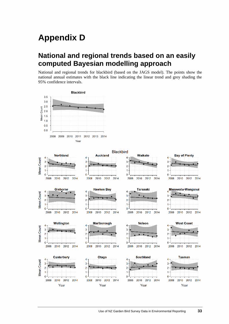
National and regional trends based on an easily computed Bayesian modelling approach National and regional trends for blackbird (based on the JAGS model). The points show the

national annual estimates with the black line indicating the linear trend and grey shading the

95% confidence intervals.


National and regional trends for Fantail (based on the JAGS model). The points show the




National and regional trends for silvereye (based on the JAGS model). The points show the




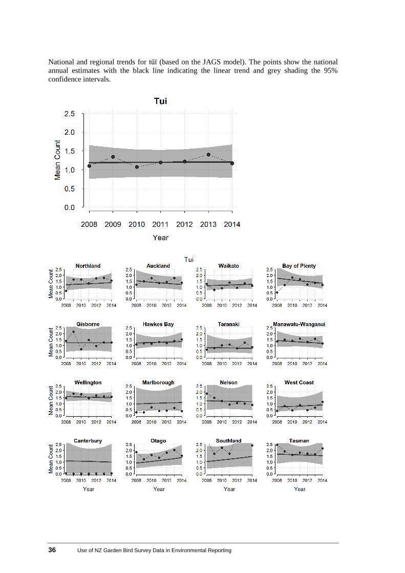
National and regional trends for tūī (based on the JAGS model). The points show the national

annual estimates with the black line indicating the linear trend and grey shading the 95%

confidence intervals.


References

Baillie SR, Rehfisch MM. (eds) 2006. National and site-based alert systems for UK birds. Research

Report 226. UK, British Trust for Ornithology.

Bates D, Maechler M, Bolker B, Walker S. 2015a. lme4: Linear mixed-effects models using Eigen and

S4. R package version 1.1-8. Retrieved from http://CRAN.R-project.org/package=lme4 (13 August

2015).

Bates D, Maechler M, Bolker BM, Walker S. 2015b. Fitting Linear Mixed-Effects Models using lme4.

ArXiv e-print; in press, Journal of Statistical Software. Retrieved from http://arxiv.org/abs/1406.5823

(13 August 2015).

Burnham KP, Anderson DR. 2002. Model Selection and Multimodel Inference: A Practical Information-

Theoretic Approach, 2nd edn. New York, Springer-Verlag.

Fewster RM, Buckland ST, Siriwardena GM, Baillie SR, Wilson JD. 2000. Analysis of population trends

for farmland birds using generalized additive models. Ecology 81: 1970–1984.

Green P, MacLeod CJ. (in review). simr: an R package for power analysis of linear mixed models by

simulation. (Submitted to Methods in Ecology and Evolution)

R Core Team. 2015. R: A language and environment for statistical computing. Vienna, Austria, R

Foundation for Statistical Computing. Version 3.1.3. Retrieved from http://www.R-project.org/ (13

August 2015).

Spurr E. 2007. New Zealand garden bird survey 2006. Notornis 54: 246.

Spurr EB. 2008a. New Zealand garden bird survey July 2007. Southern Bird 35: 9.

Spurr E. 2008b. New Zealand garden bird survey 2007. Notornis 55: 52.

Spurr EB. 2012a. New Zealand garden bird survey – analysis of the first four years. New Zealand Journal

of Ecology 36: 287–299.

Spurr EB. 2012b. New Zealand garden bird survey. Kararehe Kino – Vertebrate Pest Research 20: 12–

13.

Spurr E. 2014. Tūī and pīwakawaka soar. Forest & Bird 352: 16.

Spurr E. 2015a. House sparrow takes top spot. Forest & Bird 356: 29.

Spurr E. 2015b. Top 10 birds in New Zealand gardens. Birds New Zealand 6: 9.

http://www.r-project.org/

Date post:	03-Mar-2020
Category:	Documents
Upload:	others
View:	2 times
Download:	0 times

Use of NZ Garden Bird Survey Data in Environmental …...Use of NZ Garden Bird Survey Data in...

Documents