51
User Manual Software IT-Flood V.2.2 Flood hazard modelling AUTHOR (S): Natalia León Laura López Juan Velandia Luis Yamin PUBLICATION DATE: 27/05/2018 VERSION: 2.2
User Manual Software
IT-Flood V.2.2
Flood hazard modelling
AUTHOR (S): Natalia León Laura López
Juan Velandia Luis Yamin
PUBLICATION DATE: 27/05/2018
VERSION: 2.2
User Manual Software
CAPRA IT-Flood
2
Copyright
Copyright © 2018 UNIVERSIDAD DE LOS ANDES
THE SOFTWARE IS PROVIDED "AS IS", WITHOUT WARRANTY OF ANY KIND, EXPRESS OR
IMPLIED, INCLUDING BUT NOT LIMITED TO THE WARRANTIES OF MERCHANTABILITY,
FITNESS FOR A PARTICULAR PURPOSE AND NONINFRINGEMENT. IN NO EVENT SHALL
THE AUTHORS OR COPYRIGHT HOLDERS BE LIABLE FOR ANY CLAIM, DAMAGES OR
OTHER LIABILITY, WHETHER IN AN ACTION OF CONTRACT, TORT OR OTHERWISE,
ARISING FROM, OUT OF OR IN CONNECTION WITH THE SOFTWARE OR THE USE OR
OTHER DEALINGS IN THE SOFTWARE.
https://opensource.org/licenses/MIT
Universidad de los Andes – CAPRA PLATFORM
Carrera 1 Este No. 19A-40, Edificio Mario Laserna, Piso 6 / Bogotá, Colombia - Tel: (57-1) 3324312/14/15.
Contact us: [email protected]
User Manual Software
CAPRA IT-Flood
3
Contents Introduction ........................................................................................................................................ 5
1.1. Introduction ........................................................................................................................ 6
1.2. Problem description.......................................................................................................... 6
1.3. Theoretical framework ..................................................................................................... 6
Mathematical model ................................................................................................................... 6
Hydrological analysis ................................................................................................................... 7
Hydraulic analysis ........................................................................................................................ 8
1.4. Analysis flow chart ............................................................................................................ 8
Software Installation .......................................................................................................................... 9
2.1. Minimum installation requirements .............................................................................. 10
Minimum hardware and software requirements ..................................................................... 10
2.2. Recommended hardware requirements ...................................................................... 10
Processor ................................................................................................................................... 10
RAM Memory ............................................................................................................................ 10
Removable unit ......................................................................................................................... 10
Other software .......................................................................................................................... 10
2.3. Software requirements ................................................................................................... 10
2.4. Installation process ......................................................................................................... 11
2.5. Language configuration ................................................................................................. 11
Graphical User Interface ................................................................................................................... 12
3.1. General Description........................................................................................................ 13
3.2. Tools and Menus ............................................................................................................ 13
Datos generales window ........................................................................................................... 15
Método HEC-HMS window........................................................................................................ 17
Método HUT window ................................................................................................................ 19
Método hidrométrico window .................................................................................................. 20
Graphic interface ....................................................................................................................... 20
Setting input data and files .............................................................................................................. 21
4.1. Input parameters setting ................................................................................................ 22
4.2. File formats ...................................................................................................................... 23
General Topography .................................................................................................................. 23
Flow vs Return period curve ..................................................................................................... 24

User Manual Software
CAPRA IT-Flood
4
HEC-HMS PROJECT .................................................................................................................... 24
5.1. Output files and file format ............................................................................................ 26
Step by step tutorial ......................................................................................................................... 27
6.1. Step-by-step tutorial ....................................................................................................... 28
6.1.1. HMS method ............................................................................................................. 28
6.1.2. TUH method .............................................................................................................. 34
6.1.3. Hydrometric method ................................................................................................. 41
Software limitations ......................................................................................................................... 46
7.1. Software limitations ........................................................................................................ 47
Problems and errors ......................................................................................................................... 48
8.1. Problems and errors ....................................................................................................... 49
References ........................................................................................................................................ 50
9.1. References ...................................................................................................................... 51

User Manual Software
CAPRA IT-Flood
5
Chapter 1
Introduction

User Manual Software
CAPRA IT-Flood
6
1.1. Introduction IT-Flood software was created for flood analysis (fluvial or overflow), using a probabilistic and
deterministic methodology assessment. In the probabilistic approach, IT-Flood considers
precipitation variability to generate multiple flow scenarios for the same return period. On the
other side, in the deterministic approach, IT-Flood uses flow estimations associated with return
periods extracted from an estimation vs return period curve. The flow estimations by both
methodologies are used as input data for HEC-RAS software, in order to perform the
hydrodynamic analysis and obtained the depth, mean velocity and/or duration of each scenario.
This manual is a guide to using IT-Flood. The manual provides an introduction and overview of the
software, installation instructions, how to get started, its commands, a step-by-step example with
five modeling scenarios, the problems and limitations of the software.
1.2. Problem description Each year floods causes major disasters, for that reason a flood analysis software is required to
analyze, prevent and mitigate this disasters affectations. IT-Flood allows the user simulate series of
scenarios and as a result, an AME Flood file is generated. This AME can be used as an input in
CAPRA-GIS to assess flood risk.
1.3. Theoretical framework Flood is consider as the invasion of water, for overflow or excess of surface runoff or its
accumulation on flat land, caused by the lack of natural or artificial drainage. In general, the
magnitude of a flood is caused by hydrometeorological processes, which depends of rain intensity,
and their spatial distribution, the size of the affected hydrological basin, soil characteristics and
the basin drainage.
Mathematical model
Hydrological and hydrodynamic models allows obtaining intensity parameters associated with a probabilistic occurrence, which defines the hazard in a study area.
Hydrological analysis
Rain excess can cause flood risk by river overflow; this attaches directly the precipitation and the
topography characteristics of the surrounding terrain. For this reason, hydrological models are
based in precipitation-runoff interactions; if this relation is excessive, flooding is produce.
Hydraulic analysis
Hydraulic models require detailed information of river tributaries, its slope and transversal
sections characteristics. Hydrodynamic models can be classify as 1D, quasi-2D, 2D and 3D. The first
two although less sophisticate are widely used due to their ability to describe the river behavior
and their great computational efficiency (Pappenberger, et al., 2006)
User Manual Software
CAPRA IT-Flood
7
River behavior in 1D models is represented through cross sections; these sections can include the
main river and the floodplain. However, floodplains may have complex flow patterns in 2D, so it
may be more appropriated to use a model 1D for the river and 2D for the floodplain (Ranzi, et al.,
2011). The modeler must have the necessary criteria to select the most appropriate model in base
on the particular characteristics of their problem and the information,.
One of the most used 1D models is the HEC-RAS (Hydrologic Engineering Center), which solves the
Saint Venant equations through a method of finite differences to discretize the equations of
continuity and momentum in the case of non-permanent flow in open channels. As a particular
case, the condition of permanent flow can be analyzed.
Hydrological analysis
In the software, the flow estimation for hazard analysis can be done in three ways: a hydrological model in HEC-HMS software, rain-runoff model based on the Triangular Unitary Hydrograph (HUT- acronym in Spanish) and by entering a flow curve vs return period. The first two approaches have the capacity to account stochastic storms contained in the AME rain file and the third approach corresponds to a conventional assessment without sources of uncertainty.
HEC-HMS method
For each precipitation stochastic scenario, the hydrograph generated upstream of the flood zone
is determined, using the hydrological model built on the software HEC-HMS (US Army Corps of
Engineers). This numerical model allows simulating the processes involved in the transformation
of rainfall-runoff in the basin.
The program consists of a generalized modeling system capable of representing a large number of
different basins. The basin model is constructed by separating the hydrological cycle into easy
manipulated parts and by determining boundaries around the basins of interest. A mathematical
model can represent any mass of energy flow, each mathematical model is suitable under
different conditions, for this reason it is necessary to have knowledge of the basin and engineering
criteria to choose the best methodology in each case. For more information, see
http://www.hec.usace.army.mil/software/hec-hms/.
Triangular Unitary Hidrograph method
For each rain stochastic scenario the flow is determined using the information of the basin under study, delimiting the main channel and using information of: depth of precipitation, different types of run-off and general topography of the basin. The procedure uses the curve number method, developed by the Soil Conservation Service (SCS). The general methodology consists of two parts, in the first, an estimate of the run off volume is made and in the second, the runoff distribution time, including the peak flow is determined.
Hydrometric method
The complexity of the physical processes involved in hydraulic events makes it almost impossible to have 100 percent reliable estimates based on the laws of mechanics or physics, either because the methods are insufficient or because the resulting mathematical model is very complicated. An
User Manual Software
CAPRA IT-Flood
8
alternative in hydrological analysis is the application of the concepts of probability theory and statistics.
In the case of the hydrometric method, the information of the flows is obtained directly through flow curves vs Return period. These curves are obtained by analyzing the frequencies of the hydrometric data collected at the site of interest by fitting a probability distribution to the observed data. For details of the adjustment, procedure to the probability distributions see (Chow, Maidment, & Mays, 1994). IT-Flood software uses the flow curve vs. Return Period entered by the user, to obtain flows with different return periods through the linear interpolation of the curve. This approach corresponds to the traditional analysis in which uncertainty is not considered in the inflows to the hydrodynamic model.
Hydraulic analysis To perform the simulation of the flood footprints associated with the routing of swelling through channels, channels or rivers, the hydraulic model of the HEC-RAS program developed by the Hydrologic Engineering Center of US Army Corps of Engineers. This numerical model allows performing the analysis of permanent and non-permanent flow, in one-dimensional flow gradually varying in free lamina. For more information, see http://www.hec.usace.army.mil/software/hec-ras/.
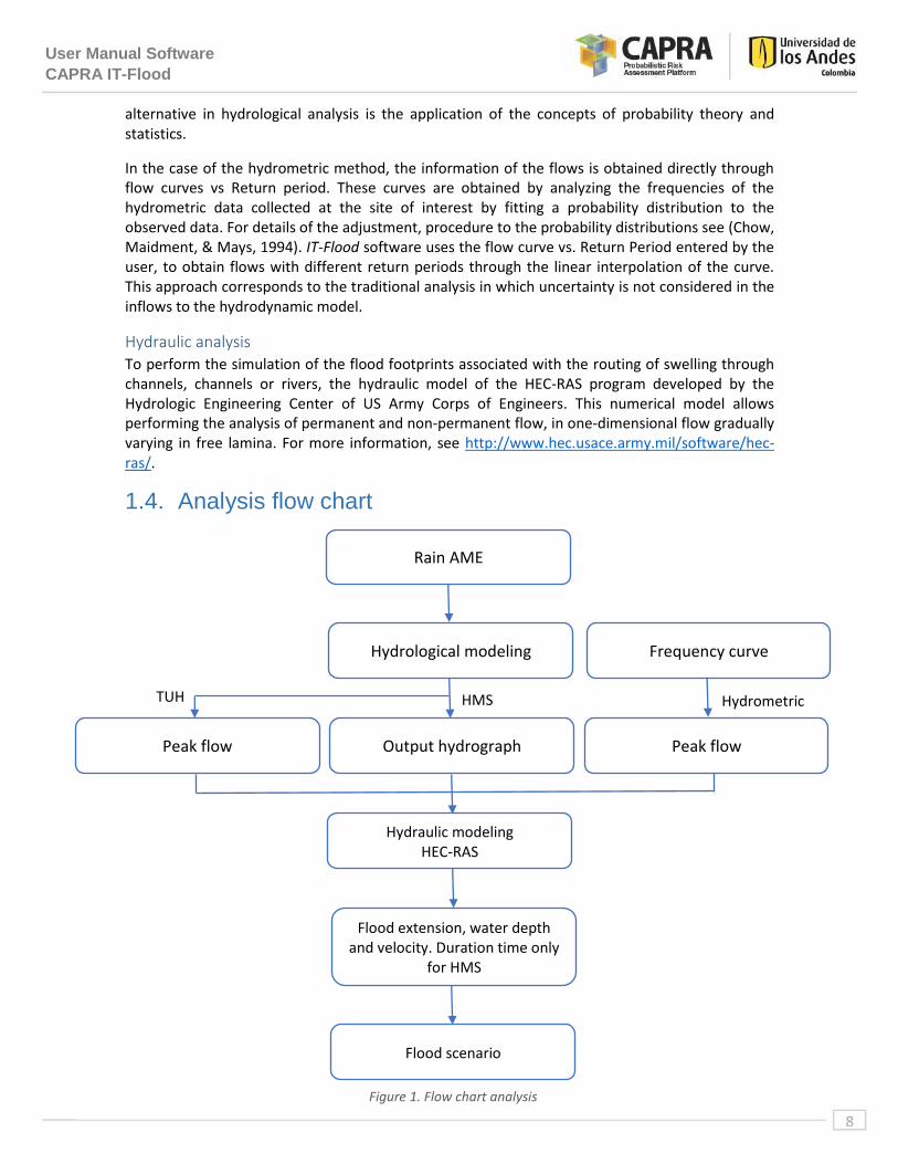
1.4. Analysis flow chart
Hydraulic modeling HEC-RAS
Flood extension, water depth and velocity. Duration time only
for HMS
HMS
Rain AME
Hydrological modeling
Peak flow
TUH
Peak flow
Frequency curve
Output hydrograph
Flood scenario
Hydrometric
Figura 1. Model flow chart Figure 1. Flow chart analysis
User Manual Software
CAPRA IT-Flood
9
Chapter 2
Software Installation

User Manual Software
CAPRA IT-Flood
10
2.1. Minimum installation requirements
Minimum hardware and software requirements The following are the minimum hardware requirements for the IT-Flood installation:
PC or compatible computer with Pentium III processor (or higher) and processor speed
over 1.5 GHz.
Operating systems: Microsoft XP or Higher
Free hard drive capacity of 250 Mb or Higher.
512 Mb Extended Memory (RAM)
CD-ROM or diskette unit (Depending on installers set up).
Microsoft framework V2.0 or higher and the language package
2.2. Recommended hardware requirements The following are the minimum hardware requirements for the CAPRA-GIS installation:
Processor - PC or compatible computer with Pentium III processor (or higher) and processor speed over
1.5 GHz.
- Operating systems: Microsoft XP or Higher
RAM Memory - Free hard drive capacity of 250 Mb or Higher.
- 512 Mb Extended Memory (RAM).
Removable unit - CD-ROM or diskette unit (Depending on installers set up)
Other software Microsoft framework V2.0 or higher and the language package (if CAPRA-GIS is already
installed, this is included)
2.3. Software requirements IT-Flood requires the following software for its correct operation:
HEC-RAS 4.1 of the US Army Corps of Engineers. Available in:
(http://www.hec.usace.army.mil/software/hec-ras/downloads.aspx)
HEC-HMS 4.0 of the US Army Corps of Engineers. Available in:
(http://www.hec.usace.army.mil/software/hec-hms/downloads.aspx)

User Manual Software
CAPRA IT-Flood
11
2.4. Installation process
1. If you don’t have HEC-RAS and/or HEC-HMS installed in the computer, you should download
the programs in the versions mentioned above from the following links:
HEC-RAS 4.1 (http://www.hec.usace.army.mil/software/hec-ras/downloads.aspx)
HEC-HMS 4.0 (http://www.hec.usace.army.mil/software/hec-hms/downloads.aspx)
2. Download the installation package from the CAPRA platform (https://ecapra.org/topics/flood)
3. Enter in windows explorer and select the file where installers are located.
4. Run the setup.exe program. This command starts the installation program; please follow
carefully each step indicated by the installation assistant.
2.5. Language configuration For a correct functioning of the software, it is recommended to use the tool in Spanish. For
changing the language in Windows 10, it is required to change the computer parameters as follow:
1. Open the control panel
2. Select the Clock and Region option
3. Select Region
4. In the Location field select Spanish (Mexico) as shown in Figure 2
5. Click Ok
Figure 2. Language configuration
User Manual Software
CAPRA IT-Flood
12
Chapter 3
Graphical User
Interface

User Manual Software
CAPRA IT-Flood
13
3.1. General Description IT-Flood is a software that allows flood hazard modeling, which is made with information provided
by the user and consists in a georeferenced map, a model in HEC -RAS 4.1, hydrological
information in the software HEC-HMS, rain spatial information and a rain AME either hurricane or
not hurricane.
The interface is showed in Figure 3, the tool bar is in the top (red box), and the windows where the
user enter data to perform the simulation is the blue box, finally in the green box, the graphic
interface is shown.
Figure 3. IT-Flood interface
3.2. Tools and Menus This section presents the different tools, menus and command of the software.
File menu
The following commands from the file menu of IT-Flood main window allow the users to create,
open, save and exit from the project. The function and localization of each command are explain
below.
User Manual Software
CAPRA IT-Flood
14
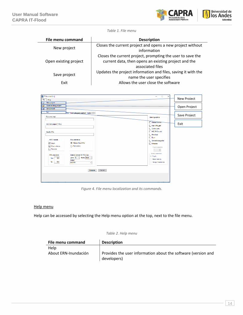
Table 1. File menu
File menu command Description
New project Closes the current project and opens a new project without
information
Open existing project Closes the current project, prompting the user to save the
current data, then opens an existing project and the associated files
Save project Updates the project information and files, saving it with the
name the user specifies Exit Allows the user close the software
Figure 4. File menu localization and its commands.
Help menu
Help can be accessed by selecting the Help menu option at the top, next to the file menu.
Table 2. Help menu
File menu command Description
Help About ERN-Inundación Provides the user information about the software (version and
developers)
New Project
Open Project
Save Project
Exit

User Manual Software
CAPRA IT-Flood
15
Figure 5. Help menu localization
Tool bar
The tool bar includes a list of icons, the first three icons belongs to the File menu, the forth one is
to run the program and computed flood AME, the fifth one open HEC-RAS and the last ones are
from the Help menu.
Figure 6. Tool bar
Datos generales window This contain the basic information the user must enter to the software, in this window the user
introduces the reference map, the HEC-RAS project, the folder in which the program should save
the results (Results AME), the flow estimation method and the geographic coordinates from the
place, as shown in Figure 7.
Help
About ERN-Inundación

User Manual Software
CAPRA IT-Flood
16
Figure 7. Datos generales window
Mapa de referencia
To enter the information associated with the Mapa de referencia, the user must double-click on
the text box below the Mapa referencia legend. The following figure shows the dialog box that will
appear to locate the path of the file that contains the reference map information associated with
the study area.
Figure 8. Mapa de referencia selection
Proyecto HEC-RAS
The file containing the HEC-RAS Project must be loaded; this project contains the information
associated with the flood analysis referred to the UTM coordinate system.

User Manual Software
CAPRA IT-Flood
17
AME de resultados
The user selects the place where the Project is going to be save and the project´s name. This
output file will be generated by IT-Flood after the calculation.
Opciones y parámetros de cálculo
In this section, the user can select the calculation of the depth, medium velocity and/or duration,
all as hazards associated with the study area. Analogously in this area, the user will decide
between the use of the HEC-HMS method, the triangular unitary hydrograph method, or the
hydrometric method to estimate the flow. It will also define the resolution of the AME, where the
user assign the number of pixels in X-axis and Y-axis direction for the results AME. Finally, in this
section, the user will set both the UTM zone, the hemisphere and the reference geodesic system
(Datum) associated with the study area.
Método HEC-HMS window The user provides the hydrological information of the zone, for this it is required the rainfall AME,
the HEC-HMS project, the temporal rain distribution information and the scenarios the user wants
to calculate (Figure 9).
Figure 9. Método HEC-HMS window
Distribución temporal de tormentas
From the precipitation analysis, the user obtains the spatial distribution of the storms; the user
must specify the percentage of rainfall with respect to the total depth of water that has fallen in
each decile of the total duration of the event.
Distribución temporal
de tormentas
Puntos de entrada de
caudal
Nombre de la corrida
HEC-HMS
Cálculo fraccionado

User Manual Software
CAPRA IT-Flood
18
Cálculo fraccionado
In this section, scenarios to be modeled are written in the box, it is necessary to include the initial
and final scenario. If only one scenario is going to be modeled, it is necessary to set this scenario as
the initial and final scenario
Puntos de entrada de caudal
If the river has tributaries, the user should select the option 2+, so the program is going to read the
HEC-HMS file and the user should introduce the hydrologic element of each one of the tributaries
and the main river (the software read and load the River, Reach and Cross Section information)
If there are tributaries in the study area, the 2+ button in the "Puntos de entrada de caudal" box
should be marked, like it is shown in Figure 10.
Figure 10. Options in Puntos de entrada de caudal box
By selecting the 2+ button the corresponding tab is activated indicating the cross sections of the
hydraulic model that correspond to possible boundary conditions, as shown in the following
figure. The last column must be filled out by the user in such a way that each section is related to a
hydrological element of the HEC-HMS model.
Figure 11. 2+ Windows information
User Manual Software
CAPRA IT-Flood
19
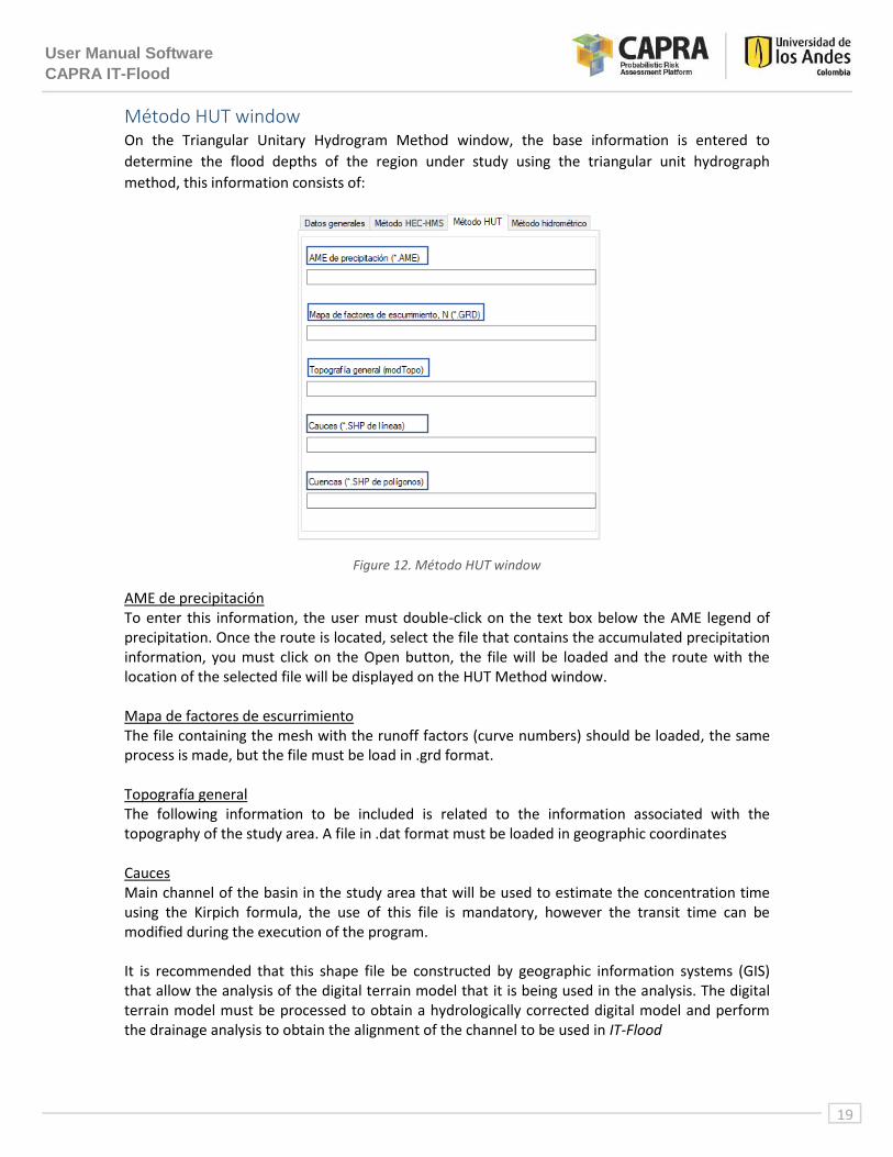
Método HUT window On the Triangular Unitary Hydrogram Method window, the base information is entered to
determine the flood depths of the region under study using the triangular unit hydrograph
method, this information consists of:
Figure 12. Método HUT window
AME de precipitación To enter this information, the user must double-click on the text box below the AME legend of precipitation. Once the route is located, select the file that contains the accumulated precipitation information, you must click on the Open button, the file will be loaded and the route with the location of the selected file will be displayed on the HUT Method window. Mapa de factores de escurrimiento The file containing the mesh with the runoff factors (curve numbers) should be loaded, the same process is made, but the file must be load in .grd format. Topografía general The following information to be included is related to the information associated with the topography of the study area. A file in .dat format must be loaded in geographic coordinates Cauces Main channel of the basin in the study area that will be used to estimate the concentration time using the Kirpich formula, the use of this file is mandatory, however the transit time can be modified during the execution of the program. It is recommended that this shape file be constructed by geographic information systems (GIS) that allow the analysis of the digital terrain model that it is being used in the analysis. The digital terrain model must be processed to obtain a hydrologically corrected digital model and perform the drainage analysis to obtain the alignment of the channel to be used in IT-Flood

User Manual Software
CAPRA IT-Flood
20
Cuencas Corresponds to the delimitation of the hydrological basin in the study area, a file in .shp (polygon). This file must be in geographic coordinates and will only contain the polygon of the basin that will be considered for the calculation of runoff.
Método hidrométrico window Select the file that contains the flow information associated with the study area, the file must be
loaded in .qtr format. In this section, the user will set the value 100 (value assigned "by default" by
IT-Flood) as the number of scenarios to be evaluated in this method.
Graphic interface This window allows the user to observe graphically the data entered, after the modeling is
performed and the AME creation is finished, it is shown in the graphical panel as shown below:
Figure 13. AME result in the graphic interface

User Manual Software
CAPRA IT-Flood
21
Chapter 4
Setting input data and
files

User Manual Software
CAPRA IT-Flood
22
4.1. Input parameters setting IT-Flood software requires multiple parameters and data supplied by the user, so it can be
performance. Table 3 describes the input data and the associated file format.
Table 3. Inputs parameters for IT-Flood
Parameter Description .file
Datos generales window
Mapa de referencia (reference map)
Corresponds to the contour map of the region under study, this information is used for the user to interact
with the program and can verify that the general information entered is within the limits of the study
area.
*.shp
Proyecto HEC-RAS (HEC-RAS Project)
The file containing the HEC-RAS Project must be loaded; this project contains the information
associated with the flood analysis referred to the UTM coordinate system.
*.prj
Resultados AME IT-Flood will generate this output file after the
calculation. *.AME
Resolución del AME The user defines the resolution for the resulting AME
in both directions. Positive number
Estimación de gastos The flow estimation can be made through 3 methods,
the user select which one it is going to be used. -
Datos para convertir UTM a GEO
The user will set both the UTM zone, the hemisphere and the reference geodesic system (Datum)
associated with the study area. -
Método HEC-HMS
AME de precipitación File that contains the precipitation information for the
study area *.AME
Proyecto HEC-HMS Contains the information associated with the
hydrological analysis of the study basin *.HMS
Distribución temporal de tormentas
The user must specify the percentage of rainfall with respect to the total depth of water that has fallen in
each decile of the total duration of the event. -
Puntos de entrada de caudal
Related to the boundary conditions given by the hydrological model, which correspond to the inlet flow upstream of the hydraulic model and to the
lateral flow inputs produced by different tributaries present in the analysis section.
If there are tributaries in the study area, the 2+ button
in the "Flow entry points" box should be marked
-
User Manual Software
CAPRA IT-Flood
23
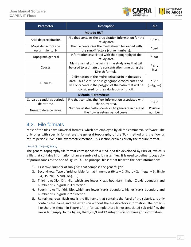
Parameter Description .file
Método HUT
AME de precipitación File that contains the precipitation information for the
study area *.AME
Mapa de factores de escurrimiento, N
The file containing the mesh should be loaded with the runoff factors (curve numbers).
*.grd
Topografía general Information associated with the topography of the
study area *.dat
Cauces Main channel of the basin in the study area that will
be used to estimate the concentration time using the Kirpich formula.
*.shp (lines)
Cuencas
Delimitation of the hydrological basin in the study area. This file must be in geographic coordinates and will only contain the polygon of the basin that will be
considered for the calculation of runoff.
*.shp (polygons)
Método Hidrométrico
Curva de caudal vs periodo de retorno
File that contains the flow information associated with the study area.
*.qtr
Número de escenarios Number of stochastic scenarios to generate in base of
the flow vs return period curve. Positive number
4.2. File formats Most of the files have universal formats, which are employed by all the commercial software. The
only ones with specific format are the general topography of the TUH method and the flow vs
return period curve in the hydrometric method. This section explains briefly the require format.
General Topography The general topography file format corresponds to a modTopo file developed by ERN-AL, which is
a file that contains information of an ensemble of grid raster files. It is used to define topography
of porous zones as the one of Figure 14. The principal file is *.dat file with the next information:
1. First row: Number of sub-grids that compose the general grid.
2. Second row: Type of grid variable format in number (Byte – 1, Short – 2, Integer – 3, Single
– 4, Double – 5 and Long – 6).
3. Third row: Xlo, Xhi, Nlo, which are lower X-axis boundary, higher X-axis boundary and
number of sub-grids in X direction.
4. Fourth row: Ylo, Yhi, Nlo, which are lower Y-axis boundary, higher Y-axis boundary and
number of sub-grids in Y direction.
5. Remaining rows: Each row is the file name that contains the *.grd of the subgrids. It only
contains the name and the extension without the file directory information. The order is
like the one shown in Figure 14 . If for example there is not associated sub-grid file, the
row is left empty. In the figure, the 1,2,8,9 and 12 sub-grids do not have grid information.

User Manual Software
CAPRA IT-Flood
24
Figure 14. ModTopo general sub-grid order
Flow vs Return period curve The *.qtr file is a text file with final extension qtr. The file contains the next information:
1. First row: Number of pair groups (Flow and return period) that composed the curve.
2. Remaining rows: Pair of data separated by a comma. First comes the flow and next the
return period.
The next figure shows the general format:
Figure 15, *.qtr format example
HEC-HMS PROJECT The HEC-HMS project contains a basin model, meteorological model and control specification. The
proposed methodology employs the following parameters for its operation: an associated grid cell
file of the basin in the basin model, a gridded precipitation in the meteorological model and the
grid data in the control specification; it is recommended to generate the model with HEC-GeoHMS
(http://www.hec.usace.army.mil/software/hec-geohms/downloads.aspx)
User Manual Software
CAPRA IT-Flood
25
Chapter 5
Visualization output
files
User Manual Software
CAPRA IT-Flood
26
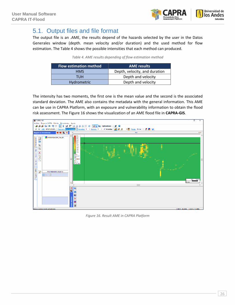
5.1. Output files and file format The output file is an .AME, the results depend of the hazards selected by the user in the Datos
Generales window (depth. mean velocity and/or duration) and the used method for flow
estimation. The Table 4 shows the possible intensities that each method can produced.
Table 4. AME results depending of flow estimation method
Flow estimation method AME results
HMS Depth, velocity, and duration
TUH Depth and velocity
Hydrometric Depth and velocity
The intensity has two moments, the first one is the mean value and the second is the associated
standard deviation. The AME also contains the metadata with the general information. This AME
can be use in CAPRA Platform, with an exposure and vulnerability information to obtain the flood
risk assessment. The Figure 16 shows the visualization of an AME flood file in CAPRA-GIS.
Figure 16. Result AME in CAPRA Platform

User Manual Software
CAPRA IT-Flood
27
Chapter 6
Step by step tutorial

User Manual Software
CAPRA IT-Flood
28
6.1. Step-by-step tutorial This chapter provides examples how to perform the software with the three possible different
methods (HEC-HMS, TUH and hydrometric).
6.1.1. HMS method For the tutorial it is used a simplified segment of the Rocha River in Bolivia, with 5 different
scenarios each one with a different return period (5, 10, 25, 50 and 100 years). The step-by-step
process is explained in the next pages. Copy the Input folder in C:\. This file contains the necessary
files for the example.
Necessary files
Boundary: MapaReferencia_Rocha.shp
HEC-RAS project: RioRocha.prj
Rain AME : AMEPrecipitacion_Rocha.AME
HEC-HMS project: Rocha.hms Contents
Starting a New Project
Entering required Data
Performing the simulation
Viewing Results
6.1.1.1. Starting a new Project
To begin this example, open IT-Flood from desktop or start menu and the main window should
appear as shown in Figure 17.
Figure 17. IT-Flood interface
User Manual Software
CAPRA IT-Flood
29
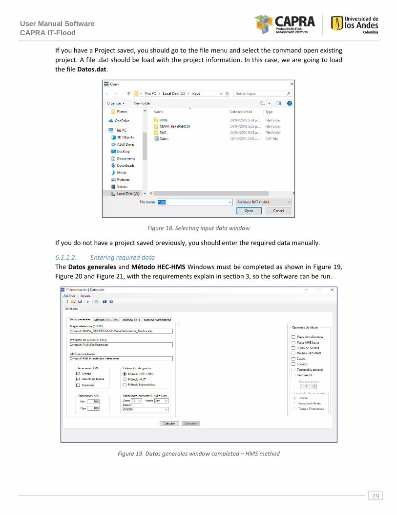
If you have a Project saved, you should go to the file menu and select the command open existing
project. A file .dat should be load with the project information. In this case, we are going to load
the file Datos.dat.
Figure 18. Selecting input data window
If you do not have a project saved previously, you should enter the required data manually.
6.1.1.2. Entering required data
The Datos generales and Método HEC-HMS Windows must be completed as shown in Figure 19,
Figure 20 and Figure 21, with the requirements explain in section 3, so the software can be run.
Figure 19. Datos generales window completed – HMS method

User Manual Software
CAPRA IT-Flood
30
Figure 20. Método HMS window completed
Figure 21. 2+ window completed
6.1.1.3. Performing the simulation
After complete 6.1.1.2. Steps click the Calcular button and the software will load the metadata.
When this information is loaded the message in Figure 22 appears, click the Aceptar button and
the calculation of the AME for each scenario starts.

User Manual Software
CAPRA IT-Flood
31
Figure 22. Charging AME metadata in main window – HMS method
Figure 23. AME Metadata loaded window – HMS method
User Manual Software
CAPRA IT-Flood
32
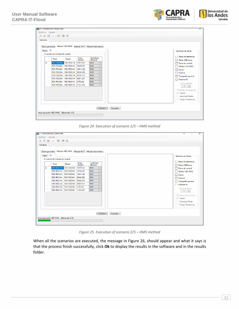
Figure 24. Execution of scenario 1/5 – HMS method
Figure 25. Execution of scenario 2/5 – HMS method
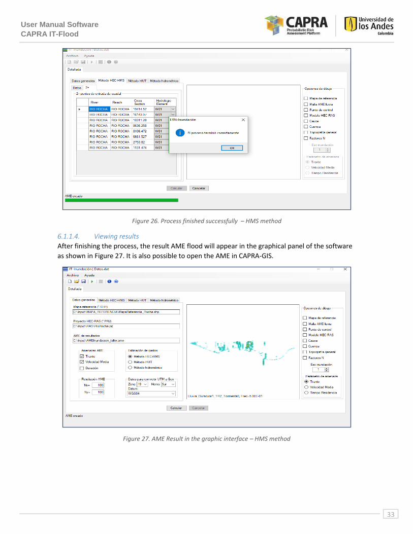
When all the scenarios are executed, the message in Figure 26, should appear and what it says is
that the process finish successfully, click Ok to display the results in the software and in the results
folder.
User Manual Software
CAPRA IT-Flood
33
Figure 26. Process finished successfully – HMS method
6.1.1.4. Viewing results
After finishing the process, the result AME flood will appear in the graphical panel of the software
as shown in Figure 27. It is also possible to open the AME in CAPRA-GIS.
Figure 27. AME Result in the graphic interface – HMS method
User Manual Software
CAPRA IT-Flood
34
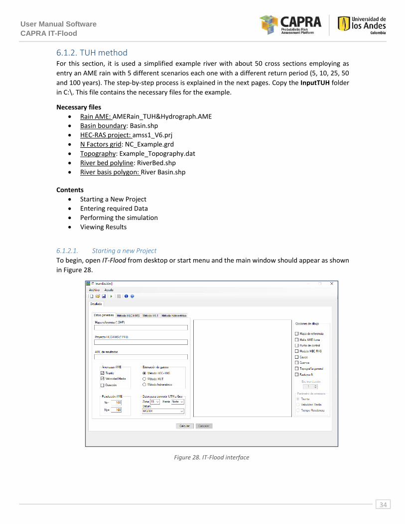
6.1.2. TUH method For this section, it is used a simplified example river with about 50 cross sections employing as
entry an AME rain with 5 different scenarios each one with a different return period (5, 10, 25, 50
and 100 years). The step-by-step process is explained in the next pages. Copy the InputTUH folder
in C:\. This file contains the necessary files for the example.
Necessary files
Rain AME: AMERain_TUH&Hydrograph.AME
Basin boundary: Basin.shp
HEC-RAS project: amss1_V6.prj
N Factors grid: NC_Example.grd
Topography: Example_Topography.dat
River bed polyline: RiverBed.shp
River basis polygon: River Basin.shp Contents
Starting a New Project
Entering required Data
Performing the simulation
Viewing Results
6.1.2.1. Starting a new Project
To begin, open IT-Flood from desktop or start menu and the main window should appear as shown
in Figure 28.
Figure 28. IT-Flood interface
User Manual Software
CAPRA IT-Flood
35
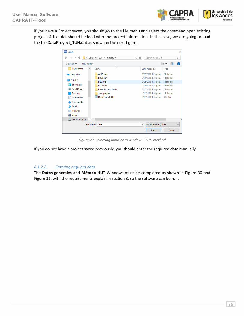
If you have a Project saved, you should go to the file menu and select the command open existing
project. A file .dat should be load with the project information. In this case, we are going to load
the file DataProyect_TUH.dat as shown in the next figure.
Figure 29. Selecting input data window – TUH method
If you do not have a project saved previously, you should enter the required data manually.
6.1.2.2. Entering required data
The Datos generales and Método HUT Windows must be completed as shown in Figure 30 and
Figure 31, with the requirements explain in section 3, so the software can be run.

User Manual Software
CAPRA IT-Flood
36
Figure 30. Datos generales window completed – TUH method
Figure 31. Método HUT window completed

User Manual Software
CAPRA IT-Flood
37
6.1.2.3. Performing the simulation
After complete 6.1.2.2. Steps click the Calcular button and the software will load the metadata.
When this information is loaded, the message in Figure 32 appears. Edit the AME metadata
information if it is necessary.
Figure 32. Charging AME metadata in main window – TUH method
Click Accept button and the software will ask to introduce a coefficient of variation value as shown
in Figure 33. Click the Ok button and the program will calculate in base of basin and bed shapefiles
the mean slope of the basin. It will pop up a window asking the user if the slope is correct or if not,
it gives the possibility that the user edit manually the value as Figure 34 displays.

User Manual Software
CAPRA IT-Flood
38
Figure 33. Coefficient of variation window - TUH method
Figure 34. Basin mean slope value window – TUH method

User Manual Software
CAPRA IT-Flood
39
Select the Ok button and the software will show the parameters that compose the triangular unit
hydrograph of the basin as shown in the next figure. The user can edit each parameter manually if
it is necessary.
Figure 35. Unit hydrograph parameters window – TUH
Click Aceptar button and the calculation of the AME flood for each scenario starts as it can be seen
in Figure 36.
Figure 36. Execution of scenario 1/5– TUH method

User Manual Software
CAPRA IT-Flood
40
When all the scenarios are executed, the message in Figure 37 should appear and what it says is
that the process finish successfully, click Ok to finish the process.
Figure 37. Process finished successfully– TUH method
6.1.2.4. Viewing results
After finishing the process, the result AME flood will appear in the graphical panel of the software
as shown in Figure 38. It is also possible to open the AME in CAPRA-GIS.
Figure 38. AME Result in the graphic interface – TUH method

User Manual Software
CAPRA IT-Flood
41
6.1.3. Hydrometric method For this section, it is used a simplified example river with about 50 cross sections as the TUH
example. However, the method does not require rain data instead, it uses the flow vs return
period curve. It will generate randomly five scenarios for the example. The step-by-step process is
explained in the next pages. Copy the InputHydrometric folder in C:\. This file contains the
necessary files for the example.
Necessary files
Flow vs return period curve: FlowReturnPeriod.qtr
HEC-RAS project: amss1_V6.prj Contents
Starting a New Project
Entering required Data
Performing the simulation
Viewing Results
6.1.3.1. Starting a new Project
To begin, open IT-Flood from desktop or start menu and the main window should appear as shown
in Figure 39.
Figure 39. IT-Flood interface
If you have a Project saved, you should go to the file menu and select the command open existing
project. A file .dat should be load with the project information. In this case, we are going to load
the file DataProyect_Hydrometric.dat as shown in the next figure.

User Manual Software
CAPRA IT-Flood
42
Figure 40. Selecting input data window – Hydrometric method
If you do not have a project saved previously, you should enter the required data manually.
6.1.3.2. Entering required data
The Datos generales and Método hidrométrico Windows must be completed as shown in Figure
41 and Figure 42, with the requirements explain in section 3, so the software can be run.
Figure 41. Datos generales window completed – Hydrometric method

User Manual Software
CAPRA IT-Flood
43
When the flow vs return period is loaded, the software will show the curve in the Método
Hidrométrico window.
Figure 42. Método hidrométrico window completed
6.1.3.3. Performing the simulation
After complete 6.1.3.2. Steps click the Calcular button and the software will load the metadata.
When this information is loaded, the message in Figure 43 appears. Edit the AME metadata
information if it is necessary.
Figure 43. Charging AME metadata in main window – Hydrometric method
User Manual Software
CAPRA IT-Flood
44
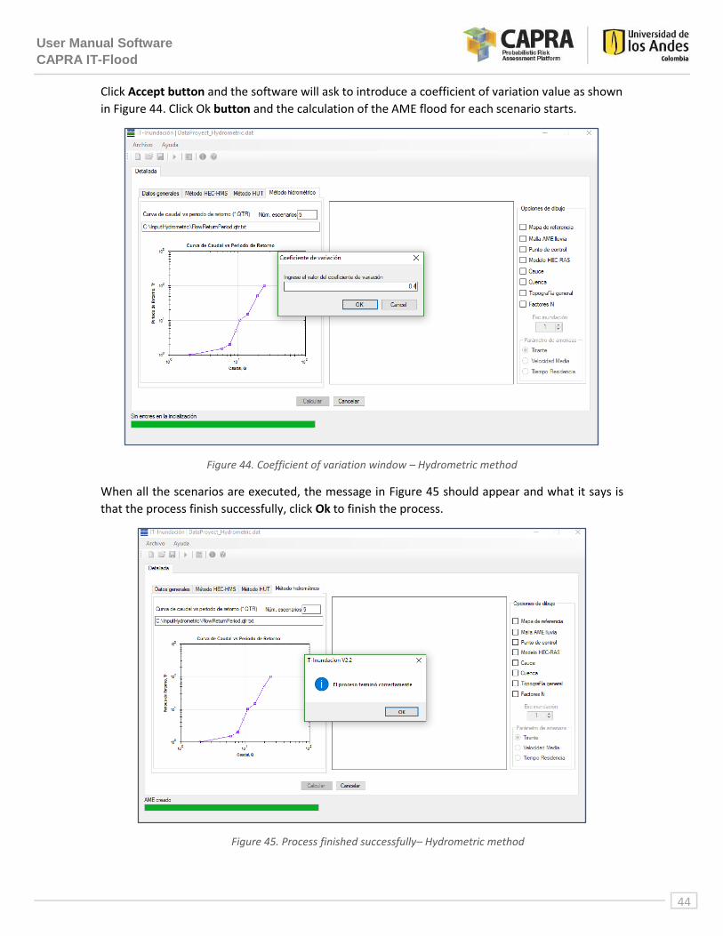
Click Accept button and the software will ask to introduce a coefficient of variation value as shown
in Figure 44. Click Ok button and the calculation of the AME flood for each scenario starts.
Figure 44. Coefficient of variation window – Hydrometric method
When all the scenarios are executed, the message in Figure 45 should appear and what it says is
that the process finish successfully, click Ok to finish the process.
Figure 45. Process finished successfully– Hydrometric method
User Manual Software
CAPRA IT-Flood
45
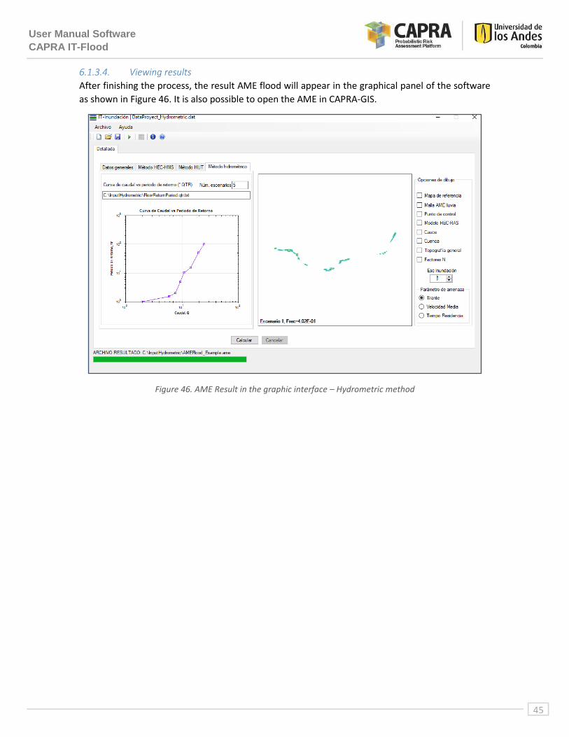
6.1.3.4. Viewing results
After finishing the process, the result AME flood will appear in the graphical panel of the software
as shown in Figure 46. It is also possible to open the AME in CAPRA-GIS.
Figure 46. AME Result in the graphic interface – Hydrometric method
User Manual Software
CAPRA IT-Flood
46
Chapter 7
Software limitations

User Manual Software
CAPRA IT-Flood
47
7.1. Software limitations The most important limitations of the software are listed below:
The software only works with HEC-RAS 4.1 that means that only allows 1D modeling.
Currently limited version only runs 20 scenarios.

User Manual Software
CAPRA IT-Flood
48
Chapter 8
Problems and errors

User Manual Software
CAPRA IT-Flood
49
8.1. Problems and errors The identified problems at the time of creation of this manual are:
Projection error, when re-projecting to geographic coordinates it is possible that a small
misalignment occurs.
If the computer language is not in Spanish, there are some translate errors in the interface
for others languages ( i.e. some words remain in Spanish).
If the HEC-RAS model have lakes or ponds, in the HEC-HMS window: Puntos de entrada de
caudal, table 2+ does not appear the name of the hydraulic element, so an error window
displays. However, the software is capable of running by dismissing the error.
At the time of calculations, the program is inefficient and it loads several times the same
file/information before proceeding with the calculation.

User Manual Software
CAPRA IT-Flood
50
Chapter 9
References

User Manual Software
CAPRA IT-Flood
51
9.1. References
Chow, V. T., Maidment, D., & Mays, L. (1994). Applied Hydrology. McGraw-Hill Science
Engineering.
CONAGUA. (2011). Manual para el control de inundaciones. Obtenido de
http://cenca.imta.mx/pdf/manual-para-el-control-de-inundaciones.pdf.
Cronshey, R. (1986). Urban Hydrology for Small Watersheds. US Dept. of Agriculture, Soil
Conservation Service, Engineering Division.
ERN-AL (Consorcio Evaluación de Riesgos Naturales – América Latina). (2009). Tomo I.
Metodología de Modelación Probabilista de Riesgos Naturales. Modelos de Evaluación de
Amenazas Naturales y Selección. CEPREDENAC, ISDR, IDB,GFDRR, WB.
Kirpich, Z. (1940). Time of concentration of small agricultural watersheds. Civil Engineering, 10(6),
362.
León, N. (2014). Implementación de los Programas HEC-HMS y HEC-RAS en la Plataforma CAPRA
para Evaluación de Riesgo por Inundación. Bogotá: Universidad de los Andes.
Mockus, V. (1957). Use of storm and watershed characteristics in syntetic unit hidrograph analysis
and application. US Department of Agriculture, Soil Conservation Service, Latham, MD.
Pappenberger, F., Matgen, P., Beven, K., Henry, J.-B., Pfister, L., & Frapoint, P. (2006). Influence of
uncertain boundary conditions and model structure on flood inundation predictions.
Advances in Water Resources, 29(10), 1430-1449.
Potosme, E., & Castro, M. (2005). Inundaciones fluviales. e. p. I. y. C. Metodologías para el análisis
y manejo de los riesgos naturales. Managua.
Ranzi, R., Mazzoleni, M., Milanesi, L., Pilotti, M., Ferri, M., Giuriato, F., . . . Brilly, M. (2011). Critical
review of non structural measures for water related risks. KULTURisk.
Snider, D., Woodward, D., Hoeft, C., Merkel, W., Chaison, K., & Fox, H. (2007). Part 630 Hydrology
National Engineering Handbook Chapter 16 Hydrographs. USDA. Natural Resources
Conservation Service.


