129
For Research Use Only. Not for use in diagnostic procedures. P/N Axiom ™ Analysis Suite 2.0 UserGuide P/N 703307 Rev. 3

Axiom™Analysis Suite 2.0UserGuide
For Research Use Only. Not for use in diagnostic procedures.P/N P/N 703307 Rev. 3

2
TrademarksAffymetrix®, Axiom™, Eureka™ GeneChip®, NetAffx®, Command Console®, Powered by Affymetrix™, GeneChip-compatible™, Genotyping Console™, DMET™, GeneTitan®, Axiom®, CytoScan®, and GeneAtlas® are trademarks or registered trademarks of Affymetrix, Inc. All other trademarks are the property of their respective owners.
All other trademarks are the property of their respective owners.
Limited License NoticeAffymetrix hereby grants to buyer a non-exclusive, non-transferable, non-sublicensable license to Affymetrix' Core Product IP to use the product(s), but only in accordance with the product labels, inserts, manuals and written instructions provided by Affymetrix. "Core Product IP" is the intellectual property owned or controlled by Affymetrix as of the shipment date of a product that covers one or more features of the product that are applicable in all applications of the product that are in accordance with the product labels, inserts, manuals and written instructions provided by Affymetrix. The license granted herein to buyer to the Core Product IP expressly excludes any use that: (i) is not in accordance with the product labels, inserts, manuals and written instructions provided by Affymetrix, (ii) requires a license to intellectual property that covers one or more features of a product that are only applicable within particular fields of use or specific applications, (iii) involves reverse engineering, disassembly, or unauthorized analysis of the product and/or its methods of use, or (iv) involves the re-use of a consumable product. Buyer understands and agrees that except as expressly set forth, no right or license to any patent or other intellectual property owned or controlled by Affymetrix is granted upon purchase of any product, whether by implication, estoppel or otherwise. In particular, no right or license is conveyed or implied to use any product provided hereunder in combination with a product or service not provided, licensed or specifically recommended by Affymetrix for such use. Furthermore, buyer understands and agrees that buyer is solely responsible for determining whether buyer possesses all intellectual property rights that may be necessary for buyer's specific use of the product, including any rights from third parties.
PatentsSoftware products may be covered by one or more of the following patents: U.S. Patent Nos. 5,733,729; 5,795,716; 5,974,164; 6,066,454; 6,090,555; 6,185,561; 6,188,783; 6,223,127; 6,228,593; 6,229,911; 6,242,180; 6,308,170; 6,361,937; 6,420,108; 6,484,183; 6,505,125; 6510,391; 6,532,462; 6,546,340; 6,687,692; 6,607,887; 7,062,092 and other U.S. or foreign patents.
Copyright© 2016 Affymetrix, Inc. All rights reserved.

Contents
Chapter 1 Introduction . . . . . . . . . . . . . . . . . . . . . . . . . . . . . . . . . . . . . . . . . . . . . . . . . . . . . 8
Overview . . . . . . . . . . . . . . . . . . . . . . . . . . . . . . . . . . . . . . . . . . . . . . . . . . . . . . . . . . . . . . . . . .8Software and Hardware Requirements . . . . . . . . . . . . . . . . . . . . . . . . . . . . . . . . . . . . . . . . . . . .8
Sample Data Size Estimates and Required Disk Space . . . . . . . . . . . . . . . . . . . . . . . . . . . . . . .8Installation Instructions . . . . . . . . . . . . . . . . . . . . . . . . . . . . . . . . . . . . . . . . . . . . . . . . . . . . . . .9Starting Axiom Analysis Suite . . . . . . . . . . . . . . . . . . . . . . . . . . . . . . . . . . . . . . . . . . . . . . . . . . .9Using the Preferences Window Tab . . . . . . . . . . . . . . . . . . . . . . . . . . . . . . . . . . . . . . . . . . . . .11
Changing the Default Library Folder/Path . . . . . . . . . . . . . . . . . . . . . . . . . . . . . . . . . . . . . . .11Setting Up Proxy Server Access . . . . . . . . . . . . . . . . . . . . . . . . . . . . . . . . . . . . . . . . . . . . . . .12Updating NetAffx Library/Annotations . . . . . . . . . . . . . . . . . . . . . . . . . . . . . . . . . . . . . . . . .12Enabling/Disabling Check for Library File Updates at Start Up . . . . . . . . . . . . . . . . . . . . . . . .14
Installing Custom Array Library Files . . . . . . . . . . . . . . . . . . . . . . . . . . . . . . . . . . . . . . . . . . . . .14Uninstalling Axiom Analysis Suite . . . . . . . . . . . . . . . . . . . . . . . . . . . . . . . . . . . . . . . . . . . . . . .15
Windows 7 . . . . . . . . . . . . . . . . . . . . . . . . . . . . . . . . . . . . . . . . . . . . . . . . . . . . . . . . . . . . .15Windows 10 . . . . . . . . . . . . . . . . . . . . . . . . . . . . . . . . . . . . . . . . . . . . . . . . . . . . . . . . . . . .15
Chapter 2 Performing an Analysis . . . . . . . . . . . . . . . . . . . . . . . . . . . . . . . . . . . . . . . . . . . 16
Setting Up an Analysis . . . . . . . . . . . . . . . . . . . . . . . . . . . . . . . . . . . . . . . . . . . . . . . . . . . . . . .16Selecting a Mode (Workflow) . . . . . . . . . . . . . . . . . . . . . . . . . . . . . . . . . . . . . . . . . . . . . . . .16Selecting an Array Type . . . . . . . . . . . . . . . . . . . . . . . . . . . . . . . . . . . . . . . . . . . . . . . . . . . .17Importing CEL Files . . . . . . . . . . . . . . . . . . . . . . . . . . . . . . . . . . . . . . . . . . . . . . . . . . . . . . . .17Importing CEL Files by Text . . . . . . . . . . . . . . . . . . . . . . . . . . . . . . . . . . . . . . . . . . . . . . . . . .17Removing Selected CEL Files . . . . . . . . . . . . . . . . . . . . . . . . . . . . . . . . . . . . . . . . . . . . . . . . .18
Setting Up an Analysis Configuration . . . . . . . . . . . . . . . . . . . . . . . . . . . . . . . . . . . . . . . . . . . .18Selecting an Analysis Configuration . . . . . . . . . . . . . . . . . . . . . . . . . . . . . . . . . . . . . . . . . . .18Using the Analysis Settings Fields . . . . . . . . . . . . . . . . . . . . . . . . . . . . . . . . . . . . . . . . . . . . .19
Sample QC Fields . . . . . . . . . . . . . . . . . . . . . . . . . . . . . . . . . . . . . . . . . . . . . . . . . . . . . . .19Genotyping Fields . . . . . . . . . . . . . . . . . . . . . . . . . . . . . . . . . . . . . . . . . . . . . . . . . . . . . . .20
Saving your Analysis Configuration . . . . . . . . . . . . . . . . . . . . . . . . . . . . . . . . . . . . . . . . . . . . .21Modifying an Existing Analysis Configuration . . . . . . . . . . . . . . . . . . . . . . . . . . . . . . . . . . . . . .21Setting Up Threshold Settings . . . . . . . . . . . . . . . . . . . . . . . . . . . . . . . . . . . . . . . . . . . . . . . . .22
Customizing Thresholds . . . . . . . . . . . . . . . . . . . . . . . . . . . . . . . . . . . . . . . . . . . . . . . . . . . .22Sample QC . . . . . . . . . . . . . . . . . . . . . . . . . . . . . . . . . . . . . . . . . . . . . . . . . . . . . . . . . . . .23SNP QC . . . . . . . . . . . . . . . . . . . . . . . . . . . . . . . . . . . . . . . . . . . . . . . . . . . . . . . . . . . . . .23
Assigning an Output Folder Path . . . . . . . . . . . . . . . . . . . . . . . . . . . . . . . . . . . . . . . . . . . . .25Assigning a New Output Folder Path . . . . . . . . . . . . . . . . . . . . . . . . . . . . . . . . . . . . . . . .25Adding Sub-Folders . . . . . . . . . . . . . . . . . . . . . . . . . . . . . . . . . . . . . . . . . . . . . . . . . . . . .25
Assigning a Batch Name . . . . . . . . . . . . . . . . . . . . . . . . . . . . . . . . . . . . . . . . . . . . . . . . . . . .25Running your Analysis . . . . . . . . . . . . . . . . . . . . . . . . . . . . . . . . . . . . . . . . . . . . . . . . . . . . . . .26Using the Dashboard Window Tab . . . . . . . . . . . . . . . . . . . . . . . . . . . . . . . . . . . . . . . . . . . . . .27
Open Selected Result(s) . . . . . . . . . . . . . . . . . . . . . . . . . . . . . . . . . . . . . . . . . . . . . . . . . . . .28Remove Selected Result(s) . . . . . . . . . . . . . . . . . . . . . . . . . . . . . . . . . . . . . . . . . . . . . . . . . .28Browsing For Existing Analysis Results . . . . . . . . . . . . . . . . . . . . . . . . . . . . . . . . . . . . . . . . .28Browsing for Existing Suitcases . . . . . . . . . . . . . . . . . . . . . . . . . . . . . . . . . . . . . . . . . . . . . . .28

Chapter 3 The Viewer: Summary Window and Sample Table . . . . . . . . . . . . . . . . . . . . . 30
Viewing Options . . . . . . . . . . . . . . . . . . . . . . . . . . . . . . . . . . . . . . . . . . . . . . . . . . . . . . . . . . .31Split-Screen Options . . . . . . . . . . . . . . . . . . . . . . . . . . . . . . . . . . . . . . . . . . . . . . . . . . . . . . .31Changing a Tab Window to a Full Screen Windows . . . . . . . . . . . . . . . . . . . . . . . . . . . . . . .33Adjusting the Window Size . . . . . . . . . . . . . . . . . . . . . . . . . . . . . . . . . . . . . . . . . . . . . . . . .34
Summary Window/Tab . . . . . . . . . . . . . . . . . . . . . . . . . . . . . . . . . . . . . . . . . . . . . . . . . . . . . .35Data Analysis Summary . . . . . . . . . . . . . . . . . . . . . . . . . . . . . . . . . . . . . . . . . . . . . . . . . . . .35Viewing the Plate Barcode Table Details . . . . . . . . . . . . . . . . . . . . . . . . . . . . . . . . . . . . . . . .36
Sample Table . . . . . . . . . . . . . . . . . . . . . . . . . . . . . . . . . . . . . . . . . . . . . . . . . . . . . . . . . . . . . .37Importing Sample Attributes . . . . . . . . . . . . . . . . . . . . . . . . . . . . . . . . . . . . . . . . . . . . . . . .38Column Headers . . . . . . . . . . . . . . . . . . . . . . . . . . . . . . . . . . . . . . . . . . . . . . . . . . . . . . . . .38
Rearranging Columns . . . . . . . . . . . . . . . . . . . . . . . . . . . . . . . . . . . . . . . . . . . . . . . . . . . .39Sorting Columns . . . . . . . . . . . . . . . . . . . . . . . . . . . . . . . . . . . . . . . . . . . . . . . . . . . . . . .39Single-Click Sorting Method . . . . . . . . . . . . . . . . . . . . . . . . . . . . . . . . . . . . . . . . . . . . . . .39Hiding the Column . . . . . . . . . . . . . . . . . . . . . . . . . . . . . . . . . . . . . . . . . . . . . . . . . . . . . .39
Filtering Column Data . . . . . . . . . . . . . . . . . . . . . . . . . . . . . . . . . . . . . . . . . . . . . . . . . . . . . . .40Adding Filters (Method 1) . . . . . . . . . . . . . . . . . . . . . . . . . . . . . . . . . . . . . . . . . . . . . . . . . . .40
Text-based Columns . . . . . . . . . . . . . . . . . . . . . . . . . . . . . . . . . . . . . . . . . . . . . . . . . . . . .40Numeric Data Columns . . . . . . . . . . . . . . . . . . . . . . . . . . . . . . . . . . . . . . . . . . . . . . . . . .41Showing Filtered Data Only . . . . . . . . . . . . . . . . . . . . . . . . . . . . . . . . . . . . . . . . . . . . . . .42Clearing an Individual Filter . . . . . . . . . . . . . . . . . . . . . . . . . . . . . . . . . . . . . . . . . . . . . . .43Clearing All Current Filters . . . . . . . . . . . . . . . . . . . . . . . . . . . . . . . . . . . . . . . . . . . . . . . .43
Adding Filters (Method 2) . . . . . . . . . . . . . . . . . . . . . . . . . . . . . . . . . . . . . . . . . . . . . . . . . . .43Copying Column Data . . . . . . . . . . . . . . . . . . . . . . . . . . . . . . . . . . . . . . . . . . . . . . . . . . . . .46Setting User Colors . . . . . . . . . . . . . . . . . . . . . . . . . . . . . . . . . . . . . . . . . . . . . . . . . . . . . . .46
Assigning a Color to a Sample . . . . . . . . . . . . . . . . . . . . . . . . . . . . . . . . . . . . . . . . . . . . .46Importing Assigned Colors . . . . . . . . . . . . . . . . . . . . . . . . . . . . . . . . . . . . . . . . . . . . . . . .47
Viewing User Colors in the Cluster Graph . . . . . . . . . . . . . . . . . . . . . . . . . . . . . . . . . . . . . . .48Removing an Assigned User Color . . . . . . . . . . . . . . . . . . . . . . . . . . . . . . . . . . . . . . . . . .49
Searching Keywords . . . . . . . . . . . . . . . . . . . . . . . . . . . . . . . . . . . . . . . . . . . . . . . . . . . . . . .49Box Plots . . . . . . . . . . . . . . . . . . . . . . . . . . . . . . . . . . . . . . . . . . . . . . . . . . . . . . . . . . . . . . . . .50
Viewing the Default Box Plots . . . . . . . . . . . . . . . . . . . . . . . . . . . . . . . . . . . . . . . . . . . . . . .50Changing the Box Plot’s Scale Setting Ranges . . . . . . . . . . . . . . . . . . . . . . . . . . . . . . . . . . .51Adding a New Box Plot . . . . . . . . . . . . . . . . . . . . . . . . . . . . . . . . . . . . . . . . . . . . . . . . . . . .51Reading Box Plot Percentiles . . . . . . . . . . . . . . . . . . . . . . . . . . . . . . . . . . . . . . . . . . . . . . . . .52Saving the Current Box Plot View . . . . . . . . . . . . . . . . . . . . . . . . . . . . . . . . . . . . . . . . . . . . .52
Scatter Plot . . . . . . . . . . . . . . . . . . . . . . . . . . . . . . . . . . . . . . . . . . . . . . . . . . . . . . . . . . . . . . .53Viewing the Default Scatter Plot . . . . . . . . . . . . . . . . . . . . . . . . . . . . . . . . . . . . . . . . . . . . . .53Changing the Scatter Plot’s Setting Ranges . . . . . . . . . . . . . . . . . . . . . . . . . . . . . . . . . . . . .54Adding a New Scatter Plot and Selecting its X and Y Properties . . . . . . . . . . . . . . . . . . . . . .54Customizing Color By Settings . . . . . . . . . . . . . . . . . . . . . . . . . . . . . . . . . . . . . . . . . . . . . . .56Saving the Current Scatter Plot View . . . . . . . . . . . . . . . . . . . . . . . . . . . . . . . . . . . . . . . . . .57
Plate Views . . . . . . . . . . . . . . . . . . . . . . . . . . . . . . . . . . . . . . . . . . . . . . . . . . . . . . . . . . . . . . .58Viewing the Default Plate Views . . . . . . . . . . . . . . . . . . . . . . . . . . . . . . . . . . . . . . . . . . . . . .58Adding a New Plate View Metric . . . . . . . . . . . . . . . . . . . . . . . . . . . . . . . . . . . . . . . . . . . . .59Saving the Current Plate View . . . . . . . . . . . . . . . . . . . . . . . . . . . . . . . . . . . . . . . . . . . . . . .60
Concordance Checks . . . . . . . . . . . . . . . . . . . . . . . . . . . . . . . . . . . . . . . . . . . . . . . . . . . . . . . .60Running a Concordance Check . . . . . . . . . . . . . . . . . . . . . . . . . . . . . . . . . . . . . . . . . . . . . .60
Reanalyzing Samples . . . . . . . . . . . . . . . . . . . . . . . . . . . . . . . . . . . . . . . . . . . . . . . . . . . . . . . .62
Chapter 4 The Viewer: SNP Summary Table and Cluster Plot. . . . . . . . . . . . . . . . . . . . . . 63
SNP Summary Table . . . . . . . . . . . . . . . . . . . . . . . . . . . . . . . . . . . . . . . . . . . . . . . . . . . . . . . . .63Using the SNP Summary Table . . . . . . . . . . . . . . . . . . . . . . . . . . . . . . . . . . . . . . . . . . . . . . . . .64
Setting your SNP Summary Table View . . . . . . . . . . . . . . . . . . . . . . . . . . . . . . . . . . . . . . . . .64Adding and Removing Table Columns . . . . . . . . . . . . . . . . . . . . . . . . . . . . . . . . . . . . . . .64Selecting Annotations . . . . . . . . . . . . . . . . . . . . . . . . . . . . . . . . . . . . . . . . . . . . . . . . . . .65
Saving your Table Column View . . . . . . . . . . . . . . . . . . . . . . . . . . . . . . . . . . . . . . . . . . . . . .65Copying Selected Row(s) . . . . . . . . . . . . . . . . . . . . . . . . . . . . . . . . . . . . . . . . . . . . . . . . . . .66Copying Selected Cell(s) . . . . . . . . . . . . . . . . . . . . . . . . . . . . . . . . . . . . . . . . . . . . . . . . . . . .66Changing or Reverting Genotype Calls . . . . . . . . . . . . . . . . . . . . . . . . . . . . . . . . . . . . . . . . .66
Reanalyzing your SNP Summary Table Data . . . . . . . . . . . . . . . . . . . . . . . . . . . . . . . . . . . . . . .67Regenerate SNP Metric . . . . . . . . . . . . . . . . . . . . . . . . . . . . . . . . . . . . . . . . . . . . . . . . . . . . .67Running PS Supplemental . . . . . . . . . . . . . . . . . . . . . . . . . . . . . . . . . . . . . . . . . . . . . . . . . .70Running OTV Caller . . . . . . . . . . . . . . . . . . . . . . . . . . . . . . . . . . . . . . . . . . . . . . . . . . . . . . .71
Managing your SNP List . . . . . . . . . . . . . . . . . . . . . . . . . . . . . . . . . . . . . . . . . . . . . . . . . . . . . .72Saving your current SNP List . . . . . . . . . . . . . . . . . . . . . . . . . . . . . . . . . . . . . . . . . . . . . . . . .72Exporting your SNP List . . . . . . . . . . . . . . . . . . . . . . . . . . . . . . . . . . . . . . . . . . . . . . . . . . . .72Importing a SNP List . . . . . . . . . . . . . . . . . . . . . . . . . . . . . . . . . . . . . . . . . . . . . . . . . . . . . . .72Using your Saved SNP List . . . . . . . . . . . . . . . . . . . . . . . . . . . . . . . . . . . . . . . . . . . . . . . . . .73
Displaying SNPs in a SNP list . . . . . . . . . . . . . . . . . . . . . . . . . . . . . . . . . . . . . . . . . . . . . . .73Displaying SNPs that are not in your SNP List . . . . . . . . . . . . . . . . . . . . . . . . . . . . . . . . . .74
Cluster Plot . . . . . . . . . . . . . . . . . . . . . . . . . . . . . . . . . . . . . . . . . . . . . . . . . . . . . . . . . . . . . . .74Using the Cluster Plot . . . . . . . . . . . . . . . . . . . . . . . . . . . . . . . . . . . . . . . . . . . . . . . . . . . . . .75
Displaying a SNP Cluster Plot that Corresponds with a SNP . . . . . . . . . . . . . . . . . . . . . . . .75Setting New Scale Setting Ranges . . . . . . . . . . . . . . . . . . . . . . . . . . . . . . . . . . . . . . . . . . . .76Customizing Color By Settings . . . . . . . . . . . . . . . . . . . . . . . . . . . . . . . . . . . . . . . . . . . . . . .76Selecting Multiple Samples in a Cluster Plot . . . . . . . . . . . . . . . . . . . . . . . . . . . . . . . . . . . . .78Changing a Sample’s Call for a Single SNP . . . . . . . . . . . . . . . . . . . . . . . . . . . . . . . . . . . . . .78
Reverting a Single Call . . . . . . . . . . . . . . . . . . . . . . . . . . . . . . . . . . . . . . . . . . . . . . . . . . .79Reverting Multiple Calls . . . . . . . . . . . . . . . . . . . . . . . . . . . . . . . . . . . . . . . . . . . . . . . . . .79
Displaying Cluster Model Data . . . . . . . . . . . . . . . . . . . . . . . . . . . . . . . . . . . . . . . . . . . . . . .79Saving the Current Cluster Plot View . . . . . . . . . . . . . . . . . . . . . . . . . . . . . . . . . . . . . . . . . .79

Chapter 5 Allele Translation . . . . . . . . . . . . . . . . . . . . . . . . . . . . . . . . . . . . . . . . . . . . . . . . 80
About Translations . . . . . . . . . . . . . . . . . . . . . . . . . . . . . . . . . . . . . . . . . . . . . . . . . . . . . . . . . .80Performing Allele Translation . . . . . . . . . . . . . . . . . . . . . . . . . . . . . . . . . . . . . . . . . . . . . . . . . .80
Allele Translation Options . . . . . . . . . . . . . . . . . . . . . . . . . . . . . . . . . . . . . . . . . . . . . . . . . . .82Translation Reports . . . . . . . . . . . . . . . . . . . . . . . . . . . . . . . . . . . . . . . . . . . . . . . . . . . . . . . . .83
Comprehensive and Summary Translation Report . . . . . . . . . . . . . . . . . . . . . . . . . . . . . . . . .84Summary Translation Report . . . . . . . . . . . . . . . . . . . . . . . . . . . . . . . . . . . . . . . . . . . . . . . .84Phenotype Translation Report . . . . . . . . . . . . . . . . . . . . . . . . . . . . . . . . . . . . . . . . . . . . . . . .85Phenotype Report . . . . . . . . . . . . . . . . . . . . . . . . . . . . . . . . . . . . . . . . . . . . . . . . . . . . . . . .85
Opening Translation Report in MS Excel . . . . . . . . . . . . . . . . . . . . . . . . . . . . . . . . . . . . . . . . . .86Available Report Fields and Descriptions . . . . . . . . . . . . . . . . . . . . . . . . . . . . . . . . . . . . . . . . . .87
Array Tracking . . . . . . . . . . . . . . . . . . . . . . . . . . . . . . . . . . . . . . . . . . . . . . . . . . . . . . . . . . .87Gene-specific . . . . . . . . . . . . . . . . . . . . . . . . . . . . . . . . . . . . . . . . . . . . . . . . . . . . . . . . . . . .87Marker-specific . . . . . . . . . . . . . . . . . . . . . . . . . . . . . . . . . . . . . . . . . . . . . . . . . . . . . . . . . .89Tracking Edited Genotype Calls . . . . . . . . . . . . . . . . . . . . . . . . . . . . . . . . . . . . . . . . . . . . . .90Uncalled Report . . . . . . . . . . . . . . . . . . . . . . . . . . . . . . . . . . . . . . . . . . . . . . . . . . . . . . . . . .90
Chapter 6 Exporting . . . . . . . . . . . . . . . . . . . . . . . . . . . . . . . . . . . . . . . . . . . . . . . . . . . . . . 91
Using the Sample Table Export Options . . . . . . . . . . . . . . . . . . . . . . . . . . . . . . . . . . . . . . . . . .91Using the SNP Summary Table Export Options . . . . . . . . . . . . . . . . . . . . . . . . . . . . . . . . . . . . .91
Exporting the Current Table . . . . . . . . . . . . . . . . . . . . . . . . . . . . . . . . . . . . . . . . . . . . . . . . .91Exporting All Data . . . . . . . . . . . . . . . . . . . . . . . . . . . . . . . . . . . . . . . . . . . . . . . . . . . . . . . .91Exporting Signature SNPs . . . . . . . . . . . . . . . . . . . . . . . . . . . . . . . . . . . . . . . . . . . . . . . . . . .92Exporting Genotyping Data . . . . . . . . . . . . . . . . . . . . . . . . . . . . . . . . . . . . . . . . . . . . . . . . .92
Result Output Formats . . . . . . . . . . . . . . . . . . . . . . . . . . . . . . . . . . . . . . . . . . . . . . . . . . .93Call Output Formats . . . . . . . . . . . . . . . . . . . . . . . . . . . . . . . . . . . . . . . . . . . . . . . . . . . . .93Exported Data Selections . . . . . . . . . . . . . . . . . . . . . . . . . . . . . . . . . . . . . . . . . . . . . . . . .93Input and Output Files . . . . . . . . . . . . . . . . . . . . . . . . . . . . . . . . . . . . . . . . . . . . . . . . . . .93Changing the SNP Identifier . . . . . . . . . . . . . . . . . . . . . . . . . . . . . . . . . . . . . . . . . . . . . . .94Changing the Current Annotation File (Optional) . . . . . . . . . . . . . . . . . . . . . . . . . . . . . . .95Adding and Removing Annotation Columns . . . . . . . . . . . . . . . . . . . . . . . . . . . . . . . . . . .95
Exporting Cluster Plots to PDF . . . . . . . . . . . . . . . . . . . . . . . . . . . . . . . . . . . . . . . . . . . . . . .96
Chapter 7 External Tools. . . . . . . . . . . . . . . . . . . . . . . . . . . . . . . . . . . . . . . . . . . . . . . . . . . 98
Axiom CNV Tool 1.1 . . . . . . . . . . . . . . . . . . . . . . . . . . . . . . . . . . . . . . . . . . . . . . . . . . . . . . . .98

Appendix A Copy Number Aware Genotyping. . . . . . . . . . . . . . . . . . . . . . . . . . . . . . . . . . . 99
Setting Up a CN-aware Genotyping Analysis . . . . . . . . . . . . . . . . . . . . . . . . . . . . . . . . . . . . . .99Selecting a Mode (Workflow) . . . . . . . . . . . . . . . . . . . . . . . . . . . . . . . . . . . . . . . . . . . . . . .100Importing CEL Files . . . . . . . . . . . . . . . . . . . . . . . . . . . . . . . . . . . . . . . . . . . . . . . . . . . . . . .100CN-aware Genotyping Analysis Settings . . . . . . . . . . . . . . . . . . . . . . . . . . . . . . . . . . . . . . .101
Sample QC . . . . . . . . . . . . . . . . . . . . . . . . . . . . . . . . . . . . . . . . . . . . . . . . . . . . . . . . . . .101Genotyping . . . . . . . . . . . . . . . . . . . . . . . . . . . . . . . . . . . . . . . . . . . . . . . . . . . . . . . . . .102
Threshold Settings specific to CN-aware Genotyping . . . . . . . . . . . . . . . . . . . . . . . . . . . . .103Sample QC . . . . . . . . . . . . . . . . . . . . . . . . . . . . . . . . . . . . . . . . . . . . . . . . . . . . . . . . . . .103CN QC . . . . . . . . . . . . . . . . . . . . . . . . . . . . . . . . . . . . . . . . . . . . . . . . . . . . . . . . . . . . . .103SNP QC . . . . . . . . . . . . . . . . . . . . . . . . . . . . . . . . . . . . . . . . . . . . . . . . . . . . . . . . . . . . .103
Assigning an Output Folder Path . . . . . . . . . . . . . . . . . . . . . . . . . . . . . . . . . . . . . . . . . . . .104Assigning a Batch Name . . . . . . . . . . . . . . . . . . . . . . . . . . . . . . . . . . . . . . . . . . . . . . . . . . .104
Running your CN-aware Genotyping Analysis . . . . . . . . . . . . . . . . . . . . . . . . . . . . . . . . . . . .105Viewing your CN-aware Genotyping Analysis . . . . . . . . . . . . . . . . . . . . . . . . . . . . . . . . . . . . .105
Summary Report . . . . . . . . . . . . . . . . . . . . . . . . . . . . . . . . . . . . . . . . . . . . . . . . . . . . . . . .106Sample Table . . . . . . . . . . . . . . . . . . . . . . . . . . . . . . . . . . . . . . . . . . . . . . . . . . . . . . . . . . .108SNP Summary Table . . . . . . . . . . . . . . . . . . . . . . . . . . . . . . . . . . . . . . . . . . . . . . . . . . . . . .109CN Summary Table and CN Region Plot . . . . . . . . . . . . . . . . . . . . . . . . . . . . . . . . . . . . . . .110
CN Summary Table (Overview) . . . . . . . . . . . . . . . . . . . . . . . . . . . . . . . . . . . . . . . . . . . .110CN Region Plot (Overview) . . . . . . . . . . . . . . . . . . . . . . . . . . . . . . . . . . . . . . . . . . . . . . .110
Overview and Use of the Best Practices Workflow . . . . . . . . . . . . . . . . . . . . . . . . . . . . . . . . .111
Appendix B About Allele Translation . . . . . . . . . . . . . . . . . . . . . . . . . . . . . . . . . . . . . . . . . 113
Overview . . . . . . . . . . . . . . . . . . . . . . . . . . . . . . . . . . . . . . . . . . . . . . . . . . . . . . . . . . . . . . . .113Gene Table Layout for Haplotyping . . . . . . . . . . . . . . . . . . . . . . . . . . . . . . . . . . . . . . . . . . . .113Biological Annotations in Translation Reports . . . . . . . . . . . . . . . . . . . . . . . . . . . . . . . . . . . . .115Impact of Phase Ambiguity in Haplotyping . . . . . . . . . . . . . . . . . . . . . . . . . . . . . . . . . . . . . . .115Diplotype to Phenotype Translation . . . . . . . . . . . . . . . . . . . . . . . . . . . . . . . . . . . . . . . . . . . .117Creating a Custom Metabolizer Library File . . . . . . . . . . . . . . . . . . . . . . . . . . . . . . . . . . . . . .117Metabolizer Library File Format . . . . . . . . . . . . . . . . . . . . . . . . . . . . . . . . . . . . . . . . . . . . . . .118Reference Databases Used in Translation Data Curation . . . . . . . . . . . . . . . . . . . . . . . . . . . . .119
Appendix C Definitions . . . . . . . . . . . . . . . . . . . . . . . . . . . . . . . . . . . . . . . . . . . . . . . . . . . . 120
Sample QC Metrics . . . . . . . . . . . . . . . . . . . . . . . . . . . . . . . . . . . . . . . . . . . . . . . . . . . . . . . .120Annotations and Columns . . . . . . . . . . . . . . . . . . . . . . . . . . . . . . . . . . . . . . . . . . . . . . . . . . .123Concordance Columns . . . . . . . . . . . . . . . . . . . . . . . . . . . . . . . . . . . . . . . . . . . . . . . . . . . . .125Threshold Names . . . . . . . . . . . . . . . . . . . . . . . . . . . . . . . . . . . . . . . . . . . . . . . . . . . . . . . . . .125SNP Summary Table Definitions . . . . . . . . . . . . . . . . . . . . . . . . . . . . . . . . . . . . . . . . . . . . . . .127

Chapter 1
Introduction
Overview
Axiom Analysis Suite enables you to perform the following functions: Run QC and Genotyping Algorithms.
View QC Data within tables and graphs at a Sample and/or SNP level.
View Cluster Graphs with the ability to change calls and/or highlight by attribute.
Export your Data.
Software and Hardware Requirements
Sample Data Size Estimates and Required Disk SpaceBefore using Axiom Analysis Suite, make sure you have enough disk space. See Table 1.1 for size estimates. The estimates shown include the contents of the batch name folder2.
1Minimum storage requirements are for a single run. Total storage space should include additional space fordata storage of input and output files from current and previously completed analyses. In addition, youmust have a minimum of 5GB of free space on your C: drive to run an analysis.
2A batch name folder is auto-generated during the analysis process. This folder includes all the necessaryfiles needed to view your analysis results in the Viewer.
3Input is the storage size required for CEL files to be analyzed. Output is the storage size required foranalysis results files.
64-bit Operating System Speed Memory (RAM)
Available Disk Space1 Web Browser
Microsoft Windows® 7 (64 bit) Professional with Service Pack 1
2.83 GHz Intel Pentium Quad Core Processor
16 GB RAM 150 GB HD + data storageSee Table 1.1.
IE 8.0 and above
Microsoft Windows 10 (64 bit) Professional
2.83 GHz Intel Pentium Quad Core Processor
16 GB RAM 150 GB HD + data storageSee Table 1.1.
IE 8.0 and above
Table 1.1 Sample Data Size Estimates
# of Markers Storage Type3 50 samples 100 samples 500 samples 1000 samples 5000 samples
50K InputOutputTotal
1.33 GB158 MB1.49 GB
2.66 GB286 MB2.95 GB
13.3 GB1.27 GB14.57 GB
26.6 GB2.51 GB29.11 GB
133 GB12.4 GB145.4 GB
500K InputOutputTotal
1.33 GB1.53 GB2.86 GB
2.66 GB2.77 GB5.43 GB
13.3 GB12.6 GB25.9 GB
26.6 GB25.0 GB51.6 GB
133 GB124 GB257 GB
850K InputOutputTotal
1.33 GB2.59 GB3.92 GB
2.66 GB4.69 GB7.35 GB
13.3 GB21.4 GB34.7 GB
26.6 GB42.4 GB69.0 GB
133 GB209 GB342 GB

Chapter 1 | Introduction 9
Installation Instructions1. Go to www.affymetrix.com, then navigate to the following location:
Home > Products > Microarray Solutions > Instruments and Software > Software
2. Locate and download the zipped Axiom Analysis Suite software package.
3. Unzip the file, then double-click AxiomAnalysisSuiteSetup.exe.
4. Follow the on-screen instructions to complete the installation.
If your system has a previous version installed, the following message appears: (Figure 1.1)
Acknowledge the message, click OK, then go to Uninstalling Axiom Analysis Suite on page 15.
Starting Axiom Analysis Suite1. Double-click on the Axiom Analysis Suite Desktop shortcut or click
Start > All Programs > Affymetrix > Axiom Analysis Suite.
The following window appears: (Figure 1.2)
Figure 1.1 Uninstall required message
Figure 1.2 Opening window

Chapter 1 | Introduction 10
2. Enter a new profile name or click the down-arrow to select an existing profile name.
3. Click OK.
The following window appears: (Figure 1.3)
Figure 1.3 Main window

Chapter 1 | Introduction 11
Using the Preferences Window TabClick the Preferences window tab (Figure 1.4) to setup or change a library path, edit Proxy settings, download or update Library/Annotation files.
Changing the Default Library Folder/Path
Do the following to change the default Library folder/path:
1. Click Browse (right of library path field).
The Select Library Folder window appears.
2. Navigate to the new location you want the library folder to reside.
3. Click New Folder.
4. Rename the New Folder (as you normally would), then click Select Folder.
Figure 1.4 Main Preferences window
IMPORTANT: The library folder contains the library and annotation files required to run theAxiom Analysis Suite software.

Chapter 1 | Introduction 12
Your newly assigned Library folder is set and reflected in the Library Folder directory/path field, as shown in Figure 1.5.
Setting Up Proxy Server AccessIf your system has to pass through a Proxy Server before it can access the Affymetrix NetAffx server (Internet), click the Edit button. (Figure 1.6)
The following window appears: (Figure 1.7)
5. Click the Enable Proxy Server Settings check box (Figure 1.7), then contact your IT department for help with completing the required text fields.
6. Click OK.
Updating NetAffx Library/Annotations1. Click on the Update button. (Figure 1.8)
Figure 1.5 Populated Library Path example
Figure 1.6 Proxy Settings
Figure 1.7 Proxy Settings Editor window
Figure 1.8 Update button

Chapter 1 | Introduction 13
The following window appears: (Figure 1.9)
2. Enter your User name and Password, then click OK.
The NetAffx Update window appears. (Figure 1.10)
3. You must click the check box(es) that correspond with the type of CEL files you want to analyze.
Click the Check/Uncheck All check box to select/deselect all the listed check boxes.
4. Click OK.
An Installing Updates progress bar appears.
Figure 1.9 NetAffx Login window
NOTE: If you are unable to connect to the NetAffx Download Center, make sure you haveentered the correct NetAffx User name and Password, have an active Internet connection, andproper Proxy Server settings.
If you do not have a NetAffx account, go to www.affymetrix.com, click "NetAffx", then click"Register".
Click OK, then try to login to the NetAffx Download Center again.
Figure 1.10 NetAffx Update window

Chapter 1 | Introduction 14
Enabling/Disabling Check for Library File Updates at Start Up1. This check box (Figure 1.11) is checked by default to enable automatic Library File update alerts each
time you launch the Axiom Analysis Suite application. (Recommended)
Installing Custom Array Library Files
1. Download the zip package provided to you by Affymetrix Bioinformatics Services.
2. Unzip the contents of the analysis library files into a single sub-folder within the library file folder.
For multi-species designs, each species should be in its own sub-folder. There should be no other folders within each sub-folder and all annotation information must be in the same location as the .CDF file.
Figure 1.11 Auto-update notifications check box
IMPORTANT: Library files for custom designs must be manually installed.

Chapter 1 | Introduction 15
Uninstalling Axiom Analysis Suite
The Axiom Analysis Suite 2.0 installer does not support upgrade installations, therefore you must uninstall the existing version of Axiom Analysis Suite before installing version 2.0.
Windows 71. Click Start > Control Panel.
The Control Panel window appears.
2. Click the View by drop-down menu (upper-right), then click to select Category.
3. In the Programs category, click Uninstall a program.
The Programs and Features window appears.
4. Click to select Axiom Analysis Suite, then click Uninstall.
5. Follow the on-screen instructions.
6. After the uninstall process is complete, close the Programs and Features window.
7. Use Windows Explorer as you normally would to navigate to the directory: C:\Program Files\Affymetrix
8. Verify that the Axiom Analysis Suite folder has been removed.
9. If the folder is present, double-click on it to open it.
10. Search for any files you want to keep, then move them to different (easily accessible) location.
11. Delete the Axiom Analysis Suite folder.
12. Close all open windows, then install version 2.0, as described in the Installation Instructions on page 9.
Windows 101. Click the Windows icon (bottom left corner).
2. Click All apps > Windows System > Control Panel.
The Control Panel window appears.
3. In the Programs category, click Uninstall a program.
The Programs and Features window appears.
4. Click to select Axiom Analysis Suite, then click Uninstall.
5. Follow the on-screen instructions.
6. After the uninstall process is complete, close all open windows.
7. Use Windows Explorer as you normally would to navigate to the directory: C:\Program Files\Affymetrix
8. Verify that the Axiom Analysis Suite folder has been removed.
9. If the folder is present, double-click on it to open it.
10. Search for any files you want to keep, then move them to different (easily accessible) location.
11. Delete the Axiom Analysis Suite folder.
12. Close all open windows, then install version 2.0, as described in the Installation Instructions on page 9.
NOTE: Administrative rights to the computer are required before you can uninstall theAxiom Analysis Suite software. For your convenience, no existing library files or usersettings are removed during the uninstall process.
Chapter 2
Performing an Analysis
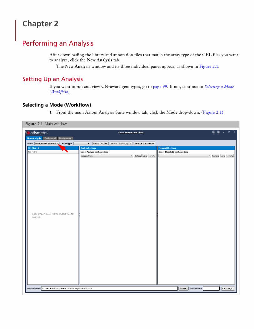
After downloading the library and annotation files that match the array type of the CEL files you want to analyze, click the New Analysis tab.
The New Analysis window and its three individual panes appear, as shown in Figure 2.1.
Setting Up an AnalysisIf you want to run and view CN-aware genotypes, go to page 99. If not, continue to Selecting a Mode (Workflow).
Selecting a Mode (Workflow)1. From the main Axiom Analysis Suite window tab, click the Mode drop-down. (Figure 2.1)
Figure 2.1 Main window

Chapter 2 | Performing an Analysis 17
2. Click to select the workflow you want to use.
Best Practices Workflow (Default): This workflow performs quality control analysis for samples and
plates, genotypes those samples which pass the defined QC thresholds, and then categorizes the probe
sets to identify those whose genotypes are recommended for statistical tests in downstream study.
Details are available in the Axiom Genotyping Solution Data Analysis Guide found on
www.affymetrix.com.
Sample QC: This workflow performs the quality control analysis for samples and plates. Note this
workflow does not produce genotype calls for the passing samples.
Genotyping: This performs genotyping on the imported CEL files, regardless of the sample and plate
QC metrics. Note: Including samples that do not pass defined QC thresholds may reduce the quality
of the results for passing samples.
Summary Only: This workflow produces a summary of the intensities for the probe sets for use in copy
number analysis tools. Note: Summary Only does not perform sample QC nor genotyping.
Selecting an Array Type1. Click the Array Type drop-down to select the array type to be used in your Workflow.
Importing CEL Files1. Click Import CEL Files.
The Add CEL Files window appears.
2. Navigate to your CEL file location. Make sure the CEL Files you select coincide with the array type you selected earlier, otherwise a warning message appears.
3. Single-click on a CEL file or Ctrl click, Shift click, or press Ctrl A (to select multiple files).
4. Click Open.
The CEL Files pane populates and displays your selected CEL files. (Figure 2.2)
Importing CEL Files by Text1. Click Import CEL Files by Txt.
The Import CEL Files by Txt window appears.
2. Navigate to the .txt file that contains the list of CEL files you want to process.
Figure 2.2 Populated CEL File pane example
IMPORTANT: Your CEL file *.txt list must start with the header cel_files and include fullCEL file path(s) with only forward slashes and no quotes, as shown in Figure 2.3.

Chapter 2 | Performing an Analysis 18
Make sure the CEL Files you select coincide with the array type you selected earlier, otherwise a warning message appears.
3. Single-click on a CEL file or Ctrl click, Shift click, or press Ctrl A (to select multiple files).
4. Click Open.
Your CEL Files pane populates and displays each CEL file extracted from your selected text file.
Removing Selected CEL FilesUse this option to remove unwanted CEL files.
1. Single-click on a CEL file or Ctrl click, Shift click, or press Ctrl A (to select multiple files), then click Remove Selected Files.
Setting Up an Analysis ConfigurationThe Analysis Settings are populated based on the Mode (Workflow) chosen. For example, if Genotyping mode is selected, the Sample QC section of the Analysis Settings is hidden and only the Genotyping section is visible.
Selecting an Analysis Configuration1. It is highly recommended you click the drop-down menu (Figure 2.4) and select the option that best
matches the number of samples you want to analyze.
Choosing Create New requires the analysis setting fields to be entered manually. For more information, see Using the Analysis Settings Fields on page 19.
Figure 2.3 Text CEL file list example shown in Notepad
NOTE: The default configuration options displayed in the drop-down menu are based onyour array type.
Figure 2.4 Select an analysis configuration drop-down menu

Chapter 2 | Performing an Analysis 19
After selecting the appropriate default for the number of your samples, the Analysis Setting pane auto-populates, as shown in Figure 2.5.
Using the Analysis Settings FieldsFollow the instructions below to create a new analysis configuration or edit a pre-populated field(s).
Sample QC Fields
1. Click the Analysis File drop-down button to select the appropriate XML file.
2. Click the Prior Model File Browse button.
The Prior Model File window appears.
3. Navigate and select the appropriate file, then click Open.
Your newly assigned filename is displayed.
4. (Optional) Click the SNP List File Browse button.
The SNP List File window appears.
5. Navigate and select the appropriate file, then click Open.
Your newly assigned filename is displayed.
6. (Optional) Click the Gender File Browse button.
The Gender File window appears.
7. Navigate and select the appropriate file, then click Open.
Your assigned filename is displayed.
8. (Optional) Click the Hints/Inbred File Browse button.
Figure 2.5 Auto-populated Analysis Setting pane example
Chapter 2 | Performing an Analysis 20
The Hints/Inbred File window appears.
9. Navigate and select the appropriate file, then click Open.
Your newly assigned path is displayed.
10. Click the either the Inbred or Hints radio button.
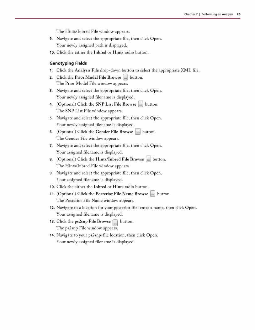
Genotyping Fields
1. Click the Analysis File drop-down button to select the appropriate XML file.
2. Click the Prior Model File Browse button.
The Prior Model File window appears.
3. Navigate and select the appropriate file, then click Open.
Your newly assigned filename is displayed.
4. (Optional) Click the SNP List File Browse button.
The SNP List File window appears.
5. Navigate and select the appropriate file, then click Open.
Your newly assigned filename is displayed.
6. (Optional) Click the Gender File Browse button.
The Gender File window appears.
7. Navigate and select the appropriate file, then click Open.
Your assigned filename is displayed.
8. (Optional) Click the Hints/Inbred File Browse button.
The Hints/Inbred File window appears.
9. Navigate and select the appropriate file, then click Open.
Your assigned filename is displayed.
10. Click the either the Inbred or Hints radio button.
11. (Optional) Click the Posterior File Name Browse button.
The Posterior File Name window appears.
12. Navigate to a location for your posterior file, enter a name, then click Open.
Your assigned filename is displayed.
13. Click the ps2snp File Browse button.
The ps2snp File window appears.
14. Navigate to your ps2snp-file location, then click Open.
Your newly assigned filename is displayed.
Chapter 2 | Performing an Analysis 21
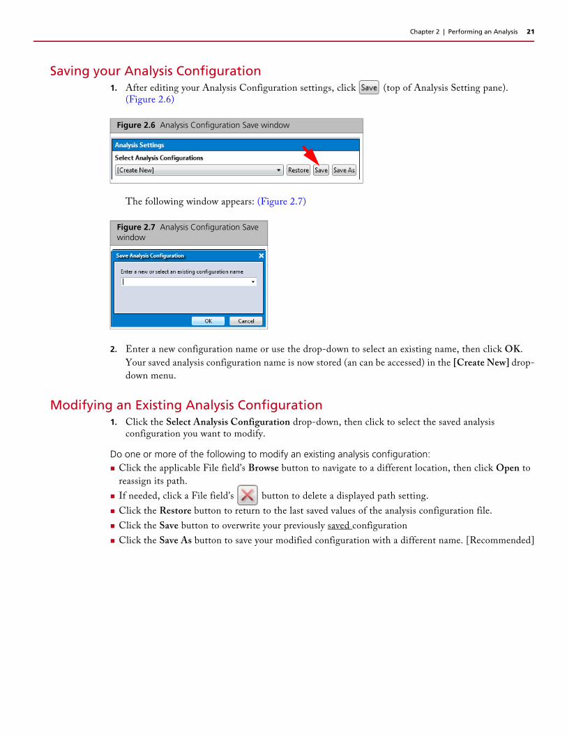
Saving your Analysis Configuration1. After editing your Analysis Configuration settings, click (top of Analysis Setting pane).
(Figure 2.6)
The following window appears: (Figure 2.7)
2. Enter a new configuration name or use the drop-down to select an existing name, then click OK.
Your saved analysis configuration name is now stored (an can be accessed) in the [Create New] drop-
down menu.
Modifying an Existing Analysis Configuration1. Click the Select Analysis Configuration drop-down, then click to select the saved analysis
configuration you want to modify.
Do one or more of the following to modify an existing analysis configuration: Click the applicable File field’s Browse button to navigate to a different location, then click Open to
reassign its path.
If needed, click a File field’s button to delete a displayed path setting.
Click the Restore button to return to the last saved values of the analysis configuration file.
Click the Save button to overwrite your previously saved configuration
Click the Save As button to save your modified configuration with a different name. [Recommended]
Figure 2.6 Analysis Configuration Save window
Figure 2.7 Analysis Configuration Save window

Chapter 2 | Performing an Analysis 22
Setting Up Threshold SettingsThe settings shown in the Threshold Setting pane (Figure 2.8) are based on the Mode (Workflow) you selected.
For Sample QC and SNP QC name definitions, see page 125.
Customizing Thresholds
1. Click the Select Threshold Configuration drop-down (Figure 2.9) to select an appropriate Default Threshold for your starting point.
Figure 2.8 Automated QC Mode Threshold Settings pane example
Figure 2.9 Select Threshold Configuration
NOTE: All Thresholds are set to Greater Than or Equal To. On the other hand, DMET arraytypes have a set threshold setting of Less Than or Equal To. These comparison signs areset and cannot be changed.

Chapter 2 | Performing an Analysis 23
Sample QCAll the Sample QC Threshold Settings are populated with default values.
1. Click inside each text field to enter a different value, as shown in Figure 2.10.
Click the text field’s button to return its value back to its last saved value within the threshold configuration file.
SNP QC
1. Click the species-type drop-down menu to select a different species type.
2. Click inside each text field to enter a different value, as shown in Figure 2.11.
Click the text field’s button to return its value back to its last saved value within the threshold configuration file.
3. Use the hom-ro and hom-het drop-down menus to change their True or False values.
4. Click inside the num-minor-allele-cutoff text field to enter a different value, as shown in Figure 2.12.
Figure 2.10 Threshold Name text field example
NOTE: General Rule: The het-so-otv-cutoff should be less or equal to het-so-cutoff.
Figure 2.11 SNP QC text fields
Figure 2.12 SNP QC text fields

Chapter 2 | Performing an Analysis 24
5. The priority-order option enables you to change the order of categories when determining which probesets are selected as the best probeset for a SNP. To change the priority-order of your SNP QC Metric, click .
The following window appears: (Figure 2.13)
6. Click and hold onto the selection you want to move, then drag and drop it into its new position. After
you get the order of priority you want, click OK.
Click the priority-order field’s button to return the list back to its default priority.
7. Use the recommended checklist to choose the PS_Classification conversion types for your analysis.
To change the recommended options, click .
The following window appears: (Figure 2.13)
8. Click to check/uncheck the available recommended options, then click OK.
Figure 2.13 Change the Priority Order window
Figure 2.14 Recommended window
NOTE: If all recommended options are unchecked, the software uses the following defaultvalues:
For Human: PolyHighResolution, NoMinorHom, MonoHighResolution, and Hemizygous.For Diploid: PolyHighResolutionFor Polyploid: PolyHighResolution

Chapter 2 | Performing an Analysis 25
Assigning an Output Folder Path
Assigning a New Output Folder Path
1. Click the Output Folder path’s Browse button. (Figure 2.15)
An Explorer window appears.
2. Navigate to the recommended path
C:\Users\Public\Documents\AxiomAnalysisSuite\Output, then click Select Folder.
Your selected output folder path is now displayed.
Adding Sub-Folders
To add sub-folders to your newly assigned result path’s folder:
1. Click the Output Folder’s Browse button to return to your assigned output path and/or folder.
2. In the Explorer window, click New Folder.
3. Enter a sub-folder name.
4. Click Select Folder.
The newly created sub-folder now appears in the output result information window.
5. Repeat the above steps 1-4 to add more sub-folders, then click Select Folder.
Assigning a Batch NameThe batch file is produced while your analysis is running and includes all the necessary files needed to view your analysis in the Axiom Analysis Suite Viewer.
1. Enter a name in the Batch Name field. (Figure 2.16)
Figure 2.15 Output Folder field
TIP: To better organize your output results, you can add sub-folders to your newlyassigned output result path’s folder.
IMPORTANT: Each Batch Name you create must be unique.
Figure 2.16 Enter a Batch Name
NOTE: A folder (with the same name as your entered batch name) is auto-generatedduring the analysis process. This folder includes all the necessary files needed to viewyour analysis results in the Viewer.

Chapter 2 | Performing an Analysis 26
Running your Analysis1. Click Run Analysis.
If you have not saved any changes to your configured Analysis Settings, a Save Analysis Configuration window appears. (Figure 2.17) Click Yes.
Enter a new analysis name or use the drop-down to select a previously saved name, then click OK.
If you have not saved any changes to your configured Threshold Settings, a Save Threshold Configuration window appears. (Figure 2.20)Click Yes.
Enter a new threshold name or use the drop-down to select a previously saved name, then click OK.
Figure 2.17 Save Analysis Configuration prompt window
Figure 2.18 Save Analysis Configuration window
Figure 2.19 Save Threshold Settings prompt window
Figure 2.20 Save Threshold Settings window

Chapter 2 | Performing an Analysis 27
The Dashboard window/tab appears and shows the status of your running analysis. (Figure 2.21) Click to cancel an analysis in progress.
Using the Dashboard Window TabThe Dashboard tab window displays existing results. (Figure 2.22)
Figure 2.21 Dashboard window/tab - Status bar and Stop button example
Figure 2.22 Dashboard window
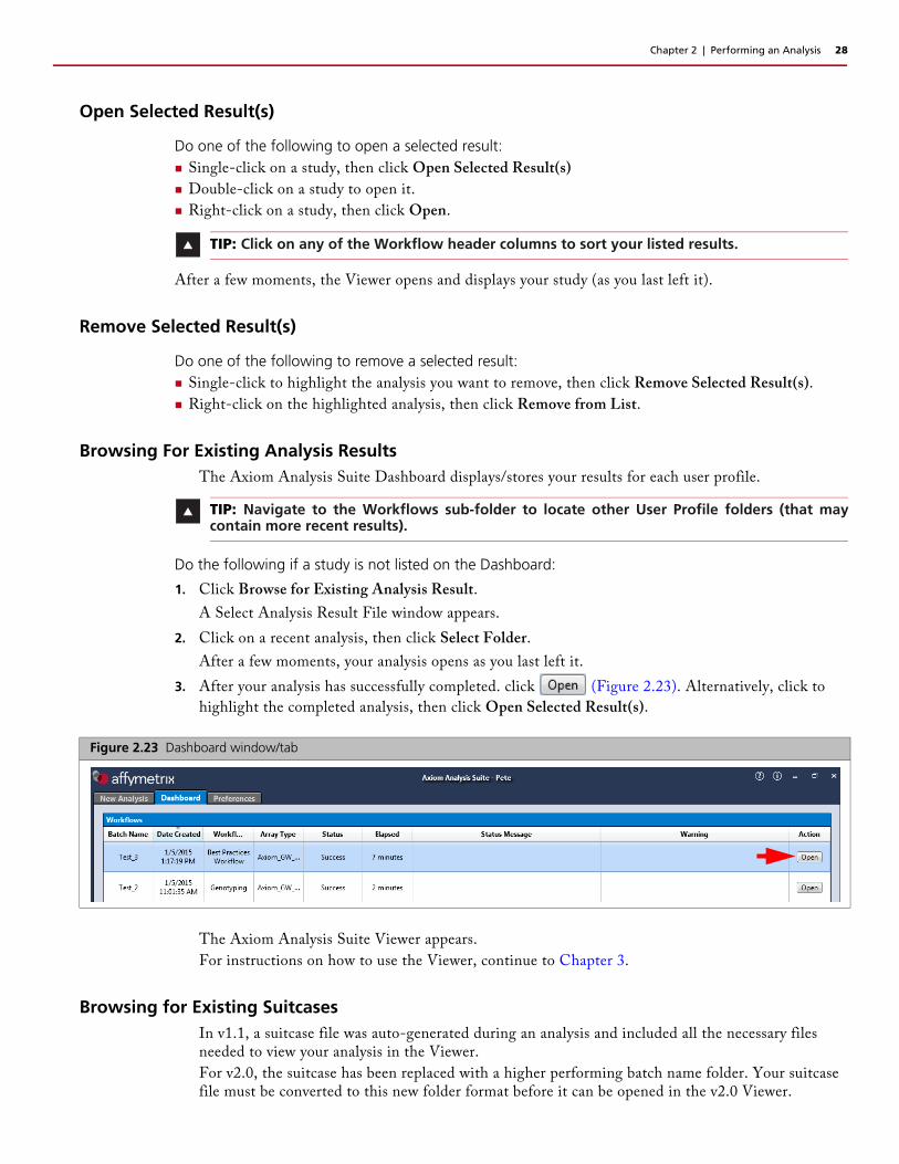
Chapter 2 | Performing an Analysis 28
Open Selected Result(s)
Do one of the following to open a selected result: Single-click on a study, then click Open Selected Result(s)
Double-click on a study to open it.
Right-click on a study, then click Open.
After a few moments, the Viewer opens and displays your study (as you last left it).
Remove Selected Result(s)
Do one of the following to remove a selected result: Single-click to highlight the analysis you want to remove, then click Remove Selected Result(s).
Right-click on the highlighted analysis, then click Remove from List.
Browsing For Existing Analysis ResultsThe Axiom Analysis Suite Dashboard displays/stores your results for each user profile.
Do the following if a study is not listed on the Dashboard:
1. Click Browse for Existing Analysis Result.
A Select Analysis Result File window appears.
2. Click on a recent analysis, then click Select Folder.
After a few moments, your analysis opens as you last left it.
3. After your analysis has successfully completed. click (Figure 2.23). Alternatively, click to
highlight the completed analysis, then click Open Selected Result(s).
The Axiom Analysis Suite Viewer appears.
For instructions on how to use the Viewer, continue to Chapter 3.
Browsing for Existing SuitcasesIn v1.1, a suitcase file was auto-generated during an analysis and included all the necessary files needed to view your analysis in the Viewer.
For v2.0, the suitcase has been replaced with a higher performing batch name folder. Your suitcase file must be converted to this new folder format before it can be opened in the v2.0 Viewer.
TIP: Click on any of the Workflow header columns to sort your listed results.
TIP: Navigate to the Workflows sub-folder to locate other User Profile folders (that maycontain more recent results).
Figure 2.23 Dashboard window/tab

Chapter 2 | Performing an Analysis 29
Do the following to convert your suitcase file to a batch name folder:
1. Click Browse for Existing Suitcase.
A Select Analysis Result File window appears.
2. Click to highlight a suitcase file, then click Open.
An Axiom Analysis Suite Suitcase Conversion message window appears. (Figure 2.24)
3. If you want to retain your v1.0 suitcase file for archiving purposes, leave the Delete suitcase file after successful conversion check box unchecked. Click on this check box if you want your suitcase file to be auto-deleted after it is converted.
4. Click OK.
Allow a few moments for your suitcase file to convert to the v1.1 batch name folder format.
The Axiom Analysis Suite Viewer appears.
For instructions on how to use the Viewer, continue to Chapter 3.
Figure 2.24 Convert suitcase file to batch name folder message

Chapter 3
The Viewer: Summary Window and Sample Table
After setting up and successfully running an analysis, as described in Chapter 2, the Axiom Analysis Suite Viewer opens. (Figure 3.1)
Figure 3.1 Main Viewer window

Chapter 3 | The Viewer: Summary Window and Sample Table 31
Viewing OptionsAs shown in Figure 3.1 on page 30, the Viewer (by default) displays a side-by-side split-screen configuration.
Split-Screen Options
To change side by side split-screen to a top and bottom configuration:
1. Click the Horizontal Split icon. (Figure 3.2)
To disable the split-screen:
1. Click the Disable Split-Screen icon. (Figure 3.3)
The split-screen becomes 1 window. (Figure 3.4)
Figure 3.2 Split Horizontal View icon and window layout example
Figure 3.3 Disable Split-Screen icon

Chapter 3 | The Viewer: Summary Window and Sample Table 32
2. Click on any window tab (Figure 3.4) to view it in full window mode.
To return to the default side by side split-screen configuration:
1. Click the Vertical Split icon. (Figure 3.5)
Figure 3.4 Full window view example
Figure 3.5 Vertical Split icon
Chapter 3 | The Viewer: Summary Window and Sample Table 33
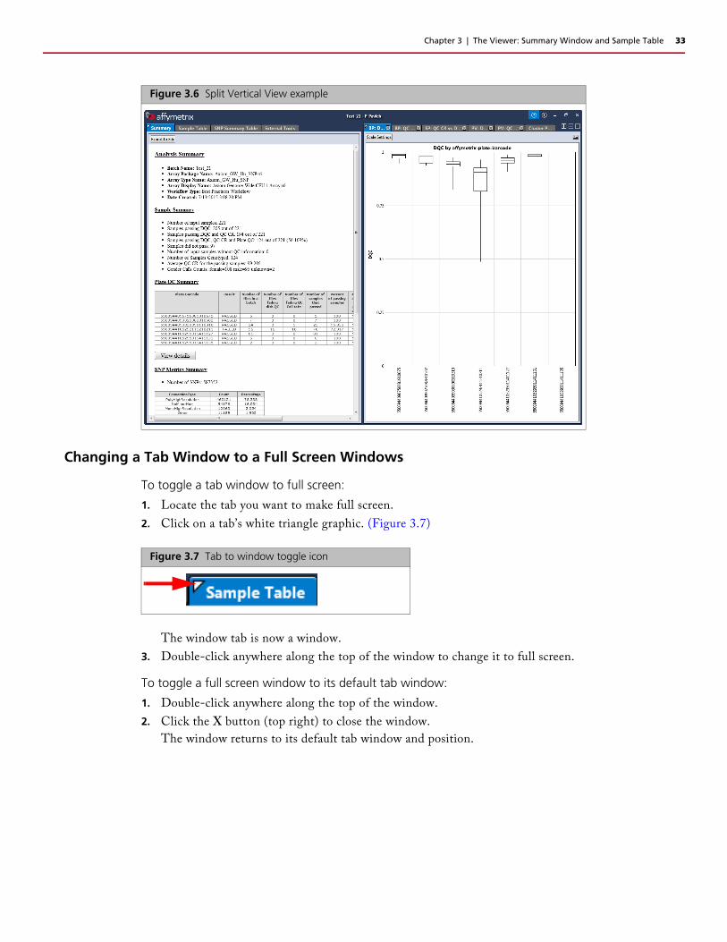
Changing a Tab Window to a Full Screen Windows
To toggle a tab window to full screen:
1. Locate the tab you want to make full screen.
2. Click on a tab’s white triangle graphic. (Figure 3.7)
The window tab is now a window.
3. Double-click anywhere along the top of the window to change it to full screen.
To toggle a full screen window to its default tab window:
1. Double-click anywhere along the top of the window.
2. Click the X button (top right) to close the window.
The window returns to its default tab window and position.
Figure 3.6 Split Vertical View example
Figure 3.7 Tab to window toggle icon

Chapter 3 | The Viewer: Summary Window and Sample Table 34
Adjusting the Window Size
To change the size of a window pane:
1. Click, hold, then drag the edge of the window pane (Figure 3.8) to resize it.
Figure 3.8 Split Vertical View example

Chapter 3 | The Viewer: Summary Window and Sample Table 35
Summary Window/TabThe Summary window/tab (Figure 3.9) displays a summary snapshot of your analysis, including detailed threshold values, and tables based on your analysis.
Data Analysis Summary
NOTE: Each workflow type reports different information within the Analysis Summary window. Figure 3.9 is an example of a Best Practices workflow.
Figure 3.9 Summary window tab
Analysis Summary: Contains informa-tion about the array type, the workflow run and the date processed
Sample Summary: Breaks down the sample QC for your analysis run and dis-plays the number that pass each of your QC Thresholds. In addition, it provides the average QC Call Rate (CR) and breakdown of the gen-ders found within your batch of samples.
Plate QC Summary: Contains sample QC information for each plate including the number samples failing DQC, QC Call Rate, the Percent of passing samples. and the average Call Rate for your passing samples.
SNP Metrics Summary: This section con-tains a summary of the categorization of the SNPs in the analysis by PS_Classification. For more information on these categories see “Regenerate SNP Metric” on page 67.
Sample QC Thresholds: Displays the Sample QC Thresholds used for your analysis run and their associated SNP QC Metrics.
SNP QC Thresholds: Displays the Thresholds used for your analysis run and their associated SNP QC Metrics.
Export to File: Click this button to export the Summary report as a PDF file.

Chapter 3 | The Viewer: Summary Window and Sample Table 36
Viewing the Plate Barcode Table Details1. In the Summary window tab, click . (Figure 3.9)
A window opens and displays a text file version of your Sample QC information (by plate). (Figure 3.10)
Figure 3.10 Notepad window

Chapter 3 | The Viewer: Summary Window and Sample Table 37
Sample Table
Figure 3.11 Sample Table window tab
NOTE: Depending on the Threshold values you set (prior to running your analysis), color-codedPass or Fail cells may appear in the table, as shown in Figure 3.11.

Chapter 3 | The Viewer: Summary Window and Sample Table 38
Importing Sample Attributes
To import sample attributes into your Sample Table:
1. Click the Import Sample Attributes drop-down.
2. Click to select either Import from ARR Files or Import from CSV/Tab-Delimited Text File.
An Explorer window appears.
3. Navigate to the applicable file location, then click Open.
Column HeadersThe default Sample Table column view is as shown. (Figure 3.13)
To show or hide table columns:
1. Click the Show/Hide Columns drop-down menu.
2. Click each available column name’s check box to show it or remove it from the table. See Annotations and Columns on page 123 for their definitions.
3. Click outside the Show/Hide Columns drop-down menu to close it.
To save your customized Sample Table column view:
1. Click Save View.
The following window appears: (Figure 3.14)
2. Enter a name for your custom table view, then click OK.
Your newly saved name is now added to the Apply View drop-down menu.
IMPORTANT: Your text-based CEL file must start with the header Sample Filename andinclude the full CEL file name, as shown in Figure 3.2.
Figure 3.12 Tab-delimited text CEL file example shown in Excel
Figure 3.13 Default Sample Table Columns
Figure 3.14 Save New Custom View

Chapter 3 | The Viewer: Summary Window and Sample Table 39
To show ALL available columns within the Sample Table:
1. Click the Apply View drop-down menu, then select All Columns View.
Rearranging Columns
1. Click on a column you want to move.
2. Drag it (left or right) to its new location.
3. Release the mouse button.
The column is now in its new position.
Sorting Columns
1. Select a column, then right-click on it.
A right-click menu appears. (Figure 3.15)
2. Click to select either Sort By Ascending (A-Z) or Sort By Descending (Z-A).
Single-Click Sorting Method
1. Single-click on a column header to sort its data in an ascending order. Single-click on the same column header to sort its data in a descending order
Hiding the Column
1. Select the column you want to hide from the table, then right-click on it.
A right-click menu appears. (Figure 3.15)
2. Click the Hide Column check box to remove it from the table.
Figure 3.15 Right-click Column Menu

Chapter 3 | The Viewer: Summary Window and Sample Table 40
Filtering Column Data
Adding Filters (Method 1)1. Select a column, then right-click on it.
The following window appears: (Figure 3.16)
2. Click Filter.
Text-based ColumnsIf the column you want to filter contains text-based data, the Contains drop-down menu appears. (Figure 3.17)
To apply a filter to a text-based column:
1. Click the Contains drop-down menu to select a filtering property. (Figure 3.18)
2. Click inside the text entry box to enter a value. (Figure 3.18)
NOTE: All Sample Table columns are filterable.
Figure 3.16 Right-click Column Menu
Figure 3.17 Filter Properties
Figure 3.18 Drop-down Menu

Chapter 3 | The Viewer: Summary Window and Sample Table 41
3. OPTIONAL: Click to add additional filters.
4. Click the Or or And radio button to choose Or or AND relationship logic. (Figure 3.19)
5. Repeat steps 1-4 as needed.
6. To remove a filter(s), click .
Numeric Data ColumnsIf the column you want to filter contains numeric data, a symbol drop-down menu appears. (Figure 3.20)
To apply a filter to a value-based column:
1. Click the Symbol Value drop-down menu to select the filtering symbol you want. (Figure 3.21)
2. Click inside the text entry box to enter the value(s). (Figure 3.21)
Figure 3.19 Or or And Relationship Logic
Figure 3.20 Filter Properties
Figure 3.21 Drop-down Menu

Chapter 3 | The Viewer: Summary Window and Sample Table 42
3. OPTIONAL: Click to add filter(s).
4. Click the Or or And radio button to choose Or or AND relationship logic. (Figure 3.22)
5. If needed, repeat steps 1-4.
6. Click OK.
To remove a filter(s), click .
Showing Filtered Data Only Click the Show Filtered Only check box to show only the data that passes the filters.
Uncheck this box to show all data, including data that did not pass your filter criteria setting(s). In this mode, data that passes the filter appears in light gray, as shown in Figure 3.23.
Figure 3.22 Or or And Relationship Logic
Figure 3.23 Sample Table window tab - Show Filter Only unchecked example

Chapter 3 | The Viewer: Summary Window and Sample Table 43
Clearing an Individual Filter
1. Right-click on the filtered column you want to clear.
The following window appears: (Figure 3.24)
2. Click Clear Current Column Filter.
The filter is removed.
Clearing All Current Filters Click the Filters drop-down, then select Clear Current Filters. (Figure 3.25)
Adding Filters (Method 2)
1. Click the Filters drop-down menu, then click Manage Filters.
The Manage Filters window appears. (Figure 3.26)
Figure 3.24 Right-click Column Menu
Figure 3.25 Filters Menu
TIP: Use this method if you want to change more than one of your Sample Table column filtersat the same time.
Figure 3.26 Manage Filters window
Chapter 3 | The Viewer: Summary Window and Sample Table 44
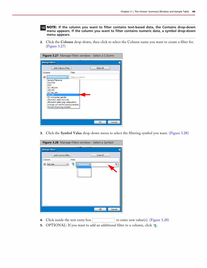
2. Click the Column drop-down, then click to select the Column name you want to create a filter for. (Figure 3.27)
3. Click the Symbol Value drop-down menu to select the filtering symbol you want. (Figure 3.28)
4. Click inside the text entry box to enter new value(s). (Figure 3.28)
5. OPTIONAL: If you want to add an additional filter to a column, click .
NOTE: If the column you want to filter contains text-based data, the Contains drop-downmenu appears. If the column you want to filter contains numeric data, a symbol drop-downmenu appears.
Figure 3.27 Manage Filters window - Select a Column
Figure 3.28 Manage Filters window - Select a Symbol

Chapter 3 | The Viewer: Summary Window and Sample Table 45
6. Click the Or or And radio button to choose Or or AND relationship logic. (Figure 3.29)
7. If needed, click Add Column Filter, then repeat the above steps. (Figure 3.30)
8. Click OK.
To remove a filter(s), click .
Click Clear All to remove ALL filters in the Manage Filters window.
Figure 3.29 Manage Filters window - OR or AND Relationship
Figure 3.30 Manage Filters window - Adding another Column Filter

Chapter 3 | The Viewer: Summary Window and Sample Table 46
Copying Column Data
To copy column data to your clipboard:
1. Click to select a column you want to copy to a clipboard, then right-click on it.
The following window appears: (Figure 3.31)
2. Click Copy Column.
The column data is now ready for pasting (Ctrl v).
Setting User ColorsUse this feature to more easily identify different sets between the Sample Table and Cluster Graph.
Assigning a Color to a Sample
1. Right-click on the sample you want to assign a color to.
A menu appears. (Figure 3.32)
2. Mouse over Set User Color.
A color pallet appears.
3. Click on the color you want.
Figure 3.31 Right-click Column Menu
Figure 3.32 Right-click menu - Set User Color
Chapter 3 | The Viewer: Summary Window and Sample Table 47
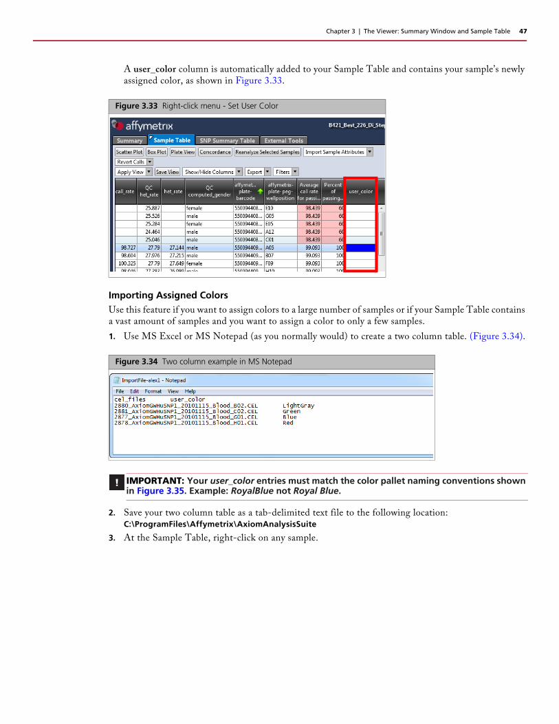
A user_color column is automatically added to your Sample Table and contains your sample’s newly assigned color, as shown in Figure 3.33.
Importing Assigned ColorsUse this feature if you want to assign colors to a large number of samples or if your Sample Table contains a vast amount of samples and you want to assign a color to only a few samples.
1. Use MS Excel or MS Notepad (as you normally would) to create a two column table. (Figure 3.34).
2. Save your two column table as a tab-delimited text file to the following location:C:\ProgramFiles\Affymetrix\AxiomAnalysisSuite
3. At the Sample Table, right-click on any sample.
Figure 3.33 Right-click menu - Set User Color
Figure 3.34 Two column example in MS Notepad
IMPORTANT: Your user_color entries must match the color pallet naming conventions shown in Figure 3.35. Example: RoyalBlue not Royal Blue.

Chapter 3 | The Viewer: Summary Window and Sample Table 48
A menu appears. (Figure 3.35)
4. Mouse over Set User Color.
5. Click on Import File...
An Import User Colors Explorer window appears.
6. Click to highlight your (.TXT) file, then click Open.
The two column table entries are now incorporated into the Sample Table.
7. Scroll the Sample Table right to see the added user_color column and assigned sample colors.
Viewing User Colors in the Cluster Graph1. From the Cluster Graph, click the Color By drop-down menu. (Figure 3.36)
Figure 3.35 Right-click menu - Set User Color - Import File
Figure 3.36 Color By menu - user_color
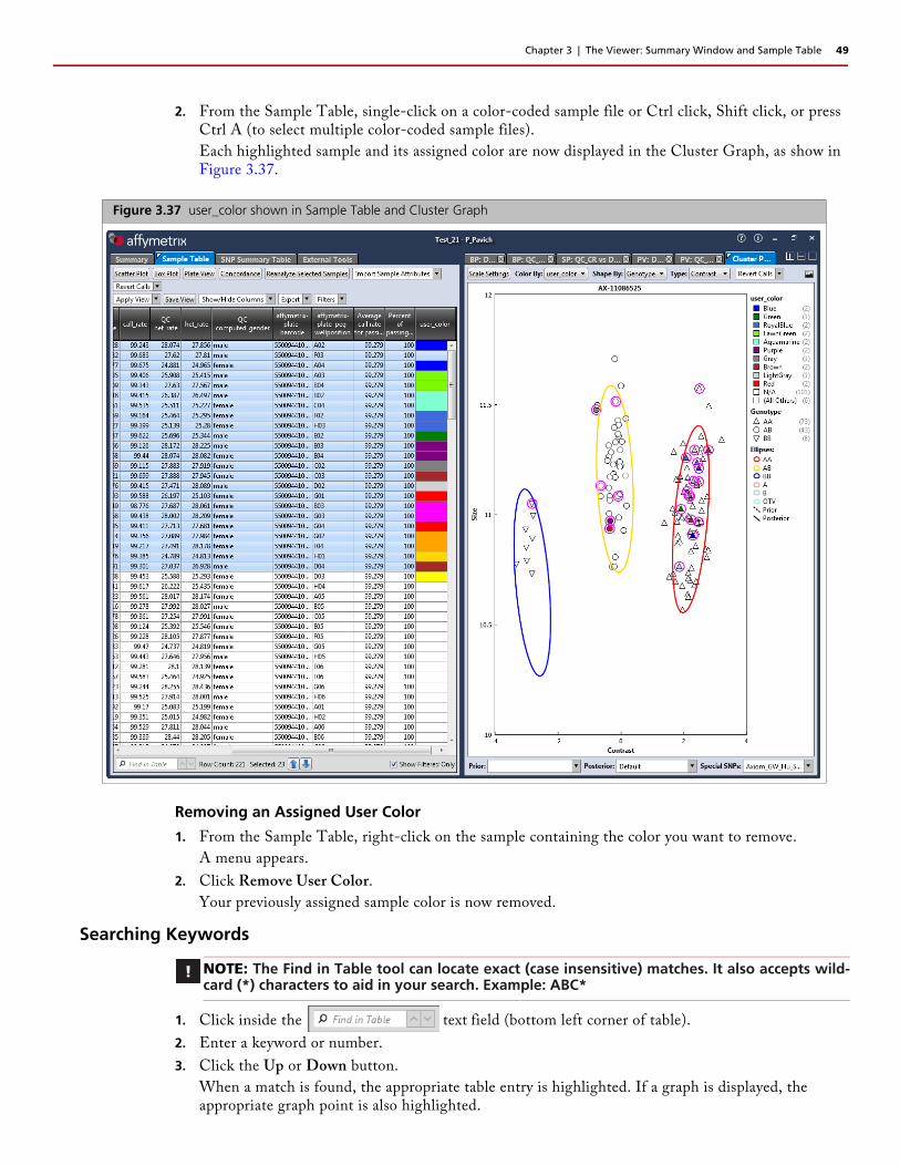
Chapter 3 | The Viewer: Summary Window and Sample Table 49
2. From the Sample Table, single-click on a color-coded sample file or Ctrl click, Shift click, or press Ctrl A (to select multiple color-coded sample files).
Each highlighted sample and its assigned color are now displayed in the Cluster Graph, as show in Figure 3.37.
Removing an Assigned User Color
1. From the Sample Table, right-click on the sample containing the color you want to remove.
A menu appears.
2. Click Remove User Color.
Your previously assigned sample color is now removed.
Searching Keywords
1. Click inside the text field (bottom left corner of table).
2. Enter a keyword or number.
3. Click the Up or Down button.
When a match is found, the appropriate table entry is highlighted. If a graph is displayed, the appropriate graph point is also highlighted.
Figure 3.37 user_color shown in Sample Table and Cluster Graph
NOTE: The Find in Table tool can locate exact (case insensitive) matches. It also accepts wild-card (*) characters to aid in your search. Example: ABC*

Chapter 3 | The Viewer: Summary Window and Sample Table 50
Box Plots
Viewing the Default Box PlotsBy default, the Viewer generates 2 Box Plots.
Figure 3.38 Table and Box Plot 1
NOTE: You you cannot change a plot’s axis values after it has been created. However, you canchange its scale and coloring properties. See Changing the Box Plot’s Scale Setting Ranges onpage 51.
To change a Box Plot’s axis properties, you must create a new Box Plot. See Adding a NewBox Plot on page 51.
Chapter 3 | The Viewer: Summary Window and Sample Table 51
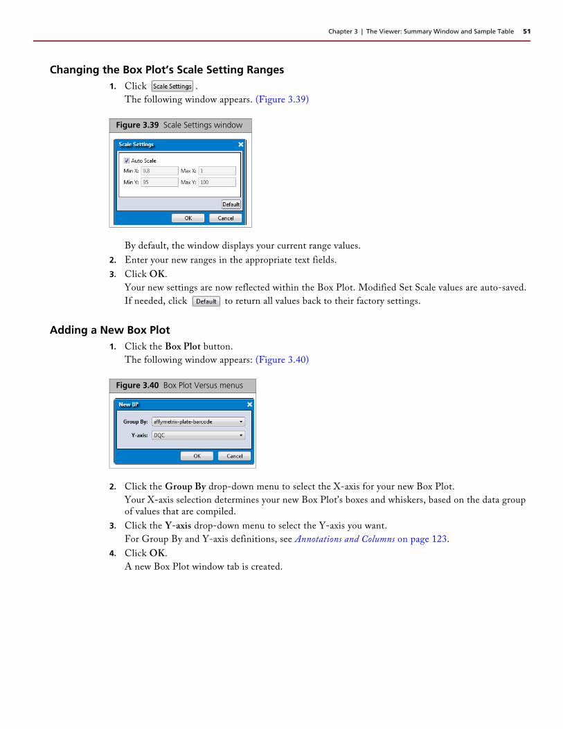
Changing the Box Plot’s Scale Setting Ranges1. Click .
The following window appears. (Figure 3.39)
By default, the window displays your current range values.
2. Enter your new ranges in the appropriate text fields.
3. Click OK.
Your new settings are now reflected within the Box Plot. Modified Set Scale values are auto-saved.
If needed, click to return all values back to their factory settings.
Adding a New Box Plot1. Click the Box Plot button.
The following window appears: (Figure 3.40)
2. Click the Group By drop-down menu to select the X-axis for your new Box Plot.
Your X-axis selection determines your new Box Plot’s boxes and whiskers, based on the data group of values that are compiled.
3. Click the Y-axis drop-down menu to select the Y-axis you want.
For Group By and Y-axis definitions, see Annotations and Columns on page 123.
4. Click OK.
A new Box Plot window tab is created.
Figure 3.39 Scale Settings window
Figure 3.40 Box Plot Versus menus

Chapter 3 | The Viewer: Summary Window and Sample Table 52
Reading Box Plot Percentiles (Figure 3.41)
At any time, click X to remove a window/tab. (Figure 3.42)
Saving the Current Box Plot View1. Click the Save Image button.
An Explorer window appears.
2. Navigate to where you want to save the .PNG file, enter a filename, then click Save.
Figure 3.41 Box Plot percentiles
Figure 3.42 New Window/Tab
100%
75%50%25%
0%

Chapter 3 | The Viewer: Summary Window and Sample Table 53
Scatter PlotBy default, the Viewer generates 1 Scatter Plot of QC call_rate vs. DQC. The data displayed in the plot are colored and shaped by QC computed_gender, as shown in Figure 3.43.
Viewing the Default Scatter Plot1. Click to highlight a table entry to view its location within the Scatter Plot or click on a data point to
highlight its corresponding entry in the Sample Table. (Figure 3.43)
Figure 3.43 Table and Scatter Plot
NOTE: You cannot change the default Scatter Plot’s pre-defined X and Y definitions, howeveryou can change its Scale Settings and Color By and Shape By configuration.
To change a Scatter Plot’s axis properties, you must create a new Scatter Plot. See Adding aNew Scatter Plot and Selecting its X and Y Properties on page 54.

Chapter 3 | The Viewer: Summary Window and Sample Table 54
Changing the Scatter Plot’s Setting Ranges1. Click .
The following window appears. (Figure 3.44)
By default, the window displays your current range values.
2. Enter your new ranges in the appropriate text fields.
3. Click OK.
Your new settings are now reflected within the Scatter Plot. Modified Set scale values are auto-saved.
If needed, click to return all values back to their factory settings.
Adding a New Scatter Plot and Selecting its X and Y Properties1. Click the Scatter Plot button.
The following window appears: (Figure 3.45)
2. Use the drop-down menus to select your Plot’s versus scenario (X and Y axis). See Appendix C, Definitions on page 120 for definitions.
3. Click OK.
A new Scatter Plot window tab is created.
At any time, click X to remove a window/tab. (Figure 3.46)
Figure 3.44 Scale Settings window
Figure 3.45 Scatter Plot Versus menus
Figure 3.46 New Window/Tab

Chapter 3 | The Viewer: Summary Window and Sample Table 55
4. Click the Color By and Shape By drop-down menus to select the combination view you want. See Sample QC Metrics on page 120 for Color By and Shape By definitions.
A legend appears within the plot. (Figure 3.47)
The graph can display up to 10 different colors and up to 10 different shapes. If the attributes selected for display have more than 10 categories, categories 1 through 9 are displayed normally, but categories 10 and higher get grouped together.
If your study has more than 10 values: If the value is text, the software takes the first nine values and assigns each a color or shape. The
remaining values are put into a bin called “Other¨. All values in the Other bin have the same color or shape.
If the value is a date or number, the software divides the range of data into 10 equal bins and assigns a color or shape to each bin. If the data includes one or more outliers, it is possible to have one value in a particular bin and all other values in another bin.
NOTE: Your imported sample attributes are also available for use within the Color By andShape By drop-down menus. For information on importing sample attributes, go to ImportingSample Attributes on page 38.
Figure 3.47 Color By and Shape By Legend example

Chapter 3 | The Viewer: Summary Window and Sample Table 56
Customizing Color By Settings1. Click .
The Color Scale Configuration window appears. (Figure 3.48)
2. Use the provided text fields and color drop-down menus to customize your Color By selection.
Auto Scale check box (when checked) uses the actual minimum (lower bound) and maximum (upper
bound) as your min/max scale. Uncheck the Auto Scale check box to enter your min and max number
scales in the provided fields.
Click the Cutoff Type drop-down menu to select your cutoff preference.
Above Cutoff Failing - This presents a hard visual cutoff graph of all values that fail ABOVE the
Cutoff value entered. The Above Cutoff data is represented by the color defined for Max. (Green in
Figure 3.48)
Below Cutoff Failing - This presents a hard visual cutoff graph of all values that fail BELOW the
Cutoff value entered. The Below Cutoff data is represented by the color defined for Min. (Red in
Figure 3.49)
Figure 3.48 Color By options
Figure 3.49 Below Cutoff

Chapter 3 | The Viewer: Summary Window and Sample Table 57
No Cutoff - This presents a smooth 3-point gradient of your defined Max, Min, and colors.
(Figure 3.50)
3. Click OK.
Your Cutoff preference, entered values, and color selections are now displayed on the graph and saved
for future use. If needed, click to revert all values back to their factory settings.
Saving the Current Scatter Plot View1. Click the Save Image button.
An Explorer window appears.
2. Navigate to where you want to save the .PNG file, enter a filename, then click OK.
Figure 3.50 No Cutoff

Chapter 3 | The Viewer: Summary Window and Sample Table 58
Plate ViewsBy default, the Viewer generates 2 Plate Views. Plate View 1’s metric is set to DQC by Plate. Plate View 2’s metric is set to QC call_rate by Plate. To display a different metric you must create a new Plate View. For more details, see Adding a New Plate View Metric on page 59.
The Plate Views display the currently selected (highlighted) metric from the Sample Table and are a graphic representation of the plate used. For example, 96 count plate layouts are shown in Figure 3.51.
Viewing the Default Plate Views1. Click to highlight a table entry to view its location within the Plate View or click on a plate position
to highlight its corresponding table entry. (Figure 3.51)
Figure 3.51 Table and Plate View 1
NOTE: You cannot change a default Plate View, however you can change its Scale Settings,as well as gradient and coloring. See To customize your Plate View settings: on page 59.

Chapter 3 | The Viewer: Summary Window and Sample Table 59
Adding a New Plate View MetricThe default Plate Views cannot be altered, therefore you must click the Plate View button to create a new Plate View to reflect your Metric change.
1. Click the Plate View button.
The following window appears: (Figure 3.52)
2. Use the drop-down menus to select your Plate View’s Metric setting. See the tables in Appendix C, Definitions on page 120 for Metric definition.
3. Click OK.
The new Plate View window tab appears.
At any time, click X to remove a window/tab. (Figure 3.53)
To customize your Plate View settings:
1. Click .
The Color Scale Configuration window appears. (Figure 3.54)
2. Use the provided text fields and color drop-down menus to customize your Color By selection.
Auto Scale check box (when checked) uses the actual minimum (lower bound) and maximum (upper bound) as your min/max scale. Uncheck the Auto Scale check box to enter your min and max number scales in the provided fields. Note: If the Auto Scale check box remains unchecked, you must enter new scale limits for each subsequent analysis.
Figure 3.52 Plate View Metric setting
Figure 3.53 New Window/Tab
Figure 3.54 Color Scale options

Chapter 3 | The Viewer: Summary Window and Sample Table 60
Click the Cutoff Type drop-down menu to select the appropriate cutoff (based on the custom Cutoff value you entered).
3. Click OK.
Your new preferences are now displayed and saved for future use.
At any time, click the Default button to revert all the Color Scale Configuration window values back to their factory setting.
Saving the Current Plate View1. Click the Save Image button.
An Explorer window appears.
2. Navigate to where you want to save the .PNG file, enter a filename, then click OK.
Concordance Checks Compare all combinations enables you to compare the SNP calls for all samples. The concordance
between all pairwise comparisons for the samples in the dataset/suitcase are reported.
Compare to reference enables you to compare every sample to a single reference file.
Running a Concordance Check1. Click the Concordance button.
The following window appears: (Figure 3.55)
To compare all combinations:
1. Make sure the Compare all combinations radio button is selected.
2. By default, the Compare all SNPs button is selected. If needed, click the Compare signature SNPs within the SNP Summary Table, or Compare signature SNPs radio button.
3. Click OK.
After a few moments, the following Concordance window tab appears: (Figure 3.56)
Figure 3.55 Concordance window
NOTE: The amount of time to calculate concordance is proportional to the number of samplesand SNPs. It is highly recommended you use <1000 SNPs for an All versus All concordancecheck.

Chapter 3 | The Viewer: Summary Window and Sample Table 61
For definitions of the Concordance columns, see Concordance Columns on page 125.
To compare to reference:
1. Click the Compare to reference button.
The Browse for the reference file field is now activated.
2. Click the Browse button.
A Windows Explorer window appears.
3. Navigate to the appropriate reference file location, then click Open.
Your Reference file is displayed.
4. By default, the Compare all SNPs button is selected. If needed, click the Compare signature SNPs within the SNP Summary Table, or Compare signature SNPs radio button.
5. Click OK.
After a few moments, a Concordance window tab appears.
Figure 3.56 Default Concordance Table example
NOTE: The reference file you select can have more than two columns. However, only the first2 columns are used during the Compare to Reference concordance check. Also, your referencegenotypes must be reported using letter call codes (e.g. AA, AB, BB, NoCall).

Chapter 3 | The Viewer: Summary Window and Sample Table 62
Reanalyzing Samples
To reanalyze sample(s) displayed in the Sample Table:
1. Single-click on a CEL file or Ctrl click, Shift click, or press Ctrl A (to select multiple files).
2. Click the Reanalyze Selected Samples button.
The following message appears. (Figure 3.57)
3. Click OK.
The Viewer closes. Your selected samples are displayed and ready for re-analysis in a New Analysis window tab. (Figure 3.58)
4. See Chapter 2, Performing an Analysis on page 16 for instructions on setting up an analysis.
Figure 3.57 Viewer will be closed message
Figure 3.58 New Analysis window tab

Chapter 4
The Viewer: SNP Summary Table and Cluster Plot
SNP Summary TableFigure 4.1 represents a standard SNP Summary Table
Figure 4.2 on page 64 represents a SNP Summary Table with CN-aware genotyping and Allele
Translation. The button only appears if supported arrays are available. See
Chapter 5, Allele Translation on page 80 for more information.
A SNP Summary Table with CN-aware genotyping also displays a count of calls for hemizygous genotypes (n_A, n_B) and a count of ZeroCN calls (n_CN0), as shown in Figure 4.2. These additional columns appear for arrays that support copy number-aware genotyping. For more information, see Appendix A, Copy Number Aware Genotyping on page 99.
Figure 4.1 SNP Summary Table window

Chapter 4 | The Viewer: SNP Summary Table and Cluster Plot 64
Using the SNP Summary Table
Setting your SNP Summary Table View1. Click the Apply View drop-down. (Figure 4.3)
The Default View is the initial table view and includes a preset number of columns.
The All Columns View displays the maximum available columns.
Adding and Removing Table Columns
1. Click the Show/Hide Columns drop-down. (Figure 4.4)
A list of available columns appear.
Figure 4.2 SNP Summary Table with CN-aware genotyping and Allele Translation
Figure 4.3 Apply View drop-down
Figure 4.4 Show/Hide Columns drop-down
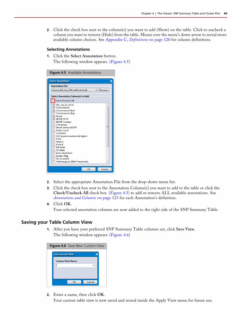
Chapter 4 | The Viewer: SNP Summary Table and Cluster Plot 65
2. Click the check box next to the column(s) you want to add (Show) on the table. Click to uncheck a column you want to remove (Hide) from the table. Mouse over the menu’s down arrow to reveal more available column choices. See Appendix C, Definitions on page 120 for column definitions.
Selecting Annotations
1. Click the Select Annotation button.
The following window appears. (Figure 4.5)
2. Select the appropriate Annotation File from the drop-down menu list.
3. Click the check box next to the Annotation Column(s) you want to add to the table or click the Check/Uncheck All check box (Figure 4.5) to add or remove ALL available annotations. See Annotations and Columns on page 123 for each Annotation’s definition.
4. Click OK.
Your selected annotation columns are now added to the right side of the SNP Summary Table.
Saving your Table Column View1. After you have your preferred SNP Summary Table columns set, click Save View.
The following window appears: (Figure 4.6)
2. Enter a name, then click OK.
Your custom table view is now saved and stored inside the Apply View menu for future use.
Figure 4.5 Available Annotations
Figure 4.6 Save New Custom View

Chapter 4 | The Viewer: SNP Summary Table and Cluster Plot 66
Copying Selected Row(s)1. Right-click on a row you want to copy. Optional: Single-click on a row or Ctrl click, Shift click, or
press Ctrl A (to select multiple rows).
A menu appears. (Figure 4.7)
2. Click Copy Selected Row(s).
The row data is now ready for pasting (Ctrl v).
Copying Selected Cell(s)1. Right-click on a cell you want to copy. Optional: Single-click on a row or Ctrl click, Shift click, or
press Ctrl A (to select multiple cells).
A menu appears. (Figure 4.7)
2. Click Copy Selected Cell(s).
The cell data is now ready for pasting (Ctrl v).
Changing or Reverting Genotype CallsReverting Calls changes them back to what they were originally called by the algorithm. No other history is saved, only its current and original values.
1. Click the Change/Revert Calls drop-down.
The following menu appears: (Figure 4.8)
To change genotype calls by text file:
1. Click Change Calls By Text File.
An Explorer window appears.
2. Navigate to the text file’s location.
Figure 4.7 Right-click menu
Figure 4.8 Revert Calls drop-down menu
IMPORTANT: Your Change Call by Text file must start with the header probeset_id anduse numeric or alphabetic codes for the genotype, as shown in Figure 4.9. It also cannotcontain any annotation columns.
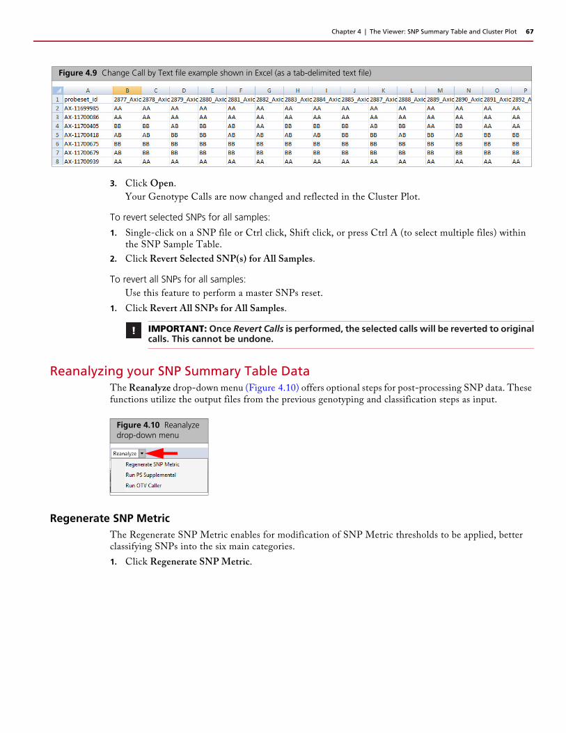
Chapter 4 | The Viewer: SNP Summary Table and Cluster Plot 67
3. Click Open.
Your Genotype Calls are now changed and reflected in the Cluster Plot.
To revert selected SNPs for all samples:
1. Single-click on a SNP file or Ctrl click, Shift click, or press Ctrl A (to select multiple files) within the SNP Sample Table.
2. Click Revert Selected SNP(s) for All Samples.
To revert all SNPs for all samples:Use this feature to perform a master SNPs reset.
1. Click Revert All SNPs for All Samples.
Reanalyzing your SNP Summary Table DataThe Reanalyze drop-down menu (Figure 4.10) offers optional steps for post-processing SNP data. These functions utilize the output files from the previous genotyping and classification steps as input.
Regenerate SNP MetricThe Regenerate SNP Metric enables for modification of SNP Metric thresholds to be applied, better classifying SNPs into the six main categories.
1. Click Regenerate SNP Metric.
Figure 4.9 Change Call by Text file example shown in Excel (as a tab-delimited text file)
IMPORTANT: Once Revert Calls is performed, the selected calls will be reverted to originalcalls. This cannot be undone.
Figure 4.10 Reanalyze drop-down menu

Chapter 4 | The Viewer: SNP Summary Table and Cluster Plot 68
The following window appears: (Figure 4.11)
1. Use the drop-down to select the appropriate Posterior File or click its Browse button.
An Explorer window appears.
2. Navigate to Posterior File you want to use, then click Open.
3. Choose an appropriate ps2snp File (recommended), as described in Saving your Analysis Configuration on page 21.
4. Select the Threshold Configuration you want to use, as described inCustomizing Thresholds on page 22.
5. Use the SNP QC drop-down menus, and text fields to setup the regeneration of your SNP Metric.
6. To change the priority-order of your SNP QC Metric, click .
Figure 4.11 Regenerate SNP Metric window

Chapter 4 | The Viewer: SNP Summary Table and Cluster Plot 69
The following window appears: (Figure 4.12)
7. Click and hold onto the selection you want to move, then drag and drop it into its new position. After
you get the order of priority you want, click OK.
8. To change the recommended options, click .
The following window appears: (Figure 4.12)
9. Click to check/uncheck the available recommended options. At anytime, click a field’s button to return its value back to its default setting.
10. Click OK.
After the process is complete, your SNP Summary Table is updated.
Figure 4.12 Change the Priority Order window
Figure 4.13 Recommended window

Chapter 4 | The Viewer: SNP Summary Table and Cluster Plot 70
Running PS SupplementalThe PS_Supplemental performs further classification that may be needed for polyploid organisms, complex genomes, or inbred populations.
1. Click Run PS Supplemental.
The following window appears: (Figure 4.14)
1. Use the drop-down to select the appropriate Posterior File or click its Browse button.
An Explorer window appears.
2. Navigate to Posterior File you want to use, then click Open.
3. Select the Threshold Configuration you want to use, as described in Customizing Thresholds on page 22.
4. Use the PS Supplemental drop-down menus, and text fields to setup and run your PS Supplemental.
5. To change the variance-class options, click .
Figure 4.14 Run PS Supplemental window

Chapter 4 | The Viewer: SNP Summary Table and Cluster Plot 71
The following window appears: (Figure 4.12)
6. Click to check/uncheck the available variance-class options.
7. Click OK.
Running OTV CallerThe OTV Caller is intended for SNPs that have been classified as OTV or markers with unusually large Y-dimension variance (as identified by PS_Supplemental).
OTV Caller function performs post-processing analysis to identify miscalled clustering and identify which samples should be in the OTV cluster and which samples should remain in the AA, AB, or BB clusters. Samples in the OTV cluster are re-labeled as OTV.
1. Click Run OTV Caller.
The following window appears: (Figure 4.14)
1. Use the drop-down to select the appropriate Posterior File or click its Browse button.
An Explorer window appears.
2. Navigate to Posterior File you want to use, then click Open.
3. Click the Select Pid File’s Browse button.
An Explorer window appears.
4. Navigate to Pid File you want to use, then click Open.
5. Click OK.
Figure 4.15 Variance-class window
Figure 4.16 Run OTV Caller window

Chapter 4 | The Viewer: SNP Summary Table and Cluster Plot 72
Managing your SNP ListThe Axiom Analysis Suite enables lists of SNPs to be saved with the application.
Use the Manage SNP List drop-down menu (Figure 4.17) to perform one of the following:
Saving your current SNP List1. To save all SNPs currently displayed in the SNP Summary Table, click Create SNP List from Table.
The following window appears: (Figure 4.18)
2. Enter a name, then click OK.
Exporting your SNP ListBefore exporting a SNP List you must first create one. If no SNP Lists are detected, a message box appears. Click OK to acknowledge the message, then go to Saving your current SNP List to create a SNP List.
1. Click Export Saved SNP List to Text File.
An Explorer window appears.
2. Navigate to an export location, enter a name, then click Save.
Importing a SNP List1. Click Import SNP List to Batch.
An Explorer window appears.
2. Navigate to your SNP List location containing your tab-delimited text file.
Figure 4.17 Manage SNP List drop-down menu
Figure 4.18 Save SNP List
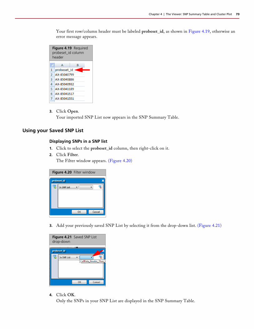
Chapter 4 | The Viewer: SNP Summary Table and Cluster Plot 73
Your first row/column header must be labeled probeset_id, as shown in Figure 4.19, otherwise an error message appears.
3. Click Open.
Your imported SNP List now appears in the SNP Summary Table.
Using your Saved SNP List
Displaying SNPs in a SNP list
1. Click to select the probeset_id column, then right-click on it.
2. Click Filter.
The Filter window appears. (Figure 4.20)
3. Add your previously saved SNP List by selecting it from the drop-down list. (Figure 4.21)
4. Click OK.
Only the SNPs in your SNP List are displayed in the SNP Summary Table.
Figure 4.19 Required probeset_id column header
Figure 4.20 Filter window
Figure 4.21 Saved SNP List drop-down

Chapter 4 | The Viewer: SNP Summary Table and Cluster Plot 74
Displaying SNPs that are not in your SNP List
1. Click to select the probeset_id column, then right-click on it.
2. Click Filter.
3. Click the In SNP List drop-down, then click to select Not in SNP List. (Figure 4.22)
4. Click the Saved SNP List drop-down, select your saved SNP List, then click OK.
Your SNPs from the SNP List are no longer displayed in the SNP Summary Table.
Cluster PlotThe Cluster Plot displays the SNP calls for selected samples as a set of points in the clustering space used for making the calls. A visual inspection of select Cluster Plots aids in identifying problematic SNPs and enables you to manually change calls.
As shown in Figure 4.23, use the Type option above the plot to switch between Signal view (left plot) and Contrast view (right plot). Note: Only the Contrast view displays the ellipses that illustrate the prior and posterior knowledge of genotype cluster positions.
Figure 4.22 Saved SNP List drop-down
Figure 4.23 Cluster window tab
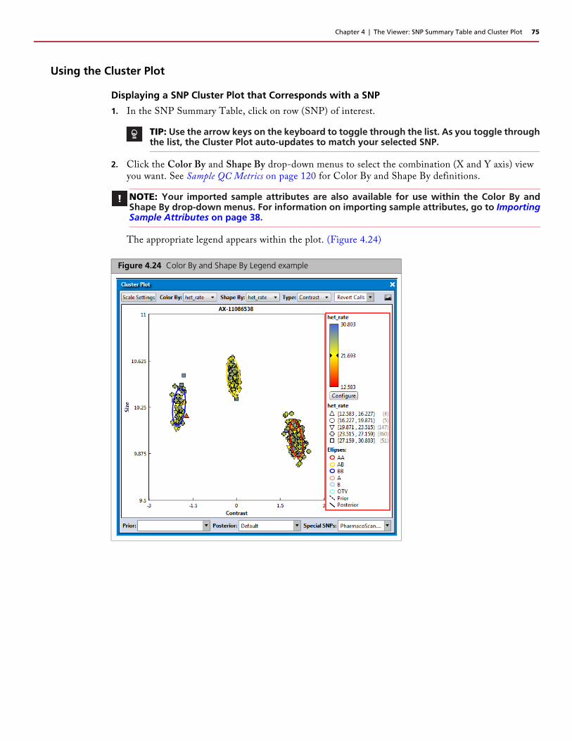
Chapter 4 | The Viewer: SNP Summary Table and Cluster Plot 75
Using the Cluster Plot
Displaying a SNP Cluster Plot that Corresponds with a SNP
1. In the SNP Summary Table, click on row (SNP) of interest.
2. Click the Color By and Shape By drop-down menus to select the combination (X and Y axis) view you want. See Sample QC Metrics on page 120 for Color By and Shape By definitions.
The appropriate legend appears within the plot. (Figure 4.24)
TIP: Use the arrow keys on the keyboard to toggle through the list. As you toggle throughthe list, the Cluster Plot auto-updates to match your selected SNP.
NOTE: Your imported sample attributes are also available for use within the Color By andShape By drop-down menus. For information on importing sample attributes, go to ImportingSample Attributes on page 38.
Figure 4.24 Color By and Shape By Legend example

Chapter 4 | The Viewer: SNP Summary Table and Cluster Plot 76
Setting New Scale Setting Ranges1. Click .
The following window appears. (Figure 4.25)
By default, the window displays your current range values.
2. Enter your new ranges in the appropriate text fields.
3. Click OK.
Click to return all values back to their factory settings.
Customizing Color By Settings1. Click .
The Color Scale Configuration window appears. (Figure 4.26)
2. Use the provided text fields and color drop-down menus to customize your Color By selection.
Auto Scale check box (when checked) uses the actual minimum (lower bound) and maximum (upper
bound) as your min/max scale. Uncheck the Auto Scale check box to enter your min and max number
scales in the provided fields. Note: If the Auto Scale check box remains unchecked, you must enter new
scale limits for each subsequent analysis.
Click the Cutoff Type drop-down menu to select your cutoff preference.
Above Cutoff Failing - This presents a hard visual cutoff graph of all values that fail ABOVE the
Cutoff value entered. The Above Cutoff data is represented by the color defined for Max. (Green in
Figure 4.26)
Figure 4.25 Scale Settings window
Figure 4.26 Color By options

Chapter 4 | The Viewer: SNP Summary Table and Cluster Plot 77
Below Cutoff Failing - This presents a hard visual cutoff graph of all values that fail BELOW the
Cutoff value entered. The Below Cutoff data is represented by the color defined for Min. (Red in
Figure 4.27)
No Cutoff - This presents a smooth 3-point gradient of your defined Max, Min, and colors.
(Figure 4.28).
3. Click OK.
Your Cutoff preference, entered values, and color selections are now displayed on the graph and saved for future use. If needed, click the Default button to revert ALL values back to their factory setting.
Figure 4.27 Below Cutoff
Figure 4.28 No Cutoff

Chapter 4 | The Viewer: SNP Summary Table and Cluster Plot 78
Selecting Multiple Samples in a Cluster Plot1. Drag the cursor around a group of samples to draw a pink-dotted closed loop around them, as shown
inFigure 4.29.
2. Release the mouse button to select the group of lassoed samples. (Figure 4.30)
Changing a Sample’s Call for a Single SNP1. Highlight the sample or samples you want to modify, then right-click on them.
A menu appears.
2. Click Change Call, then move your cursor to the right, then click to select a different call, an OTV (Off Target Variant), or No Call. (Figure 4.31)
Figure 4.29 Selecting multiple samples
Figure 4.30 Selecting multiple samples
Figure 4.31 Change Call menu

Chapter 4 | The Viewer: SNP Summary Table and Cluster Plot 79
The Call is now changed, but not the position. The image may or may not change, as it depends on the Color By and Shape By options you selected.
Reverting a Single Call
1. Single-click to highlight the Call you want to revert back, then right-click on it.
A menu appears.
2. Click Revert Call.
Reverting Multiple Calls
1. Drag the cursor around a group of samples to draw a pink-dotted closed lasso shape around them.
2. Release the mouse button to highlight your selected samples.
3. Click the Revert Call drop-down menu (Figure 4.32), then click to select Revert Selected Call(s).
Displaying Cluster Model DataBy default, the Prior, Posterior, and Special SNPs drop-down selections are preset to best suit the currently displayed Cluster Plot.
1. Click the appropriate drop-down menu (Figure 4.33), then click to select a new setting.
If you select Browse, an Explorer window appears. Navigate to your folder location as you normally would, then click Open to display your data within the graph.
Selecting None, conceals (hides) the selected graph data.
Saving the Current Cluster Plot View1. Click the Save Image button.
An Explorer window appears.
2. Navigate to where you want to save the .PNG file, enter a filename, then click OK.
NOTE: If the array supports CN-aware Genotyping, additional Call Code choices appear.
Figure 4.32 Revert Calls drop-down menu
Figure 4.33 Cluster Model Data drop-down menus

Chapter 5
Allele Translation
This chapter contains:
About Translations
Performing Allele Translation
Translation Reports on page 83
About TranslationsFor supported array types (e.g. PharmacoScan), Axiom Analysis Suite will provide the option to convert (translate) the genotype calls of an important subset of SNPs to functional allele calls using standardized nomenclature wherever possible. The software enables you to:
Quickly identify possible rare alleles or missing data.
Identify haplotype and SNP-level sequence variation in the test samples.
Annotate the reported genotypes across translated SNPs to indicate genomic, mRNA, or peptide
changes resulting from any observed variation.
Predict general gene activity based on detected diplotypes.
Refer to Appendix B, About Allele Translation on page 113 for more information.
Performing Allele TranslationThe Perform Allele Translation operation is available only if the following conditions are met:
The library folder must include the same library package (Array Type with revision number) used to generate the batch results.
Inside the matched library package folder, the files with the extensions *.dc_annot.csv and *.translation must exist.
To perform an allele translation:
1. From an open batch in the Viewer, navigate to the SNP Summary Table, then click the Perform Allele Translation button, as shown in Figure 5.1.
Figure 5.1 SNP Summary Table window

Chapter 5 | Allele Translation 81
The Perform Allele Translation window appears. (Figure 5.2)
2. At the Perform Allele Translation window, use the provided drop-down menus to select an Annotation File, Translation File, and an optional Metabolizer File.
Figure 5.2 Perform Allele Translation window
NOTE: If you disagree with the phenotype interpretations, you may want to leave the Metabolizer File option blank. (Figure 5.2) A Phenotype report will not be created if this option is not used.

Chapter 5 | Allele Translation 82
Allele Translation OptionsRefer to Table 5.1 and Table 5.2 for descriptions of the available Allele Translation options.
Table 5.1 Allele Translation options
Select Options Description
SNP List Filter Choose this option to translate only the genotypes of SNPs in a user-specified probeset list. Click the Browse button to select the marker list, or select from SNP lists you're already imported to the batch results.WARNING: If you supplied a custom optional SNP List File for Genotyping in Analysis Settings when setting up your analysis, you should either filter on the same marker list for Allele Translation, or filter on an even more restrictive list. Otherwise, you may see SNPs with NotAvailable calls in your translation reports. The presence of NotAvailable calls may increase the number of reported haplotype possibilities.
Report only the first named haplotype in the translation file (Default)
This option is only relevant IF you filter by a SNP List AND if the SNP List contains some (but not all) of the available probesets in a gene that is allele translated. If both conditions are met, then it is possible that your SNP List excludes a probeset needed to differentiate among two or more named haplotypes in the translation library file.
Selecting this option means that only the first haplotype will be reported from the set of possible haplotypes that are non-distinguishable due to probeset exclusion. The haplotypes are ordered by name from left to right in the translation library file.
For example, in gene CYP1A1, the *2C haplotype may be differentiated from the *1 haplotype by a variation in a single probeset. If this probeset is omitted, and the data indicates that both *1 and *2C are possible (due to a NoCall at that probeset), then only *1 is reported as a possibility (since *1 is listed before *2C in the translation library file).
The disadvantage of selecting this option is that you may be excluding the actual haplotype for a tested sample. The advantage of selecting this option is that you may want to exclude haplotypes that are differentiable only by probesets you have decided not to translate, AND you agree that the selection of which haplotype to report is correct.
OR
Report combined name that includes all haplotypes that are no longer differentiated
This option is only relevant IF you filter by a SNP List AND if the SNP List contains some (but not all) of the available probesets in a gene that is allele translated. If both conditions are met, then it is possible that your SNP List excludes a probeset needed to differentiate among two or more named haplotypes in the translation library file.
Selecting this option means that a combined haplotype name will be reported using the set of possible haplotypes that are non-distinguishable due to probeset exclusion.
For example, in gene CYP1A1, the *2C haplotype may be differentiated from the *1 haplotype by a variation in a single probeset. If this probeset is omitted, and the data indicates that both *1 and *2C are possible (due to a NoCall at that probeset), then "*1_or_*2C" is reported as a possibility.
The advantage of selecting this option is that you are not excluding possible haplotypes. The disadvantage of selecting this option is that the report will include haplotypes that require a variant allele of a probeset you have decided to exclude for translation.
Note: This option is only available if you do not need a phenotype report, as phenotyping requires haplotype names to not change (depending on the set of probesets used for translation). To enable this option that excludes the generation of a phenotype report, you must deselect the usage of the metabolizer library file. To do this, click (right of the Metabolizer File option).
Include Sample Attributes Click this check box to include sample attributes in the translation reports.This option is enabled if you have imported sample attributes to your analysis results.

Chapter 5 | Allele Translation 83
3. After completing the Allele Translation selections, click OK.
When the translation is finished, an Explorer window appears displaying the folder containing the translation reports and corresponding run log.
Translation ReportsAxiom Analysis Suite can provide a number of translation reports are organized as follows:
Comprehensive Translation - Displays one row per translated SNP for each sample. Provides information on each SNP in addition to haplotype calls.
Summary Translation - An abbreviated version of the Comprehensive report, which displays at least one row for every translated gene for each sample. It also includes rows for every genotype where the translation identifies a variant call. It also includes rows listing SNPs with missing data. In the Summary report only, if no SNPs responsible for functional changes report a variant allele, then information for those SNPs is replaced with a comment to this effect. If a copy number state of zero is indicated, then information for SNPs in that gene is replaced with a comment to this effect, and the copy number haplotype code is reported in the Known Call field.
Phenotype Translation - Displays one row per phenotyped gene for each sample, based on the diplotypes from the source Comprehensive Translation report
Uncalled probeset list - A list of probesets with NoCall genotype calls from SNPs used for translation. This probeset list can then be importing into the Batch, so that you can filter the SNP Summary Table by the uncalled.ps SNP list. This provides a quick way to review the cluster plots of probesets with missing data, and possibly edit the calls directly to "fill in" the missing data in preparation for another round of allele translation reports.
Uncalled - A list of NoCall genotype calls from SNPs used for translation. This report is useful for identifying samples and SNPs for follow up genotyping.
MD5 - An electronic signature that can be used to verify that the comprehensive and phenotype reports have not been modified. Interested users can contact [email protected] for information on accessing tools to verify the integrity of the translation results files.
Log file - A list of messages generated by the software as the data is processed. This file is useful for troubleshooting errors.
Table 5.2 More Allele Translation options
Select Translation Results Folder
Description
Output Root Path The path to the output folder for the translation reports and log. Click its Browse button to set the path.
Export Folder Name The new folder name for the translation results, whose default name has the date-time format YYYY-MM-DD_HHMMSS_translations. Confirm the default or enter a new folder name.

Chapter 5 | Allele Translation 84
Comprehensive and Summary Translation ReportThe basic layout of this report is shown in Figure 5.3
Summary Translation ReportTo make this report easier to read, bold and regular fonts are used. For example, genotype calls are represented in bold, as shown in Figure 5.4.
Figure 5.3 Example: Basic layout of a Comprehensive and Summary Translation report
Figure 5.4 Example: Summary Translation report

Chapter 5 | Allele Translation 85
Phenotype Translation ReportThe basic layout of this report is shown in Figure 5.5.
Phenotype ReportThe basic layout of this report is shown in Figure 5.6.
Figure 5.5 Example: Phenotype Translation report
Figure 5.6 Example: Phenotype report
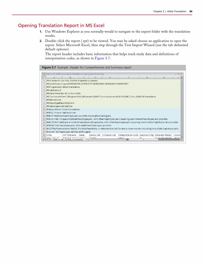
Chapter 5 | Allele Translation 86
Opening Translation Report in MS Excel1. Use Windows Explorer as you normally would to navigate to the export folder with the translation
results.
2. Double-click the report (.rpt) to be viewed. You may be asked choose an application to open the report. Select Microsoft Excel, then step through the Text Import Wizard (use the tab-delimited default options).
The report header includes basic information that helps track study data and definitions of interpretation codes, as shown in Figure 5.7.
Figure 5.7 Example: Header for Comprehensive and Summary report

Chapter 5 | Allele Translation 87
Available Report Fields and Descriptions
Array TrackingRefer to Table 5.3 for descriptions of the available Array Tracking fields.
Gene-specificRefer to Table 5.4 for descriptions of the available Gene-specific fields.
Table 5.3 Array Tracking fields
Array Tracking fields Description
Index A row index in the format: [filename index]-[gene index within filename]-[Probe Set ID index within gene]. This field can be parsed for sorting or row filtering. For the phenotype report, the index is shortened to [filename index]-[gene index within filename]
Filename Name of the sample file.
NOTE: Haplotypes are not reported for genes whose Interpretation Code is NoHap. The fields described in the table below will therefore be empty for these genes. The exception is if the gene reports a gene deletion, in which case the associated haplotype names are reported.
Table 5.4 Gene-specific fields
Gene-specific fields Description
Associated Gene Gene symbol
Phenotype Call In the Phenotype report, the predicted phenotype given the supplied Known Call diplotypes. Multiple comma-separated phenotypes are reported when multiple Known Call diplotypes are associated with different phenotypes. Most genes use the following terminology when the default metabolizer library file is selected: UM = ultra-rapid metabolizer RM = rapid metabolizer NM = normal metabolizer IM = intermediate metabolizer PM= poor metabolizer
Variations on these terms also exist to describe some level of uncertainty: NM_or_IM = normal or intermediate metabolizer IM_or_PM =intermediate or poor metabolizer Not_PM = not a poor metabolizer unknown = unknown metabolizer state
Some genes use different phenotype terms to be consistent with literature usage. Refer to the header of the phenotype report for additional information.
Users are responsible for reviewing the *.metabolizer library file for accuracy! Users may modify the *.metabolizer file as needed, and are not restricted to this terminology. Refer to Diplotype to Phenotype Translation on page 117 for more information.

Chapter 5 | Allele Translation 88
Gene Activity In the Phenotype report, the predicted pair of gene activities given the supplied Known Call diplotypes. Multiple comma-separated activity pairs are reported when multiple Known Call diplotypes are associated with different activity pairs. Most genes use the following terminology when Affymetrix's metabolizer library file is selected: increased = increased gene function normal = normal gene function reduced: reduced gene function no = no gene function unknown = unknown or uncertain gene function
Some genes use different phenotype terms to be consistent with literature usage.
Users are responsible for reviewing the *.metabolizer library file for accuracy! Users may modify the *.metabolizer file as needed, and are not restricted to this terminology. Refer to Diplotype to Phenotype Translation on page 117 for more information.
Known Call Haplotype pairs (diplotypes) identified in the gene of interest. When more than one pair of haplotypes is implicated (due to phase ambiguity in compound heterozygous samples), the reported diplotypes are separated by a comma.
Unknown Call When the gene table includes haplotyping SNPs and a complete diplotype pair cannot be identified in a sample, one or more unknown haplotypes is assumed. This is designated as UNK in the report. Multiple haplotype pairs (diplotypes) that have unknown alleles are separated with a comma in this field. An example record might be in the format: *2/UNK,*13/UNK,*24/UNK,*32/UNK to indicate that there are at least 4 defined alleles consistent with the data, but each would require matching to a haplotype pattern that does not exist in the translation library file.
Interpretation Code This diplotype interpretation code indicates whether one and only one unique haplotype pair is consistent with the data (UNIQ), whether there are multiple haplotype pairs consistent with the observed genotypes (MULT) and whether these are observed in conjunction with other unknown haplotypes (UNIQ+UNK or MULT+UNK). Additional codes indicate that no known haplotype pairs have been identified (UNDH) or if there is missing data leading to additional haplotype possibilities. The missing data could be NoCall or NotAvailable (NC/PRA/NA). The PossibleRareAllele call is not used by Axiom Analysis Suite.
For genes for which copy number state is available, the following interpretation codes may also appear: CN_HybridLoss = Partial gene deletion is detected, so haplotype pair calling is not
available. CN_HybridGain = Partial gene duplication is detected. If a non-wild-type allele is
detected, the software can't determine whether the variant allele is on the partial copy of the gene.
CN_Gain = Gene duplication is detected, but the software cannot determine which haplotype(s) are duplicated. For this reason you won't see xN nomenclature in the reported haplotype pairs.
CN_NoCall = Copy Number state not reported, so there is less confidence in the reported haplotype pairs.
CN_Error = Genotypes from multiple Copy Number states are detected, so haplotype pair calling is not available. This can happen if you manually edit a genotype call in such a way as to change the SNP's copy number state. For example, if you change a "NoCall_1" genotype (a NoCall for a CN=1 sample) to a "BB" CN=2 genotype, its copy number has changed. This would cause allele translation problems if other SNPs for this sample for the same gene have genotypes of a different copy number state.
Table 5.4 Gene-specific fields
Gene-specific fields Description

Chapter 5 | Allele Translation 89
Marker-specificRefer to Table 5.5 for descriptions of the available Marker-specific fields.
NOTE: Marker annotations will always be the same throughout the reports for a given SNP.
Fields in the Marker Information section of the Comprehensive and Summary reports include the biological information at the SNP level, along with the interpreted genotypes identified in each sample
Table 5.5 Marker-specific fields
Marker-specific fields Description
Summary Flag(marker annotation)
This annotation field contains an abbreviated name when structural or functional differences are known to result with mutations at the SNP locus. For triallelic SNPs, there may be more than one flag. For example, ABCB1_c.2677G>T>A(A893SorT) marker is triallelic and can result in different function changes in the protein. The two summary flags for the marker are thus reported "A893S,A893T”.
This flag is set to No (N) for neutral hitch-hiker SNPs or ones that result in synonymous changes in the gene product.
Relevant Alleles(marker annotation)
This annotation field is the full listing of haplotype-based alleles defined in the gene table that contain the variant version of the marker. For non-haplotype-based SNPs, this is an abbreviated name indicating the protein change that results when the variant base is present.
Common Name(marker annotation)
A SNP identifier describing either the gene location, coding change or dbSNP rsID for the SNP. The Common Name is retrieved from the translation library file, and may not be the same as the Common Name seen within Axiom Analysis Suite (which instead uses the Common Name in the *.annot.db library file)
Probe Set ID Unique identifier for the SNP.
Basecall The observed bases, also known as the "raw" genotypes.
Reference Base This field generally indicates the more common allele in biallelic SNPs. Certain genes use a particular GenBank entry as the "Reference genome" and the observed allele at each marker across the gene is then reported as Reference.
Variant Base These are the alternate alleles for each SNP. When there is more than one variant allele (e.g. triallelic SNPs) the alternate alleles are reported together and separated by a comma (e.g. A,T).
Call The first level of translation of the Basecall field, replacing the individual nucleotide calls with the associated reference (Ref) or variant (Var) allele state. For Basecalls associated with copy numbers less than 2, this field will show haplotype names as needed. This field will be empty if the Basecall value has an unclear call.
Haplotype Marker(marker annotation)
Differentiates SNPs used to make haplotype calls or single-marker variant calls. Y = A flag to indicate that the Allele translation algorithm will match allele variants in
blocks of SNPs defining haplotypes in the gene tables. Called haplotypes are reported in the "Known Calls" and Unknown Calls of the report.
N = A flag to indicate that the haplotype background of a variant is not known. Genotyping results for these SNPs are only reported in the "Call" column.
Change for Variant(marker annotation)
Amino acid substitution or other structural change (such as splicing variant, promoter mutation, Frame shift mutation, etc.) caused by the presence of the variant allele.
cDNA Change(marker annotation)
Location of the mutation on a reference mRNA sequence.

Chapter 5 | Allele Translation 90
Tracking Edited Genotype CallsRefer to Table 5.6 for descriptions of the available fields for tracking edited genotype calls.
Uncalled ReportRefer to Table 5.7 for descriptions of the available fields for uncalled reports.
Genome Position(marker annotation)
This is the chromosomal position of the mutation.
dbSNP RS ID(marker annotation)
The dbSNP identifier for the marker.
NOTE: Fields for tracking genotyping changes are recorded in the Change Tracking portion of the translation reports (located immediately before the User Defined Sample Information section of the report).
Table 5.6 Fields for tracking edited genotype calls
Tracking Edited Genotype Calls
Description
Original Basecall This field reports the original genotype for the sample. The field is not empty when the user has edited the call within Axiom Analysis Suite.
Override Comment This field reports edited in AxAS if the call has been edited within Axiom Analysis Suite.
NOTE: The Reference Allele and Variant Allele values of the Uncalled report are the same as the Reference Base and Variant Base values of the Comprehensive and Summary reports.
Table 5.7 Uncalled Report
Uncalled Report Description
Filename Name of the sample file.
Gene Gene symbol.
Common Name The Common Name defines the gene and positional information about the genetic change tested with the probeset.
Basecall The Uncalled report contains all the NoCall genotypes from SNPs used for allele translation.
Override Comment User-specified annotation field that enables an audit trail of the source of genotyping results done outside of Axiom Analysis Suite. In the Uncalled report, this field is primarily useful when creating a copy of this file to use as an Override file. The Override file may be useful for Affymetrix Power Tool users.
Reference Allele Reference base indicates the allele in a reference sequence known to be present at this genetic location. Generally this is the more common allele at SNPs with low minor allele frequency (<1%).
Variant Allele The variant base(s) defined by the marker are alternative known genotypes known to be present at this genetic location. For triallelic SNPs, the reporting format is: A,T for ABCB1_68883G>T(S893A) because two specific mutations are known to occur at this genomic location (G>A and G>T).
Table 5.5 Marker-specific fields
Marker-specific fields Description

Chapter 6
Exporting
Using the Sample Table Export Options1. Click the Export drop-down.
Your Export options appear. (Figure 6.1)
2. Click Export Current Table or Export All Data.
A Save As window appears.
3. Click on an existing folder or click New Folder to choose a new save location.
4. Type a filename for the table, then click Save.
The table data is now saved as a tab-delimited .txt file.
Using the SNP Summary Table Export Options1. Click the Export drop-down.
The following window appears: (Figure 6.2)
Exporting the Current Table
To export the columns and rows currently displayed in the table:
1. Click Export Current Table.
An Explorer window appears.
2. Enter a filename, then click Save.
The current table data is now saved and exported as a tab-delimited text file.
Exporting All DataTo export all columns and rows, including hidden and filtered data:
1. Click Export All Data.
An Explorer window appears.
2. Enter a filename, then click Save.
All data in the table (displayed or not) is saved and exported as a tab-delimited text file.
Figure 6.1 Sample Table Export Menu
Figure 6.2 SNP Summary Table Export menu
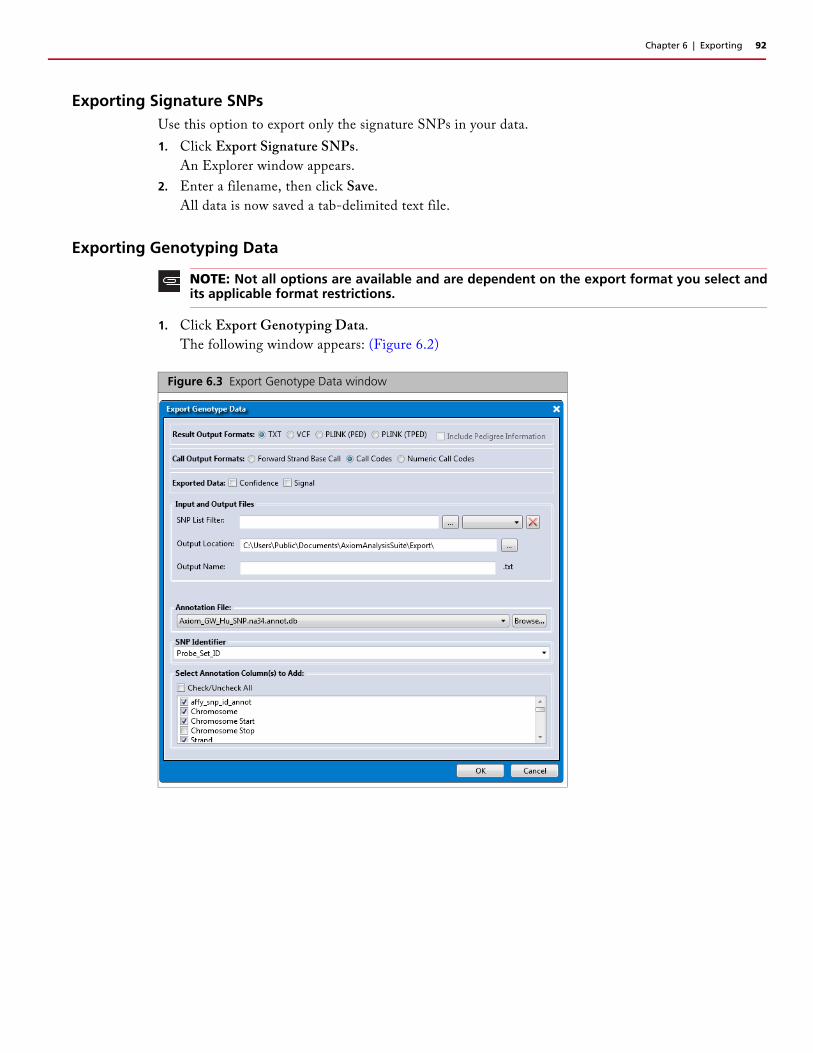
Chapter 6 | Exporting 92
Exporting Signature SNPsUse this option to export only the signature SNPs in your data.
1. Click Export Signature SNPs.
An Explorer window appears.
2. Enter a filename, then click Save.
All data is now saved a tab-delimited text file.
Exporting Genotyping Data
1. Click Export Genotyping Data.
The following window appears: (Figure 6.2)
NOTE: Not all options are available and are dependent on the export format you select andits applicable format restrictions.
Figure 6.3 Export Genotype Data window

Chapter 6 | Exporting 93
Result Output Formats
1. Click the radio button to select the Result Output Format you want use.
2. Optional: If you selected a PLINK format, make sure you click the Include Pedigree Information check box. Not checking this box may require special handling (within PLINK) to make your exported output work properly.
Call Output Formats
1. Click the radio button to select the appropriate Call Output Format (Figure 6.5) you want to use.
Exported Data Selections
1. Click inside the check box(es) to check the additional type(s) of Exported Data (Figure 6.6) you want to include.
Input and Output Files (Figure 6.7)
SNP List Filter (Optional)
1. To restrict the output to a list of SNPs (probeset_IDs) contained in a file, click the SNP List Filter field’s Browse button (Figure 6.7).
An Explorer window appears.
Figure 6.4 Result Output Format selections
IMPORTANT: If you are exporting genotypes into a PLINK format, make sure your SampleAttributes include an Index ID and Pedigree Information (Family ID, Individual ID, Father ID,Mother ID, Sex, and Affection Status).
Figure 6.5 Call Output Format selections
NOTE: Numeric Call Codes are exported using the following representation: -1 = NoCall, 0 = AA, 1 = AB, and 2 = BB.
Figure 6.6 Exported Data selections
Figure 6.7 Input and Output Files selections

Chapter 6 | Exporting 94
2. Navigate to the SNP Filter List location, then click Open.
The SNP Filter List field is now populated. (Figure 6.8)
3. Click the SNP List Filter’s drop-down menu to view and select a previously saved SNP List. (Figure 6.8)
Output Location (Required)
1. Click the Output Location field’s Browse button.
An Explorer window appears.
2. Navigate to an output location, create a new folder if needed, then click Select Folder button.
The Output Location path is displayed. (Figure 6.8)
Output Name (Required)
1. Use the output name already in the Output Name field, or click inside the field to enter a new name. Note: Your output name’s file extension reflects the Results Output Format you selected in Step 1.
Changing the SNP Identifier
1. Click the drop-down arrow, then click to select the SNP Identifier you want to use. (Figure 6.9)
Figure 6.8 SNP List Filter and Output path
NOTE: Only SNPs that have a value for the selected annotation are exported. For example,markers that have a dbSNP RSID are exported, while markers without a dbSNP RSID are notexported.
If the selected SNP Identifier has more than 1 probeset mapped to it, it will have multipleentries in the exported file.
Figure 6.9 SNP Identifier

Chapter 6 | Exporting 95
Changing the Current Annotation File (Optional)
1. To change the currently displayed Annotation File, click the Annotation File field’s Browse button (Figure 6.10).
An Explorer window appears.
2. Navigate to the appropriate Annotation File location, then click Open.
Your newly selected Annotation file is displayed.
Adding and Removing Annotation Columns
1. Click the check box next to the Annotation Column(s) you want to add to your format results or click to uncheck/remove a column. Check/Uncheck All check box to add or remove ALL available annotations. (Figure 6.10)
2. After the Export Genotype Data form is complete, click OK.
3. Your newly exported data now reside in the output location you defined in Step 1 on page 94.
Figure 6.10 Select Annotation Column(s) pane

Chapter 6 | Exporting 96
Exporting Cluster Plots to PDFThis exporting option generates a specific number of cluster plots from the selected Conversion Type choices.
1. Click Export Cluster Plots to PDF.
The following window appears: (Figure 6.11)
2. Click Browse.
An Explorer window appears.
3. Navigate to a desired location, then enter a name for your PDF report.
4. Click Save.
You are returned to the Report Settings window.
5. In the Picture Settings section, click either:
All SNPs from Current Table
Random SNPs from Current Table
6. Click inside the applicable Count field(s) to enter how many cluster pots you want to export.
Click the Default button to revert your modified counts back to their original states.
7. Click to check a Conversion Type(s) you want to add to the report or click the Check/Uncheck All check box, then click OK.
A Please Wait message and progress bar appear. Allow several minutes if multiple Conversion Type PDF report(s) were selected.
An Explorer window (where you saved the PDF Report location in Step 3) appears.
8. Double-click on the PDF Report you want to view.
Figure 6.11 Report Settings window

Chapter 6 | Exporting 97
The PDF Report opens. (Figure 6.12)
Figure 6.12 PDF Report example

Chapter 7
External Tools
Axiom Analysis Suite auto-detects any previously installed application that may further analyze your genotype results. When a compatible application is detected, an External Tools window tab is generated, as shown in Figure 7.1.
Axiom CNV Tool 1.11. Click the Axiom CNV Tool button.
The application opens. (Figure 7.2)
For details on how to use the Axiom CNV Tool 1.1 application, refer to its User Guide (P/N 703216 Rev. 2)
Figure 7.1 External Tools window tab
NOTE: The Axiom Analysis Suite can be left open/active if you are using an external application to further view your data. However, you must exit and close the Axiom Analysis Suite before editing its data with an external application.
Figure 7.2 CNV Tool - Main window

Appendix A
Copy Number Aware Genotyping
If the array content and library package supports it, the Genotyping and Best Practices workflows perform predefined region copy number analysis (referenced below as CN-aware genotyping).
The resulting copy number state predictions can then be used at the point of SNP genotyping to report additional types of genotype calls. This is useful to accurately genotype SNPs in high copy number variable regions. For example, if the copy number state in a region is predicted to be 0, then there is no DNA to genotype, and the sample should not be genotyped using a diploid genotyping model.
With CN-aware genotyping: SNPs in a CN=0 region can be called as “ZeroCN”
SNPs in a CN=1 region can be called with hemizygous genotype codes such as “A”, “B”, “NoCall_1”
SNPs in a CN=2 or higher region will continue to be called with diploid genotype codes such as
“AA”, “AB”, “BB”, “NoCall”
Special SNPs (those on chromosomes Y, MT, and non-PAR X) will also be assigned hemizygous
and ZeroCN genotype codes when expected copy number is less than 2.
The CN Reference Model library file, used by the CN engine, defines which probesets are associated
with a predefined CN region. Only those probesets (and Special SNPs) take advantage of CN-aware
genotyping to report ZeroCN and hemizygous calls when CN<2.
The PharmacoScan solution is an example of an Axiom array/assay that has the content and library package to support CN-aware genotyping.
Setting Up a CN-aware Genotyping AnalysisBefore setting up a CN-aware genotyping analysis, click the New Analysis window tab, then click the Array Type drop-down menu to confirm an array such as PharmacoScan is available, as shown in Figure A.1. If it is, continue to Selecting a Mode (Workflow).
NOTE: It is possible for the CN engine to assign a CN state to probesets between two measuredCN regions. For example, if two adjacent regions predict the same CN state, then that CN statecan be assigned to probesets between the two adjacent regions.
Figure A.1 Preferences window tab
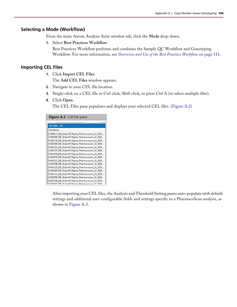
Appendix A | Copy Number Aware Genotyping 100
Selecting a Mode (Workflow)From the main Axiom Analysis Suite window tab, click the Mode drop-down.
1. Select Best Practices Workflow.
Best Practices Workflow performs and combines the Sample QC Workflow and Genotyping
Workflow. For more information, see Overview and Use of the Best Practices Workflow on page 111.
Importing CEL Files1. Click Import CEL Files.
The Add CEL Files window appears.
2. Navigate to your CEL file location.
3. Single-click on a CEL file or Ctrl click, Shift click, or press Ctrl A (to select multiple files).
4. Click Open.
The CEL Files pane populates and displays your selected CEL files. (Figure A.2)
After importing your CEL files, the Analysis and Threshold Setting panes auto-populate with default
settings and additional user-configurable fields and settings specific to a PharmacoScan analysis, as
shown in Figure A.3.
Figure A.2 Cell File pane

Appendix A | Copy Number Aware Genotyping 101
For information on the non-PharmacoScan specific analysis and threshold fields, see Setting Up an
Analysis on page 16 and Setting Up Threshold Settings on page 22.
CN-aware Genotyping Analysis Settings
Sample QC
GT Analysis File: Parameters file for the genotyping step that calculates QC Call Rate.
Prior Model File: Defines prior knowledge of SNP cluster locations. This file has the same format as
a posteriors file, which is generated by the genotyping step. This means that you can "train" on a custom
data set, and use the updated knowledge of cluster locations as a "seed" to possibly improve future
genotyping batches. This file must contain two row entries for the GENERIC and GENERIC:1
probesets (if there are any probesets to be genotyped that are not listed in this file).
SNP List File: A file of probeset IDs to genotype. For Sample QC it defines the probesets used to
calculate QC Call Rate.
Gender File: A file specifying the desired gender of every sample. If supplied, software will use values
in this file instead of the computed gender. Gender impacts genotyping of chromosome X and Y SNPs.
Figure A.3 Example: Auto-populated Analysis and Threshold Setting panes
IMPORTANT: Only experienced users should modify default analysis settings.
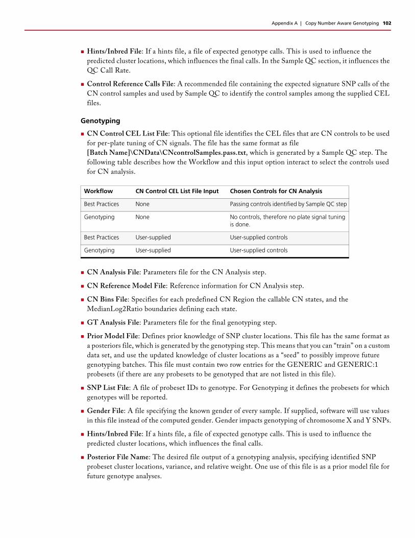
Appendix A | Copy Number Aware Genotyping 102
Hints/Inbred File: If a hints file, a file of expected genotype calls. This is used to influence the
predicted cluster locations, which influences the final calls. In the Sample QC section, it influences the
QC Call Rate.
Control Reference Calls File: A recommended file containing the expected signature SNP calls of the
CN control samples and used by Sample QC to identify the control samples among the supplied CEL
files.
Genotyping
CN Control CEL List File: This optional file identifies the CEL files that are CN controls to be used
for per-plate tuning of CN signals. The file has the same format as file
[Batch Name]\CNData\CNcontrolSamples.pass.txt, which is generated by a Sample QC step. The
following table describes how the Workflow and this input option interact to select the controls used
for CN analysis.
CN Analysis File: Parameters file for the CN Analysis step.
CN Reference Model File: Reference information for CN Analysis step.
CN Bins File: Specifies for each predefined CN Region the callable CN states, and the
MedianLog2Ratio boundaries defining each state.
GT Analysis File: Parameters file for the final genotyping step.
Prior Model File: Defines prior knowledge of SNP cluster locations. This file has the same format as
a posteriors file, which is generated by the genotyping step. This means that you can “train” on a custom
data set, and use the updated knowledge of cluster locations as a “seed” to possibly improve future
genotyping batches. This file must contain two row entries for the GENERIC and GENERIC:1
probesets (if there are any probesets to be genotyped that are not listed in this file).
SNP List File: A file of probeset IDs to genotype. For Genotyping it defines the probesets for which
genotypes will be reported.
Gender File: A file specifying the known gender of every sample. If supplied, software will use values
in this file instead of the computed gender. Gender impacts genotyping of chromosome X and Y SNPs.
Hints/Inbred File: If a hints file, a file of expected genotype calls. This is used to influence the
predicted cluster locations, which influences the final calls.
Posterior File Name: The desired file output of a genotyping analysis, specifying identified SNP
probeset cluster locations, variance, and relative weight. One use of this file is as a prior model file for
future genotype analyses.
Workflow CN Control CEL List File Input Chosen Controls for CN Analysis
Best Practices None Passing controls identified by Sample QC step
Genotyping None No controls, therefore no plate signal tuning is done.
Best Practices User-supplied User-supplied controls
Genotyping User-supplied User-supplied controls

Appendix A | Copy Number Aware Genotyping 103
ps2snp File: If multiple probeset designs exist on the array for a given SNP (for example, one forward
and one reverse strand design), then the ps2snp file is used by the SNP classification step to identify
the best performing probeset for the SNP, using the priority-order setting in the SNP QC section in
the New Analysis tab. This text file has two tab delimited columns with the headers probeset_id and
snpid (snpid = affy_snp_id).
Threshold Settings specific to CN-aware Genotyping
Sample QC
Control Comparisons
For identifying control samples, this is the minimum number of SignatureSNP probesets compared to a reference.
Control Concordance
For identifying control samples, this is the minimum percent concordance of SignatureSNP calls to a reference.
CN QCMAPD: Median Absolute Pairwise Difference of log2ratio signals of adjacent copy number (CN) probesets must be below this value to make CN calls.
Waviness SD: Waviness Standard Deviation of log2 ratio signals of copy number (CN) probesets must be below this value to make CN calls.
SNP QCThe following SNP QC thresholds are also used for SNPs that have haploid and ZeroCN clusters:
hom-ro-hap-1-cutoff: Minimum acceptable value for the correctness of the horizontal position of the
haploid clusters (Ratio Offset) when a SNP has one haploid genotype.
hom-ro-hap-2-cutoff: Minimum acceptable value for the correctness of the horizontal position of the
haploid clusters (Ratio Offset) when a SNP has two haploid genotypes.
hom-hap-X-cutoff: Minimum acceptable value for the correctness of the horizontal position of the
haploid clusters relative to the homozygous clusters.
hom-hap-Y-lower-cutoff: Maximum acceptable value for the correctness of the vertical position of the
haploid clusters relative to homozygous clusters.
hom-hap-Y-upper-cutoff: Maximum acceptable value for the correctness of the vertical position of the
haploid clusters relative to homozygous clusters.
CN0-hap-X-cutoff: Minimum acceptable value for the correctness of the horizontal position of the
ZeroCN cluster relative to the haploid clusters.
CN0-hap-Y-cutoff: Minimum acceptable value for the correctness of the vertical position of the ZeroCN
cluster relative to the haploid clusters.
CN0-dip-X-cutoff: Minimum acceptable value for the correctness of the horizontal position of the
ZeroCN cluster relative to the diploid clusters.
CN0-dip-Y-cutoff: Minimum acceptable value for the correctness of the vertical position of the ZeroCN
cluster relative to the diploid clusters.
IMPORTANT: Only experienced users should modify default threshold settings.

Appendix A | Copy Number Aware Genotyping 104
Assigning an Output Folder Path1. Click the Output Folder path’s Browse button. (Figure A.4)
An Explorer window appears.
2. Navigate to the recommended path C:\Users\Public\Documents\AxiomAnalysisSuite\Output, then
click Select Folder.
Your selected output folder path is now displayed.
Assigning a Batch NameThe batch file is produced while your analysis is running and includes all the necessary files needed to view your analysis in the Axiom Analysis Suite Viewer.
1. Enter a name in the Batch Name field. (Figure A.5)
Figure A.4 Output Folder field
Figure A.5 Enter a Batch Name
NOTE: A folder (with the same name as your entered batch name) is auto-generatedduring the analysis process. This folder includes all the necessary files needed to viewyour analysis results in the Viewer.

Appendix A | Copy Number Aware Genotyping 105
Running your CN-aware Genotyping Analysis1. Click .
The Dashboard window tab appears. (Figure A.6)
After Success is displayed in the Status column (Figure A.6), click .
The button will not appear if a processing error occurs. If a message appears stating that no
samples passed QC, click the Open Selected Result(s) button to review the analysis result that may
need troubleshooting.
The Axiom Analysis Suite Viewer opens in a new window (Figure A.7) and displays your completed
PharmacoScan analysis results.
Viewing your CN-aware Genotyping AnalysisAfter processing arrays that support CN-aware genotyping, the following is added to the Axiom Analysis Suite Viewer:
New entries in the Summary Report, Sample Table, and SNP Summary Table.
Cluster Plot also displays hemizygous and ZeroCN clusters for SNPs in CN regions.
CN Summary Table, with Export CN Data option.
A CN Region Plot window tab.
Exported Genotype Reports now reflect new call types (for some formats).
Exported VCF formats now include CN and SNP calls.
Figure A.6 Dashboard window tab
TIP: Open additional Viewer windows to make comparisons between your completeddata analyses easier. To do this, click the Dashboard window tab, then click on the Openbutton again.

Appendix A | Copy Number Aware Genotyping 106
Summary Report
After successfully running a Sample QC or Best Practices workflow, the Summary report’s Plate QC Summary section features two additional fields, as shown in Figure A.7.
Number of controls found - This metric is a count of samples identified as controls based on high signature SNP concordance to expected calls in the Control Reference Calls library file.
Controls in normal wells - The Control Reference Calls library file lists the expected plate wells for the control samples. This metric will report "Yes" if all the detected control samples are in the expected plate wells. It is OK to put the control samples in any wells you choose.
After successfully running a Genotyping or Best Practices workflow, the Summary report’s CN Summary section features a table of information for each plate, as shown in Figure A.7.
Figure A.7 Viewer window tabs

Appendix A | Copy Number Aware Genotyping 107
Refer to Table A.1 for descriptions of each CN Summary Report column.
Table A.1 CN Summary Report
CN Summary Report Description
Number of files analyzed Count of CEL files supplied to the Genotyping step (which includes CN analysis).
Number of samples failing CNQC
Count of CEL files that fail copy number quality control checks, which is the result of a comparison of measured MAPD and waviness SD metrics against thresholds. Samples that fail CN QC report a CN state of NoCall, and their SNPs are called without the benefit of CN-aware genotyping.
Number of samples passing CNQC
Count of CEL files that pass copy number quality control checks.
Number of controls analyzed
Count of CEL files supplied to the Genotyping step that are identified as controls.
Number of controls failing CNQC
Count of control CEL files that fail copy number quality control checks, which is the result of a comparison of measured MAPD and waviness SD metrics against thresholds. Controls that fail CN QC report a CN state of NoCall, and their SNPs are called without the benefit of CN-aware genotyping.
Note: Special SNPs still report haploid and ZeroCN calls because their calls use predicted gender to determine CN state.
Number of controls for CN tuning
Count of control CEL files that pass copy number quality control checks.
CN tuned using controls If Number of controls for CN tuning > 0, then this value is "Yes". This means that CN signals are adjusted based on the signal measured in the control samples from the same plate. If the controls are appropriate for the samples being processed, this adjustment can improve CN calling accuracy.

Appendix A | Copy Number Aware Genotyping 108
Sample Table
After successfully running a CN analysis, additional columns appear within the Sample Table, as shown in Figure A.8.
Refer to Table A.2 for descriptions of each added Sample Table column.
Figure A.8 Sample Table after a CN Analysis run
Table A.2 Added Sample Table columns after running a CN Analysis
Sample Table Description
MAPD Median Absolute Pairwise Difference of log2ratio signals of adjacent copy number (CN) probesets.
WavinessSD Waviness Standard Deviation of log2ratio signals of adjacent copy number (CN) probesets
CN passes MAPD "Yes" if the sample's MAPD value is not greater than the MAPD threshold used by CN QC.
CN passes WavinessSD "Yes" if the sample's WavinessSD value is not greater than the WavinessSD threshold used by CN QC
CN passes QC "Yes" if the sample passes both MAPD and WavinessSD threshold tests. If "no", the sample reports a CN state of NoCall, and its SNPs are called without the benefit of CN-aware genotyping.
Note: Special SNPs will still report haploid and ZeroCN calls because their calls use predicted gender to determine CN state.
Control chosen "Yes" if the control was listed in the CN Control CEL List file supplied for CN analysis.
Control used "1" if the control was used to adjust CN signals of all samples in the same plate. The value will be 1 if Control chosen = 1 and CN passes QC = Yes.
Number of controls for CN tuning
A count of control samples used to adjust the CN signals for the given sample. This value will be the same for all samples on the same plate.
CN tuned using controls If Number of controls for CN tuning > 0, then this value is "Yes". This means that CN signals are adjusted based on the signal measured in the control samples from the same plate. If the controls are appropriate for the samples being processed, this adjustment can improve CN calling accuracy.

Appendix A | Copy Number Aware Genotyping 109
SNP Summary Table
After successfully running a CN-aware genotyping analysis, additional columns appear within the SNP Summary Table, as shown in Figure A.9.
Refer to Table A.3 for descriptions of each added SNP Summary Table column.
Figure A.9 SNP Summary Table after a CN Analysis run
Table A.3 Added SNP Summary Table columns after CN-aware genotyping is performed
SNP Summary Table Description
n_A Count of hemizygous "A" calls.
n_B Count of hemizygous "B" calls.
n_CN0 Count of ZeroCN calls.
CopyNumIssue(hidden by default)
Copy Number Issue is "1" if the probeset is assigned to the "Other" ConversionType because the haploid or ZeroCN clusters are in an unusual location compared to each other or to the diploid clusters.

Appendix A | Copy Number Aware Genotyping 110
CN Summary Table and CN Region Plot
The Genotyping and Best Practices workflows perform predefined region copy number analysis (if the array content and library package support it). If this is the case, a CN Summary Table and CN Region Plot window tab appear in the Axiom Analysis Suite Viewer, as shown in Figure A.10.
CN Summary Table (Overview) The CN Summary Table gives a count of samples called with a given copy number state (CN_State)
for a given copy number region (CN_Region).
CN_States that cannot be reported are displayed as empty with a gray background. If the CN_State can be reported but no samples in the batch report that CN State, then the count is 0. As long as the default CN Bins library file is used during analysis setup, the only samples that will report a CN_State of NoCall are those that fail Copy Number QC.
Selecting a specific CN_Region row in the table updates the associated CN Region Plot.
The button Export Copy Number Data copies several CN reports to another location specified by the user. Note that CN_States for each CN_Region for each sample are also available in a VCF format export of genotyping data, available from the SNP Summary Table tab.
CN Region Plot (Overview) The CN Region Plot displays the MedianLog2Ratio of each genotyped sample for the copy number
region selected in the CN Summary Table, grouped by affymetrix-plate-barcode.
Selecting a sample or samples in the CN Region Plot also selects the same samples in the Sample Table and the Cluster Plot, and vice versa.
Genes with a CN of 2 typically have a MedianLog2Ratio centered at 0, which indicates that the signals of probesets used for CN estimation are similar to the expected signals for a CN=2 sample.
CN States are called by comparing the MedianLog2Ratio to the thresholds defined in the CN Bins library file selected during analysis setup. CN States cannot be edited in the Viewer.
Sometimes between-plate assay variation can shift the observed MedianLog2Ratio values away from 0 for CN=2 samples. Fortunately, if the assay includes appropriate control samples on the assay plate, then the copy number signals can be tuned using the control samples. If CN plate correction was done, then the default "Shape By" metric "CN tuned using controls" identifies which samples had their CN measurements adjusted using the plate controls.
Figure A.10 CN Summary Table and CN Plot window tabs
Appendix A | Copy Number Aware Genotyping 111
Overview and Use of the Best Practices WorkflowThe recommended genotyping method is to use information from a batch of samples to improve the calling of individual samples. To this end, the cluster locations in signal space for each probeset (see the Cluster Plot) adapt in a Bayesian fashion to the supplied data. Prior knowledge of cluster locations influences the final calls. The more samples that are supplied in a batch, the more the final cluster locations will be influenced by the supplied data.
The dynamic nature of this genotyping algorithm means that if a given sample's CEL file is genotyped in a group of 24 CEL files, or in a group of 2400 CEL files, you can expect that some SNPs may experience a changed call (call <-> NoCall, or sometimes call 1 <-> call 2). This is more likely to happen if the SNP's data quality is not great (close clusters), if there are strong between-plate effects in cluster positions, or for very low Minor Allele Frequency SNPs where good information on rare genotype cluster positions may not be available before genotyping. Calling accuracy of both rare and common SNPs is improved even for small batch sizes if enough prior knowledge of cluster locations is available.
The batch nature of the genotyping means that if there are some samples of poor data quality in a group of good quality samples, then sometimes the poor quality samples will harm the calling accuracy of the good samples. For this reason, Axiom Analysis Suite's “Best Practices Workflow” can be thought of as a two-step process:
Step 1 Sample QC: Identify and exclude the poor quality sample CEL files.
Step 2 Genotyping: Genotype only the sample CEL files that pass Step 1.
Step 1: The Sample QC Workflow performs the following steps:
Genotype a small set of SNPs used to uniquely identify each sample ("Signature SNPs"). This
method uses static calling boundaries, so a given sample's calls are not influenced by other samples.
DishQC: Calculate DishQC metric to exclude worst-performing CEL files from next step. For this
method, a given sample's metrics are not influenced by other samples.
QC Call Rate: Initial cluster genotyping on remaining samples for selected QC SNPs, to identify
and remove any additional CEL files with low QC call rates. For this method, batch information
from other samples influences a given samples QC call rates. Genotypes are not stored.
Plate QC: Compare the average QC Call Rate of passing samples within a plate against the threshold
"Average call rate for passing samples". If the metric is below this threshold, all the samples on the
plate will fail Plate QC, and will not be genotyped.
For supported arrays like PharmacoScan, auto-identify reagent control samples by comparing
measured SignatureSNP genotypes from all CEL files against reference genotypes. A control is
identified if [number of Signature SNPs with a call is >= "Control comparisons"] AND
[Concordance % of signature SNP calls compared with reference genotypes is >= "Control
concordance"]. Control samples that pass all sample QC checks will be used in the subsequent
Genotyping workflow, unless overridden by the user.
Step 2: Genotyping can be run by itself or as part of the Best Practices Workflow. When run as part of
the Best Practices Workflow, only CEL files passing Sample QC are genotyped. When run by itself,
the user has full control of which samples to genotype. Genotyping does the following steps:
For supported arrays like PharmacoScan, collate normalized signals for CN probesets of interest
For supported arrays like PharmacoScan, perform predefined-region CN analysis. This step also
calculates CN-specific QC metrics MAPD and wavinessSD. Samples that fail CN QC have their
CN states reset to NoCall. If control samples are supplied (by user or by Sample QC step), then
plate-based signal correction is performed. Control samples that fail CN QC are not used for plate-
based signal correction.

Appendix A | Copy Number Aware Genotyping 112
For supported arrays like PharmacoScan, CN results are supplied as an input to the next genotyping
step.
Perform genotyping, using either default or user-supplied input options. Genotypes are saved.
Generate summary statistics on each SNP.
NOTE: When running the Genotyping workflow outside of the Best Practices workflow,the PharmacoScan user will need to supply a CN Control CEL List file. If this is not done,plate signal correction is not performed, and CN results may suffer. When running theBest Practices Workflow, the file [Batch Name]\CNData\CNcontrolSamples.pass.txt fromthe Sample QC step is supplied for CN analysis.
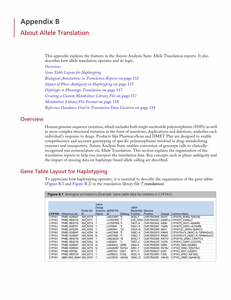
Appendix B
About Allele Translation
This appendix explains the features in the Axiom Analysis Suite Allele Translation reports. It also describes how allele translation operates and its logic.
Overview
Gene Table Layout for Haplotyping
Biological Annotations in Translation Reports on page 115
Impact of Phase Ambiguity in Haplotyping on page 115
Diplotype to Phenotype Translation on page 117
Creating a Custom Metabolizer Library File on page 117
Metabolizer Library File Format on page 118
Reference Databases Used in Translation Data Curation on page 119
OverviewHuman genome sequence variation, which includes both single nucleotide polymorphisms (SNPs) as well as more complex structural variation in the form of insertions, duplications and deletions, underlies each individual's response to drugs. Products like PharmacoScan and DMET Plus are designed to enable comprehensive and accurate genotyping of specific polymorphisms involved in drug-metabolizing enzymes and transporters. Axiom Analysis Suite enables conversion of genotype calls to clinically-recognized star nomenclature via Allele Translation. This section explains the organization of the translation reports to help you interpret the translation data. Key concepts such as phase ambiguity and the impact of missing data on haplotype-based allele calling are described.
Gene Table Layout for HaplotypingTo appreciate how haplotyping operates, it is essential to describe the organization of the gene tables (Figure B.1 and Figure B.2) in the translation library file (*.translation)
Figure B.1 Biological annotations [Example: Gene table data for markers in CYP1A1]

Appendix B | About Allele Translation 114
Biological annotations: The first set of columns in the table are annotations for the markers in each of the translated genes. Haplotype descriptions: The columns beyond the Common Name field contain information used for interpretation and translation of the gene file.
Following the columns enumerating the Reference and Variant alleles, haplotypes and markers in the gene are listed. In this example, CYP1A1 has 10 haplotypes described and they are named in the column headers. In addition, there are five additional markers for rare variants that can also be identified in this gene. Notice that the first haplotype described in this table is CYP1A1*1A, and that all markers except the last five are haplotyping markers (see the Haplotype field). Markers are characterized as "non-haplotyping" if their behavior in existing haplotypes is not known. For example, a variant has been identified in this gene resulting in a non-synonymous change in the protein (CYP1A1_134G>A(G45D)), but the haplotype background of that variant is not available in the literature references used (for example, the Karolinska reference database; http://www.cypalleles.ki.se/).
Figure B.1 illustrates the way that haplotypes are called. Notice that the haplotype names appear in the header of each gene table (for CYP1A1, when all markers are tested, this is *1, *2C, *3, *4, etc). Only differences from the reference haplotype appear in the haplotype columns, and the change for the altered base is indicated. For example, CYP1A1*2C contains one difference relative to CYP1A1*1, specifically a mutation 5'-prime to the gene, defined by the probe "CYP1A1*2C_2454A>G(I462V)".
The Defining field in the translation file lists the effect that a variant allele of this marker has. For example, because a variant at the final probe in the table, "CYP1A1_2458C>G(A463G)", results in a structural change in the protein, this marker is flagged with the name of the amino acid change that results: alanine at position 463 of the protein is a glycine in this variant (A463G). Although not shown in this gene, if a marker contains a variant allele in multiple haplotypes, then the marker does not uniquely define a single haplotype. That marker would then have an "N" (No) in the Defining field.
Haplotype field names with a # prefix, and rows with a # prefix in the Probe Set ID field are "commented out", and not used for translation.
Figure B.2 Haplotype descriptions [Example gene table data for markers in CYP1A1]
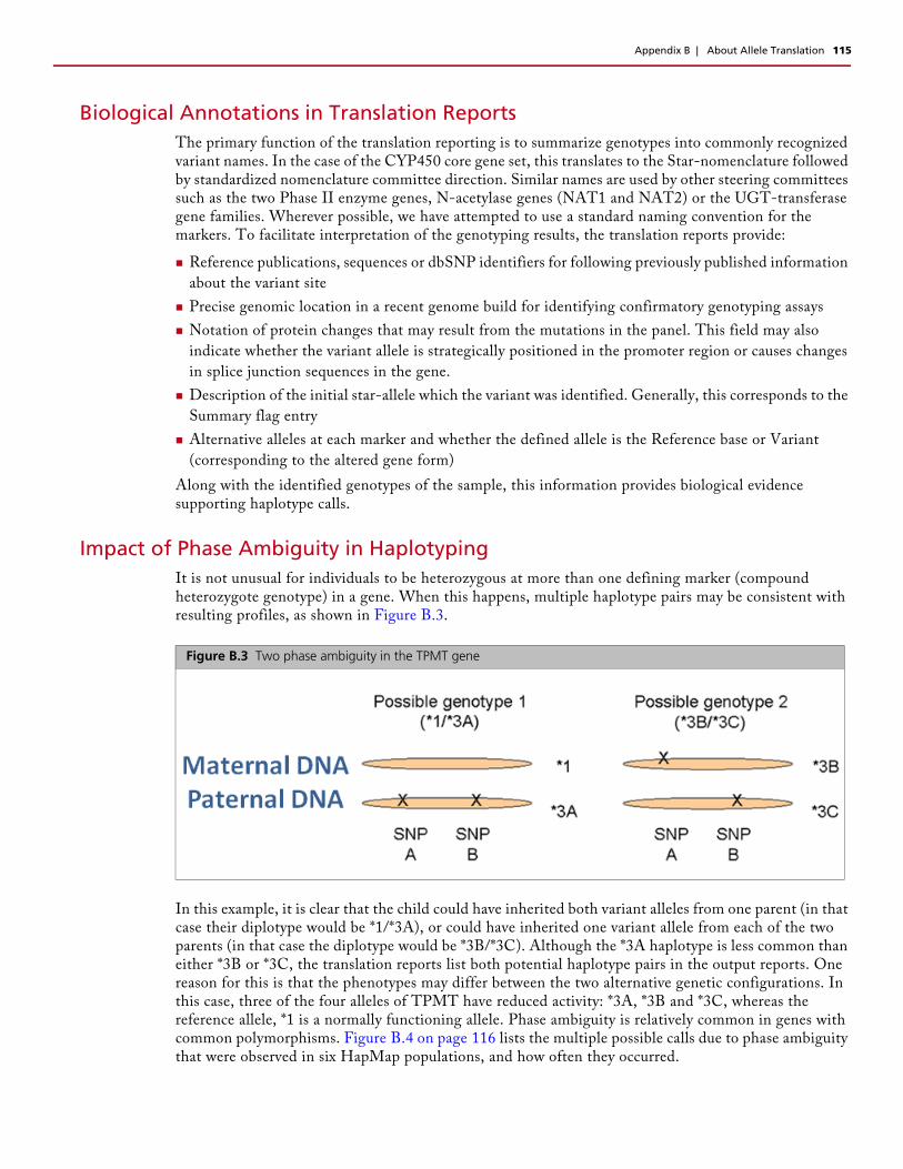
Appendix B | About Allele Translation 115
Biological Annotations in Translation ReportsThe primary function of the translation reporting is to summarize genotypes into commonly recognized variant names. In the case of the CYP450 core gene set, this translates to the Star-nomenclature followed by standardized nomenclature committee direction. Similar names are used by other steering committees such as the two Phase II enzyme genes, N-acetylase genes (NAT1 and NAT2) or the UGT-transferase gene families. Wherever possible, we have attempted to use a standard naming convention for the markers. To facilitate interpretation of the genotyping results, the translation reports provide:
Reference publications, sequences or dbSNP identifiers for following previously published information
about the variant site
Precise genomic location in a recent genome build for identifying confirmatory genotyping assays
Notation of protein changes that may result from the mutations in the panel. This field may also
indicate whether the variant allele is strategically positioned in the promoter region or causes changes
in splice junction sequences in the gene.
Description of the initial star-allele which the variant was identified. Generally, this corresponds to the
Summary flag entry
Alternative alleles at each marker and whether the defined allele is the Reference base or Variant
(corresponding to the altered gene form)
Along with the identified genotypes of the sample, this information provides biological evidence supporting haplotype calls.
Impact of Phase Ambiguity in HaplotypingIt is not unusual for individuals to be heterozygous at more than one defining marker (compound heterozygote genotype) in a gene. When this happens, multiple haplotype pairs may be consistent with resulting profiles, as shown in Figure B.3.
In this example, it is clear that the child could have inherited both variant alleles from one parent (in that case their diplotype would be *1/*3A), or could have inherited one variant allele from each of the two parents (in that case the diplotype would be *3B/*3C). Although the *3A haplotype is less common than either *3B or *3C, the translation reports list both potential haplotype pairs in the output reports. One reason for this is that the phenotypes may differ between the two alternative genetic configurations. In this case, three of the four alleles of TPMT have reduced activity: *3A, *3B and *3C, whereas the reference allele, *1 is a normally functioning allele. Phase ambiguity is relatively common in genes with common polymorphisms. Figure B.4 on page 116 lists the multiple possible calls due to phase ambiguity that were observed in six HapMap populations, and how often they occurred.
Figure B.3 Two phase ambiguity in the TPMT gene

Appendix B | About Allele Translation 116
It is worth pointing out that the predicted phenotypes of some of these alternative diplotype calls are identical, and in these cases the Phenotype report will then report a single phenotype. When phase ambiguity is encountered and the Phenotype report does not resolve the multiple calls to a single Phenotype Call, follow-up metabolic screening may be merited to differentiate the actual genetic configuration of the test samples.
Figure B.4 Example: Observed phase ambiguities in DMET Plus in a data set of six HapMap populations with 597 individuals and no children.

Appendix B | About Allele Translation 117
Diplotype to Phenotype TranslationAllele translations include a Phenotype report if the required metabolizer library file has been selected. The Phenotype report further translates the reported diplotypes (star allele pairs) from a subset of genes in the Comprehensive report into one of several phenotypes (e.g. "Poor Metabolizer"). As the software reads the comprehensive.rpt file, it will try to match Known Call diplotype values for each gene of each sample to one row of the metabolizer library file table. If a match is found, the associated phenotype and allele activities are written to the phenotype.rpt. If a match is not found, a Phenotype Call of "unknown" is reported. More information on this software feature is available in the DMET™ Plus Allele Translation white paper.
If you do not want to generate a phenotype report, leave the Metabolizer File option blank in the Perform Allele Translation dialog.
If you want to report phenotypes for only a subset of genes, there are two ways to accomplish this:
1. Import a custom SNP List into the workspace containing probesets from only the genes of interest.
At the point when you normally perform allele translation, select the option to filter to just probesets
in this list.
Or
2. Create a copy of the metabolizer file that only contains the genes of interest.
If you want to change what phenotypes are reported for a particular combination of diplotypes, or you would like to change what is written to the header of the Phenotype Translation report, you will need to create and use a custom version of the .metabolizer library file. Instructions for doing this follow.
Creating a Custom Metabolizer Library FileIf you choose to create a custom metabolizer table, Affymetrix recommends using the Affymetrix-supplied metabolizer file as a template. Save a copy of this file with a new name.
To be recognized by Axiom Analysis Suite, the file:
Must have the file extension *.metabolizer, where the * indicates your custom text.
Must be encoded in ANSI, not Unicode or other encoding.
Must exist in the library folder used by Axiom Analysis Suite.
Must be selected for use from the Configuration -> Options menu, in the Translations tab.
Must be properly formatted. It is recommended that you use a file comparison utility to verify that the
only changes between the original and modified files are expected changes.
If you want to add phenotype reporting (for genes not currently in the metabolizer library file) the gene names and star allele names you want to add must exist in the *.translation library file used to generate the *_comprehensive.rpt file.
NOTE: Users are responsible for reviewing the metabolizer library file for accuracy!
Phenotype Call and Gene Activity interpretations for a Known Call are supported bydiffering levels of evidence from in vivo and/or in vitro research studies. Refer tometabolizer library file for a list of references. The actual phenotype and gene activitiesmay be dependent on the substrate and dose.
NOTE: Use caution if editing the metabolizer file with Microsoft Excel. For example, Excel inserts quotation marks around text containing commas, which may make the file unreadable by Axiom Analysis Suite.
Before using the file with Axiom Analysis Suite, open it in another text editor and remove any unexpected text such as quotation marks.
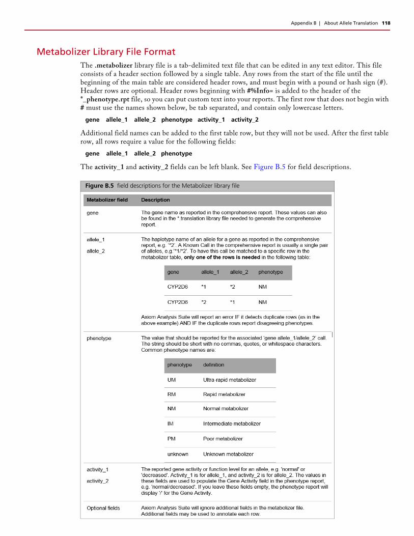
Appendix B | About Allele Translation 118
Metabolizer Library File FormatThe .metabolizer library file is a tab-delimited text file that can be edited in any text editor. This file consists of a header section followed by a single table. Any rows from the start of the file until the beginning of the main table are considered header rows, and must begin with a pound or hash sign (#). Header rows are optional. Header rows beginning with #%Info= is added to the header of the *_phenotype.rpt file, so you can put custom text into your reports. The first row that does not begin with # must use the names shown below, be tab separated, and contain only lowercase letters.
Additional field names can be added to the first table row, but they will not be used. After the first table row, all rows require a value for the following fields:
The activity_1 and activity_2 fields can be left blank. See Figure B.5 for field descriptions.
gene allele_1 allele_2 phenotype activity_1 activity_2
gene allele_1 allele_2 phenotype
Figure B.5 field descriptions for the Metabolizer library file
Appendix B | About Allele Translation 119
Reference Databases Used in Translation Data CurationThe databases used to curate the allele translation gene tables include:
PharmGKB - Stanford University Pharmacogenomics reference database
http://www.pharmgkb.org
Karolinska cytochrome P450 gene standard nomenclature
http://www.cypalleles.ki.se
Database of NAT genes (Democritus University of Thrace)
http://nat.mbg.duth.gr
Database of UGT genes
https://www.pharmacogenomics.pha.ulaval.ca/ugt-alleles-nomenclature
Drug interaction database (University of Indiana)
http://medicine.iupui.edu/clinpharm/ddis
PubMed - On-line National Library of Medicine publication database
http://www.ncbi.nlm.nih.gov/pubmed
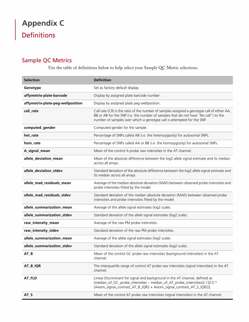
Appendix C
Definitions
Sample QC MetricsUse the table of definitions below to help select your Sample QC Metric selections.
Selection Definition
Genotype Set as factory default display.
affymetrix-plate-barcode Display by assigned plate barcode number.
affymetrix-plate-peg-wellposition Display by assigned plate peg wellposition.
call_rate Call rate (CR) is the ratio of the number of samples assigned a genotype call of either AA, BB or AB for the SNP (i.e. the number of samples that do not have ``No call'') to the number of samples over which a genotype call is attempted for the SNP.
computed_gender Computed gender for the sample.
het_rate Percentage of SNPs called AB (i.e. the heterozygosity) for autosomal SNPs.
hom_rate Percentage of SNPs called AA or BB (i.e. the homozygosity) for autosomal SNPs.
A_signal_mean Mean of the control A probe raw intensities in the AT channel.
allele_deviation_mean Mean of the absolute difference between the log2 allele signal estimate and its median across all arrays.
allele_deviation_stdev Standard deviation of the absolute difference between the log2 allele signal estimate and its median across all arrays.
allele_mad_residuals_mean Average of the median absolute deviation (MAD) between observed probe intensities and probe intensities fitted by the model.
allele_mad_residuals_stdev Standard deviation of the median absolute deviation (MAD) between observed probe intensities and probe intensities fitted by the model.
allele_summarization_mean Average of the allele signal estimates (log2 scale).
allele_summarization_stdev Standard deviation of the allele signal estimates (log2 scale).
raw_intensity_mean Average of the raw PM probe intensities.
raw_intensity_stdev Standard deviation of the raw PM probe intensities.
allele_summarization_mean Average of the allele signal estimates (log2 scale).
allele_summarization_stdev Standard deviation of the allele signal estimates (log2 scale).
AT_B Mean of the control GC probe raw intensities (background intensities) in the ATchannel.
AT_B_IQR The interquartile range of control AT probe raw intensities (signal intensities) in the ATchannel.
AT_FLD Linear Discriminant for signal and background in the AT channel, defined as(median_of_GC_probe_intensities – median_of_AT_probe_intensities)2 / [0.5 *(Axiom_signal_contrast_AT_B_IQR2 + Axiom_signal_contrast_AT_S_IQR2)].
AT_S Mean of the control AT probe raw intensities (signal intensities) in the AT channel.

Appendix C | Definitions 121
AT_S_IQR The interquartile range of control AT probe raw intensities (signal intensities) in the ATchannel.
AT_SBR Signal to background ratio in the AT channel, defined as Axiom_signal_contrast_AT_S/ Axiom_signal_contrast_AT_B.
C_signal_mean Mean of the control C probe raw intensities in the GC channel.
cluster_distance_mean Average distance to the cluster center for the called genotype.
cluster_distance_stdev Standard deviation of the distance to the cluster center for the called genotype.
cn-probe-chrXY-ratio_gender Gender ratio Y/X = cn-probe-chrXY-ratio_gender_meanY/ cn-probe-chrXY-ratio_gender_meanX.
cn-probe-chrXY-ratio_gender_meanX The average probe intensity (raw, untransformed) of X chromosome non-polymorphicprobes.
cn-probe-chrXY-ratio_gender_meanY The average probe intensity (raw, untransformed) of Y chromosome non-polymorphicprobes.
cn-probe-chrXY-ratio_gender_ratio Gender ratio Y/X = cn probe chrXY-ratio_gender_meanY/ cn probe chrXYratio_gender_meanX.
CV_GC The coefficient of variation in the GC channel.
DQC Dish QC
G_signal_mean Mean of the control G probe raw intensities in the GC channel.
GC_B Mean of control AT probe raw intensities (background intensities) in the GC channel.
GC_B_IQR The interquartile range of control AT probe raw intensities (background intensities) inthe GC channel.
GS_S Mean of control GC probe raw intensities (signal intensities) in the GC channel.
GS_S_IQR Interquartile range of control GC probe raw intensities (signal intensities) in the GCchannel.
GC_SBR Signal to background ratio in the GC channel, defined as Axiom_signal_contrast_GC_S/ Axiom_signal_contrast_GC_B.
log_diff_qc A cross channel QC metric, defined as mean(log(AT_SBR))/std(log(AT_SBR)) +mean(log(GC_SBR))/std(log(GC_SBR)), where signal and background are calculated forcontrol non-polymorphic probes after intensity normalization.
QC_allele_deviation_mean Average of the absolute difference between the log2 allele signal estimateand its median across all arrays.
QC_allele_deviation_stdev Standard deviation of the absolute difference between the log2 allele signalestimate and its median across all arrays.
QC_allele_mad_residuals_mean Average of the median absolute deviation (MAD) between observed probeintensities and probe intensities fitted by the model.
QC_allele_mad_residuals_stdev Standard deviation of the median absolute deviation (MAD) betweenobserved probe intensities and probe intensities fitted by the model.
QC_allele_summarization_mean Average of the allele signal estimates (log2 scale).
QC_allele_summarization_stdev Standard deviation of the allele signal estimates (log2 scale).
QC_call_rate Call rate at the default or user-specifiedthreshold for autosomal SNPs.
Selection Definition

Appendix C | Definitions 122
QC_cluster_distance_mean Average distance to the cluster center for the called genotype.
QC_cluster_distance_stdev Standard deviation of the distance to the cluster center for the calledgenotype.
QC_computed_gender Computed gender for the sample.
QC_het_rate Percentage of SNPs called AB (i.e. the heterozygosity) for autosomal SNPs in a Sample QC.
QC_hom_rate Percentage of SNPs called AA or BB (i.e. the homozygosity) for autosomal SNPs in a Sample QC.
QC_total_call_rate Call rate at the default or user-specified threshold for all SNPs.
QC_total_het_rate Percentage of SNPs called AB (i.e., the heterozygosity) for all SNPs.
QC_total_hom_rate Percentage of SNPs called AA or BB (i.e. the homozygosity) for all SNPs.
reagent_discrimination_value Value assigned to the reagent.
reagent_version The reagent version used for processing the arrays, based on data intensity values.You can only perform batch genotyping analysis on CEL files processed using the samereagent version.
saturation_AT Fraction of features in the AT channel with intensity greater than or equal to 3800.IMPORTANT: This metric/column does not appear for CEL files QC’d with GTC v.4.1 (orearlier).
saturation_GC Fraction of features in the GC channel with intensity greater than or equal to 3800.IMPORTANT: This metric/column does not appear for CEL files QC’d with GTC v.4.1 (orearlier).
T_signal_mean Mean of the control T probe raw intensities in the AT channel.
total_call_rate Call rate at the default or user-specified threshold for all SNPs.
total_het_rate Percentage of SNPs called AB (i.e., the heterozygosity) for all SNPs.
total_hom_rate Percentage of SNPs called AA or BB (i.e. the homozygosity) for all SNPs.
Selection Definition

Appendix C | Definitions 123
Annotations and ColumnsUse the table of definitions below to help select your SNP Summary Table columns and annotations.
Column Name Description
Probe Set ID The Affymetrix unique identifier for the set of probes used to detect a particular Single Nucleotide Polymorphism (SNP probe sets only).
Affx SNP ID The Affymetrix unique identifier for the set of probes used to detect a particular Single Nucleotide Polymorphism (SNP). (SNP probe sets only, not available for Axiom™ Genome-Wide Human Array).
dbSNP RS ID The dbSNP ID that corresponds to this probe set or SNP. The dbSNP at the National Center for Biotechnology Information (NCBI) attempts to maintain a unified and comprehensive view of known single nucleotide polymorphisms (SNPs), small scale insertions/deletions, polymorphic repetitive elements, and microsatellites from TSC and other sources. The dbSNP is updated periodically, and the dbSNP version used for mapping is given in the dbSNP version field. For more information, please see: http://www.ncbi.nlm.nih.gov/SNP/ (SNP probe sets only).
Chromosome The chromosome on which the SNP is located on the current Genome Version.
Chromosome Start The nucleotide base start position where the SNP is found. The genomic coordinates given are in relation to the current genome version and may shift as subsequent genome builds are released.
Chromosome Stop The nucleotide base stop position where the SNP is found. The genomic coordinates given are in relation to the current genome version and may shift as subsequent genome builds are released.
Strand Genomic strand that the SNP resides on.
Cytoband Cytoband location of the SNP derived from the SNP physical map and the chromosome band data provided by UCSC.
Strand Vs dbSNP Indicates whether the SNP is on the same or reverse strand as compared to dbSNP (SNP probe sets only).
ChrX pseudo-autosomal region SNPs on the X Chromosome which are mapped to the two pseudo-autosomal region have a value of 1 or 2 in this field. All other SNPs are indicated by 0. A value of “1” indicates that the marker maps to the PAR-1 region and a value of “2” indicates that the marker maps to the PAR-2 region. A value of “0” indicates that the marker does not map to either of the two PAR regions.
Probe Count The total number of probes in the probe set.
Flank The nucleotide sequence surrounding the SNP. This is a 33-mer sequence with 16 nucleotides on either end of the SNP position. The alleles at the SNP position are provided in the brackets (SNP probe sets only).
Allele A The allele of the SNP that is in lower alphabetical order. When comparing the allele data on NetAffx to the allele data for the corresponding RefSNP record in dbSNP, the alleles reported here could be different from the alleles reported for the corresponding RefSNP on the dbSNP web site. This difference arises mainly from the reference genomic strand that was chosen to define the alleles by Affymetrix. To choose the reference genomic strand, we follow a convention based on the alphabetic ordering of the sequence surrounding the SNP. Sometimes the reference strand on the dbSNP is different from NetAffx, and the alleles could represent reverse complement of those provided on dbSNP (SNP probe sets only).

Appendix C | Definitions 124
Allele B The allele of the SNP that is in higher alphabetical order. When comparing the allele data on NetAffx to the allele data for the corresponding RefSNP record in dbSNP, the alleles reported here could be different from the alleles reported for the corresponding RefSNP on the dbSNP web site. This difference arises mainly from the reference genomic strand that was chosen to define the alleles by Affymetrix. To choose the reference genomic strand, we follow a convention based on the alphabetic ordering of the sequence surrounding the SNP. Sometimes the reference strand on the dbSNP is different from NetAffx, and the alleles could represent reverse complement of those provided on dbSNP (SNP probe sets only).
Associated Gene SNPs were associated with human genes by comparing the genomic locations of the SNPs to genomic alignments of human mRNA sequences. In cases where the SNP is within a known gene, NetAffx reports the association. Additionally, for genes with exon or CDS annotations, NetAffx reports whether or not the SNP is in an exon, and in the coding region. If the SNP is not within a known gene, NetAffx reports the closest genes in the genomic sequence, and the distance and relationship of the SNP relative to the genes. A SNP is upstream of a gene if it is located closer to the 5' end of the gene and is downstream of a gene if it is located closer to the 3' end of the gene.
Genetic Map Describes the genetic location of the SNP derived from three separate linkage maps (deCODE, Marshfield, or SLM). The physical distance between the markers is assumed to be linear with their genetic distance. The genetic location is computed using the linkage maps from the latest physical location of the SNP and the neighboring microsatellite markers (SNP probe sets only).
Microsatellite Describes the nearest microsatellite markers (upstream, downstream and overlapping) for the SNP.
Enzyme Fragment Lists the enzyme, the restriction fragment containing the SNP and the fragment length. The Whole Genome Assay protocol detects SNPs that are contained within the genomic restriction fragments to simplify the sequence background for genotyping arrays (not available for Axiom Genome-Wide Human Array).
Copy Number Variation When available, a description of Copy Number Variation Region (CN) probe sets as described by the Database of Genomic Variants (not available for Axiom Genome-Wide Human Array).
SNP Interference This column is for Copy Number probe sets. It indicates whether or not a known SNP overlaps a copy number probe (CN probe sets only, not available for Axiom Genome-Wide Human Array).
In Final List This column annotates extended content for genotyping arrays. A value of “1” indicates that the marker is included in the final version of the library file and a value of “0” indicates that the marker is not included in the final version of the library file (SNP probe sets only, not available for Axiom Genome-Wide Human Array).
% GC The fraction of bases that are G or C in a window of 250,000 bases to each side of the SNP or CN position. All positions that are nearer to the end than 250,001 are set to the value of the position at 250,001 from that end. Position and chromosome values for SNPs and CN probes were mapped to the position of bases in the FASTA files for the build of the genome used in this release of NetAffx, and these bases were then used for all calculations (not available for Axiom Genome-Wide Human Array).
Heterozygous Allele Frequencies Describes the heterozygous frequency of the allele from Yoruba, Japanese, Han Chinese and CEPH studies using the Affymetrix genotyping arrays. (SNP probe sets only)
Allele Sample Size Sample size used for Allele Frequency estimates (SNP probe sets only).
Allele Frequencies Describes the major and minor frequency of the allele from Yoruba, Japanese, Han Chinese and CEPH studies using the Affymetrix genotyping arrays (SNP probe sets only).
Minor Allele Indicates the Minor Allele of a SNP (SNP probe sets only).
Column Name Description

Appendix C | Definitions 125
Concordance ColumnsUse the table of definitions below to help select your Concordance columns.
Threshold NamesUse the table of definitions below to help select Threshold names.
Minor Allele Frequency The Minor Allele Frequency of a SNP (SNP probe sets only).
OMIM ID Furnishes OMIM and Morbid Map IDs and their respective gene titles. This database contains information from the Online Mendelian Inheritance in Man® (OMIM®) database, which has been obtained under a license from the Johns Hopkins University. This database/product does not represent the entire, unmodified OMIM® database, which is available in its entirety at www.ncbi.nlm.nih.gov/omim/.
Column Name Description
Base The first sample in the comparison.
Reference The second sample in the comparison.
#SNPs Called Number of SNPs common to both sample and reference files with genotype calls.
#Concordant SNP’s Number of called SNPs that have the same genotype call.
%Concordance Percentage of called SNPs that have the same genotype call.
Threshold Name Description
Sample QC
axiom_dishqc_DQC A sample’s dish QC value must be larger than 'DQC' to pass sample QC.
qc_call_rate A sample’s call rate value must be larger than 'QC call_rate' to pass genotyping QC.
plate_qc_percentsamplespassed If a plate’s percent of passing samples is smaller than this number, all samples on the plate will show a warning in the Sample Table.
plate_qc_averagecallrate A plate’s average QC call rate of passing samples must be larger than this number to pass plate QC.
species-type Species types include: Diploid, Human, and Polyploid.
SNP QC
cr-cutoff Threshold for call rate. If not specified, the default for human is 95 and for diploid and polyploid is 97.
fld-cutoff Cut-off value for cluster quality (FLD).
het-so-cutoff Cut-off value for the correctness of the vertical position of the heterozygous cluster (Strength Offset).
het-so-otv-cutoff Cut-off value for the existence of a fourth cluster below the heterozygous cluster (OTV).
hom-ro-1-cutoff Cut-off value for the correctness of the horizontal position of the homozygous clusters (Ratio Offset) when a SNP has one genotype.
Column Name Description

Appendix C | Definitions 126
hom-ro-2-cutoff Cut-off value for the correctness of the horizontal position of the homozygous clusters when a SNP has two genotypes.
hom-ro-3-cutoff Cut-off value for the correctness of the horizontal position of the homozygous clusters when a SNP has three genotypes
hom-ro Flag indicating whether the metric HomRO is used in classification.
hom-het Flag indicating whether the metric HomHet is used in classification. The HomHet metric identifies two-cluster SNPs/probesets with one homozygote cluster and one heterozygote cluster. This checks if the minor homozygote cluster is missing, which is unreasonable for highly inbred species (e.g. wheat). This metric should be turned on when classifying SNPs/probesets in highly inbred species.
num-minor-allele-cutoff The number of minor alleles.
priority-order When performing probeset selection, the best probeset is selected according to the priority order of probeset conversion types.
recommended Use this checklist to choose your ps_classification conversion types for your analysis.
Threshold Name Description

Appendix C | Definitions 127
SNP Summary Table DefinitionsUse the table of definitions below to help select your SNP Summary Table columns.
Column Name Description
SNPID The Affymetrix unique identifier for the set of probes used to detect a particular Single Nucleotide Polymorphism (SNP).
SNP Call Rate Call Rate for that SNP across all samples in the batch.
SNP %AA Percentage of AA calls for this SNP in this batch.
SNP %AB Percentage of AB calls for this SNP in this batch.
SNP %BB Percentage of BB calls for this SNP in this batch.
Minor Allele Frequency The allele frequency for the A allele is calculated as:
Where the Total # Calls does not include the No Calls.The B allele frequency is .
The minor allele frequency is the Min(PA, PB).

Appendix C | Definitions 128
H-W p-value Hardy Weinberg p-value is a measure of the significance of the discrepancy between the observed ratio or heterozygote calls in a population and the ratio expected if the population was in Hardy Weinberg equilibrium.
There are two statistical tests used for HWE. When AA, AB, and BB counts are all >=10, a Chi-squared testis used. When one or more of the AA, AB, and BB counts are <10, an Exact test is used. An Exact test meansthat the p-value is calculated exactly and not approximated from a population distribution.
Where:
Where CDF is the Cumulative Distributive Function for the chi-squared distribution.
The Exact test used is the one implemented in R package "HardyWeinberg" for more information see:[2] Haldane, J., 1954. An exact test for randomness of mating. J. Genet. 52 631-635.[3] Levene, H., 1949. On a matching problem arising in genetics. Ann. Math. Stat. 20 91-94.
H. W. Statistic If the count of samples for at least one cluster is <10, then H.W. Statistic is 1. The Exact test is used to determine HWE. A 0 value indicates that there are more than 10 samples per cluster and a chi-squared test is used to determine HWE.
Column Name Description
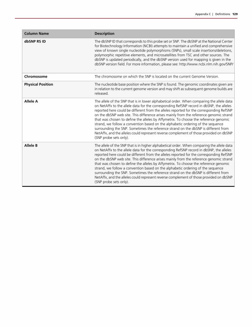
Appendix C | Definitions 129
dbSNP RS ID The dbSNP ID that corresponds to this probe set or SNP. The dbSNP at the National Center for Biotechnology Information (NCBI) attempts to maintain a unified and comprehensive view of known single nucleotide polymorphisms (SNPs), small scale insertions/deletions, polymorphic repetitive elements, and microsatellites from TSC and other sources. The dbSNP is updated periodically, and the dbSNP version used for mapping is given in the dbSNP version field. For more information, please see: http://www.ncbi.nlm.nih.gov/SNP/.
Chromosome The chromosome on which the SNP is located on the current Genome Version.
Physical Position The nucleotide base position where the SNP is found. The genomic coordinates given are in relation to the current genome version and may shift as subsequent genome builds are released.
Allele A The allele of the SNP that is in lower alphabetical order. When comparing the allele data on NetAffx to the allele data for the corresponding RefSNP record in dbSNP, the alleles reported here could be different from the alleles reported for the corresponding RefSNP on the dbSNP web site. This difference arises mainly from the reference genomic strand that was chosen to define the alleles by Affymetrix. To choose the reference genomic strand, we follow a convention based on the alphabetic ordering of the sequence surrounding the SNP. Sometimes the reference strand on the dbSNP is different from NetAffx, and the alleles could represent reverse complement of those provided on dbSNP (SNP probe sets only).
Allele B The allele of the SNP that is in higher alphabetical order. When comparing the allele data on NetAffx to the allele data for the corresponding RefSNP record in dbSNP, the alleles reported here could be different from the alleles reported for the corresponding RefSNP on the dbSNP web site. This difference arises mainly from the reference genomic strand that was chosen to define the alleles by Affymetrix. To choose the reference genomic strand, we follow a convention based on the alphabetic ordering of the sequence surrounding the SNP. Sometimes the reference strand on the dbSNP is different from NetAffx, and the alleles could represent reverse complement of those provided on dbSNP (SNP probe sets only).
Column Name Description


