User’s Guide to NOVAS Version F3.1 Naval Observatory Vector Astrometry Software

Fortran Edition

George Kaplan Jennifer Bartlett Alice Monet John Bangert Wendy Puatua

U.S. Naval Observatory March 2011

Approved for Public Release

F-3

User’s Guide to NOVAS Version F3.1 Naval Observatory Vector Astrometry Software For tran Edition

In this document, hyperlinks are in blue.

Table of Contents

Introduction F-7 Citing NOVAS F-8 Abbreviations and Symbols Frequently Used (Table) F-9 Chapter 1 Astronomical Background F-11 1.1 Astronomical Coordinate Systems F-11 1.2 Computing Observable Quantities F-14 1.3 Time Scales for Astronomy F-17 1.4 The Adopted Models for Precession and Nutation F-19 1.5 A New Model for the Rotation of the Earth about its Axis F-20 1.6 Terrestrial-Celestial Relationships F-21 Chapter 2 Installing NOVAS F-23 2.1 List of Distribution Files (Table) F-23 2.2 Basic Installation Procedure F-23 2.3 Using External Solar System Ephemeris Files F-25 2.4 Making the NOVAS External Data Files More Efficient F-26 2.5 Do I Have to Use a CIO File? F-27 2.6 The NOVAS Low-Accuracy Mode and the Alternative Subroutines F-27 Chapter 3 Sample Calculations F-29 3.1 Initialization F-29 3.2 Setting Time Arguments F-30 3.3 Example 1—Position of a Star F-31 3.4 Example 2—Position of the Moon F-32 3.5 Example 3—Greenwich Sidereal Time F-34 3.6 Example 4—Other Frequently Requested Quantities F-35 Chapter 4 Description of Individual Subroutines F-37 NOVAS Fortran Subroutine, Function, and Entry Names (Table) F-37 PLACE F-40 SIDTIM F-44 TERCEL F-45 CELTER F-46 ZDAZ F-47 CATRAN F-49 GETHIP F-51 APSTAR F-52 TPSTAR F-53

F-4

VPSTAR F-54 LPSTAR F-55 ASSTAR F-56 APPLAN F-57 TPPLAN F-58 VPPLAN F-59 LPPLAN F-60 ASPLAN F-61 PRECES F-62 EQECL F-63 CIORA F-65 EROT F-65 HIACC F-66 LOACC F-66 GETVEC F-67 SETDT F-68 CELPOL F-69 ETILT F-70 SOLSYS F-71 IDSS F-73 SOLSYS Version 1 F-74 SOLSYS Version 2 F-76 Specifications for Subroutine AUXPOS F-77 SOLSYS Version 3 F-79 Chapter 5 Equinox- and CIO-Based Paradigms Compared F-81 5.1 Computing Hour Angles F-81 5.2 Other Computational Considerations F-82 5.3 How NOVAS Implements the CIO-Based Paradigm F-83 Appendix A Overview of How NOVAS Has Changed F-85 A.1 Important Changes in Calls F-85 A.2 PLACE: A New General-Purpose “Place” Subroutine F-85 A.3 New Reference Systems F-86 A.4 New Models for Precession and Nutation F-87 A.5 A New Model for the Rotation of the Earth about its Axis F-88 A.6 New Features F-89 A.7 New Terminology F-89 Appendix B List of Changes from NOVAS F2.0 to F3.1 F-91 B.1 New Subroutines F-91 B.1.1 New Subroutines in NOVAS F3.0 F-91 B.1.2 New Subroutines in NOVAS F3.1 F-93 B.2 Changes to NOVAS F Calling Sequences F-93 B.2.1 Changes to Calling Sequences from F2.0 to F3.0 F-93

F-5

B.2.2 Changes to Calling Sequences from F3.0 to F3.1 F-94 B.3 Significant Internal Changes to Code F-94 B.3.1 Significant Internal Changes to Code from F2.0 to F3.0 F-94 B.3.2 Significant Internal Changes to Code from F3.0 to F3.1 F-98 B.4 Other Internal Code Changes F-98 B.4.1 Other Internal Code Changes from F2.0 to F3.0 F-98 B.4.2 Other Internal Code Changes from F3.0 to F3.1 F-98 Appendix C How to Set Up the JPL Ephemerides F-99 C.1 Overview F-99 C.2 Step-by-Step Guide F-99 Appendix D A Comparison of SOFA and NOVAS F3.0 F-103 D.1 Goal F-103 D.2 Procedure F-103 D.3 Results F-104 D.4 Addendum I: NOVAS F3.0 Code F-105 D.5 Addendum II: SOFA Code F-106 Appendix E List of Internal Calls F-111

F-6

F-7

Introduction The Naval Observatory Vector Astrometry Software (NOVAS) is a source-code library for computing various commonly needed quantities in positional astronomy. The code exists in two languages, Fortran and C, plus Python wrappers are now available for the C. The Fortran version goes back to the late 1970s, but has been updated periodically to use new, more accurate models that represent the evolving standards of the international astronomical and geodetic communities. The C version was first introduced in 1996 and provides the same functionality and accuracy. In full-accuracy calculations using the same data sources, differences in the results from Fortran and C editions of NOVAS, for the same calculation, should not exceed 6 × 10−8 arcseconds (3 × 10−13 radians) for solar system bodies and 7 × 10−10 arcseconds (3 × 10−15 radians) for stars. NOVAS can provide, in one or two subroutine or function calls, the instantaneous celestial position of any star or planet in a variety of coordinate systems. NOVAS also provides access to all of the “building blocks” that go into such computations—single-purpose subroutines for common astrometric algorithms, such as those for precession, nutation, aberration, parallax, etc. NOVAS calculations are accurate at the sub-milliarcsecond level. The NOVAS package is an easy-to-use facility that can be incorporated into data reduction programs, telescope control systems, and simulations. NOVAS is used in the production of the U.S. parts of The Astronomical Almanac. The algorithms used by the NOVAS routines are based on a vector and matrix formulation that is rigorous and consistent with recent recommendations by the International Astronomical Union (IAU). Objects within and outside the solar system are treated similarly and the position vectors formed and operated on by the NOVAS routines are defined within either the Barycentric Celestial Reference System (BCRS) or the Geocentric Celestial Reference System (GCRS), as appropriate. Both of these systems are described in IAU resolutions passed in 2000. GCRS quantities are converted to more familiar coordinate systems, such as the equator and equinox of date, by applying standard rotations. Three levels of subroutines or functions are involved: basic, utility, and supervisory. Basic-level subroutines supply the values of fundamental variables, such as the nutation angles and the heliocentric positions of solar system bodies, for specific epochs. Utility-level subroutines perform computations corresponding to individual physical effects or transformations (aberration, light-bending, precession, polar motion, etc.). Supervisory-level subroutines call the basic and utility subroutines in the proper order to compute the apparent coordinates of stars or solar system bodies for specific dates and times. If desired, users can interact exclusively with the supervisory-level routines and not become concerned with the details of the geometry or physical models involved in the computation.

F-8

Previous versions of NOVAS were based on the algorithms described in Kaplan et al. (1989) Astron. J., 97, 1197.1

USNO Circular 180

Although the phenomena that are considered and the overall sequence of calculations remains much the same, many of the models have been improved sub-stantially over the last two decades in response to increased accuracy in observing techniques. Specifically, version 3.0 of NOVAS, released in 2009 and described in

,2

USNO Circular 179

implements the resolutions on astronomical reference systems and Earth rotation models passed at the IAU General Assemblies in 1997, 2000, and 2006. An explanation of the recent IAU resolutions can be found in Kaplan (2005),

,3

The IAU Resolutions on Astronomical Reference Systems, Time Scales, and Earth Rotation Models: Explanation and Implementation, which contains much more information on topics only briefly touched on in this document. NOVAS 3.0 also improves the accuracy of its star and planet position calculations by including several small effects not previously implemented in the code; see, for example, Klioner (2003) Astron. J., 125, 1580. In addition, some new convenience functions have been added in NOVAS 3.0. The current version, NOVAS 3.1, provides some more capabilities and fixes some bugs.

Citing NOVAS If you use NOVAS, please send us an e-mail4

that outlines your application. This information helps justify further improvements to NOVAS. Your comments and suggestions are also welcome.

This user's guide is the official reference for NOVAS F3.1 and may be cited as Kaplan, G., Bartlett, J., Monet, A., Bangert, J., & Puatua, W., 2011, User’s Guide to NOVAS Version F3.1 (Washington, DC: USNO). In addition, we ask that you also direct your readers to the NOVAS website.5

The official reference for NOVAS 3.0 is USNO Circular 180, which is Kaplan, G., Bangert, J., Bartlett, J., Puatua, W., & Monet, A. (2009) User’s Guide to NOVAS 3.0, USNO Circular 180 (Washington, DC: USNO). The official reference for all versions of NOVAS prior to 3.0 is the 1990 software report announcing its release, which is Kaplan, G. (1990) “NOVAS: U. S. Naval Observatory,” Bull. AAS, 22, 930.

1 Parts were reprinted in Chapter 3 of Seidelmann (1992), Explanatory Supplement to the Astronomical Almanac (University Science Books) 2 http://www.usno.navy.mil/USNO/astronomical-applications/publications/circ-180 3 http://www.usno.navy.mil/USNO/astronomical-applications/publications/circ-179 4 http://www.usno.navy.mil/help/astronomy-help 5 The current version of NOVAS may be obtained at http://www.usno.navy.mil/USNO/astronomical-applications/software-products/novas

F-9

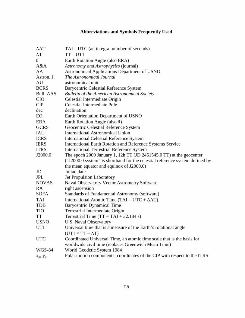
Abbreviations and Symbols Frequently Used ∆AT TAI – UTC (an integral number of seconds) ∆T TT – UT1 θ Earth Rotation Angle (also ERA) A&A Astronomy and Astrophysics (journal) AA Astronomical Applications Department of USNO Astron. J. The Astronomical Journal AU astronomical unit BCRS Barycentric Celestial Reference System Bull. AAS Bulletin of the American Astronomical Society CIO Celestial Intermediate Origin CIP Celestial Intermediate Pole dec declination EO Earth Orientation Department of USNO ERA Earth Rotation Angle (also θ) GCRS Geocentric Celestial Reference System IAU International Astronomical Union ICRS International Celestial Reference System IERS International Earth Rotation and Reference Systems Service ITRS International Terrestrial Reference System J2000.0 The epoch 2000 January 1, 12h TT (JD 2451545.0 TT) at the geocenter

(“J2000.0 system” is shorthand for the celestial reference system defined by the mean equator and equinox of J2000.0)

JD Julian date JPL Jet Propulsion Laboratory NOVAS Naval Observatory Vector Astrometry Software RA right ascension SOFA Standards of Fundamental Astronomy (software) TAI International Atomic Time (TAI = UTC + ∆AT) TDB Barycentric Dynamical Time TIO Terrestrial Intermediate Origin TT Terrestrial Time (TT = TAI + 32.184 s) USNO U.S. Naval Observatory UT1 Universal time that is a measure of the Earth’s rotational angle

(UT1 = TT – ∆T) UTC Coordinated Universal Time, an atomic time scale that is the basis for

worldwide civil time (replaces Greenwich Mean Time) WGS-84 World Geodetic System 1984 xp, yp Polar motion components; coordinates of the CIP with respect to the ITRS

F-10

F-11

Chapter 1 Astronomical Background At its highest level, NOVAS computes the precise positions of selected celestial objects at specified dates and times, as seen from a given location on or near the Earth. There are a number of coordinate systems in which such positions can be expressed. Dates and times are specified in several astronomical time scales, depending on the application. Users of NOVAS should have a basic knowledge of astronomical coordinate systems and time; terms like right ascension, declination, hour angle, ecliptic, equinox, precession, and sidereal time should be familiar. A number of texts on fundamental astronomyfor example, Green (1985), Spherical Astronomy (Cambridge University Press)provide the essential concepts. For more technical descriptions of the latest international standards on reference systems, USNO Circular 179,6

The Astronomical Almanac

cited in the Introduction, can provide the background. Circular 179 documents the algorithms for many important calculations in NOVAS. Others are described in the Kaplan et al. (1989) Astron. J. paper mentioned in the Introduction or in the Explanatory Supplement to the Astronomical Almanac. In addition, two glossaries may be useful to NOVAS users: one published in ,7

IAU Working Group on Nomenclature for Fundamental Astronomy and one compiled by

the .8

A very cursory overview of some of the most important aspects of the astronomical calculations performed by NOVAS follows. In this chapter, names of subroutines relevant to the subject being discussed are shown in [BRACKETS]. Special terms referred to in IAU resolutions are printed in bold when first mentioned; other relevant terms with widely accepted meanings in astronomy are initially printed in italics. 1.1 Astronomical Coordinate Systems Astronomical coordinate systems have traditionally been based on the extension of the Earth’s equatorial plane to infinity, along with a fiducial direction in that plane, the equinox. The direction of the equinox is along the line of nodes where the equatorial and ecliptic planes meet. Because the Earth’s equator and ecliptic are both in motion (the equator’s motion is described by precession and nutation; the ecliptic’s motion is due to the Earth’s orbital variations), an infinite number of such coordinate systems exist, each one corresponding to the orientation of the two planes at a specific date and time. The situation is complicated by the fact that for some purposes in the past it was convenient to consider only precession—and to neglect nutation—in defining celestial coordinate systems, so that we can have, for any given date and time, both a mean system (in which only precession is considered) and a true system (in which both precession and nutation are taken into account). Thus we have the mean system of [some] date, the true system of date, the mean system of 2000.0, etc. [PRECES, NUTATE, GCRSEQ]

6 http://www.usno.navy.mil/USNO/astronomical-applications/publications/circ-179 7 http://asa.usno.navy.mil/SecM/Section_M.html 8 http://syrte.obspm.fr/iauWGnfa/NFA_Glossary.html

F-12

Sidereal time is closely tied to the equatorial coordinate systems: one day of sidereal time is marked by successive transits of the equinox across a specific geographic meridian, and local sidereal time is just the apparent right ascension of stars transiting the observer’s meridian. Like the equatorial coordinate systems, sidereal time comes in two flavors, mean and apparent, based on, respectively, the mean and true equinox and the system of right ascension that each defines. [SIDTIM] In the last few decades of the 20th century, several IAU working groups led a general re-examination of astronomical coordinate systems at a very basic level. Part of the motivation was quite practical: most large ground-based telescopes were no longer built on equatorial mounts, and the equatorial coordinate systems were irrelevant to increasingly important space observations. Furthermore, the most precise fundamental measurements—those that by their nature are most closely related to the equatorial systems—are now obtained from Very Long Baseline Interferometry (VLBI), a radio technique that has no direct sensitivity to the equinox. Another important consideration was the need for astronomical coordinate systems that were part of a general relativistic framework. All of these factors were folded into some very important resolutions passed by the IAU in 1997 and 2000, which form the basis for the coordinate systems used in the current version of NOVAS. These resolutions have introduced concepts and terminology that may not be familiar to astronomers used to the traditional systems and names, which were used in the previous versions of NOVAS. The new systems are outlined in the following paragraphs, but see USNO Circular 1799

for a much more complete description.

One of the resolutions passed by the IAU in 2000 defined two systems of space-time coordinates, one for the solar system and the other for the near-Earth environment, within the framework of General Relativity, by specifying the form of the metric tensors for each and the 4-dimensional space-time transformation between them. The former is called the Barycentric Celestial Reference System (BCRS) and the latter is called the Geocentric Celestial Reference System (GCRS). The BCRS is the system appropriate for the basic ephemerides of solar system objects and astrometric reference data on galactic and extragalactic objects, i.e., the data in astrometric star catalogs. The GCRS is the system appropriate for describing the rotation of the Earth, the orbits of Earth satellites, and geodetic quantities such as instrument locations and baselines. The directions of astronomical objects as seen from the geocenter can also be expressed in the GCRS. The analysis of precise observations inevitably involves quantities expressed in both systems and the transformations between them. Subroutines in NOVAS may work with BCRS vectors, GCRS vectors, or both with appropriate conversions. If the orientation of the BCRS axes in space is specified, the orientation of the GCRS axes then follows from the relativistic transformation between the two systems. The orientation of the BCRS is given by what is called the International Celestial Reference System (ICRS). The ICRS is a triad of coordinate axes with their origin at the solar system barycenter and

9 http://www.usno.navy.mil/USNO/astronomical-applications/publications/circ-179

F-13

with axis directions effectively defined by the adopted coordinates of about 200 extragalactic radio sources observed by VLBI (listed in Section H of The Astronomical Almanac). The abbreviations BCRS and ICRS are often used interchangeably, because the two concepts are so closely related: the ICRS is the orientation of the BCRS; the BCRS is the metric for the ICRS. The extragalactic radio sources that define the ICRS orientation are assumed to have no observable intrinsic angular motions. Thus, the ICRS is a “space-fixed” system (more precisely, a kinematically non-rotating system) and as such it has no associated epoch—its axes always point in the same directions with respect to distant galaxies. However, the ICRS was set up to approximate the conventional system defined by the Earth’s mean equator and equinox of epoch J2000.0; the alignment difference is at the 0.02-arcsecond level, which is negligible for many applications. [FRAME] Reference data for positional astronomy, such as the data in astrometric star catalogs (e.g., Hipparcos, UCAC, or 2MASS) or barycentric planetary ephemerides (e.g., JPL’s DE405) are now specified within the ICRS; more precisely stated, they are specified within the BCRS, with respect to the ICRS axes. In the near-Earth environment, celestial coordinates and related quantities are expressed with respect to the GCRS or reference systems that are derived from it. Because the orientation of the GCRS is derived from that of the BCRS, the GCRS can be thought of as the “geocentric ICRS.” Besides the GCRS itself, the two reference systems most commonly used for expressing the apparent directions of astronomical objects as seen from the Earth are the true equator and equinox of date and the Celestial Intermediate Reference System. Both are obtained from simple rotations of the GCRS, and in both cases, the fundamental plane is the true equator of date. [GCRSEQ] In the new terminology, the true or instantaneous equator is the plane orthogonal to the Celestial Intermediate Pole (CIP), which is the celestial pole defined by the adopted precession and nutation algorithms (see section 1.4). The only difference between these two systems is the origin of right ascension: the points on the equator where RA = 0 are, respectively, the true equinox and the Celestial Intermediate Origin (CIO). The CIO is a recently introduced fiducial point on the equator that rigorously defines one rotation of the Earth (see section 1.5). [CIOLOC] The GCRS and the two equatorial systems obtained from it have their origin at the geocenter. For topocentric coordinates or vectors, referred to an observer at a specific location on or near the surface of the Earth, there are analogous coordinate systems, although no semantic distinction is usually made between them and their geocentric equivalents. In NOVAS, the topocentric equivalent of the GCRS is referred to as the “local GCRS,” and its spatial axes are assumed to be obtained from the GCRS by a Galilean transformation (simple shift of origin without a change in orientation). The two topocentric equator-of-date systems are obtained similarly.

F-14

Reference System for NOVAS Input Data: NOVAS now assumes that input reference data, such as catalog star positions and proper motions, and the basic solar system ephemerides, are provided in the ICRS (that is, within the BCRS as aligned to the ICRS axes), or at least are consistent with it to within the data’s inherent accuracy. [PLACE, SOLSYS] The latter case will probably apply to most FK5-compatible data specified with respect to the mean equator and equinox of J2000.0 (the “J2000.0 system”). The distinction between the ICRS and the J2000.0 system becomes important only when an accuracy of 0.02 arcsecond or better is important. [FRAME] Nevertheless, because NOVAS is designed for the highest accuracy applications, the ICRS is mentioned as the reference system of choice for many input arguments to NOVAS subroutines. Reference Systems for NOVAS Output Data: For output coordinates (e.g., the position of Mars on a certain date), there are three options for the coordinate system. (The coordinates themselves can be right ascension and declination or the components of a unit vector.) You can request coordinates expressed in the GCRS, the equator and equinox of date, or the Celestial Intermediate Reference System (equator and CIO of date). These coordinate systems can be requested for either geocentric or topocentric output. [PLACE, GCRSEQ] NOVAS can also convert topocentric right ascension and declination, with respect to the equator and equinox of date, to local horizon coordinates, zenith distance and azimuth. [ZDAZ] The angular shift due to atmospheric refraction can be included as an option. Another routine is available to transform right ascension and declination to ecliptic longitude and latitude. Still another transforms right ascension and declination to galactic longitude and latitude. [EQECL, EQGAL] Reference System for the Location of the Observer: The location of an Earth-based observer is specified in NOVAS by longitude, latitude, and height with respect to the World Geodetic System 1984 (WGS-84) reference ellipsoid. Coordinates provided by GPS (if uncorrected for the local datum) are referred to WGS-84, which is also sometimes called the Earth-centered, Earth-fixed (ECEF) system. The International Terrestrial Reference System (ITRS) is a geocentric rectangular coordinate system used for high-precision work. WGS-84 coordinates are functionally equivalent (within a few centimeters) to ITRS coordinates. Thus, the geodetic positions used by NOVAS are consistent with the ITRS. [GEOPOS] 1.2 Computing Observable Quantities NOVAS is mostly used for computing, for a selected object, the instantaneous angular coordinates (or the equivalent unit vector components) at which it might be observed, within one of several user-selected coordinate systems. Obviously the values of the angular coordinates computed by NOVAS depend on the coordinate system requested, but several phenomena can affect the observed position of a star or planet and are independent of the coordinate system. For stars, these effects are proper motion, parallax, gravitational light bending, aberration, and atmospheric refraction.

F-15

• Proper motion (generalized): the 3-D space motion of the star, relative to that of the solar system barycenter, between the catalog epoch and the date of interest. Assumed linear and computed from the catalog proper motion components, radial velocity, and parallax. Projected onto the sky, the motion amounts to less than 1 arcsecond per year (usually much less) except for a few nearby stars. [VECTRS, PROPMO]

• Parallax: the change in our perspective on stars in the solar neighborhood due to the position of the Earth in its orbit. Its magnitude is (distance in parsecs)-1 and hence is always less than 1 arcsecond. [GEOCEN]

• Gravitational light bending: the apparent deflection of the light path in the gravitational field of the Sun and (to a much lesser extent) the other planets. Although it reaches 1.8 arcsecond at the limb of the Sun, it falls to 0.05 arcsecond 10º from the Sun and amounts to no more than a few milliarcseconds over the hemisphere of the sky opposite the Sun. [GRVDEF, GRVD]

• Aberration: the change in the apparent direction of light caused by the observer’s velocity with respect to the solar system barycenter. Independent of distance, it is equal approximately to v/c, expressed as an angle. Therefore, it can reach 21 arcseconds for observers on the surface of the Earth and somewhat more for instruments in orbit. [ABERAT]

• Atmospheric refraction: the total angular change in the direction of the light path through the Earth’s atmosphere; applies only to an observer on or near the surface of the Earth. The direction of refraction is always assumed to be parallel to the local vertical and a function only of zenith distance (although these assumptions may not be true in all cases). At optical wavelengths, its magnitude is zero at the zenith, about 1 arcminute at a zenith distance of 45°, and 0.5° at the horizon. Refraction is roughly proportional to the atmospheric pressure at the observer, but it also depends on other atmospheric parameters and the observational wavelength. [ZDAZ, REFRAC]

The same effects are relevant to objects in the solar system, except that the proper motion calculation is replaced by a function that retrieves the object’s barycentric position from its ephemeris, as part of an iterative light-time calculation. [LITTIM, SOLSYS] Extragalactic objects can be considered to be stars with zero parallax and proper motion. The star or planet positions computed by considering all these effects obviously depend on the location of the observer; so that an observer on the surface of the Earth will see a slightly different position than one at the geocenter, the differences being greater for solar system objects, especially nearby ones (reaching about 1º for the Moon). In computing these effects, the same subroutines are used for stars and planets, because NOVAS uses position vectors rather than directions; that is, internally, it places all objects at their computed distance from the solar system barycenter. (Objects of unknown distance are placed on the “NOVAS celestial sphere” at a radius of 1 Gpc = 2 × 1014 AU.) [VECTRS] These vectors are all defined within the BCRS until the relativistic aberration calculation is

F-16

applied, which effectively takes an input vector in the BCRS and produces an output vector in the GCRS. Nomenclature: When all these effects are accounted for, we obtain star or planet coordinates in the GCRS that reflect where the star or planet actually appears in the sky. The coordinates can then be transformed to other reference systems if desired. We will call the results of this process, generically, the “apparent position” or “observed position” of the object. However, some caution with the semantics is in order, because the term apparent place has traditionally been reserved specifically for the star or planet position we obtain by applying all these effects (except refraction) for a geocentric observer, with the coordinates expressed with respect to the true equator and equinox of date. For an observer on the surface of the Earth, the corresponding term is topocentric place. If the apparent star or planet position is instead expressed with respect to the mean equator and equinox of J2000.0, the terms used in NOVAS have been virtual place and local place, respectively. (Although these last two terms were suggested in the Kaplan et al. (1989) Astronomical Journal paper previously cited, there is no evidence that they have been widely used outside of the context of NOVAS.) The above terminology is reflected in the names of the high-level subroutines that perform the computations, where “AP” stands for “apparent place”, “TP” stands for “topocentric place”, etc. [APSTAR, APPLAN, TPSTAR, TPPLAN, VPSTAR, VPPLAN, LPSTAR, LPPLAN] In addition, there is an astrometric place calculation used for some differential measurements; it is the same as virtual place except that light bending and aberration (and refraction) are not computed, under the assumption that these effects are the same for all objects within a small field of view. [ASSTAR, ASPLAN] In response to the introduction of the new IAU-recommended coordinate systems, we must make some adjustments and additions to the nomenclature. The mean equator and equinox of J2000.0, considered as a geocentric system, has been replaced by the GCRS. The IAU Working Group on Nomenclature (2003–2006) recommended that the term proper place be used for what is called virtual place in NOVAS. With the introduction of the Celestial Intermediate Reference System, with its right ascension origin at the CIO, we now have two more possibilities for apparent positions, one geocentric and one topocentric. The geocentric coordinates are called the object’s intermediate place, and right ascension measured with respect to the CIO is called intermediate right ascension. The complete table of nomenclature for apparent positions of various types, updated for NOVAS 3.0 and later, is given below.

F-17

Final Coordinate System Observer at Geocenter

Observer near Surface of Earth

True equator and equinox of date apparent place topocentric place Celestial Intermediate Reference System intermediate place [no name]

GCRS proper place or virtual place local place

GCRS astrometric place* [no name] *a variant of proper or virtual place, in which some calculations are omitted

The only difference between a position expressed in the Celestial Intermediate Reference System and the same position expressed with respect to the true equator and equinox of date is an offset in right ascension, the equation of the origins. The equation of the origins is the angle between the equinox and the CIO, both of which lie on the instantaneous equator. [EQXRA] NOVAS subroutine PLACE can be used to compute all of these types of positions; the input arguments allow you to select both the location of the observer and the coordinate system in which the computed position is to be expressed. These selections make the nomenclature superfluous. PLACE does not apply atmospheric refraction, but that can be added by a subsequent call to ZDAZ. [PLACE, ZDAZ] 1.3 Time Scales for Astronomy As explained in USNO Circular 179,10

basically two kinds of time scales are used in astronomy: those that are based on the Système International (SI) second (“atomic time”) and those that are tied to the irregular rotation of the Earth; in essence, “lab” time and “astronomical” time, respectively. There are also theoretical time scales, not kept by any real clocks, that are the time basis for—that is, the fourth dimension of—the BCRS and GCRS.

We almost always start with Coordinated Universal Time (UTC), which is the worldwide basis for civil time, distributed by GPS, WWV, cell phones, TV, etc. UTC is based on SI seconds at sea level on the rotating Earth. From UTC, one adds an integral number of (SI) seconds to obtain International Atomic Time (TAI): TAI = UTC + ∆AT, where ∆AT is a total count of leap seconds in UTC. (For example, for 2011, ∆AT = 34 s.) For a complete table of ∆AT values, see the EO web site.11

The addition of a leap second to UTC, which increases ∆AT by 1 s, is usually done, when needed, at 23:59:59 UTC on December 31 and is announced about six months in advance.

NOVAS Time Arguments: Typically, the first input argument to most NOVAS subroutines is the time of interest (for example, the time of an observation), expressed as a Julian date. Julian dates are simply a convenient format for representing a date and time in any time 10 http://www.usno.navy.mil/USNO/astronomical-applications/publications/circ-179 11 http://maia.usno.navy.mil/ser7/tai-utc.dat

F-18

scale, and are discussed below. Two time scales are used as the basis for most of the Julian dates that are input arguments to the higher level NOVAS routines. The first is Terrestrial Time (TT), which is effectively just a constant offset from TAI: TT = TAI + 32.184s. Therefore, TT = UTC + ∆AT + 32.184s. Historically, TT is considered continuous with the obsolete time scales Ephemeris Time (ET) and Terrestrial Dynamical Time (TDT). It is meant to be a smooth and continuous “coordinate” time scale independent of the rotation of the Earth. The second time scale is Universal Time (UT1), which is based on the rotation of the Earth. It is needed for computing sidereal time or the Earth Rotation Angle (ERA), which in turn allows one to compute hour angles, altitude and azimuth, or other topocentric quantities. UT1 is also obtained from UTC: UT1 = UTC + (UT1−UTC). The value of UT1−UTC is available in a daily-interval tabulation on the IERS web site12

Bulletin B (data marked “P” are

predictions); IERS publishes historical values in .13

Note that the values of UT1−UTC often change at the millisecond level over one day. In computing the topocentric direction of a celestial object with respect to Earth-fixed axes (e.g., altitude and azimuth), 1 arcsecond accuracy in the final angles requires to 67 ms accuracy in UT1. Since UT1−UTC can have an absolute value up to 900 ms, it is an important correction for all but the crudest applications; that is, in most cases it is not acceptable to approximate UT1 as being equal to UTC.

A few of the lower level NOVAS subroutines use time arguments based on Barycentric Dynamical Time (TDB). TDB differs from TT only by periodic variations (due mainly to the Earth’s elliptical orbit and described by General Relativity), the largest of which has an amplitude of 1.6 ms and a period of one year. [TIMES] The difference between the two time scales can often be neglected in practice and this is noted in the subroutine preambles where appropriate. TDB is equivalent to Teph, the barycentric coordinate time argument of the Jet Propulsion Laboratory planetary and lunar ephemerides. As previously mentioned, time is specified within NOVAS as Julian dates, which can be used for any of the above time scales. Julian dates are a simple count of days since noon on 4713 BC January 1, so that any date in recorded human history has a positive Julian date (JD). Over 2.4 million days have elapsed since JD 0, and thus, for current dates, seven digits of precision are taken up just by the day count; if the JD is given by a standard double-precision floating-point number, about 9 digits are left to represent the time of day. Therefore, we expect a double-precision floating-point JD can represent time to a precision of about 10-9 day ≈ 100 μs. However, after further examination, Kaplan, Bartlett, and Harris (2011) 14

12 http://maia.usno.navy.mil/ser7/mark3.out

determined that the actual precision is closer to 20.1 μs. In those NOVAS routines where more precision is appropriate, the JD can be split between two input arguments, one that carries the high-order part of the JD (e.g., the day count) and the other that carries the low-

13 http://www.iers.org/IERS/EN/Publications/Bulletins/bulletins.html 14 Kaplan, G., Bartlett J., & Harris, W. 2011, The Error in the Double Precision Representation of Julian Dates, USNO-AA Tech. Note 2011-02

F-19

order part (e.g., the fraction of a day). Note that for 0h (TT, UT1, or TDB), the fractional part of the Julian date is 0.5. An online calendar-date-to-Julian-date converter is available at the AA web site.15

NOVAS has utility routines to convert between calendar date and Julian date and vice versa. They work for any time scale; that is, their input and output arguments should be considered to be just different ways of expressing the same instant within the same time scale. [JULDAT, CALDAT]

The epoch J2000.0 is considered to be an event at the geocenter at Julian date 2451545.0 TT, which is 2000 January 1, 12h TT. The difference ∆T = TT – UT1, expressed in seconds, should be pre-specified to NOVAS for use in subsequent calculations for a specific date. [SETDT] This value is important for certain NOVAS subroutines that need to use both TT and UT1 internally but that require only one type of input time argument. A table of historical ∆T values is on pages K9–K10 of The Astronomical Almanac; more recent values and predictions can be found online at the EO web site.16

finals.data

Values of ∆T can also be computed from ∆T = 32.184s + ∆AT – (UT1–UTC). For example, on 2010 December 1, ∆T = 66.3054s, which is based on a ∆AT value of 34 s and a UT1–UTC value of –0.1214 s (obtained from 17

section 1.6 and rounded to the

nearest ten-thousandth of a second). More information on ∆T is given in below. 1.4 The Adopted Models for Precession and Nutation Astronomers realized over a decade ago that the old standard models for precession and nutation were in need of revision. The value of the angular rate of precession in longitude adopted by the IAU in 1976—and incorporated into the widely used precession formulation by Lieske and collaborators—is too large by about 0.3 arcsecond per century (3 milliarcseconds per year). The amplitudes of a number of the largest nutation components specified in the 1980 IAU Theory of Nutation are also known to be in error by several milliarcseconds. Both the precession and nutation errors are significant relative to current observational capabilities. Thus, the resolutions passed by the IAU in 2000 mandated an improvement to the precession and nutation formulations. NOVAS 3.0 and later incorporate the models adopted in response to these resolutions. [PRECES, NUTATE] The precession model is the P03 solution of Capitaine, et al. (2003) A&A, 412, 567, as recommended by the IAU Working Group on Precession and the Ecliptic. The final report of the working group is Hilton et al. (2006) Celest. Mech. Dyn. Astr., 94, 351. The P03 precession model was formally adopted by the IAU in 2006. The nutation model is taken from Mathews et al. (2002) J. Geophys. Res., 107, B4, ETG 3. This model, referred to as the IAU 2000A nutation, consists of 1365 trigonometric terms, more than ten times the number in the previous model. [NOD, NU2000A] Because evaluation of nutation has always been the most computationally

15 http://www.usno.navy.mil/USNO/astronomical-applications/data-services/cal-to-jd-conv 16 http://www.usno.navy.mil/USNO/earth-orientation/eo-products/long-term 17 http://maia.usno.navy.mil/ser7/finals.data (See http://maia.usno.navy.mil/ser7/readme.finals for file format.)

F-20

intensive task in NOVAS, you may notice an increase in execution time for some NOVAS applications. To reduce execution time, NOVAS 3.0 and later provide an optional reduced-accuracy mode in which a truncated nutation series is used. This nutation series is specific to NOVAS and is referred to as 2000K. [LOACC, NU2000K] It consists of the largest 488 terms in the IAU 2000A series and provides an accuracy of about 0.1 milliarcsecond (specifically, 0.1 milliarcsecond for Δψ and about 0.04 milliarcsecond for Δε and Δψ sin ε). An even shorter IAU-approved nutation series, IAU 2000B, accurate to about 1 milliarcsecond, is currently available only in the C edition of NOVAS. More information on the implementation of nutation in NOVAS can be found section 2.6 and in Kaplan (2009), USNO Circular 181,18

Nutation Series Evaluation in NOVAS 3.0.

As mentioned in section 1.1, the celestial pole described by the new precession and nutation models (with very small observational corrections) is called the Celestial Intermediate Pole (CIP). The true equator of date, also called the instantaneous equator or the intermediate equator, is the plane orthogonal to the direction of the CIP. The CIP is also the rotational pole on the surface of the Earth (see section 1.6). 1.5 A New Model for the Rotation of the Earth about its Axis IAU resolutions passed in 2000 also dealt in a very fundamental way with how the Earth’s spin around its axis is described. The conventional treatment is based on the equinox and sidereal time; Greenwich (or local) sidereal time is just the Greenwich (or local) hour angle of the equinox of date. However, the equinox is constantly moving due to precession, so that sidereal time combines two angular motions, the Earth’s rotation and the precession of its axis. (In the case of apparent sidereal time, nutation is also included.) One rotation of the Earth is about 8 ms longer than one mean sidereal day. For about two decades, people who routinely deal with the most precise measurements of the Earth’s rotation have been advocating for a change in the way it is described, and their ideas were introduced in resolutions passed by the IAU in 2000. In this new paradigm, the reference point on the moving celestial equator for the description of Earth rotation is called the Celestial Intermediate Origin (CIO). Unlike the equinox, this point has no motion along the equator at all; as the orientation of the equator changes in space due to precession and nutation, the CIO remains on the equator but its instantaneous motion is always at right angles to it. [CIOLOC, CIORA] Thus, loosely speaking, two transits of the CIO across a terrestrial meridian define one rotation of the Earth. The CIO is a point on the celestial equator near RA = 0 (in the Celestial Intermediate Reference System, it defines RA = 0), and there is a corresponding point on the terrestrial equator near longitude = 0 called the Terrestrial Intermediate Origin (TIO). For all astronomical purposes, the TIO can be considered a point fixed at geodetic longitude zero on the Earth’s rotational equator.19

18 http://www.usno.navy.mil/USNO/astronomical-applications/publications/circ-181

In the

19 The CIO and TIO are technically examples of non-rotating origins, although neither is fixed within its respective coordinate system. However, the slow drift of the TIO, due to polar motion, with respect to standard

F-21

new paradigm, the rotation of the Earth is specified by the angle (in the instantaneous equatorial plane) between the TIO and the CIO, which is a linear function of universal time (UT1). This angle is called the Earth Rotation Angle (ERA) and is designated by θ. [EROT] Some internal calculations in NOVAS can be performed using either the equinox or the CIO as the fundamental fiducial point on the moving astronomical equator. The user can select the basis for these calculations; the default is to use the equinox. The results are identical to within a microarcsecond around the current time and the computational burden is about the same. [EQINOX, CIOTIO] 1.6 Terrestrial-Celestial Relationships NOVAS uses the International Terrestrial Reference System (ITRS) for specifying locations and directions on or near the surface of the Earth. As mentioned at the end of section 1.1, the ITRS is consistent, to within a few centimeters, with WGS-84 coordinates provided by GPS, and it is sometimes referred to as the Earth-centered, Earth-fixed system (ECEF). The ITRS is a geocentric system with the directions of its axes defined by the coordinates of a large number of observing stations, in a way completely analogous to the definition of the ICRS by the coordinates of extragalactic radio sources. The ITRS z-axis is toward the north geodetic pole and its x-axis is toward a point at longitude and latitude zero; the y-axis forms a right-handed system with the other two axes. Practical applications of astronomical data often require relating terrestrial coordinates to celestial coordinates and vice versa. For example, we may want the position of a celestial object expressed with respect to the local horizon system. [ZDAZ] Or, we may have a vector, expressed in an Earth-fixed system, that represents some instrumental axis, and we would like to know where that vector is pointed on the celestial sphere. NOVAS can perform the terrestrial-to-celestial transformation or its inverse; specifically, the transformation from the ITRS to the GCRS or the GCRS to the ITRS. [TERCEL, CELTER] These transformations are a series of rotations that, taken together, represent the instantaneous orientation of the Earth in space. [PRECES, NUTATE, CIOBAS, SIDTIM, EROT, WOBBLE] Not all aspects of the Earth’s orientation are predictable. Polar motion represents the small shift of the geodetic north pole (the ITRS z-axis) with respect to the rotational axis (the CIP), the largest part of which must be determined from observations. Typically, the total shift amounts to a few tenths of an arcsecond (1-2 µrad, 10 meters) and is specified by the parameters xp and yp. The observational determinations are designated simply as x and y, and current values are available from IERS Bulletin A.20

geodetic coordinates (the International Terrestrial Reference System, or, effectively, WGS-84) amounts to only 1.5 millimeters per century and is completely negligible for astronomical purposes.

Past values can be obtained at the

20 http://maia.usno.navy.mil/ser7/ser7.dat

F-22

EO web site.21 USNO Circular 179 For most purposes we can set xp=x and yp=y (see 22

section 6.5.2 or the IERS Conventions 2010 section 5.5.1). Several NOVAS subroutines require as input the xp and yp values for the date of interest, although, if the final accuracy requirements are no better than 1 arcsecond, these values can be set to zero.

Section 1.3 above recommends that the value of ∆T be specified to NOVAS before calculations are performed for a given range of dates. [SETDT] Because this value is used in only a few internal computations where the conversion from one time scale to another is not critical, the value of ∆T needs to be accurate to only about one second; therefore, one value will typically apply to all dates for a given year. Finally, the new IAU precession and nutation models are neither perfect nor complete, and for very high accuracy applications, observational corrections are sometimes needed. These corrections now amount to less than 1 milliarcsecond (5 nrad). These corrections are available from the same sources as the polar motion determinations, and are designated as dX and dY (note that the units are milliarcseconds). In the rare cases where they are needed, they are pre-specified to NOVAS for use in subsequent calculations for a specific date. [CELPOL]

(Return to Table of Contents)

21 http://www.usno.navy.mil/USNO/earth-orientation/eo-products/daily 22 http://www.usno.navy.mil/USNO/astronomical-applications/publications/circ-179

F-23

Chapter 2 Installing NOVAS 2.1 List of Distribution Files The list of the 14 files in the Fortran distribution23

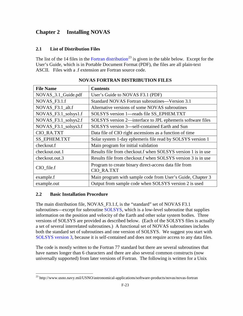
is given in the table below. Except for the User’s Guide, which is in Portable Document Format (PDF), the files are all plain-text ASCII. Files with a .f extension are Fortran source code.

NOVAS FORTRAN DISTRIBUTION FILES

File Name Contents NOVAS_3.1_Guide.pdf User’s Guide to NOVAS F3.1 (PDF) NOVAS_F3.1.f Standard NOVAS Fortran subroutines—Version 3.1 NOVAS_F3.1_alt.f Alternative versions of some NOVAS subroutines NOVAS_F3.1_solsys1.f SOLSYS version 1—reads file SS_EPHEM.TXT NOVAS_F3.1_solsys2.f SOLSYS version 2—interface to JPL ephemeris software files NOVAS_F3.1_solsys3.f SOLSYS version 3—self-contained Earth and Sun CIO_RA.TXT Data file of CIO right ascensions as a function of time SS_EPHEM.TXT Solar system 1-day ephemeris file read by SOLSYS version 1 checkout.f Main program for initial validation checkout.out.1 Results file from checkout.f when SOLSYS version 1 is in use checkout.out.3 Results file from checkout.f when SOLSYS version 3 is in use

CIO_file.f Program to create binary direct-access data file from CIO_RA.TXT

example.f Main program with sample code from User’s Guide, Chapter 3 example.out Output from sample code when SOLSYS version 2 is used 2.2 Basic Installation Procedure The main distribution file, NOVAS_F3.1.f, is the “standard” set of NOVAS F3.1 subroutines—except for subroutine SOLSYS, which is a low-level subroutine that supplies information on the position and velocity of the Earth and other solar system bodies. Three versions of SOLSYS are provided as described below. (Each of the SOLSYS files is actually a set of several interrelated subroutines.) A functional set of NOVAS subroutines includes both the standard set of subroutines and one version of SOLSYS. We suggest you start with SOLSYS version 3, because it is self-contained and does not require access to any data files. The code is mostly written to the Fortran 77 standard but there are several subroutines that have names longer than 6 characters and there are also several common constructs (now universally supported) from later versions of Fortran. The following is written for a Unix

23 http://www.usno.navy.mil/USNO/astronomical-applications/software-products/novas/novas-fortran

F-24

command-line environment, but the corresponding operations in other environments should be obvious. The source code can be compiled and object files produced by typing

gfortran -c NOVAS_F3.1.f NOVAS_F3.1_solsys1.f NOVAS_F3.1_solsys2.f NOVAS_F3.1_solsys3.f

where you can substitute for “gfortran” the name of the particular Fortran compiler you use. The four object files that are created will have a “.o” extension rather than “.f”, but the main part of the name will be the same as for the corresponding source code file. NOVAS is simply a group of subroutines, so there is no main (calling) program; you must supply that. You may wish initially to use the validation program checkout.f:

gfortran checkout.f NOVAS_F3.1.o NOVAS_F3.1_solsys3.o If successful, this will produce a working executable, a.out. For now, make sure that the file CIO_RA.TXT is not in the working directory. If you type a.out on the command line, the executable will run and produce an output file called checkout.out. (On some systems, you will need to specify the path for a.out in order to execute the program.) At the beginning of execution, you will receive two warning messages on your display about Jupiter and Saturn not being available; these messages simply alert you to the fact that the gravitational deflection of light subroutine cannot use Jupiter or Saturn as deflecting bodies when SOLSYS version 3 is in use (only the Sun’s deflection is evaluated). You should compare the results in the file checkout.out to the contents of file checkout.out.3 supplied in the distribution. The results should be identical. You should also re-run a.out with the file CIO_RA.TXT in the working directory. When present in the working directory, NOVAS will use this file for certain computations relating to the Celestial Intermediate Origin; otherwise (as in the first run) NOVAS will use an internal computational procedure for those computations. The results should be identical at the microarcsecond level and should therefore produce no numerical differences in the output file, although the label on the sidereal time results that reads “using internal CIO” should change to “using external CIO”. If computational speed is a factor for your application, you may wish to test which method is faster on your system (but read section 2.4 below before doing so). This setup of NOVAS—using SOLSYS version 3—will provide the positions of stars or extragalactic objects with errors not exceeding 0.3 milliarcsecond (if your input catalog data is that good) or the Sun with an error not exceeding 1 arcsecond. It will not provide the positions of solar system objects other than the Sun. For more general or demanding applications, NOVAS must use another version of SOLSYS.

F-25

2.3 Using External Solar System Ephemeris Files If you need to compute star or radio source positions to better than 0.3 milliarcsecond, or the positions of the Sun to better than 1 arcsecond, or the positions of solar system bodies other than the Sun, you will have to use subroutine SOLSYS version 1 or 2, which use external ephemeris files. SOLSYS version 2 calls the JPL software that accesses one of the JPL “development ephemerides” (DEnnn). If, for example, you have already installed the JPL software and file for ephemeris DE405, the command for linking NOVAS to DE405 might be something like

gfortran myprog.f NOVAS_F3.1.o NOVAS_F3.1_solsys2.o ~/mylibs/jpl/jplsubs.o

where ~/mylibs/jpl is the directory in which you have stored the compiled JPL software, here called jplsubs.o. The ephemeris file itself might be stored elsewhere, in a directory path known to jplsubs; NOVAS does not access the JPL ephemeris file directly. In most installations, the JPL software reads the file on Fortran logical unit 12. If successful, the above command will produce a working executable, a.out. Establishing a working copy of the JPL software and the DE405 binary files on your system is not, unfortunately, a trivial process. The files for doing that can be obtained directly from JPL24 Appendix C as discussed in . If you do not have a JPL ephemeris already installed, you should try SOLSYS version 1, which reads and interpolates the supplied ephemeris file SS_EPHEM.TXT. This file is a formatted (ASCII) file containing the BCRS (barycentric) rectangular coordinates (in AU) of the Sun, eight planets, Pluto, and the Moon, with records at 1-day intervals. The supplied file contains the coordinates for the years 2000 to 2020, inclusive, taken from JPL’s DE405 ephemeris. The interpolation errors of SOLSYS version 1 are negligible (a few meters or less) for all objects other than the Moon and Mercury; for the Moon the errors can amount to 450 meters (maximum angular error 0.3 arcsecond) and for Mercury the errors can reach 280 meters (maximum angular error 0.8 milliarcsecond). It would be straightforward to construct a file similar to SS_EPHEM.TXT from an ephemeris other than DE405—the specifications for the file are given in the description of SOLSYS version 1 in Chapter 4, and in the subroutine’s prolog. The command to link your program with NOVAS for this case would be

gfortran myprog.f NOVAS_F3.1.o NOVAS_F3.1_solsys1.o The file SS_EPHEM.TXT (or its alias) must be in the working directory at execution time. The file is read on Fortran logical unit 20. You can direct NOVAS to use a different file

24 http://ssd.jpl.nasa.gov/?planet_eph_export

F-26

name or logical unit number at execution time by calling subroutine FILDEF at the start of your program, before any other NOVAS calls. You can re-run the test program, checkout.f, with either SOLSYS version 1 or SOLSYS version 2 linked in. For SOLSYS version 1, or for SOLSYS version 2 when the JPL DE405 ephemeris is used, the output should be identical to the contents of checkout.out.1. 2.4 Making the NOVAS External Data Files More Efficient As described above, NOVAS can be run without any reference to external data files by using SOLSYS version 3 and making sure that CIO_RA.TXT is not in the working directory. However, if either of the files SS_EPHEM.TXT (read by SOLSYS version 1) or CIO_RA.TXT (read by CIOLOC) are used, you can eliminate some unproductive search time by simply truncating them to include only the range of dates that are relevant for your particular applications. Both files are plain-text (ASCII) files that can be modified by any text editor. The first record in each file is a header, which should remain as such (although its contents are not used by NOVAS), but all the other records contain a Julian date and information for that date. The records are in ascending date order. Simply trim from the beginning and ending of those files any records for dates that you are sure you will never need; allow at least ten extra dates on each end to allow the internal interpolation scheme to work properly. For example, SS_EPHEM.TXT contains data for years 2000 through 2020 but you may need only the range from 2010 to 2015. It is more important to trim off the “before” dates than it is the “after” dates. Leave the data within your overall anticipated date range as is—that is, do not attempt to make several groups of dates within the same file. The file that you create must end up (after the header record) as a fixed-interval file running from the first date to the last date with no gaps. The file CIO_RA.TXT, which contains the right ascension of the CIO in the GCRS, lists six centuries of data, most of which is seldom used, so trimming it down is a good idea. In addition, you can make access to the data in CIO_RA.TXT even more efficient by converting it to binary direct-access format. Use program CIO_file.f to do that. This program is simple and self-contained—it does not need a link to NOVAS or anything else—and it requires no input from you. Simply make sure that CIO_RA.TXT (as you have edited it) is in the working directory and type

gfortran CIO_file.f

a.out The program will create a file called CIO_RA.DA. To get NOVAS to use it instead of CIO_RA.TXT, use the following subroutine call, before any other NOVAS call: CALL CIOFIL ( lun, ‘CIO_RA.DA’, 2 )

F-27

where lun is the Fortran logical unit number of your choice that NOVAS will use for reading the file. You can replace the file name CIO_RA.DA with whatever name you choose for the file; it can be a complete path (for example, /users/myaccount/novas/cio.bin) up to 40 characters long. 2.5 Do I have to Use a CIO File? If a CIO file (either CIO_RA.TXT or CIO_RA.DA or whatever you choose to call them) is not present when NOVAS needs to determine the location of the CIO, NOVAS will simply revert to using an internal computation for this information. The results differ by at most only a few microarcseconds, and those differences are reached only for dates before 1900 or after 2200. The two approaches represent two independent algorithms for determining the location of the CIO on the equator, and the tiny differences for dates that are several centuries from now are of no practical consequence (see Chapter 5). Small differences in execution time for the two approaches may occur, but those timing differences are likely to vary with the specific application—depending, for example, on the order and spread of the dates that are processed by NOVAS. For some applications, an external file may not be desirable. Because in many simple NOVAS applications, the location of the CIO is never needed, the best scheme is probably to start without using a CIO file. If your application’s execution time is critical, you might want to experiment to see whether using one of the CIO files affects its performance one way or the other. 2.6 The NOVAS Low-Accuracy Mode and the Alternative Subroutines NOVAS has a “low-accuracy” mode that can be invoked at any time by calling subroutine LOACC (it has no arguments). In this mode, a shortened nutation series is used; evaluating the series for nutation is usually the main computational burden in NOVAS, so using low accuracy mode improves execution time, often noticeably. This mode can be used when the accuracy requirements are not better than 0.1 milliarcsecond. The resulting time for Earth-rotation computations may be reduced by about two-thirds. You can revert to high-accuracy mode at any time by calling HIACC; high-accuracy mode is the default so it is not necessary to call HIACC initially. In high-accuracy mode, the IAU 2000A nutation series (1,365 terms) is used; in low-accuracy mode, the NOVAS 2000K nutation series (488 terms) is used. See section 1.4. If your accuracy requirements are no better than about 0.05 arcsecond, you may wish to consider using alternative versions of two NOVAS subroutines. Swapping these subroutines can reduce the computational load for most applications considerably. The file NOVAS_F3.1_alt.f contains alternative versions of GRVDEF and NOD. Subroutine GRVDEF computes the gravitational deflection of light while NOD supervises the nutation series computation. The alternative version of GRVDEF is a dummy, which does not make any change to the input direction vector. The alternative version of NOD contains a very short nutation series (13 terms) that is used in NOVAS low-accuracy mode. Even after switching to the alternative version of NOD, calling LOACC is required in order to use this 13-term nutation series.

F-28

The standard version of GRVDEF should always be used if you have to compute the positions of objects that may pass close to the Sun. The gravitational deflection can exceed 0.05 arcsecond within 10º of the Sun.

(Return to Table of Contents)

F-29

Chapter 3 Sample Calculations The sample Fortran code discussed in this chapter can be found in the file example.f, which is part of the distribution; it is a main program that can be linked to the NOVAS subroutines and executed, e.g.

gfortran example.f NOVAS_F3.1.o NOVAS_F3.1_solsys2.o jplsubs.o The results, when SOLSYS version 2 is used, are given in the file example.out. (To use it with SOLSYS version 1, follow the comments in the file. In which case, the low-order digits of some of the results will be different, most noticeably for the Moon.) The program checkout.f, also part of the distribution, provides other examples of NOVAS subroutine calls. NOVAS has a number of high-level subroutines that make it easy to obtain frequently needed information on the positions of celestial objects, and some of these will be described below. Before calling these subroutines, however, you might want to use some set-up calls. Note that all floating-point arguments to NOVAS subroutines, input or output, are DOUBLE PRECISION. 3.1 Initialization CALL LOACC or CALL HIACC: Determines accuracy mode, which affects only certain computations (most importantly, nutation) relating to the Earth’s orientation in space. The default mode is high accuracy. Call LOACC for calculations that need not be more accurate than 0.1 milliarcsecond, which will be the case for many practical applications. (See section 2.6 on installing alternative subroutines for even lower accuracy calculations.) The accuracy mode stays in effect until another call to LOACC or HIACC. CALL EQINOX or CALL CIOTIO: Determines internal computation scheme—whether the equinox or the CIO will be used as the origin of right ascension on the moving equator within certain NOVAS subroutines that can work either way. This call does not affect any output options; NOVAS produces the same data using either scheme. However, calling CIOTIO is best if you are specifically requesting data with respect to the CIO. Equinox mode is the default. IEARTH, a variable, appears as an input argument in several subroutine calls shown below. In previous versions of NOVAS, IEARTH was the value of the body identification number for the Earth. In NOVAS F3.0 and F3.1, the value of this argument is not used; for backwards compatibility, the argument has been kept as a placeholder in the subroutines that previously required it. Although it can have any integer value,

IEARTH = 3 is a logical choice.

F-30

3.2 Setting Time Arguments CALL SETDT ( DELTAT ): Sets the value of ∆T in seconds (see sections 1.3 and 1.6) for a group of dates to be processed, usually about a year’s worth. The value of DELTAT should be good to the nearest second or better for the range of dates to be covered. Generally, that will require a call to SETDT for each year of dates to be processed, with the value of DELTAT appropriately set. You will also have to consider how you will handle dates and times. As described in section 1.3, NOVAS uses either of two time scales, TT or UT1, as the basis for the time input argument to its higher-level subroutines. However, you may be working with UTC, Coordinated Universal Time. UTC is the basis for civil time systems worldwide and, because it is distributed quite accurately by GPS, is often used as the time-tag for observations. The key relationship is

TT = UTC + ∆AT + 32.184s where ∆AT is an integer representing the total count of leap seconds in UTC (for example, for 2011, ∆AT = 34s). Equivalently,

TT = TAI + 32.184s where TAI is International Atomic Time. If you will only be dealing with the geocentric celestial coordinates of objects, TT is all you will need. If you will also be computing topocentric coordinates (for a specific location on the surface of the Earth), you will also need to obtain UT1. The key relationship is

UT1 = UTC + (UT1–UTC) where UT1–UTC is interpolated from the daily values of this quantity published by the IERS.25

UT1 = TT – ∆T Alternatively,

although for this purpose, a more accurate value of ∆T (and one that is changed more often) will be needed than is generally used for the argument of SETDT. See section 1.3 for more information on time scales, including sources of data that can be used for the values of ∆AT, UT1–UTC, and ∆T. You can convert a date and time in the common format (year/month/day/hour/minute/second) to a Julian date, which is used by NOVAS for time arguments, by calling JULDAT. Dates and times based on UTC, TT, or UT1 (or any other time scale) can be converted using JULDAT; the output Julian date simply has the same basis as the input date and time. In the examples below, we will be using 2008 April 24, 10:36:18.0 UTC as the time of interest; this corresponds to a Julian date of 2454580.9441875 UTC.26

25 http://maia.usno.navy.mil/ser7/mark3.out

We will also use a ∆AT value of 33s and a UT1–UTC value of −0.387845s, which are appropriate for this date.

26 A “UTC Julian date” is something of a non sequitur, because UTC is not continuous (because of leap seconds). Here we are simply using JULDAT with UTC input to obtain a value that allows us to compute Julian dates in more well-behaved time scales.

F-31

DATA IYEAR, MONTH, IDAY, HOUR, LEAPS, UT1UTC, XP, YP /

. 2008, 4, 24, 10.605D0, 33, -0.387845D0, -0.002D0, +0.529D0 / So if we use CALL JULDAT ( 2008, 4, 24, 10.605D0, UTCJD ) the output argument, UTCJD, will have a value of 2454580.9441875. The next few lines of code should be something like TTJD = UTCJD + ( LEAPS + 32.184D0 ) / 86400.D0 UT1JD = UTCJD + UT1UTC / 86400.D0 DELTAT = 32.184D0 + LEAPS – UT1UTC CALL SETDT ( DELTAT ) where 86400.D0 is the number of seconds in a day, and the value of DELTAT (∆T) would be computed to be 65.571845 (seconds). If we had known the value of DELTAT (∆T) to start with, rather than the value of UT1UTC (UT1–UTC), then the lines immediately above could have been replaced by TTJD = UTCJD + ( LEAPS + 32.184D0 ) / 86400.D0 UT1JD = TTJD – DELTAT / 86400.D0 CALL SETDT ( DELTAT ) 3.3 Example 1—Position of a Star Suppose we have the catalog data from star FK6 1307 (Groombridge 1830) for epoch J2000.0, expressed in the ICRS:

ICRS right ascension at J2000.0 (hours): RA2000 = 11.88299133D0 ICRS declination at J2000.0 (degrees): DC2000 = 37.71867646D0 Proper motion in RA (milliarcseconds per year): PMRA = 4003.27D0 Proper motion in dec (milliarcseconds per year): PMDEC = –5815.07D0 Parallax (milliarcseconds): PARX = 109.21D0 Radial velocity (kilometers per second): RV = –98.8D0

To obtain the apparent geocentric place of the star on our date of interest, with respect to the equator and equinox of that date, simply call APSTAR, supplying it with the catalog quantities: CALL APSTAR ( TTJD, IEARTH, RA2000, DC2000, PMRA, PMDEC, PARLX, RV, . RA, DEC ) The output coordinates, RA and DEC (hours and degrees, respectively), represent the apparent geocentric coordinates of the star, with respect to the true equator and equinox of date. The computation takes into account all time-dependent effects that shift the star’s

F-32

position from its catalog coordinates (except atmospheric refraction, which is location- and weather-dependent): the star’s space motion to the date of interest, parallax due to the Earth’s position in its orbit, gravitational light-bending in the solar system, aberration due to the Earth’s orbital velocity, and the precession and nutation of the Earth’s axis. Important note: Hipparcos catalog data, although expressed with respect to the ICRS, refer to epoch 1991.25 and must be converted to epoch J2000.0 before being used as input arguments to any NOVAS subroutine. Use subroutine GETHIP to do this. (For example, see the code in checkout.f.) Most other modern catalogs, including the FK6 (used above), Tycho-2, UCAC, etc., provide data for epoch J2000.0 that need no conversion. If we want the apparent topocentric place of the star, that is, the star’s position as it would be seen (except for refraction) from a particular location on Earth, such as off the Atlantic Coast near Truro, Massachusetts

DATA GLON, GLAT, HT / -70.D0, 42.D0, 0.D0 / where GLON and GLAT are the location’s geodetic longitude and latitude (degrees, with east longitude and north latitude positive) and HT is the height of the location above sea level (meters). Then, the call to APSTAR should be followed by one to TPSTAR: CALL TPSTAR ( UT1JD, GLON, GLAT, HT, RAT, DECT ) where RAT and DECT reflect the position of the star as it would be seen from that particular location—the small differences from the geocentric coordinates RA and DEC arise mainly from diurnal aberration. TPSTAR uses catalog data on the star from the previous call to APSTAR. 3.4 Example 2—Position of the Moon Obtaining the coordinates of solar system objects other than the Sun requires that SOLSYS version 1 or 2 must be in use. Use subroutine APPLAN:

MOON = IDSS (‘MOON’) CALL APPLAN ( TTJD, MOON, IEARTH, RA, DEC, DIS )

where, again, RA and DEC are the apparent geocentric coordinates of the Moon (hours and degrees, respectively), with respect to the true equator and equinox of date, and DIS is the true (Euclidean) geocentric distance (AU) at time TTJD. IDSS returns the body identification number for a solar system object based on the version of SOLSYS in use. The computation of the angular coordinates of solar system objects takes light-time into account, along with the other effects (light bending, aberration, precession, and nutation) that also apply to stars.

F-33

To get the topocentric celestial coordinates of the Moon, call TPPLAN immediately after APPLAN: CALL TPPLAN ( UT1JD, GLON, GLAT, HT, RAT, DECT, DIST ) However, there is a single subroutine, PLACE, that can be used for all types of positions of both stars and solar system objects. In fact, APSTAR, TPSTAR, APPLAN, and TPPLAN (and several other similar subroutines) are actually just special-purpose front-ends to PLACE. PLACE uses three array arguments, STAR and OBSERV for input and SKYPOS for output, dimensioned as follows:

DIMENSION STAR(6), OBSERV(6), SKYPOS(7) as well as several scalar arguments. For the coordinates of solar system bodies, array STAR does not need to be loaded; it is used only for stars. For observers on or near the surface of the Earth, OBSERV should be loaded with the observer’s geodetic coordinates: OBSERV(1) = GLON OBSERV(2) = GLAT OBSERV(3) = HT OBSERV(4) = 0.D0 OBSERV(5) = 0.D0 OBSERV(6) = 0.D0 (If only geocentric coordinates are of interest, this array need not be loaded.) When using PLACE to compute the topocentric positions of nearby solar system objects, it is advisable, for high-accuracy work, to load OBSERV(4) with the value of ∆T (in seconds) for the date requested. Otherwise, PLACE uses the value of ∆T from the last call to SETDT, which may not be accurate for the date and time of interest. In this case, it does not matter, because we are dealing with only a single date and a single value of ∆T, which we have provided to SETDT. The call to PLACE to obtain topocentric coordinates of the Moon, with respect to the true equator and equinox of date then is CALL PLACE ( TTJD, ‘MOON’, 1, 1, STAR, OBSERV, SKYPOS ) after which the output array will contain:

SKYPOS(1): Unit vector x component SKYPOS(2): Unit vector y component SKYPOS(3): Unit vector z component SKYPOS(4): Right Ascension (hours) SKYPOS(5): Declination (degrees) SKYPOS(6): True distance (AU) SKYPOS(7): Radial velocity (kilometers per second)

F-34

Here, (x,y,z) is a unit vector in the apparent direction of the Moon, in the same coordinate system as the right ascension and declination (i.e., it is exactly equivalent to the spherical coordinates). PLACE has many options for both input and output; refer to its description in Chapter 4 or look at the beginning of the PLACE code. Once you have the topocentric celestial coordinates of an object, these can be transformed into local altitude and azimuth by a call to ZDAZ. If we have used PLACE to obtain the topocentric coordinates, we set

RAT = SKYPOS(4) DECT = SKYPOS(5)

then CALL ZDAZ ( UT1JD, XP, YP, GLON, GLAT, HT, RAT, DECT, IREFR, . ZD, AZ, RAR, DECR ) where IREFR is a refraction option (set IREFR = 0 for no refraction, or IREFR = 1 for standard atmospheric refraction), and XP and YP are the IERS pole coordinates xp and yp for the date of interest. (You can set XP = YP = 0.D0 if the required accuracy is not better than 1 arcsecond.) The output coordinates, ZD, AZ, RAR, and DECR, are, respectively, the zenith distance (degrees), azimuth (degrees), right ascension (hours), and declination (degrees). The output values of ZD, RAR, and DECR are affected by atmospheric refraction if IREF = 1. If IREF = 0, the output right ascension and declination values are the same as the input values. ZD and AZ are referred to the horizon system that is tangent to the Earth’s reference ellipsoid at the observer’s location; that is, the deflection of the vertical (the local undulation of the geoid) is not taken into account. 3.5 Example 3—Greenwich Sidereal Time To obtain Greenwich sidereal time, call SIDTIM: CALL SIDTIM ( UT1JD, 0.D0, K, GST ) where GST is the output sidereal time (hours): Greenwich mean sidereal time if K = 0, Greenwich apparent sidereal time if K = 1. This subroutine and several others allow for a “split” input UT1 Julian date—high- and low-order parts in the first two arguments—for increased precision. Generally, the split would be at the Julian date’s decimal point, with the day count in the first argument and the fraction of a day in the second. However, using two arguments for the Julian date provides more precision only if the fractional part of the Julian date has been handled separately all along. We have not done that, so here, the entire Julian date is just placed in the first argument and the second argument is set to 0.D0.

F-35

To compute local sidereal time (either mean or apparent), add the longitude (east positive) expressed in hours: ST = GST + GLON / 15.D0 The result may have to be reduced to the range 0 to 24 hours by statements similar to the following:

IF ( ST .GE. 24.D0 ) ST = ST - 24.D0 IF ( ST .LT. 0.D0 ) ST = ST + 24.D0 The quantity that is analogous to Greenwich apparent sidereal time in the CIO-based paradigm is θ, the ERA. It can be computed from: CALL EROT ( UT1JD, 0.D0, ERA ) where ERA is the Earth Rotation Angle (degrees). EROT, like SIDTIM, allows for a split input UT1 Julian date. See Chapter 5 for information on the difference between Greenwich apparent sidereal time and the ERA, and how hour angles are computed in the two paradigms. 3.6 Example 4—Other Frequently Requested Quantities In the following subroutine calls, vectors are used. Vectors are simply double-precision arrays with a dimension of 3. Most NOVAS internal calculations are performed with vectors and matrices. The following vectors are referred to below: DIMENSION POS(3), VEL(3), POSE(3), VTER(3), VCEL(3) To obtain the barycentric or heliocentric coordinates (BCRS vectors) of a solar system body, for example, Mars, call SOLSYS: CALL SOLSYS ( TDBJD, IDSS(‘MARS’), K, POS, VEL, IERR ) where we can often approximate TDBJD = TTJD,27

SOLSYS

and the output position and velocity vectors are POS and VEL (components in AU and AU/day, respectively). For barycentric positions, set K = 0; for heliocentric positions, set K = 1. IERR is an error flag returned, which normally has a value of 0 if everything is OK. Each version of has a corresponding version of IDSS, which returns the required body identification number.

27 Strictly, SOLSYS requires a TDB-based Julian date as input. TDB differs from TT by at most 1.7 ms; see section 1.3. If this time difference is important, use subroutine TIMES to determine the difference between the two time scales and adjust TDBJD accordingly. For the example here, neglecting the difference can lead to an error in the position of Mars of about 50 meters.

F-36

If POS is a heliocentric vector, it can be transformed to the ecliptic system (fixed ecliptic of J2000.0) by calling EQEC: CALL EQEC ( 0.D0, 0, POS, POSE ) where POSE is the output vector in the ecliptic system (same units as POS). POSE could then easily be converted to heliocentric spherical coordinates: ecliptic longitude, ecliptic latitude, and radius vector.

CALL ANGLES ( POSE, ELON, ELAT ) ELON = ELON * 15.D0 R = DSQRT (POSE(1)**2 + POSE(2)**2 + POSE(3)**2)

Finally, it is sometimes useful to transform a vector from the terrestrial reference system to the celestial reference system. The vector might represent a geographic position, a geodetic reference line or direction, or an instrumental axis. For this transformation, the vector starts out as an Earth-fixed vector expressed with respect to the ITRS axes. For example, the vector toward the local vertical (orthogonal to the ellipsoid at the place of interest) is simply (cos φ cos λ, cos φ sin λ, sin φ), where φ is the geodetic latitude and λ is the longitude. A vector along a telescope’s polar axis would nominally point toward (0,0,1) in this system. Any such ITRS vector can be transformed into the equivalent GCRS vector with a single call to TERCEL: CALL TERCEL ( UT1JD, 0.D0, XP, YP, VTER, VCEL ) where VTER is the input vector (terrestrial, ITRS) and VCEL is the equivalent output vector (celestial, GCRS). The components of VTER can be in any units; VCEL will be in the same units. VCEL will sweep around the celestial sphere as the Earth rotates, i.e., as UT1JD advances. (TERCEL, like SIDTIM, allows for a split input UT1 Julian date.) Use ANGLES to obtain VCEL’s instantaneous spherical coordinates: CALL ANGLES ( VCEL, RA, DEC ) where RA and DEC are the GCRS right ascension and declination (hours and degrees, respectively) of the point on the celestial sphere toward which VCEL points. At any UT1JD, VCEL can be compared to the directions of stars computed by PLACE for the equivalent TTJD, with LOCATN = 1 and ICOORD = 0.

(Return to Table of Contents)

F-37

Chapter 4 Descriptions of Individual Subroutines

NOVAS FORTRAN SUBROUTINE, FUNCTION, AND ENTRY NAMES

Entry Name Level Purpose PLACE * super Computes the apparent direction of a star or solar system body, given the

time and observer’s location. Direction is expressed in one of several selectable coordinate systems.

SIDTIM super Computes Greenwich sidereal time, either mean or apparent. TERCEL ** super Transforms arbitrary vector in rotating Earth-fixed (ITRS) system to

space-fixed (GCRS) system. Terrestrial-to-celestial transformation. CELTER *** super Transforms arbitrary vector in rotating Earth-fixed (ITRS) system to

space-fixed (GCRS) system. Terrestrial-to-celestial transformation. ZDAZ super Transforms topocentric RA and dec to zenith distance and azimuth.

Optionally accounts for atmospheric refraction. CATRAN super Transforms a star’s catalog quantities for a change of epoch and/or equator

and equinox. GETHIP super Converts Hipparcos catalog data at epoch J1991.25 to epoch J2000.0. APSTAR super Computes the apparent place of a star, given its catalog data. TPSTAR super If called after APSTAR, returns topocentric place of same star, given

geodetic location of observer. VPSTAR super Computes the virtual place of a star, given its catalog data. LPSTAR super If called after VPSTAR, returns local place of same star, given geodetic

location of observer. ASSTAR super Computes the astrometric place of a star, given its catalog data. MPSTAR super Computes the ICRS/J2000.0 place of a star, given its apparent place. APPLAN super Computes the apparent place of a planet or other solar system body. TPPLAN super If called after APPLAN, returns topocentric place of same planet, given

geodetic location of observer. VPPLAN super Computes the virtual place of a planet or other solar system body. LPPLAN super If called after VPPLAN, returns local place of same planet, given geodetic

location of observer. ASPLAN super Computes the astrometric place of a planet or other solar system body. ABERAT util Adjusts position vector for aberration of light due to motion of Earth. ANGLES util Converts position vector to RA and dec. CIOBAS * util Returns orthonormal basis vectors, with respect to GCRS, of right-handed

system defined by CIP (z-direction) and CIO (x-direction). DLIGHT * util For a star, returns difference in light-time between solar system barycenter

and observer. Or, returns the light-time from observer to point on light ray closest to a given solar system body.

ECEQ * util Converts ecliptic position vector to equatorial position vector. EQEC * util Converts equatorial position vector to ecliptic position vector. EQECL * util Converts RA and dec to ecliptic longitude and latitude. EQGAL * util Converts ICRS RA and dec to galactic longitude and latitude. EROT * util Returns ERA (θ) for given UT1 Julian date. FRAME * util Transforms vector between dynamical reference system (mean equator and

equinox of J2000.0) and ICRS. GCRSEQ * util Converts GCRS RA and dec to coordinates with respect to the equator of

date (mean or true).

F-38

Entry Name Level Purpose

GEOCEN util Changes origin of coordinates from barycenter of solar system to center of mass of Earth.

GEOPOS * util Computes geocentric position and velocity, in GCRS, of observer on or near the surface of Earth.

GETVEC * util Retrieves last computed position on the sky as a unit vector. GRVD * util Corrects position vector for deflection of light in gravitational field of

given body. GRVDEF ** util Computes total gravitational deflection of light for an object due to major

solar system bodies. LIMANG * util Determines angle of object above or below earth's limb (horizon). LITTIM * util Computes the position of a solar system body antedated for light-time. NUTATE util Applies nutation to position vector. PRECES util Applies precession to position vector. PROPMO util Updates the position vector of a star to allow for its space motion. RADVL * util Predicts radial velocity of observed object as would be measured by

spectroscopy. SETDT * util Allows specification of ΔT value for calculation of sidereal time, etc. SPIN util Rotates vector by specified angle about the z-axis. TERRA util Converts geodetic coordinates to geocentric position vector. VECTRS util Converts a star’s RA, dec, proper motion, etc., to position and velocity

vectors. WOBBLE util Adjusts Earth-fixed vector for polar motion. ASTCON * basic Supplies values of astronomical constants. CALDAT basic Computes calendar date and time, given Julian date. CELPOL basic Allows for the specification of celestial pole offsets for high-precision

applications. CIOFIL * basic Specifies logical unit number and file identifier of input file containing

series of CIO RA values. CIOLOC * basic Returns location of CIO as RA with respect to either GCRS origin or true

equinox of date, given TDB Julian date. CIORA * basic Computes true right ascension of the CIO, given TT Julian date. CIORD * basic Returns array of Julian dates and corresponding values of RA of CIO (in

GCRS), given TDB Julian date and number of dates desired. CIOTIO * basic Switches internal computation scheme to use CIO as origin of RA for

certain routines; best choice when requesting data with respect to CIO. EECT2000 * basic Returns complementary terms for equation of the equinoxes. EQINOX * basic Switches internal computation scheme to use equinox as origin of RA for

certain routines; default mode. EQXRA * basic Computes intermediate RA of the equinox, given TDB Julian date. ETILT basic Provides information on orientation of Earth’s axis: obliquity, nutation

parameters, etc. FUNARG basic Computes fundamental arguments (mean elements) of the Sun and Moon. GETDT * basic Returns current value of ∆T. HIACC * basic Switches to high-accuracy mode for certain calculations relating to Earth

orientation; default mode. IDSS * basic Returns body identification number, given name of solar system body, for

version of SOLSYS in use. JULDAT basic Computes Julian date, given calendar date and time. LOACC * basic Switches to low-accuracy mode for certain calculations relating to Earth

orientation; acceptable for applications that do not require accuracy better than 0.1 milliarcsecond.

F-39

Entry Name Level Purpose NOD basic Supervises the calculation of nutation parameters and provides nutation in

longitude and obliquity. NU2000A * basic Evaluates high-accuracy nutation series (IAU 2000A model). NU2000K * basic Evaluates low-accuracy nutation series (truncated version of IAU 2000A). REFDAT basic Allows for the specification of weather observations, etc., for refraction

calculation. REFRAC basic Computes atmospheric refraction in zenith distance. SOLSYS basic Provides position and velocity vectors of a solar system body. TIMES basic Converts Barycentric Dynamical Time (TDB) to Terrestrial Time (TT).

* New subroutine, function, or entry in NOVAS F3.0. ** Name change from NOVAS F2.0: TERCEL was PNSW; GRVDEF was SUNFLD. *** New subroutine in NOVAS F3.1. Descriptions of some of the most frequently used NOVAS subroutines follow. The comments in the source code at the beginning of each NOVAS subroutine are intended to provide enough information for correct usage. In the documentation that follows, arguments marked in are input arguments to the subroutine: values for these must be supplied by the calling program. Arguments marked out are output arguments from the subroutine: the subroutine computes and returns values for these. Note that all floating point arguments are DOUBLE PRECISION.

F-40

PLACE Entry: CALL PLACE ( TJD, OBJECT, LOCATN, ICOORD, STAR, OBSERV,

SKYPOS ) Purpose: Computes the apparent direction of a star or solar system body at a specified

time and in a specified coordinate system. Arguments: INTEGER LOCATN, ICOORD

DOUBLE PRECISION TJD, STAR(6), OBSERV(6), SKYPOS(7) CHARACTER OBJECT

TJD: TT Julian date for place (in). OBJECT: Character string identifying object of interest (in):

For a solar system body, specify the name using all upper-case letters (‘SUN’, ‘MOON’, ‘JUPITER’, etc.), or specify the body identification number in a 4-character string of the form ‘=nnn’, where nnn is the body identification number. For a star, provide a blank string, the word ‘STAR’, or any string beginning with ‘*’.

LOCATN: Code specifying location of observer (in): LOCATN = 0 for observer at geocenter LOCATN = 1 for observer on or near surface of the Earth LOCATN = 2 for observer on near-Earth spacecraft

ICOORD: Code specifying coordinate system of output position (in): ICOORD = 0 for GCRS (or “local GCRS”) ICOORD = 1 for true equator and equinox of date ICOORD = 2 for true equator and CIO of date (Celestial

Intermediate Reference System) ICOORD = 3 for ICRS astrometric coordinates, i.e., without

light deflection or aberration STAR: Array of catalog data for star (not referred to if solar system

body requested)(in): STAR(1) = ICRS right ascension at J2000.0 in hours STAR(2) = ICRS declination at J2000.0 in degrees STAR(3) = ICRS proper motion in RA in milliarcseconds/year STAR(4) = ICRS proper motion in dec in milliarcseconds/ year STAR(5) = parallax in milliarcseconds STAR(6) = radial velocity in kilometers/second (Further star array elements are reserved for future use.)

OBSERV: Array of data specifying location of observer (in): For LOCATN = 0, not used

F-41

For LOCATN = 1, OBSERV(1) = observer’s geodetic (WGS-84) longitude

(east positive) in degrees OBSERV(2) = observer’s geodetic (WGS-84) latitude

(north positive) in degrees OBSERV(3) = observer’s height above Earth’s reference

ellipsoid (approximately, height above mean sea level) in meters

OBSERV(4) = value of ∆T in seconds (∆T = TT – UT1) OBSERV(5) = (not used, reserved for future use) OBSERV(6) = (not used, reserved for future use) For LOCATN = 2, OBSERV(1) = geocentric X in km OBSERV(2) = geocentric Y in km OBSERV(3) = geocentric Z in km

OBSERV(4) = geocentric X-dot in km/s OBSERV(5) = geocentric Y-dot in km/s OBSERV(6) = geocentric Z-dot in km/s

SKYPOS: Array of output data specifying object’s place on the sky at time TJD, with respect to the specified output coordinate system (out): SKYPOS(1) = X, dimensionless SKYPOS(2) = Y, dimensionless SKYPOS(3) = Z, dimensionless SKYPOS(4) = apparent, topocentric, or astrometric right

ascension in hours SKYPOS(5) = apparent, topocentric, or astrometric declination

in degrees SKYPOS(6) =true (geometric, euclidian) distance to solar system body in AU at time TJD, or 0.D0 for star SKYPOS(7) = radial velocity in kilometers per second (Further

SKYPOS array elements are reserved for future use.) Discussion:

This subroutine computes the apparent direction of a star or solar system body at a specified time and in a specified coordinate system. The algorithms used are based on Kaplan, et al. (1989), Astron. J., 97, 1197, with some enhancements from Klioner (2003), Astron. J., 125, 1580.

The apparent direction of a star computed by this subroutine takes into account the star’s proper motion (linear 3-D space motion) from the catalog epoch to the date requested, parallax, the gravitational deflection of light by solar system bodies (mostly the Sun), and aberration. The same effects are computed for solar system bodies, except that the proper motion calculation is replaced by an algorithm that retrieves the object’s barycentric position from its ephemeris, as part of an iterative light-time calculation. Extragalactic objects are

Z is toward CIO; X is

toward true equinox

unit vector toward object

F-42

treated as stars with zero proper motion and parallax. The result in all cases is an apparent direction expressed in the GCRS, which is optionally transformed into either of two other output coordinate systems, as specified by argument ICOORD.

“Astrometric place” is a variant of the above calculation that is appropriate for some types of differential measurements. Light bending and aberration are ignored under the assumption that they are the same for all objects within a small area of the sky. Astrometric places are expressed in the ICRS.

The observer’s location may be at the geocenter, on or near the surface of the Earth, or in orbit around the Earth, as specified by the arguments LOCATN and OBSERV.

PLACE does not take into account atmospheric refraction (which would be appropriate only for observers on or near the surface of the Earth), but its effect can be added by a subsequent call to subroutine ZDAZ.

For stars, the required input data, stored in array STAR, are the standard five astrometric quantities from a catalog, together with radial velocity if known. Any parameter should be set to 0.D0 if its value is unknown. All catalog data used as input to this subroutine must apply to epoch J2000.0 and be expressed with respect to the ICRS. (For Hipparcos catalog data, see subroutine GETHIP.) Extragalactic objects should be treated as stars, but with all input parameters set to 0.D0 except for the catalog right ascension and declination. For solar system bodies, array STAR is not referred to; instead, the argument OBJECT must contain the name of the body (or its identification number), from the list of objects supported by the version of subroutine SOLSYS in use.

The values of LOCATN and ICOORD for various kinds of place are:

LOCATN = 0, ICOORD = 0 ⇒ virtual place (= proper place LOCATN = 1, ICOORD = 0 ⇒ local place

)

LOCATN = 0, ICOORD = 1 ⇒ LOCATN = 1, ICOORD = 1 ⇒

apparent place

LOCATN = 0, ICOORD = 2 ⇒ topocentric place

LOCATN = 1, ICOORD = 2 ⇒ topocentric intermediate place intermediate place

LOCATN = 0, ICOORD = 3 ⇒ LOCATN = 1, ICOORD = 3 ⇒ topocentric astrometric place

astrometric place

(Only the place names underlined above are widely recognized outside of the context of NOVAS.)

NOVAS subroutines APSTAR, TPSTAR, APPLAN, TPPLAN, etc., are now just special-purpose front-ends to PLACE.

Important: If LOCATN = 1 (observer on or near surface of Earth), a value of ∆T in seconds is required. The value will be taken from OBSERV(4), unless that element is 0.D0,

F-43

in which case the last value of ∆T defined by the user in a call to SETDT will be used. Whether taken from OBSERV(4) or SETDT, the value of ∆T will be used internally for determining the ERA (θ) needed for computing topocentric places. An error in ∆T of 1s can result a topocentric place error of up to 0.3 arcsecond for the Moon, but proportionally less for more distant bodies (e.g., 3 milliarcseconds for Venus at its closest). Distance errors of up to 500 m (3 × 10-9

SKYPOS(7), the radial velocity, is the predicted radial velocity measure (z) times the speed of light, an inherently spectroscopic quantity. For a star, it includes all effects, such as gravitational red shift, contained in the catalog barycentric radial velocity measure, which is assumed given in STAR(6). For a solar system body, it applies to a fictitious emitter at the center of the observed object, assumed to be massless (no gravitational red shift), and does not in general apply to reflected light.

AU) can also result, independent of distance. If errors of this magnitude are important, care needs to be taken in specifying a more accurate value of ∆T. An error in ∆T of 1s will not result in a significant error in the topocentric places of stars.

Arrays STAR and SKYPOS may be expanded in the future. Such expansion could be provided for in the calling code by dimensioning these arrays with 20 and 10 elements, respectively, even though this subroutine does not now refer to elements beyond STAR(6) and SKYPOS(7).

(Return to subroutine entry list)

F-44

SIDTIM Entry: CALL SIDTIM ( TJDH, TJDL, K, GST ) Purpose: Computes the Greenwich sidereal time, either mean or apparent, at a specific

UT1 time. Arguments: INTEGER K

DOUBLE PRECISION TJDH, TJDL, GST

TJDH: UT1 Julian date for sidereal time, high-order part (in). TJDL: UT1 Julian date for sidereal time, low-order part (in). K: Sidereal time selection code (in):

K = 0 produces Greenwich mean sidereal time K = 1 produces Greenwich apparent sidereal

GST: Greenwich (mean or apparent) sidereal time in hours (out).

Discussion:

This subroutine computes Greenwich sidereal time, either mean (if K = 0) or apparent (if K = 1).

The input Julian date, which must be in the UT1 time scale, may be split into two parts to ensure the highest precision in the computation. For example, set TJDH equal to the integral part of the Julian date and set TJDL equal to the fractional part. Generally, this will be advantageous only if the low-order part has been treated separately within the calling program; for example, if the time of day has been stored in its own variable(s), from which TJDL is constructed.

For many applications the position of the split is not critical as long as the sum TJDH + TJDL is correct: in particular, when used with computers providing 16 decimal digits of precision in DOUBLE PRECISION variables, this subroutine will yield values of GST precise to about 0.1 millisecond even if TJDH contains the entire Julian date and TJDL = 0.D0.

If K = 1 (for apparent sidereal time), the output value of GST will correctly reflect the celestial pole offset in longitude if routine CELPOL has previously been called.

(Return to subroutine entry list)

F-45

TERCEL Entry: CALL TERCEL ( TJDH, TJDL, XP, YP, VEC1, VEC2 ) Purpose: Transforms a vector from the terrestrial system (ITRS) to the celestial system

(GCRS). Arguments: DOUBLE PRECISION TJDH, TJDL, XP, YP, VEC1(3), VEC2(3)

TJDH: UT1 Julian date for transformation, high-order part (in). TJDL: UT1 Julian date for transformation, low-order part (in). XP: Conventionally defined xp

YP: Conventionally defined y

coordinate of Celestial Intermediate Pole with respect to ITRS pole, in arcseconds (in).

p

VEC1: Vector referred to ITRS axes (terrestrial system) (in).

coordinate of Celestial Intermediate Pole with respect to ITRS pole, in arcseconds (in).

VEC2: Vector referred to GCRS axes (celestial system) (out). Discussion:

This subroutine rotates a vector from the terrestrial to the celestial system. Specifically, it transforms a vector in the ITRS (a rotating Earth-fixed system) to the GCRS (a local space-fixed system) by applying rotations for polar motion, Earth rotation, nutation, precession, and the dynamical-to-GCRS frame tie. The input vector might represent a cardinal direction at the observer’s position, a geodetic baseline, or some instrumental axis. The units for the vector components are arbitrary and the output vector will have the same units as the input vector. Geodetic coordinates in the WGS-84 system, also sometimes called the Earth-centered, Earth-fixed (ECEF) system, can be considered to be compatible with the ITRS.

This subroutine allows for the input UT1 time to be represented as a split Julian date. See the discussion in the description of subroutine SIDTIM.

Set XP = YP = 0.D0 to omit the polar motion rotation.

See also subroutine SETDT to set the value of ∆T (∆T = TT – UT1) to be used by this subroutine and others.

Both TJDH and TJDL should be non-negative for normal use (TJDL = 0.D0 is OK). A negative value of TJDH is used to invoke a special option where the output vector is produced with respect to the equator and equinox of date, and the date for which the transformation applies is taken from TJDL only. This special option works only in equinox mode.

F-46

CELTER performs the reverse transformation, rotating the vector from the celestial system (GCRS) to the terrestrial system (ITRS). The arguments are as described above, except that for CELTER, VEC1 is the vector with respect to the GCRS (in) and VEC2 is the vector with respect to the ITRS (out).

(Return to subroutine entry list)

F-47

ZDAZ Entry: CALL ZDAZ ( UJD, XP, YP, GLON, GLAT, HT, RA, DEC, IREFR, ZD, AZ, RAR, DECR ) Purpose: Transforms topocentric right ascension and declination to zenith distance and

azimuth; can also adjust coordinates for atmospheric refraction. Arguments: INTEGER IREFR

DOUBLE PRECISION UJD, XP, YP, GLON, GLAT, HT, RA, DEC, ZD, AZ, RAR, DECR

UJD: UT1 Julian date, or equivalent Greenwich apparent sidereal

time in hours, for coordinate calculation (in). XP: Conventionally defined xp

YP: Conventionally defined y

coordinate of Celestial Intermediate Pole with respect to ITRS pole, in arcseconds (in).

p

GLON: Observer’s geodetic (WGS-84) longitude (east positive) in degrees (in).

coordinate of Celestial Intermediate Pole with respect to ITRS pole, in arcseconds (in).

GLAT: Observer’s geodetic (WGS-84) latitude (north positive) in degrees (in).

HT: Height of observer above the Earth’s reference ellipsoid (approximately, height above mean sea level) in meters (in).

RA: Topocentric right ascension of object of interest, in hours, referred to true equator and equinox of date (in).

DEC: Topocentric declination of object of interest, in degrees, referred to true equator and equinox of date (in).

IREFR: Atmospheric refraction option (in): IREFR = 0 omits refraction IREFR = 1 applies refraction

ZD: Topocentric zenith distance in degrees, affected by refraction if IREFR = 1 (out).

AZ: Topocentric azimuth (measured east from north) in degrees (out).

RAR: Topocentric right ascension of object of interest, in hours, referred to true equator and equinox of date, affected by refraction if IREFR = 1 (out).

DECR: Topocentric declination of object of interest, in degrees, referred to true equator and equinox of date, affected by refraction if IREFR = 1 (out).

F-48

Discussion:

This subroutine takes the topocentric celestial coordinates of an object and computes the equivalent local horizon coordinates. The subroutine uses a method that properly accounts for polar motion, which is significant at the sub-arcsecond level. Atmospheric refraction can be included in the transformation, and if so, refraction is applied to both kinds of coordinates (this can be useful for telescope pointing). Refraction, when requested, is computed by subroutine REFRAC.

RA and DEC, the input topocentric right ascension and declination, can be obtained from PLACE (with LOCATION = 1 and ICOORD = 1), TPSTAR, or TPPLAN. UJD, the input time argument, may be specified either as a UT1 Julian date (e.g., 2451251.299358D0) or an hour and fraction of Greenwich apparent sidereal time (e.g., 19.184592D0). Values for XP and YP, the coordinates of the pole, can be obtained from IERS28

In this subroutine, the directions ZD = 0.D0 (the zenith) and AZ = 0.D0 (north) are considered fixed in the terrestrial frame. Specifically, the zenith is along the geodetic normal (orthogonal to the ellispsoid at the observer’s position), and north is toward the ITRS pole. Geophysical deflection of the vertical is not considered.

Bulletins A and B, although XP and YP can be set to 0.D0 if sub-arcsecond accuracy is not needed. (If refraction is requested, sub-arcsecond accuracy is unlikely.) The observer’s height, HT, is used only for refraction, that is, if IREFR = 1.

If IREFR = 0 (no refraction), then RAR = RA and DECR = DEC.

(Return to subroutine entry list)

28http://www.iers.org/IERS/EN/Publications/Bulletins/bulletins.html

F-49

CATRAN Entry: CALL CATRAN ( IT, DATE1, RA1, DEC1, PMRA1, PMDEC1, PARX1,

RV1, DATE2, RA2, DEC2, PMRA2, PMDEC2, PARX2, RV2 )

Purpose: Transforms a star’s catalog quantities for a change of epoch and/or equator

and equinox. It can also be used to transform catalog quantities on the dynamical equator and equinox of J2000.0 to the ICRS, or vice versa.

Arguments: INTEGER IT

DOUBLE PRECISION DATE1, RA1, DEC1, PMRA1, PMDEC1, PARX1, RV1, DATE2,RA2,DEC2,PMRA2,PMDEC2,PARX2,RV2

IT: Transformation option (in):

IT = 1 changes epoch (same mean equator and equinox) IT = 2 changes mean equator and equinox (same epoch) IT = 3 changes mean equator and equinox and epoch

IT = 4 changes mean equator and equinox of J2000.0 to ICRS IT = 5 changes ICRS to mean equator and equinox of J2000.0 DATE1: TT Julian date, or year, of original catalog data (the following

six arguments) (in). RA1: Original mean right ascension in hours (in). DEC1: Original mean declination in degrees (in). PMRA1: Original proper motion in RA in milliarcseconds/year (in). PMDEC1: Original proper motion in dec in milliarcseconds/year (in). PARX1: Original parallax in milliarcseconds (in). RV1: Original radial velocity in kilometers/second (in). DATE2: TT Julian date, or year, for transformed output data (the

following six arguments) (in). RA2: Transformed mean right ascension in hours (out). DEC2: Transformed mean declination in degrees (out). PMRA2: Transformed proper motion in RA in milliarcseconds/year

(out). PMDEC2: Transformed proper motion in dec in milliarcseconds/year

(out). PARX2: Transformed parallax in milliarcseconds (out). RV2: Transformed radial velocity in kilometers/second (out).

Discussion:

Subroutine CATRAN performs various transformations on star catalog data. Only catalog reference data, not observed quantities, should be processed by this subroutine.

F-50

For IT = 1, 2, or 3, two dates, DATE1 and DATE2, must be specified: the input data is associated with the first date, and the output data is associated with the second date. Two transformations are available:

IT = 1: The star’s data is updated to account for the star’s space motion between the first and second dates, within a fixed reference system. That is, the epoch of the data is changed, but not the equator and equinox (or other system).

IT = 2: The reference frame within which the star’s coordinates and proper motion are expressed is rotated corresponding to precession between the first and second dates. The star’s position in space is not changed. That is, the equator and equinox of the data are changed, but not the epoch.

Setting IT = 3 requests both transformations, and is the most common case.

The two date arguments, DATE1 and DATE2, may be specified either as a Julian date (e.g., 2433282.5D0) or a Julian year and fraction (e.g., 1950.0D0). (Values less than 10000.D0 are assumed to represent years.)

The IT = 1 and IT = 3 transformations are appropriate only for objects with linear (or no) space motion; do not use them for components of binary stars. Also, this subroutine cannot be properly used to bring data from old star catalogs into the modern system, because old catalogs were compiled using a set of constants (in particular, the rate of precession) that are incompatible with modern values.

The IT = 2 and IT = 3 transformations involve the dynamical system, that is, the moving mean equator and equinox. The mean equator and equinox of J2000.0 was the most common reference system for modern astrometric catalog data before the ICRS was introduced in 1998. Now, catalog data is usually referred to the ICRS, which is a reference system fixed with respect to distant extragalactic objects, not defined by any Earth motions and with no associated date.

The IT = 4 transformation is used to convert catalog quantities from the mean equator and equinox of J2000.0 (the “J2000.0 system”) to the ICRS. The IT = 5 transformation is the opposite. The arguments DATE1 and DATE2 are ignored for these transformations.

Subroutine FRAME can be used to transform vectors from the J2000.0 system to the ICRS or vice versa.

See subroutine GETHIP for transforming Hipparcos catalog data to epoch J2000.0.

(Return to subroutine entry list)

F-51

GETHIP Entry: CALL GETHIP ( RAH, DECH, PMRAH, PMDECH, PARXH, RVH, RA2, DEC2, PMRA2, PMDEC2, PARX2, RV2) Purpose: Converts Hipparcos catalog data at epoch J1991.25 to epoch J2000.0. Arguments: DOUBLE PRECISION RAH, DECH, PMRAH, PMDECH, PARXH, RVH,

RA2, DEC2, PMRA2, PMDEC2, PARX2, RV2

RAH: Hipparcos right ascension in degrees (in). DECH: Hipparcos declination in degrees (in). PMRAH: Hipparcos proper motion in milliarcseconds/year (in). PMDECH: Hipparcos proper motion in declination in milliarcseconds/

year (in). PARXH: Hipparcos parallax in milliarcseconds (in). RVH: Radial velocity at Hipparcos epoch in kilometers/second (in). RA2: ICRS right ascension at J2000.0 in hours (out). DEC2: ICRS declination at J2000.0 in degrees (out). PMRA2: ICRS proper motion in RA at J2000.0 in milliarcseconds/year

(out). PMDEC2: ICRS proper motion in dec at J2000.0 in milliarcseconds/year

(out). PARX2: Parallax at J2000.0 in milliarcseconds (out). RV2: Radial velocity at J2000.0 in kilometers/second (out).

Discussion:

This subroutine takes Hipparcos catalog data, which is published for epoch J1991.25, and transforms it to epoch J2000.0 for use with NOVAS subroutines such as PLACE, APSTAR, TPSTAR, VPSTAR, etc. The Hipparcos (input) right ascension is expressed in degrees, as in the catalog, while the J2000.0 (output) right ascension is given in hours, compatible with other NOVAS subroutines. Subroutine CATRAN (with IT = 1) is called internally to perform the epoch transformation. The reference frame for both input and output is the ICRS.

This subroutine should be used only for Hipparcos stars with linear space motion.

Radial velocity (RVH) is not given in the Hipparcos catalog and must be obtained from another source. If a value is not known, set RVH = 0.D0. The radial velocity is important for only a small number of nearby, high-proper-motion stars.

(Return to subroutine entry list)

F-52

APSTAR Entry: CALL APSTAR ( TJD, N, RAI, DECI, PMRA, PMDEC, PARLAX,

RADVEL, RA, DEC ) Purpose: Computes the apparent place of a star at a specific time, given its position,

proper motion, and other catalog data (at epoch J2000.0, with respect to ICRS).

Arguments: INTEGER N

DOUBLE PRECISION TJD, RAI, DECI, PMRA, PMDEC, PARLAX, RADVEL, RA, DEC

TJD: TT Julian date for apparent place (in). N: Any integer. Formerly, the body identification number for the

Earth—now just a place holder, no longer used (in). RAI: ICRS right ascension of star at J2000.0 in hours (in). DECI: ICRS declination of star at J2000.0 in degrees (in). PMRA: ICRS proper motion in RA at J2000.0 in milliarcseconds/year

(in). PMDEC: ICRS proper motion in dec at J2000.0 in milliarcseconds/year

(in). PARLAX: Parallax in milliarcseconds (in). RADVEL: Radial velocity in kilometers/second (in). RA: Apparent right ascension of star at time TJD, in hours, referred

to the true equator and equinox of date (out). DEC: Apparent declination of star at time TJD, in degrees, referred to

the true equator and equinox of date (out). Discussion:

This subroutine computes the apparent place of a star for time TJD. The word “star” as used here refers to any object outside the solar system. For extragalactic objects, the input arguments PMRA, PMDEC, PARLAX, and RADVEL should be set to 0.D0. These input arguments should also be set to 0.D0 if the corresponding data are unknown or zero within the errors of measurement.

Efficiency is maximized when successive calls to APSTAR have the same value for TJD, since many quantities that are functions only of time are thereby saved and reused.

APSTAR works by calling PLACE with LOCATN = 0 and ICOORD = 1.

(Return to subroutine entry list)

F-53

TPSTAR Entry: CALL TPSTAR ( UJD, GLON, GLAT, HT, RA, DEC) Purpose: Computes the topocentric place of a star at a specific time and observer

location, using data from a previous call to subroutine APSTAR. Arguments: DOUBLE PRECISION UJD, GLON, GLAT, HT, RA, DEC

UJD: UT1 Julian date, or the equivalent Greenwich apparent sidereal time in hours, for topocentric place (in).

GLON: Observer’s geodetic (WGS-84) longitude (east positive) in degrees (in).

GLAT: Observer’s geodetic (WGS-84) latitude (north positive) in degrees (in).

HT: Observer’s height above the Earth’s reference ellipsoid (approximately, height above mean sea level) in meters.

RA: Topocentric right ascension of star at time UJD, in hours, referred to the true equator and equinox of date (out).

DEC: Topocentric declination of star at time UJD, in degrees, referred to the true equator and equinox of date (out).

Discussion:

This routine computes the topocentric place of a star (neglecting atmospheric refraction) for the location specified by the arguments GLON, GLAT, and HT, for time UJD. TPSTAR assumes that APSTAR has been previously called; it uses data from the previous APSTAR call in its computation. In particular, all information on the star is obtained from the prior APSTAR call.

The UT1 epoch that is specified here in argument UJD must correspond to the TT epoch previously supplied to APSTAR in its argument TJD. That is, the same instant must be specified for APSTAR in the TT time scale and for TPSTAR in the UT1 time scale. (The difference TT – UT1 is currently of order one minute.) Note that TPSTAR allows the value of the Greenwich apparent sidereal time, in hours, equivalent to the UT1 epoch, to be specified in the argument UJD instead of the UT1 Julian date.

Atmospheric refraction can be subsequently applied to RA and DEC by subroutine ZDAZ.

TPSTAR works by calling PLACE with LOCATN = 1 and ICOORD = 1.

(Return to subroutine entry list)

F-54

VPSTAR Entry: CALL VPSTAR ( TJD, N, RAI, DECI, PMRA, PMDEC, PARLAX,

RADVEL, RA, DEC ) Purpose: Computes the virtual place (proper place) of a star at a specific time, given its

position, proper motion, and other catalog data (at epoch J2000.0, with respect to ICRS).

Arguments: INTEGER N

DOUBLE PRECISION TJD, RAI, DECI, PMRA, PMDEC, PARLAX, RADVEL, RA, DEC

TJD: TT Julian date for virtual place (in). N: Any integer. Formerly, the body identification number for the

Earth—now just a place holder, no longer used (in). RAI: ICRS right ascension of star at J2000.0 in hours (in). DECI: ICRS declination of star at J2000.0 in degrees (in). PMRA: ICRS proper motion in RA at J2000.0 in milliarcseconds/year

(in). PMDEC: ICRS proper motion in dec at J2000.0 in milliarcseconds/year

(in). PARLAX: Parallax in milliarcseconds (in). RADVEL: Radial velocity in kilometers/second (in). RA: Virtual (or proper) right ascension of star at time TJD, in hours,

referred to the GCRS (out). DEC: Virtual (or proper) declination of star at time TJD, in degrees,

referred to the GCRS (out).

Discussion:

See the discussion for subroutine APSTAR. Subroutine VPSTAR is identical to APSTAR in input arguments and use. Here, however, the output arguments provide the virtual place (also called the proper place) of the star. The virtual place (proper place) is essentially the apparent place expressed in the GCRS.

VPSTAR works by calling PLACE with LOCATN = 0 and ICOORD = 0.

(Return to subroutine entry list)

F-55

LPSTAR Entry: CALL LPSTAR ( UJD, GLON, GLAT, HT, RA, DEC ) Purpose: Computes the local place of a star at a specific time and observer location,

using data from a previous call to subroutine VPSTAR. Arguments: DOUBLE PRECISION UJD, GLON, GLAT, HT, RA, DEC

UJD: UT1 Julian date, or the equivalent Greenwich apparent sidereal time in hours, for local place (in).

GLON: Observer’s geodetic (WGS-84) longitude (east positive) in degrees (in).

GLAT: Observer’s geodetic (WGS-84) latitude (north positive) in degrees (in).

HT: Observer’s height above the Earth's reference ellipsoid (approximately, height above mean sea level) in meters.

RA: Local right ascension of star at time UJD, in hours, referred to the mean equator and equinox of J2000.0 (out).

DEC: Local declination of star at time UJD, in degrees, referred to the mean equator and equinox of J2000.0 (out).

Discussion:

See the discussion for TPSTAR. LPSTAR is identical to TPSTAR in input arguments and use. Here, however, it is subroutine VPSTAR that must have been previously called and here the output arguments provide the local place of the star. The local place is essentially the topocentric place expressed in the “local GCRS”.

LPSTAR works by calling PLACE with LOCATN = 1 and ICOORD = 0.

(Return to subroutine entry list)

F-56

ASSTAR Entry: CALL ASSTAR ( TJD, N, RAI, DECI, PMRA, PMDEC, PARLAX,

RADVEL, RA, DEC ) Purpose: Computes the astrometric place of a star at a specific time, given its position,

proper motion, and other catalog data (at epoch J2000.0, with respect to ICRS).

Arguments: INTEGER N

DOUBLE PRECISION TJD, RAI, DECI, PMRA, PMDEC, PARLAX, RADVEL, RA, DEC

TJD: TT Julian date for astrometric place (in). N: Any integer. Formerly, the body identification number for the

Earth—now just a place holder, no longer used (in). RAI: ICRS right ascension of star at J2000.0 in hours (in). DECI: ICRS declination of star at J2000.0 in degrees (in). PMRA: ICRS proper motion in RA at J2000.0 in milliarcseconds/year

(in). PMDEC: ICRS proper motion in dec at J2000.0 in milliarcseconds/year

(in). PARLAX: Parallax in milliarcseconds (in). RADVEL: Radial velocity in kilometers/second (in). RA: Astrometric right ascension of star at time TJD, in hours,

referred to the ICRS (out). DEC: Astrometric declination of star at time TJD, in degrees, referred

to the ICRS (out).

Discussion:

See the discussion for subroutine APSTAR. Subroutine ASSTAR is identical to APSTAR in input arguments and use. Here, however, the output arguments provide the astrometric place of the star in the ICRS.

ASSTAR works by calling PLACE with LOCATN = 0 and ICOORD = 3.

(Return to subroutine entry list)

F-57

APPLAN Entry: CALL APPLAN ( TJD, L, N, RA, DEC, DIS ) Purpose: Computes the apparent place of a planet or other solar system body at a

specific time, using the barycentric ephemeris provided by subroutine SOLSYS.

Arguments: INTEGER L,N

DOUBLE PRECISION TJD, RA, DEC, DIS

TJD: TT Julian date for apparent place (in). L: Body identification number for the planet or other body whose

apparent place is desired; see argument M of subroutine SOLSYS (in).

N: Any integer. Formerly, the body identification number for the Earth—now just a place holder, no longer used (in).

RA: Apparent right ascension of body L at time TJD, in hours, referred to the true equator and equinox of date (out).

DEC: Apparent declination of body L at time TJD, in degrees, referred to the true equator and equinox of date (out).

DIS: True geometric distance between body L and the Earth at time TJD, in AU (out).

Discussion:

This subroutine computes the apparent place of a planet or other solar system body. Your choice of the version of subroutine SOLSYS in use determines the source of the body’s barycentric rectangular coordinates used in the calculation. The value of input argument L, which identifies the planet or other solar system body of interest, must correspond to argument M of SOLSYS. The value of L can be obtained from a call to IDSS, e.g., L = IDSS (‘SUN’).

Efficiency is maximized when successive calls to APPLAN have the same value for TJD, because many quantities that are functions only of time are thereby saved and reused.

APPLAN works by calling PLACE with LOCATN = 0 and ICOORD = 1.

(Return to subroutine entry list)

F-58

TPPLAN Entry: CALL TPPLAN ( UJD, GLON, GLAT, HT, RA, DEC, DIS ) Purpose: Computes the topocentric place of a planet or other solar system body at a

specific time and observer location, using data from a previous call to subroutine APPLAN.

Arguments: DOUBLE PRECISION UJD, GLON, GLAT, HT, RA, DEC, DIS

UJD: UT1 Julian date, or the equivalent Greenwich apparent sidereal time in hours, for topocentric place (in).

GLON: Observer’s geodetic (WGS-84) longitude (east positive) in degrees (in).

GLAT: Observer’s geodetic (WGS-84) latitude (north positive) in degrees (in).

HT: Observer’s height above the Earth’s reference ellipsoid (approximately, height above mean sea level) in meters.

RA: Topocentric right ascension of body at time UJD, in hours, referred to the true equator and equinox of date (out).

DEC: Topocentric declination of body at time UJD, in degrees, referred to the true equator and equinox of date (out).

DIS: True geometric distance between body and observer at time UJD, in AU (out).

Discussion:

This routine computes the topocentric place of a planet or other solar system body (neglecting atmospheric refraction) for the location specified by the arguments GLON, GLAT, and HT, for the time specified by the argument UJD. TPPLAN assumes that APPLAN has been previously called; it uses data from the previous APPLAN call in its computation. In particular, the solar system body is identified and its ephemeris is obtained in the prior APPLAN call.

The UT1 epoch that is specified here in argument UJD must correspond to the TT epoch previously supplied to APPLAN in its argument TJD. That is, the same instant must be specified for APPLAN in the TT time scale and for TPPLAN in the UT1 time scale. (The difference TT – UT1 is currently of order one minute.) TPPLAN allows the value of the Greenwich apparent sidereal time, in hours, equivalent to the UT1 epoch, to be specified in the argument UJD instead of the UT1 Julian date.

Atmospheric refraction can be applied to RA and DEC by subroutine ZDAZ.

TPPLAN works by calling PLACE with LOCATN = 1 and ICOORD = 1. (Return to subroutine entry list)

F-59

VPPLAN Entry: CALL VPPLAN ( TJD, L, N, RA, DEC, DIS ) Purpose: Computes the virtual place (proper place) of a planet or other solar system

body at a specific time, using the barycentric ephemeris provided by subroutine SOLSYS.

Arguments: INTEGER L, N

DOUBLE PRECISION TJD, RA, DEC, DIS

TJD: TT Julian date for virtual place (in). L: Body identification number for the planet or other body whose

virtual place is desired; see argument M of subroutine SOLSYS (in).

N: Any integer. Formerly, the body identification number for the Earth—now just a place holder, no longer used (in).

RA: Virtual (proper) right ascension of body L at time TJD, in hours, referred to the GCRS (out).

DEC: Virtual (proper) declination of body L at time TJD, in degrees, referred to the GCRS (out).

DIS: True geometric distance between body L and the Earth at time TJD, in AU (out).

Discussion:

See the discussion for subroutine APPLAN. Subroutine VPPLAN is identical to APPLAN in input arguments and use. Here, however, the output arguments provide the virtual place (also called the proper place) of the planet or other solar system body. The virtual place (proper place) is essentially the apparent place expressed in the GCRS.

VPPLAN works by calling PLACE with LOCATN = 0 and ICOORD = 0.

(Return to subroutine entry list)

F-60

LPPLAN Entry: CALL LPPLAN ( UJD, GLON, GLAT, HT, RA, DEC, DIS ) Purpose: Computes the local place of a planet or other solar system body at a specific

time and observer location, using data from a previous call to subroutine VPPLAN.

Arguments: DOUBLE PRECISION UJD, GLON, GLAT, HT, RA, DEC, DIS

UJD: UT1 Julian date, or the equivalent Greenwich apparent sidereal time in hours, for local place (in).

GLON: Observer’s geodetic (WGS-84) longitude (east positive) in degrees (in).

GLAT: Observer’s geodetic (WGS-84) latitude (north positive) in degrees (in).

HT: Observer’s height above the Earth's reference ellipsoid (approximately, height above mean sea level) in meters.

RA: Local right ascension of body at time UJD, in hours, referred to the local GCRS (out).

DEC: Local declination of body at time UJD, in degrees, referred to the local GCRS (out).

DIS: True geometric distance between body and observer at time UJD, in AU (out).

Discussion:

See the discussion for TPPLAN. LPPLAN is identical to TPPLAN in input arguments and use. Here, however, it is subroutine VPPLAN that must have been previously called and here the output arguments provide the local place of the planet or other solar system body. The local place is essentially the topocentric place expressed in the “local GCRS”.

LPPLAN works by calling PLACE with LOCATN = 1 and ICOORD = 1.

(Return to subroutine entry list)

F-61

ASPLAN Entry: CALL ASPLAN ( TJD, L, N, RA, DEC, DIS ) Purpose: Computes the astrometric place of a planet or other solar system body at a

specific time, using the barycentric ephemeris provided by subroutine SOLSYS.

Arguments: INTEGER L, N

DOUBLE PRECISION TJD, RA, DEC, DIS

TJD: TT Julian date for astrometric place (in). L: Body identification number for the planet or other body whose

virtual place is desired; see argument M of subroutine SOLSYS (in).

N: Any integer. Formerly, the body identification number for the Earth—now just a place holder, no longer used (in).

RA: Astrometric right ascension of body L at time TJD, in hours, referred to the ICRS (out).

DEC: Astrometric declination of body L at time TJD, in degrees, referred to the ICRS (out).

DIS: True geometric distance between body L and the Earth at time TJD, in AU (out).

Discussion:

See the discussion for subroutine APPLAN. Subroutine ASPLAN is identical to APPLAN in input arguments and use. Here, however, the output arguments provide the astrometric place of the planet or other solar system body in the ICRS.

ASPLAN works by calling PLACE with LOCATN = 0 and ICOORD = 3.

(Return to subroutine entry list)

F-62

PRECES Entry: CALL PRECES ( TJD1, POS1, TJD2, POS2 ) Purpose: Precesses a position vector from the mean equator and equinox of an arbitrary

date to the mean equator and equinox of J2000.0, or vice versa. Arguments: DOUBLE PRECISION TJD1, POS1(3), TJD2, POS2(3)

TJD1: TDB (or TT) Julian date of the first equatorial system (in). POS1: Position vector in the first equatorial system (mean equator and

equinox of TJD1); units and origin arbitrary (in). TJD2: TDB (or TT) Julian date of the second equatorial system (in). POS2: Position vector in the second equatorial system (mean equator

and equinox of TJD2); units and origin same as POS1 (out).

Discussion:

This subroutine precesses the input position vector, POS1, from the equator and equinox of TJD1 to the equator and equinox of TJD2; the resulting vector is POS2.

One of the two input Julian dates must be standard epoch J2000.0—either TJD1 or TJD2 must be 2451545.0D0 exactly. To precess a vector from one arbitrary date to another, call PRECES twice, using J2000.0 as the “middle” date. That is, in the first call, TJD1 = first Julian date, and TJD2 = 2451545.0D0; in the second call, TJD1 = 2451545.0D0, and TJD2 = second Julian date.

Formally, the current precession algorithm is a function of Barycentric Dynamical Time (TDB), but using TT as the basis for the input Julian dates results in a maximum error of only about 3 × 10-9 arcseconds, which is totally negligible. Standard epoch J2000.0, although formally defined in the TT time scale, is the same in the TT and TDB time scales to the precision given by double-precision Julian dates: at J2000.0, TT – TDB ≈ 10-4 second ≈ 10-9

day.

(Return to subroutine entry list)

F-63

EQECL Entry: CALL EQECL ( TJD, ICOORD, RA, DEC, ELON, ELAT ) Purpose: Converts right ascension and declination to ecliptic longitude and latitude. Arguments: INTEGER ICOORD DOUBLE PRECISION TJD, RA, DEC, ELON, ELAT

TJD: TDB (or TT) Julian date of equator, equinox, and ecliptic used for coordinates (in).

ICOORD: Coordinate system selection (in): ICOORD = 0: Mean equator and equinox of date ICOORD = 1: True equator and equinox of date RA: Right ascension in hours, referred to selected equator and

equinox of date (in). DEC: Declination in degrees, referred to selected equator and

equinox of date (in). ELON: Ecliptic longitude in degrees, referred to the ecliptic and

selected equinox of date (out). ELAT: Ecliptic latitude in degrees, referred to the ecliptic of date (out).

Discussion:

This subroutine converts the equatorial position of an object into the equivalent ecliptic position: equatorial coordinates, RA and DEC, are converted to ecliptic coordinates, ELON and ELAT. This subroutine can be used for any kind of barycentric or geocentric coordinates—the conversion involves a simple rotation and should be regarded as just formalism. As in subroutine PRECES, the input Julian date can be based on either the TDB or TT time scales, with negligible resulting error.

RA and DEC can be expressed with respect to either the mean equator and equinox of date TJD (if ICOORD = 0) or the true equator and equinox of date TJD (if ICOORD = 1).

The representation of the ecliptic used for celestial coordinates is a smoothly moving mean plane described as part of the precession development. However, the mean and true equators intersect this ecliptic at different points. Therefore, the equinox, which serves as the origin of ecliptic longitude as well as the origin of right ascension, is different in the two cases. ELON will be expressed with respect to the same equinox as RA.

If TJD = 0.D0 and ICOORD = 0, the subroutine assumes RA and DEC are expressed with respect to the ICRS and provides ELON and ELAT with respect to the ecliptic and mean equinox of J2000.0.

F-64

See subroutines EQEC and ECEQ for the conversion of vectors between equatorial and ecliptic systems.

(Return to subroutine entry list)

F-65

CIORA Entry: CALL CIORA ( TJD, RACIO ) Purpose: Provides the right ascension of the Celestial Intermediate Origin (CIO). Argument: DOUBLE PRECISION TJD, RACIO

TJD: TT Julian date for CIO right ascension (in). RACIO: Right ascension of the CIO, in hours (+ or –), with respect to

the true equinox of date (out). Discussion:

This call supplies the true right ascension of the Celestial Intermediate Origin (CIO). RACIO = – (equation of the origins)

RACIO = Greenwich apparent sidereal time – ERA where all quantities are expressed in hours.

EROT Entry: CALL EROT ( TJDH, TJDL, THETA ) Purpose: Provides the Earth Rotation Angle (ERA), θ. Argument: DOUBLE PRECISION TJDH, TJDL, THETA

TJDH: UT1 Julian date for ERA, high-order part (in). TJDL: UT1 Julian date for ERA, low-order part (in). THETA: ERA in degrees (out).

Discussion: This call supplies the ERA, θ, which is the geocentric angle, in the instantaneous equatorial plane (true equator), between the directions toward the Terrestrial Intermediate Origin (TIO) and the Celestial Intermediate Origin (CIO). This subroutine allows for the input UT1 time to be represented as a split Julian date. See the discussion in the description of subroutine SIDTIM.

(Return to subroutine entry list)

F-66

HIACC Entry: CALL HIACC Purpose: Specifies that Earth orientation calculations are to be performed at full (IAU

standard) accuracy. Arguments: (None)

Discussion: This routine instructs NOVAS to perform Earth orientation calculations, in particular, the evaluation of the nutation series and the equation of the equinoxes, at full accuracy according to recommended IAU models. This mode is the default; normally it would only be necessary to call HIACC to resume full accuracy calculations after a call to LOACC.

LOACC Entry: CALL LOACC Purpose: Specifies that Earth orientation calculations are to be performed at reduced

accuracy. Arguments: (None)

Discussion: This routine instructs NOVAS to perform Earth orientation calculations, in particular the evaluation of the nutation series and the equation of the equinoxes, at reduced accuracy. Even at reduced accuracy, the calculations are good to 0.1 milliarcsecond, or better, if the standard set of NOVAS subroutines is used. The reduced-accuracy mode will provide noticeably faster performance for many types of calculations while still providing overall angular accuracy that is adequate for most applications. To resume full accuracy calculations, call HIACC. If the alternative version of subroutine NOD is in use (see installation instructions in section 2.6), a call to LOACC will result in a significant improvement in performance (up to a factor of 100 for some calculations), although angular errors of up to 0.05 arcsecond may arise.

(Return to subroutine entry list)

F-67

GETVEC Entry: CALL GETVEC ( UVEC ) Purpose: Provides the unit vector corresponding to the last-computed object

coordinates. Argument: DOUBLE PRECISION UVEC(3)

UVEC: Unit vector corresponding to last-computed object position,

expressed in same reference system as the scalar coordinates (out).

Discussion:

This call supplies the unit vector that corresponds to the last object position computed by any NOVAS subroutine. It provides a simple way to obtain the vector that is equivalent to a pair of spherical coordinates, for example, right ascension and declination. It would normally be used following a call to one of the NOVAS subroutines that return only scalar results (APSTAR, APPLAN, EQECL, etc.). The reference system in which the vector is expressed is the same as for the previously calculated spherical coordinates.

(Return to subroutine entry list)

F-68

SETDT Entry: CALL SETDT ( DELTAT ) Purpose: Specifies the value of ∆T = TT – UT1 for subsequent internal use by NOVAS

subroutines. Argument: DOUBLE PRECISION DELTAT DELTAT: Value of ∆T in seconds (in).

Discussion:

This routine allows for the specification of ∆T, the difference in seconds between the TT and UT1 time scales, to be used by NOVAS in subsequent calculations. The value of ∆T that you specify by a call to SETDT will be used by various NOVAS subroutines until you explicitly change it by another call.

Generally, the value of DELTAT needs to be accurate to only about one second, which means that a single call can be used for about a year’s span of dates. The only exception is for the computation of accurate topocentric positions of bodies in the inner solar system (especially the Moon); see the note on this in the description of subroutine PLACE.

(Return to subroutine entry list)

F-69

CELPOL Entry: CALL CELPOL ( TJD, ITYPE, DPOLE1, DPOLE2 ) Purpose: Allows for the specification of celestial pole offsets for high-precision

applications. Arguments: INTEGER ITYPE DOUBLE PRECISION TJD, DPOLE1, DPOLE2 TJD: TDB or TT Julian date for celestial pole offset values (in). ITYPE: Type of pole offsets (in): ITYPE = 1: dψ and dε (ecliptic angles) ITYPE = 2: dX and dY (GCRS angles)

DPOLE1: Pole offset 1 (dψ or dX) in milliarcseconds (in). DPOLE2: Pole offset 2 (dε or dY) in milliarcseconds (in).

Discussion:

This routine is actually an entry point into subroutine ETILT that allows for the specification of celestial pole offsets for very high precision applications. The offsets describe the observed position of the Celestial Intermediate Pole (CIP) with respect to the position computed from the standard precession and nutation models. The offsets are subsequently applied as corrections to the nutation in longitude and nutation in obliquity within ETILT. Thus, ETILT’s output arguments OBLT, EQEQ, DPSI, and DEPS will be affected. Because other NOVAS subroutines, such as SIDTIM, call ETILT to obtain data related to the Earth’s orientation in space, the celestial pole offsets specified here are propagated through the data that the various NOVAS subroutines provide.

Daily values of the celestial pole offsets are published, for example, in IERS29 Bulletins A and B. The celestial pole offsets effectively correct for errors or incompleteness in the standard precession or nutation models. If you use CELPOL, make sure it is called before any other routines for a given date. Values of the pole offsets that you specify by a call to CELPOL will be used by ETILT until you explicitly change them.

Important

: For compatibility with the precession and nutation models used in NOVAS 3.0 and later, specify ITYPE = 2 and use only IERS dX and dY values with respect to “IAU 2000A” (sometimes labeled “IAU 2000”). These pole offset values will generally not exceed 0.5 milliarcsecond and, therefore, CELPOL would need to be called only when very high accuracy is required.

(Return to subroutine entry list)

29 http://www.iers.org/IERS/EN/Publications/Bulletins/bulletins.html

F-70

ETILT Entry: CALL ETILT ( TJD, OBLM, OBLT, EQEQ, DPSI, DEPS ) Purpose: Computes quantities related to the orientation of the Earth’s rotation axis at a

given time. Arguments: DOUBLE PRECISION TJD, OBLM, OBLT, EQEQ, DPSI, DEPS

TJD: TDB (or TT) Julian date for requested data (in). OBLM: Mean obliquity of the ecliptic at time TJD, in degrees (out). OBLT: True obliquity of the ecliptic at time TJD, in degrees (out). EQEQ: Equation of the equinoxes at time TJD, in time seconds (out). DPSI: Nutation in longitude at time TJD, in arcseconds (out). DEPS: Nutation in obliquity at time TJD, in arcseconds (out).

Discussion:

This subroutine computes various quantities related to the orientation of the Earth’s rotation axis (vector toward Celestial Intermediate Pole) with respect to the ecliptic plane at a specific time. The computation involves a call to subroutine NOD to evaluate the nutation series.

The output values of the last four arguments will correctly reflect the celestial pole offsets if routine CELPOL has previously been called.

(Return to subroutine entry list)

F-71

SOLSYS Entry: CALL SOLSYS (TJD,M,K, POS,VEL,IERR) Purpose: Provides the position and velocity vectors of a planet or other solar system

body at a specific time. The origin of coordinates may be either the barycenter of the solar system or the center of mass of the Sun.

Arguments: INTEGER M, K, IERR

DOUBLE PRECISION TJD, POS(3), VEL(3)

TJD: TDB Julian date for planet position and velocity (in). M: Body identification number for the planet or other solar system

body whose position and velocity are desired (in). K: Origin selection code (in):

K = 0 for origin at solar system barycenter K = 1 for origin at center of mass of Sun

POS: ICRS position vector of body M at time TJD, in AU (out). VEL: ICRS velocity vector of body M at time TJD, in AU/day (out). IERR: Return code (out)

IERR = 0 is normal exit, everything OK IERR = 1 means TJD before first possible date IERR = 2 means TJD after last possible date IERR = 3 means some other problem, e.g., invalid value for M, etc.

Discussion:

This subroutine supplies values for the components of the position vector POS and velocity vector VEL for body M at time TJD. The vectors computed by SOLSYS are expressed with respect to ICRS axes, in the BCRS metric. The vectors are barycentric if K = 0 and heliocentric if K = 1.

There are several versions of SOLSYS, each with its own internal logic. Some use internally stored data or series expansions; others refer to external data files. Additional documentation (see below) is usually required for the proper use of each version. You are, of course, free to supply your own version(s), providing that the arguments conform to the above specifications.

The values of the body identification number, M, will in general differ from one SOLSYS version to another; consult the documentation for the specific version in use. Usually, M = 1 refers to Mercury, M = 2 refers to Venus, M = 3 refers to the Earth, etc., but the identification numbers for bodies such as the Sun or Moon differ across implementations. Furthermore, some versions of SOLSYS support only a subset of the major solar system

F-72

bodies. The minimum requirement is support for the Sun and Earth. Here, “Earth” refers to the geocenter and not the Earth/Moon barycenter.

Each version of SOLSYS is packaged together with a function called IDSS, which provides the body identification number, given a solar system body’s name; for example, M = IDSS (‘MARS’). See the description of IDSS immediately following.

If you supply your own version of SOLSYS, you must also supply a corresponding version of IDSS.

Some versions of SOLSYS support “split” Julian dates across successive calls. That is, they recognize –1.D0 ≤ TJD ≤ 1.D0 as representing a fraction of a day that is to be paired with the integral part of the Julian date from a preceding call. Splitting the dates allows the fraction of the day to be specified to much greater precision than is possible in a single call. For example, suppose you call SOLSYS with TJD equal to d1+f1, an ordinary Julian date—d1 is the Julian day count and f1 is the fraction of a day. If the time of day needs to be specified more precisely (equivalent to better than 0.1 millisecond), you can simply make a second call to SOLSYS with TJD equal to the fraction of a day f2; without the day count included in TJD, f2 can be given to much more precision than f1. In the second call, SOLSYS would interpret the Julian date that you want as d1+f2, with the extra precision in f2 preserved. (It does not matter whether the fractions f1 and f2 are similar.) If you continue to call SOLSYS with fractional TJD values (f3, f4, …), it will interpret them in the same way (paired with the same integer day number d1

) until you again set TJD to be a full Julian date. You can test whether the version of SOLSYS in use supports this option: if IDSS ( ‘JD’ ) equals 2, the split Julian date option is supported, otherwise not.

Documentation follows for the following versions of SOLSYS:

Version 1 reads 1-day planetary coordinate file Version 2 provides interface to JPL ephemeris software Version 3 evaluates self-contained Earth and Sun

(Return to subroutine entry list)

Example of split Julian dates: Suppose IDSS(‘JD’) = 2, indicating that the version of SOLSYS in use supports split Julian dates in successive calls. Then, in the following sequence of calls, the requested Julian date is interpreted as shown: Effective Julian date of data returned: CALL SOLSYS ( 2462387.1234567D0, … ) 2462387.1234567 CALL SOLSYS ( 0.98765432109876543D0, … ) 2462387.98765432109876543 CALL SOLSYS ( 0.6624965422153D0, … ) 2462387.6624965422153 CALL SOLSYS ( 2471932.7892D0, … ) 2471932.7892 CALL SOLSYS ( –0.1D0, … ) 2471931.9 However, if IDSS(‘JD’) = 1, the split Julian date option is not supported. In that case, in the second, third, and fifth calls above, the TJD values would be interpreted as complete Julian dates, which would correspond to calendar dates in early 4713 B.C. This would in most cases lead to an IERR = 1 return.

F-73

Integer Function IDSS

Entry: IDSS ( NAME ) Purpose: Returns value of the body identification number for the named solar system

body. Argument: CHARACTER*(*) NAME NAME: Name of solar system body, in all capital letters (in).

Function Value Out: INTEGER IDSS

Value of the body identification number for solar system body named, or -9999 if the body is not supported or the name cannot be recognized.

Discussion: This function provides the body identification number for the named body, for use as an argument to NOVAS subroutines such as SOLSYS, APPLAN, etc. The body name should be all caps and can be any length; most versions of this subroutine use only the first three or four letters. A version of this function is supplied with each version of subroutine SOLSYS. SOLSYS defines the body identification numbers to be used. If NAME is ‘JD’, the returned function value indicates whether the version of SOLSYS in use supports split Julian dates in successive calls. In this case, a value of 1 indicates that split Julian dates are not supported, and a value of 2 indicates that they are supported.

(Return to subroutine entry list)

F-74

SOLSYS Version 1

This version of SOLSYS reads and interpolates a formatted file of planetary coordinates at one-day intervals. This ephemeris file must have the following characteristics:

• The first record in the file is a header record of no specific format. The header is followed by data records.

• Each data record must be formatted (plain-text ASCII) and must contain the barycentric (BCRS) rectangular coordinates of the Sun and planets, or other solar system bodies, for a specific date. The coordinates are given in AU, with respect to the ICRS axes. The data records must be at 1-day intervals of TDB, with dates increasing. The format for each data record is ( F10.2, n(3F16.12) ), where n is the number of bodies with coordinates in the file (data for at least the Sun and Earth must be given, so n must be at least 2). The order of quantities in the data records is:

(1) TDB Julian date (2) Sun X (3) Sun Y (4) Sun Z (5) First planet X (6) First planet Y (7) First planet Z (8) Second planet X (9) Second planet Y : etc. The Sun’s coordinates must always be given first in the record. The body identification numbers will be M = 0 for the Sun, M = 1 for the first planet, M = 2 for the second planet, etc. The Earth (geocenter, not the Earth-Moon barycenter) must be one of the planets. This version of SOLSYS reads the ephemeris file, converts the barycentric coordinates to heliocentric coordinates if required, computes velocities, and performs the necessary interpolation (7-point Lagrangian interpolation) to supply the correct position and velocity vector components for any arbitrary value of the time argument TJD. TJD values must, of course, be confined to within the span of time represented by the coordinate file. The file-positioning logic in this version is such that values of TJD may, in successive calls to this subroutine, be in any order; but efficiency is maximized if the TJD values are in ascending order in successive calls.

F-75

A one-day ephemeris file named SS_EPHEM.TXT, conforming to these specifications, is provided as part of the NOVAS Fortran distribution. The file contains the coordinates of 11 bodies (Sun, eight planets, Pluto, and the Moon), taken from the JPL DE405 ephemeris, and covers years 2000 to 2020, inclusive (see sections 2.3 and 2.4). The file is read on Fortran logical unit 20. The body identification numbers to be used with it are: Sun, M=0; Mercury, M=1; Venus, M=2; Earth, M=3; Mars, M=4; Jupiter, M=5; Saturn, M=6; Uranus, M=7; Neptune, M=8; Pluto, M=9; Moon, M=10. (Use function IDSS to obtain these numbers.) The interpolation errors for most bodies are less than 1 m in position and 1 mm/s in velocity. The maximum interpolation error of the Earth’s position can reach 6 meters. These errors are all negligible. For Mercury, however, the interpolation errors in position and velocity can reach 280 m and 10 mm/s, respectively; and for the Moon, the errors can reach 480 m and 18 mm/s. The position errors for Mercury and the Moon can affect angular coordinates computed by NOVAS by as much as 0.0008 arcsecond for Mercury and 0.3 arcsecond for the Moon, although typical errors will be much less (the average error is about 1/6 the maximum error). Since these errors are due to interpolation, they will be similar even if another ephemeris file is used. You are free to supply your own ephemeris file as long as it conforms to the above specifications. You can change the file name, unit number on which it is read, number of bodies in each record, and the format used to read each record by calling subroutine FILDEF, which is packaged with SOLSYS version 1 (see code). If you change the ephemeris file, you may also have to modify function IDSS. SOLSYS version 1 does not support split Julian dates in successive calls. SOLSYS version 1 has an additional error code: IERR = 4 means that there was a problem opening the ephemeris file.

(Return to subroutine entry list)

F-76

SOLSYS Version 2

This version of SOLSYS reads a planetary/lunar ephemeris file from the Jet Propulsion Laboratory and supplies barycentric or heliocentric positions and velocities. This version calls JPL subroutines CONST and DPLEPH, which in turn call several other JPL routines. It is the JPL subroutines that read, decode, and evaluate the ephemeris data; SOLSYS version 2 simply provides a “front end” for the JPL ephemerides. You are responsible for obtaining both the JPL ephemeris file and the corresponding JPL subroutines (see Appendix C). This version requires the JPL package of 1997, which supports the JPL planetary/lunar ephemerides30

The body identification numbers to be used with this version are: Sun, M=10; Mercury, M=1; Venus, M=2; Earth, M=3; Mars, M=4; Jupiter, M=5; Saturn, M=6; Uranus, M=7; Neptune, M=8; Pluto, M=9; Moon, M=11. (Use function

DE200, DE405, and DE406. DE405 and DE406 provide ICRS compatibility.

IDSS to obtain these numbers.)

Body identification numbers outside the range 1–11 will result in a call from SOLSYS to subroutine AUXPOS. AUXPOS is meant to supply positions of “auxiliary” solar system bodies, such as asteroids or comets. A dummy version of AUXPOS is provided, but you can substitute a working version of your own that would allow you to obtain, for example, apparent places of these other bodies simply by using a body identification number outside the range 1–11 when calling subroutines such as PLACE or APPLAN. The specifications for AUXPOS are given below. If such bodies are of no interest, just leave the dummy version of AUXPOS in place.

SOLSYS version 2 supports split Julian dates in successive calls. If you supply a working version of AUXPOS, it does not need to support split Julian dates.

(Return to subroutine entry list)

30 The current version of JPL planetary/lunar ephemerides and accompanying software is available at http://ssd.jpl.nasa.gov/?planet_eph_export

F-77

Specifications for Subroutine AUXPOS

User-supplied subroutine called by SOLSYS version 2 (dummy version is provided)

Entry: CALL AUXPOS ( TJD, M, K, POS, VEL, JERR ) Purpose: Provides the position and velocity vectors of a planet, asteroid, comet, or other

solar system body at a specific time. The origin of coordinates may be either the barycenter of the solar system or the center of mass of the Sun. Called from SOLSYS version 2 when the body identification number passed to SOLSYS is outside the range 1–11.

Arguments: INTEGER M, K, JERR

DOUBLE PRECISION TJD, POS(3), VEL(3)

TJD: TDB Julian date for auxiliary body position and velocity (in). M: Body identification number for the auxiliary body whose

position and velocity are required (in). K: Origin selection code (in):

K = 0 sets origin at solar system barycenter K = 1 sets origin at center of mass of Sun

POS: ICRS position vector of body M at time TJD, in AU (out). VEL: ICRS velocity vector of body M at time TJD, in AU/day (out). JERR: Return code (out):

IERR = 0 is normal exit, everything OK IERR = 1 means TJD before first possible date IERR = 2 means TJD after last possible date IERR = 3 means some other problem, e.g., invalid value for M, etc.

Discussion:

This subroutine can be used to provide the positions of asteroids, comets, trans-neptunian objects, or even spacecraft. It can also be used to provide an alternative to the JPL ephemeris for any of the major planets. Because AUXPOS is called only from SOLSYS version 2 (when necessary), use of AUXPOS is transparent to supervisory-level NOVAS subroutines.

The values of the arguments TJD, M, and K passed to this routine are identical to those passed to SOLSYS. However, this routine will be called only when M < 1 or M > 11. Subroutine AUXPOS should be coded in such a way that it can efficiently supply the vectors POS and VEL for random values of TJD, since the values of TJD in successive calls to AUXPOS will not necessarily be in ascending order. AUXPOS does not need to support split Julian dates in successive calls.

F-78

The supervisory-level NOVAS subroutines that call SOLSYS, such as PLACE or APPLAN, require velocity information only for the Earth. Positions of solar system bodies required by NOVAS subroutines are all barycentric. Therefore, although the argument list for AUXPOS is given above in its most general form, for calls originating from within NOVAS (via SOLSYS), K = 0 and POS is the only vector that needs to be returned.

The internal logic of this routine is entirely your choice. The components of the vectors POS and VEL may be read in from an external file, calculated internally from orbital elements, computed from the evaluation of Fourier or Chebyshev series, interpolated from an internally stored array, or obtained in any other way. You can also assign values of M (outside the range 1–11) to specific objects as you like.

If you supply you own version of AUXPOS, you might consider also replacing the version of IDSS that is packaged with SOLSYS version 2 so that IDSS could supply the body identification numbers for all the bodies that are supported by SOLSYS and AUXPOS.

(Return to subroutine entry list)

F-79

SOLSYS Version 3

This version of SOLSYS provides the position and velocity of the Earth or Sun without reference to any external data file. The heliocentric position and velocity of the Earth are computed by evaluating a trigonometric series that is a truncated and modified version of Newcomb’s Theory of the Sun. When barycentric positions and velocities are required, a number of additional approximations are involved; therefore, barycentric positions and velocities computed by this version of SOLSYS are less accurate than heliocentric positions and velocities. This version of SOLSYS produces data within the following error limits (compared to the JPL DE405 ephemeris) for dates within two centuries of J2000.0:

Earth heliocentric positions: 650 km Earth heliocentric velocities: 0.2 m/s Earth barycentric positions: 5000 km Earth barycentric velocities: 0.4 m/s The maximum errors in the Sun’s barycentric position and velocity are similar to those of the Earth, although of course the Sun’s heliocentric position and velocity are identically zero.

When this version of SOLSYS is used in the computation of the apparent place of the Sun, it will contribute not more than 1-arcsecond error (usually less than 0.5-arcsecond error). When this version of SOLSYS is used in the computation of apparent places of stars, it will contribute not more than 0.3-milliarcsecond error.

The errors in positions and velocities from this version of SOLSYS will increase gradually outside of the four-century span, centered on J2000.0, for which it was optimized. This version of SOLSYS will return IERR = 1 for Julian dates prior to 2340000.5 (August 1694) and IERR =2 for Julian dates after 2560000.5 (December 2296).

This version of SOLSYS does not support split Julian dates in successive calls.

This version of SOLSYS calls subroutine PRECES, and certain expressions in the SOLSYS algorithm have been adjusted to conform to the IAU 2006 precession.

The body identification numbers to be used with this version are: Sun, M=0 or M=1; and Earth, M=2 or M=3.

(Return to subroutine entry list)

(Return to Table of Contents)

F-80

F-81

Chapter 5 Equinox- and CIO-Based Paradigms Compared 5.1 Computing Hour Angles The equinox- and CIO-based celestial reference systems are part of two computational schemes for accounting for the Earth’s instantaneous orientation with respect to the stars. These two methods represent the same phenomena (as they obviously must) but in slightly different order. The overall matrix that embodies, for a given instant, the terrestrial-to-celestial (ITRS-ICRS) transformation is the same for both schemes. Therefore, the value of observable quantities will not be affected by the choice of which paradigm is used for the computations. Therefore, in NOVAS, quantities such as declination and hour angle, which are in principle measurable angles, should have the same values regardless of the way in which they are computed. Since both the equinox-based and CIO-based paradigms are based on the instantaneous (true) equator of date—the plane orthogonal to the Celestial Intermediate Pole (CIP)—declinations are, in fact, completely unaffected. How are hour angles of celestial objects computed in the old and new paradigms? Assume that we are considering Greenwich hour angles, that is, hour angles measured from the meridian of geodetic longitude zero (the X-Z plane of the ITRS), without polar motion. In the equinox-based scheme, we compute the topocentric place of the object of interest with respect to the true equator and equinox of date. Then, we compute Greenwich apparent sidereal time and subtract the object’s apparent right ascension to form the hour angle. In the CIO-based scheme, we compute the object’s topocentric place with respect to the true equator and CIO of date. To form the hour angle, we compute the ERA and subtract the CIO-based right ascension (also called the intermediate right ascension). The two results should be identical. The following table summarizes the two equivalent procedures for hour angle and the NOVAS subroutines that would be used for each, assuming that polar motion is neglected. The procedures outlined here provide the Greenwich hour angle (GHA) of a star; only the first step would be different for a solar system body.

F-82

Equinox-Based Method CIO-Based Method Use subroutine

APSTAR followed by TPSTAR — or — PLACE with OBJECT = ′STAR′, LOCATN = 1, and ICOORD = 1

PLACE with OBJECT = ′STAR′, LOCATN = 1, and ICOORD = 2

… to obtain RA and DEC topocentric right ascension and declination of the star with respect to the true equator and equinox of date (in hours and degrees, respectively)

RA and DEC topocentric right ascension and declination of the star with respect to the true equator and CIO of date (in hours and degrees, respectively)

Then use subroutine

SIDTIM with K = 1 EROT

… to obtain GST Greenwich apparent sidereal time (in hours)

THETA Earth Rotation Angle, θ (in degrees)

Compute Greenwich hour angle

GHA = GST – RA (in hours)

GHA = THETA / 15.D0 – RA (in hours)

The computed GHA may have to be reduced to the range −12h to +12h. Subroutines APSTAR and PLACE require time arguments in the TT time scale, while TPSTAR, SIDTIM, and EROT require time arguments in the UT1 time scale. The two procedures should yield the same value of GHA to within a microarcsecond around the present time and identical values for DEC. To obtain the local hour angle in either method, simply add the observer’s longitude (east positive) in appropriate units to the GHA . The common notion of hour angle becomes somewhat problematic when polar motion is taken into account, because what we usually regard as the Greenwich (or observer’s) meridian—a plane of constant geodetic longitude—is not, in general, parallel to an hour circle on the celestial sphere when the geodetic pole and the CIP are not coincident. See the discussion in section 6.5.4 of USNO Circular 179.31

5.2 Other Computational Considerations Three high-level NOVAS subroutines that involve Earth rotation, SIDTIM, TERCEL, and CELTER can perform their internal calculations using either the equinox-based paradigm or the CIO-based paradigm. As previously mentioned, SIDTIM computes sidereal time. TERCEL performs the terrestrial-to-celestial transformation, and CELTER performs the celestial-to-terrestrial transformation. (ZDAZ is indirectly involved because it calls TERCEL.) The method used within the three routines is selected by a prior call to either

31 http://www.usno.navy.mil/USNO/astronomical-applications/publications/circ-179

F-83

EQINOX or CIOTIO (without any arguments), which remains in effect until changed by the opposite call. Because no external differences manifest in how SIDTIM, TERCEL, or CELTER are used, and because the two computational paradigms yield answers that are consistent within a few microarcseconds over many centuries, a practical basis for a choice seldom occurs. However, the equinox method is much more efficient if mean sidereal time is to be computed. The equinox-based paradigm is the default, that is, it is used unless CIOTIO has been called. Therefore, it will also be the mode for any existing programs that are not updated to make this choice explicit. Finally, another of the new Earth-rotation-related subroutines is worth mentioning. For a given TT Julian date, CIORA provides the right ascension of the CIO with respect to the true equinox of date. With a sign reversal, this quantity is the equation of the origins, the direction of the true equinox measured in the equator eastward (+) from the CIO. Because the equinox and CIO are simply different right ascension origins on the instantaneous equator, CIORA provides the angular difference between the origins of these two systems. The equation of the origins is also the difference, expressed as an angle, between the ERA and Greenwich apparent sidereal time. 5.3 How NOVAS Implements the CIO-Based Paradigm The equinox-based paradigm is, of course, the historical basis for NOVAS. One of its key pieces is the precession algorithm (implemented by PRECES), which uses the equinox as its azimuthal coordinate; that is, it transforms celestial coordinates from the mean equator and equinox of one date to the mean equator and equinox of another date. Even though the recommended precession formulation has been replaced twice over the last half-century, this aspect of it has remained unchanged. Another key piece is the algorithm for sidereal time (implemented by SIDTIM), which is based on a sidereal day that is defined by successive transits of the equinox. The sidereal time formula must always be matched to the precession algorithm, since mean sidereal time must account for the precession of the equinox in right ascension; this has been consistently done in NOVAS. To use the CIO-based paradigm, we must know where the CIO is in some well-defined coordinate system. Unlike the equinox, the CIO is not defined by static geometry but by its motion, so its position at any time is given by the result of an integral that has been evaluated either analytically or numerically. In NOVAS, both results are available: the position of the CIO can be taken from an external file that is the output of a numerical integration, or it can be obtained from an analytical expression for the equation of the origins (see sections 6.5.1.1 and 6.5.1.2 of USNO Circular 17932

).

The NOVAS implementation of the CIO-based Earth rotation paradigm for a given date is based on the construction of the Celestial Intermediate Reference System for that date, using vectors toward the Celestial Intermediate Pole (CIP) and the Celestial Intermediate Origin (CIO). These two directions define, respectively, the z-axis and x-axis of the celestial 32 http://www.usno.navy.mil/USNO/astronomical-applications/publications/circ-179

F-84

intermediate system. The direction toward the CIP in the GCRS can be computed by passing the vector (0,0,1) through subroutines NUTATE, PRECES, and FRAME in succession. Given the direction of the CIP, the other piece of required information is the location of the CIO for the same date, which is provided by CIOLOC, described below. The basis vectors of the intermediate system, with respect to the GCRS, are computed by CIOBAS (see section 6.5.1 of USNO Circular 179 for the algorithms). Having these basis vectors available allows NOVAS to transform any vector in the GCRS to the intermediate system easily. The only other quantity used in the CIO-based paradigm is the ERA, which is trivial to compute and provided by EROT. Subroutine CIOLOC obtains the location of the CIO for a given date in one of two ways, and an output argument, K, indicates which way was used. If an external file of CIO right ascension values is available (nominally called CIO_RA.TXT and located in the current directory), then CIOLOC will provide the GCRS right ascension of the CIO and will set K to 1. If this file is not available, then CIOLOC will provide the true right ascension of the CIO (the arc on the instantaneous equator from the equinox to the CIO), obtained from a series expansion, and will set K to 2. CIOBAS can work with either coordinate of the CIO. The two methods are equivalent within several microarcseconds over six centuries centered on the year 2000 (it is not clear which is more correct). To do the hard work, CIOLOC calls either CIORD (for K = 1) or EQXRA (for K = 2). CIOLOC always initially calls CIORD to see if the external file of CIO right ascensions is present. If it is, CIORD reads and interpolates the file, which is the output from a numerical integration covering years 1700 to 2300 and directly provides the right ascension of the CIO in the GCRS. You can specify the path/name of this file, its type (sequential or direct-access), and the logical unit number on which it is to be read, by using a call to CIOFIL, which must precede any CIO-based computation. If you don’t call CIOFIL, CIORD will look for a formatted sequential file named CIO_RA.TXT in the current directory (folder) and, if present, will read it on logical unit 24. A copy of CIO_RA.TXT (7.5 Mbytes) is provided as part of the NOVAS Fortran distribution, along with a utility program called CIO_file.f to convert it to a binary direct-access file (2.9 Mbytes) if desired (see sections 2.2, 2.4, and 2.5). If the file is not present, then CIOLOC calls EQXRA to evaluate the equation of the origins from a closed-form expression that includes the evaluation of nutation in longitude, a lengthy series of trigonometric terms. The result locates the CIO with respect to the equinox on the instantaneous equator. At no point does NOVAS use the CIO locator, s, which is described in IERS documents and The Astronomical Almanac.

(Return to Table of Contents)

F-85

Appendix A Overview of How NOVAS Has Changed A detailed list of the changes in the NOVAS Fortran code from the previous versions (F2.0 of 1998 and F3.0 of 2009) is given in Appendix B. The following paragraphs are meant to provide some perspective on these changes for people who are already familiar with NOVAS. Most of the modifications have been made in response to resolutions passed by the IAU in 2000 and 2006 that recommended new models for fundamental astronomy, within a new conceptual framework. To the greatest extent possible, the calling sequences for the highest-level (and most used) functions from the previous versions of NOVAS have been preserved—but there are a few important exceptions. NOVAS 3.0 has many new calls. A.1 Important Changes in Calls Probably the most important change to existing NOVAS calls is the change of proper motion and parallax units in the calls to APSTAR, VPSTAR, and ASSTAR, CATRAN, and GETHIP, all of which deal with star positions. The units have been changed as follows: proper motion in RA: from seconds of RA/century to milliarcseconds/ year proper motion in dec: from arcseconds per century to milliarcseconds/year parallax: from arcseconds to milliarcseconds These changes have been made to conform to the units used in most modern star catalogs (e.g., Hipparcos, Tycho-2, or the FK6), which in turn follow from the observational techniques now used in the construction of such catalogs. Obviously, star data previously used with NOVAS must either be replaced or transformed. The transformation equations from “old” to “new” units are as follows: PMRNEW = PMROLD * 150.D0 * DCOS (DEC0 * DEGRAD) ; proper motion, RA PMDNEW = PMDOLD * 10.D0 ; proper motion, dec PAXNEW = PAXOLD * 1000.D0 ; parallax where DEC0 is the catalog declination (J2000.0 or ICRS) of the star in degrees and DEGRAD is the degrees-to-radians conversion factor (0.01745329…). The other major change to a high-level subroutine is that PNSW has been renamed to TERCEL (it carries out the terrestrial-to-celestial transformation), with a change to the time argument. All other changes to existing NOVAS calls involve lower-level routines not frequently invoked by most users; these are detailed in Appendix B. A.2 PLACE: A New General-Purpose “Place” Subroutine All computational code to compute apparent, topocentric, virtual, astrometric, etc., places of stars or planets has now been consolidated into a single new subroutine called PLACE. The

F-86

familiar calls to APSTAR, APPLAN, TPSTAR, etc., still work as before but are now just “front-ends” to PLACE. This change eliminated much duplicate code and also provides more flexibility and possible future additions (such as binary star orbits or nonlinear terms in proper motion). PLACE can also provide star or planet positions within the Celestial Intermediate Reference System that is part of the new paradigm for Earth rotation calculations (see below). PLACE provides its output position both in spherical coordinates (right ascension, declination, and, for solar system bodies, geometric distance) and as a unit vector. PLACE also provides radial velocity. PLACE accepts the specification of solar system bodies by name, e.g., ‘MARS’, ‘SATURN’, or ‘SUN’, thus increasing the readability of code. You may want to consider changing your calls to APSTAR, APPLAN, etc., to the equivalent calls to PLACE. A.3 New Reference Systems The IAU resolutions of 2000 defined several new reference systems for fundamental astronomy. These are described in section 1.1 of this document and in Chapters 1, 3, and 6 of USNO Circular 179.33

Briefly, they are:

Barycentric Celestial Reference System (BCRS)—Replaces the barycentric system based on the mean equator and equinox of J2000.0. Used for data tabulated in astrometric catalogs and fundamental solar system ephemerides. Geocentric Celestial Reference System (GCRS)—Replaces the geocentric system based on the mean equator and equinox of J2000.0. Used for geocentric apparent positions of celestial objects, measurements and coordinates in the near-Earth environment, and artificial Earth satellite ephemerides.

The BCRS and GCRS are nearly parallel systems, related by a relativistic transformation. International Celestial Reference System (ICRS)—The name applied to the orientation of the axes of the BCRS, based on the adopted coordinates of several hundred extragalactic radio sources that are assumed to have no net systematic motion. The resulting orientation is close to, but not exactly aligned with the mean equator and equinox of J2000.0. The ICRS is a “space-fixed” (kinematically non-rotating) system.

Because of their close relationship, the abbreviations “BCRS” and “ICRS” are often used interchangeably.

Celestial Intermediate Reference System—A system for geocentric apparent positions of stars and planets based on the true (instantaneous) equator of date and a zero point of right ascension at the Celestial Intermediate Origin (CIO) (see section A.5).

33 http://www.usno.navy.mil/USNO/astronomical-applications/publications/circ-179

F-87

The geocentric system based on the true equator and equinox of date is also still used for geocentric apparent positions of stars and planets.

These reference systems are now used for the input and output arguments to NOVAS subroutines. For example, NOVAS 3.0 and later assume that input reference data, such as catalog star positions and proper motions, and the basic solar system ephemerides, are provided in the ICRS (that is, within the BCRS as aligned to the ICRS axes), or at least are consistent with it to within the data’s inherent accuracy. The distinction between the ICRS and the system defined by the mean equator and equinox of J2000.0 (the “J2000.0 system”) becomes important only when an accuracy of 0.02 arcsecond or better is needed. Nevertheless, because NOVAS is designed for the highest accuracy applications, you will now see the ICRS mentioned as the reference system of choice for many input arguments to NOVAS subroutines. Because the ICRS axes are not precisely aligned to those of the J2000.0 system, a new subroutine called FRAME transforms vectors between the two systems. This transformation is a very small fixed rotation. FRAME is used for both barycentric vectors (BCRS to or from the barycentric J2000.0 system) and geocentric vectors (GCRS to or from the geocentric J2000.0 system). FRAME is called many times, in both directions, within the NOVAS code. It is needed because precession (and nutation) can properly be applied only to vectors in a real equatorial system; vectors in the GCRS (geocentric ICRS) must be transformed, via FRAME, to the J2000.0 system before PRECES is used. If your code only interacts with the highest-level NOVAS subroutines, all this is transparent to you. However, if you use PRECES within your own code, you should precede it by a call to FRAME (with the middle argument K > 0) if your input vector is expressed in the GCRS, that is, if it is derived from an input source based on the ICRS. Output data from many of the supervisory-level NOVAS subroutines can be expressed in the GCRS or either of two equator-of-date systems, the true equator and equinox of date, or the Celestial Intermediate Reference System. The latter two systems differ only in their right ascension origins, and in the new paradigm they are understood to be derived from the GCRS by applying a few rotations. A.4 New Models for Precession and Nutation As described in section 1.4, new models for both precession and nutation have been adopted by the IAU and have been incorporated into NOVAS. Although the underlying developments for these effects are different than in NOVAS 2.0, from a programming point of view, little has changed. The subroutines that directly involve precession and nutation—PRECES, NUTATE, ETILT, NOD, and SIDTIM—work the same as before, but with slightly different results. The new nutation model has more than ten times the number of trigonometric terms than the previous model. Since evaluation of nutation has always been

F-88

the most computationally intensive task in NOVAS, you may notice an increase in execution time for some NOVAS applications. However, that extra computation time can be reduced: Earth rotation calculations can be per-formed in either high- or low-accuracy mode. A call to either HIACC or LOACC (without arguments) sets the accuracy, which remains in effect until changed. High-accuracy mode is the default, with the various models evaluated at the few-microarcsecond level. For nutation, for example, a 1365-term trigonometric series is evaluated for each unique date. Neither the models nor current observations are accurate at this level, however; so much of the increased computational burden is unproductive. A call to LOACC sets the Earth rotation computations (and only those computations) in NOVAS to an accuracy of 0.1 milliarcsecond. The computation time for these calculations is, thereby, reduced by about two-thirds. A.5 New Model for the Rotation of the Earth about its Axis IAU resolutions passed in 2000 established a new geometric paradigm for how we describe the Earth’s spin around its axis. Both the old and new paradigms are based on the instantaneous (true) equator of date, but they use different fiducial points on the equator as the origin of right ascension, and different time-like quantities (actually, time-dependent angles) to describe the rotation of the Earth. As described in section 1.4 and Chapter 5, the conventional scheme is based on the equinox and sidereal time; in the new paradigm, the reference point is called the Celestial Intermediate Origin (CIO) and the time-like quantity is called the ERA. A more complete explanation of the new concepts, along with the algorithms used with them, can be found in Chapter 6 of USNO Circular 179.34

NOVAS 3.0 and later implement both the equinox- and CIO-based computational schemes. Implementing the CIO-based paradigm has required the addition of many new subroutines, along with new code added to existing subroutines. First, subroutine PLACE is coded to provide output right ascensions with respect to either the equinox or the CIO. Subroutine GCRSEQ can similarly convert GCRS right ascensions and declinations to their equatorial equivalents (for a given date), with output right ascensions measured with respect to either zero point. CIORA provides the angle between the two zero points, that is, the difference between the two right ascension systems. Subroutines CIOLOC, CIOBAS, and CIORD provide lower-level support to these computations. Subroutine EROT computes the ERA for any instant. Two high-level NOVAS subroutines that involve Earth rotation, SIDTIM and TERCEL (the latter replaces the old PNSW) have been re-coded to perform their internal calculations using either the equinox-based or CIO-based paradigm. NOVAS 3.1 subroutine CELTER can also operate using either mode. The method used is selected by a prior call to either EQINOX or CIOTIO (without arguments), which remains in effect until changed. The equinox-based paradigm is the default, that is, it is used unless CIOTIO has been called.

34 http://www.usno.navy.mil/USNO/astronomical-applications/publications/circ-179

F-89

A.6 New Features The following subroutines have been added to NOVAS that provide new functionality and convenience. PLACE: A new general-purpose apparent place subroutine (see section A.2). IDSS: An integer function that returns a solar system body’s identification number (which is used in various NOVAS subroutine calls), given the body’s name as a character string. For example, IDSS(‘MARS’) usually equals 4. Because IDSS is a function, it can be referred to within calls to other NOVAS subroutines, e.g., CALL APPLAN (TTJD,IDSS(‘JUPITER’),IDSS(‘EARTH’),RAJUP,DECJUP,DISJUP) (If you supply your own version of subroutine SOLSYS, you must also now supply a corresponding version of IDSS.) GETVEC: A subroutine that returns the last NOVAS-computed celestial position (apparent or astrometric place, etc.) as a unit vector. The vector is expressed in the same reference system as the previously supplied spherical coordinates. EQECL: Converts right ascension and declination to ecliptic longitude and latitude. Also, EQEC and ECEQ convert vectors from an equatorial to an ecliptic basis and vice versa, respectively. EQGAL: Converts ICRS right ascension and declination to galactic longitude and latitude. GCRSEQ: Converts GCRS (geocentric ICRS) right ascension and declination to one of the equatorial systems of date. ASTCON: Supplies the value of an astronomical constant, given its name as a character string. The values of all fundamental astronomical constants used by NOVAS are stored within this subroutine and nowhere else. The names of the constants available and the units used for each are listed in the subroutine’s preamble. For example, CALL ASTCON (‘ERAD’,1.D0,RADIUS) returns, in argument RADIUS, the value of the equatorial radius of the Earth in meters. CELTER (NOVAS 3.1): Transforms a vector from the celestial system (GCRS) to the terrestrial system (ITRS), reverse of TERCEL. A.7 New Terminology Not surprisingly, the IAU resolutions on reference systems and Earth rotation have required some new terminology, and an IAU Working Group on Nomenclature for Fundamental Astronomy was established for the 2003–2006 triennium to sort it all out. New terms and

F-90

abbreviations now appear in comment statements in many of the NOVAS subroutines, including the preambles where the input and output arguments are described. The most important terms are described in Chapter 1 of this document and further information can be found in USNO Circular 179.35

(Return to Table of Contents)

35 http://www.usno.navy.mil/USNO/astronomical-applications/publications/circ-179

F-91

Appendix B List of Changes from NOVAS F2.0 to F3.1

B.1 New Subroutines B.1.1 New Subroutines in NOVAS F3.0 ASTCON—provides values of astronomical constants. CIOBAS—returns orthonormal basis vectors for Celestial Intermediate Reference System

with respect to the GCRS. Requires previous call to CIOLOC. CIOFIL—allows the specification of the external file of CIO right ascensions that CIORD

reads. CIOLOC—returns the right ascension of the CIO at a given TDB Julian date, either with

respect to the GCRS or the true equator and equinox of date. CIORA—returns the value of the true right ascension of the CIO for a given TDB Julian

date. CIORD—called from CIOLOC, reads and returns a set of values of the GCRS right

ascension of the CIO, near a given TDB Julian date, from an external file (either formatted sequential or binary direct-access).

CIOTIO—specifies that the CIO-based method is to be used for Earth-rotation calculations. DLIGHT—evaluates the difference in light-time to a star between the solar system

barycenter and the Earth. ECEQ—converts an ecliptic position vector to an equatorial position vector. EECT2000—from IERS (Wallace),36

EQEC—converts an equatorial position vector to an ecliptic position vector.

evaluates 34-term series for “complementary terms” in equation of the equinoxes. Uses new function ANMP from same source to normalize angles in the range of –π ≤ angle ≤ +π.

EQECL—converts equatorial RA and dec to ecliptic longitude and latitude. EQGAL—converts ICRS RA and dec to galactic longitude and latitude. EQINOX—specifies that equinox-based method is to be used for Earth rotation calculations,

default. EQXRA—returns the value of the equation of the origins, i.e., the right ascension of the

equinox in the Celestial Intermediate Reference System, from an analytical expression. The equation of the origins is the arc on the true equator of date from the CIO to the equinox, measured positively to the east.

EROT—evaluates the ERA, θ.

36 Based on the work of Capitaine, Wallace, & McCarthy (2003), which is also discussed in Chapter 5 of the IERS Conventions (2010).

F-92

FRAME—sets up frame tie matrix and transforms vector from dynamical mean J2000.0 system to ICRS, or vice versa. FRAME implements a first-order matrix with second-order corrections to the diagonal elements, patterned after what is given in the Hilton and Hohenkerk (2004) A&A paper. Given the smallness of the angles involved and their uncertainties, this approach is quite adequate.

GCRSEQ—transforms GCRS RA & dec to RA & dec on mean or true equator of date. For true equator of date, either the true equinox or the CIO can be specified as the origin of right ascension.

GEOPOS—called from PLACE to compute the geocentric position and velocity vectors of an observer on or above the surface of the Earth.

GETDT—retrieves ΔT value (in days) previously specified via SETDT (in seconds). GETMOD—retrieves method/accuracy mode for Earth rotation calculations. GETVEC—allows the user to retrieve the last-computed celestial position as a unit vector. GRVDEF— replacement for SUNFLD that supervises the evaluation of gravitational

deflection of light due to the Sun, Jupiter, and other solar system bodies. Calls new subroutine GRVD to do the deflection calculation for each body.

HIACC—specifies that high-accuracy (~1 μas) algorithms are to be used for Earth rotation calculations, default.

IDSS—returns the body identification number of a specified solar system body, to be used in calls to SOLSYS, APSTAR, APPLAN, etc. Actually a FUNCTION. The solar system body is specified by its name (all upper case letters) in the character variable that is the single input argument. For example, IDSS(‘EARTH’) = 3 (usually). A version of IDSS must now be packaged with each version of SOLSYS.

LIMANG—evaluates where an observed object is with respect to the Earth’s limb (horizon), given the geocentric position vectors of the observer and the object. PLACE calls LIMANG for the topocentric cases in deciding whether to include the gravitational deflection of light due to the Earth itself.

LITTIM—called from PLACE to antedate the position of a solar system body for light-time. LOACC—specifies that low-accuracy (~0.1 milliarcsecond) algorithms are to be used for

Earth rotation calculations. NU2000A—from IERS (Wallace), evaluates IAU 2000A nutation series (nutation only). NU2000K—modification of NU2000A, evaluates truncated version of full IAU 2000 A.

More accurate than IAU 2000 B series. Also uses a consistent set of expressions for the fundamental arguments, those of Simon et al. (1994). Accuracy: about 0.1 milliarcsecond for Δψ, about 0.04 milliarcsecond for Δε and Δψ sin ε.

PLACE—New, general-purpose subroutine for computing apparent, topocentric, virtual, astrometric, etc., places of stars and planets. All substantive code for performing these calculations has been moved from APSTAR, TPSTAR, APPLAN, etc., into PLACE. In the call to PLACE, the object requested is specified by name, using a character argument, e.g., ‘SUN’, ‘MOON’, ‘JUPITER’, ‘STAR’, etc. The type of place requested is specified by two input codes, one indicating the location of the observer and the other

F-93

indicating the coordinate system of the output positions. APSTAR, TPSTAR, APPLAN, etc., now are just “front-ends” to PLACE.

RADVL—called from PLACE to compute the radial velocity of observed object with respect to the observer.

RESUME—reverts to method/accuracy mode used prior to latest change (by CIOTIO, EQINOX, LOACC, HIACC, or SETMOD).

SETDT—allows user specification of ΔT ( = TT – UT1) value in seconds. The ΔT value set here is used in SIDTIM, TERCEL, CELTER (NOVAS 3.1), and, in certain circumstances, in PLACE.

SETMOD—sets method/accuracy mode for Earth rotation calculations. SETVEC—stores the last-computed celestial position vector. B.1.2 New Subroutine in NOVAS F3.1 CELTER—transforms a vector from the celestial system (GCRS) to the terrestrial system

(ITRS). B.2 Changes to NOVAS F Calling Sequences B.2.1 Changes to Calling Sequences from F2.0 to F3.0 APSTAR, VPSTAR, ASSTAR, CATRAN, GETHIP, VECTRS—proper motion units (in

both RA and dec) changed to milliarcseconds per year (proper motion in RA includes cos δ factor), parallax units changed to milliarcseconds.

TPSTAR, TPPLAN, LPSTAR, LPPLAN—the user’s option to specify the input time argument as apparent sidereal time in hours is now discouraged; specifying the corresponding UT1 Julian date is now recommended. Sidereal time input is still supported but might not be in future NOVAS releases.

PRECES, CATRAN—one of the input epochs must now be 2451545.0 (J2000.0). Can no longer do two arbitrary epochs (the new precession expressions are not as flexible as Newcomb’s or Lieske’s).

CATRAN—has two new transformation options: IT = 4 rotates data from the mean equator and equinox of J2000.0 to the ICRS and IT = 5 does the opposite rotation.

WOBBLE—Julian date argument added. PNSW—name changed to TERCEL (TERrestrial-to-CELestial transformation). Input

argument changed to UT1 Julian date in a pair of double-precision words. CELPOL—input corrections to pole position can now be either (dX, dY) or (dψ, dε), the

choice specified by a new input argument. Units must now be in milliarcseconds. A Julian date is also now required input.

SPIN—no longer specifically associated with sidereal time. Now applies a rotation about the current z-axis, with angle expressed in degrees.

F-94

SUNFLD—replaced by GRVDEF, a more general subroutine that evaluates the gravitational deflection of light due to several solar system bodies.

SOLSYS version 2—can accept a split Julian date if provided in two successive calls; see description in section B.3.

SOLSYS version 3—M=10 now provides coordinates of the Earth, not the Sun; other values of M unaffected.

All of the high-level subroutines (PLACE, APSTAR, APPLAN, etc.) now assume that they are working with ICRS data; this goes for the input RA, dec, and proper motion components for the star routines, and the position and velocity vectors obtained from SOLSYS (e.g., from DE405) in both the star and planet routines. VPSTAR, LPSTAR, VPPLAN, LPPLAN, ASSTAR, ASPLAN, and MPSTAR produce output positions in the GCRS or ICRS.

B.2.2 Changes to Calling Sequences from F3.0 to F3.1 While no direct changes to calling sequences occurred between NOVAS F3.0 and F3.1, WOBBLE now provides an additional input option. WOBBLE— if the Julian date input is negative, the inverse transformation (terrestrial

intermediate system to ITRS) is applied. B.3 Significant Internal Changes to Code B.3.1 Significant Internal Changes to Code from F2.0 to F3.0 Common error conditions will now generate error messages sent to unit=* (standard output,

usually the terminal screen). Each error message always begins with the name of the subroutine that produced it and is a plain-English description of the problem.

All subroutines that need astronomical constants now call ASTCON to obtain the values they need on their first call. Those values are SAVEd for use on subsequent calls. Those values are:

SPEED OF LIGHT IN METERS/SECOND — A DEFINING PHYSICAL CONSTANT: c = 299,792,458 LIGHT-TIME FOR ONE ASTRONOMICAL UNIT IN TDB SECONDS, FROM DE405: a(sec) = 499.0047838061 SPEED OF LIGHT IN AU/DAY: c(AU/day) = 86400 / a(sec) LENGTH OF ASTRONOMICAL UNIT IN METERS: a = a(sec) × c HELIOCENTRIC GRAVITATIONAL CONSTANT IN METERS3/SECOND2, FROM DE405:

GS = 1.32712440017987 × 1020 GEOCENTRIC GRAVITATIONAL CONSTANT IN METERS3/SECOND2, FROM DE405:

GM = 3.98600433 × 1014

F-95

EQUATORIAL RADIUS OF EARTH IN METERS, FROM IERS CONVENTIONS (2003):

r⊕ = 6,378,136.6 FLATTENING FACTOR OF EARTH, FROM IERS CONVENTIONS (2003): f = 1 / 298.25642 NOMINAL MEAN ROTATIONAL ANGULAR VELOCITY OF EARTH, IN RADIANS/SECOND, FROM IERS CONVENTIONS (2003): ω = 7.2921150 × 10-5

RECIPROCAL MASSES (SUN MASS/BODY MASS) FOR SOLAR SYSTEM BODIES SUN = 1 MOON = 27,068,700.387534 MERCURY = 6,023,600 VENUS = 408,523.71 EARTH = 332,946.050895 MARS = 3,098,708 JUPITER = 1,047.3486 SATURN = 3,497.898 URANUS = 22,902.98 NEPTUNE = 19,412.24 PLUTO = 135,200,000 EARTH-MOON BARYCENTER = 328,900.561400

DE405 values are used for many of these, which are in TDB (Teph) units. NOVAS output is practically insensitive to changes in low-order digits of the above constants; they are mostly used for relatively small corrections, such as the gravitational deflection of light. Probably the light-time for 1 AU is the most important, because it is used for the light-time correction. The constants that really matter in NOVAS are the coefficients to the series expansions in the individual subroutines, i.e., the constants that are embedded in the models for precession, nutation, etc.

APSTAR, TPSTAR, APPLAN, TPPLAN, VPSTAR, LPSTAR, VPPLAN, LPPLAN, ASSTAR, ASPLAN—now are simply “front-ends” to specific calls to PLACE. All substantive apparent place calculations of various kinds are now done only in PLACE. The following changes in the basic algorithms were made:

(1) Calls to FRAME were added in appropriate places to transform between the ICRS and the dynamical system.

(2) In updating a star’s position for proper motion, the epoch of interest is now corrected for the difference in light-time between the solar system barycenter (the reference point for the input catalog data) and the Earth itself. (This affects only stars with the greatest proper motions, and then only at the 0.1-milliarcsecond level). Uses the new subroutine DLIGHT to compute the epoch offset.

(3) The “Doppler factor,” k, is included in the computation of stars’ space motion vectors (see note on VECTRS).

(4) Modifications were made related to the change in gravitational deflection algorithms from SUNFLD to the more-general GRVDEF (see note on GRVDEF).

F-96

(5) Code has been introduced that allows a place to be expressed in the Celestial Intermediate Reference System (equator of date with CIO as right ascension origin).

(6) Code has been added that allows the input of an observer’s instantaneous geocentric position and velocity vectors (with respect to the true equator and equinox of date) for a topocentric place calculation; this is included to support satellite observations.

TERCEL, SOLSYS—calls to FRAME added at appropriate places. (In SOLSYS, the call to FRAME is commented out for DE405 and later JPL ephemerides, since DE405 is in ICRS.)

CATRAN, GETHIP, VECTRS—code adjusted for new proper motion and parallax units. CATRAN—code added to call FRAME for new IT = 4 and IT = 5 options that rotate data

between dynamical J2000.0 system and ICRS. VECTRS, CATRAN—1/(sin(parallax)) now used to compute distance rather than 1/parallax;

an inconsequential change, just to make the expression formally correct. Also, the “Doppler Factor,” k, mentioned in the Hipparcos documentation and other papers, is now applied in computing the space-motion vector. The change in the units of proper motion and parallax is also implemented here. The computational distance used for objects of zero parallax has been increased to 1 Gpc (2.06 x 1014 AU).

SIDTIM—returns value of sidereal time, either mean or apparent. Internally can work by either of two methods as set by previous call to SETMOD, EQINOX, or CIOTIO: Equinox-based method: Evaluates expression for mean sidereal time given in Capitaine

et al. (2003), A&A, 412, 567, eq. (42). The ERA, θ, is obtained from EROT. For apparent sidereal time, the equation of the equinoxes, including the “complementary terms,” is obtained from ETILT.

CIO-based method: Obtains sidereal time from eq. (6) given in Kaplan (2003) in IAU XXV, Joint Discussion 16: The International Celestial Reference System, Maintenance and Future Realizations (USNO), p. 196. That equation is based on the position of the true equinox of date in the Celestial Intermediate Reference System, the basis of which is obtained from CIOBAS. The ERA, θ, is obtained from EROT. Mean sidereal time, when requested, is obtained by subtracting the equation of the equinoxes, obtained from ETILT.

In either method, SIDTIM/EROT evaluates θ using the input UT1 epoch, but other components of sidereal time are evaluated using TDB (set equal to TT), with TT = UT1 + ΔT. Default value is ΔT = 64 sec, applicable at or near 2000; for highest precision applications, ΔT value can be set via prior call to SETDT.

TERCEL—performs the terrestrial-to-celestial transformation on a given vector, i.e., the total rotation from the ITRS to the GCRS. Internally can work by either of two methods as set by previous call to SETMOD, EQINOX, or CIOTIO:

Equinox-based method: Evaluates the old-style transformation as per previous subroutine PNSW, but with a call to FRAME added at the end to put final vector in GCRS. Uses apparent sidereal time, obtained from SIDTIM.

CIO-based method: Performs the transformation of eq. (4) given in Kaplan (2003) (reference above), based on the Celestial Intermediate Reference System. The

F-97

orthonormal basis of the system is obtained from CIOBAS and the ERA, θ, is obtained from EROT.

In either method, the “fast angle” (rotation about z axis) is evaluated using the input UT1 epoch, but other components of the transformation are evaluated using TDB (set equal to TT), with TT=UT1+ΔT. Default value is ΔT=64 sec, applicable at or near 2000; for highest precision applications, ΔT value can be set via prior call to SETDT.

ETILT—now evaluates a more complete series for the complementary terms in the equation of the equinoxes (formerly just the two largest terms). Internally works in either high- or low-accuracy mode as set by previous call to SETMOD, HIACC, or LOACC:

High-accuracy mode: Obtains the sum of the terms from function EECT2000. Low-accuracy mode: Obtains the sum of the terms from a 9-term internal series. ETILT uses the expression for the mean obliquity from the P03 precession formulation. PRECES—now evaluates precession-angle polynomials for the IAU 2006 precession model

(also called P03). Some code changes made to ensure reversibility of transformation (to/from J2000.0).

NOD—now just calls either of the nutation subroutines, NU2000A (from the IERS) or NU2000K (a reduced-accuracy version of NU2000A), to do the hard work; does not contain nutation series itself. Which nutation subroutine is called depends on whether high-accuracy or low-accuracy mode has been chosen for Earth rotation calculations (see new subroutines SETMOD, LOACC, HIACC).

FUNARG—now evaluates expressions for the fundamental solar and lunar arguments from Simon et al. (1994), A&A, 282, 663. However, IERS subroutine NU2000A, that evaluates the full nutation series, develops its fundamental arguments internally (a mixed bag of expressions).

WOBBLE—very tiny (inconsequential for most applications) rotation about z axis added to matrix to correct ITRS longitude origin to TIO, using recently published approximation to TIO longitude as a function of time (which required the new time argument added to this subroutine). Essentially, this changes W rotation to W'. Also changed matrix element expressions from first-order approximations to exact expressions for increased precision.

ZDAZ—improved algorithm for refraction geometry implemented. SOLSYS version 1—ephemeris file that is read has been changed to formatted (ASCII); the

coordinates in the file must now be barycentric, with respect to the ICRS axes; and the interpolation is now 7-point Lagrangian. The code has also been considerably cleaned up.

SOLSYS version 2—call to the JPL ephemeris-access routine has been changed from the single-argument JD call to the double-argument JD call; that is, from PLEPH to DPLEPH. SOLSYS now splits the integral part of the input Julian date from the fractional part and sends these to DPLEPH separately. The result is the same as a call to PLEPH with the JD in one piece. But there is now code such that if, in a subsequent call to SOLSYS, the JD is between −1 and +1, SOLSYS will interpret it as a fraction of a day to be used with the integral part of the JD from the previous call. This scheme

F-98

ensures that there is no effect on existing applications that directly call SOLSYS, but it provides a higher-precision option if two calls in succession are used in this way. (The way to test whether any version of SOLSYS can use split JDs is to check whether the value of IDSS(‘JD’) is 1 or 2, with 2 meaning that Julian dates can be split between successive calls.)

SOLSYS version 3—adjustments for IAU 2006 precession; more sophisticated (and accurate) conversion from heliocentric to barycentric coordinates.

B.3.2 Significant Internal Changes to Code from F3.0 to F3.1 CIOLOC—dimensions of placeholder variable A set to avoid possible compiler warnings PRECES—precession rotation matrix now initialized to the identity matrix. This change

fixes a bug that occurs when the input and output Julian dates are both 2451545.0. B.4 Other Internal Code Changes B.4.1 Other Internal Code Changes from F2.0 to F3.0

Many minor changes have been made in the code. Obviously many of the comment statements had to be revised, and others added, which are too numerous to try to list. Some of the code is now more Fortran-77-like and less Fortran-66-like, especially in the subroutines in which other changes had to be made, but a uniform scrub was not done. NOVAS still has plenty of ancient-looking code, it is still all-caps, and some GO TOs remain. On the other hand, since NOVAS is mostly computational, flowing top-to-bottom within each subroutine, without any complicated logic, it hardly matters.

Some variable names were changed. For example, the variable PI in some subroutines was used for the parallax and not the mathematical constant π=3.14159…, which could be confusing. In these cases, the parallax variable name is now PX. The input (catalog) RA and dec for many subroutines had been named RAM and DECM, the M indicating “mean;” these are now RAI and DECI, the I indicating “ICRS.” Many similar trivial changes have been made. B.4.2 Other Internal Code Changes from F3.0 to F3.1

For consistency throughout NOVAS and with IERS Conventions, the variables representing the coordinates of the celestial intermediate pole with respect to the ITRS pole were renamed to XP and YP. This change is most notable in the input arguments of TERCEL, WOBBLE, and ZDAZ.

The references cited in EECT2000 have been updated and clarified.

(Return to Table of Contents)

F-99

Appendix C How to Set Up the JPL Ephemerides

C.1 Overview

As described elsewhere in this document, NOVAS requires access to a high-accuracy solar system ephemeris in order to compute places of solar-system bodies and the highest-accuracy star places. High-accuracy solar system ephemerides are now being produced by groups in the U. S., France, and Russia. NOVAS directly supports only the “development ephemerides,” typically designated as “DEnnn,” produced by the JPL in the U.S. In NOVAS, SOLSYS version 2 provides access to these ephemerides. This version of SOLSYS is simply a front-end to JPL-provided software, which reads and interpolates a binary, direct-access ephemeris file. The binary ephemeris file is created from ASCII data files and software supplied by JPL. The JPL software must be tailored for your specific computer architecture.

This appendix describes how to set up the binary ephemeris file and the JPL software that reads it on your system. After this has been successfully done, the JPL software must be linked into any NOVAS application that uses SOLSYS version 2. The procedures outlined below worked on an Intel-based Mac OS X system using the open-source gfortran compiler and JPL software available in February 2009. The resulting binary, direct-access ephemeris file was successfully transferred to and used on other Intel-based computers running Microsoft Windows XP and Linux. Thus, our procedures are tailored for computers containing Intel processors, which include many systems running Microsoft Windows, Mac OS X, and Linux. Providing specific procedures for all combinations of computer processors, operating systems, and compilers is beyond the scope of this User’s Guide. Furthermore, the procedures in the appendix are intended simply as a guide; the USNO cannot provide technical support regarding the JPL software.

C.2 Step-by-Step Guide

Step 1: Connect to the JPL ftp site. All the files needed to install the JPL ephemerides are available via anonymous ftp from ssd.jpl.nasa.gov. This can be accomplished through most modern Web browsers by typing: ftp://ssd.jpl.nasa.gov in the address (URL) field. When connected, go to the pub/eph/planets/ directory.

Step 2: Download the JPL software, ASCII ephemeris files, and corresponding test data file. Follow the “CONTENTS TO BE RETRIEVED BY THE USER” instructions in the file README.txt, which is also available as a webpage.37

37 http://ssd.jpl.nasa.gov/?planet_eph_export

We recommend following the instructions for “non-UNIX users” regardless of your computer’s operating system. Our experience at the USNO has been that the installation process is more a function of your computer’s processor (hardware) than its operating system. The test data file, testpo.xxx, may be found in both the same directory as the ASCII ephemeris files and in the separate test data directory.

F-100

The characters used to terminate lines, the end-of-line codes, vary among operating systems. Some systems use carriage returns (CR), some use line feeds (LF), and some use both. The end-of-line codes may not be properly translated between operating systems when files are copied from one system to another, depending on how the files are transferred and on what options are invoked. If you have trouble reading or using any of the files downloaded from JPL, check the encoding to ensure it is appropriate to your system.

Step 3: Configure the asc2eph.f file provided by JPL. For computer systems with Intel processors, select (uncomment) the following statement at the beginning of the program: PARAMETER ( NRECL = 4 )

Step 4: Split the testeph.f file provided by JPL into two files: jplsubs.f and testeph.f. The first new file, jplsubs.f, should contain JPL subroutines FSIZER3, PLEPH (including entry DPLEPH), INTERP, SPLIT, STATE, and CONST extracted from the original JPL test program. The second revised file, testeph.f, should contain only the main program and no subroutines. JPL subroutines FSIZER1 and FSIZER2 will not be needed and are not retained in either file.

The creation of the new file, jplsubs.f, is advantageous for the long-term use of the JPL subroutines and binary ephemeris files with NOVAS. The new file contains no extraneous material and is named descriptively.

Step 5: Configure the new jplsubs.f file. a) For computer systems with Intel processors, in subroutine FSIZER3 of jplsubs.f,

uncomment and set NRECL=4

b) In subroutine FSIZER3 of jplsubs.f, identify the binary ephemeris file to be used by setting NAMFIL= 'JPLEPH' You may wish to specify a more complete file name including the appropriate directories, such as NAMFIL= '/users/mystuff/ephem/JPLEPH' to avoid having to keep an alias to this binary file in all your working directories.

c) In subroutine FSIZER3 of jplsubs.f, set KSIZE to the correct value for the specific ephemeris being used (see the comments in the code); e.g., set KSIZE = 2036

d) In subroutine

for DE405.

STATE of jplsubs.f, select (uncomment) CALL FSIZER3(NRECL,KSIZE,NRFILE,NAMFIL) leaving the lines containing CALL FSIZER1 and CALL FSIZER2

Step 6: Compile and create executables.

as comments.

a) Create executable application asc2eph by compiling and linking file asc2eph.f. b) Create executable application testeph by compiling and linking files testeph.f

and jplsubs.f.

F-101

NOTE for Windows systems: Some Fortran compilers may produce files with an “.exe” extension, i.e., asc2eph.exe and testeph.exe. If so, ignore the “.exe” extension when using those applications in the following steps.

Step 7: Concatenate the ASCII data files and convert the concatenated file to binary form. Follow the instructions in the “ASCII to BINARY (for non-UNIX users)” section of the usrguide file, which is located in the pub/eph/planets directory. The resulting binary ephemeris file will be named JPLEPH, or whatever name you specified in Step 5b.

Step 8: Test the binary ephemeris file. Follow the instructions in the “TESTING THE BINARY FILE” section of the usrguide file, which is located in the pub/eph/planets directory. You should have already downloaded the appropriate test data file in Step 2.

NOTE: In testing, jplsubs.f returned different values for some dates when compiled with Lahey/Fujitsu Fortran 95 and GNU Fortran 4.1.2 under Red Hat Enterprise Linux ES release 4 (Nahant Update 9).

Step 9: Use the binary ephemeris file with NOVAS. After successfully completing the test, compile and link NOVAS subroutine SOLSYS version 2 (NOVAS_F3.1_solsys2.f) and the JPL subroutines contained in jplsubs.f with your application code. Unless you specified otherwise in Step 5b, the binary JPL ephemeris file, or an alias to it, should reside in the same directory as your executable application.

(Return to Table of Contents)

F-102

F-103

Appendix D A Comparison of SOFA and NOVAS F3.0

The Standards of Fundamental Astronomy (SOFA)38

Generally, NOVAS is independent of SOFA, although there are two IERS routines in NOVAS that have code identical to their SOFA counterparts: NU2000A, which evaluates the full 1,365-term IAU 2000A nutation series, is the same as iau_NUT00A in SOFA; and function EECT2000, which evaluates the “complementary terms” in the equation of the equinoxes, is the same as iau_EECT00 in SOFA.

library is the official collection of approved software for positional astronomy, operating under the auspices of IAU Division 1 (Fundamental Astronomy). There are both Fortran and C versions. An international SOFA Reviewing Board manages the collection.

In the document SOFA Tools for Earth Attitude, also known as the “SOFA Cookbook” (IAU, 2009, Software version 4, Document revision 1.1), there are several examples of the transformation between terrestrial and celestial coordinate systems. Here we look at how one of those examples plays out in both SOFA and NOVAS.

D.1 Goal

These tests were designed to compare the transformation from the celestial to terrestrial reference systems, GCRS to ITRS, using the IAU 2000A/2006 models for precession and nutation. Specifically, we used NOVAS_F3.0g.f (the “g” beta version of NOVAS 3.0 Fortran) with mode = 0, which specifies the use of the CIO-based method at full accuracy. With SOFA, we used the example in section 5.5 of the SOFA Cookbook titled “IAU 2006/2000A, CIO based, using classical angles.” The goal was to verify that these (mostly) independent software systems produced results that agree at a level that is at least an order of magnitude better than the best observational results.

D.2 Procedure

The test program for NOVAS F3.0 and SOFA follow in the Addendum I and II, respectively. The input parameters, which were taken from the SOFA Cookbook, were as follows:

UT1 = 2400000.5 + 54195.4999991658 days ∆T = 65.25607389 s (SOFA does not use ∆T; this is the difference between the TT

and UT1 Julian dates in the SOFA example, expressed in seconds)

Polar coordinates: XP = 0.0349282, YP = 0.4833163 arcseconds

CIP offsets: DX = 0.1725, DY = –0.265 milliarcseconds

The SOFA subroutine iau_NUT06A includes small corrections to the nutation series arising from the P03 precession that are not used in the NOVAS calculations. The corrections amount to only a few microarcseconds (µas) for current dates. 38 http://www.iausofa.org/

F-104

A series of tests were done, with and without corrections for polar motion, precession and nutation, and the P03 correction in SOFA, and the resulting rotation matrices were compared.

NOVAS does not directly produce an overall GCRS-to-ITRS rotation matrix as SOFA does. The NOVAS rotation matrix was constructed simply by passing the three vectors (1,0,0), (0,1,0), and (0,0,1) in succession through subroutine TERCEL.

D.3 Results

Initially, the rotation matrices differed by about 3 µas, which was almost entirely a rotation about the z-axis and was larger than expected. This discrepancy was traced to the way the UT1 Julian date was divided into two parts, which is necessitated because of the high precision that was needed. The best agreement with the SOFA results is obtained when the UT1 Julian date in the NOVAS program is expressed as

2400000.5 + 54195.4999991658…

That is, it was necessary to split the UT1 Julian date for NOVAS in exactly the same place as in the SOFA example.

Using this representation of UT1, the following results were obtained:

Polar Motion CIP Offsets P03 Corrections CIO_RA file / EQINOX mode

Difference (µas)

No No No No 0.25814 No No Yes No 1.6752 No Yes Yes No 1.6728 Yes Yes Yes No 1.6735 Yes Yes No No 0.28679 Yes Yes No CIO_RA file 0.34369 Yes Yes No EQINOX mode 0.28644

The table shows that the latest Fortran releases of NOVAS and SOFA agree at the sub-microarcsecond level in the transformation between the celestial and terrestrial reference systems when the same Earth orientation parameters and conventions are used. In this case, including the P03 corrections in the SOFA nutation adds a discrepancy on the order of 1.4 µas. Inclusion of the CIP offsets and polar motion does not significantly add to the differences in the two formulations, as long as the parameters used are identical in the two cases. Use of the external CIO_RA file in the NOVAS calculation adds about 0.05 µas to the difference for the above case, while using equinox mode for the NOVAS computations does not have a significant effect on the results.

F-105

D.4 Addendum I: NOVAS F3.0 Code PROGRAM terceltest C-----Transform vectors from ITRS to GCRS DOUBLE PRECISION tjdh, tjdl, xp, yp, delt, vec1(3), . vec2(3), tjd, dx, dy INTEGER num, mode DATA delt /65.25607389d0/, num / 0 / CALL setdt (delt) dx = +0.1750d0 dy = -0.2259d0 C dy = 0d0 C dx = 0d0 C-----Open the input file of Julian dates,CIO coords,ITRS vector OPEN (UNIT = 15, FILE = 'tercel-test-input.dat', . STATUS = 'OLD', ACCESS = 'SEQUENTIAL') 10 READ (15,*, END = 20) num, tjdh, tjdl, xp, yp, vec1 C----- Set transformation method, accuracy level, and UT1-UTC. tjd = tjdh + tjdl CALL celpol (tjd,2,dx,dy) C CALL ciotio CALL eqinox CALL hiacc C----- Rotate vec1 from ITRS to GCRS = vec2 CALL TERCEL(tjdh,tjdl,xp,yp,vec1,vec2) WRITE (*,101) num, vec2 GO TO 10 20 CONTINUE 101 FORMAT (i1,3(4x,f20.17)) STOP END

F-106

D.5 Addendum II: SOFA Code * SOFA examples IMPLICIT NONE * Arcseconds to radians DOUBLE PRECISION AS2R PARAMETER ( AS2R = 4.848136811095359935899141D-6 ) * 2Pi DOUBLE PRECISION D2PI PARAMETER ( D2PI = 6.283185307179586476925287D0 ) CHARACTER PM INTEGER IY, IM, ID, IH, MIN, J INTEGER IHMSF(4) DOUBLE PRECISION SEC, XP, YP, DUT1, : DDP80, DDE80, DX00, DY00, DX06, DY06, : DJMJD0, DATE, TIME, UTC, DAT, : TAI, TT, TUT, UT1, RP(3,3), DP80, DE80, : DPSI, DEPS, EPSA, RN(3,3), RNPB(3,3), : EE, GST, RC2TI(3,3), RPOM(3,3), : RC2IT(3,3), X, Y, S, : RC2I(3,3), ERA, DP00, DE00, RB(3,3), : RPB(3,3), V1(3), V2(3), DDP00, DDE00 DOUBLE PRECISION R1(3,3), R2(3,3), R3(3,3), R4(3,3), R5(3,3) DOUBLE PRECISION iau_OBL80, iau_EQEQ94, iau_ANP, iau_GMST82, : iau_ERA00, iau_SP00, iau_EE00, iau_GMST00, : iau_S06,TERMAT(3,3), TERTRANS(3,3), : SOFMAT(3,3), SOFTRANS(3,3) DOUBLE PRECISION DROT, DJMJDATE, UTHI, UTLO C..... OPEN (UNIT = 16, FILE = 'tercel_matrix', STATUS = 'OLD', . ACCESS = 'SEQUENTIAL') READ (16,90) TERMAT 90 FORMAT ( 1x, 3e24.12 ) WRITE (*,'( 3(f20.15) )') TERMAT C OPEN (UNIT = 17, FILE = 'sofa_matrix', STATUS = 'OLD', . ACCESS = 'SEQUENTIAL') READ (17,95) SOFMAT 95 FORMAT ( 1x, 3f24.17 ) C WRITE (*,'( 3(f20.15) )') SOFMAT C..... * UTC. IY = 2007 IM = 4 ID = 5 IH = 12 MIN = 0 SEC = 0D0 WRITE ( *, '(1X,''date'',I6.4,2(''/'',I2.2))' ) IY, IM, ID WRITE ( *, '(1X,''time'',I4,I3,F5.1,'' UTC'')' ) IH, MIN, SEC

F-107

* Polar motion (arcsec->radians). XP = 0.0349282D0 * AS2R YP = 0.4833163D0 * AS2R WRITE ( *, '(/1X,''X_p ='',SP,F13.9,'' arcsec'')' ) XP/AS2R WRITE ( *, '( 1X,''Y_p ='',SP,F13.9,'' arcsec'')' ) YP/AS2R * UT1-UTC (s). DUT1 = -0.072073685D0 WRITE ( *, '(/1X,''UT1-UTC ='',SP,F16.12,'' s'')' ) DUT1 * Nutation corrections wrt IAU 1976/1980 (mas->radians). DDP80 = -55.0655D0 * AS2R/1000D0 DDE80 = -6.3580D0 * AS2R/1000D0 WRITE ( *, '(/1X,''dDpsi (1980) ='',SP,F13.9,'' arcsec'')' ) : DDP80 / AS2R WRITE ( *, '( 1X,''dDeps (1980) ='',SP,F13.9,'' arcsec'')' ) : DDE80 / AS2R * CIP offsets wrt IAU 2000A (mas->radians). DX00 = 0.1725D0 * AS2R/1000D0 DY00 = -0.2650D0 * AS2R/1000D0 WRITE ( *, '(/1X,''dX (2000) ='',SP,F13.9,'' arcsec'')' ) : DX00 / AS2R WRITE ( *, '( 1X,''dY (2000) ='',SP,F13.9,'' arcsec'')' ) : DY00 / AS2R * CIP offsets wrt IAU 2006/2000A (mas->radians). DX06 = 0.1750D0 * AS2R/1000D0 DY06 = -0.2259D0 * AS2R/1000D0 C DX06 = 0d0 C DY06 = 0d0 * AS2R/1000D0 WRITE ( *, '(/1X,''dX (2006) ='',SP,F13.9,'' arcsec'')' ) : DX06 / AS2R WRITE ( *, '( 1X,''dY (2006) ='',SP,F13.9,'' arcsec'')' ) : DY06 / AS2R * TT (MJD). CALL iau_CAL2JD ( IY, IM, ID, DJMJD0, DATE, J ) TIME = ( 60D0*(60D0*DBLE(IH) + DBLE(MIN)) + SEC ) / 86400D0 UTC = DATE + TIME CALL iau_DAT ( IY, IM, ID, TIME, DAT, J ) TAI = UTC + DAT/86400D0 TT = TAI + 32.184D0/86400D0 WRITE ( *, '(/1X,''TT = 2400000.5 +'',F22.15 )' ) TT * UT1. TUT = TIME + DUT1/86400D0 UT1 = DATE + TUT WRITE ( *, '(/1X,''UT1 = 2400000.5 +'',F22.15 )' ) UT1 * ========================= * IAU 2006/2000A, CIO-based * ========================= WRITE ( *, '(/1X,'' =========================''' //

F-108

: '/1X,''4) IAU 2006/2000A, CIO-based''' // : '/1X,'' ========================='')' ) * CIP and CIO, IAU 2006/2000A. C-----Report inputs to CIP calculation CALL iau_XYS06A ( DJMJD0, TT, X, Y, S ) * Add CIP corrections. X = X + DX06 Y = Y + DY06 * Report CIP and s. WRITE ( *, '(/1X,''X ='',SP,F22.15)' ) X/AS2R WRITE ( *, '( 1X,''Y ='',SP,F22.15)' ) Y/AS2R WRITE ( *, '( 1X,''s ='',SP,F13.9,'' arcsec'')' ) S/AS2R * GCRS to CIRS matrix. CALL iau_C2IXYS ( X, Y, S, RC2I ) C WRITE (*,*) 'X,Y,S/AS2R: ',X, Y, S/AS2R * Report. CALL REPMAT ( 'NPB matrix, CIO-based (RC2I)', RC2I ) * Earth rotation angle. C C----- Set TUT to the value used in Tercel WRITE (*,*) 'DJMJD0, DATE, TUT: ', DJMJD0, DATE, TUT C DJMJDATE = 2400000.5d0 C TUT = 54195.4999991658d0 C UTHI = 2454195.0d0 C UTLO = 0.99999916581146d0 C ERA = iau_ERA00 ( DJMJD0, DATE+TUT ) C ERA = iau_ERA00 ( UTHI, UTLO ) C ERA = iau_ERA00 ( DJMJD0+DATE, TUT ) WRITE ( *, '(1X)' ) WRITE ( *, '(1X,''ERA ='',F19.16,'' rad'' )' ) ERA WRITE ( *, '(1X,'' ='',F16.12,'' deg'' )' ) ERA*360D0/D2PI CALL iau_D2TF ( 9, ERA/D2PI, PM, IHMSF ) WRITE ( *, '(1X,'' ='',3I3.2,''.'',I9.9 )' ) IHMSF * Form celestial-terrestrial matrix (no polar motion yet). CALL iau_CR ( RC2I, RC2TI ) CALL iau_RZ ( ERA, RC2TI ) * Report. CALL REPMAT ( 'celestial to terrestrial matrix (no polar motion)',

F-109

: RC2TI ) CALL iau_CR (RC2TI,R3) * Polar motion matrix (TIRS->ITRS, IERS 2003). CALL iau_POM00 ( XP, YP, iau_SP00(DJMJD0,TT), RPOM ) * Form celestial-terrestrial matrix (including polar motion). CALL iau_RXR ( RPOM, RC2TI, RC2IT ) C Transpose TERMAT CALL TRANSPOSE ( TERMAT, TERTRANS ) CALL TRANSPOSE ( SOFMAT, SOFTRANS ) * Report. CALL REPMAT ( 'celestial to terrestrial matrix', RC2IT ) CALL REPMAT ( 'tercel_transposed matrix', TERTRANS ) C WRITE ( *, '(1X)' ) C WRITE (*,'( 3(f20.15) )') TERMAT * Copy for later comparison. CALL iau_CR ( RC2IT, R4 ) * Compare result to TERCEL_Transposed matrix WRITE ( *, '(1X)' ) WRITE (*,'( 1x,''w/ pm result vs tercel ='',e20.10,'' uas'')') . DROT ( R4, TERTRANS ) *1D6 / AS2R * Compare SOFA w/P03 and SOFA w/o P03 WRITE ( *, '(1X)' ) WRITE (*,'( 1x,''sofa w/p03 vs w/o p03 ='',e20.10,'' uas'')') . DROT ( R4, SOFTRANS ) *1D6 / AS2R END *----------------------------------------------------------------------* SUBROUTINE REPMAT ( S, R ) IMPLICIT NONE CHARACTER*(*) S DOUBLE PRECISION R(3,3) WRITE (*,'(/1X,A/SP,2(3F22.17/),3F22.17)') S,R(1,1),R(1,2),R(1,3), : R(2,1),R(2,2),R(2,3), : R(3,1),R(3,2),R(3,3) C WRITE ( *, '(1X)' ) C WRITE (*,*) S C WRITE (*,'(3f22.17)') R END *----------------------------------------------------------------------* DOUBLE PRECISION FUNCTION DROT ( RMA, RMB ) * * Express the difference between two rotation matrices RMA,RMB as an * amount of rotation R about some arbitrary axis.

F-110

* IMPLICIT NONE DOUBLE PRECISION RMA(3,3), RMB(3,3) DOUBLE PRECISION RMBT(3,3), RM(3,3), RV(3), R * Multiply the first matrix by the inverse of the second. CALL iau_TR ( RMB, RMBT ) CALL iau_RXR ( RMBT, RMA, RM ) * Express the result as an r-vector. CALL iau_RM2V ( RM, RV ) * Return the magnitude (the amount of rotation in radians). CALL iau_PM ( RV, R ) DROT = R END *----------------------------------------------------------------------* SUBROUTINE TRANSPOSE (R, RT) * * Transpose 3x3 matrix R ---> RT * IMPLICIT NONE DOUBLE PRECISION R(3,3), RT(3,3) INTEGER i, j * DO i = 1, 3 DO j = 1, 3 RT(i,j) = R(j,i) ENDDO ENDDO * END *______________________________________________________________________*

(Return to Table of Contents)

F-111

Appendix E List of Internal Calls ABERAT called by:

PLACE

ANGLES called by:

GCRSEQ MPSTAR PLACE

ANMP called by:

EECT2000

PLACES entry APPLAN not called

PLACES entry APSTAR not called

PLACES entry ASPLAN not called

PLACES entry ASSTAR not called

ASTCON called by:

ABERAT CATRAN DLIGHT GEOCEN GEOPOS GRVD

GRVDEF LIMANG PLACE RADVL TERRA VECTRS

AUXPOS called by:

SOLSYS

CALDAT not called

CATRAN called by:

GETHIP

ETILT entry CELPOL not called

CELTER not called

CIOBAS called by:

CELTER CIORA GCRSEQ PLACE SIDTIM TERCEL

CIORD entry CIOFIL not called

CIOLOC called by:

CELTER CIORA GCRSEQ PLACE SIDTIM TERCEL

CIORA not called

CIORD called by:

CIOLOC

F-112

SETMOD entry CIOTIO not called

CONST called by:

SOLSYS

DLIGHT called by:

GRVDEF PLACE

DPLEPH called by:

SOLSYS

ECEQ not called

EECT2000 called by:

ETILT

EQEC called by:

EQECL

EQECL not called

EQGAL not called

SETMOD entry EQINOX called by:

GEOPOS ZDAZ

EQXRA called by:

CIOLOC SIDTIM

EROT called by:

CELTER SIDTIM TERCEL

ETILT called by:

ECEQ EQEC EQXRA GEOPOS NUTATE SIDTIM

FRAME called by:

CATRAN CELTER CIOBAS CIORA ECEQ EQEC

ETILT GCRSEQ GEOPOS PLACE SIDTIM TERCEL

FUNARG called by:

ETILT NU2000K

GCRSEQ not called

GEOCEN called by:

F-113

GRVDEF LITTIM PLACE

GEOPOS called by:

PLACE

SETDT entry GETDT called by:

CELTER GEOPOS SIDTIM TERCEL

GETHIP not called

SETMOD entry GETMOD called by:

CELTER ETILT NOD SIDTIM TERCEL

GETVEC not called

GRVD called by:

GRVDEF

GRVDEF called by:

PLACE

SETMOD entry HIACC not called

IDSS called by:

GRVDEF LITTIM PLACE

JULDAT not called

LIMANG called by:

PLACE

LITTIM called by:

PLACE

SETMOD entry LOACC not called

PLACES entry LPPLAN not called

PLACES entry LPSTAR not called

MPSTAR not called

NOD called by:

ETILT

NU2000A called by:

NOD

F-114

NU2000K called by:

NOD

NUTATE called by:

CELTER CIOBAS CIORA GCRSEQ GEOPOS

PLACE SIDTIM TERCEL

PLACE called by:

MPSTAR PLACES

PLACES not called

GEOPOS entry PLACST called by:

PLACES

PRECES called by:

CATRAN CELTER CIOBAS CIORA ETILT GCRSEQ

GEOPOS MPSTAR PLACE SIDTIM TERCEL

PROPMO called by:

PLACE

RADVL called by:

PLACE

REFRAC entry REFDAT not called

REFRAC called by:

ZDAZ

SETMOD entry RESUME called by:

GEOPOS ZDAZ

SETDT not called

SETMOD not called

GETVEC entry SETVEC called by:

ANGLES CATRAN CELTER ECEQ EQEC

EQGAL MPSTAR PLACE TERCEL

SIDTIM called by:

CELTER GEOPOS TERCEL

F-115

SOLSYS called by:

GRVDEF LITTIM PLACE

SPIN called by:

CELTER TERCEL

TERCEL called by:

ZDAZ

TERRA called by:

GEOPOS

TIMES called by:

CELTER CIORA ECEQ EQEC GCRSEQ

PLACE SIDTIM TERCEL

PLACES entry TPPLAN not called

PLACES entry TPSTAR not called

VECTRS called by:

MPSTAR PLACE

PLACES entry VPPLAN not called

PLACES entry VPSTAR not called

WOBBLE called by:

CELTER TERCEL

ZDAZ not called

(Return to Table of Contents)

F-116