User's Guide to SEAWAT: - Florida - USGS

Techniques of Water-Resources Investigationsof the U.S. Geological Survey

BOOK 6Chapter A7

A Computer Program For Simulation ofThree-Dimensional Variable-DensityGround-Water Flow

User’s Guide to SEAWAT:

User’s Guide to SEAWAT: A ComputerProgram for Simulation of Three-DimensionalVariable-Density Ground-Water Flow

By Weixing Guo1 an d Christian D. Langevin2

U.S. Geological Survey

Techniques of Water-Resources Investigations 6-A7

Tallahassee, Florida2002

1CDM Missimer, Fort Myers, Fla.2U.S. Geological Survey, Miami, Fla.

U.S. DEPARTMENT OF THE INTERIORGALE A. NORTON, Secretary

U.S. GEOLOGICAL SURVEYCharles G. Groat, Director

Use of trade, product, or firm names in this publication is for descriptive purposes only and does not imply endorsement by the U.S. Geological Survey

2002

For sale by theU.S. Geological SurveyInformation ServicesBox 25286 Federal CenterDenver, CO 80225

Or call: 1-888-ASK-USGS

Library of Congress Cataloging-in-Publications Data

User’s Guide to SEAWAT: A Computer Program for Simulation of Three-Dimensional Variable-Density Ground-Water Flow / by Weixing Guo and Christian D. Langevin.

p. cm. -- (U.S. Geological Survey Techniques of Water-Resources Investigations ; 6 A7)Includes bibliographical references.ISBN 0-607-99257-3

Contents III

PREFACE

This report describes the SEAWAT program, which can be used to simulate three-dimensional, variable-density, ground-water flow. The performance of the program hasbeen tested in a variety of applications. Future applications, however, might reveal errorsthat were not detected in the test simulations. Users are encouraged to notify the U.S.Geological Survey of any errors found in this User Guide for the computer program byusing the address on the back of the report title page. Updates might occasionally be madeto both the User Guide and SEAWAT program. Users can check for updates on the Internetat URL http://water.usgs.gov/software/ground_water.html/.

IV Contents

Contents V

CONTENTS

Abstract .................................................................................................................................................................................. 1Chapter 1: Introduction .......................................................................................................................................................... 3

Purpose and Scope ....................................................................................................................................................... 4Development of SEAWAT ........................................................................................................................................... 4Acknowledgments........................................................................................................................................................ 5

Chapter 2: Mathematical Description of Variable-Density Ground-Water Flow .................................................................. 7Basic Assumptions....................................................................................................................................................... 7Concept of Equivalent Freshwater Head ..................................................................................................................... 7Governing Equation for Ground-Water Flow .............................................................................................................. 9Darcy’s Law for Variable-Density Ground-Water Flow..............................................................................................11

General Form of Darcy’s Law ...........................................................................................................................11Assumption of Axes Alignment with Principal Permeability Directions..........................................................12Darcy’s Law in Terms of Equivalent Freshwater Head .....................................................................................12

Governing Equation for Flow in Terms of Freshwater Head ......................................................................................14Governing Equation for Solute Transport....................................................................................................................15Boundary and Initial Conditions..................................................................................................................................15

Dirichlet Boundary.............................................................................................................................................16Neumann Boundary ...........................................................................................................................................16Cauchy Boundary...............................................................................................................................................16Initial Conditions ...............................................................................................................................................17

Sink and Source Terms ................................................................................................................................................17Concentration and Density...........................................................................................................................................18

Chapter 3: Finite-Difference Approximation for the Variable-Density Ground-Water Flow Equation ................................19Finite-Difference Approximation for the Flow Equation ............................................................................................19Construction of System Equations...............................................................................................................................25

Chapter 4: Design and Structure of the SEAWAT Program...................................................................................................27Temporal Discretization...............................................................................................................................................28Explicit Coupling of Flow and Transport ....................................................................................................................29Implicit Coupling of Flow and Transport ....................................................................................................................30Structure of the SEAWAT Program .............................................................................................................................31

Packages.............................................................................................................................................................33Array Structure and Memory Allocation ...........................................................................................................33

Chapter 5: Modifications of MODFLOW and MT3DMS.....................................................................................................35Matrix and Vector Accumulators .................................................................................................................................35Modifications of the Basic Flow Equation ..................................................................................................................36

Addition of Relative Density-Difference Term .................................................................................................36Addition of Solute Mass Accumulation Term ...................................................................................................36Conversion from Volume Conservation to Mass Conservation.........................................................................37Conversion from Fluid Volume Storage to Fluid Mass Storage ........................................................................37Conversion between Confined and Unconfined Conditions..............................................................................38Vertical Flow Calculation for Dewatered Conditions........................................................................................38Variable-Density Flow for Water-Table Case ....................................................................................................41

Modifications of MODFLOW Stress Packages...........................................................................................................43Well (WEL) Package .........................................................................................................................................43River (RIV) Package..........................................................................................................................................44Drain (DRN) Package ........................................................................................................................................48Recharge (RCH) Package ..................................................................................................................................50Evapotranspiration (EVT) Package ...................................................................................................................51General-Head Boundary (GHB) Package..........................................................................................................53Time-Varying Constant Head (CHD) Package ..................................................................................................54

Modification of MODFLOW Solver Packages ...........................................................................................................54MODFLOW-MT3DMS Link Package and Modifications to MT3DMS ....................................................................54

VI Contents

Chapter 6: Instructions for Using SEAWAT.......................................................................................................................... 55Preparation of MODFLOW Input Packages for SEAWAT ......................................................................................... 55

Basic (BAS) Package ........................................................................................................................................ 55Output Control (OC) Option ............................................................................................................................. 56Block-Centered Flow (BCF) Package............................................................................................................... 56Well (WEL) Package......................................................................................................................................... 57Drain (DRN) Package ....................................................................................................................................... 57River (RIV) Package ......................................................................................................................................... 58Evapotranspiration (EVT) Package................................................................................................................... 58General-Head Boundary (GHB) Package ......................................................................................................... 59Recharge (RCH) Package.................................................................................................................................. 59Time-Varying Constant Head (CHD) Package.................................................................................................. 59Solver (SIP, SOR, PCG) Packages .................................................................................................................... 60

Preparation of MT3DMS Input Packages for SEAWAT ............................................................................................. 60Basic Transport (BTN) Package........................................................................................................................ 60Advection (ADV) Package................................................................................................................................ 62Source/Sink Mixing (SSM) Package................................................................................................................. 62

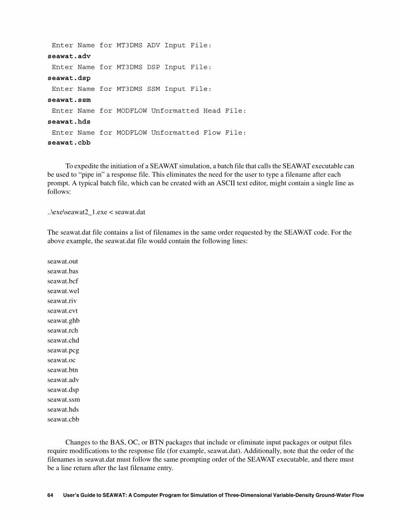
Running SEAWAT....................................................................................................................................................... 63Output Files and Post Processing ................................................................................................................................ 65Calculation of Equivalent Freshwater Head................................................................................................................ 65Tips for Designing SEAWAT Models ......................................................................................................................... 66

Chapter 7: Benchmark Problems........................................................................................................................................... 69Box Problems .............................................................................................................................................................. 69

Case 1 ................................................................................................................................................................ 69Case 2 ................................................................................................................................................................ 70

Henry Problem ............................................................................................................................................................ 70Elder Problem.............................................................................................................................................................. 72HYDROCOIN Problem .............................................................................................................................................. 73

References Cited.................................................................................................................................................................... 76

FIGURES

1. Schematic showing two piezometers, one filled with freshwater and the other with saline aquifer water,open to the same point in the aquifer.......................................................................................................................... 8

2. Diagram showing representative elementary volume in a porous medium................................................................ 93. Schematic showing relation between a coordinate system aligned with the principal axes of permeability

and the upward z-axis ................................................................................................................................................. 124. Generalized flow chart of the SEAWAT program ...................................................................................................... 275. Schematic showing example of the explicit scheme used to couple the flow and transport equations...................... 296. Schematic showing example of the implicit scheme used to couple the flow and transport equations ..................... 317. Flow chart showing step-by-step procedures of the SEAWAT program .................................................................... 328. Schematic showing cell indices and variable definitions for the case of a partially dewatered cell underlying

an active model cell .................................................................................................................................................... 399. Schematic showing conceptual representation of flow between two cells for the water-table case .......................... 41

10. Diagram showing conceptual model and variable description for river leakage in MODFLOW and SEAWAT ...... 4511. Diagram showing conceptual model and variable description for drain leakage in MODFLOW and SEAWAT...... 4912. Grid showing boundary conditions and model parameters for the Henry problem ................................................... 7013. Graphs showing comparison between SEAWAT and SUTRA for the Henry problem.............................................. 7114. Grid showing boundary conditions and model parameters for the Elder problem..................................................... 7215. Finite-difference grid used to simulate the Elder problem ......................................................................................... 7316. Schematics showing comparison between SEAWAT, SUTRA, and Elder’s solution for the Elder problem

over time..................................................................................................................................................................... 7417. Grid showing boundary conditions and model parameters for the HYDROCOIN problem ..................................... 7518. Graph showing comparison between SEAWAT and MOCDENSE for the HYDROCOIN problem......................... 75

TABLE

1. MODFLOW and MT3DMS packages used in SEAWAT........................................................................................... 33

Contents VII

CONVERSION FACTORS AND VERTICAL DATUM

Sea level: In this report, “sea level” refers to the National Geodetic Vertical Datum of 1929(NGVD of 1929)−a geodetic datum derived from a general adjustment of the first-orderlevels nets of the United States and Canada, formerly called Sea Level Datum of 1929.

Multiply By To obtain

gram (g) 0.03527 ounce

liter (L) 0.2642 gallon

meter (m) 3.281 foot

meter per day (m/d) 3.281 foot per day

kilogram (kg) 2.205 pound

kilogram per day (kg/d) 2.205 pound per day

kilogram per cubic meter (kg/m3) 0.06243 pound per cubic foot

square meter per day (m2/d) 10.76 square foot per day

cubic meter per day (m3/d) 35.31 cubic foot per day

VIII Contents

Abstract 1

User’s Guide to SEAWAT: A ComputerProgram for Simulation of Three-DimensionalVariable-Density Ground-Water Flow

By Weixing Guo1 and Christian D. Langevin2

Abstract

The SEAWAT program was developed to simulate three-dimensional, variable-density,transient ground-water flow in porous media. The source code for SEAWAT was developed bycombining MODFLOW and MT3DMS into a single program that solves the coupled flow andsolute-transport equations. The SEAWAT code follows a modular structure, and thus, newcapabilities can be added with only minor modifications to the main program. SEAWAT readsand writes standard MODFLOW and MT3DMS data sets, although some extra input may berequired for some SEAWAT simulations. This means that many of the existing pre- and post-processors can be used to create input data sets and analyze simulation results. Users familiarwith MODFLOW and MT3DMS should have little difficulty applying SEAWAT to problemsof variable-density ground-water flow.

MODFLOW was modified to solve the variable-density flow equation by reformulatingthe matrix equations in terms of fluid mass rather than fluid volume and by including the appro-priate density terms. Fluid density is assumed to be solely a function of the concentration ofdissolved constituents; the effects of temperature on fluid density are not considered. Tempo-rally and spatially varying salt concentrations are simulated in SEAWAT using routines fromthe MT3DMS program. SEAWAT uses either an explicit or implicit procedure to couple theground-water flow equation with the solute-transport equation. With the explicit procedure, theflow equation is solved first for each timestep, and the resulting advective velocity field is then

1CDM Missimer, Fort Myers, Fla.2U.S. Geological Survey, Miami, Fla.

2 User’s Guide to SEAWAT: A Computer Program for Simulation of Three-Dimensional Variable-Density Ground-Water Flow

used in the solution to the solute-transport equation. This procedure for alternately solving theflow and transport equations is repeated until the stress periods and simulation are complete.With the implicit procedure for coupling, the flow and transport equations are solved multipletimes for the same timestep until the maximum difference in fluid density between consecutiveiterations is less than a user-specified tolerance.

The SEAWAT code was tested by simulating five benchmark problems involving vari-able-density ground-water flow. These problems include two box problems, the Henry prob-lem, Elder problem, and HYDROCOIN problem. The purpose of the box problems is to verifythat fluid velocities are properly calculated by SEAWAT. For each of the box problems,SEAWAT calculates the appropriate velocity distribution. SEAWAT also accurately simulatesthe Henry problem, and SEAWAT results compare well with those of SUTRA. The Elder prob-lem is a complex flow system in which fluid flow is driven solely by density variations. Resultsfrom SEAWAT, for six different times, compare well with results from Elder’s original solutionand results from SUTRA. The HYDROCOIN problem consists of fresh ground water flowingover a salt dome. Simulated contours of salinity compare well for SEAWAT and MOCDENSE.

CHAPTER 1--Introduction 3

CHAPTER 1INTRODUCTION

Ground water contains dissolved constituents, such as the salts commonly found in seawater.At relatively low concentrations, dissolved constituents do not substantially affect fluid density. As soluteconcentrations increase, however, the mass of the dissolved constituents can substantially affect the fluiddensity. If the spatial variations in fluid density are minimal, regardless of the actual density value, field andmathematical methods for quantifying rates and patterns of ground-water flow are relatively straightfor-ward. Where spatial variations in fluid density are present, such as in coastal aquifers, investigations ofground-water flow are more complicated because the density variations can substantially affect rates andpatterns of fluid flow. In many of these hydrogeologic settings, an accurate representation of variable-density ground-water flow is necessary to characterize and predict ground-water flow rates, travel paths,and residence times.

Spatial variations in fluid density that affect ground-water flow have been observed in a wide rangeof hydrogeologic settings. For example, in coastal aquifers, an interface exists between fresh ground waterflowing toward the ocean and saline ground water. Across the interface, the fluid density may increase fromthat of freshwater (about 1,000 kg/m3) to that of seawater (about 1,025 kg/m3), an increase of about 2.5percent. Field observations and mathematical analyses have shown that this relatively minor variation inground-water density has a substantial effect on ground-water flow rates and patterns. An understanding ofvariable-density ground-water flow, therefore, can be important in many types of studies of coastal aquifers,such as studies of saltwater intrusion, contaminated site remediation, and fresh ground-water discharge intooceanic water bodies.

Characterization of variable-density ground-water flow also can be important for studies of aquiferstorage and recovery (ASR). ASR projects typically involve the injection of surface water into an aquiferduring times of surplus and retrieval of this same water during times of demand. If the native water qualityof the aquifer selected for ASR is brackish or saline, the storage times and recovery efficiencies can beaffected by the density differences between the injected water and the native aquifer water. In some situa-tions, the freshwater “bubble” can migrate upward in response to the differences in fluid density.

The theory of variable-density ground-water flow has been studied for many years, beginning withthe early work of Ghyben (1888) and Herzberg (1901). Later, Hubbert (1940) presented a simple equationrelating the elevation of a sharp interface to freshwater heads measured on the interface and to the densitiesof saltwater and freshwater. Henry (1964) used a semianalytical solution to define the location and shape ofthe interface under the condition of a constant seaward flux of freshwater toward an oceanic boundary.Several other analytical and numerical solutions since then have been developed for the original Henryproblem, including Pinder and Cooper (1970), Lee and Cheng (1974), Huyakorn and others (1987), Vossand Souza (1987), and Croucher and O’Sullivan (1995).

There is a wide range of private and public domain computer codes that can be used to simulate vari-able-density ground-water flow. For example, the U.S. Geological Survey (USGS) offers the finite-elementSUTRA code (Voss, 1984) and the finite-difference HST3D (Kipp, 1997) and MOCDENSE (Sanford andKonikow, 1985) codes. These codes contain powerful options for simulating a wide range of complex prob-lems. Although many hydrogeologists are familiar with the constant-density MODFLOW (McDonald andHarbaugh, 1988) code, there are fewer hydrogeologists familiar with the complex variable-density codes.Thismanual describes the SEAWAT code, which is based on the 1988 version of the MODFLOW code, anddemonstrates how those familiar with MODFLOW and the solute-transport code, MT3DMS (Zheng andWang, 1998), should have little difficulty developing variable-density models of ground-water flow.


Purpose and Scope

The purpose of this report is to document a computer program (SEAWAT) that simulatesvariable-density, transient, ground-water flow in three dimensions. Two popular computer programs,MODFLOW and MT3DMS, were used in the development of SEAWAT. This report is divided into sevenchapters. Chapter 1 is an introduction to the development of SEAWAT. Chapter 2 contains a mathematicaldevelopment of variable-density ground-water flow in terms of freshwater head and includes a discussionof Darcy’s law for variable-density flow. The finite-difference equation for flow of variable-density water,using a block-centered scheme, is presented in Chapter 3. The design and structure of the SEAWAT programare presented in Chapter 4. Additionally, this chapter discusses the solution procedures implemented inMODFLOW and MT3DMS and describes how the timestep calculated by MT3DMS (based on stabilitycriteria) is used as the timestep in SEAWAT. The major modifications made to the block-centered flow(BCF) package and the stress packages (RIV, DRN, WEL, RCH, EVT, CHD, and GHB) of MODFLOW arediscussed in Chapter 5. Instructions for preparing input files for individual MODFLOW and MT3DMSpackages for use in SEAWAT are explained in Chapter 6. Several benchmark problems solved usingSEAWAT are presented in Chapter 7.

This report should be used to supplement the documentations of MODFLOW and MT3DMS, whichare available in the public domain. The documentation for MODFLOW and MT3DMS can be obtained fromthe USGS and the Hydrogeology Group at the University of Alabama, respectively.

Development of SEAWAT

The original SEAWAT concept of combining MODFLOW and MT3D into a single program tosimulate three-dimensional variable-density ground-water flow was first documented by Guo and Bennett(1998). Later, as part of a U.S. Geological Survey project to quantify submarine ground-water discharge toBiscayne Bay, Fla. (Langevin, 2001), the SEAWAT program was improved, updated, and verified against anumber of benchmark test problems (Langevin and Guo, 1999; Guo and others, 2001). This user’s manualpresents the concept behind the original SEAWAT code (Guo and Bennett, 1998) and documents the recentchanges and improvements that extend the applicability of the SEAWAT code to a wide range of variable-density ground-water flow problems.

The source code for SEAWAT was developed by combining MODFLOW and MT3DMS into a singleprogram that solves the coupled flow and solute-transport equations. The SEAWAT code follows a modularstructure, so new capabilities can be added with only minor modifications to the source code. MODFLOWwas modified to conserve fluid mass rather than fluid volume and uses equivalent freshwater head as theprincipal dependent variable. In the revised form of MODFLOW, the cell-by-cell flow is calculated fromfreshwater head gradients and relative density-difference terms. The resulting flow field is passed toMT3DMS for transport of solute; an updated density field is then calculated from the new solute concentra-tions and incorporated back into MODFLOW as relative density-difference terms.

For the convenience of hydrologists and modelers familiar with MODFLOW and MT3DMS, thechanges in input files for MODFLOW and MT3DMS were kept to a minimum. Thus, existing input files forthe standard versions of MODFLOW and MT3DMS can be revised for SEAWAT with minor modifications.Because no additional data files are needed to run SEAWAT, individuals familiar with MODFLOW andMT3DMS should be able to use SEAWAT with few difficulties. SEAWAT reads and writes standardMODFLOW and MT3DMS data sets, which are easily manipulated with the commercially available pre-and post-processors. These processors substantially reduce the length of time it takes to create input datasets and evaluate model results.

CHAPTER 1--Introduction 5

Acknowledgments

The authors would like to express great appreciation to Gordon D. Bennett of S.S. Papadopulos &Associates, Inc., for his significant and generous contributions to the development of SEAWAT in the pastyears. Gordon provided numerous comments and suggestions that substantially improved the quality of thisuser’s documentation and the SEAWAT program.

The authors also would like to extend appreciation to other individuals who helped with thedevelopment of the SEAWAT code, particularly Chunmiao Zheng from the University of Alabama;Charlie Andrews from S.S. Papadopulos and Associates, Inc; Tom Missimer from CDM Missimer; andArlen Harbaugh, Leonard Konikow, Ward Sanford, Barclay Shoemaker, Eric Swain, and Clifford Voss fromthe USGS. The authors also would like to thank Barbara Howie, Rhonda Howard, Michael Deacon,Stephen Garabedian, and Arlen Harbaugh for providing insightful reviews of the SEAWAT documentation.Beta testing of the SEAWAT program was performed by Trayle Kulshan at Stanford University;Amy Johnson and Jeff Weaver from Water Management Consultants; James Schneider from the Universityof South Florida; Mike Riley from S.S. Papadopulos & Associates, Inc; and Barclay Shoemaker,Alyssa Dausman, Melinda Wolfert, Raul Patterson, David Garces, and David Kirby from the USGS. Appre-ciation also is extended to Jim Tomberlin, Haymeli Castillo, and Taina Camacho for help with report prep-aration.


CHAPTER 2--Mathematical Description of Variable-Density Ground-Water Flow 7

CHAPTER 2MATHEMATICAL DESCRIPTION OF VARIABLE-DENSITYGROUND-WATER FLOW

This chapter develops the governing equations that describe variable-density ground-water flow andsolute transport in porous media. The theory of variable-density ground-water flow is usually developed andpresented in terms of fluid pressure and fluid density. In this chapter, however, the variable-density ground-water flow equation is developed in terms of equivalent freshwater head and fluid density. The purpose fordeveloping the flow equation in terms of equivalent freshwater head, rather than pressure, is discussed inthis chapter and later in Chapter 5 where modifications to the MODFLOW computer program are presented.

Basic Assumptions

The development presented here is based on the usual assumptions that Darcy’s law is valid (laminarflow); the standard expression for specific storage in a confined aquifer is applicable; the diffusive approachto dispersive transport based on Fick’s law can be applied; and isothermal conditions prevail. The porousmedium is assumed to be fully saturated with water. A single, fully miscible liquid phase of very smallcompressibility also is assumed.

Concept of Equivalent Freshwater Head

SEAWAT is based on the concept of freshwater head, or equivalent freshwater head, in a salineground-water environment. A thorough understanding of this concept is required in developing the equa-tions of variable-density ground-water flow as used in the SEAWAT program and in interpreting calculatedresults. The subsequent discussion is intended to provide readers with an understanding of equivalent fresh-water head and its relation to head.

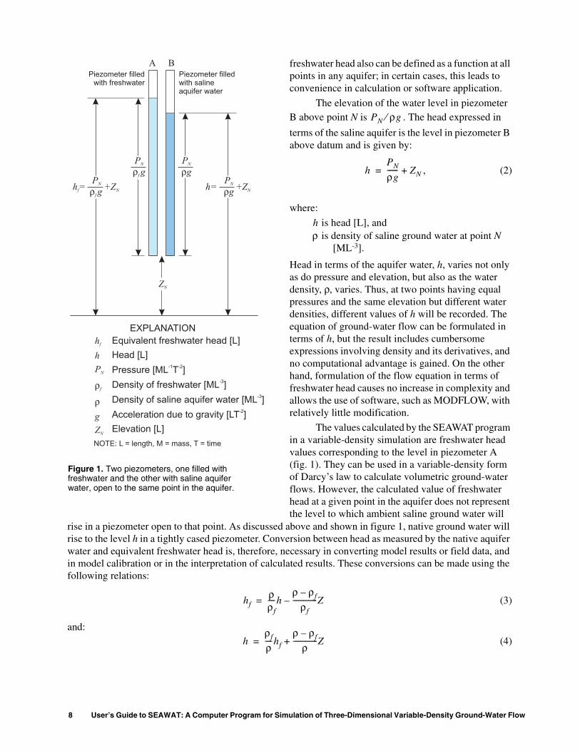
Two piezometers open to a given point, N, in an aquifer containing saline water are shown in figure 1.Piezometer A contains freshwater and is equipped with a mechanism that prevents saline water in the aqui-fer from mixing with freshwater in the piezometer, while still allowing the piezometer to respond accuratelyto the pressure at point N. Piezometer B contains water identical to that present in the saline aquifer at pointN. The height of the water level in piezometer A above point N is . The freshwater head at point N

is the elevation of the water level in piezometer A above datum, and thus is given by:

, (1)

where:hf is equivalent freshwater head [L],

PN is pressure at point N [ML-1T-2],ρf is density of freshwater [ML-3]g is acceleration due to gravity [LT-2], and

ZN is elevation of point N above datum [L].

Piezometers filled with freshwater would seldom if ever be used in field studies of a saline aquifer(although pressure transducers calibrated to read values of freshwater head could certainly be implementedwithout difficulty). However, the point here is not that field measurements would ever be made in terms offreshwater head, but rather that because pressure and elevation are defined at all points in any aquifer,

PN ρf⁄ g

hf

PN

ρfg-------- ZN+=


A BPiezometer filled

with freshwaterPiezometer filledwith salineaquifer water

h = +Zf N

PN

ρf gh= +ZN

PN

ρg

PN

ρg

PN

ρf g

ZN

Equivalent freshwater head [L]

Head [L]

Pressure [ML T ]

Density of freshwater [ML ]

Density of saline aquifer water [ML ]

Acceleration due to gravity [LT ]

Elevation [L]

-1 -2

-3

-3

-2

h

h

P

g

Z

f

N

f

N

ρ

ρ

NOTE: L = length, M = mass, T = time

EXPLANATION

freshwater head also can be defined as a function at allpoints in any aquifer; in certain cases, this leads toconvenience in calculation or software application.

The elevation of the water level in piezometerB above point N is . The head expressed in

terms of the saline aquifer is the level in piezometer Babove datum and is given by:

, (2)

where:

h is head [L], andρ is density of saline ground water at point N

[ML-3].

Head in terms of the aquifer water, h, varies not onlyas do pressure and elevation, but also as the waterdensity, ρ, varies. Thus, at two points having equalpressures and the same elevation but different waterdensities, different values of h will be recorded. Theequation of ground-water flow can be formulated interms of h, but the result includes cumbersomeexpressions involving density and its derivatives, andno computational advantage is gained. On the otherhand, formulation of the flow equation in terms offreshwater head causes no increase in complexity andallows the use of software, such as MODFLOW, withrelatively little modification.

The values calculated by the SEAWAT programin a variable-density simulation are freshwater headvalues corresponding to the level in piezometer A(fig. 1). They can be used in a variable-density formof Darcy’s law to calculate volumetric ground-waterflows. However, the calculated value of freshwaterhead at a given point in the aquifer does not representthe level to which ambient saline ground water will

PN ρg⁄

hPN

ρg------ ZN+=

rise in a piezometer open to that point. As discussed above and shown in figure 1, native ground water willrise to the level h in a tightly cased piezometer. Conversion between head as measured by the native aquiferwater and equivalent freshwater head is, therefore, necessary in converting model results or field data, andin model calibration or in the interpretation of calculated results. These conversions can be made using thefollowing relations:

(3)

and:(4)

hfρρf

----hρ ρ– f

ρf

--------------Z–=

hρf

ρ----hf

ρ ρ– f

ρ--------------Z+=

Figure 1. Two piezometers, one filled withfreshwater and the other with saline aquiferwater, open to the same point in the aquifer.


ρqx ρqx+ x∆

∆x

Fluid density [ML ]

Specific discharge at [LT ]

Specific discharge at [LT ]

Distance along the axis [L]

-3

-1

-1

x

x x

x

+∆

ρ

∆

q

q

x

x

x+ x∆


EXPLANATION

where Z is elevation [L]. Equations 3 and 4 are obtained by eliminating pressure between equations 1 and2, and solving for the respective head value.

Governing Equation for Ground-Water Flow

A representative elementary volume (REV) in a porous medium is shown in figure 2. Based on theprinciple of mass conservation for fluid and solute, the rate of accumulation of mass stored in the REV isequal to the algebraic sum of the mass fluxes across the faces of the element and the mass exchange due tosinks or sources. The mathematical expression for the conservation of mass is:

, (5)

where:

∇ is the gradient operator ,

ρ is the fluid density [ML-3],

is the specific discharge vector [LT-1],

ρ is the density of water entering from asource or leaving through a sink[ML-3],

qs is the volumetric flow rate per unitvolume of aquifer representingsources and sinks [T-1],

θ is porosity [dimensionless], and

t is time [T].

∇ ρq( ) ρqs+⋅–∂ ρθ( )

∂t--------------=

∂∂x----- ∂

∂y----- ∂

∂x-----+ +

q

The left-hand side of equation 5 is the net flux of mass through the faces of the REV, plusthe rate (ρqs) at which mass enters from sources or leaves through sinks located in the REV. The right-hand

side of equation 5 is the time rate of change in the mass stored in the REV over a given period and can beexpanded with the chain rule as:

. (6)

The changes of porosity considered here are restricted to those associated with the change of fluidpressure; therefore, the change of porosity with time is mathematically represented as:

. (7)

Under isothermal conditions, fluid density is a function of fluid pore pressure and solute concentration;therefore, the equation of the state for fluid density is:

, (8)

∇ ρq( )⋅

∂ ρθ( )∂t

-------------- ρ∂θ∂t------ θ∂ρ

∂t------+=

∂θ∂t------ ∂θ

∂P------∂P

∂t------=

ρ f P C,( )=

Figure 2. Representative elementaryvolume in a porous medium.


where:P is fluid pore pressure [ML-1T-2], andC is solute concentration [ML-3].

Differentiating equation 8 with respect to time gives:

. (9)

Substituting equations 7 and 9 into equation 6 gives:

. (10)

The first two terms in the right-hand side of equation 10 represent the rate of fluid mass accumulationdue to ground-water storage effects (for example, due to the compressibility of the bulk porous material andfluid compressibility). The third term on the right-hand side of equation 10 represents the rate of fluid massaccumulation due to the change of solute concentration.

The relation between porosity, pressure, and the compressibility of a bulk porous material is given byBear (1979) as:

, (11)

where ξ is the compressibility of the bulk porous material [M-1LT2]. The coefficient of water compressibilityis defined as (Bear, 1979):

, (12)

where ζ is the coefficient of water compressibility [M-1LT2]. Using equations 11 and 12, equation 10 can berewritten as:

. (13)

The term, , represents the volume of water released from storage in a unit volume of aconfined elastic aquifer per unit change in pressure:

, (14)

where Sp is the specific storage in terms of pressure [M-1LT2]. Substitution of equation 14 into 13 gives:

. (15)

A more thorough discussion of storativity is presented by Bear (1979).

∂ρ∂t------ ∂ρ

∂P------∂P

∂t------ ∂ρ

∂C-------∂C

∂t-------+=

∂ ρθ( )∂t

-------------- ρ∂θ∂t------ θ∂ρ

∂t------ ρ∂θ

∂P------∂P

∂t------ θ∂ρ

∂P------∂P

∂t------ θ ∂ρ

∂C-------∂C

∂t-------+ +=+=

ξ 11( θ )–

----------------- ∂θ∂P------=

ζ 1ρ--- ∂ρ

∂P------=

∂ ρθ( )∂t

-------------- ρ ξ 1 θ–[ ] ζθ+( )∂P∂t------ θ ∂ρ

∂C-------∂C

∂t-------+=

ρ ξ 1 θ–[ ] ζθ+( )

Sp ξ 1 θ–[ ] ζθ+( )=

∂ ρθ( )∂t

-------------- ρSp∂P∂t------ θ ∂ρ

∂C-------∂C

∂t-------+=


The first term in the right-hand side of equation 15 is the rate of fluid mass accumulation due to fluidpore pressure change, and the second term is the rate of fluid mass accumulation due to the change of soluteconcentration. Further discussion of the second term in the right-hand side of equation 15 is presented later.

Substituting equation 15 into equation 5, the flow equation becomes:

. (16)

Equation 16 is the general form of the partial differential equation for variable-density ground-water flowin porous media.

If density is constant, the term in equation 16 is zero, and the remaining density terms cancel.The resulting equation would conserve fluid mass and fluid volume for a constant density system, but wouldconserve only fluid volume for a variable-density system. The flow equation based on fluid volume conser-vation is often cited for the case of uniform density (for example, de Marsily, 1986). As Bear (1972) pointsout, however, the use of an equation based on volume balance is inappropriate when substantial density ortemperature gradients are present. Evans and Raffensperger (1992) compared the mass- and volume-basedstream functions for variable-density ground-water flow and found that the differences between the streamfunctions, calculated using the mass-based stream function and volume-based stream function, could reach9.55 percent for their particular test problem after a calculation period of 600 years. They concluded thatmass fluxes rather than volumetric fluxes must be used to describe the flow of ground water if the variationin fluid density is substantial.

Darcy’s Law for Variable-Density Ground-Water Flow

The governing equation for variable-density ground-water flow includes a term for specificdischarge, which is calculated with Darcy’s law. In this section, the variable-density form of Darcy’s law ispresented.

General Form of Darcy’s Law

Mass fluxes are defined as the product of fluid density and the specific discharge, or volumetric flowper unit cross-sectional area of bulk porous medium. Darcy’s law for a fluid of variable density can beexpressed by the equations:

, (17)

, (18)

and:

, (19)

where:qx,qy,qz are the individual components of specific discharge,

µ is the dynamic viscosity [ML-1T-1],kx,ky,kz represent intrinsic permeabilities [L2] in the three coordinate directions, and

g is the gravitational constant [LT-2] and treated here as a positive scalar quantity.

∇ ρq( )⋅– ρqs ρSp∂P∂t------ θ ∂ρ

∂C-------∂C

∂t-------+=+

∂ρ ∂C⁄

qx

kx

µ----–

∂P∂x------=

qy

ky

µ----–

∂P∂y------=

qz

kz

µ---- ∂P

∂z------ ρg+–=


In this formulation, it is assumed that the three principal directions of permeability are aligned with theorthogonal x-, y-, and z-coordinate system. The z-coordinate axis, representing the vertical, is positiveupward.

Note that in equation 19, the density, ρ, is that of the fluid at the calculation point (and time) forwhich specific discharge is to be determined. The density term reflects the direct action of gravity on a fluidelement at the calculation point and only affects the component of specific discharge in the vertical direction.It should be kept in mind, however, that the overall pressure distribution in a porous medium is controlled,in part, by the overall fluid density distribution, and thus, horizontal components of specific discharge alsoare affected by density variations in the system.

Assumption of Axes Alignment with Principal Permeability Directions

The assumption that the principal axes of permeability are horizontal and vertical is usually accept-able for an aquifer with horizontal bedding. A more general form of Darcy’s law is required when the prin-cipal directions of permeability do not coincide with the horizontal and vertical x-, y-, and z-coordinatesystem. The simplest approach is to abandon the x-, y-, and z-coordinate system, and instead use a coordinatesystem aligned with the principal directions of permeability as shown in figure 3. If γ represents the directionnormal to the bedding and α and β represent the principal directions of permeability parallel to the bedding,the pressure gradients acting in the α, β, and γ directions can be formulated independently. Because none ofthe coordinate directions are horizontal, although they are orthogonal to one another, a component of thegravitational force applies in each coordinate direction. This leads to the following expression of Darcy's law:

, (20)

, (21)

and:

, (22)

where:qα,qβ,qγ represent the specific discharge components in the

coordinate axes aligned with permeability directions [LT-1],

kα,kβ,kγ are the permeabilities in these directions [L2], and

δα,δβ,δγ are the angles between the respective coordinate axes andthe upward vertical direction.

Darcy’s Law in Terms of Equivalent Freshwater Head

Darcy's law can also be expressed in terms of the freshwater heador elevation above an arbitrary datum of the water surface in a piezom-eter filled with freshwater. Note that it is not assumed that the aquiferitself contains freshwater of uniform density, but rather that piezometersopen to the aquifer have been filled with freshwater, and a mechanismprevents the dissolved salts in the aquifer water from mixing with thewater in the piezometers. As shown in figure 1, the elevation of the

qαkαµ----- ∂P

∂α------- ρg δαcos+ –=

qβkβµ----- ∂P

∂β------ ρg δβcos+ –=

qγkγµ---- ∂P

∂γ------ ρg δγcos+ –=

δβ

δγ

α

β

γ

z

δα

Figure 3. Relation between acoordinate system aligned withthe principal axes of permeabil-ity and the upward z-axis.


water surface in a piezometer has two components: the elevation of the point of measurement above somedatum, z, and the height of the fluid column in the piezometer itself. Because the piezometer is assumed tocontain freshwater having a fixed density, ρf, the height of the water column within the piezometer is

P/ρf g, where P is the pressure at the piezometer opening. Thus, the freshwater head, hf, at this point is equalto (P/ρf g,) + z and the pressure is given by:

. (23)

For the dipping-aquifer problem (fig. 3), equation 23 is first differentiated with respect to the coordi-nate direction α, which yields:

. (24)

Substituting this expression into equation 20 and noting that , the following relation isobtained:

. (25)

It is important to note that both ρf, the density of freshwater in the piezometers and ρ, the density of water

in the formation at the point of velocity calculation, appear in equation 25. These two density terms shouldnot be confused.

The freshwater hydraulic conductivity, Kf, in the α direction is defined as:

, (26)

where µf [ML-1T-1] represents the viscosity of freshwater under standard conditions (for example, 20 degrees

Celsius and 1 atmospheric pressure). Using this term for freshwater hydraulic conductivity, equation 20 canbe written as:

. (27)

Similarly, equation 21 can be written as:

, (28)

and equation 22 as:

. (29)

Note that for a horizontally stratified aquifer, equations 27 to 29 would reduce to:

, (30)

P ρfg hf z–( )=

∂P∂α------- ρfg

∂hf

∂α------- ρfg

∂z∂α-------–=

δcos α∂z∂α-------=

qαkα–

µ-------- ρfg

∂hf

∂α------- ρfg

∂z∂α-------– ρg

∂z∂α-------+=

Kfαkαρfg

µf

--------------=

qα Kfα–µf

µ----

∂hf

∂α-------

ρ ρf–

ρf

-------------- ∂z

∂α-------+=

qβ Kfβ–µf

µ----

∂hf

∂β-------

ρ ρf–

ρf

-------------- ∂z

∂β------+=

qγ Kfγ–µf

µ----

∂hf

∂γ-------

ρ ρf–

ρf

-------------- ∂z

∂γ-----+=

qx Kfx–µf

µ----

∂hf

∂x-------=


, (31)

and:

. (32)

For many practical applications, the term µf/µ in equations 27 to 32 can be considered equal to one;

it can be assumed that the viscosity of water in the formation is essentially the same as that of freshwater,even though differences in density are present. Variations in fluid viscosity arise primarily because of vari-ations in water temperature. Where substantial temperature variations are absent and where hydraulicconductivity has been measured at the same water temperature for which velocity is to be calculated, theviscosity correction usually can be neglected.

Governing Equation for Flow in Terms of Freshwater Head

With the definition of freshwater head and Darcy’s law in terms of freshwater head, the governingequation for ground-water flow (eq. 16) can be written in terms of equivalent freshwater head. Expandingthe left-hand side of equation 16 and rearranging yield:

. (33)

Differentiation of equation 23 with respect to time shows that can be expanded as

. Using this form and substituting Darcy’s law as given in equations 27 to 29 for the components

of specific discharge yield:

(34)

The specific storage in terms of pressure, Sp (eq. 14), includes the compressibility of the water, which

in turn, depends on the water density, ρ, at the point of calculation (eq. 12). The assumption is made herethat the difference between the compressibility coefficients of saltwater and freshwater can be neglected inthat:

, (35)

where ζf is the compressibility coefficient for freshwater. The specific storage, in terms of freshwater head,

Sf [L-1], or the volume of water released from storage in a unit volume of aquifer per unit decline in

freshwater head is given by Bear (1979) as:

. (36)

qy Kfy–µf

µ----

∂hf

∂y-------=

qz Kfz–µf

µ----

∂hf

∂z-------

ρ ρf–

ρf

-------------- +=

∂∂α------- ρqα( )–

∂∂β------ ρqβ( )–

∂∂γ----- ρqγ( ) ρSP

∂P∂t------ θ ∂ρ

∂C-------∂C

∂t------- ρqs–+=–

∂P ∂t⁄ρfg ∂hf ∂t⁄

∂∂α------- ρKfα

∂hf

∂α-------

ρ ρf–

ρf

-------------- ∂Z∂α-------+

∂∂β------ ρKfβ

∂hf

∂β-------

ρ ρf–

ρf

--------------∂Z∂β------+

+

∂∂γ-----+ ρKfγ

∂hf

∂γ-------

ρ ρf–

ρf

--------------∂Z∂γ------+

ρSpgρf

∂hf

∂t------- θ ∂ρ

∂C-------∂C

∂t------- ρqs.–+=

ζ 1ρ--- ∂ρ

∂P------ ζf

1ρf

---- ∂ρ∂P------=≈=

Sf gρf ξ 1 θ )– ζfθ ]+([=


By using equations 14 and 35, the term Spgρf in equation 34 can be replaced by the term Sf, which yields:

(37)

Equation 37 is the governing equation for variable-density flow in terms of freshwater head as used inSEAWAT.

Governing Equation for Solute Transport

In addition to the flow equation that was developed (eq. 37), a second partial differential equation isrequired to describe solute transport in the aquifer. Ground-water flow causes the redistribution of soluteconcentration, and the redistribution of solute concentration alters the density field, thus, affecting ground-water movement. Therefore, the movement of ground water and the transport of solutes in the aquifer arecoupled processes, and the two equations must be solved jointly.

Solute mass is transported in porous media by the flow of ground water (advection), molecular diffu-sion, and mechanical dispersion. The transport of solute mass in ground water can be described by thefollowing partial differential equation (Zheng and Bennett, 1995):

, (38)

where:D is the hydrodynamic dispersion coefficient [L2T-1],

is the fluid velocity [LT-1],Cs is the solute concentration of water entering from sources or sinks [ML-3], andRk (k=1, …, N) is the rate of solute production or decay in reaction k of N different reactions [ML-3T-1].

When fluid density varies, the concentration gradient, , should actually be formulated as ρ∇(C/ρ)(de Marsily, 1986, p. 239). This is only necessary for brines of high density; however for fluid densities inthe seawater range, the change introduced by this expression is negligible, and the transport equation asformulated in equation 38 may be used.

Boundary and Initial Conditions

Boundary and initial conditions must be specified to solve the differential equations for flow (eq. 37)and transport (eq. 38) in a particular problem. Mathematical boundaries are commonly defined in three cate-gories: Dirichlet (constant head or concentration), Neumann (specific flux), and Cauchy (head-dependentflux or mixed boundary condition). The physical features and processes, which impose boundary conditionson ground-water regimes, normally include streams and other surface-water bodies, drains, low-permeabil-ity boundaries, seepage faces, evapotranspiration, discharging wells, injection wells and recharge. In simu-lation theory, many of the boundary conditions are commonly implemented through the sink/source term inequations 37 and 38; that approach is followed in this model. There is a separate section that furtherdescribes sink and source terms.

∂∂α------- ρKfα

∂hf

∂α-------

ρ ρf–

ρf

-------------- ∂Z∂α-------+

∂∂β------ ρKfβ

∂hf

∂β-------

ρ ρf–

ρf

--------------∂Z∂β------+

+

∂∂γ----- ρKfγ

∂hf

∂γ-------

ρ ρf–

ρf

--------------∂Z∂γ------+

ρSf

∂hf

∂t------- θ ∂ρ

∂C-------∂C

∂t------- ρqs.–+=+

∂C∂t------- ∇ D ∇C⋅( )⋅= ∇ vC( )⋅

qs

θ----Cs Rk

k 1=

N

∑+––

v

∇C


Dirichlet Boundary

A Dirichlet boundary (also referred to as Type I) is one in which the value of head or concentration isspecified at all points along the boundary. The head or concentration value may vary from point to point oras a function of time and is treated as a known quantity in the solution of the equation. In terms of flow simu-lation, a specified head implies that flow toward or away from the boundary occurs in proportion to thedifference between the specified head at the boundary and the calculated head at points directly adjacent tothe boundary. This is simulated by not solving a flow equation at the specified-head cell. In terms of solutetransport, a specified concentration implies that the dispersive flux toward or away from the boundaryoccurs in response to the difference between the specified boundary concentration and the calculatedconcentration at points directly adjacent to the boundary. Advective solute flux into the modeled area froma specified concentration boundary depends on the flow from the boundary and the specified concentrationvalue. Advective solute flux toward any type of boundary depends on the calculated concentration of thewater at points adjacent to the boundary and on the flow toward the boundary.

A physical example of an external Dirichlet boundary might be a fully penetrating stream or othersurface-water body on the boundary of the model domain along which head or concentration is specified.An example of an internal Dirichlet boundary might be a drain operating at a specified water level in theinterior of the model domain.

Neumann Boundary

The Neumann boundary (also referred to as Type II) represents the condition in which the gradient ofthe dependent variable is specified normal to the boundary. For ground-water flow, this boundary conditionresults in a specified flux of water into or out of the modeled area. For solute transport, the concentrationgradient is specified normal to the boundary. This results in a specified dispersive flux of solute across theNeumann boundary. Although the Neumann boundary for solute transport ensures a specified dispersiveflux, the advective solute flux depends on the ground-water flow velocity normal to the boundary and thecalculated concentration on the boundary. Thus, the total solute flux across a Neumann boundary cannot bespecified prior to simulation.

An impermeable boundary represents a special case of the Neumann condition for flow and transport,where the gradients of head and concentration are zero such that neither flow nor dispersive solute flux mayoccur, and advective solute flux is precluded by the absence of flow. An impermeable boundary (commonlycalled a no-flow boundary) is simulated by specifying cells for which a flow equation is not solved. Addi-tionally, the flow between a no-flow cell and an adjacent cell is zero. A nonzero Neumann boundary is simu-lated using sink/source terms. An example of a nonzero Neumann boundary in flow simulation might be asurface-water body from which seepage occurs at a prescribed rate.

Cauchy Boundary

A head-dependent flow condition represents a Cauchy boundary (also referred to as Type III) for thesimulation of flow (Anderson and Woessner, 1992). The Cauchy boundary for solute transport, however, isnot analogous because boundary conditions for solute transport may contain both advective and dispersivecomponents, whereas boundary conditions for flow contain only the flow component. With the Cauchyboundary for flow, a control head is specified, but this control head prevails at some hydraulic separationfrom the boundary. The head on the boundary itself is calculated in the simulation, but is linked to the controlhead through a conductance term, which may represent, for example, the semipermeable material on the bedof a stream or the local head loss through convergent flow into a drain. The flow, Qb, into or from a head-

dependent flow boundary is calculated as:


, (39)

where:

COND is the conductance term,

hc is the specified control head, and

hi,j,k is the calculated head at the boundary cell, which is linked through the conductance term.

Examples of the head-dependent condition are provided by the River (RIV), Drain (DRN),Evapotranspiration (EVT), and General-Head Boundary (GHB) packages of MODFLOW; the first three ofthese nonlinear variations involve limiting values of head beyond which the flow value, Qb, takes on a fixedvalue, making these nonlinear variations of the head-dependent flux boundary condition.

The Cauchy boundary for solute transport represents a boundary on which both concentration andconcentration gradient are specified (Zheng and Bennett, 1995). This implies that the dispersive flux acrossthe boundary is specified and that the advective flux across the boundary will vary only to the extent thatthe flow across the boundary in the transport simulation varies. A Cauchy boundary condition in the trans-port model, which coincides with a Neumann boundary condition in the flow regime, will result in a spec-ified total flux of solute mass across the boundary.

Initial Conditions

Initial conditions represent starting values for the dependent variable, such as freshwater head forground-water flow and concentration for solute transport, at some starting time. Initial conditions for bothflow and transport must be specified for transient simulations.

Sink and Source Terms

The third term on the right-hand side of equation 37 and the third term on the left-hand side of equa-tion 38 are the sink/source terms for water and solute, respectively. These terms quantify the exchange ofwater and solute mass between the aquifer and such features as discharging wells, injection wells, andrecharge. Sinks and sources may be areally distributed or localized. Areally distributed sinks or sourcesinclude recharge and evapotranspiration; localized sinks and sources may include wells, drains, and rivers.In the case of sources, which provide a mechanism for bringing solute mass into the flow systems, soluteconcentration of the source water must be specified. The concentration of water removed at a sink generallyis the simulated value for the cell containing the sink and may represent information useful in model cali-bration. Evapotranspiration, which is typically thought to remove only freshwater from the flow system, isan exception.

The strength (that is, the mass of solute per unit time) of a source or sink component in the transportequation depends on the volumetric flow rate and solute concentration of the water entering the sink or leav-ing through the source. For a transport source, the concentration is specified; for a sink, the calculatedconcentration of the water in the aquifer as it enters the sink is used. The flow terms are identical to thoseused for the corresponding source or sink in the flow equation. Solutes entering the flow field by dissolutionof minerals from the aquifer generally would not be treated as part of the source term, but rather as part ofthe chemical reaction term, Rk, in equation 38.

Qb COND hc hi j k, , )–(=


Concentration and Density

The second term on the right-hand side of equation 37 represents the change of fluid mass in the REVdue to the change in solute concentration. To evaluate this term, the relation between solute concentrationand fluid density is required. For isothermal conditions, fluid density is predominantly affected by the soluteconcentration and fluid pore pressure. The effects of pore pressure on fluid density are included in the stor-age term (eq. 9). An empirical relation between the density of saltwater and concentration was developedby Baxter and Wallace (1916):

, (40)

where:

E is a dimensionless constant having an approximate value of 0.7143 for salt concentrations rangingfrom zero to that of seawater, and

C is the salt concentration [ML-3].

The derivative of equation 40 with respect to salt concentration is:

. (41)

Substituting this relation into equation 37, the governing equation is rewritten as:

(42)

Sometimes salt concentration is measured as salinity and expressed as mass/mass (for example, gramsper kilogram or parts per thousand). Salinity is defined as the total amount of solid material in gramscontained in 1 kg of seawater when all the carbonate is converted to oxide, the bromine and iodine arereplaced by chloride, and all organic matter is completely oxidized (Chow, 1964). The value of salinity isoften close to the dissolved-solids concentration; however, the salinity cannot be used directly in equation40, but must rather be converted to concentration in units of mass/volume. The conversion for a dilute solu-tion is relatively simple; for example, parts per million can approximately be treated as milligrams per liter(Freeze and Cherry, 1979). For a solution with higher concentrations of solute, such as seawater, the conver-sion is more complicated because of the change in volume of the solution, which accompanies a change insalt concentration. For example, the solution volume increases about 1 percent when 35 g of salt are addedto 1 L of water. The volume change of a solution with high concentration depends on many factors, and theconversion from units of mass/mass to units of mass/volume must, therefore, generally be based on empir-ical relations.

Equations 40 to 42 are applied only for typical seawaters for which the relation between fluid densityand solute concentration can be expressed as a linear function as in equation 40. If the fluid has a differentcomposition from typical seawater or the salt concentration in the fluid is much higher than normal seawaterconcentration, then these equations may not be valid. In that case, a different empirical relation between saltconcentration and fluid density (similar to eq. 40) should be developed for that particular application.

ρ ρf EC+=

∂ρ∂C------- E=

∂∂α------- ρKfα

∂hf

∂α-------

ρ ρf–

ρf

-------------- ∂Z∂α-------+

∂∂β------ ρKfβ

∂hf

∂β-------

ρ ρf–

ρf

--------------∂Z∂β------+

+

∂∂γ----- ρKfγ

∂hf

∂γ-------

ρ ρf–

ρf

--------------∂Z∂γ------+

ρSf

∂hf

∂t------- θE

∂C∂t------- ρqs.–+=+

CHAPTER 3--Finite-Difference Approximation for the Variable-Density Ground-Water Flow Equation 19

CHAPTER 3FINITE-DIFFERENCE APPROXIMATION FOR THEVARIABLE-DENSITY GROUND-WATER FLOW EQUATION

For variable-density ground-water conditions, flow and solute transport are linked processes. Thismeans that a fully coupled solution to the flow and transport equations is required to properly representdynamic ground-water flow. For most problems, it is difficult, if not impossible, to develop analytical solu-tions for these coupled governing equations; therefore, numerical methods generally are required.

This chapter contains the development of the finite-difference approximation for the variable-densityflow equation that is used in SEAWAT. The finite-difference equation for variable-density ground-waterflow is developed using sign conventions and nomenclature similar to those used by McDonald andHarbaugh (1988) in the documentation of MODFLOW. As a result, the similarities and differences betweenthe flow equation in MODFLOW and the flow equation in SEAWAT are readily apparent.

The numerical methods used by the MT3DMS program to simulate solute transport in a constant-density flow field are directly used in SEAWAT to simulate solute transport in a variable-density flow field.Because the solute-transport equation is applicable for both constant and variable-density flow conditions,it was not necessary to make substantial changes to the MT3DMS program prior to the incorporation intoSEAWAT. For this reason, the finite-difference and other methods used to solve the solute-transport equa-tion are not presented. Instead, interested users are referred to the MT3DMS documentation (Zheng andWang, 1998) for a detailed description of the equations and methods used to solve the solute-transportequation.

Finite-Difference Approximation for the Flow Equation

The finite-difference method is commonly used to solve partial differential equations, wherein a gridis overlain on the area of interest, dividing the domain into individual model cells. The finite-differenceapproximation to the partial differential equation is then applied to the discretized model domain. Theassumption is then made that the concept of an REV can be applied to each model cell. Both MODFLOWand MT3DMS use cell-centered grids. In this formulation, the dependent variables obtained in the finite-difference solution represent average values (assumed to exist at the cell center) for the respective cells.SEAWAT also uses a block-centered grid because it is used for both MODFLOW and MT3DMS. The subse-quent discussion of the finite-difference approximation of the variable-density ground-water flow equation,therefore, is based on the concept of a cell-centered grid, although the general approach could easily beapplied to other grid designs.

The terms on the left-hand side of the governing equation for variable-density ground-water flow(eq. 42) account for the difference between inflow and outflow of mass per unit volume of aquifer acrossthe faces of a differential element of aquifer (for example, a model cell). The first term on the right-handside of equation 42 represents the time rate of change of liquid mass (which includes both water and solute)per unit volume of aquifer due to pressure changes in the system. The second term on the right-hand side ofequation 42 represents the time rate of change of fluid mass per unit volume of aquifer due to the change insolute concentration. This second term is calculated from the concentrations obtained in the solution of thesolute-transport equation. As the concentrations reach dynamic equilibrium, this term becomes negligible.Thus, the flow field does not reach steady state until the solute concentrations remain constant in time.The third term on the right-hand side represents the mass flux due to sources and sinks.


With a central finite-difference scheme in space and a backward finite-difference scheme in time, thefinite-difference approximation for the partial differential equation of ground-water flow is:

(43)

where:

i,j,k are row, column, and layer indices, respectively.Aj,k is the area of the finite-difference cell normal to the α axis [L2] such that Aj,k = ∆βj ⋅ ∆γk, and

similarly for other coordinate directions,Zi,j,k is the cell center elevation [L],

n is the timestep number,

Vi,j,k is the volume of the cell [L3] such that V i,j,k =∆αi ∆βj ∆γk, and

Qs is the volumetric flow rate of the sink/source term [L3T-1].

The subscripts i+1/2, i-1/2, j+1/2, j-1/2, k+1/2 and k-1/2 refer to the value of a property or variable betweentwo neighboring cells (for example, the harmonic mean for hydraulic conductivity). In equation 43, the fsubscript is dropped for convenience from the freshwater-equivalent hydraulic conductivity terms, and thissimplified notation is used throughout the rest of this section. The equivalent freshwater head values on theleft-hand side of equation 43 refer to the n+1 timestep. If the timestep superscript is not listed with thevariable, as is the case with the freshwater head values on the left-hand side of equation 43, the variable isevaluated at the n+1 timestep.

In equation 43, there are two types of density terms calculated at boundaries between model cells. The

density term, , converts the volumetric flow rate to a mass flux. In SEAWAT, this density term is calculatedbefore each iteration of the flow equation using an upstream weighting algorithm. For example, if flow is

from cell i,j,k to cell i,j,k+1, then the term would be assigned a density value equal to . If,

however, the flow direction were reversed (from i,j,k+1 to i,j,k), then would be assigned a value

equal to . The other density term calculated at cell boundaries in equation 43 is denoted by ρ and is

simply the arithmetic average of fluid density between neighboring cells. These density values are used in

ρ̂i 1 2⁄ j k, ,+Kα i 1 2 j k, ,⁄+,

∆αi 1 2 j k,,⁄+-----------------------------Aj k, hf i 1 j k, ,+, hf i j k, , ,–

ρi 1 2 j k, ,⁄+ ρ– f

ρf

-------------------------------- Zi 1 j k, ,+ Zi j k, ,–( )+

ρ̂i 1 2⁄– j k, ,–Kα i 1 2 j k, ,⁄–,

∆αi 1 2 j k,,⁄–----------------------------Aj k, hf i j k, , , hf i 1– j k, , ,–

ρi 1 2 j k, ,⁄– ρ– f

ρf

-------------------------------- Zi j k, , Zi 1– j k, ,–( )+

ρ̂i j 1 2 k,⁄+,+Kβ i j, 1 2 k,⁄+,∆βi j, 1 2 k,⁄+

----------------------------Ai k, hf i j 1+ k,, , hf i j k, , ,–ρi j 1 2⁄ k,+, ρf–

ρf

--------------------------------- Zi j 1 k,+, Zi j k, ,–( )+

ρ̂i j 1 2⁄– k, ,–Kβ i j, 1 2 k,⁄–,

∆βi j 1 2 k,⁄–,----------------------------Ai k, hf i j k, , , hf i j, 1– k, ,–

ρi j, 1 2 k,⁄– ρ– f

ρf

-------------------------------- Zi j k, , Zi j 1– k, ,–( )+

ρ̂i j k, 1 2⁄+,+Kγ i j k 1 2⁄+,,,∆γi j k 1 2⁄+,,

---------------------------Ai j, hf i j k, 1+, , hf i j k, , ,–ρi j k, 1 2⁄+, ρf–

ρf

---------------------------------- Zi j k, 1+, Zi j k, ,–( )+

ρ̂i j k 1 2⁄–, ,–Kγ i j k, , 1 2⁄–,

∆γi j k 1 2⁄–, ,---------------------------Ai j, hf i j k, , , hf i j k 1–, , ,–

ρi j k 1 2⁄–, , ρ– f

ρf

-------------------------------- Zi j k, , Zi j k 1–, ,–( )+

ρi j k, , Sf i j k, , ,hf i j k, , ,

n 1+hf i j k, , ,

n–

tn 1+ tn–---------------------------------- θE

∂C∂t-------+

Vi j k, , ρQs( )i j k, , ,–=

ρ̂

ρ̂i j k 1 2⁄+, , ρi j k, ,

ρ̂i j k 1 2⁄+, ,

ρi j k 1+, ,


the density-difference terms within the brackets on the left side of equation 43; as discussed previously, thedensity-difference terms are required in Darcy’s Law when gradients of freshwater head are used in a salineenvironment.

Following the concepts of McDonald and Harbaugh (1988), several of the coefficients in equation 43can be grouped together to form the conductance term, COND [L2T-1]:

, (44)

where:A represents the area normal to flow [L2], andL represents the distance along the flow path [L].

Following this convention, equation 43 can be rewritten as:

(45)

CONDAKL

--------=

ρ̂i 1 2 j k, ,⁄+ CCi 1 2 j k, ,⁄+ hf i 1+ j k, , , hf i j k, , ,–ρi 1 2 j k,,⁄+ ρf–

ρf

--------------------------------- Zi 1 j k,,+ Zi j k, ,–( )+

ρ̂i 1 2 j k, ,⁄– CCi 1 2 j k,,⁄– hf i j k,, , hf i 1– j k, , ,–ρi 1 2 j k,,⁄– ρf–

ρf

--------------------------------- Zi j k,, Zi 1– j k, ,–( )+–

ρ̂i j 1 2 k,⁄+, CRi j, 1 2 k,⁄+ hf i j 1+ k,, , hf i j k, , ,–ρi j, 1 2 k,⁄+ ρf–

ρf

---------------------------------- Zi j 1 k,+, Zi j k, ,–( )++

ρ̂i j 1 2 k,⁄–, CRi j, 1 2 k,⁄– hf i j k,, , hf i j, 1– k, ,–ρi j, 1 2 k,⁄– ρf–

ρf

--------------------------------- Zi j k,, Zi j, 1– k,–( )+–

ρ̂i j k 1 2⁄+, , CVi j k,, 1 2⁄+ hf i j k,, 1+, hf i j k, , ,–ρi j k,, 1 2⁄+ ρf–

ρf

----------------------------------- Zi j k,, 1+ Zi j k, ,–( )++

ρ̂i j k 1 2⁄–, , CVi j k,, 1 2⁄–– hf i j k,,, hf i j k 1–, , ,–ρi j k,, 1 2⁄– ρf–

ρf

----------------------------------- Zi j k,, Zi j k 1–, ,–( )+

ρi j k, , Sf i j k, , ,hf i j k, , ,

n 1+hf i j k, , ,

n–

tn 1+ tn–------------------------------------ θE

∂C∂t-------+

= Vi j k, , ρQs( )i j k, , ,–


where CC, CR, and CV refer to the conductance factors along columns, rows, and normal to layers,respectively [L2T-1]. Equation 45 can be rewritten as:

(46)

ρ̂i 1 2 j k, ,⁄+ CCi 1 2 j k, ,⁄+ hf i 1+ j k, , , hf i j k, , ,–[ ]

ρ̂i 1 2 j k, ,⁄+ CCi 1 2 j k, ,⁄+

ρi 1 2 j k,,⁄+ ρf–

ρf---------------------------------------- Zi 1 j k,,+ Zi j k, ,–( )+

ρ̂i 1 2 j k, ,⁄– CCi 1 2 j k,,⁄–– hf i j k, , , hf i 1– j k, , ,–[ ]

ρ̂i 1 2 j k, ,⁄– CCi 1 2 j k,,⁄–

ρi 1 2 j k,,⁄– ρf–

ρf---------------------------------------- Zi j k,, Zi 1– j k, ,–( )–

ρ̂i j 1 2 k,⁄+,+ CRi j, 1 2 k,⁄+ hf i j 1+ k, , , hf i j k, , ,–[ ]

ρ̂i j 1 2 k,⁄+, CRi j, 1 2 k,⁄+

ρi j, 1 2 k,⁄+ ρf–

ρf----------------------------------------- Zi j 1 k,+, Zi j k, ,–( )+

ρ̂i j 1 2 k,⁄–, CR– i j, 1 2 k,⁄– hf i j k, , , hf i j, 1– k, ,–[ ]

ρ̂i j 1 2 k,⁄–, CR– i j, 1 2 k,⁄–

ρi j, 1 2 k,⁄– ρf–

ρf----------------------------------------- Zi j k,, Zi j, 1– k,–( )

ρ̂i j k 1 2⁄+, , CV+ i j k,, 1 2⁄+ hf i j k,, 1+, hf i j k, , ,–[ ]

ρ̂i j k 1 2⁄+, , CVi j k,, 1 2⁄+

ρi j k,, 1 2⁄+ ρf–

ρf-------------------------------------------- Zi j k,, 1+ Zi j k, ,–( )+

ρ̂i j k 1 2⁄–, , CV– i j k,, 1 2⁄– hf i j k,,, hf i j k 1–, , ,–[ ]

ρ̂i j k 1 2⁄–, , CV– i j k,, 1 2⁄–

ρi j k,, 1 2⁄– ρf–

ρf------------------------------------------- Zi j k,, Zi j k 1–, ,–( )

ρi j k, , Sf i j k, , ,hf i j k, , ,

n 1+hf i j k, , ,

n–

tn 1+ tn–--------------------------------------------- θE

∂C∂t-------+

= Vi j k, , ρQs( )i j k, , .–


The signs in equation 46 can be rearranged to give:

(47)

Equation 47 is the finite-difference equation for three-dimensional flow of variable-density ground water asimplemented in SEAWAT. Using the following expression for the relative density-difference terms:

, (48)

where:

, (49a)

, (49b)

, (49c)

ρ̂i 1 2 j k, ,⁄+ CCi 1 2 j k, ,⁄+ hf i 1+ j k, , , hf i j k, , ,–[ ]

ρ̂i 1 2 j k, ,⁄+ CCi 1 2 j k, ,⁄+

ρi 1 2 j k,,⁄+ ρf–

ρf---------------------------------------- Zi 1 j k,,+ Zi j k, ,–( )+

ρ̂i 1 2 j k, ,⁄– CCi 1 2 j k,,⁄–+ hf i 1– j k, , , hf i j k, , ,–[ ]

ρ̂i 1 2 j k, ,⁄– CCi 1 2 j k,,⁄–

ρi 1 2 j k,,⁄– ρf–

ρf---------------------------------------- Zi 1 j k, ,– Zi j k, ,–( )+

ρ̂i j 1 2 k,⁄+,+ CRi j, 1 2 k,⁄+ hf i j 1+ k, , , hf i j k, , ,–[ ]

ρ̂i j 1 2 k,⁄+, CRi j, 1 2 k,⁄+

ρi j, 1 2 k,⁄+ ρf–

ρf----------------------------------------- Zi j 1 k,+, Zi j k, ,–( )+

ρ̂i j 1 2 k,⁄–,+ CRi j, 1 2 k,⁄– hf i j 1– k, , , hf i j, k, ,–[ ]

ρ̂i j, 1 2 j k, ,⁄– CRi j 1 2 k,⁄–,ρi j, 1 2 k,⁄– ρf–

ρf----------------------------------------- Zi j 1 k,–, Zi j, k,–( )+

ρ̂i j k 1 2⁄+, , CV+ i j k,, 1 2⁄+ hf i j k,, 1+, hf i j k, , ,–[ ]

ρ̂i j k 1 2⁄+, , CVi j k,, 1 2⁄+

ρi j k,, 1 2⁄+ ρf–

ρf-------------------------------------------- Zi j k,, 1+ Zi j k, ,–( )+

ρ̂i j k 1 2⁄–, , CV+ i j k,, 1 2⁄– hf i j k,, 1–, hf i j k, , ,–[ ]

ρ̂i j k 1 2⁄–, , CVi j k,, 1 2⁄–

ρi j k,, 1 2⁄– ρf–

ρf------------------------------------------- Zi j k 1–,, Zi j k, ,–( )+

ρi j k, , Sf i j k, , ,hf i j k, , ,

n 1+hf i j k, , ,

n–

tn 1+ tn–--------------------------------------------- θE

∂C∂t-------+

= Vi j k, , ρQs( )i j k, , .–

Di j k, , Di 1 2 j k, ,⁄+ Di 1 2 j k, ,⁄– Di j 1 2 k,⁄+, Di j 1 2 k,⁄–, Di j k 1 2⁄+, , Di j k 1 2⁄–, ,+ + + + +=

Di 1 2⁄+ j k, , ρ̂i 1 2 j k, ,⁄+ CCi 1 2 j k, ,⁄+ρi 1 2 j k,,⁄+ ρf–

ρf

--------------------------------- Zi 1 j k,,+ Zi j k, ,–( )=

Di 1 2 j k,,⁄– ρ̂i 1 2 j k,,⁄– CCi 1 2 j k,,⁄–ρi 1 2 j k,,⁄– ρf–

ρf

--------------------------------- Zi 1 j k,,– Zi j k, ,–( )=

Di j, 1 2 k,⁄+ ρ̂i j, 1 2 k,⁄+ CRi j, 1 2 k,⁄+ρi j, 1 2 k,⁄+ ρf–

ρf

---------------------------------- Zi j 1 k,+, Zi j k, ,–( )=


, (49d)

, (49e)

and:. (49f)

Equation 47 becomes:

(50)

Equation 50 implies that model layers can be either horizontal or tilted. When model layers are tilted,Di+1/2,j,k, Di-1/2,j,k, Di,j+1/2,k, Di,j-1/2,k contribute to the mass flux across the four faces normal to model layers.

When the model layers are horizontal, Di+1/2,j,k, Di-1/2,j,k, Di,j+1/2,k, Di,j-1/2,k become zero. For this case,

equation 50 reduces to:

(51)

Di j, 1 2 k,⁄– ρ̂i j, 1 2 k,⁄– CRi j, 1 2 k,⁄–ρi j, 1 2 k,⁄– ρf–

ρf

--------------------------------- Zi j 1 k,–, Zi j, k,–( )=

Di j k,, 1 2⁄+ ρ̂i j k,, 1 2⁄+ CVi j k,, 1 2⁄+ρi j k,, 1 2⁄+ ρf–

ρf

----------------------------------- Zi j k,, 1+ Zi j k, ,–( )=

Di j k,, 1 2⁄– ρ̂i j k,, 1 2⁄– CVi j k,, 1 2⁄–ρi j k,, 1 2⁄– ρf–

ρf

----------------------------------- Zi j k 1–,, Zi j k, ,–( )=

ρ̂i 1 2 j k, ,⁄+ CCi 1 2 j k, ,⁄+ hf i 1+ j k, , , hf i j k, , ,–[ ] ρ̂i 1 2 j k, ,⁄– CCi 1 2 j k,,⁄– hf i 1– j k, , , hf i j k, , ,–[ ]+

ρ̂i j, 1 2 k,⁄+ CR+ i j, 1 2 k,⁄+ hf i j 1+ k, , , hf i j k, , ,–[ ] ρ̂i j, 1 2 k,⁄– CRi j, 1 2 k,⁄– hf i j 1– k, , , hf i j, k, ,–[ ]+

ρ̂i j k,, 1 2⁄+ CV+ i j k,, 1 2⁄+ hf i j k,, 1+, hf i j k, , ,–[ ] ρ̂i j k,, 1 2⁄– CVi j k,, 1 2⁄– hf i j k 1–,,, hf i j k, , ,–[ ] Di j k, ,+ +

ρf i j k, , , Sf i j k, , ,hf i j k, , ,

n 1+hf i j k, , ,

n–

tn 1+ tn–------------------------------------ θE

∂C∂t-------+

= Vi j k, , ρQs( )i j k, , .–

ρ̂i 1 2 j k, ,⁄+ CCi 1 2 j k, ,⁄+ hf i 1+ j k, , , hf i j k, , ,–[ ] ρ̂i 1 2 j k, ,⁄– CCi 1 2 j k,,⁄– hf i 1– j k, , , hf i j k, , ,–[ ]+

ρ̂+ i j 1 2 k,⁄+, CRi j, 1 2 k,⁄+ hf i j 1+ k, , , hf i j k, , ,–[ ] ρ̂i j 1 2 k,⁄–, CRi j, 1 2 k,⁄– hf i j 1– k, , , hf i j, k, ,–[ ]+ +

ρ̂i j k 1 2⁄+, , CVi j k,, 1 2⁄++ hf i j k,, 1+, hf i j k, , ,–ρi j k,, 1 2⁄+ ρf–

ρf

--------------------------------- Zi j k,, 1+ Zi j k, ,–( )+

ρ̂i j k 1 2⁄–, , CVi j k,, 1 2⁄–+ hf i j k,, 1–, hf i j k, , ,–ρi j k,, 1 2⁄– ρf–

ρf

--------------------------------- Zi j k,, 1– Zi j k, ,–( )+

ρf i j k, , , Sf i j k, , ,hf i j k, , ,

n 1+hf i j k, , ,

n–

tn 1+ tn–------------------------------------ θE

∂C∂t-------+

= Vi j k, , ρQs( )i j k, , .–


If variations in fluid density are not considered, equation 51 reduces to:

(52)

Equation 52 is the finite-difference equation solved in a conventional MODFLOW application (McDonaldand Harbaugh, 1988).

Construction of System Equations

At timestep n+1, equation 50 can be rearranged so that all terms containing the dependent variable,hf at time n+1, are on the left-hand side and all terms that do not contain the unknown are on the right-hand-side. The equation becomes:

(53)

As noted in Chapter 2, the strength of the source/sink terms may be head dependent. Thus, the fluxbetween a sink/source and an aquifer can be proportional to the head difference between the aquifer andsink/source feature, such as drains and rivers. For other cases, the flux between a sink/source and an aquifermay not depend on the head in the aquifer (for example, wells and recharge). Formulation of sink/sourceterms will be presented in Chapter 5, which discusses the modification of individual packages required inSEAWAT.

All the terms, except for the relative density-difference term Di,j,k in the left-hand side of equation 53,explicitly contain the dependent variable, hf, at time level n+1. The terms in the right-hand side of equation53 do not contain the dependent variable at time level n+1.

All density values, except for the freshwater density, should correspond to the same time level as thefreshwater heads. In SEAWAT, the density terms are treated as “constants” when the flow equation is formu-lated and solved for freshwater head. This simplification is acceptable for most cases as long as the timestepis sufficiently short or the change of fluid density is relatively slow compared to the change of freshwaterhead. Because the relative density-difference term, Di,j,k, is evaluated using the solute concentration from

CCi 1 2 j k, ,⁄+ hf i 1+ j k, , , hi j k, ,–[ ] CCi 1 2 j k,,⁄– hi 1– j k, , hi j k, ,–[ ]+

CRi j, 1 2 k,⁄+ hi j 1+ k, , hi j k, ,–[ ] CRi j, 1 2 k,⁄– hi j 1– k, , hi j, k,–[ ]+ +

C+ Vi j k,, 1 2⁄+ hi j k,, 1+ hi j k, ,–[ ] CVi j k,, 1 2⁄– hi j k 1–,, hi j k, ,–[ ]+

Sf i j k, , ,hi j k, ,

n 1+hi j k, ,

n–

tn 1+ tn–------------------------------= Vi j k, , Qs i j k, , , .–

ρ̂i 1 2 j k, ,⁄+ CCi 1 2 j k, ,⁄+ hf i 1+ j k, , ,n 1+ ρ̂i 1 2 j k, ,⁄+ CCi 1 2 j k, ,⁄+ hf i j k, , ,

n 1+–

ρ̂i 1 2 j k, ,⁄– CCi 1 2 j k, ,⁄– hf i 1– j k, , ,n 1+ ρ̂i 1 2 j k, ,⁄– CCi 1 2 j k, ,⁄– hf i j k, , ,

n 1+–+

ρ̂i j, 1 2 k,⁄+ CR+ i j, 1 2 k,⁄+ hf i j 1+ k, , ,n 1+ ρ̂i j, 1 2 k,⁄+ CRi j, 1 2 k,⁄+ hf i j k, , ,

n 1+–

ρ̂i j, 1 2 k,⁄– CRi j, 1 2 k,⁄– hf i j, 1– k, ,n 1+ ρ̂i j, 1 2 k,⁄– CRi j, 1 2 k,⁄– hf i j, k, ,

n 1+–+

ρ̂i j k, , 1 2⁄+ CV+ i j k, , 1 2⁄+ hf i j k, , 1+,n 1+ ρ̂i j k, , 1 2⁄+ CVi j k, , 1 2⁄+ hf i j k, ,,

n 1+–

ρ̂i j k, , 1 2⁄– CV+ i j k, , 1 2⁄– hf i j k, , 1–,n 1+ ρ̂i j k, , 1 2⁄– CVi j k, , 1 2⁄– hf i j k, ,,

n 1+–

D+ i j k, , ρi j k, , Sf i j k, , ,Vi j k, ,

tn 1+ tn–---------------------hf i j k, , ,

n 1+ ρi j k, , Sf i j k, , ,h– f i j k, , ,

n

tn 1+ tn–--------------------- θE

∂C∂t-------+

Vi j k, , ρQs( )i j k, , .–=–


the previous timestep (or previous iteration of the same timestep if the flow and transport equations areimplicitly coupled), Di,j,k in equation 53 represents a “constant” value for each cell, in the sense that it is notaffected by the heads at the new time level n+1. It follows that the relative density-difference term can betreated as a constant when the flow equation is solved iteratively. Thus, the relative density-difference term,Di,j,k, can be moved to the right-hand side of equation 53. Then equation 53 becomes:

(54)

Because none of the terms in the right-hand side of equation 54 explicitly contain the dependent variable, hf

at time level n+1, they can be lumped together and treated as one constant in the solution procedure.

Equation 54 is the finite-difference approximation of flow for cell (i,j,k). As previously mentioned, asimilar equation can be written for each cell inside the model domain. If N active cells are inside the modeldomain, there are N equations similar to equation 54 for the N active cells. Following the general matrixnotation:

, (55)

where:

[A] is the coefficient matrix with size N by N (a sparse matrix where most entries are zero except forthose falling on the seven diagonals for a three-dimensional model),

{hf} is the unknown vector of size N (the freshwater head at each cell) at the new time level, and

{B} is a vector of size N, which accumulates all known or constant terms appearing on the right-handside of equation 55.

For this reason, the vector B is sometimes referred to as the RHS (right-hand side) accumulator inMODFLOW. In SEAWAT, the RHS accumulator is different compared with MODFLOW because each termis multiplied by fluid density. Thus, the RHS accumulator in SEAWAT has dimensions of [MT-1] comparedwith the RHS accumulator in MODFLOW, which has dimensions of [L3T-1].

Equation 55 can be solved using standard methods applicable to a system of linear equations and isidentical to the system of equations solved by MODFLOW. Readers should refer to the MODFLOW docu-mentation (McDonald and Harbaugh, 1988) for further information.

ρ̂i 1 2 j k, ,⁄+ CCi 1 2 j k, ,⁄+ hf i 1+ j k, , ,n 1+ ρ̂i 1 2 j k, ,⁄+ CCi 1 2 j k, ,⁄+ hf i j k, , ,

n 1+–

ρ̂i 1 2 j k, ,⁄– CCi 1 2 j k, ,⁄– hf i 1– j k, , ,n 1+ ρ̂i 1 2 j k, ,⁄– CCi 1 2 j k, ,⁄– hf i j k, , ,

n 1+–+

ρ̂i j, 1 2 k,⁄+ CR+ i j, 1 2 k,⁄+ hf i j, 1+ k, ,n 1+ ρ̂i j, 1 2 k,⁄+ CRi j, 1 2 k,⁄+ hf i j k, , ,

n 1+–

ρ̂i j, 1 2 k,⁄– CRi j, 1 2 k,⁄– hf i j, 1– k, ,n 1+ ρ̂i j, 1 2 k,⁄– CRi j, 1 2 k,⁄– hf i j k, , ,

n 1+–+

ρ̂i j k, , 1 2⁄+ CV+ i j k, , 1 2⁄+ hf i j k, , 1+,n 1+ ρ̂i j k, , 1 2⁄+ CVi j k, , 1 2⁄+ hf i j k, ,,

n 1+–

ρ̂i j k, , 1 2⁄– CV+ i j k, , 1 2⁄– hf i j k, , 1–,n 1+ ρ̂i j k, , 1 2⁄– CVi j k, , 1 2⁄– hf i j k, ,,

n 1+–

ρi j k, , Sf i j k, , ,Vi j k, ,

tn 1+ tn–-------------------------hf i j k, , ,

n 1+–

ρi j k, , Sf i j k, , ,h– f i j k, , ,

n

tn 1+ tn–------------------------- θE

∂C∂t-------+

Vi j k, , ρQs( )i j k, , D– i j k, , .–=

A[ ] hf{ } B{ }=

CHAPTER 4--Design and Structure of the SEAWAT Program 27

CHAPTER 4DESIGN AND STRUCTURE OF THE SEAWAT PROGRAM

The SEAWAT code is MODFLOW and MT3DMS combined into a single program that solves thecoupled flow and solute-transport equations. Parts of the original MODFLOW code were modified toinclude the relative density-difference terms and the term that quantifies the rate of mass accumulation dueto changes in solute concentration, and the entire flow equation was reformulated to conserve mass ratherthan fluid volume. The coupling between flow and transport is performed through a synchronous timestep-ping approach that cycles between MODFLOW solutions of the flow equation and MT3DMS solutions ofthe transport equation (fig. 4).

SEAWAT includes both explicit and implicit methods for coupling the flow and solute-transport equa-tions. With the explicit method, a lagged approach is used for assigning fluid densities in the flow equation.This means that fluid densities are calculated with solute concentrations from the previous timestep. Advec-tive fluxes from the flow solution for the current timestep are then used in the current solution to the trans-port equation. This cycling mechanism results in an explicit coupling of the flow and transport equations.

With the implicit coupling method, solutions to theflow and transport equations are repeated, andconcentrations and densities are updated within eachtimestep until the maximum difference in fluiddensity at a single cell for consecutive iterations isless than a user-specified value.

The present version of SEAWAT is writtenwith MODFLOW-88 and MT3DMS. In linkingthese two codes, the SEAWAT program was codedand designed to meet the following three objectivesin order of importance:

1. Simulations provide an accurate solution to thevariable-density ground-water flow equation;

2. The program maintains a modular structure,which makes it easy to modify and improve; and

3. Modifications to the original MODFLOW andMT3DMS subroutines and input files are kept toa minimum to allow users of these programs togain rapid familiarity with SEAWAT and to allownewer versions of MODFLOW and MT3DMS tobe easily incorporated into SEAWAT.

The third objective was only partially achievedbecause many of the MODFLOW proceduresrequired modification to accommodate the variable-density form of the ground-water flow equation.

This chapter presents the overall design andstructure of the SEAWAT program and provides theframework for Chapter 5, which provides details ofthe modifications of MODFLOW and MT3DMS.MODFLOW and MT3DMS are lengthy programsthat do much more than simply solve equations.Both programs perform read and write operations,track volumetric and mass budgets, and so forth. For

START

INITIALIZE STRESS PERIOD

CALCULATE LENGTH OF TIMESTEP

SOLVE FLOW

SOLVE TRANSPORT

UPDATE FLUID DENSITIES

LARGEDENSITYCHANGE

YES

NO

END OFSTRESSPERIOD

NO

YES

NOEND OFSIMULATION

YES

END

IMP

LIC

ITC

OU

PL

ING

LO

OP

(OP

TIO

NA

L)

TIM

ES

TE

PL

OO

P

ST

RE

SS

PE

RIO

DL

OO

P

Figure 4. Generalized flow chart of the SEAWATprogram.


this reason, the phrases “solve the flow equation” or “solve the transport equation” are used herein to referto only those parts of MODFLOW or MT3DMS, respectively, which are actually required to solve theparticular equation.

Temporal Discretization

The temporal discretization scheme implemented in the SEAWAT code is a combination of theschemes used by MODFLOW and MT3DMS. This section reviews the temporal discretization schemesimplemented in the conventional versions of MODFLOW and MT3DMS and presents the approachimplemented in SEAWAT.

For a conventional MODFLOW application, the total simulation period is divided into one or morestress periods. During a single stress period, flow rates and boundary heads−with the exception of the Time-Varying Constant Head (CHD) package−remain constant. Each stress period is further divided into one ormore timesteps to produce results that are more accurate or to allow output from the model to be saved forselected times. During each timestep, MODFLOW solves the flow equation for the period from tn to tn+1.

MT3DMS was originally designed to work with MODFLOW. In a conventional MODFLOW-MT3DMS application, spatial and temporal variations in fluid density are assumed to be so small as to haveno measurable effect on the flow field. Thus, a practical procedure was developed in which the flow simu-lation is first performed with MODFLOW, and during the simulation, flow information (saturated thickness,cell-by-cell discharge rates, and boundary flows) required by MT3DMS to solve the solute-transport equa-tion is stored in a MODFLOW-MT3DMS link file. This link file is then used in a subsequent MT3DMS runin which only solute transport is simulated.

MT3DMS further divides each MODFLOW timestep into transport steps. The term, transport step,was introduced to avoid confusion with a MODFLOW timestep. A transport step, however, is the timestepor time increment used by MT3DMS to solve the transport equation (eq. 38), and thus, is conceptuallyanalogous to a MODFLOW timestep. MODFLOW timesteps are further divided into transport steps inMT3DMS because of stability requirements with the explicit solution schemes implemented in MT3DMS.For example, Zheng and Wang (1998) list the stability constraints and accuracy requirements for thetransport of conservative species with the explicit finite-difference scheme as:

advection, ,(56a)

dispersion, , (56b)

and:

sink/source, , (56c)

where:

∆t is the length of the timestep, and

∆x,∆y,∆z are the dimensions of the model cell.

MT3DMS uses the stability constraints and accuracy requirements in equation 56a-c to calculate themaximum permissible length of transport steps; therefore, the lengths of transport steps are not specified bythe user, but rather calculated by the program. The stability constraint for advection requires flow velocities

∆t1

vx

∆x------

vy

∆y------

vz

∆z------+ +

---------------------------------≤

∆t0.5

Dxx

∆x2---------

Dyy

∆y2---------

Dzz

∆z2--------+ +

----------------------------------------≤

∆tθqs

-------≤


to calculate transport step lengths. For a given MODFLOW timestep, extending from tn to tn+1, MT3DMS

uses the velocities calculated for the end of the timestep, tn+1, in equation 56a-c to calculate the length andnumber of transport steps required over the interval tn to tn+1.

In addition to the explicit solvers for the transport equation, MT3DMS also has an implicit iterativeprocedure called the generalized conjugate gradient (GCG) solver (Zheng and Wang, 1998). With theimplicit solver, the user is allowed to specify the lengths of transport steps. In many cases, the implicit solvermay reduce the number of transport steps required for a simulation. The lengths of transport steps, however,may be limited by accuracy requirements, and convergence issues may arise if the specified transportlengths are too long.

The above procedure involves the calculation of the full sequence of head and flow values prior tothe start of transport calculation and cannot be used in a variable-density program because of the interde-pendence of the flow and transport equations. In SEAWAT, stress periods are divided into timesteps. If anexplicit solver is used for transport, the timestep lengths are calculated during the simulation by SEAWATto satisfy the stability constraints and accuracy requirements (eq. 56a-c), and thus, the number of timestepsis not known prior to execution. Both the flow and transport equations are solved during a SEAWATtimestep. For the coupling of the flow and the transport equations, the SEAWAT program contains twoapproaches, explicit and implicit. The explicit approach requires less computer time but may not be as accu-rate as the implicit approach. Additionally, smaller timesteps may be required for the explicit approachcompared to those needed for the implicit approach. Descriptions of these coupling options are presented inthe subsequent sections.

Explicit Coupling of Flow and TransportThe following sequence is used in SEAWAT to advance the simulation through time if the user specifies

an explicit coupling between flow and transport (fig. 5).

Figure 5. Example of the explicit scheme used to couple the flow andtransport equations.

∆t1 ∆t2 ∆t3

∂t

∂Cρ0 0= ( ); = 0f C

∂ ∆t t2

∂C C -C2 1ρ2 2= ( ); =f C

∂ ∆t t1

∂C C -C1 0ρ1 1= ( ); =f C

TIME

1

2

3

TIM

ES

TE

P

Distribution of fluid density at end of timestep [ML ]

Distribution of solute concentration at end of timestep [ML ]

Field of specific discharge at end of timestep [LT ]

n

n

n

-3

-3

-1

C

q

ρn

n

n

C1

q1

C2

q2

C3

q3

FLOW

TRANSPORT

FLOW

TRANSPORT

FLOW

TRANSPORT

t0 t1 t2 t3

1. The flow equation is solvediteratively using the modifiedMODFLOW routines to calculateheads at a time t1, representing theend of the initial timestep. Thisiterative solution procedure isperformed with fluid densitiesfrom the previous stress period, orwith densities calculated from theinitial solute concentrations if it isthe first stress period. The lengthof the initial timestep, ∆t1, isspecified by the user through theinput variable INITIALDT or isassigned a default value if noinput is specified. The defaultvalue currently used in SEAWATis 0.01 time units; the defaultvalue would be 0.01 day, forexample, if the units selected fortime are days.


2. Values of specific discharge for time t1 at model boundaries and within the model domain arecalculated from the results of the flow simulation and passed to the transport routines to representflow over the time interval ∆t1.

3. Solute concentrations for time t1 are determined by solving the transport equation over the timeinterval ∆t1.

4. Fluid densities for t1, which are used in solving the flow equation for the second timestep, arecalculated from the t1 solute concentrations.

5. The length of ∆t2 is calculated according to the stability constraints and accuracy requirements,using velocities calculated for the beginning of that time period. This calculated timestep lengthfor ∆t2 should always be greater than the length of the initial timestep length, ∆t1. A calculatedvalue for ∆t2 less than ∆t1 indicates rapidly changing concentration and density fields at thebeginning of the stress period. If ∆t1, which has a default value of 0.01 time units unlessotherwise specified by the user, is greater than ∆t2, SEAWAT displays a warning message. At thispoint, the user needs to go back to step 1 and shorten the value of INITIALDT, and rerunSEAWAT.

6. The flow equation is solved to calculate heads and flows for the end of the second step, t2, usingthe fluid densities that were calculated in the first timestep.

7. Solute concentrations for time t2 are determined by solving the transport equation over the timeinterval ∆t2. These concentrations are then used to calculate fluid densities for t2.

8. The stability constraints and accuracy requirements are used to calculate the maximum timesteplength for ∆t3, and the sequence is repeated.

When the explicit coupling approach is used in SEAWAT, three criteria should be considered: (1)instability problems may occur during solution of the flow equation because densities are calculated usingthe previous timestep concentrations; (2) the lengths of timesteps, which are calculated to satisfy the stabil-ity constraints and accuracy requirements of the transport equation, are based on velocities calculated forthe end of the preceding timestep; and thus (3) there is a lag of one timestep in the application of the stabilityconstraints and accuracy requirements. The constraints that should be applied to timestep n are actuallyapplied to timestep n+1. Because this coupling approach is explicit, additional simulations with reducedtimestep lengths should be performed to verify that consistent results are obtained.

Implicit Coupling of Flow and Transport

The implicit approach involves the solution of the flow and transport equations in an iterativesequence for each timestep until the consecutive differences in the calculated fluid densities are less than auser-specified value (fig. 6). Referring to the explicit approach outlined previously, the implicit couplingapproach will repeat steps 2, 3, and 4 within each timestep until the consecutive change in fluid density isless than a user-specified convergence value. The implicit coupling approach results in heads, concentra-tions, densities, and flows that pertain to the end of the timestep.

The implicit coupling approach in the current version of SEAWAT only works when a MT3DMSfinite-difference method (as opposed to a particle-tracking-based method) is used to solve the solute-trans-port equation. The implicit coupling approach was not programmed for the particle-based solution methodsbecause of the computer memory that would be required to store particle information. As the implicitcoupling approach may solve the transport equation more than one time for each timestep, the same startingparticle distribution would have to be used for each solution.


TRANSPORT

FLOW

FLOW

FLOW

1,1

1,2

1,3

2,1

2,2

3,1

3,2

∆t2 ∆t3

TIME

TIM

ES

TE

P,

IMP

LIC

ITC

OU

PL

ING

ITE

RA

TIO

N

Distribution of fluid density at end of timestep and end of coupling iteration [ML ]

Distribution of solute concentration at end of timestep and end of coupling iteration [ML ]

Field of specific discharge at end of timestep and end of coupling iteration [LT ]

n ncpl

n ncpl

n ncpl

-3

-3

1-

C

q

ρn,ncpl

n,ncpl

n,ncpl

ρ1 0 1,0, = f C( )

ρ1 1 1 1, ,= f C( )

ρ1,2 1,2= f C( )

ρ1,3 1,3= f C( )

ρ2,1 2,1= f C( )

ρ2,2 2,2= f C( )

ρ3,1= f C( )3,1

TRANSPORT

TRANSPORT

C1,2

C1,1

C1 3,

q1,1

q1,2

q1,3

FLOW q2,1

C2 2,

C2,1

q2,2

TRANSPORT

TRANSPORT

FLOW

q3,2

C3,2

q3,1

C3,1TRANSPORT

FLOW

TRANSPORT

FLOW

t1 t2 t3∆t1t0

With the implicit coupling approach, the user may specify the lengths of the timesteps. In a conven-tional application of MT3DMS, the implicit GCG solver can increase the lengths of transport steps, reducethe number of transport steps, and substantially reduce the amount of time required for a computer toperform the simulation. While the GCG solver may be used in SEAWAT to increase the lengths of timesteps,the advantages may not be as large as with conventional applications of MT3DMS because of the interde-pendence between flow and transport. As with the explicit coupling approach, repeated simulations withshorter timesteps can help verify the numerical accuracy of results.

Structure of the SEAWAT Program

The structure of the original MODFLOW and MT3DMS programs is a main program that performscalls to subroutines. This is the general approach used by SEAWAT, whereby the main SEAWAT programmakes calls to MODFLOW, MT3DMS, and SEAWAT subroutines. The main SEAWAT program was writ-ten by adding appropriate MT3DMS and SEAWAT subroutine calls to the main MODFLOW program andsynchronizing the timesteps.

The original MODFLOW and MT3DMS main programs are divided into “procedures,” which arecategories of tasks that fall under the same general purpose. Because SEAWAT primarily consists ofMODFLOW and MT3DMS, the main SEAWAT program also is divided into procedures. The flow chartfor SEAWAT procedures is presented in figure 7.

Figure 6. Example of the implicit scheme used to couple the flow and transport equations.


EXPLANATION

START DEFINE ALLOCATE READ AND PREPARE

STRESS

READ AND PREPARE

READ AND PREPARE

COEFFICIENT

ADVANCE

ADVANCE

FORMULATE

FORMULATE

APPROXIMATE

DONEITERATING

NO

YES

SAVE ADVECTIVE FLUXES

IMPLICITSOLVER

FORMULATE

APPROXIMATE

COEFFICIENT

NO

YES

YES

NO

YES

NO

YES

NO

YES

NO

DONEITERATING

CALCULATE DENSITY

SOLVE

LARGEDENSITYCHANGE

OUTPUT CONTROL

BUDGET

OUTPUT

BUDGET

OUTPUT

MORETIMESTEPS

MORESTRESS

PERIODS

END

IMP

LIC

ITC

OU

PL

ING

LO

OP

(OP

TIO

NA

L)

TIM

ES

TE

PL

OO

P

ST

RE

SS

PE

RIO

DL

OO

P

SEAWAT procedure

Flow procedure

Transport procedure

Figure 7. Step-by-step procedures of the SEAWAT program.


Packages

The 1988 version of MODFLOW and the MT3DMS version of MT3D are used in SEAWAT. Both ofthese codes utilize the “package” approach in which features and options may be turned on or off by usersdepending on the requirements of the specific problem. Table 1 lists the packages that are available in thecurrent version of SEAWAT. Several additional MODFLOW packages, introduced after the 1988 version ofMODFLOW was released, also are included in SEAWAT to extend the applicability of the program to awide range of problems. These additional or updated packages include the BCF2 package (McDonald andothers, 1992), EVT package that allows evapotranspiration to be withdrawn from the highest active cell(Swain and others, 1996), CHD package (Leake and Prudic, 1988), PCG2 package (Hill, 1990), andLKMT3D package (Zheng and Wang, 1998).

Array Structure and Memory Allocation

Both MODFLOW and MT3DMS utilize the same general approach for allocating computer memory.In the original versions of MODFLOW and MT3DMS, a single array, called the X array, is used to storemost of the information for a simulation. In the SEAWAT code, four main arrays are used: X array(for MODFLOW information), Y array (for real MT3DMS information), IY array (for integer MT3DMSinformation), and Z array (for SEAWAT-specific information). Computer memory for each of these arraysis allocated during run time using the FORTRAN 90 statements—ALLOCATABLE and ALLOCATE.

Table 1. MODFLOW and MT3DMS packages used in SEAWAT

Package Acronym Program Reference

Basic BAS MODFLOW McDonald and Harbaugh (1988)

Block-Centered Flow BCF2 MODFLOW McDonald and others (1992)

Well WEL MODFLOW McDonald and Harbaugh (1988)

Drain DRN MODFLOW McDonald and Harbaugh (1988)

River RIV MODFLOW McDonald and Harbaugh (1988)

Evapotranspiration EVT MODFLOW Swain and others (1996)

General-Head Boundary GHB MODFLOW McDonald and Harbaugh (1988)

Recharge RCH MODFLOW McDonald and Harbaugh (1988)

Strongly Implicit Procedure SIP MODFLOW McDonald and Harbaugh (1988)

Successive Over-Relaxation SOR MODFLOW McDonald and Harbaugh (1988)

Preconditioned Conjugate Gradient Solver PCG2 MODFLOW Hill (1990)

Output Control OC MODFLOW McDonald and Harbaugh (1988)

Time-Variant Constant Head CHD MODFLOW Leake and Prudic (1988)

LinkMT3D LKMT3D MODFLOW Zheng and Wang (1998)

Basic Transport BTN MT3DMS Zheng and Wang (1998)

Advection ADV MT3DMS Zheng and Wang (1998)

Dispersion DSP MT3DMS Zheng and Wang (1998)

Source/Sink Mixing SSM MT3DMS Zheng and Wang (1998)

Reaction RCT MT3DMS Zheng and Wang (1998)

Generalized Conjugate Gradient Solver GCG MT3DMS Zheng and Wang (1998)


CHAPTER 5--Modifications of MODFLOW and MT3DMS 35

CHAPTER 5MODIFICATIONS OF MODFLOW AND MT3DMS

Under the SEAWAT approach, two separate computer programs, MODFLOW and MT3DMS, weremodified and combined into one program. Among these modifications are the conversion of volumetricfluxes to mass fluxes and the addition of relative density-difference terms and solute-mass accumulationterms to the basic finite-difference equation solved by MODFLOW. Additionally, modifications were madeto each of the stress packages of MODFLOW because mass fluxes and freshwater heads are used inSEAWAT. Modifications of MT3DMS are relatively minor and mainly affect internal data transfer andmanipulation. This chapter focuses on the modifications made to the block-centered flow (BCF) packageand the following stress packages implemented in MODFLOW:

• Well (WEL) package

• River (RIV) package

• Drain (DRN) package

• Recharge (RCH) package

• Evapotranspiration (EVT) package

• General-Head Boundary (GHB) package

• Time-Varying Constant Head (CHD) package

This chapter shows how the equations, as originally formulated in MODFLOW, were modified torepresent variable-density ground-water flow. To simplify this documentation, presentation of theFORTRAN source code is excluded because much of the SEAWAT program is unmodified MODFLOWand MT3DMS code. Modifications to the original MODFLOW and MT3DMS programs are marked in thesource code where the changes were made.

Matrix and Vector Accumulators

SEAWAT uses the same approach as MODFLOW for constructing the matrix equations that describeground-water flow. Equation 55 shows the general form of the matrix equation solved by SEAWAT and isidentical in form to the one solved by MODFLOW. The [A] matrix represents coefficients of equivalentfreshwater head, of which a portion is stored in a three-dimensional array called the HCOF accumulator.The {B} vector represents constant terms on the right-hand side of equation 55 and is stored in a three-dimensional array called the RHS accumulator. MODFLOW and SEAWAT pass these accumulators andother terms into subroutines that solve for head or equivalent freshwater head, respectively.

As part of the solution procedure, a series of subroutines assemble the RHS and HCOF accumulators.Prior to assembly, the RHS and HCOF accumulators are initialized with values of zero. During the assem-bly, consecutive calls to various subroutines add to or subtract from the accumulators in order to includestorage effects, sources, sinks, and other components. In the following sections, the RHS accumulator is

referred to in mathematical expressions as and . represents the value of RHS

for cell (i,j,k) up to that point in the series of assembly subroutines. The term represents the new

value of RHS at cell (i,j,k) after the mathematical expression from that subroutine has been applied. Note,

however, that the final value of passed into the solver cannot be determined until the entire

sequence of assembly routines has been called.

RHSi j k, ,old RHSi j k, ,

new RHSi j k, ,old

RHSi j k, ,new

RHSi j k, ,new


Modifications of the Basic Flow Equation

In Chapter 3, the finite-difference equation for freshwater head in cell (i,j,k) was developed with thesimplification that relative density-difference terms are kept constant within each timestep (or within eachsolution of the flow equation if the implicit coupling approach is utilized). Inspection of the flow equationsolved by SEAWAT (eq. 50) suggests that it is similar in mathematical form to the equation solved byMODFLOW (eq. 52). Thus, the solution techniques implemented in the original version of MODFLOWalso can be used to solve the variable-density flow equation if the code is appropriately modified to includethe density terms.

Addition of Relative Density-Difference Term

The relative density-difference term for a model cell, as defined in equation 48 (and in more detail ineq. 49a-f), is treated as constant during solution of the flow equation. With the explicit approach for couplingflow and transport, the density values are calculated from solute concentrations from the previous timestep(or initial concentrations for the first timestep). With the implicit approach for coupling flow and transport,the density values are calculated from solute concentrations from the previous iteration of that timestep.

SEAWAT adds the relative density-difference term to the RHS accumulator using the followingexpression:

. (57)

Note that one or more of the six components of the relative density-difference term (eq. 49a-f) may equalzero if the fluid density is the same as the density of freshwater, or if the elevations of two adjacent cellcenters are the same.

Weiss (1982) developed a similar approach for the steady-state situation when fluid density does notchange with time. With that approach, “pseudo sources” are calculated for each model cell prior to simula-tion. The “pseudo sources,” which represent the relative density-difference terms, are then treated asconstants during a simulation with a constant density ground-water flow model.

Addition of Solute Mass Accumulation Term

A similar approach to that used for the density-difference terms also can be used to include the termfor solute mass accumulation. The term for solute mass accumulation can be added to the RHS accumulatorbecause the term does not contain the principal variable, freshwater head. With the explicit couplingapproach, the partial derivative for solute concentration, , is evaluated using concentrations from the

previous timestep. With the implicit coupling approach, is evaluated using concentrations from the

previous coupling iteration. With either approach, is zero for the first timestep of a simulation.

For the explicit coupling approach, SEAWAT uses the following expression to include the term forsolute mass accumulation in the RHS accumulator:

. (58)

For the implicit coupling approach, a similar equation is used to update the RHS accumulator except that theconcentrations from a previous coupling iteration are used rather than concentrations from a previoustimestep.

RHSi j k, ,new

RHSi j k, ,old

Di j k, ,–=

∂C ∂t⁄∂C ∂t⁄

∂C ∂t⁄

RHSi j k, ,new

RHSi j k, ,old θE

Ci j k, ,n 1–

Ci j k, ,n 2–

–

tn 1–∆-------------------------------Vi j k, ,+=


Conversion from Volume Conservation to Mass Conservation

Volumetric fluxes are converted to mass fluxes by multiplying by fluid density. This is accomplishedby multiplying the conductance terms by fluid density. In MODFLOW, three-dimensional arrays called CC,CR and CV contain values of conductance in each direction. The conductance values stored in these threearrays are calculated as the harmonic mean of the transmissivity between two adjacent nodes. For example,the conductance along a column is calculated with the following equation:

, (59)

where:

DELR is the grid width along the row [L],TC is the transmissivity for each cell in the column direction [L2T-1], and

DELC is the grid width along the column [L].

These conductance arrays may or may not be updated during simulations depending on the aquifer type(LAYCON) specified by the user.

In SEAWAT, three new arrays (RHOCR, RHOCC, and RHOCV) are used to hold the mass conduc-tances, which are the conductance values multiplied by fluid density. The original conductance arrays (CR,CC, and CV) are still used to hold the values of conductance in each direction. The new arrays are calculatedas the product of the conductance terms and the fluid density in the upstream direction. An example of theexpression is:

. (60)

Whether or not the conductance terms are updated, these three new arrays are recalculated within eachiteration of the flow equation. The three mass conductance arrays are passed into the solver, rather than theoriginal conductance arrays, because the system of equations is conserving fluid mass, not fluid volume.

Conversion from Fluid Volume Storage to Fluid Mass Storage

For a layer in which the storage coefficient remains constant during the simulation, the storageformulation is based on a direct application of the storage expression that applies to an individual cell, (i,j,k).In MODFLOW, the storage expression has the form:

, (61)

where:

∆V/∆t is the volumetric rate of accumulation of water in the cell;

SSi,j,k is the specific storage of the material in cell i,j,k; and

∆rj,∆ci,∆vk are the cell dimensions.

In SEAWAT, the storage formulation has the form:

, (62)

CCi 1 2 j k, ,⁄+ 2DELRTCi j k, , TCi 1 j k, ,+

TCi j k, , DELCi 1+ TCi 1 j k, ,+ DELCi+-----------------------------------------------------------------------------------------=

RHOCCi 1 2 j k, ,⁄+ ρ̂i 1 2 j k, ,⁄+ CCi 1 2 j k, ,⁄+=

∆V∆t------- SSi j k, , ∆rj∆ci∆vk( )

hi j k, ,n

hi j k, ,n 1–

–

tn tn 1––-----------------------------=

∆m∆t-------- ρi j k, , SSi j k, , ∆rj∆ci∆vk( )

hf i j k, , ,n

hf i j k, , ,n 1–

–

tn tn 1––------------------------------------=


where ∆m/∆t is the rate of mass accumulation of water in the cell. Using the storage concept defined inMODFLOW, mass storage capacity, SC1i,j,k, can be defined as:

. (63)

Equation 62 then can be rewritten as:

. (64)

Conversion Between Confined and Unconfined Conditions

The primary value for specific storage is only adequate if the water level in each individual cellremains above the top of the cell during an entire simulation or below the top of the cell during an entiresimulation. If the water level in a cell crosses the top of the cell during a simulation, the aquifer “converts”from confined to water-table (unconfined) conditions, or vice versa. When these conditions are likely, theuser may invoke a storage term conversion by specifying the appropriate layer-type flag (LAYCON).

In SEAWAT, a check is made after each iteration of the flow equation to determine if the head in a cellis above the top of the cell. This check is only performed if the layer is specified as “convertible”(for example, LAYCON = 2 or 3). Because the check depends on the elevation of the water table, the headis used rather than the freshwater head. The expression for calculating head at cell (i,j,k) is:

, (65)

where hi,j,k is the head value [L]. The head value (as opposed to the value of freshwater head) is used todetermine if the water table is above the top of the cell. The storage conversion mechanism is invoked onlywhen the head crosses the top of the cell during the simulation. When the storage conversion is necessary,the rate of fluid mass accumulation in storage in cell (i,j,k) is formulated as follows:

, (66)

where:

SCB is the “current” storage capacity during the iteration in progress,TOP is the elevation of the top of the model cell, andSCA is the storage capacity in effect in cell (i,j,k) at the start of the timestep.

Note that the freshwater head value is used in the storage calculation, but the actual head is used to checkfor the onset of storage conversion. This is because the change in freshwater head serves as an indicator ofpressure change, which is ultimately responsible for storage accumulation, whereas the actual head isrequired to measure water-level movement.

Vertical Flow Calculation for Dewatered Conditions

MODFLOW accounts for the special case of downward vertical flow into a dewatering cell by addingcorrection terms to the RHS accumulator (fig. 8). Similar conditions might be encountered in a SEAWATsimulation; therefore, correction terms based on the variable-density form of Darcy’s law are used toaccount for downward flow into a dewatering cell.

SC1i j k, , ρi j k, , SSi j k, , ∆rj∆ci∆vk( )=

∆m∆t-------- SC1i j k, ,

hf i j k, , ,n

hf i j k, , ,n 1–

–

tn tn 1––------------------------------------=

hi j k, ,ρf

ρi j k, ,------------hf i j k, , ,

ρi j k, , ρf–

ρi j k, ,-----------------------Zi j k, ,+=

∆m∆t--------

SCB hf i j k, , ,n

TOPi j k, ,–( ) SCA TOPi j k, , hf i j k, , ,n 1–

–( )+

tn tn 1––----------------------------------------------------------------------------------------------------------------------------=


ρi,j,k

Zi,j,k

Zi,j,k+1

ρi,j,k+1

i,j,k

Qi,j,k+1/2

i,j,k+1

i,j,k


EXPLANATION

Indices that refer to row, column, and layer,respectively, of a finite-difference model grid


Head [L]

Flow rate [L T ]3 -1

Fluid density [ML ]-3

Elevation of cell center [L]

Top elevation of model cell [L]

hf

h

Q

ρ

Z

TOP

hi,j,k+1

TOPi,j,k+1

ρi,j,k-1

Zi,j,k-1

Zi,j,k

ρi,j,k

i,j,k-1

Qi,j,k-1/2

i,j,k

hi,j,k

TOPi,j,k

CORRECTION TOOVERLYING CELL

CORRECTION TOUNDERLYING CELL

QC

QC

Flow correction [L T ]3 -1Qc

Noting that MODFLOW layers are numbered from top downward, the downward vertical flow fromupper cell (i,j,k) to lower cell (i,j,k+1) is normally computed with the following equation:

, (67)

where is the mass flux of fluid between the two cells [MT-1].

Equation 67 is based on the assumption that cell (i,j,k+1) is fully saturated, which means that thewater level in cell (i,j,k+1) is higher than the top of the cell. There are, however, situations in which cell(i,j,k+1) could become partially unsaturated while the overlying cell remains saturated. In this case, flowbetween cell (i,j,k) and cell (i,j,k+1) does not depend on the head in cell (i,j,k+1). In this case, the “actual”

mass flux, , between cell (i,j,k) and cell (i,j,k+1), which is partially dewatered, is:

Qi j k 1 2⁄+, ,m ρ̂i j k 1 2⁄+, , CVi j k 1 2⁄+, , hf i j k, 1+, , hf i j k,, ,–

ρi j k 1 2⁄+, , ρf–

ρf

---------------------------------- Zi j k, 1+, Zi j k,, )–(+=

Qi j k 1 2⁄+, ,m

Qam

Figure 8. Cell indices andvariable definitions for thecase of a partially dewatered cellunderlying an active model cell.A correction term is added to theoverlying cell and subtractedfrom the underlying cell toaccount for the inaccurate flowrate that would be calculatedwith the uncorrected finite-differ-ence equation. Note that in eachcase, cell indices are rewrittenso that the correction is appliedto cell i,j,k.


. (68)

Although equation 68 may not seem intuitive, it was derived from the variable-density form of Darcy’s law.

The correction term, , is calculated by subtracting equation 68 from equation 67 to give:

. (69)

The RHS accumulator is updated with the following equation to include this correction:

(70)

To overcome the problem of having the principal variable within the correction term, the value for hf,i,j,k+1

is taken from the preceding iteration of the flow equation, rather than from the current iteration.

In a similar manner, a correction term must also be applied to the cell that is being dewatered. In thiscase, the cell (i,j,k) is being dewatered and is receiving flow from the overlying cell (i,j,k-1). In the standardfinite-difference equations shown in Chapter 3, the mass flux computed for this situation would erroneouslybe calculated according to the following equation:

, (71)

but the “actual” mass flux is:

. (72)

The correction term, which is calculated by subtracting equation 72 from 71, is:

. (73)

This correction for the dewatering cell is handled by modifying the RHS accumulator according to thefollowing expression:

. (74)

As before, to overcome the problem of having the principal variable within the correction term, the valuefor hf,i,j,k is taken from the preceding iteration of the flow equation, rather than from the current iteration.

Qam ρ̂i j k 1 2⁄+, , CVi j k 1 2⁄+, , Zi j k, , hf i j k,, ,–

ρi j k 1 2⁄+, ,ρf

------------------------ TOPi j k, 1+, Zi j k,, )–(+=

Qcm

Qcm ρ̂i j k 1 2⁄+, , CVi j k 1 2⁄+, , hf i j k, 1+, , Zi j k 1+,,–

ρi j k 1 2⁄+, ,ρf

------------------------ Zi j k, 1+, TOPi j k 1+,, )–(+=

RHSi j k, ,new

RHSi j k, ,old

=

ρ̂i j k 1 2⁄+, , CVi j k 1 2⁄+, , hf i j k, 1+, , Zi j k 1+, ,–ρi j k 1 2⁄+, ,

ρf------------------------------- Zi j k, 1+, TOPi j k 1+, , )–(+ .+

Qi j k 1 2⁄–, ,m ρ̂i j k 1 2⁄–, , CVi j k 1 2⁄–, , hf i j k, 1–, , hf i j k,, ,–

ρi j k 1 2⁄–, , ρf–

ρf

---------------------------------- Zi j k, 1–, Zi j k,, )–(+=

Qam ρ̂i j k 1 2⁄–, , CVi j k 1 2⁄–, , hf i j k 1–,, , Zi j k 1–,,–

ρi j k 1 2⁄–, ,ρf

----------------------- Zi j k 1–, , TOPi j k,, )–(+=

Qcm ρ̂i j k 1 2⁄–, , CVi j k 1 2⁄–, , Zi j k,, hf i j k,, ,–

ρi j k 1 2⁄–, ,ρf

----------------------- TOPi j k,, Zi j k,, )–(+=

RHSi j k, ,new

RHSi j k, ,old ρ̂i j k 1 2⁄–, , CVi j k 1 2⁄–, , Zi j k,, hf i j k, , ,–

ρi j k 1 2⁄–, ,ρf

------------------------------- TOPi j k,, Zi j k, , )–(++=


BOTi,j,k

hf

h

ZWT/2,i,j,kρi,j,k

Zi,j,k

Zi+1,j,k

ZWT/2,i+1,j,k

BOTi+1,j,k

ρi+1,j,k

i,j,k

Qi+1/2,j,k

i+1,j,k

i,j,k


EXPLANATION

Indices that refer to row, column, and layer,respectively, of a finite-difference model grid

low rate [L T

Elevation of cell water [L]

Elevation of vertical midpoint between the watertable and the bottom of the model cell [L]

3 -1]


Head [L]

F

Fluid density [ML-3

]

h

h

Q

Z

Z

f

WT/2

ρ

BOT

Variable-Density Flow for Water-Table Case

As previously shown, the general form of Darcy’s law used by SEAWAT to calculate the mass fluxbetween cell (i,j,k) and (i+1, j, k) is:

. (75)

For the water-table case (fig. 9), however, equation 75 cannot accurately represent the mass flux betweencell (i,j,k) and (i+1, j, k) for two reasons. First, the concept of equivalent freshwater head does not applywhen the evaluation point is above the water table. For example, when the center elevation of a model cellis above the water table, the equivalent freshwater head will decrease as fluid density increases (if the watertable were to remain at the same elevation). This would suggest that for a fixed water-table elevation, if ρi,j,k

were to increase, then Qi+1/2,j,k would decrease, resulting in an inaccurate flow rate. The second reason thatequation 75 is not appropriate for the water-table case relates to the elevation for which the equivalentfreshwater head is evaluated. To accurately calculate flow between two cells, the equivalent freshwater headshould be calculated halfway between the water-table elevation, h, and the bottom of the cell, BOT. Thiselevation is designated by ZWT/2 and corresponds to the vertical midpoint between the water table and thebottom of the cell (fig. 9).

Qi 1 2 j k, ,⁄+m ρ̂i 1 2 j k, ,⁄+ CCi 1 2 j k, ,⁄+ hf i 1 j k, ,+, hf i j k, , ,–

ρi 1 2 j k, ,⁄+ ρf–

ρf

---------------------------------- Zi 1 j k, ,+ Zi j k, ,–( )+=

Figure 9. Conceptual representation of flow between two cells forthe water-table case.


Based on this conceptual model for the water-table case, a better expression for the mass flux betweencell (i,j,k) and (i+1,j,k) is:

Qmi + 1/2,j,k

= i + 1/2,j,kCCi + 1/2,j,k [hf,WT/2,i + 1,j,k

-hf,WT / 2,i,j,k] + (ZWT / 2,i + 1,j,k -ZWT / 2,i,j,k), (76)

where hf,WT/2,i,j,k and hf,WT/2,i+1,j,k are the equivalent freshwater heads at ZWT/2,i,j,k and ZWT/2,i+1,j,k, respectively.These equivalent freshwater heads can be calculated from the equivalent freshwater heads at the cell centersby assuming hydrostatic conditions within the model cell:

, (77)

and:

. (78)

By substituting equations 77 and 78 into equation 76, the expression for flow between cell (i,j,k) and(i+1,j,k) in terms of the equivalent freshwater head at the cell centers is:

(79)

In SEAWAT, the method for using equation 79 to solve for the water-table case is similar to the correctionmethod used by MODFLOW and SEAWAT for the dewatered case. If equation 75 represents the flowcalculated by SEAWAT without any adjustments for the water-table case, a correction term can be calculatedby subtracting the actual flow (eq. 79) from equation 75. The correction term can then be incorporated intothe RHS accumulator to adjust for error that would result from using equation 75. Through algebraicmanipulation, the water-table correction term for flow between cell (i , j,k) and (i+1, j, k) is:

(80)

The correction term is a function of ZWT/2, which is:

. (81)

The addition of the correction term for the water-table case adds nonlinearity to the flow equation becausehead is a function of equivalent freshwater head. This problem is partially treated by using the equivalent

ρ̂

ρi 1 2 j k, ,⁄+ ρf–

ρf-------------------------------------------

hf WT 2 i j k, , ,⁄, hf i j k, , ,ρi j k, , ρf–

ρf

----------------------- Zi j k, , Z– WT 2 i j k, , ,⁄( )+=

hf WT 2 i 1+ j k, , ,⁄, hf i 1+ j k, , ,ρi 1+ j k, , ρf–

ρf

----------------------------- Zi 1 j k, ,+ Z– WT 2 i 1+ j k, , ,⁄( )+=

Qi 1 2 j k, ,⁄+m ρ̂i 1 2 j k, ,⁄+ CCi 1 2⁄+ j k, , hf i 1 j k, ,+,

ρi 1 j k, ,+ ρf–

ρf

----------------------------- Zi 1 j k, ,+ ZWT 2 i 1 j k, ,+,⁄–( )+=

hf i j k, , ,–ρ– i j k, , ρf–

ρf

-------------------------- Zi j k, , ZWT 2 i j k, , ,⁄–( )ρi 1 2⁄+ j k, , ρf–

ρf

---------------------------------- ZWT 2 i 1 j k, ,+,⁄ ZWT 2 i j k, , ,⁄–( )+ + .

Qcm ρ̂i 1 2 j k, ,⁄+ CCi j k, ,

ρi 1 2 j k, ,⁄+ ρf–

ρf

---------------------------------- Zi 1 j k, ,+ Zi j k, ,– ZWT 2 i j k, , ,⁄ ZWT 2 i 1 j k, ,+,⁄–+( )=

ρi 1+ j k, , ρf–

ρf

----------------------------- ZWT 2 i,⁄ 1+ j k, , Zi 1 j k, ,+–( )ρi j k, , ρf–

ρf

----------------------- Zi j k, , ZWT 2 i j k, , ,⁄–( )+ + .

ZWT 2⁄h BOT+

2---------------------=


freshwater head from the previous iteration of the flow equation to solve for the ZWT/2 terms prior to

calculating the correction term.

This development of the correction term for the water-table case was presented for flow between cell(i,j,k) and (i+1,j,k). For a two-dimensional water-table layer, there may be up to four correction terms, onefor each horizontally adjacent cell. These correction terms are used to update the RHS accumulator accord-ing to the following expression:

(82)

Modifications of MODFLOW Stress Packages

Modifications to the original package subroutines in MODFLOW were required because the flowequation in SEAWAT conserves mass, which means that all terms added to the RHS accumulator must bewritten as mass fluxes. Additionally, all terms added to the HCOF accumulator must be coefficients offreshwater head. Modifications to each of the stress packages in MODFLOW are described in the subse-quent sections.

Well (WEL) Package

The WEL package is used to represent specified source or sink boundaries within the model domain.These specified flux boundaries may be injection wells or extraction wells. Original MODFLOW subrou-tines were modified to include the effects of injection and extraction wells. The RHS accumulator is updatedby adding or subtracting the mass flux of the well. The mass flux is equal to the flow rate of the well, QWELL,multiplied by the appropriate fluid density, ρWELL. Conditional statements are used within the SEAWAT

program to determine the density of the well fluid. If the well is an extraction well, the fluid density is equalto the density in the model cell. If the well is an injection well, the fluid density is calculated from theconcentration of the well injection fluid. The concentration of injected fluid, CWELL, is specified in theSource/Sink Mixing (SSM) package of MT3DMS. These steps are summarized with the following mathe-matical expressions:

RHSi j k, ,new RHSi j k, ,

old ρ̂i 1 2 j k, ,⁄+ CRi 1 2 j k, ,⁄+

ρi 1 2 j k, ,⁄+ ρf–

ρf------------------------------------------- Zi 1 j k, ,+ Zi j k, ,– ZWT 2 i j k, , ,⁄ Z–

WT 2 i 1 j k, ,+,⁄+( )+=

ρi 1 j k, ,+ ρf–

ρf

----------------------------- ZWT 2 i 1 j k, ,+,⁄ Zi 1 j k, ,+–( )ρi j k, , ρf–

ρf

----------------------- Zi j k, , ZWT 2 i j k, , ,⁄–( )+ +

ρ̂i 1 2 j k, ,⁄– CRi 1 2 j k, ,⁄–

ρi 1 2 j k, ,⁄– ρf–

ρf------------------------------------------ Zi 1– j k, , Zi j k, ,– ZWT 2 i j k, , ,⁄ Z–

WT 2 i 1– j k, ,,⁄+( )+

ρi 1 j k, ,– ρf–

ρf

----------------------------- ZWT 2 i 1– j k, ,,⁄ Zi 1 j k, ,––( )ρi j k, , ρf–

ρf

----------------------- Zi j k, , ZWT 2 i j k, , ,⁄–( )+ +

ρ̂i j, 1 2 k,⁄+ CCi j, 1 2 k,⁄+

ρi j, 1 2 k,⁄+ ρf–

ρf------------------------------------------- Zi j 1 k,+, Zi j k, ,– ZWT 2 i j k, , ,⁄ Z–

WT 2 i j 1 k,+,,⁄+( )+

ρi j 1 k,+, ρf–

ρf

----------------------------- ZWT 2 i j 1 k,+, ,⁄ Zi j 1 k,+,–( )ρi j k, , ρf–

ρf

----------------------- Zi j k, , ZWT 2 i j k, , ,⁄–( )+ +

ρ̂i j, 1 2 k,⁄– CCi j, 1 2 k,⁄–

ρi j, 1 2 k,⁄– ρf–

ρf------------------------------------------ Zi j 1– k,, Zi j k, ,– ZWT 2 i j k, , ,⁄ Z–

WT 2 i j 1– k,,,⁄+( )+

ρi j 1– k,, ρf–

ρf

--------------------------- ZWT 2 i j 1 k,–, ,⁄ Zi j 1– k,,–( )ρi j k, , ρf–

ρf

----------------------- Zi j k, , ZWT 2 i j k, , ,⁄–( ) .+ +


For an extraction well (Qwell < 0):

. (83)

For an injection well (Qwell > 0):

. (84)

Accordingly, the RHS accumulator is updated with the following expression:

. (85)

River (RIV) Package

The RIV package in MODFLOW is commonly used to approximate leakage to or from a stream orriver. The conceptual model is based on the vertical leakage of water across river bottom sediments (fig. 10).The cross section of the river is assumed to be rectangular with impermeable vertical sides. Leakage into orout of the model cell is dependent on the stage in the river (hRIV), the value of head in the model cell (hi,j,k),and a conductance value. The conductance of the river is mathematically defined as:

, (86)

where:

CONDRIV is the conductance of the riverbed [L2T-1],L is the length of the river segment in the model cell [L],w is the width of the river [L],

Kseds is the hydraulic conductivity of the river bottom sediments [LT-1], andbseds is the thickness of the river bottom sediments [L].

The elevation of the base of the river bottom sediments is specified as RBOT, an input parameter forthe RIV package. When the head in the model cell is above RBOT, river leakage (QRIV) is calculated using

the following form of Darcy’s law:

. (87)

The sign convention used by MODFLOW treats ground-water sources as positive and sinks as negative.QRIV, therefore, is positive if the aquifer is receiving river leakage and negative if the aquifer is providing

baseflow to the river. If hi,j,k falls below RBOT, the RIV package uses a slightly different equation forleakage:

. (88)

This approach restricts the maximum leakage rate and is a reasonable approximation for leakage when thewater table falls below the base of a saturated river bottom deposit.

To incorporate river leakage into the system of MODFLOW equations, the RHS and HCOF accumu-lators are updated using the following conditions and expressions:

For hi,j,k > RBOT:

ρwell ρi j k, ,=

ρwell ρf Cwell E⋅+=

RHSi j k, ,new

RHSi j k, ,old ρwell Qwell⋅–=

CONDRIV

L w Kseds⋅ ⋅bseds

-----------------------------=

QRIV CONDRIV hRIV hi j k, , )–(⋅=

QRIV CONDRIV hRIV RBOT )–(⋅=


bseds


EXPLANATION

ρi,j,k

hRIV

QRIV

hi,j,k

RBOT

MODFLOW

QRIV

SEAWAT

ρRIV

hRIV

hi,j,k

hf,i,j,k

hf,RIV

RBOT

Zi,j,k

h

h

RBOT

h

h

b

Z

RIV

i,j,k

f,RIV

f,i,j,k

seds

i,j,k

ρ

ρRIV

i,j,k

RIVQ

Head in the river [L]

Head in the model cell [L]

Bottom elevation of the river bed sediments [L]

Equivalent freshwater head in the river relative to the

top of the river bed [L]

Equivalent freshwater head in the model cell [L]

Thickness of river bed sediments [L]

Elevation of the center of the model cell [L]

Density of the river water [ML ]

Density of the water in the model cell [ML ]

Flux of water from the river to the aquifer [L T ]

-3

-3

3 -1

Figure 10. Conceptual model and variable description for river leakage inMODFLOW and SEAWAT.


, (89)

and:

. (90)

For hi,j,k <= RBOT:

. (91)

In SEAWAT, the mathematical treatment of river leakage is more complicated because a variable-density form of Darcy’s law is required. Additionally, the river leakage must be converted from a volumetricflux to a mass flux using the appropriate fluid density. The conceptual model of variable-density river leak-age is shown in figure 10. To provide the reader with an understanding of how to incorporate a head-depen-dent, variable-density package into SEAWAT, the development of the river leakage equations is presentedin detail.

The conceptual model for variable-density river leakage is based on vertical flow across river bottomsediments. The general form of Darcy’s law for variable-density vertical flow is:

. (92)

In this form, positive flow is in the positive z direction (upward).

The objective of the following steps is to rewrite equation 92 into a form that can be added to the RHSand HCOF accumulators in SEAWAT. This means that pressure will be replaced with freshwater head, theconceptual model for river leakage will be used to reformulate the equation, and leakage will be convertedfrom volumetric flux to mass flux.

The equation for pressure (eq. 23) is substituted into equation 92, which is then rearranged to give:

. (93)

The equivalent freshwater hydraulic conductivity, Kf, is defined as:

. (94)

Substituting equation 94 into equation 93 gives:

. (95)

As previously discussed, the dynamic viscosity of water is slightly dependent on the concentration ofdissolved constituents, but for many applications it can be assumed that is one. With this

simplification, equation 95 reduces to:

. (96)

HCOFi j k, ,new

HCOFi j k, ,old

CONDRIV–=

RHSi j k, ,new

RHSi j k, ,old

CONDRIV hRIV⋅–=

RHSi j k, ,new

RHSi j k, ,old

CONDRIV hRIV RBOT )–(–=

Qz A–kµ--- dP

dz------- ρg+=

Qz Akρfg

µ-----------

dhf

dz-------

ρ ρf–

ρf

--------------+–=

Kf

kρfg

µf

-----------=

Qz AKf

µf

µ----

dhf

dz-------

ρ ρf–

ρf

--------------+–=

µf µ⁄

Qz

AKf

dz--------- dhf

ρ ρf–

ρf

--------------dz+–=


Equation 96 is one form of the equation for vertical, variable-density ground-water flow. In applyingthis equation to the RIV package in SEAWAT, it was assumed that energy (pressure and elevation) lossesassociated with the vertical flow occur primarily across the river bottom materials, and that losses acrossthe upper part of the model cell underlying the river are small by comparison. It was further assumed thatfluid density is essentially uniform within the cell. Under these assumptions the head, expressed in terms ofthe cell fluid, does not vary with vertical distance through the cell; thus, the value for head is the same atRBOT and the cell center. However, the values of freshwater head at RBOT and at the cell center must differunder these conditions and are related by:

, (97)

and the equation for river leakage is:

, (98)

where ρ is the average fluid density of the river and the model cell. By substituting equation 97 into equation98, and introducing a new term called the equivalent freshwater river conductance, CONDf,RIV, where:

, (99)

the equation for river leakage (changing the sign to the MODFLOW sign convention of positive into themodel cell) becomes:

. (100)

The volumetric river leakage, QRIV, is converted to a mass river leakage by multiplying QRIV by the upstream

fluid density , where is equal to ρi,j,k if flow is out of the cell or ρRIV if flow is into the model cell.

The following expressions are used to add the river leakage to the RHS and HCOF accumulators.Note that the actual head in the model cell hi,j,k is used in the conditional statements rather than the equiva-

lent freshwater head hf,i,j,k.

For hi,j,k > RBOT:

, (101)

and:

. (102)

For hi,j,k RBOT:

. (103)

hf RBOT, hf i j k, , ,ρi j k, , ρf–

ρf

----------------------- Zi j k, , RBOT–( )+=

QRIV

AKf seds,bseds

-------------------- hf RIV, hf RBOT,–ρ ρf–

ρf

--------------bseds+–=

CONDf RIV,AKf seds,

bseds

--------------------=

QRIV C– ONDf RIV, hf i j k, , , CONDf RIV, hf RIV,

ρi j k, , ρf–

ρf--------------------------– Zi j k, , RBOT–( )

ρ ρf–

ρf-------------- bseds++⋅=

ρ̂ ρ̂

HCOFi j k, ,new

HCOFi j k, ,old ρ̂ CONDf RIV,⋅–=

RHSi j k, ,new

RHSi j k, ,old ρ̂ CONDRIV hf RIV,

ρi j k, , ρf–

ρf

-----------------------– Zi j k, , RBOT–( )ρ ρf–

ρf

--------------bseds+⋅–=

≤

RHSi j k, ,new

RHSi j k, ,old ρRIV CONDf R, IV hf RIV, RBOT–

ρRIV ρf–

ρf

---------------------bseds+⋅–=


For the constant-density case simulated by MODFLOW, the thickness of the river bottom sedimentsis lumped into the conductance term. In the variable-density equations for river leakage, however, bseds is in

the conductance term (CONDf,RIV) and the leakage equation. This means that bseds must be specified by the

user for SEAWAT to appropriately include the effects of variable-density river leakage.

Drain (DRN) Package

The DRN package in MODFLOW uses a head-dependent flux condition to withdraw water from amodel cell if the head in the model cell is higher than the drain elevation (fig. 11). The equations used byMODFLOW are as follows:

For hi,j,k > hDRN:

. (104)

For hi,j,k < hDRN:

, (105)

where:

QDRN is the volumetric flux to the drain [L3T-1],

CONDDRN is the conductance of the drain [L2T-1], and

hDRN is the control stage of the drain [L].

With the above formulation, the RHS and HCOF accumulators are updated according to the followingcondition and expressions:

For hi,j,k > hDRN:

, (106)

and:

. (107)

In adapting the DRN package to SEAWAT, it was assumed that the density of water in the drain wouldbe equal at all times to that in the model cell (i,j,k) to which the drain is connected, and that the level of waterin the drain would remain fixed by engineered or natural controls at a head level, hDRN (fig. 11). Under these

assumptions, the volumetric flow from the cell into the drain is given by the equations used by MODFLOW(eqs. 104 and 105), where CONDDRN is the drain conductance for water of density, ρi,j,k, which is the density

of the water present in the cell. The drain conductance term, CONDDRN, is related to the drain conductancefor freshwater, CONDf,DRN, by:

. (108)

QDRN CONDDRN hDRN hi j k, ,–( )⋅=

QDRN 0=

HCOFi j k, ,new

HCOFi j k, ,old

CONDDRN–=

RHSi j k, ,new

RHSi j k, ,old

CONDDRN hDRN⋅–=

CONDf DRN, CONDDRN

ρf

ρi j k, ,------------=



EXPLANATION

Head in the model cell [L]

Head in the drain [L]

Equivalent freshwater head in the model cell [L]

Equivalent freshwater head in the drain [L]

Elevation of the drain bottom [L]

Elevation of the center of the model cell [L]

Density of the water in the model cell [ML ]

Flux of water from the aquifer to the drain [L T ]

-3

3 -1

h

h

Z

i,j,k

f,i,j,k

DRN

h

h

Z

DRN

f,DRN

i,j,k

ρi,j,k

DRNQ

ρi,j,k

hDRNQDRN

hi,j,k

MODFLOW

QDRN

SEAWAT

ρi,j,khDRN

hi,j,k

h f,i,j,khf,DRN

Zi,j,k

ZDRN

Figure 11. Conceptual model and variable description for drain leakage inMODFLOW and SEAWAT.


Applying equation 4 to the drain, where again the density of water in the drain is the same as that in themodel cell, ρi,j,k, gives:

, (109)

where, as shown in figure 11, ZDRN is the elevation of the bottom of the drain. Substituting equations 65,

108, and 109 into 104 yields:

. (110)

Equation 110 is multiplied by ρi,j,k to obtain an expression for mass flux into the drain.

To incorporate the effects of the drain into SEAWAT, the HCOF and RHS accumulators are updatedaccording to the following expressions:

For hi,j,k > hDRN:

, (111)

and:

. (112)

In the constant-density case simulated by MODFLOW, the user need only specify the stage within thedrain and the conductance. Because the drain formulation in SEAWAT is written for the variable-densitycase, the user also needs to specify the elevation of the drain bottom, ZDRN.

Recharge (RCH) Package

The RCH package in MODFLOW is used to add aerial recharge to a model. If the recharge rates arenegative, the RCH package also can be used to withdraw ground water from a model. In the input data sets,the recharge rate (RECH) is entered in dimensions of [LT-1], but is converted to a volumetric flux (QRCH) bymultiplying by the cell area. A positive value for RECH adds water to a model cell; a negative value forRECH withdraws ground water from a model cell. The recharge quantity is included in the MODFLOWsystem of equations by subtracting the volumetric flux from the RHS accumulator. The expression is:

. (113)

SEAWAT uses this same approach, except the volumetric flux is converted to a mass flux. If QRCH ispositive, the recharge density is calculated from the concentration of the recharge fluid specified in theMT3DMS data sets. If QRCH is negative, the recharge density is set equal to the fluid density of that modelcell, which is the approach used by MT3DMS for negative recharge. Therefore, the expressions for deter-mining the appropriate recharge density, ρRCH, are as follows:

hDRN

ρf

ρi j k, ,------------hf DRN,

ρi j k, , ρf–

ρi j k, ,-----------------------ZDRN+=

QDRN CONDf DRN, hf DRN, hf i j k, , ,–ρi j k, , ρf–

ρf

-----------------------– Zi j k, , ZDRN–( )⋅=

HCOFi j k, ,new

HCOFi j k, ,old

CONDf DRN, ρi j k, ,⋅–=

RHSi j k, ,new

RHSi j k, ,old ρi j k, , CONDf DRN, hf DRN,

ρi j k, , ρf–

ρf

-----------------------– Zi j k, , ZDRN–( )⋅–=

RHSi j k, ,new

RHSi j k, ,old

QRCH–=


For RECH > 0:

. (114)

For RECH < 0:

, (115)

where CRCH is the concentration of the recharge fluid [ML-3]. Accordingly, the RHS accumulator is updated

with the following expression:

. (116)

Evapotranspiration (EVT) Package

The EVT package in MODFLOW is used to simulate ground-water withdrawals from an aquifer. Therate of ground-water withdrawal (QEVT) is dependent on the depth from a user-specified surface, SURF, to

the position of the water table. When the water table is below the extinction depth, EXTD, the evapotrans-piration rate is equal to zero. When the water table is above SURF, QEVT is equal to the maximum evapo-

transpiration rate (QMAX). Values of QMAX are positive in the input data sets, but the values of QEVT that result

from the equations are negative. In the input data sets, QMAX is expressed as [LT-1] but is multiplied by thearea of the model cell to convert to a volumetric flux. When the water table is between SURF and EXTD,QEVT is linearly interpolated between QMAX and zero, depending on the depth to the water table.

Mathematically, the conceptual model for evapotranspiration is written with the following conditionsand expressions:

For hi,j,k > SURF:

. (117)

For hi,j,k < (SURF – EXTD):

. (118)

For (SURF – EXTD) < hi,j,k < SURF:

. (119)

MODFLOW incorporates these conditions into the RHS and HCOF accumulators with the followingequations:

For hi,j,k > SURF:. (120)


No change in RHS or HCOF.


, (121)

and:

ρRCH ρf CRCH E⋅+=

ρRCH ρi j k, ,=

RHSi j k, ,new

RHSi j k, ,old ρRCH QRCH⋅–=

QEVT Q– MAX=

QEVT 0=

QEVT

Q– MAX

EXTD-----------------hi j k, , QMAX–

QMAX SURF⋅EXTD

----------------------------------+=

RHSi j k, ,new

RHSi j k, ,old

QMAX+=

HCOFi j k, ,new

HCOFi j k, ,old QMAX

EXTD----------------–=


. (122)

In SEAWAT, the ground-water flow equation is written in terms of freshwater head, hf,i,j,k. The concep-

tual model for evapotranspiration, however, poses QEVT as a function of the water-table position (hi,j,k). Thismeans that the MODFLOW equations for QEVT are not appropriate for variable-density cases. Accordingly,

the equations for QEVT in SEAWAT are adjusted by substituting an expression for the actual head hi,j,k into

the original MODFLOW equations and rewriting in terms of freshwater head hf,i,j,k.

When equation 65 is substituted into equation 119, the following equation results for QEVT:

. (123)

In SEAWAT, the RHS and HCOF accumulators are updated using the following conditions and equa-tions. The conditional statements use the actual head hi,j,k rather than the freshwater head hf,i,j,k, and evapo-

transpiration is expressed as a mass flux rather than volumetric flux by multiplying by the density of theevapotranspiration fluid ρEVT. The expressions are:

For hi,j,k > SURF:

. (124)


No change in RHS or HCOF.


, (125)

and

. (126)

With MT3DMS, users are allowed to specify the concentration of the evapotranspiration fluid with-drawn from a cell. The conversion from volumetric to mass flux uses ρEVT, which is calculated from the

concentration of the evapotranspiration water, CEVT, using the following equation:

. (127)

If the concentration of the evapotranspiration fluid is not specified, the density of freshwater is used toconvert the volumetric evapotranspiration rate to a mass flux.

RHSi j k, ,new

RHSi j k, ,old

QMAX

QMAX SURF⋅EXTD

----------------------------------–+=

QEVT

Q– MAX

EXTD-----------------

ρf

ρi j k, ,------------hi j k, ,

QMAX

EXTD----------------Zi j k, ,–

ρi j k, , ρf–

ρi j k, ,----------------------- QMAX

QMAX SURF⋅EXTD

----------------------------------+–=

RHSi j k, ,new

RHSi j k, ,old ρEVT QMAX⋅+=

HCOFi j k, ,new

HCOFi j k, ,old ρEVT

QMAX

EXTD----------------

ρf

ρi j k, ,------------⋅–=

RHSi j k, ,new

RHSi j k, ,old ρEVT

QMAX

EXTD----------------Zi j k, ,

ρi j k, , ρf–

ρi j k, ,----------------------- QMAX

QMAX SURF⋅EXTD

----------------------------------–++=

ρEVT ρf CEVT E⋅+=


General-Head Boundary (GHB) Package

The GHB package in MODFLOW is one of the more robust packages available for simulating a widerange of boundary conditions. General-head boundaries are head-dependent boundaries where the volumetricflux, QGHB, is proportional to the head difference. The form of Darcy’s law used to characterize the flux is:

, (128)

where:CONDGHB is the conductance of the GHB [L2T-1], and

hGHB is the head value for the GHB.

MODFLOW incorporates this type of boundary condition into the system of equations by updating the RHSand HCOF accumulators with the following expressions:

, (129)

and:

. (130)

For constant-density simulations, equation 128 is valid for horizontal or vertical flow between themodel domain and the general-head boundary. In SEAWAT simulations, however, the variable-density formof Darcy’s law is dependent on elevation as well as the head difference, which means that the elevation ofthe general-head boundary reservoir is important. The GHB package in SEAWAT was designed so thatreservoirs for the general-head boundaries could be located anywhere around the cell. Accordingly, thefollowing equation is used to quantify the volumetric flux between a general-head boundary and a modelcell:

, (131)

where:CONDf,GHB is the equivalent freshwater conductance of the general-head boundary [L2T-1],

hf,GHB is the equivalent freshwater head of the general-head boundary [L],

ρ is the average fluid density of the general-head boundary reservoir and the model cell [ML-3],

and

ZGHB is the elevation of the base of the general-head boundary reservoir [L].

SEAWAT incorporates the effects of the general-head boundary into the system of equations byupdating the HCOF and RHS accumulators with the appropriate mass flux:

, (132)

and:

, (133)

QGHB CONDGHB hGHB hi j k, ,–( )⋅=

HCOFi j k, ,new

HCOFi j k, ,old

CONDGHB–=

RHSi j k, ,new

RHSi j k, ,old

CONDGHB hGHB⋅–=

QGHB CONDf GHB, hf GHB, hf i j k, , ,–ρ ρf–

ρf

-------------- ZGHB Zi j k, ,–( )+⋅=

HCOFi j k, ,new

HCOFi j k, ,old ρ̂ CONDf GHB,⋅–=

RHSi j k, ,new

RHSi j k, ,old ρ̂ CONDf GHB, hf GHB,

ρ ρf–

ρf

-------------- ZGHB Zi j k, ,–( )+⋅ ⋅–=


where: is the upstream-weighted fluid density with a value of ρGHB if flow is into the model cell, and ρi,j,k

if flow is out of the model cell. The value for ρGHB is calculated from the concentration of the general-head

boundary specified in the MT3DMS input data set.

The elevation of the general-head boundary (ZGHB) is not standard input for the general-head bound-

ary package. If this information is omitted from the GHB package, SEAWAT assumes the reservoir for thegeneral-head boundary is at the same elevation as the center elevation for the model cell.

Time-Varying Constant Head (CHD) Package

The CHD package allows the values for constant head cells to change during a stress period. Usersenter a starting and ending head value for each constant head cell, and the program linearly interpolates ahead value at the appropriate times based on the elapsed time within the stress period. The CHD packagewas modified to allow SEAWAT users the option to enter either equivalent freshwater heads or heads. If theuser enters equivalent freshwater heads, SEAWAT linearly interpolates an equivalent freshwater head valuefor the end of the timestep. If the user enters heads, however, SEAWAT converts the head value that waslinearly interpolated to an equivalent freshwater head using equation 3 and the fluid density calculated forthat cell. Therefore, if the solute concentration in the CHD cell changes during the simulation, the user hasthe option to specify the head (or stage if the CHD cell represents a surface-water feature) rather than equiv-alent freshwater head.

Modification of MODFLOW Solver Packages

There are no modifications to the source code of the solver packages, but there are changes in the mainprogram where the statements call the solvers. SEAWAT passes the arrays RHOCC, RHOCR, and RHOCVinto the solvers, which are the conductance arrays multiplied by the upstream-weighted fluid density. TheRHOCC, RHOCR, and RHOCV arrays are updated during each iteration of the flow equation with thecurrent upstream-weighted fluid density. These mass conductances are passed to the solvers because allterms in the HCOF and RHS accumulators are written as mass terms rather than as volumetric terms.

MODFLOW-MT3DMS Link Package and Modifications to MT3DMS

The link package passes advective fluxes for the model domain and boundaries, along with saturatedcell thicknesses, from the flow model component to the transport model component. The link subroutines,which include one subroutine for each stress package, were updated with the appropriate variable-densityflow equations for the different boundary conditions so that the link package is consistent with the variable-density equations previously discussed.

There are only minor modifications to MT3DMS. These modifications do not change the way thetransport equation is solved, but only facilitate the mechanics of running MODFLOW and MT3DMS withina single code. For this reason, a description of the relatively minor changes to MT3DMS is not presented inthis document.

ρ̂

CHAPTER 6--Instructions for Using SEAWAT 55

CHAPTER 6INSTRUCTIONS FOR USING SEAWAT

A principal advantage in using SEAWAT is that the program reads and writes standard MODFLOWand MT3DMS data sets. Users of MODFLOW and MT3DMS can easily apply SEAWAT to problemsinvolving variable-density ground-water flow; however, users not familiar with MODFLOW and MT3DMSshould accustom themselves with these programs before using SEAWAT. The MODFLOW and MT3DMSmanuals provide detailed instructions for selecting simulation options, creating input files, and processingmodel results. This chapter assumes that SEAWAT users have access to these manuals and are familiar withthe concepts and limitations of the programs. Users should also recognize that solute-transport modelingpresents additional considerations and requirements in addition to those for flow modeling (Zheng andBennett, 1995). For example, the quasi three-dimensional approach should not be used with SEAWAT.Instead, a true three-dimensional approach with an increased level of vertical discretization may be requiredto accurately simulate solute-transport and variable-density flow patterns.

In the next sections, instructions for preparing input files for individual MODFLOW and MT3DMSpackages for use in SEAWAT are explained. Input files for the packages are divided into records. In mostcases, records used for SEAWAT are the same as records for MODFLOW and MT3DMS. Information forthese identical records is not included in this chapter. If, however, a record contains additional informationthat is specific to SEAWAT, then this information is included in this chapter. An input variable within arecord that is highlighted in bold indicates that the variable is specific to SEAWAT or that a change has beenmade to facilitate data entry for SEAWAT.

Preparation of MODFLOW Input Packages for SEAWAT

The MODFLOW input packages for SEAWAT are:

• Basic (BAS) package• Output Control (OC) option• Block-Centered Flow (BCF) package• Well (WEL) package• Drain (DRN) package• River (RIV) package• Evapotranspiration (EVT) package• General-Head Boundary (GHB) package• Recharge (RCH) package• Time-Varying Constant Head (CHD) package• Solver packages, including Strongly Implicit Procedure (SIP), Successive Over-Relaxation (SOR), and

Preconditioned Conjugate Gradient (PCG)

Basic (BAS) Package

For a SEAWAT simulation, the user is required to develop an input file for the BAS package.

Record 4 Data: IUNIT(24)

Format: 24I3

SEAWAT uses the IUNIT array (like MODFLOW) to determine which stress pack-ages and solver are used for the flow portion of the variable-density simulation. Packages areactivated by entering a positive integer into the appropriate position in the IUNIT array.


The value of the integer is the FORTRAN unit number that will be used to open the input filefor that package. The list below shows the location of the particular packages within the IUNITarray.

IMPORTANT: FORTRAN unit numbers 1, 6, and 35 to 49 are reserved for SEA-WAT files. These numbers should not be used by the user for MODFLOW input or output files.

Record 8 Data: SHEAD(NCOL,NROW)

Module: U2DREL (one array for each layer in grid)

The starting heads entered in this record should represent equivalent freshwaterheads.

Record 9 Data: PERLEN, NSTP, TSMULT

Format: F10.0, I10, F10.0

Information in record 9 is required for the BAS package, but SEAWAT does not usethis information. These same parameters are also required for the MT3DMS Basic Transport(BTN) package. SEAWAT uses the time parameters from the BTN package to determine stressperiod information.

Output Control (OC) Option

The output control (OC) option is used to control the results that are saved from the flow portion ofthe variable-density simulation. Results pertaining to flow include heads, drawdowns, cell-by-cell flowterms, and budget information. Concentrations and other solute-transport results are saved according to thestandard MT3DMS instructions.

Block-Centered Flow (BCF) Package

The user is required to develop an input file for the BCF package. This file contains information aboutspatially distributed input parameters such as hydraulic conductivity, aquifer tops and bottoms, and storagecoefficients.

Record 1 Data: ISS, IBCFCB, HDRY, IWDFLG, WETFCT, IWETIT, IHDWET,

IWTABLE

Format: 2I10, F10.0, I10, F10.0, 2I10, I10

ISS is the steady-state flag. When ISS is set to one, SEAWAT will solve the steady-state form of the flow equation. This does not mean that the solute-transport part of the modelwill automatically run to steady state. For most applications, the user should specify transientflow conditions (ISS equal to zero) because the redistribution of salt in the aquifer may affectflow patterns.

The input variable, IWTABLE, determines if the corrections for the variable-den-sity water-table case will be included in the solution to the flow equation. If IWTABLE is zero(or not specified), SEAWAT will not use equation 82 to correct for variable-density flow under

1 2 3 4 5 6 7 8 9 10 11 12

BCF WEL DRN RIV EVT XXX GHB RCH SIP XXX SOR OC

13 14 15 16 17 18 19 20 21 22 23 24

PCG XXX XXX XXX XXX XXX XXX CHD XXX LKMT XXX XXX


water-table conditions. If IWTABLE is greater than zero, SEAWAT will use equation 82 to cor-rect for variable-density flow. Because equation 82 adds nonlinearity to the flow equation, thesolvers may not converge for complicated water-table conditions. The user, therefore, has theoption to run SEAWAT with or without the corrections.

Record 6 Data: SF1(NCOL,NROW)

Format: U2DREL

SF1 is the primary storage coefficient. Values for SF1 should be entered as equiv-alent freshwater storage coefficients.

Record 7 Data: TRAN(NCOL,NROW)

Format: U2DREL

TRAN is the transmissivity along rows. Values for TRAN should be entered asequivalent freshwater transmissivity values.

Record 8 Data: HY(NCOL,NROW)

Format: U2DREL

HY is the hydraulic conductivity along rows and should be entered as equivalentfreshwater hydraulic conductivity.

Record 10 Data: VCONT(NCOL,NROW)

Format: U2DREL

VCONT is the vertical hydraulic conductance and should be entered in equivalentfreshwater terms.

Record 11 Data: SF2(NCOL,NROW)

Format: U2DREL

SF2 is the secondary storage coefficient. Values for SF2 should be entered as equiv-alent freshwater storage coefficients.

Well (WEL) Package

As in a standard MODFLOW simulation, an input file for the WEL package is required for aSEAWAT simulation if a nonzero integer is entered in position 2 of the IUNIT array in the BAS package.

Record 3 Data: K, I, J, Qwell

Format: 3I10, F10.0

For extraction wells, the pumping rate (Qwell) is less than zero, and the concentra-tion of the fluid withdrawn from the aquifer is equal to the concentration of the model cell thatcontains the extraction well. For injection wells, Qwell is greater than zero. If the concentrationof the injection fluid is greater than zero, the user specifies this information in the MT3DMSsource/sink mixing (SSM) package. The user cannot specify different concentrations for twoinjection wells in the same model cell. This limitation is described in more detail later.

Drain (DRN) Package

An input file for the DRN package is required for a SEAWAT simulation if a nonzero integer is enteredin location 3 of the IUNIT array in the BAS package.

Record 1 Data: MXDRN, IDRNCB, IDRNELEV

Format: 3I10


To accurately simulate the flow of variable-density ground water to a drain, theelevation of the drain bottom also is required. A positive value for the flag, IDRNELEV, indi-cates that drain bottom elevations are included in record 3 for each drain. If IDRNELEV isequal to zero, SEAWAT sets the elevation of the drain bottom to the elevation of the centerof the model cell.

Record 3 Data: K, I, J, hf,DRN, CONDf,DRN, ZDRN

Format: 3I10, 3F10.0

The variable hf,DRN represents the equivalent freshwater stage within the drain.The variable CONDf,DRN is the equivalent freshwater conductance of the drain sediments.The variable ZDRN is the bottom elevation of the drain.

River (RIV) Package

An input file for the RIV package is required for a SEAWAT simulation if a nonzero integer is enteredin location 4 of the IUNIT array in the BAS package.

Record 1 Data: MXRIVR, IRIVCB, IRBDTHK

Format: 3I10

To accurately simulate the flow of variable-density ground water to a river, thethickness of the river bottom sediments is required. A positive value for the flag, IRBDTHK,indicates that river bottom thicknesses are included in record 3 for each river. If IRBDTHK isequal to zero, SEAWAT sets the thickness of the river bottom sediments (bseds) equal to thedistance between the river bottom (RBOT) and the vertical center of the cell (Zi,j,k).

Record 3 Data: K, I, J, hf,RIV, CONDf,RIV, RBOT, bseds


The variable hf,RIV is the equivalent freshwater head of the river. The variableCONDf,RIV is the equivalent freshwater conductance of the river bottom sediments. The variableRBOT is the elevation of the river bottom. The variable bseds is the thickness of the river bottomsediments (distance over which the resistance to flow occurs).

The concentration of river water is specified in the MT3DMS SSM package.The user cannot specify different concentrations for two river boundaries in the same modelcell. This limitation is described in more detail later.

Evapotranspiration (EVT) Package

An input file for the EVT package is required for a SEAWAT simulation if a nonzero integer is enteredin location 5 of the IUNIT array in the BAS package.

Record 1 Data: NEVTOP, IEVTCB

Format: 2I10

Another evapotranspiration option, originally developed by Swain and others(1996), was added to the SEAWAT code. If NEVTOP is equal to 3, evapotranspiration is with-drawn from the highest active cell in the model. This option is not included in the standardversion of MODFLOW.

SEAWAT allows a nonzero concentration for the evapotranspiration fluid with-drawn from the model. The concentration value is specified in the MT3DMS SSM package.


General-Head Boundary (GHB) Package

An input file for the GHB package is required for a SEAWAT simulation if a nonzero integer isentered in location 17 of the IUNIT array in the BAS package.

Record 1 Data: MXGHB, IGHBCB, IGHBELEV

Format: 3I10

To accurately simulate the flow of variable-density ground water to general-headboundaries, the elevation of the general-head boundary is required. A nonzero value for theflag, IGHBELEV, indicates that elevations for the general-head boundaries are included inrecord 3 for each boundary. If IGHBELEV is equal to zero, SEAWAT sets the elevation of thegeneral-head boundary (ZGHB) to the center elevation of the model cell (Zi,j,k). In this case, flowbetween the general-head boundary and the model cell is calculated with the equation for hor-izontal ground-water flow.

Record 3 Data: K, I, J, hf,GHB, CONDf,GHB, ZGHB


The variable hf,GHB is the equivalent freshwater head within the general-headboundary. The variable CONDf,GHB is the equivalent freshwater conductance of the general-head boundary. The variable ZGHB is the elevation of the general-head boundary from whichthe equivalent freshwater head (hf,GHB) is calculated.

The concentration of source water is specified in the MT3DMS SSM package. Theuser cannot specify different concentrations for two general-head boundaries in the same modelcell. This limitation is described in more detail in the description of the MT3DMS SSM inputinstructions.

Recharge (RCH) Package

There are no special considerations, in terms of data input, for using the RCH package in SEAWAT.Recharge rates can be positive or negative. If a positive recharge value is specified, the concentration of therecharge fluid can be specified in the MT3DMS SSM package. If a negative value is specified for recharge,fluid is withdrawn from the model at the concentration and density of the model cell.

Time-Varying Constant Head (CHD) Package

An input file for the CHD package is required for a SEAWAT simulation if a nonzero integer isentered in location 20 of the IUNIT array in the BAS package.

Record 1 Data: MXCHD, ICHDSALT

Format: 2I10

If the CHD input package contains head values in terms of equivalent freshwaterheads (default), ICHDSALT must be zero. If the CHD input package contains head values,ICHDSALT must be greater than zero.

Record 3 Data: K, I, J, SHEAD, EHEAD

Format: 2I10

The head values in record 3 represent the starting and ending head values for thestress period, where SHEAD represents the head and the start of the stress period and EHEADrepresents the head at the end of the stress period. Users may enter SHEAD and EHEAD aseither equivalent freshwater heads or heads, depending on the value of ICHDSALT. If headvalues are entered, SEAWAT calculates an equivalent freshwater value during the simulationusing the calculated fluid density in the CHD model cell.


Solver (SIP, SOR, PCG) Packages

Users may select one of the three solver packages implemented in MODFLOW to solve the variable-density ground-water flow equation. These solver packages are Strongly Implicit Procedure (SIP), Succes-sive Over-Relaxation (SOR), and Preconditioned Conjugate Gradient (PCG).

When setting input parameters for the solver packages, convergence criteria for head should bemore tightly specified for variable-density simulations. For example, the criteria for head convergence(HCLOSE) may have to be set about four to six orders of magnitude lower than for constant densitysimulations.

The RCLOSE parameter, specified for the PCG solver, has dimensions of mass flux instead ofvolumetric flux. This means that the RCLOSE parameter may be set higher than for a constant densitysimulation, by a factor of the average fluid density.

Preparation of MT3DMS Input Packages for SEAWAT

In the subsequent sections, instructions for preparing individual MT3DMS packages for SEAWAT areexplained. An input variable highlighted in bold indicates that it is specific to SEAWAT, or a change hasbeen made to facilitate data entry for SEAWAT. The MT3DMS packages for SEAWAT are:

• Basic transport (BTN) package• Advection (ADV) package• Dispersion (DSP) package• Source/Sink Mixing (SSM) package• Reaction (RCT) package• Generalized Conjugate Gradient (GCG) solver package

There are no special considerations for designing DSP, RCT, and GCG packages to run withSEAWAT. Thus, no information for these packages is presented.

Basic Transport (BTN) Package

The basic transport (BTN) package is required for a SEAWAT simulation. Users should ensure thatinput parameters in the BTN are consistent with input parameters in the MODFLOW input files.A2 Record: NLAY, NROW, NCOL, NPER, NCOMP, MCOMP

Format: 6I10

The version of MT3DMS used in SEAWAT can be used to simulate the transportof more than one chemical species. In SEAWAT, the first species (NCOMP = 1) is used to relateconcentration to fluid density. The transport of other species also may be simulated withSEAWAT, but the concentrations of those species will not affect density.

A4 Record: TUNIT, LUNIT, MUNIT

Format: 3A4

The equation of state, which relates fluid density to the solute concentration, isembedded in the SEAWAT program. The equation of state used in SEAWAT requires that thedimensions of concentration be the same as the dimensions of density [ML-3]. Additionally, theunits of solute concentration used in the simulation must be the same as the units of density.To use the correct value for freshwater density, the SEAWAT program requires that the units forlength and mass be specified in an input file. To minimize the difference in input from a standardMODFLOW/MT3DMS application, SEAWAT uses the units of mass and length specified in theinput file for the BTN package.


These units are used to select the equation of state that relates solute concentrationto fluid density. In standard MT3DMS applications, the entries for simulation time (TUNIT),length (LUNIT), and mass (MUNIT) are used only as labels in the output file and do not affectthe calculation results. SEAWAT can use either metric or English units for concentration anddensity, but only one of the two units may be used to describe the problem.

If the international metric system is preferred, the specified unit of length must bemeters and the unit of mass must be kilograms. Thus, the entries for the units of length and massmust be “M” or “m” and “KG” or “kg.” For example, the input line may look like:

DAY M KG

SEAWAT will read this record, and automatically assign the density of freshwater as 1,000kg/m3 and the density of seawater as 1,025 kg/m3.

If the English system is preferred, the unit of length must be feet and the unit ofmass must be pounds. Thus, the entries for units of length and mass must be “FT” or “ft” and“LB” or “lb.” For example, the input line may look like:

DAY FT LB

SEAWAT will read these entries and automatically assign the freshwater density as 62.44 lb/ft3

(pounds per cubic feet) and the density of seawater as 64.00 lb/ft3.

SEAWAT uses the units of length and mass specified in the BTN package to selectthe appropriate equation of state for fluid density. SEAWAT also assumes that all values of con-centration listed in the input files (such as initial concentration) have the same units of mass percubic length as specified in the BTN units list. Additionally, the unit of the length specified heremust be consistent with the unit of length used in MODFLOW.

A9 Array: HTOP(NCOL,NROW)

Reader: RARRAY

For models with an unconfined layer, it is important to specify HTOP slightlyhigher than the highest expected elevation of the water table. HTOP is used to calculate thecenter elevation for each cell in the upper layer.

A21 Record: PERLEN, NSTP, TSMULT, INITIALDT

Format: F10.0, I10, 3F10.0

PERLEN is the length of the stress period. In a standard MODFLOW simulation,the user specifies the number and lengths of timesteps for the flow solution, but in SEAWATthe program determines the lengths of timesteps unless the GCG solver is used. The input vari-ables, NSTP and TSMULT, can be used in SEAWAT to select times for output of flow informa-tion according to the values set in the OC option. NSTP and TSMULT also can be used to forceshorter timesteps at the beginning of a stress period. SEAWAT calculates the lengths oftimesteps according to stability criteria, but also decreases the length of a timestep according tooutput times requested by the user. Therefore, if the flow field is changing rapidly due to apumping well, for example, the user can decrease the lengths of timesteps at the beginning ofthe stress period by setting appropriate values for NSTP and TSMULT.

As discussed in Chapter 4, a short initial timestep is required to start each stressperiod. The user specifies the length of the initial timestep (INITIALDT). If INITIALDT isnot included in the input file, SEAWAT uses a default value of 0.01 time units as the initialtimestep for that stress period. SEAWAT will print a warning message on the screen if the lengthof the second timestep, which is calculated by SEAWAT, is smaller than the length of the firsttimestep. Users receiving this warning should decrease the value of INITIALDT so that errorsdo not result from the initial velocity field used to start the stress period.


Note that INITIALDT is entered for each stress period. This means thatINITIALDT can change during the simulation from stress period to stress period.

A23 Record: DT0, MXSTRN, TTSMULT, TTSMAX

Format: 8F10.0

Due to restrictions in the length of a transport step, SEAWAT may require a sub-stantial number of transport steps to complete a stress period. For this reason, MXSTRN shouldbe set large enough to avoid the possibility of the program stopping because too many transportsteps were required to finish the stress period. The user also may want to try different values forDT0. The maximum length of a transport step will be calculated by SEAWAT based on restric-tions in solving the transport equation. These restrictions, however, do not include a restrictionbased on the timestep lag between the solution to the transport equation and the solution to theflow equation. Therefore, the user may want to verify that the one step lag used in SEAWATdoes not affect the model results by rerunning SEAWAT with a small value for DT0. For mostcases, the results from a run with a small value of DT0 will compare well with the results froma simulation in which SEAWAT calculates the length of the transport step.

Advection (ADV) Package

The ADV package contains simulation options for representing the advection part of the solute-transport equation.

B1 Record: MIXELM, PERCEL, MXPART, NADVFD, NSWTCPL, DNSCRIT

Format: I10, F10.0, 2I10, I10, F10.0

To activate the implicit coupling between the flow and transport equations inSEAWAT, two additional parameters are required within the ADV package. NSWTCPL is themaximum number of coupling iterations that SEAWAT will perform. DNSCRIT is the conver-gence parameter for the coupling between flow and transport and has units of fluid density.If the maximum density difference between two consecutive coupling iterations is not less thanDNSCRIT, the program will continue to iterate on the flow and transport equations or willterminate if NSWTCPL is exceeded.

Much effort is required in determining the appropriate method and parameters forsolving the solute-transport equation. Most of these options and parameters are found in theADV package. Users are strongly encouraged to obtain a firm understanding of these differentparameters and methods implemented in MT3DMS for solving the solute-transport equation.Without an accurate solution to the solute-transport equation, SEAWAT cannot produce accu-rate results.

Source/Sink Mixing (SSM) Package

Source concentrations in the SSM package are entered using the same units as specified in the BTNpackage. There cannot be more than one source of the same boundary type in the same cell unless the sourceconcentrations are equal for both boundaries. For example, there cannot be two RIV boundaries with differ-ent concentrations in the same model cell. SEAWAT does not give an error if this situation occurs and willproceed by assigning the first source concentration in the SSM package to all of the boundaries of that typein that cell.


Running SEAWAT

SEAWAT runs in a similar manner as MODFLOW-88. Perhaps the best method with a personalcomputer is to open a DOS window and change directories to the subdirectory that contains the input files.The SEAWAT executable is then initiated by typing the path name (if necessary) and the name of theSEAWAT executable. After the executable is initiated from the DOS window, SEAWAT prompts the userfor filenames of the different packages and the names of the output files to create. An example is presentedbelow with the user responses in bold.

SEAWAT: A COMPUTER PROGRAM FOR SIMULATION OF THREE-DIMENSIONAL VARIABLE-DENSITY GROUND-WATER FLOW

VERSION 2.10February 2002written by:

WEIXING GUOCDM Missimer

CHRISTIAN LANGEVINU.S. Geological Survey

This program is public domain and is released on the condition that neither the U.S. Geological Survey nor the United States Government may be held liable for any damages resulting from their authorized or unauthorized use.

Enter Name for SEAWAT Output Listing File:seawat.out Enter Name for MODFLOW BAS Input File:seawat.bas Enter Name for MODFLOW BCF Input File:seawat.bcf Enter Name for MODFLOW WEL Input File:seawat.wel Enter Name for MODFLOW RIV Input File:seawat.riv Enter Name for MODFLOW EVT Input File:seawat.evt Enter Name for MODFLOW GHB Input File:seawat.ghb Enter Name for MODFLOW RCH Input File:seawat.rch Enter Name for MODFLOW PCG Input File:seawat.pcg Enter Name for MODFLOW OpC Input File:seawat.oc Enter Name for MT3DMS BTN Input File:seawat.btn ***** Density of Fresh Water is 1000 kg/m3


Enter Name for MT3DMS ADV Input File:

seawat.adv

Enter Name for MT3DMS DSP Input File:

seawat.dsp

Enter Name for MT3DMS SSM Input File:

seawat.ssm

Enter Name for MODFLOW Unformatted Head File:

seawat.hds

Enter Name for MODFLOW Unformatted Flow File:

seawat.cbb

To expedite the initiation of a SEAWAT simulation, a batch file that calls the SEAWAT executable canbe used to “pipe in” a response file. This eliminates the need for the user to type a filename after eachprompt. A typical batch file, which can be created with an ASCII text editor, might contain a single line asfollows:

..\exe\seawat2_1.exe < seawat.dat

The seawat.dat file contains a list of filenames in the same order requested by the SEAWAT code. For theabove example, the seawat.dat file would contain the following lines:

seawat.outseawat.basseawat.bcfseawat.welseawat.rivseawat.evtseawat.ghbseawat.rchseawat.chdseawat.pcgseawat.ocseawat.btnseawat.advseawat.dspseawat.ssmseawat.hdsseawat.cbb

Changes to the BAS, OC, or BTN packages that include or eliminate input packages or output filesrequire modifications to the response file (for example, seawat.dat). Additionally, note that the order of thefilenames in seawat.dat must follow the same prompting order of the SEAWAT executable, and there mustbe a line return after the last filename entry.


Output Files and Post Processing

Output files from a SEAWAT simulation generally consist of standard MODFLOW output files andstandard MT3DMS output files. There are, however, several differences in the output files that are uniqueto SEAWAT. These differences include the following.

• The listing file, which contains general information about a simulation, consists of MODFLOW andMT3DMS output.

• The listing file may become very large if the user chooses to print information such as heads,drawdowns, dispersion coefficients, and so forth.

• Heads and drawdowns are written in terms of equivalent freshwater values.

• SEAWAT uses a temporary file, called $file.umt, to store advective fluxes for the current timestep.The user may delete this file at the end of a simulation.

• The flow terms in the cell-by-cell flow file are expressed as volumetric fluxes rather than mass fluxes.This file, therefore, can be subsequently used for particle tracking or generating fluid-budgetinformation for zones within the model domain.

• The cell-by-cell flow file also can contain an additional array identified by the text string “DCDT.”The DCDT array stores the rate change in fluid volume due to the change in concentration. TheDCDT array is written at the same times as data from the BCF package. Users should refer todescriptions of the input parameters ICBCFL and IBCFCB within the BCF input file for moreinformation.

Calculation of Equivalent Freshwater Head

In a conventional MODFLOW application, boundary heads typically are assigned by interpolatingbetween measured values of head in the available observation wells. In a SEAWAT application, themeasured heads presumably represent values of h, which must be converted to freshwater heads throughequation 3 to serve as MODFLOW boundary heads under SEAWAT. This implies that the monitoring wellsmust be tightly cased piezometers open to only a short vertical interval. Additionally, the density of thewater in the casing of each well must be uniform and equal to the density of the ground water outside thewell screen, and this density must be known with reasonable certainty for each monitoring well. To theextent that data are available, therefore, the assignment of boundary heads generally is made by convertingobserved water levels in the field to equivalent freshwater heads using equation 3, and interpolating amongthe calculated values.

In any three-dimensional MODFLOW simulation, uncertainty arises where a monitoring well actu-ally has a lengthy screen. (The measured water level is then a composite value for the interval penetratedby the screen, rather than a point measurement that can be associated with a particular depth.) WithSEAWAT, the uncertainty associated with a long screen is increased by the possibility that density (in addi-tion to the variation in pressure and elevation) may vary with depth through the screened interval. Even inwells that have a short screen, density variation with depth may occur within the well casing, particularlywhere the salinity of the ground water opposite the well screen has greatly varied with time in the periodprior to measurement or where the well was not fully purged after drilling. In these instances and if data areavailable on the vertical distribution of salinity within the casing, an average density for the water, ρav, inthe casing may be calculated as:

, (134)ρav1

ZW ZS–------------------ ρ Z( ) Zd

ZS

ZW

∫=


where:Zw is the elevation of the water level in the well,Zs is the elevation of the top of the well screen, and

ρ(Z) represents the density of the water in the casing expressed as a function of elevation.

The variable, ρav, then can be used in place of ρ in equation 3 to calculate the equivalent freshwater head at

the screened depth of the well.

Comparison of calculated and observed water levels in model calibration under SEAWAT must gener-ally be carried out after first converting the calculated freshwater heads to water levels corresponding to fielddensities through equation 4 or converting the observed water levels to equivalent freshwater heads throughequation 3. Interpretation of calculated results to predict field water levels similarly requires conversion ofcalculated freshwater heads to heads expressed in terms of the aquifer water using equation 4.

Tips for Designing SEAWAT Models

Getting started with any new modeling software requires an investment of time and effort to becomefamiliar with the intricacies of that particular program. Although SEAWAT was designed to be relativelyeasy to use, new users may encounter some problems in getting the code to work properly. The purpose ofthis section is to discuss some of the potential problems that users may face when designing a SEAWATmodel and provide tips for avoiding the most common errors.

Perhaps the best approach for designing a new SEAWAT model is to start with a simple cross-sectional model that runs relatively quickly. Initially, the simple model should only contain a few flow pack-ages and have only a single transport mechanism, such as advection. By designing a model in this manner,the user creates a simple tool that can be used to quickly evaluate appropriate grid resolution, aquifer param-eters, hydrologic stresses, numerical dispersion, computer run times, solver limitations, and transportoptions. The simple cross-sectional model can then be used throughout the development of larger, more-detailed models of increasing complexity. Development of a simple cross-sectional model is particularlyrecommended for first-time users of SEAWAT.

As previously stated, one of the benefits of SEAWAT is that it uses standard MODFLOW andMT3DMS input files with minor optional modifications. This benefit, however, can lead to runtime errorsor erroneous model results if the MODFLOW input files are not consistent with the MT3DMS input files.For example, the number of rows, columns, and layers must be included in both the MODFLOW BAS andMT3DMS BTN input files. In the current version, SEAWAT does not check for consistency between inputfiles, and thus, unexpected model results may occur if the input files are not properly constructed. One ofthe best ways to avoid this type of error is to use a thoroughly tested preprocessor to create the input files.

One very important consideration in the design of a variable-density ground-water flow model is theselection of appropriate grid resolution. Appropriate grid resolution in a horizontal direction can often bedetermined by following the guidelines for constant-density simulation of flow and solute transport (Ander-son and Woessner, 1992; Zheng and Bennett, 1995). The grid resolution in the vertical direction, however,often requires a much greater level of detail to represent the complex flow patterns near areas of highconcentration gradients. At present, there is no way to determine the required level of resolution prior toperforming a simulation. Experience suggests that 10 model layers per aquifer unit seem to be adequate, butusers are encouraged to perform numerical experiments with different levels of grid resolution in order todetermine the most appropriate number of layers. Experience also has shown that models designed withspatially uniform cell volumes are less prone to numerical instabilities than models designed with variablecell volumes. These requirements for grid design can have important implications for converting an existing,constant-density flow model into a variable-density SEAWAT model. Many constant-density flow modelsare designed with variable cell volumes so that the tops and bottoms of a model layer follow the tops andbottoms of an aquifer unit. The grid resolution for these models, particularly in the vertical direction, mustcommonly be increased before a simulation with SEAWAT will give accurate results.


In general, there are two options for treating the lengths of timesteps; they can be calculated bySEAWAT according to the criteria discussed in Chapter 4, or they can be specified by the user if the implicitfinite-difference method is used to solve the solute-transport equation. If the timestep lengths are calculatedby SEAWAT during runtime, there can be circumstances when the timestep lengths are too short to allowreasonable simulation times. The user usually has a number of options for lengthening the timesteps whenthis situation occurs. First, the user should open the listing file, and search for the sections that list the maxi-mum step sizes. MT3DMS, and thus SEAWAT, list the maximum step size for the different criteria; theshortest timestep is the one used for the calculation. Included in this section of the listing file is the modelcell (layer, row, and column) where the limitation in timestep length occurs. In many instances, experiencehas shown that there is an error (possibly conceptual) in aquifer parameters, boundary conditions, or initialconditions near the limiting model cell. Often times, when the error is corrected, the calculated timesteplengths will be substantially longer. Another option for lengthening the timesteps is to increase the value ofPERCEL (the courant number)−the fraction of a model cell in which advection can occur in any one direc-tion. Whereas increases in PERCEL may increase the timestep lengths, the resulting solution may be lessaccurate compared to a run with a smaller value for PERCEL.

The concept of steady-state or transient conditions can be confusing when referring to variable-density models because of the coupled flow and solute-transport components. Flow is considered at steadystate when the heads do not change with time; transport is at steady state when the concentrations do notchange with time. In designing a SEAWAT model, the flow portion should be specified as transient for mostproblems (ISS set to zero in the MODFLOW BCF input file). SEAWAT will work when the steady-stateoption is activated, but in some instances, the flow portion of the model will not converge. There is no optionto run the transport model as steady state, so most SEAWAT simulations will be transient with respect toflow and solute transport.

One of the most common simulations that users may perform with SEAWAT is one in which themodel is run with constant hydrologic stresses until heads and concentrations do not change with time. Atthis point, the model has come to steady state with respect to flow and transport. Although there are anumber of ways to determine when the model has reached steady state, perhaps the easiest way is to plotthe total solute mass in the model as a function of time. This information is available in a file called,mt3d001.mas. In most long-term simulations, the SEAWAT model reaches steady state when the total solutemass in the model does not change with time. An exception to this is the case where a plume of solute movesthrough the model domain, and no solute is lost to internal or external boundaries.

In many variable-density simulations, the goal is to evaluate temporal changes in concentration andhead. For most of these types of simulations, it is important that the initial heads and concentrations are atequilibrium with one another and that they have come to equilibrium with the imposed hydrologic stresses.It is also important that the initial heads are represented as equivalent freshwater values and that concentra-tions are represented as total dissolved solids. If initial heads and concentrations are not at equilibrium, theymay not be solutions to the variable-density ground-water flow equation, and thus, they may change at thestart of the simulation for reasons other than expected. Two types of simulations can be used to produceappropriate initial conditions for this type of transient model. The first is a SEAWAT model that has beenrun to steady state using representative hydrologic conditions from that time period or one hydrologicallysimilar. The other is a transient SEAWAT model with temporally varying stresses that has been run repeat-edly, each time with the initial conditions set from the results of the previous run, until the model producesthe same results each time. The user should determine the best approach for the particular problem.

MT3DMS contains powerful options for solving the solute-transport equation. Selection of the bestmethod depends primarily on the particular problem and usually involves a compromise between accuracyand length of computer runtime. For example, the implicit finite-difference solver can, in many circum-stances, allow SEAWAT to take long timesteps, but the numerical dispersion resulting from this method canpose severe limitations for problems involving sharp fronts with large concentration gradients. The total-variation-diminishing (TVD) solver will often provide accurate solutions for problems with sharp fronts anduniform cell volumes, but may require relatively short timesteps. The method of characteristic (MOC)


schemes, which can be computationally intensive, will often provide acceptable answers when many of theother methods will not work. Users should experiment with all of the methods and options to find the onethat provides the most accurate results with the shortest runtimes.

One of the most time-consuming problems that some users may encounter is trying to achieve conver-gence with the flow portion of the SEAWAT model. In many instances, convergence problems are due toerrors in the input files, but once found the errors can be easily corrected. Some of the most common errorsin the input files are often the result of failing to convert boundary heads to equivalent freshwater heads orusing inconsistent units, inappropriate storage coefficients, a value of zero specified for porosity in theMT3DMS BTN input file, or a flow residual in the PCG input file that was not converted to a mass flux.Complex models and conceptual errors in model design can also cause problems with convergence. Forexample, problems with wetting and drying, which are difficult for many constant-density models to solve,will often cause convergence problems for SEAWAT, as will some water-table problems and conditions withlayer conversions from confined to unconfined. Some common conceptual errors that may cause conver-gence problems include using inappropriate initial conditions, applying rapidly changing boundary condi-tions with insufficient temporal discretization, or assigning drastically different values to adjacent zones ofaquifer properties.

The SEAWAT results that are typically evaluated at the end of a run include the ASCII output listingfile and binary files that contain equivalent freshwater heads, solute concentrations, and cell-by-cell flows.When the appropriate input options are specified, the ASCII output listing file provides useful informationabout the fluid mass balance and the solute mass balance (also included in mt3d001.mas). Users shouldverify that mass-balance errors are within an acceptable range. Users also should plot contours or colorfloods (color gradations) of equivalent freshwater heads and solute concentrations for selected simulationtimes. When a model has been designed properly and SEAWAT produces an accurate solution, users shouldexpect to see values of equivalent freshwater head that rapidly increase with depth compared to contoursfrom a similar simulation of a constant-density system. This rapid increase will only be observed in areas ofthe model that have solute concentrations greater than freshwater. Users should remember that for most vari-able-density models, flow lines will not be perpendicular to contours of equivalent freshwater head, evenwith a system that is isotropic with respect to permeability. Perhaps the best way to evaluate flow directionsfrom a SEAWAT run is to plot the vectors of discharge, which can be calculated from data in the cell-by-cellflow file. Users also should closely evaluate plots of solute concentration. In addition to providing usefulinformation about the flow system, plots of solute concentration can indicate areas of numerical dispersionor numerical instabilities.

CHAPTER 7--Benchmark Problems 69

CHAPTER 7BENCHMARK PROBLEMS

SEAWAT was verified by running four different problems and comparing the results to those fromother variable-density codes. Voss and Souza (1987) suggest that new variable-density codes should betested and verified by running four or five benchmark problems that vary in complexity. These benchmarkproblems are listed below with the reference that describes the problem.

• Box problems (Voss and Souza, 1987)• Henry problem (Voss and Souza, 1987)• Elder problem (Voss and Souza, 1987)• HYDROCOIN problem (Konikow and others, 1997)

This chapter presents the development and results for the above referenced benchmark problems. Foreach of the four problems evaluated, the results from SEAWAT compare well with the results from othernumerical codes.

Box Problems

The purpose of the box problems is to verify that fluid velocities are properly calculated by SEAWAT.While inconsistent approximations for velocity are more likely to occur with finite-element models, the boxproblems also provide a good test for the finite-difference approximation used by SEAWAT. There are twodifferent cases of the box problem (Voss and Souza, 1987). In the first case, SEAWAT is tested by simulatingflow within a two-dimensional, vertical cross-sectional model with no-flow boundaries on all sides. Thesize of the model domain and values for hydraulic conductivity and porosity are inconsequential. Longitu-dinal dispersivity values should be set to a length similar in size to the length of a model cell, and the diffu-sion coefficient and transverse dispersivity value should be set to zero. The initial conditions within the boxconsist of a layer of freshwater overlying a layer of saltwater−a stable configuration for fluid density. Whenthis model is run with steady-state conditions, the interface between freshwater and saltwater should remainin the same layer of the model. For the second case, horizontal flow is induced by specifying different, buthydrostatic constant heads on the left and right sides of the box. Descriptions of these two cases are providedin the subsequent sections.

Case 1

For the first case, SEAWAT was used to simulate flow for 50,000 days. The model simulates variable-density ground-water flow in a two-dimensional cross section with 1 row, 20 columns, and 20 layers. Thesize for each model cell is 100-m horizontal by 100-m vertical. No-flow boundaries surround the model onall sides. The initial concentrations were based on freshwater overlying seawater. Initial concentrations are0 kg/m3 for layers 1 to 17 and 35 kg/m3 for layers 18 to 20. Initial freshwater heads were calculated toachieve hydrostatic conditions (no vertical flow). A uniform and isotropic value for hydraulic conductivitywas set to 100 m/d; the porosity was set to 0.01, and the value for longitudinal dispersivity was set to 100m (the length of the cell dimensions). The transverse dispersivity value was set to zero.

The SIP and PCG packages of MODFLOW and the GCG package with the finite-difference optionof MT3DMS were used for case 1, and there was no vertical mixing, provided that the tolerances were setproperly. The SIP solver was used with a head convergence criterion of 1 x 10-8 m to solve the flow equation.Larger values for the head convergence criterion produced erroneous vertical flow patterns that causedmixing of the fluid layers. The PCG solver would not converge for this first case probably because the modelis surrounded by no-flow boundaries and does not have a specified head value within the model domain.The GCG solver was used with a courant number (number of cells or fraction of a cell that a parcel of watercan advect during one timestep) of 1.0 to solve the solute-transport equation.


SE

AW

AT

ER

HY

DR

OS

TA

TIC

DISTANCE, IN METERS

1.0 METER

0

QC

inin

,

1.0 2.00

No-flow boundary

porosity, = 0.35

seawater concentration, = 35 kilograms per cubic meter

fluid density of seawater, = 1,025 kilograms per cubic meter

fluid density of freshwater, = 1,000 kilograms per cubic meter

inflow rate, = 5.702 cubic meters per day per meter

inflow concentration, = 0.0 kilograms per cubic meter

equivalent freshwater hydaulic conductivity, = 864 meters per day

longitudinal and transverse dispersivity, = = 0.0 meter

molecular diffusion, = 1.62925 square meters per day (case 1)

molecular diffusion, = 0.57024 square meter per day (case 2)

θ

ρρ

α α

C

Q

C

K

D

D

s

s

f

in

in

f

L T

m

m

Case 2

The same dimensions, initial conditions, and aquifer properties used for case 1 were used in case 2;however, the boundary conditions and solution parameters were different between the two cases. Forcolumns 1 and 20, constant heads were specified to induce flow in the positive x-direction. These heads(1.0 m for column 1 and 0.0 m for column 20) were adjusted to equivalent freshwater heads using verticalhydrostatic conditions and the initial concentrations as specified for the first case. The PCG solver wassuccessfully used with a head convergence criterion of 1 x 10-7 m and a flow residual of 10 kg/d. Case 2 wasrun for 50,000 days, and no dispersion or vertical mixing was simulated between the freshwater and salt-water. With these aquifer parameters and boundary conditions, the flow velocity is 5 m/d, which means thata fluid particle travels across the model 125 times during the simulation. This suggests that the simulationtime is sufficiently long to ensure that SEAWAT adequately simulates this test problem.

Henry Problem

Henry (1964) presented an analytical solution for a problem of ground water flowing toward aseawater boundary. Because an analytical solution was available for the Henry problem, many numericalcodes have been evaluated and tested with the Henry solution. Segol (1993) showed, however, that theHenry solution was not exact because Henry (1964) eliminated, for computational reasons, mathematicalterms from the solution that he thought to be insignificant. When Segol (1993) recalculated Henry’s solutionwith the additional terms, the improved answer was slightly different from the original solution. With thenew solution, Segol (1993) showed that numerical codes, such as SUTRA (Voss, 1984), could reproducethe correct answer for the Henry problem.

The basic design of the Henry problem is shown in figure 12. The cross-sectional box is 2-m long, by1-m high, and by 1-m wide. A constant flux of fresh ground water is applied to the left boundary at a rate(Qin) of 5.702 m3/d per meter with a concentration (Cin) equal to zero. A constant head boundary is applied

to the right side of the box to represent seawater hydrostatic conditions. The right boundary representsseawater hydrostatic conditions. The upper and lower model boundaries are no flow.

Figure 12. Boundary conditions and model parameters for the Henry problem.


1%

0 0.2 0.4 0.6 0.8 1 1.2 1.4 1.6 1.8 2

Case 1:

molecular diffusion = 1.6295 m /d(meters squared per day)

2

ELE

VA

TIO

N,IN

ME

TE

RS

1

0.8

0.6

0.4

0.2

0

Case 2:

molecular diffusion = 0.57024 m /d(meters squared per day)

2

ELE

VA

TIO

N,IN

ME

TE

RS

1

0.8

0.6

0.4

0.2

0

X-DISTANCE, IN METERS

0 0.2 0.4 0.6 0.8 1 1.2 1.4 1.6 1.8 2


5% 10%

25%

50%

75%

90%

95%

1%

25%

50%

75%

90%95%

99%

5%10%

EXPLANATION

SUTRA contours of relative concentration, in percent(Segol, 1993)

SEAWAT contours of relative concentration, in percent

The Henry problem caused further confusion among the modeling community because someresearchers attempting to verify numerical codes calculated an erroneous value for molecular diffusion thatdid not correlate with the original value used by Henry (Voss and Souza, 1987). For this reason, someresearchers consider there to be two cases of the Henry problem: one in which the value for moleculardiffusion (Dm) is 1.62925 m2/d and another with a value of 0.57024 m2/d.

The finite-difference model grid used to discretize the problem domain consists of 1 row with 21columns and 10 layers. Each cell, with the exception of the cells in column 21, is 0.1 by 0.1 m in size. Cellsin column 21 are 0.01-m horizontal by 0.1-m vertical. The narrow column of cells in column 21 was usedto more precisely locate the seawater hydrostatic boundary at a distance of 2 m. The WEL package was usedto assign injection wells, with constant inflow rates of 0.5702 m3/d to each cell of column 1. Constant fresh-water heads were assigned to the cells in column 21 using a head value of 1.0 m and a concentration of35 kg/m3. The concentration for inflow from these constant head cells was specified at 35 kg/m3.

For both cases of the Henry problem, the implicit finite-difference solver (GCG) with the upstream-weighting scheme was used to solve the transport equation. The initial timestep was specified as 0.001 day,and a timestep multiplier of 1.9 was used to increase subsequent timesteps. For both cases, 23 timesteps wererequired to run the 1-day simulation period. The comparison between SEAWAT results and results fromSUTRA (Segol, 1993) are shown for the Henry problem in figure 13. Contours of relative salinity concen-tration are in good agreement for both cases.

Figure 13. Comparison between SEAWAT and SUTRA for the Henry problem.


No-flow boundary

Constant-concentration

boundary Cs = 285.7

Constant-concentration

boundary C = 0.0

Constantpressureboundary

P = 0

Constantpressure

boundary

P = 0

150

ME

TE

RS

300 METERS

600 METERS

porosity, = 0.10

salt concentration, = 285.7 kilograms per cubic meterfluid density at = 1,200 kilograms per cubic meter

fluid density of freshwater, = 1,000 kilograms per cubic meter

equivalent freshwater hydaulic conductivity, = 0.411 meter per day

longitudinal and transverse dispersivity, = = 0.0 meter

molecular diffusion coefficient, = 0.308 square meter per day

θ

ρρ

α α

CC

K

D

s

s s,

f

f

L T

m

Elder Problem

The Elder problem was originally designed for heat flow (Elder, 1967), but Voss and Souza (1987)recast the problem as a variable-density ground-water problem in which fluid density is a function of saltconcentration. The Elder problem is commonly used to verify variable-density ground-water codes. Thegeometry and boundary conditions for the problem are shown in figure 14. A constant-concentration bound-ary is specified for a portion of the upper boundary. Molecular diffusion is the sole mechanism for hydro-dynamic dispersion during the simulation, which runs for 20 years. Salt from the constant-concentrationboundary diffuses into the model domain and initiates complex vortices that redistribute the salt massthroughout the model. A constant-concentration boundary with a value of zero is specified for the lowestlayer in the model. Two outlet cells with constant head values of zero are specified for the upper left andright boundaries. These constant head cells allow salt to diffuse into the model by providing an outlet forfluid and salt mass.

The finite-difference grid used with SEAWAT to simulate the revised Elder problem (fig. 15) is simi-lar in resolution to the finite-element grid used by Voss and Souza (1987). The SEAWAT grid consists of1 row with 44 columns and 27 layers. Each cell is 13.63-m horizontal by 6-m vertical. For layer 1, cells incolumns 1 to 11 and 34 to 44 are inactive. Cells in layer 1 from columns 12 to 33 are designated as constantconcentration with a value of 285.7 kg/m3. Using the equation of state in SEAWAT, this concentration valuecorresponds to the appropriate fluid density of 1,200 kg/m3. In layer 2, constant heads are specified with avalue of 150.0 m for the first and last columns, which provide a fluid outlet. For layers 2 to 27, the first andlast columns are bounded by no-flow conditions. All of the cells in layer 27 also have a specified concen-tration of 0.0 kg/m3, and there are no-flow conditions along the bottom face.

Initial concentrations within the model domain are set to zero, except for those in layer 1, which areset to 285.7 kg/m3. Initial heads are set everywhere to zero. Hydraulic conductivity generally is uniform andisotropic with a value of 0.411 m/d. For layers 1 and 27, however, the horizontal and vertical hydraulicconductivities are set to 1 x 10-5 m/d to restrict flow within the top and bottom layers. The storage coefficientis uniformly set to zero, and the porosity value is uniformly set to 0.1. A value of 0.308 m2/d is used as thecoefficient of molecular diffusion.

Figure 14. Boundary conditions and model parameters for the Elder problem.


1

EXPLANATION

11 12 33 34 44COLUMN

1

LA

YE

R

27

INACTIVE

ACTIVE

CONSTANT CONCENTRATION Layer 1 has a concentration valueof 285.7 kilograms per cubic meter. Layer 27 has a concentrationvalue of 0.0 kilograms per cubic meter.

CONSTANT HEAD A value of 150 meters is specified for theconstant heads

–

–

600 meters

150meters

∆x = 13.63 meters

∆z = 6 meters

The PCG solver was used with a head convergence criterion of 1 x 10-7 m and a flow convergence of1 kg/d. For the transport equation, the GCG solver was used with a courant number of 0.1 to limit the sizeof the timesteps. The average size of the timesteps was about 3 days, taking 2,321 timesteps to run the20-year simulation. Relative salinity concentrations from SEAWAT are compared with results from SUTRA(Voss and Souza, 1987) and the original documentation results from Elder (1967) for six different times(fig. 16). Although some differences are evident, there appears to be a reasonably good match between thepatterns from SEAWAT and those of SUTRA (Voss and Souza, 1987) and Elder (1967).

HYDROCOIN Problem

The purpose of the Hydrologic Code Intercomparison (HYDROCOIN) project was to evaluate theaccuracy of selected ground-water modeling codes. One of the problems used for testing is the HYDRO-COIN problem. The problem presented here is based on case 5 that was reevaluated with the MOCDENSEcode by Konikow and others (1997). The general geometry and boundary conditions for the HYDROCOINproblem are shown in figure 17. A sloping pressure boundary is imposed across the top of the box that issurrounded on the sides and bottom by no-flow conditions. Along the base of the middle part of the model,a constant-concentration condition is applied to represent the top of a salt dome. As ground water flowsalong the bottom boundary and over the salt dome, salt disperses into the system and collects in the lowerright corner of the model domain.

The finite-difference grid used by SEAWAT (and MOCDENSE) consists of 1 row with 45 columnsand 76 layers. Each cell is 20-m horizontal by 4-m vertical. The head values for the sloping constant-headboundary vary linearly between 10.080 m at the center of the first column and 0.113 m at the center of thelast column (column 45). Fluid that enters the model domain from this upper boundary has a concentration

Figure 15. Finite-difference grid used to simulate the Elder problem.


of zero and a fluid density of 1,000 kg/m3. The left and right boundaries are no flow. For the bottom layer,cells in columns 1 to 15 and 31 to 45 are inactive. Between these inactive cells, a constant-concentrationboundary is specified with a concentration value of 280 kg/m3

.

A uniform and isotropic value of 0.8476 m/d was assigned for equivalent freshwater hydraulicconductivity in all layers, except for the bottom layer where the hydraulic conductivity was set at 8.475 x10-4 m/d (three orders of magnitude lower than the rest of the model domain). This low value for hydraulicconductivity in the bottom layer limits salt from entering the model domain through advection−an importantstipulation of the HYDROCOIN problem (Konikow and others, 1997). A value of 0.2 was uniformlyassigned for porosity; the values of longitudinal and transverse dispersivity were set at 20 and 2 m, respec-tively; and molecular diffusion was set at zero.

For the HYDROCOIN problem, the standard version of MOCDENSE was modified to use a nonlin-ear equation of state to relate fluid density to solute concentration (Konikow and others, 1997). TheSEAWAT code also was modified to use this slightly different equation of state. The equation of state usedby the modified SEAWAT and MOCDENSE programs is represented by the following equation:

(135)1ρ--- C

ρs

----- 1 C–ρf

-------------+=

SEAWAT line of relative salinity concentration, in percent

SUTRA line of relative salinity concentration, in percent (Voss and Souza, 1987)

Elder line of relative salinity concentration, in percent (Voss and Souza, 1987)

EXPLANATION

1 year 10 years

2 years 15 years

3 years 20 years

20

60

20

60

20

60

20

60

20

60

2060

20

20

20

Figure 16. Comparison between SEAWAT, SUTRA, and Elder’s solution for the Elder problem over time.


Sloping pressure boundary

DISTANCE, IN METERS

0

300

9000

No-flowboundary

Salt dome (C ,s sρ )

DE

PT

H,IN

ME

TE

RS

porosity, = 0.2

equivalent freshwater hydraulic conductivity, = 0.8476 meter per day

longitudinal dispersivity, = 20 meters

molecular diffusion coefficient, = 0 square meters per day

relative inflow concentration, = 0 kilograms per cubic meter

inflow

θ

αK

D

C

f

L

m

f

transverse dispersivity, = 2 meters

fluid density, = 1,000 kilograms per cubic meter

salt dome relative concentration, = 1.0

fluid density at = 1,200 kilograms per cubic meter

α

ρ

ρ

T

f

s s

C

C

s

,

(C ,f ρf)

300 METERS

where ρs is the density of the brine (1,200 kg/m3) at a relative salinity concentration of 1.0 (Konikow and

others, 1997). In the SEAWAT data sets, the salinity value for the salt dome is set at 280 kg/m3 -concentration that would result in a fluid density of 1,200 kg/m3 with the equation of state normally used bySEAWAT. Because equation 135 requires relative concentrations, the modified version of SEAWATconverts the concentrations to relative concentrations before applying equation 135.

The comparison of simulated results between SEAWAT and MOCDENSE is shown in figure 18.The relative salinity concentrations simulated by the two codes generally are consistent with one another;however, there is a discrepancy toward the upper right part of the model domain. While SEAWAT tends toproduce slightly higher salinity concentrations in this region, the comparison between the two codes isconsidered acceptable.

Figure 17. Boundary conditions and model parameters for the HYDROCOIN problem.

0

0

-100

-200

-300

ELE

VA

TIO

N,IN

ME

TE

RS

300 600 900

0.1

0.2

0.3

0.05

SEAWAT salinity contours, in relative concentration

MOCDENSE salinity contours, in relative concentration (Konikow and others, 1997)


Figure 18. Comparison between SEAWAT and MOCDENSE for the HYDROCOIN problem.


REFERENCES CITED

Anderson, M.P., and Woessner, W.W., 1992, Applied groundwater modeling: Simulation of flow andadvective transport: San Diego, Calif., Academic Press, 381 p.

Baxter, G.P., and Wallace, C.C., 1916, Changes in volume upon solution in water of halogen salts of alkalimetals: IX, American Chemical Society Journal, no. 38, p. 70-104.

Bear, J. 1972, Dynamics of fluids in porous media: New York, Dover Publications, Inc., 764 p.

——— 1979, Hydraulics of groundwater: New York, McGraw-Hill Book Company, 569 p.

Chow, V.T., 1964, Handbook of Applied Hydrology: New York, McGraw-Hill Book Company.

Croucher, A.E., and O’Sullivan, M.J., 1995, The Henry problem for saltwater intrusion: Water ResourcesResearch, v. 31, no. 7, p. 1809-1814.

de Marsily, G., 1986, Quantitative hydrogeology: Groundwater hydrology for engineers: San Diego, Calif.,Academic Press, 440 p.

Elder, J.W.,1967, Transient convection in a porous medium: Journal of Fluid Mechanics, v. 27, no. 3,p. 609-623.

Evans, D.G. and Raffensperger, J.P., 1992, On the stream function for variable-density groundwater flow:Water Resources Research, v. 28, no. 8, p. 2141-2145.

Freeze, R.A. and Cherry, J.A., 1979, Groundwater: Englewood Cliffs, N.J., Prentice-Hall, 604 p.

Ghyben, W.B., 1888, Nota in verband met de voorgenomen putboring nabij Amsterdam, Tijdschrift van LetKoninklijk Inst. Van Ing.

Guo, Weixing, and Bennett, G.D., 1998, Simulation of saline/fresh water flows using MODFLOW, inPoeter, E., and others, MODFLOW ‘98 Conference, Golden, Colorado, 1998, Proceedings: Golden,Colorado, v. 1, p. 267-274.

Guo, Weixing, Langevin, C.D., and Bennett, G.D., 2001, Improvements to SEAWAT and application of thevariable-density modeling program in southern Florida, in Poeter, E., and others, MODFLOW 2001and Other Modeling Odysseys Conference, Colorado School of Mines, Golden, Colorado, v. 2, p. 621-627.

Henry, H.R., 1964, Effects of dispersion on salt encroachment in coastal aquifers: U.S. Geological SurveyWater-Supply Paper, 1613-C, p. C71-C84.

Herzberg, A. 1901, Die Wasserversorgung einiger nordseebader: J. Gasbeleucht. Wasserversorg., 44,p. 815-819.

Hill, M., 1990, Preconditioned conjugate-gradient 2 (PCG2), a computer program for solving groundwaterequations: U.S. Geological Survey Water-Resources Investigations Report 90-4048, 43 p.

Hubbert, M.K., 1940, The theory of groundwater motion: Journal of Geology, v. 48, no. 8, p. 785-944.

Huyakorn, P.S., Anderson, P.F., Mercer, J.W., and White, Jr., H.O., 1987, Saltwater intrusion in aquifer:Development and testing of a three-dimensional finite-element model: Water Resources Research,v. 23, no. 2, p. 293-312.

Kipp, K.L., 1997, Guide to the revised heat and solute transport simulator: HST3D—Version 2:U.S.Geological Survey Water-Resources Investigations Report 97-4157, 149 p.

References Cited 77

Konikow, L.F., Sanford, W.E. and Campbell, P.J., 1997, Constant-concentration boundary condition:Lessons from the HYDROCOIN variable-density groundwater benchmark problem: Water ResourcesResearch, v. 33, no. 10, p. 2253-2261.

Langevin, C.D., 2001, Simulation of ground-water discharge to Biscayne Bay, southeastern Florida: U.S.Geological Survey Water-Resources Investigations Report 00-4251, 127 p.

Langevin, C.D., and Guo, Weixing, 1999, Improvements to SEAWAT, a variable-density modeling code[abs.], in EOS, Transactions, v. 80, no. 46., p. F-373.

Leake, S.A. and Prudic, D.E., 1988, Documentation of a computer program to simulate aquifer-systemcompaction using the modular finite-difference ground-water flow model: U. S. Geological SurveyOpen-File Report 88-482, 80 p.

Lee, C., and Cheng, R., 1974, On seawater encroachment in coastal aquifers: Water Resources Research,v. 10, no. 5, p. 1039-1043.

McDonald, M.G., and Harbaugh, A.W., 1988, A modular three-dimensional finite-difference ground-waterflow model: U.S. Geological Survey Techniques of Water Resources Investigations, book 6, chapterA1, 586 p.

McDonald, M.G., Harbaugh, A.W., Orr, B.R., and Ackerman, D.J., 1992, A method of converting no-flowcells to variable-head cells for the U.S. Geological Survey modular finite-difference groundwater flowmodel: U. S. Geological Survey Open-File Report 91-536, 99 p.

Pinder, G.F., and Cooper, H.H., 1970, A numerical technique for calculating the transient position of thesaltwater front: Water Resources Research, v. 6, no. 3, p. 875-882.

Sanford, W.E., and Konikow, L.F., 1985, A two-constituent solute-transport model for ground-water havingvariable density. U.S. Geological Survey Water-Resources Investigations Report 85-4279, 88 p.

Segol, G., 1993, Classic groundwater simulations: Proving and improving numerical models: EnglewoodCliffs, N.J., PTR Prentice Hall, 531 p.

Swain, E.D., Howie, B.B., and Dixon, Joann, 1996, Description and field analysis of a coupled ground-water/surface-water flow model (MODFLOW/BRANCH) with modifications for structures andwetlands in southern Dade County, Florida: U.S. Geological Survey Water-Resources InvestigationsReport 96-4118, 67 p.

Voss, C.I., 1984, A finite-element simulation model for saturated-unsaturated, fluid-density-dependentground-water flow with energy transport or chemically-reactive single-species solute transport: U.S.Geological Survey Water-Resources Investigation Report 84-4369, 409 p.

Voss, C. I. and Souza, W. R, 1987, Variable density flow and solute transport simulation of regional aquiferscontaining a narrow freshwater-saltwater transition zone: Water Resources Research, v. 23, no. 10,p. 1851-1866.

Weiss, Emanual, 1982, A model for the simulation of flow of variable-density ground water in threedimensions under steady-state conditions: U.S. Geological Survey Open-File Report 82-352, 59 p.

Zheng, C., and Bennett, G.D., 1995, Applied contaminant transport modeling, theory and practice:Van Nostrand Reinhold, 440 p.

Zheng, C., and Wang, P.P., 1998, MT3DMS, A modular three-dimensional multispecies transport model forsimulation of advection, dispersion and chemical reactions of contaminants in groundwater systems:Vicksburg, Miss., Waterways Experiment Station, U.S. Army Corps of Engineers.

Guo and Langevin −− TW

RI, Bk. 6, Chap. A7U

ser’s Guide to SEAW

AT: A Com

puter Program for Sim

ulation of Three-Dim

ensional Variable-Density G

round-Water Flow

Date post:	12-Feb-2022
Category:	Documents
Upload:	others
View:	2 times
Download:	0 times

User's Guide to SEAWAT: - Florida - USGS

Documents