N92-19737 USER'S MANUAL FOR THREE DIMENSIONAL FDTD VERSION A CODE FOR SCATTERING FROM FREQUENCY-INDEPENDENT DIELECTRIC MATERIALS by John H. Beggs, Raymond J. Luebbers and Karl S. Kunz Electrical and Computer Engineering Department The Pennsylvania State University University Park, PA 16802 (814) 865-2362 January 1992 https://ntrs.nasa.gov/search.jsp?R=19920010495 2018-07-15T17:35:06+00:00Z
Transcript
N92-19737
USER'S MANUAL FOR
THREE DIMENSIONAL FDTD VERSION A
CODE FOR SCATTERING FROM FREQUENCY-INDEPENDENT
DIELECTRIC MATERIALS
by
John H. Beggs, Raymond J. Luebbers and Karl S. Kunz
SUBROUTINES RADEYX, RADEZX, RADEZY, RADEXY, RADEXZ and
RADEYZ .....................
SUBROUTINE HXSFLD .................
SUBROUTINE HYSFLD .................
SUBROUTINE HZSFLD ..................
SUBROUTINE DATSAV ..................
FUNCTIONS EXI, EYI and EZI ..............
FUNCTION SOURCE ...................
FUNCTIONS DEXI, DEYI and DEZI ............
FUNCTION DSRCE ....................
SUBROUTINE ZERO ...................
INCLUDE FILE DESCRIPTION (COMMONA.FOR) .......
RCS COMPUTATIONS ...................
RESULTS ........................
SAMPLE PROBLEM SETUP .................
NEW PROBLEM CHECKLIST ................
COMMONA.FOR .....................
SUBROUTINE BUILD .................
SUBROUTINE SETUP ...................
FUNCTIONS SOURCE and DSRCE .............
SUBROUTINE DATSAV ..................
2
4
4
7
8
8
8
9
9
9
I0
i0
I0
ll
iI
ii
ii
ii
12
12
12
12
12
12
13
13
13
13
14
14
14
15
16
16
16
17
17
XIII.
XIV.
TABLE OF CONTENTS(cont.)
REFERENCES.....................
FIGURE TITLES ....................
17
17
4
I. INTRODUCTION
The Penn State Finite Difference Time Domain Electromagnetic
Scattering Code Version A is a three dimensional numerical
electromagnetic scattering code based upon the Finite Difference
Time Domain Technique (FDTD). The supplied version of the code
is one version of our current three dimensional FDTD code set.
This manual provides a description of the code and corresponding
results for the default scattering problem. The manual is
organized into fourteen sections: introduction, description of
the FDTD method, Operation, resource requirements, Version A code
capabilities, a brief description of the default scattering
geometry, a brief description of each subroutine, a description
of the include file (COMMONA.FOR), a section briefly discussing
Radar Cross Section (RCS) computations, a section discussing the
scattering results, a sample problem setup section, a new problem
checklist, references and figure titles.
II. FDTD METHOD
The Finite Difference Time Domain (FDTD) technique models
transient electromagnetic scattering and interactions with
objects of arbitrary shape and/or material composition. The
technique was first proposed by Yee [I] for isotropic, non-
dispersive materials in 1966; and has matured within the past
twenty years into a robust and efficient computational method.
The present FDTD technique is capabable of transient
electromagnetic interactions with objects of arbitrary and
complicated geometrical shape and material composition over a
large band of frequencies. This technique has recently been
extended to include dispersive dielectric materials, chiral
materials and plasmas.
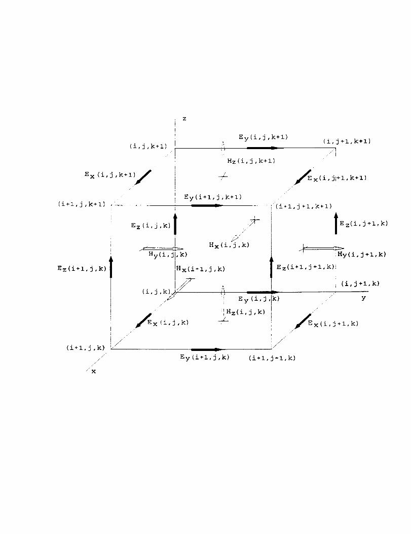
In the FDTD method, Maxwell's curl equations are discretized
in time and space and all derivatives (temporal and spatial) are
approximated by central differences. The electric and magnetic
fields are interleaved in space and time and are updated in a
second-order accurate leapfrog scheme. The computational space
is divided into cells with the electric fields located on the
edges and the magnetic fields on the faces (see Figure i). FDTD
objects are defined by specifying dielectric and/or magnetic
material parameters at electric and/or magnetic field locations.
Two basic implementations of the FDTD method are widely used
for electromagnetic analysis: total field formalism and scattered
field formalism. In the total field formalism, the electric and
magnetic field are updated based upon the material type present
at each spatial location. In the scattered field formalism, the
incident waveform is defined analytically and the scattered field
is coupled to the incident field through the different material
types. For the incident field, any waveform, angle of incidence
and polarization is possible. The separation of the incident and
scattered fields conveniently allows an absorbing boundary to beemployed at the extremities of the discretized problem space toabsorb the scattered fields.
This code is a scattered field code, and the total E and Hfields may be found by combining the incident and scatteredfields. Any type of field quantity (incident, scattered, ortotal), Poynting vector or current are available anywhere within
the computational space. These fields, incident, scattered and
total, may be found within, on or about the interaction object
placed in the problem space. By using a near to far field
transformation, far fields can be determined from the near fields
within the problem space thereby affording radiation patterns and
RCS values. The accuracy of these calculations is typically
within a dB of analytic solutions for dielectric and magnetic
sphere scattering. Further improvements are expected as better
absorbing boundary conditions are developed and incorporated.
III. OPERATION
Typically, a truncated Gaussian incident waveform is used to
excite the system being modeled, however certain code versions
also provide a smooth cosine waveform for convenience in modeling
dispersive materials. The interaction object is defined in the
discretized problem space with arrays at each cell location
created by the discretization. All three dielectric material
types for E field components within a cell can be individually
specified by the arrays IDONE(I,J,K), IDTWO(I,J,K),
IDTHRE(I,J,K). This models arbitrary dielectric materials with
= _0" By an obvious extension to six arrays, magnetic materials
with _ _ _o can be modeled.
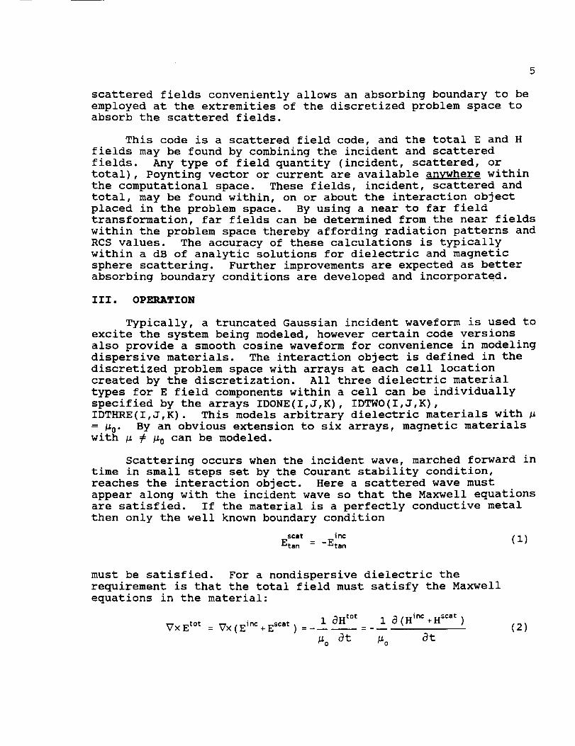
Scattering occurs when the incident wave, marched forward in
time in small steps set by the Courant stability condition,
reaches the interaction object. Here a scattered wave must
appear along with the incident wave so that the Maxwell equations
are satisfied. If the material is a perfectly conductive metal
then only the well known boundary condition
sc,t inc (1)Eta n = -Eta n
must be satisfied. For a nondispersive dielectric the
requirement is that the total field must satisfy the Maxwell
Additionally the incident wave, defined as moving unimpeded
through a vacuum in the problem space, satisfies everywhere in
the problem the Maxwell equations for free space
1 OH inc_TX E inc.....
Po at
(5)
aE inc_TxH inc:
o at(6)
Subtracting the second set of equations from the first yields the
Maxwell equations governing the scattered fields in the material:
1 @H sca'Vx E scat= (7 )
/_o at
aE inc
?XH scat= (_-8o)__at
a E scat+GE inc+6_ +aE scat (8)
at
Outside the material this simplifies to:
1 aH scat_Tx E scat= (9 )
/_o at
a E scatVxH scat =¢ (i0)
o at
Magnetic materials, dispersive effects, non-linearities,
etc., are further generalizations of the above approach. Based
on the value of the material type, the subroutines for
calculating scattered E and H field components branch to the
appropriate expression for that scattered field component and
7
that component is advanced in time according to the selectedalgorithm. As many materials can be modeled as desired, thenumber equals the dimension selected for the flags. If materialswith behavior different from those described above must bemodeled, then after the appropriate algorithm is found, thecode's branching structure allows easy incorporation of the newbehavior.
IV. RESOURCE REQUIREMENTS
The number of cells the problem space is divided into times
the six components per cell set the problem space storage
requirements
Storage=NC × 6 components/cell x 4 bytes/component (ii)
and the computational cost
Operations=NC x 6 comp/cell x i0 ops/component x N (12)
where N is the number of time steps desired.
N typically is on the order of ten times the number of cells
on one side of the problem space. More precisely for cubical
cells it takes _ time steps to traverse a single cell when the
time step is set by the Courant stability condition
AxAt- _x = cell size dimension (13)
The condition on N is then that
I I
N - 10x (_NC _) NC _number cells on a side
of the problem space
(14)
The earliest aircraft modeling using FDTD with approximately 30
cells on a side required approximately 500 time steps. For more
recent modeling with approximately i00 cells on a side, 2000 or
more time steps are used.
For (i00 cell) 3 problem spaces, 24 MBytes of memory are
required to store the fields. Problems on the order of this size
have been run on a Silicon Graphics 4D 220 with 32 MBytes of
memory, IBM RISC 6000, an Intel 486 based machine, and VAX
11/785. Storage is only a problem as in the case of the 486
where only 16 MBytes of memory was available. 3This limited theproblem space size to approximately (80 cells) .
8
For (i00 cell) 3 problem_ with approximately 2000 time steps,there is a total of 120 x i_ operations to perform. The speedsof the previously mentioned machines are 24 MFLOPs (4 processor
upgraded version), i0 MFL_PS, 1.5 MFLOPS, _nd 0.2 MFLOPs. '0_erun times are then 5 x i0 seconds, 12 x i0" seconds, 80 x 1
seconds and 600 x 103 seconds, respectively. In hours the times
are 1.4, 3.3, 22.2 and 167 hours. Problems of this size are
possible on all but the last machine and can in fact be performed
on a personal computer (486) if one day turnarounds arepermissible.
V. VERSION A CODE CAPABILITIES
The Penn State University FDTD Electromagnetic Scattering
Code Version A has the following capabilities:
i) Ability to model lossy dielectric and perfectly conductingscatterers.
2) First and second order outer radiation boundary condition
(ORBC) operating on the electric fields for dielectric or
perfectly conducting scatterers.
3) Near to far zone transformation capability to obtain far zonescattered fields.
4) Gaussian and smooth cosine incident waveforms with arbitrary
incidence angles.
5) Near zone field, current or power sampling capability.
6) Companion code for computing Radar Cross Section (RCS).
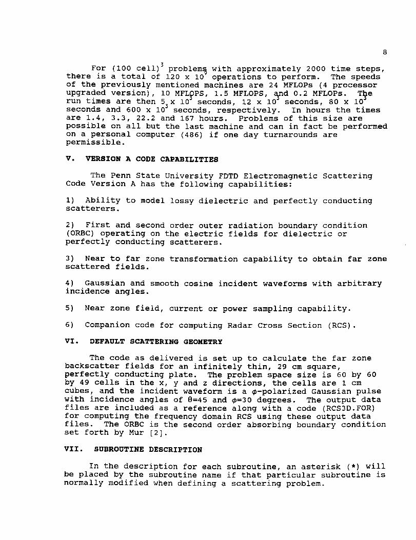
VI. DEFAULT SCATTERING GEOMETRY
The code as delivered is set up to calculate the far zone
backscatter fields for an infinitely thin, 29 cm square,
perfectly conducting plate. The problem space size is 60 by 60
by 49 cells in the x, y and z directions, the cells are 1 cm
cubes, and the incident waveform is a _-polarized Gaussian pulse
with incidence angles of 8=45 and _=30 degrees. The output data
files are included as a reference along with a code (RCS3D.FOR)
for computing the frequency domain RCS using these output data
files. The ORBC is the second order absorbing boundary condition
set forth by Mur [2].
VII. SUBROUTINE DESCRIPTION
In the description for each subroutine, an asterisk (*) will
be placed by the subroutine name if that particular subroutine is
normally modified when defining a scattering problem.
9
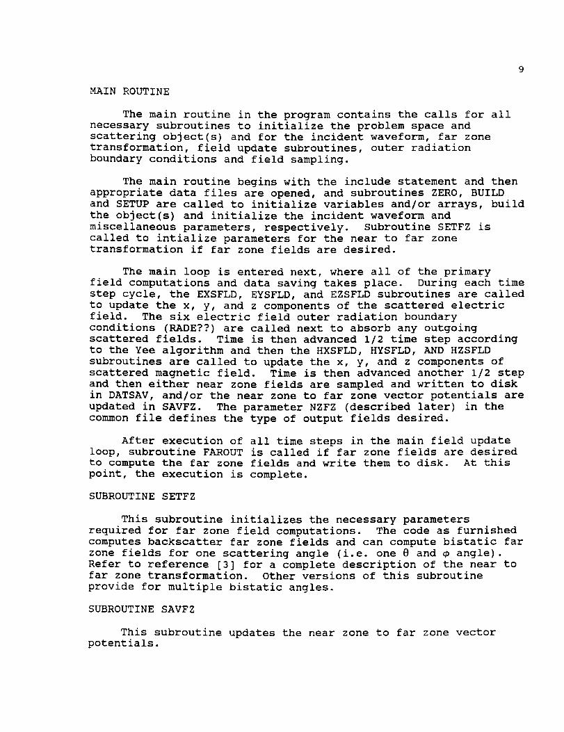
MAIN ROUTINE
The main routine in the program contains the calls for allnecessary subroutines to initialize the problem space andscattering object(s) and for the incident waveform, far zonetransformation, field update subroutines, outer radiationboundary conditions and field sampling.
The main routine begins with the include statement and thenappropriate data files are opened, and subroutines ZERO, BUILDand SETUP are called to initialize variables and/or arrays, buildthe object(s) and initialize the incident waveform andmiscellaneous parameters, respectively. Subroutine SETFZ iscalled to intialize parameters for the near to far zonetransformation if far zone fields are desired.
The main loop is entered next, where all of the primaryfield computations and data saving takes place. During each timestep cycle, the EXSFLD, EYSFLD, and EZSFLD subroutines are calledto update the x, y, and z components of the scattered electricfield. The six electric field outer radiation boundaryconditions (RADE??) are called next to absorb any outgoingscattered fields. Time is then advanced 1/2 time step accordingto the Yee algorithm and then the HXSFLD, HYSFLD, AND HZSFLDsubroutines are called to update the x, y, and z components ofscattered magnetic field. Time is then advanced another 1/2 stepand then either near zone fields are sampled and written to diskin DATSAV, and/or the near zone to far zone vector potentials areupdated in SAVFZ. The parameter NZFZ (described later) in thecommon file defines the type of output fields desired.
After execution of all time steps in the main field updateloop, subroutine FAROUT is called if far zone fields are desiredto compute the far zone fields and write them to disk. At thispoint, the execution is complete.
SUBROUTINESETFZ
This subroutine initializes the necessary parametersrequired for far zone field computations. The code as furnishedcomputes backscatter far zone fields and can compute bistatic farzone fields for one scattering angle (i.e. one 8 and _ angle).Refer to reference [3] for a complete description of the near tofar zone transformation. Other versions of this subroutineprovide for multiple bistatic angles.
SUBROUTINESAVFZ
This subroutine updates the near zone to far zone vectorpotentials.
i0
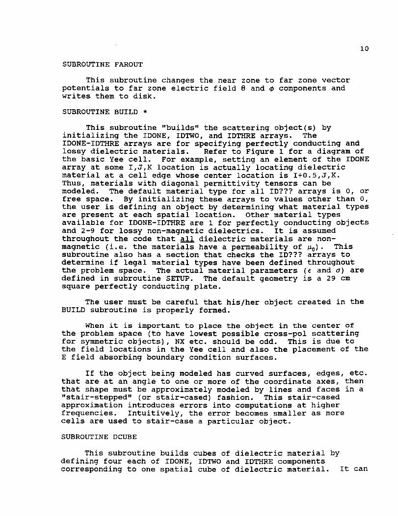
SUBROUTINEFAROUT
This subroutine changes the near zone to far zone vectorpotentials to far zone electric field 8 and _ components andwrites them to disk.
SUBROUTINEBUILD *
This subroutine "builds" the scattering object(s) byinitializing the IDONE, IDTWO, and IDTHRE arrays. TheIDONE-IDTHRE arrays are for specifying perfectly conducting andlossy dielectric materials. Refer to Figure 1 for a diagram ofthe basic Yee cell. For example, setting an element of the IDONEarray at some I,J,K location is actually locating dielectricmaterial at a cell edge whose center location is I+0.5,J,K.Thus, materials with diagonal permittivity tensors can bemodeled. The default material type for all ID??? arrays is 0, orfree space. By initializing these arrays to values other than 0,the user is defining an object by determining what material typesare present at each spatial location. Other material typesavailable for IDONE-IDTHRE are 1 for perfectly conducting objectsand 2-9 for lossy non-magnetic dielectrics. It is assumedthroughout the code that all dielectric materials are non-
magnetic (i.e. the materials have a permeability of _0)" This
subroutine also has a section that checks the ID??? arrays to
determine if legal material types have been defined throughout
the problem space. The actual material parameters (E and _) are
defined in subroutine SETUP. The default geometry is a 29 cm
square perfectly conducting plate.
The user must be careful that his/her object created in the
BUILD subroutine is properly formed.
When it is important to place the object in the center of
the problem space (to have lowest possible cross-pol scattering
for symmetric objects), NX etc. should be odd. This is due to
the field locations in the Yee cell and also the placement of the
E field absorbing boundary condition surfaces.
If the object being modeled has curved surfaces, edges, etc.
that are at an angle to one or more of the coordinate axes, then
that shape must be approximately modeled by lines and faces in a
"stair-stepped" (or stair-cased) fashion. This stair-cased
approximation introduces errors into computations at higher
frequencies. Intuitively, the error becomes smaller as more
cells are used to stair-case a particular object.
SUBROUTINE DCUBE
This subroutine builds cubes of dielectric material by
defining four each of IDONE, IDTWO and IDTHRE components
corresponding to one spatial cube of dielectric material. It can
Ii
also be used to define thin (i.e. up to one cell thick)dielectric or perfectly conducting plates. Refer to commentswithin DCUBE for a description of the arguments and usage of thesubroutine.
SUBROUTINESETUP *
This subroutine initializes many of the constants requiredfor incident field definition, field update equations, outerradiation boundary conditions and material parameters. Thematerial parameters E and _ are defined for each material typeusing the material arrays EPS and SIGMA respectively. The arrayEPS is used for the total permittivity and SIGMA is used for theelectric conductivity. These arrays are initialized in SETUP tofree space material parameters for all material types and thenthe user is required to modify these arrays for his/herscattering materials. Thus, for the lossy dielectric materialtype 2, the user must define EPS(2) and SIGMA(2). The remainderof the subroutine computes constants used in field updateequations and boundary conditions and writes the diagnosticsfile.
SUBROUTINE EXSFLD
This subroutine updates all x components of scatteredelectric field at each time step except those on the outerboundaries of the problem space. IF statements based upon theIDONE array are used to determine the type of material presentand the corresponding update equation to be used. Thesescattered field equations are based upon the development given in[4].
SUBROUTINE EYSFLD
This subroutine updates all y components of scatteredelectric field at each time step except those on the outerboundaries of the problem space. IF statements based upon theIDTWO array are used to determine the type of material presentand the corresponding update equation to be used.
SUBROUTINEEZSFLD
This subroutine updates all z components of scatteredelectric field at each time step except those on the outerboundaries of the problem space. IF statements based upon theIDTHRE array are used to determine the type of material presentand the corresponding update equation to be used.
SUBROUTINESRADEYX, RADEZX, RADEZY, RADEXY, RADEXZ and RADEYZ
These subroutines apply the outer radiation boundaryconditions to the scattered electric field on the outer
12
boundaries of the problem space.
SUBROUTINEHXSFLD
This subroutine updates all x components of scatteredmagnetic field at each time step. The standard non-magneticupdate equation is used.
SUBROUTINEHYSFLD
This subroutine updates all y components of scatteredmagnetic field at each time step. The standard non-magneticupdate equation is used.
SUBROUTINEHZSFLD
This subroutine updates all z components of scatteredmagnetic field at each time step. The standard non-magneticupdate equation is used.
SUBROUTINEDATSAV *
This subroutine samples near zone scattered field quantitiesand saves them to disk. This subroutine is where the quantitiesto be sampled and their spatial locations are to be specified andis only called_if near zone fields only are desired 0r if b_h
n ear_and_far__zonefields_aKe_des_. Total field quantities can
also be sampled. See comments within the subroutine for
specifying sampled scattered and/or total field quantities. When
sampling magnetic fields, remember the 6t/2 time difference
between E and H when writing the fields to disk. Sections of
code within this subroutine determine if the sampled quantities
and the spatial locations have been properly defined.
FUNCTIONS EXI, EYI and EZI
These functions are called to compute the x, y and z
components of incident electric field. The functional form of
the incident field is contained in a separate function SOURCE.
FUNCTION SOURCE *
This function contains the functional form of the incident
field. The code as furnished uses the Gaussian form of the
incident field. An incident smooth cosine pulse is also
available by uncommenting the required lines and commenting out
the Gaussian pulse. Thus, this function need only be modified if
the user changes the incident pulse from Gaussian to smooth
cosine. A slight improvement in computing speed and
vectorization may be achieved by moving this function inside each
of the incident field functions EXI, EYI and so on.
13
FUNCTIONS DEXI, DEYI and DEZI
These functions are called to compute the x, y and zcomponents of the time derivative of incident electric field.The functional form of the incident field is contained in aseparate function DSRCE.
FUNCTION DSRCE *
This function contains the functional form of the timederivative of the incident field. The code as furnished uses thetime derivative of the Gaussian form of the incident field. Asmooth cosine pulse time derivative is also available byuncommenting the required lines and commenting out the Gaussianpulse. Thus, the function need only be modified if the userchanges from the Gaussian to smooth cosine pulse. Again, aslight improvement in computing speed and vectorization may beachieved by moving this function inside each of the timederivative incident field functions DEXI, DEYI and so on.
SUBROUTINEZERO
This subroutine initializes various arrays and variables tozero.
VIII. INCLUDE FILE DESCRIPTION (COMMONA.FOR) *
The include file, COMMONA.FOR, contains all of the arrays
and variables that are shared among the different subroutines.
This file will require the most modifications when defining
scattering problems. A description of the parameters that are
normally modified follows.
The parameters NX, NY and NZ specify the size of the problem
space in cells in the x, y and z directions respectively. For
problems where it is crucial to center the object within the
problem space, then NX, NY and NZ should be odd. The parameter
NTEST defines the number of near zone quantities to be sampled
and NZFZ defines the field output format. Set NZFZ=0 for near
zone fields only, NZFZ=I for far zone fields only and NZFZ=2 for
both near and far zone fields. Parameter NSTOP defines the
maximum number of time steps. DELX, DELY, and DELZ (in meters)
define the cell size in the x, y and z directions respectively.
The 8 and _ incidence angles (in degrees) are defined by THINC
and PHINC respectively and the polarization is defined by ETHINC
and EPHINC. ETHINC=I.0, EPHINC=0.0 for 8-polarized incident
field and ETHINC=0.0, EPHINC=I.0 for _-polarized incident fiel_s.Parameters AMP and BETA define the maximum amplitude and the e
temporal width of the incident pulse respectively. BETA
automatically adjusts when the cell size is changed and normally
should not be changed by the user. The far zone scattering
angles are defined by THETFZ and PHIFZ. The code as furnished
14
performs backscatter computations, but these parameters could bemodified for a bistatic computation.
IX. RCS COMPUTATIONS
A companion code, RCS3D.FOR, has been included to compute
RCS versus frequency. It uses the file name of the FDTD far zone
output data (FZOUT3D.DAT) and writes a data file of far zone
electric fields versus time (FZTIME.DAT) and RCS versus frequency
(3DRCS.DAT). The RCS computations are performed up to the i0
cell/l 0 frequency limit. Refer to comments within this code forfurther details.
X. RESULTS
As previously mentioned, the code as furnished models an
infinitely thin, 29 cm square, perfectly conducting plate and
computes backscatter far zone scattered fields at angles of 8=45
and _=30 degrees.
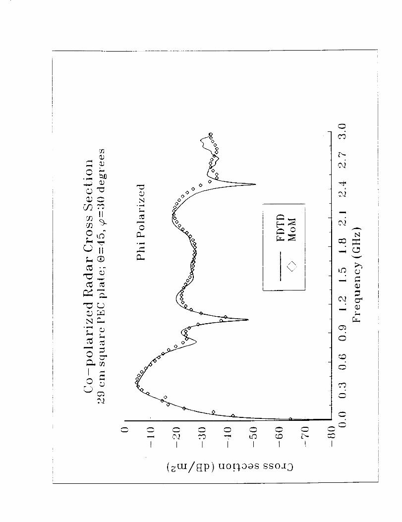
Figures 2-3 shows the co-polarized far zone electric field
versus time and the co-polarized RCS for the 29 cm square
perfectly conducting plate.
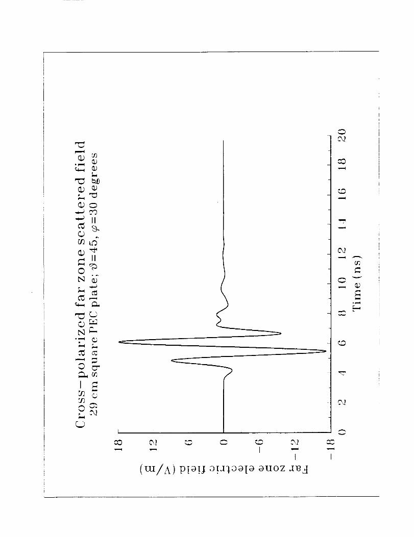
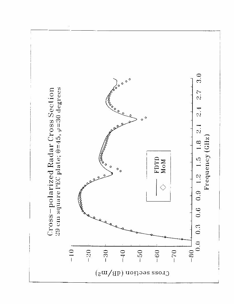
Figures 4-5 shows the cross-polarized far zone electric
field versus time and the cross-polarized RCS for the 29 cm
square perfectly conducting plate.
XI. SAMPLE PROBLEM SETUP
The code as furnished models an infinitely thin, 29 cm
square, perfectly conducting plate and computes backscatter far
zone scattered fields at angles of 8=45 and _=30 degrees. The
corresponding output data files are also provided, along with a
code to compute RCS using these data files. In order to change
the code to a new problem, many different parameters need to be
modified. A sample problem setup will now be discussed.
Suppose that the problem to be studied is RCS backscatter
versus frequency from a 28 cm by 31 cm perfectly conducting plate
with a 3 cm dielectric coating with a dielectric constant of 4_ 0
using a 8-polarized field. The backscatter angles are e=30.0 and
_=60.0 degrees and the frequency range is up to 3 Ghz.
Since the frequency range is up to 3 Ghz, the cell size must
be chosen appropriately to resolve the field IN ANY MATERIAL at
the highest frequency of interest. A general rule is that the
cell size should be i/i0 of the wavelength at the highest
frequency of interest. For difficult geometries, 1/20 of a
wavelength may be necessary. The free space wavelength at 3 GHz
is 10=10 cm and the wavelength in the dielectric coating at 3 GHz
is 5 cm. The cell size is chosen as 1 cm, which provides a
15
resolution of 5 cells/l in the dielectric coating and i0 cells/l 0in free space. Numerical studies have shown that choosing thecell size _ 1/4 of the shortest wavelength in any material isthe practical lower limit. Thus the cell size of 1 cm is barelyadequate. The cell size in the x, y and z directions is set inthe common file through variables DELX, DELY and DELZ. Next theproblem space size must be large enough to accomodate thescattering object, plus at least a five cell boundary (i0 cells
is more appropriate) on every side of the object to allow for the
far zone field integration surface. It is advisable for plate
scattering to have the plate centered in the x and y directions
of the problem space in order to reduce the cross-polarized
backscatter and to position the plate low in the z direction to
allow strong specular reflections multiple encounters with the
ORBC. A i0 cell border is chosen, and the problem space size is
chosen as 49 by 52 by 49 cells in the x, y and z directions
respectively. As an initial estimate, allow 2048 time steps so
that energy trapped within the dielectric layer will radiate.
Thus parameters NX, NY and NZ in COMMONA.FOR would be changed to
reflect the new problem space size, and parameter NSTOP is
changed to 2048. If all transients have not been dissipated
after 2048 time steps, then NSTOP will have to be increased.
Truncating the time record before all transients have dissipated
will corrupt frequency domain results. Parameter NZFZ must be
equal to 1 since we are interested in far zone fields only. To
build the object, the following lines are inserted into the BUILDsubroutine:
The PEC plate is built last on the bottom of the dielectricslab to avoid any air gaps between the dielectric material andthe PEC plate. In the common file, the incidence angles THINCand PHINC have to be changed to 30.0 and 60.0 respectively, thecell sizes (DELX, DELY, DELZ) are set to 0.01, and thepolarization is set to ETHINC=I.0 and EPHINC=0.0 for e-polarizedfields. Since dielectric material 2 is being used for thedielectric coating, the constitutive parameters EPS(2) andSIGMA(2) are set to 4E0 and 0.0 respectively, in subroutineSETUP. This completes the code modifications for the sampleproblem.
XII. NEW PROBLEM CHECKLIST
This checklist provides a quick reference to determine if
all parameters have been defined properly for a given scattering
problem. A reminder when defining quantities within the code:
use MKS units and specify all angles in degrees.
COMMONA.FOR:
I) Is the problem space sized correctly? (NX, NY, NZ)
2) For near zone fields, is the number of sample points correct?
(NTEST)
3) Is parameter NZFZ defined correctly for desired field
outputs?
4) Is the number of time steps correct? (NSTOP)
5) Are the cell dimensions (DELX, DELY, DELZ) defined correctly?
6) Are the incidence angles (THINC, PHINC) defined correctly?
7) Is the polarization of the incident wave defined correctly
(ETHINC, EPHINC)?
8) For other than backscatter far zone field computations, are
the scattering angles set correctly? (THETFZ, PHIFZ)
SUBROUTINE BUILD:
i) Is the object completely and correctly specified?
SUBROUTINE SETUP:
i) Are the constitutive parameters for each material specified
correctly? (EPS and SIGMA)
17
FUNCTIONS SOURCEand DSRCE:
I) If the Gaussian pulse is not desired, is it commented out andthe smooth cosine pulse uncommented?
SUBROUTINEDATSAV:
i) For near zone fields, are the sampled field types and spatiallocations correct for each sampling point? (NTYPE, IOBS, JOBS,MOBS)
XIII. REFERENCES
[1] K. S. Yee, "Numerical solution of initial boundary value
problems involving Maxwell's equations in isotropic media,"
IEEE Trans. Antennas Propaqat., vol. AP-14, pp. 302-307, May
1966.
[2] G. Mur, "Absorbing boundary conditions for the Finite-
Difference approximation of the Time-Domain Electromagnetic-
Field Equations," IEEE Trans. Electromaqn. Compat., vol.
EMC-23, pp. 377-382, November 1981.
[3] R.J. Luebbers et. al., "A Finite Difference Time-Domain Near
Zone to Far Zone Transformation," I_EE Trans. Antennas
Propaqat., vol. AP-39, no. 4, pp. 429-433, April 1991.
[4] R. Holland, L. Simpson and K. S. Kunz, "Finite-Difference
Time-Domain Analysis of EMP Coupling to Lossy Dielectric